Minimal geodesics along volume preserving maps, through ...

HAL Id: hal-01152168https://hal.archives-ouvertes.fr/hal-01152168v2

Submitted on 15 Dec 2016

HAL is a multi-disciplinary open accessarchive for the deposit and dissemination of sci-entific research documents, whether they are pub-lished or not. The documents may come fromteaching and research institutions in France orabroad, or from public or private research centers.

L’archive ouverte pluridisciplinaire HAL, estdestinée au dépôt et à la diffusion de documentsscientifiques de niveau recherche, publiés ou non,émanant des établissements d’enseignement et derecherche français ou étrangers, des laboratoirespublics ou privés.

Minimal geodesics along volume preserving maps,through semi-discrete optimal transport

Quentin Mérigot, Jean-Marie Mirebeau

To cite this version:Quentin Mérigot, Jean-Marie Mirebeau. Minimal geodesics along volume preserving maps, throughsemi-discrete optimal transport. SIAM Journal on Numerical Analysis, Society for Industrial andApplied Mathematics, 2016, 54 (6), pp.3465-3492. 10.1137/15M1017235. hal-01152168v2

Minimal geodesics along volume preserving maps,

through semi-discrete optimal transport

Quentin Mérigot∗† Jean-Marie Mirebeau∗‡

August 30, 2016

Abstract

We introduce a numerical method for extracting minimal geodesics along the group ofvolume preserving maps, equipped with the L2 metric, which as observed by Arnold [Arn66]solve the Euler equations of inviscid incompressible uids. The method relies on the general-ized polar decomposition of Brenier [Bre91], numerically implemented through semi-discreteoptimal transport. It is robust enough to extract non-classical, multi-valued solutions ofEuler's equations, for which the ow dimension - dened as the quantization dimension ofBrenier's generalized ow - is higher than the domain dimension, a striking and unavoid-able consequence of this model [Shn94]. Our convergence results encompass this generalizedmodel, and our numerical experiments illustrate it for the rst time in two space dimensions.

1 Introduction

The motion of an inviscid incompressible uid, moving in a compact domainX ⊆ Rd, is describedby the Euler equations [Eul65]

∂tv + (v · ∇)v = −∇p div v = 0, (1)

coupled with the impervious boundary condition v · n = 0 on ∂Ω. Here v denotes the uidvelocity, and p the pressure acts as a Lagrange multiplier for the incompressibility constraint.As observed by Arnold [Arn66], Euler equations (1) yield in Lagrangian coordinates the geodesicequations along the group SDiff of dieomorphisms of X with unit jacobian, equipped with theL2 metric. Indeed, let s : [0, 1]→ SDiff be a smooth time dependent family of dieomorphismsof X, describing the evolution over time of the position of the uid particles. The position ofthe particle emanating from x at time t will be denoted indierently st(x) or s(t, x), while thedieomorphism at time t is denoted s(t) or st. The Eulerian velocity v and acceleration a ofthe uid particles are given by v(t, s(t, x)) = ∂ts(t, x) and a(t, s(t, x)) = ∂tts(t, x). The jacobianconstraint det∇s = 1 yields div v = 0, whereas the equation of geodesics on SDiff merelystates that acceleration is a gradient, a(t, x) = −∇p(t, x), which is equivalent to (1, Left). Thisformalism leads to two natural problems for Euler equations:

• The Cauchy problem, forward in time: given the initial position and velocity of the uidparticles, nd their subsequent positions at all positive times. This amounts to computingthe exponential map on the lie group SDiff.

∗CNRS, Université Paris-Dauphine, UMR 7534, CEREMADE, Paris, France.†ANR grant TOMMI, ANR-11-BS01-014-01‡ANR grant NS-LBR, ANR-13-JS01-0003-01

1

• The boundary value problem: given some observed initial and nal positions of the uidparticles, nd their intermediate states. This amounts to computing a minimizing geodesicon SDiff.

This manuscript is devoted to the boundary value problem only. More precisely, consider aninviscid incompressible uid owing during the time interval [0, 1], and a map s∗ : X → X givingthe nal position s∗(x) of each uid particle initially at position x ∈ X. In this paper, we intro-duce a new numerical scheme for nding a minimizing geodesic joining the initial congurations∗ = Id to the nal one s∗

minimize

ˆ 1

0‖s(t)‖2dt, subject to

∀t ∈ [0, 1], s(t) ∈ S,s(0) = s∗, s(1) = s∗.

(2)

We denoted by S ⊆ L2(X,Rd) the space of maps preserving the Lebesgue measure on X, which indimension d ≥ 3 is the closure of SDiff. More formally, we let Leb denote the Lebesgue measureon X, rescaled so as to be a probability measure, and we let f#µ denote the push-forward of ameasure µ by a measurable map f , dened by f#µ(A) := µ(f−1(A)). Then the space S is thecollection of measurable maps s : X → X obeying s# Leb = Leb.

The motivation for this rst relaxation replacing SDiff with the closed subset S of L2 is that the optimized functional in (2) does not penalize the spatial derivatives of s, which areinvolved in the unit jacobian constraint dening SDiff. Despite this relaxation, the optimizationproblem (2) needs not have a minimizer in s ∈ H1([0, 1],S) in dimension d ≥ 3 [Shn94], andminimizing sequences (sn)n∈N may instead display oscillations reminiscent of an homogeneizationphenomenon. A second relaxation is therefore necessary, see [FD12] for a review.

Generalized ows Brenier introduced in [Bre89] a second relaxation of the minimizing geodesicproblem (2) based on generalized ows, which allow particles to split and their paths to cross.This surprising behavior is an unavoidable consequence of the lack of viscosity in Euler's equa-tions, which amounts to an innite Reynolds number. Generalized ows are also relevant indimension d ∈ 1, 2 if the underlying physical model actually involves a three dimensional do-main X × [0, ε]3−d in which one neglects the uid acceleration in the extra dimensions [Bre08].Consider the space of continuous paths (of uid particles)

Ω := C0([0, 1], X).

A generalized ow, in Brenier's sense [Bre89], is a probability measure µ over the space Ω ofpaths. We denote by et(ω) := ω(t) the evaluation map at time t ∈ [0, 1]. Given a generalizedow µ ∈ Prob(Ω), the pushforward measure et #µ can be understood as the distribution ofparticles at time t under the ow. The generalized ow is incompressible if for every timet ∈ [0, 1], et #µ coincides with the uniform probability measure on the domain X. Rescaling thedomain if necessary we assume that X has unit area, so that the uniform probability measureLeb is simply the restriction of the Lebesgue measure to X.

The use of generalized ows turns the highly non-linear incompressibility constraint s(t) ∈ Sinto a linear constraint et #µ = Leb. Note the similarity with Kantorovich's linearization ofthe non-linear mass preservation constraint in Monge's optimal transport problem. This idealeads to a convex relaxation of the minimizing geodesic distance problem (2), linearizing both

2

X

v(x)

s0(x)

st(x)

X

t = 0 t = 1

X X

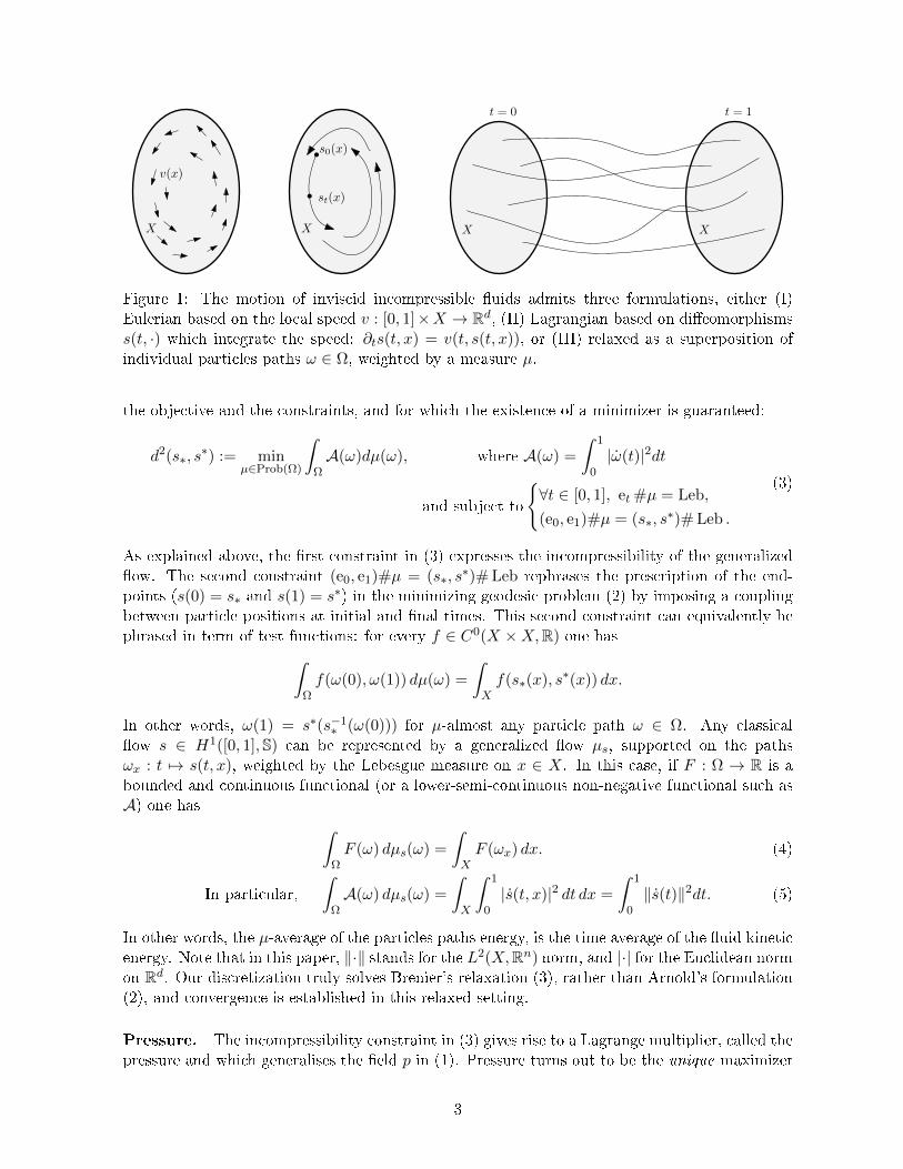
Figure 1: The motion of inviscid incompressible uids admits three formulations, either (I)Eulerian based on the local speed v : [0, 1]×X → Rd, (II) Lagrangian based on dieomorphismss(t, ·) which integrate the speed: ∂ts(t, x) = v(t, s(t, x)), or (III) relaxed as a superposition ofindividual particles paths ω ∈ Ω, weighted by a measure µ.

the objective and the constraints, and for which the existence of a minimizer is guaranteed:

d2(s∗, s∗) := min

µ∈Prob(Ω)

ˆΩA(ω)dµ(ω), where A(ω) =

ˆ 1

0|ω(t)|2dt

and subject to

∀t ∈ [0, 1], et #µ = Leb,

(e0, e1)#µ = (s∗, s∗)# Leb .

(3)

As explained above, the rst constraint in (3) expresses the incompressibility of the generalizedow. The second constraint (e0, e1)#µ = (s∗, s

∗)# Leb rephrases the prescription of the end-points (s(0) = s∗ and s(1) = s∗) in the minimizing geodesic problem (2) by imposing a couplingbetween particle positions at initial and nal times. This second constraint can equivalently bephrased in term of test functions: for every f ∈ C0(X ×X,R) one has

ˆΩf(ω(0), ω(1)) dµ(ω) =

ˆXf(s∗(x), s∗(x)) dx.

In other words, ω(1) = s∗(s−1∗ (ω(0))) for µ-almost any particle path ω ∈ Ω. Any classical

ow s ∈ H1([0, 1], S) can be represented by a generalized ow µs, supported on the pathsωx : t 7→ s(t, x), weighted by the Lebesgue measure on x ∈ X. In this case, if F : Ω → R is abounded and continuous functional (or a lower-semi-continuous non-negative functional such asA) one has

ˆΩF (ω) dµs(ω) =

ˆXF (ωx) dx. (4)

In particular,

ˆΩA(ω) dµs(ω) =

ˆX

ˆ 1

0|s(t, x)|2 dt dx =

ˆ 1

0‖s(t)‖2dt. (5)

In other words, the µ-average of the particles paths energy, is the time average of the uid kineticenergy. Note that in this paper, ‖·‖ stands for the L2(X,Rn) norm, and |·| for the Euclidean normon Rd. Our discretization truly solves Brenier's relaxation (3), rather than Arnold's formulation(2), and convergence is established in this relaxed setting.

Pressure. The incompressibility constraint in (3) gives rise to a Lagrange multiplier, called thepressure and which generalises the eld p in (1). Pressure turns out to be the unique maximizer

3

m0 mT−1

s∗

. . .

πS(mT−1). . .

m1 mT

s∗

πS(m1)

S

MN

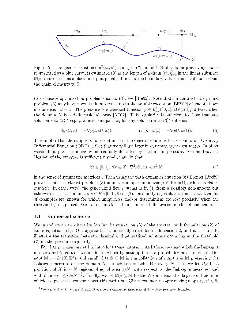
Figure 2: The geodesic distance d2(s∗, s∗) along the manifold S of volume preserving maps,

represented as a blue curve, is estimated (9) as the length of a chain (mi)Ti=0 in the linear subspace

MN , represented as a black line, plus penalizations for the boundary values and the distance fromthe chain elements to S.

to a concave optimization problem dual to (3), see [Bre93]. Note that, in contrast, the primalproblem (3) may have several minimizers up to the notable exception [BFS09] of smooth owsin dimension d = 1. The pressure is a classical function p ∈ L2

loc( ]0, 1[, BV(X)), at least whenthe domain X is a d-dimensional torus [AF07]. This regularity is sucient to show that anysolution s to (2) (resp. µ-almost any path ω, for any solution µ to (3)) satises

∂tts(t, x) = −∇p(t, s(t, x)), resp. ω(t) = −∇p(t, ω(t)). (6)

This implies that the support of µ is contained in the space of solutions to a second-order OrdinaryDierential Equation (ODE), a fact that we will use later in our convergence estimates. In otherwords, uid particles move by inertia, only deected by the force of pressure. Assume that theHessian of the pressure is suciently small, namely that

∀t ∈ [0, 1], ∀x ∈ X, ∇2p(t, x) ≺ π2 Id (7)

in the sense of symmetric matrices1. Then using the path dynamics equation (6) Brenier [Bre89]proved that the relaxed problem (3) admits a unique minimizer µ ∈ Prob(Ω), which is deter-ministic. In other word, the generalized ow µ stems as in (4) from a possibly non-smooth butotherwise classical minimizer s ∈ H1([0, 1], S) of (2). Inequality (7) is sharp, and several familiesof examples are known for which uniqueness and/or determinism are lost precisely when thethreshold (7) is passed. We present in 5 the rst numerical illustration of this phenomenon.

1.1 Numerical scheme

We introduce a new discretization for the relaxation (3) of the shortest path formulation (2) ofEuler equations (1). Our approach is numerically tractable in dimension 2, and is the rst toillustrate the transition between classical and generalized solutions occurring at the threshold(7) on the pressure regularity.

For that purpose we need to introduce some notation. As before, we denote Leb the Lebesguemeasure restricted to the domain X, which by assumption is a probability measure on X. De-note M := L2(X,Rd), and recall that S ⊆ M is the collection of maps s ∈ M preserving theLebesgue measure on the domain X, i.e. s# Leb = Leb. For every N ∈ N, we let PN be apartition of X into N regions of equal area 1/N , with respect to the Lebesgue measure, and

with diameter ≤ CPN−1d . Finally, we let MN ⊆ M be the N -dimensional subspace of functions

which are piecewise constant over this partition. Given two measure-preserving maps s∗, s∗ ∈ S,

1We write A ≺ B, where A and B are two symmetric matrices, if B −A is positive denite.

4

discretization parameters T,N ∈ N, and a penalization factor λ 1, we introduce the functionalwhich to m ∈MT+1

N associates

E(T,N, λ; m) := T∑

0≤i<T‖mi+1 −mi‖2 + λ

(‖m0 − s∗‖2 + ‖mT − s∗‖2 +

∑1≤i<T

d2S(mi)

). (8)

We denoted by d2S the squared-distance to the space S of measure-preserving maps, dened

as usual by d2S(m) = infs∈S ‖m − s‖2. Comparing this with (2), we recognize the standard

discretization of the length of the discrete path (m0, · · · ,mT ), as well as an implementation bypenalization of the boundary value constraints. The last term corresponds to a penalizationof the incompressibility constraints, or more precisely a penalization of the squared distancebetween the maps mi and the set S of measure preserving maps. The discrete optimizationproblem we consider is then

E(T,N, λ) := minm∈MT+1

N

E(T,N, λ;m) (9)

The problem (9), considered as a function ofm ∈MT+1N , is anN(T+1)d-dimensional optimization

problem. It makes sense to consider (8) and (9) whenever one attempts to approximate a shortestpath joining two points s∗, s

∗ of a subset S of a Hilbert space H, internally approximated bysubspaces (MN )N≥0. Our rst result Proposition 1.1 uses no additional assumptions. In contrast,the numerical implementation strategy, and the other results 1.2, crucially rely on the specicproperties of the set S of measure preserving maps.

The key properties of the functional (8) follow from those of the squared distance function d2S,

which are established in Proposition 5.1. It is continuously dierentiable on an open dense set.However it is non-convex (in fact semi-concave) due to the non-convexity of the set S, forbiddingus to guarantee that the global minimum of (9) is found by our numerical solver. Nonetheless,our numerical experiments show that quasi-Newton methods give convincing results, see 5.

Distance to S and semi-discrete optimal transport. Before entering the analysis of (9), wewant to emphasize that the inner-subproblems, namely the computation of the squared distancesd2S(mi), are numerically tractable thanks to two main ingredients: Brenier's polar factorization[Bre91], and semi-discrete optimal transport. Brenier's polar factorization theorem asserts thatthe distance between any m ∈ M and the set S of measure-preserving maps equals the cost oftransporting the image measure m# Leb back to the Lebesgue measure, namely

d2S(m) = inf

s∈S‖m− s‖2 = W 2

2 (m# Leb,Leb), (10)

where W2 is the Wasserstein distance for the quadratic transport cost. Given any m ∈ MN ,the pushforward measure m# Leb is the sum of N Dirac measures of mass 1/N , located atthe N values of the piecewise constant map m on the partition PN . Computing (10) thereforeamounts to the computation of the Wasserstein distance between a nitely supported measureand the Lebesgue measure, a special instance of a problem called semi-discrete optimal transport.Ecient computational methods for this problem have been proposed [AHA98, Mer11, Lév14],relying on Kantorovich duality and on tools from computational geometry. Let η be the uniformprobability measure over a nite set Y ⊆ Rd with cardinal N . Kantorovich duality asserts that

W 22 (η,Leb) = sup

f :X→R,g:Y→Rf(x)+g(y)≤‖x−y‖2

ˆXf(x) dLeb(x) +

ˆXg(y) dη(y).

5

For any xed g : Y → R the largest f : X → R obeying the constraint is given by

f(x) := miny∈Y‖x− y‖2 − g(y).

This function is piecewise quadratic over a partition (Lagy(g))y∈Y of X into convex polyhedra

Lagy(g) :=x ∈ X | ∀z ∈ Y, ‖x− y‖2 − g(y) ≤ ‖x− z‖2 − g(z)

.

Eliminating the optimization variable f , Kantorovitch duality reads

W 22 (η,Leb) = sup

g:Y→R

∑y∈Y

ˆLagy(g)

(‖x− y‖2 − g(y)) dx+1

N

∑y∈Y

g(y). (11)

This partition of X is called the Laguerre diagram of (Y, g) in computational geometry andcan be computed in near-linear time in R2 using existing software2 [cga]. Specically, we usethe 2D regular triangulations package in CGAL [Yvi13]. The maximization problem (11) is anunconstrained, concave and twice continuously dierentiable maximization problem, which iseciently solved via Newton or quasi-Newton methods. Semi-discrete optimal transport hasbecome a reliable and ecient building block for PDE discretizations [BCMO14].

As discussed above, the chosen discretization of the Euler equations intrinsically leads to anoptimal transport problem of semi-discrete type - from a nite collection of Diracs playing therole of uid particles to the standard Lebesgue measure - hence our choice of discretization (11).A variety of alternative approaches have been developed for other instances of computationaloptimal transport, based for instance on a pressure-less uid model [BBG02, PPO13], mono-tone discretizations of Monge-Ampere equation [BFO14, BCM14], regularization via entropypenalization [BCC+15, CPR15], or adaptive strategies for the linear programming discretization[OR15, Sch15].

1.2 Main results

Our results on the proposed discretization (8) are split into two parts. A convergence analysisrst shows how to construct discrete generalized ows out of minimizers of E(T,N, λ), supportedon nitely many piecewise linear paths and which converge to a solution µ ∈ Prob(Ω) of (3).This analysis requires upper bounds on the discrete energies E(T,N, λ), which are established ina second part and under adequate a-priori assumptions on the continuous solution. Importantly,two sets of assumptions are considered, encompassing the favorable case where a classical solutionto Arnold's formulation (2) exists, and the general case where only Brenier's relaxation (3) iswell posed.

Convergence analysis. We present two results establishing the convergence of the discretizedproblem (9) minimizers towards solutions of (3) as the number of timesteps T grows to inn-ity. The rst proposition shows that one can build short chains of incompressible maps out ofminimizers of (9). It involves the quantity

E ′(T,N, λ;m) := (1 + 4T/λ)E(T,N, λ;m). (12)

2In R3 the worst-case complexity of the Laguerre diagram is quadratic in the number of points, but thiscorresponds to degenerate cases, so that semi-discrete optimal can also be solved eciently on R3 [Lév14].

6

X

Pj

t = 0 t = 1

ωj(i/T )Pj

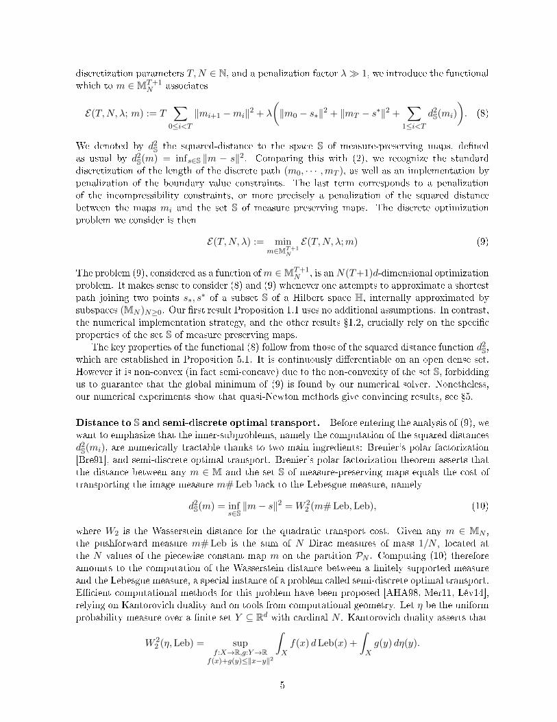
Figure 3: (Left) A partition PN cuts the domain X into N region of equal area and roughlyisotropic shape. (Right) To a sequence (mi)

Ti=0 ∈ MT+1

N one can associate N piecewise linearpaths (ωj)

Nj=1, by interpolating the map values at the times 0, 1/T, · · · , T/T for each region

of the partition PN .

Proposition 1.1. Let m = (mi)Ti=0 ∈MT+1

N and let (si)Ti=0 be the chain of incompressible maps

dened by: s0 = s∗, sT = s∗, and si is a projection of mi onto S for all 1 ≤ i < T . Then

T∑

0≤i<T‖si+1 − si‖2 ≤ E ′(T,N, λ;m).

Unfortunately, such discrete chains of incompressible maps need not converge as T → ∞to a continuous path s : [0, 1] → S, due to the lack of compactness of S. Note also that theinterpolates (1− δ)si + δsi+1, 0 ≤ δ ≤ 1, 0 ≤ i ≤ T , need not belong to the non-convex set S.

The next proposition establishes, under condition, convergence towards a solution of (3) inthe sense of generalized ows, a framework which enjoys the desired convexity and compactnessproperties. In order to state this result, we associate to each m = (mi)

Ti=0 in MT+1

N a generalized

ow µm ∈ Prob(Ω) uniformly supported on N paths. For every j ∈ 1, . . . , N, we denote mji

the (constant) value of mi on the j-th region of the partition PN of X and we dene a path ωjby interpolating linearly between these points, that is

∀0 ≤ i ≤ N, ωj(i/t) = mji .

The construction of these paths is illustrated in Figure 3. Finally µm ∈ Prob(Ω) is the uniformprobability measure over the nite set of paths ω1, . . . , ωN ⊆ Ω. We present in 2.2 a refor-mulation of the discrete energy (8) based on the generalized ow µm ∈ Prob(Ω), which mimicsBrenier's linear relaxation (3) of Euler's equations.

Proposition 1.2. Assume that E ′(Tk, Nk, λk;mk) → D∗ and Tk, Nk, λk → +∞ as k → ∞.Then a subsequence of the generalized ows µk associated to mk weak-* converges to a owµ ∈ Prob(Ω) satisfying

´ΩA dµ ≤ D∗ and obeying the constraints of (3).

Corollary 1.3. Under the assumptions of Proposition 1.2, one has D∗ ≥ d(s∗, s∗). If equality

holds, then the limit µ is a solution to (3).

Interestingly, the proof of Proposition 1.2, presented 2.2, relies on a reinterpretation of thediscretization (8) of Arnold's geodesic formulation (2) of Euler equations, which turns out to bethe natural discretization of Brenier's relaxation (3) as well.

7

m0

m1· · ·

mTm0m1

mT

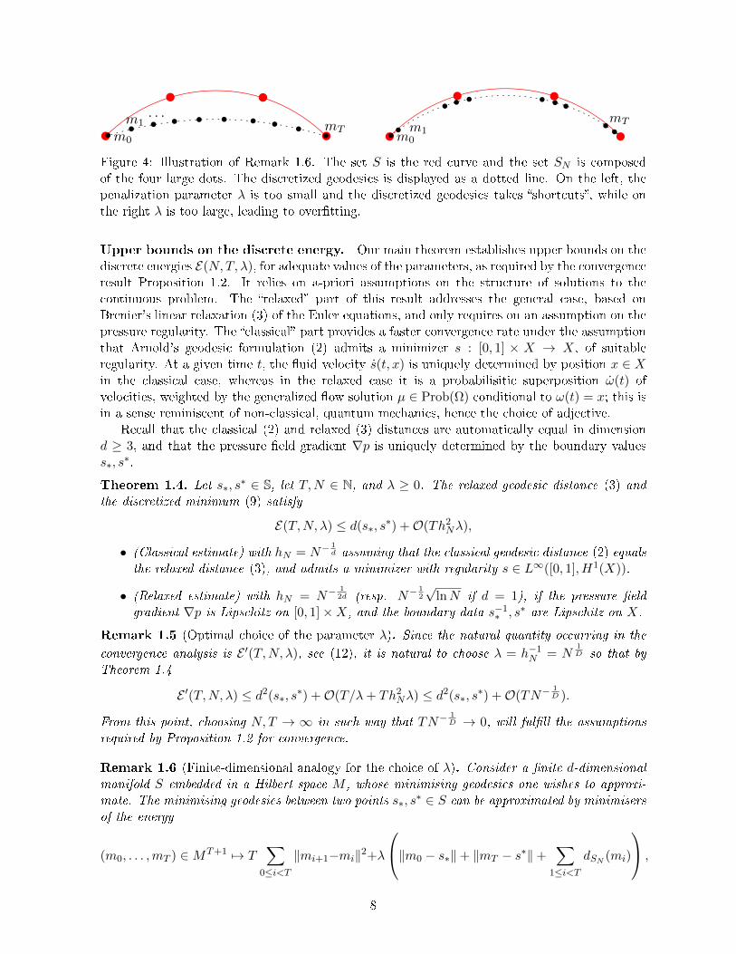
Figure 4: Illustration of Remark 1.6. The set S is the red curve and the set SN is composedof the four large dots. The discretized geodesics is displayed as a dotted line. On the left, thepenalization parameter λ is too small and the discretized geodesics takes shortcuts, while onthe right λ is too large, leading to overtting.

Upper bounds on the discrete energy. Our main theorem establishes upper bounds on thediscrete energies E(N,T, λ), for adequate values of the parameters, as required by the convergenceresult Proposition 1.2. It relies on a-priori assumptions on the structure of solutions to thecontinuous problem. The relaxed part of this result addresses the general case, based onBrenier's linear relaxation (3) of the Euler equations, and only requires on an assumption on thepressure regularity. The classical part provides a faster convergence rate under the assumptionthat Arnold's geodesic formulation (2) admits a minimizer s : [0, 1] × X → X, of suitableregularity. At a given time t, the uid velocity s(t, x) is uniquely determined by position x ∈ Xin the classical case, whereas in the relaxed case it is a probabilisitic superposition ω(t) ofvelocities, weighted by the generalized ow solution µ ∈ Prob(Ω) conditional to ω(t) = x; this isin a sense reminiscent of non-classical, quantum mechanics, hence the choice of adjective.

Recall that the classical (2) and relaxed (3) distances are automatically equal in dimensiond ≥ 3, and that the pressure eld gradient ∇p is uniquely determined by the boundary valuess∗, s

∗.

Theorem 1.4. Let s∗, s∗ ∈ S, let T,N ∈ N, and λ ≥ 0. The relaxed geodesic distance (3) and

the discretized minimum (9) satisfy

E(T,N, λ) ≤ d(s∗, s∗) +O(Th2

Nλ),

• (Classical estimate) with hN = N−1d assuming that the classical geodesic distance (2) equals

the relaxed distance (3), and admits a minimizer with regularity s ∈ L∞([0, 1], H1(X)).

• (Relaxed estimate) with hN = N−12d (resp. N−

12

√lnN if d = 1), if the pressure eld

gradient ∇p is Lipschitz on [0, 1]×X, and the boundary data s−1∗ , s∗ are Lipschitz on X.

Remark 1.5 (Optimal choice of the parameter λ). Since the natural quantity occurring in the

convergence analysis is E ′(T,N, λ), see (12), it is natural to choose λ = h−1N = N

1D so that by

Theorem 1.4

E ′(T,N, λ) ≤ d2(s∗, s∗) +O(T/λ+ Th2

Nλ) ≤ d2(s∗, s∗) +O(TN−

1D ).

From this point, choosing N,T → ∞ in such way that TN−1D → 0, will fulll the assumptions

required by Proposition 1.2 for convergence.

Remark 1.6 (Finite-dimensional analogy for the choice of λ). Consider a nite d-dimensionalmanifold S embedded in a Hilbert space M , whose minimising geodesics one wishes to approxi-mate. The minimising geodesics between two points s∗, s

∗ ∈ S can be approximated by minimisersof the energy

(m0, . . . ,mT ) ∈MT+1 7→ T∑

0≤i<T‖mi+1−mi‖2+λ

‖m0 − s∗‖+ ‖mT − s∗‖+∑

1≤i<TdSN (mi)

,

8

where SN is a sampling of the manifold S with N points. The choice of the optimal λ in term ofconvergence speed depends on the dimension of the manifold S and on the number of points N .Figure 4 illustrates that if λ is too small, the discrete geodesics takes shortcuts, while if λ is toolarge it forms clusters around points in the discretization SN . Note also that, for a xed N andλ→∞, the optimization problem becomes combinatorial.

Establishing the upper bounds of Theorem 1.4 requires one to construct, for each choice ofN,T , a candidate m ∈MT+1

N for the discrete problems (9) from a minimizer µ ∈ Prob(Ω) of thecontinuous problem (3). To do so, we approximate the probability measure µ by a measure µNuniformly supported over N paths. This amounts to solving a quantization problem [GG92] inthe innite-dimensional space Ω. Fortunately, the optimal speed of convergence of µN towardsµ can be bounded in terms of the box dimension D of the support of µ (see Denition 4.1). This

explains why the decay rate hN = N−1D in Theorem 1.4 depends, through the constant D, on

the structure of the problem solution µ.When the generalized ow µ is induced by a classical solution, as in (4), the particle tra-

jectories are determined by their initial position x ∈ X ⊆ Rd, so that µ is supported on ad-dimensional manifold, implying D = d. In the relaxed estimate however, the trajectories par-ticles obey a second order ordinary dierential equation (6) and are thus determined by theirinitial position and velocity (x, v) ∈ X ×Rd ⊆ R2d provided Picard-Lindelof/Cauchy-Lipschitz'stheorem applies [CL55]. The quantization dimension of the generalized ow is thus 2d in theworst case, but intermediate dimensions d < D < 2d are also common, see 5.

Outline. Propositions 1.1 and 1.2 are proved in 2. Theorem 1.4 is established in 3 (Classicalestimate) and in 4 (Relaxed estimate). Numerical experiments are presented 5.

Remark 1.7 (Monge-Ampere gravitation). Some models of reconstruction of the early universe[Bre11] involve actions of a form closely related to our discrete energy functional (9), for theparameter value λ = 2: ˆ 1

0

(1

2‖m(t)‖2 + inf

s∈S‖m(t)− s‖2

)dt.

2 Convergence analysis

We prove Proposition 1.1 in 2.1 and Proposition 1.2 in 2.2, on the length of chains of incom-pressible maps, and the convergence of generalized ows respectively.

2.1 Length of a chain of incompressible maps

The announced Proposition 1.1 immediately follows from Lemma 2.1 below. It relies on a thefollowing identity, valid for any elements a, b of a Hilbert space, and any ε > 0:

(1 + ε)−1‖a+ b‖2 ≤ ‖a‖2 + ε−1‖b‖2. (13)

Indeed subtracting the LHS to the RHS of (13) we obtain (1 + ε)−1‖ε 12a− ε− 1

2 b‖2 ≥ 0.

Lemma 2.1. For any T ∈ N∗, any penalization λ > 0, and any (m, s) ∈ (M× S)T+1 one has

T∑

0≤i<T‖si+1 − si‖2 ≤ (1 + 4T/λ)

T ∑0≤i<T

‖mi+1 −mi‖2 + λ∑

0≤i≤T‖mi − si‖2

. (14)

9

Proof. Let 0 ≤ i < T . Choosing a := si+1 − si, and b := mi+1 −mi − a, we obtain

(1 + ε)−1‖mi+1 −mi‖2 ≤ ‖si+1 − si‖2 + ε−1‖(si −mi)− (si+1 −mi+1)‖2

≤ ‖si+1 − si‖2 + 2ε−1(‖si −mi‖2 + ‖si+1 −mi+1‖2).

Summing over 0 ≤ i < T yields

(1 + ε)−1∑

0≤i<T‖mi+1 −mi‖2 ≤

∑0≤i<T

‖si+1 − si‖2 + 2ε−1∑

0≤i≤Tαi‖si −mi‖2,

with α0 = αT = 1, αi = 2 otherwise. Choosing ε = 4T/λ concludes the proof.

2.2 Convergence towards generalized solutions

This subsection is devoted to the proof of Proposition 1.2. The discrete optimization problem (9)is inspired by Arnold's formulation (2) of Euler equations as a minimizing geodesic problem overS. Our rst lemma shows that, in the equivalent form (24), it could as well be regarded as a dis-cretization of Brenier's relaxation (3). The terms W 2

2 (et#µm,Leb), where m ∈MT+1N and µm is

the induced generalized ow, can indeed be regarded as penalizations of the relaxed incompress-ibility constraint et#µ = Leb in (3). The other term W 2

2 ((e0, e1)#µm, (s∗, s∗)# Leb) enforces

the proximity between the two couplings (e0, e1)#µm and (s∗, s∗)# Leb on X2 as required in (3).

Lemma 2.2. Let m = (mi)Ti=0 ∈MT+1

N and µm ∈ Prob(ω) be the induced generalized ow. ThenE(T,N, λ;m) equals

ˆΩA(ω)dµm(ω)+λ

(ˆX|m0(x)−s∗(x)|2 + |mT (x)−s∗(x)|2dx+

∑1≤i<Tt=i/T

W 22 (et#µm,Leb)

). (15)

In addition,

W 22 ((e0, e1)#µm, (s∗, s

∗)# Leb) ≤ˆX|m0(x)− s∗(x)|2 + |mT (x)− s∗(x)|2dx. (16)

Proof. Mimicking (5) at the discrete level, we obtain

ˆΩA(ω)dµ(ω) =

1

N

∑1≤j≤N

ˆ 1

0|ωj(t)|2dt =

T

N

∑0≤i<T1≤j≤N

|mji+1 −m

ji |2 = T

∑0≤i<T

‖mi+1 −mi‖2,

On the other hand, Brenier's polar factorization theorem (10) yields W 22 (et #µm,Leb) = d2

S(m),which gives (24).

The Wasserstein distance from (e0, e1)#µm = (m0,m1)# Leb to (s∗, s∗)# Leb appears on

the LHS of (16). By denition, it is indeed bounded by the cost, appearing on the RHS,of the explicit transport plan π = ((m0,mT ), (s∗, s∗))# Leb ∈ Prob(X2 × X2), which sends(m0(x),mT (x)) 7→ (s∗(x), s∗(x)) for all x ∈ X.

Our next step is to estimate the average violation of incompressibility by the discrete solution.

Lemma 2.3. Let µm be the generalized ow associated to some m ∈MT+1N . Then

ˆ 1

0W 2

2 (et #µm,Leb) dt ≤ 1

4T 2E ′(T,N, λ;m).

10

Proof. Let t ∈ [0, 1], which we write t = (i+ α)/T with 0 ≤ i < T , 0 ≤ α ≤ 1. Then using (13)we obtain for any ε > 0,

W 22 (et #µm,Leb) = inf

s∈S‖(1−α)mi+αmi+1−s‖2 ≤ (1+ε)

(‖α(mi+1 −mi)‖2 + ε−1 inf

s∈S‖mi − s‖2

)Integrating over t ∈ [0, 1], and using that either α ≤ 1/2 or 1− α ≤ 1/2, we obtain

ˆ 1

0W 2

2 (et #µ,Leb)dt ≤ 1 + ε

T

∑0≤i<T

(1

4‖mi+1 −mi‖2 + ε−1 inf

s∈S‖mi − s‖2

)

which is precisely the announced estimate when ε = 4T/λ.

The convergence announced in Proposition 1.2, nally results from general compactness andcontinuity arguments.

Proof of Proposition 1.2. Let Tk, Nk, λk,mk, µk and D∗ be as in the statement of Proposition1.2. The sublevel sets of the action, such as for any ε > 0

µ ∈ Prob(Ω);

ˆΩA(ω)dµ(ω) ≤ D∗ + ε.

are weak-* sequentially compact by [Bre93]. Taking a subsequence if necessary, we assume that(µk) converges towards a µ∗ ∈ Prob(Ω), which thus satises

´ΩA dµ∗ ≤ D∗ + ε for any ε > 0,

hence´

ΩA dµ∗ ≤ D∗ as announced.The functional F : µ 7→ W 2

2 ((e0, e1)#µ, (s∗, s∗)# Leb) is weak-* continuous on Prob(Ω). By

(16) one has F (µk) ≤ 1λkE(Tk, Nk, λk;mk)→ 0 as k →∞, hence F (µ∗) = 0 which implies

(e0, e1)#µ∗ = (s∗, s∗)# Leb .

Similarly, the functional G : µ 7→´ 1

0 W22 (et #µ,Leb) dt is weak-* lower semi-continuous on

Prob(Ω), as follows from Fatou's lemma and the continuity of µ 7→ W 22 (et #µ,Leb) for any

t ∈ [0, 1]. By Lemma 2.3 one has G(µk)→ 0 as k →∞, hence G(µ∗) = 0 and therefore the limitgeneralizered ow obeys the incompressibility constraints

∀t ∈ [0, 1], et #µ = Leb .

3 Classical estimate

We establish in this section the rst part of our main result, Theorem 1.4. By assumption,we consider a minimizer s of the shortest path problem (2), and assume that it has regularitys ∈ L∞([0, 1], H1(X)). Let also T,N, λ be the discrete problem parameters.

Dene si := s(i/T ) for all 0 ≤ i ≤ T , and note that s0 = s∗ and sT = s∗. Let alsomi := PN (si), for all 0 ≤ i ≤ T , where PN : M → MN denotes the orthogonal projection. Thisconstruction is illustrated on Figure 5. The proof, short and elementary, proceeds by estimatingthe distance from mi to si and to mi+1, and then summing over the index 0 ≤ i ≤ T .

11

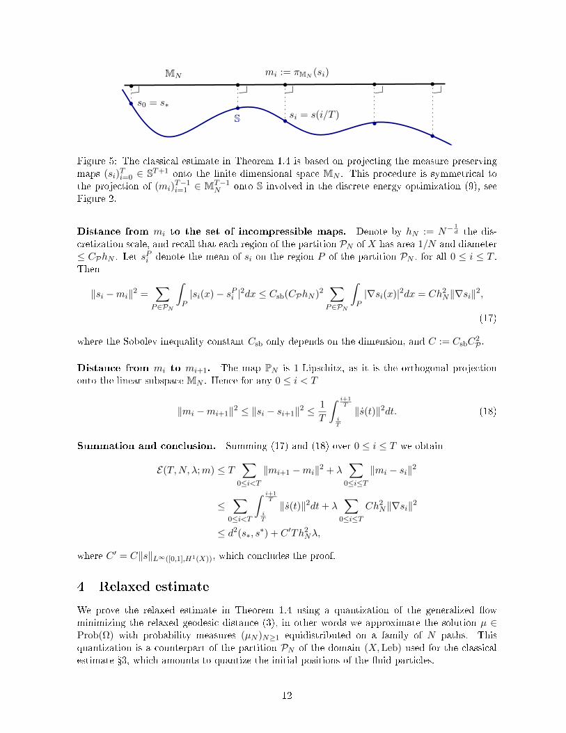
s0 = s∗si = s(i/T )

mi := πMN(si)

S

MN

Figure 5: The classical estimate in Theorem 1.4 is based on projecting the measure preservingmaps (si)

Ti=0 ∈ ST+1 onto the nite dimensional space MN . This procedure is symmetrical to

the projection of (mi)T−1i=1 ∈ MT−1

N onto S involved in the discrete energy optimization (9), seeFigure 2.

Distance from mi to the set of incompressible maps. Denote by hN := N−1d the dis-

cretization scale, and recall that each region of the partition PN of X has area 1/N and diameter≤ CPhN . Let s

Pi denote the mean of si on the region P of the partition PN , for all 0 ≤ i ≤ T .

Then

‖si −mi‖2 =∑P∈PN

ˆP|si(x)− sPi |2dx ≤ Csb(CPhN )2

∑P∈PN

ˆP|∇si(x)|2dx = Ch2

N‖∇si‖2,

(17)

where the Sobolev inequality constant Csb only depends on the dimension, and C := CsbC2P .

Distance from mi to mi+1. The map PN is 1-Lipschitz, as it is the orthogonal projectiononto the linear subspace MN . Hence for any 0 ≤ i < T

‖mi −mi+1‖2 ≤ ‖si − si+1‖2 ≤1

T

ˆ i+1T

iT

‖s(t)‖2dt. (18)

Summation and conclusion. Summing (17) and (18) over 0 ≤ i ≤ T we obtain

E(T,N, λ;m) ≤ T∑

0≤i<T‖mi+1 −mi‖2 + λ

∑0≤i≤T

‖mi − si‖2

≤∑

0≤i<T

ˆ i+1T

iT

‖s(t)‖2dt+ λ∑

0≤i≤TCh2

N‖∇si‖2

≤ d2(s∗, s∗) + C ′Th2

Nλ,

where C ′ = C‖s‖L∞([0,1],H1(X)), which concludes the proof.

4 Relaxed estimate

We prove the relaxed estimate in Theorem 1.4 using a quantization of the generalized owminimizing the relaxed geodesic distance (3), in other words we approximate the solution µ ∈Prob(Ω) with probability measures (µN )N≥1 equidistributed on a family of N paths. Thisquantization is a counterpart of the partition PN of the domain (X,Leb) used for the classicalestimate 3, which amounts to quantize the initial positions of the uid particles.

12

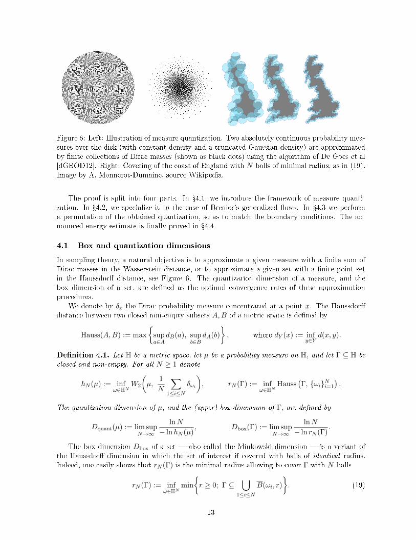
Figure 6: Left: Illustration of measure quantization. Two absolutely continuous probability mea-sures over the disk (with constant density and a truncated Gaussian density) are approximatedby nite collections of Dirac masses (shown as black dots) using the algorithm of De Goes et al[dGBOD12]. Right: Covering of the coast of England with N balls of minimal radius, as in (19).Image by A. Monnerot-Dumaine, source Wikipedia.

The proof is split into four parts. In 4.1, we introduce the framework of measure quanti-zation. In 4.2, we specialize it to the case of Brenier's generalized ows. In 4.3 we performa permutation of the obtained quantization, so as to match the boundary conditions. The an-nounced energy estimate is nally proved in 4.4.

4.1 Box and quantization dimensions

In sampling theory, a natural objective is to approximate a given measure with a nite sum ofDirac masses in the Wasserstein distance, or to approximate a given set with a nite point setin the Haussdor distance, see Figure 6. The quantization dimension of a measure, and thebox dimension of a set, are dened as the optimal convergence rates of these approximationprocedures.

We denote by δx the Dirac probability measure concentrated at a point x. The Haussdordistance between two closed non-empty subsets A,B of a metric space is dened by

Hauss(A,B) := max

supa∈A

dB(a), supb∈B

dA(b)

, where dY (x) := inf

y∈Yd(x, y).

Denition 4.1. Let H be a metric space, let µ be a probability measure on H, and let Γ ⊆ H beclosed and non-empty. For all N ≥ 1 denote

hN (µ) := infω∈HN

W2

(µ,

1

N

∑1≤i≤N

δωi

), rN (Γ) := inf

ω∈HNHauss

(Γ, ωiNi=1

).

The quantization dimension of µ, and the (upper) box dimension of Γ, are dened by

Dquant(µ) := lim supN→∞

lnN

− lnhN (µ), Dbox(Γ) := lim sup

N→∞

lnN

− ln rN (Γ).

The box dimension Dbox of a set also called the Minkowski dimension is a variant ofthe Haussdor dimension in which the set of interest if covered with balls of identical radius.Indeed, one easily shows that rN (Γ) is the minimal radius allowing to cover Γ with N balls

rN (Γ) := infω∈HN

min

r ≥ 0; Γ ⊆

⋃1≤i≤N

B(ωi, r)

. (19)

13

Box and Haussdor dimension coincide for compact manifolds, but dier in general. For instance,all countable sets have Haussdor dimension zero, whereas one can check that

Dbox

(([0, 1] ∩Q)d

)= d, Dbox

(1

n; n ∈ N∗

)=

1

2.

The quantization dimension of a measure is bounded above by the box dimension of itssupport, as shows the following elementary result of quantization theory. We refer the reader to[GG92] for more details on this rich subject.

Proposition 4.2. Let H be a metric space, and let µ ∈ Prob(H) be supported on a set Γ. ThenDquant(µ) ≤ max2, Dbox(Γ). More precisely for any D > 0, one has as N →∞

rN (Γ) = O(N−1D ) ⇒ hN (µ) = O

N−

1D if D > 2,

N−12

√lnN if D = 2,

N−12 if D < 2.

(20)

Proof. Let N ∈ N be xed. For each 1 ≤ i ≤ N let Mi ⊆ H be a set of i points such thatΓ ⊆ ∪ω∈MiB(ω, 2ri), with ri := ri(Γ). We construct a sequence of points ωi ∈ H, and anincreasing sequence of measures ρi supported on Γ and of mass i/N , inductively starting withi = N and nishing with i = 1. Initialization: ρN := µ.

Induction: for each 1 ≤ i ≤ N , we construct ωi and ρi−1 in terms of ρi. Let indeed ωi ∈Mi

be such that Bi := B(ωi, 2ri) satises ρi(Bi) ≥ 1/N . Such a point exists since |ρi| = i/N ,#(Mi) = i, and supp(ρi) ⊆ Γ. Then let ρi−1 := ρi− 1

Nρi(Bi)ρi, so that ρi−ρi−1 is a non-negative

measure of mass 1N supported on Bi. One has

hN (µ)2 ≤W 22

(µ,

1

N

∑1≤i≤N

δωi

)≤

∑1≤i≤N

W 22

(ρi − ρi−1,

1

Nδωi

)≤ 1

N

∑1≤i≤N

(2ri)2.

The comparison (20) of the decay rates of hN (µ) and rN (Γ) immediately follows. Finally thecomparison of the dimensions follows from (20).

4.2 Quantization dimension of a generalized ow

We specialize in this subsection the measure µ, support Γ and embedding metric space H towhich we apply the results of 4.1. Let µ ∈ Prob(Ω) be a generalized ow minimizing therelaxed geodesic distance (3). This measure is concentrated on the set Γ of paths obeyingNewton's second law of motion

Γ := ω ∈ C2([0, 1], X); ∀t ∈ [0, 1], ω(t) = −∇p(t, ω(t)), (21)

where the pressure gradient ∇p : [0, 1] × X → Rd is assumed to have Lipschitz regularity,following the assumptions of Theorem 1.4. We regard Γ as embedded in the Hilbert spaceH := H1([0, 1],Rd), which plays a natural role in the problem of interest (3) and is equippedwith the norm

‖ω‖2H :=

ˆ 1

0|ω|2 + |ω|2.

Note that H continuously embeds in C0([0, 1],Rd), hence the evaluation maps et : H→ Rd : ω 7→ω(t) are continuous with a common Lipschitz constant denoted Ce.

14

Notation 4.3 (Problem constants). The following quantities are referred to as the problemconstants: the dimension d, the constant CP related to the partitions, the Lipschitz regularityconstants C∗ and C

∗ of the boundary conditions s−1∗ and s∗, the maximum norm and the Lipschitz

regularity regularity constant of the pressure gradient ∇p. Given two expressions A,B, we writeA . B i A ≤ CB for some constant C that only depends on the problem constants.

Using a general existence and stability result for ODEs, Lemma 4.4, we show that Γ is inbijection with a compact subset of R2d, in Lemma 4.5.

Lemma 4.4. Let F ∈ C0([0, 1] × Rn,Rn) be Lipscshitz in the second variable, uniformly withrespect to the rst variable: ∃L,∀t ∈ [0, 1],∀y1, y2 ∈ Rn, |F (t, y1)−F (t, y2)| ≤ L|y1−y2|. Then themap Rn → L2([0, 1],Rn), associating to each y0 ∈ Rn the solution to the ODE y′(t) = F (t, y(t))with initial condition y(0) = y0, is bi-Lipschitz onto its image with regularity constant eL.

Proof. The Picard-Lindelof/Cauchy-Lipschitz Theorem [CL55] guarantees the existence of aunique solution to the considered ODE. If y1, y2 are two such solutions, then for any t ∈ [0, 1]

|y1(t)− y2(t)| = |F (t, y1(t))− F (t, y2(t))| ≤ L|y1(t)− y2(t)|

Thus for any t ∈ [0, 1]

e−Lt|y1(0)− y2(0)| ≤ |y1(t)− y2(t)| ≤ eLt|y1(0)− y2(0)|,

hence by integration over t ∈ [0, 1], as announced

e−L|y1(0)− y2(0)| ≤ ‖y1 − y2‖L2([0,1]) ≤ eL|y1(0)− y2(0)|.

The image of the generalized ow µ by the map of initial position and momentum, used inthe next lemma, is often called a minimal measure [BFS09].

Lemma 4.5. The map E0 : Γ→ X ×Rd : ω 7→ (ω(0), ω(0)) is bijective and bi-Lipschitz onto itsimage, which is a compact set. The Lipschitz régularity constants, and the image diameter, canbe bounded in terms of the problem constants, see Notation 4.3.

Proof. The function F (t, x, v) := (v,−∇p(t, x)) is Lipschitz on [0, 1]×X ×Rd, with a regularityconstant determined by that of ∇p. It can be extended to [0, 1]× R2d. Applying Lemma 4.4 toF in dimension n = 2d, we obtain as announced that E0 is bi-Lipschitz onto its image. Notethat the norm ‖(ω, ω)‖L2([0,1]) appearing in this estimate is precisely ‖ω‖H.

By construction, ω(t) and ω(t) are uniformly bounded for all ω ∈ Γ, and all t ∈ [0], respec-tively by the diameter of X and the maximum norm of ∇p. This implies an upper bound onω(0), observing for instance that

|ω(0)− ω(1)| =∣∣∣∣ˆ 1

0ω(t) dt

∣∣∣∣ ≥ |ω(0)| −ˆ 1

0|ω(t)− ω(0)|dt ≥ |ω(0)| −

ˆ 1

0|ω(t)|dt.

As announced, the image of Γ by E0 is bounded, hence compact since it is clearly closed.

Since there is no ambiguity, we denote in the rest of this section hN := hN (µ). The infor-mation gathered on the set Γ supporting µ yields upper and lower bounds on the decay rate of(hN ), obtained respectively in Corollary 4.6 and Proposition 4.7.

Corollary 4.6. One has hN . N−12d (resp. hN . N−

12

√lnN if d = 1) for all N ≥ 2.

15

Proof. By Lemma 4.5, the set Γ is in bi-Lipschitz bijection with a compact set K ⊆ R2d. HencerN (Γ) . rN (K) . N−

12d , and the upper estimate follows from (20).

The quantization scale hN is also bounded below, and is minimal for classical solutions.

Proposition 4.7. One has hN & N−1d for all N ≥ 1. If the generalized ow µ in fact represents

a classical solution s to Euler's equations, and ∇s is bounded on [0, 1] × X, then this lower

estimate is sharp: hN . N−1d .

Proof. Since X is a domain of unit area, there exists c > 0 depending only on the dimension dand such that W2(Leb, νN ) ≥ cN− 1

d for any measure νN supported at N points of Rd. The rstpoint follows: for any measure µN supported at N points of H

cN−1d ≤W2(Leb, e0 #µN ) = W2(e0 #µ, e0 #µN ) ≤ CeW2(µ, µN ) = CehN .

Second point: for each x ∈ X, introduce the path ωx : [0, 1] → Rd : t 7→ s(t, x). ThenΦ : (X,Leb) → (Γ, µ) : x 7→ ωx is measure preserving and Lipschitz, with regularity constantdenoted CΦ (which we regard as a problem constant). Let νN be a discrete probability measure,with one Dirac mass of weight 1/N in each region of the partition PN . Since these regions havediameter ≤ CPN−

1d , we conclude that

hN ≤W2(µ,Φ#νN ) = W2(Φ# Leb,Φ#νN ) ≤ CΦW2(Leb, νN ) ≤ CΦCPN− 1d .

4.3 Permutation of the quantization of µ and boundary conditions

We have shown 4.2 that the generalized ow, solution to Brenier's relaxation of Euler's equations(3), could be approximated (quantized) by a nite family of particle paths, with a controlledconvergence rate. This is not yet sucient however to construct a good candidate for the discreteenergy (8), despite its relaxed reformulation (24). For that purpose one needs to permute thepaths, so as to match the boundary conditions, as required by the energy term (16).

We show in Lemma 4.8 that an optimal quantization exists, we suitably permute it in Lemma4.9 and estimate a rst boundary term, and we estimate the second boundary term in Proposition4.10. In this subsection and the next, we x the integer N and allow ourselves a slight abuseof notation: elements ωj , Pj , ρj , . . . indexed by 1 ≤ j ≤ N do implicitly depend on N , althoughthat second index ωNj , P

Nj , ρ

Nj , . . . is omitted for readability.

Lemma 4.8. The inmum dening hN is attained, see Denition 4.1. As a result there exists(ωj)

Nj=1 ∈ HN and probability measures (ρj)

Nj=1 on Γ such that

µ =1

N

∑1≤j≤N

ρj h2N =

1

N

∑1≤j≤N

ˆΓ‖ω − ωj‖2H dρj(ω) (22)

Furthermore, ωj is the barycenter of ρj for each 1 ≤ j ≤ N .

Proof. Let (ωj)Nj=1 be a candidate quantization, and let π be the transport plan associated to

W 22 ( 1

N

∑Nj=1 δωj , µ). Then the measures ρj : A 7→ N π(ωj × A), 1 ≤ j ≤ N , are probabilities

which average to µ, and the transport cost is the RHS of (22). The quantization energy, i.e.the squared Wasserstein distance, is decreased when replacing ωj with the barycenter bj of ρj ,

1 ≤ j ≤ N , by the amount 1N

∑Nj=1 |ωj−bi|2. Hence ωj = bj for all 1 ≤ j ≤ N if the quantization

is optimal. Note also that the barycenter of ρj belongs to G := Hull(Γ) by construction.

16

Since Γ is a compact subset of a Hilbert space, the convex hull closure G is also compact, forthe strong topology induced by ‖ · ‖H. The quantization energy (ωj)

Nj=1 7→ W 2

2 ( 1N

∑Nj=1 δωj , µ)

attains its minimum on GN by compactness, and by the previous argument it is the globalminimum on HN .

Let µN denote the equidistributed probability on the set ωj ; 1 ≤ j ≤ N of Lemma 4.8.

Lemma 4.9. The paths (ωj)Nj=1 of the quantization µN , and the regions (Pj)

Nj=1 of the partition

PN , can be indexed in such way that∑1≤j≤N

ˆPj

|ωj(0)− s∗(x)|2dx . h2N . (23)

Proof. Let (Pj)Nj=1 be an arbitrary indexation of PN . Let aj be the barycenter of region Pj , and

bj the barycenter of the image region s∗(bj). For any 1 ≤ j ≤ N one has by assumptionˆPj

|bj − s∗(x)|2dx ≤ˆPj

|s∗(aj)− s∗(x)|2dx ≤ C2∗

ˆPj

|aj − x|2dx ≤1

N(C∗CPN

− 1d )2,

where C∗ denotes the Lipschitz regularity constant of s−1∗ . Denoting by νN the discrete measure

equidistributed at the N points (bj)Nj=1, we obtain

W2(νN ,Leb) ≤√√√√ ∑

1≤j≤N

ˆPj

|bj − s∗(x)|2dx . N−1d .

On the other hand W2(Leb, e0 #µN ) ≤ CeW2(µ, µN ) = CehN . Thus W2(νN , e0 #µN ) . hN ,

since W2 denes a distance, and since hN & N−1d by Proposition 4.7. This optimal transport

problem between the discrete measures νN and e0 #µN determines an optimal assignment ΓN →BN . Up to a permutation of the paths (ωj)

Nj=1, we assume that this assignment is represented

by the common indexation (ωj)Nj=1 of ΓN and (bj)

Nj=1 of BN . Finally∑

1≤j≤N

ˆPj

|ωj(0)− s∗(x)|2dx =∑

1≤j≤N

ˆPj

|bj − s∗(x)|2dx+W 22 (νN , e0 #µN ) . h2

N .

Proposition 4.10. Using the indexation of Lemma 4.9, one has∑1≤j≤N

ˆPj

|ωj(1)− s∗(x)|2dx ≤ Ch2N .

Proof. The generalized boundary condition of (3) states that ω(1) = s∗∗(ω(0)) for µ-almost everyω ∈ Γ, where s∗∗ := s∗ s−1

∗ . Denoting by C∗∗ the Lipschitz regularity constant of s∗∗, we obtainfor any 1 ≤ j ≤ N and any x ∈ X

|ωj(1)− s∗(x)|2 =

∣∣∣∣ˆΓs∗∗(ω(0))− s∗(x) dρj(ω)

∣∣∣∣2 ≤ ˆΓ|s∗∗(ω(0))− s∗(x)|2 dρj(ω)

≤ (C∗∗ )2

ˆΓ|ω(0)− s∗(x)|2 dρj(ω) ≤ 2(C∗∗ )

2

(ˆΓ|ω(0)− ωj(0)|2 dρj(ω) + |ωj(0)− s∗(x)|2

).

By summation and integration we conclude, using Lemma 4.9 in the second line,∑1≤j≤N

ˆPj

|ωj(1)− s∗(x)|2 dx .∑

1≤j≤N

1

N

ˆΓ|ωj(0)− ω(0)|2 dρj(ω) +

∑1≤j≤N

ˆPj

|ωj(0)− s∗(x)|2 dx

≤ C2eW

22 (µN , µ) + Ch2

N . h2N .

17

4.4 Final estimate

We conclude in this subsection the proof of Theorem 1.4 (Relaxed estimate). Let µ ∈ Prob(Ω)be a generalized ow minimizing (3), with an associated Lipschitz pressure gradient. We x theparameters (T,N), and consider an optimal quantization µN supported on N paths (ωj)

Nj=1 as

in Lemma 4.8. For each 0 ≤ i ≤ T , let mi ∈ N be the piecewise constant map on the partitionPN dened by

∀1 ≤ j ≤ N, ∀x ∈ Pj , mi(x) := ωj(i/T ).

In the following, we bound each of the terms of the energy E(T,N, λ;m) ≥ E(T,N, λ). ByLemma 4.9 and Proposition 1.2, one has respectively

‖m0 − s∗‖2 . h2N , ‖mT − s∗‖2 . h2

N .

Regarding the distance to incompressible maps, one has for any 1 ≤ i < T , with t := i/T

infs∈S‖mi − s‖ = W2(Leb, et #µN ) = W2(et #µ, et #µN ) ≤ CeW2(µ, µN ) = CehN .

We use the Cauchy-Schwartz inequality to bound the action:

T∑

0≤i<T‖mi+1 −mi‖2 =

1

N

∑1≤j≤N

T∑

0≤i<T

∣∣∣∣ωj( i+ 1

T

)− ωj

(i

T

)∣∣∣∣2 ≤ 1

N

∑1≤j≤N

ˆ 1

0|ωj(t)|2dt

=1

N

∑1≤j≤N

ˆ 1

0

∣∣∣∣ˆΓω dρj(ω)

∣∣∣∣2 ≤ 1

N

∑1≤j≤N

ˆ 1

0

ˆΓ|ω|2 dρj(ω) dt = d2(s∗, s

∗).

Concluding, the value E(T,N, λ) is bounded by

T∑

0≤i<T‖mi+1−mi‖2+λ

‖m0 − s∗‖2 + ‖mT − s∗‖2 +∑

1≤i<Tinfs∈S‖mi − s‖2

≤ d2(s∗, s∗)+O(Th2

Nλ).

5 Numerical experiments

5.1 Minimization algorithm and choice of penalization

We rely on a quasi-Newton method to compute a (local) minimum of the discretized problem (9),as summarized in Algorithm 1. This means that we need to compute the value of the functional

m ∈MT+1N 7→ T

∑0≤i<T

‖mi+1 −mi‖2 + λ

(‖m0 − s∗‖2 + ‖mT − s∗‖2 +

∑1≤i<T

d2S(mi)

). (24)

and its gradient, where d2S(m) = infs∈S ‖m− s‖2. The only diculty is to evaluate the squared

distance d2S to the set of measure-preserving vector elds and its gradient. As explained in the

introduction, Brenier's Polar Factorization Theorem implies that for any vector-valued functionm ∈M,

d2S(m) = W 2

2 (m# Leb,Leb).

When m belongs to MN , the measure m# Leb is nitely supported, and the computation of theWasserstein distance can be performed using a solver for semi-discrete optimal transport, suchas [AHA98, Mer11, dGBOD12, Lév14]. The next proposition gives an explicit formulation forthe gradient in term of the optimal transport plan. Note that the expression of the gradient of

18

the semi-discrete Kantorovitch functional with respect to the position of the points also appearsin the appendix of [dGBOD12].

Recall thatMN is the set of piecewise constant functions on the tessellation PN := (Pj)1≤j≤Nof X. The diagonal DN in MN is the set of functions m in MN such that m(Pj) = m(Pk) forsome j 6= k. The set MN \ DN is a dense open set in MN .

Proposition 5.1. The functional d2S is dierentiable almost everywhere on MN and continuously

dierentiable on MN \ DN . The gradient of d2S at m ∈MN \ DN is explicit: with xj = m(Pj),

∇d2S(m)

∣∣Pj

= 2(xj − bary(T−1(xj))) (25)

where T : X → m(X) is the piecewise constant optimal transport map between Leb and thenitely supported measure m# Leb, and bary(S) =

´S xdx/Leb(S) is the isobarycenter of S

Proof. The functional F := d2S − ‖ · ‖2 is concave as an inmum of linear functions:

F(m) = d2S(m)− ‖m‖2 = inf

s∈S‖m− s‖2 − ‖m‖2 = inf

s∈S

[−2〈m|s〉+ ‖s‖2

],

where 〈·, ·〉 denotes the L2(X) scalar product. This implies in particular that F and therefored2S is dierentiable almost everywhere on MN . Given m in MN \ DN , dene xj = m(Pj) and

let T : X → Rd be the optimal transport plan from Leb to m# Leb = 1N

∑Nj=1 δxj . The

transport plan is indeed always representable by a function when the source measure is absolutelycontinuous with respect to the Lebesgue measure. Let Vj = T−1(xj) be the partition ofX inducedby this transport plan. Then

F(m) = W 22 (m# Leb,Leb)− ‖m‖2 =

N∑j=1

ˆVj

‖xj − x‖2 − ‖xj‖2dx

= 〈m|G(m)〉+

N∑j=1

ˆVj

‖x‖2dx

where G(m) ∈ MN is the piecewise constant function on X given by G(m)|Pj = −2 bary(Vj).

For any m′ in MN and x′j = m′(Vj), one has

F(m′) = W 22 (m′# Leb,Leb)− ‖m′‖2 ≤

N∑j=1

ˆVj

‖x′j − x‖2 − ‖x′j‖2dx

= F(m) + 〈m′ −m|G(m)〉

This shows that G(m) belongs to the superdierential to F at m. In addition, by the continuityof optimal transport plans, the map m ∈MN \DN 7→ G(m) is continuous. To summarize, on theopen domain MN \DN the concave function F possesses a continuous selection of supergradient.This implies that F is of class C1 on this domain, with ∇F (m) = G, and the result follows.

Remark 5.2 (Computation of d2S). The computation of the squared distance to measure-preserving

maps d2S and its gradient rely on the variational approach used in the proof of the above propo-

sition. We use the CGAL library [cga] to evaluate F and its rst and second derivatives, and asimple damped Newton's algorithm to compute its maximum. The implementation is available athttps://github.com/mrgt/PyMongeAmpere.

19

Construction of the initial solution Since the discrete energy (8) is non-convex, the con-struction of the inital guess is important. We follow a time-renement strategy already used byBrenier [Bre08] to construct a good initial guess. Assuming that we have already a local mini-mizer for Tk = 2k+1, we use linear interpolation to construct an initial guess for Tk+1 = 2k+1+1.The optimization is then performed from this inital guess, using a quasi-Newton algorithm forthe energy (8).

Choice of the penalization parameter The optimal choice of λ in (8) depends on thequantization dimension D = Dquant(µ) of the generalized solution µ ∈ Prob(Ω) that one expects

to recover: namely λN = N−1D , see Remark 1.5. We call D the ow dimension, and regard it as

as the intrinsic dimensionality of the problem which determines its computational diculty. Fora classical solution, this dimension agrees with the ambient dimension i.e. D = d, while for anon-deterministic solution the quantization dimension can be up to 2d. Intermediate dimensionsd < D < 2d are also common [Bre89]. In our numerical experiments we set λN = N

13 , a decision

justied a-posteriori by the numerical estimation of the quantization dimension of the computedsolution, see Figure 8.

Note that the numerical error in (1.5) is governed (for a xed number T of time steps) by

the quantity λ−1 + h2Nλ, and that hN = O(N−

12d ) under the assumptions of Theorem 1.4. The

choice λN = N1α thus yields a convergent scheme whenever α > d, although convergence rates

are improved if α is close to the ow dimension D, so that λN ≈ N1D ≈ h−1

N .

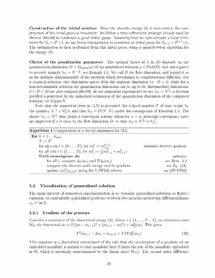
Algorithm 1 Computation of a (local) minimizer for (24).

For k = 1 . . . kmax

T := 2k

for all even t ∈ 0, . . . , T, let mki := mk−1

i/2 initialize discrete geodesic

for all odd t ∈ 1, . . . , T, let mki := 1

2(mki−1 +mk

i+1)Until convergence do optimize

for all i, compute dS(mi) and ∇dS(mi) see Rem. 5.2compute the discrete path energy and its gradient see Eq. (24)update (mk

i )0≤t≤T using the L-BFGS scheme see [BLNZ95]

5.2 Visualization of generalized solution

The main interest of numerical experimentation is to visualize generalized solutions to Euler'sequation, or equivalently generalized geodesics between two measure-preserving dieomorphismss∗, s

∗ in S.

5.2.1 Gradient of the pressure

Consider a minimizer of the discretized energy (8). Given i ∈ 1, . . . , T − 1, mi minimizes overMN the functional m 7→ T (‖m−mi−1‖2 + ‖mi+1 −m‖2) + λd2

S(m). This gives

T 2(mi−1 − 2mi +mi+1) = Tλ∇d2S(mi). (26)

This equation is a discretized counterpart of the rule that the acceleration of a geodesic on anembedded manifold, is normal to that manifold (here S plays the role of the manifold, embeddedin M, which is internally approximated by the linear space MN ). The second order dierence

20

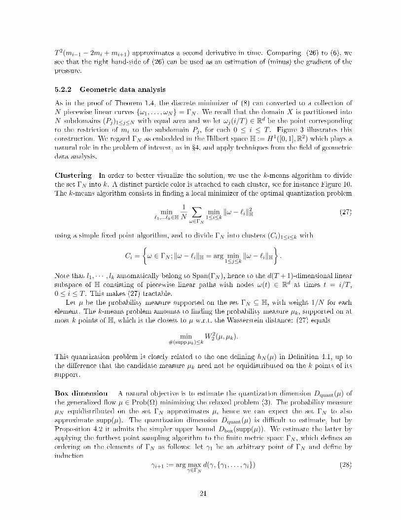
T 2(mi−1 − 2mi + mi+1) approximates a second derivative in time. Comparing (26) to (6), wesee that the right hand-side of (26) can be used as an estimation of (minus) the gradient of thepressure.

5.2.2 Geometric data analysis

As in the proof of Theorem 1.4, the discrete minimizer of (8) can converted to a collection ofN piecewise-linear curves ω1, . . . , ωN = ΓN . We recall that the domain X is partitioned intoN subdomains (Pj)1≤j≤N with equal area and we let ωj(i/T ) ∈ Rd be the point correspondingto the restriction of mi to the subdomain Pj , for each 0 ≤ i ≤ T . Figure 3 illustrates thisconstruction. We regard ΓN as embedded in the Hilbert space H := H1([0, 1],R2) which plays anatural role in the problem of interest, as in 4, and apply techniques from the eld of geometricdata analysis.

Clustering In order to better visualize the solution, we use the k-means algorithm to dividethe set ΓN into k. A distinct particle color is attached to each cluster, see for instance Figure 10.The k-means algorithm consists in nding a local minimizer of the optimal quantization problem

min`1,...`k∈H

1

N

∑ω∈ΓN

min1≤i≤k

‖ω − `i‖2H (27)

using a simple xed point algorithm, and to divide ΓN into clusters (Ci)1≤i≤k with

Ci =

ω ∈ ΓN ; ‖ω − `i‖H = arg min

1≤j≤k‖ω − `i‖H

.

Note that l1, · · · , lk automatically belong to Span(ΓN ), hence to the d(T + 1)-dimensional linearsubspace of H consisting of piecewise linear paths with nodes ω(t) ∈ Rd at times t = i/T ,0 ≤ i ≤ T . This makes (27) tractable.

Let µ be the probability measure supported on the set ΓN ⊆ H, with weight 1/N for eachelement. The k-means problem amounts to nding the probability measure µk, supported on atmost k points of H, which is the closest to µ w.r.t. the Wasserstein distance: (27) equals

min#(suppµk)≤k

W 22 (µ, µk).

This quantization problem is closely related to the one dening hN (µ) in Denition 4.1, up tothe dierence that the candidate measure µk need not be equidistributed on the k points of itssupport.

Box dimension A natural objective is to estimate the quantization dimension Dquant(µ) ofthe generalized ow µ ∈ Prob(Ω) minimizing the relaxed problem (3). The probability measureµN equidistributed on the set ΓN approximates µ, hence we can expect the set ΓN to alsoapproximate supp(µ). The quantization dimension Dquant(µ) is dicult to estimate, but byProposition 4.2 it admits the simpler upper bound Dbox(supp(µ)). We estimate the latter byapplying the furthest point sampling algorithm to the nite metric space ΓN , which denes anordering on the elements of ΓN as follows: let γ1 be an arbitrary point of ΓN and dene byinduction

γi+1 := arg maxγ∈ΓN

d(γ, γ1, . . . , γi) (28)

21

As in Denition 4.1, denote by ri = ri(ΓN ) is the smallest r ≥ 0 such that ΓN can be covered byi balls of radius r. For 1 i N , the ratio log(i)/ log(1/ri(ΓN )) is expected to approximatelog(i)/ log(1/ri(supp(µ))) and thus the desired Dbox(suppµ).

Lemma 5.3. Let εi := maxγ∈Γ d(γ, γ1, . . . , γi), where γi is dened as in (28). Then,(1− log(2)

log(1/εi)

)log(i)

log(1/εi)≤ log(i)

log(1/ri)≤ log(i)

log(1/εi)

Proof. By construction, ri ≤ εi. Moreover, the balls centered at the points γ1, . . . , γi and withradius εi/2 are disjoint, so that ri ≥ εi/2.

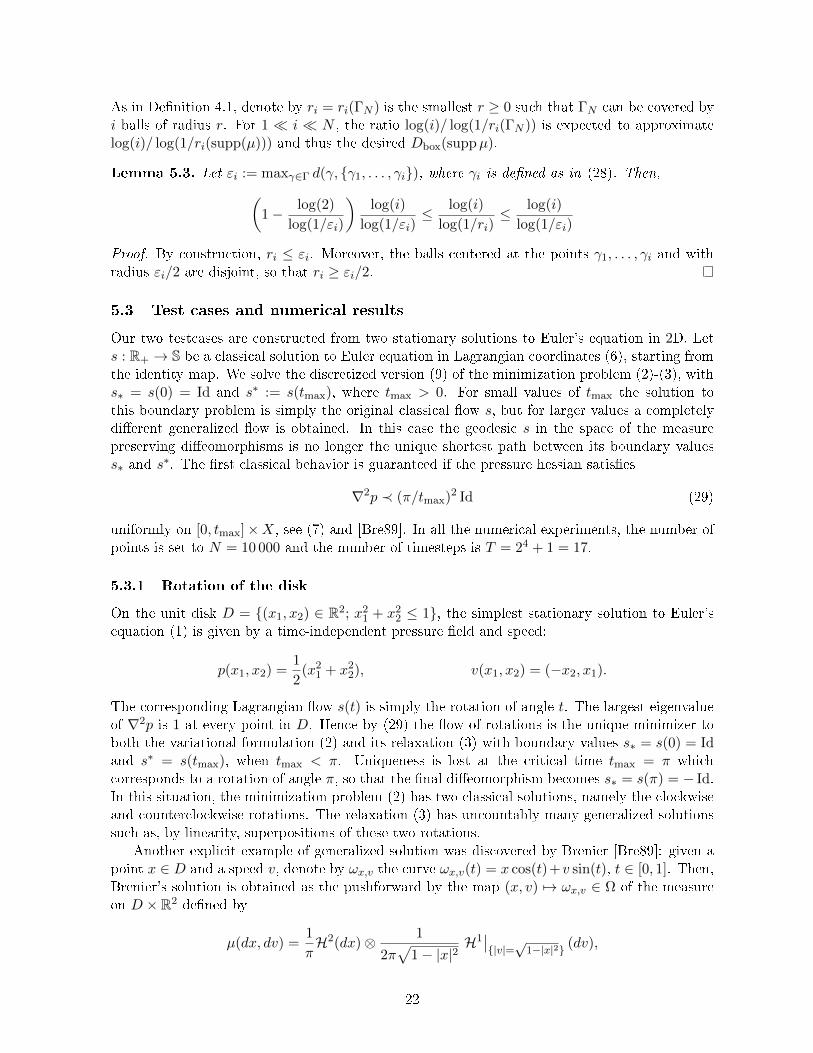
5.3 Test cases and numerical results

Our two testcases are constructed from two stationary solutions to Euler's equation in 2D. Lets : R+ → S be a classical solution to Euler equation in Lagrangian coordinates (6), starting fromthe identity map. We solve the discretized version (9) of the minimization problem (2)-(3), withs∗ = s(0) = Id and s∗ := s(tmax), where tmax > 0. For small values of tmax the solution tothis boundary problem is simply the original classical ow s, but for larger values a completelydierent generalized ow is obtained. In this case the geodesic s in the space of the measurepreserving dieomorphisms is no longer the unique shortest path between its boundary valuess∗ and s

∗. The rst classical behavior is guaranteed if the pressure hessian satises

∇2p ≺ (π/tmax)2 Id (29)

uniformly on [0, tmax]×X, see (7) and [Bre89]. In all the numerical experiments, the number ofpoints is set to N = 10 000 and the number of timesteps is T = 24 + 1 = 17.

5.3.1 Rotation of the disk

On the unit disk D = (x1, x2) ∈ R2; x21 + x2

2 ≤ 1, the simplest stationary solution to Euler'sequation (1) is given by a time-independent pressure eld and speed:

p(x1, x2) =1

2(x2

1 + x22), v(x1, x2) = (−x2, x1).

The corresponding Lagrangian ow s(t) is simply the rotation of angle t. The largest eigenvalueof ∇2p is 1 at every point in D. Hence by (29) the ow of rotations is the unique minimizer toboth the variational formulation (2) and its relaxation (3) with boundary values s∗ = s(0) = Idand s∗ = s(tmax), when tmax < π. Uniqueness is lost at the critical time tmax = π whichcorresponds to a rotation of angle π, so that the nal dieomorphism becomes s∗ = s(π) = − Id.In this situation, the minimization problem (2) has two classical solutions, namely the clockwiseand counterclockwise rotations. The relaxation (3) has uncountably many generalized solutionssuch as, by linearity, superpositions of these two rotations.

Another explicit example of generalized solution was discovered by Brenier [Bre89]: given apoint x ∈ D and a speed v, denote by ωx,v the curve ωx,v(t) = x cos(t)+v sin(t), t ∈ [0, 1]. Then,Brenier's solution is obtained as the pushforward by the map (x, v) 7→ ωx,v ∈ Ω of the measureon D × R2 dened by

µ(dx, dv) =1

πH2(dx)⊗ 1

2π√

1− |x|2H1∣∣|v|=√

1−|x|2 (dv),

22

where Hk denotes the k-dimensional Hausdor measure. In particular, the quantization dimen-sion of the solution is 3 = 2 + 1. We refer to [BFS09] for more examples of optimal ows, andconstruct four dimensional one. Let µr be dened by combining (i) a classical rotation on theannulus D \D(r), with D(r) = x ∈ R2; |x| ≤ r and (ii) Brenier's solution rescaled by a factorr on the disc D(r). Then µr is an optimal generalized ow of quantization dimension 3, whereasthe averaged ow

´ 10 µrdr is also optimal by linearity, and has quantization dimension 4.

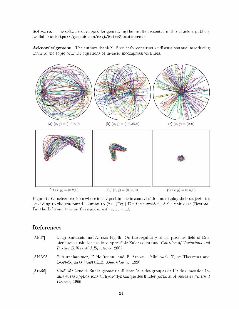
Numerical results The numerical solutions computed by our algorithm for the critical timetmax = π are highly non-deterministic. To see this, we select a small neighborhood around severalpoints in the unit disk D and look at the trajectories emanating from this small neighborhood.As shown in Figure 7, the trajectories emanating from each neighborhood at initial time tendto ll up the disk at intermediate times before gathering again on a small neighborhood at naltime. In addition, each indivual trajectory looks like an ellipse, as in Brenier's explicit solution.Second, we estimate the box dimension of the support of the numerical solution (as explained in5.2). The estimated dimension is slightly above 3.

5.3.2 Beltrami ow on the square

On the unit square S = [−1/2, 1/2]2, we consider the Beltrami ow constructed from the time-independent pressure and speed:

p(x1, x2) =1

2(sin(πx1)2 + sin(πx2)2)

v(x1, x2) = (− cos(πx1) sin(πx2), sin(πx1) cos(πx2))

The maximum eigenvalue of the pressure Hessian ∇2p is π2, and [Bre89] implies that the asso-ciated ow is minimizing between s∗ = s(0) = Id and s∗ = s(tmax) for tmax ≤ 1. Because thesquare has much less symmetries than the disk, generalized solutions constructed from this oware not as well understood as those occuring from rotations of the disk.

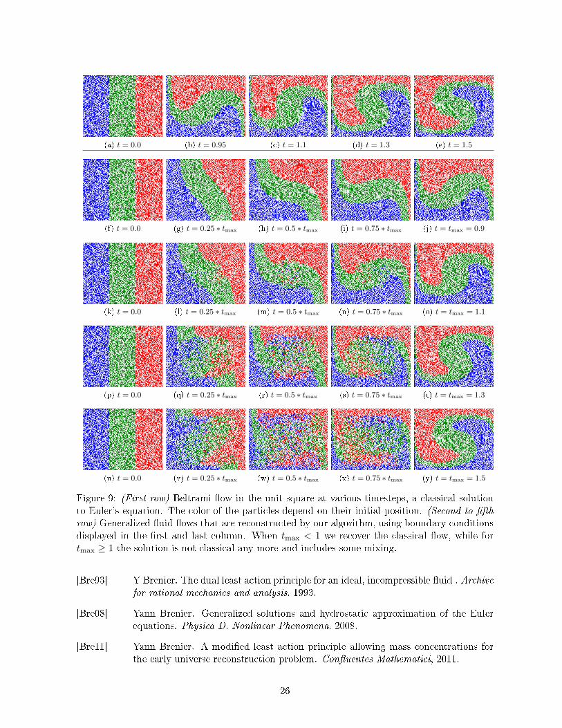
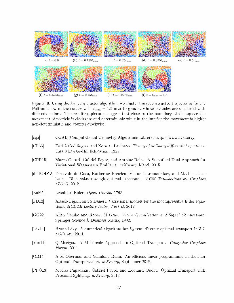
Numerical results Our numerical results suggest the following observations. First, as shownin Figure 9, the computed solutions with boundary values s∗ = Id and s∗ = s(tmax) approximatethe classical ow if tmax < 1, and are non-deterministic generalized ows if tmax > 1. Thissuggests the sharpness of the bound given by [Bre89]. Interestingly, even for tmax > 1, thenumerical solutions seem to remain deterministic in a neighborhood of the boundary of the cube.This can be seen more clearly in Figure 10, where the particles have been divided into clustersusing the k-means algorithm (the clustering algorithm is explained in 5.2.2).

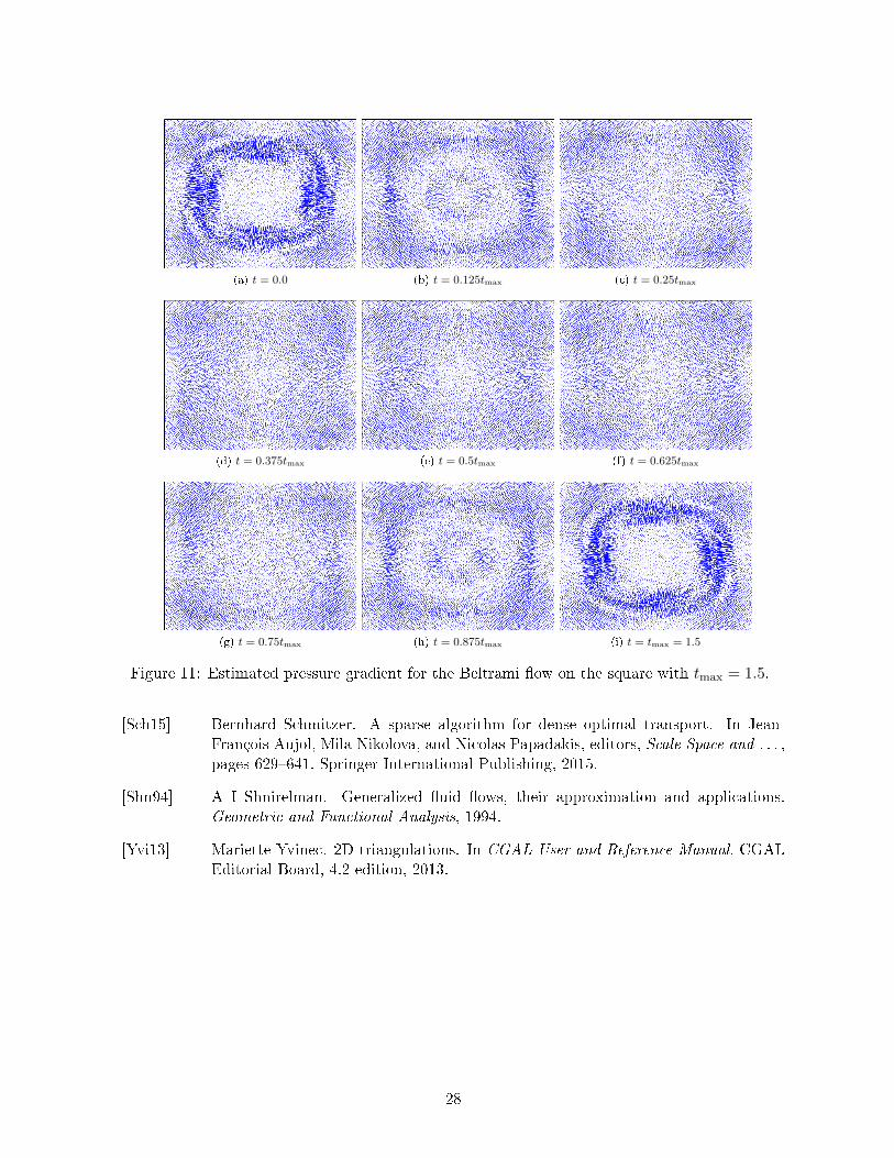
The pressure gradient is estimated as in 5.2.1 and is displayed in Figure 11. These pic-tures seem to indicate a loss of regularity of the pressure near the initial and nal times. Thiscorroborates the result of [AF07] according to which the pressure belongs to L2

loc( ]0, T [, BV(X)).Figure 7 suggests that the even for tmax = 1.5, the reconstructed solution for the Beltrami ow

are more deterministic than the solution to the disk inversion. We estimate the box dimensionof the support of the solution using the method explained in 5.2.2. The results are displayedin Figure 8. The estimated dimension is D = 2 for the deterministic solution (tmax = 0.9)but it increases as the maximum time (and therefore the amount of non-determinism) increases.Finally, we note that the estimated dimensions for tmax ∈ 1.1, 1.3, 1.5 seem to be strictlybetween 2 and 3, suggesting a fractal structure for the support of the solution. This would needto be conrmed by a mathematical study.

23

Software. The software developed for generating the results presented in this article is publiclyavailable at https://github.com/mrgt/EulerSemidiscrete

Acknowledgement The authors thank Y. Brenier for constructive discussions and introducingthem to the topic of Euler equations of inviscid incompressible uids.

(a) (x, y) = (−0.7, 0) (b) (x, y) = (−0.35, 0) (c) (x, y) = (0, 0)

(d) (x, y) = (0.2, 0) (e) (x, y) = (0.35, 0) (f) (x, y) = (0.5, 0)

Figure 7: We select particles whose initial position lie in a small disk, and display their trajectoriesaccording to the computed solution to (8). (Top) For the inversion of the unit disk (Bottom)For the Beltrami ow on the square, with tmax = 1.5.

References

[AF07] Luigi Ambrosio and Alessio Figalli. On the regularity of the pressure eld of Bre-nier's weak solutions to incompressible Euler equations. Calculus of Variations andPartial Dierential Equations, 2007.

[AHA98] F Aurenhammer, F Homann, and B Aronov. Minkowski-Type Theorems andLeast-Squares Clustering. Algorithmica, 1998.

[Arn66] Vladimir Arnold. Sur la géométrie diérentielle des groupes de Lie de dimension in-nie et ses applications à l'hydrodynamique des uides parfaits. Annales de l'institutFourier, 1966.

24

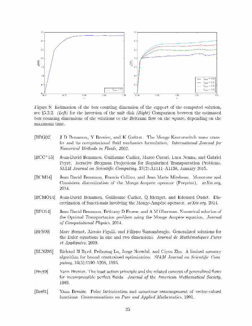
Figure 8: Estimation of the box counting dimension of the support of the computed solution,see 5.2.2. (Left) for the inversion of the unit disk (Right) Comparison between the estimatedbox counting dimensions of the solutions to the Beltrami ow on the square, depending on themaximum time.

[BBG02] J D Benamou, Y Brenier, and K Guittet. The Monge-Kantorovitch mass trans-fer and its computational uid mechanics formulation. International Journal forNumerical Methods in Fluids, 2002.

[BCC+15] Jean-David Benamou, Guillaume Carlier, Marco Cuturi, Luca Nenna, and GabrielPeyré. Iterative Bregman Projections for Regularized Transportation Problems.SIAM Journal on Scientic Computing, 37(2):A1111A1138, January 2015.

[BCM14] Jean-David Benamou, Francis Collino, and Jean-Marie Mirebeau. Monotone andConsistent discretization of the Monge-Ampere operator (Preprint). arXiv.org,2014.

[BCMO14] Jean-David Benamou, Guillaume Carlier, Q Merigot, and Edouard Oudet. Dis-cretization of functionals involving the Monge-Ampère operator. arXiv.org, 2014.

[BFO14] Jean-David Benamou, Brittany D Froese, and A M Oberman. Numerical solution ofthe Optimal Transportation problem using the MongeAmpère equation. Journalof Computational Physics, 2014.

[BFS09] Marc Bernot, Alessio Figalli, and Filippo Santambrogio. Generalized solutions forthe Euler equations in one and two dimensions. Journal de Mathématiques Pureset Appliquées, 2009.

[BLNZ95] Richard H Byrd, Peihuang Lu, Jorge Nocedal, and Ciyou Zhu. A limited memoryalgorithm for bound constrained optimization. SIAM Journal on Scientic Com-puting, 16(5):11901208, 1995.

[Bre89] Yann Brenier. The least action principle and the related concept of generalized owsfor incompressible perfect uids. Journal of the American Mathematical Society,1989.

[Bre91] Yann Brenier. Polar factorization and monotone rearrangement of vector-valuedfunctions. Communications on Pure and Applied Mathematics, 1991.

25

(a) t = 0.0 (b) t = 0.95 (c) t = 1.1 (d) t = 1.3 (e) t = 1.5

(f) t = 0.0 (g) t = 0.25 ∗ tmax (h) t = 0.5 ∗ tmax (i) t = 0.75 ∗ tmax (j) t = tmax = 0.9

(k) t = 0.0 (l) t = 0.25 ∗ tmax (m) t = 0.5 ∗ tmax (n) t = 0.75 ∗ tmax (o) t = tmax = 1.1

(p) t = 0.0 (q) t = 0.25 ∗ tmax (r) t = 0.5 ∗ tmax (s) t = 0.75 ∗ tmax (t) t = tmax = 1.3

(u) t = 0.0 (v) t = 0.25 ∗ tmax (w) t = 0.5 ∗ tmax (x) t = 0.75 ∗ tmax (y) t = tmax = 1.5

Figure 9: (First row) Beltrami ow in the unit square at various timesteps, a classical solutionto Euler's equation. The color of the particles depend on their initial position. (Second to fthrow) Generalized uid ows that are reconstructed by our algorithm, using boundary conditionsdisplayed in the rst and last column. When tmax < 1 we recover the classical ow, while fortmax ≥ 1 the solution is not classical any more and includes some mixing.

[Bre93] Y Brenier. The dual least action principle for an ideal, incompressible uid . Archivefor rational mechanics and analysis, 1993.

[Bre08] Yann Brenier. Generalized solutions and hydrostatic approximation of the Eulerequations. Physica D. Nonlinear Phenomena, 2008.

[Bre11] Yann Brenier. A modied least action principle allowing mass concentrations forthe early universe reconstruction problem. Conuentes Mathematici, 2011.

26

(a) t = 0.0 (b) t = 0.125tmax (c) t = 0.25tmax (d) t = 0.375tmax (e) t = 0.5tmax

(f) t = 0.625tmax (g) t = 0.75tmax (h) t = 0.875tmax (i) t = tmax = 1.5

Figure 10: Using the k-means cluster algorithm, we cluster the reconstructed trajectories for theBeltrami ow in the square with tmax = 1.5 into 10 groups, whose particles are displayed withdierent collors. The resulting pictures suggest that close to the boundary of the square themovement of particle is clockwise and deterministic while in the interior the movement is highlynon-deterministic and counter-clockwise.

[cga] CGAL, Computational Geometry Algorithms Library. http://www.cgal.org.

[CL55] Earl A Coddington and Norman Levinson. Theory of ordinary dierential equations.Tata McGraw-Hill Education, 1955.

[CPR15] Marco Cuturi, Gabriel Peyré, and Antoine Rolet. A Smoothed Dual Approach forVariational Wasserstein Problems. arXiv.org, March 2015.

[dGBOD12] Fernando de Goes, Katherine Breeden, Victor Ostromoukhov, and Mathieu Des-brun. Blue noise through optimal transport. ACM Transactions on Graphics(TOG), 2012.

[Eul65] Leonhard Euler. Opera Omnia. 1765.

[FD12] Alessio Figalli and S Daneri. Variational models for the incompressible Euler equa-tions. HCDTE Lecture Notes, Part II, 2012.

[GG92] Allen Gersho and Robert M Gray. Vector Quantization and Signal Compression.Springer Science & Business Media, 1992.

[Lév14] Bruno Lévy. A numerical algorithm for L2 semi-discrete optimal transport in 3D.arXiv.org, 2014.

[Mer11] Q Merigot. A Multiscale Approach to Optimal Transport. Computer GraphicsForum, 2011.

[OR15] A M Oberman and Yuanlong Ruan. An ecient linear programming method forOptimal Transportation. arXiv.org, September 2015.

[PPO13] Nicolas Papadakis, Gabriel Peyré, and Edouard Oudet. Optimal Transport withProximal Splitting. arXiv.org, 2013.

27

(a) t = 0.0 (b) t = 0.125tmax (c) t = 0.25tmax

(d) t = 0.375tmax (e) t = 0.5tmax (f) t = 0.625tmax

(g) t = 0.75tmax (h) t = 0.875tmax (i) t = tmax = 1.5

Figure 11: Estimated pressure gradient for the Beltrami ow on the square with tmax = 1.5.

[Sch15] Bernhard Schmitzer. A sparse algorithm for dense optimal transport. In Jean-François Aujol, Mila Nikolova, and Nicolas Papadakis, editors, Scale Space and . . . ,pages 629641. Springer International Publishing, 2015.

[Shn94] A I Shnirelman. Generalized uid ows, their approximation and applications.Geometric and Functional Analysis, 1994.

[Yvi13] Mariette Yvinec. 2D triangulations. In CGAL User and Reference Manual. CGALEditorial Board, 4.2 edition, 2013.

28