Local Linear Regression on Manifolds and its Geometric Interpretation Ming-Yen Cheng and Hau-Tieng Wu Abstract High-dimensional data analysis has been an active area, and the main fo- cuses have been variable selection and dimension reduction. In practice, it occurs often that the variables are located on an unknown, lower-dimensional nonlinear manifold. Under this manifold assumption, one purpose of this paper is regression and gradient estimation on the manifold, and another is developing a new tool for manifold learning. To the first aim, we suggest directly reducing the dimensionality to the intrinsic dimension d of the manifold, and perform- ing the popular local linear regression (LLR) on a tangent plane estimate. An immediate consequence is a dramatic reduction in the computation time when the ambient space dimension p d. We provide rigorous theoretical justifica- tion of the convergence of the proposed regression and gradient estimators by carefully analyzing the curvature, boundary, and non-uniform sampling effects. A bandwidth selector that can handle heteroscedastic errors is proposed. To the second aim, we analyze carefully the behavior of our regression estimator both in the interior and near the boundary of the manifold, and make explicit its relationship with manifold learning, in particular estimating the Laplace- Beltrami operator of the manifold. In this context, we also make clear that it is important to use a smaller bandwidth in the tangent plane estimation than in the LLR. Simulation studies and the Isomap face data example are used to illustrate the computational speed and estimation accuracy of our methods. KEY WORDS: diffusion map; dimension reduction; high-dimensional data; manifold learning; nonparametric regression. SHORT TITLE: Manifold Adaptive Regression And Manifold Learning Ming-Yen Cheng is Professor, Department of Mathematics, National Taiwan University, Taipei 106, Taiwan (Email: [email protected]). Hau-Tieng Wu is Postdoctoral Research Associate, Program in Applied and Computational Mathematics, Princeton University, Princeton, NJ 08544, USA (Email: [email protected]). Cheng’s research was supported in part by the National Science Council grant NSC97-2118-002-001-MY3 and the Mathematics Division, National Center of Theoretical Sciences (Taipei Office). The authors like to thank Professor Peter Bickel for instructive comments. arXiv:1201.0327v3 [math.ST] 30 Jul 2012

Welcome message from author
This document is posted to help you gain knowledge. Please leave a comment to let me know what you think about it! Share it to your friends and learn new things together.
Transcript

Local Linear Regression on Manifolds and itsGeometric Interpretation
Ming-Yen Cheng and Hau-Tieng Wu
Abstract
High-dimensional data analysis has been an active area, and the main fo-
cuses have been variable selection and dimension reduction. In practice, it
occurs often that the variables are located on an unknown, lower-dimensional
nonlinear manifold. Under this manifold assumption, one purpose of this paper
is regression and gradient estimation on the manifold, and another is developing
a new tool for manifold learning. To the first aim, we suggest directly reducing
the dimensionality to the intrinsic dimension d of the manifold, and perform-
ing the popular local linear regression (LLR) on a tangent plane estimate. An
immediate consequence is a dramatic reduction in the computation time when
the ambient space dimension p d. We provide rigorous theoretical justifica-
tion of the convergence of the proposed regression and gradient estimators by
carefully analyzing the curvature, boundary, and non-uniform sampling effects.
A bandwidth selector that can handle heteroscedastic errors is proposed. To
the second aim, we analyze carefully the behavior of our regression estimator
both in the interior and near the boundary of the manifold, and make explicit
its relationship with manifold learning, in particular estimating the Laplace-
Beltrami operator of the manifold. In this context, we also make clear that it
is important to use a smaller bandwidth in the tangent plane estimation than
in the LLR. Simulation studies and the Isomap face data example are used to
illustrate the computational speed and estimation accuracy of our methods.
KEY WORDS: diffusion map; dimension reduction; high-dimensional data; manifold
learning; nonparametric regression.
SHORT TITLE: Manifold Adaptive Regression And Manifold Learning
Ming-Yen Cheng is Professor, Department of Mathematics, National Taiwan University, Taipei106, Taiwan (Email: [email protected]). Hau-Tieng Wu is Postdoctoral Research Associate,Program in Applied and Computational Mathematics, Princeton University, Princeton, NJ 08544,USA (Email: [email protected]). Cheng’s research was supported in part by the NationalScience Council grant NSC97-2118-002-001-MY3 and the Mathematics Division, National Center ofTheoretical Sciences (Taipei Office). The authors like to thank Professor Peter Bickel for instructivecomments.
arX
iv:1
201.
0327
v3 [
mat
h.ST
] 3
0 Ju
l 201
2
1 Introduction
High-dimensional data arise frequently in many fields of the contemporary science.
In addition, it is common that the sample size is small relative to the dimension-
ality of the data. Such intrinsically complex data structure introduces new chal-
lenges in statistical analysis and inference, and requires innovative methods and
theories [13, 17]. In this context, we focus on the regression problem, which plays
an important role in understanding the relationship between the response variable
and the predictors. Conventionally, the probability density function (p.d.f.) of the
predictor vector is assumed to be non-degenerate. In this case, variable selection
and dimension reduction are fundamental issues and have been extensively studied
[12, 14, 41, 13, 15, 23, 38, 39]. However, these problems remain difficult in the non-
parametric regression setting, because commonly the models are built in the ambient
space and the curse of dimensionality is a serious issue [20, 10, 44].
Recently, it has been noticed that, in practice, the predictor vector often takes on
values in a lower-dimensional, nonlinear manifold. More specifically, in the cryo Elec-
tron Microscopy problem [16], the images are located on the 3-dimensional manifold
SO(3); in the radar signal example the data can be modeled as being sampled from
the Grassmannian manifold [6]; natural images are argued to be lying on a Klein bot-
tle [4]; the general manifold model for image and signal analysis is considered in [31];
and spherical, circular and oriental data are distributed on special types of manifolds
[25]; to name but a few. Based on the manifold assumption, in the past few years,
numerous papers have been devoted to learning the manifold, or more generally the
underlying structure [7, 21, 36], and a few have addressed regression on manifolds
[30, 3, 1].
In the manifold learning literature, the Nadaraya-Watson kernel regression esti-
mator has been used to construct an estimator of the Laplace-Beltrami operator of
the manifold; however, to avoid the boundary blowup problem, Neuman’s boundary
condition is required [7]. When the p-dimensional predictor is non-degenerate in Rp,
it is well known that the asymptotic bias of the traditional LLR in the Euclidean
setup is related to the Laplacian of the regression function and that it alleviates the
boundary effect [34]. Thus, it is interesting to see if these properties still hold for
2
some properly constructed LLR in the manifold setup, as it will enable us to obtain
a new estimator for the Laplace-Beltrami operator of the manifold with a different
boundary condition.
Besides, due to the rich geometric structure, when the predictors are concentrated
on a manifold, regression models that taking into account the geometric structure of
the manifold are intuitively appealing. In [30, 24] the kernel regression estimator
is constructed directly on the manifold, using the true geodesic distance both in
determining the nearest neighbors and in constructing the kernel weights. Another
approach is to employ the usual LLR in the ambient space Rp with regularization
imposed on the coefficients in the directions perpendicular to a tangent plane estimate
[1]. However, there are several interesting and important issues left unsolved. First,
although the idea of constructing kernel estimators on the manifold in [30, 24] is
appealing, it is unrealistic to make use of the geodesic distance. It is non-trivial to
construct LLR on the manifold without knowing the manifold structure. Second, it
remains unknown whether the methods in [1] alleviate the boundary effect, and it is
not obvious whether the asymptotic biases have any connections with the Laplace-
Beltrami operator of the manifold. Third, when p is large, fitting LLR in Rp as in [1]
can be computationally expensive even if regularization has been imposed. Fourth,
in [1] the bandwidth used in the tangent plane estimation is the same as the one
employed in the LLR. It is unclear if we can benefit from using different bandwidths
in these two steps. Fifth, the quantity “exterior derivative dxf |x0” in [1, (4.5)] is subtle
and the details are missing. Furthermore, the topology of the embedded manifold,
in particular, the condition number [29], is another important issue that needs to be
taken care of.
Motivated by the above observations, in this paper, we explore further the Rieman-
nian geometric structure of the manifold, in particular the tangent bundle structure,
and construct the LLR directly on an estimate of the tangent plane to the manifold,
without knowing the geodesic distance and manifold structure. Specifically, we first
estimate the intrinsic dimension d, and deal with the condition number issue when
determining the nearest neighbors using the Euclidean distance. Subsequently, we ob-
tain an estimate of the embedded tangent plane based on local principal component
3
analysis (PCA). Finally, we construct the LLR on the tangent plane estimate using
the coordinates of the nearest neighbors with respect to the orthonormal basis. We
call our approach the Manifold Adaptive Local Linear Estimator for the Regression
(MALLER). In addition, we suggest a procedure for selecting the bandwidth in the
regression step that can handle heteroscedastic errors, which arise often in practice.
A consequence of the proposed MALLER is an estimator for the gradient and the
Laplace-Beltrami operator of the manifold.
Throughout this paper the dimension p is kept as a fixed number and we assume
the predictors are observed without any noise. Thus, if the sample size n is large
enough compared to the intrinsic dimension d, the tangent plane can be estimated
accurately so that the dimensionality of the data can be reduced from p to d. Under
this circumstance, the first consequence is a much more computationally efficient
scheme when p is large and p d, since all the computations in the regression
step depend only on d. Another consequence is the ability to handle the practical
situations where n is less than p, in which case no sparsity conditions like those in
[1] are needed for MALLER to work. The isomap face data analysis illustrates these
points.
We provide detailed theoretical justification of the convergence of MALLER by
carefully analyzing the curvature, non-uniform sampling and boundary effects. In par-
ticular, the MALLER and gradient estimators achieve the respective optimal rates of
convergence pertaining to nonparametric regression on d-dimensional manifolds. In
addition, the subtle relationship between the bandwidth used in the tangent plane
estimation and the one used in the LLR is made explicit: it is crucial that the former
should be of a smaller order than the latter, otherwise larger biases are introduced
in the LLR on the tangent plane estimate and in the Laplace-Beltrami estimator
mentioned below. This issue is particularly important when estimating the Laplace-
Beltrami operator. Moreover, MALLER enjoys both the automatic boundary correc-
tion and the design adaptive properties possessed by the LLR in the Rd setup [34].
These properties have strong implications in manifold learning. In particular, if the
manifold has a smooth boundary, the Laplace-Beltrami operator estimated by our
method MALLER is different from the one estimated by employing the Nadaraya-
4

Watson kernel method, in the sense that the two are under different boundary condi-
tions. Since the main focus of this paper is regression on manifolds, further theoretical
properties and applications of the new estimator of the Laplace-Beltrami operator are
left as a future work.
The rest of this paper is organized as follows. The proposed MALLER algorithm
and a bandwidth selection procedure are introduced in Sections 2 and 3 respectively.
Asymptotic results for the conditional mean squared errors of MALLER and the gra-
dient estimator in both the interior and boundary of the manifold are given in Section
4. In Section 5 we examine finite sample performance of MALLER and compare it
with those of [1] through one simulation study and application to the isomap face
dataset, and we demonstrate the efficacy of our gradient estimator via a simulated
example. Section 6 gives a brief introduction of the diffusion map framework and
discusses application of MALLER to estimating the Laplace-Beltrami operator of the
manifold. In Section 7, besides addressing the relationship between MALLER and
the NEDE algorithm in [1, (4.6)], we discuss various related open questions and fu-
ture directions in both regression on manifolds and manifold learning. Proofs of the
theoretical results can be found in the Supplementary, which also contains a brief in-
troduction to the exterior derivative, covariant derivative and gradient of a function
on the manifold.
2 Model and Estimation Procedure
Let Y denote the scalar response variable and let X be a p-dimensional random vec-
tor. Assume that the distribution of X is concentrated on a d-dimensional compact,
smooth Riemannian manifold M embedded in Rp via ι : M → Rp, where M may have
boundary. We consider the following regression model
Y = m(ι−1(X)) + σ(ι−1(X)) ε, (2.1)
where ε is a random error independent of X with E(ε) = 0 and Var(ε) = 1, and both
the regression function m and the conditional variance function σ2 are defined on M.
Let (Xl, Yl)nl=1 denote a random sample observed from model (2.1) with X :=
Xlnl=1 being sampled from X. Then, given x ∈ M, the problem is to estimate
5

nonparametrically m(x), and its higher order covariant derivatives at x if m is smooth
enough, based on (Xl, Yl)nl=1. Here, x may or may not belong to X . For the sake of
clearness, we should distinguish between the point x ∈ ι(M) and the point ι−1(x) ∈ M.
However, to simplify the notation, for the rest of this paper we use the same symbol
x to denote x ∈ ι(M) or ι−1(x) ∈ M and use X to denote X ∈ ι(M) or ι−1(X) ∈ M
unless there is any ambiguity in the context. In addition, throughout this paper we
assume that the sample size n d and X is not contaminated by error. In the
following subsections we discuss the steps in the MALLER algorithm : (1) estimating
the intrinsic dimension d of the manifold, (2) determining the true nearest neighbors
of x on M using the Euclidean distance, (3) estimating the embedded tangent plane
by local PCA, and (4) constructing LLR on the embedded tangent plane estimate.
Before going into the details, the MALLER algorithm is summarized below.
The MALLER Algorithm:
1. Calculate the MLE intrinsic dimension estimate d in [22], and treat it as d.
2. For the given x, hpca and h determineN truex,hpca
andN truex,h , the two sets of estimates
of the true nearest neighbors of x on M within a Euclidean ball of radius√hpca
and√h respectively, which are defined by (2.2).
3. Employ the local PCA based on the points in N truex,hpca
to get an orthonormal
basis Uk(x)dk=1 for the embedded tangent plane estimate at x, thus obtaining
xlnl=1, the coordinates of the projections of Xl − xnl=1 onto the affine space
spanned by Uk(x)dk=1 with respect to this basis. See Section 2.3 for the details.
4. For given kernel K and bandwidth h, obtain βx by the LLR (2.4) based onxl : Xl ∈ N true
x,h
. Then we can compute the regression, embedded gradient and
covariant derivative estimators defined in (2.9), (2.10) and (2.11) respectively.
2.1 Intrinsic dimension estimation
Given the manifold assumption, in general the intrinsic dimension d of the manifold
M is unknown a priori and needs to be estimated based on the sample X . There exist
many methods for estimating the intrinsic dimension and we have picked the maxi-
mum likelihood estimation (MLE) method introduced in [22] to estimate d and denote
6

the estimated dimension by d. Since d n, we assume the estimated dimension d is
correct and hence will not distinguish between d and d.
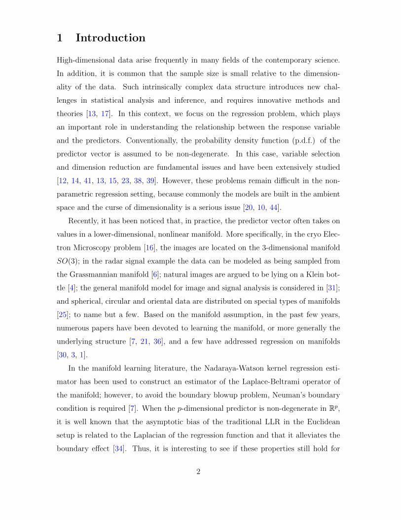
2.2 Determining the nearest neighbors
Numerically determining the neighbors of x ∈ M using the Euclidean distance is
problematic due to the embedding structure of the manifold, that is, the condition
number of the embedded manifold [29]. The reach of M is defined as the largest
number τ ≥ 0 so that for every 0 ≤ r < τ , the open normal bundle of M of radius
r is still embedded in Rp. Since M is assumed to be compact, we know τ > 0. The
quantity 1/τ is referred to as the “condition number” of M [29]. For the given x ∈ M
and any δ > 0, denote respectively the set of Euclidean√δ-neighbors of x from X
and the set of geodesic√δ-neighbors of x from X as
N Rpx,δ =
Xj ∈ X : ‖Xj − x‖Rp <
√δ
and NMx,δ =
Xj ∈ X : d(Xj, x) <
√δ,
where d(·, ·) is the geodesic distance. When δ is small enough, it is shown in Lemma
A.2.4 in the Supplementary that N Rpx,δ is roughly the same as NM
x,δ, which is the main
fact rendering the whole algorithm feasible. However, when√δ exceeds 2τ , NM
x,δ
might be a strict subset of N Rpx,δ . See Figure 1. This fact combined with the lack of a
priori knowledge of M, in particular, the geodesic distance and the condition number
1/τ , lead to the problem. Since the manifold structure is our main concern, we need
to learn NMx,δ. The problem is thus reduced to determining which points in N Rp
x,δ are in
NMx,δ and which are not. To cope with this problem, we apply the “self-tuning spectral
clustering” algorithm [40] to the set N Rpx,δ . We denote
N truex,δ :=
Xj ∈ N Rp
x,δ : Xj is in the same cluster as x. (2.2)
Then, according to Lemma A.2.4 in the Supplementary, N truex,δ is an accurate estimate
of NMx,δ.
2.3 Embedded tangent plane estimation
Write the tangent plane of the manifold at x ∈ M as TxM. Denote by ι∗ the total
differential of ι and by ι∗TxM the embedded tangent plane in Rp. Note that ι∗TxM is
7
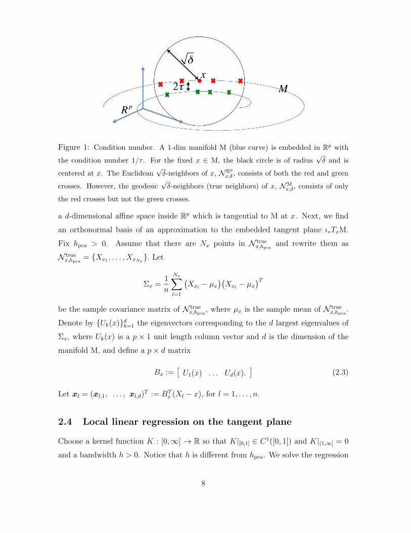
Figure 1: Condition number. A 1-dim manifold M (blue curve) is embedded in Rp with
the condition number 1/τ . For the fixed x ∈ M, the black circle is of radius√δ and is
centered at x. The Euclidean√δ-neighbors of x, NRp
x,δ , consists of both the red and green
crosses. However, the geodesic√δ-neighbors (true neighbors) of x, NM
x,δ, consists of only
the red crosses but not the green crosses.
a d-dimensional affine space inside Rp which is tangential to M at x. Next, we find
an orthonormal basis of an approximation to the embedded tangent plane ι∗TxM.
Fix hpca > 0. Assume that there are Nx points in N truex,hpca
and rewrite them as
N truex,hpca
= Xx1 , . . . , XxNx. Let
Σx =1
n
Nx∑l=1
(Xxl − µx
)(Xxl − µx
)Tbe the sample covariance matrix of N true
x,hpca, where µx is the sample mean of N true
x,hpca.
Denote by Uk(x)dk=1 the eigenvectors corresponding to the d largest eigenvalues of
Σx, where Uk(x) is a p × 1 unit length column vector and d is the dimension of the
manifold M, and define a p× d matrix
Bx :=[U1(x) . . . Ud(x).
](2.3)
Let xl = (xl,1, . . . , xl,d)T := BT
x (Xl − x), for l = 1, . . . , n.
2.4 Local linear regression on the tangent plane
Choose a kernel function K : [0,∞] → R so that K|[0,1] ∈ C1([0, 1]) and K|(1,∞] = 0
and a bandwidth h > 0. Notice that h is different from hpca. We solve the regression
8

problem (2.1) at x via considering the following local linear least squares fitting on
the estimated tangent plane:
βx = argminβ∈Rd+1
n∑l=1
(Yl − β0 −
d∑k=1
βkxl,k
)2
IN truex,h
(Xl)Kh(Xl, x), (2.4)
where β = (β0, β1, . . . , βd)T , Kh(Xl, x) := h−d/2K
(‖Xl − x‖Rp
/√h), and I is the
indicator function. Denote
Y = (Y1, . . . , Yn)T and m =(m(ι−1(X1)), . . . ,m(ι−1(Xn))
)T. (2.5)
Denote by Xx the n× (d+ 1) design matrix related to x:
Xx =
[1 . . . 1
x1 . . . xn
]T, (2.6)
and Wx the kernel weight matrix:
Wx = diag(Kh(X1, x)IN true
x,h(X1), . . . , Kh(Xn, x)IN true
x,h(Xn)
), (2.7)
which is a diagonal matrix of size n× n. Then (2.4) can be written as
βx = argminβ∈Rd+1
(Y − Xxβ)TWx(Y − Xxβ). (2.8)
It is straightforward to show that the minimizer in (2.8) is
βx = (XTxWxXx)
−1XTxWxY
if (XTxWxXx)
−1 exists. The invertibility of XTxWxXx will be shown in the Supplemen-
tary. Our estimator of m(x) MALLER is given by
m(x, h) := vT1 βx = vT1 (XTxWxXx)
−1XTxWxY , (2.9)
where vk ∈ Rd+1 is a (d+1)×1 unit vector with the k-th entry being 1. If the interest
is to estimate the embedded gradient of m at x, the following estimator is considered:
ι∗gradm(x) :=d∑i=1
∇∂i(x)m(x, h)Ui(x). (2.10)
where grad denotes the gradient,
∇∂i(x)m(x, h) := vTi+1βx, (2.11)
9
and ∂i(x)di=1 is the orthonormal basis of TxM closest to the estimated orthonormal
basis Uk(x)dk=1 in the sense described in Lemma A.2.6 in the Supplementary. We
mention that the gradient on the manifold is closely related to the covariant derivative
and the exterior derivative. The relationship between these quantities is summarized
in the Supplementary.
From (2.6) and (2.8) we can see that the key ingredient in the estimators (2.9),
(2.10) and (2.11) is finding the coordinate of a given point related to a chosen basis and
approximate locally the regression function by a linear function of that coordinate. A
consequence of this fact is dimension reduction. Indeed, since d may be much smaller
than p, having obtained xlnl=1, locally at x we convert the p-dimensional regression
problem to a d-dimensional one, by paying the price of additional sampling error
coming from the tangent plane approximation and the curvature of the manifold.
Nonetheless, it is shown in Section 4 and Section 5 that the effect of this extra
sampling error on the MALLER is negligible and does not contribute to the leading
term in the estimation error, provided that hpca is smaller than h.
3 Bandwidth Selection
Selection of the local PCA bandwidth hpca is a less important problem than choosing
the bandwidth h in the regression step, as it is discussed in Section 4 that hpca should
be smaller than h and of a smaller order than the optimal order of h. We refer to [36]
for selection of hpca. Suppose that for a given choice of hpca, the tangent plane estimate
has been obtained. The aim is finding the optimal value of h so as to minimize the
asymptotic conditional MSE of the MALLER, which is provided in (4.5). When the
random errors are homoscedastic, the modified generalized cross-validation (mGCV)
suggested in [3] can be used. Specifically, let HmGCV = λ1, . . . , λB be a set of
candidate bandwidths, where λi > 0, i = 1, . . . , B, and B ∈ N, and for each point
x we choose a block of data points (Xj, Yj)j∈J . For each h ∈ HmGCV, define the
mGCV of h by
mGCV(h) =(
1 + 2atrJ (h)) 1
n1
∑j∈J
(Yj − m(Xj, h)
)2
,
10

where atrJ (h) := 1n1
∑j∈J v
T1 (XT
XjWXjXXj)
−1v1h−d/2K(0), n1 is the number of points
in J , and m(Xj, h) is the MALLER (2.9) of m(Xj) based on bandwidth h. Then
hmGCV,m is chosen as the value of h in HmGCV which minimizes mGCV(h).
In the presence of heteroscedastic random errors, we adopt the following additional
step to deal with the bandwidth selection problem. Note that the optimal bandwidth
has to balance between the conditional bias and the conditional variance, which de-
pends on σ2(x). Thus, with the pilot mGCV bandwidth hmGCV,m we get the first
estimate of m(Xl) by the MALLER, denoted as m(Xl, hmGCV,m), l = 1, . . . , n, and
we apply the method suggested in [5] to estimate σ2(x). We choose this method since
the random error ε might have a heavy tailed distribution. Defining the residuals as
rl :=(Yl − m(Xl, hmGCV,m)
)2
, l = 1, . . . , n,
we evaluate the following minimization problem
(α0(x), α(x)) = argminα0∈R,α∈Rd
∑Xl∈N true
x,hmGCV,r
(log(rl+1/n)−α0−αTBT
x (Xl−x))2KhmGCV,r
(Xl, x),
where hmGCV,r is the bandwidth determined by minimizing the mGCV upon the data
set (Xl, log(rl + 1/n))nl=1. The estimated value of σ2(x) is then defined as
σ2(x) := eα0(x)
[1
n
n∑l=1
rle−α0(x)
]−1
.
Finally we select the bandwidth for MALLER given in (2.9) at x ∈ M. Denote the op-
timal bandwidth at x as hopt(x). Fix a candidate bandwidths setHopt = λ1, . . . , λB,which may be different from HmGCV, where B ∈ N and λi > 0, i = 1, . . . , B. For
each h ∈ Hopt, estimate the conditional bias and the conditional variance of m(x, h)
respectively by
b(x, h) = 2[m(x, h)− m(x, h/2)],
which is based on the asymptotic bias expression given in (A.30) of the Supplementary
and (4.10), and
v(x, h) = vT1 (XTxWxXx)
−1XTxWxSxWxXx(XT
xWxXx)−1v1,
which is based on the finite sample variance expression given in (A.31) of the Supple-
mentary, where Sx is a n×n diagonal matrix Sx = diagσ2(X1), . . . , σ2(Xn). The
11

conditional MSE of m(x, h) is then estimated by
MSE(x, h) := b(x, h)2 + v(x, h).
The value of h ∈ Hopt, denoted as hopt(x), which minimizes MSE(x, h) is then used
to approximate hopt(x). With hopt(x), we can evaluate m(x, hopt(x)). We do not
claim the optimality of the bandwidth selection in this algorithm. For example, when
the point x is near the boundary of the manifold, the bandwidth should be chosen
differently. We choose this bandwidth selection scheme since it is commonly used and
is easy to implement [33, 11]. Further study on the bandwidth selection problem in
the manifold setup is an important and open problem and is out of the scope of this
paper.
4 Theory
Before stating the main theorems describing the behaviors of the proposed MALLER
given in Section 2, we set up more notation. Recall the assumption in Section 2 that
M is a d-dimensional compact smooth Riemannian manifold embedded in Rp via ι.
Let the metric g on M be the one induced from the canonical metric of the ambient
space Rp. The exponential map at x ∈ M is denoted as expx. Denote by d(x, y) the
distance between x, y ∈ M. The volume form on M induced from g is denoted as dV .
Given δ ≥ 0, denote the set of points close to the boundary ∂M with distance less
than δ as
Mδ =x ∈ M : min
y∈∂Md(x, y) ≤ δ
. (4.1)
When δ > 0 is small enough, we denote the geodesic ball with radius δ and center
x ∈ M as BMδ (x). Denote BRq
δ (x) as the ball in Rq, q ∈ N, with radius δ and center
x ∈ Rq and Sq−1 as the standard q − 1 sphere embedded in Rq with the induced
metric. Define
BMδ (x) := ι−1
(BRpδ (x) ∩ ι(M)
)⊂ M, (4.2)
which is an approximate of the geodesic ball BMδ (x). Denote by ∇ the Levi-Civita
connection, ∆ the Laplace-Beltrami operator and Hess the Hessian operator of (M, g).
Denote by Ric the Ricci curvature of (M, g). The second fundamental form of the
embedding ι at x is denoted by IIx.
12

4.1 Assumptions
Let the random vector X : Ω → Rp be a measurable function with respect to the
probability space (Ω,F , P ). To make the definition clear, in this paragraph we make
clear the role of ι to distinguish between x ∈ M and ι(x) ∈ ι(M). Suppose the range of
X is supported on ι(M). In this case, the p.d.f. of X is not well-defined as a function
on Rp if the intrinsic dimension d of M is less than p. To define properly the p.d.f. of
X, let B be the Borel sigma algebra of ι(M), and denote by PX the probability measure
of X, defined on B, induced from P . Assume that PX is absolutely continuous with
respect to the volume measure on ι(M), that is, dPX(x) = f(ι−1(x))ι∗dV (x), where
f ∈ C2(M). Thus, for an integrable function ζ : ι(M)→ R, we have
Eζ(X) =
∫Ω
ζ(X(ω))dP (ω) =
∫ι(M)
ζ(x)dPX(x)
=
∫M
ζ(x)f(ι−1(x))ι∗dV (x) =
∫M
ζ(ι(y))f(y)dV (y), (4.3)
where the second equality follows from the fact that PX is the induced probability
measure, and the last one comes from the change of variable x = ι(y). In this sense
we interpret f as the p.d.f. of X on M.
The kernel function K : [0,∞] → R used in the proposed MALLER is assumed
to be compactly supported in [0, 1] so that K|[0,1] ∈ C1([0, 1]). Denote
µi,j :=
∫BRd
1 (0)
Ki(‖u‖Rd)‖u‖jRddu
and we normalize K so that µ1,0 = 1. Note that we can also consider more general
kernel functions. For example, any C1(R) function with proper decaying property
can be chosen. More general bandwidth like a positive definite symmetric bandwidth
matrix H considered in [34] can also be considered. Since the analysis under these
more general conditions is the same except for the wrinkle caused by the extra error
terms, we focus on the above setup to make the analysis clear.
We make the following assumptions in the analysis.
(A1) h→ 0 and nhd/2 →∞ as n→∞.
(A2) f belongs to C2(M) and satisfies
0 < infx∈M
f(x) ≤ supx∈M
f(x) <∞. (4.4)
13

(A3) For every given h > 0 and every point x ∈ M√h, the set BM√h(x)∩M contains a
non-empty interior set. The purpose of this assumption is to avoid the potential
degeneracy near the boundary.
(A4) Assume that h1/2pca < min(2τ, inj(M)) and h1/2 < min(2τ, inj(M)), where inj(M)
is the injectivity radius of M and 1/τ is the condition number of M [29]. Please
see step 2 of the algorithm for precise definition of τ .
4.2 Main Theory
We state our main theorems here and postpone the proofs to the Supplementary.
Theorem 4.1. Suppose hpca n−2/(d+1) and h ≥ hpca. When x ∈ M\M√h, the
conditional mean square error (MSE) of the estimator m(x, h) is
MSEm(x, h)|X = h2µ2
1,2
4d2(∆m(x))2 +
1
nhd/2µ2,0σ
2(x)
f(x)
+O(h3 + h2h3/4pca ) +Op
( 1
n1/2hd/4−2+
1
nhd/2−1+
1
n3/2h3d/4
).
(4.5)
Next, we consider the case when x is close to the boundary. To ease the notation,
for x ∈ M√h and h > 0, define a (d+ 1)× (d+ 1) matrix νi,x:
νi,x :=
νi,x,11 νi,x,12
νTi,x,12 νi,x,22
:=
∫1√hD(x)
Ki(‖u‖)du∫
1√hD(x)
Ki(‖u‖)uTdu∫1√hD(x)
Ki(‖u‖)udu∫
1√hD(x)
Ki(‖u‖)uuTdu
,(4.6)
where for i = 1, 2, νi,x,11 ∈ R, νi,x,12 is a 1× d matrix, νi,x,22 is a d× d matrix and
D(x) := exp−1x (BM√
h(x) ∩M) ⊂ TxM. (4.7)
We also define
C :=
[1 0
0 h12 Id
]. (4.8)
Here, Ik denotes the k × k identity matrix for any k ∈ N.
Theorem 4.2. Suppose x ∈ M√h, hpca n−2/(d+1) and h ≥ hpca. The conditional
MSE of the estimator m(x, h) is
MSEm(x, h)|X =h2
4
[tr(Hessm(x)ν1,x,22
)]2
ν21,x,11
+vT1 ν
−11,xν2,xν
−11,xv1
nhd2
σ2(x)
f(x)(4.9)
+Op
(h3/4pcah
3/2 + h1/2pcah
2)
+Op
( 1
n1/2hd/4−2+
1
nhd/2−1/2+
1
n3/2h3d/4
)14

Notice that in both Theorem 4.1 and 4.2, the minimum of the conditional MSE
is achieved when h n−2/(d+4), which is strictly larger than hpca.
Corollary 4.1. Suppose ∂M is smooth, x ∈ M√h, hpca n−2/(d+1) and h ≥ hpca.
Then the conditional bias of m(x, h) is asymptotically a linear combination of the
second order covariant derivative of m:
Em(x, h)−m(x)|X =h
2
d∑k=1
ck(x)∇2∂k,∂k
m(x) +Op(h12h3/4
pca +hh1/2pca ) +Op
( 1
n12h
d4−1
),
(4.10)
where ∂kdk=1 is a normal coordinate determined in Lemma A.2.6 of the Supplemen-
tary and ck(x) is uniformly bounded for all k = 1, . . . , d.
Recall that when the p.d.f. of the random vector X is well-defined on Rp, de-
noted as f , so that suppf satisfies some weak conditions, it is shown in [34] that the
conventional LLR is unbiased up to the second order term even when x is close to
the boundary. Additionally, the LLR is design adaptive, that is, the asymptotic bias
does not depend on f . These properties render the LLR popular in applications. In
the degenerate case i.e. X lies on the manifold M, we can see from the proofs of
Theorem 4.1 and Theorem 4.2 that MALLER also processes these nice properties.
There properties of MALLER have important implications from the manifold learning
viewpoint, which will be discussion in Section 6.
4.3 Gradient and Covariant Derivative Estimate
When the p.d.f. f of X is non-degenerate on Rp, it is well known that the traditional
LLR provides an estimate of the gradient of m [34, 11]. In the manifold setup, the
notion of differentiation is generalized naturally to the “covariant derivative”, and
hence the gradient if the manifold is Riemannian. A brief introduction of the notion
of covariant derivative, gradient, exterior derivative and their relationship is provided
in the Supplementary A.1. In this subsection, we show that MALLER provides an
estimate of the covariant derivative of m.
Theorem 4.3. Suppose x ∈ M\M√h, hpca n−2/(d+1) and h ≥ hpca. The conditional
15

MSE for the estimator ∇∂i(x)m(x, h) given in (2.11) is
MSE∇∂i(x)m(x, h)|X = h2
[µ1,2
d
∇∂if(x)
f(x)∆m(x)−
µ1,2d∫Sd−1 θ
THessm(x)θθ∇θf(x)dθ
|Sd−1|f(x)
]2
+1
nhd2
+1
dµ2,2σ2(x)f(x)
µ21,2
+Op(h52 + h
32h
34pca) +Op
( 1
n12h
d4− 3
2
+1
nhd2
+1
n32h
3d4
+1
),
where ∂i(x)di=1 is an orthonormal basis of TxM described in Lemma A.2.6 of the
Supplementary.
Theorem 4.4. Suppose x ∈ M√h, hpca n−2/(d+1) and h ≥ hpca. The conditional
MSE for the estimator ∇∂i(x)m(x, h) given in (2.11) is
MSE∇∂i(x)m(x, h)|X = h
(vTi+1ν
−11,x
2
∫1√hD(x)
K(‖u‖)uTHessm(x)u
1
u
du
)2
+vTi+1ν
−11,xν2,xν
−11,xvi+1
nhd2
+1
σ2(x)
f(x)+Op
(h
12h
34pca + hh
12pca
)+Op
( 1
n12h
d4− 3
2
+1
nhd2
+ 12
+1
n32h
3d4
),
where ∂i(x)di=1 is an orthonormal basis of TxM described in Lemma A.2.6 of the
Supplementary.
Based on Theorem 4.3, 4.4 and Section A.1 of the Supplementary, we know that
the estimator (2.10) indeed can be used to estimate the embedded gradient of m.
Since the application of the estimate of the gradient is not the focus of this paper, we
refer the readers to [7, 26].
5 Numerical Examples
To demonstrate the applicability of the proposed algorithm MALLER, we test it on
a series of simulations and a real dataset and compared it with the nonparametric ex-
terior derivative estimator (NEDE), nonparametric adaptive lasso exterior derivative
estimator (NALEDE), nonparametric exterior derivative estimator for the “large p,
small n” (NEDEP) and nonparametric adaptive lasso exterior derivative estimator for
the “large p, small n” (NALEDEP) proposed in [1], for which the codes are provided
16
by the authors of [1]∗. The code for implementation of MALLER is in the authors’
homepage†.
All the observed values of the predictors in both the training dataset and the
testing dataset are normalized by x0l := (xl − µ)/s, where µ is the sample mean of
xlnl=1, l = 1, . . . , n + 10 and s = maxi,j=1,...,n ‖xi − xj‖Rp . In order to facilitate
the notation we write xl instead of x0l in the sequel. In step 1 of our algorithm, we
used the MLE dimension estimation code provided by the authors of [22]‡ to evaluate
the intrinsic dimension of the manifold. In step 2, we used the code provided by the
authors of [40]§. In step 3, we chose hpca = 0.015. In the bandwidth selection step, for
each regressant, we worked out the bandwidth selection procedure given in Section
3 on 21 logarithmically equi-spaced candidate bandwidths in the interval [0.01, 0.1]
when d = 1 and [0.01, hd] when d > 1, where
hd =1
4
(dΓ(d/2)√
πΓ ((d+ 1)/2)
)2/d
(0.1)1/d. (5.1)
This choice of hd is motivated by the following facts. Fix d > 1. The volume of
Sd is |Sd| = 2πd+12
Γ( d+12
), where Γ is the Gamma function, and the volume of a geodesic
ball of radius 0 < δ(d) 1 centered at x ∈ Sd, denoted as BSd
δ(d)(x), is approxi-
mately δ(d)d|Sd−1|d
= 2πd/2δ(d)d
dΓ(d/2). Thus, the ratio of the volume of BSd
δ(d)(x) to |Sd| is
r(d, δ(d)) = δ(d)dΓ((d+1)/2)√πdΓ(d/2)
. Suppose δ(d) = δ 1 for all d, then r(d, δ) gets smaller as
d increases. That is, if the number of data points sampled from Sd is the same and δ(d)
is fixed for all d, the number of data points located in BSd
δ(d)(x) decreases to zero expo-
nentially. This fact plays a role in the numerics, especially in the bandwidth selection
problem, since in practice the number of neighboring points is not controllable. We
thus choose the largest bandwidth hd by solving (2√hd)dΓ((d+1)/2)√πdΓ(d/2)
= r(1, 0.1) =√
0.1π
,
which leads to (5.1). We emphasize the non-optimality of this scheme to set the
candidate bandwidths for general manifolds of dimension d, which is out of the scope
of this paper. The kernel function K used in step 4 of our MALLER algorithm was
taken as K(u) = exp(−7u2)I[0,1](u).
∗http://www.eecs.berkeley.edu/~aaswani/EDE_Code.zip†http://www.math.princeton.edu/~hauwu/regression.zip‡http://www.stat.lsa.umich.edu/~elevina/mledim.m§http://www.vision.caltech.edu/lihi/Demos/SelfTuningClustering.html
17

In Sections 5.1 – 5.2 we report the root average square estimation error (RASE)
to measure the accuracy of different estimators:
RASE =
√√√√ 1
10
n+10∑i=n+1
∣∣m(xi)−m(xi)∣∣2,
where m(xi) is the result of each estimator.
We ran our simulations and data analysis on a computer having 96GB of ram,
two Intel Xeon X5570 CPUs, each with four cores running at 2.93GHz. No parallel
computation was implemented.
5.1 Simulated data: regression on the Klein bottle
Consider the 2-dimensional closed and smooth manifold, the Klein bottle, embedded
in R4, which is parametrized by φKlein : [0, 2π)× [0, 2π)→ R4 so that
(u, v)φKlein7→
((2 cos v + 1) cosu, (2 cos v + 1) sinu, 2 sin v cos(u/2), 2 sin v sin(u/2)
).
We sampled n = 1500 or 1000 points uniformly from [0, 2π) × [0, 2π), denoted as
(Ul, Vl)nl=1, and then obtained the corresponding n observations Xlnl=1 on the pre-
dictors X by the parametrization φKlein. Notice that the uniform sampling design on
[0, 2π)× [0, 2π) corresponds to a non-uniform sampling design on the Klein bottle. To
generate the responses Ylnl=1 corresponding to Xlnl=1, note that the mapping φKlein
is 1-1 and onto, so any (u, v) in [0, 2π) × [0, 2π) can be written as (u, v) = φ−1Klein(x)
for some x in the embedded Klein bottle. So, consider the following regression model
on the Klein bottle:
Y := m(X) + σ(X) ε,
where
m(X) := 7 sin(4U) + 5 cos(2V )2 + 6 exp−32((U − π)2 + (V − π)2),
σ(X) := σ0(1 + 0.1 cos(U) + 0.1 sin(V )),
ε ∼ N (0, 1) is independent of X, and σ0 is the noise level (in Y ) which determines
the signal-to-noise ratio
snrdb := 10 log10
(VarY
σ20
).
18

Furthermore, let
W = X + σXη,
where σX ≥ 0, and η is a bivariate normal random vector with zero mean and identity
covariance matrix, independent of X and ε. Consider estimating m(X) based on
observations on (W,Y ). In this case, W = X and X is observed without error when
σX = 0, and W is X contaminated with error when σX > 0. In the simulations,
we took σX = 0 or 0.2 and snrdb = 5 or 2. For each simulated sample, we drew
n observations (Wi, Yi)ni=1 to form the training dataset. Then, independent of the
training sample, we sampled randomly 10 points Win+10i=n+1 as the regressants and
tried to estimate the values of m at Xn+j10j=1 based on (Wi, Yi)ni=1.
We evaluated the performance of each estimator by computing the average and
standard deviation of its RASE’s over 200 realizations. The estimated dimension by
the MLE intrinsic dimension estimator was 2 for all of the 200 realizatioins, as is
expected. The results of all the estimators and their computation time are listed in
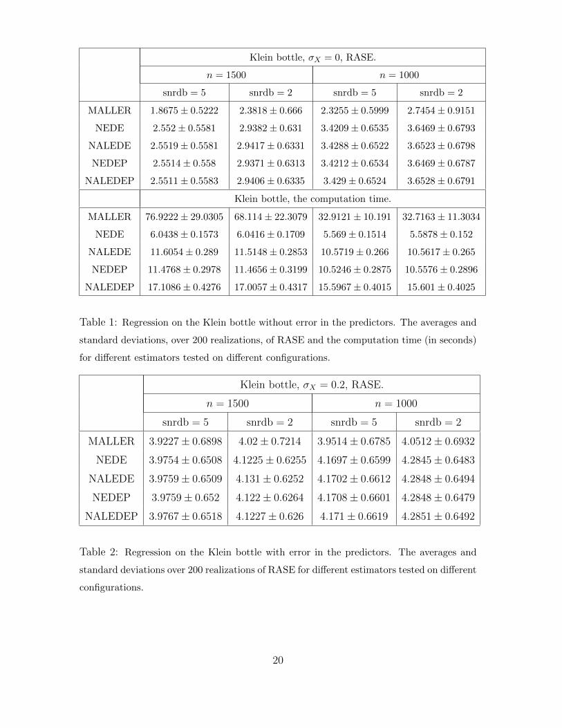
Table 1 and Table 2, from which we can draw the following conclusions. When there
is no error-in-variable, i.e. σX = 0, MALLER outperforms the four competitors in
all of the cases, with significantly smaller RASE average and similar RASE standard
deviation. Also, the MALLER performs well when there exists error in the predictors.
The fact that the computation time for MALLER is longer than that for the other four
estimators can be explained as follows. Besides the sample size n, the computation
time for the estimators in [1] also depend on the ambient space dimension p which
is 4 in this example. On the other hand, in addition to n, the computation time
for MALLER also depends on the estimated intrinsic dimension d which is 2 in this
example. This fundamental difference between MALLER and those in [1] will become
apparent when p increases and p d, as in the Isomap face example discussed in
Section 5.2.
5.2 Real data: Isomap face data
We further tested our algorithm on the Isomap face dataset [37]¶. The dataset consists
of 698 64 × 64 images, denoted as I64l 698
l=1, parametrized by three variables: the
¶http://isomap.stanford.edu/datasets.html
19
Klein bottle, σX = 0, RASE.
n = 1500 n = 1000
snrdb = 5 snrdb = 2 snrdb = 5 snrdb = 2
MALLER 1.8675± 0.5222 2.3818± 0.666 2.3255± 0.5999 2.7454± 0.9151
NEDE 2.552± 0.5581 2.9382± 0.631 3.4209± 0.6535 3.6469± 0.6793
NALEDE 2.5519± 0.5581 2.9417± 0.6331 3.4288± 0.6522 3.6523± 0.6798
NEDEP 2.5514± 0.558 2.9371± 0.6313 3.4212± 0.6534 3.6469± 0.6787
NALEDEP 2.5511± 0.5583 2.9406± 0.6335 3.429± 0.6524 3.6528± 0.6791
Klein bottle, the computation time.
MALLER 76.9222± 29.0305 68.114± 22.3079 32.9121± 10.191 32.7163± 11.3034
NEDE 6.0438± 0.1573 6.0416± 0.1709 5.569± 0.1514 5.5878± 0.152
NALEDE 11.6054± 0.289 11.5148± 0.2853 10.5719± 0.266 10.5617± 0.265
NEDEP 11.4768± 0.2978 11.4656± 0.3199 10.5246± 0.2875 10.5576± 0.2896
NALEDEP 17.1086± 0.4276 17.0057± 0.4317 15.5967± 0.4015 15.601± 0.4025
Table 1: Regression on the Klein bottle without error in the predictors. The averages and
standard deviations, over 200 realizations, of RASE and the computation time (in seconds)
for different estimators tested on different configurations.
Klein bottle, σX = 0.2, RASE.
n = 1500 n = 1000
snrdb = 5 snrdb = 2 snrdb = 5 snrdb = 2
MALLER 3.9227± 0.6898 4.02± 0.7214 3.9514± 0.6785 4.0512± 0.6932
NEDE 3.9754± 0.6508 4.1225± 0.6255 4.1697± 0.6599 4.2845± 0.6483
NALEDE 3.9759± 0.6509 4.131± 0.6252 4.1702± 0.6612 4.2848± 0.6494
NEDEP 3.9759± 0.652 4.122± 0.6264 4.1708± 0.6601 4.2848± 0.6479
NALEDEP 3.9767± 0.6518 4.1227± 0.626 4.171± 0.6619 4.2851± 0.6492
Table 2: Regression on the Klein bottle with error in the predictors. The averages and
standard deviations over 200 realizations of RASE for different estimators tested on different
configurations.
20

horizontal orientation, the vertical orientation, and the illumination direction. Thus,
the data were sampled from a 3-dimensional manifold embedded in R64×64. When we
view each image as a point in R64×64, the ambient space dimension p = 64×64 is large,
so in [1] the authors suggested to rescale the images from 64×64 to 7×7 pixels in size.
Denote the resized images of size k×k as Ikl 698l=1, where k = 1, . . . , 64. We performed
200 replications of the following experiment, which is suggested in [1]. Fix k = 7. We
randomly split I7l 698
l=1 into a training set consisting of 688 images and a testing set
consisting of 10 images. The horizontal orientation of the images in the testing set
were then estimated based on the training set. Table 3, which summaries the results,
shows that MALLER improves on the existing methods substantially in the sense
of reduced RASE average and standard deviation. We mention that NEDEP and
NALEDEP behave worse than NEDE and NALEDE due to the frequent occurrence
of blowup in the iteration, and the reported results are the best ones among several
trials we carried out.
Isomap face database, k = 7
RASE computation time
MALLER 1.2168± 0.8131 131.5847± 17.5136
NEDE 1.7852± 1.2122 34.4606± 4.5847
NALEDE 1.7759± 1.1995 170.7088± 28.8193
NEDEP 1.8685± 1.2413 53.7212± 8.3594
NALEDEP 2.8095± 3.6525 187.3745± 31.2623
Table 3: The averages and standard deviations, over 200 replications, of RASE and com-
putation time in seconds for different estimators tested on the resized Isomap face data
I7l 698l=1.
Next, we carried out another 200 replications of the same experiment but with
k = 14, 21, or 28. The MLE intrinsic dimension estimate was 3 in all the replications
when k = 7, 14 or 21, and was 4 all the time when k = 28. The results are given in
Table 4. We mention that when k = 14, 21 or 28, it took long time to compute the
methods in [1] and the experiment cannot be finished within a reasonable time frame,
so we decided not to include them in the comparison. When k = 7, 8, . . . , 16, the
21
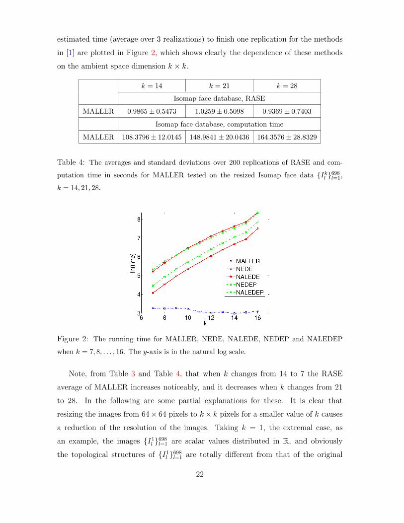
estimated time (average over 3 realizations) to finish one replication for the methods
in [1] are plotted in Figure 2, which shows clearly the dependence of these methods
on the ambient space dimension k × k.
k = 14 k = 21 k = 28
Isomap face database, RASE
MALLER 0.9865± 0.5473 1.0259± 0.5098 0.9369± 0.7403
Isomap face database, computation time
MALLER 108.3796± 12.0145 148.9841± 20.0436 164.3576± 28.8329
Table 4: The averages and standard deviations over 200 replications of RASE and com-
putation time in seconds for MALLER tested on the resized Isomap face data Ikl 698l=1,
k = 14, 21, 28.
Figure 2: The running time for MALLER, NEDE, NALEDE, NEDEP and NALEDEP
when k = 7, 8, . . . , 16. The y-axis is in the natural log scale.
Note, from Table 3 and Table 4, that when k changes from 14 to 7 the RASE
average of MALLER increases noticeably, and it decreases when k changes from 21
to 28. In the following are some partial explanations for these. It is clear that
resizing the images from 64× 64 pixels to k× k pixels for a smaller value of k causes
a reduction of the resolution of the images. Taking k = 1, the extremal case, as
an example, the images I1l 698
l=1 are scalar values distributed in R, and obviously
the topological structures of I1l 698
l=1 are totally different from that of the original
22

images. This fact indicates that over-resizing the images leads to the distortion of
the topology, which partially explains the increase of the RASE of MALLER when k
changes from 14 to 7. Further, the fact that the RASE average dropped again when k
changes from 21 to 28 may be explained by the reason that, as the estimated intrinsic
dimension increased from 3 to 4, the extra dimension helps to reduce the estimation
error introduced by the complex geometric structure when the resolution is high. We
emphasize that the above explanations for the RASE average fluctuation need to be
quantified with further analysis, which is out of the scope of this paper and will be
reported in a future work.
In conclusion, the Isomap face database example shows the strength of MALLER:
once the number of observations n is large enough compared with the intrinsic di-
mension d of the manifold, which may be small compared with the dimension p of
the ambient space, our method provides improvement over existing estimators from
both the viewpoints of the prediction error and computation time.
5.3 Gradient and Covariant Derivative Estimation
We tested our estimator ι∗gradm(x), given in (2.10), on the 2-dimensional torus T
embedded in R3 via ι, which is parametrized by, except for a set of measure zero,
φ : (u, v) 7→ ((2 + cos(v)) cos(u), (2 + cos(v)) sin(u), sin(v)) , (5.2)
where (u, v) ∈ I := (0, 2π) × (0, 2π). Considered model (2.1), where X = φ(U, V ),
the regression function m : T→ R is given by
m(φ(u, v)) = cos(u) sin(4v + 1),
ε ∼ N (0, 1) and σ(ι−1(X)) = σ0(1 + 0.1 cos(U) + 0.1 sin(V )) with σ0 chosen so that
snrdb= 5 or 40. A direct calculation leads to
ι∗gradm(φ(u, v)) =
sin2(u) sin(4v + 1)− 4 cos(u)2 sin(v) cos(4v + 1)
− sin(u) cos(u) sin(4v + 1)− 4 sin(u) cos(u) sin(v) cos(4v + 1)
4 cos(u) cos(v) sin(4v + 1)
.
(5.3)
The detailed calculation of (5.3) can be found in the Supplementary.
23
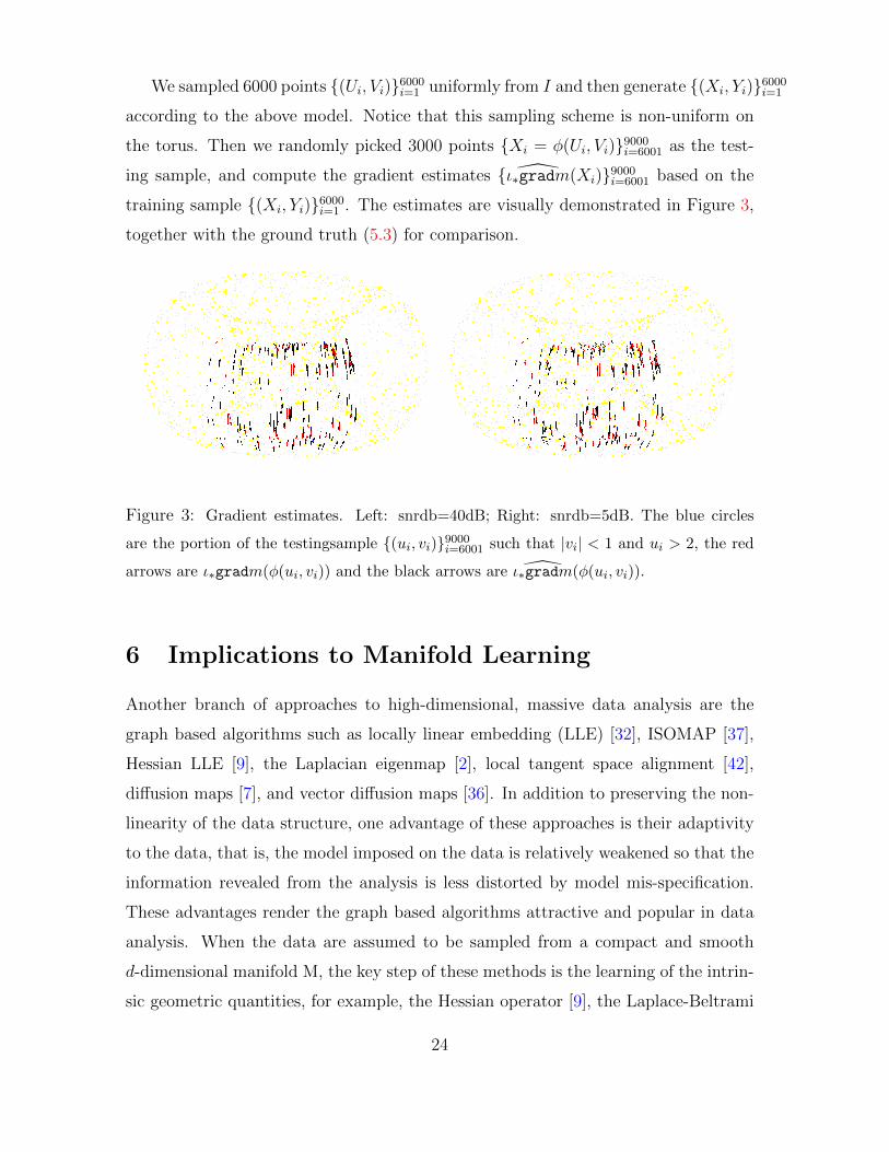
We sampled 6000 points (Ui, Vi)6000i=1 uniformly from I and then generate (Xi, Yi)6000
i=1
according to the above model. Notice that this sampling scheme is non-uniform on
the torus. Then we randomly picked 3000 points Xi = φ(Ui, Vi)9000i=6001 as the test-
ing sample, and compute the gradient estimates ι∗gradm(Xi)9000i=6001 based on the
training sample (Xi, Yi)6000i=1 . The estimates are visually demonstrated in Figure 3,
together with the ground truth (5.3) for comparison.
Figure 3: Gradient estimates. Left: snrdb=40dB; Right: snrdb=5dB. The blue circles
are the portion of the testingsample (ui, vi)9000i=6001 such that |vi| < 1 and ui > 2, the red
arrows are ι∗gradm(φ(ui, vi)) and the black arrows are ι∗gradm(φ(ui, vi)).
6 Implications to Manifold Learning
Another branch of approaches to high-dimensional, massive data analysis are the
graph based algorithms such as locally linear embedding (LLE) [32], ISOMAP [37],
Hessian LLE [9], the Laplacian eigenmap [2], local tangent space alignment [42],
diffusion maps [7], and vector diffusion maps [36]. In addition to preserving the non-
linearity of the data structure, one advantage of these approaches is their adaptivity
to the data, that is, the model imposed on the data is relatively weakened so that the
information revealed from the analysis is less distorted by model mis-specification.
These advantages render the graph based algorithms attractive and popular in data
analysis. When the data are assumed to be sampled from a compact and smooth
d-dimensional manifold M, the key step of these methods is the learning of the intrin-
sic geometric quantities, for example, the Hessian operator [9], the Laplace-Beltrami
24
operator [2, 7] or the connection Laplacian [36]. What we are concerned with in this
section is the estimation of the Laplace-Beltrami operator ∆ of M, considered in the
diffusion map framework [7], via MALLER. We refer the readers to these literature
for further discussions and references. Throughout this section, we make use of the
same assumptions and notation as in Sections 2 and 4.
We start with discussing the relationship between the diffusion map framework and
generalizing the Nadaraya-Watson kernel regression method to the manifold setup.
Suppose M is compact, smooth and without boundary. Fix a bandwidth h > 0. First
we define a n× n weight matrix W and a n× n diagonal matrix D by
W (i, j) = K
(‖Xi −Xj‖Rp√
h
)and D(i, i) =
n∑j=1
W (i, j). (6.1)
Then A := D−1W can be interpreted as a Markov transition matrix of a discrete
random walk over the sample points Xini=1, where the transition probability in a
single step from the sample point Xi to the sample point Xj is given by A(i, j).
Note that A can be used to generalize the Nadaraya-Watson kernel method orig-
inally defined for nonparametric regression on Rp to the manifold M setup. Indeed,
given the regression model (2.1), define this generalized Nadaraya-Watson estimator
mNW of m at Xi as
mNW (Xi, h) := (AY )(i) =
∑nj=1K
(‖Xi−Xj‖Rp√
h
)Yj∑n
j=1K(‖Xi−Xj‖Rp√
h
) , i = 1, . . . , n,
i.e. take A as the smoothing matrix of mNW (·, h). Clearly the conditional expectation
of the estimator mNW (Xi, h) becomes
EmNW (Xi, h)
∣∣X = (Am)(i) =
∑nj=1 K
(‖Xi−Xj‖Rp√
h
)m(Xj)∑n
j=1 K(‖Xi−Xj‖Rp√
h
) , (6.2)
where m is defined in (2.5). When m ∈ C3(M) and Xi /∈ M√h, the asymptotic
expansion of (6.2) has been shown in [7, 18, 35]. Indeed, we have, as n→∞,
(Am)(i) = m(Xi) + hµ1,2
2d
(∆m(Xi) + 2
m(Xi)∆f(Xi)
f(Xi)
)+O(h2) +Op
( 1
n12h
d4− 1
2
).
Note that in [7] the kernel is normalized so that µ1,0 = 1 and µ1,2/d = 2. When
f is constant, the second order conditional bias term contains information about
25
the Laplace-Beltrami operator of (M, g). This fact, however, is in general ignored
when the focus is the nonparametric regression problem. On the contrary, since
knowledge of the Laplace-Beltrami operator leads to abundant information about
the manifold, in [7] the matrix L0 := h−1(D−1W − In) and its relationship with the
Laplace-Beltrami operator are extensively studied, and the eigenvectors of A are used
to define the diffusion map. When f is not constant, the f -dependence is removed
by the following normalization [7]. Define a n × n weight matrix W1 and a n × n
diagonal matrix D1 by
W1 = D−1WD−1, and D1(i, i) =n∑j=1
W1(i, j) (6.3)
where W and D are defined in (6.1), and
L1 = h−1(D−1
1 W1 − In).
When n→∞, it is shown in [7] that for any m ∈ C3(M) the matrix L1 satisfies the
following convergence:
(L1m)(i) =µ1,2
2d∆m(Xi) +O(h) +Op
( 1
n1/2hd/4+1/2
). (6.4)
Notice that the effect of the normalization (6.3) is actually to cancel out the effect
of the non-uniformality in f on the matrix L0. We remark that the matrix D−11 W1
can thus be used as the smoothing matrix of a new estimator of m which is design
adaptive.
If we view the Nadaraya-Watson kernel method on Rp as the local zero-order
polynomial regression, the LLR on Rp can be viewed as the first-order companion of
the Nadaraya-Watson kernel method which takes the local slope into account [34]. We
discuss extensively its generalization to the regression on manifold setup in Section
2, its large sample behaviors in Section 4, and its numerical results are demonstrated
in Section 5. Recall that the conditional bias of MALLER, given in (A.30) of the
Supplementary, depends on the Laplace-Beltrami operator:
Em(X, h)−m(X)|X = hµ1,2
2d∆m(X) +O(h2 + hh3/4
pca) +Op
( 1
n1/2hd/4−1
).
26

This fact leads us to build up an alternative matrix to approximate the Laplace-
Beltrami operator. Fix h > 0 and consider the following n× n matrix
Ap =
vT1 (XT
X1WX1XX1)
−1XTX1WX1
...
vT1 (XTXn
WXnXXn)−1XTXn
WXn
, (6.5)
where the i-th entry is defined by (2.6), (2.7), and (2.9). Note that Ap is the smoothing
matrix of MALLER, that is, ApY =(m(X1, h), . . . , m(Xn, h)
)Tfrom (2.9). Using
this smoothing matrix and defining
Lp = h−1(Ap − In
),
for any m ∈ C3(M), we directly have
(Lpm)(i) =µ1,2
2d∆m(Xi) +O(h+ h3/4
pca) +Op
( 1
n1/2hd/4
). (6.6)
Thus the matrix Lp can be used to construct an estimator of the Laplace-Beltrami
operator ∆. Notice that we do not need an extra step to handle the non-constant
p.d.f. issue here because the design adaptive property of m(X, h) ensures that the
leading term in the right-hand side of (6.6) is independent of f . With the estimator
Lp of ∆, massive data analysis can be carried out in the same way as those in the
diffusion map framework if the manifold assumption is reasonable. We remark that
the knowledge of the non-constant p.d.f. is useful in some problems. For example, in
[7, 28] the authors showed a strong connection between the non-constant p.d.f. with
the Fokker-Plank operator, which is useful in the low-dimensional representation of
stochastic systems.
In Figure 4, some numerical results of estimating the ∆ of M by this new method
are demonstrated. We sampled 1000, 2000 and 4000 points uniformly from the S2,
S3 and S4 embedded in R3, R4 and R5 respectively, and built the matrix Lp from the
sample points with h = 0.1. It is a well known fact that the l-th eigenvalue of the
Laplace-Beltrami operator of Sk is −l(l+k−1) with multiplicity(k+lk
)−(k+l−2k
), where(·
·
)is the binomial coefficient. The results in Figure 4 show that the new estimator
for the Laplace-Beltrami operator agrees with this well known fact numerically.
Up to now there are two ways to estimate the Laplace-Beltrami operator: one is
based on generalizing the Nadaraya-Watson kernel method to the manifold setup as
27

Figure 4: From left to right: bar plots of the first 30 eigenvalues of Lp when the data
points were sampled uniformly from S2, S3 and S4. Note that the first few eigenvalues
of ∆ are 0,−2,−6,−12 for S2, 0,−3,−8,−14 for S3 and 0,−4,−10,−18 for S4, and the
multiplicities of the first few eigenvalues of ∆ are 1, 3, 5, 7 for S2, 1, 4, 9, 16 for S3 and
1, 5, 14, 30 for S4. This fact is well resembled by the corresponding spectrum of Lp.
suggested by (6.4) and studied in [7], and the other is based on MALLER, which gen-
eralizes the LLR to the manifold setup, as suggested by (6.6). The difference between
these two approaches is most obvious when the manifold has smooth boundary.
Suppose M is compact, smooth and its boundary ∂M is non-empty and smooth.
When Xi ∈ M√h, the asymptotic behavior of D−11 W1 has been shown in the proof of
Proposition 10 of [7]:
(D−11 W1m)(i) = m(X0) +
√hC1∂νm(X0) +O(h) +Op
( 1
n1/2hd/4−1/2
), (6.7)
where C1 = O(1), X0 ∈ ∂M is the point on the boundary ∂M closest to Xi, and
ν is the normal direction at X0. If the√h-order term is non-zero, the estimator
(L1m)(i) in (6.4) blows up when h→ 0. To avoid this blowup and to get an estimate
of the Laplace-Beltrami operator on M, the Neuman’s boundary condition ∂m∂ν
= 0 is
necessary. Thus, solving the eigenvalue problem of L1 is a discrete approximation to
solving the eigenvalue problem of the Laplace-Beltrami operator with the Neuman’s
boundary condition.
The situation is totally different for the proposed estimator Lp. The asymptotic
behavior of the conditional bias of MALLER at Xi ∈ M√h provided in Corollary 4.1
leads to
(Lpm)(i) =1
2
d∑k=1
ck(Xi)∇2∂k,∂k
m(Xi) +Op(h−1/2h3/4
pca + h1/2pca) +Op
( 1
n1/2hd/4
). (6.8)
Thus, we know that when Xi is near the boundary, the estimator Lp does not blow
up when h→ 0, and a different boundary condition can be imposed.
28

Notice that the importance of using different bandwidths in the tangent plane
estimation and in the LLR on the tangent plane becomes clear from (6.6) and (6.8).
Indeed, if we take hpca < h then it follows from (6.6) (resp. (6.8)) that the first order
error of the estimator for the Laplace-Beltrami operator inside the manifold is smaller
than the order h3/4 (resp. h1/4).
In Figure 5, we demonstrate the eigenvectors of the estimator Lp for the Laplace-
Beltrami operator of a manifold with boundary. Specifically, we sampled 2000 points
Xl2000l=1 uniformly from the interval [0, 1] embedded in R, and evaluated the eigen-
vectors of Lp built on Xl2000l=1 . Notice that the eigenvectors shown in Figure 5 can
not happen, except for the first one, if the Laplace-Beltrami operator satisfies the
Neuman’s condition. The survey of the boundary condition suitable for the estimator
Lp is out of the scope of this paper, and we leave it as a future work.
Figure 5: From left to right: the first four eigenvectors of Lp and the first 10 eigenvalues
of Lp when sampling from [0, 1]. The first two eigenvalues are zero. Notice that the second,
third and fourth eigenvectors can not happen if the Laplace-Beltrami operator satisfies the
Neuman’s condition.
7 Discussions
When the p-dimensional predictor vector X has some d-dimensional manifold struc-
ture, we obtain MALLER by constructing the traditional LLR on the estimated em-
bedded tangent plane, which is of dimension d instead of p. Consequently, both the
estimation accuracy and computational speed depend only on d but not on p. Keeping
p, d, n as fixed numbers, this feature is particularly advantageous when d n < p, as
is shown in the Isomap face database example in the numerical section. We mention
that MALLER works in this case hinges on the capability of estimating the tangent
29

plane. Since our model is noise free in the predictors, this capability can be explained
by the theoretical findings in [19] and [27]. In [27], the spike model is studied and the
recovery of the subspace spanned by the response vectors is guaranteed even if p ≥ n,
when there is no noise [27, (2.13)]. Under the manifold setup, locally the manifold
model behaves like the Euclidean space, so it is expected to have similar results as
those in [27], which is shown in [19]. Furthermore, we emphasize that, while in [1] this
case is modeled as the large p small n problem, where p grows with n, and sparsity
conditions and thresholding are employed, here we treat p as a fixed number and take
the fact that n is larger than d.
7.1 The Relationship with NEDE
MALLER is not the first LLR regression scheme proposed to adapt to the mani-
fold structure. NEDE, given in [1], is a manifold-adaptive LLR constructed in the
p-dimensional ambient space with regularization imposed on the directions perpen-
dicular to the estimated embedded tangent plane. At the first glance MALLER seems
to be a special case of NEDE [1, (4.6)] by taking λn =∞ in [1, (4.6)]. However, there
are several distinct differences between the two methods. In this section we follow
the notation used in [1].
First, when λn = ∞ for all n, although β in [1, (4.6)] is forced to be located
on the estimated embedded tangent plane, the NEDE algorithm still runs in the
ambient space and the minimization problem in [1, (4.6)] becomes ill-posed. Indeed,
the solution in [1, (4.6)] depends on the inverse of the matrix Cn + λnPn/nhd+2,
which is unstable to solve when λn = ∞. This numerical instability of NEDE when
λn = ∞ can also be shown numerically. As an illustration, we ran NEDE with
λn = e100 (within the machine precision) on the Isomap face database with the images
downsized to 7×7 pixels. Then, it happened that the optimal value of d chosen by the
NEDE algorithm was close to 49 = 7× 7 = p (48.325± 1.3019 over 100 replications)
due to the degeneracy of Cn +λnPn/nhd+2, and the final RASE was 12.3684± 6.1161
(over 100 replications), which is roughly ten times of the RASE of MALLER. Even
when we set d = 3 and λn = e100 in the NEDE algorithm and tested it on the same
7× 7-pixel images, the final RASE was still 10.5829± 6.0986 after 100 replications.
30

Second, even if NEDE [1, (4.6)] is stable to solve when λn = ∞, the bandwidth
selection problem in NEDE still depends on p, which leads to different results com-
pared with MALLER. Specifically, the selected bandwidth would be larger and hence
the bias is increased.
Third, in NEDE the bandwidth used in the tangent plane estimation is taken to
be the same as the one used in the LLR estimation, while in MALLER we estimate
the tangent plane using a different bandwidth hpca which by the asymptotic analysis
should be taken to be smaller than the bandwidth h in the LLR step. Thus, the tan-
gent plane estimate obtained by NEDE is different from that obtained by MALLER.
Since this estimation error does not contribute to the leading bias term, the differ-
ence is not significant in the regression problem. However, if we would like to have a
better estimator of the Laplace-Beltrami operator, this error becomes significant, as
is shown in Section 6.
In conclusion, MALLER is different from NEDE even if the parameter λn in NEDE
is set to ∞, both theoretically and numerically. And, the key features that render
the two algortihms different are those mentioned above, not the more sophisticated
method MALLER uses to select the bandwidth in the LLR.
7.2 Future Directions
To sum up this paper, here are several issues left open and are of interest for future
research:
1. Like in any smoothing methods, bandwidth selection is crucial for the proposed
MALLER. Our bandwidth selection procedure is built on balancing between
estimates of the conditional bias and variance. Although this approach worked
well in our numerical studies, there is still room for improvement.
2. We include in our algorithm a clustering tool to alleviate numerical problems
caused by the condition number, without having to estimate the condition num-
ber. This is not the ultimate solution; instead, the ideal solution is to estimate
the condition number, and then use that information in the subsequent steps.
31
3. In this paper we consider the case where the predictor vector is directly observ-
able. In some situations, the predictor vector itself is subject to noise, and the
tangent plane and regression estimation steps has to be adjusted accordingly.
This is closely related to the deconvolution and measurement error problems in
the literature, in the Euclidean setup.
4. In MALLER, the dimensionality is reduced to the intrinsic structure of the
predictors. The dimensionality may be further reduced by taking into account
the relationship between the response and the predictors [38, 39].
5. The smoothing matrix of MALLER is shown to be useful for estimating the
Laplace-Beltrami operator with the boundary condition different from Neu-
man’s condition, it is worthwhile to investigate further such a new set of tools
for manifold learning.
6. In applications, the response itself may be multivariate as well. The case when
the responses are positive-definite matrices and the predictor vector is non-
degenrated in Rp was considered by [43]. It is interesting to investigate the case
when both the response and the predictor vector have manifold structures.
References
[1] A. Aswani, P. Bickel, and C. Tomlin. Regression on manifolds: Estimation of
the exterior derivative. Ann. Stat., 39(1):48–81, 2011.
[2] M. Belkin and P. Niyogi. Laplacian Eigenmaps for Dimensionality Reduction
and Data Representation. Neural. Comput., 15(6):1373–1396, June 2003.
[3] P. J. Bickel and B. Li. Local polynomial regression on unknown manifolds.
Lecture Notes-Monograph Series, 54:177–186, 2007.
[4] G. Carlsson, T. Ishkhanov, V. de Silva, and A. Zomorodian. On the local be-
havior of spaces of natural images. Int. J. Comput. Vision, 76:1–12, 2008.
[5] L.-H. Chen, M.-Y. Cheng, and L. Peng. Conditional variance estimation in
heteroscedastic regression models. J. Stat. Plan. Infer., 139(2):236 – 245, 2009.
32

[6] Y. Chikuse. Statistics on special manifolds. Springer, New York, 2003.
[7] R. R. Coifman and S. Lafon. Diffusion maps. Appl. Comput. Harmon. Anal.,
21(1):5–30, 2006.
[8] M.P. do Carmo and F. Flaherty. Riemannian Geometry. Birkhauser Boston,
1992.
[9] D. L. Donoho and C. Grimes. Hessian eigenmaps: Locally linear embedding
techniques for high-dimensional data. P. Natl. Acad. Sci. USA, 100(10):5591–
5596, 2003.
[10] J. Fan, Y. Feng, and R. Song. Nonparametric independence screening in sparse
ultra-high-dimensional additive models. J. Am. Stat. Assoc., 106(494):544 – 557,
2011.
[11] J. Fan and I. Gijbels. Local Polynomial Modelling and Its Applications. Chapman
and Hall/CRC, 1996.
[12] J. Fan and R. Li. Variable selection via nonconcave penalized likelihood and its
oracle properties. J. Am. Stat. Assoc., 96(456):1348 – 1340, 2001.
[13] J. Fan and J. Lv. Sure independence screening for ultrahigh dimensional feature
space. J. R. Stat. Soc. Series B, 70(5):849 – 911, 2008.
[14] J. Fan and H. Peng. Nonconcave penalized likelihood with a diverging number
of parameters. Ann. Stat., 32(3):928 – 961, 2004.
[15] J. Fan and R. Song. Sure independence screening in generalized linear models
with np-dimensionality. Ann. Stat., 38(6):3567 – 3604, 2010.
[16] J. Frank. Three-Dimensional Electron Microscopy of Macromolecular Assem-
blies: Visualization of Biological Molecules in Their Native State. Oxford Uni-
versity Press, New York, 2nd edition, 2006.
[17] P. Hall, J. S. Marron, and A. Neeman. Geometric representation of high dimen-
sion, low sample size data. J. R. Stat. Soc. Series B, 67(3):427 – 444, 2005.
33

[18] M. Hein, J. Audibert, and U. von Luxburg. From graphs to manifolds - weak
and strong pointwise consistency of graph Laplacians. In Proceedings of the 18th
Conference on Learning Theory (COLT), pages 470–485, 2005.
[19] D.N. Kaslovsky and F.G. Meyer. Optimal tangent plane recovery from noisy
manifold samples. arXiv:1111.4601v1, 2011.
[20] J. Lafferty and L. Wasserman. Redeo: sparse, greedy nonparametric regession.
Ann. Stat., 36(1):28–63, 2008.
[21] G. Lerman and T. Zhang. Probabilistic recovery of multiple subspaces in point
clouds by geometric lp minimization. arXiv:1002.1994v2, 2010.
[22] E. Levina and P. J. Bickel. Maximum likelihood estimation of intrinsic dimension.
In L. Saul, Y. Weiss, and L. Bottou, editors, Adv. Neur. In., volume 17, pages
777 – 784, Cambridge, MA, 2005. MIT Press.
[23] R. Li and H. Liang. Variable selection in semiparametric regression modeling.
Ann. Stat., 36(1):261 – 286, 2008.
[24] J.-M. Loubes and B. Pelletier. A kernel-based classifier on a riemannian manifold.
Stat. Decn., 26:35 – 51, 2008.
[25] K. Mardia and P. Jupp. Directional Data. Wiley, New York, 2000.
[26] S. Mukherjee, Q. Wu, and D.-X. Zhou. Learning gradients on manifolds.
Bernoulli, 16(1):181–207, 2010.
[27] B. Nadler. Finite sample approximation results for principal component analysis:
A matrix perturbation approach. Ann. Stat., 36(6):2791–2817, December 2008.
[28] B. Nadler, S. Lafon, R. R. Coifman, and I. G. Kevrekidis. Diffusion maps,
spectral clustering and reaction coordinates of dynamical systems. Appl. Comput.
Harmon. Anal., 21(1):113–127, 2006.
[29] P. Niyogi, S. Smale, and S. Weinberger. Finding the homology of submanifolds
with high confidence from random samples. In Twentieth Anniversary Volume:,
pages 1–23. Springer New York, 2009.
34
[30] B. Pelletier. Nonparametric regression estimation on closed riemannian mani-
folds. J. Nonparametr. Stat., 18(1):57 – 67, 2006.
[31] G. Peyre. Manifold models for signals and images. Comput. Vis. Image Und.,
113(2):249 – 260, 2009.
[32] S. T. Roweis and L. K. Saul. Nonlinear dimensionality reduction by locally linear
embedding. Science, 290(5500):2323–2326, 2000.
[33] D. Ruppert. Empirical-bias bandwidths for local polynomial nonparametric re-
gression and density estimation. J. Am. Stat. Assoc., 92(439):1049 – 1062, 1997.
[34] D. Ruppert and M. P. Wand. Multivariate locally weighted least squares regres-
sion. Ann. Stat., 22(3):1346–1370, 1994.
[35] A. Singer. From graph to manifold Laplacian: The convergence rate. Appl.
Comput. Harmon. Anal., 21(1):128–134, 2006.
[36] A. Singer and H.-T. Wu. Vector diffusion maps and the connection Laplacian.
Comm. Pure Appl. Math., 65(8):1067–1144, 2012.
[37] J. B. Tenenbaum, V. de Silva, and J. C. Langford. A Global Geometric Frame-
work for Nonlinear Dimensionality Reduction. Science, 290(5500):2319–2323,
2000.
[38] Y. Xia. A constructive approach to the estimation of dimension reduction direc-
tions. Ann. Stat., 35(6):2654 – 2690, 2007.
[39] Y. Xia. A multiple-index model and dimension reduction. J. Am. Stat. Assoc.,
103(484):1631 – 1640, 2008.
[40] L Zelnik-Manor and P Perona. Self-tuning spectral clustering. Adv. Neur. In.,
2(1601-1608):1601–1608, 2004.
[41] C. Zhang, Y. Jiang, and Y. Chai. Penalized bregman divergence for large-
dimensional regression and classification. Biometrika, 97(3):551 – 560, 2010.
35

[42] Z. Zhang and H. Zha. Principal manifolds and nonlinear dimensionality reduction
via tangent space alignment. SIAM J. Sci. Comput., 26:313 – 338, 2004.
[43] H. Zhu, Y. Chen, J.G. Ibrahim, Y. Li, and W. Lin. Intrinsic regression models
for positive-definite matrices with applications to diffusion tensor imaging. J.
Am. Stat. Assoc., 104(487):1203 – 1212, 2009.
[44] L.-P. Zhu, L. Li, R. Li, and L.-X. Zhu. Model-free feature screening for ultrahigh-
dimensional data. J. Am. Stat. Assoc., 106(496):1464 – 1475, 2011.
36
Supplementary Materials for “Local Linear Regressionon Manifolds and its Geometric Interpretation”
by Ming-Yen Cheng, and Hau-Tieng Wu
A.1 Exterior derivative, covariant derivative and
gradient
In this appendix we provide the required differential geometry background about the
covariant derivative, gradient, exterior derivative and their relationships. We refer
the readers to [8] for more details.
We start from recalling the definition of the gradient vector field of a given function
defined on the Euclidean space. Given m : Rd → R, the gradient vector field or the
total differentiation, denoted as ∇m is defined as
∇m :=
(∂m
∂x1
, . . . ,∂m
∂xd
)so that for v ∈ Rd we have the directional derivative
∇vm(x) := (∇m)(v) := limt→0
m(x+ tv)−m(x)
t. (A.1)
Often we use another notation to represent the directional derivative:
〈∇m(x), v〉 := ∇vm(x) (A.2)
This definition, however, can not be generalized to the manifold setup directly. In-
deed, the quantity x+tv in (A.1) does not make sense in general. To obtain a suitable
notion of differentiation, we consider the following definitions. Fix a differentiable d-
dim manifold M and a C1 function m : M → R. For a given differentiable vector
field V , locally around x ∈ M we can find a curve c(t) so that c(0) = x ∈ M and
c′(0) = Vx, the value of V at x so that V acts on m at x by
V m(x) :=dm(c(t))
dt
∣∣∣t=0. (A.3)
The exterior derivative of m, denoted as dm at x is defined as:
((dm)V )(x) := 〈(dm)x, Vx〉 := V m(x), (A.4)
1
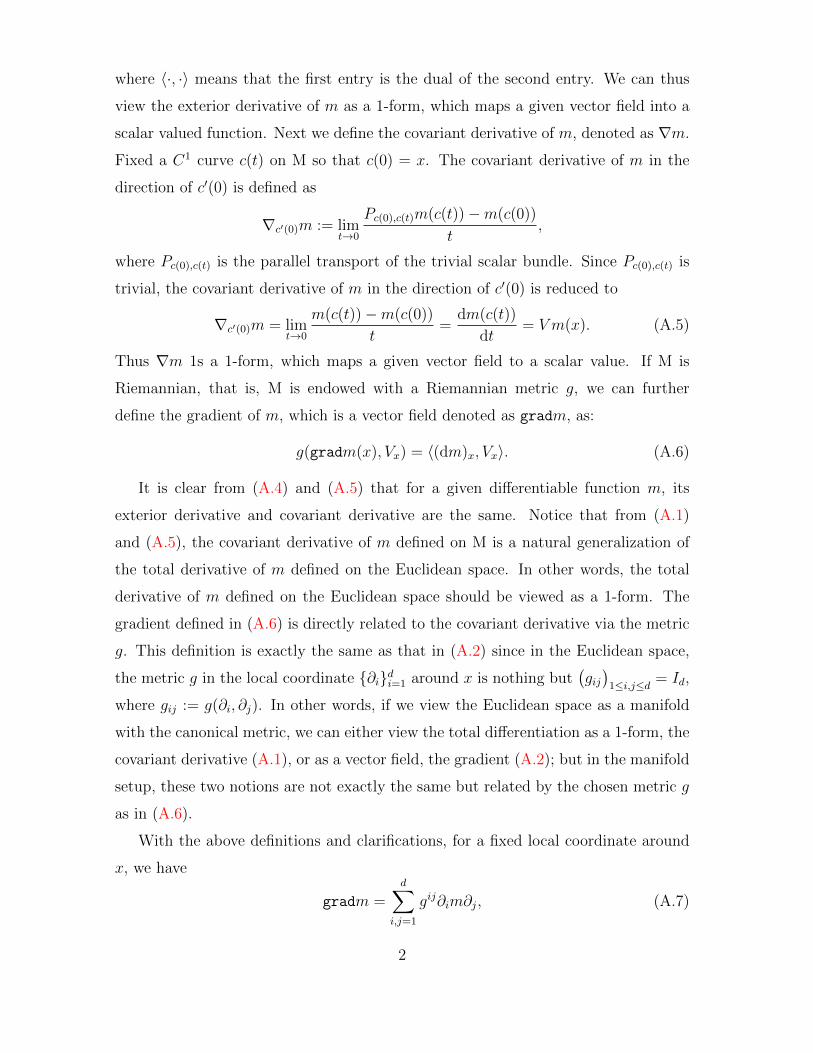
where 〈·, ·〉 means that the first entry is the dual of the second entry. We can thus
view the exterior derivative of m as a 1-form, which maps a given vector field into a
scalar valued function. Next we define the covariant derivative of m, denoted as ∇m.
Fixed a C1 curve c(t) on M so that c(0) = x. The covariant derivative of m in the
direction of c′(0) is defined as
∇c′(0)m := limt→0
Pc(0),c(t)m(c(t))−m(c(0))
t,
where Pc(0),c(t) is the parallel transport of the trivial scalar bundle. Since Pc(0),c(t) is
trivial, the covariant derivative of m in the direction of c′(0) is reduced to
∇c′(0)m = limt→0
m(c(t))−m(c(0))
t=
dm(c(t))
dt= V m(x). (A.5)
Thus ∇m 1s a 1-form, which maps a given vector field to a scalar value. If M is
Riemannian, that is, M is endowed with a Riemannian metric g, we can further
define the gradient of m, which is a vector field denoted as gradm, as:
g(gradm(x), Vx) = 〈(dm)x, Vx〉. (A.6)
It is clear from (A.4) and (A.5) that for a given differentiable function m, its
exterior derivative and covariant derivative are the same. Notice that from (A.1)
and (A.5), the covariant derivative of m defined on M is a natural generalization of
the total derivative of m defined on the Euclidean space. In other words, the total
derivative of m defined on the Euclidean space should be viewed as a 1-form. The
gradient defined in (A.6) is directly related to the covariant derivative via the metric
g. This definition is exactly the same as that in (A.2) since in the Euclidean space,
the metric g in the local coordinate ∂idi=1 around x is nothing but(gij)
1≤i,j≤d = Id,
where gij := g(∂i, ∂j). In other words, if we view the Euclidean space as a manifold
with the canonical metric, we can either view the total differentiation as a 1-form, the
covariant derivative (A.1), or as a vector field, the gradient (A.2); but in the manifold
setup, these two notions are not exactly the same but related by the chosen metric g
as in (A.6).
With the above definitions and clarifications, for a fixed local coordinate around
x, we have
gradm =d∑
i,j=1
gij∂im∂j, (A.7)
2

where ∂ldl=1 is the coordinate around x, ∂im is defined by (A.3) and(gij)
1≤i,j≤d is
the inverse of(gjk)
1≤i,j≤d, while the covariant derivative of m is
dm = ∇m =d∑l=1
∂lmdxl,
where dxldl=1 is the dual of ∂ldl=1. Thus, if we choose a normal coordinate around
x so that gij = δij at x, where δij denotes the kronecker delta, the coefficients of the
covariant derivative of m at x is the same as the coefficients of the gradient of m at x.
Note that gradm(x) (or dm(x)) is the same regardless the choice of the local basis.
Notice that as is stated in Theorem 4.3 and 4.4, the estimated first order covariant
derivative of m, ∇∂im(x, h), depends on the estimated basis of ι∗TxM. Thus, we have
to take this basis into account to estimate the embedded gradient of m, ι∗∇m(x), as
is considered in (2.10). Notice that since MALLER provides the estimate of ∇∂lm at
x for l = 1, . . . , d, we can get the estimate of the covariant derivative or the exterior
derivative of m by taking the dual basis of ∂ldl=1 into consideration.
We demonstrate the detailed calculation of the gradient given in (5.3). Since
φ(u, v) = ((2 + cos(v)) cos(u), (2 + cos(v)) sin(u), sin(v)), It is clear that
dφ =
−(2 + cos(v)) sin(u) − sin(v) cos(u)
(2 + cos(v)) cos(u) − sin(v) sin(u)
0 cos(v)
.By denoting e1 = (1, 0) ∈ R2 and e2 = (0, 1) ∈ R2, we get a set of embedded vector
fields defined on φ([0, 2π)× [0, 2π)):
E1 =dφ(e1)
‖dφ(e1)‖= (− sin(u), cos(u), 0)
and
E2 =dφ(e2)
‖dφ(e2)‖= (− sin(v) cos(u),− sin(v) sin(u), cos(v)),
which are orthonormal with related to the canonical metric of R3. Since ι is an iso-
metric embedding of the torus into R3, Ei = ι∗∂i, i = 1, 2, where ∂i is an orthonormal
frame defined on the torus. Thus, by (A.7) the embedded gradient of m at ι(x) can
be evaluated by
ι∗(gradm(x)) = ∂1m(x)ι∗∂1(x) + ∂2m(x)ι∗∂2(x) = ∂1m(x)E1(x) + ∂2m(x)E2(x),
(A.8)
3

where ∂i(x) is the value of ∂i at x. By definition, we have
∂1m(x) =dm(c1(t))
dt|t=0 =
dm(φ(u+ t2+cos(v)
, v))
dt=− sin(u) sin(4v + 1)
2 + cos(v)
∂2m(x) =dm(c2(t))
dt|t=0 =
dm(φ(u, v + t))
dt= 4 cos(u) cos(4v + 1)
where ι(x) = φ(u, v), ci(0) = x and c′i(0) = ∂i(x) for i = 1, 2. Note that dφ(e1) is
not of unit norm, so we have to normalize e1 by 2 + cos(v) when we evaluate ∂1m(x).
Plugging the above into (A.8), we get (5.3).
A.2 Proofs
The following lemmas are needed to finish the proofs of the theoretical results. The
proofs of the first three lemmas can be found in [36]. The first lemma describes how
the volume form depends on the curvature. The second lemma describes how to
express the relationship between two points on the manifold M after being embedded
in Rp. Recall that the notion of “subtraction” between two points on M is not
well defined. However, once these two points are embedded to Rp, the notion of
“subtraction” makes sense, and the result of subtraction can be expressed by some
geometric quantities of M and the embedding itself. The third lemma describes the
error when we try to estimate the geodesic distance between two close points on M
by the Euclidean distance between their embedded points. Notice that in practice
the geodesic distance between two close points on M is unknown a priori, and we can
only estimate it by the Euclidean distance between their embedded points.
Lemma A.2.1. In polar coordinates around x ∈ M, the volume form dV is
dV (expx tθ) =(td−1 + td+1Ric(θ, θ) +O(td+2)
)dtdθ,
where θ ∈ TxM, ‖θ‖ = 1 and t > 0.
Lemma A.2.2. Fix x ∈ M and denote by expx the exponential map at x. With the
identification of Tι(x)Rp with Rp, for θ ∈ TxM with ‖θ‖ = 1 and t 1, we have
ι(
expx tθ)
= ι(x) + tι∗θ + t2IIx(θ, θ)
2+O(t3). (A.1)
4
Lemma A.2.3. Suppose x, y ∈ M such that y = expx(tθ), where θ ∈ TxM and
‖θ‖ = 1. If t 1, then t = ‖ι(x)− ι(y)‖Rp 1 satisfies
t = t+1
24‖IIx(θ, θ)‖t3 +O(t4). (A.2)
By combining the above lemmas, we get the following two lemmas. In Lemma
A.2.4, we quantify the volume error introduced by estimating the geodesic distance
between two points x, y ∈ M by the Euclidean distance between ι(x) ∈ Rp and
ι(y) ∈ Rp. In Lemma A.2.5, we collect some routine calculus.
Lemma A.2.4. Fix x ∈ M and 0 < δ 1. For vi ∈ Sp−1, i = 1, . . . , `, we have∫BMδ (x)
Π`i=1〈y − x, vi〉dV (y) =
∫BMδ (x)
Π`i=1〈y − x, vi〉dV (y) +O(δd+`+2).
where
BMδ (x) := ι−1
(BRpδ (x) ∩ ι(M)
)⊂ M.
In particular, the volume of BMδ (x) differs from that of BM
δ (x) by O(δd+2).
Proof. By direct calculation:∫BMδ (x)
Π`i=1〈y − x, vi〉dV (y)
=
∫ δ+O(δ3)
0
∫Sd−1
Π`i=1〈tι∗θ +O(t2), vi〉
[td−1 +O(td+1)
]dθdt
=
∫ δ
0
∫Sd−1
Π`i=1〈tι∗θ +O(t2)
[td−1 +O(td+1)
]dθdt+O(δd+l+2)
=
∫BMδ (x)
Π`i=1〈y − x, vi〉dV (y) +O(δd+l+2),
where the first equality comes from Lemma A.2.1, Lemma A.2.2 and Lemma A.2.3
and the others comes from direction calculations.
Lemma A.2.5. Fix x ∈ M\M√h, where h 1, v ∈ Rp, a function φ ∈ C2(M) and
the kernel function K compactly supported in [0, 1] so that K|[0,1] ∈ C1([0, 1]). Then
5

for each ` ∈ N we have:
(a) EK`h(X, x)φ(X) = µ`,0f(x)φ(x) +O(h);
(b) EK`h(X, x)(X − x)φ(X)
= hµ`,2
d∑l=1
[φ(x)ι∗∂l∇∂lf(x) + f(x)ι∗∂l∇∂lφ(x)
]+f(x)φ(x)
2|Sd−1|
∫Sd−1
IIx(θ, θ)dθ
+O(h32 );
(c) E(K`h(X, x)(X − x)(X − x)Tφ(X)
)i,j
=
hµ`,2df(x)φ(x) +O(h2) when 1 ≤ i = j ≤ d
O(h2) otherwise;
(d) EK`h(X, x)(X − x)(X − x)T 〈X − x, v〉φ(X)
= h2 µ`,4|Sd−1|
∫Sd−1
ι∗θι∗θ
T 〈ι∗θ, v〉(φ(x)∇θf(x) + f(x)∇θφ(x)
)+f(x)φ(x)
2
(ι∗θι∗θ
T 〈II(θ, θ), v〉+ IIx(θ, θ)ι∗θT + ι∗θIIx(θ, θ)
T)〈ι∗θ, v〉
dθ
+O(h5/2).
Proof. These expectations are evaluated by Taylor’s expansion and by Lemma A.2.1
to Lemma A.2.4. We start with evaluating (a).
EK`h(X, x)φ(X) =
∫BM√
h(x)
K`h(y, x)φ(y)f(y)dV (y)
=
∫BM√
h(x)
K`h(y, x)φ(y)f(y)dV (y) +O(h)
=
∫Sd−1
∫ √h0
h−d/2(K`( t√
h
)+O
( t3√h
))(φ(x) + t∇θφ(x) +O(t2)
)×(f(x) + t∇θf(x) +O(t2)
)(td−1 +O(td+1)
)dtdθ +O(h)
=µ`,0f(x)φ(x) +O(h),
where the first equality comes from (4.3), the second equality comes from Lemma
A.2.3 and Lemma A.2.4, the third equality comes from the Taylor’s expansion and
Lemma A.2.1 and the last equality comes from the symmetry of Sd−1. Indeed, the
odd moments in the integral vanish because Sd−1 is symmetric.
6
Next, by the same arguments as those leading to (a) and Lemma A.2.2, the left
hand side of (b) becomes:
EK`h(X, x)(X − x)φ(X) =
∫BM√
h(x)
K`h(y, x)(y − x)φ(y)f(y)dV (y)
=
∫BM√
h(x)
K`h(y, x)(y − x)φ(y)f(y)dV (y) +O(h3/2)
=
∫Sd−1
∫ √h0
h−d/2(K`( t√
h
)+O
( t3√h
))(tι∗θ +
t2
2IIx(θ, θ) +O(t3)
)×(φ(x) + t∇θφ(x) +O(t2)
)(f(x) + t∇θf(x) +O(t2)
)×(td−1 + Ric(θ, θ)td+1 +O(td+2)
)dtdθ +O(h3/2)
= h
∫Sd−1
∫ 1
0
K` (t)(φ(x)ι∗θ∇θf(x) + f(x)ι∗θ∇θφ(x)
+IIx(θ, θ)f(x)φ(x)
2
)td+1dtdθ +O(h
32 ). (A.3)
A direct calculation shows that∫Sd−1
θ∇θf(x)dθ =d∑
l,k=1
∂i∇∂kf(x)
∫Sd−1
θlθkdθ =|Sd−1|d
d∑l=1
∂l∇∂lf(x). (A.4)
By plugging (A.4) into (A.3) we conclude (b).
By the same arguments as those leading to (b), we get (c):
E(K`h(X, x)(X − x)(X − x)Tφ(X)
)i,j
=
∫BM√
h(x)
K`h(y, x)(y − x)(y − x)Tφ(y)f(y)dV (y)
=
∫Sd−1
∫ √h0
h−d/2(K( t√
h
)+O
( t3√h
))(t2ι∗θι∗θ
T +O(t3))
×(φ(x) + t∇θφ(x) +O(t2)
)(f(x) + t∇θf(x) +O(t2)
)×(td−1 + Ric(θ, θ)td+1 +O(td+2)
)dtdθ +O(h2)
= hf(x)φ(x)
∫Sd−1
∫ 1
0
K (t) ι∗θ(ι∗θ)T td+1dtdθ +O(h2)
=
hµ`,2df(x)φ(x) +O(h2) when 1 ≤ i = j ≤ d
O(h2) otherwise, (A.5)
where the last equality comes from the fact that ι∗ is linear.
7

Equation (d) follows from the same arguments as in the above:
EK`h(X, x)(X − x)(X − x)T 〈X − x, v〉φ(X)
=
∫BM√
h(x)
K`h(y, x)(y − x)(y − x)T 〈y − x, v〉φ(y)f(y)dV (y)
=
∫Sd−1
∫ √h0
1
hd/2
K( t√
h
)(t2ι∗θ(ι∗θ)
T +t3
2
(IIx(θ, θ)ι∗θ
T + ι∗θIIx(θ, θ)T))
×(t〈ι∗θ, v〉+
t2
2〈II(θ, θ), v〉
)(φ(x) + t∇θφ(x)
)(f(x) + t∇θf(x)
)td−1
+O(td+5)
dtdθ +O(h5/2)
= h2 µ`,4|Sd−1|
∫Sd−1
ι∗θι∗θ
T 〈ι∗θ, v〉(φ(x)∇θf(x) + f(x)∇θφ(x)
)+f(x)φ(x)
2
(ι∗θι∗θ
T 〈II(θ, θ), v〉+ IIx(θ, θ)ι∗θT + ι∗θIIx(θ, θ)
T)〈ι∗θ, v〉
dθ
+O(h5/2).
Next we describe how the local PCA provides the estimate of the tangent plane.
Although locally a manifold M is close to some Euclidean space, there is always a
gap caused by the curvature of M. Lemma A.2.6 states its influence on the tangent
plane estimation by the local PCA.
Lemma A.2.6. Suppose hpca n−2d+1 . Then, if x ∈ M\M√h, the eignvectors
Ul(x)dl=1 corresponding to the d largest eigenvalues of the sample covariance ma-
trix Σx formed in the local PCA differ from an orthonormal basis ∂k(x)dk=1 to TxM
by:
Ul(x) = ι∗∂l(x) +Op(h5/4pca )wl +Op(h
3/4pca )w⊥l for l = 1, . . . , d, (A.6)
where wl ∈ ι∗TxM, w⊥l ⊥ ι∗TxM, and ‖wl‖ = ‖w⊥l ‖ = 1, and, if x ∈ M√h,
Ul(x) = ι∗∂l(x) +Op(h3/4pca )wl +Op(h
1/2pca )w⊥l for l = 1, . . . , d, (A.7)
where wl ∈ ι∗TxM, w⊥l ⊥ ι∗TxM, and both wl and w⊥l are of O(1).
Suppose hpca O(n−2d+2 ) and x ∈ M\M√h, then a better convergence rate is
achieved. Indeed, (A.6) becomes
Ul(x) = ι∗∂l(x) +Op(h3/2pca )wl +Op(hpca)w
⊥l for l = 1, . . . , d.
8
The proof of this lemma follows the same lines as those in [36] except some wrinkles
caused by the two differences mentioned above. We now detail these wrinkles and
refer the readers to [36] for the detailed proof.
Proof. Fix x ∈ M\M√h. Choose a normal coordinate ∂k(x)dk=1 around x and assume
M is properly rotated and translated so that x = 0p×1 and ei = ι∗∂i(x), for i =
1, . . . , d, where 0p×1 is the p × 1 zero vector and ei is the unit length p × 1 vector
with the i-th entry 1. Denote Zx := χBRp√hpca
(x)∩ι(M)(X)X, where χ is the indicator
function.
For later use, we prepare some calculations. First, since f ∈ C2(M) and M is
compact, by plugging ` = 1 and v1 = el into Lemma A.2.5 and taking Taylor’s
expansion, we have
E〈Zx, el〉 =
∫BM√
hpca(x)
〈y, el〉f(y)dV (y) (A.8)
=
∫Sd−1
∫ √hpca
0
⟨tι∗θ +
t2
2IIx(θ, θ), el
⟩(f(x) + t∇θf(x)) td−1dtdθ +O(h
d2
+3/2pca )
=O(hd2
+1pca ).
Similar calculation leads to:
E〈Zx, ek〉〈Zx, el〉 =
|Sd−1|d
f(x)hd/2+1pca +O(h
d/2+2pca ) for 1 ≤ k = l ≤ d
O(hd/2+2pca ) otherwise.
(A.9)
With (A.8) and (A.9), we can finish the proof. Recall that the sample mean of
N truex,hpca
is denoted by µx. Then, it follows from the Central Limit Theorem (CLT)
and (A.8) that
〈µx, el〉 =1
n
Nx∑k=1
〈Xxk , el〉 =
O(hd/2+1pca ) +Op
(n−12 h
d/4+1pca
)if l = 1, . . . , d
O(hd/2+1pca ) +Op
(n−12 h
d/4+2pca
)otherwise.
Since hd/2+1pca dominates n−1/2h
d/4+1pca asymptotically, due to the assumption hpca
n−2d+2 , we conclude that
µx = Op
(hd/2+1
pca
). (A.10)
9

Next we consider the sample covariance matrix Σx. By (A.8), (A.9), (A.10), and
similar calculation as in the above, we have
Σx(i, j) =1
n
Nx∑l=1
〈Xxl − µx, ei〉〈Xxl − µx, ej〉
=
E〈Zx, ei〉〈Zx, ej〉+Op
(hd+2
pca
)+Op
(n−12 h
d/4+1pca
)if 1 ≤ i, j ≤ d
E〈Zx, ei〉〈Zx, ej〉+Op
(hd+2
pca
)+Op
(n−12 h
d/4+2pca
)if d+ 1 ≤ i, j ≤ p
E〈Zx, ei〉〈Zx, ej〉+Op
(hd+2
pca
)+Op
(n−12 h
d/4+3/2pca
)otherwise,
where the second Op term comes from the finite sample variance. By (A.9) and the
assumption hpca n−2d+1 , we get
Σx =|Sd−1|f(x)
dhd/2+1
pca
Id 0d×p−d
0p−d×d 0p−d×p−d
+
Op(h1/2pca) Op(hpca)
Op(hpca) Op(hpca)
,
where 0m×m′ is the zero matrix of size m ×m′, for any m,m′ ∈ N. As a result, we
get the equation (B.44) in [36]. Then we can analyze Σx by the perturbation theory
exactly in the same way as in [36], so we skip the details. When x ∈ M√h, the same
calculation applies and we skip the details.
Before proving Theorem 4.1 and Theorem 4.2, we prepare some notation and
setups. Fix x. Recall that Bx is a p×d matrix with the k-th column Uk(x) determined
by the local PCA. Denote y := BTx (y − x) and xl := BT
x (Xl − x), where y ∈ M and
Xl ∈ X . To simplify the notation, we denote
H := BxHessm(x)BTx ,
Sx := diag(σ2(ι−1(X1)), . . . , σ2(ι−1(Xn))
),
Qm(x) :=[xT1 Hessm(x)x1 . . . xTnHessm(x)xn
]T.
10

For a given function φ : M 7→ R, ` ∈ N and v ∈ Rp, we define
E`0(φ) := EK`h(X, x)φ(X),
E`1(φ) := EK`h(X, x)(X − x)φ(X),
E`2(φ) := EK`h(X, x)(X − x)(X − x)Tφ(X),
E`3,v(φ) := EK`h(X, x)(X − x)(X − x)T 〈X − x, v〉φ(X),
q1 :=1
n
n∑l=1
Kh(Xl, x)xTl Hessm(x)xl,
q2 :=1
n
n∑l=1
Kh(Xl, x)xTl Hessm(x)xlxl.
A.2.1 [Proof of Theorem 4.1]
Proof. Fix x ∈ M. Denote by Uk(x)dk=1 the orthonormal set determined by local
PCA. Choose an orthonormal basis ekpk=1 of Rp, where ek is the p × 1 unit norm
column vector with the k-th entry 1, and assume ι is properly rotated and translated
so that x = 0p×1 and ei = ι∗∂i(x) for i = 1, . . . , d, where 0p×1 is the p-dimensional
zero vector.
With the notation Y and m defined in (2.5), clearly we have
Em(x, h)|X = vT1 (XTxWxXx)
−1XTxWxEY = vT1 (XT
xWxXx)−1XT
xWxm. (A.11)
Take y = expx(tθ), where t = O(h1/2) and ‖θ‖ = 1. By Lemma A.2.2 we have
tι∗θ = ι(y)− x− t2
2IIx(θ, θ) +O(t3), (A.12)
which by Lemma A.2.6 leads to
〈ι∗θ, Uk(x)〉 = 〈ι∗θ, ι∗∂k〉+Op(h5/4pca), (A.13)
since w⊥k is perpendicular to ι∗θ, and
〈IIx(θ, θ), Uk(x)〉 = Op(h3/4pca), (A.14)
since the second fundamental form IIx is perpendicular to the embedded tangent
plane ι∗TxM. Therefore, for j = 1, . . . , d, we have
〈tι∗θ, ej〉 = 〈tι∗θ, Uj(x)−Op(h5/4pca)wj〉 (A.15)
11
= 〈y − x, Uj(x)〉 − t2
2〈IIx(θ, θ), Uj(x)〉+Op(h
1/2h5/4pca)
= 〈y − x, Uj(x)〉+Op(hh3/4pca + h1/2h5/4
pca)
= yj +Op(hh3/4pca),
where the first equality holds due to Lemma A.2.6, the second equality holds due to
(A.12), the third equality holds due to (A.14), and the last equality holds due to the
assumption that hpca ≤ h. By Taylor’s expansion on M, (A.15), and the assumption
that hpca ≤ h,
m(y)−m(x) (A.16)
= tθ∇m(x) +t2
2Hessm(x)(θ, θ) +O(t3)
=d∑j=1
〈tι∗θ, ej〉∇∂jm(x) +1
2
d∑i,j=1
〈tι∗θ, ei〉〈tι∗θ, ej〉Hessm(x)(∂i, ∂j) +O(h32 )
= yT∇m(x) +1
2yTHessm(x)y +Op(hh
34pca),
where the second equality is obtained by rewriting θ =∑d
k=1 g(θ, ∂k(x))∂k(x) =∑dk=1〈ι∗θ, ek〉∂k(x), because ι is isometric. Since the kernel K is compactly supported,
m is bounded, and M is smooth and compact, (A.16) leads to
Wxm = Wx
(Xx
[ m(x)
∇m(x)
]+
1
2Qm(x) +Op(hh
34pca)), (A.17)
where Xx is defined in (2.6) and Wx is defined in (2.7). By plugging (A.17) into
(A.11), the conditional bias is reduced to
Em(x, h)−m(x)|X = vT1 (XTxWxXx)
−1XTxWx(Qm(x) +Op(hh
34pca)). (A.18)
Now we evaluate (A.18). By direct expansion, we have
1
nXTxWxXx =
1n
∑nl=1 Kh(Xl, x) 1
n
∑nl=1Kh(Xl, x)xTl
1n
∑nl=1Kh(Xl, x)xl
1n
∑nl=1 xlKh(Xl, x)xTl
. (A.19)
Denote by 1 the constant function with value 1. By the CLT, we have
1
n
n∑l=1
Kh(Xl, x) = E10(1) +Op
( 1
n12h
d4
), (A.20)
12

1
n
n∑l=1
Kh(Xl, x)xl = BTx E
11(1) +Op
( 1
n12h
d4− 1
2
), (A.21)
and1
n
n∑l=1
xlKh(Xl, x)xTl = BTx E
12(1)Bx +Op
( 1
n12h
d4−1
). (A.22)
Note that in (A.21), the random variables Kh(Xl, x)xlnl=1 are not independent since
xl = BTx (Xl−x) and Bx is evaluated from the random samples Xlnl=1, and hence
the CLT can not be applied directly. However, once we rewrite the left-hand side of
(A.21) as BTx
(1n
∑nl=1 Kh(Xl, x)(Xl−x)
), the summands become independent, and
the CLT can be applied. The same comment applies to (A.22). The expectation in
(A.20) is clear from Lemma A.2.5. The expectation in (A.21) becomes
BTx E
11(1) = h
µ1,2
dBTx
d∑j=1
ι∗∂j∇∂jf(x)
+h
∫Sd−1
∫ 1
0
K(t)BTx IIx(θ, θ)f(x)
2td+1dtdθ +O(h
32 )
= hµ1,2
dBTx
d∑j=1
ι∗∂j∇∂jf(x) +Op(hh34pca) +O(h
32 )
= hµ1,2
d∇f(x) +Op(h
32 ),
where the first equality holds due to Lemma A.2.5, the second equality holds due to
(A.14) and the third equality holds due to (A.13) and the assumption that hpca ≤ h.
Similarly, the expectation in (A.22) becomes
BTx E
12(1)Bx = hf(x)
∫Sd−1
∫ 1
0
K (t) θθT td+1dtdθ +Op(hh54pca) +O(h2)
= hµ1,2
df(x)Id +Op(h
2),
where the first equality comes from Lemma A.2.5 and (A.13). As a result, (A.19)
becomes
1
nXTxWxXx =
f(x) hµ1,2d∇f(x)T
hµ1,2d∇f(x) hµ1,2
df(x)Id
+
O(h) +Op
(1
n1/2hd/4
)O(h3/2) +Op
(1
n1/2hd/4−1/2
)O(h3/2) +Op
(1
n1/2hd/4−1/2
)O(h2) +Op
(1
n1/2hd/4−1
) .13

Since h → 0 and nhd/2 → ∞ as n → ∞, we know 1nXTxWxXx is invertible with
probability tending to 1 as n → ∞. Also, since f(x) + O(h) + Op
(1
n1/2hd/4
)and
hµ1,2df(x)Id +O(h2) +Op
(1
n1/2hd/4−1
)are also invertible with probability tending to 1
as n→∞, by the binomial inverse theorem,
( 1
nXTxWxXx
)−1
=
f(x)−1 −f(x)−2∇f(x)T
−f(x)−2∇f(x) h−1 dµ1,2f(x)
Id
(A.23)
+
O(h) +Op
(1
n1/2hd/4
)O(h1/2) +Op
(1
n1/2hd/4+1/2
)O(h1/2) +Op
(1
n1/2hd/4+1/2
)O(1) +Op
(1
n1/2hd/4+1
) .Next we consider 1
nXTxWxQm(x). By a direct calculation,
1
nXTxWxQm(x) =
q1
q2
. (A.24)
Note that, for any n× n matrix Z and any n× 1 column vector v,
vTZv = tr(ZvvT ). (A.25)
By (A.25) and the CLT, we have
q1 =1
n
n∑l=1
Kh(Xl, x)(Xl − x)TH(Xl − x)
= tr(H
1
n
n∑l=1
Kh(Xl, x)(Xl − x)(Xl − x)T)
= tr(HE1
2(1))
+Op
( 1
n1/2hd/4−1
). (A.26)
We evaluate tr(HE2
)by
tr(HE1
2(1))
= hf(x)tr(H
∫Sd−1
∫ 1
0
K (t) ι∗θι∗θT td+1dtdθ
)+O(h2)
= hf(x)
∫Sd−1
∫ 1
0
K(t)θTHessm(x)θtd+1dtdθ +O(h2)
= hµ1,2
df(x)∆m(x) +Op(h
2), (A.27)
where the first equality comes from Lemma A.2.5, the second equality comes from
(A.13) and (A.25) and the last equality holds due to the symmetry of Sd−1 and the
definition of the Laplace-Beltrami operator.
14
Then we evaluate q2 in (A.24). Choose ekpk=1 as an orthonormal basis of Rp and
rewrite Xl−x =∑p
k=1〈Xl−x, ek〉ek. Note that the random variables Kh(Xl, x)(Xl−x)(Xl − x)T 〈Xl − x, ek〉 are independent. By (A.25) and the CLT,
q2 =1
n
n∑l=1
Kh(Xl, x)tr(H(Xl − x)(Xl − x)T
)BTx (Xl − x) (A.28)
= BTx
p∑k=1
tr(H
1
n
n∑l=1
Kh(Xl, x)(Xl − x)(Xl − x)T 〈Xl − x, ek〉)ek
= BTx
p∑k=1
tr(HE1
3,ek(1))ek +Op
( 1
n12h
d4− 3
2
).
By the same arguments as those for q1, we have
BTx
p∑k=1
tr(HE1
3,ek(1))ek
= h2 µ1,2
|Sd−1|BTx
p∑k=1
tr(H
∫Sd−1
ι∗θι∗θT [〈ι∗θ, ek〉∇θf(x) +
f(x)
2〈II(θ, θ), ek〉]dθ
)ek
+h2µ1,2f(x)
2|Sd−1|BTx
p∑k=1
tr(H
∫Sd−1
[IIx(θ, θ)ι∗θT + ι∗θIIx(θ, θ)
T ]〈ι∗θ, ek〉dθ)ek
= h2 µ1,2
|Sd−1|
∫Sd−1
θTHessm(x)θθ∇θf(x)dθ +Op(h5/2),
where the first equality holds by Lemma A.2.5 and the second equality holds by
(A.13), (A.14), (A.25) and (A.28).
As a result, (A.24) becomes
1
nXTxWxQm(x) =
hµ1,2df(x)∆m(x)
h2 µ1,2|Sd−1|
∫Sd−1 θ
THessm(x)θθ∇θf(x)dθ
+
Op(h2) +Op
(1
n1/2hd/4−1
)Op(h
52 ) +Op
(1
n12 hd/4−
32
) (A.29)
Lastly, since m ∈ C3(M) and M is compact, a simple uniform bound combined with
(A.23) yields that the remainder term in (A.18) is Op(hh3/4pca). Plug (A.23), (A.29)
and this result into (A.18), we conclude that
Em(x, h)−m(x)|X = hµ1,2
2d∆m(x) +Op(h
2 + hh3/4pca) +Op
( 1
n12h
d4−1
). (A.30)
15
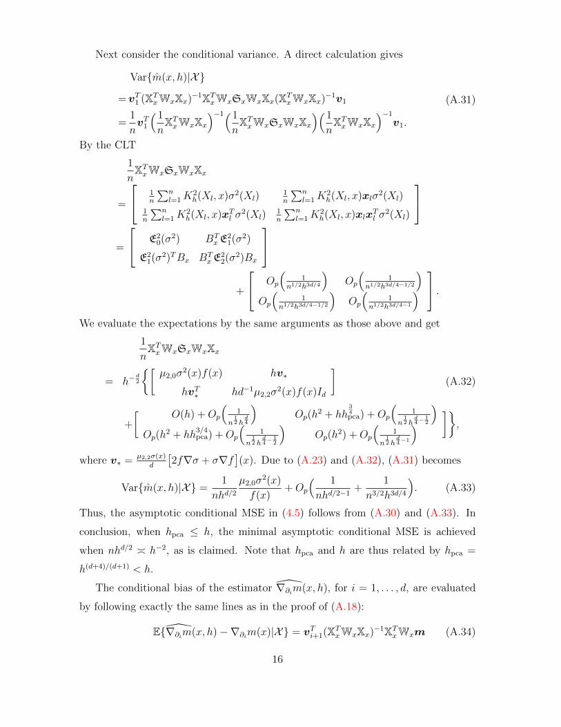
Next consider the conditional variance. A direct calculation gives
Varm(x, h)|X
=vT1 (XTxWxXx)
−1XTxWxSxWxXx(XT
xWxXx)−1v1
=1
nvT1
( 1
nXTxWxXx
)−1( 1
nXTxWxSxWxXx
)( 1
nXTxWxXx
)−1
v1.
(A.31)
By the CLT
1
nXTxWxSxWxXx
=
1n
∑nl=1K
2h(Xl, x)σ2(Xl)
1n
∑nl=1 K
2h(Xl, x)xlσ
2(Xl)
1n
∑nl=1K
2h(Xl, x)xTl σ
2(Xl)1n
∑nl=1K
2h(Xl, x)xlx
Tl σ
2(Xl)
=
E20(σ2) BT
x E21(σ2)
E21(σ2)TBx BT
x E22(σ2)Bx
+
Op
(1
n1/2h3d/4
)Op
(1
n1/2h3d/4−1/2
)Op
(1
n1/2h3d/4−1/2
)Op
(1
n1/2h3d/4−1
) .We evaluate the expectations by the same arguments as those above and get
1
nXTxWxSxWxXx
= h−d2
[µ2,0σ
2(x)f(x) hv∗
hvT∗ hd−1µ2,2σ2(x)f(x)Id
](A.32)
+
[O(h) +Op
(1
n12 h
d4
)Op(h
2 + hh34pca) +Op
(1
n12 h
d4−
12
)Op(h
2 + hh3/4pca) +Op
(1
n12 h
d4−
12
)Op(h
2) +Op
(1
n12 h
d4−1
) ],
where v∗ = µ2,2σ(x)
d
[2f∇σ + σ∇f
](x). Due to (A.23) and (A.32), (A.31) becomes
Varm(x, h)|X =1
nhd/2µ2,0σ
2(x)
f(x)+Op
( 1
nhd/2−1+
1
n3/2h3d/4
). (A.33)
Thus, the asymptotic conditional MSE in (4.5) follows from (A.30) and (A.33). In
conclusion, when hpca ≤ h, the minimal asymptotic conditional MSE is achieved
when nhd/2 h−2, as is claimed. Note that hpca and h are thus related by hpca =
h(d+4)/(d+1) < h.
The conditional bias of the estimator ∇∂im(x, h), for i = 1, . . . , d, are evaluated
by following exactly the same lines as in the proof of (A.18):
E∇∂im(x, h)−∇∂im(x)|X = vTi+1(XTxWxXx)
−1XTxWxm (A.34)
16
= ∇∂im(x) + vTi+1(XTxWxXx)
−1XTxWxQm(x)/2 +O(h1/2h3/4
pca).
By plugging (A.23) and (A.29) into (A.34), we obtain
E∇∂im(x, h)−∇∂im(x)|X (A.35)
=− hµ1,2
d
∇f(x)T
f(x)∆m(x) + h
d∫Sd−1 θ
THessm(x)θθ∇θf(x)dθ
|Sd−1|f(x)
+O(h32 + h
12h
34pca) +Op
( 1
n12h
d4− 1
2
).
The conditional variance term of ∇∂im(x, h) comes from (A.23) and (A.32):
Var∇∂im(x, h)|X (A.36)
=vTi+1(XTxWxXx)
−1(XTxWxSxWxXx)(XT
xWxXx)−1vi+1
=1
nhd/2+1
dµ2,2σ2(x)f(x)
µ1,2
+Op
( 1
nhd/2
)+Op
( 1
n3/2h3d/4+1
).
The conditional MSE is then obtained directly and it leads to the conclusion that the
minimal asymptotic conditional MSE is achieved when nhd/2 h−3.
A.2.2 [Proof of Theorem 4.2]
Proof. The proof is smilier to that of Theorem 4.1 except the boundary effect. We
use the same notation Uk(x)dk=1, ekpk=1 as those in the proof of Theorem 4.1 and
the same assumption for ι. Note that the equalities (A.11) and (A.31) still hold. Take
y = expx tθ ∈ M, where t = O(√h) and ‖θ‖ = 1. By Lemma A.2.2, Lemma A.2.6
and (A.12), we have for j = 1, . . . , d
〈tι∗θ, ej〉 = 〈tι∗θ, Uj(x) +Op(h3/4pca)wj〉 (A.37)
= 〈ι(y)− x, Uj(x)〉 − t2
2〈IIx(θ, θ), Uj(x)〉+Op(h
3/4pcah
1/2) +O(h3/2)
= yj +O(h3/4pcah
1/2 + h1/2pcah),
By the same arguments as that in (A.16) and by (A.37), we have
m(y)−m(x) = tθ∇m(x) +t2
2Hessm(x)(θ, θ) +O(t3)
=d∑j=1
〈tι∗θ, ej〉∇∂jm(x) +1
2
d∑i,j=1
〈tι∗θ, ei〉〈tι∗θ, ej〉Hessm(x)(∂i, ∂j) +O(h32 )
=yT∇m(x) +1
2yTHessm(x)y +Op(h
3/4pcah
1/2 + h1/2pcah),
17
which leads to the following equality
Wxm = Wx
(Xx
[ m(x)
∇m(x)
]+
1
2Qm(x) +Op(h
3/4pcah
1/2 + h1/2pcah)
)since the kernel K is compactly supported. By a direct calculation, the conditional
bias is reduced to
Em(x)−m(x)|X = vT1 (XTxWxXx)
−1XTxWx[Qm(x)/2+Op(h
3/4pcah
1/2+h1/2pcah)]. (A.38)
By taking the boundary effect into consideration and the similar arguments as those
in the proof of Theorem 4.1, we have
1
nXTxWxXx = f(x)Cν1,xC
+
Op(√h) +Op
(1
n12 h
d4
)Op(h) +Op
(1
n12 h
d4−
12
)Op(h) +Op
(1
n12 h
d4−
12
)Op(h
32 ) +Op
(1
n12 h
d4−1
) where ν1,x and C are respectively defined in (4.6) and (4.8). The invertibility of
1nXTxWxXx follows from the assumption (4.4) and (4.1). Indeed, from (4.4) and (4.1)
we know
f(x)ν1,x,11 = f(x)
∫h−1/2 exp−1
x D
K(y)dy > 0,
and hence Minkowski’s inequality implies that with probability tending to 1, the
invertibility holds. The binomial inverse theorem yields that( 1
nXTxWxXx
)−1
=C−1ν−1
1,xC−1
f(x)(A.39)
+
Op(√h) +Op
(1
n12 h
d4
)Op(1) +Op
(1
n12 h
d4+1
2
)Op(1) +Op
(1
n12 h
d4+1
2
)Op(h
− 12 ) +Op
(1
n12 h
d4+1
) ,where
ν−11,x :=
[ ν111,x ν12
1,x
(ν121,x)
T ν221,x
], ν11
1,x := (ν1,x,11 − ν1,x,12ν−11,x,22ν
T1,x,12)−1,
ν221,x :=
(ν1,x,22 − νT1,x,12ν1,x,11ν1,x,12
)−1, and ν12
1,x := −(ν−11,x,11ν1,x,12)ν22
1,x.
The term 1nXTxWxQm(x) in (A.38) is evaluated by following the same lines as those
in (A.24) except for the boundary effect. By the same arguments as those used to
18

calculate the term q1 in (A.24), we have
q1 =
∫expxD(x)
Kh(y, x)(y − x)TH(y − x)f(y)dV (y) +Op
( 1
n1/2hd/4−1
)= hf(x)
∫1√hD(x)
K(‖u‖)uTHessm(x)udu+Op(h3/2) +Op
( 1
n1/2hd/4−1
),
where the first equality comes from the CLT and the second equality comes from
Lemma A.2.4 and the change of variable. Choose ekpk=1 as an orthonormal basis of
Rp. By the same arguments as those in (A.28),
q2 = BTx
p∑k=1
tr(H
∫expxD(x)
Kh(y, x)(y − x)(y − x)T 〈y − x, ek〉
×f(y)dV (y))ek +Op
( 1
n12h
d4− 3
2
)= h3/2f(x)
∫1√hD(x)
K(‖u‖)uTHessm(x)uudu+Op(h2) +Op
( 1
n12h
d4− 3
2
),
where the first equality comes from (A.25) and the second one comes from the as-
sumption hpca ≤ h. Since m ∈ C3 and M is compact, the remainder term in (A.38)
is bounded by Op(h3/4pcah1/2 + h
1/2pcah). Thus, since hpca ≤ h by assumption, it follows
from (A.25) that
Em(x, h)−m(x)|X (A.40)
= hvT1 ν
−11,x
2
∫1√hD(x)
K(‖u‖)uTHessm(x)u[ 1
u
]du
+Op(h34pcah
12 + h
12pcah) +Op
( 1
n12h
d4−1
)= h
tr(Hessm(x)ν1,x,22)
2(ν1,x,11 − ν1,x,12ν−11,x,22ν1,x,21)
+Op(h34pcah
12 + h
12pcah) +Op
( 1
n12h
d4−1
).
The conditional variance is evaluated by the same lines as those in (A.32):
1
nXTxWxSxWxXx = h−
d2σ2(x)f(x)Cν2,xC (A.41)
+h−d2
Op(h1/2) +Op
(1
n1/2hd/4
)Op(h) +Op
(1
n1/2hd/4−1/2
)Op(h) +Op
(1
n1/2hd/4−1/2
)Op(h
3/2) +Op
(1
n1/2hd/4−1
) ,which when combined with (A.39) leads to
(XTxWxXx)
−1(XTxWxSxWxXx)(XT
xWxXx)−1 (A.42)
19

=1
nhd2
σ2(x)
f(x)C−1ν−1
1,xν2,xν−11,xC
−1
+1
nhd2
Op(h12 ) +Op
(1
n12 h
d4
)Op(1) +Op
(1
n12 h
d4+1
2
)Op(1) +Op
(1
n12 h
d4+1
2
)Op(h
−12 ) +Op
(1
n12 h
d4+1
) .From (A.42), since vT1C
−1 = vT1 , we have
Varm(x, h)|X =vT1 ν
−11,xν2,xν
−11,xv1
nhd2
σ2(x)
f(x)+Op
( 1
nhd2− 1
2
+1
n32h
3d4
).
Putting this together with (A.40) we obtain the conditional MSE of m(x, h).
With (A.39), (A.41) and the fact that vTi+1C−1 = h−1/2vTi+1, the conditional bias
and the conditional variance of the estimator of the first order covariance derivative
of m(x) are clear by the same calculation. For i = 1, . . . , d,
E∇∂im(x, h)−∇∂im(x)|X (A.43)
=√hvTi+1ν
−11,x
2
∫1√hD(x)
K(‖u‖)uTHessm(x)u[ 1
u
]du
+Op(h3/4pca + h1/2
pcah12 ) +Op
( 1
n12h
d4
+1
)and
Var∇∂im(x, h)|X =vTi+1ν
−11,xν2,xν
−11,xvi+1
nhd/2+1
σ2(x)
f(x)(A.44)
+Op
( 1
nhd2
+ 12
+1
n32h
3d4
).
Then the conditional MSE of ∇∂im(x, h) follows from the above results.
A.2.3 [Proof of Corollary 4.1]
Proof. The proof is finished by simplifying the conditional bias term (A.40) when the
boundary ∂M is smooth. We should show that the conditional bias term is actually
the linear combination of second order covariant derivatives of m at x. We first
symmetrize the integration domain D(x) as follows. Suppose
x∂ = argminy∈∂M
d(y, x)
20
and
h(x) = miny∈∂M
d(y, x) <√h.
Choose a normal coordinate ∂idi=1 on the geodesic ball BM√h(x) around x so that
x∂ = expx(h(x)∂d(x)). Divide D(x) into slices Sη ⊂ Rd−1, that is,
D(x) = ∪√h
η=−√hSη,
where
Sη := v ∈ Rd−1 : ‖(v, η)‖Rd <√h,
and η ∈ [−√h,√h]. Define Sη so that
Sη := ∩d−1i=1 (RiSη ∩ Sη),
where Ri is the reflection of Rd with respect to the i-th coordinate. The symmetriza-
tion of D(x) is thus defined as
D(x) := ∪√h
η=−√hSη.
Since ∂M is a smooth (d − 1)-dimensional manifold, by Lemma A.2.2 we can ap-
proximate exp−1x (expxD(x)∩ ∂M) by a homogeneous degree 2 polynomial defined on
Texp−1(x∂) exp−1x (expxD(x) ∩ ∂M), whose graph is symmetric in all coordinates, with
error O(h3/2). Thus, the error of approximating Sη by Sη is of order O(h3/2) and
hence the volume of the set D(x)∆D(x) is
Vol(D(x)∆D(x)
)= O(hd/2+1). (A.45)
We also denote
α(x) :=
∫1√hD(x)
K(‖u‖)du, (A.46)
β(x) :=
∫1√hD(x)
K(‖u‖)uddu, (A.47)
Γ(x) := diag(γ1(x), . . . , γd(x)), (A.48)
γi(x) :=
∫1√hD(x)
K(‖u‖)u2idu, i = 1, . . . , d. (A.49)
Thus, since D(x) is symmetric in the first d− 1 directions, by (A.45) we have∫1√hD(x)
K(‖u‖)du =
∫1√hD(x)
K(‖u‖)du+O(h) = α(x) +O(h),
21
∫1√hD(x)
K(‖u‖)uTdu =
∫1√hD(x)
K(‖u‖)uTdu+O(h) = βvTd (x) +O(h),
and ∫1√hD(x)
K(‖u‖)uuTdu =
∫1√hD(x)
K(‖u‖)uuTdu+O(h) = Γ(x) +O(h).
Hence, we get the following equations:
ν111,x =
1
α(x)− β(x)2γd(x)+O(h), (A.50)
ν121,x =
−β(x)γd(x)
α(x)− β(x)2γd(x)vTd +O(h), (A.51)
ν221,x = Γ(x)−1 +O(h). (A.52)
Similarly, by the symmetry of D(x), we have
∫1√hD(x)
K(‖u‖)uTHessm(x)u
1
u
du
=
∫1√hD(x)
K(‖u‖)uTHessm(x)u
1
u
du+O(h). (A.53)
Plugging (A.50), (A.51), (A.52), and (A.53) into (A.40) leads to
tr(Hessm(x)ν1,x,22)
2(ν1,x,11 − ν1,x,12ν−11,x,22ν1,x,21)
=
∑dk=1 γk(x)γd(x)∇2
∂k,∂km(x)
2[α(x)γd(x)− β(x)2], (A.54)
which finishes the claim. Moreover, by the Cauchy-Schwartz inequality, α(x)γd(x)−β(x)2 > 0 for all x ∈ M√h. Since M is compact, the uniform boundedness of
γk(x)γd(x)α(x)γd(x)−β(x)2
holds as is claimed.
22
Related Documents