Mineralogy, porosity and fluid control on thermal conductivity of sedimentary rocks

Geophysical Journal (1989) 98, 525-542

Mineralogy, porosity and fluid control on thermal conductivity of sedimentary rocks

Frkdkric Brigaud and Guy Vasseur Centre Gkologique et Giophysique, Universitk des Sciences er Techniques du Languedoc, 4 Place Eug2ne Bataillon, 34060 Montpellier Cedex, France

Accepted 1989 March 17. Received 1989 January 16; in original form 1988 September 26

SUMMARY Estimates of thermal conductivity of the main non-clay and clay sedimentary minerals are presented, especially for the case of argillaceous ones. These estimates are averaged estimates based on the interpretation of laboratory conductivity, porosity and mineralogy measurements performed on small volumes (of the order of 100cm3) of water-saturated, moist and air-saturated samples. The sampling is representative of the main sedimentary rocks (sandstones, carbonates, evaporites and shales), and it is composed of samples considered as structurally isotropic material.

First, we experimentally verify the first-order control of mineralogy, porosity and fluid content on bulk conductivity, and we demonstrate that such influences may be predicted accurately using a geometric mean model, as long as isotropic samples are used. Then we interpret the data using an inverse method, in order to estimate the average mineral conductivities of the main non-clay and clay minerals which give the best fit to the individual laboratory measurements through the geometric mean model.

The analysis is based on measurements on 82 non-clay samples and 29 clay samples taken on oil-well cores or cuttings, on outcrops and on artificially recompacted samples. Estimates of average mineral conductivities returned by the inversion process, for the main non-clay minerals, are similar to generally admitted values: 7.7 W m-' K-' for quartz, 3.3 W m-I K-' for calcite, 5.3 W m-l K-' for dolomite and 6.3 W m-' K-' for anhydrite. Values obtained for the clay minerals are systematically lower than those obtained for non-clay ones, they are of the order of 1.9 W m-' K-' for illite and smectite, 2.6 W m-' K-' for kaolinite and 3.3 W m-l K-' for chlorite.

These estimates, combined with porosity and mineralogy data, are used with the geometric mean model in order to verify its first-order validity for predicting thermal conductivity of small volumes of porous isotropic sedimentary rocks. The bulk conductivity is predicted with an accuracy of the order of f 1 0 per cent for moist or water-saturated samples, and of the order of f 2 0 per cent for air-saturated samples.

Key words: mineral thermal conductivity, in situ thermal conductivity, geometric mean model, stochastic inversion method

1 INTRODUCTION

Great efforts are being made in modelling the heat (and mass) transport phenomena in sedimentary basins at various scales (lithospheric, basin and intra-basin scales). In this context, the in situ thermal conductivity is a key parameter for modelling the present and past thermal structure. Numerous methods have been proposed for measuring the thermal conductivity in laboratory conditions (Carslaw & Jaeger 1959; Von Herzen & Maxwell 1959; Woodside & Messmer 1961; Sass, Lachenbruch & Munroe 1971) or in in situ conditions (Beck 1965; Beck, Anglin & Sass 1971). However, these techniques fall short of regional ap- plicability for basin thermal structure prediction, unless

tremendous numbers of measurements are made. In most oil-exploration basins, routinely recorded well-log data are extensively available. They provide us with detailed information on lithology, porosity and structure. It is of great interest to use this information for predicting the in situ thermal conductivity structure, after proper calibration using laboratory thermal conductivity measurements.

The variations of bulk conductivity of most sedimentary rocks commonly range in value from 1.5 W m-' K-' for shales to 4.5 W m-l K-' for sandstones. These variations depend mainly on mineralogy (Zierfuss 1969; Horai 1971; Plewa 1976), on porosity (Ratcliffe 1960; Woodside & Messmer 1961; Sugawara & Yoshizawa 1961; Zierfuss 1969; Anand, Sommerton & Gomaa 1973; Plewa 1976) and,

525

526

hence, on fluid content (Assad 1955; Woodside & Messmer 1961; Anand, Sommerton & Gomaa 1973). It also depends to a smaller extent on the rock structure: stratification, distribution, orientation, size and shape of the components (Zierfuss & Van Der Vliet 1956; Karl 1965; Bertaux, Bienfait & Jolivet 1975; Plewa 1976). The general trend is that non-argillaceous rocks exhibit higher conductivities than argillaceous ones, and that conductivity decreases with increasing porosity. As an additional factor, temperature also plays a significant role on thermal conductivity (Karl 1965; Clark 1966; Kappelmeyer & Haenel 1974; Hasan 1978).

In order to estimate the thermal conductivity of sedimentary formations at basin scale, with the best accuracy possible, it is essential to define precisely the contribution of each component (minerals and fluids) to bulk conductivity. The best control we can get comes from laboratory conductivity, mineralogy and porosity measurements performed on small volume samples (on the order of a few to a hundred cubic centimeters). Thermal conductivity for non-clay sedimentary minerals is rather well known (Horai 1971); on the other hand, there is a lack of information concerning clay minerals. Published data on thermal conductivity of clays are generally unreliable, because no distinctions are made on the mineralogy and saturation conditions of the experiments. Aims of this study are to estimate “dry grain” thermal conductivities for the major sedimentary minerals, mainly clays, and to propose a thermal conductivity model for small-scale bulk conductivity including the contribution of all constituents (minerals and fluids).

We retain the basic assumption that the bulk conductivity of a multi-component sedimentary rock may be expressed as a function of the conductivity of each component constituting the rock, and of its relative proportions. The possible effect of structure is therefore neglected; this is justified for our data set. Concerning multi-component rocks, various expressions have been proposed for modelling their conductivity as a function of individual contribution, the most commonly used being .the geometric mean model (Horai 1971; Horai & Baldridge 1972). Although it has no physical basis, this model seems to have been as successful as other more sophisticated ones and is clearly the simplest (Woodside & Messmer 1961; Drury and Jessop 1983; Sekiguchi 1984).

We apply the geometric mean model to a set of small volume samples representative of the main sedimentary rocks. Our data set consists of laboratory conductivity, porosity and mineralogy measurements. First, we experimentally determine the effects of mineralogy, porosity and fluid on bulk conductivity. Second, we interpret quantitatively these data using an inverse method, in order to estimate the average mineral conductivities of the main sedimentary non-clay and clay minerals which give the best fit to the individual laboratory measurements through the geometric mean model.

2 DATA COLLECTION

2.1 Sample description

We use two subsets. The first subset is composed of 82 samples having little or no clay fraction: sandstones,

F. Brigaud and G. Vasseur

limestones, dolomites, and anhydrites. Most of these samples come from consolidated cores obtained in deep oil-exploration wells. The others have various origins: they are unconsolidated or recompacted pulverized specimens, and specimens sampled on outcrops. For clay materials, it is almost impossible to work with cores for various reasons: (i) cores in clays are difficult to obtain, the material having a tendency to break up in the process; and (ii) even if a core is obtained, the material may be subject to volumetric expansion and /or desiccation in laboratory conditions. The second subset is composed of 29 clay samples obtained by other means. We sampled some kaolinites in a mine of the Paris basin that we maintained in in situ saturation conditions. Some artificially recompacted pulverized specimens of smectites, kaolinites, illite-smectites and illite- kaolinites were made available to us by the Commissariat 5 1’Energie Atomique of France. These samples were recompacted under various pressures, and they also reach various degrees of saturation; they may be considered as “moist” samples with their interstitial voids being partly filled with water and partly with air.

On some consolidated non-clay samples, a horizontal stratification was visible; whereas, on natural clays, no stratification has been visually detected. Unconsolidated samples, and recompacted ones, exhibit no macroscopic stratification; hence, they may be considered as isotropic material.

2.2 Sample preparation

The samples must be conditioned in such a way that they are in the same physical state whether the conductivity or the porosity is measured. For conductivity measurements we used two techniques: (i) on the whole data set, a transient line-source method was used; and (ii) on a subset of consolidated samples, we applied a steady-state divided-bar technique. With the first technique it is necessary to use samples of at least 100 cm3; and with the second one we use disks 3 cm in diameter and with thicknesses varying from 0.2 to lcm. With the two techniques, as well as for porosity measurements, water-saturation is achieved with air-bubble- free tap water in a moderate vacuum. Samples are left aside for 24 hr to settle, before they are actually measured. Then the samples are dried in an oven at 100 “C for 24 hr, before measurements on air-saturated samples are made.

With the first technique, the main steps of the preparation may be described as follows:

(i) On unconsolidated samples, only water-saturated conductivity measurements are made. The samples are crushed to obtain a uniform grain sue, in order to avoid significant heterogeneities compared to the size of the thermal conductivity line probe. A small grain size for the powder is also preferred (less than 250pm), in order to prevent convective heat transfer through the mixture (Horai 1971). The unconsolidated samples are packed uniformly into a hard plastic half cylinder, with an open side.

(ii) All water-saturated samples are wrapped up with an impermeable thin plastic paper, in order (a) to avoid desiccation, (b) to protect it from leaking during the measurement process and (c) to minimize the thermal contact resistance (Beck 1975, 1976).

Thermal conductivity in sedimentary rocks 527

(iii) The consolidated samples are polished on the measured side to obtain the smoothest face possible.

With the second technique (1) small cores (3cm in diameter) are taken from the samples, then (2) disks with various thicknesses are cut along the cores and (3) the two faces of the disks are smoothed and plated with silver, in order to minimize the thermal contact resistance.

2.3 Conductivity measurements

The transient line-source method is a needle probe method (Bullard 1954; Carslaw & Jaeger 1959; Von Herzen & Maxwell 1959) modified for a half-infinite medium (Fernandez, Banda & Rojas 1986). The flow of heat is radial; therefore, the conductivity is measured in a plane perpendicular to that line. On most of the cored samples, crossed measurements were made: the cores being sampled with their axis corresponding to the vertical direction of the well, the heater parallel to the vertical measures the conductivity parallel to the bedding plane (All). On the other hand, the heater perpendicular to the vertical measures the conductivity partly parallel and partly perpendicular to the

stratification ( A x ) . In that case, Grubbe, Haenel & Zoth (1983) showed that the thermal conductivity perpendicular to the stratification (A,) is given by:

All measurements, made using the divided-bar method (Bertaux, Bienfait & Jolivet 1975), were made along the core axis: these are perpendicular thermal conductivities (A,) because the core axis is perpendicular to the stratification.

Reproducibility of thermal conductivity determination is typically better than 5 per cent with the transient method, and better than 3 per cent with the steady-state method. All results are summarized in Table 1.

2.4 Mineralogy characterization

This is done using a semi-quantitative X-ray diffraction analysis, based on peak heights interpretation, relative to standard values for minerals. These analyses are performed on small volumes of rocks (on the order of lcm3) representative of the samples (Jenkins & De Vries 1967).

Table 1. Thermal conductivity measurements. a) on 82 water- and air-saturated samples with little or no clay fraction

No SAMPLES NMES

1 2 3 4 5 6 7 8 9 10 11 12 13 14 15 16 17 18 19

ss 20 21 22 23 24 25 26 27 28 29 30 31 32 33 34 35 36 37 38 39 40

-52 c: SR51 SR52 SH51 SH52 SH53 SH54 SH55 KMDl KMD2 KMD3 F31 F32 N61 GLJMl F104N1 FlOCN2 F104N3 F106D F106E F106F N7101 N7102 N7103 N7104 N7105 N7106 N7107 N7108 N7109 QZITE SSFONl SSFON2 N7110 rn

N7111 N7112 SAFS SAFl rn sAF7 SAF2 rn

WATER IN WRES AIR IN PORES

I1

6.70 3.45 3.55 3.50 3.10 4.10 3.51 8.08 3.20 3.63 2.91 2.58 2.38 4.04 3.30 5.66 5.28 5.25 5.40 6.17 6.66 4.46 4.46 5.47 4.78 4.60 4.26 4.43 4.26 4.80 7.14 6.70 6.20 1.28 1.35 1.37 2.55 3.58 3.20 3.39

A,

6.54 3.41 3.55 3.52 3.08 3.93 3.26 3.88 3.20 3.63 2.81 2.40 2.36 3.96 3.30 5.66 5.28 5.25 5.40 6.12 6.49 4.46 4.46 5.47 4.78 4.60 4.26 4.43 4.26 4.80 7.14 6.70 6.20 1.28 1.35 1.37 2.55 3.58 3.20 3.39

A. ADB.

6.38 6.25 3.37 3.55 3.54 3.54 3.81 3.06 3.11 3.77 3.03 3.69 3.51 3.20 3.33 3.63 2.81 2.23 2.34 3.88 3.30 5.66 5.28 5.25 5.40 6.07 6.32 4.46 4.46 5.47 4.78 4.60 4.26 4.43 4.26

7.14 6.70 6.20 1.28 1.35 1.37 2.55 3.58 3.20 3.39

4.80

k ,I

5.89 1.86 1.10 2.10 2.05 2.59 2.85 2.87

1.15

1.67 1.29 2.87 2.87 4.03 3.85 3.61 4.47 5.34 5.01 2.76 2.15 3.25 3.12 3.19 2.31 2.24 1.53 2.64 6.69 4.43 3.66

A, A.

5.67 5.46 1.95 2.04 1.10 1.10 2.13 2.16 2.07 2.09 2.50 2.41 2.52 2.23 2.65 2.45

1.15 1.15

1.45 1.26 1.21 1.13 2.64 2.43 2.80 2.73 4.03 4.03 3.85 3.85 3.61 3.61 4.89 4.31 5.15 4.97 4.75 4.50 2.76 2.76 2.15 2.15 3.25 3.25 3.12 3.12 3.19 3.19 2.31 2.31 2.24 2.24 1.53 1.53 2.64 2.64 6.69 6.69 4.43 4.83 3.66 3.66

A D B ,

5.73

1.21 2.69 2.23

2.72 1.55

528 F. Brigaud and G. Vasseur

Table 1. Thermal conductivity measurements (continued).

No SAMPLES WATER IN PORES AIR IN PORES NAMES

kit I, 1. IDB. k,1 I, A. ADB,

41 SR53 3.29 3.14 3.00 2.84 2.42 2.35 2.28 1.91 42 DA1 5.75 5.51 5.28 5.05 5.71 5.24 4.81 4.73 43 N7113 PI 1.33 1.33 1.33 44 N7114 rn 1.22 1.22 1.22 45 N7115 rn 1.31 1.31 1.31 46 N7116 1.42 1.42 1.42

CSS 47 N7117 1.44 1.44 1.44 48 N7118 PI 1.49 1.49 1.49 49 SFNA 1.68 1.68 1.68 50 SFNE uc 1.69 1.69 1.69 51 SFNC uc 1.72 1.72 1.72 52 SFND uc 1.35 1.35 1.35 53 SFNE uc 1.27 1.27 1.27

54 MRM3 = 2.81 2.74 2.67 2.60 2.55 2.55 2.55 2.55 55 CALM" 3.13 3.13 3.13 2.89 2.89 2.89

2.94 2.96 2.94 2.64 2.64 2.64 56 M A R B c 2.18 2.18 2.18 57 MACAR = 2.93 2.93 2.93

58 GLJM1 3.30 3.30 3.30 2.87 2.80 2.73 59 CA37A 2.41 2.41 2.41 0.87 0.87 0.87

LS 60 CA36B 2.25 2.25 2.25 0.87 0.87 0.87 61 CA28A 2.08 2.08 2.08 0.69 0.69 0.69 62 CA30A 1.88 1.88 1.88 0.67 0.67 0.67 63 CA2lA 1.68 1.68 1.68 0.55 0.55 0.55 68 CA24A 1.73 1.73 1.73 0.56 0.56 0.56 65 CA26B 1.56 1.56 1.56 0.43 0.43 0.43 66 CA3lB 0.33 0.33 0.33

67 VB71 4.49 4.42 4.35 4.16 3.53 3.49 3.45 3.60 68 VB72 4.86 4.54 4.24 4.26 4.40 4.06 3.75 3.89 69 VB73 3.13 3.02 2.91 2.70 2.18 2.08 1.98 2.11 70 VB12 5.57 5.48 5.39 4.91 5.00 4.76 0.53 4.81 71 DOLOET 5.40 5.40 5.40 4.77 4.77 8.77 72 DOMANl = 4.83 4.83 4.83 3.91 3.91 3.91

DOL 73 DOMAN2 4.70 4.70 4.70 4.14 4.14 4.14 74 BDOL4 rn 2.64 2.64 2.64 75 BDOL5 2.23 2.23 2.23 76 BDOLl 2.12 2.12 2.12 77 BDOL6 PI 2.96 2.96 2.96 78 BDOLlO c( 2.46 2.46 2.46 79 BDOL8 *I 2.37 2.37 2.37

80 vB74 6.34 6.20 6.06 6.26 6.03 5.70 5.39 5.92 ANH 81 VB75 6.67 6.22 5.80 6.02 5.70 5.36 5.04 5.55

82 ANH = 5.79 a) Notes. Conductivities are in W m-l K-'. All (parallel to stratification) and A, (in the stratification) are measured with the transient line-source method. Al (perpendicular to stratification) is computed as A:/Al, . ADB, (perpendicular to stratification) is measured with the divided-bar. SS stands for sandstones, CSS for clayey sandstones, LS for limestones, DOL for dolomites, and ANH for anhydrites. Symbols following the names indicate the texture: C stands for consolidated cores, UC for unconsolidated cores, M for mixtures samples-water (cuttings or sands), no symbol corresponds to consolidated specimens sampled on outcrops.

Table 1. Thermal conductivity measurements (continued). b) on 29 moist or water-saturated clay samples

No SAMPLES AIR+WATER NAMES ORWATER

IN PORES A

1 SMECIR 1.65 2 S M E a R 1.53 3 SMEC3R 1.69 SMIL 4 SMECXR 1.53

SMEC 5 SMECSR 1.70 6 SMECXR 1.63 7 S M E U R 1.69 8 S M E a R 1.72 9 SMEC9R 1.64

No SAMPLES AIR+WATER NAMES ORWATER

IN PORES A

16 SMILl 1.23 17 SMIL2R 1.27 18 SMIWR 1.26 19 S M I U R 1.32

20 M B N ~ ~ 1.99 21 MBN2N 1.99 22 A N I N 1.58 23 AN2N 1.66 24 AN3N 1.76

10 ILKAOIR 1.23 KAO 25 CHN4N 2.10 11 ILKA02R 1.00 26 CHNSN 2.04


Table 1. Thermal conductivity measurements (continued). ILKA 12 ILKA03R 0.94

13 ILKA04R 0.99 14 ILKAOSR 1.02 15 ILKA06R 0.94

27 TRNIN 2.66 28 TRN2N 2.86 29 TRN3N 2.84

Notes. Conductivities are in W m-l K-’. A is measured with the transient line-source method (no orientation with regard to stratification). Symbols following the names indicate the texture: R stands for recompacted samples, and N stands for natural clays. SMEC stands for smectite, ILKA for illite-kaolinite, SMIL for illite-smectite, and KAO for kaolinites .

For a given sample, two successive analyses are made: (i) the non-clay minerals are characterized, in terms of weight fractions; and (ii) the weight fractions of the clay minerals are measured on the residual part of the sample. The technique used gives a fairly good estimate of the weight content of a mineral relative to the total weight; the accuracy is of the order of 5 per cent.

In order to make these measurements compatible with porosity measurements (volumetric fraction of voids), the weight fractions must be transformed into volumetric fractions using the grain densities of the minerals. The grain densities of the main non-clay minerals are well known; on the other hand, for clay minerals, it is a varying notion depending on the chemical poles and on whether the mineral is considered with or without its bounded water. This is especially the case with smectites (swelling clays), whose density may vary from 2.2 to 2.7 g cm-, according to Fertl & Frost (1980), or even from 2 to 3 g cm-, according to Deer, Howie & Zussman (1969). In those clays, the two types of effects are combined: smectites range in value from 2.6 to 2.9 g cma3 whether “dry” montmorillonites (alumi- nous smectite type) or “dry” nontronites (ferrous smectite type) are concerned; they range in value from 2.2 to 2.4 g cm-, if they have their total bound water adsorbed. This is the maximum variation range in clays. The other clay minerals are subject to grain density variations reflecting mainly chemical changes; they have less or no bound water.

According (i) to what we know about the precise mineralogy, from X-ray diffraction (for example, smectites

are actually montmorillonites), and (ii) to the modelling of bulk thermal conductivity (contribution of minerals and total fluid fraction), we use the average “dry” grain densities presented in Table 2.

2.5 Solid and fluid content measurements

As stated earlier, we make a distinction between saturated and moist samples. Three successive measurements are made on all samples: (1) they are weighed saturated or moist (WS, or WS;), (2) then they are weighed saturated or moist immersed in water (WS, or WS;), and (3) they are weighed dried (WS,).

The weight fraction of water (wwater) and the volumetric fraction of water are deduced from these measurements by:

ws, - ws, WSl

ws; - ws; ws; Or wwater= mwater =

ws, - ws, ws, - ws, - v,,, ws; - ws; ws; - ws;‘ L i t e r =

@water =

(3)

Equation (2) corresponds to water-saturated consolidated or unconsolidated samples (mixtures), Vpvc is the volume of the half plastic cylinder used for measurements on

Table 2. Grain density estimates of main sedimentary minerals.

MINERALS DENSITY (g/cm3)

[REFS. ( ) I (1) ( 2 ) ( 3 ) ( Q )

QUARTZ 2.65 2.65 CALCITE 2.72 2.72-2.94 DOLOMITE 2.86 2.86-2.93 -RITE 2.98 SIDERITE 3 . 8 1 ORTHOSE 2.58 ALBITE 2 . 6 1 2.63 SMECTITE 2.88 KAOLINITE 2.61-2.68 CHORITE ILLITE 2.60-2.90 HIXED-LAYERS

2.65 2 . 7 1 2.87 2.96 3.94 2.55 2.62 2-3 2.20-2.70 2.66 2.60-2.68 3 .39 2 .60-2 .96 2.90 2.66-2.69

VALUES USED

2.65 2 . 7 1 2.87 2.96 3 .94 2.57 2 . 6 1 2.63 2.63 2.78 2.66 2.65

Notes. References are (1) Horai (1971), (2) Serra (1979), (3) Deer et al. (1969) and (4) Fertl& Frost (1979). For mixed-layers, we consider an illite-smectite clay type and attribute a mean grain density between smectite and illite.

530 F. Brigaudand G. Vasseur

Table 3. Volumetric mineral, water and air content in samples. a) samples with little to no clay fraction

VOLUMETRIC HINERAL AND POROSITY FRACTIONS (in X )

No QRTZ CALC DOLO AMiY SIDE ORTH ALBI SHEC KBOL CHLO ILL1 MX-L 4

1 2 3 4 5 6 7 8 9 10 11 12 1 3 10 1 5

93.0 95.2 80.9 60.3 39.3 51.5 37 .9 9.0 5.7 33 .9 2 5 . 1 6.6 64.7 84 .9 81.7 21.6 5.7 27.7 42.3 7.4 39.5 21.8

1 6 89.9 1 7 91.9 18 87 .9 19 86.9 2 0 83.9 2 1 82.9 22 87.0 23 94 .0 2 0 85.0 25 77.0 2 6 85.9 27 91.2 28 77.9 2 9 80.1 30 90.0 3 1 100 3 2 100 3 3 100 3 6 51.9 35 68.3 3 6 63.2 37 100 38 100 3 9 100 6 0 100 01 53.5 4 2 65 .9 43 1 6 . 0 0 4 29 .4 0 5 33.7 4 6 3 6 . 1 07 36.0 6 8 21.3 6 9 33.3 5 0 33.3 5 1 36.3 5 2 22.2 5 3 20.2

5 4 5 5 5 6 5 7 58 5 9 6 0 6 1 6 2 63 64 6 5 66

67 68 69 70 7 1 7 2 73 7 4 7 5 7 6 77

3.7

16.7

13.5 1 0 . 5 11.3 1 2 . 8 1 2 . 0 1 3 . 5

82.6 100 76.7 76.7 57 .8 8.6 100 100 100 100 100 100 100 100

94.6 98.9 82.5 6.7 89.3 1 0 . 7 100 77.4 77.4 85.6 85 .6 85.6 85 .6

5.6 0.7 3.8 4.5 10.6

23 .5 16.3 26.6 23.5 22.5 26.0

3 4 . 1 34.3

7 .2 22.5 1 5 . 1

8 .2 3 7.0 1 3 . 6 56.0 17.7 56.7

6.2 12.3 6 . 1 b.2 5 . 1 18.8

2.5 7.6 2.4 5.6

1 2 . 1 1.3 11 .8

1 6 . 1 1 7 . 1

6.0

11.3 5 . 1

2 2 . 1 3.3

1.0 0.4 0.3

10.5

13.4

5.6

3.1

24 .1 1 . 6 9 . 1 1 . 5

16.9 16.9 14.3 13.0 10.7 8.0 16.9 8 .9 11.0

28.5 18.0 2 7 . 1 7 .1

38.9 1 7 . 5 36.2 1 1 . 9 30.4 1 3 . 7 28.2 15.2 31 .3 10.3 35.9 16 .2

5 . 1 12 .6 17.9 24.9 12.6 17 .9 24.9 5 . 1

7 .2 11 .6 16 .4 22.9 6 . 1 11.0 17.3 32.5 7.2 11.2 17 .5 32.9

13 .0

15 .0 23.0

2.8

10.0

1 4 . 1 12.0 11.0

7.6 10.4 1 3 . 0

6.2 6.2 5.7

10 .9 11.1

8 . 0 29.5 23.3 16.3 12.0 11 .7

8.2 10.3 17.0 27 .1 27 .2 27.0 29.0

9.0 6.0

12.2 14.4 11.0 10.7

5.0 5.0

1 3 . 1 1 9 . 9

7.9 10.8 10.7 1 6 . 1 1 7 . 1 15.2 13.2 0.8 7.9

11.0 62.8 60 .2 56 .6 43.6 31.8 34.6 32.7 1 8 . 1

8.9 8 5 . 1 52.3 52 .9 61.0 47 . O 45.4 39.2 38 .9 38.7 53 .4 58.2

1 3 . 9 3.4 7.8 0.6

23.3 1.0 23.3 1 . 4

17.4 15.0 1 . 7 0.8 19 .2 21.3 29.6 30.2 38.8 39.5 48.0 60 .9

5 .4 1.1

10.7

20.3 2.4 20.3 2.4 13.7 0.8 1 3 . 7 0.8 13.7 0.8 13 .9 0 . 8

2 .0 1.8

13.7 5.3 2 .6 3 . 8 2 . 4

25 .1 36.7 38 .0 2 7 . 1

Thermal conductivity in sedimentmy racks 531

T a b 3. (a) Volumetric mineral, water and air content in samples (continued).

VOLDKETRIC MINERAL AND POROSITY FRACTIONS (in X )

No QRTZ CALC DOLO ANHY SIDE ORTH ALBI SWEC KAOL CHU) ILL1 MX-L ,$

78 85.6 13.7 0.8 40.7 79 85.6 13.7 0.8 30.8

80 100 2.5 8 1 100 1 . 2 82 100 5.5

(a) Notes. Volumetric mineral fractions are deduced from X-ray diffraction analysis and grain densities (Table 2). These fractions are relative to matrix; multiply by 1 - I$ to get the correct proportions used in equation (10). I$ is deduced from weight measurements. Numbers are related to Table la, for corresponding samples.

Table 3. Volumetric mineral, water and air content in samples (continued).

b) on clay samples.

NO

1 2 3 4 5 6 7 8 9

10 11 1 2 1 3 l b 15

1 6 17 18 1 9

20 2 1 22 23 24 25 26 27 28 29

QRTZ

27.9 27.9 27.9 27.9 27.9 27.9 27.9 27.9 27.9

7.0 7.0 7.0 7.0 7 .O 7.0

9.0 9.0 9.0 9.0

26.0 26.0

1.0 1.0 1 .0

40.9 40.9 42.9 42.9 42.9

VOLUMETRIC XINERAL AND POROSITY FRACTIONS (in X )

CALC

1.9 1.9 1.9 1.9 1.9 1.9 1.9 1.9 1.9

1.0 1.0 1.0 1.0 1.0 1.0

3.9 3.9 3.9 3.9

ANHY ORTH SHEC

70.2 70.2 70.2 70.2 70.2 70.2 70.2 70.2 70.2

66.3 66.3 66.3 66.3

3.6 1.0 3.6 1 . 0 6.3 6.3 6.3 2.7 1.0 2.7 1.0 1.8 1.0 1.8 1.0 1.8 1.0

KAOL

18.2 18.2 18.2 18.2 18.2 18.2

66.0 66.0 92.7 92.7 92.7 55.3 55.3 54.3 54.3 54.3

ILL1

68.8 68.8 68.8 68.8 68.8 68.8

20.9 20.9 20.9 20.9

3.4 3.4

22.4 27.5 22.7 23.0 21.7 23.9 20.3 24.6 19.9

5 16.9 5 25.6 5 26.9 5 26.6 5 20.7 5 22.6

25.8 28.2 26.0 27.3

31.7 32.2 37.6 37.2 35 .1 28.6 29.0 28.2 26.7 27.9

6.

4.5 1.6 3.7 b.2 3.7 3.1 5.9 2.2 6.5

15.9 9.9 9.7

10.8 8.6

13.2

6.9 1.9 6.2 6.6

Notes. Same remarks as in Table 3a, for water and mineral fractions. @a is deduced from matrix and water fractions. Numbers are related to Table lb, for corresponding samples.

unconsolidated samples; equation (3) corresponds to moist samples.

From equations (1)-(3), we can calculate the bulk density of the sample (Pbulk):

Pwat A w a t e r

“‘water Pbulk = 9 (4)

where pwater is the density of tap water (taken equal to 1 g cm-’). The volumetric fraction of solid (@solid) is given by:

Pbulk - (Pwatcrpwater

Psolid

qj . = solid 9

where psolid is the solid density of the sample, as deduced from mineralogy and average grain densities by:

where 5 is the volumetric fraction of the jth mineral, with the pi “dry” grain density. The volumetric fraction of air (@air), in moist samples, is given by:

@air = - (@water -k @solid). (7)

The choice of average grain densities (Table 2) is a critical step in the study of three-phase samples (moist samples with


7r

solid, water and air phases), as we shall demonstrate later in the discussion.

All results concerning the volumetric fractions of minerals, water and air are summarized in Table 3. The accuracy of these estimates is of the order of 5 per cent for the minerals and 2 per cent for water and air.

/

3 QUALITATIVE ANALYSIS OF THE RESULTS

n 6

-Y 5-

E 3 4 -

2

- I

I

W

' 3 -

2-

3.1 Assessment on the validity of conductivity measurements

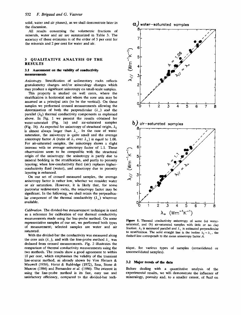
Anbotropy. Stratification of sedimentary rocks reflects granulometry changes andlor mineralogy changes which may produce a significant anisotropy on small-scale samples.

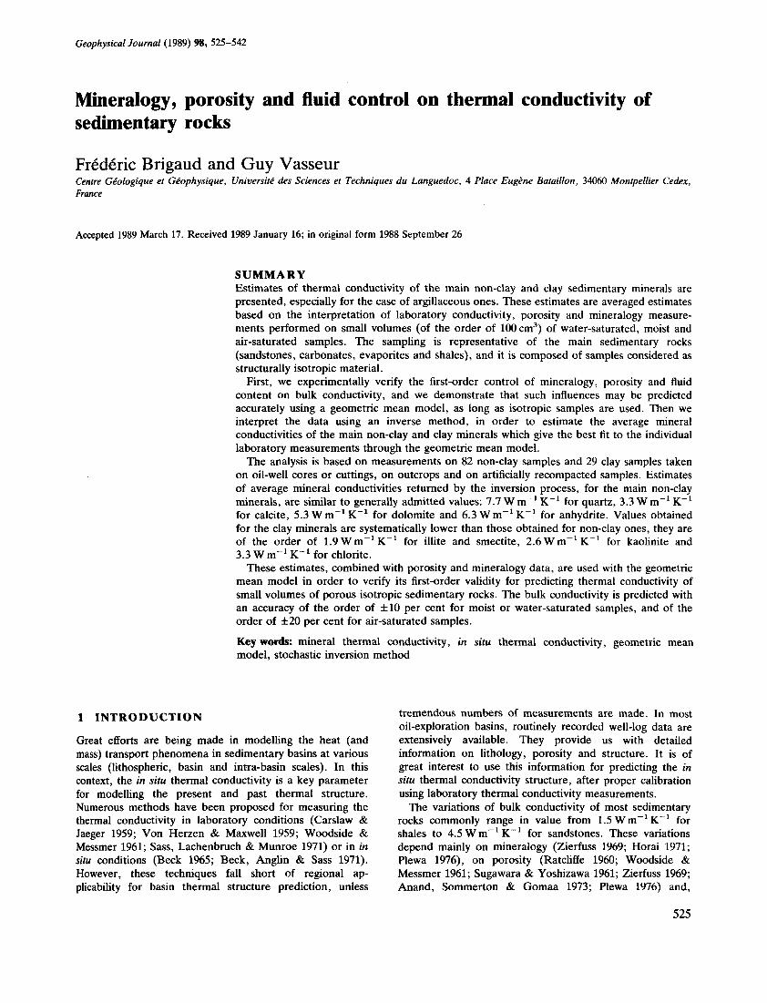
This property is studied on well cores, where the stratification is horizontal and where the core axis may be assumed as a principal axis (to be the vertical). On these samples we performed crossed measurements allowing the determination of both the perpendicular (A,) and the parallel (Al,) thermal conductivity components as explained above. In Fig. 1 we present the results obtained for water-saturated (Fig. la) and air-saturated samples (Fig. lb). As expected for anisotropy of structural origin, All is almost always larger than A,. In the case of water saturation, the anisotropy is quite small and the average anisotropy factor A (ratio of All over A,) is equal to 1.06. For air-saturated samples, the anisotropy shows a slight increase with an average anisotropy factor of 1.1. These observations seem to be compatible with the structural origin of the anisotropy: the anisotropy is partly due to mineral bedding in the stratification, and partly to porosity layering; when low-conductivity fluid (air) replaces higher- conductivity fluid (water), and anisotropy due to porosity layering is enhanced.

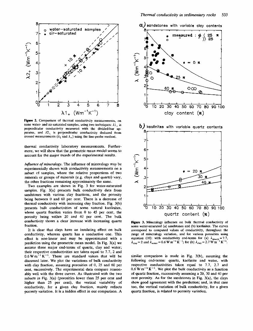
On our set of crossed measured samples, the average anisotropy factor is rather low, whether we consider water or air saturation. However, it is likely that, for some particular sedimentary rocks, the anisotropy factor may be significant. In the following, we shall retain the perpendicular component of the thermal conductivity (A,) wherever available.

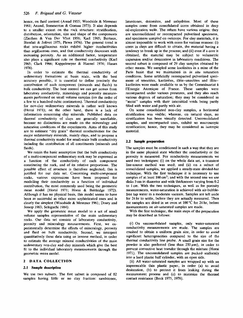
Calibration. The divided-bar measurement technique is used as a reference for calibration of our thermal conductivity measurements made using the line-probe method. On some representative samples of our set, we performed both types of measurement; selected samples are water and air saturated.

With the divided-bar the conductivity was measured along the core axis (A,), and with the line-probe method A, was deduced from crossed measurements. Fig. 2 illustrates the comparison of thermal conductivity measurements using the two methods. The results show a good agreement to within 10 per cent, which emphasizes the validity of the transient line-source method, as already shown by Von Herzen & Maxwell (1959), Horai & Baldridge (1972), Sass, Stone & Munroe (1984) and Fernandez et al. (1986). The interest in using the line-probe method is its fast, easy use and satisfactory efficiency, compared to the divided-bar tech-

U) water-saturated samples

'0 '1 1 2 3 4 5 6 7 8

b ) air-saturated samples

n I Y

Y

I E 3 W

2 x

'0 < 1 2 3 4 5 6 7 8

A, (Wm-'K-') F i i 1. Thermal conductivity anisotropy of some (a) water- saturated, and (b) air-saturated samples with little or no clay fraction. All is measured parallel and A, is estimated perpendicular to stratification. The solid straight line is the isoline All = )Il, the dashed line corresponds to the mean anisotropy factor A.

nique, for various types of samples (consolidated or unconsolidated samples).

3.2 Major trends of the data

Before dealing with a quantitative analysis of the experimental results, we will demonstrate the influence of mineralogy, porosity and, to a smaller extent, of fluid on


water-saturated samples / / * air-saturated

c - 6 I Y - 5 - I E 3 4 - W

d 3 - x 2-

I ' 0 1 2 3 4 5 6 7 8

A1 + (Wrn-lK-') Figure 2. Comparison of thermal conductivity measurements, on some water- and air-saturated samples, using two techniques: A l , is perpendicular conductivity measured with the divided-bar apparatus, and A2, is perpendicular conductivity deduced from crossed measurements (All and A,) using the line-probe method.

thermal conductivity laboratory measurements. Further- more, we will show that the geometric mean model seems to account for the major trends of the experimental results.

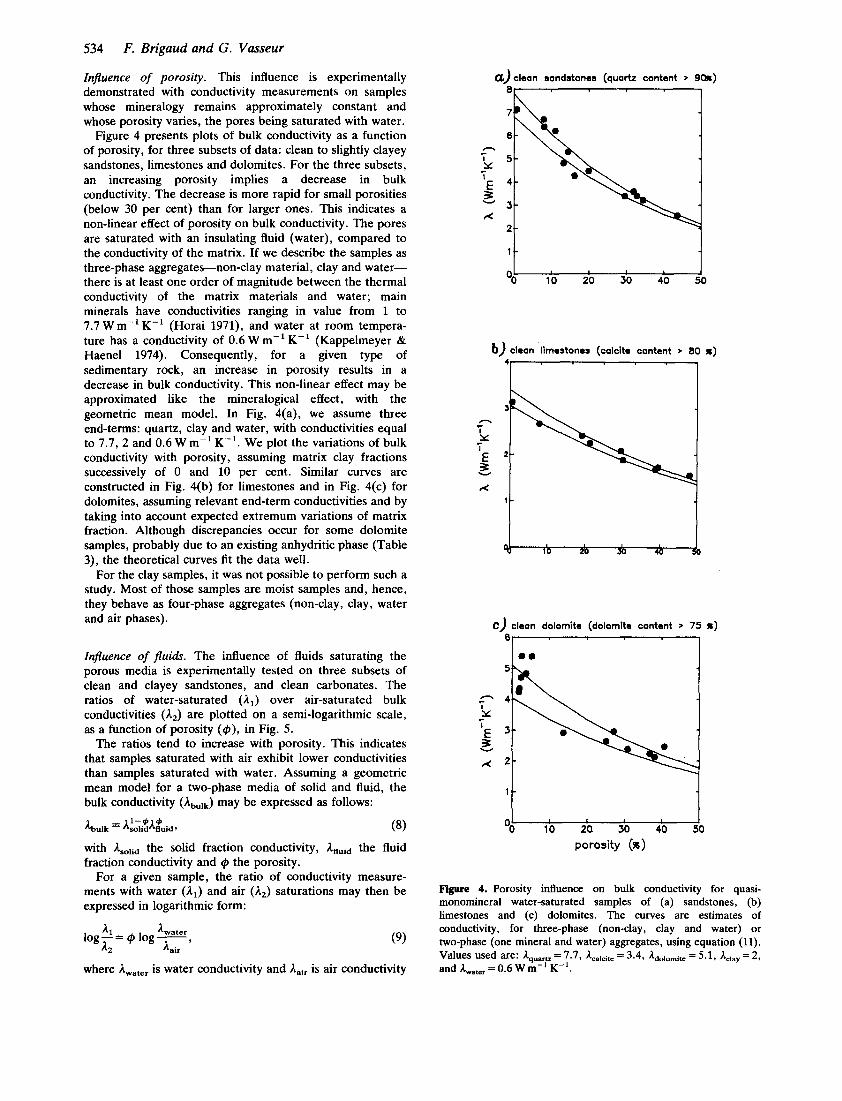
Influence of mineralogy. The influence of mineralogy may be experimentally shown with conductivity measurements on a subset cf samples, where the relative proportions of two minerals or groups of minerals (e.g. clays and quartz) vary, the other fractions remaining approximately the same.

Two examples are shown in Fig. 3 for water-saturated samples. Fig. 3(a) presents bulk conductivity data from sandstones with various clay fractions, and the porosity being between 0 and 60 per cent. There is a decrease of thermal conductivity with increasing clay fraction. Fig. 3(b) presents bulk conductivities of some natural kaolinites, whose quartz fraction varies from 0 to 45 per cent, the porosity being within 20 and 40 per cent. The bulk conductivity shows a clear increase with increasing quartz fraction.

It is clear that clays have an insulating effect on bulk conductivity, whereas quartz has a conductive one. This effect is non-linear and may be approximated with a prediction using the geometric mean model. In Fig. 3(a) we assume three major end-terms of quartz, clay and water; their respective conductivities are taken equal to 7.7, 2 and 0.6Wm-'K-'. These are standard values that will be discussed later. We plot the variations of bulk conductivity with clay fraction, assuming porosities of 0, 25 and 60 per cent, successively. The experimental data compare reason- ably well with the three curves. As illustrated with the two subsets in Fig. 3(a) (porosities lower than 25 per cent and higher than 25 per cent), the vertical variability of conductivity, for a given clay fraction, mainly reflects porosity variation. It is a hidden effect in our comparison. A

a) sandstones with variable clay contents 81 8 8 8 8 8 I . measured I I : ! % I I \

n I Y I

- c

E 3 v

x

O:, Ib i o i o 40 i o sb .;o a0 sb d o clay content (w)

b) kaolinites with variable quartz contents 8

7

6 n

Y I

7 5

E 4 3

c

3

2

1

v

x

9

9 x 2 0 s

I I I I I I , I I

10 20 30 40 50 60 70 80 90 100

quartz content (w) Figure 3. Mineralogy influence on bulk thermal conductivity of some water-saturated (a) sandstones and (b) kaolinites. The curves correspond to computed values of conductivity, throughout the range of mineralogy variation, and for various porosities using equation (10): with conductivity end-terms for (a) A,,,, = 7.7, Aday = 2 and A,,,, = 0.6 W m-' K-'; for (b) Aclay = 2.7 W m-' K-'.

similar comparison is made in Fig. 3(b), assuming the following end-terms: quartz, kaolinite and water, with respective conductivities taken equal to 7.7, 2.7 and 0.6 W m-l K-'. We plot the bulk conductivity as a function of quartz fraction, successively assuming a 20, 30 and 40 per cent porosity. As for the sandstones in Fig. 3(a), the clays show good agreement with the prediction; and, in that case too, the vertical variation of bulk conductivity, for a given quartz fraction, is related to porosity variation.

534

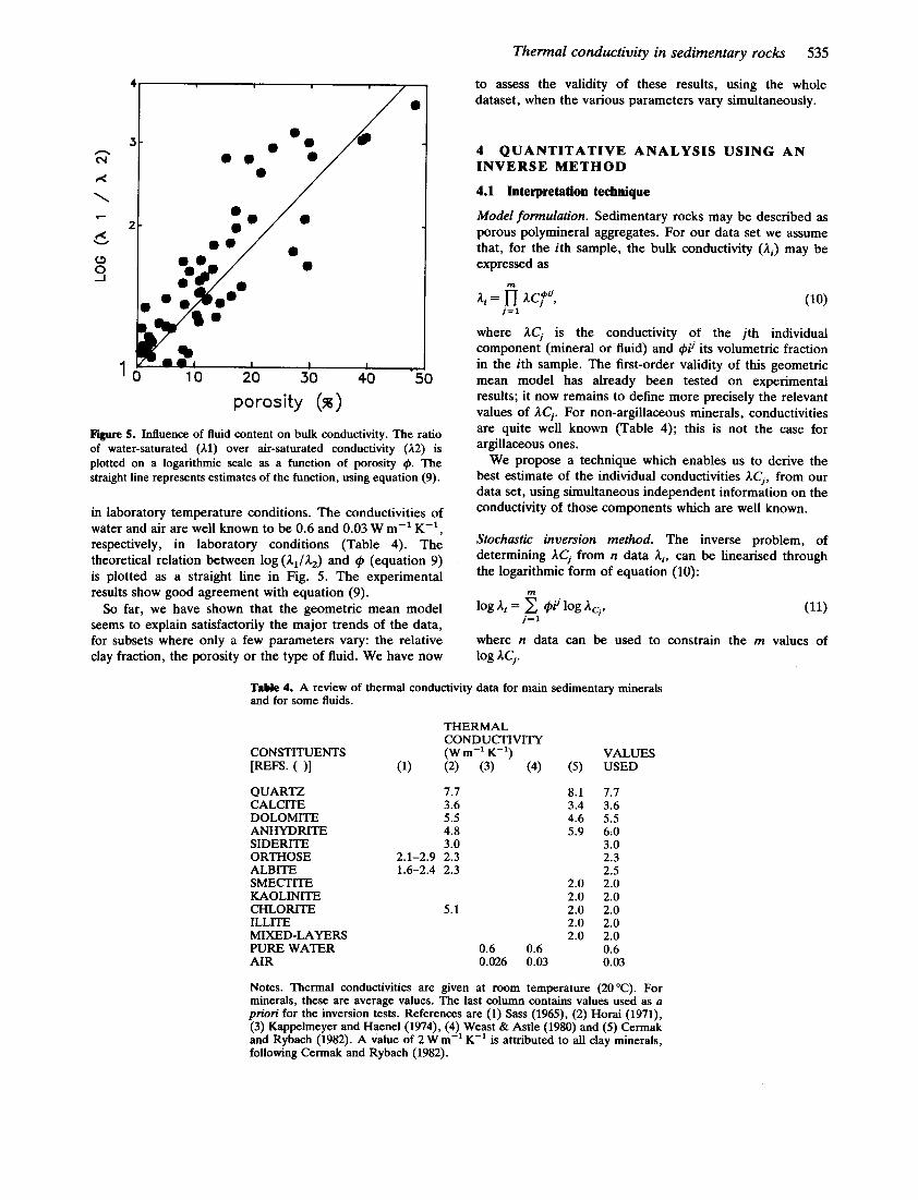
Influence of porosity. This influence is experimentally demonstrated with conductivity measurements on samples whose mineralogy remains approximately constant and whose porosity varies, the pores being saturated with water.

Figure 4 presents plots of bulk conductivity as a function of porosity, for three subsets of data: clean to slightly clayey sandstones, limestones and dolomites. For the three subsets, an increasing porosity implies a decrease in bulk conductivity. The decrease is more rapid for small porosities (below 30 per cent) than for larger ones. This indicates a non-linear effect of porosity on bulk conductivity. The pores are saturated with an insulating fluid (water), compared to the conductivity of the matrix. If we describe the samples as three-phase aggregates-non-clay material, clay and water- there is at least one order of magnitude between the thermal conductivity of the matrix materials and water; main minerals have conductivities ranging in value from 1 to 7.7 W m-l K-' (Horai 1971), and water at room temperature has a conductivity of 0.6 W m-l K-' (Kappelmeyer & Haenel 1974). Consequently, for a given type of sedimentary rock, an increase in porosity results in a decrease in bulk conductivity. This non-linear effect may be approximated like the mineralogical effect, with the geometric mean model. In Fig. 4(a), we assume three end-terms: quartz, clay and water, with conductivities equal to 7.7, 2 and 0.6 W rn-l K-'. We plot the variations of bulk conductivity with porosity, assuming matrix clay fractions successively of 0 and 10 per cent. Similar curves are constructed in Fig. 4(b) for limestones and in Fig. 4(c) for dolomites, assuming relevant end-term conductivities and by taking into account expected extremum variations of matrix fraction. Although discrepancies occur for some dolomite samples, probably due to an existing anhydritic phase (Table 3), the theoretical curves fit the data well.

For the clay samples, it was not possible to perform such a study. Most of those samples are moist samples and, hence, they behave as four-phase aggregates (non-clay, clay, water and air phases).

F. Brigaud and G. Vasseur

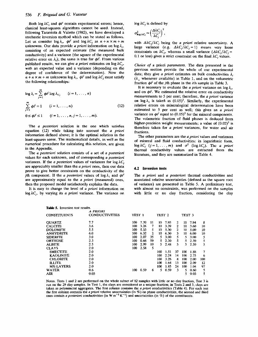
Influence of fluids. The influence of fluids saturating the porous media is experimentally tested on three subsets of clean and clayey sandstones, and clean carbonates. The ratios of water-saturated (A1) over air-saturated bulk conductivities (A,) are plotted on a semi-logarithmic scale, as a function of porosity (#), in Fig. 5.

The ratios tend to increase with porosity. This indicates that samples saturated with air exhibit lower conductivities than samples saturated with water. Assuming a geometric mean model for a two-phase media of solid and fluid, the bulk conductivity (AbUlk) may be expressed as follows:

with Amlid the solid fraction conductivity, Afluid the fluid fraction conductivity and 4 the porosity.

For a given sample, the ratio of conductivity measurements with water (A,) and air (A,) saturations may then be expressed in logarithmic form:

A1 Awater log-= # log-, A, Lair

(9)

where Awater is water conductivity and Aair is air conductivity

U)clean sandstones (quartz content > 90s)

2 -

l t

Ol4 1 0 io io 40 510

b) clean limestones (calcite content > 80 I)

'7

C ) clean dolomite (dolomite content > 75 I) 6 1

' t 10 ;a $0 40 i o

porosity (%)

Figure 4. Porosity influence on bulk conductivity for quasi- monomineral water-saturated samples of (a) sandstones, (b) limestones and (c) dolomites. The curves are estimates of conductivity, for three-phase (non-clay, clay and water) or two-phase (one mineral and water) aggregates, using equation (1 1). Values used are: Aqua*- = 7.7, Acalcitc = 3.4, = 5.1, Aclsy = 2, and A,,.,,,, = 0.6 W rn-l K-'.


to assess the validity of these results, using the whole dataset, when the various parameters vary simultaneously.

4

0

c3 s

2 O O / O 0

0 0

0 10 20 30 porosity (w>

Figure 5. Influence of fluid content on bulk conductivity. The ratio of water-saturated ( I l ) over air-saturated conductivity (A2) is plotted on a logarithmic scale as a function of porosity 8. The straight line represents estimates of the function, using equation (9).

in laboratory temperature conditions. The conductivities of water and air are well known to be 0.6 and 0.03 W m-l K-', respectively, in laboratory conditions (Table 4). The theoretical relation between log (AJA,) and @ (equation 9) is plotted as a straight line in Fig. 5 . The experimental results show good agreement with equation (9).

So far, we have shown that the geometric mean model seems to explain satisfactorily the major trends of the data, for subsets where only a few parameters vary: the relative clay fraction, the porosity or the type of fluid. We have now

4 QUANTITATIVE ANALYSIS USING AN INVERSE METHOD

4.1 Interpretation technique

Model formulation. Sedimentary rocks may be described as porous polymineral aggregates. For our data set we assume that, for the ith sample, the bulk conductivity (Ai) may be expressed as

... ... Ai = n AC?,

j = 1

where ACj is the conductivity of the jth individual component (mineral or fluid) and @i' its volumetric fraction in the ith sample. The first-order validity of this geometric mean model has already been tested on experimental results; it now remains to define more precisely the relevant values of AC,. For non-argillaceous minerals, conductivities are quite well known (Table 4); this is not the case for argillaceous ones.

We propose a technique which enables us to derive the best estimate of the individual conductivities AC,, from our data set, using simultaneous independent information on the conductivity of those components which are well known.

Stochastic inversion method. The inverse problem, of determining ACj from n data Ai, can be linearised through the logarithmic form of equation (10):

where n data can be used to constrain the m values of log nc,.

Table 4. A review of thermal conductivity data for main sedimentary minerals and for some fluids.

CONSTITUENTS [REFS. ( 11 QUARTZ CALCITE DOLOMITE ANHYDRITE SIDERITE ORTHOSE ALBITE SMECTITE KAOLIN ITE CHLORITE ILLITE MIXED-LAYERS PURE WATER AIR

THERMAL CONDUCTIVITY (W m-l K-')

(1) (2) (3) (4)

7.7 3.6 5.5 4.8 3.0

1.6-2.4 2.3 2.1-2.9 2.3

5.1

0.6 0.6 0.026 0.03

(5)

8.1 3.4 4.6 5.9

2.0 2.0 2.0 2.0 2.0

VALUES USED

7.7 3.6 5.5 6.0 3.0 2.3 2.5 2.0 2.0 2.0 2.0 2.0 0.6 0.03

Notes. Thermal conductivities are given at room temperature (20°C). For minerals, these are average values. The last column contains values used as a priori for the inversion tests. References are (1) Sass (1965), (2) Horai (1971), (3) Kappelmeyer and Haenel (1974), (4) Weast & Astle (1980) and (5) Cermak and Rybach (1982). A value of 2 W m-l K-' is attributed to all clay minerals, following Cermak and Rybach (1982).


Both log ACj and $ii contain expenmental errors; hence, classical least-squares algorithms cannot be used. Instead, following Tarantola & Valette (1982), we have developed a stochastic inversion method which can be stated as follows. Let us consider log Ai, @ti and logACj as n + n x m + m unknowns. Our data provide a priori information on log Ai, consisting of an expected estimate (the measured bulk conductivity) and a variance (the square of the experimental relative error on Ai); the same is true for $iJ. From various published results, we can give a priori estimates on log ACi, with an expected value and a variance (depending on the degree of confidence of the determination). Now the n + n x m + m unknowns log Ai, $ii and log ACj must satisfy the following relationships:

m ... log ki = C $2 log A ~ , ( i = I , . . . , n )

~

j=1

m

The a posteriori solution is the one which satisfies equation (12) while taking into account the a priori information defined above; it is the optimal solution in the least-squares sense. The mathematical details, as well as the numerical procedure for calculating this solution, are given in the Appendix.

The a posteriori solution consists of a set of a posteriori values for each unknown, and of corresponding a posteriori variances. If the a posteriori values of variances for log ACj are appreciably smaller than the a priori ones, then our data prove to give better constraints on the conductivity of the jth component. If the a posteriori values of log& and @ii are approximately equal to the a priori (measured) ones, then the proposed model satisfactorily explains the data.

It is easy to change the level of a priori information on logACj, by varying its a priori variance. The variance on

Table 5. Inversion test results.

CONSTITUENTS CONDUCTIVITIES A PRIORI

QUARTZ CALCITE DOLOMITE ANHYDRITE SIDERITE ORTHOSE ALBITE CLAYS

SMECTITE KAOLINITE CHLORITE ILLITE MX-LAYERS

WATER AIR

7.7 3.6 5.5 6.0 3.0 2.3 2.5 2.0 2.0 2.0 2.0 2.0 2.0 0.6 0.03

log ACj is defined by

with AACj/ACj being the a priori relative uncertainty. A large variance (e.g. AACjlACj = 1 ) means very loose constraints on ACj, whereas a small variance (AACjlACj = 0.1 or less) gives a strict constraint on the final ACj values.

Choice of a priori parameters. The data presented in the previous section provide the whole of our experimental data; they give a priori estimates on bulk conductivities Ai (A, whenever available) in Table 1, and on the volumetric fraction $iJ of the jth phase in the ith sample in Table 3.

It is necessary to evaluate the a priori variance on log hi, and on $iJ. We estimated the relative error on conductivity measurements to 5 per cent; therefore, the a priori variance on log& is takeii as (0.05)2. Similarly, the experimental relative errors on mineralogical determination have been estimated to 5 per cent as well; this gives an a priori variance on $ii equal to (0.05)* for the mineral components. The volumetric fraction of fluid phases is deduced from higher-precision weight measurements; a value of (0.02)* is therefore taken for a priori variances, for water and air fractions.

The other parameters are the a priori values and variances of mineral and fluid conductivities: in logarithmic form, logACj ( j = 1, . . . , m) and C? (log ACj). The a priori thermal conductivity values are extracted from the literature, and they are summarized in Table 4.

4.2 Inversion tests

The a priori and a posteriori thermal conductivities and associated relative uncertainties (defined as the square root of variance) are presented in Table 5. A preliminary test, with almost no constraints, was performed on the samples with little or no clay fraction, considering the clay

TEST 1 TEST 2 TEST 3

100 7.70 11 10 7.95 2 10 7.94 8 100 3.26 7 10 3.39 2 10 3.60 10 100 5.33 5 10 5.30 2 10 5.00 10 100 6.32 2 10 6.30 3 10 6.00 10 100 2.07 35 5 3.00 5 5 3.00 5 100 0.66 59 5 2.30 5 5 2.30 5 100 2.99 19 5 2.48 5 5 2.50 5 100 2.58 5

100 1.51 37 100 1.88 7 100 2.24 14 100 2.75 6 100 3.26 8 100 2.00 100 100 1.64 13 100 2.09 12 100 1.85 24 100 1.04 97

100 0.59 6 5 0.59 3 5 0.60 5 5 0.03 5

Notes. Tests 1 and 2 are performed on the whole subset of 82 samples with little or no clay fraction, Test 3 is run on the 29 clay samples. In Test 1, the clays are considered as a unique fraction; in Tests 2 and 3, clays are taken as polymineral aggregates. The first column contains the a priori conductivities (Table 4). For each test the first column contains the a priori relative uncertainties (in %) on phase conductivities, the second and third ones contain a posteriori conductivities (in W m-l K-') and uncertainties (in %) of the constituents.


constituents as a single fraction (Test 1). The results of this test show the validity of the chosen a priori conductivity values for the major non-clay m i n e r a l v u a r t z , calcite, dolomite and anhydrite. Irrelevant values are obtained for the minor non-clay minerals (siderite, orthose and albite). Considering these results, in the following computations (Tests 2 and 3) a priori uncertainties are fixed to 10 per cent for major non-clay minerals. Bulk conductivities of our samples are quite insensitive to the contribution of the minor constituent conductivities; therefore, in order to avoid numerical instabilities we fixed the a priori conductivities (according to published data, in Table 4) and uncertainties (to 5 per cent). Water and air are also given special treatment, considering that their thermal conductivities are quite well known in laboratory conditions; their a priori uncertainties are fixed to 5 per cent. On the other hand, clay mineral thermal conductivities are set free to vary (a priori uncertainties of 100 per cent).

In order to estimate the thermal conductivity of the clay minerals, the algorithm has been applied to the 82 water-saturated samples with minor or no clay fraction (Test 2) and to the 29 water-saturated or moist clay samples (Test 3). All samples are now considered as polymineral non-clay and/or clay mineral aggregates.

4.3 Final results

Results of the computations are given as a posteriori constituent thermal conductivities and associated relative uncertainties. These uncertainties measure the quality of the solution. The a posteriori uncertainty associated with a given constituent depends mainly on its representativeness in the data set; the more abundant a constituent, the smaller the a posteriori uncertainty.

The results obtained, for Tests 2 and 3, indicate that the occurrences of clay minerals are different for the two subsets, as shown by the a posteriori uncertainties; they are an indication of how cautiously the results concerning the clay minerals should be interpreted. Thus, in Test 2, thermal conductivity estimates for chlorite, illite and kaolinite are reliable; on the other hand, values for smectites and mixed-layers are not (large uncertainties). In Test 3, results obtained for kaolinite, smectite and illite (in decreasing order of occurrence) are somewhat higher than those obtained in Test 2; mixed-layers are almost missing, and there is no chlorite.

For chlorite, the value returned by the inversion in Test 2 is considerably lower (on the order of 3.3 f 0.3 W m-’ K-l) than the average value proposed by Horai (1971) and reported in Table 4 (5.1 Wrn-lK-’). Part of the discrepancy might arise from the fact that we are considering a sedimentary chlorite rather than a low-grade metamorphic mineral; sedimentary chlorite is seldom pure, but often associated with other minerals in intermediate phases (Deer, Howie & Zussman 1969). The value returned for kaolinite in Test 1 is 2 .24f0 .31 Wm-’ K-’; it is increased to 2.75 W m-’ K-’ in Test 2. For smectite, the solution in Test 1 gives a value of 1.51 f 0.55 W m-’ K-’ and 1.88 f 0.13 W m-l K-’ in Test 2. For mixed-layers, we obtain a value of 1.85 f 0.45 W m-’ K-’ in Test 1.

These results may be further interpreted in terms of phase

conductivities and fractions. Indeed, the model returns estimates of the contribution of each phase (conductivity and fraction), whose validity is verified for non-clay mineral conductivities (according to published data, in Table 4). Hence, one may interpret values obtained for minerals as average “dry” grain thermal conductivities, assuming that our data set is representative of nearly isotropic sedimentary rocks (cf. Fig. 1).

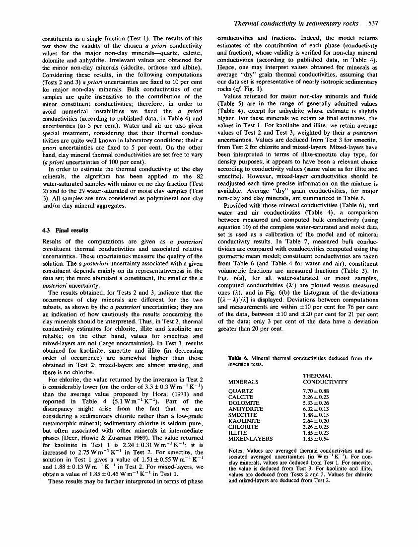
Values returned for major non-clay minerals and fluids (Table 5) are in the range of generally admitted values (Table 4), except for anhydrite whose estimate is slightly higher. For these minerals we retain as final estimates, the values in Test 1. For kaolinite and illite, we retain average values of Test 2 and Test 3, weighted by their a posteriori uncertainties. Values are deduced from Test 3 for smectite, from Test 2 for chlorite and mixed-layers. Mixed-layers have been interpreted in terms of illite-smectite clay type, for density purposes; it appears to have been a relevant choice according to conductivity values (same value as for illite and smectite). However, mixed-layer conductivities should be readjusted each time precise information on the mixture is available. Average “dry” grain conductivities, for major non-clay and clay minerals, are summarized in Table 6.

Provided with those mineral conductivities (Table 6), and water and air conductivities (Table 4), a comparison between measured and computed bulk conductivity (using equation 10) of the complete water-saturated and moist data set is used as a calibration of the model and of mineral conductivity results. In Table 7, measured bulk conductivities are compared with conductivities computed using the geometric mean model; constituent conductivities are taken from Table 6 (and Table 4 for water and air), constituent volumetric fractions are measured fractions (Table 3). In Fig. 6(a), for all water-saturated or moist samples, computed conductivities (A‘) are plotted versus measured ones (A), and in Fig. 6(b) the histogram of the deviations [(A - A)’/A] is displayed. Deviations between computations and measurements are within f 1 0 per cent for 76 per cent of the data, between f 1 0 and f 2 0 per cent for 21 per cent of the data; only 3 per cent of the data have a deviation greater than 20 per cent.

Table 6. Mineral thermal conductivities deduced from the inversion tests.

MINERALS QUARTZ CALCITE DOLOMITE ANHYDRITE SMECTITE KAOLINITE CHLORITE ILLITE MIXED-LAYERS

THERMAL CONDUCTIVITY 7.70 f 0.88 3.26 f 0.23 5.33 f 0.26 6.32 f 0.13 1.88 f 0.15 2.64 f 0.20 3.26 f 0.25 1.85 f 0.23 1.85 f 0.54

Notes. Values are averaged thermal conductivities and associated averaged uncertainties (in W m-l K-’). For non- clay minerals, values are deduced from Test 1. For smectite, the value is deduced from Test 3. For kaolinite and illite, values are deduced from Tests 2 and 3. Values for chlorite and mixed-layers are deduced from Test 2.

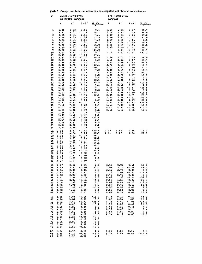
Table 7. Comparison between measured and computed bulk thermal conductivities.

NO

1 2 3 4 5 6 7 8 9 10 11 12 13 14 15 16 17 18 19 20 21 22 23 24 25 26 27 28 29 30 31 32 33 34 35 36 37 38 39 00 01 42 43 04 45 06 07 08 49 50 51 52 53

54 55 56 57 58 59 60 61 62 63 64 65

67 68 69 70 71 72 73 74 75 76 77 78 79

80 81

A

6.38 3.37 3.55 3.54 3.06 3.77 3.03 3.69 3.20 3.63 2.81 2.23 2.34 3.88 3.30 5.66 5.28 5.25 5.40 6.07 6.32 4.46 4.46 5.47 4.78 4.60 4.26 4.43 4.26 4.80 7.14 6.70 6.20 1.28 1.35 1.37 2.55 3.58 3.20 3.39 3.00 5.28 1.33 1.22 1.31 1.42 1.44 1.49 1.68 1.69 1.72 1.35 1.27

2.67 3.13 2.94 2.93 3.30 2.41 2.25 2.08 1.88 1.68 1.73 1.56

4.35 4.24 2.91 5.39 5.40 4.83 4.70 2.64 2.23 2.12 2.96 2.46 2.37

6.06 5.80

WATER-SATURATED OR MOIST SAMPLES

82 5.79

A *

5.83 3.51 3.71 3.63 3.21 3.76 3.69 3.67 3.55 3.42 3.30 2.33 2.30 3.38 3.75 5.09 4.91 5.17 5.14 5.74 5.68 4.71 4.10 5.19 4.39 5.07 4.82 4.08 4.44 4.87 7.54 6.29 5.82 1.23 1.42 1.55 2.53 3.42 3.20 3.34 3.32 4.56 1.41 1.37 1.38 1.21 1.57 1.46 1.76 1.77 1.82 1.27 1.17

2.62 3.23 2.83 2.81 3.08 2.36 2.27 1.98 1.96 1.69 1.67 1.45

4.83 5.07 3.62 4.83 5.04 4.37 4.50 2.92 2.28 2.22 2.80 2.10 2.59

5.96 6.14 5.55

A - A '

0.55 -0.14 -0.16 -0.09 -0.15 0.01 -0.66 0.02 -0.35 0.21 -0.49 -0.10 0.04 0.50

-0.45 0.57 0.37 0.08 0.26 0.33 0.64 -0.25 0.06 0.28 0.39 -0.47 -0.56 0.35 -0.18 -0.07 -0.40 0.41 0.39 0.05 -0.07 -0.18 0.02 0.16 0.00 0.05 -0.32 0.73 -0.08 -0.15 -0.07 0.21 -0.13 0.03 -0.08 -0.08 -0.10 0.08 0.10

0.05 -0.10 0.11 0.12 0.22 0.05 -0.02 0.10 -0.08 -0.01 0.06 0.11

-0.48 -0.83 -0.71 0.56 0.36 0.46 0.20 -0.28 -0.05 -0.10 0.16 0.36 -0.22

0.10 -0.34 0.24

AIR-SATURATED SAMPLES

(3*loo A

8.6 -4.2 -4.4 -2.6 -4.8 0.2

-21.8 0.5

-11.0 5.7

-17.4 -4.6 1.8

12.8 -13.6 10.1 7.0 1.4 4.8 5.0 10.1 -5.5 1.4 5.2 8.2

-10.2 -13.1 7.9 -4.3 -1.4 -5.7 6.1 6.2 3.9

-5.3 -12.8

0.7 4.5 0.0 1.4

-10.8 13.7 -6.2

-12.0 -5.5 14.6 -8.7 2.2

-4.8 -4.7 -5.7 5.9 8.3

2.1 -3.1 3.7 4.0 6.8 2.2 -1.0 5.0

-4.0 -0.6 3.4 7.2

-11.1 -19.5 -24.5 10.4 6.7 9.5 4.3

-10.5 -2.4 -4.8 5.5

14.7 -9.2

1.7 -5.9 4.1

5.46 2.04 1.10 2.16 2.09 2.41 2.23 2.45

1.15

1.26 1.13 2.43 2.73 4.03 3.85 3.61 4.31 4.97 4.50 2.76 2.15 3.25 3.12 3.19 2.31 2.24 1.53 2.64 6.69 4.43 3.66

2.28 4.81

2.55 2.89 2.64 2.18 2.73 0.87 0.87 0.69 0.67 0.55 0.56 0.43

0.33 3.45 3.75 1.98 4.53 4.77 3.91 4.14

5.39 5.04

A '

4.56 1.45 1.85 2.23 2.23 2.64 2.87 2.69 2.14 1.52

1.03 0.96 2.56 3.11 3.53 3.19 3.73 3.74 4.95 4.90 3.17 2.42 4.08 3.16 3.68 2.98 2.45 2.82 3.27 7.37 4.97 4.18

1.94 3.47

2.07 3.17 2.73 2.68 2.98 1.33 1.20 0.81 0.79 0.53 0.51 0.34

0.19 4.54 4.80 2.40 4.12 4.66 3.89 4.17

5.53 5.93

A - A '

0.87 0.59 -0.75 -0.07 -0.14 -0.23 -0.64 -0.24 -0.59 -0.37

0.23 0.17 -0.13 -0.39 0.50 0.66 -0.12 0.57 0.02

-0.40 -0.41 -0.27 -0.83 -0.04 -0.49 -0.67 -0.22 -1.29 -0.63 -0.68 -0.54 -0.53

0.34 1.34

0.48 -0.28 -0.09 -0.50 -0.25 -0.46 -0.33 -0.12 -0.12 0.02 0.05 0.09

0.14 -1.09 -1.05 -0.42 0.41 0.11 0.02 -0.03

-0.14 -0.89

(*-*') ~ 8100

15.9 28.9 -67.8 -3.0 -6.5 -9.6 -28.5 -9.7

-37.9 -32.3

18.0 15.1 -5.4

-14.1 12.3 17.1 -3.2 13.3 0.3 -9.0

-14.8 -12.8 -25.5 -1.2

-15.5 -28.9 -9.4 -84.2 -23.9 -10.1 -12.1 -14.3

15.1 27.8

18.9 -9.7 -3.3

-22.8 -9.2 -52.3 -38.0 -17.9 -18.1

3.9 8.6

20.1

43.2 -31.7 -28.0 -21.0

9.0 2.4 0.6 -0.8

-2.5 -17.7


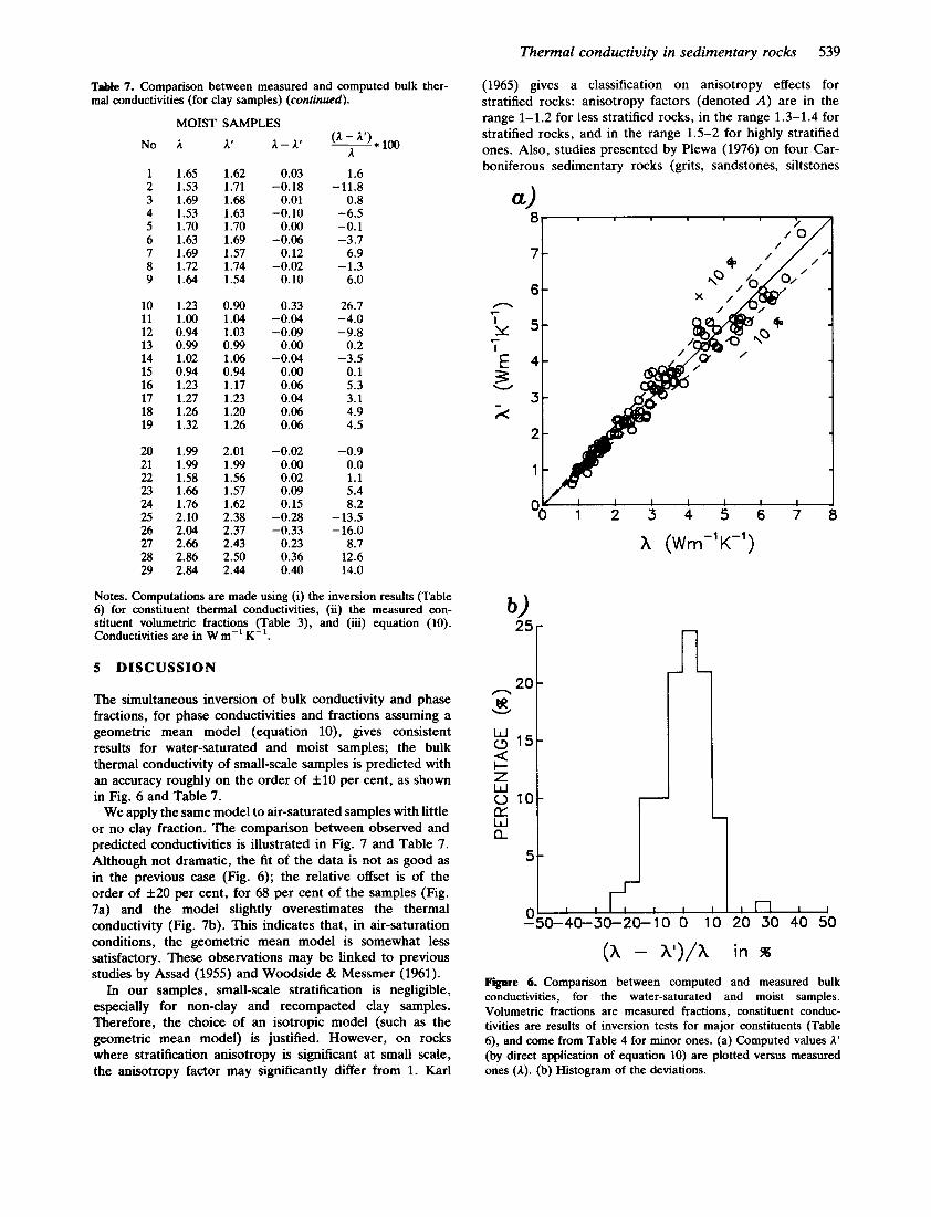
Table 7. Comparison between measured and computed bulk thermal conductivities (for clay samples) (continued).

MOIST SAMPLES No A

1 1.65 2 1.53 3 1.69 4 1.53 5 1.70 6 1.63 7 1.69 8 1.72 9 1.64

10 1.23 11 1.00 12 0.94 13 0.99 14 1.02 15 0.94 16 1.23 17 1.27 18 1.26 19 1.32

20 1.99 21 1.99 22 1.58 23 1.66 24 1.76 25 2.10 26 2.04 27 2.66 28 2.86 29 2.84

A'

1.62 1.71 1.68 1.63 1.70 1.69 1.57 1.74 1.54

0.90 1.04 1.03 0.99 1.06 0.94 1.17 1.23 1.20 1.26

2.01 1.99 1.56 1.57 1.62 2.38 2.37 2.43 2.50 2.44

A-A'

0.03 -0.18

0.01 -0.10

0.00 -0.06

0.12 -0.M

0.10

0.33 -0.04 -0.09

0.00 -0.04

0.00 0.06 0.04 0.06 0.06

-0.02 0.00 0.02 0.09 0.15

-0.28 -0.33

0.23 0.36 0.40

( A - A') * A 1.6

-11.8 0.8

-6.5 -0.1 -3.7

6.9 -1.3

6.0

26.7 -4.0 -9.8

0.2 -3.5

0.1 5.3 3.1 4.9 4.5

-0.9 0.0 1.1 5.4 8.2

-13.5 -16.0

8.7 12.6 14.0

Notes. Computations are made using (i) the inversion results (Table 6) for constituent thermal conductivities, (ii) the measured constituent volumetric fractions (Table 3), and (iii) equation (10). Conductivities are in W m-l K-'.

5 DISCUSSION

The simultaneous inversion of bulk conductivity and phase fractions, for phase conductivities and fractions assuming a geometric mean model (equation lo), gives consistent results for water-saturated and moist samples; the bulk thermal conductivity of small-scale samples is predicted with an accuracy roughly on the order of f10 per cent, as shown in Fig. 6 and Table 7.

We apply the same model to air-saturated samples with little or no clay fraction. The comparison between observed and predicted conductivities is illustrated in Fig. 7 and Table 7. Although not dramatic, the fit of the data is not as good as in the previous case (Fig. 6); the relative offset is of the order of f20 per cent, for 68 per cent of the samples (Fig. 7a) and the model slightly overestimates the thermal conductivity (Fig. 7b). This indicates that, in air-saturation conditions, the geometric mean model is somewhat less satisfactory. These observations may be linked to previous studies by Assad (1955) and Woodside & Messmer (1961).

In our samples, small-scale stratification is negligible, especially for non-clay and recompacted clay samples. Therefore, the choice of an isotropic model (such as the geometric mean model) is justified. However, on rocks where stratification anisotropy is significant at small scale, the anisotropy factor may significantly differ from 1. Karl

(1965) gives a classification on anisotropy effects for stratified rocks: anisotropy factors (denoted A) are in the range 1-1.2 for less stratified rocks, in the range 1.3-1.4 for stratified rocks, and in the range 1.5-2 for highly stratified ones. Also, studies presented by Plewa (1976) on four Car- boniferous sedimentary rocks (grits, sandstones, siltstones

8

7

6 n

I

I

.-

c Y 5

€ 4 3

2 W

3

2

1

X (Wm-'K-')

b ) 25

20 n B? W

g 15

2 Z W

L1L W

0 10

a 5

0 - J -

0-40-30-20-10 0 10

(A - A')/A Figure 6. Comparison between computed

20 30 40 50

in SB

and measured bulk conductivities, for the water-saturated and moist samples. Volumetric fractions are measured fractions, constituent conductivities are results of inversion tests for major constituents (Table 6), and come from Table 4 for minor ones. (a) Computed values A' (by direct application of equation 10) are plotted versus measured ones (A). (b) Histogram of the deviations.


a)

- A - -

n

I

I

c

Y c

E 3

2 W

-

h (Wm-‘K-’)

-

(A - A‘)/A in w Figure 7. Comparison between computed and measured bulk conductivities, for air-saturated samples. Volumetric fractions are measured fractions, constituent conductivities are results of inversion tests for major constituents (Table 6), and come from Table 4 for minor ones. (a) Computed values I‘ (by direct application of equation 10) are plotted versus measured ones (A). (b) Histogram of the deviations.

and argillites) indicate that (i) A is of the order of 1.1 or less for granular rock types such as grits and sandstones and (ii) A is of the order of 2 for highly lithified argillites. A similar range is indicated by Kappelmeyer & Haenel (1974) for various sedimentary rocks. Interpretation of measurements by Sass & Galanis (1983), made on a core

of shale of Cretaceous age in nearly in situ moisture conditions, indicates values for A in the range 1-1.3. It appears that the anisotropy effect is mainly correlated with the degree of stratification for all sedimentary rocks and, moreover, it is increased with the lithification process for shales. Independent information on the magnitude of anisotropy at small scale, and on the structure of the bedding planes, should permit further refinements of our approximations, for anisotropic rocks. In such cases the model inadequately takes this effect into account. The small-scale stratification problem remains unresolved, especially for clays.

Using inversion theory, average “dry grain” conductivities of each constituent have been evaluated. For major non-clay minerals and fluids, the proposed values are very consistent with published ones. Results for clay minerals are more problematic to interpret, because of different results between the two subsets. In order to explain the observed discrepancies between the two subsets for these minerals, one may formulate two hypotheses. One may invoke the presence of air in some clays, in the second subset, mainly for illite-rich samples (samples 10-19 in Table 3b). The volumetric fraction of air is computed using an assumption on the grain density psolid (equations 4-7). The wrong choice for pSolid would result in an error on the computed matrix conductivity (A&.,,id). It may be shown that an overestimation of grain density of 0.1 g cm-3 (Ap,,,,,) will result in a relative error on computed Awlid of the order of 16 per cent. Such a bias cannot be excluded, but seems unlikely to us. One may also invoke structural differences: clays may react differently to saturation, whether they are laminated, dispersed, in “pore lining”, or in “pore bridging”, in a non-clay mineral dominated matrix, as compared to clay minerals in a clay dominated matrix.

In any case, as previously stated in other studies, the clays exhibit systematically lower values than non-clay minerals. Smectite, illite and illite-smectite have average conductivities on the order of 2-4-times smaller than quartz and carbonates. Kaolinite and chlorite exhibit intermediate conductivities: for kaolinite, it is on the ‘order of 1-3-times lower than major non-clay mineral values; chlorite has a value similar to calcite, and 2.3-times smaller than quartz.

Beyond this quantitative precision on individual values of clay mineral conductivities, and the adequacy of the model with small-scale quasi-isotropic bulk conductivity, the ultimate goal is to provide an improvement in the prediction of in situ thermal conductivity of sedimentary formations at basin scale. Several authors have dealt with the in situ prediction problem. Some direct measurement attempts have been made (Beck et al. 1971) and various predictive methods, using empirical correlations between conductivity and some well-log physical parameters, have been proposed (Goss, Combe & Timur 1975; Houbolt & Wells 1980; Vacquier et al. 1988). These methods require calibrations that depend on mineralogy, porosity and fluid fraction of the formation.

All these methods are subordinate to a precise estimate of formation conductivity at small scale. The smallest unit that one can easily define in a sedimentary formation is the lithologic unit. It may be characterized by a given mineralogy and may be subject to porosity and/or saturation changes. The use of the geometric mean model, or another


more appropriate one in the case of anisotopy, will give a precise estimate on the conductivity of that unit. Then this estimation might be used as a calibration for further interpretations. From there, and knowing that in terms of well logging such a unit will correspond to a given electro-facies, the use of a combination of well logs (gamma ray, neutron, density and sonic) will allow us to predict the in siru formation conductivity (Brigaud, Chapman & Le Douaran 1989). The thermal structure of the basin will then be predicted by taking into account vertical lithology variations (large-scale stratification anisotropy) in the well, and lateral facies changes in formations (facies anisotropy) between wells. The precision in the prediction will then be dependent upon (i) mineralogical information on the lithologies and (ii) on well-log data density.

ACKNOWLEDGMENTS

We thank the Service d'Etude et de Stockage des dCchets from the Commissariat 6 1'Energie Atomique of France and in particular Mr Dardaine and Mr Beziat for providing us with some samples. We also thank Prof. Jolivet from the Institut de Physique du Globe of Paris who gave useful advice for dealing with thermal conductivity problems and who performed some conductivity measurements. We are particularly grateful to the SociCtC Nationale Elf Aquitaine (Production) for financing this work and for providing us with laboratory facilities.

REFERENCES

Albarede, F. & Provost, A., 1976. Petrological and geochemical massbalance equations-an algorithm for least-square fitting and general error analysis, Computers and Geosciences, 3,

Anand, J., Sommerton, W. H. & Gomaa, E., 1973. Predicting thermal conductivities of formations from other known properties, SOC. Petrol. Eng. J . , W , 267-273.

Assad, Y., 1955. A study of the thermal conductivity of fluid bearing porous rocks, PhD thesis, University of California, Berkeley.

Beck, A. E., 1965. Techniques of measuring heat flow on land, in Terrestrial heat flow, Geophys. Monograph 8, pp. 24-57, ed. Lee, W. H. K., AGU, Washington.

Beck, A. E., Anglin, F. M. & Sass, J. H., 1971. Analysis of heat flow data-In situ thermal conductivity measurements, Can. J . Earth Sci., 8, 1-19.

Beck, A. E., 1975. A potential systematic error when measuring the thermal conductivity of porous rocks saturated with a low-conductivity fluid, in Heat flow and geodynamics. Tectonophysics, 41, 9-16.

Beck, A. E., 1976. An improved method of computing the thermal conductivity of fluid-filled sedimentary rocks, Geophysics, 41,

Bertaw, M. G., Bienfait, G. & Jolivet, J., 1975. Etude des proprittts thermiques des milieux granulaires, Ann. Gkophys.,

Brigaud, F., Chapman, D. S. & Le Douaran, S., 1989. Thermal conductivity in sedimentary basins predicted from lithologic data and geophysical well logs, Bull. Am. Ass. Petrol. Geol. in press.

Bullard, E. C., 1954. The flow of heat through the floor of the Atlantic Ocean, Proc. Royal SOC. London, 222, 408-429.

Carslaw, H. S . & Jaeger, J. C., 1959. Conduction of Heat in Solids, 2nd edn, Oxford University Press, Oxford.

Cermak, V. & Rybach, L., 1982. Thermal conductivity and specific heat of minerals and rocks, in Physical properties of rocks, 1-a, Landolt-Bornstein, pp. 305-403, ed. Angenheister, G . , Springer Verlag.

309-326.

133-144.

31, 191-206.

Clark, Jr., S. P. (ed.), 1966. Handbook of Physical Constants, Geol. SOC. Am., Mem. 97.

Deer, W. A., Howie, R. A. & Zussman, J., 1969. Introduction to Rock Forming Minerals, John Wiley, New York.

Drury, M. J. & Jessop, A. M., 1983. The estimation of rock thermal conductivity from mineral content-An assessment of techniques, Zbl. Geol. Paleont. Teil I , H1/2, 35-48.

Fernandez, M., Banda, E. & Rojas, E., 1986. Heat pulse line-source method to determine thermal conductivity of consolidated rocks, Rev. Sci. Instrum., 57, 2832-2836.

Fertl, W. H. & Frost Jr., E., 1979. Evaluation of shaly clastic reservoir rocks, SOC. Pet. Eng. AIME, Annu. Fall Tech. Conf. Exhib., Pap. no 54, 1-12.

Goss, R. D., Combs, J. & Timur, A., 1975. Prediction of thermal conductivity in rocks from other physical parameters and from standard geophysical well logs, SPLWA l&h A . Logging Symposium., pp. 1-21.

Grubbe, K., Haenel, R. & Zoth, G., 1983. Determination of the vertical component of thermal conductivity by line source methods, Zbl. Geol. Paleont. Teil I , 1/2,49-56.

Hasan, S . E., 1978. Thermophysical properties of rocks, Symp. Rock Mechanics, 1, 210-214.

Horai, K., 1971. Thermal conductivity of rock-forming minerals, J. Geophys. Res., 76, 1278-1308.

Horai, K. & Baldridge, S., 1972. Thermal conductivity of nineteen igneous rocks-I-Application of the needle probe method to the measurement of the thermal conductivity of rocks, Phys. Earth planet Int., 5 , 151-156.

Houbolt, J. J. U. C. & Wells, P. R. A., 1980. Estimation of heat flow in oil wells based on a relation between heat conductivity and sound velocity, Geol. Minjbouw, 59, 215-224.

Jenkins, R. & De Vries, J. L., 1967. Practical X-Ray Spectrometry, Macmillan, London.

Kappelmeyer, 0. & Haenel, R., 1974. Geothermics with Special Reference to Application, Geoexploration Monograph, series 1, number 4, Gebruder Borntraeger, Berlin.

Karl, R., 1965. Gesteinsphysikalische Parameter-Freiberger Forschungshefte C197, Geophysik.

Plewa, S . , 1976. Correlation between thermal conductivity and other physical parameters of rocks, in Geoelectric and geothermal studies, pp. 49-52, ed. Adam, A. KAPG Geophysical Monograph, Akademiai Kiado, Budapest.

Ratcliffe, E. H., 1960. The thermal conductivities of ocean sediments, J . geophys. Res., 65, 1535-1541.

Roy, R. F., Beck, A. E. & Touloukian, Y. S., 1981. Thermophysical properties of rocks, in Physical properties of Rocks and Minerals pp. 409-502, eds Touloukian, Y. S., Judd, W. R. & Ho, C. Y., McGraw-Hill, New York.

Sass, J. H., 1965. The thermal conductivity of fifteen feldspar specimens, J . geophys. Res., 70, 4064-4065.

Sass, J. H., Lachenbruch, A. H. & Munroe, R. J., 1971. Thermal conductivity of rocks from measurements on fragments and its application to heat flow determination, J . geophys. Res., 76,

Sass, J. H. & Galanis Jr., S. P., 1983. Temperatures, thermal conductivity, and heat flow from a well in Pierre Shale near Hayes, South Dakota, U.S. Geological Survey, Open File Report 79-356.

Sass, J. H., Stone, C. & Munroe, R. J., 1984. Thermal conductivity determinations on solid rock-a comparison between a steady-state divided-bar apparatus and a commercial transient line-source device, J . Volcanol. geotherm. Res., 20, 145-153.

Sekiguchi, K., 1984. A method for determining terrestrial heat flow in oil basins areas, Tectonophysics, 103, 67-69.

Serra, O . , 1979. Diagraphies difftrtes, Bases de I'interprttation, Acquisition des donntes diagraphiques; Tome 1, Bull. Cent. Rech. Exp. Prod., Mem. 1, Elf Aquitaine.

Sugawara, A. & Yoshizawa, Y., 1961. An investigation on the thermal conductivity of porous materials and its application to porous rock, Aust. J. Phys., 14, 468-480.

Tarantola, A. & Valette, B., 1982. Generalized nonlinear inverse problems solved using a least squares criterion, Rev. Geophys. Space Phys., 20,219-232.

Vacquier, V., Mathieu, Y., Legendre, E. & Blondin, E., 1988. An experiment on estimating the thermal conductivity of

3391-3401.


sedimentary rocks from oil well logging, Bull. Am. Ass. Petrol. Geol., 72, 758-764.

Von Herzen, R. & Maxwell, A. E., 1959. The measurements of thermal conductivity of deep-sea sediments by a needle probe method, J . geophys. Res., 64, 1557-1563.

Weast, R. C. & Astle, M. J . , 1980. Handbook of Chemistry and Physics, 61th edn, CRC Press, Boca Raton.

Woodside, W. & Messmer, J . H., 1961. Thermal conductivity of porous media-I Unconsolidated sands-I1 Consolidated rocks, I . appl. Phys., 32, 1688-1706.

Zierfuss, H. & Van Der Vliet, G. , 1956. Laboratory measurements of heat conductivity of sedimentary rocks, Bull. Am. Ass. Petrol. Geol. 40, 2475-2488.

Zierfuss, H., 1969. Heat conductivity of some carbonate rocks and clayey sandstones, Bull. Am. Ass. Petrol. Geol., 53, 251-260.

APPENDIX

The problem given by equation (12) is quite similar to the one handled by Albarede & Provost (1976) for geochemistry purposes. First, the inequality constraints are satisfied by switching the variable 4iJ; we write @ii = sin' Wj. Then, we define a (n + m x n + m) vector X having the following components:

x = (log Al, . . . , log A,, Y;, . . . , Y7, log ACI, . . . , log A,,).

The a priori values are given by a vector value X,,, corresponding to experimental values and assumed A,, and a covariance matrix em which can be assumed to be diagonal (each term being the square of a priori error).

Following Tarantola & Valette (1982), the problem is then to define the value of X which gives the minimum of the quadratic form

(X - &)T . P,-,' - (X - &)

12). subject to the equality and inequality constraints (equation

By using an iterative procedure, a fixed-point algorithm yields the optimal solution by the recurrence formula: Xk+l

= & + co. F Z . (Fk ' c o * FZ)-' ' [Fk ' (xk - &) -f(xk)],

F is the matrix of partial derivatives, at the current point xk. F is equal to

fi corresponding to each equality in equation (12). The a posteriori variance is obtained by

C, = P, . F ~ - ( F . em. F ~ ) - ' . F . P,. This last formula is strictly verified only when equality

relations, relating the components of X, are linear. In the non-linear case, they give a useful estimate of a posteriori variance. The square root of the diagonal C,, will be used as an estimate of the a posteriori error, over each component of X.

Mineralogy, porosity and fluid control on thermal conductivity of sedimentary rocks

Documents