May 28, 2013 RTI Project 0213061 Millsboro Inhalation Exposure and Biomonitoring Study Final Report Prepared for State of Delaware Department of Natural Resources and Environmental Control Department of Health and Social Services Dover, DE Prepared by RTI International 3040 Cornwallis Road Research Triangle Park, NC 27709-2194

Welcome message from author
This document is posted to help you gain knowledge. Please leave a comment to let me know what you think about it! Share it to your friends and learn new things together.
Transcript

7/30/2019 Millsboro Biomonitoring Study Final Report
http://slidepdf.com/reader/full/millsboro-biomonitoring-study-final-report 1/91
May 28, 2013
RTI Project 0213061
Millsboro Inhalation Exposure andBiomonitoring Study
Final Report
Prepared for
State of Delaware
Department of Natural Resources and Environmental Control
Department of Health and Social Services
Dover, DE
Prepared by
RTI International
3040 Cornwallis Road
Research Triangle Park, NC 27709-2194

7/30/2019 Millsboro Biomonitoring Study Final Report
http://slidepdf.com/reader/full/millsboro-biomonitoring-study-final-report 2/91

7/30/2019 Millsboro Biomonitoring Study Final Report
http://slidepdf.com/reader/full/millsboro-biomonitoring-study-final-report 3/91
ii
States (Ondov, 2006) The exception to this occurred with personal level samples. Personal samples were
enriched with Bromine (avg. 686.4 ng/m3) when compared to outdoor samples collected during this
study (avg. 3.9 ng/m3). These elements have several potential indoor sources, including environmental
tobacco smoke, which would require further sampling and data analysis to identify.
Results for the blood biospecimen samples showed that none of the analytes were above the
reference values for the 32 participants during either season. Urinary Arsenic and Selenium were above
the reference ranges in 12 of the participants during Season 1 while these same two metals were
similarly above reference values in 8 of the participants during Season 2. Although uncertain, this may
be attributable to dietary exposure. Further investigation would be needed to better understand this
finding.
The MIEBS resulted in high quality data that could serve as a baseline for additional studies in
the future. The motivated Sussex County residents willing to participate in this exposure health study
contributed significantly to the quality of the data collected. Data revealed expected spatial and
elemental distributions with concentration differences being observed between indoor, personal,
outdoor, and background sampling locations. Significantly, data demonstrated that ambient background
PM2.5 concentrations in southern Delaware are driven by long-range airborne transport from
neighboring upwind states and metropolitan areas.

7/30/2019 Millsboro Biomonitoring Study Final Report
http://slidepdf.com/reader/full/millsboro-biomonitoring-study-final-report 4/91
iii
Table of ContentsExecutive Summary ........................................................................................................................................ i
Table of Contents ......................................................................................................................................... iii
List of Figures ................................................................................................................................................ v
List of Tables ............................................................................................................................................... vii
Forward ...................................................................................................................................................... viii
Acknowledgments ........................................................................................................................................ ix
List of Acronyms ............................................................................................................................................ x
Introduction .................................................................................................................................................. 1
Background ............................................................................................................................................... 1
Study Purpose and Goals .......................................................................................................................... 1
Data for Objective 1—Evaluation of IRPP Operating Capacity ............................................................. 2
Data for Objective 2—Contribution of Out-of-State Sources to Sussex County PM2.5 Exposures ........ 2
Data for Objective 3—Contribution of Other Sources to PM2.5 Exposure ............................................ 2
Data for Objective 4—Collect Biological Specimens ............................................................................. 2
Hypotheses ............................................................................................................................................... 3
Report Framework .................................................................................................................................... 3
Study Methodology ....................................................................................................................................... 4
Sample Analysis ......................................................................................................................................... 7
Gravimetric Analysis ............................................................................................................................. 7
Environmental Tobacco Smoke/Brown Carbon and Black Carbon Analysis ......................................... 7
X-Ray Fluorescence Analysis ................................................................................................................. 8
Urine Analysis ........................................................................................................................................ 8
Blood Analysis ....................................................................................................................................... 8
Data Quality Results ...................................................................................................................................... 8
Sample Results .............................................................................................................................................. 9
Seaford Site ............................................................................................................................................... 9
Fixed Site Data ........................................................................................................................................ 10
Outdoor PM2.5 Residential Data .............................................................................................................. 16
Indoor PM2.5 Residential Data ................................................................................................................. 21

7/30/2019 Millsboro Biomonitoring Study Final Report
http://slidepdf.com/reader/full/millsboro-biomonitoring-study-final-report 5/91
iv
Personal PM2.5 Data ................................................................................................................................ 26
Residential Temperature and Humidity .................................................................................................. 32
Questionnaires ........................................................................................................................................ 32
Biospecimen Samples ............................................................................................................................. 32
Evaluation of Study Objectives and Hypothesis ......................................................................................... 49
Objective 1 .............................................................................................................................................. 49
Objective 2 .............................................................................................................................................. 50
Objective 3 .............................................................................................................................................. 53
Objective 4 .............................................................................................................................................. 57
Conclusions ................................................................................................................................................. 57
Recommendations ...................................................................................................................................... 58
References .................................................................................................................................................. 61
Appendices ..................................................................................................................................................... I
Appendix A: Questionnaire Data ............................................................................................................... I
Appendix B: Reference Ranges for Analytes in Blood or Serum (Provided by DHSS) .............................. VI
Appendix C: Reference Ranges for Analytes in Urine (Provided by DHSS) ............................................. VII
Appendix D: Data Quality Indicator Determination Methods ............................................................... VIII
Glossary ...................................................................................................................................................... XVI
7/30/2019 Millsboro Biomonitoring Study Final Report
http://slidepdf.com/reader/full/millsboro-biomonitoring-study-final-report 6/91
v
List of FiguresFigure 1. Participant Sampling area (Red circle) with number of participants in each sector denoted
(including two replacement participants for 2012), Fixed Sites (Green), and NRG Energy power plant
(Yellow) during both Season 1 and 2 of the MIEBS Study. Note the Seaford monitor is not shown. .......... 6
Figure 2. Distributions of Seaford Site PM2.5, BrC, and BC concentrations during Season 1 (Red, NRG
Energy power plant not operating) & Season 2 (Blue, power plant operating) along with geometric
means (asterisks). Values below the MDL were assigned a value of the MDL divided by square root of 2.
.................................................................................................................................................................... 11
Figure 3. Comparison of XRF data Collected at the Seaford Site from 2011 and 2012. ............................. 11
Figure 4. Comparison of collocated Seaford FRM and RTI PEM during both seasons. ............................... 12
Figure 5. Distributions of Fixed Site PM2.5 concentrations during Season 1 (Red, NRG Energy power plant
not operating) & Season 2 (Blue, power plant operating) along with geometric means (asterisks). Values
below the MDL were assigned a value of the MDL divided by square root of 2. ....................................... 13
Figure 6. Distributions of Fixed Site BrC concentrations during Season 1 (Red, NRG Energy power plant
not operating) & Season 2 (Blue, power plant operating) along with geometric means (asterisks). Values
below the MDL were assigned a value of the MDL divided by square root of 2. ....................................... 14
Figure 7. Distributions of Fixed Site BC concentrations during Season 1 (Red, NRG Energy power plant
not operating) & Season 2 (Blue, power plant operating) along with geometric means (asterisks). Values
below the MDL were assigned a value of the MDL divided by square root of 2. ....................................... 15
Figure 8. XRF Results from 2011 Fixed Site ambient samplers, Trace elements above MDL not shown. .. 17
Figure 9. XRF Results from 2012 Fixed Site ambient samplers, Trace elements above MDL not shown. .. 17
Figure 10. Distributions of outdoor residential PM2.5 concentrations during Season 1 (Red, NRG Energy
power plant not operating) & Season 2 (Blue, power plant operating) along with geometric means
(asterisks). Values below the MDL were assigned a value of the MDL divided by square root of 2. ......... 18
Figure 11. Distributions of outdoor residential BrC concentrations during Season 1 (Red, NRG Energy
power plant not operating) & Season 2 (Blue, power plant operating) along with geometric means
(asterisks). Values below the MDL were assigned a value of the MDL divided by square root of 2. ......... 19
Figure 12. Distributions of outdoor residential BC concentrations during Season 1 (Red, NRG Energy
power plant not operating) & Season 2 (Blue, power plant operating) along with geometric means
(asterisks). Values below the MDL were assigned a value of the MDL divided by square root of 2. ......... 20
Figure 13. XRF analysis of outdoor residential samples from 2011 & 2012. .............................................. 21
Figure 14. Distributions of indoor residential PM2.5 concentrations during Season 1 (Red, NRG Energy
power plant not operating) & Season 2 (Blue, power plant operating) along with geometric means
(asterisks). Values below the MDL were assigned a value of the MDL divided by square root of 2. ......... 22Figure 15. Distributions of indoor residential ETS concentrations during Season 1 (Red, NRG Energy
power plant not operating) & Season 2 (Blue, power plant operating) along with geometric means
(asterisks). Values below the MDL were assigned a value of the MDL divided by square root of 2. ......... 23

7/30/2019 Millsboro Biomonitoring Study Final Report
http://slidepdf.com/reader/full/millsboro-biomonitoring-study-final-report 7/91
7/30/2019 Millsboro Biomonitoring Study Final Report
http://slidepdf.com/reader/full/millsboro-biomonitoring-study-final-report 8/91
vii
List of TablesTable 1. Detailed list of sampling days for Season 1. .................................................................................... 6
Table 2. Detail list of sampling days for Season 2. ........................................................................................ 7
Table 3. Data validity distributions for PM2.5 samples for season 1 by sampling location............................ 9
Table 4. Data validity distributions for PM2.5 samples for season 2 by sampling location. .......................... 9
Table 5. Average temperatures and relative humidities for Season 1 & Season 2 participants. ............... 32
Table 6. 2011 Concentrations of metals in urine (ppb).[i] ........................................................................... 33
Table 7. 2012 Concentrations of metals in urine (ppb). [i] .......................................................................... 34
Table 8. 2011 and 2012 blood metals concentrations (ppb). ..................................................................... 35
Table 9. Participants for whom any of the analytes in blood or urine exceeded high reference value (*
indicates a measurement above the reference value). .............................................................................. 37
Table 10. Pearson correlations of PM mass with biospecimen elements by year. .................................... 40
Table 11. Pearson correlations of ETS mass with biospecimen elements by year. .................................... 41
Table 12. Pearson correlations of BC mass with biospecimen elements by year. ..................................... 43
Table 13.Pearson correlations of elements on personal filters by XRF with biospecimen elements by
year. ............................................................................................................................................................ 46
Table 14. Pearson correlations of elements on personal filters by XRF with biospecimen elements across
years. ........................................................................................................................................................... 47
Table 15. Evaluation of exceedances for Arsenic and Selenium in the context of possible ingestion
routes. ......................................................................................................................................................... 48
Table 16. Percentage of the personal PM2.5 exposure due to ambient, indoor residential, and other
sources. Data are presented by season, and stratified by residences without significant ETS and all
residences (ETS and non-ETS). Average and standard deviation for each source are presented. Ambient
and indoor percentages are calculated from the personal, indoor, and outdoor data. The “Other” source
consists of proximity to localized sources within the participant’s home, transportation, and indoors at
other locations; it is calculated by difference. ............................................................................................ 56
Table 17. Summarized participant questionnaire results Season 1. .............................................................. I
Table 18. Summarized participant questionnaire results Season 2. ............................................................. II
Table 19. Summarized residential questionnaire results Season 1. ............................................................ III
Table 20. Summarized residential questionnaire results Season 2. ............................................................ IV
Table 21. Summarized additional questionnaire data taken during season 2. ............................................ V
Table 22. Target DQI's for each metric and analyte. ................................................................................... IX
Table 23. Target quantitative DQI's for XRF analysis. .................................................................................. XI
Table 24. Actual DQIs from MIEBS Seasons 1 & 2. .................................................................................... XIIITable 25. Actual DQIs for XRF Analysis of MIEBS Season 1 & 2 data. ........................................................ XIII
7/30/2019 Millsboro Biomonitoring Study Final Report
http://slidepdf.com/reader/full/millsboro-biomonitoring-study-final-report 9/91
viii
ForwardThe Millsboro Inhalation Exposure and Biomonitoring Study (MIEBS) was performed to assess
the role of the NRG Energy power plant in Millsboro, Delaware in increasing the exposure of Sussex
County residents to particulate matter, metals, and selected organic contaminants. The study involved
the collection of outdoor air quality data, indoor air quality data, personal air quality data, biospecimen
data, and questionnaire data in the Fall of 2011 and the Fall of 2012. This report presents the objectives,
methods, results, and conclusions of the study.
This study has been a partnership between the Delaware Department of Natural Resources and
Environmental Control (DNREC) and the Delaware Department of Health and Social Services (DHSS),
with technical assistance from RTI International who was contracted to perform the environmental
sampling and analysis.

7/30/2019 Millsboro Biomonitoring Study Final Report
http://slidepdf.com/reader/full/millsboro-biomonitoring-study-final-report 10/91
ix
AcknowledgmentsForemost, this study would not be possible without the participation and support of the Sussex
County residents. Thirty-five Sussex County residents participated in the study, while numerous others
expressed a willingness to participate.
This project was underwritten by the Delaware Department of Natural Resources and
Environmental Control and the Delaware Cancer Consortium, in collaboration with the Delaware Health
Fund.
Several RTI International (RTI) staff contributed significantly to this project. Dr. Jonathan
Thornburg and Dr. James Raymer were co-Principal Investigators. Dr. Quentin Malloy managed the daily
technical details of sample collection and analysis. Michael Philips recruited the study participants.
Cortina Johnson and Jocelin Deese-Spruill spent six weeks in Delaware in 2011 and 2012 working with
the participants to collect the particulate matter samples. Meaghan McGrath and Andrea McWilliams
analyzed the collected environmental samples. Larry Michael performed the statistical analysis of thedata. Lastly, Wayne Dawson is a Sussex County resident hired by RTI as a temporary contractor to assist
with sample collection.
RTI conducted this project in conjunction with the Delaware Department of Natural Resources
and Environmental Control (DNREC) and Delaware Health and Social Services Division of Public Health
(DPH). Elizabeth Frey (DNREC), Lisa Henry (DPH), and Richard Perkins (DPH) provided oversight of the
project. Mohammed Majeed (DNREC) performed air dispersion modeling to aid siting of the fixed site air
monitors and identify areas for participant recruitment. Susan Mitchell, R.N. (DPH) collected the
biological specimens from the participants. The Delaware Public Health Laboratory, under the direction
of Tara Lydick, analyzed the biological specimens. Richard Greene (DNREC) provided extensive
comments that improved the quality of this report.

7/30/2019 Millsboro Biomonitoring Study Final Report
http://slidepdf.com/reader/full/millsboro-biomonitoring-study-final-report 11/91
x
List of Acronymsµg: Microgram
BC: Black Carbon
BrC: Brown Carbon
Cm: Measured concentration of a spiked sample
Cs: Measured concentration of a spiked solution
Csample: Measured concentration of a sample
Cstd: Measured concentration of a certified standard
Cu: Measured concentration of an unspiked sample
DHSS: Delaware Department of Health and Social Services
DNREC: Delaware Department of Natural Resources and Environmental Control
DPHL: Delaware Public Health Laboratory
DQI: Data Quality Indicator
ETS: Environmental Tobacco Smoke
FRM: Federal Reference Method
ICP-DRC/MS: Inductively Coupled Plasma-Dynamic Reaction Cell/Mass Spectrometry
ICP-MS: Inductively Coupled Plasma-Mass Spectrometry
LPM: Liter Per Minute
MDL: Minimum Detection Limit
MIEBS: Millsboro Inhalation Exposure and Biomonitoring Study
MQL: Minimum Quantification Limit
P/I: Personal-to-Indoor ratio
PEM: Personal Exposure Monitor
PM: Particulate Matter
PM2.5: Particulate Matter with an aerodynamic diameter equal to or less than 2.5 micrometers
RSD: Relative Standard Deviation
RTI: Research Triangle Institute
SD: Standard Deviation
SPME-GC: Solid-Phase Micro Extraction-Gas Chromatography
TAD: Time Activity Diary
VOC: Volatile Organic Compound
XRF: X-Ray Fluorescence

7/30/2019 Millsboro Biomonitoring Study Final Report
http://slidepdf.com/reader/full/millsboro-biomonitoring-study-final-report 12/91
1
Introduction
Background
Evidence is increasing that long-term human exposure to particulate matter (PM) has negative
impacts on human health, including adverse respiratory and cardiovascular effects (Dockery 2001; Ito et
al. 2011). It has also been demonstrated that acute exposures to elevated PM can lead to a myriad of
health end points, including non-accidental mortality, total mortality, respiratory deaths, and morbidity
(Goldberg et al. 2001; Laden et al. 2000; Hoek et al. 2001; Zanobetti, Schwartz, and Dockery 2000).
However, there exists a need for more information about the amount and composition of this PM as it
relates to health end points of the exposed population. Those who live close to sources of PM2.5 (PM
with an aerodynamic diameter equal to or less than 2.5 micrometers) are especially vulnerable to the
negative impacts; therefore, federal and state agencies have made it a priority to gather more
information concerning the health outcomes of long-term exposure to these particles.
Research has shown the spatial gradients in PM2.5 to be smaller than PM10 (PM with an
aerodynamic diameter equal to or less than 10 micrometers) with concentrations being higher in urban
areas and close to point sources, but temporal trends are stronger with PM2.5 (Environment Canada-
Health Canada 2000; Thornburg et al. 2009; Rodes et al. 2010). It has also been noted that strong diurnal
trends exist with the chemical composition of PM2.5 (Cheung et al. 2011). Many factors influence these
gradients, including temperature, wind direction, and human activity patterns. Because of the regional
nature of PM2.5, the adverse health effects associated with it are more widespread and can be harder to
link to specific sources. This is especially compounded by the paucity of personal exposure data.
Study Purpose and Goals
This study centers around the DESIGN I plan presented to the Department of Natural Resources
and Environmental Control (DNREC) by RTI International in June 2008 (DNREC-OTS, 2008). The DESIGN I
plan described a multi-media exposure study in Sussex County that would serve as a pilot effort as a
prelude to a statewide study. The scope of the DESIGN I plan was reduced in accordance with the
available budget resources. The final study design yielded the Millsboro Inhalation Exposure and
Biomonitoring Study (MIEBS). Although MIEBS was developed to explore inhalation exposure pathways,
it is possible alternative exposure routes, such as seafood consumption, may be of interest though
outside the scope of MIEBS (Greene and Crecelius, 2006). MIEBS addressed four objectives over the
course of an 18-month study. MIEBS had the following objectives:
1) Evaluate the impacts of the NRG Energy power plant operating capacity on PM2.5 exposure levels
of the Sussex County population.
2) Ascertain the relative contributions of upwind sources in Virginia, Maryland, Pennsylvania, New
York, and the New England area on the PM2.5 exposure of the Sussex County population.
3) Establish the contribution of point, local, and personal sources to the Sussex County
population’s exposure to PM2.5.
4) Collect biological samples for dose measurements of the Sussex County population.

7/30/2019 Millsboro Biomonitoring Study Final Report
http://slidepdf.com/reader/full/millsboro-biomonitoring-study-final-report 13/91
2
Objectives one, two, and three focused on the NRG Energy power plant, other ambient sources, and
residential sources and their impact on the inhalation exposures of the surrounding Sussex County
population. Objective four attempted to link the participants PM2.5 exposures to their dose of specific
chemical species.
Data for Objective 1—
Evaluation of NRG Energy Power Plant Operating CapacityTo evaluate the effect of the NRG Energy power plant operating capacity on PM2.5 exposures of
the Sussex County population, air samples were collected in a variety of locations over the course of two
periods (non-operating and operating). The locations included fixed site monitors located upwind and
downwind of the power plant. In addition to the fixed sites, samples were taken outside and inside
participants’ houses along with personal air samples. It should be noted that NRG Energy power
electricity generation load fluctuated daily during the second season.
Measurements for this objective included not only PM2.5 mass, but also PM2.5 composition,
which included environmental tobacco smoke (ETS), brown carbon (BrC), black carbon (BC), and metals.
Metals were identified for analysis based on previous studies by DNREC (DNREC, 2006) along with thecurrent U.S. Environmental Protection Agency (EPA) criteria document (U.S. EPA 2004).
Data for Objective 2—Contribution of Out-of-State Sources to Sussex County PM2.5 Exposures
In addition to evaluating the effect of the NRG Energy power plant operating capacity, RTI
determined the relative contribution of sources in upwind states such as Pennsylvania, Maryland, and
Virginia to Sussex County PM2.5. For this objective, meteorological data and optimal spatial distribution
of monitors was key. Data from the same samples were used to address Objectives 1 and 2 through
proper spatial planning of sampler deployment.
Data for Objective 3—Contribution of Other Sources to PM2.5 Exposure
Data collection for Objective 3 used the same sampling platforms as used in Objective 1. This
information was used to locate potential sources of PM2.5 other than the NRG Energy power plant,
which could significantly contribute to the exposure of the Sussex County population. The
questionnaires and permitting database mining were used in conjunction with the personal sampling to
gather detailed data concerning personal exposures.
Data for Objective 4—Collect Biological Specimens
Blood, hair, and urine samples were collected from each participant once during each sampling
campaign. These biospecimens were used to investigate changes in personal PM2.5 measures (mass, ETS)
with changes in human exposure. Of particular interest were changes in PM2.5 that might be associated
with the NRG Energy power plant. Blood and urine samples were analyzed by DHSS. Blood samples were
analyzed for VOCs and metals and urine samples were analyzed for metals. Blood, urine, and hair were
archived for potential future analysis of other environmental pollutants. Blood and urine samples were
archived at -80C.

7/30/2019 Millsboro Biomonitoring Study Final Report
http://slidepdf.com/reader/full/millsboro-biomonitoring-study-final-report 14/91
3
Hypotheses
The hypotheses for each objective are outlined below. The details describing how each
hypothesis was tested are provided in more detail in the following section.
Objective 1
Hypothesis 1: Contributions of the NRG Energy power plant to ambient PM2.5 concentrations in Sussex
County will increase with increasing usage of the electricity generating capacity of the power plant.
Indoor residential and personal PM2.5 concentrations will not be affected.
Objective 2
Hypothesis 2: Upwind source contributions to ambient Sussex County PM2.5 levels will be detectable,
and their relative contribution to the PM2.5 concentration will decrease as the load on the NRG Energy
power plant increases. However, exact sources will be difficult to determine unless a unique emissions
profile exists.
Hypothesis 3: The relative contribution of upwind sources from bordering states to the ambient PM2.5
concentration will decrease as usage of the energy generating capacity from the NRG Energy power
plant increases.
Objective 3
Hypothesis 4: Relative contributions of other point PM2.5 sources to ambient concentrations will
decrease after the NRG Energy power plant increases its electricity generation.
Hypothesis 5: Personal sources will contribute more to PM2.5 exposure relative to during the low
electricity generation period than during the high generation sampling period.
Objective 4
Hypothesis 6: Markers for PM2.5 exposure from NRG Energy power plant emissions in biological
specimens will increase as the load demand on the power plant increases.
Report Framework
The structure of this report presents the study methodology, data quality summary, PM2.5
concentration and biospecimen data presentation, evaluation of the hypotheses, and the study
conclusions/recommendations. The study methodology summarizes the study area, participants, and
sample collection methods. The data quality summary provides an overview of data capture for each
metric, including reasons for invalid samples. Subsequent sections present PM2.5 concentrations from
each sampling season along with corresponding environmental tobacco smoke (ETS) and black carbon
(BC) measurements. Particulate metals analysis performed by X-ray fluorescence (XRF) is also presented
during discussion of results from each sample type. Following the data presentation, discussion of the
7/30/2019 Millsboro Biomonitoring Study Final Report
http://slidepdf.com/reader/full/millsboro-biomonitoring-study-final-report 15/91
4
study objectives and hypotheses in the context of the previously presented data is performed followed
by conclusions and recommendations by RTI.
Study Methodology
RTI conducted two sampling periods for the MIEBS in October through November of 2011 and
October through November of 2012. Data acquired during the first sampling campaign (hereinafter
referred to as Season 1) captured PM concentrations while the NRG Energy power plant was shut-down
for the installation of pollution control technologies. The second campaign (hereinafter referred to
Season 2) took place after the power plant had resumed operation. Sample collection consisted of
personal exposure, residential indoor, residential outdoor, and ambient fixed site monitoring. Figure 1
presents the area of Sussex County sampled, and the three sectors where recruited participants reside.
Four fixed site ambient monitors near the power plant are also shown; the DNREC ambient monitoring
site, not shown, is located in Seaford, Delaware.
Multiple types of personal exposure monitors collected PM2.5 filter samples. RTI used the
MicroPEM to collect PM2.5 personal exposure samples. Participants wore the MicroPEM unit during
their normal, daily activities. Participants did not wear the unit while bathing or sleeping. The MicroPEM
operated at 0.5 LPM and collected PM2.5 on a 25 mm Teflo® filter (Gelman Sciences, Ann Arbor,
Michigan, 3 µm porosity) during both seasons. Participants during the second season used MicroPEM
units that also contained nephelometers which permitted real-time PM2.5 mass concentration to be
collected. RTI deployed Personal Exposure Monitors (PEMS, MSP Corporation, Minneapolis, MN) as
stationary residential indoor, residential outdoor, and ambient PM2.5 samplers. A PEM unit is a single
channel PM2.5 inlet operating at either 2 or 4 liters per minute (LPM) with a 37 mm Teflo filter and 2 µm
porosity.
RTI recruited and enrolled 32 participants for each season. Participant retention was high, with
29 recruits (91%) participating in both sampling seasons. Three replacement participants were recruited
in 2012 from the same sector (Figure 1) as the participants that withdrew. Participants were grouped
into eight cohorts of 4 participants each. There was no constraints put on participant involvement for
smokers, nor was questionnaire data collected that related to their smoking habits. Eight participants
per week were scheduled to complete the campaign within the 4-week window available. The exception
to this was during the second sampling season when Hurricane Sandy forced a suspension in all
sampling activities during the course of four days (October 29-November 1).
The five fixed sites operated continuously with filters being replaced every 24 hours, except at
the Seaford site, which operated on a 1-in-3 day schedule corresponding to the DNREC PM2.5 FRM
monitor. The four 24-hour fixed site monitors were located within a 2.5 mile radius of the power plant,
whereas the Seaford site was located 21-miles west of the power plant, therefore data obtained from
the Seaford site is presented separately in order to uncover potential regional transport of power plant
associated PM2.5. Tables 1 and 2 provide a detailed overview of the sampling schedule and frequency of
visits during the each campaign. The appointment schedule minimized time burdens on the participants

7/30/2019 Millsboro Biomonitoring Study Final Report
http://slidepdf.com/reader/full/millsboro-biomonitoring-study-final-report 16/91
5
and avoided conflict with the Thanksgiving holiday. Personal, indoor, and outdoor sampling occurred
daily for each participant. After each 24-hour period, technicians arrived at a prearranged time to
retrieve the used samplers and replace them with fresh samplers. Also during this time, technicians
administered a short questionnaire (time-activity diary or TAD) about the participant’s activities the
previous day. At the beginning of each participant 3-day sampling period technicians also conducted a
residential survey to gather information about each residence. Lastly, a temperature and humidity
sensor (HOBO) was placed within each participant’s household during the 3-day sampling period.
Hair, blood, and urine samples were collected from all participants by a registered DHSS nurse at the
first appointment time. Due to scheduling constraints and minimization of time burden to the
participant, the urine samples were not always the first morning void. All biospecimen samples were
immediately transported to the Delaware Public Health Laboratory. Blood and urine were kept at 0°C
during transport. Metals in both blood and urine samples were analyzed by Inductively Coupled Plasma-
Mass Spectrometry (ICP-MS). No metals were speciated or creatinine adjusted because creatinine data
was not collected during the 2011 period.

7/30/2019 Millsboro Biomonitoring Study Final Report
http://slidepdf.com/reader/full/millsboro-biomonitoring-study-final-report 17/91
6
Figure 1. Participant Sampling area (Red circle) with number of participants in each sector denoted
(including two replacement participants for 2012), Fixed Sites (Green), and NRG Energy power plant
(Yellow) during both Season 1 and 2 of the MIEBS Study. Note the Seaford monitor is not shown.
Table 1. Detailed list of sampling days for Season 1.
Participant Sampling Schedule: Season 1
Cohort 1 Cohort 2 Cohort 3 Cohort 4
Oct 27-29 Oct 30-Nov 1 Nov 3 -5 Nov 6-8
Cohort 5 Cohort 6 Cohort 7 Cohort 8
Nov 10-12 Nov 13-15 Nov 17-19 Nov 19-21
Fixed Site Sampling Schedule
Northwest Southeast Northeast West-SW
Oct 27-Nov 21 Oct 27-Nov 21 Oct 27-Nov 21 Oct 27-Nov 21
Seaford Site Sampling Schedule
Oct 27, Oct 30, Nov 2, Nov 5, Nov 8, Nov 11, Nov 14, Nov 17, Nov 20
7/30/2019 Millsboro Biomonitoring Study Final Report
http://slidepdf.com/reader/full/millsboro-biomonitoring-study-final-report 18/91
7
Table 2. Detail list of sampling days for Season 2.
Participant Sampling Schedule: Season 2
Cohort 1 Cohort 2 Cohort 3 Cohort 4
Oct 19-21 Oct 22-24 Oct 26 -28 Nov 2-4
Cohort 5 Cohort 6 Cohort 7 Cohort 8
Nov 5-7 Nov 9-11 Nov 12-14 Nov 16-18
Fixed Site Sampling Schedule
Northwest Southeast Northeast West-SW
Oct 19-Nov 18 Oct 19-Nov 18 Oct 19-Nov 18 Oct 19-Nov 18
Seaford Site Sampling Schedule
Oct 21, Oct 24, Oct 27, Nov 2, Nov 5, Nov 8, Nov 11, Nov 14, Nov 17
Sample Analysis
Gravimetric Analysis
Filter samples collected by the PEM were analyzed by gravimetric analysis following a minimum
of 24 hours of equilibration in an environmental weighing chamber. The techniques used to perform the
gravimetric analysis and considerations to successfully perform these at low mass loadings have been
reported elsewhere (Lawless and Rodes, 1999; Williams et al., 2000d, 2003a).
Environmental Tobacco Smoke/Brown Carbon and Black Carbon Analysis
Quantification of ETS/BrC and BC was performed following gravimetric analysis by means of a
novel optical absorbance analysis method. This technique involved a multi-wavelength spherical
photometer to speciate the PM2.5 determining the absorbance of the collected PM2.5 across several
different wavelengths. Since ETS/BrC absorbs at near UV wavelengths and BC absorbs much more
strongly than ETS at wavelengths near the IR region, this method allows for non-destructive speciation
of filter bound PM2.5. Details of this method are described elsewhere (Lawless et al., 2004). BrC is
generally defined as light absorbing organic matter in atmospheric particulate matter of various origins,
including humic like substances, tarry material from combustion or bioaerosols (Andreae and Gelencsér
2006). However, distinguishing BrC from ETS requires wavelengths that are not currently available with
the instrumentation. Previous research however has demonstrated that ETS concentrations outdoors
are typically much lower than BrC concentrations; therefore, for purposes of this report, BrC is used
during discussion of outdoor PM2.5 speciation, while ETS is used when discussing indoor or personal level
speciation.

7/30/2019 Millsboro Biomonitoring Study Final Report
http://slidepdf.com/reader/full/millsboro-biomonitoring-study-final-report 19/91
8
X-Ray Fluorescence Analysis
Following gravimetric and optical analysis, the Teflon filters were analyzed for selected elements
by X-ray fluorescence (XRF). Details about the normal XRF operational procedures employed for these
types of samples have been reported by Dzubay et al. (1988) and Landis et al. (2001).
Urine AnalysisUrine samples were tested by Delaware Public Health Laboratory (DPHL) for trace metals (Ba,
Be, Cd, Co, Cs, Mo, Pb, Pt, Sb, Tl, U, W) by inductively coupled plasma mass spectrometry (ICP/MS) and
inductively coupled dynamic reaction cell-plasma mass spectrometry (ICP-DRC/MS) (As, Se). This
method utilizes small volumes of urine that are spiked with known internal standard solution in an
acidified dilute matrix. The method is based upon that utilized by the Centers for Disease Control and
Prevention. Plasma is used to ionize the sample and mass spectrometric scanning of resulting specific
isotopes to identify the metal species in question. A DRC is used for As and Se to reduce the possibility of
interferences from isobaric, doubly charged, and polyatomic species. This provides excellent accuracy,
specificity, dynamic range, precision, and multi-element capability. No metals were speciated or
creatinine adjusted.
Blood Analysis
DPHL analyzed blood metals (Cd, Hg, Pb) by ICP/MS. This method utilizes small volumes of blood
that are spiked with known internal standard solution in a basic diluent matrix. Similar to urine analysis,
blood samples are ionized and then a mass spectrometer scans the resulting specific isotopes to identify
the metals in question.
Blood Volatile Organic Compounds (VOCs) were analyzed by isotope dilution solid phase micro
extraction gas chromatography (SPME-GC/MS). This method utilizes small volumes of blood that are
spiked with known isotopically labeled internal standard solution. A microfiber is used to absorb the
volatile components released from the blood in the head space of the vial when heated. The
components are then desorbed into a heated inlet, separated via GC, ionized, then fragmented into
charged fragments which are collected and separated on the basis of their mass / charge ratio with the
mass spectrometer. This method is based on a method used by the Centers for Disease Control and
Prevention.
Data Quality ResultsTables 3 and 4 present data capture rate for 2011 and 2012 by sample type. Sample collection
during each sampling season was generally in excess of 90%.

7/30/2019 Millsboro Biomonitoring Study Final Report
http://slidepdf.com/reader/full/millsboro-biomonitoring-study-final-report 20/91
9
Table 3. Data validity distributions for PM2.5 samples for season 1 by sampling location.
validity code Outdoor Indoor
Personal
(MicroPEM)
Fixed
Sites Seaford
0 4 6 21 1 0
1 1 0 11 4 02 101 104 64 110 11
% valid 95.28 94.55 66.67 95.65 100.00
Reasons for invalid samples during the first season can be divided into three categories:
Hardware issues (e.g. pump failure; 20 samples)
Sample issues (e.g. filters physically damaged; 7 samples)
Participant coordination issues (e.g. participant not home at time of visit; 5 samples)
Table 4. Data validity distributions for PM2.5 samples for season 2 by sampling location.
validity code Outdoor Indoor
Personal
(MicroPEM)
Fixed
Sites Seaford
0 6 7 18 7 1
1 3 0 7 6 0
2 94 95 71 103 8
% valid 91.26 93.13 73.96 88.79 88.88
Reasons for invalid samples during the second season can be divided into three categories:
Hurricane Sandy (18 samples)
Filter weight issues (filter weight exceeded 2 standard deviation or negative; 11 samples)
Hardware issues (7 samples)
Other (e.g. missing data file, voided filter; 3 samples)
Sample Results
Seaford Site
RTI operated a PEM sampler at the DNREC Seaford site during the MIEBS. This PEM was
collocated with a FRM sampler operated by DNREC. Filter sampling for this location followed the 1-in-3
day cycle of the DNREC FRM sampler. Distributions of PM2.5, BrC, and BC concentrations for the PEM
operated at the Seaford site for both seasons are presented in Figure 2. Lower and upper whiskers
within Figure 2 represent the minimum and maximum values, the box encompasses the interquartile
7/30/2019 Millsboro Biomonitoring Study Final Report
http://slidepdf.com/reader/full/millsboro-biomonitoring-study-final-report 21/91
10
range (25th percent to 75th percent) of the data; the horizontal line in the box represents the median or
50th percentile value; and the star represents the arithmetic average of the data. All subsequent data
presented as box-and-whisker plots within this report all conform to this standard.
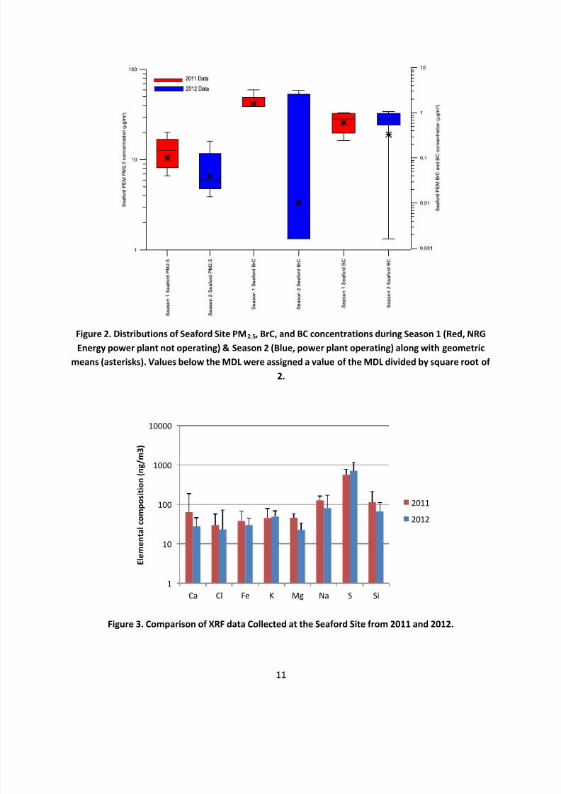
PM2.5 data for the Seaford monitoring site were lognormally distributed. Geometric mean PM2.5
concentrations during Season 2 (6.7 ± SD 1.6 µg/m3
) were reduced by 40% in comparison to Season 1concentrations (11.1 ± SD 1.5 µg/m3). BrC was also reduced from Season 1 to Season 2, with
concentrations dropping from 1.7 ± SD 1.4 µg/m3 during Season 1 to 0.01 ± SD 31.6 µg/m3 during Season
2. This trend in decreasing PM2.5 from Season 1 to Season 2 continued with BC decreasing between
Season 1 (0.6 ± SD 1.7 µg/m3) and Season 2 (0.34 ± SD 8.8 µg/m3). After transformation of the data to a
normal distribution, T-Test’s of the PM2.5, BrC, and BC indicate that the differences of means between
seasons were not significant at an alpha value of 0.01. Operating capacity of the NRG Energy power
plant was not available during the 2012 sampling period, therefore a correlation between PM2.5
reductions with power plant operation was not possible.
Evaluation of the XRF data (Figure 3) collected during the two sampling seasons reveals thatalthough there was a 26% increase in Sulfur content during this time, it was accompanied by reductions
in most other elements, including Calcium (56%), Chlorine (22%), Iron (21%), Magnesium (51%), Sodium
(37%), and Silicon (41%). T-Tests (α=0.01) of the normally transformed results between seasons
indicates that there are no significant differences with the exception of Magnesium, which had a P-value
of 0.0002. Because most of the elements that were reduced in mass between the two seasons originate
from crustal material, they are most prevalent in their oxide form, a fact which could account for the
overall mass reduction from Season 1 to Season 2.
Figure 4 illustrates the comparison between the Seaford FRM PM2.5 concentration and the RTI
collocated PEM sampler for both seasons (not blank corrected). The first season showed a reasonable
correlation (R-squared =0.85). However, the Seaford FRM samples were biased low, possibly due to the
increased face velocity of the FRM inducing additional volatilization of filter bound nitrate as has been
documented in comparison of PM2.5 filters with different filter face velocities (CARB, 1998). The FRM has
a face velocity five times greater than the 2 LPM PEM. In contrast to Season 1, comparison of RTI PEM
from Season 2 and Seaford FRM samples showed extremely good agreement, with a correlation
coefficient of 0.98. This increased correlation could be due to increased filter face velocity of RTI PEMs
during the switch to 4 LPM samplers which have a face velocity equal to 40% of the FRM.
Fixed Site Data
PEM samplers were attached to permanent structures at four locations (North, South, East, and
West) within approximately 2.5 miles of the NRG Energy power plant. These fixed site samplers
operated continuously for 24 hours, with filters from these samplers being collected each day
throughout the sampling phase. Fixed site samplers during Season 1 operated at 2 LPM, while Season 2
samplers were operated at 4 LPM. Figures 5-7 below detail the PM2.5, BrC, and BC concentration
distributions at these sites during Season 1 and Season 2.
7/30/2019 Millsboro Biomonitoring Study Final Report
http://slidepdf.com/reader/full/millsboro-biomonitoring-study-final-report 22/91
11
Figure 2. Distributions of Seaford Site PM2.5, BrC, and BC concentrations during Season 1 (Red, NRG
Energy power plant not operating) & Season 2 (Blue, power plant operating) along with geometric
means (asterisks). Values below the MDL were assigned a value of the MDL divided by square root of
2.
Figure 3. Comparison of XRF data Collected at the Seaford Site from 2011 and 2012.
1
10
100
1000
10000
Ca Cl Fe K Mg Na S Si
E l e
m e n t a l c o m p o s i t i o n ( n g / m 3 )
2011
2012

7/30/2019 Millsboro Biomonitoring Study Final Report
http://slidepdf.com/reader/full/millsboro-biomonitoring-study-final-report 23/91
12
Figure 4. Comparison of collocated Seaford FRM and RTI PEM during both seasons.
.
2012
y = 0.9934x + 0.861
R² = 0.9788
2011
y = 1.0615x - 5.2906
R² = 0.8463
0
2
4
6
8
10
12
14
16
0 2 4 6 8 10 12 14 16
S e a f o r d P E M
f i l t e r ( u g / m 3 )
Seaford FRM filter (ug/m3)
1:1 Line 2012 2011

7/30/2019 Millsboro Biomonitoring Study Final Report
http://slidepdf.com/reader/full/millsboro-biomonitoring-study-final-report 24/91
13
Figure 5. Distributions of Fixed Site PM2.5 concentrations during Season 1 (Red, NRG Energy power
plant not operating) & Season 2 (Blue, power plant operating) along with geometric means (asterisks).
Values below the MDL were assigned a value of the MDL divided by square root of 2.
7/30/2019 Millsboro Biomonitoring Study Final Report
http://slidepdf.com/reader/full/millsboro-biomonitoring-study-final-report 25/91
14
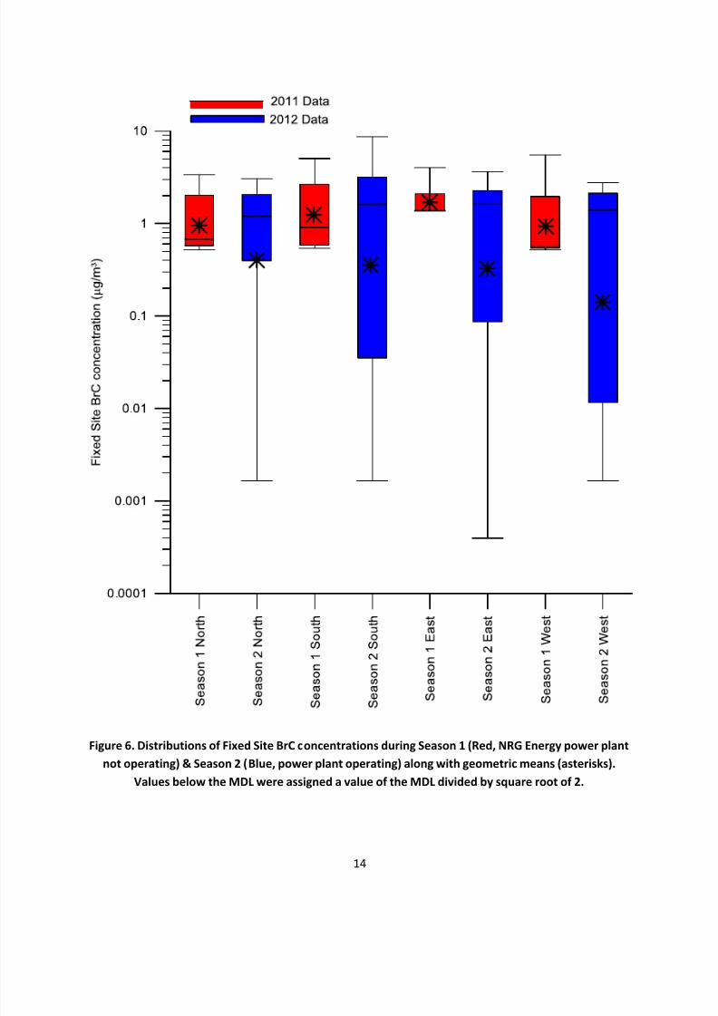
Figure 6. Distributions of Fixed Site BrC concentrations during Season 1 (Red, NRG Energy power plant
not operating) & Season 2 (Blue, power plant operating) along with geometric means (asterisks).
Values below the MDL were assigned a value of the MDL divided by square root of 2.

7/30/2019 Millsboro Biomonitoring Study Final Report
http://slidepdf.com/reader/full/millsboro-biomonitoring-study-final-report 26/91
15
Figure 7. Distributions of Fixed Site BC concentrations during Season 1 (Red, NRG Energy power plant
not operating) & Season 2 (Blue, power plant operating) along with geometric means (asterisks).
Values below the MDL were assigned a value of the MDL divided by square root of 2.

7/30/2019 Millsboro Biomonitoring Study Final Report
http://slidepdf.com/reader/full/millsboro-biomonitoring-study-final-report 27/91
16
PM2.5 was lower during Season 2 (when the NRG Energy power plant was operational) as
compared to Season 1 (when the power plant was not operational), with average concentrations being
reduced to 6.5 ± SD 1.7 µg/m3 from 12.1 ± SD 2.0 µg/m3. T-Tests of normally transformed fixed site PM2.5
data indicated this measured reduction was significant at a level of 0.01. This difference in significance
despite similar measured PM2.5 concentrations between Seaford and the fixed sites is most likely due to
the lower number of total samples collected at Seaford (n=17) versus the fixed sites (n=204). BrC
concentrations decreased from Season 1 to Season 2 with average BrC concentrations being 1.2 ± SD 2.0
µg/m3 during Season 1 and 0.3 ± SD 16.8 µg/m3 during Season 2, representing a significant change when
evaluated at a significance level of 0.01. BC was similar between seasons (0.4 ± SD 2.0 µg/m3 during
Season 1 versus 0.4 ±SD 3.9 µg/m3 during Season 2), and therefore the change between seasons was
determined to be not significant at the same test levels as used in other T-tests.
The near 46% reduction in observed ambient PM2.5 from Season 1 to Season 2 for the 4 fixed
sites can be understood by examining the XRF data collected during each season (Figures 8 and 9). A
47% reduction in average Silicon concentration (significant at a level of α=0.01) was seen between
seasons. The clear spatial trends observed with Silicon between sites during Season 1 indicate that thereis a strong source to the West-Southwest of the study area. This is in contrast to Season 2, during which
a homogenous distribution of Silicon was observed, indicating the source during Season 1 either
reduced emissions or ceased emission of Silicon altogether. Silicon is a common crustal element,
therefore, the reduction may be linked to the 39% increase in precipitation between seasons. Also of
note is an approximately 11% increase in Sulfur detected in Season 2 PM2.5 samples (not significant at a
level of α=0.01). Although it is presumable the increased Sulfur content is a result of the power plant, no
other metals commonly associated with coal-fired power plants, such as Selenium, Iron, and Cadmium,
were detected. Therefore, linking the increased Sulfur to the NRG Energy power plant is not supported
by the XRF analysis
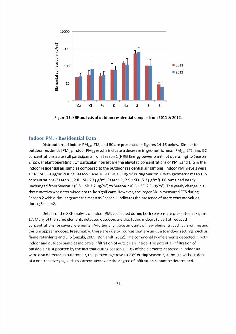
Outdoor PM2.5 Residential Data
Figures 10-12 show a general overall decrease in outdoor residential PM2.5 and the associated
BrC and BC from 2011 (NRG Energy power plant not operating) to 2012 (power plant operating), with
the average PM2.5 decreasing from 16.2 ± SD 1.5 µg/m3 in Season 1 to 6.5 ± SD 2.0 µg/m3 in Season 2. At
the same time, BrC and BC were reduced from 2.9 ± SD 2.3 and 0.9 ± SD 2.0 µg/m3 respectively to 0.3 ±
SD 15.4 and 0.6 ± SD 2.4 µg/m3. Reductions in all three PM2.5 mean concentrations were determined to
be significant at a test level of 0.01. Similar to the fixed sites and the Seaford site, all metrics in outdoor
residential samples were reduced between seasons, with PM2.5, BrC, and BC being reduced by 60%, 90%,
and 33% respectively. Further examination of the outdoor residential PM2.5 elemental composition
revealed a significant (α=0.01) increase in Chlorine content (Figure 13). Additional species that werefound to vary between seasons include Sulfur and Iron, though these variations were determined to not
be significant. Elucidating the origin of the observed PM2.5 reduction requires incorporation of additional
measurements of atmospheric constituents, such as sulfur dioxide, nitrogen dioxide, and PM speciation
(nitrate, organic carbon fractions), which was beyond the scope of the current work.

7/30/2019 Millsboro Biomonitoring Study Final Report
http://slidepdf.com/reader/full/millsboro-biomonitoring-study-final-report 28/91
17
Figure 8. XRF Results from 2011 Fixed Site ambient samplers, Trace elements above MDL not shown.
Figure 9. XRF Results from 2012 Fixed Site ambient samplers, Trace elements above MDL not shown.
1
10
100
1000
10000
Ca Cl Fe K Na S Si
E l e m e n t a l c o m p o s i t i o n ( n
g / m 3 )
North
South
East
West
1
10
100
1000
Ca Cl Fe K Na S Si
E l e m e n t a l c o m p o s i t i o n ( n g / m 3 )
North
South
East
West

7/30/2019 Millsboro Biomonitoring Study Final Report
http://slidepdf.com/reader/full/millsboro-biomonitoring-study-final-report 29/91
18
Figure 10. Distributions of outdoor residential PM2.5 concentrations during Season 1 (Red, NRG Energy
power plant not operating) & Season 2 (Blue, power plant operating) along with geometric means
(asterisks). Values below the MDL were assigned a value of the MDL divided by square root of 2.

7/30/2019 Millsboro Biomonitoring Study Final Report
http://slidepdf.com/reader/full/millsboro-biomonitoring-study-final-report 30/91
19
Figure 11. Distributions of outdoor residential BrC concentrations during Season 1 (Red, NRG Energypower plant not operating) & Season 2 (Blue, power plant operating) along with geometric means
(asterisks). Values below the MDL were assigned a value of the MDL divided by square root of 2.

7/30/2019 Millsboro Biomonitoring Study Final Report
http://slidepdf.com/reader/full/millsboro-biomonitoring-study-final-report 31/91
20
Figure 12. Distributions of outdoor residential BC concentrations during Season 1 (Red, NRG Energy
power plant not operating) & Season 2 (Blue, power plant operating) along with geometric means
(asterisks). Values below the MDL were assigned a value of the MDL divided by square root of 2.
7/30/2019 Millsboro Biomonitoring Study Final Report
http://slidepdf.com/reader/full/millsboro-biomonitoring-study-final-report 32/91
21
Figure 13. XRF analysis of outdoor residential samples from 2011 & 2012.
Indoor PM2.5 Residential Data
Distributions of indoor PM2.5, ETS, and BC are presented in Figures 14-16 below. Similar to
outdoor residential PM2.5, indoor PM2.5 results indicate a decrease in geometric mean PM2.5, ETS, and BC
concentrations across all participants from Season 1 (NRG Energy power plant not operating) to Season
2 (power plant operating). Of particular interest are the elevated concentrations of PM2.5 and ETS in the
indoor residential air samples compared to the outdoor residential air samples. Indoor PM2.5 levels were
12.6 ± SD 3.8 µg/m
3
during Season 1 and 10.9 ± SD 3.3 µg/m
3
during Season 2, with geometric mean ETSconcentrations (Season 1, 2.8 ± SD 6.3 µg/m3; Season 2, 2.9 ± SD 15.2 µg/m3). BC remained nearly
unchanged from Season 1 (0.5 ± SD 3.7 µg/m3) to Season 2 (0.6 ± SD 2.5 µg/m3). The yearly change in all
three metrics was determined not to be significant. However, the larger SD in measured ETS during
Season 2 with a similar geometric mean as Season 1 indicates the presence of more extreme values
during Season2.
Details of the XRF analysis of indoor PM2.5 collected during both seasons are presented in Figure
17. Many of the same elements detected outdoors are also found indoors (albeit at reduced
concentrations for several elements). Additionally, trace amounts of new elements, such as Bromine and
Cerium appear indoors. Presumably, these are due to sources that are unique to indoor settings, such as
flame retardants and ETS (Suzuki, 2009; Böhlandt, 2012). The commonality of elements detected in both
indoor and outdoor samples indicates infiltration of outside air inside. The potential infiltration of
outside air is supported by the fact that during Season 1, 73% of the elements detected in indoor air
were also detected in outdoor air, this percentage rose to 79% during Season 2, although without data
of a non-reactive gas, such as Carbon Monoxide the degree of infiltration cannot be determined.
1
10
100
1000
10000
Ca Cl Fe K Na S Si Zn
E l e m e n t a l c o m p o s t i o
n ( n g / m 3 )
2011
2012

7/30/2019 Millsboro Biomonitoring Study Final Report
http://slidepdf.com/reader/full/millsboro-biomonitoring-study-final-report 33/91
22
Figure 18 illustrates the indoor to outdoor ratio of the common elements between indoor and
outdoor samples for both sampling seasons. A ratio greater than 1 suggests the sources for an element
Figure 14. Distributions of indoor residential PM2.5 concentrations during Season 1 (Red, NRG Energy
power plant not operating) & Season 2 (Blue, power plant operating) along with geometric means
(asterisks). Values below the MDL were assigned a value of the MDL divided by square root of 2.

7/30/2019 Millsboro Biomonitoring Study Final Report
http://slidepdf.com/reader/full/millsboro-biomonitoring-study-final-report 34/91
23
Figure 15. Distributions of indoor residential ETS concentrations during Season 1 (Red, NRG Energy
power plant not operating) & Season 2 (Blue, power plant operating) along with geometric means
(asterisks). Values below the MDL were assigned a value of the MDL divided by square root of 2.

7/30/2019 Millsboro Biomonitoring Study Final Report
http://slidepdf.com/reader/full/millsboro-biomonitoring-study-final-report 35/91
24
Figure 16. Distributions of indoor residential BC concentrations during Season 1 (Red, NRG Energy
power plant not operating) & Season 2 (Blue, power plant operating) along with geometric means
(asterisks). Values below the MDL were assigned a value of the MDL divided by square root of 2.

7/30/2019 Millsboro Biomonitoring Study Final Report
http://slidepdf.com/reader/full/millsboro-biomonitoring-study-final-report 36/91
25
Figure 17. Comparison of XRF analysis for indoor residential PM2.5 during 2011 & 2012.
Figure 18. Indoor residential-outdoor residential ratio of select elements.
1
10
100
1000
10000
Br Ca Ce Cl Cu Fe K Mg Na P S Si Zn
E l e m e n t a l c o m p o s i t i o
n ( n g / m 3 )
2011
2012

7/30/2019 Millsboro Biomonitoring Study Final Report
http://slidepdf.com/reader/full/millsboro-biomonitoring-study-final-report 37/91
26
originate indoors, whereas a ratio less than 1 suggests the majority of an element originates from
outdoor sources. The ratios greater than or near unity found during this study are consistent with other
residential studies (Brown et al., 2012). For most elements, such as Calcium, Sulfur, and Zinc, the ratios
were consistent from season to season. This consistency suggests the emission rate of these elements
remained the same during each season. Other elements, such as Potassium, Sodium, and Silicon,
showed decreases in their indoor/outdoor ratio. This decrease could be linked to either a decrease in
their emission rate while the number of sources remained consistent or reduction of emission sources
during the time period between the first and second sampling season. The lower emission rate or
reduction of sources would result from changes in the residents’ activity patterns. Furthermore, the
consistent indoor/outdoor ratio of elements between seasons coupled with previous research suggests
that indoor/outdoor ratios of elements provide insight into the degree of infiltration (Johnson, 2008).
Personal PM2.5 Data
The RTI MicroPEM units monitored personal level exposure to PM2.5. These units contained filters
on which PM2.5 was captured. Additionally the MicroPEMs used during Season 2 contained
nephelometers which permitted real-time measurement of PM2.5 concentrations. Figures 19-21 showthe variability in personal level PM2.5, ETS, and BC measurements made during both sampling seasons.
Personal level exposure to PM2.5 was considerably higher than outdoor or indoor concentrations.
This is consistent with findings of previous studies conducted elsewhere (Williams et al., 2003; Rodes et
al., 2010; Williams et al., 2012). Season 1 personal level PM2.5 concentrations had a geometric mean of
19.6 ± SD 3.4 µg/m3, while Season 2 concentrations were 23.2 ± SD 5.7 µg/m3 (gravimetric) and 24.1 ±
SD 2.7 µg/m3 (nephelometer). T-Test of these values indicated there was no significant difference
between gravimetric or nephelometer data between seasons. However, these concentrations are 55%
and 113% more than the indoor concentrations observed during the same time period and 21% and
257% more than the outdoor concentrations seen during the respective seasons.
The high personal level concentrations are primarily driven by ETS exposure. Examination of
individual level data supports this conclusion. Of the 20 participants during Season 1 whose personal
exposure levels were in excess of the Federal 24 hour PM2.5 standard of 35 µg/m3, 65% of them were
also within the top 20 participants in terms of ETS concentration. This percentage increased during
Season 2, where 89% of the top 18 participants in terms of ETS exposure also had personal PM2.5
exposure levels in excess of 35 µg/m3. Therefore, although ETS concentrations averaged 1.0 ± SD 7.5
µg/m3 for Season 1 and 2.1 ± SD 31.3 µg/m3 during Season 2, they accounted for the vast majority of
samples with elevated PM2.5 concentrations. To further illustrate the impact of ETS on personal
exposure, Figure 22 compares real-time PM2.5
acquired with the MicroPEM nephelometer from a
participant with high ETS concentrations to that of a participant with low ETS concentrations. The
household with high ETS tended to have a higher background concentration and several spikes in PM2.5
mass were observed. These spikes are thought to be due to the passive combustion and extinguishing of
cigarettes, an act which leads to large amounts of PM2.5, however without questionnaire data indicating
the presence of smokers within households, a definitive correlation cannot be determined. Black carbon
plays a lesser role in terms of the overall mass concentration of personal exposure than does ETS with

7/30/2019 Millsboro Biomonitoring Study Final Report
http://slidepdf.com/reader/full/millsboro-biomonitoring-study-final-report 38/91
27
Figure 19. Distributions of personal level PM2.5 concentrations during Season 1 (Red, NRG Energy
power plant not operating) & Season 2 (Blue, power plant operating) along with geometric means
(asterisks). Values below the MDL were assigned a value of the MDL divided by square root of 2.

7/30/2019 Millsboro Biomonitoring Study Final Report
http://slidepdf.com/reader/full/millsboro-biomonitoring-study-final-report 39/91
28
Figure 20. Distributions of personal level ETS concentrations during Season 1 (Red, NRG Energy power
plant not operating) & Season 2 (Blue, power plant operating) along with geometric means (asterisks).
Values below the MDL were assigned a value of the MDL divided by square root of 2.

7/30/2019 Millsboro Biomonitoring Study Final Report
http://slidepdf.com/reader/full/millsboro-biomonitoring-study-final-report 40/91
29
Figure 21. Distributions of personal level BC concentrations during Season 1 (Red, NRG Energy power
plant not operating) & Season 2 (Blue, power plant operating) along with geometric means (asterisks).
Values below the MDL were assigned a value of the MDL divided by square root of 2.

7/30/2019 Millsboro Biomonitoring Study Final Report
http://slidepdf.com/reader/full/millsboro-biomonitoring-study-final-report 41/91
30
Figure 22. 24-hr Trend of 5-minute averaged PM2.5 from high and low ETS participants.
1
10
100
1000
10000
P M 2 . 5
C o n c e n t r a t i o n ( µ g / m
3 )
Observation number
DUP-0108 (ETS 59.78 µg/m3)
DUP-0102 (ETS 0.676 µg/m3)

7/30/2019 Millsboro Biomonitoring Study Final Report
http://slidepdf.com/reader/full/millsboro-biomonitoring-study-final-report 42/91
31
1.7 ± SD 5.1 µg/m3 and 0.4 ± SD 10.2 µg/m3 being observed in seasons 1 and 2 respectively, though it
was determined to be significantly different (p-value 2.8x10⁻⁷) it is due to less than 10 instances of BC
measurements greater than 10 µg/m3 and therefore the significant difference should be viewed as
unlikely.
XRF analysis of MicroPEM filters indicated a wide variation in 15 different metals. The overalltrend of XRF analysis indicated an increase from Season 1 (NRG Energy power plant not operating) to
Season 2 (power plant operating) with the exception of Sulfur as shown in Figure 23. The additional
elements detected in personal level samples as compared in outdoor samples coupled with elevated
PM2.5 concentrations underscore the fact that understanding the local population exposure and
potential sources of cancer-causing chemicals associated with PM2.5 requires additional study of indoor
sources and participant habits.
Figure 23. XRF analysis of RTI MicroPEM filters from Seasons 1 and 2.
1
10
100
1000
10000
100000
Al Br Ca Cl Cr Cu Fe K Mg Na Ni P S Si Zn
E l e m e n t a l c o m p o s i t i o n ( n g / m 3 )
2011
2012

7/30/2019 Millsboro Biomonitoring Study Final Report
http://slidepdf.com/reader/full/millsboro-biomonitoring-study-final-report 43/91
32
Residential Temperature and Humidity
Technicians placed temperature and humidity sensors inside each participant’s household at the
beginning of the three-day sampling period. Average temperatures for all households during both
sampling seasons were 69.8 ± SD 3.0 (Season 1) and 71.3 ± SD 4.7 (Season 2) degrees Fahrenheit. The
average relative humidity for households during both seasons was 51.1 percent. Table 9 below presents
summarized data for all participants during both seasons.
Table 5. Average temperatures and relative humidities for Season 1 & Season 2 participants.
Season
Average
Temperature
(°F)
Average Relative
Humidity (%)
Season 1 69.8 ± SD 3.0 51.1 ± SD 6.4
Season 2 71.3 ± SD 4.7 51.1 ± SD 8.2
Questionnaires
Residents were given two questionnaires during the first season three-day sampling period. The
first questionnaire (Residential Survey) covered details about the physical residence participants were
living in including age of dwelling, types of heating, number of persons living there, etc. During Season
2, additional questions were asked about consumption of certain foods and dietary supplements. These
changes were made because of the measurement of higher than expected concentrations of As and Se
in some samples during Season 1; such elevations were thought to be possibly associated with diet. The
second questionnaire was a time activity diary. Participants were asked to keep track of their
movements and actions during the course of the three sampling days. Summarized data from both
questionnaires and both seasons are included in Appendix A.
Biospecimen Samples
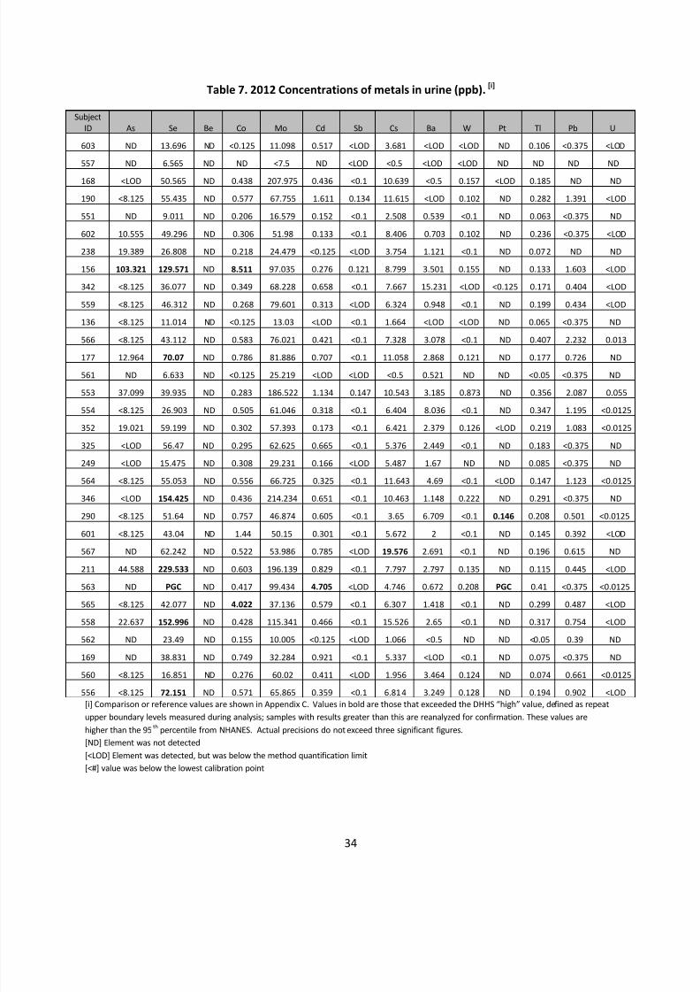
The urine and blood specimen results are listed in Tables 6-8. During Season 1, Arsenic and
Selenium were greater than reference values in 12 of the participant’s urine (Table6). Urine samples
were greater than reference values for various metals, especially arsenic and selenium in 9 of the
participants (Table 7) during Season 2. Additionally, blood metals (Table 8) were elevated for some of
the participants in both seasons, but none of the elements (Cadmium, Mercury, and Lead) were above
the high values shown in Appendix C. Participants with elevated concentration of Mercury and Lead in
2011 generally had elevated concentrations in 2012; the significance of these differences was not
tested. No VOCs were detected in blood above the lower reporting threshold during either season.Reference values for metals and VOCs in blood and urine are presented in Appendices B and C,
respectively. Hair samples were not tested but were archived for later testing, along with remaining
aliquots of the blood and urine samples.

7/30/2019 Millsboro Biomonitoring Study Final Report
http://slidepdf.com/reader/full/millsboro-biomonitoring-study-final-report 44/91
33
Table 6. 2011 Concentrations of metals in urine (ppb).[i]
Subject
ID As Se Be Co Mo Cd Sb Cs Ba W Pt Tl Pb U
557 9.118 28.766 <0.25 0.125 14.525 <0.1250 <0.10 1.506 0.638 <0.1 <0.125 <0.0500 <0.3750 <0.0125
168 <8.125 40.244 <0.25 0.236 38.066 0.276 <0.10 4.714 1.796 <0.1 <0.125 0.116 <0.3750 <0.0125
190 234.524 52.994 <0.25 0.264 32.782 0.742 <0.10 6.656 <0.50 <0.1 <0.125 0.304 0.664 <0.0125
551 12.37 29.917 <0.25 1.208 16.538 <0.1250 <0.10 3.152 <0.50 <0.1 <0.125 <0.0500 <0.3750 <0.0125
139 <8.125 44.465 <0.25 0.362 <7.50 0.128 0.134 1.245 1.209 <0.1 <0.125 0.059 <0.3750 <0.0125
238 14.048 251.126 <0.25 1.132 337.449 2.095 <0.10 20.661 2.423 0.379 <0.125 0.392 1.286 <0.0125
156 9.53 59.135 <0.25 0.249 41.108 0.132 <0.10 4.307 1.172 <0.1 <0.125 0.134 1.01 <0.0125
342 <8.125 57.772 <0.25 0.267 55.01 0.746 <0.10 6.917 7.757 <0.1 <0.125 0.266 0.5 <0.0125
559 26.692 31.569 <0.25 0.151 25.205 0.125 <0.10 3.601 <0.50 <0.1 <0.125 0.148 <0.3750 <0.0125
169 <8.125 24.955 <0.25 0.644 8.775 0.762 <0.10 4.153 0.668 <0.1 <0.125 0.05 <0.3750 <0.0125
136 <8.125 33.252 <0.25 0.125 17.347 <0.1250 <0.10 <0.5 <0.50 <0.1 0.133 0.072 <0.3750 <0.0125
566 >650 56.821 <0.25 0.719 51.201 0.191 0.167 5.852 3.065 0.171 <0.125 0.473 2.601 0.016
177 <8.125 21.302 <0.25 0.181 <7.50 <0.1250 <0.10 1.071 0.22 <0.1 <0.125 <0.0500 <0.3750 <0.0125
561 <8.125 52.915 <0.25 0.541 29.862 0.277 <0.10 3.421 2.685 0.1 <0.125 0.163 1.16 <0.0125
553 88.202 36.07 <0.25 0.472 61.705 <0.1250 0.115 13.378 4.86 0.213 <0.125 0.339 1.895 0.034
554 <8.125 98.551 <0.25 0.511 73.711 0.167 <0.10 4.957 3.581 0.278 <0.125 0.349 0.988 <0.0125
352 11.678 44.381 <0.25 0.203 56.152 0.172 <0.10 3.706 1.458 0.127 <0.125 0.114 0.773 0.002
325 <8.125 23.054 <0.25 0.125 9.117 0.149 <0.10 <0.5 <0.50 <0.1 <0.125 <0.0500 <0.3750 <0.0125
249 <8.125 12.192 <0.25 0.125 <7.50 <0.1250 <0.10 1.141 <0.50 <0.1 <0.125 <0.0500 <0.3750 <0.0125
552 <8.125 31.305 <0.25 0.125 12.38 <0.1250 <0.10 <0.5 1.45 <0.1 <0.125 <0.0500 <0.3750 <0.0125
564 <8.125 92.909 <0.25 0.31 69.406 0.5 0.15 5.771 3.034 <0.1 <0.125 0.104 0.878 <0.0125
346 <8.125 123.634 <0.25 0.167 17.617 0.238 <0.10 2.639 <0.50 <0.1 <0.125 0.09 <0.3750 <0.0125
560 62.788 72.161 <0.25 0.413 80.512 1.817 <0.10 8.839 2.243 0.158 <0.125 0.129 1.26 <0.0125
556 0.503 <0.0500 <0.1250 <0.5 <0.3750 0.125 19.948 <7.50 <0.25 0 <0.10 <0.0125 <0.125 <0.1
290 24.004 74.835 <0.25 0.609 59.696 1.048 <0.10 5.095 2.252 <0.1 <0.125 0.216 1.013 <0.0125
298 <8.125 27.154 <0.25 0.307 <7.50 0.202 <0.10 1.201 3.939 <0.1 <0.125 0.3 <0.3750 <0.0125
567 <8.125 20.866 <0.25 0.125 <7.50 <0.1250 <0.10 3.03 <0.50 <0.1 <0.125 <0.0500 <0.3750 <0.0125
211 86.361 210.974 <0.25 0.539 180.421 0.794 <0.10 7.248 2.562 <0.1 <0.125 0.102 1.427 <0.0125
563 11.005 96.178 <0.25 0.483 97.092 1.08 <0.10 6.147 1.294 <0.1 <0.125 0.163 <0.3750 <0.0125
565 8.204 27.648 <0.25 0.456 13.613 <0.1250 <0.10 1.533 1.001 <0.1 <0.125 <0.0500 <0.3750 <0.0125
558 15.458 105.83 <0.25 0.242 41.082 0.226 <0.10 12.306 1.143 <0.1 <0.125 0.441 0.48 <0.0125
562 <8.125 19.596 <0.25 0.125 <7.50 <0.1250 <0.10 <0.5 <0.50 <0.1 <0.125 <0.0500 <0.3750 <0.0125[i] Comparison or reference values are shown in Appendix C. Values in bold are those that exceeded the DHHS “high” value, defined as repeat
upper boundary levels measured during analysis; samples with results greater than this are reanalyzed for confirmation. These
values are higher than the 95th
percentile from NHANES. Actual precisions do not exceed three significant figures.
[ND] Element was not detected
[<LOD] Element was detected, but was below the method quantification limit
[<#] value was below the lowest calibration point
7/30/2019 Millsboro Biomonitoring Study Final Report
http://slidepdf.com/reader/full/millsboro-biomonitoring-study-final-report 45/91
34
Table 7. 2012 Concentrations of metals in urine (ppb). [i]
Subject
ID As Se Be Co Mo Cd Sb Cs Ba W Pt Tl Pb U
603 ND 13.696 ND <0.125 11.098 0.517 <LOD 3.681 <LOD <LOD ND 0.106 <0.375 <LOD
557 ND 6.565 ND ND <7.5 ND <LOD <0.5 <LOD <LOD ND ND ND ND
168 <LOD 50.565 ND 0.438 207.975 0.436 <0.1 10.639 <0.5 0.157 <LOD 0.185 ND ND
190 <8.125 55.435 ND 0.577 67.755 1.611 0.134 11.615 <LOD 0.102 ND 0.282 1.391 <LOD
551 ND 9.011 ND 0.206 16.579 0.152 <0.1 2.508 0.539 <0.1 ND 0.063 <0.375 ND
602 10.555 49.296 ND 0.306 51.98 0.133 <0.1 8.406 0.703 0.102 ND 0.236 <0.375 <LOD
238 19.389 26.808 ND 0.218 24.479 <0.125 <LOD 3.754 1.121 <0.1 ND 0.072 ND ND
156 103.321 129.571 ND 8.511 97.035 0.276 0.121 8.799 3.501 0.155 ND 0.133 1.603 <LOD
342 <8.125 36.077 ND 0.349 68.228 0.658 <0.1 7.667 15.231 <LOD <0.125 0.171 0.404 <LOD
559 <8.125 46.312 ND 0.268 79.601 0.313 <LOD 6.324 0.948 <0.1 ND 0.199 0.434 <LOD
136 <8.125 11.014 ND <0.125 13.03 <LOD <0.1 1.664 <LOD <LOD ND 0.065 <0.375 ND
566 <8.125 43.112 ND 0.583 76.021 0.421 <0.1 7.328 3.078 <0.1 ND 0.407 2.232 0.013
177 12.964 70.07 ND 0.786 81.886 0.707 <0.1 11.058 2.868 0.121 ND 0.177 0.726 ND
561 ND 6.633 ND <0.125 25.219 <LOD <LOD <0.5 0.521 ND ND <0.05 <0.375 ND
553 37.099 39.935 ND 0.283 186.522 1.134 0.147 10.543 3.185 0.873 ND 0.356 2.087 0.055
554 <8.125 26.903 ND 0.505 61.046 0.318 <0.1 6.404 8.036 <0.1 ND 0.347 1.195 <0.0125
352 19.021 59.199 ND 0.302 57.393 0.173 <0.1 6.421 2.379 0.126 <LOD 0.219 1.083 <0.0125
325 <LOD 56.47 ND 0.295 62.625 0.665 <0.1 5.376 2.449 <0.1 ND 0.183 <0.375 ND
249 <LOD 15.475 ND 0.308 29.231 0.166 <LOD 5.487 1.67 ND ND 0.085 <0.375 ND
564 <8.125 55.053 ND 0.556 66.725 0.325 <0.1 11.643 4.69 <0.1 <LOD 0.147 1.123 <0.0125
346 <LOD 154.425 ND 0.436 214.234 0.651 <0.1 10.463 1.148 0.222 ND 0.291 <0.375 ND
290 <8.125 51.64 ND 0.757 46.874 0.605 <0.1 3.65 6.709 <0.1 0.146 0.208 0.501 <0.0125
601 <8.125 43.04 ND 1.44 50.15 0.301 <0.1 5.672 2 <0.1 ND 0.145 0.392 <LOD
567 ND 62.242 ND 0.522 53.986 0.785 <LOD 19.576 2.691 <0.1 ND 0.196 0.615 ND
211 44.588 229.533 ND 0.603 196.139 0.829 <0.1 7.797 2.797 0.135 ND 0.115 0.445 <LOD
563 ND PGC ND 0.417 99.434 4.705 <LOD 4.746 0.672 0.208 PGC 0.41 <0.375 <0.0125
565 <8.125 42.077 ND 4.022 37.136 0.579 <0.1 6.307 1.418 <0.1 ND 0.299 0.487 <LOD
558 22.637 152.996 ND 0.428 115.341 0.466 <0.1 15.526 2.65 <0.1 ND 0.317 0.754 <LOD
562 ND 23.49 ND 0.155 10.005 <0.125 <LOD 1.066 <0.5 ND ND <0.05 0.39 ND
169 ND 38.831 ND 0.749 32.284 0.921 <0.1 5.337 <LOD <0.1 ND 0.075 <0.375 ND
560 <8.125 16.851 ND 0.276 60.02 0.411 <LOD 1.956 3.464 0.124 ND 0.074 0.661 <0.0125
556 <8.125 72.151 ND 0.571 65.865 0.359 <0.1 6.814 3.249 0.128 ND 0.194 0.902 <LOD[i] Comparison or reference values are shown in Appendix C. Values in bold are those that exceeded the DHHS “high” value, defined as repeat
upper boundary levels measured during analysis; samples with results greater than this are reanalyzed for confirmation. These values are
higher than the 95th
percentile from NHANES. Actual precisions do not exceed three significant figures.
[ND] Element was not detected
[<LOD] Element was detected, but was below the method quantification limit
[<#] value was below the lowest calibration point

7/30/2019 Millsboro Biomonitoring Study Final Report
http://slidepdf.com/reader/full/millsboro-biomonitoring-study-final-report 46/91
35
Table 8. 2011 and 2012 blood metals concentrations (ppb).
2011 (Season 1)
Subject ID
557 168 190 551 139 238 156 342 559 169 136 566 177 561 553 554
Cd <0.5 <0.5 0.698 1.316 1.329 <0.5 <0.5 <0.5 <0.5 0.788 <0.5 <0.5 <0.5 <0.5 0.681 <0.5
Hg <1 <1 <1 <1 <1 <1 2.886 <1 <1 <1 1.212 1.474 <1 <1 2.088 2.324
Pb <10 <10 26.652 <10 10.931 <10 16.699 <10 <10 <10 19.016 14.736 12.723 <10 23.818 <10
Subject ID
352 325 249 552 564 346 560 556 290 298 567 211 563 565 558 562
Cd <0.5 <0.5 <0.5 <0.5 <0.5 <0.5 <0.5 <0.5 1.15 0.812 0.644 <0.5 0.681 <0.5 <0.5 <0.5
Hg 2.04 <1 <1 <1 <1 1.43 <1 1.854 1.69 1.144 <1 3.048 <1 1.3 <1 <1
Pb 21.6 <10 <10 <10 17.537 <10 <10 <10 <10 11.31 <10 10.89 <10 <10 <10 11.63
2012 (Season 2)
Subject ID
603 557 168 190 551 602 238 156 342 559 136 566 177 561 553 554
Cd <1 <1 <LOD <1 1.034 ND <LOD ND <LOD ND <LOD ND <LOD <1 <1 ND
Hg <2 <2 <LOD <2 <LOD <LOD <LOD 2.462 ND ND <2 <2 <LOD <LOD 6.074 <2
Pb <LOD <LOD <20 25.173 <LOD <LOD <LOD <20 <LOD <20 <20 <20 <20 <20 32.912 <20
Subject ID
352 325 249 564 346 290 601 567 211 563 565 558 562 169 560 556
Cd ND <LOD <LOD <LOD <LOD <1 <LOD <1 <LOD <1 <LOD ND <LOD <1 <LOD <LOD
Hg <2 ND <2 ND <2 <2 ND ND 3.06 ND <2 <LOD <2 <LOD <LOD <2
Pb 28.3 <20 <20 28.988 <20 <LOD <LOD <LOD <20 ND <LOD <LOD <20 <20 <20 <LOD
[ND] Element was not detected
[<LOD] Element was detected, but was below the method quantification limit
[<#] value was below the lowest calibration point
The measurement of an environmental chemical in a person’s blood or urine does not by itself
mean that the chemical causes disease. Research studies are required to determine whether blood or
urine concentrations are safe or are associated with disease or adverse effects. Many of the referencelevels contained in this report were obtained from the National Health and Nutrition Examination Survey
(NHANES) Studies conducted by the Centers for Disease Control and Prevention (e.g., Fourth National
Report on Human Exposure to Environmental Contaminants, Centers for Disease Control and
Prevention, 2009; http://www.cdc.gov/exposurereport/). The NHANES studies are probability-based
population studies and reflect the analyte concentrations representative of the US population. In most
cases in this report, reference is made to the 95th percentiles, which means that the indicated

7/30/2019 Millsboro Biomonitoring Study Final Report
http://slidepdf.com/reader/full/millsboro-biomonitoring-study-final-report 47/91
36
concentrations are equal to or higher than those measured for 95% of the population. This value is
useful for determining whether or not a concentration measured in any particular public health study is
unusual. The reader is encouraged to visit the website shown above for more information about many
of the analytes measured.
Distributions of the biospecimen results for each season are shown below for blood (Figure 24)and for urine (Figure 25) for both seasons. Note that for these results, values below MDL or those that
were not detected were reported as 0.5 times the limit of detection. On average, there do not appear to
be any significant changes across seasons. However, several participants had concentrations that
exceeded the high reference value for various elements in one or both seasons (Table 9). By far the
most common exceedances were for Arsenic and Selenium. For those 2012 participants with urinary
concentrations of As or Se that were above the high reference values, we evaluated their responses to
the dietary questions added for the 2012 sampling season. Participant 156 consumed locally caught fish
(tautog), ate meat, poultry, and locally-grown produce on a on a regular basis but did not report taking
any multivitamins or Selenium containing supplements. Those participants with elevated concentrations
of Se only (346, 211. 558, and 556) reported regular consumption of meats, poultry, grains, and localproduce. Participants 346, 211, 558, and 556 all took multivitamins with participants 211 and 556
reporting taking a fish oil supplement. A key parameter in evaluation of the effect of these actions on
urinary metals concentrations is the time between providing a urine sample and consumption. In the
case of grains and local seafood, these actions were taken within the past 48 hours of providing a urine
sample; therefore the linkage between these actions is potentially stronger than those actions with no
time-related information.
An important component of this study was to evaluate how exposure to particulate matter is
associated with measures from the biospecimens. Measured PM permitted evaluation of four
characteristics: mass, ETS, Black carbon, and elemental composition. Relationships of each PM measureto each analyte/matrix combination in the biospecimens were examined. PM measurement
characteristics were averaged over the course of the three day sampling period since there was only one
biospecimen data point to reflect each participant. Non-ranked correlations were performed with the
following tables indicating how predictive each PM characteristic was for each biospecimen analyte. The
scatter plots were examined to ensure that the correlation was not being driven by a single extreme
value.
Table 10 shows the results for PM mass to be predictive of elements in blood and urine. Blood
lead appears to be associated with PM mass each year, but it is also persistent in the body. Table 11
shows the correlation of ETS with elements in blood and urine. Although significance was found for
blood mercury, blood lead, and urinary uranium, all of these appeared to be driven by a single, high
value. Table 12 shows associations of BC with elements in blood and urine. P-values <0.05 were found
for blood Cd and Pb in 2011 and blood Hg in 2012; other significant associations were clearly driven by
extreme values and should not be believed. In general, some associations were observed between some
elements with total mass, ETS, and BC, but they were not consistent across all elements or across the
two years of the study.

7/30/2019 Millsboro Biomonitoring Study Final Report
http://slidepdf.com/reader/full/millsboro-biomonitoring-study-final-report 48/91
37
Table 9. Participants for whom any of the analytes in blood or urine exceeded high reference value (*
indicates a measurement above the reference value).
[†]Participant 563 also had very high levels of Pt in urine that was reported by DPHL as “PGC” or
“parameter greater than calibration”
Participant
Id. Specimen
Measurement
Type Analyte
2011Result
(ppb)
2012Result
(ppb)
Reference
Value
136 URINE Metals PT 0.133 * ND 0.10
156 URINE Metals AS 9.53 103.321 * 64.50
156 URINE Metals CO 0.249 8.511 * 2.83
156 URINE Metals SE 59.1 129.571 * 68.00
177 URINE Metals SE 21.3 70.07 * 68.00
190 URINE Metals AS 235 * <8.125 64.50
211 URINE Metals AS 86.4 * 44.588 64.50
211 URINE Metals SE 211 * 229.533 * 68.00
238 URINE Metals MO 337 * 24.479 293.50
238 URINE Metals SE 251 * 26.808 68.00
290 URINE Metals PT <0.125 0.146 * 0.10
290 URINE Metals SE 74.8 * 51.64 68.00
346 URINE Metals SE 124 * 154.425 * 68.00
553 URINE Metals AS 88.2 * 37.099 64.50
554 URINE Metals SE 98.6 * 26.903 68.00
556 URINE Metals SE 19.9 72.151 * 68.00
558 URINE Metals SE 106 * 152.996 * 68.00
560 URINE Metals SE 72.2 * 16.851 68.00
563 URINE Metals CD 1.08 4.705 * 2.54
563 URINE Metals SE 96.2 * PGC† 68.00
564 URINE Metals SE 92.9 * 55.053 68.00
565 URINE Metals CO 0.456 4.022 * 2.83
566 URINE Metals As >650 * <8.125 64.5

7/30/2019 Millsboro Biomonitoring Study Final Report
http://slidepdf.com/reader/full/millsboro-biomonitoring-study-final-report 49/91
38
Figure 24. Blood metals distribution for all participants during 2011 (Red) and 2012 (Blue).
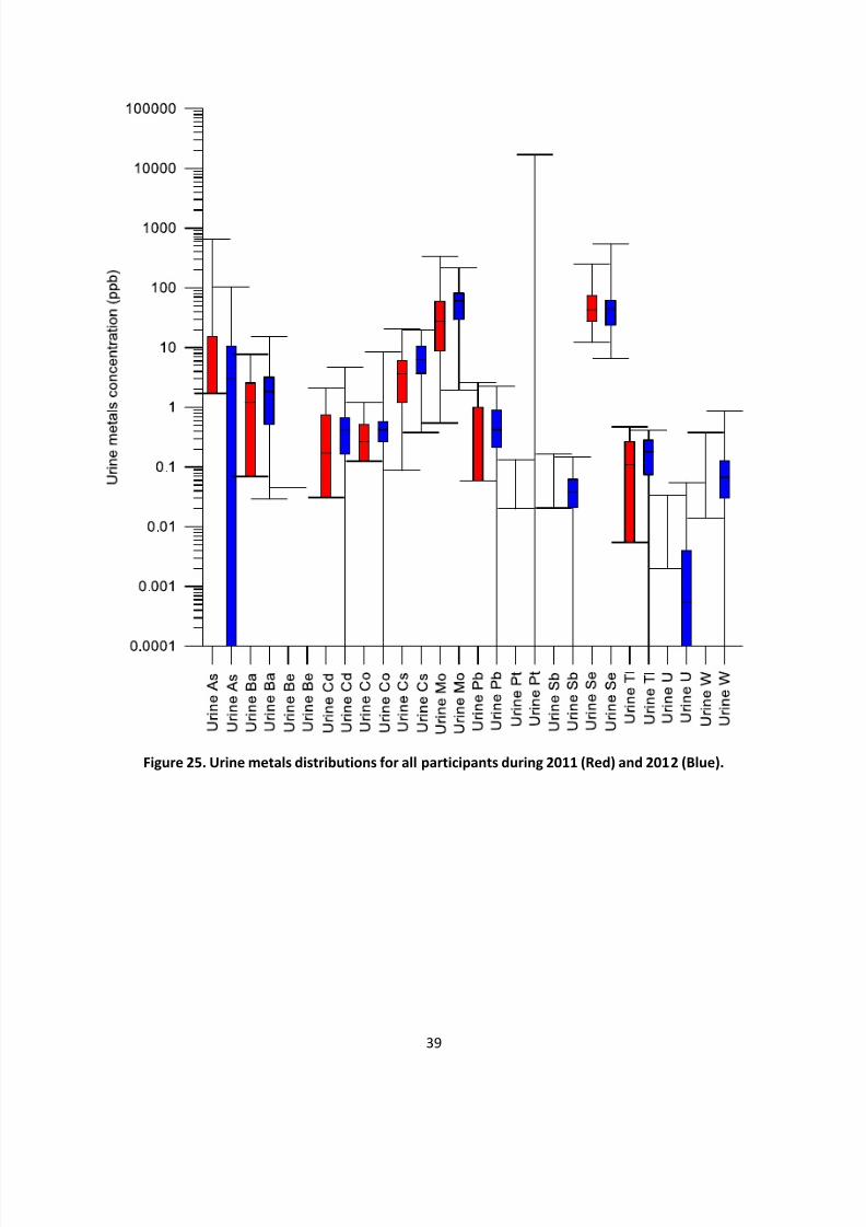
7/30/2019 Millsboro Biomonitoring Study Final Report
http://slidepdf.com/reader/full/millsboro-biomonitoring-study-final-report 50/91
39
Figure 25. Urine metals distributions for all participants during 2011 (Red) and 2012 (Blue).

7/30/2019 Millsboro Biomonitoring Study Final Report
http://slidepdf.com/reader/full/millsboro-biomonitoring-study-final-report 51/91
40
Table 10. Pearson correlations of PM mass with biospecimen elements by year.
Sample
MatrixAnalyte Year
No.
Meas.r-Square p-value
BLOOD CD 2011 28 0.2124 0.2778
BLOOD CD 2012 31 0.2800 0.1271
BLOOD HG 2011 28 -.2164 0.2687
BLOOD HG 2012 31 0.2914 0.1117
BLOOD PB 2011 28 0.4260 0.0238
BLOOD PB 2012 31 0.3664 0.0426
URINE AS 2011 28 0.0500 0.8007
URINE AS 2012 31 0.1100 0.5559
URINE BA 2011 28 0.0424 0.8305
URINE BA 2012 31 -.0323 0.8632
URINE BE 2011 28Not
Detected
Not
Detected
URINE BE 2012 31Not
Detected
Not
Detected
URINE CD 2011 28 0.0279 0.8880
URINE CD 2012 31 -.0324 0.8626
URINE CO 2011 28 -.0624 0.7526
URINE CO 2012 31 0.0298 0.8736
URINE CS 2011 28 0.0781 0.6930
URINE CS 2012 31 0.3493 0.0541
URINE MO 2011 28 -.0064 0.9741
URINE MO 2012 31 -.0201 0.9146
URINE PB 2011 28 0.0810 0.6819
URINE PB 2012 31 0.3773 0.0364
URINE PT 2011 28 -.0812 0.6812
URINE PT 2012 31 -.1659 0.3726
URINE SB 2011 28 0.5306 0.0037

7/30/2019 Millsboro Biomonitoring Study Final Report
http://slidepdf.com/reader/full/millsboro-biomonitoring-study-final-report 52/91
41
Sample
MatrixAnalyte Year
No.
Meas.r-Square p-value
URINE SB 2012 31 0.2284 0.2165
URINE SE 2011 28 0.0454 0.8185
URINE SE 2012 31 -.1953 0.2924
URINE TL 2011 28 -.0255 0.8975
URINE TL 2012 31 0.0266 0.8869
URINE U 2011 28 0.0276 0.8892
URINE U 2012 31 0.4241 0.0174*
URINE W 2011 28 -.1465 0.4568
URINE W 2012 31 0.3259 0.0736
[*] an extreme value may be driving the association
Table 11. Pearson correlations of ETS mass with biospecimen elements by year.
Sample
Matrix Analyte Year
No.
Meas. r-Square p-value
BLOOD CD 2011 28 0.3449 0.0722
BLOOD CD 2012 31 0.3139 0.0855
BLOOD HG 2011 28 -.2830 0.1445
BLOOD HG 2012 31 0.4748 0.0070*
BLOOD PB 2011 28 0.3591 0.0605
BLOOD PB 2012 31 0.3788 0.0356*
URINE AS 2011 28 0.1839 0.3488
URINE AS 2012 31 0.0559 0.7650
URINE BA 2011 28 -.2425 0.2138
URINE BA 2012 31 -.0820 0.6609
URINE BE 2011 28Not
Detected
Not
Detected
URINE BE 2012 31Not
Detected
Not
Detected
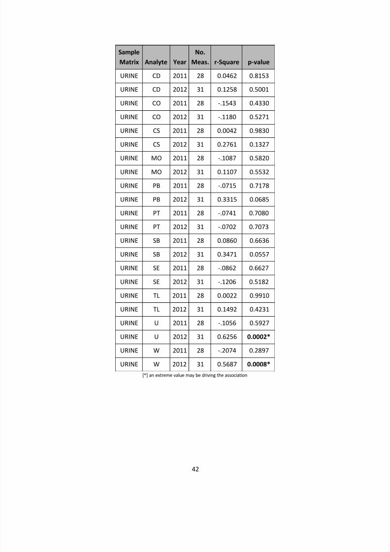
7/30/2019 Millsboro Biomonitoring Study Final Report
http://slidepdf.com/reader/full/millsboro-biomonitoring-study-final-report 53/91
42
Sample
Matrix Analyte Year
No.
Meas. r-Square p-value
URINE CD 2011 28 0.0462 0.8153
URINE CD 2012 31 0.1258 0.5001
URINE CO 2011 28 -.1543 0.4330
URINE CO 2012 31 -.1180 0.5271
URINE CS 2011 28 0.0042 0.9830
URINE CS 2012 31 0.2761 0.1327
URINE MO 2011 28 -.1087 0.5820
URINE MO 2012 31 0.1107 0.5532
URINE PB 2011 28 -.0715 0.7178
URINE PB 2012 31 0.3315 0.0685
URINE PT 2011 28 -.0741 0.7080
URINE PT 2012 31 -.0702 0.7073
URINE SB 2011 28 0.0860 0.6636
URINE SB 2012 31 0.3471 0.0557
URINE SE 2011 28 -.0862 0.6627
URINE SE 2012 31 -.1206 0.5182
URINE TL 2011 28 0.0022 0.9910
URINE TL 2012 31 0.1492 0.4231
URINE U 2011 28 -.1056 0.5927
URINE U 2012 31 0.6256 0.0002*
URINE W 2011 28 -.2074 0.2897
URINE W 2012 31 0.5687 0.0008*
[*] an extreme value may be driving the association

7/30/2019 Millsboro Biomonitoring Study Final Report
http://slidepdf.com/reader/full/millsboro-biomonitoring-study-final-report 54/91
43
Table 12. Pearson correlations of BC mass with biospecimen elements by year.
Sample
Matrix Analyte Year
No.
Meas. r-Square p-value
BLOOD CD 2011 28 0.5787 0.0013
BLOOD CD 2012 31 0.1856 0.3176
BLOOD HG 2011 28 0.0541 0.7845
BLOOD HG 2012 31 0.5403 0.0017
BLOOD PB 2011 28 0.4651 0.0126
BLOOD PB 2012 31 0.1780 0.3379
URINE AS 2011 28 0.0253 0.8983
URINE AS 2012 31 0.2155 0.2442
URINE BA 2011 28 0.2339 0.2309
URINE BA 2012 31 -.1501 0.4203
URINE BE 2011 28Not
Detected
Not
Detected
URINE BE 2012 31Not
Detected
Not
Detected
URINE CD 2011 28 -.1942 0.3221
URINE CD 2012 31 -.0536 0.7747
URINE CO 2011 28 -.0438 0.8249
URINE CO 2012 31 -.0900 0.6301
URINE CS 2011 28 0.1050 0.5948
URINE CS 2012 31 0.0130 0.9447
URINE MO 2011 28 -.1547 0.4317
URINE MO 2012 31 0.2729 0.1375
URINE PB 2011 28 0.0978 0.6204
URINE PB 2012 31 0.2402 0.1930
URINE PT 2011 28 -.1257 0.5238
URINE PT 2012 31 -.1372 0.4616
URINE SB 2011 28 0.3605 0.0595
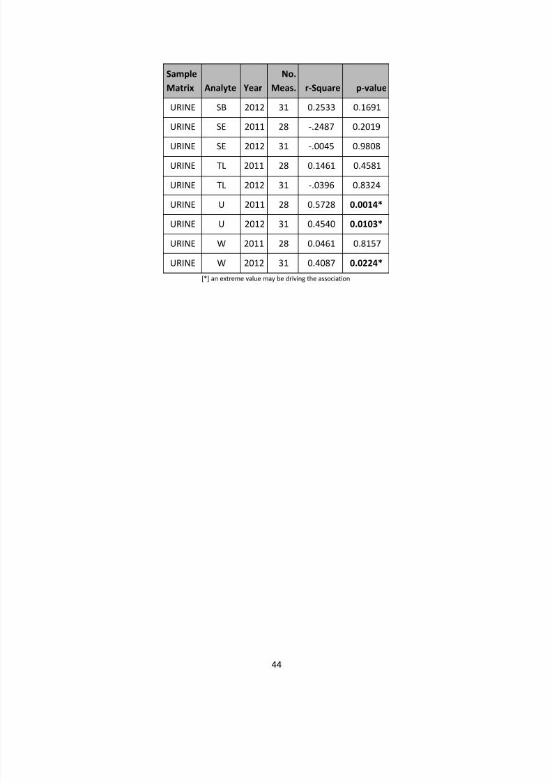
7/30/2019 Millsboro Biomonitoring Study Final Report
http://slidepdf.com/reader/full/millsboro-biomonitoring-study-final-report 55/91
44
Sample
Matrix Analyte Year
No.
Meas. r-Square p-value
URINE SB 2012 31 0.2533 0.1691
URINE SE 2011 28 -.2487 0.2019
URINE SE 2012 31 -.0045 0.9808
URINE TL 2011 28 0.1461 0.4581
URINE TL 2012 31 -.0396 0.8324
URINE U 2011 28 0.5728 0.0014*
URINE U 2012 31 0.4540 0.0103*
URINE W 2011 28 0.0461 0.8157
URINE W 2012 31 0.4087 0.0224*
[*] an extreme value may be driving the association
7/30/2019 Millsboro Biomonitoring Study Final Report
http://slidepdf.com/reader/full/millsboro-biomonitoring-study-final-report 56/91
45
Lastly, a comparison was performed between the elemental concentrations measured of the
collected personal level PM2.5 to those measured in urine or blood. Table 13 indicates the associations of
elements on personal PM filters, as measured by XRF, to the same elements measured in biospecimen
samples by year, while Table 14 compares across both years of sampling. When examined by year, three
associations were identified, but they were all found to have been driven by one or a few extreme
values and are not predictive. No significant associations were observed when the data from both years
were combined.
It does not appear that the personal PM characteristics measured in this study have strong and
consistent contributions to the analytes measured in the blood and urine from the study participants.
The lack of relationship may mean that current exposures do not result in large biospecimen changes on
the time scale of this study. In other words, measures for some of the analytes in biospecimens might
reflect long-term equilibria that are not perturbed to any great extent by the short-term change in PM.
These data might also indicate the possibility of non-inhalation routes of exposure. When considering
the biospecimen analyte concentrations that exceeded reference values (Table 9), most of the
excursions are measured for Arsenic and Selenium, two elements known to have dietary sources.Exposure to these metals has health consequences that range from cancer to other less severe
consequences which depend on both exposure amount and length. As described earlier, questions were
added to the participant survey for Season 2 to examine some potential dietary sources.
Table 15 examines the relationship between elevated urinary concentrations of Arsenic and
Selenium and various ingestion sources. Specific potential contributors to individual excursions were
examined previously. The purpose of the correlations presented in Table 15 is an attempt to see how
generalizable the findings might be to the rest of the study participants, whether or not their particular
biospecimen results where high or more typical of this group. Some of the dependent variables in the
table are categorical, i.e., they have a “yes” or “no” response. Such variables include eating grains, localproduce, rice, or meat, drinking filtered water, taking dietary supplements, eating fish/seafood, or
whether a participant’s source of drinking water was a private well or municipal water supply. Another
factor to consider is the relative amount of time spent indoor versus outdoors. This would not be
expected to influence exposure to Arsenic or Selenium, unless there is an inhalation source (not
supported by the results shown above), but could for other pollutants. This was not explored further in
this work. In any event, the data show that the consumption of seafood within 48 hours of providing a
urinary sample is significantly linked to increased urinary Arsenic levels. It is important to recognize,
however, that this study measured total (inorganic + organic) arsenic in urine, while arsenic in fish is
predominantly organic arsenic (Greene and Crecelius, 2006). Inorganic arsenic is considered toxic, while
organic arsenic is not. Further, organic arsenic is quickly excreted from the body. Total urinary arsenicvalues can occasionally increase to several thousands of ug/L after seafood consumption (Caldwell et.
al., 2009), which is well above values seen in the current study. It is also important to note that arsenic
concentrations in fish and shellfish from the local Inland Bays are not greater than concentrations in fish
and shellfish from the entire East and Gulf Coasts of the U.S. (Greene, 2010). The data also suggest that
the regular consumption of grains significantly decreases exposure to Arsenic. The reason is not
immediately obvious, but could reflect associated dietary factors or food interactions.

7/30/2019 Millsboro Biomonitoring Study Final Report
http://slidepdf.com/reader/full/millsboro-biomonitoring-study-final-report 57/91
46
Table 13.Pearson correlations of elements on personal filters by XRF with biospecimen elements by
year.
Sample
MatrixAnalyte YEAR
No.
Meas.r-square p-value
BLOOD CD 2011 28 -.2079 0.2914
BLOOD CD 2012 32 0.3086 0.0858
BLOOD PB 2011 28 -.2007 0.3090
BLOOD PB 2012 32 -.2826 0.1177
URINE AS 2011 28 -.0827 0.6786
URINE AS 2012 32 0.2072 0.2576
URINE BA 2011 28 0.6012 0.0005*
URINE BA 2012 32 -.0341 0.8544
URINE CD 2011 28 0.3484 0.0690
URINE CD 2012 32 -.0708 0.7023
URINE CO 2011 28 0.3437 0.0732
URINE CO 2012 32 0.1749 0.3413
URINE CS 2011 28 0.3982 0.0351*
URINE CS 2012 32 0.1198 0.5167
URINE PB 2011 28 0.1293 0.5155
URINE PB 2012 32 0.0025 0.9891
URINE SB 2011 28 -.1556 0.4327
URINE SB 2012 32 0.1181 0.5228
URINE SE 2011 28 0.4625 0.0123*
URINE SE 2012 32 0.3040 0.0909
[*] an extreme value may be driving the association

7/30/2019 Millsboro Biomonitoring Study Final Report
http://slidepdf.com/reader/full/millsboro-biomonitoring-study-final-report 58/91
47
Table 14. Pearson correlations of elements on personal filters by XRF with biospecimen elements
across years.
Sample
MatrixAnalyte
No.
Meas.r-square p-value
BLOOD CD 60 -.1596 0.2243
BLOOD PB 60 -.2048 0.1169
URINE AS 60 0.0001 0.9996
URINE BA 60 0.2411 0.0634
URINE CD 60 0.1024 0.4377
URINE CO 60 0.0027 0.9839
URINE CS 60 0.1561 0.2346
URINE PB 60 0.0688 0.6031
URINE SB 60 -.1323 0.3150
URINE SE 60 0.1714 0.1913
[*] an extreme value may be driving the association

7/30/2019 Millsboro Biomonitoring Study Final Report
http://slidepdf.com/reader/full/millsboro-biomonitoring-study-final-report 59/91
48
Table 15. Evaluation of exceedances for Arsenic and Selenium in the context of possible ingestion
routes.
ObsSample
MatrixAnalyte
Dependent
Variablep-value
1 URINE AS EATGRAINS (yes) 0.0197
2 URINE SE EATGRAINS (yes) 0.7692
3 URINE AS LOCALPRODUCE (yes) 0.5434
4 URINE SE LOCALPRODUCE (yes) 0.0932
5 URINE AS EATMEAT (yes) 0.5398
6 URINE SE EATMEAT (yes) 0.5162
7 URINE AS FILTERWATER (yes) 0.4991
8 URINE SE FILTERWATER (yes) 0.3070
9 URINE AS DIETSUPPL (yes) 0.4545
10 URINE SE DIETSUPPL (yes) 0.2693
11 URINE AS HERBSUPPL (yes) 0.4605
12 URINE SE HERBSUPPL (yes) 0.2525
13 URINE AS MULTIVITA (yes) 0.7515
14 URINE SE MULTIVITA (yes) 0.8090
15 URINE ASEATFISH W/in 48
hours (yes)0.0130
16 URINE SEEATFISH W/in 48
hours (yes)0.5183
17 URINE ASEATRICE W/in 48
hours (yes)0.5341
18 URINE SEEATRICE W/in 48
hours (yes)0.4590
19 URINE AS DRINKSOURCE 0.8090
20 URINE SE DRINKSOURCE 0.1388
21 URINE AS HRS_INSIDE 0.3316
22 URINE SE HRS_INSIDE 0.6585

7/30/2019 Millsboro Biomonitoring Study Final Report
http://slidepdf.com/reader/full/millsboro-biomonitoring-study-final-report 60/91
49
Evaluation of Study Objectives and HypothesisBased on the data presented in the preceding sections, the hypotheses listed in the hypotheses
section can be evaluated and answers to the study objectives can be posited.
Objective 1
Hypothesis 1: Contributions of the NRG Energy power plant to ambient PM2.5 concentrations in
Sussex County will increase with increasing usage of the electricity generating capacity of the power
plant. Indoor residential and personal PM2.5 concentrations will not be affected.
Results: Contributions of the NRG Energy power plant to ambient PM2.5 was not found to
increase with electrical generating capacity of the power plant. According to data collected, indoor and
personal PM2.5 concentrations did not appear to be affected by the operation of the power plant. This is
supported by the average 46% reduction in overall PM2.5 from Season 1 to Season 2 in all samplers with
the exception of personal monitors. The 6.8% increase in personal level PM2.5 concentrations is thought
to be due to changes in habits of the participants as indicated by the increase in XRF concentrations
across a wide variety of elements not typically associated with coal-fired power plants. However, theNRG Energy power plant operates on a variable load that depends on electricity generation needs in the
Northeast. The inconsistent operation of the power plant prevented any conclusive evidence about its
operational capacity on local PM2.5 levels from being discerned. Additionally, without additional gas and
particle speciation data, specific linkages between power plant and local PM2.5 cannot be established.
Such specific information required for the source apportionment would involve particle phase
ammonium nitrate, ammonium sulfate, and organic carbon. Gas phase Sulfur dioxide would also be
required to generate linkages between local PM2.5 and the power plant.
To support the finding that the NRG Energy power plant did not affect the Sussex County PM2.5
concentrations average daily wind directions identified the fixed site monitors located downwind andupwind of the power during each day of the study for both seasons (Figure 26). A ratio of
upwind/downwind mass concentrations less than unity indicates a source of PM2.5 between the two
monitors in question. During the first season the average upwind/downwind ratio of 1.7 ± SD 1.6
indicated no significant sources of PM2.5 between the two monitors. The same analysis carried out
during Season 2 resulted in an upwind/downwind ratio of 0.9 ± SD 0.2. At a level of α=0.01, the
upwind/downwind ratios between seasons are not statistically different, resulting in the conclusion that
the operating conditions of the power plant during the second season do not contribute to the local
PM2.5 in an appreciable amount in comparison to regional and long-range transport.

7/30/2019 Millsboro Biomonitoring Study Final Report
http://slidepdf.com/reader/full/millsboro-biomonitoring-study-final-report 61/91
50
Figure 26. Upwind/downwind ratios of fixed site monitors during both sampling seasons.
Objective 2
For the purposes of this report, Hypothesis 2 and 3 will be combined due to the similar nature of
the questions and data used to reach conclusions for each.
Hypothesis 2: Upwind source contributions to ambient Sussex County PM2.5 levels will be
detectable, and their relative contribution to the PM2.5 concentration will decrease as the load on the
NRG Energy power plant increases. However, exact sources will be difficult to determine unless a unique
emissions profile exists.
Hypothesis 3: The relative contribution of upwind sources from bordering states to the ambient
PM2.5 concentration will decrease as usage of the energy generating capacity from the NRG Energy
power plant increases.
Results: Localized upwind sources were not detectable primarily due to influence of long-range
transport and atmospheric mixing during the transport process which created a uniformly disperse air
mass. Because of the heavy influence of long-range transport and mixing, precise localized sources of
ambient PM2.5 could not be identified. This finding is supported by the similarity between the Seaford
site and four fixed site monitors indicated the predominant source of PM2.5 within Sussex County is likelydue to regional or long-range transport (Figure 27).
0
0.5
1
1.5
2
2.5
3
0 5 10 15 20 25 30 35
U p w i n d / D o w n w i n
d r a t i o
Observation number
2011 2012

7/30/2019 Millsboro Biomonitoring Study Final Report
http://slidepdf.com/reader/full/millsboro-biomonitoring-study-final-report 62/91
51
Figure 27. Comparison of Seaford and four fixed site monitors PM2.5 concentrations during 2011 (Red,NRG Energy power plant not operating) and 2012 (Blue, power plant operating) sampling seasons.
Figures 28 and 29 illustrate the PM2.5 concentration of the four fixed sites (averaged together)
and wind direction. Figure 29 illustrates an approximately 3 day delay between wind directed from
Northwest-North and maximum PM2.5 concentrations. 72-hr HYSPLIT back trajectory analysis of wind

7/30/2019 Millsboro Biomonitoring Study Final Report
http://slidepdf.com/reader/full/millsboro-biomonitoring-study-final-report 63/91
52
patterns (Figure 30) during the PM2.5 maxima indicate air masses during this time point originated from
major metropolitan areas such as New York, Boston, Baltimore, and Washington D.C.
Furthermore, the transient operation of the NRG Energy power plant prevented establishment
of relative contribution of upwind sources to Sussex County PM2.5. Without NRG Energy power plant
operational data, a qualitative conclusion that upwind sources contributed to a significant proportion of Sussex County PM2.5 would be consistent with the similarity in PM2.5 levels and chemical signatures
observed between Seasons 1 and 2 samples across semi-rural, semi-urban, and urban sites. The
homogeneity in samples indicates a more likely source of PM2.5 within Sussex County would be regional
or long-range transport.
Figure 28. Wind direction and ambient PM2.5 concentrations during 2011.
0
5
10
15
20
25
30
35
0
90
180
270
360
P M2 . 5 c o n c e n t r a t i o n ( µ g / m 3 )
W i n d d i r e c t i o n ( d e g r e e s )
Wind Direction Average ambient PM2.5

7/30/2019 Millsboro Biomonitoring Study Final Report
http://slidepdf.com/reader/full/millsboro-biomonitoring-study-final-report 64/91
53
Figure 29. Wind direction and ambient PM2.5 concentrations during 2012.
Figure 30. Back trajectory analysis for November 7th, 2012. Different color traces represent air masses
initiated at 6-hour time points during the 72-hour analysis.
Objective 3
Hypothesis 4: Relative contributions of other point PM2.5 sources to ambient concentrations will
decrease after the NRG Energy power plant increases its electricity generation.
Results: The relative contribution of local point sources were not significant enough to evaluate
their relative contribution to local PM2.5 with respect to regional and long-range PM2.5 as indicated
0
2
4
6
8
10
12
14
16
0
90
180
270
360 P M2 . 5
C o n c e n t r a t i o n ( µ g / m 3 )
W i n d D i r e c t i o n ( d e g r e e s )
Wind Direction Average ambient PM2.5

7/30/2019 Millsboro Biomonitoring Study Final Report
http://slidepdf.com/reader/full/millsboro-biomonitoring-study-final-report 65/91
54
through the homogenous nature of the PM2.5 concentration and chemical signature in both background
and fixed sites. Additional data of higher spatial and temporal resolution in Sussex County are needed to
assess the relative contribution of local point sources to PM2.5 with respect to the NRG Energy power
plant operating capacity.
Hypothesis 5: Personal sources will contribute more to PM2.5 exposure relative to during the lowelectricity generation period than during the high generation sampling period.
Results: Throughout both sampling seasons, personal sources were the predominate source of
PM2.5 exposure (19.6 ± SD 3.4 µg/m3 Season 1, 20.9 ± SD 6.5 µg/m3 Season 2). Figure 31 Panel A shows
the probability of personal PM2.5 exposures greater than 35 µg/m3 for all participants, these values are
marked as red symbols. Panel B of the same figure shows these same participant days (again marked as
red symbols) plotted as the probability of personal ETS exposures. These two figures illustrate that
during both seasons ETS was the primary cause for elevated PM2.5 exposures, although less so during
Season 1.
Sources of these ETS exposures were investigated by evaluating personal/indoor (P/I) ratios.
During Season 1, 79% of the participant days had P/I PM2.5 ratios greater than 1, however of analysis of
these same participants also indicated that only 17% of them had P/I ETS ratios greater than 1. During
Season 2, 89% of the participant days had personal/indoor ratios in excess of 1, and 66% of the
participants had P/I ETS ratios greater than 1. Thus, the majority of exposure to PM2.5 is occurring inside
of residences; however the indoor monitors were not able to capture the degree of exposure. The
personal exposure monitor worn by the participants was needed to capture their proximity to highly
transient ETS PM2.5. The elevated ETS concentrations in the personal samples during Season 2 was not
observed in the corresponding indoor monitors which indicates the participant was near the guest,
spouse, or family member that smoked cigarettes.
ETS had a profound influence on the calculated contribution of different sources to the personal
PM2.5 concentration. Following Wallace and Williams (2005), the percentage of the personal exposure
due to ambient, indoor residential, and “other” sources was calculated. The critical data required for this
calculation were 1) valid outdoor, indoor, and personal PM2.5 concentrations, 2) valid sulfur
concentration data for each sample, 3) the ETS concentration on the personal and indoor residential
sample, and 4) percentage of time spent inside the home, outside, and in other locations.
The sulfur data is used to estimate the infiltration of ambient PM2.5 into the residence, as
described in Wallace and Williams (2005). This approach is only valid if ETS concentrations within the
home are less than 5 µg/m
3
. Research has shown that ETS is the primary source of indoor generatedsulfur. As a result, ETS concentrations greater than 5 µg/m3 confound the calculation of the infiltration
factor. As noted earlier, the participant selection criteria allowed cigarette smoking by the participant or
other residents of the home to increase recruitment rates. For houses that had indoor ETS
concentrations greater than the 5 µg/m3 threshold, the mean infiltration factor for non-ETS homes was
used.

7/30/2019 Millsboro Biomonitoring Study Final Report
http://slidepdf.com/reader/full/millsboro-biomonitoring-study-final-report 66/91
55
Figure 31. Panel A) Log-probability graph highlighting those participant days with PM2.5 exposure
greater than 35 µg/m3. Panel B) Log-probability graph showing the majority of those same participant
days as also having the highest ETS concentrations.
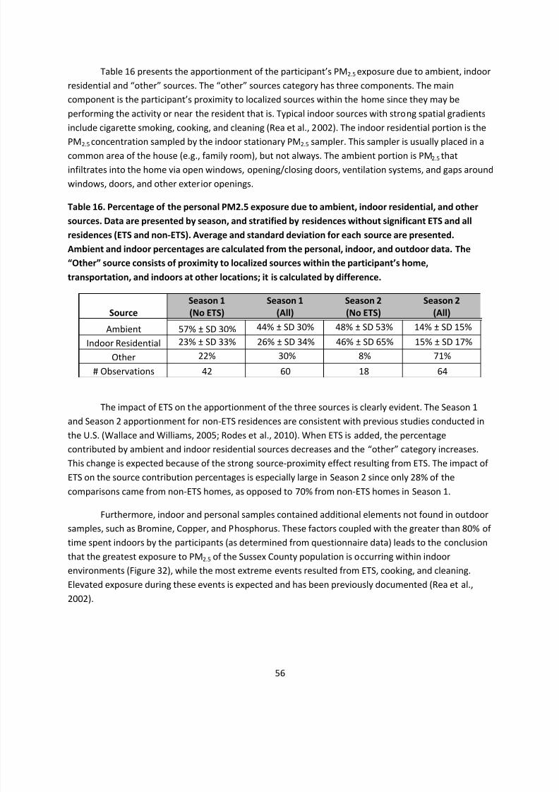
7/30/2019 Millsboro Biomonitoring Study Final Report
http://slidepdf.com/reader/full/millsboro-biomonitoring-study-final-report 67/91
56
Table 16 presents the apportionment of the participant’s PM2.5 exposure due to ambient, indoor
residential and “other” sources. The “other” sources category has three components. The main
component is the participant’s proximity to localized sources within the home since they may be
performing the activity or near the resident that is. Typical indoor sources with strong spatial gradients
include cigarette smoking, cooking, and cleaning (Rea et al., 2002). The indoor residential portion is the
PM2.5 concentration sampled by the indoor stationary PM2.5 sampler. This sampler is usually placed in a
common area of the house (e.g., family room), but not always. The ambient portion is PM2.5 that
infiltrates into the home via open windows, opening/closing doors, ventilation systems, and gaps around
windows, doors, and other exterior openings.
Table 16. Percentage of the personal PM2.5 exposure due to ambient, indoor residential, and other
sources. Data are presented by season, and stratified by residences without significant ETS and all
residences (ETS and non-ETS). Average and standard deviation for each source are presented.
Ambient and indoor percentages are calculated from the personal, indoor, and outdoor data. The
“Other” source consists of proximity to localized sources within the participant’s home,
transportation, and indoors at other locations; it is calculated by difference.
Source
Season 1
(No ETS)
Season 1
(All)
Season 2
(No ETS)
Season 2
(All)
Ambient 57% ± SD 30% 44% ± SD 30% 48% ± SD 53% 14% ± SD 15%
Indoor Residential 23% ± SD 33% 26% ± SD 34% 46% ± SD 65% 15% ± SD 17%
Other 22% 30% 8% 71%
# Observations 42 60 18 64
The impact of ETS on the apportionment of the three sources is clearly evident. The Season 1
and Season 2 apportionment for non-ETS residences are consistent with previous studies conducted in
the U.S. (Wallace and Williams, 2005; Rodes et al., 2010). When ETS is added, the percentage
contributed by ambient and indoor residential sources decreases and the “other” category increases.
This change is expected because of the strong source-proximity effect resulting from ETS. The impact of
ETS on the source contribution percentages is especially large in Season 2 since only 28% of the
comparisons came from non-ETS homes, as opposed to 70% from non-ETS homes in Season 1.
Furthermore, indoor and personal samples contained additional elements not found in outdoor
samples, such as Bromine, Copper, and Phosphorus. These factors coupled with the greater than 80% of
time spent indoors by the participants (as determined from questionnaire data) leads to the conclusion
that the greatest exposure to PM2.5 of the Sussex County population is occurring within indoorenvironments (Figure 32), while the most extreme events resulted from ETS, cooking, and cleaning.
Elevated exposure during these events is expected and has been previously documented (Rea et al.,
2002).
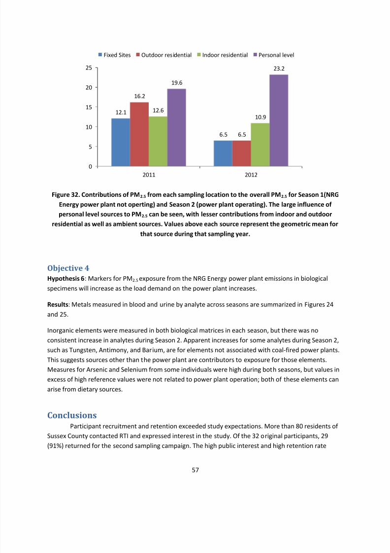
7/30/2019 Millsboro Biomonitoring Study Final Report
http://slidepdf.com/reader/full/millsboro-biomonitoring-study-final-report 68/91
57
Figure 32. Contributions of PM2.5 from each sampling location to the overall PM2.5 for Season 1(NRGEnergy power plant not operting) and Season 2 (power plant operating). The large influence of
personal level sources to PM2.5 can be seen, with lesser contributions from indoor and outdoor
residential as well as ambient sources. Values above each source represent the geometric mean for
that source during that sampling year.
Objective 4
Hypothesis 6: Markers for PM2.5 exposure from the NRG Energy power plant emissions in biological
specimens will increase as the load demand on the power plant increases.
Results: Metals measured in blood and urine by analyte across seasons are summarized in Figures 24
and 25.
Inorganic elements were measured in both biological matrices in each season, but there was no
consistent increase in analytes during Season 2. Apparent increases for some analytes during Season 2,
such as Tungsten, Antimony, and Barium, are for elements not associated with coal-fired power plants.
This suggests sources other than the power plant are contributors to exposure for those elements.
Measures for Arsenic and Selenium from some individuals were high during both seasons, but values in
excess of high reference values were not related to power plant operation; both of these elements can
arise from dietary sources.
ConclusionsParticipant recruitment and retention exceeded study expectations. More than 80 residents of
Sussex County contacted RTI and expressed interest in the study. Of the 32 original participants, 29
(91%) returned for the second sampling campaign. The high public interest and high retention rate
12.1
6.5
16.2
6.5
12.610.9
19.6
23.2
0
5
10
15
20
25
2011 2012
Fixed Sites Outdoor residential Indoor residential Personal level

7/30/2019 Millsboro Biomonitoring Study Final Report
http://slidepdf.com/reader/full/millsboro-biomonitoring-study-final-report 69/91
58
indicated Sussex County residents are interested in their health and quality of life. The community
interest and data quality achievements indicate statewide, longitudinal, multimedia exposure studies
are feasible.
Sampling conducted for PM2.5 during the fall of 2011 and 2012 indicated the geometric mean
ambient PM2.5 concentrations of the Millsboro area was 9.3 µg/m3
. The semi-rural location of Seafordhad an average PM2.5 concentration of 8.9 µg/m3, both below the Federal Standard of 15 µg/m3 and
were not statistically different at a test value of α=0.01. Sampling conducted outdoors and indoors of 35
distinct participants (32 each season) resulted in average PM2.5 concentrations of 11.3 µg/m3 and 11.8
µg/m3 respectively. The higher elevated indoor concentration is expected due to the strength and
proximity of PM2.5 sources found indoors (e.g. cooking, cleaning, candle burning, smoking, etc.). Personal
level sampling conducted during both seasons revealed geometric mean PM2.5 concentrations of 20.3
µg/m3 across both seasons. Similar to indoor PM2.5 measurements that were elevated with respect
outdoor and ambient measurement, higher personal level concentrations were presumably due to
personal proximity and strength of sources and is to be expected based on previous studies.
Analysis of the chemical and time-series analysis of the ambient PM2.5 of Sussex county reveals
the predominate source of PM2.5 within Sussex county to be regional and long-range transport of PM2.5
from upwind metropolitan locations such as Baltimore, New York City, and Boston. This can be observed
from the homogeneity of PM2.5 from a concentration as well as a compositional standpoint.
Additionally, though not part of the MIEBS, it is conceivable that due to the design of the NRG
Energy power plant stacks, the exhaust plume may lead to the majority of the PM2.5 to be deposited at
great distance from the stack, perhaps in the Atlantic. However, pollutants deposited by this mechanism
would be subject to significant dilution.
Despite the fact that control of much of the PM2.5 within Sussex County is beyond the control of Delaware officials, the majority of participants spent more than 80% of their day inside their own
homes. Thus RTI recommends performing a more detailed study of indoor PM2.5 sources as these
sources dominate the exposure of the Sussex County population to PM2.5. Results from this follow-up
study can be used to design an educational plan for the local population in an effort to reduce their
exposure and improve their long-term health.
The personal PM species measured do not have a strong and consistent contribution to the
analytes measured in the blood and urine from the study participants. The lack of a relationship may
mean that current exposures do not result in large biospecimen changes on the time scale of this study.
These data might also indicate the possibility of non-inhalation routes of exposure. Dietary and non-dietary ingestion of inorganic species should be considered for future investigation.
RecommendationsThe findings from this study suggest several recommendations for future research into the
environmental exposures that impact the health of Delaware residents. The recommendations are easily

7/30/2019 Millsboro Biomonitoring Study Final Report
http://slidepdf.com/reader/full/millsboro-biomonitoring-study-final-report 70/91
59
separated into two groups: 1) additional analyses that can be performed using the collected biological,
PM2.5 and survey data and 2) future data collection and analysis efforts.
Recommendations for further analysis of the existing samples and dataset are summarized
below.
The PM2.5 emission from the NRG Energy power plant and the resulting concentration in the
ambient air within the study area should be modeled. This analysis will estimate the fraction of
the ambient PM2.5 contributed by the power plant. RTI wanted to perform this modeling for this
report. However, the fact the power plant operated under a variable load during Fall 2012
prohibits performing any modeling until NRG Energy reports PM2.5 emission data to DNREC
(expected in late 2013). If this modeling is performed, this report should be updated to
incorporate the results and revised conclusions.
Detailed statistical analysis of the PM2.5 and biospecimen data against the collected metadata is
recommended. The objectives of this report did not include a detailed analysis of the survey,
geospatial, or meteorological data in relation to the PM2.5 and biospecimen results. A
multivariate cluster analysis, such as principal component analysis, will identify variables or
classes of variables that predict the PM2.5 and biospecimen results. The findings from this
analysis would provide valuable information into the design of a larger, statewide multimedia
exposure study.
The additional analysis of PM2.5 and biospecimen samples will provide additional details to
clarify some of the findings or provide additional data for the multivariate analysis discussed
previously. The detailed recommendations listed below can be performed individually, as a
subset, or in total.
o The total arsenic mass in the urine should be speciated into organic and inorganic
fractions. CDC has a standard method for this analysis. This data will provide insight into
the toxicity and sources of the arsenic exposure noted in the report.
o The personal PM2.5 filters should be analyzed by inductively coupled plasma – mass
spectrometry (ICP-MS) to increase the number of elements per filter that are detected.
This data would be useful for the multivariate cluster analysis.
o Measure the urinary cotinine (biomarker of ETS exposure) to confirm ETS is a major
source of PM2.5 exposure in this study. The data from this inexpensive analysis would
provide further confirmation that the study participants were exposed to high levels of
tobacco smoke.
Multiple future studies are recommended to provide the information necessary to understand
the PM2.5 exposures of Sussex County residents and all Delaware residents.
There is a need to confirm long-range transport of PM2.5 from upwind urban areas is the primary
contributor to ambient PM2.5 concentrations in Delaware. A combination of ambient PM2.5

7/30/2019 Millsboro Biomonitoring Study Final Report
http://slidepdf.com/reader/full/millsboro-biomonitoring-study-final-report 71/91
60
concentration measurements and Hysplit modeling will provide the information. RTI
recommends that daily PM2.5 samples be collected at an urban, suburban, and rural location for
at least four weeks in each season (Winter, Spring, Summer, Fall). The three sites can be existing
DNREC monitoring locations. Hysplit back-trajectory analysis, similar to the one conducted for
this study, will identify the origin of the ambient air up to 72 hours previously. A time series
correlation analysis will determine if the highest PM2.5 concentrations at the three monitoring
locations are correlated to air that originated over the metropolitan areas surrounding
Delaware.
A source apportionment study conducted at the DNREC Seaford site and one additional site near
the NRG Energy power plant would confirm the impact of long-range transport, regional
sources, and local sources (including the power plant) on PM2.5 concentrations and the Sussex
County residents’ exposure. This study would require detailed PM2.5 speciation data, including
metals (as measured for this study), nitrate, sulfate, and organic carbon fractions. Nitrogen
dioxide and sulfur dioxide gas concentration data would also be required.
Establish multimedia (air, dietary, and non-dietary ingestion) carcinogen exposure and
biospecimen distributions on a statewide level. This study would assess the broader, temporal
contribution of multiple sources to the total body burden of environmental contaminants and
account for individual behavior patterns. Exposure distributions would be captured by enrolling
participants in urban, suburban, and rural areas of Delaware and would help to establish the
baseline to monitor future exposures. This study would combine the Design I and Design II study
designs developed in 2008 (RTI, 2008).
As an initial step towards establishing a baseline, a study similar to that performed around
Millsboro could be conducted in the Wilmington area. This would provide for a comparison of
the rural Sussex County to an urban area with regard to the same pollutants. An expansion of
the methods to provide more data about the exposures (additional chemical measures in both
environmental and biological specimens) will begin to define those measures of greatest use in
the broader study.

7/30/2019 Millsboro Biomonitoring Study Final Report
http://slidepdf.com/reader/full/millsboro-biomonitoring-study-final-report 72/91
61
ReferencesAndreae, M.O. and A. Gelencsér. 2006. “Black Carbon or brown carbon? The nature of light-absorbing
carbonaceous aerosol.” Atmospheric Chemistry and Physics 6:3131-3148.
Brown, K.W., Sarnat, J.A., and P. Koutrakis. 2012. “Concentrations of PM2.5 mass and components inresidential and non-residential indoor microenvironments: The Sources and Composition of
Particulates Exposures Study.” Journal of Exposure Science and Environmental Epidemiology
22:161-172.
Böhlandt, A., R. Schierl, J. Diemer, C. Koch, G. Bolte, M. Kiranoglu, H. Fromme, and D. Nowak. 2012.
“High concentrations of cadmium, cerium, and lanthanum in indoor air due to environmental
tobacco smoke.” Science of the Total Environment 414:738-741
Caldwell, K., R.L. Jones, C.P. Verdon, J.M. Jarrett, S.P. Caudill, and J.D. Osterloh. 2009. “Levels of urinary
total and speciated arsenic in the US population: National Health and Nutrition Examination
Survey 2003-2004.” Journal of Exposure Science and Environmental Epidemiology 19: 59-68.
CARB (California Air Resources Board). September 1998. Loss of Particle Nitrate from Teflon Sampling
Filters: Effects on Measured Gravimetric Mass. Sacramento, CA: California Air Resources Board,
Research Divison.
Cheung, K., N. Daher, W. Kam, M.W. Shafer, Z. Ning, J.J. Schauer, and C. Sioutas. 2011. “Spatial and
Temporal Variation of Chemical Composition and Mass Closure of Ambient Coarse Particulate
Matter (PM10 –2.5) in the Los Angeles Area.” Atmospheric Environment 45(16):2651-2662.
DNREC-OTS (Delaware Department of Natural Resources and Environment Control- Office of the
Secretary) June, 2008 Study Designs for Pilot Testing and a Multimedia, Total Exposure Study in
Delaware. Dover, DE: Delaware Department of Natural Resources and Environment Control-
Office of the Secretary.
DNREC (Delaware Department of Natural Resources and Environmental Control). September 2006.
Enhanced Delaware Air Toxics Assessment Study —E-DATAS Project Report . Dover, DE: Delaware
Department of Natural Resources and Environmental Control, Division of Air and Waste
Management.
Dockery, D.W. 2001. “Epidemiologic Evidence of Cardiovascular Effects of Particulate Air Pollution.”
Environmental Health Perspectives 109(Suppl 4):483-486.
Dzubay, T.G., R.K. Stevens, G.E. Gordon, I. Olmez, A.E. Sheffield, and W.J. Courtney. 1988. “A composite
receptor method applied to Philadelphia aerosol.” Environmental Science and Technology 22:46-
52.

7/30/2019 Millsboro Biomonitoring Study Final Report
http://slidepdf.com/reader/full/millsboro-biomonitoring-study-final-report 73/91
62
Environment Canada-Health Canada. 2000. Priority Substances List Assessment Report: Respirable
Particulate Matter Less or Equal to Than 10 Micrometers Environment Canada. Gatineau,
Quebec: Environment Canada-Health Canada.
Goldberg, M.S., R.T. Burnett, J.C. Bailar, J. Brook, Y. Bonvalot, R. Tamblyn, R. Singh, and M.F. Valois.
2001. “The Association between Daily Mortality and Ambient Air Particle Pollution in Montreal,Quebec 1. Nonaccidental Mortality.” Environmental Research 86:12-25.
Greene, R. and E. Crecelius. 2006, “Total and inorganic arsenic in mid-atlantic marine fish and shellfish
and implications for fish advisories. Integrated Environmental Assessment and Management 2:
344-354.
Greene, R. 2010. Arsenic in the Delaware Inland Bays. November 5, 2010. Delaware Department of
Natural Resources and Environmental Control, Dover, DE.
Hoek, G., B. Brunekreef, P. Fischer, and J. Van Wijnen. 2001. “The Association between Air Pollution and
Heart Failure, Arrhythmia, Embolism, Thrombosis and Other Cardiovascular Causes of Death in aTime Series Study.” Epidemiology 12:355-357.
Ito, K., R. Mathes, Z. Ross, A. Nádas, G. Thurston, and T. Matte. 2011. “Fine Particulate Matter
Constituents Associated with Cardiovascular Hospitalizations and Mortality in New York City.”
Environmental Health Perspectives 119:467-473.
Johnson, D.L. 2008. “A first generation ingress, redistribution, and transport model of soil track-in:
DIRT.” Environmental Geochemistry and Health, 30:589-596, 2008.
Laden, F., L.M. Neas, D.W. Dockery, and J. Schwartz. 2000. “Association of fine Particulate Matter from
Different Sources with Daily Mortality in Six U.S. Cities.” Environmental Health Perspectives 108:941-947.
Lai, H.K., M. Kendall, H. Ferrier, I. Lindup, S. Alm, O. Hannien, M. Jantunen, P. Mathys, R. Colvile, M.R.
Ashmore, P. Cullinan, and M.J. Nieuwenhuijsen. 2004. “Personal exposures and
microenvironment concentrations of PM2.5, VOC, NO2, and CO in Oxford, UK.” Atmospheric
Environment 38:6399-6410.
Landis, M.S., G.A. Norris, R.W. Williams, and J.P. Weinstein. 2001. “Personal exposure to PM2.5 mass
and trace elements in Baltimore, MD, USA.” Atmospheric Environment 35:6511-6524.
Lawless, P.A., and Rodes, C.E. 1999. “Maximizing data quality in the gravimetric analysis of personalexposure sample filters”. Journal of the Air and Waste Management Association, 49:1039-1049.
Lawless, P.A., C.E. Rodes, and D.S. Ensor. 2004. Multiwavelength absorbance of filter deposits for
determination of environmental tobacco smoke and black carbon. Atmospheric Environment
38:3373 –3383.

7/30/2019 Millsboro Biomonitoring Study Final Report
http://slidepdf.com/reader/full/millsboro-biomonitoring-study-final-report 74/91
63
Ondov, J.M., T.J. Buckley, P.K. Hopke, D. Ogulei, M.B. Parlange, W.F. Rogge, K.S. Squibb, M.V. Johnston,
A.S. Wexler. 2006. “Baltimore Supersite: Highly time- and size-resolved concentrations of urban
PM2.5 and its constituents for resolution of sources and immune responses.” Atmospheric
Environment 40:S224-S237.
Rea, A.W., C. Crogham, J. Thornburg, B. Rodes, and R. Williams. 2002. “PM concentrations associatedwith personal activities based on real-time personal nephelometry data from the NERL RTP PM
panel study.” Epidemiology 13:S82-S83.
Rodes, C.E., P.A. Lawless, J. Thornburg, R.W. Williams, and C. Croghan. 2010. DEARS “Particulate Matter
Relationships: Enhanced Personal, Indoor, Outdoor, and Central Site Exposure Data for a
General Population Cohort.” Atmospheric Environment 44:1386-1399.
RTI International. Study Designs for Pilot Testing and a Multimedia, Total Exposure Study in Delaware.
Final Report. PO 40-01010000777, June 20, 2008.
Suzuki, G., A. Kida, S. Sakai, and H. Takigami. 2009. “Existence state of bromine as an indicator of thesource of brominated flame retardants in indoor dust”. Environmental Science and Technology
43:1437-1442.
Thornburg, J., C.E. Rodes, P.A. Lawless, and R.W. Williams. 2009. “Sources and Causes of Coarse
Particulate Matter Spatial Variability in Detroit, MI.” Atmospheric Environment 43:4251-4258.
U.S. EPA (Environmental Protection Agency). 2004. Air Quality Criteria for Particulate Matter . U.S.
Environmental Protection Agency, Office of Research and Development, National Center for
Environmental Assessment, Washington, DC. August. Available at
http://cfpub2.epa.gov/ncea/cfm/recordisplay.cfm?deid=87903#Download.
Wallace, L. and R. Williams. 2005. “Use of personal-indoor-outdoor sulfur concentrations to estimate the
infiltration factor, outdoor exposure factor, penetration coefficient, and deposition rate for
individual homes.” Environmental Science and Technology 39:399-414.
Williams, R. J. Suggs, C. Rodes, P. Lawless, R. Zweidinger, R. Kwok, J. Creason, and L. Sheldon. 2000.
Comparison of PM2.5 and PM10 monitors.” Journal of Exposure Analysis and Environmental
Epidemiology 10:497-505.
Williams, R. J. Suggs, A. Rea, K. Leovic, A. Vette, C. Croghan, L. Sheldon, C. Rodes, J. Thornburg, A. Ejire,
M. Herbst, W. Sanders. 2003. The Research Triangle Park particulate matter panel study: PM
mass concentration relationships.” Atmospheric Environment 37:5349-5363.
Williams, R., Rappold, A.G., Case, M., Schmitt, M., Stone, S., Jones, P., Thornburg, J., and R.B. Devlin.
2012. “Multi-pollutant Exposures in an Asthmatic Cohort.” Atmospheric Environment 61:244-
252.
Zanobetti, A., J. Schwartz, and D.W. Dockery. 2000. “Airborne Particles Are a Risk Factor for Hospital
Admissions for Heart and Lung Disease.” Environmental Health Perspectives 108:1071-1077.

7/30/2019 Millsboro Biomonitoring Study Final Report
http://slidepdf.com/reader/full/millsboro-biomonitoring-study-final-report 75/91
64
This page intentionally left blank
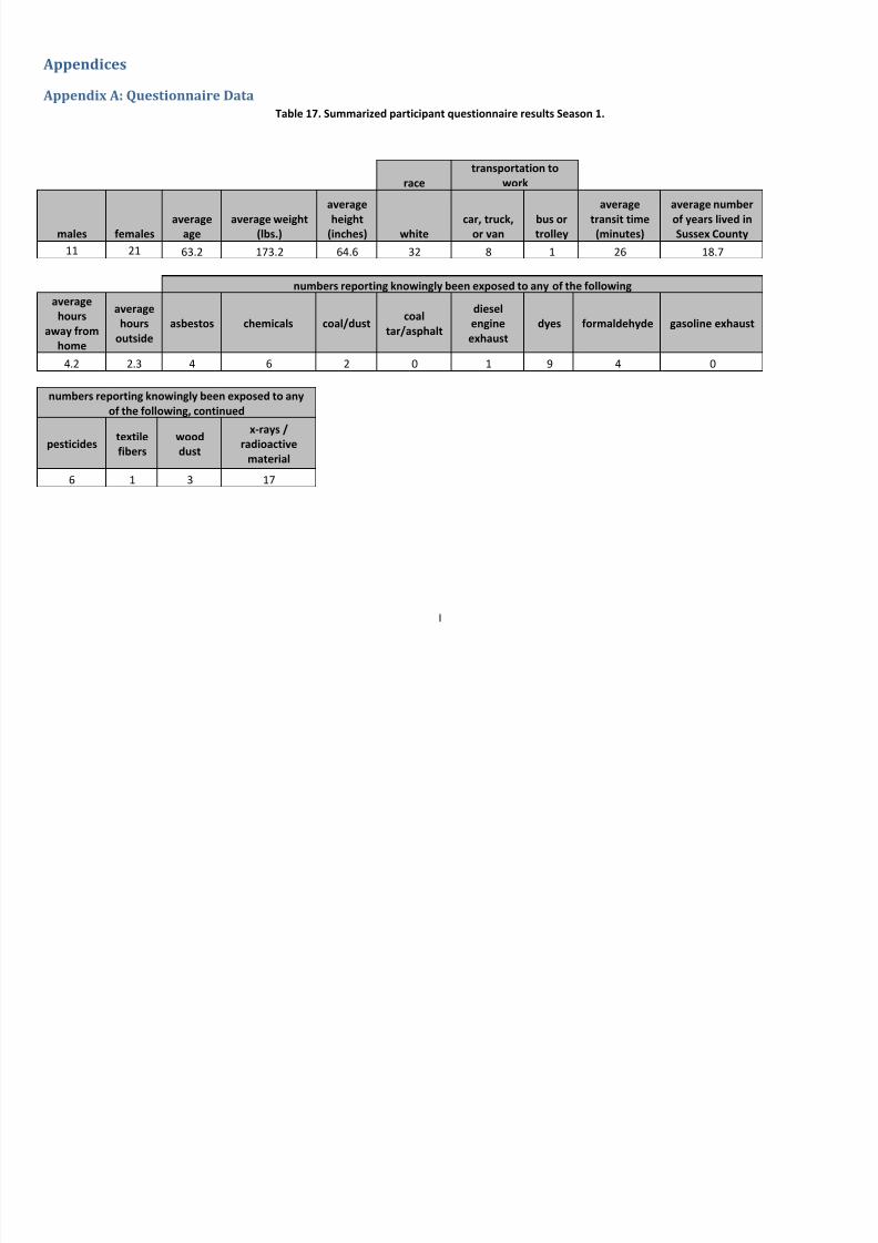
7/30/2019 Millsboro Biomonitoring Study Final Report
http://slidepdf.com/reader/full/millsboro-biomonitoring-study-final-report 76/91
I
Appendices
Appendix A: Questionnaire Data
Table 17. Summarized participant questionnaire results Season 1.
race
transportation to
work
males femalesaverage
ageaverage weight
(lbs.)
average
height(inches) white
car, truck,or van
bus ortrolley
average
transit time(minutes)
average number
of years lived inSussex County
11 21 63.2 173.2 64.6 32 8 1 26 18.7
numbers reporting knowingly been exposed to any of the following
average
hours
away from
home
average
hours
outside
asbestos chemicals coal/dustcoal
tar/asphalt
diesel
engine
exhaust
dyes formaldehyde gasoline exhaust
4.2 2.3 4 6 2 0 1 9 4 0
numbers reporting knowingly been exposed to any
of the following, continued
pesticides textilefibers
wooddust
x-rays /radioactive
material
6 1 3 17

7/30/2019 Millsboro Biomonitoring Study Final Report
http://slidepdf.com/reader/full/millsboro-biomonitoring-study-final-report 77/91
II
Table 18. Summarized participant questionnaire results Season 2.
race
transportation to
work
males females
average
age
average weight
(lbs.)
average
height
(inches) white
car, truck,
or van
bus or
trolley
average
transit time
(minutes)
average number
of years lived in
Sussex County
11 21 63.4 181.7 66.9 32 7 0 27.1 19.8
numbers reporting knowingly been exposed to any of the following
average
hours
away from
home
average
hours
outside
asbestos chemicals coal/dustcoal
tar/asphalt
diesel
engine
exhaust
dyes formaldehyde gasoline exhaust
3.6 2.4 6 6 3 0 4 3 4 3
numbers reporting knowingly been exposed to any
of the following, continued
pesticides
textile
fibers
wood
dust
x-rays /
radioactivematerial
6 3 2 10
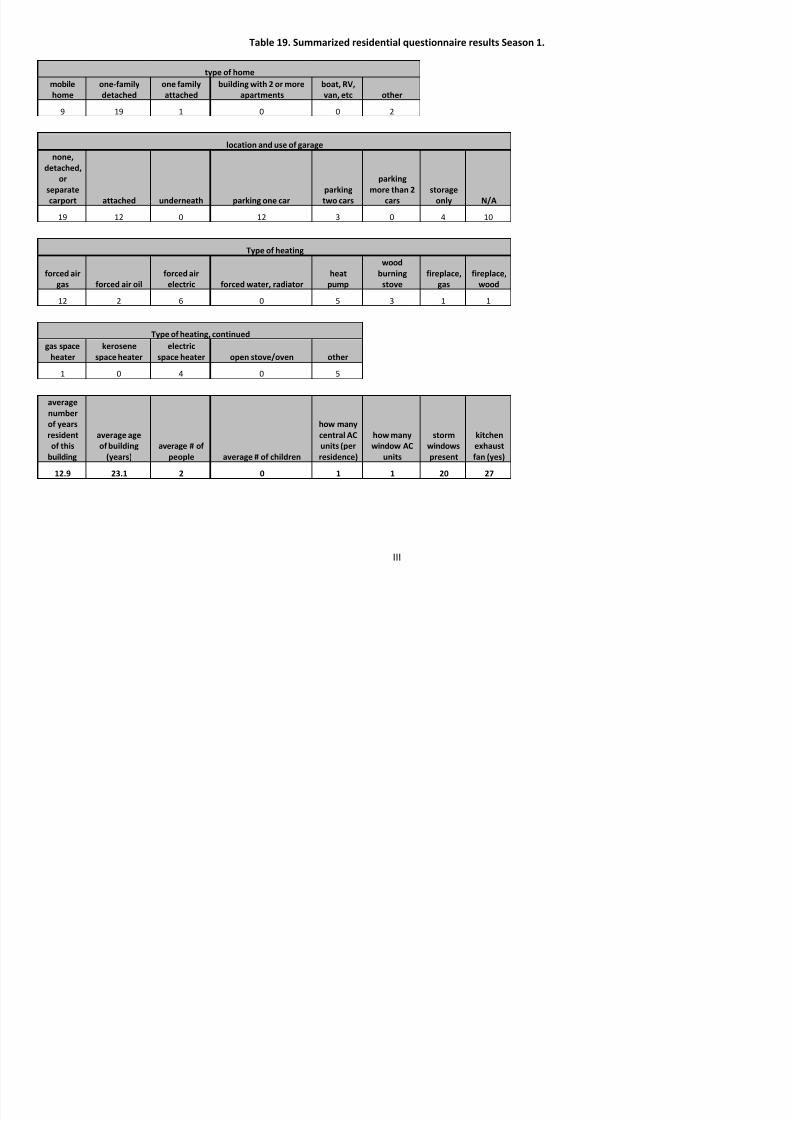
7/30/2019 Millsboro Biomonitoring Study Final Report
http://slidepdf.com/reader/full/millsboro-biomonitoring-study-final-report 78/91
III
Table 19. Summarized residential questionnaire results Season 1.
type of home
mobile
home
one-family
detached
one family
attached
building with 2 or more
apartments
boat, RV,
van, etc other
9 19 1 0 0 2
location and use of garage
none,
detached,
or
separate
carport attached underneath parking one car
parking
two cars
parking
more than 2
cars
storage
only N/A
19 12 0 12 3 0 4 10
Type of heating
forced air
gas forced air oil
forced air
electric forced water, radiator
heat
pump
wood
burning
stove
fireplace,
gas
fireplace,
wood
12 2 6 0 5 3 1 1
Type of heating, continued
gas space
heater
kerosene
space heater
electric
space heater open stove/oven other
1 0 4 0 5
average
number
of years
resident
of this
building
average age
of building
(years)
average # of
people average # of children
how many
central AC
units (per
residence)
how many
window AC
units
storm
windows
present
kitchen
exhaust
fan (yes)
12.9 23.1 2 0 1 1 20 27

7/30/2019 Millsboro Biomonitoring Study Final Report
http://slidepdf.com/reader/full/millsboro-biomonitoring-study-final-report 79/91
IV
Table 20. Summarized residential questionnaire results Season 2.
type of home
mobile
home
one-family
detached
one family
attached
building with 2 or more
apartments
boat, RV,
van, etc other
10 21 1 0 0 2
location and use of garage
none,
detached,
or
separate
carport attached underneath parking one car
parking
two cars
parking
more than 2
cars
storage
only N/A
21 13 0 13 3 0 5 13
Type of heating
forced air
gas forced air oil
forced air
electric forced water, radiator
heat
pump
wood
burning
stove
fireplace,
gas
fireplace,
wood
14 2 6 0 6 4 1 1
Type of heating, continued
gas space
heater
kerosene
space heater
electric
space heater open stove/oven other
1 0 4 0 5
average
number
of years
resident
of this
building
average age
of building
(years)
average # of
people average # of children
how many
central AC
units (per
residence)
how many
window AC
units
storm
windows
present
kitchen
exhaust
fan (yes)
12.9 22.3 2 0 1 1 16 21

7/30/2019 Millsboro Biomonitoring Study Final Report
http://slidepdf.com/reader/full/millsboro-biomonitoring-study-final-report 80/91

7/30/2019 Millsboro Biomonitoring Study Final Report
http://slidepdf.com/reader/full/millsboro-biomonitoring-study-final-report 81/91
VI
Appendix B: Reference Ranges for Analytes in Blood or Serum
Analyte Monitored Fluid
Reference Range,
95th
Percentile
NHANES 2013,
ng/mL [i] Reference Ranges
[ii]
High Value (µg/L)
[iii, iv]
Cadmium Blood 1.55 <5 μg/L >5 μg/L
Lead Blood 3.57 μg/dL <30 μg/dL >40 μg/dL
Mercury Blood 5.75 <10 μg/L >200 μg/L
1,2-Dichloroethane Serum Not Available Not defined Not defined
Benzene Serum 0.34 Not defined Not defined
Carbon tetrachloride Serum<LOD Not defined Not defined
Chloroform Serum Not Available Not defined Not defined
Ethylbenzene Serum0.15 Not defined Not defined
m- & p-Xylene Serum0.43 Not defined Not defined
o-Xylene Serum0.11 Not defined Not defined
Styrene Serum 0.15 Not defined Not defined
Tetrachloroethylene Serum0.13 Not defined Not defined
Toluene Serum0.90 Not defined Not defined
[i] Fourth National Report on Human Exposure to Environmental Chemicals, updated Tables for Adults over 20 years, March 2013,Centers for Disease Control and Prevention National Center for Environmental Health (NCEH), Environmental Health Laboratory.[ii] Tietz Textbook of Clinical Chemistry, edited by C.A. Burtis and E.R. Ashwood, 1999
[iii] Carson, B.L., Ellis III H.V., and McCann, J.L., Toxicology and Biological Monitoring of Metals in Humans, Lewis Publishers, 1986.[iv} “High” levels are repeat upper boundary levels; samples with results greater than this range are reanalyzed for confirmation.

7/30/2019 Millsboro Biomonitoring Study Final Report
http://slidepdf.com/reader/full/millsboro-biomonitoring-study-final-report 82/91
VII
Appendix C: Reference Ranges for Analytes in Urine
Element/ IsotopeMonitored Fluid
Reference Range, 95th Percentile
NHANES 2013, ng/mL [i] High Value (μg/L, PPB) [ii]
Beryllium Urine <LOD 0.2
Cobalt Urine 1.35 2.83
Molybdenum Urine 144 293.5
Cadmium Urine 1.13 2.54
Antimony Urine 0.220 0.8
Cesium Urine 11.1 16.5
Barium Urine 6.80 17.1
Tungsten Urine0.370 1.38Platinum Urine 0.017 0.1
Thallium Urine 0.410 0.62
Lead Urine 1.71 7.8
Uranium Urine 0.36 0.277
Arsenic, total Urine 93.1 64.5
Selenium, total Urine 30.9[iii]
68
[i] Second National Report on Human Exposure to Environmental Chemical, hhtp://cdc.gov/exposurereport/2nd
/metal.htm, Centers
for Disease Control and Prevention, 2013.[ii] Values provided by DE DHSS (Call level). “High “values are repeat upper boundary levels; samples with results greater than this
are reanalyzed for confirmation
[iii] value provided by DE DHSS; referenced as NHANES 1999-2000
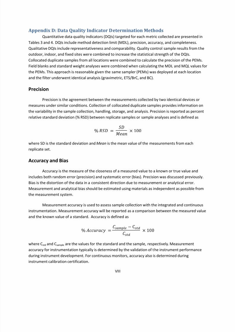
7/30/2019 Millsboro Biomonitoring Study Final Report
http://slidepdf.com/reader/full/millsboro-biomonitoring-study-final-report 83/91
VIII
Appendix D: Data Quality Indicator Determination Methods
Quantitative data quality indicators (DQIs) targeted for each metric collected are presented in
Tables 3 and 4. DQIs include method detection limit (MDL), precision, accuracy, and completeness.
Qualitative DQIs include representativeness and comparability. Quality control sample results from the
outdoor, indoor, and fixed sites were combined to increase the statistical strength of the DQIs.
Collocated duplicate samples from all locations were combined to calculate the precision of the PEMs.
Field blanks and standard weight analyses were combined when calculating the MDL and MQL values for
the PEMs. This approach is reasonable given the same sampler (PEMs) was deployed at each location
and the filter underwent identical analysis (gravimetric, ETS/BrC, and BC).
Precision Precision is the agreement between the measurements collected by two identical devices or
measures under similar conditions. Collection of collocated duplicate samples provides information on
the variability in the sample collection, handling, storage, and analysis. Precision is reported as percent
relative standard deviation (% RSD) between replicate samples or sample analyses and is defined as
where SD is the standard deviation and Mean is the mean value of the measurements from each
replicate set.
Accuracy and Bias Accuracy is the measure of the closeness of a measured value to a known or true value and
includes both random error (precision) and systematic error (bias). Precision was discussed previously.
Bias is the distortion of the data in a consistent direction due to measurement or analytical error.
Measurement and analytical bias should be estimated using materials as independent as possible from
the measurement system.
Measurement accuracy is used to assess sample collection with the integrated and continuous
instrumentation. Measurement accuracy will be reported as a comparison between the measured value
and the known value of a standard. Accuracy is defined as
where Cstd and Csample are the values for the standard and the sample, respectively. Measurement
accuracy for instrumentation typically is determined by the validation of the instrument performance
during instrument development. For continuous monitors, accuracy also is determined during
instrument calibration certification.
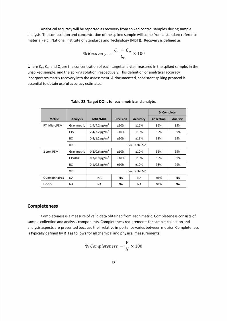
7/30/2019 Millsboro Biomonitoring Study Final Report
http://slidepdf.com/reader/full/millsboro-biomonitoring-study-final-report 84/91
IX
Analytical accuracy will be reported as recovery from spiked control samples during sample
analysis. The composition and concentration of the spiked sample will come from a standard reference
material (e.g., National Institute of Standards and Technology [NIST]). Recovery is defined as
where Cm, Cu, and Cs are the concentration of each target analyte measured in the spiked sample, in the
unspiked sample, and the spiking solution, respectively. This definition of analytical accuracy
incorporates matrix recovery into the assessment. A documented, consistent spiking protocol is
essential to obtain useful accuracy estimates.
Table 22. Target DQI's for each metric and analyte.
Metric Analysis MDL/MQL Precision Accuracy
% Complete
Collection Analysis
RTI MicroPEM Gravimetric 1.4/4.2 µg/m3
±10% ±15% 95% 99%
ETS 2.4/7.2 µg/m3
±10% ±15% 95% 99%
BC 0.4/1.2 µg/m3
±10% ±15% 95% 99%
XRF See Table 2-2
2 Lpm PEM Gravimetric 0.2/0.6 µg/m3
±10% ±10% 95% 99%
ETS/BrC 0.3/0.9 µg/m3
±10% ±10% 95% 99%
BC 0.1/0.3 µg/m3
±10% ±10% 95% 99%
XRF See Table 2-2
Questionnaires NA NA NA NA 99% NA
HOBO NA NA NA NA 99% NA
Completeness Completeness is a measure of valid data obtained from each metric. Completeness consists of
sample collection and analysis components. Completeness requirements for sample collection and
analysis aspects are presented because their relative importance varies between metrics. Completeness
is typically defined by RTI as follows for all chemical and physical measurements:

7/30/2019 Millsboro Biomonitoring Study Final Report
http://slidepdf.com/reader/full/millsboro-biomonitoring-study-final-report 85/91
X
where V is the number of measurements judged valid, and N is the number of measurements planned.
The anticipated influence of completeness for each metric on the ability to answer the study hypotheses
should be considered when the statistical design for the study is being developed.
Other Quality Criteria Instrument Detection Limit (IDL)
The quantity of the target analyte that can be measured and distinguished from zero on a
continuous monitor provides direct output of the metric of interest. It is the lowest level readable on a
display or recorded that can be distinguished from background.
Method Detection Limit (MDL), Corrected for Optimal Sample Volume
The method detection limit (MDL) is defined as the minimum concentration of substance that
can be measured and reported with a known confidence that the analyte concentration is greater than
zero and is determined from analysis of a sample in a given matrix containing the analyte. For allapplicable metrics, the equation to determine the MDL for a given analyte is:
MDL = t(n-1, a=0.68)S
where, t(n-1, a = 0.68) represents the Students’ t-test t value appropriate for a 68% confidence level
(84% one-tailed) and a standard deviation estimate with n-1 degrees of freedom. S is equal to the
standard deviation of the replicate (usually seven samples) analyses. This value is obtained from
analyzing standard samples containing the target mass between the MDL and the lowest target analyte
mass expected to be observed (or blank filters for filter media). This value is then divided by the
theoretical sample volume. For example, the theoretical volume for a 24 h PM sample collected on aPEM sampler operating at 4 L per minute is 5,760 L or 5.76 cubic meters.
Method Quantitation Limit (MQL)
For other analyses, such as gravimetric, the MQL is three times the MDL [MQL = 3 x MDL] and
within the specified limits of precision and accuracy during routine analytical operating conditions.
Tables 4 and 5 contain the current values of MQL.

7/30/2019 Millsboro Biomonitoring Study Final Report
http://slidepdf.com/reader/full/millsboro-biomonitoring-study-final-report 86/91
XI
Table 23. Target quantitative DQI's for XRF analysis.
Element MDL/MQL ng/filter Precision Accuracy
% Completeness
Collection Analysis
Sodium 70/210 20 10 95% 99%
Magnesium 70/210 20 10 95% 99%
Aluminum 500/1,500 20 10 95% 99%
Silicon 170/510 20 10 95% 99%
Phosphorous 120/360 20 10 95% 99%
Sulfur 70/210 20 10 95% 99%
Chlorine 50/150 20 10 95% 99%
Potassium 30/90 20 10 95% 99%
Calcium 40/120 20 10 95% 99%
Titanium 70/210 20 10 95% 99%
Vanadium 25/75 20 10 95% 99%
Chromium 10/30 20 10 95% 99%
Manganese 10/30 20 10 95% 99%
Iron 30/90 20 10 95% 99%
Cobalt 20/60 20 10 95% 99%
Nickel 15/45 20 10 95% 99%
Copper 15/45 20 10 95% 99%
Zinc 10/30 20 10 95% 99%
Arsenic 15/45 20 10 95% 99%
Selenium 8/24 20 10 95% 99%
Bromine 10/30 20 10 95% 99%
Rubidium 10/30 20 10 95% 99%
Strontium 10/30 20 10 95% 99%
Zirconium 80/240 20 10 95% 99%
Silver 50/150 20 10 95% 99%
Cadmium 60/180 20 10 95% 99%
Tin 80/240 20 10 95% 99%
Antimony 90/270 20 10 95% 99%

7/30/2019 Millsboro Biomonitoring Study Final Report
http://slidepdf.com/reader/full/millsboro-biomonitoring-study-final-report 87/91
XII
Element MDL/MQL ng/filter Precision Accuracy
% Completeness
Collection Analysis
Cesium 133/400 20 10 95% 99%
Barium 170/510 20 10 95% 99%
Cerium 467/1,400 20 10 95% 99%
Mercury 23/70 20 10 95% 99%
Lead 24/72 20 10 95% 99%

7/30/2019 Millsboro Biomonitoring Study Final Report
http://slidepdf.com/reader/full/millsboro-biomonitoring-study-final-report 88/91
XIII
Table 24. Actual DQIs from MIEBS Seasons 1 & 2.
Metric Analysis MDL/MQL Precision* Accuracy
% Complete
Collection Analysis
RTI MicroPEM Gravimetric:Season 1
Season 2
0.1/0.4 µg/m3
0.2/0.7 µg/m3
-
-
0.1%
0.1%
See Table 7
See Table 8
See Table 7
See Table 8
ETS:
Season 1
Season 2
0.04/0.1 µg/m3
0.01/0.03 µg/m3
-
-
-
-
See Table 7
See Table 8
See Table 7
See Table 8
BC
Season 1:
Season 2:
0.01/0.03 µg/m3
0.03/0.08 µg/m3
-
-
-
-
See Table 7
See Table 8
See Table 7
See Table 8
XRF See Table 7
PEM:2 LPM season 1
4 LPM season 2
Gravimetric:Season 1
Season 2:
0.3/0.9 µg/m3
0.02/0.08 µg/m3
10.1%
14.8%
-5.5%
-5.5%
See Table 7
See Table 8
See Table 7
See Table 8
ETS/BrC:
Season 1
Season 2
0.3/1.0. µg/m3
0.008/0.002 µg/m3
17.6%
10.0%
-
-
See Table 7
See Table 8
See Table 7
See Table 8
BC:
Season 1
Season 2
0.3/1.0. µg/m3
0.008/0.002 µg/m3
2.6%
6.0%
-
-
See Table 7
See Table 8
See Table 7
See Table 8
XRF See Table 7
Questionnaires Season 1Season 2
NA NA NA 91%100%
NA
HOBO Season 1
Season 2
NA NA NA 100%
100%
NA
[*]Precision values are averages of all filters collocated filters: n = 7 Season 1; n= 14 Season 2
Table 25. Actual DQIs for XRF Analysis of MIEBS Season 1 & 2 data.
MDL (ng/filter) MQL (ng/filter) Median Precision Accuracy
Season 1 Season 2 Season 1 Season 2 Season 1Season
2
Season
1
Season
2
Ag 211.9 223.5 635.7 670.4 0.0 0.0 - -
Al 119.1 95.2 357.3 285.7 0.0 0.0 - -
As 12.1 10.8 36.2 32.5 0.0 0.0 - -
Ba 59.4 67.2 178.3 201.5 0.0 0.0 - -
Br 12.5 11.4 37.5 34.3 0.0 0.0 - -

7/30/2019 Millsboro Biomonitoring Study Final Report
http://slidepdf.com/reader/full/millsboro-biomonitoring-study-final-report 89/91
XIV
MDL (ng/filter) MQL (ng/filter) Median Precision Accuracy
Ca 22.7 18.8 68 56.3 0.0 22.5 - -
Cd 283.1 299.5 849.4 898.6 0.0 0.0 0.0 -2.0
Ce 30.2 50.1 90.6 150.2 0.0 0.0 - -
Cl 22.6 18.4 67.8 55.1 0.0 0.0 - -Co 6.4 5.8 19.2 17.3 0.0 0.0 - -
Cr 10.9 11.6 32.8 34.9 0.0 0.0 - -
Cs 60.7 70.7 182.2 212.0 0.0 0.0 - -
Cu 10.1 6.6 30.4 19.9 0.0 0.0 - -
Fe 10.7 9.5 32 28.5 19.6 10.5 0.6 0.8
In 367.4 383.8 1102.1 1151.3 0.0 0.0 - -
K 19.1 17.9 57.2 53.8 9.4 10.9 - -
Mg 56.7 44.5 170.2 133.4 0.0 0.0 - -
Mn 8.8 8.8 26.4 26.5 0.0 0.0 - -
Na 131.4 92.4 394.2 277.3 0.0 0.0 - -
Ni 5.9 5.0 17.8 15.0 0.0 0.0 - -
P 45.7 4.7 137.2 14.0 0.0 0.0 - -
Pb 25.0 19.3 75 58.0 0.0 0.0 -0.8 1.8
Rb 13.7 13.8 41.2 41.3 0.0 0.0 - -
S 29.6 23.6 88.8 70.7 5.3 7.2 - -
Sb 712.5 709 2137.6 2127.1 0.0 0.0 - -
Se 13.5 11.7 40.4 35.1 0.0 0.0 1.3 -0.3
Si 57.4 47.7 172.3 143.2 33.1 27.1 1.1 -0.2
Sn 497.3 552.2 1491.8 1656.7 0.0 0.0 - -
Sr 18.2 154.7 54.7 464.0 0.0 0.0 - -
Ti 22.7 28.8 68.2 86.3 0.0 0.0 0.2 1.5
V 15.2 18.7 45.7 56.0 0.0 0.0 - -
Zn 10.1 7.7 30.2 23.0 0.0 27.7 - -
Zr 139.3 197.5 418 592.5 0.0 0.0 - -

7/30/2019 Millsboro Biomonitoring Study Final Report
http://slidepdf.com/reader/full/millsboro-biomonitoring-study-final-report 90/91
XV
Data validity was determined on three levels: 1) review of data collection sheets recorded by
field technicians during sampling, 2) physical inspection of filters, and 3) comparison of analysis results
against other filters collected. During each of these steps filters were given one of three levels of
validity:
Invalid (code = 0; noted handling issue or obvious filter damage which precludes analysis)
Suspect (code = 1; no noted issues, but reported value is more or less than twice the standard
deviation of the mean)
Valid (code = 2; no noted issues and data value is within two standard deviations of the mean)
During the first level of data validation, any filters that were noted as incorrectly handled were marked
as invalid due to possible contamination. The second level of data review involved visual inspection of
filters for any holes which might induce errors in analytical analysis. The final level of data validation
resulted from comparison of analytical data amongst all filters of similar sample collection parameters.
All data was entered into a comprehensive file in order to provide a unified space for data to be housed.Results from the validation procedures are displayed in Tables 7 and 8.
7/30/2019 Millsboro Biomonitoring Study Final Report
http://slidepdf.com/reader/full/millsboro-biomonitoring-study-final-report 91/91
GlossaryParticulate Matter (PM): Any material, except pure water, that exists in the solid or liquid state in the
atmosphere, such as soot, dust, smoke, fumes, and aerosols. The size of particulate matter can vary
from coarse, wind-blown dust particles to fine particle combustion products.
Particulate Matter less than 2.5 micrometers (PM2.5): A major air pollutant consisting of tiny solid orliquid particles, generally soot and aerosols. The size of the particles (2.5 micrometers or smaller, about
0.0001 inches or less) allows them to easily enter the air sacs deep in the lungs where they may cause
adverse health effects, as noted in several recent studies. PM2.5 also causes visibility reduction.
Volatile Organic Compound (VOC): This term is generally used similarly to the term "reactive organic
compounds" but excludes ethane, which the federal government does not consider to be reactive. VOCs
are hydrocarbon compounds that exist in the ambient air and contribute to the formation of smog
and/or may themselves be toxic. VOCs often have an odor, and some examples include gasoline,
alcohol, and the solvents used in paints.
Minimum Detection Limit (MDL): The minimum concentration of a substance that can be measured and
reported with 99 percent confidence that the analyte concentration is greater than zero and is
determined from analysis of a sample in a given matrix containing the analyte.
Minimum Quantification Limit: The smallest detectable concentration of analyte greater than the
detection limit where the required* accuracy (precision & bias) is achieved for the intended purpose.
Related Documents