Millimeter Wave Channel Modeling and Cellular Capacity ... · AKDENIZet al.:MILLIMETER WAVE CHANNEL MODELING AND CELLULAR CAPACITY EVALUATION 1165 Statistical models are then derived

1164 IEEE JOURNAL ON SELECTED AREAS IN COMMUNICATIONS, VOL. 32, NO. 6, JUNE 2014

Millimeter Wave Channel Modelingand Cellular Capacity Evaluation

Mustafa Riza Akdeniz, Student Member, IEEE, Yuanpeng Liu, Mathew K. Samimi, Student Member, IEEE,Shu Sun, Student Member, IEEE, Sundeep Rangan, Senior Member, IEEE,Theodore S. Rappaport, Fellow, IEEE, and Elza Erkip, Fellow, IEEE

Abstract—With the severe spectrum shortage in conventionalcellular bands, millimeter wave (mmW) frequencies between 30and 300 GHz have been attracting growing attention as a possiblecandidate for next-generation micro- and picocellular wirelessnetworks. The mmW bands offer orders of magnitude greaterspectrum than current cellular allocations and enable very high-dimensional antenna arrays for further gains via beamformingand spatial multiplexing. This paper uses recent real-world mea-surements at 28 and 73 GHz in New York, NY, USA, to derivedetailed spatial statistical models of the channels and uses thesemodels to provide a realistic assessment of mmW micro- andpicocellular networks in a dense urban deployment. Statisticalmodels are derived for key channel parameters, including the pathloss, number of spatial clusters, angular dispersion, and outage.It is found that, even in highly non-line-of-sight environments,strong signals can be detected 100–200 m from potential cell sites,potentially with multiple clusters to support spatial multiplexing.Moreover, a system simulation based on the models predicts thatmmW systems can offer an order of magnitude increase in ca-pacity over current state-of-the-art 4G cellular networks with noincrease in cell density from current urban deployments.

Index Terms—Millimeter wave radio, 3GPP LTE, cellular sys-tems, wireless propagation, 28 GHz, 73 GHz, urban deployments.

I. INTRODUCTION

THE remarkable success of cellular wireless technologieshave led to an insatiable demand for mobile data [1], [2].

The UMTS traffic forecasts [3], for example, predict that by2020, daily mobile traffic will exceed 800 MB per subscriberleading to 130 exabits (1018) of data per year for someoperators. Keeping pace with this demand will require newtechnologies that can offer orders of magnitude increases incellular capacity.To address this challenge, there has been growing interest in

cellular systems based in the so-called millimeter wave (mmW)bands, between 30 and 300 GHz, where the available band-widths are much wider than today’s cellular networks [4]–[9].The available spectrum at these frequencies can be easily

Manuscript received December 1, 2013; revised April 25, 2014; acceptedMay 25, 2014. Date of publication June 13, 2014; date of current versionJuly 14, 2014. This material is based upon work supported by the NationalScience Foundation under Grants 1116589 and 1237821 and generous supportfrom Samsung, Nokia Siemens Networks, and InterDigital Communications.The authors are with NYU WIRELESS, New York University Polytechnic

School of Engineering, Brooklyn, NY 11201 USA (e-mail: [email protected];[email protected]; [email protected]; [email protected];[email protected]; [email protected]; [email protected]).Color versions of one or more of the figures in this paper are available online

at http://ieeexplore.ieee.org.Digital Object Identifier 10.1109/JSAC.2014.2328154

200 times greater than all cellular allocations today that arecurrently largely constrained to the prime RF real estate under3 GHz [5]. Moreover, the very small wavelengths of mmWsignals combined with advances in low-power CMOS RF cir-cuits enable large numbers (≥ 32 elements) of miniaturizedantennas to be placed in small dimensions. These multipleantenna systems can be used to form very high gain, electricallysteerable arrays, fabricated at the base station, in the skin ofa cell phone, or even within a chip [6], [10]–[17]. Given thevery wide bandwidths and large numbers of spatial degrees offreedom, it has been speculated that mmW bands will play asignificant role in Beyond 4G and 5G cellular systems [8].However, the development of cellular networks in the mmW

bands faces significant technical obstacles and the precise valueof mmW systems needs careful assessment. The increase inomnidirectional free space path loss with higher frequenciesdue to Friis’ Law [18], can be more than compensated by aproportional increase in antenna gain with appropriate beam-forming. We will, in fact, confirm this property experimentallybelow. However, a more significant concern is that mmWsignals can be severely vulnerable to shadowing resulting inoutages, rapidly varying channel conditions and intermittentconnectivity. This issue is particularly concerning in cluttered,urban deployments where coverage frequently requires non-line-of-sight (NLOS) links.In this paper, we use the measurements of mmW outdoor

cellular propagation [19]–[23] at 28 and 73 GHz in New YorkCity to derive in detail the first statistical channel models thatcan be used for proper mmW system evaluation. The modelsare used to provide an initial assessment of the potential systemcapacity and outage. The NYC location was selected since it isrepresentative of likely initial deployments of mmW cellularsystems due to the high user density. In addition, the urbancanyon environment provides a challenging test case for thesesystems due to the difficulty in establishing line-of-sight (LOS)links—a key concern for mmW cellular.Although our earlier work has presented some initial analysis

of the data in [19]–[22], this work provides much more detailedmodeling necessary for cellular system evaluation. In particular,we develop detailed models for the spatial characteristics ofthe channel and outage probabilities. To obtain these models,we present several new data analysis techniques. In particular,we propose a clustering algorithm that identifies the group ofpaths in the angular domain from subsampled spatial measure-ments. The clustering algorithm is based on aK-means methodwith additional heuristics to determine the number of clusters.

0733-8716 © 2014 IEEE. Translations and content mining are permitted for academic research only. Personal use is also permitted, but republication/redistributionrequires IEEE permission. See http://www.ieee.org/publications_standards/publications/rights/index.html for more information.

AKDENIZ et al.: MILLIMETER WAVE CHANNEL MODELING AND CELLULAR CAPACITY EVALUATION 1165

Statistical models are then derived for key cluster parametersincluding the number of clusters, cluster angular spread andpath loss. For the inter-cluster power fractions, we propose aprobabilistic model with maximum likelihood (ML) parameterestimation. In addition, while standard 3GPP models such as[24], [25] use probabilistic LOS-NLOS models, we propose toadd a third state to explicitly model the possibility of outages.The key findings from these models are as follows:• The omnidirectional path loss is approximately 20 to25 dB higher in the mmW frequencies relative to currentcellular frequencies in distances relevant for small cells.However, due to the reduced wavelength, this loss canbe completely compensated by a proportional increase inantenna gain with no increase in physical antenna size.Thus, with appropriate beamforming, locations that arenot in outage will not experience any effective increase inpath loss and, in fact, the path loss may be decreased [26].

• Our measurements indicate that at many locations, energyarrives in clusters from multiple distinct angular direc-tions, presumably through different macro-level scatteringor reflection paths. Locations had up to four clusters,with an average between two and three. The presence ofmultiple clusters of paths implies the possibility of bothspatial multiplexing and diversity gains—see also [27].

• Applying the derived channel models to a standard cel-lular evaluation framework such as [24], we predict thatmmW systems can offer at least an order of magnitudeincrease in system capacity under reasonable assumptionson abundant bandwidth and beamforming. For example,we show that a hypothetical 1 GHz bandwidth TDDmmWsystem with a 100 m cell radii can provide 25 times greatercell throughout than industry reported numbers for a 20 +20 MHz FDD LTE system with similar cell density.Moreover, while the LTE capacity numbers included bothsingle and multi-user multi-input multi-output (MIMO),our mmW capacity analysis did not include any spatialmultiplexing gains. We provide strong evidence that thesespatial multiplexing gains would be significant and thusthe potential gains of mmW cellular are even larger.

• The system performance appears to be robust to outagesprovided they are at levels similar or even a little worsethan the outages we observed in the NYC measurements.This robustness to outage is very encouraging since out-ages are one of the key concerns with mmW cellular. How-ever, we also show that should outages be significantlyworse than what we observed, the system performance,particularly the cell edge rate, can be greatly impacted.

In addition to the measurement studies above, some of thecapacity analysis in this paper appeared in a conference version[28]. The current work provides much more extensive modelingof the channels, more detailed discussions of the beamformingand MIMO characteristics and simulations of features such asoutage.

A. Prior Measurements

Particularly with the development of 60 GHz LAN and PANsystems, mmW signals have been extensively characterized in

Fig. 1. Image from [19] showing typical measurement locations in NYC at28 GHz. Similar locations were used for 73 GHz.

indoor environments [29]–[35]. However, the propagation ofmmW signals in outdoor settings for micro- and picocellularnetworks is relatively less understood. Due to the lack of actualmeasured channel data, many earlier studies [4], [7], [36], [37]have thus relied on either analytic models or commercial raytracing software with various reflection assumptions. Below,we will compare our experimental results with some of thesemodels.Also, measurements in Local Multipoint Distribution Sys-

tems at 28 GHz—the prior system most close to mmWcellular—have been inconclusive: For example, a study [38]found 80% coverage at ranges up to 1–2 km, while [39]claimed that LOS connectivity would be required. Our ownprevious studies at 38 GHz [40]–[44] found that relatively long-range links (> 300 m) could be established. However, thesemeasurements were performed in an outdoor campus settingwith much lower building density and greater opportunitiesfor LOS connectivity than would be found in a typical urbandeployment.

II. MEASUREMENT METHODOLOGY

To assess mmW propagation in urban environments, ourteam conducted extensive measurements of 28 and 73 GHzchannels in New York City. Details of the measurements canbe found in [19]–[21]. Both the 28 and 73 GHz are naturalcandidates for early mmW deployments. The 28 GHz bandswere previously targeted for Local Multipoint Distribution Sys-tems (LMDS) systems and are now an attractive opportunityfor initial deployments of mmW cellular given their relativelylower frequency within the mmW range. The E-Band (71–76 GHz and 81–86 GHz) [45] has abundant spectrum and isadaptable for dense deployment, and could accommodate fur-ther expansion should the lower frequencies become crowded.To measure the channel characteristics in these frequencies,

we emulated microcellular type deployments where transmit-ters were placed on rooftops 7 and 17 meters (approximately 2to 5 stories) high and measurements were then made at a num-ber of street level locations up to 500 m from the transmitters(see Fig. 1). To characterize both the bulk path loss and spatialstructure of the channels, measurements were performed withhighly directional horn antennas (30 dBm RF power, 24.5 dBigain at both TX and RX sides, and ≈ 10◦ beamwidths in both


the vertical and horizontal planes provided by rotatable hornantennas).Since transmissions were always made from the rooftop

location to the street, in all the reported measurements below,characteristics of the transmitter will be representative of thebase station (BS) and characteristics of the receiver will berepresentative of a mobile, or user equipment (UE). At eachtransmitter (TX)—receiver (RX) location pair, the azimuth(horizontal) and elevation (vertical) angles of both the trans-mitter and receiver were swept to first find the direction of themaximal receive power. After this point, power measurementswere then made at various angular offsets from the strongestangular locations. In particular, the horizontal angles at boththe TX and RX were swept in 10◦ steps from 0 to 360◦. Verticalangles were also sampled, typically within a ±20◦ range fromthe horizon in the vertical plane. At each angular samplingpoint, the channel sounder was used to detect any signal paths.To reject noise, only paths that exceeded a 5 dB SNR thresholdwere included in the power-delay profile (PDP). Since thechannel sounder has a processing gain of 30 dB, only extremelyweak paths would not be detected in this system—See [19]–[21] for more details. The power at each angular location is thesum of received powers across all delays (i.e., the sum of thePDP). A location would be considered in outage if there wereno detected paths across all angular measurements.

III. CHANNEL MODELING AND PARAMETER ESTIMATION

A. Distance-Based Path Loss

We first estimated the total omnidirectional path loss as afunction of the TX-RX distance. At each location that was notin outage, the path loss was estimated as

PL = PTX − PRX +GTX +GRX , (1)

where PTX is the total transmit power in dBm, PRX is thetotal integrated receive power over all the angular directionsand GTX and GRX are the gains of the horn antennas. For thisexperiment, PTX = 30 dBm and GTX = GRX = 24.5 dBi.Note that the path loss (1) is obtained by subtracting theantenna gains from power measured at every pointing angle ata particular location, and summing the powers over all TX andRX pointing angles as shown in [46], and thus (1) representsthe path loss as an isotropic (omnidirectional, unity antennagain) value i.e., the difference between the average transmitand receive power seen assuming omnidirectional antennas atthe TX and RX. The path loss thus does not include anybeamforming gains obtained by directing the transmitter orreceiver correctly—we will discuss the beamforming gains indetail below.A scatter plot of the omnidirectional path losses at different

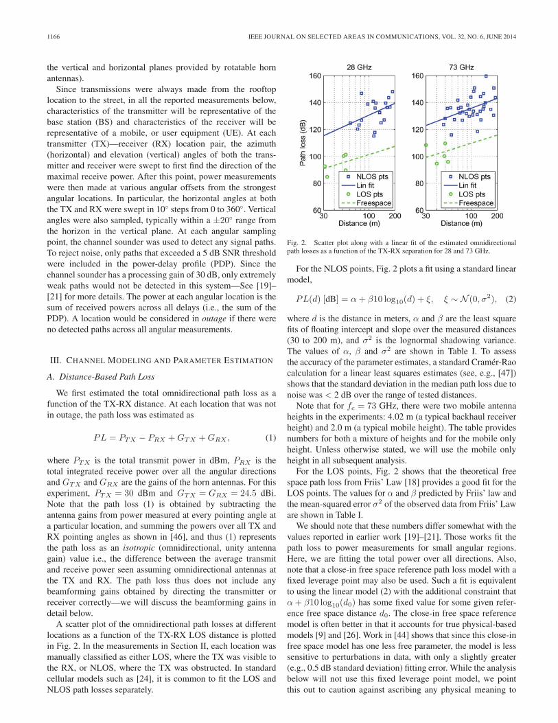
locations as a function of the TX-RX LOS distance is plottedin Fig. 2. In the measurements in Section II, each location wasmanually classified as either LOS, where the TX was visible tothe RX, or NLOS, where the TX was obstructed. In standardcellular models such as [24], it is common to fit the LOS andNLOS path losses separately.

Fig. 2. Scatter plot along with a linear fit of the estimated omnidirectionalpath losses as a function of the TX-RX separation for 28 and 73 GHz.

For the NLOS points, Fig. 2 plots a fit using a standard linearmodel,

PL(d) [dB] = α+ β10 log10(d) + ξ, ξ ∼ N (0, σ2), (2)

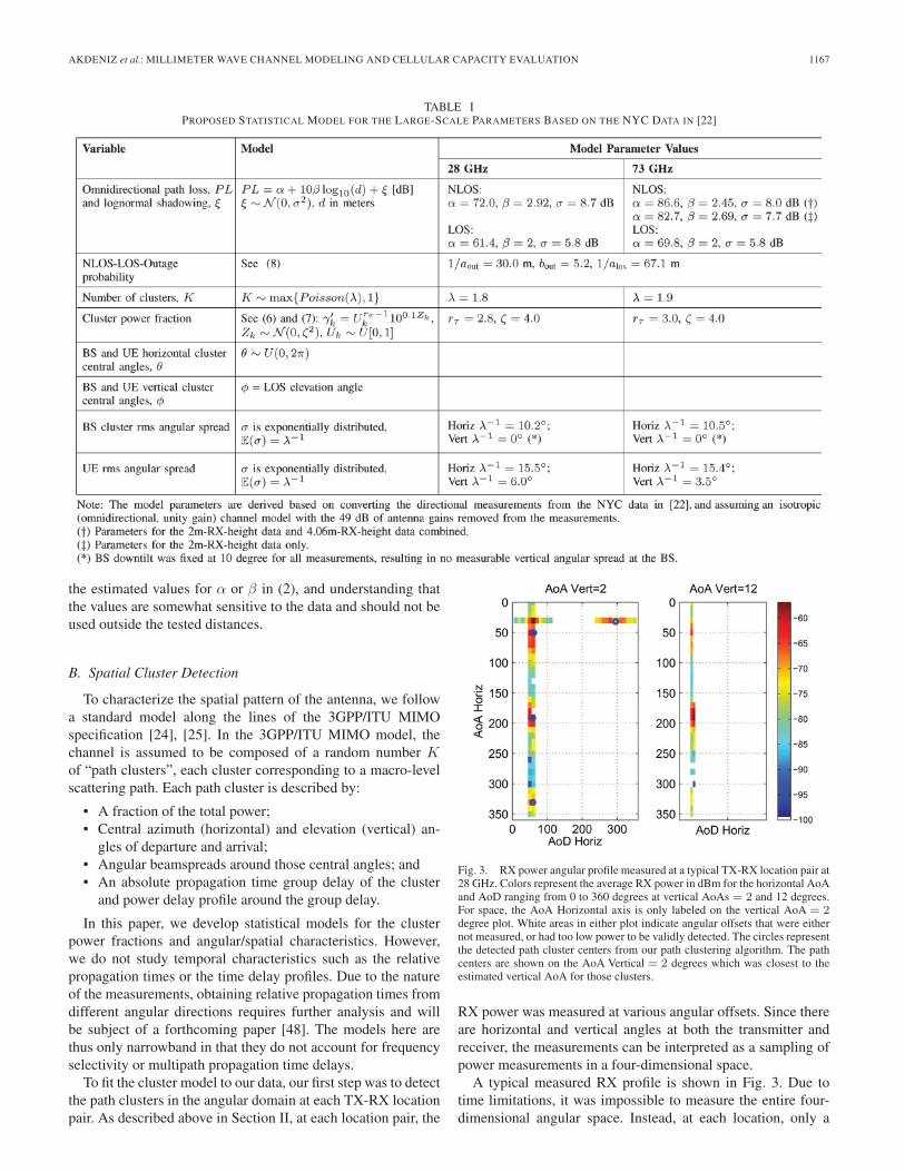
where d is the distance in meters, α and β are the least squarefits of floating intercept and slope over the measured distances(30 to 200 m), and σ2 is the lognormal shadowing variance.The values of α, β and σ2 are shown in Table I. To assessthe accuracy of the parameter estimates, a standard Cramér-Raocalculation for a linear least squares estimates (see, e.g., [47])shows that the standard deviation in the median path loss due tonoise was < 2 dB over the range of tested distances.Note that for fc = 73 GHz, there were two mobile antenna

heights in the experiments: 4.02 m (a typical backhaul receiverheight) and 2.0 m (a typical mobile height). The table providesnumbers for both a mixture of heights and for the mobile onlyheight. Unless otherwise stated, we will use the mobile onlyheight in all subsequent analysis.For the LOS points, Fig. 2 shows that the theoretical free

space path loss from Friis’ Law [18] provides a good fit for theLOS points. The values for α and β predicted by Friis’ law andthe mean-squared error σ2 of the observed data from Friis’ Laware shown in Table I.We should note that these numbers differ somewhat with the

values reported in earlier work [19]–[21]. Those works fit thepath loss to power measurements for small angular regions.Here, we are fitting the total power over all directions. Also,note that a close-in free space reference path loss model with afixed leverage point may also be used. Such a fit is equivalentto using the linear model (2) with the additional constraint thatα+ β10 log10(d0) has some fixed value for some given refer-ence free space distance d0. The close-in free space referencemodel is often better in that it accounts for true physical-basedmodels [9] and [26]. Work in [44] shows that since this close-infree space model has one less free parameter, the model is lesssensitive to perturbations in data, with only a slightly greater(e.g., 0.5 dB standard deviation) fitting error. While the analysisbelow will not use this fixed leverage point model, we pointthis out to caution against ascribing any physical meaning to


TABLE IPROPOSED STATISTICAL MODEL FOR THE LARGE-SCALE PARAMETERS BASED ON THE NYC DATA IN [22]

the estimated values for α or β in (2), and understanding thatthe values are somewhat sensitive to the data and should not beused outside the tested distances.

B. Spatial Cluster Detection

To characterize the spatial pattern of the antenna, we followa standard model along the lines of the 3GPP/ITU MIMOspecification [24], [25]. In the 3GPP/ITU MIMO model, thechannel is assumed to be composed of a random number Kof “path clusters”, each cluster corresponding to a macro-levelscattering path. Each path cluster is described by:

• A fraction of the total power;• Central azimuth (horizontal) and elevation (vertical) an-gles of departure and arrival;

• Angular beamspreads around those central angles; and• An absolute propagation time group delay of the clusterand power delay profile around the group delay.

In this paper, we develop statistical models for the clusterpower fractions and angular/spatial characteristics. However,we do not study temporal characteristics such as the relativepropagation times or the time delay profiles. Due to the natureof the measurements, obtaining relative propagation times fromdifferent angular directions requires further analysis and willbe subject of a forthcoming paper [48]. The models here arethus only narrowband in that they do not account for frequencyselectivity or multipath propagation time delays.To fit the cluster model to our data, our first step was to detect

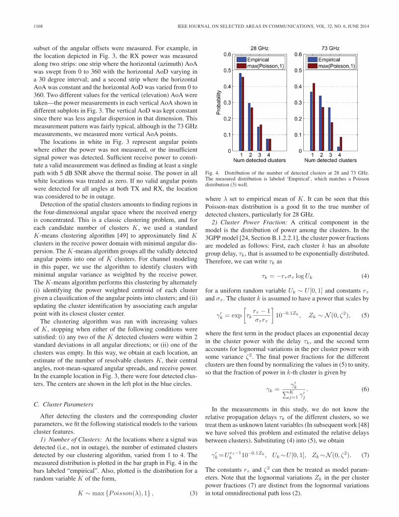
the path clusters in the angular domain at each TX-RX locationpair. As described above in Section II, at each location pair, the

Fig. 3. RX power angular profile measured at a typical TX-RX location pair at28 GHz. Colors represent the average RX power in dBm for the horizontal AoAand AoD ranging from 0 to 360 degrees at vertical AoAs = 2 and 12 degrees.For space, the AoA Horizontal axis is only labeled on the vertical AoA = 2degree plot. White areas in either plot indicate angular offsets that were eithernot measured, or had too low power to be validly detected. The circles representthe detected path cluster centers from our path clustering algorithm. The pathcenters are shown on the AoA Vertical = 2 degrees which was closest to theestimated vertical AoA for those clusters.

RX power was measured at various angular offsets. Since thereare horizontal and vertical angles at both the transmitter andreceiver, the measurements can be interpreted as a sampling ofpower measurements in a four-dimensional space.A typical measured RX profile is shown in Fig. 3. Due to

time limitations, it was impossible to measure the entire four-dimensional angular space. Instead, at each location, only a


subset of the angular offsets were measured. For example, inthe location depicted in Fig. 3, the RX power was measuredalong two strips: one strip where the horizontal (azimuth) AoAwas swept from 0 to 360 with the horizontal AoD varying ina 30 degree interval; and a second strip where the horizontalAoA was constant and the horizontal AoD was varied from 0 to360. Two different values for the vertical (elevation) AoA weretaken—the power measurements in each vertical AoA shown indifferent subplots in Fig. 3. The vertical AoD was kept constantsince there was less angular dispersion in that dimension. Thismeasurement pattern was fairly typical, although in the 73 GHzmeasurements, we measured more vertical AoA points.The locations in white in Fig. 3 represent angular points

where either the power was not measured, or the insufficientsignal power was detected. Sufficient receive power to consti-tute a valid measurement was defined as finding at least a singlepath with 5 dB SNR above the thermal noise. The power in allwhite locations was treated as zero. If no valid angular pointswere detected for all angles at both TX and RX, the locationwas considered to be in outage.Detection of the spatial clusters amounts to finding regions in

the four-dimensional angular space where the received energyis concentrated. This is a classic clustering problem, and foreach candidate number of clusters K, we used a standardK-means clustering algorithm [49] to approximately find Kclusters in the receive power domain with minimal angular dis-persion. TheK-means algorithm groups all the validly detectedangular points into one of K clusters. For channel modelingin this paper, we use the algorithm to identify clusters withminimal angular variance as weighted by the receive power.TheK-means algorithm performs this clustering by alternately(i) identifying the power weighted centroid of each clustergiven a classification of the angular points into clusters; and (ii)updating the cluster identification by associating each angularpoint with its closest cluster center.The clustering algorithm was run with increasing values

of K, stopping when either of the following conditions weresatisfied: (i) any two of the K detected clusters were within 2standard deviations in all angular directions; or (ii) one of theclusters was empty. In this way, we obtain at each location, anestimate of the number of resolvable clusters K, their centralangles, root-mean-squared angular spreads, and receive power.In the example location in Fig. 3, there were four detected clus-ters. The centers are shown in the left plot in the blue circles.

C. Cluster Parameters

After detecting the clusters and the corresponding clusterparameters, we fit the following statistical models to the variouscluster features.

1) Number of Clusters: At the locations where a signal wasdetected (i.e., not in outage), the number of estimated clustersdetected by our clustering algorithm, varied from 1 to 4. Themeasured distribution is plotted in the bar graph in Fig. 4 in thebars labeled “empirical”. Also, plotted is the distribution for arandom variableK of the form,

K ∼ max {Poisson(λ), 1} , (3)

Fig. 4. Distribution of the number of detected clusters at 28 and 73 GHz.The measured distribution is labeled ‘Empirical’, which matches a Poissondistribution (3) well.

where λ set to empirical mean of K. It can be seen that thisPoisson-max distribution is a good fit to the true number ofdetected clusters, particularly for 28 GHz.

2) Cluster Power Fraction: A critical component in themodel is the distribution of power among the clusters. In the3GPP model [24, Section B.1.2.2.1], the cluster power fractionsare modeled as follows: First, each cluster k has an absolutegroup delay, τk, that is assumed to be exponentially distributed.Therefore, we can write τk as

τk = −rτστ logUk (4)

for a uniform random variable Uk ∼ U [0, 1] and constants rτand στ . The cluster k is assumed to have a power that scales by

γ′k = exp

[τk

rτ − 1

στrτ

]10−0.1Zk , Zk ∼ N (0, ζ2), (5)

where the first term in the product places an exponential decayin the cluster power with the delay τk, and the second termaccounts for lognormal variations in the per cluster power withsome variance ζ2. The final power fractions for the differentclusters are then found by normalizing the values in (5) to unity,so that the fraction of power in k-th cluster is given by

γk =γ′k∑K

j=1 γ′j

. (6)

In the measurements in this study, we do not know therelative propagation delays τk of the different clusters, so wetreat them as unknown latent variables (In subsequent work [48]we have solved this problem and estimated the relative delaysbetween clusters). Substituting (4) into (5), we obtain

γ′k=Urτ−1

k 10−0.1Zk , Uk∼U [0, 1], Zk∼N (0, ζ2). (7)

The constants rτ and ζ2 can then be treated as model param-eters. Note that the lognormal variations Zk in the per clusterpower fractions (7) are distinct from the lognormal variationsin total omnidirectional path loss (2).


Fig. 5. Distribution of the fraction of power in the weaker cluster, whenK = 2 clusters were detected. Plotted are the measured distributions and thebest fit of the theoretical model in (6) and (7).

For the mmW data, Fig. 5 shows the distribution of thefraction of power in the weaker cluster in the case whenK = 2 clusters were detected. Also, plotted is the theoreticaldistribution based on (6) and (7) where the parameters rτ andζ2 were fit via an approximate maximum likelihood method.Since the measurement data we have does not have the relativedelays of the different clusters we treat the variable Uk in (6)as an unknown latent variable, adding to the variation in thecluster power distributions. The estimated ML parameters areshown in Table I, with the values in 28 and 73 GHz being verysimilar.We see that the 3GPPmodel with the ML parameter selection

provides an excellent fit for the observed power fraction forclusters with more than 10% of the energy. The model is likelynot fitting the very low energy clusters since our cluster detec-tion is likely unable to find those clusters. However, for caseswhere the clusters have significant power, the model appearsaccurate. Also, since there were very few locations where thenumber of clusters wasK ≥ 3, we only fit the parameters basedon the K = 2 case. In the simulations below, we will assumethe model is valid for allK.

3) Angular Dispersion: For each detected cluster, we mea-sured the root mean-squared (rms) beamspread in the differentangular dimensions. In the angular spread estimation in eachcluster, we excluded power measurements from the lowest10% of the total cluster power. This clipping introduces asmall bias in the angular spread estimate. Although these lowpower points correspond to valid signals (as described above,all power measurements were only admitted into the data setif the signals were received with a minimum power level),the clipping reduced the sensitivity to misclassifications ofpoints at the cluster boundaries. The distribution of the angularspreads at 28 GHz computed in this manner is shown inFig. 6. Based on [50], we have also plotted an exponentialdistribution with the same empirical mean. We see that theexponential distribution provides a good fit of the data. Similardistributions were observed at 73 GHz, although they are notplotted here.

Fig. 6. Distribution of the rms angular spreads in the horizontal (azimuth)AoA and AoDs. Also, plotted is an exponential distribution with the sameempirical mean.

D. LOS, NLOS, and Outage Probabilities

Up to now, all the model parameters were based on locationsnot on outage. That is, there was some power detected in at leastone delay in one angular location—See Section II. However,in many locations, particularly locations > 200 m from thetransmitter, it was simply impossible to detect any signal withtransmit powers between 15 and 30 dBm. This outage is likelydue to environmental obstructions that occlude all paths (eithervia reflections or scattering) to the receiver. The presence ofoutage in this manner is perhaps the most significant differencemoving from conventional microwave/UHF to millimeter wavefrequencies, and requires accurate modeling to properly assesssystem performance.Current 3GPP evaluation methodologies such as [24] gener-

ally use a statistical model where each link is in either a LOSor NLOS state, with the probability of being in either statebeing some function of the distance. The path loss and otherlink characteristics are then a function of the link state, withpotentially different models in the LOS and NLOS conditions.Outage occurs implicitly when the path loss in either the LOSor NLOS state is sufficiently large.For mmW systems, we propose to add an additional state,

so that each link can be in one of three conditions: LOS,NLOS or outage. In the outage condition, we assume thereis no link between the TX and RX—that is, the path loss isinfinite. By adding this third state with a random probabilityfor a complete loss, the model provides a better reflection ofoutage possibilities inherent in mmW. As a statistical model, weassume probability functions for the three states are of the form:

pout(d) = max(0, 1− e−aoutd+bout) (8a)

pLOS(d) = (1− pout(d)) e−alosd (8b)

pNLOS(d) = 1− pout(d)− pLOS(d) (8c)

where the parameters alos, aout and bout are parameters that arefit from the data. The outage probability model (8a) is similarin form to the 3GPP suburban relay-UE NLOS model [24].


Fig. 7. The fitted curves and the empirical values of pLOS(d), pNLOS(d),and pout(d) as a function of the distance d. Measurement data is based on 42TX-RX location pairs with distances from 30 m to 420 m at 28 GHz.

The form for the LOS probability (8b) can be derived on thebasis of random shape theory arguments [51]; see also [52] fora discussion of outage modeling and its effect on capacity.The parameters in the models were fit based on maximum

likelihood estimation from the 42 TX-RX location pairs in the28 GHz measurements in [23], [53]. We assumed that the sameprobabilities held for the 73 GHz. The values are shown inTable I. Fig. 7 shows the fractions of points that were observedto be in each of the three states—outage, NLOS and LOS.Also, plotted are the probability functions in (8) with the MLestimated parameter values. It can be seen that the probabilitiesprovide an excellent fit.That being said, caution should be exercised in generalizing

these particular parameter values to other scenarios. Outageconditions are highly environmentally dependent, and furtherstudy is likely needed to find parameters that are valid acrossa range of circumstances. Nonetheless, we believe that theexperiments illustrate that a three state model with an explicitoutage state can provide a better description for variability inmmW link conditions. Below, we will assess the sensitivity ofthe model parameters to the link state assumptions.

E. Small-Scale Fading Simulation

The statistical models and parameters are summarizedin Table I. These parameters all represent large-scale fad-ing characteristics, meaning they are parameters associatedwith the macro-scattering environment and change relativelyslowly [18].One can generate a random narrowband time-varying chan-

nel gain matrix for these parameters following a similar pro-cedure as the 3GPP/ITU model [24], [25] as follows: First, wegenerate random realizations of all the large-scale parameters inTable I including the distance-based omni path loss, the numberof clusters K, their power fractions, central angles and angularbeamspreads. For the small-scale fading model, each of the Kpath clusters can then be synthesized with a large number, sayL = 20, of subpaths. Each subpath will have horizontal andvertical AoAs, θrxk� , φ

rxk� , and horizontal and vertical AoDs, θ

txk�,

φtxk�, where k = 1, . . . ,K is the cluster index and � = 1, . . . , Lis the subpath index within the cluster. These angles can begenerated as wrapped Gaussians around the cluster centralangles with standard deviation given by the rms angular spreadsfor the cluster. Then, if there are nrx RX antennas and ntx TXantennas, the narrowband time-varying channel gain between aTX-RX pair can be represented by a matrix (see, for example,[54] for more details):

H(t)=1√L

K∑k=1

L∑�=1

gk�(t)urx

(θrxk� , φ

txk�

)u∗tx

(θtxk�, φ

txk�

), (9)

where gk�(t) is the complex small-scale fading gain on the �-thsubpath of the kth cluster and urx(·) ∈ C

nrx and utx(·) ∈ Cntx

are the vector response functions for the RX and TX antennaarrays to the angular arrivals and departures. The small-scalecoefficients would be given by

gk�(t)= gk�e2πitfdmax cos(ωk�), gk� ∼ CN (0, γk10

−0.1PL),

where fdmax is the maximum Doppler shift, ωk� is the angleof arrival of the subpath relative to the direction of motionand PL is the omnidirectional path loss. The relation betweenωk� and the angular arrivals θrxk� and φrx

k� will depend on theorientation of the mobile RX array relative to the motion. Notethat the model (9) is only a narrowband model since we havenot yet characterized the delay spread. As mentioned above, awideband statistical model has been developed in subsequentwork [48] for 28 GHz.

IV. COMPARISON TO 3GPP CELLULAR MODELS

A. Path Loss Comparison

It is useful to briefly compare the distance-based path losswe observed for mmW signals with models for conventionalcellular systems. To this end, Fig. 8 plots the median effectivetotal path loss as a function of distance for several differentmodels:• Empirical NYC: These curves are the omnidirectional pathloss predicted by our linear model (2). Plotted is themedian path loss

PL(d) [dB] = α+ 10β log10(d), (10)

where d is the distance and the α and β parameters are theNLOS values in Table I. For 73 GHz, we have plotted the2.0 m UE height values.

• Free space: The theoretical free space path loss is givenby Friis’ Law [18]. We see that, at d = 100 m, the freespace path loss is approximately 30 dB less than themodel we have experimentally measured for both LOSand NLOS channels in New York City. Thus, many of theworks such as [7], [36] that assume free space propagationmay be somewhat optimistic in their capacity predictions.Also, it is interesting to point out that one of the modelsassumed in the Samsung study [4] (PLF1) is precisely freespace propagation+20 dB—a correction factor that is alsosomewhat more optimistic than our experimental findings.


Fig. 8. Comparison of distance-based path loss models. The curves labeled“Empirical NYC” are the mmW models derived in this paper for 28 and73 GHz. These are compared to free space propagation for the same frequenciesand 3GPP Urban Micro (UMi) model for 2.5 GHz.

• 3GPP UMi: The standard 3GPP urban micro (UMi) pathloss model with hexagonal deployments [24] is given by

PL(d) [dB] = 22.7 + 36.7 log10(d) + 26 log10(fc), (11)

where d is distance in meters and fc is the carrier fre-quency in GHz. Fig. 8 plots this path loss model atfc = 2.5 GHz. We see that our propagation models atboth 28 and 73 GHz predict omnidirectional path lossesthat, for most of the distances, are approximately 20 to25 dB higher than the 3GPP UMi model at 2.5 GHz.However, since the wavelengths at 28 and 73 GHz areapproximately 10 to 30 times smaller, this path loss canbe entirely compensated with sufficient beamforming oneither the transmitter or receiver with the same physicalantenna size. Moreover, if beamforming is applied on bothends, the effective path loss can be even lower in themmW range. We conclude that, barring outage events andmaintaining the same physical antenna size, mmW signalsdo not imply any reduction in path loss relative to currentcellular frequencies, and in fact, can be improved overtoday’s systems [26].

B. Spatial Characteristics

We next compare the spatial characteristics of the mmWand microwave models. To this end, we can compare theexperimentally derived mmW parameters in Table I with those,for example, in [24, Table B.1.2.2.1-4] for the 3GPP urban mi-crocell model—the layout that would be closest to future mmWdeployments. We immediately see that the angular spread ofthe clusters are similar in the mmW and 3GPP UMi models.While the 3GPP UMi model has somewhat more clusters, itis possible that multiple distinct clusters were present in themmW scenario, but were not visible since we did not performany temporal analysis of the data. That is, in our clusteringalgorithm above, we group power from different time delaystogether in each angular offset.

Another interesting comparison is the delay scaling parame-ter, rτ , which governs how relative propagation delays betweenclusters affects their power faction. Table I shows values of rτof 2.8 and 3.0, which are in the same range as the values inthe 3GPP UMi model [24, Table B.1.2.2.1-4] suggesting thatthe power delay may be similar. This property would, however,require further confirmation with actual relative propagationdelays between clusters.

C. Outage Probability

One final difference that should be noted is the outage proba-bility. In the standard 3GPP models, the event that a channelis completely obstructed is not explicitly modeled. Instead,channel variations are accounted for by lognormal shadowingalong with, in certain models, wall and other obstruction losses.However, we see in our experimental measurements that chan-nels in the mmW range can experience much more significantblockages that are not well-modeled via these more gradualterms. We will quantify the effects of the outages on the systemcapacity below.

V. CHANNEL SPATIAL CHARACTERISTICSAND MIMO GAINS

A significant gain for mmW systems derives from the ca-pability of high-dimensional beamforming. Current technol-ogy can easily support antenna arrays with 32 elements andhigher [6], [10]–[17]. Although our simulations below willassess the precise beamforming gains in a micro-cellular typedeployment, it is useful to first consider some simple spatialstatistics of the channel to qualitatively understand how largethe beamforming gains may be and how they can be practicallyachieved.

A. Beamforming in Millimeter Wave Frequencies

However, before examining the channel statistics, we needto point out two unique aspects of beamforming and spatialmultiplexing in the mmW range. First, a full digital front-endwith high resolution A/D converters on each antenna acrossthe wide bandwidths of mmW systems may be prohibitive interms of cost and power, particularly for mobile devices [4]–[6], [55]. Most commercial designs have thus assumed phased-array architectures where signals are combined either in RFwith phase shifters [56]–[58] or at IF [59]–[61] prior to theA/D conversion. While greatly reducing the front-end powerconsumption, this architecture may limit the number of separatespatial streams that can be processed since each spatial streamwill require a separate phased-array and associated RF chain.Such limitations will be particularly important at the UE.A second issue is the channel coherence: due to the high

Doppler frequency it may not be feasible to maintain the chan-nel state information (CSI) at the transmitter, even in TDD. Inaddition, full CSI at the receiver may also not be available sincethe beamforming must be applied in analog and hence the beammay need to be selected without separate digital measurementson the channels on different antennas.


B. Instantaneous vs. Long-Term Beamforming

Under the above constraints, we begin by trying to assesswhat the rough gains we can expect from beamforming areas follows: Suppose that the transmitter and receiver applycomplex beamforming vectors vtx ∈ C

ntx and vrx ∈ Cnrx ,

respectively. We will assume these vectors are normalized tounity: ‖vtx‖ = ‖vrx‖ = 1. Applying these beamforming vec-tors will reduce the MIMO channel H in (9) to an effectiveSISO channel with gain given by

G(vtx,vrx,H) = |v∗rxHvtx|2 .

The maximum value for this gain would be

Ginst(H) = max‖vtx‖=‖vrx‖=1

G(vtx,vrx,H),

and is found from the left and right singular vectors of H. Wecan evaluate the average value of this gain as a ratio:

BFGaininst := 10 log10

[EGinst(H)

Gomni

], (12)

where we have compared the gain with beamforming to theomnidirectional gain

Gomni :=1

nrxntxE‖H‖2F , (13)

and the expectations in (12) and (13) can be taken over the smallscale fading parameters in (9), holding the large-scale fadingparameters constant. The ratio (12) represents the maximumincrease in the gain (effective decrease in path loss) fromoptimally steering the TX and RX beamforming vectors. It iseasily verified that this gain is bounded by

BFGaininst ≤ 10 log10(nrxntx), (14)

with equality when H in (9) is rank one—that is, there is noangular dispersion and the energy is concentrated in a singledirection. In mmW systems, if the gain bound (14) can beachieved, the gain would be large: for example, if ntx = 64 andnrx = 16, the maximum gain in (14) is 10 log10((64)(16)) ≈30 dB. We call the gain in (12) the instantaneous gain since itrepresents the gain when the TX and RX beamforming vectorscan be selected based on the instantaneous small-scale fadingrealization of the channel, and thus requires CSI at both the TXand RX. As described above, such instantaneous beamformingmay not be feasible.We therefore consider an alternative and more conservative

approach known as long-term beamforming as described in[62]. In long-term beamforming, the TX and RX adapt thebeamforming vectors to the large-scale parameters (which arerelatively slowly varying) but not the small-scale ones. Oneapproach is to simply align the TX and RX beamforming direc-tions to the maximal eigenvectors of the covariance matrices,

Qrx := E[HH∗], Qtx := E[H∗H], (15)

where the expectations are taken with respect to the small-scale fading parameters assuming the large-scale parametersare constant. Since the small-scale fading is averaged out, these

covariance matrices are coherent over much longer periods oftime and can be estimated much more accurately.When the beamforming vectors are held constant over the

small-scale fading, we obtain a SISO Rayleigh fading channelwith an average gain of EG(vtx,vrx,H), where the expecta-tion is again taken over the small-scale fading. We can definethe long-term beamforming gain as the ratio between the av-erage gain with beamforming and the average omnidirectionalgain in (13),

BFGainlong = 10 log10

[EG(vtx,vrx,H)

Gomni

], (16)

where the beamforming vectors vtx and vrx are selectedfrom the maximal eigenvectors of the covariance matricesQrx

andQtx.The long-term beamforming gain (16) will be less than the

instantaneous gain (12). To simplify the calculations, we canapproximately evaluate the long-term beamforming gain (16),assuming a well-known Kronecker model [63], [64],

H ≈ 1

Tr(Qrx)Q1/2

rx PQ1/2tx , (17)

where P is an i.i.d. matrix with complex Gaussian zero mean,unit variance components. Under this approximate model, it iseasy to verify that the gain (16) is given by the sum

BFGainlong ≈ BFGainTX + BFGainRX , (18)

where the RX and TX beamforming gains are given by

BFGainRX =10 log10

[λmax(Qrx)

(1/nrx)∑

i λi(Qrx)

](19a)

BFGainTX =10 log10

[λmax(Qtx)

(1/ntx)∑

i λi(Qtx)

], (19b)

where λi(Q) is the ith eigenvalue of Q and λmax(Q) is themaximal eigenvalue.Fig. 9 plots the distributions of the long-term beamforming

gains for the UE and BS using the experimentally-derived chan-nel model for 28 GHz along with (19) (Note that BFGainRX

and BFGainTX can be used for either the BS or UE—thegains are the same in either direction). In this figure, we haveassumed a half-wavelength 8 × 8 uniform planar array at theBS transmitter and 4 × 4 uniform planar array at the UE re-ceiver. The beamforming gains are random quantities since theydepend on the large-scale channel parameters. The distributionof the beamforming gains at the TX and RX along the servinglinks are shown in Fig. 9 in the curves labeled “Serving links”.Since we have assumed nrx = 42 = 16 antennas and ntx =82 = 64 antennas, the maximum beamforming gains possiblewould be 12 and 18 dB, respectively, and we see that long-term beamforming is typically able to get within 2–3 dB of thismaximum. The average gain for instantaneous beamformingwill be somewhere between the long-term beamforming curveand the maximum value, so we conclude that loss from long-term beamforming with respect to instantaneous beamformingis typically bounded by 2–3 dB at most.Also, plotted in Fig. 9 is the distribution of the typical

gain along an interfering link. This interfering gain provides a


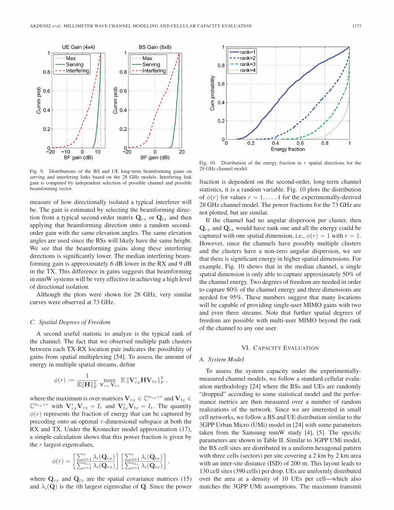
Fig. 9. Distributions of the BS and UE long-term beamforming gains onserving and interfering links based on the 28 GHz models. Interfering linkgain is computed by independent selection of possible channel and possiblebeamforming vector.

measure of how directionally isolated a typical interferer willbe. The gain is estimated by selecting the beamforming direc-tion from a typical second-order matrix Qrx or Qtx and thenapplying that beamforming direction onto a random second-order gain with the same elevation angles. The same elevationangles are used since the BSs will likely have the same height.We see that the beamforming gains along these interferingdirections is significantly lower. The median interfering beam-forming gain is approximately 6 dB lower in the RX and 9 dBin the TX. This difference in gains suggests that beamformingin mmW systems will be very effective in achieving a high levelof directional isolation.Although the plots were shown for 28 GHz, very similar

curves were observed at 73 GHz.

C. Spatial Degrees of Freedom

A second useful statistic to analyze is the typical rank ofthe channel. The fact that we observed multiple path clustersbetween each TX-RX location pair indicates the possibility ofgains from spatial multiplexing [54]. To assess the amount ofenergy in multiple spatial streams, define

φ(r) :=1

E‖H‖2Fmax

Vrx,Vtx

E ‖V∗rxHVtx‖2F ,

where the maximum is over matricesVrx ∈ Cnrx×r andVtx ∈

Cntx×r with V∗

rxVrx = Ir and V∗txVtx = Ir. The quantity

φ(r) represents the fraction of energy that can be captured byprecoding onto an optimal r-dimensional subspace at both theRX and TX. Under the Kronecker model approximation (17),a simple calculation shows that this power fraction is given bythe r largest eigenvalues,

φ(r) =

[∑ri=1 λi(Qrx)∑nrx

i=1 λi(Qrx)

] [∑ri=1 λi(Qtx)∑ntx

i=1 λi(Qtx)

],

where Qrx and Qtx are the spatial covariance matrices (15)and λi(Q) is the ith largest eigenvalue of Q. Since the power

Fig. 10. Distribution of the energy fraction in r spatial directions for the28 GHz channel model.

fraction is dependent on the second-order, long-term channelstatistics, it is a random variable. Fig. 10 plots the distributionof φ(r) for values r = 1, . . . , 4 for the experimentally-derived28 GHz channel model. The power fractions for the 73 GHz arenot plotted, but are similar.If the channel had no angular dispersion per cluster, then

Qrx and Qtx would have rank one and all the energy could becaptured with one spatial dimension, i.e., φ(r) = 1 with r = 1.However, since the channels have possibly multiple clustersand the clusters have a non-zero angular dispersion, we seethat there is significant energy in higher spatial dimensions. Forexample, Fig. 10 shows that in the median channel, a singlespatial dimension is only able to capture approximately 50% ofthe channel energy. Two degrees of freedom are needed in orderto capture 80% of the channel energy and three dimensions areneeded for 95%. These numbers suggest that many locationswill be capable of providing single-user MIMO gains with twoand even three streams. Note that further spatial degrees offreedom are possible with multi-user MIMO beyond the rankof the channel to any one user.

VI. CAPACITY EVALUATION

A. System Model

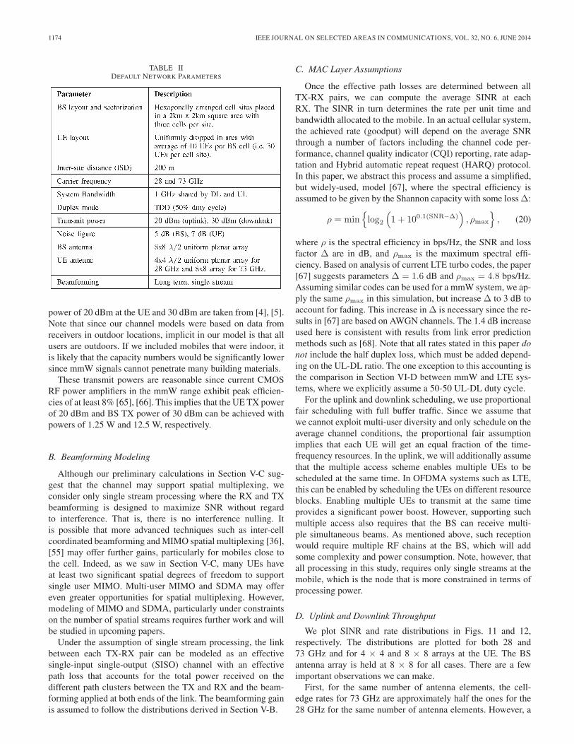
To assess the system capacity under the experimentally-measured channel models, we follow a standard cellular evalu-ation methodology [24] where the BSs and UEs are randomly“dropped” according to some statistical model and the perfor-mance metrics are then measured over a number of randomrealizations of the network. Since we are interested in smallcell networks, we follow a BS and UE distribution similar to the3GPP Urban Micro (UMi) model in [24] with some parameterstaken from the Samsung mmW study [4], [5]. The specificparameters are shown in Table II. Similar to 3GPP UMi model,the BS cell sites are distributed in a uniform hexagonal patternwith three cells (sectors) per site covering a 2 km by 2 km areawith an inter-site distance (ISD) of 200 m. This layout leads to130 cell sites (390 cells) per drop. UEs are uniformly distributedover the area at a density of 10 UEs per cell—which alsomatches the 3GPP UMi assumptions. The maximum transmit


TABLE IIDEFAULT NETWORK PARAMETERS

power of 20 dBm at the UE and 30 dBm are taken from [4], [5].Note that since our channel models were based on data fromreceivers in outdoor locations, implicit in our model is that allusers are outdoors. If we included mobiles that were indoor, itis likely that the capacity numbers would be significantly lowersince mmW signals cannot penetrate many building materials.These transmit powers are reasonable since current CMOS

RF power amplifiers in the mmW range exhibit peak efficien-cies of at least 8% [65], [66]. This implies that the UE TX powerof 20 dBm and BS TX power of 30 dBm can be achieved withpowers of 1.25 W and 12.5 W, respectively.

B. Beamforming Modeling

Although our preliminary calculations in Section V-C sug-gest that the channel may support spatial multiplexing, weconsider only single stream processing where the RX and TXbeamforming is designed to maximize SNR without regardto interference. That is, there is no interference nulling. Itis possible that more advanced techniques such as inter-cellcoordinated beamforming andMIMO spatial multiplexing [36],[55] may offer further gains, particularly for mobiles close tothe cell. Indeed, as we saw in Section V-C, many UEs haveat least two significant spatial degrees of freedom to supportsingle user MIMO. Multi-user MIMO and SDMA may offereven greater opportunities for spatial multiplexing. However,modeling of MIMO and SDMA, particularly under constraintson the number of spatial streams requires further work and willbe studied in upcoming papers.Under the assumption of single stream processing, the link

between each TX-RX pair can be modeled as an effectivesingle-input single-output (SISO) channel with an effectivepath loss that accounts for the total power received on thedifferent path clusters between the TX and RX and the beam-forming applied at both ends of the link. The beamforming gainis assumed to follow the distributions derived in Section V-B.

C. MAC Layer Assumptions

Once the effective path losses are determined between allTX-RX pairs, we can compute the average SINR at eachRX. The SINR in turn determines the rate per unit time andbandwidth allocated to the mobile. In an actual cellular system,the achieved rate (goodput) will depend on the average SNRthrough a number of factors including the channel code per-formance, channel quality indicator (CQI) reporting, rate adap-tation and Hybrid automatic repeat request (HARQ) protocol.In this paper, we abstract this process and assume a simplified,but widely-used, model [67], where the spectral efficiency isassumed to be given by the Shannon capacity with some lossΔ:

ρ = min{log2

(1 + 100.1(SNR−Δ)

), ρmax

}, (20)

where ρ is the spectral efficiency in bps/Hz, the SNR and lossfactor Δ are in dB, and ρmax is the maximum spectral effi-ciency. Based on analysis of current LTE turbo codes, the paper[67] suggests parameters Δ = 1.6 dB and ρmax = 4.8 bps/Hz.Assuming similar codes can be used for a mmW system, we ap-ply the same ρmax in this simulation, but increase Δ to 3 dB toaccount for fading. This increase inΔ is necessary since the re-sults in [67] are based on AWGN channels. The 1.4 dB increaseused here is consistent with results from link error predictionmethods such as [68]. Note that all rates stated in this paper donot include the half duplex loss, which must be added depend-ing on the UL-DL ratio. The one exception to this accounting isthe comparison in Section VI-D between mmW and LTE sys-tems, where we explicitly assume a 50-50 UL-DL duty cycle.For the uplink and downlink scheduling, we use proportional

fair scheduling with full buffer traffic. Since we assume thatwe cannot exploit multi-user diversity and only schedule on theaverage channel conditions, the proportional fair assumptionimplies that each UE will get an equal fraction of the time-frequency resources. In the uplink, we will additionally assumethat the multiple access scheme enables multiple UEs to bescheduled at the same time. In OFDMA systems such as LTE,this can be enabled by scheduling the UEs on different resourceblocks. Enabling multiple UEs to transmit at the same timeprovides a significant power boost. However, supporting suchmultiple access also requires that the BS can receive multi-ple simultaneous beams. As mentioned above, such receptionwould require multiple RF chains at the BS, which will addsome complexity and power consumption. Note, however, thatall processing in this study, requires only single streams at themobile, which is the node that is more constrained in terms ofprocessing power.

D. Uplink and Downlink Throughput

We plot SINR and rate distributions in Figs. 11 and 12,respectively. The distributions are plotted for both 28 and73 GHz and for 4 × 4 and 8 × 8 arrays at the UE. The BSantenna array is held at 8 × 8 for all cases. There are a fewimportant observations we can make.First, for the same number of antenna elements, the cell-

edge rates for 73 GHz are approximately half the ones for the28 GHz for the same number of antenna elements. However, a


Fig. 11. Downlink (top plot)/uplink (bottom plot) SINR CDF at 28 and73 GHz with 4 × 4 and 8 × 8 antenna arrays at the UE. The BS antenna arrayis held at 8 × 8.

4 × 4 λ/2-array at 28 GHz would take about the same area asan 8 × 8 λ/2 array at 73 GHz. Both would be roughly 1.5×1.5 cm2, which could be easily accommodated in a handheldmobile device. In addition, we see that 73 GHz 8 × 8 rate andSNR distributions are very close to the 28 GHz 4 × 4 distri-butions, which is reasonable since we are keeping the antennasize constant. Thus, we can conclude that the loss from going tothe higher frequencies can be made up from larger numbers ofantenna elements without increasing the physical antenna area.As a second point, we can compare the SINR distributions

in Fig. 11 to those of a traditional cellular network. Althoughthe SINR distribution for a cellular network at a traditional fre-quency is not plotted here, the SINR distributions in Fig. 11 areactually slightly better than those found in cellular evaluationstudies [24]. For example, in Fig. 11, only about 5 to 10% ofthe mobiles appear under 0 dB, which is a lower fraction thantypical cellular deployments. We conclude that, although mmWsystems have an omnidirectional path loss that is 20 to 25 dBworse than conventional microwave frequencies, short cell radiicombined with highly directional beams are able to completelycompensate for the loss.As one final point, Table III provides a comparison of

mmW and current LTE systems. The LTE capacity numbers

Fig. 12. Downlink (top plot)/uplink (bottom plot) rate CDF at 28 and 73 GHzwith 4 × 4 and 8 × 8 antenna arrays at the UE. The BS antenna array is heldat 8 × 8.

are taken from the average of industry reported evaluationsgiven in [24]—specifically Table 10.1.1.1-1 for the downlinkand Table 1.1.1.3-1 for the uplink. The LTE evaluations includeadvanced techniques such as SDMA, although not coordinatedmultipoint. For the mmW capacity, we assumed 50-50 UL-DLTDD split and a 20% control overhead in both the UL andDL directions. Note that in the spectral efficiency numbers forthe mmW system, we have included the 20% overhead, butnot the 50% UL-DL split. Hence, the cell throughput is givenby C = 0.5ρW , where ρ is the spectral efficiency, W is thebandwidth, and the 0.5 accounts for the duplexing.Under these assumptions, we see that the mmW system for

either the 28 GHz 4 × 4 array or 73 GHz 8 × 8 array providesa significant > 25-fold increase of overall cell throughput overthe LTE system. Of course, most of the gains are simply comingfrom the increased spectrum: the operating bandwidth of mmWis chosen as 1 GHz as opposed to 20 + 20 MHz in LTE—sothe mmW system has 25 times more bandwidth. However, thisis a basic mmW system with no spatial multiplexing or otheradvanced techniques—we expect even higher gains when ad-vanced technologies are applied to optimize the mmW system.While the lowest 5% cell edge rates are less dramatic, they stilloffer a 10 to 13 fold increase over the LTE cell edge rates.


TABLE IIImmW AND LTE CELL THROUGHPUT/CELL EDGE RATE COMPARISON

E. Directional Isolation

In addition to the links being in a relatively high SINR, aninteresting feature of mmW systems is that thermal noise domi-nates interference. Although the distribution of the interferenceto noise ratio is not plotted, we observed that in 90% of thelinks, thermal noise was larger than the interference—often dra-matically so. We conclude that highly directional transmissionsused in mmW systems combined with short cell radii result inlinks that are in relatively high SINR with little interference.This feature is in stark contrast to current dense cellular deploy-ments where links are overwhelmingly interference-dominated.

F. Effect of Outage

One of the significant features of mmW systems is thepresence of outage—the fact that there is a non-zero probabilitythat the signal from a given BS can be completely blockedand hence not detectable. The parameters in the hybrid LOS-NLOS-outage model (8) were based on our data in one regionof NYC. To understand the potential effects of different outageconditions, Fig. 13 shows the distribution of rates under vari-ous NLOS-LOS-outage probability models. The curve labeled“hybrid, dshift = 0” is the baseline model with parametersprovided in Table I that we have used up to now. These arethe parameters based on fitting the NYC data. This model iscompared to two models with heavier outage created by shiftingpout(d) to the left by 50 m and 75 m, shown in the secondand third curves. The fourth curve labeled “NLOS + outage,dshift = 50 m” uses the shifted outage and also removes allthe LOS links—hence all the links are either in an outage orNLOS state. In all cases, the carrier frequency is 28 GHz andwe assumed a 4 × 4 antenna array at the UE. Similar findingswere observed at 73 GHz and 8 × 8 arrays.We see that, even with a 50 m shift in the outage curve (i.e.,

making the outages occur 50 m closer than predicted by ourmodel), the system performance is not significantly affected.However, when we increase the outage even more by dshift =75 m, we start to see that many UEs cannot establish a con-

Fig. 13. Downlink (top plot)/uplink (bottom plot) rate CDF under the linkstate model with various parameters. The carrier frequency is 28 GHz. dshift isthe amount by which the outage curve in (8a) is shifted to the left.

nection to any BS since the outage radius becomes comparableto the cell radius, which is 100 m. In other words, there is anon-zero probability that mobiles physically close to a cell maybe in outage to that cell. These mobiles will need to connect


to a much more distant cell. Therefore, we see the dramaticdecrease in edge cell rate. Note that in our model, the front-to-back antenna gains are assumed to be infinite, so mobiles thatare blocked to one sector of a cell site cannot see any othersectors.Fig. 13 also shows that the throughputs are greatly benefited

by the presence of LOS links. Removing the LOS links sothat all links are in either a NLOS or outage states resultsin a significant drop in rate. However, even in this case, themmW system offers a greater than 20 fold increase in rate overthe current LTE system. It should be noted that the capacitynumbers reported in [9], which were based on an earlier versionof this paper, did not include any LOS links.We conclude that, in environments with outages condition

similar to, or even somewhat worse than the NYC environmentwhere our experiments were conducted, the system will bevery robust to outages. This is extremely encouraging sincesignal outage is one of the key concerns for the feasibilityof mmW cellular in urban environments. However, shouldoutages be dramatically worse than the scenarios in our exper-iments (for example, if the outage radius is shifted by 75 m),many mobiles will indeed lose connectivity even when theyare near a cell. In these circumstances, other techniques suchas relaying, denser cell placement or fallback to conventionalfrequencies will likely be needed. Such “near cell” outagewill likely be present when mobiles are placed indoors, orwhen humans holding the mobile device block the paths tothe cells. These factors were not considered in our mea-surements, where receivers were placed at outdoor locationswith no obstructions near the cart containing the measurementequipment.

VII. CONCLUSION

We have provided the first detailed statistical mmW channelmodels for several of the key channel parameters includingthe path loss, spatial characteristics and outage probabilities.The models are based on real experimental data collected inNew York City at 28 and 73 GHz. The models reveal thatsignals at these frequencies can be detected at least 100 m to200 m from the potential cell sites, even in absence of LOSconnectivity. In fact, through building reflections, signals atmany locations arrived with multiple path clusters to supportspatial multiplexing and diversity.Simple statistical models, similar to those in current cellular

standards such as [24] provide a good fit to the observations.Cellular capacity evaluations based on these models predictan order of magnitude increase in capacity over current state-of-the-art 4G systems under reasonable assumptions on theantennas, bandwidth and beamforming. These findings providestrong evidence for the viability of small cell outdoor mmWsystems even in challenging urban canyon environments suchas New York City.The most significant caveat in our analysis is the fact that

the measurements, and the models derived from those mea-surements, are based on outdoor street-level locations. Typicalurban cellular evaluations, however, place a large fraction ofmobiles indoors, where mmW signals will likely not penetrate.

Complete system evaluation with indoor mobiles will needfurther study. Also, indoor locations and other coverage holesmay be served either via multihop relaying or fallback toconventional microwave cells and further study will be neededto quantify the performance of these systems.

ACKNOWLEDGMENT

The authors would like to deeply thank several studentsand colleagues for providing the path loss data [19]–[22] thatmade this research possible: Yaniv Azar, Felix Gutierrez,DuckDong Hwang, Rimma Mayzus, George MacCartney,ShuaiNie, JocelynK.Schulz,KevinWang,GeorgeN.Wong, andHang Zhao. This work also benefited significantly from dis-cussions with our industrial partners in the NYU WIRELESSprogram including Samsung, Qualcomm, NSN, and Intel.

REFERENCES

[1] Cisco Visual Network Index: Global Mobile Traffic Forecast Update,Cisco, San Jose, CA, USA, 2013.

[2] “Traffic and market data report,” Kista, Sweden, 2011.[3] “MOBILE traffic forecasts: 2010–2020 report,” in Proc. UMTS Forum

Rep., Zürich, Switzerland, 2011, vol. 44, pp. 1–92.[4] F. Khan and Z. Pi, “Millimeter-wave Mobile Broadband (MMB): Un-

leashing 3–300 GHz spectrum,” in Proc. IEEE Sarnoff Symp., Mar. 2011,pp. 1–6.

[5] F. Khan and Z. Pi, “An introduction to millimeter-wave mobile broadbandsystems,” IEEE Commun. Mag., vol. 49, no. 6, pp. 101–107, Jun. 2011.

[6] T. S. Rappaport, J. N. Murdock, and F. Gutierrez, “State of the art in60-GHz integrated circuits and systems for wireless communications,”Proc. IEEE, vol. 99, no. 8, pp. 1390–1436, Aug. 2011.

[7] P. Pietraski, D. Britz, A. Roy, R. Pragada, and G. Charlton, “Millimeterwave and terahertz communications: Feasibility and challenges,” ZTECommun., vol. 10, no. 4, pp. 3–12, Dec. 2012.

[8] F. Boccardi, R. W. Heath, Jr., A. Lozano, T. L. Marzetta, and P. Popovski,“Five disruptive technology directions for 5G,” IEEE Commun. Mag.,vol. 52, no. 2, pp. 74–80, Feb. 2014.

[9] S. Rangan, T. S. Rappaport, and E. Erkip, “Millimeter-wave cellular wire-less networks: Potentials and challenges,” Proc. IEEE, vol. 102, no. 3,pp. 366–385, Mar. 2014.

[10] C. Doan, S. Emami, D. Sobel, A. Niknejad, and R. Brodersen, “Designconsiderations for 60 GHz CMOS radios,” IEEE Commun. Mag., vol. 42,no. 12, pp. 132–140, Dec. 2004.

[11] C. Doan, S. Emami, A. Niknejad, and R. Brodersen, “Millimeter-waveCMOS design,” IEEE J. Solid-State Circuits, vol. 40, no. 1, pp. 144–155,Jan. 2005.

[12] Y.-P. Zhang and D. Liu, “Antenna-on-chip and antenna-in-package solu-tions to highly integrated millimeter-wave devices for wireless communi-cations,” IEEE Trans. Antennas Propag., vol. 57, no. 10, pp. 2830–2841,Oct. 2009.

[13] F. Gutierrez, S. Agarwal, K. Parrish, and T. S. Rappaport, “On-chip inte-grated antenna structures in CMOS for 60 GHz WPAN systems,” IEEE J.Sel. Areas Commun., vol. 27, no. 8, pp. 1367–1378, Oct. 2009.

[14] J. Nsenga, A. Bourdoux, and F. Horlin, “Mixed analog/digital beamform-ing for 60 GHz MIMO frequency selective channels,” in Proc. IEEE ICC,2010, pp. 1–6.

[15] S. Rajagopal, S. Abu-Surra, Z. Pi, and F. Khan, “Antenna array design formulti-gbps mmwave mobile broadband communication,” in Proc. IEEEGLOBECOM, 2011, pp. 1–6.

[16] K.-C. Huang and D. J. Edwards, Millimetre Wave Antennas for GigabitWireless Communications: A Practical Guide to Design and Analysis in aSystem Context. Hoboken, NJ, USA: Wiley, 2008.

[17] F. Rusek et al., “Scaling up MIMO: Opportunities and challenges withvery large arrays,” IEEE Signal Process. Mag., vol. 30, no. 1, pp. 40–60,Jan. 2013.

[18] T. S. Rappaport, Wireless Communications: Principles and Practice,2nd ed. Upper Saddle River, NJ, USA: Prentice-Hall, 2002.

[19] Y. Azar et al., “28 GHz propagation measurements for outdoor cellularcommunications using steerable beam antennas in New York City,” inProc. IEEE ICC, 2013, pp. 5143–5147.


[20] H. Zhao et al., “28 GHz millimeter wave cellular communication mea-surements for reflection and penetration loss in and around buildings inNew York City,” in Proc. IEEE ICC, 2013, pp. 5163–5167.

[21] M. K. Samimi et al., “28 GHz angle of arrival and angle of departure anal-ysis for outdoor cellular communications using steerable beam antennasin New York City,” in Proc. IEEE VTC, 2013, pp. 1–6.

[22] T. S. Rappaport et al., “Millimeter wave mobile communications for 5Gcellular: It will work!” IEEE Access, vol. 1, pp. 335–349, May 2013.

[23] S. Sun and T. S. Rappaport, “Multi-beam antenna combining for28 GHz cellular link improvement in urban environments,” in Proc. IEEEGLOBECOM, Atlanta, GA, USA, Dec. 2013, pp. 3859–3864.

[24] “Further advancements for E-UTRA physical layer aspects,” Sophia-Antipolis, France, TR 36.814 (release 9), 2010.

[25] “M.2134: Requirements related to technical performance for IMT-advanced radio interfaces,” Geneva, Switzerland, Tech. Rep., 2009.

[26] T. S. Rappaport, R. W. Heath, Jr., R. Daniels, and J. Murdock,Millimeter Wave Wireless Communications. Upper Saddle River, NJ,USA: Prentice-Hall, 2015.

[27] A. Adhikary et al., “Joint spatial division and multiplexing for mm-wavechannels,” IEEE J. Sel. Areas Commun., to be published.

[28] M. R. Akdeniz, Y. Liu, S. Rangan, and E. Erkip, “Millimeter wavepicocellular system evaluation for urban deployments,” in Proc. IEEEGlobecom Workshops, Dec. 2013, pp. 105–110.

[29] T. Zwick, T. Beukema, and H. Nam, “Wideband channel sounder withmeasurements and model for the 60 GHz indoor radio channel,” IEEETrans. Veh. Technol., vol. 54, no. 4, pp. 1266–1277, Jul. 2005.

[30] F. Giannetti, M. Luise, and R. Reggiannini, “Mobile and personal commu-nications in 60 GHz band: A survey,” Wirelesss Pers. Commun., vol. 10,no. 2, pp. 207–243, Jul. 1999.

[31] C. R. Anderson and T. S. Rappaport, “In-building wideband partition lossmeasurements at 2.5 and 60 GHz,” IEEE Trans. Wireless Commun., vol. 3,no. 3, pp. 922–928, May 2004.

[32] P. Smulders and A. Wagemans, “Wideband indoor radio propagation mea-surements at 58 GHz,” Electron. Lett., vol. 28, no. 13, pp. 1270–1272,Jun. 1992.

[33] T. Manabe, Y. Miura, and T. Ihara, “Effects of antenna directiv-ity and polarization on indoor multipath propagation characteristics at60 GHz,” IEEE J. Sel. Areas Commun., vol. 14, no. 3, pp. 441–448,Apr. 1996.

[34] E. Ben-Dor, T. S. Rappaport, Y. Qiao, and S. J. Lauffenburger,“Millimeter-wave 60 GHz outdoor and vehicle AOA propagationmeasurements using a broadband channel sounder,” in Proc. IEEEGLOBECOM, 2011, pp. 1–6.

[35] H. Xu, V. Kukshya, and T. S. Rappaport, “Spatial and temporal character-istics of 60 GHz indoor channel,” IEEE J. Sel. Areas Commun., vol. 20,no. 3, pp. 620–630, Apr. 2002.

[36] H. Zhang, S. Venkateswaran, and U. Madhow, “Channel modeling andMIMO capacity for outdoor millimeter wave links,” in Proc. IEEEWCNC, Apr. 2010, pp. 1–6.

[37] S. Akoum, O. E. Ayach, and R. W. Heath, Jr., “Coverage and capacityin mmWave cellular systems,” in Proc. Asilomar Conf. Signals, Syst.Comput., Pacific Grove, CA, USA, Nov. 2012, pp. 688–692.

[38] A. Elrefaie and M. Shakouri, “Propagation measurements at 28 GHz forcoverage evaluation of local multipoint distribution service,” in Proc.Wireless Commun. Conf., Aug. 1997, pp. 12–17.

[39] S. Seidel and H. Arnold, “Propagation measurements at 28 GHzto investigate the performance of Local Multipoint Distribution Ser-vice (LMDS),” in Proc. IEEE Global Telecommun. Conf., Nov. 1995,pp. 754–757.

[40] T. S. Rappaport et al., “Broadband millimeter-wave propagation mea-surements and models using adaptive-beam antennas for outdoor urbancellular communications,” IEEE Trans. Antennas Propag., vol. 61, no. 4,pp. 1850–1859, Apr. 2013.

[41] T. S. Rappaport, E. Ben-Dor, J. Murdock, and Y. Qiao, “38 GHz and60 GHz angle-dependent propagation for cellular and peer-to-peer wire-less communications,” in Proc. IEEE ICC, Jun. 2012, pp. 4568–4573.

[42] T. S. Rappaport, E. Ben-Dor, J. Murdock, Y. Qiao, and J. Tamir, “Cellularbroadband millimeter wave propagation and angle of arrival for adaptivebeam steering systems,” in Proc. IEEE RWS, Jan. 2012, pp. 151–154.

[43] J. Murdock, E. Ben-Dor, Y. Qiao, J. Tamir, and T. S. Rappaport, “A38 GHz cellular outage study for an urban outdoor campus environment,”in Proc. IEEE WCNC, Apr. 2012, pp. 3085–3090.

[44] G. R. MacCartney, Jr., J. Zhang, S. Nie, and T. S. Rappaport, “Path lossmodels for 5G millimeter wave propagation channels in urban micro-cells,” in Proc. IEEE GLOBECOM, Dec. 2013, pp. 3109–3121.

[45] J. A. Wells, “Faster than fiber: The future of multi-Gb/s wireless,” IEEEMicrow. Mag., vol. 10, no. 3, pp. 104–112, May 2009.

[46] G. R. MacCartney, Jr., M. K. Samimi, and T. S. Rappaport, “Omnidirec-tional path loss models in New York City at 28 GHz and 73 GHz,” inProc. IEEE PIMRC, Washington, DC, USA, Sep. 2014, to be published.

[47] H. L. Van Trees, Detection, Estimation and Modulation Theory, Part I.New York, NY, USA: Wiley, 2001.

[48] M. K. Samimi and T. S. Rappaport, “Ultra-wideband statistical channelmodel for non line of sight millimeter-wave urban channels,” in Proc.IEEE GLOBECOM, Exhib. Ind. Forum, to be published.

[49] C. M. Bishop, Pattern Recognition and Machine Learning. New York,NY, USA: Springer-Verlag, 2006, ser. Information Science and Statistics.

[50] P. Kyösti et al., WINNER II Channel Models Part II Radio ChannelMeasurement and Analysis Results, 2007, IST-4-027756 WINNER IID1.1.2 V1.0.

[51] T. Bai and R. W. Heath, Jr., “Coverage and Rate Analysis for MillimeterWave Cellular Networks,” Mar. 2014, arXiv:1402.6430v2 [cs.ITpey1a].

[52] T. Bai, R. Vaze, and R. W. Heath, Jr., “Analysis of Blockage Effects onUrban Cellular Networks,” Sep. 2013, arXiv preprint arXiv:1309.4141.

[53] S. Nie, G. R. MacCartney, Jr., S. Sun, and T. S. Rappaport, “28 GHz and73 GHz signal outage study for millimeter wave cellular and backhaulcommunications,” in Proc. IEEE ICC, to be published.

[54] D. Tse and P. Viswanath, Fundamentals of Wireless Communication.Cambridge, U.K.: Cambridge Univ. Press, 2007.

[55] A. Alkhateeb, O. E. Ayach, G. Leus, and R.W. Heath, Jr., “Hybrid precod-ing for millimeter wave cellular systems with partial channel knowledge,”in Proc. ITA Workshop, Feb. 2013, pp. 1–5.

[56] D. Parker and D. Z. Zimmermann, “Phased arrays-Part I: Theory andarchitecture,” IEEE Trans. Microw. Theory Tech., vol. 50, no. 3, pp. 678–687, Mar. 2002.

[57] K.-J. Koh and G. M. Rebeiz, “0.13-μm CMOS phase shifters for X-, Ku-and K-band phased arrays,” IEEE J. Solid-State Circuits, vol. 42, no. 11,pp. 2535–2546, Nov. 2007.

[58] K.-J. Koh and G.M. Rebeiz, “Amillimeter-wave (40–45 GHz) 16-elementphased-array transmitter in 0.18-μm SiGe BiCMOS technology,” IEEE J.Solid-State Circuits, vol. 44, no. 5, pp. 1498–1509, May 2009.

[59] P. E. Crane, “Phased array scanning system,” U.S. Patent 4 731 614,Mar. 15, 1988.

[60] S. Raman, N. S. Barker, and G. M. Rebeiz, “A W-band dielectric lens-based integrated monopulse radar receive,” IEEE Trans. Microw. TheoryTech., vol. 46, no. 12, pp. 2308–2316, Dec. 1998.

[61] X. Guan, H. Hashemi, and A. Hajimiri, “A fully integrated 24-GHz eight-element phased-array receiver in silicon,” IEEE J. Solid-State Circuits,vol. 39, no. 12, pp. 2311–2320, Dec. 2004.

[62] A. Lozano, “Long-term transmit beamforming for wireless multicasting,”in Proc. IEEE ICASSP, 2007, vol. 3, pp. III-417–III-420.

[63] J. P. Kermoal, L. Schumacher, K. I. Pedersen, P. E. Mogensen, andF. Frederiksen, “A stochastic MIMO radio channel model with experi-mental validation,” IEEE J. Sel. Areas Commun., vol. 20, no. 6, pp. 1211–1226, Aug. 2002.

[64] D. McNamara, M. Beach, and P. Fletcher, “Spatial correlation in indoorMIMO channels,” in Proc. IEEE PIMRC, 2002, vol. 1, pp. 290–294.

[65] S. Pinel et al., “A 90 nm CMOS 60 GHz radio,” in Proc. IEEE Int. Solid-State Circuits Conf., 2008, pp. 130–601.

[66] C. Marcu et al., “A 90 nm CMOS low-power 60 GHz transceiver with in-tegrated baseband circuitry,” IEEE J. Solid-State Circuits, vol. 44, no. 12,pp. 3434–3447, Dec. 2009.

[67] P. Mogensen et al., “LTE capacity compared to the Shannon bound,” inProc. IEEE VTC, 2007, pp. 1234–1238.

[68] J. C. Ikuno, C. Mehlfuhrer, and M. Rupp, “A novel link error predic-tion model for OFDM systems with HARQ,” in Proc. IEEE ICC, 2011,pp. 1–5.

Mustafa Riza Akdeniz (S’09) received the B.S.degree in electrical and electronics engineering fromBogazici University, Istanbul, Turkey, in 2010. He iscurrently working toward the Ph.D. degree in electri-cal and computer engineering at New York Univer-sity Polytechnic School of Engineering, Brooklyn,NY, USA, with Prof. Rangan. His research interestsinclude wireless communications, channel modeling,and information theory.


Yuanpeng Liu received the B.S. degree from theUniversity of Electronic Science and Technology ofChina, Chengdu, China, in 2007 and the M.S. andPh.D. degrees from New York University (NYU)Polytechnic School of Engineering, Brooklyn, NY,USA, in 2009 and 2013, respectively, all in electricalengineering. His research at NYU was primarilyfocused on information theoretic study of wirelesschannels and millimeter-wave broadband access sys-tem design.

Mathew K. Samimi (S’13) received the B.S. de-gree in applied physics in 2012 from Columbia Uni-versity, New York, NY, USA, and the M.S. degreein electrical engineering in 2014 from New YorkUniversity Polytechnic School of Engineering,Brooklyn, NY, USA, where he is currently work-ing toward the Ph.D. degree in electrical engi-neering with Prof. Rappaport in developing futuremillimeter-wave statistical spatial channel modelsfor next-generation ultrawideband mobile cellular indense urban environments.

Shu Sun (S’13) received the B.S. degree in ap-plied physics from Shanghai Jiao Tong University,Shanghai, China, in 2012. She is currently workingtoward the Ph.D. degree in electrical engineering atNew York University Polytechnic School of Engi-neering, Brooklyn, NY, USA. Since August 2012,she has been with NYU WIRELESS, New YorkUniversity Polytechnic School of Engineering. Shehas coauthored two conference publications andis now working on a millimeter-wave (mmWave)propagation measurements campaign for 5G cellular

mmWave communication systems.

Sundeep Rangan (M’02–SM’14) received theB.A.Sc. degree from the University of Waterloo,Waterloo, ON, Canada, and the M.Sc. and Ph.D.degrees from the University of California, Berkeley,CA, USA, all in electrical engineering. He has heldpostdoctoral appointments with the University ofMichigan, Ann Arbor, MI, USA, and Bell Labo-ratories. In 2000, he cofounded (with four others)Flarion Technologies, a spin-off of Bell Laborato-ries that developed Flash OFDM, the first cellularOFDM data system. In 2006, Flarion was acquired

by Qualcomm Technologies. He was a Director of Engineering at Qualcomminvolved in OFDM infrastructure products. In 2010, he joined the Departmentof Electrical and Computer Engineering, New York University PolytechnicSchool of Engineering, Brooklyn, NY, USA, where he is currently an Asso-ciate Professor. His research interests are in wireless communications, signalprocessing, information theory, and control theory.

Theodore (Ted) S. Rappaport (S’83–M’84–SM’91–F’98) is the David Lee/Ernst WeberProfessor of Electrical and Computer Engineeringwith New York University (NYU) PolytechnicSchool of Engineering, Brooklyn, NY, USA, andis the Founding Director of NYU WIRELESS. Healso holds professorships with Courant Institute ofMathematical Sciences and the School of Medicine,NYU. He founded major wireless research centers atVirginia Polytechnic Institute and State University,Blacksburg, VA, USA; The University of Texas at

Austin, Austin, TX, USA; and New York University, New York, NY, USA, andfounded two wireless technology companies that were sold to publicly tradedfirms. He is a highly sought-after Technical Consultant, having testified beforethe U.S. Congress and having served the ITU. He has advised more than 100students, has more than 100 patents issued and pending, and has authored orcoauthored several books, including the best seller Wireless Communications:Principles and Practice, Second Edition (Prentice Hall, 2002). His latest book,Millimeter Wave Wireless Communications, is the first comprehensive text onthe subject and is published by Pearson/Prentice Hall.

Elza Erkip (S’93–M’96–SM’05–F’11) received theB.S. degree in electrical and electronics engineer-ing from Middle East Technical University, Ankara,Turkey, and the M.S. and Ph.D. degrees in electri-cal engineering from Stanford University, Stanford,CA, USA. Currently, she is a Professor of elec-trical and computer engineering with New YorkUniversity Polytechnic School of Engineering,Brooklyn, NY, USA. Her research interests are ininformation theory, communication theory and wire-less communications.

Dr. Erkip is a Member of the Science Academy Society of Turkey. Shereceived the National Science Foundation CAREER award in 2001, theIEEE Communications Society Stephen O. Rice Paper Prize in 2004, theIEEE ICC Communication Theory Symposium Best Paper Award in 2007,and the IEEE Communications Society Award for Advances in Communi-cation in 2013. She coauthored a paper that received the IEEE InternationalSymposium on Information Theory Student Paper Award in 2007. Currently,she is a Distinguished Lecturer and a Member of the Board of Governors ofIEEE Information Theory Society. Dr. Erkip is a Guest Editor of the IEEEJOURNAL ON SELECTED AREAS IN COMMUNICATIONS in 2014. She was anAssociate Editor of the IEEE TRANSACTIONS ON INFORMATION THEORYfrom 2009 to 2011, an Associate Editor of the IEEE TRANSACTIONS ON

COMMUNICATIONS from 2006 to 2008, a Publications Editor of the IEEETRANSACTIONS ON INFORMATION THEORY from 2006 to 2008 and a GuestEditor of the IEEE Signal Processing Magazine in 2007. She was a GeneralChair of the IEEE International Symposium of Information Theory in 2013;a Technical Program Chair of the International Symposium on Modeling andOptimization in Mobile, Ad Hoc, and Wireless Networks (WiOpt) in 2011; aTechnical Program Chair of the IEEE GLOBECOM Communication TheorySymposium in 2009; the Publications Chair of the IEEE Information TheoryWorkshop, Taormina, in 2009; the Technical Area Chair for the MIMO Com-munications and Signal Processing track of Asilomar Conference on Signals,Systems, and Computers in 2007; and a Technical Program Chair of the IEEECommunication Theory Workshop in 2006.

Millimeter Wave Channel Modeling and Cellular Capacity ... · AKDENIZet al.:MILLIMETER WAVE CHANNEL MODELING AND CELLULAR CAPACITY EVALUATION 1165 Statistical models are then derived

Documents