MIDAS SVX Combined CTD & SVP - Valeport Velocity...MIDAS SVX Combined CTD & SVP Operating Manual Section 2, Page 5 0650816b.doc 2 OPENING DATALOG 400 Double clicking the desktop icon

© Valeport Limited

MIDAS SVX Combined CTD & SVP Operating Manual Section 2, Page 1 0650816b.doc

MIDAS SVX Combined CTD & SVP

Section 2 - Software Operation

© Valeport Limited


CHAPTER DESCRIPTION PAGE

1 INTRODUCTION...................................................................................................................... 4 1.1 Installation............................................................................................................................ 4

2 OPENING DATALOG 400......................................................................................................... 5

3 ESTABLISHING COMMUNICATIONS ....................................................................................... 6

4 INSTRUMENT SETUP................................................................................................................ 8 4.1 Standard............................................................................................................................... 8

4.1.1 Set Button ................................................................................................................... 8 4.1.2 Data Output ................................................................................................................... 9 4.1.3 Pressure Tare Setting....................................................................................................... 9 4.1.4 Logging Options........................................................................................................... 10 4.1.5 Clock Settings & Delay Start ......................................................................................... 10 4.1.6 Quick Setup ................................................................................................................. 11

4.1.6.1 Saving a Quick Setup Regime............................................................................ 11 4.1.6.2 Selecting a Quick Setup Regime........................................................................ 11

4.1.7 Sampling Modes & Patterns .......................................................................................... 11 4.1.7.1 Single Mode...................................................................................................... 12 4.1.7.2 Hold Mode ....................................................................................................... 12 4.1.7.3 Continuous Mode ............................................................................................. 13 4.1.7.4 Trip Mode......................................................................................................... 13 4.1.7.5 Burst Mode ....................................................................................................... 14 4.1.7.6 CMA (Continuous Moving Average) .................................................................. 15

4.2 Sensor Setup ...................................................................................................................... 16 4.2.1 Trip Mode ................................................................................................................. 17 4.2.2 Tare Option ................................................................................................................. 17 4.2.3 User Calibration ........................................................................................................... 18

4.3 Advanced ...................................................................................................................... 19 4.3.1 Output Separator.......................................................................................................... 19 4.3.2 Local Conditions .......................................................................................................... 19 4.3.3 Conditional Sampling ................................................................................................... 20

4.3.3.1 Setting up Conditional Sampling ....................................................................... 20 4.3.3.2 Conditional Sampling Triggers........................................................................... 20 4.3.3.3 Conditional Sampling ‘Off’ Triggers................................................................... 21

5 RUNNING THE INSTRUMENT................................................................................................ 22 5.1 Hardware Switch On.......................................................................................................... 22 5.2 Software Switch On............................................................................................................ 22

5.2.1 Method 1 ................................................................................................................. 22 5.2.2 Method 2 ................................................................................................................. 22 5.2.3 Run ................................................................................................................. 22

5.3 Real Time Data................................................................................................................... 23 5.3.1 Real Time Data Logging ............................................................................................... 23 5.3.2 Select Max Viewable Data Points ................................................................................. 23

6 UPLOAD & MEMORY............................................................................................................. 24 6.1 Upload ...................................................................................................................... 24

6.1.1 File Table ................................................................................................................. 24 6.1.2 Site Information............................................................................................................ 25 6.1.3 Change File Name........................................................................................................ 25 6.1.4 Upload Parameters ....................................................................................................... 25 6.1.5 Memory Management .................................................................................................. 26 6.1.6 Upload Files................................................................................................................. 26

6.2 Translate ...................................................................................................................... 27

© Valeport Limited


CHAPTER DESCRIPTION PAGE

7 DATA VIEWING...................................................................................................................... 29 7.1 Opening Stored Data Files .................................................................................................. 29 7.2 Simple Display ................................................................................................................... 30 7.3 Scroll Display ..................................................................................................................... 31 7.4 Graphical Display .............................................................................................................. 32

7.4.1 Scroll & Focus .............................................................................................................. 34 7.4.2 Rotate ................................................................................................................. 35 7.4.3 Move ................................................................................................................. 35 7.4.4 Zoom ................................................................................................................. 36 7.4.5 Depth ................................................................................................................. 36

8 CALCULATION....................................................................................................................... 37

9 ABOUT ........................................................................................................................... 38

10 CALCULATION FORMULAE ................................................................................................... 39 10.1 Salinity ...................................................................................................................... 39 10.2 Density Anomaly Gamma................................................................................................... 41 10.3 Speed Of Sound ................................................................................................................. 42

10.3.1 Standard Formulae ....................................................................................................... 43 10.3.1.1 Pressure/Depth Relationship.............................................................................. 43 10.3.1.2 Wood (1949) .................................................................................................... 43 10.3.1.3 Wilson (October 1960) ..................................................................................... 44 10.3.1.4 Medwin (1975) ................................................................................................. 45 10.3.1.5 Chen and Millero (1977) ................................................................................... 46 10.3.1.6 Del Grosso (1974)............................................................................................. 47 10.3.1.7 MacKenzie (1981)............................................................................................. 48

10.3.2 Discussion ................................................................................................................. 49 10.3.2.1 Development of Formulae................................................................................. 49 10.3.2.2 Comparison of Formulae................................................................................... 49 10.3.2.3 The Pressure/Depth Algorithm........................................................................... 50

10.3.3 Conclusions ................................................................................................................. 51

© Valeport Limited


1 INTRODUCTION

DataLog 400 is the user interface program supplied with all 400 Series systems from Valeport Ltd, including the MIDAS SVX Combined CTD & SVP. The program is written in Delphi, and will run on all PCs operating Windows 95 or above. As is the nature of all software, the faster the computer, the better the software will perform. As an absolute minimum, we recommend the following PC specification: • Pentium 100MHz (or equivalent) • 32Mbyte RAM • CDROM Drive • 1 spare comm port • 100Mbyte Disk Space Note that installation of DataLog 400 itself requires only 5.4Mbyte of disk space. However, Windows will utilise a large amount of disk space as “virtual memory” (upwards of 20Mbyte), which must be taken into account. Further, note that an 8Mbyte binary file from the instrument will translate to over 55Mbyte of calibrated text files – make sure that there is enough hard disk space to allow for translation of any uploaded files. This manual will guide the operator through all the functions that DataLog 400 and the MIDAS SVX have to offer, including the wide variety of sampling regimes (including conditional sampling), data extraction and data viewing. Please note that although DataLog 400 offers a variety of data display modes, users may wish to utilise a standard spreadsheet package such as Microsoft Excel for data manipulation.

1.1 INSTALLATION

As with all installation programs, we recommend that all other applications be closed before commencing installation. DataLog 400 is supplied on a single CDROM. It does not feature an Auto-run facility, so users will be required to insert the CDROM into their CD drive, and run the Setup.exe program manually. This can be done either by selecting Run from the Start menu, and browsing for the Setup.exe file under the CD drive (typically drive D or E), or by clicking on the Setup.exe program under the CD drive in Windows Explorer. The Setup.exe program will launch a wizard that will guide the user through the remainder of the installation process. By default, the installation program will create a new directory in which to install DataLog 400, although you may change this if you wish:

C:\Program Files\DataLog 400 On completion of installation, a window will appear with a shortcut icon to the program. This may be dragged onto the desktop if required: Note that DataLog 400 software is distributed free with the equipment – therefore no password or software key is required for installation. To Run the software, simply double click the Desktop icon. The following pages describe the operation of the software.

© Valeport Limited


2 OPENING DATALOG 400

Double clicking the desktop icon ( ), or running the DataLog 400.exe program through Windows Explorer, will reveal the following screen, which allows access to all major DataLog 400 functions. Note that all features are accessed through a selection of tabs at the top of the page – there is no menu bar. Also note that at any point in the software, only tabs which are relevant will be visible. The Calculation and About tabs, which are less important in terms of instrument operation and data viewing, are covered in later Chapters.

If the user wishes to close down DataLog 400 at any time, simply click on the Exit button: If for any reason communications are lost, the “Stop Trying” button may be used. Clicking on this button will return the user to this point in the software: The major functions that DataLog 400 will allow at this point are as follows. Each function is described fully at subsequent chapters in this manual. Note also the section of the screen titled “Real Time Data”. Please refer to Chapter 5 for details of this section.

Establishes communications with the instrument, and causes the unit to wait for further instructions. See Chapter 3. Puts the instrument into Run mode. This button should only be used if the user is confident of the current instrument settings. See Chapter 5.

View an existing data file, either previously uploaded and translated, or saved from the real time output. See Chapter 7. If the user wishes to translate any previously uploaded binary files into viewable text files, click on this button, and refer to Chapter 6.2.

© Valeport Limited


3 ESTABLISHING COMMUNICATIONS

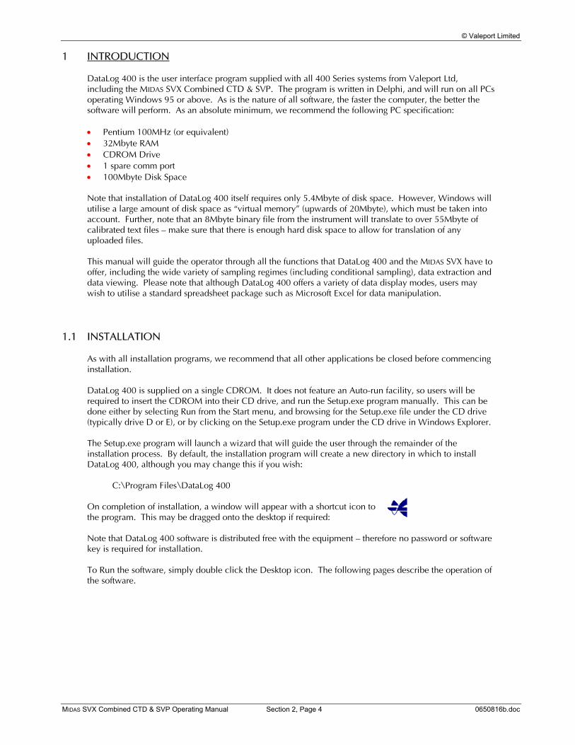
After connecting the instrument to the PC using the 3m Y lead as described in Section 1 of this manual, the first step in establishing communications with the instrument is to select the correct communications (comm) port. A drop down menu allows the user to select from up to 4 available comm ports. Selecting the incorrect comm port is the most likely reason for any failure to communicate. Note that all Valeport 400 Series instruments (i.e. instruments designed to work with DataLog 400) are fitted with three standard digital data outputs – RS232, RS485 and RS422 – and one optional output, FSK modem. RS232 format can be read directly by a PC comm port. If using any of the other 3 methods, the PC will need to be fitted with a suitable interface, which will either be a special adaptor unit supplied by Valeport, or in the form of an additional circuit board added to the PC. If using RS485 or FSK communications, please check the box next to the comm port selection box. This will slightly alter the protocol that DataLog 400 uses to communicate with the instrument (note that FSK comms defaults to 19200 baud rate). It is important that the boxes are left unchecked if just standard RS232 communications or RS422 communications are being used. The next step in establishing communications is to select the required baud rate. The instrument will automatically detect which baud rate is being used, but note that the longer the cable being used, the slower the rate that will be required. A guide to suitable baud rates is given in the drop down menu. Note also that even some new PCs may be fitted with low quality comm ports – users may find that a lower baud rate is necessary. Next, ensure that the instrument is turned on! If running on internal batteries, turn the switch on the 3m Y lead to the INT position. If running on external power, turn the switch to the EXT position, and make sure that the power supply is turned on. All Valeport 400 Series instruments (i.e. instruments designed to work with DataLog 400) can be interrupted at any point during their operation, whether they are actually in the process of sampling or in a sleep mode between bursts. Finally, click on the Interrupt button: During operation, DataLog 400 will show the current status of the software at the bottom of the screen:

The left hand section shows the software status, the centre section shows the last response from the instrument, and the right hand section shows the PC date and time. The Autobauding procedure by which the instrument detects which baud rate is being used may take up to 15 seconds to complete – please be patient while the software shows “Attempting to Communicate”. After the baud rate has been established, the instrument will send various pieces of information to the software, including Serial Number, type and number of sensors fitted, current sampling setup and so on. Again, this may take some seconds to complete, so please be patient!

© Valeport Limited


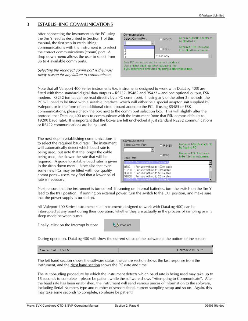
Once DataLog 400 has communicated with the instrument, an information screen appears detailing connection information, and basic sensor information such as serial number, code and name of all fitted sensors, and software version. To clear this screen, simply click on OK.

© Valeport Limited


4 INSTRUMENT SETUP

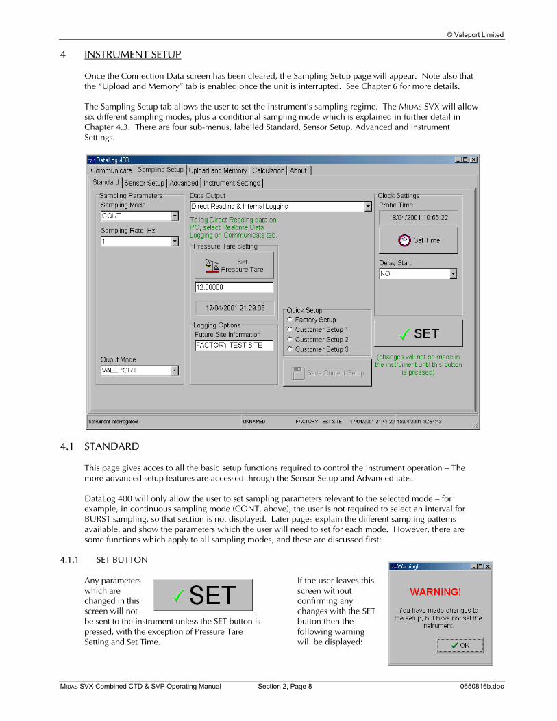
Once the Connection Data screen has been cleared, the Sampling Setup page will appear. Note also that the “Upload and Memory” tab is enabled once the unit is interrupted. See Chapter 6 for more details. The Sampling Setup tab allows the user to set the instrument’s sampling regime. The MIDAS SVX will allow six different sampling modes, plus a conditional sampling mode which is explained in further detail in Chapter 4.3. There are four sub-menus, labelled Standard, Sensor Setup, Advanced and Instrument Settings.

4.1 STANDARD

This page gives acces to all the basic setup functions required to control the instrument operation – The more advanced setup features are accessed through the Sensor Setup and Advanced tabs. DataLog 400 will only allow the user to set sampling parameters relevant to the selected mode – for example, in continuous sampling mode (CONT, above), the user is not required to select an interval for BURST sampling, so that section is not displayed. Later pages explain the different sampling patterns available, and show the parameters which the user will need to set for each mode. However, there are some functions which apply to all sampling modes, and these are discussed first:

4.1.1 SET BUTTON

Any parameters which are changed in this screen will not be sent to the instrument unless the SET button is pressed, with the exception of Pressure Tare Setting and Set Time.

If the user leaves this screen without confirming any changes with the SET button then the following warning will be displayed:

© Valeport Limited


4.1.2 DATA OUTPUT

The MIDAS SVX can operate in three data output modes. The data may either be logged to the internal memory (Internal Logging), output in real time (Direct Reading), or both of these together (Direct Reading and Internal Logging). Simply select the required data output mode from the drop down menu. Note the green information point under this part of the screen – if real time data is being output to PC, it can be logged as a separate text file – please refer to Chapter 5.3.1.

4.1.3 PRESSURE TARE SETTING

The user may wish to set a Pressure Tare value. In underwater instruments, pressure sensors are usually of the absolute type – that is to say, they measure the total pressure exerted on the transducer face, including atmospheric pressure. It is often the case that the user wishes to disregard the atmospheric pressure, particularly in short term deployments where it is unlikely to change significantly over the deployment period. If this is the case, then a Tare value can be set. This is done by positioning the instrument at sea level, and taking a pressure reading. This reading is recorded in the instrument as being the atmospheric pressure at time of deployment, and may be subtracted from all subsequent pressure readings. Press the Set Pressure Tare button to take a Pressure Tare reading. The current Pressure Tare value is indicated in the text box below the button. Alternatively, the user may enter their own desired value for the Pressure Tare by simply typing in the text box and then clicking the Set Pressure Tare button. This is particularly useful for resetting the Tare value to zero. Having taken a Pressure Tare reading, the user still has the choice of whether or not to actually subtract this value from the subsequent pressure readings, or just keep it as a record of the atmospheric pressure at time of deployment. Please refer to the Sensor Setup tab to confirm whether the Tare value should actually be used or not (Chapter 4.2.2)

© Valeport Limited


4.1.4 LOGGING OPTIONS

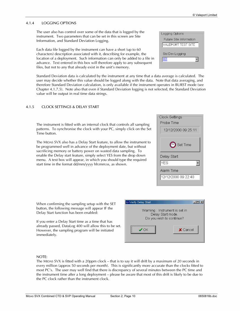
The user also has control over some of the data that is logged by the instrument. Two parameters that can be set in this screen are Site Information, and Standard Deviation Logging. Each data file logged by the instrument can have a short (up to 60 characters) description associated with it, describing for example, the location of a deployment. Such information can only be added to a file in advance. Text entered in this box will therefore apply to any subsequent files, but not to any that already exist in the unit’s memory. Standard Deviation data is calculated by the instrument at any time that a data average is calculated. The user may decide whether this value should be logged along with the data. Note that data averaging, and therefore Standard Deviation calculation, is only available if the instrument operates in BURST mode (see Chapter 4.1.7.5). Note also that even if Standard Deviation logging is not selected, the Standard Deviation value will be output in real time data strings.

4.1.5 CLOCK SETTINGS & DELAY START

The instrument is fitted with an internal clock that controls all sampling patterns. To synchronise the clock with your PC, simply click on the Set Time button. The MIDAS SVX also has a Delay Start feature, to allow the instrument to be programmed well in advance of the deployment date, but without sacrificing memory or battery power on wasted data sampling. To enable the Delay start feature, simply select YES from the drop down menu. A text box will appear, in which you should type the required start time in the format dd/mm/yyyy hh:mm:ss, as shown. When confirming the sampling setup with the SET button, the following message will appear IF the Delay Start function has been enabled: If you enter a Delay Start time as a time that has already passed, DataLog 400 will allow this to be set. However, the sampling program will be initiated immediately. NOTE: The MIDAS SVX is fitted with a 20ppm clock – that is to say it will drift by a maximum of 20 seconds in every million (approx 50 seconds per month). This is significantly more accurate than the clocks fitted to most PC’s. The user may well find that there is discrepancy of several minutes between the PC time and the instrument time after a long deployment – please be aware that most of this drift is likely to be due to the PC clock rather than the instrument clock.

© Valeport Limited


4.1.6 QUICK SETUP

Many work schedules require that standard customer specified sampling regimes are used. To allow for this, DataLog 400 will store up to three such regimes, as well as Valeport’s own factory default setup.

4.1.6.1 SAVING A QUICK SETUP REGIME

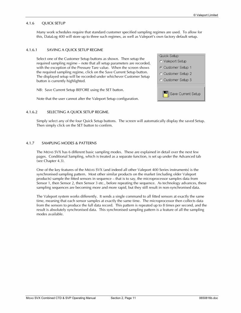
Select one of the Customer Setup buttons as shown. Then setup the required sampling regime – note that all setup parameters are recorded, with the exception of the Pressure Tare value. When the screen shows the required sampling regime, click on the Save Current Setup button. The displayed setup will be recorded under whichever Customer Setup button is currently highlighted. NB: Save Current Setup BEFORE using the SET button. Note that the user cannot alter the Valeport Setup configuration.

4.1.6.2 SELECTING A QUICK SETUP REGIME.

Simply select any of the four Quick Setup buttons. The screen will automatically display the saved Setup. Then simply click on the SET button to confirm.

4.1.7 SAMPLING MODES & PATTERNS

The MIDAS SVX has 6 different basic sampling modes. These are explained in detail over the next few pages. Conditional Sampling, which is treated as a separate function, is set up under the Advanced tab (see Chapter 4.3). One of the key features of the MIDAS SVX (and indeed all other Valeport 400 Series instruments) is the synchronised sampling pattern. Most other similar products on the market (including older Valeport products) sample the fitted sensors in sequence – that is to say, the microprocessor samples data from Sensor 1, then Sensor 2, then Sensor 3 etc., before repeating the sequence. As technology advances, these sampling sequences are becoming more and more rapid, but they still result in non-synchronised data. The Valeport system works differently. It sends a single command to all fitted sensors at exactly the same time, meaning that each sensor samples at exactly the same time. The microprocessor then collects data from the sensors to produce the full data record. This pattern is repeated up to 8 times per second, and the result is absolutely synchronised data. This synchronised sampling pattern is a feature of all the sampling modes available.

© Valeport Limited


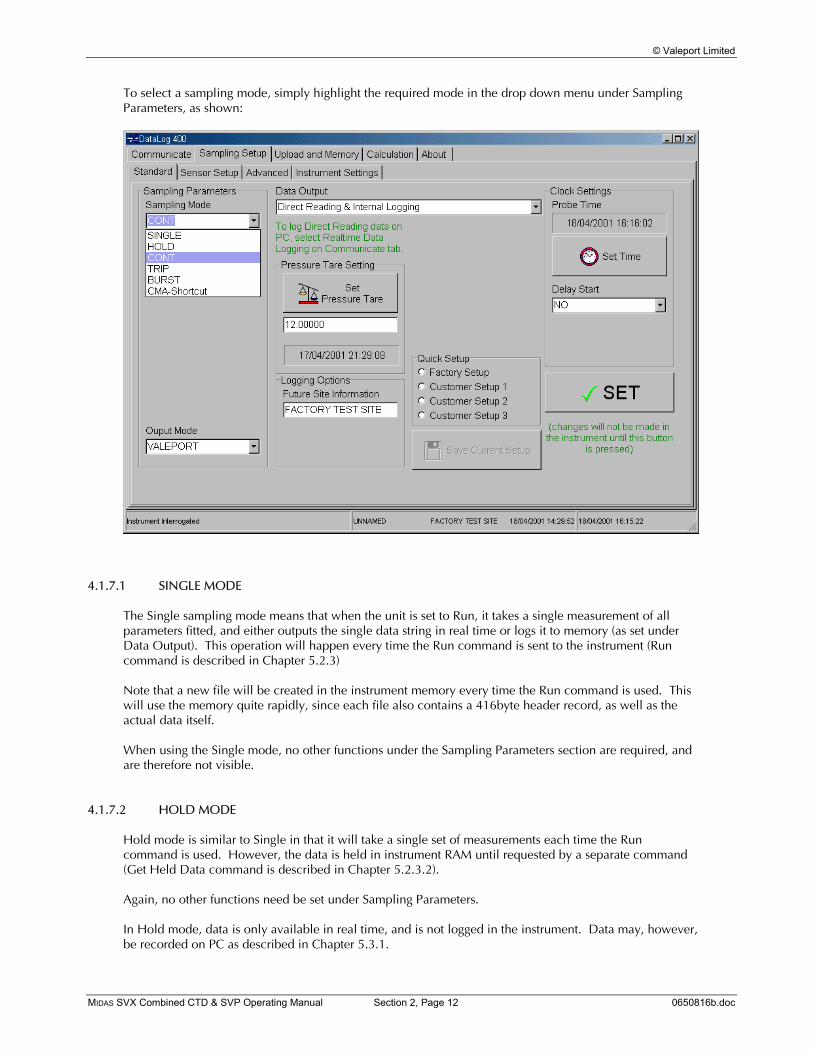
To select a sampling mode, simply highlight the required mode in the drop down menu under Sampling Parameters, as shown:

4.1.7.1 SINGLE MODE

The Single sampling mode means that when the unit is set to Run, it takes a single measurement of all parameters fitted, and either outputs the single data string in real time or logs it to memory (as set under Data Output). This operation will happen every time the Run command is sent to the instrument (Run command is described in Chapter 5.2.3) Note that a new file will be created in the instrument memory every time the Run command is used. This will use the memory quite rapidly, since each file also contains a 416byte header record, as well as the actual data itself. When using the Single mode, no other functions under the Sampling Parameters section are required, and are therefore not visible.

4.1.7.2 HOLD MODE

Hold mode is similar to Single in that it will take a single set of measurements each time the Run command is used. However, the data is held in instrument RAM until requested by a separate command (Get Held Data command is described in Chapter 5.2.3.2). Again, no other functions need be set under Sampling Parameters. In Hold mode, data is only available in real time, and is not logged in the instrument. Data may, however, be recorded on PC as described in Chapter 5.3.1.

© Valeport Limited


4.1.7.3 CONTINUOUS MODE

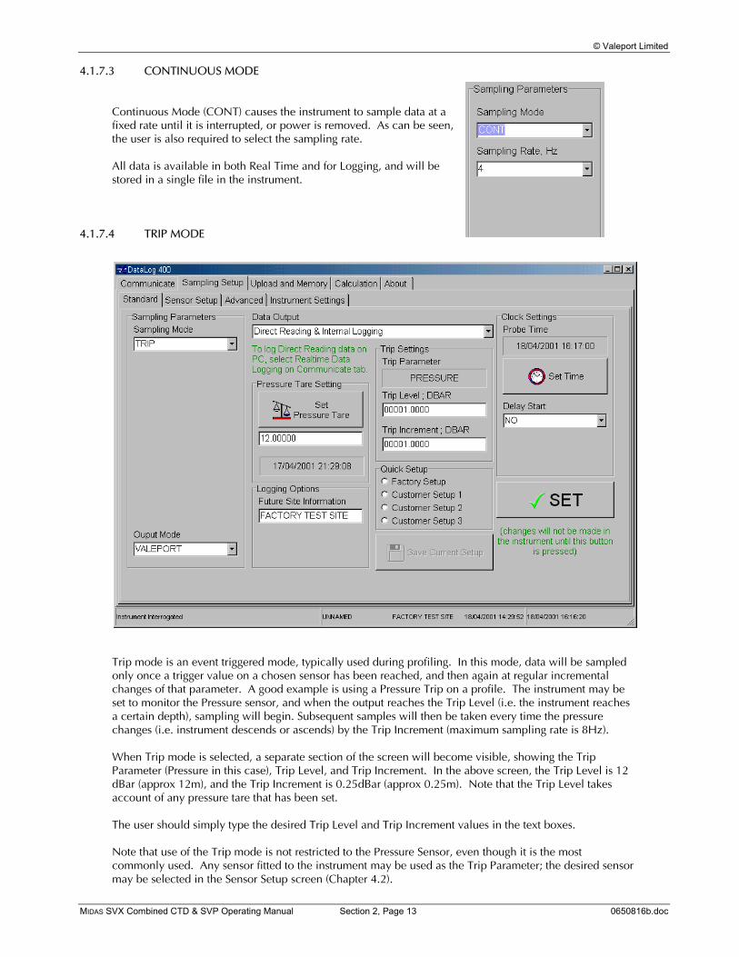
Continuous Mode (CONT) causes the instrument to sample data at a fixed rate until it is interrupted, or power is removed. As can be seen, the user is also required to select the sampling rate. All data is available in both Real Time and for Logging, and will be stored in a single file in the instrument.

4.1.7.4 TRIP MODE

Trip mode is an event triggered mode, typically used during profiling. In this mode, data will be sampled only once a trigger value on a chosen sensor has been reached, and then again at regular incremental changes of that parameter. A good example is using a Pressure Trip on a profile. The instrument may be set to monitor the Pressure sensor, and when the output reaches the Trip Level (i.e. the instrument reaches a certain depth), sampling will begin. Subsequent samples will then be taken every time the pressure changes (i.e. instrument descends or ascends) by the Trip Increment (maximum sampling rate is 8Hz). When Trip mode is selected, a separate section of the screen will become visible, showing the Trip Parameter (Pressure in this case), Trip Level, and Trip Increment. In the above screen, the Trip Level is 12 dBar (approx 12m), and the Trip Increment is 0.25dBar (approx 0.25m). Note that the Trip Level takes account of any pressure tare that has been set. The user should simply type the desired Trip Level and Trip Increment values in the text boxes. Note that use of the Trip mode is not restricted to the Pressure Sensor, even though it is the most commonly used. Any sensor fitted to the instrument may be used as the Trip Parameter; the desired sensor may be selected in the Sensor Setup screen (Chapter 4.2).

© Valeport Limited


4.1.7.5 BURST MODE

Burst Mode offers the user the greatest flexibility in sampling setup. Generally speaking, the sampling programme causes the instrument to take a set number of samples at a chosen rate, then go into sleep mode for a defined period of time before waking up and repeating the sequence. The user may set the desired sampling rate, the number of samples in the burst, and the interval between bursts. In this way, the deployment time of the instrument may be greatly extended. Burst mode is particularly suitable for long term studies, where specific parameters do not change rapidly and overall trends are more significant. Parameters that the user must set are therefore: Sample Rate Select 1, 2, 4 or 8Hz from the drop down menu Period This is the number of samples in the Burst (minimum 1).

In this example, 20 samples at 4 Hz will take 5 seconds. Interval This is how often a burst will occur, in seconds. Note

that the instrument requires a minimum of 20 seconds between the end of one burst and the start of the next – DataLog 400 will not allow an interval less than this to be set. If the user tries to set a shorter interval than this, the minimum interval possible with the present Sampling Rate and Period will be entered automatically.

Average Type Finally, the user has a choice of three data averaging

modes, which require further explanation: When using Burst mode, the MIDAS SVX is capable of calculating the mean value of data during a measurement burst, for each parameter fitted. The user has the following options: NONE No data averaging is performed over the burst. The instrument will log and output every

measurement made during the burst. FIXED The instrument will wait until the end of the burst, and will then calculate the mean value of

each parameter over the burst. If the burst is cut short by the user attempting to communicate with the instrument, then the average of that burst will be calculated as the mean of all measurements that were made.

MOVING The user can also create a Moving Average window. A new

text box will appear asking the user to choose the moving average length required, which may be any number up to the number of samples in the burst. The instrument will log and output the mean value of the previous ‘x’ measurements made in the burst, where ‘x’ is the Moving Average length. The output will be updated with every sample until the end of the burst. For example, in the above screen, if a Moving Average length of 5 samples were set, the output would be as follows:

Sample No. Output Sample No. Output

1 Mean of Sample 1 5 Mean of Samples 1,2,3,4,5 2 Mean of Samples 1,2 6 Mean of Samples 2,3,4,5,6 3 Mean of Samples 1,2,3 19 Mean of Samples 15,16,17,18,19 4 Mean of Samples 1,2,3,4 20 Mean of Samples 16,17,18,19,20

Finally, if either the Fixed or Moving Average option is selected, the instrument will also calculate the Standard Deviation of the data. This value will always be output in real time, but the user may decide that in order to conserve memory, it does not need to be logged. Please refer to Chapter 4.1.4 for details of how to turn the internal logging of Standard Deviation On/Off.

© Valeport Limited


4.1.7.6 CMA (CONTINUOUS MOVING AVERAGE)

This mode is a specific configuration of the Burst mode, where data is output continuously. Users may wish to use this output instead of the standard Continuous mode if data averaging or Standard Deviation data is required. The user is simply required to enter the Sample Rate (1,2,4 or 8Hz), and the length of the Moving Average window in samples. In this mode, the instrument will run indefinitely, always outputting the mean of the last ‘x’ samples, where ‘x’ is the number of samples in the Moving Average window. As with the standard Burst mode, the user may select whether or not to log the Standard Deviation of the data (see Chapter 4.1.4). Note that a continuous moving average regime can be setup manually by the user using the Burst mode. This mode is simply a shortcut to such a setup.

Note also that the instrument interprets CMA mode as a Burst mode. If an instrument is setup in CMA mode, the sampling regime will be recorded in the instrument as a Burst mode. This means that when the instrument is subsequently interrogated, the screen will show that the instrument is set in Burst mode, as shown left. Note that the screen shows the key points for setting a Continuous Moving Average manually: 1. The sampling period must be the same as the sampling rate, giving a

duration of 1 second. 2. The Sampling Interval must be set to 1 second.

© Valeport Limited


4.2 SENSOR SETUP

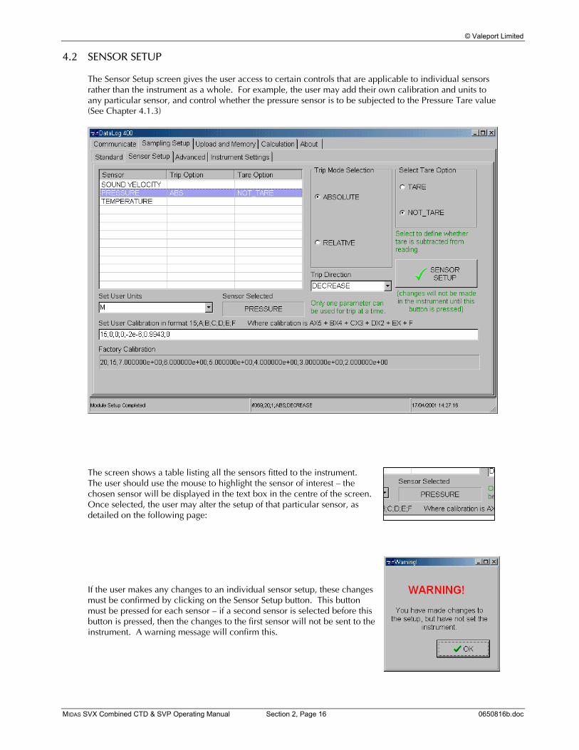
The Sensor Setup screen gives the user access to certain controls that are applicable to individual sensors rather than the instrument as a whole. For example, the user may add their own calibration and units to any particular sensor, and control whether the pressure sensor is to be subjected to the Pressure Tare value (See Chapter 4.1.3)

The screen shows a table listing all the sensors fitted to the instrument. The user should use the mouse to highlight the sensor of interest – the chosen sensor will be displayed in the text box in the centre of the screen. Once selected, the user may alter the setup of that particular sensor, as detailed on the following page: If the user makes any changes to an individual sensor setup, these changes must be confirmed by clicking on the Sensor Setup button. This button must be pressed for each sensor – if a second sensor is selected before this button is pressed, then the changes to the first sensor will not be sent to the instrument. A warning message will confirm this.

© Valeport Limited


4.2.1 TRIP MODE

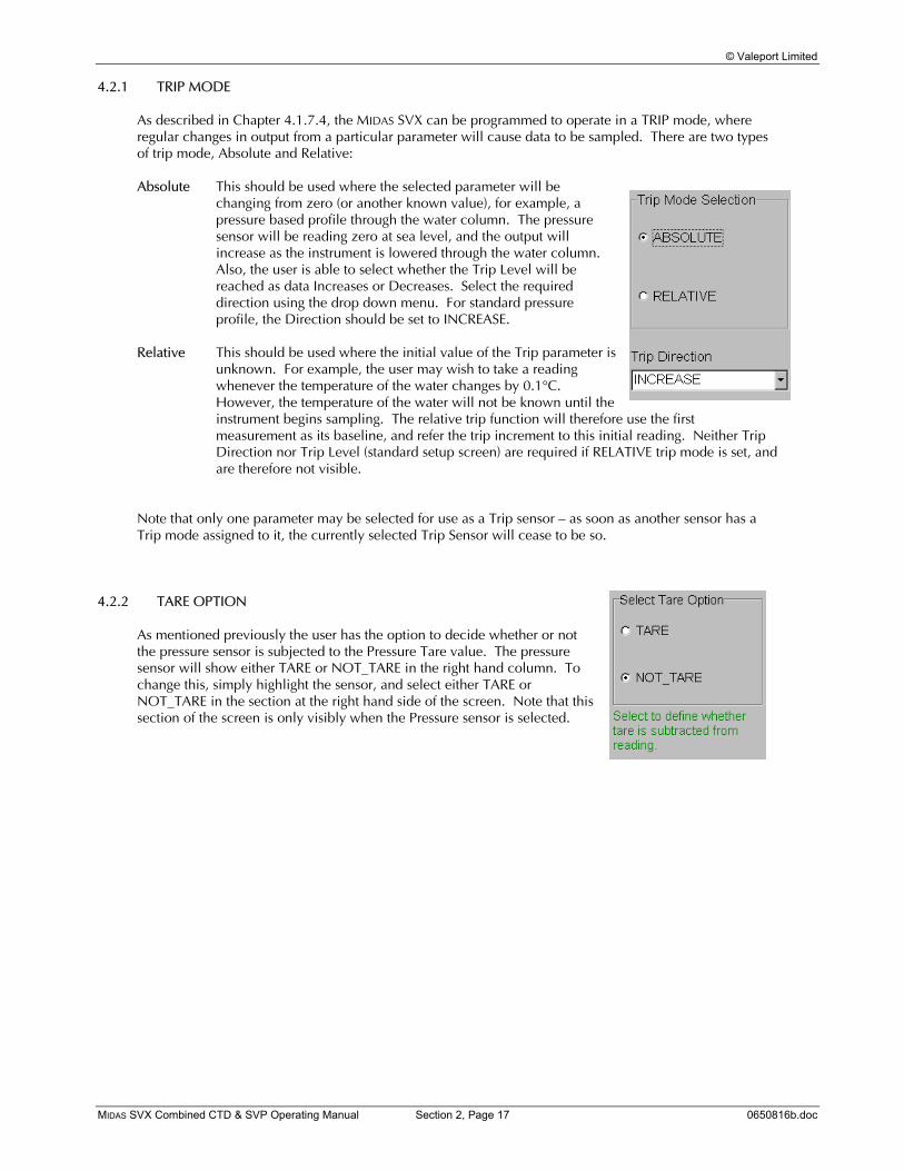
As described in Chapter 4.1.7.4, the MIDAS SVX can be programmed to operate in a TRIP mode, where regular changes in output from a particular parameter will cause data to be sampled. There are two types of trip mode, Absolute and Relative: Absolute This should be used where the selected parameter will be

changing from zero (or another known value), for example, a pressure based profile through the water column. The pressure sensor will be reading zero at sea level, and the output will increase as the instrument is lowered through the water column. Also, the user is able to select whether the Trip Level will be reached as data Increases or Decreases. Select the required direction using the drop down menu. For standard pressure profile, the Direction should be set to INCREASE.

Relative This should be used where the initial value of the Trip parameter is

unknown. For example, the user may wish to take a reading whenever the temperature of the water changes by 0.1°C. However, the temperature of the water will not be known until the instrument begins sampling. The relative trip function will therefore use the first measurement as its baseline, and refer the trip increment to this initial reading. Neither Trip Direction nor Trip Level (standard setup screen) are required if RELATIVE trip mode is set, and are therefore not visible.

Note that only one parameter may be selected for use as a Trip sensor – as soon as another sensor has a Trip mode assigned to it, the currently selected Trip Sensor will cease to be so.

4.2.2 TARE OPTION

As mentioned previously the user has the option to decide whether or not the pressure sensor is subjected to the Pressure Tare value. The pressure sensor will show either TARE or NOT_TARE in the right hand column. To change this, simply highlight the sensor, and select either TARE or NOT_TARE in the section at the right hand side of the screen. Note that this section of the screen is only visibly when the Pressure sensor is selected.

© Valeport Limited


4.2.3 USER CALIBRATION

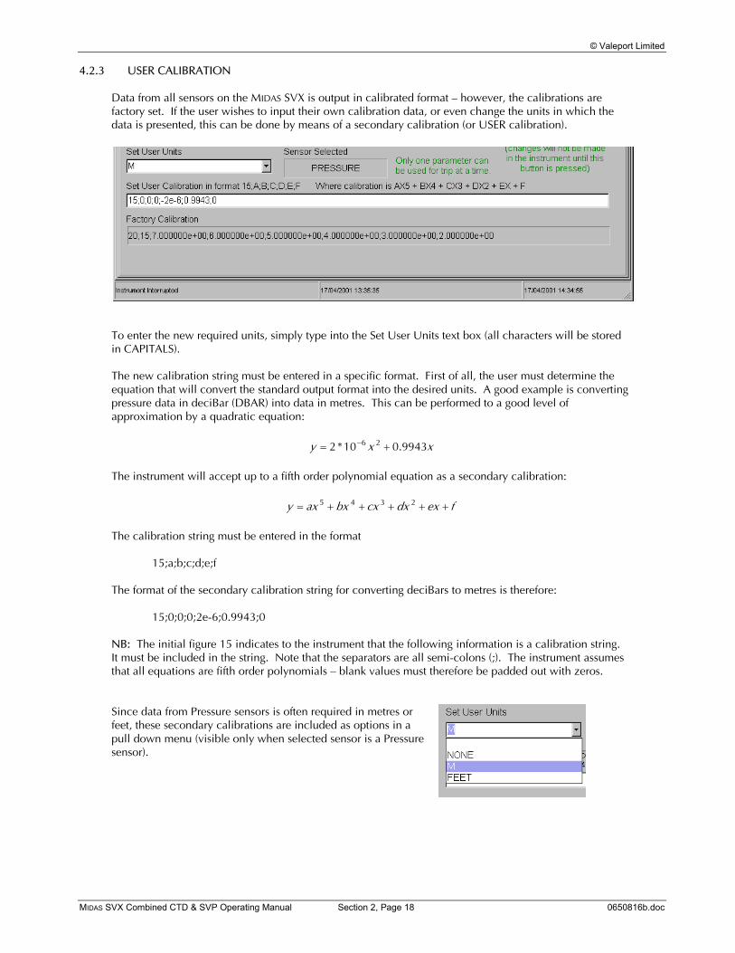
Data from all sensors on the MIDAS SVX is output in calibrated format – however, the calibrations are factory set. If the user wishes to input their own calibration data, or even change the units in which the data is presented, this can be done by means of a secondary calibration (or USER calibration).

To enter the new required units, simply type into the Set User Units text box (all characters will be stored in CAPITALS). The new calibration string must be entered in a specific format. First of all, the user must determine the equation that will convert the standard output format into the desired units. A good example is converting pressure data in deciBar (DBAR) into data in metres. This can be performed to a good level of approximation by a quadratic equation:

xxy 9943.010*2 26 += − The instrument will accept up to a fifth order polynomial equation as a secondary calibration:

fexdxcxbxaxy +++++= 2345 The calibration string must be entered in the format

15;a;b;c;d;e;f The format of the secondary calibration string for converting deciBars to metres is therefore:

15;0;0;0;2e-6;0.9943;0 NB: The initial figure 15 indicates to the instrument that the following information is a calibration string. It must be included in the string. Note that the separators are all semi-colons (;). The instrument assumes that all equations are fifth order polynomials – blank values must therefore be padded out with zeros. Since data from Pressure sensors is often required in metres or feet, these secondary calibrations are included as options in a pull down menu (visible only when selected sensor is a Pressure sensor).

© Valeport Limited


4.3 ADVANCED

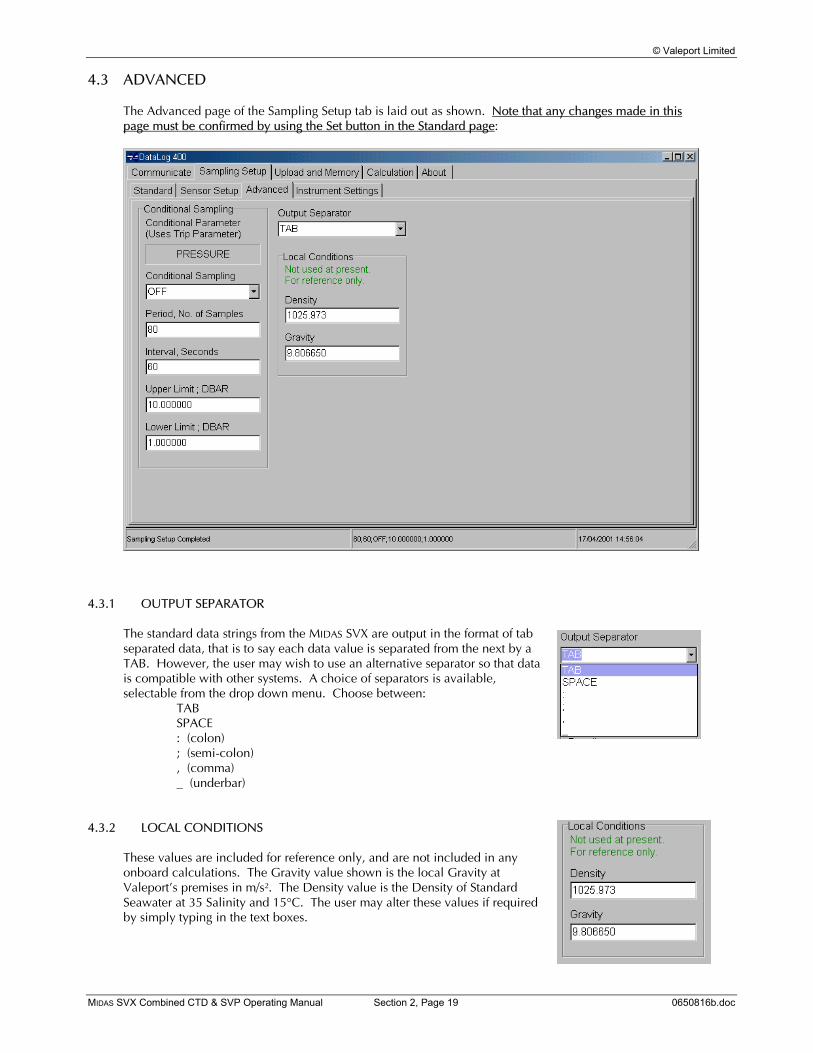
The Advanced page of the Sampling Setup tab is laid out as shown. Note that any changes made in this page must be confirmed by using the Set button in the Standard page:

4.3.1 OUTPUT SEPARATOR

The standard data strings from the MIDAS SVX are output in the format of tab separated data, that is to say each data value is separated from the next by a TAB. However, the user may wish to use an alternative separator so that data is compatible with other systems. A choice of separators is available, selectable from the drop down menu. Choose between:

TAB SPACE : (colon) ; (semi-colon) , (comma) _ (underbar)

4.3.2 LOCAL CONDITIONS

These values are included for reference only, and are not included in any onboard calculations. The Gravity value shown is the local Gravity at Valeport’s premises in m/s². The Density value is the Density of Standard Seawater at 35 Salinity and 15°C. The user may alter these values if required by simply typing in the text boxes.

© Valeport Limited


4.3.3 CONDITIONAL SAMPLING

Conditional Sampling is one of the most powerful features of Valeport range of 400 series instruments. Put simply, the instrument will monitor any specified sensor, and only begin full sampling if the output from that sensor reaches a specified level. The conditional sampling feature therefore allows long-term deployment of instruments, but restricting data gathering only to periods of specific interest. Examples may include monitoring of a pressure sensor so that logging only occurs when the instrument is submerged, or of a fluorometer to restrict sampling to only happen during a plankton bloom. Conditional Sampling is only available if the instrument is set to run in Burst or Continuous modes. In both cases, the chosen sensor will be monitored in a simple Burst pattern, set up as described below. If the mean value of data gathered during that burst exceeds the designated limit, then the full sampling regime (either Burst, Continuous or Continuous Moving Average) as set in the Standard Setup screen (Chapter 4.1) will begin. Note that during a conditional burst, no data is logged.

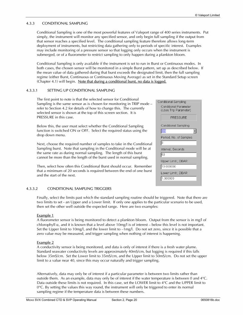
4.3.3.1 SETTING UP CONDITIONAL SAMPLING

The first point to note is that the selected sensor for Conditional Sampling is the same sensor as is chosen for monitoring in TRIP mode – refer to Section 4.2 for details of how to change this. The currently selected sensor is shown at the top of this screen section. It is PRESSURE in this case. Below this, the user must select whether the Conditional Sampling function is switched ON or OFF. Select the required status using the drop down menu. Next, choose the required number of samples to take in the Conditional Sampling burst. Note that sampling in the Conditional mode will be at the same rate as during normal sampling. The length of this burst cannot be more than the length of the burst used in normal sampling. Then, select how often this Conditional Burst should occur. Remember that a minimum of 20 seconds is required between the end of one burst and the start of the next.

4.3.3.2 CONDITIONAL SAMPLING TRIGGERS

Finally, select the limits past which the standard sampling routine should be triggered. Note that there are two limits to set - an Upper and a Lower limit. If only one applies to the particular scenario to be used, then set the other well outside the expected range. Here are two examples: Example 1 A fluorometer sensor is being monitored to detect a plankton bloom. Output from the sensor is in mg/l of chlorophyll α, and it is known that a level above 10mg/l is of interest – below this level is not important. Set the Upper limit to 10mg/l, and the lower limit to –1mg/l. Do not set zero, since it is possible that a zero value may be measured, and trigger sampling when nothing of interest is happening. Example 2 A conductivity sensor is being monitored, and data is only of interest if there is a fresh water plume. Standard seawater conductivity levels are approximately 40mS/cm, but logging is required if this falls below 35mS/cm. Set the Lower limit to 35mS/cm, and the Upper limit to 50mS/cm. Do not set the upper limit to a value near 40, since this may occur naturally and trigger sampling. Alternatively, data may only be of interest if a particular parameter is between two limits rather than outside them. As an example, data may only be of interest if the water temperature is between 0 and 4°C. Data outside these limits is not required. In this case, set the LOWER limit to 4°C and the UPPER limit to 0°C. By setting the values this way round, the instrument will only be triggered to enter its normal sampling regime if the temperature data is between these numbers.

© Valeport Limited


4.3.3.3 CONDITIONAL SAMPLING ‘OFF’ TRIGGERS

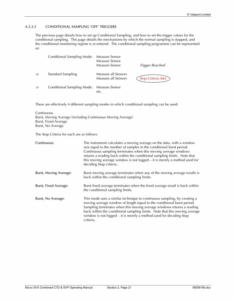
The previous page details how to set up Conditional Sampling, and how to set the trigger values for the conditional sampling. This page details the mechanisms by which the normal sampling is stopped, and the conditional monitoring regime is re-entered. The conditional sampling programme can be represented as:

Conditional Sampling Mode: Measure Sensor Measure Sensor Measure Sensor Trigger Reached

⇒ Standard Sampling Measure all Sensors

Measure all Sensors Stop Criteria Met ⇒ Conditional Sampling Mode: Measure Sensor

etc. There are effectively 4 different sampling modes in which conditional sampling can be used: Continuous Burst, Moving Average (including Continuous Moving Average) Burst, Fixed Average Burst, No Average The Stop Criteria for each are as follows: Continuous: The instrument calculates a moving average on the data, with a window

size equal to the number of samples in the conditional burst period. Continuous sampling terminates when this moving average windows returns a reading back within the conditional sampling limits. Note that this moving average window is not logged – it is merely a method used for deciding Stop criteria.

Burst, Moving Average: Burst moving average terminates when any of the moving average results is

back within the conditional sampling limits. Burst, Fixed Average: Burst fixed average terminates when the fixed average result is back within

the conditional sampling limits. Burst, No Average: This mode uses a similar technique to continuous sampling, by creating a

moving average window of length equal to the conditional burst period. Sampling terminates when this moving average windows returns a reading back within the conditional sampling limits. Note that this moving average window is not logged – it is merely a method used for deciding Stop criteria.

© Valeport Limited


5 RUNNING THE INSTRUMENT

Once the user has set the instrument up as required, the instrument may be set into Run mode. There are three methods of doing this:

5.1 HARDWARE SWITCH ON

If the user intends to deploy the equipment to only log data, and does not intend to view data in real time, then use this method. Once the instrument has been set up as required, turn it off by removing any external power supply, or disconnecting the 3m Y lead. Then, simply fit the 10way Subconn style switch plug that is supplied with the instrument. There is a link in this plug that serves to turn the unit on using the internal batteries. The designated sampling regime will then begin.

5.2 SOFTWARE SWITCH ON

5.2.1 METHOD 1

If the user is confident of the current instrument settings, and wishes to Run the instrument whilst it is connected to PC, then the Run button may be pressed as soon as DataLog 400 is opened. The software will communicate with the instrument automatically, in order to determine which sensors are fitted, and in which mode the instrument is set up.

5.2.2 METHOD 2

If the user has used the Interrupt button to communicate with the instrument, and subsequently viewed and/or Set the sampling regime, then the Communicate tab to should be selected to allow access to the Run button.

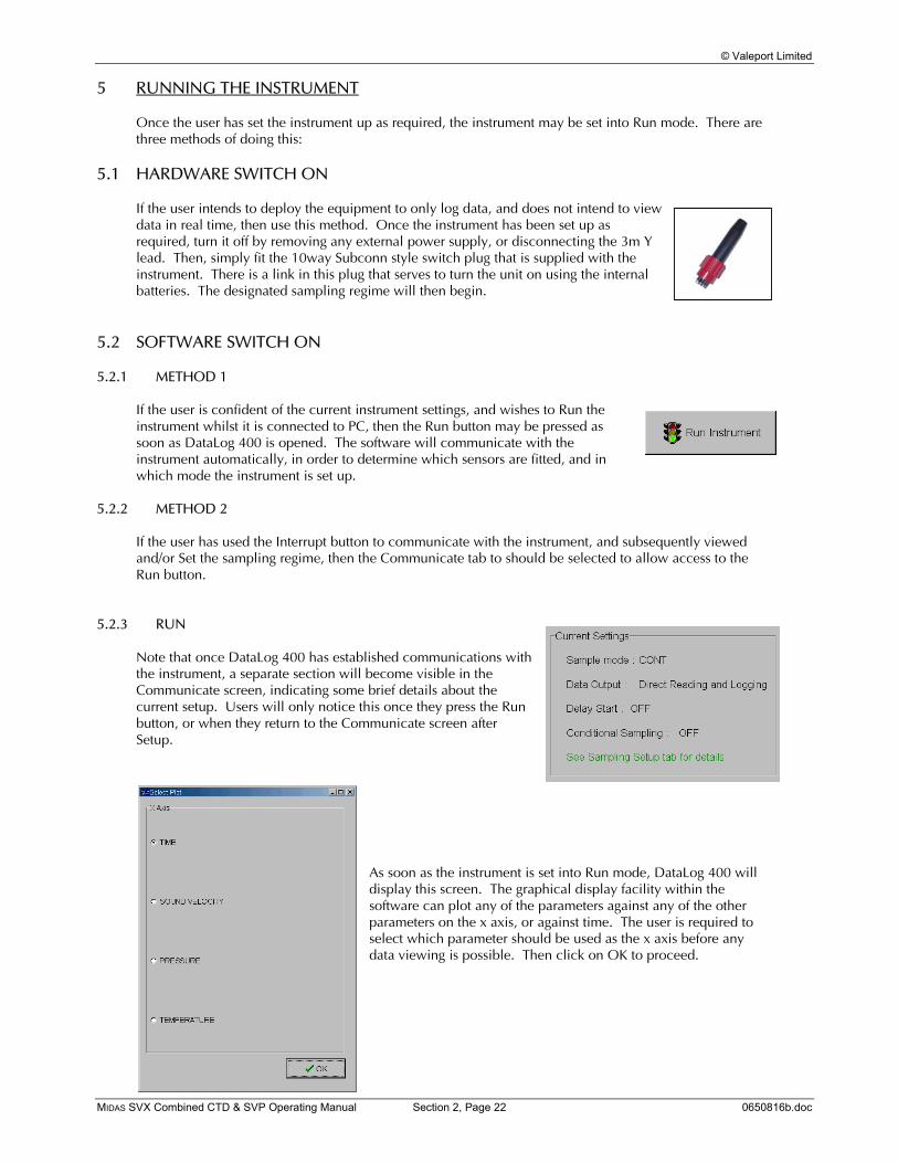
5.2.3 RUN

Note that once DataLog 400 has established communications with the instrument, a separate section will become visible in the Communicate screen, indicating some brief details about the current setup. Users will only notice this once they press the Run button, or when they return to the Communicate screen after Setup.

As soon as the instrument is set into Run mode, DataLog 400 will display this screen. The graphical display facility within the software can plot any of the parameters against any of the other parameters on the x axis, or against time. The user is required to select which parameter should be used as the x axis before any data viewing is possible. Then click on OK to proceed.

© Valeport Limited


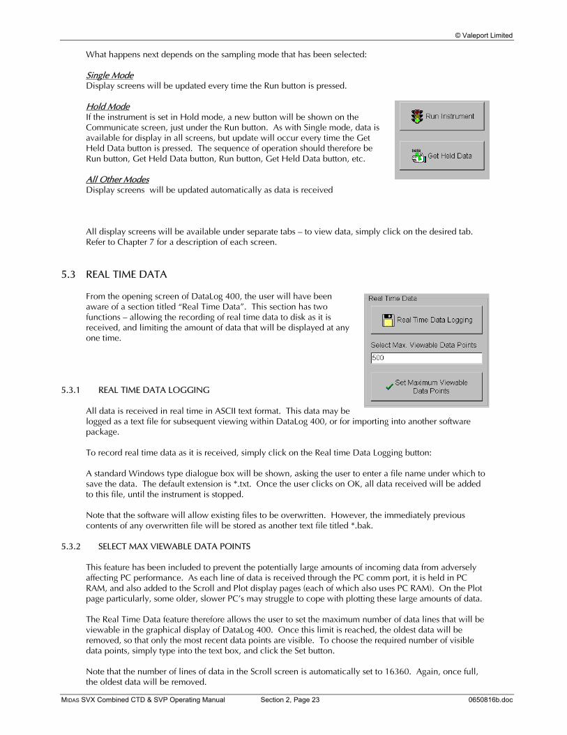
What happens next depends on the sampling mode that has been selected: Single Mode Display screens will be updated every time the Run button is pressed. Hold Mode If the instrument is set in Hold mode, a new button will be shown on the Communicate screen, just under the Run button. As with Single mode, data is available for display in all screens, but update will occur every time the Get Held Data button is pressed. The sequence of operation should therefore be Run button, Get Held Data button, Run button, Get Held Data button, etc. All Other Modes Display screens will be updated automatically as data is received All display screens will be available under separate tabs – to view data, simply click on the desired tab. Refer to Chapter 7 for a description of each screen.

5.3 REAL TIME DATA

From the opening screen of DataLog 400, the user will have been aware of a section titled “Real Time Data”. This section has two functions – allowing the recording of real time data to disk as it is received, and limiting the amount of data that will be displayed at any one time.

5.3.1 REAL TIME DATA LOGGING

All data is received in real time in ASCII text format. This data may be logged as a text file for subsequent viewing within DataLog 400, or for importing into another software package. To record real time data as it is received, simply click on the Real time Data Logging button: A standard Windows type dialogue box will be shown, asking the user to enter a file name under which to save the data. The default extension is *.txt. Once the user clicks on OK, all data received will be added to this file, until the instrument is stopped. Note that the software will allow existing files to be overwritten. However, the immediately previous contents of any overwritten file will be stored as another text file titled *.bak.

5.3.2 SELECT MAX VIEWABLE DATA POINTS

This feature has been included to prevent the potentially large amounts of incoming data from adversely affecting PC performance. As each line of data is received through the PC comm port, it is held in PC RAM, and also added to the Scroll and Plot display pages (each of which also uses PC RAM). On the Plot page particularly, some older, slower PC’s may struggle to cope with plotting these large amounts of data. The Real Time Data feature therefore allows the user to set the maximum number of data lines that will be viewable in the graphical display of DataLog 400. Once this limit is reached, the oldest data will be removed, so that only the most recent data points are visible. To choose the required number of visible data points, simply type into the text box, and click the Set button. Note that the number of lines of data in the Scroll screen is automatically set to 16360. Again, once full, the oldest data will be removed.

© Valeport Limited


6 UPLOAD & MEMORY

The MIDAS SVX is fitted with a standard 8Mbyte memory. This consists of a single 8Mbyte Flash memory chip. However, there is space on the memory board for up to 4 of these chips, so available memory sizes are 8, 16, 24 or 32 Mbyte. The capacity of this memory depends on the sampling regime chosen. Some sample capacity calculations are given in the first Section of the manual. There are two stages to accessing logged data, Upload and Translate.

6.1 UPLOAD

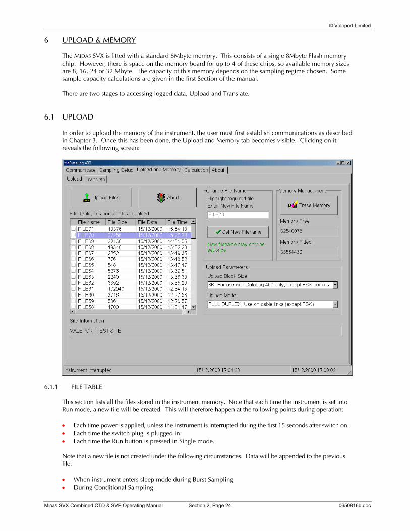
In order to upload the memory of the instrument, the user must first establish communications as described in Chapter 3. Once this has been done, the Upload and Memory tab becomes visible. Clicking on it reveals the following screen:

6.1.1 FILE TABLE

This section lists all the files stored in the instrument memory. Note that each time the instrument is set into Run mode, a new file will be created. This will therefore happen at the following points during operation: • Each time power is applied, unless the instrument is interrupted during the first 15 seconds after switch on. • Each time the switch plug is plugged in. • Each time the Run button is pressed in Single mode. Note that a new file is not created under the following circumstances. Data will be appended to the previous file: • When instrument enters sleep mode during Burst Sampling • During Conditional Sampling.

© Valeport Limited


The file table lists all the stored files, with the most recent file displayed at the top of the screen. The table includes the following information about each file: File Name This is automatically generated by the instrument, in the form FILE#, where # is the

next number in sequence. There is no limit to the maximum number of files that can be stored, apart from the physical capacity of the memory.

File Size This shows the size of each file in bytes. Note that each file contains a certain amount

of header information, such as calibration coefficients, date, time and sampling regime. The size of the header information will vary slightly, but is usually in the region of 400 bytes.

File Date/Time These two columns give the date and time at which the file was created. Finally, notice that each file has a small check box next to it on the left-hand side. Click on the box next to each file that required uploading.

6.1.2 SITE INFORMATION

Before a deployment, the user may enter brief details about the proposed site, to aid in identification afterwards. This section of the screen shows the site information assigned to the highlighted file in the File Table. Please see Chapter 4.1.4 for details of how to enter Site Information.

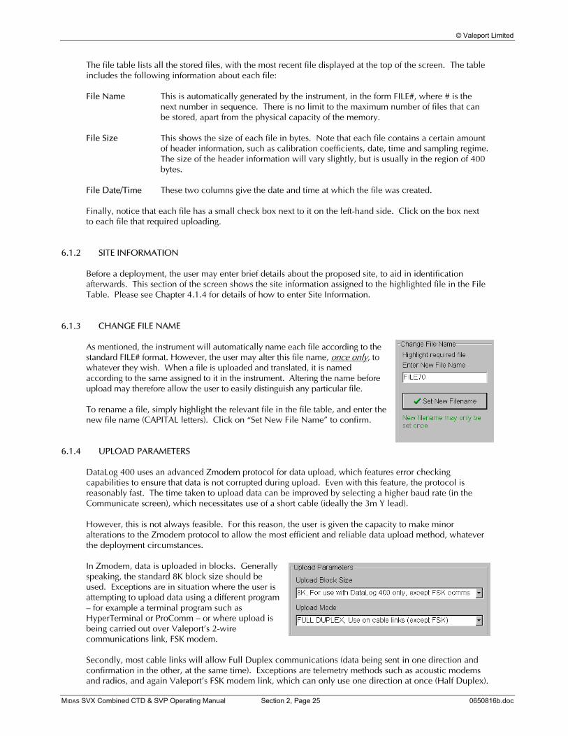
6.1.3 CHANGE FILE NAME

As mentioned, the instrument will automatically name each file according to the standard FILE# format. However, the user may alter this file name, once only, to whatever they wish. When a file is uploaded and translated, it is named according to the same assigned to it in the instrument. Altering the name before upload may therefore allow the user to easily distinguish any particular file. To rename a file, simply highlight the relevant file in the file table, and enter the new file name (CAPITAL letters). Click on “Set New File Name” to confirm.

6.1.4 UPLOAD PARAMETERS

DataLog 400 uses an advanced Zmodem protocol for data upload, which features error checking capabilities to ensure that data is not corrupted during upload. Even with this feature, the protocol is reasonably fast. The time taken to upload data can be improved by selecting a higher baud rate (in the Communicate screen), which necessitates use of a short cable (ideally the 3m Y lead). However, this is not always feasible. For this reason, the user is given the capacity to make minor alterations to the Zmodem protocol to allow the most efficient and reliable data upload method, whatever the deployment circumstances. In Zmodem, data is uploaded in blocks. Generally speaking, the standard 8K block size should be used. Exceptions are in situation where the user is attempting to upload data using a different program – for example a terminal program such as HyperTerminal or ProComm – or where upload is being carried out over Valeport’s 2-wire communications link, FSK modem. Secondly, most cable links will allow Full Duplex communications (data being sent in one direction and confirmation in the other, at the same time). Exceptions are telemetry methods such as acoustic modems and radios, and again Valeport’s FSK modem link, which can only use one direction at once (Half Duplex).

© Valeport Limited


6.1.5 MEMORY MANAGEMENT

This section indicates the total amount of memory fitted to the instrument, in bytes, and the amount which remains unused (again in bytes). It also contains the most dangerous button in the software – the Erase Memory button. Take care when erasing memory. Although the user is asked twice for confirmation, they should ensure that all required data has been uploaded prior to erasing the memory.

Once memory has been erased, it cannot be recovered.

6.1.6 UPLOAD FILES

Once the desired files have been selected, simply click on the Upload Files button to initiate the data upload procedure. Data will be automatically uploaded into a subdirectory of the DataLog 400 directory, labelled according to the serial number of the instrument. This subdirectory will be created if necessary. The following screen will be shown:

The screen gives an indication of the progress of the upload of the current file – note that this screen will automatically disappear when the current file has uploaded. It will then reappear for each file that is uploaded. At any stage, upload can be stopped by using the Cancel button on the above screen, or the Abort button in DataLog 400. When data has been uploaded the following message will appear:

© Valeport Limited


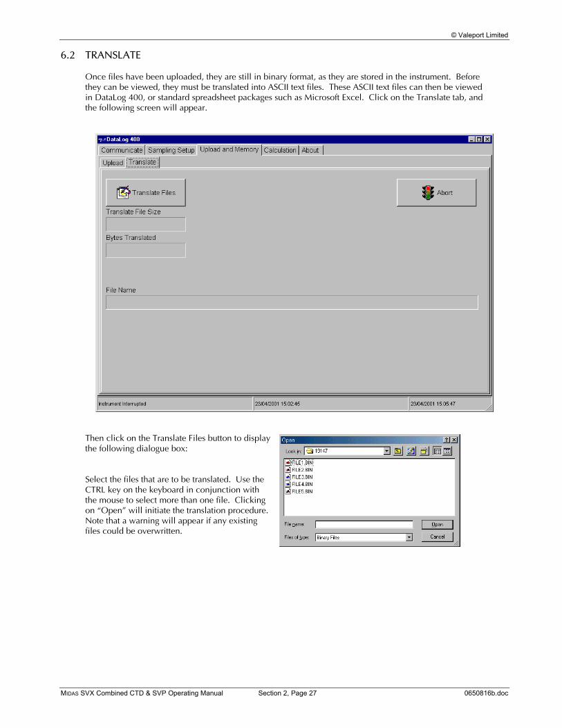
6.2 TRANSLATE

Once files have been uploaded, they are still in binary format, as they are stored in the instrument. Before they can be viewed, they must be translated into ASCII text files. These ASCII text files can then be viewed in DataLog 400, or standard spreadsheet packages such as Microsoft Excel. Click on the Translate tab, and the following screen will appear.

Then click on the Translate Files button to display the following dialogue box: Select the files that are to be translated. Use the CTRL key on the keyboard in conjunction with the mouse to select more than one file. Clicking on “Open” will initiate the translation procedure. Note that a warning will appear if any existing files could be overwritten.

© Valeport Limited


It is possible, even likely, that certain deployments will result in a single file of 8Mbyte or more. As explained in Chapter 5.3.2, the number of lines of data that DataLog 400 will graph can be set by the user, but it should be noted that some spreadsheet packages have a maximum number of data lines of 16360 (including DataLog 400 itself in Scroll display mode). For this reason, DataLog 400 will attempt to break very large files into several smaller ones. The user is asked to select how many lines of data should be included in each translated file. The screen shows several pieces of information: The projected file size for the file that is about to be translated, in bytes. The number of spreadsheet lines. If this is changed then “Set” should be clicked to confirm. The approximate amount of sampling time that a full 16360 lines of data would contain – this is intended as a guide only, and is based on the sampling frequency of the selected file. The size of a full 16360 line file. As can be seen, the selected file in this example is only marginally smaller than a full spreadsheet. Translation will then commence when the OK button is pressed.

The screen will show the size of the file that is being translated, and two progress indicators. The first shows the number of bytes of the binary file that have so far been translated, and below this is a visual indicator in the form of a blue bar. Finally, the name of the file that is being created is shown. As can be seen, the stem of the file name comes from the name of the binary file (File5). The extension in this case is .000. In the case of large files, where the original binary file is broken into several translated text files (see previous page), this extension will increase by one for each separate file. For example, the second file in the sequence would be named File5.001

To translate further files, simply click the Translate Files button to open further binary files. To abort the translation procedure at any time, click on the Abort button. Proceed to Chapter 7 for details of how to view translated files in DataLog 400.

© Valeport Limited


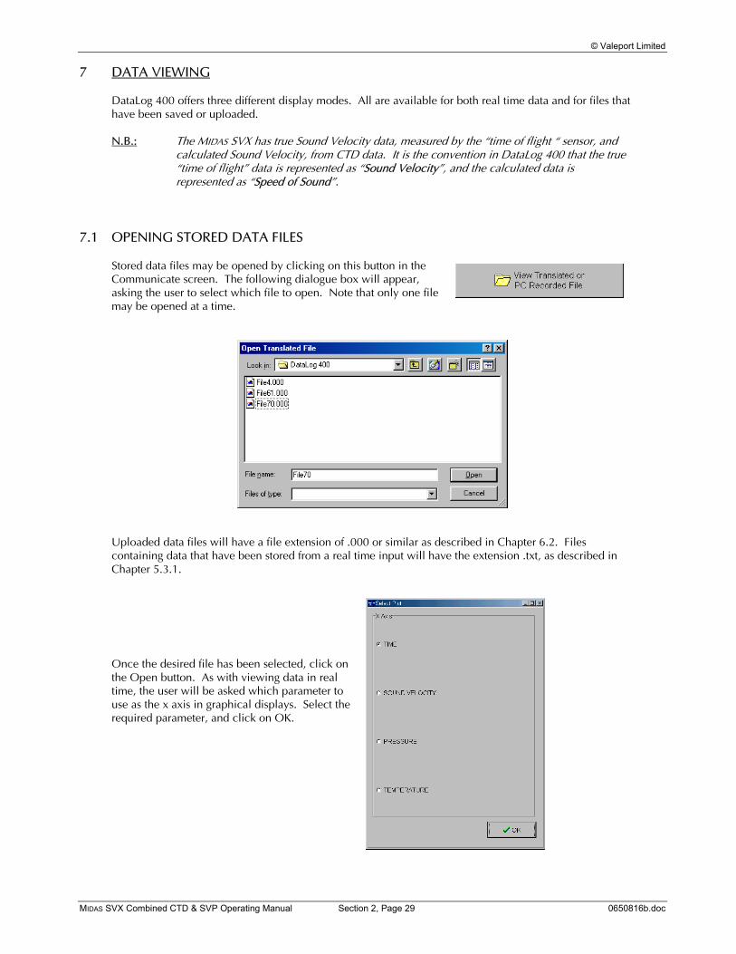
7 DATA VIEWING

DataLog 400 offers three different display modes. All are available for both real time data and for files that have been saved or uploaded. N.B.: The MIDAS SVX has true Sound Velocity data, measured by the “time of flight “ sensor, and

calculated Sound Velocity, from CTD data. It is the convention in DataLog 400 that the true “time of flight” data is represented as “Sound Velocity”, and the calculated data is represented as “Speed of Sound”.

7.1 OPENING STORED DATA FILES

Stored data files may be opened by clicking on this button in the Communicate screen. The following dialogue box will appear, asking the user to select which file to open. Note that only one file may be opened at a time.

Uploaded data files will have a file extension of .000 or similar as described in Chapter 6.2. Files containing data that have been stored from a real time input will have the extension .txt, as described in Chapter 5.3.1. Once the desired file has been selected, click on the Open button. As with viewing data in real time, the user will be asked which parameter to use as the x axis in graphical displays. Select the required parameter, and click on OK.

© Valeport Limited


7.2 SIMPLE DISPLAY

The simple display is designed primarily for real time use. It is available for use with uploaded data files, but will simply display each data point in turn as it is read from memory, and then fix on the final data recorded in the file. The function of the simple display is to provide the user with a readout of the last set of data received by the PC.

The display gives the date and time of the last data point, and then the last output of each fitted parameter. In Burst modes, the standard deviation of the data is also given. Note the check box at the top right corner of the screen – while this is checked, the screen will continue to be updated. Some older PCs may struggle to update all displays at fast data rates, so disabling unwanted displays may help. To disable the display, simply uncheck the box. To re-enable, re-check the box – the next data point received will be displayed as normal.

© Valeport Limited


7.3 SCROLL DISPLAY

The scroll display provides the user with a record of all data received by the software (subject to the maximum number of lines, 16360). The screen shows the date and time at the left-hand side, followed by data from each fitted parameter. Again, if in Burst mode, standard deviation data will be included.

Note that the columns of data are sizeable, after the first two lines of data have been received. Simply position the mouse over the edge of a column title, and use the left mouse button to drag the column to a suitable size. As with the Simple display, this screen can be disabling by unchecking the Enable check box at the top right corner. Re-checking the box re-enables the display, and data will continue to be added when the next data line is received.

© Valeport Limited


7.4 GRAPHICAL DISPLAY

The graphical display facility in DataLog 400 is an integral feature of the Delphi programming language in which DataLog 400 is written. Consequently, there are many features of this display type that are beyond what is absolutely necessary for functional data display. Such features include adding a picture to the background of the graph, and changing the size of the border around the image. This manual does not cover the majority of these features, but instead concentrates on those features that are necessary to enable standard data displays. Users familiar with standard Windows functions and common programmes such as Microsoft Excel will be able to customise their graphical displays as they wish, simply by exploring the many features available. When the user first views the graphical display, they will be presented with a blank page:

All graph functions are controlled with the various buttons at the top of the screen. The first button to use is the Graph Edit button – this allows the user to decide which parameters are to be graphed, and in which format. Clicking on this button reveals the following screen:

© Valeport Limited


All the fitted parameters are shown as being available for graphing against time. Simply click on the check box against each parameter to indicate whether it is to be graphed or not. To alter the colour of any parameter, simply double click on the coloured line adjacent to each parameter, and select from the variety of available colours. Further modifications to line style can be made by selecting the upper Series tab, followed by Format, and the Border button. Finally, users may double click on the icon to the left of each parameter to alter the graph type. DataLog 400 is best able to display data at rapid rates using the “Fast Line” style, which is the default. However, users may wish to select other styles to suit their own preference. As can be seen from the screen on the previous page, there are several other tabs available to alter the appearance of the graph. This manual does not cover all these options, but be assured that DataLog 400 will revert to its default style if closed down and reopened. The example screen below shows only a single parameter checked for display, simply for reasons of clarity. Note that secondary y axes will appear for each parameter checked, and each will autoscale to show the full range of data. The scale may be manually set under the Chart, Axis, Scale tab. The x axis will also autoscale as new data is received, and will then slide as the maximum number of viewable data points is reached (Chapter 5.3.2).

Note that once the graph has been set up, the function buttons are inactivated and greyed out. This inactivation is simply to conserve PC RAM for data display, and the buttons may be reactivated simply by clicking on the toolbar. The functions of the other buttons are as follows:

Clicking on this button will allow the user to print the graph. A preview page is shown, allowing the user to alter page size, margin size and printer. Simply press Print when the page is shown as required. This button copies the graph as currently displayed to the PC clipboard, for import into other programs as a bitmap.

© Valeport Limited


The remainder of the icons on the graphical display page allow the user to control certain features of the graph using the mouse.

7.4.1 SCROLL & FOCUS

The first icon (default icon when the screen opens) gives the mouse two functions. By holding down the right mouse button, it is possible to scroll both axes of the graph, simply by dragging the mouse in the appropriate direction.

By holding down the left button, the user may focus onto a particular section of the graph. Simply drag and draw a box over the required section of data, starting at the top left corner. To focus out again, drag and draw a box on the graph starting at any other corner. The remaining icons alter the 3 dimensional properties of the graphical display. If any are selected, the graph will automatically switch into 3D mode, but at any time, 3D mode can be toggled on and off by using the 3D button.

© Valeport Limited


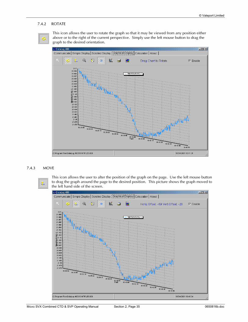
7.4.2 ROTATE

This icon allows the user to rotate the graph so that it may be viewed from any position either above or to the right of the current perspective. Simply use the left mouse button to drag the graph to the desired orientation.

7.4.3 MOVE

This icon allows the user to alter the position of the graph on the page. Use the left mouse button to drag the graph around the page to the desired position. This picture shows the graph moved to the left hand side of the screen.

© Valeport Limited


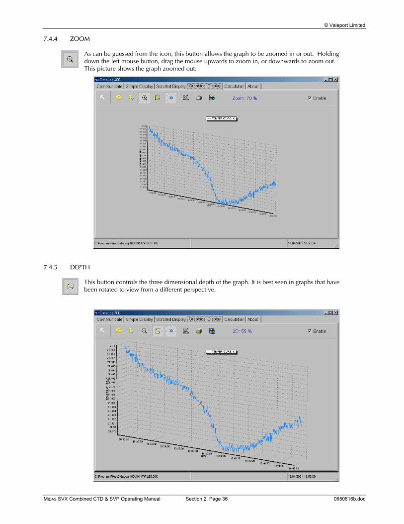
7.4.4 ZOOM

As can be guessed from the icon, this button allows the graph to be zoomed in or out. Holding down the left mouse button, drag the mouse upwards to zoom in, or downwards to zoom out. This picture shows the graph zoomed out:

7.4.5 DEPTH

This button controls the three dimensional depth of the graph. It is best seen in graphs that have been rotated to view from a different perspective.

© Valeport Limited


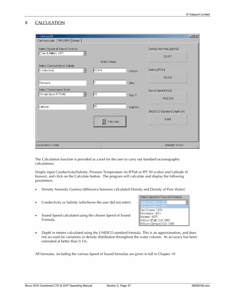
8 CALCULATION

The Calculation function is provided as a tool for the user to carry out standard oceanographic calculations. Simply input Conductivity/Salinity, Pressure Temperature (in IPT68 or IPT 90 scales) and Latitude (if known), and click on the Calculate button. The program will calculate and display the following parameters: • Density Anomaly Gamma (difference between calculated Density and Density of Pure Water) • Conductivity or Salinity (whichever the user did not enter). • Sound Speed calculated using the chosen Speed of Sound

Formula. • Depth in metres calculated using the UNESCO standard formula. This is an approximation, and does

not account for variations in density distribution throughout the water column. Its accuracy has been estimated at better than 0.1m.

All formulae, including the various Speed of Sound formulae are given in full in Chapter 10

© Valeport Limited


9 ABOUT

The About tab, available for selection at all times, shows Valeport’s contact details and software version. If the About tab is selected after the user has interrupted the unit operation, then the instrument serial number and internal firmware version will also be shown.

© Valeport Limited


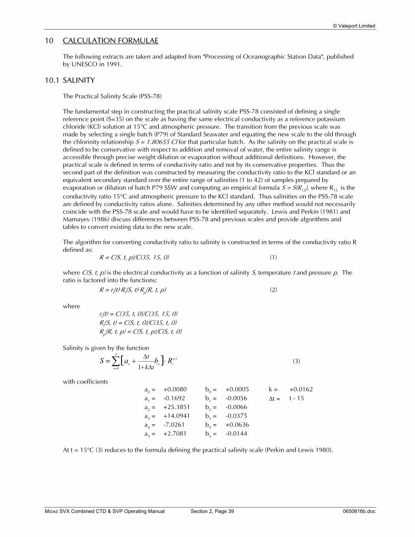
10 CALCULATION FORMULAE

The following extracts are taken and adapted from "Processing of Oceanographic Station Data", published by UNESCO in 1991.

10.1 SALINITY

The Practical Salinity Scale (PSS-78) The fundamental step in constructing the practical salinity scale PSS-78 consisted of defining a single reference point (S=35) on the scale as having the same electrical conductivity as a reference potassium chloride (KCl) solution at 15°C and atmospheric pressure. The transition from the previous scale was made by selecting a single batch (P79) of Standard Seawater and equating the new scale to the old through the chlorinity relationship S = 1.80655 Cl for that particular batch. As the salinity on the practical scale is defined to be conservative with respect to addition and removal of water, the entire salinity range is accessible through precise weight dilution or evaporation without additional definitions. However, the practical scale is defined in terms of conductivity ratio and not by its conservative properties. Thus the second part of the definition was constructed by measuring the conductivity ratio to the KCl standard or an equivalent secondary standard over the entire range of salinities (1 to 42) of samples prepared by evaporation or dilution of batch P79 SSW and computing an empirical formula S = S(R15), where R15 is the conductivity ratio 15°C and atmospheric pressure to the KCl standard. Thus salinities on the PSS-78 scale are defined by conductivity ratios alone. Salinities determined by any other method would not necessarily coincide with the PSS-78 scale and would have to be identified separately. Lewis and Perkin (1981) and Mamayev (1986) discuss differences between PSS-78 and previous scales and provide algorithms and tables to convert existing data to the new scale. The algorithm for converting conductivity ratio to salinity is constructed in terms of the conductivity ratio R defined as: R = C(S, t, p)/C(35, 15, 0) (1) where C(S, t, p) is the electrical conductivity as a function of salinity S, temperature t and pressure p. The ratio is factored into the functions:

R = rt(t).Rt(S, t).Rp(R, t, p) (2) where

rt(t) = C(35, t, 0)/C(35, 15, 0) Rt(S, t) = C(S, t, 0)/C(35, t, 0) Rp(R, t, p) = C(S, t, p)/C(S, t, 0)

Salinity is given by the function

S a b Rnn

n t

nt

k t=

=

[ ] /+ ⋅+

∑ ∆

∆10

52 (3)

with coefficients

a0 = +0.0080 b0 = +0.0005 k = +0.0162 a1 = -0.1692 b1 = -0.0056 ∆t = t - 15 a2 = +25.3851 b2 = -0.0066 a3 = +14.0941 b3 = -0.0375 a4 = -7.0261 b4 = +0.0636 a5 = +2.7081 b5 = -0.0144

At t = 15°C (3) reduces to the formula defining the practical salinity scale (Perkin and Lewis 1980).

© Valeport Limited


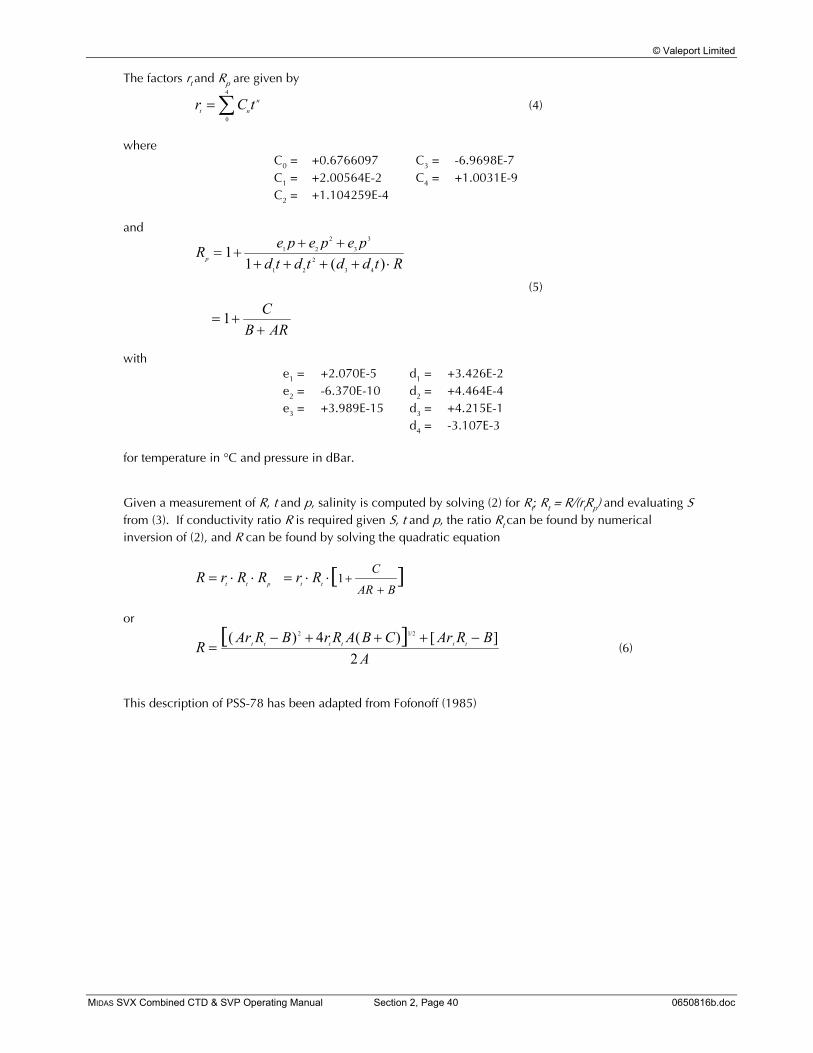
The factors rt and Rp are given by

r C tt n

n= ∑0

4

(4)

where

C0 = +0.6766097 C3 = -6.9698E-7 C1 = +2.00564E-2 C4 = +1.0031E-9 C2 = +1.104259E-4

and

R e p e p e pd t d t d d t R

CB AR

p = ++ +

+ + + + ⋅

= ++

11

1

1 2

2

3

3

1 2

2

3 4( )

(5)

with

e1 = +2.070E-5 d1 = +3.426E-2 e2 = -6.370E-10 d2 = +4.464E-4 e3 = +3.989E-15 d3 = +4.215E-1 d4 = -3.107E-3

for temperature in °C and pressure in dBar. Given a measurement of R, t and p, salinity is computed by solving (2) for Rt; Rt = R/(rtRp) and evaluating S from (3). If conductivity ratio R is required given S, t and p, the ratio Rt can be found by numerical inversion of (2), and R can be found by solving the quadratic equation

R r R R r Rt t p t t

C

AR B= ⋅ ⋅ = ⋅ ⋅ +

+ [ ]1

or

RAr R B r R A B C Ar R B

At t t t t t=

− + + + −[ ]( ) ( ) [ ]/2 1 242

(6)

This description of PSS-78 has been adapted from Fofonoff (1985)

© Valeport Limited


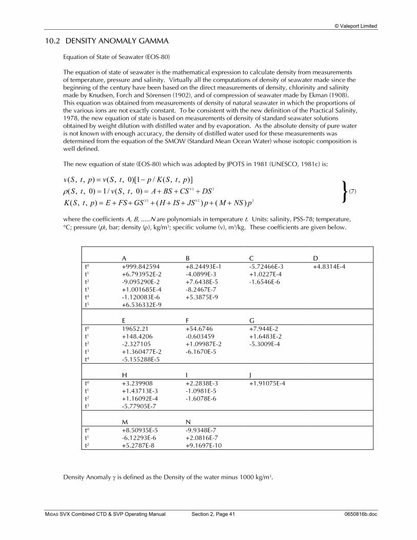
10.2 DENSITY ANOMALY GAMMA

Equation of State of Seawater (EOS-80) The equation of state of seawater is the mathematical expression to calculate density from measurements of temperature, pressure and salinity. Virtually all the computations of density of seawater made since the beginning of the century have been based on the direct measurements of density, chlorinity and salinity made by Knudsen, Forch and Sörensen (1902), and of compression of seawater made by Ekman (1908). This equation was obtained from measurements of density of natural seawater in which the proportions of the various ions are not exactly constant. To be consistent with the new definition of the Practical Salinity, 1978, the new equation of state is based on measurements of density of standard seawater solutions obtained by weight dilution with distilled water and by evaporation. As the absolute density of pure water is not known with enough accuracy, the density of distilled water used for these measurements was determined from the equation of the SMOW (Standard Mean Ocean Water) whose isotopic composition is well defined. The new equation of state (EOS-80) which was adopted by JPOTS in 1981 (UNESCO, 1981c) is: v S t p v S t p K S t pS t v S t A BS CS DS

K S t p E FS GS H IS JS p M NS p

( , , ) ( , , )[ / ( , , )]( , , ) / ( , , )( , , ) ( ) ( )

/

/ /

= −= = + + += + + + + + + +

0 10 1 0 3 2 2

3 2 3 2 2

ρ }(7)

where the coefficients A, B, .....N are polynomials in temperature t. Units: salinity, PSS-78; temperature, °C; pressure (p), bar; density (ρ), kg/m3; specific volume (v), m3/kg. These coefficients are given below.

A

B

C

D

t0 +999.842594 +8.24493E-1 -5.72466E-3 +4.8314E-4 t1 +6.793952E-2 -4.0899E-3 +1.0227E-4 t2 -9.095290E-2 +7.6438E-5 -1.6546E-6 t3 +1.001685E-4 -8.2467E-7 t4 -1.120083E-6 +5.3875E-9 t5 +6.536332E-9

E F

G

t0 19652.21 +54.6746 +7.944E-2 t1 +148.4206 -0.603459 +1.6483E-2 t2 -2.327105 +1.09987E-2 -5.3009E-4 t3 +1.360477E-2 -6.1670E-5 t4 -5.155288E-5

H I

J

t0 +3.239908 +2.2838E-3 +1.91075E-4 t1 +1.43713E-3 -1.0981E-5 t2 +1.16092E-4 -1.6078E-6 t3 -5.77905E-7

M N

t0 +8.50935E-5 -9.9348E-7 t1 -6.12293E-6 +2.0816E-7 t2 +5.2787E-8 +9.1697E-10

Density Anomaly γ is defined as the Density of the water minus 1000 kg/m3.

© Valeport Limited


10.3 SPEED OF SOUND

The following information, discussion and conclusions are taken from Special Publication No.34 of the Hydrographic Society, prepared by JM Pike and FL Beiboer of METOCEAN plc. The report is entitled "A Comparison Between Algorithms for the Speed of Sound in Seawater". The following abbreviations and units are used:

V Computed speed of sound in seawater (m/s) T Temperature (°C) S Salinity φ Latitude in degrees g(φ) Gravitational acceleration at the given latitude (m/s2) Pb Hydrostatic pressure (bar) (1bar = 105Pa = 10/g(φ) (kg/cm2) Pk Hydrostatic pressure (kg/cm2) D Depth (m)

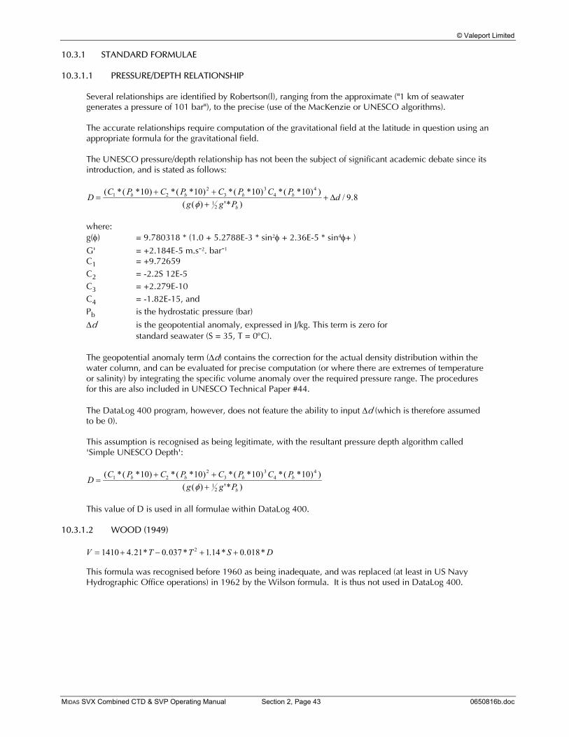
© Valeport Limited


10.3.1 STANDARD FORMULAE

10.3.1.1 PRESSURE/DEPTH RELATIONSHIP

Several relationships are identified by Robertson(l), ranging from the approximate ("1 km of seawater generates a pressure of 101 bar"), to the precise (use of the MacKenzie or UNESCO algorithms). The accurate relationships require computation of the gravitational field at the latitude in question using an appropriate formula for the gravitational field. The UNESCO pressure/depth relationship has not been the subject of significant academic debate since its introduction, and is stated as follows:

DC P C P C P C P

g g Pdb b b b

b

=+ +

++

( *( * ) *( * ) *( * ) *( * ) )( ( ) '* )

/ .1 22

33

44

12

10 10 10 109 8

φ∆

where: g(φ) = 9.780318 * (1.0 + 5.2788E-3 * sin2φ + 2.36E-5 * sin4φ+ )

G' = +2.184E-5 m.s-2. bar-1 C1 = +9.72659 C2 = -2.2S 12E-5 C3 = +2.279E-10 C4 = -1.82E-15, and Pb is the hydrostatic pressure (bar)

∆d is the geopotential anomaly, expressed in J/kg. This term is zero for standard seawater (S = 35, T = 0°C). The geopotential anomaly term (∆d) contains the correction for the actual density distribution within the water column, and can be evaluated for precise computation (or where there are extremes of temperature or salinity) by integrating the specific volume anomaly over the required pressure range. The procedures for this are also included in UNESCO Technical Paper #44. The DataLog 400 program, however, does not feature the ability to input ∆d (which is therefore assumed to be 0). This assumption is recognised as being legitimate, with the resultant pressure depth algorithm called 'Simple UNESCO Depth':

DC P C P C P C P

g g Pb b b b

b

=+ +

+( *( * ) *( * ) *( * ) *( * ) )

( ( ) '* )1 2

23

34

4

12

10 10 10 10φ

This value of D is used in all formulae within DataLog 400.

10.3.1.2 WOOD (1949)

V T T S D= + − + +1410 4 21 0 037 1 14 0 0182. * . * . * . * This formula was recognised before 1960 as being inadequate, and was replaced (at least in US Navy Hydrographic Office operations) in 1962 by the Wilson formula. It is thus not used in DataLog 400.

© Valeport Limited


10.3.1.3 WILSON (OCTOBER 1960)

Full Version The full version of this formula is: V V V V VT P S STP= + + + +1449 14. , where V T E T E T E T

V E P E P E P E PV S E S

V S E T E T E P E P E P T E

T

P k k k k

S

STP k k k

= − − − − + −

= − + − + − − −

= − + − −

= − − − + − + − − − + − +

4 5721 4 4532 2 2 6045 4 7 9851 6

1 60272 1 1 0268 5 3 5216 9 3 3603 121 39799 35 1 69202 3 35

35 1 1244 2 7 7711 7 7 7016 5 1 2943 7 3 1580 8 1 5790

2 3 4

2 3 4

2

2 2

. * . * . * . *

. * . * . * . *. *( ) . *( )

( ) *( . * . * . * . * . * * . −

+ − − + − + −

+ − − + −

+ − −

91 8607 4 7 4812 6 4 5283 8

2 529 7 1 8563 91 9646 10

2

2 3

2 2

3

* * )*( . * . * . * )

*( . * . * )*( . * )

P TP E T E T E T

P E T E TP E T

k

k

k

k

Wilson states that the formula is valid to within ± 0.3 m/s in the ranges: -4°C < T < 30°C; 0 < S < 37 1 kg/cm2; < Pk < 1000 kg/cm2.

where P Pgk b= ⋅10( )φ

Simplified Version A simplified version of this formula, which is believed to have been used for a number of offshore surveys, is: V T E T E T E T S E D= + − − − − + − − − + −1 449 14 4 5721 4 4532 2 2 6045 4 1 39799 1 1244 2 35 1 643 22 3. . . * . * . * ( . [ . * ]) *( ) . * The range of validity is likely to be comparable to the full version, with simplification (and inaccuracy) introduced by replacing the pressure terms with a depth term (of unknown provenance), and ignoring 4th order temperature terms (inter alia).

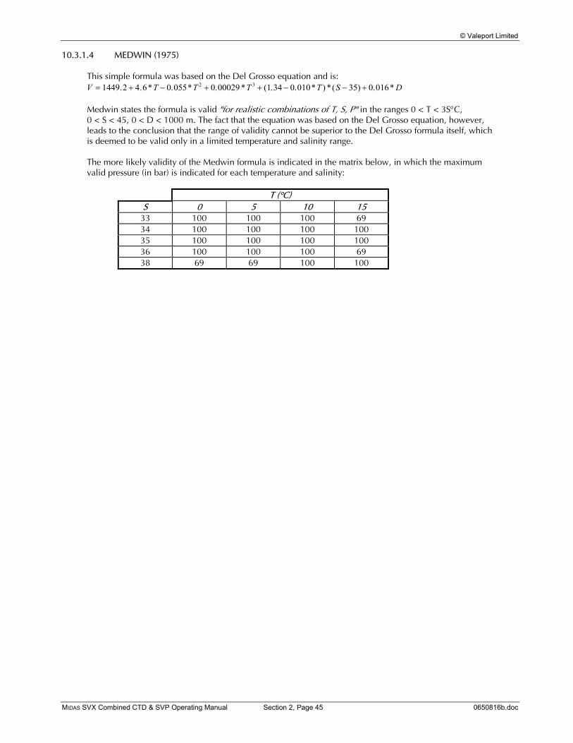
© Valeport Limited


10.3.1.4 MEDWIN (1975)

This simple formula was based on the Del Grosso equation and is: V T T T T S D= + − + + − − +1449 2 4 6 0 055 0 00029 1 34 0 010 35 0 0162 3. . * . * . * ( . . * ) *( ) . * Medwin states the formula is valid "for realistic combinations of T, S, P" in the ranges 0 < T < 3S°C, 0 < S < 45, 0 < D < 1000 m. The fact that the equation was based on the Del Grosso equation, however, leads to the conclusion that the range of validity cannot be superior to the Del Grosso formula itself, which is deemed to be valid only in a limited temperature and salinity range. The more likely validity of the Medwin formula is indicated in the matrix below, in which the maximum valid pressure (in bar) is indicated for each temperature and salinity:

T (°C) S 0 5 10 15

33 100 100 100 69 34 100 100 100 100 35 100 100 100 100 36 100 100 100 69 38 69 69 100 100

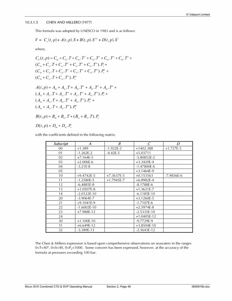
© Valeport Limited


10.3.1.5 CHEN AND MILLERO (1977)

This formula was adopted by UNESCO in 1983 and is as follows: V C t p A t p S B t p S D t p Sw= ( , )+ ( , ). + ( , ). + ( , )./3 2 2 where, C t p C C T C T C T C T C TC C T C T C T C T PC C T C T C T C T PC C T C T P

W

b

b

b

( , ) . . . . .( . . . . ).( . . . . ).( . . ).

= + + + + + ++ + + + ++ + + + ++ +

00 01 02

2

03

3

04

4

05

5

10 11 12

2

13

3

14

4

20 21 22

2

23

3

24

4 2

30 31 32

2 3

A t p A A T A T A T A TA A T A T A T A T PA A T A T A T PA A T A T P

b

b

b

( , ) . . . .( . . . . ).( . . . ).( . . ).

= + + + + ++ + + + ++ + + ++ +

00 01 02

2

03

3

04

4

10 11 12

2

13

3

14

4

20 21 22

2

23

3 2

30 31 32

2 3

B t p B B T B B T Pb( , ) . ( . ).= + + +00 01 10 11 D t p D D Pb( , ) .= +00 10 with the coefficients defined in the following matrix:

Subscript A B C D 00 +1.389 -1.922E-2 +1402.388 +1.727E-3 01 -1.262E-2 -4.42E-5 +5.03711 02 +7.164E-5 -5.80852E-2 03 +2.006E-6 +3.3420E-4 04 -3.21E-8 -1.47800E-6 05 +3.1464E-9 10 +9.4742E-5 +7.3637E-5 +0.153563 -7.9836E-6 11 -1.2580E-5 +1.7945E-7 +6.8982E-4 12 -6.4885E-8 -8.1788E-6 13 +1.0507E-8 +1.3621E-7 14 -2.0122E-10 -6.1185E-10 20 -3.9064E-7 +3.1260E-5 21 +9.1041E-9 -1.7107E-6 22 -1.6002E-10 +2.5974E-8 23 +7.988E-12 -2.5335E-10 24 +1.0405E-12 30 +1.100E-10 -9.7729E-9 31 +6.649E-12 +3.8504E-10 32 -3.389E-13 -2.3643E-12

The Chen & Millero expression is based upon comprehensive observations on seawaters in the ranges 0<T<40°, 0<S<40, 0<Pb<1000. Some concern has been expressed, however, at the accuracy of the formula at pressures exceeding 100 bar.

© Valeport Limited


10.3.1.6 DEL GROSSO (1974)

V C DC DC DC DCT S P STP= + + + +000 , where C

DC E T E T E T

DC E S E SDC P E P E PDC E T S E T P

E T P E T P

E T P

T

S

P k k k

STP k

k k

k

0002 3

2

2 3

2 2 2

3

1402 392

0 501109398873 1 0 550946843172 1 0 221535969240 3

0 132952290781 1 0 128955756844 30 156059257041 0 244998688441 4 0 883392332513 80 127562783426 1 0 635191613389 20 265484716608 7 0 159349479045 5

0 522116437235 9 0

=

= + − − + −

= + + −

= + − − −= − − + −

+ − − −

+ − −

.

. * . * .

. * . *. * . . *. * * . * *. * * . * *

. * * .438031096213 6

0 161674495909 8 0 968403156410 40 485639620015 5 0 340597039004 3

3

2 2 2

2

E T P

E S P E T SE T S P E T S P

k

k

k k

−

− − + −

+ − − −

* *

. * * . * *

. * * * . * * *

The formula is deemed to be valid only in the temperature and salinity ranges, and up to the pressures (bar), indicated in the matrix below:

T (°C) S 0 5 10 15

33 1034 1034 275 69 34 1034 1034 207 207 35 1034 1034 414 207 36 1034 1034 275 69 38 69 69 414 414

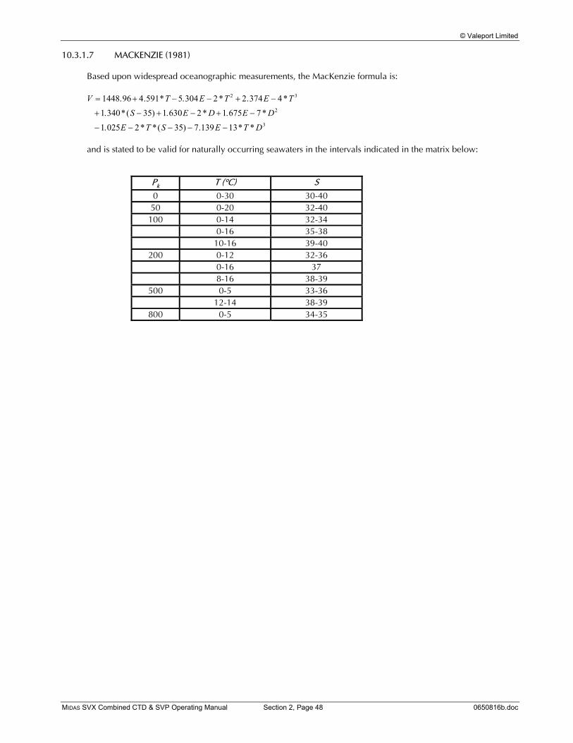
© Valeport Limited


10.3.1.7 MACKENZIE (1981)

Based upon widespread oceanographic measurements, the MacKenzie formula is: V T E T E T

S E D E D

E T S E T D

= + − − + −

+ − + − + −

− − − − −

1448 96 4 591 5 304 2 2 374 41 340 35 1 630 2 1 675 7

1 025 2 35 7 139 13

2 3

2

3

. . * . * . *. *( ) . * . *

. * *( ) . * *

and is stated to be valid for naturally occurring seawaters in the intervals indicated in the matrix below:

Pk T (°C) S 0 0-30 30-40 50 0-20 32-40 100 0-14 32-34

0-16 35-38 10-16 39-40

200 0-12 32-36 0-16 37 8-16 38-39

500 0-5 33-36 12-14 38-39

800 0-5 34-35

© Valeport Limited


10.3.2 DISCUSSION

10.3.2.1 DEVELOPMENT OF FORMULAE

A useful overview of the history of seawater speed of sound measurements and formulae is provided by Dulshaw et al. All formulae given above (and the majority of others referred to in the course of this study) were empirically derived from measurements of acoustic velocity of seawater samples whose temperature, salinity and pressure were measured in the oceans and/or varied in the laboratory. The Robertson equation is one of the few attempts to base the equations for the speed of sound on theoretical considerations alone. The Wood formula, while in use even now, wass considered as early as 1960 to be unreliable for the advancing technology and requirements of that era, and was superseded by the Wilson formula in 1961. The recognition of defects in the experimental methods of Wilson, together with the adoption of the practical salinity scale and the international equation of state for seawater (EOS-80) resulted in the Wilson formula being superseded for oceanographic purposes by the Chen & Millero formula, which still represents the formal standard for oceanographic purposes. The limitations of the Chen & Millero formula in turn were revealed by precise in situ observations of acoustic velocity with depth, and by the advent of tomographic methods to determine seawater physical properties along very large path-lengths (across oceans) and to great depths. These observations have led in recent years to the realisation that the Chen & Millero formula has distinct limitations at high pressures, and that the Del Grosso equation may be more realistic for such specialist purposes. The wide validity range for salinity and temperature of the Chen & Millero formula is of value for measurements on the continental shelf, however. The quality of fit of the Del Grosso equation to the modern high-pressure data sets (and the corrections that should consequently be applied to the Del Grosso equation) is currently the subject of some debate.

10.3.2.2 COMPARISON OF FORMULAE

The Wood and Wilson formulae do not fit modem experimental and observational data well, and should no longer be used for precise computations. This probably is the result of improvements in observational and analytical techniques over the years, together with changes in computational methods of salinity and depth. The remaining algorithms show fairly close agreement with one another, diverging as pressure increases. The Chen & Millero formula is commonly accepted for oceanographic use, and was derived from measurements over a wide salinity, temperature and pressure range.

© Valeport Limited


At high pressures (>100 bar), however, recent research suggests that the Del Grosso equation is more accurate, although this formula is valid only for a limited range of oceanic waters. The Del Grosso formula has been used as a benchmark to appraise the accuracy of the other algorithms. The following order of preference is suggested: i) Chen & Millero (only for water depths less than 1000m) ii) Del Grosso (only for water depths greater than 1000m) iii) MacKenzie (for rapid computations in oceanic waters to 8000m water depth) iv) Medwin (for rapid computations in oceanic waters to 1000m water depth) The Medwin and Wilson (simplified) formulae diverge considerably from the remaining algorithms at temperatures greater than 20°C. This is expected from two simple formulae lacking higher order temperature terms. There may be some advantages in using the MacKenzie and Medwin formulae where depth is known, and where the computation of pressure for inclusion in the Chen & Millero or Del Grosso formulae would become unnecessarily onerous. The user should be made aware, however, of the limited range of conditions of temperature, salinity and pressure over which these formulae are valid.

10.3.2.3 THE PRESSURE/DEPTH ALGORITHM

An accurate expression for computing pressure from depth (and vice versa) may be desirable:

a) for its own sake, to enable precise pressure and depth computations to be made for a variety of purposes; and

b) to enable precise speed of sound computations to be made.

When using speed of sound algorithms with a pressure term (Chen & Millero, Del Grosso), the water pressure can be measured directly, estimated from a known depth and inversion of the UNESCO pressure/depth algorithm (possibly based on a carefully calibrated conductivity/temperature/depth cast), or calculated from standard tables. According to Saunders and Fofonoff, who were the originators of the basic method adopted in the UNESCO formula, these estimates should be carried out at 5 bar pressure intervals near the surface and at 200 bar intervals for greater depths. When using speed of sound formulae with a depth term (MacKenzie or Medwin), the depth may be estimated or measured by some independent means; or computed from a pressure measurement and a conductivity/temperature depth cast. It is more likely, however, that these methods would not be used for precise purposes; they are in any case valid only for oceanic waters in which the errors in the estimation of depth, introduced through ignoring the geopotential anomaly, would not be excessive.

© Valeport Limited


10.3.3 CONCLUSIONS

1. It is recommended that use of the Wood and Wilson formulae be discontinued for precise purposes, as they do not provide good agreement with modern data sets and computational methods of salinity and depth.

2. It is of crucial importance to ensure that the formulae (of whatever origin) are used only for

observations made within the ranges of temperature, salinity and pressure for which each expression is deemed valid.

3. It is recommended that the Chen and Millero formula be used for seawaters on the continental

shelf. This incorporates a pressure term which should be measured directly; evaluated from a known depth using the full UNESCO formula and data obtained either from oceanographic tables or from a conductivity/temperature/depth cast; or the error in using the simplified UNESCO formula deliberately accepted.

4. In deep ocean waters, the Del Grosso formula is currently favoured, especially for long path-

lengths. This also uses a pressure term. 5. Where rapid computations are necessary, or where the depth is known (but not pressure), the

simple MacKenzie (9 terms) and Medwin (5 terms) formulations may prove of value. These expressions are strictly valid only for normal oceanic waters. Where depth is computed from pressure, the simplified UNESCO equation for the pressure/depth relationship could be used without introducing significant error.

6. Incorporation of the full UNESCO pressure/depth algorithm (incorporating the geopotential

anomaly) would be a useful addition to any software package, although there may be little discernible benefit to the accuracy of the speed of sound computations. The complete formula would, however, enable a full suite of precise applications to be available for use worldwide.

MIDAS SVX Combined CTD & SVP - Valeport Velocity...MIDAS SVX Combined CTD & SVP Operating Manual Section 2, Page 5 0650816b.doc 2 OPENING DATALOG 400 Double clicking the desktop icon

Documents