MIDAS Project Definition - MRIR, Miami

Last update: 7/4/2008 1

MIDAS Project Definition

A. A. Maudsley, A. Darkazanli, July 2004-

Contents

1 Introduction .............................................................................................................................. 2 2 Overview of the Data Processing Functionality ....................................................................... 2 3 Major Program Modules .......................................................................................................... 3

4 General Organization of the MIDAS Data Management System ............................................ 4

5 Data Formats ............................................................................................................................ 5 5.1 MRI .................................................................................................................................... 6

5.2 SI ........................................................................................................................................ 6 5.3 Parameter Maps ................................................................................................................. 6 5.4 MRI Segmentation ............................................................................................................. 6

6 The MIDAS Browser ............................................................................................................... 7 6.1 Series and DataSet Labels .................................................................................................. 7 6.2 Example File Open Browser .............................................................................................. 9

6.3 Example Browser Output and Underlying XML Tag Information.................................. 10 6.4 Example for Multi-Echo MRI Data ................................................................................. 12

7 The Subject.xml Format ......................................................................................................... 13 7.1 General Organization ....................................................................................................... 13

7.2 Parameters ........................................................................................................................ 14 7.3 ID Tags ............................................................................................................................. 16

7.4 Process_IDs ...................................................................................................................... 17 7.5 The DataSet Node and Multi-Channel Data .................................................................... 18 7.6 Frames, Labels, and the Register_Viewer Parameter ...................................................... 19

8 The Project.xml and xxx_Project.xml File Formats ............................................................... 20 9 Data Processing Parameter Definitions .................................................................................. 21

10 Program and Data Directory Structure ................................................................................... 22

10.1 Projects.xml Location ................................................................................................... 22

10.2 Software Directory Locations ...................................................................................... 22 10.3 Data Directory Locations ............................................................................................. 23

11 The Atlas Format .................................................................................................................... 24 12 Programming Overview ......................................................................................................... 26

12.1 The MIDAS Library ..................................................................................................... 26

12.2 Command Line Protocol .............................................................................................. 26 12.2.1 Error Handling in Batch mode .............................................................................. 27 12.2.2 Summary of Command Line Calls to All Functions ............................................ 27

13 Spectral Bases Functions and the GAVA Program ................................................................ 28 14 Miscellaneous Acknowledgements ........................................................................................ 28

A. Frame Labels .............................................................................................................................. 30 B. Metabolite Name Definitions ..................................................................................................... 32

C. Essential Tags ............................................................................................................................. 34 D. Spatial Registration .................................................................................................................... 35 E. XML Organization of Multi-Channel and Multi-TE Data ......................................................... 37 F. XML Organization of DWI/DTI Results ................................................................................... 37

MIDAS

2

G. XML Organization of Analysis Results ..................................................................................... 38 H. File Names and Extensions ........................................................................................................ 40

1 Introduction

This document describes the underlying organization of the data and processing methods of

the MIDAS project, which includes a suite of MRSI and MRI data processing, analysis, and

visualization tools that support implementation of 1H MR Spectroscopic Imaging (MRSI) for

clinical research studies. The project includes development of a database of brain metabolite

distributions in normal subjects, which will be used in the evaluation of metabolic changes in

neurological diseases, and secondarily aims to encourage the development of standardized MRSI

acquisition and processing procedures.

The software development aims include providing a high degree of automation; open source

software; minimize interactions with multiple image data formats; operation on multiple computer

systems, with an emphasis on Windows and PC/Linux systems.

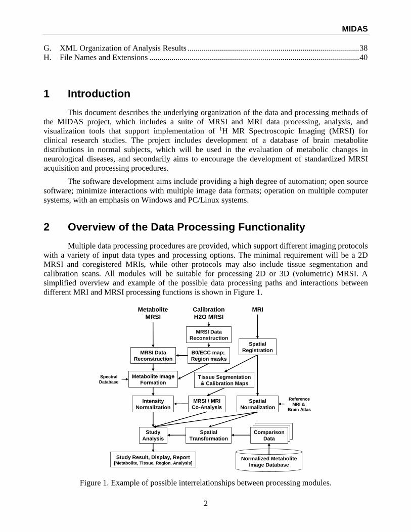
2 Overview of the Data Processing Functionality

Multiple data processing procedures are provided, which support different imaging protocols

with a variety of input data types and processing options. The minimal requirement will be a 2D

MRSI and coregistered MRIs, while other protocols may also include tissue segmentation and

calibration scans. All modules will be suitable for processing 2D or 3D (volumetric) MRSI. A

simplified overview and example of the possible data processing paths and interactions between

different MRI and MRSI processing functions is shown in Figure 1.

Study Result, Display, Report[Metabolite, Tissue, Region, Analysis]

MRSI Data

Reconstruction

B0/ECC map;

Region masks

Spectral

Database

Metabolite Image

Formation

Intensity

Normalization

Tissue Segmentation

& Calibration Maps

Spatial

Normalization

MRSI / MRI

Co-Analysis

Study

Analysis

Metabolite

MRSI

Calibration

H2O MRSI

MRI

Comparison

DataComparison

DataComparison

Data

Spatial

Transformation

Normalized Metabolite

Image Database

Reference

MRI &

Brain Atlas

Spatial

Registration

MRSI Data

Reconstruction

Figure 1. Example of possible interrelationships between processing modules.

MIDAS

3

The MRSI processing makes use of information obtained from MRI, for example to account

for relative tissue contributions in the analysis and to provide a spatial reference to a brain atlas. The

resultant data will be fitted metabolite parameters with voxel assignments in terms of brain regions.

Spatial transformations of individual results into a normalized spatial coordinate system will be

used to form a database of normal metabolite distributions, from which 'group statistics' datasets

will be calculated for different study groups.

The final study analysis is carried out for the multiparametric metabolite data and tissue

contribution analysis, using statistical comparisons against the normalized metabolite intensities

after being converted to subject coordinates. Analyses may be performed by region (e.g. lobe,

hippocampus, etc), between regions, at a single voxel, or for all voxels. Additional tools not

indicated in Fig. 1 include comprehensive MRSI and MRI display functions, data and processing

handling modules, and formation of a normalized image database.

The result of a complete MRSI processing procedure will be a multiparametric data set,

containing at each MRSI voxel:

1) All fitted spectral parameters;

2) Tissue contributions to that voxel;

3) A set of labels identifying the spatial regions and normalized coordinates for that voxel;

4) Parameters defining the spatial transformations to a normalized brain atlas;

5) Additional tags to identify regions to be tested or excluded in subsequent analysis

procedures. These will allow the operator to manually identify voxels to specifically include

or excluded from analysis.

3 Major Program Modules

The processing functions are broadly separated by developer groups, as:

1. MRSI Processing Functions

2. MRI Tissue Segmentation

3. MRI and MRSI Spatial Transformation

4. Statistical Data Analysis Tools

5. Data Display

In addition, these are supported by:

6. Data Import and Database Maintenance

7. Process Scheduler (or Pipeline)

8. Spectral Simulation (GAVA)

9. Data Simulation

Each program module can be run independently of the others. Software development of each

module is also independent. The current implementation includes modules written in C/C++, IDL,

and Java; however, all modules will make use of a standard library of functions for interacting with

the parameter information contained in the MIDAS database.

MIDAS

4

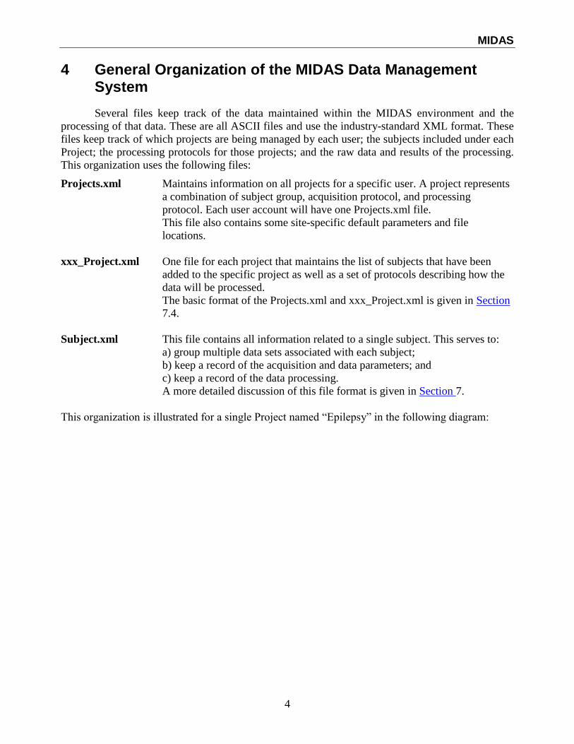
4 General Organization of the MIDAS Data Management System

Several files keep track of the data maintained within the MIDAS environment and the

processing of that data. These are all ASCII files and use the industry-standard XML format. These

files keep track of which projects are being managed by each user; the subjects included under each

Project; the processing protocols for those projects; and the raw data and results of the processing.

This organization uses the following files:

Projects.xml Maintains information on all projects for a specific user. A project represents

a combination of subject group, acquisition protocol, and processing

protocol. Each user account will have one Projects.xml file.

This file also contains some site-specific default parameters and file

locations.

xxx_Project.xml One file for each project that maintains the list of subjects that have been

added to the specific project as well as a set of protocols describing how the

data will be processed.

The basic format of the Projects.xml and xxx_Project.xml is given in Section

7.4.

Subject.xml This file contains all information related to a single subject. This serves to:

a) group multiple data sets associated with each subject;

b) keep a record of the acquisition and data parameters; and

c) keep a record of the data processing.

A more detailed discussion of this file format is given in Section 7.

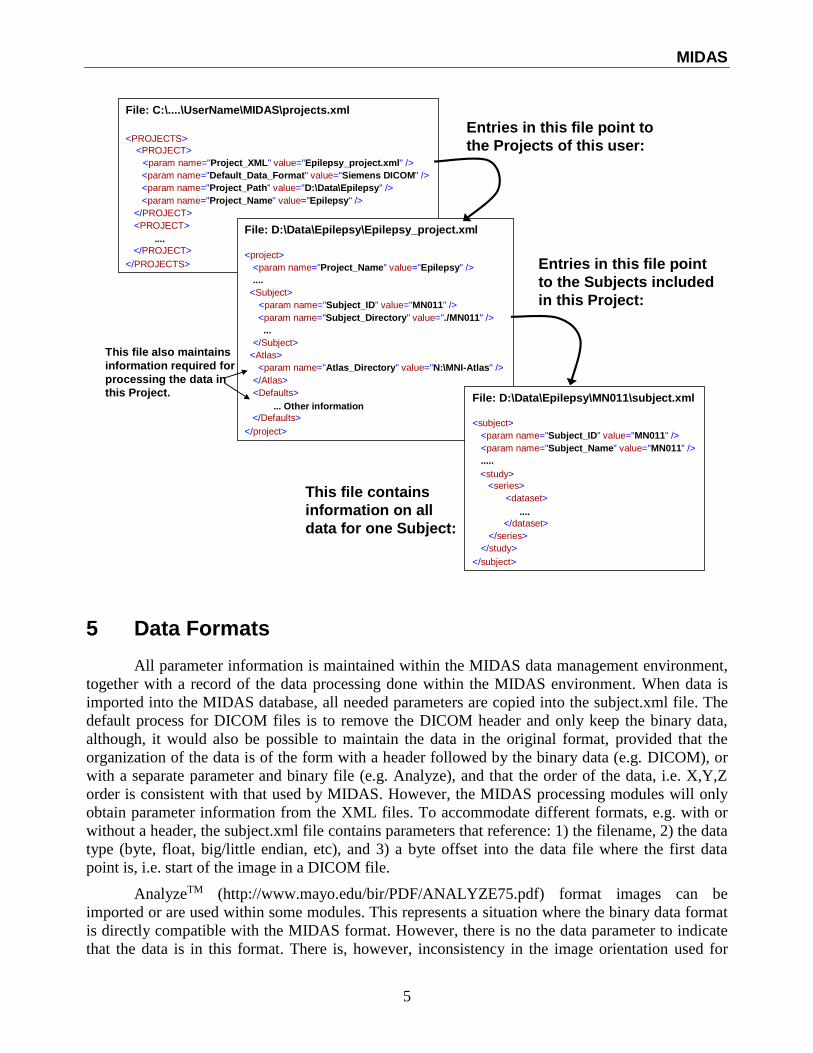
This organization is illustrated for a single Project named “Epilepsy” in the following diagram:

MIDAS

5

File: C:\....\UserName\MIDAS\projects.xml

<PROJECTS>

<PROJECT>

<param name="Project_XML" value="Epilepsy_project.xml" />

<param name="Default_Data_Format" value="Siemens DICOM" />

<param name="Project_Path" value="D:\Data\Epilepsy" />

<param name="Project_Name" value="Epilepsy" />

</PROJECT>

<PROJECT>

....

</PROJECT>

</PROJECTS>

File: D:\Data\Epilepsy\Epilepsy_project.xml

<project>

<param name="Project_Name" value="Epilepsy" />

....

<Subject>

<param name="Subject_ID" value="MN011" />

<param name="Subject_Directory" value="./MN011" />

...

</Subject>

<Atlas>

<param name="Atlas_Directory" value="N:\MNI-Atlas" />

</Atlas>

<Defaults>

... Other information

</Defaults>

</project>

File: D:\Data\Epilepsy\MN011\subject.xml

<subject>


<param name="Subject_Name" value="MN011" />

.....

<study>

<series>

<dataset>

....

</dataset>

</series>

</study>

</subject>

Entries in this file point to

the Projects of this user:

Entries in this file point

to the Subjects included

in this Project:

This file contains

information on all

data for one Subject:

This file also maintains

information required for

processing the data in

this Project.

5 Data Formats

All parameter information is maintained within the MIDAS data management environment,

together with a record of the data processing done within the MIDAS environment. When data is

imported into the MIDAS database, all needed parameters are copied into the subject.xml file. The

default process for DICOM files is to remove the DICOM header and only keep the binary data,

although, it would also be possible to maintain the data in the original format, provided that the

organization of the data is of the form with a header followed by the binary data (e.g. DICOM), or

with a separate parameter and binary file (e.g. Analyze), and that the order of the data, i.e. X,Y,Z

order is consistent with that used by MIDAS. However, the MIDAS processing modules will only

obtain parameter information from the XML files. To accommodate different formats, e.g. with or

without a header, the subject.xml file contains parameters that reference: 1) the filename, 2) the data

type (byte, float, big/little endian, etc), and 3) a byte offset into the data file where the first data

point is, i.e. start of the image in a DICOM file.

AnalyzeTM (http://www.mayo.edu/bir/PDF/ANALYZE75.pdf) format images can be

imported or are used within some modules. This represents a situation where the binary data format

is directly compatible with the MIDAS format. However, there is no the data parameter to indicate

that the data is in this format. There is, however, inconsistency in the image orientation used for

MIDAS

6

Analyze and DICOM, and in this project the orientation is defined as that used in Dicom (which is

inverted from that used in most Analyze programs). Support for other image formats such as JPEG,

TIFF etc, is not available, but may be included in the future.

Byte, 16-bit integer, and 32-bit floating point formats are used. Should it become necessary

to include data in other formats, e.g. long integer, then this data will be converted at the import

stage, e.g. to floating point.

5.1 MRI

Reconstructed MRI data is imported in Dicom format and the raw data is maintained in this

format. However, the first processing step is to concatenate the multiple-file DICOM data into a

single binary volume and apply some data conversions if necessary, e.g. to have all data in the same

orientation. The default MRI format is:

- 16 bit unsigned INTEGER. This default can be overridden and specified by the

Data_Representation parameter.

- Axial orientation; radiologist convention; right to left orientation (as if viewed from the foot

end), with the face looking up (eyes at top of the image). Slice order of volume data is

bottom (first image plane) to top (last image plane);

- The spatial position vector points to the upper left hand corner and images are painted to the

screen from top left corner to the bottom. Note, for IDL this requires setting !order=1 as

described in the installation instructions.

- Little- or big-endian, as defined in the parameter “Byte_Order”.

5.2 SI

- Complex FLOATING POINT. Complex INTEGER may also be used for the raw k-space

data.

- 1st data dimension is time or spectral data. 2nd, 3rd, and 4th data dimensions are spatial,

corresponding to MRI 1st, 2nd, 3rd spatial dimensions.

- Parameter definitions include support for 2 spectral dimensions; however, this is not

currently supported.

5.3 Parameter Maps

This data type refers to spatial distributions of any processed parameter, typically at the

resolution of the MRSI data; for example, fitted metabolite amplitude results, or B0 maps.

- Orientation is as MRI

- Data type = Float, Integer, or Byte

5.4 MRI Segmentation

The format used for the tissue segmentation results is based on Analyze format:

- Orientation as MRI

- Data type is byte, with value 255 equivalent to 100% volume contribution.

Segmentation data is stored as a FRAME (see below), and the descriptor of the

corresponding tissue type is given using the FRAME_TYPE definition tag Multiple images

representing each tissue type may be concatenated into a single file, or stored as individual files.

MIDAS

7

6 The MIDAS Browser

The MIDAS Browser provides the interface to the database to select a specific data file. The

top-level organization of the database is as:

Project Subject Study There can be multiple studies per subject, e.g. today, last year… Series There can be multiple Series per study, e.g. MRI, SI.. Dataset A Series can contain multiple data files, e.g. multiecho data

To simplify identification of the different data types by the user, a “label” is associated with

each Series and Dataset. The label assignment is first done at the time data is imported into the

MIDAS database, but other labels may also be created by a process. Although many image data

types can be interpreted from information contained in the Dicom header this is not always the case;

therefore the initial assignment is done by the operator at the time of the data import. Only a few

broad data types are defined, though these may be extended in the future to accommodate different

imaging modalities or acquisition types.

The Labels are intended to be used for visual display to the user; however, a process could

also search for a specific data type by a label name. This latter function requires that the label be

consistently used in the data import function and in any processing functions.

6.1 Series and DataSet Labels

Only a small number of labels are defined. These are in two levels, the first indicating the

image type (e.g. MRI_* or SI_*), and the second providing being used to separate different

versions, for example after processing.

The following labels are currently defined:

Level 1

(Series) Level 2

(DataSet or

Process)

Comment

MRI_PD The TR/TE may also be appended to the label (See note)

MRI_T1 “

MRI_T2 For multi-echo, the _T2 label will be used for all data (See

note)

MRI_DWI

(etc)

MRI_Ref

We can add any MRI type

MRI scan to be used for correcting the phased array data.

MRI_Seg

Tissue Segmentation – This is the result of a between series

“process” so goes under the Series level

MRI_*

MRI_Cal1

Result of some between MRI series analysis

Calibration functions, e.g. for receive & transmit sensitivity

correction, with multiple files numbered consecutively,

Cal1, Cal2, Cal3 etc.

Raw

Original

k-space data

The original image data as imported. For Dicom format this

is as multiple single-slice image files.

MIDAS

8

Volume A 3D image volume. Typically derived from concatenating

the (Dicom) series of multislice image files.

Norm

Registration

Spatially-Normalized MRI – the result of a within-series

“process”.

Registration parameters (no image data)

SI Metabolite MRS data.

SI_Ref Reference MRSI data. Typically H2O SI

Raw Time and k-space data

Spectral Processed result, frequency+space. Could include space-

time result, e.g. for B0 measurement from reference SI.

Maps

Spectral_Norm

Maps_Norm

Parameter maps at SI spatial resolution. E.g. spectral fitting

results, B0 maps, tissue density functions, etc.

Spatially-normalized Spectral data

Spatially-normalized MAPS data

SVS Single Voxel

Raw

Spectral

Analysis

Maps

Report

Maps

Report

These labels indicate the result of an analysis process on

either the Series or Dataset levels, resulting in an image

format or simple text results. A Report may contain links to

files in any commonly supported format, e.g. PDF, TIFF,

etc., which could contain plots, text reports, etc.

PET (etc) Other modalities possible. Currently PET import in ECAT7

is available.

Notes:

1. While these labels are defined for display in the browser, the three levels of the labels also

reflects the organizational structure used within the Subject.xml parameter file (described in Section

7). In brief, the first-level label (e.g. MRI, SI) is associated with each “Series” node of the XML

structure or between-series “Process” node, the second level label (e.g. T1, T2, Raw) is associated

with each “Data” node.

2. The labels ‘Seg’ (segmentation result) and ‘Norm’ (Spatially Normalized) describe data

types resulting from a process, i.e. not acquired data. The Seg label is defined on the ‘Series’ level,

and is assumed to be the result of a between-series processing operation, i.e. requiring multiple

input MRI data, and produces a new Series. The Norm label is on the ‘DataSet’ level, and

represents the result of a processing operation applied to a single series. Although MRI

segmentation can be applied to a single MRI series, this will always be treated as a between-series

processing operation.

3. For multiple echo MRI data we will only use the “MRI_T2” label. Although the ‘PD’

(proton density) type is traditionally used to indicate the first echo, this will be reserved for single

MRI contrast data that has been specifically acquired for this purpose. For a multiecho series, the

operator can still identify the fist-echo data in the browser by the TE value which gets appended to

the label.

4. The DataSet and Process labels (level 2) may be defined multiple times for each Series, e.g.

a process node for every TE of a multi-echo acquisition.

MIDAS

9

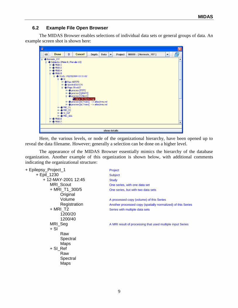
6.2 Example File Open Browser

The MIDAS Browser enables selections of individual data sets or general groups of data. An

example screen shot is shown here:

Here, the various levels, or node of the organizational hierarchy, have been opened up to

reveal the data filename. However; generally a selection can be done on a higher level.

The appearance of the MIDAS Browser essentially mimics the hierarchy of the database

organization. Another example of this organization is shown below, with additional comments

indicating the organizational structure:

+ Epilepsy_Project_1 Project + Epil_1230 Subject

+ 12-MAY-2001 12:45 Study MRI_Scout One series, with one data set + MRI_T1_300/5 One series, but with two data sets

Original Volume A processed copy (volume) of this Series Registration Another processed copy (spatially normalized) of this Series

+ MRI_T2 Series with multiple data sets 1200/20

1200/40

MRI_Seg A MRI result of processing that used multiple input Series + SI

Raw Spectral Maps

+ SI_Ref

Raw Spectral Maps

MIDAS

10

SI_Seg + 13-JUNE-2003 13:46 Another Study + Analysis A result of processing that used multiple Studies

Once the operator selects a file, the browser returns a set of IDs that define the data, study, series,

and the name of the subject.xml file.

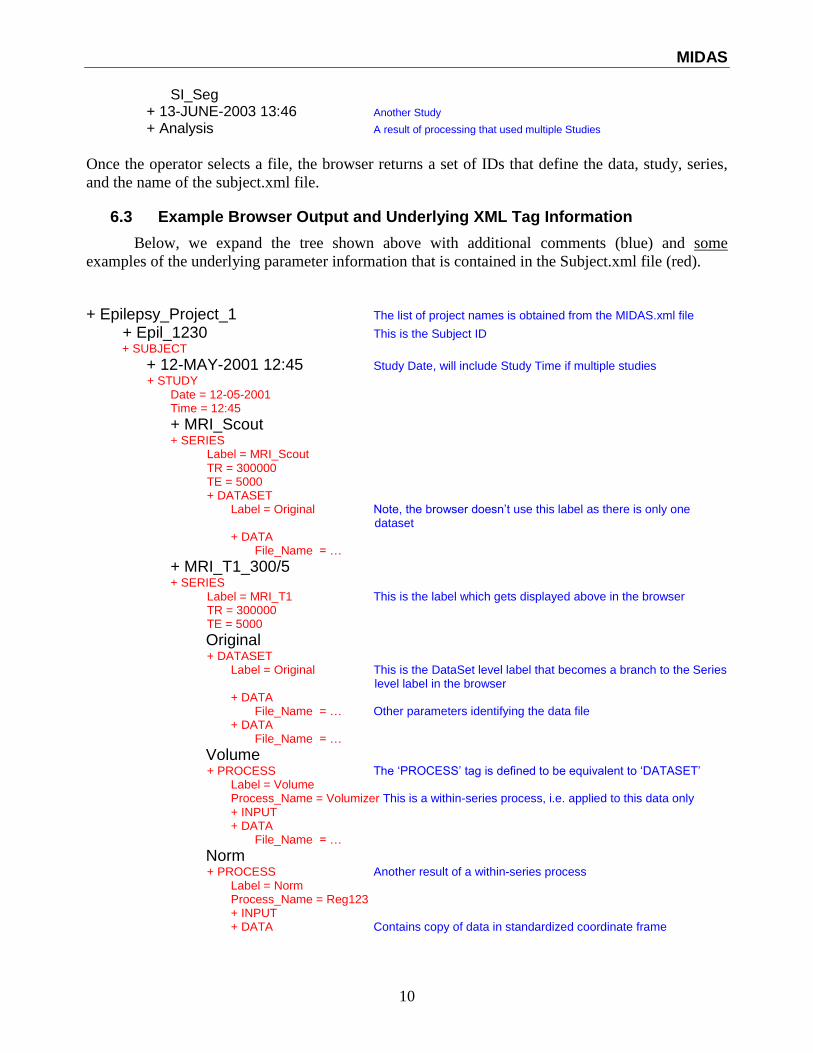
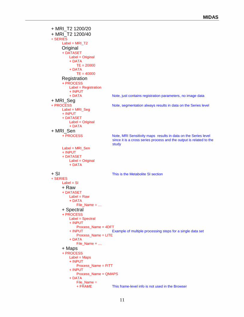
6.3 Example Browser Output and Underlying XML Tag Information

Below, we expand the tree shown above with additional comments (blue) and some

examples of the underlying parameter information that is contained in the Subject.xml file (red).

+ Epilepsy_Project_1 The list of project names is obtained from the MIDAS.xml file + Epil_1230 This is the Subject ID

+ SUBJECT

+ 12-MAY-2001 12:45 Study Date, will include Study Time if multiple studies

+ STUDY Date = 12-05-2001 Time = 12:45

+ MRI_Scout + SERIES

Label = MRI_Scout TR = 300000 TE = 5000 + DATASET

Label = Original Note, the browser doesn’t use this label as there is only one dataset

+ DATA File_Name = …

+ MRI_T1_300/5 + SERIES

Label = MRI_T1 This is the label which gets displayed above in the browser TR = 300000 TE = 5000

Original + DATASET

Label = Original This is the DataSet level label that becomes a branch to the Series level label in the browser

+ DATA File_Name = … Other parameters identifying the data file

+ DATA File_Name = …

Volume + PROCESS The ‘PROCESS’ tag is defined to be equivalent to ‘DATASET’

Label = Volume Process_Name = Volumizer This is a within-series process, i.e. applied to this data only + INPUT + DATA

File_Name = …

Norm + PROCESS Another result of a within-series process

Label = Norm Process_Name = Reg123 + INPUT + DATA Contains copy of data in standardized coordinate frame

MIDAS

11

+ MRI_T2 1200/20

+ MRI_T2 1200/40

+ SERIES Label = MRI_T2

Original + DATASET

Label = Original + DATA

TE = 20000 + DATA

TE = 40000

Registration + PROCESS

Label = Registration + INPUT + DATA Note, just contains registration parameters, no image data

+ MRI_Seg + PROCESS Note, segmentation always results in data on the Series level

Label = MRI_Seg + INPUT + DATASET


+ MRI_Sen + PROCESS Note, MRI Sensitivity maps results in data on the Series level

since it is a cross series process and the output is related to the study

Label = MRI_Sen + INPUT + DATASET


+ SI This is the Metabolite SI section + SERIES

Label = SI

+ Raw + DATASET

Label = Raw + DATA

File_Name = …

+ Spectral + PROCESS

Label = Spectral + INPUT

Process_Name = 4DFT + INPUT Example of multiple processing steps for a single data set

Process_Name = LITE + DATA

File_Name = …

+ Maps + PROCESS

Label = Maps + INPUT

Process_Name = FITT + INPUT

Process_Name = QMAPS + DATA

File_Name = + FRAME This frame-level info is not used in the Browser

MIDAS

12

Frame_Type = NAA Integral + FRAME

Frame_Type = NAA Frequency + PROCESS

Label = Registration + INPUT + DATA

+ SI_Ref This is the Water Reference SI section

+ SERIES Label = SI_Ref

+ Raw + Spectral + Maps

Notes:

1. On import, multiecho data are treated as a single series with multiple DataSet nodes.

However, if the metabolite SI and a reference SI are acquired together in an interleaved fashion, in

which case the Dicom header indicates this as a two-echo acquisition, this is changed on import to

create two separate Series.

2. The result of process that obtains data or information from a single data set and creates a

new data file is treated as a daughter of that data set, which appears as a branch in the Browser

hierarchy. A process that requires information from two or more data sets is referred to as a

between-series process (also discussed in Section 7.1), and results in a new data set on the Series,

i.e. top, level in the Browser. The results and actions of each process are defined elsewhere.

3. A PROCESS node existing under a SERIES node does not include a DATASET daughter

node, but may be considered equivalent to a DATASET.

4. A PROCESS that operates on data from multiple Series creates a node on the SERIES level,

e.g. the Tissue Segmentation process, and will contain a DATASET subnode.

6.4 Example for Multi-Echo MRI Data

The following shows another example of the browser output and underlying XML label tags

for multiecho data. Here the imported data is organized in the common DICOM manner as multiple

files each containing a single slice (Original), and this has been processed to make a second copy as

a volume (Volume):

+ MRI_T2 Original_1200/20 Original_1200/40 Volume_1200/20

Volume_1200/40 ….

+ MRI_T2

+ SERIES Label = MRI_T2

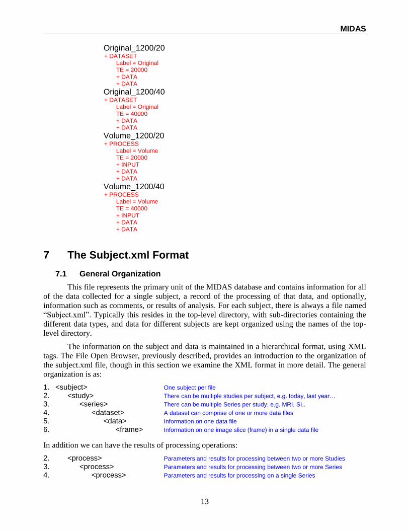
MIDAS

13

Original_1200/20

+ DATASET Label = Original TE = 20000 + DATA + DATA

Original_1200/40

+ DATASET Label = Original TE = 40000 + DATA + DATA

Volume_1200/20 + PROCESS

Label = Volume TE = 20000 + INPUT + DATA + DATA

Volume_1200/40

+ PROCESS Label = Volume TE = 40000 + INPUT + DATA + DATA

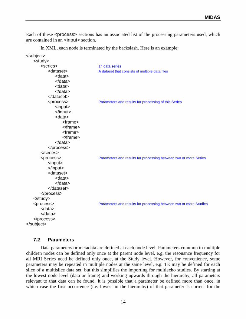
7 The Subject.xml Format

7.1 General Organization

This file represents the primary unit of the MIDAS database and contains information for all

of the data collected for a single subject, a record of the processing of that data, and optionally,

information such as comments, or results of analysis. For each subject, there is always a file named

“Subject.xml”. Typically this resides in the top-level directory, with sub-directories containing the

different data types, and data for different subjects are kept organized using the names of the top-

level directory.

The information on the subject and data is maintained in a hierarchical format, using XML

tags. The File Open Browser, previously described, provides an introduction to the organization of

the subject.xml file, though in this section we examine the XML format in more detail. The general

organization is as:

1. <subject> One subject per file 2. <study> There can be multiple studies per subject, e.g. today, last year… 3. <series> There can be multiple Series per study, e.g. MRI, SI.. 4. <dataset> A dataset can comprise of one or more data files 5. <data> Information on one data file

6. <frame> Information on one image slice (frame) in a single data file

In addition we can have the results of processing operations:

2. <process> Parameters and results for processing between two or more Studies 3. <process> Parameters and results for processing between two or more Series 4. <process> Parameters and results for processing on a single Series

MIDAS

14

Each of these <process> sections has an associated list of the processing parameters used, which

are contained in an <input> section.

In XML, each node is terminated by the backslash. Here is an example:

<subject> <study>

<series> 1st data series <dataset> A dataset that consists of multiple data files <data> </data> <data> </data> </dataset>

<process> Parameters and results for processing of this Series <input> </input> <data> <frame> </frame> <frame> </frame> </data> </process>

</series> <process> Parameters and results for processing between two or more Series

<input> </input> <dataset> <data> </data> </dataset>

</process> </study> <process> Parameters and results for processing between two or more Studies

<data> </data> </process> </subject>

7.2 Parameters

Data parameters or metadata are defined at each node level. Parameters common to multiple

children nodes can be defined only once at the parent node level, e.g. the resonance frequency for

all MRI Series need be defined only once, at the Study level. However, for convenience, some

parameters may be repeated in multiple nodes at the same level, e.g. TE may be defined for each

slice of a multislice data set, but this simplifies the importing for multiecho studies. By starting at

the lowest node level (data or frame) and working upwards through the hierarchy, all parameters

relevant to that data can be found. It is possible that a parameter be defined more than once, in

which case the first occurrence (i.e. lowest in the hierarchy) of that parameter is correct for the

MIDAS

15

selected data set. For example, on import the spectral bandwidth may be defined on the Series level,

however, subsequent processing may save only a smaller spectral region, in which case the spectral

bandwidth defined on the dataset (or data) level will be the correct one.

Some notes on the format of the parameters are:

- The “dictionary” or tag names used to define the metadata is based on DICOM; however,

some names and naming concepts have been changed for consistency or clarity, e.g.

o Spatial data dimensions are referred to as “1”, “2”, and “3”, as opposed to rows and

columns.

o Where possible, the same parameter names are used for MRI and MRS (Dicom uses

several different names).

o Any parameters including the term “patient” are replaced by “subject”.

- Subject parameter fields, such as name, and SSN, are included in the definition, but will not

be used for MIDAS project. All identifying information will be removed on importing into

the MIDAS environment, with the subject name replaced by a study ID.

- Parameter names are not case sensitive. In general the underscore is used to separate two

words, e.g. Study_Date. In this example, the capitalization of “Study” and “Date” is

preferred but not required.

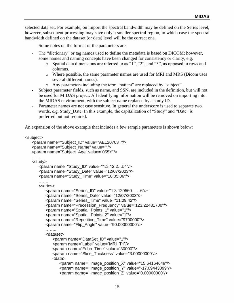
An expansion of the above example that includes a few sample parameters is shown below:

<subject>

<param name="Subject_ID" value="AE120703T"/> <param name="Subject_Name" value=""/> <param name="Subject_Age" value="055Y"/> …… <study>

<param name="Study_ID" value="1.3.12.2…54"/> <param name="Study_Date" value="12/07/2003"/> <param name="Study_Time" value="10:05:06"/> ……. <series>

<param name="Series_ID" value="1.3.120560……6"/> <param name="Series_Date" value="12/07/2003"/> <param name="Series_Time" value="11:09:42"/> <param name="Precession_Frequency" value="123.22481700"/> <param name="Spatial_Points_1" value="1"/> <param name="Spatial_Points_2" value="1"/> <param name="Repetition_Time" value="9700000"/> <param name="Flip_Angle" value="90.00000000"/> …….. <dataset>

<param name="DataSet_ID" value="1"/> <param name=”Label” value=”MRI_T1”/> <param name="Echo_Time" value="30000"/> <param name="Slice_Thickness" value="3.00000000"/> <data> <param name=" image_position_X" value="15.64164649"/> <param name=" image_position_Y" value="-17.09443099"/> <param name=" image_position_Z" value="0.00000000"/>

MIDAS

16

<param name=”File_Name” value=”myMRIdata01.dat” </data> <data>

<param name=" image_position_X" value="15.64164649"/> <param name=" image_position_Y" value="-17.09443099"/> <param name=" image_position_Z" value="3.00000000"/>

<param name=”File_Name” value=”myMRIdata02.dat” </data> ……

</dataset> </series> <process> <param name=”ID”, value=”12.456…..76869”>

<param name=”Name”, value=”4DFT”> <param name=”Process_ID”, value=”23.444.5…..665.0”>

<input> <param name=”FT1_size”, value=”1024”> ….

</input> <dataset>

<param name=”Spatial_Points_1”, value=”64”> <param name=”Spatial_Points_1”, value=”64”> <param name=”Spectral_Points_0”, value=”2048”> …..

<data> <param name=”File”, value=”mydataSI.dat”>

</data> </dataset>

</process> </study>

</subject>

7.3 ID Tags

Each Subject, Study, Series, DataSet, Data, and Process has an associated unique identifier.

These can be used to:

- check that the same data is not imported twice into a project

- pass an identifier to a process that uniquely identifies the Series, or specific data file being

used as the input to that process.

- associate one dataset with another. For example, to indicate that a water reference SI

acquisition corresponds to a metabolite acquisition.

The tags are:

Tag name Comment

Subject_ID Unique ID assigned to the subject at the time of the MR scan. Should NOT

be something that could be used to identify the subject, e.g. name or SSN.

Study_ID Equivalent to “Study_Instance_UID” from the Dicom header, which

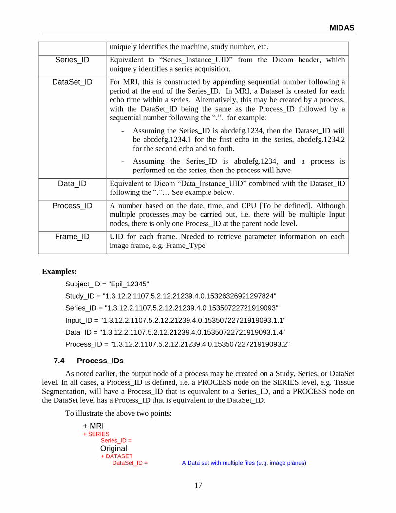
MIDAS

17

uniquely identifies the machine, study number, etc.

Series_ID Equivalent to “Series_Instance_UID” from the Dicom header, which

uniquely identifies a series acquisition.

DataSet_ID For MRI, this is constructed by appending sequential number following a

period at the end of the Series_ID. In MRI, a Dataset is created for each

echo time within a series. Alternatively, this may be created by a process,

with the DataSet_ID being the same as the Process_ID followed by a

sequential number following the “.”. for example:

- Assuming the Series_ID is abcdefg.1234, then the Dataset_ID will

be abcdefg.1234.1 for the first echo in the series, abcdefg.1234.2

for the second echo and so forth.

- Assuming the Series_ID is abcdefg.1234, and a process is

performed on the series, then the process will have

Data_ID Equivalent to Dicom “Data_Instance_UID” combined with the Dataset_ID

following the “.”… See example below.

Process_ID A number based on the date, time, and CPU [To be defined]. Although

multiple processes may be carried out, i.e. there will be multiple Input

nodes, there is only one Process_ID at the parent node level.

Frame_ID UID for each frame. Needed to retrieve parameter information on each

image frame, e.g. Frame_Type

Examples:

Subject_ID = "Epil_12345"

Study_ID = "1.3.12.2.1107.5.2.12.21239.4.0.15326326921297824"

Series_ID = "1.3.12.2.1107.5.2.12.21239.4.0.15350722721919093"

Input_ID = "1.3.12.2.1107.5.2.12.21239.4.0.15350722721919093.1.1"

Data_ID = "1.3.12.2.1107.5.2.12.21239.4.0.15350722721919093.1.4"

Process_ID = "1.3.12.2.1107.5.2.12.21239.4.0.15350722721919093.2"

7.4 Process_IDs

As noted earlier, the output node of a process may be created on a Study, Series, or DataSet

level. In all cases, a Process_ID is defined, i.e. a PROCESS node on the SERIES level, e.g. Tissue

Segmentation, will have a Process_ID that is equivalent to a Series_ID, and a PROCESS node on

the DataSet level has a Process_ID that is equivalent to the DataSet_ID.

To illustrate the above two points:

+ MRI + SERIES

Series_ID =

Original + DATASET

DataSet_ID = A Data set with multiple files (e.g. image planes)

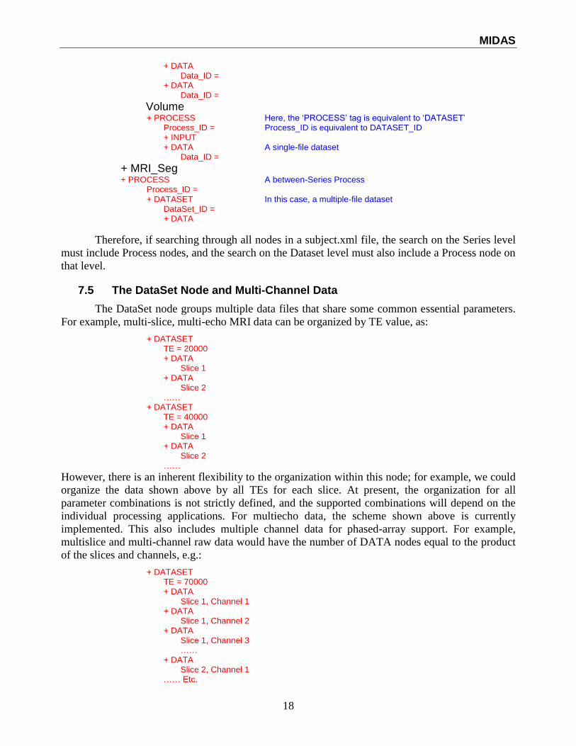
MIDAS

18

+ DATA Data_ID =

+ DATA Data_ID =

Volume + PROCESS Here, the ‘PROCESS’ tag is equivalent to ‘DATASET’

Process_ID = Process_ID is equivalent to DATASET_ID + INPUT + DATA A single-file dataset

Data_ID =

+ MRI_Seg + PROCESS A between-Series Process

Process_ID = + DATASET In this case, a multiple-file dataset

DataSet_ID = + DATA

Therefore, if searching through all nodes in a subject.xml file, the search on the Series level

must include Process nodes, and the search on the Dataset level must also include a Process node on

that level.

7.5 The DataSet Node and Multi-Channel Data

The DataSet node groups multiple data files that share some common essential parameters.

For example, multi-slice, multi-echo MRI data can be organized by TE value, as:

+ DATASET TE = 20000 + DATA

Slice 1 + DATA

Slice 2 ……


Slice 1 + DATA

Slice 2 ……

However, there is an inherent flexibility to the organization within this node; for example, we could

organize the data shown above by all TEs for each slice. At present, the organization for all

parameter combinations is not strictly defined, and the supported combinations will depend on the

individual processing applications. For multiecho data, the scheme shown above is currently

implemented. This also includes multiple channel data for phased-array support. For example,

multislice and multi-channel raw data would have the number of DATA nodes equal to the product

of the slices and channels, e.g.:


Slice 1, Channel 1 + DATA

Slice 1, Channel 2 + DATA

Slice 1, Channel 3 ……

+ DATA Slice 2, Channel 1

…… Etc.

MIDAS

19

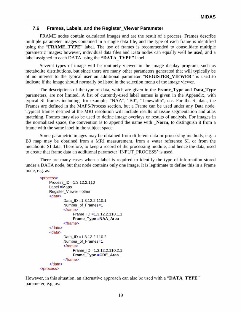
7.6 Frames, Labels, and the Register_Viewer Parameter

FRAME nodes contain calculated images and are the result of a process. Frames describe

multiple parameter images contained in a single data file, and the type of each frame is identified

using the “FRAME_TYPE” label. The use of frames is recommended to consolidate multiple

parametric images; however, individual data files and Data nodes can equally well be used, and a

label assigned to each DATA using the “DATA_TYPE” label.

Several types of image will be routinely viewed in the image display program, such as

metabolite distributions, but since there are many other parameters generated that will typically be

of no interest to the typical user an additional parameter “REGISTER_VIEWER” is used to

indicate if the image should normally be listed in the selection menu of the image viewer.

The descriptions of the type of data, which are given in the Frame_Type and Data_Type

parameters, are not limited. A list of currently-used label names is given in the Appendix, with

typical SI frames including, for example, “NAA”, “B0”, “Linewidth”, etc. For the SI data, the

Frames are defined in the MAPS/Process section, but a Frame can be used under any Data node.

Typical frames defined at the MRI resolution will include results of tissue segmentation and atlas

matching. Frames may also be used to define image overlays or results of analysis. For images in

the normalized space, the convention is to append the name with _Norm, to distinguish it from a

frame with the same label in the subject space

Some parametric images may be obtained from different data or processing methods, e.g. a

B0 map may be obtained from a MRI measurement, from a water reference SI, or from the

metabolite SI data. Therefore, to keep a record of the processing module, and hence the data, used

to create that frame data an additional parameter ‘INPUT_PROCESS’ is used.

There are many cases when a label is required to identify the type of information stored

under a DATA node, but that node contains only one image. It is legitimate to define this in a Frame

node, e.g. as:

<process> Process_ID =1.3.12.2.110 Label =Maps Register_Viewer =other <data>

Data_ID =1.3.12.2.110.1 Number_of_Frames=1 <frame>

Frame_ID =1.3.12.2.110.1.1 Frame_Type =NAA_Area

</frame> </data> <data>

Data_ID =1.3.12.2.110.2 Number_of_Frames=1 <frame>

Frame_ID =1.3.12.2.110.2.1 Frame_Type =CRE_Area

</frame> </data>

</process>

However, in this situation, an alternative approach can also be used with a “DATA_TYPE”

parameter, e.g. as:

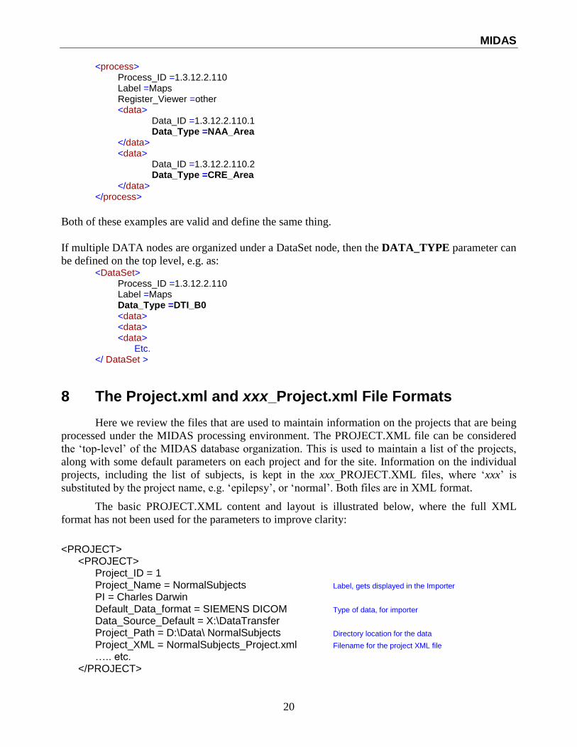
MIDAS

20

<process> Process_ID =1.3.12.2.110 Label =Maps Register_Viewer =other <data>

Data_ID =1.3.12.2.110.1 Data_Type =NAA_Area

</data> <data>

Data_ID =1.3.12.2.110.2 Data_Type =CRE_Area

</data> </process>

Both of these examples are valid and define the same thing.

If multiple DATA nodes are organized under a DataSet node, then the DATA_TYPE parameter can

be defined on the top level, e.g. as: <DataSet>

Process_ID =1.3.12.2.110 Label =Maps Data_Type =DTI_B0 <data> <data> <data> Etc.

</ DataSet >

8 The Project.xml and xxx_Project.xml File Formats

Here we review the files that are used to maintain information on the projects that are being

processed under the MIDAS processing environment. The PROJECT.XML file can be considered

the ‘top-level’ of the MIDAS database organization. This is used to maintain a list of the projects,

along with some default parameters on each project and for the site. Information on the individual

projects, including the list of subjects, is kept in the xxx_PROJECT.XML files, where ‘xxx’ is

substituted by the project name, e.g. ‘epilepsy’, or ‘normal’. Both files are in XML format.

The basic PROJECT.XML content and layout is illustrated below, where the full XML

format has not been used for the parameters to improve clarity:

<PROJECT> <PROJECT> Project_ID = 1 Project_Name = NormalSubjects Label, gets displayed in the Importer PI = Charles Darwin Default_Data_format = SIEMENS DICOM Type of data, for importer

Data_Source_Default = X:\DataTransfer Project_Path = D:\Data\ NormalSubjects Directory location for the data Project_XML = NormalSubjects_Project.xml Filename for the project XML file ….. etc. </PROJECT>

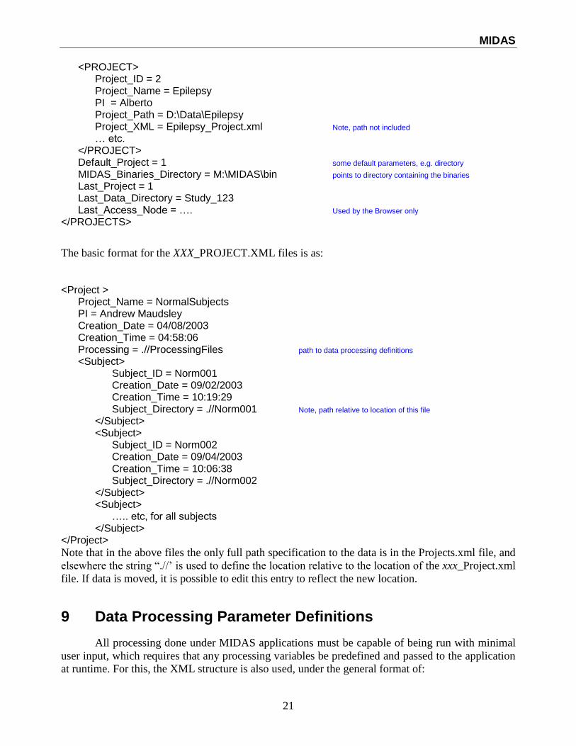
MIDAS

21

<PROJECT> Project_ID = 2 Project_Name = Epilepsy PI = Alberto Project_Path = D:\Data\Epilepsy Project_XML = Epilepsy_Project.xml Note, path not included … etc. </PROJECT> Default_Project = 1 some default parameters, e.g. directory MIDAS_Binaries_Directory = M:\MIDAS\bin points to directory containing the binaries Last_Project = 1 Last_Data_Directory = Study_123 Last_Access_Node = …. Used by the Browser only

</PROJECTS>

The basic format for the XXX_PROJECT.XML files is as:

<Project > Project_Name = NormalSubjects PI = Andrew Maudsley Creation_Date = 04/08/2003 Creation_Time = 04:58:06 Processing = .//ProcessingFiles path to data processing definitions

<Subject> Subject_ID = Norm001 Creation_Date = 09/02/2003 Creation_Time = 10:19:29 Subject_Directory = .//Norm001 Note, path relative to location of this file

</Subject> <Subject>

Subject_ID = Norm002 Creation_Date = 09/04/2003 Creation_Time = 10:06:38 Subject_Directory = .//Norm002

</Subject> <Subject>

….. etc, for all subjects </Subject>

</Project>

Note that in the above files the only full path specification to the data is in the Projects.xml file, and

elsewhere the string “.//’ is used to define the location relative to the location of the xxx_Project.xml

file. If data is moved, it is possible to edit this entry to reflect the new location.

9 Data Processing Parameter Definitions

All processing done under MIDAS applications must be capable of being run with minimal

user input, which requires that any processing variables be predefined and passed to the application

at runtime. For this, the XML structure is also used, under the general format of:

MIDAS

22

<APPLICATION_NAME> <param name="….." value="…." /> … etc. <\APPLICATION_NAME >

The processing file may contain one node only, i.e. with entries for one application only, or

with multiple nodes for multiple applications. After processing, the application will keep a copy of

the processing parameters in the <INPUT> node of the Subject.xml file, which would reflect any

changes or added information made at run time.

There are no requirements for the name of the processing file definition.

The name of the processing file will be available in the xxx_Projects.xml file for use when

batch processing is performed. However, processing applications should also be capable of running

in an ‘interactive’ mode where an operator can define the filename of any processing file.

11/8/04, Note, the single ‘master’ processing file is currently not implemented, and individual files

for each application are currently used.

10 Program and Data Directory Structure

The only fixed file location is of the “projects.XML” file. Beyond that there are few

restrictions to the directory structures, for both the MIDAS software distribution and the data;

however, the structures described in following section are recommended:

10.1 Projects.xml Location

There is a separate Projects.xml file for every user account. This allows each user to

maintain a list of only those projects that they are involved with, and for defaults such as directory

locations to be tailored for each subject. The location of this file is system specific, and is as:

Windows – Located under the default user directory, e.g. for account name ‘User’:

C:\Documents and Settings\User\MIDAS\Projects.xml

This first part of this directory path can be found under Java using the user.home system property,

or from the USERPROFILE environment variable in IDL.

Unix – located under $home/MIDAS/ Projects.xml

The first part of this path is the standard $HOME setting

10.2 Software Directory Locations

The parameter ‘MIDAS_Binaries_Directory’ in the Projects.xml file points to the location

of the directory containing the MIDAS distribution, e.g. E:\MIDAS\bin. This location is also

defined by the environmental variable MIDASBINDIR.

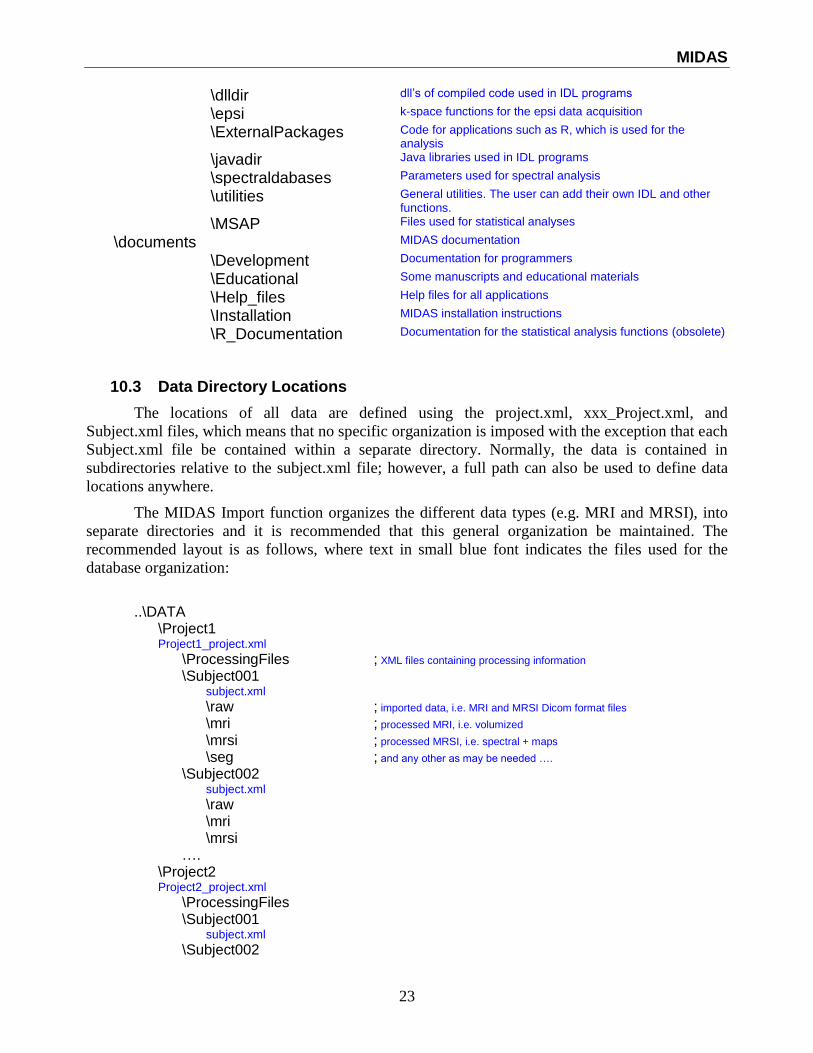
Additional directories relative to this location are as (not all are listed):

\bin Contains all binaries and IDL save files

MIDAS

23

\dlldir dll’s of compiled code used in IDL programs

\epsi k-space functions for the epsi data acquisition

\ExternalPackages Code for applications such as R, which is used for the analysis

\javadir Java libraries used in IDL programs

\spectraldabases Parameters used for spectral analysis

\utilities General utilities. The user can add their own IDL and other functions.

\MSAP Files used for statistical analyses

\documents MIDAS documentation

\Development Documentation for programmers

\Educational Some manuscripts and educational materials

\Help_files Help files for all applications

\Installation MIDAS installation instructions

\R_Documentation Documentation for the statistical analysis functions (obsolete)

10.3 Data Directory Locations

The locations of all data are defined using the project.xml, xxx_Project.xml, and

Subject.xml files, which means that no specific organization is imposed with the exception that each

Subject.xml file be contained within a separate directory. Normally, the data is contained in

subdirectories relative to the subject.xml file; however, a full path can also be used to define data

locations anywhere.

The MIDAS Import function organizes the different data types (e.g. MRI and MRSI), into

separate directories and it is recommended that this general organization be maintained. The

recommended layout is as follows, where text in small blue font indicates the files used for the

database organization:

..\DATA \Project1 Project1_project.xml

\ProcessingFiles ; XML files containing processing information \Subject001 subject.xml

\raw ; imported data, i.e. MRI and MRSI Dicom format files

\mri ; processed MRI, i.e. volumized

\mrsi ; processed MRSI, i.e. spectral + maps

\seg ; and any other as may be needed ….

\Subject002 subject.xml

\raw \mri \mrsi …. \Project2 Project2_project.xml

\ProcessingFiles \Subject001 subject.xml

\Subject002

MIDAS

24

subject.xml

…. etc.

The parameter ‘Last_Data_Directory’ in the Projects.xml file points to the location of the

last data directory used.

For every project, and atlas and corresponding reference MRI can be associated. This can

again be located anywhere; however, is typically located on the same level as the project, i.e.

..\DATA \MNI-Atlas \Atlas_data Atlas.xml ; same as Subject.xml, but describes the atlas parameters \Project1

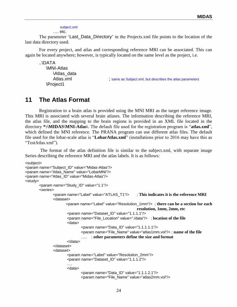
11 The Atlas Format

Registration to a brain atlas is provided using the MNI MRI as the target reference image.

This MRI is associated with several brain atlases. The information describing the reference MRI,

the atlas file, and the mapping to the brain regions is provided in an XML file located in the

directory *:\MIDAS\MNI-Atlas\. The default file used for the registration program is “atlas.xml”,

which defined the MNI reference. The PRANA program can use different atlas files. The default

file used for the lobar-scale atlas is “LobarAtlas.xml” (installations prior to 2016 may have this as

“TestAtlas.xml”).

The format of the atlas definition file is similar to the subject.xml, with separate image

Series describing the reference MRI and the atlas labels. It is as follows:

<subject> <param name="Subject_ID" value="Midas-Atlas"/> <param name="Atlas_Name" value="LobarMNI"/> <param name="Atlas_ID" value="Midas-Atlas"/> <study> <param name="Study_ID" value="1.1"/> <series>

<param name="Label" value="ATLAS_T1"/> ; This indicates it is the reference MRI <dataset>

<param name="Label" value="Resolution_1mm"/> ; there can be a section for each

resolution, 1mm, 2mm, etc <param name="Dataset_ID" value="1.1.1.1"/>

<param name="File_Location" value="./data"/> ; location of the file <data> <param name="Data_ID" value="1.1.1.1.1"/>

<param name="File_Name" value="atlas1mm.vol"/> ; name of the file

….. ; other parameters define the size and format </data> </dataset> <dataset> <param name="Label" value="Resolution_2mm"/> <param name="Dataset_ID" value="1.1.1.2"/> …. <data> <param name="Data_ID" value="1.1.1.2.1"/> <param name="File_Name" value="atlas2mm.vol"/>

MIDAS

25

….

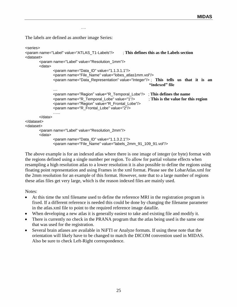
The labels are defined as another image Series:

<series>

<param name="Label" value="ATLAS_T1-Labels"/> ; This defines this as the Labels section <dataset> <param name="Label" value="Resolution_1mm"/> <data> <param name="Data_ID" value="1.1.3.1.1"/> <param name="File_Name" value="lobes_atlas1mm.vol"/>

<param name="Data_Representation" value="Integer"/> ; This tells us that it is an

“indexed” file ....

<param name=”Region” value="R_Temporal_Lobe"/> ; This defines the name

<param name="R_Temporal_Lobe" value="1"/> ; This is the value for this region

<param name=”Region” value="R_Frontal_Lobe"/> <param name="R_Frontal_Lobe" value="2"/> …... </data> </dataset> <dataset> <param name="Label" value="Resolution_2mm"/> <data> <param name="Data_ID" value="1.1.3.2.1"/> <param name="File_Name" value="labels_2mm_91_109_91.vol"/>

The above example is for an indexed atlas where there is one image of integer (or byte) format with

the regions defined using a single number per region. To allow for partial volume effects when

resampling a high resolution atlas to a lower resolution it is also possible to define the regions using

floating point representation and using Frames in the xml format. Please see the LobarAtlas.xml for

the 2mm resolution for an example of this format. However, note that to a large number of regions

these atlas files get very large, which is the reason indexed files are mainly used.

Notes:

At this time the xml filename used to define the reference MRI in the registration program is

fixed. If a different reference is needed this could be done by changing the filename parameter

in the atlas.xml file to point to the required reference image datafile.

When developing a new atlas it is generally easiest to take and existing file and modify it.

There is currently no check in the PRANA program that the atlas being used is the same one

that was used for the registration.

Several brain atlases are available in NiFTI or Analyze formats. If using these note that the

orientation will likely have to be changed to match the DICOM convention used in MIDAS.

Also be sure to check Left-Right correspondence.

MIDAS

26

12 Programming Overview

12.1 The MIDAS Library

A ‘MIDAS Library’ of functions written in Java is used to provide a common interface to

the MIDAS XML data organization. Bridge to these functions is available for IDL, and C/C++. It is

essential that all programs use this library. In this way any changes to the XML format used can be

immediately supported by all programs by simply recompiling. Documentation for this library is

provided in the Documents directory.

When a process reads parameters from the subject.xml file, it is important that the file be

closed as soon as possible, and if necessary, reopened at the end of the process to update the files.

This is necessary to allow for distributed processing implementation, where for example, operations

on different data may proceed simultaneously, but all need to access the same subject.xml file.

12.2 Command Line Protocol

Wherever possible, program modules should be able to run without operator interaction and

to be callable from the command line to enable batch, or pipelined, operation. The following

protocol is supported:

Process_name, Processing_file, xxx_Project.xml, Subject.xml, StudyID, SeriesID, String

Where:

Processing_file: The file containing the processing parameters for that application. Most

applications use XML format for this. Generally the path is not needed if it is located in the

“ProcessingFiles” directory for that project; however, this is application dependent.

xxx_Project.xml and Subject.xml: Must include the full path.

StudyID and SeriesID: These IDs are needed to be able to identify a specific data set, though may

not be needed by the application. Note that specific DataSet_IDs may not be known at the

start of processing pipeline, therefore this must always be found by the application.

Note that all parameters are optional. Generally, only the subject.xml will be required by every

application.

E.g.:

MyProg, ProcFile.xml, N:\data\MyProject.xml, N:\data\MyProject\subject.xml, ID1, ID2, -b

Support for this command-line driven processing is provided in the BATCH program for both IDL

procedure calls and external function calls. This program maintains a list of known IDL functions;

therefore, if a new processing modules is developed then the BATCH program (routine:

idlbatch\BATCH_run_processes.pro) needs to be modified to include the new module name.

Additional IDL programs can also be run under a new IDL session from the operating system

command line, in which case the process_name will be IDLDE followed by an IDL batch procedure

name that is a wrapper to make the actual call, e.g.

IDLDE.EXE @M:\bin\run4dft.pro

MIDAS

27

where the RUN_4DFT.PRO routine does the actual IDL procedure call shown above. (Note: In this

case, as parameters cannot be passed to an IDL batch procedure they will have to be written to a

temporary file that is then read by ‘run4dft.pro’, and a call similar to that shown above given.)

12.2.1 Error Handling in Batch mode

Programs run in Batch mode must report errors to the program that is responsible for

scheduling a set of processing operations. Currently, this is indicated by the presence of a text file;

however, this mechanism may be changed in the future if a different processes scheduler is

implemented. Therefore, it is strongly recommended that every process report errors using the

MIDAS library function ReportAnError(). The function is expecting that:

a) A subject has already been selected as part of running the application.

b) The name of the processing module

c) An error message, string, maximum length of 1024 bytes

d) Severity level: a numeric value where a value of 1 indicates a severe error requiring that a

series of processing steps in a batch mode be halted; and a Severity of 2 is designated for

warning errors which may be ignored by following processes.

A second function is supported in the Midas Library called ResetErrors(). This function

will remove ALL error messages in the queue.

Each reported error message will be stored in a separate text file, with a filename based on

the “module”_errorlog.txt and located in the same directory as the subject.xml file. The content of

this file includes:

a) Message date and time

b) Error severity

c) Error message

The function will keep up to 4 copies of the _errorlog.txt, with an incremented filename,

should the same module generate more than one error message without resetting the message log.

12.2.2 Summary of Command Line Calls to All Functions

(As of March 2007)

IDL Procedures batch, PipelineFile, ProjectXML, SubjectXML, StudyID volumizer, SubjectXML, StudyID, SeriesID epsi3d, SubjectXML, StudyID, SeriesID, [freq_drift=*] fdft, Procfile, SubjectXML, StudyID, SeriesID, [‘Spectral’] refdat, Procfile, SubjectXML, StudyID, SeriesID automask, Procfile, SubjectXML, StudyID, SeriesID lite, SubjectXML, StudyID, SeriesID fitt, ProcFile, SubjectXML, StudyID, SeriesID qmaps, ProcFile, SubjectXML, StudyID, SeriesID sinorm, ProjectXML, SubjectXML, StudyID manipulator, ProcFile, SubjectXML, StudyID fsl_seg, SubjectXML, StudyID analyze_import, SubjectXML, StudyID, SeriesID, Options_string OR, if a new Series is being created: analyze_import, SubjectXML, StudyID, Options_string The Options_string follows the format: options_string == DataSet_Label, Output_filename (these 2 are Essential)

MIDAS

28

[, Series=Series_Label, frame=Frame_Label, 'AppName=AppName, /swapX, /swapY, /swapZ, /Overwrite_Series, /Overwrite_Data, /Overwrite_Frame, /Delete, /ByteScale]

analyze_export, SubjectXML, StudyID, SeriesID, Options_string options_string == DataSet_Label, Output_filename (Essential) DataSet=DataSet_Number, frame=Frame_Label, /swapX, /swapY, /swapZ

DOS *.BAT Procedures runmriseg_FSL.bat SubjectXML, StudyID runmriseg_USF.bat SubjectXML, StudyID seg_FSL_T1.bat SubjectXML, StudyID seg_FSL_T1T2.bat SubjectXML, StudyID seg_USF.bat SubjectXML, StudyID

Other Programs java edu.miami.midas.mriseg.runmriseg Flags –p SubjectXML –d StudyID Where Flags=

-f <program name: fsl or bip or clp > choose different segmentation tool -s <1, 2a, 2b, 3 > number of image contrasts to be used, default is 1, 2a (T1 and T2), 2b (T1 and PD), or 3 (all features) -p <path for subject.xml> ex: c:\data\MN012\subject.xml -d <Study ID> -b : do bias correction while using usf segmentation (optional) -ob: save corrected data -ov: partial volume option (FSL package only)

13 Spectral Bases Functions and the GAVA Program

Automated spectral fitting and formation of metabolite images is performed using the FITT

program. This program uses a parametric modeling and optimization approach based on a set of

bases functions for each of the fitted metabolite spectra. These bases functions are described in a

simple ASCII table, which defines the frequency, phase, and relative amplitude of each resonance.

Additional information on this format is provided in the FITT_help file. The VESPA program,

obtained from Brian soher, is used to generate this table by computer simulation. Additional

information on this is given in the files FITT2_help and FITT2_PriorInfo.

14 Miscellaneous Acknowledgements

The primary architects of the MIDAS organizational structure are Drs. Ammar Darkazanli

and Andrew Maudsley. Additional contributions have been obtained from the MIDAS development

team that has included (in no particular order): Colin Studholme; Francois Rousseau; Yingjian Yu;

Krishna Sivasankaran; Rajesh Garugu; Yuhua Gu; Patrice Weber; Karl Young; Raj Pajare; James

Norman; Sulaiman Sheriff; Mohammed Goryawala.

In addition to the code developed by the primary MIDAS teams, and the major software

packages that are included, the MIDAS Software incorporates pieces of code inherited and

borrowed from various sources of open software, over the years. We gratefully acknowledge the

following contributions:

Various IDL Code: Christine Haupt (LITE), Scott Claflin (SID), Andreas Ebel (EPSI3D).

MIDAS

29

Support from 2DNMR in the IDL SI processing functions was provided under NIH grant

EB000730.

FSL: The FAST segmentation and other routines comes from the FSL distribution from the

Oxford group at: http://www.fmrib.ox.ac.uk/fsl/

The Prelude phase unwrap routine was derived from the FSL distribution, and developed by

Mark Jenkinson of the FMRIB Image Analysis Group.

The XMLCompare program was developed by Ammar Darkazanli.

Viewer makes use of the ImageJ library: http://rsb.info.nih.gov/ij/index.html

The VESPA program is provided courtesy of Brian Soher.

The RView program is available for download from http://rview.colin-studholme.net

PRINTRAW (GE data support) from Thomas Brosnan, Stanford University.

Also:

The BrainWeb simulated MRI data was obtained from the Montreal Neurological Institute:

http://www.bic.mni.mcgill.ca/brainweb

We applaud the Open Software initiative and if anyone has been left off this list then we apologize

and ask that you let us know.

THE END

http://www.fmrib.ox.ac.uk/fsl/

http://rsb.info.nih.gov/ij/index.html

http://rview.colin-studholme.net/

http://www.bic.mni.mcgill.ca/brainweb

Last update: 7/4/2008 30

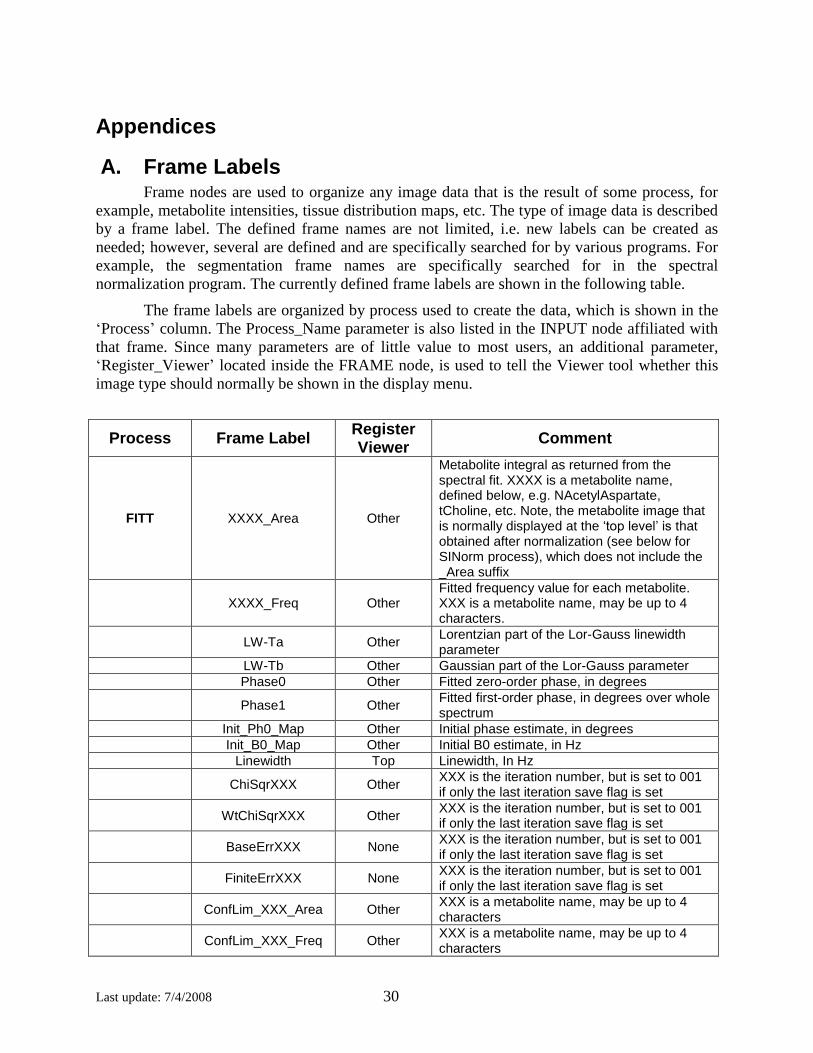
Appendices

A. Frame Labels Frame nodes are used to organize any image data that is the result of some process, for

example, metabolite intensities, tissue distribution maps, etc. The type of image data is described

by a frame label. The defined frame names are not limited, i.e. new labels can be created as

needed; however, several are defined and are specifically searched for by various programs. For

example, the segmentation frame names are specifically searched for in the spectral

normalization program. The currently defined frame labels are shown in the following table.

The frame labels are organized by process used to create the data, which is shown in the

‘Process’ column. The Process_Name parameter is also listed in the INPUT node affiliated with

that frame. Since many parameters are of little value to most users, an additional parameter,

‘Register_Viewer’ located inside the FRAME node, is used to tell the Viewer tool whether this

image type should normally be shown in the display menu.

Process Frame Label Register Viewer

Comment

FITT XXXX_Area Other

Metabolite integral as returned from the spectral fit. XXXX is a metabolite name, defined below, e.g. NAcetylAspartate, tCholine, etc. Note, the metabolite image that is normally displayed at the ‘top level’ is that obtained after normalization (see below for SINorm process), which does not include the _Area suffix

XXXX_Freq Other

Fitted frequency value for each metabolite. XXX is a metabolite name, may be up to 4 characters.

LW-Ta Other

Lorentzian part of the Lor-Gauss linewidth parameter

LW-Tb Other Gaussian part of the Lor-Gauss parameter

Phase0 Other Fitted zero-order phase, in degrees

Phase1 Other

Fitted first-order phase, in degrees over whole spectrum

Init_Ph0_Map Other Initial phase estimate, in degrees

Init_B0_Map Other Initial B0 estimate, in Hz

Linewidth Top Linewidth, In Hz

ChiSqrXXX Other

XXX is the iteration number, but is set to 001 if only the last iteration save flag is set

WtChiSqrXXX Other


BaseErrXXX None


FiniteErrXXX None


ConfLim_XXX_Area Other

XXX is a metabolite name, may be up to 4 characters

ConfLim_XXX_Freq Other


MIDAS

31

ConfLim_LW-Ta Other

ConfLim_LW-Tb Other

ConfLim_Phase0 Other

ConfLim_Phase1 Other

CramRao_XXX_Area Other


CramRao_XXX_Freq Other


CramRao_LW-Ta Other

CramRao_LW-Tb Other

CramRao_Phase0 Other

CramRao_Phase1 Other

MMol_AreaX Other X is one or more digits

MMol_PPMX Other X is one or more digits

MMol_WidthX Other X is one or more digits

QMAPS Quality_Map Top

Quality map representing regions believed to have good and inadequate quality data.

MASK Mask_Lipid Other

Mask_Brain Other

4DFT Reference Other

Image created by integration over a region of the spectrum, but primarily meant for the water integral from SI_Ref data.

PA_PhaseMap_n Other

Reference phase map for each channel, n, of a Phased Array acquisition

PA_MagnMap_n Other

Reference signal magnitude map for each channel, n, of a Phased Array acquisition

REFDAT B0_Map Top B0 Map, in Hz.

Phase_Map Other Zero-order phase map, in radians.

Ampl_Map Other Magnitude of water image.

T2Star_Map Other T2Star of the ware SI, in Hz.

ECC_Map Other Time-Phase data, in radians

QECC_Map Other QECC, Magnitude+Phase time data

SINorm XXX Top Metabolite signal distribution normalized to ‘institutional units’. XXX is a metabolite name, which are defined below

BiasField Other Signal intensity correction function at SI resolution. Represents SI signal amplitude corresponding to 100% water.

SINorm or

CoAnalysis CSF_SIMap Other

CSF distribution at SI resolution.

GM_SIMap Other Grey Matter distribution at SI resolution.

WM_SIMap Other White Matter distribution at SI resolution.

xxx_SIMap Other Distribution of any parameter, xxx, at SI resolution.

Segmentation Grey_Matter Segmentation

White_Matter Segmentation

CSF Segmentation

MIDAS

32

Other Segmentation

Scalp Segmentation

Atlas Brain Region Name Atlas TO BE DEFINED

DWI/DTI

DWI_B0 Top B0 MRI with no diffusion weighting

DWI_G1 Other

1st diffusion weighting data. Additional images with incremented numbers.

FA Top Fractional Anisotropy

ADC Top

Apparent Diffusion Coefficient (aka Mean Diffusivity)

EV0, EV1, EV2 Other Eigen vectors

Registration *_Norm As needed

When any data type is spatially transformed the same label is used with _Norm added.

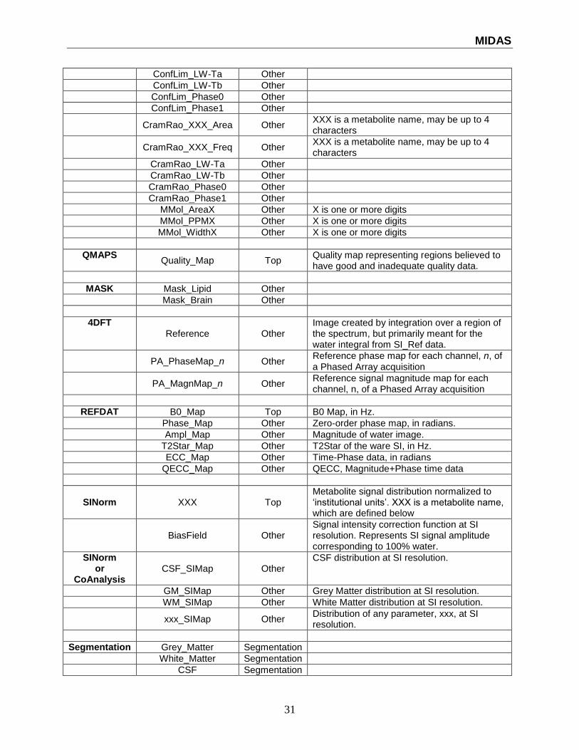
B. Metabolite Name Definitions Metabolite names are carried through from the metabolite definitions used to generate the

basis functions (in the database used by the GAVA program) to the spectral fitting program

(FITT), and then to the spectral normalization program (SINorm) which creates the final image

for display. To identify results of the spectral fitting which reflect spectral area measurements,

and then relative metabolite concentrations (after normalization), the names need to be fixed.

Therefore, the following metabolite names are used for a) the spectral database and fitting and b)

for the final normalized metabolite images:

Labels used for the spectral database and fitting

Labels used for the final metabolite images

NAA NAcetylAspartate

CR tCreatine (total Creatine)

CRE tCreatine

CHO tCholine (total Choline)

INO myo-Inositol

M-INO myo-Inositol

LAC Lactate

ALA Alanine

ASP Aspartate

ETOH Ethanol

GABA GABA

GLU Glutamate

GLN Glutamine

GLY Glycine

GLX Glx.

GLY Glycine

GPC GPC

NAAG NAAG

MIDAS

33

PCR PhosphoCreatine

PCHO Phosphocholine

SINO scyllo-Inositol

S-INO scyllo-Inositol

TAU Taurine

H2O Water

MIDAS

34

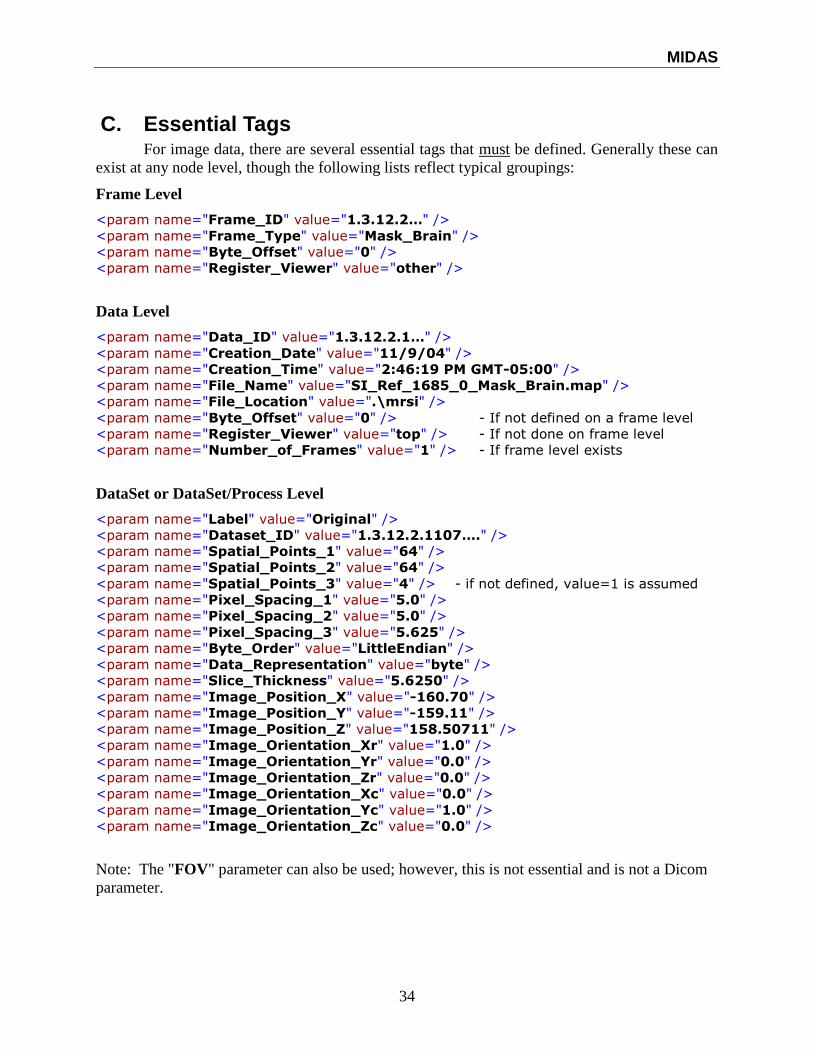
C. Essential Tags For image data, there are several essential tags that must be defined. Generally these can

exist at any node level, though the following lists reflect typical groupings:

Frame Level

<param name="Frame_ID" value="1.3.12.2…" />

<param name="Frame_Type" value="Mask_Brain" />

<param name="Byte_Offset" value="0" />

<param name="Register_Viewer" value="other" />

Data Level

<param name="Data_ID" value="1.3.12.2.1…" />

<param name="Creation_Date" value="11/9/04" />

<param name="Creation_Time" value="2:46:19 PM GMT-05:00" />

<param name="File_Name" value="SI_Ref_1685_0_Mask_Brain.map" />

<param name="File_Location" value=".\mrsi" />

<param name="Byte_Offset" value="0" /> - If not defined on a frame level

<param name="Register_Viewer" value="top" /> - If not done on frame level

<param name="Number_of_Frames" value="1" /> - If frame level exists

DataSet or DataSet/Process Level

<param name="Label" value="Original" />

<param name="Dataset_ID" value="1.3.12.2.1107…." />

<param name="Spatial_Points_1" value="64" />

<param name="Spatial_Points_2" value="64" />

<param name="Spatial_Points_3" value="4" /> - if not defined, value=1 is assumed

<param name="Pixel_Spacing_1" value="5.0" />



<param name="Byte_Order" value="LittleEndian" />

<param name="Data_Representation" value="byte" />

<param name="Slice_Thickness" value="5.6250" />

<param name="Image_Position_X" value="-160.70" />

<param name="Image_Position_Y" value="-159.11" />

<param name="Image_Position_Z" value="158.50711" />

<param name="Image_Orientation_Xr" value="1.0" />

<param name="Image_Orientation_Yr" value="0.0" />

<param name="Image_Orientation_Zr" value="0.0" />

<param name="Image_Orientation_Xc" value="0.0" />

<param name="Image_Orientation_Yc" value="1.0" />

<param name="Image_Orientation_Zc" value="0.0" />

Note: The "FOV" parameter can also be used; however, this is not essential and is not a Dicom

parameter.

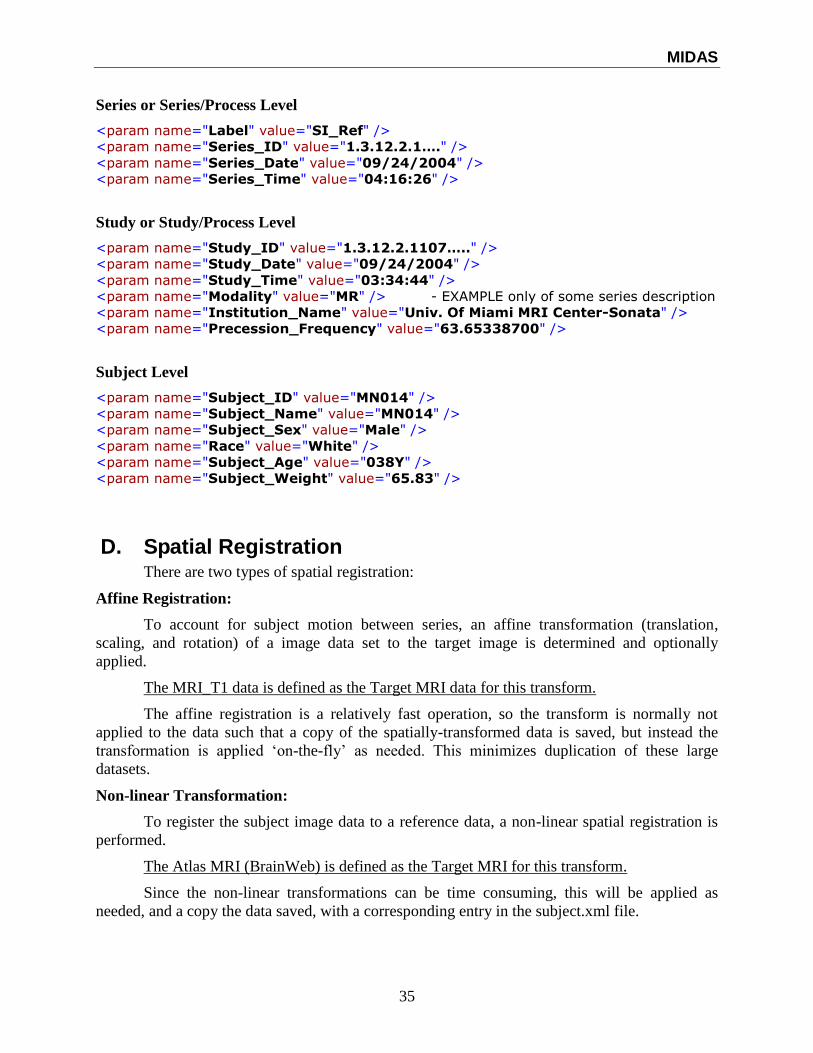
MIDAS

35

Series or Series/Process Level

<param name="Label" value="SI_Ref" />

<param name="Series_ID" value="1.3.12.2.1…." />

<param name="Series_Date" value="09/24/2004" />

<param name="Series_Time" value="04:16:26" />

Study or Study/Process Level

<param name="Study_ID" value="1.3.12.2.1107….." />

<param name="Study_Date" value="09/24/2004" />

<param name="Study_Time" value="03:34:44" />

<param name="Modality" value="MR" /> - EXAMPLE only of some series description

<param name="Institution_Name" value="Univ. Of Miami MRI Center-Sonata" />

<param name="Precession_Frequency" value="63.65338700" />

Subject Level


<param name="Subject_Name" value="MN014" />

<param name="Subject_Sex" value="Male" />

<param name="Race" value="White" />

<param name="Subject_Age" value="038Y" />

<param name="Subject_Weight" value="65.83" />

D. Spatial Registration There are two types of spatial registration:

Affine Registration:

To account for subject motion between series, an affine transformation (translation,

scaling, and rotation) of a image data set to the target image is determined and optionally

applied.

The MRI_T1 data is defined as the Target MRI data for this transform.

The affine registration is a relatively fast operation, so the transform is normally not

applied to the data such that a copy of the spatially-transformed data is saved, but instead the

transformation is applied ‘on-the-fly’ as needed. This minimizes duplication of these large

datasets.

Non-linear Transformation:

To register the subject image data to a reference data, a non-linear spatial registration is

performed.

The Atlas MRI (BrainWeb) is defined as the Target MRI for this transform.

Since the non-linear transformations can be time consuming, this will be applied as

needed, and a copy the data saved, with a corresponding entry in the subject.xml file.

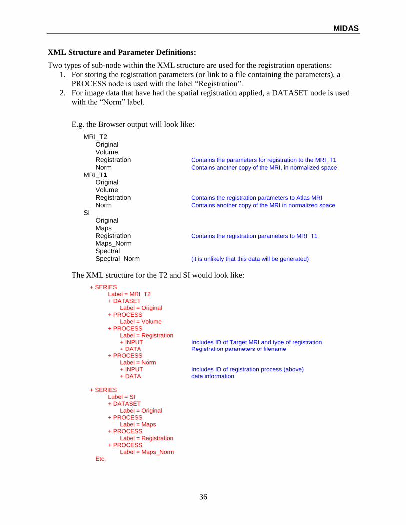
MIDAS

36

XML Structure and Parameter Definitions:

Two types of sub-node within the XML structure are used for the registration operations:

1. For storing the registration parameters (or link to a file containing the parameters), a

PROCESS node is used with the label “Registration”.

2. For image data that have had the spatial registration applied, a DATASET node is used

with the “Norm” label.

E.g. the Browser output will look like:

MRI_T2 Original Volume Registration Contains the parameters for registration to the MRI_T1 Norm Contains another copy of the MRI, in normalized space MRI_T1 Original Volume Registration Contains the registration parameters to Atlas MRI Norm Contains another copy of the MRI in normalized space SI Original Maps Registration Contains the registration parameters to MRI_T1 Maps_Norm Spectral Spectral_Norm (it is unlikely that this data will be generated)

The XML structure for the T2 and SI would look like:

+ SERIES Label = MRI_T2 + DATASET

Label = Original + PROCESS

Label = Volume + PROCESS

Label = Registration + INPUT Includes ID of Target MRI and type of registration + DATA Registration parameters of filename

+ PROCESS Label = Norm + INPUT Includes ID of registration process (above) + DATA data information

+ SERIES Label = SI + DATASET

Label = Original + PROCESS

Label = Maps + PROCESS

Label = Registration + PROCESS

Label = Maps_Norm Etc.

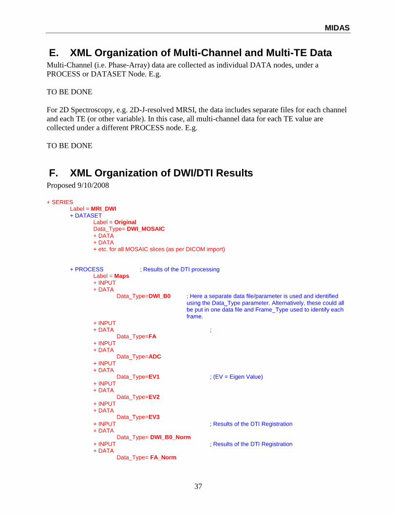
MIDAS

37

E. XML Organization of Multi-Channel and Multi-TE Data Multi-Channel (i.e. Phase-Array) data are collected as individual DATA nodes, under a

PROCESS or DATASET Node. E.g.

TO BE DONE

For 2D Spectroscopy, e.g. 2D-J-resolved MRSI, the data includes separate files for each channel

and each TE (or other variable). In this case, all multi-channel data for each TE value are

collected under a different PROCESS node. E.g.

TO BE DONE

F. XML Organization of DWI/DTI Results Proposed 9/10/2008

+ SERIES

Label = MRI_DWI

+ DATASET Label = Original Data_Type= DWI_MOSAIC

+ DATA + DATA + etc. for all MOSAIC slices (as per DICOM import)

+ PROCESS ; Results of the DTI processing

Label = Maps

+ INPUT + DATA

Data_Type=DWI_B0 ; Here a separate data file/parameter is used and identified

using the Data_Type parameter. Alternatively, these could all be put in one data file and Frame_Type used to identify each frame.

+ INPUT + DATA ;

Data_Type=FA

+ INPUT + DATA

Data_Type=ADC

+ INPUT + DATA

Data_Type=EV1 ; (EV = Eigen Value)

+ INPUT + DATA

Data_Type=EV2

+ INPUT + DATA

Data_Type=EV3

+ INPUT ; Results of the DTI Registration + DATA

Data_Type= DWI_B0_Norm


Data_Type= FA_Norm

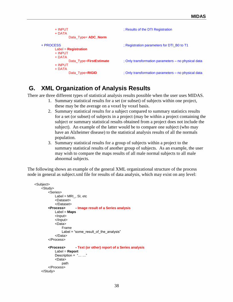
MIDAS

38


Data_Type= ADC_Norm

+ PROCESS ; Registration parameters for DTI_B0 to T1

Label = Registration

+ INPUT + DATA

Data_Type=FirstEstimate ; Only transformation parameters – no physical data

+ INPUT + DATA

Data_Type=RIGID ; Only transformation parameters – no physical data

G. XML Organization of Analysis Results There are three different types of statistical analysis results possible when the user uses MIDAS.

1. Summary statistical results for a set (or subset) of subjects within one project,

these may be the average on a voxel by voxel basis.

2. Summary statistical results for a subject compared to summary statistics results

for a set (or subset) of subjects in a project (may be within a project containing the

subject or summary statistical results obtained from a project does not include the

subject). An example of the latter would be to compare one subject (who may

have an Alzheimer disease) to the statistical analysis results of all the normals

population.

3. Summary statistical results for a group of subjects within a project to the

summary statistical results of another group of subjects. As an example, the user

may wish to compare the maps results of all male normal subjects to all male

abnormal subjects.

The following shows an example of the general XML organizational structure of the process

node in general as subject.xml file for results of data analysis, which may exist on any level:

<Subject>

<Study> <Series>

Label = MRI_, SI, etc <Dataset> </Dataset>

<Process> - Image result of a Series analysis Label = Maps

<Input> </Input> <Data>

Frame Label = “some_result_of_the_analysis”

</Data> </Process> <Process> - Text (or other) report of a Series analysis

Label = Report

Description = “… …” <Data> path

</Process> </Study>

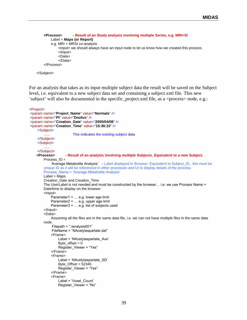
MIDAS

39

<Process> - Result of an Study analysis involving multiple Series, e.g. MRI+SI

Label = Maps (or Report)

e.g. MRI + MRSI co-analysis <input> we should always have an input node to let us know how we created this process. </input>

<Data> </Data>

</Process>

</Subject>

For an analysis that takes as its input multiple subject data the result will be saved on the Subject

level, i.e. equivalent to a new subject data set and containing a subject.xml file. This new

‘subject’ will also be documented in the specific_project.xml file, as a <process> node, e.g.:

<Project> <param name="Project_Name" value="Normals" /> <param name="PI" value="Doofus" /> <param name="Creation_Date" value="2005/04/08" /> <param name="Creation_Time" value="15:36:10" />

<Subject> ….. This indicates the existing subject data </Subject> <Subject> ….. </Subject> <Process> - Result of an analysis involving multiple Subjects. Equivalent to a new Subject.

Process_ID = ‘Average Metabolite Analysis’ - Label displayed in Browser. Equivalent to Subject_ID.. this must be unique ID as it will be referenced in other processes and UI to display details of the process. Process_Name = ‘Average Metabolite Analysis’ Label = Maps Creation_Date and Creation_Time The UserLabel is not needed and must be constructed by the browser… i.e. we use Process Name + Date/time to display on the browser. <Input>

Parameter1 = … e.g. lower age limit Parameter2 = … e.g. upper age limit Parameter3 = … e.g. list of subjects used

</Input> <Data> Assuming all the files are in the same data file, i.e. we can not have multiple files in the same data node. Filepath = “./analysis001” FileName = “NAcetylaspartate.dat”

<Frame> Label = ‘NAcetylaspartate_Ave’ Byte_offset = 0 Register_Viewer = “Yes”

</Frame> <Frame>

Label = ‘NAcetylaspartate_SD’ Byte_Offset = 52345 Register_Viewer = “Yes”

</Frame> <Frame>

Label = ‘Voxel_Count’ Register_Viewer = “No”

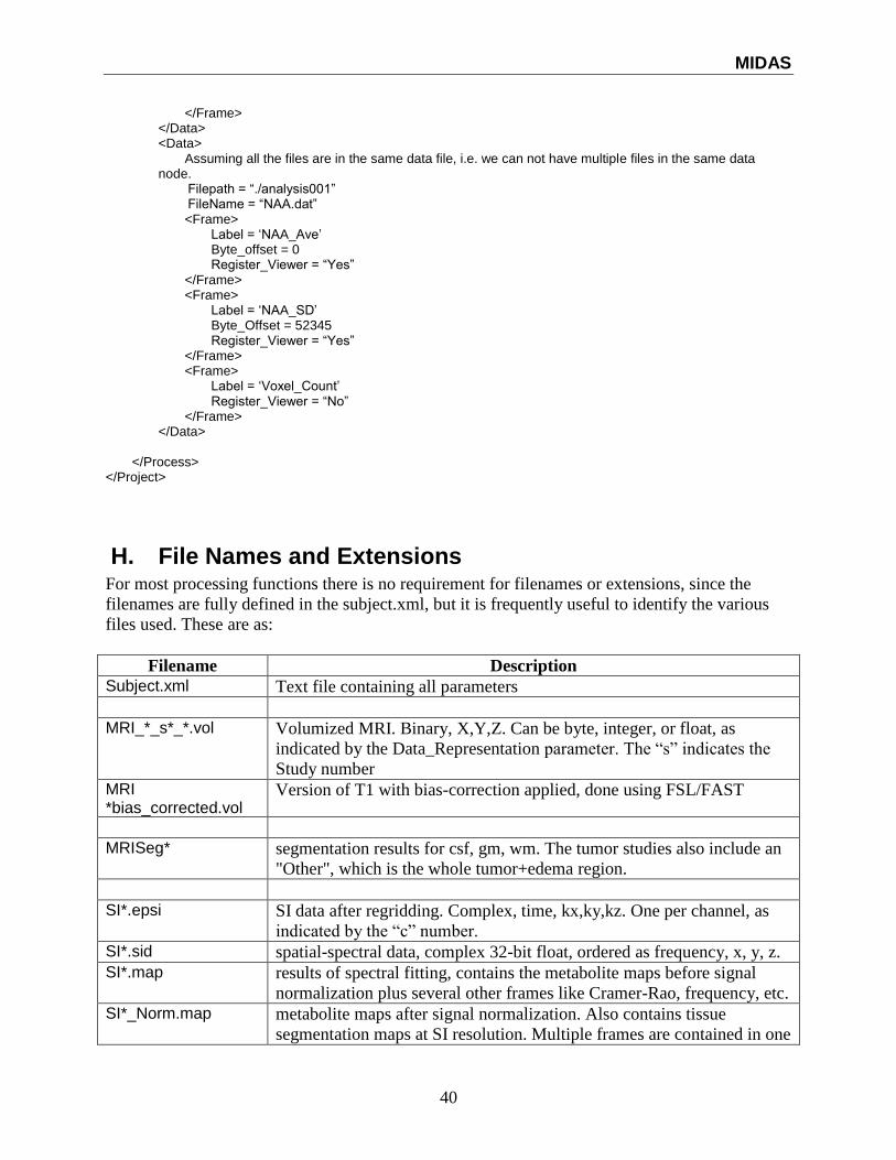
MIDAS

40

</Frame> </Data> <Data> Assuming all the files are in the same data file, i.e. we can not have multiple files in the same data node. Filepath = “./analysis001” FileName = “NAA.dat”

<Frame> Label = ‘NAA_Ave’ Byte_offset = 0 Register_Viewer = “Yes”

</Frame> <Frame>

Label = ‘NAA_SD’ Byte_Offset = 52345 Register_Viewer = “Yes”

</Frame> <Frame>

Label = ‘Voxel_Count’ Register_Viewer = “No”

</Frame> </Data>

</Process> </Project>

H. File Names and Extensions For most processing functions there is no requirement for filenames or extensions, since the

filenames are fully defined in the subject.xml, but it is frequently useful to identify the various

files used. These are as:

Filename Description

Subject.xml Text file containing all parameters

MRI_*_s*_*.vol Volumized MRI. Binary, X,Y,Z. Can be byte, integer, or float, as

indicated by the Data_Representation parameter. The “s” indicates the

Study number

MRI *bias_corrected.vol

Version of T1 with bias-correction applied, done using FSL/FAST

MRISeg* segmentation results for csf, gm, wm. The tumor studies also include an

"Other", which is the whole tumor+edema region.

SI*.epsi SI data after regridding. Complex, time, kx,ky,kz. One per channel, as

indicated by the “c” number.

SI*.sid spatial-spectral data, complex 32-bit float, ordered as frequency, x, y, z.

SI*.map results of spectral fitting, contains the metabolite maps before signal

normalization plus several other frames like Cramer-Rao, frequency, etc.

SI*_Norm.map metabolite maps after signal normalization. Also contains tissue

segmentation maps at SI resolution. Multiple frames are contained in one

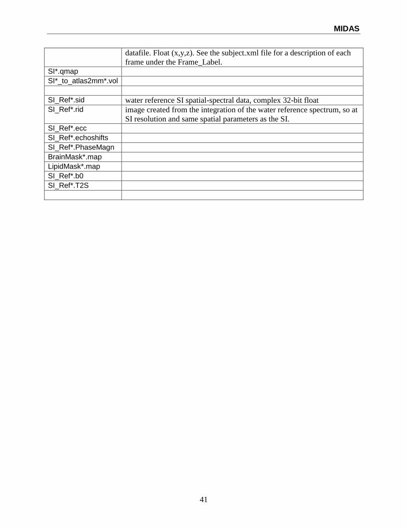
MIDAS

41

datafile. Float (x,y,z). See the subject.xml file for a description of each

frame under the Frame_Label.

SI*.qmap

SI*_to_atlas2mm*.vol

SI_Ref*.sid water reference SI spatial-spectral data, complex 32-bit float

SI_Ref*.rid image created from the integration of the water reference spectrum, so at

SI resolution and same spatial parameters as the SI.

SI_Ref*.ecc

SI_Ref*.echoshifts

SI_Ref*.PhaseMagn

BrainMask*.map

LipidMask*.map

SI_Ref*.b0

SI_Ref*.T2S