Mid-term Review Chapters 2-7

Mid-term ReviewChapters 2-7

• Review Agents (2.1-2.3)• Review State Space Search

• Problem Formulation (3.1, 3.3)• Blind (Uninformed) Search (3.4)• Heuristic Search (3.5)• Local Search (4.1, 4.2)

• Review Adversarial (Game) Search (5.1-5.4)• Review Constraint Satisfaction (6.1-6.4)• Review Propositional Logic (7.1-7.5)• Please review your quizzes and old CS-171 tests

• At least one question from a prior quiz or old CS-171 test will appear on the mid-term (and all other tests)

Review AgentsChapter 2.1-2.3

• Agent definition (2.1)

• Rational Agent definition (2.2)– Performance measure

• Task evironment definition (2.3)– PEAS acronym

Agents

• An agent is anything that can be viewed as perceiving its environment through sensors and acting upon that environment through actuators

Human agent: eyes, ears, and other organs for sensors; hands, legs, mouth, and other body parts for actuators

• Robotic agent: cameras and infrared range finders for sensors; various

motors for actuators

Rational agents

• Rational Agent: For each possible percept sequence, a rational agent should select an action that is expected to maximize its performance measure, based on the evidence provided by the percept sequence and whatever built-in knowledge the agent has.

• Performance measure: An objective criterion for success of an agent's behavior

• E.g., performance measure of a vacuum-cleaner agent could be amount of dirt cleaned up, amount of time taken, amount of electricity consumed, amount of noise generated, etc.

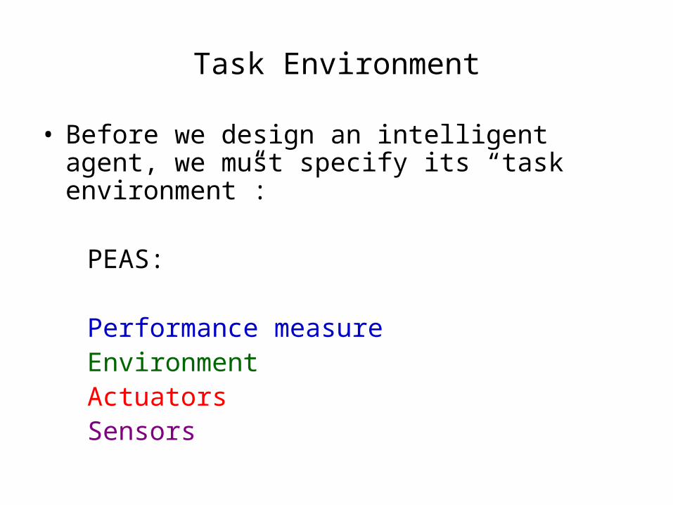
Task Environment

• Before we design an intelligent agent, we must specify its “task environment”:

PEAS:

Performance measure Environment Actuators Sensors

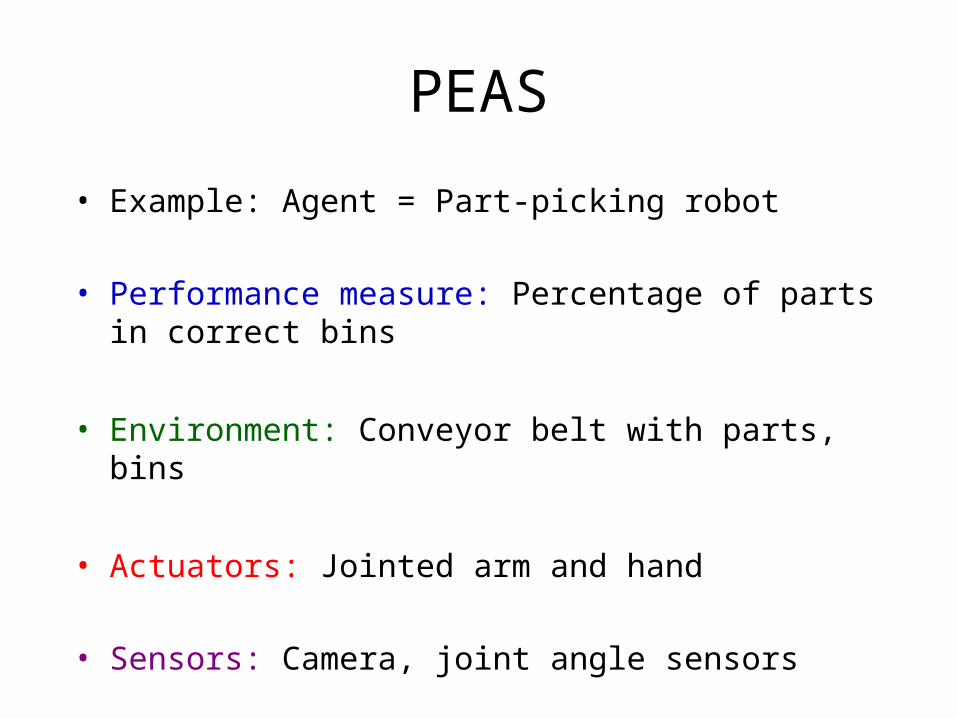
PEAS

• Example: Agent = Part-picking robot

• Performance measure: Percentage of parts in correct bins

• Environment: Conveyor belt with parts, bins

• Actuators: Jointed arm and hand

• Sensors: Camera, joint angle sensors

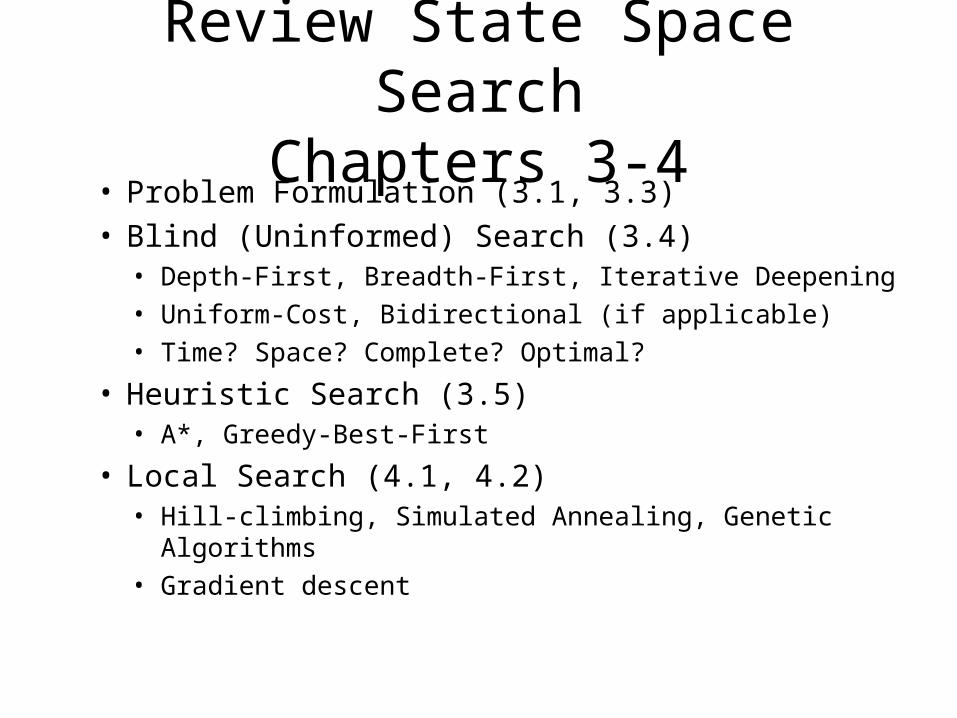
Review State Space SearchChapters 3-4

• Problem Formulation (3.1, 3.3)• Blind (Uninformed) Search (3.4)

• Depth-First, Breadth-First, Iterative Deepening• Uniform-Cost, Bidirectional (if applicable)• Time? Space? Complete? Optimal?

• Heuristic Search (3.5)• A*, Greedy-Best-First

• Local Search (4.1, 4.2)• Hill-climbing, Simulated Annealing, Genetic Algorithms• Gradient descent

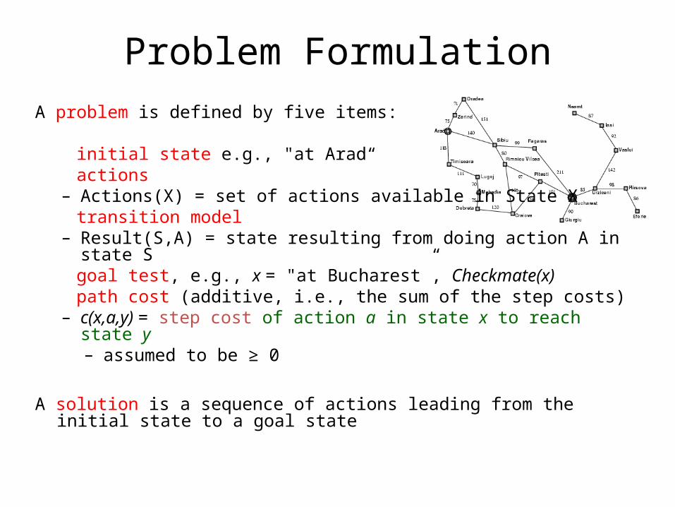
Problem FormulationA problem is defined by five items:

initial state e.g., "at Arad“ actions

– Actions(X) = set of actions available in State X transition model

– Result(S,A) = state resulting from doing action A in state S goal test, e.g., x = "at Bucharest”, Checkmate(x) path cost (additive, i.e., the sum of the step costs)

– c(x,a,y) = step cost of action a in state x to reach state y– assumed to be ≥ 0

A solution is a sequence of actions leading from the initial state to a goal state

9

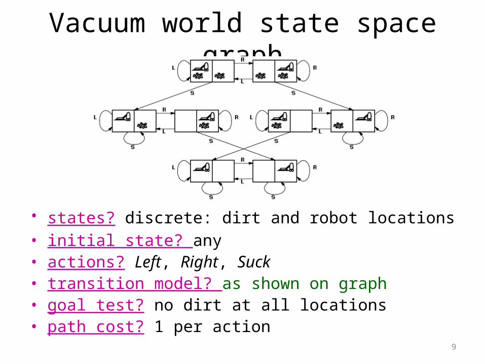
Vacuum world state space graph

• states? discrete: dirt and robot locations • initial state? any• actions? Left, Right, Suck• transition model? as shown on graph• goal test? no dirt at all locations• path cost? 1 per action

10

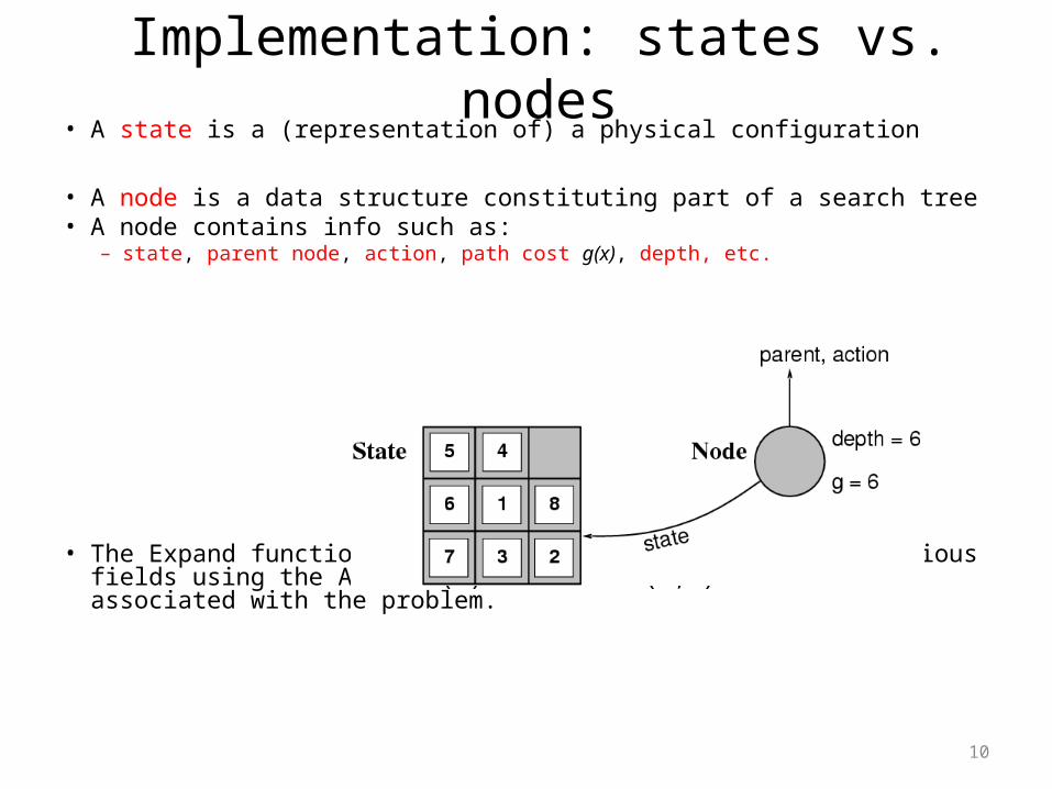
Implementation: states vs. nodes• A state is a (representation of) a physical configuration

• A node is a data structure constituting part of a search tree• A node contains info such as:

– state, parent node, action, path cost g(x), depth, etc.

• The Expand function creates new nodes, filling in the various fields using the Actions(S) and Result(S,A)functions associated with the problem.

11

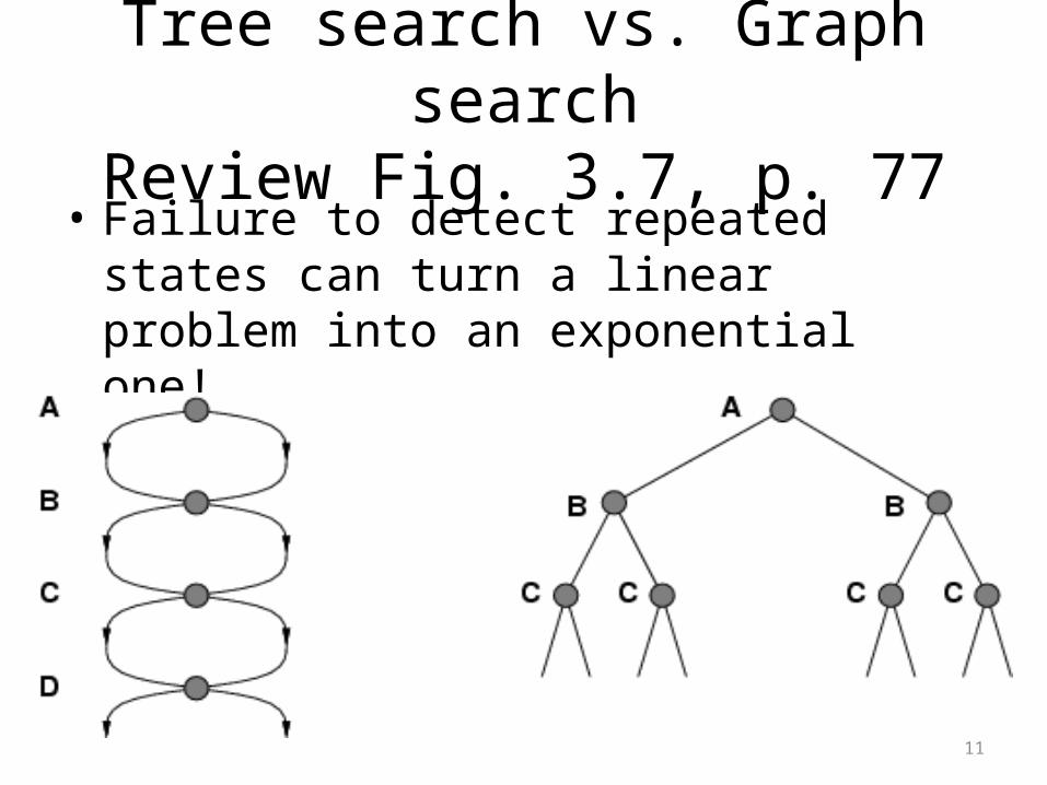
Tree search vs. Graph searchReview Fig. 3.7, p. 77

• Failure to detect repeated states can turn a linear problem into an exponential one!

• Test is often implemented as a hash table.

12

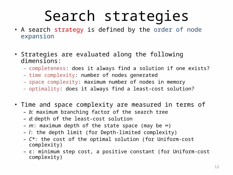
Search strategies• A search strategy is defined by the order of node expansion

• Strategies are evaluated along the following dimensions:– completeness: does it always find a solution if one exists?– time complexity: number of nodes generated– space complexity: maximum number of nodes in memory– optimality: does it always find a least-cost solution?

• Time and space complexity are measured in terms of – b: maximum branching factor of the search tree– d: depth of the least-cost solution– m: maximum depth of the state space (may be ∞)– l: the depth limit (for Depth-limited complexity)– C*: the cost of the optimal solution (for Uniform-cost complexity)– ε: minimum step cost, a positive constant (for Uniform-cost complexity)

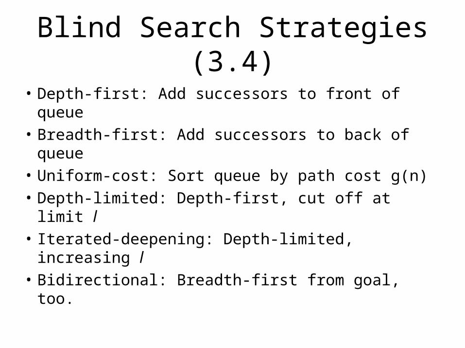
Blind Search Strategies (3.4)

• Depth-first: Add successors to front of queue• Breadth-first: Add successors to back of queue• Uniform-cost: Sort queue by path cost g(n)• Depth-limited: Depth-first, cut off at limit l• Iterated-deepening: Depth-limited, increasing l• Bidirectional: Breadth-first from goal, too.

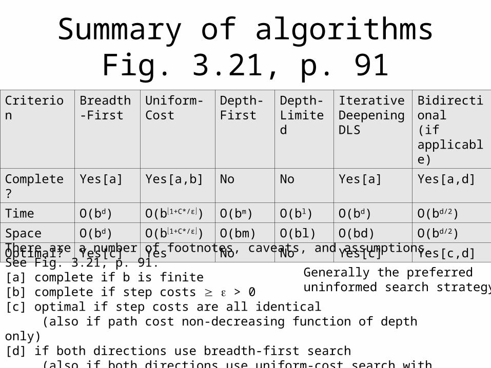
Summary of algorithmsFig. 3.21, p. 91

Generally the preferred uninformed search strategy

Criterion Breadth-First

Uniform-Cost

Depth-First

Depth-Limited

Iterative DeepeningDLS

Bidirectional(if applicable)

Complete? Yes[a] Yes[a,b] No No Yes[a] Yes[a,d]

Time O(bd) O(b1+C*/ε) O(bm) O(bl) O(bd) O(bd/2)

Space O(bd) O(b1+C*/ε) O(bm) O(bl) O(bd) O(bd/2)

Optimal? Yes[c] Yes No No Yes[c] Yes[c,d]

There are a number of footnotes, caveats, and assumptions.See Fig. 3.21, p. 91.[a] complete if b is finite[b] complete if step costs > 0[c] optimal if step costs are all identical (also if path cost non-decreasing function of depth only)[d] if both directions use breadth-first search (also if both directions use uniform-cost search with step costs > 0)

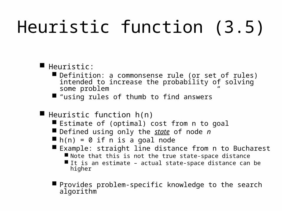
Heuristic function (3.5)

Heuristic: Definition: a commonsense rule (or set of rules) intended to

increase the probability of solving some problem “using rules of thumb to find answers”

Heuristic function h(n) Estimate of (optimal) cost from n to goal Defined using only the state of node n h(n) = 0 if n is a goal node Example: straight line distance from n to Bucharest

Note that this is not the true state-space distance It is an estimate – actual state-space distance can be higher

Provides problem-specific knowledge to the search algorithm

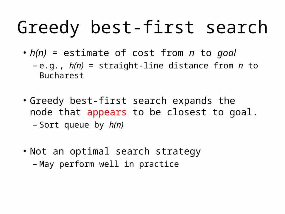
Greedy best-first search• h(n) = estimate of cost from n to goal

– e.g., h(n) = straight-line distance from n to Bucharest

• Greedy best-first search expands the node that appears to be closest to goal.– Sort queue by h(n)

• Not an optimal search strategy– May perform well in practice

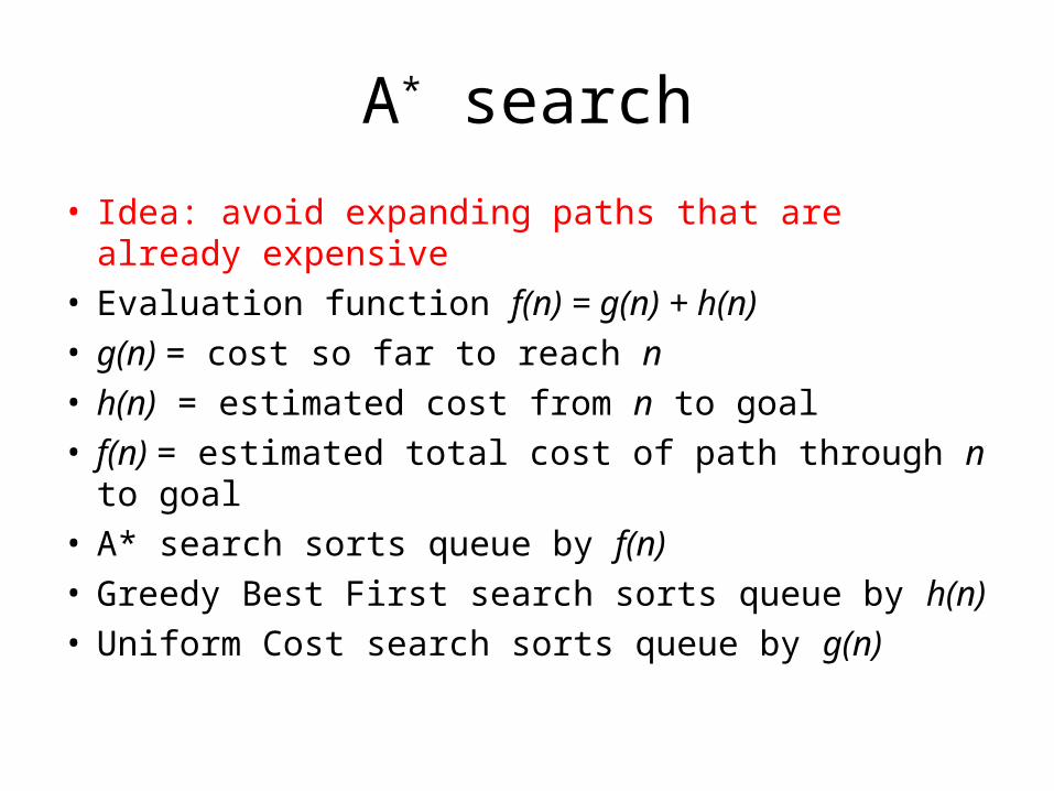
A* search

• Idea: avoid expanding paths that are already expensive

• Evaluation function f(n) = g(n) + h(n)• g(n) = cost so far to reach n• h(n) = estimated cost from n to goal• f(n) = estimated total cost of path through n to goal• A* search sorts queue by f(n)• Greedy Best First search sorts queue by h(n)• Uniform Cost search sorts queue by g(n)

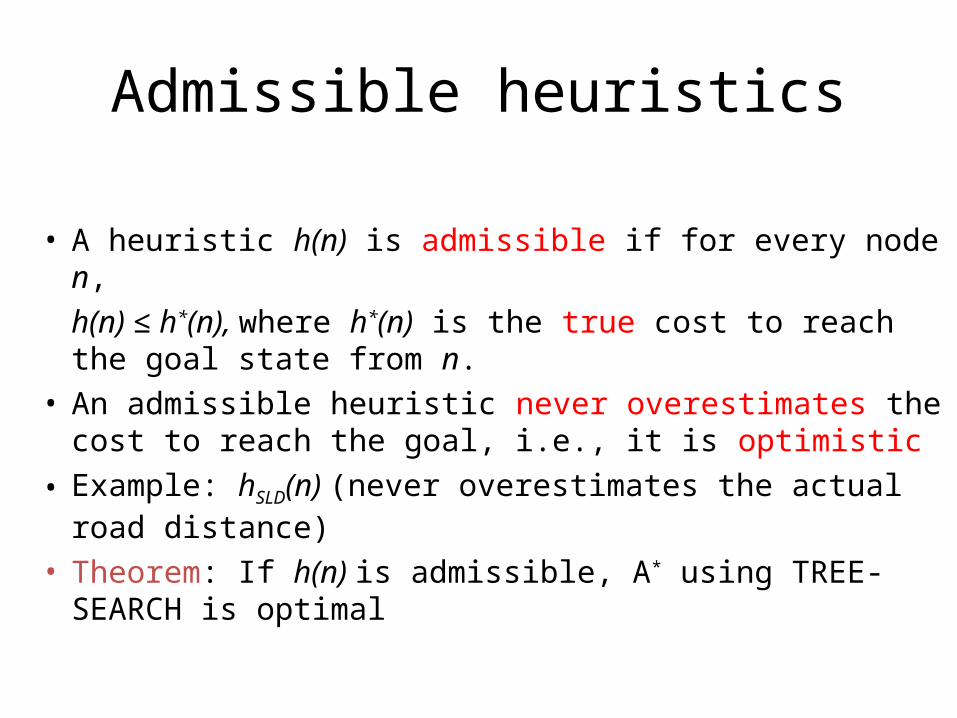
Admissible heuristics

• A heuristic h(n) is admissible if for every node n,h(n) ≤ h*(n), where h*(n) is the true cost to reach the goal state from n.

• An admissible heuristic never overestimates the cost to reach the goal, i.e., it is optimistic

• Example: hSLD(n) (never overestimates the actual road distance)

• Theorem: If h(n) is admissible, A* using TREE-SEARCH is optimal

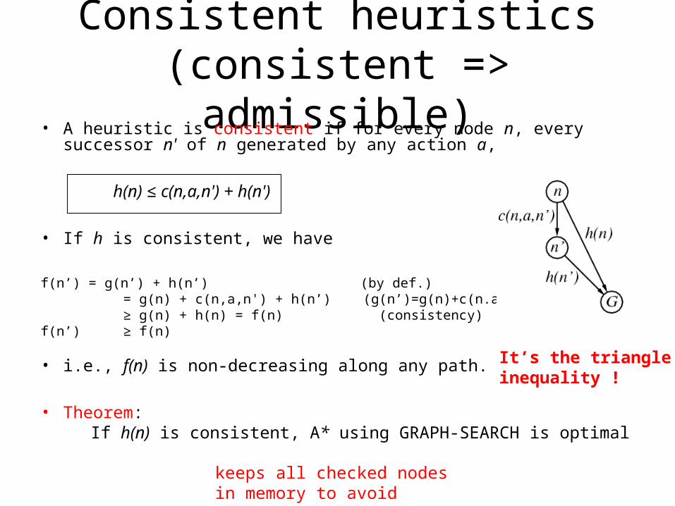
Consistent heuristics(consistent => admissible)

• A heuristic is consistent if for every node n, every successor n' of n generated by any action a,

h(n) ≤ c(n,a,n') + h(n')

• If h is consistent, we have

f(n’) = g(n’) + h(n’) (by def.) = g(n) + c(n,a,n') + h(n’) (g(n’)=g(n)+c(n.a.n’)) ≥ g(n) + h(n) = f(n) (consistency)f(n’) ≥ f(n)

• i.e., f(n) is non-decreasing along any path.

• Theorem: If h(n) is consistent, A* using GRAPH-SEARCH is optimal

It’s the triangleinequality !

keeps all checked nodes in memory to avoid repeated states

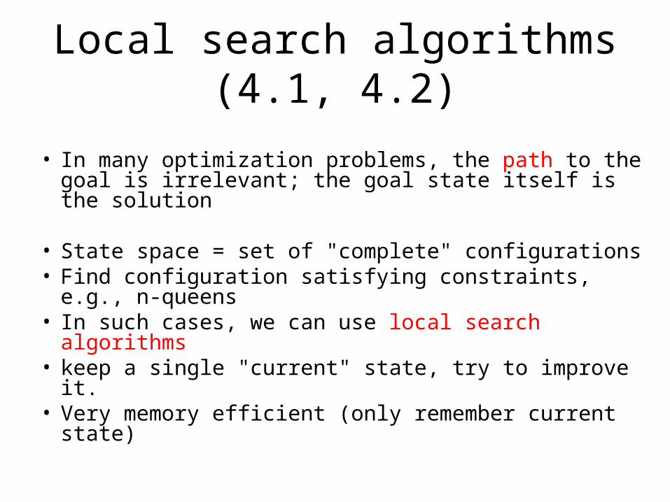
Local search algorithms (4.1, 4.2)

• In many optimization problems, the path to the goal is irrelevant; the goal state itself is the solution

• State space = set of "complete" configurations• Find configuration satisfying constraints, e.g., n-queens• In such cases, we can use local search algorithms• keep a single "current" state, try to improve it.• Very memory efficient (only remember current state)

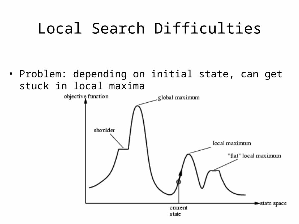
Local Search Difficulties

• Problem: depending on initial state, can get stuck in local maxima

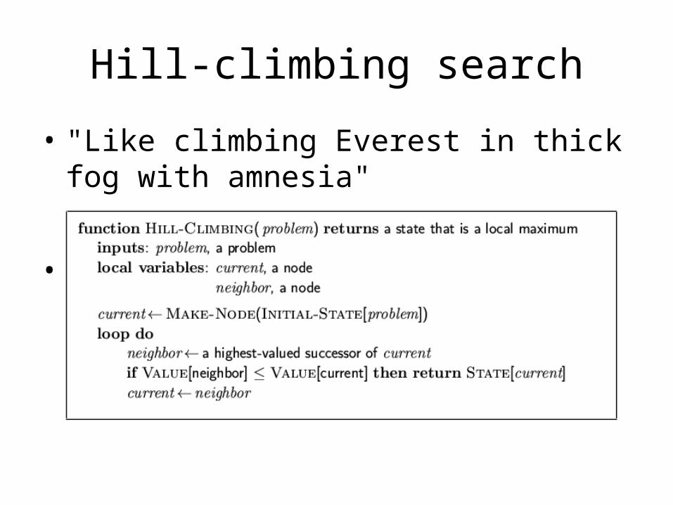
Hill-climbing search

• "Like climbing Everest in thick fog with amnesia"

•

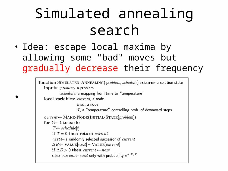
Simulated annealing search

• Idea: escape local maxima by allowing some "bad" moves but gradually decrease their frequency

•

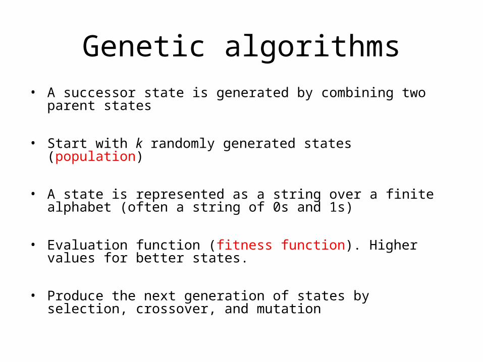
Genetic algorithms• A successor state is generated by combining two parent states

• Start with k randomly generated states (population)

• A state is represented as a string over a finite alphabet (often a string of 0s and 1s)

• Evaluation function (fitness function). Higher values for better states.

• Produce the next generation of states by selection, crossover, and mutation

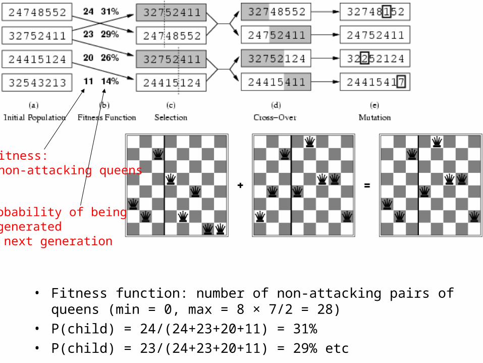
• Fitness function: number of non-attacking pairs of queens (min = 0, max = 8 × 7/2 = 28)

• P(child) = 24/(24+23+20+11) = 31%• P(child) = 23/(24+23+20+11) = 29% etc

fitness: #non-attacking queens

probability of being regeneratedin next generation

Gradient Descent

• Assume we have some cost-function: and we want minimize over continuous variables X1,X2,..,Xn

1. Compute the gradient :

2. Take a small step downhill in the direction of the gradient:

3. Check if

4. If true then accept move, if not reject.

5. Repeat.

1( ,..., )nC x x

1( ,..., )ni

C x x ix

1' ( ,..., )i i i ni

x x x C x x ix

1 1( ,.., ' ,.., ) ( ,.., ,.., )i n i nC x x x C x x x

Review Adversarial (Game) SearchChapter 5.1-5.4

• Minimax Search with Perfect Decisions (5.2)– Impractical in most cases, but theoretical basis for analysis

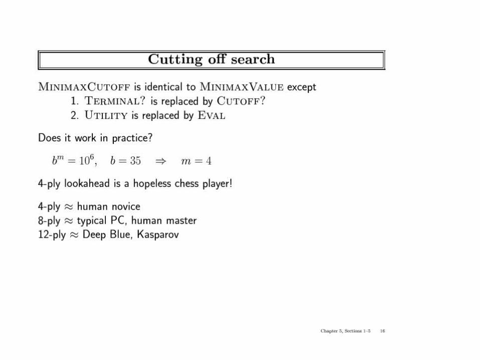
• Minimax Search with Cut-off (5.4)– Replace terminal leaf utility by heuristic evaluation function

• Alpha-Beta Pruning (5.3)– The fact of the adversary leads to an advantage in search!

• Practical Considerations (5.4)– Redundant path elimination, look-up tables, etc.

Games as Search• Two players: MAX and MIN

• MAX moves first and they take turns until the game is over– Winner gets reward, loser gets penalty.– “Zero sum” means the sum of the reward and the penalty is a constant.

• Formal definition as a search problem:– Initial state: Set-up specified by the rules, e.g., initial board configuration of chess.– Player(s): Defines which player has the move in a state.– Actions(s): Returns the set of legal moves in a state.– Result(s,a): Transition model defines the result of a move.– (2nd ed.: Successor function: list of (move,state) pairs specifying legal moves.)– Terminal-Test(s): Is the game finished? True if finished, false otherwise.– Utility function(s,p): Gives numerical value of terminal state s for player p.

• E.g., win (+1), lose (-1), and draw (0) in tic-tac-toe.• E.g., win (+1), lose (0), and draw (1/2) in chess.

• MAX uses search tree to determine next move.

An optimal procedure:The Min-Max method

Designed to find the optimal strategy for Max and find best move:

• 1. Generate the whole game tree, down to the leaves.

• 2. Apply utility (payoff) function to each leaf.

• 3. Back-up values from leaves through branch nodes:– a Max node computes the Max of its child values– a Min node computes the Min of its child values

• 4. At root: choose the move leading to the child of highest value.

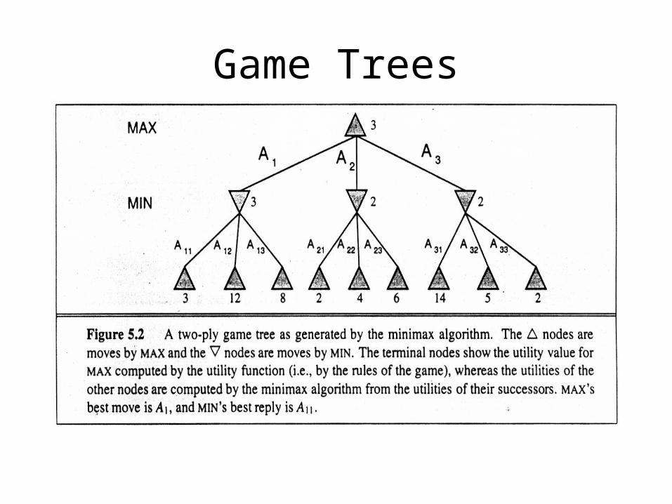
Game Trees

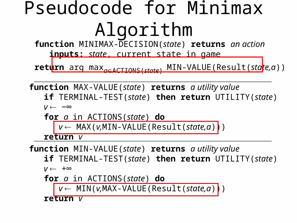
Pseudocode for Minimax Algorithm

function MINIMAX-DECISION(state) returns an action inputs: state, current state in game

return arg maxaACTIONS(state) MIN-VALUE(Result(state,a))

function MIN-VALUE(state) returns a utility value if TERMINAL-TEST(state) then return UTILITY(state) v +∞ for a in ACTIONS(state) do v MIN(v,MAX-VALUE(Result(state,a))) return v

function MAX-VALUE(state) returns a utility value if TERMINAL-TEST(state) then return UTILITY(state) v −∞ for a in ACTIONS(state) do v MAX(v,MIN-VALUE(Result(state,a))) return v

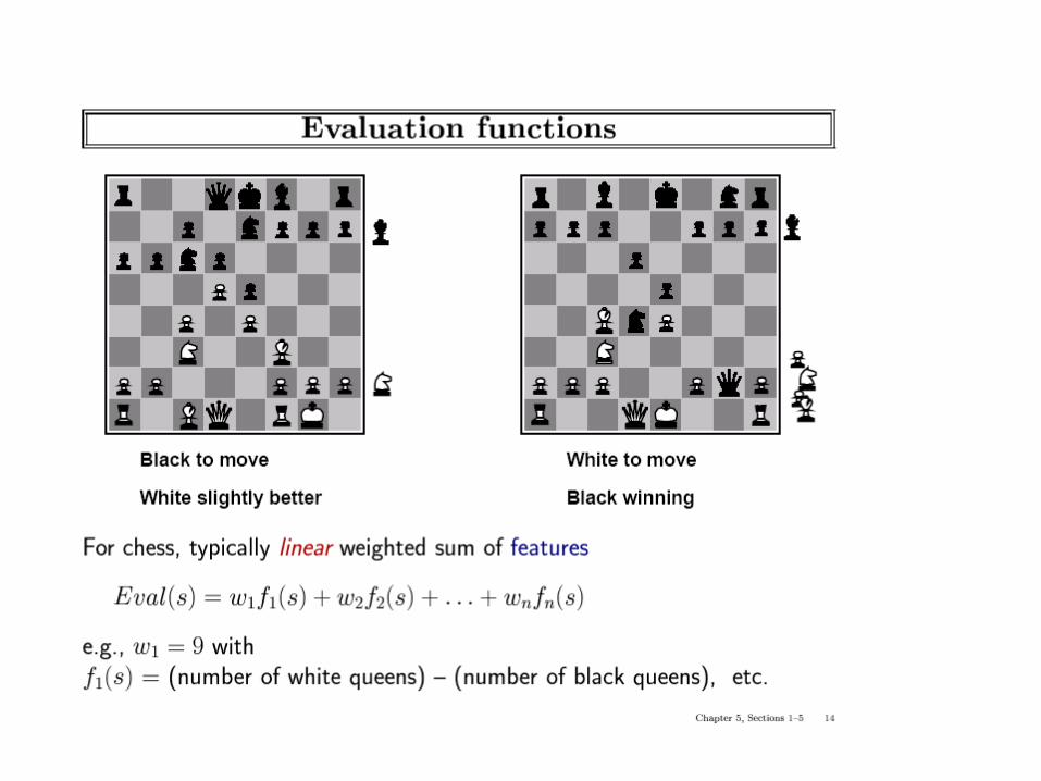
Static (Heuristic) Evaluation Functions

• An Evaluation Function:– Estimates how good the current board configuration is for a player.– Typically, evaluate how good it is for the player, how good it is for the

opponent, then subtract the opponent’s score from the player’s.– Othello: Number of white pieces - Number of black pieces– Chess: Value of all white pieces - Value of all black pieces

• Typical values from -infinity (loss) to +infinity (win) or [-1, +1].

• If the board evaluation is X for a player, it’s -X for the opponent– “Zero-sum game”

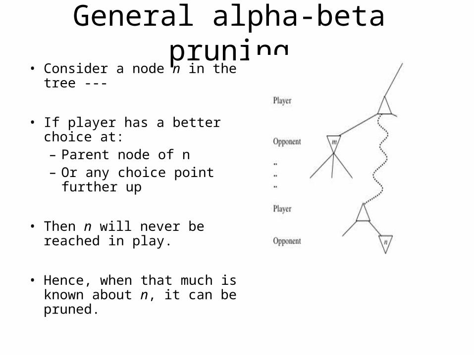
General alpha-beta pruning• Consider a node n in the tree ---

• If player has a better choice at:– Parent node of n– Or any choice point further

up

• Then n will never be reached in play.

• Hence, when that much is known about n, it can be pruned.

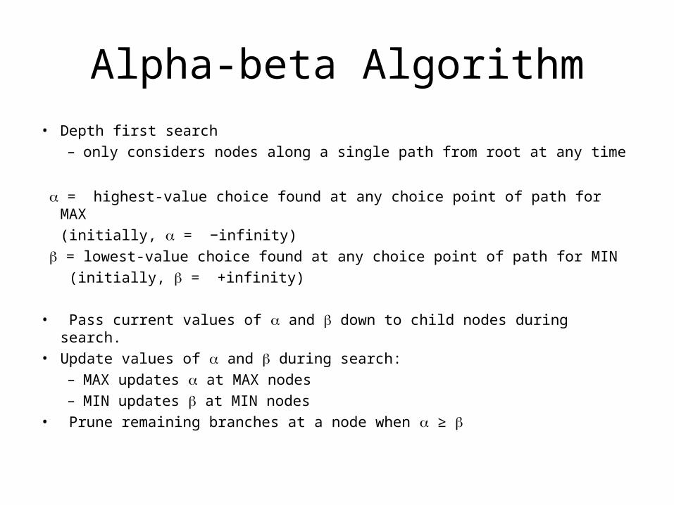
Alpha-beta Algorithm• Depth first search

– only considers nodes along a single path from root at any time

= highest-value choice found at any choice point of path for MAX(initially, = −infinity)

= lowest-value choice found at any choice point of path for MIN (initially, = +infinity)

• Pass current values of and down to child nodes during search.• Update values of and during search:

– MAX updates at MAX nodes– MIN updates at MIN nodes

• Prune remaining branches at a node when ≥

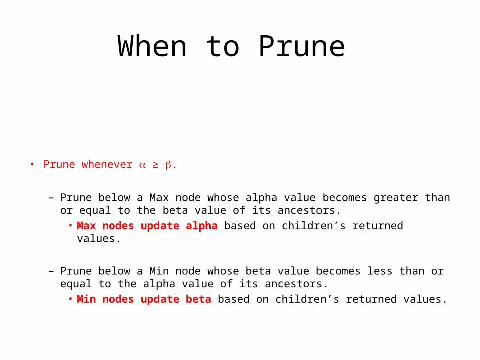
When to Prune

• Prune whenever ≥ .

– Prune below a Max node whose alpha value becomes greater than or equal to the beta value of its ancestors.

• Max nodes update alpha based on children’s returned values.

– Prune below a Min node whose beta value becomes less than or equal to the alpha value of its ancestors.

• Min nodes update beta based on children’s returned values.

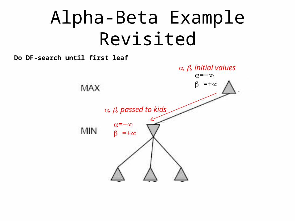
Alpha-Beta Example Revisited

, , initial valuesDo DF-search until first leaf

=− =+

=− =+

, , passed to kids

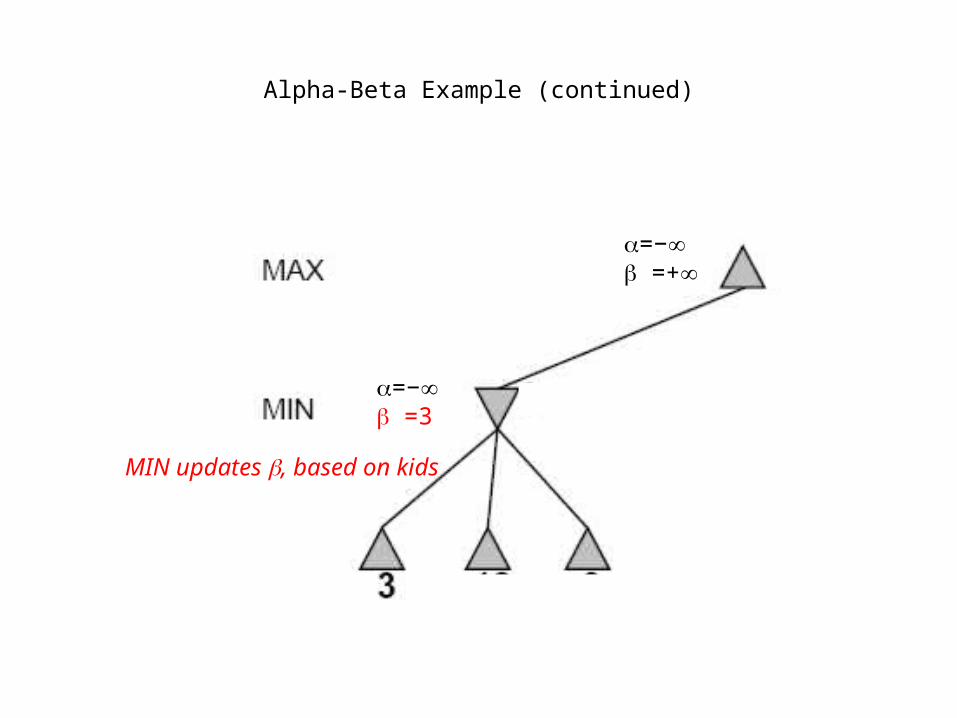
Alpha-Beta Example (continued)

MIN updates , based on kids

=− =+

=− =3

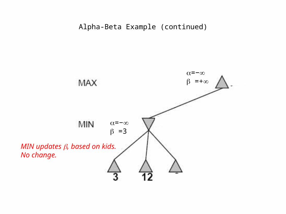
Alpha-Beta Example (continued)

=− =3

MIN updates , based on kids.No change.

=− =+

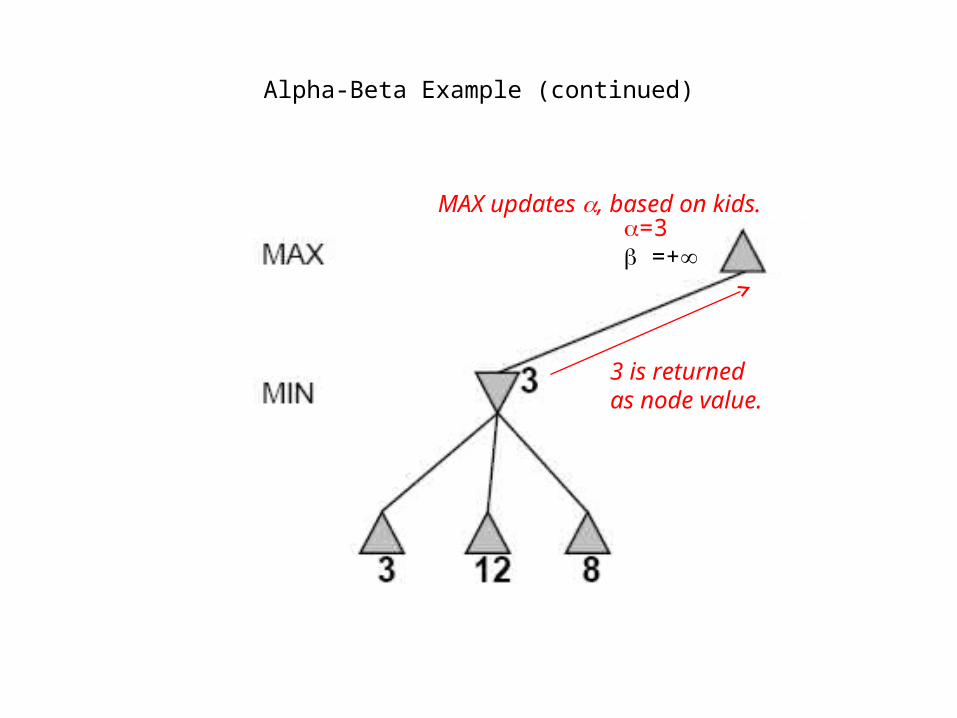
Alpha-Beta Example (continued)

MAX updates , based on kids.=3 =+

3 is returnedas node value.

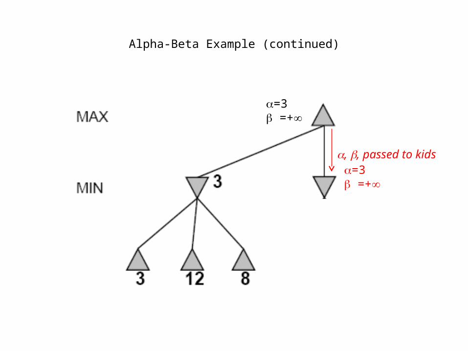
Alpha-Beta Example (continued)

=3 =+

=3 =+

, , passed to kids

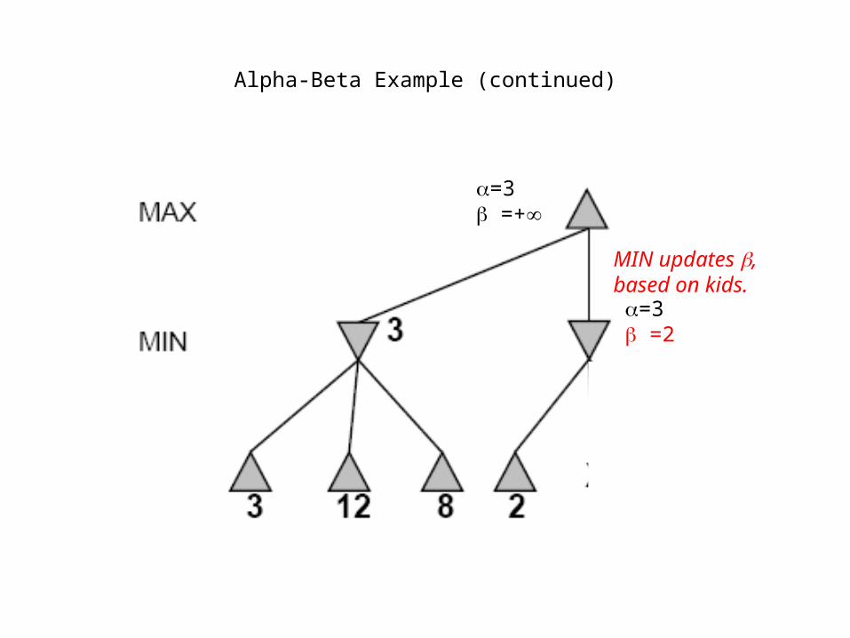
Alpha-Beta Example (continued)

=3 =+

=3 =2

MIN updates ,based on kids.

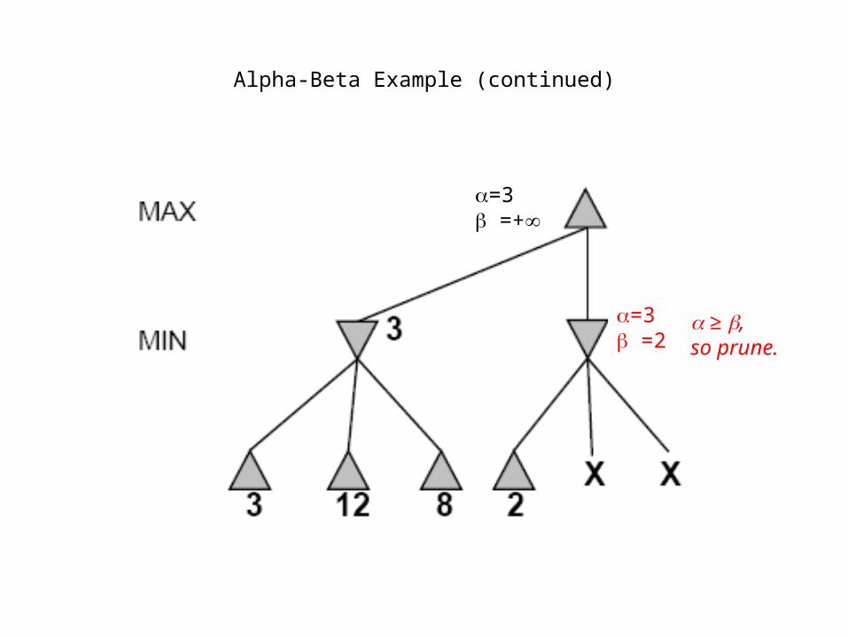
Alpha-Beta Example (continued)

=3 =2

≥ ,so prune.

=3 =+

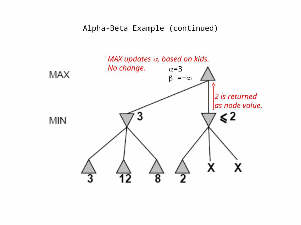
Alpha-Beta Example (continued)

2 is returnedas node value.

MAX updates , based on kids.No change. =3

=+

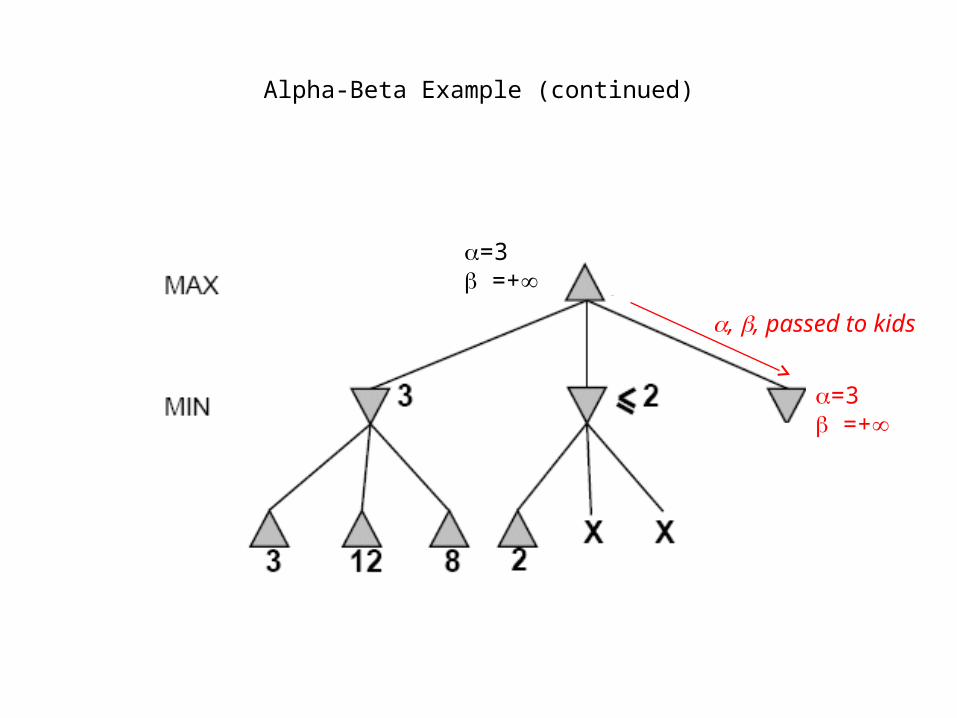
Alpha-Beta Example (continued)

,=3 =+

=3 =+

, , passed to kids

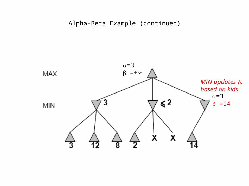
Alpha-Beta Example (continued)

,

=3 =14

=3 =+

MIN updates ,based on kids.

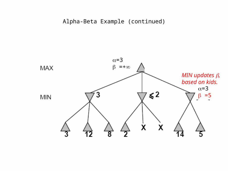
Alpha-Beta Example (continued)

,

=3 =5

=3 =+

MIN updates ,based on kids.

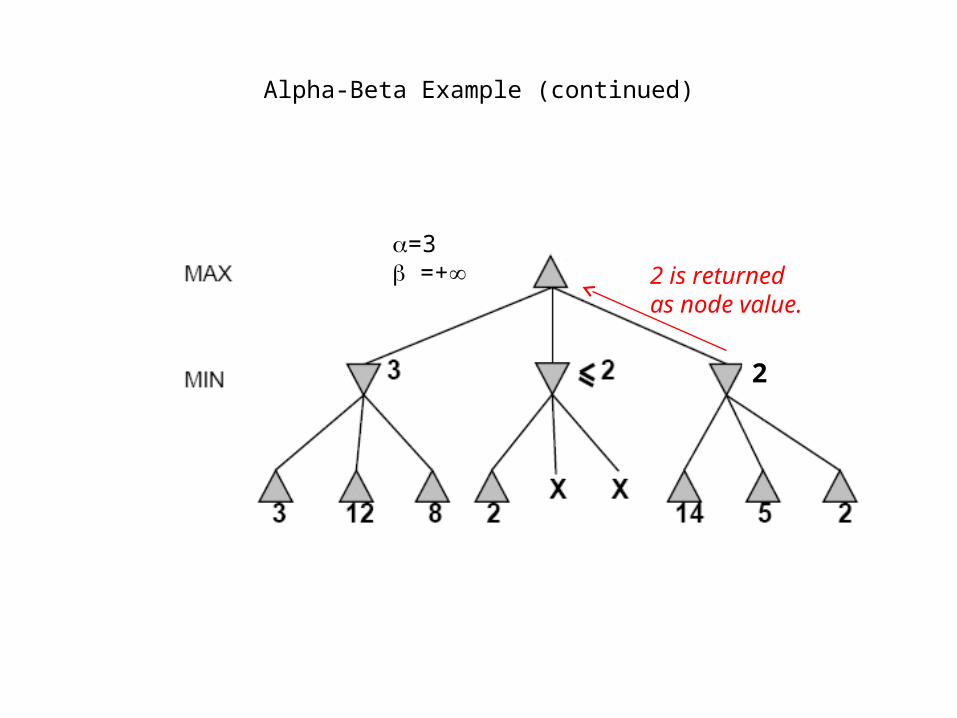
Alpha-Beta Example (continued)

=3 =+ 2 is returned

as node value.

2

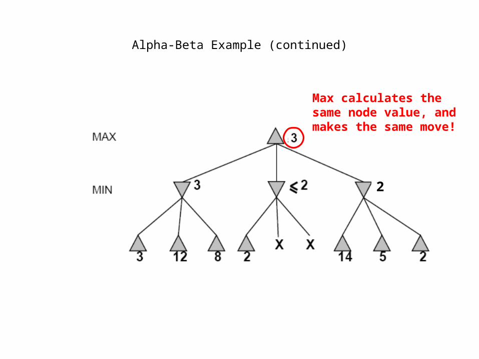
Alpha-Beta Example (continued)

Max calculates the same node value, and makes the same move!

2

Review Constraint SatisfactionChapter 6.1-6.4

• What is a CSP

• Backtracking for CSP

• Local search for CSPs

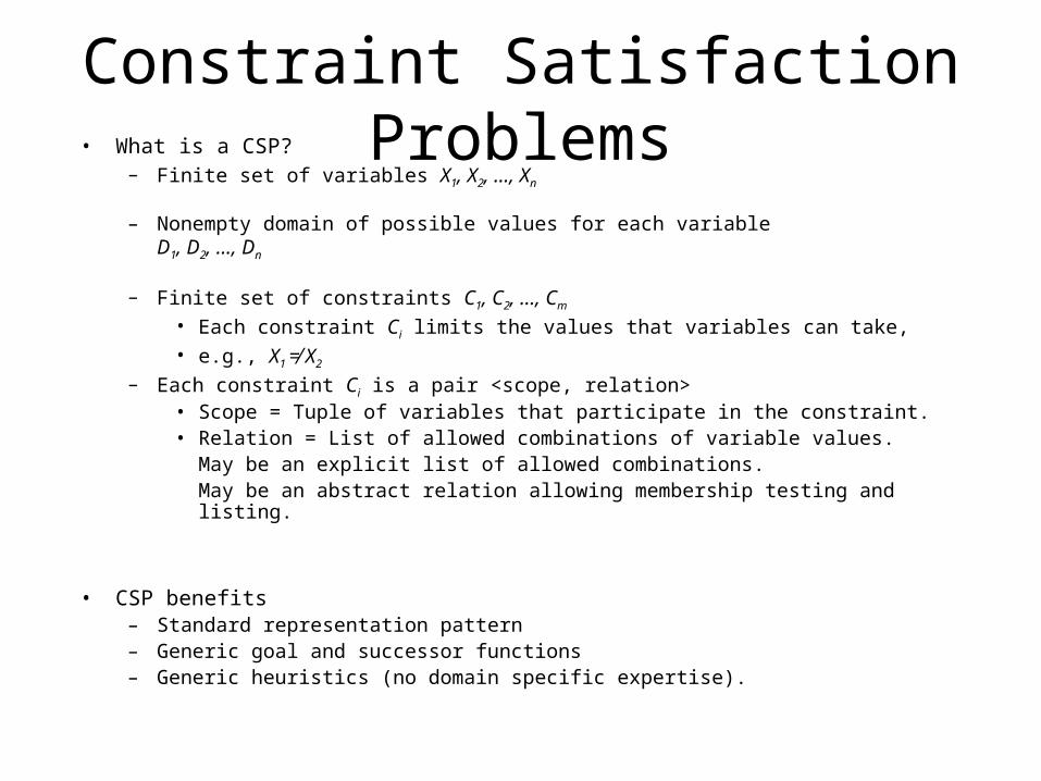
Constraint Satisfaction Problems• What is a CSP?

– Finite set of variables X1, X2, …, Xn

– Nonempty domain of possible values for each variable D1, D2, …, Dn

– Finite set of constraints C1, C2, …, Cm

• Each constraint Ci limits the values that variables can take, • e.g., X1 ≠ X2

– Each constraint Ci is a pair <scope, relation>• Scope = Tuple of variables that participate in the constraint.• Relation = List of allowed combinations of variable values.

May be an explicit list of allowed combinations.May be an abstract relation allowing membership testing and listing.

• CSP benefits– Standard representation pattern– Generic goal and successor functions– Generic heuristics (no domain specific expertise).

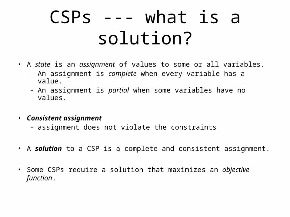
CSPs --- what is a solution?

• A state is an assignment of values to some or all variables.– An assignment is complete when every variable has a value. – An assignment is partial when some variables have no values.

• Consistent assignment– assignment does not violate the constraints

• A solution to a CSP is a complete and consistent assignment.

• Some CSPs require a solution that maximizes an objective function.

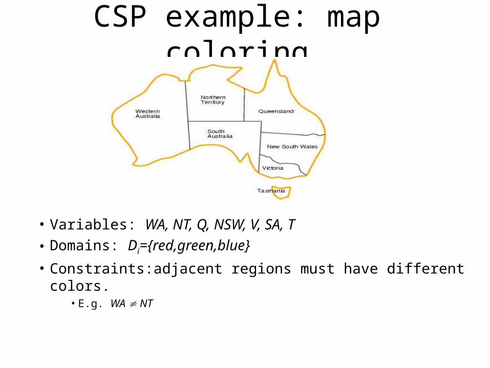
CSP example: map coloring

• Variables: WA, NT, Q, NSW, V, SA, T• Domains: Di={red,green,blue}

• Constraints:adjacent regions must have different colors.• E.g. WA NT

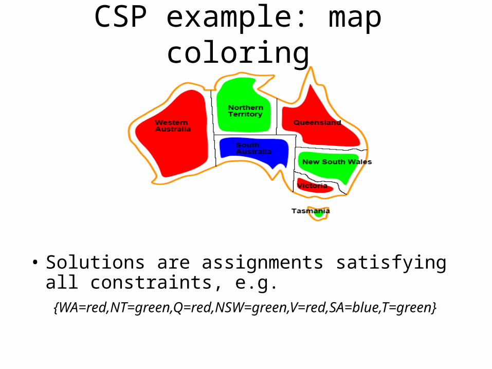
CSP example: map coloring

• Solutions are assignments satisfying all constraints, e.g. {WA=red,NT=green,Q=red,NSW=green,V=red,SA=blue,T=green}

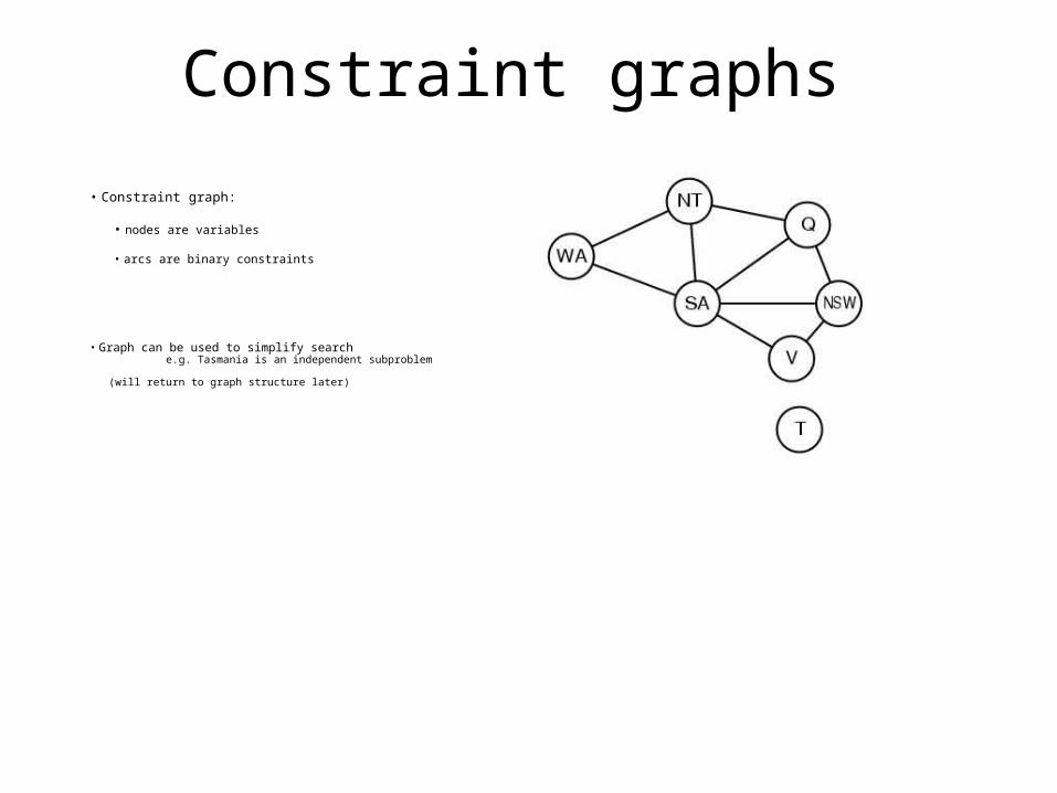
Constraint graphs

• Constraint graph:

• nodes are variables

• arcs are binary constraints

• Graph can be used to simplify search e.g. Tasmania is an independent subproblem

(will return to graph structure later)

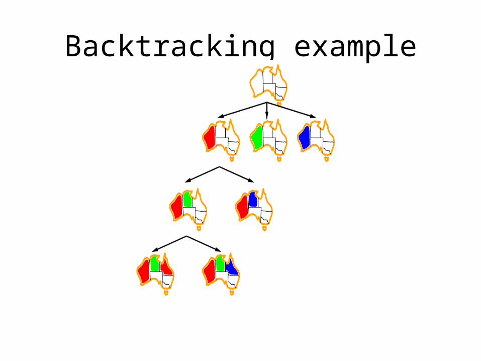
Backtracking example

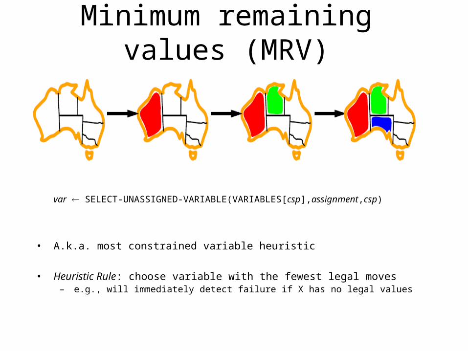
Minimum remaining values (MRV)

var SELECT-UNASSIGNED-VARIABLE(VARIABLES[csp],assignment,csp)

• A.k.a. most constrained variable heuristic

• Heuristic Rule: choose variable with the fewest legal moves– e.g., will immediately detect failure if X has no legal values

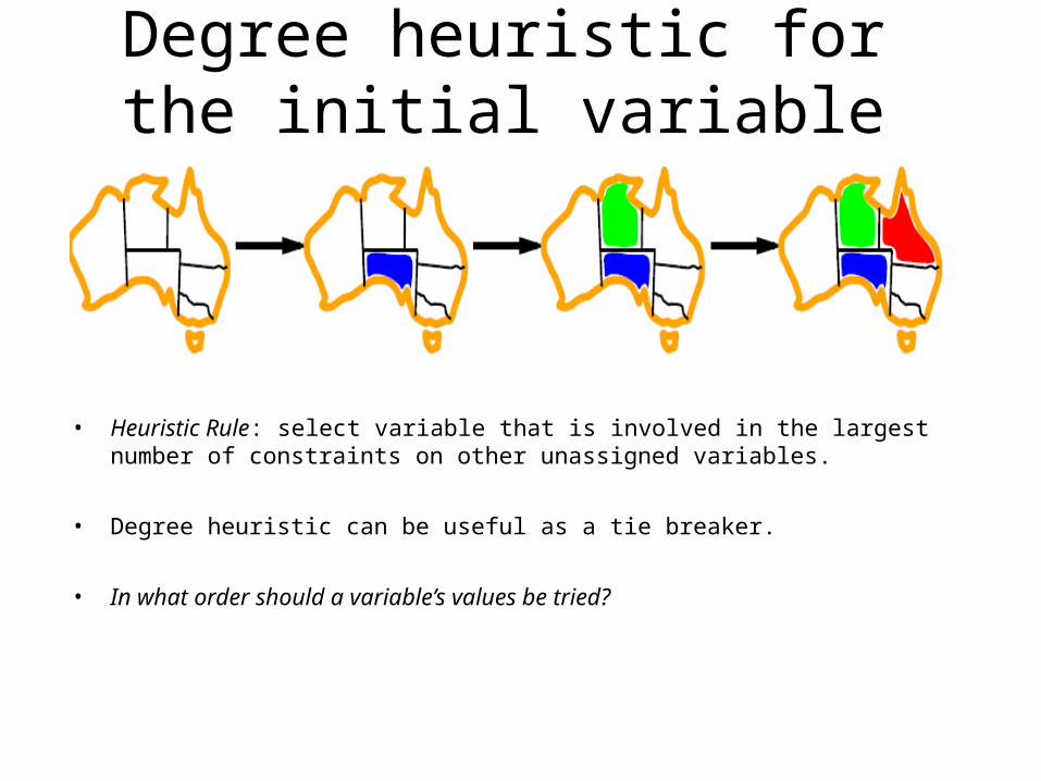
Degree heuristic for the initial variable

• Heuristic Rule: select variable that is involved in the largest number of constraints on other unassigned variables.

• Degree heuristic can be useful as a tie breaker.

• In what order should a variable’s values be tried?

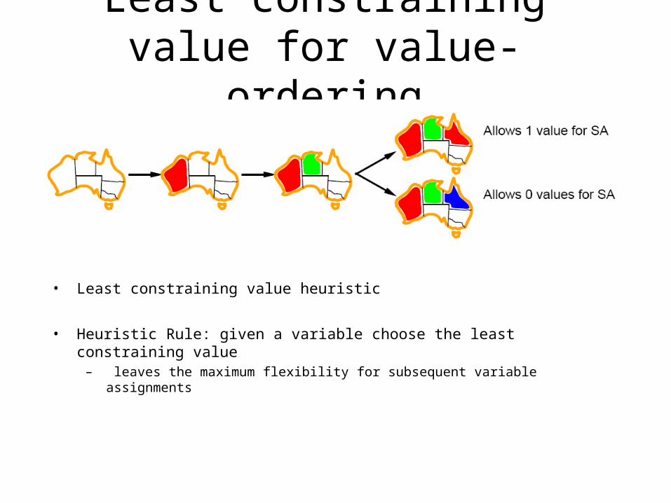
Least constraining value for value-ordering

• Least constraining value heuristic

• Heuristic Rule: given a variable choose the least constraining value– leaves the maximum flexibility for subsequent variable assignments

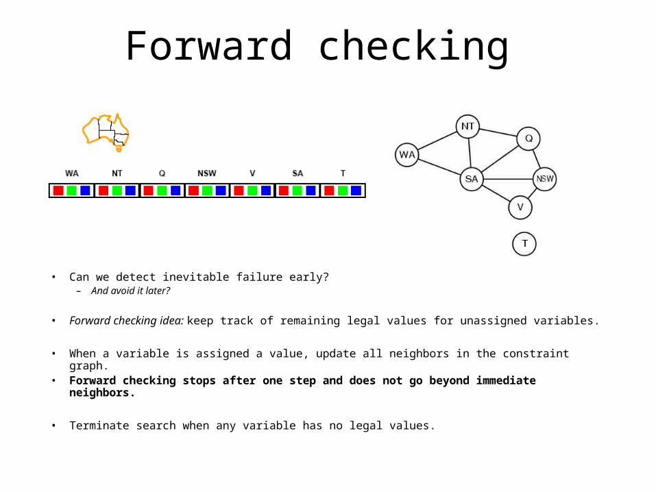
Forward checking

• Can we detect inevitable failure early?– And avoid it later?

• Forward checking idea: keep track of remaining legal values for unassigned variables.

• When a variable is assigned a value, update all neighbors in the constraint graph.• Forward checking stops after one step and does not go beyond immediate neighbors.

• Terminate search when any variable has no legal values.

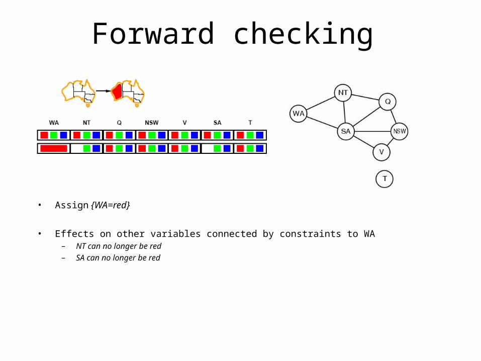
Forward checking

• Assign {WA=red}

• Effects on other variables connected by constraints to WA– NT can no longer be red– SA can no longer be red

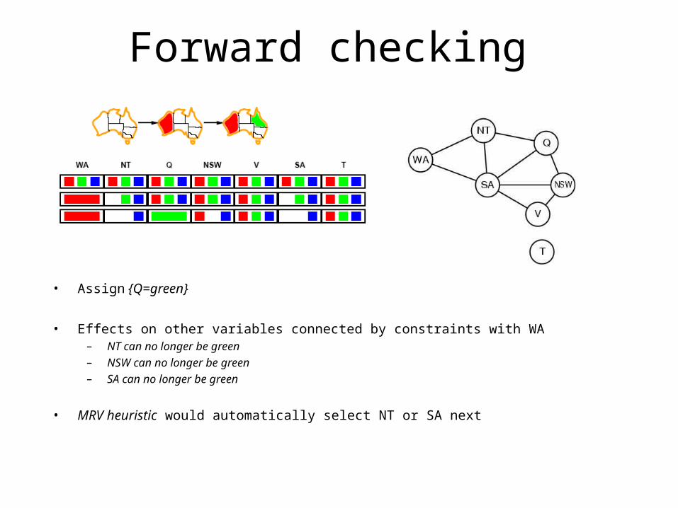
Forward checking

• Assign {Q=green}

• Effects on other variables connected by constraints with WA– NT can no longer be green– NSW can no longer be green– SA can no longer be green

• MRV heuristic would automatically select NT or SA next

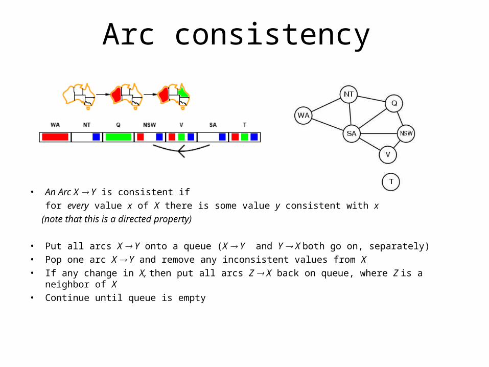
Arc consistency

• An Arc X Y is consistent iffor every value x of X there is some value y consistent with x

(note that this is a directed property)

• Put all arcs X Y onto a queue (X Y and Y X both go on, separately)• Pop one arc X Y and remove any inconsistent values from X• If any change in X, then put all arcs Z X back on queue, where Z is a neighbor of X• Continue until queue is empty

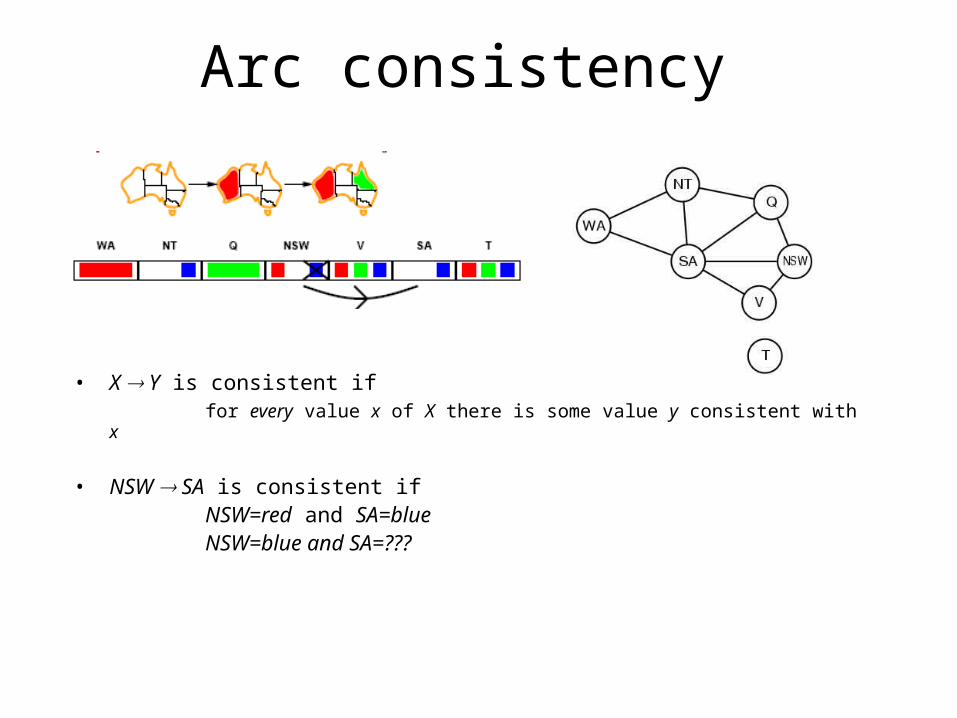
Arc consistency

• X Y is consistent iffor every value x of X there is some value y consistent with x

• NSW SA is consistent ifNSW=red and SA=blueNSW=blue and SA=???

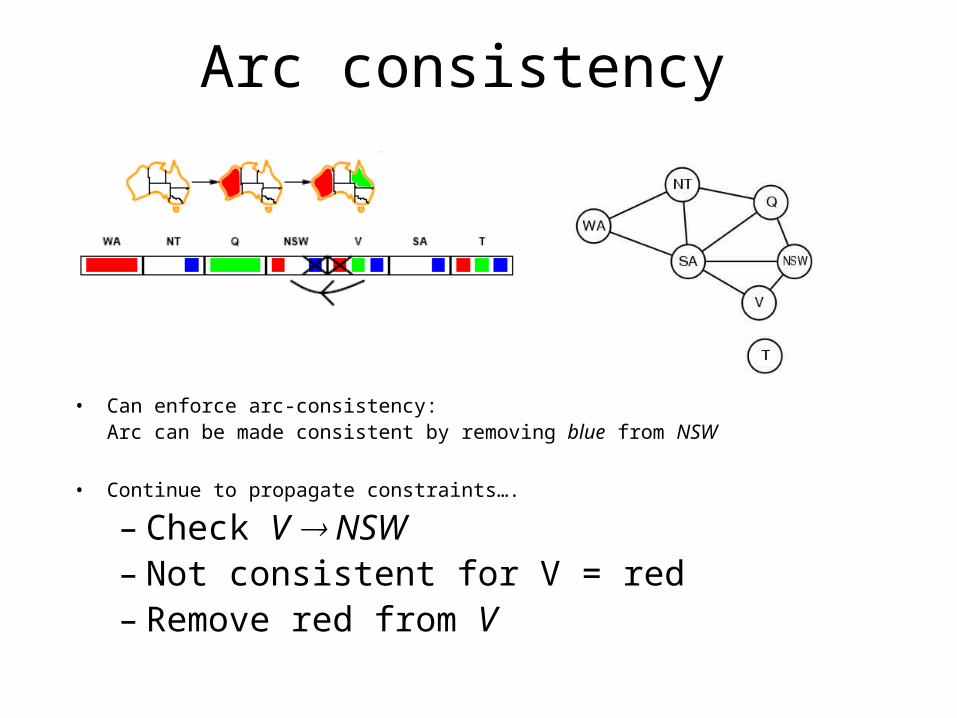
Arc consistency

• Can enforce arc-consistency:Arc can be made consistent by removing blue from NSW

• Continue to propagate constraints….

– Check V NSW– Not consistent for V = red – Remove red from V

Arc consistency

• Continue to propagate constraints….

• SA NT is not consistent

– and cannot be made consistent

• Arc consistency detects failure earlier than FC

Local search for CSPs• Use complete-state representation

– Initial state = all variables assigned values– Successor states = change 1 (or more) values

• For CSPs– allow states with unsatisfied constraints (unlike backtracking)– operators reassign variable values– hill-climbing with n-queens is an example

• Variable selection: randomly select any conflicted variable

• Value selection: min-conflicts heuristic– Select new value that results in a minimum number of conflicts with the other variables

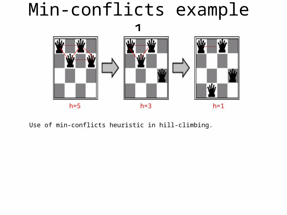
Min-conflicts example 1

Use of min-conflicts heuristic in hill-climbing.

h=5 h=3 h=1

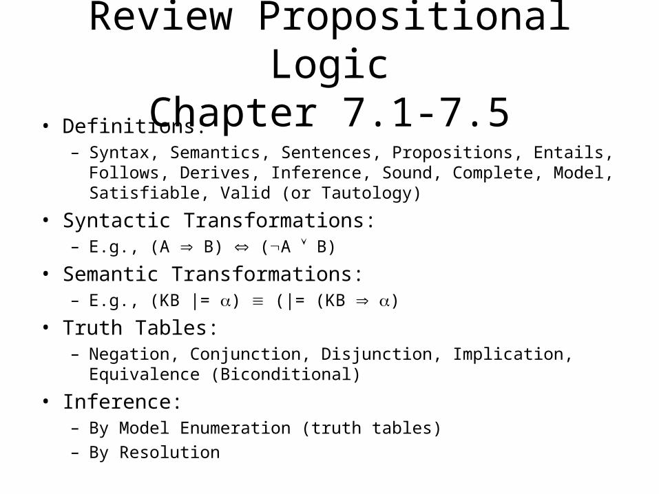
Review Propositional LogicChapter 7.1-7.5

• Definitions:– Syntax, Semantics, Sentences, Propositions, Entails, Follows, Derives,

Inference, Sound, Complete, Model, Satisfiable, Valid (or Tautology)

• Syntactic Transformations:– E.g., (A B) (A B)

• Semantic Transformations:– E.g., (KB |= ) (|= (KB )

• Truth Tables:– Negation, Conjunction, Disjunction, Implication, Equivalence

(Biconditional)

• Inference:– By Model Enumeration (truth tables)– By Resolution

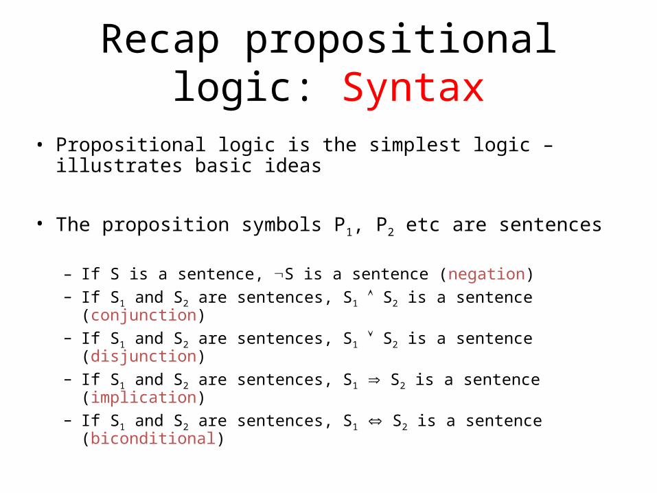
Recap propositional logic: Syntax

• Propositional logic is the simplest logic – illustrates basic ideas

• The proposition symbols P1, P2 etc are sentences

– If S is a sentence, S is a sentence (negation)– If S1 and S2 are sentences, S1 S2 is a sentence (conjunction)– If S1 and S2 are sentences, S1 S2 is a sentence (disjunction)– If S1 and S2 are sentences, S1 S2 is a sentence (implication)– If S1 and S2 are sentences, S1 S2 is a sentence (biconditional)

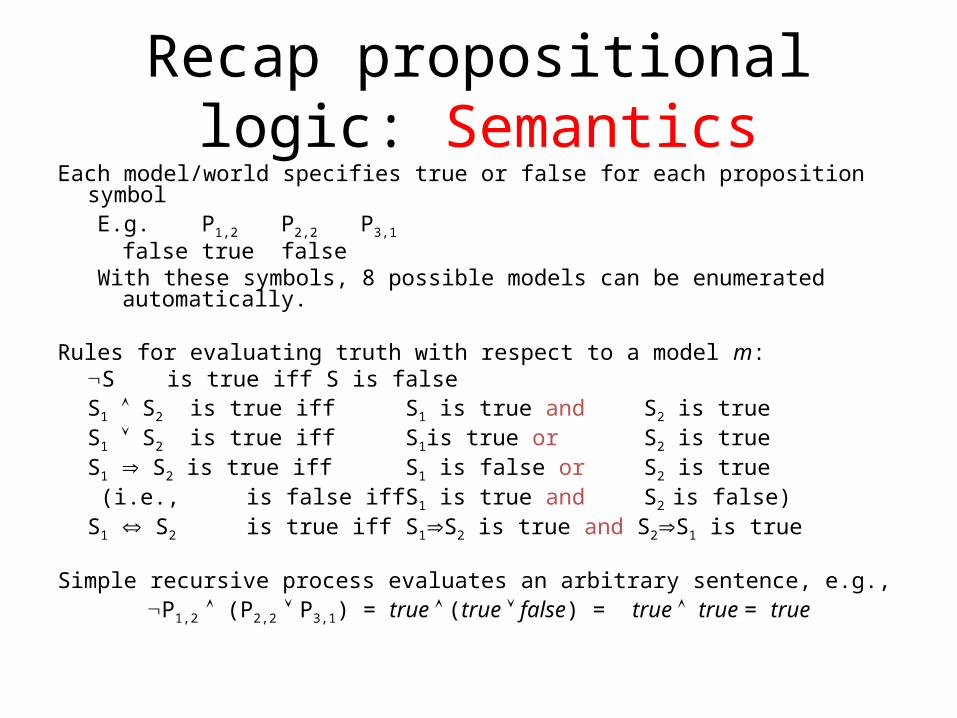
Recap propositional logic: Semantics

Each model/world specifies true or false for each proposition symbolE.g. P1,2 P2,2 P3,1

false true falseWith these symbols, 8 possible models can be enumerated automatically.

Rules for evaluating truth with respect to a model m:S is true iff S is false S1 S2 is true iff S1 is true and S2 is trueS1 S2 is true iff S1is true or S2 is trueS1 S2 is true iff S1 is false or S2 is true (i.e., is false iff S1 is true and S2 is false)S1 S2 is true iffS1S2 is true and S2S1 is true

Simple recursive process evaluates an arbitrary sentence, e.g.,P1,2 (P2,2 P3,1) = true (true false) = true true = true

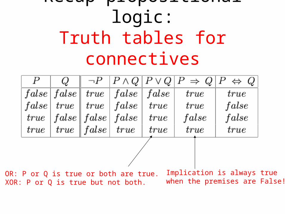
Recap propositional logic:Truth tables for connectives

OR: P or Q is true or both are true.XOR: P or Q is true but not both.

Implication is always truewhen the premises are False!

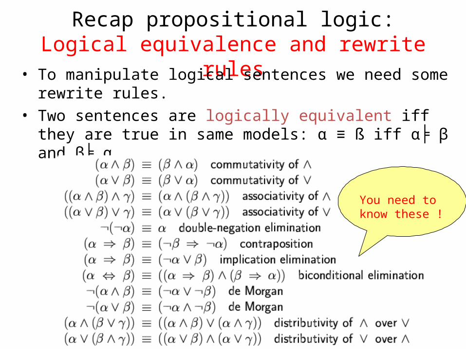
Recap propositional logic:Logical equivalence and rewrite rules

• To manipulate logical sentences we need some rewrite rules.• Two sentences are logically equivalent iff they are true in same

models: α ≡ ß iff α ╞ β and β α╞

You need to know these !

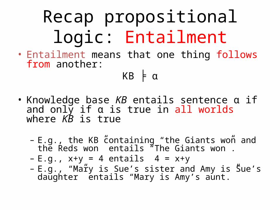
Recap propositional logic: Entailment

• Entailment means that one thing follows from another:

KB ╞ α

• Knowledge base KB entails sentence α if and only if α is true in all worlds where KB is true

– E.g., the KB containing “the Giants won and the Reds won” entails “The Giants won”.

– E.g., x+y = 4 entails 4 = x+y– E.g., “Mary is Sue’s sister and Amy is Sue’s daughter”

entails “Mary is Amy’s aunt.”

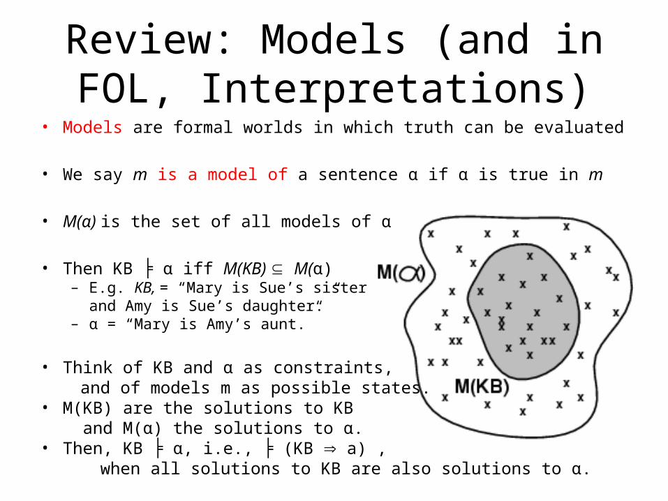
Review: Models (and in FOL, Interpretations)

• Models are formal worlds in which truth can be evaluated

• We say m is a model of a sentence α if α is true in m

• M(α) is the set of all models of α

• Then KB α iff ╞ M(KB) M(α)– E.g. KB, = “Mary is Sue’s sister

and Amy is Sue’s daughter.”– α = “Mary is Amy’s aunt.”

• Think of KB and α as constraints, and of models m as possible states.

• M(KB) are the solutions to KB and M(α) the solutions to α.

• Then, KB α, i.e., (KB ╞ ╞ a) , when all solutions to KB are also solutions to α.

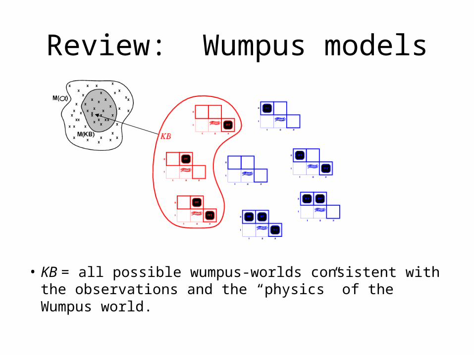
Review: Wumpus models

• KB = all possible wumpus-worlds consistent with the observations and the “physics” of the Wumpus world.

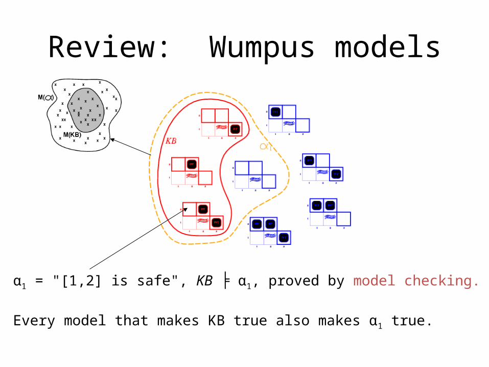
Review: Wumpus models

α1 = "[1,2] is safe", KB α╞ 1, proved by model checking.

Every model that makes KB true also makes α1 true.

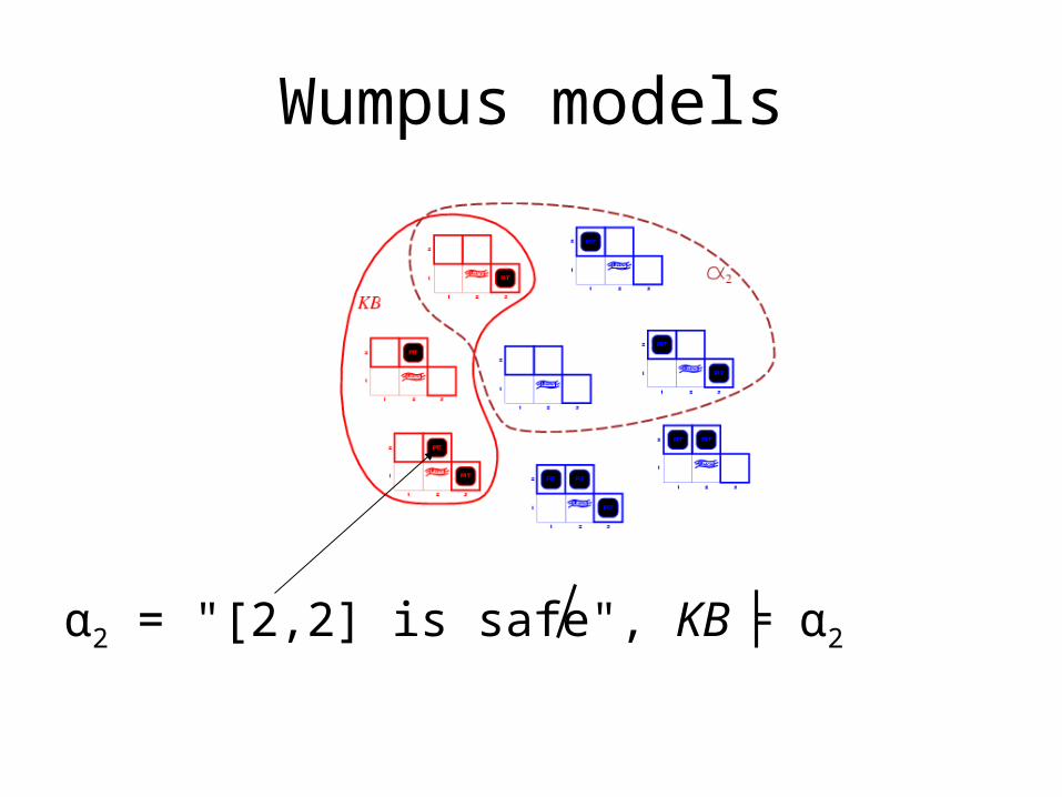
Wumpus models

α2 = "[2,2] is safe", KB α╞ 2

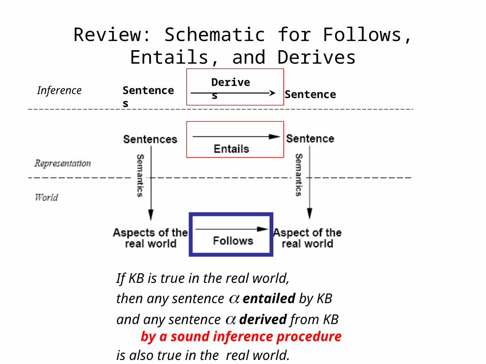
Review: Schematic for Follows, Entails, and Derives

If KB is true in the real world,

then any sentence entailed by KB

and any sentence derived from KB by a sound inference procedure

is also true in the real world.

Sentences SentenceDerives

Inference

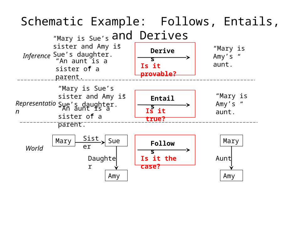
Schematic Example: Follows, Entails, and Derives

Inference

“Mary is Sue’s sister and Amy is Sue’s daughter.” “Mary is

Amy’s aunt.”Representation

Derives

Entails

FollowsWorld

Mary Sue

Amy

“Mary is Sue’s sister and Amy is Sue’s daughter.”

“An aunt is a sister of a parent.”

“An aunt is a sister of a parent.”

Sister

Daughter

Mary

Amy

Aunt

“Mary is Amy’s aunt.”

Is it provable?

Is it true?

Is it the case?

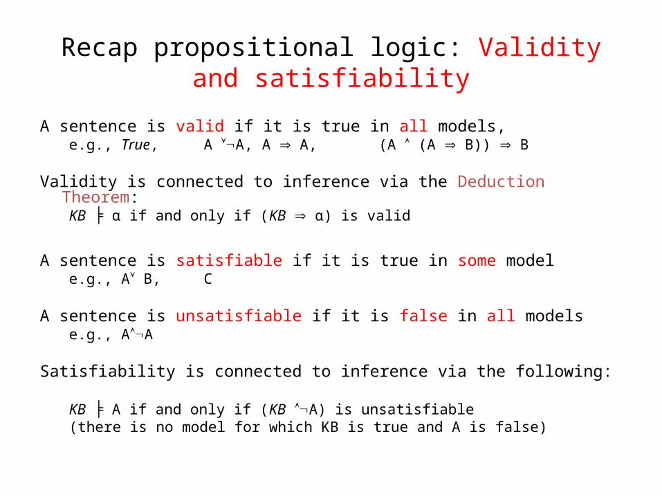
Recap propositional logic: Validity and satisfiability

A sentence is valid if it is true in all models,e.g., True, A A, A A, (A (A B)) B

Validity is connected to inference via the Deduction Theorem:KB α if and only if (╞ KB α) is valid

A sentence is satisfiable if it is true in some modele.g., A B, C

A sentence is unsatisfiable if it is false in all modelse.g., AA

Satisfiability is connected to inference via the following:

KB A if and only if (╞ KB A) is unsatisfiable(there is no model for which KB is true and A is false)

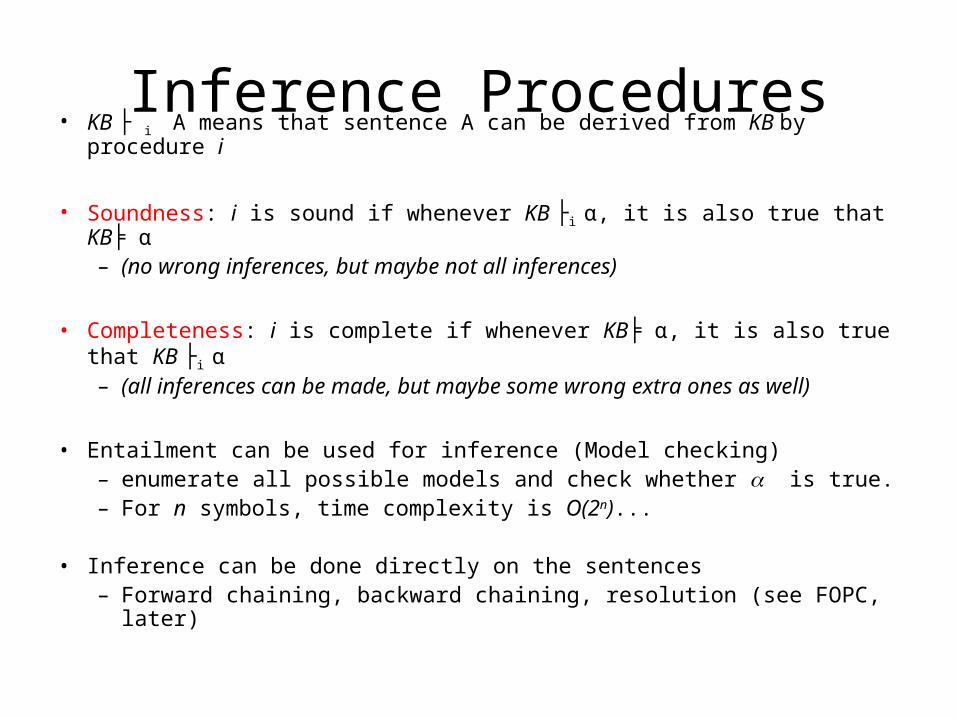
Inference Procedures• KB ├ i A means that sentence A can be derived from KB by procedure i

• Soundness: i is sound if whenever KB ├i α, it is also true that KB α╞– (no wrong inferences, but maybe not all inferences)

• Completeness: i is complete if whenever KB α, it is also true that ╞ KB ├i α– (all inferences can be made, but maybe some wrong extra ones as

well)

• Entailment can be used for inference (Model checking)– enumerate all possible models and check whether is true.– For n symbols, time complexity is O(2n)...

• Inference can be done directly on the sentences– Forward chaining, backward chaining, resolution (see FOPC, later)

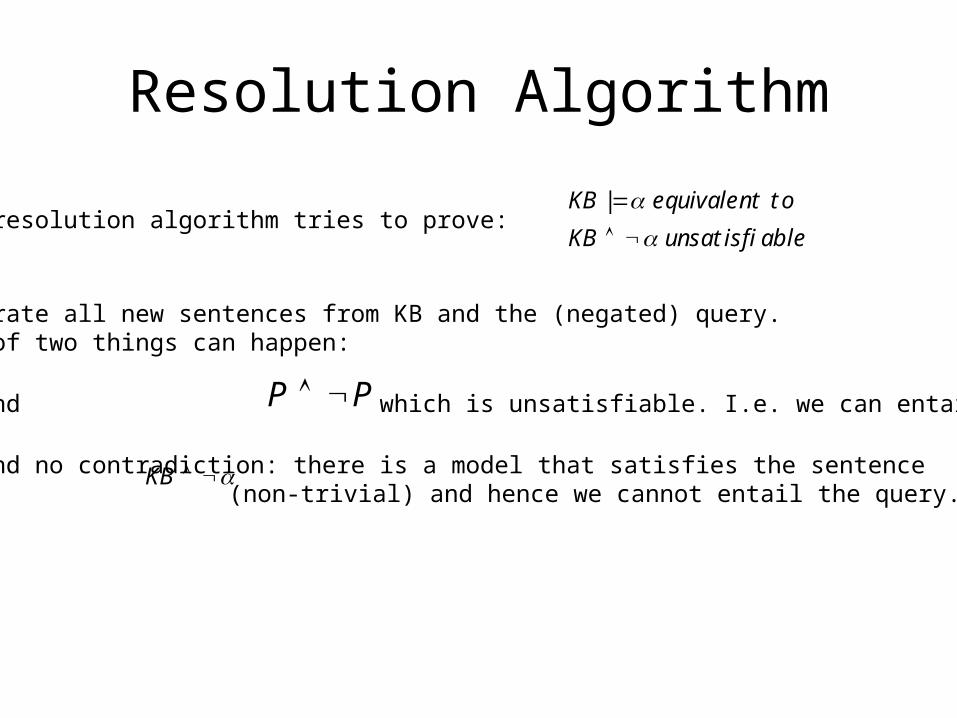
• The resolution algorithm tries to prove:

• Generate all new sentences from KB and the (negated) query.• One of two things can happen:

1. We find which is unsatisfiable. I.e. we can entail the query.

2. We find no contradiction: there is a model that satisfies the sentence (non-trivial) and hence we cannot entail the query.

Resolution Algorithm

|KB equivalent to

KB unsatisfiable

P P

KB

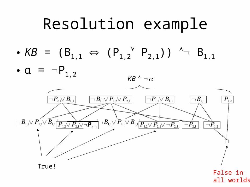
Resolution example

• KB = (B1,1 (P1,2 P2,1)) B1,1

• α = P1,2KB

False inall worlds

True!

P2,1

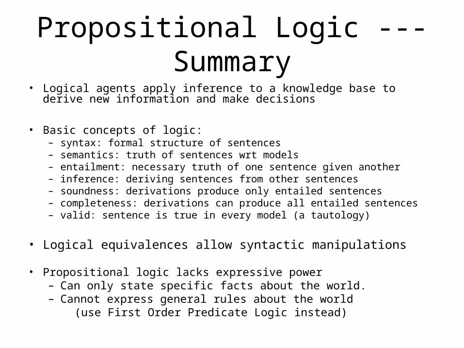
Propositional Logic --- Summary• Logical agents apply inference to a knowledge base to derive new information

and make decisions

• Basic concepts of logic:– syntax: formal structure of sentences– semantics: truth of sentences wrt models– entailment: necessary truth of one sentence given another– inference: deriving sentences from other sentences– soundness: derivations produce only entailed sentences– completeness: derivations can produce all entailed sentences– valid: sentence is true in every model (a tautology)

• Logical equivalences allow syntactic manipulations

• Propositional logic lacks expressive power– Can only state specific facts about the world.– Cannot express general rules about the world (use First Order Predicate Logic instead)

Mid-term ReviewChapters 2-7

• Review Agents (2.1-2.3)• Review State Space Search

• Problem Formulation (3.1, 3.3)• Blind (Uninformed) Search (3.4)• Heuristic Search (3.5)• Local Search (4.1, 4.2)

• Review Adversarial (Game) Search (5.1-5.4)• Review Constraint Satisfaction (6.1-6.4)• Review Propositional Logic (7.1-7.5)• Please review your quizzes and old CS-171 tests

• At least one question from a prior quiz or old CS-171 test will appear on the mid-term (and all other tests)