Microwaves - my.ece.msstate.edu

Microwaves

Microwaves in the Electromagnetic Spectrum (300 MHz - 300 GHz)

ELF Extremely Low Frequency 3-30 Hz

SLF Super Low Frequency 30-300 Hz

ULF Ultra Low Frequency 300 Hz - 3 kHz

VLF Very Low Frequency 3 kHz - 30 kHz

LF Low Frequency 30 kHz - 300 kHz

MF Medium Frequency 300 kHz - 3 MHz

HF High Frequency 3 MHz - 30 MHz

VHF Very High Frequency 30 MHz - 300 MHz

UHF Ultra High Frequency 300 MHz - 3 GHz

(decimeter waves)

SHF Super High Frequency 3 GHz - 30 GHz

(centimeter waves)

EHF Extremely High Frequency 30 GHz - 300 GHz

(millimeter waves)

? (submillimeter waves) 300 GHz - 3000 GHz

IR Infared 3000 GHz - 416,000 GHz

Microwave Properties

High bandwidth - The microwave frequency range (300 MHz - 300

GHz) is 999 times that of the entire frequency range below it.

Effect of the ionosphere - When lower frequency waves are directed

upward into the atmosphere, they experience significant

reflection due to the ionosphere. The lower frequency waves

which pass through the ionosphere suffer distortion.

Microwaves pass through the ionosphere with little effect and

are therefore utilized in satellite communications and space

transmissions.

Line-of-sight transmission/reception - The microwave receive

antenna must be within the line-of-sight of the transmit antenna.

Long distance communication on earth requires that microwave

relay stations be used.

Electromagnetic noise characteristics - The electromagnetic noise

level in nature over the 1-10 GHz frequency range is small.

This allows for the detection of very low signal levels using

sensitive receivers.

Antenna gain and directivity - The gain of an antenna is directly

proportional to its electrical size. The beamwidth of an antenna

is inversely proportional to the electrical size of its maximum

dimension. Shorter wavelengths at microwave frequencies

allow for smaller antennas. At higher frequencies (visible light-

lasers), the beamwidth gets very small and pointing accuracy of

the detector becomes a problem.

Target reflection of electromagnetic waves (radar cross section) - In

general, electrically large conducting radar targets reflect more

energy (shape is also a factor - stealth design). Thus, the higher

frequencies of microwaves are preferred for radar systems. At

millimeter waves, the wavelength becomes comparable to the

size of raindrops which results in attenuation of the incident

waves.

Absorption at resonant frequencies - various materials absorb

microwave energy (dissipated in the form of heat) at specific

resonant frequencies.

Applications of Microwaves

Wireless communications

Personal Communications Systems (PCS)

(pagers, cell phones, etc.)

Global Positioning Satellite (GPS) Systems

Wireless Local Area Computer Networks (WLANS)

Direct Broadcast Satellite (DBS) Television

Telephone Microwave/Satellite Links, etc.

Remote sensing

Radar (active remote sensing - radiate and receive)

Military applications (target tracking)

Weather radar

Ground Penetrating Radar (GPR)

Agricultural applications

Radiometry (passive remote sensing - receive inherent

emissions)

Radio astronomy

Industrial and home applications

Cooking, drying, heating

Microwave spectroscopy - molecular properties of materials

can be determined by passing microwaves through a

sample of the material and measuring the absorption

spectrum.

Analysis Techniques in Microwave Theory

In general, circuit theory is not applicable to microwave problems.

Circuit theory is derived from Maxwell’s equations based on certain

assumptions about the fields within the circuit elements. Specifically, the

circuit elements must be small relative to wavelength for circuit equations

to be valid. In this sense, microwave components must be modeled by

distributed elements, not lumped elements. For this reason, we must use

field theory solutions (Maxwell’s equations) for microwave applications.

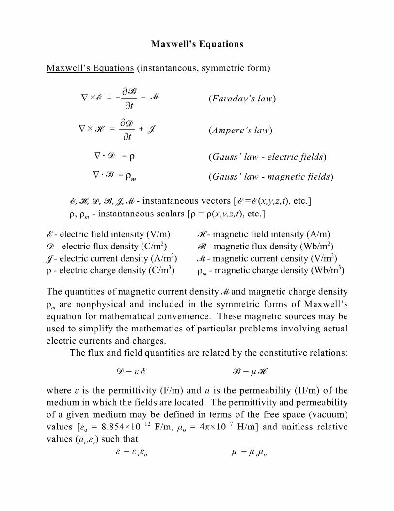
Maxwell’s Equations

Maxwell’s Equations (instantaneous, symmetric form)

(Faraday’s law)

(Ampere’s law)

(Gauss’ law - electric fields)

(Gauss’ law - magnetic fields)

E, H, D, B, J, M - instantaneous vectors [E =E (x,y,z,t), etc.]

mñ, ñ - instantaneous scalars [ñ = ñ(x,y,z,t), etc.]

E - electric field intensity (V/m) H - magnetic field intensity (A/m)D - electric flux density (C/m ) B - magnetic flux density (Wb/m )2 2

J - electric current density (A/m ) M - magnetic current density (V/m )2 2

mñ - electric charge density (C/m ) ñ - magnetic charge density (Wb/m )3 3

The quantities of magnetic current density M and magnetic charge density

mñ are nonphysical and included in the symmetric forms of Maxwell’s

equation for mathematical convenience. These magnetic sources may be

used to simplify the mathematics of particular problems involving actual

electric currents and charges.

The flux and field quantities are related by the constitutive relations:

D = å E B = ì H

where å is the permittivity (F/m) and ì is the permeability (H/m) of the

medium in which the fields are located. The permittivity and permeability

of a given medium may be defined in terms of the free space (vacuum)

o ovalues [å = 8.854×10 F/m, ì = 4ð×10 H/m] and unitless relative!12 !7

r rvalues (ì ,å ) such that

r o r oå = å å ì = ì ì

BME

D JH

D

B

The instantaneous Maxwell’s equations are valid given any type of

time-dependence for the electromagnetic fields. Most applications in

microwave engineering involve fields which have a sinusoidal (harmonic)

time-dependence. This harmonic time-dependence allows us to simplify

Maxwell’s equations by writing them in terms of phasors just like we use

in circuit analysis.

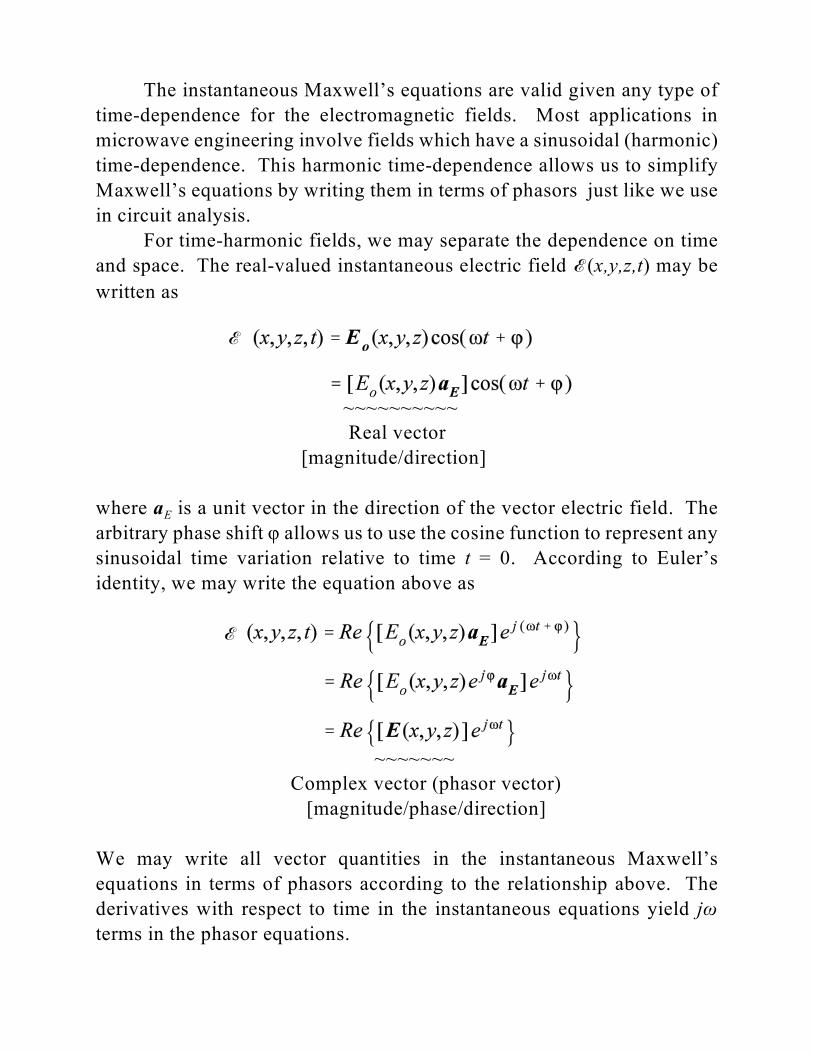
For time-harmonic fields, we may separate the dependence on time

and space. The real-valued instantaneous electric field E (x,y,z,t) may be

written as

~~~~~~~~~~

Real vector

[magnitude/direction]

Ewhere a is a unit vector in the direction of the vector electric field. The

arbitrary phase shift ö allows us to use the cosine function to represent any

sinusoidal time variation relative to time t = 0. According to Euler’s

identity, we may write the equation above as

~~~~~~~

Complex vector (phasor vector)

[magnitude/phase/direction]

We may write all vector quantities in the instantaneous Maxwell’s

equations in terms of phasors according to the relationship above. The

derivatives with respect to time in the instantaneous equations yield jù

terms in the phasor equations.

E

E

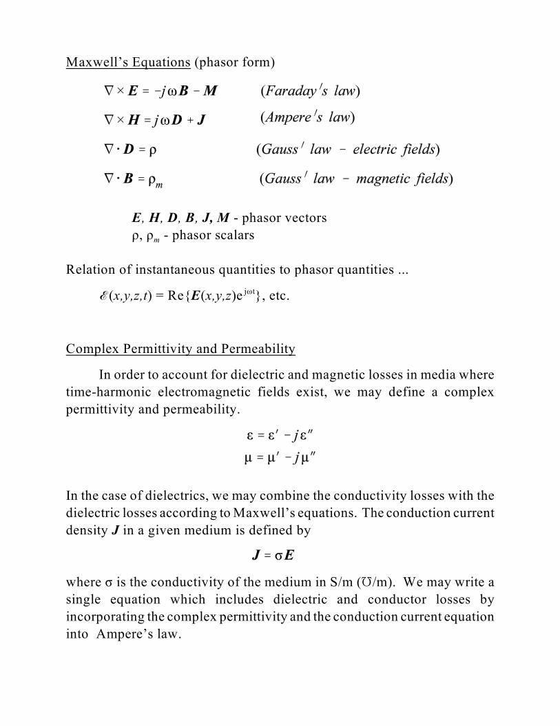
Maxwell’s Equations (phasor form)

E, H, D, B, J, M - phasor vectors

mñ, ñ - phasor scalars

Relation of instantaneous quantities to phasor quantities ...

E (x,y,z,t) = Re{E(x,y,z)e }, etc.jùt

Complex Permittivity and Permeability

In order to account for dielectric and magnetic losses in media where

time-harmonic electromagnetic fields exist, we may define a complex

permittivity and permeability.

In the case of dielectrics, we may combine the conductivity losses with the

dielectric losses according to Maxwell’s equations. The conduction current

density J in a given medium is defined by

where ó is the conductivity of the medium in S/m (É/m). We may write a

single equation which includes dielectric and conductor losses by

incorporating the complex permittivity and the conduction current equation

into Ampere’s law.

~~~~~~ ~~~~~~~~~~

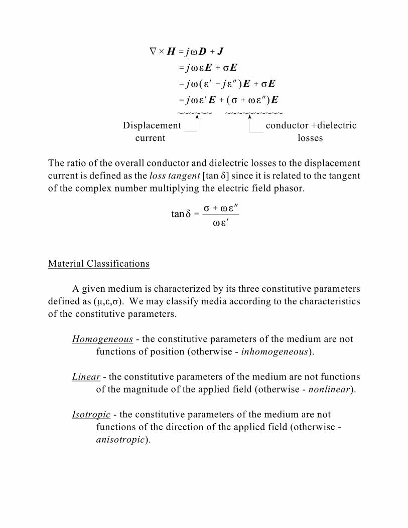
Displacement conductor +dielectric

current losses

The ratio of the overall conductor and dielectric losses to the displacement

current is defined as the loss tangent [tan ä] since it is related to the tangent

of the complex number multiplying the electric field phasor.

Material Classifications

A given medium is characterized by its three constitutive parameters

defined as (ì,å,ó). We may classify media according to the characteristics

of the constitutive parameters.

Homogeneous - the constitutive parameters of the medium are not

functions of position (otherwise - inhomogeneous).

Linear - the constitutive parameters of the medium are not functions

of the magnitude of the applied field (otherwise - nonlinear).

Isotropic - the constitutive parameters of the medium are not

functions of the direction of the applied field (otherwise -

anisotropic).

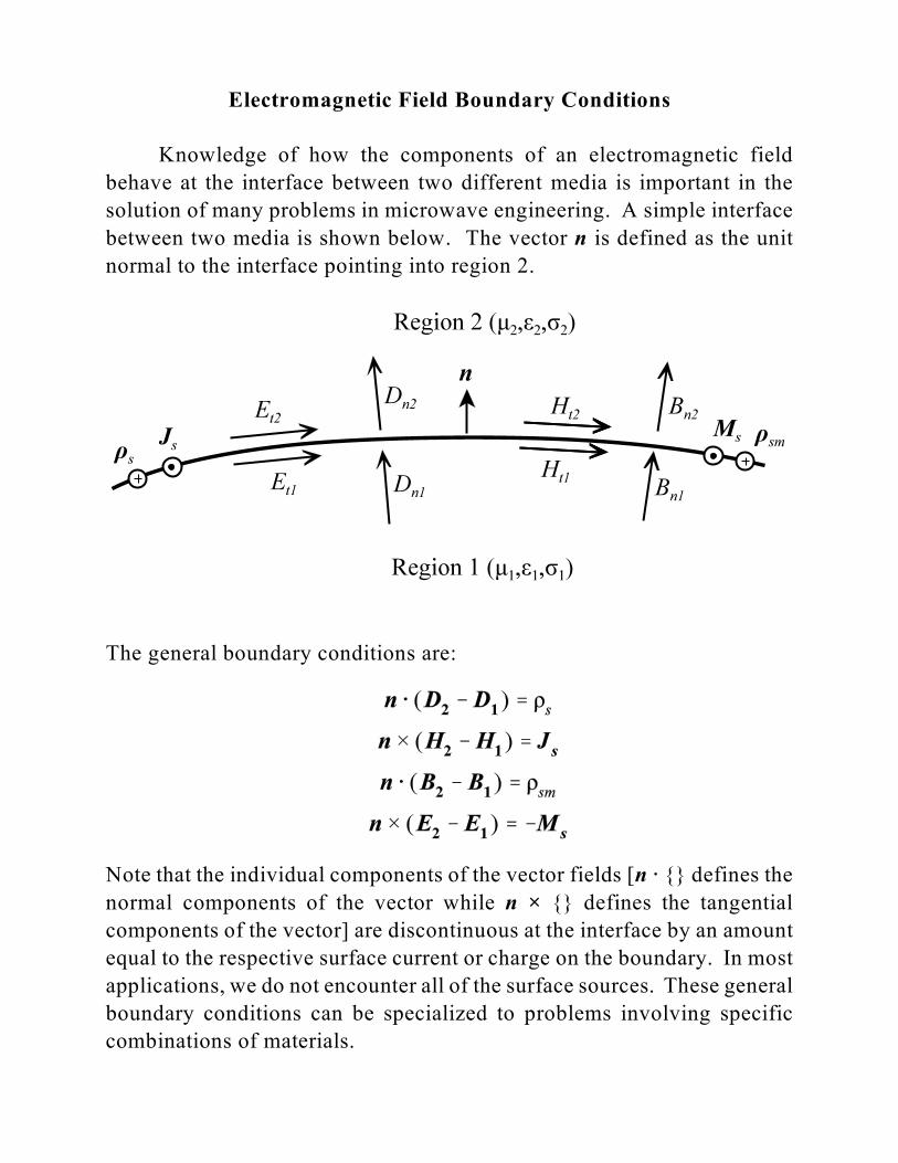
Electromagnetic Field Boundary Conditions

Knowledge of how the components of an electromagnetic field

behave at the interface between two different media is important in the

solution of many problems in microwave engineering. A simple interface

between two media is shown below. The vector n is defined as the unit

normal to the interface pointing into region 2.

The general boundary conditions are:

Note that the individual components of the vector fields [n @ {} defines the

normal components of the vector while n × {} defines the tangential

components of the vector] are discontinuous at the interface by an amount

equal to the respective surface current or charge on the boundary. In most

applications, we do not encounter all of the surface sources. These general

boundary conditions can be specialized to problems involving specific

combinations of materials.

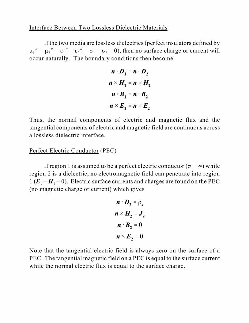
Interface Between Two Lossless Dielectric Materials

If the two media are lossless dielectrics (perfect insulators defined by

1 2 1 2 1 2ì O = ì O = å O = å O = ó = ó = 0), then no surface charge or current will

occur naturally. The boundary conditions then become

Thus, the normal components of electric and magnetic flux and the

tangential components of electric and magnetic field are continuous across

a lossless dielectric interface.

Perfect Electric Conductor (PEC)

1If region 1 is assumed to be a perfect electric conductor (ó 64) while

region 2 is a dielectric, no electromagnetic field can penetrate into region

1 11 (E = H = 0). Electric surface currents and charges are found on the PEC

(no magnetic charge or current) which gives

Note that the tangential electric field is always zero on the surface of a

PEC. The tangential magnetic field on a PEC is equal to the surface current

while the normal electric flux is equal to the surface charge.

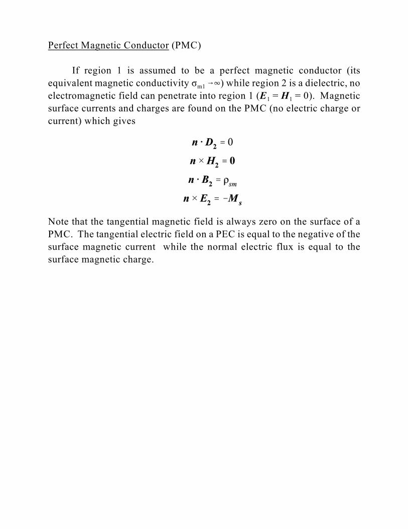
Perfect Magnetic Conductor (PMC)

If region 1 is assumed to be a perfect magnetic conductor (its

m1equivalent magnetic conductivity ó 64) while region 2 is a dielectric, no

1 1electromagnetic field can penetrate into region 1 (E = H = 0). Magnetic

surface currents and charges are found on the PMC (no electric charge or

current) which gives

Note that the tangential magnetic field is always zero on the surface of a

PMC. The tangential electric field on a PEC is equal to the negative of the

surface magnetic current while the normal electric flux is equal to the

surface magnetic charge.

Electromagnetic Waves

Maxwell’s equations show that the electric field and magnetic field

m in a source-free (J = M = 0, ñ = ñ = 0), homogeneous, linear, isotropic

medium satisfy wave equations (Helmholtz equations). The source-free

Maxwell’s equations in phasor form are

Note that taking the divergence of (1) and (2) yields (3) and (4) since

L @ L ×F = 0 for any vector F. Thus, in a source-free region, (3) and (4) are

not necessary. Taking the curl of (1) and inserting (2) yields

while taking the curl of (2) and inserting (1) yields

where k = ù %ì&å& is defined as the wavenumber of the medium. Using the

vector identity

in (5) and (6) gives

However, the divergence terms in (7) and (8) are zero in the source-free

region. This gives the wave equations (Helmholtz equations) for the

electric and magnetic field.

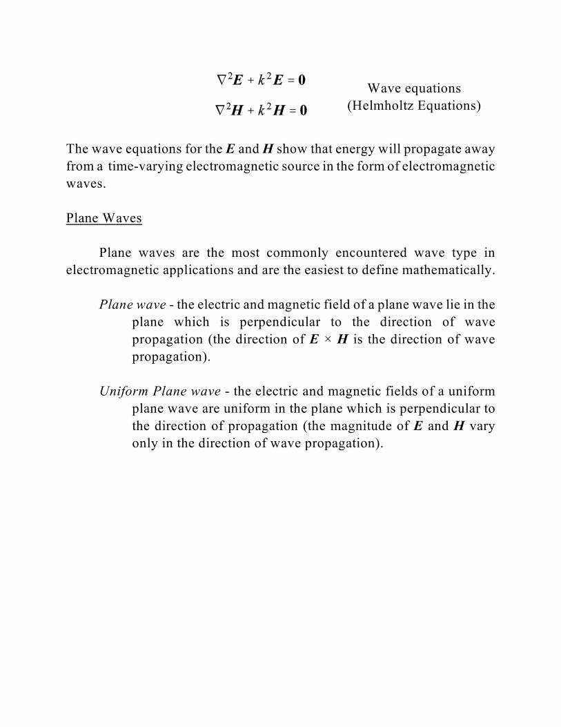
Wave equations

(Helmholtz Equations)

The wave equations for the E and H show that energy will propagate away

from a time-varying electromagnetic source in the form of electromagnetic

waves.

Plane Waves

Plane waves are the most commonly encountered wave type in

electromagnetic applications and are the easiest to define mathematically.

Plane wave - the electric and magnetic field of a plane wave lie in the

plane which is perpendicular to the direction of wave

propagation (the direction of E × H is the direction of wave

propagation).

Uniform Plane wave - the electric and magnetic fields of a uniform

plane wave are uniform in the plane which is perpendicular to

the direction of propagation (the magnitude of E and H vary

only in the direction of wave propagation).

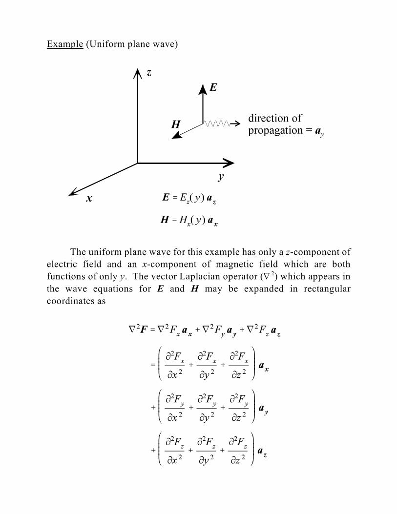
Example (Uniform plane wave)

The uniform plane wave for this example has only a z-component of

electric field and an x-component of magnetic field which are both

functions of only y. The vector Laplacian operator (L ) which appears in2

the wave equations for E and H may be expanded in rectangular

coordinates as

Linear, homogeneous,

2 order D.E.’snd

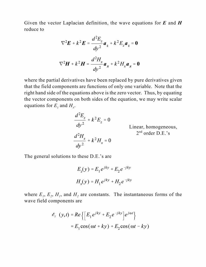
Given the vector Laplacian definition, the wave equations for E and H

reduce to

where the partial derivatives have been replaced by pure derivatives given

that the field components are functions of only one variable. Note that the

right hand side of the equations above is the zero vector. Thus, by equating

the vector components on both sides of the equation, we may write scalar

z xequations for E and H .

The general solutions to these D.E.’s are

1 2 1 2where E , E , H , and H are constants. The instantaneous forms of the

wave field components are

zE

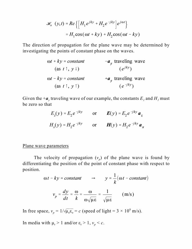
The direction of propagation for the plane wave may be determined by

investigating the points of constant phase on the waves.

y 1 1Given the +a traveling wave of our example, the constants E and H must

be zero so that

Plane wave parameters

pThe velocity of propagation (v ) of the plane wave is found by

differentiating the position of the point of constant phase with respect to

position.

p o oIn free space, v = 1/%ì&å& = c (speed of light = 3 × 10 m/s).8

pr rIn media with ì > 1 and/or å > 1, v < c.

xH

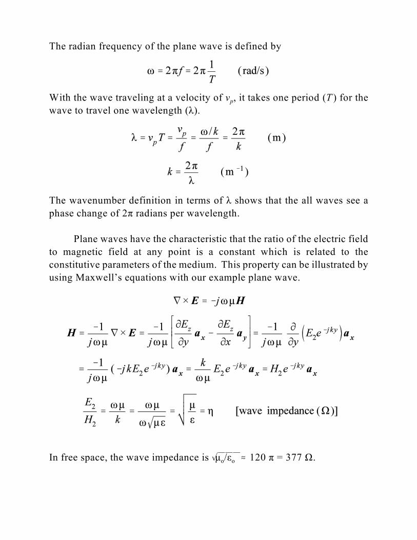
The radian frequency of the plane wave is defined by

pWith the wave traveling at a velocity of v , it takes one period (T ) for the

wave to travel one wavelength (ë).

The wavenumber definition in terms of ë shows that the all waves see a

phase change of 2ð radians per wavelength.

Plane waves have the characteristic that the ratio of the electric field

to magnetic field at any point is a constant which is related to the

constitutive parameters of the medium. This property can be illustrated by

using Maxwell’s equations with our example plane wave.

o oIn free space, the wave impedance is %ì&/&å& . 120 ð = 377 Ù.

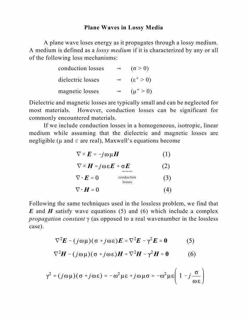
Plane Waves in Lossy Media

A plane wave loses energy as it propagates through a lossy medium.

A medium is defined as a lossy medium if it is characterized by any or all

of the following loss mechanisms:

conduction losses Y (ó > 0)

dielectric losses Y (åO > 0)

magnetic losses Y (ìO > 0)

Dielectric and magnetic losses are typically small and can be neglected for

most materials. However, conduction losses can be significant for

commonly encountered materials.

If we include conduction losses in a homogeneous, isotropic, linear

medium while assuming that the dielectric and magnetic losses are

negligible (µ and 0 are real), Maxwell’s equations become

~~~ conduction

losses

Following the same techniques used in the lossless problem, we find that

E and H satisfy wave equations (5) and (6) which include a complex

propagation constant ã (as opposed to a real wavenumber in the lossless

case).

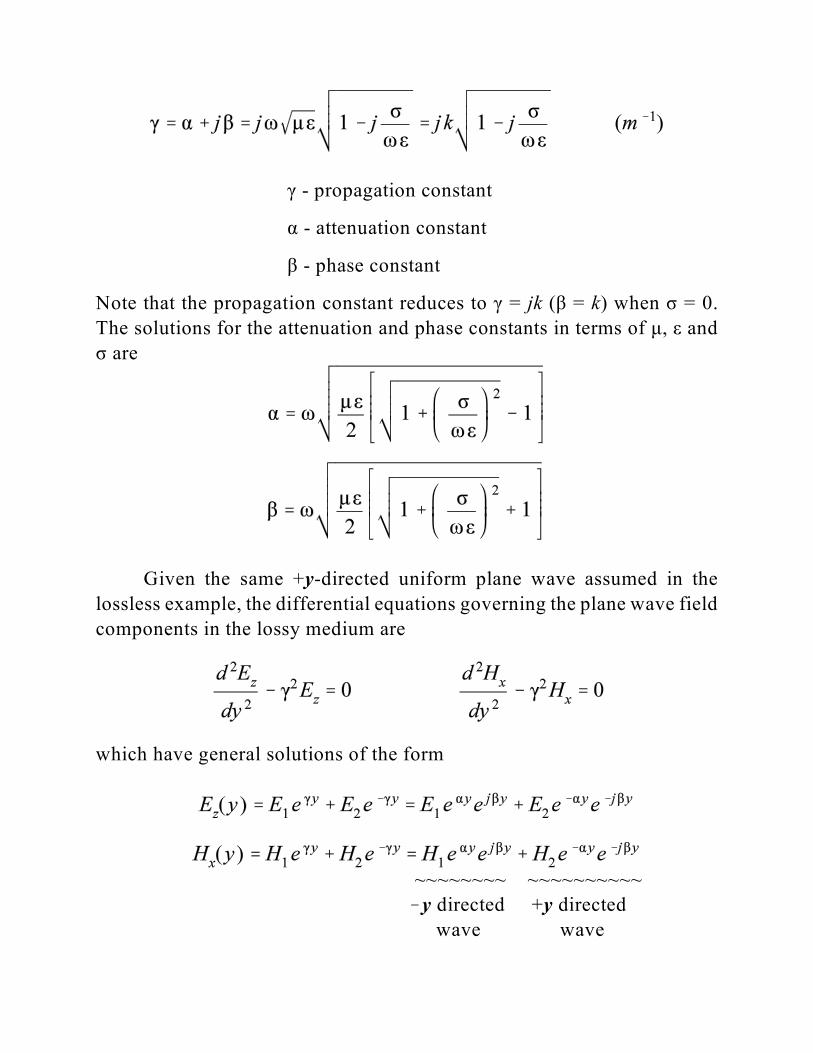
ã - propagation constant

á - attenuation constant

â - phase constant

Note that the propagation constant reduces to ã = jk (â = k) when ó = 0.

The solutions for the attenuation and phase constants in terms of ì, å and

ó are

Given the same +y-directed uniform plane wave assumed in the

lossless example, the differential equations governing the plane wave field

components in the lossy medium are

which have general solutions of the form

~~~~~~~~ ~~~~~~~~~~

!y directed +y directed

wave wave

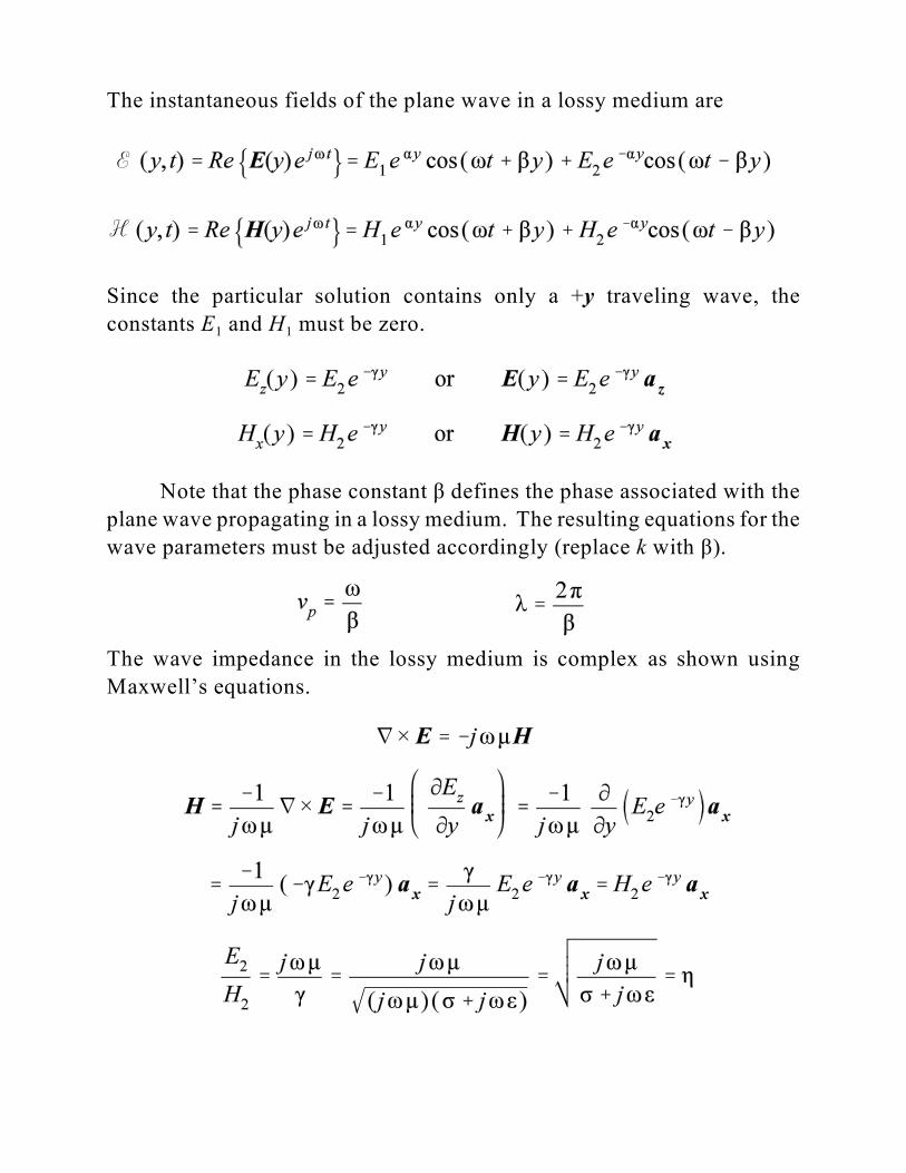
The instantaneous fields of the plane wave in a lossy medium are

Since the particular solution contains only a +y traveling wave, the

1 1constants E and H must be zero.

Note that the phase constant â defines the phase associated with the

plane wave propagating in a lossy medium. The resulting equations for the

wave parameters must be adjusted accordingly (replace k with â).

The wave impedance in the lossy medium is complex as shown using

Maxwell’s equations.

E

H

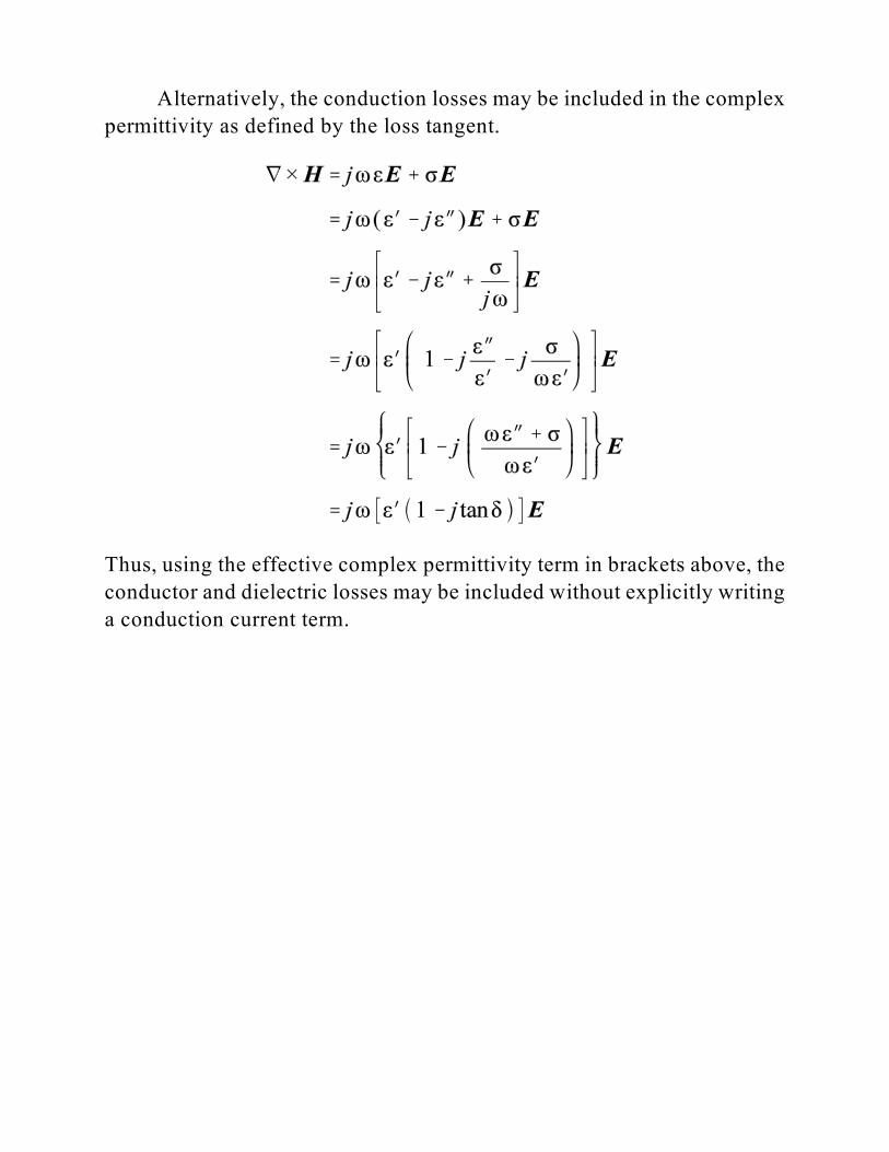
Alternatively, the conduction losses may be included in the complex

permittivity as defined by the loss tangent.

Thus, using the effective complex permittivity term in brackets above, the

conductor and dielectric losses may be included without explicitly writing

a conduction current term.

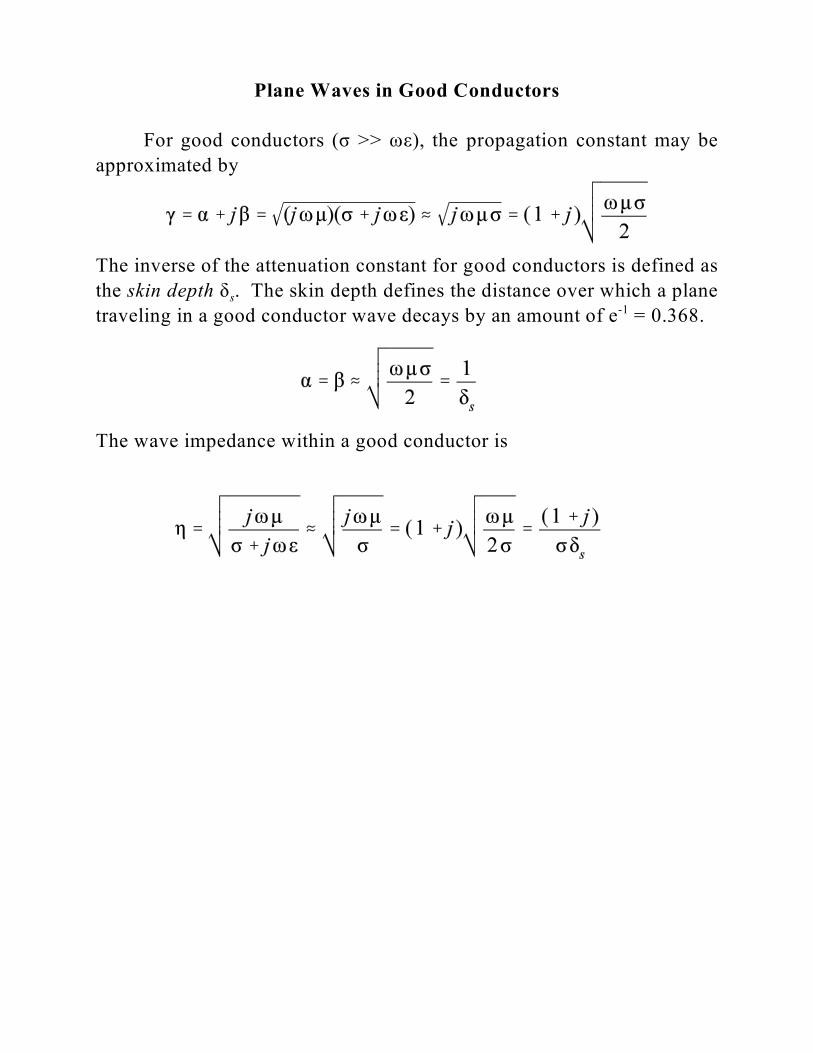
Plane Waves in Good Conductors

For good conductors (ó >> ùå), the propagation constant may be

approximated by

The inverse of the attenuation constant for good conductors is defined as

sthe skin depth ä . The skin depth defines the distance over which a plane

traveling in a good conductor wave decays by an amount of e = 0.368.-1

The wave impedance within a good conductor is

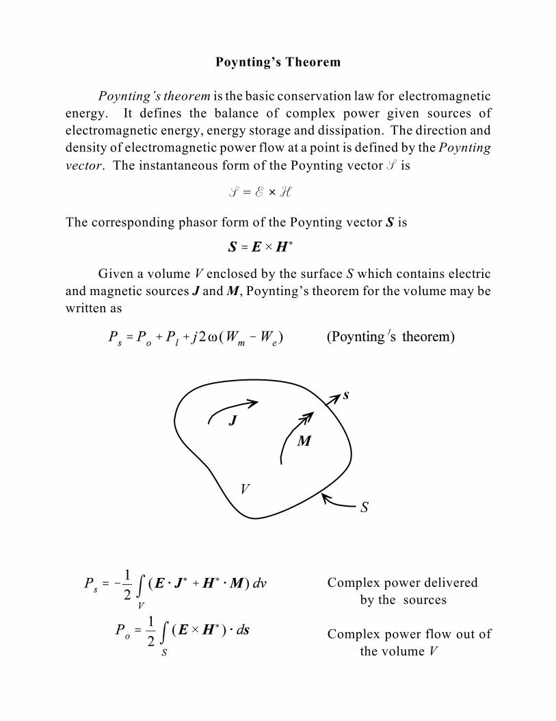
Poynting’s Theorem

Poynting’s theorem is the basic conservation law for electromagnetic

energy. It defines the balance of complex power given sources of

electromagnetic energy, energy storage and dissipation. The direction and

density of electromagnetic power flow at a point is defined by the Poynting

vector. The instantaneous form of the Poynting vector S is

S = E × H

The corresponding phasor form of the Poynting vector S is

Given a volume V enclosed by the surface S which contains electric

and magnetic sources J and M, Poynting’s theorem for the volume may be

written as

Complex power delivered

by the sources

Complex power flow out of

the volume V

~~~~~~~~~ ~~~~~~~~ ~~~~~~~

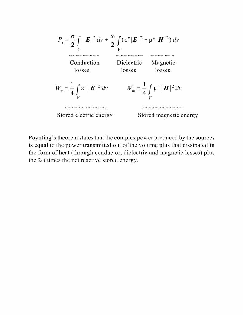
Conduction Dielectric Magnetic

losses losses losses

~~~~~~~~~~~~ ~~~~~~~~~~~~

Stored electric energy Stored magnetic energy

Poynting’s theorem states that the complex power produced by the sources

is equal to the power transmitted out of the volume plus that dissipated in

the form of heat (through conductor, dielectric and magnetic losses) plus

the 2ù times the net reactive stored energy.

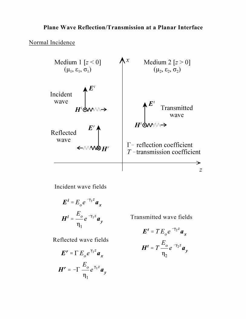
Plane Wave Reflection/Transmission at a Planar Interface

Normal Incidence

Incident wave fields

Transmitted wave fields

Reflected wave fields

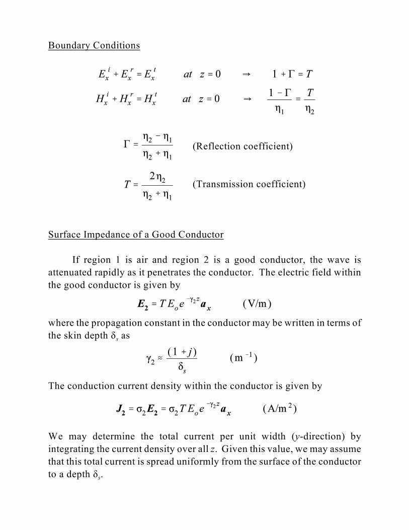
Boundary Conditions

(Reflection coefficient)

(Transmission coefficient)

Surface Impedance of a Good Conductor

If region 1 is air and region 2 is a good conductor, the wave is

attenuated rapidly as it penetrates the conductor. The electric field within

the good conductor is given by

where the propagation constant in the conductor may be written in terms of

sthe skin depth ä as

The conduction current density within the conductor is given by

We may determine the total current per unit width (y-direction) by

integrating the current density over all z. Given this value, we may assume

that this total current is spread uniformly from the surface of the conductor

sto a depth ä .

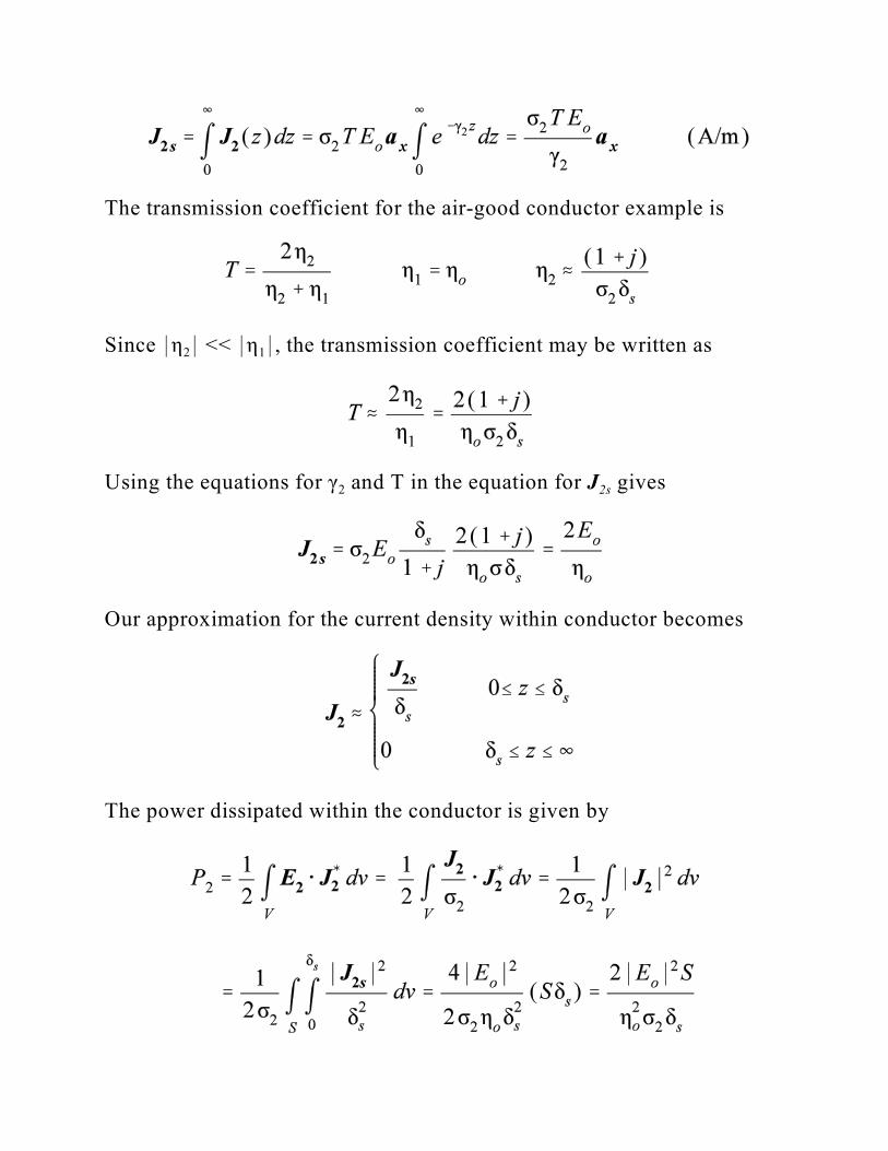
The transmission coefficient for the air-good conductor example is

2 1Since *ç * << *ç *, the transmission coefficient may be written as

2s2Using the equations for ã and T in the equation for J gives

Our approximation for the current density within conductor becomes

The power dissipated within the conductor is given by

We may express the dissipated power as

swhere R is defined as the surface resistance of the conductor and is given

by

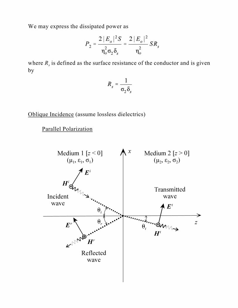
Oblique Incidence (assume lossless dielectrics)

Parallel Polarization

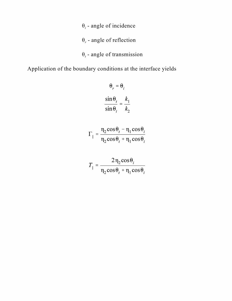
iè - angle of incidence

rè - angle of reflection

tè - angle of transmission

Application of the boundary conditions at the interface yields

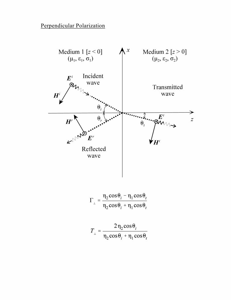
Perpendicular Polarization

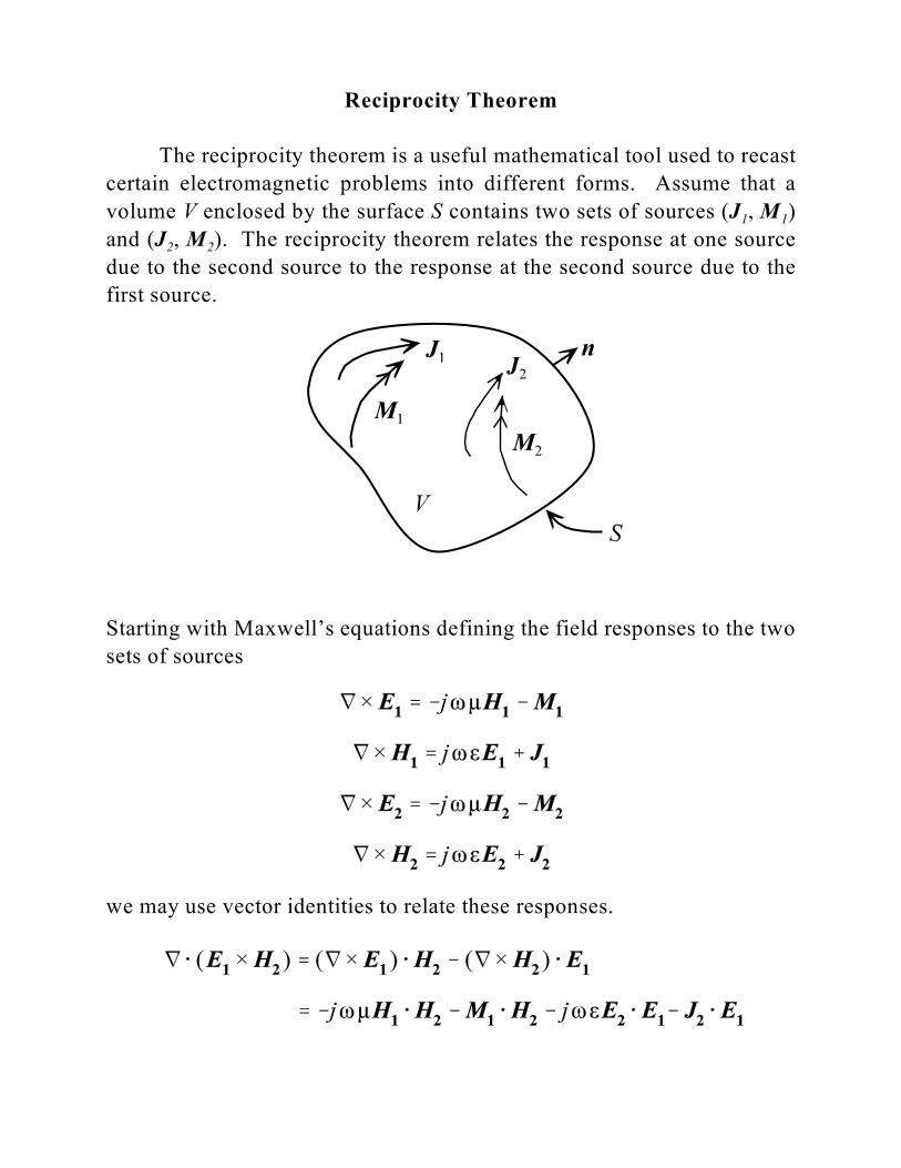
Reciprocity Theorem

The reciprocity theorem is a useful mathematical tool used to recast

certain electromagnetic problems into different forms. Assume that a

1 1volume V enclosed by the surface S contains two sets of sources (J , M )

2 2and (J , M ). The reciprocity theorem relates the response at one source

due to the second source to the response at the second source due to the

first source.

Starting with Maxwell’s equations defining the field responses to the two

sets of sources

we may use vector identities to relate these responses.

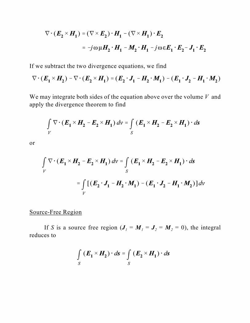
If we subtract the two divergence equations, we find

We may integrate both sides of the equation above over the volume V and

apply the divergence theorem to find

or

Source-Free Region

1 1 2 2If S is a source free region (J = M = J = M = 0), the integral

reduces to

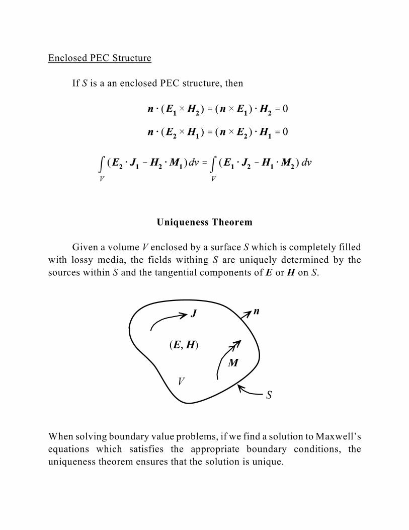
Enclosed PEC Structure

If S is a an enclosed PEC structure, then

Uniqueness Theorem

Given a volume V enclosed by a surface S which is completely filled

with lossy media, the fields withing S are uniquely determined by the

sources within S and the tangential components of E or H on S.

When solving boundary value problems, if we find a solution to Maxwell’s

equations which satisfies the appropriate boundary conditions, the

uniqueness theorem ensures that the solution is unique.

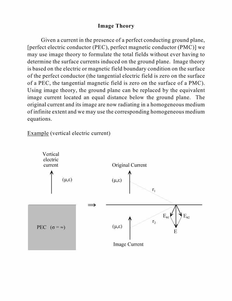
Image Theory

Given a current in the presence of a perfect conducting ground plane,

[perfect electric conductor (PEC), perfect magnetic conductor (PMC)] we

may use image theory to formulate the total fields without ever having to

determine the surface currents induced on the ground plane. Image theory

is based on the electric or magnetic field boundary condition on the surface

of the perfect conductor (the tangential electric field is zero on the surface

of a PEC, the tangential magnetic field is zero on the surface of a PMC).

Using image theory, the ground plane can be replaced by the equivalent

image current located an equal distance below the ground plane. The

original current and its image are now radiating in a homogeneous medium

of infinite extent and we may use the corresponding homogeneous medium

equations.

Example (vertical electric current)

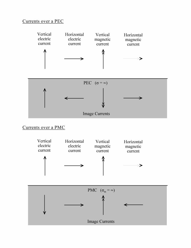
Currents over a PEC

Currents over a PMC