CSC/TM-89/6138 MICROWAVE REMOTE SENSING AND RADAR POLARIZATION SIGNATURES OF NATURAL FIELDS Prepared for NATIONAL AERONAUTICS AND SPACE ADMINISTRATION Goddard Space Flight Center Greenbelt, Maryland By COMPUTER SCIENCES CORPORATION FINAL REPORT Under Contract NAS 5-30116 Task Assignment 5183 NOVEMBER 1989 Prepared by: T. Mo Date Task Leader Approved by: / / / S. Y. Liu Date Manager, Systems and Engineering Operations https://ntrs.nasa.gov/search.jsp?R=19920003099 2018-06-10T12:07:50+00:00Z

Welcome message from author
This document is posted to help you gain knowledge. Please leave a comment to let me know what you think about it! Share it to your friends and learn new things together.
Transcript

CSC/TM-89/6138
MICROWAVE REMOTE SENSING ANDRADAR POLARIZATION SIGNATURES
OF NATURAL FIELDS
Prepared forNATIONAL AERONAUTICS AND SPACE ADMINISTRATION
Goddard Space Flight CenterGreenbelt, Maryland
By
COMPUTER SCIENCES CORPORATION
FINAL REPORT
Under
Contract NAS 5-30116Task Assignment 5183
NOVEMBER 1989
Prepared by:
T. Mo Date
Task Leader
Approved by:/
/ /
S. Y. Liu Date
Manager, Systems and
Engineering Operations
https://ntrs.nasa.gov/search.jsp?R=19920003099 2018-06-10T12:07:50+00:00Z


ACKNOWLEDGMENTS
The author is indebted to Dr. James R. Wang of the Goddard Space
Flight Center for his direction and support during the course of this study.
Also acknowledged are the efforts of Mr. Chester Tai who contributed to
the production of the graphic plots, and to the preparation of the manu-
scripts.
'w
iii
PRECEDING PAGE BLANK NOT FILMED


ABSTRACT
This report describes the theoretical models developed for simulation of
microwave remote sensing of the Earth surface from airborne/spaceborne
sensors. Theoretical model calculations were performed and the results
were compared with data of field measurements. Data studied include
polarimetric image at the frequencies of P-band (0.45 GHz), L-band
(GHz) and C-band (5 GHz), acquired with airborne polarimeters over a
test site of agricultural field. Radar polarization signatures from bare soil
surfaces and from tree-covered fields were obtained fl-om the data. The
models developed in this report include: (l) Small perturbation model of
wave scatterings from randomly rough surfaces, (2) Physical optics model,
(3) Geometrical optics model, and (4) Electromagnetic wave scattering
from dielectric cylinders of finite lengths, which replace the trees and
branches in the modeling of tree-covered field. In addition, a three-layer
emissivity model for passive remote of vegetation-covered soil surface is
also developed. The effects of surface roughness, soil moisture contents
and tree parameters on the polarization signatures were investigated.
For bare soil surfaces, it was found that the effects of surface roughness
parameters on the polarization signatures are negligibly small. This is
primarily due to the normalization process which eliminates the common
factor introduced by variation of surface roughness parameters. On the
other hand, soil moisture has significant effect on the polarization signa-
tures obtained from the small perturbation and physical optics models.
Calculations from both the small perturbation and physical optics models
show strong dependence on the radar look angle 0. However, calculated
v

results at fixed angle 0 are insensitive to frequency variation. Comparison
of the calculated and observed polarizations signatures shows good agree-
ment, especially for the results at P-band frequency.
For tree-covered fields, the theoretical models were developed for simulat-
ing the data of both polarization signature and polarization phase differ-
ence. The radius and direction of tree branches are considered as random
variables and are allowed to vary in the model. Scattering mechanisms
included in the model are: (1) Specular reflection from vertical branches
and tree trunk, followed by another Fresnel reflection from the ground
surface, (2) Backscattering from non-vertical branches, and (3) Propa-
gation through the canopy, as represented by the forward scattering ma-
trix. The simulated results for both polarization signatures and phase
differences are found to be in good agreement with the observations within
experimental uncertainty.
The results presented in this report are useful for polarimetric investigation
of the interaction between the vegetation canopy and the underlying scat-
tering surface which is ubiquitously involved in the scattering process.
.d
_4
vi
TABLE OF CONTENTSSECTION I - INTRODUCTION ........................... 1-1
SECTION 2 - SCATYERLNG MATRIX AND STOKES MATRIX ............ 2-I
SECTION 3 - DESCRIPTION OF DATA .............................. 3-1
SECTION 4- RADAR POLARIZATION SIGNATURES OF ROUGH SURFACES 4-14.1 OBSERVATIONS ............................................. 4-24.2 TIlE MODELS ............................................... 4-4
4.2.1 SMALL PERTURBATION MODEL ........................... 4-54.2.2 PItYSICAL OPTICS MODEL ................................ 4-74.2.3 GEOMETRICAL OPTICS MODEL ........................... 4-10
4.3 RESULTS .................................................. 4-11
SECTION 5 - SCATTERING MATRIX OF A CYLINDER AND POLARIZATIONSIGNATURES OF TREE-COVERED FIELDS ......................... 5-1
SECTION 6 - POLARIZATION PHASE DIFFERENCE ................... 6-1
SECTION 7 - THREE-LAYER EMISSIVITY MODEL .................... 7-i
SECTION 8 - SUMMARY AND DISCUSSION ......................... 8-1
REFERENCES ................................................. R-1
APPENDIX A - STOKES MATRIX ................................. A-IScattering Matrix from a Non-vertical Branch ........................... A-2
APPENDIX B - MULTIVIEW USER'S GUIDE ......................... B-1
vii


Figure
Figure
Figure
Figure
FigureFigure
Figure
Figure
Figure
Figure
Figure
Figure
Figure
Figure
Figure
Figure
Figure
Figure
Figure
Figure
Figure
List of Illustrations
2-1. Polarization-ellipse geometry for representation of
polarization states ............................ 2-6
2-2. Polarization signatures of three simple scattering mod-els ........................................ 2-7
3-1. Comparison of calibrated and un-calibrated
polarization signatures ......................... 3-5
4-1. Observed polarization signatures at 0 = 25 ° ...... 4-17
4-2. Observed polarization signatures at 0 = 37 ° . ..... 4-18
4-3. Observed polarization signatures at 0 = 54 ° . ..... 4-19
4-4. Small perturbation model calculations, bare field,
0 = 25 °, and SM = O.lgrn/cm 3 .................. 4-20
4-5. Small perturbation model calculations, bare field,0 = 37 °, and SM = O.lgm/cm 3 .................. 4-21
4-6. Small perturbation model calculations, bare field,0 = 54 °, and SM = O.lgrn/crn 3 .................. 4-22
4-7. Small perturbation model calculations, bare field,
0 = 25 °, and SM = 0.3gm/cm 3 .................. 4-23
4-8. Small perturbation model calculations, bare field,
0 = 37 °, and SM = 0.3gm/crn 3 .................. 4-24
4-9. Small perturbation model calculations, bare field,0 = 54 °, and SM = 0.3firn/cm 3 .................. 4-25
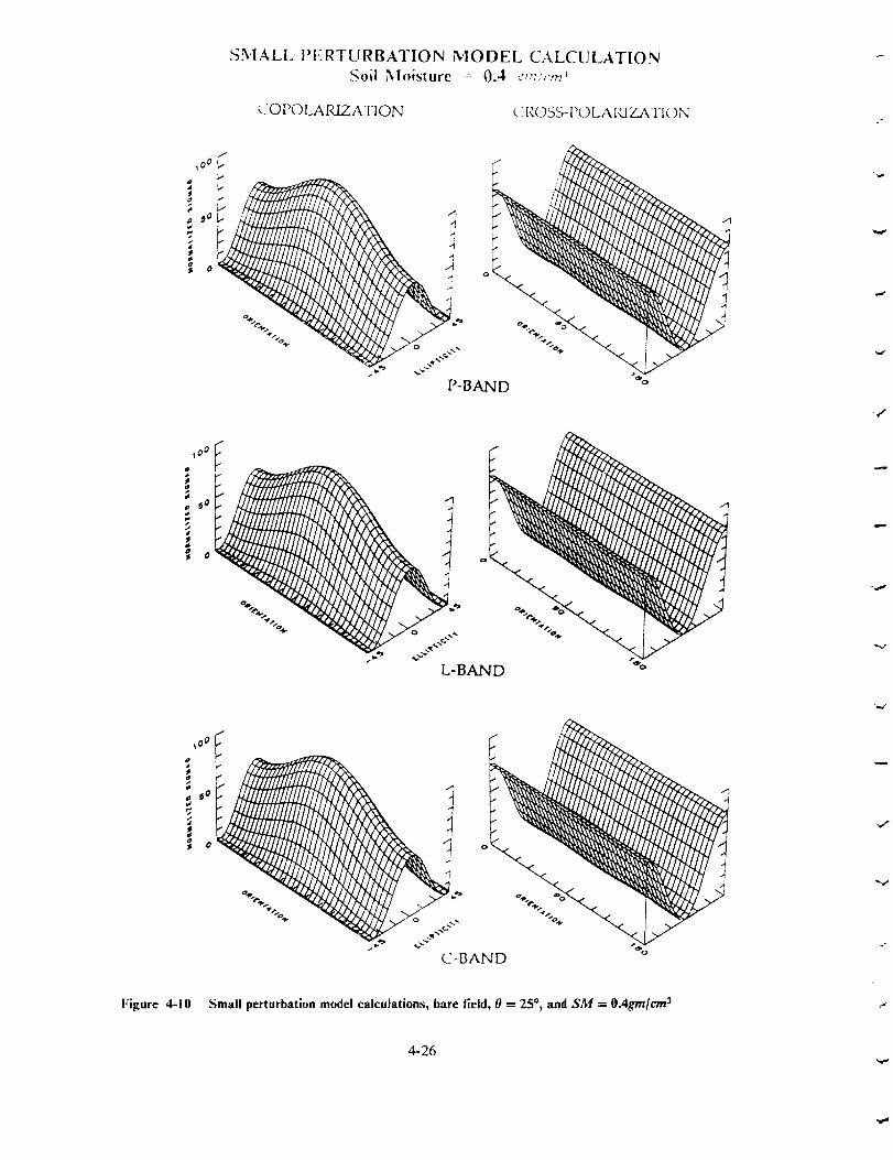
4-10. Small perturbation model calculations, bare field,
0 = 25 °, and SM = 0.4grn/crn 3 .................. 4-26
4-11. Small perturbation model calculations, bare field,
0 = 37 °, and SM = 0.4grn/cm 3 .................. 4-27
4-12. Small perturbation model calculations, bare field,0 = 54 °, and SM = 0.4grn]cm 3 .................. 4-28
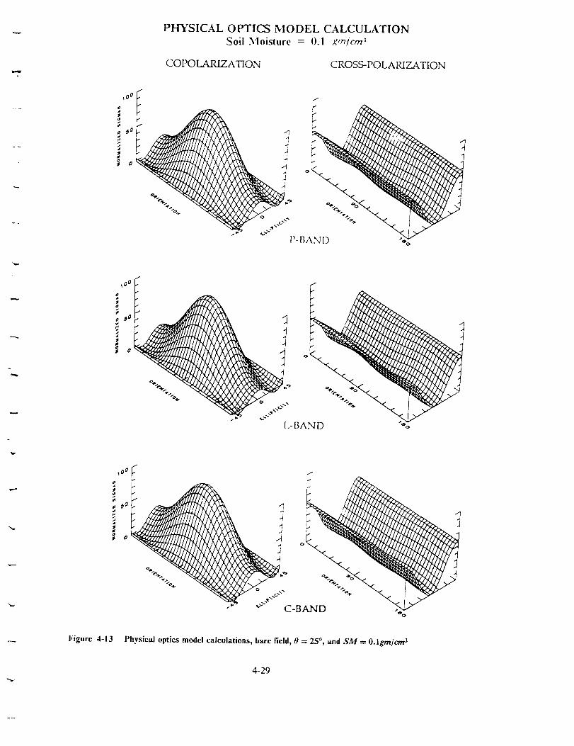
4-13. Physical optics model calculations, bare field,
0 = 25 °, and SM = 0. lgrn/crn 3 .................. 4-29
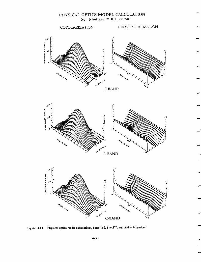
4-14. Physical optics model calculations, bare field,
0 = 37 °, and SM = O.lgrn/crn 3 .................. 4-30
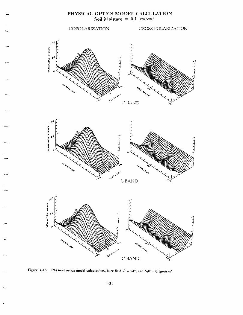
4-15. Physical optics model calculations, bare field,0 = 54 °, and SM = O.lgm/cm 3 .................. 4-31
4-16. Physical optics model calculations, bare field,
0 -- 25 °, and SM = 0.3gm/cm 3 .................. 4-32
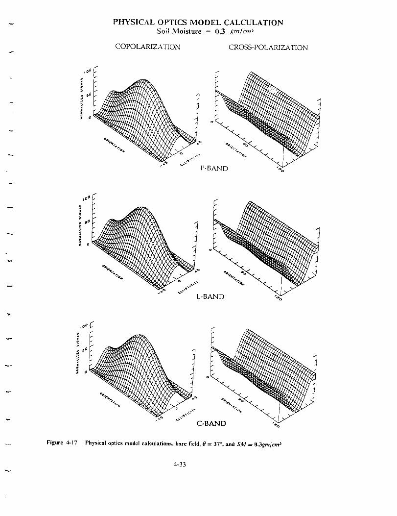
4-17. Physical optics model calculations, bare field,0 = 37 °, and SM = 0.3grn/cm 3 .................. 4-33
4-18. Physical optics model calculations, bare field,
0 = 54 °, and SM = 0.3gm/cm 3 .................. 4-34
ix
PRECEDING PAGE BLA_"_}( NOT F;LMED

Figure 4-19. Physical optics model calculations, bare field,0 = 25 °, and SM = 0.4gm/crn 3 .................. 4-35
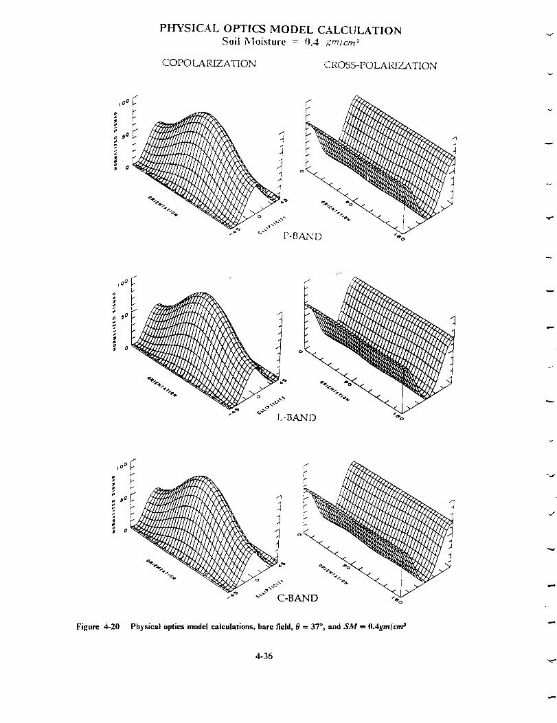
Figure 4-20. Physical optics model calculations, bare field,0 = 37 °, and SM = 0.4grn/crn 3 .................. 4-36
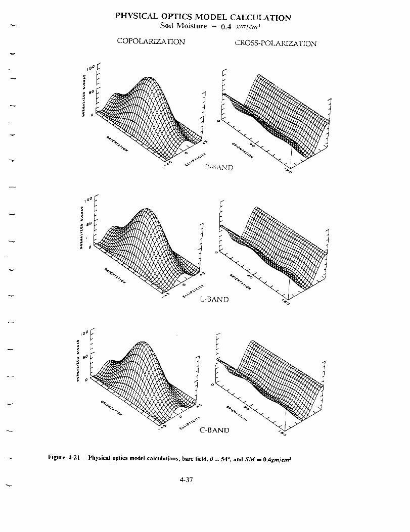
Figure 4-21. Physical optics model calculations, bare field,0 = 54 °, and SM = 0.4grn/crn 3 .................. 4-37
Figure 5-1. Sketch of tree scattering geometry ............... 5-8
Figure 5-2. Comparison of observed and simulated polarization
signatures from an orchard tree-covered field at
0 = 25°:(a) Observations, and (b) Simulations ........ 5-9
Figure 5-3. Comparison of observed and simulated polarization
signatures from an orchard tree-covered field at0 = 43°:(a) Observations, and (b) Simulations ....... 5-10
Figure 6-1. Image created from the data of SAR polarization phasedifferences acquired over an agricultural area near
Fresno, California ............................ 6-6
Figure 6-2. PPD distribution from a bare field near 0 -- 15 ° ..... 6-7
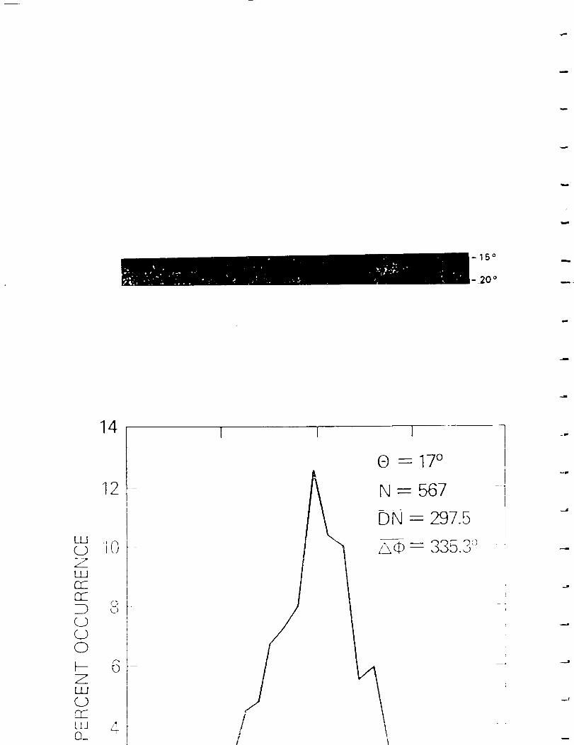
Figure 6-3. PPD distribution from a tree-covered field at 0 - 17 °. 6-8
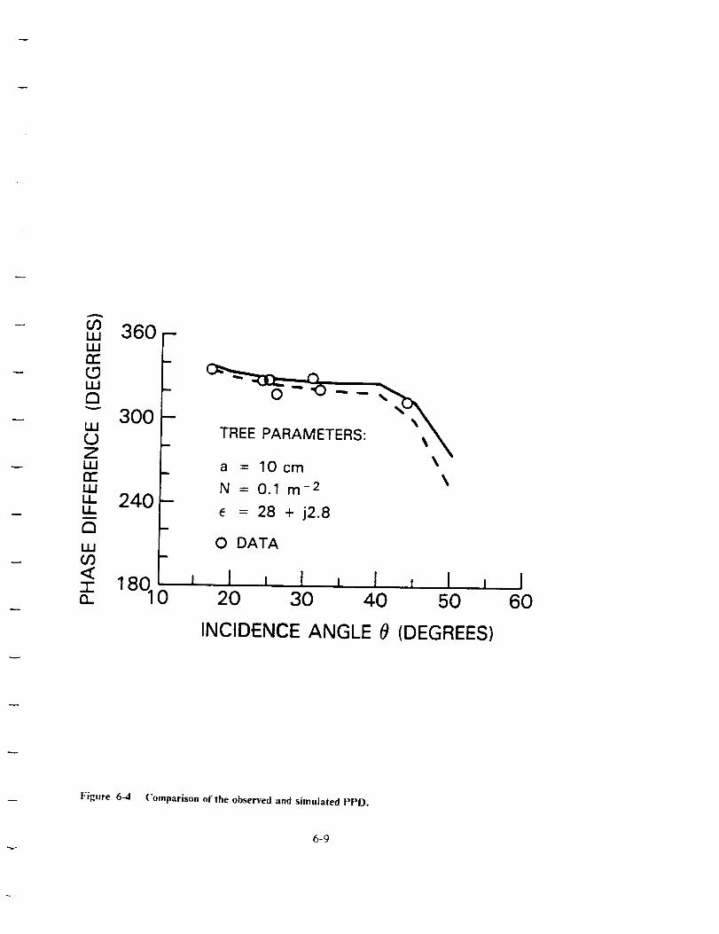
Figure 6-4. Comparison of the observed and simulated PPD .... 6-9
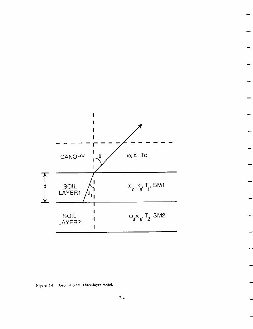
Figure 7-1. Geometry for Three-layer model ................ 7-4
Figure 7-2. Calculated results from the three-layer model ....... 7-5
Figure A-1. Scattering geometry and coordinate systems used inthe backscatterings of waves by non-vertical branches. A-6
SECTION 1 - INTRODUCTION
Remote sensing techniques using microwave sensors have been developed
for many applications (References 1 through 5) in recent years. Recent
research emphasis has been placed on measuring soil moisture and vege-
tation covers (References 6 through 12) on the Earth's surface for global
monitoring of renewable resources using spaceborne/airborne sensor sys-
tems. These are also considerable interests in using microwave sensors for
geological exploration (Reference 13) and subsurface geoarcheological
studies (References 14 and 15). Spaceborne sensors are able to provide
high-resolution imagery of even the most remote parts of the world, and
can produce large quantity of information. Furthermore, microwave
signals can penetrate clouds which render visible sensors useless and se-
verely degrade the performance of infrared sensors. Also microwave sen-
sors can be operated either day or night, under clear-sky or cloudy
conditions. For these reasons, microwave remote sensing systems are cur-
rently being adopted for various practical applications.
Remote sensing is generally classified into two classes: passive and active.
For active remote sensing, a sensor (e.g., a radar) sends out a beam of
electromagnetic waves and in the same time receives (or detects) the
1-I
backscattered waves. For passive remote sensing, the electromagnetic
power intensity emitted by a medium, such as a layer of soil, is measured
by a microwave sensor (e.g., a radiometer).
Development of theoretical models is essential in understanding how the
physical parameters of the scattering medium can affect the measure-
ments, and in interpreting the remote sensing data. Recently, theoretical
model developments contribute greatly to the understanding of the phys-
ical processes involved in the wave scatterings by vegetation and randomly
rough surfaces (References 10 through 12, and 16).
Recent approach (References 17 through 21) to experimental and theore-
tical work, developed primarily for airborne radar remote sensing, uses the
imaging radar polarimeters, to measure both the magnitude and relative
polarization phases of the backscattered waves. Using these measured
wave magnitude and polarization phase information, one can construct the
polarization signatures of the scattering targets. A polarization signature
displays the radar scattering cross sections in all possible combinations of
polarization states for both the transmit and receive waves, and it provides
a convenient way for visualization of the dominant scattering features of
scatterers. Recent studies (References 13, 18 and 20) have demonstrated
that it is a potentially useful technique for studying the characteristics of
the geological surfaces and vegetation covers. From an experimentalist's
viewpoint, it would be desirable to have a simple model for parametric
description of the scattering media with a minimum number of parameters
1-2
necessary to interpret the observed polarization signatures
polarization phasedifferences (PPD) from various scattering targets.
and
This report presents some model developments for simulation of the
measured polarization signaturesobtained from randomly rough surfaces
and tree-coveredfields. The modelsare basedon the electromagneticwave
scatterings from randomly rough surface and dielectric cylinders of finite
lengths and various magnitudes of radius, similar to the tree trunks and
branches. The scattering matrix, which relates the incident electric fields
to the scattered ones,was firstly obtained from thesemodel calculations,
and then its corresponding Stokes matrix was constructed from the ele-
ments of the scattering matrix. Polarization signatures were then calcu-
lated and displayed in three-dimensional (3-D) plots which are compared
with the observations.
The data used in this report were taken with the NASA/JPL airborne im-
aging radar polarimeter, operating at the P-band, L-band, and C-band
frequencies. The flight was over an agricultural area near Raisin City,
California. The region under the flight passeshad a variety of crops, in-
cluding cotton, lettuce, bare field, and orchard tree-coveredfield. Differ-
ent crops fields produce different polarization signatures and phase
difference between the hh- and vv-polarizations. Our primary interests in
this report are the polarization signatures. Polarization phase differences
over the tree-covered areas and the bare field are also presented. In addi-
1-3

tion, a three-layer emissivity model for
vegetation-coveredfields is also developed.
passive remote sensing of
Section 2 gives a brief description of the scattering and Stokes matrix, re-
lating to polarization signatures. The data used in tl-_isreport aredescribed
in Section 3. The results of radar polarization signatures of randomly
rough surfaces are described in Section 4, which presents both observa-
tions and calculations. Comparison of the two rcsJlts are also discussed.
Section 5 describes the modelling of wave scattering from dielectric cylin-
ders and polarization signatures from tree-covered fields, while
polarization phase differences is given in Section 6 Section 7 presentsa
model for passiveremote sensingof vegetation-covered fields. It consist of
one vegetation layer and two soil layers, which allow different soil moisture
contents in the calculation. A summary and discussion are given in Section
8. Appendix A gives the formulas related to Stokes vectors and Stokes
matrix. A user's guide to the Multiview software pockage,which processes
the polarimetric image data, is presented in Appendix B.
1-4

SECTION 2 - SCATTERING MATRIX ANDSTOKES MATRIX
For study of polarization signature, both the incident and the scattered
electromagnetic fields are commonly represented by a polarization ellipse
(Figure 2-1), which is specified by two angles, the orientation angle _b, and
the ellipticity angle Z, respectively. The backscattering cross sections can
be directly expressed in term of the Stokes matrix and these two angles of
orientation and ellipticity for both the transmit and receive waves (Refer-
ences 17 and 21).
When a plane radar wave is scattered by a target, its polarized components
of the scattered electric field E • at the far-zone region can be related to the
incident fields E i by a 2x2 complex scattering matrix [S]
[1 I1_ e'_"[ sj r slE j
(2-1)
with
S (2-2)
2-I

where r is the distance between the scatterer and the receiving antenna, k
is the wave number in free space, and the Srt (where the subscripts r, t =
h or v) is the scattering matrix element corresponding to a transmit wave
with polarization t and receive wave with polarization r, respectively. If the
scattering matrix [S] of a target is known, one can construct a 4x4 Mueller
matrix [M], which relates the scattered Stokes vector F" to the incident
Stokes vector F _ in the form (References 17 and 21)
r 2
where R denotes the transpose of R, and the matrices F", M, R, and F" are
defined in Appendix A.
The bistatic scattering cross section for any combination of transmit and
receive polarizations is given (References 21)
[o,,,¢,,,x,, z,) = M Y' (2 --4)
where (_bt, Xt) and (0r, Zr) are the orientation and ellipticity angles of the
transmit and receive polarizations, respectively. The yt and yr are the
normalized Stokes vectors for the transmit and receive waves, and are de-
fined by
2-2
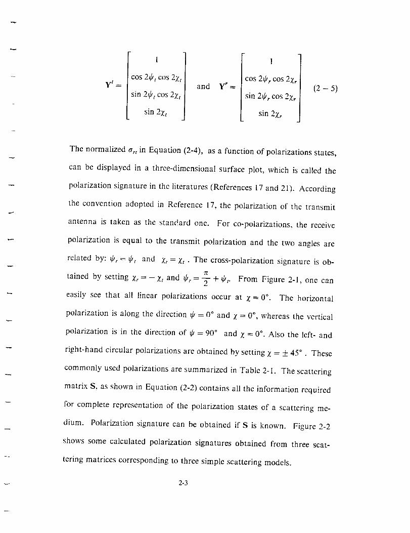
yt
1
cos 2_t cos 2Zt
sin 2_bt cos 2Zt
sin 2Zt
and yr =
1
cos 2fir cos 2:_,
sin 2fir cos 2Zr
sin 2Zr
The normalized O'rt in Equation (2-4), as a function of polarizations states,
can be displayed in a three-dimensional surface plot, which is called the
polarization signature in the literatures (References 17 and 21). According
the convention adopted in Reference 17, the polarization of the transmit
antenna is taken as the standard one. For co-polarizations, the receive
polarization is equal to the transmit polarization and the two angles are
related by: _br = Ct and Zr = Zt • The cross-polarization signature is ob-
n
tained by setting ;_ =- Xt and _'r =-_" + _'t- From Figure 2-1, one can
easily see that all linear polarizations occur at g = 0°. The horizontal
polarization is along the direction _b = O° and X = 0°, whereas the vertical
polarization is in the direction of t_ = 90 ° and X = 0°. Also the left- and
right-hand circular polarizations are obtained by setting _ = + 45 ° . These
commonly used polarizations are summarized in Table 2-I. The scattering
matrix S, as shown in Equation (2-2) contains all thc information required
for complete representation of the polarization states of a scattering me-
dium. Polarization signature can be obtained if S is known. Figure 2-2
shows some calculated polarization signatures obtained from three scat-
tering matrices corresponding to three simple scattering models.
2-3
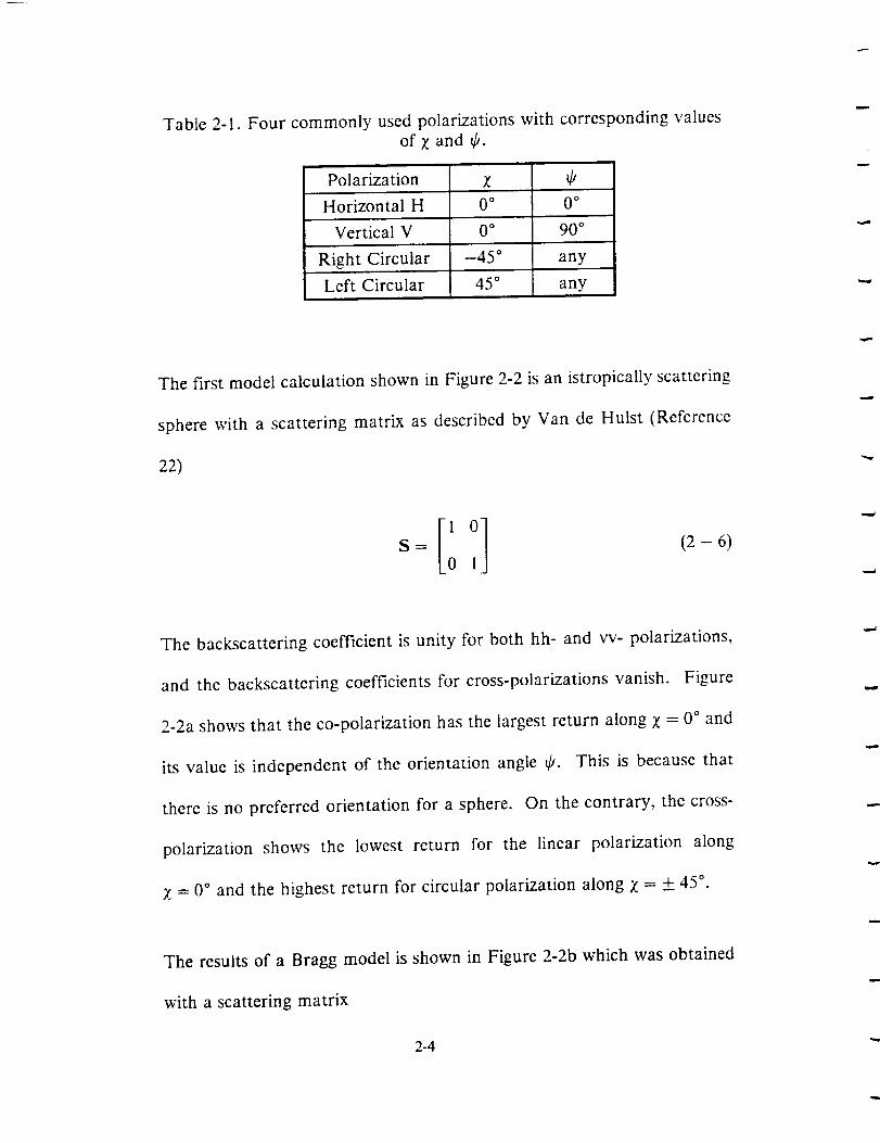
Table 2-1. Four commonly used polarizations with corresponding valuesof X and _b.
Polarization Z
Horizontal H 0 ° 0 °
Vertical V 0 ° 90 °
Right Circular -45 ° any
Left Circular 45 ° any
The first model calculation shown in Figure 2-2 is an istropically scattering
sphere with a scattering matrix as described by Van de Hulst (Reference
22)
The backscattering coefficient is unity for both hh- and vv- polarizations,
and the backscattering coefficients for cross-polarizations vanish. Figure
2-2a shows that the co-polarization has the largest return along Z = 0° and
its value is independent of the orientation angle _. This is because that
there is no preferred orientation for a sphere. On the contrary, the cross-
polarization shows the lowest return for the linear polarization along
Z = 0° and the highest return for circular polarization along Z = --+45°.
The results of a Bragg model is shown in Figure 2-2b which was obtained
with a scattering matrix
2-4

S = (2- 7)1.5
In this matrix, we have Shh < S_, therefore the ,,w-polarization in the
co-polarization is larger than the hh-polarization. According to Reference
18, the scattering from sea water can be accounted for by the Bragg model.
It will be shown in Section 3 that observed polarization signatures from
some smooth and moderately rough soil surfaces are also similar to this
Bragg model results.
Figure 2-2c shows the results which represent a dielectric dihedral corner
reflector model. The scattering matrix for this model is of the form
S= (2-8)
It requires that the matrix elements Shh and S_, differ in sign and that
I s_h[ > [S_v[. For example, the Fresnel reflection coefficients from a
smooth surface usually have such characteristics. Figure 2-2c shows that
two minima in the co-polarization and two maxima in the cross-
polarization occur at _ = 45 ° and 135 °, respectively.
It should be noted that simple models can provide results which are con-
sistent with observed polarization signatures, although one can not role out
possibilities of other scattering models.
2-5

V
h
Figure 2-1 Polarization-ellipse geometry for representation of polarization states.
2-6

ISOTROPIC SPHERE
00 I
_*'*_'_° I
o o
_¢',fe>
j
BRAGG
_°°_
"_">o.,.. o _.... ÷<"•
"" "_'o
DIHEDRAL CORNER REFLECTOR
Figure 2-2 Polarization signatures of three simple scattering models.
2-7


SECTION 3- DESCRIPTION OF DATA
This section, gives a brief description of the data used in this report. De-
tailed descriptions of the imaging data processing, using the Multiview
software package are presented in Appendix B.
The polarimetric data described here were acquired with the NASA/JPL
airborne imaging radar polarimeter operating at the frequencies of 0.45
GHz (P-band), 1.225 GHz (L-band), and 5 GHz (C-band) respectively.
Our data were acquired in two flights over a test site of agricultural fields
near Raisin City, California. The first flight of data collection was taken
on September 28, 1984 and only L-band imaging data were collected. The
areas covered during the flight included bare field, tree-covered region and
other vegetation-covered fields (References 1 and 23). The second flight
was conducted on May 23, 1988 and the polarimetric imaging data for all
three bands were acquired simultaneously over the same region which in-
cluded bare and vegetation-covered fields.
An imaging radar polarimeter measures the amplitude and phase of all
elements of the scattering matrix corresponding to each individual pixel in
a radar image. Subsequent data processing can synthesize any desired
combination of transmit and receive antenna polarization by combining
3-1

these scattering matrix elements. In the data processing, the data were
compressed for efficient storage on tape. Compression of multipolarized
data is based on the validity of reciprocity principle, i.e., the data collected
in horizontal-transmit vertical-receive (hv) mode are assumed idcntical to
the data collected in vertical-transmit horizontal-receive (vh) mode.
However, in practice the data do not reflect the above condition due to
system imperfections and ambient noise, therefore phase calibration of the
cross-polarized data is needed before data compression is performed. Ini-
tial calibration of the cross-polarized data was performed at JPL so that
the average phase difference between hv data and vh data is zero. In ad-
dition, phase calibration based on the phase difference of co-polarized data
(between hh and ,,w) is also required in order to remove errors introduced
by system imperfections. However, this step may be done after data
compression since the compression algorithm does not depend on the ac-
curacy of the phase difference between co-polarized data. The data dis-
tributed by JPL do not include this co-polarization phase calibration. The
users must perform this calibration by themselves. Typically, one chooses
to calibrate the entire image based on measurements of a small area of the
image where the phase information is known in terms of theoretical model
(Reference 24).
The JPL compressed multipolarization data are phase calibrated in cross-
polarization but not in co-polarization. A re-calibration program is in-
cluded in the Multiview software package (Reference 25) for
3-2

co-polarization phase calibration. The program asksthe user to choosea
small area of the data image. The co-polarization phase difference is cal-
culated for all pixels within the chosen area and then the mean is com-
puted. The co-polarization phases for the entire data image are then
re-calibrated based on setting this mean to zero. Here are some sug-
gestions for choosing the area to be used in the RECAL program (Refer-
ence25). The area should be large enough to assure a good statistical set
of input data for computing the phase difference between co-polarized
signals. Scattering models (Reference 12) predict that the co-polarization
phase difference for dry and slightly rough surfaces should be zero.
Therefore, one should choose a homogeneous area that is only slightly
rough. However, the area chosenshould not be too smooth becausethe
backscattering coefficients of smooth areas are susceptible to noise in the
system. Instead, this area should be of some uniformly small roughness
where the measured backscattering coefficient is bigger than that of the
system noise.
The polarimetric data distributed by JPL are in the l0 mega byte com-
pressedformat (Reference25). The Multiview software package,which is
an interactive menu-basedprogram, was used to processthesedata and to
synthesize images using various transmit and receive polarization combi-
nations for creating polarization signatures.
The importance of co-polarization phase calibration of the polarization
signatures is demonstrated in Figure 3-1 which compares a calibrated
3-3
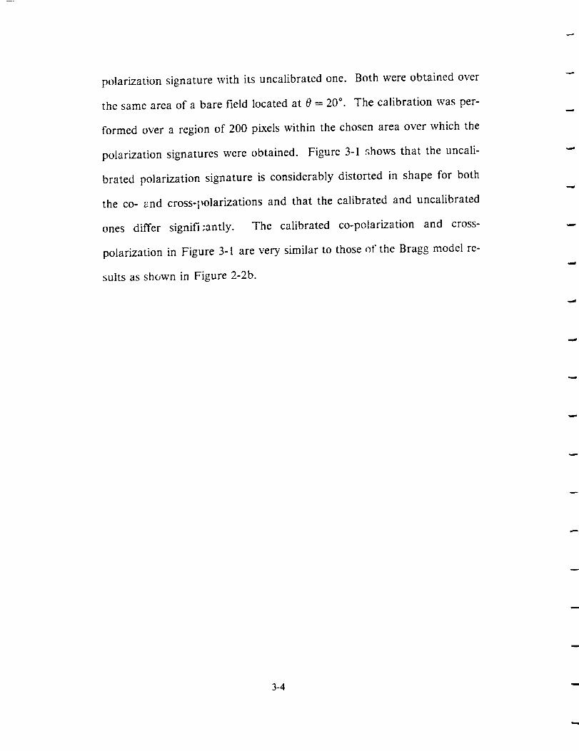
polarization signature with its uncalibrated one. Both were obtained over
the same area of a bare field located at 0 = 20 °. The calibration was per-
formed over a region of 200 pixels within the chosen area over which the
polarization signatures were obtained. Figure 3-1 shows that the uncali-
brated polarization signature is considerably distorted in shape for both
the co- and cross-l_olarizations and that the calibrated and uncalibrated
ones differ signifi:antly. The calibrated co-polarization and cross-
polarization in Figure 3-1 are very similar to those of the Bragg model re-
sults as shown in Figure 2-2b.
3-4

to o
'q pO t
f
t
0
(a) Before Calibration *o
t0 0 f
_ 0 o
"o
(b) After Calibration
Figure 3-1 Comparison of calibrated and un-calibrated polarization signatures.
3-5


SECTION 4- RADAR POLARIZATIONSIGNATURES OF ROUGH SURFACES
In the microwave remote sensing of vegetation-covered fields, there are
underlying rough surfaces involved in the scattering process. Features of
the scattering surface are usually imbedded in the observed polarization
signatures of vegetation-covered fields (References 19 and 20). Individual
effects of surface characteristics, such as surfacc roughness, soil moisture
contents and surface correlation functions on the observed polarization
signatures are not fully understood. Furthermore, interaction between the
vegetation (e.g. trees) and the underlying scattering surface make it more
difficult to determine the surface contribution to the remotely sensed data
of a polarization signature, which is supposedly to provide the prominent
features of the radar beam illuminated areas (References 17 and 18).
Thus, it would be desirable to perform an investigation of the extent the
surface characteristic parameters may affect the polarization signature.
In this section, we present some measured polarization signatures of rough
soil surfaces obtained with the JPL airborne polarimeter. For comparison,
we also performed a series of theoretical model studies of the effect of a
rough surface on the polarization signatures. The models included in the
study are (References 11 and 12): (1)the small perturbation model, (2)the
4-1

physical optics model, and (3) the geometrical optics model. The small
perturbation model is suitable for a smooth surface,while the physical and
geometrical optics models are appropriate for a moderately rough and very
rough surface, respcctively. For a very rough surface, the returned radar
signalsare probably completely unpolarized and the backscattering coeffi-
cients for such a rough surface are independent of polarization (i.e.,
= o?0-
The model calculations of polarization signatures were performed at the
frequencies of P-, L-, and C-bands under various conditions of surface
roughness and soil moisture contents.
4.1 OBSER VA TIONS
The calculated results were also compared with the observed polarization
signatures acquired with the NASA/JPL airborne imaging radar
polarimeter, operating at the P-band, L-band, and C-band frequencies.
The data were taken over an agricultural field near Raisin City, California
on May 23, 1988.
Polarization signatures in 3-dimensional (or 3-D) plots were extracted from
polarimetric image data, which were properly calibrated according to the
method described in Reference 24. A modified version of the JPL
MULTIVIEW software package (Reference 25) was used for processing
4-2
the observed data of polarimetric Stokes matrix, and for obtaining the
observedpolarization signatures.
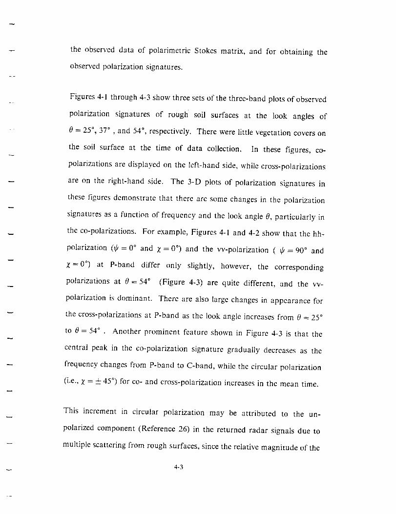
Figures 4-1 through 4-3 show three setsof the three-band plots of observed
polarization signatures of rough
0 = 25 °, 37 ° , and 54 °, respectively.
soil surfaces at the look angles of
There were little vegetation covers on
the soil surface at the time of data collection. In these figures, co-
polarizations are displayed on the left-hand side, while cross-polarizations
are on the right-hand side. The 3-D plots of polarization signatures in
these figures demonstrate that there are some changes in the polarization
signatures as a function of frequency and the look angle 0, particularly in
the co-polarizations. For example, Figures 4-1 and 4-2 show that the hh-
polarization (_9 = 0 ° and g = 0°) and the w-polarization ( _b = 90 ° and
;_=0 °) at P-band differ only slightly, however, the corresponding
polarizations at 0 = 54 ° (Figure 4-3) are quite different, and the w-
polarization is dominant. There are also large changes in appearance for
the cross-polarizations at P-band as the look angle increases from 0 --- 25 °
to 0 = 54 ° . Another prominent feature shown in Figure 4-3 is that the
central peak in the co-polarization signature gradually decreases as the
frequency changes from P-band to C-band, while the circular polarization
(i.e., 1: = -+ 45 °) for co- and cross-polarization increases in the mean time.
This increment in circular polarization may be attributed to the un-
polarized component (Reference 26) in the returned radar signals due to
multiple scattering from rough surfaces, since the relative magnitude of the
4-3
roughness to the incident wave length increases as the latter becomes
shorter.
These observed polarization signatures will be compared with the theore-
tical model calculations described in the followings.
4.2 THE MODELS
In this subsection, a brief description of the theoretical models for scatter-
ing from a randomly rough surface is presented. The surface roughness is
usually characterized by a root-mean-square (rms) surface height, s, which
specifies the vertical scale of the surface roughness, and a surface corre-
lation function p(_), which is a function of the surface correlation lengths
t and L, representing the horizontal scales of the surface roughness (Ref-
erences I1 and 12).
The three models described here are the small perturbation model, the
physical optics model, and the geometrical optics model. These models
have been extensively used for simulation of microwave remote sensing of
rough terrains (References 11 and 12). Formulas for the small perturba-
tion and geometrical optics models are relatively simple and were often
used for quick applications in the microwave remote sensing work for
prediction of backscattering coefficients from rough scattering surfaces.
Formulas related to the physical optics model (References 11 and 12) is
more complicated than those of other two models, but expressions for
4-4

scattering coefficients depending on the correlation function p({) exist in
literatures (Reference 2 I).
For application to polarimetric studies, one must specify the 2x2 scattering
matrix IS], as defined in Equations (2-1) and (2-2), which relates the
polarized components of the incident fields E t at the scatterer to the scat-
tered electric field E" at the far-zone region. Once the scattering matrix
[S] of a target is known, one can construct the 4x4 Stokes or Mueller ma-
trix [M] , which can be used to obtain the bistatic scattering cross section
in connection with the polarimetric studies for any combination of trans-
mit and receive polarizations (Equation 2-4).
In the first-order approximation of backscattering coefficients, the off-
diagonal elements of the scattering matrix IS] vanish (i.e., &v = &h = 0)
for all three scattering models (References 11 and 12). Therefore, there
are only two diagonal matrix elements Shh and Sv_ required to be specified
for the three scattering models, which will be described individually.
4.2.1 SI_IALL PERTURBATION MODEL
For a relatively smooth surface, the first-order small perturbation model
can be used to predict the backscattering coefficients from a randomly
rough surface. The scattering matrix corresponding to the small pertur-
bation model can be written in the form (Reference 21 and 27)
4-5

[ 1Shh 0
S = Uo
0 S.v
(4-1)
where
2k cos O(e - 1)Shh _ --
[cosO+ x/e-sin 20 ]2
sin20 - _(1 + sin20)S_v = 2k cos O(e -l)
[_: cos 0+ _/_- sin20 ]2
U o = k 2 cos20 W(2k sin O)
(4- 2)
where E is the relative dielectric constant of the soil and 0 is the incidence
angle. W(2k sin O) is the power spectrum (References l l and 12) of the
rough surface sampled at the spatial wave number 2k sin O.
For a Gaussian surface with a correlation length g, rms surface height s,
and correlation function p(_) = exp( - _2/_2), the power spectrum is given
by (Reference 11)
W(2k sin O) - _'':_"s-'2exp[ - (k: sin 0) 2]2
(4-3)
In study of polarization signatures, the backscattering coefficient as de-
fined in Equation (2-4) are usually normalized to the maximum value of
the co-polarization signature, therefore a common factor, such as U0, will
be cancelled in the normalization process. In such case, one does not need
4-6
to specify the exact form of the power spectrum W(2k sin 0) in this small
perturbation model.
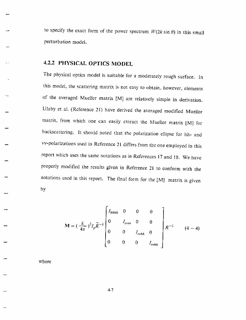
4.2.2 PHYSICAL OPTICS MODEL
The physical optics model is suitable for a moderately rough surface. In
this model, the scattering matrix is not easy to obtain, however, elements
of the averaged Mueller matrix [M] are relatively simple in derivation.
Ulaby et al. (Reference 21) have derived the averaged modified Mueller
matrix, from which one can easily extract the Mueller matrix [M] for
backscattering. It should noted that the polarization ellipse for hh- and
w-polarizations used in Reference 21 differs from the one employed in this
report which uses the same notations as in References 17 and l g. We have
properly modified the results given in Reference 21 to conform with the
notations used in this report. The final form for the [M] matrix is given
by
M = ( -1
lhhhh 0 0 0
0 I,,_ 0 0
0 0 l_h h 0
0 0 0 I_hh
R (4 -4)
where
4-7

R
1 1 0 0
1 -1 0 0
0 0 1 1
0 0 -i i
and
1
0
0
0
0 0 0
1 0 0
0 -1 0
0 0 -1
(4-6)
The four diagonal matrix elements lpqm,_ (where the subscripts p, q, m, n
= h or v are polarization indices) for backscattering are given by
Ipq,, m = In + I s (4- 7)
where
In=27Zapqa]nne-K_ V K_n _?/' j n'--'-_, p(_)nJo(2kd sin 0)_ d_n--=|
(4-8)
I s = 2rcK l e- _ _? dp(____)d¢J1(2k_ sin 0) exp[-Ko 2 p(_)]¢ d_(4-9)
4-8

with
K o = 2ks cos 0
K 1 = - 2k s 2 cos O(bpq amn q- apq bran )
(4- 10)
(4-11)
The Jo(2k_ sin 0) _nd J_(2k¢ sin 0) are the zeroth and first-order Bessel
functions, respectiv .'ly.
The quantities apq and bpq are given by Ulaby et al. (Reference 21) in terms
of surface reflcction coefficients and incidence anglc 0.
The quantity p(_) is the surface correlation function.
function is chosen to be (References 8, 11 and 12)
p(¢)= exp xr
In this study, the
(4- 12)
This correlation function characterizes a two-scale roughness model with
the large scale represented by the correlation length L and the small scale
by ¢'. Equation (4-12) reduces to a Gaussian form when _ approaches zero
and becomes exponential when { is very large. The two-scale correlation
function is more realistic in simulation of the surface roughness condition,
according to previous studies (References 8, 11 and 12).
Validity conditions recommended by Ulaby et al. (References 12 and 21)
are _2/6, L >_ 2, and 0.052_< s >0.152
4-9

4.2.3 GEOMETRICAL OPTICS MODEL
For a very rough surface, the geometrical optics model is appropriate for
prediction of backscattering. The backscattering coefficients in this model
are independent of polarization (i.e., a% = a°_) (References 12 and 21).
Furthermore, it is expected that the phase difference between the hh- and
w- polarizations is averaged to zero over a finite size of radar footprint for
a very rough surface. Therefore the scattering matrix for this model can
be written as
s: [i7] 43,The factor U o is dependent on the correlation function. For a Gaussian
correlation function with correlation length ?' and rms surface height s, one
can show that (Reference 21)
[Ug= 8,_m cos20 exp
tan20 ]/ (4- 14)
4m 2 J
where m = _2 (s/E) and R(0) is the Fresnel ref/ection coefficient at the
normal incidence 0 = 0 °. As in the case of small perturbation model, the
common factor Ug will be cancelled in the normalization procedure for the
study of polarization signatures.
This completes the description of three scattering models for scattering
surfaces with various scale of roughness. The formulas given here can be
4-10
readily applied to simulate polarization signatures observed over selected
agricultural fields with little vegetation coverage.
4.3 RESULTS
The formulas given in Section 4.2 are used for simulation of polarization
signatures and the simulated results are compared with observations (Fig-
ures 4-1 through 4-3) over an agricultural test area with little vegetation
coverage.
The calculations of polarization signatures of rough soil surfaces were
performed at three radar look angles, 0 = 25 °, 37 ° and 54 ° (corresponding
the observations available) and three volumetric soil moisture values of
0.1, 0.3 and 0.4 gm/cm 3, which correspond to dry, wet and very wet con-
ditions of the soil surface. Results at all three bands were calculated. In
addition, the formulas
roughness parameters,
polarization signatures
roughness parameters.
given in Section 4.2 also depend on surface
however, calculations showed that calculated
are insensitive to the variation of the surface
This is because of the fact that the polarization
signatures are normalized to the maximum value of the co-polarization
and the dependence of the surface roughness parameters is cancelled in the
normalization process.
4-11

The scattering and Stokes matrix, as defined in Equations (4-1) and (4-4)
also depend on soil dielectric constant, which is a function of soil moisture
and frequency.
An expression for frequency dependence of the dielectric constant of a soil
medium consisting of sand, clay, silt and soil moisture given in References
21 and 28 was used to obtain the soil dielectric constant required in cal-
culations. This expression for the dielectric constant is given in the form
Zs = gs -Je"s (4 -- 15)
where the real and imaginary parts each fit a polynomial of the form
= (a o + alS + a2C ) + (b o + blS + b2c)m v + (c o + qS + c2c)m _ (4-16)
J I."
£=£s or gs.
Here, rn_ is the soil volumetric moisture content while S and C are the sand
and clay textural components of the soil in percent by weight. The
polynomial coefficients are listed in Table 4-1 and the prediction accuracy
of the model is given by Hallikainen et al. (Reference 28).
This model is independent of soil temperature. In general, the dielectric
constant of soil changes very little with temperature for soil that is not
frozen. For soil temperatures below freezing, however, the temperature
dependence becomes more important. Variations in the real and imagi-
4-12

nary parts of _s as a function of temperature and moisture content are
shown in Reference 12 (p. 2099).
Table 4-1. Coefficients of Polynomial Expressions for Soil DielectricConstant
Freq. ao al a 2 b0 b_ b 2 c0 cl c2
(GHz)
1.4 2.862 -0.012 0.001 3.803 0.462 -0.341 119.0(16-0.500 0.633_'s 4 2.927 -0.012 -0.001 5.505 0.371 0.062 114.826-0.389 -0.547
6 1.993 0.002 0.015 38.086 -0.176 -0.633 10.72(] 1.256 1.522
8 1.997 0.002 0.018 25.579-0.017 -0.412 39.792 0.723 0.941
I0 2.502 -0.003]-0.0031 10.101 0.221 -0.004 77.487 -0.061 -0.13512 2.200 -0.001 0.012 26.473 0.013 -0.523 34.333 0.284 1.062
14 2.301 0.001 0.009 17.918 0.084 -0.282 50.14_ 0.312 0.38716 2.237 0.002 0.009 15.505 0.076 -0.217 48.26( 0.168 0.289
18 1.912 0.007 0.021 29.123-0.190-0.545 6.960 0.822 1.195
1.4 0.356 -0.003 -0.008 5.507 0.044 -0.002 17.752 -0.313 0.206/t
s 4 0.004 0.001 0.002 0.951 0.005 -0.010 16.75 c 0.192 0.290
6 -0.123 0.002 0.003 7.502 -0.058 -0.116 2.942 0.452 0.543
8 -0.201 0.003 0.003 11.266 -0.085 -0.155 0.194 0.584 0.581
l0 -0.070 0.000 0.001 6.620 0.015 -0.081 21.578 0.293 0.332
12 -0.142 0.001 0.003 11.86_ -0.059 -0.225 7.817 0.570 0.801
14 -0.096 0.001 0.002 8.583 -0.005 -0.153i 28.707 0.297 0.35716 -0.027 -0.001 0.003 6.179 0.074 -0.086 34.12_ 0.143 0.206
18 -0.0711 0.000 0.003 6.938 0.029 -0.128 29.945 0.275 0.377
The polarization signatures shown in this report were all obtained with
clay = 60%, sand = 10%, silt = 30%. The soil moisture dependence of
the dielectric constant is included in the formula. These soil textures are
approximately the same as the field conditions of our data collection.
The calculated results from the small perturbation model are shown in
figures 4-4 through 4-12, while those from the physical optics model are
4-13
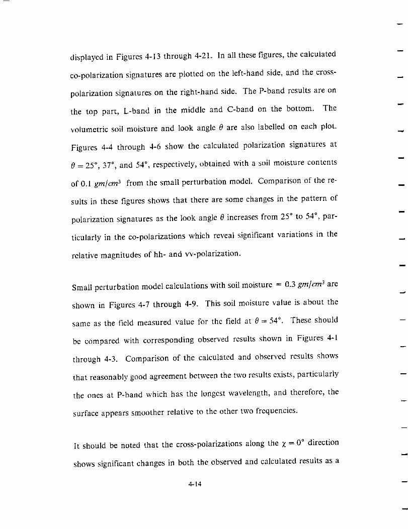
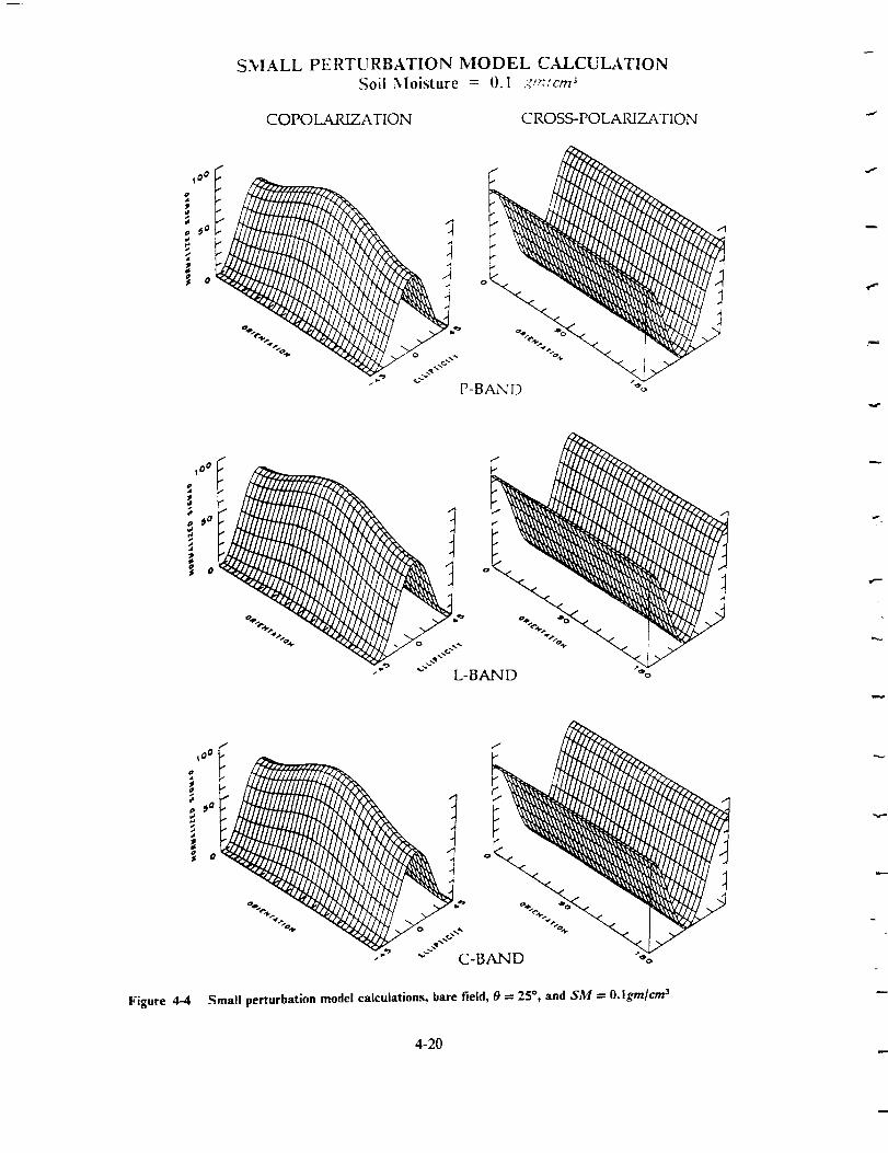
displayed in Figures 4-13 through 4-21. In all thesefigures, the calculated
co-polarization signatures are plotted on the left-hand side, and the cross-
polarization signatures on the right-hand side. The P-band results are on
the top part, L-band in the middle and C-band on the bottom. The
volumetric soil moisture and look angle 0 are also labelled on each plot.
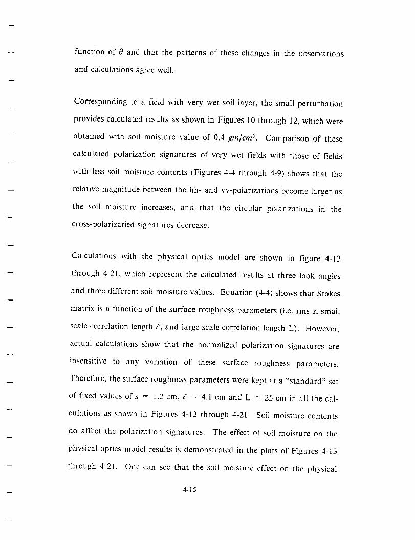
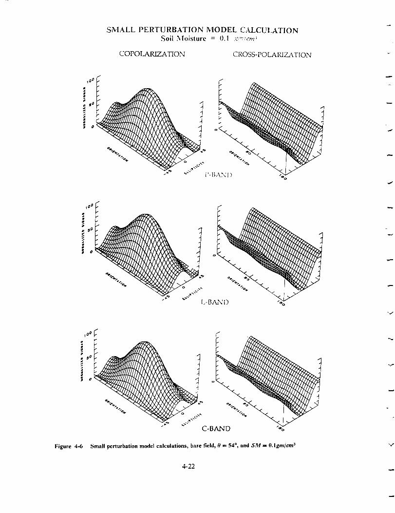
Figures 4-4 through 4-6 show the calculated polarization signatures at
0 = 25 °, 37 °, and 54 °, respectively, obtained with a soil moisture contents
of 0.1 gm/cm 3 from the small perturbation model. Comparison of the re-
suits in these figures shows that there are some changes in the pattern of
polarization signatures as the look angle 0 increases from 25 ° to 54 °, par-
ticularly in the co-polarizations which reveal significant variations in the
relative magnitudes of hh- and w-polarization.
Small perturbation model calculations with soil moisture = 0.3 grn/cm 3 are
shown in Figures 4-7 through 4-9. This soil moisture value is about the
same as the field measured value for the field at O = 54 °. These should
be compared with corresponding observed results shown in Figures 4-1
through 4-3. Comparison of the calculated and observed results shows
that reasonably good agreement between the two results exists, particularly
the ones at P-band which has the longest wavelength, and therefore, the
surface appears smoother relative to the other two frequencies.
It should be noted that the cross-polarizations along the X = 0° direction
shows significant changes in both the observed and calculated results as a
4-14
function of 0 and that the patterns of these changes in the observations
and calculations agree well.
Corresponding to a field with very wet soil layer, the small perturbation
provides calculated results as shown in Figures 10 through 12, which were
obtained with soil moisture value of 0.4 grn/cm 3. Comparison of these
calculated polarization signatures of very wet fields with those of fields
with less soil moisture contents (Figures 4-4 through 4-9) shows that the
relative magnitude between the hh- and w-polarizations become larger as
the soil moisture increases, and that the circular polarizations in the
cross-polarizatied signatures decrease.
Calculations with the physical optics model are shown in figure 4-13
through 4-21, which represent the calculated results at three look angles
and three different soil moisture values. Equation (4-4) shows that Stokes
matrix is a function of the surface roughness parameters (i.e. rms s, small
scale correlation length t', and large scale correlation length L). However,
actual calculations show that the normalized polarization signatures are
insensitive to any variation of these surface roughness parameters.
Therefore, the surface roughness parameters were kept at a "standard" set
of fixed values ofs = 1.2cm,( = 4.1 cm and L = 25cmin all the cal-
culations as shown in Figures 4-13 through 4-21. Soil moisture contents
do affect the polarization signatures. The effect of soil moisture on the
physical optics model results is demonstrated in the plots of Figures 4-13
through 4-21. One can see that the soil moisture effect on the physical
4-15

optics model results (at the same angle) is more pronounced than the case
of small perturbation model. Comparison of these calculated results with
the observed ones (Figures 4-1 through 4-3) shows that the calculations
with the volumetric soil moisture of 0.3 gm/crn 3 (Figure 4-16 through
4-18) closely match the observations (Figures 4-1 through 4-3). For ex-
ample, comparison of the results in Figure 4-18 with those in figure 4-3
shows that both the co-polarization and cross-polarizations at the P-band
frequency are in good agreement. The cross-polarization at L- and C-band
also agree well. However, there are some differences between the observed
and calculated co-polarizations at the L- and C-band.
The polarization signatures generated from geometrical optics model
(Equation 4-13) is the same as the polarization signature of an isotropically
scattering sphere as shown in Figure 2-3a. Polarization signature obtained
from geometrical optics model is independent of frequency, radar look
angle, surface roughness parameters and soil moisture contents.
4-16

OBSERVATION
COPOLARIZATION CROSS .POLARIZATION
o :,7' _1_ _
0 o
%%• L-BAND
Figure 4-1 Observed polarization signatures at 0 ----25 °
4-17

OBSERVATION
COPOLAP, dZATION CROSS-POLARIZATION
f
_0 0
!o°
_o
%
" p-BAND
J/
,,0 0
o
_o
" L-BAND
Figure 4-2 Observed polarization signatures at 0 = 37 °
4-18

OBSERVATION
COPOLARIZATION CROSS-POLARIZATION
Figure 4-3
,°°7_ ;
, I
C-BAND
Observed polarization signatures at 0 = 54 °
4-19
SMALL PERTURBATION MODEL CALCULATIONSoil 51oisture = 0.1 :-,',r:,'cm_
COPO_ATION CROSS-POLAIUZATION
/
tO o
io o
P-BAND %
f J
tO o
o
io °
*_-.o
L-BAND
/
tO o
_ o
"_"*" C-BAND "_
Figure 4-4 Small perturbation model calculations, bare field, 0 = 25 °, and SM --- O.lgm/cm 3
4-20

SMALL PERTURBATION MODEL CALCULATION
Soil _loisture = 0.1 x','_,lcm _
COPO_ATION C ROSS- PO LAILIZATION
i0°i
0 o
" I'-BANI ) "_'o
Figure 4-5
/
_0 0 /"
°% %%
- _ C-BAND _'o
Small perturbation model calculations, bare field, 0 = 37 °, and SM = O.Igm/cm _
4-21
_o°
co_OU_i_°_J
,o° I
,
J

SNIALL PERTURBATION I_IODEL CALCULATION
Soil _loisture - 0.3 ,m:,'cm _
COPOLARIZATION _ROSb-I OLAI,2IZ_\ I ION
\.
_00 I
t
f
k
d
o !4
% %
C-BAND *o
Figure 4-7 Small perturbation model calculations, bare field, 0 ----25°, and SM --- 0.3gm/crn a
4-23

SMALL PERTURBATION MODEL CALCULATION.Soil Moisture = 0.3 ;,"",?;r _
COI'OL_RIZATION C ROSS- P(.) LAI(I Z..\TION
/
10 0
,°
P-BA_D
/
S
_o o_
°'% o.% °_
• p
L-BAND
,oo_ "
_o o
C-BAND
Figure 4-8 Small perturbation model calculations, bare field, 0 = 37 °, and SM = 0.3gm/cm _
4-24

SMALL PERTURBATION MODEL CALCULATION
.<,oil Moisture = 0.3 .7-:,'cm;
COPO LARIZATION C ROSS-I t)[.Ald 2b\TI()N
N,-
Figure 4-9
,oo ( F"
P-BAND
/
_0 0 f-
t
L-BAND "%
(
o
C-BAND %
Small perturbation model calculations, bare field, 0 = 54 °, and S_W = 0.3gm/cm _
4-25
SMALL PERTURBATION MODEL CALCULATION
.Soil Moisture = 0.4 _',,':/,-m _
COPOLARIZATION C ROS_ ['O LAI(IZAIION
°_00 !
,_ _0_0 _ ° k_ "_
P-BAND %
C-BAND
Figure 4-10 Small perturbation model calculations, bare field, 0 = 25 °, and SM = 0.4gmtcm a
4-26

SMALL PERTURBATION MODEL CALCULATIONSoil 5loisture - 0.4 _"':,'c.z;
COPOIa\FdZATION C I(O55- t'k) LAIZtLAIsI()N
_0 0 _" ,.--
o o _,
P-BAND
7
%. o
L-BAND "%
',Oo
C- B t\i"_ i)
Figure 4-1 ! Small perturbation model calculations, bare field, 0 = 37% and SM = 0.4gm/cm 3
4-27

SMALL PERTURBATION MODEL CALCULATION
Soil _loisture = 0.4 _'_,':,'cm;
COPOL.ARIZATION C ROSS- t'O I.AI_.I 2LATION
_°°
1
J
g o o .4
P-BAND
100 f /
_° o
s _'J
L-BAND
'°°I
"7
o o
C-BAND
Figure 4-12 Small perturbation model calculations, bare field, 0 = 54 °, and SM = 0.4gmlcm a
4-28
PHYSICAL OPTICS MODEL CALCULATION
Soil Moisture = 0.1 _"m'Icrn3
COPOLARIZATION CROSS-POLARIZATION
I
_00 _-
: f
P-BAND
_00 _ /
i
1_ 0 /
%°
I.-BAND
_0
0 o
• C-BAND
Figure 4-13 Physical optics model calculations, bare field, 0 = 25 °, and SM = 0.1grn/cm a
4-29
PHYSICAL OPTICS MODEL CALCULATION
Soil Moisture = 0.1 g,mlcm _
COPOLARIZATION CROSS-POLARIZATION
t0 0 / /.
_o
".-.:%
P-BAND
J1
_0 0
!o o
L-BAND
,°°F
_o o
C-BAND
Figure 4-14 Physical optics model calculations, bare field, 0 = 37 °, and SM = O.lgm/cm _
4-30
PHYSICAL OPTICS MODEL CALCULATION
Soil 51oisture = 0.1 gm/cm 3
COPOLARIZATION CROSS-POLARIZATION
I0
o
%
P- 13AN D "_g
_o° _" S: E
_ 0 o
%
"o÷ o ..-_
l.- BAN D _o
I
°O c-"
_ 0 o
C BAND
Figure 4-15 Physical optics model calculations, bare field, 0 = 54 °, and SM = O.lgm/c_
4-31

,o°_
o
04's'_k_' 4p404 "
'°°f
Fig.re _-17
ph],sicalopticsmodcl c_iCutadons'b_rC field,0 = 3.7°, and SM _ o'3gml_
_.33

PHYSICAL OPTICS MODEL CALCULATION
Soil _loisture = 1).3 ,_'t,'7/cm_
COPOLARIZATION CROSS-POLAP, IZATION
f
,oo¢ l
,oo_
_orJ
; 0
I
o
I.-BAND %
_ o
f
C-BAND .,.o
Figure 4-18 Physical optics model calcu;ations, bare field, 0 = 54°, and SM = 0.3gm/cmz
4-34

v
PHYSICAL OPTICS MODEL CALCULATION
Soil Moisture = 0.4 grn/cm 3
COPO_ATION C ROSS- PO LAIUZATION
/
t_ 0 ' o
°"% .%.
?- BAN l) "_,o
/
100 /p
g
o i i_° o
-%4,
I.-BAND %
Figure 4-19 Physical optics model calculations, bare field, 0 = 25 °, and SM = 0.4gm/cm _
4-35
4
",.,7'
PHYSICAL OPTICS MODEL CALCULATION
Soil Moisture = 0.4 gm/cm _
COPOLARIZATION CROSS-POLARIZATION
J
100 1
o
" "_" ['-BA
_00 f
L-BAND
i o
_ o
Figure 4-21 Physica! optics model calculations, hate field, 0 = 54 °, and SM --- 0.4gm/cm 3
4-37


SECTION 5- SCATTERING MATRIX OFA CYLINDER AND POLARIZATIONSIGNATURES OF TREE-COVERED
FIELDS
This section describes the scattering matrix of dielectric cylinders and
polarization signatures of tree-covered fields. Figure 5-1 shows a sketch
of the main scattering mechanisms which are taken into consideration for
the calculations of radar scattering cross sections and the polarization sig-
natures of tree-covered fields. The first one consists of two specular re-
flections, first from a vertical tree trunk or branch, and then from the
ground surface. The outgoing reflected waves are also subject to forward
scatterings. The second one is reflection from the non-vertical tree
branches. A simple geometry shows that only those branches perpendic-
ular to the direction of the incoming waves contribute to the SAR back-
scattered signals. The derivation of the relevant formulas /'or this
component is given in Appendix A. Both of these two scattering processes
are subject to attenuation in passing through the canopy. Therefore, the
third process is a propagation through the canopy, and it may also be
considered as a forward scattering process.
5-1

The tree trunk and its branches are treated asdielectric cylinders of finite
lengths. Also, we assume that the length L of the cylinder is much longer
than the wavelength 2 (i.e.,L_2), and that the cylindrical radius a satisfics
the condition: 0.5 < ka < 10 and L_>a. Under these conditions, the scat-
tered waves from the vertical cylinders of tree trunk and branches propa-
gate only in the dire ztion 0, = n - 0. The scattering matrix S(0, 4)') of such
cylinders of finite length L has been shown (References 21 and 29) for both
the forward scattering case (where qS' = n) and the specular scattering case
(.where _b' = 0 °) to be in the form
°S(O, rc)=Q n=- (5-1)
2 crM
and
s(0, o°) = Q
oo
n_--OO
_dC_O
(5-2)
where Q is a factor due to finite length of the tree, and its value for the
iL The quantities C re and C rM can beabove two special cases is Q = ---.n
found in Reference 29 and are expressed in terms of the angle (re/2- 0),
cylinder radius a, and the complex dielectric constant et of the cylinder for
both the polarization TM (i.e., vertical) and TE (i.e., horizontal) waves.
5-2
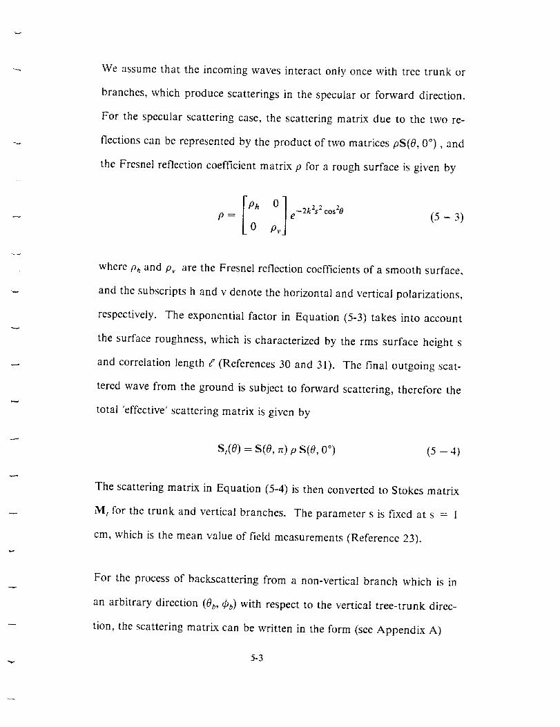
We assumethat the incoming waves interact only once with tree trunk or
branches,which produce scatterings in the specular or forward direction.
For the specular scattering case, the scattering matrix due to the two re-
flections can be represented by the product of two matrices pS(O, 0 °) , and
the Fresnel reflection coefficient matrix p for a rough surface is given by
IPO h O ] e--2k2s2c°s20 (5 3)Pv
where Ph and Pv are the Fresnel reflection coefficients of a smooth surface,
and the subscripts h and v denote the horizontal and vertical polarizations,
respectively. The exponential factor in Equation (5-3) takes into account
the surface roughness, which is characterized by the rms surface height s
and correlation length ¢' (References 30 and 31). The final outgoing scat-
tered wave from the ground is subject to forward scattering, therefore the
total 'effective' scattering matrix is given by
s,(0) = s(0, p s(0, o°) (5 -- 4)
The scattering matrix in Equation (5-4) is then converted to Stokes matrix
Mt for the trunk and vertical branches. The parameter s is fixed at s = 1
cm, which is the mean value of field measurements (Reference 23).
For the process of backscattering from a non-vertical branch which is in
an arbitrary direction (0 b, _bb) with respect to the vertical tree-trunk direc-
tion, the scattering matrix can be written in the form (see Appendix A)
5-3

where
[ ]c°s20__________a
S'(0, 0b) = Q sin20 Shh - _ S_, - fl(Shh + S_)
Cos_Ob
fl(Shh -_- Sw) -- t_ Shh + -- S wsin20
(5-5)
= sin20b sin2_bb
sin 0 b cos 0 b sin 6b
fl = sin 0
sin (hb = x/- cos(0 + 0b) COS(0 -- 0 k)sin 0 sin 0 b
(5-6)
The last formula in equation (5-6) specifies the condition for the occur-
rence of backscattering by non-vertical branches, and it requires
(0 + 0_) > 90 ° .
The quantities Shh and Svv are the same diagonal elements of scattering
matrix for vertical cylinders as defined in Equation (5-2). The outgoing
waves that are received by the antenna are the forward scattered parts,
therefore the "total" scattering matrix for the backscattering process from
non-vertical branches are given by
sh(0, 0b)= s(o, _) s'(0, 0b) (5-- 7)
where S(0, n) and S'(0, 0o) are defined in Equations (5-I) and (5-5), re-
spectively.
5-4
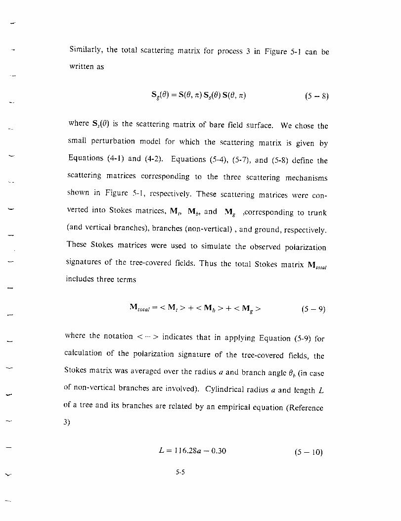
Similarly, the total scattering matrix for process 3 in Figure 5-1 can be
written as
Sg(O)= s(o, s,(o) s(o, (5-8)
where S,(0) is the scattering matrix of bare field surface. We chose the
small perturbation model for which the scattering matrix is given by
Equations (4-1) and (4-2). Equations (5-4), (5-7), and (5-8) define the
scattering matrices corresponding to the three scattering mechanisms
shown in Figure 5-I, respectively. These scattering matrices were con-
verted into Stokes matrices, M t, Mb, and Mg ,corresponding to trunk
(and vertical branches), branches (non-vertical), and ground, respectively.
These Stokes matrices were used to simulate the observed polarization
signatures of the tree-covered fields. Thus the total Stokes matrix Mto,a_
includes three terms
Mtota I = < M t > + < M b > + < Mg > (5--9)
where the notation < ... > indicates that in applying Equation (5-9) for
calculation of the polarization signature of the tree-covered fields, the
Stokes matrix was averaged over the radius a and branch angle 00 (in case
of non-vertical branches are involved). Cylindrical radius a and length L
of a tree and its branches are related by an empirical equation (Reference
3)
L = I16.28a - 0.30 (5- lo)
5-5
I,
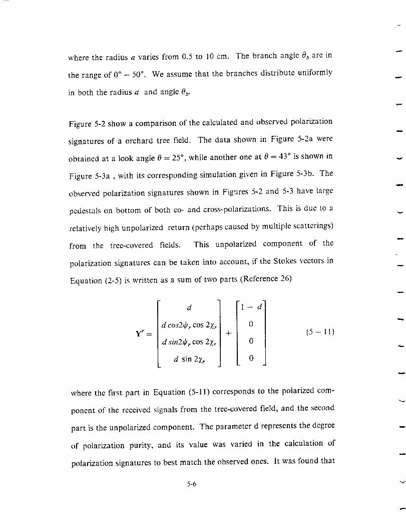
where the radius a varies from 0.5 to 10 cm. The branch angle 0b are in
the range of 0 ° - 50 °. We assume that the branches distribute uniformly
in both the radius a and angle 0 b.
Figure 5-2 show a comparison of the calculated and observed polarization
signatures of a orchard tree field. The data shown in Figure 5-2a were
obtained at a look angle 0 = 25 °, while another one at 0 = 43 ° is shown in
Figure 5-3a, with its corresponding simulation given in Figure 5-3b. The
observed polarization signatures shown in Figures 5-2 and 5-3 have large
pedestals on bottom of both co- and cross-polarizations. This is due to a
relatively high unpolarized return (perhaps caused by multiple scatterings)
from the tree-covered fields. This unpolarized component of the
polarization signatures can be taken into account, if the Stokes vectors in
Equation (2-5) is written as a sum of two parts (Reference 26)
d
d cos24,_ cos 27._
d sin2O_ cos 2)_
d sin 2Zr
1 -- d-
0
+
0
0
(5-- ll)
where the first part in Equation (5-11) corresponds to the polarized com-
ponent of the received signals from the tree-covered field, and the second
part is the unpolarized component. The parameter d represents the degree
of polarization purity, and its value was varied in the calculation of
polarization signatures to best match the observed ones. It was found that
5-6 v
the d values in the range of 0.2 - 0.4 can produce reasonably good results
for matching the observed polarization signature from the tree-covered
fields. The calculations shown in Figures 5-2 and 5-3 were obtained with
d = 0.25.
Figures 5-2 and 5-3 show that the simulated polarization signatures ob-
tained with our cylindrical tree model are in reasonably good agreement
with the observations, particularly at 0 = 25 °. The simulated vertical
polarization at 0 = 43 ° (Figure 5-3) is smaller than observation. This is
attributed to the fact that the vertically polarized Fresnel coefficient Pv is
very small in comparison to the horizontally polarized Ph. For example, if
the dielectric constant of the ground surface is assigned a numerical value
of _ = 5.0 +j 0.5, calculation gives [Pv12=0.07 and [ph12=0.24 at
0 = 43 °. This example shows that specular reflection from ground sup-
presses vertical polarization considerably at this large incidence angle. The
relatively large vertical polarization observed in Figure 5-3 is most proba-
bly originated from some scattering mechanism, which is not involved with
any specular ground reflection. The three scattering processes included in
this study seem inadequate to account for this large contribution of vertical
polarization. Further investigation in this area is required.
5-7

n .._ 00
SPECULARREFLECTION
_ TRUNK
_ T
]
l -" 1"[
FORWARDSCATTERING
Figure 5-1 Sketch of tree scattering geometry.
5-8

CO-POLARIZATION CROSS-POLARIZATION
(a) Observation at 0 25 °
% 1O0
50
o o
/
• O
(b) Calculation at 8
J
= 25 °
Figure 5-2 Comparison of observed and simulated polarization signatures from an orchard tree-covered
field at 0 = 25°:(a) Observations, and (b) Simulations.
5-9

CO-POLARIZATION CROSS-POLARIZATION
f
% 100
@
__ so£ .
O0(a) Observation at 0 = 43 °
I
%9 100 i_ 50 •
£
_ o .< o,_o_,+.>.,<b ° ,900
.,/,.
...\R,_xO\" "_ eOo,/
,y,v
(b)Calculationat 0 = 43 °
Figure 5-3 Comparison of observed and simulated polarization signatures from an orchard tree-coveredfield at 0 = 43°:(a) Observations, and (b) Simulations.
5-10
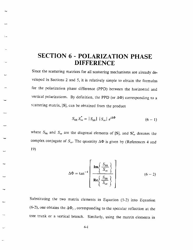
SECTION 6- POLARIZATION PHASEDIFFERENCE
Since the scattering matrices for all scattering mechanisms are already de-
veloped in Sections 2 and 5, it is relatively simple to obtain the formulas
for the polarization phase difference (PPD) between the horizontal and
vertical polarizations. By definition, the PPD (or A_) corrcsponding to a
scattering matrix, [S], can be obtained from the product
ShhS_= Iahhl Is_l e iA_ (6- 1)
where Shh and S_ are the diagonal elements of [S], and S_v denotes the
complex conjugate of Svv. The quantity A¢_ is given by (References 4 and
19)
A_ = tan -1 (6-2)
Substituting the two matrix elements in Equation (5-2) into Equation
(6-2), one obtains the A_ t , corresponding to the specular reflection at the
tree trunk or a vertical branch. Similarly, using the matrix elements in
6-I

Equations (5-3) and (5-5), we can obtain the Aq_g and Aq_b, corresponding
to the PPD for ground Fresnel reflection and backscattering from a non-
vertical branch, respectively.
Additionally, there is also a PPD due to the propagation through the
canopy. This PPD, Aq_pt, due to propagation through the trunk or vertical
branches, can be obtained from Equation (6-2) and the forward scattering
matrix elements in Equation (5-1). Similarly, the Aqbpb due to propagation
through non-vertical branches can be calculated by using the elements in
Equation (A15). Therefore, the total PPD, AS, can be written as
AO = < A_t > + < A_g > + < AOpt >, for trunk and vertical branches
= < AaP b > + < AqbpO >, for non-vertical branches (6-3)
where the average < .-- > is performed over the radius a and also over the
angle 0o in the case of non-vertical branches.
The PPD data were obtained from the same tree-covered fields, which
produced our polarization signatures. The PPD data provided by JPL
were in the complex form c = a +j b stored on magnetic tape. We created
the PPD image pixels corresponding to the quantity AO = arg(c) with a
VAX computer and an image display system. Figure 6-1 shows one of
such PPD image over the area of our investigation. The AO values (also
called pixel values) displayed in this image are in digital numbers (DN),
ranging from 0 to 255, which represents an actual PPD interval of 2n. The
PPD values can only be determined within module of 2n, and our PPD
6-2

imagevalues were originally created in the range of - _zto _z. Thus, those
PPD values, which are larger than _z,would become negative and appear
in the low DN region. In practical applications, it is more convenient to
work in the range of 0 to 2m This can be accomplished by a simple con-
version of adding 2r¢to the negative PPD values. To arrive at a correct
representative PPD distribution, a part of the histogram is moved from the
low DN region to the high DN region (where DN > 255) until a complete
PPD distribution curve is obtained.
The dark areas in Figure 6-1 indicate tow DN values and the bright spots
represent high DN's. The tree-covered fields appear as white square or
rectangular blocks in the image. The radar look angle 0 is labeled on the
right edge. The near-range part of the image corresponds to an incidence
angle 0 - 15 ° and the far range is 0 _ 55 °. Since the data were not abso-
lutely calibrated, the PPD values obtained from arg(e) are arbitrary within
an additive constant, which must be determined before one can make
comparison with any theoretically predicted results.
For an azimuthally symmetric target, it is normally expected (Reference
4) that the backscattering characteristics are the same for both hh and vv
polarizations at normal (or near normal) incidence. In this study, we as-
sumed Aq)= 0 ° for bare field targets at the near-range part (where
0 _ 15 °) within the image. In fact, it has been shown (Reference 4) that
the assumption A_(0)= 0 ° , is valid, within experimental uncertainties ,
for all bare fields in the whole incidence angle range 0 _ 15 ° - 55 °. Figure
6-3

6-2 shows a PPD distribution versus the image digital number (DN) for a
bare field at 0 _ 15 ° The mean value of these PPD values is 59.4, which
is approximately the peak position of this distribution. This mean value
from the bare field will be adopted as a zero-base reference and it will be
denoted by DN 0 = 59.4, which corresponds to the absolute 0 ° in the Aq_
distribution from al targets in the image.
Figure 6-3 displays a PPD distribution versus DN f_r a tree-covered field
at 0 -_ 17 °. The PPD distribution in Figure 6-3 sl-.ows a series of small
peaks across the whole range DN, in contrast to a s:nooth curve, as in the
case of a bare field (Figure 6-2).
The mean DN value of the PPD distribution in Figt, re 6-3 is 297.5, which
is approximately equal to the maximum peak position. One can convert
this mean DN value into the average PPD value in degrees by the formula
A_(0)- 360°255 (DN - 59.4) (6 - 4)
where the zero reference DN0 = 59.4 and the conversion factor
r = 360°/255, have been used. Similarly, the average PPD values A(I)(0)
at other six O's are obtained and these are shown in Figure 6-4 as open
circles. One can see from this plot that the PPD values decrease gradually
as 0 increases from 20 ° to 45 °. Our interest is to reproduce these data,
using the model developed in this report.
6-4

The solid and dashedcurves in Figure 6-4 representcalculated results with
our model. The solid one is for the total PPD and the dashedone excludes
the component due to propagation. The trunk radius a and tree density
used in the calculations were estimated from field survey. The complex
dielectric constant of tree trunk and branches (i.e., at) is highly variable
quantity. Field measurements indicated (Reference 32) that the diurnal
change in this parameter can be up to an order of magnitude. We varied
this parameter to obtain the results that would match the data, and found
that a large range of a t (from 20 +j2 to 40 +j4) could all yield reasonably
good results in matching the observed PPD data within experimental un-
certainty.
?
6-5
[J_J
ZW
rr
LDCP0
I.--77LLJ
.-¥.....
©_
14
12
i0
©L.)
f_
©
//
i
i
A
O3LUI..Urr"(.9I..Ua
I.U(DZu.Irr"ILlLI_U.
tmI..U(./3<"1-13..
360
300 -
240 -
B
m
18010
TREE PARAMETERS: x
\a = lOcm
N = 0.1 m -2 \
= 28 + j2.8
O DATA
I x I I I _ I20 30 40 50
INCIDENCE ANGLE 0 (DEGREES)
!6O
Figure 6-4 Comparison of the observed and simulated PPD.
6-9


SECTION 7- THREE-LAYER EMISSIVITYMODEL
This section presents a model for passive remote sensing of a vegetation-
covered soil surface. In this model, the microwave emission from the
canopy and its underlying ground soil layers are detected by a radiometer.
It is assumed that the vegetation or crop canopy forms a uniform layer
covering the soil surface and that this canopy layer has a constant tem-
perature T c. The soils is divided into two layers (Figure 7-1). Each of the
layers is assumed to have a constant temperature Ti (where i = 1 or 2) and
dielectric constant _, corresponding to its volumetric soil moisture SMV.
The vegetation layer is characterized by a single scattering albedo co and
optical depth -:.
In a previous investigation (Reference 9), Mo et al., showed that the
brightness Tp(O) above the canopy for such a vegetation-covered field can
be given by
Tp(O) = 7_(O)e -`/u + (1 - o))Tc(l - e -_lu)
+ Rl(l -- _o)Te(l -- e-_tU)e-'_l,
(7-I)
where/_ = cos 0, T_(O) is the brightness temperature of the underlying soil
surface, and R_ represent the reflectivity at the interface between the veg-
7-1
etation canopy and the top layer of soils. The subscript p (= h or v) in the
formula is a polarization index. The quantity T(ps>(O) represents the
brightness temperature just above the canopy-soil interface. It consists of
the upwards emissions from both layer 1 and layer 2 as shown in Figure
7-I. It was shown that _s)(O) can be written in the form (Reference 10)
[( )( )R2 1 (l - %)T_ + T2 (7 - 2)T(eS)(O)=eelf 1 + ---_- 1-- T - L
with
1 - R 1
eeff= l-- (RIR2)L"-'-'Z- (7-3)
where _o, is the single scattering albedo of the top soil layer and the L is
the loss factor for layer 1. The e_f[ is the effective emissivity of soil surface,
including multiple scatterings at the top and bottom surfaces of layer 1.
Following previous investigations (Reference 10), the loss factor can be
given by
Ke d ]L=exp _ (7-4)
where d is the thickness of the soil layer 1 and Ke is the extinction coeffi-
cient of the soil layer. The extinction coefficient Ke is related to the soil
dielectric constant _ by (References 10 through 12)
7-2

47_ r
K,- 2 [ Im(x/_ )[ (7- 5)
where 2 is the wavelength in flee space.
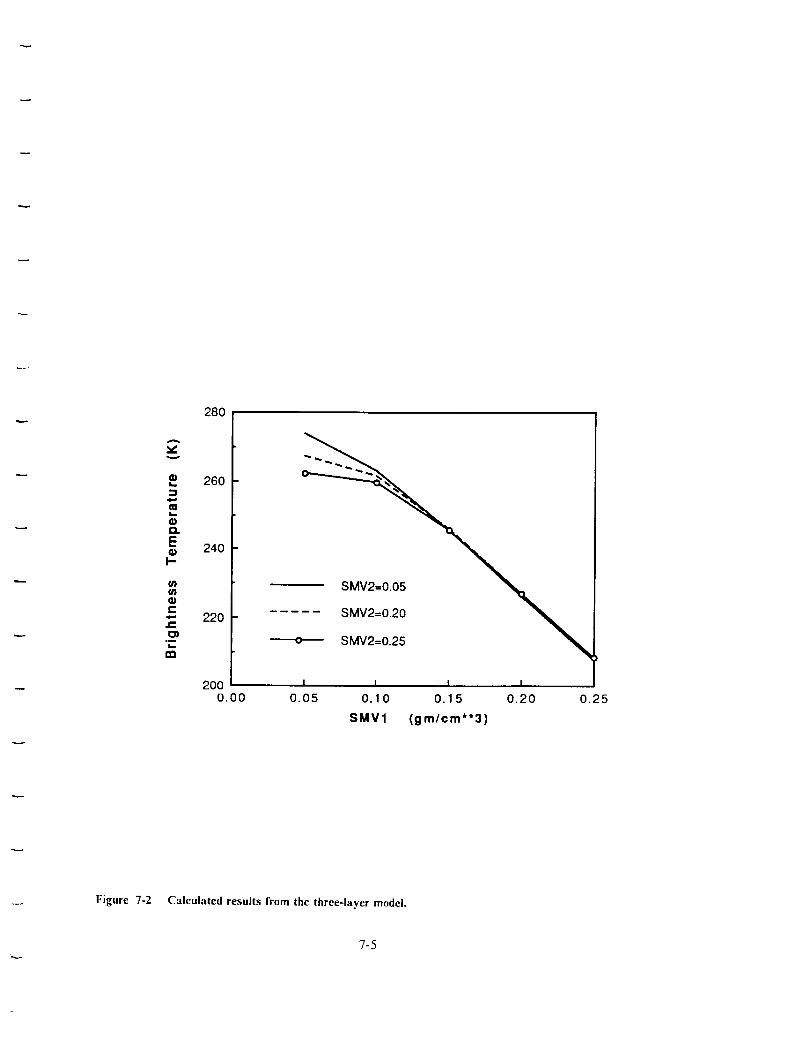
Using the formula in Equations (7-1) through (7-5), we calculate the
brightness temperatures above the canopy as a function of volumetric soil
moisture SMVI in the top layer, while the soil moisture SMV2 in layer 2
is assumed constant. Figure 7-2 shows the calculated results (L-band and
horizontal polarization at 0 = 10°), assuming three values for SMV2.
Results in Figure 7-2 show that the soil moisture in layer 2 affects the
brightness temperature above the canopy if the top soil layer is dry and
has SMV1 < 0.15 gm/crn J, above which the effect of soil moisture in layer
2 vanishes. This is because of the fact that the penetration depth of the
L-band emission decreases as the soil moisture increases and that its pen-
etration depth is less than 5 cm (the thickness of layer 1) at SMVI = 0.15
grn/cm 3. Figure 7-2 demonstrates that the calculated brightness temper-
atures with SMV2 = 0.5 and 0.25 gm/cm _ differ by 12K at SMV1 = 0.05
gm/cm 3, but only by 6K at SMV1 = 0.10 gm/cm 3. These results are in
good agreement with recent field measurements (Reference 33).
7-3
Td
±
I
, /:__I
CANOPY _/1_ _,_, Tc
I TSOIL //_ oo ,_:, , S
LAYER1/olll s e 1
I
SOIL I cod_# T2, SM2LAYER2
I
Figure 7-1 Geometry for Three-layer model.
7-4
28O
A
v
._ 260
..i
.m
Q.
E_ 240I--
ffl
1-22O
m
2OO0.00
!Mv2;o-_o \SMV2=0.25
I I I I
0.05 0.10 0.15 0.20 0.25
SMV1 (gm/cm**3)
Figure 7-2 Calculated results from the three-layer model.
7-5


SECTION 8- SUMMARY ANDDISCUSSION
We have developed a series of electromagnetic wave scattering models for
simulating the observed polarization signatures from both bare soil sur-
faces and tree-covered fields. The models are based on the electromagnetic
wave scatterings from randomly rough surface and from dielectric cylin-
ders, which replace the tree trunk and its branches. The tree branches are
allowed to vary in size (both radius and length) and in direction relative
to the vertical trunk direction.
Polarization phase differences of tree-covered fields are also investigated,
and the theoretical results are compared with observed ones.
In addition, a model for passive remote sensing of vegetation-covered sur-
face is developed. In this model, the microwave emission from the canopy
and its underlying ground soil layers are detected by a radiometer. Two
soil layers with individual temperatures and soil moisture contents are
included in the model. The model results compare favorably with field
measurements.
8-1
In simulation of observations from bare fields, we performed a series of
calculations of the polarization signatures with three theoretical models for
scattering from a randomly rough surface. The models used consist of the
small perturbation model, the physical optics model and the geometrical
optics model. The model calculations of polarization signatures were cal-
culated at P-, L- and C-band frequencies, respectively. The calculated re-
sults were compared with observed polarization signatures acquired with
the NASA/JPL airborne imaging radar polarimeter. The effects of surface
roughness parameters and soil moisture contents on the polarization sig-
natures were also studied.
It was found that the effects of parameters of surface roughness on the
polarization signature are negligibIy small. This is primarily due to the
normalization process which eliminates the effects of surface roughness
parameters on the backscattering coefficients. On the other hand, soil
moisture has significant effect on the polarization signatures obtained from
the small perturbation and physical optics models.
Calculations from both the small perturbation and physical optics models
show strong dependence on the radar look angle 0. However, calculated
polarization signature at fixed angle 0 are insensitive to frequency vari-
ation.
8-2

Comparison of the calculated and observedpolarizations signatures from
bare fields at 0 = 25 °, 0 = 37 ° and 0 = 54 °, respectively, shows good
agreement, especially for the results at P-band.
Polarization signatures obtained with the geometrical optics model are in-
dependent of frequency, radar look angle, surface roughness parameters
and soil moisture contents.
In simulation of obserYations from tree-covered fields, the main scattering
mechanisms taken into consideration in the model are: (1) Specular re-
flection from the vertical tree trunk or branch, followed by another re-
flection from the ground surface (also specularly), (2) backscattering from
non-vertical branches, and (3) propagation through the canopy, as repres-
ented by the forward scattering.
The simulated results for both polarization signatures and polarization
phase differences are in reasonably good agreement with observations.
The model can indicate which scattering mechanism is dominant in inter-
pretation of the observed polarization signatures and polarization phase
differences. Parameters of tree and surface properties may also be ex-
tracted by best matching the simulated and observed results.
The results presented in this studies should be useful for the polarimetric
investigation of interaction between the vegetation and the underlying
scattering surface which is ubiquitously involved in the scattering process.
8-3


.
.
.
.
.
*
.
_o
REFERENCES
J. R. Wang, E. T. Engman, T. Mo, T. J. Schmugge, and J. C. Shuie,
"The Effects of Soil Moisture, Surface Roughness, and Vegetation onL-Band Emission and Backscatter, " IEEE Trans. Geosci. Remote
Sensing, GE-25, pp. 825-833, 1987.
M. W. Whitt and F. T. Ulaby, "Millimeter-Wave Polarimetric Meas-
urements of Artificial and Natural Targets," IEEE Trans. Geosci.
Remote Sensing, vol.26, pp. 562-573, 1988.
J. A. Richards, G. Q. Sun, and D. S. Simonett, "L-band Radar Back-
scatter Modeling of Forest Stands, " IEEE Trans. Geosci. Remote
Sensing, GE-25, pp. 487-498, 1987.
F. T. Ulaby, D. Held, M. C. Dobson, K. C. McDonald, and T. B. A.
Senior, "Relating Polarization Phase Difference of SAR Signals to
Scene Properties," IEEE Trans. Geosci. Remote Sensing, GE-25,pp.83-92, 1987.
T. Le Tuan and H. Laur, "Multi-temporal and Dual Polarization Ob-
servations of Agricultural Crops by X-band SAR Images," 1988
International Geoscience and Remote Sensing Symposium, vol. 3, pp.1291-1294, September 12-16, 1988, Edinburgh, U K
T. Mo, T. J. Schmugge, and J. R. Wang, "Calculations of microwave
brightness temperature of rough soil surfaces: Bare field," NASA
Goddard Space Flight Center, Greenbelt, MD, Tech. Memo. 86200;
also, IEEE Trans, Geosci. Remote Sensing, vol. GE-25, pp. 47-54,1987.
T. Mo and T. J. Schmugge, "A Parameterization of the Effect of Sur-
face Roughness on Microwave Emission," IEEE Trans. Geosci. Re-
mote Sensing, GE-25, pp. 481-485, 1987.
T. Mo, J. R. Wang, and T. J. Schmugge, "Estimation of Surface
Roughness Parameters from Dual-Frequency Measurements of Radar
Backscattering Coefficients," IEEE Trans. Geosci. Remote Sensing,Vol. 26, pp. 574-579, 1988.
R-1
9. T. Mo, B. J. Choudhury, T.J. Schmugge, J. R. Wang, and T. J.Jackson, "A model for microwave emission from vegetation-coveredfields," J. Geophys. Res., vol. 87, pp. 11229-11237,1982.
10. F. T. Ulaby, R. K. Moore, and A. K. Fung, Microwave Remote
Sensing: Active and Passive , Vol. 1, Addison-Wesley Publishing
Company, Reading, Massachusetts, 1981.
11. F. T. Ulaby, R. K. Moore, and A. K. Fung, Microwave Remote
Sensing: Active and Passive , Vol. 2, Addison-Wesley Publishing
Company, Reading, Massachusetts, 1982.
12. F. T. Ulaby, 1L K. Moore, and A. K. Fung, Microwave Remote
Sensing: Active and passive , Vol. 3, Artech House, Dedham, MA,1986.
13. D. L. Evans, T. G. Farr, J. J. van Zyl, and _. A. Zebker, "Radar
Potarimetry: Analysis Tools and Applications," IEEE Trans. Geosci.
Remote Sensing, vol. 26, pp. 774-789, 1988.
14. C. Elachi, W. E. Brown, J. B. Cimino, T. Dixcn, D. L. Evans, J. P.
Ford, R. S. Saunders, C. Breed, H. Masursky, J. F. McCauley, G.
Schaber, L. Dellwid, A. England, H. MacDonald, P. Martin-Kaye,and F. Sabins, "Shuttle Imaging Radar Experiment," Science, 218, pp.
996-1003, 1982.
15. J. F. McCauley, G. G. Schaber, C. S. Breed, M. J. Grolier, C. V.
Haynes, B. lssawi, C. Elachi, and R. Blom, "Subsurface Valleys and
Geoarcheology of the Eastern Sahara Revealed by Shuttle Radar,"
Science, 218, pp. 1004-1020, 1982.
16. L. Tsang, J. A. Kong, and R. T. Shin, Theory of Microwave Remote
Sensing, John Willy, New York, 1985.
17. J. J. van Zyl, H. A. Zebker, and C. Elachi. "Imaging Radar
Polarization Signature: Theory. and Observation," Radio Science, vol
22, pp. 529-543, 1987.
18. H. A. Zebker, J. J. van Zyl, and D. N. Held, "Imaging Radar
Polarimetry from Wave Synthesis," J. Geophys. Res., vol. 92, NO. B l,
pp. 683-701, 1987.
19. T. Mo and J. R. Wang, "A Study of SAR Polarization Signature andPhase Difference of Orchard Trees", IEEE Trans. Geosci. Remote
Sensing, 1989, Submitted for publication.
20. T. Mo and J. R. Wang, "Modelling of SAR Polarization Phase Dif-ference from Trees," 1988 International Geoscience and Remote Sens-
ing Symposium, vol. 1, pp. 55-58, September 12-16, 1988, Edinburgh,UK.
R-2
21. F. T. Ulaby, K. Sarabandi, K. McDonald, M. Whitt, and M. C.Dobson, "Michigan Microwave Canopy Scattering Model(MIMICS)," Report 022486-T-1, July 1988, Department of ElectricalEngineering & Computer Science,Uiversity of Michigan, Ann Arbor,Michigan
22. H. C. van de Hulst, Light Scattering bv Small Particles, Dover Publi-cations, Inc., New York, 1981.
23. J. R. Wang, E. T. Engman, J. C. Shiue, M. Rusek, and C. Steinmeier,
"The SIR-B observations of microwave backscatter dependence on soil
moisture, surface roughness, and vegetation covers," IEEE Trans-
action on Geoscience and Remote Sensing, GE-24(4), pp. 510-516,1986.
24. H. A. Zebker and Y. gou,
Polarimeter Stokes Matrix,"
mote Sensing Symposium,Vancouver, Canada.
"Phase Calibration of Imaging Radar1989 International Geoscience and Re-
pp. 2881-2884, July 10-14, 1989,
25.
28.
29.
L. Norikane and F. Burnette, "Multiview Guide," Technical Report,August 1987, Jet Propulsion Laboratory, Pasadena, CA 91109
J. D. Kraus, Radio Astronomy, New York: McGraw Hill, 1966.
A. lshimaru, Wave Propagation and Scatterin_ in Random Media ,p.480-481, Academic Press, New York, 1978.
M. T. Hallikainen, F. T. Ulaby, M. C. Dobson, M. A. EI-Rayes, andL.-K. Wu, "Microwave Dielectric Behavior of Wet Soil - Part I: Em-
pirical Models and Experimental Observations," IEEE Trans. Geosci.
Remote Sensing, Vol. GE-23, pp. 25-34, 1985.
G. T. Ruck, D. E. Barrick, W. D. Stuart, and C. K. Krichbaum, Ra-
dar Cross-Section Handbook (see Section 4.2. pp. 266-274) , NewYork, Plenum, 1970.
30. T. Mo and T. J Schmugge, "A Parameterization of the Effect of Sur-
face Roughness on Microwave Emission," IEEE Trans. Geosci. Re-
mote Sensing, GE-25, pp. 481-485, 1987.
31. B. J. Choudhury, T. J. Schmugge, R. W. Newton, and A. Chang,"Effect of Surface Roughness on the Microwave Emission from
Soils," J. Geophys. Res., voi. 13, pp. 329-344, 1983.
32. M. C. Dobson, "Diurnal and Seasonal Variations in the Microwave
Dielectric Constant of Selected Trees," 1988 International Geoscience
and Remote Sensing Symposium, vol 3, p. 1754, September 12-16,1988, Edinburgh, U K
33. J. R. Wang, private communication, 1989.
R-3

34. F. Varosi, private communication, 1989.
R°4
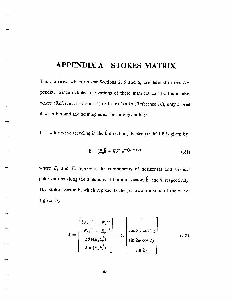
APPENDIX A - STOKES MATRIX
The matrices, which appear Sections 2, 5 and 6, are defined in this Ap-
pendix. Since detailed derivations of these matrices can be found else-
where (References 17 and 21) or in textbooks (Reference 16), only a brief
description and the defining equations are given here.
A
If a radar wave traveling in the k direction, its electric field E is given by
A
E = (Ehh + Ev_ ) e -i('t-k'r) (A1)
where E h and E_ represent the components of horizontal and vertical
A
polarizations along the directions of the unit vectors h and 5, respectively.
The Stokes vector F, which represents the polarization state of the wave,
is given by
IEhj2 + lEvi 2 1
Ev cos 2_b cos 2X
Ev'12 sin 2X
IEhlZ- I =soF = 2Re(Eh ) sin 2ff cos 2Z
21m(EhEv)
(A2)
A-1

where So = I Enl 2 + lEvi2 is the average total power carried by the wave.
The Stokes matrix [M] is defined as
M = _-1 W R -I (A4)
where
W
* " S_ "ShhShh ShvShv Shh v ShvShh
s_s;_ s_s_ s_s_ s_s;_t • t
ShhS_h Sh_S_ ShhS. Sh_S_h
" s_s_ sv_s_ s_s_SvhShh v
(A5)
and
00]R= -1 0 0 (A6)0 1 1
0 -i i
Scattering Matrix from a Non-vertical Branch
Simple geometry shows that only normally incident waves on non-vertical
branches can be backscattered and received by an airborne antenna.
Thus, we only derive the scattering matrix for normally incident waves on
the non-vertical branches.
In general, a branch is along the _b-direction, which makes angles (0b, thb)
with respect to the coordinate system (_, _, _), with the _.-direction along
A-2
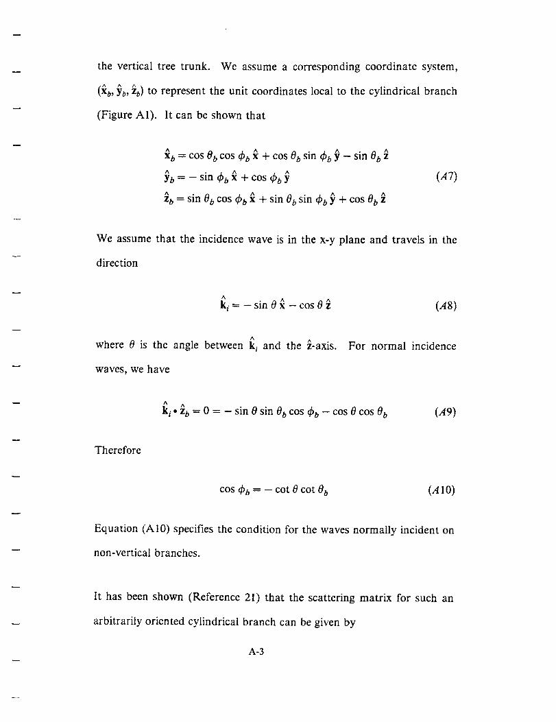
the vertical tree trunk. We assume a corresponding coordinate system,
(xb, Yb, zb) to represent the unit coordinates local to the cylindrical branch
(Figure A1). It can be shown that
xb = cos 0 b cos _b x + cos 0 b sin _bb _ - sin 0 b
Yb = - sin 4'b x + cos _bb _ (A7)
ZO = sin 0 b cos q5b _ + sin 0 b sin _bb _ + cos 0 o
We assume that the incidence wave is in the x-y plane and travels in the
direction
A
k i = - sin 0 _ - cos 0 _ (A8)
A
where 0 is the angle between k t and the _-axis.
waves, we have
For normal incidence
A A
k i • zb = 0 = - sin 0 sin 0 b cos t_b -- COS 0 COS 0 b (A9)
Therefore
cos thb = - cot 0 cot 0 b (A10)
Equation (A10) specifies the condition for the waves normally incident on
non-vertical branches.
It has been shown (Reference 21) that the scattering matrix for such an
arbitrarily oriented cylindrical branch can be given by
A-3

S'(O,Ob, dp') = Q(h_'hs) (_.) Shh (h i,h_)) (vi,h_)
L" " " J^ (v s • vs)J Svh (h i . ¥ib) (Vi. _b)
(All)
where Shy = S_n = 0 for normal incidence waves, and
Shh = Z (--1)ncTE(o) ein¢"
=- (AI2)n oo
oo
S_= Z (--1)ncTM(o)ein4f
where _b' = 0 ° for backscattering, and _b' = n for forward scattering. The
A A
polarization vectors (h_, _) for incidence waves and (h,, 5,) for scattered
waves, refer to the (_, }, _.) coordinate system, and the corresponding
A A
(h_, ^b hb ^b " " "vi) and ( s, vs) refer to the (xb, y_, zb) system. These polarization vec-
tors can be obtained from the relations,
A A A A A A /k A A A A A
h i = k i x Z, v i -- h i x k i ; hs = ks x z, vs = h s x k s (A 13)
A A
where ks = --k_ for the case of backscattering. Similarly, we have
^b ..,x ,,, ,",b ^b " Ab A ^ ."xb /"b Ah i : k i x Zb, ¥i = h X k i ; hs = ks x Zb, v s = h x ks (A 14)
Using Equations (A7) and (A8), we can find all the polarization vectors
in Equations (AI3) and (AI4), which are then combined with Equation
(A11) to obtain the required scattering matrix for backscatterings from
A-4

non-vertical branches.
text.
The final result is given in Equation (5-5) in the
Following the same procedure, we can derive the scattering matrix of for-
ward scatterings by the non-vertical branches (for normal incidence
A A
waves), if k s = k t is used in Equations (A13) and (AI4).
is
S'(0, Oh,_) = Q COS20b ]sin20 Shh + O_S,,,, -- _(Shh -- S,,,,)
_(Shh S_) c°s20_ [- - ct Shh + sin2------_ S_J
The f'mal result
(A15)
where the a, fl and sin _bb are the same as given in the text (see Equations
5-5 and 5-6). The S_h and S,_ in Equation (AI5) are defined in Equation
(A 12) with qb' = n.
A-5
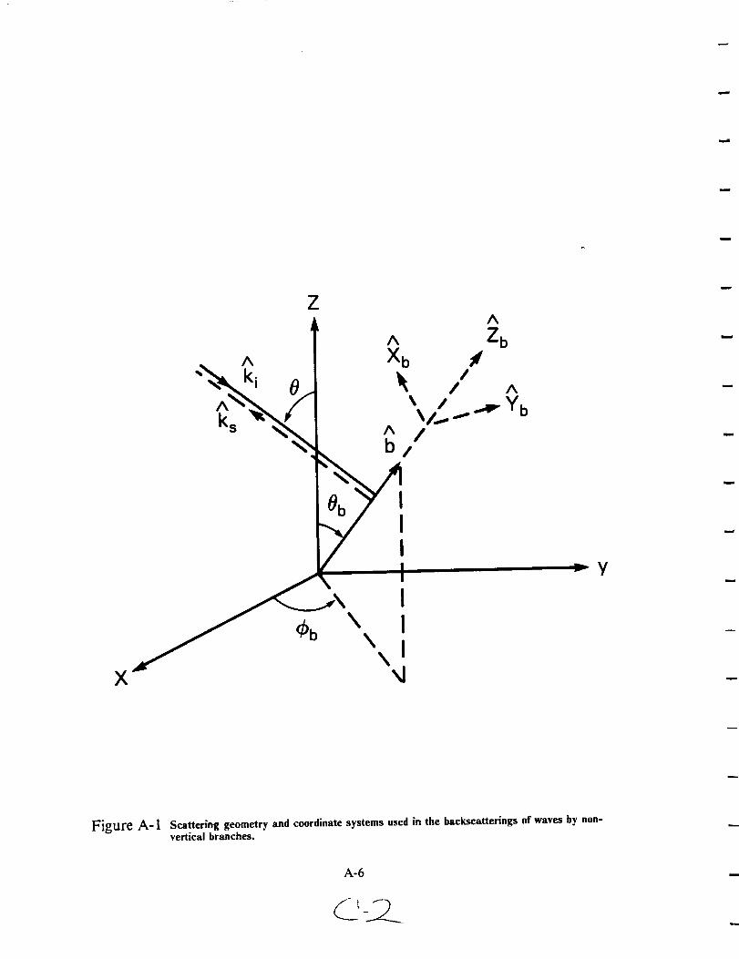
A
k S
A
ki
Z
X
Y
Figure A-1 Scattering geometry and coordinate systems used in the backscatterings of waves by non-vertical branches.
APPENDIX B - MULTIVIEW USER'SGUIDE
This user's guide was prepared to assist users of the modified version of the
JPL MULTIVIEW software package (References 25 and 34) for process-
ing the specific data acquired with the NASA/JPL SAR polarimeter. The
JPL MULTIVIEW package consists of three independent parts, each of
which may be executed separately. However, they are collectively required
to process a set of the JPL compressed polarimetry data of polarization
signatures and for proper calibration of an image file in co-polarization
phases. The three parts in the package are:
• MULTIVIEW.FOR • The main program
* RECAL.FOR • Calibration of polarimetric image
• CREATE_TP.FOR • Create total power of Stokes Vector
The original JPL MULTIVIEW software package was modified at the
Goddard Space Flight Center (GSFC) (Reference 34) and adopted for
running on the VAX computer at the GSFC Ocean Laboratory.
For detailed description of the MULTIVIEW package, the users should
refer to the JPL MULTIVIEW Guide (Reference 25). In this document,
B-I

we primarily provide the essential instructions which are required for exe-
cuting the MULTIVIEW software package with the interactive Ocean
VAX computer.
We start with reading data from the JPL tape of compressed polarimeter
data and creating data file on disk. The created imaging data file is then
re-calibrated in the co-polarization phase, using the RECAL.FOR pro-
gram. From the calibrated imaging data file, one runs the
CREATE_TP.FOR program to create a total-power image file.
After the imaging data are properly calibrated, the main MULTIVIEW
program can be executed to perform various functions. In MULTIVIEW,
there is a menu with 16 options which can be selected to perform appro-
priate studies of the polarimeter data.
The executable modules of all the programs are stored in the dataset
OCEANI$DUB2:[SIBTM.POLAR] at the Ocean VAX computer.
The followings are some examples for executing some of the modules.
(User's inputs are printed in bold in the sessions)
B.1 Examples of Terminal Session
We illustrate the running of the individual MULTIVIEW programs by
actual terminal sessions which show exactly what one would see on the
B-2

screen of the VAX terminals. Text entered by user is in bold face type.
For questions which appear to have no answer, a carriage return will bring
the default value into effect.
B.I.1 Get the Image files from the Tape
The JPL tape usually contains groups of 3 files for image data of P-, L-,
and C-bands, respectively. In this example, the second file (L-band) is
read off the tape and a image file named "L122888" is created on disk. It
should be noted that the tape read program, TAP_READ, is a locally de-
veloped program which is written in IDL (Interactive Data Language) and
is not part of the original MULTIVIEW software package. If you try to
get the first file(P band), you can skip MTU (VAX Magnetic Tape Utility)
and go directly to the DEFINE statement. The steps to get an image file
are shown on the following VAX session lines.
$ MOUI'NT/FOREIGN MFAI
SMTU
***** MTU - VAX/VMS Tape Processing Utility V5.0 *****
Enter INPUT tape drive > M'FAIEnter INPUT tape density (DEFAULT = 6250) >%MTU-W-DEVALMNT- You already have mfalDo you choose to continue < Y/N > ?Y
Enter OUTPUT tape drive (DEFAULT = 6250) >** Enter MTU function > SKIP
mounted!
** WARNING - Next few questions refer only to INPUT tape MFA1
Enter number of records or fdes to skip > IEnter type of skip (-.w, will list options) > FFA total of 1 records/fries were skipped
B-3

** Enter MTU function > EXITMTU exiting
$ DEFINE MTI MFAI$ XIDL
VAX IDL, (C) Copyright 1983-1988, Research Systems, Inc.Site 300, Licensed for use by: locfIDL > @TAP_READ
10240
Output filename
L122888
FILE OPENED SUCCESSFULLYASSOCIATED FILE SUCCESSFULLYABOUT TO READ TAPETAPE READ SUCCESSFULIDL > exit
$ DISMOUNT MFAI
B.I.2 Re-Calibration of Image Files
Image file created from the JPL polarimetric data tape requires re-
calibration by renormalizing co-polarization difference to 0 ° for all pixels
within a chosen area, which is normally a slightly rough soil surface. How
to choose such an area is at users decision.
The RECAL.FOR program within the MULTIVIEW software package is
used to re-calibrate the image file. The following example demonstrates
the re-calibration of the image file L122888 (created in B.I.1). The cali-
brated image file is named LI22888CALB (output filename).
$ RUN RECAL
B-4

Filename of data to be recalibrated --> L122888
File L122888
opened read-only on channel = 128
Output Filename -- > L122888CALBFile LI22888CALB
of size 20500 blocks created on channel = 144
general scale factor: 5.4700092E + 07calibration factors are:
( 1.000000,0.0000000E + 00) (0.7514449,0.6597958) ( 1.000000,0.0000000E + 00)
(1.000000,0.0000000E + 00)Cursor defined window -- >
enter the coordinates (x,y) of the top left comer:
100,100
enter the coordinates (x,y) of the bottom fight comer:
112,112
window Up-Left: I00 100 Low-Right: 112 112
is this okay (Y/n) ?
computing the co-phase...
number of points summed: 169
estimated co-phase in degrees: 2.739639
do you want a different window (y/N) ?
enter expected co-phase in degrees:0.0
updated calibration factors are:
(0.9988570,-4.7797505E-02) (0.9439604,0.3300586) (0.9271055,-0.3748003)
(1.000000,O.O000000E + 00)
processing line:
processing line:
processing line:processing line:
processing line:
processing line:
processing line:
processmg line:
processing line:
processing line:
processing line:
processing line:
processing line:
processing line:
processing line:
processing line:
processing line:
processing line:
processing line:processing line:
5O
100
1502O0
25O
3OO
350
4OO
45O
5OO
550
6OO
65O
7OO
750
800850
900
950
1000
B-5

B.1.3 Create Total Power
Before running MULTIVIEW, it is necessary to run the program
CREATE_TP.FOR once for each compressed data set. The program
CREATE_TP.FOR creates a 512 x 512 total-power image and stores it on
the disk in a file with the same name as the compressed data set but with
the extension '.TP.' MULTIVIEW expects a compressed data set to have
a corresponding '.TP' file with a pre-calculated total-power image.
The following terminal session illustrates the process of running
CREATE_TP.FOR to create a total power image named L122888.TP.
$ RUN CREATE_TP
Select IIS device 0 or 1 -- > 0%SYSTEM-S-NORMAL, normal successful completion
Input Filenarne -- > LI22888CALBFile L122888CALB
opeed read-only on channel = 144File LI22888CALB.tpof size 512 blocks created on channel = 160
Scale Factor ( > 1.0 yields brighter picture) -- >
A default scale factor of 1.0 will be used...
Computing scale factor of image...
Drawing initial image (total power)...1024
B-6

B.2 Running MUL TIVIEW
The 16 options in the MULTIVIEW program are:
1) Change current image size (256)2) Change current zoom factor (1)3) Erase an image4) Plot an image, given a polarization chosen from signature5) Plot an image, given an arbitrary polarization6) Compute a new polarization signature7) Toggle signature display (T)8) Change current sc de factor (1.0000)9) Toggle snap-to-grit mode (T)10) Display and Wriu 3-D signatures to disk files11) Find local maximam or minimum in polarization signature12) Find maximum or minimum in polarization signature13) Delete a polarization signature14) Compute ratio of two signatures15) Roam (512x512) window in (1024x1024) virtual display16) Quit
Option 6 is used to compute new polarization sigratures and option l0 to
create 3-D plots of co-polarization and cross-polarization signatures.
Options 10 also creates two datasets for storing data for plots. All other
options are described in Reference 25 in detail.
The following example shows a MULTIVIEW running session that creates
a set of 3-D plots:
$ RUN MULTIVIEW
< < < Welcome to MULTIVIEW, Version 1493.27 > > >
Recover Mode (y/N) --> N
Select IIS device 0 or 1 --> 0
%SYSTEM-S-NORMAL, normal successful completion
B-7

Input Filename -- > p122888ealbFile p122888calbopened read-only on channel = 176
File p 122888calb.tpopened read-only on channel = 192
Scale Factor ( > 1.0 yields brighter picture) -- >
A default scale factor of 1.0 will be used...
Computing scale factor of image...
Drawing initial image (total power)...
%SYSTEM-S-NORMAL, normal successful completion
MAIN MENU
1) Change current image size (256)2) Change current zoom factor (1)3) Erase an image4) Plot an image, given a polarization chosen from signature5) Plot an image, given an arbitrary polarization6) Compute a new polarization signature7) Toggle signature display (T)8) Change current scale factor (1.0000)9) Toggle snap-to-grid mode (T)10) Display and Write 3-D signatures to disk files11) Find local maximum or minimum in polarization signature12) Find maximum or minimum in polarization signature13) Delete a polarization signature14) Compute ratio of two signatures15) Roam (512x512) window in (1024x1024) virtual display16) Quit
Choose one -- > 6
Cursor defined area (Y/n) -- > N
Upper-Left X,Y of area in original 1024 image -- > 100,100Lower-Right X,Y of area in original 1024 image --> 112,112
Some of the pixels being looked at:%SYSTEM-S-NORMAL, normal successful completion
62 56 40 37 56 64 6554 44 57 57 73 68 5482 72 43 66 63 51 5276 52 54 50 45 41 3859 48 62 77 61 45 4251 51 38 49 47 69 5257 49 39 46 45 58 64
Is this ok (Y/n) -- > Y
B-8

%SYSTEM-S-NORMAL,normalsuccessful completionUpper-Left Comer of subset is at 100 100
Drawing Signatures...
MAIN MENU
1) Change current image size (256)2) Change current zoom factor (1)3) Erase an image4) Plot an image, given a polarization chosen from signature5) Plot an image, given an arbitrary polarization6) Compute a new polarization signature7) Toggle signature display (T)8) Change current scale factor (1.0000)9) Toggle snap-to-grid mode (T)10) Display and Write 3-D signatures to disk files11) Find local maximum or minimum in polarization signature12) Find maximum or minimum in polarization signature13) Delete a polarization signature14) Compute ratio of two signatures15) Roam (512x512) window in ( 1024x 1024) virtual display16) Quit
Choose one -- > 10
creating CO-polarization signature file: p122888calb.COPScreating CROSS-polarization signature file: p 122888calb.CRPSDrawing 3-D Signature...
The program creates two output files (named PI22888CALB.COPS and
PI22888CALB.CRPS), which contain the 3-D plot coordinates on the
VAX system. One can transfer the files to the IBM SCFMVS system by
using the following commands.
$ COPY PI22888CALB.COPS SCFMVS:: < USRID > ANY.COPS
S COPY PI22888CALB.CRPS SCFMVS:: < USRID > ANY.CRPS
Then, two datasets are created under your ID on IBM disk.
B-9

B.3 Produce 3-D Plots on IBM
The data transferred to IBM computer can be plotted, using the Template
Graphic Plotting Subroutines. A software package for plotting the
polarization signatures in 3-d surface form was developed. The 3-d plots
presented in this report were generated by this software package.
The following JCL program shows how
OPTICSMD, that requires two subroutines
GAUSS, respectively.
to execute a program
named PHOPTICS and
//USRIDOPT JOB (xxxxx,V678,10),'PHY.OPTICS MOD',TIME-- (1,59),
// MSGCLASS =A,NOTIFY-- USRID//EXEC G38PLOT,PARM.FORT ='NOMAP,NOXREF',
// PARM.LKED ='NOMAP,NOXREF',REGION.GO =0K
//FORT.SYSIN DD DSN = USRID.dsn(OPTICSMD),DISP =SHR
// DD DSN = USRID.dsn(PHOPTICS),DISP = SHR
// DD DSN = USRID.dsn(GAUSS),DISP -- SHR
//LKED.SYSLIB DD
// DD// DD DSN = SYS2.IMSLD,DISP = SHR
/,
B-IO
Related Documents