Microsoft Excel - Lecture 8 & 9

INTRODUCTION TO INFORMATION TECHNOLOGY

MICROSOFT EXCEL

SPREADSHEET

An interactive computer program consisting of rows and columns displayed on screen in a scrollable window for manipulating numbers, formulae, currency, date and text.

SPREADSHEET

Examples of spreadsheet packages include:

a)VisiCalc-visual calculatorb)Supercalc invented by computer Associates

c)Multiplan by Microsoftd)Context MBAe)Lotus 1-2-3f)Excel by Microsoftg)Quattro

What is Excel?• An integrated application software (or package) consisting of spreadsheet program, database management tool an application development environment.

• It is developed for use on Microsoft Computers

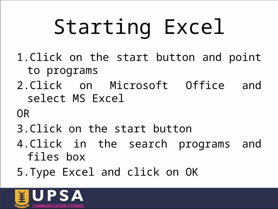
Starting Excel1.Click on the start button and point to programs

2.Click on Microsoft Office and select MS Excel

OR3.Click on the start button4.Click in the search programs and files box

5.Type Excel and click on OK

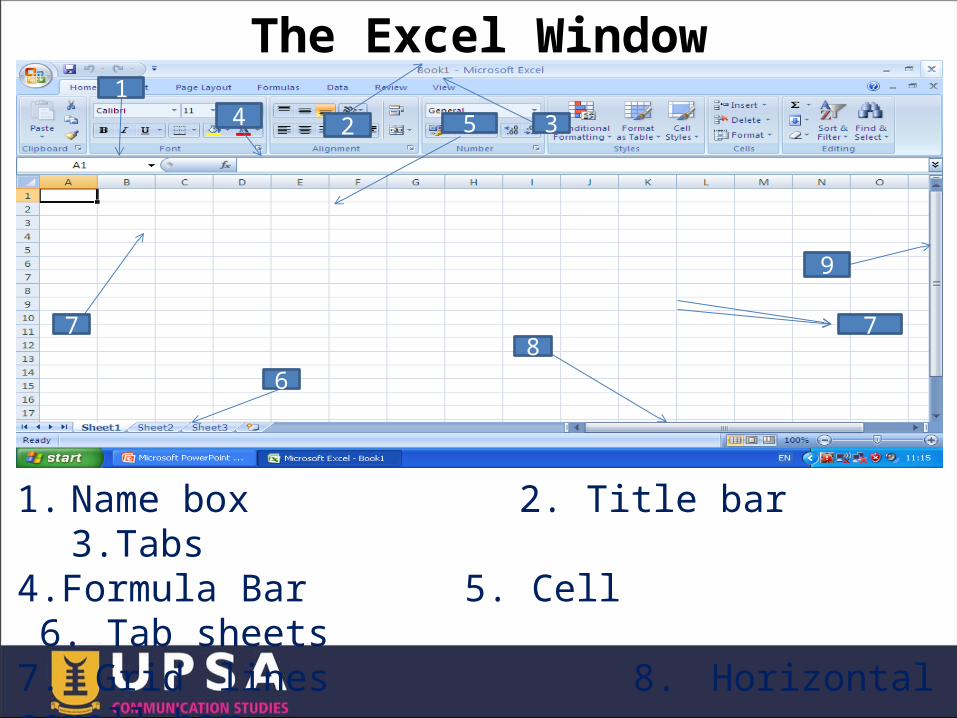
The Excel Window

1. Name box 2. Title bar 3.Tabs

4.Formula Bar 5. Cell 6. Tab sheets 7. Grid lines 8. Horizontal scroll bar 9. Vertical Scroll Bar

21

34 5

6

78

9

7

A Cell• Where a row and column intersect, is a cell.

• Any cell on the spreadsheets may contain one of the following:

1. Text, 2. value or 3. formulae.

A Workbook• Workbook Is a window within excel that holds your work.

• A new workbook contains 3 worksheets but additional sheets can be added.

A Worksheet• Worksheet A worksheet contains grid lines creating rows and columns.

• A worksheet contains 256 columns from A to IV.

• To view the last column press on CTRL plus the left arrow.

• The number or rows a worksheet contains is 65,536.

• To view the last rows press on CTRL plus the down arrow.

Exiting Excel•It is never safer to just turn off the switch to end an Excel program or any windows based application.

To exit Excel:1.Click on file and click on Exit

2.Press Alt + F4

Types Of Data Used In Excel

Excel accepts three types of data in it cells.

These are Labels, Formulas, and Values.

• Labels These are texts representing row headings and column headings.

• Formula These are instructions that cell tell Excel how to manipulate values.

• Values These are simply numbers that are entered into the cells.

Types Of Files Used In Excel• There are four types of files that excel

uses:1.Data Files: A file that stores the

specifics of your work, including excel workbooks, word processing documents, graphic images, database information etc.

2.Foreign Files: A file created by any other software other than the software at hand.

3.Template file: An Excel file with the extension. XLT extension that have settings and attributes you want to use in a new excel workbook applications.

4.Workbook file: An Excel file that contains one or more worksheets

Entering Data Into A Cell

• To enter data into a cell, click on the cell to activate it then type into the cell.

• Navigational keys can be used to move around the cell.

Editing The Worksheet• Editing a worksheet includes

not only revising the cell contents but also making changes on the structure or organization of the worksheet.

• The editing keys are in the table below:

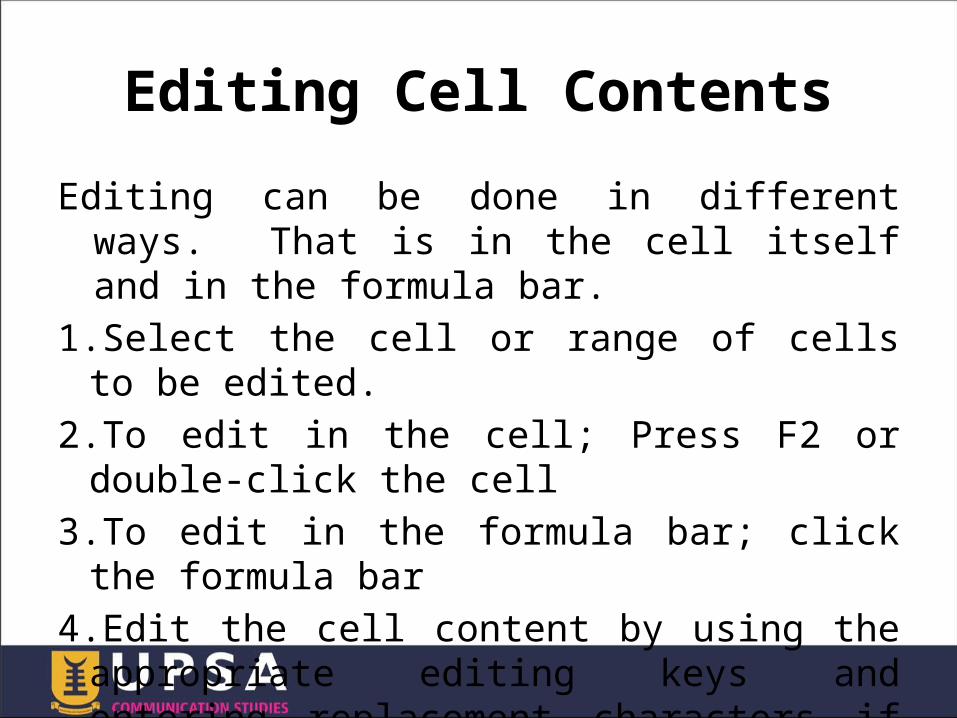
Editing Cell ContentsEditing can be done in different ways. That is in the cell itself and in the formula bar.

1.Select the cell or range of cells to be edited.

2.To edit in the cell; Press F2 or double-click the cell

3.To edit in the formula bar; click the formula bar

4.Edit the cell content by using the appropriate editing keys and entering replacement characters if any.

5.Press the enter key

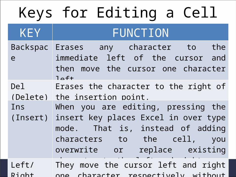
KEY FUNCTIONBackspace

Erases any character to the immediate left of the cursor and then move the cursor one character left.

Del (Delete)

Erases the character to the right of the insertion point.

Ins (Insert)

When you are editing, pressing the insert key places Excel in over type mode. That is, instead of adding characters to the cell, you overwrite or replace existing character to the left and right.Left/

Right Arrow

They move the cursor left and right one character respectively without deleting any characters.

HOME/END The Home/End keys move the cursor to the beginning and end of the cell entry respectively without deleting any characters.

Keys for Editing a Cell

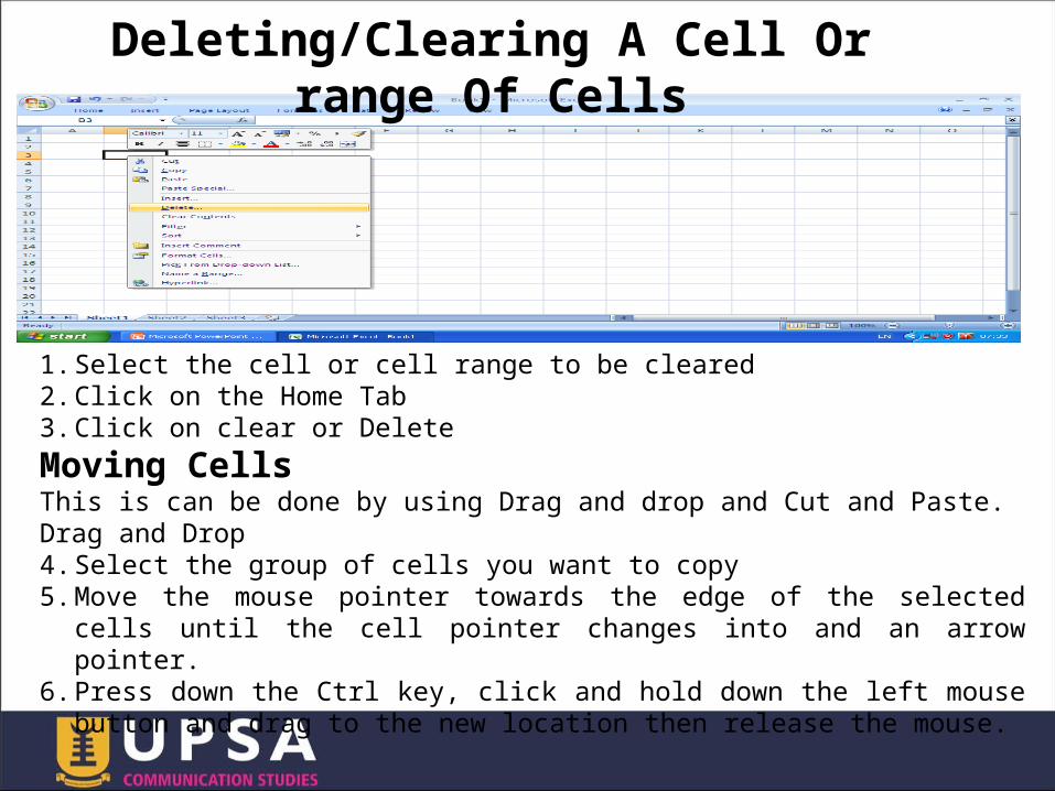
1.Select the cell or cell range to be cleared2.Click on the Home Tab3.Click on clear or DeleteMoving CellsThis is can be done by using Drag and drop and Cut and Paste. Drag and Drop4.Select the group of cells you want to copy5.Move the mouse pointer towards the edge of the selected

cells until the cell pointer changes into and an arrow pointer.

6.Press down the Ctrl key, click and hold down the left mouse button and drag to the new location then release the mouse.

Deleting/Clearing A Cell Or range Of Cells

Copying Formulas1.Select the cell that contains the formula you want to copy.

2.Click on Edit and click on copy3.Select the cells in which you want to copy to.

4.Click on the Home Tab and click on paste.

Using Autofill• The easiest method for entering repeating incrementing data or days of the week, months in a year is to use autofill feature.

1.Make sure that the cells have values

2.Select the range of cells.3.Position the mouse pointer over fill handle so that it becomes a small Black cross.

4.Hold down the left mouse button and drag the pointer over the cells vertically and horizontally.

5.Release the mouse button

Deleting Rows/Columns1.Select the column or row to be deleted

2.Click on Home Tab3.Click on delete4.Choose entire Row or Column depending on which way you want the remaining cells to be moved after the deletion.

Inserting Rows/ColumnsWith the insert, you can insert one or more cell(s), or entire Row(s) and Column(s).

5.Select the Row or Column to be inserted

6.Click on Insert Menu and click on Rows or Columns.

Deleting/Inserting Rows/Columns

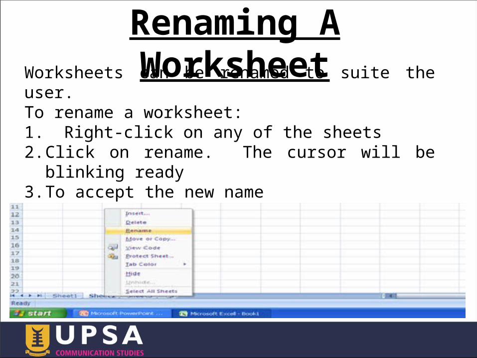
Worksheets can be renamed to suite the user. To rename a worksheet:1. Right-click on any of the sheets2.Click on rename. The cursor will be

blinking ready3.To accept the new name4.Type the new name and press the enter

key

Renaming A Worksheet

Inserting A New Worksheet 1.Right-Click on any worksheet2.Click on insert3.On the dialogue box that will be provided click on worksheet

4.Click on OKHiding A column/Row5.Select the column/ Row to hide6.Click on the window menu7.Click on hideTo unhide a Column/Row click on the window menu and click on Unhide.

Inserting A New Worksheet & Hiding a Column/Row

Freezing/Unfreezing Panes• Follow these steps to freeze panes in a

worksheet:• Position the cell cursor based on what you

want to freeze:– Columns: Select the column to the right of the columns you want to freeze. Rows: Select the row below the rows you want to freeze.

– Columns and rows: Click the cell below the rows and to the right of the columns you want to freeze — essentially, the first cell that isn't frozen.

• In the Window group of the View tab, choose Freeze Panes→Freeze Panes.

• In the Window group of the View tab, choose Freeze Panes→Unfreeze Panes to unlock the fixed rows and columns.

Inserting Date and TimeTo insert date and time:1.Click on the Home Tab2.Click on cells3.Click on the Number Group4.Click on Date or time and select any date or time format.

5.Click on OK.

Formatting a CellDisplaying the Percentage Sign1. Select the values in the cell you want to apply the percentage sign to.

2.Click on the Home Tab and click on cells.

3.Click on the Number Group.4.Click on the percentage sign and click on OK.

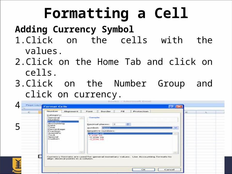
Adding Currency Symbol 1.Click on the cells with the values.

2.Click on the Home Tab and click on cells.

3.Click on the Number Group and click on currency.

4.Drop down the list and click on any currency symbol.

5.Click on OK.

Formatting a Cell

Formatting a CellNaming A RangeNames are easier to remember than cell addresses and you can use range names in formulas. To name a range:

1.Select the cells in the range and you want to name.

2.Click inside the Name box and delete what is there.

3.Type a name for the range of cells and press the enter key.

Formatting a Cell• To Wrap A Text In A Cell1.Click on the cell with the text2.Click on the Home Tab and click on cells

3.Click on the Alignment Group4.Click on the Wrap Text box and click on OK

• To Shrink A Text To Fit Into A Cell1.Click on the cell with the text2.Click on the Home Tab and click on cells

3.Click on the Alignment Group4.Click on the shrink To Fit check box, click on OK.

1.Click on the Home Tab and click on cells

2.Select the number of cells you want to merge

3.Click on the Alignment Group4.Click on the merge cells check box and click on OK.

Merging Cells

• Excel needs information before it can calculate a formula.

• It needs something to operate on called on operand or argument and

• it needs some instructions that tells it what you want to do on an operator.

Creating Formulas

Creating Formulas• Operands are the inputs or quantities in a formula.

• They can be part of the formula itself or stored in other cells.

• The operands that excel uses are values, text, cell references, names and worksheet functions.

• Operators are commands that you give to formulas to specify how you want a formula to treat operands.

• Each category of formulas has it own set of operator.

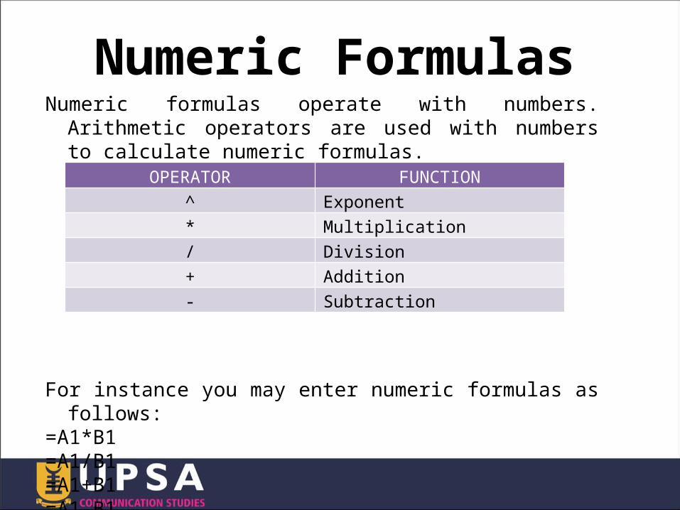
Numeric formulas operate with numbers. Arithmetic operators are used with numbers to calculate numeric formulas.

For instance you may enter numeric formulas as follows:

=A1*B1=A1/B1=A1+B1=A1-B1=A^2

OPERATOR FUNCTION^ Exponent* Multiplication/ Division+ Addition- Subtraction

Numeric Formulas

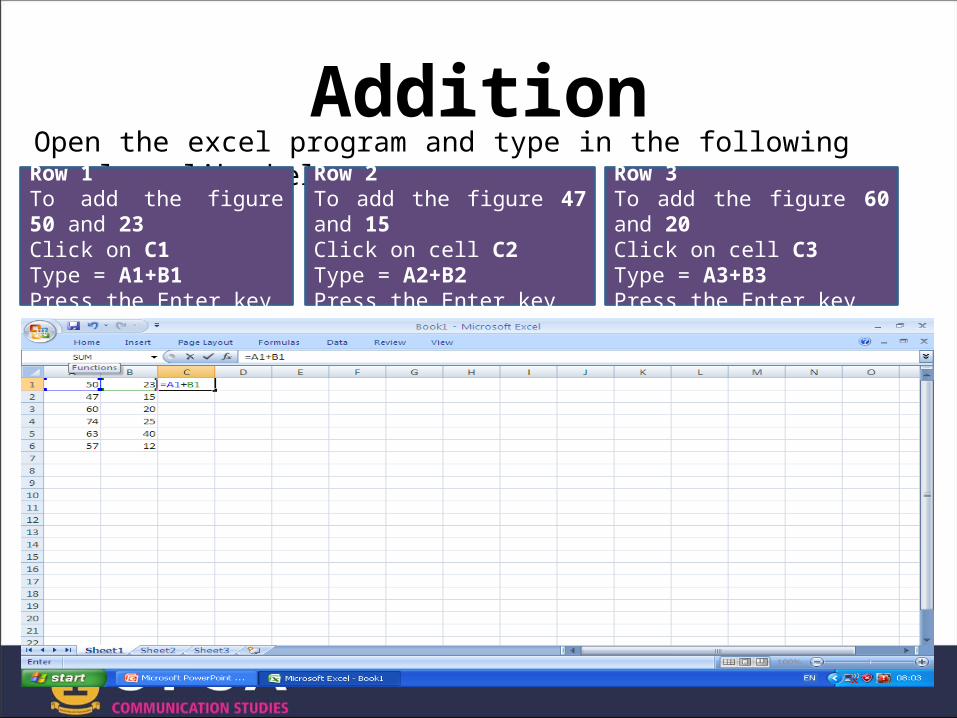
Open the excel program and type in the following values like below.Row 1

To add the figure 50 and 23Click on C1Type = A1+B1Press the Enter key

Row 2To add the figure 47 and 15Click on cell C2Type = A2+B2Press the Enter key

Row 3To add the figure 60 and 20Click on cell C3Type = A3+B3Press the Enter key

Addition

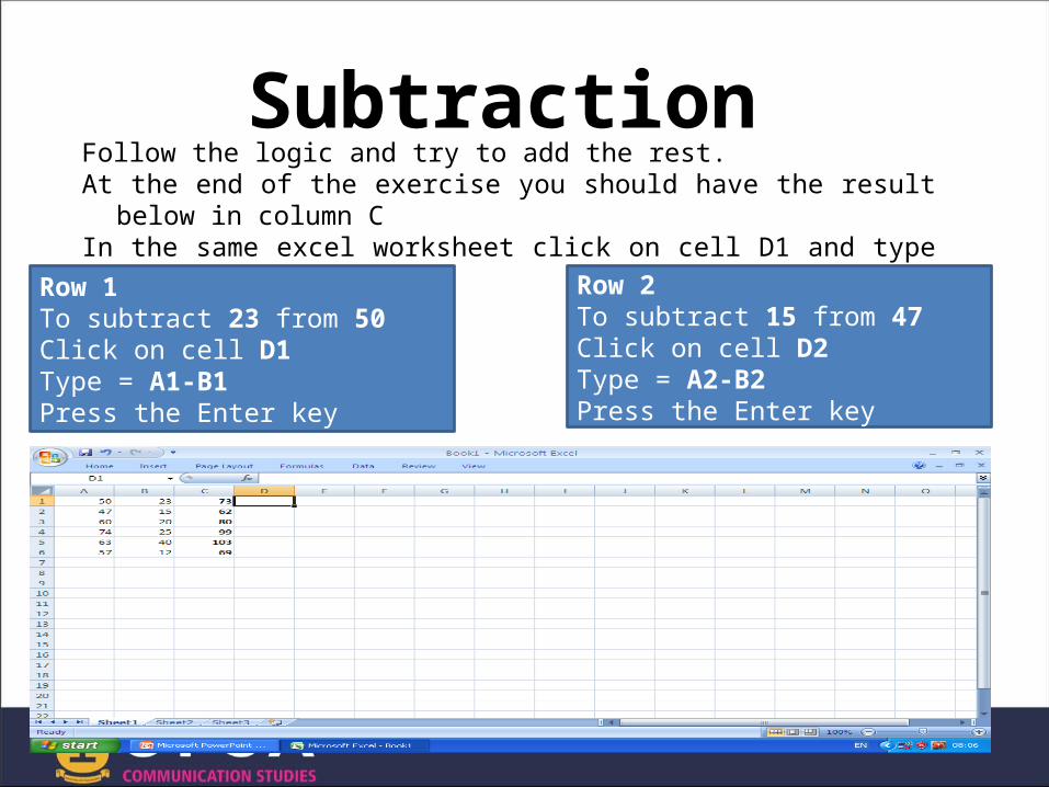
Follow the logic and try to add the rest.At the end of the exercise you should have the result

below in column CIn the same excel worksheet click on cell D1 and type

what you see below:Row 1To subtract 23 from 50Click on cell D1Type = A1-B1Press the Enter key

Row 2To subtract 15 from 47Click on cell D2Type = A2-B2Press the Enter key

Subtraction

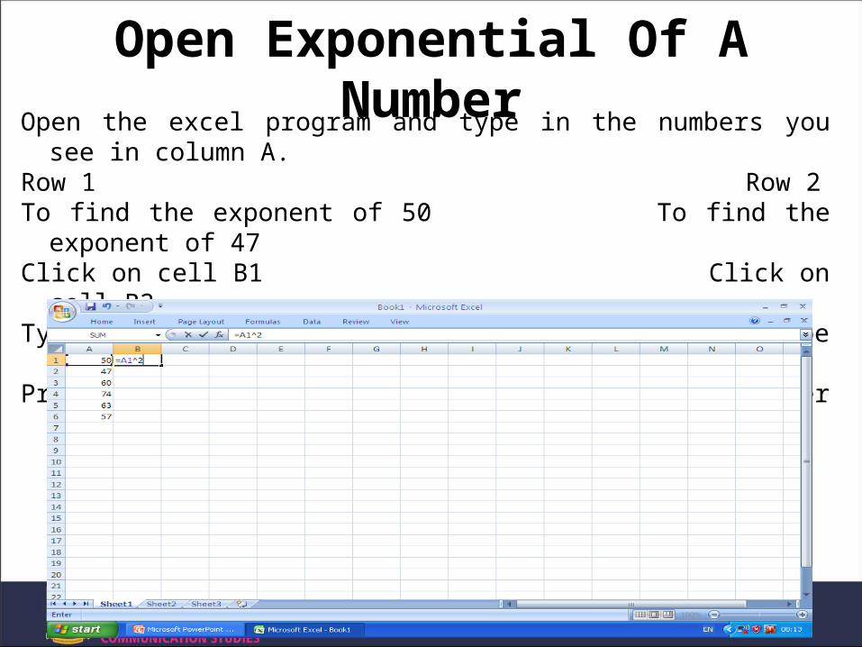
Open the excel program and type in the numbers you see in column A.

Row 1 Row 2To find the exponent of 50 To find the exponent of 47

Click on cell B1 Click on cell B2

Type =A1^2 Type =A2^2

Press the Enter key Press enter Key

Open Exponential Of A Number

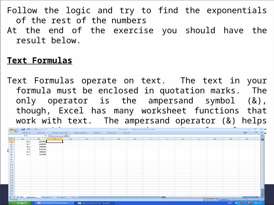
Follow the logic and try to find the exponentials of the rest of the numbers

At the end of the exercise you should have the result below.

Text Formulas

Text Formulas operate on text. The text in your formula must be enclosed in quotation marks. The only operator is the ampersand symbol (&), though, Excel has many worksheet functions that work with text. The ampersand operator (&) helps to combine text operands. Example of text formula:

=“Profit made in the year”&” “&” October 2005”

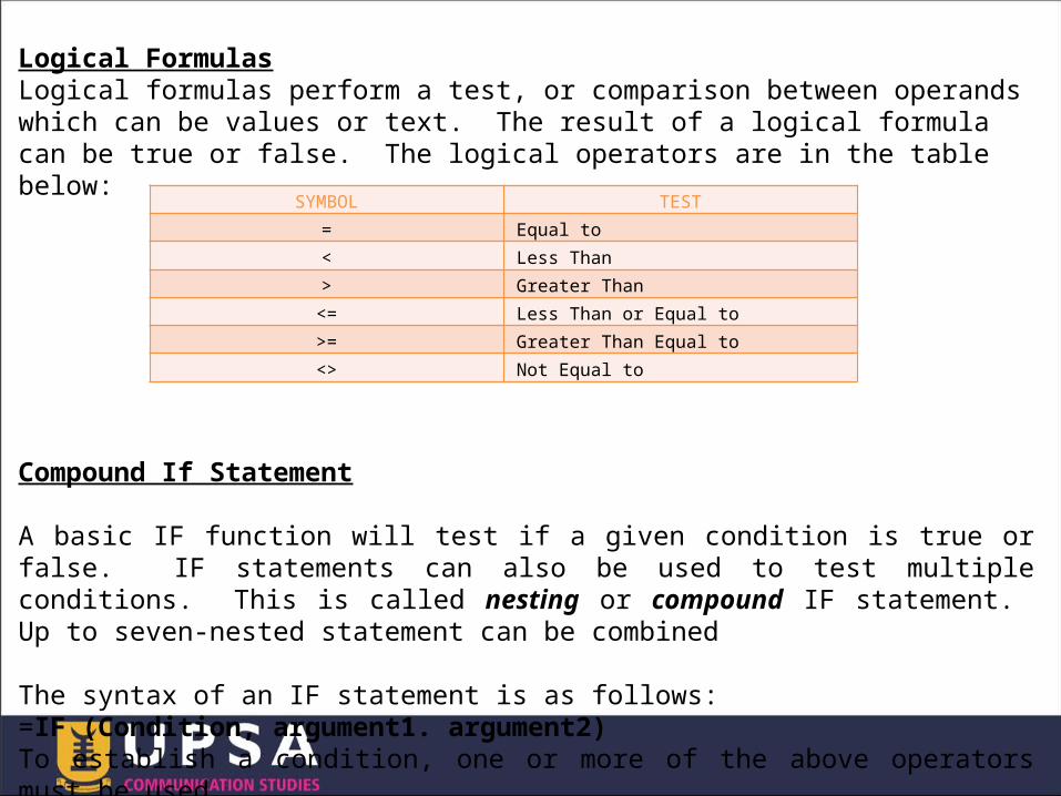
Logical FormulasLogical formulas perform a test, or comparison between operands which can be values or text. The result of a logical formula can be true or false. The logical operators are in the table below:

Compound If Statement

A basic IF function will test if a given condition is true or false. IF statements can also be used to test multiple conditions. This is called nesting or compound IF statement. Up to seven-nested statement can be combined

The syntax of an IF statement is as follows:=IF (Condition, argument1. argument2)To establish a condition, one or more of the above operators must be used

SYMBOL TEST= Equal to< Less Than> Greater Than<= Less Than or Equal to>= Greater Than Equal to<> Not Equal to

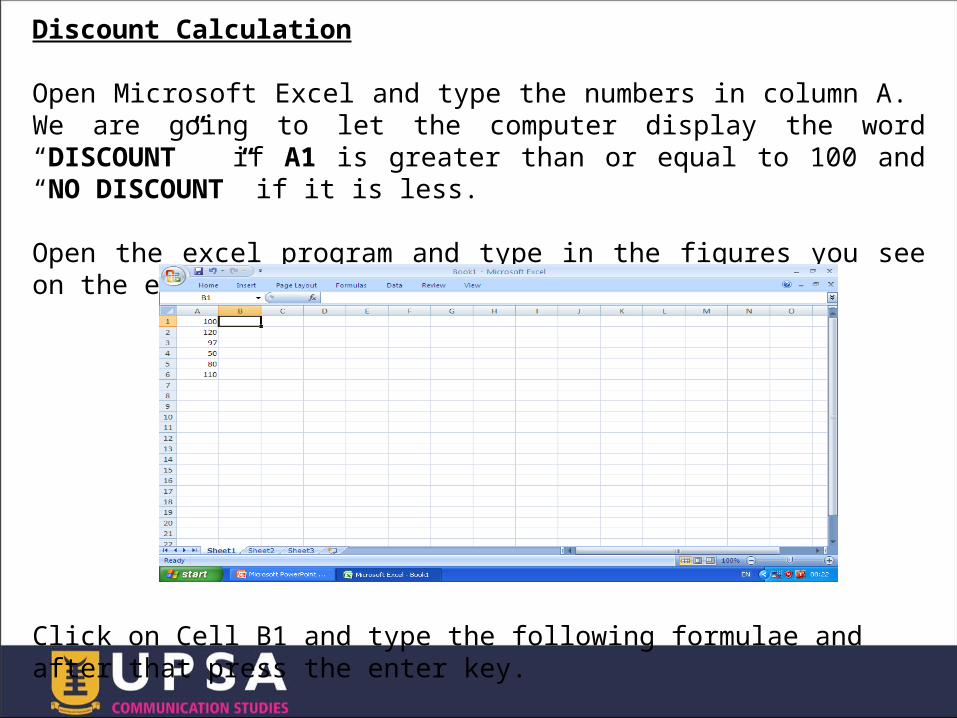
Discount Calculation

Open Microsoft Excel and type the numbers in column A. We are going to let the computer display the word “DISCOUNT” if A1 is greater than or equal to 100 and “NO DISCOUNT” if it is less.

Open the excel program and type in the figures you see on the excel window.

Click on Cell B1 and type the following formulae and after that press the enter key.

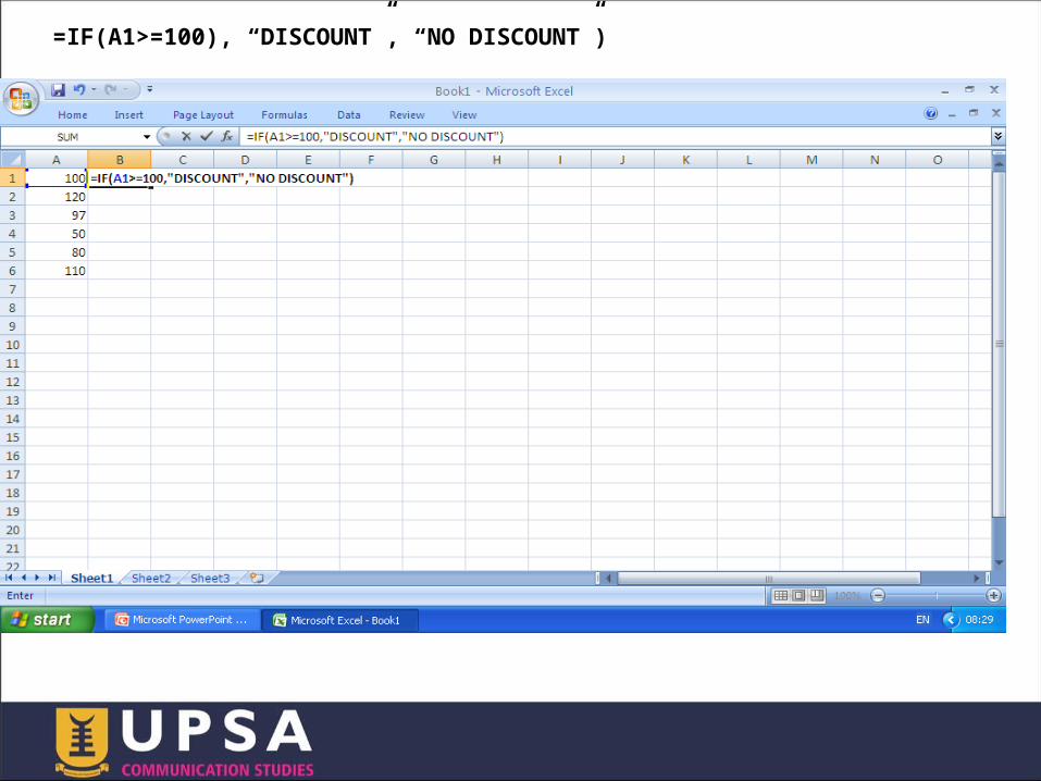
=IF(A1>=100), “DISCOUNT”, “NO DISCOUNT”)

D1 ▼ ƒx

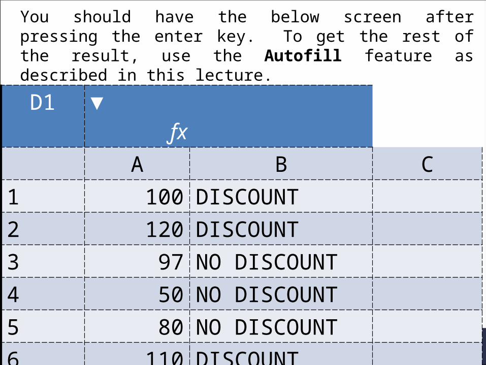
A B C1 100 DISCOUNT2 120 DISCOUNT3 97 NO DISCOUNT4 50 NO DISCOUNT5 80 NO DISCOUNT6 110 DISCOUNT

You should have the below screen after pressing the enter key. To get the rest of the result, use the Autofill feature as described in this lecture.

Professor’s Grading Software• Professor Darlington is a Senior Lecturer at

Owen State University, North Carolina. He uses software designed by him to grade his students. This software was designed using Excel’s ability) to accept compound statements. The Professor uses the following number scale for grade equivalents.

• Greater than – 89 A+• From 70 – 79 A• From 60 – 69 B• From 50 – 59 C• From 40 – 49 D• Less than 40 F

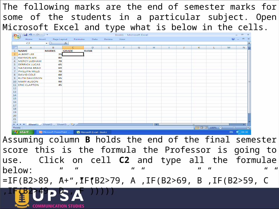
The following marks are the end of semester marks for some of the students in a particular subject. Open Microsoft Excel and type what is below in the cells.

Assuming column B holds the end of the final semester score this is the formula the Professor is going to use. Click on cell C2 and type all the formulae below:=IF(B2>89,”A+”,IF(B2>79,”A”,IF(B2>69,”B”,IF(B2>59,”C”,IF(B2>49,”D”,”F”)))))

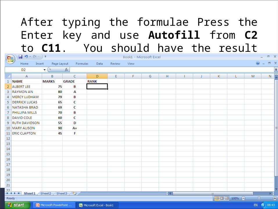
After typing the formulae Press the Enter key and use Autofill from C2 to C11. You should have the result below in column C under GRADE.

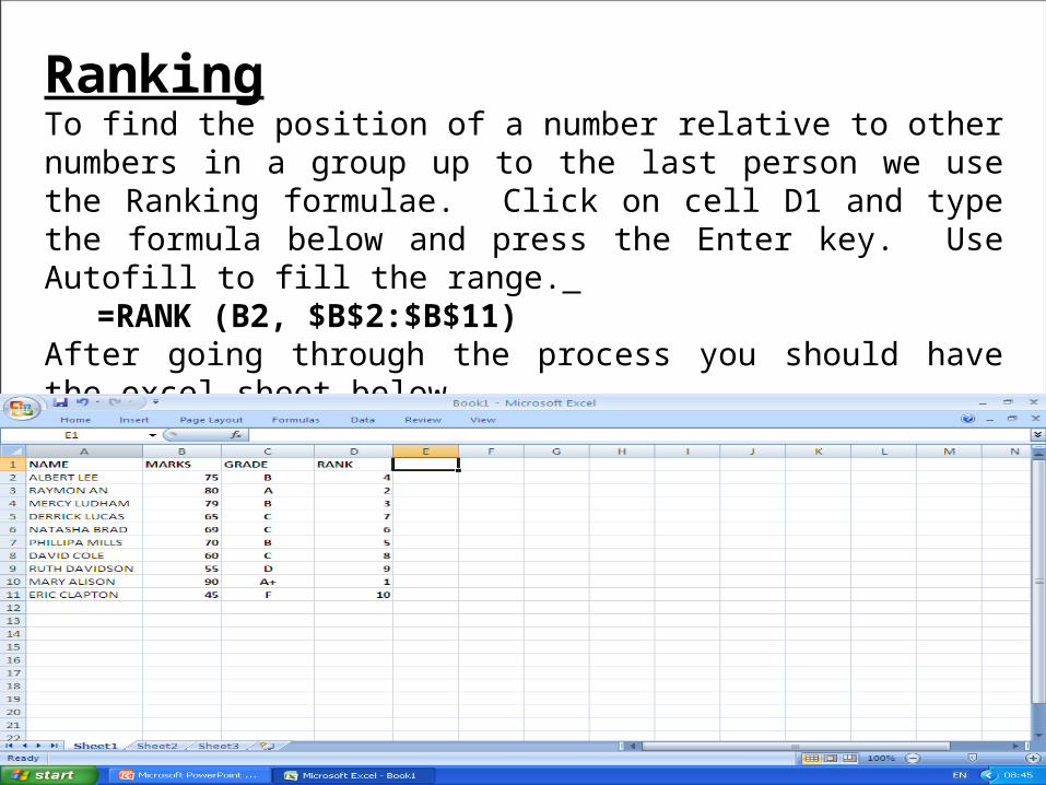
RankingTo find the position of a number relative to other numbers in a group up to the last person we use the Ranking formulae. Click on cell D1 and type the formula below and press the Enter key. Use Autofill to fill the range.

=RANK (B2, $B$2:$B$11)After going through the process you should have the excel sheet below.

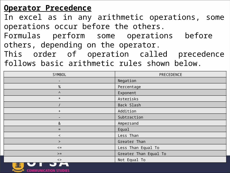
Operator PrecedenceIn excel as in any arithmetic operations, some operations occur before the others. Formulas perform some operations before others, depending on the operator. This order of operation called precedence follows basic arithmetic rules shown below.

SYMBOL PRECEDENCE- Negation% Percentage^ Exponent* Asterisks/ Back Slash+ Addition- Subtraction& Ampersand= Equal< Less Than> Greater Than<= Less Than Equal To>= Greater Than Equal To<> Not Equal To

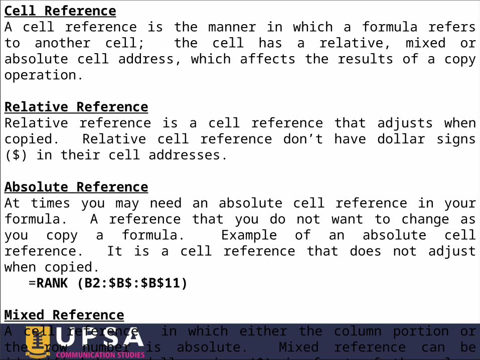
Cell ReferenceA cell reference is the manner in which a formula refers to another cell; the cell has a relative, mixed or absolute cell address, which affects the results of a copy operation.

Relative ReferenceRelative reference is a cell reference that adjusts when copied. Relative cell reference don’t have dollar signs ($) in their cell addresses.

Absolute ReferenceAt times you may need an absolute cell reference in your formula. A reference that you do not want to change as you copy a formula. Example of an absolute cell reference. It is a cell reference that does not adjust when copied.

=RANK (B2:$B$:$B$11)

Mixed ReferenceA cell reference in which either the column portion or the row number is absolute. Mixed reference can be identified by a dollar sign ($) in front of the column letter or the row number of the cell address, but not both.

Changing A Cell Reference Type

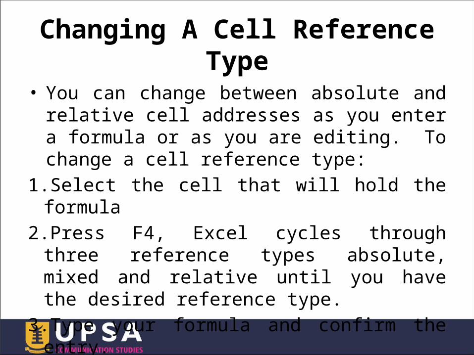
• You can change between absolute and relative cell addresses as you enter a formula or as you are editing. To change a cell reference type:

1.Select the cell that will hold the formula

2.Press F4, Excel cycles through three reference types absolute, mixed and relative until you have the desired reference type.

3.Type your formula and confirm the entry.

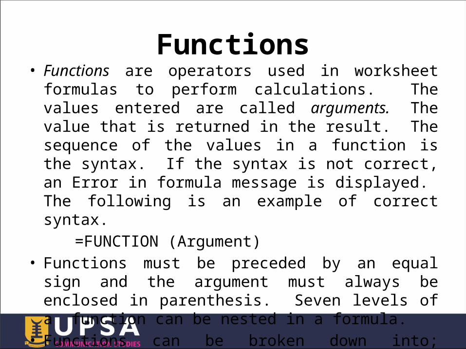
Functions• Functions are operators used in worksheet formulas to perform calculations. The values entered are called arguments. The value that is returned in the result. The sequence of the values in a function is the syntax. If the syntax is not correct, an Error in formula message is displayed. The following is an example of correct syntax.

=FUNCTION (Argument)• Functions must be preceded by an equal sign and the argument must always be enclosed in parenthesis. Seven levels of a function can be nested in a formula.

• Functions can be broken down into; financial, statistical, Text, Date and Time, Logical etc.

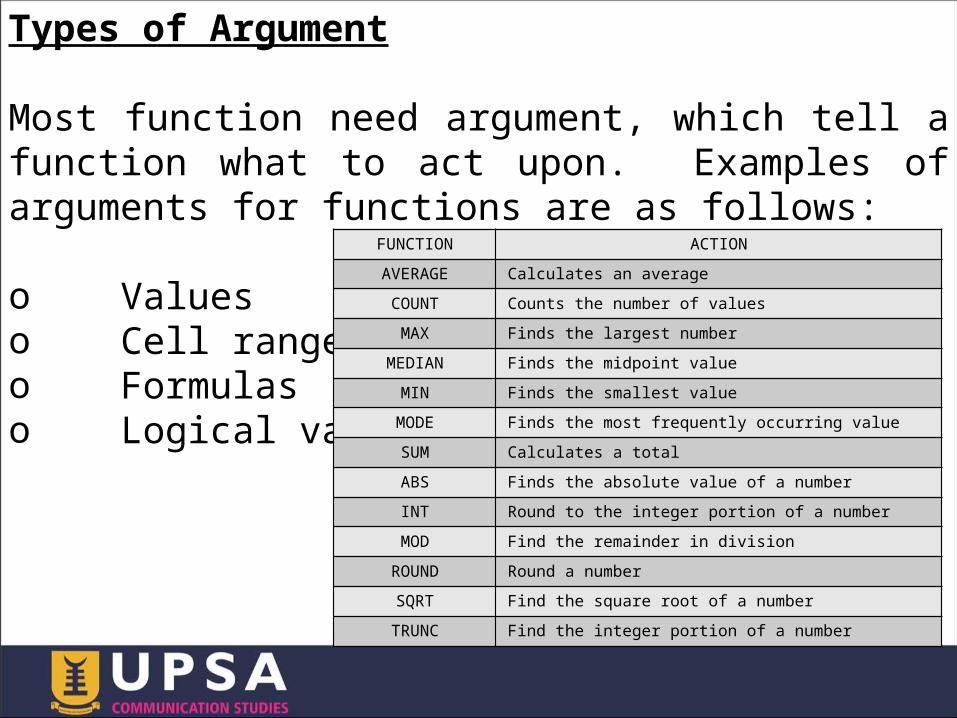
Types of Argument

Most function need argument, which tell a function what to act upon. Examples of arguments for functions are as follows:

o Valueso Cell rangeo Formulaso Logical values

FUNCTION ACTIONAVERAGE Calculates an averageCOUNT Counts the number of valuesMAX Finds the largest number

MEDIAN Finds the midpoint valueMIN Finds the smallest valueMODE Finds the most frequently occurring valueSUM Calculates a totalABS Finds the absolute value of a numberINT Round to the integer portion of a numberMOD Find the remainder in division

ROUND Round a numberSQRT Find the square root of a numberTRUNC Find the integer portion of a number

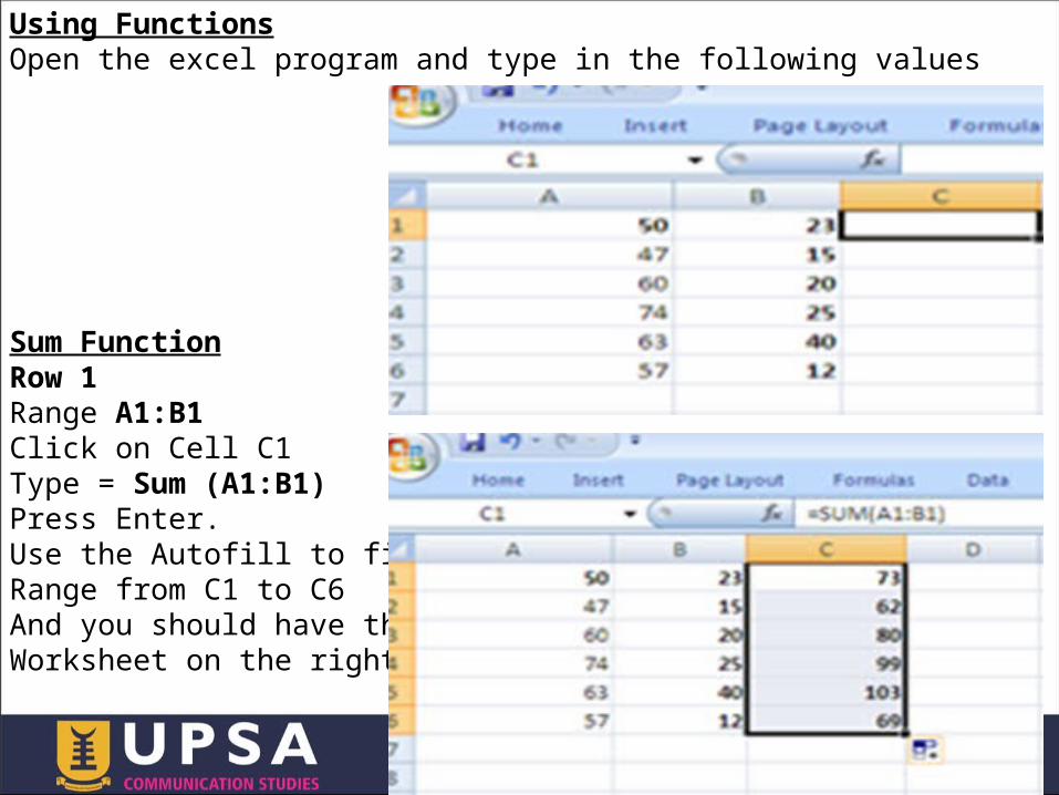
Using FunctionsOpen the excel program and type in the following values

Sum FunctionRow 1Range A1:B1Click on Cell C1Type = Sum (A1:B1)Press Enter.Use the Autofill to fill theRange from C1 to C6And you should have theWorksheet on the right.

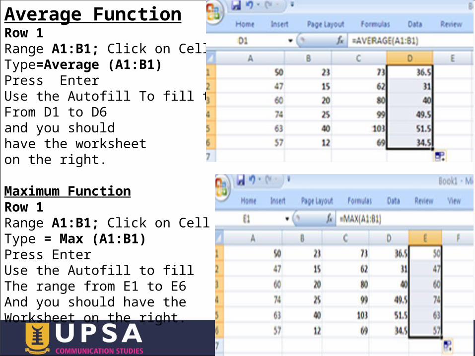
Average FunctionRow 1Range A1:B1; Click on Cell D1Type=Average (A1:B1)Press EnterUse the Autofill To fill the rangeFrom D1 to D6and you should have the worksheeton the right.

Maximum FunctionRow 1Range A1:B1; Click on Cell E1Type = Max (A1:B1)Press EnterUse the Autofill to fillThe range from E1 to E6And you should have the Worksheet on the right.

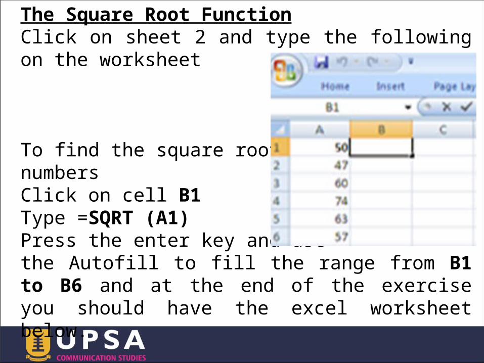
The Square Root FunctionClick on sheet 2 and type the following on the worksheet

To find the square root of the numbersClick on cell B1Type =SQRT (A1)Press the enter key and use the Autofill to fill the range from B1 to B6 and at the end of the exercise you should have the excel worksheet below.

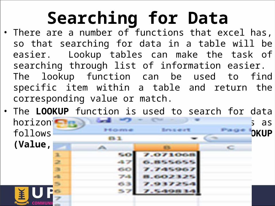
Searching for Data• There are a number of functions that excel has, so that searching for data in a table will be easier. Lookup tables can make the task of searching through list of information easier. The lookup function can be used to find specific item within a table and return the corresponding value or match.

• The LOOKUP function is used to search for data horizontally and vertically. The syntax is as follows: =VLOOKUP (Value, Array) =HLOOKUP (Value, Array)

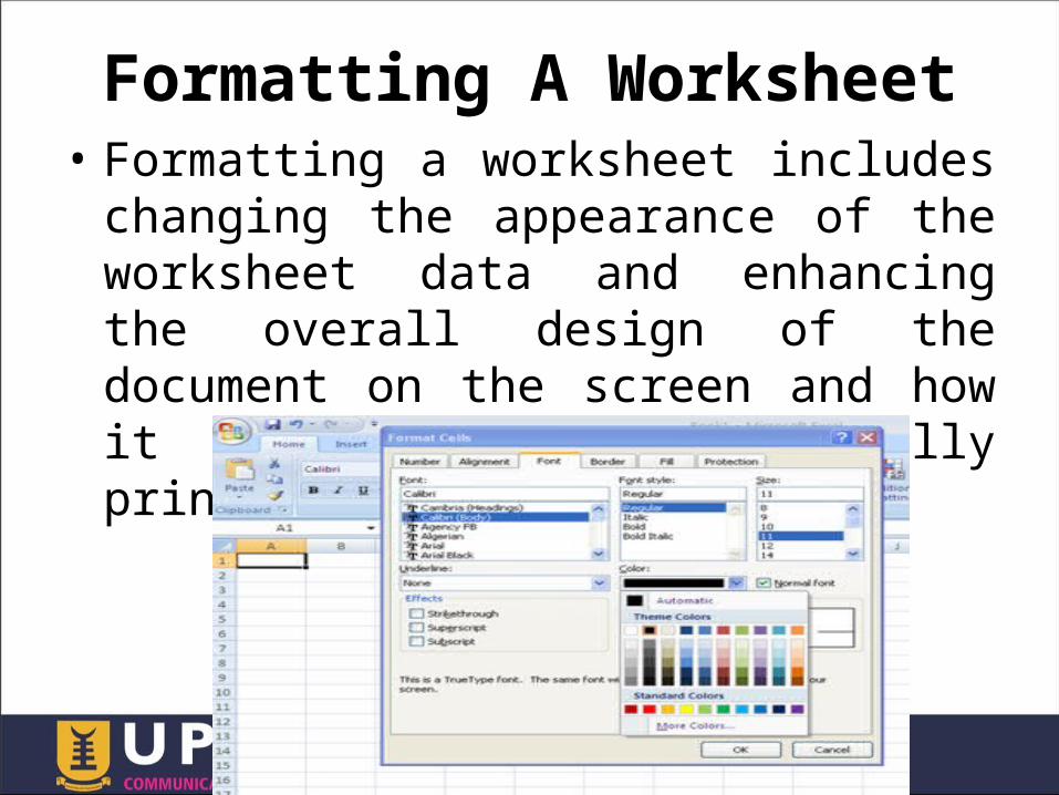
Formatting A Worksheet• Formatting a worksheet includes changing the appearance of the worksheet data and enhancing the overall design of the document on the screen and how it looks when it is finally printed.

• Select the range to which you want to apply the font

• Click on Home Tab and click on cells

• Click the font group and select the font you want from the font list box

• Click on OK.

Applying Fonts And Attributes

Applying Colours• Select the range to which you want to apply the font

• Click on Home Tab and Click on cells

• Click on the font group and• Choose colour• Select colour• Click on OK

Adding Borders• Borders are lines that can be added along any side of a range.

• To add borders.• Select the range of cells you want to border

• Click on Home Tab and click on cells• Click on the border tab, from the border group options choose the side of the range you want to border.

• Choose the border style from the style group option

• Click on OK.

Applying Patterns• Excel has a variety of patterns that you can use. Shading is the most popular type of pattern used.

• To add a pattern to a cell or range of cells:

1.Select the cell range2.Click on the Home Tab; click

on Format in the Cell Group; click on Format in the menu

3.Click on the Fill tab and use pattern colour or pattern style

Applying Automatic Format

• To apply the Auto Format• Select the cell range to format• Click on the Home tab• Click on either Format as Table or Cell Styles, select a Format style

• Click on OK

Using Graphics• One of the best ways to analyze worksheet data is to represent it graphically by creating a chart.

• A chart can quickly and efficiently tell the story of the worksheet.

Creating A Chart• A chart is therefore a graphical representation of worksheet data.

• In Excel charts can be done in the same worksheet or a separate worksheet.

• There are a lot of chart types that you can use. Bar (3-D), Pie (3-D), column (3-D), XY (Scatter), 3-D surface. Etc.

• Open Excel and type the information below in the cells.

• You are going to plot a graph of NAMES against MARKS.

• With the MARKS as Y-axis and NAMES as the X-axis.

ALBERT LEE

RAYMON AN

MERCY LUDHAM

DERRICK LUCAS

NATASHA BRAD

PHILLIPA MILLS

DAVID COLE

RUTH DAVIDSON

MARY ALISON

ERIC CLAPTON

0

20

40

60

80

100Examination

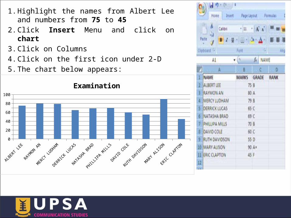
1.Highlight the names from Albert Lee and numbers from 75 to 45

2.Click Insert Menu and click on chart

3.Click on Columns4.Click on the first icon under 2-D5.The chart below appears:

Protecting A worksheet• To prevent against destruction of the worksheet, it is a must to protect the worksheet.

• Excel provides several ways of protecting worksheets and parts of worksheets.

• This will prevent against erasing critical formulae or value.

Protecting A worksheet• To Protect a Worksheet:1.Click on Review tab. 2.Click on any one of the several Protections 3.E.g. Click on Protect Sheet4.Type in the password to use in the textbox5.Select which part of the Sheet you want to protect6.Click on OK. Password can be applied so that those cells can only be unlocked if the password is known.• To Unprotect a Worksheet1.Click on Tools Menu,2.point to protection3.Click on Unprotect

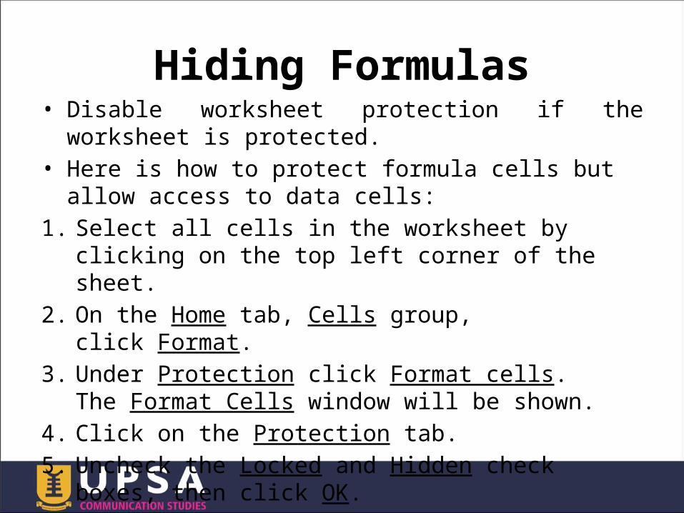
Hiding Formulas• Disable worksheet protection if the worksheet is protected.

• Here is how to protect formula cells but allow access to data cells:

1. Select all cells in the worksheet by clicking on the top left corner of the sheet.

2. On the Home tab, Cells group, click Format.

3. Under Protection click Format cells. The Format Cells window will be shown.

4. Click on the Protection tab.5. Uncheck the Locked and Hidden check

boxes, then click OK.

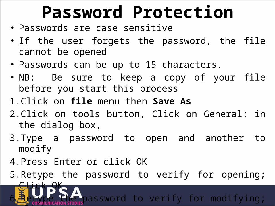
Password Protection• Passwords are case sensitive• If the user forgets the password, the file cannot be opened

• Passwords can be up to 15 characters.• NB: Be sure to keep a copy of your file before you start this process

1.Click on file menu then Save As2.Click on tools button, Click on General; in the dialog box,

3.Type a password to open and another to modify

4.Press Enter or click OK5.Retype the password to verify for opening; Click OK

6.Retype the password to verify for modifying; Click OK

7.Click on Save

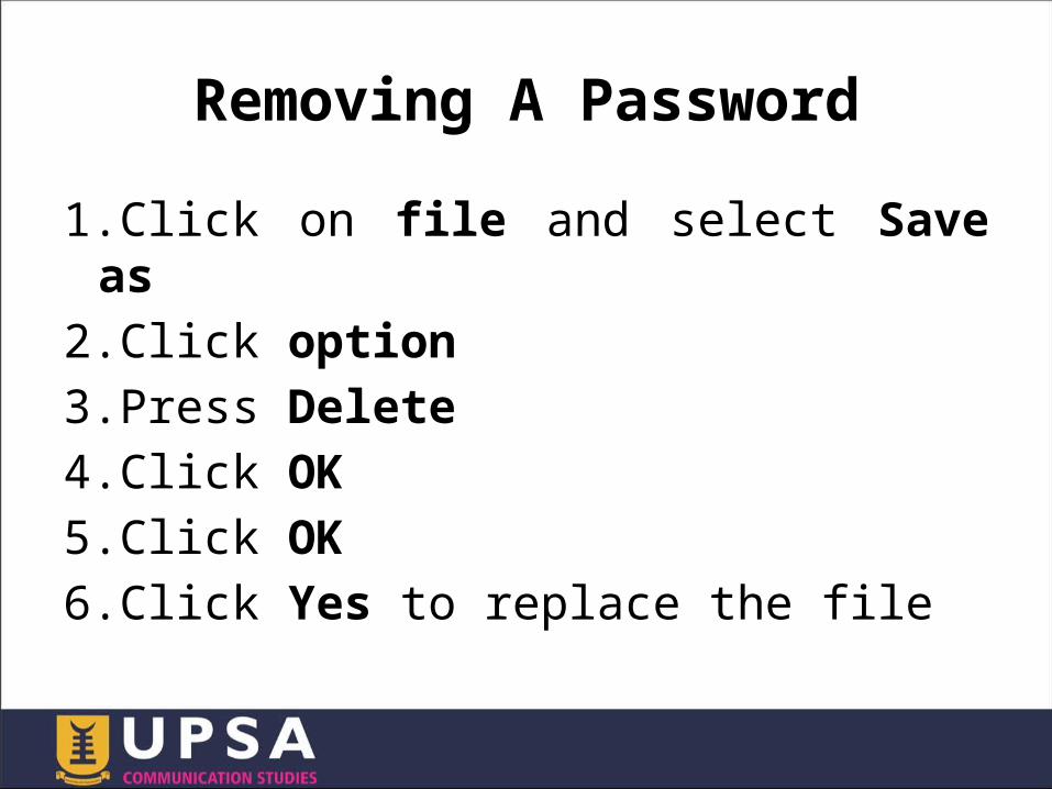
Removing A Password1.Click on file and select Save as

2.Click option3.Press Delete4.Click OK5.Click OK6.Click Yes to replace the file

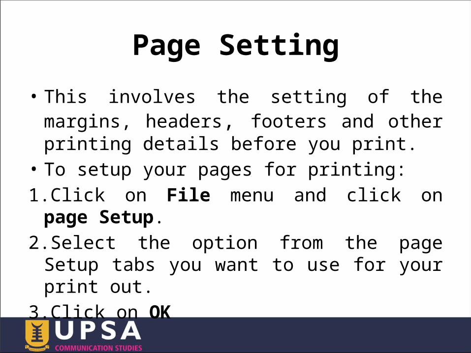
Page Setting• This involves the setting of the margins, headers, footers and other printing details before you print.

• To setup your pages for printing:1.Click on File menu and click on page Setup.

2.Select the option from the page Setup tabs you want to use for your print out.

3.Click on OK

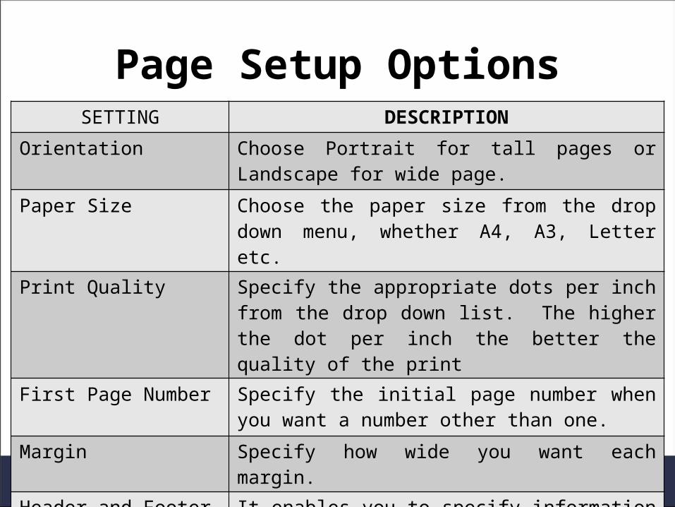
SETTING DESCRIPTIONOrientation Choose Portrait for tall pages or

Landscape for wide page.Paper Size Choose the paper size from the drop

down menu, whether A4, A3, Letter etc.

Print Quality Specify the appropriate dots per inch from the drop down list. The higher the dot per inch the better the quality of the print

First Page Number Specify the initial page number when you want a number other than one.

Margin Specify how wide you want each margin.

Header and Footer It enables you to specify information such as filename, date time, authors initials that will appear at the top or bottom of the printed page.

Page Setup Options

Function Keys & Their Actions

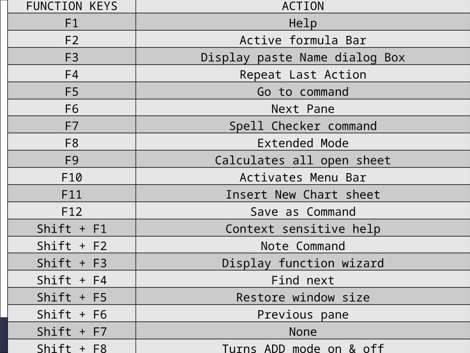
FUNCTION KEYS ACTIONF1 HelpF2 Active formula BarF3 Display paste Name dialog BoxF4 Repeat Last ActionF5 Go to commandF6 Next PaneF7 Spell Checker commandF8 Extended ModeF9 Calculates all open sheetF10 Activates Menu BarF11 Insert New Chart sheetF12 Save as Command

Shift + F1 Context sensitive helpShift + F2 Note CommandShift + F3 Display function wizardShift + F4 Find nextShift + F5 Restore window sizeShift + F6 Previous paneShift + F7 NoneShift + F8 Turns ADD mode on & offShift + F9 Calculates active worksheetShift + F10 Activates shortcut menu

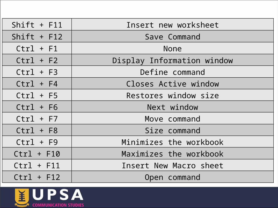
Shift + F11 Insert new worksheetShift + F12 Save CommandCtrl + F1 NoneCtrl + F2 Display Information windowCtrl + F3 Define commandCtrl + F4 Closes Active windowCtrl + F5 Restores window sizeCtrl + F6 Next windowCtrl + F7 Move commandCtrl + F8 Size commandCtrl + F9 Minimizes the workbookCtrl + F10 Maximizes the workbookCtrl + F11 Insert New Macro sheetCtrl + F12 Open command

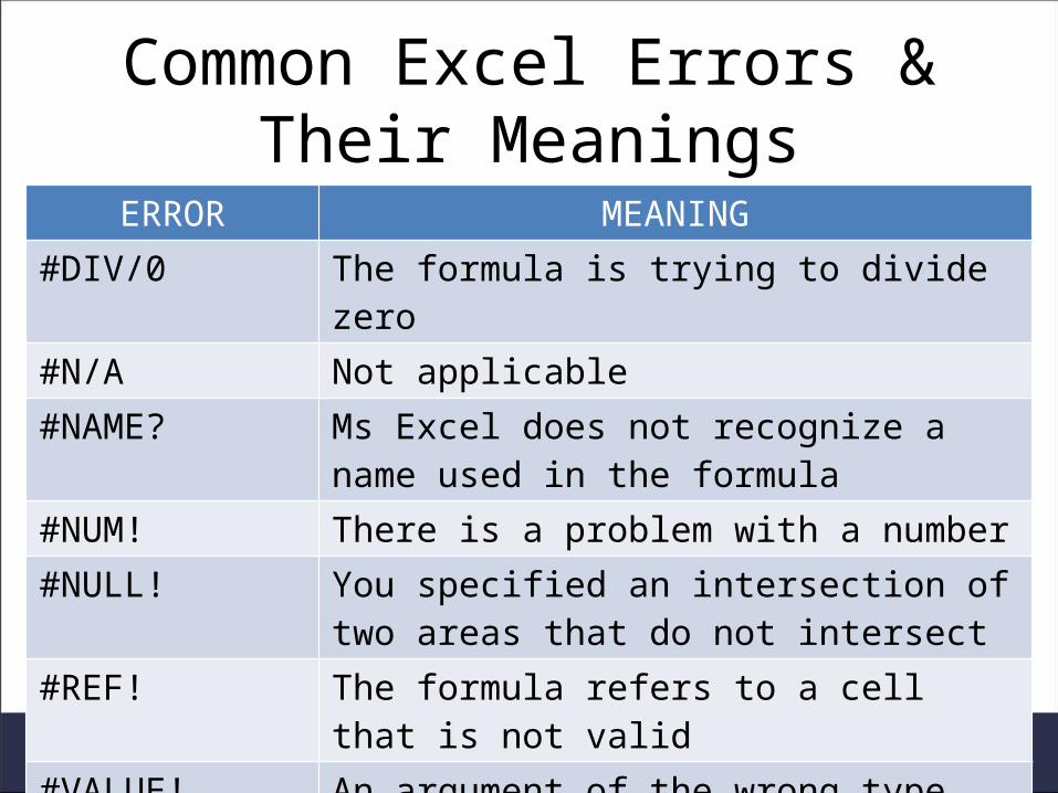
ERROR MEANING#DIV/0 The formula is trying to divide

zero#N/A Not applicable#NAME? Ms Excel does not recognize a

name used in the formula#NUM! There is a problem with a number#NULL! You specified an intersection of

two areas that do not intersect#REF! The formula refers to a cell

that is not valid#VALUE! An argument of the wrong type

Common Excel Errors & Their Meanings