Microeconomics

Chapter 3Chapter 3Elasticity of Demand Elasticity of Demand

and Supplyand Supply

Some terms to remember:Some terms to remember:

• ElasticityElasticity - the responsiveness of demand/supply to a change in its determinant.

• Price ElasticityPrice Elasticity - the percentage change in quantity compared to a percentage change in price.

• Arc ElasticityArc Elasticity - the coefficient of price elasticityof demand between 2 points along the demand curve.

• Point ElasticityPoint Elasticity - the coefficient of price elasticity of demand at one point along the demand curve.

• Coefficient of ElasticityCoefficient of Elasticity - absolute value of elasticity.

• Income Elasticity of DemandIncome Elasticity of Demand - percentage change in quantity demanded compared to the percentage change in income.

• Cross Elasticity of DemandCross Elasticity of Demand - percentage change in quantity demanded of one good compared to the percentage change in the price of a related good.

• Total RevenueTotal Revenue - price multiplied by quantity.

• Inferior GoodsInferior Goods - goods which are bought when income leves are low, the demand for which tends to decrease when income increases.

• Normal GoodsNormal Goods - goods for which demand tends to increase when income increases.

• Substitute GoodsSubstitute Goods - goods used in place of each other.

• Complementary GoodsComplementary Goods - goods that supplement each other and are, therefore, used together.

• Engel CurveEngel Curve - a curve depicting the quantities of a good the consumer is willing to buy at all income levels, assuming ceteris paribus.

• Prestige Goods Prestige Goods - are goods bought for the status and prestige they give to the consumer, and are bought when the prices are high.

• Price Elasticity of DemandPrice Elasticity of Demand - or the dgree of responsiveness of quantity demanded to a change in price is measured by dividing the percentage in quantity demanded by the percentage change in price.

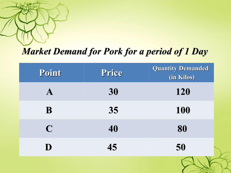
Market Demand for Pork for a period of 1 DayMarket Demand for Pork for a period of 1 Day

PointPoint PricePrice Quantity Demanded Quantity Demanded

(in Kilos)(in Kilos)

AA 3030 120120

BB 3535 100 100

CC 4040 8080

DD 4545 5050

• ElasticElastic - the percentage change in the percentage change in quantity demanded is higher than the quantity demanded is higher than the percentage change in price, the elasticity percentage change in price, the elasticity coefficient is greater than 1. coefficient is greater than 1.

• InelasticInelastic - - the percentage change in the percentage change in quantity demanded less than the quantity demanded less than the percentage change in price, the elasticity percentage change in price, the elasticity coefficient is less than 1.coefficient is less than 1.

• UnitaryUnitary - Should quantity demanded Should quantity demanded change in the same proportion as the change in the same proportion as the change in price, the elasticity coefficient change in price, the elasticity coefficient is equal to 1.is equal to 1.

• Price Elasticity of Demand has two Price Elasticity of Demand has two measures :measures :

1. Arc Elasticity1. Arc Elasticity - the coefficient of the - the coefficient of the price elasticity of demand between two price elasticity of demand between two points along the demand curve.points along the demand curve.

Q - change in quantity demandedQ - change in quantity demanded

P - change in priceP - change in price

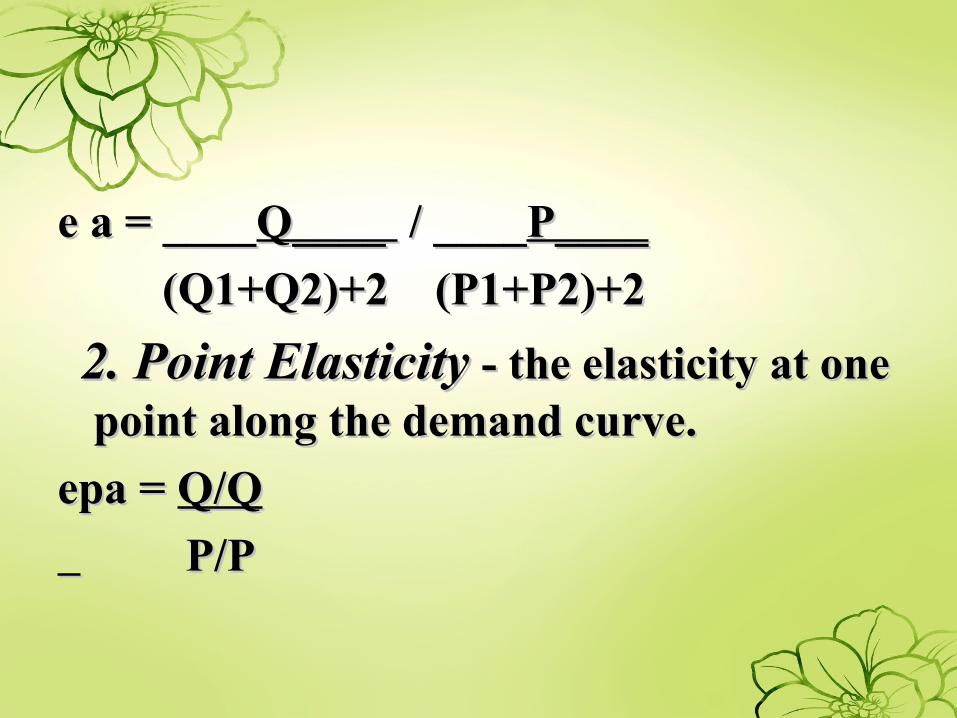
e a = ____e a = ____Q____ Q____ / ____ / ____P____P____

(Q1+Q2)+2 (P1+P2)+2(Q1+Q2)+2 (P1+P2)+2

2. Point Elasticity2. Point Elasticity - the elasticity at one - the elasticity at one point along the demand curve.point along the demand curve.

epa = epa = Q/QQ/Q

P/PP/P

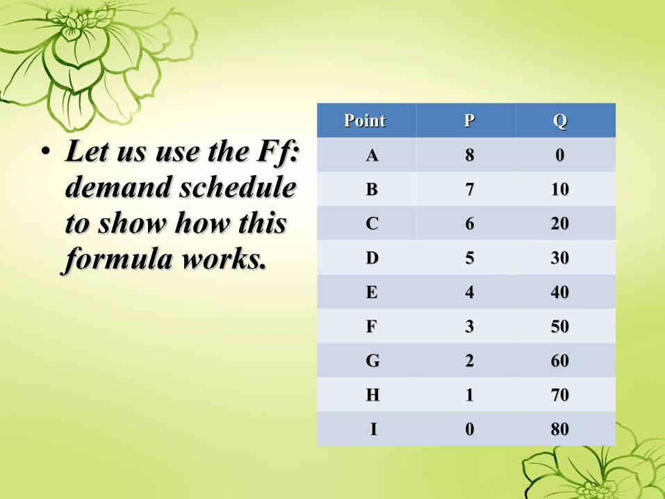
• Let us use the Ff: Let us use the Ff: demand schedule demand schedule to show how this to show how this formula works.formula works.

PointPoint PP QQ

AA 88 00

BB 77 1010

CC 66 2020

DD 55 3030

EE 44 4040

FF 33 5050

GG 22 6060

HH 11 7070

II 00 8080

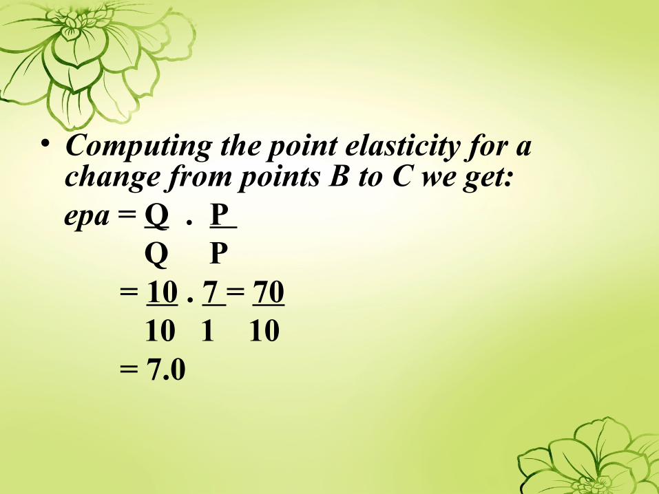
• Computing the point elasticity for a change from points B to C we get:

epa = Q . P Q P = 10 . 7 = 70 10 1 10 = 7.0

Thank You !!!Thank You !!!

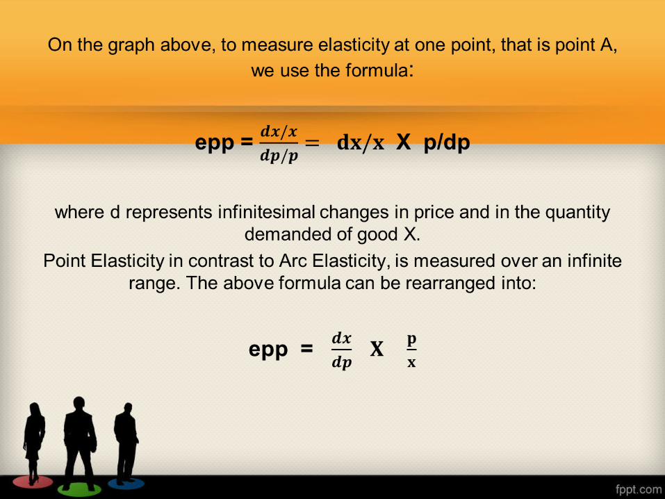
Point Elasticity

Point Elasticity

The measurement of point elasticity is more exact than that of arc elasticity.

It measures only one point on the demand curve, such as point A on the following

graph:

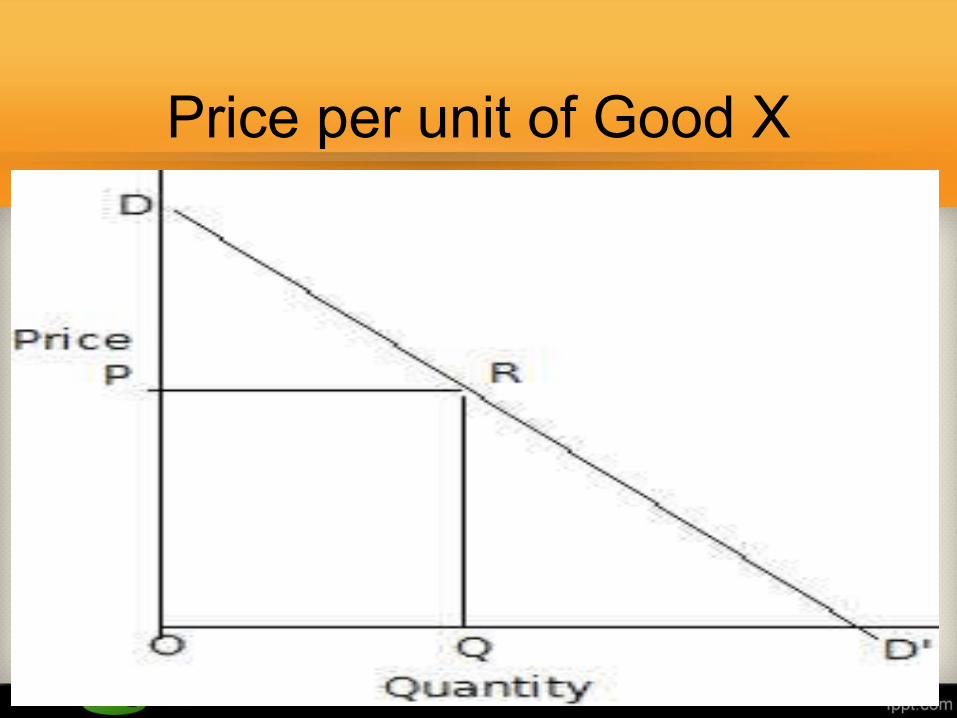
Price per unit of Good X

Arc Elasticity

• becomes point elasticity when the distance between the two points originally measured

becomes zero.

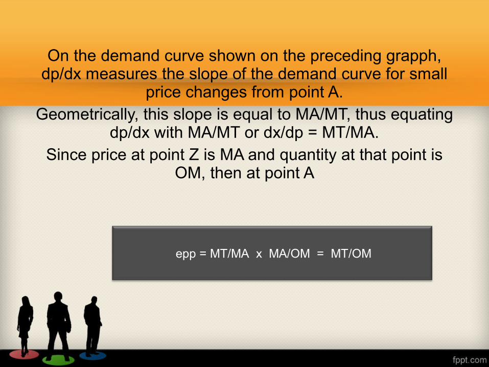
On the demand curve shown on the preceding grapph, dp/dx measures the slope of the demand curve for small

price changes from point A.Geometrically, this slope is equal to MA/MT, thus equating

dp/dx with MA/MT or dx/dp = MT/MA.Since price at point Z is MA and quantity at that point is

OM, then at point A

epp = MT/MA x MA/OM = MT/OM

Commodities and Their Elasticities

We already learned that the more essential a good is to the consumer, the more inelastic will be the demand for the

good.

The less of a necessity a good is, the more elastic is the demand for it.

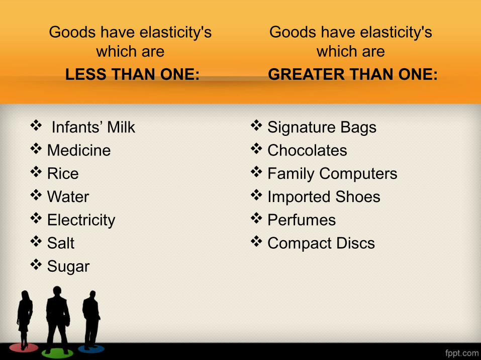
Infants’ Milk Medicine Rice Water Electricity Salt Sugar

Goods have elasticity's which are

GREATER THAN ONE:

Signature Bags Chocolates Family Computers Imported Shoes Perfumes Compact Discs

Goods have elasticity's which are

LESS THAN ONE:

Substitution and Price Elasticity of Demand

The degree of substitution betweem a products and related products determines its price elasticity of demand.

The extent of substitution depends on the substitution effect.

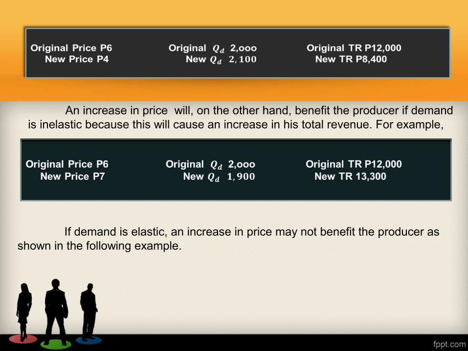
An increase in price will, on the other hand, benefit the producer if demand is inelastic because this will cause an increase in his total revenue. For example,

If demand is elastic, an increase in price may not benefit the producer as shown in the following example.

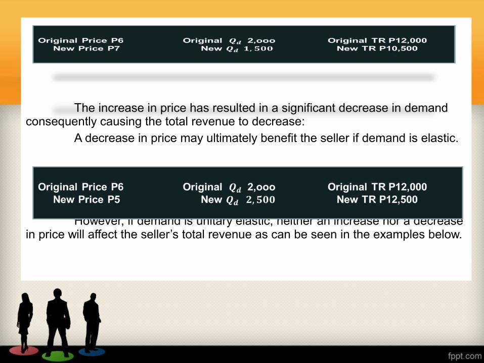
The increase in price has resulted in a significant decrease in demand consequently causing the total revenue to decrease:

A decrease in price may ultimately benefit the seller if demand is elastic.

However, if demand is unitary elastic, neither an increase nor a decrease in price will affect the seller’s total revenue as can be seen in the examples below.

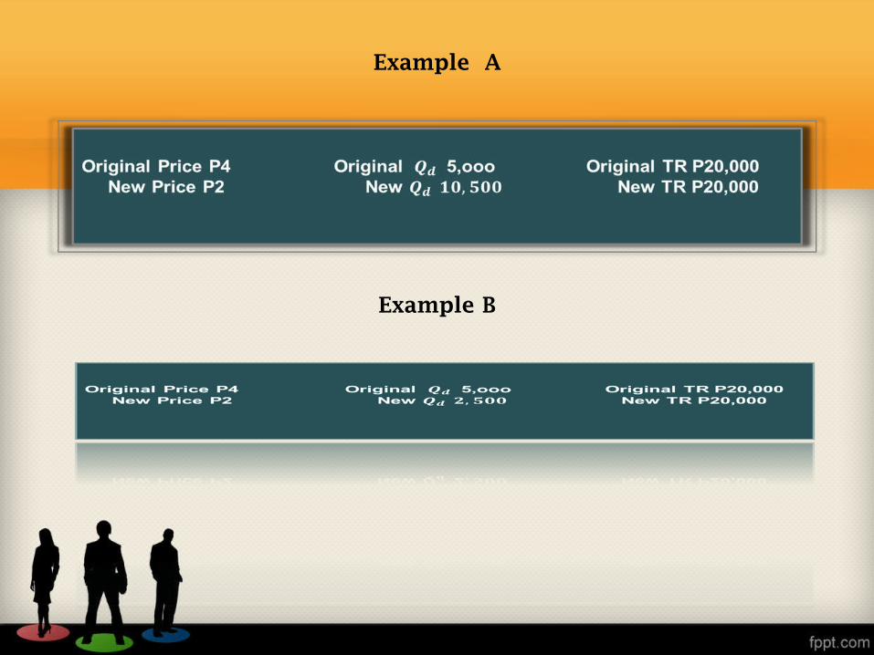
Example A

Example B

Thank You

* A change in price and quantity demanded (QD) can increase revenue and earnings depending on the price elasticity of demand

Elasticity condition

A decrease in price would increase earnings if demand were price elastic enough to stretch Quantity Demanded (QD) and revenue in order to offset the increase in in cost with more quantity produced

A seller can increase earnings with a decrease in price if the product were substitutable enough to wrest considerable demand from rival products to maximize elasticity.

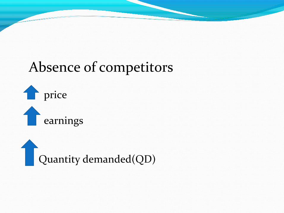
Absence of competitors price

earnings Quantity demanded(QD)

The Tax Burden When a good is sold a sales tax has to be paid to the

government on the sale of commodity

The buyer and the seller shoulders the burden is dependent mostly on the degree of elasticity of the demand for the goods

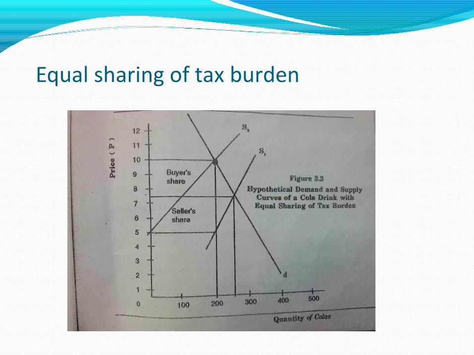
Equal sharing of tax burden

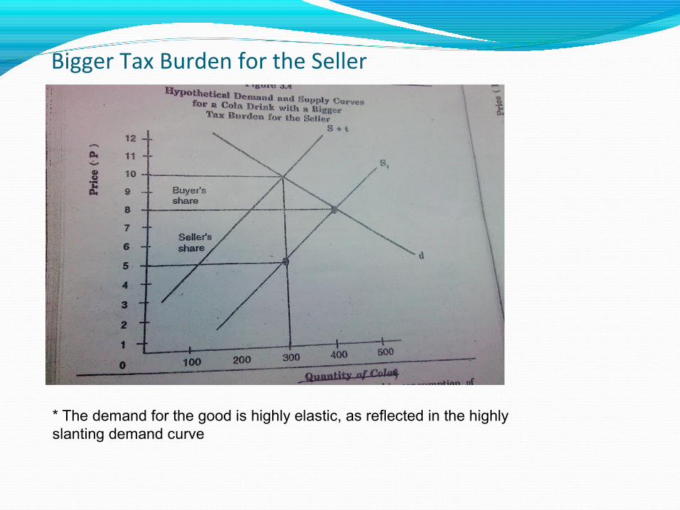
Bigger Tax Burden for the Seller

* The demand for the good is highly elastic, as reflected in the highly slanting demand curve

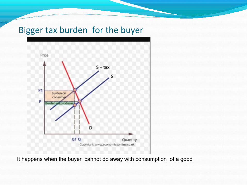
Bigger tax burden for the buyer

It happens when the buyer cannot do away with consumption of a good

A measure of the relationship between a change in the quantity demanded for a particular good and a change in real income. The formula for calculating income elasticity of demand is:

INCOME ELASTICITY OF DEMAND= % CHANGE IN DEMAND/% CHANGE IN INCOME

THREE TYPES OF GOODS:

1. SUPERIOR GOODS- is a good/service that you are more likely to purchase as your expendable income increases.

2. INFERIOR GOODS- Is a good/services that decreases in demand when consumer income rises(or rises in demand when consumer income decreases)

3. NORMAL GOODS-are those goods for which demand rises when income rises and falls when income falls.

ENGEL’S LAW

Economic theory that the proportion of income spent on food decreases as income increases, other factors remaining constant. This law does not suggest that the money spent on food falls with increase in income, but in instead that the percentage of income spent on food rises slower than the percentage increase in income.

CONSUMPTION LINE

Also termed propensity-to-consume line or consumption function, shows the relation between consumption expenditures and income for the households sector. The income measure commonly used is national income or disposable income. Occasionally a measure of aggregate production such as gross domestic product, is used instead

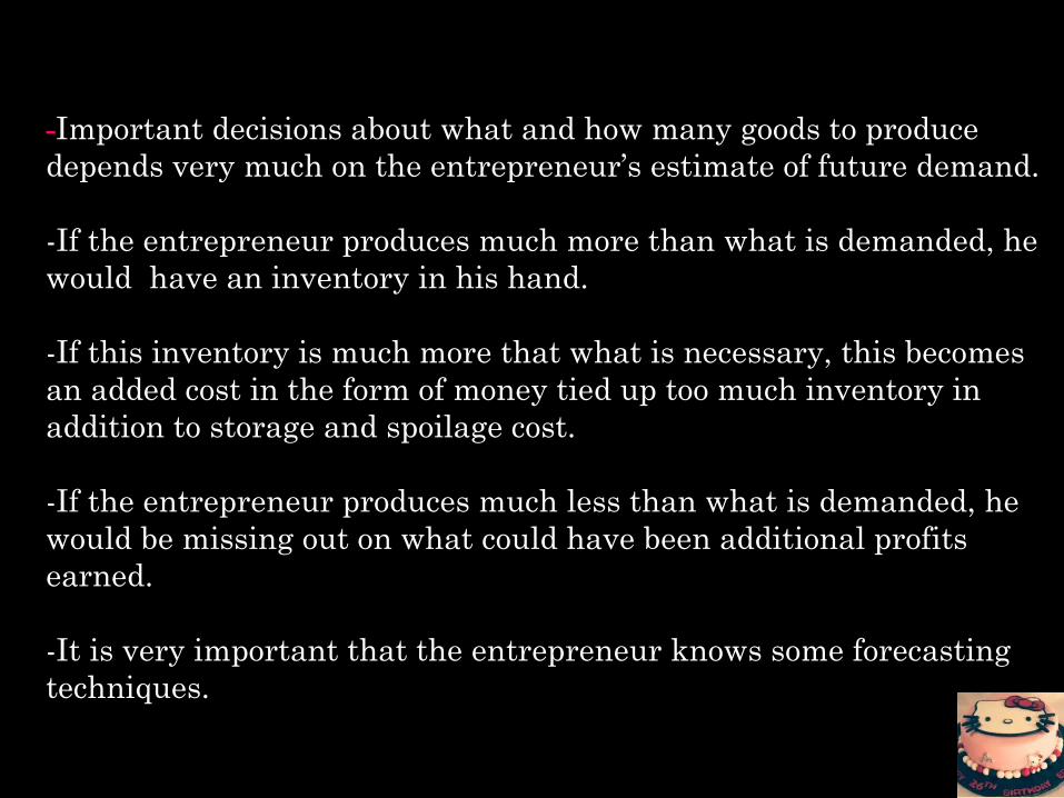
-Important decisions about what and how many goods to produce depends very much on the entrepreneur’s estimate of future demand.

-If the entrepreneur produces much more than what is demanded, he would have an inventory in his hand.

-If this inventory is much more that what is necessary, this becomes an added cost in the form of money tied up too much inventory in addition to storage and spoilage cost.

-If the entrepreneur produces much less than what is demanded, he would be missing out on what could have been additional profits earned.

-It is very important that the entrepreneur knows some forecasting techniques.

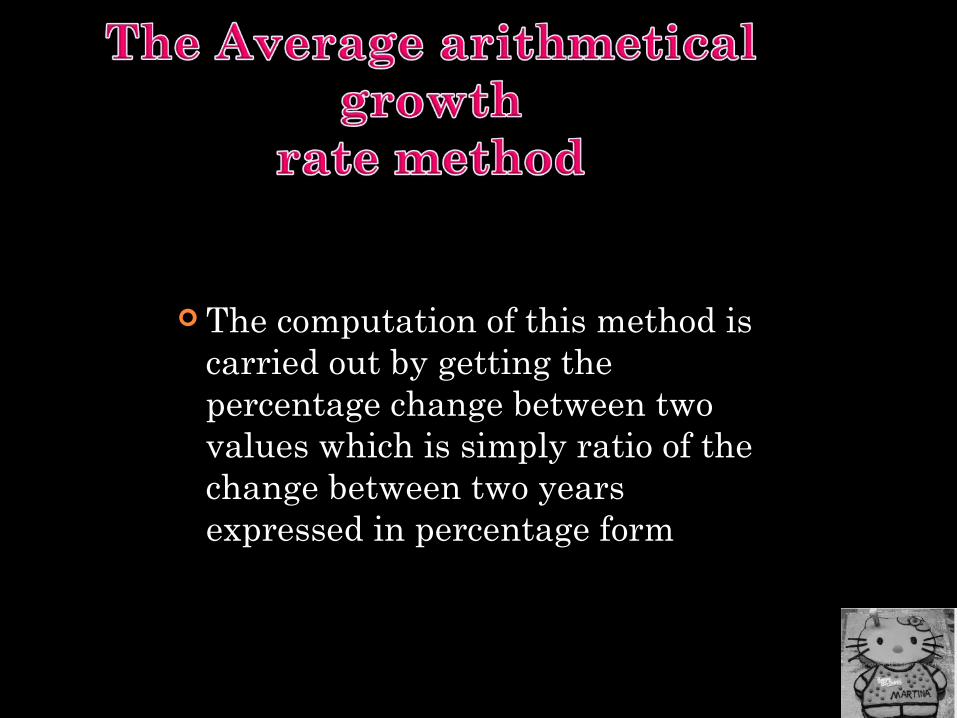
The computation of this method is carried out by getting the percentage change between two values which is simply ratio of the change between two years expressed in percentage form

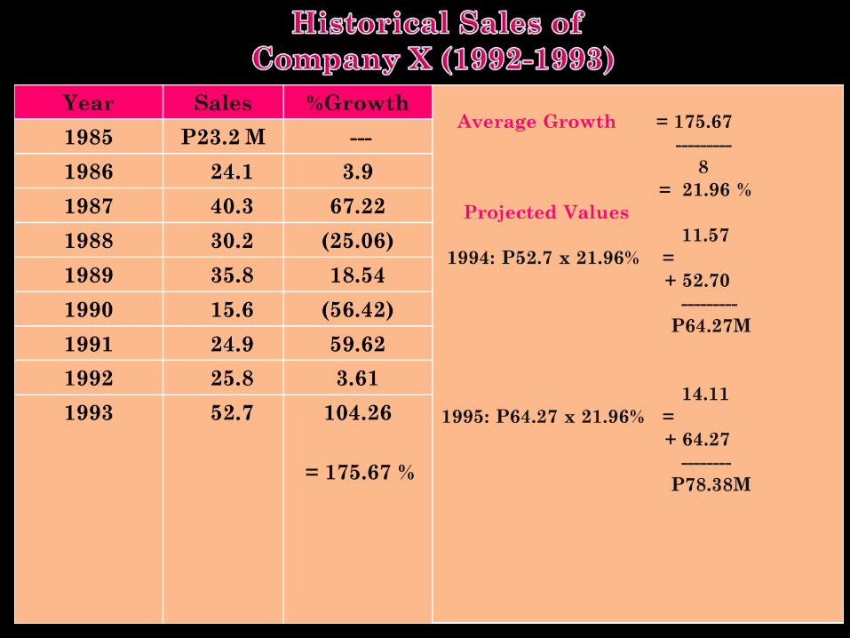
= 175.67 %

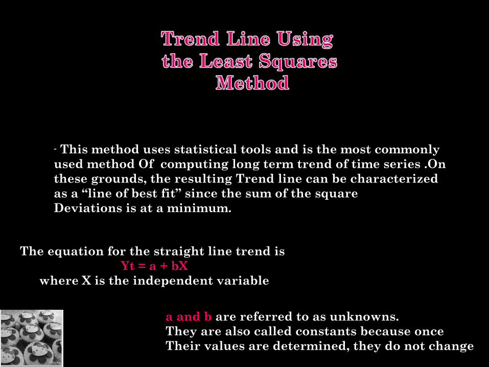
- This method uses statistical tools and is the most commonly used method Of computing long term trend of time series .On these grounds, the resulting Trend line can be characterized as a “line of best fit” since the sum of the squareDeviations is at a minimum.

The equation for the straight line trend is Yt = a + bX

where X is the independent variable

a and b are referred to as unknowns.They are also called constants because once Their values are determined, they do not change

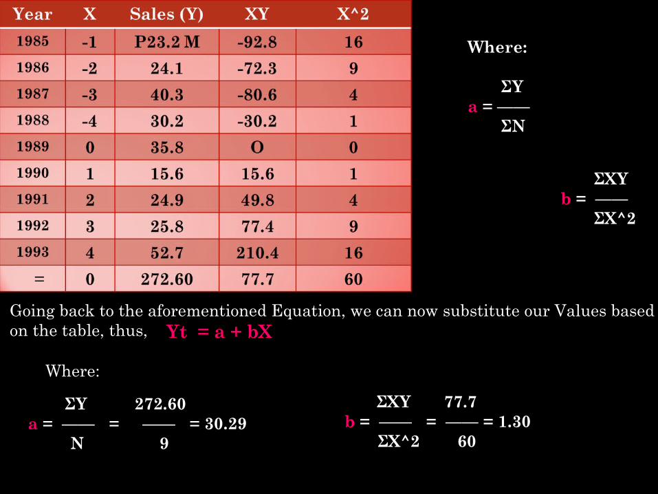
Where: ΣYa = —— ΣN

ΣXYb = —— ΣX^2

Going back to the aforementioned Equation, we can now substitute our Values based on the table, thus, Yt = a + bX

Where:

ΣY 272.60 a = —— = —— = 30.29 N 9

ΣXY 77.7 b = —— = —— = 1.30 ΣX^2 60

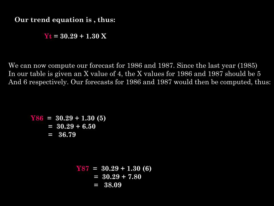
Our trend equation is , thus: Yt = 30.29 + 1.30 X

We can now compute our forecast for 1986 and 1987. Since the last year (1985)In our table is given an X value of 4, the X values for 1986 and 1987 should be 5 And 6 respectively. Our forecasts for 1986 and 1987 would then be computed, thus:

Y86 = 30.29 + 1.30 (5) = 30.29 + 6.50 = 36.79

Y87 = 30.29 + 1.30 (6) = 30.29 + 7.80 = 38.09