1. One assumption of the supply and demand model is that all goods bought and sold are identical. Why do you suppose economists commonly make this assumption? Does the supply and demand model lose its usefulness if goods are not identical? 1. Economists make this assumption, along with many others, in order to capture the meaningful relationships of the real world in simplified models. The models then can predict how variables within these relationships change in response to economic factors. If goods are not identical, many predictions of the model will still prove to be correct. However, we would be less confident in the predictions resting most heavily on that assumption. 2. List the assumptions of the supply and demand model. Then, for each assumption, give one example of a market in which the assumption is satisfied, and one example of a market in which that assumption is not satisfied. Is it reason- able to use the supply and demand model when assumptions are violated? 2. Assumption 1. We focus on supply and demand in a single market. This assumption is satisfied if we look at the market for hotel rooms in Lincoln, Nebraska, which is likely to be independent of the market for hotel rooms in other cities. This assumption is not satisfied if we look at the market for gold in Lincoln, Nebraska, which would be dependent on gold’s global supply and demand. Assumption 2. All goods sold in the market are identical. This assumption is satisfied if we look at the market for a commodity such as crude oil. If we look at shoes, the fact that there are countless distinctions between different types and styles of shoes means that the assumption is not satisfied. Assumption 3. All goods sold in the market sell for the same price, and everyone has the same information. This assumption is satisfied in a market such as retail gasoline stations. Although gas prices differ by a few cents per gallon between retailers, they match one another within a fairly close range. And prices are visible to anyone in the vicinity of the gas station. An example of a market where this assumption is not satisfied would be home furnishings. A furniture item such as a desk, for example, could have a significant price range, with the price of the most expensive desk being multiple times higher than that of an inexpensive one. Assumption 4. There are many buyers and sellers in the market. This assumption is satisfied in the market for fresh fruit, where there are many small orchards supplying produce and many consumers shopping for peaches, apples, oranges, and pears. In contrast, the market for intercity passenger rail transportation in the United States has only one seller: Amtrak. Such a market would not satisfy the assumption. The supply and demand model can still be useful even when these four assumptions are not met, because the basic economic relationships captured in the model apply even outside the boundaries of such assumptions. *3. The demand for organic carrots is given by the following equation: Q O D = 75 – 5 P O + P C + 2I where P O is the price of organic carrots, P C is the price of conventional carrots, and I is the average consumer income. Notice how this isn’t a standard demand curve that just relates the quantity of organic carrots demanded to the price of organic carrots. This demand function also describes how other factors affect demand—namely, the price of another good (conventional carrots) and income. a. Graph the inverse demand curve for organic carrots when P C = 5 and I = 10. What is the choke price? b. Using the demand curve drawn in (a), what is the quantity demanded of organic carrots when P O = 5? When P O = 10? c. Suppose P C increases to 15, while I remains at 10. Calculate the quantity demanded of organic carrots. Show the effects of this change on your graph and indicate the choke price. Has there been a change in the demand for organic carrots, or a change in the quantity demanded of organic carrots? Supply and Demand 2 1

Welcome message from author
This document is posted to help you gain knowledge. Please leave a comment to let me know what you think about it! Share it to your friends and learn new things together.
Transcript
1. One assumption of the supply and demand model is that all goods bought and sold are identical. Why do you suppose
economists commonly make this assumption? Does the supply and demand model lose its usefulness if goods are not
identical?
1. Economists make this assumption, along with many others, in order to capture the meaningful relationships of the
real world in simplifi ed models. The models then can predict how variables within these relationships change in
response to economic factors. If goods are not identical, many predictions of the model will still prove to be correct.
However, we would be less confi dent in the predictions resting most heavily on that assumption.
2. List the assumptions of the supply and demand model. Then, for each assumption, give one example of a market in
which the assumption is satisfi ed, and one example of a market in which that assumption is not satisfi ed. Is it reason-
able to use the supply and demand model when assumptions are violated?
2. Assumption 1. We focus on supply and demand in a single market. This assumption is satisfi ed if we look at the
market for hotel rooms in Lincoln, Nebraska, which is likely to be independent of the market for hotel rooms in
other cities. This assumption is not satisfi ed if we look at the market for gold in Lincoln, Nebraska, which would be
dependent on gold’s global supply and demand.
Assumption 2. All goods sold in the market are identical. This assumption is satisfi ed if we look at the market
for a commodity such as crude oil. If we look at shoes, the fact that there are countless distinctions between different
types and styles of shoes means that the assumption is not satisfi ed.
Assumption 3. All goods sold in the market sell for the same price, and everyone has the same information. This
assumption is satisfi ed in a market such as retail gasoline stations. Although gas prices differ by a few cents per
gallon between retailers, they match one another within a fairly close range. And prices are visible to anyone in the
vicinity of the gas station. An example of a market where this assumption is not satisfi ed would be home furnishings.
A furniture item such as a desk, for example, could have a signifi cant price range, with the price of the most expensive
desk being multiple times higher than that of an inexpensive one.
Assumption 4. There are many buyers and sellers in the market. This assumption is satisfi ed in the market for
fresh fruit, where there are many small orchards supplying produce and many consumers shopping for peaches,
apples, oranges, and pears. In contrast, the market for intercity passenger rail transportation in the United States has
only one seller: Amtrak. Such a market would not satisfy the assumption.
The supply and demand model can still be useful even when these four assumptions are not met, because the
basic economic relationships captured in the model apply even outside the boundaries of such assumptions.
*3. The demand for organic carrots is given by the following equation:
Q O D = 75 – 5 P O + P C + 2I
where P O is the price of organic carrots, P C is the price of conventional carrots, and I is the average consumer income.
Notice how this isn’t a standard demand curve that just relates the quantity of organic carrots demanded to the price of
organic carrots. This demand function also describes how other factors affect demand — namely, the price of another
good (conventional carrots) and income.
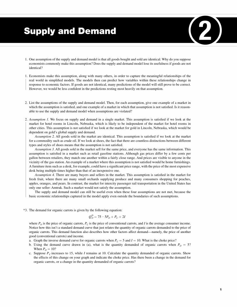
a. Graph the inverse demand curve for organic carrots when P C = 5 and I = 10. What is the choke price?
b. Using the demand curve drawn in (a), what is the quantity demanded of organic carrots when P O = 5?
When P O = 10?
c. Suppose P C increases to 15, while I remains at 10. Calculate the quantity demanded of organic carrots. Show
the effects of this change on your graph and indicate the choke price. Has there been a change in the demand for
organic carrots, or a change in the quantity demanded of organic carrots?
Supply and Demand 2
1
Goolsbee2e_Solutions_Manual_Ch02.indd 1Goolsbee2e_Solutions_Manual_Ch02.indd 1 30/09/15 9:33 AM30/09/15 9:33 AM
Microeconomics 2nd Edition Goolsbee Solutions ManualFull Download: https://testbanklive.com/download/microeconomics-2nd-edition-goolsbee-solutions-manual/
Full download all chapters instantly please go to Solutions Manual, Test Bank site: testbanklive.com
2 Part 1 Basic Concepts
d. What happens to the demand for organic carrots when the price of conventional carrots increases? Are organic and
conventional carrots complements or substitutes? How do you know?
e. What happens to the demand for organic carrots when the average consumer’s income increases? Are carrots a
normal or an inferior good?
3. a. We begin with the demand equation and substitute
the given values for P C and I:
Q O D = 75 – 5 P O + P C + 2I
Q O D = 75 – 5 P O + 5 + (2 × 10)
This simplifi es to
Q O D = 100 – 5 P O
To fi nd the inverse demand curve, we want to rear-
range terms to express P as a function of Q:
5 P O = 100 – Q O D
P O = 20 – 0.2 Q O D
The choke price can be found by solving for the price that corresponds to a quantity demanded of zero:
P O = 20 – (0.2 × 0) = 20
b. Substitute 5 for P O in the demand function to fi nd Q O D :
Q O D = 100 – 5 P O = 100 – 5(5) = 75
Substitute 10 for P O in the inverse demand function to fi nd Q O D :
P O = 20 – 0.2 Q O D
10 = 20 – 0.2 Q O D
10 = 0.2 Q O D
50 = Q O D
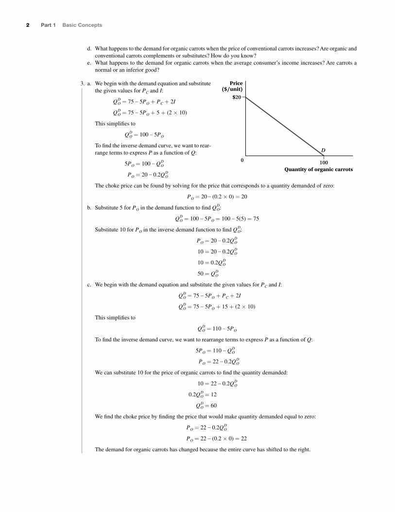
c. We begin with the demand equation and substitute the given values for P C and I:
Q O D = 75 – 5 P O + P C + 2I
Q O D = 75 – 5 P O + 15 + (2 × 10)
This simplifi es to
Q O D = 110 – 5 P O
To fi nd the inverse demand curve, we want to rearrange terms to express P as a function of Q:
5 P O = 110 – Q O D
P O = 22 – 0.2 Q O D
We can substitute 10 for the price of organic carrots to fi nd the quantity demanded:
10 = 22 – 0.2 Q O D
0.2 Q O D = 12
Q O D = 60
We fi nd the choke price by fi nding the price that would make quantity demanded equal to zero:
P O = 22 – 0.2 Q O D
P O = 22 – (0.2 × 0) = 22
The demand for organic carrots has changed because the entire curve has shifted to the right.
Quantity of organic carrots
Price($/unit)
$20
1000
D
Goolsbee2e_Solutions_Manual_Ch02.indd 2Goolsbee2e_Solutions_Manual_Ch02.indd 2 30/09/15 9:33 AM30/09/15 9:33 AM
Supply and Demand Chapter 2 3
d. The demand for organic carrots has increased, shift-
ing the demand curve to the right. This shows that the
two goods are substitutes for one another, because an
increase in the price of conventional carrots has led to
a higher quantity of organic carrots demanded at any
given price.
e. There is a positive coeffi cient (+2) on the variable
for income. This means that an increase in income
will shift the demand for organic carrots to the right.
As a consequence, we know that organic carrots are a
normal good.
*4. Out of the following events, which are likely to cause the demand for coffee to increase? Explain your answers.
a. An increase in the price of tea
b. An increase in the price of doughnuts
c. A decrease in the price of coffee
d. The Surgeon General’s announcement that drinking coffee lowers the risk of heart disease
e. Heavy rains causing a record-low coffee harvest in Colombia
4. a. Since tea and coffee are the classic examples of substitutes, as the price of tea increases, the demand for coffee is
likely to increase.
b. An increase in the price of doughnuts decreases the quantity demanded of doughnuts. Because doughnuts and
coffee are complements, this will likely decrease the demand for coffee.
c. A decrease in the price of coffee will decrease the quantity demanded of coffee via a movement along the demand
curve.
d. The Surgeon General’s announcement will likely increase the number of people who are interested in drinking
coffee and, thus, increase the demand for coffee.
e. Heavy rain will decrease the supply of coffee. This can be shown as an inward shift of the supply curve. As a
result, the equilibrium price increases and the equilibrium quantity decreases. This adjustment is accomplished
via a movement along the demand curve.
5. How is each of the following events likely to shift the supply curve or the demand curve for fast-food hamburgers in
the United States? Make sure you indicate which curve (curves) is affected and if it shifts out or in.
a. The price of beef triples.
b. The price of chicken falls by half.
c. The number of teenagers in the economy falls due to population aging.
d. Mad cow disease, a rare but fatal medical condition caused by eating tainted beef, becomes common in the United
States.
e. The Food and Drug Administration publishes a report stating that a certain weight-loss diet, which encourages the
intake of large amounts of meat, is dangerous to one’s health.
f. An inexpensive new grill for home use that makes delicious hamburgers is heavily advertised on television.
g. The minimum wage rises.
5. a. An increase in the price of beef represents an increase in the cost of an input. This will cause the supply curve to
shift in as the production becomes more expensive.
b. Demand for fast-food hamburgers in the United States will likely shift in since many consumers see chicken and beef
as substitutes. As chicken becomes less expensive, more people will consume chicken and reduce their consumption
of hamburgers, resulting in a decrease in the demand for fast-food hamburgers.
c. The demand curve shifts in.
d. Consumers’ awareness of the mad cow disease shifts the demand for fast-food hamburgers in.
e. Fewer people will follow this diet, causing the demand curve to shift in.
f. As consumers purchase the advertised inexpensive new grill, they are more likely to prepare hamburgers at home.
Given that at-home hamburgers and fast-food hamburgers are likely to be substitutes in the minds of consumers,
the demand for fast-food hamburgers can be expected to shift in.
g. An increase in the minimum wage increases the supplier’s cost of production, which leads to a decrease in supply.
This is shown as a shifting in of the supply curve.
Quantity of organic carrots
Price($/unit)
$2220
10
11010060500
D2D1
Goolsbee2e_Solutions_Manual_Ch02.indd 3Goolsbee2e_Solutions_Manual_Ch02.indd 3 30/09/15 9:33 AM30/09/15 9:33 AM

4 Part 1 Basic Concepts
6. The supply of wheat is given by the following equation:
Q W S = – 6 + 4 P W – 2 P C – P F
where Q W S is the quantity of wheat supplied, in millions of bushels; P W is the price of wheat per bushel; P C is the price
of corn per bushel; and P F is the price of tractor fuel per gallon.
a. Graph the inverse supply curve when corn sells for $4 a bushel and fuel sells for $2 a gallon. What is the supply
choke price?
b. How much wheat will be supplied at a price of $4? $8?
c. What will happen to the supply of wheat if the price of corn increases to $6 per bushel? Explain intuitively; then
graph the new inverse supply carefully and indicate the new choke price.
d. Suppose instead that the price of corn remains $4, but the price of fuel decreases to $1. What will happen to the
supply of wheat as a result? Explain intuitively; then graph the new inverse supply. Be sure to indicate the new
choke price.
6. a. We begin with the supply equation and substitute val-
ues for the price of corn and the price of tractor fuel:
Q W S = – 6 + 4 P W – 2PC – PF
Q W S = – 6 + 4 P W – (2 × 4) – 2
Q W S = –16 + 4 P W
Now we rearrange terms to express price as a func-
tion of quantity supplied:
4 P W = 16 + Q W S
P W = 4 + 0.25 Q W S
To fi nd the price that would make quantity supplied equal to zero, substitute a zero for Q W S :
P W = 4 + (0.25 × 0) = 4
The supply choke price is 4.
b. Using the supply equation, when P W = 4:
Q W S = –16 + (4 × 4) = –16 + 16 = 0
When PW = 8:
Q W S = –16 + (4 × 8) = –16 + 32 = 16
c. Wheat and corn are substitutes in production, so an
increase in the selling price of corn that causes farm-
ers to grow more corn will decrease the supply of
wheat. Start with the supply equation again, substi-
tuting the value of 6 for the price of corn and 2 for the
price of fuel:
Q W S = – 6 + 4 P W – 2PC – PF
Q W S = – 6 + 4 P W – (2 × 6) – 2
Q W S = –20 + 4 P W
Convert this to an inverse supply function by express-
ing price as a function of quantity:
Q W S = –20 + 4 P W
4 P W = 20 + Q W S
P W = 5 + 0.25 Q W S
The price that would make Q W S equal to zero is 5. This is the supply choke price.
4$5
Quantity
Price($/unit)
S1
S2
$4
Quantity
S
Price($/unit)
Goolsbee2e_Solutions_Manual_Ch02.indd 4Goolsbee2e_Solutions_Manual_Ch02.indd 4 30/09/15 9:33 AM30/09/15 9:33 AM
Supply and Demand Chapter 2 5
d. Start with the supply equation again, substituting the
value of 4 for the price of corn and the value of 1 for
the price of fuel:
Q W S = – 6 + 4 P W – 2 P C – P F
Q W S = – 6 + 4 P W – (2 × 4) – 1
Q W S = –15 + 4 P W
Convert this to an inverse supply function by express-
ing price as a function of quantity:
4 P W = 15 + Q W S
4 P W = 15 + Q W S
P W = 3.75 + 0.25 Q W S
At a price of 3.75, quantity supplied would be zero. This is the supply choke price.
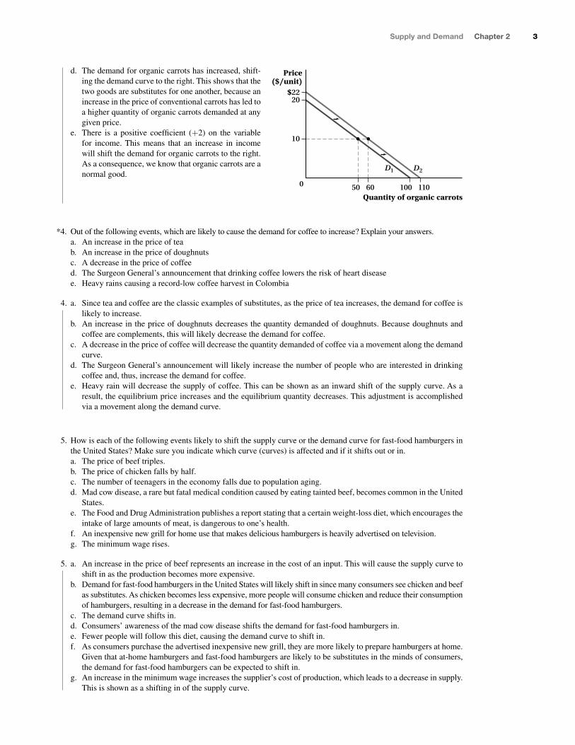
7. Collectors of vintage lightning rods formerly had to drift from antique store to antique store hoping to fi nd a lightning
rod for sale. The invention of the Internet reduced the cost of fi nding lighting rods available for sale.
a. Draw a diagram showing how the invention and popularization of the Internet have caused the demand curve for
lightning rods to shift.
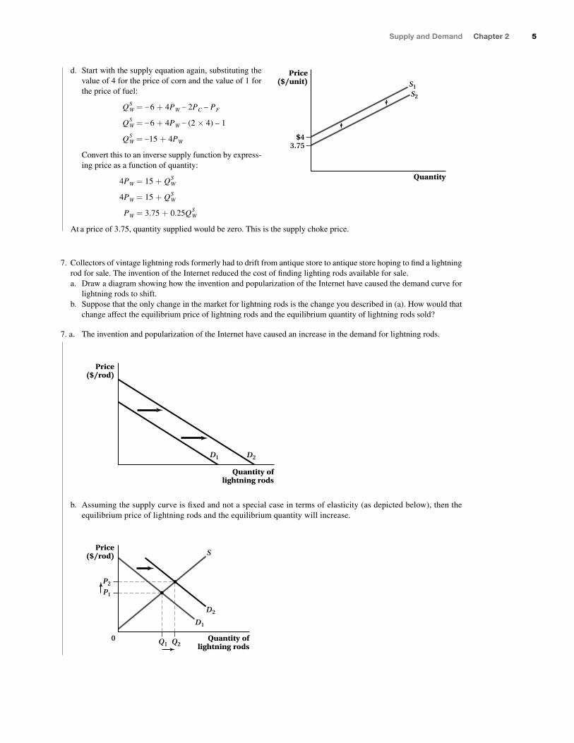
b. Suppose that the only change in the market for lightning rods is the change you described in (a). How would that
change affect the equilibrium price of lightning rods and the equilibrium quantity of lightning rods sold?
7. a. The invention and popularization of the Internet have caused an increase in the demand for lightning rods.
Quantity oflightning rods
Price($/rod)
D2D1
b. Assuming the supply curve is fi xed and not a special case in terms of elasticity (as depicted below), then the
equilibrium price of lightning rods and the equilibrium quantity will increase.
Price($/rod)
0 Quantity oflightning rods
S
D1
D2
P1
Q1 Q2
P2
$43.75
Quantity
Price($/unit) S1
S2
Goolsbee2e_Solutions_Manual_Ch02.indd 5Goolsbee2e_Solutions_Manual_Ch02.indd 5 30/09/15 9:33 AM30/09/15 9:33 AM
6 Part 1 Basic Concepts
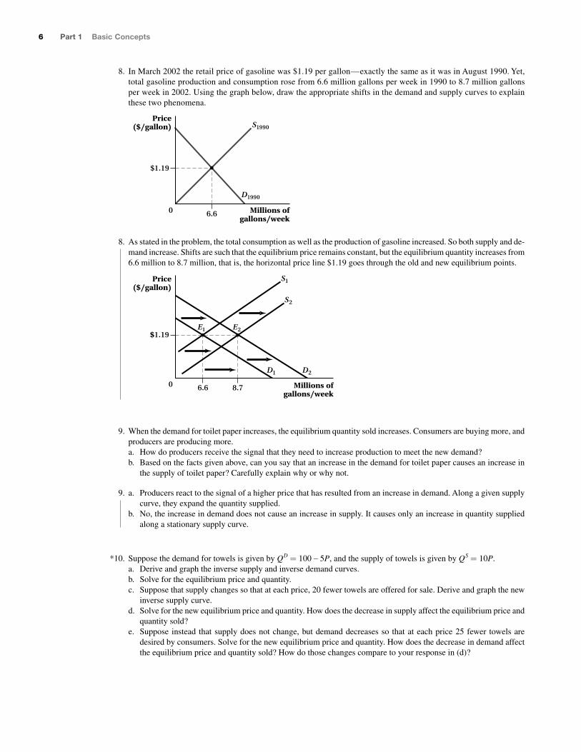
8. In March 2002 the retail price of gasoline was $1.19 per gallon — exactly the same as it was in August 1990. Yet,
total gasoline production and consumption rose from 6.6 million gallons per week in 1990 to 8.7 million gallons
per week in 2002. Using the graph below, draw the appropriate shifts in the demand and supply curves to explain
these two phenomena.
6.6
$1.19
Price($/gallon)
0 Millions ofgallons/week
S1990
D1990
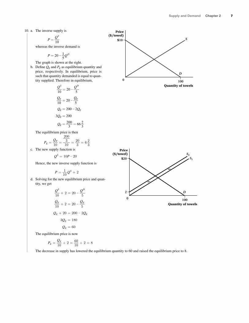
8. As stated in the problem, the total consumption as well as the production of gasoline increased. So both supply and de-
mand increase. Shifts are such that the equilibrium price remains constant, but the equilibrium quantity increases from
6.6 million to 8.7 million, that is, the horizontal price line $1.19 goes through the old and new equilibrium points.
Millions ofgallons/week
Price($/gallon)
$1.19
D2
S2
D1
S1
0
E2E1
6.6 8.7
9. When the demand for toilet paper increases, the equilibrium quantity sold increases. Consumers are buying more, and
producers are producing more.
a. How do producers receive the signal that they need to increase production to meet the new demand?
b. Based on the facts given above, can you say that an increase in the demand for toilet paper causes an increase in
the supply of toilet paper? Carefully explain why or why not.
9. a. Producers react to the signal of a higher price that has resulted from an increase in demand. Along a given supply
curve, they expand the quantity supplied.
b. No, the increase in demand does not cause an increase in supply. It causes only an increase in quantity supplied
along a stationary supply curve.
10. Suppose the demand for towels is given by Q D = 100 – 5P, and the supply of towels is given by Q S = 10P.
a. Derive and graph the inverse supply and inverse demand curves.
b. Solve for the equilibrium price and quantity.
c. Suppose that supply changes so that at each price, 20 fewer towels are offered for sale. Derive and graph the new
inverse supply curve.
d. Solve for the new equilibrium price and quantity. How does the decrease in supply affect the equilibrium price and
quantity sold?
e. Suppose instead that supply does not change, but demand decreases so that at each price 25 fewer towels are
desired by consumers. Solve for the new equilibrium price and quantity. How does the decrease in demand affect
the equilibrium price and quantity sold? How do those changes compare to your response in (d)?
*
Goolsbee2e_Solutions_Manual_Ch02.indd 6Goolsbee2e_Solutions_Manual_Ch02.indd 6 30/09/15 9:33 AM30/09/15 9:33 AM
Supply and Demand Chapter 2 7
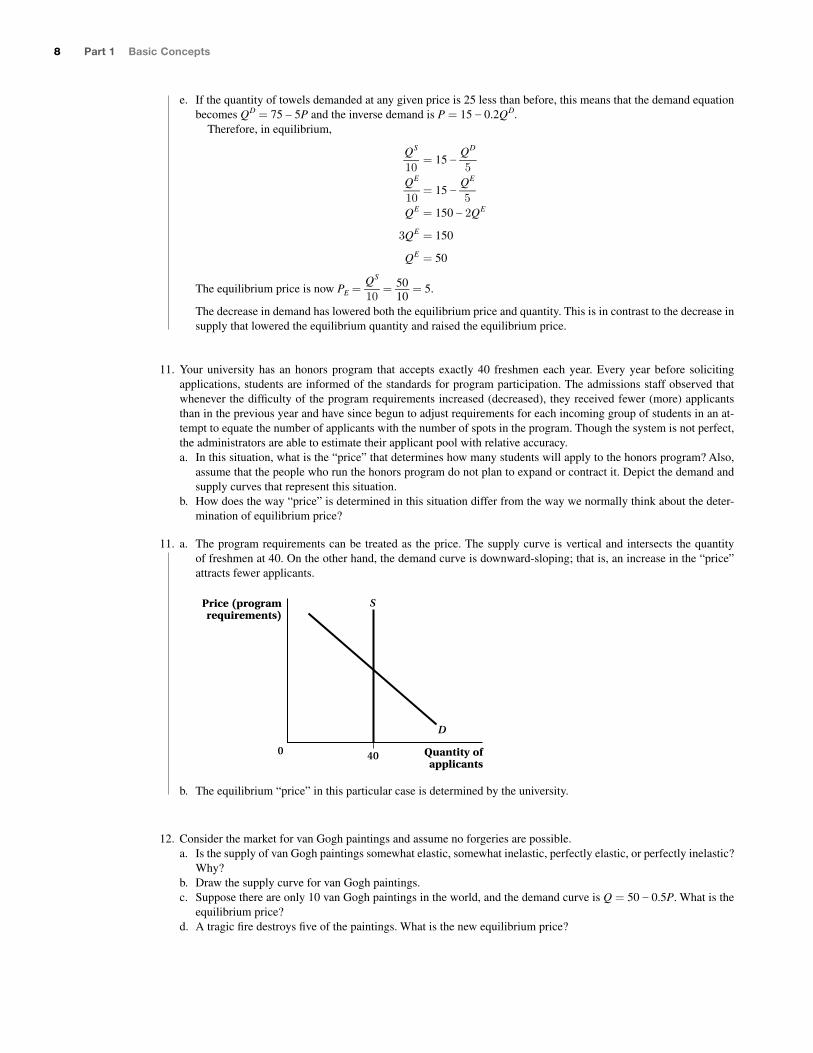
10. a. The inverse supply is
P = Q S
_ 10
whereas the inverse demand is
P = 20 – 1 _
5 Q D
The graph is shown at the right.
b. Defi ne Q E and P E as equilibrium quantity and
price, respectively. In equilibrium, price is
such that quantity demanded is equal to quan-
tity supplied. Therefore in equilibrium,
Q S
_ 10
= 20 – Q D
_ 5
Q E
_ 10
= 20 – Q E
_ 5
Q E = 200 – 2 Q E
3 Q E = 200
Q E = 200
_ 3 = 66
2 _
3
The equilibrium price is then
P E = Q E
_ 10
=
200 _
3
_ 10
= 20 _
3 = 6
2 _
3
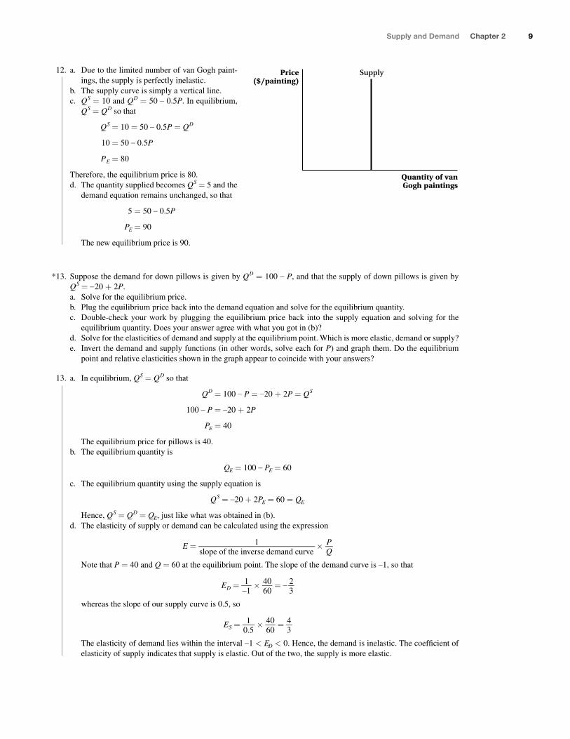
c. The new supply function is
Q S = 10P – 20
Hence, the new inverse supply function is
P = 1 _
10 Q S + 2
d. Solving for the new equilibrium price and quan-
tity, we get
Q S
_ 10
+ 2 = 20 – Q D
_ 5
Q E
_ 10
+ 2 = 20 – Q E
_ 5
Q E + 20 = 200 – 2 Q .E
3 Q E = 180
Q E = 60
The equilibrium price is now
P E = Q E
_ 10
+ 2 = 60 _
10 + 2 = 8
The decrease in supply has lowered the equilibrium quantity to 60 and raised the equilibrium price to 8.
Quantity of towels
Price($/towel)
$10
1000
D
S
Quantity of towels
Price($/towel)
$20
2
1000
D
S2
S1
Goolsbee2e_Solutions_Manual_Ch02.indd 7Goolsbee2e_Solutions_Manual_Ch02.indd 7 30/09/15 9:33 AM30/09/15 9:33 AM
8 Part 1 Basic Concepts
e. If the quantity of towels demanded at any given price is 25 less than before, this means that the demand equation
becomes Q D = 75 – 5P and the inverse demand is P = 15 – 0.2 Q D .
Therefore, in equilibrium,
Q S
_ 10
= 15 – Q D
_ 5
Q E
_ 10
= 15 – Q E
_ 5
Q E = 150 – 2 Q E
3 Q E = 150
Q E = 50
The equilibrium price is now P E = Q S
_ 10
= 50
_ 10
= 5.
The decrease in demand has lowered both the equilibrium price and quantity. This is in contrast to the decrease in
supply that lowered the equilibrium quantity and raised the equilibrium price.
11. Your university has an honors program that accepts exactly 40 freshmen each year. Every year before soliciting
applications, students are informed of the standards for program participation. The admissions staff observed that
whenever the diffi culty of the program requirements increased (decreased), they received fewer (more) applicants
than in the previous year and have since begun to adjust requirements for each incoming group of students in an at-
tempt to equate the number of applicants with the number of spots in the program. Though the system is not perfect,
the administrators are able to estimate their applicant pool with relative accuracy.
a. In this situation, what is the “price” that determines how many students will apply to the honors program? Also,
assume that the people who run the honors program do not plan to expand or contract it. Depict the demand and
supply curves that represent this situation.
b. How does the way “price” is determined in this situation differ from the way we normally think about the deter-
mination of equilibrium price?
11. a. The program requirements can be treated as the price. The supply curve is vertical and intersects the quantity
of freshmen at 40. On the other hand, the demand curve is downward-sloping; that is, an increase in the “price”
attracts fewer applicants.
Quantity ofapplicants
Price (programrequirements)
400
D
S
b. The equilibrium “price” in this particular case is determined by the university.
12. Consider the market for van Gogh paintings and assume no forgeries are possible.
a. Is the supply of van Gogh paintings somewhat elastic, somewhat inelastic, perfectly elastic, or perfectly inelastic?
Why?
b. Draw the supply curve for van Gogh paintings.
c. Suppose there are only 10 van Gogh paintings in the world, and the demand curve is Q = 50 – 0.5P. What is the
equilibrium price?
d. A tragic fi re destroys fi ve of the paintings. What is the new equilibrium price?
Goolsbee2e_Solutions_Manual_Ch02.indd 8Goolsbee2e_Solutions_Manual_Ch02.indd 8 30/09/15 9:33 AM30/09/15 9:33 AM
Supply and Demand Chapter 2 9
12. a. Due to the limited number of van Gogh paint-
ings, the supply is perfectly inelastic.
b. The supply curve is simply a vertical line.
c. Q S = 10 and Q D = 50 – 0.5P. In equilibrium,
Q S = Q D so that
Q S = 10 = 50 – 0.5P = Q D
10 = 50 – 0.5P
P E = 80
Therefore, the equilibrium price is 80.
d. The quantity supplied becomes Q S = 5 and the
demand equation remains unchanged, so that
5 = 50 – 0.5P
P E = 90
The new equilibrium price is 90.
13. Suppose the demand for down pillows is given by Q D = 100 – P, and that the supply of down pillows is given by
Q S = – 20 + 2P.
a. Solve for the equilibrium price.
b. Plug the equilibrium price back into the demand equation and solve for the equilibrium quantity.
c. Double-check your work by plugging the equilibrium price back into the supply equation and solving for the
equilibrium quantity. Does your answer agree with what you got in (b)?
d. Solve for the elasticities of demand and supply at the equilibrium point. Which is more elastic, demand or supply?
e. Invert the demand and supply functions (in other words, solve each for P) and graph them. Do the equilibrium
point and relative elasticities shown in the graph appear to coincide with your answers?
13. a. In equilibrium, Q S = Q D so that
Q D = 100 – P = –20 + 2P = Q S
100 – P = –20 + 2P
P E = 40
The equilibrium price for pillows is 40.
b. The equilibrium quantity is
Q E = 100 – P E = 60
c. The equilibrium quantity using the supply equation is
Q S = –20 + 2 P E = 60 = Q E
Hence, Q S = Q D = Q E , just like what was obtained in (b).
d. The elasticity of supply or demand can be calculated using the expression
E = 1 ___
slope of the inverse demand curve ×
P _ Q
Note that P = 40 and Q = 60 at the equilibrium point. The slope of the demand curve is –1, so that
E D = 1 _
–1 ×
40 _
60 = –
2 _
3
whereas the slope of our supply curve is 0.5, so
E S = 1 _
0.5 ×
40 _
60 =
4 _
3
The elasticity of demand lies within the interval –1 < E D < 0. Hence, the demand is inelastic. The coeffi cient of
elasticity of supply indicates that supply is elastic. Out of the two, the supply is more elastic.
*
Quantity of vanGogh paintings
Price($/painting)
Supply
Goolsbee2e_Solutions_Manual_Ch02.indd 9Goolsbee2e_Solutions_Manual_Ch02.indd 9 30/09/15 9:33 AM30/09/15 9:33 AM
10 Part 1 Basic Concepts
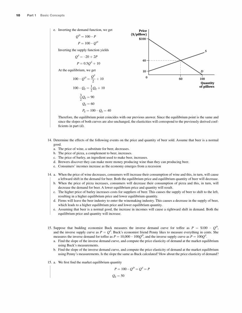
e. Inverting the demand function, we get
Q D = 100 – P
P = 100 – Q D
Inverting the supply function yields
Q S = –20 + 2P
P = 0.5 Q S + 10
At the equilibrium, we get
100 – Q D = Q S
_ 2 + 10
100 – Q E = 1 _
2 Q E + 10
3 _
2 Q E = 90
Q E = 60
P E = 100 – Q E = 40
Therefore, the equilibrium point coincides with our previous answer. Since the equilibrium point is the same and
since the slopes of both curves are also unchanged, the elasticities will correspond to the previously derived coef-
fi cients in part (d).
14. Dete rmine the effects of the following events on the price and quantity of beer sold. Assume that beer is a normal
good.
a. The price of wine, a substitute for beer, decreases.
b. The price of pizza, a complement to beer, increases.
c. The price of barley, an ingredient used to make beer, increases.
d. Brewers discover they can make more money producing wine than they can producing beer.
e. Consumers’ incomes increase as the economy emerges from a recession
14. a. When the price of wine decreases, consumers will increase their consumption of wine and this, in turn, will cause
a leftward shift in the demand for beer. Both the equilibrium price and equilibrium quantity of beer will decrease.
b. When the price of pizza increases, consumers will decrease their consumption of pizza and this, in turn, will
decrease the demand for beer. A lower equilibrium price and quantity will result.
c. The higher price of barley increases costs for suppliers of beer. This causes the supply of beer to shift to the left,
resulting in a higher equilibrium price and lower equilibrium quantity.
d. Firms will leave the beer industry to enter the winemaking industry. This causes a decrease in the supply of beer,
which leads to a higher equilibrium price and lower equilibrium quantity.
e. Assuming that beer is a normal good, the increase in incomes will cause a rightward shift in demand. Both the
equilibrium price and quantity will increase.
15. Suppose that budding economist Buck measures the inverse demand curve for toffee as P = $100 – Q D , and the inverse supply curve as P = Q S . Buck’s economist friend Penny likes to measure everything in cents. She
measures the inverse demand for toffee as P = 10,000 – 100Q D , and the inverse supply curve as P = 100Q S . a. Find the slope of the inverse demand curve, and compute the price elasticity of demand at the market equilibrium
using Buck’s measurements.
b. Find the slope of the inverse demand curve, and compute the price elasticity of demand at the market equilibrium
using Penny’s measurements. Is the slope the same as Buck calculated? How about the price elasticity of demand?
15. a. We fi rst fi nd the market equilibrium quantity
P = 100 – Q D = Q S = P
Q E = 50
Quantityof pillows
Price($/pillow)
$100
10
40
100600
D
S
Goolsbee2e_Solutions_Manual_Ch02.indd 10Goolsbee2e_Solutions_Manual_Ch02.indd 10 30/09/15 9:33 AM30/09/15 9:33 AM
Supply and Demand Chapter 2 11
The equilibrium price is
P E = 50
The slope of the inverse demand curve is –1; hence, the price elasticity of demand is
E D = 1 _
–1 ×
$50 _
50 = –1
The demand at the equilibrium is unit-elastic.
b. The market equilibrium quantity is
P = $10,000 – 100 Q D = 100 Q S = P
Q E = 50
The equilibrium price is
P E = 5,000 cents
The slope of the inverse demand function is –100. The price elasticity of demand is
E D = 1 _
–100 ×
5,000 _
50 = –1
The slope is 100 times greater compared to Buck’s calculations. However, the price elasticity of demand is un-
changed because the price elasticity of supply and that of demand are not affected by the unit of measurement
used.
16. Some policy makers have claimed that the U.S. government should purchase illegal drugs, such as cocaine, to in-
crease the price that drug users will face and therefore reduce their consumption. Does this idea have any merit? Illus-
trate this logic in a simple supply and demand framework. How does the elasticity of demand for illegal drugs relate
to the effi cacy of this policy? Are you more or less willing to favor this policy if you are told demand is inelastic?
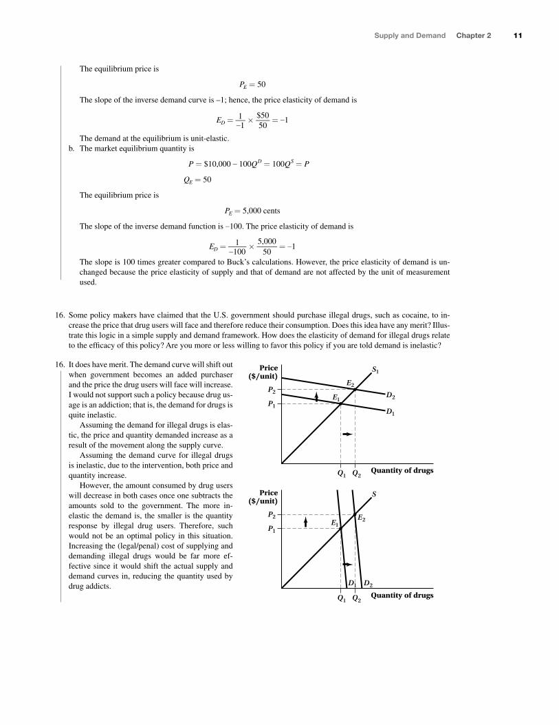
16. It does have merit. The demand curve will shift out
when government becomes an added purchaser
and the price the drug users will face will increase.
I would not support such a policy because drug us-
age is an addiction; that is, the demand for drugs is
quite inelastic.
Assuming the demand for illegal drugs is elas-
tic, the price and quantity demanded increase as a
result of the movement along the supply curve.
Assuming the demand curve for illegal drugs
is inelastic, due to the intervention, both price and
quantity increase.
However, the amount consumed by drug users
will decrease in both cases once one subtracts the
amounts sold to the government. The more in-
elastic the demand is, the smaller is the quantity
response by illegal drug users. Therefore, such
would not be an optimal policy in this situation.
Increasing the (legal/penal) cost of supplying and
demanding illegal drugs would be far more ef-
fective since it would shift the actual supply and
demand curves in, reducing the quantity used by
drug addicts.
Quantity of drugs
Price($/unit)
D1
D2
S1
P1
P2
Q1 Q2
E1
E2
Quantity of drugs
Price($/unit)
S
D2
E1
E2
P1
P2
Q1 Q2
D1
Goolsbee2e_Solutions_Manual_Ch02.indd 11Goolsbee2e_Solutions_Manual_Ch02.indd 11 30/09/15 9:33 AM30/09/15 9:33 AM
12 Part 1 Basic Concepts
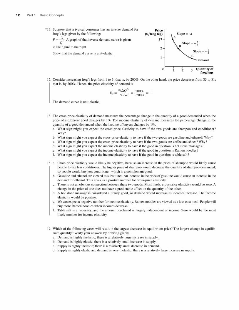
17. Suppose that a typical consumer has an inverse demand for
frog’s legs given by the following:
P = 3 _
Q D . A graph of that inverse demand curve is given
in the fi gure to the right.
Show that the demand curve is unit-elastic.
17. Consider increasing frog’s legs from 1 to 3; that is, by 200%. On the other hand, the price decreases from $3 to $1;
that is, by 200%. Hence, the price elasticity of demand is
E D = %� Q D
_ %�P
= 200%
_ –200%
= –1
The demand curve is unit-elastic.
18. The cross-price elasticity of demand measures the percentage change in the quantity of a good demanded when the
price of a different good changes by 1%. The income elasticity of demand measures the percentage change in the
quantity of a good demanded when the income of buyers changes by 1%.
a. What sign might you expect the cross-price elasticity to have if the two goods are shampoo and conditioner?
Why?
b. What sign might you expect the cross-price elasticity to have if the two goods are gasoline and ethanol? Why?
c. What sign might you expect the cross-price elasticity to have if the two goods are coffee and shoes? Why?
d. What sign might you expect the income elasticity to have if the good in question is hot stone massages?
e. What sign might you expect the income elasticity to have if the good in question is Ramen noodles?
f. What sign might you expect the income elasticity to have if the good in question is table salt?
18. a. Cross-price elasticity would likely be negative, because an increase in the price of shampoo would likely cause
people to use less conditioner. The higher price of shampoo would decrease the quantity of shampoo demanded,
so people would buy less conditioner, which is a complement good.
b. Gasoline and ethanol are viewed as substitutes. An increase in the price of gasoline would cause an increase in the
demand for ethanol. This gives us a positive number for cross-price elasticity.
c. There is not an obvious connection between these two goods. Most likely, cross-price elasticity would be zero. A
change in the price of one does not have a predictable effect on the quantity of the other.
d. A hot stone massage is considered a luxury good, so demand would increase as incomes increase. The income
elasticity would be positive.
e. We can expect a negative number for income elasticity. Ramen noodles are viewed as a low-cost meal. People will
buy more Ramen noodles when incomes decrease.
f. Table salt is a necessity, and the amount purchased is largely independent of income. Zero would be the most
likely number for income elasticity.
19. Which of the following cases will result in the largest decrease in equilibrium price? The largest change in equilib-
rium quantity? Verify your answers by drawing graphs.
a. Demand is highly inelastic; there is a relatively large increase in supply.
b. Demand is highly elastic; there is a relatively small increase in supply.
c. Supply is highly inelastic; there is a relatively small decrease in demand.
d. Supply is highly elastic and demand is very inelastic; there is a relatively large increase in supply.
*
1
$3
2
1
Price($/frog leg)
0 Quantity offrog legs
2 3
A
B
Demand
Slope = –3
Slope = – 43
C
Slope = – 13
Goolsbee2e_Solutions_Manual_Ch02.indd 12Goolsbee2e_Solutions_Manual_Ch02.indd 12 30/09/15 9:33 AM30/09/15 9:33 AM

Supply and Demand Chapter 2 13
19. a. Because demand is inelastic, the rightward shift of sup-
ply will cause a fairly signifi cant decrease in price.
b. If the demand curve is fl at and the shift in supply is rela-
tively small, then price decreases only slightly.
c. The price will fall due to the decrease in demand. Equi-
librium quantity decreases only slightly because the sup-
ply curve is steep.
d. This scenario will result in the largest decrease in price
because the demand curve is steep and the supply curve
is fl at.
Price
0 Quantity
S
ΔQ
ΔP E2
E1
D2
D1
Price
Quantity
D
S1
S2
E1
E2P2
Q1 Q2
P1
Price
0 Quantity
D
ΔQ
ΔP
S1
S2
E1
E2
Price
0 Quantity
D
ΔP
ΔQ
S1
E1E2
S2
Goolsbee2e_Solutions_Manual_Ch02.indd 13Goolsbee2e_Solutions_Manual_Ch02.indd 13 30/09/15 9:33 AM30/09/15 9:33 AM

Goolsbee2e_Solutions_Manual_Ch02.indd 14Goolsbee2e_Solutions_Manual_Ch02.indd 14 30/09/15 9:33 AM30/09/15 9:33 AM
Solution
Solution
1. Suppose that the supply of specialty workstation laptops is represented by Q S = 1,000 + P, where price is measured in dollars and quantity is measured in units.
a. Now suppose that the demand for the laptops is Q D = 9,000 – P – 0.05I, where I is income. What are the current equilibrium price and quantity if income is $100,000?
b. Suppose that income falls to $80,000. What is the new equation for the demand? c. What will be the new equilibrium price and quantity after the income increase? d. Is the laptop workstation a normal or an inferior good? Answer the question using a partial derivative.
1. a. If income is $100,000, demand is Q D = 9,000 – P – 0.05(100,000) = 4,000 – P. The equilibrium condi-tion then is 1,000 + P = 4,000 – P or P = 1,500. At this price, Q D = 4,000 – 1,500 = 2,500 (or to double-check, Q S = 1,000 + 1,500 = 2,500). Price therefore is $1,500 per workstation laptop and 2,500 of these specialty computers are sold.
b. If income is $80,000, demand is Q D = 9,000 – P – 0.05(80,000) = 5,000 – P. c. At the new income level, the equilibrium condition is 1,000 + P = 5,000 – P or P = 2,000. At this
price, Q D = 5,000 – 2,000 = 3,000 (or alternatively, Q S = 1,000 + 2,000 = 3,000). Price therefore is now $2,000 per workstation laptop and 3,000 specialty computers are sold (or alternatively, Q S = 1,000 + 2,000 = 3,000).
d. The workstation is an inferior good since ∂ Q D _
∂I = –0.05 < 0.
2. Suppose that the supply of a flat panel TV stand is represented by Q S = 8P – 20 P i – 200, where P is the price of the stand and P i is the price of the hardware needed to hold the stand together. All prices are in dollars and quantity is in units. Assume that the current hardware price is $5.
a. Suppose that the demand for the TV stand is Q D = 4,700 – 2P + 0.5I, where P is the price and I is a representative household’s income. What are the current equilibrium price and quantity if income is $1,000?
b. Suppose that income falls to $800. What is the new equation for the demand for TV stands as a function of price P? Does this correspond to an increase or decrease in the demand for the TV stands? Does the demand curve shift to the left or right?
c. Suppose that the price of the hardware increases to $6. What is the new equation for the supply of TV stands as a function of price P? Does this correspond to an increase or decrease in supply? Does the supply curve shift to the left or right?
d. What will be the new equilibrium price and quantity of the TV stand after the changes in supply and de-mand [after all changes in parts (b) and (c)]?
2. a. At these values, supply is Q S = 8P – 20(5) – 200 = 8P – 300 and demand for the TV stand is Q D = 4,700 – 2P + 0.5(1,000) = 5,200 – 2P. Equilibrium price is 8P – 300 = 5,200 – 2P, or P = 550. Equi-librium quantity is Q D = 5,200 – 2(550) = 4,100 (or, alternately, Q S = 8(550) – 300 = 4,100). At the equilibrium price of $550, 4,100 stands are sold.
b. After the increase in income, the new demand equation is Q D = 4,700 – 2P + 0.5(800) = 5,100 – 2P, which tells us that a decrease in income leads to a decrease in the demand for the TV stands, and a shift in the demand curve to the left.
c. After the increase in the price of the hardware, the new supply equation is Q S = 8P – 20(6) – 200 = 8P – 320. Supply decreases, and the supply curve shifts to the left.
d. The new equilibrium price is 5,100 – 2P = 8P – 320 or P = 542, and the new equilibrium quantity is Q D = 5,100 – 2(542) = 4,016 (or, alternately, Q S = 8(542) – 320 = 4,016). The price therefore is now $542, and 4,016 stands are sold.
The Calculus of Equilibrium and Elasticities 2
Online Appendix

2A-2 Part 1 Basic Concepts
Solution
Solution
3. From the original setup in Problem 2, suppose that the quantity supplied of flat panel TV stands is represented by Q S = 8P – 20 P i – 200, where P is the price of the stand and P i is the price of hardware inputs, and that quantity demanded is Q D = 4,700 – 2P + 0.5I, where I is income. Assume that at the equilibrium, income is $1,000 and the hardware price is $5.
a. Calculate the income elasticity of demand using calculus. b. Calculate an input elasticity of supply using calculus. (Hint: Think about cross-price elasticities on the
demand side as being analogous to input elasticities on the supply side.)
3. a. The income elasticity of demand is E D = ∂ Q D _
∂I I
_ Q D
= 0.5 1,000 _
4,100 ≈ 0.122.
b. The input elasticity of supply is E S = ∂ Q S _
∂ P i
P i _
Q S = –20 5 _
4,100 ≈ –0.024.
4. Suppose that the inverse demand curve for a dinner-for-two special at a small local restaurant can be ex-pressed as P = 4,900 – 3Q D 2 , where price is expressed in dollars and quantity in number of specials. What is the price elasticity of demand when 40 specials are purchased?
4. When quantity is 40,
P = 4,900 – 3(40) 2 = $100
Using the demand equation, ∂P _
∂ Q D = –3(2)Q 2–1 = – 6Q. At Q = 40, this value is –6(40) = –240. The price
elasticity of demand is E D = 1 _ ∂P
_ ∂ Q D
P _
Q D = 1 _
–240 100 _
40 ≈ –0.01. Demand for this particular dinner special,
therefore, is very inelastic.
While much of this material will be review for most students, many may not have used supply and
demand equations before. If you take your time explaining these equations and how to solve for
equilibrium, students will master this skill quickly.
teaching tip
2.1 Markets and ModelsA. What Is a Market?
1. A market can be defined by many things.a. Type of product soldb. Particular locationc. A point in time
B. Key Assumptions of the Supply and Demand Model1. We restrict our focus to supply and demand in a single market.
Definition: Supply is the combined amount of a good that all producers in a market are willing to sell.Definition: Demand is the combined amount of a good that all consumers in a market are willing to buy.
2. All goods bought and sold in the market are identical.Definition: Commodities are products traded in markets in which consumers view different varieties of the good as essentially interchangeable.
3. All goods sold in the market sell for the same price and everyone has the same information about prices, the quality of the goods being sold, and so on.
4. There are many buyers and sellers in the market.
2.2 DemandA. Factors That Influence Demand
1. Price2. The Number of Consumers3. Consumer Income or Wealth
4. Consumer Tastes5. Prices of Other Goods
Definition: A substitute is a good that can be used in place of another good.Definition: A complement is a good that is purchased in combination with another good.
B. Demand Curves1. Graphical Representation of the Demand Curve
Definition: A demand curve is the relationship between the quantity of a good that consum-ers demand and the good’s price, holding all other factors constant.a. Demand curves generally slope downward. As price falls, quantity demanded rises.
You may want to introduce the concepts of normal and inferior goods here, although they are not for-
mally defined until Chapter 5. Students generally have heard these terms before in Principles courses
and understand what they are and how income affects the demand for each differently.
teaching tip
2-1
Supply and Demand 2
Goolsbee2e_Ch02_IR.indd 2-1Goolsbee2e_Ch02_IR.indd 2-1 03/02/16 3:09 PM03/02/16 3:09 PM
2-2 Chapter 2 Supply and Demand
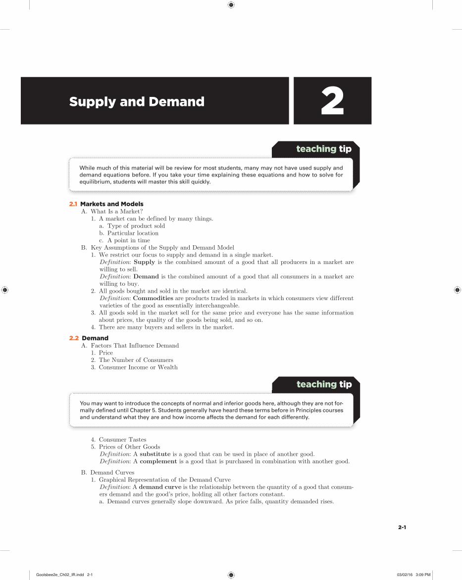
Figure 2.1 Demand for Tomatoes
A
B
200 400 600 800 1,000
$5
4
3
2
1
Price(dollars/pound)
0 Quantity oftomatoes (pounds)
Demand D1
2. Mathematical Representation of the Demand Curvea. Any demand curve can be represented by an equation.b. The demand curve in Figure 2.1 can be represented by Q = 1,000 – 200P.Definition: Demand choke price is the price at which no consumer is willing to buy a good and quantity demanded is zero; it is the vertical intercept of the inverse demand curve.Definition: Inverse demand curve is a demand curve written in the form of price as a func-tion of quantity demanded.
c. The inverse demand curve can be represented as P = 5 – 0.005Q.C. Shifts in Demand Curves
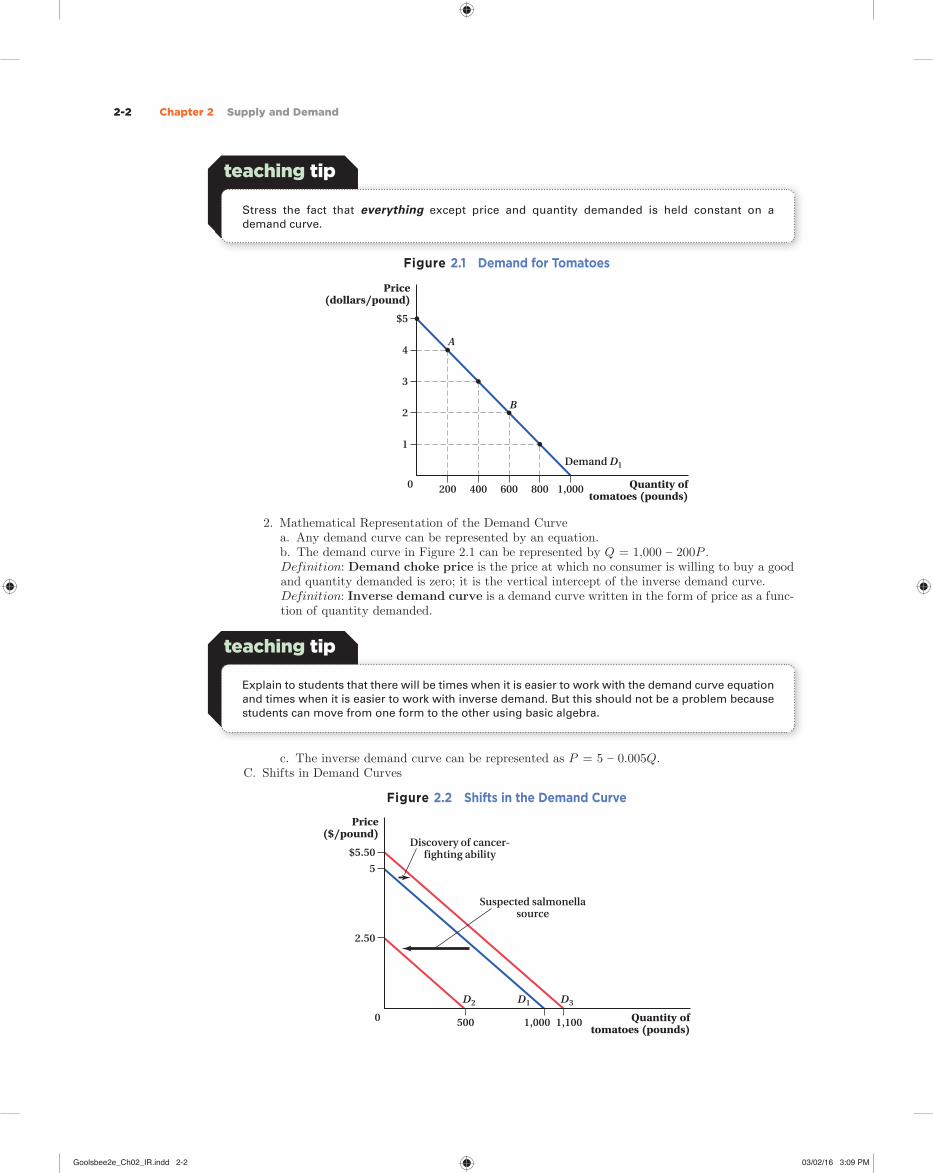
Figure 2.2 Shifts in the Demand Curve
500
Discovery of cancer-fighting ability
1,000 1,100
$5.50
5
2.50
Price($/pound)
0 Quantity oftomatoes (pounds)
D3D2 D1
Suspected salmonellasource
teaching tip
Stress the fact that everything except price and quantity demanded is held constant on a
demand curve.
teaching tip
Explain to students that there will be times when it is easier to work with the demand curve equation
and times when it is easier to work with inverse demand. But this should not be a problem because
students can move from one form to the other using basic algebra.
Goolsbee2e_Ch02_IR.indd 2-2Goolsbee2e_Ch02_IR.indd 2-2 03/02/16 3:09 PM03/02/16 3:09 PM
Supply and Demand Chapter 2 2-3
Definition: Change in quantity demanded is a movement along the demand curve that occurs as a result of a change in the good’s price.Definition: Change in demand is a shift of the entire demand curve caused by a change in a determinant of demand other than the good’s own price.
Make sure you get students thinking of an increase in demand as a shift out (or to the right) rather
than up. Likewise, a decrease in demand is a shift in or left (rather than down). This becomes very
important when students think about changes in supply.
teaching tip
D. Why Is Price Treated Differently from the Other Factors That Affect Demand?1. There are three reasons economists focus on the effect of a good’s price:
a. Price is typically one of the most important factors that influence demand.b. Prices can be changed frequently and easily.c. Price is the only factor that also exerts a large, direct influence on the supply side of the
market.
2.3 SupplyA. Factors That Influence Supply
1. Price2. Suppliers’ Costs of Production
Definition: Production technology is the processes used to make, distribute, and sell a good.
3. The Number of Sellers4. Sellers’ Outside Options
B. Supply Curves
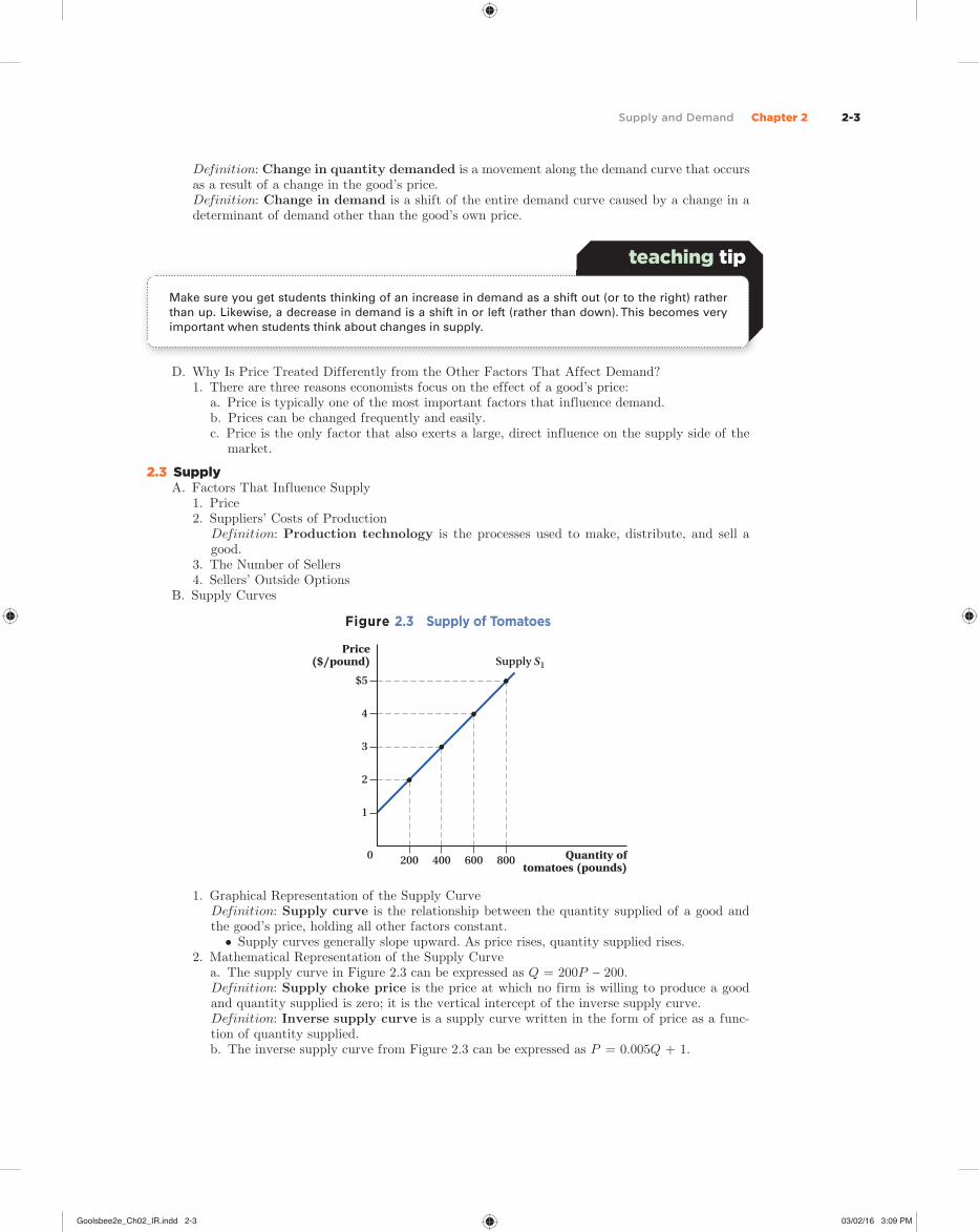
Figure 2.3 Supply of Tomatoes
200 400 600 800
$5
4
3
2
1
Price($/pound)
0 Quantity oftomatoes (pounds)
Supply S1
1. Graphical Representation of the Supply CurveDefinition: Supply curve is the relationship between the quantity supplied of a good and the good’s price, holding all other factors constant.
• Supply curves generally slope upward. As price rises, quantity supplied rises.2. Mathematical Representation of the Supply Curve
a. The supply curve in Figure 2.3 can be expressed as Q = 200P – 200.Definition: Supply choke price is the price at which no firm is willing to produce a good and quantity supplied is zero; it is the vertical intercept of the inverse supply curve.Definition: Inverse supply curve is a supply curve written in the form of price as a func-tion of quantity supplied.b. The inverse supply curve from Figure 2.3 can be expressed as P = 0.005Q + 1.
Goolsbee2e_Ch02_IR.indd 2-3Goolsbee2e_Ch02_IR.indd 2-3 03/02/16 3:09 PM03/02/16 3:09 PM

2-4 Chapter 2 Supply and Demand
C. Shifts in the Supply Curve
Figure 2.4 Shifts in the Supply Curve
200 400 600 800
$5
4
3
2
1
Price($/pound)
0 Quantity oftomatoes (pounds)
S1
S2
S3
Drought
Fasterharvester
200pounds
Definition: Change in quantity supplied is a movement along the supply curve that occurs as a result of a change in the good’s price.Definition: Change in supply is a shift of the entire supply curve caused by a change in a determinant of supply other than the good’s own price.
D. Why Is Price Also Treated Differently for Supply? 1. Price is the only factor that influences both supply and demand.
2.4 Market EquilibriumDefinition: Market equilibrium is the point at which the quantity demanded by consumers exactly equals the quantity supplied by producers.
• The point at which the demand and supply curves intersectDefinition: Equilibrium price is the only price at which quantity supplied equals quantity de-manded.
Figure 2.5 Market Equilibrium
Qe = 400
$5
Pe = 3
1
Price($/pound)
0 Quantity oftomatoes (pounds)
Supply S1
E
Demand D1
A. The Mathematics of Equilibrium1. To solve for the equilibrium price, we equate quantity supplied with quantity demanded.
Q D = Q S
1,000 – 200Pe = 200P
e – 200
Pe = $3
Goolsbee2e_Ch02_IR.indd 2-4Goolsbee2e_Ch02_IR.indd 2-4 03/02/16 3:09 PM03/02/16 3:09 PM
Supply and Demand Chapter 2 2-5
2. To solve for equilibrium quantity, we plug the equilibrium price into either the supply or demand equation.
Q D = 1,000 – 200Pe = 1,000 – 200(3) = 1,000 – 600 = 400
Q S = 200Pe – 200 = 200(3) – 200 = 600 – 200 = 400.
B. Why Markets Move toward Equilibrium
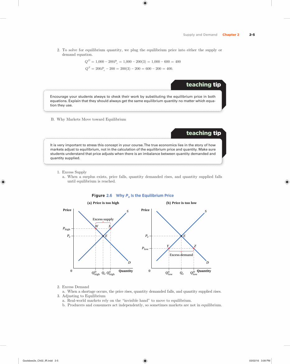
1. Excess Supplya. When a surplus exists, price falls, quantity demanded rises, and quantity supplied falls
until equilibrium is reached.
Figure 2.6 Why P e Is the Equilibrium Price
Price
0 Quantity
S
E
Excess supply
W X
D
Phigh
QeQDhigh
QDlow
Pe
QShigh
QSlow
(a) Price is too high
Price
0 Quantity
S
E
Excess demand
Y Z
D
Plow
Qe
Pe
(b) Price is too low
2. Excess Demanda. When a shortage occurs, the price rises, quantity demanded falls, and quantity supplied rises.
3. Adjusting to Equilibriuma. Real-world markets rely on the “invisible hand” to move to equilibrium.b. Producers and consumers act independently, so sometimes markets are not in equilibrium.
Encourage your students always to check their work by substituting the equilibrium price in both
equations. Explain that they should always get the same equilibrium quantity no matter which equa-
tion they use.
teaching tip
It is very important to stress this concept in your course. The true economics lies in the story of how
markets adjust to equilibrium, not in the calculation of the equilibrium price and quantity. Make sure
students understand that price adjusts when there is an imbalance between quantity demanded and
quantity supplied.
teaching tip
Goolsbee2e_Ch02_IR.indd 2-5Goolsbee2e_Ch02_IR.indd 2-5 03/02/16 3:09 PM03/02/16 3:09 PM

2-6 Chapter 2 Supply and Demand
C. The Effects of Demand ShiftsExample: Suppose a news story reports that tomatoes are suspected of being the source of a salmonella outbreak.• At every price, the quantity of tomatoes buyers who want tomatoes will fall.• This shifts the demand curve to the left.• The new demand curve is Q = 500 – 200P.• Setting Q D = Q S , we get:
500 – 200 P 2 = 200 P 2 – 200
400 P 2 = 700
P 2 = $1.75
• The equilibrium quantity is:
Q D = 500 – 200P = 500 – 200(1.75) = 500 – 350 = 150.
Q S = 200P – 200 = 200(1.75) – 200 = 350 – 200 = 150.
• Therefore, the equilibrium price and quantity both fall.
2.1 additional fi gure it out
The supply and demand for monthly gym member-ships are given as Q S = 10P – 300 and Q D = 600 – 10P, where P is the monthly price of a membership.
1. If the current price for memberships is $50 per
month, is the market in equilibrium?
2. Would you expect the price to rise or fall?
3. If so, by how much?
Solution:
There are two ways to solve the problem:
1. Compute quantity demanded and quantity
supplied at a price of $50.
2. Solve for the market equilibrium price and
quantity.
Q S = 10P – 300 = 10 × 50 – 300 = 200
Q D = 600 – 10P = 600 – 10 × 50 = 100
Therefore, since Q D < Q S , the market is not in equilibrium. There is a surplus, so we can expect the price to fall.
3. Solving for equilibrium, we get:
Q S = Q D
10P – 300 = 600 – 10P
P = $45, Q = 150
Therefore, price must fall by $5, and 50 more mem-berships are sold.
2.2 additional fi gure it out
Draw a supply and demand diagram of the market for generators in Tampa, Florida.
1. Suppose a hurricane watch is issued, and some residents expect to lose power. Using the supply and
demand diagram, show what will happen to the equilibrium price and quantity in the market for generators
in Tampa.
2. Does this change reflect a change in demand or a change in the quantity demanded?
Goolsbee2e_Ch02_IR.indd 2-6Goolsbee2e_Ch02_IR.indd 2-6 03/02/16 3:09 PM03/02/16 3:09 PM
Supply and Demand Chapter 2 2-7
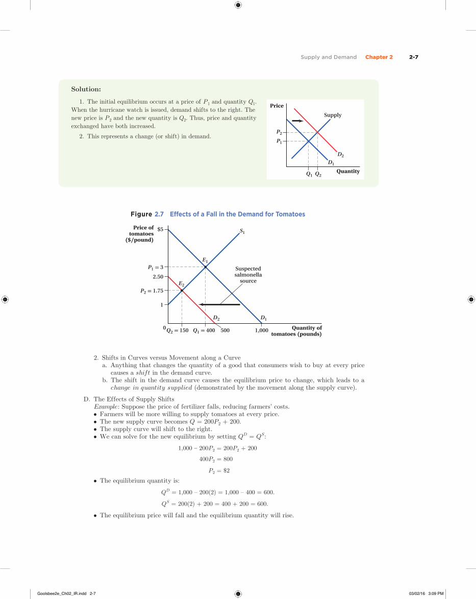
Figure 2.7 Eff ects of a Fall in the Demand for Tomatoes
Q1 = 400 500 1,000
$5
2.50
P1 = 3
1
Price oftomatoes
($/pound)
0 Quantity oftomatoes (pounds)
P2 = 1.75
Q2 = 150
S1
E1
D1D2
E2
Suspectedsalmonella
source
2. Shifts in Curves versus Movement along a Curvea. Anything that changes the quantity of a good that consumers wish to buy at every price
causes a shift in the demand curve.b. The shift in the demand curve causes the equilibrium price to change, which leads to a
change in quantity supplied (demonstrated by the movement along the supply curve).
D. The Effects of Supply ShiftsExample: Suppose the price of fertilizer falls, reducing farmers’ costs.• Farmers will be more willing to supply tomatoes at every price.• The new supply curve becomes Q = 200 P 2 + 200.• The supply curve will shift to the right.• We can solve for the new equilibrium by setting Q D = Q S :
1,000 – 200 P 2 = 200 P 2 + 200
400 P 2 = 800
P 2 = $2
• The equilibrium quantity is:
Q D = 1,000 – 200(2) = 1,000 – 400 = 600.
Q S = 200(2) + 200 = 400 + 200 = 600.
• The equilibrium price will fall and the equilibrium quantity will rise.
Solution:
1. The initial equilibrium occurs at a price of P 1 and quantity Q 1 .
When the hurricane watch is issued, demand shifts to the right. The
new price is P 2 and the new quantity is Q 2 . Thus, price and quantity
exchanged have both increased.
2. This represents a change (or shift) in demand.
Price
Quantity
Supply
D2
D1
P1
Q2Q1
P2
Goolsbee2e_Ch02_IR.indd 2-7Goolsbee2e_Ch02_IR.indd 2-7 03/02/16 3:09 PM03/02/16 3:09 PM
2-8 Chapter 2 Supply and Demand
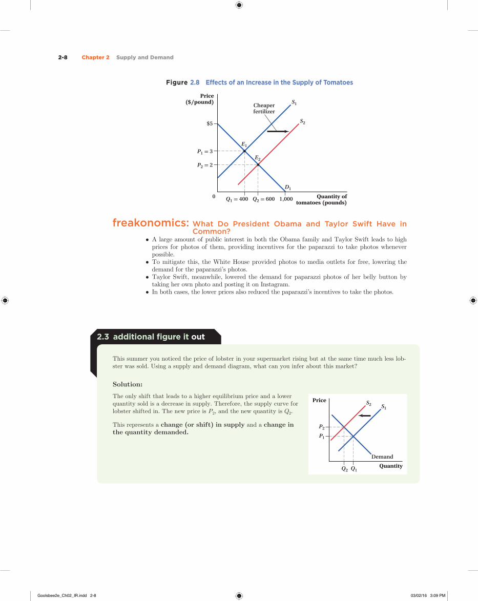
Figure 2.8 Eff ects of an Increase in the Supply of Tomatoes
Q2 = 600 1,000
$5
P1 = 3
Price($/pound)
0 Quantity oftomatoes (pounds)
P2 = 2
Q1 = 400
S1
S2
D1
Cheaperfertilizer
E2
E1
freakonomics: What Do President Obama and Taylor Swift Have in Common?
• A large amount of public interest in both the Obama family and Taylor Swift leads to high prices for photos of them, providing incentives for the paparazzi to take photos whenever possible.
• To mitigate this, the White House provided photos to media outlets for free, lowering the demand for the paparazzi’s photos.
• Taylor Swift, meanwhile, lowered the demand for paparazzi photos of her belly button by taking her own photo and posting it on Instagram.
• In both cases, the lower prices also reduced the paparazzi’s incentives to take the photos.
2.3 additional fi gure it out
This summer you noticed the price of lobster in your supermarket rising but at the same time much less lob-ster was sold. Using a supply and demand diagram, what can you infer about this market?
Solution:
The only shift that leads to a higher equilibrium price and a lower quantity sold is a decrease in supply. Therefore, the supply curve for lobster shifted in. The new price is P 2 , and the new quantity is Q 2 .
This represents a change (or shift) in supply and a change in the quantity demanded.
Price
Quantity
Demand
S2 S1
P1
Q2 Q1
P2
Goolsbee2e_Ch02_IR.indd 2-8Goolsbee2e_Ch02_IR.indd 2-8 03/02/16 3:09 PM03/02/16 3:09 PM
Supply and Demand Chapter 2 2-9
E. Summary of Effects1. Table 2.2 summarizes the changes in equilibrium price and quantity for any shift in supply
and demand.
Impact on Equilibrium
Curve that Shifts Direction of Shift Price Quantity
Demand Curve
Out (increase in D )
In (decrease in D )
Supply Curve
Out (increase in S )
In (decrease in S )
Table 2.2 Eff ect of Shifts in Demand and Supply Curves in Isolation
application
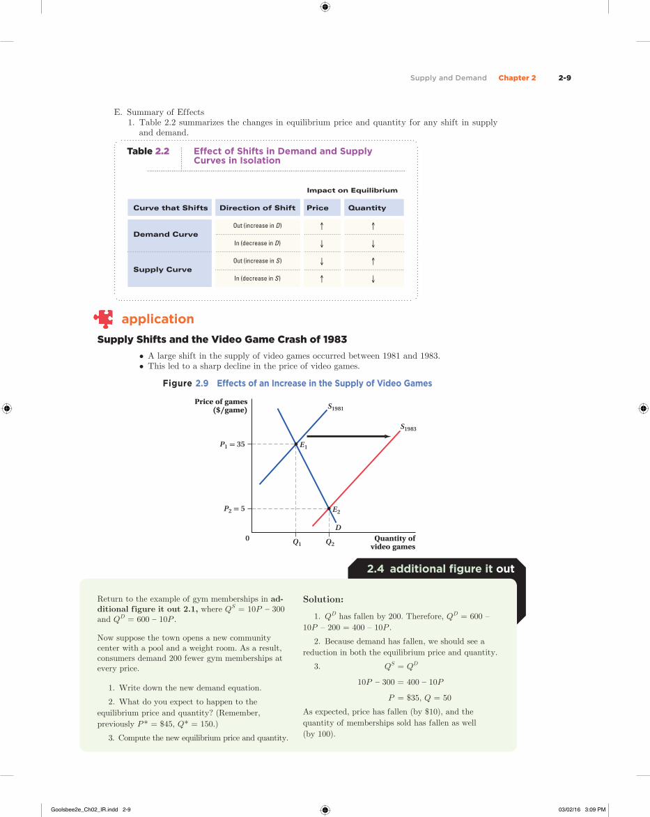
Supply Shifts and the Video Game Crash of 1983
• A large shift in the supply of video games occurred between 1981 and 1983.• This led to a sharp decline in the price of video games.
Figure 2.9 Eff ects of an Increase in the Supply of Video Games
Price of games($/game)
0 Quantity ofvideo games
S1981
S1983
E1
D
E2
P1 = 35
Q2Q1
P2 = 5
2.4 additional fi gure it out
Return to the example of gym memberships in ad-ditional figure it out 2.1, where Q S = 10P – 300 and Q D = 600 – 10P.
Now suppose the town opens a new community center with a pool and a weight room. As a result, consumers demand 200 fewer gym memberships at every price.
1. Write down the new demand equation.
2. What do you expect to happen to the
equilibrium price and quantity? (Remember,
previously P* = $45, Q* = 150.)
3. Compute the new equilibrium price and quantity.
Solution:
1. Q D has fallen by 200. Therefore, Q D = 600 –
10P – 200 = 400 – 10P.
2. Because demand has fallen, we should see a
reduction in both the equilibrium price and quantity.
3. Q S = Q D
10P – 300 = 400 – 10P
P = $35, Q = 50
As expected, price has fallen (by $10), and the
quantity of memberships sold has fallen as well
(by 100).
Goolsbee2e_Ch02_IR.indd 2-9Goolsbee2e_Ch02_IR.indd 2-9 03/02/16 3:09 PM03/02/16 3:09 PM

2-10 Chapter 2 Supply and Demand
F. What Determines the Size of Price and Quantity Changes?1. Size of the Shift2. Slopes of the Curves
a. Demand shifts i. Relatively flat supply: small change in equilibrium price and a large change in equilib-
rium quantity.ii. Relatively steep supply: large change in equilibrium price and a small change in equi-
librium quantity.b. Supply shifts
i. Relatively flat demand: small change in equilibrium price and a large change in equi-librium quantity.
ii. Relatively steep demand: large change in equilibrium price and a small change in equi-librium quantity.
Figure 2.10 Size of Equilibrium Price and Quantity Changes, and the Slopes of the Demand and Supply Curves
Price
0 Quantity
S
ΔPa
(a) Demand curve shift withflatter supply curve
ΔQa
D1
E1
E2
D2
Price
0 Quantity
D
ΔQd
ΔPd
(d) Supply curve shift withsteeper demand curve
S1
S2
E1
E2
Price
0 Quantity
D
ΔPc
(c) Supply curve shift withflatter demand curve
ΔQc
S1
E1
E2
S2
Price
0 Quantity
S
ΔQb
ΔPb
(b) Demand curve shift withsteeper supply curve
E1
E2
D1
D2
application
The Supply Curve of Housing and Housing Prices: A Tale of Two Cities
• The relative slope of the supply curve determines the size of the effect of an increase in demand.
• New York has a relatively steep supply of housing, while Houston has a relatively flat supply of housing.
• Between 1977 and 2009, the population of New York grew by about 15%, while Houston’s population more than doubled.
• But because the supply of housing is flatter for Houston than for New York, housing prices did not rise as much in Houston as they did in New York.
Goolsbee2e_Ch02_IR.indd 2-10Goolsbee2e_Ch02_IR.indd 2-10 03/02/16 3:09 PM03/02/16 3:09 PM

Supply and Demand Chapter 2 2-11
Figure 2.11 Population Indices for New York and Houston, 1977–2013
Year
250
200
150
100
50
0
Population(1977 = 100)
Houston
New YorkCity
2007199719871977 1992 20021982 2012
Figure 2.12 Housing Price Indices for New York and Houston, 1977–2013
Year
Inflation–adjusted OFHEOhouse price index (1977 = 100)
Year
300
250
200
150
100
50
0
2007199719871977 1992 20021982
New YorkCity
Houston
2012
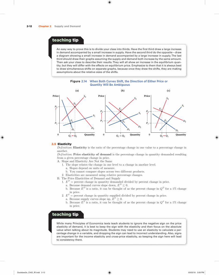
G. Changes in Market Equilibrium When Both Curves Shift1. As a rule, when both curves shift at the same time, we will know with certainty the direction
of the change of either the equilibrium price or the equilibrium quantity but not both.
Figure 2.13 Example of a Simultaneous Shift in Demand and Supply
Price
0 Quantity
D1
S1
S2
D2
E2E1
P1
Q2 Q1
P2
2. Each separate shift in supply and demand leads to a unique result. That is why two simultane-ous shifts will not move equilibrium price and quantity in the same ways.
Goolsbee2e_Ch02_IR.indd 2-11Goolsbee2e_Ch02_IR.indd 2-11 03/02/16 3:09 PM03/02/16 3:09 PM
2-12 Chapter 2 Supply and Demand
Figure 2.14 When Both Curves Shift, the Direction of Either Price or Quantity Will Be Ambiguous
Price
0 Quantity
D1D2
S2
S1
P1
Q2Q1
P2
E1
E2
Price
0 Quantity
D1
D2
S2
S1
P1
Q1 = Q2
P2
E1
E2
Price
0 Quantity
D1
D2
S2
S1
P1
Q1Q2
P2
E1
E2
(a) (b) (c)
2.5 Elasticity Definition: Elasticity is the ratio of the percentage change in one value to a percentage change in
another. Definition: Price elasticity of demand is the percentage change in quantity demanded resulting
from a given percentage change in price.A. Slope and Elasticity Are Not the Same
1. The slope relates the change in one level to a change in another level.a. Slopes depend on units of measure.b. You cannot compare slopes across two different products.
2. Elasticities are measured using relative percentage changes.B. The Price Elasticities of Demand and Supply
1. E D = percent change in quantity demanded divided by percent change in price.a. Because demand curves slope down, E D ≤ 0.b. Because E D is a ratio, it can be thought of as the percent change in Q D for a 1% change
in price.2. E S = percent change in quantity supplied divided by percent change in price.
a. Because supply curves slope up, E S ≥ 0.b. Because E S is a ratio, it can be thought of as the percent change in Q S for a 1% change
in price.
teaching tip
An easy way to prove this is to divide your class into thirds. Have the first third draw a large increase
in demand accompanied by a small increase in supply. Have the second third do the opposite—draw
a diagram showing a small increase in demand accompanied by a large increase in supply. The last
third should draw their graphs assuming the supply and demand both increase by the same amount.
Then ask your class to describe their results. They will all show an increase in the equilibrium quan-
tity; but they will differ with the effects on equilibrium price. Emphasize to them that it is always best
to draw simultaneous shifts on separate graphs, because once they draw the shifts, they are making
assumptions about the relative sizes of the shifts.
teaching tip
While many Principles of Economics texts teach students to ignore the negative sign on the price
elasticity of demand, it is best to keep the sign with the elasticity and then focus on the absolute
value when talking about its magnitude. Students may need to use an elasticity to calculate a per-
centage change in a variable, and dropping the sign can lead to incorrect understanding. Also, signs
are important for the income elasticity and cross-price elasticity, so keeping the sign here will lead
to consistency there.
Goolsbee2e_Ch02_IR.indd 2-12Goolsbee2e_Ch02_IR.indd 2-12 03/02/16 3:09 PM03/02/16 3:09 PM
Supply and Demand Chapter 2 2-13
C. Price Elasticities and Price Responsiveness1. When demand (supply) is very price-sensitive, a small change in price will lead to large
changes in quantities demanded (supplied).2. This means that the numerator of the elasticity expression, the percentage change in quantity,
will be very large compared to the percentage change in price in the denominator.3. The availability of substitutes is a factor that can lead to price elasticities of demand with
larger magnitudes.4. The ability of producers to adjust their production is an important factor that influences the
magnitude of the price elasticity of supply.
application
Demand Elasticities and the Availability of Substitutes
• The availability of substitutes results in a greater responsiveness on the part of the consumer to changes in prices.
• As a result, the demand for broad groupings of goods (e.g., juice) is less elastic than is the demand for more narrowly defined, more easily substitutable goods (e.g., Shredded Wheat brand breakfast cereal).
• An extreme example of the effect of substitution possibilities is the finding that the price elasticity of demand for easily substitutable CPUs and memory chips on a price search engine Web site is on the order of −25.
5. Elasticities and Time Horizonsa. In the short run, consumers and producers are often limited in their ability to change their
behaviors. Therefore, demand and supply will often be less elastic in the short run.b. Larger-magnitude elasticities imply flatter demand and supply curves. As a result, long-run
demand and supply curves tend to be flatter than their short-run versions.6. Classifying Elasticities by Magnitude
Definition: Elastic means having a price elasticity with an absolute value greater than 1: | E D | > 1.Definition: Inelastic means having a price elasticity with an absolute value less than 1: | E D | < 1.Definition: Unit elastic means having a price elasticity with an absolute value equal to 1: | E D | = 1.Definition: Perfectly inelastic means having a price elasticity that is equal to zero; there is no change in quantity demanded or supplied for any change in price: | E D | = 0.Definition: Perfectly elastic means having a price elasticity that is infinite; any change in price leads to an infinite change in quantity demanded or supplied: | E D | = ∞.
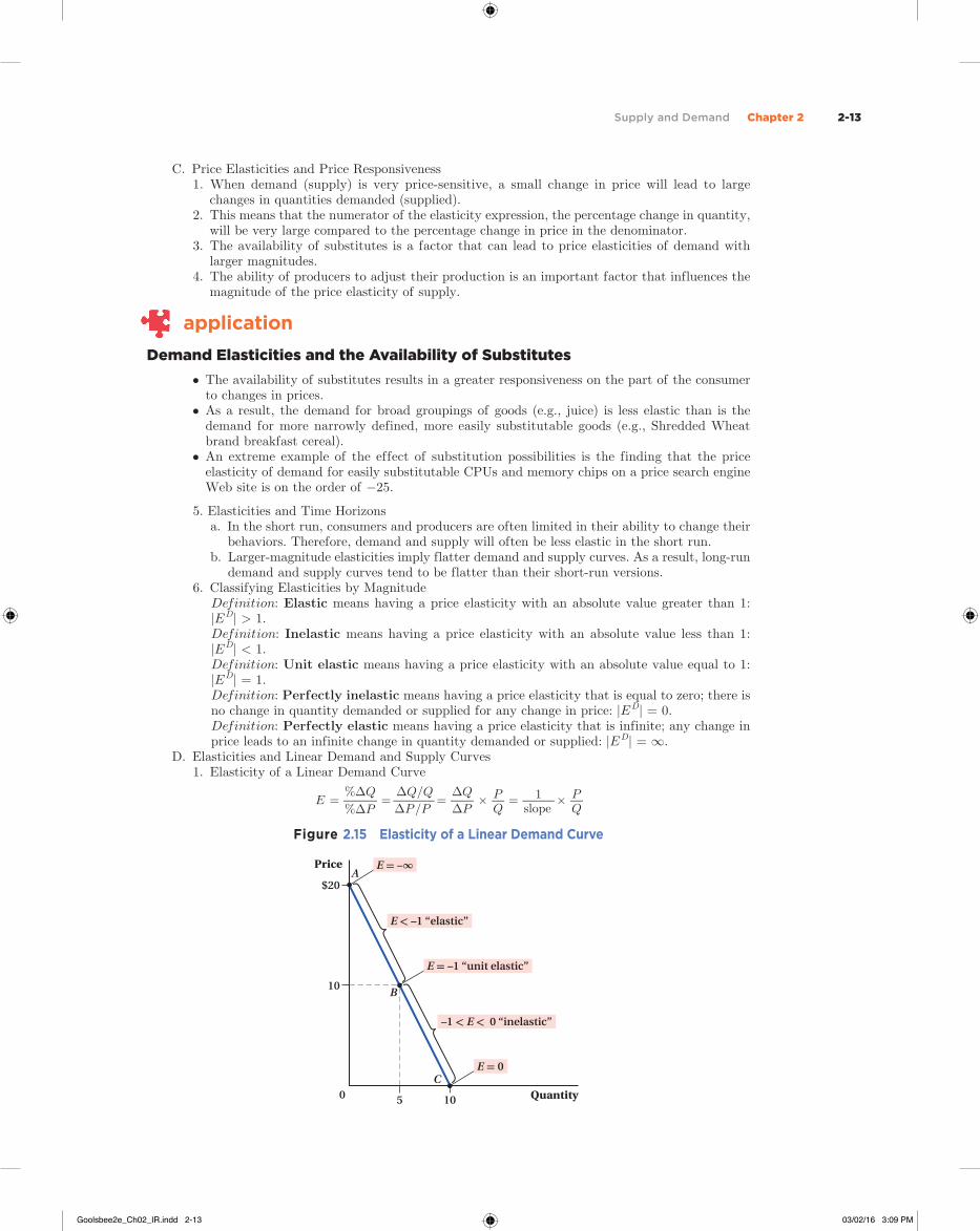
D. Elasticities and Linear Demand and Supply Curves1. Elasticity of a Linear Demand Curve
E = %ΔQ _
%ΔP =
ΔQ/Q _
ΔP/P =
ΔQ _
ΔP × P _
Q = 1 _
slope × P _
Q
Figure 2.15 Elasticity of a Linear Demand Curve
10
10
$20
Price
0 Quantity5
A
B
C
E < –1 “elastic”
–1 < E < 0 “inelastic”
E = –∞
E = –1 “unit elastic”
E = 0
Goolsbee2e_Ch02_IR.indd 2-13Goolsbee2e_Ch02_IR.indd 2-13 03/02/16 3:09 PM03/02/16 3:09 PM

2-14 Chapter 2 Supply and Demand
E. Perfectly Inelastic and Perfectly Elastic Demand and Supply1. Perfectly Inelastic
a. Any change in price leads to no change in quantity demanded (supplied).b. The demand (supply) curve will be vertical.
Figure 2.17 Perfectly Inelastic and Perfectly Elastic Demand or Supply Curves
Price
0 Quantity
(a) Perfectly inelastic (b) Perfectly elastic
P′
Q′
Price
0 Quantity
Demand or supply
Demandor supply
2.5 additional fi gure it out
The demand for movie tickets in a small town is given as Q D = 1000 – 50P.
1. Calculate the price elasticity of demand when
the price of tickets is $5.
2. Calculate the price elasticity of demand when
the price of tickets is $12.
3. At what price is the price elasticity of demand
unit elastic?
4. What happens to the price elasticity of
demand as you move down a linear demand curve?
Solution:
The price elasticity of demand is given as E D =
ΔQ _
ΔP × P _
Q .
For this demand curve, ΔQ _
ΔP is constant and
equal to –50.
1. When P = $5, Q D = 750. Therefore, E D =
– 50 × 5 _ 750
= – 0.3333. Demand is inelastic.
2. When P = $12, Q D = 400. Therefore, E D =
– 50 × 12 _ 400
= – 1.5. Demand is elastic.
3. Demand is unit elastic when E D = –1.
Therefore, we substitute –1 for E D and then solve
for P:
–1 = –50 × P _
1,000 – 50P
–(1,000 – 50P) = –50P
1,000 – 50P = 50P
100P = 1,000
P = $10
Demand will be unit elastic at a price of $10.
4. As you move down a linear demand curve,
demand becomes less elastic (more inelastic).
Figure 2.16 Elasticity of a Linear Supply Curve
100
Price
0 Quantity200 350
B
C
DSupply
P/Q falls as wemove up the
supply curve.
A
$9
6
4
2
E = +∞
Goolsbee2e_Ch02_IR.indd 2-14Goolsbee2e_Ch02_IR.indd 2-14 03/02/16 3:09 PM03/02/16 3:09 PM
Supply and Demand Chapter 2 2-15
2. Perfectly Elastica. Any change in price leads to an infinite change in quantity demanded (supplied).b. The demand (supply) curve is a horizontal line.
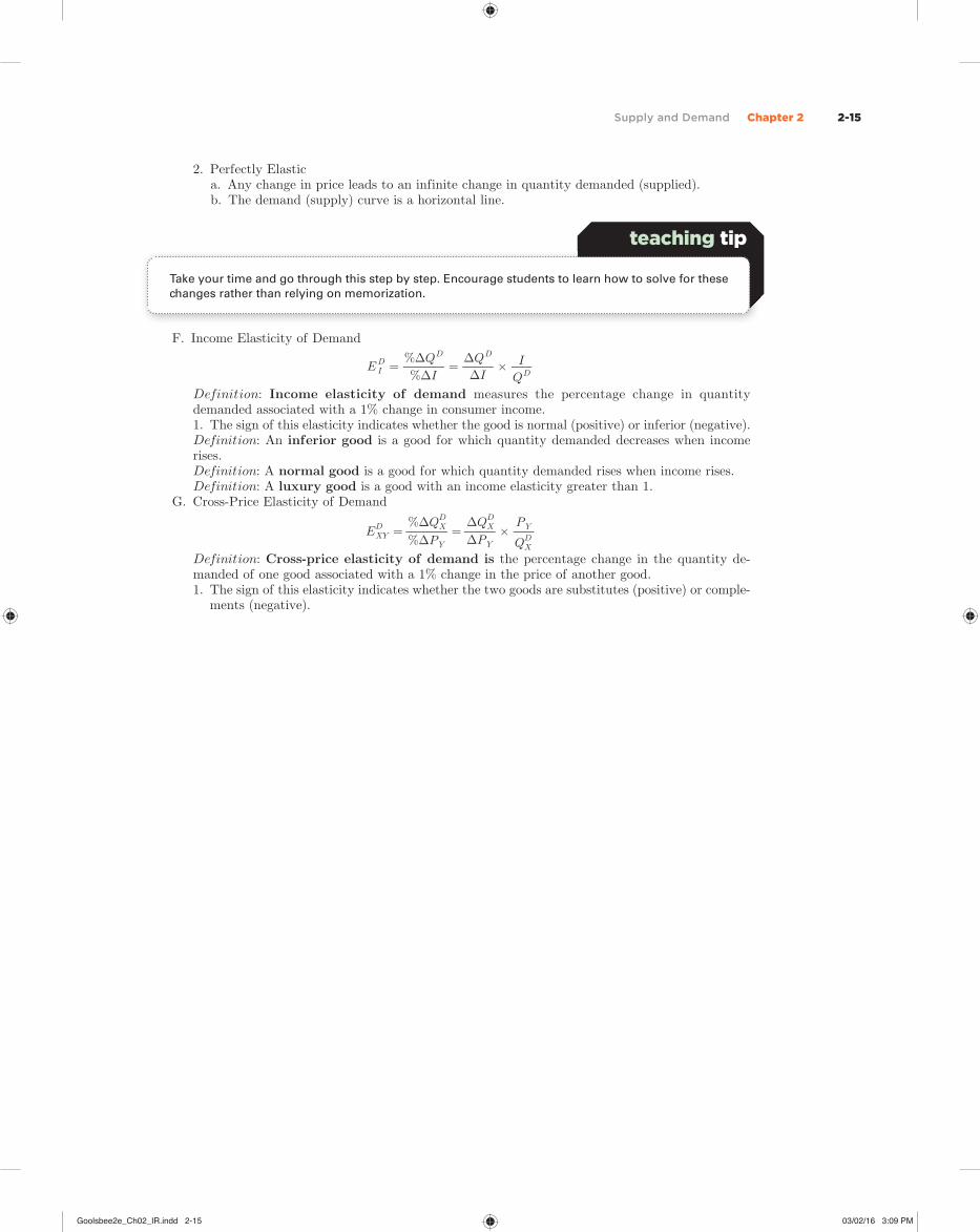
F. Income Elasticity of Demand
E I D =
%Δ Q D _
%ΔI =
Δ Q D _
ΔI × I
_ Q D
Definition: Income elasticity of demand measures the percentage change in quantity demanded associated with a 1% change in consumer income.1. The sign of this elasticity indicates whether the good is normal (positive) or inferior (negative).Definition: An inferior good is a good for which quantity demanded decreases when income rises.Definition: A normal good is a good for which quantity demanded rises when income rises.Definition: A luxury good is a good with an income elasticity greater than 1.
G. Cross-Price Elasticity of Demand
E XY
D =
%Δ Q X D _
%Δ P Y =
ΔQ X D _
Δ P Y ×
P Y _
Q X D
Definition: Cross-price elasticity of demand is the percentage change in the quantity de-manded of one good associated with a 1% change in the price of another good.1. The sign of this elasticity indicates whether the two goods are substitutes (positive) or comple-
ments (negative).
Take your time and go through this step by step. Encourage students to learn how to solve for these
changes rather than relying on memorization.
teaching tip
Goolsbee2e_Ch02_IR.indd 2-15Goolsbee2e_Ch02_IR.indd 2-15 03/02/16 3:09 PM03/02/16 3:09 PM

This text provides a number of math supplements — from the chapter Figure It Out features to the in-text calculus appendices and math review appendix. Why add another appendix? These online appendices give us an opportunity to illustrate additional — and often more advanced — mathematical techniques that can be applied to the economics you learn throughout the course. Some online appendices will build on concepts explored in the chapters themselves, whereas others will provide richer detail on the mathemat-ics in the in-text calculus appendices. As with the other math supplements, the online appendices provide information and techniques that may further your understanding of economics, but are not intended as substitutes for what you would learn in your college mathematics courses.
In this first online appendix, we use calculus to describe the effect of changes in variables other than the good’s own price on equilibrium outcomes. We also calculate and apply a variety of supply and demand elasticities using calculus, enabling us to calculate elasticities in a wider variety of circumstances than those shown in the text.
DemandA demand curve is a representation of a relationship between the quantity of a good that consumers demand and that good’s price, holding all other factors constant. Let’s consider the hypothetical linear demand curve for tomatoes from the text: Q D = 1,000 – 200P, where Q D is the quantity demanded of tomatoes in pounds and P is the price in dollars per pound. Note that this demand equation is written so that quantity is a function of price only.
The definition of a demand curve, however, is more general. Particularly, it speci-fies that demand may also depend on “other factors” (which we then hold constant for our calculations of demand curves). In the chapter we learned that when other factors change (such as changes in income, the prices of related goods, or tastes), the demand curve shifts. It is therefore useful to think about an “expanded” demand function for which quantity demanded is a function not only of the good’s own price but also of some of these other factors.
As a relatively simple example, consider adding the prices of related goods and in-come to the linear demand curve: Q D = 900 – 200P + 100 P s – 600 P c + 0.01I, where P s and P c are the prices of a substitute good and of a complementary good respectively and I is income. Why might we include the prices of substitute and complementary goods in the demand curve for tomatoes? As we saw in the text, a change in the price of a substitute for a good (a good that can be used in place of another good) affects demand for the original good. Similarly, a change in the price of a good that is used in combination with another (a complement) also affects the good’s demand.
Let’s use the demand for tomatoes to explore these relationships more fully. Suppose peppers are a substitute for tomatoes with price P s , and the people enjoy eating lettuce with tomatoes, so it is a complementary good with price P c .
Assume lettuce and peppers each cost $1 per unit, and that the average consumer income is $60,000. Note that at these values Q D = 900 – 200P + 100(1) – 600(1) + 0.01(60,000). Simplifying this, we see that the demand curve written only as a function of price is Q D = 1,000 – 200P — the same relationship as in the text!
Chapter 2 Online Appendix: The Calculus of Equilibrium and Elasticities
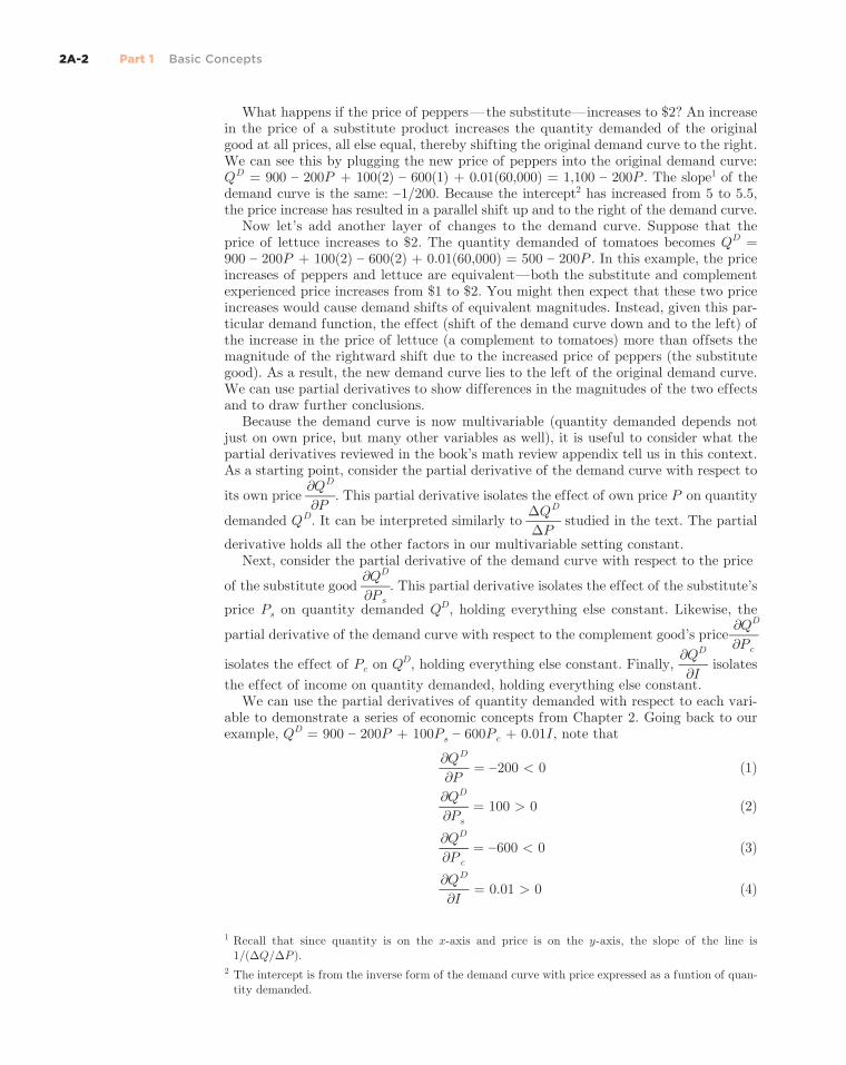
2A-2 Part 1 Basic Concepts
What happens if the price of peppers — the substitute — increases to $2? An increase in the price of a substitute product increases the quantity demanded of the original good at all prices, all else equal, thereby shifting the original demand curve to the right. We can see this by plugging the new price of peppers into the original demand curve: Q D = 900 – 200P + 100(2) – 600(1) + 0.01(60,000) = 1,100 – 200P. The slope1 of the demand curve is the same: – 1/200. Because the intercept2 has increased from 5 to 5.5, the price increase has resulted in a parallel shift up and to the right of the demand curve.
Now let’s add another layer of changes to the demand curve. Suppose that the price of lettuce increases to $2. The quantity demanded of tomatoes becomes Q D = 900 – 200P + 100(2) – 600(2) + 0.01(60,000) = 500 – 200P. In this example, the price increases of peppers and lettuce are equivalent — both the substitute and complement experienced price increases from $1 to $2. You might then expect that these two price increases would cause demand shifts of equivalent magnitudes. Instead, given this par-ticular demand function, the effect (shift of the demand curve down and to the left) of the increase in the price of lettuce (a complement to tomatoes) more than offsets the magnitude of the rightward shift due to the increased price of peppers (the substitute good). As a result, the new demand curve lies to the left of the original demand curve. We can use partial derivatives to show differences in the magnitudes of the two effects and to draw further conclusions.
Because the demand curve is now multivariable (quantity demanded depends not just on own price, but many other variables as well), it is useful to consider what the partial derivatives reviewed in the book’s math review appendix tell us in this context. As a starting point, consider the partial derivative of the demand curve with respect to
its own price ∂ Q D _
∂P . This partial derivative isolates the effect of own price P on quantity
demanded Q D . It can be interpreted similarly to � Q D _
�P studied in the text. The partial
derivative holds all the other factors in our multivariable setting constant. Next, consider the partial derivative of the demand curve with respect to the price
of the substitute good ∂ Q D _
∂ P s . This partial derivative isolates the effect of the substitute’s
price P s on quantity demanded Q D , holding everything else constant. Likewise, the
partial derivative of the demand curve with respect to the complement good’s price ∂ Q D _
∂ P c
isolates the effect of P c on Q D , holding everything else constant. Finally, ∂ Q D _
∂I isolates
the effect of income on quantity demanded, holding everything else constant. We can use the partial derivatives of quantity demanded with respect to each vari-
able to demonstrate a series of economic concepts from Chapter 2. Going back to our example, Q D = 900 – 200P + 100 P s – 600 P c + 0.01I, note that
∂ Q D _
∂P = – 200 < 0 (1)
∂ Q D _
∂ P s = 100 > 0 (2)
∂ Q D _
∂ P c = – 600 < 0 (3)
∂ Q D _
∂I = 0.01 > 0 (4)
1 Recall that since quantity is on the x-axis and price is on the y-axis, the slope of the line is 1/(ΔQ/ΔP).
2 The intercept is from the inverse form of the demand curve with price expressed as a funtion of quan-tity demanded.
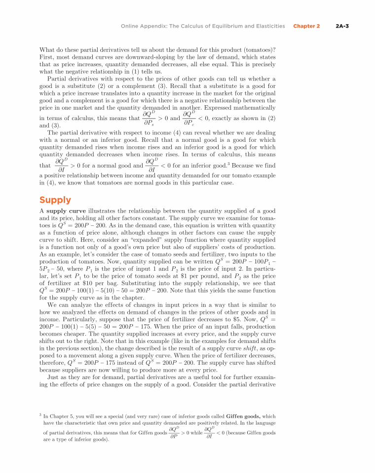
Online Appendix: The Calculus of Equilibrium and Elasticities Chapter 2 2A-3
What do these partial derivatives tell us about the demand for this product (tomatoes)? First, most demand curves are downward-sloping by the law of demand, which states that as price increases, quantity demanded decreases, all else equal. This is precisely what the negative relationship in (1) tells us.
Partial derivatives with respect to the prices of other goods can tell us whether a good is a substitute (2) or a complement (3). Recall that a substitute is a good for which a price increase translates into a quantity increase in the market for the original good and a complement is a good for which there is a negative relationship between the price in one market and the quantity demanded in another. Expressed mathematically
in terms of calculus, this means that ∂ Q D _
∂ P s > 0 and
∂ Q D _
∂ P c < 0, exactly as shown in (2)
and (3).The partial derivative with respect to income (4) can reveal whether we are dealing
with a normal or an inferior good. Recall that a normal good is a good for which quantity demanded rises when income rises and an inferior good is a good for which quantity demanded decreases when income rises. In terms of calculus, this means
that ∂ Q D _
∂I > 0 for a normal good and
∂ Q D _
∂I < 0 for an inferior good.3 Because we find
a positive relationship between income and quantity demanded for our tomato example in (4), we know that tomatoes are normal goods in this particular case.
SupplyA supply curve illustrates the relationship between the quantity supplied of a good and its price, holding all other factors constant. The supply curve we examine for toma-toes is Q S = 200P – 200. As in the demand case, this equation is written with quantity as a function of price alone, although changes in other factors can cause the supply curve to shift. Here, consider an “expanded” supply function where quantity supplied is a function not only of a good’s own price but also of suppliers’ costs of production. As an example, let’s consider the case of tomato seeds and fertilizer, two inputs to the production of tomatoes. Now, quantity supplied can be written Q S = 200P – 100 P 1 – 5 P 2 – 50, where P 1 is the price of input 1 and P 2 is the price of input 2. In particu-lar, let’s set P 1 to be the price of tomato seeds at $1 per pound, and P 2 as the price of fertilizer at $10 per bag. Substituting into the supply relationship, we see that Q S = 200P – 100(1) – 5(10) – 50 = 200P – 200. Note that this yields the same function for the supply curve as in the chapter.
We can analyze the effects of changes in input prices in a way that is similar to how we analyzed the effects on demand of changes in the prices of other goods and in income. Particularly, suppose that the price of fertilizer decreases to $5. Now, Q S = 200P – 100(1) – 5(5) – 50 = 200P – 175. When the price of an input falls, production becomes cheaper. The quantity supplied increases at every price, and the supply curve shifts out to the right. Note that in this example (like in the examples for demand shifts in the previous section), the change described is the result of a supply curve shift, as op-posed to a movement along a given supply curve. When the price of fertilizer decreases, therefore, Q S = 200P – 175 instead of Q S = 200P – 200. The supply curve has shifted because suppliers are now willing to produce more at every price.
Just as they are for demand, partial derivatives are a useful tool for further examin-ing the effects of price changes on the supply of a good. Consider the partial derivative
3 In Chapter 5, you will see a special (and very rare) case of inferior goods called Giffen goods, which have the characteristic that own price and quantity demanded are positively related. In the language
of partial derivatives, this means that for Giffen goods ∂Q D _
∂P > 0 while
∂ Q D _
∂I < 0 (because Giffen goods
are a type of inferior goods).
2A-4 Part 1 Basic Concepts
of the supply curve with respect to a good’s own price ∂Q S _
∂P . This partial derivative now
isolates the effect of own price P on quantity supplied Q S and can be interpreted as the change in quantity supplied for a given change in price, holding all other factors in this
multivariable setting constant. In our example, ∂Q S _
∂P = 200 > 0. The fact that this partial
derivative is positive is consistent with the law of supply, which indicates that as price in-creases, quantity supplied increases so that supply curves generally have a positive slope.
In addition to the partial derivative of the quantity supplied with respect to own price, consider the partial derivatives of the supply curve with respect to the prices of
the inputs ∂ Q S
_ ∂ P 1
and ∂ Q S
_ ∂ P 2
. These partial derivatives isolate the effects of the
input prices on quantity supplied Q S . We expect that quantity supplied will decrease if input prices rise (and will increase if input prices fall), all else equal. Therefore, our
expectation is that ∂ Q S _
∂ P 1 < 0 and
∂ Q S _
∂ P 2 < 0. For our example, we find that this is true:
∂ Q S _
∂ P 1 = –100 < 0 and
∂ Q S _
∂ P 2 = – 5 < 0.
Comparative Statics By extending our supply and demand framework to one of many variables, we can now model the effects on equilibrium price and quantity of a change in variables other than a good’s own price. This type of before and after modeling of an equi-librium is often called comparative statics. As a starting point, consider the equi-librium condition (quantity demanded equals quantity supplied) with variables in addition to the good’s own price included. We can then solve for a new equilibrium after a change in the value of an additional variable, and solve for the new equi-librium using the algebraic methods in Chapter 2. An example is provided in the following Figure It Out.
2OA.1 fi gure it out
Let’s continue the example from Figure It Out 2.3 in the textbook. As in the text, suppose that the supply of lemonade is represented by Q S = 40P, where quantity is measured in pints and price is measured in cents per pint.
a. Now suppose that the demand for lemonade is Q D = 7,000 – 10P – 0.02I, where I is
income. What are the current equilibrium price and quantity if income is $100,000?
b. Suppose that income increases to $125,000. What is the new equation for the
demand of lemonade?
c. What will be the new equilibrium price and quantity of lemonade after the income
increase?
d. Is lemonade a normal or an inferior good? Answer the question using a partial
derivative and its interpretation.
Online Appendix: The Calculus of Equilibrium and Elasticities Chapter 2 2A-5
Solution:
a. The original equilibrium price and quantity are found by substituting income into
the demand relationship and then setting this equal to the supply side:
Q D = 7,000 – 10P – 0.02(100,000)
= 7,000 – 10P – 2,000
= 5,000 – 10P
Note that the demand side is equivalent to the demand curve, as given in the problem
in the text.
Setting quantity demanded equal to quantity supplied, we get
Q D = Q S
5,000 – 10P = 40P
50P = 5,000
P = 100
This corresponds to $1 since price is in cents.
To obtain the quantity, we can substitute into the supply or demand equations (or
both to check):
Q D = 5,000 – 10(100) = 4,000 or Q S = 40(100) = 4,000
This corresponds to 4,000 pints.
b. Now, Q D = 7,000 – 10P – 0.02(125,000) = 4,500 – 10P. Note that the increase in
income decreases quantity demanded at each price and results in a parallel shift of the
demand curve downward and to the left.
c. Setting quantity demanded equal to quantity supplied yields
Q D = Q S
4,500 – 10P = 40P
50P = 4,500
P = 90
To get quantity, we can substitute P into the supply or demand equation (or both to check):
Q D = 4,500 – 10(90) = 3,600 or Q S = 40(90) = 3,600
Thus, price is now $0.90 and quantity is 3,600 pints.
Note that as income increases, both quantity and price fall.
d. Lemonade is an inferior good here because ∂ Q D _
∂I = – 0.02 < 0 and therefore quantity
demanded decreases with income. This is consistent with the directions of the quan-tity and price changes identified above.
2A-6 Part 1 Basic Concepts
Figure 2.11 in the text examines how an equal magnitude shift of the demand curve (and supply curve) affects equilibrium price and quantity differently depending on the relative steepness or flatness of the supply curve (and demand curve). Note that for the example in the Figure It Out above, the supply curve is relatively flat. Consider instead a supply curve of Q S = 10P + 3,000, which is steeper. Note that despite having a different slope and intercept, this curve has the property of going through the original equilibrium because
Q D = Q S
5,000 – 10P = 10P + 3,000
20P = 2,000
P = 100
Q D = 5,000 – 10(100) = 4,000
Q S = 10(100) + 3,000 = 4,000
Now consider the effects of an increase in income to $125,000. Setting the new demand curve as in the Figure It Out example equal to this alternate supply, we find that 4,500 – 10P = 10P + 3,000 or P = 75. To obtain the quantity, we can substitute into the supply or demand equations (or both to check). From demand, Q D = 4,500 – 10(75) = 3,750. The same income increase therefore leads to a lower equilibrium price and higher equilibrium quantity (P = 75, Q = 3,750) when supply is steeper, and a higher equilibrium price and lower quantity (P = 90, Q = 3,600) when supply is flat-ter. Thus, the price decrease is greater in the case of steep supply, and the quantity decrease is greater in the case of flat supply. This is the same pattern identified in the discussion around Figure 2.11. (Note, however, that the figure illustrates a rightward shift of demand, as opposed to the leftward one in this problem.) The methods here can be used to extend beyond the case of just one curve shifting, to cases in which both supply and demand simultaneously shift, resulting in an even wider range of possible outcomes.
We can also use calculus to examine comparative statics for marginal changes in variables other than price. As an example, let’s look at the case of a change in income. The equilibrium condition expressed as a function of income is Q D (P(I),I) = Q S (P(I)). We want to know how price and quantity change with income, but we don’t want to hold everything else constant in the background (i.e., we want to analyze the effects of an income change on actual equilibrium price and quantity). To start, we can differenti-ate the equilibrium with respect to income4:
∂ Q D _
∂P dP _
dI +
∂Q D _
∂I =
∂Q S _
∂P dP _
dI
Rearranging this equation, we can see that
∂ Q D _
∂I =
∂Q S _
∂P dP _
dI –
∂Q D _
∂P dP _
dI
= dP _ dI
( ∂ Q S _
∂P –
∂ Q D _
∂P )
We can then solve for the derivative of price with respect to income:
dP _ dI
= ∂ Q D _
∂I _
∂ Q S _
∂P –
∂ Q D _
∂P
4 This condition uses the chain rule from calculus. This rule states that for the function f(x) = g(h(x)),
the derivative can be calculated as df(x) _
dx =
dg(x) _
dh(x) ×
dh(x) _
dx .
Online Appendix: The Calculus of Equilibrium and Elasticities Chapter 2 2A-7
To make this more concrete, let’s reconsider the case in the previous Figure It Out in which Q D = 7,000 – 10P – 0.02I and Q S = 40P. For that example,
dP _ dI
= – 0.02 _ 40 – (–10)
= – 0.0004
This means that the $25,000 increase in income in that example lowers the equilibrium
price by $10 (– 0.0004 × $25,000). Likewise, the change in quantity is d Q S _
dI =
∂ Q S _
∂P dP _
dI
= 40(– 0.0004) = – 0.016, so the $25,000 increase in income lowers equilibrium quantity by 400 (– 0.016 × $25,000). These are the same changes in the price and quantity of lemonade found in the Figure It Out example.
ElasticitiesNote that the effect of an income change on equilibrium quantity is different from the effect of an income change on quantity demanded (or likewise on quantity sup-plied). For the latter, we can use calculus to calculate a partial derivative, as we did in
part (d) of the Figure It Out exercise. The partial derivative ∂ Q D _
∂I , for example, lets us
know that for a very small increase in income — holding all else equal — quantity demanded
changes by ∂ Q D _
∂I units. These units, however, are difficult to interpret. As a result, econo-
mists turn to another calculation that allows for easier interpretation: elasticities.In calculus terms, elasticities are partial derivatives. Consider the price elasticity of
demand, which can be written as
E D = ∂ Q D _
∂P P _
Q D
where Q D is quantity demanded and P is price. Note the similarities to the formula at the top of page 47 of the text. The price
elasticity of supply can be written as E S = ∂ Q S _
∂P P _
Q S . Similarly, the income elasticity of
demand can be written as E I D =
∂ Q D _
∂I I _
Q D , where I is income, and the cross-price
elasticity of demand can be written using subscripts as in the chapter as E XY D
=
∂ Q X D _
∂ P Y P Y _
Q X D , where P Y is the price of a related good (e.g., a substitute or a complement)
to good X.
Total Expenditure and the Price Elasticity of DemandWe can also use calculus to derive the relationship between (1) total expenditure changes from price changes and (2) the elasticity of demand. Total expenditure, and likewise total revenue, can be expressed as R(P) = P × Q D (P), where quantity is expressed as a func-tion of price. We can therefore think about maximizing this function with respect to P:
max P × Q D (P)
We can find the first-order condition by taking the derivative of the total expenditure function with respect to P and then setting this derivative equal to zero. The first-order condition5 therefore is
d Q D (P) _
dP P + Q D (P) = 0
P
5 This first-order condition uses the product rule from calculus. This rule states that for the function
f(x) = g(x) × h(x), the derivative can be calculated as df(x) _
dx =
dh(x) _
dx g(x) +
dg(x) _
dx h(x).
2A-8 Part 1 Basic Concepts
Rearranging, we can see that
d Q D (P) _
dP P = – Q D (P)
d Q D (P) _
dP P _
Q D (P) = –1
Note that the left side of this equality is simply the price elasticity of demand6, so E D = –1. This means that expenditure is maximized when demand is unit-elastic.7 When demand is inelastic (when the price elasticity of demand is less than 1 in absolute value), consumer expenditure increases with a price increase. Expressed with calculus,
this means that for inelastic demand, dR(P) _
dP > 0. This can be shown by examining the
case that d Q D (P) _
dP P + Q D (P) > 0. Rearranging this,
d Q D (P) _
dP P > – Q D (P). Dividing
both sides by Q D (P), we see that E D > –1. Because E D is a negative number for a downward-sloping demand curve, this condition corresponds to inelastic demand.
Similarly, for elastic demand (when the price elasticity of demand is greater than 1 in absolute value), consumer expenditure decreases for a price increase, meaning that
dR(P)
_ dP
< 0. Therefore, only in the case of unit-elastic demand (when the price
elasticity of demand is exactly 1 in absolute value) would consumer expenditure be at a maximum (as it should be given the optimization exercise outlined above)!
6 The price elasticity of demand here is expressed as a standard derivative instead of a partial derivative since we wrote the total expenditure function to be a function of just P.
7 See Figure 2.19 in the text for a graphical representation. Formal optimization techniques (for finding maxima and minima) and a review of derivatives are presented in the Math Review Appendix in the back of your textbook.
2OA.2 fi gure it out
Suppose that the inverse demand curve for hospital scrubs in bright floral prints can be expressed as P = 80 – 10Q 0.5 , where price is in dollars and quan-tity is in thousand sets (top and bottom). What is the price elasticity of demand at a quantity of 25,000 sets?
Solution:
Note that this is a nonlinear demand curve since quantity Q is raised to a power other than 1 and therefore the relationship between price and quantity is nonlinear. As a tool, calculus provides a way to calculate the price elasticity of demand for this equa-tion at a given quantity. First, note that when quan-tity is 25,000 sets, P = 80 – 10(25) 0.5 = 80 – 10(5) = 30, and therefore a set of floral scrubs costs $30. The
price elasticity of demand formula is E D = ∂ Q D _
∂P P _
Q D =
1 _ ∂P _ ∂ Q D
P _ Q D
. Using the demand curve equation, we can
see that ∂P _ ∂ Q D
= –10(0.5) Q 0.5 – 1 = –5Q –0.5 . At a
quantity of 25,000 sets, this value is –5(25) –0.5 = –1. Making the appropriate substitutions, we find that
E D = 1 _ –1
30 _ 25
= –1.2. Sets of floral hospital scrubs
therefore are price-elastic, because hospital workers may switch to other patterns when price increases. Notice that this method can be used similarly for in-come and cross-price elasticities in situations when demand is nonlinear and for supply elasticities when supply is nonlinear.
Online Appendix: The Calculus of Equilibrium and Elasticities Chapter 2 2A-9
1. Suppose that the supply of specialty workstation laptops is represented by Q S = 1,000 + P, where price is measured in dollars and quantity is mea-sured in units.
a. Now suppose that the demand for the laptops is Q D = 9,000 – P – 0.05I, where I is income. What are the current equilibrium price and quantity if income is $100,000?
b. Suppose that income falls to $80,000. What is the new equation for the demand?
c. What will be the new equilibrium price and quan-tity after the income decrease?
d. Is the laptop workstation a normal or an inferior good? Answer the question using a partial derivative.
2. Suppose that the supply of a flat panel TV stand is represented by Q S = 8P – 20 P i – 200, where P is the price of the stand and P i is the price of the hardware needed to hold the stand together. All prices are in dollars and quantity is in units. Assume that the current hardware price is $5.
a. Suppose that the demand for the TV stand is Q D = 4,700 – 2P + 0.5I, where P is the price and I is a representative household’s income. What are the current equilibrium price and quantity if income is $1,000?
b. Suppose that income falls to $800. What is the new equation for the demand for TV stands as a func-tion of price P? Does this correspond to an increase or decrease in the demand for the TV stands? Does the demand curve shift to the left or right?
c. Suppose that the price of the hardware increases to $6. What is the new equation for the supply of TV stands as a function of price P? Does this correspond to an increase or decrease in supply? Does the supply curve shift to the left or right?
d. What will be the new equilibrium price and quan-tity of the TV stand after the changes in supply and demand [after all changes in parts (b) and (c)]?
3. From the original setup in Problem 2, suppose that the quantity supplied of flat panel TV stands is rep-resented by Q S = 8P – 20 P i – 200, where P is the price of the stand and P i is the price of hardware inputs, and that quantity demanded is Q D = 4,700 – 2P + 0.5I, where I is income. Assume that at the equilibrium, income is $1,000 and the hard-ware price is $5.
a. Calculate the income elasticity of demand using calculus.
b. Calculate the input elasticity of supply using calculus. (Hint: Think of cross-price elasticities on the demand side as being analogous to “input” elasticities on the supply side.)
4. Suppose that the inverse demand curve for a dinner-for-two special at a small local restaurant can be ex-pressed as P = 4,900 – 3 Q 2 , where price is expressed in dollars and quantity in number of specials. What is the price elasticity of demand when 40 specials are purchased?
Problems

Supply and Demand
2

Introduction 2
Chapter Outline
2.1 Markets and Models
2.2 Demand
2.3 Supply
2.4 Market Equilibrium
2.5 Elasticity
2.6 Conclusion
2Introduction
In this chapter, we introduce the supply and demand model. We will:
• Describe the basics of supply and demand.
• Use equations and graphs to represent supply and demand.
• Analyze markets for goods and services using the supply and demand model.

Markets and Models 2.1
What is a market?
A market is characterized by a specific:
1. Product or service being bought and sold
2. Location
3. Point in time
Markets facilitate exchange, including economic resources and final goods and services.
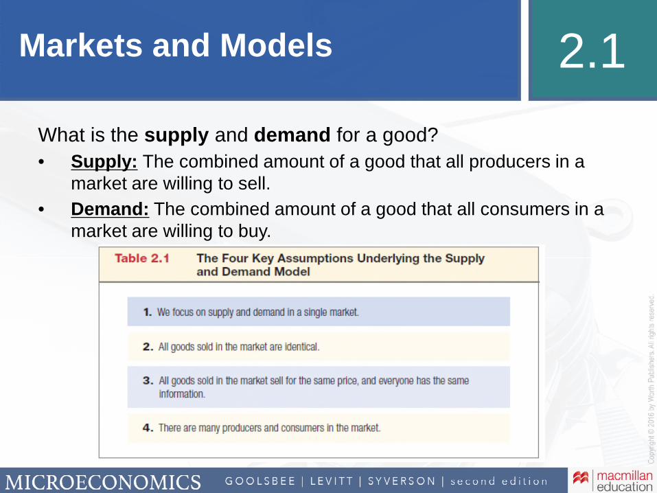
Markets and Models 2.1
What is the supply and demand for a good?
• Supply: The combined amount of a good that all producers in a market are willing to sell.
• Demand: The combined amount of a good that all consumers in a market are willing to buy.
Demand 2.2
What factors influence the demand for a good or service?
1. Price
2. Number of consumers
3. Consumer income or wealth
4. Consumer tastes
5. Prices of other, related goods
‒ Complements and substitutes
Demand 2.2
Many factors influence demand for goods and services. Is there one factor that stands out?
• Focus on how the price of a good influences the quantity demanded by consumers.
• Demand curve: Describes the relationship between quantity of a good that consumers demand and the good’s price, holding all other factors constant.

Demand 2.2
Figure 2.1 Demand for Tomatoes

Demand 2.2
Consider the market for oranges. We want to map out the quantity (in pounds) demanded by local consumers at various prices ($/pound)
0 400 800 1,200 1,600 2,000 2,400 Quantity of oranges (pounds)
Price of oranges ($/pound)
1
2
3
4
5
$6
REMEMBER TO ALWAYS LABEL GRAPHS!
At $6, consumers demand no oranges‒ This is known as the demand choke
price.
As the price drops, consumers demand a greater quantity of oranges.
We draw a demand curve that connects all the observed price-quantity combinations.
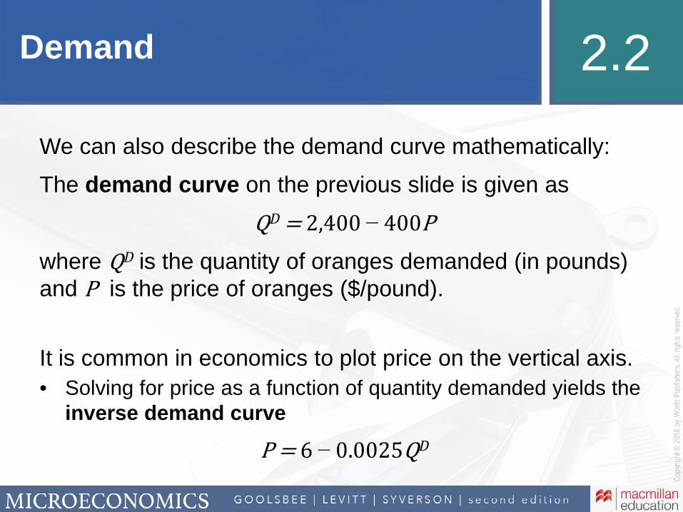
Demand 2.2
We can also describe the demand curve mathematically:
The demand curve on the previous slide is given as
D −
where D is the quantity of oranges demanded (in pounds) and is the price of oranges ($/pound).
It is common in economics to plot price on the vertical axis.
• Solving for price as a function of quantity demanded yields the inverse demand curve
− D
Demand 2.2
What about the other factors that influence demand?
• The demand curve is graphed in two dimensions; all other factors are assumed constant.
‒ Change in quantity demanded: A movement along the demand curve that occurs as a result of a change in the good’s price
• If another factor changes, the demand curve will shift.
− Change in demand: A shift of the entire demand curve caused by a change in a non-price factor that affects demand
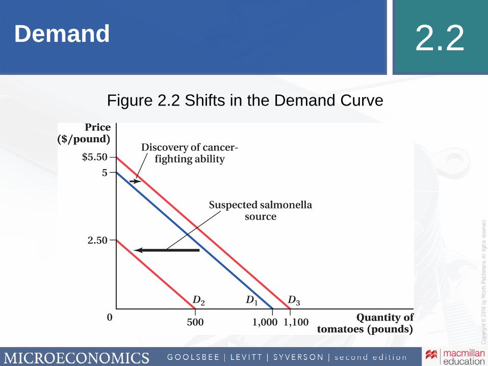
Demand 2.2
Figure 2.2 Shifts in the Demand Curve

2Mad Cow Disease and the Demand for Beef
Bovine spongiform encephalopathy (Mad Cow Disease), is a potentially fatal disease contracted through the consumption of infected beef products
Schlenker and Villas-Boas (2009) investigate the impact of the announcement of the first confirmed case of MCD in the US (December 23, 2003) on daily beef sales for a national supermarket chain.
The authors find a significant drop in the quantity of beef purchased following the announcement.
‒ Approximately 21% less beef was purchased in the following 35 days.
How do we represent this “shock” using demand curves?
Citation: Wolfram Schlenker and Sofia B. Vilas-Boas. 2009. Consumer and Market Responses to Mad Cow Disease. American Journal of Agricultural Economics 91(4):1140−1152.
Image: FreeDigitalPhotos.net
Image: FreeDigitalPhotos.net

2
0Quantity of beef per day (millions of pounds)
Price of beef($/pound)
$3
4 5
Demand curve prior to announcement of MCD
Demand curve after announcement of MCD
Prior to discovery, consumers demand 5 million pounds of beef per day at $3 per pound (numbers are examples).
Post-discovery, health concerns cause demand to shift inward, reducing quantity demanded at $3 by 1 million pounds per day.
Citation: Wolfram Schlenker and Sofia B. Vilas-Boas. 2009. Consumer and Market Responses to Mad Cow Disease. American Journal of Agricultural Economics
91(4):1140−1152.
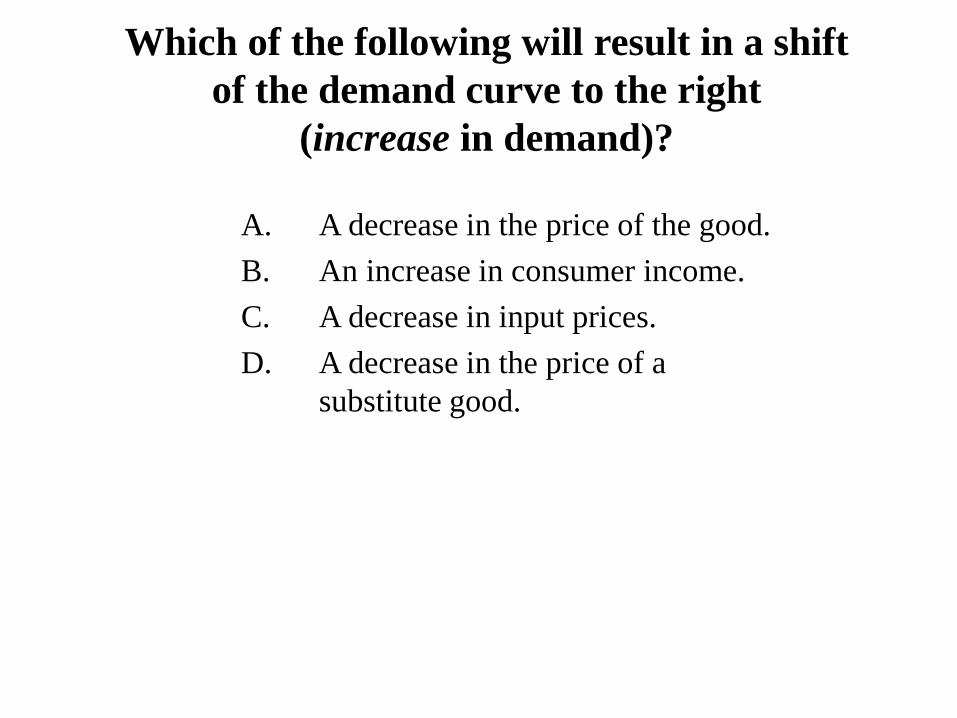
Which of the following will result in a shift of the demand curve to the right
(increase in demand)?
A. A decrease in the price of the good.
B. An increase in consumer income.
C. A decrease in input prices.
D. A decrease in the price of a substitute good.
Demand 2.2
Why do we treat price differently?
1. Price is usually the most important factor influencing demand.
2. Prices in most markets can change easily and often.
3. Price is the one factor of demand that is most likely to also measurably impact the supply of a good.
‒ Therefore, price ties together the two sides of the model.
Now to the supply side of the model.

Supply 2.3
What factors influence the supply of a good or service?
1. Price
2. Production costs
‒ Includes the processes used to make, distribute, and sell a good (production technology)
3. Number of sellers
4. Sellers’ outside options
‒ Price of good in other markets and prices of other, related goods
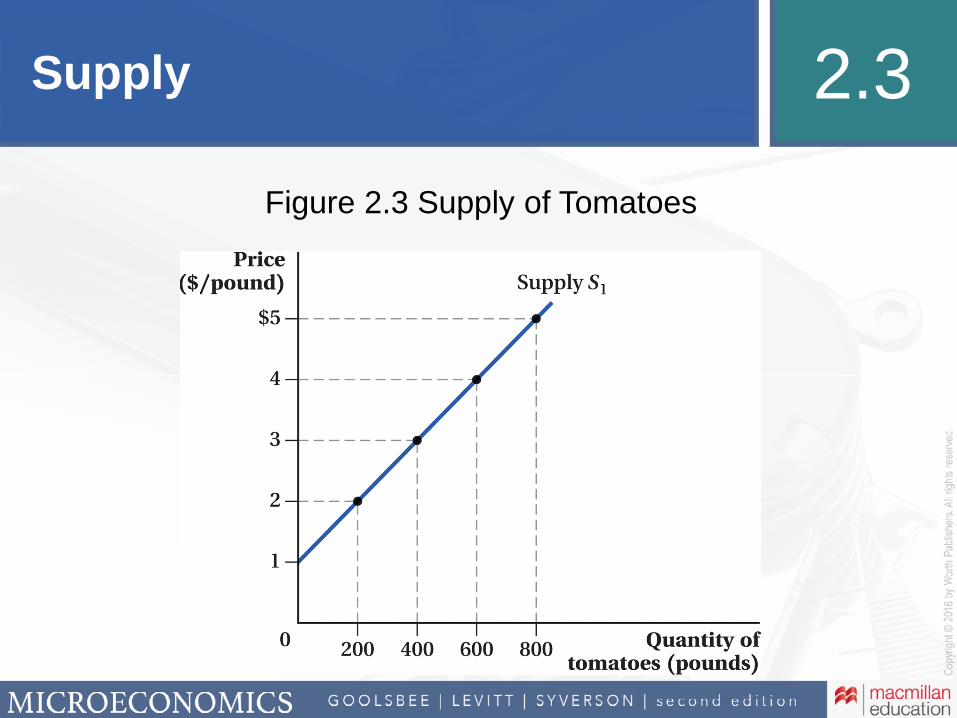
Supply 2.3
Figure 2.3 Supply of Tomatoes

Supply 2.3We can describe the relationship between the quantity of oranges supplied (in pounds) and the price ($/pound) with a supply curve.
0 400 800 1,200 1,600 Quantity of oranges (pounds)
Price of oranges ($/pound)
1
2
3
4
5
$6At the price of $2 per pound or less, suppliers find it unprofitable to sell any oranges so they are unwilling to supply any
- This is known as the supply choke price.
As the price increases beyond $2, suppliers will provide more and more oranges to the market.
Just as with demand, we connect the observed price-quantity combinations using a supply curve.
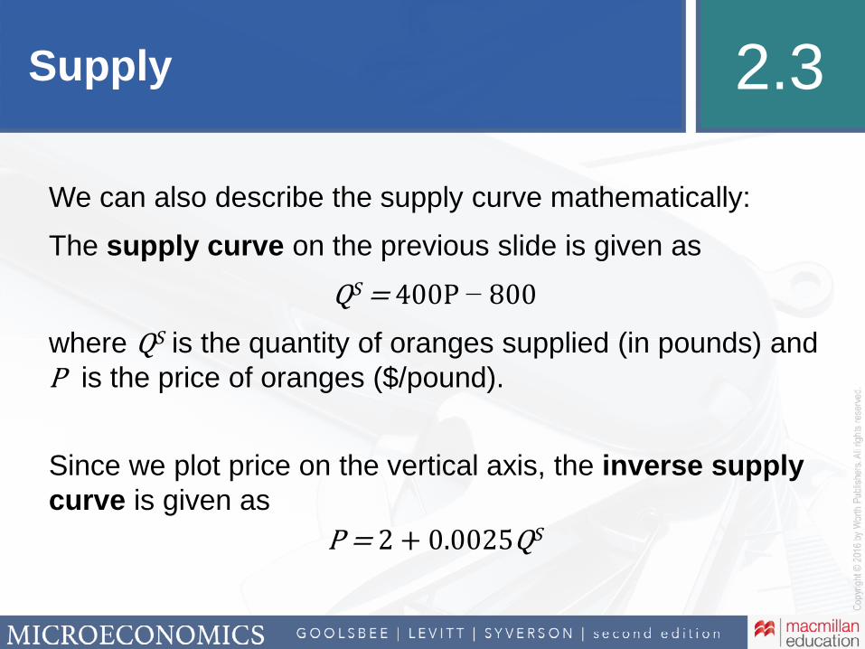
Supply 2.3
We can also describe the supply curve mathematically:
The supply curve on the previous slide is given as
S −
where S is the quantity of oranges supplied (in pounds) and is the price of oranges ($/pound).
Since we plot price on the vertical axis, the inverse supply curve is given as
S
Supply 2.3
What about the other factors that influence supply?
• The supply curve is also graphed in two dimensions; all other factors are assumed constant.
‒ Change in quantity supplied: A movement along the supply curve that occurs as a result of a change in the good’s price.
• If another factor changes, the supply curve will shift.
‒ Change in supply: A shift of the entire supply curve caused by a change in a non-price factor that affects supply.
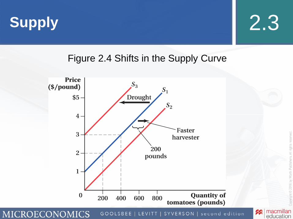
Supply 2.3
Figure 2.4 Shifts in the Supply Curve

2Solar Panels and Polysilicon
Solar energy is often touted as a key ingredient in the future of energy, but has historically been cost-prohibitive.
Recently, prices for solar modules have fallen rapidly, pushing the cost of solar power closer to “grid parity.”
‒ Grid parity means solar can compete with other sources of energy on a cost basis.
One of the key reasons has to do with the cost of production. The price of polysilicon, a semiconductor that is the basis for most solar systems, dropped more than 90% between 2008 and 2011.
How can we describe this phenomenon using supply curves?
Citation: Roca, M. and B. Sills. November 10, 2011. “Solar Glut Worsens as Supply Surge Cuts Prices 93%: Commodities.” Bloomberg News, www.bloomberg.com
Image: FreeDigitalPhotos.net
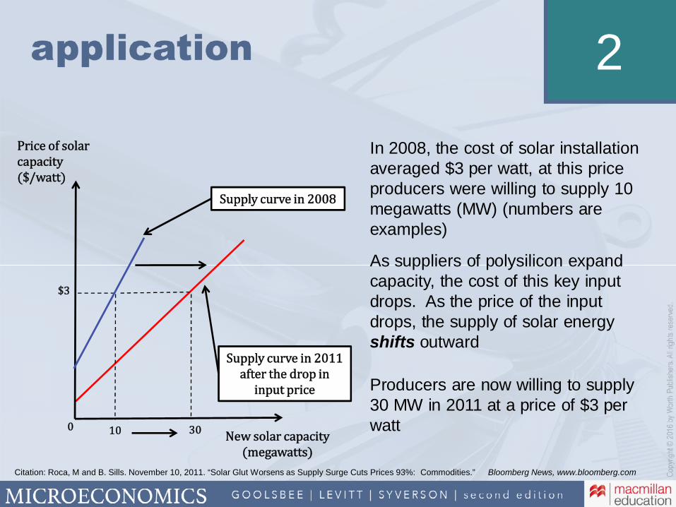
2
0New solar capacity
(megawatts)
Price of solar capacity ($/watt)
$3
10 30
Supply curve in 2008
Supply curve in 2011 after the drop in
input price
In 2008, the cost of solar installation averaged $3 per watt, at this price producers were willing to supply 10 megawatts (MW) (numbers are examples)
As suppliers of polysilicon expand capacity, the cost of this key input drops. As the price of the input drops, the supply of solar energy shifts outward
Producers are now willing to supply 30 MW in 2011 at a price of $3 per watt
Citation: Roca, M and B. Sills. November 10, 2011. “Solar Glut Worsens as Supply Surge Cuts Prices 93%: Commodities.” Bloomberg News, www.bloomberg.com
Which of the following will result in a shift of the supply curve to the right
(increase in supply)?
A. A decrease in the price of the good.
B. An increase in consumer income.
C. A decrease in input prices.
D. A decrease in the price of a substitute good.
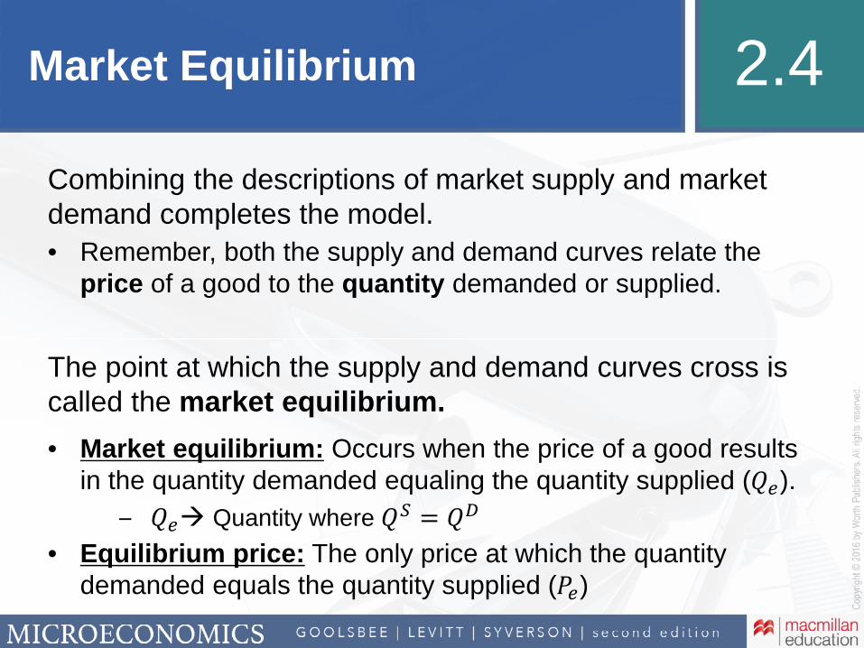
Market Equilibrium 2.4
Combining the descriptions of market supply and market demand completes the model.
• Remember, both the supply and demand curves relate the price of a good to the quantity demanded or supplied.
The point at which the supply and demand curves cross is called the market equilibrium.
• Market equilibrium: Occurs when the price of a good results in the quantity demanded equaling the quantity supplied ( �).
� Quantity where � �
• Equilibrium price: The only price at which the quantity demanded equals the quantity supplied ( �)
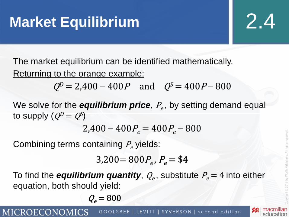
Market Equilibrium 2.4
The market equilibrium can be identified mathematically.
Returning to the orange example:D − S −
We solve for the equilibrium price, e , by setting demand equal to supply ( D S)
− e e −
Combining terms containing e yields:
e e
To find the equilibrium quantity, e , substitute e into either equation, both should yield:
e
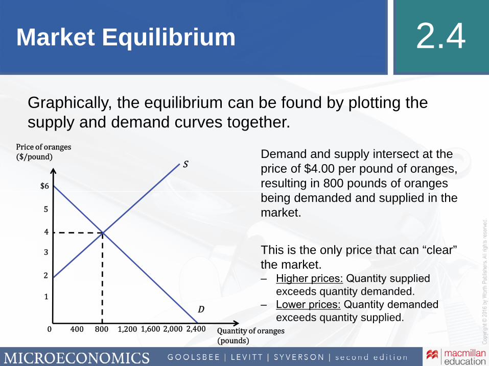
Market Equilibrium 2.4
Graphically, the equilibrium can be found by plotting the supply and demand curves together.
0 400 800 1,200 1,600 2,000 2,400 Quantity of oranges (pounds)
Price of oranges ($/pound)
1
2
3
4
5
$6
Demand and supply intersect at the price of $4.00 per pound of oranges, resulting in 800 pounds of oranges being demanded and supplied in the market.
This is the only price that can “clear”the market.‒ Higher prices: Quantity supplied
exceeds quantity demanded.‒ Lower prices: Quantity demanded
exceeds quantity supplied.
S
D

Market Equilibrium 2.4
Why markets move toward equilibrium
First, if e, quantity supplied will exceed quantity demanded, resulting in Excess Supply.
• S D
• Excess supply is also referred to as a surplus.
• To sell their products, producers must lower prices.
‒ As prices fall, quantity demanded increases and quantity supplied decreases until the market reaches an equilibrium at a lower price.
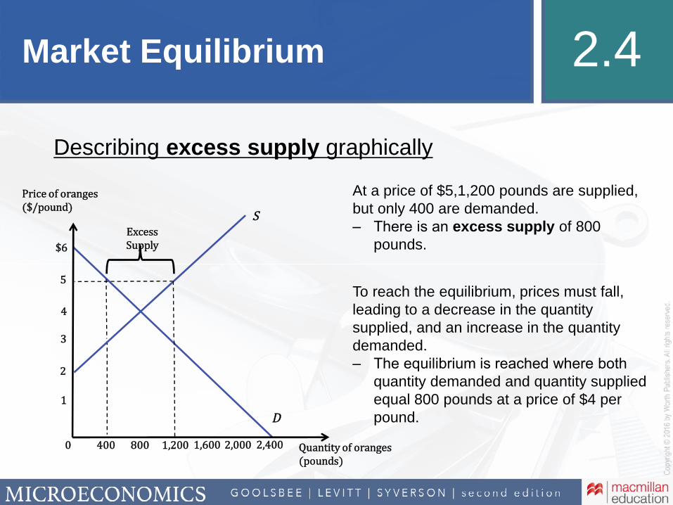
Market Equilibrium 2.4
Describing excess supply graphically
0 400 800 1,200 1,600 2,000 2,400 Quantity of oranges (pounds)
Price of oranges ($/pound)
1
2
3
4
5
$6
At a price of $5,1,200 pounds are supplied, but only 400 are demanded.‒ There is an excess supply of 800
pounds.
To reach the equilibrium, prices must fall, leading to a decrease in the quantity supplied, and an increase in the quantity demanded.‒ The equilibrium is reached where both
quantity demanded and quantity supplied equal 800 pounds at a price of $4 per pound.
S
D
Excess Supply
Market Equilibrium 2.4
Why markets move toward equilibrium
Likewise, e, quantity demanded will exceed quantity supplied, resulting in Excess Demand.• D S
• Excess demand is also referred to as a shortage.
• The shortage will induce buyers to bid up the price.
‒ As prices rise, quantity demanded will fall and quantity supplied will rise until the market reaches equilibrium at a higher price.

Market Equilibrium 2.4
Describing excess demand graphically
0 400 800 1,200 1,600 2,000 2,400 Quantity of oranges (pounds)
Price of oranges ($/pound)
1
2
3
4
5
$6
At a price of $3,400 pounds are supplied, but 1,200 pounds are demanded.‒ There is an excess demand of 800 pounds.
To reach the equilibrium, prices must rise, leading to a decrease in the quantity demanded, and an increase in the quantity supplied.‒ The equilibrium is reached where both
quantity demanded and quantity supplied equal 800 pounds at a price of $4 per pound
‒ .
S
D
Excess Demand
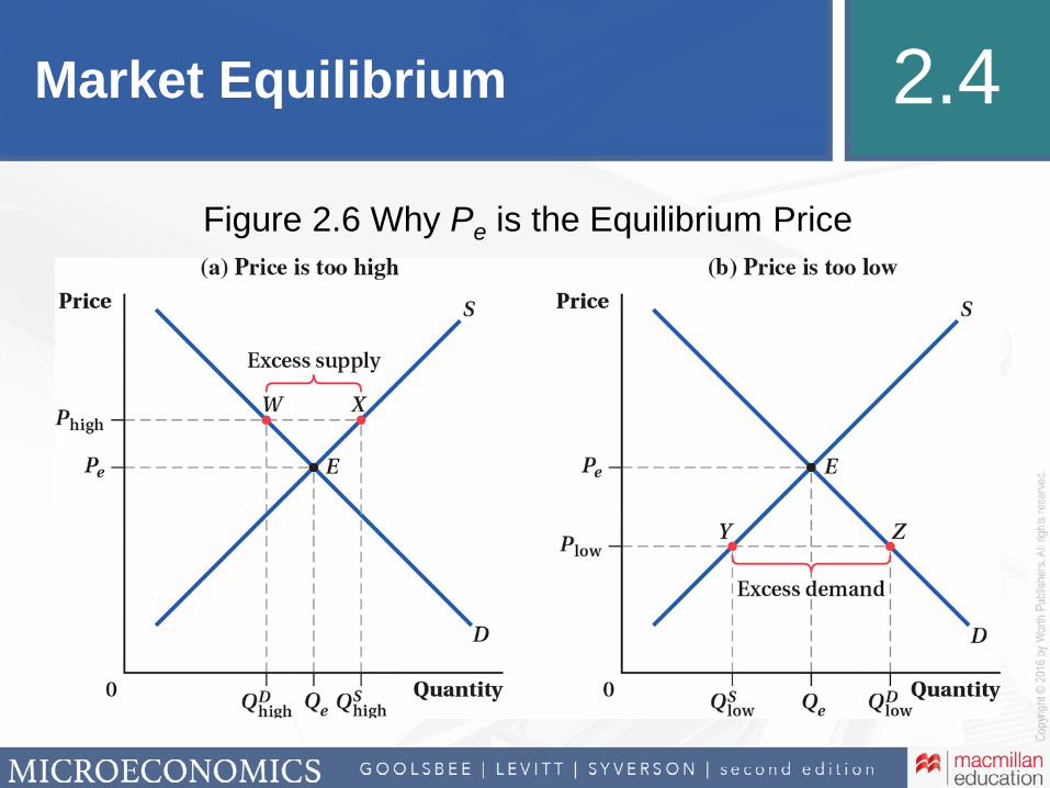
Market Equilibrium 2.4
Figure 2.6 Why Pe is the Equilibrium Price

In-text figure it out
The demand and supply for a monthly cell phone plan with unlimited texts can be represented by
D −S −
where is the monthly price, in dollars.
Answer the following questions:
a. If the current price for a contract is $40 per month, is the market in equilibrium?
b. Would you expect the price to rise, fall, or be unchanged?
c. If so, by how much? Explain.

In-text figure it out
a. Two ways to solve the problem:
1. Compute quantity supplied and demanded at a price of $40, or
2. Solve for the equilibrium price, and compare with $40.
Using the first method
D − −S − −
D S , so the market is not in equilibrium as there is excess demand (shortage).
b. What must happen to price?
Price needs to rise… but by how much?
c. Solve for equilibrium price and quantity (second method)
S D − −
Price must fall by $10, and 10 more contracts will be sold

Additional figure it out
The demand and supply for monthly gym memberships are given as
D −S −
where is the monthly price, in dollars
Answer the following questions:
a. If the current price for memberships is $50 per month, is the market in equilibrium?
b. Would you expect the price to rise or fall?
c. If so, by how much?

Additional figure it out
a. Two ways to solve the problem:
1. Compute quantity supplied and demanded at a price of $50, or
2. Solve for the equilibrium price, and compare with $50,
Using the first method
D − −S − −
S D, and the market is not in equilibrium as there is excess supply (surplus).
b. What must happen to price?
Price needs to fall… but by how much?
c. Solve for equilibrium price and quantity (second method)
S D − −
Price must fall by $5, and 50 more memberships are sold.
Market Equilibrium 2.4
What happens to the market equilibrium when there is a shift in demand or supply?
Remember the factors that can shift the demand curve:
• Number of consumers
• Wealth or income
• Consumer tastes
• Prices of related goods (complements or substitutes)
and those that shift the supply curve:
• Number of producers
• Costs of production
• Producer outside options

Market Equilibrium 2.4
In January, 2012, the FDA announced it had detected low levels of carbendazim, a potentially dangerous fungicide, in samples of orange juice.
How will this announcement affect the market for oranges?
• Supply side—the levels detected were not sufficient to induce action by FDA; assume no impact on supply.
• Demand side—bad press can have negative impacts on demand for food products (like the oranges used to make orange juice).
‒ What should happen?
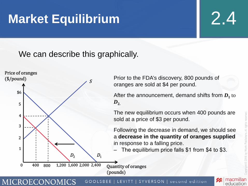
Market Equilibrium 2.4
We can describe this graphically..
0 400 800 1,200 1,600 2,000 2,400 Quantity of oranges (pounds)
Price of oranges ($/pound)
1
2
3
4
5
$6
Prior to the FDA’s discovery, 800 pounds of oranges are sold at $4 per pound.
After the announcement, demand shifts from D1 to D2.
The new equilibrium occurs when 400 pounds are sold at a price of $3 per pound.
Following the decrease in demand, we should see a decrease in the quantity of oranges suppliedin response to a falling price.‒ The equilibrium price falls $1 from $4 to $3.
S
D1D2
In-text figure it out
Draw a standard supply and demand diagram of the market for paperback books in a small coastal town.
Answer the following questions:
a. Suppose a hurricane knocks out electrical power for an extended time. Unable to watch television or use a computer, people must resort to reading books for entertainment. Using the supply and demand diagram, show what will happen to the equilibrium price and quantity of paperback books in the small coastal town.
b. Does this change reflect a change in demand or a change in the quantity demanded?

In-text figure it out
Q1 Q2 Quantity of paperback books
Price of ($/dollars)
P1
P2
S
D1
D2
a. The initial equilibrium occurs at a price of P1 and quantity Q1.
When the hurricane hits and people want more books because they can’t watch television or use the computer, demand shifts outward.
The new equilibrium price is P2, and the new quantity is Q2.
‒ So, price and quantity exchanged have both increased.
b. This represents a change (or shift) in demand.
Additional figure it out
Draw a standard supply and demand diagram of the market for generators in Tampa, Florida.
Answer the following questions:
a. Suppose a hurricane watch is issued, and some residents expect to lose power. Using the supply and demand diagram, show what will happen to the equilibrium price and quantity in the Tampa market for generators.
b. Does this change reflect a change in demand or a change in the quantity demanded?

Additional figure it out
Q1 Q2 Quantity of generators
Price of generators ($)
P1
P2
S
D1
D2
a. The initial equilibrium occurs at a price of P1 and quantity Q1.
When the hurricane watch is issued, the demand for generators shifts outward.
The new equilibrium price is P2, and the new quantity is Q2.
‒ So, price and quantity have both increased.
b. This represents a change (or shift) in demand.
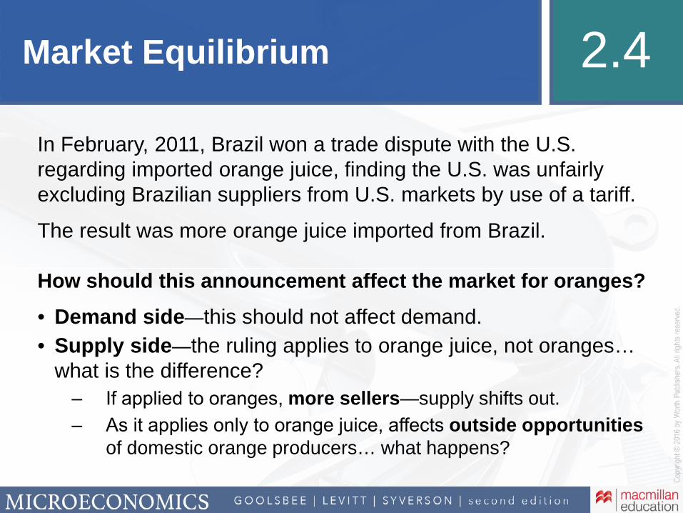
Market Equilibrium 2.4
In February, 2011, Brazil won a trade dispute with the U.S. regarding imported orange juice, finding the U.S. was unfairly excluding Brazilian suppliers from U.S. markets by use of a tariff.
The result was more orange juice imported from Brazil.
How should this announcement affect the market for oranges?
• Demand side—this should not affect demand.
• Supply side—the ruling applies to orange juice, not oranges… what is the difference?
‒ If applied to oranges, more sellers—supply shifts out.
‒ As it applies only to orange juice, affects outside opportunities of domestic orange producers… what happens?
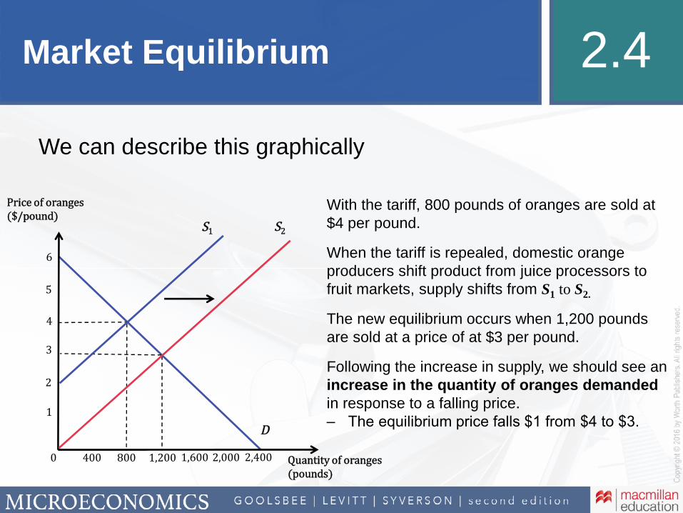
Market Equilibrium 2.4
We can describe this graphically
0 400 800 1,200 1,600 2,000 2,400 Quantity of oranges (pounds)
Price of oranges ($/pound)
1
2
3
4
5
6
With the tariff, 800 pounds of oranges are sold at $4 per pound.
When the tariff is repealed, domestic orange producers shift product from juice processors to fruit markets, supply shifts from S1 to S2.
The new equilibrium occurs when 1,200 pounds are sold at a price of at $3 per pound.
Following the increase in supply, we should see an increase in the quantity of oranges demanded in response to a falling price.‒ The equilibrium price falls $1 from $4 to $3.
S1
D
S2
In-text figure it out
Last month, you noticed the price of asparagus rising, and you also noted that there was less asparagus being sold than in the prior month.
Answer the following question:
Using a supply and demand diagram, what can you infer about the behavior of the supply and demand for asparagus?
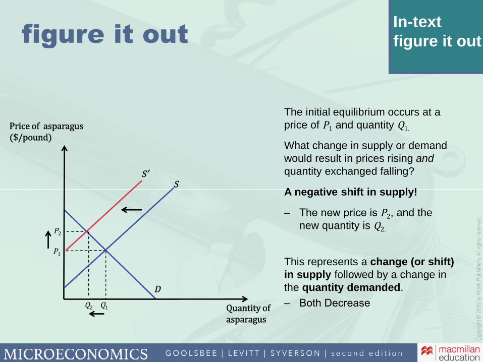
In-text figure it out
Q1Q2 Quantity of asparagus
Price of asparagus ($/pound)
P1
P2
D
SS′
The initial equilibrium occurs at a price of P1 and quantity Q1.
What change in supply or demand would result in prices rising and quantity exchanged falling?
A negative shift in supply!
‒ The new price is P2, and the new quantity is Q2.
This represents a change (or shift) in supply followed by a change in the quantity demanded.
‒ Both Decrease
Additional figure it out
This summer, you noticed the price of lobster in your supermarket rising, and also that there was much less lobster being sold.
Answer the following question:
Using a supply and demand diagram, what can you infer about this market?

Additional figure it out
Q1Q2 Quantity of lobsters
Price of lobster ($)
P1
P2
D
SS′
The initial equilibrium occurs at a price of P1 and quantity Q1.
What change in supply or demand would result in prices rising and quantity exchanged falling?
A negative shift in supply!
‒ The new price is P2, and the new quantity is Q2.
This represents a change (or shift) in supply followed by a change in the quantity demanded.
‒ Both Decrease
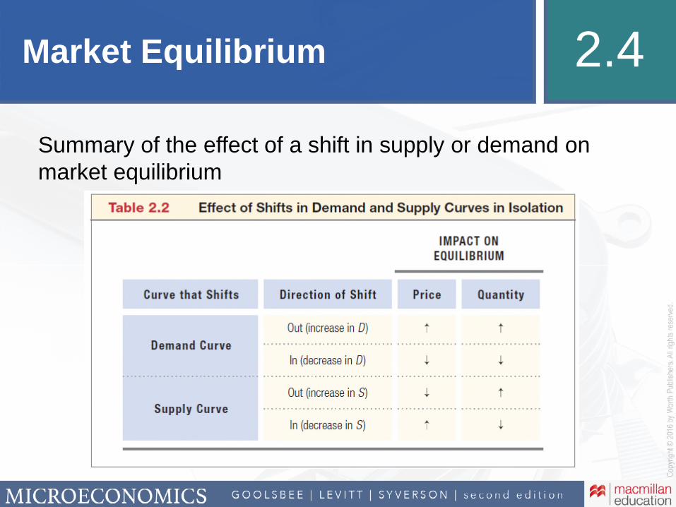
Market Equilibrium 2.4
Summary of the effect of a shift in supply or demand on market equilibrium
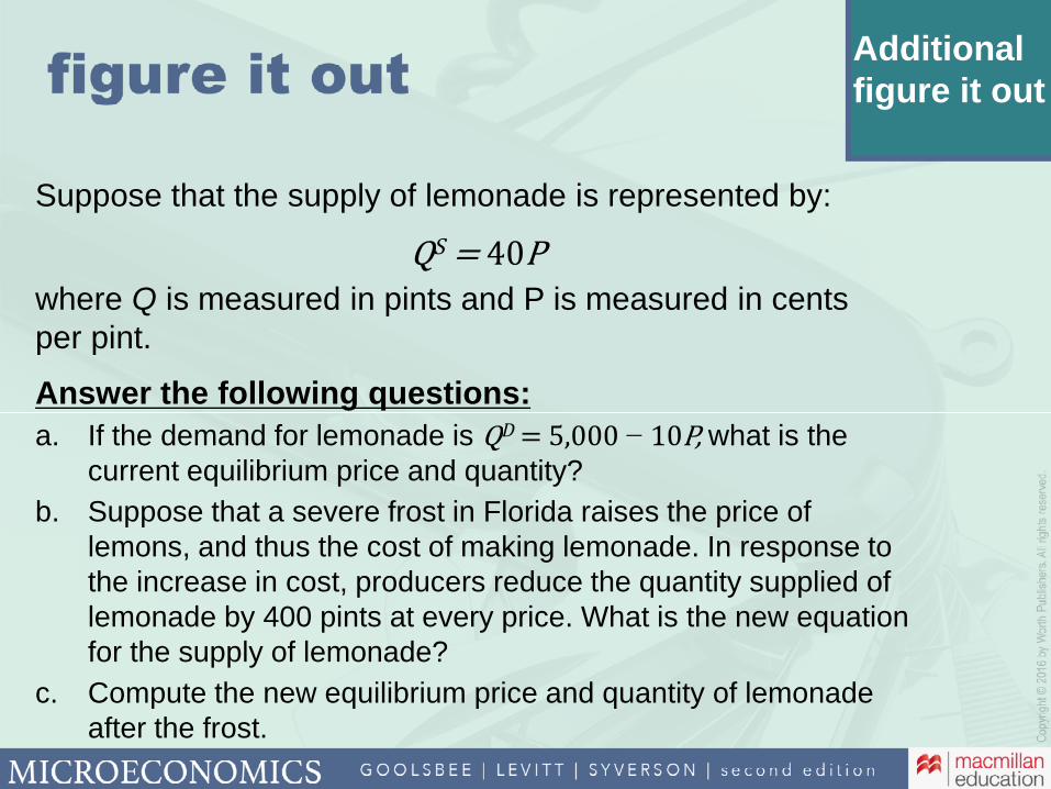
Additional figure it out
Suppose that the supply of lemonade is represented by:
S
where Q is measured in pints and P is measured in cents per pint.
Answer the following questions:
a. If the demand for lemonade is D − what is the current equilibrium price and quantity?
b. Suppose that a severe frost in Florida raises the price of lemons, and thus the cost of making lemonade. In response to the increase in cost, producers reduce the quantity supplied of lemonade by 400 pints at every price. What is the new equation for the supply of lemonade?
c. Compute the new equilibrium price and quantity of lemonade after the frost.
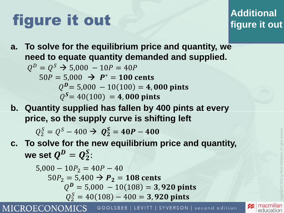
Additional figure it out
a. To solve for the equilibrium price and quantity, we need to equate quantity demanded and supplied.
� � ∗
�
�
b. Quantity supplied has fallen by 400 pints at every price, so the supply curve is shifting left
�� � �
�
c. To solve for the new equilibrium price and quantity,
we set
�
� ��
��
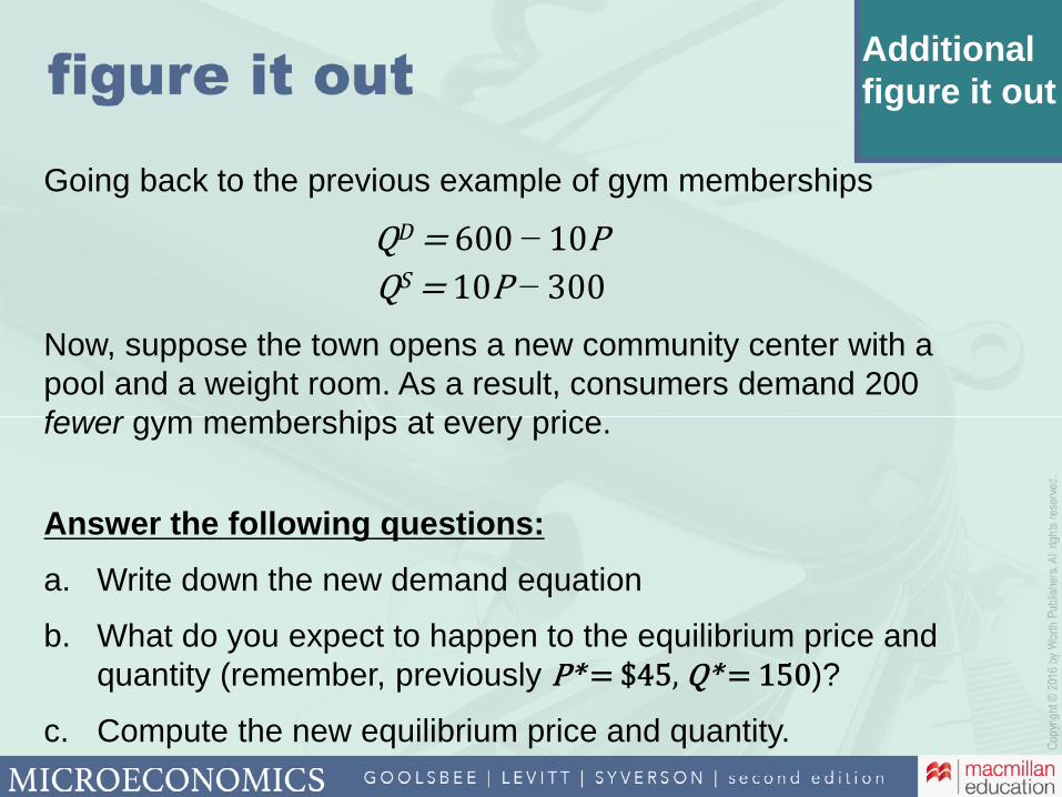
Additional figure it out
Going back to the previous example of gym memberships
D −S −
Now, suppose the town opens a new community center with a pool and a weight room. As a result, consumers demand 200 fewer gym memberships at every price.
Answer the following questions:
a. Write down the new demand equation
b. What do you expect to happen to the equilibrium price and quantity (remember, previously )?
c. Compute the new equilibrium price and quantity.
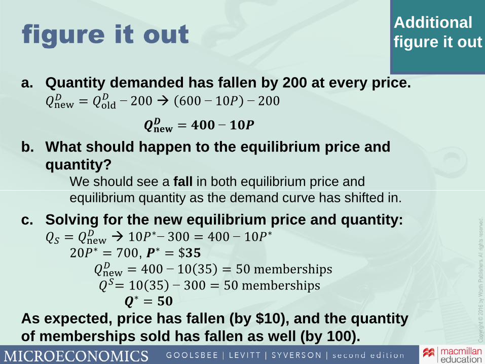
Additional figure it out
a. Quantity demanded has fallen by 200 at every price.
����
���� − − −
���� −
b. What should happen to the equilibrium price and quantity?
We should see a fall in both equilibrium price and equilibrium quantity as the demand curve has shifted in.
c. Solving for the new equilibrium price and quantity:
� ���� ∗− − ∗
∗ , ∗
���� −� −
∗
As expected, price has fallen (by $10), and the quantity of memberships sold has fallen as well (by 100).
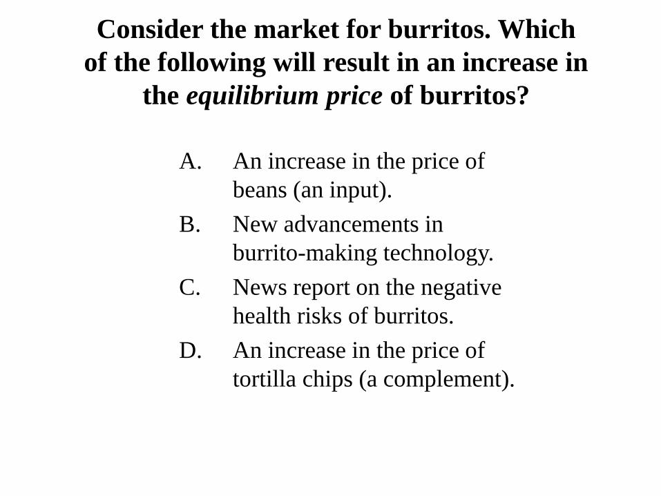
Consider the market for burritos. Which of the following will result in an increase in
the equilibrium price of burritos?
A. An increase in the price of beans (an input).
B. New advancements in burrito-making technology.
C. News report on the negative health risks of burritos.
D. An increase in the price of tortilla chips (a complement).

Consider the market for burritos. Which of the following will result in an increase in the
equilibrium quantity of burritos?
A. An increase in the price of beans (an input).
B. An increase in the price of tortilla chips (a complement).
C. New advancements in burrito-making technology.
D. News report on the negative health risks of burritos.
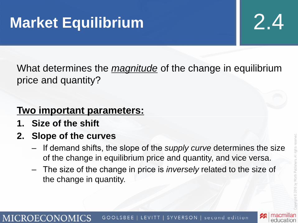
Market Equilibrium 2.4
What determines the magnitude of the change in equilibrium price and quantity?
Two important parameters:
1. Size of the shift
2. Slope of the curves
‒ If demand shifts, the slope of the supply curve determines the size of the change in equilibrium price and quantity, and vice versa.
‒ The size of the change in price is inversely related to the size of the change in quantity.
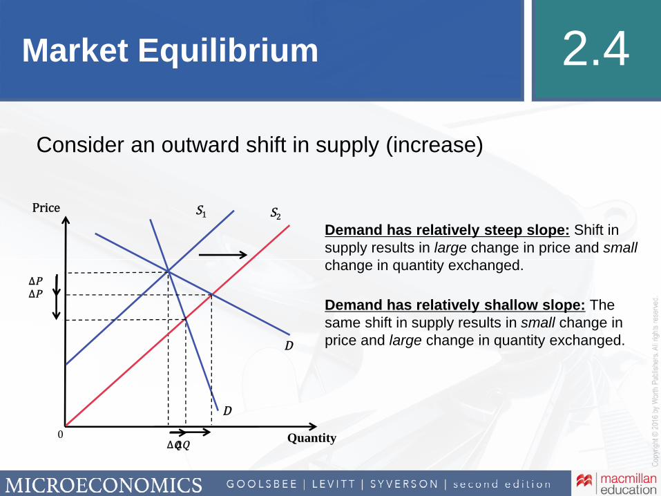
Market Equilibrium 2.4
Consider an outward shift in supply (increase)
0 Quantity
Price
D
ΔQ
S1 S2
Demand has relatively steep slope: Shift in supply results in large change in price and small change in quantity exchanged.
Demand has relatively shallow slope: The same shift in supply results in small change in price and large change in quantity exchanged.
ΔP
D
ΔP
ΔQ
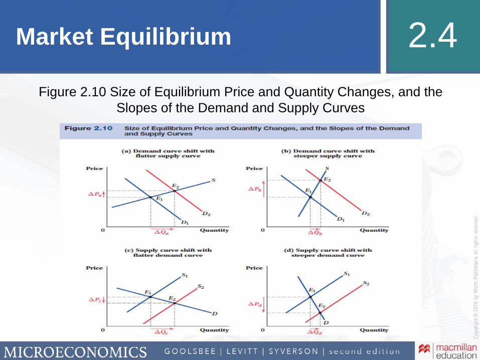
Market Equilibrium 2.4
Figure 2.10 Size of Equilibrium Price and Quantity Changes, and the Slopes of the Demand and Supply Curves

Market Equilibrium 2.4
Sometimes, supply and demand shift simultaneously!
Example:
Hurricane Katrina and the New Orleans housing market
• Katrina destroyed many homes. What happens to supply?
• The hurricane displaced thousands of residents, many of which have not returned. What happens to demand?
‒ How will these shifts affect the housing market equilibrium in New Orleans?
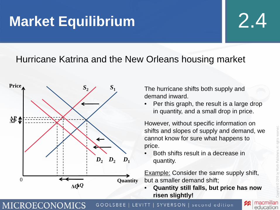
Market Equilibrium 2.4
Hurricane Katrina and the New Orleans housing market
0 Quantity
Price S2 S1 The hurricane shifts both supply and demand inward. • Per this graph, the result is a large drop
in quantity, and a small drop in price.
However, without specific information on shifts and slopes of supply and demand, we cannot know for sure what happens to price.• Both shifts result in a decrease in
quantity.
Example: Consider the same supply shift, but a smaller demand shift; • Quantity still falls, but price has now
risen slightly!
ΔP
ΔQ
D2 D1
ΔP
ΔQ
D2
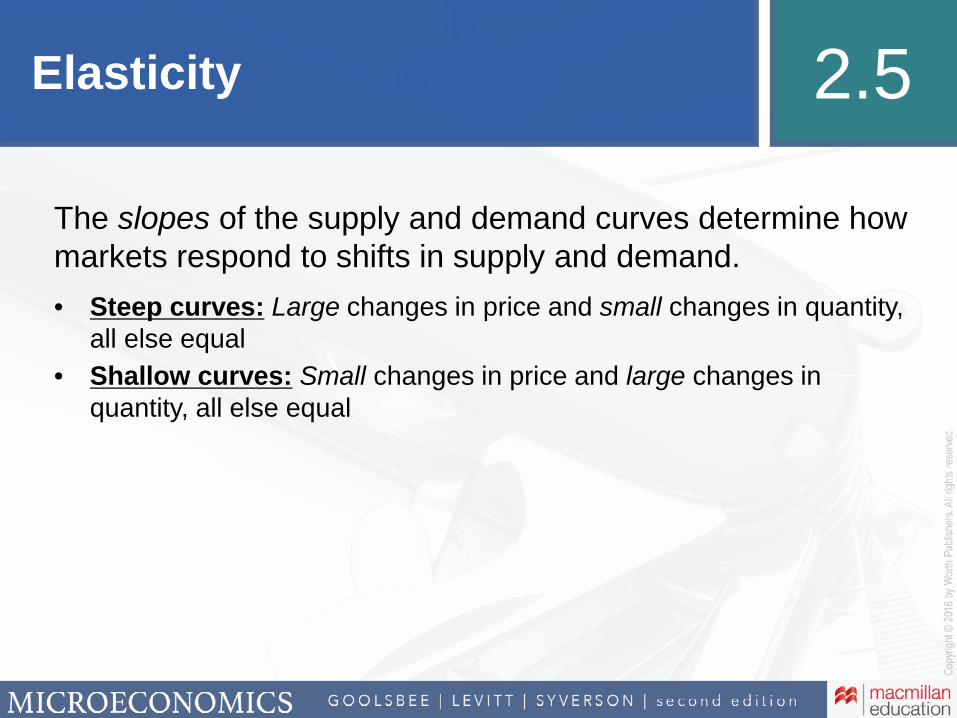
Elasticity 2.5
The slopes of the supply and demand curves determine how markets respond to shifts in supply and demand.
• Steep curves: Large changes in price and small changes in quantity, all else equal
• Shallow curves: Small changes in price and large changes in quantity, all else equal
Elasticity 2.5
Elasticity
• Unit-less measure that describes the sensitivity of quantity demanded or supplied to changes in price, income, or price of related goods.
• Percentage change in one variable (e.g., quantity) divided by the percentage change in another (e.g., price)
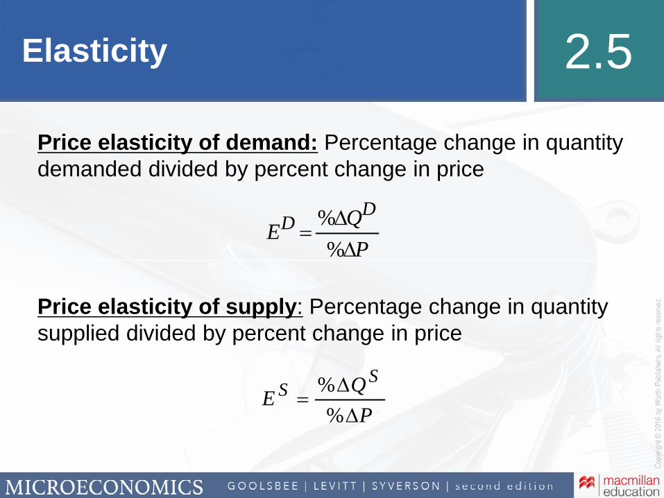
Elasticity 2.5
Price elasticity of demand: Percentage change in quantity demanded divided by percent change in price
Price elasticity of supply: Percentage change in quantity supplied divided by percent change in price
P
QE
DD
%
%
P
QE
SS
%
%
Elasticity 2.5
When price elasticity of demand is high…
• Relatively small increases in price result in relatively large drops in quantity demanded.
• Examples?
‒ McDonald’s hamburgers, Campbell's Soup, Snickers bar…
When price elasticity of demand is low…
• Relatively large increases in price result in relatively small drops in quantity demanded.
• Examples?
‒ Gasoline, tap water, cigarettes …
The price elasticity of demand is represented by the following formula:
A. ΔQD/ΔP
B. ΔP/ΔQD
C. %ΔQD/%ΔP
D. None of the above is correct.
Elasticity 2.5
What variables affect the elasticity of demand?
1. Availability of close substitutes
2. Breadth of the market
3. Type of product
‒ Necessity or luxury item
4. Percentage of income spent on the good
5. Time horizon of the analysis
What variables affect the elasticity of supply?
1. The ease at which production capacity can be expanded
2. Time horizon of the analysis
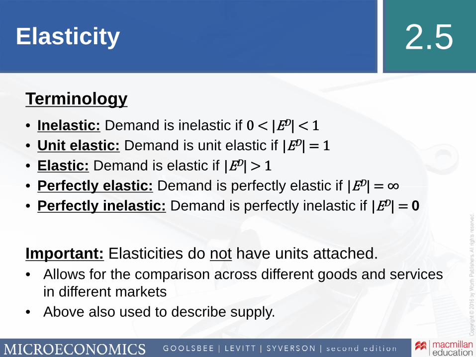
Elasticity 2.5
Terminology
• Inelastic: Demand is inelastic if D
• Unit elastic: Demand is unit elastic if D
• Elastic: Demand is elastic if D
• Perfectly elastic: Demand is perfectly elastic if D
• Perfectly inelastic: Demand is perfectly inelastic if D 0
Important: Elasticities do not have units attached.
• Allows for the comparison across different goods and services in different markets
• Above also used to describe supply.

2
The Price of Gasoline and Traffic Congestion
Burger and Kaffine (2009) investigate gas prices, highway speed, and congestion in Los Angeles between 2001 and 2006.
In theory, higher gasoline prices should reduce highway speeds because driving slowly tends to increase efficiency.
The authors find drivers do not slow down when traffic is light; however, during rush hour, average speeds actually increase
about 3.3 miles per hour for every $1.00/gallon.
They attribute this to reduced congestion; drivers respond to high prices by taking fewer trips, or using public transportation.
Accounting for the relationship between vehicle miles travelled (VMT) and congestion, the authors estimate the price elasticity of demand for VMT to be approximately −0.15 (inelastic).
Citation: Burger, N.E. and D.T. Kaffine. 2009. “Gas Prices, Traffic, and Freeway Speeds in Los Angeles.” The Review of Economics and Statistics 91(3): 652-657.
Image: FreeDigitalPhotos.net
Image: FreeDigitalPhotos.net
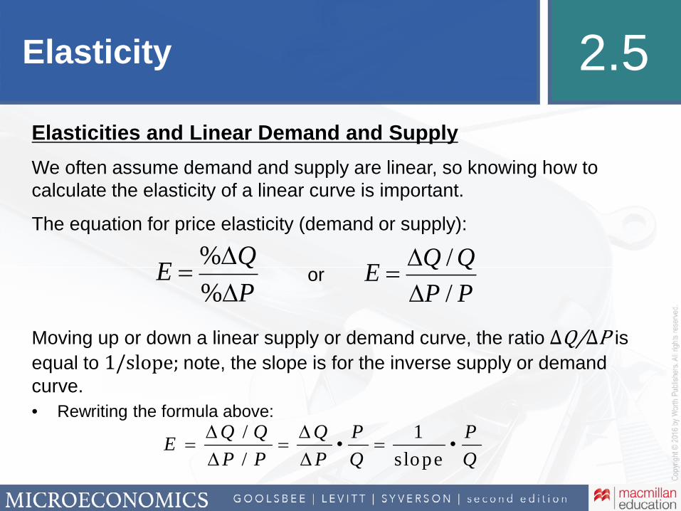
Elasticity 2.5
Elasticities and Linear Demand and Supply
We often assume demand and supply are linear, so knowing how to calculate the elasticity of a linear curve is important.
The equation for price elasticity (demand or supply):
or
Moving up or down a linear supply or demand curve, the ratio is
equal to note, the slope is for the inverse supply or demand curve.
• Rewriting the formula above:
E =%DQ
%DPE =
DQ / Q
DP / P
/ 1• •
/ slope
Q Q Q P PE
P P P Q Q
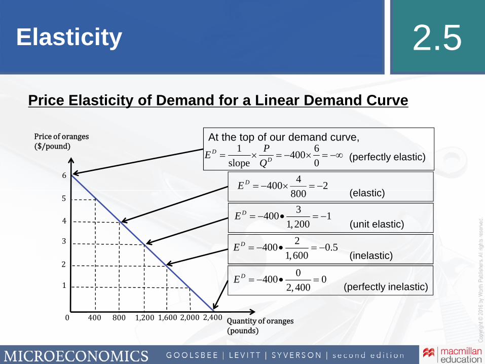
Elasticity 2.5
0 400 800 1,200 1,600 2,000 2,400 Quantity of oranges (pounds)
Price of oranges ($/pound)
1
2
3
4
5
6
At the top of our demand curve,
(perfectly elastic)1 6
400slope 0
D
D
PE
Q
(elastic)2
800
4400 DE
(unit elastic)
3400 1
1,200DE
(inelastic)
2400 0.5
1,600DE
(perfectly inelastic)
0400 0
2, 400DE
Price Elasticity of Demand for a Linear Demand Curve
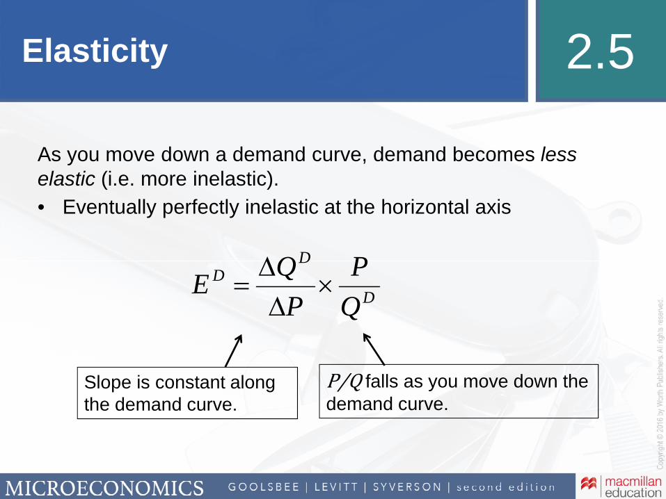
Elasticity 2.5
As you move down a demand curve, demand becomes less elastic (i.e. more inelastic).
• Eventually perfectly inelastic at the horizontal axis
D
DD
Q
P
P
QE
Slope is constant along the demand curve.
falls as you move down the demand curve.
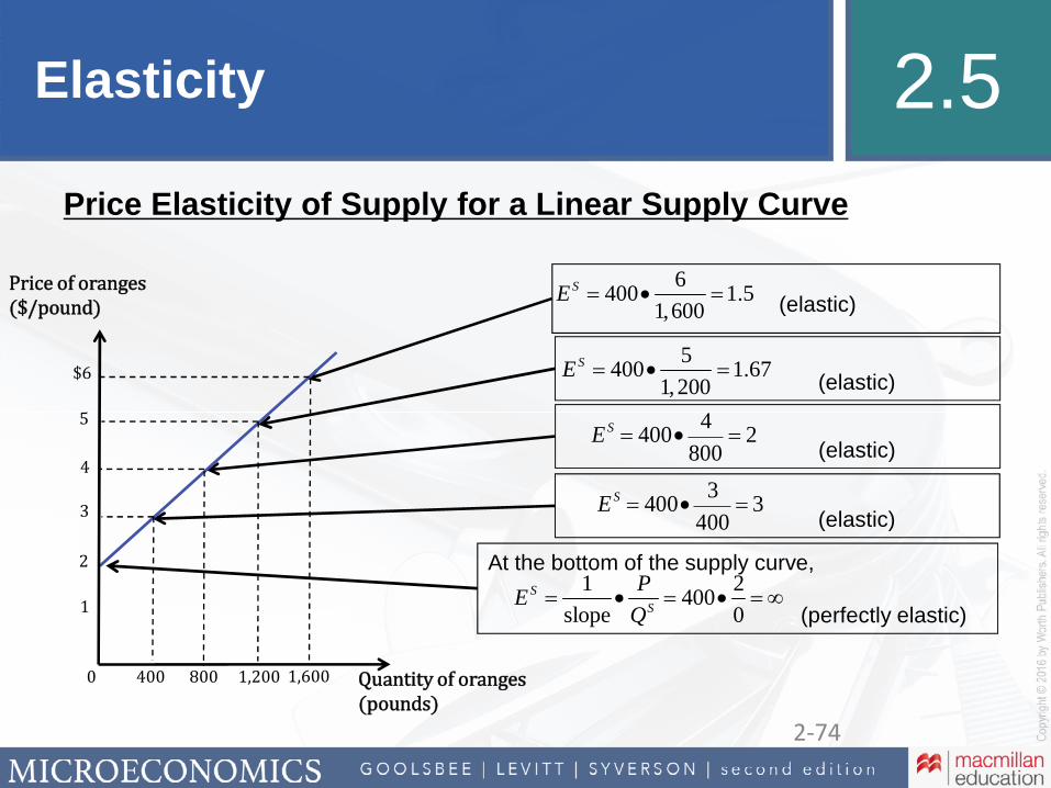
Elasticity 2.5
Price Elasticity of Supply for a Linear Supply Curve
2-74
(elastic)6
400 1.51,600
SE
(elastic)5
400 1.671,200
SE
(elastic)E S = 400·
4
800= 2
(elastic)E S = 400·
3
400= 3
At the bottom of the supply curve,
(perfectly elastic)
1 2400
slope 0S
S
PE
Q
0 400 800 1,200 1,600 Quantity of oranges (pounds)
1
2
3
4
5
$6
Price of oranges ($/pound)
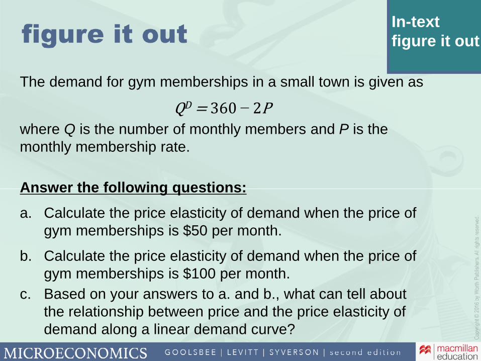
In-text figure it out
The demand for gym memberships in a small town is given as
D −
where Q is the number of monthly members and P is the monthly membership rate.
Answer the following questions:
a. Calculate the price elasticity of demand when the price of gym memberships is $50 per month.
b. Calculate the price elasticity of demand when the price of gym memberships is $100 per month.
c. Based on your answers to a. and b., what can tell about the relationship between price and the price elasticity of demand along a linear demand curve?
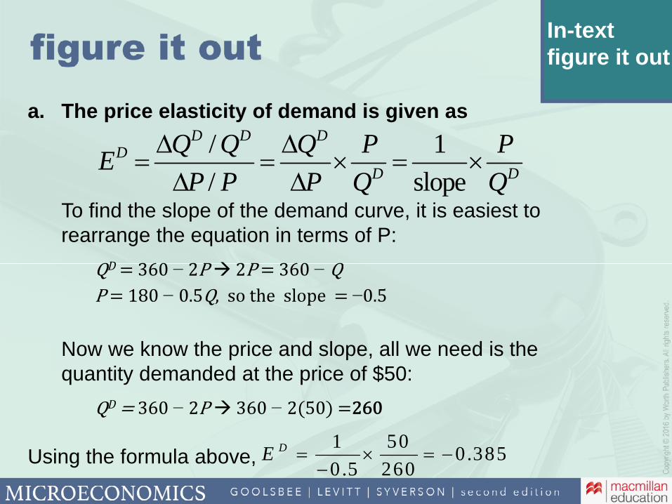
In-text figure it out
a. The price elasticity of demand is given as
To find the slope of the demand curve, it is easiest to rearrange the equation in terms of P:
D − −
− −
Now we know the price and slope, all we need is the quantity demanded at the price of $50:
D − −
Using the formula above,
/ 1
/ slope
D D DD
D D
Q Q Q P PE
P P P Q Q
1 500.385
0.5 260DE
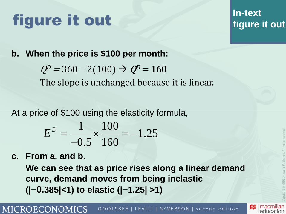
In-text figure it out
b. When the price is $100 per month:
D − D
At a price of $100 using the elasticity formula,
c. From a. and b.
We can see that as price rises along a linear demand curve, demand moves from being inelastic
(|−0.385|<1) to elastic (|−1.25| >1)
1 1001.25
0.5 160DE
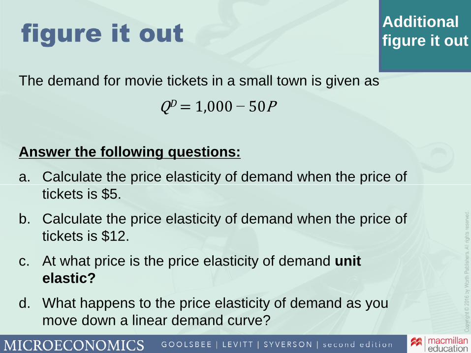
Additional figure it out
The demand for movie tickets in a small town is given as
D −
Answer the following questions:
a. Calculate the price elasticity of demand when the price of tickets is $5.
b. Calculate the price elasticity of demand when the price of tickets is $12.
c. At what price is the price elasticity of demand unit elastic?
d. What happens to the price elasticity of demand as you move down a linear demand curve?
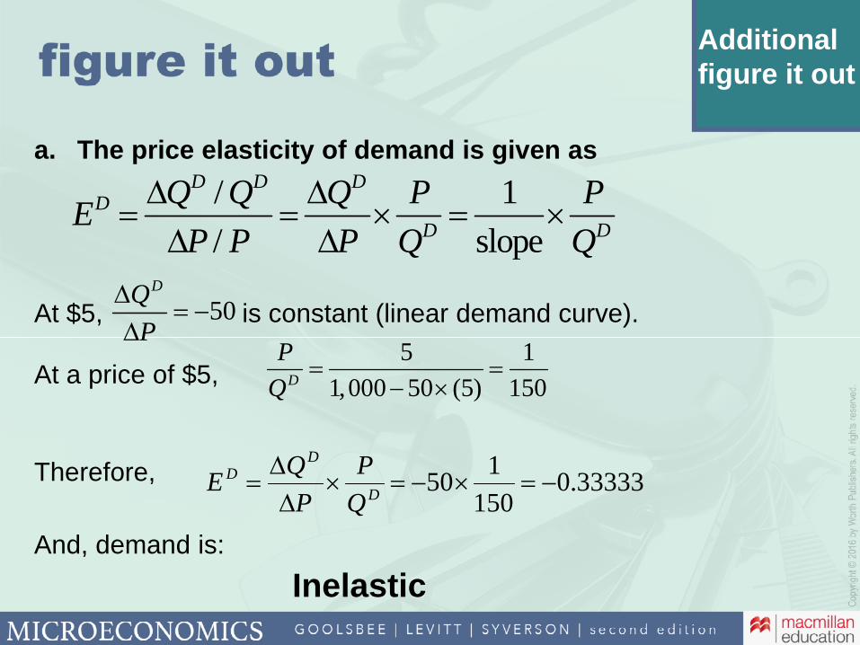
Additional figure it out
a. The price elasticity of demand is given as
At $5, is constant (linear demand curve).
At a price of $5,
Therefore,
And, demand is:
Inelastic
/ 1
/ slope
D D DD
D D
Q Q Q P PE
P P P Q Q
50DQ
P
5 1
1,000 50 (5) 150D
P
Q
33333.0150
150
D
DD
Q
P
P
QE
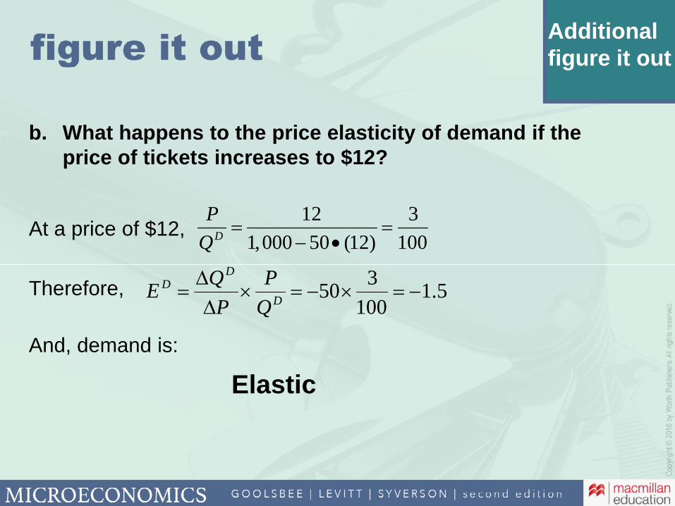
Additional figure it out
b. What happens to the price elasticity of demand if the price of tickets increases to $12?
At a price of $12,
Therefore,
And, demand is:
Elastic
12 3
1,000 50 (12) 100D
P
Q
5.1100
350
D
DD
Q
P
P
QE
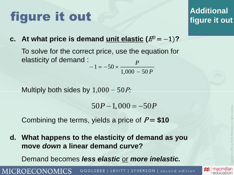
Additional figure it out
c. At what price is demand unit elastic ( D ?
To solve for the correct price, use the equation for elasticity of demand :
Multiply both sides by −
Combining the terms, yields a price of $10
d. What happens to the elasticity of demand as you move down a linear demand curve?
Demand becomes less elastic or more inelastic.
50 1,000 50P P
P
P
50000,1501
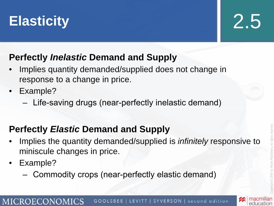
Elasticity 2.5
Perfectly Inelastic Demand and Supply
• Implies quantity demanded/supplied does not change in response to a change in price.
• Example?
‒ Life-saving drugs (near-perfectly inelastic demand)
Perfectly Elastic Demand and Supply
• Implies the quantity demanded/supplied is infinitely responsive to miniscule changes in price.
• Example?
‒ Commodity crops (near-perfectly elastic demand)
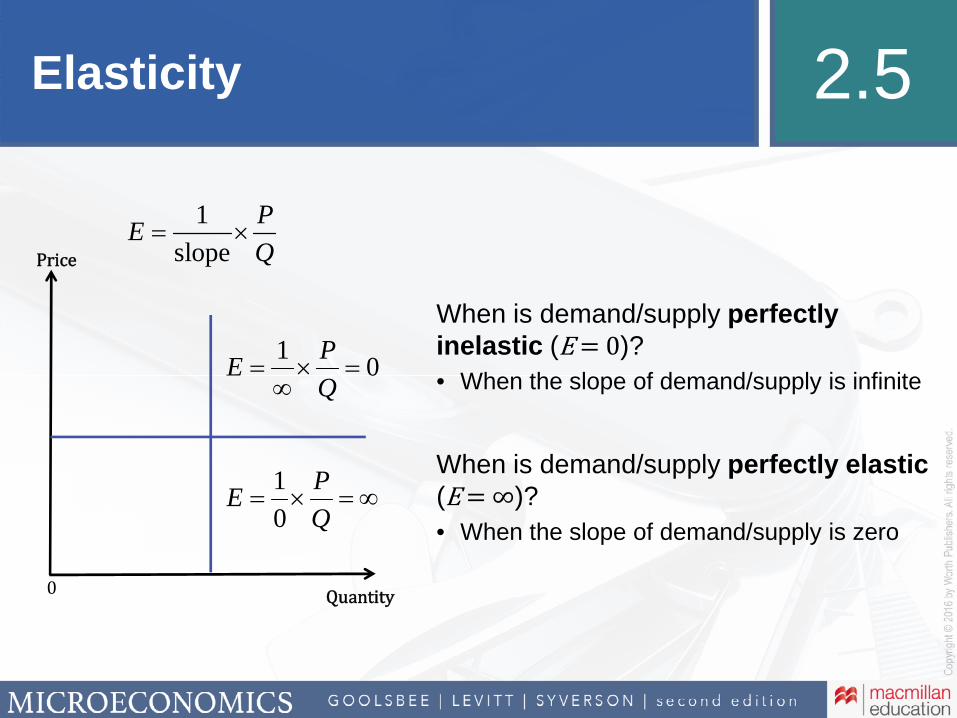
Elasticity 2.5
0 Quantity
Price
When is demand/supply perfectly inelastic ( )?
• When the slope of demand/supply is infinite
When is demand/supply perfectly elastic( )?
• When the slope of demand/supply is zero
1
slope
PE
Q
01
Q
PE
Q
PE
0
1

If the price elasticity of demand, ED = −0.5, we say the good has:
A. Inelastic demand.
B. Elastic demand.
C. Unit elastic demand.
D. Perfectly inelastic demand.
If the price elasticity of demand, ED = −1, we say the good has:
A. Inelastic demand.
B. Elastic demand.
C. Unit elastic demand.
D. Perfectly inelastic demand.
If the price elasticity of supply, ES = ∞, we say the good has:
A. Inelastic supply.
B. Elastic supply.
C. Unit elastic supply.
D. Perfectly elastic supply.
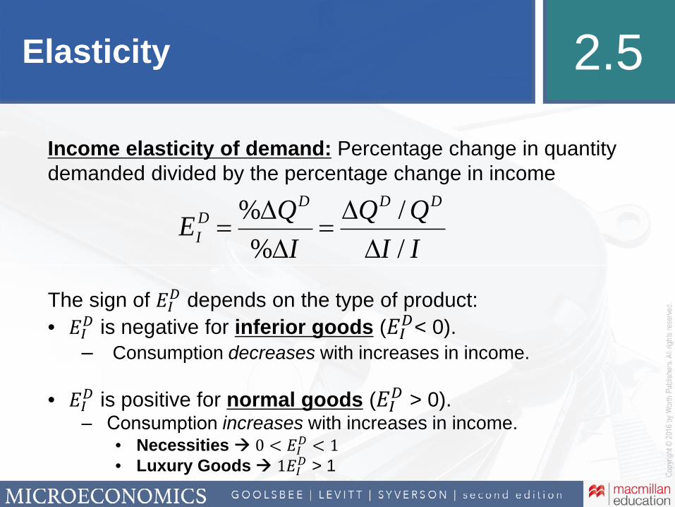
Elasticity 2.5
Income elasticity of demand: Percentage change in quantity demanded divided by the percentage change in income
The sign of �� depends on the type of product:
• �� is negative for inferior goods ( < 0).‒ Consumption decreases with increases in income.
• �� is positive for normal goods ( > 0).‒ Consumption increases with increases in income.
• Necessities ��
• Luxury Goods �� > 1
EID =
%DQD
%DI=
DQD / QD
DI / I
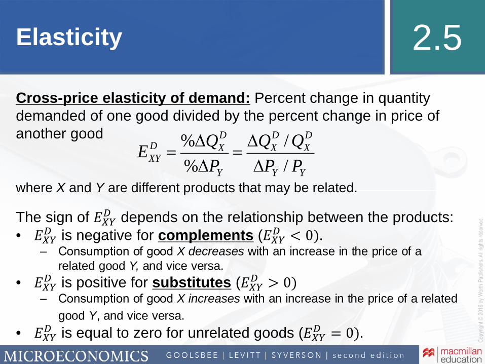
Elasticity 2.5
Cross-price elasticity of demand: Percent change in quantity demanded of one good divided by the percent change in price of another good
where X and Y are different products that may be related.
The sign of ��� depends on the relationship between the products:
• ��� is negative for complements ( ��
�
‒ Consumption of good X decreases with an increase in the price of a related good Y, and vice versa.
• ��� is positive for substitutes ( ��
�
‒ Consumption of good X increases with an increase in the price of a related
good Y, and vice versa.
• ��� is equal to zero for unrelated goods ( ��
�
EXYD =
%DQXD
%DPY
=DQX
D / QXD
DPY / PY
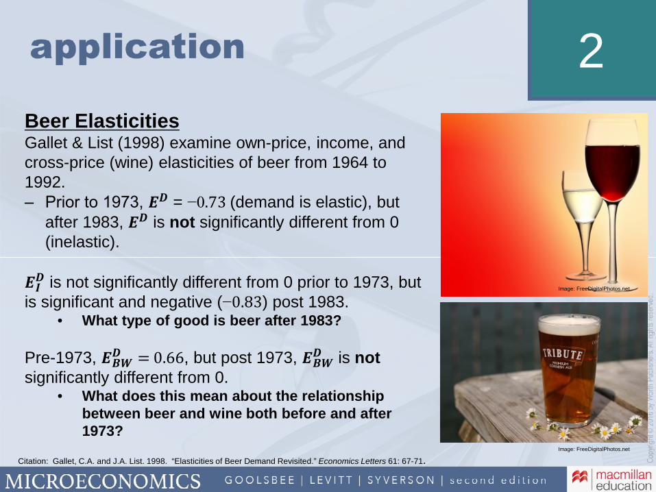
2
Image: FreeDigitalPhotos.net
Image: FreeDigitalPhotos.net
Beer ElasticitiesGallet & List (1998) examine own-price, income, and cross-price (wine) elasticities of beer from 1964 to 1992.‒ Prior to 1973, � = −0 (demand is elastic), but
after 1983, � is not significantly different from 0 (inelastic).
�� is not significantly different from 0 prior to 1973, but
is significant and negative (− ) post 1983.• What type of good is beer after 1983?
Pre-1973, ��� , but post 1973, ��
� is notsignificantly different from 0.
• What does this mean about the relationship between beer and wine both before and after 1973?
Citation: Gallet, C.A. and J.A. List. 1998. “Elasticities of Beer Demand Revisited.” Economics Letters 61: 67-71.

2
Citation: Gallet, C.A. and J.A. List. 1998. “Elasticities of Beer Demand Revisited.” Economics Letters 61: 67-71.
What might explain changes in elasticities over time?
Consumer tastes: Release of information regarding negative health effects beginning in the 1970s may have led to reduced demand.
• Increased proportion of drinkers who are less health conscious and/or addictive in nature
‒ Evidence suggests heavy drinkers are less price-sensitive to alcohol, hence the change to inelastic.
‒ Poorer consumers generally have less education and are less health conscious, hence the move to an inferior good.
• Change in beer-wine relationship from substitutes to unrelated goods perhaps due to increased product differentiation (e.g., microbreweries, lite beers) in the beer industry
Image: FreeDigitalPhotos.net
Image: FreeDigitalPhotos.net
If the cross-price elasticity of demand, ED
XY < 0, we say the goods are:
A. Normal.
B. Inferior.
C. Substitutes.
D. Complements.
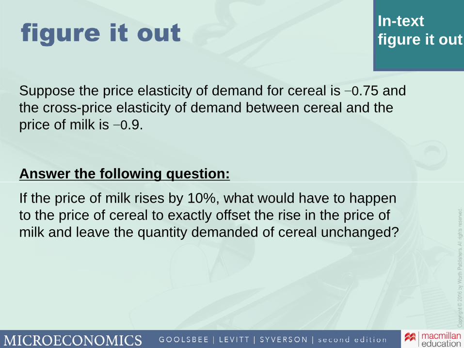
In-text figure it out
Suppose the price elasticity of demand for cereal is −0.75 and the cross-price elasticity of demand between cereal and the price of milk is −0.9.
Answer the following question:
If the price of milk rises by 10%, what would have to happen to the price of cereal to exactly offset the rise in the price of milk and leave the quantity demanded of cereal unchanged?
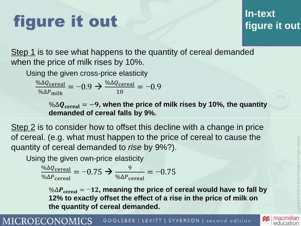
In-text figure it out
Step 1 is to see what happens to the quantity of cereal demanded when the price of milk rises by 10%.
Using the given cross-price elasticity %∆�������
%∆�����−
%∆�������
��−
%∆������� = −�, when the price of milk rises by 10%, the quantity demanded of cereal falls by 9%.
Step 2 is to consider how to offset this decline with a change in price of cereal. (e.g. what must happen to the price of cereal to cause the quantity of cereal demanded to rise by 9%?).
Using the given own-price elasticity%∆�������
%∆�������−
�
%∆�������−
%∆������� = −��, meaning the price of cereal would have to fall by 12% to exactly offset the effect of a rise in the price of milk on the quantity of cereal demanded.
Conclusion 2.6
This chapter has introduced one of the most basic models in economics: the Supply and Demand model.
Forthcoming chapters:
• Examine the factors of production underlying supply.
• Introduce consumer theory, which underlies market demand.
• Examine situations in which assumptions fail to reflect reality (e.g., the impact of uncertainty).
In Chapter 3, we will discover how consumers and producers benefit from markets, and examine the impact of government regulation on market outcomes.
Microeconomics 2nd Edition Goolsbee Solutions ManualFull Download: https://testbanklive.com/download/microeconomics-2nd-edition-goolsbee-solutions-manual/
Full download all chapters instantly please go to Solutions Manual, Test Bank site: testbanklive.com
Related Documents