MICROEARTHQUAKE AND BACKGROUND SEISMIC. NOISE STUDIES OF MOUNT ETNA, SICILY Thesis sul,Aitted by MOHAMMED MUNIRUZZAMAN, B.Sc., M.Sc., D.I.C. for the Degree of Doctor of Philosophy of the University of London Department of Geophysics Imperial College of Science and Technology December 1977 London SW7

Welcome message from author
This document is posted to help you gain knowledge. Please leave a comment to let me know what you think about it! Share it to your friends and learn new things together.
Transcript

MICROEARTHQUAKE AND BACKGROUND SEISMIC. NOISE
STUDIES OF MOUNT ETNA, SICILY
Thesis
sul,Aitted by
MOHAMMED MUNIRUZZAMAN, B.Sc., M.Sc., D.I.C.
for the
Degree of Doctor of Philosophy
of the
University of London
Department of Geophysics
Imperial College of Science and Technology
December 1977 London SW7

"If the facts are correctly
observed there must be some
means of explaining and
co-ordinating them rt
Bullard, 1965
tO my
Mother

ABSTRACT
Mount Etna is a very complex volcano, famous for
its persistent eruptions through the ages. However, very
little is known about the mechanism of these eruptions. In
an attempt to improve the situation, two microearthquake and
background seismic noise surveys were carried out in the late
summer of 1974 and the early summer of 1975, respectively.
The 1974 survey was conducted with a high-gain,
high-sensitivity, seismograph. During the 30-day sampling
period, an average of about seven microearthquakes were
recorded per day. Study of the signatures of these events
revealed three broad groupings, the first having an impulsive
P arrival and a distinguishable P-S phase, and the second and
third having impulsive and emersion arrivals respectively,
and no distinguishable P and S phases. The cumulative fre-
quency versus magnitude relationship for the first group
produced a b-value (recurrence curve slope) of 0.99 . This
agrees well with the only other value available for the area,
1.01. The b-value for the second and third groups combined
was found to be 1.78. No other value is available for com-
parison. The first group is thought to be of the class known
as volcano-tectonic microearthquakes, and to be tectonic in
origin, resulting from the re-distribution of stress due to
the movement of magma, and the second and third to be volcanic
microearthquakes resulting from the activity of the volcano
itself.
Four high-gain portable seismographs were operated
during the 1975 survey, and recorded an average of about two
events per day. As the recorded microearthquakes were small
(with estimated magnitudes ranging between 0 and 1.5), hypo-
centres could be located for only two tectonic and one vol-
canic microearthquake. The results are consistent with the
tectonic event being deep-seated, at an estimated depth of
not more than 20 km, and the volcanic event shallow and

probably arising from the summit area.
No conclusion could be reached regarding magmatic
reservoirs beneath Etna, due mainly to the paucity of
recorded microearthquakes.
Spatial and temporal analysis of the background
seismic noise revealed a dominant frequency range of between
about 1.2 and 2.9 Hz, with very little variation in the
recorded amplitudes. The source of the disturbance was
located between the Northeast Crater and a point about 3 km
NW of the Central Crater. Using the constraints of the
present seismic survey, a possible mechanism of tremor, based
on elementary thermodynamic considerations, is examined.
Spectra of the tectonic microearthquakes appear to
be spikey, with important peaks up to about 10 Hz. Volcanic
microearthquakes, on the other hand, have smoother spectra,
with dominant peaks between 1 and 5 Hz. It is, however,
difficult to distinguish between these types of microearth-
quakes on their frequency contents alone.

5
CONTENTS
ABSTRACT
3
CONTENTS
5
ACKNOWLEDGEMENTS
9
CHAPTER I INTRODUCTION
1.1 Introduction
11
1.2 Method of Investigation 13
1.3 Scope of Thesis 17
CHAPTER II BACKGROUND INFORMATION ON MOUNT ETNA
2.1 Introduction 19
2.2 Geological Features of Sicily 24
2.3 Geological Setting of Mount Etna 28
2.3.1 Tectonic Control of Mount Etna 31
2.4 A Brief Tectonic History 33
CHAPTER III SEISMIC INVESTIGATIONS OF MOUNT ETNA
DURING AUG. - SEPT. 1974
3.1 Introduction 39
3.2 The Seismic Equipment 42
3.2.1 The Smoked Drum Microearthquake Recorder 42
3.2.2 Optimization of Signal-to-Noise Ratio 46
3.2.3 Handling of Records 47
3.3 The Recording Sites 49
3.4 Analysis of. Data 53
3.4.1 Classification of Microearthquakes 54
3.4.2 Distribution of S-P Intervals 60
3.4.3- Microearthquake Occurrence Rate 63
3.5 Microearthquakes and the Problem of Magnitude Determination 69
3.5.1 Magnitude and Cumulative Frequency of Earth- quakes Originating from Volcanoes 72

6
3.5.2 Derivation of b-value from Maximum Trace Amplitudes 74
3.6 Determination of the b-value from the 1974 Data 75
(1) A-type Microearthquakes 76
(2) B-type Microearthquakes 83
3.7 Energy Considerations 86
CHAPTER IV SEISMIC INVESTIGATIONS OF MOUNT ETNA
DURING MAY - JUNE 1975
4.1 Introduction 89
4.2 The Recording System 91
(1) The Geostore Tape Recorder 95
(2) The Seismometers 99
(3) The Amplifier-Modulator 99
(4) The Field Test Box 100
4.2.1 The Equipment Setting up and Operating Procedure 101
4.2.2 The Analogue Playback System 103
4.2.3 Playing Back Geostore Tapes 104
4.2.4 The Store 4 Tape Recorder 112
4.3 Analysis of Data 113
4.3.1 Seismic Activity of the Volcano 115
4.3.2 Distribution of S-P Intervals 121
4.3.3 Magnitudes 122
4.3.4 b-values 122
4.3.5 Seismic Method of Locating Magma Chambers 123
4.4 Review of Techniques used to Locate Local Earthquakes 126
4.4.1 Other Location Techniques 131
4.4.2 A Brief Discussion of Programme HYPO 135
4.4.3 Location of Microearthquakes on Etna Using Programme HYPO 137

7
CHAPTER V SPECTRAL CHARACTERISTICS OF MICROEARTH-
QUAKES AND BACKGROUND SEISMIC NOISE
5.1 Introduction
5.2 Selection of Data for Digitization
5.2.1 Digitization of Seismic Data
5.2.2 Conversion of Punched Paper-Tape
5.3 Introduction to Power Spectral Analysis
145
151
154
160
160
5.3.1 Power Spectrum via the Auto-correlation Function 165
5.3.2 Pre-Whitening 170
5.3.3 Some Practical Aspects of Spectral Esti- mation _ 171
5.4 Data Analysis and Results 174
5.4.1 Part I: Background Seismic Record 174
5.4.1.1 Station 1: Serra La Nave 175
5.4.1.2 Station 2: IC Bench Mark 182
5.4.1.3 Station 3: Forestale Hut 184
5.4.1.4 Station 4: Monte S. Maria 184
5.4.2 Inter-Station Comparison and Source Location 188
5.4.3 Mechanics of Volcanic Tremor 197
5.4.4 Part 2: Microearthquake Analysis 203
5.4.4.1 A-type Microearthquake 204
5.4.4.2 B-type Microearthquake 209
5.4.5 Comparison Between the two Types of Micro- earthquakes 215
CHAPTER VI DISCUSSIONS
6.1 Comparative Study of the 1974 and 1975 Field Investigations 217
6.2 A Brief Description of the Activity of Mount Etna During the Two Recording Periods 219
6.3 Significance of the Present Findings 221
6.4 Predicting Eruptions on Mount Etna 228

8
CHAPTER VII SUMMARY OF CONCLUSIONS AND RECOMMEN-
DATIONS FOR FURTHER STUDY
7.1 Summary of Conclusions
234
7.2 Recommendations for Further Study 237
REFERENCES
239
APPENDICES
249
9
ACKNOWLEDGEMENTS
The author would like to take this opportunity to
thank all those contributors without whom the investigation
described would not have been possible.
I am especially grateful to my supervisor Professor
R.G. Mason for his critical suggestions, comments and the
final reading of the manuscript.
Thanks are due to Burmah Eastern Oil Company for
providing much of the financial assistance for the research,
when the author was on leave of absence from the Jahangir
Nagar University, Dacca, Bangladesh.
I am greatly indebted to the United Kingdom Natural
Environment Research Council, for meeting the field work
expenses and also providing the Geostore recording equipment.
I am also grateful to the personnel, especially Mr. K. Chappel
and Mr. G. McGonnegall, of the Seismological Observatory at
Eskdalemuir for providing the Geostore reproduction facilities
and assisting me in their efficient handling.
Special thanks are due to Mr. M.G. Bill for helping
the author with the field work, and Mr. K. O'Hara for help in
smoothing out some of the electronics difficulties.
Thanks are also extended to the Imperial College
Computer Centre for the use of their excellent computing
facilities, the University of Catania for letting the author
use the seismic vault at Serra La Nave, the personnel at the

10
Institute of Volcanology, Catania, and my friends and
colleagues in the Department for many useful discussions.
Finally my deep appreciation to my parents for their
encouragement during the course of my research, and to
Miss M.T.M. Chock for the final typing of the thesis.

Monglu
29 ;Graniti
pisciaro
Rovrtel o
osch
Cavallaro
avoscuro
1343.
S7Lanzarite • 1278
Roccella Valdemone
P.diCastelluzzo 1162 Malvagnp
11 R`PBadi ( 510'
' ,cella pr.'""
r''Mandrazi 1125 Fonda; 11.
,1
7114 'itiesa io!to ■. 4 Nino
M.Paiano
M.Pomaro
Borg o Schisina • r.°Cpte 1374 1065
59 M57Grande s iRoccatiorita
100
cavilla di ( Sicilia 1
',,Motta Cznaztris.
1205
M.Trefina'ite 1260
8.9"MOrfl?
8.9°PianO\Tor
P','Valchnte Cant.
4 r"Cerasa-,
fa Colla rearte 1611
1507 . ()orb° Secco
sottP
kbba;;;1 anlac
863. M.Dolce
to
M.la Nave 1273
,rotta d. Palombe
! Can fere Mar neve
Plicate M.Maletto 1773
Grotta clelleVanette
1916 2414
2100
Linguaglossa 'Grotto delle
Van elle
J --M.Ve.
Casterg
C tena M;Ca.81cdi9niera
.4., Ling uaglossa 525
..,,,;,1.7-erren-,\.riq 585 ,,M.CaMpanaro
\ IF ntc -
Cafatabian6 600
11.)Plk
).2 0 1711
itirci+ 9:19
iana, • alk-
i° fluinef Cortone
S.Vdner
BENCH MARK
M.Rivulia
Bronte
FORESTALE HUT
• M.Rtivula
1510 M.Rosso 1876
M,Albano 6'.•/ntralio, 1727
M.TUrchio 12;1 C.Ballioti 282
07>
‘,A....E t na, ks N P n 91 b e i i 0 )
33?3 044ervalorin Rif.
M.Gemmellaro 29524.
f *Rif Torre Rif .Lt d. Filosofo
Montagnola. t la k de/ 8 Montagnola e65-0 1585 M.Zoccolaro 2500
''C L:>,,,,.. 7 ( (: a Rii.Menza 1739
1, -' "p4,.., ,,,,,/Q Ca /1?ccqi.era mrsaf, za ' • ToCn; ; rk i • `P
c.1.-.)
,
M. Ciras'a" 1526
Rinazzo
Casella
Nunziata'f Fonda chello
_SAKI ornazzii‘- -
S Giovanni Monitthello
MHO
Micchia
Carr bba •••` Sired.,
'YN1:1.01ta
t Riposto
reArchirafi
11r, "ardo
1,47Spitalieri
Mo
a
Pietralunga--
382 f.rdi
.C. Capaan
P:elaBarc- 5
Pa terno
°'Girgenti St. di Schettino
.... ( Ranno /
— . ' N:la<zcavilla
Nalik \ 'd -.4. \ 750
..---- :1 Mazzeglia 4.. , %._ riath Licodia
Ragalna
d< 3 FENICIA 24
MON CA TA
111 SERRA LA NAVE
vq Sarr
- ...... Passo)Cannelli • )) M11.Altearip Malopas.S
1241, 1198
Tgr eria $. kfio nevi
5_ti S cchter
e/2/74,,-
'ozzifio ,i • -.
Stazzo
A !Tidy
S.Tecla
saw
S Maria la I/ca la
'VA E S Ca terina
Gazzena
Rocca S".Plioz 4z2uta ,
M sus -" Peei ra
I. Nicol Tr as gni
MadMi Mom .., ieri .,,.'" --7'1.,--
c4,g7 sp . 41,9sca4/
Annunztata N. Ls.cq,6,.. 1.----M-'eils
''...— 698 ',11NTA1
Ltt ...
1 _c___
Ac
420 Cam orotondo 565 Gravin. Etneo
di Card
30 Bivio Asara S.6iovann, Piano Ta vole Galermo St di !Pad d meter,
Belpasso C. Landolina.
Trappeto
5 1 o
t. di Aynelleria Birio Bottog
I / Mona s.eastasia
Viagfand
-/Canntzzaro
,15
177S.Ann.i CapoMulini
Act Trezza /
'l eCic/opi /
•
Ad Castello /
/„.9
//4,9
/ /
•
8
ruSO
'1;1: ygruna
tn a
Ne'sim a •-•-r CATAN IA
• • • I ,
.5Ferro 125
ania[61
Salim
Scn1;1 di I :206(10(1 (

11
CHAPTER I
INTRODUCTION
1.1 INTRODUCTION
Volcanoes and earthquakes are confined to the same
worldwide belts. This has been known for a long time.
Aristotle thought earthquakes were caused by the rumblings of
pent up wind whose outlets were volcanoes. A more modern
concept would be that the seismicity and volcanicity are
related to the interactions at major plate boundaries.
There are numerous volcanoes around the world
which remain dormant for most of their active lives; sometimes
however, perhaps not very often during their lifetime,
volcanoes erupt. Catastrophic volcanic eruptions are one
of the most formidable of natural phenomena, which sometimes
take the lives of hundreds of people and lead directly to
enormous losses of material and property.
There have been a large number of reported eruptions
in the historical record, some of them extremely large, but
there must have been many others that passed unnoticed because
they occurred in uninhabited areas. For example, the eruption
of Vesuvius in A.D.74, which lasted for only two days,
completely obliterated both the ancient cities of Pompeii
and Herculaneum,and killed thousands of people. The 1883
eruptions of Krakatoa lasted for about 100 days killing as
many as 36,000 people, though not by the direct effects of

12
explosions, suffocating gases and lava flows, but indirectly
through the tsunamis, or tidal waves, triggered off by the
eruptions. And in the present century, the 1902 eruption
of Mount Pelee in the Carribbean Island of Martinique "burned,
boiled and suffocated to death 30,000 people" of the island,
and completely destroyed the thriving town of St. Pierre.
Not all volcanoes have such a violent history. Thus
Mount Etna,one of the world's most prolific volcanoes, has
had more eruptions in historical times than any other volcano,
according to MacDonald(1972), the first recorded Etnean
eruption dating back to about 394 B.C. However,few eruptions
on Etna have resulted in any great loss of life, despite the
high density of population on its slopes. That is probably
why Etna on the whole is often regarded as a benefactor rather
than something to be feared. These factors, combined with
the fact that during the last century only four eruptions
destroyed human habitations, is the main reason why so little
geophysical interest has been taken in the possibility of
forecasting eruptions on Etna.
The most fundamental geophysical approach to the
study of a volcano is through its seismicity, which can be
expected to yield information about dynamic aspects of• its
mechanism. The very little seismic work that has been done
in the area of Etna has been either in the form of volcanic
tremor studies (Shomozuru, 1971; Schick and Riuscetti, 1973;
Riuscetti and Schick, 1977) or short-period microearthquake
studies (Latter, 1966; Lo Bascio et al., 1976; Guerra et al.,
1976). This thesis is an attempt at establishing the
13
'relative activity' of the volcano by studying the micro-
earthquakes as well as background noise conditions around
it.
1.2 METHOD OF INVESTIGATION
The seismic investigation of volcanic phenomena is
a very recent and newly found branch of volcanology. Before
the beginning of the twentieth century, volcanology depended on
eye-witness observations,and consisted mainly in geological
and petrological investigations. But at the turn of the
century instrumental recording of earthquakes and volcanic
tremor became possible, temporarily at first, but soon
developing into continuous observations at permanent obser-
vatories. The Americans pioneered the work of volcano
observation on the Kilauea and Mauna Loa volcanoes in the
island of Hawaii. In other countries, Japan and the
U.S.S.R. being the foremost amongst them, studies are being
conducted to investigate the connection between earthquakes
and other seismic phenomenoa associated with volcanoes, and
other volcanic activity in general.
Strong earthquakes have been known to occur prior
to a major eruption (Shimozuru, 1971), but it would take
tens or hundreds of years to gather reliable data to predict
the activity of a volcano based on such information. It was
Asada (1957) and Asada et al. (1958) who showed that in an
active region, orders of magnitude increase in the number of
recorded earthquakes could be obtained by the use of ultra-

14
sensitive seismographs capable of recording the small earth-
quakes generally known as microearthquakes. In regions
where the total seismicity is relatively low, it becomes more
important to use high-gain seismographs in order to obtain
a useful sample of earthquakes in a reasonably short time.
The use of such equipment to record microearthquake is now
fairly common (Oliver et al., 1966; Matumoto and Ward, 1967;
Ward et al., 1969) in the investigation of both tectonic and
volcanic type seismicity. Although a single small shock
does not have the significance of a major shock, microearth-
quakes are important because of their high rate of occurrence
and wide spatial distribution. Microearthquakes have been
used by various authors (e.g. Oliver et al., 1966; Crosson,
1972; Hadley and Combs, 1974) to delineate active structures
that might otherwise have taken a long time to discover.
The seismic research of volcanoes at the present
time seems to have developed along two broad lines:
(1) Classification of microearthquakes on the basis of their
cumulative frequency versus magnitude relationship (Minakami,
1960) or attempts to characterize the source of certain
seismic events that have peculiar or strange signatures
(Koyanagi, 1968) and (2) Changes in (a) the occurrence rate,
and (b) the location, of microearthquakes with time, and their
relationship with the observed volcanic activity or surface
deformation around the volcano (Eaton, 1962; Kubotera and
Yoshikawa, 1963).

15
As mentioned before, very few studies of either
of the above two general types have previously been attempted
on Mount Etna. It might also be mentioned that no serious
attempt has yet been made to study the broad underlying
structure of Etna using seismic techniques.
In undertaking the study of microearthquakes
associated with Mount Etna it was decided to begin the in-
vestigation by making a reconnaissance survey of the area.
The aims were to determine the frequency of occurrence of
microearthquakes and compare them with similar events ob-
served with high-gain seismographs in other volcanic areas
(e.g. Matumoto and Ward, 1967; Unger, 1969; Westhusing,
1974; Wood, 1974). If the results obtained were encouraging,
it was intended to select various sites around the volcano
for a more detailed survey the following year.
The reconnaissance survey produced good results.
It was then decided to carry out a more detailed survey using
a four-station array of three-component seismographs. This
was a much more ambitious programme and one of the most de-
tailed ever to be attempted on Etna so far. In particular,
it was intended to (1) locate the origin of as many micro-
earthquakes as possible in order to establish their spatial
relationship within the volcano, (2) study the signature of
these events for comparison with microearthquakes recorded
on volcanoes elsewhere, (3) make a simple compilation of the
'activity and seismicity' of the volcano based on the cumulative
frequency of microearthquakes versus their magnitude (or

16
amplitude) relationship and (4) map the magma chamber by
recording the attenuation of the S-wave from sites around
the volcano. This method of seismic mapping of the magma
chamber has been successfully employed by Kubota and Berg
(1967) in studying the Katmai Volcanic Range. Some success
was met in achieving the first three of these aims, but in-
sufficient data was obtained for the location of magma
chambers.
There is a general agreement among seismologists
investigating volcanic processes, about the importance of the
study of volcanic tremors for a deeper understanding of the
mechanism of volcanic activity in general, and for predicting
eruptions in particular (see for instance Sassa, 1935; Dibble,
1969; Clacy, 1972; Decker, 1973). Unlike microearthquakes,
volcanic tremor is a more or less continuous oscillating
ground motion found in association with nearly all active
volcanoes. It is a unique phenomenon in that it has no
correspondence with any other phenomenon being studied by
seismic methods, except possibly geyser fields and regions
of geothermal activity (Rinehart, 1965; Nicholls and Rinehart,
1967; Goforth et al., 1972; Douze and Sorrels, 1972; Iyer
and Hitchcock, 1974).
In order, thus, to gain a better understanding of
the generation of volcanic tremor on Etna, and its variation
in space and time,it was decided to spectrally analyse selected
sections of tremor records. Spectral analyses of volcanic
tremor on Etna were previously carried out by Shimozuru (1971),

17
Schick and Riuscetti (1973), Lo Bascio et al. (1976), Guerra
et al. (1976) and Riuscetti and Schick (1977). To complete
the study of Mount Etna it was also decided to spectrally
analyse selected microearthquakes,to gain more information
about their nature and source mechanism.
1.3 SCOPE OF THESIS
A brief introduction to the objectives of this thesis
and the present state of the seismic investigation of volcanic
phenomena has already been presented.
An introduction to Mount Etna is given in Chapter
II, which deals also with the geology of Sicily, current views
on the evolution of, and tectonic control on,Mount Etna,and
briefly with the tectonic history of the area.
Chapter III deals with the first of the two micro-
earthquake surveys carried out on Etna. Brief accounts are
given of sites, and the recording instrument. Various statis-
tical studies of the recorded microearthquakes are presented
and comparisons made with recordings on other volcanoes.
Chapter IV is in effect an extension of Chapter III,
dealing with the second survey, in which simultaneous record-
ings were made at two or more stations. Apart from the usual
statistical studies of microearthquakes, the screening effect
of the shear waves and the location of these events are also
discussed.
Seismic background noise studies are thought to be

18
very important for a better understanding of the workings
of a volcano. Chapter V deals with the spectral analysis
of background seismic noise, and a tentative interpretation
is presented to explain the source and mechanism of their
generation. Spectral characteristics of selected micro-
earthquakes are also described, and comparisons made with
background seismic noise recordings.
Results obtained during the two surveys are
presented in Chapter VI. Attempts have then been made to
explain these findings in terms of the known activity of
the volcano.
Chapter VII, the final chapter, includes a summary
of the conclusions reached and suggestions for further work
on Mount Etna.

19
CHAPTER II
BACKGROUND INFORMATION ON MOUNT ETNA
2.1 INTRODUCTION
Mount Etna is the largest volcano in Europe. It is
essentially a central volcano,and its summit is at a height of
3323m. The central part of the latter is located at 37°45'N,
15°01'E of Greenwich, towering over the eastern slopes of
Sicily.
Etna covers an area of nearly five hundred square
miles and has a circumference of over ninety miles. Its base
is roughly eliptical, with a major-axis (north-south) of
approximately thirty miles and a minor axis (east-west) of
nearly twenty-five miles. Unlike the steep-sided volcanoes
such as Stromboli and Vesuvius, Etna has a gently dipping slope
and a much broader profile.
The summit of Etna is flat and truncated and has a
large terminal crater. It is irregular in shape, for it
represents the coalescing of the true summit cone and the
lesser neighbouring cones of the North-eastern crater (Fig. 2.1).
The diameter of the base of the summit proper is about 1000m
and the crater is about 550m in diameter. The crater of the
summit cone is called the Central Crater,and within it are two
smaller cones. They are called the 1964 crater, or the Chasm,
and the Bocca Nuova - a collapse crater. The Chasm at present
is connected to the central conduit and is about 270m in

To rre del
Ph ilosofo
0 1
km
20
Figure 2.1 Probable outline of the summit region.

21
diameter at the surface (Murray et al., 1974). Guest (1973)
gives a good description of the geology of the summit region
as it was in 1971,which is essentially the same as today.
The Central Crater dates back about three hundred
years or more, while the Chasm is about fifteen years old.
During the last twenty years there have been two major eruptions
from the Central Crater, the 1956 and the 1964 eruptions,
while the majority of the rest were from the North-east Crater.
Despite the large number of recorded eruptions of Mount Etna
over the centuries, very little is known about the mechanics
of its eruptions, the chief reason being its complex nature,
which is well reflected in Rittmann's (1962) classification
of it as a "composite - volcano a shield volcano over-
lain by a stratovolcano (predominantly trachyandesite)".
On the eastern flank of the volcano is the impressive
Valle del Bove. This deep valley has a width of about five
kilometres and its steep walls rise between 600 and 1100m
above the bottom of the valley. These walls consist of
alternating layers of lava and tuff,which are cut by numerous
dykes, thus allowing the study of the internal structures of
the volcano.
Looking at Etna, one is impressed by the number of
parasitic eruption centres scattered over its flanks. In
fact, (mainly) between the 2500 metre and the 800 metre con-
tour lines there are as many as 200 flank eruption sites,
(Rittmann,1963) which are generally located along radial
fissures (Wilcoxson, 1967). (See Figure 2.2).

N I
22
Figure 2.2. Addentive cones and sites of major flank eruptions. Heavy lines
indicate the boundary of Ft, nean volcanic formations, and the clotted area ind-
icates the rim of the caldera of the Valle del Bove. (After Hittmann, 1973).
23
There is no obvious progressive phase of preliminary
action through which Etna must pass before a full-scale
eruption occurs, as is the case with Vesuvius, and predictions
of eruptions have so far been based more on tumescence and
other secondary effects. As with most repeatedly erupting
volcanoes, there obviously is some sort of cyclic pattern
of activity on Etna,but this is not sufficiently well under-
stood for eruptions to be predicted with any degree of accuracy.
Once the activity has begun, and a fissure has opened,
however, Etna follows a typical pattern. Along the trend
of the flank fissure a series of craters are formed. The
type of activity in each depends primarily on its position in
an elevation sequence. The highest and first—formed vents
on the.fissures are explosive outlets discharging little else
but excess volatiles and the pulverised fragments of older
materials. Proceeding downwards in elevation, the next crater
forcibly expels small pyroclastic ejecta, such as incandescent
lava blobs and solid fragments, which form small cones of
cinder, ash and lapilli. The next vents eject somewhat
larger volcanic bombs, less explosively, and form spatter
cones, and finally the lowest craters are responsible for
copious lava flows. From the top to the bottom of the
fissure there is a decided diminution of explosive activity.
The size and persistent active nature of Etna has
inspired awe and admiration in many Greek and Roman scholars
of the past. The volcano was considered to be the origin
of fire, and the house of the fire-God Vulcan. It was also
24
identified with the giant Typhon, as well as the site of
the fight of Zeus and the giants. There is also the well-
known legend of Empedocles (fifth century B.C.) committing
suicide in the crater of Etna. Today, however, Etna arouses
more interest amongst the scientific community than among
poets and classical scholars of the present time.
2.2 GEOLOGICAL FEATURES OF SICILY
For a proper understanding of the evolution and
the tectonic history of Etna it is important to understand
how it fits into the geological structure of Sicily. Geo-
logically, Sicily can be divided into four major structural
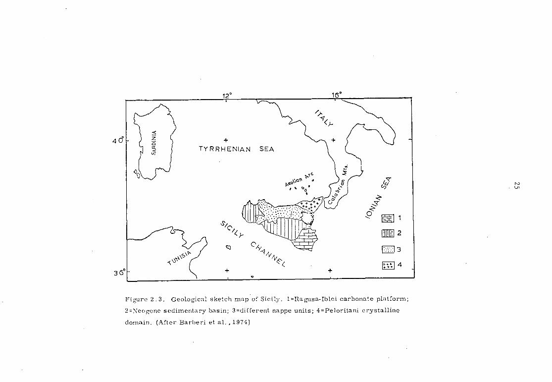
units (Caire, 1970). From south to north, they are:
1. Foreland of the Sicilian Alpine Chain
The most southerly unit is represented by the
stable Ragusan-Iblei Carbonate platform (Fig. 2.3). This
carbonate formation is not affected by Alpine folding, and
can be considered as a prolongation (or the equivalent) of
the Sahara beyond the Sicilian - Tunisian Basin.
The Ragusan platform is broken up by a network of
normal faults striking SSW and SSE. It is separated from
the Caltanisetta Basin (see 2 below) by a system of faults
and flexures which extend to the NNE into the Iblean moun-
tains. These were the passages during the early Miocene
of basaltic extrusions that underlie the Quaternary volcano
of Mount Etna.
4
3e
Figure 2.3, Geological sketch map of Sicily. 1=Ragusa-Iblei carbonate platform;
2=Neogene sedimentary basin; 3=different nappe units; 4=Peloritani crystalline
domain. (After Barberi et al, , 1974)

26
2. Middle Sicily and the Basin of Re-sedimentation
Middle Sicily includes all of western Sicily and
ends towards the east in the region of Catania, between the
Ragusa Plateau to the south and the Nebrodi and the Peloritani
Massifs to the north. The structural unit is here re-
presented by Mio-Pliocene basins, where fragments and debris •
from different facies zones have been deposited. One of
these basins, the most important, is the Central Sicilian or
Caltanissetta Basin. Due to the tectonic uplift of Sicily
during the lower Pliocene times, upper Pliocene and lower
Quaternary deposits are now to be found in this basin up to
a height of several hundred metres above sea level.
3. The Flysch Nappes
The northern half of Sicily, except for the north-
western and northeastern extremities, is occupied by a sequence
of Cretaceous to Miocene flysch nappes. This is a term applied
to the widespread deposits of sandstones, shales and clays which
lie on the nor -Li-fern and southern borders of the Alps in asso-
ciation with large bodies of rocks that have moved forwards
for considerable distances from their original positions,
either by overthrusting or by recumbent folding. These nappes
are similar to, or even identical with, their corresponding
equivalents in North Africa. They appear as a structural
edifice similar to that in Algeria. From Sicily to Calabria
they show, in plan view, curving boundaries concave to the
northwest, and overthrusts which moved from the insides to
the outsides of these arcs.

27
Figure 2.4. Volcanic rocks of eastern Sicily, Capo Passero and Pachino
(Cretaceous); Iblean mountains (Neogene to lower Pleistocene); Mount Etna
(lower Quarternary to Recent). (After Rittrnann, 1973),

28
4. The Peloritani Massif
To the northeast is the uppermost unit, the
Peloritani Massif, which is the Sicilian continuation of the
Calabrian arc. It includes a metamorphic basement with
granite intrusions affected by reversal and overthrusting
towards the south. With these geological features of Sicily
in mind, let us try and explain the present tectonic setting
of Mount Etna.
2.3 GEOLOGICAL SETTING OF MOUNT ETNA
The south-eastern part of Sicily has been the site
of volcanism of a dominantly basaltic nature since the middle
Triassic period (Cristofolini, 1973). This volcanism occurred
in a submarine environment, giving rise to pillow-lavas and
hyaloclastites through fissures cutting a carbonate platform.
The oldest exposed rocks in the area are the Cretaceous Vol-
canics of Pachino and Capo Passero (Fig. 2.4). Further north,
in the Iblean mountains, volcanic rocks of Miocene, Pliocene
and Pleistocene age occur. Much older volcanic rocks have,
however, been found in drillings for petroleum in Ragusa.
In the middle Quaternary period the area presently
occupied by Mount Etna was a gulf in which clays of Sicilian
origin were deposited. It appears that at some point during
this time submarine fissure eruptions of basaltic magma broke
out on the floor of this shallow gulf. These eruptions
produced mostly spilitized pillow lavas and hyaloclastites,
exposed at present on the coast north of Catania. The

29
Figure 2.5. Hypothetical profiles at the various stages in the evoluti-
on of the volcano that occupied the Valle del Bove. Stage 4 represents
the destruction of the Trifoglietto volcano before the formation of the
post-Trifoglietto cones, arrows indicate migration of active vents.
(After Klerx, 1970),

30
initial submarine eruptions gradually became sub-aerial as
a result of the tectonic uplift of Sicily. These sub-
aerial volcanoes later on built up the complex of Mount Etna.
Figure 2.4 illustrates this northward migration of volcanic
activity in time, from the Cretaceous volcanics of Capo
Passero in the south to Mount Etna itself in the north.
The sedimentary basin upon which Mount Etna rests
consists broadly of flysch type deposits of Cretaceous to
Miocene age in the north, Miocene sandstones in the west,
and Pleistocene alluvial deposits in the Plain of Catania
to the south.
The huge caldera-like feature on the eastern slope
of Mount Etna offers us some insight into the complex tectonic
processes the volcano underwent. This depression is known
as the Valle del Bove, and its walls reveal at least three
significant stages of its development before the present time
(Klerx, 1968). The first position occupied by the volcano
was at the Valle del Calanna, and then the two subsequent
stages of the Trifoglietto volcano in the Valle del Bove.
These volcanoes maintained a pattern of westward migrating
activity, resulting in the present volcanic centre, Mongibello.
Figure 2.5 shows a hypothetical profile at four stages in
the evolution of this volcano. Various theories have been
proposed to explain the origin of the Valle del Bove, among
which Kieffer's (1969) 'explosive-origin' theory seems to be
the most quoted. Kieffer proposes that the Valle del Bove
dates from about 5000 years B.P. and that most of the material

31
after the explosion was transported to the east to form the
large detrital fan which overlies the lava in the coastal
area to the east of Etna.
Klerx and Evrard (1970) made a gravity survey of
the Valle del Bove and came out with a positive anomaly of
27 mgals situated over the site Kieffer had earlier proposed
as the centre of the Trifoglietto. This was interpreted by
them as being the now solidified small basic or ultra-basic
magma chamber at the root of the Trifoglietto. Yokoyama
(1963), however, showed that a negative anomaly is associated
with pumiceous calderas. If his findings are true, it is
difficult to reconcile Kieffer's pumice eruption theory with
Yokoyama's gravity results.
2.3.1 TECTONIC CONTROL OF MOUNT ETNA
Mount Etna is very strongly controlled by a system of
faults (Rittmann, 1973; Romano, 1970). Figure 2.6 shows that
the two major fault systems south of the volcano trend roughly the
NNE and NNW, while a WNW trend is dominant toinorth. To the
west of the volcano the fissural trends are less obvious and
it is almost impossible to find evidence' of any fault in that
region. However, the ENE sinistral strike slip faults
(Ritsema, 1969) have considerable influence on the basement
of Etna, as is reflected by the distribution of various
eruptive centres (see Section 2.1 and Fig. 2.3).
The major structural feature of eastern Sicily is
however the Messina Fault, an active normal fault striking NE
through the Straits of Messina. The 1783 Calabrian earthquake,

32
Figure 2.6. Tectonic frame - work of eastern Sicily.

33
and the Messina earthquake of 1908, emphasize the tectonically
active nature of this fault. The realization of this has
prompted Italian workers to initiate distance measurements
across the Straits of Messina, to establish any differential
movement between mainland Italy and Sicily (Caputo et al., 1974).
'There is some evidence that the Etnean region is
rising isostatically. The uplift of the sedimentary basement
of Etna is proved by the outcrop of Sicilian clay (Quaternary)
at an altitude of 800 m on the eastern, and at 1050 m on the
western slope of the volcano (Rittmann, 1973). The rate of
uplift has been calculated by Grindley (1973), to be of the
order of 1 mm/yr. Francavigalia (1959) and Ogniben (1963)
think of the uplifted basement as a WNW-ESE trending anticline,
and Rittmann (1963) favours a horst-like feature controlled
by a N-S trending normal fault parallel to the Ionian graben.
2.4 A BRIEF TECTONIC HISTORY
In order to understand the present structural setting
of Mount Etna, it is essential to construct the past movements
of Sicily relative to Africa and Europe. In this section an
attempt has been made to reconstruct this movement on the
basis of various geophysical data as well as on the distri-
bution,age and nature of volcanism in eastern Sicily.
Paleomagnetic data from the outcrops of volcanic
rocks of Capo Passero dykes in the Ragusan platform indicate
that, at least since the upper Cretaceous time, Sicily has
been part of the African plate. The Plio- Pleiostocene pole
for Sicily evaluated from the Mount Iblei lavas, is also con-
34
sistent with the upper Tertiary-Quaternary pole for Europe
(Barberi et al., 1974). The conclusion that can be be
drawn from this result is that Sicily, as part of the African
plate, collided with the European plate towards the end of
the Oligocene, producing the island-arc volcanism of the
Aeolian Islands. In the lower Miocene, the thrusting nappes
and metamorphic belt of the Peloritanian mountains to the
north of Mount Etna were formed (Grindley, 1973) and since
the late Miocene times Sicily has been part of the European
continent (Barberi et al., 1974).
The Aeolian Island arc is located at the boundary
between the converging African and European plates, and the
volcanism is considered to be in a senile state (Belderson
et al., 1974). The Aeolian arc displays a transition in
lava composition from calc-alkaline to shoshonitic suite,
over a period of less than one million years. This rapid
variation is thought to be suggestive of a deepening Benioff
zone (Barberi et al., 1974a). Both shallow and deep focus
seismicity occur in the area. Shallow focus seismicity
characterizes the Sicilian-Calabrian fold belt, whereas much
of the deep-seismic activity occurs in the SE Tyrrhenian
basin, at a depth of 200-350 km (Ninkovich and Hayes, 1972).
Ritsema (1969) and Caputo et al. (1972) have shown that this
WNW seismic plane has a limited lateral extent of about 225 km
and dips at 500-600 beneath the Tyrrhenian Sea. Focal solutions
of these earthquakes (McKenzie, 1970 and 1972) show a thrust
mechanism on the E-W plane. This mechanism is consistent
with the Gibraltar Morocco-Algeria line, and the north Sicily

35
seismic line seems to be its prolongation.
Despite the close proximity of Mount Etna to the
Aeolian Islands there is no close relationship between the
two. Mount Etna volcanic rocks have a low 87Sr/86Sr ratio
(0.7033) compared with the average for Aeolian rocks (0.7045).
This shows that Etna's source magma has not been contaminated
by crustal assimilation. The volcanic rocks of the Sicily
Channel on the other hand have the same 87
Sr/86
Sr ratio as
those of Mount Etna, which suggests a similar tectonic setting
for the two volcanic regions.
An E-W seismic sounding was recently carried out by
Giese et al. (1973) across North Sicily, and their analysis
showed a crustal thickness of 38 km in the Etna region.
Barberi et al. (1973) showed that the crustal thickness
increases from the Sicily Channel in the south to the northern
edge of Sicily (= 40 km), and that the crust/mantle interface
is very diffused in this region. The crustal thickness
however remains constant along the northern part of Sicily
but sharply decreases to the north,where the plate is sub-
ducted under the Tyrrhenian Sea. Recent echo-soundings in
the Ionian Sea have shown that a poorly developed ridge
system (Beldersen et al., 1974) exists concentric to the
Calabrian arc. The existence of the Calabrian ridge implies
crustal shortening related to the compression which is asso-
ciated with the Benioff zone beneath the Calabrian arc. The
compression is probably a result of the south-easterly motion
of the Tyrrhenian region.

Figure 2.7. Probable positions of plate boundaries at the present time . Direction of arrows indicate
relative motion of the African and Eurasian plates. Boundaries at which lithosphere is being created
are shown by double lines and boundaries at which plates are being consumed, by lines at right angles.
(After McKenzie, 1970; and Barberi et al., 1974).
_37
To sum up, we see that Mount Etna lies just south
of a diffuse plate boundary, with a ridge system running ENE
in the Ionian Sea. These relationships are shown in
Figure 2.7.
Many investigators have tried to explain the peculiar
structural position of Etna. Mount Etna not only is situated
in what would normally be expected to be a non-volcanic zone,
but is active and producing magma. In order to produce an
integrated picture of the area, Barberi et al. (1974) relate
the fluctuations of the geochemistry of the volcanic products
to the compressional and distentional tectonics of the area,
thought to have been brought about by the changing nature of
the African and European plate interactions since the Triassic
period. Eastern Sicily, however, has been the border zone
of the colliding continental plates since the upper Miocene.
This gave rise to a local distensive tectonics related to
the stress field directed normally to the motion of the oceanic
lithosphere. Barberi et al. (1974),however, do not explain
how "distensive tectonics" exist on top of a subducting plate.
Grindley (1973) overcomes the problem by proposing a high
rate of arc migration for the plate and, indeed "rates of arc
migration are sufficiently rapid" even though eastern Sicily
is being uplifted at the rate of 1 mm/year, to allow crustal
dilatation normal to the Calabrian arc.
These features of the plate tectonic setting of
Mount Etna have attracted special attention in the region
and at present there are several geological and geophysical

38
programmes in the area other than the work described in this
study. It is hoped that as more data becomes available we
shall be able to understand these peculiarities of Mount
Etna more fully.

39
CHAPTER III
SEISMIC INVESTIGATIONS OF MOUNT ETNA
DURING AUG - SEPT 1974
3.1 INTRODUCTION
The 1974 reconnaissance seismic survey of Mount
Etna was inspired by the fact that for several years the
Geophysics Department of the Imperial College had been in-
volved in geophysical studies of Mount Etna, with NERC
support, aimed at investigating its changing shape during
the various phases of eruptive activity. One aspect of this
problem is the location of magma chambers, for which seismic
methods might be particularly useful. It was thus hoped
that a seismic survey in the form of microearthquake and back-
ground seismic noise recordings would add a new dimension to
the understanding of this complex volcano.
The instrument used for the survey was a Spreng-
nether MEQ 800 microearthquake recorder with a 1,1KI Willmore
seismometer (Fig. 3.1). The MEQ 800 has proved to be highly
satisfactory for recording tectonic microearthquakes and had
earlier been used for seismic studies in Iran (Mohajer - Ashjai,
1975; Hedayati, 1976). No published information was available
concerning its suitability for studying volcanic microearth-
quakes,though it was thought likely that it had been used
elsewhere for the purpose.
There are, in various respects essential differences

Figure 3.1. The Sprengnether MEQ 800 portable seismograph.
41
between observations of volcanic, as opposed to tectonic,
earthquakes. Firstly, volcanic earthquakes are, in general,
shallower in origin and have much smaller magnitudes.
Secondly, in most cases it is very difficult to observe the
high-frequency waves of volcanic earthquakes, because of
absorption. As a consequence, seismographs of high magni-
fication have to be used. On the other hand, the seismic
background noise of volcanoes is normally very high, due
mainly to the continuous volcanic tremors. This thus sets
a limit to the maximum usable magnification of seismographs
on volcanoes,which in turn sets a limit on the smallest micro-
earthquake detectable at each site.
At the present time, seismic observations of vol-
canoes are usually made via telemetering system. This avoids
the problem of installing heavy and expensive equipment near
active craters, fissure zones and so on, where most of the
volcanic earthquakes originate. Telemetering systems were
first used at the Hawaiian and Asama (Japan) volcano obser-
vatories. There are two systems in common use, (1) tele-
metering by cable, in which the seismometer (sometimes with
a pre-amplifier) is connected to the observatory by cable,
and (2) telemetering by radio. The former has limited appli-
cations, as there is always the risk of damage to the cables,
transducers and amplifiers, and recording equipment by
lightning. In addition, there is the problem of laying the
cables, sometimes over long distances and over obstructions of
various kinds. The second method has the advantage of range,
but the cost of setting up such a telemetering system is very

42
high, and provision of the necessary power is sometimes a
problem. A radio-linked system has been successfully used
by the Japanese on Sakura-Zima volcano, and on Etna itself
such a system is in use by the University of Catania.
Telemetering systems (had they been available) were
obviously not appropriate for the reconnaissance survey. In
fact, the Sprengnether seismograph proved highly satisfactory
for the purpose, being reasonably portable, not too difficult
to provide with power, and producing an easily appraisable
record. Between 6 August and September 4th 1974, nine sites
were investigated, eight of which were on compact lavas,
volcanic agglomerate or re-worked volcanics, at elevations of
between 1500m and 2500m. The ninth site was situated at
an altitude of about 800m on a sedimentary basement near
Bronte (for description of sites and their locations refer
to Section 3.5). At some sites, recordings were terminated
after only a few hours, while at others they extended over
several weeks, depending on the suitability of the site,
particularly as regards the background noise level.
3.2 THE SEISMIC EQUIPMENT
3.2.1 THE SMOKED-DRUM MICROEARTHQUAKE RECORDER
The Sprengnether MEQ800 is a self-contained portable
smoked-drum seismic recording system with a high gain, wide-
sensitivity range. It was used with a single component
vertical Willmore MK I seismometer having a natural frequency
of 1 Hz.

battery IZ V dc
i ) I c amplifier Pre—amP,
a.
seismometer
r — — — — a It•n —1
time mark
clock 4
disploy
control
r. OwIlo •••• 1 I external— battery Char g er
row I
Figure 3.2. Block diagram of the Sprengnether MEQ 800.
44
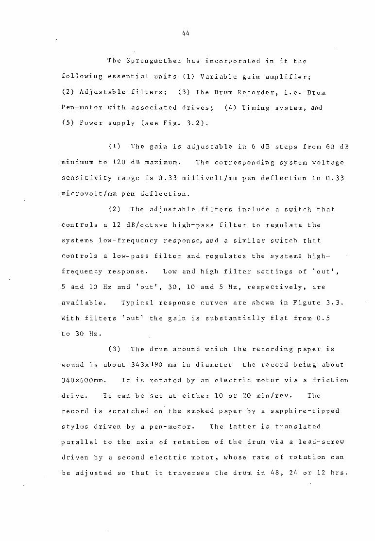
The Sprengnether has incorporated in it the
following essential units (1) Variable gain amplifier;
(2) Adjustable filters; (3) The Drum Recorder, i.e. Drum
Pen-motor with associated drives; (4) Timing system, and
(5) Power supply (see Fig. 3.2).
(1) The gain is adjustable in 6 dB steps from 60 dB
minimum to 120 dB maximum. The corresponding system voltage
sensitivity range is 0.33 millivolt/mm pen deflection to 0.33
microvolt/mm pen deflection.
(2) The adjustable filters include a switch that
controls a 12 dB/octave high-pass filter to regulate the
systems low-frequency response, and a similar switch that
controls a low-pass filter and regulates the systems high-
frequency response. Low and high filter settings of 'out',
5 and 10 Hz and 'out', 30, 10 and 5 Hz, respectively, are
available. Typical response curves are shown in Figure 3.3.
With filters 'out' the gain is substantially flat from 0.5
to 30 Hz.
(3) The drum around which the recording paper is
wound is about 343x190 mm in diameter the record being about
340x600mm. It is rotated by an electric motor via a friction
drive. It can be set at either 10 or 20 min/rev. The
record is scratched on the smoked paper by a sapphire-tipped
stylus driven by a pen-motor. The latter is translated
parallel to the axis of rotation of the drum via a lead-screw
driven by a second electric motor, whose rate of rotation can
be adjusted so that it traverses the drum in 48, 24 or 12 hrs.

0.1 1.0 10
100 Frequency (Hz)
Figure 3.3. Response curve for the Sprengnether MEQ 800 seismograph system. Settings at diff-
erent combinations of high- and low-pass filters. ■

46
Depending on the combination of rotation and traverse
rates used, the separation between the adjacent lines may
be 1, 2 or 4 mm.
(4) Precision timing is provided by a crystal
oscillator which drives a digital clock. The latter is
made to deflect the trace for 2.0 sec in every minute and
for 4.0 sec at the hour. The crystal clock also provides
an accurate 60 Hz output, which is used to stabilize the rate
of rotation of the drive motors. The clock is accurate to
±0.1 sec/month within the temperature range 0o - 50°C.
(5) The necessary ±12V power supply is derived
from four internal 12 volt, 1.5 AH rechargeable sealed lead-
acid batteries arranged in a series/parallel combination.
This enables the batteries to be replaced one at a time
without interrupting the power supply (and the quartz clock).
Provision is made for changing the batteries while the in-
strument is in operation, also for operating it from external
batteries.
3.2.2 OPTIMIZATION OF SIGNAL-TO-NOISE RATIO
As the magnitudes of volcanic microearthquakes are
usually small, seismographs of relatively high magnification
must be used. The usual magnification of the seismograph
depends of course on the background noise level. The main
contributions to the background noise are the wind-induced
noise, microseisms, and the continuous volcanic tremor. The
wind, the microseisms and the volcanic tremor set a lower
limit below which microearthquakes cannot be detected.
47
Because of the difference in spectral content between the
wanted signal and the unwanted noise, some improvement in
the signal-to-noise ratio can be obtained by suitable
adjustment of the filters. Various combinations of low
and high cut filters were used to give at each site what
was judged to b.e the best result. The final result, i.e.
the ability to distinguish characteristics of the wanted
signal against the background noise, could also be optimized
by appropriate adjustment of the gain. In practice, the
amplifier gains were normally set between 60 and 90 dB,
giving an effective overall magnification of between 1x10³
and 3.2x10⁴.
3.2.3 HANDLING OF RECORDS
The paper used for the smoked records was a non-
absorbent, 80 pound heavy enamelled paper, that was fixed to
the recording drum by rubber cement and adhesive tape. It
was smoked by means of a kerosine burner, the drum being
rotated slowly over the large smokey flame until it was
uniformly blackened. When the stylus has traversed the drum,
the latter is removed from the recorder and replaced by a
second drum,previously smoked. This record is then fixed
while still on the drum, by rotating it in a shellac/alcohol
solution, after which it is removed and dried in the air for
an hour or two before storage. Surplus shellac is removed
from the drum by wiping it with a rag soaked in alcohol.

48
LL MG
B
P
E
N
(a)
•
lava cement cemented volcanics
(b)
Figure 3.4. Serra La Nave seismic vault, (a) plan of station
(b) construction of basement. (After Bottari and Riuscetti, 1967).
49
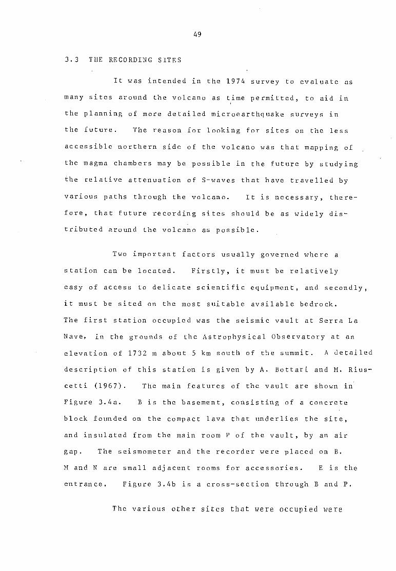
3.3 THE RECORDING SITES
It was intended in the 1974 survey to evaluate as
many sites around the volcano as time permitted, to aid in
the planning of more detailed microearthquake surveys in
the future. The reason for looking for sites on the less
accessible northern side of the volcano was that mapping of
the magma chambers may be possible in the future by studying
the relative attenuation of S-waves that have travelled by
various paths through the volcano. It is necessary, there-
fore, that future recording sites should be as widely dis-
tributed around the volcano as possible.
Two important factors usually governed where a
station can be located. Firstly, it must be relatively
easy of access to delicate scientific equipment, and secondly,
it must be sited on the most suitable available bedrock.
The first station occupied was the seismic vault at Serra La
Nave, in the grounds of the Astrophysical Observatory at an
elevation of 1732 m about 5 km south of the summit. A detailed
description of this station is given by A. Bottari and M. Rius-
cetti (1967). The main features of the vault are shown in
Figure 3.4a. B is the basement, consisting of a concrete
block founded on the compact lava that underlies the site,
and insulated from the main room P of the vault, by an air
gap. The seismometer and the recorder were placed on B.
M and N are small adjacent rooms for accessories. E is the
entrance. Figure 3.4b is a cross-section through B and P.
The various other sites that were occupied were

Table 3.1
Site Descriptions
Station
Latitude Longitude Elevation Foundation Remarks (N) (E) (m)
Serra La Nave (1)
Basement of Ski Club (2)
Torre del Philosofo (3)
Rifugio Citelli (4)
IC Bench Mark Site near Rifugio Citelli (5)
Inside a '71 lava cave (6)
37° 41' 40" 14° 58' 26" 1732 Lava flow Serra La Nave Observatory
37° 42' 32" 14° 59' 58" 2100 Uncompact Midway between Rifugio Lava flow Sapienza and Piccolo
Rifugio
37° 44' 13" 15° 00' 05" 2913 Lava flow On the basement inside the Torre del Philosofo
37° 45' 56" 15° 03' 36" 1743 Lava flow On the basement inside the Rifugio Citelli
37° 46' 02" 15° 03' 30" 1690 Lava flow On an exposed bedrock near Rifugio Citelli (IC levelling site, u)
37° 44' 13" 14° 59' 44" 2900 Inside a
500 m west of Torre del Lava cave Philosofo, inside '71
lava cave
/contd

Station Latitude (N)
Longitude (E)
Elevation (m)
Foundation Remarks
Inside lava (7)
a '74 cave
37° 44' 37" 14° 55' 48" 1680 Lava flow
Inside a small lava cave
near the '74 eruption site
Near Monte Nero (8)
37° 42' 57" 14° 59' 19" 2250 Lava flow Inside a small lava cave near Monte Nero
Bronte (9)
37° 46' 03" 14° 59' 35" 800 Sedimentary rock
On an exposure of sedimen- tary rock before entering Bronte

Randazzo
Linguaglossa
0 10 km
52
Figure 3.5. Sketch map around Mount Etna showing all the nine sites occ-
upied during the 1974 investigation. (The lines connecting the various towns
indicate motorable roads).

53
either on exposed bedrock, tuff, compact lava, or in the
basement of some abandoned building. Seismograms obtained
from exposed bedrocks were of very good quality, showing
very little background disturbances. One such site was
near the Rifugio Citelli (IC bench mark site, Wadge, 1974).
It was decided to use it for future work. The lava caves
near the '74 eruption, and the Monte Nero site, also produced
good quality recordings, but very small earthquakes were
masked by high background noise. This was particularly
true for the Monte Nero site. The basement sites at the
Rifugio Citelli, Ski Club and Torre del Philosofo were con-
sidered to be unsuitable for future work because of the con-
stant presence of tourists and vehicles.
Table 3.1 gives a brief description of the various
characteristics of the recording sites, and their relative
locations, and Figure 3.5 shows the sites occupied in the
1974 study of Etna. All the stations occupied during
the course of the 1974 investigations lie within the altitude
range of 1500 and 2500m. except the one site at Bronte, which
was at a much lower elevation (- 800m).
3.4 ANALYSIS OF DATA
The seismograms obtained from the Sprengnether MEQ
800 are smoked paper records, and with the recording parameters
used in the 1974 survey cover a period of 24 hrs. These
seismograms present ground velocity for a given site, as a
function of time within the frequency limits as indicated in
Section 3.3 and Figure 3.3.

54
Figures 3.6 and 3.7 show examples of recordings
taken at the Serra La Nave seismic observatory. The first
shows a record taken during a period of high background
noise, and Figure 3.7a is a record taken at the same site
during a quiet period.
The 1974 investigation resulted in records for all
or part of 30 days, representing samples from nine different
sites. No attempt was made at detailed analysis in the
field, though the records were of course appraised with a
view to deciding for how long the instrument should be left
at a particular site.
With the help of a magnifying glass records can be
read to about 0.1 sec. Although the time resolution is
adequate to pick the arrival times of the P-waves to an
accuracy of 0.1 sec, S-wave arrivals are more difficult to
pick and are accurate to no better than about 0.5 sec.
The determination of magnitude raises various problems,
when a portable system is employed on a survey, where very
little seismic data is available. Various methods were tried
in an attempt to get around those problems, but met with
limited success. A brief discussion of the present available
methods of magnitude determination, and problems involved, are
discussed in a separate section.
3.4.1 CLASSIFICATION OF MICROEARTHQUAKES
Microearthquakes are identified as high-frequency
envelopes of short duration (L' 1 min) superimposed on a con-

Figure 3.6. Seismogram of A-type microearthquakes recorded at Serra La Nave. Note the
impulsive first arrival and the small S- P interval.
lJ1 lJ1
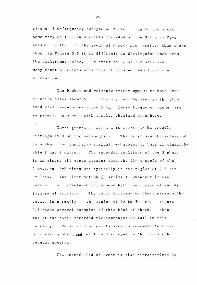
56
tinuous low-frequency background noise. Figure 3.6 shows
some very well-defined events recorded at the Serra La Nave
seismic vault. In the event of shocks much swaller than those
shown in Figure 3.6 it is difficult to distinguish them from
the background noise. In order to be on the safe side
many doubtful events were thus eliminated from final con-
sideration.
The background volcanic tremor appears to have fre-
quencies below about 5 Hz. The microearthquakes on the other
hand have frequencies above 5 Hz. These frequency ranges are
in general agreement with results obtained elsewhere.
Three groups of microearthquakes can be broadly
distinguished on the seismograms. The first are characterized
by a sharp and impulsive arrival, and appear to have distinguish-
able P and S phases. The recorded amplitude of the S phase
is in almost all cases greater than the first cycle of the
P wave, and S-P times are typically in the region of 2.5 sec
or less. The first motion (P arrival), whenever it was
possible to distinguish it, showed both compressional and di-
latational arrivals. The total duration of these microearth-
quakes is normally in the region of 10 to 50 sec. Figure
3.6 shows several examples of this kind of shock. About
18% of the total recorded microearthquakes fall in this
category. These kind of events seem to resemble tectonic
microearthquakes, and will be discussed further in a sub-
sequent section.
The second kind of event is also characterized by

Figure 3. 7a. Seismogram of B-type microearthquakes showing impulsive first arrival and
no distinguishable P-S phases (recorded at Serra La Nave).

Figure 3. 7b. Seismogram of B-type microearthquakes showing emersion arrival and no
distinguishable P-S phases (recorded at Ie bench mark).
VI (X)
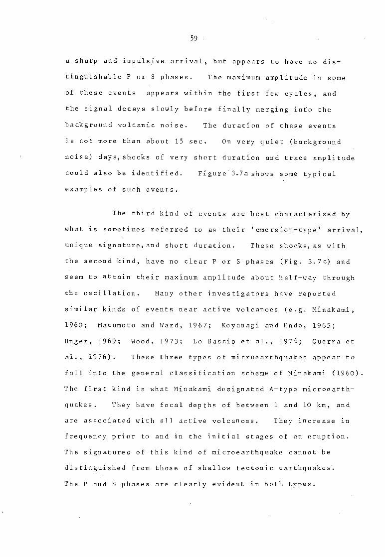
59
a sharp and impulsive arrival, but appears to have no dis-
tinguishable P or S phases. The maximum amplitude in some
of these events appears within the first few cycles, and
the signal decays slowly before finally merging into the
background volcanic noise. The duration of these events
is not more than about 15 sec. On very quiet (background
noise) days, shocks of very short duration and trace amplitude
could also be identified. Figure 3.7ashows some typical
examples of such events.
The third kind of events are best characterized by
what is sometimes referred to as their 'emersion-type' arrival,
unique signature,and short duration. These shocks, as with
the second kind, have no clear P or S phases (Fig. 3.7c) and
seem to attain their maximum amplitude about half-way through
the oscillation. Many other investigators have reported
similar kinds of events near active volcanoes (e.g. Minakami,
1960; Matumoto and Ward, 1967; Koyanagi and Endo, 1965;
Unger, 1969; Wood, 1973; Lo Bascio et al., 1976; Guerra et
al., 1976). These three types of microearthquakes appear to
fall into the general classification scheme of Minakami (1960).
The first kind is what Minakami designated A-type microearth-
quakes. They have focal depths of between 1 and 10 km, and
are associated with all active volcanoes. They increase in
frequency prior to and in the initial stages of an eruption.
The signatures of this kind of microearthquake cannot be
distinguished from those of shallow tectonic earthquakes.
The P and S phases are clearly evident in both types.

60
The second and third types appear to be similar
to Minakami's (1960) B-type volcanic microearthquakes.
They have hypocentres limited to an area about one kilometer
in radius around the active craters. In almost all cases
the hypocentres are much shallower than the A-type volcanic
microearthquakes, and they commonly occur in swarms. Since
surface waves are predominant, the S phase is not clearly
defined.
However, the critical criterion for defining both
the A and B-type volcanic microearthquakes are their b-values,
determined from the magnitude/frequency relationship,
discussed more fully in Section 3.6.
The above described microearthquakes are very dif-
ferent from the other principal type of event, not recorded
during the present survey. These are teleseisms from distant
earthquakes. Teleseisms are characterized by a low frequency
P phase and a long S-P interval. The duration of such shocks
is generally measured in terms of minutes, and they involve
long-period surface waves with relatively low amplitudes.
3.4.2 DISTRIBUTION OF S-P INTERVALS
Figure 3.8 shows the normalized frequency distribution
of S-P times at two recording stations, Serra La Nave and
Monte Nero. The distribution has been normalized for 1000 hrs
of continuous recording at both stations. It is seen from
the diagram that 68% of all the recorded shocks at Serra La
Nave have S-P times of between 1.1 and 2.0 sec while, at the

N N
station 1
0 2 4
6
(S- P) sec
station
0 2 4
6
(S-P) sec
SO
60
80
GO
40
20
40
20
Figure 3.8. Normalized frequency distribution (for 1000 hrs.) of microearthquakes
versus distance from the recording stations. Distances are in terms of S-P intervals.
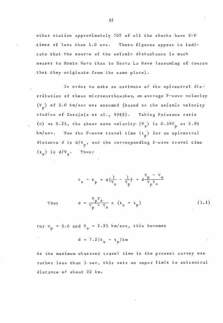
62
other station approximately 70% of all the shocks have S-P
times of less than 1.0 sec. These figures appear to indi-
cate that the source of the seismic disturbance is much
nearer to Monte Nero than to Serra La Nave (assuming of course
that they originate from the same place).
In order to make an estimate of the epicentral dis-
tribution of these microearthquakes, an average P-wave velocity
(V p) of 5.0 km/sec was assumed (based on the seismic velocity
studies of Cassinis et al., 1969). Taking Poissons ratio
(a) as 0.25, the shear wave velocity (Vs) is 0.59Vp or 2.95
km/sec. Now the P-wave travel time (t ) for an epicentral
distance d is d/V , and the corresponding S-wave travel time
(ts) is d/V
s. Thus:
Thus
1 1 V - V
i s - tp = d(-- - --) = d
V V V V p s
V V d = (ts
- t ) p V p-sV s
(3.1)
For V = 5.0 and Vs = 2.95 km/sec, this becomes
d = 7.2(ts - t )km
As the maximum observed travel time in the present survey was
rather less than 3 sec, this sets an upper limit to epicentral
distance of about 22 km.

63
3.43 MICROEARTHQUAKE OCCURRENCE RATE
As explained in the introduction, the main purpose
of the 1974 field survey was to gain experience of handling
equipment at the sub-zero temperatures on Mount Etna, prior
to the making of a more detailed survey the following year,
also to obtain a measure of the level of seismic activity
of the volcano.
During this 30 days of recording, nine stations
were occupied (Fig. 3.5). The total recording time at each
station, the number of hours of useable record, the number
of microearthquakes of each type recorded, and the average
daily rate are given in Table 3.2. In calculating the
occurrence rate (shocks/day) the figures were in some cases
derived from recording periods of less than a day, and in
others more. The results are thus to be interpreted with
caution. Obviously, the shorter the recording time the less
reliable will be the average daily rate. These results
indicate that, seismically, the most active area was the IC
bench mark site (station 5). This site is approximately
2.0 km from the 1971 eruption site. Although this result
was arrived at from only two days of recording, it is interest-
ing to note the proximity of this, the most active recording
site, to the '71 eruption. It might also be noted that all
the events recorded at station 5 are of the B-type, a kind of
shock that is believed to be connected with the active part of
a volcano. The other two sites that show comparable activity
are Serra La Nave (maximum = 22 shocks/day) and Monte Nero
(maximum = 9 shocks/day). The microearthquakes recorded

64
Table 3.2
Microearthquake Activity
August/September 1974
Station
Recording time (hrs)
No. of microearthquakes Number per day
Total Usable A-type B-type Total
Serra La Nave
Basement of Ski Club
Torre del Philosofo
Rifugio Citel- li
IC Bench Mark (near Rifu- gio Citelli)
Inside a '71 Lava Cave
Inside a '74 Lava Cave
Near Monte Nero
Near Bronte
269.00
5.30
18.50
6.20
44.00
12.00
12.50
143.50
9.0
261.00
0
0
0
43.50
0
12.25
143.0
8.30
13
-
_
-
0
-
_
15
1
63
_
-
_
55
_
-
10
-
76
-
-
55
-
_
25
1
7
_
30
-
-
4
3
65
at Serra La Nave are a mixture of both A and B-type events,
with the latter predominating. At Monte Nero, on the other
hand, over 50% of all the recorded shocks are of the first
kind. Unlike Serra La Nave,however, no small events could
be identified at this station because of the constant
presence of high amplitude background noise. At other
locations the recording times were too short for any conclusion
to be drawn. These microearthquake occurrence-rates give
some indication of the seismic activity of an area and have
the advantage of being derivable from recordings extending
over short periods of time (though of course the shorter
the period the less the certainty of obtaining a fair sample).
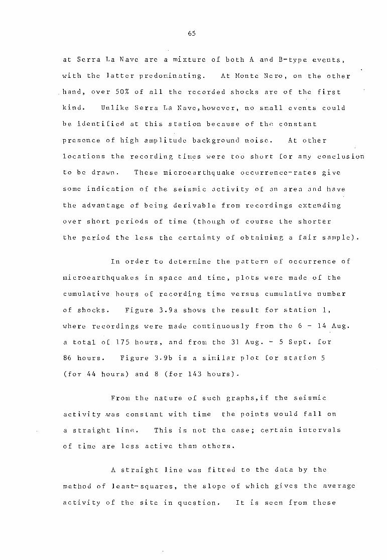
In order to determine the pattern of occurrence of
microearthquakes in space and time, plots were made of the
cumulative hours of recording time versus cumulative number
of shocks. Figure 3.9a shows the result for station 1,
where recordings were made continuously from the 6 - 14 Aug.
a total of 175 hours, and from the 31 Aug. - 5 Sept. for
86 hours. Figure 3.9b is a similar plot for station 5
(for 44 hours) and 8 (for 143 hours).
From the nature of such graphs,if the seismic
activity was constant with time the points would fall on
a straight line. This is not the case; certain intervals
of time are less active than others.
A straight line was fitted to the data by the
method of least-squares, the slope of which gives the average
activity of the site in question. It is seen from these

EN
8 0 STATION 1
60
40
50 100 150 200
100
0
20 0 *3 (-
l.'5\
(6-14 aug )
HOURS Figure 3. 9a. Cumulative number of microearthquakes versus cumulative noise free recording
time, for Serra La Nave during the two periods (as indicated). The straight lines are least-
square fits for the respective periods.

0 50 100 150 200
HOURS
Figure 3. 9b. Cumulative number of microearthquakes recorded versus cumulative noise free
recording time, for IC bench mark and Monte Nero. The straight lines are least-square fit to
the data, at the respective sites.
100
80
20
60
EN
40
- STATION 5
— STATION
_30 aug)

68
graphs that at station 1 the rate was very much greater in
early September than it was three weeks earlier.
Another quantity, called the 'average activity' of
the volcano,was calculated. This was defined as the total
number of microearthquakes divided by the total number of
days of usable record,and was found to be approximately
7 shocks/day. It is interesting to compare this figure with
the results obtained in other volcanic regions. Matumoto
and Ward (1967) investigating Mount Katmai and vicinity in
Alaska quote a normal rate of between 40 and 80 shocks per
day, with as many as 190 shocks on an exceptionally active
day. At Mount Tsukuba Japan, Asada (1957) recorded 200
events per .day. At Kilauea volcano the average activity
ranges from 50-100 per day (Moore and Krivoy, 1964). Wood
(1974), during a microearthquake survey of various Central
American volcanoes, recorded from as few as 7 events/day at
Masaya volcano to more than 1500 events/day at San Cristobal
volcano. Del Pezzo et al. (1974) investigating Mount Strom-
boli recorded as many as 212 events/day. On Mount Etna
itself Guerra et al. (1976) recorded up to 3 events/day.
These numbers and comparisons, however, must be interpreted
qualitatively, as these observations are very much dependent
on the interpreter and the type of equipment used. If any
conclusions can be drawn from these results, it is that at
the time of the reconnaisance survey of Etna the microearth- activity
quake4though low by comparison with some volcanoes, was not
exceptionally so.

69
3.5 MICROEARTHQUAKES AND THE PROBLEM OF MAGNITUDE DETER-
MINATION
The concept of magnitude was first introduced by
Richter (1935) to measure the size of shallow earthquakes
in California. For this purpose he defined magnitude as
the logarithm of the maximum recorded (trace) amplitude
(expressed in microns) by a Wood-Anderson torsion seismo-
graph with specified constants (free period = 0.8 sec,
maximum magnification = 2800, damping factor = 0.8) when the
seismograph was at an epicentral distance of 100 km. This
quantity is now known as• the local magnitude, ML, but has never
been very much used outside California. However, the basic
idea was later extended for use at greater distances (still
for shallow depth) by defining the magnitude Ms, which is
based on the maximum amplitude (A) of surface waves having a
period (T) of about 20+ 2 seconds. Another magnitude mb,
known as the body wave magnitude, makes use of the amplitude
(A) of the body waves at large distances from the epicentre
and for events at any depth. Ms and Mb are the two magnitude
measures now in common use.
In practice, ML, can be determined for local earth-
quakes, but in applying it to microearthquakes modifications
have to be made,for the following reasons:
(1) Because microearthquakes are so local, the amplitudes
of the shocks depend more on the hypocentral distance
than on the epicentral distance.
(2) The high-frequency,high-sensitivity,seismo graph used
70
in this study differs considerably from the Wood-
Anderson seismograph, which is the reference standard
on the Richter scale.
(3) Crustal structure affects significantly the attenuation
of near events.
In addition, some workers e.g. Mohajer-Ashjai (1975)
and Hedayati (1976), have found that the small dynamic range
of smoked-drum microearthqua.ke recorders limits the use of
magnitude relations based on record amplitude. Thus, if
the gain is set so that the minimum detectable amplitude is
1 mm, and the pen excursion limited to + 12.5 mm, to avoid
undue interference between adjacent traces, then the seismo-
graph can only deal with an amplitude range of 12.5 to 1
(or a magnitude range of little more than 1) without saturating
the record. Fortunately, this was not a serious problem in
the present case, as only a few A-type microearthquakes and
no B-type had large enough trace amplitudes to reach satu-
ration level. This indicates that in general (as was pointed
out in Section 3.1) volcanic microearthquakes have much
smaller magnitudes than (non-volcanic) tectonic microearth-
quakes.
To overcome these problems (especially 1, 2 and 3)
recourse is often taken to a method developed by Tsumura
(1967). Tsumura's method evolved from a study of the
microearthquakes recorded at the Wakayama network in Japan,
which showed that a relationship exists between the magnitude
ofa local earthquake and the duration of its recorded signal

71
above the background noise level. Tsumura found that for
earthquakes whose epicentral distances were less than 200 km,
and which occurred at depths of less than 60 km, the magnitude
could be related to the signal duration by the expression
M = et + 13logD (3.2)
where M = local magnitude
D = signal duration of the microearthquake in sec
and a and (3 are constants.
For epicentral distances of up to 1000 km, the
expression is still valid, except for the addition of what is
known as a time term (strictly speaking a distance term)
Tsumura (1967). The final expression is then
M = a + 13logD Y(A)
For the Wakayama region y(A) = 0.001, where A (the epicentral
distance) is in units of kilometers.
The first requirement of the method is thus a measure-
ment of the signal duration for a number of microearthquakes
(recorded in the portable system) whose magnitudes have been
assigned by conventional methods. A least-square fit to these
points give values of a and It is interesting to note
that a in Eqn. (3.2) is the magnitude corresponding to a signal
duration of 1 sec.
Tsumura's (1967) method has the advantage that it is
simple and easy to use when a and are available. As magni-
tude determined this way is dependent on the logarithm of the

72
signal duration, the method is relatively insensitive to
uncertainties in the latter.
However, one big disadvantage of the method is
that a depends upon the instrument being used and also upon
local geological factors. As a result, the instrument has
to be calibrated for each microearthquake survey.
The method has been used, apparently with success,
in various parts of the world. Thus Tsumura (1967) used it
to study the Wakayama region of Japan, and Crosson (1972),
the Puget Sound region of Washington state. Others who have
used the method are Lee et al. (1972) for Central Californian
microearthquakes, Real and Teng (1974) for Southern California,
and Langenkamp and Combs (1974) for the Elsinore Fault zone,
also in Southern California. More recently, Mohajer-Ashjai
(1975) and Hedayati (1976) applied it to their seismotectonic
studies of Iran.
It is interesting to note that for the same region
e.g. Southern California, Real and Teng (1974) and Langenkamp
and Combs (1974) quote results which vary in their a values
by as much as 88%. The 8 values are,however,more consistent.
3.5.1 MAGNITUDE AND CUMULATIVE FREQUENCY OF EARTHQUAKES
ORIGINATING FROM VOLCANOES
An important fact first noted by Gutenberg and
Richter (1954) is that, considering the earthquakes occurring
in a given area within a given time, the number having a
73
magnitude greater than a given value decreases logarithmically
with magnitude. This can be expressed by the relation:
logN = a - bM
where N is the number of earthquakes of magnitude greater
than M, and a and b are constants, a may have any value,
since it represents the total number of earthquakes of magni-
tude greater than zero, and hence depends on the seismicity
of the area and the length of the period under consideration.
b, however, which is the slope of what is generally referred
to as the recurrence curve, and represents the magnitude dis-
tribution of the earthquakes, is relatively constant for a
given region, though varying from region to region, and generally
lies between 0.5 and 3.5 (Isacks and Oliver, 1964). The
important fact about b is that its value depends on the nature
of the earthquake and it therefore has diagnostic valudn
distinguishing, for example, between tectonic and volcanic events.
Regarding microearthquakes originating from volcanoes,
the most important study of cumulative frequency versus magni-
tude was made by Minakami (1960), who explains how to distin-
guish between the various types of microearthquakes from their
b-values. From his investigations of the A-type volcanic
microearthquakes originating from Hawaii and Aso-San volcanoes
he concluded that the slope, or b-value, of these earthquakes
lies between 0.8 and 1.2, about the same as for normal tectonic
earthquakes in may parts of the world. As to the B-type
volcanic microearthquakes, his data from Asama-Yama, Sukra-Zima
and Usu-San seems to indicate b-values of from about 1.8 to

N(A) = -(m-1)
kA -(m-1)
74
3.5, generally very much larger than the b-values of .A-type
microearthquakes. Thus the two types of microearthquakes
can be distinguished not only by their visual characteristics
but also by their quite different b-values.
3.5.2 DERIVATION OF b-VALUE FROM MAXIMUM TRACE AMPLITUDES
If it is assumed that the number 6N(A) of micro-
earthquakes whose trace amplitude lies between A and A+dA
is inversely proportional to some power m(> 1) of A, then
SN(A) = kA 111(SA
where k is a constant.
Integrating from A = co to A
Or logN(A) = const -(m-l)logA
Replacing logA by M, this is seen to be equivalent to the
expression for the number of shocks of magnitude > M ,
logN = a - bM
the b being equal to m-1 i.e. m = b+1.
Attention was first drawn to this relationship by
Ishimoto and Lida (1939) while studying the earthquakes
occurring in the Kanto District of Japan. It was subsequently
investigated by Suzuki (1953, 1954, 1958, 1959) who confirmed
that Ishimoto-Iida's formula holds good irrespective of the

75
place of observation and of the magnification, as well as the
response characteristics, of the recording instruments.
Suzuki (1959) found that this relation sometimes holds also
for aftershocks sequences of great earthquakes, but it was
Asada et al. (1951) who found that the relation holds also
for microearthquakes.
As can be seen from the above discussion, the
frequency distribution of A is equivalent to the frequency
distribution of magnitude. Thus the objective of investi-
gating the magnitude versus occurrence frequency relationship
in the microearthquake case can be accomplished through
studying the frequency distribution of the maximum trace
amplitude.
3.6 DETERMINATION OF THE b-VALUE FROM THE 1974 DATA
Determination of the b-value in the expression
logN = a-bM, requires some means for determining the magni-
tudes of the microearthquakes being studied. There are
basically two ways of doing this, by using Tsumura's (1967)
relation between magnitude and signal duration
M = a + SlogD
or by using an amplitude relation of the form
M = logA + k
(since we were not using the Wood-Anderson seismograph, the
uncertainty in estimating M will then lie in the constant k).

76
The first method is used here to study A-type, and the second
method to study B-type, microearthquakes.
(1) A-type Microearthquakes
In using Tsumura's relation
M = a +
as a means for obtaining the M in the recurrence formula
logN = a - bM
and hence enabling the b-value to be determined, it is not
necessary to actually calculate the a or the M, though it is
necessary to determine (3 as an intermediate step. The proce-
dure is as follows:
Eliminating M separately from the recurrence formula and
Tsumura's relation and from the Tsumura's formula and the
relation
M = logA + k
we obtain, respectively,
logN = Q - bnogD
and
logA = R t (3logD
where Q = a-ba and R = a-k, both of which are constants.
N, A and D are all measurable quantities. Thus, by plotting
log N against log D, a value can be found for b13. Similarly,
by plotting log A against log D, a value can be obtained for
and hence for b.
77
Two possible reading errors will however have to
be taken into account in the determination of R and 3.
Firstly, the trace amplitude A cannot be read to an accuracy
of better than 0.3 mm. Secondly, the estimated values of
the signal duration (D) in the present case are perhaps
accurate to no better than + 5.0 seconds. Fortunately,
both quantities appear as logarithms in the expressions, and
in the present analysis the effects due to the errors in
reading A were considered small in comparison with the reading
errors in D, and hence were neglected. The signal duration
was based on the time interval from the initial P arrival
until, as far as can be judged, the recorded seismic signal
falls to the same level as prior to the arrival of the micro-
earthquake.
Twenty-one well-recorded A-type microearthquakes
were selected for this study from two adjacent stations
(Serra La Nave and Monte Nero). 3 was first found from a
plot of logA versus logD (Fig. 3.10), using seven of the
twenty-one events whose amplitudes could be read with the
necessary accuracy (Table 3.3). The fit is good but is of
course based on a small amount of data. 3 was found to be
+0.62, and R, -0.08. No independent estimate of 3 is avail-
able in the area for comparison.
Figure 3.11 is a least-square fit to the plot of
logN versus 3logD, using the above value of r3. The b-value (based
on all the twenty-one events, Table 3.4) in this case is found to
be 0.99 + 0.03. This lies within the range commonly found for volcano-
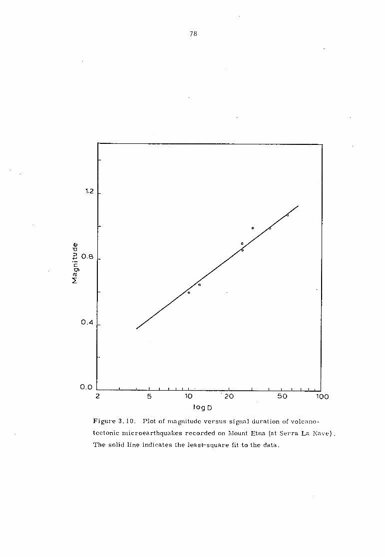
1.2
0.B
rn 2
0.4
0.0
78
2 5 10 20
50 100
log D
Figure 3.10. Plot of magnitude versus signal duration of volcano-
tectonic microearthqua.kes recorded on Mount Etna (at Serra La Nave).
The solid line indicates the least-square fit to the data.

79
Table 3.3
List of A-type Microearthquakes Used to Determine the 8-value
Signal Duration (D) Trace Amplitude (A)
(sec) (mm)
10 4.0
12 4.5
25 8.0
25 7.5
30 9.0
40 10.0
55 12.0
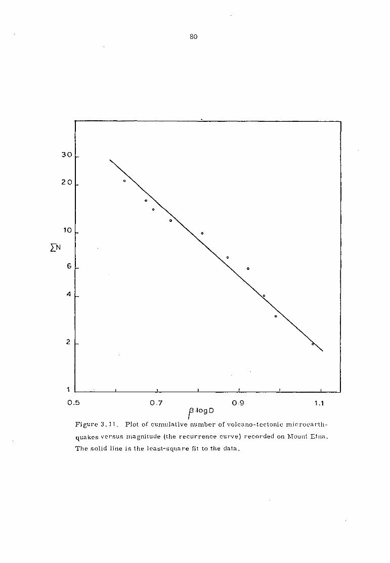
80
30
20
10
EN
6
4
2
1
O
O
O
1
0.5
0.7
0.9
1 .1 13-log D
Figure 3.11. Plot of cumulative number of volcano-tectonic microearth-
quakes versus magnitude (the recurrence curve) recorded on Mount Etna.
The solid line is the least-square fit to the data.

81
Table 3.4
List of A-type Microearthquakes Used to Determine the b-value
Signal Duration (D)
(sec)
(3logD EN
10 0.62 21
12 0.67 16
13 0.69 13
15 0.73 12
20 0.81 10
25 0.87 7
30 0.92 5
35 0.96 4
40 0.99 3
55 1.08 2

82
tectonic microearthquakes. It would be interesting to per-
form this analysis on a large sample of microearthquakes
whose magnitudes are well known. If we accept the above
analysis, the b-value for these shocks seem to support the
previous belief that these microearthquakes are tectonic,
or A-type volcanic, microearthquakes. Various other
investigators have reported recording this kind of shock.
Unger (1969) in an investigation of the microearthquake
activity of Mount Rainier, Washington, obtained a b-value of
0.82. Westhusing (1974) made a reconnaissance survey of the
seismic activity in the volcanoes of the Cascade Range,
Oregon, and obtained a b-value of 0.80. On Mount Etna itself
Guerra et al. (1976) calculated a b-value of 1.01 + 0.05 during
and after the 1974 eruption. Matumoto and Ward (1967) during
a 39 day recording period in Mount Katmai and vicinity, Alaska,
recorded 1800 events. A log-log plot of cumulative frequency
versus the maximum trace amplitude produced a b-value of 1.42.
This b-value is thought to represent a mixture of tectonic
and volcanic type seismicity.
Large b-values have also been found elsewhere for
supposedly tectonic earthquakes. Thus Sykes (1970) estimated
the b-value of two earthquake swarms originating from the
Mid-Atlantic Ridge. In both cases his b-values (1.3) are
higher than would have been expected had the earthquakes been
tectonic in origin. His conclusion was that along rift
zones, where the temperature is high, earthquakes occur as a
cataclastic process, hence the large b-value.

83
(2) B-type Microearthquakes
Fifty-five volcanic microearthquakes recorded at
the IC bench mark site were selected for the analysis. The
recorded trace amplitude A in this case ranged from 0.5 to
3.0 mm. The probable reading errors in the amplitude is
about + 0.3 mm.
Figure 3.12 shows a plot of the cumulative number
of microearthquakes versus the logarithm of trace amplitude
(the trace amplitudes of the fifty-five microearthquakes have
been divided into six groups, each with an interval of
0.5 mm, see Table 3.5). It is seen that in the amplitude
range between 1.0 mm and 3.0 mm the curve can be approximated
by a straight line. A least square: fit to the data gives
a b-value of 1.78 + 0.04. Departure of the points from a
straight line for amplitudes less than about 1 mm suggests
that this is the approximate detection threshold for the
microearthquakes in this survey.
Thus the determination of the recurrence slope
agrees well, at least within the calculated limits of un-
certainty, with those of Minakami's (1960) B-type microearth-
quakes in Hawaii and Japan. Del Pezzo et al. (1974) made
a similar survey of Stromboli, and their b-value shows good
agreement with the present findings. Microearthquakes
recorded at St. Augustine volcano, Alaska,by Mauk and Kienle
(1973) yielded b-values mostly between 1.7 and 2.5.
The significance of the b-value for both the volcano
and volcano-tectonic microearthquakes recorded in this in-
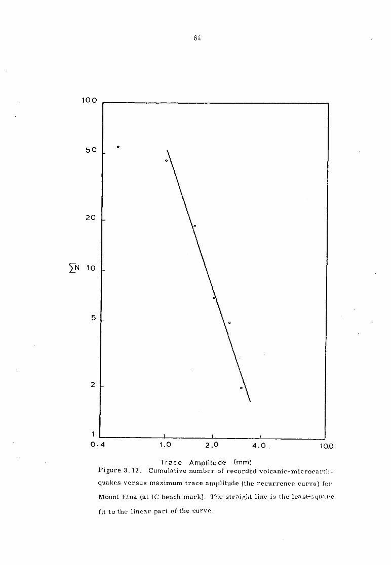
84
Trac e Amplitude (mm) Figure 3.12. Cumulative number of recorded volcanic-microearth-
quakes versus maximum trace amplitude (the recurrence curve) for
Mount Etna (at IC bench mark). The straight line is the least-square
fit to the linear part of the curve.

85
Table 3.5
List of B-type Microearthquakes Used to Determine the b-value
Trace Amplitude (A) EN
(min)
A . min - 0.5 55
0.6 - 1.0 46
1.1 - 1.5 19
1.6 - 2.0 7
2.1 - 2.5 5
2.6 - 3.0 2

86
vestigation will be discussed in detail in Chapter 6.
3.7 ENERGY CONSIDERATIONS
The magnitude of an earthquake, as was shown in an
earlier section (3.5), is a quantitative measure of its size
determined from the amplitudes of the elastic wave it generates.
The scale of magnitude now almost universally accepted was
first developed by Richter. It was later modified to take
into account earthquakes of any size and at any distance.
The main significance of the magnitude lies in the fact that
it permits a classification of earthquakes based upon the
energy released. When an earthquake occurs,the original
potential energy of strain stored in the rock is dissipated
in the following ways:
(1) Part of the original potential energy goes into
mechanical work, as in raising crustal blocks
against gravity, or in crushing material in the
fault zone.
(2) Part is dissipated as heat.
(3) Some is stored in other places as potential energy.
(4) The rest is radiated as seismic elastic waves.
It is thought that in the Californian earthquake of
1906 as much as 1.75 x 1024
ergs of energy was released,
mainly in displacing crustal blocks. The Pamir earthquake
of 1911 (magnitude 7.6) was calculated by Jeffreys (as reported
by Richter, 1958) to have released about 1021 ergs. Sagisaka
(also reported by Richter, 1958) estimated that about 3.1 x 10²⁰
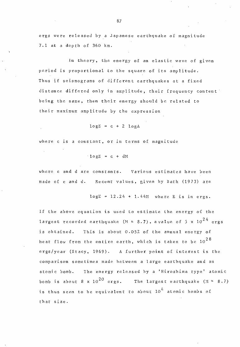
87
ergs were released by a Japanese earthquake of magnitude
7.1 at a depth of 360 km.
In theory, the energy of an elastic wave of given
period is proportional to the square of its amplitude.
Thus if seismograms of different earthquakes at a fixed
distance differed only in amplitude, their frequency content
being the same, then their energy should be related to
their maximum amplitude by the expression
logE = c + 2 logA
where c is a constant, or in terms of magnitude
logE = c + dM
where c and d are constants. Various estimates have been
made of c and d. Recent values, given by Bath (1973) are
logE = 12.24 + 1.44M where E is in ergs.
If the above equation is used to estimate the energy of the
largest recorded earthquake (M = 8.7), avalue of 5 x 1024 ergs
is obtained. This is about 0.05% of the annual energy of
heat flow from the entire earth, which is taken to be 1028
ergs/year (Stacy, 1969). A further point of interest is the
comparison sometimes made between a large earthquake and an
atomic bomb. The energy released by a 'Hiroshima type' atomic
bomb is about 8 x 10²⁰
ergs. The largest earthquake (M = 8.7)
is thus seen to be equivalent to about 104 atomic bombs of
that size.
88
The energy released in a microearthquake is ob-
viously a very small fraction of that of a large earthquake,
but the same physical principles might be expected to hold
for both.
If the above equation is used to calculate the
energies of the A-type microearthquakes recorded in 1974, we
obtain values of the order of 1013 ergs. The energy released
by the B-type microearthquakes is about one order less, i.e.
around 1012
ergs.
It must however be remembered that since the micro-
earthquake recorder could not be calibrated in the field
against magnitudes determined independently by properly
standardized permanent observatories, the estimated magnitudes,
and hence the energy values quoted above, are very approximate.

89
CHAPTER IV
SEISMIC INVESTIGATIONS OF MOUNT ETNA
DURING MAY - JUNE 1975
4.1 INTRODUCTION
In December 1974, analysis of the microearthquake
data on Etna showed the volcano to be in a moderately seis-
mically active state, and that the signature and characteris-
tics of the microearthquakes were not fundamentally different
from those recorded on other volcanoes around the world.
This provided the impetus to carry out a more detailed study
in May - June 1975. For this survey, four stations were
operated simultaneously using Geostore magnetic tape recorders,
borrowed fromthe NERC pool (Fig. 4.1),the Sprengnether micro-
earthquake recorder being used to monitor the seismic signal
at one of them. The various seismic phenomena observed from
this study, and their volcanological significance, are dis-
cussed in this and the following chapters.
The first station occupied during the 1975 investi-
gation was the Serra La Nave seismic vault (a brief description
of which was given in Section 3.3). The station became
operational on the 30th May. Apart from the routine check-up
of instruments and changing of batteries, the recorder gave no
trouble. This station operated continuously until the 16th
of June, when a violent thunderstorm struck the area. Al-
though the instrument otherwise continued to operate satis-
factorily, the Geostore clock was completely upset, probably
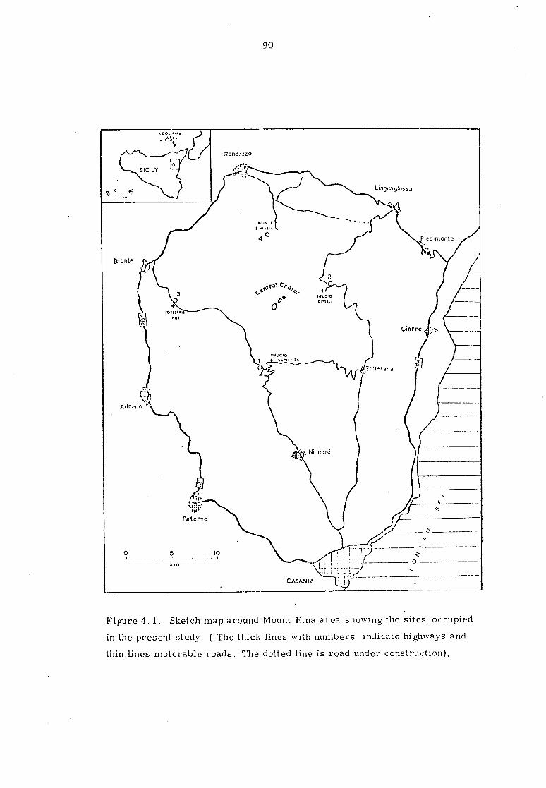
Randazzo
lingua glossa
Cronte
Adrano
•FY
Pa t erno
0 5 1?
km
A(01.•./ •Or•
• 1..
CATANIA
90
Figure 4.1. Sketch map around Mount Etna area showing the sites occupied
in the present study. ( The thick lines with numbers indicate highways and
thin lines motorable roads. The dotted line is road under construction).

91
because of induction effects. The time of occurrence of
microearthquakes subsequent to the storm could no longer be
determined from the timing pulses, and the instrument was
finally dismantled on the 19th June.
The second station,at the IC bench mark site near
the Rifugio Citelli (see Fig. 4.1),worked continuously from
the 2nd to 18th June '75 and gave no trouble whatsoever.
The third station, in the Forestale area,could not
be set up before the 7th June, and proved to be the most
troublesome of all. A new site had to be found for this
station because the necessary permission could not be procured
for re-occupation of the 1974 site. When the instrument
started operating, it was discovered that the clock was
malfunctioning. The fault was corrected but the clock worked
for a short while only and broke down again. The seismograph
then worked intermittently for the next few days, when finally
after the thunderstorm of June 16th it stopped altogether.
The fourth station, below Monte S. Maria, became
operational on the 8th June and worked intermittently until
the 11th. From then onwards it recorded continuously until
the 18th June.
Table 4.1 lists the station parameters.
4.2 THE RECORDING SYSTEM
The Geostore recording system consists of four basic
units: (1) Geostore Magnetic Tape Recorder, (2) Seismometer,

Table 4.1
Network Station Data
Station Latitude Longitude
Elevation
Foundation Remarks
(N) (E) (m)
Serra La Nave
(1)
37° 41' 40" 14° 58' 26" 1732 Lava flow Same station as
occupied in 1974.
IC Bench Mark 37° 46' 02" 15° 03' 30" 1690 Lava flow Displaced 5m to the
(2) NE of the 1974 site.
Forestale Hut 37° 44' 45" 14° 51' 43" 1150 Lava flow On a river bed about
(3) 10m NW of the hut.
Monte S. Maria
(4)
37° 49' 23" 14° 59' 53" 1675 Lava flow Same site as was
inspected last year.

93
Figure 4.2. The Geostore portable seismograph.
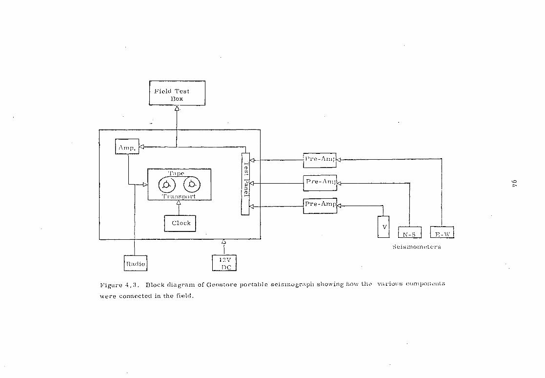
Field Test 13ox
Anip.
Tape
Transport
Clock
Pre-Anii.<1-
Pre-Amp<
Pre-Anirt
1 TAT-s E-W
Seismometers
12V DC Radio
Figure 4.3. Block diagram of Geostore portable seismograph showing how the various components
were connected in the field.

95
(3) Amplifier-Modulator and '(4) Field Test Box. The various
units are shown in Figure 4.2 and illustrated diagrammati-
cally in Figure 4.3.
The Geostore system has not been used in volcanic
environmentsbefore,although it was successfully used earlier
by Hedayati (1976) in Iran.
A brief description of the different recording units
used in the present study is given below.
(1) The Geostore Tape Recorder
The Geostore is a precision recording system for
the acquisition and retention of seismic and other low band-
width data. It accurately records FM data over a long period
with very low power consumption. The Geostore tape recorder
however differs from other FM recorders in that it contains
no provision for frequency modulating a signal within itself,
thus all inputs to this unit intended for the data channels
must be FM signals, this however does not apply to an external
'Standard Radio Time Signal'. Eleven data channels are
normally available, except in cases requiring the extended
recording capability in the bi-directional mode, which doubles
the recording time but reduces the number of signal channels
150
15 from eleven to five. Recording speeds of 16
to -67-id ips
are provided,giving maximum recording times of 170 to 680
hours. Accuracy of recording speed is maintained by a phase-
lock servo system referenced to a crystal oscillator. The
8" tape spool hold 2400 ft (730 m) of 1.0 to 1.2 mil, in

10 10 20 30 40 50 6
Time Frame
Day of Year
4 —1-1111-11-11—FLIU 1.11-1
RP. R
1. 40 to to f 4 11 1 .t. Lo 14 4 -4 1... t 1 I 14 a. to I 4 1 I
1111LILIULTULTUIRFlL1111
Hours Minutes —
Pc R
Index Count
o 5 = 0.8 sec. duration 10 sec, marks
Position Identifiers
= 0.1; sec. duration - End of frame marks
Roference
,?,L Po denote 1 minute mark
Irtinary coded ciecimal hits - One = 0.5 sec Zero = 0.2 sec
Unsued bits 0.2 sec Clock interval --- 1 sec. Time frame interva! = 1 min.
Time Decoded reads:
Year = Zero
Day of year = 16
Hours =
Minutes = 1
Figure 4.4a. Vela - Standard Time Code used with the Geostore system.

Commencement of the first blip 055 sec Duration of a short blip 100 msec Duration of the long blip 500 msec
Figure 4.4-b. Signature of the I3BC World Service Radio Broadcast used in the present recordings.

98
tape.
The time encoder is an integral part of the re-
corder and provides time code (before recording data it is
necessary to set the time code to zero,or to date and time),
an accurate flutter compensation signal, and a capstan servo
reference frequency. The timing signals from the encoder
are accurate to one part in 106 over the full operating
temperature (-20°C to +50°C) range, and recording is in
accordance with Vela Uniform Code for one minute time frames.
Timing is in days, hours and seconds, which can be read
numerically. The time decoded frame for one such unit is
shown in Figure 4.4a. When the key operated security switch
is turned,a push button associated with each digit enables
the date/time to be updated. Facilities are also provided
to allow the recording of a broadcast time code onto a data
channel. The channel concerned may be used solely for the
radio time code, solely for data, or in an automatic sequenc-
ing mode (radio recorded for every 40 sec every hour). The
centre tracks on each record head are used to record a
reference track whiCh is used by the Base Reproducer (to be
discussed later on) to improve the overall signal-to-noise
ratio of the system. A 37-way socket is provided which, in
conjunction with the Field Test Box (see 4), will monitor
selected points within the recorder, in order to verify the
correct functioning of the equipment.
A 12 volt power supply is required to operate the
equipment, normally a car battery. Facilities are available

99
for changing batteries without disturbing recording or time.
(2) The Seismometers
Six Geospace HS 10 and six Willmore NK'IT seismo-
meters were available. The former has a natural frequency
of 2 Hz, a coil resistance of 390 ohms and an intrinsic
voltage sensitivity of 1.36 v/cm/sec, and a frequency response
essentially flat between 2 and 50 Hz. The Willmore MK II
seismometers have a natural frequency of 1 Hz, a coil resis-
tance of 50 ohms,a sensitivity of 1.50 v/cm/sec, and a fre-
quency response flat in the region between 0.3 and 1 Hz,
beyond which it falls off sharply.
The six Willmore seismometers were used in pairs
to record the two horizontal components at each of three of
the stations, the HS 10's being used to record the horizontal
components at the fourth station and the vertical component
at all four.
(3) The Amplifier-Modulator
The seismometer is often situated at some distance
from the recorder, and connected to it by long cable or radio
link. The Amplifier-Modulator is intended to be installed
close to the seismometer, and serves the dual function of
pre-amplifier and frequency modulator, converting the ampli-
tude modulated output of the seismometer into a frequency
modulated signal for direct recording on the magnetic tape
recorder. The carrier frequency is 676 Hz, and the maximum
linear frequency deviation is 40% i.e. the maximum frequency

100
with which it can deal is 270 Hz.
The Amplifier-Modulator requires a single voltage
supply in the range 10 - 18V d.c. , which is normally fed along
the signal lines but may be fed in locally through a separate
connector. The typical power consumption at 12V is 75 mW.
The Amplifier-Modulator has ten switched gain ranges so that
40% frequency deviation is produced by input voltages of
0.25 mV to 250 mV. The operating temperature of the unit
is -20°C to +50°C.
The Amplifier-Modulator is fitted with a socket
for connection to the Field Test Box so that operational
checks can be performed without disconnecting it from the
system.
(4) The Field Test Box
The Geostore recorder, which is basically a magnetic
tape recorder, contains no provision for monitoring what is
being recorded, this function being provided by the Field Test
Box. This consists of a strip chart recorder which can be
used as a 'short-run' seismograph or it may be used to monitor
any channel whilst the Geostore system is in use. It was
not possible to carry this unit to Sicily because of excess
weight problems. Instead,an alternative Field Test Box was
carried that was much smaller in size and lesser in weight
than the one mentioned above. This test unit however produced
only audio signals when connected to the various recording
channels in the Geostore system.

101
4.2.1 THE EQUIPMENT SETTING UP AND OPERATING PROCEDURE
Each individual site was carefully selected for
freedom from traffic noise, ease of access, stability of
bedrock,and for low background noise. A detailed survey
conducted in the previous year with the Sprengnether MEQ 800
provided the necessary information.
A magnetic compass was used to align the horizontal
seismometers so that they were in the geographical N-S and
E-W directions. The seismometers were then emplaced by
digging through the thin soil, so that their legs were firmly
in contact with the bed rock. They were then connected to
the three available data channels in the Geostore via three
Amplifier-Modulators. External radio connections were made
to a separate data channel. The time code,using the Vela-
Standard,was recorded on a fixed channel. Power to the
system was supplied by a heavy duty 12 volt, 54 AH battery.
Before recording any data,it was necessary to set
the time code. The clock on the Geostore was set against
a chronometer kindly made available by the personnel at the
Astrophysical Observatory. The days and hours were set to
their correct GMT values. In the present investigation one
recording speed was used (15/320 ips) , giving a d.c. to 16 Hz
bandwidth in real time, and an effective -48 dB of signal-to-
noise ratio. The overall magnification of the portable
system depended on the gain level used in the field. Through-
out the whole recording period an amplifier gain of 86 dB was

102
105
0-1
rn
2
3
10 t_ l I t { I t
1 5 10
50
100 Frequency (Hz)
Figure 4.5. Response curve for the Geostore seismograph system.

103
used, giving a magnification of about 1 x 10⁴. The approxi-
mate frequency versus magnification curve of the Geostore
system operating at full gain is shown in Figure 4.5 (compare
this response curve with that of the MEQ 800 given in Fig.
3.3).
An ordinary 'Zenith' radio receiver was used to pick
up the BBC world service hourly broadcast signals. A played-
back section of this time signal is shown in Figure 4.4b.
Each tape on the seismograph provided from four to six days
continuous record. The battery was replaced by a freshly
charged one every three to four days,at which time routine
maintenance was performed on the instrument. The whole
Geostore system, whenever possible, was placed either in a ti
shed or cave, and ,covered with plastic sheet.
After the termination of twenty recording days,
nine magnetic tapes were brought back to London for further
analysis.
4.2.2 THE ANALOGUE PLAYBACK SYSTEM
For selection of those parts of the tape suitable
for detailed study it is necessary to have some means of
displaying the record in analogue form. For this purpose
'The Geostore Base Reproducer' is available. In the present
case the magnetic tapes were taken to the Eskdalemuir Seis-
mological Observatory for transcription, as this was thought
to be more convenient than transporting the equipment to
Imperial College.

104
The Base Reproducer comprises a mains operated
tape deck and an electronics unit,housed in separate
cabinets. Two different head assemblies are available
with the tape deck,the choice of which depends on whether
uni- or bi-directional recording is employed in the field.
For uni-directional recordings a full 14-track head assembly
is used, and the tape replayed in one pass. In the case of
bi-directional recording, the first replay run would re-
produce half the tracks only. The take-up spool would then
be transferred to the left hand side of the reproducer and
a second run made for the remaining tracks.
A subtractive flutter compensation is used to reduce
the base line noise and thereby improve the signal-to-noise
ratio on all' data channels. The compensated data outputs
and the time code output are fed to a 15-way output socket.
Additionally, a monitor switch enables any one channel to be
switched independently to a separate BNC socket. From
either of these outputs the final signals may be fed to a
chart recorder (a Jet Pen Recorder in our case), computer or
other analysing equipment.
4.2.3 PLAYING BACK GEOSTORE TAPES
Since a gain setting of 86 dB was used throughout,
plenty of background noise was recorded on the tapes. It
was thus essential to remove the background noise before any
microearthquake could be well identified. From known work
on volcanic background noise (Shimozuru, 1971; Schick and

105
Riuscetti, 1973; Lo Bascio et al., 1976; Guerra et al.,
1976) it was decided to set the low-cut filter at 1 Hz and
the high-cut filter at'30 Hz.
At first, it was intended to pick up events by
playing the Geostore tapes on to an oscilloscope screen,
but that proved difficult. It thus became necessary to
play out the whole tape onto paper. The following steps
were taken in order to ensure the best results.
(1) Five channels were selected on the Jet Pen
'Recorder and these were in turn connected to the Base Re-
producer. The channels selected were as follows:
(i) The time signal.
(ii) The vertical HS 10 seismometer.
(iii) The horizontal (N-S) Willmore MK II or
HS 10 seismometer.
(iv) The horizontal (E-W) Willmore MK II or
HS 10 seismometer.
(v) The radio time signal.
(2) A time decoder unit was connected to channel
(i) i.e. the time signal.
(3) A suitable combination of tape playback speed
and chart recorder speed was first found. When searching
for events, 34 ips playback speed and 10 mm per sec chart
speed was found most suitable. After an event had been
identified, a combination of 15/16 ips tape playback and
100 mm per sec chart paper speed gives the best definition
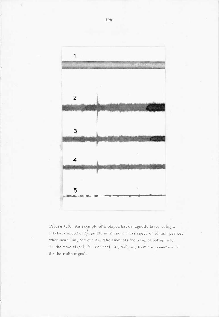
106
5 0,—.4igago..........4b....-.4b—rargeb.■•■••■-••■•■■■••••••••••■110~00..40—•
Figure 4.6. An example of a played back magnetic tape, using a 3
playback speed of 3-4 ips (95 mm) and a chart speed of 10 mm per sec
when searching for events. The channels from top to bottom are
1 : the time signal, 2 : Vertical, 3 : N-S, 4 : E-\V components and
5 : the radio signal.

la • • • %%%%% • 6. •1■1. ■•■■•• •11.■ •
•• .•■•■ ■-••■ ot■ ammo= wwww, •■■• •■ ••=, om.■ •■•■ mom. 11■11
2 •
....,41A ,*.r.',4.4041#44,44;.-W0000kriq.000;00,11,S '7',7,1,1010,4-y4,44.0.4-4#4*4*,iwob*.010,440.48611*-141440i
4 hAit-vormr 4,4*,..tvepti--1644,444 ii1,9(1944411•41$111441.--0.0P4-0•00.*****".4,Kw**444410,0*-4411
5
■•••••••{
Figure 4. 7a. Reproduction of an A-type microearthquake recorded by the Geostore using
a playback speed of 15/16 ips (24 mm) and a chart speed of 100 mm per second. The channels
indicated are the same as in Figure 4.6.
3.
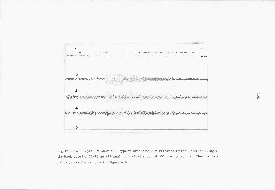
• • • ••• 1••• • • •—• • •
ad am... .•■• ir
■••••• •■• • • ■••• • • • • •-••■ ■•■•• • ■•■ • • •
11■•■■ e ••••• ••••• .■••
2 ,g4111,1;,4.4,-,04,4,40,444.#404.0frowifito , I! .11 , t`A ',1004#4WA,W.1416vivfli•04400400444011010,44 !, h
3
9144101,1141r4,11 .
:1.1\0 Iflq0 ■1,111;711114:ey r4;14:1ili•,,L °1;114f,\o'leAlftririPJA;eliiikte4;1:114#
4 so*-4m.p.#1,,,0044:0;:iioxfoll;0! ! I 41.."0,,P,0 '41.011N,#14.1v, ,,A0,11.111.1,,tri410k4e,sk*I1-44:1.-Kowi,44,144,1
5
Figure 4. 7b. Reproduction of a B- type microearthquake recorded by the Geostore using a playback speed of 15/16 ips (24 mm) and a chart speed of 100 mm per second. The channels indicated are the same as in Figure 4.6.

rr
-f),Al'ok*kri"
5
3 -
Figure 4. 7c. Reproduction of a B-type microearthquake recorded by the Geostore using a
playback speed of 15/16 ips (24 mm) and a chart speed of 100 mm per second . The channels
indicated are the, same as in Figure 4.6.

110
of onset time and first motion.
(4) The tapes were thus replayed at 80 times the
recording speed using the first combination,and 20 times
using the second.
(5) The low and high-cut filters were set to 80
and 2400 Hz on the first combination and 20 and 600 Hz on
the second combination,respectively. This gave an effective
passband of 1 and 30 Hz at the recording speed.
(6) The tape was started and played through the
first combination (32 and 10) until an event was found
(Fig. 4.6). On finding the event, the time was noted from
the time decoder unit, and the tape rewound a short way.
It was then played back using the second combination (15/16
and 100). Figure 4.7a show the same event, and Figures 4.7b
and 4.7c are two more examples, when played back using the
second combination.
(7) The BBC radio signals were always played back
using the second combination. A replayed version is shown
in Figure 4.4b.
(8) As a second tape (from a different station)
was replayed, care was taken to search the tape thoroughly
at known times of events identified on the first tape.
(9) The same procedure was followed for all sub-
sequent stations.
With practice, it is easy to pick out events from
the background noise. Time marks are indistinguishable on
the first combination but are legible on the second. It
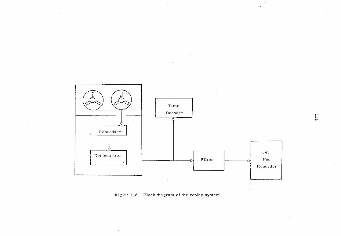
Time
Decoder
Repr oducer
C> Filter
Jet
Pen
Recorder
Figure 4.8. Block diagram of the replay system.
112
takes about 6 to 10 hours to go thoroughly over one tape,
the time taken depending of course on the number of events.
Figure 4.8 is a schemmetic diagram of the replay
system.
4.2.4 THE STORE-4 TAPE RECORDER
For the subsequent frequency analysis of the micro-
earthquakes and volcanic background noise it was decided to
transcribe the Geostore tapes on to the four channel 1" tape
of a Racal Thermionic Store-4 tape recorder. This was
thought to be a more efficient course than to have to rely
on the availability of the Geostore playback unit either
for borrowing to use at Imperial College or for use elsewhere.
The Store-4 instrumentation recorder is designed
to record four frequency modulated channels on 6.24 mm (I in)
magnetic tape. The recorder was used with instrumentation
tape 35 um thick (BASF, triple play) 2400 ft long and with
a spool diameter of 64 in. Seven recording speeds are avail-
15 able from TT, to 60 ips, selected by means of a rotary switch.
The Geostore playback unit was run at a tape speed of 15/16
ips, which is 20 times the original record speed. During
transcribing on the Store 4, both the input and replay output
signals were monitored by means of a signal monitor meter.
The Store 4 was operated from the 230 V a.c. mains.
The four channels recorded were:
(i) The vertical component.

113
(ii) The horizontal (N-S) component.
(iii) The horizontal (E-W) component
(iv) The time signal.
In order to check the quoted figures of overall
system linearity, ±0.3% deviation from best straight line
through zero, and the harmonic distortion of < 1% at maximum
modulation level, the following test was carried out. A
small section of the output signal from the Geostore playback
unit was centred around zero and stored on an oscilloscope
screen. The same section was first recorded on the Store-4
recorder then played back and superimposed on the stored
signal on the scope. From visual inspection of the records,
no apparent distortion between the two signals could be seen.
This test was carried out for a large number of tape sections
recorded at different times and places.
It was thus concluded that the Store-4 reproduces
the original signal faithfully to within the manufacturers
specifications.
4.3 ANALYSIS OF DATA
Visual inspection of the records revealed the same
three broad types of microearthquakes as were observed in
the reconnaissance survey of 1974 and discussed in Section
3.4. Whenever an event was identified as an A-type micro-
earthquake the horizontal component readings were used to
facilitate the readings of S arrivals. The S-P intervals
for the 1975 microearthquakes generally ranged from about

114
0.1 sec (in which case the epicentres are very near the
recording station) to about 6 sec. The longer S-P intervals
(.?. 3 sec), absent in 1974, might well arise from shocks
associated with the local tectonic processes rather than
with volcano-tectonic processes, as was the case in 1974.
The other two types of events (sharp impulsive
arrival with no S-P phases, and emersion arrival, also with
no S-P phase) defined as B-type microearthquakes in Section
3.4 produced similar kinds of traces on all three components.
Both types will be discussed more fully in subsequent sections.
During interpretation of these played-back analogue
records care was taken to avoid intervals with high background
noise, and whenever possible the microearthquakes recorded at
one station were compared with those recorded at the other
stations. Primary timing pulses were provided by the
Geostore clock, and these were checked against the standard
BBC broadcast. Events could thus be read to an accuracy of
about 0.05 sec.
Only three events provided seismic signals with
sufficient signal-to-noise ratios at three stations to allow
reasonable determination of their probable origin.
Two had identifiable phases and could be used for
computer location by the programme HYPO developed in the
Department. The third event had no clear phases (B-type
shock) and a geometrical method was employed to locate the
epicentre (Bath, 1973).
Apart from these microearthquakes, two other events
with identifiable phases were recorded at two stations. A

115
crude method of locating their epicentres on the basis of
their S-P intervals is given.
Bath (1973) discussed the possibility of crudely
locating the epicentres of small events recorded at one
station only on all three components. Epicentres for a
few such well-recorded events were determined by this method.
The procedure is discussed in detail in Section 4.4.3.
Volcanic tremors sometimes provide useful infor-
mation about the volcano (see Chapters 1 & 5), and if
intelligently monitored can be used for predicting eruptions.
Continuous volcanic tremors were recorded throughout the whole
recording period of observation. Their origin, mechanism
and possible source are discussed in Chapter 6.
Preliminary selection of both the A and B-type
microearthquakes for spectral analysis was also made at
this stage, and the results are discussed in the second part
of Chapter 5.
4.3.1 SEISMIC ACTIVITY OF THE VOLCANO
Statistics relevant to the occurrence rate of the
A and B-type microearthquakes at the various stations are
given in Table 4.2. Columns 1, 2, 3 and 8 of the table
list the name of the stations, the total and useful hours of
recording time and the total number of microearthquakes,
respectively. The columns of particular interest are 4, 5,
6, 7 and 9. Columns 6 and 7 show the number of events that

116
Table 4.2
Microearthquake Activity
Recording Time (hr)
Number of Events
A
S-P(sec)
B Total Per/Day Total Usable Total
<2.5 >2.5
Station
Serra La Nave 500.0 490.0 6 3 9 31 40 2
IC Bench
384.0 380.0 7 4 12(1?) 24 36 2 Mark
Forestale 24.0 22.0 2 0 2 3 5 5
Hut
Monte
150.0 148.0 2 2 6(2?) 7 13 2 S. Maria

Station 1
1 10 14
June
b
18 I I I
30 May
117
12
Station 2
N
n 6
I I I t
31 2 May
10
June
( b)
I I !
14 18
( a)
12
N
Figure 4. 9(a-b). Graphs showing the total number of recorded
events (N) plotted against the total recording interval (indicated
by arrows). The dotted and blank area in each column indicate
the number ofvolcano-tectonic and volcanic-microearthquakes
respectively.

Station 4
••••••■■
1 1 I I!
6 10 14 18 June
(d)
118
( C)
Station 3
Fri 1 I 1 1 1
10
14
1B
June
Figure 4. 9(c-d). Graphs showing the total number of recorded
events (N) plotted against the total recording interval (indicated
by arrows). The dotted and blank area in each column indicate
the number of volcano-tectonic and volcanic-microearthquakes
respectively.
12
N
12
8
N
4
0 6

119
were broadly classified as A and B-type microearthquakes.
The question mark against some of these numbers indicates
their doubtful classification. The division of the A-type
events (columns 4 and 5) into S-P times of 0 - 2.5 sec
and 2.6 - 6.0 sec respectively were based on the 1974 results.
The division is somewhat arbitrary but any events with S-P
interval greater than 2.5 sec are thought not to be strictly
volcano-tectonic microearthquakes, as they originate almost
20 km away from any recording stations (see Section 3.4.2),
and possibly come from depths of >10 km, where the influence
of the volcano in inducing events of this nature might be
considered small. These type of events constitute about
half the total A-type microearthquakes.
The figures in column 4 and 8 indicate that 20% of
the total recorded events (excluding events with S-P > 2.5 sec)
were of the A-type, while the figures in column 9 give the
microearthquake occurrence rate (excluding any event with
S-P > 2.5 sec).
Figure 4.9(a-d) shows the number of microearthquakes
(excluding non-volcanic events) recorded at each station,
plotted as histograms of the number of events per day. It
is seen that there is no significant variation in the micro-
earthquake occurrence rates (shocks/day) at the three record-
ing stations. This is probably indicative of the volcano as
a whole having reached some kind of 'seismic stability'.
During this time no 'abnormal' movement of the magma took
place, neither was any fumarolic activity above 'normal'

st. 2 st. 4
ni 4
N
6
3
st. 1 st. 3
6
0 2
4
6
S - p (sec)
S - P (sec)
(a)
( b )
Figure 4. 10(a-b).. Graphs showing the frequency distribution of microearthquakes plotted
against distances from the recording stations (in terms of S-P intervals).

121
noticed. These findings seem to be supported by Prof.
Rittmann (verbal communication, '75) who described the
volcano during the 1975 recording period as being "very
quiet". An anomalous behaviour was however noticed at
station 3, where the seismic activity level is more than
double than that at the other stations. This difference,
however, may not be significant, because of the short re-
cording time, the microearthquake occurrence rate being
based on only 22 hours of useful recordings.
It should be noted that during this short period
of study no 'swarm type' bursts of energy, often seen else-
where (Eaton, 1962; Robson et al., 1962; Matomuto and Ward,
1967; Mauk and Johnston, 1973), were observed, which further
indicates the 'relative quiet' nature of the volcano during
the 1975 recording period.
4.3.2 DISTRIBUTION OF S-P INTERVALS
Figures 4.10(a-b) show the distributions of S-P
intervals for microearthquakes recorded at the four stations.
At station 1, 2 and 3 the largest number of events fall in
the S-P interval 0-2 sec, whereas at station 4 no events
are found with an S-P interval of less than 1 sec. Some
events are also distributed at the various stations with S-P
intervals of 4, 5 and 6 sec. The distribution of the S-P
times of all the recording stations taken together however
seems to indicate a strong clustering of events. These
groups have S-P values of 0-2 sec and 3-6 sec respectively.
122
If one assumes (see Section 4.4.3) an average P wave velocity
of 5.0 km/sec,the first group involves activity at distances
ranging up to 15 km, and the second group at distances of
between 20 and 40 km from the recording stations.
These results suggests that the first group (0-2 sec)
reflects adjustments to tectonic stresses within and around
the volcano itself. Furthermore,the stress build-up appears
to be concentrated in the area between stations 4, 1 and 2
(see Fig. 4.1). The second group (3-6 sec) appears to be
associated with local tectonic forces much further away from
the volcano.
4.3.3 MAGNITUDES
Estimation of Richter magnitudes was not possible
in the present study as none of the Geostores could be cali-
brated in the field against magnitudes determined at permanent
observatories. However,a rough estimate of the body-wave
magnitude was made from the duration of the seismic signal
using the values of R and obtained from the 1974 results
(see Section 3.4.7). Though the instruments used in the
two years were quite different, there is no reason why the
R and 0 values should be much different. Using the 1974
values of -0.08 and +0.62 for R and Q respectively the body
wave magnitude of the A-type microearthquakes appear to range
between 0.4 and 1.5.
4.3.4 b-VALUES
The total number of events recorded during the 1975
123
survey was insufficient for determination of the b-value.
4.3.5 SEISMIC METHOD OF LOCATING MAGMA CHAMBERS
The finding of molten-pockets and considerations
on their depth have so long been purely speculative.
Recently,however,Gorshkov (1958) found that the waves from
distant earthquake passing under a group of volcanoes in the
Kamchatka suffered considerable weakening of the shear wave
(S-wave). This attenuation was believed to have been caused
by the presence of vast magma reservoirs in the upper part
of the mantle, most probably at depths of between 50 and
70 km.
For a long time,this was the only available experi-
mental evidence of shear wave attenuation by molten pockets
of magma. Subsequently, many reports have been published
of similar observations in other volcanic areas (e.g. Firstov
and Shirokov, 1971; Farberov and Gorelchik, 1971; Kubota
and Berg, 1967; Matumoto, 1971; Shimozuru, 1971a).
Kubota and Berg (1967), for instance, carried out
several independent geophysical investigations looking for
evidence for magma in the Katmai volcanic range. They
observed a high value of 0.3 for Poisson's ratio, and the
screening of the predominantly vertical component of the
elastic shear waves. Local negative Bouguer anomalies also
suggested the presence of low density material at shallow
depths. The magma chambers were located using calculated
wave paths for the rays exhibiting S-wave screening.

124
The most extensive investigation to date on the
screening of S-waves was however carried out by Matumoto
(1971) in the vicinity of Mount Katmai, Alaska. During
an investigation extending from the summer of 1965 through
1967,as many as 40 to 50 events were recorded per day, the
body wave magnitudes of which ranged from 0 to 3. Hypo-
centres were mostly shallow, < 10 km, although some occurred
at depths ranging up to 150 km. Approximately 500 micro-
earthquakes were simultaneously recorded at two stations.
In some cases both P-and S-waves were recorded at one of
the stations, but only P-waves and no, or very weak, shear
waves at the other. The latter were also characterized by
an increase in the apparent period of the P-waves, thought
to be due to the absorbtion of higher frequencies.
The association of these two phenomena, the lack
of an S-wave and the increase in the period of the P-wave, is
not however very common throughout the whole area, but is
confined rather to events originating from specific areas.
Wave paths from hypocentres to recording stations plotted for
twenty-five of these events strongly suggest that the dis-
appearance of S-waves and probably the increase in the
apparent period of P-waves are related directly to existing
active volcanoes or possible magma chambers, magma pockets
and zones of partial melting.
The phenomenon of partial or total screening of
the shear waves by pockets of magma seems at the moment to
be well established. As to the size and extent of these

125
pockets there is still a great deal of controversy. It
is hoped that as more data becomes available these problems
will be resolved.
One of the aims of the present project was to seek
evidence for the existence of molten pockets by analysing
S-wave attenuation and the increase in the apparent period
of the P-waves, but approximately twenty days of recording
did not provide suitable data for an analysis of this nature
to be carried out.
It may not be out of place to mention here that
the observation of shear wave attenuation and P-wave delays
in local microearthquakes is one of the techniques being
currently used to delineate liquid bodies in a geothermal
environment. Local attenuation of shear waves from earth-
quakes have been observed in the geothermal areas in Yellow-
stone National Park (Eaton et al., 1975) and St. Lucia,
West Indies (Aspinal et al., 1976).
Teleseismic P delays have also been observed in
Yellowstone National Park and Long Valley Caldera, U.S.A.
(Steeples and Iyer, 1975). These P velocity delays are
consistent with their interpretation of an anamolous thermal
zone, 300° - 400°C above normal. Combs and Ratstein (1975)
also observed a decrease in the ratio of the P and S velocities,
in the Coso geothermal area, California, U.S.A.. They
interpreted this as due to the existence of a vapour-dominated
reservoir where steam-filled voids cause a decrease in P

126
velocity.
4.4 REVIEW OF TECHNIQUES USED TO LOCATE LOCAL EARTHQUAKES
Any source of seismic disturbance, either an earth-
quake or an explosion, is defined by the following parameters:
(1) The time of the event, or the origin time
of the seismic disturbance.
(2) The geographic latitude and longitude of the
epicentre (point on the earth's surface verti-
cally above the source).
(3) The depth of the source, or focal depth (the
source is also known as the focus or hypocentre) .
(4) The size of the event (expressed normally as
the magnitude, or in terms of the energy released).
In order to calculate the various parameters in
1, 2 and 3, only time measurements are needed at the various
seismograph stations, while the parameter in 4 requires
measurements of amplitudes and periods. The location of an
earthquake is thus concerned with the determination of a
number of unknowns. Let us examine what is the least number
of seismograph stations necessary for such a calculation.
To determine the focus of an earthquake requires
the solution of a set of simultaneous equations, one for each
station , of the form:
(cp i-(1)0)2 + (X.-X )2 + (z.-Z o )2 = V2(t.-To )
2 1 o 1 p
(4.1)

127
where, 4)., A, z. = co-ordinates of the stations,
(T) o , A , Zo
= co-ordinates of the focus, o
t. = arrival time of the earthquake
to station i
To
= origin time of the earthquake
V = propagation velocity of the P wave
As the arrival times of P are usually the primary
data with which one has to work, a minimum of five recording
stations are necessary to determine the five unknowns
(4) o ,A,Zo,To
,Vp) in the above equation. But if, in
o
addition, information is available on azimuth, obtained from
the horizontal components of the P wave, or on arrival times
for other waves (for instance S), then the number of stations
can be reduced correspondingly. The common practice today,
however, is to base the determination on as many different
stations as possible. Local deviations exist from assumed
travel-time tables depending, for instance, on local structure,
and therefore a least square calculation technique is applied.
The error limits of the results obtained can then be estimated.
A number of computer programmes have been developed
over the years, based on the least square iterative process,
to locate near seismic events using readings from a net of
local stations. Flinn(1960) used direct P and S arrival
times to locate some of the local earthquakes recorded by
the Australian National University network of nine seismic
stations. Nordquist (1962) developed for the Pasadena net-
work a programme for determining the source and origin time
of a local earthquake, using the times of arrival of direct
128
and refracted P-waves. Considerable improvement upon the
existing programmes have been achieved by Engdahl and
Gunst (1966), whose single pass programme COAST computes a
first approximation to the hypocentre using only five
stations, subsequent to which it determines the refined
hypocentre and earthquake magnitude. An improved hypo-
central location can now be obtained by the crustal model
programme HYPOLAR written by Eaton (1969), who takes as
crustal model a uniform half-space overlain by a layer of
constant velocity.
All these non-linear techniques calculate the four
hypocentral parameters, latitude 40), longitude (a0), depth
but not of focus (Z0), and origin time (T0)4independently. As
James et al. (1969), pointed out, the four-parameter least-
square approach gives solutions that depend upon the number
and configuration of the observing stations, as well as the
initial hypocentral approximation. For instance,an earth-
quake that occurred just outside the Arequipa network (in
Central Peru) on Feb 6, 1965, and was recorded at all nine
stations, provided a range of solutions that was dependent
on which of the different subsets of the nine station data
were used for the calculations. The total variation in
origin time was more than 30 sec and in depth 110 km,and the
position of the epicentre varied by more than 20.
One of the fundamental sources of instability in
the least-square iterative process is the interdependence
of the computed variables. In order to overcome these

129
problems, James et al. (1969) proposed using a three-para-
meter least-square method. The independent variables,
(P o, A o and Zo are calculated by the usual least-square
iterative process from the P arrivals, and S waves are used
to calculate To from the relationship
T = T - VkTsp
o
V (4.2)
where T = arrival time of P
= time interval between S and P wave arrivals sp
V V Vk
- s p (S-P wave function) V -V s p
Vs = propagation velocity of S wave
(4.3)
and the other symbols have their usual meaning.
More recently, Crampin (1970),and Crampin and
Willmore (1973), developed a programme (FAMG) that attempts
to provide more stable and reliable solutions. Their improve-
ment has been achieved by the addition of the time-term to
the least-square iterative process described earlier. They
argue that the previous programmes made no allowances for
any variation of structure within the network, and are not
adequate when the time-term is comparable to the total travel
time.
The time-term, which depends on the velocity struc-
ture beneath the shot and recording point (Fig. 4.11),is given
by the equation (Berry and West, 1966).
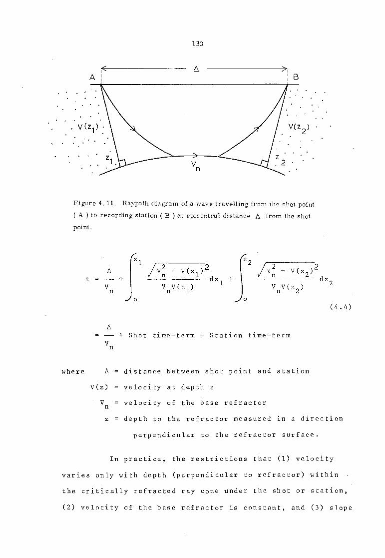
130
Figure 4.11. Ra:vpath diagram of a wave travelling from The shot point
( A ) to recording station ( B ) at epicentral distance A from the shot
point.
zi A
/V 2 vn
- v(z1 dz)2
+ t = + 1 V
n VnV(z
1)
Jo (4.4)
A = + Shot time-term + Station time-term
Vn
where A = distance between shot point and station
V(z) = velocity at depth z
Vn = velocity of the base refractor
z = depth to the refractor measured in a direction
perpendicular to the refractor surface.
In practice, the restrictions that (1) velocity
varies only with depth (perpendicular to refractor) within
the critically refracted ray cone under the shot or station,
(2) velocity of the base refractor is constant, and (3) slope

131
and curvature of the refracting surface is small, must be
reasonably well satisfied for successful application of the
above equation. The need for the addition of the time-
term is well demonstrated by Berry and West (1966),while
trying to explain the anomalous seismic velocity behaviour
in the Canadian shield.
Crampin and Willmore's (1973) FAMG programme com-
putes the hypocentral parameters of local earthquakes recorded
within a small network where the travel-time equations are
derived from the geometric ray paths in known geological
structures, modified by the time-term at each point.
Thus the successful application of FAMG, and the
determination of the focal position with the necessary degree
of precision,dependsupon the following conditions (1) the
velocity structure in the area is assumed to be known accurate-
ly for a suitable time-term analysis (2) there exists a
sufficient number of event arrivals with good azimuthal
distribution, covering a wide range of distances.
4.4.1 OTHER LOCATION TECHNIQUES
Microearthquakes recorded at three or more stations
with distinguishable P and S phases can be located using the
techniques mentioned earlier. If, however, a B-type micro-
earthquake is recorded at only three stations, the above
method cannot be used.
The following section discusses the location tech-

132
nique for such microearthquakes when recordings are avail-
able from three (for B-type event) or from one station,
with three-component recordings.
The first method to be discussed is the 'circle-
method', which is suitable for locating B-type microearth-
quakes recorded at three stations.
For simplicity it is assumed that the wave velocity
V is constant. It is also assumed that the arrival times
tl' t2 and t3 for the first arrivals at the three stations
1, 2 and 3 have been accurately measured,and that t3 < t2 < tl.
Next, with stations 1 and 2 as centres,circles are constructed
with radii equal to V(t1-t
3) and V(t
2-t
3) respectively.
Then the epicentre 0 is the centre of a circle which passes
through the station 3 and is tangential to the two above
mentioned circles (Fig. 4.12).
In practical applications, it is possible to find
the location of 0 after a few trials with no need to perform
any calculations.
In order to determine the epicentre of a microearth-
quake recorded at only one station, we have to determine the
distance and the direction from where it is coming. Of the
two unknowns, the distance is the easier to calculate. It
is usually obtained from the time-difference between the
different phases, and in the case of microearthquakes it is
generally S-P. The direction is more difficult to determine
accurately because of the higher requirements on the quality

133
Figure 4.12. Determination of epicentre 0, by the circle method. t1 ,
t2 and t
3 are the first arrival times of a B-type microearthquake at
the three stations 1, 2 and 3 respectively.
of the record. Thus if the amplitude of an event is avail-
able from the measurements of the three components, the
resultant of these give the direction to the source.
Figure 4.13 illustrates this procedure. It should however
be remembered that the three components can only be combined
vectorially if all the three seismometers have the same
response curve. If this is not the case, then the trace
amplitudes have first to be transformed into the correspond-
ing ground amplitudes, and then combined to give the azimuth.
When in practice an epicentral distribution is ob-
tained from the records of only one station,it is advisable
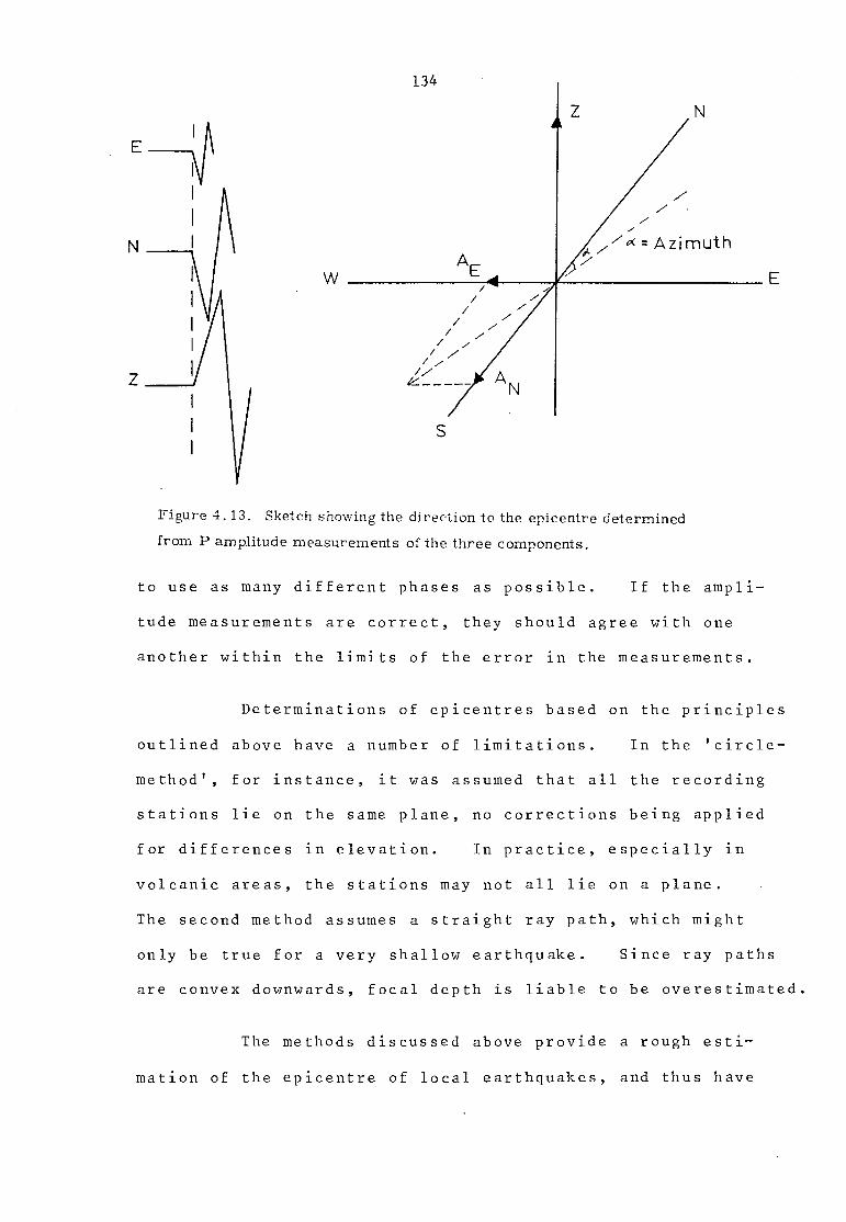
134
z
AE
mid =: Azimuth
E
7
Figure 4.13. Sketch showing the direction to the epicentre determined
from P amplitude measurements of the three components.
to use as many different phases as possible. If the ampli-
tude measurements are correct, they should agree with one
another within the limits of the error in the measurements.
Determinations of epicentres based on the principles
outlined above have a number of limitations. In the 'circle-
method', for instance, it was assumed that all the recording
stations lie on the same plane, no corrections being applied
for differences in elevation. In practice, especially in
volcanic areas, the stations may not all lie on a plane.
The second method assumes a straight ray path, which might
only be true for a very shallow earthquake. Since ray paths
are convex downwards, focal depth is liable to be overestimated.
The methods discussed above provide a rough esti-
mation of the epicentre of local earthquakes, and thus have
135
very limited application.
4.4.2 A BRIEF DISCUSSION OF PROGRAMME HYPO
In the present investigation, as only two micro-
earthquakes with identifiable P and S phases were recorded
at as many as three stations, and the velocity structure is
not known accurately enough for a time-term analysis, it was
decided to develop the programme HYPO, mentioned earlier,
taking the pecularities of the present situation into account.
Programme HYPO, however, involves the following simplified
assumptions:
(1) The structures are assumed to be isotropic
and homogeneous with the velocities of P-and S-waves constant
with depth.
(2) The average P-wave velocity V is taken as
5.25 km/sec (the actual value probably ranges between 5.0
and 5.50 km/sec).
Determination of the hypocentre requires solution
of Eqn . (4.1). However,restriction to stations closer than
15 km allows the use of a rectangular co-ordinate system.
Equation (4.1) can thus be re-written in the form
2 2 2 2 (x.-X
o ) + (y.-Y o ) + (z.-Z
o ) = 2
(t.-T o) (4.5)
where i = 1, 2, 3 in the present case, and xi , yi, zi are the
co-ordinates of stations, and Xo, Y
o, Zo
are the co-ordinates
of the focus, and the other symbols have their usual meaning.

136
As the ratio of S to P velocities is constant
(assumed here as 0.59) Eqn. (4.2) can be simplified to
give
(To)i = t (T ).
sp 1 (4.6)
0.7
Equation (4.5) is now solvable for Xi, Yo by a second order
determinant. Zo is found by substituting these values into
any of Eqn. (4.5).
As the assumed average velocity V is not well sub- P
stantiated, three values of V (5.25, 5.0, 5.50 km/sec) were
tried, to obtain a range of hypocentres for each event.
The programme is set up for rectangular co-ordinates,
but it is desirable to feed in and read out locations in
latitude and longitude. A mapping function was devised to
convert geographical co-ordinates to rectangular co-ordinates
(Hosmer, 1919).
Now x = N(X-X)cosq)
2
y= Rm("o) (x /2N)tan o
2
whence (I) = (1)0 + Y/R (x /2NR)tan()g0 m m
. o + (x / N )sec(I)
(4.7)
(4.8)
where X = longitude
(I) = latitude
o = longitude of the origin of rectangular co-ordinates
*This corresponds to Poisson's ratio = 0.235, a representative value for rocks near the surface.
137
(I)o = latitude of the origin of rectangular co-ordinates
Rm = radius of curvature of the earth in the plane
of the meridian, at the latitude of the
origin of co-ordinates
N = radius of curvature of the earth in the prime
vertical, at the latitude of the origin of co-
ordinates.
Equations (4.7) and (4.8) are sufficiently accurate
for the present purpose (for stations less than 150 km away from
the origin of co-ordinates, the error involved is less than 0.1
km) . The co-ordinates of Serra La Nave (37.69° , 14.97°) were
taken as the origin, for which N = 6378.16 and Rm = 6335.47.
This method of locating hypocentres was successfully
applied earlier by Westphal and Lang (1967) in monitoring the
local seismic events at the Fairview Peak area in Nevada.
More recently, Westhusing (1974) used the technique to locate
microearthquakes in the volcanoes of the Cascade Range, Oregon.
4.4.3 LOCATION OF MICROEARTHQUAKES ON ETNA USING PROGRAMME
HYPO
Two well defined shocks with identifiable P and S
phases were located using the computer programme HYPO. Table
4.3 gives the average velocity models used in the present
calculations and Table 4.4 gives the result in terms of lati-
tude, longitude, depth and origin time. The epicentral
distribution of the events corresponding to the three models
are given in Figure 4.14 (indicated by crosses, and labelled,

138
Table 4.3
Average Velocity Model Used for
Hypocentral Determination
Model Depth (km)
1 20
2 20
3 20
5.00 2.95 All models
based on
5.25 3.09 crustal
structure
5.50 3.25 given by
Cassinis et
al. (1969)
P wave velocity
S wave velocity Remarks (km/sec) (km/sec)

Table 4.4
Location of Microearthquakes Recorded
on Mount Etna
MODEL 1
(d
Date
mon yr)
Origin
(hr min
Time
sec)
Latitude
(deg min sec)
Longitude
(deg min sec)
Depth
(km)
11 06 75 19 58 28.45 37 48 32.02 15 00 12.70 7.793
12 06 75 19 27 11.89 37 46 28.51 15 09 20.50 19.030
MODEL 2
11 06 75 19 58 28.45 37 48 30.71 15 00 29.37 8.983
12 06 75 19 27 11.89 37 46 33.44 15 10 20.65 19.336
MODEL 3
12 06 75 19 58 28.45 37 48 27.63 15 00 47.43 10.137
12 06 75 19 27 11.89 37 46 40.29 15 11 47.42 18.600

N
A station •
c"--- extent of lava flow
0 km 10
140
Figure 4.14. Map showing the epicentre of rnicroearthquakes analysed in
the present study, The crosses (a l ), the hatched area (a2 ), and the open
circies (a3) are epicentres for A-type events and the dotted area (b1 ) that of
a B-type event. (For full explanation see text),

141
1 10 km
10
15
20
Figure 4.15. Depth of focus of two A-type (indicated by crosses)
and a B-type event (indicated by the dotted area). For full explana-
tion see text.

A
A
Vk
=
=
=
Vk
V V sp
epicentral
s-tp)km
(S-P p
V-V s•
where
and
142
al). Figure 4.15 is an E-W cross-section through the centre
of the volcano, showing the depth of focus of the above two
events. These have been plotted only as a function of
depth and of radial distance from the summit crater. The
horizontal and vertical extent of the crosses in both the
figures indicates the spatial uncertainty of the epicentres,
as well as the foci of the events using the above models.
It can be seen from the figures that for the shallow focus
earthquake the epicentre is much better located than for the
deeper earthquake, whereas the depth of the focus is much
better controlled in the latter case.
The shallower of the two shocks lies at a depth of
between about 7 and 10 km, and is probably related to the
volcano-tectonics of Etna. These types of shocks are what
Minakami (1960) described as A-type microearthquakes. The
second, much deeper, shock is probably related to the non-
volcanic tectonics of the area.
Proper epicentral location, as discussed earlier,
requires the event to be recorded in at least three stations.
Due to instrumental problems, as well as their small magni-
tudes, most of these microearthquakes were recorded at not
more than two stations. Approximate locations were obtained
for two shocks recorded in stations (2 & 1), and (2 & 4)
using the relation
distance from recording stations,
wave function)
and the other symbols have their usual meaning. Both these

143
microearthquakes occur within 5 to 13 km of the recording
stations,within the hatched area in Figure 4.14 (labelled,
a2).
As mentioned in Section 4.4.1,a B-type microearth-
quake was recorded in three stations (1, 2 & 4). A geo-
metric method was used to locate its epicentre. The dotted
area near the Central Crater (Fig. 4.14 & 4.15) seems to be
the origin of this shock (labelled, b1). The maximum
apparent velocity which would be compatible with the obser-
vations of the first arrivals at the three stations is 1.09
km/sec. This low seismic wave propagation velocity can be
explained as due to the presence of unconsolidated tuff and
pumice in the top layers of the volcano.
It is interesting to note in this connection the
findings of Latter (1971) on Vulcano, one of the islands of
the Aeolian arc. In an investigation of the propagation
velocities in the superficial rocks of the volcano he obtained
a first P-wave arrival velocity range of 0.98 - 1.02 km/sec.
This is in good agreement with the present result, probably
because unconsolidated material on volcanoes have nearly the
same propagation velocities.
Some very small magnitude microearthquakes were
analysed by the technique mentioned in Section 4.4.1. These
microearthquakes were recorded at only one station and thus
the methods of Section 4.4 could not be used.
Obviously,three components are necessary and suffi-
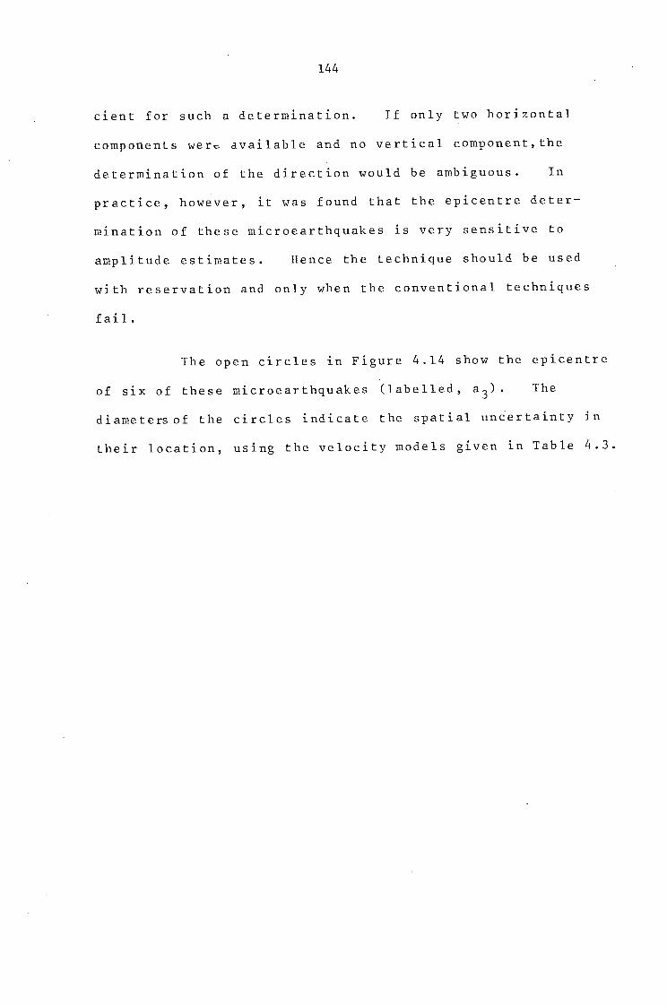
144
cient for such a determination. If only two horizontal
components wer,, available and no vertical component,the
determination of the direction would be ambiguous. In
practice, however, it was found that the epicentre deter-
mination of these microearthquakes is very sensitive to
amplitude estimates. Hence the technique should be used
with reservation and only when the conventional techniques
fail.
The open circles in Figure 4.14 show the epicentre
of six of these microearthquakes (labelled, a3). The
diametersof the circles indicate the spatial uncertainty in
their location, using the velocity models given in Table 4.3.

145
CHAPTER V
SPECTRAL CHARACTERISTICS OF MICROEARTHQUAKES
AND BACKGROUND SEISMIC NOISE
5.1 INTRODUCTION
The importance of seismometric observation of vol-
canoes for predicting eruptions has been examined in Chapter
I, and in Chapters III and IV the results of the 1974 and
1975 fieldwork on Mount Etna have been discussed, mainly in
terms of the magnitude and recurrence frequency of the re-
corded microearthquakes. Information of a quite different
kind can be obtained from spectral analysis, both of micro-
earthquakes and of volcanic tremor, the background seismic
noise of volcanic origin, as distinct from the normal micro-
seismic background.
Spectral analysis provides information about the
frequency content and the distribution of power, and thus
enables changes in frequency content with time to be recog-
nized. Such changes appear in some cases to be related
to the eruptive state of a volcano, a matter that can be
tested in the case of any particular volcano by observation
over a prolonged period of time. Where found to exist, such
changes have possible application in the prediction of
eruptions.
The first seismometric observations of volcanic
tremor possibly dates back to about 1910 when Omori (1911)

146
studied the eruption of Mount Usu in Japan. Many reports
have been published since then of the eruptions of volcanoes,
Mauna Loa and Kilauea in Hawaii by Jager (1920), Finch
(1943, 1949), Eaton and Richter (1960); Vesuvius in Italy
by Imbo (1935); Ruapehu in New Zealand by Dibble (1969);
some Central African volcanoes by Berg and Janessen (1960);
Meakan-dake in Japan by Sakuma (1957) etc.
Various types of volcanic tremor have been dis-
tinguished. For example, in the Strombolian and Hawaiian
type eruptions, volcanic tremors are directly related to
eruptions, whereas in others, tremors are not accompanied
by simultaneous eruptive activity.
The individual waveforms or phases are difficult
to identify for any type of volcanic tremor. However, they
seem to share many characteristics, such as velocity of
propagation, attenuation of wave energy etc, with seismic
surface waves. As a result, many investigators think they
are mainly composed of the latter kind of wave (Kubotera,
1974).
Spectral characteristics of volcanic tremor vary
from volcano to volcano. They also vary with time, depending
on the state of activity of the volcano. In practice, they
are also influenced by factors external to the volcano, such
as the nature of the propagation path and the frequency response
of the seismograph. For instance, to study the short-period
components of volcanic tremors, the seismographs employed
3
r
Figure 5.1. Examples of played back magnetic-tape record of volcanic tremor. The channels
from top to bottom are, 1 : the time signal, 2 : Vertical, 3 : N-S, 4 : E-W components and
5 the radio signal.
148
in the present investigation were adequate. However,
volcanic tremors sometimes have long-period components
(Minakami and Sakuma, 1953; Shimozuru, 1971; Kubotera,
1974). For the observation of these kinds of tremors,
long-period seismographs are necessary, and it was not
therefore possible to study the long-period components
during the present investigation.
Examples of fast played-back magnetic tape record
of volcanic tremor recorded during this investigation are
shown in Figure 5.1.
Many suggestions have been made as to the origin
of volcanic tremors. Most fall into one of two categories,
(1) attributing them to the movement of magma, or (2) relating
them to phenomena associated with gases.
The proponents of the first process believe that
tremors are caused by the turbulent flow of magma or by the
free oscillations of a hypothetical magma chamber within the
volcano. Finch (1949) studied the seismograms of volcanic
tremor (for Kilauea) recorded at the Hawaiian Volcano Obser-
vatory during various phases of its eruptive activity. He
noticed, for instance, that the seismographs recorded small
tremors almost continuously, and in general the tremors were
most conspicuous when Kilauea was most active. He also
noticed that when magmatic activity totally ceased, volcanic
tremor also disappeared. Wood, as reported by Finch (1949),
had previously suggested that these tremors were associated
with the outbreak of fountains in an active lava lake

149
(Halemaumau). But Finch observed that there was no obvious
connection between the two. For instance the 1922 eruption
produced tremors at a time when no lava was visible at
Halemaumau, although lava outpouring from a nearby rift
(Puna) indicated underground movement of magma. The above
observations lead him to suggest that volcanic tremors had
a more "deep-seated origin" than envisaged by Wood. Thus
Finch suggests that these tremors could be induced by the
"vertical surgings of magma in the conduit under Halemaumau"
or by "pulsating horizontal discharge" of magma.
During eruptions, or high volcanic activity, the
processes suggested by Finch (1949) may be partly responsible
for the observed volcanic tremor. It is however difficult
to visualize (in the absence of further evidence) how such
a physical process can be sustained for long periods (weeks
and sometimes months) that is capable of producing volcanic
tremor without any significant variation either in its period
or amplitude.
Sassa (1936) made an extensive survey of Mount Aso,
Japan (1929-1933) both during its active and its repose
periods. He classified the recorded volcanic tremors into
three distinct groups according to their wave characteristics.
The first group had periods between 0.4 and 0.6 sec, the second
group about 1 sec and the third group between 3.5 and 7.0 sec.
Volcanic tremors of the first kind (0.4-0.6 sec)
were thought to be a kind of Rayleigh wave, generated by sur-

150
face eruptions and internal eruptions at very shallow places.
The second kind (period 1 sec) was considered to be generated
by "internal eruption of volcanic gases". Volcanic tremors
of the third kind (3.5-7.0 sec) are believed to be generated
by the oscillation of the magmatic chamber. The variation
in periods are supposed to be related to the physical as
well as to the chemical conditions both inside the chamber
as well as in vents around the volcano.
If Sassa's (1936) explanation of the generation of
volcanic tremor are accepted, the recording of three or even
two types of wave group during a single survey probably
indicates the complexity of volcanic processes, even for a
small (in comparison with Etna) volcano such as Aso.
The above two broad categories of the origin of
volcanic tremors, or a combination of both, appear to be accepted
by seismologists as the primary cause of volcanic tremor in
nearly all volcanoes (Omer, 1950; Sakuma, 1957; Steinberg
and Steinberg, 1975). The degree of dominance depends ,
of course, on the particular volcano being investigated.
Among other processes thought to be responsible for
volcanic tremors are continuous microfracturing of rocks
combined with changes in temperature, discrete dislocation
in rocks surrounding dykes while they are intruding, or the
oscillation of water at temperatures above 600°C (the gas
phase above the magma chamber is predominantly composed of
water vapour), generally known as the 'Leidenfrost Effect'.
The sinusoidal wave trains recorded by Latter (1971) on the

151
Aeolian Island of Vulcano are thought to be due to this effect.
In this chapter the spectral characteristics of
some selected microearthquake and volcanic tremor records
are studied, a tentative source location based on the
attenuation of tremor amplitudes at the various stations
is attempted, and finally a possible source mechanism is
proposed for Mount Etna.
5.2 SELECTION OF DATA FOR DIGITIZATION
It would be prohibitively expensive and quite
unnecessary to digitize the whole of the recorded data at
the density required for useful analysis. It is necessary,
therefore, to inspect the whole of the data and to select
from it those portions containing interesting information.
The procedure followed was to play back one of the recorded
channels (from the Racal Store-4 instrumentation recorder,
see Section 4.2.4), displaying the output on an oscilloscope
screen, and to visually inspect the trace. Any sections
contaminated by unwanted noise, or showing signal dropout
due to malfunctioning of transducer etc, were rejected.
The time of the selected portion was noted from the time
decoder unit (the time decoder unit was connected to channel
4 of the Store-4, and displays hours and minutes) and the
three channels of the appropriate time-span were then replayed
in turn.
The analogue signal must now be converted into
digital form. In doing this certain basic principles of
152
sampling theory must be followed, so that the reconstructed
signal, obtained from the discrete signals x(iAt), where
i = 1,2,...N and At is the sampling interval,represents
the original signal x(t) with acceptable accuracy.
The process of analogue-to-digital (A/D) conversion
is equivalent to a convolution of a continuous signal x(t)
with an infinite Dirac comb in the time domain,
00
A(t,At) = A 6(t-nAt)
n= - 03
Expressed mathematically, this becomes, (Kanasewich, 1975)
+00
x(t)V(t,At) = x(tn)At . d(t-nAt)
(5.1)
n= _ co
The right-hand side of the above equation,if ex-
panded in a Fourier series,takes the simple form of the
sampled signal as a series of amplitude modulated waves
00 03
x(tn)At . 6(t-nAt) = x(t) + 2) x(tk
)cos(27fkAt) (5.2)
n= - 00 k=1
The 'd.c.' term x(t) on the right-hand side of the
above equation yields the correct spectrum of the designated
signal. The second term,however,interferes constructively
at frequencies 3 / 1/At' 2/ At'
'At and so on, producing 'side

153
lobes' all with the same strength as the 'd.c.' term.
1 i Thus, if the sampling frequency TT is much higher than the
maximum frequency in x(t) Eqn. (5.2) will then yield the
correct results over the frequency range of interest. In
fact, the barest minimum is that Tit
must exceed twice the
highest frequency in x(t).
• = Sampling point
fit = 0.2 sec
1 sec
Figure 5.2. Two aliased sine waves displaying identical sample points.
The 1 Hz signal is resolved but the 4 Hz is not.
One half the sampling frequency is called the
1 Nyquist or folding frequency f -N 2At' and it must be greater
than the highest frequency in x(t). Figure 5.2 illustrates
the impossibility of resolving a frequency greater than the
Nyquist frequency.
Thus if any signals are present with frequencies
higher than f N' their power will be reflected back or aliased
into the power spectrum over the principal range. It is

154
therefore essential to filter out frequencies above fN.
Aliasing is sometimes referred to as folding, as
the frequency spectrum can be obtained by folding it back
about the Nyquist frequency.
5.2.1 DIGITIZATION OF THE SEISMIC DATA
Suitable sections of the analogue record obtained
from a playback of the magnetic tapes (described more fully
in Section 4.2.3) were digitized using an Oscar-J Chart
Measurer. This indirect method of digitizing the original
data, by first converting it to an analogue strip-chart
record and then manually digitizing, is extremely slow and
inevitably downgrades the data. To digitize 40 sec of
seismic signal, for instance, at a sampling interval of
.0.02 sec would require about 3-4 days of work, and when one
considers the vast amount of digitized data that was required
for the analysis in this study it proved to be very time
consuming.
A direct method in which the original tape-stored
data is electronically digitized has the advantage of being
fast and of avoiding the human factor involved in manual
digitization. It was therefore decided to digitize the
data electronically, using the A/D system of the Mechanical
Engineering Department of Imperial College.
The hardware of this system has been described by
Bloxham et al. (1972). It consists essentially of two

155
basic units (1) the playback and (2) the A/D converter.
The playback unit consists of a Racal Store-4
instrumentation recorder, a four channel amplifier (developed
in the Department) to accomodate three unfiltered and one
filtered seismic channel, the filter, a time decoder for
enabling selected parts of the tape to be identified, an
adjustable timing unit for controlling the signal sampling
rate, and an oscilloscope for monitoring the amplifier out-
puts.
The A/D converter is an asynchronous multiplexed
10-bit converter. It has a core store of 8 K and is designed
for an input voltage of 0-10. Four 5x10⁻⁴
sec pulses
obtained from the timer unit connect it sequentially to the
four amplifier outputs. The sampling frequency (for a group
of four values) was set at 50 Hz for background seismic
noise and 100 Hz for microearthquakes. With these sampling
frequencies, seismic sections of 40 sec and 20 sec duration
respectively could be digitized.
Prior to digitization, suitable sections were
selected using the time decoder unit, and the playback gains
were adjusted to give an optimum signal level of -10V.
The signals were monitored on the scope via the amplifier
during digitization, as a check on the input signal to the
converter.
The A/D converter operates in conjunction with a
PDP-15 computer. The latter has a 256 K word disc, 18-bit

L
Figure 5.3. The digitization set up.

157
-
Stots 4
4 3
Amplifier
Filter Time
Decoder
1 0.0 0
00 0 0
V V V
L
A/D Converter
PDP- 15
Line
Printer
Tektronix
Terminal
Figure 5.4. Block diagram of the digitization set up.
158
word length and a total core storage of 16 K. To digitize
20 sec or 40 sec lengths of record (depending on whether
the section being digitized is a microearthquake or a back-
ground volcanic noise) a systems programme, called GE08,
was developed by Dr. Wing of the Mechanical Engineering
Department. The digitized data is first stored in the
A/D unit in 10-bit words. It is next buffered into the
PDP-15 computer where two 10-bit words are repacked into a
new 18-bit word. The digitized signals were then dumped
onto an 8-track paper tape in two separate 4 K sections.
Additional facilities incorportaed in the system
were a Tektronix Terminal and a line printer output. Before
producing any paper tape, the four digitized channels were
in turn displayed in part on the terminal screen. If any
or all of the channels were found unsatisfactory, the
digitized data could be rejected. The line printer output
produces hard copies, in two separate blocks, of the first
two hundred values corresponding to the two 4 K sections.
The digitization set-up is shown in Figure 5.3 and the various
steps are illustrated diagramatically in Figure 5.4. The
digitized values are dumped onto the paper tape in BCD.
Each digitized value in the form of a three digit number
represents in millivolts (x10) the location on the 0-10V
converter range.
It is interesting to compare the time needed to
digitize 40 sec data by this A/D system, with the Oscar
J-Chart Measurer. The whole operation of digitization can

BCD
,•• Otic Vit ar: eariir ere' ii.'" -CC`CE C CC:E4 - e
s'o
s 1.
tt --------td.-,_L \\ . 00 C Cc. FE - ocecc Fc ci c c c- ,_ cccccc.c ,... L.
.... u c c \\,...........iss;r ac „... : r c Pcccc ccc c ,- i-- ;...bc.....c.,....i.n.,..c...s...„,..c.r.c.c..r.a.c..c...... c , ---- -,------re.,-----
CONVERT
octal
00000000000000000000 02310257023202730224 026502 5022102720213 022202110251'502220233 020502 ',2022602330261 0234021502540214021/
00000000000000000224 02250213026202260233 02630232023302430207 02430222026202230245 02300224020502400273 02630262023102330262
02520213024202130251 02050236023302530226 02140243023402460233 02530275021702340210- 02440241021202070223 02100205021202450273
02300211020102250243 02650225024302130264 02060215025402050227 02420233025002210235 02430246024602500254 02540207020302510223
02470234022202740222 02230245020302360243 02220227022402230267 02130215023302410230 02160243027202410240 02430222023102440245
decimal
165 139 273 233 193 65 172 231 226 100 147 239 215 212 169 242 179 197 243 235 102 341 2E:1 244 . 156 323 244 245 106 122 94 218 220 199 100 220 307 190 109 261 106 1:1 162 247 145 109 147 227 190 147 301 253 123 264 275 232 139 331 107 225 192 346 179 241 194 261 263 220 265 135 156 230 309 44 116 250 26(3 20 109 268 126 242 203 242 64 330 303 236 56 233 156 210 204 293 293 221 319 159 217 264 223 94 38 254 160 196 125 240 142 279 225 240 136 226 144 227 209 144 175 246 190 152 238 231 250 250 304 237 272 261 123 262 142 217 7 246 91 310 243 220 127 215 193 231 167 00 177 226 261 177 244 233 319 174 271 259 207 209 164 246 1.15 237 18 2;,:fs 45 325 96 209 202 205 315 215 323 112 316 275 179 159 176 251 100 124 21 210 155 211 92 240 171 312 313 231 204 301 296 226 272 215 150 260
CHANL
TRACE NUMBER = 165,193,226,215,179,182,156,106,220,307 TRACE NUMBER = 2 139,060,180,212,197,341,323,122,199,198 TRACE NUMBER = 3 273,172,147,169,243,281,244 ,094,1001, 109 TRACE = 4 21:3,231,239,242,235,244,245,218,220,261
Uigure 5,5. Paper — tape conversion diagram.

160
be accomplished in about 10 min, the bulk of which however
is taken up in punching, rewinding, and storing the paper
tape.
5.2.2 CONVERSION OF PUNCHED PAPER TAPE
The digitized values as mentioned earlier are dumped
onto the paper tape in BCD. In order to use these data for
future analysis the BCD values must be converted to decimal
values. This is achieved by the use of the computer programme
CONVERT. CONVERT calculates the octal value of each frame,
and converts them to decimal values. Programme CHANL next
reassembles these mixed formated data into four separate
channels and stores them as permanent files in the Imperial
College CDC 6400 computer.
Figure 5.5 shows the paper tape output obtained
from the A/D converter and punched in BCD. Also shown are
the subsequent steps of conversion into octal, decimal values,
and their final storage as permanent files. Details of the
paper tape conversion procedure can be found in the ICCC
handout entitled. 'Batch Paper Tape Under Kronoss'. The
paper tape data thus obtained can be checked by comparing
it with the hard copy obtained previously from the line
printer.
5.3 INTRODUCTION TO POWER SPECTRAL ANALYSIS
After the analogue data has been digitized and
stored in permanent files, the next step is the analysis of

161
the data. Volcanic tremor data are generally described
in terms of the power spectral density function (also called
autospectral density function). The power spectral density
function, which is the Fourier transform of the auto-
correlation function, furnishes information about the seismic
data in the frequency domain.
The basic concepts involved in the estimation of
the power spectrum is that any signal X(t), arbitrary to
within certain limits, can be represented as a continuous
superposition of sine waves, with amplitudes and phases
determined by the Fourier transform (FT) relationship
(Richards, 1967).
+00
X(t) = G(f)e27ift
df (5.3)
-00
r+- G(f) = X(t)e
-27ift dt (5.4)
G(f) is known as the FT of X(t), and X(t) is the inverse FT
of G(f). The existence of the above equations for various
classes of functions and conditions are discussed in Popoulis
(1962), Bracewell (1965), Lanczos (1966) etc. Physically,
the FT represents the distribution of signal strength with
frequency i.e. it is a density-function. For example, if
X is measured in volts and t in seconds, the dimensions of
G(f) are 'volt-second'. The spectrum of G(f), as seen from

P = Lt T oo
f ,-+T12
X(t)2dt
_112
(5.5)
162
Eqn. (5.3), is generally a complex function, and extends
over all frequencies from minus to plus infinity.
The power of the signal X(t) is defined by,
and the corresponding power spectrum is given by,
P(f ) = Lt T-3. co
IG(f)1 2 (5.6)
In practice, however, only records of finite length,
T, are available. The finite length time series can be
thought of as an infinite time series viewed through a time
window of length T. Thus if X(t) is the signal in the
range -co < t +co the signal actually measured in the finite
interval can be written as,
x(t) = X(t)W(t) (5.7)
When transformed into the frequency domain, the finite inter-
val transform x(t) is the convolution of the transforms X(t)
and the window W(t). The transform of the window W(t) is
known as the spectral window. The spectral window of a
rectangular wave function is shown in Figure 5.6,and is
given by (Jenkins and Watts, 1969).
sinirfT W(f) = T
(5.8) 7fT

g(f) = x(t)e-27ift
dt
s.
_
T/ 2
T/2
The power of the signal x(t) is
T/2
x(t)2dt
/
p
163
w(t) W (f)
t >„, f
N 21-r — — 2)T - T/ 2 .1- T/2
Figure 5.6. A rectangular wave function and it' s Fourier transform.
Thus if a finite length of the record is available, the FT
given by Eqn. (5.1) and (5.2) becomes
x(t) =fc° g(f)e27ift
df
and the corresponding power spectrum is given by
p(f) = 11g(f)1 2
(5.9)
(5.10)
(5.11)
(5.12)
1 where the term y is inserted to make p(f) independent of the
duration of the data (Richards, 1967).

164
The requirement of any reliable power spectral
analysis is thus to estimate the accuracy of various func-
tions obtained from finite amounts of data, in our case
to make p(f) a reliable estimate of P(f). This can only
be achieved if x(t) does not vary with time, that is if
x(t) is a stationary random time-series (Blackman and Tukey,
1958).
The calculation of the power-spectrum via Eqn. (5.12)
(for any numerical computation, Eqn. (5.12) must however be
replaced by a finite sum, see for instance Jenkins and Watts,
1969) gives a very erratic spectrum p(f), which fails to
converge in any statistical sense to a limiting value, no
matter how large T is made or how small the sampling interval
(At) is chosen. A criterion that is often used to describe
the reliability of the spectrum, is the error parameter
- rms deviation of power from average power (Ap)
average power (Pav) (5.13)
The error parameter, c, associated with the power spectrum
calculated by using Eqn. (5.10) has c r=2 1. That means the
root mean square deviation of power from the average is equal
to the average power itself. Clearly,th.is is not a satis-
factory procedure for calculating the power spectrum. One
way of getting round the problem would be to take M individual
segments and then taking the average of the individual p(f).
This would give an error parameter (Richards, 1967)
(5.14)

165
As can be seen from the above equation, increasing M decreases
E, but this unfortunately has the effect of broadening the
individual peaks in p(f). M and T are,however,related to
the spectral resolution (broadening) of the peaks in p(f)
by
Af = T (5.15)
In practice, however, the error parameter can be more easily
calculated from the formula (which follows from Eqn. (5.13))
[ 1
2
TAf (5.16)
Equation (5.16) shows that decreasing the resolution, increasing
Af, gives a smaller value for c. The same result can also
be obtained by averaging or smoothing Eqn. (5.11) and (5.9)
to obtain the power spectrum. A more efficient and reliable
way of calculating the power spectrum is,however,via the
autocorrelation function (Jenkins and Watts, 1969), details
of which are given in the next section.
5.3.1 POWER SPECTRUM VIA THE AUTOCORRELATION FUNCTION
The autocorrelation function of a stationary series
X(t), - t + m , is given b
r+172
R(u) = Lt X(t)X(t+u)du
_T/ 2
(5.17)
,-+T/ 2
which is normalized so that ,2 X(t) dt represents the total

166
power of the system. The autocorrelation function is a
function only of the lag u, and under this condition
R(0) = 1. The power spectrum can then be calculated by
taking the Fourier transform of the autocorrelation function
(Bracewell, 1965), i.e.
(+Co
P(f) = R(u)e-27ifu
du (5.18)
The P(f) thus calculated is generally known as the power
spectral density function. The power spectral density
function not only gives information about the distribution
of power with frequency but in addition provides means for
comparing two time-series recorded, for example, by two
different instruments.
For a continuous finite length of record, the auto-
correlation function is given by (Blackman and Tukey, 1958).
r(u) - x(t-11)x(t+-1-1)du 2 2 (5.19)
where the lag lul Tm < Tn
, where Tn is the length of the ,
record and Tm is the maximum lag we want to use. The power
spectrum is given by
p (f) = r(u)e-27ifu
du (5.20)

167
The spectral window corresponding to r(u) can be calculated
from Eqn. (5.19) and is given by
r(u) = 2T sin27fT 2ufT
(5.21)
It is seen that calculating the p(f) via the auto-.
correlation function decreases the error parameter by Z.
The resolution can, however, be controlled by changing the
integration limits in Eqn. (5.20) from T to Tm
r+ Tm
P f = r(u)e-27ifu
du (5.22)
-Tm
The resolution then becomes 7T-. It must,however,be remem- m
bered that, if attempts were made to decrease E too much
by increasing m without increasing T, the resolution would
become so poor as to render p(f) meaningless.
The spectrum calculated using the spectral window
given by Eqn. (5.22) produces large sidelobes. These side-
lobes result in an apparent shift of power from the mainlobe
frequencies to the sidelobe frequencies. The sidelobes
can be reduced by multiplying r(u) by some suitable lag
window D(u) rather than truncating it with a rectangular
function (Blackman and Tukey, 1958). The lag windows can
be chosen so that the spectral resolution and the associated
p(f) are satisfactory for the problem being investigated.
Generally, in the design of any lag window the aim is to
concentrate the main lobe of D(u) near f = 0, keeping the
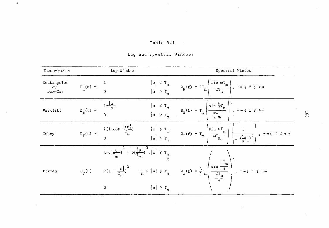
rn CO
Spectral Window
DR(f) = 2T
m
sin wTm f < 4.00
wT m
DB(f) = T
m
sin 2
t.,1)
m
2
— co S f + co
Tm
DT(f) = T
m
sin wTm
1 f +co
wTm 1 -(
()T )
2
M
Lag and
Description Lag Window
Rectangular Or
Box-Car DR(u) =
1
0
Bartlett DB(u) =
1 l u l M
0
Tukey DT(u) =
71111 1(1+ cos ) T
m 0
Spectral Windows
lul .< Tm
lul > Tm
HI Tm
1111 > Tm
lui Tm
lul > Tm
Table 5.1
1 11m 1 2 11 3 11
1-6(T
) + 6(Tu ) "u i Tm
wT m sin --4—
wTm 4
Parzen 3 DP (u) 2(1 - 1u1 ) T
Tm
< lul < T T m
m D - 4 m
f +co
0
lul > Tm

169
U
A Vd(U)
.... '..'''':- '--: --
N.. 'N..." . • .''., Rectangular DR(u) \■
N.‘. . Bartlett
. Tukey DB(u)
\ N.... \
\ '''' \ Parzen DI(u) \ ..,
\\ \ \
D (A P \ s"...\
\ . \ ∎\
• `‘ %ND8 (u)
\ \ D(u)•\ ‘ N 0 (u) P •• •••„
D(u)g\ R
-..
..„.. rs,. "‘„, • T ... .
. N. . ... '.. .
... --, N
— . • ■-----:.":_-,.-N
0.2 0.4 0 6 0.8 M
Figure 5.7. Some common lag windows.
D(f) 2M
Rectangular DR( f) 1.BM Bartlett DB(`)
Tukey DT(f) Parzen D (f)
1.4M
Figure 5.8. Spectral windows corresponding to the lag windows
shown above.
1.0
0.8
0.6
0.4
0.2
0.0

170
sidelobes as small as possible. In order to concentrate
the main lobe, D(u) has to be made flat. To reduce the
sidelobes,however,D(u) has to be made smooth and gently
changing, remembering that D(u) must vanish outside the
limits IT m 1. Equation (5.22) then becomes,
rri-Tm
p(f) =
D(u)r(u)e-27ifu
du (5.23)
-'lm
Various lag windows have been suggested from time
to time, to incorporate the various features discussed above.
Table 5.1 lists those in common use,and Figures 5.7 and 5.8
are their diagrammatic representations.
The Parzen window was used here in the calculation
of the power spectrum. One reason for choosing the Parzen
window was the fact that it gives estimates of the power
spectrum with extremely low side lobes.
5.3.2 PRE-WHITENING
Power spectral estimates are most precise when the
power is evenly distributed over the whole range of frequen-
cies. It sometimes happens that the power has one or more
broad peaks. The average value of the power at any parti-
cular frequency, f, may be greatly distorted during computa-
tion, since the effect of the spectral window is to spread
the power from the large peaks to adjacent frequencies. To
avoid this, the data is first passed through a filter which

171
compensates or pre-emphasises the frequencies with lower
amplitudes, and the spectrum then calculated in the usual
way. This technique of bringing the resultant spectrum
close to that of white noise is known as pre-whitening.
However, after the spectrum has been obtained,an inverse
pre-whitening filter has to be applied to remove the effect
of the pre-whitening filter. For the present work,pre-
whitening was not necessary. It must be remembered, though,
that if the time series has a non-zero average, or a linear
trend, a strong zero-frequency (d.c.) peak will be intro-
duced in p(f). A zero-frequency peak also produces side-
lobes, which distort the power spectrum and hence must be
removed from the time series before any analysis. The
d.c. level can be set to zero by subtracting the mean from
the signal. The linear trend can be removed by fitting
a straight line to the time series before the calculation
of p(f). Removal of the d.c. level and the linear trend,
before the analysis, are in fact special cases of the
application of pre-whitening filters. .
5.3.3 SOME PRACTICAL ASPECTS OF SPECTRAL ESTIMATION
The discussion of the previous sections related
to estimation of the power spectra of continuous finite
length analogue record. For a digitized time series the
calculations are similar except that the integrals must be
replaced by summations. In the present case the following
procedure was adopted.
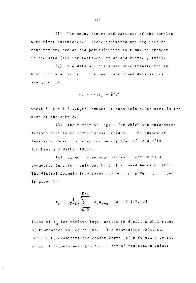
172
(1) The mean, square and variance of the samples
were first calculated. These estimates are required to
test for any trends and periodicities that may be present
in the data (see for, instance Bendat and Piersol, 1971).
(2) The data at this stage were transformed to
have zero mean value. The new transformed data values
are given by:
xk = x(t)i - Tc(t)
where i, k = 1,2...K,the number of data points,and R(t) is the
mean of the sample.
(3) The number of lags M for which the autocorre-
lations were to be computed was decided. The number of
lags were chosen to be approximately K/4, K/5 and K/10
(Jenkins and Watts, 1965).
(4) Since the autocorrelation function is a
symmetric function, only one half of it need be calculated.
The digital formula is obtained by modifying Eqn. (5.19),and
is given by:
K-m
) rm (K1m)
xkxic+111 m = 0,1,2...M -
m=0
Plots of rm for various lags assist in deciding what range
of truncation values to use. The truncation point was
decided by examining the chosen correlation function to see
where it becomes negligible. A set of truncation values
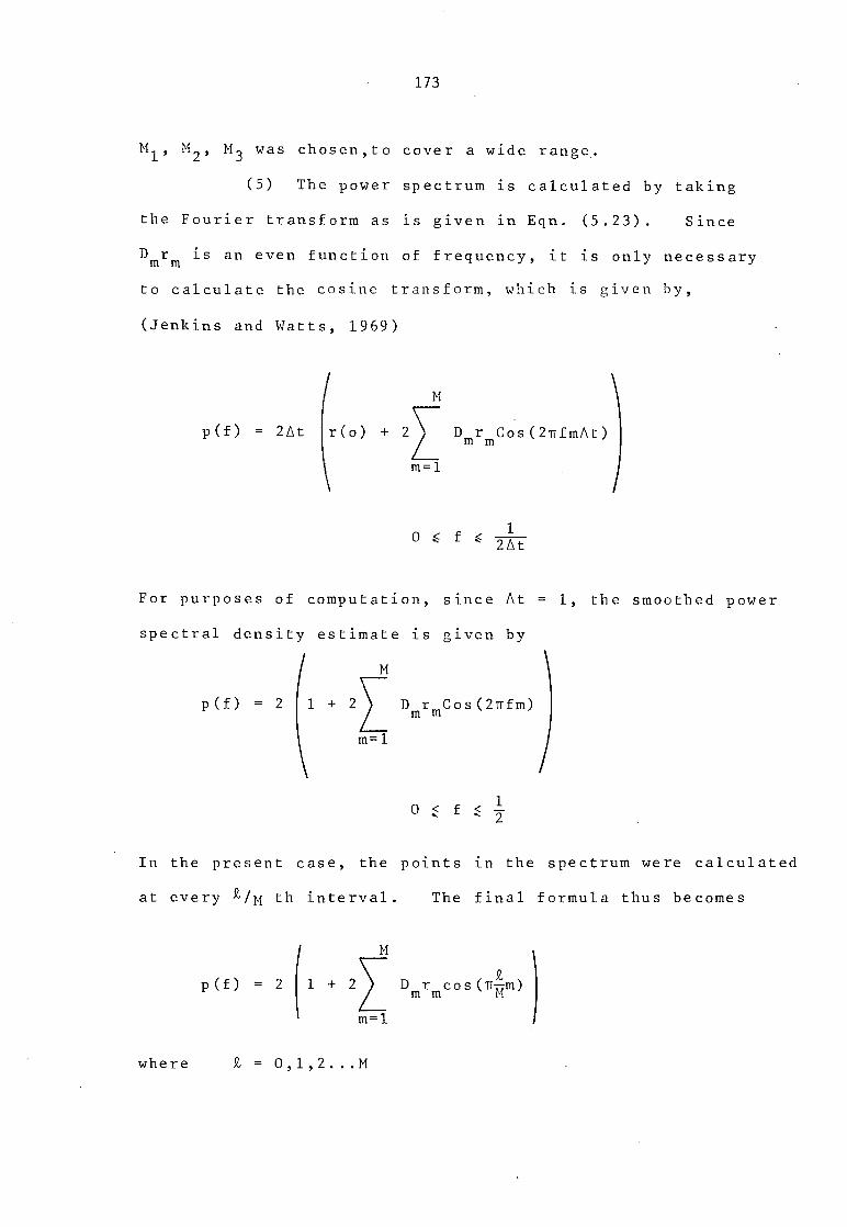
M
P(f) = 21\t Ir(o) +
m=1
0
purposes of computation, For
D m r mCos(27fmAt)
■
I
f 1
2At
173
M1, M
2, M3 was chosen,to cover a wide range.
(5) The power spectrum is calculated by taking
the Fourier transform as is given in Eqn. (5.23). Since
D m rm is an even function of frequency, it is only necessary
to calculate the cosine transform, which is given by,
(Jenkins and Watts, 1969)
since At = 1, the smoothed power
spectral density estimate is given by
M
1 +
m=1
p(f) = 2 DmrmCos(27fm)
0 f 1
2
In the present case, the points in the spectrum were calculated
at every 16 /14 th interval. The final formula thus becomes
(
p(f) = 2 1 +
M
D m r mcos(74"m)
m=1
where Q = 0,1,2...M

174
5.4 DATA ANALYSIS AND RESULTS
The analyses in this section were performed on
the three unfiltered channels, all three channels being used
for the volcanic tremor studies and the vertical component
alone for the microearthquakes. The fourth, unfiltered,
channel was primarily used for monitoring the output, using '
an oscilloscope, and also during the digitization of vol-
canic tremor as an anti-aliasing filter for the vertical
component. This filtered channel,however,did not provide
any additional information and hence is not included in
the subsequent analysis.
For the convenience of discussion, this section has
been divided into two parts. The first part deals with
volcanic tremor and the second part with microearthquakes.
5.4.1 PART I: BACKGROUND SEISMIC RECORD
In order to study the spatial as well as the temporal
variation in the background noise, selected portions of the
recorded data were digitized according to the following scheme.
(1) For station 1 (Serra La Nave) the data were
digitized every hour,approximately on the hour,for 40 sec.
12 sections of punched paper tape were obtained. Thus the
first digitized section was for 40 sec after 13 June 12 hr
59 min, and so on.
(2) For station 2 (IC bench mark) and 4 (Monte S.
Maria) the digitization was carried out from the 12 June 23 hr
59 min,but at every alternate hour. 12 punched paper tapes.
175
were thus obtained for each station. For station 3 (Pores-
tale Hut) the digitization was carried out once only,because
of the limited amount of data available.
All spectra are plotted as a function of the log
power density against the log frequency (Hz). The spectrum
of the vertical component was plotted first and whenever
available was followed by the spectra of N-S and E-W com-
ponents. Figures 5.9 to 5.16 show the spectra obtained at
the various sites. The number against each curve indicates
the time of the analysed signal (see Appendix 2A, 2B, 2C, 2D).
5.4.1.1 STATION 1: SERRA LA NAVE
A total of nine power spectra was utilized for the
final analysis at this station. The N-S component seis-
mometer was inoperative most of the time, due to mechanical
failure. As none of the Geostores was calibrated in the
field,it was not possible to calculate the power of the
signal in absolute terms.
Relevant information as to the approximate time,
bandwidth of the spectrum, distribution of total power in
the various frequency bands etc., of the analysed signal are
given in Appendix 2A.
It is seen from this table that the dominant fre-
quency (defined as the frequency associated with the peak
amplitude of the Fourier spectrum) is quite consistent and
ranges between 1.18 and 1.76 Hz. In two instances,however,

Pow
er D
ens
ity
0.40
0 . 2 0
0 .0 3
0.10
1
2 3 4 5 1
2 3 4 5
Frequency (Hz)
Figure 5.9. Plots of power density versus log frequency ( Hz ) for background seismic noise recordings obtained
at Serra La Nave ( station 1 ). The number associated with each curve indicates the hour of analysis in a 24 hour
period ( see Appendix 2A ).

1 2 3 4 5
Frequency (Hz)
Figure 5.10. Caption as in Figure 5.9.
0.40
0.20
0.03
1 2 3 4 5

0.40
0.03
1
2 3 4 5 1 Frequency (Hz)
Figure 5. 11. Caption as in Figure 5. 9.

179
they range between 1.77 and 2.35 Hz. As we were interested
in the 'gross-structure' of the spectrum, individual peaks
were thus not resolved. These frequency ranges seem to be
in good agreement with the volcanic tremor measurements
carried out on Mount Etna by Shimozuru (1971), Schick and
Riuscetti (1973), Lo Bascio et al. (1976), and Guerra et al.
(1976).
An interesting feature of some of the power density
plots, in addition to the dominant frequency, is the occurrence
of a small peak between 3.54 and 4.12 Hz. This peak does
not occur in the corresponding horizontal seismometer; the
seismic signal cannot thus be associated with the volcanic
activity. The spurious peak could be either of external
origin, the nature of which is difficult to establish at this
stage or more likely due to an error in the digitization
process.
More than 60% of the total power in the vertical
component is concentrated in the narrow frequency band of
1.18 to 2.94 Hz, whereas that in the E-W appears to range
between 0.59 and 2.94 Hz.
The relative Fourier amplitude values associated
with the dominant frequencies range between a maximum of
0.57 (arbitrary units) to a minimum of 0.48 (arbitrary units).
The corresponding horizontal component values range between
0.61 and 0.53. No direct comparison can,however,be made
between these two sets of values, as the horizontal and

Po w
er
Den
s ity
0. 2 0
0.03
0 . 40
0.10
1 2
3 4 5 1 2 3 4 5
1 Frequency (Hz)
Figure 5.12. Plots of power density versus log frequency ( Hz ) for background seismic noise recordings obtained at
IC bench mark ( station 2 ). The number associated with each curve indicates the hour of analysis in a 24 hour period
( see Appendix 2B ).

0.40
0.03
Frequency (Hz)
Figure 5.13. Caption as in Figure 5.12.

182
vertical seismometers had different frequency responses,
but they will be used later for inter-station comparison
(see Section 5.4.2).
The ratios of the various components are sometimes
used to determine the nature of the seismic signal. The
data from station 4 (Monte S. Maria), where similar seismo-
meters were employed, will be used to discuss the nature of
this wave.
5.4.1.2 STATION 2: IC BENCH MARK
Power density values at this station,with other
relevant information,are listed in Appendix 2B. Figures
5.12 and 5.13 are plots obtained from such calculations.
The shape of the power density curves are familiar bell-
shaped, as at Serra La Nave. The dominant frequency is,
however,slightly shifted towards higher values (2.36 - 2.94
Hz), except in two instances where they range between 1.77
and 2.35 Hz.
Power in the vertical component appears to be more
spread out towards higher frequencies than at station 1.
More than 60% of the total power lies between 1.18 and 3.53
Hz.
The relative Fourier amplitude values associated
with the dominant frequencies range between a maximum of
0.54 and a minimum of 0.44 for the vertical, 0.56 and 0.44
for the N-S, and 0.43 and 0.37 for the E-W components,

0
L
0 0
0.40
0.20
0.10
0.03
1
2 3 4 5
Frequency (Hz)
Figure 5.14. Plot of log power density versus log frequency ( Hz ) for background seismic noise recordings obtained
at Forestale Hut station 3 ). The number associated with the curve indicate the hour of analysis in a 24 hour period
( see Appendix 2C ).

184
respectively. As at station 1,no direct comparison can
be made between the vertical and the other components, but
the two horizontal recordings appear to indicate a higher
(Fourier amplitude) value for the N-S component.
5.4.1.3 STATION 3: FORESTALE HUT
A small section of background noise data was
analysed. The results are tabulated in Appendix 2C and
shown in Figure 5.14. The dominant frequency range is
1.77 - 2.35. However,not enough reliable data is avail-
able in this station to define an accurate dominant frequency
range.
5.4.1.4 STATION 4: MONTE S. MARIA
Seven digitized seismic sections were used for the
spectral analysis at this station. Results of the calcu-
lation are tabulated in Appendix 2D and shown in Figures
5.15 and 5.16. The dominant frequency at this station
appears to lie between 1.77 and 2.94 Hz, and more than 60%
of the total power is confined within that limit. The
relative Fourier amplitude values associated with the
dominant frequencies range between a maximum of 0.62 and
a minimum of 0.54.
In order to gain a better understanding of the
nature of this background disturbance,relative average
Fourier amplitude values were calculated for the 3-components.
Table 5.2 gives the result.

0.40
0.20
a, 0
a)L-0 10
0
0.03
1
2 3 4 5 1 2 3 4 5 1 2 3 4 5
F requency (Hz)
Figure 5.15. Plots of power density versus log frequency ( Hz ) for background seismic noise recordings obtained at
Monte S. Maria ( station 4 ). The number associated with each curve indicates the hour of analysis in a 24 hour period
( see Appendix 21) ).

0.40
0.20 >, 4-a (r) ._ a, a
L a) 0.10 3 0 a.
0.03
1 2 3 4 5 1 2 3 4 5 1 2 3 4 5
Frequency (Hz)
Figure 5.16, Caption as in Figure 5.15.

187
Table 5,2
Average Fourier Amplitude Estimates for
Monte S. Maria
(Arbitrary Units)
Frequency Interval
Component
V N-S E-W
0.0 - 0.58 0.08 0.07 0.05
0.59 - 1.17 0.13 0.13 0.13
1.18 - 1.76 0.35 0.38 0.39
1.77 - 2.35 0.57 0.58 0.55
2.36 - 2,94 0.51 0.45 0.49
2.95 - 3.53 0.38 0.36 0.36
3.54 - 4.12 0.24 0.27 0.25
4.13 - 4.71 0.18 0.19 0.19
4.72 - 5.30 0.12 0.15 0.14
5.31 - 5.89 0.11 0.13 0.13

188
It is seen from the table that at the dominant
frequency the N-S component has the highest relative
amplitude. Since this seismometer predominantly records
the rod■01 component of the shear wave, the recorded
waves are probably of Rayleigh type. Kubotera (1974),
while investigating Aso volcano in Japan, recorded volcanic
tremors having periods of between 0.4 and 0.6 sec, i.e.
frequencies of between 1.7 and 2.5 Hz. These, he thought,
were of the Rayleigh type. Though no direct comparison
exists between Etna and Aso volcanoes, the dominant periods
of between 0.34 and 0.56 sec recorded at this station
support the belief that they may be of the Rayleigh type
as well.
5.4.2 INTER-STATION COMPARISON AND SOURCE LOCATION
In order to gain a better understanding of the
nature and the source of the volcanic tremor, estimates of
the average Fourier amplitudes (Table 5.3) were made at the
various stations and plotted in Figure 5.17. Only the
vertical components were used for the comparisons, as this
was the only component for which the same type of seismometer
(HS 10) was used at all four stations. Thus the plots in
Figure 5.17 represent the mean spectrum obtained from the
hourly samples for station 1, and two-hourly samples for
stations 2 and 4, over the 12 hr period commencing at
13 June 13 hr 59 min.
In the frequency domain, each of the spectra cl)(w),

189
Table 5.3
Average Fourier Amplitude Estimates
at the Various Stations
(Arbitrary Units)
Station Frequency Interval Serra La
Nave IC Bench
Mark Monte S.
0.0 - 0.58 0.04 0.09 0.06
0.59 - 1.17 0.22 0.23 0.13
1.18 - 1.76 0.53 0.40 0.35
1.77 - 2.35 0.50 0.47 0.57
2.36 - 2.94 0.39 0.44 0.51
2.95 - 3.53 0.28 0.35 0.38
3.54 - 4.12 0.26 0.31 0.24
4.13 - 4.71 0.21 0.23 0.18
4,72 - 5.30 0.19 0.19 0.12
5.31 - 5.89 0.14 0.18 0.11
Maria
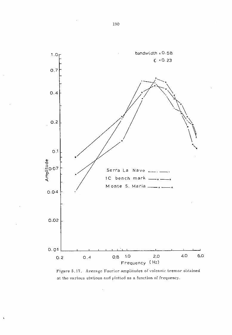
Serra La Nave
IC bench mark
Monte S. Maria
190
1 . 0
0 . 7
0.4
0.2
0 .1
E
bandwidth = 0.58
C = 0. 23
0.04
0.02
0.01
0.2 0.4 0.8 1.0 2.0 Frequency ( Hz)
Figure 5.17. Average Fourier amplitudes of volcanic tremor obtained
at the various stations and plotted as a function of frequency.
4.0 6.0
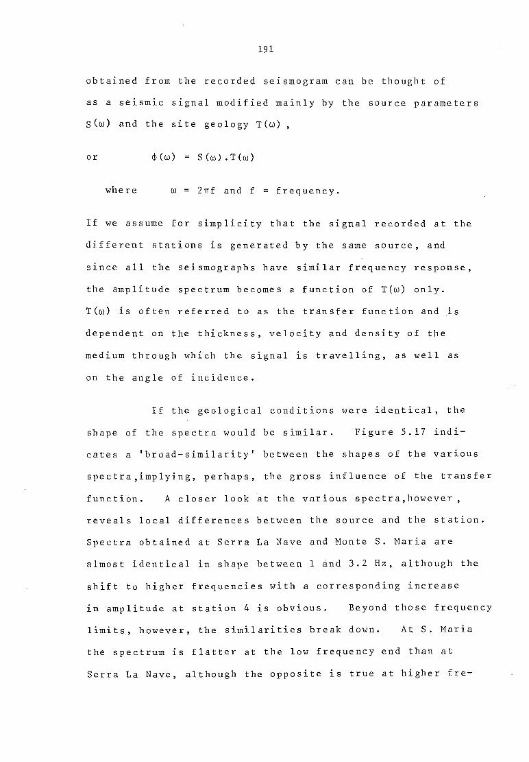
191
obtained from the recorded seismogram can be thought of
as a seismic signal modified mainly by the source parameters
S(w) and the site geology T(w)
Or (1)(0)) = S(W).T(W)
where w = 27f and f = frequency.
If we assume for simplicity that the signal recorded at the
different stations is generated by the same source, and
since all the seismographs have similar frequency response,
the amplitude spectrum becomes a function of T(w) only.
T(w) is often referred to as the transfer function and is
dependent on the thickness, velocity and density of the
medium through which the signal is travelling, as well as
on the angle of incidence.
If the geological conditions were identical, the
shape of the spectra would be similar. Figure 5.17 indi-
cates a 'broad-similarity' between the shapes of the various
spectra,implying, perhaps, the gross influence of the transfer
function. A closer look at the various spectra,however,
reveals local differences between the source and the station.
Spectra obtained at Serra La Nave and Monte S. Maria are
almost identical in shape between 1 and 3.2 Hz, although the
shift to higher frequencies with a corresponding increase
in amplitude at station 4 is obvious. Beyond those frequency
limits, however, the similarities break down. At. S. Maria
the spectrum is flatter at the low frequency end than at
Serra La Nave, although the opposite is true at higher fre-

192
quencies. These observations may imply preferential
screening of frequencies from the source to the two stations.
At the IC bench mark, however, the spectrum is much broader
than at the other two stations and the dominant frequency
appears to be around 2 Hz. The important question seems,
however, how much of the spectra (P(w) are shaped by the
source mechanism S(w), and how much by the properties of the
medium T(w). With our present knowledge of Etna it is
difficult to answer these questions satisfactorily.
Because of the non-impulsive character of volcanic
tremor, it is not possible to apply the usual travel time
techniques used to located microearthquakes. However, an
approximate location of the source can sometimes be obtained
by mapping the differences in amplitude of the seismic signal
at the various locations. Seismic waves are reduced in
amplitude as they propagate through the earth, due mainly
to (1) absorption of energy in the medium of transmission
and (2) geometrical spreading.
When a wave passes through a medium,the elastic
energy associated with the wave motion is gradually absorbed
by it, reappearing ultimately in the form of heat. This
process is called absorption, and is responsible for the
eventual complete disappearance of the wave motion. The
mechanism by which the elastic energy is transformed into
heat is not understood clearly. During the passage of a
wave, heat is generated during the compressive phase and
absorbed during the expansive phase. The process is not

193
perfectly reversible since,the heat conducted away during
the compression is not equal to the heat flowing back
during the expansion. Internal friction, and many other
mechanisms, such as loss of energy involved in the creation
of new surface (fracturing near an explosion) piezoelectric
and thermoelectric effects, viscous losses in the fluid
filling the rock pores, etc, contribute to the absorption
of energy.
The attenuation of plane waves due to absorption
of energy is of the familiar exponential form (Parasnis, 1972)
A = Aoexp(-6fVr)
where A = recorded amplitude
Ao = amplitude at source
= logarithmic decrement
f = frequency
r = distance in km
V = the velocity in km/sec.
The influence of the second factor (i.e. at large
distances from the source waves are reduced in amplitude in
inverse proportion to the distance travelled),combined with
the first,can be written as
Ao A = —o r
SV r) 6Vr )
The solid line in Figure 5.18 shows the relative
values (A) plotted as a function of distance,using the above

194
1
2 4 7
10
20 Distance (km)
Figure 5.18. Relative amplitudes of the volcanic tremor ( obtained at
stations 1, 2 & 4) plotted as a function of distance from the Central Crat-
er ( open circles ) and the Northeast Crater ( solid circles ).

195
relation. V, the velocity, was taken as 1 km/sec (corres-
ponding to the surface wave velocity calculated in Section
4.4.3), Sas 0.025 (typical value of earth material in bulk)
and fas 2.0 Hz (the dominant frequency recorded during this
investigation). Also shown, by open and solid circles
(numbers against them refer to the station) are the relative
amplitudes,taking the origin of the tremors as the Central
and the Northeast Crater respectively.
It is seen from Figure 5.18 that the amplitude
values at Serra La Nave and S. Maria appear to follow the
exponential law, when the Northeast Crater is taken as the
seismic source, whereas at the IC bench mark it is about
29% short of the expected value. Two possible explanations
of the low amplitudes at the IC bench mark site are that the
Northeast Crater is not the source of the volcanic tremor,
and that the tremors are highly attenuated between the
Northeast Crater and the station, possibly due to the presence
of very loose material, or less likely due to the presence
of liquid bodies in the area.
Since only three stations are involved, it is
possible to find, either formally or by trial and error, a
unique location for the source that satisfies the observed
relative amplitudes. The location is found to be about
3 km NW of the Central Crater. During the recording period,
lava was erupting from new boccas 2 km to the north,at about
2,500 m (Murray et al. 1977), followed occasionally by
Strombolian activity at the Northeast Crater.
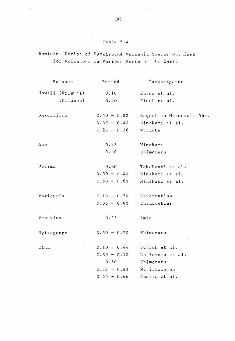
196
Table 5.4
Dominant Period of Background Volcanic Tremor Obtained
for Volcanoes in Various Parts of the World
Volcano
Hawaii (Kilauea)
(Kilauea)
Sakurajima
Period
O.10
O.50
Investigator
Eaton et al.
Finch et al.
O.40 - 0.80 Kagoshima Meteoral. Obs.
O.33 - 0.40 Minakami et al.
O.25 - 0.38 Watanbe
Aso 0.25 Minakami
0.20 Shimozuru
Oosima O.30
Takahashi et al.
O.30 - 0.40
Minakami et al.
0.50 - 0.60
Minakami et al.
Paricutin 0.10 - 0.20 Cavarrubias
O.35 - 0.60 Cavarrubias
Vesuvius 0.63 Imbo
Nyiragongo 0.50 - 0.70 Shimozuru
Etna 0.10 - 0.44 Schick et al.
O.33 - 0.50 Lo Boscio et al.
O.50 Shimozuru
0.35 - 0.83 Muniruzzaman
O.55 - 0.66 Guerra et al.

197
The conclusion that can be drawn from the above
observation is that, during the '75 investigation, the
source of the seismic disturbance probably lies to the north
of the Central Crater somewhere between the Northeast Crater
and a point about 3 km northwest of the Central Crater.
The studies of the background seismic noise con-
ditions at other volcanoes also indicate certain dominant
periods - characteristic of each volcano. Table 5.4 lists
the dominant period of volcanic tremor of some important
volcanoes around the world,along with the present findings.
It is seen from the table that there is a wide range of
dominant periods even for the same volcano. For instance ,
the Hawaiian volcano appears to have frequencies whose
periods range from 0.10 - 0.50 sec. This is,however,to be
expected,as measurements were carried out by different in-
vestigators at different stages of the volcanic cycle.
The present findings, however, seem to be in good agreement
with those of other workers on Etna using similar kinds of
instruments.
5.4.3 MECHANICS OF VOLCANIC TREMOR
The various theories that have been proposed from
time to time to explain the causes of volcanic tremor have
been discussed briefly in the introduction. In this section
we shall take a closer look at one of these explanations,
that appears to be favoured by seismologists working on Etna,

198
and examine how far it is successful in explaining our
observations.
In the course of the present volcanic tremor sur-
vey we have established certain features that seem to
characterize these processes:
(1) The presence of continuous volcanic tremor through-
out the whole period of investigation (- 20 days).
(2) The amplitudes and frequencies exhibit very
little variation in space and time (at least
over 24 hours).
Any proposed mechanism thus must be able to explain
these features, taking the known geology of the area into
account.
Possible sources of the kinetic energy released
may be the continuous micro-fracturing, and dislocation of
rocks surrounding dykes and sills. But Schick & Riuscetti
(1973) in their analysis found that the vanishing seismic
moment (defined as <u> = Mo/pA, where <u> is the average
dislocation or average slip over the fault surface, p is the
rigidity, Mo is the source moment, and A is the area of the
fault slip, see for instance Brune, 1968) for these processes
speak against such a source mechanism.
Volcanic tremors are thought to be generated by
a physical process known as 'self-oscillation' (see for
instance Andronov et al., 1960). The self-oscillations are,

199
however, characterized by certain features. The common
feature is their ability to perform self-oscillations which
do not depend, generally speaking, on the initial conditions
but are determined by the properties of the system itself.
Thus, whatever the initial conditions, undamped oscillations
are established, and these undamped oscillations are stable.
However, in any self-vibrating system,energy losses occur,
and maintenance of the oscillations requires an input of
energy. Thus there is bound to be a source of energy for
this process. In other words a self-oscillating system is
an apparatus which produces a periodic process at the expense
a non-periodic source of energy.
An analysis of volcanic tremor indicates the time
constancy of its amplitude and period. Thus the properties
of volcanic tremor and of a self-oscillator are quite
similar. One possible source of the necessary energy that
must be considered is the kinetic energy of gas flow.
A close look at the mechanics of gas flow through
the magmatic channels will probably reveal more information
about the conditions under which these oscillations are set
up. The following analysis is due mainly to Steinberg and
Steinberg (1975). To a first approximation,the motion of
gases through the channels resembles the motion of viscous
gases through a thermally insulated vertical cylindrical tube.
Under these conditions,the equations of the flow may be written
as
dW kXW dZ 2
2D( 7 - 1)
(5 .24)
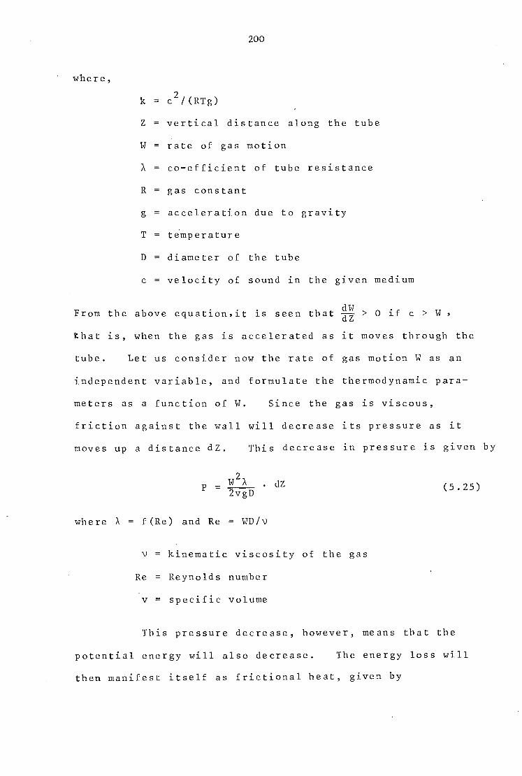
200
c2/(RTg)
vertical distance along the tube
rate of gas motion
X = co—efficient of tube resistance
gas constant
acceleration due to gravity
temperature
diameter of the tube
velocity of sound in the given medium
-z- dW
From the above equation,it is seen that (71 > 0 if c > W
that is, when the gas is accelerated as it moves through the
tube. Let us consider now the rate of gas motion W as an
independent variable, and formulate the thermodynamic para-
meters as a function of W. Since the gas is viscous,
friction against the wall will decrease its pressure as it
moves up a distance dZ. This decrease in pressure is given by
P — W2X . dZ
2vgD
where X = f(Re) and Re = WD/v
(5.25)
V = kinematic viscosity of the gas
Re = Reynolds number
v = specific volume
This pressure decrease, however, means that the
potential energy will also decrease. The energy loss will
then manifest itself as frictional heat, given by
where,
k =
Z =
W =
R =
g =
T =
D =
c =
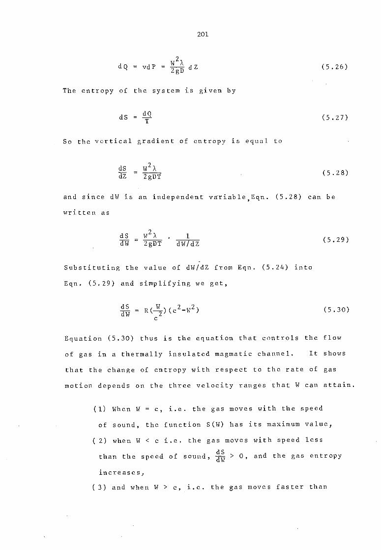
201
W2A , "7
dQ = vdP 2 D `
The entropy of the system is given by
dS = dQ T
So the vertical gradient of entropy is equal to
dS W2X dZ 2gDT
(5.26)
(5.27)
(5.28)
and since dW is an independent variable,Eqn. (5.28) can be
written as
dS W2X . 1
dW 2gDT dW/dZ
Substituting the value of dW/dZ from Eqn. (5.24) into
Eqn. (5.29) and simplifying we get,
dS W 2 2 = R(---E)(c -W ) dW
(5.29)
(5.30)
Equation (5.30) thus is the equation that controls the flow
of gas in a thermally insulated magmatic channel. It shows
that the change of entropy with respect to the rate of gas
motion depends on the three velocity ranges that W can attain.
(1) When W = c, i.e. the gas moves with the speed
of sound, the function S(W) has its maximum value,
(2) when W < c i.e. the gas moves with speed less
vi dS
than the speed of sound, T > 0, and the gas entropy
increases,
(3) and when W > c, i.e. the gas moves faster than

202
dS the speed of sound, -,TTI < 0, and the gas entropy
decreases.
Experiments (as reported by Steinberg and Stein-
berg, 1975), however,have indicated that the transition from
less than, through and greater than the velocity of sound
is impossible when gas flowing along the tube encounters
resistance. However, when the gas velocity W reaches the
local sound velocity c (known as the critical value) intense
vibrations are set up in the viscous gas. These
vibrations impart large amounts of energy and (an
increase in the gas entropy) to the volcanic edifice,which
in turn is thought to give rise to volcanic tremor.
Measurements of gas velocities (as reported by
Tazieff, 1972) were carried out on an eruptive vent in the
Bouca Nova (Mount Etna) by a wheel anemometer. Velocities
of about 160 m/sec were recorded (and the acceleration
exceeded 10 g). If these velocities are regarded as typical
gas velocities during volcanic paroxysms, it is unlikely that
gas velocities exceed this value during repose periods
(although data in this respect is very inadequate).
It thus appears, from a discussion of the current
views on volcanic tremor, that no single process can satis-
factorily explain the causes of volcanic tremor on Mount
Etna. However, from the evidences gathered so far the most
probable cause seems to be viscous gas flow*. This gas
The magma of Etna normally contains 1-2% by weight of dis- solved volatiles. These volatiles come out of solution when the pressure in the magma column drops below a critical value (Wadge, 1974).

203
originates by the degassing of magma in the upper part of
the vent. The top of the central magma column of Etna is
at atmospheric pressure most of the time,and Wadge (1974)
suggests that degassing take place with the help of con-
vection currents within the column, such as has been ob-
served at several lava lakes. Whatever the physical process
of degassing, it appears unlikely that the viscous gas always
flows at supersonic speed on Etna to establish the 'self-
oscillation', as has been envisaged by Steinberg & Steinberg
(1975). It appears more likely that tremors are set up by
the expanding gas front at places of widening vents. In
our proposed model the frequencies and amplitudes of the
volcanic tremor are thus determined by the parameters of
the system , that is, to a first approximation, by the
dimensions of the channels. And in a complex volcanic
apparatus, such as Etna, it is thought that there are many
channels through which volcanic gases may be released. The
volcanic tremor recorded on a seismogram is thus the resultant
of the sum of a number of harmonic oscillators (set up by
the expanding gas front), the amplitudes of which appear to
follow a Gaussian distribution.
5.4.4 PART 2: MICROEARTHQUAKE ANALYSIS
In order to investigate the spectral contents of
microearthquakes, 13 selected events of both A and B-type
were digitized at 100 samples/sec (giving a Nyquist frequency
of 50 Hz),and analysed.

204
5.4.4.1 A-TYPE MICROEARTHQUAKES
Power density estimates for six A-type microearth-
quakes recorded at the various stations during the period of
the investigation are tabulated in Appendix 3A, and Figures
5.19 to 5.22 are their power density versus frequency plots.
All the microearthquakes have very small magnitudes, as
none of them was recorded at more than one station.
Figures 5.19a and 5.19b show the spectral charac-
teristics of two of these microearthquakes, recorded at
station 2 (the IC bench mark site). Both these events have
the first important peak between 1.39 and 1.85 Hz and the
spectra in general have a rather smooth appearance. The
dominant frequencies seem to range between 2.54 and 3.01 Hz
for Figure 5.19a and between 2.08 and 2.54 Hz for Figure
5.19b. There is a remarkable similarity between the shape
of the spectra, and both have three major peaks in the prin-
cipal frequency range. The power of the microearthquakes
effectively reduces to zero beyond about 6.50 Hz. Both
these events appear to have originated from the same source
and possibly by a similar mechanism.
Figures 5.20a and 5.20b are the spectra of a further
two events recorded at station 2. These microearthquakes
have dominant frequencies between 2.07 and 2.53 Hz (Fig. 5.20a)
and between 3.27 and 3.73 Hz (Fig. 5.20b) respectively.
The shape of the spectrum has a spikey appearance, and in
general has a greater high frequency content than the two
microearthquakes discussed earlier. Figure 5.21 is the

O. 350 bandwidth . 0.23
C= 0.52
0
0
0
0
0 0
0.175
Pow
er
Den
sity
( a) ( b) 0
\o/ 0
ol 0
0 0
0
°."o-o No....0,o•o"0/0\ /0,0,
0.0 0 0 0-0
0 0 / 1 0
0
oo o o
\ 0- 0 0
o 0 0
0 2.5 5.0 7.5 0 2.5 5.0 7.5 Frequency ( Hz)
Figure 5.19 (a-b). Plots of power density versus frequency (Hz) for A-type microearthquakes recorded at IC
bench mark (station 2).

O
0.175
Pow
er
Den
sity
O
fO
1 0
O o
( b)
O
A,/ \ O 0.0 0
\ 0 0 0 00 0 0
0 \
O
( a)
0.3 5 0 bandwidth :-. 0.23
=0.52
0
0
0 0 0 .
00 0
0 2.5 5.0 7.5 0 2.5 50 7.5 Frequency ( Hz)
Figure 5.20 (a-b). p lots of power density versus frequency (Hz) for A-type microearthquakes recorded at IC bench
mark (station 2).
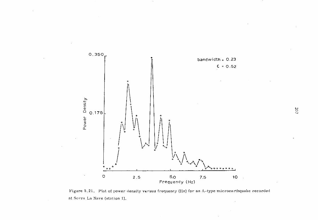
0. 350_ 0 bandwidth = 0.23
C. = 0.52
0
0
0 0
0 0 o/ 0,0,0\
0 \ 0, t -0 0 0 00000
0
0
0 0
0 0
0 2.5 5.0 7.5 10
Frequency (Hz)
Figure 5.21. Plot of power density versus frequency (Hz) for an A-type microearthquake recorded
at Serra La Nave (station 1).
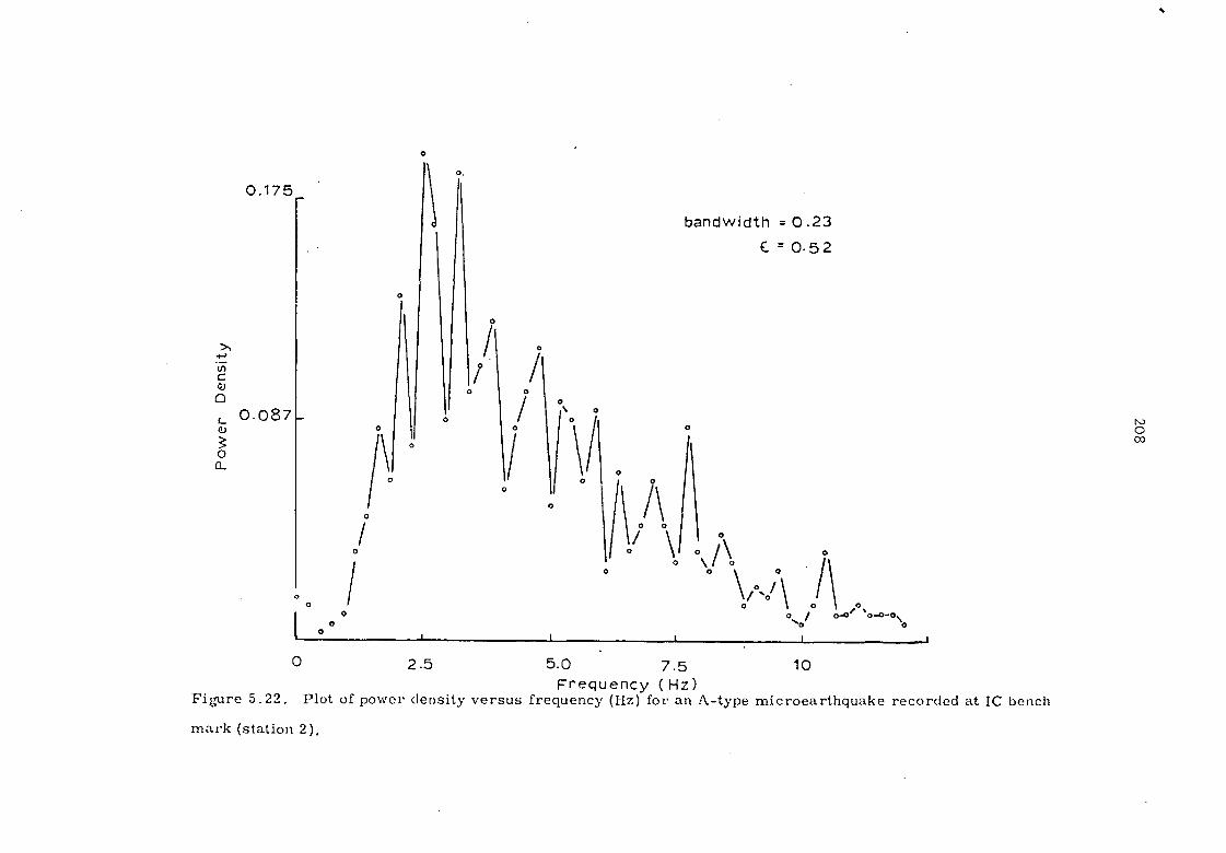
0
QJ
0 0.087
Qi
O a_
0
0
0
0
0
0
0
0, 0
0.175_
bandwidth = 0.23
E. = 0.52
0
0/\
0
o / 0-0/ '0-0-0
0 CO
0 2.5 5.0 7.5 10 Frequency (Hz)
Figure 5.22. Plot of power density versus frequency (Hz) for an A-type microearthquake recorded at IC bench
mark (station 2).

209
spectrum of a similar microearthquake recorded in station 1
(Serra La Nave). It has a dominant frequency between 3.47
and 3.93 Hz. The higher frequency components in this case
extend to about 8.0 Hz.
In contrast to the spectrum discussed above,
Figure 5.22 (recorded at station 2) has a very spikey appearance.
The frequencies in Figure 5.22 converge to a maximum value
of about 10.50 Hz with a dominant frequency between 2.32
and 2.78 Hz. The gradual transition (in the three groups)
from a relatively smooth and lower frequency content to
more spikey and higher frequencies are apparent.
The above observation would seem to imply that,
other factors (like the transmission path, source mechanism,
focal depth etc.) remaining constant, the frequencies of
the microearthquakes appear to be a function of the magni-
tudes (proportional to the duration of the oscillation)
though this is not a general rule.
5.4.4.2 B-TYPE MICROEARTHQUAKES
Power density estimates for seven B-type micro-
earthquakes recorded at the various stations are tabulated
in Appendix 3B, and Figure 5.23 to 5.26 gives their power
density versus frequency plots. The seven selected micro-
earthquakes cover a period of nine recording days,and each
event is independent of the occurrence of the other.
The first four of the seven power density plots

0
( a)
0
0 0 0 .0 0.6. \
O 0 0 \
0.0 0.0,0 0 0 0 o
I 0 0 of
0
0 (b)
0
0.0 ,0 10\ 0 0.0.0 \ / 0
• o 0 0 0 0 0
6 o 0 o o
0o 0-1
0 . 700
bandwidth = 0.23
E.= 0.52
Pow
er D
ensi
ty
0.350
0 0 0'
0 2.5 5.0 7.5 0 2.5 5.0 7.5 Fr,=•quencv ( Hz )
Figure 5.23 (a-b). Plots of power density versus frequency (Hz) for B-type microearthquakes recoeded at Serra La
Nave (station 1).

0.700
in
0
t 0.350
0 •a. (a)
/01
0.0 0
\ o 0, / 0% 0 0, .0
0 O 0 0 0 0 0 0 0
o o
o o'
o °"0.01 0̀ 0 o/
\ Po o o. o• °
0,0
0 0 0
„, 0...0.0
bandwidth. 0.23 C =0.52
0
NJ O
O
( b)
0
0
0
0 2.5 5.0 7.5 0 2.5 5.0 7.5 Frequency (Hz)
Figure 5.24 (a-b). Plots of power density versus frequency (Hz) for B-type microearthquakes recorded at Forestale
Hut (station 3).

0.700 bandwidth .0.23
C = 0.52
a)
0.350 a)
0 a.
0
I \ 0
o 0
0
O
o 0 0 0 0 0
° • 0 0 0. 0 0 0 e d
0 2 .5 5.0 7.5 Frequency (Hz)
Figure 5.25. Plot of power density versus frequency (Hz) for a B-type microearthquake
recorded at Serra La Nave (station 1).

0
0
0
0
0
0
0
0
( a)
0.350
0.175 0 a.
0
bandwidth = 0.23
C =0.52
0 2.5 5.0 7.5 0 2.5 5.0 7.5 Frequency ( Hz)
Figure 5.26 (a-b). Plots of power density versus frequency (Hz) for B-type microearthquakes recorded at Serra La
Nave (station 1).
( b)
0
0 o / 2r. o o
0 0 "" 0 0
o
0 o"- P o 0."°
o o
0 0
o a' \ • 0

214
(Fig. 5.23 - 5.24) have very simple spectral diagrams.
These microearthquakes are characterized by single dominant
peaks between 1.16 and 1.85 Hz, and small amplitude peaks
between 2.82 and 4.89 Hz. There is very little variation
in the total power contents of the various spectra in the
dominant frequency range and over 70% of the total power of
the microearthquakes is concentrated in the narrow band
between 0.71 and 3.54 Hz.
The next three spectral diagrams (Fig. 5.25 - 5.26)
are not only characterized by single dominant peaks between
1.16 and 2.08 Hz, but in addition have pronounced peaks
between 2.32 and 5.77 Hz. Unlike the first four spectra
discussed above, power in these microearthquakes is distri-
buted over the higher frequencies as well.
From the above discussion, it appears that all
the analysed B-type microearthquakes are characterized by
a low dominant frequency peak between 1.16 and 2.08 Hz.
In some cases, high frequency peaks are also present between
2.32 and 5.77 Hz. Almost all the power of the events lies
between 1 and 6 Hz.
Lo Bascio et al. (1976) analysed some similar
microearthquakes on Etna and observed dominant spectral
peaks around 2.0 and 6.0 Hz. Their findings seem to indi-
cate slightly higher frequencies than in the present survey.
However, the difference might•be explained by the volcano
being in a different state of activity at the two times.

215
It is interesting to note that some of the high
frequency components of the spectrum discussed above are
multiples of the fundamental frequency (e.g. 1.39 and
4.15 Hz). Probably, the fundamental frequency is related
to the explosions in the vent,and under suitable conditions
sets the higher frequency modes into oscillations.
5.4.5 COMPARISON BETWEEN THE TWO TYPES OF MICROEARTHQUAKES
The present study of the spectral characteristics
of the two types of microearthquakes have revealed that
A-type microearthquakes (small magnitude, shallow depth
and originating within a few kilometers of the recording
station) contain frequencies whose periods range up to about
0.09 sec. These figures, however, represent the average
of both the P and S arrivals, as no facilities were
available to analyse these separately. Unger (1969) re-
ports a period of 0.06 to 0.15 sec for the P phase and 0.10
to 0.20 sec for the S phase for the microearthquakes recorded
on Mt. Rainier, Washington. Though no direct comparison
can be made between the two volcanoes, it seems that the
volcano-tectonic shocks recorded on Etna are not fundamentally
different from those recorded in other parts of the world.
The B-type mi.croearthquakes,on the other hand,appear
to have frequencies whose periods range up to a maximum of
0.15 sec. The spectra of these shocks look much simpler
and do not exhibit the wide range of frequencies seen in
the volcano-tectonic shocks. The power in all the analysed

216
events is concentrated in two frequency bands (1.16 to
1.85 Hz and 2.82 to 4.89 Hz) and there is little power
beyond about 6.5 Hz.
It thus appears from the above, that it is diffi-
cult to differentiate A- and B-type events by their frequency
content alone, however, the shape of the spectra, and the
presence of a very dominant low frequency peak, might give
us some indications as to which type they are.

217
CHAPTER VI
DISCUSSIONS
6.1 COMPARATIVE STUDY OF THE 1974 AND 1975 FIELD INVESTI-
GATIONS
The 1974 and 1975 field investigations of Mount
Etna (as described in Chapters III and IV) were carried out
at different times of their respective years, using two
different recording instruments. The first (Aug. - Sept.
1974), conducted as a reconnaissance survey, was carried out
using a high-gain, high-frequency portable seismograph producing
visual smoked paper records. The second (May - June 1975),
intended as a more detailed study, was carried out using
4 Geostore magnetic tape recorders, each connected to three
seismometers.
During the first survey an average of 7 microearth-
quakes were recorded per day. This is about 3.5 times the
daily rate during the second period. These results are
based on a total of 486 hours of useful recording for the
first, and a maximum of 490 hours (at Serra La Nave) for the
second. Thus the two surveys covered roughly equal lengths
of time. During the reconnaissance survey approximately
18% of the total recorded events were of the A-type and 20%
during the second survey (these percentages, however, exclude
any A-type events with S-P > 2.5 sec). The proportion of
B-type events, on the other hand, showed an overall decrease

218
of about 2% between 1974 and 1975.
As regard the types of microearthquakes being
recorded at any one station, only at Serra La Nave (station 1)
was enough data obtained for a meaningful analysis to be
possible. During the first survey, 17% were A-type and during
the second, 19% (these percentages again exclude events with
S-P > 2.5 sec).
It may be recalled that no event with an S-P > 2.5
sec were recorded during the'74 survey, whereas during the
second they numbered as many as nine. Why tectonic micro-
earthquakes with S-P > 2.5 sec should have been recorded
only during the second survey is difficult to say. The
only conclusion that can be drawn is that the more distant,
tectonic,faults were inactive during 1974.
As data from only one station was available, it was
not possible to locate foci in 1974. With the four
instruments available in 1975, depth estimates were possible
for two A-type events. The first (depth - 10 km) is probably
related to volcano-tectonic processes and the second (depth
- 20 km) to tectonic forces. The depth of the other six
(A-type) events are not available. The B-type microearth-
quakes, as expected, originate from within 1 km of the Central
Crater.
From visual inspection, the volcanic tremor on the
smoked paper record appears to contain frequencies below about
5.0 Hz. Detailed analysis (from '75 recordings), however,

219
indicates that the dominant frequencies ranged between 1.20
and 2.90 Hz. A tentative source location indicated the
origin of these disturbances in between the Northeast Crater and
3 km NW of the Central Crater. Spectral analysis of micro-
earthquakes, on the other hand, appears to indicate lower
frequencies for the B-type events, but this again is not a
general rule.
An interesting feature of the '75 investigations
is that if an arbitrary north-south line is drawn through
the volcano via the Central Crater, most of the microearth-
quake activity is found to be concentrated on the eastern
half of the volcano.
Before we attempt an explanation of these findings,
let us take a look at the 'state of the volcano' during those
two periods.
6.2 A BRIEF DESCRIPTION OF THE ACTIVITY OF MOUNT ETNA DURING
THE TWO RECORDING PERIODS
Before the start of the 1974 field investigations
Mount Etna had remained dormant, since the eruption of 1971.
It resumed its activity again on the 28 September 1974 (Murray
et al. 1977) in the Northeast Crater. This, Strombolian,
activity lasted for about five months, after which lava flowed
out from new boccas 2 km to the north at an altitude of about
2500 m. The rate of eruption was estimated to be upto 1.5
m3/sec during this phase. Figure 6.1 shows the approximate
location of this flow.
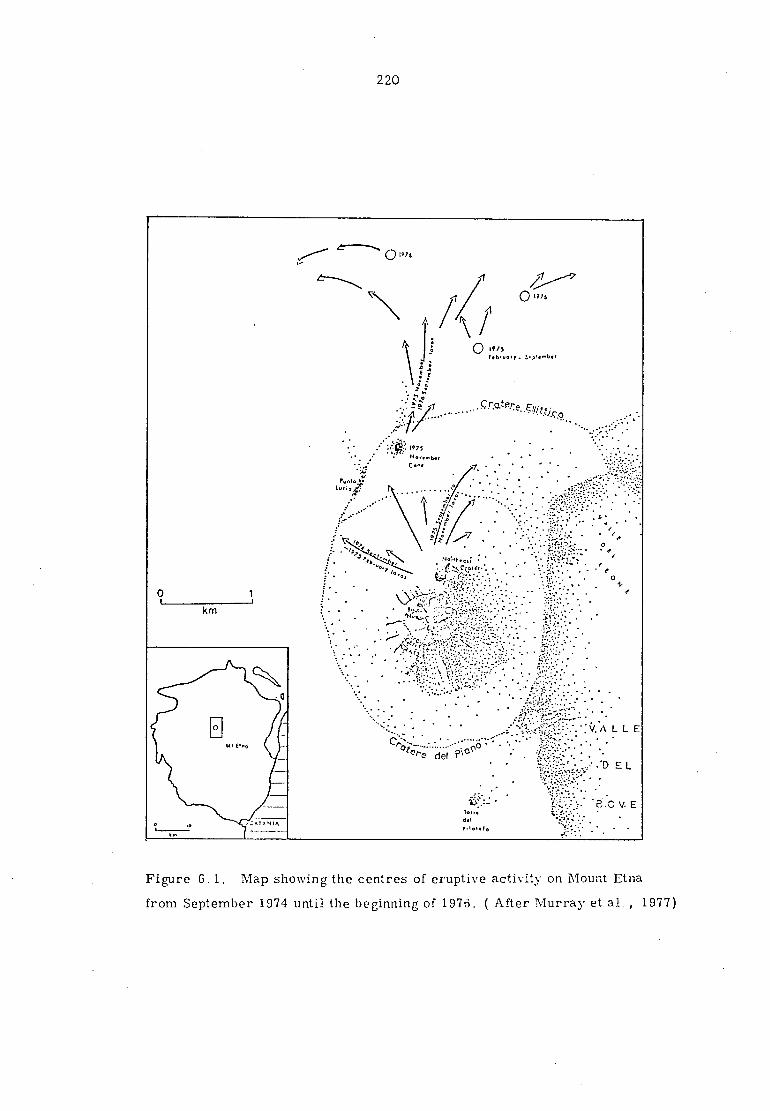
220
Figure 6.1. Map showing the centres of eruptive activity on Mount Etna
from September 1974 until the beginning of 1976. ( After Murray et al. , 1977)

221
The state of the volcano during 1975 seems to have
alternated between emission of lava flow on the north flank
and activity at the Northeast Crater. The emission of
lava that started around 23/24 February continued inter-
mittently until 12 September, 1975, after which effusion
stopped in the north flank and Strombolian activity accompanied
by lava flow erupted from the Northeast Crater. Rates of
eruption were measured upto 0.9 m3/sec during this period,
which terminated on 28 November 1975. On November 29 a fissure
450 m long opened east-northeast of Punta Lucia, at an elevation
of 2900 m. This was accompanied by an intense Strombolian
activity, that resulted in the formation of a 40 m high cone
(Murray et al., 1977). Figure 6.1 also shows these new
eruption sites. In the early parts of 1976, a collapse pit
approximately 170 m x 70 m was formed on the west flank of
the Northeast Crater. This was accompanied by the emission
of ash and the onset of intense sulphur-bearing fumarolic
activity.
With the activity of the volcano during those two
periods in mind, attempts are made in the following sections
to explain the results of the present findings.
6.3 SIGNIFICANCE OF THE PRESENT FINDINGS
It will be seen from the preceding description of
the activity of Etna that the 1974 survey commenced about
seven weeks prior to the resumption of volcanic activity on
the 28th of September of that year. During the first three
days of observations, only a few microearthquakes were

222
recorded. From the 10th to the 14th August, however, about
4 events were recorded per day (a mixture of both A and
B-type events), almost a four-fold increase on the previous
days recordings. From the 15th to the 17th August the
seismograph was installed at three new sites (see Table 3.2),
and seismograms obtained during that period proved to be so
noisy that it was not possible to pick out microearthquakes
from the background. On the afternoon of the 17th, however,
the seismograph was moved to near the IC bench mark site, and
during the next 44 hours, 55 B-type microearthquakes were
recorded. The instrument was then moved again to two new
sites. From the 23rd onwards until the 30th August, the
seismograph was installed near Monte Nero, and on the average
about 4 events were recorded each day (again a mixture of both
A and B-type microearthquake) , after which until the termi-
nation of the recording period,about 10 events were recorded
every day, at Serra La Nave. In this case, as well, the
recorded events were a mixture of both A and B-type micro-
earthquakes.
Figure 6.2 illustrates the noticeable increase in
the number of microearthquakes about a month and a half prior
to the outbreak of the September 1974 eruption. The
exceptionally high number of B-type microearthquakes recorded
at the IC bench mark might have been due to an appreciable
movement of magma during that particular period, and this
movement might have taken place from or via the Rifugio Citelli
area.
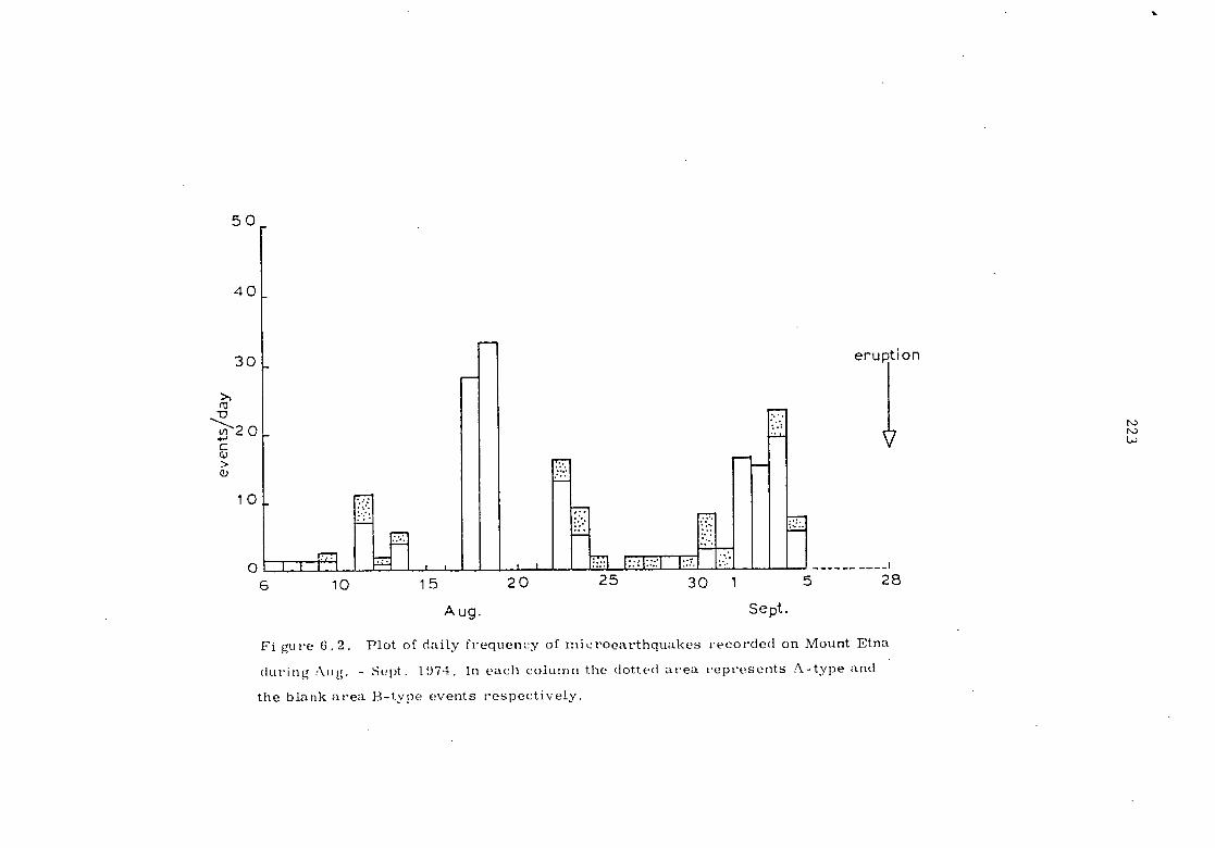
I
eruption
40
30
10
50
6 10 15 20 25 30 5 28
Aug. Sept.
Fi gure 6.2. Plot of daily frequency of microearthquakes recorded on Mount Etna
during Aug. - Sept. 1974. In each column the dotted area represents A-type and
the blank area 13-type events respectively.

• 224
These findings appear to be in agreement with
investigators working on other volcanoes. In fact, one of
the methods often used to predict eruptions on volcanoes is
by observing this increased seismicity. Prediction will
be discussed further in the next section.
During the second occupation the volcano was in a
state of 'quiet effusion'. Throughout the whole recording
period the seismic activity level was more or less constant
(see Section 4.3.1 and Fig. 4.9 a-d).
It has been mentioned briefly in Section 3.4.1 that
one of the critical criteria used to distinguish between A-
and B-type microearthquakes is their respective b-values.
Let us take a look at these values and examine how they are
related to the activity of the volcano during those two periods.
It is known that shallow earthquakes occur as a
result of fracture in the earth's crust, and that the larger
the earthquake's magnitude,the smaller is its chance of
occurrence. This simple relationship between the cumulative
frequency and magnitude was put into its present mathematical
form by Gutenberg and Richter (1954). However, many investi-
gators today suggest much wider implications of the relation-
ship than was previously thought to exist (Mogi, 1962, 1962a,
1963, 1967; Minakami, 1960).
In a number of experiments performed under controlled
laboratory conditions, Mogi (1962, 1962a) thoroughly investi-
gated the b-values of events due to microfacturing of
225
various materials subjected to stresses under conditions
thought to exist in the crust of the earth. His results
on various samples such as homogeneous brittle material
(pine resin), brittle material of heterogeneous structure
(pine resin including mechanical irregularities) and hetero-
geneous brittle material in a granular state (granular pumice
or coal) indicated that the b-value increased as the specimens
became weaker and less homogeneous. He thus concluded that
the variation in the b-values from region to region can be
attributed to the mechanical structure of the medium and the
spatial distribution of external stress.
Scholz (1968, 1968a) similarly studied the magnitude/
frequency relation of microfracturing of rocks under uniaxial
and triaxial loading. His laboratory experiments differ from
Mogi's in that he used a much higher frequency component of
the microfracturing energy. He was thus able to record
events several orders of magnitude greater from a single
specimen. He showed that the b-value of these microfractures
depends primarily on stress, and that variations in the local
stress field may cause observed variations in the b-value.
His investigations further confirmed that under a given
condition the constants 'a'* and 'b' in the Gutenberg-Richter's
recurrence curve depend on the fracture mechanism and trans-
mission properties of the medium as well as on the response
characteristics of the instrument.
Note also that the 'a' value is proportional to the total number of earthquakes recorded and is hence related to the duration of the observing period.

226
It appears- from these experiments that the mechanism
of the generation of earthquakes and the formation of fractures
during simulated laboratory tests are very similar. The
experiments have further confirmed that different b—values
found under different conditions are a direct result of the
stress concentration in the area,and to a lesser extent on
the type of rocks present.
This naturally raises the question of the A— and
B—type microearthquakes recorded in these surveys. Since
the b—values of A—type microearthquakes closely resemble those
of tectonic shocks, it appears that they both originate from
similar mechanisms inside the earths crust. The local stress
build up is due to changes within the volcano, and this
results in tectonic faulting. Thus A—type microearthquakes
originate primarily from faulting along planes of failure
in the rocks surrounding the volcano. This failure might
have been brought about by volcanic processes where the stress
concentration is sufficient to cause a rupture in the rocks.
When considered in this fashion, the A—type microearthquakes
are seen to be associated with the volcano in an indirect
way. In order to investigate this mechanism more fully it
is necessary to study the geographic distribution of the
initial motion of the microearthquakes, but unfortunately
this was not possible in the first survey as only one seismo-
graph was available, or during the second, because of the
paucity of microearthquakes. (It is hoped that in future
more data will be available to enable a study of this nature.)

227
The B-type microearthquakes are unique in that
they are only recorded in a volcanic region. They have no
analogy in the microearthquakes generated by tectonic faulting.
The high b-value in the first survey indicates a localized
stress concentration, probably in and around the Northeast
Crater region, where the rocks are weak and heterogeneous.
Unfortunately, no b-value is available for the second survey.
The localized stress build-up, mentioned above, is possibly
due to the expansion in volume of the magma as it rises near
the Crater bottom. This upward movement of the column results
in a separation of the volatiles, and a new stress distribution.
This excess stress is later on released as small earthquakes.
Some investigators,e.g. Craig et al.( 1976),have
shown the existence of B-type microearthquakes under very
different circumstances. In their investigation of Mount
Saint Helens, a strato-volcano in the Cascade Range of Washing-
ton State, they found B-type microearthquakes associated with
the glaciers on the mountains. This, however, can not be
the cause of B-type microearthquakes on Mount Etna.
Thus we have seen that the b-values associated with
the cumulative frequency versus magnitude (or amplitude in
the present case) of the microearthquakes provided some very
interesting information about the origin of these events.
However, longer recording periods are necessary if we are to
understand the volcano-seismic activity of Mount Etna more
fully.
It has been proposed earlier (see Section 5.4.3) that

228
volcanic tremor on Mount Etna is the resultant of the sum of
a number of harmonic oscillators set up by the expanding gas
front. In this section it was seen that the volcanic micro-
earthquake is a consequence of the release of excess
localized stress concentration, brought about by the upward
movement of the magma. In addition, both the volcanic
tremor and volcanic microearthquakes were found to have low
frequencies (below about 5 Hz, in the 1975 survey). The
location of both the source of volcanic tremor and the epi-
centre of at least one B-type event indicate their association
with the active part of the volcano.
It appears from the above analysis that volcanic
tremor and B-type microearthquakes are two different manifes-
tations of the same physical process. Under 'suitable con-
ditions' of the movement of the magma, one process is favoured
over the other. Just what these 'suitable conditions' are
is difficult to say. This is particularly so for Etna,
where so little geophysical data is available.
It is worth finishing this chapter with a discussion
of the influence of what has been said so far on the possibility
of predicting eruption on Mount Etna. In the following
section some of these aspects, e.g. microearthquake occurrence
rate, seismicity and volcanic tremor analysis that are
relevant to predicting eruptions will be discussed.
6.4 PREDICTING ERUPTIONS ON MOUNT ETNA
To be able to predict volcanic eruptions, a relation-

229
ship has first to be found between the eruption and the
various phenomena preceding it, and for the forecast to be
useful this relationship must enable the date or time, place
or magnitude (or intensity), of the eruption to be predicted
within certain defined limits. Unfortunately, the pecula-
rities of the connection between seismic and volcanic activity
are so specific to each volcano that so far no common formula
has evolved for predicting the precise time of an eruption
with any degree of certainty. Nevertheless,useful methods
have been developed in specific cases, based on the results
of instrumental observations of earthquakes, crustal move-
ments, and other phenomena, originating from the volcano itself.
It has been found,for example, that certain types
of microearthquakes are more directly related to volcanic
processes than others. Microearthquakes, capable of being
detected by a sensitive short-period seismograph, occur at
all stages of the eruptive cycle at all active volcanoes.
However, prior to an eruption significant changes have been
noticed in the frequency of volcanic microearthquakes. Thus
prediction involves essentially the monitoring of microearth-
quakes and the comparison of day-to-day occurrence rates.
However, there are difficulties. Firstly, there appear to be
large variations with time in the background level of seis-
micity at most volcanoes. Secondly, and perhaps more
important, criteria have to be established for judging the
significance of changes in the occurrence rate.
Figures 6.3 and 6.4 are examples gathered from
volcanoes in different parts of the world, which show changes

Eruption occured on Jan .7. 1,f f
_1400
1000 N
600
20 —
N 0
AUG SEP OCT NOV 1968
DEC JAN FEB 1939
Figure 6.3. Plot of daily frequency of microearthquakes ( N ) recorded at Merapi
volcano, Indenesia prior to an eruption. Note change of scale from mid - December
to mid - January. ( After Shimozuru et al. , 1969 ).
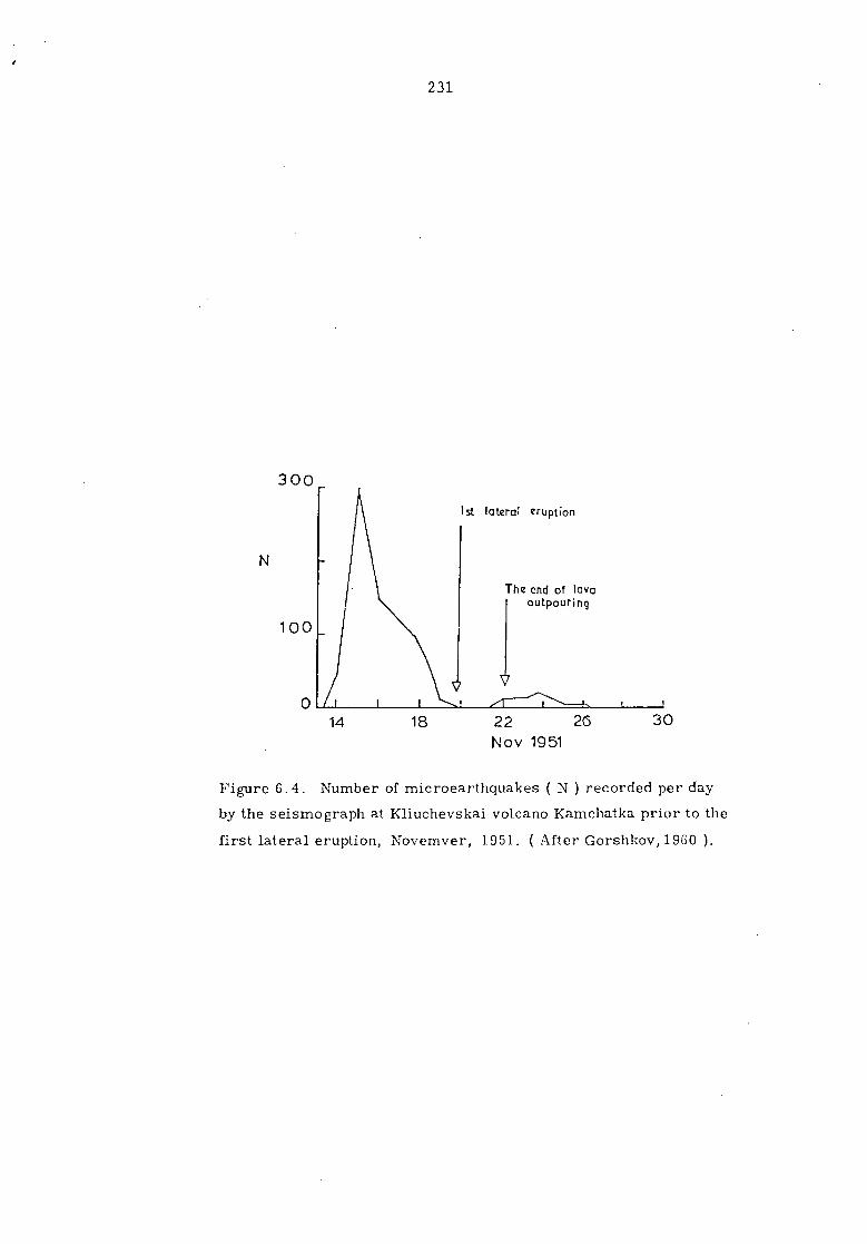
231
300
1st lateral eruption
N
100
The end of lava outpouring
14 18 22 26
30 Nov 1951
Figure 6.4. Number of microearthquakes N ) recorded per day
by the seismograph at Kliuchevskai volcano Kamchatka prior to the
first lateral eruption, Novemver, 1951. ( After Gorshkov, 1960 ).

232
of more than one hundred times in the background level of seis-
micity prior to an eruption. However, this is not a general
rule. Harlow, as reported by Decker (1973), studied the
relationship between earthquakes and volcanic eruptions for
71 cases and found that for 58% there was an increase in the
number of earthquakes before an eruption, while in 38% there
was an increase in earthquakes without any eruption, and in
4% there was an eruption without any increase in earthquakes.
As mentioned previously, very little seismic data
exists for Mount Etna. In spite of its reconnaissance nature,
this investigation forms one of the major studies yet carried
out in the area, and thus serves as a guide to future work.
In hindsight, it appears that the increased seismicity recorded
about forty-five days prior to the 28 Sept. 1974 eruption was
indeed a precursory event. It was unfortunate that we had
to stop recording about 24 days before this eruption.
In addition to the microearthquake studies, conti-
nuous monitoring of volcanic tremor on Mount Etna might provide
valuable information about the state of activity of the
volcano. In fact, during the monitoring of volcano Aso in
1932 - 1933, Sassa (1936) observed that prior to an eruption
the amplitude of the volcanic tremor increased suddenly and
remained constant for a short period. This was then followed
by a rapid decay in amplitude, and then a period of quiescence,
followed finally by an explosive eruption. In Hawaii, high
amplitude volcanic tremor is the most diagnostic index that an
eruption has begun or is about to begin (Decker, 1973). In

233
New Zealand, the volcanic tremor has been successfully used
to forecast eruptions from between 10 hours and 7 days in
advance.
Unfortunately, analysis of volcanic tremor was not
possible during the first survey, and no significant variation
in the tremor amplitudes was observed in 1975.

234
CHAPTER VII
SUMMARY OF CONCLUSIONS AND RECOMMENDATIONS
FOR FURTHER STUDY
7.1 SUMMARY OF CONCLUSIONS
This project has demonstrated clearly that it is
possible to investigate the seismic activity of Mount Etna
in a relatively short period of time, using simple instrumen-
tation and recording sites without the normal observatory
facilities.
Below is a summary of the most important conclusions
reached from this investigation, and recommendations for
further study.
Cl) Mi,croearthquake activity exceeding 7 events
per day was recorded on Mount Etna during the reconnaissance
survey of Aug. - Sept. 1974. The volcano displayed 'low to
moderate seismicity' during that period, a result arrived at
by comparing the microearthquake activity of Mount Etna with
that of other active volcanoes around the world.
(2) The signature and characteristics of these
microearthquakes were similar to those recorded on other
active volcanoes. Firstly were the volcano-tectonic micro-
earthquakes (classified as A-type) which had an impulsive
first arrival and a distinguishable P-S phase. Secondly,
the volcanic microearthquakes (classified as B-type), which
had an impulsive or an emersion type arrival and no distin-

235
guishable P-S phase. About 82% of the total recorded
events were of this type.
(3) The S-P distribution of the A-type microearth-
quakes showed their origin to be about 20 km from the record-
ing stations.
(4) Plots of microearthquakes in space and time
indicated that the seismic activity was not a constant in
time. Certain intervals of time appeared more active than
others. Seismically,the IC bench mark site (near Rifugio
Citelli) was found to be most active. It is believed that
the movement of magma took place via or from below this site
prior to the 1974 eruption.
(5) The b-values for A-type (0.99) and B-type
(1.78) microearthquakes, obtained in the present survey, are
consistent with those obtained in other parts of the world.
By analogy with laboratory studies of various rock
samples, the high b-value (1.78) of B-type microearthquake
appears to be due to inhomogenity and localized stress con-
centration in the crateral region of the volcano.
(6) The energy of the largest microearthquake
recorded during this survey appears to be approximately
6 x 10¹³
ergs.
(7) Results from the second field survey (May-June
1975) showed the volcano to be in a seismically 'quiet state',
with only about 2 recordable events per day. This is in
agreement with observation of the active craters at that time.
Both A- and B-type microearthquakes were recorded during this
time, the former constituting about 20% of the total and the

236
latter about 80%.
(8) The S-P distribution of these microearthquakes
indicates two distinct groupings, the first group being at
an epicentral distance of about 15 km and the second at about
40 km from the recording stations.
Only two events were recorded at more than two
stations during the whole period and it was therefore not
possible to look for evidence of shear wave screening.
(9) Using P- and S-wave velocities of 5.25 + 0.25
km/sec and 3.10 + 0.15 km/sec respectively,and the standard
S-P technique, these two events appear to have originated at
depths of about 10 km and 20 km respectively. The first is
thought to be related to volcano-tectonic processes and the
second to local tectonic forces.
Six other A-type events were located using the three
components recorded at a single station, together with the
S-P travel time.
In general, it was not possible to locate the B-type
microearthquakes, because of their small amplitudes. However
one such event was located using the arrival times at three
stations. The data is consistent with an origin within the
crateral region of the volcano and an average surface wave
velocity of 1.09 km/sec.
(10) Spectral analysis of the background seismic
noise shows a dominant frequency of between 1.2 and 2.9 Hz.
Hourly samples over 24 hour periods do not indicate any
significant variation in either the frequency or the amplitude
of these tremors, at any given station.

237
From an analysis of the attenuation of the ampli-
tude of volcanic tremor, at the various stations, it was
found that the source of disturbance was between the
Northeast Crater and 3 km NW of the Central Crater.
(11) The volcanic tremors are thought to originate
from oscillations induced by degassing processes, the tremor,
recorded on a seismogram being the resultant of a number of
random harmonic oscillators set up by the expanding gas front.
(12) Location, as well as the frequency contents,
of the B-type microearthquakes and the volcanic tremors
support the view that they originate from similar source
mechanisms inside the volcano.
(13) A-type microearthquakes appear to have a
frequency range from about 1.40 Hz to above 10.00 Hz. The
B-type microearthquakes,on the other,hand seem to have domi-
nant frequencies in the range 1.0 and 5.0 Hz. It is con-
cluded from these observations that it is difficult to classify
events on their frequency contents alone.
7.2 RECOMMENDATIONS FOR FURTHER STUDY
Attention has been drawn in various sections of this
thesis to the lack of geophysical data available for Mount
Etna. Seismic investigations on Etna have so far been limited
to either microearthquake or volcanic tremor studies for short
intervals of time. These surveys,though useful in providing
short term information about the present day activity of the
volcano, do not give much idea about the structure of the
volcano, mechanism of the generation of microearthquakes, or

238
even the variation in activity throughout the year.
In order to understand these more fully, studies
of the volcano on the following lines are recommended:
(1) Seismic velocity studies (e.g. by refraction
techniques or otherwise) of the volcano itself, and also the
deep basement structure. It may be mentioned here that little
data exists in this respect.
(2) Mapping pockets of liquid bodies by S-wave
screening of local or distant earthquakes by suitably placed
recording instruments.
(3) Extensive studies of both the microearthquake
and volcanic tremor by continuously monitoring them through-
out the year. These studies are necessary if we are to under-
stand how the volcano behaves during various phases of its
eruptive cycle.
(4) Efforts should be made to study the mechanism
of their generation as well as their distribution in space
and time.
It is hoped that the present findings,along with the
above suggestions,will serve as the basis for further seismic
work in the area.

239
REFERENCES
Andronov, A.A., Vitt, A.A. and Khaikin, S.E. 1966. Theory of oscillations. Pergamon Press Ltd. Oxford.
Asada, T. 1957. Observations of nearby microearthquakes with ultra-sensitive seismometers. J. Phys. Earth. 5, 83-113.
Asada, T., Suyehiro, S. and Akamatu, K. 1958. Observations of nearby microearthquakes with ultra-sensitive seismometers at Matsushiro, Japan. J. Phys. Earth. 6, 23-33.
Asada, T., Suzuki, Z. and Tomoda, Y. 1951. Notes on the energy and frequency of earthquakes. Bull. Earthq. Res. Inst. 29, 289-293.
Aspinal, W.P., Michael, M.O. and Tomblin, J.F. 1976. Evidence for fluid bodies beneath the Sulphur Springs geo- thermal region, St. Lucia, West Indies. Geophys. Res. Lett. 3(2), 89-90.
Barberi, F., Civetta, L., Gasparini, P., Innocenti, F., Scan- done, R. and Villari, L. 1974. Evolution of a section of the Africa-Europe plate boundary. Paleomanetic and volcanological evidence from Sicily. Earth Plan. Sci. Lett. 22, 123-132.
Barberi, F., Ferra, G., Keller, J., Innocenti, F. and Villari, L. 1974a. Evolution of Eolian arc volcanism. Earth Plan. Sci. Lett. 21, 269-276.
Barberi, F., Gasparini, P. and Villari, L. 1973. Volcanism of South Tyrrhenian Sea and its geodynamic impli- cations. J. Geophys. Res. 78, 5221-5232.
Bath, M. 1973. Introduction to Seismology. Halstead Press, New York.
Belderson, R.H., Kenyon, N.H. and Stride, A.H. 1974. Cala- brian ridge, anewly discovered branch of the Medi- terranean ridge. Nature, 274, 453.
Bendat, J.S. and Piersol, A.G. 1971. Random Data Analysis and Measurement Procedures. Wiley Interscience, New York.
Berg, E. and Jenessen, 1960. Microseismes et seismes pre- cedant l'eruption du Nyamuragira-Kitzimbanyi (Afrique Central) 1958. Bull. Volc. 23, 63-68.

240
Berry, M.J. and West, G.F. 1966. An interpretation of the first arrival data of the Lake Superior experiment by the time term method. Bull. Seism. Soc. Am. 56, 141-171.
Blackman, R.M. and Tukey, J.W. 1958. The measurement of power spectra. Dover Publications, New York.
Bloxham, R.D. and others, 1972. Computer control for Imperial College engines development. C.M.E. 19(9), 58-61.
Bottari, A. and Riuscetti, M. 1967. La statzione sismica di Serra La Nave Sull' Etna. Annali di Geofisica. 22, 243-264.
Bracewell, R. 1965. The Fourier transform and its applications. McGraw-Hill, New York.
Brune, J.N. 1968. Seismic moment, seismicity and rate of slip along major fault zones. J. Geophys. Res. 73, 777-784.
Bullard, E.G. 1965. Concluding remarks, symposium on con- tinental drift. Phil. Trans. R. Soc. A. 258, 322.
Caire, A. 1970. Sicily in its Mediterranean setting. Geology and history of Sicily. Petroleum Expl. Soc. of Libya, Tripoli, 145-170.
Caputo, M., Folloni, G., Pieri, L. and Unguendoli, M. 1974. Geodimetric control across the Straits of Messina. Geophys. J.R. Astr. Soc. 38, 1-8.
Caputo, M., Panza, G.F. and Postpischl, D. 1972. New evidence about the deep structure of the Lipari arc. Tectono- physics, 15, 1-13.
Cassinis, R., Finetti, I., Giese, P., Morelli, C., Steinmetz, L. and Vecchia, 0. 1969. Deep seismic refraction research on Sicily. Boll. di Geofis. XI, 43-44, 140-160.
Clacy, G.R.T. 1972. Analysis of seismic events recorded with a slow motion tape recorder near Chateau Tongariro, New Zealand, during Feb. 18, 1966 to Dec. 31, 1966. Bull. Volc. 36, 20-28.
Combs, J. and Rotstein, Y. 1975. Microearthquake studies at the Coso geothermal area, China Lake, California. Second UN Symposium on the development and use of geothermal resources, San Francisco , Proceedings, 2, 909-916.
Craig, S.W. and Malone, S.D. 1976. Mt. Saint Helens seismic events: Volcanic earthquakes or glacial noises? Geophys. Res. Lett. 3(3), 197-200.

241
Crampin, S. 1970. A method for the location of near seismic events using travel-times along ray paths. Geophys.. J.R. Astr. Soc. 21, 535-539.
Crampin, S. and Willmore P.L. 1973. Small earthquakes ob- served with local seismometer networks. Phil. Trans. R. Soc. London, A. 274, 383-387.
Cristofolini, R. 1973. Recent trends in the study of Etna. Phil. Trans. R. Soc. London, A. 274, 17-35.
Crosson, R. 1972. Small earthquakes, structure and tectonics of Puget Sound region. Bull. Seis. Soc. Am. 62, 1133-1173.
Decker, R.W. 1973. State of art in volcano forecasting. Bull. Volc. 37, 372-393.
Del Pezzo, E., Guerra, I., Lo Bascio, A., Luongo, G., Nappi, G. and Scarpa, R. 1974. Microtremors and volcanic explosions at Stromboli - Part 2. Bull. Volc. 38, 1023-1036.
Dibble, R.R. 1969. Seismic power recordings during hydro- thermal eruptions from Ruapehu crater lake in April, 1968. J. Geophys. Res. 74, 6545-6551.
Douze, E.Y. and Sorrells, G.G. 1972. Geothermal ground noise surveys. Geophys. 37, 813-824.
Eaton, G.P., Christiansen, R.L., Iyer, H.M., Pitt, A.M., Mabey, D.R., Blank, H.R., Zietz, I. and Gettings, M.E. 1975. Magma beneath Yellowstone National Park. Science, 188, 787-796.
Eaton, J.P. 1962. Crustal structure and volcanism in Hawaii, crust of the Pacific basin. Geophys. Mono. 6, 13-29.
Eaton, J.P. 1969. HYPOLAR - a computer program for deter- mining hypocentres of local earthquakes in an earth consisting of uniform flat layers over a half space. U.S. Geol. Sur. Open file report.
Eaton, J.P. and Richter, D.H. 1960. The 1959 eruption of Kilauea. GeOtimes, IV, 5, 24-27.
Engdahl, E.R. and Gunst, R.H. 1966. Use of a high speed computer for the preliminary determination of earth- quake hypocentres. Bull. Seism. Soc. Am. 56, 325-336.
Farberov, A.I. and Gorelchik, V.I. 1971. Anomalous seismic effects under volcanoes and some features of deep seated structure of volcanic area. Bull. Volc. 35, 212-224.

242
Finch, R.H. 1943. The seismic prelude to the 1942 eruption of Mauna Loa. Bull. Seism. Soc. Am. 33, 73-78.
Finch, R.H. 1949. Volcanic tremor. Bull. Seism. Soc. Am. 39, 73-78.
Firstov, P.P. and Shirokov, V.A. 1971. Seismic investigation of the root of the Kliuchevskaya group volcanoes, Kamchatka. Bull. Volc. 35, 164-172.
Flinn, E.A. 1960. Local earthquake location with an electronic computer. Bull. Seism. Soc. Am. 50, 467-470.
Francaviglia, A. 1959. L'imbasamento sedimentario dell'Etna e it golfo pre-Etneo. Boll. Serv. Geol. Ital. 81, 4-5, 583-684.
Giese, P., Morelli, C. and Steinmetz, L. 1973. Main features of crustal structure in western and southern Europe based on data of explosion seismology. Tectono- physics, 20, 367-379.
Goforth, T.T., Douze, E.J. and Sorrells, G.G. 1972. Seismic noise measurements in a geothermal area. Geophys. Prosp. 20, 76-82.
Gorshkov, G.S. 1958. On some theoretical problems in volcan- ology. Bull. Volc. 19, 103-114.
Gorshkov, G.S. 1960. Some results of seismometric investi- gations at the Kamchatka Volcanological Station. Bull. Volc. 23, 121-128.
Grindley, G.W. 1973. Structural control of volcanism at Mt. Etna. Phil. Trans. R. Soc. A. 274, 165-175.
Guest, J.E. 1973. The summit of Mt. Etna prior to the 1971 eruption. Phil. Trans. R. Soc. A. 274, 63-78.
Guerra, I., Lo Bascio, A., Luongo, G. and Scarpa, R. 1976. Seismic activity accompanying the 1974 eruption of Mt. Etna, J. Vol. Geoth. Res. 1, 347-362.
Gutenberg, B. and Richter, C.F. 1954. Seismicity of the earth and associated phenomena. Princeton University Press, Princeton, New Jersey.
Hadley, D. and Combs, J. 1974. Microearthquake distribution and mechanism of faulting in the Fontana , SanBernardino area of Southern California. Bull. Seism. Soc. Am. 64, 1477-1499.
Hedayati, A. 1976. Microearthquakes, seismicity and tectonics of the north-central Persian plateau. Ph.D. Thesis. University of London.

243
Hosmer, G.L. 1919. Geodesy. John Wiley and Sons Inc. New York.
Imbo, G. 1935, Agitazione asmonica Vesuviano. Annali Osserv. Vesuviano, Napoli, 163.
Isacks, B. and Oliver, J. 1964. Seismic waves with fre- quencies from 1 to 100 cps recorded in a deep mine in Northern New Jersey. Bull. Seism. Soc. Am. 54, 1941-1979.
Ishimoto, M. and Iida, K. 1939. Observations sur les seismes enregistres par la microseismographe construit dernierement (1). Bull. Earthq. Res. Inst. 17, 443-478.
Iyer, H.M. and Hitchcock, T. 1974. Seismic noise measure- ments in Yellowstone National Park Geophys. 39, 4, 389-400.
Jagger, T.A. 1920. Seismometric investigations of the Hawaiian lava column. Bull. Seism. Soc. Am. 10, 204.
James, D.E., Sacks, I.S., Lanzol, E. and Aparicio, P.G. 1969. On locating local earthquakes using small networks. Bull. Seism. Soc. Am. 59, 1201-1212.
Jenkins, G.M. and Watts, D.G. 1969. Spectral analysis and its applications. Holden-Day, San Francisco.
Kanasewich, E.R. 1975. Time Sequence Analysis in Geophysics. The University of Alberta Press, Alberta.
Kieffer, G. 1969. Origine explosive de la Valle del Bove (Etna Sicilie). C.R. Acad. Sci. Paris, 269, 1938- 1941.
Klerkx, J. 1968. Etude Geologique et petrologique del la Valle del Bove (Etna). Thesis. University de Liege.
Klerkx, J. and Evrard, P. 1970. Les anomalies gravimetriques del'Etna (Sicile) et l'evolution du Trifoglietto. Ann. Soc. Geol. Belg. 93, 145-147.
Koyanagi, R.Y. 1968. Earthquakes from common sources beneath Kilauea and Mauna Loa volcanoes in Hawaii from 1962- 1965. U.S. Geol. Survey Prof. Paper 600-C, 120-125.
Koyanagi, R.Y. and Endo, E.T. 1965. Hawaii seismic events during 1963. U.S. Geol. Survey Prof. Paper 625-B, 13-16.
Kubota, S. and Berg, E. 1967. Evidence for magma in Katmai Volcanic Range. Bull. Volc. 31, 175-214.

244
Kubotera, A. 1974. Volcanic tremors at Aso volcano. Physical Volcanology. Edited by Civetta et al. Elsevier Sci. Pub. Co. Amsterdam, 29-47.
Kubotera, A. and Yosikawa, K. 1963. Prediction of volcanic eruption from Aso and Sakurazima and some related geophysical problems. Bull. Volc. 26, 297-317.
Lanczos, C. 1966. Discourse on Fourier series. University Mathematical Monographs, London.
Langenkamp, D.F. and Combs, J. 1974. Microearthquake study of the Elsinore fault zone, Southern California. Bull. Seism. Soc. Am. 64, 187-203.
Latter, J.H. 1966. The relationship between seismicity and volcanism in the Sicilian volcanoes. Proc. Geol. Soc. London, 1637, 58-59.
Latter, J.H. 1971. Near surface seismicity of Vulcano, Aeolian Islands, Sicily. Bull. Volc. 35, 117-126.
Lee, W.H., Bennet, R.E. and Meagher, K.L. 1972. A method of estimating the magnitude of local earthquakes from signal duration. U.S. Geol. Surv. Open file report.
Lo Bascio, A., Nappi, G. and Scarpa, R. 1976. Seismicity of Etna during November 1973. Boll. di Geofisica, 70, 92-97.
Matumoto, A. 1971. Seismic body waves observed in the vicinity of Mount Katmai, Alaska, and evidence for the exis-tence of molten chambers. Geol. Soc. Am. Bull. 82, 2905-2920.
Matumoto, A. and Ward, P. 1967. Microearthquake study of Mt. Katmai and vicinity, Alaska. J. Geophys. Res. 72, 2557-2568.
Mauk, F.J. and Johnston, M.J.S. 1973. On triggering of volcanic eruptions by earth tides. J. Geophys. Res. 78, 3356-3362.
Mauk, F.J. and Kienle, J. 1973. Microearthquakes at St. Augus- tine Volcano, Alaska, triggered by earth tides. Science, 182, 386-389.
McKenzie, D.P. 1970. The plate tectonics of the Mediterranean region. Nature, 226, 239-245.
McKenzie, D.P. 1972. Active tectonics of the Mediterranean region. Geophys. J.R. Astr. Soc. 30, 109-185.
McDonald, G.A. 1972. Volcanoes, Prentice-Hall, New Jersey.

245
Minakami, T. 1960. Fundamental research for predicting volcanic eruptions. Bull. Earthq. Res. Inst. 38, 497-544.
Minakami, T. and Sakuma, S. 1953. Reports on volcanic activities and volcanological studies concerning them in Japan during 1948-1951. Bull. Volc. 14, 79-130.
Mogi, K. 1962. The magnitude frequency relation for elastic shocks accompanying fractures for various materials and some related problems in earthquakes. Bull. Earthq. Res. Inst. 40, 831-853.
Mogi, K. 1962a. The fracture of a semi-infinite body caused by an inner stress, origin and its relation to earth- quake phenomenon. Bull. Earthq. Res. Inst. 40, 815-829.
Mogi, K. 1963. The fracture of semi-infinite body and its relation to the earthquake phenomenon. Bull. Earthq. Res. Inst. 41, 595-615.
Mogi, K. 1967. Regional variation in magnitude frequency relation of earthquakes. Bull. Earthq. Res. Inst. 45, 313-325.
Mohajer-Asjhai, A. 1975. Recent and contemporary crustal deformation in Eastern Iran. Ph.D. Thesis. University of London.
Moore, J.G. and Krivoy, H.L. 1964. The 1962 flank eruptions of Kilauea volcano and the structure of East Rift Zone. J. Geophys. Res. 69, 2033-2045.
Murray, J.B., Guest, J.E. and Butterworth 1977. A large ground deformation on Mount Etna Volcano. Nature, 266, 338-340.
Murray, J.B., Wright, M., Foster, J.H. and Baker, A. 1974. Map of summit area of Mount Etna in 1973,United Kingdom Research on Mount Etna. R. Soc. London.
Nicholls, H.R. and Rinehart, J.S. 1967. Geophysical studies of the geyser action in Yellowstone National Park. J. Geophys. Res. 72, 4651-4663.
Ninkovich, D. and Hays, J.D. 1972. Mediterranean island arcs and the origin of high potash volcanics. Earth Plan. Sci. Lett. 16, 331-345.
Nordquist, J.M. 1962. A special purpose program for earth- quake location with an electronic computer. Bull. Seism. Soc. Am. 52, 431-437.

246
Ogniben, L. 1966. Lineamenti idrogeologici dell' Etna. Riv. Min. Sicil. 24, 100-102.
Oliver, J., Ryall, A., Brune, J.N. and Slemmons, D.B. 1966. Microearthquake activity recorded by portable seismographs of high sensitivity. Bull. Seism. Soc. Am. 56, 899-924.
Omer, G.C. 1950. Volcanic tremor. Bull. Seism. Soc. Am. 40, 175-194.
Omori, F. 1911-1918. The Usu-San eruption and the earthquakes and elevation phenomena. I, II. Bull. Imp. Earthq. Invest. Comm. 5, 1-38; 101-107.
Papoulis, A. 1962. The Fourier integral and its applications. McGraw-Hill Book Comp. Inc. New York.
Parasnis, D.S. 1972. Principles of applied Geophysics, Chapman & Hall Ltd. London.
Real, C.R. and Teng, T.L. 1974. Local Richter magnitude and total signal duration in Southern California. Bull. Seism. Soc. Am. 63, 1809-1827.
Richards, P.I. 1967. Computing reliable power spectra. IEEE Spectrum, 83-90.
Richter, C.F. 1935. An instrumental earthquake scale. Bull. Seism. Soc. Am. 25, 1-32.
Richter, C.F. 1958. Elementary Seismology. Freeman and Comp. San Francisco.
Rinehart, J.S. 1965. Earth tremors generated by Old Faithful Geyser. Science, 150, 494-496.
Ritsema, A.R. 1969. Seismic data of the Western Mediterranean and the problem of oceanization. Verhand. Kon. Ned. Geol. Mijn. XXVI, 105-120. (Symposium on the problem of oceanization in the Western Mediterranean).
Rittmann, A. 1962. Volcanoes and their activity. John Wiley & Sons, New York.
Rittmann, A. 1963. Vulcanismus and tektonick der Atna. Geol. Rund. 53,,788-800.
Rittmann, A. 1973. Structure and evolution of Mt. Etna. Phil. Trans. R. Soc. London, A. 274, 5-16.
Rittmann, A. 1975. (Personal Communication). Intern. Inst. Volc. Catania, Sicily.

247
Riuscetti, M. and Schick, R. and Seidl, D. 1977. Spectral parameters of volcanic tremors at Etna. J. Volc. Geoth. Res. 2, 289-298.
Robson, G.R., Barr, K.G. and Smith, G.W. 1962. Earthquake series in St. Kitts-Nevis, 1961-1962. Nature, 195, 972-974.
Romano, R. 1970. Tectonic control on magmatic differentiation; an example. Bull. Volc. 34, 823-832.
Sakuma, S. 1957. Volcanic tremor at eruption of Meakandake. J. Fac. Sci. Hokkaido Univ. 7, I(1).
Sassa, K. 1936. Micro-seismometric study on eruptions of volcano Aso. Mem. Coll. Sci. Kyoto Univ. 19, 11-56.
Schick, R. and Riuscetti, M. 1973. An analysis of volcanic tremors at South Italian volcanoes. Zeitschrift fUr Geophys. 39, 247-262.
Scholz, C.H. 1968. Micro-fracturing and the inelastic deformation of rock in compression. J. Geophys. Res. 73, 1417-1432.
Scholz, C.H. 1968a. The frequency magnitude relation of micro-faulting in rock and its relation to earth- quakes. Bull. Seism. Soc. Am. 58, 399-415.
Shimozuru, D. 1971. A seismological approach to the prediction of volcanic eruption. UNESCO, Earth Sci. Mono. 8, Paris, 19-45.
Shimozuru, D. 1971a. Geophysical evidences for suggesting the existence of molten pockets in the earth's upper mantle. Geol. Soc. Am. Bull. 82, 181-195.
Shimozuru, D., Miyazaki, T., Gyoda, N. and Matahelumual, J. 1969. Volcanological survey of Indonesian volcanoes. Bull. Earthq. Res. Inst. 47, 969-990.
Stacy, F.D. 1969. Physics of the earth. John Wiley & Sons Inc. New York.
Steeples, D.W. and Iyer, H.M. 1975. Teleseismic P wave delays in geothermal exploration. Second UN Symposium on the Development and Use of Geothermal Resources, San Francisco. Proceedings 2, 1199-1206.
Steinberg, G.S. and Steinberg, A.S. 1975. On possible causes of volcanic tremor. J. Geophys. Res. 80, 1600-1604.
Suzuki, Z. 1953. A statistical study on the occurrence of small earthquakes. I. Sc. Rep. Tohuku Univ. 5, 177-182.
248
Suzuki, Z. 1954. A statistical study on the occurrence of small earthquakes. II. Sc. Rep. Tohoku Univ. 6, 105-118.
Suzuki, Z. 1958. A statistical study on the occurrence of small earthquakes. III. Sc. Rep. Tohoku Univ. 10, 15-27.
Suzuki, Z. 1959. A statistical study on the occurrence of small earthquakes. IV. Sc. Rep. Tohoku Univ. 11, 10-54.
Sykes, N.R. 1970. Earthquake swarms and sea-floor spreading. J. Geophys. Res. 75, 6598-6611.
Tsumura, K. 1967. Determination of earthquake magnitude from total duration of oscillation. Bull. Earth. Res. Inst. 15, 7-18.
Tazieff, H. 1971. A dynamic approach to the problem of fore- casting volcanic paroxysms. UNESCO, Earth Sci. Mon. 8, Paris, 127-130.
Unger, J. 1969. The microearthquake activity of Mt. Rainier, Washington. Ph.D. Thesis. Dartmouth College.
Wadge, G. 1974. Volcanic deformation and the eruptive mecha- nisms of Mt. Etna. Ph.D. Thesis. London University.
Ward, P.L., Palmason, G. and Drake, C. 1969. Microearthquake survey of the mid-Atlantic ridge in Iceland. J. Geophys. Res. 74, 665-685.
Westhusing, J.K. 1974. Reconnaissance surveys of near-event seismic activity in the volcanoes of the Cascade Range, Oregon. Bull. Volc. 37, 258-286.
Westphal, W.H. and Lange, A.L. 1967. Local seismic monitoring - Fairview Peak Area, Nevada. Bull. Seism. Soc. Am. 57, 1279-1298.
Wilcoxson, K. 1967. Volcanoes. Cassell & Comp. Ltd. London.
Wood, R. 1974. Microearthquakes at Central American volcanoes. Bull. Seism. Soc. Am. 64, 275-277.
Yokoyama, I. 1963. Structure of caldera and gravity anomaly. Bull. Volc. 26, 67-72.

249
APPENDIX 2A
POWER DENSITY ESTIMATES FOR VOLCANIC TREMOP STATION : SERRA LA NAVE
SAMPLING INTERVAL = 0.02 SEC PANDMIDTH = 0.58 HZ TOTAL POWER UNDER ANY CURVE s 1
TIME , 5MT1 FREQUENCY INTERVAL FRACTION OF TOTAL POWER D-HP/MIN .H2. v H- C E- M
CURVE NO.
44 13 59 0.00 - 0.58 0.002 - 0.017 (1) 0.59 - 1.17 0.021 0.109
1.18 - 1.76 0.255 1.77 - 2.39 0.2?? 201: 2.36 - 2.94 0.183 0.182 2.95 - 3.53 0.093 0.078 3.54 - 4.12 0.081 0.0?6 4.13 - 4.71 0.n1;°.1 0.07:3 4.72 - 5.7:11 0.051 0.020 5.31 - 5.89 0.029 0.018
44 14 59 (2)
0.00 - 0.58 0.001 0.02? 0.59 - 1.17 0.045 0.161 1.18 - 1.76 0.294 0.??0 1.77 - 2.2:5 0.292 2.36 - 2.94 0.114 0.101 2.95 - 0.074 0.056 3.54 - 4.12 0.078 4.13 - 4.71 0.040 0.021 4.72 - 5.2:0 0.028 0.019 5.31 - 5.89 0.017 0.011;
44 16 59 (3)
0.00 - 0.58 0.001 0.018 0.59 - 1.17 0.0:740 0.123 1.18 - 1.76 0.294 1.77 0.262: 0.188 2.36 2.94 0.141 - 0.143 2.95 - 74.53 0.073 0.047 3.54 - 4.12 0. 07 A 4.13 - 4.71 0.053 0.022 4.72 - 0.0:?5 0.017 5.31 - 5.89 0.018 0.018
44 17 59 (4)
0.00 - 0.58 0.004 0.024 0.59 - 1.17 0.033 0.152 1.18 - 1.76 0.299 0.310 1.77 - 2.35 0.228 0.198 2.36 - 2.94 0.181 0.11;1 2.95 - 0.081 0. 047 3.54 - 4.12 0.087 0.029 4.13 - 4.71 0.060 0.025 4.72 - 5.7:0 0.055 0.021 5.31 - 5.89 0.024 0.017

-P.
ro
c.n
cn 4 -P. ro ro
co -A
c.n
'JD
CO
1-0
1:0 -
1-1
Cr'. ' A
CO
'4
)
1111111111
c.n cn
4:.• co ro
cc. c.)
.—
c_n AD
co 'A
1-11
10 CO
- c.n
-.J
CO
r0
co ro
r_n 41 4
1 C
O 1-
0 1-0 I-. 1-•
• . • • • • .- • • .
0) 'A
)-•
ro
cn Cr.
0)
c,
III II
I !III
cn (.9 41 41
ro ro
co co
▪ 1-- ro co - cn Cr-, - A
co
ro
c_n 41 41 co n) ro
.c,
• • • • • • • • • •
-.1
fn ▪ c.)
k-a
• c.n
ro
cn
1.71
CO
1111111111
cii c
n 41 4.- co ro ro
c
co co
ro ▪ 41.:_n cr.
CO
4.
c.n
f_n 41 -P. (.0 ro ro
C..
C.
kJ) C.) -
A
1-&
(-
11
rci co
cfl
0)
1111111111
cn c.n 4 -P. C.) ro ro
o:. co -.J
cn
.=
.
NI co
c.n Cr. -.1
O
D
4.
4.
r_n
c.fl
f_11
4.. 4. 1-.0 n) ro
c.
• •
• • • • •
• •
-..1
...C
I-.
J r_n
ro
1:1%
',CI c
I I
I I
I I
I I
cn
4.•
co ro
OD
10
(n
ro
l_r1
CO
11 II
It
II
II
II
II
II
I 1
11
1.
I I
I •
•
•
•
•
•
•
•
•
•
rn rn rn
n) n) cD
I-. 4
1 4
Ch
41
CD OD ON CD
co 41-
c.)
_rj
c_n
1:c1 (A N
I
1111111111
• • • • • • • • • •
1 10 1.0
ro ro CO
C.) ..1)iT
-,0
%,
ro
1-• r0
ro
.1)
110
r0 n) CD r
n
▪ 44
. 0)
C. CO
0%
41 0) cn CD
▪ -
d CD Op f
t) ro co 41 ro
I I
I I
I I
I I
I I
I I
▪ •
1
•
•
•
•
•
•
11
ri) flo
ro
▪ cc, cc, 4.... co (
...)
o--. ,._
n
•
• •
•
•
•
•
•
•
•
_
ro
ro co 01
▪ 1
1.)
c.n
0) c.
f.--
•
(_11
...p
... ro
.4
) ro
•
1 1
I 1
I 1
I 1
I 1
I II
•
• •
•
•
•
•
•
•
•
en en en rn en roco ro CD
1-"
ro o) -A
g)
ro
co ch -A AD
O
D
4-
-.J CD
• • • • • • • • • •
ro
ro
_q g
.
cr N
I -.1 C.
ro
co ro cc, co
ro
1 1
1 1
I I
I 1
I 1
•
• •
•
•
1
•
•
•
•
ro ro
(.fl ro co 4.,-.j
ro
ro
ro
ro
Cr)
••
••
••
••
••
ro
sm
ro co 41 Cr., 0) f_
n
ro
ro
C.r
1 q
*. CO
0) Cr
-, 0
% ri)
III I
1 1
1 I
I 1
-
ro
ro ro
41 co co r0 c_n
cc,
,--
co co
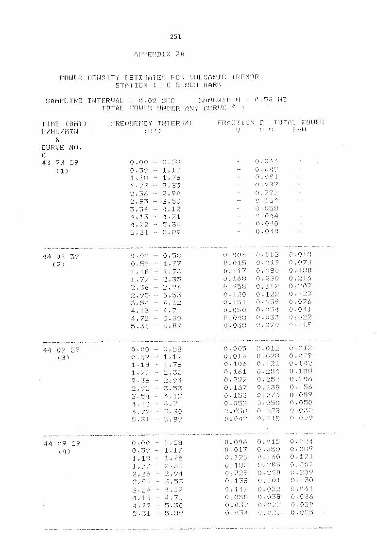
251
APPENDIX 2D
POWER DENSITY ESTIMAIES FOR VOLCANIC 'IREHOR STATION IC :BENCH MARK
SAMPLING INTERVAL .:, 0,02 SEC DANDWIDIH 0,50 HZ TOTAL POWER UNDER ANY CURT T. 1
TIME (OMT) D/HR/MIN
& CURVE NO
43 23 59
FREQUENCY
0,00
IN1ERWL FRACTION Or JOTAL POWER • • 1.'1
(1) 0,59 0,049 1,18 1,76 1,77 2,35 2,36 2^94 2,95 3.53 0, 161 3.54 4,12 0,050 4+13 4,71 4,72 0,010 5,31 5489 0,019
44 01 59 0,00 - 0,50 f..),()()6 ()-()1 0
(2) 0,59 O^ O15 () , 01..--.) ,
1,18 () „ () ( ) , 180 1,77 - 2,35 O ^168 O.23O O,216 2,36 -258 (.) 0 + 2,95 - 3,53 !̂12O 0,1 3,54 - 4+12 059 0,O76 4,13 0 : 01.51 (01 4,72 - 5,30 0,018 0,033 0:022 5,31 - 5,89 0.038
07 09 0,00 - 0,58 0,005 0,012 0,012
(3) 0,59 - 1,17 0,016 0,028 0,079 1.18 - 1,76 0,106 0,121 0,112
1,77 - 2,35 0,161 0,251 0,188 2,36 - 2,91 0,227 0,254 0,206
2,95 - 3,53 0,167 0,138 0,156
3,51 - 1 , 12 0,153 0,076 0,089 4,13 - 4,71 0,052 0,000 0+050
1,72 - 5,30 0,058 0-020 0,03,!
5,31 - 5,09
44 09 59 0,00 - 0,50 0,006 0,015 0,024
(4) 0,59 - 1.17 0,017 C. 0,009 1,18 - 1,76 0,125 0,160 0,171
1,77 - 2,35 0,182 0,288 0,207
2,36 - 2,94 O.229 O^228 0 , ()
2,95 - 3,53 () „ 1.3!"..3 ^101 O.13O
3,54 - 1,12 , 117 ,O61 4,13 - 4,71 0,0159 O^O38 O^(.)36 1,72 - 5,30 0,037 0,027 0,029 5,31 - 5,09

252
44 13 59 0,00 - 0,016 0,007 (5) 0,59 1,17 , 060 0,016
1,10 0-111 0,110 1,77 2,35 0,291 0,237 2,36 0,170 0,230 2,95 3,53 0,132 0,121 3,54 1,12 0-100 0, 112 4,13 4,71 0,015 0,002 4,72 0,033 0,052 5,31 5,a9 0 016
--------------------- 44 15 59 0,00 - 0,50 0,011 0,010 0,011
(6) 0,59 - 1,17 0,114 033 0,117 1,10 - 1,76 0,200 0, !23 1,77 - 2,35 0,224 0,310 °,224
0,114 0,11 0.111 2,95 - 3,53 0,120 0,121 0,120 3,51 - 1,12 4,13 - 1,71 4,72 - 5,30 5,31 - 5,09
•••••-•••• ••• • •• • ••
44 19 59 0,00 - 0,50 (,006 0,011 0,017 (7) 0,39 - 1,17 0,026
1,18 1,76 0,129 11/, 1.77 - '2..36 • 2,95 - 3,53 3,54 - 4,12
- 1J,30 0,02j
5,71 -
••••••••••••• • •• • • • • • • •• •
11 21 59 0,50 0,000 0 01.!. 0,017 (0) -
1 ,76 2,35
2,36 - 2,94 0,224' 0„1-;„. 3,53 (,, ,)05 0,111 0,123
3,51 - 4,13 - 1..;1 0,052 1,72 - 0,03/:- 0.021 5,31 - 5„T2
44 23 59 o,00 - 0,005 0,017 0,019 (9) 1.17 0,021 0,039 0,151
, 1,10 - 1,76 0,130 0,130 0,184 O^l9» 0,315 0,233
2,36 - 2,94 0,189 O 19? 3,53
3,51 - 1,12 0,121 0, 00;:, 4,13 - 4,71 0,001 0 01- 0, 015 1,-/2 - 3,70 O,O6i 0 0 028
-
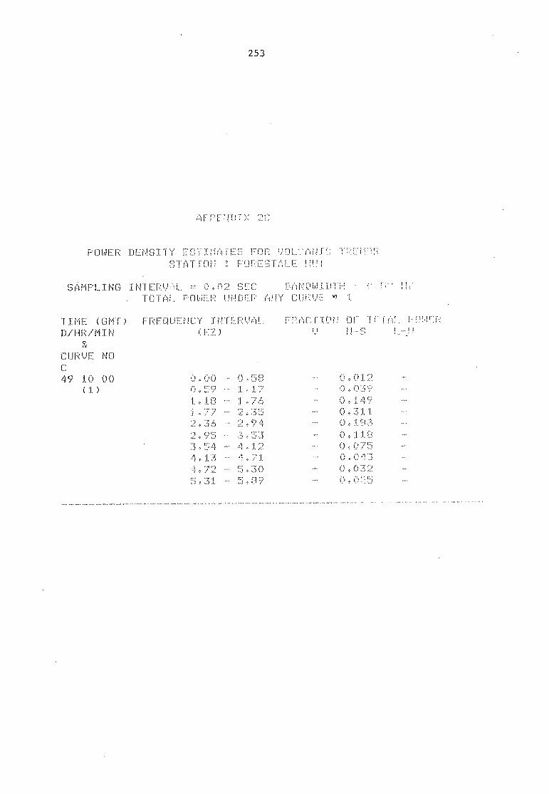
253
APPEnTX 2C
POWER DENSITY 1-0R VOLf:nNI STATION FORESTUF !Th!
SAMPLING INIERVL = 0,02 SEC BANDi.,HUTH • TOTAL POWER UNDEP ANY CURVE
IINE (GMT) FREQUENCY INTERVAL FPACTTN! OF INA!. D/HR/MIN (HZ)
CURVE NO
49 10 00 0.00 - 0,58 0,012 (1)
1,18 - 1,76 0,149 1,77 - 2,35 0,311 2.36 - 2.94 0,193 2,95 - 3,53 3,54 - 4,12 0,075 4,13 - 4,71 0,013 4,72 - 5.,30 0,032

254
APPENDIX 2D
POWER DENSTAY ESTIMATES FOR VOLCANIC TREMOR STATION MONTE S, MARTA
SAMPLING INTERVAL = 0,02 SEC BANDWIMH = 0,50 HZ TOTAL POWER UNDER ANY CURVE I
.TIME (GMT) D/HR/MIN
CURVE NO
FREqUENCY INTERVAL (HZ)
FRACTION 9F 1...; H'S
TOTAL POWER E-U
43 23 59 0,50 0.003 O,()()4
(1) 1,17 0, (.) :I. 0 , ()1.1 1,10 0^O86 O^131 0 , :I. ()
- 2,35 6 , 3 1. 7
3 0„J.T....) 0,108 0,121 -- 4,12 0,053 0,063 0,045
4,1.3 4,71 0,022 0,031 0,020 4.5 „ 3() 0 , (.P3 O,O17 () (),I.
5.31 -- 5,89 0,006 0,012 0,014
44 01. 59 0,00 - 0,50 0, (00:1. O,OO4 O,004 (2) 1,1/ () () :I. 0 0 1. 5 0.010
1,18 - 1,76 0 9 2 O,156 0,119 1,77 - 2,35 O^324 0 0,240 2,34 - 2.T4 O,294 O,222 0,207 Z^95 - 3,53 O^142 O.119 0,143 3,54 - 4,12 0,060 0,069 0,060 4.13 - 4,71 O , O37 0,031. 0,030
() , 016 0 , 015 5.31 - 5,89 0,007 0,013 0,016
44 03 59 0,00 - 0,58 O.002 0 () 0 4 C.) , 0 0 3. (3) 0,59 - 1.17 (*) 0 1. 9 O^O2O
1,18 - 4 () (.) 1^77 - 2.35 0,329 0,360 0,306 2,36 - 2,94 O^241 () , ()4 () , 21.3 2,95 - 3,53 O,142 () :I. 2 2 0 :I. 2 1. 3,54 - 1,12 0 0 6 3 0,064 4,13 - 4,71 0 0 3 () 0 , 0 3 1 () , 0 :3 6 4,72 - 5,30 0^O17 (,) 0 1 6 0 0 1. 9
5^89 0 0 0 11. 0 0 :1. 4 0 0 1 9
44 O5 59 „ ()0 •- O^58 O^OO2 O.002 0,003
(4) O^ ,17 0,018 0 4 0 1. 7 0 , 0 1 3 , •-• 1,76 0^110 O^115 0 0 9 9
1^7 2,35 2 2 0 0^3R9 O^278 , •-• 2 , 4 0 2 8 8 0,191 0,223
3.53 O^ 17() O,133 () :1. 6 4^12 O^072 () () () :7 5
, :1. 3 • -- 4 7 :I. 0 , 0 3 4 0 , 3 4 () , 0 4 3 4.72 0,015 0,019 0.022 5.31 - 5,09 0, 0 1 4 O.021

255
44 13 59 ( 5 )
„ ()()
|̂1O„
-- O.5O
•
„
-••
0 1. (3
O^
0 212
]33
2
0
, 1 .3
1..) 1 3'2 O, 069
.
O32 5 , 89 (.) I !^015 (.) ..).2 2
• •
44 15 59 • 0 , f.) 0 - 0 , 1..:.--;:::; 0 , (...!0'..:) ,.-..) , f.::: 0 :::.!: 0 , ̂(`O2
( ..) ) '...) , ',...',9 -• 1,17 1,18 -- 1. , '21.) f..) , ..........; :1. 1. 0 , 215
O ...........::3'...3
........'. , .;-..,-.'..-., -.. 2^'24 0 . ̀ ,.::: :i. '';;:.
',...! ...:....:::, •-• 3.53 0 , 11. 1-.3 ,..) (F ''l '.:.) .: .1. 1....?;
3,54 - 4,12 (..„, .,, 05'2 (.:, . ,......"(....-., 0 () „ 0 ,!,?'.....).
4,13 - 4,71 0 , ,....)....:_..:3
4.72 - 5 , 30 (.'„. , () :1. 1_ (.) , (,) 1. ',....). (...., , 0 :I.'?
5.31 -.. I.-..::, , 8?
. . . .
44 23 59 O^OO • O,58 O^0 , 1 5 0 , 0 !..)
(7) O^ ^17
1 ^18 ,139 O, O51
, „ • 3 0 1A:3 '1. O-1:33
, 1 4 ^13 , 4^72 5.3O 1.7 S.O58 O-016
«^016 0 E),
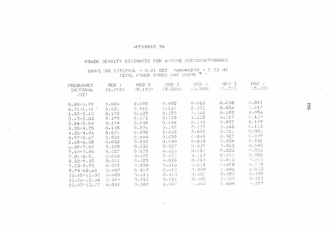
(NI
7:TO(. ;,-C.00 9''..T-9E4TT
0 I.-.00"0 S..•."T.T-1.;;;...?"0T
(.. .:::.0'..-0 4..000 t,9"0T-176'6
0.:, .. '.......T.f.....,, 11(1 Cl
TT(....."0 J.'1::."6-Z,Z.i$
o' c.
e..,Zi..0
.",S..‘.0''(2., SE0"0
9T0',..',
60"/..-62",..-.'
Tf...:-...:.' t.,.20'C 22W0 ovOvu 2t,0'0 220'0 82"9 -89'g
' TTT"0 041..0"6 S90'0 080"0 T.(..0'0 96"i/ -'n't,
C0 29T"0 .....'6T"0 :
,r..S0"6 i'*.A...7"C I Ot.T."0
S. .9"0 f....',.=C OT .J.:"0 I 06T"0 2C4E-2.T"1:::
TSOIO '."0 '..'2,cfT'0 (..'2.-0 ,ET"0 ,D.'..T"0 ZTZ-i...V'T
9200 TZ040 .
TTO"0 $000 OTO-(. SO0'0 S000 t.,00'0 04/"0-00"0
(-LH)
(C6T'E)
T .kr
HICIMCN TO"0 ONT1JPMS
d0A ),ITSNAG. dDMOd
XIGNDddV

TT0'0
000' C00 TT0'0
2T0"0 900'0 1,....T0"0
8T0''0 2.C.:0'0 82'5" -29"
220'0 620'0 c't,.0"0
..00 620,"0
H-T'0 Z90'0
60Tv0 CZT40 N:..50'0 Z.90'0
o D.DT's0 Z6.P0 OgT"0
222'0 2 Z2 I,0 0 " 0 90 t. 4 T °
8S0'0 EtiOvc. 890'0 2Z..0"0 5:60'0 tTT'0 Ttr"T-TZ.+0
20:Y0 600'0 ay..00'0 ZO0'0 OZ.°0 -00'0
Ln (7.H)
ODH T
27.-0 T0'0 ONTM:INVS
Aliswn dAMOd
Related Documents


