General rights Copyright and moral rights for the publications made accessible in the public portal are retained by the authors and/or other copyright owners and it is a condition of accessing publications that users recognise and abide by the legal requirements associated with these rights. Users may download and print one copy of any publication from the public portal for the purpose of private study or research. You may not further distribute the material or use it for any profit-making activity or commercial gain You may freely distribute the URL identifying the publication in the public portal If you believe that this document breaches copyright please contact us providing details, and we will remove access to the work immediately and investigate your claim. Downloaded from orbit.dtu.dk on: Apr 10, 2020 Microbial Enhanced Oil Recovery - Advanced Reservoir Simulation Nielsen, Sidsel Marie Publication date: 2010 Document Version Publisher's PDF, also known as Version of record Link back to DTU Orbit Citation (APA): Nielsen, S. M. (2010). Microbial Enhanced Oil Recovery - Advanced Reservoir Simulation. Kgs. Lyngby, Denmark: Technical University of Denmark.

Welcome message from author
This document is posted to help you gain knowledge. Please leave a comment to let me know what you think about it! Share it to your friends and learn new things together.
Transcript

General rights Copyright and moral rights for the publications made accessible in the public portal are retained by the authors and/or other copyright owners and it is a condition of accessing publications that users recognise and abide by the legal requirements associated with these rights.
Users may download and print one copy of any publication from the public portal for the purpose of private study or research.
You may not further distribute the material or use it for any profit-making activity or commercial gain
You may freely distribute the URL identifying the publication in the public portal If you believe that this document breaches copyright please contact us providing details, and we will remove access to the work immediately and investigate your claim.
Downloaded from orbit.dtu.dk on: Apr 10, 2020
Microbial Enhanced Oil Recovery - Advanced Reservoir Simulation
Nielsen, Sidsel Marie
Publication date:2010
Document VersionPublisher's PDF, also known as Version of record
Link back to DTU Orbit
Citation (APA):Nielsen, S. M. (2010). Microbial Enhanced Oil Recovery - Advanced Reservoir Simulation. Kgs. Lyngby,Denmark: Technical University of Denmark.
Sidsel Marie NielsenPh.D. ThesisJuly 2010
Microbial Enhanced Oil Recovery– Advanced Reservoir Simulation

Microbial Enhanced Oil Recovery
– Advanced Reservoir Simulation
Sidsel Marie Nielsen
Center for Energy Resources Engineering
Department of Chemical and Biochemical Engineering
Technical University of Denmark
Kongens Lyngby, Denmark

Technical University of DenmarkDepartment of Chemical and Biochemical EngineeringBuilding 229, DK-2800 Kongens Lyngby, DenmarkPhone +45 45252800, Fax +45 [email protected]
Copyright c© Sidsel Marie Nielsen, 2010ISBN -13: 978-87-92481-31-3Printed by Frydenberg A/S, Copenhagen, Denmark
2

Preface
This thesis is submitted as a partial fulfillment of the requirement for obtaining thePhD degree at the Technical University of Denmark (DTU). The work has mainlytaken place at the Center for Energy Resources Engineering and at the Department ofChemical and Biochemical Engineering at DTU. The duration of the PhD study wasthree years finishing August 2010. The project is partly financed by DONG Energy,Forsker Uddannelsesradet, and DTU in the MP2T graduate school. During my PhDstudy, I have been fortunate to have the opportunity to spend four months in 2009 atthe University of Southern California (USC), Los Angeles, USA.
During the course of the study, a number of people have provided their help and sup-port, for which I am very grateful. First of all, I would like to thank my supervisorsat DTU, Alexander A. Shapiro, Michael L. Michelsen and Erling H. Stenby, for theirguidance, encouragement and many valuable inputs, but most of all for their patienceand allowing me to pursue my own ideas and interest. A special thanks to my externalsupervisor Kristian Jessen and his family for the friendly welcoming during my stay atUSC. I am grateful for his guidance and many suggestions.I would also like to thank my dear colleagues at CERE for providing a fun and stimu-lating research environment, especially thanks for your encouragement when necessary.
Finally, I would like to thank my husband Kim and our son Esben for their patienceand for following me overseas to USC in Los Angeles to experience new things in a timethat had already been rich on experiences and challenges, being a newly started family.
Kongens Lyngby, July 2010
Sidsel Marie Nielsen
3

iv
4
Summary
In this project, a generic model has been set up to include the two main mechanismsin the microbial enhanced oil recovery (MEOR) process; reduction of the interfacialtension (IFT) due to surfactant production, and microscopic fluid diversion as a partof the overall fluid diversion mechanism due to formation of biofilm. The construction ofa one-dimensional simulator enables us to investigate how the different mechanisms andthe combination of these influence the displacement processes, the saturation profilesand thus the oil recovery curves.
The reactive transport model describes convection, bacterial growth, substrate con-sumption, and surfactant production in one dimension. The system comprises oil, wa-ter, bacteria, substrate, and surfactant. There are two flowing phases: Water and oil.We introduce the partition of surfactant between these two phases determined by a par-titioning constant. Another effect is attachment of the bacteria to the pore walls andformation of biofilm. It leads to reduction of porosity and, under some assumptions, toincrease the fraction of oil in the flow.
Surfactant is our key component in order to reduce IFT. The surfactant concentrationin the water phase must reach a certain concentration threshold, before it can reducethe interfacial tension and, thus, the residual oil saturation. The relative permeabilitiesdepend on the water phase concentration, so when surfactant is moved into the oilphase, the effect from the surfactant on the oil production is reduced. Therefore, thetransfer part of the surfactant to oil phase is equivalent to its “disappearance”. The oilphase captures the surfactant, but it may as well be adsorbed to the pore walls in theoil phase.
We have looked into three methods how to translate the IFT reduction into changes ofthe relative permeabilities. Overall, these methods produce similar results. Separateinvestigations of the surfactant effect have been performed through exemplifying simu-lation cases, where no biofilm is formed. The water phase saturation profiles are foundto contain a waterfront initially following the saturation profile for pure waterflooding.At the oil mobilization point – where the surfactant effect starts to take place – a suf-ficient surfactant concentration has been built up in order to mobilize the residual oil.A second waterfront is produced, and an oil bank is created. The recovery curve con-sists of several parts. Initially, the recovery curve follows pure waterflooding recoveryuntil breakthrough of the oil bank. The next part of the recovery curve continues until
5

vi Summary
breakthrough of the second waterfront. The incline is still relatively steep due to a lowwater cut. In the last part, the curve levels off.
Partitioning of surfactant between the oil and water phase is a novel effect in the contextof microbial enhanced oil recovery. The partitioning coefficient determines the time lagbefore the surfactant effect can be seen. The surfactant partitioning does not changefinal recovery, but a smaller partitioning coefficient gives a larger time lag before thesame maximum recovery is reached. However, if too little surfactant stays in the waterphase, we cannot obtain the surfactant effect.
The final recovery depends on the distance from the inlet to the oil mobilization point.Additionally, it depends on, how much the surfactant-induced IFT reduction lowersthe residual oil. The surfactant effect position is sensitive to changes in growth rate,and injection concentrations of bacteria and substrate, which then determine the finalrecovery. Variations in growth rate and injection concentration also affect the time laguntil mobilization of residual oil occurs. Additionally, the final recovery depends on,how much the surfactant-induced interfacial tension reduction lowers the residual oilsaturation. The effects of the efficiency of surfactants are also investigated.
The bacteria may adhere to the pore walls and form a biofilm phase. The bacteriadistribution between the water and biofilm phase is modeled by the Langmuir expression,which depends on the bacteria concentration in the water phase. The surface availablefor adsorption is scaled by the water saturation, as bacteria only adsorb from the waterphase. The biofilm formation implies that the concentration of bacteria near the inletincreases. In combination with surfactant production, the biofilm results in a highersurfactant concentration in the initial part of the reservoir. The oil that is initiallybypassed in connection with the surfactant effect, can be recovered as formation ofbiofilm shortens the distance from the inlet to the point of oil mobilization. The effectof biofilm formation on the displacement profiles and on the recovery is studied in thepresent work.
Formation of biofilm also leads to porosity reduction, which is coupled to modificationof permeability. This promotes the fluid diversion mechanism. A contribution to fluiddiversion mechanism is microscopic fluid diversion, which is possible to investigate ina one-dimensional system. The relative permeability for water is modified according toour modified version of the Kozeny-Carman equation. Bacteria only influence the waterand biofilm phases directly, so the oil phase remains the same. We have assessed theeffect from biofilm formation together with microscopic fluid diversion. When sufficientamount of surfactant is produced in the water phase, the effect from surfactant generatesa larger contribution to recovery compared to microscopic fluid diversion.
To study the MEOR performance in multiple dimensions, the one-dimensional modelwith the surfactant effect alone has been implemented into existing simulators; a stream-line simulator and a finite difference simulator. In the streamline simulator, the effectof gravity is introduced using an operator splitting technique. The gravity effect sta-bilizes oil displacement causing markedly improvement of the oil recovery, when theoil density becomes relatively low. The general characteristics found for MEOR inone-dimensional simulations are also demonstrated both in two and three dimensions.
6

vii
Overall, this MEOR process conducted in a heterogeneous reservoir also produces moreoil compared to waterflooding, when the simulations are run in multiple dimensions.
The work presented in this thesis has resulted in two publications so far.
7

viii
8
Resume
Formalet med denne afhandling er at konstruere en generel model, der inkluderer deto primære mekanismer i mikrobiel forbedret olie indvinding (MEOR); reduktion afolie-vand grænsefladespændingen (IFT) ved bakteriel produktion af surfaktant samtmikroskopisk fluid omdirigering ved dannelse af biofilm. Konstruktionen af en en-dimensionel simulator gør det muligt at undersøge, hvorledes de forskellige mekanismerpavirker fortrængningsprocessen, mætningsprofilen and herved olieindvindingskurven.
Den reaktive transport model beskriver konvektion, bakterievækst, næringsforbrug ogproduktion af surfaktant i en dimension. Systemet bestar af olie, vand, bakterier, næringog surfaktant. Der er to flydende faser: Olie og vand. Vi har introduceret fordeling afsurfaktant mellem olie- og vandfasen, hvor fordelingen er bestemt ved en fordelingskoef-ficient. En anden effekt er bakterieadsorption pa porevæggene, hvorved biofilm dannes.Dette fører til reduktion af porøsiteten, og under nogle antagelser øges fraktionen af oliei flowet.
Surfaktant er vores hovedkomponent, der reducerer IFT. Surfaktantkoncentrationen ivandfasen skal na en vis grænseværdi, før surfaktant kan sænke IFT og hermed ogsa denresiduale olie. Idet den relative permeabilitet afhænger af vandfasekoncentrationen afsurfaktant, vil effekten af surfaktant pa olieproduktionen mindskes, nar en fraktion afsurfaktant bevæger sig over i oliefasen. Det svarer det til, at surfaktantfraktionen, derer overført til oliefasen, er “forsvundet”. Surfaktantfraktionen, der er fanget i oliefasen,kan lige sa vel være adsorberet til porevæggen i oliefasen.
Vi har undersøgt tre metoder for at overføre reduktionen af IFT til ændring af denrelative permeabilitet. Totalt set, giver de tre metoder lignende resultater. Separateundersøgelser af surfaktant effekten er udført ved simuleringseksempler, hvori der ikkedannes biofilm. Vandmætningsprofilen karakteriseres ved en front, som ogsa opstar vedren vandinjektion. Ved oliemobiliseringspunktet, hvor effekten af surfaktant indtræder,er tilstrækkeligt med surfaktant dannet til at kunne mobilisere den residuale olie. En an-den vandfront dannes, mens en oliebanke opstar. Indvindingskurven bestar af flere dele.Første del af kurven følger profilen for ren vandinjektion ind til oliebankens gennem-brud. Den næste del af indvindingskurven forsætter indtil gennembruddet for den andenvandfront. Indvindingkurven er endnu stejl, idet oliefraktionen af produktionsvæskener høj. I den sidste del flader kurven ud.
I forbindelse med MEOR er fordeling af surfaktant mellem olie- og vandfasen en ny
9

x Resume
tilgang. Fordelingskoefficienten bestemmer tidsforsinkelsen, før effekten fra surfaktantindtræder. Surfaktantfordelingen ændrer ikke ved indvindingsgraden, men en mindrefordelingskoefficient medfører en større tidsforsinkelse, før den maksimale indvindingopnas. Dog kan surfaktanteffekten ikke opnas, hvis andelen af surfaktant, der forbliveri vandfasen, er for lille.
Det vises, at indvindingsgraden afhænger af afstanden fra injektionsbrønden til oliemo-biliseringspunktet. Desuden afhænger indvindingen af, hvor meget reduktionen af IFTkan sænke den residuale oliemætning. Positionen for surfaktanteffektens indtrædelseer følsom over for forandringer i den bakterielle væksthastighed samt injektionskoncen-trationerne af bakterier og næring, hvorfor dette bestemmer indvindingsgraden. Vari-ationer i bakterievæksthastigheden og injektionskoncentrationerne pavirker ogsa tids-forsinkelsen, før oliemobilisering sker. Indvindingsgraden afhænger desuden af, hvormeget den surfaktant-inducerede IFT sænker den residuale oliemætning. Effektivitetenaf surfaktant er ogsa undersøgt i afhandlingen.
Bakterier adsorberer til poreoverfladerne og danner biofilm. Ved at benytte Lang-muir udtrykket, der er en funktion af bakteriekoncentrationen i vandfasen, fordelesbakterierne fordeles mellem vand- og biofilmfasen. Overfladen af porerne, der er tilgæn-gelig for adsorption, er skaleret med vandmætningen, idet bakterier kun adsorbererfra vandfasen. Dannelse af biofilm medfører, at koncentrationen af bakterier nær injek-tionsbrønden stiger. I kombination med surfaktant produktion betyder biofilmdannelse,at der opnas en højere koncentration af surfaktant ved begyndelsen af reservoiret. Olie,som førhen blev forbigaet ved surfaktanteffekten alene, indvindes nu, idet dannelsenaf biofilm forkorter afstanden fra indgangen til oliemobiliseringspunktet. I denne sam-menhæng er effekten af surfaktant pa fortrængningsprofilerne samt olieindvindingenundersøgt.
Dannelse af biofilm bidrager ogsa til reduktion af porøsiteten, der pavirker perme-abiliteten. Dette fører til fluid omdirigeringsmekanismen. Et bidrag til fluid omdirige-ringsmekanismen er mikroskopisk fluid omdirigering, som er muligt at undersøge i voresen-dimensionelle system. Den relative permeabilitet for vand ændres i overensstemmelsemed vores modificerede Kozeny-Carman ligning. Bakterier pavirker vand- og biofilm-faserne direkte, mens oliefasen forbliver uændret. Ved hjælp af simuleringseksemplerhar vi undersøgt den kombinerede effekt af biofilm og mikroskopisk fluid omdiriger-ing. Nar surfaktant produceres i tilstrækkelige mængder i vandfasen, bliver effekten frasurfaktant betydeligt større sammenlignet med mikroskopisk fluid omdirigering.
For at undersøge MEOR processen i flere dimensioner, er den en-dimensionelle modelblevet implementeret i to eksisterende simulatorer; en strømningsliniesimulator og enfinite diffence simulator. I strømningslinie simulatoren er bidraget fra tyngdekrafteninkluderet ved at benytte operator opsplitning. Tyngdekraften stabiliserer fortrængnin-gen af olie, hvilket medfører forbedringer af olieindvindingsgraden, nar densiteten afolien er tilpas lav. De generelle karakteristika for MEOR processen i en dimension, sesogsa i bade to og tre dimensioner. Samlet set giver denne MEOR process, som er udførti et heterogent reservoir og er modelleret i flere dimensioner, en større produktion afolie sammenlignet med ren vandindjektion.
10

xi
Arbejdet, der er præsenteret i denne afhandling, har indtil videre resulteret i to pub-likationer.
11

xii
12

Contents
Preface iii
Summary v
Resume ix
1 Background 1
1.1 Introduction . . . . . . . . . . . . . . . . . . . . . . . . . . . . . . . . . . 11.2 Enhancement of oil production and recovery . . . . . . . . . . . . . . . . 31.3 Petroleum microbiology . . . . . . . . . . . . . . . . . . . . . . . . . . . 3
1.3.1 Physical factors . . . . . . . . . . . . . . . . . . . . . . . . . . . . 41.3.2 Chemical factors . . . . . . . . . . . . . . . . . . . . . . . . . . . 51.3.3 Microbial growth and nutrients . . . . . . . . . . . . . . . . . . . 61.3.4 Metabolites . . . . . . . . . . . . . . . . . . . . . . . . . . . . . . 71.3.5 Attachment and detachment processes . . . . . . . . . . . . . . . 71.3.6 Chemotaxis . . . . . . . . . . . . . . . . . . . . . . . . . . . . . . 8
1.4 MEOR mechanisms . . . . . . . . . . . . . . . . . . . . . . . . . . . . . 81.4.1 Results from laboratory and field trials . . . . . . . . . . . . . . 91.4.2 Reduction of oil-water interfacial tension . . . . . . . . . . . . . . 101.4.3 Fluid diversion . . . . . . . . . . . . . . . . . . . . . . . . . . . . 121.4.4 Reduction of oil viscosity . . . . . . . . . . . . . . . . . . . . . . 131.4.5 Compatibility . . . . . . . . . . . . . . . . . . . . . . . . . . . . . 14
1.5 Objectives . . . . . . . . . . . . . . . . . . . . . . . . . . . . . . . . . . . 161.6 Publications . . . . . . . . . . . . . . . . . . . . . . . . . . . . . . . . . . 17
2 The reactive transport model 19
2.1 Review of MEOR model approaches . . . . . . . . . . . . . . . . . . . . 192.2 The general model . . . . . . . . . . . . . . . . . . . . . . . . . . . . . . 21
2.2.1 Fractional flow function . . . . . . . . . . . . . . . . . . . . . . . 222.3 Specific model formulation . . . . . . . . . . . . . . . . . . . . . . . . . . 23
2.3.1 Assumptions . . . . . . . . . . . . . . . . . . . . . . . . . . . . . 242.3.2 Component mass balances . . . . . . . . . . . . . . . . . . . . . . 262.3.3 Relative Permeability . . . . . . . . . . . . . . . . . . . . . . . . 272.3.4 Reactions . . . . . . . . . . . . . . . . . . . . . . . . . . . . . . . 28
13
xiv Contents
2.3.5 Bacteria Partition . . . . . . . . . . . . . . . . . . . . . . . . . . 30
2.3.6 Surfactant Partition . . . . . . . . . . . . . . . . . . . . . . . . . 31
2.3.7 Porosity changes . . . . . . . . . . . . . . . . . . . . . . . . . . . 32
2.4 Implementation . . . . . . . . . . . . . . . . . . . . . . . . . . . . . . . . 33
2.4.1 General approaches . . . . . . . . . . . . . . . . . . . . . . . . . . 33
2.4.2 Reduction of oil-water interfacial tension . . . . . . . . . . . . . . 33
2.4.3 Permeability Modifications . . . . . . . . . . . . . . . . . . . . . 41
2.4.4 Microscopic fluid diversion . . . . . . . . . . . . . . . . . . . . . . 46
2.5 Summary of model . . . . . . . . . . . . . . . . . . . . . . . . . . . . . . 46
3 Solution procedure 49
3.1 Dimensionless form . . . . . . . . . . . . . . . . . . . . . . . . . . . . . . 50
3.2 Discretization scheme . . . . . . . . . . . . . . . . . . . . . . . . . . . . 51
3.3 Application of Newton-Raphson procedure . . . . . . . . . . . . . . . . . 52
4 One-dimensional simulations 57
4.1 Selection of parameters . . . . . . . . . . . . . . . . . . . . . . . . . . . 57
4.2 Verification of simulator . . . . . . . . . . . . . . . . . . . . . . . . . . . 61
4.3 Surfactant effect . . . . . . . . . . . . . . . . . . . . . . . . . . . . . . . 63
4.3.1 Characteristics due to surfactant effect . . . . . . . . . . . . . . . 63
4.3.2 Effect of surfactant partitioning . . . . . . . . . . . . . . . . . . . 65
4.3.3 Effect of growth rate . . . . . . . . . . . . . . . . . . . . . . . . . 66
4.3.4 Effect of substrate and bacterial injection concentrations . . . . . 67
4.3.5 Comparison of interpolation methods . . . . . . . . . . . . . . . 68
4.3.6 Effect of surfactant efficiency . . . . . . . . . . . . . . . . . . . . 70
4.4 Effect of biofilm formation . . . . . . . . . . . . . . . . . . . . . . . . . . 72
4.4.1 Parameters revisited . . . . . . . . . . . . . . . . . . . . . . . . . 72
4.4.2 Effect of bacteria adsorption . . . . . . . . . . . . . . . . . . . . 73
4.4.3 Effect of water relative permeability . . . . . . . . . . . . . . . . 75
4.4.4 Assumption about constant viscosities . . . . . . . . . . . . . . . 77
4.5 Combination of mechanisms . . . . . . . . . . . . . . . . . . . . . . . . . 79
4.5.1 Parameters revisited . . . . . . . . . . . . . . . . . . . . . . . . . 79
4.5.2 Biofilm formation with surfactant effect . . . . . . . . . . . . . . 79
4.5.3 Microscopic fluid diversion with surfactant effect . . . . . . . . . 80
4.6 Summary of 1D results . . . . . . . . . . . . . . . . . . . . . . . . . . . . 82
5 Streamline simulations 85
5.1 Introduction . . . . . . . . . . . . . . . . . . . . . . . . . . . . . . . . . . 86
5.2 The multi-dimensional model . . . . . . . . . . . . . . . . . . . . . . . . 86
5.2.1 Solution methods . . . . . . . . . . . . . . . . . . . . . . . . . . . 87
5.2.2 Gravity . . . . . . . . . . . . . . . . . . . . . . . . . . . . . . . . 89
5.3 Parameters . . . . . . . . . . . . . . . . . . . . . . . . . . . . . . . . . . 90
5.4 Verification of implementation . . . . . . . . . . . . . . . . . . . . . . . . 93
5.5 Comparison of 2D results . . . . . . . . . . . . . . . . . . . . . . . . . . 93
5.6 The MEOR characteristics . . . . . . . . . . . . . . . . . . . . . . . . . . 95
5.7 Simulations in 2D with gravity effect . . . . . . . . . . . . . . . . . . . . 95
5.8 Simulations in 3D with gravity effect . . . . . . . . . . . . . . . . . . . . 97
14

Contents xv
5.9 Summary of multidimensional results . . . . . . . . . . . . . . . . . . . . 99
6 Conclusion 101
7 Future work 105
A Parameters in Langmuir expression 107
B Multivariable Newton iteration 109
C Analytical solution of Buckley-Leverett equation 111
Nomenclature 113
Bibliography 117
15

xvi Contents
16
Chapter 1
Background
The purpose of this chapter is to set the basis for the modeling work presented in the
following chapters. The chapter introduces the microbiology of a petroleum reservoir
and the microbial enhanced oil recovery (MEOR) explaining the mechanisms that are
responsible for the enhancement of oil recovery. Results from laboratory experiments
and field trials are also presented to highlight the potential of the MEOR. The chapter
is rounded off with presenting the objectives for this PhD project.
1.1 Introduction
The principle source of fluid fuels is the hydrocarbon resources. The finite nature of our
hydrocarbon reserves has been discussed as discoveries of new oil reservoirs decrease.
For the present techniques of oil recovery, a large amount of oil remains in the reservoir
after secondary flooding, where the oil reservoirs must be abandoned as the production
is no longer economically feasible. Methods of enhanced oil recovery (EOR) have been
developed, but they are often considered economically unattractive (Green and Willhite,
1998; Lazar et al., 2007; Maudgalya et al., 2007; Sen, 2008). In several cases, MEOR
has shown its potential as a tertiary oil recovery method. The microorganisms require
only cheaper substrates to perform MEOR, so from an economical point of view, the
process itself is affordable compared to other EOR processes (Maudgalya et al., 2007;
Lazar et al., 2007).
A long-term goal is to be able to design a robust MEOR process. This task can seem
cumbersome, since microorganisms are involved in multiple mechanisms at the same
17

2 Background
time and they can change physiology in response to fluctuations in their surroundings
(Van Hamme et al., 2003; Sen, 2008). Together with experimental procedures such as
core floodings and field trials, a step on the way is the development of simulation tools
in order to understand and reveal the full potential of MEOR.
ZoBell (1947) was one of the pioneers in MEOR, where residual oil was recovered by
application of microorganisms. Since then many researchers has performed MEOR
laboratory experiments and field tests with different degrees of success (Lazar et al.,
2007; Maudgalya et al., 2007). The most active applications of the MEOR process are
as listed below (Bryant and Burchfield, 1989; Brown, 1992; Maudgalya et al., 2007;
Amro, 2008; Rafique and Ali, 2008).
• Use of microbial systems for permeability modification to improve water flooding
sweep efficiency.
• Use of microorganisms to produce gas, surfactant, acids and alcohols improving
recovery in the course of flooding throughout the reservoir
• Single-well stimulation: treatment of a wellbore zone for removal of near-wellbore
paraffin deposits or other consituents leading to formation damage, or for oil
mobilization in the region around the wellbore.
Our focus is chosen within the two first applications, where MEOR flooding is looked
into. The field trials have generally shown improvement of oil production or oil recov-
ery, but there have been very fluctuating improvements of oil recovery, and the technical
performance in many field trials has been inconsistent (Youssef et al., 2007; Maudgalya
et al., 2007). Major improvements of recovery have been found in laboratory experi-
ments, while smaller improvements have been found in the field trials (Maudgalya et al.,
2007).
Bryant and Lockhart (2002) and Gray et al. (2008) present in their work a critical
analysis of MEOR. They have performed an assessment analysis based on estimates for
each MEOR mechanism using general reactor analysis and mass balance calculations.
They conclude that only a small part of the mechanisms taking place during MEOR,
have any prospect for enhancing oil recovery. More likely combination of the mechanisms
can lead to a significant enhancement of oil recovery. Generally, further studies are
required in order to perform a more complete assessment of the MEOR process (Gray
et al., 2008).
18

1.2 Enhancement of oil production and recovery 3
1.2 Enhancement of oil production and recovery
The goal of the EOR methods is to recover more oil from the underground oil fields. In
the literature, the oil recovery and the enhancement of the oil production are measured
in several ways. For instance, the enhancement is ’extra oil recovered in relation to
residual oil after waterflooding’, ’extra oil recovered in relation to the original oil in
place’, ’reduction of watercut’, or ’increased oil production’.
In this work, we choose to use oil recovery as the oil that has been recovered over the
original oil in place (OOIP):
oil produced
original oil in place· 100 = %OOIP (1.1)
We attempt to present oil recoveries as % OOIP or the increment in oil recovery over
that of waterflooding, still using increment in OOIP.
1.3 Petroleum microbiology
Many kinds of microorganisms are found within the reservoir. Regarding indigenous mi-
croorganisms, Magot et al. (2000) emphasize that anaerobic microorganisms are consid-
ered true inhabitants. Anaerobes ferment and cannot use oxygen as O2 for respiration,
and for strict anaerobes, the presence of oxygen is toxic. Both aerobic and faculta-
tively aerobic microorganisms have also been found. The aerobes can respire, while the
facultative aerobes are able to grow either as aerobes or anaerobes determined by the
nutrient availability and environmental conditions (Madigan et al., 2003). Regarding
the presence of aerobes and facultative aerobes, the role as true inhabitants is uncertain
and thus considered contamintants. Contaminant microorganisms are transferred to the
reservoir through fluid injection or during drilling devices (Magot et al., 2000).
Concerning the anaerobic condition in the reservoir and the difficulty in supplying oxy-
gen, it is regarded more feasible to inject anaerobic species such as Clostridium instead
of aerobic species such as e.g. Pseudomonas (Jang et al., 1984; Aslam, 2009a). The
applicability of Pseudomonas in a MEOR process is questionable, even though it is a
hydrocarbon-degrading bacteria, able to survive with oil as the primary carbon source
(Blanchet et al., 2001; Aslam, 2009a).
Commonly used bacterial species are Bacillus and Clostridium. The Bacillus species
produce surfactants, acids and some gases, and Clostridium produce surfactants, gases,
alcohols and solvents. Few Bacillus species also produce polymers. Microorganisms
that have been used for MEOR, are listed in table 1.1 (Bryant and Burchfield, 1989).
Bacillus and Clostridium are often able to bear extreme conditions existing in the oil
19

4 Background
Table 1.1: Bacteria that are used in MEOR and their products (Bryant and Burchfield, 1989).Facultative means that the organism can grow with or without the presence of oxygen.
Family Respiration type Products
Clostridium Anaerobic Gases, acids, alcohols andsurfactants
Bacillus Facultative Acids and surfactants
Pseudomonas Aerobic Surfactants and polymers,can degrade hydrocarbons
Xanthomonas Aerobic Polymers
Leuconostoc Facultative Polymers
Desulfovibrio Anaerobic Gases and acids, sulfate-reducing
Arthrobacter Facultative Surfactants and alcohols
Corynebacterium Aerobic Surfactants
Enterobacter Facultative Gases and acids
reservoirs. The survival originates from the ability to form spores. The spores are dor-
mant, resistant forms of the cells (Bryant and Burchfield, 1989), which can survive in
stressful environments exposing them to high temperature, drying, and acid. The dura-
tion of the dormancy can be extremely long and yet the survival rate is large (Madigan
et al., 2003).
Microorganisms are complex in their way of responding to the surrounding environ-
ment. The cells change physiological state in order to have optimal chances for survival
meaning that substrate consumption, growth and metabolite production may change
significantly (Van Hamme et al., 2003).
Microorganisms present in an oil reservoir or other porous media are subjected to many
physical (temperature, pressure, pore size/geometry), chemical (acidity, oxidation po-
tential, salinity) and biological factors (cell processes) (Marshall, 2008). The most im-
portant cellular processes are growth, cell decay, chemotaxis, and cell attachment and
detachment to pore walls (Ginn et al., 2002). Often, the microorganisms are considered
as a black box, where only the important substrates and metabolites are taken into
account (Nielsen et al., 2003).
1.3.1 Physical factors
The oil reservoirs are harsh environments for microorganisms. The reservoir tempera-
ture can be up to 150 ◦C. Data suggest that microorganisms may grow at temperatures
20
1.3 Petroleum microbiology 5
below 82 ◦C as microorganisms were only isolated from reservoirs below this tempera-
ture (Magot et al., 2000). The microorganisms depend on their enzyme function. High
temperatures can disrupt the enzyme function due to denaturation or disruption around
the catalyzing sites (Marshall, 2008; Madigan et al., 2003). The effect obtained from
the high pressure is more indirect as changes in gene expression and protein synthesis
occur (Marshall, 2008) and thus influence the physiological and metabolic state (Magot
et al., 2000).
The pore size is a physical constraint for microorganisms to penetrate the reservoir.
Bacteria are mainly applied because of their small size around 2 μm (Madigan et al.,
2003). For instance, the size of a specific Bacillus strain rod is 4 × 1.5 μm (Sharma and
Georgiou, 1993). For tight reservoirs, bacteria might be in the same order of magnitude
as the pores. Penetration of bacteria is regarded possible in reservoirs with minimum
pore diameters of at least 2 μm (Marshall, 2008) and preferably from 6–10 μm (Sharma
and Georgiou, 1993, estimated from filtration theory).
1.3.2 Chemical factors
The pH in the reservoir is often as low as 3–7 as the high pressure lets gases dissolve in the
fluids (Magot et al., 2000). The acidity determines the microbial surface charge affecting
the bacteria transport trough the reservoir. The bacterial growth rate is reduced by
acidity, where the ionization of membrane transport proteins can alter the transport
efficiency (Marshall, 2008).
The transport of the bacteria depends on physiology. If the bacterial surface is solely
hydrophobic, the bacteria tend to stick together and will be transported in flocs. On the
other hand, the hydrophilic bacteria will more often flow as single bacteria (Crescente
et al., 2006).
The water existing in the reservoir is fresh to salt-saturated water being a combination
of connate reservoir water and injected saline sea water. The salinity influences the
growth, where the microorganisms have to sustain the optimal salinity of cellular fluids
to maintain enzymatic action (Madigan et al., 2003).
A thermodynamically favorable oxidation potential are crucial for microbial survival.
For bacterial growth to take place, electron donors and acceptors must be present, where
they become oxidized and reduced in the biochemical processes, respectively. In aerobic
respiration, oxygen as O2 is the terminal electron acceptor, where large amounts of
energy are obtained used in growth and maintenance processes. When oxygen is not
present, only anaerobic processes occur. Specific for the petroleum reservoir, the redox
potential is very low and electron acceptors such as ferric ion, nitrate and sulfate are
21

6 Background
utilized. The water contains sulphate and carbonate at various concentrations, which
have led to assume that the major metabolic processes occurring naturally are sulfate
reduction, methanogenesis, acetogenesis and fermentation (Magot et al., 2000; Marshall,
2008).
1.3.3 Microbial growth and nutrients
The microbial growth is determined by the presence of different nutrients. Cell nutrient
requirements are wide, but some nutrients are required in larger amounts than others.
The primary nutrients consumed is carbon and nitrogen, which are the main constituent
parts of the cell and enter many cell processes (Madigan et al., 2003). The substrates
for growth of hydrocarbon-degrading bacteria include different crude oil components
such as n-alkanes, homocyclic aromatic compounds, polycyclic aromatic compounds,
nitrogen and sulfur heterocyclics (Van Hamme et al., 2003).
The large requirements for carbon and nitrogen cause these compounds to be limiting
nutrients, and thereby determine the growth rate. However, if the substrate concen-
tration is too high, then substrate inhibition may occur (Nielsen et al., 2003). Other
essential nutrients are phosphorus, sulfur, potassium and magnesium, and they are re-
quired in a much smaller amount (Madigan et al., 2003).
Trace elements such as e.g. iron, zinc and manganese are critical to cell function even
though the amount required is small. The trace elements play a structural role in
various enzymes and catalysts. However, as only tiny amounts are required, the natural
occurrence is abundant. Other essential compounds for some organisms are vitamins
and amino acids, which are required only in small amounts as they are important for
enzymatic function (Madigan et al., 2003).
If microbial transport happens over a large distance in the reservoir then the injec-
tion of nutrients should be performed, so the nutrient supply is kept at a reasonable
concentration. It should be taken into account that the transport differs for nutrients
and microorganisms (Bryant and Burchfield, 1989). Especially, the effect from dilution
should be considered, when the nutrient mix with the reservoir water.
Inside the bacteria, many processes take place, catalyzed by different complexes. Proper
function of these complexes in order for the bacterium to survive, requires energy for
maintenance. Often, maintenance is negligible compared to the energy spent for growth
and metabolite production, but occasionally a significant part of the energy goes to
maintenance. As an example, some bacteria in a highly acidic environment spends
large amounts of energy to sustain the optimal pH within the cell (Nielsen et al., 2003).
22
1.3 Petroleum microbiology 7
1.3.4 Metabolites
Some conditions will promote one kind of metabolites while other conditions promote
a whole different set of metabolites. Maintaining a certain physiological state of mi-
croorganisms in oil reservoirs could be difficult as many uncertainty factors exist (Van
Hamme et al., 2003). For microorganisms producing a certain metabolite, the possi-
bility for the metabolite inhibiting growth and its own metabolite production occurs
(Nielsen et al., 2003), so a necessary metabolite concentration can not be reached.
The metabolites include biosurfactants, biopolymers, solvents, acids and gases as listed
in table 1.1 (Van Hamme et al., 2003). As an example, a commonly produced acid is
acetate, but benzoate, butyrate, formate and propionate are also found (Magot et al.,
2000).
1.3.5 Attachment and detachment processes
The porous media has a large surface area to volume. This leads to much contact with
the surface during transport of components. Nutrients usually do not adsorb markedly,
but a metabolite such as surfactant exists in smaller amounts and has a greater tendency
to adsorb. Nutrients and metabolites will to a lesser extent also attach to pore wall,
compared to bacteria (Kim, 2006).
1.3.5.1 Formation of biofilm
Bacteria generally stick to all kind of surfaces forming biofilms (Characklis and Wilderer,
1989; Shafai and Vafai, 2009). Biofilm consists of a number of immobile cells, sticky
polysaccharides, dissolved components, particular material and water. The water con-
stitutes a large part of the biofilm. The biofilm acts as a micro-environment, where
the biofilm matrix water exchanges solutes such as nutrients and waste products with
the surroundings. There may be limitation of transport to and from the biofilm. This
is mainly determined by the thickness of the biofilm and the internal biofilm porosity
(Thullner, 2009).
Bacteria such as Pseudomonas form biofilm with only one layer of cell, where other
species form multilayered biofilms (Characklis and Wilderer, 1989). The multilayered
biofilms can form large mushroom shapes valving from the surface, in order to increase
the surface area for solute transport to and from the biofilm (Characklis and Wilderer,
1989; Thullner, 2009). The bacterial growth in the adsorbed phase is occasionally lower,
which is considered a consequence of the limitations in transport of nutrient (Murphy
and Ginn, 2000).
23
8 Background
In the context of porous media, the bacteria size may not be much smaller than the
pore size. Thus, the pore size may also constrain how many layers of cell a biofilm
can be composed of. If pore sizes are small, biofilm accumulation can be enhanced by
the process of filtration (Characklis and Wilderer, 1989), but otherwise the retention of
bacteria is primarily determined by the adsorption process (Stevik et al., 2004).
Kim (2006) suggests that attachment to the pore walls is a process that primarily
depend on the properties of media, rock surface and cell surface. Some studies suggest
that microorganisms perform active adhesion/detachment processes as a response to
the local nutrient availability and as a survival mechanism (Ginn et al., 2002; Rockhold
et al., 2004). Detachment from the biofilm is also caused by erosion, which is the removal
of small particles from the surface of the biofilm caused by shear stresses (Characklis
and Wilderer, 1989).
1.3.6 Chemotaxis
Chemotaxis is a part of the cell response to a chemical gradient for motile bacteria.
Bacteria move toward an increasing concentration of beneficial substances such as nu-
trients and away from detrimental substances such as toxins (Sen et al., 2005; Kim,
2006). The movement requires energy as the bacteria use their flagellar motor in order
to tumble towards direction of e.g. the nutrient (Valdes-Parada et al., 2009). Therefore
chemotaxis is strongly coupled to the bacterial growth rate (Ginn et al., 2002). In the
context of oil reservoirs, chemotaxis may take place by motile bacteria, but the effect
from chemotaxis is regarded minimal.
1.4 MEOR mechanisms
The MEOR process applies microorganisms that are already present in the reservoir or
microorganisms that are adapted to the harsh environment. Injection of microorganisms
is performed in order ensure growth and production of specific metabolites.
Indigenous microorganisms are mostly activated by injection of substrates, whereas
exogenous microorganisms are injected with their substrates or in between slugs of sub-
strates. Regarding continuous injection, the plugging of the reservoir injection well
becomes an issue if the microbial injection concentration is too high (Aslam, 2009a). To
keep the cost low, the selected media is generally molasses, corn syrup or other indus-
trial waste products (Bryant and Burchfield, 1989; Lazar et al., 2007; Aslam, 2009a).
However, the application of cheaper substrates would require quality control (Bryant
and Burchfield, 1989).
24
1.4 MEOR mechanisms 9
The microorganisms penetrates the reservoir, while they consume substrates, grow pro-
duce different important metabolites. A combination of different mechanisms rely on
the microbes or their metabolites to mobilize residual oil or improve the areal sweep.
The most important MEOR mechanisms are listed below.
• Reduction of interfacial tension and alteration of wettability due to in situ surfac-
tant production
• Fluid diversion due to microbial growth and polymer production (bacterial plug-
ging)
• Viscosity reduction of oil by degradation oil components or gas production
The latter mechanisms is mainly regarded a beneficial side effect, but can partly con-
tribute to increase the oil production (Jenneman et al., 1984; Banat, 1995; Bryant and
Burchfield, 1989; Bryant et al., 1989; Chisholm et al., 1990; Sarkar et al., 1994; Desouky
et al., 1996; Vadie et al., 1996; Delshad et al., 2002; Feng et al., 2002; Maudgalya et al.,
2007; Gray et al., 2008; Sen, 2008; UTCHEM, 2000).
During experimental work multiple processes takes place at the same time, so the mecha-
nisms can be difficult to separate from each other (Maudgalya et al., 2007). Some studies
are set-up mainly to investigate one MEOR mechanism, but it is still not possible to
ascribe the enhancement of oil recovery entirely to one mechanism.
The energy-rich nutrients such as sugars are easy to consume, which is why these nutri-
ent are the first to be consumed by the microorganisms. Therefore, viscosity reduction
of oil mainly occurs, when oil is the carbon source for bacterial growth. Generally, when
nutrients are injected, reduction of interfacial tension and fluid diversion are the main
mechanisms to take place, while viscosity reduction becomes more important during
MEOR with oil as the sole carbon source.
1.4.1 Results from laboratory and field trials
MEOR floodings conducted in the laboratory are generally more successful than the field
trials. The flooding experiments are restricted in size and performed under controlled
conditions in a limited time range. As an advantage, the laboratory experiments have
the possibility for fine tuning the process. MEOR floodings in the laboratory obtain
extra oil recoveries up to 20% OOIP over that of waterflooding (Jang et al., 1984;
Bryant and Douglas, 1988; Bryant et al., 1989; Chisholm et al., 1990; Deng et al., 1999;
Sugihardjo and Pratomo, 1999; Feng et al., 2002; Mei et al., 2003; Ibrahim et al., 2004;
Feng et al., 2006; Crescente et al., 2006; Amro, 2008; Zhaowei et al., 2008; Samir et al.,
2010).
25

10 Background
Field trials run for a longer time, but often the MEOR process has not run long enough
to utilize the full potential. Therefore, success is measured as an increase in the oil
production and a decrease in water cut instead of showing what final recovery achieve-
ments, when the maximum MEOR recovery is reached (Maudgalya et al., 2007). The
good performance should also show that the effect from MEOR extends for a sufficient
period of time confirming the stability of the MEOR implementation (Segovia et al.,
2009). As an example, Gullapalli et al. (2000) conducted a field trial for 8 months and
the biofilm formed within the reservoir was still stable after these months indicating
that the biofilm could remain stable, but no long term effect was investigated.
Conclusions on stability and the MEOR performance should be based on results that
also include the long term effect (Portwood, 1995; Maudgalya et al., 2007; Brown, 2010).
Field trials have been performed with different degrees of success (Bryant and Douglas,
1988; Grula et al., 1989; Jenneman, 1989; Streeb and Brown, 1992; Buciak et al., 1995;
Dietrich et al., 1996; Deng et al., 1999; Gullapalli et al., 2000; Maure et al., 2001;
Brown and Vadie, 2002; Nagase et al., 2002; Feng et al., 2002; Hitzman et al., 2004;
Maure et al., 2005; Feng et al., 2006; Maudgalya et al., 2007; Zhaowei et al., 2008; Bao
et al., 2009). Portwood (1995) presents the evaluation of 322 field trials conducted in
USA. The MEOR process is found successful in 78 % of the trials demonstrating that
a decrease in the oil production decline rate. The oil production has increased with an
average of 36 %. During the unsuccessful field trials, there was no apparant effect from
MEOR.
Other field trials showed around up to 25 % increase in oil production (Vadie et al.,
1996; Hitzman et al., 2004). Brown and Vadie (2002) present their field results, where
8 out of 15 wells show a positive response to MEOR. No effect from MEOR is seen on
the remaning wells. Two of these wells are considered uneconocmical and thus closed.
Based on estimations of the pre-MEOR and MEOR decline curves, the increment in oil
recovery is expected to be 3–4 % OOIP.
1.4.2 Reduction of oil-water interfacial tension
Microorganisms produce surfactants as secondary metabolites. The surfactants are in-
volved in different cell processes: Transport of water-insoluble compounds into the cell,
biofilm formation and adhesion of cell on different surfaces. Specifically, hydrocarbon-
oxidizing bacteria always produce surfactants in order to promote hydrocarbon pene-
tration into the cells (Nazina et al., 2003).
Surfactants are biphilic molecules consisting of a hydrophilic and a hydrophobic part.
Surfactants interact with; each other, surfaces with different polarity, adsorb at water-
air and water-oil boundaries and cause wetting of hydrophobic surfaces. They may
26
1.4 MEOR mechanisms 11
also form structures that resemble lipid films or membranes and reduces the surface
and interfacial tensions (IFT) of solutions (Nazina et al., 2003). Surfactant lowers IFT
and mobilizes oil that cannot be displaced by water alone (Chisholm et al., 1990; Zekri
and Almehaideb, 1999; Sen, 2008). The formed oil-in-water emulsion flows having a
improvement of the effective mobility ratio until unfavorably conditions occurs, where
the surfactant is diluted or lost due to adsorption to the pore wall (Sen, 2008).
Generally, oil-water systems have IFT around 30 mN/m (Bryant and Burchfield, 1989;
McInerney et al., 2005; Gray et al., 2008; Crescente et al., 2008). Experimental work
has shown that surfactants can lower the oil-water IFT to around 10−3 mN/m (Bryant
and Burchfield, 1989; Sharma and Georgiou, 1993; Crescente et al., 2008). Ghojavand
et al. (2008) find an IFT at 0.1 mN/m, which corresponds to a two orders of magnitude
reduction, but this tends to be the typical reduction (Gray et al., 2008). It should
be mentioned the existence of cases with only a 5–30 % reduction of IFT, but this is
also achieved using oil as the sole carbon source (Sugihardjo and Pratomo, 1999; Halim
et al., 2009). Green and Willhite (1998) recommend that IFT for chemical surfactant
flood should be from 10−2 to 10−3 mN/m, while Gray et al. (2008) propose that the oil
recovery will be improved, when IFT is reduced to 0.4 mN/m and lower.
During surfactant flooding, a major problem is adsorption of surfactant to the rock
surface. Thus, the efficient concentration of surfactant decreases resulting in a concen-
tration possibly lower than required. This problem exists during the MEOR process,
but it is regarded limited, when the surfactant is produced in situ. With the thorough
penetration of microorganisms into the reservoir, a locally high surfactant concentration
can be achieved (Jenneman et al., 1984; Chisholm et al., 1990; Sunde et al., 1992; Zekri
and Almehaideb, 1999).
Researchers present different results from their experimental work, where some studies
only have minor IFT reductions (McInerney et al., 2005; Kowalewski et al., 2006) and
only a little or no improvement of recovery, while others have presented major IFT
reductions together with good incremental recoveries from 2 to 20 % OOIP (Bryant
and Douglas, 1988; Deng et al., 1999; Feng et al., 2002; Bordoloi and Konwar, 2008). In
the experiments, the effect from the surfactant can only be partly ascribed to surfactant
production as other mechanisms interfere. Still, the surfactant effect is investigated in
both the laboratory and in the fields, where the latter is expected to result in only
moderate performances.
The effect from the surfactant can be obtained, when a certain threshold concentration
is achieved (critical micelle concentration), but some researchers questions whether is
possible actually to achieve the required amounts of surfactant (Bryant and Lockhart,
2002; Gray et al., 2008). To mobilize oil, the general engineering criteria is that the
surfactant concentration should be 10-20 mg/l (Youssef et al., 2007). Field tests show
27
12 Background
surfactant concentrations in the production fluids to be around 90 mg/l (Youssef et al.,
2007) and 210–350 mg/l (McInerney et al., 2005). Fortunately, these results reveal that
surfactant actually can be produced in the oil fields at much higher concentrations than
are needed. Thus, it shows that the effect from surfactant has the potential to be an
efficient MEOR mechanism (McInerney et al., 2005).
1.4.3 Fluid diversion
The theory of fluid diversion or selective plugging is applicable in an oil reservoir with
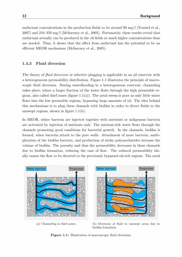
a heterogeneous permeability distribution. Figure 1.1 illustrates the principle of macro-
scopic fluid diversion. During waterflooding in a heterogeneous reservoir, channeling
takes place, where a larger fraction of the water flows through the high permeable re-
gions, also called thief zones (figure 1.1(a)). The areal sweep is poor as only little water
flows into the low permeable regions, bypassing large amounts of oil. The idea behind
this mechanisms is to plug these channels with biofilm in order to divert fluids to the
unswept regions, shown in figure 1.1(b).
In MEOR, either bacteria are injected together with nutrients or indigenous bacteria
are activated by injection of nutrients only. The nutrient-rich water flows through the
channels promoting good conditions for bacterial growth. In the channels, biofilm is
formed, when bacteria attach to the pore walls. Attachment of more bacteria, multi-
plication of the biofilm bacteria, and production of sticky polysaccharides increase the
volume of biofilm. The porosity and thus the permeability decreases in these channels
due to biofilm formation, reducing the ease of flow. The reduced permeability ide-
ally causes the flow to be diverted to the previously bypassed oil-rich regions. The areal
ProductionWater injection
(a) Channeling in thief zones.
Water injection Production
Biofilm
(b) Diversion of fluid to unswept areas due tobiofilm formation.
Figure 1.1: Illustration of macroscopic fluid diversion.
28

1.4 MEOR mechanisms 13
sweep efficiency has increased and, hence, the oil recovery is improved (Updegraff, 1983;
Jenneman et al., 1984; MacLeod et al., 1988; Bryant and Burchfield, 1989; Kowalewski
et al., 2006; Sen, 2008; Aslam, 2009a,b).
In order to apply fluid diversion successfully, several criteria should be fulfilled (Jenne-
man et al., 1984). It depends on:
1. Controlled penetration of microorganisms throughout the reservoir
2. Controlled transport of nutrients for microbial growth and metabolism
3. Reduction of the apparent permeability of the reservoir rock as a result of microbial
growth and metabolism
The risk of bacterial plugging is occurrence of undesirable plugging especially in the well
bore region (Jack et al., 1989; Gray et al., 2008; Aslam, 2009a), which can generally
lead to damages to the reservoir, reducing the oil production (Lazar et al., 2007).
The mechanisms of fluid diversion are investigated both in the laboratory and in the
field trials, where extra oil is recovered. Tracer tests confirm that fluid diversion does
occur (Nagase et al., 2002; Aslam, 2009b). Laboratory experiments find that the average
permeability is reduced by 20–70 % (Gandler et al., 2006; Aslam, 2009b). Raiders et al.
(1985, 1986) found a significant reduction of permeability together with an incremental
oil recovery over that of water flooding at 5–20 % OOIP.
For practical application of fluid diversion, nutrients with bacteria or nutrients solely for
the indigenous bacteria are injected into the reservoir. Then the reservoir is shut down
for a period of time in order to let the bacteria grow and plug the selected thief zones.
Post-flush is waterflooding or nutrient flooding to recover the previously bypassed oil
(Sugihardjo and Pratomo, 1999; Gullapalli et al., 2000).
1.4.4 Reduction of oil viscosity
The reduction of oil viscosity occurs due to effects such as bacterial degradation of oil
or dissolution of components such as surfactants or solvents into the oil phase. The oil
mobility is improved by a reduction of oil viscosity (Brown, 1992; Deng et al., 1999). .
Peihui et al. (2001) conduct flooding experiments injecting bacteria into cores, where
sole carbon source (substrate) is oil components. Concurrently, growth happens on
behalf of digestion of the oil components. The viscosity of crude oil is reduced from
28 mPa·s to 18 mPa·s together with a reduction of IFT from 36 mN/m to 8 mN/m. A
chromatographic analysis shows that the ratio between light and heavy oil components,∑C21−/
∑C21+, increases 54 % due to bacterial degradation of oil components.
29
14 Background
The corefloodings reveal an incremental oil recovery of 10 % OOIP over that of water-
flooding, eventhough a part of the oil is lost due to bacterial digestion (Peihui et al.,
2001).
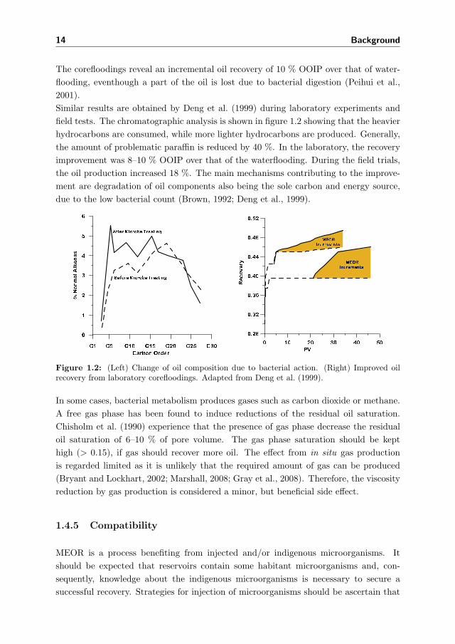
Similar results are obtained by Deng et al. (1999) during laboratory experiments and
field tests. The chromatographic analysis is shown in figure 1.2 showing that the heavier
hydrocarbons are consumed, while more lighter hydrocarbons are produced. Generally,
the amount of problematic paraffin is reduced by 40 %. In the laboratory, the recovery
improvement was 8–10 % OOIP over that of the waterflooding. During the field trials,
the oil production increased 18 %. The main mechanisms contributing to the improve-
ment are degradation of oil components also being the sole carbon and energy source,
due to the low bacterial count (Brown, 1992; Deng et al., 1999).
Figure 1.2: (Left) Change of oil composition due to bacterial action. (Right) Improved oilrecovery from laboratory corefloodings. Adapted from Deng et al. (1999).
In some cases, bacterial metabolism produces gases such as carbon dioxide or methane.
A free gas phase has been found to induce reductions of the residual oil saturation.
Chisholm et al. (1990) experience that the presence of gas phase decrease the residual
oil saturation of 6–10 % of pore volume. The gas phase saturation should be kept
high (> 0.15), if gas should recover more oil. The effect from in situ gas production
is regarded limited as it is unlikely that the required amount of gas can be produced
(Bryant and Lockhart, 2002; Marshall, 2008; Gray et al., 2008). Therefore, the viscosity
reduction by gas production is considered a minor, but beneficial side effect.
1.4.5 Compatibility
MEOR is a process benefiting from injected and/or indigenous microorganisms. It
should be expected that reservoirs contain some habitant microorganisms and, con-
sequently, knowledge about the indigenous microorganisms is necessary to secure a
successful recovery. Strategies for injection of microorganisms should be ascertain that
30

1.4 MEOR mechanisms 15
injected and indigenous microorganisms are compatible in the sense that their collabo-
ration is beneficial. Otherwise, this could have an adverse effect, where the indigenous
microorganisms could overgrow and outcompete the microorganisms of interest. This
will most probably provide a less successful recovery (Bryant and Burchfield, 1989;
Sharma and Georgiou, 1993; Maudgalya et al., 2007; Marshall, 2008).
A typical example of the indigenous bacteria found in the reservoir is sulfate-reducing
bacteria (SRB). Besides the risk of outcompeting the MEOR microorganisms, other
problems arise. Care must be taken, because the seawater used for flooding contains
sulfate, stimulating growth of SRB (Bryant and Burchfield, 1989). SRB produce the
toxic and corrosive gas, hydrogen sulfide, which lead to problems such as reservoir sour-
ing, contamination of gas and oil, corrosion of metal surfaces and plugging of reservoirs
due to the precipitation of metal sulfides and subsequently a reduction of the oil recovery
(Davidova et al., 2001; Van Hamme et al., 2003).
The growth of SRB depends of reduction of sulfate to sulfide coupled to the oxida-
tion of hydrogen and a wide variety of organic electron donors. Normally, electron
donors in oil reservoirs are in slight excess entailing that the activity of SRB is limited
to the availability of sulfate being the terminal electron acceptor (Davidova et al., 2001).
Based on the different problems caused by SRB, a counter-strategy is developed. Nitrate-
reducing bacteria (NRB) are added with nitrate to outcompete SRB. Nitrate and sulfate
are terminal electron acceptors for NRB and SRB, respectively. The bacteria compete
for the available electron donors based on the thermodynamics, kinetics and redox po-
tential. An advantage for NRB is that reduction of nitrate to nitrogen or ammonia
provides more Gibbs free energy than the sulfate reduction. Another advantage is that
growth of SRB is inhibited, when the redox potential of the environment is raised. In
addition, some nitrate-reducing bacteria are able to oxidize the sulfides removing the
toxic sulfide by reaction with nitrite (Davidova et al., 2001; Eckford and Fedorak, 2002).
The hydrogen sulfide in production fluids and gases is a major problem, but there
are examples of reducing the hydrogen sulfide production during the MEOR process.
Hitzman et al. (2004) present results from the field trials, where the oil production is
increased by 24 % in combination with reductions of the hydrogen sulfide production.
The concentration in the produced gas goes from 80 ppm to 5 ppm, and the concen-
tration in the production water drops from 20 ppm to less than 1 ppm. In this case,
the bacteria in the MEOR process have a positive influence, reducing the hydrogen
sulfide production (Hitzman et al., 2004), but it remains unclear which mechanisms are
responsible (Davidova et al., 2001).
Overall, it is important to consider, which microorganisms are already present in reser-
voir and their compatibility with injected microorganisms in order to obtain a robust
MEOR process.
31

16 Background
1.5 Objectives
The main concern of this project is to investigate how each mechanism and the combi-
nation of mechanisms influence both the saturation profiles and the oil recovery. This
should be done by setting up a generic mathematical model (chapter 2) in order to
construct a one-dimensional simulator (chapter 3). The model should comprise the rel-
evant components and phases, so the necessary reactions and partitions can take place.
The model is generic in the sense that the parameters are selected to obtain reason-
able accordance with the experimental work, but still the type of microorganism and
reservoir remains unspecific. Especially, the influence on the saturation profiles and
recovery curves becomes important as the characteristics for the MEOR process should
be determined (chapter 4).
Surfactant is the key component for reducing IFT. We shall have to look into the pro-
duction of surfactants with different efficiencies, where the surfactants are characterized
by critical micelle concentrations and minimum attainable IFTs. Different methods
should be applied in order to translate the IFT reduction into the changes of the rela-
tive permeabilities (chapter 2). The efficient surfactant concentration is the important
issue for mobilizing residual oil. However, surfactant does adsorb to pore walls, which
reduces the actual effect of surfactant. The reduced effect of surfactant should also
be considered. The influence of the surfactant effect together with the importance of
selected process parameters are to be investigated (chapter 4).
Bacteria are transported through the porous media and generally they tend to stick to
surfaces such as pore walls. The formation of bacterial biofilm influence the bacteria
transport. The mathematical model should be able to handle that bacteria adsorb to
form biofilm and thus changes the porosity. The permeability is generally modified
due to porosity changes. The biofilm formation should be investigated resolving the
effect on both the absolute and relative permeabilities (chapter 3). The influence on the
saturation profiles should be investigated determining their contribution to the enhanced
oil recovery (chapter 4).
Working with simulators in one dimension gives some indications of the MEOR pro-
cess behavior in multiple dimensions. To study the MEOR performance in multiple
dimensions, the 1D model should be implemented in existing simulators; a streamline
simulator and a finite difference simulator (chapter 5). The mechanism for surfactant
only is to be investigated, as the model that includes formation of biofilm and the
resulting porosity reductions, is not well suited for streamline simulators.
32
1.6 Publications 17
1.6 Publications
The work performed during my PhD have so far lead to two publications. Parts of
the work in chapter 2 about the model set-up and section 4.3 about the effect from
surfactant has resulted in the following article:
Nielsen, S. M., A. A. Shapiro, M. L. Michelsen, and E. H. Stenby (2010). 1D
simulations for microbial enhanced oil recovery with metabolite partitioning.
Transport Porous Med 85, 785–802.
Parts of the work performed in chapter 5 about MEOR in the streamline simulator,
which is based on the model presented in chapter 2, has lead to publication of a confer-
ence paper:
Nielsen, S. M., K. Jessen, A. A. Shapiro, M. L. Michelsen, and E. H. Stenby (2010).
Microbial enhanced oil recovery: 3D simulation with gravity effects. SPE-131048
presented at the EUROPEC/EAGE Conference and Exhibition, Barcelona, Spain,
14–17 June.
33

18 Background
34

Chapter 2
The reactive transport model
A simulator is constructed to investigate how the important MEOR mechanisms in-
fluence the saturation profiles and the oil recovery. Reduction of oil-water interfacial
tension due to surfactant production and fluid diversion due to the formation of biofilm,
are regarded the major mechanisms (cf. section 1.4). The one-dimensional simulator is
used to investigate the characteristics for MEOR.
This chapter introduces the model for MEOR where the primary mechanisms are in-
cluded. Section 2.1 is a review of different MEOR models describing how the modeling
is approached. Section 2.2 presents the general reactive transport equations. Then the
model approach taken in this project and its assumptions are presented in section 2.3.
The implementation of the mechanisms is introduced in section 2.4.
2.1 Review of MEOR model approaches
Modeling of MEOR includes several approaches. There are both one-dimensional models
(Zhang et al., 1992; Sarkar et al., 1994; Sharma and Georgiou, 1993; Desouky et al., 1996)
and models extendable to two and three dimensions (Islam, 1990; Islam and Gianetto,
1993; Chilingarian and Islam, 1995; Chang et al., 1991; Wo, 1997; Delshad et al., 2002;
UTCHEM, 2000; Sugai et al., 2007; Behesht et al., 2008). All models are based on
the mass balance which will later be presented as the combination of equations (2.2)
and (2.3). Researchers use either two or three phases presenting either an oil-water
or oil-water-gas system. Only Islam (1990) models how the gas phase influences the
flooding system. The UTCHEM simulator is developed at University of Texas, Austin.
35
20 The reactive transport model
MEOR is one of the built-in features in the simulator. MEOR or bioremediation can
be coupled with other chemical features such as the effects from gas, surfactant and
polymer. Simulation results for MEOR cases agree well with core flooding experiments
(Delshad et al., 2002). Still, thorough simulations studies of MEOR have not yet been
presented using UTCHEM.
In the MEOR literature, the oil phase generally consists of oil only. The water phase
includes the remaining components being bacteria, substrates and metabolites. The
two flowing phases and their components are considered immiscible. Bacteria attach to
the pore walls, where they form biofilm. The mathematical description of the bacterial
attachment and detachment processes in connection with biofilm formation has overall
two approaches. One approach utilizes equilibrium partitioning of bacteria assuming
that equilibrium is fast compared to convection. This gives a relation between flowing
and adsorbed bacteria. The adsorption is often described by the Langmuir isotherm
(Sarkar et al., 1994; Delshad et al., 2002; Desouky et al., 1996; Behesht et al., 2008). The
other approach applies rate expressions for the attachment and detachment processes.
This implies an extra mass balance for the attached bacteria, where rate processes
describe that bacteria grow, enter and leave the biofilm (Chang et al., 1991; Zhang
et al., 1992; Islam, 1990). The attachment and detachment rate expressions exist in
many versions, but they are generally modified derivations from the colloid filtration
theory (Tufenkji, 2007).
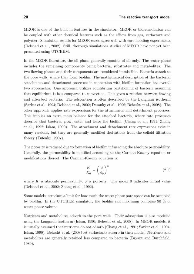
The porosity is reduced due to formation of biofilm influencing the absolute permeability.
Generally, the permeability is modified according to the Carman-Kozeny equation or
modifications thereof. The Carman-Kozeny equation is:
K
K0=
(φ
φ0
)3
(2.1)
where K is absolute permeability, φ is porosity. The index 0 indicates initial value
(Delshad et al., 2002; Zhang et al., 1992).
Some models introduce a limit for how much the water phase pore space can be occupied
by biofilm. In the UTCHEM simulator, the biofilm can maximum comprise 90 % of
water phase volume.
Nutrients and metabolites adsorb to the pore walls. Their adsorption is also modeled
using the Langmuir isotherm (Islam, 1990; Behesht et al., 2008). In MEOR models, it
is usually assumed that nutrients do not adsorb (Chang et al., 1991; Sarkar et al., 1994;
Islam, 1990). Behesht et al. (2008) let surfactants adsorb in their model. Nutrients and
metabolites are generally retained less compared to bacteria (Bryant and Burchfield,
1989).
36

2.2 The general model 21
Surfactant is a metabolite produced within the reservoir and is assumed only to be
present in the water phase. When the surfactant concentration reaches a certain
threshold, the interfacial tension drops affecting the relative permeabilities (Lake, 1989;
Kowalewski et al., 2006). Models take the change in interfacial tension into account
by reducing residual oil and residual water. The capillary number depends of IFT and
is used to estimate the change in residual oil saturation (Lake, 1989). Often, the ap-
proach is empirical, where interpolation is performed between two relative permeability
curves for a high and a low interfacial tension (Coats, 1980). The interpolation func-
tion depends on either a purely empirical function based on experimental results or the
capillary number (Coats, 1980; Islam, 1990; Sarkar et al., 1994).
2.2 The general model
The models for MEOR is based on the general description of isothermal, multiphase,
multicomponent fluid flow in porous media from the basic conservation laws (Lake et al.,
1984; Lake, 1989).
The mass conservation equation may include a term for accumulation, convective fluxes,
and a net production term. The net production covers sources such as injection and
production wells, and reaction (Lake, 1989; Orr, 2007; Gerritsen and Durlofsky, 2005).
The mass conservation equation is set up for each component i, where its contribution
in each phase is included.
∂
∂t
⎛⎝φ0
∑j
ωijsj
⎞⎠+∇ ·
⎛⎝∑
j
ωijuj
⎞⎠ = Ri +Qi (2.2)
where j is the phase, i is the component, ωij are component mass concentration in
phase j, u is the linear velocity (eqn. (2.3)), t is the time, φ0 is the porosity, and the
net production for component i is the reaction term Ri, and well term Qi.
The Darcy law for a
uj = −K krjμj
· (∇P − ρj g∇D) (2.3)
where K is the absolute permeability tensor, krj is the relative permeability for phase
j, P is pressure, ρj is the phase density, and g is gravitational acceleration. The length
variables are x, y and z, and the depth is D being downwards positive and equals to
the direction of the z axis, The Darcy law (eqn. (2.3)) determines the velocity pattern
of the flowing phases based on the pressure gradient, gravitational gradient and the
37
22 The reactive transport model
permeabilities.
For the MEOR system presented here, the fluid flow is one-dimensional and the effect
from gravity is excluded. We use the mass balance terms; accumulation, convection and
reaction. The reactions are strongly coupled. The source terms also cover injection and
production corresponding to the wells.
2.2.1 Fractional flow function
The flow of a phase can be rewritten for a one-dimensional model system, where the
capillary pressure and the effect from gravity are considered negligible. The Darcy law
is derived from equation (2.3) and becomes (Orr, 2007):
uj = K λj
(∂P∂x
)(2.4)
where λj is the phase mobility:
λj =krjμj
(2.5)
The total fluid flow is obtained by summing over all flow velocities of the phases, which
is given by eq. (2.4). The total fluid flow is:
ut = uo + uw ⇒ (2.6)
ut = −K (λw + λo)
(∂P
∂x
)(2.7)
The total mobility λt is introduced as the sum of phase mobilities.
λt =∑j
λj (2.8)
The total mobility changes during the flooding process and therefore the pressure field
also changes. The total mobility is determined by the phase relative permeabilities that
are functions of saturation (Gerritsen and Durlofsky, 2005).
Combination of equations (2.4) and (2.7) produces the following relation for phase
velocity:
uj = ut fj (2.9)
where fj is the fractional flow function
fj =λj
λt(2.10)
38
2.3 Specific model formulation 23
Rock
Water phase
Biofilm phase
Oil phase
φ so0 φ sw0
(1−φ0)φ0σ
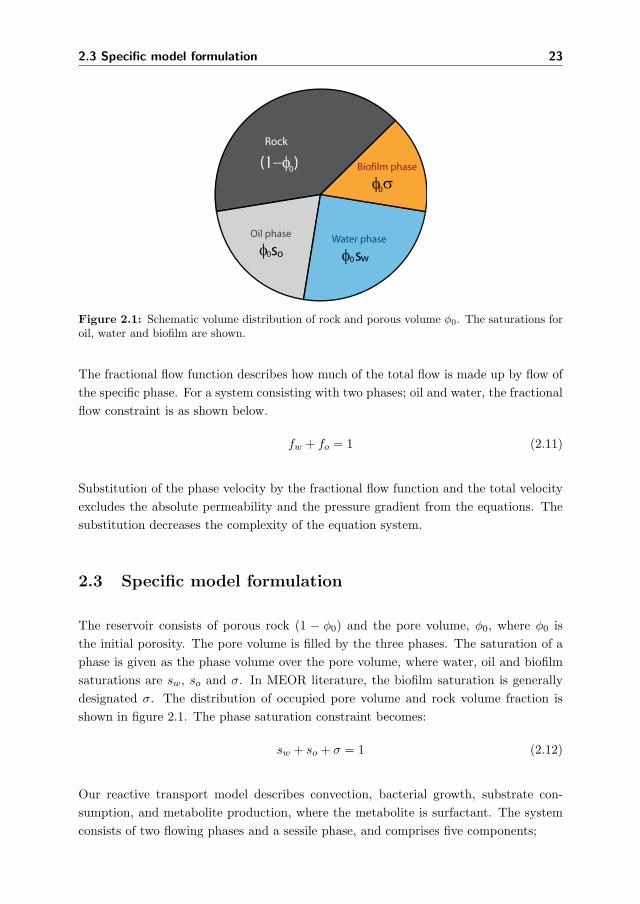
Figure 2.1: Schematic volume distribution of rock and porous volume φ0. The saturations foroil, water and biofilm are shown.
The fractional flow function describes how much of the total flow is made up by flow of
the specific phase. For a system consisting with two phases; oil and water, the fractional
flow constraint is as shown below.
fw + fo = 1 (2.11)
Substitution of the phase velocity by the fractional flow function and the total velocity
excludes the absolute permeability and the pressure gradient from the equations. The
substitution decreases the complexity of the equation system.
2.3 Specific model formulation
The reservoir consists of porous rock (1 − φ0) and the pore volume, φ0, where φ0 is
the initial porosity. The pore volume is filled by the three phases. The saturation of a
phase is given as the phase volume over the pore volume, where water, oil and biofilm
saturations are sw, so and σ. In MEOR literature, the biofilm saturation is generally
designated σ. The distribution of occupied pore volume and rock volume fraction is
shown in figure 2.1. The phase saturation constraint becomes:
sw + so + σ = 1 (2.12)
Our reactive transport model describes convection, bacterial growth, substrate con-
sumption, and metabolite production, where the metabolite is surfactant. The system
consists of two flowing phases and a sessile phase, and comprises five components;
39

24 The reactive transport model
Oil Metabolite
MetaboliteWater
Substrate BacteriaBacteriaSubstrate MetaboliteBacteria
Bacteria (biofilm)
Figure 2.2: Picture illustrating the system consisting of two flowing phases; water and oil,and the sessile biofilm phase. Red arrows indicate the possible reactions, which actually takeplace in the both water and biofilm phases. Purple arrows indicate partition between phases bysurfactant/metabolite and bacteria.
Phases
• Oil
• Water
• Bacteria
Components
• Oil (o)
• Water (w)
• Substrate (s)
• Bacteria (b)
• Metabolite/surfactant (m)
The mass concentration of component i in phase j is designated ωij . The biofilm
comprises bacteria only, so the biofilm bacteria equal the saturation for the biofilm
phase and the symbol for the biofilm bacteria becomes σ.
The water phase may consist of water, bacteria, substrate and metabolite. The oil phase
consists primarily of oil, but contains also metabolite. The novel approach is the parti-
tion of metabolite between the oil and water phases. Figure 2.2 illustrates components
and phases of system. The biofilm bacteria grow, while substrate is consumed directly
from the water phase and the metabolite produced is secreted into the water phase.
2.3.1 Assumptions
The model is based on the following assumptions, where some simplifications are intro-
duced:
1. Fluid flow is one-dimensional and takes place in uniform porous medium.
2. Negligible diffusion.
3. Isothermal system as reservoir fluctuations in temperature is regarded minimal
(Sarkar et al., 1994).
40
2.3 Specific model formulation 25
4. Incompressibility of the fluids meaning that the densities remains constant. Gen-
erally, this is a valid assumption for fluid flows (Sarkar et al., 1994; Orr, 2007).
5. No volume change on mixing (Orr, 2007), because of the lack of thermodynamical
data for most of the components.
6. The simple form of the fractional flow function, eq. (2.10), is used as capillary
pressure is considered negligible (Lake, 1989).
7. No volume change on reaction, when reaction converts components of same den-
sity. When reactants and products have different densities, the volume changes.
We choose to use the same densities here, but the code can handle different den-
sities of reactants.
8. Constant viscosity of phases, which is a legitimate assumption for the water phase,
when the bacteria concentration is low. The oil phase viscosity is here always
assumed constant as no gas is produced and the main carbon source is injected
substrates.
9. The pressure difference remains at a level, where injectivity can be maintained.
10. Continuous injection of nutrient and bacteria takes place.
11. The mechanisms responsible for bacterial retainment can be lumped into expres-
sion, which then includes the adsorption process during formation of biofilm.
12. Decay of bacteria is left out and instead an effective growth rate is used.
13. Application of anaerobic bacteria as their survivability is considered over aerobic,
when exposed to reservoir conditions.
14. No indigenous bacteria present.
15. Bacterial growth rate can be described by Monod kinetics being independent on
temperature, pressure, pH and salinity (Ginn et al., 2002; Islam, 1990; Kim, 2006;
Nielsen et al., 2003; Zhang et al., 1992).
16. Regarding growth rate, only one substrate is limiting for growth as the other
possible substrates is assumed to be in excess.
17. No inhibition of growth by substrates or metabolites.
18. Bacteria adsorb to the pore walls forming a biofilm, which is described by equi-
librium partitioning (Behesht et al., 2008). The distribution of bacteria is instan-
taneous, and the distribution kinetics is neglected.
19. Both flowing and sessile bacteria have the same growth rate (Zhang et al., 1992).
Most models assume that similar growth occurs in flowing and sessile phases.
41

26 The reactive transport model
20. Biofilm bacteria take up substrate from the water phase for growth and secrete
metabolites directly into the water phase. There is no mass transfer resistance
(Chen et al., 1998).
21. Maintenance of bacterial processes is considered negligible. For instance, a low pH
reservoir would require a substantial amount of energy to maintain an optimal pH
and cellular processes within the bacteria (Molz et al., 1986; Zhang et al., 1992;
Sarkar et al., 1994). Therefore, the reservoir conditions is assumed not to stress
the bacteria in such a degree that maintenance becomes important (UTCHEM,
2000; Chang et al., 1991).
22. Chemotaxis is considered not to happen.
23. The main metabolite is surfactant and other metabolites are considered negligible.
24. Surfactant can be distributed between both phases. The distribution is instanta-
neous, and the distribution kinetics is neglected.
25. No substrate and metabolite adsorption on the pore walls. The adsorption of
substrates such as molasses and sucrose is limited meaning that negligibility of
their adsorption is reasonable (Wo, 1997).
2.3.2 Component mass balances
According to equations (2.2) and (2.3), the mass balances for each component are set
up in a one-dimensional system.
Bacteria
Bacteria exist as flowing bacteria in the water phase, ωbw, and as a volume fraction
occupied by the biofilm, σ. The bacteria partition between the water phase and the
biofilm using equilibrium adsorption. The biofilm saturation is a function of flowing
bacteria, and the partitioning is described in details in section 2.3.5. The mass balance
covers the total bacteria, which constitute bacteria found in both the water phase and
the biofilm.
∂
∂t(φ0ωbw sw + φ0σρb) +
∂
∂x(utωbwfw) = φ0(Rb +Qb) (2.13)
where ut is the linear velocity, ρb is the bacteria density, fj is the fractional flow function
of phase j, x is the length variable, t is the time, φ0 is the initial porosity, Rb is bacteria
net production, and Qb is the bacteria well term. The reaction terms for bacteria,
substrate and metabolite are elaborated in section 2.3.4.
42
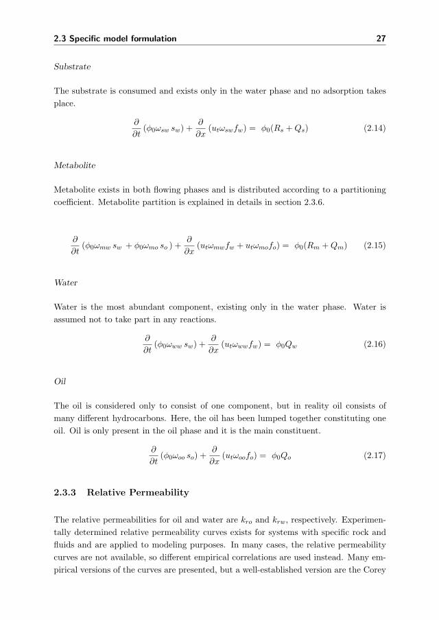
2.3 Specific model formulation 27
Substrate
The substrate is consumed and exists only in the water phase and no adsorption takes
place.
∂
∂t(φ0ωsw sw) +
∂
∂x(utωswfw) = φ0(Rs +Qs) (2.14)
Metabolite
Metabolite exists in both flowing phases and is distributed according to a partitioning
coefficient. Metabolite partition is explained in details in section 2.3.6.
∂
∂t(φ0ωmw sw + φ0ωmo so ) +
∂
∂x(utωmwfw + utωmofo) = φ0(Rm +Qm) (2.15)
Water
Water is the most abundant component, existing only in the water phase. Water is
assumed not to take part in any reactions.
∂
∂t(φ0ωww sw) +
∂
∂x(utωwwfw) = φ0Qw (2.16)
Oil
The oil is considered only to consist of one component, but in reality oil consists of
many different hydrocarbons. Here, the oil has been lumped together constituting one
oil. Oil is only present in the oil phase and it is the main constituent.
∂
∂t(φ0ωoo so) +
∂
∂x(utωoofo) = φ0Qo (2.17)
2.3.3 Relative Permeability
The relative permeabilities for oil and water are kro and krw, respectively. Experimen-
tally determined relative permeability curves exists for systems with specific rock and
fluids and are applied to modeling purposes. In many cases, the relative permeability
curves are not available, so different empirical correlations are used instead. Many em-
pirical versions of the curves are presented, but a well-established version are the Corey
43
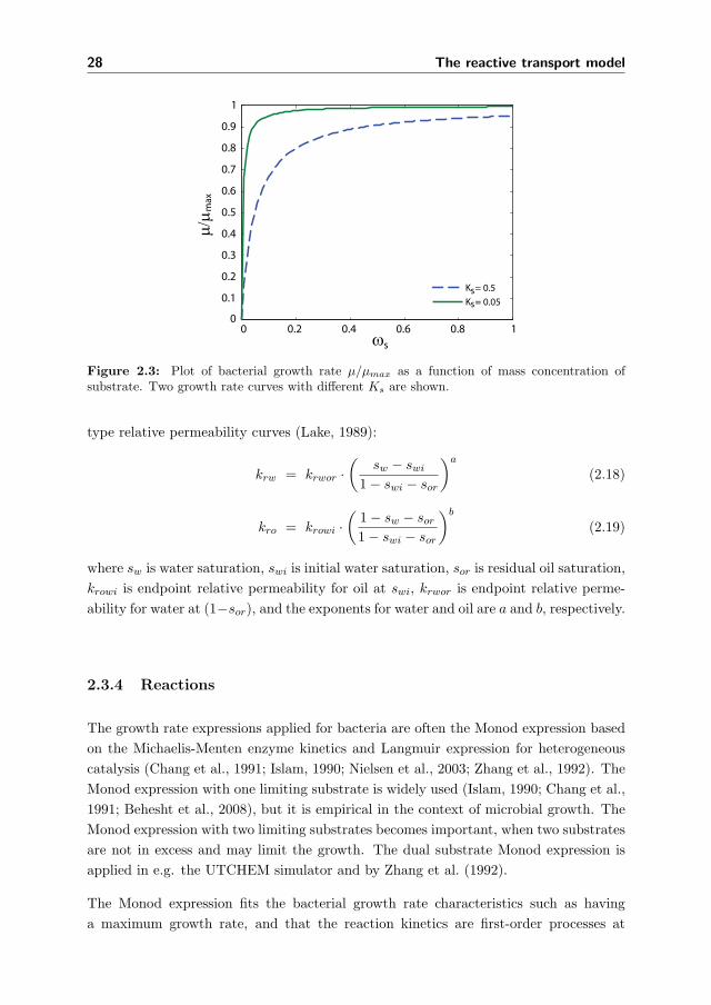
28 The reactive transport model
0 0.2 0.4 0.6 0.8 10
0.1
0.2
0.3
0.4
0.5
0.6
0.7
0.8
0.9
1
ω
μ/μ
K = 0.5K = 0.05
s
ss
max
Figure 2.3: Plot of bacterial growth rate μ/μmax as a function of mass concentration ofsubstrate. Two growth rate curves with different Ks are shown.
type relative permeability curves (Lake, 1989):
krw = krwor ·
(sw − swi
1− swi − sor
)a
(2.18)
kro = krowi ·
(1− sw − sor1− swi − sor
)b
(2.19)
where sw is water saturation, swi is initial water saturation, sor is residual oil saturation,
krowi is endpoint relative permeability for oil at swi, krwor is endpoint relative perme-
ability for water at (1−sor), and the exponents for water and oil are a and b, respectively.
2.3.4 Reactions
The growth rate expressions applied for bacteria are often the Monod expression based
on the Michaelis-Menten enzyme kinetics and Langmuir expression for heterogeneous
catalysis (Chang et al., 1991; Islam, 1990; Nielsen et al., 2003; Zhang et al., 1992). The
Monod expression with one limiting substrate is widely used (Islam, 1990; Chang et al.,
1991; Behesht et al., 2008), but it is empirical in the context of microbial growth. The
Monod expression with two limiting substrates becomes important, when two substrates
are not in excess and may limit the growth. The dual substrate Monod expression is
applied in e.g. the UTCHEM simulator and by Zhang et al. (1992).
The Monod expression fits the bacterial growth rate characteristics such as having
a maximum growth rate, and that the reaction kinetics are first-order processes at
44

2.3 Specific model formulation 29
low substrate concentrations (Nielsen et al., 2003). The knowledge about inhibition
effects from metabolites is important in order to realize whether a necessary metabolite
concentration can be achieved (Deng et al., 1999).
The Monod growth rate for one limiting substrate without any inhibition will be used
in this work:
μ = μmax ·ωsw
Ks + ωsw[day−1] (2.20)
where μmax is the maximum growth rate, and Ks is the half saturation constant. Fig-
ure 2.3 shows the Monod expression for with two different half saturation constants.
A larger saturation constant means that the substrate concentration should be larger
before half the maximum growth rate is obtained (Nielsen et al., 2003).
Another expression is the semi-empirical Contois equation, which differs from the Monod
expression (Sarkar et al., 1994).
μ =μmax
1 +Dcωbw
ωsw
(2.21)
where Dc is a constant. The growth rate is inhibited by bacteria themselves, which
Nielsen et al. (2003) find very unlikely. They propose that the self-inhibition originates
from other unknown factors.
Sugai et al. (2007) presents the modified Moser equation resembling the Monod expres-
sion, where it only differs in having exponents on the substrate concentrations. The
exponents can be useful for fitting to experimental data (Nielsen et al., 2003). In gen-
eral, many growth rate expressions rely on batch experiments and the choice of model
depends on the best fit with the obtained data point (Chang et al., 1991; Sarkar et al.,
1994; Desouky et al., 1996; Sugai et al., 2007).
The reaction term for bacteria depends on the growth rate, where the total production
of bacteria is a function of the total bacteria concentration and the growth rate. The
corresponding reaction term Rb is expressed as
Rb = Ysb (sw ωbw + ρbσ)μ, (2.22)
where the parameter Ysb is the yield of bacteria on substrate, and ωbw is the bacterial
mass concentration of the water phase.
During growth, bacteria produce several metabolites and consume different substrates,
but only the most important ones are included in the model. Therefore, the model
covers only one substrate and one metabolite in the reactions. The reaction terms for
45

30 The reactive transport model
metabolite and substrate are:
Rm = Ysm (sw ωbw + ρbσ)μ, (2.23)
Rs = −qb − qm, (2.24)
and Ysm is the yield of surfactant (m) on substrate (Nielsen et al., 2003; Zhang et al.,
1992). The yield coefficients determine the fraction of substrate that goes to bacteria and
metabolite. Generally, the largest amount of substrate is converted to bacteria. Other
researchers have considered production of metabolites when the substrate concentration
is only above a threshold point (Zhang et al., 1992; Behesht et al., 2008). The approach
originates from the fact that some metabolites are only formed when the surrounding
environment is rich in substrate.
In practice, bacterial decay occurs meaning that a portion of the bacteria does not
contribute to growth. We assume that the growth rate is the net growth rate.
2.3.5 Bacteria Partition
Many researchers use the additional mass balance for the biofilm bacteria (Islam, 1990;
Chang et al., 1991; Zhang et al., 1992; UTCHEM, 2000). We choose equilibrium ad-
sorption to avoid introduction of several parameters whose values are only estimated.
Therefore, the effect of bacterial adsorption is investigated using this simpler approach.
Equilibrium adsorption utilizes that a function describes the bacteria partition (Sarkar
et al., 1994; Desouky et al., 1996; Delshad et al., 2002; Behesht et al., 2008). The Lang-
muir equation relates a concentration of bacteria to the amount of bacteria adsorbed to
the pore walls. The Langmuir expression is derived from the assumption only one layer
of adsorbing components. The biofilm formed by the attached bacteria is assumed to
contain no water or other substances, which makes it a cell-dense biofilm. The bacteria
exists only flowing in the water phase and as sessile biofilm bacteria. Therefore, the
bacteria can only adsorb from the water phase to enter the biofilm. Hence, we assume
that the water phase concentration of bacteria, ωbw, determines the amount of bacteria
that attach to the pore walls.
The mass of bacteria adsorbed pr. unit area is:
Mb =w1 ωbw
1 + w2 ωbw[kg/m2] (2.25)
where w1 and w2 are the Langmuir constants.
The amount of bacteria that adsorbs, depends on the pore wall area available. The
specific surface of porous rock S is 105–106 m2/m3 total volume. The contact area
46

2.3 Specific model formulation 31
between pore walls and the water phase is assumed to reflect the area available for
adsorption, so the efficient surface area S is the specific surface area scaled with the
water phase saturation.
S =S
φ0
(swsmaxw
)[m2/m3 PV] (2.26)
where the maximum obtainable water saturation is unity.
Combination of equation (2.25) and (2.26) gives the mass of bacteria adsorbing to the
pore walls as a function of the water phase concentration of bacteria.
σ ρb = S ·Mb [kg bacteria adsorbed/m3 PV]
=
(S · swφ smax
w
)w1 ωbw
1 + w2 ωbw(2.27)
The amount of bacteria adsorbed is (σ ρb). A low concentration of bacteria in the water
phase shows linearity between the flowing and adsorbed bacteria. The ratio w1/w2
multiplied with the specific surface is the maximum obtainable adsorption of bacteria:
(σ ρb)max = Sw1
w2(2.28)
2.3.6 Surfactant Partition
The novel approach is partitioning of surfactant. The approach has not been included
in other MEOR models so far. Partitioning of surfactant depends of the distribution
coefficient Ki (Ravera et al., 2000). The surfactant mass concentration in water and
oil phase are ωmw and ωmo, respectively. The surfactant is distributed according to the
amounts of water and oil:ωmw
ωmo= Ki
ωww
ωoo(2.29)
Surfactant exists in small amounts compared to water and oil. Partitioning of surfactant
takes place, but is dependent on rate of diffusion to obtain equilibrium (Ravera et al.,
2000). We assume fast exchange between phases and hence instant equilibrium.
The surfactant concentration in the water phase must reach a certain concentration
threshold, before surfactant can reduce the interfacial tension. A large distribution
coefficient means that most surfactant is present in the water phase. The relative
permeabilities depend on the water phase mass concentration, so when surfactant is
moved into the oil phase, there will be a smaller effect from the surfactant. Therefore,
47

32 The reactive transport model
transfer part of the surfactant to oil phase is equivalent to its ”disappearance”, so that
the total effect from surfactant is reduced. The adsorption of surfactant to the pore walls
is not directly included in the model, but practically the disappearance also includes
this. The model lets surfactant go into the oil phase, where a large part of the oil and
subsequently the surfactant in the oil phase do not flow. The oil phase captures the
surfactant, but it may as well be adsorbed to the pore walls in the oil phase.
2.3.7 Porosity changes
The initial pore volume φ0 does not change in this model as the rock volume remains
unchanged. The actual porosity available for flow is affected by the formation of biofilm.
Therefore, the actual porosity φ depends on the initial porosity and the biofilm satura-
tion.
φ = φ0(1− σ) (2.30)
The biofilm phase contribution to the porosity change has been taken into consideration
in the definition of saturations. The pore volume consists of saturations of the water,
oil and biofilm phases (cf. eq. (2.12)).
48

2.4 Implementation 33
2.4 Implementation
This section contains the implementation of the most important mechanisms in MEOR.
Reduction of oil-water interfacial tension and fluid diversion are regarded the primary
mechanisms, which leaves out reduction of oil viscosity mechanisms. The mechanisms
was introduced in section 1.4, and the implementation builds on the model presented
earlier in this chapter.
2.4.1 General approaches
In the MEOR literature, there are different approaches for implementation of the mech-
anisms. There exists literature from other research areas, where these mechanisms are
also important. As an example, bioremediation deals with bacteria in the underground
working with models that describe the transport and biological processes (Murphy and
Ginn, 2000; Tufenkji, 2007). Other EOR processes and generally in the oil industry,
many investigations have been performed to clarify the influence of interfacial tensions
on the relative permeabilities (Coats, 1980; Kumar et al., 1985; John et al., 2005; Shen
et al., 2006).
2.4.2 Reduction of oil-water interfacial tension
In the literature, there is no actual agreement on how the IFT affects the residual
saturations and relative permeability curves (Coats, 1980; Kumar et al., 1985; John
et al., 2005; Shen et al., 2006). Researchers obtain different effects on the relative
permeability curves unable to clarify the influence of the parameters (Al-Wahaibi et al.,
2006). Generally, researchers suggest that the relative permeability curves show some
dependence on IFT. A lower IFT decreases the capillary resistance, resulting in relative
permeability curves with:
• Reduced curvature
• Reduced residual saturations
• Increasing end point relative permeabilities as the lines will approach full misci-
bility
When IFT goes toward zero, the relative permeability curves approach a unit slope line
for which the relative permeability is simply equal to the phase saturation (Coats, 1980;
Al-Wahaibi et al., 2006).
49
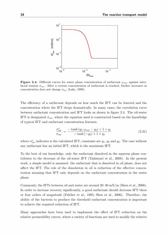
34 The reactive transport model
10−6
10−4
10−2
10−4
10−2
100
102
σow
[m
N/m
]
ωmw
Figure 2.4: Different curves for water phase concentration of surfactant ωmw against inter-facial tension σow. After a certain concentration of surfactant is reached, further increases inconcentration does not change σow (Lake, 1989).
The efficiency of a surfactant depends on how much the IFT can be lowered and the
concentration where the IFT drops dramatically. In many cases, the correlation curve
between surfactant concentration and IFT looks as shown in figure 2.4. The oil-water
IFT is designated σow, where the equation used is constructed based on the knowledge
of typical IFT and surfactant concentration features.
σ∗owσow
=− tanh (q3 ωmw − q2) + 1 + q1
− tanh (−q2) + 1 + q1(2.31)
where σ∗ow indicates is the calculated IFT, constants are q1, q2 and q3. The case without
any surfactant has an initial IFT, which is the maximum IFT.
To the best of our knowledge, only the surfactant dissolved in the aqueous phase con-
tributes to the decrease of the oil-water IFT (Tadmouri et al., 2008). In the present
work, a simple model is assumed: the surfactant that is dissolved in oil phase, does not
affect the IFT. The role of the dissolution in oil is reduction of the effective concen-
tration meaning that IFT only depends on the surfactant concentration in the water
phase.
Commonly, the IFTs between oil and water are around 20–30 mN/m (Shen et al., 2006).
In order to increase recovery significantly, a good surfactant should decrease IFT three
or four orders of magnitude (Fulcher et al., 1985; Shen et al., 2006). Therefore, the
ability of the bacteria to produce the threshold surfactant concentration is important
to achieve the required reduction of IFT.
Many approaches have been used to implement the effect of IFT reduction on the
relative permeability curves, where a variety of functions are used to modify the relative
50
2.4 Implementation 35
permeability curves. Often, the Corey relative permeabilities shown in section 2.3.3
are applied. The Corey type permeability curves utilize parameters such as residual
saturations and exponents, which are parameters becoming a function of the reduced
IFT (Al-Wahaibi et al., 2006). One example is application of the capillary number,
which is a function of IFT. The capillary number is related to the residual oil saturation,
which is directly applied in the expression for the relative permeability curves (Green
and Willhite, 1998; Al-Wahaibi et al., 2006). Another approach proposed by Coats
(1980) modifies the relative permeability curves by interpolation between two sets of
curves at two different IFTs. The interpolation function ranges between those two IFTs.
Generally, the approach to modify the relative permeability utilize either the capillary
number approach or the interpolation approach. However, there are also cases, where
the methods are combined e.g. using the capillary number as the interpolation function.
Based on the methods applied to modify the relative permeability, three approaches are
presented in the following sections:
1. The capillary number method
2. Coats interpolation between relative permeabilities
3. Interpolation of each parameter in the Corey type relative permeabilities
As suggested in the latter methods, the parameters included in the Corey relative per-
meability expression are interpolated on its own. Interpolation of various parameters
has been performed in other versions (Fulcher et al., 1985; Kumar et al., 1985; Shen
et al., 2006).
2.4.2.1 The capillary number method
The capillary number Nca is ratio of viscous to capillary forces and thus being dependent
on changes in oil-water interfacial tension σow.
Nca =μw v
σow(2.32)
where Nca is the dimensionless capillary number, μw is viscosity of displacing fluid, and
v is the ’characteristic’ linear velocity. For general water flooding reservoirs, the capil-
lary number is at about 10−6 under normal reservoir conditions (Green and Willhite,
1998). In order to effectively mobilize the residual oil, the capillary number increases to
around 10−3. The capillary number increases by velocity increments, increments of wa-
ter viscosity, and IFT reductions. The reduction of IFT can raise the capillary number
51

36 The reactive transport model
10−8 10−6 10−4 10−2 1000
0.2
0.4
0.6
0.8
1.0
1.2
1.4
N
s
ca
/so
ro
r
For simulation
Curve by Taber
*
*
Figure 2.5: Capillary desaturation curve. Green and Willhite (1998) have collected curves for
dependencies betweens∗or
sorand N∗
ca, where s∗
or is the modified residual oil saturation. The graphdisplays the curve (blue, dash) applied in this work and the curve by Taber (1969) (full, black).
significantly, because IFT can be changed far more compared to the other parameters.
Experiments show a dependency between capillary number and normalized residual
oil saturation s∗or/sor, where s∗or is the modified residual oil saturation and sor is the
residual oil saturation after waterflood. This is also known as the capillary desaturation
curve. Green and Willhite (1998) present several data showing this dependency, which
is determined for e.g. more rock types. The experiments lead to the different curves,
where the reduction of the residual oil saturation differs at each curve. The decline
rates differs and different capillary numbers are required before reductions occur, but
they produce the same curve behavior.
Figure 2.5 shows one example of the capillary desaturation curve, being an approxima-
tion of the curve presented by Taber (1969). The capillary desaturation curve is applied
in the simulations. The capillary desaturation curve has the following mathematical
description.s∗orsor
=− tanh (p1 (N
∗
ca)− p3) + 1 + p2− tanh (p1 (N0
ca)− p3)) + 1 + p2(2.33)
where ∗ is the index for a modified/calculated variable, N0ca is the capillary number at
initial conditions also corresponding to minimum capillary number, constants are p1, p2
and p3.
Figure 2.6 shows the procedures for the three methods, where the capillary number
method is covered by subfigures 2.6(a)–(b). A new residual oil saturation s∗or is predicted
from the reduction in IFT. The calculated residual oil is then applied in the Corey
equations, equation (2.18) and (2.19), producing the modified relative permeability
curves, which are shown in figure 2.6(b). The curves stretch from swi to (1 − s∗or) and
the gradient also become smaller.
52

2.4 Implementation 37
sw
krw kro
swi 1-sor*1-sor
sw
krw kro
kro(initial)
swi 1-sor 1-sor*
krw(initial)
sw
krw kro
swi 1-sor*1-sor
sw
krw k ro
kro(initial)
swi 1-sor 1-sor*
krw(initial)
s wi*
a* b*
krowi
krwor
*
*
sw
krw kro
swi swi* 1-sor*1-sor
sw
krw k ro
s wi swi*
kro(misc)
krw(misc)
kro(base)
krw(base)
1-sor*1-sor
f(σ )ow
sw
krw kro
swi swi* 1-sor 1-sor*
f(σ )ow
sw
krw kro
kro(initial)
s wi swi* 1-sor 1-sor*
krw(initial)
Capillary number method Coats’ method Corey interpolation method
a) c) g)
b) d) h)
e)
f )
s wi*
Figure 2.6: Graphic illustration of the procedure for the different interpolation methods; thecapillary number method (a–b), Coats’ interpolation method (c–f), and Corey interpolation ofparameters method (g–h).
53

38 The reactive transport model
2.4.2.2 Coats’ interpolation between relative permeability curves
Coats’ correlation is stated to be used in many commercial simulators for modeling
the effect of miscibility on relative permeability (Al-Wahaibi et al., 2006), even though
it is not based on any theory, but developed to describe the changes in the relative
permeability curves by IFT reductions (Coats, 1980). Coats (1980) models the changes
of two-phase gas and oil relative permeability curves due to reductions of IFT. The
method is shown for water and oil:
g(σow) =
(σow
σow,base
) 1n
(2.34)
s∗wi = g(σow) swi (2.35)
s∗or = g(σow) sor (2.36)
krw = g(σow) krw(base) + [1− g(σow)] krw(misc) (2.37)
kro = g(σow) kro(base) + [1− g(σow)] kro(misc), (2.38)
where σow is current IFT, g(σow) interpolation function with values from unity at the
highest IFT towards zero at lower IFT. The index ∗ means modified/calculated values.
The modified residual saturations, equations 2.35 and 2.36, are interpolation between
zero and the initial residual saturation, where the residual saturations drop as IFT de-
creases. kr(base) is the relative permeability curve at largest interfacial tension ’σow,base’
being a function of both residual saturations corresponding to the initial Corey equa-
tions, eqns. (2.18) and (2.19)). kr(misc) is the linear relative permeability curve at lowest
IFT also being a function of both residual saturations but generally the straight line case
approaching full miscibility (Coats, 1980; Al-Wahaibi et al., 2006). n is an adjustable
exponent normally in the range of 4–10, which is used to fit to the experimental relative
permeability curves. When n is larger, the interpolation function becomes less sensitive
toward IFT reductions and thus the relative permeabilities change less toward the full
miscibility curves.
Figure 2.6(c)–(f) depicts the procedure for Coats’ method. The procedure is initiated
by an interpolation, where initial and current IFT are used to create the interpolation
function ranging between initial values and zero. The newly calculated residual satura-
tions, s∗or and s∗wi, are found. In figure 2.6d, the interpolation function is used to modify
the relative permeability curve to obtain the corrected krj(misc) and krj(base). The curves
now stretch between s∗wi and (1−s∗or). Figure 2.6(e) depicts that the interpolation func-
tion, eqn. (2.34), is used to interpolate between base and misc relative permeability
curves for water and oil, equations (2.37) and (2.38). In this way, interpolation between
the straight line and the curved line corresponds to modifications of curvature. The
54
2.4 Implementation 39
initial and final curves are shown in figure 2.6(f), where the final curves has become
more straight compared to the initial curves. This means that the residual saturations
and to some extent the exponents all are functions of IFT, while the capillary number
method only changes residual oil saturation directly.
2.4.2.3 Interpolation of parameters in Corey type relative permeabilities
This method is applied in a similar manner as Shen et al. (2006) presented in their
work. However, our inclusion of the parameters results in being a new approach. We
apply interpolation of more Corey parameters. One advantage is that experimentally
determined changes in the relative permeabilities can more easily be approximated by
this method.
The difference between capillary number and Corey interpolation method is the trans-
lation of IFT reduction to changes in the relative permeability curves. The methods are
different with regard to e.g. sensitivity. We have chosen to use the interpolation func-
tion presented by Coats (1980), equation (2.34). The interpolation can be performed
for each parameter given in the Corey type permeabilities, cf. eq. (2.18) and (2.19).
s∗or = g(σow) · sor (2.39)
s∗wi = g(σow) · swi (2.40)
k∗rowi = g(σow) · krowi + [1− g(σow)] (2.41)
k∗rwor = g(σow) · krwor + [1− g(σow)] (2.42)
a∗ = g(σow) · a+ [1− g(σow)] (2.43)
b∗ = g(σow) · b+ [1− g(σow)] (2.44)
Again, the residual saturations are interpolated between zero and initial saturations like
performed by Coats (1980). A modified approach could be another usage of interpolation
function in relation to residual water, because the residual water saturation changes
differently than the residual oil saturation (Amaefule and Handy, 1982; Kumar et al.,
1985). As the curves are supposed to go towards the straight line curve, the end point
values, equations (2.41) and (2.42), are interpolations between the initial end point
values and unity, and the exponents is interpolated between unity and initial value,
which in our case is two.
Figure 2.6(g)–(h) depicts the procedure for the Corey parameter interpolation method.
Similar to Coats’ method, the procedure is initiated by creating an interpolation func-
tion. The interpolated parameters, equations (2.39)–(2.44), are applied to the Corey
55

40 The reactive transport model
relative permeability equations. The resulting curves are shown in figure 2.6(h), where
the curves straighten and span broader on the water saturation axis due to reductions
in residual saturations, increased end point values at residual saturations, and reduction
of exponents.
2.4.2.4 Applicability
This section has presented a method for implementing the reduction of IFT. Three
approaches have been presented for modifying the relative permeability for water and
oil. The approaches have some resemblance, so we regard that they perform similar. In
chapter 4, we illustrate the performance of the different approaches for changing IFT
in context of MEOR.
56

2.4 Implementation 41
2.4.3 Permeability Modifications
Bacteria form biofilm, reducing the porosity and thus the permeability. In the MEOR
literature, the general approach is application of the Carman-Kozeny equation and
modifications thereof (Chisholm et al., 1990; Zhang et al., 1992; UTCHEM, 2000).
The following version of the Kozeny-Carman relation has been used in work concerning
MEOR (Chisholm et al., 1990; Zhang et al., 1992):
K
K0=
(φ
φ0
)γ
(2.45)
The exponent γ is normally around 3 (Chisholm et al., 1990; Zhang et al., 1992), but
is used with values between 2 and 5 (Clement et al., 1996). In bioremediation, many
investigations have been performed on the applicability of the Kozeny-Carman equation
or similar expressions. Generally, they are performed on systems with only one phase
(Clement et al., 1996; Thullner, 2009). Overall, the results show reasonable fits, but
they propose no final conclusion (Thullner, 2009).
Several other approaches have also been proposed. Sarkar et al. (1994) suggest a perme-
ability reduction model applying effective medium theory, which utilizes the distribution
function for pore sizes and permeabilities. Islam (1990) proposes empirical relationship
to modify the permeabilities for pluggable and non-pluggable pores as a function of
attached bacteria.
Generally, the porosity reductions is considered only to influence the absolute perme-
ability. However, Wo (1997) proposes modifications of the relative permeability for the
water phase only, because bacteria are present in the water phase. They enter the
biofilm phase due to adsorption from the water phase.
Different approaches for modifying the permeabilities have been introduced. The fol-
lowing sections go through two approaches:
• Modifications of absolute permeability
• Modifications of the relative permeability for the water only
2.4.3.1 Absolute permeability
According to the approach coming from one phase studies, the porosity modification
affects both phases equally, influencing the absolute permeability (Thullner, 2009). The
57
42 The reactive transport model
total Darcy velocity ut can also be written as:
ut = −Kλt∇P (2.46)
where K is absolute permeability, λt is total mobility (eq. (2.8)), and P is pressure (cf.
section 2.2).
The total Darcy velocity shows that a reduction of the absolute permeability influences
the other variables contained in the expression above. The reduced permeability forces
either the pressure difference to become larger or the total flow to decrease. In our
system of equations, the fractional flow function is applied, so the change in either flow
rate or the pressure gradient will not influence the system. The fractional flow is a
function of only the relative permeabilities and the viscosities. For the one-dimensional
system, we will see no effect from modifications of the absolute permeability.
Simulations with changes in absolute permeability should not performed in only one
dimension as this is basically unrealistic (Islam, 1990). In one dimension, the absolute
permeability starts to drop near injection site when bacteria are injected. Therefore, the
flow through the entire reservoir is determined by the lowest permeability found near the
injection site and plugging can take place. On the other hand, simulations performed in
two or three dimensions create realistic cases, where the full fluid diversion mechanism
can be investigated. In conclusion, absolute permeability changes should only be studied
in two or three dimensions (Islam, 1990).
The considerations reveal that the effect from modifying the absolute permeability is not
investigated here. In the context of this approach, we only study the influence from the
formation of biofilm. Meanwhile, we hold the assumption that the actual modifications
that would happen, does not influence the total flow rate and keeps the pressure within
a sound range.
Saturation
The presence of biofilm encompasses that the relative permeability should remain un-
changed. The relative permeability is calculated based on the water phase saturation,
but the biofilm phase reduces the actual pore volume available for flow. The pres-
ence of the biofilm should be taken into account in order to obtain the same relative
permeability curves independent of the biofilm saturation.
The bacteria exist only in the water and biofilm phases. Formation of biofilm occurs by
bacteria leaving the water phase and enter the biofilm phase, but what happens in the
water and biofilm phases does not influence the oil phase. Therefore, the water phase
58

2.4 Implementation 43
saturation that would have existed if no biofilm had formed, is:
s = sw + σ (2.47)
Application of s in the relative permeability calculations gives unchanged relative per-
meability curves krj for both oil and water phases:
krj = k0rj(sw + σ) = krj(s) (2.48)
In the context of studying the influence from biofilm, the relative permeabilities do not
experience a distinction between absence or presence of the biofilm.
2.4.3.2 Water phase relative permeability
The formation of biofilm is a process that involves bacteria coming from the water phase
and adsorb to the pore walls. Similar to the previous approach, the oil phase is not
affected by the processes taking place in the water and biofilm phases, and the relative
permeability for oil stays the same. The absolute permeability remains unchanged. The
lumped saturation for the water and biofilm phases defined in equation (2.47) is used.
kro = kro(s) (2.49)
2.4.3.3 The original Kozeny-Carman equation
The Kozeny-Carman equation is used to relate the pressure drop of a fluid through a
packed bed column of solids (McCabe et al., 2005).
uj =1
180α2s d
2 φ3
(1− φ)2
(ΔP
)(2.50)
where uj is the velocity of the fluid phase j, αs is the sphericity coefficient being in
the order of unity, d is an effective sphere diameter of solid grains, φ is porosity, P is
pressure, and is the length of the column. From this equation, other authors have
derived the Kozeny-Carman relation, equation (2.45).
Combining the Kozeny-Carman equation with the Darcy law in the form shown as
equation (2.3) gives the following expression for the permeability (Wang and Tarabara,
2009) :
(krw ·K) =1
180α2s d
2 φ3
(1− φ)2(2.51)
59

44 The reactive transport model
The result is that the product of absolute and relative permeability can be written as a
function of sphericity, grain diameter and porosity.
2.4.3.4 The modified Kozeny-Carman relation
We use equation (2.51) to produce the ratio between the permeability with and without
the formation of biofilm. This leads to an expression for the relative permeability for
water, as only the relative permeability for water is changed.
krwk0rw
=d2
d20
φ3
φ30
(1− φ0)2
(1− φ)2(2.52)
The relative permeability for water becomes a function of grain size and porosity, while
it excludes the absolute permeability from the expression. The index 0 indicates the
initial case, associated with no bacterial adsorption. No index indicates the current
state with biofilm formation.
The presence of biofilm reduces the pore volume available for fluid flow. This implies
that more solid is produced. Before any biofilm formation takes place, the solid is only
rock (1− φ0). The formation of biofilm adds volume to the solid (φ0σ):
Solid: Rock (1− φ0)
Solid: Rock with biofilm (1− φ0) + φ0σ
The ratio between the actual porosity with biofilm and the initial porosity is found by
rewritings of porosity definition, equation (2.30).
φ
φ0= (1− σ) (2.53)
The porosity decreases as more biofilm forms.
Assume that the addition of non-flowing volume of the solid material is uniformly dis-
tributed between all the spherical rock grains, meaning that all grains grow equally.
Volume addition to a grain increases the diameter, where the volume corresponds to
the diameter to power one third, according the formula for sphere volume. The diameter
ratio is determined from the volume ratio:
d
d0= 3
√1− φ0 + φ0σ
1− φ0= 3
√1 +
φ0σ
1− φ0(2.54)
where d and d0 are grain diameters with and without biofilm, respectively.
The ratios, equations (2.53) and (2.54), are substituted into equation (2.52) that de-
60

2.4 Implementation 45
scribes the ratio for the water relative permeability. After rearrangements, the modified
relative permeability for the water phase becomes:
krw(s, φ) = k0rw(s) ·
[(1 +
φ0σ
1− φ0
)8/3
(1− σ)3
](2.55)
where k0rw(s), is the relative permeability for water without biofilm formation. Therefore,
it is also a function of initial relative permeability for water, where the lumped saturation
s is applied.
Comparison
We assume that the Kozeny-Carman equation can also be directly applied for changing
the relative permeability for the water phase only. Thullner (2009) reviews several
relations between porosity and permeability changes of one-phase flow in porous media,
but concludes that no final correlation exists. A comparison between the regularly
used and the modified Kozeny-Carman equation is shown in figure 2.7, equation (2.45)
and equation (2.55), respectively. The curves differ a little, where the regular version is
more concave compared to the modified version. The curves reveal that the effect on the
relative permeability becomes significant, when the biofilm saturation reaches around
0.1 for the regular version and around 0.2 for the modified version. Generally, the
biofilm formation should be extensive in order to modify the permeability significantly.
We choose to continue working the modified Kozeny-Carman expression, eq. (2.55), to
include the effect from biofilm formation.
0 0.2 0.4 0.6 0.8 10
0.1
0.2
0.3
0.4
0.5
0.6
0.7
0.8
0.9
1
σ
k rw/K
rw0
Modified Regular
Figure 2.7: Comparison of modified and regular Kozeny-Carman relation for water relativepermeability, respectively eqn. (2.55) and eqn. (2.45) with γ = 3.
61

46 The reactive transport model
2.4.4 Microscopic fluid diversion
The formation of biofilm promotes fluid diversion. This mechanism is explained in
details in section 1.4.3. Fluid diversion utilizes the changes of flow paths, and thus it
can only be fully investigated in a multidimensional system (Islam, 1990). As we only
look at a one-dimensional system, we do not investigate the full effect of fluid diversion.
In relation to fluid diversion, the modification of the relative permeability of water occurs
in the thief zones, where biofilm grows in the beginning. We study the effect taking
place on the microscopic level. While the relative permeability for water is reduced,
the relative permeability for oil remains the same. This entails mobilization of more
oil causing the fractional flow of oil to increase. We designate this effect microscopic
fluid diversion, because the incremental flow of oil takes place on the microscopic level.
Microscopic fluid diversion partly contributes to the overall process of fluid diversion.
The contribution from microscopic fluid diversion is investigated in chapter 4.
2.5 Summary of model
The reactive transport model set up in this chapter describes convection, bacterial
growth, substrate consumption, and surfactant production. It is two-phase flow com-
prising five components; oil, water, bacteria, substrate, and surfactant. The water phase
may consist of water, bacteria, substrate and surfactant. In the context of MEOR, a
novel approach is the partition of surfactant between both phases. The oil phase consists
primarily of oil, but contains also surfactant. We apply the fractional flow function, and
the relative permeabilities are the Corey type expressions.
The reactions are substrate consumption, bacteria multiplication and surfactant pro-
duction. The bacterial growth rate is the Monod expression for one limiting substrate,
so the reaction rate depends on the bacteria and substrate concentrations.
Surfactant reduces IFT, modifying the relative permeabilities. We have looked into three
methods how to translate the IFT reduction into changes of the relative permeabilities;
the capillary number method, Coats’ method, and the Corey relative permeability in-
terpolation method. The surfactant concentration in the water phase must reach a
certain concentration threshold, before surfactant can reduce the interfacial tension. A
large distribution coefficient means that most surfactant is present in the water phase.
The relative permeabilities depend on the water phase concentration, so when surfac-
tant is moved into the oil phase, there will be a smaller effect from the surfactant on
the flow. Therefore, transfer part of the surfactant to oil phase is equivalent to its
”disappearance”, so that the total effect from surfactant is reduced.
62
2.5 Summary of model 47
The bacteria partition between phases according to the Langmuir expression dependent
on the bacteria concentration in the water phase. The adsorbed bacteria constitute the
biofilm phase. The surface available for adsorption is scaled by the water saturation, as
bacteria only adsorb from the water phase. We assume no transport limitations in the
biofilm, causing the bacteria in the water and biofilm phases to have the same growth
rate.
The formation of biofilm leads to porosity reduction, which is coupled to the modification
of permeability. The modification of absolute permeability that could take place, is
not investigated as the model is one-dimensional. An effect contributing to the fluid
diversion mechanisms, is microscopic fluid diversion, where the relative permeability for
water only, is modified. This happens due to the fact that the biofilm is formed only
at the water-occupied zones or pores where bacteria live. Bacteria only influence the
water and biofilm phases, while the oil phase remains the same.
63

48 The reactive transport model
64

Chapter 3
Solution procedure
The model for MEOR was developed in chapter 2. The mathematical model comprises
three phases; oil and water are the flowing phases, and biofilm is the sessile phase. Some
components belong to more phases, but this is only the case for bacteria and metabo-
lite. The main constituents, oil and water, do not mix. The possible combinations of
component and phases are shown in table 3.1.
Table 3.1: Phases and constituent components.
Phase
Component Oil Water Biofilm
Water - ωww -
Oil ωoo - -
Substrate - ωsw -
Bacteria - ωbw ωba
Metabolite ωmo ωmw -
The component mass concentrations in the phase are ωij [kg/m3 phase]. Another form
of the variable concentrations are
Ωij = ωij · sj (3.1)
This is mass concentration which is then related to the pore volume [kg/m3 PV]. The
65
50 Solution procedure
overall concentration of a component comes by summation:
Ωi =∑j
Ωij =∑j
ωij · sj (3.2)
During the solution procedure, application of the different mass concentrations are use-
ful.
The program coding is performed in Fortran, and Matlab is used for visualization of
the results.
3.1 Dimensionless form
The transport equations (2.13)–(2.17) are rewritten in dimensionless form.
An important parameter is α describing the duration before the one reservoir pore
volume has been injected. This is a parameter that measures the progress of the flooding
process.
α =φ0 L
uinj
=φ0AL
Qinj(3.3)
where uinj is the linear injection velocity, Qinj is the volumetric injection velocity, A is
the reservoir cross sectional area, L is the length of the reservoir, and φ0 is the initial
porosity. One of the dimensionless variables is the reservoir length:
ξ =x
L(3.4)
The fraction, ξ, can also be interpreted as the volumetric fraction of the total pore
volume. The dimensionless time τ is pore volumes injected [PVI]:
τ =Qinj
φ0AL· t
=t
α(3.5)
The dimensionless injection velocity ud is defined as:
ud =utuinj
(3.6)
The injection velocity is here shown as the linear velocity relation, but the volumetric
66

3.2 Discretization scheme 51
velocity fraction is primarily used during the calculations.
Application of the dimensionless variables turns the transport equations into the dimen-
sionless form. The transport equation for component i in all phases j is:
∂
∂τ
⎛⎝∑
j
ωij sj
⎞⎠+
∂
∂ξ
⎛⎝ud
∑j
ωijfj
⎞⎠ = α (Ri +Qi) (3.7)
The transport equations easily become more compact using the overall component con-
centration, Ωi, and Fi, which as the overall component flux. The compact transport
equation is:
∂Ωi
∂τ+
∂Fi
∂ξ= α (Ri +Qi) (3.8)
where
Fi = ud∑j
ωijfj (3.9)
3.2 Discretization scheme
The mathematical model equations, eq. (3.8), are solved numerically using a semi-
implicit finite difference technique, where the component mass balances and the total
volume balance are satisfied.
(n+1,k+1)(n+1,k)(n+1,k-1)
Figure 3.1: Subdivision of volumes.
The reservoir volume is subdivided into volume blocks Δξ, where ξ both relates the
volume and the length fraction of the reservoir. The time step is Δτ . The spatial and
time indices are k and n, respectively. Each discretization point ξk corresponds to a
volume block at a specific time τn+1. This is illustrated in figure 3.1. It is assumed that
each block is well-mixed, having the same composition in the entire block.
The general implicit scheme of discretization for component i becomes (Aziz et al.,
2003), when the new step to be calculated is (n+ 1, k):
Ωn+1i,k − Ωn
i,k + ΔτΔξ ·
(Fn+1i,k − Fn+1
i,k−1
)= Δτ · α · (Rn+1
i,k +Qn+1i,k ) (3.10)
67

52 Solution procedure
F i,k-1n+1
F i,k+1n+1
Ω i,kn
Ω i,kn+1
R i,kn+1
Figure 3.2: Tanks-in-series approach. The composition of block k at the present time (n+ 1)is Ωn+1
i,k and depends on; the composition of that block in the previous time Ωni,k, the influx
Fi determined by the previous block (k − 1) at present time τn+1, and the efflux Fi from thecurrent block k at present time τn+1. The reaction Ri also relies on the composition of thecurrent block.
The implicit discretization produces a fully coupled system of equations. The tanks-
in-series approach is applied meaning that the solution of all blocks at one time step
is not calculated simultaneously. Instead, the volume blocks are solved in a sequential
manner. The approach is illustrated in figure 3.2, where the composition of a block k
at a new time (n+1) depends on; the composition of that block k in the previous time
n, the influx from the beforehand block (k− 1) at this time step (n+1), and the efflux
from the current block (n+ 1, k). The reaction Ri also relies on the composition of the
current block (n+ 1, k).
The tanks-in-series approach entails that the fully implicitness is retarded. There are
some forward mixing of components from the initial injection, but this is regarded minor.
Therefore, the method is considered semi-implicit. The choice of method implies that
large matrix operations is avoided and the calculation load is reduced.
Injection and production wells are located in the first and the last block, respectively.
The injection well is taken into account in the influx to the first block. Similarly, the
production well is included considering the efflux from the last block.
3.3 Application of Newton-Raphson procedure
The multivariable Newton-Raphson method applies to solve the system of equations for
each discrete block k at each time step (n + 1). Therefore, the primary variables and
the corresponding equations have to be specified.
68
3.3 Application of Newton-Raphson procedure 53
Primary variables
The model utilizes a mass balance for each of the five components. The main dependent
variables are selected to be total concentrations. The total volume balance is also taken
into account. The volumetric flow ud is added as an variable to include the possibility for
volume changes, if a component reacts and the density of the product differs. Therefore,
the primary variables are:
Ωw, Ωo, Ωm, Ωs, Ωb, and ud
The relation between total and phase concentrations are as shown in equation (3.2).
Flash calculations
Usually, the flash calculations utilize the total composition, temperature, pressure, and
thermodynamical data to distribute the components between phases. Due to lack of
thermodynamical data and no volume change on mixing, the flash calculations use
partitioning coefficients, making up a simple flash without the necessity for iterating.
Sections 2.3.5 and 2.3.6 presented the partitioning of bacteria and metabolite, respec-
tively. The bacteria and metabolite fractions in each phase are initially calculated. The
components are divided between the phases, and the volume of each phase is calculated
by adding the partial volumes for components in that phase.
The saturations are necessary for calculating the fractional flow function. For a block,
the relation between the volume of a phase Vj and total pore volume VT gives the
saturations:
σ =Va
VT(3.11)
sw =Vw
VT(3.12)
so = 1− (sw + σ) (3.13)
Reaction term
In block k, reactions take place during the time Δτ and depend on the composition
at time τn+1. The Monod expression, equation (2.20), determines the bacterial growth
rate. The total concentration of bacteria enter the reactions, because bacteria grow
equally whether they are located in the water or the biofilm phase. The reaction terms
69

54 Solution procedure
for bacteria, metabolite and substrate are the discrete version of eqs. (2.22)–(2.24):
Rn+1b,k = YsbΩ
n+1b,k μ (3.14)
Rn+1m,k = YsmΩn+1
b,k μ (3.15)
Rn+1s,k = −Rn+1
b,k −Rn+1m,k (3.16)
The bacterial growth rate is calculated as shown below, where the phase concentration
of substrate at present time is estimated from the overall concentration and the water
saturation from the previous time step.
μ =μmax
Ωn+1b,k
snw,k
Ks +Ωn+1
b,k
snw,k
(3.17)
Mass and volume conservation
Application of the Newton-Raphson method on each block (n+ 1, k) calculates the six
primary variables. The procedure requires six equations, which is the discrete compo-
nent mass balances and the total volume balance. Importantly, the solution scheme is
set up such that the mass and volume balances are satisfied.
The Newton-Raphson method is explained in details in appendix B. The system is
set up as a multivariable Newton problem, where a numerical Jacobian matrix is used.
Iterations are performed until convergence. The function that is searched to become
zero, is the check function vector, F :
F =
⎧⎪⎪⎨⎪⎪⎩VT −
∑j Vj = 0
Ωni,k +
ΔτΔξ · F
n+1i,k−1 +Δτ αRn+1
i,k − Ωn+1i,k − Δτ
Δξ · Fn+1i,k = 0
(3.18)
where i = {w, o, b, s,m}. The different terms was shown in figure 3.2.
The procedure for the solution of each block volume is listed below.
1. Guess on variables Ωw, Ωo, Ωm, Ωs, Ωb and ud.
2. From equation (2.29), the mass concentration of metabolite in water and
oil phases are calculated.
3. The bacteria are distributed between water and biofilm phases according
to equation (2.27). The saturation from the previous step snw,k is used for
producing the water phase concentration of bacteria.
70

3.3 Application of Newton-Raphson procedure 55
4. Water, oil and biofilm phase volumes are found.
5. In order to obtain the fractional flow function, the saturations are found.
6. Influx Fn+1i,k−1 is determined from previous calculation step.
7. Efflux from current step Fn+1i,k is calculated.
8. Net production Rn+1i,k is found according to the reactions eqs. (3.14)-(3.16).
9. Calculation of the check function F , eq. (3.18) and the application of the
Newton-Raphson method, cf. appendix B.
10. Find the next guess on primary variables.
11. Estimate the error from the check function.
Repetition of steps until convergence.
Often, convergence occurs fast due to quadratic convergence of the method, but con-
vergence requires a starting guess reasonably close to the solution (Aziz et al., 2003).
Therefore, convergence takes place, when the time step size Δτ remains small compared
to the block volume.
71

56 Solution procedure
72
Chapter 4
One-dimensional simulations
Several mechanisms govern the MEOR process. It is difficult to distinguish between
the contributions of the different mechanisms. The simulation studies enable us to in-
vestigate each mechanism separately and in combination. We look at the effect from
surfactant production, biofilm formation and microscopic fluid diversion. Simulations
are performed revealing the characteristics for the most important MEOR mechanisms
and their contribution to the overall enhancement of oil recovery.
The mathematical model was set up in chapter 2, and specifically the implementation
of mechanisms was described in section 2.4. The system of equations are solved as
presented in chapter 3.
4.1 Selection of parameters
Before simulations are carried out, the selection parameters are presented to produce
simulation results as close as possible to the reality. The selected parameters are listed
in table 4.1 (p. 58).
Reservoir properties
The reservoir simulation is considered to be one-dimensional. The reservoir part has
the length 400 m and the cross section is 100 × 100 m. The porosity is 0.40. This gives
73
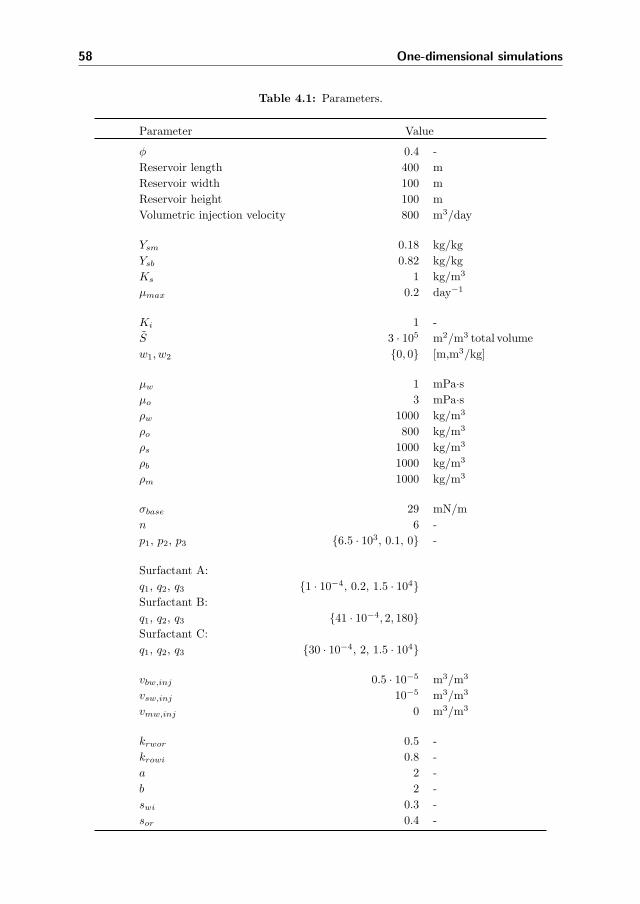
58 One-dimensional simulations
Table 4.1: Parameters.
Parameter Value
φ 0.4 -
Reservoir length 400 m
Reservoir width 100 m
Reservoir height 100 m
Volumetric injection velocity 800 m3/day
Ysm 0.18 kg/kg
Ysb 0.82 kg/kg
Ks 1 kg/m3
μmax 0.2 day−1
Ki 1 -
S 3 · 105 m2/m3 total volume
w1, w2 {0, 0} [m,m3/kg]
μw 1 mPa·s
μo 3 mPa·s
ρw 1000 kg/m3
ρo 800 kg/m3
ρs 1000 kg/m3
ρb 1000 kg/m3
ρm 1000 kg/m3
σbase 29 mN/m
n 6 -
p1, p2, p3 {6.5 · 103, 0.1, 0} -
Surfactant A:
q1, q2, q3 {1 · 10−4, 0.2, 1.5 · 104}
Surfactant B:
q1, q2, q3 {41 · 10−4, 2, 180}
Surfactant C:
q1, q2, q3 {30 · 10−4, 2, 1.5 · 104}
vbw,inj 0.5 · 10−5 m3/m3
vsw,inj 10−5 m3/m3
vmw,inj 0 m3/m3
krwor 0.5 -
krowi 0.8 -
a 2 -
b 2 -
swi 0.3 -
sor 0.4 -
74

4.1 Selection of parameters 59
a pore volume (PV) of 1.6·106 m3. The injection is 800 m3/day implying that injection
of one PV takes 5.5 years.
Injection fluid
The injection fluid consists primarily of water. A small fraction comprises substrate
and bacteria. The injection mode is continuous, even though many field tests utilize
slug injection. The reservoir is assumed not to contain any indigenous bacteria.
Besides in MEOR, injection of bacteria with substrates also takes place in research areas
such as bioremediation and water technology. Many different injection concentrations
are used, ranging from 10−5 to 101 kg substrate/m3 (Behesht et al., 2008; Chang et al.,
1991; Soleimani et al., 2009; Sen et al., 2005; Sarkar et al., 1994), which also corresponds
to 10−8 to 10−2 volume fraction. Volume fraction is the injection parameter vsw,inj used
in the program code. We have chosen a substrate volumetric fraction 10−5 thus being
in the low end of the interval. The injection fraction of bacteria is assumed to be similar
to the substrate concentration.
Fluid properties
The main constituent of the water phase is water. Therefore, the water phase viscosity
is regarded to be constant. Under high bacteria concentrations, the viscosity could be
more affected, but this is assumed not to be the case. Similarly, the main constituent
of the oil phase is oil, and the oil viscosity is considered to be constant. The densities
are also listed in table 4.1, where oil has a lower density than the other components.
Properties for bacterial growth and reaction
Different constants have been used in earlier MEOR models. The maximum growth
rate μmax is found to range between 0.02 to 14.4 day−1 (Zhang et al., 1992; Desouky
et al., 1996; Wo, 1997; Delshad et al., 2002). The maximum growth rate is chosen to be
kept low at 0.2 day−1, because it is assumed that these are anaerobic bacteria, which
grows slower than aerobic bacteria. In addition, the reservoir is a stressful environment
for bacterial influencing the growth rate. The half saturation constant Ks is found to
range between 0.045 to 8 kg/m3 (Islam, 1990; Delshad et al., 2002; Sen et al., 2005). A
median value at 1 kg/m3 is chosen.
75

60 One-dimensional simulations
Zhang et al. (1992) presents a value for the yield of bacteria on substrate Ysb to be
0.82 kg/kg, which is a value used in several other simulation studies (Sharma and
Georgiou, 1993; Delshad et al., 2002). This leaves the yield of metabolite on substrate
Ysm to be 0.18 kg/kg.
Adsorption
Bacteria adsorb to the pore walls and form biofilm. The equilibrium partitioning dis-
tributes the bacteria between the biofilm and water phases according to the Langmuir
expression, eq. (2.27). For low bacteria concentrations, the adsorption is linear.
The specific surface is determined as the surface area available for adsorption. Section
2.3.5 presents that the range is 105–106 m2/m3, which originates from the many small
pores surfaces in the porous rock. We choose a value of 3 · 105 m2/m3.
The derivation of the full Langmuir expression for our case is performed in section 2.3.5.
The Langmuir values, w1 and w2, are chosen in such a way that 75 % of the porous
volume can become saturated with biofilm, corresponding to (σ ρb)max, eq. (2.28). We
select the value of w2, so approximately half of the bacteria adsorb. The values are listed
in table 4.1, and another approach to obtain the same parameter values, are shown in
appendix A.
When no bacteria adsorb and form biofilm, the bacteria only exist in the water phase.
This results in that constant w1 in the Langmuir type equilibrium expression is zero.
Reduction of interfacial tension
The correlation between IFT and the mass concentration of surfactant is earlier shown
as equation (2.31). We use a very efficient surfactant A and a less efficient surfactant B.
Both sets of constants are listed in table 4.1. The choice of parameters entails curves
that have a critical micelle concentration (CMC) at 1 · 10−4 and 3 · 10−2 kg/m3 with
the minimum obtainable IFT at 2 · 10−3 mN/m and 6 · 10−2 mN/m for surfactant A
Table 4.2: Overview over surfactant parameters and properties. CMC is critical micelle con-centration.
Surfactant q1 q2 q3 CMC[kg/m3]
σmin
[mN/m]
A 1 · 10−4 0.2 1.5 · 104 1 · 10−4 2 · 10−3
B 41 · 10−4 2 180 3 · 10−2 6 · 10−2
C 30 · 10−4 2 1.5 · 104 4 · 10−4 4 · 10−2
76
4.2 Verification of simulator 61
and surfactant B, respectively. Surfactant A and surfactant B are used in the one-
dimensional simulations, while surfactant C is used in chapter 5 for the multidimensional
streamline simulations.
Capillary desaturation curve
For the capillary number method, the dependence between normalized residual oil sat-
uration and capillary number is given by equation (2.33). The curve was shown earlier
as figure 2.5 (p. 36). The constants are chosen such that a reasonable description of
the original curve is obtained. However, it should be mentioned that the curve levels off
and has a minimum achievable saturation. The original curve has no information above
a concentration. After this concentration, we let the curve level off, not lowering the
saturation further. Our minimum residual saturation then becomes 0.08 of the initial
residual saturation.
4.2 Verification of simulator
Before application of the developed model, verification of the simulator is performed,
which is conducted by comparison between the analytical and numerical solution of the
well-known Buckley-Leverett equation.
The system is a reservoir containing water and oil only, which make up the the two
flowing phases. Injection of pure water takes place, displacing oil. The sum of the
oil and water saturation is unity, which is why solution of one transport equation is
required. The transport of water is described by equation (2.16). In the absence of
other components in the water phase, the equation written in dimensionless coordinates
using eqs. (3.4) and (3.5), reduces to:
∂sw∂τ
+∂ fj∂ξ
= 0 (4.1)
where the fractional flow function depends on the water saturation. The velocity always
equals injection velocity removing the dimensionless velocity, eq. (3.6).
The analytical solution is shortly derived in appendix C according to Bedrikovetsky
(1993):
ξ
τ= f ′w(sw), for 0 <
ξ
τ< Df (4.2)
77
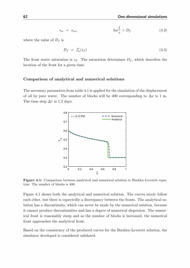
62 One-dimensional simulations
sw = swi, forξ
τ> Df (4.3)
where the value of Df is
Df = f ′w(sf ) (4.4)
The front water saturation is sf . The saturation determines Df , which describes the
location of the front for a given time.
Comparison of analytical and numerical solutions
The necessary parameters from table 4.1 is applied for the simulation of the displacement
of oil by pure water. The number of blocks will be 400 corresponding to Δx is 1 m.
The time step Δτ is 1.2 days.
0 0.2 0.4 0.6 0.8 10.2
0.3
0.4
0.5
0.6
0.7
0.8
ξ
s w
τ = 0.15 PVI Numerical
Analytical
Figure 4.1: Comparison between analytical and numerical solution to Buckley-Leverett equa-tion. The number of blocks is 400.
Figure 4.1 shows both the analytical and numerical solution. The curves nicely follow
each other, but there is expectedly a discrepancy between the fronts. The analytical so-
lution has a discontinuity, which can never be made by the numerical solution, because
it cannot produce discontinuities and has a degree of numerical dispersion. The numer-
ical front is reasonably steep and as the number of blocks is increased, the numerical
front approaches the analytical front.
Based on the consistency of the produced curves for the Buckley-Leverett solution, the
simulator developed is considered validated.
78
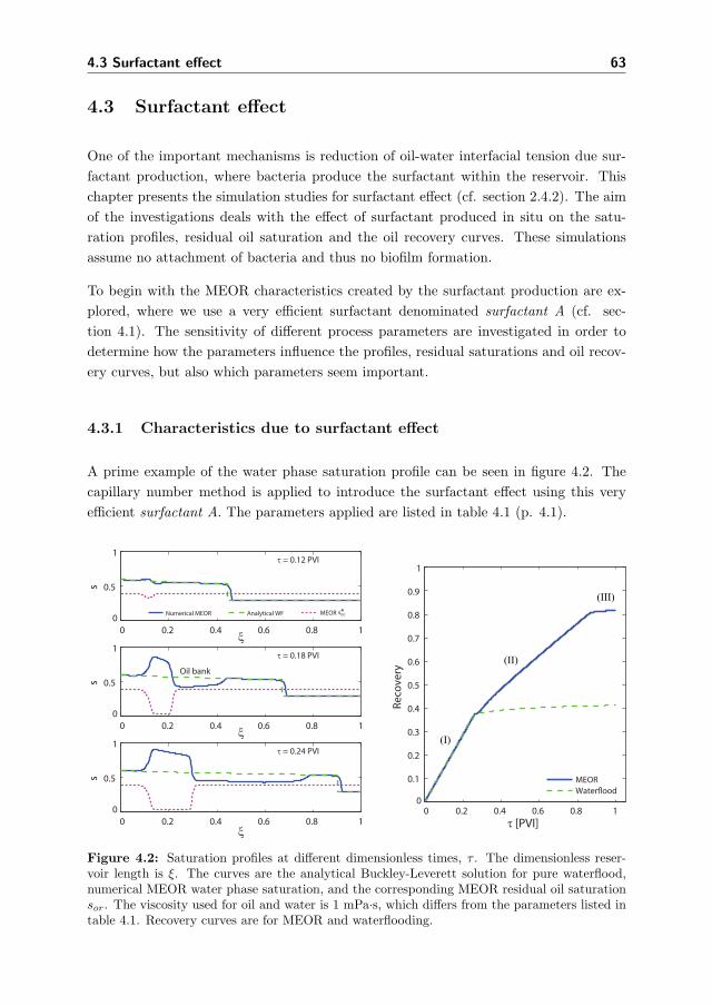
4.3 Surfactant effect 63
4.3 Surfactant effect
One of the important mechanisms is reduction of oil-water interfacial tension due sur-
factant production, where bacteria produce the surfactant within the reservoir. This
chapter presents the simulation studies for surfactant effect (cf. section 2.4.2). The aim
of the investigations deals with the effect of surfactant produced in situ on the satu-
ration profiles, residual oil saturation and the oil recovery curves. These simulations
assume no attachment of bacteria and thus no biofilm formation.
To begin with the MEOR characteristics created by the surfactant production are ex-
plored, where we use a very efficient surfactant denominated surfactant A (cf. sec-
tion 4.1). The sensitivity of different process parameters are investigated in order to
determine how the parameters influence the profiles, residual saturations and oil recov-
ery curves, but also which parameters seem important.
4.3.1 Characteristics due to surfactant effect
A prime example of the water phase saturation profile can be seen in figure 4.2. The
capillary number method is applied to introduce the surfactant effect using this very
efficient surfactant A. The parameters applied are listed in table 4.1 (p. 4.1).
0 0.2 0.4 0.6 0.8 10
0.5
1
ξ
s
τ = 0.12 PVI
Numerical MEOR Analytical WF MEOR sor
0 0.2 0.4 0.6 0.8 10
0.5
1τ = 0.18 PVI
ξ
s
0 0.2 0.4 0.6 0.8 10
0.5
1τ = 0.24 PVI
ξ
s
0 0.2 0.4 0.6 0.8 10
0.1
0.2
0.3
0.4
0.5
0.6
0.7
0.8
0.9
1
τ [PVI]
Reco
very
MEORWaterflood
Oil bank
(I)
(II)
(III)
*
Figure 4.2: Saturation profiles at different dimensionless times, τ . The dimensionless reser-voir length is ξ. The curves are the analytical Buckley-Leverett solution for pure waterflood,numerical MEOR water phase saturation, and the corresponding MEOR residual oil saturationsor. The viscosity used for oil and water is 1 mPa·s, which differs from the parameters listed intable 4.1. Recovery curves are for MEOR and waterflooding.
79

64 One-dimensional simulations
The MEOR solution is injected, producing a water front like during waterflooding. As
bacteria and substrate penetrate the reservoir, more bacteria and surfactant are pro-
duced. When enough surfactant is produced, the interfacial tension reduces significantly
affecting the relative permeabilities. The interfacial tension reduction mobilizes oil cre-
ating the oil mobilization point. More water will accumulate producing a second water
front with surfactant. This results in a traveling oil bank, which occasionally catches up
with the first front as a consequence of different front velocities. If the oil bank catches
up with the first front, the water front now having a new saturation will be slowed down.
On the other hand, as long as the oil bank does not catch up, the water front will be
located at the position of the front for pure waterflooding and breakthrough occurs at
the time for pure waterflooding breakthrough.
The recovery curve is also shown in figure 4.2. When the oil bank catches up with the
waterfront, it results in production with steepest incline in recovery curve for an extra
period of time (I), as water breakthrough occurs later. The second part of the curve
(II) has a smaller inclination than the first part (I), which results from a larger water
cut relative to the first part of the recovery curve. The water saturation is lower until
breakthrough of the surfactant water front, where the recovery curve levels off (III).
If the oil bank does not catch up with the water front, the recovery curve follows the
waterflooding recovery curve until the oil bank breakthrough. Islam (1990) produces a
recovery curve similar to the latter curve, where the oil bank does not catch up with
the water front. Our incremental recovery is around 40% OOIP using the very efficient
surfactant. It should be emphasized, that the incremental recovery depends on the
0 0.2 0.4 0.6 0.8 1
10−8
10−6
10−4
10−2
100
ξ
Volu
me
frac
tion
τ = 0.24 PVI
Substrate
Bacteria
Surfactant (mw)
Total surfactant (m)
sor
*
Figure 4.3: The volume fraction of constituents. The surfactant is shown both as total sur-factant and surfactant in the water phase. The calculated residual oil is shown as well in orderto see the effect from surfactant.
80

4.3 Surfactant effect 65
specific surfactant and the actual reservoirs. A less efficient surfactant mobilizes less
oil.
Due to no adsorption of bacteria, the substrate and bacteria are transported together
in the water phase. The substrate is consumed by the bacteria during the flooding. If
the bacteria concentration is high enough, all substrate is consumed before the outlet
and no reaction can occur.
Figure 4.3 shows the volume fractions of substrate, bacteria, total metabolite and
metabolite existing in the water phase. The volume fractions are shown in a semilog
plot to be able to compare the smaller and the larger amounts. The calculated residual
oil is shown as well to see the effect from surfactant. The residual oil decreases around
the threshold concentration.
4.3.2 Effect of surfactant partitioning
Partitioning of surfactant between phases is a novel approach. Figure 4.4 shows satu-
ration profiles (left) and recovery curves (right) for the different cases of partitioning.
When the distribution coefficient is small, surfactant is mainly located in the oil phase.
Less surfactant is then present in the water phase and more surfactant should be pro-
duced in order to decrease residual oil saturation markedly. The time before changes in
residual oil occur, is longer, but the mobilization point is located at the same distance
from the inlet (not shown). The time delay means that the oil bank is created later,
and the recovery curve follows pure waterflooding recovery until breakthrough of the
oil bank. This becomes even more clear for the case with Ki = 10−1, where the oil
bank is produced later giving a oil bank breakthrough time around 0.7 PVI. However,
0 0.2 0.4 0.6 0.8 10.2
0.3
0.4
0.5
0.6
0.7
0.8
0.9
1
ξ
s
0 0.2 0.4 0.6 0.8 10
0.1
0.2
0.3
0.4
0.5
0.6
0.7
0.8
0.9
τ [PVI]
Reco
very
Ki = 10 3
Ki = 10 0
Ki = 10 −2
Ki = 10 3
Ki = 10 0
Ki = 10 −1
Ki = 10 −2
τ = 0.15 PVI
Figure 4.4: Water phase saturation profiles and recovery curves for different values of distri-bution coefficient Ki.
81

66 One-dimensional simulations
the final recovery will become equal to the case with the larger partitioning coefficients
after 2 PVI, as the mobilization points are alike.
When surfactant is mainly present in the oil phase (Ki = 10−2), sufficient surfactant
cannot be produced in order to obtain a water phase surfactant concentration large
enough to mobilize oil. No effect from surfactant takes place at the these conditions.
The water phase saturation profile and recovery curve result in being the same as during
waterflooding. Therefore, the performance of MEOR is dependent on how surfactant
partitions between the phases.
4.3.3 Effect of growth rate
The growth rate can be difficult to maintain in a reservoir as reservoir conditions may
change. We demonstrate the effect of growth rate only by changing the maximum
growth rate μmax.
Cases for different maximum growth rates are shown in figure 4.5. A larger growth rate
at 2 day−1 results in a faster surfactant production and the mobilization point appears
closer to the inlet. An order of magnitude reduction of the growth rate to 0.2 day−1 pro-
longs the time before the surfactant effect can be seen, but also determines the distance
from the inlet before the residual oil decreases. Another order of magnitude reduction
in growth rate to 0.02 day−1 shows no effect from surfactant as an insufficient amount
of surfactant is produced. The oil recovery curve is then equal to the recovery curve for
pure waterflooding.
0 0.2 0.4 0.6 0.8 10.2
0.3
0.4
0.5
0.6
0.7
0.8
0.9
1
ξ
s
μ = 0.2 day−1
μ = 2.0 day−1
μ = 0.02 day−1
0 0.2 0.4 0.6 0.8 10
0.1
0.2
0.3
0.4
0.5
0.6
0.7
0.8
0.9
τ [PVI]
Reco
very
τ = 0.15 PVI
max
max
max
μ = 0.2 day−1
μ = 2.0 day−1
μ = 0.02 day−1max
max
max
Figure 4.5: Water phase saturation profiles and recovery curves for different maximum growthrates μmax.
82

4.3 Surfactant effect 67
A high level of oil recovery can only be achieved, if we are able to maintain a certain
growth rate. This should be considered, as reservoirs are often heterogeneous and thus
many environmental factors influence the growth rate.
4.3.4 Effect of substrate and bacterial injection concentrations
The bacterial growth rate is dependent on both substrate and bacteria concentration.
Therefore, the recovery is expected to be dependent on the injection concentrations.
The injected amounts of substrate and bacteria also set the upper limit for how much
surfactant that can be produced. Figure 4.6 shows saturation profiles and recovery
curves using the capillary number method at different concentrations. Doubling of the
injection concentration (2×) initiates the surfactant effect at an earlier time, and the oil
mobilization point emerges closer to the inlet. The largest difference between double and
regular injection concentrations (1×) relies on the residual oil that is not mobilized from
the inlet to the mobilization position. For half the injection concentration (0.5×), we
see a significant delay before the surfactant effect initiates. Here, the incremental oil is
approximately only half the incremental recovery compared to the two other cases. The
mobilization position is found around half the reservoir length (not shown graphically)
meaning that large amounts of oil will not be mobilized.
The injection concentrations determine the time before residual oil becomes mobilized,
and the point of initial mobilization. Between the inlet and the mobilization point, a
large amount of residual oil is not mobilized, which reduces the final recovery. This
clearly demonstrates that injection concentrations should be considered carefully to
utilize the full potential of MEOR.
0 0.2 0.4 0.6 0.8 10
0.2
0.4
0.6
0.8
1
ξ
s
τ=0.19 PVI
2x1x0.5x
0 0.5 1 1.50
0.2
0.4
0.6
0.8
1
τ [PVI]
Reco
very
2x1x0.5x
Figure 4.6: Water phase saturation profiles and recovery curves capillary number method fordifferent injection concentrations that is given relative to the injection concentration listed intable 4.1.
83

68 One-dimensional simulations
0 0.2 0.4 0.6 0.8 10
0.2
0.4
0.6
0.8
1
ξ
s
τ=0.19 PVI
COATSCOREYNCA
0 0.5 1 1.50
0.2
0.4
0.6
0.8
1
τ [PVI]
Reco
very
COATSCOREYNCA
Figure 4.7: Water phase saturation profiles and recovery curves for the three methods. NCAis the capillary number method.
4.3.5 Comparison of interpolation methods
The three methods affect saturation profiles in the same way, but the capillary number
method makes sharper profile changes, cf. figure 4.7. Coats’ method and the Corey
interpolation method are smoother producing larger zones of a reduced residual oil
saturation. The sensitivity for Coats and Corey interpolation methods depends on the
parameter n. In our case, n is 6. A larger n produces curves that are less sensitive to
changes in interfacial tension, producing a smaller reduction of the residual oil. The
final recovery for the three methods is very similar, but there are small differences. The
minimum residual oil differs a little between the methods, but also the mobilization
points are unlike. Coats’ method and the Corey interpolation method have mobilization
points closer to the inlet. As an example, Coats’ method produces a lower residual oil
saturation and the mobilization point is very near the inlet resulting in a recovery being
a little larger than the two other methods.
All methods investigated are sensitive to distribution of surfactant, growth rate, sub-
strate and bacterial concentration. The incremental recovery for the three methods has
only minor differences ranging between 38–44 % OOIP, so the recovery outcomes are
very alike. Due to this interpolation approach, the best method for making simulations
depends on the specific case to model. Therefore, the choice of method should rely on
experimental data in order to have a method that describes the specific cases.
4.3.5.1 Interpolation of Corey parameters
So far, the curves presented using interpolation of the Corey parameters only includes
modification of residual oil. This project also uses interpolation of the remaning para-
meters.
84

4.3 Surfactant effect 69
The saturation profile for the case with interpolation of residual oil only and both resid-
ual saturations are shown in figure 4.8(a). Interpolation of the residual water saturation
mobilizes less oil in terms of producing a smaller oil bank and less water accumulates.
Moreover, the water saturation profile becomes more smooth when applying the in-
terpolation of residual water. The smoothness is also seen for the Coats interpolation
method, which interpolated both residual saturations.
The modification of residual water may be too extensive. Some researchers suggest that
the residual water changes less with the reduction of IFT (Kumar et al., 1985). This
change implies a different interpolation function for residual water, which could be less
sensitive to IFT reductions.
0 0.2 0.4 0.6 0.8 10
0.2
0.4
0.6
0.8
1
ξ
s w
τ = 0.2 PVI
sor
+ swisor
(a) Interpolation of sor and swi.
0 0.2 0.4 0.6 0.8 10
0.2
0.4
0.6
0.8
1
ξ
s w
τ = 0.2 PVI
sor
s + exponentsor
(b) Interpolation of sor and exponents.
0 0.2 0.4 0.6 0.8 10
0.2
0.4
0.6
0.8
1
ξ
s w
τ = 0.2 PVI
sor
s + endpointsor
(c) Interpolation of sor and end points.
0 0.2 0.4 0.6 0.8 10
0.2
0.4
0.6
0.8
1
ξ
s w
τ = 0.2 PVI
s or
s + exponents + end pointswis or +
(d) Interpolation of all parameters; sor, swi, ex-ponents and end points.
Figure 4.8: Interpolation of different parameters in the Corey relative permeabilities. Theparameter are residual saturations, sor and swi, the exponents and the endpoints, where theeffect from different combinations of interpolated parameters are shown. All curves are comparedagainst the Corey interpolation method for residual oil only (cyan full line).
85
70 One-dimensional simulations
Figure 4.8(b) depicts the saturation profile, where the residual oil saturation and the
exponents are interpolated. Applying interpolation of both exponents gives more linear
relative permeability curves. The water saturation profile reveals an increment of accu-
mulated water and thus a bigger oil bank from oil mobilization. Interpolation of both
residual saturations and of the exponents produces a saturation profile (not shown),
which is a cross between the two curves shown as figures 4.8(a) and figure 4.8(b).
In the chosen procedure, interpolation of end points takes place between their initial
value and unity. Initially, the lowest end point value is for water and therefore its
endpoint value will be increased more. The profile is depicted in figure 4.8(c). A slight
reduction water accumulation and the oil bank is noticeable, so the profiles is not very
sensitive to interpolation of the end points. The influence of end point interpolations
should be verified by experimental studies such as proposed by Shen et al. (2006).
Figure 4.8(d) presents the saturation profile, where all parameters are selected for in-
terpolation. The profile reveals that the oil bank is smaller due to the interpolation of
residual water and endpoints.
4.3.6 Effect of surfactant efficiency
In our work, the surfactant produced by the bacteria is designated surfactant A and is
considered very efficient having both a low threshold before oil-water interfacial tension
starts to drop, and produce a several orders of magnitude reduction of the interfacial
tension. We have specially restricted ourselves with this case of extremely efficient
MEOR, in order to demonstrate the influence of the different physical phenomena and
model approximations on the process. The recovery achieved in the laboratory studies
is usually lower (Chisholm et al., 1990; Banat, 1995; Zekri and Almehaideb, 1999; Sen,
2008). This is explained by the fact that the threshold concentration, which should be
obtained before the effect of surfactant takes place, is higher than in our simulations.
Applying MEOR has a dramatical effect on the oil recovery, when using the very efficient
surfactant presented. It clearly demonstrates that surfactant partitioning, growth rate
and injection concentration of substrate and bacteria are critical process parameters.
The way how the surfactant influence the saturation profiles and oil recovery curves
becomes very apparent using this very efficient surfactant.
Figure 4.9 shows simulation results for a less efficient surfactant, which is designated
surfactant B. A larger amount of surfactant B is required (around 10 mg surfactant/L)
(Youssef et al., 2007) and the lowest interfacial tension obtainable is 0.06 mN/m (Gray
et al., 2008). The incremental recovery is 9 % OOIP over that of waterflooding. Similar
to the first case, the saturation profiles and the oil recovery curves are still sensitive
86
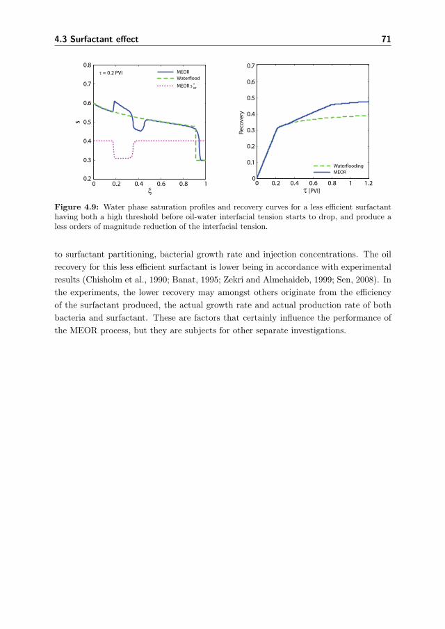
4.3 Surfactant effect 71
0 0.2 0.4 0.6 0.8 10.2
0.3
0.4
0.5
0.6
0.7
0.8
ξ
s
τ = 0.2 PVI MEOR
Waterflood
MEOR s or*
0 0.2 0.4 0.6 0.8 1 1.20
0.1
0.2
0.3
0.4
0.5
0.6
0.7
τ [PVI]
Reco
very
WaterfloodingMEOR
Figure 4.9: Water phase saturation profiles and recovery curves for a less efficient surfactanthaving both a high threshold before oil-water interfacial tension starts to drop, and produce aless orders of magnitude reduction of the interfacial tension.
to surfactant partitioning, bacterial growth rate and injection concentrations. The oil
recovery for this less efficient surfactant is lower being in accordance with experimental
results (Chisholm et al., 1990; Banat, 1995; Zekri and Almehaideb, 1999; Sen, 2008). In
the experiments, the lower recovery may amongst others originate from the efficiency
of the surfactant produced, the actual growth rate and actual production rate of both
bacteria and surfactant. These are factors that certainly influence the performance of
the MEOR process, but they are subjects for other separate investigations.
87
72 One-dimensional simulations
4.4 Effect of biofilm formation
The main question for this section is how the retention of the bacteria changes the
saturation profile and the recovery curve.
Several studies have been conducted on one-phase flow systems in porous medium using
microorganisms in the context of bioremediation (Vandevivere et al., 1995; Clement
et al., 1996; Thullner, 2009). One of the big challenges is predicting the modification of
the absolute and relative permeabilities according to pore space plugging and porosity
reduction due to biofilm formation in the porous medium.
4.4.1 Parameters revisited
The parameters applied when modeling biofilm formation only without any surfactant
is listed in table 4.1 (p. 58). The exceptions from that is explained below.
Injection of a very high bacteria concentration applying biofilm-forming bacteria entails
a risk of plugging the injection area severely and damaging the formation rock. Aslam
(2009a) suggest that the injected bacteria concentration should be maximum 109 cell/ml.
This corresponds to a volumetric fraction of 1 · 10−12 m3/m3, when using a bacteria
size of 1 μm3. However, actual biofilm consists of a large fraction of stagnant water
captured inside the biofilm (Madigan et al., 2003). In practice, the required bacterial
count could be significantly smaller, depending on the biofilm structure and thus its
actual composition.
The injected substrate concentration is 8 · 10−3 m3/m3. Metabolite is also produced,
but we consider it to be an inert tracer compound distributed between the two flowing
phases. This leaves out the effect generated by surfactant.
The attachment of bacteria to form a biofilm is determined by the Langmuir adsorption
expression, eq. (2.27). As highlighted the parameters are chosen in such a way that
bacteria can maximum occupy 75 % of the pore volume, and the bacteria is almost
evenly distributed between the biofilm and the water phase. Simulations are also used
to conclude on the influence of parameters for bacterial adsorption.
Application of the Langmuir expression to maintain a maximum 75 % occupation of
pore volume utilizes the basic parameters:
w1 = 1 · 10−3 · w2 [m]
w2 = 1.7 · 10−3 m3/kg (4.5)
88

4.4 Effect of biofilm formation 73
0 100 200 300 400 5000
100
200
300
400
500
Ωbw
Ωb
a
Langmuir
Unit slope line
Figure 4.10: The Langmuir expression for the base case shown with the unit slope line. Thesaturation is set to 0.6.
For the linear case, the parameters are
w1 = 4 · 10−6 m
w2 = 0 m3/kg (4.6)
so w1 is the same as w1 found in equation (4.5).
The expression using the current values is depicted in figure 4.10. The initial part of the
curve changes almost linearly, while it goes toward the maximum occupation of 75 %
corresponding to 750 kg/m3 pore volume, if the porous medium is fully saturated with
water.
4.4.2 Effect of bacteria adsorption
The goal of this section is to investigate the effect of bacteria adsorption and disappear-
ance from the flow alone, without the effect on the absolute or relative permeability. We
compare the transport of biofilm-forming bacteria compared to the transport without
bacterial adsorption. The adsorption of bacteria depends on the water phase saturation
(cf. section 2.4.3).
Figure 4.11 shows the difference between the case without adsorption of bacteria and
the case with bacteria forming biofilm. Bacterial transport is retarded as the bacteria
attach to the pore walls, while no adsorption entails that bacteria travel together with
the substrate. The area with the high concentration of bacteria has a high consumption
rate, resulting in utilization of all the substrate around.
89

74 One-dimensional simulations
A peak of bacteria emerges at some distance from the inlet, as it takes time before a sub-
stantial amounts of bacteria have been produced. The biofilm formation causes faster
transport of substrate relative to the bacteria, leading to unconsumed substrate bypass-
ing the bacteria. This is in accordance with experimental results (Youssef et al., 2007).
Due to equilibrium partition, the bacteria leave the biofilm when the concentration of
flowing bacteria becomes smaller. Generally, the equilibrium approach corresponds to a
method of stalling the bacterial transport increasing their breakthrough time (Tufenkji,
2007).
The profiles using the Langmuir relation and the linear relation gives the same results
(not shown), because the bacteria concentration mainly remains in the linear region.
Thus, we will not present the curves for linear part as they do not result in new infor-
mation.
0 0.1 0.2 0.3 0.40
0.5
1τ = 0.08 PVI
ξ
Satu
ratio
n
s
w sw
+σ
0 0.1 0.2 0.3 0.40
0.005
0.01
Satu
ratio
n
ξ
σ
0 0.1 0.2 0.3 0.40
0.005
0.01
ξ
Volu
me
frac
tion
Total bacteriaAdsorbed bacteriaSubstrate
(a) No adsorption.
0 0.1 0.2 0.3 0.40
0.5
1τ = 0.08 PVI
ξ
Satu
ratio
n
s
w sw
+σ
0 0.1 0.2 0.3 0.40
0.005
0.01
Satu
ratio
n
ξ
σ
0 0.1 0.2 0.3 0.40
0.005
0.01
ξ
Volu
me
frac
tion
Total bacteriaAdsorbed bacteriaSubstrate
(b) Biofilm formation.
Figure 4.11: Influence of biofilm on the retention of bacteria. Graphs are for water saturation,biofilm saturation and volumetric fractions of the pore volume for substrate and bacteria.
90

4.4 Effect of biofilm formation 75
4.4.3 Effect of water relative permeability
The other approach modifies the relative permeability for water only, according to the
biofilm-induced porosity reduction. This effect is microscopic fluid diversion: it reduces
permeability for water only, since bacteria adsorb only form water-filled pores. Thus,
the formation of biofilm alone helps decreasing the fraction of water in the flow and
increasing the recovery. The approach was presented in section 2.4.3.
The presence of biofilm produces a delay in bacterial breakthrough. According to the
presentation of this approach in section 2.4.3, the biofilm is estimated to occupy around
20 % of the pore space, before the relative permeability for water is reduced enough to
enhance the oil recovery. The surface available for adsorption is scaled with the water
saturation, entailing that less biofilm is formed at small biofilm saturations.
First task is to investigate how much the porosity should change before there is a
markedly effect on the saturation profiles and recovery curves. In the next numerical
experiment, we inject bacteria that are independent of substrate concentration and
growth. It should be noted that the injection concentration is too high for practical
applications but it is purely used for illustration.
Figure 4.12 depicts both the saturation profile and oil recovery for injection with bacteria
alone. The saturation profile in figure 4.12(a) shows the regular displacement front and,
0 0.2 0.4 0.6 0.8 10
0.5
1τ = 0.21 PVI
ξ
Satu
ratio
n
s
w sw
+σ
0 0.2 0.4 0.6 0.8 10
0.5
1
ξ
Volu
me
frac
tion
Total bacteriaAdsorbed bacteria
(a) Saturation profile.
0 0.2 0.4 0.6 0.8 10
0.2
0.4
0.6
0.8
1
τ [PVI]
Reco
very
No modificationModification
(b) Recovery curves.
Figure 4.12: Injection bacteria only in order to study the effect of high bacterial concentration.The recovery curve is compared with the recovery without any modification of the relativepermeability.
91

76 One-dimensional simulations
additionally, a small second front appears. The total volumetric fraction of bacteria is
0.5 and the adsorbed bacteria result in a biofilm saturation at 0.24. The small second
front leads to a minor enhancement of the oil recovery.
The recovery curves for cases with and without modification of the water relative per-
meability curves are depicted in figure 4.12(b). The curves show that the oil recovery is
improved compared to waterflooding. The recovery curves follows the curve for water-
flooding until breakthrough of the second water front. A biofilm saturation at 0.24 is
reached, which produces an incremental oil recovery of 1.9 % OOIP. The result is listed
in table 4.3 together with a similar simulation example.
The other simulation example displays less adsorption, which is introduced by a lower
w2. The biofilm saturation is 0.17, leading to an incremental recovery of 1.2 % OOIP.
To obtain a significant improvement of oil recovery, the biofilm saturation should be at
around 0.2 or preferably higher to improve the oil production. Thus, a relatively large
amount of bacteria needs to be injected, or in the realistic case, a large amount of bac-
teria is required to be produced by growing within the reservoir, before an incremental
oil recovery is obtained.
The results rely on the reduced porosity that modifies the relative permeability for water
only. This effect is microscopic fluid diversion (cf. section 2.4.3). It partially contributes
to the overall fluid diversion process. However, it will only contribute, when the biofilm
formation is substantial.
Table 4.3: Incremental recovery by changing water relative permeability.
Bacteria volume fraction w2 Biofilm saturation Incremental recovery
0.48 1.7 · 10−3 0.17 1.2 % OOIP
0.50 1 · 10−2 0.24 1.9 % OOIP
4.4.3.1 MEOR simulations
In order to obtain a sufficiently high concentration of bacteria, large amounts of sub-
strate have to be injected. When the volumetric injection fraction of bacteria is as
low as 10−12 m3/m3, the bacteria have to multiply extensively to achieve the necessary
saturation. Therefore, it is important to inject sufficient amounts of substrate in order
to secure growth.
Figure 4.13 illustrates the curve obtained for MEOR with a substrate injection fraction
of 0.4. Due to the availability of substrate, the bacteria grow fast leading to formation
of biofilm that changes the porosity.
Substrate is consumed during its transportation through the reservoir. A peak of sub-
92
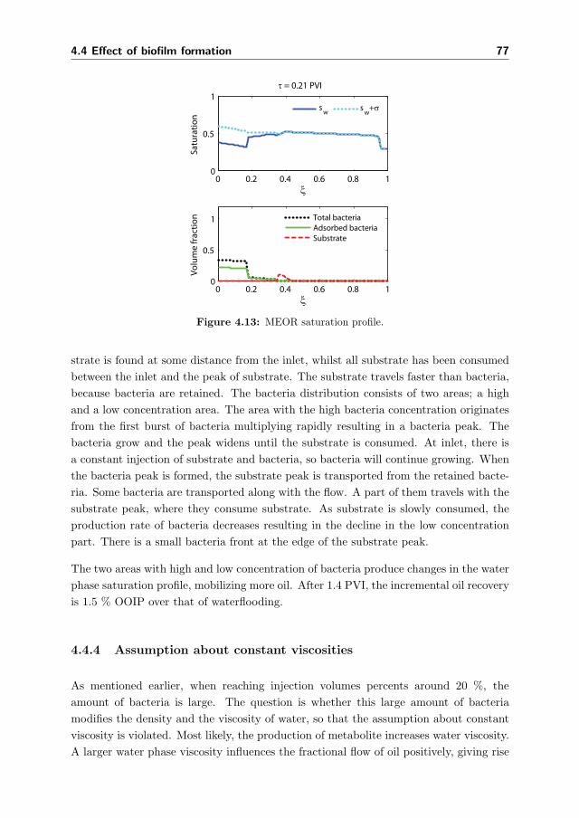
4.4 Effect of biofilm formation 77
0 0.2 0.4 0.6 0.8 10
0.5
1τ = 0.21 PVI
ξSa
tura
tion
s
w sw
+σ
0 0.2 0.4 0.6 0.8 10
0.5
1
ξ
Volu
me
frac
tion
Total bacteriaAdsorbed bacteriaSubstrate
Figure 4.13: MEOR saturation profile.
strate is found at some distance from the inlet, whilst all substrate has been consumed
between the inlet and the peak of substrate. The substrate travels faster than bacteria,
because bacteria are retained. The bacteria distribution consists of two areas; a high
and a low concentration area. The area with the high bacteria concentration originates
from the first burst of bacteria multiplying rapidly resulting in a bacteria peak. The
bacteria grow and the peak widens until the substrate is consumed. At inlet, there is
a constant injection of substrate and bacteria, so bacteria will continue growing. When
the bacteria peak is formed, the substrate peak is transported from the retained bacte-
ria. Some bacteria are transported along with the flow. A part of them travels with the
substrate peak, where they consume substrate. As substrate is slowly consumed, the
production rate of bacteria decreases resulting in the decline in the low concentration
part. There is a small bacteria front at the edge of the substrate peak.
The two areas with high and low concentration of bacteria produce changes in the water
phase saturation profile, mobilizing more oil. After 1.4 PVI, the incremental oil recovery
is 1.5 % OOIP over that of waterflooding.
4.4.4 Assumption about constant viscosities
As mentioned earlier, when reaching injection volumes percents around 20 %, the
amount of bacteria is large. The question is whether this large amount of bacteria
modifies the density and the viscosity of water, so that the assumption about constant
viscosity is violated. Most likely, the production of metabolite increases water viscosity.
A larger water phase viscosity influences the fractional flow of oil positively, giving rise
93

78 One-dimensional simulations
to increase in oil recovery. The incremental oil recovery due to biofilm formation can
be around 2 % OOIP. Therefore, underestimation of the viscosity actually corresponds
to underestimation of the oil recovery.
94
4.5 Combination of mechanisms 79
4.5 Combination of mechanisms
Both MEOR mechanisms are combined in this section. Surfactant is produced and
biofilm is formed. The amount of surfactant produced strongly influences the residual
oil saturation and improves the oil recovery. The surfactant is responsible for modifi-
cations of the relative permeability curves due to surfactant-induced reduction of IFT.
Modification of the relative permeability for water induces the effect from microscopic
fluid diversion, which partly contributes to the overall fluid diversion mechanism (cf.
section 2.4.3).
4.5.1 Parameters revisited
The general parameters used in the simulations are listed in table 4.1 (p. 58). The
bacterial surfactant is surfactant B, which is the least efficient surfactant investigated.
The surfactant properties are shown in table 4.2 (p. 60). The surfactant concentration is
translated into modifications of the relative permeabilities utilizing the capillary number
method (cf. section 2.4.2).
The exceptions concerning biofilm is the same as presented earlier in section 4.4.1.
The injection concentration of substrate is 2 · 10−2 m3/m3, which is a little lower than
previous. The Langmuir expression for bacterial partitioning utilizes w2 = 10−2.
4.5.2 Biofilm formation with surfactant effect
Surfactant is produced both by sessile and flowing bacteria. The bacteria are retained as
they form a biofilm, and this can have a positive effect on the surfactant concentration.
Figure 4.14(a) shows the saturation profiles for the case without adsorption of bacteria.
The substrate is consumed by the peak of bacteria. After that point, the bacteria
are transported without any reactions taking place. As shown in section 4.3 about the
surfactant effect, there is a distance from the injector to the point of mobilization, before
the residual saturation decreases. The saturation profile characteristically contains two
displacement fronts and formation of an oil bank.
Figure 4.14(b) shows the same case except that bacteria form biofilm. The bacteria are
retained leading to a higher bacteria concentration near the inlet. The biofilm bacteria
produce surfactant implying that the sufficient surfactant concentration is achieved
faster and closer to the inlet. A small amount of substrate is not fully consumed and
bypasses the bacteria. The biofilm formation leads to reduction of IFT already at the
inlet due the increased concentration of bacteria producing surfactant. The formation
95

80 One-dimensional simulations
0 0.2 0.4 0.6 0.8 10
0.5
1τ = 0.21 PVI
ξ
Satu
ratio
n
s
w sw
+σ sor
*
0 0.2 0.4 0.6 0.8 10
0.02
0.04
0.06
ξ
Volu
me
frac
tion
Total bacteriaAdsorbed bacteriaSubstrate
(a) No adsorption.
0 0.2 0.4 0.6 0.8 10
0.5
1τ = 0.21 PVI
ξ
Satu
ratio
n
s
w sw
+σ sor
*
0 0.2 0.4 0.6 0.8 10
0.02
0.04
0.06
ξVo
lum
e fr
actio
n
Total bacteriaAdsorbed bacteriaSubstrate
(b) Biofilm formation with w2 = 3.4 · 10−3.
Figure 4.14: Comparison between MEOR cases with and without biofilm formation. Thesurfactant effect is included.
of biofilm moves the point of mobilization closer to the inlet. The effect is seen as the
decrease in residual oil saturation at the inlet, especially comparing with the residual
oil saturation curve in figure 4.14(a).
The case with surfactant alone to change the relative permeabilities produces after 1.4
PVI an incremental recovery of 13.0 % OOIP over that of waterflooding. When biofilm
is formed, the incremental recovery becomes 13.6 % OOIP. The increase of another
0.6 % OOIP in oil recovery is produced due to the sessile bacteria producing surfactant
near the inlet. Bacteria adsorbing to the pore walls improve the effect from surfactant
due to the increased local concentration of surfactant. However, the influence on the
recovery is minor.
4.5.3 Microscopic fluid diversion with surfactant effect
We consider the combined effect of surfactant production, formation of biofilm and
microscopic fluid diversion. As shown previously in section 4.4.3 about the effect from
biofilm, the biofilm saturation has to reach around 0.20 before a positive influence on
the recovery can be attained with the microscopic fluid diversion.
Figure 4.15 depicts the results of computations for this case. In order to show a successful
scenario, the injection concentration of substrate has been increased to 0.2 m3/m3. The
biofilm saturation is 0.2 in the area with the high bacteria concentration. The residual oil
96

4.5 Combination of mechanisms 81
saturation drops like in the previous case with the combined effect of biofilm formation
and surfactant production (figure 4.14). In addition, the biofilm formation introduces
the effect from microscopic fluid diversion, which reduces the residual oil saturation
further. After 1.4 PVI, the incremental oil recovery becomes 14.9 % OOIP over that
of waterflooding, which is an improvement of another 0.7 % OOIP compared to the
case with the effect from surfactant and biofilm formation (not shown). The effect from
biofilm and microscopic fluid diversion together contributes with an improvement of
1.3 % OOIP.
In conclusion, an incremental oil recovery of almost 15 % OOIP can be achieved by
the combined effect of surfactant, biofilm formation and the resulting microscopic fluid
diversion. Each mechanism contributes to the overall effect, where the main contribution
comes from production of surfactant.
0 0.2 0.4 0.6 0.8 10
0.5
1τ = 0.2 PVI
ξ
Satu
ratio
n
s
w sw
+σ sor
*
0 0.2 0.4 0.6 0.8 10
0.2
0.4
0.6
ξ
Volu
me
frac
tion
Total bacteriaAdsorbed bacteriaSubstrate
Figure 4.15: Saturation profile indicating the effect from surfactant, biofilm formation, andmodification of relative permeability for water.
97

82 One-dimensional simulations
4.6 Summary of 1D results
The illustrative simulation results show the characteristics of the water phase saturation
profiles and the corresponding oil recovery curves for MEOR. To begin with we have
looked into the mechanism that reduces the oil-water interfacial tension. Surfactants are
produced by the bacteria, while biofilm formation does not take place. The water phase
saturation profile is found to contain a waterfront initially following the waterfront for
pure waterflooding. At the oil mobilization point – where the surfactant effect starts
to take place – surfactant has been built up mobilizing residual oil producing a second
waterfront also containing bacteria, substrate and surfactant. An oil bank is created,
and in some cases, it catches up with the waterfront. The recovery curve consists of
several parts. The recovery curve follows pure waterflooding recovery until breakthrough
of the oil bank. The next part of the recovery curve continues until breakthrough of
the second waterfront containing surfactant. The incline is still relatively steep due to
a low water cut. In the last part, the curve levels off.
Partitioning of surfactant between the oil and water phase is a novel approach in the
context of MEOR. The partitioning coefficient only determines the time lag before the
surfactant effect can be seen. For a surfactant mainly present in the water phase, the
delay is small, but for cases with the main part being located in oil phase, it takes longer
before the surfactant effect occurs. The position for the surfactant effect does not change
final recovery with different partitioning, but a smaller partitioning coefficient gives a
larger time lag before the same maximum recovery is reached. However, if too little
surfactant stays in the water phase (Ki = 10−2), we cannot obtain the surfactant effect.
It has been found that the final recovery depends on the distance from the inlet to the oil
mobilization point. Additionally, it depends on, how much the surfactant-induced IFT
reduction lowers the residual oil. The surfactant effect position is sensitive to changes
in maximum growth rate, and injection concentrations of bacteria and substrate, which
then determine the final recovery. Variations in growth rate and injection concentra-
tion also affect the time lag until mobilization of residual oil occurs, influencing how
long the MEOR recovery follows the pure waterflooding recovery curve. For the cases
investigated, the recovery curves are less affected.
We have investigated three methods for implementing reductions of interfacial tension;
the capillary number method, Coats’ method, and the Corey relative permeability inter-
polation method. The final oil recovery is similar for the three methods, producing an
incremental recovery of 38–44 % OOIP. The differences in recovery are due to method
variations in the minimum obtained residual oil, the attained distance from the inlet to
the position for the initial surfactant effect, and the sensitivity to IFT reduction.
The method that interpolates the parameters of the Corey relative permeabilities, ap-
98
4.6 Summary of 1D results 83
pears promising. Interpolation of residual oil and the exponents only, increases the
water accumulation, and more oil is mobilized. The second front produced due to IFT
reduction becomes more steep. When residual oil together with residual water and the
endpoint saturations are applied as interpolation parameters, the second front becomes
smoother. Less water accumulates, decreasing the mobilization of residual oil. The
sets of interpolation parameters influence the saturation profiles in different ways. This
leads to a suggestion for application of a modified interpolation function for e.g. residual
water, which could improve the fit with experimental relative permeability curves for
different interfacial tensions.
A less efficient surfactant is also investigated, where this surfactant has a higher thresh-
old concentration, before the effect from the surfactant takes place, and a smaller IFT
reduction. This results in an incremental oil recovery of 9 % OOIP. Compared to the
increment of around 40 % OOIP for the more efficient surfactant, this improvement of
oil recovery is lower, but it is still considered significant.
Bacterial transport is slowed down, when biofilm is formed. The biofilm saturation
increases due to the continuous injection of bacteria and substrate, and to the growth
of bacteria in both the biofilm and water phase. When biofilm is formed together with
production of surfactant, the saturation profile is affected. The biofilm formation implies
that the concentration of bacteria near the inlet increases. At the same time, these
bacteria produce surfactant, resulting in attainment of a larger surfactant concentration
near the inlet. The effect from surfactant only displays an incremental oil recovery of
13.0 % OOIP. In comparison, the effect from both biofilm formation and surfactant
production leads to an increment of 13.6 % OOIP, so biofilm formation enhances the
oil recovery by another 0.6 % OOIP. The formation of biofilm removes or shortens the
distance, before the oil mobilization takes place, but the influence on the oil recovery is
minor.
An effect contributing to the fluid diversion mechanisms, is microscopic fluid diversion.
This happens due to the fact that the biofilm is formed only at the water-occupied
zones or pores where bacteria live. The porosity decreases due to biofilm formation,
and the relative permeability for the water phase only is reduced according to our
modified version of the Kozeny-Carman equation. Simulations illustrate that the biofilm
saturation should reach about 0.2, before a markedly improvement of the oil recovery can
be seen. The incremental oil recovery is 1.3 % OOIP. Combination of biofilm formation,
microscopic fluid diversion, and surfactant production improves the oil recovery even
more. We achieve an increment in recovery of almost 15 % OOIP, having the main
contribution from the surfactant effect.
99

84 One-dimensional simulations
100
Chapter 5
Streamline simulations
The two-phase model for MEOR in one dimension is presented earlier in chapter 2.
The model includes the most important MEOR mechanisms, where bacteria produce
surfactant and can adhere to the pore walls forming biofilm. The interesting question is
whether the same characteristics that appeared in the one-dimensional case, also occurs
when the model is extended to two and three dimensions.
A streamline simulator is an excellent tool for fast upscaling from one dimension to
two or three dimensions, because of its utilization of one-dimensional solutions along
the streamlines. Therefore, the MEOR solver for one dimension is implemented in an
existing streamline simulator. The existing streamline simulator additionally comprises
a finite difference simulator. The two types of simulators are subject for comparison.
The implementation includes only the effect from surfactant as the biofilm formation is a
phenomenon not well dealt with in the streamline simulator due to its strong influence
on permeabilities and thus the streamline paths. We set up simulation examples to
illustrate the multidimensional MEOR performance.
The simulators used have been put at my disposal by the Chemical Engineering De-
partment, University of Southern California, USA. The simulators are modified to be
able to contain more components, include reactions, and to perform correct gravity
calculations. Gravity is included using an operator splitting approach.
101

86 Streamline simulations
5.1 Introduction
Todays streamline methods have been developed from the streamtube approach. The
flow domain is divided into streamtubes and the geometry of the tubes is taken into
account (Datta-Gupta, 2000). Their geometry delivers a side of disadvantages, when
simulating in multiple dimensions. The streamline application has gone through several
steps of development since the streamtubes were used. The details of development in the
streamline approach can be found in Batycky (1997) or Thiele (1991), and Datta-Gupta
(2000) has produced an excellent review on the application of streamline simulators.
The current streamline technology now utilizes the time-of-flight concept, which elim-
inates the necessity of keeping track of the geometry. The time of flight is the travel
time for a tracer along a streamline. The application of streamlines decouples a 2D
or 3D problem into multiple 1D equations, which are less heavy to solve. The space
coordinate is the time-of-flight variable (Datta-Gupta, 2000).
One phenomena that often acts across the streamlines is the effect from gravity. There-
fore, the streamline simulators often underestimate gravity effect. To properly account
for the gravity cross flow, operator splitting is a good option (Batycky, 1997; Beren-
blyum, 2004).
An advantage of the streamline simulation over the finite difference approach is that
the computation time is often smaller and has a smaller impact of numerical dispersion
(King and Datta-Gupta, 1998). On the other hand, the finite difference simulators
better handle physical phenomena that transport fluid across the streamlines (Batycky,
1997).
The conventional simulators are often based on a finite difference methods, where many
variations exist. An example is UTCHEM developed by University of Texas, Austin.
The latter also has a wide utilization range for both waterfloodings and chemical EOR
methods. UTCHEM has the possibility for applying both MEOR and bioremediation
(Delshad et al., 2002), but more extensive studies could be presented using UTCHEM.
Comparison of the two simulation approaches gives a possibility to see the differences
in the methods and verify the simulators against each other.
5.2 The multi-dimensional model
The general transport model in more dimensions was shown earlier in section 2.2. The
assumptions presented in section 2.3 is considered still to hold, except that the model
is extended to multiple dimensions.
102

5.2 The multi-dimensional model 87
Summations of the Darcy velocity for the phases, eq. (2.3), gives the total velocity:
ut = −K (λt∇P − λg∇D) (5.1)
where
λg = λwρw + λoρo (5.2)
The Darcy velocity vector is ut, K is the absolute permeability tensor, λt is the total
mobility earlier described in equation (2.8), P is pressure, D is depth. The total gravity
mobility λg depends on the phase mobilities and the phase densities ρj (Berenblyum,
2004). The depth is assumed to be equal to the z coordinate.
For an incompressible fluids and non-deformable rock, the gradient of the total velocity
must be equal to zero (Batycky, 1997):
∇ · ut = 0
∇ · [−K (λt∇P − λg∇D)] = 0 (5.3)
In the well area, eq. (5.3) equals the total well volumetric flow rate Qt.
∇ · ut = Qt (5.4)
Thus, the multidimensional system of equations are the pressure equation (5.4) com-
bined with a mass balance equations for each component, equation (2.2).
5.2.1 Solution methods
The reservoir is divided into grid blocks in a conventional manner, where each grid block
has a porosity, permeability and initial composition assigned.
Several solution methods have been used for solving the system of equations. A fully
implicit method can be applied, but it produces a substantial amount of numerical
dispersion (Aziz et al., 2003). Therefore, the solution procedure for both simulators is
based on the standard IMPEC framework (implicit pressure explicit composition). The
outline of the IMPEC solution procedure is presented below (Berenblyum, 2004):
1. The pressure equation, eq. (5.3) or eq. (5.4), is solved implicitly for the pressure
values in each grid block based on mobilities determined by block composition
from previous time step.
2. The velocity field is computed by using the Darcy velocity for each phase, eq. (2.3).
3. The reactions are calculated based on the composition of the previous time step.
103
88 Streamline simulations
4. The mass balances, eq. (2.2), for each component are solved applying the pressures
calculated in step 1 and the reactions in step 3.
5. Return to step 1.
The solution of the pressure equation produces a coupled system of linear equations,
where the IMPEC method produces coefficient matrices with diagonal bands only con-
taining numbers. The number of diagonal bands increase with the number of dimen-
sions. The pressure equation are mainly solved using iterative methods for sparse linear
systems, but solving the equations is still a substantial part of the computational load
(Aziz et al., 2003).
5.2.1.1 Finite difference procedure
The finite difference (FD) simulator requires solution of the pressure equation, eq. (5.3),
each time the composition has been updated during a time step. This often leads to
large computation times (Berenblyum, 2004). Gravity is taken into account through
the velocity field, when the pressure equations are solved.
5.2.1.2 Streamline procedure
In the streamline (SL) simulator, the pressure equations are also solved using IMPEC.
The solution in composition can be propagated several time steps along the streamlines,
before an update of the pressures is required. The time step between pressure updates
is thus much larger in the SL simulator compared to the FD simulator (Datta-Gupta,
2000).
In the SL simulator, the numerical solution procedure is:
• The pressure equation is solved implicitly on the finite difference grid using the
composition from the previous time step.
• The Darcy velocities of each block are computed based on the pressure.
• Streamlines are traced from injection wells.
• The resulting 1D component equations are solved along the streamlines with time-
of-flight as a coordinate variable (Datta-Gupta, 2000).
• The component composition is mapped back from the streamline grid to the finite
difference grid.
104

5.2 The multi-dimensional model 89
• Due to operator splitting between convective flux and gravity flux, the gravity
lines are made based on columns in the finite difference grid. The 1D gravity
equations are solved along each gravity line (Jessen and Orr, 2004).
• The component composition is updated.
Mapping between the finite difference grid and the streamline grid can also produce
some amount of dispersion that negatively influences the effect from surfactant in the
MEOR process. Therefore, the pressure updates should be kept to a minimum avoiding
too many smearing out translations between the grids.
5.2.2 Gravity
The total velocity field is also based on the gravity and determines the streamlines. The
gravity effect is driven by the density differences between the flowing phases, but the
propagation of the fluids along the streamlines does not account for the gravity effect.
The fractional flow function could include the gravity, but operator splitting is an ex-
cellent alternative for including gravity in a streamline simulator (Batycky, 1997; Jessen
and Orr, 2004). The method has earlier shown good agreement with results produced
by the conventional simulator Eclipse.
The convective and the gravity fluxes can be separated by means of operator splitting
resulting solution of component mass balances in a sequential manner. A time step
starts with a convective step, which is shown here as a modified version of eq. (2.2).
φ0∂Ωi
∂t+∇Fi = Ri +Qi (5.5)
Earlier, the overall concentration Ωi was defined in eq. (3.2) and the overall flux Fi
in eq. (3.9). The overall flow is based on the fractional flow function, which does not
contain gravity.
The convective step is followed by the gravity step, which only accounts for the gravity
effects:
φ0∂Ωi
∂t+∇Gi = 0 (5.6)
where
Gi = Kz
∑j
ωijλj
(λg
λt − ρj g
)∂D
∂z(5.7)
105

90 Streamline simulations
k
k+1
k
k+1
ok
o
w
w
a) b)
oo
o
w
w
wk+½
k-½
k+½
k-½
Gravity stepk
k+1 k+1
k
k
k
k+1
k+1
k+1
Figure 5.1: Blocks are designated k and k+1. Each block contains a segment of the oil phaseand a segment of the water phase, which for instance for block k are ok and wk. a) Initial state.b) The segments are moved according to the fluxes, and the block composition can be calculatedfrom the segments contained in the block after the gravity step. Adapted from Jessen and Orr(2004).
The density phase density is ρj , Gi is the gravity flux vector, Kz is absolute permeability
in z direction, ωij is the phase concentration for component i, λt is total mobility, λg
is gravity mobility, and the gradient ∂D∂z equals unity as the z axis equals the depth
direction D, which is also the direction for the gravity.
The gravity segregation utilizes a pseudo-immiscible approach (Jessen and Orr, 2004),
where phase segment fluxes along gravity lines are found based on their phase density
differences and mobilities corresponding to overall phase compositions. Figure 5.1 de-
picts the idea of the method, where figure 5.1(a) illustrates the initial state with two
immiscible segments for the oil (o) and water (w) phases for two neighboring blocks k
and (k+1). The segments are moved between blocks according to the calculated fluxes,
which results in the segment distribution shown in figure 5.1(b). The new overall com-
position can now be calculated from the segments now contained in the block (Jessen
and Orr, 2004). In this way, the phase equilibrium calculation is avoided.
5.3 Parameters
The parameters used in the simulations are shown in table 5.1. The reservoir is initially
assumed not to contain any bacteria or other indigenous microorganisms. Bacteria
and substrate in solution are continuously injected into the reservoir. The injection
composition is given in terms of volumetric fractions vij,inj . The surfactant produced
by the bacteria is assumed to be surfactant C. The details of the surfactant can be found
the section 4.1.
106

5.3 Parameters 91
Table 5.1: Parameters used in the SL and FD simulations.
μmax 0.2 day−1
Ks 1 kg/m3
Ysm 0.18 kg/kg
Ysb 0.82 kg/kg
φ 0.4 -
Reservoir length (1D) 400 m
Reservoir width (1D) 100 m
Reservoir height (1D) 100 m
Volumetric injection velocity (1D) 800 m3/day
Δx, Δy, Δz (for 2D and 3D) 1 m
μw 0.5 mPa·s
μo 0.7 mPa·s
ρw 1000 kg/m3
ρo 800 kg/m3
ρs 1000 kg/m3
ρb 1000 kg/m3
ρm 1000 kg/m3
σbase 29 mN/m
n 6 -
p1, p2, p3 {6.5 · 103, 0.1, 0} -
Ki 1 -
Surfactant C:
q1, q2, q3 30 · 10−4, 2, 1.5 · 104 -
vbw,inj 0.5 · 10−5 m3/m3
vsw,inj 10−5 m3/m3
vmw,inj 0 m3/m3
krwor 0.6 -
krowi 0.9 -
a 2 -
b 2 -
swi 0.2 -
sor 0.2 -
107
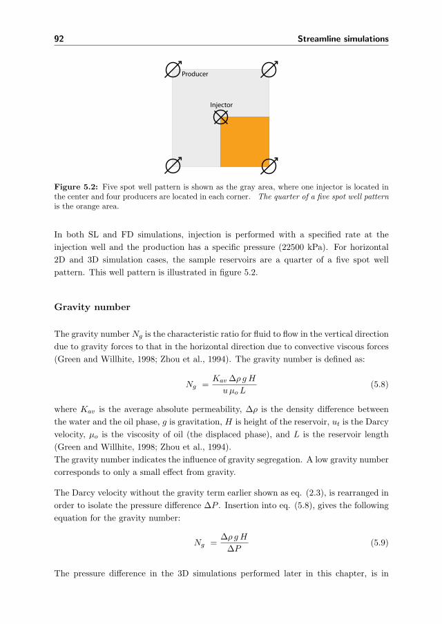
92 Streamline simulations
Injector
Producer
Figure 5.2: Five spot well pattern is shown as the gray area, where one injector is located inthe center and four producers are located in each corner. The quarter of a five spot well patternis the orange area.
In both SL and FD simulations, injection is performed with a specified rate at the
injection well and the production has a specific pressure (22500 kPa). For horizontal
2D and 3D simulation cases, the sample reservoirs are a quarter of a five spot well
pattern. This well pattern is illustrated in figure 5.2.
Gravity number
The gravity number Ng is the characteristic ratio for fluid to flow in the vertical direction
due to gravity forces to that in the horizontal direction due to convective viscous forces
(Green and Willhite, 1998; Zhou et al., 1994). The gravity number is defined as:
Ng =Kav Δρ g H
uμo L(5.8)
where Kav is the average absolute permeability, Δρ is the density difference between
the water and the oil phase, g is gravitation, H is height of the reservoir, ut is the Darcy
velocity, μo is the viscosity of oil (the displaced phase), and L is the reservoir length
(Green and Willhite, 1998; Zhou et al., 1994).
The gravity number indicates the influence of gravity segregation. A low gravity number
corresponds to only a small effect from gravity.
The Darcy velocity without the gravity term earlier shown as eq. (2.3), is rearranged in
order to isolate the pressure difference ΔP . Insertion into eq. (5.8), gives the following
equation for the gravity number:
Ng =Δρ g H
ΔP(5.9)
The pressure difference in the 3D simulations performed later in this chapter, is in
108

5.4 Verification of implementation 93
average 4600 kPa, and the gravity is 9.81 m/s2. The remaining parameters are listed
in table 5.1. We apply an oil density of both 800 and 500 kg/m3, resulting in gravity
numbers at 0.004 and 0.01, respectively. These gravity numbers indicate that the effect
from convection mainly dominates. Therefore, we only expect a moderate effect from
gravity on the saturation profiles and oil recovery.
5.4 Verification of implementation
In figure 5.3, results from the explicit 1D simulator, the SL simulator, and the FD
simulator show that the simulators produce the same water phase saturation profiles in
1D displacement. It confirms that the 1D model has been properly implemented into
the multidimensional schemes in both simulators.
0 0.2 0.4 0.6 0.8 10
0.2
0.4
0.6
0.8
1
ξ
s
τ=0.5 PVI
SL newslimtube 1D simFD old
Figure 5.3: Comparison between original 1D simulator (explicit version), the streamline sim-ulator (SL), and finite difference simulator (FD) for MEOR with 200 blocks. All three curvesare located at the top of each other.
5.5 Comparison of 2D results
Comparison between the SL and FD simulators is performed by running MEOR simula-
tions in a homogeneous square ”reservoir”, with injection into the upper left corner and
production from the lower right corner (figure 5.4). Comparison between the simulators
shows that their solutions are similar with only minor differences. The FD simulator
produces a smoother propagation front compared to the SL simulator, due to higher
numerical dispersion.
109
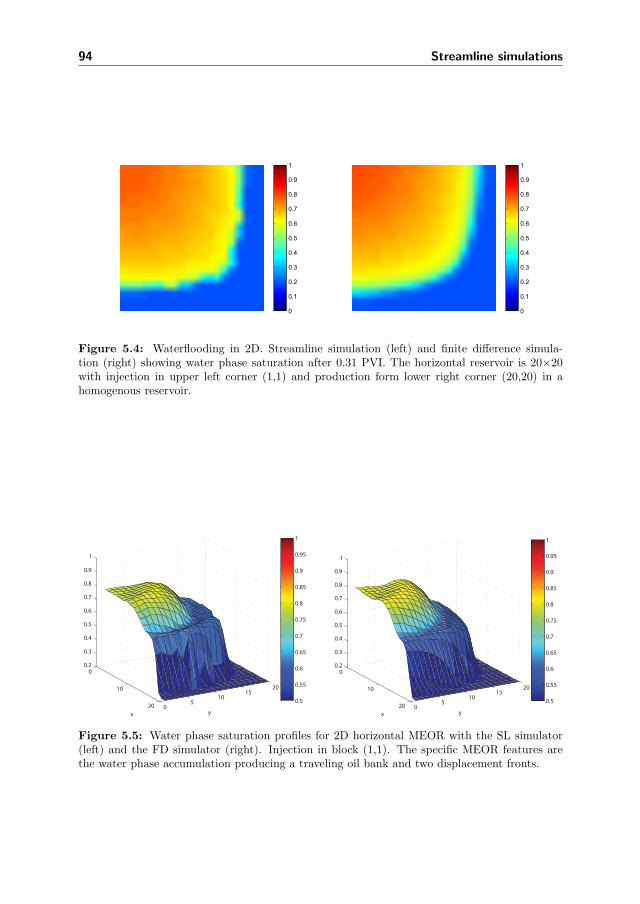
94 Streamline simulations
0
0.1
0.2
0.3
0.4
0.5
0.6
0.7
0.8
0.9
1
0
0.1
0.2
0.3
0.4
0.5
0.6
0.7
0.8
0.9
1
Figure 5.4: Waterflooding in 2D. Streamline simulation (left) and finite difference simula-tion (right) showing water phase saturation after 0.31 PVI. The horizontal reservoir is 20×20with injection in upper left corner (1,1) and production form lower right corner (20,20) in ahomogenous reservoir.
0
10
20 05
1015
20
0.2
0.3
0.4
0.5
0.6
0.7
0.8
0.9
1
yx
0.5
0.55
0.6
0.65
0.7
0.75
0.8
0.85
0.9
0.95
1
0
10
20 05
1015
20
0.2
0.3
0.4
0.5
0.6
0.7
0.8
0.9
1
yx
0.5
0.55
0.6
0.65
0.7
0.75
0.8
0.85
0.9
0.95
1
Figure 5.5: Water phase saturation profiles for 2D horizontal MEOR with the SL simulator(left) and the FD simulator (right). Injection in block (1,1). The specific MEOR features arethe water phase accumulation producing a traveling oil bank and two displacement fronts.
110
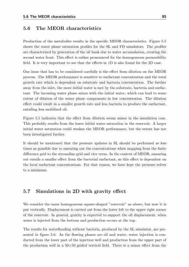
5.6 The MEOR characteristics 95
5.6 The MEOR characteristics
Production of the metabolite results in the specific MEOR characteristics. Figure 5.5
shows the water phase saturation profiles for the SL and FD simulators. The profiles
are characterized by generation of the oil bank due to water accumulation, creating the
second water front. This effect is rather pronounced for the homogeneous permeability
field. It is very important to see that the effects in 1D is also found for the 2D case.
One issue that has to be considered carefully is the effect from dilution on the MEOR
process. The MEOR performance is sensitive to surfactant concentration and the total
growth rate which is dependent on substrate and bacteria concentration. The further
away from the inlet, the more initial water is met by the substrate, bacteria and surfac-
tant. The incoming water phase mixes with the initial water, which can lead to some
extent of dilution of the water phase components in low concentration. The dilution
effect could result in a smaller growth rate and less bacteria to produce the surfactant,
entailing less mobilized oil.
Figure 5.5 indicates that the effect from dilution seems minor in the simulation case.
This probably results from the lower initial water saturation in the reservoir. A larger
initial water saturation could weaken the MEOR performance, but the extent has not
been investigated further.
It should be mentioned that the pressure updates in SL should be performed as less
times as possible due to smearing out the concentrations when mapping from the finite
difference grid to the streamline grid and vice versa. In the context of MEOR, smearing
out entails a smaller effect from the bacterial surfactant, as this effect is dependent on
the local surfactant concentrations. For that reason, we have kept the pressure solves
to a minimum.
5.7 Simulations in 2D with gravity effect
We consider the same homogeneous square-shaped ”reservoir” as above, but now it is
put vertically. Displacement is carried out from the lower left to the upper right corner
of the reservoir. In general, gravity is expected to support the oil displacement, when
water is injected from the bottom and production occurs at the top.
The results for waterflooding without bacteria, produced by the SL simulator, are pre-
sented in figure 5.6. As the flowing phases are oil and water, water injection is con-
ducted from the lower part of the injection well and production from the upper part of
the production well in a 50×50 grided vertical field. There is a minor effect from the
111
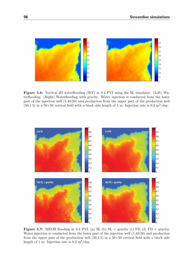
96 Streamline simulations
0
0.1
0.2
0.3
0.4
0.5
0.6
0.7
0.8
0.9
1
0
0.1
0.2
0.3
0.4
0.5
0.6
0.7
0.8
0.9
1
Figure 5.6: Vertical 2D waterflooding (WF) at 0.4 PVI using the SL simulator. (Left) Wa-terflooding. (Right) Waterflooding with gravity. Water injection is conducted from the lowerpart of the injection well (1,43:50) and production from the upper part of the production well(50,1:5) in a 50×50 vertical field with a block side length of 1 m. Injection rate is 0.2 m3/day.
0
0.1
0.2
0.3
0.4
0.5
0.6
0.7
0.8
0.9
1
0
0.1
0.2
0.3
0.4
0.5
0.6
0.7
0.8
0.9
1
0
0.1
0.2
0.3
0.4
0.5
0.6
0.7
0.8
0.9
1
0
0.1
0.2
0.3
0.4
0.5
0.6
0.7
0.8
0.9
1
(a) SL
(b) SL + gravity
(c) FD
(d) FD + gravity
Figure 5.7: MEOR flooding at 0.4 PVI. (a) SL (b) SL + gravity (c) FD (d) FD + gravity.Water injection is conducted from the lower part of the injection well (1,43:50) and productionfrom the upper part of the production well (50,1:5) in a 50×50 vertical field with a block sidelength of 1 m. Injection rate is 0.2 m3/day.
112

5.8 Simulations in 3D with gravity effect 97
gravity. The FD simulator gives similar results (not shown), where fingering towards
the production well occurs less markedly.
MEOR 2D simulations
Figure 5.7 shows 2D MEOR with and without gravity carried out by both simulators.
The standard MEOR case without gravity supports the fact that the FD fronts become
smoother and the SL produces more fingering. This was also seen at the previous MEOR
flooding simulations. The MEOR characteristics are also present the 2D vertical case
with gravity.
The SL simulation with gravity shows small perturbations in the saturations, but the
figure illustrates basically the same features as the FD simulation. It can be seen that
gravity to some extent stabilizes the displacement of oil. For the current case, the
gravity effect results in a slightly larger oil production, but the improvement is only
1 % OOIP after 1 PVI for both waterflooding and MEOR.
The incremental oil recovery after 1 PVI is 9 % OOIP, when comparing MEOR with
waterflooding under the influence of gravity. The maximum attainable recovery during
waterflooding (1D) after infinite time is 75 % OOIP and this is already achieved after
1 PVI during MEOR. This demonstrates the potential of MEOR. The MEOR recovery
after 2.4 PVI reaches 88 % OOIP for the current set-up.
5.8 Simulations in 3D with gravity effect
Figure 5.8 illustrates some layers of the heterogeneous permeability field used for the
3D simulations, which are performed only by the SL simulator. The grid is 50×50×10
with injection in (1,1,1:10) being located in upper left corner and production occurs
in blocks (50,50,1:2). The water phase saturations for the layers located in the top,
middle and bottom are presented in figure 5.9 and figure 5.10 without and with gravity,
respectively. Importantly, both profiles show two displacement fronts characterizing the
MEOR displacement. This is seen as shifts from blue to green area and from green to
red area.
As expected with gravity, more water is located in the bottom layers. Recovery after
1 PVI is 78 % OOIP without gravity and 79 % OOIP with gravity. The recovery is
only slightly increased due to gravity, which was also seen for the vertical 2D case. The
recovery for waterflooding is 69 % OOIP. Thus, also for this case MEOR results in a
noticeable increment of recovery.
113

98 Streamline simulations
Top Layer
Middle Layer
Bottom Layer
50
100
>150
Figure 5.8: Illustation of permeability field for 3D simulations.
Top Layer
Middle Layer
Bottom Layer
0.2
0.4
0.6
0.8
Figure 5.9: MEOR 3D simulation results without gravity after 0.5 PVI. Grid is 50×50×10with injection in (1,1,1:10) being located in upper left corner and production occurs in blocks(50,50,1:2). Injection rate is 2 m3/day.
Top Layer
Middle Layer
Bottom Layer
0. 2
0. 4
0. 6
0. 8
Figure 5.10: MEOR 3D simulation results with gravity after 0.5 PVI. Grid is 50×50×10with injection in (1,1,1:10) being located in upper left corner and production occurs in blocks(50,50,1:2). Injection rate is 2 m3/day.
Top Layer
Middle Layer
Bottom Layer
0.2
0.4
0.6
0.8
Figure 5.11: MEOR 3D simulation results like fig. 5.10 with gravity after 0.5 PVI. Only theoil density is reduced from 800 kg/m3 to 500 kg/m3.
114
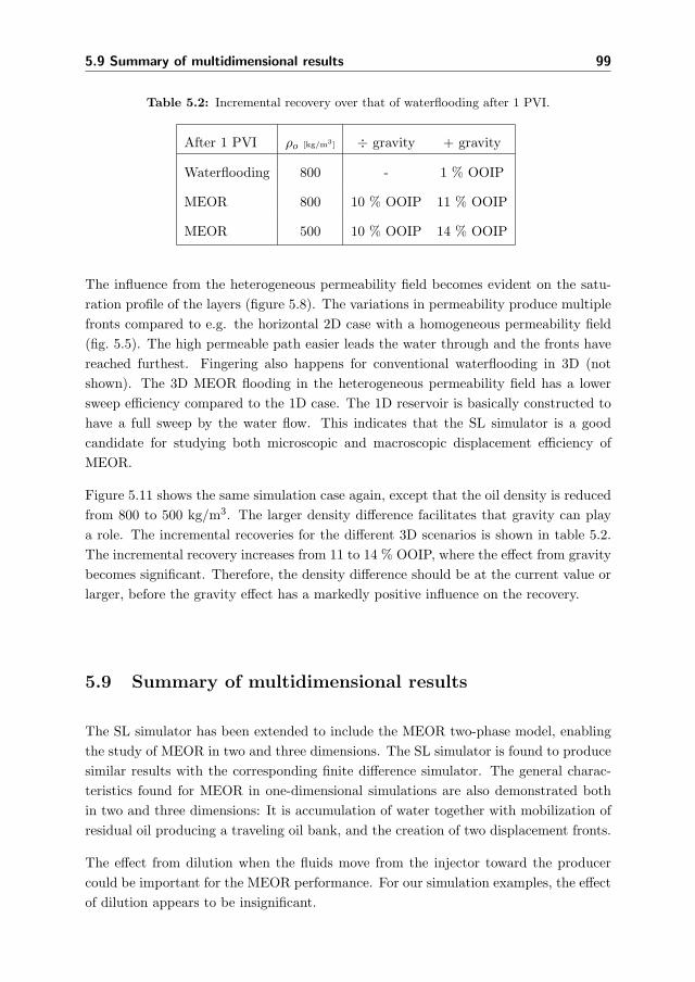
5.9 Summary of multidimensional results 99
Table 5.2: Incremental recovery over that of waterflooding after 1 PVI.
After 1 PVI ρo [kg/m3] ÷ gravity + gravity
Waterflooding 800 - 1 % OOIP
MEOR 800 10 % OOIP 11 % OOIP
MEOR 500 10 % OOIP 14 % OOIP
The influence from the heterogeneous permeability field becomes evident on the satu-
ration profile of the layers (figure 5.8). The variations in permeability produce multiple
fronts compared to e.g. the horizontal 2D case with a homogeneous permeability field
(fig. 5.5). The high permeable path easier leads the water through and the fronts have
reached furthest. Fingering also happens for conventional waterflooding in 3D (not
shown). The 3D MEOR flooding in the heterogeneous permeability field has a lower
sweep efficiency compared to the 1D case. The 1D reservoir is basically constructed to
have a full sweep by the water flow. This indicates that the SL simulator is a good
candidate for studying both microscopic and macroscopic displacement efficiency of
MEOR.
Figure 5.11 shows the same simulation case again, except that the oil density is reduced
from 800 to 500 kg/m3. The larger density difference facilitates that gravity can play
a role. The incremental recoveries for the different 3D scenarios is shown in table 5.2.
The incremental recovery increases from 11 to 14 % OOIP, where the effect from gravity
becomes significant. Therefore, the density difference should be at the current value or
larger, before the gravity effect has a markedly positive influence on the recovery.
5.9 Summary of multidimensional results
The SL simulator has been extended to include the MEOR two-phase model, enabling
the study of MEOR in two and three dimensions. The SL simulator is found to produce
similar results with the corresponding finite difference simulator. The general charac-
teristics found for MEOR in one-dimensional simulations are also demonstrated both
in two and three dimensions: It is accumulation of water together with mobilization of
residual oil producing a traveling oil bank, and the creation of two displacement fronts.
The effect from dilution when the fluids move from the injector toward the producer
could be important for the MEOR performance. For our simulation examples, the effect
of dilution appears to be insignificant.
115

100 Streamline simulations
In the SL simulator, the effect of gravity is introduced using an operator splitting tech-
nique. The gravity effect stabilizes the oil displacement causing slight incremental oil
recovery, which is also indicated from the gravity number. Decreasing the oil density
prompts that gravity may play a role. This leads to markedly improvement of incre-
mental oil recovery.
Overall, the MEOR process produces more oil compared to waterflooding. Three-
dimensional simulations, compared to one-dimensional, make it possible to not only
study the sweep efficiency, but also the displacement efficiency on the reservoir scale,
affected by the three-dimensional geometry and reservoir heterogeneities.
116

Chapter 6
Conclusion
A generic model has been set up to include the two main mechanisms in the MEOR
process; reduction of IFT due to surfactant production, and microscopic fluid diversion
as a part of the overall fluid diversion mechanism due to formation of biofilm.
In the context of MEOR, our novel approach is the partition of surfactant between oil
and water. Surfactant is the key component in order to reduce interfacial tension (IFT).
We have looked into three methods how to translate the IFT reduction into changes of
the relative permeabilities: the capillary number method, Coats’ method, and the Corey
relative permeability interpolation method. These methods produce similar results, with
small variations in the minimum obtained residual oil, the attained distance from the
inlet to the position for the initial surfactant effect, and the sensitivity to interfacial
tension reduction.
Separate investigations of the surfactant effect have been performed through exempli-
fying simulation cases, where no biofilm is formed. The water phase saturation profiles
are found to contain a waterfront initially following the saturation profile for pure wa-
terflooding. At the oil mobilization point – where the surfactant effect starts to take
place – sufficient surfactant has been built up mobilizing residual oil producing a second
waterfront. An oil bank is created, and in some cases, it catches up with the water-
front. The recovery curve consists of several parts. Initially, the recovery curve follows
pure waterflooding recovery until breakthrough of the oil bank. The next part of the
recovery curve continues until breakthrough of the second waterfront. The incline is
still relatively steep due to a low water cut. In the last part, the curve levels off.
The surfactant concentration in the water phase must reach a certain concentration
117

102 Conclusion
threshold before surfactant can reduce the interfacial tension. The relative permeabili-
ties depend on the water phase concentration, so when surfactant is moved into the oil
phase, there will be a smaller effect from the surfactant on the flow. Therefore, transfer
part of the surfactant to oil phase is equivalent to its “disappearance”, so that the total
effect from surfactant is reduced. The oil phase captures the surfactant, but it may as
well be adsorbed to the pore walls in the oil phase.
The influence from partitioning of surfactant only determines the time lag before the
surfactant effect can be seen. The position for the surfactant effect does not change
final recovery with different partitioning. However, if too little surfactant stays in the
water phase, we cannot obtain the surfactant effect.
It has been found that the final recovery depends on the distance from the inlet to the
oil mobilization point. A long distance means that oil in the beginning of the reservoir
is not recovered. The surfactant effect position is sensitive to changes in growth rate,
and injection concentrations of bacteria and substrate. Variations in growth rate and
injection concentration to a smaller extent affect the time lag until mobilization of
residual oil occurs.
Additionally, the final recovery depends on, how much the surfactant-induced IFT re-
duction lowers the residual oil, which is also a result of efficiency of the surfactant. A
super efficient surfactant produces an incremental recovery recovery around 40 % OOIP
over that of waterflooding. Application of a less efficient – and probably more realistic
– surfactant results in an incremental oil recovery of 9 % OOIP, but it is still considered
a significant improvement.
The adsorbed bacteria adhere to the pore walls and constitute the biofilm phase. The
biofilm formation implies that the concentration of bacteria near the inlet increases.
In combination with surfactant production, the biofilm results in a higher surfactant
concentration in the initial part of the reservoir. The oil that is initially bypassed in
relation to the surfactant effect, can be recovered as formation of biofilm shortens the
distance to the oil mobilization point. In a sample simulation, the effect from surfactant
only displays an incremental oil recovery of 13.0 % OOIP. In comparison, the effect from
both biofilm formation and surfactant production leads to an increment of 13.6 % OOIP.
The formation of biofilm to a minor extent enhances the oil recovery.
The formation of biofilm promotes fluid diversion. A contribution to this mechanism is
microscopic fluid diversion, which is possible to investigate in a one-dimensional system.
This happens due to the fact that the biofilm is formed only at the water-occupied zones
or pores where bacteria live. The porosity decreases due to biofilm formation, and the
relative permeability for the water phase alone is reduced, according to our modified
version of the Kozeny-Carman equation. This results in decreasing the mobility of water
and, correspondingly, a higher fraction of oil in the flow. Simulation cases study the
118

Conclusion 103
effect from biofilm formation together with microscopic fluid diversion. The biofilm
saturation should reach about 0.2, before there is a markedly improvement of the oil
recovery. The incremental oil recovery is 1.3 % OOIP.
Combination of biofilm formation, microscopic fluid diversion, and surfactant produc-
tion improves the oil recovery even more. We achieve an increment in recovery of almost
15 % OOIP.
The one-dimensional studies for the mechanisms separately and in combination show
that all the mechanisms contribute to improvement of the oil recovery. The mechanisms
produce their characteristic effect on the saturation profile and thus on the recovery
curve. When sufficient amounts of surfactant can be produced, the effect from surfactant
generates a larger effect compared to microscopic fluid diversion.
To study the MEOR performance in multiple dimensions, the 1D model with the sur-
factant effect only has been implemented into existing simulators; a streamline simula-
tor and a finite difference simulator. In the streamline simulator, the one-dimensional
simulator is used for propagating the solution along each streamline, which makes it
easier to implement the model. In addition, the effect of gravity is introduced using
an operator splitting technique. The gravity effect stabilizes oil displacement causing
markedly improvement of the oil recovery, when the oil density becomes relatively low.
The general characteristics found for MEOR in one-dimensional simulations are also
demonstrated both in two and three dimensions. Overall, the MEOR in multiple di-
mensions in heterogeneous reservoirs also produces more oil compared to waterflooding.
In our simulations for model reservoirs, characteristic effects and orders of magnitude
of recovery improvement were found to be similar to one-dimensional simulations. This
will probably change if more heterogeneous reservoirs will be considered.
119

104 Conclusion
120

Chapter 7
Future work
The model developed in this thesis is generic building on general knowledge of microbial
and reservoir processes. For achieving the long-term goal of designing a robust MEOR
process, the model should be modified to describe MEOR with specific bacteria under
specific reservoir conditions. The model should be “fed” with necessary particular infor-
mation coming from laboratory experimental data and field tests. In order to obtain the
necessary information, collaboration with other researchers in petroleum microbiology
and engineering should be established. Other collaborators could be researchers working
with bioremediation or ground water contamination, where they possess some expertise
on transport of bacteria in the underground. One subject that should be focused on, is
arrangement of field trials. Obtaining specific information on the basis of the field trial
data is a specific task that needs a separate development.
Microscopic fluid diversion has been investigated as a part of the fluid diversion mech-
anism. We suggest that the model should be extended to two or three dimensions to
see the full effect of fluid diversion. Especial attention should be paid to highly het-
erogeneous media where formation of biofilm may lead to not only microscopic, but
also meso- and macroscopic fluid diversion: hindering water breakthrough through high
permeable zones or systems of fractures.
Fluid diversion is supposed to increase areal sweep, while the effect of surfactant is
to recover more oil, where the water has already flown. The two effects are clearly
complementary. Their combination in three dimensions should also be investigated.
In this work, it is assumed that biofilm consists of bacteria only. As mentioned, the
actual biofilm is also composed of a water-filled matrix, sticky polysaccharides, and
121
106 Future work
many substrates and metabolites. All these additions may affect biofilm growth rate
and thickness, as well as surfactant production in it. Therefore, they are suggested to
be included in later models. Especially, the water content should be included, in order
to estimate the influence from biofilm.
The porous media are composed of pores of different sizes. Therefore, the transport of
bacteria through the reservoir also depends on processes such as straining and physical
filtration. The straining process is a function of the pore geometry, where a bacterium
too large to allow passage through a pore is trapped. Physical filtration is the removal
of particle mass from solution via collision with and deposition on the internal porous
surface (Ginn et al., 2002). Investigations should be performed to be able to describe
physical transport of the bacteria. The attachment process for initiating a biofilm,
is an excellent target for further studies. This gives rise to a new direction in the
MEOR modeling, where bacterial transport is modeled in the framework of the deep
bed filtration theory. Relevant deterministic or stochastic models may be applied.
In connection to MEOR, futurre models should also be able to include the presence
of different bacteria. Oil fields do contain indigenous bacteria, or bacteria enter the
reservoir during water injection. The indigenous bacteria may comprise different types of
bacteria representing a bacterial community. For activating the community in a specific
way, knowledge about the community collaboration is important. In addition, bacteria
injected into the reservoir should also be able to properly compete with the indigenous
bacteria or well site bacteria. Generally, there is a need for models that can deal with
bacterial communities, because it can very likely be important for the performance of
the MEOR process. Interaction between the different bacterial populations may need
development of new approaches, similar to population balance models, but taking into
account multiphase character of the flow and bacterial filtration.
Injection of substrates should be done with care to secure that the substrates will favor
the growth of specific MEOR bacteria. A model that combines different substrates with
the bacterial diversity is another step on the way toward designing a robust MEOR
process.
122

Appendix A
Parameters in Langmuir expression
To support the choice of parameters for the Langmuir expression in section 4.1, we lookat the parameters differently. The same result is obtained by approaching it anotherway.
Assume that we have bacteria with a diameter of db =1μm, and the bacteria densityis as given in table 4.1. The maximum amount of bacteria pr area becomes a productof the number of bacteria per surface area and the mass of one bacteria, when onebacterium is considered a cube with the side length db, and covers the surface in onelayer:
Mb,max ≈1
(db)2· (d3bρb) = dbρb (A.1)
where ρb is the density of the bacterium given in table 4.1.
Application of equation (2.28) gives a maximum pore volume of 75 %, which agreeswith the result found using the other approach.
123

108 Parameters in Langmuir expression
124

Appendix B
Multivariable Newton iteration
The Newton iteration solves the matrix system below (Aziz et al., 2003). The correctionfactor δ is found, which is the correction to the new variable vector y to approach thesolution of the system.
J(yn) · δ = −F(yn) (B.1)
yn+1 = yn + δ (B.2)
This will be repeated until convergence, which is evaluated from an error estimate|F(y)|2. Often, |δ|2 is used as error estimator, but I choose |F(y)|2, because it takesdifferent scales of components into account. The tolerance is set to 10−8. The Newtoniteration is characterized by showing quadratic convergence, when the initial guess isclose enough to the true zero. In this case, the initial guess is considered reasonable,when conditions from the previous time step and position are used, and concurrentlysmall time steps are taken, so changes will be small.
In order to setup the matrix system above, the Jacobian should be manufactured. Thedefinition of the Jacobian is:
Jij =∂Fi
∂yj(B.3)
The Jacobian is chosen to be numerical as this makes the system more flexible. Thenumerical Jacobian will be calculated as shown in equation (B.4).
Jij =ΔFi
Δyj=Fi(y + εj)−Fi(y)
εj(B.4)
The perturbation εj will be in the order of 10−5.
125

110 Multivariable Newton iteration
126
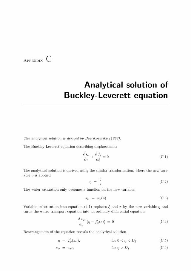
Appendix C
Analytical solution of
Buckley-Leverett equation
The analytical solution is derived by Bedrikovetsky (1993).
The Buckley-Leverett equation describing displacement:
∂sw∂τ
+∂ fj∂ξ
= 0 (C.1)
The analytical solution is derived using the similar transformation, where the new vari-able η is applied.
η =ξ
τ(C.2)
The water saturation only becomes a function on the new variable:
sw = sw(η) (C.3)
Variable substitution into equation (4.1) replaces ξ and τ by the new variable η andturns the water transport equation into an ordinary differential equation.
d swdη
(η − f ′w(s)
)= 0 (C.4)
Rearrangement of the equation reveals the analytical solution.
η = f ′w(sw), for 0 < η < Df (C.5)
sw = swi, for η > Df (C.6)
127

112 Analytical solution of Buckley-Leverett equation
where the value of Df is
Df = f ′w(sf ) (C.7)
Here, the front water saturation is sf . The saturation determines Df , which describesthe location of the front in terms of η. It is known that the fractional flow is zero atinitial saturation swi, and the tangent on the fractional flow curve at the front saturationfw(sf ) goes through the initial point.The front water saturation is determined from the knowledge about the fractional flowfirst derivative.
f ′w =fw(sf )− 0
sf − swi(C.8)
128
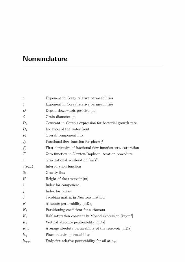
Nomenclature
a Exponent in Corey relative permeabilities
b Exponent in Corey relative permeabilities
D Depth, downwards positive [m]
d Grain diameter [m]
Dc Constant in Contois expression for bacterial growth rate
Df Location of the water front
Fi Overall component flux
fj Fractional flow function for phase j
f ′j First derivative of fractional flow function wrt. saturation
F Zero function in Newton-Raphson iteration procedure
g Gravitational acceleration [m/s2]
g(σow) Interpolation function
Gi Gravity flux
H Height of the reservoir [m]
i Index for component
j Index for phase
J Jacobian matrix in Newtons method
K Absolute permeability [mDa]
Ki Partitioning coefficient for surfactant
Ks Half saturation constant in Monod expression [kg/m3]
Kz Vertical absolute permeability [mDa]
Kav Average absolute permeability of the reservoir [mDa]
krj Phase relative permeability
krowi Endpoint relative permeability for oil at swi
129

114 Nomenclature
krwor Endpoint relative permeability for water at (1− sor)
L Length of the reservoir [m]
The length of the column, where the pressure drop is investigated [m]
n Exponent in Coats’ interpolation function
nc Number of components
Ng Gravity number
np Number of phases
P Pressure [kPa]
p1 Constant in surfactant concentration - IFT correlation
p2 Constant in surfactant concentration - IFT correlation
p3 Constant in surfactant concentration - IFT correlation
q1 Constant in expression for the desaturation curve
q2 Constant in expression for the desaturation curve
q3 Constant in expression for the desaturation curve
Qi Well term for component [m3/day]
Qt Total well volumetric flow rate [m3/day]
Ri Reaction meaning net production of component
s Sum of water and biofilm saturations [m3/m3]
sf Saturation of the water front [m3/m3]
sj Saturation of phase j [m3/m3]
sor Residual oil saturation [m3/m3]
swi Initial water saturation [m3/m3]
S Specific surface [m2/m3 totalvolume]
S Efficient specific surface [m2/m3 PV]
t Time [day]
ud Dimensionless velocity
uj Phase velocity [m/s]
ut Total flow velocity [m/s]
uinj Injection velocity [m/day]
v Linear velocity [m3/day]
Vj Volume of a phase in a block [m3]
VT Total pore volume of a block [m3]
vij,inj Volumetric injection fraction
w1 Constant in the Langmuir expression for partitioning of bacteria [m]
w2 Constant in the Langmuir expression for partitioning of bacteria [m3/kg]
130
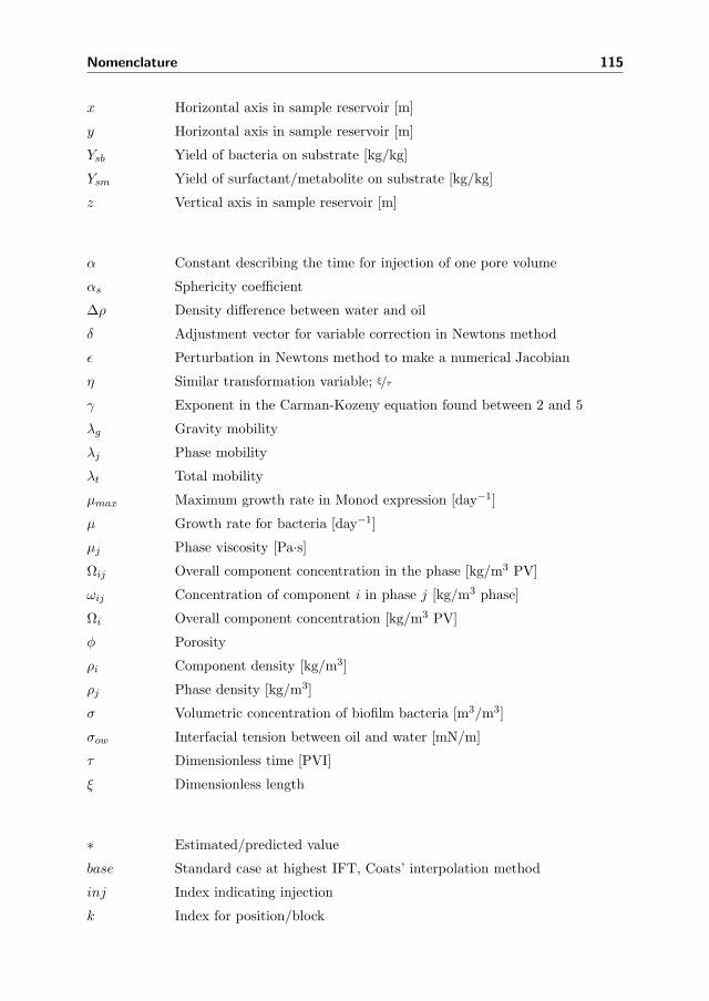
Nomenclature 115
x Horizontal axis in sample reservoir [m]
y Horizontal axis in sample reservoir [m]
Ysb Yield of bacteria on substrate [kg/kg]
Ysm Yield of surfactant/metabolite on substrate [kg/kg]
z Vertical axis in sample reservoir [m]
α Constant describing the time for injection of one pore volume
αs Sphericity coefficient
Δρ Density difference between water and oil
δ Adjustment vector for variable correction in Newtons method
ε Perturbation in Newtons method to make a numerical Jacobian
η Similar transformation variable; ξ/τ
γ Exponent in the Carman-Kozeny equation found between 2 and 5
λg Gravity mobility
λj Phase mobility
λt Total mobility
μmax Maximum growth rate in Monod expression [day−1]
μ Growth rate for bacteria [day−1]
μj Phase viscosity [Pa·s]
Ωij Overall component concentration in the phase [kg/m3 PV]
ωij Concentration of component i in phase j [kg/m3 phase]
Ωi Overall component concentration [kg/m3 PV]
φ Porosity
ρi Component density [kg/m3]
ρj Phase density [kg/m3]
σ Volumetric concentration of biofilm bacteria [m3/m3]
σow Interfacial tension between oil and water [mN/m]
τ Dimensionless time [PVI]
ξ Dimensionless length
∗ Estimated/predicted value
base Standard case at highest IFT, Coats’ interpolation method
inj Index indicating injection
k Index for position/block
131
116 Nomenclature
misc Linear case at lowest IFT, Coats’ interpolation method
n Index for time step
0 Index indicating the initial state
b Index for bacteria
m Index for metabolite/surfactant
o Index for oil
s Index for substrate
w Index for water
EOR Enhanced oil recovery
IFT Interfacial tension
MEOR Microbial enhanced oil recovery
NRB Nitrate reducing bacteria
OOIP Original oil in place
PV Pore volume
PVI Pore volumes injected
SRB Sulfate reducing bacteria
132

Bibliography
Al-Wahaibi, Y. M., C. A. Grattoni, and A. H. Muggeridge (2006, September). Drainageand imbibition relative permeabilities at near miscible conditions. J Petrol Sci Eng 53,239–253.
Amaefule, J. O. and L. L. Handy (1982). The effect of interfacial tensions on relativeoil/water permeabilities of consolidated porous media. SPE J 22, 371–381.
Amro, M. M. (2008). Multidisciplinary challenge for microbial enhanced oil recovery(MEOR). SPE-120820 presented at Saudi Arabia Section Technical Symposium, Al-Khobar, Saudi Arabia, 10–12 May.
Aslam, U. (2009a). Mehcanisms of microbe propagation in heterogeneous porous mediaand analysis of various MEOR processes involved in microbe transportation. SPE-119010 presented at Middle East Oil and Gas Show and Conference, Bahrain, Kingdomof Bahrain, 15–18 March.
Aslam, U. (2009b). Microbial plugging: A cost-effective approach for improved sweepefficiency through permeability reduction. SPE-119023 presented at Production andOperations Symposium, Oklahoma City, Oklahoma, USA, 4–8 April.
Aziz, K., L. Durlofsky, and H. Tchelepi (2003). Notes on petroleum reservoir simulation.Department of Petroleum Engineering, School of Earth Sciences, Stanford University,California, USA.
Banat, I. M. (1995). Biosurfactants production and possible uses in microbial enhancedoil recovery and oil pollution remediation: A review. Bioresource Technol 51, 1 – 12.
Bao, M., X. Kong, G. Jiang, X. Wang, and X. Li (2009). Laboratory study on activatingindigenous microorganisms to enhance oil recovery in Shengli Oilfield. J Petrol SciEng 66, 42 – 46.
Batycky, R. P. (1997). A three-dimensional two-phase field scale streamline simulator.Ph. D. thesis, Department of Petroleum Engineering, Stanford University, California,USA.
Bedrikovetsky, P. G. (1993). Mathematical theory of oil and gas recovery. Kluwer
133

118 Bibliography
Academic Publishers, London.
Behesht, M., R. Roostaazad, F. Farhadpour, and M. R. Pishvaei (2008). Model devel-opment for MEOR process in conventional non-fractured reservoirs and investigation ofphysico-chemical parameter effects. Chem Eng Technol 7, 953–963.
Berenblyum, R. A. (2004). Streamline simulation with capillary effects applied topetroleum engineering problems. Ph. D. thesis, Department of Chemical Engineering,Technical University of Denmark, Denmark.
Blanchet, D., A. Grabowski, and J.-P. Vandecasteele (2001). Microbiology of oil degra-dation in reservoirs. SPE-71449 presented at ATCE, New Orleans, Louisiana, USA,30 September–3 October.
Bordoloi, N. and B. Konwar (2008). Microbial surfactant-enhanced mineral oil recoveryunder laboratory conditions. Colloid Surface B 63 (1), 73 – 82.
Brown, F. (1992). Microbes: The practical and environmental safe solution to produc-tion problems, enhanced production, and enhanced oil recovery. SPE-23955 presented atPermian Basin Oil and Gas Recovery Conference, Midland, Texas, USA, 18–20 March.
Brown, L. R. (2010). Microbial enhanced oil recovery (MEOR). Curr Opin Microbiol 13,1–5.
Brown, L. R. and A. A. Vadie (2002). Slowing production decline and extending theeconomic life of an oil field: New MEOR technology. SPE Reserv Eval Eng 5, 33–41.
Bryant, R. and T. Burchfield (1989). Review of microbial technology for improving oilrecovery. SPE Reservoir Eng 4, 151–154.
Bryant, R., T. Burchfield, K. Chase, K. Bertus, and A. Stepp (1989). Optimization ofoil mobilization, transport of microbes and metabolites, and effects of additives. SPE-19686 presented at ATCE, San Antonio, Texas, USA, 8–11 October.
Bryant, R. S. and J. Douglas (1988). Evaluation of microbial systems in porous mediafor EOR. SPE Reservoir Eng 3, 489–495.
Bryant, S. L. and T. P. Lockhart (2002). Reservoir engineering analysis of microbialenhanced oil recovery. SPE-63229 presented at ATCE, Dallas, Texas, USA, 1–4 October.
Buciak, J., A.Vazquez, R. Frydman, J. Mediavilla, and R. Bryant (1995). Enhanced oilrecovery by means of microorganisms: Pilot test. SPE Advanced Technology Series 4,144–149.
Chang, M.-M., F. Chung, R. Bryant, H. Gao, and T. Burchfield (1991). Modelling andlaboratory investigation of microbial transport phenomena in porous media. SPE-22845presented at ATCE, Dallas, Texas, USA, 6–9 October .
Characklis, W. G. and P. A. Wilderer (Eds.) (1989). Structure and function of biofilms.John Wiley and Sons.
Chen, B., J. Wang, and S. Wo (1998). A generalized Godunov method for enhanced oilrecovery processes with microbial permeability modification in 1-D coreflood models.
134

Bibliography 119
Iterative Methods in Scientific Computation. EMACS Publication.
Chilingarian, G. V. and M. R. Islam (1995). A three-dimensional numerical simulatorfor microbial enhanced oil recovery. Scientia Iranica 2, 55–64.
Chisholm, J., S. Kashikar, R. Knapp, M. McInerney, and D. Menzie (1990). Microbialenhanced oil recovery: Interfacial tension and gas-induced relative permeability effects.SPE-20481 presented at ATCE, New Orleans, Louisiana, USA, 23–26 September.
Clement, T. P., B. Hooker, and R. S. Skeen (1996). Macroscopic models for predictingchanges in saturated porous media properties caused by microbial growth. GroundWater 34, 934–942.
Coats, K. H. (1980, October). An equation of state compositional model. SPE J 20,363–376.
Crescente, C., A. Rekdal, A. Abraiz, O. Torsaeter, L. Hultmann, A. Stroen, K. Ras-mussen, and E. Kowalewski (2008). A pore level study of MIOR displacement mech-anisms in glass micromodels using Rhodococcus sp. 094. SPE-110134 presented at theIOR Symposium,Tulsa, Oklahoma, USA, 19–23 April.
Crescente, C., O. Torsaeter, L. Hultmann, A. Stroem, , K. Rasmussen, andE. Kowalewski (2006). An experimental study of driving mechanisms in MIOR pro-cesses by using Rhodococcus sp. 094. SPE-100033 presented at the IOR Symposium,Tulsa, Oklahoma, USA, 22–26 April.
Datta-Gupta, A. (2000). Streamline simulation: A technology update. SPE-65604. JPetrol Technol 52, 68–73.
Davidova, I., M. Hicks, P. Fedorak, and J. Suflita (2001). The influence of nitrate onmicrobial processes in oil industry production waters. J Ind Microbiol Biot 27, 80–86.
Delshad, M., K. Asakawa, G. A. Pope, and K. Sepehrnoori (2002). Simulations of chem-ical and microbial enhanced oil recovery methods. SPE-75237 at the IOR Symposium,Tulsa, Oklahoma, USA, 13–17 April.
Deng, D., C. Li, Q. Ju, P. Wu, F. L. Dietrich, and Z. H. Zhou (1999). Systematicextensive laboratory studies of microbial EOR mechanisms and microbial EOR appli-cation results in Changqing Oilfield. SPE-54380 presented at Asia Pacific Oil and GasConference and Exhibition, Jakarta, Indonesia, 20–22 April.
Desouky, S. M., M. M. Abdel-Daim, M. H. Sayyouh, and A. S. Dahab (1996). Modellingand laboratory investigation of microbial enhanced oil recovery. J Petrol Sci Eng 15,309–320.
Dietrich, F., F. Brown, Z. Zhou, and M. Maure (1996). Microbial EOR technologyadvancement: Case studies on successful projects. SPE-36746 presented at ATCE,Denver, Colorado, USA, 6–9 October.
Eckford, R. and P. Fedorak (2002). Planktonic nitrate-reducing bacteria and sulfate-reducing bacteria in some western Canadian oil field waters. J Ind Microbiol Biot 29,83–92.
135

120 Bibliography
Feng, Q., F. Ni, B. Qin, X. Ma, C. Ji, and X. Wang (2006). Review of MEOR tech-nology application in Dagang Oilfield for the last decade. SPE-100791 presented atthe SPE Asia Pacific Oil and Gas Conference and Exhibition, Adelaide, Australia, 11–13 September.
Feng, Q., J. Zhou, Z. Chen, X. Wang, F. Ni, and H. Yang (2002). Study on EORmechanisms by microbial flooding. SPE-79176 presented at ATCE, Abuja, Nigeria,5–7 August.
Fulcher, R. A., T. Ertekin, and C. D. Stahl (1985). Effect of capillary number and itsconstituents on 2-phase relative permeability curves. J Petrol Technol 37 (2), 249–260.
Gandler, G. L., A. Gbosi, S. L. Bryant, and L. N. Britton (2006). Mechanistic under-standing of microbial plugging for improved sweep efficiency. SPE-100048 presented atthe IOR Symposium, Tulsa, Oklahoma, USA, 22–26 April.
Gerritsen, M. G. and L. J. Durlofsky (2005). Modeling fluid flow in oil reservoirs. AnnuRev Fluid Mech 37, 211–238.
Ghojavand, H., F. Vahabzadeh, E. Roayaei, and A. K. Shahraki (2008). Productionand properties of a biosurfactant obtained from a member of the Bacillus subtilis group(PTCC 1696). J Colloid Interf Sci 324, 172 – 176.
Ginn, T., B. Wood, K. Nelson, T. Scheibe, E. Murphy, and T. Clement (2002). Processesen microbial transport in the natural subsurface. Adv Water Resour 25, 1017–1042.
Gray, M. R., A. Yeung, J. M. Foght, and H. W. Yarranton (2008). Potential microbialenhanced oil recovery processes: A critical analysis. SPE-114676 presented at ATCE,Denver, Colorado, USA, 21–24 September.
Green, D. W. and G. P. Willhite (1998). Enhanced oil recovery, Volume 6. SPE TextbookSeries.
Grula, E. A., H. H. Russell, D. Bryant, and M. Kenaga (1989). Oil displacement byanaerobic and facultatively anaerobic bacteria. Microbial enhanced oil recovery, pp.113–124. Elsevier Science Publishers B. V.
Gullapalli, I. L., J. H. Bae, K. Hejl, and A. Edwards (2000). Laboratory design andfield implementation of microbial profile modification process. SPE Reserv Eval Eng 3,42–49.
Halim, A. Y., U. D. Fauzi, S. Siregar, E. Soewono, A. Y. Gunawan, D. I. Astuti, andN. Juli (2009). Microbial enhanced oil recovery: An investigation of bacteria ability tolive and alter crude oil physical characteristics in high pressure condition. SPE-123506presented at Asia Pacific Oil and Gas Conference and Exhibition, Jakarta, Indonesia,4–6 August.
Hitzman, D. O., M. Dennis, and D. C. Hitzman (2004). Recent successes: MEOR usingsynergistic H2S prevention and increased oil recovery systems. SPE-89453 presented atthe IOR Symposium, Tulsa, Oklahoma, USA, 17–21 April.
Ibrahim, Z., M. I. Omar, K. S. Foo, E. J. Elias, and M. Othman (2004). Simulation
136

Bibliography 121
analysis of microbial well tratment of Bokor Field, Malaysia. SPE-88453 presented atAsia Pacific Oil and Gas Conference and Exhibition, Perth, Australia, 18–20 October.
Islam, M. (1990). Mathematical modeling of microbial enhanced oil recovery. SPE-20480presented at ATCE, New Orleans, Louisiana, USA, 23–26 September.
Islam, M. R. and A. Gianetto (1993). Mathematical modelling and scaling up of micro-bial enhanced oil recovery. J Can Petrol Technol 32, 30–36.
Jack, T. R., J. Shaw, N. Wardlaw, and J. W. Costerton (1989). Microbial plugging inenhanced oil recovery. Microbial Enhanced Oil Recovery, pp. 125–148. Elsevier SciencePublishers B. V.
Jang, L.-K., M. M. Sharma, and T. F. Yen. (1984). The transport of bacteria in porousmedia and its significance in microbial enhanced oil recovery. SPE-12770 presented atCalifornia Regional Meeting, Long Beach, California, USA, 11–13 April .
Jenneman, G., R. Knapp, M. McInerney, D. Menzie, and D. Revus (1984). Experimentalstudies of in-situ microbial enhanced recovery. SPE-10789. SPE J 24, 33–37.
Jenneman, G. E. (1989). The potential for in-situ microbial applications. Microbialenhanced oil recovery, pp. 37–74. Elsevier Science Publishers B. V.
Jessen, K. and F. M. Orr (2004). Gravity segregation and compositional streamlinesimulation. SPE-89448 presented at the IOR Symposium, Tulsa, Oklahoma, USA, 17–21 April.
John, A., C. Han, M. Delshad, G. A. Pope, and K. Sepehrnoori (2005). A new generationchemical-flooding simulator. SPE J 10, 206–216.
Kim, S.-B. (2006). Numerical analysis of bacterial transport in saturated porous media.Hydrol Process 20, 1177–1186.
King, M. J. and A. Datta-Gupta (1998). Streamline simulation: A current perspective.In Situ 22, 91–140.
Kowalewski, E., I. Rueslatten, K. Steen, G. Bødtker, and O. Torsæter (2006). Microbialimproved oil recovery – bacterial induced wettability and interfacial tension effects onoil production. J Petrol Sci Eng 52, 275–286.
Kumar, S., S. J. Torabzadeh, and L. L. Handy (1985). Relative permeability functionsfor high- and low-tension systems at elevated temperatures. SPE-13670 presented atthe California Regional Meeting, Bakersfield, California, USA, 27–29 March.
Lake, L. W. (1989). Enhanced oil recovery. Prentice-Hall, Inc.
Lake, L. W., G. A. Pope, G. F. Garey, and K. Sepehrnoori (1984). Isothermal, multi-phase, multicomponent fluid flow in permeable media. In Situ 8, 1–40.
Lazar, I., I. G. Petrisor, and T. F. Yen. (2007). Microbial enhanced oil recovery (MEOR).Petrol Sci Technol 25, 1353 –1366.
MacLeod, F., H. Lappin-Scott, and J. Costerton (1988). Plugging of model rock system
137

122 Bibliography
by using starved bacteria. Appl Environ Microb 54, 1365–1372.
Madigan, M., J. Martinko, and J. Parker (2003). Brock: Biology of microorganisms(Tenth ed.). Prentice-Hall.
Magot, M., B. Ollivier, and B. Patel (2000). Microbiology of petroleum reservoirs.Anton van Lee 77, 103–116.
Marshall, S. L. (2008). Fundamental aspects of microbial enhanced oil recovery: Aliterature survey. Technical report, CSIRO Land and Water, Floreat, Western Australia.
Maudgalya, S., R. M. Knapp, and M. J. McInerney (2007). Microbially enhanced oilrecovery technologies. A review of the past, present and future. SPE-106978 presented atthe Production and Operations Symposium, Oklahoma City, Oklahoma, USA, 30 March–3 April.
Maure, A., F. Dietrich, U. Gomez, J. Vallesi, and M. Irusta (2001). Waterfloodingoptimization using biotechnology: 2-year field test, La Ventana Field, Argentina. SPE-69652 presented at Latin American and Caribbean Petroelum Engineering Conference,Buenos Aires, Argentina, 25–28 March.
Maure, A., A. A. Saldana, and A. R. Juarez (2005). Biotechnology application to EORin Talara off-shore oil fields, northwest Peru. SPE-94934 presented at Latin Americanand Caribbean Petroleum Engineering Conference, Rio de Janeiro, Brazil, 20–23 June.
McCabe, W. L., J. C. Smith, and P. Harriot (Eds.) (2005). Unit Operations of ChemicalEngineering (Seventh ed.). McGraw-Hill, New York.
McInerney, M. J., K. Duncan, N. Youssef, T. Fincher, S. K. Maudgalya, M. J. Folmsbee,R. Knapp, R. R. Simpson, N. Ravi, and D. Nagle (2005). Development of microorgan-isms with improved transport and biosurfactant activity for enhanced oil recovery. Tech-nical report, Department of Botany and Microbiology, and Department of PetroleumEngineering, University of Oklahoma, USA.
Mei, S., L. Wei, L. Guangzhi, H. Peihui, H. Zhaowei, C. Xinghong, and W. Ying (2003).Laboratory study on MEOR after polymer flooding. SPE-84865 presented at the IORConference in Asia Pacific, Kuala Lumpur, Malaysia, 20–21 October .
Molz, F., M. Widdowson, and L. Benefield (1986). Simulation of microbial growthdynamics coupled to nutrient and oxygen transport in porous media. Water ResourRes 8, 1207–1216.
Murphy, E. and T. Ginn (2000). Modeling microbial processes in porous media. Hydro-geol J 8, 142–158.
Nagase, K., S. T. Zhang, H. Asami, N. Yazawa, K. Fujiwara, H. Enomoto, C. X. Hong,and C. X. Liang (2002). A successful field test of microbial eor process in Fuyu Oil-field, China. SPE-75238 presented at the IOR Symposium,Tulsa, Oklahoma, USA, 13–17 April.
Nazina, T., D. Sokolova, A. Grigoryan, Y.-F. Xue, S. Belyaev, and M. Ivanov (2003).Production of oil-releasing compounds by microorganisms from the Daqing Oil Field,
138
Bibliography 123
China. Hydrogeol J 72, 206–211.
Nielsen, J., J. Villadsen, and G. Liden (2003). Bioreaction engineering principles (Firsted.). New York: Kluwer Academic/Plenum Publishers.
Nielsen, S. M., K. Jessen, A. A. Shapiro, M. L. Michelsen, and E. H. Stenby (2010). Mi-crobial enhanced oil recovery: 3D simulation with gravity effects. SPE-131048 presentedat the EUROPEC/EAGE Conference and Exhibition, Barcelona, Spain, 14–17 June.
Nielsen, S. M., A. A. Shapiro, M. L. Michelsen, and E. H. Stenby (2010). 1D simulationsfor microbial enhanced oil recovery with metabolite partitioning. Transport PorousMed 85, 785–802.
Orr, F. M. (2007). Theory of gas injection processes. TIE-LINE Publications.
Peihui, H., S. Fengrong, and S. Mei (2001). Petroleum hydrocarbon as a sole car-bon source. SPE-72128 presented in the Asia Pacific IOR Conference, Kuala Lumpur,Malaysia, 8–9 October.
Portwood, J. T. (1995). A commercial microbial enhanced oil recovery technology: Eval-uation of 322 projects. SPE-29518 presented at the Production Operations Symposium,Oklahoma City, Oklahoma, USA, 2–4 April.
Rafique, M. A. and U. Ali (2008). Microbial enhanced oil recovery (MEOR) with specialemphasis to the ”uneconomical reserves”. SPE-113272 presented at the Indian Oil andGas Technical Conference and Exhibition, Mumbai, India, 4–6 March.
Raiders, R., D. Freeman, G. Jenneman, R. Knapp, and M. McInerney (1985). The useof microorganisms to increase the recovery of oil from cores. SPE-14336 presented atATCE, Las Vegas, Nevada, USA, 22–25 September.
Raiders, R., T. Maher, R. Knapp, and M. Mclnerney (1986). Selective plugging andoil displacement in crossflow core systems by microorganisms. SPE-15600 presented atATCE, New Orleans, Louisiana, USA, 5–6 October.
Ravera, F., M. Ferrari, and L. Liggieri (2000). Adsorption and partitioning of surfactantin liquid-liquid systems. Adv Colloid Interfac 88, 129–177.
Rockhold, M. L., R. R. Yarwood, and J. S. Selker (2004). Coupled microbial andtransport processes in soils. Vadose Zone J 3, 368–383.
Samir, M., M. A. El Ela, S. El Marsafy, S. El Tayeb, A. A. Waly, and M. H. Sayyouh(2010). New incubated Pseudomonas aeruginosa bacteria for increasing oil recoveryunder reservoir conditions. SPE-126104 presented at the North Africa Technical Con-ference and Exhibition, Cairo, Egypt, 14–17 February .
Sarkar, A., G. Georgiou, and M. Sharma (1994). Transport of bacteria in porous media:II. A model for convective transport and growth. Biotechnol Bioeng 44, 499–508.
Segovia, G. C., V. A. Huerta, and G. C. Gutierrez (2009). Improving MEOR perfor-mance by a selection methodology in mature oilfields. SPE-123072 presented at LatinAmerican and Caribbbean Petroleum Engineering Conference, Cartagena, Colombia,3 May –3 June.
139

124 Bibliography
Sen, R. (2008). Biotechnology in petroleum recovery: The microbial EOR. Prog EnergCombust 34 (6), 714 – 724.
Sen, T., D. Das, K. Khilar, and G. Suraishkumar (2005). Bacterial transport in porousmedia: New aspects of the mathematical model. Colloids Surface A 260, 53–62.
Shafai, M. and K. Vafai (2009). Biofilm affected characteristics of porous structures.Int J Heat Mass Tran 52, 274–581.
Sharma, M. and G. Georgiou (1993). Microbial Enhanced Oil Recovery Research –Final Report prepared for U.S. Department of Energy. Technical report, Departmentof Petroleum Engineering, University of Texas, Austin, USA.
Shen, P., B. Zhu, X.-B. Li, and Y.-S. Wu (2006). The influence of interfacial tension onwater/oil two-phase relative permeability. SPE-95405 presented at the IOR Symposium,Tulsa, Oklahoma, USA, 22–26 April.
Soleimani, S., P. J. V. Geel, O. B. Isgor, and M. B. Mostafa (2009). Modeling ofbiological clogging in unsaturated porous media. J Contamin Hydrol 106, 39–50.
Stevik, T. K., K. Aa, G. Ausland, and J. F. Hanssen (2004). Retention and removal ofpathogenic bacteria in wastewater percolating through porous media: A review. WaterRes 38, 1355 – 1367.
Streeb, L. P. and F. G. Brown (1992). MEOR – Altamont/Bluebell Field project.SPE-24334 presented at Rocky Mountain Regional Meeting, Casper, Wyoming, USA,18–21 May.
Sugai, Y., H. Chengxie, T. Chida, and H. Enomoto (2007). Simulation studies onthe mechnisms and performances of MEOR using polymer producing microorganismClostridium sp. TU-15A. SPE-110173 presented at Asia Pacific Oil and Gas Conferenceand Exhibition, Jakarta, Indonesia, 30 October–1 November.
Sugihardjo, E. H. L. and S. W. Pratomo (1999). Microbial core flooding experimentsusing indigenous microbes. SPE-57306 presented at Asia Pacific IOR Conference, KualaLumpur, Malaysia, 25–26 October.
Sunde, E., J. Beeder, R. K. Nilsen, and T. Torsvik (1992). Aerobic microbial enhancedoil recovery for offshore use. SPE-24204 presented at the IOR Symposium, Tulsa, Ok-lahoma, USA, 22–24 April.
Taber, J. (1969). Dynamic and static forces required to remove a discontinuous oil phasefrom porous media containing both oil and water. SPE J 9, 3–12.
Tadmouri, R., C. Zedde, C. Routaboul, J.-C. Micheau, and V. Pimienta (2008). Parti-tion and water/oil adsorption of some surfactants. J Phys Chem B 112, 12318–12325.
Thiele, M. R. (1991). Modeling multiphase flow in heterogeneous media using stream-tubes. Ph. D. thesis, Department of Petroleum Engineering, Stanford University, USA.
Thullner, M. (2009). Comparison of bioclogging effects in saturated porous media withinone- and twodimensional flow systems. Ecol Eng 36, 176–196.
140
Bibliography 125
Tufenkji, N. (2007). Modeling microbial transport in porous media: Traditional ap-proaches and recent developments. Adv Water Resour 30, 1455–1469.
Updegraff, D. M. (1983). Plugging and penetration of petroleum reservoir rock bymicroorganisms. In E. C. Donaldson and J. B. Clark (Eds.), Proceedings of the 1982International Conference on Microbial Enhancement of Oil Recovery.
UTCHEM (2000). Technical Documentation for UTCHEM 9.0 – A three dimen-sional chemical flood simulator. Reservoir Engineering Research Program, Center forPetroleum and Geosystems Engineering at the University of Texas at Austin, USA.
Vadie, A. A., J. O. Stephens, and L. R. Brown (1996). Utilization of indigenous mi-croflora in permeability profile modification of oil bearing formations. SPE-35448 pre-sented at the IOR Symposium Tulsa, Oklahoma, USA, 21–24 April.
Valdes-Parada, F. J., M. L. Porter, K. Narayanaswamy, R. M. Ford, and B. D. Wood(2009). Upscaling microbial chemotaxis in porous media. Adv Water Resour 32, 1413– 1428.
Van Hamme, J., A. Singh, and O. Ward (2003). Recent advances in petroleum micro-biology. Microbiol Mol Bio R 67, 503–549.
Vandevivere, P., P. Baveye, D. S. de Lozada, and P. DeLeo (1995). Microbial cloggingof saturated soils and aquifer materials: Evaluation of mathematical models. WaterResour Res 31, 2173–2180.
Wang, F. and V. V. Tarabara (2009). Permeability of fiber-filled porous media: Kozeny-Carman-Ethier modeling approach. Environ Eng Sci 26, 1149–1155.
Wo, S. (1997). The mathematical modeling and numerical approaches for microbialpermeability modification enhanced oil recovery processes. Ph. D. thesis, Graduate Schoolof The University of Wyoming, USA.
Youssef, N., D. R. Simpson, K. E. Duncan, M. J. McInerney, M. Folmsbee, T. Fincher,and R. M. Knapp (2007). In situ biosurfactant production by Bacillus strains injectedinto a limestone petroleum reservoirg. Appl Environ Microbiol 73, 1239–1247.
Zekri, A. Y. and R. A. Almehaideb (1999). Project of increasing oil recovery from UAEreservoirs using bacteria flooding. SPE-56827 presented at ATCE, Houston, Texas,USA, 3–6 October.
Zhang, X., R. Knapp, and M. McInerney (1992). A mathematical model for enhancedoil recovery process. SPE-24202 presented at IOR Symposium, Tulsa, Oklahoma, USA,22–24 April.
Zhaowei, H., H. Peihui, L. Jianjun, C. Jianfei, G. Menghua, and C. Xinghong (2008).The application of hydrocarbon-degrading bacteria in Daqing’s low permeability, highparaffin content oilfields. SPE-114344 presented at the IOR Symposium, Tulsa, Okla-homa, USA, 19–23 April.
Zhou, D., F. J. Fayers, and F. M. Orr (1994). Scaling of multiphase flow in simple hetero-geneous porous media. SPE-27833 presented at the IOR Symposium, Tulsa, Oklahoma,
141

126 Bibliography
USA, 17–20 April.
ZoBell, C. E. (1947). Bacterial release of oil from oil-bearing materials. World Oil 126,36–47.
142


Center for Energy Resources Engineering
Department of Chemical and
Biochemical Engineering
Technical University of Denmark
Søltofts Plads, Building 229
DK-2800 Kgs. Lyngby
Denmark
Phone: +45 4525 2800
Fax: +45 4525 4588
Web: www.kt.dtu.dk
ISBN : 978-87-92481-31-3
Related Documents