Microbeam pull-in voltage topology optimization including material deposition constraint

Microbeam pull-in voltage topology optimization includingmaterial

deposition constraintE. Lemaire, V. Rochus, J.-C. Golinval, P. Duysinx

Aerospace and Mechanical Engineering Department, University of Liege, B52, Chemin deschevreuils 1, B4000 Liege Belgium

Abstract

Because of the strong coupling between mechanical and electrical phenomenon existing inelectromechanical microdevices, some of them experience, above a given driving voltage, anunstable behavior called pull-in effect. The present paper investigates the application of topol-ogy optimization to electromechanical microdevices for the purpose of delaying the unstablebehavior by maximizing their pull-in voltage. Within the framework of this preliminary study,the pull-in voltage maximization procedure is developed on the basis of electromechanical mi-crobeams reinforcement topology design problem. The proposed sensitivity analysis requiresonly the knowledge of the microdevice pull-in state and of the first eigenmode of the tangentstiffness matrix. As the pull-in point research is a highly non-linear problem, the analysisis based on a monolithic finite element formulation combined with a normal flow algorithm(homotopy method). An application of the developed method is proposed and the resultis compared to the one obtained using a linear compliance optimization. Moreover, as, theresults provided by the developed method do not comply with manufacturing constraints, adeposition process constraint is added to the optimization problem and its effect on the finaldesign is also tested.

Keywords : Topology optimization, electromechanical coupling, pull-in, manufacturing con-straint

1 Introduction

The main idea underlying topology optimization is to avoid arbitrary decision on the con-nectivity or shape during the design stage of a structure. In consequence, the optimizationproblem is formulated as the research of the optimal material distribution maximizing a givenobjective function following some design constraints such as reliability constraints or manu-facturing constraints. As proposed by seminal works [1, 2], the material distribution can berepresented using an indicator function equal to ’1’ if material is present and ’0’ where it isvoid.

However, the topology optimization discrete form (0-1) is very difficult to solve becauseof its highly combinatorial nature. Usually, the highly combinatorial formulation is avoidedby allowing the indicator function to vary continuously from 0 to 1. Contrary to the dis-crete version, the continuous problem can be solved using sensitivity analysis and efficientmathematical programming algorithms. Then, the indicator function can be considered asa density function representing the density of a porous material. Most often, the topologyoptimization problem is solved on the discretized version of the continuum mechanics problemusing a finite element approximation. The density function is generally represented on this

1

mesh by attaching to each element a density design variable µ. Unfortunately, the resultingoptimization problem is in general mathematically ill-posed and additional modifications areneeded (see reference [3]) as inclusion of a perimeter constraint or filtering of the sensitivitieswhich is presented in the following.

Next, considering a finite element mesh of the design domain, the properties of eachelement have to be estimated for continuous values of its density variable. This can first beperformed on the basis of a microstructural approach using homogenization theory in order toensure the physical meaning of the interpolation [1] or more simply by introducing a fictitiousmaterial model like the famous SIMP power law [2] which proposes to compute the YoungModulus E using a power law interpolation,

E = µpE0

where E0 is the design material Young Modulus.Currently, topology optimization has been applied as a systematic design tool to many

problems involving one physics (see [4] for a review) like structural, electrical or magneticproblems (see Wang [5]). Conversely, the application of topology optimization to multi-physics problems is now under development. One of the earliest introductions of coupledbehavior in topology optimization has been performed by Sigmund [6] for the optimal designof electrothermomechanical actuators. The problem considered by Sigmund includes threedifferent physical fields, namely electric, thermal and mechanic. The analysis is based on astaggered scheme, which means that physical problems are solved successively. Since the cou-pling between physical problems is sequential, the solution can be reached without iteration.Given the electric input and output points, Sigmund’s objective is to maximize the displace-ment in one direction of a target node. Moreover, Sigmund proposes extensions of the methodto include large deformation assumptions, bi-material and multi-objective problems. Morerecently another improvement of the method has been proposed by Yin and Ananthasuresh[7]. They introduced a more accurate modeling of thermal convection and show under whichconditions it can influence the final structure.

Topology optimization of electrostatically actuated microsystems has been originally pro-posed by Raulli and Maute [8]. These authors develop a topology optimization procedurefor electrostatic force inverters. Their method is general since the optimization process canmodify the topology of both physical domains at the price of a rather complicated staggeredmodeling. Nevertheless, original and interesting results are obtained. Later, Liu et al. [9] haveproposed a topology optimization procedure aiming to maximize the mechanical complianceof electrostatically actuated devices. The method described by Liu et al. [9] makes use ofSAND (Simultaneous Analysis ans Design) and of a level-set representation of the geometry.Moreover, topology optimization of electrostatic force inverters has also been studied veryrecently by Yoon and Sigmund [10] using the classical density distribution formulation and amonolithic analysis. Another interesting contribution in this field is the one from Abdalla etal. [11]. Using a simplified modeling based on a beam model, they have established a sizingmethod to adjust the thickness or width evolution along an electromechanical microbeam inorder to maximize its pull-in voltage.

The present paper, synthesizing and deepening the authors’ proceeding paper [12], ex-tends the approach developed by Abdalla et al. using topology optimization combined witha monolithic electromechanical modeling provided by a multiphysic finite element approachimplemented in OOFELIE [13]. The use of a coupled finite element analysis providing a field

2

description of the electrostatics allows a more precise modeling of the electrostatic domainas proposed by references [8, 10]. Moreover, the monolithic nature of our approach givesrise to a less complicated and more stable procedure while topology optimization leads to amore general optimization problem. As stated by the next section, pull-in effect is relatedto a non linear instability phenomenon and resembles buckling topology optimization prob-lem which has been studied by several papers during last years (see for instance references[14, 15, 16, 17]). Pull-in appears in some electromechanical microdevices such as actuatorsand sensors and may damage them. Therefore, pull-in effect has to be kept away from theoperating range of such microsystems. This could be done with the help of optimization byintroducing a constraint over the pull-in voltage while optimizing a performance criterion suchas the maximum displacement of an actuator, the capacitance of an RF switch or the stiffnessof an accelerometer. However, in order to separate the difficulties of this kind of optimiza-tion problem, the present paper intends to investigate first the control of pull-in voltage intopology optimization. Therefore, the optimization problem that is here considered consistsin maximizing the pull-in voltage of a microbeam with a restriction on the available materialvolume in order to obtain a non-trivial optimization problem.

However, as often in topology optimization, numerical results of our optimization proce-dure are too complicated to be produced using usual layer deposition manufacturing process.Recent work by Agrawal and Ananthasuresh [18] proposes an interesting reformulation of theoptimization problem in order to handle layer deposition manufacturing constraint. In thispaper, rather than reformulating the optimization problem, we investigate the possibility toconsider the manufacturing constraint by introducing linear constraints in the optimizationproblem.

The paper begins with a brief description of the pull-in effect and its underlying physicalphenomena. Next, we present the numerical methods used to compute the pull-in pointand the sensitivities of the objective function. The knowledge of the pull-in configuration isrequired by sensitivity analysis. It is computed using a homotopy method coupled with thefinite element modeling. The third section is dedicated to formulation of the optimizationproblem. The optimization problem and its hypotheses are posed and the implementationof a fabrication constraint is discussed. Before the conclusions, numerical applications of thedeveloped method are proposed.

2 Electromechanical simulation and sensitivity evaluation

2.1 Pull-in phenomenon

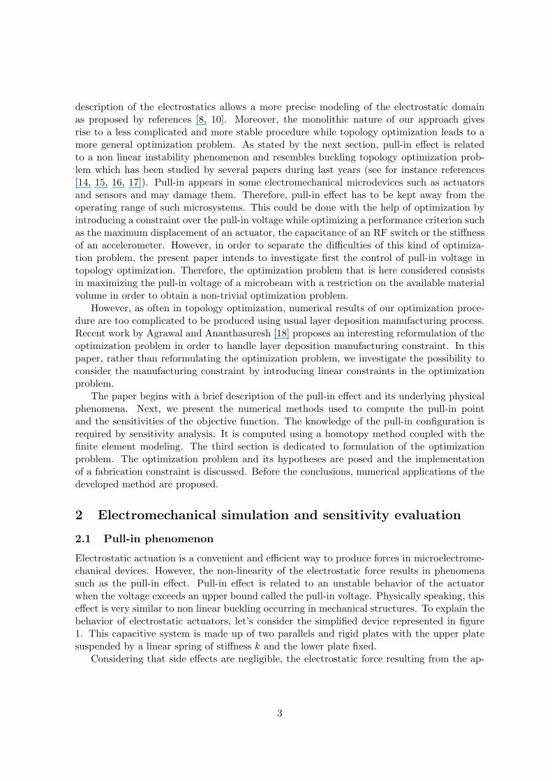
Electrostatic actuation is a convenient and efficient way to produce forces in microelectrome-chanical devices. However, the non-linearity of the electrostatic force results in phenomenasuch as the pull-in effect. Pull-in effect is related to an unstable behavior of the actuatorwhen the voltage exceeds an upper bound called the pull-in voltage. Physically speaking, thiseffect is very similar to non linear buckling occurring in mechanical structures. To explain thebehavior of electrostatic actuators, let’s consider the simplified device represented in figure1. This capacitive system is made up of two parallels and rigid plates with the upper platesuspended by a linear spring of stiffness k and the lower plate fixed.

Considering that side effects are negligible, the electrostatic force resulting from the ap-

3

V

k

x

d0

Figure 1: Simplified electromechanical actuator

plication of a voltage V between the plates can be written [19],

fe =ε0

2AV 2

(d0 − x)2(1)

Where ε0 denotes the permittivity of the media separating the plates (i.e. vacuum), A is thecapacitor surface, d0 the initial distance between the plates and x the displacement of theupper plate. Moreover, the restoring force from the spring is simply given by,

fr = −kx

After applying the Newton’s second law and a few manipulation of the resulting equation,we can obtain the following equilibrium equation giving the voltage as a function of thedisplacement.

V =

√2kx (d0 − x)2

ε0A(2)

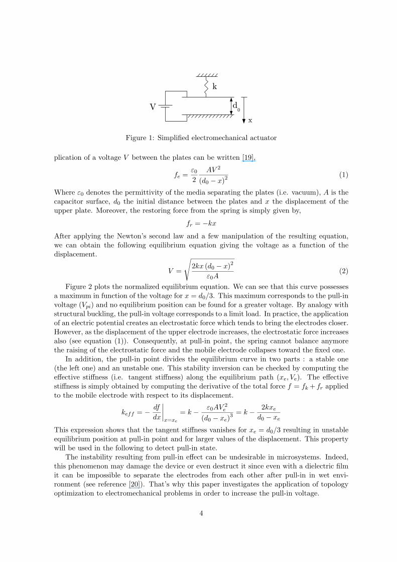
Figure 2 plots the normalized equilibrium equation. We can see that this curve possessesa maximum in function of the voltage for x = d0/3. This maximum corresponds to the pull-involtage (Vpi) and no equilibrium position can be found for a greater voltage. By analogy withstructural buckling, the pull-in voltage corresponds to a limit load. In practice, the applicationof an electric potential creates an electrostatic force which tends to bring the electrodes closer.However, as the displacement of the upper electrode increases, the electrostatic force increasesalso (see equation (1)). Consequently, at pull-in point, the spring cannot balance anymorethe raising of the electrostatic force and the mobile electrode collapses toward the fixed one.

In addition, the pull-in point divides the equilibrium curve in two parts : a stable one(the left one) and an unstable one. This stability inversion can be checked by computing theeffective stiffness (i.e. tangent stiffness) along the equilibrium path (xe, Ve). The effectivestiffness is simply obtained by computing the derivative of the total force f = fk + fr appliedto the mobile electrode with respect to its displacement.

keff = − df

dx

∣∣∣∣x=xe

= k − ε0AV 2e

(d0 − xe)3 = k − 2kxe

d0 − xe

This expression shows that the tangent stiffness vanishes for xe = d0/3 resulting in unstableequilibrium position at pull-in point and for larger values of the displacement. This propertywill be used in the following to detect pull-in state.

The instability resulting from pull-in effect can be undesirable in microsystems. Indeed,this phenomenon may damage the device or even destruct it since even with a dielectric filmit can be impossible to separate the electrodes from each other after pull-in in wet envi-ronment (see reference [20]). That’s why this paper investigates the application of topologyoptimization to electromechanical problems in order to increase the pull-in voltage.

4

0 0.2 0.4 0.6 0.8 10

0.2

0.4

0.6

0.8

1

d/d0

V/V

pi

StableUnstablePull−in

Figure 2: Equilibrium curve of the simplified actuator

2.2 Monolithic finite element formulation

The multiphysic modeling methods can be divided into two main groups. The first type ofmethods is the staggered methods (see Raulli et al. [8] for instance) where each physical fieldis solved separately and global coupled convergence is obtained using an iterative procedure.Staggered methods have the advantage to be simpler to implement since one can use existingcomputing codes to solve each physical field. However, staggered methods lack convergencein some difficult cases. For instance, in electromechanical simulations, staggered methodsbecome unreliable when approaching pull-in. Therefore, it is difficult to compute accuratelythe pull-in point using this type of method.

Since precise knowledge of the pull-in configuration is needed by the optimization process,we choose here to use a method from the second set, namely monolithic methods. Contraryto staggered methods, monolithic methods consider the global problem and solve all physicalfields at the same time. For instance, the monolithic finite element formulation developedby Rochus et al. [21] which is used here, allows computing a global tangent stiffness matrixincluding both mechanical and electrostatic problems.

In order to achieve a multiphysic coupling, Rochus et al. compute the internal work byintegrating the Gibbs energy density on the computational domain Ω, resulting in,

Wint =12

∫Ω

STT dΩ︸ ︷︷ ︸mech.

− 12

∫Ω(u)

DTE dΩ︸ ︷︷ ︸elec.

where the product between the strain tensor S and the stress tensor T corresponds to me-chanical energy, while the product between D the dielectric displacement vector and E theelectric field vector is equal to the electric energy contribution. Notice that the electrical termis integrated over the deformed domain Ω (u) which depends on the mechanical displacementsu.

By applying virtual work principle and discretizing the problem, Rochus et al. obtain anon linear equilibrium equation of the type,

r = fint − fext = 0 (3)

5

expressing that the difference between internal forces fint and the external forces fext repre-sented by the residual vector r has to be zero.

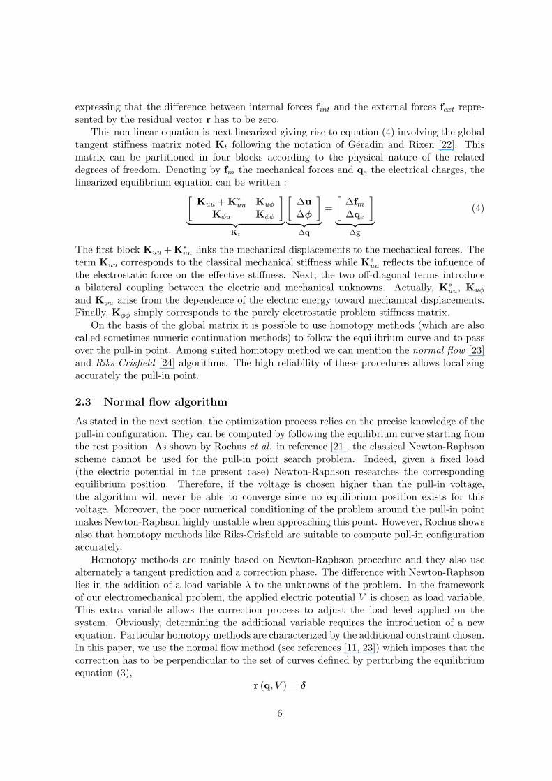
This non-linear equation is next linearized giving rise to equation (4) involving the globaltangent stiffness matrix noted Kt following the notation of Geradin and Rixen [22]. Thismatrix can be partitioned in four blocks according to the physical nature of the relateddegrees of freedom. Denoting by fm the mechanical forces and qe the electrical charges, thelinearized equilibrium equation can be written :[

Kuu + K∗uu Kuφ

Kφu Kφφ

]︸ ︷︷ ︸

Kt

[∆u∆φ

]︸ ︷︷ ︸

∆q

=[

∆fm∆qe

]︸ ︷︷ ︸

∆g

(4)

The first block Kuu + K∗uu links the mechanical displacements to the mechanical forces. The

term Kuu corresponds to the classical mechanical stiffness while K∗uu reflects the influence of

the electrostatic force on the effective stiffness. Next, the two off-diagonal terms introducea bilateral coupling between the electric and mechanical unknowns. Actually, K∗

uu, Kuφ

and Kφu arise from the dependence of the electric energy toward mechanical displacements.Finally, Kφφ simply corresponds to the purely electrostatic problem stiffness matrix.

On the basis of the global matrix it is possible to use homotopy methods (which are alsocalled sometimes numeric continuation methods) to follow the equilibrium curve and to passover the pull-in point. Among suited homotopy method we can mention the normal flow [23]and Riks-Crisfield [24] algorithms. The high reliability of these procedures allows localizingaccurately the pull-in point.

2.3 Normal flow algorithm

As stated in the next section, the optimization process relies on the precise knowledge of thepull-in configuration. They can be computed by following the equilibrium curve starting fromthe rest position. As shown by Rochus et al. in reference [21], the classical Newton-Raphsonscheme cannot be used for the pull-in point search problem. Indeed, given a fixed load(the electric potential in the present case) Newton-Raphson researches the correspondingequilibrium position. Therefore, if the voltage is chosen higher than the pull-in voltage,the algorithm will never be able to converge since no equilibrium position exists for thisvoltage. Moreover, the poor numerical conditioning of the problem around the pull-in pointmakes Newton-Raphson highly unstable when approaching this point. However, Rochus showsalso that homotopy methods like Riks-Crisfield are suitable to compute pull-in configurationaccurately.

Homotopy methods are mainly based on Newton-Raphson procedure and they also usealternately a tangent prediction and a correction phase. The difference with Newton-Raphsonlies in the addition of a load variable λ to the unknowns of the problem. In the frameworkof our electromechanical problem, the applied electric potential V is chosen as load variable.This extra variable allows the correction process to adjust the load level applied on thesystem. Obviously, determining the additional variable requires the introduction of a newequation. Particular homotopy methods are characterized by the additional constraint chosen.In this paper, we use the normal flow method (see references [11, 23]) which imposes that thecorrection has to be perpendicular to the set of curves defined by perturbing the equilibriumequation (3),

r (q, V ) = δ

6

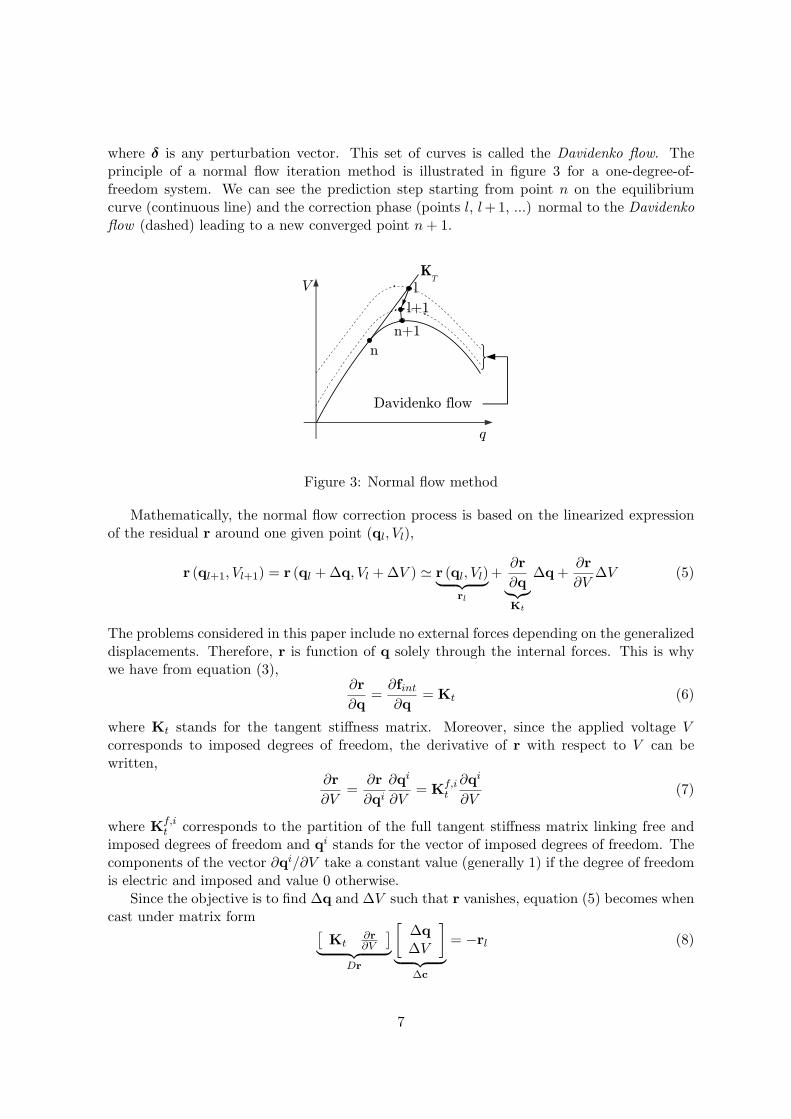
where δ is any perturbation vector. This set of curves is called the Davidenko flow. Theprinciple of a normal flow iteration method is illustrated in figure 3 for a one-degree-of-freedom system. We can see the prediction step starting from point n on the equilibriumcurve (continuous line) and the correction phase (points l, l +1, ...) normal to the Davidenkoflow (dashed) leading to a new converged point n + 1.

KT

n

n+1

Davidenko flow

V

q

l

l+1

Figure 3: Normal flow method

Mathematically, the normal flow correction process is based on the linearized expressionof the residual r around one given point (ql, Vl),

r (ql+1, Vl+1) = r (ql + ∆q, Vl + ∆V ) ' r (ql, Vl)︸ ︷︷ ︸rl

+∂r∂q︸︷︷︸Kt

∆q +∂r∂V

∆V (5)

The problems considered in this paper include no external forces depending on the generalizeddisplacements. Therefore, r is function of q solely through the internal forces. This is whywe have from equation (3),

∂r∂q

=∂fint

∂q= Kt (6)

where Kt stands for the tangent stiffness matrix. Moreover, since the applied voltage Vcorresponds to imposed degrees of freedom, the derivative of r with respect to V can bewritten,

∂r∂V

=∂r∂qi

∂qi

∂V= Kf,i

t

∂qi

∂V(7)

where Kf,it corresponds to the partition of the full tangent stiffness matrix linking free and

imposed degrees of freedom and qi stands for the vector of imposed degrees of freedom. Thecomponents of the vector ∂qi/∂V take a constant value (generally 1) if the degree of freedomis electric and imposed and value 0 otherwise.

Since the objective is to find ∆q and ∆V such that r vanishes, equation (5) becomes whencast under matrix form [

Kt∂r∂V

]︸ ︷︷ ︸Dr

[∆q∆V

]︸ ︷︷ ︸

∆c

= −rl (8)

7

To ensure perpendicularity between the correction vector ∆c and the Davidenko flow, onesimply imposes that w ·∆c = 0 where w is the tangent to the Davidenko flow computed byextracting the kernel of Dr. Next, to introduce the perpendicularity constraint in system ofequations (8), w is partitioned into a vector dq/ds and a scalar dV/ds, s being a curvilinearabscissa, [

Kt∂r∂V

dqds

dVds

]·[

∆q∆V

]=

[−rl

0

](9)

In our multi-physic problem, the vector of unknowns ∆c includes both voltages and me-chanical displacements. Moreover, in MEMS context, the order of magnitude differencebetween electric and mechanical unknowns is generally large (voltage of at least 1 V anddisplacement about 1 µm). Therefore, in practice, to achieve a stable computation, it isnecessary to normalize the problem in such a way that all components of vector c are of thesame order of magnitude. As a result, the load variable is changed to V/V where V is thenormalization factor of the electric potentials.

2.4 Pull-in voltage sensitivity analysis

Considering the finite element formulation presented above, the conditions governing pull-instate can be obtained. First of all, the pull-in point is located on the equilibrium curve andtherefore, the equilibrium equation (3) has to be verified. Secondly, we have seen for the singledegree of freedom system that the tangent stiffness vanishes at pull-in point. For multipledegrees of freedom, this means that pull-in occurs when the tangent stiffness matrix becomessingular. Sum of all, pull-in conditions are similar to the one obtained in reference [17] fornon-linear buckling and can be written,

r (q, V ) = 0det (Kt (q, V )) = 0

Using these equations, it is possible to obtain an analytical expression of the pull-in voltagesensitivities with respect to the topology optimization design variables namely, the pseudo-densities µ. This expression is highly useful since it provides an efficient way to computenumerically consistent sensitivities. The sensitivities equation can be established startingfrom the equilibrium equation by using a similar approach to references [11, 17]. At first, theequilibrium equation (3) is derived with respect to the pseudo-density µi,

∂

∂µi(r (q, V ) = 0) ⇔ ∂r

∂µi+

∂r∂q

∂q∂µi

+∂r∂V

∂V

∂µi= 0

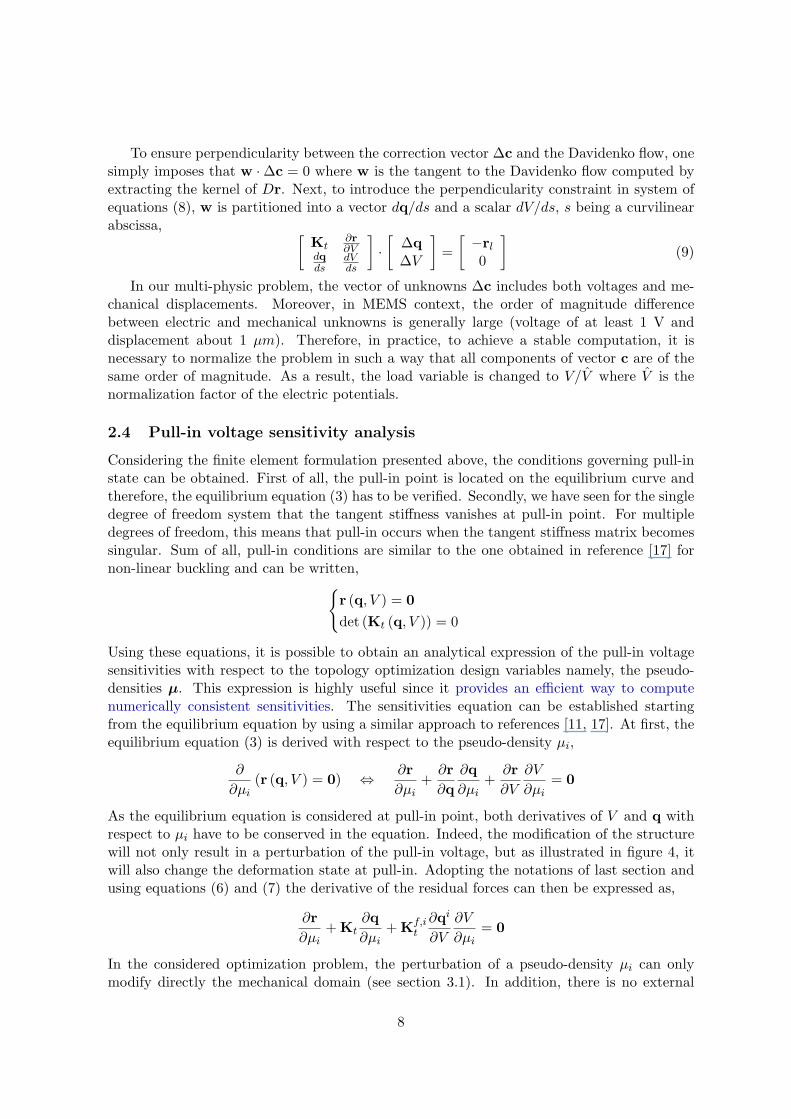
As the equilibrium equation is considered at pull-in point, both derivatives of V and q withrespect to µi have to be conserved in the equation. Indeed, the modification of the structurewill not only result in a perturbation of the pull-in voltage, but as illustrated in figure 4, itwill also change the deformation state at pull-in. Adopting the notations of last section andusing equations (6) and (7) the derivative of the residual forces can then be expressed as,

∂r∂µi

+ Kt∂q∂µi

+ Kf,it

∂qi

∂V

∂V

∂µi= 0

In the considered optimization problem, the perturbation of a pseudo-density µi can onlymodify directly the mechanical domain (see section 3.1). In addition, there is no external

8

q

V

(¢q,¢V)¹+¢¹

¹

Pull-in

Figure 4: Evolution of the pull-in curve resulting from a perturbation of µi.

force in the considered problems. Therefore, the variation of r resulting from a densityperturbation comes solely from the mechanical contribution to the internal forces fint. Sincewe consider small displacements, we have finally,

∂S∂µi

q + Kt∂q∂µi

+ Kf,it

∂qi

∂V︸ ︷︷ ︸∂r/∂V

∂V

∂µi= 0 (10)

if S denotes linear stiffness matrix of the mechanical part of the system. This last equationresembles the one obtained by Abdalla et al., while the last term is different. However, thephysical meaning of this term remains the same since ∂r/∂V also represents the derivativeof the electrical forces with respect to the load variable (V ). Indeed, an increment of voltagewill only affect the electric energy. Therefore, ∂r/∂V has a purely electrical origin and in factwe can write

∂r∂V

= Kf,it

∂qi

∂V= −∂felec

∂V

where felec represents the electric contribution to the internal forces. Please note that thisvector contains both mechanical electrostatic forces and electric charges.

Since the tangent stiffness matrix Kt is singular at pull-in point, the product of this matrixwith its first eigenvector p is equal to zero (i.e. Ktp = 0). Moreover, we consider that p isnormalized such that the following equation is verified,

pTKf,it

∂qi

∂V= −1

Consequently, the left multiplication by pT of equation (10) at pull-in point gives the followingexpression.

∂Vpi

∂µi= pT ∂S

∂µiq (11)

The last equation corresponds to the sensitivity of the pull-in voltage with respect to thedesign variable µi. This expression can be evaluated knowing the pull-in configuration of thecurrent structure q and the corresponding Kt eigenmode p. Therefore, the computation ofthe sensitivities with respect to every variable requires solely one pull-in point search. Thesensitivities provided by equation (11) have been compared with respect to finite differences inorder to validate the implementation of the analysis and sensitivity computation procedures.

However, particular care has to be taken when using this sensitivity expression. Indeed, ifp, the first eigenmode of Kt corresponds to a multiple eigenvalue, the optimization problem

9

is then non differentiable. This problem has already been treated for dynamic eigenvaluesoptimization where non differentiability is addressed by using a min-max scheme in order toinclude several eigenvalues in the optimization problem [25]. However, in the present paper,the optimization problem applications under consideration are unlikely to present multipleeigenvalues and therefore we did not had to use a min-max formulation.

2.5 Analysis implementation

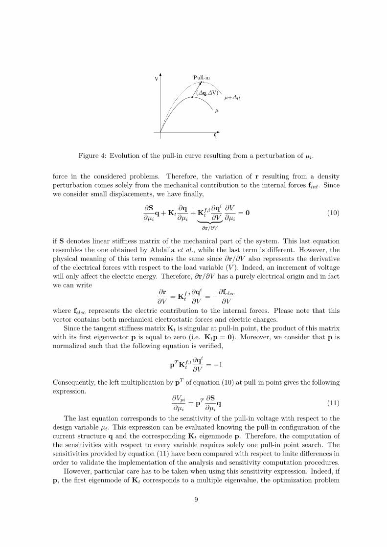
Using the tangent stiffness matrix provided by the monolithic finite element formulation, thenormal flow algorithm is able to follow the equilibrium curve even along its unstable side.Additional elements are added to the normal flow algorithm in order to integrate it into theoptimization procedure as shown by the optimization loop flowchart given in figure 5.

Stopping criteria ?No

Yes

Optimization phase

Correction loop

Electrostatic meshadaptation

Optimization

End

Pull-in point search

Tangent predictor

Step size computation

Sensitivities computation

(q0, V

0)=(0,0)

Optimization loop

Pull-in point ?

Yes

No

k=k+1

q pik

,V pik,ppi

k

q pik−1,V pi

k−1

Figure 5: Flowchart of the optimization procedure

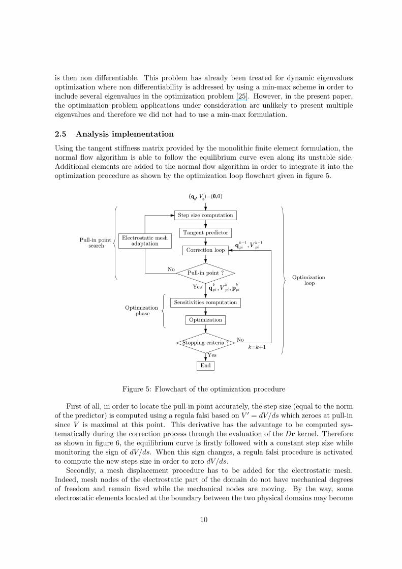
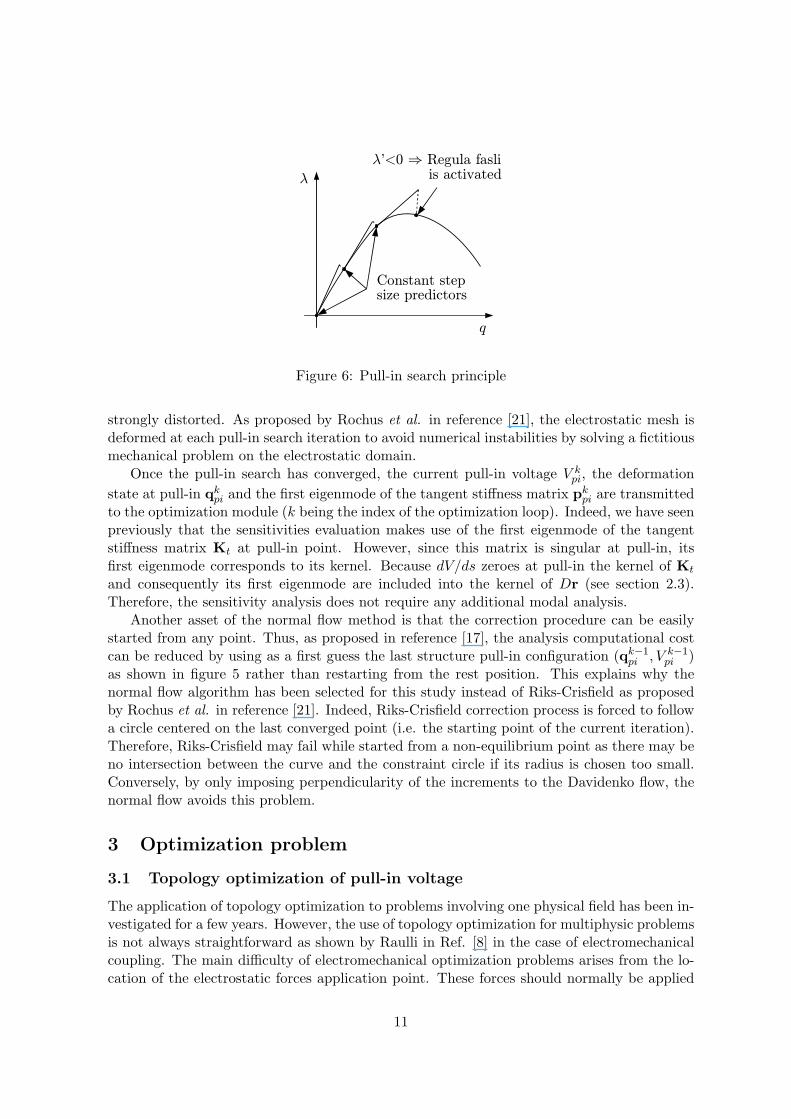
First of all, in order to locate the pull-in point accurately, the step size (equal to the normof the predictor) is computed using a regula falsi based on V ′ = dV/ds which zeroes at pull-insince V is maximal at this point. This derivative has the advantage to be computed sys-tematically during the correction process through the evaluation of the Dr kernel. Thereforeas shown in figure 6, the equilibrium curve is firstly followed with a constant step size whilemonitoring the sign of dV/ds. When this sign changes, a regula falsi procedure is activatedto compute the new steps size in order to zero dV/ds.

Secondly, a mesh displacement procedure has to be added for the electrostatic mesh.Indeed, mesh nodes of the electrostatic part of the domain do not have mechanical degreesof freedom and remain fixed while the mechanical nodes are moving. By the way, someelectrostatic elements located at the boundary between the two physical domains may become

10

¸'<0 ) Regula fasli is activated

q

Constant step size predictors

¸

Figure 6: Pull-in search principle

strongly distorted. As proposed by Rochus et al. in reference [21], the electrostatic mesh isdeformed at each pull-in search iteration to avoid numerical instabilities by solving a fictitiousmechanical problem on the electrostatic domain.

Once the pull-in search has converged, the current pull-in voltage V kpi, the deformation

state at pull-in qkpi and the first eigenmode of the tangent stiffness matrix pk

pi are transmittedto the optimization module (k being the index of the optimization loop). Indeed, we have seenpreviously that the sensitivities evaluation makes use of the first eigenmode of the tangentstiffness matrix Kt at pull-in point. However, since this matrix is singular at pull-in, itsfirst eigenmode corresponds to its kernel. Because dV/ds zeroes at pull-in the kernel of Kt

and consequently its first eigenmode are included into the kernel of Dr (see section 2.3).Therefore, the sensitivity analysis does not require any additional modal analysis.

Another asset of the normal flow method is that the correction procedure can be easilystarted from any point. Thus, as proposed in reference [17], the analysis computational costcan be reduced by using as a first guess the last structure pull-in configuration (qk−1

pi , V k−1pi )

as shown in figure 5 rather than restarting from the rest position. This explains why thenormal flow algorithm has been selected for this study instead of Riks-Crisfield as proposedby Rochus et al. in reference [21]. Indeed, Riks-Crisfield correction process is forced to followa circle centered on the last converged point (i.e. the starting point of the current iteration).Therefore, Riks-Crisfield may fail while started from a non-equilibrium point as there may beno intersection between the curve and the constraint circle if its radius is chosen too small.Conversely, by only imposing perpendicularity of the increments to the Davidenko flow, thenormal flow avoids this problem.

3 Optimization problem

3.1 Topology optimization of pull-in voltage

The application of topology optimization to problems involving one physical field has been in-vestigated for a few years. However, the use of topology optimization for multiphysic problemsis not always straightforward as shown by Raulli in Ref. [8] in the case of electromechanicalcoupling. The main difficulty of electromechanical optimization problems arises from the lo-cation of the electrostatic forces application point. These forces should normally be applied

11

at the boundary between void and solid. However, with topology optimization this boundaryis usually unclear since there is often a smooth transition between void and solid.

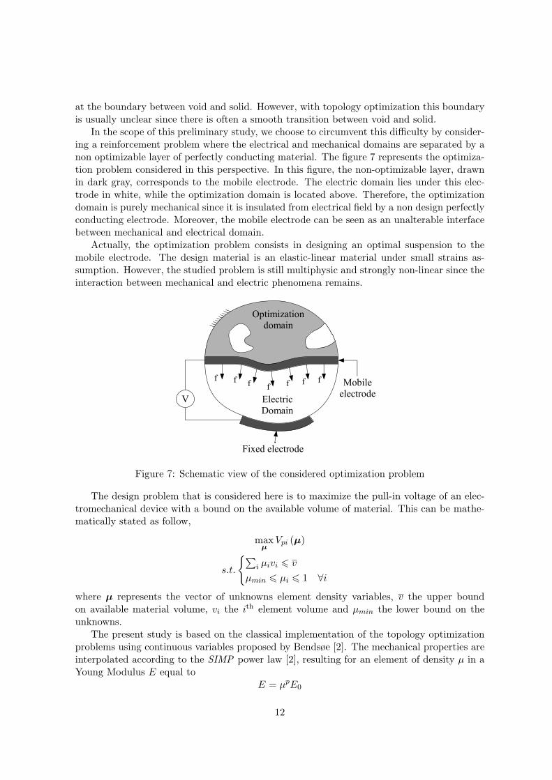
In the scope of this preliminary study, we choose to circumvent this difficulty by consider-ing a reinforcement problem where the electrical and mechanical domains are separated by anon optimizable layer of perfectly conducting material. The figure 7 represents the optimiza-tion problem considered in this perspective. In this figure, the non-optimizable layer, drawnin dark gray, corresponds to the mobile electrode. The electric domain lies under this elec-trode in white, while the optimization domain is located above. Therefore, the optimizationdomain is purely mechanical since it is insulated from electrical field by a non design perfectlyconducting electrode. Moreover, the mobile electrode can be seen as an unalterable interfacebetween mechanical and electrical domain.

Actually, the optimization problem consists in designing an optimal suspension to themobile electrode. The design material is an elastic-linear material under small strains as-sumption. However, the studied problem is still multiphysic and strongly non-linear since theinteraction between mechanical and electric phenomena remains.

V

f f f f f f f

Electric Domain

Optimization domain

Fixed electrode

Mobile electrode

Figure 7: Schematic view of the considered optimization problem

The design problem that is considered here is to maximize the pull-in voltage of an elec-tromechanical device with a bound on the available volume of material. This can be mathe-matically stated as follow,

maxµ

Vpi (µ)

s.t.

∑i µivi 6 v

µmin 6 µi 6 1 ∀i

where µ represents the vector of unknowns element density variables, v the upper boundon available material volume, vi the ith element volume and µmin the lower bound on theunknowns.

The present study is based on the classical implementation of the topology optimizationproblems using continuous variables proposed by Bendsøe [2]. The mechanical properties areinterpolated according to the SIMP power law [2], resulting for an element of density µ in aYoung Modulus E equal to

E = µpE0

12

where E0 is the original Young Modulus of the design material and p is the penalty param-eter. However, this formulation leads to a mathematically ill-posed optimization problem ashighlighted by references [26, 27, 3]. To remedy this difficulty, we choose to use a sensitivityfiltering procedure to regularize the optimization problem. This heuristic method, originallyproposed by Sigmund [27], replaces the sensitivity of each element by a weighted average ofthe original sensitivities existing in its neighborhood.

Thanks to the sensitivity analysis described in section 2.4, it is possible to use math-ematical programming optimization algorithms based on a sequential convex programmingapproach (see reference [28]). These optimizers have proved to be very efficient even whenhandling a large number of design variables as it is the case in topology optimization. Severalprograms have been developed following this concept as for instance MMA by Svanberg [29]and CONLIN by Fleury [30] the latter being used in the present paper. Nevertheless, becauseof the monotonic character of CONLIN an adaptive move limit strategy similar to the oneproposed by Svanberg in reference [29] has been implemented in order to prevent oscillationsof the optimization process occurring in some applications. The goal of the adaptation pro-cedure is to decrease the maximum allowed variation of a variable which oscillates in orderto stabilize the optimization process.

The stopping criterion of the optimization loop is based on the greatest variation ofthe design variables between two successive iterations. By the way, we consider that theoptimization process has reached convergence when the design variable greatest absolutemodification drops under 0.01.

3.2 Fabrication constraint

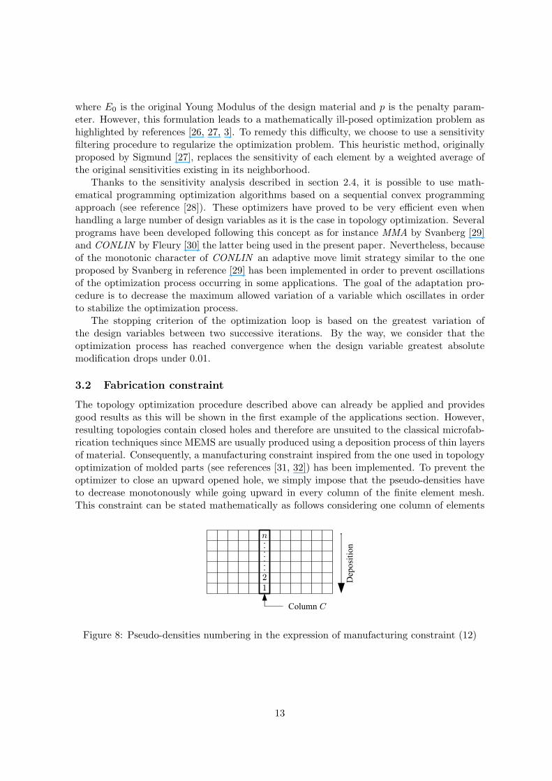
The topology optimization procedure described above can already be applied and providesgood results as this will be shown in the first example of the applications section. However,resulting topologies contain closed holes and therefore are unsuited to the classical microfab-rication techniques since MEMS are usually produced using a deposition process of thin layersof material. Consequently, a manufacturing constraint inspired from the one used in topologyoptimization of molded parts (see references [31, 32]) has been implemented. To prevent theoptimizer to close an upward opened hole, we simply impose that the pseudo-densities haveto decrease monotonously while going upward in every column of the finite element mesh.This constraint can be stated mathematically as follows considering one column of elements

12

n.......

Deposition

Column C

Figure 8: Pseudo-densities numbering in the expression of manufacturing constraint (12)

13

where pseudo-densities are numbered according to figure 8,

1 > µ1 > µ2

...µi−1 > µi > µi+1 if 2 6 i 6 n− 1

...µn−1 > µn > µmin

(12)

Conversely to the method proposed by Agrawal and Ananthasuresh [18], this constraint doesnot allow considering multi-material processes. However, it avoids a reformulation of theoptimization problem and gives rises to optimal structures free of closed cavities.

The implementation of this kind of constraints results in a number of linear constraintsapproximately equal to the number of design variables. When using dual optimizer likeCONLIN, such a huge number of linear constraints is a high penalty since it gives rise to asmuch dual variables and reduces the optimizer efficiency.

To reduce the amount of dual variables, it is possible to convert the linear constraints intoside constraints, namely,

µki 6 µk

i 6 µki ∀i ∈ 1, 2, . . . , n (13)

where the lower bound µki and the upper bound µk

i are constants given to the optimizer beforeiteration k. Therefore, in order to prevent the optimizer from violating (12) and to avoid aflipping of the variables, the side constraints expression has to be more conservative than theoriginal linear constraints. We choose to compute the bounds as follow,

µki =

µk−1

i − µk−1i −µk−1

i+1

2 if 1 6 i 6 n− 1µmin if i = n

µki =

1 if i = 1

µk−1i +

µk−1i−1 −µk−1

i

2 if 2 6 i 6 n

Then, the drawback of this zero order approximation of (12) is a strong reduction of theadmissible design space. As a result, the variables modification by the optimizer becomessmaller and the number of global iterations (i.e. analysis and optimization) to reach optimumwill increase drastically. Nevertheless, with fewer dual variables, it is now possible to solvethe optimization problem.

4 Applications

This section proposes numerical examples in order to illustrate the efficiency of the developedmethod as well as the usefulness of the manufacturing constraint.

4.1 Clamped-clamped beam topology optimization

The first application example of the developed method consists in the design of an optimalreinforcement suspension for a clamped-clamped microbeam. The problem is schematicallyrepresented with its dimensions in figure 9. As we can see, every side nodes of the prescribed

14

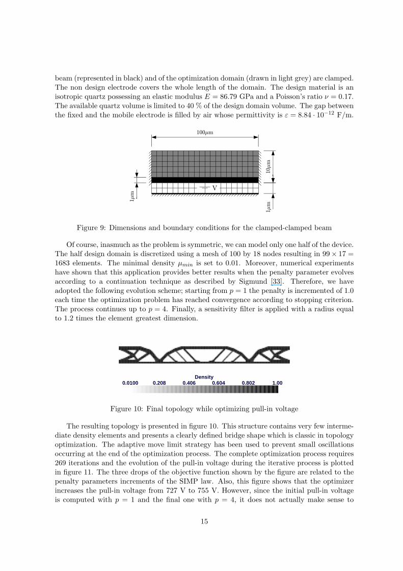
beam (represented in black) and of the optimization domain (drawn in light grey) are clamped.The non design electrode covers the whole length of the domain. The design material is anisotropic quartz possessing an elastic modulus E = 86.79 GPa and a Poisson’s ratio ν = 0.17.The available quartz volume is limited to 40 % of the design domain volume. The gap betweenthe fixed and the mobile electrode is filled by air whose permittivity is ε = 8.84 · 10−12 F/m.

100¹m

10¹m

1¹m

1¹m

V

Figure 9: Dimensions and boundary conditions for the clamped-clamped beam

Of course, inasmuch as the problem is symmetric, we can model only one half of the device.The half design domain is discretized using a mesh of 100 by 18 nodes resulting in 99× 17 =1683 elements. The minimal density µmin is set to 0.01. Moreover, numerical experimentshave shown that this application provides better results when the penalty parameter evolvesaccording to a continuation technique as described by Sigmund [33]. Therefore, we haveadopted the following evolution scheme; starting from p = 1 the penalty is incremented of 1.0each time the optimization problem has reached convergence according to stopping criterion.The process continues up to p = 4. Finally, a sensitivity filter is applied with a radius equalto 1.2 times the element greatest dimension.

DensityDensity0.01000.0100 0.208 0.208 0.406 0.406 0.604 0.604 0.802 0.802 1.00 1.00

Figure 10: Final topology while optimizing pull-in voltage

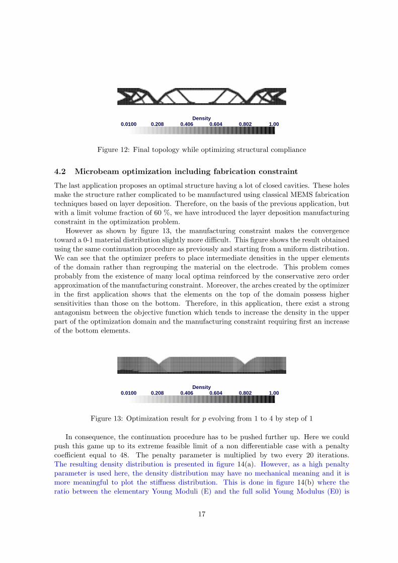
The resulting topology is presented in figure 10. This structure contains very few interme-diate density elements and presents a clearly defined bridge shape which is classic in topologyoptimization. The adaptive move limit strategy has been used to prevent small oscillationsoccurring at the end of the optimization process. The complete optimization process requires269 iterations and the evolution of the pull-in voltage during the iterative process is plottedin figure 11. The three drops of the objective function shown by the figure are related to thepenalty parameters increments of the SIMP law. Also, this figure shows that the optimizerincreases the pull-in voltage from 727 V to 755 V. However, since the initial pull-in voltageis computed with p = 1 and the final one with p = 4, it does not actually make sense to

15

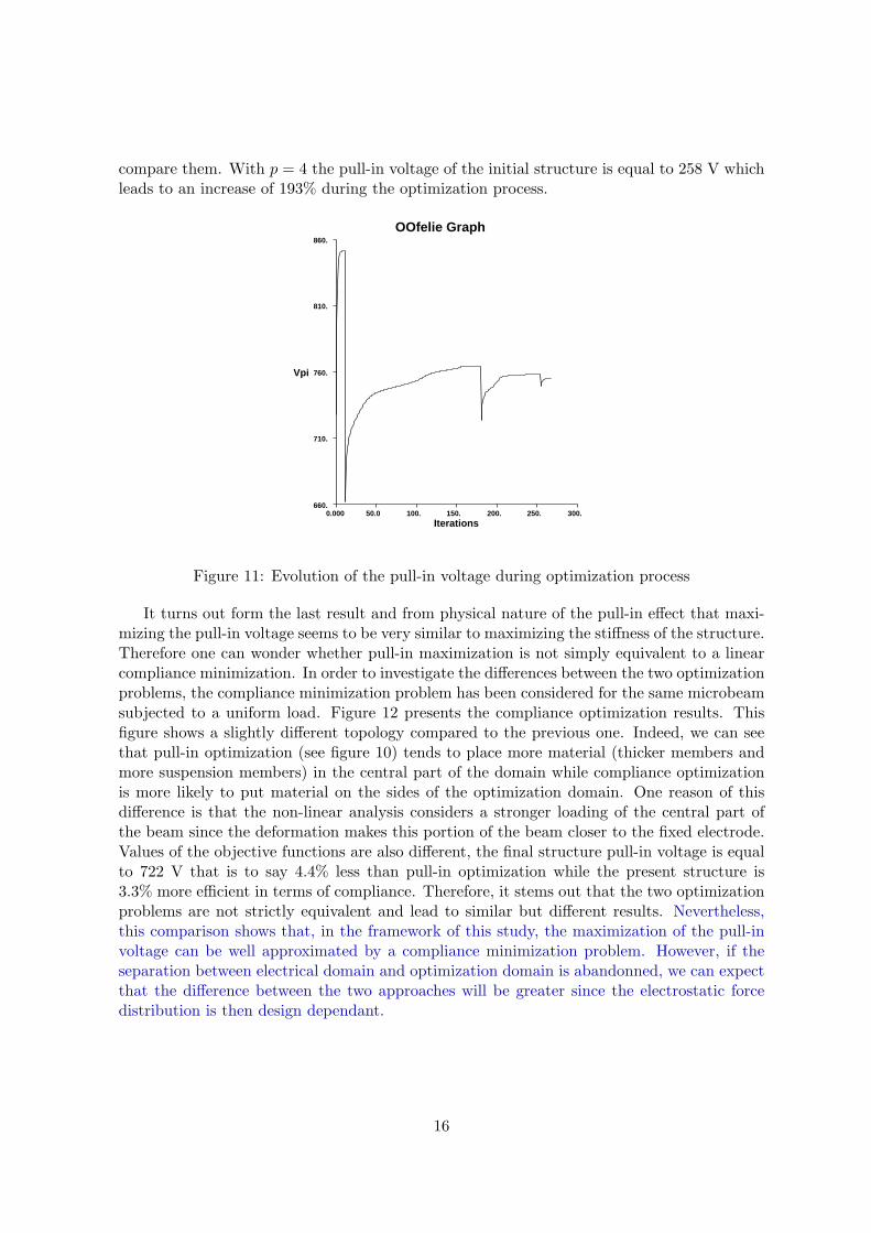
compare them. With p = 4 the pull-in voltage of the initial structure is equal to 258 V whichleads to an increase of 193% during the optimization process.

OOfelie Graph

Iterations

OOfelie Graph

Iterations0.000 0.000 50.0 50.0 100. 100. 150. 150. 200. 200. 250. 250. 300. 300.

VpiVpi

860. 860.

810. 810.

760. 760.

710. 710.

660. 660.

Figure 11: Evolution of the pull-in voltage during optimization process

It turns out form the last result and from physical nature of the pull-in effect that maxi-mizing the pull-in voltage seems to be very similar to maximizing the stiffness of the structure.Therefore one can wonder whether pull-in maximization is not simply equivalent to a linearcompliance minimization. In order to investigate the differences between the two optimizationproblems, the compliance minimization problem has been considered for the same microbeamsubjected to a uniform load. Figure 12 presents the compliance optimization results. Thisfigure shows a slightly different topology compared to the previous one. Indeed, we can seethat pull-in optimization (see figure 10) tends to place more material (thicker members andmore suspension members) in the central part of the domain while compliance optimizationis more likely to put material on the sides of the optimization domain. One reason of thisdifference is that the non-linear analysis considers a stronger loading of the central part ofthe beam since the deformation makes this portion of the beam closer to the fixed electrode.Values of the objective functions are also different, the final structure pull-in voltage is equalto 722 V that is to say 4.4% less than pull-in optimization while the present structure is3.3% more efficient in terms of compliance. Therefore, it stems out that the two optimizationproblems are not strictly equivalent and lead to similar but different results. Nevertheless,this comparison shows that, in the framework of this study, the maximization of the pull-involtage can be well approximated by a compliance minimization problem. However, if theseparation between electrical domain and optimization domain is abandonned, we can expectthat the difference between the two approaches will be greater since the electrostatic forcedistribution is then design dependant.

16

DensityDensity0.01000.0100 0.208 0.208 0.406 0.406 0.604 0.604 0.802 0.802 1.00 1.00

Figure 12: Final topology while optimizing structural compliance

4.2 Microbeam optimization including fabrication constraint

The last application proposes an optimal structure having a lot of closed cavities. These holesmake the structure rather complicated to be manufactured using classical MEMS fabricationtechniques based on layer deposition. Therefore, on the basis of the previous application, butwith a limit volume fraction of 60 %, we have introduced the layer deposition manufacturingconstraint in the optimization problem.

However as shown by figure 13, the manufacturing constraint makes the convergencetoward a 0-1 material distribution slightly more difficult. This figure shows the result obtainedusing the same continuation procedure as previously and starting from a uniform distribution.We can see that the optimizer prefers to place intermediate densities in the upper elementsof the domain rather than regrouping the material on the electrode. This problem comesprobably from the existence of many local optima reinforced by the conservative zero orderapproximation of the manufacturing constraint. Moreover, the arches created by the optimizerin the first application shows that the elements on the top of the domain possess highersensitivities than those on the bottom. Therefore, in this application, there exist a strongantagonism between the objective function which tends to increase the density in the upperpart of the optimization domain and the manufacturing constraint requiring first an increaseof the bottom elements.

DensityDensity0.01000.0100 0.208 0.208 0.406 0.406 0.604 0.604 0.802 0.802 1.00 1.00

Figure 13: Optimization result for p evolving from 1 to 4 by step of 1

In consequence, the continuation procedure has to be pushed further up. Here we couldpush this game up to its extreme feasible limit of a non differentiable case with a penaltycoefficient equal to 48. The penalty parameter is multiplied by two every 20 iterations.The resulting density distribution is presented in figure 14(a). However, as a high penaltyparameter is used here, the density distribution may have no mechanical meaning and it ismore meaningful to plot the stiffness distribution. This is done in figure 14(b) where theratio between the elementary Young Moduli (E) and the full solid Young Modulus (E0) is

17

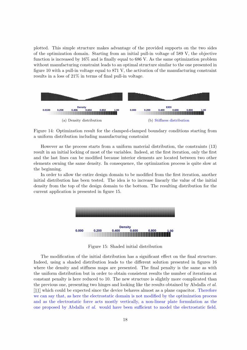
plotted. This simple structure makes advantage of the provided supports on the two sidesof the optimization domain. Starting from an initial pull-in voltage of 589 V, the objectivefunction is increased by 16% and is finally equal to 686 V. As the same optimization problemwithout manufacturing constraint leads to an optimal structure similar to the one presented infigure 10 with a pull-in voltage equal to 871 V, the activation of the manufacturing constraintresults in a loss of 21% in terms of final pull-in voltage.

1.00 1.00 DensityDensity

0.01000.0100 0.208 0.208 0.406 0.406 0.604 0.604 0.802 0.802

(a) Density distribution

1.00 1.00 E/E0E/E0

0.000 0.000 0.200 0.200 0.400 0.400 0.600 0.600 0.800 0.800

(b) Stiffness distribution

Figure 14: Optimization result for the clamped-clamped boundary conditions starting froma uniform distribution including manufacturing constraint

However as the process starts from a uniform material distribution, the constraints (13)result in an initial locking of most of the variables. Indeed, at the first iteration, only the firstand the last lines can be modified because interior elements are located between two otherelements owning the same density. In consequence, the optimization process is quite slow atthe beginning.

In order to allow the entire design domain to be modified from the first iteration, anotherinitial distribution has been tested. The idea is to increase linearly the value of the initialdensity from the top of the design domain to the bottom. The resulting distribution for thecurrent application is presented in figure 15.

1.00 DensityDensity

0.000 0.000 0.200 0.200 0.400 0.400 0.600 0.600 0.800 0.800 1.00

Figure 15: Shaded initial distribution

The modification of the initial distribution has a significant effect on the final structure.Indeed, using a shaded distribution leads to the different solution presented in figures 16where the density and stiffness maps are presented. The final penalty is the same as withthe uniform distribution but in order to obtain consistent results the number of iterations atconstant penalty is here reduced to 10. The new structure is slightly more complicated thanthe previous one, presenting two hinges and looking like the results obtained by Abdalla et al.[11] which could be expected since the device behaves almost as a plane capacitor. Thereforewe can say that, as here the electrostatic domain is not modified by the optimization processand as the electrostatic force acts mostly vertically, a non-linear plate formulation as theone proposed by Abdalla et al. would have been sufficient to model the electrostatic field.

18

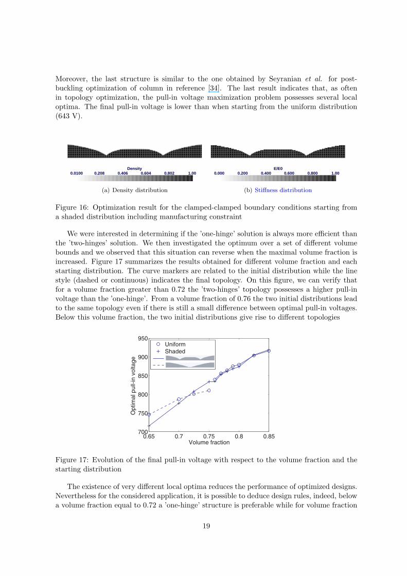
Moreover, the last structure is similar to the one obtained by Seyranian et al. for post-buckling optimization of column in reference [34]. The last result indicates that, as oftenin topology optimization, the pull-in voltage maximization problem possesses several localoptima. The final pull-in voltage is lower than when starting from the uniform distribution(643 V).

1.00 1.00 DensityDensity

0.01000.0100 0.208 0.208 0.406 0.406 0.604 0.604 0.802 0.802

(a) Density distribution

1.00 1.00

OOfelie Graph

E/E0E/E00.000 0.000 0.200 0.200 0.400 0.400 0.600 0.600 0.800 0.800

(b) Stiffness distribution

Figure 16: Optimization result for the clamped-clamped boundary conditions starting froma shaded distribution including manufacturing constraint

We were interested in determining if the ’one-hinge’ solution is always more efficient thanthe ’two-hinges’ solution. We then investigated the optimum over a set of different volumebounds and we observed that this situation can reverse when the maximal volume fraction isincreased. Figure 17 summarizes the results obtained for different volume fraction and eachstarting distribution. The curve markers are related to the initial distribution while the linestyle (dashed or continuous) indicates the final topology. On this figure, we can verify thatfor a volume fraction greater than 0.72 the ’two-hinges’ topology possesses a higher pull-involtage than the ’one-hinge’. From a volume fraction of 0.76 the two initial distributions leadto the same topology even if there is still a small difference between optimal pull-in voltages.Below this volume fraction, the two initial distributions give rise to different topologies

0.65 0.7 0.75 0.8 0.85700

750

800

850

900

950

Volume fraction

Optim

al pull-

in v

oltage

UniformShaded

Figure 17: Evolution of the final pull-in voltage with respect to the volume fraction and thestarting distribution

The existence of very different local optima reduces the performance of optimized designs.Nevertheless for the considered application, it is possible to deduce design rules, indeed, belowa volume fraction equal to 0.72 a ’one-hinge’ structure is preferable while for volume fraction

19

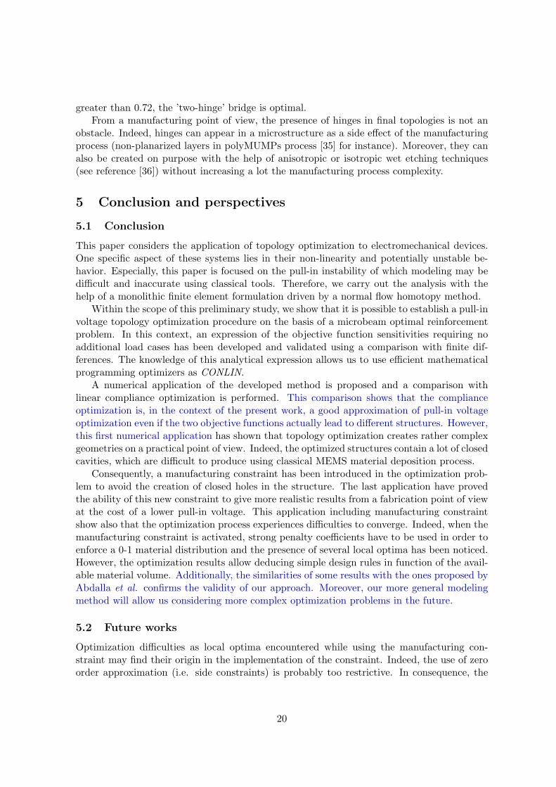
greater than 0.72, the ’two-hinge’ bridge is optimal.From a manufacturing point of view, the presence of hinges in final topologies is not an

obstacle. Indeed, hinges can appear in a microstructure as a side effect of the manufacturingprocess (non-planarized layers in polyMUMPs process [35] for instance). Moreover, they canalso be created on purpose with the help of anisotropic or isotropic wet etching techniques(see reference [36]) without increasing a lot the manufacturing process complexity.

5 Conclusion and perspectives

5.1 Conclusion

This paper considers the application of topology optimization to electromechanical devices.One specific aspect of these systems lies in their non-linearity and potentially unstable be-havior. Especially, this paper is focused on the pull-in instability of which modeling may bedifficult and inaccurate using classical tools. Therefore, we carry out the analysis with thehelp of a monolithic finite element formulation driven by a normal flow homotopy method.

Within the scope of this preliminary study, we show that it is possible to establish a pull-involtage topology optimization procedure on the basis of a microbeam optimal reinforcementproblem. In this context, an expression of the objective function sensitivities requiring noadditional load cases has been developed and validated using a comparison with finite dif-ferences. The knowledge of this analytical expression allows us to use efficient mathematicalprogramming optimizers as CONLIN.

A numerical application of the developed method is proposed and a comparison withlinear compliance optimization is performed. This comparison shows that the complianceoptimization is, in the context of the present work, a good approximation of pull-in voltageoptimization even if the two objective functions actually lead to different structures. However,this first numerical application has shown that topology optimization creates rather complexgeometries on a practical point of view. Indeed, the optimized structures contain a lot of closedcavities, which are difficult to produce using classical MEMS material deposition process.

Consequently, a manufacturing constraint has been introduced in the optimization prob-lem to avoid the creation of closed holes in the structure. The last application have provedthe ability of this new constraint to give more realistic results from a fabrication point of viewat the cost of a lower pull-in voltage. This application including manufacturing constraintshow also that the optimization process experiences difficulties to converge. Indeed, when themanufacturing constraint is activated, strong penalty coefficients have to be used in order toenforce a 0-1 material distribution and the presence of several local optima has been noticed.However, the optimization results allow deducing simple design rules in function of the avail-able material volume. Additionally, the similarities of some results with the ones proposed byAbdalla et al. confirms the validity of our approach. Moreover, our more general modelingmethod will allow us considering more complex optimization problems in the future.

5.2 Future works

Optimization difficulties as local optima encountered while using the manufacturing con-straint may find their origin in the implementation of the constraint. Indeed, the use of zeroorder approximation (i.e. side constraints) is probably too restrictive. In consequence, the

20

modification of the implementation of the manufacturing constraint is one of the first tasksthat will be addressed.

Nevertheless, the present paper shows the possibility to control pull-in voltage in topologyoptimization. Therefore, we are now able to study more complex optimization problemswhere pull-in voltage will more likely appear as a constraint. For instance, optimization ofelectrostatic actuators to maximize displacement of the output point can be considered.

Moreover, stresses are another important feature in MEMS considering the large numberof cycles experienced by these devices. The addition of local stress constraints in topologyoptimization has already been treated by Duysinx and Bendsøe [37]. A similar approach canbe used in order to ensure the strength of the device.

Finally, another important goal in our research will be to remove the restriction of theseparation between mechanical and electric domain. This step will enlarge the optimizationprocess freedom, allowing the modification of the interface between the physical domains asin Raulli et al. [8] and Yoon et al. [10]. This modification requires taking into account theelectrical effects in the optimization domain and in consequence the modeling of the electricalbehavior for intermediate densities. Additionally, it will then be possible to study the designof plane electrodes topology which are often seen in microdevices.

6 Acknowledgments

This research was has been realized under research project ARC 03/08-298 ’Modeling, Mul-tiphysics Simulation and Optimization of Coupled Problems - Application to Micro Electro-Mechanical Systems’ supported by the Communaute Francaise de Belgique. The secondauthor acknowledges the financial support of the Belgian National Fund for Scientific Re-search. Moreover, the authors want to thank Professor C. Fleury for making the CONLINsoftware available.

References

[1] M. Bendsøe, N. Kikuchi, Generating optimal topologies in structural design using ahomogenization method, Comput. Methods Appl. Mech. Engrg. 71 (2) (1988) 197–224.

[2] M. Bendsøe, Optimal shape design as a material distribution problem, Struct. Opt. 1(1989) 193–202.

[3] O. Sigmund, J. Petersson, Numerical instabilities in topology optimization: A surveyon procedures dealing with checkerboards, mesh-dependencies and local minima, Struct.Opt. 16 (1) (1998) 68–75.

[4] M. Bendsøe, O. Sigmund, Topology optimization : theory, methods, and applications,Springer Verlag.

[5] S. Wang, J. Kang, Topology optimization of nonlinear magnetostatics, IEEE Transac-tions on Magnetics 38 (2002) 1029–1032.

[6] O. Sigmund, Design of multiphysic actuators using topology optimization - Part I : Onematerial structures. - Part II : Two-material structures, Comput. Methods Appl. Mech.Engrg. 190 (49–50) (2001) 6577–6627.

21

[7] L. Yin, G. Ananthasuresh, A novel topology design scheme for the multi-physics problemsof electro-thermally actuated compliant micromechanisms, Sens. & Act. 97–98 (2002)599–609.

[8] M. Raulli, K. Maute, Topology optimization of electrostatically actuated microsystems,Struct. & Mult. Opt. 30 (5) (2005) 342–359.

[9] Z. Liu, J. Korvink, M. Reed, Multiphysics for structural topology optimization, SensorLetters 4 (2006) 191–199.

[10] G. Yoon, O. Sigmund, Topology optimization for electrostatic system, in: Proceedingsof the 7th World Congress on Structural and Multidisciplinary Optimization, 2007, pp.1686–1693.

[11] M. Abdalla, C. Reddy, W. Faris, Z. Gurdal, Optimal design of an electrostatically actu-ated microbeam for maximum pull-in voltage, Comp. & Struct. 83 (2005) 1320–1329.

[12] E. Lemaire, P. Duysinx, V. Rochus, J.-C. Golinval, Improvement of pull-in voltage ofelectromechanical micorbeams using topology optimization, in: III European Conferenceon Computational Mechanics, 2006.

[13] I. Klapka, A. Cardona, M. Geradin, An object-oriented implementation of the finiteelement method fro coupled problems, Revue Europeenne des Elements Finis 7 (5) (1998)469–504.

[14] M. Neves, H. Rodrigues, J. Guedes, Generalized topology design of structures with abuckling load criterion, Struct. Opt. 10 (1995) 71–78.

[15] T. Buhl, C. Pedersen, O. Sigmund, Stiffness design of geometrically nonlinear structuresusing topology optimization, Struct. & Mult. Opt. 19 (2000) 93–104.

[16] S. Rahmatalla, C. Swan, Continuum structural topology optimization of buckling-sensitive structures, AIAA 41 (6) (2003) 1180–1189.

[17] R. Kemmler, A. Lipka, E. Ramm, Large deformation and stability in topology optimiza-tion, Struct. & Mult. Opt. 30 (2005) 459–476.

[18] M. Agrawal, G. Ananthasuresh, On including lmanufacturing constraints in the topologyoptimization of surface-micromachined structures, in: 7th World Congress on Structuraland Multidisciplinary Optimization, 2007, pp. 2256–2265.

[19] J. Reitz, F. Milford, R. Christy, Foundations of electromagnetic theory, 3rd Edition,Addison-Wesley, 1979.

[20] W. van Spengen, R. Puers, I. de Wolf, A physical model to predict stictions in mems,Journal of Micromechanics and Microengineering 190.

[21] V. Rochus, D. J. Rixen, J.-C. Golinval, Monolithic modelling of electro-mechanical cou-pling in micro-structures, Int. J. Numer. Meth. Engng. 65 (4) (2006) 461–493.

[22] M. Geradin, D. Rixen, Mechanical Vibrations : Theory and Application to StructuralDynamics, 2nd Edition, John Wiley & Sons Ltd., 1997.

22

[23] S. Ragon, Z. Gurdal, L. Watson, A comparison of three algorithms for tracing nonlinearequilibrium paths of structural systems, Int. J. Solids Struct. 39 (2002) 689–698.

[24] M. Crisfield, Non-linear finite element analysis of solids and structures, Wiley, New York,1991.

[25] A. Seyranian, E. Lund, N. Olhof, Multiple eigenvalues in structural optimization prob-lems, Struct. Opt. 8 (1994) 207–227.

[26] H. A. Eschenauer, N. Olhoff, Topology optimization of continuum structures: A review,Applied Mechanics Reviews 54 (4) (2001) 331–390.

[27] O. Sigmund, On the design of compliant mechanisms using topology optimization, Mech.Struct. Mach. 25 (4) (1997) 493–526.

[28] C. Fleury, Mathematical programming methods for constrained optimization : dualmethods, Vol 150 of Progress in astronautics and aeronautics, AIAA chap 7 (1993)123–150.

[29] K. Svanberg, The method of moving asymptotes - a new method for structural optimiza-tion, Int. J. Numer. Meth. Engng. 24 (2) (1987) 359–373.

[30] C. Fleury, Conlin : an efficient dual optimizer based on convex approximation concepts,Struct. & Mult. Opt. 1 (2) (1989) 81–89.

[31] M. Zhou, R. Fleury, Y. Shyy, H. Thomas, J. Brennan, Progress in topology optimizationwith manufacturing constraints, in: 9th AIAA/ISSMO Symposium on MutlidisciplinaryAnalysis and Optimization, AIAA, Atlanta, Georgia, 2002.

[32] M. Zhou, Y. Shyy, H. Thomas, Topology optimization with manufacturing constraints,in: 4th World Congress of Structural and Multidisciplinary Optimization, Dalian, China,2001.

[33] O. Sigmund, Materials with prescribed constitutive parameters: An inverse homogeniza-tion problem, Int. J. Solids Struct. 31 (1994) 2313–2329.

[34] A. Seyranian, O. Privalova, The lagrange problem on an optimal column: old and newresults, Struct. Opt. 25 (2003) 393–410.

[35] J. Carter, A. Cowen, B. Hardy, R. Mahadevan, M. Stonefield, S. Wilcenski, PolyMUMPsdesign hanbook, MEMSCAP, 11th Edition (2005).

[36] S. Senturia, Microsystem Design, Kluwer Academic Publisher, 2001.

[37] P. Duysinx, M. Bendsøe, Topology optimization of continuum structures with local stressconstraints, Int. J. Numer. Meth. Engng. 43 (1998) 1453–1478.

23