Micro-scale habitat associations of woody plants in a neotropical cloud forest

Journal of Vegetation Science && (2012)

Micro-scale habitat associations of woody plants in aneotropical cloud forest

Alicia Ledo, David F.R.P. Burslem, Sonia Cond�es & Fernando Montes

Keywords

Andes; Dispersal limitation; Habitat

partitioning; Montane tropical forest; Peru;

Spatial pattern; Species co-existence

Nomenclature

(Ledo et al. 2012)

Received 26 January 2012

Accepted 22 October 2012

Co-ordinating Editor: Miquel De C�aceres

Ledo, A. (corresponding author,

[email protected]) & Cond�es, S.

([email protected]): Universidad

Polit�ecnica deMadrid, Escuela T�ecnica

Superior de Ingenieros deMontes, Ciudad

Universitaria, s/n. 28040, Madrid, Spain

Burslem, D.F.R.P. ([email protected]):

School of Biological Sciences, University of

Aberdeen, Cruickshank Building, St Machar

Drive, Aberdeen

AB24 3UU, UK

Montes, F. ([email protected]): CIFOR-INIA,

Carretera de La Coru~na Km 7.5, 28040, Madrid,

Spain

Abstract

Questions: Species–habitat associations may contribute to the maintenance of

species richness in tropical forests, but previous research has been conducted

almost exclusively in lowland forests and has emphasized the importance of

topography and edaphic conditions. Is the distribution of woody plant species in

a Peruvian cloud forest determined by microhabitat conditions?What is the role

of environmental characteristics and forest structure in habitat partitioning in a

tropical cloud forest?

Location: Cloud Forest, north Peruvian Andes.

Methods: We examined species–habitat associations in three 1-ha plots using

the torus-translation method. We used three different criteria to define habitats

for habitat partitioning analyses, based onmicrotopography, forest structure and

both sets of factors. The number of species associated either positively or nega-

tively with each habitat was assessed.

Results: Habitats defined on the basis of environmental conditions and forest

structure discriminated a greater number of positive and negative associations at

the scale of our analyses in a tropical cloud forest.

Conclusions: Both topographic conditions and forest structure contribute to

small-scale microhabitat partitioning of woody plant species in a Peruvian tropi-

cal cloud forest. Nevertheless, canopy species were most correlated with the dis-

tribution of environmental variables, while understorey species displayed

associations with forest structure.

Introduction

The spatial structure of plant populations conveys impor-

tant information that may help to understand the mainte-

nance of the high diversity of species-rich plant

communities (Law et al. 2001). Numerous studies have

observed that tropical tree species have clumped distribu-

tions (Condit et al. 2000; Plotkin et al. 2002; Wiegand

et al. 2007). The main causes of aggregation are dispersal

limitation (Hubbell et al. 1999) and associations with het-

erogeneous environmental conditions (Clark et al. 1993;

Harms et al. 2001). It is nowwidely accepted that both fac-

tors play an important role in species distribution, although

the relative importance of each factor may differ among

study systems. For example, in a lowland forest in Peru

measured environmental variables explained 40% of vari-

ation in species distribution (Phillips et al. 2003), while

environmental variables alone explained only 10–12% of

variation in tree distribution for lowland forests in Panama

(Chust et al. 2006). Spatial variation that remains unex-

plained in these studies may arise because of unmeasured

environmental correlates, and autocorrelation due to dis-

persal limitation (Pacala & Tilman 1994; Hubbell et al.

1999). Consequently, future mechanistic theories and

models must take into account not only habitat partition-

ing but also dispersal limitation (Chave 2004). Other

mechanisms, such as gap recruitment, may also play a role

in species clustering (Hubbell et al. 1999; Plotkin et al.

2000). However, the role of stand structure and light avail-

ability are not often included in analyses of habitat associa-

tions, although a number of studies have determined that

elevation, slope (Harms et al. 2001; Comita et al. 2007;

Suzuki et al. 2009) and soil nutrients (John et al. 2007;

Bohlman et al. 2008) define habitats for tropical forest

trees.

Analysis of niche partitioning presents an additional dif-

ficulty because the niche concept differs among authors

(Morin 2011). Some authors include only physical

Journal of Vegetation ScienceDoi: 10.1111/jvs.12023© 2012 International Association for Vegetation Science 1

environmental variables within their definition of a plant’s

niche (MacArthur 1972), while others include both envi-

ronmental and biotic variables (Chase & Leibold 2003;

Grubb 1976). Limiting resources and competitive exclusion

have also been introduced into the definition of the niche

(Hutchinson 1957). In addition to characterizing the vari-

ables implicated in habitat or niche partitioning, it is also

important to clarify the spatial and temporal scale of analy-

sis. Habitat–species associations vary with the scale of obser-

vation (Gentry 1988; Kneitel & Chase 2004; Paoli et al.

2006), and microhabitat diversity may possess a dynamic

component reflecting spatio-temporal variation in resource

availability (Chase & Leibold 2003; Leigh et al. 2004).

In this paper we present a study of species habitat associ-

ations in a montane cloud forest in the Peruvian Andes. At

our study site the majority of free-standing woody plant

species display a clumped distribution, and the size of clus-

ters is partially related to primary dispersal mode, life form

and shade tolerance (Ledo et al. 2012). Cloud forests are

extremely fragile ecosystems, and their existence depends

on the convergence of high humidity and suitable temper-

ature conditions (Hamilton 1995). Cloud forests also occur

in environments that typically possess steeper gradients in

elevation than lowland environments (Bruijnzeel et al.

2011). Hence, we predict that changes in environmental

conditions and their importance as drivers of species distri-

butions may be more apparent in montane cloud forest

than in lowland tropical forests, where a significant pro-

portion of previous research has been conducted.

We examined fine-scale species–habitat associations in

three 1-ha plots in a Peruvian Andean cloud forest and

analysed whether and towhat extent these habitat associa-

tions act on the species composition of the woody plant

community. We tested the prediction that species–habitat

associations exist among species in this community, and

consequently, that the presence of different microhabitats

would affect species distributions. We addressed the ques-

tion of whether (1) topographic and environmental condi-

tions, (2) forest structure or (3) a combination of the two

factors acting together weremost important. This approach

reflects our interest in understanding the relative impor-

tance of forest structure and microenvironmental condi-

tions on small-scale habitat partitioning. Moreover, it

sheds light on the mechanisms that lead species distribu-

tions and community assembly.

Methods

Study site

This study was conducted in Monte de Neblina de Cuyas,

which is a neotropical montane cloud forest situated in

northern Peru (Piura region, Ayabaca province), in the

western Andean range (4º34–36′ S; 79º41–43′ W). This is a

relic forest that once formed part of a larger cloud forest

belt that occupied an extensive area of the Andean range

(Gentry 1995). The main cause of the decline in forest

cover was probably conversion for agriculture and pasture,

although we cannot verify this. The Monte de Neblina de

Cuyas cloud forest currently covers~400 ha. To our knowl-

edge, the only anthropogenic disturbance that has ever

occurred is illegal logging, although this is rare and only

affects the edges of the forest. Most of the illegal logging

and extraction of medicinal plants takes place in secondary

forest near local villages. To our knowledge, no hunting

activity exists or has existed in the area.

The study site was situated at altitudes ranging from

2359 to 3012 m a.s.l. The main part of the study area is sit-

uated on southwest-facing slopes. According to K€oppen

(1936), the location has a cold temperate climate with a

dry winter. The mean annual temperature is 15 °C, vary-ing between 8.5 °C and 18 °C. Mean annual precipitation

is around 1200 mm, and is generally very intense during

the summer (December–May). In years when the ENSO

(El Ni~no Southern Oscillation) phenomenon occurs, the

precipitation increases substantially (Romero et al. 2007).

In the winter the frequency of winds increases and gales

sometimes occur. The forest has been identified as an

Important Bird Area (Freile & Santander 2005), even

though it has now been seriously altered (Ledo et al.

2009). There is a high level of endemism in the forest and

several taxa included in the IUCN Red List are threatened

by the on-going loss of habitat.

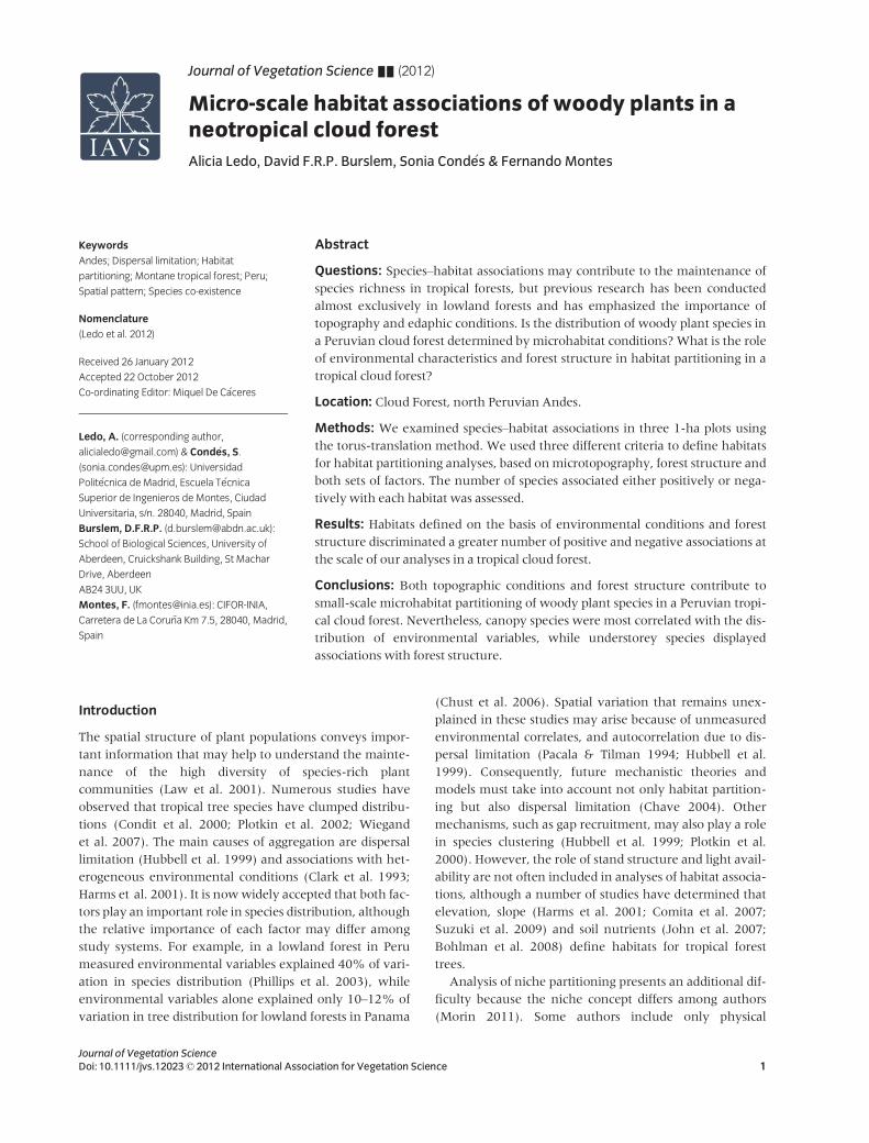
Plot establishment and lightmeasurements

The inventory was carried out betweenMarch and August

2008. Three 1-ha plots were established in randomly

selected locations in the inner part of the forest, at least

200 m from the forest edge, to avoid edge effects (Fig. 1).

All freestanding woody plants � 1.3 m in height (diameter

at breast height, DBH), without any diameter restriction,

were mapped in each 1-ha plot. To map the woody plants,

different sampling points were situated in the plot. The

UTM coordinates and elevation of the first point (a corner)

were measured using a GPS device, and from this informa-

tion, the actual coordinates and elevation of each plot were

obtained. Once all the woody plants had been measured at

the first sampling point within a radius of approximately

15 m (using a vertex hypsometer and a compass), the next

sampling point was located. The distance and angle

between sampling points were double-checked to corrobo-

rate their exact positions. This process was repeated until

the whole plot was covered. Every plant was numbered

and the species, diameter (measured with a calliper) and

height (measured with a vertex hypsometer) were

recorded.

Journal of Vegetation Science2 Doi: 10.1111/jvs.12023© 2012 International Association for Vegetation Science

Plant–habitat associations in cloud forest A. Ledo et al.

The number of woody plants found in the plots was

4500 individuals ha�1. The mean DBH was 12.2 cm.

About 80% of the measured woody plants had a DBH of

less than 5 cm, whereas 5% had a DBH more than 20 cm;

comprising 180 individuals ha�1. There were 39 different

woody plant species per ha; however, only 22 species were

represented by more than 50 individuals per plot. We clas-

sified those species into two main categories, according to

life form: canopy species (comprising canopy and emer-

gent species) and low stature species (comprising understo-

rey and pioneer gap species). Detailed information on the

woody plant species measured in the plots and their spatial

organization can be found in Ledo et al. (2012).

Forty-two randomly selected locations were sampled for

light in each plot by taking hemispherical photographs

with a FC-E8 fish-eye lens attached to a Nikon Coolpix

4500 camera body. The camera was levelled horizontally

20 cm above the ground and oriented to true north using

a compass with a spirit level. We processed the images

using the software Hemiview (Hale & Edwards 2002).

Values were obtained for visible sky, direct site factor,

indirect site factor and global site factor (GSF). We derived

elevation in the plots from the first point measured with

the GPS device, using the X, Y and Z coordinates of all the

measured woody plants and auxiliary points; ca. 5000

points per ha. We then built a digital elevation model

(DEM) for each plot in ArcMap® v. 9.2 and derived slope,

curvature and aspect on a 2 9 2 m grid.

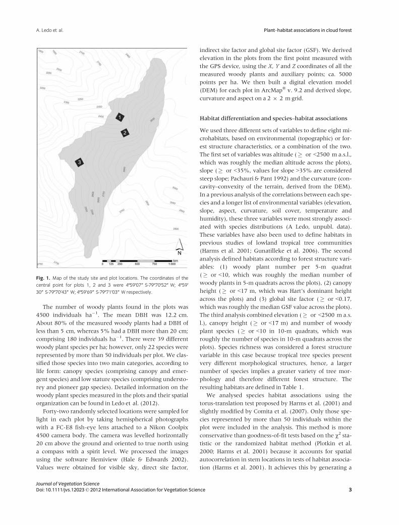
Habitat differentiation and species–habitat associations

We used three different sets of variables to define eight mi-

crohabitats, based on environmental (topographic) or for-

est structure characteristics, or a combination of the two.

The first set of variables was altitude (� or <2500 m a.s.l.,

which was roughly the median altitude across the plots),

slope (� or <35%, values for slope >35% are considered

steep slope; Pachauri & Pant 1992) and the curvature (con-

cavity–convexity of the terrain, derived from the DEM).

In a previous analysis of the correlations between each spe-

cies and a longer list of environmental variables (elevation,

slope, aspect, curvature, soil cover, temperature and

humidity), these three variables were most strongly associ-

ated with species distributions (A Ledo, unpubl. data).

These variables have also been used to define habitats in

previous studies of lowland tropical tree communities

(Harms et al. 2001; Gunatilleke et al. 2006). The second

analysis defined habitats according to forest structure vari-

ables: (1) woody plant number per 5-m quadrat

(� or <10, which was roughly the median number of

woody plants in 5-m quadrats across the plots), (2) canopy

height (� or <17 m, which was Hart’s dominant height

across the plots) and (3) global site factor (� or <0.17,which was roughly themedian GSF value across the plots).

The third analysis combined elevation (� or <2500 m a.s.

l.), canopy height (� or <17 m) and number of woody

plant species (� or <10 in 10-m quadrats, which was

roughly the number of species in 10-m quadrats across the

plots). Species richness was considered a forest structure

variable in this case because tropical tree species present

very different morphological structures, hence, a larger

number of species implies a greater variety of tree mor-

phology and therefore different forest structure. The

resulting habitats are defined in Table 1.

We analysed species habitat associations using the

torus-translation test proposed by Harms et al. (2001) and

slightly modified by Comita et al. (2007). Only those spe-

cies represented by more than 50 individuals within the

plot were included in the analysis. This method is more

conservative than goodness-of-fit tests based on the v2 sta-tistic or the randomized habitat method (Plotkin et al.

2000; Harms et al. 2001) because it accounts for spatial

autocorrelation in stem locations in tests of habitat associa-

tion (Harms et al. 2001). It achieves this by generating a

Fig. 1. Map of the study site and plot locations. The coordinates of the

central point for plots 1, 2 and 3 were 4º59′07″ S-79º70′52″ W; 4º59′

30″ S-79º70′43″ W; 4º59′69″ S-79º71′03″ W respectively.


A. Ledo et al. Plant–habitat associations in cloud forest

Table

1.Variablesusedto

definehab

itatsunderthethreedifferentcriteria.

Topographicalvariab

les

Foreststructure

variab

les

Topographicandforest

structure

variab

les

Hab

itat

Elevation

Slope

Curvature

Hab

itat

Canopy

height

Number

woodyplants

GSF

Hab

itat

Elevation

Canopy

height

Number

species

Upperelevation,

highslope,

spurs(UeHsS)

�2550

�35

+Highercanopy,

dense

area,bright

place

(HcD

aBp)

�17

�10

�0.17

Upperelevation,higher

canopy,rich

composition(UeHcR

c)

�2550

�17

�10

Upperelevation,

highslope,

gullies(UeHsG

)

�2550

�35

�Highercanopy,

dense

area,shad

y

place

(HcD

aSp)

�17

�10

<0.17

Upperelevation,higher

canopy,poor

composition(UeHcP

c)

�2550

�17

<10

Upperelevation,

lowslope,

spurs(UeLsS)

�2550

<35

+Highercanopy,

openness

area,

brightplace

(HcO

aBp)

�17

<10

�0.17

Upperelevation,

lowercanopy,

rich

composition(UeLcRc)

�2550

<17

�10

Upperelevation,

lowslope,

gullies(UeLsG)

�2550

<35

�Highercanopy,

openness

area,

shad

yplace

(HcO

aSp)

�17

<10

<0.17

Upperelevation,

lowercanopy,poor

composition(UeLcPc)

�2550

<17

<10

Lowerelevation,

highslope,

spurs(LeHsS)

<2550

�35

+Lowercanopy,

dense

area,

brightplace

(LcD

aBp)

<17

�10

�0.17

Lowerelevation,higher

canopy,rich

composition(LeHcR

c)

<2550

�17

�10

Lowerelevation,

highslope,

gullies(LeHsG

)

<2550

�35

�Lowercanopy,

dense

area,

shad

yplace

(LcD

aSp)

<17

�10

<0.17

Lowerelevation,higher

canopy,poor

composition(LeHcP

c)

<2550

�17

<10

Lowerelevation,

lowslope,

spurs(LeLsS)

<2550

<35

+Lowercanopy,

openness

area,

brightplace

(LcO

aBp)

<17

<10

�0.17

Lowerelevation,

lowercanopy,

rich

composition(LeLcRc)

<2550

<17

�10

Lowerelevation,

lowslope,

gullies(LeLsG)

<2550

<35

�Lowercanopy,

openness

area,

shad

yplace

(LcO

aSp)

<17

<10

<0.17

Lowerelevation,

lowercanopy,poor

composition(LeLcPc)

<2550

<17

<10



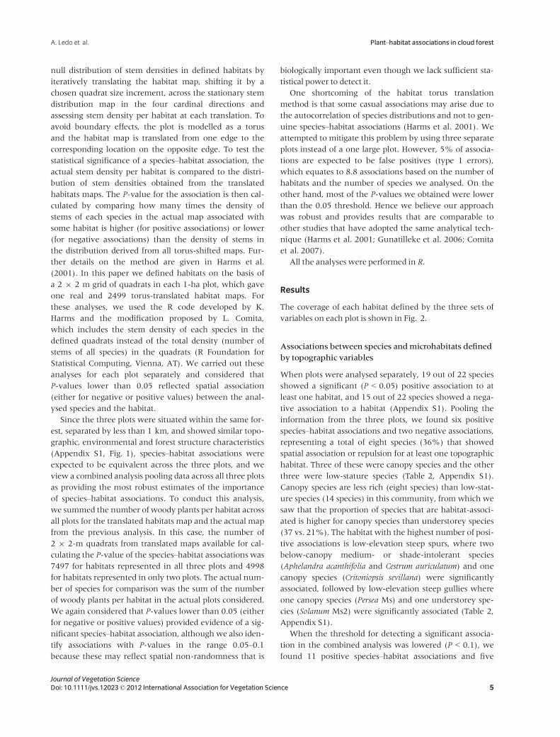
null distribution of stem densities in defined habitats by

iteratively translating the habitat map, shifting it by a

chosen quadrat size increment, across the stationary stem

distribution map in the four cardinal directions and

assessing stem density per habitat at each translation. To

avoid boundary effects, the plot is modelled as a torus

and the habitat map is translated from one edge to the

corresponding location on the opposite edge. To test the

statistical significance of a species–habitat association, the

actual stem density per habitat is compared to the distri-

bution of stem densities obtained from the translated

habitats maps. The P-value for the association is then cal-

culated by comparing how many times the density of

stems of each species in the actual map associated with

some habitat is higher (for positive associations) or lower

(for negative associations) than the density of stems in

the distribution derived from all torus-shifted maps. Fur-

ther details on the method are given in Harms et al.

(2001). In this paper we defined habitats on the basis of

a 2 9 2 m grid of quadrats in each 1-ha plot, which gave

one real and 2499 torus-translated habitat maps. For

these analyses, we used the R code developed by K.

Harms and the modification proposed by L. Comita,

which includes the stem density of each species in the

defined quadrats instead of the total density (number of

stems of all species) in the quadrats (R Foundation for

Statistical Computing, Vienna, AT). We carried out these

analyses for each plot separately and considered that

P-values lower than 0.05 reflected spatial association

(either for negative or positive values) between the anal-

ysed species and the habitat.

Since the three plots were situated within the same for-

est, separated by less than 1 km, and showed similar topo-

graphic, environmental and forest structure characteristics

(Appendix S1, Fig. 1), species–habitat associations were

expected to be equivalent across the three plots, and we

view a combined analysis pooling data across all three plots

as providing the most robust estimates of the importance

of species–habitat associations. To conduct this analysis,

we summed the number of woody plants per habitat across

all plots for the translated habitats map and the actual map

from the previous analysis. In this case, the number of

2 9 2-m quadrats from translated maps available for cal-

culating the P-value of the species–habitat associations was

7497 for habitats represented in all three plots and 4998

for habitats represented in only two plots. The actual num-

ber of species for comparison was the sum of the number

of woody plants per habitat in the actual plots considered.

We again considered that P-values lower than 0.05 (either

for negative or positive values) provided evidence of a sig-

nificant species–habitat association, although we also iden-

tify associations with P-values in the range 0.05–0.1

because these may reflect spatial non-randomness that is

biologically important even though we lack sufficient sta-

tistical power to detect it.

One shortcoming of the habitat torus translation

method is that some casual associations may arise due to

the autocorrelation of species distributions and not to gen-

uine species–habitat associations (Harms et al. 2001). We

attempted to mitigate this problem by using three separate

plots instead of a one large plot. However, 5% of associa-

tions are expected to be false positives (type 1 errors),

which equates to 8.8 associations based on the number of

habitats and the number of species we analysed. On the

other hand, most of the P-values we obtained were lower

than the 0.05 threshold. Hence we believe our approach

was robust and provides results that are comparable to

other studies that have adopted the same analytical tech-

nique (Harms et al. 2001; Gunatilleke et al. 2006; Comita

et al. 2007).

All the analyses were performed in R.

Results

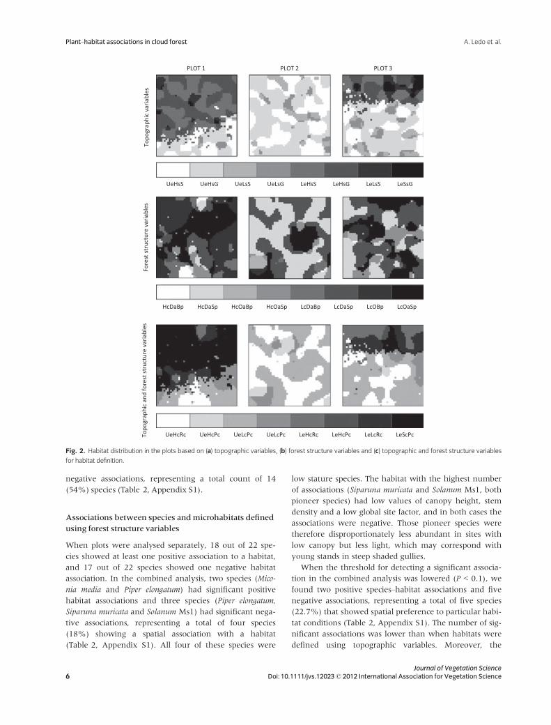
The coverage of each habitat defined by the three sets of

variables on each plot is shown in Fig. 2.

Associations between species andmicrohabitats defined

by topographic variables

When plots were analysed separately, 19 out of 22 species

showed a significant (P < 0.05) positive association to at

least one habitat, and 15 out of 22 species showed a nega-

tive association to a habitat (Appendix S1). Pooling the

information from the three plots, we found six positive

species–habitat associations and two negative associations,

representing a total of eight species (36%) that showed

spatial association or repulsion for at least one topographic

habitat. Three of these were canopy species and the other

three were low-stature species (Table 2, Appendix S1).

Canopy species are less rich (eight species) than low-stat-

ure species (14 species) in this community, from which we

saw that the proportion of species that are habitat-associ-

ated is higher for canopy species than understorey species

(37 vs. 21%). The habitat with the highest number of posi-

tive associations is low-elevation steep spurs, where two

below-canopy medium- or shade-intolerant species

(Aphelandra acanthifolia and Cestrum auriculatum) and one

canopy species (Critoniopsis sevillana) were significantly

associated, followed by low-elevation steep gullies where

one canopy species (Persea Ms) and one understorey spe-

cies (Solanum Ms2) were significantly associated (Table 2,

Appendix S1).

When the threshold for detecting a significant associa-

tion in the combined analysis was lowered (P < 0.1), we

found 11 positive species–habitat associations and five



negative associations, representing a total count of 14

(54%) species (Table 2, Appendix S1).


using forest structure variables

When plots were analysed separately, 18 out of 22 spe-

cies showed at least one positive association to a habitat,

and 17 out of 22 species showed one negative habitat

association. In the combined analysis, two species (Mico-

nia media and Piper elongatum) had significant positive

habitat associations and three species (Piper elongatum,

Siparuna muricata and Solanum Ms1) had significant nega-

tive associations, representing a total of four species

(18%) showing a spatial association with a habitat

(Table 2, Appendix S1). All four of these species were

low stature species. The habitat with the highest number

of associations (Siparuna muricata and Solanum Ms1, both

pioneer species) had low values of canopy height, stem

density and a low global site factor, and in both cases the

associations were negative. Those pioneer species were

therefore disproportionately less abundant in sites with

low canopy but less light, which may correspond with

young stands in steep shaded gullies.

When the threshold for detecting a significant associa-

tion in the combined analysis was lowered (P < 0.1), we

found two positive species–habitat associations and five

negative associations, representing a total of five species

(22.7%) that showed spatial preference to particular habi-

tat conditions (Table 2, Appendix S1). The number of sig-

nificant associations was lower than when habitats were

defined using topographic variables. Moreover, the

Fig. 2. Habitat distribution in the plots based on (a) topographic variables, (b) forest structure variables and (c) topographic and forest structure variables

for habitat definition.



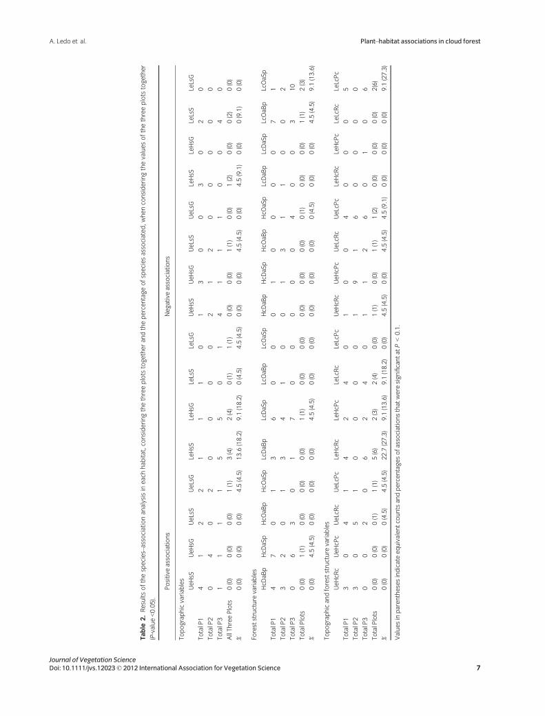
Table

2.Resultsofthespecies–associationanalysisineachhab

itat,consideringthethreeplotstogetherandthepercentageofspeciesassociated,whenco

nsideringthevaluesofthethreeplots

together

(P-value<0.05).

Positive

associations

Negativeassociations

Topographicvariab

les

UeHsS

UeHsG

UeLsS

UeLsG

LeHsS

LeHsG

LeLsS

LeLsG

UeHsS

UeHsG

UeLsS

UeLsG

LeHsS

LeHsG

LeLsS

LeLsG

TotalP1

41

22

11

10

13

00

30

20

TotalP2

04

02

00

00

21

20

00

00

TotalP3

11

11

55

01

41

11

00

40

AllThreePlots

0(0)

0(0)

0(0)

1(1)

3(4)

2(4)

0(1)

1(1)

0(0)

0(0)

1(1)

0(0)

1(2)

0(0)

0(2)

0(0)

%0(0)

0(0)

0(0)

4.5(4.5)

13.6(18.2)

9.1(18.2)

0(4.5)

4.5(4.5)

0(0)

0(0)

4.5(4.5)

0(0)

4.5(9.1)

0(0)

0(9.1)

0(0)

Foreststructure

variab

les

HcD

aBp

HcD

aSp

HcO

aBp

HcO

aSp

LcDaB

pLcDaSp

LcOaB

pLcOaSp

HcD

aBp

HcD

aSp

HcO

aBp

HcO

aSp

LcDaB

pLcDaSp

LcOaB

pLcOaSp

TotalP1

47

01

36

00

01

00

00

71

TotalP2

32

01

34

10

01

31

10

02

TotalP3

06

30

17

00

00

04

00

310

TotalPlots

0(0)

1(1)

0(0)

0(0)

0(0)

1(1)

0(0)

0(0)

0(0)

0(0)

0(0)

0(1)

0(0)

0(0)

1(1)

2(3)

%0(0)

4.5(4.5)

0(0)

0(0)

0(0)

4.5(4.5)

0(0)

0(0)

0(0)

0(0)

0(0)

0(4.5)

0(0)

0(0)

4.5(4.5)

9.1(13.6)

Topographicandforeststructure

variab

les

UeHcRc

UeHcP

cUeLcRc

UeLcPc

LeHcR

cLeHcPc

LeLcRc

LeLcPc

UeHcRc

UeHcPc

UeLcRc

UeLcPc

LeHcRc

LeHcPc

LeLcRc

LeLcPc

TotalP1

30

41

42

40

10

04

00

05

TotalP2

30

51

00

00

19

16

00

00

TotalP3

00

20

62

40

11

26

01

06

TotalPlots

0(0)

0(0)

0(1)

1(1)

5(6)

2(3)

2(4)

0(0)

1(1)

0(0)

1(1)

1(2)

0(0)

0(0)

0(0)

2(6)

%0(0)

0(0)

0(4.5)

4.5(4.5)

22.7(27.3)

9.1(13.6)

9.1(18.2)

0(0)

4.5(4.5)

0(0)

4.5(4.5)

4.5(9.1)

0(0)

0(0)

0(0)

9.1(27.3)

Valuesinparenthesesindicateequivalentcountsandpercentagesofassociationsthat

were

significantat

P<0.1.



associations to forest structure variables were less consis-

tent among plots (Table 2, Appendix S1).


using topographic and forest structure variables

When plots were analysed separately 22 species (100%)

showed a positive association to at least one habitat, and 17

out of these 22 species showed a negative association

(Appendix S1) to habitats, defined on the basis of both

topographic and forest structure variables. In the analysis

combining data from all three plots, ten species showed

positive habitat associations and five species had negative

associations (P < 0.05). A total of 11 species (50%) showed

(either positive or negative) spatial associations with a habi-

tat (Table 2, Appendix S1). These associations were found

for canopy (DrimysMs, PerseaMs) as well as low-stature (Ce-

strum auriculatum, Iochroma squamosum, Miconia denticulata,

Miconia media, Piper elongatum, Solanum Ms1 and Solanum

Ms2) species. Five species were positively associated with

tall forest at lower elevations with a high species richness

(habitat LcHcRC, Table 2), which represents closed canopy

mature forest with a high species count. The habitat with

the highest number of negative associations represents

shorter forest at low elevations with a low species richness

(habitat LeLcPc, Table 2), which corresponds to canopy

gaps. Under this criterion, many species displayed at least

one association (positive or negative) with a determined

habitat (Table 2, Appendix S1). Nevertheless, all the most

abundant species in the forest (the pioneer Solanum Ms1,

the understorey species Piper elongatum and the canopy spe-

cies DrymsMs and PerseaMs) displayed spatial associations.

When topographic as well as forest structure variables

were combined in the definition of habitats, the number of

species with significant associations (P < 0.05) was higher

(15 species) than when either topographic (nine species)

or forest structure (five species) variables were used in iso-

lation. There was also more agreement among plots when

habitats were defined using both topographic and forest

structure variables (Table 2). Increased consistency of hab-

itat associations among plots is probably indicative of a

more robust result. When the threshold for detecting a sig-

nificant association was lowered (P < 0.1), we found 15

positive species–habitat associations and 11 negative asso-

ciations, representing a total of 16 species (72%) that

showed spatial non-randomness with respect to habitat

conditions (Table 2, Appendix S1).

Discussion

Species–habitat associations

The habitat association method proposed by Harms et al.

(2001) allowed us to corroborate the existence of micro-

habitat associations for woody plant species in a Peruvian

cloud forest community. Analogous habitat associations

have been observed in a number of tropical lowland forests

and are now a widely accepted characteristic of tropical

tree communities (Phillips et al. 2003; Chave 2004; Guna-

tilleke et al. 2006; Lai et al. 2009).

The scale of observation and the variables used to differ-

entiate habitats in our study were different to those

employed in previous studies. The fact that biophysical

gradients lead to habitat associations at large scales in tropi-

cal forests is strongly supported in the literature: one of the

clearest examples is the existence of altitudinal vegetation

zones (Gentry 1988). Habitat associations also occur at

meso-scales of 1–50 ha (Harms et al. 2001; Valencia et al.

2004; Comita et al. 2007) and landscape scales of~400 ha

(Paoli et al. 2006), but analyses at small scales have rarely

been conducted (but see John et al. 2007). Our analyses

using 2 9 2 m quadrats show that microhabitat differenti-

ation and microhabitat–species association also exist at this

very fine scale. Moreover, the scale of species–habitat asso-

ciations is set more on the mean habitat patch size than on

the size of quadrats. Fine-scale analysis is important

because it allows us to gain a clearer understanding of

micro-niche differentiation, whichmay be key to biodiver-

sity conservation (Leigh et al. 2004). Both micro- and

macro-scale processes need to be considered in theories

explaining the maintenance of plant community diversity

(Whittaker et al. 2001).

Previous studies have generally defined habitats and

species distributions using topographic characteristics, such

as elevation or slope (Gunatilleke et al. 2006; Comita et al.

2007), soil nutrients (P�elissier et al. 2001; Phillips et al.

2003; John et al. 2007) or both (Costa et al. 2005; Suzuki

et al. 2009). In this paper we examined the importance of

both environmental and forest structure variables to the

differentiation of microhabitats within the forest. We have

carried out a number of analyses to compare the results

obtained using different criteria for defining habitats, and

have identified clear differences (Table 2). Hence, the way

in which habitats are defined is of particular importance.

One shortcoming of this method is that the habitats must

be selected a priori, and the habitat definition has a notable

effect on the results.Without information on the ecological

preferences of the species, or the range in which species

respond differentially to a variable (e.g. the slope limit for

the occurrence of certain species), the selection of variables

is inherently arbitrary and may be incomplete if an

unmeasured environmental variable is important for cer-

tain species. For example, although canopy height is rarely

taken into account in analyses of species distributions, we

have found that areas with a taller forest canopy might be

considered different microhabitats, since the distribution

of certain species was related to this variable (Appendix



S1). In our study site, species associated with taller forest

included both canopy species, such as PerseaMs andMorus

insignis, and species of low stature, such as Miconia media,

Piper elongatum and SolanumMs. Nevertheless, the effect of

arbitrariness in habitat definition in species–habitat associ-

ations could be also somewhat reduced if the species were

allowed to be associated with combinations of habitats and

not only single habitats in the statistical test, as in the

method proposed by De C�aceres et al. (2010).

Our use of three replicate plots (instead of one large

plot) allowed us to determine whether species–habitat

associations were consistent in different parts of the forest.

This approach helps to avoid misinterpretations caused by

fortuitous species–habitat co-occurrence resulting from

dispersal limitation in a given area. We found that while

some associations were consistent among plots, many asso-

ciations only appeared in one or two plots, and the results

for the other(s) were different. This divergence was most

apparent when forest structure variables were used for

defining habitats (Appendix S1). When the three plots

were considered together, the number of significant associ-

ations decreased. The associations identified at the scale of

a single plot, but not in the combined analysis across all

three plots, may have arisen either because the distribution

of a species coincides with the presence of a habitat that

differs in subtle ways between plots in a manner that were

not captured by our habitat definitions, or because of spa-

tial variation in the size class and age structure of species’

populations, because habitat associations may vary

through ontogeny (Comita et al. 2007). However, inde-

pendent of the cause, our results indicate that habitat parti-

tioning only affects the spatial distribution of some species

within a community. It is important to note that these

findings are only valid for the habitats we defined and at

the scale of analysis used in this paper.

Variables implicated inmicrohabitat partitioning and

factors involved in species distribution

The inclusion of both environmental and forest structure

conditions together discriminated most strongly among

species and generated the most consistent results among

plots (Table 2). Environmental variables were most

strongly correlated with the distribution of canopy species,

while forest structure variables displayed associations with

the distribution of understorey species. Therefore, the

combination of environmental and forest structure vari-

ables highlighted associations with a larger number of spe-

cies across both life forms than either set of variables in

isolation.

At intermediate and large scales, elevation is the most

important factor determining species occurrence (Gentry

1988; Steege et al. 2006). However, our analyses also

highlight the importance of forest structure and small-scale

disturbances. Species that occurred in plot 3 but not in

plots 1 and 2 (Aphelandra acanthifolia and Siparuna muri-

cata) illustrate the role of stand disturbances in species dis-

tribution. These species appear to be associated with

habitats characterized by lower elevations (Appendix S1).

It is therefore potentially surprising that they do not appear

in plot 1, which is at a lower elevation. However, the

occurrence of these species is related to factors other than

altitude. Plot 3 is situated above a track with a gentle slope,

and the creation of the trackmay have facilitated the estab-

lishment of disturbance-dependent species that typically

occur at forest edges and canopy gaps but not in undis-

turbed mature forest. This is most noticeable for Aphelan-

dra, which is negatively associated with well-developed

stands (Appendix S1). The distribution of this species is

probably related to specific microclimatic conditions rather

than to altitude. These microclimatic conditions arise from

dynamic stand processes and are therefore inherently

unpredictable. Different microclimatic conditions may also

correlate with altitudinal gradients, and indeed they often

vary in a parallel manner. A similar interpretation of the

importance of environmental conditions on the distribu-

tion of species was expressed by Whittaker et al. (2001),

who advocated that geographic patterns of species richness

should not be termed “latitudinal gradients”.

Evidence of micro-niche partitioning

We found that many species were associated either posi-

tively or negatively with specific habitats, and this may be

interpreted as an indication of micro-niche separation at

the scale of our analysis. Some pioneer species occur in

association with microhabitats that indicate specialization

to a narrow niche defined by occupancy of micro-gaps.

This result conforms to previous research on tropical forest

trees (Clark et al. 1993; Chesson 2000), and supports the

idea that pioneer species are strongly affected by microcli-

mate conditions. Our results also identified habitat associa-

tions for some canopy and emergent species, which

suggests that different species and/or functional groups

have different patterns of habitat association. Canopy spe-

cies are more strongly related to micro-topographic vari-

ables than understorey species, which appear to depend

more on forest structure variables (Appendix S1). These

findings support the hypothesis that canopy gaps are par-

ticularly important for maintenance of pioneer species

(Whitmore 1978; Schnitzer & Carson 2001).

A drawback when attempting to study species–niche

association is that there is no universally agreed definition

of the ‘niche’ (Morin 2011). Classical micro-niche defini-

tions sometimes include only physical environmental con-

ditions (MacArthur 1972). In other cases, the niche



implies a wide range of variables. Hutchinson (1957)

defined the niche as an n-dimensional hypervolume,

where each variable n is an environmental or biological

variable and the resources that define the requirements of

a species to maintain or increase its population. However,

the term microhabitat we have been using in this paper is

close to the ‘niche’ concept defined by Grubb (1976) and

by Chase & Leibold (2003), which includes both environ-

mental and biotic conditions. To avoid confusion, we avoid

the term ‘niche’ and replace it here by microhabitat. The

microhabitats we defined in this study include both forest

structure and environmental variables. This perspective

has implications for our understanding of the mechanisms

that drive tree species distributions and community struc-

ture. Environmental and forest structure conditions may

co-vary at small scales, since they are mutually dependent.

Soil nutrient availability, another important factor influ-

encing species distributions (John et al. 2007; Bohlman

et al. 2008), may also vary in parallel with topography and

forest structure.

Many current authors agree that spatio-temporal varia-

tion of resource availability is an important mechanism for

the maintenance of species richness (Wright 2002). We

advocate that both forest structure and environmental

characteristics have both static and dynamic components,

and these may vary within forests at small scales. In addi-

tion, the two sets of variables may co-vary in a variety of

ways and/or vary on different temporal and spatial scales.

This environmental complexity generates a high diversity

of microhabitats and, consequently, a greater range of

establishment opportunities for the species that comprise

the community. Our results suggest that microhabitat spe-

cialization is an important factor contributing to commu-

nity structure for woody plants of a Peruvian cloud forest.

Acknowledgements

Wewould like to thank Liza Comita for the R code and her

helpful comments, and Wilder Caba for help with field-

work. Most of the research for this paper was carried out

during the first author’s stay at Aberdeen University. The

research was funded through a PhD grant from the Uni-

versidad Polit�ecnica de Madrid and the fieldwork was

partly supported by the Consejo Social de la Universidad

Polit�ecnica deMadrid.

References

Bohlman, S.A., Laurance, W.F., Laurance, S.G., Nascimento, H.

E.M., Fearnside, P.M. & Andrade, A. 2008. Importance of

soils, topography and geographic distance in structuring cen-

tral Amazonian tree communities. Journal of Vegetation Science

19: 863–874.

Bruijnzeel, L.A., Scatena, F.N. & Hamilton, L.S. 2011. Tropical

montane cloud forest. Science for conservation and management.

Cambridge University Press, Cambridge, UK.

Chase, J.M. & Leibold,M.A. 2003. Ecological niches: linking classical

and contemporary approaches. University of Chicago Press,

Chicago, IL, US.

Chave, J. 2004. Neutral theory and community ecology. Ecology

Letters 7: 241–253.

Chesson, P. 2000. Mechanisms of maintenance of species diver-

sity.Annual Review of Ecology and Systematics 31: 343–366.

Chust, G., Chave, J., Condit, R., Aguilar, S., Lao, S. & Perez, R.

2006. Determinants and spatial modeling of tree beta-diver-

sity in a tropical forest landscape in Panama. Journal of Vege-

tation Science 17: 83–92.

Clark, D.B., Clark, D.A. & Rich, P.M. 1993. Comparative analysis

of microhabitat utilization by saplings of nine tree species in

neotropical rain forest. Biotropica 25: 397–407.

Comita, L.S., Condit, R. & Hubbell, S.P. 2007. Developmental

changes in habitat associations of tropical trees. Journal

of Ecology 95: 482–492.

Condit, R., Ashton, P.S., Baker, P., Bunyavejohewin, S., Guna-

tileke, S., Gunatilleke, N., Hubbell, S.P., Foster, R.B., Itoh,

A., LaFrankie, J.V., Lee, H.S., Losos, E., Manokaran, N.,

Sukumar, R. & Yamakura, T. 2000. Spatial patterns in

the distribution of tropical tree species. Science 288: 1414–

1418.

Costa, F.R.C., Magnusson, W.E. & Luizao, R.C. 2005. Mesoscale

distribution patterns of Amazonian understorey herbs in

relation to topography, soil andwatersheds. Journal of Ecology

93: 863–878.

De C�aceres, M., Legendre, P. & Moretti, M. 2010. Improving

indicator species analysis by combining groups of sites. Oikos

119: 1674–1684.

Freile, J.F. & Santander, T. 2005. �Areas Importantes para la Con-

servaci�on de las Aves en Ecuador. In: BirdLife International

(eds.) �Areas importantes para la conservaci�on de las aves en los

andes tropicales: sitios prioritarios para la conservaci�on de la biodiv-

ersidad. pp. 283–470. BirdLife International y Conservation

International Quito, Ecuador.

Gentry, A.H. 1988. Changes in plant community diversity

and floristic composition on environmental and geographi-

cal gradients. Annals of the Missouri Botanical Garden 75:

1–34.

Gentry, A.H. 1995. Patterns of Diversity and Floristic Composi-

tion in Neotropical Montane Forest. In: Churchil, S.P.(ed.)

Biodiversity and conservation of neotropical montane forest. pp.

103–126. The New York Botanical Garden, Brooklyn, NY,

US.

Grubb, P.J. 1977. The maintenance of species-richness in plant

communities: the importance of the regeneration niche.

Biological Reviews 52: 107–145.

Gunatilleke, C.V.S., Gunatilleke, I.A.U.N., Esufali, S., Harms, K.

E., Ashton, P.M.S., Burslem, D.F.R.P. & Ashton, P.S. 2006.

Species–habitat associations in a Sri Lankan dipterocarp

forest. Journal of Tropical Ecology 22: 371–384.



Hale, S.E. & Edwards, C. 2002. Comparison of film and digital

hemispherical photography across a wide range of canopy

densities.Agricultural and Forest Meteorology 112: 51–56.

Hamilton, L.S. 1995. Mountain cloud forest conservation and

research: a synopsis. Mountain Research and Development 15:

259–266.

Harms, K.E., Condit, R., Hubbell, S.P. & Foster, R.B. 2001. Habi-

tat associations of trees and shrubs in a 50-ha neotropical for-

est plot. Journal of Ecology 89: 947–959.

Hubbell, S.P., Foster, R.B., O’Brien, S.T., Harms, K.E., Condit, R.,

Wechsler, B., Wright, S.J. & Loo de Lao, S. 1999. Light-gap

disturbances, recruitment limitation, and tree diversity in a

neotropical forest. Science 283: 554–557.

Hutchinson, G.E. 1957. Concluding remarks. Cold Spring Harbor

Symposia on Quantitative Biology 22: 415–427.

John, R., Dalling, J.W., Harms, K.E., Yavitt, J.B., Stallard, R.F.,

Mirabello, M., Hubbell, S.P., Valencia, R., Navarrete, H., Val-

lejo, M. & Foster, R.B. 2007. Soil nutrients influence

spatial distributions of tropical tree species. Proceedings of the

National Academy of Sciences of the United States of America 104:

864–869.

Kneitel, J.M. & Chase, J.M. 2004. Trade-offs in community ecol-

ogy: linking spatial scales and species coexistence. Ecology

Letters 7: 69–80.

K€oppen, W. (ed) 1936. Das Geographische System der Klimate.

Gerbr€uder Bontr€ager, Berlin.

Lai, J., Mi, X., Ren, H. & Ma, K. 2009. Species–habitat associa-

tions change in a subtropical forest of China. Journal of Vege-

tation Science 20: 415–423.

Law, R., Purves, D.W., Murrell, D.J. & Dieckmann, U. 2001.

Causes and effects of small-scale spatial structure in plant

populations, In: Silvertown, J. & Antonovics, J. (eds.)

Integrating ecology and evolution in a spatial context. pp. 21–44.

Blackwell Science, Oxford, UK.

Ledo, A., Montes, F. & Cond�es, S. 2009. Species dynamics in a

Montane Cloud Forest: identifying factors involved in

changes in tree diversity and functional characteristics. Forest

Ecology andManagement 258: S75–S84.

Ledo, A., Montes, F. & Cond�es, S. 2012. Different spatial organi-

zation strategies of woody plant species in a montane cloud

forest.Acta Oecologica 38: 49–57.

Leigh, E.G., Davidar, P., Dick, C.W., Puyravaud, J.P., Terborgh,

J., Steege, H. & Wright, J.S. 2004. Why do some tropical for-

ests have somany species of trees? Biotropica 36: 447–473.

MacArthur, R.H. 1972. Geographical ecology: patterns in the distribu-

tion of species. Princeton University Press, Princeton, NJ, US.

Morin, P.J. 2011. Community ecology, 2nd edn. Wiley-Blackwell,

Oxford, UK.

Pacala, S.W. & Tilman, D. 1994. Limiting similarity in mechanis-

tic and spatial models of plant competition in heterogeneous

environments. The American Naturalist 143: 222–257.

Pachauri, A.K. & Pant, M. 1992. Landslide hazardmapping based

on geological attributes. Engineering Geology 32: 81–100.

Paoli, G.D., Curran, L.M. & Zak, D.R. 2006. Soil nutrients and

beta diversity in the Bornean Dipterocarpaceae: evidence for

niche partitioning by tropical rain forest trees. Journal of

Ecology 94: 157–170.

P�elissier, R., Dray, S. & Sabatier, D. 2001. Within-plot relation-

ships between tree species occurrences and hydrological soil

constraints: an example in French Guiana investigated

through canonical correlation analysis plant. Ecology 162:

143–156.

Phillips, O.L., N�u~nez-Vargas, P., Lorenzo-Monteagudo, A., Pe~na-

Cruz, A., Chuspe Zans,M.E., Galiano-S�anchez,W., Yli-Halla,

M. & Rose, S. 2003. Habitat association among Amazonian

tree species: a landscape-scale approach. Journal of Ecology

91: 757–775.

Plotkin, J.B., Potts, M.D., Leslie, N., Manokaran, M., LaFrankie,

J.V. & Ashton, P.S. 2000. Species–area curves, spatial aggre-

gation, and habitat specialization in tropical forests. Journal

of Theoretical Biology 207: 81–99.

Plotkin, J.B., Chave, J. & Ashton, P.S. 2002. Cluster analysis of

spatial patterns in malaysian tree species. The American Natu-

ralist 160: 629–644.

Romero, C.C., Baigorria, G.A. & Stroosnijder, L. 2007. Changes

of erosive rainfall for El Ni~no and La Ni~na years in the

northern Andean highlands of Peru. Climatic Change 85: 343–

356.

Schnitzer, S.A. & Carson, W.P. 2001. Treefall gaps and the main-

tenance of species diversity in a tropical forest. Ecology 82:

913–919.

Steege, H., Pitman, N.C.A., Phillips, O.L., Chave, J., Sabatier, D.

& Duque, A. 2006. Continental-scale patterns of canopy tree

composition and function across Amazonia. Nature 443:

444–447.

Suzuki, R.O., Numata, S., Okuda, T., Supardi, M.N.N. & Kachi,

N. 2009. Growth strategies differentiate the spatial patterns

of 11 dipterocarp species coexisting in a Malaysian tropical

rain forest. Journal of Plant Research 122: 81–93.

Valencia, R., Foster, R., Villa, G., Condit, R., Svenning, J.C.,

Hernandez, C., Romoleroux, K., Losos, E., Magard, E. &

Balslev, H. 2004. Tree species distributions and local habitat

variation in the Amazon: large forest plot in eastern Ecuador.

Journal of Ecology 92: 214–229.

Whitmore, T.C. 1978. Gaps in the forest canopy. In: Tomlinson,

P.B & Zimmerman, M.H. (eds.) Tropical trees as living systems.

pp. 639–655. Cambridge University Press, Cambridge, UK.

Whittaker, R.J., Willis, K.J. & Field, R. 2001. Scale and species

richness: towards a general, hierarchical theory of species

diversity. Journal of Biogeography 28: 453–470.

Wiegand, T., Gunatilleke, S., Gunatilleke, N. & Okuda, T.

2007. Analyzing the spatial structure of a Sri Lankan tree

species with multiple scales of clustering. Ecology 88: 3088–

3102.

Wright, S.J. 2002. Plant diversity in tropical forests: a review of

mechanisms of species coexistence.Oecologia 130: 1–14.



Supporting Information

Additional supporting information may be found in the

online version of this article:

Appendix S1. Results of the species–habitat associa-

tion analysis when (a) topographic variables (b) forest

structure variables and (c) topographic and forest structure

variables were used to define habitats. The low-stature and

mid-canopy species are indicated by ‘L’ and the canopy

and emergent species with ‘C’. The ‘+’ symbol indicates sig-

nificant association with plot 1, the ‘•’ symbol with plot 2

and the ‘Θ’ symbol with plot 3. The grey cells indicate a sig-

nificant association when the three plots are analysed

together.



Micro-scale habitat associations of woody plants in a neotropical cloud forest

Documents