Michael Stocks - Biologi, bioteknik och bioinformatik

Population Genetic Analysis and Demographic Inference of Four

Spruce Species from the Qinghai-Tibetan Plateau

Michael Stocks

Degree project in biology, Master of science (2 years), 2009Examensarbete i biologi 45 hp till masterexamen, 2009Biology Education Centre and Department of Evolutionary Functional Genomics, Uppsala UniversitySupervisor: Professor Martin Lascoux

Population Genetic Analysis and Demographic

Inference of Four Spruce Species from the

Qinghai-Tibetan Plateau

Michael Stocks∗

Abstract

Geological upheaval has altered the topology and climate of theQinghai-Tibetan Plateau considerably over the last 10 million years.12-14 nuclear loci were sampled from four conifers in the genus Piceathat occupy regions on and around the plateau. P. likiangensis, P.purpurea & P. wilsonii are found on the eastern edge of the plateauwith ranges that overlap to varying degrees, whilst P. schrenkiana isfound in isolated mountain ranges northwest of the Qinghai-TibetanPlateau. Nucleotide diversity amongst the three eastern spruce specieswas higher than in previously studied Picea from North America andEurope, implying that recent glaciations have not had as big an effecton Asian species as has been observed in boreal species. Further anal-ysis of population structure and demographic history using coalescentbased methods imply a complex relationship amongst recently divergedspecies, with evidence for post-divergent gene flow being detected byMIMAR. The Isolation with Migration model implemented in MIMARgives divergence times which coincide with studies of stable isotopes inmarine and land fossils that approximate when the plateau began todry out.

∗Department of Evolutionary Functional Genomics, Uppsala University

2

Introduction

The origin of new species is never simply defined by gargantuan events thatestablish impenetrable mountain ranges, oceans or deserts that tidily splita species in two. In reality, even the most dramatic of geological events takeplace on relatively long time scales, with local environmental and ecologicalconditions changing gradually. The fate of a species is intrinsically linked toits environment, shaping its demographic history. For example, favourableconditions may lead to a range expansion, while non-favourable conditionsmay lead to more restricted natural ranges. Differing demographic scenarios,such as population expansions or bottlenecks, leave genome-wide patterns ofpolymorphism in DNA sequences that can be analysed to make populationgenetic inferences.

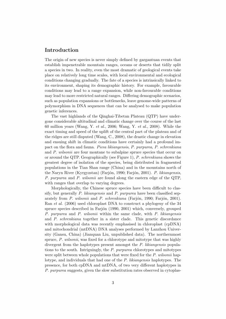
The vast highlands of the Qinghai-Tibetan Plateau (QTP) have under-gone considerable altitudinal and climatic change over the course of the last60 million years (Wang, Y. et al., 2006; Wang, Y. et al., 2008). While theexact timing and speed of the uplift of the central part of the plateau and ofthe ridges are still disputed (Wang, C., 2008), the drastic change in elevationand ensuing shift in climatic conditions have certainly had a profound im-pact on the flora and fauna. Picea likiangensis, P. purpurea, P. schrenkianaand P. wilsonii are four montane to subalpine spruce species that occur onor around the QTP. Geographically (see Figure 1), P. schrenkiana shows thegreatest degree of isolation of the species, being distributed in fragmentedpopulations in the Tian Shan range (China) and in the mountains north ofthe Naryn River (Kyrgyzstan) (Farjon, 1990; Farjon, 2001). P. likiangensis,P. purpurea and P. wilsonii are found along the eastern edge of the QTP,with ranges that overlap to varying degrees.

Morphologically, the Chinese spruce species have been difficult to clas-sify, but generally P. likiangensis and P. purpurea have been classified sep-arately from P. wilsonii and P. schrenkiana (Farjon, 1990; Farjon, 2001).Ran et al. (2006) used chloroplast DNA to construct a phylogeny of the 34spruce species described in Farjon (1990, 2001) which, conversely, groupedP. purpurea and P. wilsonii within the same clade, with P. likiangensisand P. schrenkiana together in a sister clade. This genetic discordancewith morphological data was recently emphasised in chloroplast (cpDNA)and mitochondrial (mtDNA) DNA analyses performed by Lanzhou Univer-sity (Gansu, China) (Jianquan Liu, unpublished data). The northernmostspruce, P. wilsonii, was fixed for a chlorotype and mitotype that was highlydivergent from the haplotypes present amongst the P. likiangensis popula-tions to the south. Intriguingly, the P. purpurea chlorotypes and mitotypeswere split between whole populations that were fixed for the P. wilsonii hap-lotype, and individuals that had one of the P. likiangensis haplotypes. Thepresence, for both cpDNA and mtDNA, of two very different haplotypes inP. purpurea suggests, given the slow substitution rates observed in cytoplas-

3

mic organelles in conifers (Jaramillo-Correa et al., 2003), that asymmetricalintrogression of organelle haplotypes may be occurring.

Asymmetrical introgression has been observed in a number of studies on

Figure 1: Map showing the locations of P. likiangensis (yellow), P. purpurea (purple), P.schrenkiana (red) & P. wilsonii (green) on and around the Qinghai-Tibetan Plateau.

natural populations (e.g. Slotte et al., 2008), and could easily be attributedto selection or a bias inherent in the estimation process. A recent study byCurrat et al. (2008), however, used simulations to show that asymmetricalintrogression could occur, in the absence of selection, due to purely demo-graphic reasons. When a population invades the range of another residentpopulation, asymmetrical gene flow would occur from the local to the in-vading species, as interbreeding events occurring at the leading edge of theadvance would gradually dilute the invading population.

If interspecific asymmetrical introgression were to have occurred betweenpreviously divergent populations it illustrates the potential ebb and flow ofparapatric and sympatric speciation. While allopatric models of speciationcan be mathematically and intuitively simpler, there is mounting evidencethat the more complex processes involved in parapatric and sympatric spe-ciation might be more common than once thought. There are, naturally,difficulties when the traditional bifurcating pattern of evolution is blurreddue to post-divergent or interspecific gene flow, but it is clear that some ofthese complicated scenarios can leave informative patterns of variation and

4

introgression in sequences, and it is of relevance to try to understand howto interpret these signals in polymorphism data. Coalescent simulations ofcryptic speciation, however, offer a quantitative and statistical frameworkwith which to answer some of these more testing questions.

Kingman’s (1982a, 1982b) n-coalescent is a mathematical approximationof the ancestral process, whereby lineages coalesce backwards in time untilthe Most Recent Common Ancestor (MRCA) of the sample is reached. Bymodelling only those lineages ancestral to the sample, it makes for a moreefficient approach than forward-in-time models that require modelling eachindividual. Another advantageous aspect of the coalescent is that large sam-ple sizes are not necessarily needed as the probability of the MRCA of thesample being the MRCA of the entire population is (n−1)/(n+1) (Saunderset al., 1984). Further extensions of the coalescent have led to the modellingof the ancestral process with, for example, recombination (Hudson, 1983;Griffiths, 1991; Griffiths & Marjoram, 1996), selection (Krone & Neuhauser,1997; Neuhauser & Krone, 1997) or substructure (Notohara, 1990; Herbots,1997), allowing the hypothesis testing of a range of evolutionary and demo-graphic scenarios. Specifically, the inclusion of coalescent based Bayesianstatistical methods (e.g. Nielsen & Wakeley, 2001; Beaumont et al., 2002)in estimating population divergence parameters has allowed a fresh look atspeciation.

Allopatric speciation has been commonly depicted in population genet-ics using the isolation model, where a panmictic ancestral population ofeffective population size NA splits t generations ago into two descendantpopulations of effective population size N1 and N2, with no gene flow occur-ring after divergence. The polymorphisms observed between species underthe isolation model have been categorised by Wakeley & Hey (1997) into dis-tinct groups depending on their frequencies in the descendant populations.Sites for which polymorphisms are present in both descendent populationsare referred to as shared polymorphisms (Ss), whereas polymorphisms con-fined solely to a single population are referred to as private polymorphisms(SX1 or SX2, where 1 and 2 refer to populations 1 and 2 respectively). Andfinally, if a polymorphism becomes fixed in one of the populations and isabsent from the other then it is referred to as a fixed polymorphism (Sf ).By counting the number of segregating sites present in each of the two popu-lations, irrespective of the frequency in the other population, you also get S1

and S2 (the number of segregating sites in populations 1 and 2 respectively),which allows us to relate each of the groups of polymorphic sites with theothers:

S1 = SX1 + SSS2 = SX2 + SS

S = SX1 + SX2 + SS + SF

5

Formally, the isolation model is described by the following parameters: θA =4NAµ, θ1 = 4N1µ and θ2 = 4N2µ, where NA, N1 and N2 refer to the effectivepopulation sizes of the ancestral and descendent populations respectively,µ is the per generation mutation rate and τ is the time in the past (ingenerations) when the two populations diverged. The population scaledmutation parameter, θ, can be estimated by the number of segregating sitesdivided by a coefficient reflecting the structure of the neutral genealogythrough the estimate provided by Watterson (1975):

θW =Sn

1 + 12 . . .+

1n−1

(1)

where Sn is the number of segregating sites and n is the number of individ-uals sampled. Using this estimation for θ and considering the relationshipsbetween the groups of segregating sites it is possible to derive the expectedvalues for SX1, SX2, Ss and Sf , and the number of those expected to occurbefore and after the time of divergence. Given observed values for the seg-regating sites it is then possible to solve for the parameters θ1, θ2, θA and τthat define the isolation model. To incorporate gene flow between divergingpopulations Nielsen & Wakeley (2001) described the isolation with migra-tion (IM) model by adding the parameters M1 = 2N1m and M2 = 2N2m,where Nie is the effective population size of the respective populations andm1 is the proportion of population 1 that is replaced each generation bymigrants from population 2.

In order to statistically evaluate different values for the parameters withinthe IM model, Markov chain Monte Carlo (MCMC) methods were imple-mented in a Bayesian and likelihood framework (Nielsen & Wakeley, 2001;Hey & Nielsen, 2004; Hey & Nielsen, 2007). Given the observed data (X)and a set of parameters of interest (Θ), Bayesian inference sets up a jointdistribution (P (X,Θ)), that is simply the product of the prior distribution(P (Θ)) and the likelihood (P (X|Θ)) (Gilks, Richardson & Spiegelhalter,1996). The prior distribution represents prior knowledge that may be avail-able for the data, and together with the likelihood gives a full probabilitymodel: P (X|Θ) = P (X|Θ)P (Θ). Bayes theorem, after the observation ofthe data (X), allows the determination of the distribution of the parameters(Θ) conditional on the data (X), the posterior distribution:

P (Θ|X) =P (Θ)P (X|Θ)

P (X)(2)

The likelihood function contained in the posterior distribution (P (X|Θ))is the probability of observing the data given a set of unknown parameters,but is often difficult to explicitly define for a given model (Stephens, 2001).Felsenstein (1988), by treating the genealogy as a nuisance variable, definedthe likelihood of the parameters given the data (proportional to P (X|Θ))

6

as:L(Θ|X) ∝ Pr(X|Θ) =

∑G∈ψ

Pr(X|G)P (G|Θ) (3)

where G is the genealogy and ψ refers to all the possible gene genealogies.However, given that the number of gene genealogies increases exponentiallywith the number of samples, the calculation of the likelihood for all possiblegenealogies is extremely difficult for large samples. By considering a priordistribution (P (Θ)) in a Bayesian framework, a joint posterior density,

P (G,Θ|X) =P (X|G)P (G|Θ)P (Θ)

P (X)(4)

can be used to simulate a Markov chain for a sample of the genealogies togive an estimate of P (Θ|X) (Hey & Nielsen, 2007).

The use of a uniformly distributed prior then allows P (Θ|X) to be esti-mated as:

P (Θ|X) ≈ 1k

k∑i=1

P (Θ|Gi) (5)

where Gi refers to samples of the marginal distribution

P (G|X) = P (X|G)P (G)/P (X) (6)

generated by MCMC simulations. This posterior density is then, assuminga uniform prior, proportional to the likelihood of the parameters (Hey &Nielsen, 2007).

Samples are drawn from the marginal distribution using a Markov chain,whereby the next state depends only on the current state, and not onthe history of the chain (Gilks, Richardson & Spiegelhalter, 1996). TheMCMC approach updates the parameters of the model in accordance withthe Metropolis-Hastings criterion:

min

{1,P (X|G∗)P (G∗|Θ)P (G∗ → G)P (X|G)P (G|Θ)P (G→ G∗)

}(7)

where P (G → G∗) refers to the probability of G* being proposed as thenext state from G and vice versa. Hey & Nielsen (2004) originally imple-mented this approach in their program IM, whereby the model used assumedno intralocus recombination. In samples where intralocus recombination isknown to occur, loci (or sections of loci) can be removed to avoid breakingthis assumption, but this can drastically reduce the amount of data anal-ysed. The program MIMAR (Becquet & Przeworski, 2007), in summarizingthe polymorphism data, allows for intralocus recombination by using ances-tral recombination graphs (Hudson, 1983) to generate genealogies under thecoalescent according to the parameters proposed by the MCMC approach.Values for the parameters of the IM model are randomly selected and used to

7

perform coalescent simulations. After each simulation, polymorphism datais calculated for the simulated values and compared to the statistics fromthe observed data. The posterior density is calculated for each step of thesimulations and used to determine the parameter values for the simulationsin the following step. After a large number of simulations, a distribution ofthe parameter posterior densities can be obtained with the mode giving anestimate of each parameter.

MIMAR estimates several parameters that are of interest in this study.Firstly, the divergence time (τ) between P. purpurea, P. schrenkiana andP. wilsonii gives an estimate of the timing of speciation and can also beused as a measure of relatedness amongst the species. Secondly, estimatesof the rates of post-divergent gene flow can potentially tell something aboutthe mode of speciation. If there is no migration detected occurring afterdivergence then a more sudden, allopatric form of speciation could be in-ferred. If migration is detected occurring after divergence then it could beinferred that a more gradual, sympatric form of speciation took place. Themigration rate estimates between P. purpurea and P. wilsonii are of specialinterest in light of evidence from organelle data that introgression has po-tentially occurred, and an estimate of gene flow in autosomal DNA wouldhelp to clarify the relationship between these two species.

8

Materials & Methods

Obtaining & Sequencing the DNA: Seeds were collected from 15, 6, 4and 6 populations of Picea likiangensis, P. purpurea, P. schrenkiana and P.wilsonii respectively, with up to 16 individuals sampled per population bycolleagues at Lanzhou University (Gansu, China) (see Appendix: Table 5).The collected seeds were stored in a cold room and then soaked in wa-ter at 4◦C overnight before the haploid megagametophytes were extracted.Altogether 172 megagametophytes were used for DNA extraction carriedout with Qiagen PCR Purification kits using the CTAB method (Doyle &Doyle, 1990) (see Table 6 for a list of primers). Fourteen (P. likiangensis,P. purpurea and P. wilsonii) and twelve (P. schrenkiana) loci (PtIF2009,4cl, col2, ebs, FT3, GI, M002, M007D1, PCH, Sb16, Sb29, Sb62, sel1364,sel1390, xy1420 and ztl) were sequenced on an ABI 3130XL DNA Sequencerusing the ABI Prism Bigdye Terminator Cycle Sequencing Ready ReactionKit at Lanzhou University (Gansu, China) or by Macrogen (Seoul, Korea).Contig assembly and base calling was performed using PHRED and PHRAP(Ewing & Green, 1998; Ewing et al., 1998), and CONSED (Gordon et al.,1998) was used to edit the sequences for analysis.

Nucleotide Diversity & Tests of the Standard Neutral Model: Thenumber of segregating sites (S), number of singletons (η1), average num-ber of pairwise nucleotide differences (π) (Tajima, 1983), minimum numberof recombination events (Rm) (Hudson & Kaplan, 1985), θW (Watterson,1975), Tajima’s D (Tajima, 1989) and Fu & Li’s D* and F* statistics (Fu &Li, 1993) were calculated using compute which is part of the analysis pack-age that utilises the libsequence C++ class library for evolutionary geneticanalysis (Thornton, 2003). The expected number of singletons (η1) of the

folded site frequency spectrum was calculated using E(ηi) = θ1i+ 1n−i

1+δi,n−1(Fu,

1995; Griffiths & Tavare, 1998), where n is the number of samples, i is thenumber of samples containing the mutation (i.e. 1 in the case of a singleton)and δi,n−1 is the Kronecker delta whose value is 1 if i = j and 0 if i 6= j. Fay& Wu’s H (Zeng et al., 2006) was calculated using DnaSP ver. 4.50 (Rozaset al., 2003) and required the use of an out-group to determine the derivedallele. The list of out-groups used for each population is given in Appendix:Table 4. Tests of significance for Tajima’s D, Fu & Li’s D* and F* and Fay& Wu’s H for each locus were performed in DnaSP assuming a standardneutral model with recombination (using the output from rhothetapost, seebelow).

Expected distributions for the summary statistics were obtained usingthe program ms (Hudson, 2002). Tajima’s D, Fu & Li’s F* and Fay & Wu’sH were chosen as the summary statistics that represented the data in themost informative manner. D and F* were calculated by the program msstats

9

(Thornton, 2003) from the data simulated in ms and the normalised versionof Fay & Wu’s H (Zeng et al., 2006) was calculated using a Python code fromthe estimate of θH (Fay & Wu, 2000) given by msstats (some of the scriptsused in the analysis are available at http://www.mspopgen.com). 1,000,000simulations were performed under the standard coalescent with recombina-tion (using the output from rhothetapost, see below), with π used as anestimate of θ. Frequency distributions of the expected summary statisticswere plotted for each of the four species using the statistical package R (RDevelopment Core Team, 2007) alongside the observed values for compari-son and 5% quantiles to test for significance.

Population Structure: Wright’s fixation index (FST ; Wright, 1951), asapplied in this study, assesses population structure by comparing the prob-ability of identity by descent of pairs picked from within a deme to theprobability of identity by descent picked randomly from the total popula-tion (Gillespie, 2004). Estimates of FST within and between species werecarried out using the population genetics data analysis package Arlequinver. 3.11 (Excoffier, 2005) and can be used as an indicator of populationstructure. To further understand the genetic structure of the populations aclustering algorithm was used as implemented in the software package Struc-ture ver. 2.2 (Pritchard et al., 2000; Falush et al., 2003; Falush et al., 2007).Structure uses multilocus data to create clusters of individuals that are inboth Hardy-Weinberg and linkage equilibrium. The admixture model wasused with a burnin period of 150,000 steps followed by a further 8,000,000steps, and repeated multiple times to ensure consistency in the results. Thelikelihoods of different values of K (the inferred number of populations) wasassessed with K = 3 having the highest likelihood, and so this value wasused to perform the longer runs described above.

Recombination: The population scaled recombination rate, ρ, was firstestimated per locus per species using the composite likelihood method (Hud-son, 2001) as implemented by the program pairwise in LDhat 2.1 (McVeanet al., 2002). ρ for diploid species is equal to 4Ner, where 4Ne is the popu-lation scalar and r is the product of the per site recombination rate and thephysical distance across the region analysed. The loci with the minimumand maximum estimated values for ρ were then used as bounds for the mul-tilocus estimation of ρ that was performed using the libsequence programrhothetapost (Haddrill et al., 2005; Thornton & Andolfatto, 2006). rho-thetapost is an approximate Bayesian and rejection sampling method thatgives joint multilocus estimates of ρ and θ. Random values of ρ and θ weredrawn from a uniform prior and used to simulate 10 loci for which the meanπ, S and Rm were calculated and compared with the observed values. Ifthe simulated values were within tolerance ε of the observed values then therandomly picked values for ρ and θ were accepted. Two runs were performed

10

in rhothetapost. The first run collected 12,000 accepted values for ρ and θwhere ε was 0.2 and the bounds for the prior were those given by LDhat.The statistical package R was then used to determine the 0.5% and 99.5%quantiles of the marginal distributions for ρ and θ, and these were thenused as the bounds of a new uniform prior for a second rhothetapost run.In the second run ε was set to 0.05 and 12,000 more acceptances were col-lected, from which the modes were used to give the final estimates of ρ and θ.

Polymorphism data: A Python code was used to count the numberof fixed differences and shared and private polymorphisms. The differentgroups of polymorphisms described by Wakeley & Hey (1997) were countedusing out-groups to discern the derived from the ancestral allele as positedby Becquet & Przeworski (2007), and these were counted between each pairof populations to input into MIMAR. An additional count was done betweenthe three populations P. likiangensis, P. purpurea and P. wilsonii as it wasdeemed important in assessing the extent of polymorphism sharing betweeneach pair of populations. The categories described in Wakeley & Hey (1997)were extended to incorporate the combinations required for three popula-tions. Private polymorphisms (SX1, SX2 & SX3) refer to those that occuronly in one population, exclusively shared polymorphisms (SS12, SS23 &SS13) refer to those that are present in specific pairs of populations and uni-versally shared polymorphisms (SS123) refer to those that are shared by allthree populations. There are also fixed differences that can be observed forindividual populations only (Sf1, Sf2 & Sf3), although none were presentin the three populations studied here.

MIMAR: Input files were prepared for MIMAR incorporating the length(L), number of individuals (n) and the numbers of fixed differences andshared and private polymorphisms for each locus for each pair of speciescompared. For each species pair the respective estimates of ρ given byrhothetapost were averaged to give a mean ρ specific to each pairwise com-parison. An estimation of the per generation mutation rate per site, µ, wasrequired to assign mutations to the genealogy in MIMAR and two sourceswere considered for this. Bouille & Bousquet (2005) used morphological fos-sil evidence and a molecular clock estimate based on three nuclear loci tocalculate the mutation rate in the genus Picea. Willyard et al. (2007), onthe other hand, used 11 nuclear loci and 4 chloroplast loci from the genusPinus calibrated using fossil evidence to fix the divergence time of the Pinussubgenera. Due to the higher number of loci used and the better calibrationin Willyard et al. (2007) it was decided that the mutation rate from thisstudy of 1.01×10−9 (mean of the lower and upper bounds) per site per yearwould be used. Given a 25 year generation time (Brown et al., 2004), the persite per generation mutation rate is 2.5×10−8. It may seem counterintuitiveto use an estimation taken from Pinus instead of Picea but any differences

11

in the mutation rates between these two genera were judged to be smallcompared to the potential variance given by the small number of loci usedin the study by Bouille & Bousquet (2005), that could have distorted theestimate.

Preliminary runs were carried out to optimise, for each parameter, thevariances of the kernel distributions used to determine new values for thenext step of the MCMC, and this was assessed by the level of convergenceand the acceptance rates. Convergence was monitored by referring to themixing and autocorrelation graphs produced using a modified version ofthe R script provided with MIMAR. Due to time constraints, only twoof the pairwise species comparisons were performed: P. purpurea with P.schrenkiana, and P. purpurea with P. wilsonii. These two comparisons wereimportant as they could 1) give an idea of the divergence times between P.schrenkiana and the three other species, and 2) determine whether therehas been introgression occurring between P. purpurea and P. wilsonii. Dueto problems obtaining good estimates of migration in the P. purpurea / P.wilsonii comparison, runs were performed with the migration rates fixed tosymmetrical. In earlier runs the estimated rates of migration were approxi-mately symmetrical, so it was deemed to be more important to obtain goodestimates under this assumption. After exploratory simulations, 20 millionsteps were run for the P. purpurea / P. schrenkiana and P. purpurea / P.wilsonii comparisons. A burnin period equivalent to 10% of the total num-ber of steps was discarded to ensure that the posterior distributions wereindependent of their starting points. To further ensure that convergence hadbeen reached, two runs of each comparison were performed simultaneouslywith different starting seeds to certify that the same result was reached eachtime. Subsequent posterior distributions were attained and smoothed usingR.

12

Results

Nucleotide Diversity: In total 33,663 base pairs of nuclear DNA wereanalysed from Picea likiangensis, P. purpurea, P. schrenkiana and P. wilsonii,with 256, 211, 49 and 164 segregating sites identified respectively. Estimatesof nucleotide diversity are shown in Table . The average number of pair-wise differences per base pair, π, indicated that nucleotide diversity washighest in P. purpurea (0.006240), followed by P. wilsonii (0.005744) andP. likiangensis (0.005584), with P. schrenkiana having the lowest diversity(0.002205). Accordingly, estimates of nucleotide diversity given by θW werehighest in P. purpurea (0.007784) and lowest in P. schrenkiana (0.002246),but with estimates of P. likiangensis (0.006332) in this case being slightlyhigher than that of P. wilsonii (0.006106). Estimates of ρ (per base pair)given by rhothetapost are shown in Appendix: Table 14 and were of the sameorder of magnitude in P. likiangensis (0.01193), P. purpurea (0.01019) andP. wilsonii (0.01059), but smaller in P. schrenkiana (0.0075).

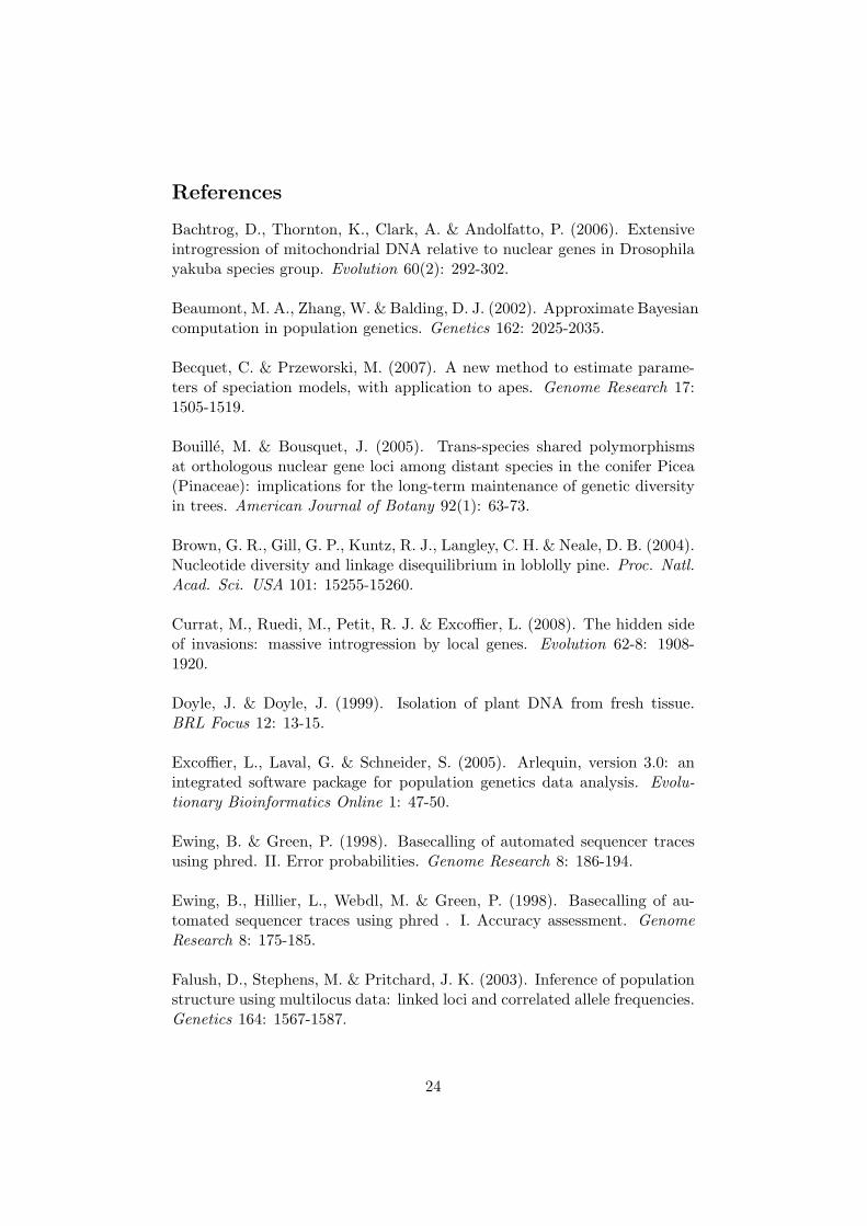
Tests of the standard neutral model: Tajima’s D (D) and Fu & Li’sD* (D*) and F* (F*) (see Table ) were negative in all four species, andonly P. wilsonii had a positive Fay & Wu’s H. None of the neutrality testswere significant when averaged across all loci, but there were a number ofloci that departed significantly from neutrality when tested individually (seeAppendix: Tables 7 to 10). Fay & Wu’s H was significantly positive for 7separate loci in P. wilsonii but as the pattern seemed mostly consistentacross all loci it was deemed to be more likely due to demographics thanselection. A significant excess of higher frequency variants was detected atthe ft3 and sb29 loci in P. schrenkiana, but this can be explained by thethinner sampling undertaken for this individual as relatively few individualswere sampled at these loci (16 and 13 respectively). Other significantly neg-ative loci for D, D* and F* in P. purpurea and P. likiangensis appear to bemore extreme values of a genome wide pattern of negative values and werenot excluded from further analyses. Locus 2009 was consistently positive forvalues of D, D* and F* in P. likiangensis, P. purpurea and P. wilsonii but,as only one value (Tajima’s D in P. purpurea) was significant, the locus wasnot excluded from the analyses. To further assess whether the loci werecompatible with the standard neutral model, coalescent simulations werecarried out under the standard neutral model with recombination. Sum-mary statistics were calculated for the simulated data and compared to theobserved data, and the distributions are shown in figure 2. Observed valuesof D, F* and H do not deviate significantly (5%) from what would be ex-pected under the standard neutral model with recombination. The observedvalue of F* for P. purpurea showed an excess of singletons when comparedwith π, further indicating that demographic factors, rather than selection,are responsible for the significance in the locus specific analyses. For illus-

13

tration purposes (see Figure 2), values of Fay & Wu’s H less than -7 werenot included in the distributions. While not statistically correct, this didnot noticeably alter the shape of the distributions or change any of the con-clusions reached.

Population Structure: FST was calculated between each pair of species(see Table 2) and similar levels of differentiation (0.52864, 0.52578 and0.5134) were observed between P. schrenkiana and P. likiangensis, P. pur-purea and P. wilsonii respectively. FST was lowest between P. likiangen-sis and P. purpurea (0.06856), followed by P. purpurea and P. wilsonii(0.10501), and P. likiangensis and P. wilsonii. Structure ver. 2.2 wasused to infer cryptic population structure within the four species consid-ered jointly, with three being the number of inferred populations with thehighest likelihood. The three species P. likiangensis, P. schrenkiana andP. wilsonii appear to form three genetically differentiated clusters (see Fig-ure 15), with P. purpurea being made up of variation attributable to eachof these clusters (see Appendix: Table 15). Interestingly P. wilsonii seemsto be the most structurally differentiated, while the more geographicallydistant P. schrenkiana appears to cluster closer to P. likiangensis. The ma-jority of P. purpurea individuals cluster with those of P. likiangensis ratherthan P. wilsonii, however there are P. purpurea individuals that cluster withP. wilsonii as well as P. wilsonii individuals that group closer to P. likian-gensis.

Shared Polymorphism and MIMAR Analyses: No fixed differenceswere observed between P. likiangensis, P. purpurea and P. wilsonii, that

Table 1: Nucleotide diversity and tests of the standard neutral model for the four sprucespecies where n is the average number of individuals sampled at each locus, L is the averagelength of the loci, S is the total number of segregating sites observed for all loci, η1 andE(η1) are the total number of observed and expected singletons, θW is Watterson’s estimateof θ per base pair averaged across all loci and π is the average number of pairwise nucleotidedifferences per base pair for all loci. Tests of the standard neutral model based on thefrequency spectrum are averaged over all loci.

Species n L S η1[E(η1)] θW π

P. likiangensis 34 645 256 98 [59] 0.006332 0.005584P. purpurea 19 576 211 115 [53] 0.007784 0.006240P. schrenkiana 17 601 49 18 [17] 0.002246 0.002205P. wilsonii 19 577 164 65 [49] 0.006106 0.005744

Species Tajima’s D Fu & Li’s D∗ Fu & Li’s F ∗ Fay & Wu’s H

P. lik. -0.505634 -0.739421 -0.817759 -0.072349P. pur. -0.802918 -1.257076 -1.324762 -0.683949P. sch. -0.461984 -0.397038 -0.463501 -1.186889P. wil. -0.381706 -0.690811 -0.725818 0.799697

14

Tajima's D−3 −2 −1 0 1 2 3 4

0

10000

20000

30000

40000

50000

P. likiangensis

Fu & Li's F*−4 −2 0 2

0

10000

20000

30000

40000

Fay & Wu's H−6 −4 −2 0 2

0

10000

20000

30000

Tajima's D−3 −2 −1 0 1 2 3 4

0

10000

20000

30000

40000

50000

P. purpurea

Fu & Li's F*−4 −3 −2 −1 0 1 2 3

0

10000

20000

30000

40000

Fay & Wu's H−6 −4 −2 0 2

0

5000

10000

15000

20000

25000

30000

35000

Tajima's D−3 −2 −1 0 1 2 3

0

10000

20000

30000

40000

P. schrenkiana

Fu & Li's F*−4 −3 −2 −1 0 1 2 3

0

10000

20000

30000

Fay & Wu's H−6 −4 −2 0 2

0

10000

20000

30000

40000

50000

60000

Tajima's D−3 −2 −1 0 1 2 3 4

0

10000

20000

30000

40000

50000

P. wilsonii

Fu & Li's F*−4 −3 −2 −1 0 1 2 3

0

10000

20000

30000

40000

Fay & Wu's H−6 −4 −2 0 2

0

10000

20000

30000

Figure 2: Expected distributions of Tajima’s D, Fu & Li’s F* and Fay & Wu’s H for eachof the four spruce species under the standard neutral model with recombination, using π asan estimate for θ, and with ρ estimated using rhothetapost. Solid vertical lines represent theobserved values of each statistic averaged over the loci, with the dotted lines representingthe 2.5 and 97.5% confidence intervals.

are located on or around the QTP. There were, however, fixed differencesobserved between each of these species and the more isolated P. schrenkiana(see Appendix: Tables 12 & 13). When polymorphism data was calculatedfor the three QTP species simultaneously (see Figure 4 and Appendix: Ta-ble 11) the majority of the segregating sites were classified as either beingprivate to individual populations (87 in P. likiangensis, 71 in P. purpureaand 65 in P. wilsonii) or shared between all populations (67). There wereless segregating sites that were shared exclusively between pairs of popula-tions (32 between P. likiangensis and P. purpurea, 23 between P. purpureaand P. wilsonii and 4 between P. likiangensis and P. wilsonii).

Table 2: Between species estimates of FST for each pair of spruce species, with the diagonalvalues representing within species estimates of FST .

P. lik. P. pur. P. sch. P. wil.

P. lik. 0.157 - - -P. pur. 0.069 0.048 - -P. sch. 0.529 0.526 0.148 -P. wil. 0.165 0.105 0.513 0.083

15

Figure 3: Clustering of individuals from each spruce species for each of the k = 3 clustersperformed in the Structure analysis.

Table 3: Modes of the posterior densities from one of the two independent runs for each ofthe parameters estimated in MIMAR.

θ1 θ2 θA Tgen M1 M2

P. pur./P. sch. 0.00822 0.00127 0.00605 64300 0.48 0.5P. pur./P. wil. 0.00941 0.00456 0.00615 21625 0.69 0.69

Estimates of population divergence parameters from MIMAR areshown in Table 3 and the posterior densities, for each pairwise compari-son, of one of the two independent runs are shown in Appendix: Figures 5& 6. The divergence times show P. purpurea and P. wilsonii to be themost recently diverged (21,625 generations ago), with P. purpurea and P.schrenkiana separating 64,300 generations ago. Approximately symmetricalmigration was detected between P. purpurea and P. schrenkiana, indicat-ing that gene flow had occurred after speciation. For the P. purpurea andP. wilsonii pairwise comparison, problems were encountered obtaining goodestimates for the migration rates. In order to improve the resolution themigration rates were fixed to be symmetrical, and subsequently a low rateof migration was observed between the two species. The values for ances-tral θ were estimated to be 0.00615 for the comparison between P. purpureaand P. wilsonii, and 0.00605 in the P. purpurea and P. schrenkiana pairing.Appendix: Table 16 shows a comparison of the values of θ given by MIMAR

16

against estimates from other methods and can give an indication of how wellthe IM model approximates the system studied. Estimates from MIMARfor P. purpurea were closest to Watterson’s estimate of θ, whilst estimatesfor both P. schrenkiana and P. wilsonii were lower than those produced byany of the other methods.

Figure 4: Venn diagram illustration of the number of polymorphisms shared between andprivate to three of the spruce species.

17

Discussion

The distribution of variation amongst diverging populations can be usedto make inferences about the demographic and evolutionary origins of thespecies studied. Polymorphisms shared between two diverging populationsoccur, assuming an infinite sites model, either because of the retention ofancestral polymorphisms or as a result of post-divergent gene flow. In re-cently diverged populations, where lineage sorting may still be occurring, itcan be very difficult to infer which shared polymorphisms are retained froman ancestral population and which ones are the result of introgression. Intheir mathematical treatment of the genealogical species concept, Hudson &Coyne (2002) calculated the probability of observing reciprocal monophylyfor differing numbers of loci. Reciprocal monophyly applies if all sampledloci from a genealogical species are phylogenetically shown to be more closelyrelated to each other than to alleles of the same locus in other genealogicalspecies. For 15 nuclear loci the time it would take to have a 50% probabilityof observing reciprocal monophyly is 8.9 Ne generations (where Ne is theeffective size of the population). Using π as an estimate for θ, a mutationrate of 2.5 × 10−8 per base pair and assuming a 25 year generation time itwould take 13.9 and 4.9 million years for P. purpurea and P. schrenkianarespectively to have a 50% probability of observing reciprocal monophyly. Ifthe studied species’ morphological similarity is consistent with a relativelyrecent divergence time then we would expect a large number of alleles in thefour species to have been retained from a common ancestral population.

Variation within the three species of the QTP was considerably higherthan recent estimates of nucleotide diversity per site (π) observed in bo-real spruce species such as P. abies (0.003838), P. glauca (0.004824) and P.mariana (0.003199) (Chen et al., submitted), all of which have much largernatural ranges. This most likely reflects that the boreal species have beenmore severely affected by the glacial patterns in the northern hemisphere,and this is to some extent reflected in the neutrality tests. Estimates ofTajima’s D for the two boreal species P. abies (-0.897) and P. mariana(-0.779) were more negative than those obtained for all the Asian sprucespecies considered here except P. purpurea (-0.803). The low diversity ob-served in P. schrenkiana is somewhat expected given its limited and frag-mented distribution, and is lower than the widely distributed boreal species.Both its diversity and Tajima’s D are, on the other hand, similar to thoseobserved in P. breweriana, a Tertiary relict with a very small distributionrange confined to Northern California (Chen et al., submitted).

Analysis of population structure performed in the program Structureclustered P. wilsonii individuals quite distinctly from the other species, withP. likiangensis, instead of grouping with the other two eastern species, hav-ing a cline of individuals clustering towards P. schrenkiana. One possibleexplanation for this is that P. schrenkiana shares a more recent common an-

18

cestor with P. likiangensis than P. likiangensis shares with P. wilsonii, in-dicating that P. wilsonii may not be as closely related as originally thought.This explanation, however, is not reflected in the shared polymorphism data.Differences between P. likiangensis and P. schrenkiana are such that 12polymorphisms have gone to fixation since their divergence, whereas no fixeddifferences were observed between P. likiangensis and P. wilsonii.

The Structure algorithm assigned P. purpurea in equal proportions toeach of the populations inferred using the program, with individuals clus-tering close to P. likiangensis, P. schrenkiana and P. wilsonii. The clus-tering pattern and the relatively high level of genetic diversity observed inP. purpurea could suggest that it is the result of hybridisation between P.likiangensis and P. wilsonii, but if that were true then one would not expectas many private polymorphisms, as its genetic variation would be made upof contributions from P. likiangensis and P. wilsonii, leading to more sharedpolymorphisms. However, many of the polymorphisms are singletons so it ispossible that the private alleles are the result of demographic factors, suchas population growth. It is also contradicted by estimates of FST betweenspecies which, in accordance with morphological classifications, indicate thatP. purpurea has diverged least from P. likiangensis, although this could alsobe as a result of substructure within P. likiangensis that can artificially lowerestimates (Gillespie, 2004). P. purpurea’s intermediate clustering could bedue to the retention of ancestral alleles, but it could also be due to intro-gression from one, or possibility two of the species.

Lanzhou’s study of cpDNA and mtDNA (Jianquan Liu, unpublisheddata) showed a similar pattern whereby some of the P. purpurea popula-tions were fixed for the divergent P. wilsonii haplotypes, while some hadorganelle haplotypes more like P. likiangensis. Interestingly, there were alsosome P. likiangensis individuals that had the P. wilsonii organelle haplo-types which, because of the large difference between each of the haplotypes,strongly indicates that introgression of organelle haplotypes may have oc-curred from P. wilsonii to P. purpurea. It could be that the patterns arecaused by adaptation to local environmental conditions, but given the num-ber of mutational differences and the low mutation rate observed in conifers(Jaramillo-Correa et al., 2003), this explanation seems unlikely. Whilst se-lection can never be ruled out, it is important to consider whether certainnon-selective processes could be responsible for the patterns observed in thedata.

Recent simulations of introgression patterns performed by Currat et al.(2008) could explain the interesting patterns observed in organelle DNA.Their simulations showed that neutral demographic factors could be usedto explain patterns of asymmetrical introgression, whereby gene flow occursfrom the local into the invading species. This asymmetrical introgressionis due to the “progressive dilution of the gene pool of the invading speciesby the few interbreeding events occurring at the wave front” (Currat et al.,

19

2008), and requires only minimal interbreeding success for complete intro-gression to take place. In situations where the two species are competingfor local resources and the invading species (e.g. P. purpurea) replaces thelocal species (e.g. P. wilsonii), then complete introgression of the invadingspecies occurs even if the interbreeding success rate is low. In ranges thatP. purpurea and P. wilsonii both inhabit, P. wilsonii is generally the rarerof the two (Farjon, 1990), suggesting that even if it is being outcompetedfor resources, complete introgression has still occurred.

Whilst the organelle data showed evidence for extensive introgression ofhaplotypes, the estimates of post-divergent gene flow between P. purpureaand P. wilsonii from MIMAR were not so clear. While there is evidence ofgene flow in both directions, the migration rate is low and it is possible thatthis could simply be due to their recent divergence, or as a result of the vio-lation of one or more assumptions of the IM model. However, several studieshave shown evidence for the higher introgression of organelle over autosomalDNA. For example, Bachtrog et al. (2006) showed extensive introgressionof mitochondrial haplotypes in Drosophila yakuba, and Takahata & Slatkin(1984), when considering a neutral mtDNA genotype and non-lethal hy-brids, showed that it only takes a small amount of immigration to establishan mtDNA haplotype in a new population. Under the model described byCurrat et al. (2008), introgression occurs most when intraspecific gene flowbetween demes is low, as introgressed haplotypes will compete more withthose of the invading species. This has implications for loci that are inher-ited uniparentally because their restricted gene flow would lead to greaterintrogression compared to nuclear DNA, and could explain why evidencefor migration is stronger for organelle DNA than for autosomal DNA. It isalso important to consider that the estimates of migration from MIMARare averaged over the time since divergence, and so if gene flow occurredrelatively recently then the estimates would still appear to be small.

The divergence time between P. purpurea and P. wilsonii was also es-timated using MIMAR and gave a divergence time of 21,625 generations,which equates to 540,625 and 1,081,250 years assuming a generation time of25 or 50 years respectively. Within-species patterns of nucleotide diversitycould help to explain these complex patterns of divergence and convergence.The segregating sites observed in P. purpurea contain a large proportionof singletons (double the expected number) and, as a result, estimates ofTajima’s D and Fu & Li’s F* are negative. This implies that the genealogyof P. purpurea is represented, to a greater extend than in the other species,by long external branches that are characteristic of population growth. Thiscould suggest that, after diverging from a lineage ancestral to P. likiangensis,P. purpurea expanded into the range of P. wilsonii, leading to introgressionof organelle haplotypes from the local species (P. wilsonii) into the invad-ing species (P. purpurea). Potentially, this could account for P. purpurea’sphylogenetic and morphological grouping with P. likiangensis, as well as the

20

patterns of introgression observed in Lanzhou’s organelle study.It is important to treat the MIMAR results with a certain amount of

care, as the IM model is based on certain assumptions that do not hold inthis case. Firstly, the two diverging populations are assumed to be the twomost closely related with no other populations contributing genes. Whendealing with extensively studied species it may be known whether this as-sumption holds, but for the spruce species on and around the QTP theevolutionary relationship amongst them is not fully understood. There arealso other significant spruce species in the area (e.g. P. crassifolia, P. asper-ata or P. meyeri) that may be contributing to the gene-pool. Secondly, thedivergence time between P. purpurea and P. wilsonii is so recent that nofixed differences were observed. It is difficult to understand fully how thiscould affect the estimates, but it is entirely possible that the gene flow thatwe observe could be as a result of breaking one or more of these assumptions.

An indication of how these assumptions have affected the results fromMIMAR can be ascertained by comparing the values of θ estimated fromeach of the different methods. Estimates of θ obtained for P. purpureashowed values closest to θW , which is another method that does not con-sider the frequency of each polymorphism. Statistics that do not considerthe frequency of polymorphisms are sensitive to low frequency variants, suchas singletons, that can make the estimate higher than would be expected. P.purpurea shows an excess of singletons, so it is expected that estimates fromMIMAR would inflate θ in a similar way. θW was also formulated based onthe standard neutral model (Watterson, 1975), so it could be considered tobe the statistic most suited to comparisons with MIMAR. Estimates of θ forP. schrenkiana and P. wilsonii from MIMAR were lower than any of thevalues given by other methods, which implies that other estimates given bythe MIMAR analysis should be considered with care.

The estimates of post-divergent gene flow between P. purpurea and P.schrenkiana indicated that there has been symmetrical introgression occur-ring after divergence. P. schrenkiana’s geographical isolation prevents anypresent day introgression, but the suggestion of post-divergent introgressionis perhaps better understood with reference to the results from Structure,where P. purpurea was made up of equal amounts of variation from each ofthe inferred clusters. These results imply that the ancestral lineages wererepresented more by a panmictic metapopulation that would have occupiedareas across the present day QTP, when the altitude and climatic conditionswere more favourable for spruce species. While there has been considerabledisagreement over estimates for the uplift of the plateau (Wang, C., 2008),studies of stable isotopes in marine and land fossils in the Kunlun Mountainarea (Yang et al., 2008) have concluded that the climate was warm and wetduring the late Pliocene (2-3 mya), and that since then there is evidencefor a drying out towards the more arid climate we see today. The diver-gence time between P. purpurea and P. schrenkiana estimated by MIMAR

21

of 64,300 generations is equivalent to 1.61 or 3.22 million years, assuming ageneration time of 25 or 50 years respectively, which corresponds with theperiod in which the drying up of the QTP began. Interestingly, this impliesthat the geographic barrier between P. schrenkiana and the other sprucespecies developed only as an indirect result of the uplift of the plateau, asthe area gradually dried out. In this context, if geographic isolation pro-ceeded relatively slowly, post-divergent migration could have occurred.

Before coming to more confident conclusions it would be important toconsider methods that allow for the simultaneous analysis of more thantwo species, such as Approximate Bayesian Computation (Beaumont et al.,2002), and to more specifically investigate whether the standard neutralmodel describes the variation observed in the spruce species better thanother demographic scenarios. Other spruce species inhabit the area of studyso it is necessary to investigate if they contribute significantly to the sampledgene pool. However, the patterns observed in the sequence data illustrateto a certain extent how the QTP uplift, and a constantly changing environ-ment, acts to diverge and converge differing populations to give the complexpicture we see today. By considering analyses performed on molecular se-quence data together with knowledge of changing climatic conditions, anunderstanding of the interplay between environment and genotype can bereached.

22

Acknowledgements

I would first like to thank my supervisor Martin Lascoux for giving me theopportunity to do the project within the department, helping me with vari-ous aspects of the theory and analysis and for introducing me to populationgenetics in the first place. Padraic Corcoran, Pontus Skoglund and ThomasKallman read through early versions of the manuscript and participated inendless discussions on various aspects of population genetics theory. I wouldlike to thank Li Yuan and Sofia Hemmila for doing a lot of the lab work, andJun Chen for giving me sound advice in how to best implement MIMAR.I would also like to thank Lanzhou University for supplying the seeds usedin the extractions and would finally like to thank my parents for generouslyfunding me throughout my education.

23

References

Bachtrog, D., Thornton, K., Clark, A. & Andolfatto, P. (2006). Extensiveintrogression of mitochondrial DNA relative to nuclear genes in Drosophilayakuba species group. Evolution 60(2): 292-302.

Beaumont, M. A., Zhang, W. & Balding, D. J. (2002). Approximate Bayesiancomputation in population genetics. Genetics 162: 2025-2035.

Becquet, C. & Przeworski, M. (2007). A new method to estimate parame-ters of speciation models, with application to apes. Genome Research 17:1505-1519.

Bouille, M. & Bousquet, J. (2005). Trans-species shared polymorphismsat orthologous nuclear gene loci among distant species in the conifer Picea(Pinaceae): implications for the long-term maintenance of genetic diversityin trees. American Journal of Botany 92(1): 63-73.

Brown, G. R., Gill, G. P., Kuntz, R. J., Langley, C. H. & Neale, D. B. (2004).Nucleotide diversity and linkage disequilibrium in loblolly pine. Proc. Natl.Acad. Sci. USA 101: 15255-15260.

Currat, M., Ruedi, M., Petit, R. J. & Excoffier, L. (2008). The hidden sideof invasions: massive introgression by local genes. Evolution 62-8: 1908-1920.

Doyle, J. & Doyle, J. (1999). Isolation of plant DNA from fresh tissue.BRL Focus 12: 13-15.

Excoffier, L., Laval, G. & Schneider, S. (2005). Arlequin, version 3.0: anintegrated software package for population genetics data analysis. Evolu-tionary Bioinformatics Online 1: 47-50.

Ewing, B. & Green, P. (1998). Basecalling of automated sequencer tracesusing phred. II. Error probabilities. Genome Research 8: 186-194.

Ewing, B., Hillier, L., Webdl, M. & Green, P. (1998). Basecalling of au-tomated sequencer traces using phred . I. Accuracy assessment. GenomeResearch 8: 175-185.

Falush, D., Stephens, M. & Pritchard, J. K. (2003). Inference of populationstructure using multilocus data: linked loci and correlated allele frequencies.Genetics 164: 1567-1587.

24

Falush, D., Stephens, M. & Pritchard, J. K. (2007). Inference of popu-lation structure using multilocus genotype data: dominant markers and nullalleles. Molecular Ecology Notes 7: 574-578.

Farjon, A. (1990). Pinaceae: drawings and descriptions of the genera Abies,Cedrus, Pseudolarix, Keteleeria, Nothotsuga, Tsuga, Cathaya, Pseudotsuga,Larix and Picea. [Regnum Vegetable 121]. Koenigstein : Koeltz ScientificBooks.

Farjon, A. (2001). World checklist and bibliography of Conifers, Secondedn. Royal Bot. Gard., Kew, England.

Fay, J. C. & Wu, C.-I. (2000). Hitchhiking under positive Darwinian se-lection. Genetics 155: 1405-1413.

Felsenstein, J. (1988). Phylogenies from molecular sequences-inference andreliability. Ann. Rev. Genet. 22: 521-565.

Fu, Y.-X. (1995). Statistical properties of segregating sites. Theoret. Pop.Biol. 48: 172-197.

Fu, Y.-X. & Li, W.-H. (1993). Statistical tests of neutrality of mutations.Genetics 133: 693-709.

Gilks, W., Richardson, S. & Spiegelhalter, D. (1996). Markov Chain MonteCarlo in practice. (Chapman and Hall/CRC, Boca Raton, FL).

Gillespie, J. H. (2004). Population genetics - A Concise Guide. The JohnHopkins University Press, Baltimor, Maryland, USA.

Gordon, D., Abajian, C. & Green, P. (1998). Consed: a graphical toolfor sequence finishing. Genome Research 8: 195-202.

Griffiths, R. C. (1991). The two-locus ancestral graph, in Selected Pro-ceedings of the Symposium on Applied Probability (I. V. Basawa and R. L.Taylor, eds), pp. 100-117, Institute of Mathematical Statistics, Hayward,CA, USA.

Griffiths, R. C. & Marjoram, P. (1996). Ancestral inference from samples ofDNA sequences with recombination. J. Comp. Biol. 3: 479-502.

Griffiths, R. C. & Tavare, S. (1998). The age of a mutation in a generalcoalescent tree. Commun. Statist.-Stochastic Models 14: 373-295.

25

Haddrill, P. R., Thornton, K. R., Charlesworth, B. & Andolfatto, P. (2005).Multilocus patterns of nucleotide variability and the demographic and se-lection history of Drosophila melanogaster populations. Genome Res. 15:790-799.

Herbots, H. M. (1997). The structured coalescent. in Progress in Popu-lation Genetics and Human Evolution (IMA Volumes in Mathematics andIts Applications, vol. 87) (P. Donnelly and S. Tavare, eds), pp. 231-255,Springer-Verlag, New York.

Heuertz, M., De Paoli, E., Kllman, T., Larsson, H., Jurman, I., Morgante,M., Lascoux, M. & Gyllenstrand, N. (2006). Multilocus patterns of nu-cleotide diversity, linkage disequilibrium and demographic history of NorwaySpruce [Picea abies (L.) Karst]. Genetics 174: 2095-2105.

Hey, J. & Nielsen, R. (2004). Multilocus methods for estimating popula-tion sizes, migration rates and divergence times, with applications to thedivergence of Drosophila pseudoobscura and D. persimilis. Genetics 167:747-760.

Hey, J. & Nielsen, R. (2007). Integration within the Felsenstein equation forimproved Markov chain Monte Carlo methods in population genetics. Proc.Natl. Acad. Sci. U.S.A. 104(8): 2785-2790.

Hudson, R. R. (1983). Properties of a neutral allele model with intragenicrecombination. Theor. Pop. Biol. 23: 183-201.

Hudson, R. R. (2001). Two-locus sampling distributions and their appli-cation. Genetics 159: 1805-1817.

Hudson, R. R. (2002). Generating samples under a Wright-Fisher neutralmodel. Bioinformatics 18: 337-338.

Hudson, R. R. & Coyne, J. A. (2002). Mathematical consequences of thegenealogical species concept. Evolution 56(8): 1557-1565.

Hudson, R. R. & Kaplan, N. L. (1985). Statistical properties of the numberof recombination events in the history of a sample of DNA-sequences. Ge-netics 111: 147-164.

Jaramillo-Correa, J. P., Bousquet, J., Beaulieu, J., Isabel, N., Perron, M.& Bouille, M. (2003). Cross-species amplification of mitochondrial DNAsequence-tagged-site markers in conifers: the nature of polymorphism andvariation within and among species in Picea. Theor. Appl. Genet. 106:

26

1353-1367.

Kingman, J. F. C. (1982a). The coalescent. Stochast. Proc. Appl. 13:235-248.

Kingman, J. F. C. (1982b). On the genealogy of large populations. J.Appl. Prob. 19A: 27-43.

Krone, S. M. & Neuhauser, C. (1997). Ancestral processes with selection.Theoret. Pop. Biol. 51: 210-237.

Lamothe, M., Meirmans, P. & Isabel, N. (2006). A set of polymorphicEST-derived markers for Picea species. Molecular Ecology Notes 6: 237-240.

McVean, G., Awadalla, P. & Fearnhead, P. (2002). A coalescent-basedmethod for detecting and estimating recombination from gene sequences.Genetics 160: 1231-1241.

Neuhauser, C. & Krone, S. M. (1997). The genealogy of samples in modelswith selection. Genetics 145: 519-534.

Nielsen, R. & Wakeley, J. (2001). Distinguishing migration from isolation:a Markov chain Monte Carlo approach. Genetics 158: 885-896.

Notohara, M. (1990). The coalescent and the genealogical process in ge-ographically structured populations. J. Math. Biol. 29: 59-75.

Perry, D.J. & Bousquet, J. (1998). Sequence-tagged-site (STS) markersof arbitrary genes: development, characterization and analysis of linkage inblack spruce. Genetics 149: 1089-1098.

Pritchard, J. K., Stephens, M. & Donnelly, P. (2000). Inference of pop-ulation structure using multilocus genotype data. Genetics 155: 945-959.

Ran, J-H., Wei, X-X. & Wang, X-Q. (2006). Molecular phylogeny andbiogeography of Picea (Pinaceae): Implications for phylogeographical stud-ies using cytoplasmic haplotypes. Mol. Phylogenet. Evol. 41: 405-419.

R Developments Core Team (2007). R: a language and environment forstatistical computing. R Foundation for Statistical Computing, Vienna.

Rozas, J., Snchez-DelBarrio, J.C., Messeguer, X. & Rozas, R. (2003). DnaSP,DNA polymorphism analyses by the coalescent and other methods. Bioin-formatics 19: 2496-2497.

27

Saunders, I. W., Tavare, S. & Watterson, G. A. (1984). On the geneal-ogy of nested subsamples from a haploid population. Adv. Appl. Prob. 16:471-491.

Slotte, T., Huang, H., Lascoux, M. & Ceplitis, A. (2008). Polyploid specia-tion did not confer instant reproductive isolation in Capsella (Brassicaceae).Mol. Bio. Evol. 25: 1472-1481.

Stephens, M. (2001). Inference under the coalescent in Handbook of Sta-tistical Genetics, eds Balding D.J., Bishop, M. & Cannings, C. (Wiley, WestSussex, UK).

Syring, J., Willyard, A., Cronn, R.C. & Liston, A. (2005). Evolutionaryrelationships among Pinus (Pinaceae) subsections inferred from multiplelow-copy nuclear loci. American Journal of Botany 92: 2086-2100.

Tajima, F. (1983). Evolutionary relationship of DNA sequences in finitepopulations. Genetics 105: 437-460.

Tajima, F. (1989). Statistical method for testing the neutral mutation hy-pothesis by DNA polymorphism. Genetics 123: 585-595.

Takahata, N. & Slatkin, M. (1984). Mitochondrial gene flow. Proc. Natl.Sci. USA. 81: 1764-1767.

Temesgen. B., Brown, G. R., Harry, D. E., Kinlaw, C. S., Sewell, M. M.& Neale, D. B. (2001). Genetic mapping of expressed sequence tag poly-morphism (ESTP) markers in loblolly pine (Pinus taeda L.). Theor. Appl.Genet. 102: 664-675.

Thornton, K. (2003). libsequence: a C++ class library for evolutionarygenetic analysis. Bioinformatics 19 (17): 2325-2327.

Thornton, K. & Andolfatto, P. (2006). Approximate Bayesian Inferencereveals evidence for a recent, severe, bottleneck in a Netherlands populationof Drosophila melanogaster. Genetics 172: 1607-1619.

Wakeley, J. & Hey, J. (1997). Estimating ancestral population parame-ters. Genetics 145: 847-855.

Wang, C., Zhao, X., Liu, Z., Lippert, P. C., Graham, S. A., Coe, R. S.,Yi, H., Zhu, L., Liu, S. & Li, Y. (2008). Constraints on the early uplift his-tory of the Tibetan Plateau. Proc. Natl. Acad. Sci. U.S.A. 105: 4987-4992.

28

Wang, Y., Deng, T. & Biasetti, D. (2006). Ancient diets indicate signif-icant uplift of southern Tibet after ca. 7 Ma. Geology 34: 309-312.

Wang, Y., Wang, X., Xu, Y., Zhang, C., Li, Q., Tseng, Z. J., Takeuchi, G.& Deng, T. (2008). Stable isotopes in fossil mammals, fish and shells fromKunlun Pass Basin, Tibetan Plateau: Paleo-climatic and paleo-elevationimplications. Earth and Planetary Science Letters 270: 73-85.

Watterson, G. A. (1975). On the number of segregating sites in the ge-netical models without recombination. Theoret. Pop. Biol. 7: 256-276.

Willyard, A., Syring, J., Gernandt, D. S., Liston, A. & Cronn, R. (2007).Fossil calibration of molecular divergence infers a moderate mutation rateand recent radiations for Pinus. Mol. Biol. Evol. 24(1): 90-101.

Wright, S. (1951). The genetical structure of populations. Ann. Eugen-ics 15: 323-354.

Zeng, K., Fu, Y-X., Shi, S. & Wu, C-I. (2006). Statistical tests for de-tecting positive selection by utilizing high-frequency variants. Genetics 174:1431-1439.

29

Appendix

Table 4: List of the outgroups used to infer the ancestral allele, with accession numbersand references supplied.

Locus Outgroups Accessions/References

sel1364 P. abies, P. breweriana, P. glauca, P. mar-iana, Pinus taeda †

Heuertz et al. (2006), † AM269163

sel1390 P. abies, P. breweriana, P. glauca, P. mar-iana

Heuertz et al. (2006)

xy1420 P. abies∗, P. breweriana †, P. glauca †, P.mariana †

∗Heuertz et al. (2006), † Chen et al. (sub-mitted)

Ft3 P. abies, P. breweriana, P. glauca, P. mar-iana

Chen et al. (submitted)

Gi P. abies∗, P. breweriana †, P. glauca †, P.mariana †

∗Heuertz et al. (2006), † Chen et al. (sub-mitted)

Sb16 P. abies, P. breweriana, P. glauca, P. mar-iana


Sb29 P. abies, P. breweriana, P. glauca, P. mar-iana


2009 Cathaya argyrophylla, Pinus densata DQ424832, DQ2329904cl Cathaya argyrophylla, Larix sukaczewii AF144505, EU280880ebs P. abies AM267810.1Pch P. abies∗, P. breweriana∗, Cathaya argy-

rophylla, Pinus taeda

∗Chen et al. (submitted), DQ424820,X66727 S54300

M002 P. glauca, Pinus halepensis DQ120066.1, AY705798M007D1 Pinus monticola AY596275

30

Table 5: List of the sampled individuals with their location and altitude.

Species Population Location Latitude Longitude Altitude (m) n

P. lik.(n = 80)

Chengk10 Kangding, SC 30◦18.340 101◦32.118 3550 10Chengk09 Ganzi, SC 31◦27.132 100◦06.639 3446 6Chengk04 Hongyuan, SC 31◦37.125 99◦59.266 3229 3LJQ07302 Changdu, TB 30◦40.955 97◦15.508 4331 4LJQ07313 Dege, SC 31◦55.592 98◦49.308 3741 5LJQ07318 Yushu, QH 32◦15.837 96◦55.470 3656 4LJQ07322 Nangqian, QH 31◦59.585 96◦37.913 3633 3LJQ07330 Leiwuqi, TB 31◦56.511 96◦26.653 4303 5

LiZ Zhongdian, YN 28◦18.911 99◦44.985 3170 7LiL Lijian, YN 27◦20.00 99◦40.00 2900 6TBS Tianbaoshan, YN 27◦35.592 99◦52.465 3770 7LL Linzhi, TB 29◦45.90 94◦16.96 3430 7

LJQ07296 Basu, TB 29◦31.769 96◦46.730 4120 4LJQ07271 Linzhi, TB 29◦37.235 94◦37.619 4162 5LJQ07272 Lulang, TB 29◦34.110 94◦33.481 3476 4

P. pur.(n = 31)

Chengk01 Songpan, SC 32◦53.196 103◦53.538 3229 6ZH Songpan, SC 32◦45.15 103◦49.10 3180 6

Z-0610061 Ruoergai, SC 34◦01.471 102◦44.478 3108 5Z-0610073 Luqu, GS 34◦30.238 102◦39.767 3045 1Z-0610083 Zeku, QH 35◦16.553 101◦55.629 2997 6Z-0610085 Tongren, QH 35◦32.867 102◦13.860 3027 7

P. sch.(n = 22)

YL Yili, XJ 43◦20.441 81◦48.016 1967 3BJG Qitai, XJ 49◦36.673 89◦35.948 876 6GZG Huocheng, XJ 44◦28.931 81◦08.462 2130 5HX Wulumuqi, XJ 43◦12.291 87◦07.083 2000 8

P. wil.(n = 42)

QH Huzhu, QH 36◦57.47 102◦27.51 2322 16LJQ0610171 Xunhua, QH 35◦47.619 102◦40.634 2526 7

TLG Yongdeng, GS 36◦41.10 102◦45.62 2100 4XLS Yuzhong, GS 35◦47.58 104◦02.73 2400 6Db Diebu, GS 34◦14.50 103◦15.27 3100 7QZ Zhangxian, GS 34◦90.00 104◦50.00 2200 2

31

Table 6: List of primers used to amplify the loci used with the corresponding references.

Locus Primer pairs (5’-3’) Reference

2009F: CACAGTTCCCCACAGCAAC

Temesgen et al. (2001)R: ACAAGCGGTTCAGTGGCTC

4clMontF:GCCAATCCTTTTTACAAGC

Syring et al. (2005)4clRStrob:CTGCTTCTGTCATGCCGTA

col2COL2-1306L GATACCTGCCTTCCGCCACAT

Chen et al. (submitted)COL2-1004L GACCTGTAAAAGAGGGGAGCOL2-518L CGGCGGACGATTTAGGATTGG

ebsF: GTCGTTCGCCTGCCTCGTTTCAG

Heurtz et al. (2006)EBS R: CAGGGTTGTACGGCATTCACATTTGC

ft3FT3 PG-37u GTGGAAGACAAGCATCTCT

Chen et al. (submitted)FT3 F-163u GGCAACGTTGTCGGAGACFT3 F-865L TTCTGGGCATTGAAGTAAACTG

giGI560U CAGGCAAGGCAATGGCAGAAGGGC

Heurtz et al. (2006)GI2235L ATACAAGTCCCGCATGGCTGTTAT

M002F:CGAGGCGGCTTCTATCTG

Lamothe et al. (2006)R:TGGAAACCGTGTACAGTCG

M007D1F:ACAGAAGATGTGTGTGCGG

Lamothe et al. (2006)R:GTTTGGACACTTAGATGTGTAG

pchF: CTGGGCCACTTTCTTCTATC http://www.pierrotoninra.fr

/genetics/pinus/primers.htmlR: CAAGCCCTCTCAGGTCAC

sb16Sb16 F GTTCCGCCACCATATGAC Perry & Bousquet et al.

(1998)Sb16 R GCTCATTCAGCTACAAAAGC

sb29Sb29 F AGCGGCATTGAACAGAGTAAC Perry & Bousquet et al.

(1998)Sb29 R AATGGAAATGAAGGCAGACTC

sb62Sb62 F TGAGATCCGTGGCTGAAGAG Perry & Bousquet et al.

(1998)R GATAACGCCGGAGAGATAGAG

sel13641364 F CCGGAACAGATGGAAGTGCT

Heurtz et al. (2006)1364 R CCTTCAGTTGCTGTCCCACCC

sel1390F GCAAGGATTAATGCCCACCAC

Heurtz et al. (2006)1390 R AGATCCGTCCAGCACAAAGC

xy14201420-131u CAAGTCGTTCGCGCCGCTGGTGA

Heurtz et al. (2006)1420-423L AGCACAATTACAGTGGCGTCGTG

ZTLZTL-1466u TTACAGTTGGAGGGCAGTTGAACC

Chen et al. (submitted)ZTL-1248u TCACGGTTGACACCTAGAGAZTL-3’2492L AGGGCGTAATCAAGCAGCACAATCT

32

Table 7: Nucleotide diversity and tests of the standard neutral model for each locus in P.likiangensis. Significant departures from expected values under the standard neutral modelare shown in bold.

Locus n L S η1 θW π Tajima’s D Fu & Li’s D∗ Fu & Li’s F∗ Fay & Wu’s H1364 51 458 5 2 0.002442 0.001065 -1.3608 -0.0837 -1.1710 0.41101390 57 543 15 4 0.006428 0.007625 0.5590 -0.3282 -0.0269 -1.20681420 33 513 13 7 0.006244 0.003736 -1.3006 -1.6787 -1.8306 1.52082009 45 480 12 1 0.005753 0.007958 1.1549 0.9505 1.2000 1.06974cl 24 600 17 5 0.007587 0.009801 1.0459 -0.0821 0.3039 1.1159col2 21 1282 35 14 0.007588 0.005557 -1.0480 -0.6255 -0.8783 2.8476EBS 37 748 6 3 0.001961 0.001168 -1.0984 -1.2349 -1.3938 0.5451ft3 34 617 19 8 0.007636 0.006847 -0.3503 -1.2304 -1.1692 -6.1890gi 42 664 11 8 0.003850 0.002080 -1.3823 -2.9604 -2.8828 -2.1649M002 31 460 21 6 0.011707 0.008765 -0.8747 -0.1722 -0.4681 1.3376M007D1 24 595 14 3 0.006344 0.005554 -0.4359 0.3519 0.1338 1.3478pch 30 559 5 2 0.002258 0.001316 -1.1380 -0.6084 -0.8893 0.6437sb16 31 778 30 15 0.009881 0.006005 -1.4092 -1.6206 -1.8297 0.9936sb29 24 478 11 8 0.006175 0.004747 -0.7832 -2.3043 -2.1562 -0.6232sb62 33 488 19 5 0.009653 0.012207 0.9005 -0.0579 0.2965 -5.3428ZTL 24 1063 23 7 0.005800 0.004906 -0.5691 -0.1457 -0.3224 2.5362Average 34 645 16 6 0.006332 0.005584 -0.5056 -0.7394 -0.8178 -0.0723

Table 8: Nucleotide diversity and tests of the standard neutral model for each locus in P.purpurea. Significant departures from expected values under the standard neutral model areshown in bold.

Locus n L S η1 θW π Tajima’s D Fu & Li’s D∗ Fu & Li’s F∗ Fay & Wu’s H1364 23 452 5 4 0.002997 0.001137 -1.8209 -2.1359 -2.3679 0.48221390 17 507 16 6 0.009353 0.008864 -0.2027 -0.2945 -0.3102 -0.52941420 20 503 11 5 0.006173 0.005397 -0.4463 -0.9661 -1.0097 1.70532009 20 490 8 1 0.004602 0.007336 2.0025 0.7769 1.3028 0.34744cl 10 600 18 8 0.010605 0.010519 -0.0379 -0.2032 -0.1827 -4.1778col2 - - - - - - - - - -EBS 20 738 16 12 0.006182 0.003486 -1.6242 -2.2341 -2.3668 -5.5474ft3 14 642 14 7 0.006894 0.006744 -0.0884 -1.2691 -1.2695 -4.3956GI 20 664 4 4 0.001698 0.000602 -1.8679 -2.6269 -2.7841 -1.5158M002 19 457 23 15 0.014463 0.008483 -1.6094 -1.8596 -2.0743 1.3860M007D1 16 591 19 9 0.009689 0.007812 -0.7760 -0.7358 -0.8612 0.1667pch 22 566 10 8 0.005089 0.001992 -2.0756 -2.5125 -2.7702 0.8485sb16 20 831 30 18 0.010343 0.006362 -1.5094 -1.6104 -1.8421 3.2632sb29 16 472 13 10 0.008375 0.005266 -1.4385 -1.6670 -1.8877 1.2833sb62 22 544 24 8 0.012517 0.013357 0.2537 -0.2608 -0.1232 -2.8918ZTL - - - - - - - - - -Average 19 576 15 8 0.007784 0.006240 -0.8029 -1.2571 -1.3248 -0.6839

Table 9: Nucleotide diversity and tests of the standard neutral model for each locus in P.schrenkiana. Significant departures from expected values under the standard neutral modelare shown in bold.

Locus n L S η1 θW π Tajima’s D Fu & Li’s D∗ Fu & Li’s F∗ Fay & Wu’s H1364 18 473 2 0 0.001237 0.001349 0.2204 0.8846 0.8103 0.44441390 16 500 8 2 0.004926 0.004700 -0.1690 0.7322 0.6329 -1.83331420 19 572 3 3 0.001501 0.000552 -1.7188 -2.3451 -2.4981 -1.69012009 10 441 3 2 0.002427 0.001729 -1.0345 -0.8049 -0.9618 0.62224cl 12 708 1 1 0.000468 0.000235 -1.1405 -1.3297 -1.4433 -col2 - - - - - - - - - -EBS 18 812 3 1 0.001074 0.000757 -0.8196 -0.0848 -0.3245 0.5229ft3 16 653 12 4 0.005572 0.007139 1.0742 -0.0539 0.2969 -6.4667gi 19 664 2 1 0.000862 0.000581 -0.7780 -0.5736 -0.7202 0.3275M002 20 529 0 0 0.000000 0.000000 - - - -M007D1 - - - - - - - - - -pch - - - - - - - - - -SB16 19 832 1 1 0.000344 0.000127 -1.1648 -1.5203 -1.6305 0.0994SB29 13 479 8 1 0.005393 0.006437 0.7496 0.8822 0.9654 -3.1795sb62 20 543 6 2 0.003149 0.002852 -0.3008 -0.1542 -0.2257 -0.7158ZTL - - - - - - - - - -Average 17 601 4 2 0.002246 0.002205 -0.4620 -0.3970 -0.4635 -1.1869

33

Table 10: Nucleotide diversity and tests of the standard neutral model for each locus in P.wilsonii. Significant departures from expected values under the standard neutral model areshown in bold.

Locus n L S η1 θW π Tajima’s D Fu & Li’s D∗ Fu & Li’s F∗ Fay & Wu’s H1364 23 455 4 3 0.002382 0.000938 -1.6790 -1.7957 -2.0368 0.39921390 22 503 16 2 0.009182 0.010370 0.4697 0.8701 0.8746 1.24681420 18 509 11 4 0.006283 0.006857 0.3334 -0.2606 -0.1072 1.67322009 20 480 8 1 0.004727 0.007293 1.8294 0.7769 1.2457 -0.72634cl 15 600 11 3 0.005638 0.005556 -0.0566 0.2483 0.1898 -1.0762col2 - - - - - - - - - -EBS 20 762 9 7 0.003329 0.002245 -1.1201 -2.2354 -2.2187 0.5790ft3 16 643 15 6 0.007123 0.007229 0.0586 -1.2267 -1.3934 -2.0500gi 19 664 4 3 0.001724 0.001004 -1.2293 -1.6545 -1.7692 0.5556M002 23 457 21 8 0.012505 0.009104 -1.0055 -0.5548 -0.8075 3.2846M007D1 6 591 8 6 0.005938 0.005198 -0.7353 -0.6826 -0.7463 1.8667pch 19 584 1 1 0.000490 0.000180 -1.1648 -1.5203 -1.6305 0.0994sb16 20 836 23 10 0.007823 0.005985 -0.9059 -0.9633 -1.1837 1.2316sb29 13 447 11 5 0.007968 0.006888 -0.5489 -0.6166 -0.6867 0.5385sb62 29 543 22 6 0.010374 0.011576 0.4104 -0.0563 0.1082 3.5739ZTL - - - - - - - - - -Average 19 577 12 5 0.006106 0.005744 -0.3817 -0.6908 -0.7258 0.7997

Table 11: The number of shared polymorphisms and fixed differences observed for eachlocus between P. likiangensis, P. purpurea and P. wilsonii.

Fixed Private SharedLocus P. lik. P. pur. P. wil. P. lik. P. pur. P. wil. lik-pur lik-wil pur-wil lik-pur-wil1364 0 0 0 1 2 4 3 1 0 01390 0 0 0 5 6 6 0 1 3 71420 0 0 0 6 2 5 3 0 2 12009 0 0 0 5 1 1 0 0 0 64cl 0 0 0 4 5 4 5 0 0 7col2 - - - - - - - - - -EBS 0 0 0 4 10 6 1 0 2 2ft3 0 0 0 7 1 3 1 0 0 11gi 0 0 0 9 2 4 1 0 0 1M002 0 0 0 11 10 9 1 2 3 9M007D1 0 0 0 9 6 2 5 0 4 2pch 0 0 0 4 9 1 1 0 0 0sb16 0 0 0 15 8 9 8 0 4 6sb29 0 0 0 3 1 3 2 0 4 3sb62 0 0 0 4 8 8 1 0 1 12ZTL - - - - - - - - - -Total 0 0 0 87 71 65 32 4 23 67

34

Table 12: The number of shared polymorphisms and fixed differences observed for eachlocus for the P. purpurea vs. P. schrenkiana and P. purpurea vs. P. wilsonii comparisons.

pur. vs wil. pur. vs sch.locus S1 S2 Ss Sf Multi S1 S2 Ss Sf Multi1364 5 4 0 0 0 4 3 0 2 01390 6 7 10 0 0 12 4 3 2 11420 5 5 3 0 3 9 2 1 0 12009 1 1 7 0 0 4 2 4 0 04cl 9 4 8 0 1 10 0 7 0 1EBS 10 7 6 0 0 15 3 1 1 0ft3 2 2 12 0 0 2 1 11 0 0GI 4 4 0 0 0 4 2 0 0 0M002 11 9 12 0 0 20 0 2 1 0M007D1 13 2 6 0 0 - - - - -pch 9 1 1 0 0 - - - - -sb16 19 10 12 0 1 27 1 2 0 1sb29 3 3 7 0 1 10 6 2 1 1sb62 7 9 13 0 1 22 5 1 0 1Total 104 68 97 0 7 139 29 34 7 6

Table 13: The total number of shared polymorphisms and fixed differences observed forseveral pairwise species comparisons.

Species N1 N2 S1 S2 Ss Sf Multipur. vs wil. 19 19 104 68 97 0 7pur. vs lik. 19 34 92 88 104 0 9sch. vs lik. 16 34 30 147 28 12 4sch. vs wil. 16 19 28 112 38 14 4wil. vs lik. 19 34 92 119 68 0 6pur. vs sch. 19 16 139 29 34 7 6

35

Table

14:

Th

em

ean

,m

od

ean

dco

nfi

den

cein

terv

als

for

the

esti

mate

sofρ

giv

enby

rhoth

etapo

st,

plu

sth

eaver

aged

valu

esfo

rea

chof

the

pair

wis

eco

mp

ari

son

sth

at

wer

eu

sed

as

an

inp

ut

for

MIM

AR

.

ρθ

Pair

wis

eA

ver

ages

Mea

nM

ode

0.5

%99.5

%M

ean

Mode

0.5

%99.5

%P.lik.

P.pur.

P.sc

h.

P.wil.

P.lik.

0.0

11997

0.0

1193

0.0

06388

0.0

19922

0.0

055

0.0

053225

0.0

0429

0.0

0692

--

--

P.pur.

0.0

11674

0.0

1019

0.0

04747

0.0

23361

0.0

06649

0.0

063225

0.0

04942

0.0

08666

0.0

1106

--

-P.sc

h.

0.0

07254

0.0

075

0.0

00763

0.0

26922

0.0

0192

0.0

019

0.0

01168

0.0

02854

0.0

09715

0.0

08845

--

P.wil.

0.0

10493

0.0

1059

0.0

04046

0.0

210914

0.0

05775

0.0

060275

0.0

04359

0.0

07612

0.0

1126

0.0

1039

0.0

09045

-

Table

15:

Ass

ign

men

tp

rob

ab

ilit

ies

for

each

of

the

thre

ein

ferr

edcl

ust

ers

inth

efo

ur

spru

cesp

ecie

s,w

ith

the

stan

dard

dev

iati

on

giv

enin

bra

cket

s.

Sp

ecie

sC

lust

er1

Clu

ster

2C

lust

er3

Sam

ple

size

P.lik.

0.2

70

(0.0

01)

0.1

37

(0.0

01)

0.5

93

(0.0

01)

80

P.pur.

0.3

38

(0.0

02)

0.2

95

(0.0

01)

0.3

66

(0.0

01)

31

P.sc

h.

0.8

50

(0.0

01)

0.0

63

(0.0

01)

0.0

87

(0.0

02)

22

P.wil.

0.1

38

(0.0

01)

0.7

43

(0.0

00)

0.1

19

(0.0

00)

42

Table

16:

Est

imate

sof

the

pop

ula

tion

scale

dm

uta

tion

para

met

er,θ,

giv

enby

each

of

the

met

hod

su

sed

inth

est

ud

y.

MIM

AR

Sp

ecie

sθ W

πrh

oth

etap

ost

pur.

/sc

h.

pur.

/wil.

P.lik.

0.0

06332

0.0

05584

0.0

053225

--

P.pur.

0.0

07784

0.0

0624

0.0

063225

0.0

082

0.0

0941

P.sc

h.

0.0

02246

0.0

02205

0.0

019

0.0

0127

-P.wil.

0.0

06106

0.0

05744

0.0

060275

-0.0

0456

36

Fig

ure

5:

Post

erio

rd

istr

ibu

tion

sof

the

para

met

ers

esti

mate

din

MIM

AR

for

P.purp

ure

avs

.P.sc

hre

nki

ana

37

Fig

ure

6:

Post

erio

rd

istr

ibu

tion

sof

the

para

met

ers

esti

mate

din

MIM

AR

for

P.purp

ure

avs

.P.wilso

nii

38

Michael Stocks - Biologi, bioteknik och bioinformatik

Documents