Michael Pennino, Brown University, and Matt Vadeboncoeur ...

Soil monitoring using the Soil monitoring using the Quantitative Pit MethodQuantitative Pit Method

Lessons from 25 years of diggingLessons from 25 years of digging

Michael Pennino, Brown UniversityMichael Pennino, Brown UniversityM tth A V d b U i it f NHM tth A V d b U i it f NHMatthew A. Vadeboncoeur, University of NHMatthew A. Vadeboncoeur, University of NH

Steven P. Hamburg, Brown UniversitySteven P. Hamburg, Brown University

Outline

• Method Description, history• Who else has used the method? Why?• Who else has used the method? Why?• What have we learned about the study

t ?systems?• What have we learned about the

method?• 25 years of repeated measures in post-y p p

agricultural forest stand (Bald Mtn.)

How to dig a quantitative pit, part 1

•0.5 m2 (70.7 cm square) frame secured to ground with rebar Frame is the reference forground with rebar. Frame is the reference for all depth measurements, must be immobile.

•Excavation orthogonal to frame.

•O horizons removed, weighed, and bagged.

•Depth to soil surface is taken before and after removing the O at 25 grid pointsremoving the O, at 25 grid points.

How to dig a quantitative pit, part 1

•0.5 m2 (70.7 cm square) frame secured to ground with rebar Frame is the reference forground with rebar. Frame is the reference for all depth measurements, must be immobile.

•Excavation orthogonal to frame.

•O horizons removed, weighed, and bagged.

•Depth to soil surface is taken before and after removing the O at 25 grid pointsremoving the O, at 25 grid points.

Sampling by depth Sampling by horizon

OOOOOOieieOOieie

OOOO

A

OOaaOOaaOOieieOOieie

0-10cmOOaaOOaa

AP0 10cm

B

10-30cm

B

30-50cm30 50cm

C50cm -C

Federer ChronosequenceSite M5 (clearcut 1977)Wildcat Mtn, Jackson NH

Field Process Lab Process

Refrigerated. roots picked, washed, weighedg p , , g

ocks

bsam

ple

rea)

Mill

Laye

r

wei

ghin

g Storage

FF B

l(6

% s

ubby

ar

2mm

Wile

y

Oie

L

r-dr

ying

, w

94% subsample

Ai

Subsampling, milling

Analytic Subsampleoven-dry mass (60ºC)

C, N, Ca, Mg, P, etc. concentrations


Refrigerated, sorted, washed, weighed

velarge rootswet mass >6mm rocks

air dry mass

g , , , g

) Lay

er

6mm

sie

v

All material>6mm wet mass

All material ying

air-dry mass

>6mm organicmaterialair-dry mass

Storage

Oa

(A) a e a

<6mmwet mass A

ir-dr

y air-dry mass

Subsampling, milling




eve

large rootswet mass

air dry masssubsample

Refrigerated, sorted, washed, weighed

Soi

l Lay

er

12m

m s

ie rocks >12mmwet mass

rocks and ying

air-dry mass

2 12 k

subsampleStorage

Min

eral

S

oc s a dsoil <12mmwet mass A

ir-dr

y 2-12mm rocksair-dry mass

m s

ieve

<2mm soilair dry mass

2mm air-dry mass

subsamplesSubsampling, milling



Advantages of quantitative pits• Direct measurement of soil mass per unit area

obviates the need to estimate bulk density and ycoarse fraction in order to arrive at nutrient stock data.

• Size of pit averages out some of the fine-scale h t it i t d ith iheterogeneity associated with coring.

• Ability to sample around / beneath obstructing• Ability to sample around / beneath obstructing rocks and roots, to depth of up to 2 m.

• Accurate sampling of roots <2 cm is a “bonus”

Intensive Ca Study, Bartlett Exp. ForestSite C8 (clearcut c. 1890)( )

Disadvantages of quantitative pits

• LABOR INTENSIVE! ~2 10 person days each for field work alone~2-10 person-days each for field work alone.(translates to ~$100-600 per pit for field labor).

• Impact to study system is necessarily greater th f i t h ithan for coring techniques.

• Limited replication within study sites(we generally excavate ~3 pits per ha;mean distance between pits ~30-50 m).

History of the methodWhat we’ve changed since 1980:

2 2• Pits are now 0.5m2 rather than 1m2

• Depth – deeper pits allow us to address questions about chemistry of parent material, nutrient supply, weathering

• Stainless steel tools• Digital balances• Digital balances• All calculations now in spreadsheets

L f hi i d b k l• Lots of archiving and back-up samples

What have we learned?

• Over last 25 years Hamburg and othersOver last 25 years Hamburg and others have collected a lot of quantitative soil datadata

• Want to understand what has been done and what it tells us about:and what it tells us about:– Necessity to do quantitative

measurementsmeasurements – Scales of spatial variability

T l i bilit d t d d t ti– Temporal variability and trend detection

Comparing Quantitative pit studies

• A work in progress…p g– We are trying to evaluate the effectiveness of the

quantitative pit method by comparing the results of other studies that use the same methodother studies that use the same method.

– I have done a review of the literature to see how effective the quantitative pit method has been for different purposes.

– I will be showing you some of the data I have collected.

The First Quantitative PitsThe First Quantitative Pits

• First quantitative pit in 1980 by StevenFirst quantitative pit in 1980 by Steven Hamburg (Hamburg 1984)

Bald mountain site– Bald mountain site– 21 pits over seven sites

Last pits dug there were in 2005– Last pits dug there were in 2005• Second use (Huntington 1988)

– 1983 Watershed 5 at HBEF– 59 pits over 22 ha

Quantitative Soil Pits in the White Mountains

Hubbard Brook W5Hubbard Brook W51983: 591983: 59

Bald Mtn.Bald Mtn.19801980--82: 21@7 sites82: 21@7 sites

Location of Papers using Quantitative Pit th dmethod

• Total papers: 40, including 1 thesisPapers in the White Mountains area: 23• Papers in the White Mountains area: 23– HBEF Watershed 5: 17– Bartlett Experimental Forest: 3– WMNF: 1– Mount Moosilauke: 1– Grafton County: 1

• Papers in the other parts of the United States: 12– Northeast region: 9 (ME MA NY CT RI and PA)Northeast region: 9 (ME, MA, NY, CT, RI, and PA)– Northwest region: 3 (Washington, Oregon)

• Papers outside the US: 5– Czech Republic: 3

Amazon: 2– Amazon: 2• Journals:

– Soil Sci. Soc. Am. J., Geoderma, Can. J. Soil Sci., Forest Science, Can. J. For. Res., Soil Science, Biogeochemistry, Forest Ecology and Management, Ecological Applications Ecosystems Water Air and Soil Pollution Science ofEcological Applications, Ecosystems, Water, Air and Soil Pollution, Science of the Total Environment

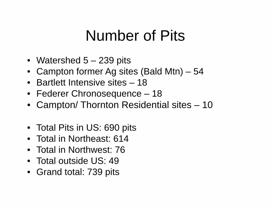
Number of PitsNumber of Pits• Watershed 5 – 239 pitsp• Campton former Ag sites (Bald Mtn) – 54• Bartlett Intensive sites – 18

F d Ch 18• Federer Chronosequence – 18 • Campton/ Thornton Residential sites – 10

• Total Pits in US: 690 pits• Total in Northeast: 614• Total in Northwest: 76 • Total outside US: 49

Grand total: 739 pits• Grand total: 739 pits

Survey of Soil Pit UsesSurvey of Soil Pit Uses• The quantitative soil pit has been used to q p

measure:– Soil Mass

B lk D it– Bulk Density– LOI (OM content)– Total C Total N P and STotal C, Total N, P, and S– Exchangeable cations: Ca, Mg, K, and Na– Exchangeable acidity: H, Al– Root biomass– Different types of carbon: alkyl, aromatic, carbonyl

Difficulties in evaluating this method

Lack of Comparability 1. Not everyone uses the exact same method

• 0.71m × 0.71m (0.5m2) versus 0.5m × 0.5m pits (0.25m2)2. Not everyone is measuring the same things

• i.e. Soil mass, bulk density, carbon, nutrientse So ass, bu de s ty, ca bo , ut e ts3. Not everyone reports what they measure in the

same way. • Each layer or total solum• Each layer or total solum• The layer thickness for each study varies• % , content, or concentration• Some papers don’t report SE or CV values• Some papers don t report SE or CV values• The number of pits per area varies

Huntington 1988Huntington 1988• Location: Hubbard Brook Experimental Forest, NH, Watershed 5

59 i 22 h• 59 pits over 22 ha• Objective: To determine whether an intensive sampling design could

achieve N and C pool size estimates with sufficiently small confidence limits.

Layer C CV N CV Mass CVMg C /ha % kg N /ha % Mg /ha %

Oie 11 67 460 61 22 57Oa 20 95 870 88 66 830-10cm 32 29 1,600 31 490 3610-20cm 27 46 1,200 45 520 50>20cm 73 72 3,100 74 2,200 63

• Sampling Intensity

FF 30 74 1,300 68 88 70MS 130 45 5,900 48 3,200 50Solum 160 38 7,200 38 3,300 47

• Sampling Intensity– Need 60 pits to detect 20% change with 95% confidence interval.

Huntington 1989Huntington 1989• Location: Hubbard Brook Experimental Forest, NH, Watershed 5

59 i 22 h• 59 pits over 22 ha

• Objective: to evaluate the quantitative pit method at bulk density estimation and compare measured values with values predicted byestimation and compare measured values with values predicted by regression analysis.

Layer Bulk Density CV Rock Volume CVMg /m3 % % of total %Mg /m % % of total %

Oa 0.22 104 n.a. n.a. 0-10cm 0.73 32 0.35 263

10-20cm 0.84 37 0.56 16520cm-C 0.92 33 0.87 79

Fahey 1988Fahey 1988• Location: HBEF, watershed 5• 58 pits over 22 ha

Objective: to quantify the importance of element release from tree root• Objective: to quantify the importance of element release from tree root systems after forest harvest.

Size class Sample Root density CV Species (cm) size (g/cm3 ) %Species (cm) size (g/cm3 ) %Sugar Maple 1-2 20 0.41 6.6

2-5 20 0.44 6.15-10 21 0.48 7.6

Yellow Birch 1-2 20 0.39 9.2

Root biomass

2-5 20 0.42 7.45-10 16 0.47 5.9

Beech 1-2 20 0.42 10.52-5 20 0.44 10.15 10 16 0 54 11 9Root biomass

Soil depth Root biomass (g/m 2) by root diameter classes (ram)0.6-1.0 1.0-2.5 2.5-5.0 5-10 >10 Total

Forest floor 40 63 123 216 745 1,187 (303)0 10

5-10 16 0.54 11.9

0-10 cm 37 57 69 109 133 605 (77)10-20 cm 26 46 50 69 248 440(118)>20 cm 31 70 73 88 182 444(87)Total 134 (13) 235 (25) 315 (25) 482 (47) 1,509(394) 2,676 (539)

Other Watershed 5 papersOther Watershed 5 papers• Measuring effects of whole-tree harvesting:

J h C E 1990 1991 & b 1995 1997 1998• Johnson, C.E. 1990, 1991a & b, 1995, 1997, 1998

– Changes in soil mass, SOM, bulk density, horizonization, exchangeable cations, acidity, C & N content, trace metals (Zn & Pb), & measuring sample size.

• Zhang 1999

– Changes in sulfur constituents

• Dai 1999

– Iron (Fe)

• Pardo 2002

– 15N– N

• Hamburg 2003

– Ca pools

• Ussiri 2003 and 2007

– Chemical and structural characteristics of SOM

Fernandez 1993Fernandez 1993• Location: The Bear Brook Watershed, eastern Maine• 24 pits over two 600-m2 plots• Measured: fine earth course fragment mass LOI N P exch cations exch• Measured: fine earth, course fragment mass, LOI, N, P, exch. cations, exch.

acidity, coarse frag. volume, soil volum.• Objective: To compare the quantitative sample method with the conventional

face-sampling morphological approach in order to characterize vertical trends in soil nutrient pool sizes.

Soil mass CV

Root mass CV Total C CV

Bulk density CV

Layer Mg/ha % Mg/ha % Mg C/ha % g/cm %O horizon 280 121 10 105 44 41 0.14 42E horizon 1,200 102 2 100 8 45 1.03 335cm-Increment 550 29 1 120 11 42 0.65 405-40cm 2,400 46 4 170 30 51 0.89 2340cm-C 3,100 44 1 220 19 103 1.39 29T t l S l 7 500 22 18 73 111 26

Layer# Pits 95% conf. # Pits 95% conf.

O horizon 622 50 73 1890 20

Total CSoil Mass

Sampling Intensity:

Total Solum 7,500 22 18 73 111 26 n.a. n.a.

E horizon 477 45 90 205cm-Increm 36 13 77 195-40cm 92 20 114 2240cm-C 83 19 455 45

Number of samples required for estimates of mean element pools plus or minus 10%

Wibiralske 2004Wibiralske 2004• Location: Pocono Plateau in northeastern Pennsylvania

40 i 22 k 2• 40 pits over 22 km2

• Objective: to assess the association of soil and vegetation nutrient capital with plant community type and parent material (Illinoian orcapital with plant community type and parent material (Illinoian or Wisconsinan till) type in the Pocono barrens.

• These are results from the site on Illinoian soil with barrens type t tivegetation.

Soil mass CV

Bulk density CV C conc. CVy

Layer Mg/ha % g/cm3 % % %Oi-Oe 63.6 35 — — 45.2 6Oa 136 54 — — 26.8 280 10 cm 702 38 0 87 22 4 2 450-10 cm 702 38 0.87 22 4.2 4510-20 cm 850 26 1.04 24 2.2 2920-50 cm 3410 21 1.36 19 0.7 90

Yanai et al. 2006, Park et al. 2007, Vadeboncoeur et al. 2007Location: White Mountains National Forest• Location: White Mountains National Forest

• 36 pits over 190 km2

• Pits excavated in hardwood sites of varying ages (post-logging)

• Objective: Accurate budgeting of C, N, and base cations in aggrading forestsbase ca o s agg ad g o es s

• Described root patterns with soil depth and distance to trees validated the HBEF rootdistance to trees, validated the HBEF root allometry equations (Whittaker et al. 1974).


333333

BartlettBartlett

33 27 @ 9 sites27 @ 9 sites(2003(2003--2004)2004)

Hubbard Brook W5Hubbard Brook W51983: 591983: 59


Yanai 2006, Vadeboncoeur 2007, Park 2007

Federer Chronoseq & Bartlett Intensive sites

Carbon Nitrogen exch. Ca apatite Ca coarse frac (%) Layer mean CV mean CV mean CV mean CV mean CV

g/ m2 % g/ m2 % g/ m2 % g/ m2 % g/ m2 %g/ m2 % g/ m2 % g/ m2 % g/ m2 % g/ m2 % Oie 933 51 35 59 Oa 2564 105 106 96 11.7 127 2.0 114 0-10 2778 33 133 35 8.5 81 3.6 175 0.2 72 10-30 3030 32 134 36 4.7 139 4.5 125 0.2 66 10-20 2202 58 107 50 5.4 78 8.0 159 0.2 81 20-30 1652 47 78 43 4.0 73 9.5 144 0.2 66 30+ 3734 70 167 74 7.4 65 36.2 92 0.3 48 30-50 1719 36 83 40 3.5 123 11.1 127 0.3 57 50-C 1445 72 79 73 3.0 101 31.6 105 0.4 53 C0-25 1041 100 48 90 8.8 257 92.6 160 0.3 55 C25-50 645 112 27 111 28.1 203 165.5 134 0.3 62

Yanai 2006, Vadeboncoeur 2007, Park 2007Soil layer

Layer thickness CV

Coarse fraction CV Soil mass CV

(cm) (%) (% volume) (%) (kg/m2) (%)O 13.2 35 n.a. n.a. n.a. n.a.0-10cm 10.8 3 30 121 61 4310-20cm 9.3 4 18 67 79 1820-30cm 11.8 13 20 43 98 1930+ 50.1 20 17 82 417 9C0-C25 23.5 54 200C25-C50 28.7 45 240

Young Stands Transitional Stands Older StandsRoot diameter Layer g/m2 CV (%) g/m2 CV (%) g/m2 CV (%)

Root Biomass

oot d a ete aye g/ C (%) g/ C (%) g/ C (%)0-1 mm forest floor 90 98 172 46 261 76

0–10cm 260 31 236 81 227 4610–30cm 139 14 180 82 267 1130cm-C horizon 258 93 106 150 184 37C horizon 23 64 84 61 21 47

1-2 mm forest floor 16 122 32 38 31 400–10cm 48 51 50 20 35 6310–30cm 22 56 46 138 50 6430cm-C horizon 25 20 33 186 34 122C horizon 2 122 19 77 3 82

2-5 mm forest floor 20 147 69 25 51 770–10cm 78 3 84 17 89 810–30cm 45 49 64 19 106 8330cm-C horizon 21 82 40 184 45 191C horizon 13 226 18 109 2 122

Guadinski 2000Guadinski 2000• Location: Harvard Forest, MA• Pit size: 0.5 m x 0.5 mPit size: 0.5 m x 0.5 m• 2 pits over 28 ha• Objective: to quantify below ground carbon cycles

• No SE or CV values for MS depthsBulk Density Soil C

Total C Stocky

Horizon g/cm3 SEg C/ Kg soil SE g C/ m2 SE

Oi 0.06 0.01 450 20 380 110Oea 0.1 0.02 470 10 1640 750Oea 0.1 0.02 470 10 1640 750

Range Range RangeA 0.35 0.03 270 30 2,400 820AP 0 54 0 13 60 1 2 620 660AP 0.54 0.13 60 1 2,620 660Bwl 0.85 0.07 20 1 1,245 190Bw2 0.93 0.04 6 1 510 110Total 8,800 1,310

Silver 2000Silver 2000• Location: Tapajos National Forest (TNF), 50km south of

Santarem Para BrazilSantarem, Para, Brazil• Objective: to explore the role of soil texture in below ground C

storage, nutrient pool sizes and N fluxes in highly weathered Amazonian forest ecosystem

• 23 pits over 1,000 haSandy Soils C CV N CV P CV

Mg C/ha % Mg N/ha % kg P/ha %Forest floor 4.39 32 0.18 33 4.44 410–10 cm

Soil 12.07 17 0.89 20 67 22Fine root 1.48 22 0.05 24 1.59 21

Coarse root 6 163 0 09 167 2 99 142Coarse root 6 163 0.09 167 2.99 14210–40 cm

Soil 29.78 19 3.44 18 277.5 6Total root 13.88 96 0.2 90 5.18 97

40-100cmSoil 39.28 17 3.44 18 563.4 0

Total root 6 122 0.09 133 0.93 123

Total Below ground 112.88 — 8.38 — 923.06 —

Kram 1995Kram 1995• Location: Czech Republic, at the Lysina (27.3 ha) and Pluhuv Bor (22 ha)

catchments, located near Marianske Lazne.• 5 quantitative soil pits were used to estimate soil mass• 5 quantitative soil pits were used to estimate soil mass. • Objective: to compare biogeochemical patterns of basic cations in two forested

catchments exhibiting extremely different lithologies which serve as end-members of ecosystem sensitivity to acidic deposition.

Layers Exch Bases SOM Total C ClayLayers Exch. Bases SOM Total C Claymmolc /m2 kg /m2 kg C /m2 kg /m2

LysinaOi + Oe 150 1.9 1 NDOa 440 6.7 3.7 ND0-10cm 300 2 8 1 7 0 23

The quantitative

it d 0 10cm 300 2.8 1.7 0.2310-20cm 220 2 0.8 0.1720-30cm 240 2.3 1.7 0.1230-40cm 230 3.1 1 0.1140-43cm (to C) 150 1.4 0.4 0.09Forest floor 590 8.6 4.7 ND

pits were used to estimate soil mass.

o est oo 590 8 6Mineral soil (O-40cm) 980 10.1 5.2 0.63Pluhuv BorOi + Oe 370 2.3 1.2 NDOa 1,000 2.3 1.2 ND0-10cm 390 3.2 1.4 0.42

No SE or CV values were given

10-20cm 1,070 2.3 0.8 0.9820-30cm 3,360 2.2 0.2 1.6530-40cm 5,260 2.1 0.1 1.53Forest floor 1,370 4.6 2.4 NDMineral soil (O-40cm) 10,100 9.8 2.6 4.58

Austin 2006Austin 2006• Location: the towns of Campton and Thornton in Grafton County, NH.• 5 pits over Campton (135 km2) and Thornton (130 km2).

• Objective: study effects of past land-use history on soil nutrient dynamics.

Soil C content before and after housing development

Land-Use Disturbed Undisturbed

DepthHistory

# pits Mg C /ha CV(%) Mg C /ha CV(%)Total Plowed 2 108 35 143 27

Pasture 2 62 11 137 25Woodlot 1 139 14 120 38Average 96 41 136 9

0-20cm Plowed 2 37 38 88 25Pasture 2 34 9 84 15Woodlot 1 46 15 110 32Average 38 26 92 26g

>20cm Plowed 2 71 45 55 51Pasture 2 28 14 30 70Woodlot 1 93 30 15 87Average 59 58 41 68


333333

BartlettBartlett

33 27 @ 9 sites27 @ 9 sites(2003(2003--2004)2004)

Hubbard Brook W5Hubbard Brook W51983: 591983: 59 22

2222

22


222222

Quantitative Pit vs Coring Method• Example 1: Kulmatiski 2003

– Location: Yale-Myers Forest in northeastern Connecticut

Quantitative Pit vs. Coring Method

– 18 pits over 3,173 ha– Objective: compare the ability of the quantitative and core sampling techniques to detect

a 10% change in total soil C and N pools.

The pit technique estimated total C storage at 5 64 +/ 0 32 kg/m2 (n =18 CV = 6%)– The pit technique estimated total C storage at 5.64 +/- 0.32 kg/m2 (n =18, CV = 6%)

– The core technique estimated total C storage at 5.63+/0.29 kg/m2 (n = 56, CV = 5%)

– The pit sampling procedure took twice as long as the coring procedure. Th li d 1 5 h l t t l t 15• The core sampling procedure: 1.5 person-hours per plot to sample to 15 cm.

• The pit sampling procedure: 3.5 person-hours per lot to sample to 15 cm. • An additional 4.5 h in the field were required to sample to 60 cm using the pit technique.

Pit CV C CV C CVPit CV Core CV Core CV(n=18) % (n=18) % (n=56) %

%C 3.64 12 3.12 6 3.34 3%N 0 23 13 0 2 10 0 22 41%N 0.23 13 0.2 10 0.22 41Bulk Density 0.94 4 0.78 3 0.81 2

Quantitative Pit vs Coring Method• Example 1: Kulmatiski 2003 - Continued

Th t h i d d i i th l l ti ll i f


– The core technique reduced variance in the sample population, allowing fewer samples to detect a 10% change in nutrient storage (21 core vs. 29 pit samples).

– The pit technique allowed quantitative sampling below 15 cm and direct p q q p gmeasurement of large coarse fragments.

– Our data suggest that composite core sampling is more efficient than, but well supplemented by, pit sampling.

– The accuracy gained with the pit technique may not outweigh the loss in sample sizes that result from an extensive sampling effort (Conkling et al., 2002).

Pit CV C CV C CVPit CV Core CV Core CV(n=18) % (n=18) % (n=56) %

%C 3.64 12 3.12 6 3.34 3%N 0 23 13 0 2 10 0 22 41%N 0.23 13 0.2 10 0.22 41Bulk Density 0.94 4 0.78 3 0.81 2

Quantitative Pit vs Coring Method• Example 2: Harrison 2003


– Location: Cedar River Watershed, 60km SW of Seattle, WA

– Objective: Compare 4 methods for estimating soil C:(i) large pit (0.5 m2) excavation, (ii) dug pit with 54-mm hammer-core bulk-density sampling, (iii) 31-mm soil push sampler and (iv) clod methodsampler, and (iv) clod method.

– 2 sites each with 3 pits over 45 m2

– The pit excavation method with sand-displacement volume measurements, which is by far the most labor-intensiveand time-consuming was considered the “standard” byand time-consuming, was considered the standard by which other methods were compared, as it didn’t contain any obvious biases.

Quantitative Pit vs Coring MethodQuantitative Pit vs. Coring Method• Example 2: Harrison 2003 – Continuedp

– Soil core methods overestimated the <2-mm soil fraction (samples taken between large rocks).

– Core methods often didn’t work due to the high rockcontent (>50%) of the Everett soil.

– The results suggest that to accurately assess total C pools in these soils, sampling should include both the >2-mm soil fraction and deep soil layers.

– In soils containing a substantial amount of coarse fraction material, we suggest that excavated pits or a similar sampling approach be used.similar sampling approach be used.

Quantitative Pit vs Coring Method• Example 3: Park 2007

– Location: Bartlett Experimental Forest, White Mts., NH


– Objective: to more accurately measure root biomass.

– Roots: average CV of 28% for the 0-1 mm roots and 45% for the 1- 2 mm roots.

– To estimate live fine root biomass with a 20% margin of error at 95% confidence would require seven cores or five soil pits.

– A 10% margin of error could be obtained with 28 cores or 20 pits.

– Less effort to collect cores than to excavate pits, even taking into account th l b f i dthe larger number of cores required.

– Coring is a very efficient method for studying fine roots (<2 mm) in upper soil horizons, but it is not as effective as soil pits in estimating large roots or roots in rocky soilroots in rocky soil.

– The cores overestimated fine-root biomass by 27% compared with pits.

Comparing the resultsComparing the resultsHuntington 198860 pits over 22 ha

Fernandez 199312 pits over 0 06 ha

Wibiralske 200440 pits over 2 200 ha60 pits over 22 ha

= 2.7 pits/ha12 pits over 0.06 ha=200 pits/ha

40 pits over 2,200 ha= 0.02 pits/ha

Layer Soil

Mass CV LayerSoil

mass CV LayerSoil

mass CVy y yMg /ha % Mg/ha % Mg/ha %

Oie 22 57 O horizon 280 121 Oi-Oe 63.6 35Oa 66 83 E horizon 1,200 102 Oa 136 54

5cm-0-10cm 490 36

5cmIncrement 550 29 0-10 cm 702 38

10- 20cm 520 50 5-40cm 2,400 4610-20 cm 850 26 20-50

>20cm 2,200 63 40cm-C 3,100 4420 50 cm 3410 21

FF 88 70MS 3 200 50MS 3,200 50

Solum 3,300 47Total Solum 7,500 22

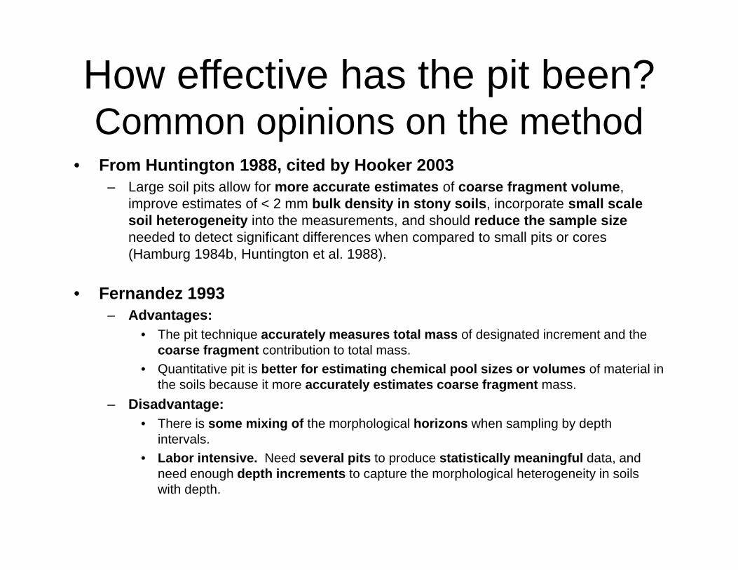
How effective has the pit been?

• From Huntington 1988, cited by Hooker 2003

Common opinions on the method– Large soil pits allow for more accurate estimates of coarse fragment volume,

improve estimates of < 2 mm bulk density in stony soils, incorporate small scale soil heterogeneity into the measurements, and should reduce the sample sizeneeded to detect significant differences when compared to small pits or cores (H b 1984b H ti t t l 1988)(Hamburg 1984b, Huntington et al. 1988).

• Fernandez 1993– Advantages: g

• The pit technique accurately measures total mass of designated increment and the coarse fragment contribution to total mass.

• Quantitative pit is better for estimating chemical pool sizes or volumes of material in the soils because it more accurately estimates coarse fragment mass.

– Disadvantage: • There is some mixing of the morphological horizons when sampling by depth

intervals. • Labor intensive. Need several pits to produce statistically meaningful data, and y g

need enough depth increments to capture the morphological heterogeneity in soils with depth.


For element pools

Common opinions on the method

• Canary 2000– Could not accurately determine soil bulk density in rocky soils with

standard soil core or clod methods. Instead, used quantitative pit.– 75% of soil C to 85 cm was found below the A horizon and 40% was

found below 25 cm. • Whitney 2004

– Sampling performed to depths > 1 m increase total nutrient pools. • Harrison 2003

– To accurately assess total C pools in these soils, sampling should y p p ginclude both the >2-mm soil fraction and deep soil layers.

– In soils containing a substantial amount of coarse fraction material, we suggest that excavated pits or a similar sampling approach be used.


For Roots

Common opinions on the method

• Yanai 2007– Quantitative pit method allows a depth distribution of roots to be

measured in rocky soils. – Using soil cores would have missed 1/3 of the fine roots in the organic

horizon and top 10cm of soil. – Soil pits also allow larger roots to be studied than do soil cores.

• Vadeboncoeur 2007– Quantitative pit estimates of root biomass in the >2 cm size class have

large relative errors.• Fahey 1988

– Recommend using a hybrid approach (quantitative pits and regression analysis) to estimate woody root biomass. Because of the high

i ti i l i l i th tit ti it th dvariation in large size classes using the quantitative pit methods.

A work in progress:

• Not a lot of consistency across reports, even for the same th d

Where to go next in the analysis?method.

• Need a way to accurately compare results of the different studiesstudies.

• Continue to search for other papers in the literature.

• Add more information from the results from pits in White Mts. and HBEF W5 data, such as Chris Johnson’s resampling workwork.

• We are open to thoughts on what criteria we should use to evaluate the method and decide whether it should be e a uate t e et od a d dec de et e t s ou d berepeated in the future.


333333

BartlettBartlett

33 27 @ 9 sites27 @ 9 sites(2003(2003--2004)2004)

Hubbard Brook W5Hubbard Brook W51983: 591983: 59 22

2222

22


2222

1992: 12@ 4 sites1992: 12@ 4 sites2003 : 6 @ 2 sites2003 : 6 @ 2 sites2005: 15 @ 5 sites2005: 15 @ 5 sites

22

Grafton County, NH- 4,500 km2

population 82 000Question

- population 82,000

Does land-use history affect patterns of carbon accumulation in northeastern hardwood forests?

Approach•Well documented land-use history•Quantitative pit method for

measuring soilsmeasuring soils•Repeat measurements over 25 y of:

•Tree inventoryF t fl

Boston

•Forest floor•Mineral soil

200 km

% cleared land, 1860

Bartlett

Hubbard Brook

BaldMtnMtn.

50 km

Why does understanding old-field succession matter?

• ~ 70% of the New England landscape is second• ~ 70% of the New England landscape is second-growth forests growing on former agricultural lands

• We know relatively little about how much carbon is accumulating on abandoned agricultural lands

• Recent reports suggest that there is much less carbon accumulating in the temperate zone thancarbon accumulating in the temperate zone than previously thought

Cook Farm, Campton NHSite 5 (former plowed field,allowed to reforest since 1932)allowed to reforest since 1932)

OOie

O

A

Oa

EOa

Oie

APE

B

B

B

Logged site (Bartlett)

relatively

Former plowed field

homogenized top 20cmrelativelyundisturbed soil profile

homogenized top 20cm

Berry Farm, Campton NHSite 4 (former potato field,continuously unforested since 1860)

40

45

Site 3

35

40

)

Site 5

Site 6

Pasture

25

30

C (M

g/ha

)

15

20

rest

floo

r

10

15

Fo

0

5

0 25 50 75 100

years since abandonment

40

45Site 3

Site 5

35

40

)

Site 5

Site 6

Pasture

HBEF W6

25

30

C (M

g/ha

) HBEF W6

15

20

rest

floo

r

10

15

Fo

0

5

0 25 50 75 100


120

forested sitesmowed sites

100

80

g/ha

)

40

60

Ap

C (M

20

40 Site 3Site 5Site 6

0

20site 4site 9

0 25 50 75 100


140

100

120

)

80

100

r C

(g/m

2)C

(Mg

/ha)

60

+ AP

laye

r+

AP

laye

r C

20

40FF +

If we look at these as a chronosequence, there’s a smallnon-significant C accumulation (0.3 Mg C/ha/yr; p=0.12)

FF +

0

20

0 25 50 75 100


140Site 3Sit 5

100

120

a)

Site 5Site 6

80

100

C (M

g/ha

60

+ A

P la

yer

20

40FF +

However, there is no consistent trend among sites.

0

20

0 25 50 75 100


120

mowed sites forested sites

100

80

(Mg/

ha)

40

60

B-la

yer C

(

20

40B

Site 3Site 5Site 6

0

20site 4site 9

0 25 50 75 100


mowed sites250

forested sites

200

)

150

C (M

g/ha

)

100

al S

olum

Site 3

50

Tota

Site 5Site 6site 4

0

site 9Pasture

0 25 50 75 100


300Site 3Site 5Sit 6

Aboveground Tree Biomass250

/ha)

Site 6Pasture

g/ha

)

200

omas

s (M

gom

ass

(Mg

150

ound

live

bo

nd li

ve b

io

100

Abov

egro

oveg

roun

50Abo

00 25 50 75 100

time since abandonment (years)

300Site 3Site 5Sit 6 10

0+ite

s

250

g/ha

)

Site 6Pasture 200HBEF W6 (L hardwd)HBEF W5 (all elev)

Ran

ge o

f yr

old

si

200

omas

s (M

g Federer Chronoseq

150

ound

live

b

100

Abov

egro

50

00 25 50 75 100


250

Site 3Si 5

200

g/ha

)al

l roo

ts) Site 5

Site 6

150

C s

tock

(Mg

t inc

ludi

ng a

100

em T

otal

Cho

rizon

(but

50

Eco

syst

ecl

udin

g B

h

50

exc

Ecosystem total C accumulation =1.4 Mg/ha/yr (p <0.001)

00 20 40 60 80 100


300

350Mineral SoilForest Floor

250

300

)

Belowground biomassAboveground biomass

200

ck (M

g/ha

100

150

C s

toc

50

00 0 34 46 48 59 60 61 63 73 75 88 87site age:

d

Site4

Site9

Site3

Site3

Site5

Site3

Site5

P Site6

Site5

Site6

Site6

W6*

* Hubbard Brook W6 data from Fahey et al. 2005

Hub

bard

Bro

ok *

Question

Does land-use history affect patterns of carbon accumulation in northeastern hardwood forests?

Yes!

BUT, not in the ways the literature would indicate

• Soils are a much smaller sink than chronosequencedata would suggest

• Tree biomass will take longer to reach maximum

• Overall less carbon will accumulate on theOverall less carbon will accumulate on thelandscape than previously predicted

Michael Pennino, Brown University, and Matt Vadeboncoeur ...

Documents