T RAJECTORY -BASED OPERATIONS by MICHAEL DOMARATZKI A thesis submitted to the School of Computing in conformity with the requirements for the degree of Doctor of Philosophy Queen’s University Kingston, Ontario, Canada August 2004 Copyright c Michael Domaratzki, 2004

Welcome message from author
This document is posted to help you gain knowledge. Please leave a comment to let me know what you think about it! Share it to your friends and learn new things together.
Transcript
TRAJECTORY-BASED OPERATIONS
by
MICHAEL DOMARATZKI
A thesis submitted to the
School of Computing
in conformity with the requirements for
the degree of Doctor of Philosophy
Queen’s University
Kingston, Ontario, Canada
August 2004
Copyright c©Michael Domaratzki, 2004
Abstract
Shuffle on trajectories was introduced by Mateescu et al. [147] as a method of generalizing sev-
eral studied operations on words, such as the shuffle, concatenation and insertion operations. This
natural construction has received significant and varied attention in the literature. In this thesis, we
consider several unexamined areas related to shuffle on trajectories.
We first examine the state complexity of the shuffle on trajectories. We find that the density of
the set of trajectories is an appropriate measure of the complexity of the associated operation, since
low density sets of trajectories yield less complex operations.
We introduce the operation of deletion along trajectories, which serves as an inverse to shuffle
on trajectories. The operation is also of independent interest, and we examine its closure properties.
The study of deletion along trajectories also leads to the study of language equations and systems
of language equations with shuffle on trajectories.
The notion of shuffle on trajectories also has applications to the theory of codes. Each shuffle on
trajectories operation defines a class of languages. Several of these language classes are important in
the theory of codes, including the prefix-, suffix-, biprefix-codes and the hypercodes. We investigate
these classes of languages, decidability questions, and related binary relations.
We conclude with results relating to iteration of shuffle and deletion on trajectories. We charac-
terize the smallest language closed under shuffle on trajectories or deletion along trajectories, as well
as generalize the notion of primitive words and primitive roots. Further examination of language
equations are also possible with the iterated counterparts of shuffle and deletion along trajectories.
i
Acknowledgments
I am grateful for everything my supervisor Dr. Salomaa has done for me during the course of our
time together. His support has been outstanding and he has dedicated many hours to helping me
improve this work, and to our collaborations.
I am grateful to the anonymous referees who have made suggestions for the journal and conference
versions of the results presented here.
I would also like to thank the members of my examining committee, Dr. Ilie, Dr. Kashyap, Dr.
Skillicorn and Dr. Tennent, for their comments and suggestions which have improved this thesis.
I am in debt to Alexander Okhotin for discussions, collaboration, his answering of my questions,
making elegant figures, and not killing me, though I’m sure he would have preferred it.
The following people have also helped me through discussions on the topics in this thesis: Mark
Daley, Masami Ito, Alexandru Mateescu, Jeff Shallit, and Petr Sosık.
kristy, amelia and jasper, for everything.
A proof is a proof. What kind of a proof? It’s a proof.
A proof is proof, and when you have a good proof,
it’s because it’s proven.
–Jean Chretien (Sept. 5, 2002).
ii

Co-Authorship
The work in Chapter 4 is joint work with my supervisor, Dr. K. Salomaa [43, 46]. Portions of
Chapter 7, most notably Sections 7.3, 7.5 and 7.7, are also joint work with Dr. Salomaa [44].
iii
Statement of Originality
I, Michael Domaratzki, certify that all results in this thesis are original, unless otherwise noted.
Specifically, those results due to other authors which have appeared in the literature have been cited
as necessary.
The work in this thesis has either appeared [43, 36, 37, 39, 40] or is to appear [44, 46] in the
literature.
iv

Contents
Abstract i
Acknowledgments ii
Co-Authorship iii
Statement of Originality iv
Contents v
List of Figures xii
1 Introduction 1
1.1 Formal Languages and Operations: Introduction and Motivation . . . . . . . . . . 1
1.2 Descriptional Complexity of Languages . . . . . . . . . . . . . . . . . . . . . . . 3
1.3 Codes and Trajectories . . . . . . . . . . . . . . . . . . . . . . . . . . . . . . . . 4
1.4 Language Equations . . . . . . . . . . . . . . . . . . . . . . . . . . . . . . . . . . 5
1.5 Iteration . . . . . . . . . . . . . . . . . . . . . . . . . . . . . . . . . . . . . . . . 6
1.6 Organization . . . . . . . . . . . . . . . . . . . . . . . . . . . . . . . . . . . . . . 7
2 Preliminary Definitions 8
2.1 Formal Language Theory . . . . . . . . . . . . . . . . . . . . . . . . . . . . . . . 8
v

2.2 Regular Languages . . . . . . . . . . . . . . . . . . . . . . . . . . . . . . . . . . 10
2.3 Grammars . . . . . . . . . . . . . . . . . . . . . . . . . . . . . . . . . . . . . . . 13
2.4 Complexity Theory . . . . . . . . . . . . . . . . . . . . . . . . . . . . . . . . . . 14
2.5 Decidability . . . . . . . . . . . . . . . . . . . . . . . . . . . . . . . . . . . . . . 16
2.6 Families of Languages . . . . . . . . . . . . . . . . . . . . . . . . . . . . . . . . 17
2.7 Shuffle on Trajectories . . . . . . . . . . . . . . . . . . . . . . . . . . . . . . . . 18
2.7.1 Examples . . . . . . . . . . . . . . . . . . . . . . . . . . . . . . . . . . . 19
2.7.2 Algebraic Properties . . . . . . . . . . . . . . . . . . . . . . . . . . . . . 20
3 Related Work 21
3.1 Introduction . . . . . . . . . . . . . . . . . . . . . . . . . . . . . . . . . . . . . . 21
3.2 Shuffle . . . . . . . . . . . . . . . . . . . . . . . . . . . . . . . . . . . . . . . . . 21
3.2.1 Iteration . . . . . . . . . . . . . . . . . . . . . . . . . . . . . . . . . . . . 22
3.2.2 Decomposition . . . . . . . . . . . . . . . . . . . . . . . . . . . . . . . . 23
3.2.3 Grammar Formalisms . . . . . . . . . . . . . . . . . . . . . . . . . . . . 24
3.3 Insertion and Deletion Operations . . . . . . . . . . . . . . . . . . . . . . . . . . 25
3.3.1 Insertion Operations . . . . . . . . . . . . . . . . . . . . . . . . . . . . . 25
3.3.2 Deletion Operations . . . . . . . . . . . . . . . . . . . . . . . . . . . . . 27
3.3.3 Interaction . . . . . . . . . . . . . . . . . . . . . . . . . . . . . . . . . . 28
3.3.4 Iteration . . . . . . . . . . . . . . . . . . . . . . . . . . . . . . . . . . . . 29
3.3.5 Decomposition and Related Language Equations . . . . . . . . . . . . . . 30
3.4 Shuffle on Trajectories . . . . . . . . . . . . . . . . . . . . . . . . . . . . . . . . 30
3.4.1 Infinite Words . . . . . . . . . . . . . . . . . . . . . . . . . . . . . . . . . 30
3.4.2 Fairness . . . . . . . . . . . . . . . . . . . . . . . . . . . . . . . . . . . . 31
3.4.3 Related Concepts . . . . . . . . . . . . . . . . . . . . . . . . . . . . . . . 31
3.4.4 Splicing on Routes . . . . . . . . . . . . . . . . . . . . . . . . . . . . . . 33
3.4.5 Concurrent Work . . . . . . . . . . . . . . . . . . . . . . . . . . . . . . . 34
vi

4 Descriptional Complexity 36
4.1 Introduction . . . . . . . . . . . . . . . . . . . . . . . . . . . . . . . . . . . . . . 36
4.2 General State Complexity Bounds . . . . . . . . . . . . . . . . . . . . . . . . . . 37
4.3 Slenderness and Trajectories . . . . . . . . . . . . . . . . . . . . . . . . . . . . . 40
4.3.1 Perfect Shuffle . . . . . . . . . . . . . . . . . . . . . . . . . . . . . . . . 41
4.3.2 Bounds on Slender Trajectories . . . . . . . . . . . . . . . . . . . . . . . 44
4.4 Future Directions . . . . . . . . . . . . . . . . . . . . . . . . . . . . . . . . . . . 53
4.4.1 Polynomial Density Trajectories . . . . . . . . . . . . . . . . . . . . . . . 53
4.4.2 Exponential Density Trajectories . . . . . . . . . . . . . . . . . . . . . . . 53
4.4.3 Other Open Problems . . . . . . . . . . . . . . . . . . . . . . . . . . . . . 54
4.5 Conclusions . . . . . . . . . . . . . . . . . . . . . . . . . . . . . . . . . . . . . . 54
5 Deletion along Trajectories 55
5.1 Introduction . . . . . . . . . . . . . . . . . . . . . . . . . . . . . . . . . . . . . . 55
5.2 Definitions . . . . . . . . . . . . . . . . . . . . . . . . . . . . . . . . . . . . . . . 56
5.3 Closure and Characterization Results . . . . . . . . . . . . . . . . . . . . . . . . . 57
5.3.1 Recognizing Deletion Along Trajectories . . . . . . . . . . . . . . . . . . 61
5.3.2 Equivalence of Trajectories . . . . . . . . . . . . . . . . . . . . . . . . . . 62
5.4 Regularity-Preserving Sets of Trajectories . . . . . . . . . . . . . . . . . . . . . . 63
5.5 i-Regularity . . . . . . . . . . . . . . . . . . . . . . . . . . . . . . . . . . . . . . 72
5.6 Filtering and Deletion along Trajectories . . . . . . . . . . . . . . . . . . . . . . . 75
5.7 Splicing on Routes . . . . . . . . . . . . . . . . . . . . . . . . . . . . . . . . . . 76
5.8 Inverse Word Operations . . . . . . . . . . . . . . . . . . . . . . . . . . . . . . . 80
5.8.1 Left Inverse . . . . . . . . . . . . . . . . . . . . . . . . . . . . . . . . . . 81
5.8.2 Right Inverse . . . . . . . . . . . . . . . . . . . . . . . . . . . . . . . . . 83
5.9 Conclusions . . . . . . . . . . . . . . . . . . . . . . . . . . . . . . . . . . . . . . 84
vii
6 Trajectory-Based Codes 85
6.1 Introduction . . . . . . . . . . . . . . . . . . . . . . . . . . . . . . . . . . . . . . 85
6.2 Definitions . . . . . . . . . . . . . . . . . . . . . . . . . . . . . . . . . . . . . . . 87
6.3 General Properties of T -codes . . . . . . . . . . . . . . . . . . . . . . . . . . . . 88
6.4 The Binary Relation defined by Trajectories . . . . . . . . . . . . . . . . . . . . . 92
6.4.1 Anti-symmetry . . . . . . . . . . . . . . . . . . . . . . . . . . . . . . . . 93
6.4.2 Reflexivity . . . . . . . . . . . . . . . . . . . . . . . . . . . . . . . . . . 94
6.4.3 Positivity . . . . . . . . . . . . . . . . . . . . . . . . . . . . . . . . . . . 94
6.4.4 ST-Strictness . . . . . . . . . . . . . . . . . . . . . . . . . . . . . . . . . 94
6.4.5 Cancellativity . . . . . . . . . . . . . . . . . . . . . . . . . . . . . . . . . 95
6.4.6 Compatibility . . . . . . . . . . . . . . . . . . . . . . . . . . . . . . . . . 96
6.4.7 Transitivity . . . . . . . . . . . . . . . . . . . . . . . . . . . . . . . . . . 98
6.4.8 Monotonicity . . . . . . . . . . . . . . . . . . . . . . . . . . . . . . . . . 103
6.4.9 Well-Foundedness . . . . . . . . . . . . . . . . . . . . . . . . . . . . . . 105
6.5 Transitivity and Bases . . . . . . . . . . . . . . . . . . . . . . . . . . . . . . . . . 106
6.6 Convexity and Transitivity . . . . . . . . . . . . . . . . . . . . . . . . . . . . . . 110
6.7 Closure Properties . . . . . . . . . . . . . . . . . . . . . . . . . . . . . . . . . . . 113
6.7.1 Closure under Boolean Operations . . . . . . . . . . . . . . . . . . . . . . 113
6.7.2 Closure under Catenation . . . . . . . . . . . . . . . . . . . . . . . . . . . 114
6.7.3 Closure under Inverse Morphism . . . . . . . . . . . . . . . . . . . . . . . 115
6.7.4 Closure under Reversal . . . . . . . . . . . . . . . . . . . . . . . . . . . . 118
6.8 Maximal T -codes . . . . . . . . . . . . . . . . . . . . . . . . . . . . . . . . . . . 118
6.8.1 Decidability and Maximal T -Codes . . . . . . . . . . . . . . . . . . . . . 119
6.8.2 Transitivity and Embedding T -codes . . . . . . . . . . . . . . . . . . . . 123
6.9 Finiteness of all T -codes . . . . . . . . . . . . . . . . . . . . . . . . . . . . . . . 127
6.9.1 Finiteness of Regular T -codes . . . . . . . . . . . . . . . . . . . . . . . . 128
6.9.2 Finiteness of Context-free T -codes . . . . . . . . . . . . . . . . . . . . . 130
viii

6.9.3 Finiteness of T -codes . . . . . . . . . . . . . . . . . . . . . . . . . . . . . 132
6.9.4 Decidability and Finiteness Conditions . . . . . . . . . . . . . . . . . . . 137
6.9.5 Up and Down Sets . . . . . . . . . . . . . . . . . . . . . . . . . . . . . . 137
6.9.6 T -Convexity Revisited . . . . . . . . . . . . . . . . . . . . . . . . . . . . 139
6.10 Conclusions . . . . . . . . . . . . . . . . . . . . . . . . . . . . . . . . . . . . . . 140
7 Language Equations 141
7.1 Introduction . . . . . . . . . . . . . . . . . . . . . . . . . . . . . . . . . . . . . . 141
7.2 Solving One-Variable Equations . . . . . . . . . . . . . . . . . . . . . . . . . . . 142
7.2.1 Solving X T L = R and X ;T L = R . . . . . . . . . . . . . . . . . . 142
7.2.2 Solving L T X = R and L ;T X = R . . . . . . . . . . . . . . . . . . 143
7.2.3 Solving {x} T L = R . . . . . . . . . . . . . . . . . . . . . . . . . . . . 144
7.2.4 Solving {x};T L = R . . . . . . . . . . . . . . . . . . . . . . . . . . . 144
7.3 Decidability of Shuffle Decompositions . . . . . . . . . . . . . . . . . . . . . . . 146
7.3.1 1-thin sets of trajectories . . . . . . . . . . . . . . . . . . . . . . . . . . . 151
7.4 Solving Quadratic Equations . . . . . . . . . . . . . . . . . . . . . . . . . . . . . 152
7.5 Existence of Trajectories . . . . . . . . . . . . . . . . . . . . . . . . . . . . . . . 153
7.6 Undecidability of One-Variable Equations . . . . . . . . . . . . . . . . . . . . . . 155
7.7 Undecidability of Shuffle Decompositions . . . . . . . . . . . . . . . . . . . . . . 159
7.8 Undecidability of Existence of Trajectories . . . . . . . . . . . . . . . . . . . . . 162
7.9 Systems of Language Equations . . . . . . . . . . . . . . . . . . . . . . . . . . . 165
7.10 Conclusions . . . . . . . . . . . . . . . . . . . . . . . . . . . . . . . . . . . . . . 169
8 Iteration of Trajectory Operations 171
8.1 Introduction . . . . . . . . . . . . . . . . . . . . . . . . . . . . . . . . . . . . . . 171
8.2 Definitions . . . . . . . . . . . . . . . . . . . . . . . . . . . . . . . . . . . . . . . 172
8.3 Iterated Shuffle on Trajectories . . . . . . . . . . . . . . . . . . . . . . . . . . . . 173
8.3.1 Left-Associativity and a Simplified Definition . . . . . . . . . . . . . . . . 173
ix
8.3.2 Some examples . . . . . . . . . . . . . . . . . . . . . . . . . . . . . . . . 175
8.3.3 Iteration and Density . . . . . . . . . . . . . . . . . . . . . . . . . . . . . 176
8.4 Iterated Deletion . . . . . . . . . . . . . . . . . . . . . . . . . . . . . . . . . . . 177
8.4.1 Iterated Scattered Deletion . . . . . . . . . . . . . . . . . . . . . . . . . . 179
8.4.2 Density and Iterated Deletion . . . . . . . . . . . . . . . . . . . . . . . . 184
8.5 Additional Closure Properties . . . . . . . . . . . . . . . . . . . . . . . . . . . . . 184
8.6 T -Closure of a Language . . . . . . . . . . . . . . . . . . . . . . . . . . . . . . . 186
8.6.1 Shuffle-T Quotient . . . . . . . . . . . . . . . . . . . . . . . . . . . . . . 186
8.6.2 T -closure . . . . . . . . . . . . . . . . . . . . . . . . . . . . . . . . . . . 188
8.6.3 Codes and Shuffle-Closed Languages . . . . . . . . . . . . . . . . . . . . 190
8.7 Deletion Closure of a Language . . . . . . . . . . . . . . . . . . . . . . . . . . . 191
8.7.1 Del-T Quotient . . . . . . . . . . . . . . . . . . . . . . . . . . . . . . . . 191
8.7.2 T -del-closure . . . . . . . . . . . . . . . . . . . . . . . . . . . . . . . . . 193
8.8 T -Shuffle Base . . . . . . . . . . . . . . . . . . . . . . . . . . . . . . . . . . . . 196
8.9 Shuffle-Free Languages . . . . . . . . . . . . . . . . . . . . . . . . . . . . . . . . 198
8.10 T -Primitive Words . . . . . . . . . . . . . . . . . . . . . . . . . . . . . . . . . . 200
8.10.1 T -Primitivity and T -roots . . . . . . . . . . . . . . . . . . . . . . . . . . 200
8.10.2 Freeness and Uniqueness of T -Primitive Roots . . . . . . . . . . . . . . . 202
8.11 Language Equations Revisited . . . . . . . . . . . . . . . . . . . . . . . . . . . . 208
8.11.1 Arden-like Equations . . . . . . . . . . . . . . . . . . . . . . . . . . . . . 209
8.11.2 A Language Equation for ( T )+(L) . . . . . . . . . . . . . . . . . . . . 211
8.12 Conclusions . . . . . . . . . . . . . . . . . . . . . . . . . . . . . . . . . . . . . . 213
9 Conclusions 214
9.1 Results and Focus . . . . . . . . . . . . . . . . . . . . . . . . . . . . . . . . . . . 214
9.2 Open Problems . . . . . . . . . . . . . . . . . . . . . . . . . . . . . . . . . . . . 216
9.3 Further Research Directions . . . . . . . . . . . . . . . . . . . . . . . . . . . . . 217
x

9.3.1 Confluence of ωT . . . . . . . . . . . . . . . . . . . . . . . . . . . . . . . 217
9.3.2 Codes Defined by Multiple Sets of Trajectories . . . . . . . . . . . . . . . 218
9.3.3 Semantic Trajectory-Based Operations . . . . . . . . . . . . . . . . . . . 218
Bibliography 221
Index 241
xi
List of Figures
2.1 A DFA, illustrated. . . . . . . . . . . . . . . . . . . . . . . . . . . . . . . . . . . 12
2.2 Some examples of shuffle on trajectories and their algebraic properties. . . . . . . 20
4.1 A two-state NFA accepting the set T = 0∗1∗ of trajectories. . . . . . . . . . . . . . 40
5.1 Construction of the words in M1 and M2 from the action of M . . . . . . . . . . . . 70
6.1 Two factorizations of t . . . . . . . . . . . . . . . . . . . . . . . . . . . . . . . . . 134
8.1 Summary of minimum-density regular languages and regular sets of trajectories
demonstrating non-closure properties for iterated shuffle on trajectories. . . . . . . 178
8.2 Summary of minimum-density regular languages and regular sets of trajectories
demonstrating non-closure properties for iterated deletion along trajectories. . . . . 184
xii
Chapter 1
Introduction
1.1 Formal Languages and Operations: Introduction and Motivation
Formal language theory, the study of abstract sets of words over a fixed alphabet of symbols, is one
of the oldest research areas in the theory of computing. Despite its age, formal language theory also
continues to attract new attention, especially its application to various fields, including the theory of
codes, bio-informatics and many others.
Arguably, at the core of formal language theory are two central concepts: that generative de-
vices, such as automata and grammars, can be used to define a class of languages, and that languages
can be combined to form new languages using language operations. Mateescu and Salomaa state
that “a major part of formal language theory can be viewed as the study of finitary devices for gener-
ating infinite languages” [148, p. 2]. The importance of language operations is a slightly more subtle
point. However, we cannot underestimate their power: for instance, language operations themselves
are at the heart of several fundamental language generation systems–for instance, regular expres-
sions, L-systems and context-free grammars. Further, we can mention the study of concepts such
as cones and abstract families of languages (AFLs), for which closure properties under language
operations are the defining characteristics.
The two concepts of generative devices and language operations form the starting point for any
1

CHAPTER 1. INTRODUCTION 2
meaningful study of formal language theory. In particular, closure properties of classes of languages
under various language operations give us insight into the both the power of the classes and the
power of the operations. Closure properties also help us to meaningfully compare two classes of
languages.
However, operations on languages also have crucial importance as emerging areas of research
gain importance. In particular, the interpretation of strands of DNA as words in a formal language
has been the subject of much research recently, in theoretical areas as well as areas fundamentally
linked to the use of DNA as a natural computing method. The language operations under investiga-
tion are models of the manner in which DNA strands interact under various settings.
A fundamental development in the area of language equations was the introduction of the notion
of shuffle on trajectories, defined by Mateescu et al. [147]. Shuffle on trajectories is a framework
for defining word operations based on a set of trajectories, a language which specifies the way in
which the corresponding operation behaves. Thus, shuffle on trajectories is a parameterized class of
language operations: each choice of a set of trajectories yields a distinct language operation. The
idea of replacing the study of word operations by the study of languages is a major innovation, and
leads to very clear, unified results on the applicable language operations.
Operations modeled by shuffle on trajectories include concatenation, the most fundamental
language-theoretic operation, the standard shuffle operation, which has a long history in the study
of formal languages, as well as many variants of the shuffle operation, including insertion, literal
shuffle, perfect shuffle and many others. Each of these operations has been the subject of study in
the literature, both for specific applications – including the theory of codes, concurrency theory and
other areas – as well as for research into the formal properties of these operations, and their effect
on classes of languages.
This thesis examines the concept of trajectories in greater detail. In particular, we seek to unify
several different areas of research in theoretical computer science by investigating each of them in
the framework of shuffle on trajectories. By formalizing each of these areas, we provide new insight
into their fundamental results. Results such as decidability problems and closure properties can be
CHAPTER 1. INTRODUCTION 3
examined in a uniform way, often leading to much simpler proofs.
One result of this research is a demonstration that the shuffle on trajectories formalism, intro-
duced as a unification for word operations, is also important as a unification for more complex
constructs. For instance, we define classes of languages related to codes using the shuffle on trajec-
tories model. By doing so, we can model an entire class of languages by a single set of trajectories.
This further re-enforces the value of the trajectory model.
In the following four sections, we present an informal description of the main areas of research in
this thesis: descriptional complexity, the theory of codes, language equations and iterated language
operations.
1.2 Descriptional Complexity of Languages
Descriptional complexity is the study of measures of complexity of languages and operations. It is
a very broad area, and includes much work on varied classes of languages. We focus our work on
descriptional complexity on the regular languages, a fundamental class of languages. For regular
languages, the main focus of work on descriptional complexity is on state complexity. The (deter-
ministic, nondeterministic) state complexity of a regular language is the minimal number of states
in any (deterministic, nondeterministic) finite automata accepting that language. Given a binary lan-
guage operation α under which the regular languages are closed, the (worst case) state complexity
of α is a function f such that for all regular languages L1, L2 accepted by automata of size n1, n2,
there exists an automaton of size f (n1, n2) accepting α(L1, L2). For instance, if we are interested
in the union operation, it is known that an automaton of size n1n2 can be found accepting the union
of two languages which are accepted by automata of size n1 and n2.
Recently, research into the state complexity of regular languages has seen a great deal of activity.
This work is motivated by the desire to have reliable estimates of the amount of memory required
for automata when certain language operations are applied. This is crucial in applied areas where
finite automata are used in practice, for instance, in pattern matching, natural language processing,
CHAPTER 1. INTRODUCTION 4
and other areas.
We examine the state complexity of shuffle on trajectories in Chapter 4. Being an infinite class
of operations, shuffle on trajectories presents some unique challenges; previous results on the state
complexity of operations have focused on single operations, rather than an entire family of opera-
tions. However, the fact that shuffle on trajectories is a class of language operations parameterized
by a set of trajectories–which is itself a language–allows us to make interesting comparisons be-
tween the descriptional complexity of a set of trajectories and the state complexity of the resulting
shuffle on trajectories operation. We find that another descriptional complexity measure of lan-
guages, namely the density of a language, gives us interesting insight into the relationship between
the complexity of a set of trajectories and the complexity of the resulting language operation. In
particular, we find that less dense sets of trajectories correspond to less complex operations, in terms
of state complexity.
1.3 Codes and Trajectories
A code is a language which has strong decodability properties: given a sequence of words from a
code which are concatenated together, there is only one way to recover the original code words from
the concatenated sequence. Codes have many applications, including compression, error detection
and security [97, pp. 511–512].
Subclasses of the class of codes, such as prefix codes and hypercodes, are often studied for
interesting combinatorial and mathematical properties. This is sometimes know as the theory of
variable-length codes. In Chapter 6, we present our contribution to this area, which we call T -
codes. Intuitively, T -codes represent the natural extension of certain subclasses of codes, including
prefix codes and hypercodes, which are defined via shuffle on trajectories. With the definition of
T -codes, we can present results about classes of T -codes by arguing instead about the associated
sets of trajectories T . This yields general results about properties of interest for T -codes.
We note that the idea of a general method for defining several code-like classes of languages

CHAPTER 1. INTRODUCTION 5
has received some attention in the literature. We briefly note some of this work in Section 6.1.
However, we feel that the notion of a T -code, in using shuffle on trajectories, has the advantage of
being general enough to capture several classes of codes studied in the literature on variable length
codes, but at the same time, is specific enough to allow us to obtain interesting results. Specifically,
decidability properties are often trivial in the framework of T -codes.
1.4 Language Equations
The study of language equations, that is, equations or systems of equations consisting of constant
languages, language operations, and unknowns, and which are solved in terms of languages, is one
of the oldest areas in the theory of computation. Many fundamental areas of computer science are
intricately linked to the study of language equations.
As an example, we note the context-free languages, which are crucial in the design of program-
ming languages and compilers. The theory of context-free grammars as a generative device is well
developed. However, each context-free grammar is equivalent to a system of language equations,
and many deep results in this area have been obtained (see, e.g., Autebert et al. [10]).
Our study of language equations will focus on equations whose operations are taken from the
class of operations defined by shuffle on trajectories. In studying the decidability of the existence
of solutions to such an equation, it will be useful to define the notion of an inverse to shuffle on
trajectories. This inverse is known as deletion along trajectories. We first study the properties of
deletion along trajectories in Chapter 5, and apply it to language equations in Chapter 7.
The inverse of a language operation, first defined by Kari [106], allows us to solve language
equations much in the same way we solve equations such as a + x = b, where a, b are integers
and x is unknown, and, as noted by Kari, our inverse works in a similar manner to how subtraction
works as an inverse to addition. In particular, given our equation, we can recover the unknown value
by applying the inverse operation to the known constants, much in the same way as in solving the
equation a + x = b.
CHAPTER 1. INTRODUCTION 6
We further study language equations with two unknowns. In this case, the constructions in-
volved are more complicated. However, we succeed in characterizing a large class of trajectories,
including many studied operations, with which we are able to positively solve the decidability prob-
lem for language equations in two unknowns. For all of the equation forms we consider, we also
obtain complementary undecidability results.
1.5 Iteration
In Chapter 8, we investigate iterated versions of trajectory-based operations. Our main motivation
is the examination of languages which are closed under a fixed shuffle on trajectories or deletion
along trajectories operation. There is a simple relationship between languages which are closed
under shuffle on (resp., deletion along) trajectories and the iterated shuffle on (resp., deletion along)
trajectories operation.
We also examine other applications of iterated trajectory-based operations. In particular, we
examine the concept of primitivity, the property of a word not being able to be expressed as the
power of another word, as it is related to shuffle on trajectories. The concept of primitivity, in
relation to the concatenation operation, is a natural concept in formal language theory, an interesting
intersection between the theory of formal languages and combinatorics, and also the source of one
of the most well-known open problems in formal language theory–namely, whether or not the set
of all primitive words is a context-free language. Primitivity was extended to both shuffle and
insertion by Kari and Thierrin [118] and to a very general class of operations by Hsiao et al. [69].
In Chapter 8, we find that with a slightly more natural definition of iterated shuffle on trajectories,
we find that the notion of primitivity can be examined without some of the assumptions made in
the more general case of Hsiao et al. [69]. We also consider extensions to the very well-known
results of Lyndon and Schutzenberger via shuffle on trajectories. This allows us to further examine
conditions of uniqueness and existence of primitive roots of words.
We also revisit language equations in Chapter 8 and characterize the solution to certain explicit

CHAPTER 1. INTRODUCTION 7
language equations involving shuffle on trajectories using its iterated counterpart. This is in contrast
to the implicit language equations examined in Chapter 7, where we examined the question of the
decidability of the existence of solutions. Our characterizations of the solutions of explicit language
equations is a parallel of classic language equations which have been studied in the literature.
1.6 Organization
This thesis is organized as follows. Chapter 2 is devoted to preliminary definitions, and may be
referred to as necessary by the reader. Chapter 3 examines related work on shuffle, iteration and
shuffle on trajectories.
In Chapter 4, we discuss the complexity of the shuffle on trajectories operation in terms of
state complexity, a much studied measure of the complexity of an operation which acts on regular
languages.
Chapter 5 develops the concept of deletion along trajectories. We show that it serves as an
inverse to shuffle on trajectories, in the sense defined by Kari [106]. We also examine the closure
properties of deletion on trajectories.
In Chapter 6, we apply the framework of traditional code classes to shuffle on trajectories. This
gives a generalization of many classical code classes. We examine many previously studied aspects
of codes in this general setting.
Chapter 7 examines the solutions to equations involving shuffle and deletion along trajectories.
Several questions for several forms of equations are examined, as well as certain forms of systems
of equations involving shuffle on trajectories.
Finally, in Chapter 8, we consider the iteration of shuffle and deletion on trajectories. We are
particularly interested in the relationship between iteration and the smallest language closed under
shuffle on trajectories.
We conclude in Chapter 9 by examining some open problems raised in this thesis. We also
discuss possible future research areas related to the trajectories model.

Chapter 2
Preliminary Definitions
We now review some notions that will be used in this thesis, as well as the main definition of shuffle
on trajectories, which will be used throughout this thesis. Readers familiar with the concepts below
should feel free to consult this chapter only as necessary.
2.1 Formal Language Theory
For additional background in formal languages and automata theory, please see Yu [201] or Hopcroft
and Ullman [68]. Let6 be a finite set of symbols, called letters. The set 6 is an alphabet. Then 6∗
is the set of all finite sequences of letters from 6, which are called words. The empty word ǫ is the
empty sequence of letters. Given two words w = w1w2 · · ·wn and x = x1 · · · xm where xi , w j ∈ 6
for all 1 ≤ i ≤ m and 1 ≤ j ≤ n, their concatenation wx is the word w1w2 · · ·wnx1x2 · · · xm . The
length of a word w = w1w2 · · ·wn ∈ 6∗, where wi ∈ 6, is n, and is denoted |w|. Note that ǫ is the
unique word of length 0. A language L is any subset of6∗. If w ∈ 6∗, we will denote the language
consisting only of w by w instead of {w}. For a language L ⊆ 6∗, by |L| we denote its cardinality
as a set.
Let L ⊆ 6∗ be a language. By L, we mean 6∗ − L , the complement of L . Let L1, L2 be
languages. By L1L2 we mean the concatenation of L1 and L2, given by L1L2 = {xy : x ∈ L1, y ∈
8

CHAPTER 2. PRELIMINARY DEFINITIONS 9
L2}. If L is a language and n ≥ 0, then the set Ln is defined recursively as follows: L0 = {ǫ},
Ln+1 = Ln L for all n ≥ 0. We denote L∗ = ∪n≥0Ln and L+ = ∪n≥1Ln . If L1, . . . , Lk ⊆ 6∗ are
languages, we use the notation∏k
i=1 L i = L1L2 · · · Lk . If L is a language and k is a natural number,
then we denote L≤k = ∪ki=0 L i .
Given two languages L1, L2 ⊆ 6∗, the left quotient of L2 by L1 is denoted L1 \ L2 and is given
by
L1 \ L2 = {x ∈ 6∗ : ∃y ∈ L1 such that yx ∈ L2}.
Similarly, the right quotient (or simply quotient, if there is no confusion) of L2 by L1 is denoted
L2/L1 and is given by
L2/L1 = {x ∈ 6∗ : ∃y ∈ L1 such that xy ∈ L2}.
The shuffle operation is defined as follows: if x, y ∈ 6∗ are words, then the shuffle of x and y,
denoted x y is defined by
x y = {n∏
i=1
xi yi : x =n∏
i=1
xi , y =n∏
i=1
yi ; xi , yi ∈ 6∗ ∀1 ≤ i ≤ n}.
If L1, L2 are languages, then L1 L2 is given by L1 L2 = {x y : x ∈ L1, y ∈ L2}.
We denote by N the set of natural numbers: N = {0, 1, 2, . . . }. If we wish to refer to the positive
numbers, we will use the notation N+ = {1, 2, . . . , }. Let I ⊆ N. If there exist n0, p ∈ N, p > 0,
such that for all x ≥ n0, x ∈ I ⇐⇒ x + p ∈ I , then we say that I is ultimately periodic (u.p.).
For n,m ∈ N, we use the notation m|n to denote that m is a divisor of n, that is, there exists k ∈ N
such that n = km.
Given a set X , we use the notation 2X = {Y : Y ⊆ X}. Given alphabets 6,1, a morphism
is a function h : 6∗ → 1∗ satisfying h(xy) = h(x)h(y) for all x, y ∈ 6∗. Given a morphism h :
6∗→ 1∗ and a language L ⊆ 6∗, then the image of L under h is given by h(L) = {h(x) : x ∈ L},
while if L ′ ⊆ 1∗, the inverse image of L ′ under h is defined by h−1(L ′) = {x ∈ 6∗ : h(x) ∈ L ′}.
A substitution is a function h : 6∗ → 21∗
satisfying h(xy) = h(x)h(y) for all x, y ∈ 6∗. Given
a substitution h : 6∗ → 21∗
and a language L ⊆ 6∗, then the image of L under h is given

CHAPTER 2. PRELIMINARY DEFINITIONS 10
by h(L) = ∪x∈Lh(x). We say that a substitution is regular if h(a) ∈ REG for all a ∈ 6 (see
Section 2.2 below for the definitions of the regular languages and REG).
Given a word w ∈ 6∗ and a ∈ 6, |w|a is the number of occurrences of a in w. For instance, if
w = abbaa, then |w|a = 3 and |w|b = 2. If w ∈ 6∗ is a word, alph(w) = {a ∈ 6 : |w|a > 0} . If
L ⊆ 6∗, alph(L) = ∪w∈Lalph(w).
For an alphabet 6 = {a1, a2, . . . , an} with a specified order a1 < a2 < · · · < an , the Parikh
mapping is given by 9 : 6∗→ Nn, as follows:
9(w) = (|w|ai)ni=1.
It is extended to 9 : 26∗ → 2Nn
as expected. For instance, if 6 = {a, b} with a < b, and
x = abbaa, then 9(x) = (2, 3). If L = {anbnan : n ≥ 0}, then 9(L) = {(2n, n) : n ≥ 0}.
The inverse mapping is given by 9−1 : 2Nn → 26∗
is given by 9−1(S) = {u ∈ 6∗ : 9(u) ∈ S}
for all S ⊆ Nn. A language L ⊆ 6∗ is said to be commutative if L = 9−1(9(L)). Thus, L is
commutative if rearranging the letters from any word in L always yields a word in L . For instance,
the language L = {aab, aba, baa, ab, ba} is commutative. For any language L , com(L) is the
commutative closure of L , i.e., com(L) = {v ∈ 6∗ : ∃u ∈ L such that 9(u) = 9(v)}. For
instance, com({abc}) = {abc, acb, bac, bca, cab, cba}.
We say that a language L ⊆ 6∗ is bounded if there exist w1, w2, . . . , wk ∈ 6∗ such that
L ⊆ w∗1w∗2 · · ·w∗k . If L is not bounded we say that it is unbounded. The languages L1 = {anb2ncn :
n ≥ 0} and L2 = (ab)∗ + (cd)∗ are bounded, as L1 ⊆ a∗b∗c∗ and L2 ⊆ (ab)∗(cd)∗. The language
L3 = {a, b}∗ is known to be unbounded.
2.2 Regular Languages
We now describe finite automata and regular languages. A deterministic finite automaton (DFA) is a
five-tuple M = (Q,6, δ, q0, F) where Q is a finite set of states, 6 is an alphabet, δ : Q ×6→ Q
is a transition function, q0 ∈ Q is a distinguished start state, and F ⊆ Q is the set of final states. We
CHAPTER 2. PRELIMINARY DEFINITIONS 11
extend δ to Q ×6∗ in the usual way: if q ∈ Q and w ∈ 6∗, then define δ(q, w) = q if w = ǫ and
δ(q, w) = δ(δ(q, w′), a)
if w = w′a for some w′ ∈ 6∗ and a ∈ 6.
A word w ∈ 6∗ is accepted by M if δ(q0, w) ∈ F . The language accepted by M , denoted
L(M), is the set of all words accepted by M . A language is called regular if it is accepted by some
DFA.
A nondeterministic finite automaton (NFA) is a five-tuple M = (Q,6, δ, q0, F)where Q,6, q0
and F are as in the deterministic case, while δ : Q × (6 ∪ {ǫ}) → 2Q is the nondeterministic
transition function. Again, δ is extended to Q × 6∗ in the natural way. To define the action of δ
formally, we require a few notions. First define a binary relation Rǫ ⊆ Q2. The relation is given by
qi Rǫq j if q j ∈ δ(qi , ǫ). Let R∗ǫ be the reflexive, transitive closure of Rǫ . Define cl : Q → 2Q by
cl(q) = {q ′ : q R∗ǫ q ′}.
Thus, cl(q) is the set of all states that are reachable from q by following some path of ǫ-transitions
in M . Further, let cl(S) = ∪q∈Scl(q) for all S ⊆ Q. We may now define δ as a function from
Q ×6∗ to 2Q : if q ∈ Q then δ(q, ǫ) = cl(q) and for all a ∈ 6 and w ∈ 6∗,
δ(q, wa) = cl
⋃
q ′∈δ(q,w)δ(q ′, a)
.
A word w is accepted by M if δ(q0, w)∩ F 6= ∅. It is known that the language accepted by an NFA
is regular. We denote the class of regular languages by REG.
For a DFA or NFA M , we say that M is complete if δ is a complete function, i.e., if δ(q, a) is
defined for all q ∈ Q and a ∈ 6.
We can draw a DFA or NFA as a directed graph using the following conventions:
(a) states are drawn as vertices, labelled with their name;
(b) transitions are drawn as directed edges, labelled with the letter of the transition. Thus, if
δ(q1, a) = q2, there is a directed edge (q1, q2) with label a;
CHAPTER 2. PRELIMINARY DEFINITIONS 12
(c) final states are indicated as vertices with double circles;
(d) the start state is indicated with an unlabelled arrow entering it.
For example, the DFA given in Figure 2.1 has start state 1, final state set {2} and transitions δ(1, b) =
δ(2, b) = 1 and δ(1, a) = δ(2, a) = 2.
1 2 aa
b
b
Figure 2.1: A DFA, illustrated.
We also introduce the Myhill-Nerode congruence on 6∗. Given a language L ⊆ 6∗, we denote
the Myhill-Nerode congruence with respect to L on 6∗ by ≡L . Given x, y ∈ 6∗, x ≡L y if and
only if, for all z ∈ 6∗,
xz ∈ L ⇐⇒ yz ∈ L .
We note that ≡L is an equivalence relation and that a language L is regular if and only if ≡L has
finite index [68, Thm. 3.9].
Finally, we define regular expressions. Let 6 be an alphabet. A regular expression is a word
over the alphabet {∅, ǫ, (, ), ∗,+} ∪6 defined as follows:
(a) the following are regular expressions: ǫ,∅ and a for all a ∈ 6;
(b) if r1, r2 are regular expressions, so are (r1r2) and (r1 + r2);
(c) if r1 is a regular expression, so is (r∗1 ).
Given a regular expression r , it defines a language L(r) as follows:
(a) L(ǫ) = {ǫ}, L(∅) = ∅ and L(a) = {a};
(b) L((r1 + r2)) = L(r1) ∪ L (r2);

CHAPTER 2. PRELIMINARY DEFINITIONS 13
(c) L((r1r2)) = L(r1)L(r2);
(d) L((r∗1 )) = L(r1)∗.
Parentheses in regular expressions may be omitted, subject to the following precedence rules: ∗
has the highest precedence, then concatenation, then +. It is known that regular expressions define
exactly the regular languages.
2.3 Grammars
We now turn to three classes of languages defined by grammars: context-free languages (CFLs),
linear context-free languages (LCFLs) and context-sensitive languages (CSLs). These classes are
denoted CF, LCF, and CS, respectively. While we describe them formally, it will suffice to note the
following well-known inclusions, all of which are proper:
REG ( LCF ( CF ( CS. (2.1)
For each of CF, LCF, CS, a grammar is a four-tuple G = (V,6, P, S), where V is a finite set
of non-terminals, 6 is a finite alphabet, P ⊆ ((V ∪ 6)∗V (V ∪ 6)∗) × (V ∪ 6)∗ is a finite set of
productions, and S ∈ V is a distinguished start non-terminal. If (α, β) ∈ P , we usually denote this
by α→ β.
Such a grammar is a context-free grammar (CFG) if P ⊆ V × (V ∪ 6)∗, a linear context-free
grammar (LCFG) if P ⊆ V×(6∗V6∗∪6∗), and a context-sensitive grammar (CSG) if (α, β) ∈ P
implies α = ηAζ and β = ηγ ζ for some η, ζ, γ ∈ (V ∪6)∗, with γ 6= ǫ and A ∈ V .
IF G = (V,6, P, S) is a grammar (CFG, LCFG or CSG), then given two words α, β ∈ (V ∪
6)∗, we denote α ⇒G β if α = α1α2α3, β = α1β2α3 for α1, α2, α3, β2 ∈ (V ∪ 6)∗ and α2 →
β2 ∈ P . Let⇒∗G denote the reflexive, transitive closure of⇒G . Then the language generated by a
grammar G = (V,6, P, S) is given by
L(G) = {x ∈ 6∗ : S ⇒∗G x}.
If a language is generated by a CFG (resp., LCFG, CSG), then it is a CFL (resp., LCFL, CSL).

CHAPTER 2. PRELIMINARY DEFINITIONS 14
2.4 Complexity Theory
We now consider Turing machines. Our presentation is largely based on Hopcroft and Ullman [68,
Ch. 7]. A Turing machine (TM) is a seven-tuple M = (Q,6, Ŵ, δ, q0, B, F) where Q is a finite set
of states, Ŵ is a finite tape alphabet, B ∈ Ŵ is the blank symbol, 6 ⊆ Ŵ − B is the input alphabet,
δ is the transition function given by δ : Q × Ŵ → Q × Ŵ × {L , R}, q0 ∈ Q is the start state, and
F ⊆ Q is the set of final states. This model of TM is deterministic. A nondeterministic variant is
also possible.
Given a TM M , an instantaneous description (ID) of M is a word w1qw2 ∈ Ŵ∗QŴ∗. We
interpret the ID as meaning that the TM is in state q with tape contents w1w2 and the head currently
positioned on the first character of w2. We define a relation⇒M on the set of IDs as follows: given
IDs w1q1w2, u1q2u2,
w1q1w2 ⇒M u1q2u2 ⇐⇒
u1 = w1γ,w2 = βu2, and δ(q1, β) = (q2, γ , R),
or w1 = u1γ,w2 = αw′2, u2 = γβw′2 and δ(q1, α) = (q2, β, L).
Let⇒∗M be the transitive and reflexive closure of⇒M . The language accepted by M , denoted L(M)
is
L(M) = {w ∈ 6∗ : q0w⇒∗M α1qα2 such that q ∈ F, α1, α2 ∈ Ŵ∗}.
Given a language L , if there exists a TM M such that L = L(M), we say that L is recursively
enumerable (r.e.). We denote the set of r.e. languages by RE.
Say that a TM M halts on input x if it eventually reaches an ID which has no next move, i.e.,
the current ID has no successors under⇒M . We may assume without loss of generality that when
a word is accepted by M , M halts. However, if an input word is not accepted, we note that M may
not halt.
If L is accepted by a TM M such that M halts on all inputs, we say that L is recursive. The
set of all recursive languages is denoted by REC. The inclusions (2.1) may be extended as follows
(again, the inclusions below are proper):
CS ( REC ( RE.

CHAPTER 2. PRELIMINARY DEFINITIONS 15
Nondeterminism does not affect the classes REC and RE.
We now refine the class of languages computed by a Turing machine. Given a TM M , we
say that M uses space c on input w if M scans at most c tape cells during the computation on w,
i.e., max{|v| : q0w ⇒∗M vqu, w, v, u ∈ Ŵ∗} ≤ c. Let n be the length of the input to a TM
(i.e., the length of the word w such that q0w is the initial ID of the TM). If a deterministic (resp.,
nondeterministic) TM uses at most O(s(n)) space on any input of length n, then we say that the
language L(M) is in DSPACE(s) (resp., NSPACE(s)). It is known that CS = NSPACE(n), i.e., the
context-sensitive languages correspond exactly to the class of languages accepted in linear space by
a nondeterministic TM. We similarly define the classes DTIME( f ) and NTIME( f ).
The following classes are also useful to us:
P =⋃
k≥1
DTIME(nk);
NP =⋃
k≥1
NTIME(nk).
Given a function g : 6∗ → 6∗, we say that g is computable in DSPACE(s) (resp., NSPACE(s),
DTIME( f ), NTIME( f )) if there exists a TM M operating in DSPACE(s) (resp., NSPACE(s), DTIME( f ),
NTIME( f )) such that for all w ∈ 6∗, q0w⇒∗M u1qu2 with q ∈ F and u1u2 = g(w). Further, g(w)
is the only such tape contents which results from halting on input w.
A function f : N → N is said to be space-constructible if there exists a TM M such that
L(M) ∈ NSPACE( f ) and, for all n ≥ 0, there exists some x ∈ 6n such that M uses exactly f (|x|)
space on input x .
Given two languages L ′, L , we say that L ′ is reducible to L if there exists a function g : 6∗→
6∗ such that x ∈ L ′ if and only if g(x) ∈ L . If g is computable in DSPACE(log), then we say that
L ′ is log-space reducible to L .
Let C be a class of languages. The language L is C-hard if L ′ is reducible to L for all L ′ ∈ C.
The language L is C-complete if L ∈ C and L is C-hard. For both P and NP, completeness can be
defined with respect to log-space reductions.

CHAPTER 2. PRELIMINARY DEFINITIONS 16
2.5 Decidability
In this section, we briefly describe the concept of decidability and undecidability, and recall the Post
correspondence problem (PCP) and several meta-theorems for proving undecidability.
We will often consider problems when discussing undecidability. A problem P is simply a
predicate, in the following sense: “given an input x , does P(x) hold?” For example, if P is the
problem of primality, and x is an integer (encoded over our alphabet 6), P(x) holds if and only
if x is a prime number. Thus, if x is suitably encoded over an alphabet 6, P naturally defines a
language over 6∗, namely, those x such that P(x) holds. Let L P be this corresponding language
(we sometimes simply identify P with the corresponding language, and do not use the notation L P).
We say that a problem P is decidable if L P ∈ REC. Otherwise, P is said to be undecidable.
The Post correspondence problem (PCP) is a basic undecidable problem which is often useful
in many language-theoretic situations. An instance of PCP is
M = (u1, u2, . . . , un; v1, v2, . . . , vn)
where n ≥ 1 and ui , vi ∈ 6∗ for 1 ≤ i ≤ n. A solution to M is a list i1, i2, . . . , im such that m ≥ 1,
1 ≤ i j ≤ n for all 1 ≤ j ≤ m andm∏
j=1
ui j=
m∏
j=1
vi j.
The following result states that finding solutions to a PCP instance is undecidable [68, Thm. 8.8]:
Theorem 2.5.1 Given an alphabet 6 and a PCP instance M = (u1, . . . , un; v1, . . . , vn), where
n ≥ 1 ui , vi ∈ 6∗ for 1 ≤ i ≤ n, it is undecidable whether there is a solution for M.
We will also use the following undecidability result:
Theorem 2.5.2 Let 6 be an alphabet with |6| ≥ 2 and G = (V,6, P, S) be an LCFG. It is
undecidable whether L(G) = 6∗.
In what follows, a predicate on 26∗
is simply a class of languages satisfying some property.
By a predicate on a class of languages C, we simply mean the restriction of the predicate from 26∗

CHAPTER 2. PRELIMINARY DEFINITIONS 17
to C. If P is a predicate and a language L ⊆ 6∗ satisfies P , we will denote this fact by P(L).
For example, if PR is the predicate defined by the regular languages, then PR(L) implies that L is
regular. A predicate P on C is non-trivial if P /∈ {∅, C}.
Meta-theorems are powerful tools for proving undecidability. In this thesis, we will appeal to
the following meta-theorem, due to Hunt and Rosenkrantz [70, Thm. 2.10], which will allow us to
prove undecidability results for LCF.
Theorem 2.5.3 Let P be a predicate on LCF over 6∗ such that P(6∗) holds and either of the sets
{L ′ : L ′ = x \ L , x ∈ 6+, L ∈ LCF and P(L)}
or
{L ′ : L ′ = L/x, x ∈ 6+, L ∈ LCF and P(L)}
is a proper subset of LCF. Then given an LCFG G, it is undecidable whether P(L(G)) holds.
The following is a corollary of Theorem 2.5.3. It is also a particular case of Greibach’s Theorem
(see, e.g., Hopcroft and Ullman [68, Thm. 8.14]).
Corollary 2.5.4 Let P be a non-trivial predicate on LCF over 6∗ such that P(6∗) holds and P is
preserved under quotient. Then given an LCFG G, it is undecidable whether P(L(G)) holds.
2.6 Families of Languages
We will require some definitions and notations relating to classes of languages. Let C1, C2 be classes
of languages. Then let
C1 ∧ C2 = {L1 ∩ L2 : L i ∈ Ci , i = 1, 2};
co-C1 = {L : L ∈ C1}.
Our notation ∧ comes from Ginsburg [51], and should not be confused with C1 ∩ C2 = {L : L ∈
C1 and L ∈ C2}.

CHAPTER 2. PRELIMINARY DEFINITIONS 18
Recall that a cone (or full trio) is a class of languages closed under morphism, inverse morphism
and intersection with regular languages [148, Sect. 3].
We will also use the notion of immune languages. Let C be a class of languages. A language L
is said to be C-immune if L is infinite and for all infinite languages L ′ ⊆ L , L ′ /∈ C. Immunity was
introduced for classes of languages by Flajolet and Steyaert [49]; we also refer the interested reader
to Balcazar et al. [14] for an introduction to immunity as it relates to complexity theory.
2.7 Shuffle on Trajectories
The shuffle on trajectories operation is a method for specifying the ways in which two input words
may be merged, while preserving the order of symbols in each word, to form a result. Each trajectory
t ∈ {0, 1}∗ with |t|0 = n and |t|1 = m specifies the manner in which we can form the shuffle on
trajectories of two words of length n (as the left input word) and m (as the right input word). The
word resulting from the shuffle along t will have a letter from the left input word in position i if the
i-th symbol of t is 0, and a letter from the right input word in position i if the i-th symbol of t is 1.
We now give the definition of shuffle on trajectories, originally due to Mateescu et al. [147].
Shuffle on trajectories is defined by first defining the shuffle of two words x and y over an alphabet
6 on a trajectory t , a word over {0, 1}. We denote the shuffle of x and y on trajectory t by x t y.
If x = ax ′, y = by′ (with a, b ∈ 6) and t = et ′ (with e ∈ {0, 1}), then
x et ′ y =
a(x ′ t ′ by′) if e = 0;
b(ax ′ t ′ y′) if e = 1.
If x = ax ′ (a ∈ 6), y = ǫ and t = et ′ (e ∈ {0, 1}), then
x et ′ ǫ =
a(x ′ t ′ ǫ) if e = 0;
∅ otherwise.
If x = ǫ, y = by′ (b ∈ 6) and t = et ′ (e ∈ {0, 1}), then
ǫ et ′ y =
b(ǫ t ′ y′) if e = 1;
∅ otherwise.

CHAPTER 2. PRELIMINARY DEFINITIONS 19
We let x ǫ y = ∅ if {x, y} 6= {ǫ}. Finally, if x = y = ǫ, then ǫ t ǫ = ǫ if t = ǫ and ∅ otherwise.
It is not difficult to see that if t = ∏ni=1 0 ji 1ki for some n ≥ 0 and ji, ki ≥ 0 for all 1 ≤ i ≤ n,
then we have that
x t y ={n∏
i=1
xi yi : x =n∏
i=1
xi , y =n∏
i=1
yi ,
with |xi | = ji , |yi | = ki for all 1 ≤ i ≤ n}
if |x| = |t|0 and |y| = |t|1 and x t y = ∅ if |x| 6= |t|0 or |y| 6= |t|1.
We extend shuffle on trajectories to sets T ⊆ {0, 1}∗ of trajectories as follows:
x T y =⋃
t∈T
x t y.
Further, for L1, L2 ⊆ 6∗, we define
L1 T L2 =⋃
x∈L1y∈L2
x T y.
2.7.1 Examples
We now consider some examples of shuffle on trajectories. Let x = abc and y = de. If t = 00011,
then x t y = abcde. If t = 00111, then x t y = ∅. Thus, we can see that if T = 0∗1∗, we have
that
L1 T L2 = L1L2,
i.e., T = 0∗1∗ gives the concatenation operation.
If x = abc, y = de, and t = 01001, then x t y = adbce. If t = 01010, then x t y =
adbec. Thus, we have that if T = (0+ 1)∗, then
L1 T L2 = L1 L2,
i.e., T = {0, 1}∗ gives the shuffle operation. This is the least restrictive set of trajectories.
If T = 0∗1∗0∗, then T is the insertion operation← (see, e.g, Kari [106]) which is defined by
x ← y = {x1 yx2 : x1, x2 ∈ 6∗, x1x2 = x} for all x, y ∈ 6∗. Some other examples of operations
defined by shuffle on trajectories are given in Figure 2.2 in the following section.

CHAPTER 2. PRELIMINARY DEFINITIONS 20
2.7.2 Algebraic Properties
We will require some algebraic properties of shuffle on trajectories throughout this thesis. These
properties have been studied by Mateescu et al. [147].
Let T ⊆ {0, 1}∗. We say that T is complete if, for all x, y ∈ 6∗, x T y 6= ∅, i.e., there exists
some z ∈ 6∗ such that z ∈ x T y. The set T is said to be deterministic if, for all x, y ∈ 6∗,
|x T y| ≤ 1. Say that T is associative (resp., commutative) if the corresponding operation T is
associative (resp., commutative), i.e., x T (y T z) = (x T y) T z for all x, y, z ∈ 6∗ (resp.,
x T y = y T x for all x, y ∈ 6∗). For characterizations and decidability of these properties,
we refer the reader to Mateescu et al. [147, Sect. 4]. We summarize several examples of shuffle on
trajectories and their algebraic properties in Figure 2.2.
Name T Complete? Determ.? Assoc.? Commutative?
Concatenation 0∗1∗√ √ √ ×
Insertion 0∗1∗0∗√ × × ×
Shuffle (0+ 1)∗√ × √ √
Perfect Shuffle (01)∗ × √ × ×Balanced Insertion {0i 12 j 0i : i, j ≥ 0} × √ √ ×
Bi-catenation 0∗1∗ + 1∗0∗√ × × √
Figure 2.2: Some examples of shuffle on trajectories and their algebraic properties.

Chapter 3
Related Work
3.1 Introduction
In this chapter, we review the literature relevant to this thesis. Our focus is on word operations, such
as shuffle, insertion, and quotient, which are specific instances of the formalisms we present in this
thesis. We focus primarily on research which is either of theoretical interest, or relates directly to
the topics we investigate later in the thesis.
3.2 Shuffle
Shuffle is one of the most studied operations on formal languages which is not among the defining
operations of regular expressions. Ginsburg and Spanier introduce a definition of shuffle in 1965
[53] in their study of generalized sequential machines. This is the first reference to shuffle as an
operation on languages we have been able to find. The natural application of shuffle as a model
for interleaving processes yielded much research into shuffle and related operations. In an early
paper on shuffle, Ogden et al. show that there exist DCFLs L1, L2 such that L1 L2 is NP-complete
[156]. Hausler and Zeiger [63] give an interesting representation theorem for r.e. languages using
the homomorphic image of the intersection of a regular language and the shuffle of two fixed Dyck
21

CHAPTER 3. RELATED WORK 22
languages.
We now consider three specific areas of research on arbitrary shuffle: iterated shuffle, shuffle
decompositions and grammar formalisms involving shuffle.
3.2.1 Iteration
The iteration of shuffle has received much attention in the literature over the last thirty years. This
operation is defined much in the same way as Kleene closure: given a language L its shuffle closure
is defined as
( )∗(L) =⋃
i≥0
( )i(L),
where ( )0(L) = {ǫ}, ( )i+1(L) = ( )i (L) L for all i ≥ 0. Several notations are used in the
literature for denoting ( )∗(L), including L⊗ and L†.
Much of the interest in shuffle closure comes from the theory of concurrency and formal soft-
ware engineering research communities. For example, Shaw, in describing the shuffle closure oper-
ation in the context of flow expressions, notes that shuffle closure is a “concurrent analogue of [the
Kleene closure operation]”, which “is useful where there may be a variable number of interleaves
of some flow [of control], for example in describing systems in which processes or resources may
be dynamically created and destroyed. [182, p. 243]”. Riddle also performed early research into
software engineering using the shuffle closure operation [170]. While the shuffle closure operation
is fundamental to this research, various authors (including both Shaw and Riddle) also incorpo-
rate synchronization methods for research into software engineering. More recently, Igarashi and
Kobayashi [71] cite shuffle expressions as a valid manner in specifying trace sets for use in their
formal analysis of resource usage.
Other research into iterated shuffle has proceeded from a purely theoretical standpoint. Warmuth
and Haussler [198] show the following elegant result:
Theorem 3.2.1 Let 6 = {a, b, c}. Given words u, v ∈ 6∗, it is NP-complete to determine whether
u ∈ ( )∗(v).

CHAPTER 3. RELATED WORK 23
Imreh et al. [74] have written on the shuffle closure of commutative regular languages. In
particular, they give two characterizations of when the shuffle closure of a commutative regular
language is again regular.
3.2.2 Decomposition
The shuffle decomposition problem has received much attention recently. For shuffle on trajectories,
the problem was introduced by Mateescu et al. [147], who asked, given a language L , is it possible to
write L = L1 T L2 for some L1, L2, T , where the complexity of L1, L2, T are “somehow smaller
[147, p. 38]” than the complexity of L (e.g., each are situated lower in the Chomsky hierarchy
than L). They called such a simpler expression for L a parallelization of L , and noted that some
languages, such as the non-context free languages L = {ww : w ∈ 6∗} and L = {anbn2: n ≥ 0}
do not have parallelizations into context-free languages.
Campeanu et al. [21] have studied the problem of deciding whether a regular language R has
a parallelization R = L1 L2, i.e., the case when T = (0 + 1)∗. If such a parallelization exists,
and L1, L2 6= {ǫ}, such an expression is called a (non-trivial) shuffle decomposition. Despite much
effort, Campeanu et al. [21] were not able to resolve whether it is decidable, given a regular language
R, whether R has a non-trivial shuffle decomposition. For certain subclasses of regular languages,
Campeanu et al. were able to positively decide whether a language from that subclass has a non-
trivial shuffle decomposition.
Ito [75] has also examined the shuffle decomposition problem for regular languages. Let I(n,6)
be the class of all regular languages over 6 which are accepted by some DFA with at most n states.
The main result of Ito [75] is the following:
Theorem 3.2.2 Given a regular language R ⊆ 6∗ and n ∈ N, it is decidable whether there exist
L1, L2 with L1 ∈ I(n,6) and L2 6= {ǫ} such that R = L1 L2.
The general problem of determining whether a regular language has a non-trivial shuffle decom-
position is still open. We will examine the shuffle decomposition problem with respect to a set of

CHAPTER 3. RELATED WORK 24
trajectories T (i.e., deciding whether there exists L1, L2 such that R = L1 T L2) in Chapter 7.
Iwama [84] has considered shuffle decomposition in a different sense. Say that languages
(L1, . . . , Ln) are uniquely shuffle-decomposable if each word in z ∈ L1 L2 · · · Ln can be
represented uniquely as z ∈ x1 x2 · · · xn with xi ∈ L i for 1 ≤ i ≤ n. Given regular
languages (L1, . . . , Ln), Iwama gives an algorithm to decide whether they are uniquely shuffle-
decomposable.
3.2.3 Grammar Formalisms
In the theory of concurrency and software engineering, several models have been proposed which
adjoin grammars and regular expressions with shuffle and iterated shuffle.
Several papers have considered the class of languages defined by regular expressions adjoined
with shuffle and iterated shuffle. This class of languages, under various names, has been extensively
studied, and we can only give a list of the work done so far, including that of Gisher [55], Araki et
al. [8], Araki and Tokura [7], Jedrezejowicz [87, 88, 89, 90, 91, 92], Janzten [86], Jedrzejowicz and
Szipietowski [93], and many others.
Guo et al. [56] have introduced synchronization expressions, which are regular expressions
augmented with a restricted form of shuffle. Synchronization expressions were developed as a
model for specifying the synchronization which occurs between processes in a parallel system. The
notion of synchronization expressions has been further examined by Salomaa and Yu [177, 178] and
Clerbout et al. [26, 27, 172].
The concept of shuffle-star height (analogous to the usual (Kleene-) star height) has been im-
plicitly studied by Gisher [55] and subsequently by Jedrezejowicz [88, 89, 90], where it was first
shown that there exist languages of shuffle-star height n for all n ≥ 0, over an alphabet of size 3n
[89]. Jedrezejowicz [90] later extended this to show that there exist languages of shuffle-star height
n for all n ≥ 0 over an alphabet of size seven. Jedrezejowicz leaves open the problem of whether
the alphabet size seven is optimal, as well as the problem of characterizing all morphisms which
preserve shuffle-star height [90, Rem. 5.2].
CHAPTER 3. RELATED WORK 25
Araki and Tokura [7] investigate decision problems for regular expressions augmented with
shuffle and shuffle-closure, and show, e.g., that the membership and emptiness problems for these
expressions are decidable, while their equivalence and containment problems are undecidable. Fur-
ther decidability problems are studied by Jedrezojowicz [91].
Shoudai [183] describes a P-complete language using shuffle expressions.
3.3 Insertion and Deletion Operations
We now consider results on insertion and deletion operations. The insertion operations we consider
are those modelled by shuffle on trajectories, and thus have special relevance to the work in this
thesis. We do not survey research on insertion operations which are not modelled by shuffle on tra-
jectories, e.g., the work of Kari [107] on controlled insertion and deletion. The deletion operations
we will survey are primarily those which can be modelled by deletion on trajectories, which we
introduce in Chapter 5.
3.3.1 Insertion Operations
Besides shuffle and concatenation, the (sequential) insertion operation is perhaps the most natural
operation which inserts all of the symbols of one word into another. It is defined as follows:
u← v = {u1vu2 : u1u2 = u}.
We noted in Section 2.7.1 that insertion is a particular case of shuffle on trajectories. Kari has stud-
ied the properties of insertion [104, 106], including the solutions of language equations involving
insertion. We generalize these results in Chapter 7.
The bi-catenation operation is defined as follows: u ⊙ v = {uv, vu}. The bi-catenation oper-
ation was defined by Shyr and Yu [187], and further studied by Hsiao et al. as a particular case
of their general study of binary word operations [69]. Shyr and Yu are motivated by considering
bi-catenation as a restriction of shuffle, and related code-theoretic properties.
CHAPTER 3. RELATED WORK 26
Kari and Thierrin [114, 115] have defined the operation of k-insertion as follows: given k ≥ 0,
the k-insertion of u, v ∈ 6∗ is defined as
u ←k v = {u1vu2 : u = u1u2, |u2| ≤ k}.
We note that k-insertion can be modelled by shuffle on trajectories, and also that
u← v =⋃
k≥0
u←k v.
The k-insertion operation is motivated by Kari and Thierrin as follows:
Even though insertion generalizes catenation, catenation cannot be obtained as a partic-
ular case of it, as we cannot force the insertion to take place at the end of the word. The
k-insertion provides the control needed to overcome this drawback. The k-insertion is
thus more nondeterministic than catenation, but more restrictive than insertion. [115,
p. 479]
Kari and Thierrin [114] study the k-insertion (and corresponding k-deletion) closure of a lan-
guage. They also define the notion of k-prefix codes [114], which are a particular case of T -codes
introduced in Chapter 6. However, we note that k-prefix codes are one of the few cases of research
into codes where a novel definition is based primarily on a new language operation, rather than a
new binary relation on words.
Berard [16] has introduced both the literal and initial literal shuffle operations. The motivation
is modelling concurrent processes; literal shuffle models synchronized transmission where “each
transmitter emits, in turn, one elementary signal [16, p. 51]”. Both literal and initial literal shuffle
are particular cases of shuffle on trajectories, and are given by T = (0∗ + 1∗)(01)∗(0∗ + 1∗) and
T = (01)∗(0∗ + 1∗), respectively. Literal shuffle has been further studied by Tanaka [191] on the
closure of the class of prefix codes under literal shuffle, and by Ito and Tanaka [81] who consider
the density of initial literal shuffles. Moriya and Yamasaki [154] have studied literal shuffle on
ω-words.

CHAPTER 3. RELATED WORK 27
3.3.2 Deletion Operations
Many deletion operations which are specific instances of the deletion along trajectories model we
suggest in Chapter 5 have been considered in the literature. This shows the usefulness of the deletion
along trajectories model.
The most studied deletion operations are the left- and right-quotient operations. The first formal
study of quotient appears to be by Ginsburg and Spanier [52], who show three fundamental results
on right-quotient: that the right-quotient of a CFL by a regular language (or of a regular language by
a CFL) is a CFL, that CF is not closed under quotient, and given two CFLs L1, L2, it is undecidable
whether L1/L2 is a CFL. Ginsburg and Spanier attribute the notion of quotient to the “SHARE
Theory of Information Handling Committee [52, p.487]”.
Latteux et al. [130] show that a restricted class of CFLs, called the one-counter languages,
are closed under quotient, and that every recursively enumerable language can be expressed as the
quotient of two LCFLs.
Another well-studied deletion operation is known as scattered deletion. Given two words x, y ∈
6∗, their scattered deletion, denoted x ; y, is given by
x ; y ={
n+1∏
i=1
xi : x = (n∏
i=1
xi yi)xn+1, y =n∏
i=1
yi with xi , y j ∈ 6∗}.
We extend ; to languages as expected. The scattered deletion operation, a natural operation on
words, has a long history in the literature. For instance, the scattered deletion operation is an implicit
operation in the theory of flow expressions (see, e.g., Shaw [182]).
Kari (as Santean [179]) appears to be the first author to have formally studied the scattered
deletion operation (under the name literal subtraction) and established several closure properties.
This investigation is continued by Kari in a subsequent paper [105].
Also investigated by Kari [105] are several other deletion operations, some of which are mod-
elled by our framework (e.g., sequential deletion), and others which are not (e.g., controlled dele-
tion, parallel deletions and deletion with permuted components). Closure properties of each of these
operations are investigated.
CHAPTER 3. RELATED WORK 28
The sequential deletion operation is given by x → y = {x1x2 : x1 yx2 = x}. Kari et al. [111]
explore results on the cardinality of w → L , for w ∈ 6∗ and L ⊆ 6∗, as well as the decidability
of the following problem: given a finite set F , do there exist w ∈ 6∗ and L ⊆ 6∗ such that
F = w→ L?
Language equations involving deletion have been studied by Kari [106]. Recently, Kari and
Sosık have continued the investigation of language equations involving scattered deletion, quotient
and sequential deletion [113].
Meduna [153] has introduced an interesting deletion operation, called middle quotient, defined
as follows:
L1|L2 = {w ∈ 6∗ : ∃v ∈ L2 such that vwv ∈ L1}.
The main motivation for introducing this operation is that for any recursively enumerable language
L , there exist linear CFLs L1, L2 such that L = L1|L2 [153].
A popular topic in the theory of formal languages is proportional removals. Given a binary
relation r ⊆ N2, the proportional removal of a language L ⊆ 6∗ with respect to r is the language
P(r, L) = {x ∈ 6∗ : ∃y ∈ 6∗ such that xy ∈ L and (|x|, |y|) ∈ r}.
Proportional removals have been studied by Stearns and Hartmanis [189], Amar and Putzolu [4, 5]
Seiferas and McNaughton [180], Kosaraju [120, 121, 122], Kozen [123], Zhang [205], the author
[35], and others. We study proportional removals extensively in Chapter 5.
Berstel et al. [17] consider filtering, which is a deletion operation specified by a sequence of
natural numbers s ⊆ N. We will see that filtering is a specific case of deletion along trajectories.
Necessary and sufficient conditions on a sequence of natural numbers preserving regularity are given
by Berstel et al. [17].
3.3.3 Interaction
Kari [102] has studied conditions on which the operations of insertion and deletion are reversible
and deterministic. In particular, given the inverse operations (intuitively, but also in a sense we will

CHAPTER 3. RELATED WORK 29
define in Chapter 5) of (sequential) insertion and deletion, Kari examines under what conditions on
words u, v the language (u← v)→ v consists of only one word.
3.3.4 Iteration
Iterated insertion and deletion operations have been studied by Ito et al. [78, 79], and Kari and
Thierrin [117]. The iterated insertion operations considered are sequential insertion, shuffle and
k-insertion; the corresponding iterated deletion operations are also considered. In each case, the
authors consider the residual of a language L under the studied operation, and show its relation
to the closure of L under the corresponding insertion operation. We generalize these notions for
shuffle and deletion along trajectories in Chapter 8.
Ito and Silva [80] have examined closure properties of iterated scattered and sequential deletion.
Two open problems proposed by Ito and Silva have been solved by the author and Okhotin [42].
Ito et al. [82] have examined shuffle-closed languages, strongly shuffle-closed languages and ex-
tended shuffle bases. Characterizations of (strongly) shuffle-closed commutative regular languages
are obtained. The notion of extended bases has been developed in the more general setting of binary
word operations by Hsiao et al. [69].
Kari and Thierrin have generalized the notion of primitivity from Kleene closure to iterated
shuffle and insertion [118]. In a broader setting, Hsiao et al. [69] have considered iteration and
primitivity of arbitrary word operations. However, the setting is so general that obtaining results
often requires many assumptions, and results such as closure properties and decidability cannot be
obtained.
An interesting application of results on iteration of insertion and deletion operations was noted
by Parkes and Thomas [161, 162]. In particular, the word problem for the syntactic monoid of a
regular language R can be expressed as the intersection of the insertion- and deletion-closure of
R, which were introduced by Ito et al. [78]. Similar observations were made by Tully [194], but
phrased in more group-theoretic terms. Ramesh Kumar and Rajan [169] have further explored the
concepts introduced by Tully.

CHAPTER 3. RELATED WORK 30
3.3.5 Decomposition and Related Language Equations
The problem of decomposition of languages for insertion operations has not been widely studied,
except for the case of concatenation. Given a regular language R, the problem of determining
whether there exist L1, L2 such that R = L1L2 has been considered by Conway [28], Kari [106],
and Kari and Thierrin [117]. This problem is decidable. Choffrut and Karhumaki [25] and Polak
[167] have considered more general systems of equations and inequalities (see also Baader and
Kusters [11] and Baader and Narendran [13], who reduce solving similar systems of equations to
solving a single language equation). The equations considered by Choffrut and Karhumaki and
Polak include the decomposition equation R = X1 X2 studied previously by Conway, Kari and Kari
and Thierrin, but also include equations of the form R = r(X1, . . . , Xn), where R is a regular
language and r(X1, . . . , Xn) is a regular expression over the variables X1, . . . , Xn .
Given a language R, we say that it is prime if R = L1L2 implies that {L1, L2} = {{ǫ}, R}.
Salomaa and Yu [176] show that the problem of deciding whether a regular language is prime is
decidable; see also Mateescu et al. [151]. Wood [199] has given conditions on R which ensure that
a decomposition R = L1L2 is unique.
3.4 Shuffle on Trajectories
As already mentioned, shuffle on trajectories was defined by Mateescu et al. [147]. Harju et al. [61]
consider the syntactic monoids recognizing a language constructed from regular languages with
shuffle on trajectories. We examine the complementary question for deletion along trajectories in
Section 5.3.1. We now describe other areas of research related to shuffle on trajectories.
3.4.1 Infinite Words
While we do not deal with infinite words in this thesis, the concept of shuffle on trajectories for
infinite words has received attention in the literature. Mateescu et al. [147] introduced the notion
of shuffle on trajectories for infinite words along with shuffle on trajectories for finite words, and
CHAPTER 3. RELATED WORK 31
examined similar algebraic properties for infinite trajectories as for finite trajectories. Trajectories
for infinite words are called ω-trajectories. Kadrie et al. [101] have defined a binary relation defined
on 6ω and briefly examined its properties (we consider the analog for finite words in Chapter 6).
3.4.2 Fairness
Defining a fair operation, that is, one which allows both input languages to have a corresponding
letter be “shuffled in” during some reasonable time frame, has been the subject of research related
to shuffle on trajectories.
Mateescu et al. [147] use the concept of fairness as an example of the usefulness of the model
of shuffle on trajectories. They define explicit sets of trajectories and ω-trajectories which have the
desired fairness properties. Mateescu et al. [152] have extended this to study fairness of multiple
languages, which requires defining an extended shuffle on trajectories operation to operation on n
languages instead of two. Mateescu and Mateescu [145] have examined the fair and associative
trajectories on ω-words.
3.4.3 Related Concepts
The notion of shuffle on trajectories has been used in other interesting settings, including grammars,
combinatorics and timed automata. We survey these now.
Grammar Formalisms
Martin-Vide et al. [142] introduce the notion of contextual grammars on trajectories. These are an
extension of the notion of a contextual grammar by the addition of a set of trajectories.
In particular a contextual grammar with contexts shuffled on trajectories (abbreviated CST) is a
four-tuple G = (6, B,C, T ) where 6 is an alphabet, B,C are finite languages over 6, called the
base and contexts, respectively, and T = (Tc)c∈C is a family of trajectories indexed by elements of
C , i.e., for each c ∈ C , Tc ⊆ {0, 1}∗.
CHAPTER 3. RELATED WORK 32
The generation of words in G is accomplished as follows: let x, y ∈ 6∗. Then we use the
notation x ⇒G y to denote the fact that there exists c ∈ C such that y ∈ x Tcc. Let ⇒∗G be
the reflexive and transitive closure of ⇒G . Then the language generated by G = (6, B,C, T ) is
denoted L(G) and is given by
L(G) = {w ∈ 6∗ : ∃x ∈ B such that x ⇒∗G w}.
Martin-Vide et al. give the following example: let G = (6, B,C, T ) be given by 6 = {a, b},
B = {ǫ}, C = {aa, bb} and T = (Taa, Tbb), where Taa = Tbb = {01n01n : n ≥ 0}. Then
L(G) = {ww : w ∈ {a, b}∗}.
Martin-Vide et al. investigate the relationship between CST and other contextual grammar
classes. They also examine the relationship between the complexity of the members of T as lan-
guages and the generative capacity of G.
Mateescu has also extended the notion of co-operating distributed grammars (CD grammars)
to encompass the notion of trajectories [143]. A CD grammar on trajectory T is a six-tuple Ŵ =
(V,6, S, P0, P1, T ) where V is a finite set of non-terminals, 6 is a finite alphabet, S ∈ V is a
distinguished start state, P0, P1 ⊆ V × (V ∪6)∗ are two finite sets of productions, and T ⊆ {0, 1}∗
is the set of trajectories.
Let⇒i denote the relation defined by the CFG G i = (V,6, S, Pi), as defined in Section 2.3, for
i = 0, 1. Then a word w ∈ 6∗ is generated by Ŵ if there exist t ∈ T of length n and αi ∈ (V ∪6)∗
for 1 ≤ i ≤ n such that if t = t1t2 · · · tn with ti ∈ {0, 1} then for all 1 ≤ i ≤ n− 1 αi ⇒ti αi+1, with
S = α1 and w = αn. The language generated by Ŵ, denoted L(Ŵ), is the set of all words generated
by Ŵ. The usual notion of a CD grammar corresponds to T = 0∗1∗. Other more complicated notions
of acceptance are also considered. The notion of CD grammars on trajectories is also generalized to
grammars with n sets of productions P0, P1, . . . , Pn−1, and a set of trajectories T ⊆ {0, . . . , n−1}∗.

CHAPTER 3. RELATED WORK 33
Timed Automata
Krishnan [124] has utilized the notion of trajectories in the context of discrete event systems and
timed automata. The concept of a trajectory is extended to the concept of a scheduler for real-time
events.
Combinatorics
The notion of shuffle on trajectories has been employed in an interesting combinatorial setting. In
particular, Vajnovski [195] has constructed a Gray code for the so-called Motzkin words; the use of
shuffle on trajectories in the construction is essential. We do not describe Gray codes or Motzkin
words here, the reader may consult [195] for definitions. Baril and Vajnovski [15] also define a
Gray code for derangements (permutations with no fixed points), again using shuffle on trajectories
in a combinatorial setting.
Vajnovski has also used the concept of shuffle on trajectories as a combinatorial constructor
for multiset permutations [196] (given n0, n1, n2, . . . , nk ≥ 0, a multiset permutation is a sequence
integers in which i appears ni times for all 0 ≤ i ≤ k). A combinatorial constructor enables one to
construct complex combinatorial objects (in this case, multiset permutations) out of simpler objects,
which is a common theme in combinatorial research. The construction of Vajnovski allows Gray
code generation of multiset permutations by a so-called loopless method [196], by using shuffle on
trajectories.
3.4.4 Splicing on Routes
The notion of shuffle on trajectories was extended by Mateescu [144] to encompass certain splicing
operations. This extension is called splicing on routes. We give the formal definition of splicing on
routes in Section 5.7. Splicing on routes is a proper extension of shuffle on trajectories, and also
encompasses several unary operations. We discuss the unary operations modelled by splicing on
routes in Section 5.7. Bel-Enguix et al. use the concept of splicing on routes to model dialog in

CHAPTER 3. RELATED WORK 34
natural language [12].
3.4.5 Concurrent Work
Independent to this thesis, the concept of deletion on trajectories has been introduced by Kari and
Sosık [112]. The authors develop the same framework, and investigate similar closure properties
and decidability of solutions to language equations in one variable. Algebraic properties not studied
in this thesis are also considered by Kari and Sosık. Unlike the case of shuffle on trajectories, these
algebraic characterizations for deletion along trajectories are satisfied only by trivial deletion oper-
ations. For example, a deletion operation ⋄ modelled by deletion along trajectories is commutative
if and only if L1 ⋄ L2 ⊆ {ǫ} for all languages L1, L2 [112].
Kari and Sosık [112] also introduce the notion of substitution and right-difference on trajecto-
ries. This concept is similar to shuffle and deletion along trajectories, but involves substitution of
words rather than interleaving of words. The reader is referred to Kari and Sosık for details. The
notion of substitution and right-difference on trajectories is further investigated and applied to the
modelling of noisy channels by Kari et al. [110].
The use of shuffle and deletion along trajectories has been employed by Kari et al. [108] to
investigate properties of bonding in DNA strands. The formalism defined by Kari et al. is called
bond-free properties. There are similarities between bond-free properties and the notion of T -codes
developed in Chapter 6. We discuss these similarities in greater detail in Chapter 6. Kari et al. [109]
have extended this work on bond-free properties, with particular emphasis on DNA strands satisfy
constraints based on the Hamming distance.
Deletion on trajectories has also been used as a tool to characterize when commutative languages
are regular by the author and others [41]. We do not examine this application in this thesis.
Work on decidability of language equations involving shuffle on trajectories has been continued
by the author and Salomaa [45]. In particular, it is shown that there exists a fixed linear context-
free set of trajectories T such that the following problem is undecidable: “given regular languages
R1, R2, R3, does R1 T R2 = R3 hold?” Similar results are given for language equations of the

CHAPTER 3. RELATED WORK 35
form R1 T X = R3 where R1, R3 are regular and X is unknown.

Chapter 4
Descriptional Complexity
4.1 Introduction
Descriptional complexity of formal languages deals with the problems of concise descriptions of
languages in terms of generative or accepting devices. For instance, the (deterministic) state com-
plexity of a regular language L is the minimal number of states in any deterministic finite automaton
accepting L [204]. Nondeterministic state complexity of a regular language is similarly defined
[48, 65, 66].
There is much interest in descriptional complexity as it relates to the efficiency of implementing
operations on languages. For instance, if f is a binary operation which preserves regular lan-
guages, then research in state complexity typically seeks to express the worst-case state complexity
of f (L1, L2) as a function of the state complexities of L1 and L2. Informally, we refer to this ex-
pression for the complexity of f (L1, L2) as the state complexity of f . For a survey of worst-case
state complexity for finite and regular languages, see Yu [202, 203]. We note that research into
average-case state complexity (instead of worst-case) of f has also been examined by Nicaud [155]
and the author [35].
For shuffle on trajectories, Mateescu et al. [147] and Harju et al. [61] both give proofs that, given
a regular set of trajectories T and regular languages L1, L2, the operation L1 T L2 always yields
36
CHAPTER 4. DESCRIPTIONAL COMPLEXITY 37
a regular language. Thus, it is reasonable to consider the state complexity of shuffle on trajectories;
this is the goal of this chapter.
It is known that each set T ⊆ {0, 1}∗ defines a unique operation T (to see this, consider
that 0∗ T 1∗ = T ). Therefore, the family of shuffle on trajectory operations is very complex,
and in this study we only begin to address the many questions which arise from studying the state
complexities of these operations. We incorporate other measures of complexity used in formal
languages and automata theory, including nondeterministic state complexity and language density
(for a definition of density of languages, see Section 4.3).
In particular, we establish a general upper bound, and improve it in the case when the set of
trajectories T has constant density. For sets of trajectories with density one, we obtain a lower bound
that is of the same order as the upper bound when the state complexity of the set of trajectories grows
with respect to the state complexity of the component languages.
We also consider a result of Yu et al. [204] on the state complexity of the concatenation opera-
tion. We show that the state complexity of L1L2 can be improved in the case that L2 can be easily
accepted by a NFA. However, this is not an improvement in the worst case.
4.2 General State Complexity Bounds
Given a regular language L , define the (deterministic) state complexity of L , denoted sc(L), by
sc(L) = min{|Q| : M = (Q,6, δ, q0, F) is a DFA accepting L}.
It is well known that for a regular language L , sc(L) is the index of ≡L , the Myhill-Nerode con-
gruence with respect to L . The nondeterministic state complexity of a regular language L is defined
similarly by
nsc(L) = min{|Q| : M = (Q,6, δ, q0, F) is an NFA accepting L}.
Nondeterministic state complexity has recently been studied by Holzer and Kutrib [65, 66] and
Ellul [48].
CHAPTER 4. DESCRIPTIONAL COMPLEXITY 38
The following theorem [147, Thm. 5.1] states that regular sets of trajectories preserve regularity.
It serves as the starting point of this chapter:
Theorem 4.2.1 Let L1, L2 be regular languages over6∗ and let T ⊆ {0, 1}∗ be a regular language.
Then L1 T L2 is a regular language.
The construction given by Mateescu et al. [147, Thm. 5.1] yields our most general upper bound
on the state complexity of shuffle on trajectories. We state our upper bound in terms of nondeter-
ministic state complexity:
Lemma 4.2.2 Let L1, L2 be regular languages over 6∗ and T ⊆ {0, 1}∗ be a regular set of trajec-
tories. Then
sc(L1 T L2) ≤ 2nsc(L1)nsc(L2)nsc(T ).
Proof. We construct a NFA M ′ accepting L1 T L2. Let Mi = (Q i ,6, δi , qi , Fi ) be minimal
NFAs accepting L i for i = 1 and 2, and let MT = (QT , {0, 1}, δT , qT , FT ) be a minimal NFA
accepting T .
Let M ′ = (Q,6, δ, q0, F) be an NFA with Q = Q1 × Q2 × QT , q0 = [q1, q2, qT ], F =
F1 × F2 × FT and δ given by
δ([qi , q j , qk], a) = {[q, q j , q ′] : q ∈ δ1(qi , a), q ′ ∈ δT (qk, 0)}
∪ {[qi , q, q ′] : q ∈ δ2(q j , a), q ′ ∈ δT (qk, 1)}
for all qi ∈ Q1, q j ∈ Q2, qk ∈ QT and a ∈ 6. Then it is easily verified that L(M ′) = L1 T L2.
Since M ′ is an NFA with nsc(L1)nsc(L2)nsc(T ) states, the result easily follows, since any NFA
with n states can be simulated by a DFA with 2n states.
Thus, we have the following interesting corollary:
Corollary 4.2.3 Let L1, L2 be regular languages over 6∗ and T ⊆ {0, 1}∗ be a regular set of
trajectories. If
sc(L1 T L2) = 2sc(L1)sc(L2)sc(T )

CHAPTER 4. DESCRIPTIONAL COMPLEXITY 39
then sc(L i ) = nsc(L i) for i = 1, 2 and sc(T ) = nsc(T ).
Proof. As nsc(L) ≤ sc(L) for all regular languages L , the result is evident.
Using the idea of Lemma 4.2.2, we may slightly modify a result of Yu et al. [204] concerning
concatenation:
Theorem 4.2.4 Let L1, L2 ⊆ 6∗ be regular languages. Then
sc(L1L2) ≤ sc(L1)2nsc(L2) − k2nsc(L2)−1,
where k is the number of final states in the minimal DFA accepting L1.
This is not an improvement in the worst case, but it again shows that if L1, L2 are languages
with sc(L1 L2) = sc(L1)2sc(L2) − k2sc(L2)−1 then nsc(L2) = sc(L2). This applies to the lower
bound given by Yu et al.: Let MB = ({p0, p1, . . . , pn}, {a, b, c}, δB , p0, {pn−1}) be a DFA with δB
given by
δB(pi , a) = pi ;
δB(pi , b) = pi+1;
δB(pi , c) = p1;
where the indices are taken modulo n. Then if L = L(MB), sc(L) = nsc(L). Thus, the language
given by the above DFA cannot be accepted by an NFA with any less states.
Also note that Theorem 4.2.4 demonstrates that there exist sets of trajectories T for which
Lemma 4.2.2 is not optimal. In particular, concatenation is given by the set of trajectories T = 0∗1∗,
that is, T = ·, the concatenation operator. Since nsc(0∗1∗) = sc(0∗1∗)− 1 = 2 (see Figure 4.1),
Lemma 4.2.2 gives sc(L1L2) ≤ 4nsc(L1)nsc(L2). However, by Theorem 4.2.4, we get that
sc(L1 L2) ≤ sc(L1)2nsc(L2) ≤ 2nsc(L1)+nsc(L2).
Thus, we have the following problem:

CHAPTER 4. DESCRIPTIONAL COMPLEXITY 40
0
1
1
Figure 4.1: A two-state NFA accepting the set T = 0∗1∗ of trajectories.
Open Problem 4.2.5 For what regular sets of trajectories T ⊆ {0, 1}∗ does the construction given
by Lemma 4.2.2 give a construction which is best possible?
Consider unrestricted shuffle, given by the set of trajectories T = (0 + 1)∗. The bound of
Lemma 4.2.2 in this case is 2nsc(L1)nsc(L2). Campeanu et al. [22] have shown that there exist lan-
guages L1 and L2 accepted by incomplete DFAs having, respectively, n and m states such that any
incomplete DFA accepting L1 L2 has at least 2nm−1 states. This bound is optimal for incomplete
DFAs, however; for complete DFAs it gives only the lower bound 2(sc(L1)−1)(sc(L2)−1). However, we
regard this as near enough to our goal of Lemma 4.2.2 for our purposes, i.e., we regard T = (0+1)∗
as an example of a set of trajectories T satisfying Open Problem 4.2.5.
4.3 Slenderness and Trajectories
In this section, we consider the opposite question to Open Problem 4.2.5. That is, we are interested
in finding T ⊆ {0, 1}∗ such that Lemma 4.2.2 is not optimal, and in fact, is a very poor bound.
To define such T , we examine another descriptional complexity measure on languages, that of the
density. Informally, the density of a language measures the number of words of each length. We find
that sets of trajectories T with very small density yield operations T with small state complexity,
compared to Lemma 4.2.2.
We now give the definition of the density function of a language L ⊆ 6∗. For all n ≥ 0, define
pL : N→ N as
pL(n) = |L ∩6n|.

CHAPTER 4. DESCRIPTIONAL COMPLEXITY 41
That is, pL(n) gives the number of words of length n in L . By the density of a language L , we
informally mean the asymptotic behaviour of pL . The following important result of Szilard et
al. [190, Thm. 3] characterizes the density of regular languages:
Theorem 4.3.1 A regular language R over 6 satisfies pR(n) ∈ O(nk), k ≥ 0 if and only if R can
be represented as a finite union of regular expressions of the following form:
xy∗1 z1 · · · y∗t zt
where x, y1, z1, · · · , yt , zt ∈ 6∗, and 0 ≤ t ≤ k + 1.
Call a language L slender if pL(n) ∈ O(1) [168]. If a regular language R has polynomial
density O(nk), let t be the smallest integer such that R = ∪ti=1xi y∗i,1zi,1 · · · y∗i,ki
zi,ki, 0 ≤ ki ≤ k+1,
i = 1, . . . , t . Then call t the UkL-index of L . If k = 0, we call t the USL-index of L (languages
with USL index t are called t-thin by Paun and Salomaa [168]; slender regular languages were also
characterized independently by Shallit [181, Lemma 3, p. 336]).
4.3.1 Perfect Shuffle
We first consider a common example of a slender set of trajectories, that of perfect (or balanced
literal) shuffle. Recall that perfect shuffle is given by the set of trajectories Tp = (01)∗; we denote
the perfect shuffle operation by p. Thus, for x, y ∈ 6∗, x = x1x2 · · · xm , y = y1y2 · · · yn, where
xi , y j ∈ 6, the perfect shuffle of x and y is
x p y =
x1 y1x2 y2 · · · xm ym if m = n;
∅ otherwise.
The following result can be obtained directly. However, we will defer the proof by stating that it is
an immediate corollary of Lemma 4.3.4, which appears below in Section 4.3.2:
Lemma 4.3.2 Let L1, L2 be regular languages with sc(L i ) = ni for i = 1, 2. Then
sc(L1 p L2) ≤ 2n1n2.

CHAPTER 4. DESCRIPTIONAL COMPLEXITY 42
We can show this to be optimal for all n1, n2 over a two-letter alphabet.
Lemma 4.3.3 Let 6 = {a, b}. Let n1, n2 ≥ 0 be integers. Then there exist regular languages
L1, L2 ⊆ 6∗ with sc(L i ) = ni for i = 1, 2 such that sc(L1 p L2) = 2n1n2.
Proof. Let L1 = {x ∈ {a, b}∗ : |x|a ≡ 0 (mod n1)} and L2 = {x ∈ {a, b}∗ : |x|b ≡ 0 (mod n2)}.
It is easily verified that sc(L1) = n1 and sc(L2) = n2. We claim that sc(L1 p L2) ≥ 2n1n2.
We consider words of the form a2i b j for 0 ≤ i < n1 and 0 ≤ j ≤ 2n2 − 1. For any pairs
[i1, j1] 6= [i2, j2], we have that a2i1 b j1 6≡L a2i2 b j2 (where L = L1 p L2). To show this, we show
that any two distinct words w1 = a2i1 b j1 and w2 = a2i2 b j2 can be distinguished with the word
u = a2(n1−i1)b2n2− j1 . We establish now that w1 6≡L w2 by showing that w1u ∈ L while w2u 6∈ L .
Case (i): j1, j2 both odd. Let 0 ≤ j ′1, j ′2 < n2 be integers such that j1 = 2 j ′1 + 1 and j2 = 2 j ′2 + 1.
Consider w1u = a2i1 b2 j ′1+1a2(n1−i1)b2(n2− j ′1)−1. Then w1u = v1 p v2 where
v1 = ai1 b j ′1+1an1−i1 bn2− j ′1−1;
v2 = ai1 b j ′1an1−i1 bn2− j ′1.
Thus |v1|a = n1 and |v2|b = n2 and so w1u ∈ L .
As for w2u = a2i2 b2 j ′2+1a2(n1−i1)b2(n2− j ′1)−1, we have w2u = v3 p v4 where
v3 = ai2 b j ′2+1an1−i1 bn2− j ′1−1;
v4 = ai2 b j ′2an1−i1 bn2− j ′1.
Then note that |v3|a = n1−i1+i2 and |v4|b = n2− j ′1+ j ′2. Since 0 ≤ i1, i2 < n1 and 0 ≤ j ′1, j ′2 < n2,
and under the assumptions that one of i1 6= i2 and j1 6= j2 is true, we have either v3 6∈ L1 or v4 6∈ L2.
Thus, w2u 6∈ L .
Case (ii): j1, j2 both even. Let 0 ≤ j ′1, j ′2 < n2 be integers such that j1 = 2 j ′1 and j2 = 2 j ′2.
Consider w1u = a2i1 b2 j ′1a2(n1−i1)b2(n2− j ′1). Again, decomposing w1u as w1u = v1 p v2 yields
v1 = v2 = ai1 b j ′1an1−i1 bn2− j ′1.

CHAPTER 4. DESCRIPTIONAL COMPLEXITY 43
Thus, as |v1|a = n1 and |v2|b = n2 we have v1 ∈ L1, v2 ∈ L2 and w1u ∈ L .
Considering w2u = a2i2 b2 j ′2a2(n1−i1)b2(n2− j ′1), we can write w2u = v3 p v4 where
v3 = v4 = ai2 b j ′2an1−i1 bn2− j ′1
and so |v3|a = n1− i1+ i2 and |v4|b = n2− j ′1+ j ′2. Our assumption that one of i1 6= i2 and j1 6= j2
is true implies that v3 = v4 6∈ L1 ∩ L2. Thus, w2u 6∈ L .
Case (iii): j1 even and j2 odd. Let 0 ≤ j ′1, j ′2 < n2 be integers such that j1 = 2 j ′1 and j2 = 2 j ′2 + 1.
Now w1u = a2i1 b2 j ′1a2(n1−i1)b2(n2− j ′1). As in case (ii), we have seen that w1u ∈ L . Consider
w2u = a2i2 b2 j ′2+1a2(n1−i1)b2(n2− j ′1). Thus |w2u| ≡ 1 (mod 2) and there do not exist words v3, v4
such that v3 p v4 = w2u.
Case (iv): j1 odd and j2 even. Let 0 ≤ j ′1, j ′2 < n2 be integers such that j1 = 2 j ′1 + 1 and j2 = 2 j ′2.
Consider w1u = a2i1 b2 j ′1+1a2(n1−i1)b2(n2− j ′1)−1. Then as we have seen in case (i), w1u ∈ L . However,
consider w2u = a2i1 b2 j ′1a2(n1−i1)b2(n2− j ′1)−1. As |w2u| ≡ 1 (mod 2), there do not exist words v3, v4
such that w2u = v3 p v4.
In the unary case, for any two words ai , a j , we have
aip a j =
ai+ j = a2i if i = j ;
∅ otherwise.
Thus, we see that for unary languages L1, L2 ⊆ a∗,
L1 p L2 = h(L1 ∩ L2)
where h : a∗ → a∗ is the morphism defined by h(a) = a2. Thus, we can show that for unary
languages
sc(L1 p L2) = 2sc(L1 ∩ L2).
The state complexity of intersection on unary languages is well-studied [155, 163, 202]. For in-
stance, if gcd(n1, n2) = 1, we can take L1 = (an1)∗ and L2 = (an2)∗ [184]. Thus, for these
languages sc(L1 p L2) = 2n1n2. However, if gcd(n1, n2) > 1, the situation is more interesting.
CHAPTER 4. DESCRIPTIONAL COMPLEXITY 44
For this case, see Pighizzini and Shallit [163]. We also note the work of Nicaud on the average state
complexity of intersection [155].
4.3.2 Bounds on Slender Trajectories
We may now relate slenderness of sets of trajectories to state complexity. Our first result handles
the case where T = uv∗.
In what follows, if u is a word of length n, then u(i) represents the (i + 1)-st letter of u for all
0 ≤ i ≤ n − 1. Further, let n = {0, 1, 2, . . . , n − 1}.
Lemma 4.3.4 Let T = uv∗ where u, v ∈ {0, 1}∗. Let L i be regular languages over 6, with
sc(L i ) = ni , i = 1, 2. Let L = L1 T L2. Then
sc(L) ≤ |uv|n1n2. (4.1)
Proof. For i = 1, 2, let L i be accepted by a DFA Mi = (Q i ,6, δi , qi , Fi ) with |Q i | = ni . We
describe M = (Q,6, δ, q0, F) such that L(M) = L1 T L2.
Let n = |uv|. We let Q = Q1 × Q2 × n, q0 = [q1, q2, 0], and give δ by
δ([qi , q j , k], a) =
[δ1(qi , a), q j , k + 1] if (uv)(k) = 0 and k < n − 1;
[δ1(qi , a), q j , |u|] if (uv)(k) = 0 and k = n − 1;
[qi , δ2(q j , a), k + 1] if (uv)(k) = 1 and k < n − 1;
[qi , δ2(q j , a), |u|] if (uv)(k) = 1 and k = n − 1.
Finally we let F = F1 × F2 × {|u|}. It is easily verified that L(M) accepts the desired language.
We now give a bound for sets of trajectories T = uv∗w with w 6= ǫ.
Lemma 4.3.5 Let T = uv∗w where u, v,w ∈ {0, 1}∗ and w 6= ǫ. Let L i be regular languages over
6, with sc(L i ) = ni , i = 1, 2. Let L = L1 T L2. Then
sc(L) ≤ n1n2
|u| + 1+ |v|(n1n2)
⌈|w||v|⌉+1 − n1n2
n1n2 − 1
. (4.2)
CHAPTER 4. DESCRIPTIONAL COMPLEXITY 45
Proof. For i = 1, 2, let L i be accepted by a DFA Mi = (Q i ,6, δi , qi , Fi ) with |Q i | = ni . We
describe M = (Q,6, δ, q0, F) such that L(M) = L1 T L2.
Let n = |u|, m = |v| and s = |w|. Let b /∈ 6 be a fixed new letter. We choose
Q = Q1 × Q2 × {n ∪ {b}} ∪ Q1 × Q2 ×m×⌈ s
m⌉⋃
i=1
(Q1 × Q2)i . (4.3)
Further, we let q0 = [q1, q2, 0] ∈ Q1 × Q2 × n.
For notational convenience, we define a set of functions γα,β,a : Q1 × Q2 → Q1 × Q2 for all
0 ≤ α ≤ ⌈ sm⌉ − 1, 0 ≤ β < m, a ∈ 6, as follows
γα,β,a([p1, p2]) =
[δ1(p1, a), p2)] if w(m · α + β) = 0;
[p1, δ2(p2, a))] if w(m · α + β) = 1;
for all [p1, p2] ∈ Q1×Q2. Further, we let γ ′β,a : Q1×Q2 → Q1×Q2 be defined for all 0 ≤ β < m
and a ∈ 6 by
γ ′β,a([qi , q j ]) =
[δ1(qi , a), q j )] if v(β) = 0;
[qi , δ2(q j , a))] if v(β) = 1.
The full function δ is given by the following definitions. First, let [qi , q j , k] ∈ Q1 × Q2 × n.
Then,
δ([qi , q j , k], a) =
[δ1(qi , a), q j , k + 1] if k < n − 1 and u(k) = 0;
[qi , δ2(q j , a), k + 1] if k < n − 1 and u(k) = 1;
[δ1(qi , a), q j , b] if k = n − 1 and u(k) = 0;
[qi , δ2(q j , a), b] if k = n − 1 and u(k) = 1.
(4.4)
If [qi , q j , b] ∈ Q1 × Q2 × {b},
δ([qi , q j , b], a) = [γ ′0,a(qi , q j ), 1, γ0,0,a(qi , q j )] ∈ Q1 × Q2 ×m× Q1 × Q2. (4.5)

CHAPTER 4. DESCRIPTIONAL COMPLEXITY 46
Now we can define δ on the set Q1 × Q2 ×m×⋃⌈sm ⌉
i=1 (Q1 × Q2)i . Let r ≤ ⌈ s
m⌉.
δ([qi , q j , k, p(1)1 , p
(1)2 , . . . , p
(r)1 , p
(r)2 ], a)
=
[γ ′k,a(qi , q j ), k + 1, γ0,k,a(p(1)1 , p
(1)2 ), . . . , γr−1,k,a(p
(r)1 , p
(r)2 )],
if 0 < k < m − 1;
[γ ′k,a(qi , q j ), 0, γ0,k,a(p(1)1 , p
(1)2 ), . . . , γr−1,k,a(p
(r)1 , p
(r)2 )],
if k = m − 1;
[(γ ′0,a(qi , q j ), 1, γ0,k,a(qi , q j ), γ1,k,a(p(1)1 , p
(1)2 ), . . . , γr,k,a(p
(r)1 , p
(r)2 )],
if k = 0, r < ⌈s/m⌉;
[(γ ′0,a(qi , q j ), 1, γ0,k,a(qi , q j ), γ1,k,a(p(1)1 , p
(1)2 ), . . . , γr−1,k,a(p
(r−1)1 , p
(r−1)2 )],
if k = 0, r = ⌈s/m⌉.
The letter b distinguishes the case when we have not read any copies of v or w. We need a special
letter to indicate this is the situation.
Let f ∈ m be chosen so that f ≡ s (mod m). With this, we can define F by
F = Q1 × Q2 × f × (Q1 × Q2)⌈s/m⌉−1 × F1 × F2.
Intuitively, we can explain the construction of M as follows. We note that the above parallel
branches [p( j )1 , p
( j )2 ], simulating a computation along w, are always separated by exactly m input
letters. Thus in a state
[qi , q j , i, p(1)1 , p
(1)2 , . . . , p
(r)1 , p
(r)2 ], r ≤ ⌈ s
m⌉, (4.6)
the index i can keep track of the positions also of the r parallel branches along the suffix w of T :
the ℓ-th pair is reading the ((ℓ− 1) · m + i)-th letter of w.
When the index i goes from m − 1 to zero, for each 1 ≤ j ≤ r − 1 the j -th pair of states
[p( j )1 , p
( j )2 ] is shifted into the ( j + 1)-st position (at the same time performing the appropriate state
transition simulating M1 or M2). The first pair [p(1)1 , p
(1)2 ] will then be added (based on the states
[qi , q j ]) to simulate the new computation that branches out from the loop v and into the suffix w.

CHAPTER 4. DESCRIPTIONAL COMPLEXITY 47
The r-th computation is terminated when it reaches the end of w, that is, after s computation steps.
Thus, we can have at most ⌈s/m⌉ active computations on the suffix w of the trajectory.
Note that the transition function of M can implicitly code the wordw as follows. When applying
the transition function to a pair [p( j )1 , p
( j )2 ], 1 ≤ j ≤ r , and knowing the index i (in the notations of
(4.6)), the indices i and j exactly specify the position in the word w. Thus M knows whether this
position in w is a 0 or a 1 and can simulate a computation step of M1 or M2, respectively. This is
implied by the definition of the functions γα,β,a.
The following corollary follows easily by induction, noting that
L1 T1∪T2L2 = (L1 T1
L2) ∪ (L1 T2L2).
Corollary 4.3.6 Let T ⊆ {0, 1}∗ be a slender regular language with USL-index t, and write
T =t⋃
i=1
uiv∗i wi .
Then there exists a function K , depending only on the integers |ui |, |vi |, |wi |, 1 ≤ i ≤ t , such that
sc(L1 T L2) ≤ K (sc(L1)sc(L2))t+s
where
s =t∑
i=1
⌈ |wi ||vi |
⌉.
Our aim is to obtain a lower bound for the shuffle operation on trajectories with USL index
1. It seems likely that the bound (4.2) cannot be reached for any fixed set of trajectories (and for
all values of sc(L i ),i = 1, 2). In particular, if |w| is fixed and sc(L i ) can grow arbitrarily, then it
seems impossible that the⌈|w||v |
⌉parallel computations on the suffix w could simultaneously reach
all combinations of states of the DFAs for L1 and L2. Note that if the computation of M contains
parallel branches that simulate the computations of Mi (1 ≤ i ≤ 2), in states Pi ⊆ Q i , then all the
states of Pi need to be reachable from a single state of Mi with inputs of length at most |w|.
For the above reason, we consider a lower bound for sets of trajectories uv∗w where the length
of v and of w can depend on the sizes of the minimal DFAs for the component languages L1 and

CHAPTER 4. DESCRIPTIONAL COMPLEXITY 48
L2. Furthermore, to simplify the notations below we give lower bound results for sets of trajectories
of the form v∗w, i.e., u = ǫ. It would be straightforward to modify the construction for prefixes u
of arbitrary length to include the additive term n1n2 · (|u| + 1) from (4.2).
Lemma 4.3.7 Let 6 = {a, b, c}. For any n1, n2 ∈ N there exist regular languages L i ⊆ 6∗ with
sc(L i ) = ni , i = 1, 2, and a set of trajectories T = v∗w, where v,w ∈ {0, 1}∗, such that
sc(L1 T L2) ≥ (n1n2)⌈ |w||v| ⌉+1.
The ratio |w|/|v| above can be chosen to be arbitrarily large.
Proof. Let L1, L2 be defined as L1 = {w ∈ 6∗ : |w|a ≡ 0 (mod n1)} and, L2 = {w ∈ 6∗ : |w|b ≡
0 (mod n2)}. Clearly sc(L i) = ni , i = 1, 2. Denote
n = max(n1, n2)− 1 and m = 2n.
For the set of trajectories we choose
T = ((01)m)∗(10)mk, k ≥ 1. (4.7)
Note that sc(T ) = 2m(k + 1). Define L = L1 T L2. The set S ⊆ 6(2k+1)m is defined to consist of
all words
S = {w1 · · ·wk+1 :
wi ∈ {a, c}m p{b, c}m, 1 ≤ i ≤ k, wk+1 ∈ {a, c}n p{b, c}n}. (4.8)
If w ∈ S, then we denote by w1, w2, . . . , wk+1 the unique components of w as described by (4.8).
For w ∈ S and 1 ≤ i ≤ k + 1, we define the following quantities
A(w, a, i) = (i∑
j=1
|w j |a) mod n1, A(w, b, i) = (i∑
j=1
|w j |b) mod n2.
Claim 4.3.8 Let w,w′ ∈ S. If there exists 1 ≤ i ≤ k + 1 such that
[A(w, a, i), A(w, b, i)] 6= [A(w′, a, i), A(w′, b, i)] (4.9)
then w 6≡L w′.

CHAPTER 4. DESCRIPTIONAL COMPLEXITY 49
Proof. Assume i exists such that (4.9) holds and let xi ∈ ni, i = 1, 2, be the integers such that
x1 ≡ −A(w, a, i) (mod n1) and x2 ≡ −A(w, b, i) (mod n2).
Choose
ui =
((bx2cn−x2) p(a
x1cn−x1))c2m(i−1) if i ≤ k,
((ax1cn−x1) p(bx2cn−x2))c2mk if i = k + 1.
To establish our claim it is sufficient to show that
wui ∈ L and w′ui 6∈ L . (4.10)
Let w = w1 · · ·wk+1, w′ = w′1 · · ·w′k+1 ∈ S be such that (4.9) holds for some index i . For
each 1 ≤ j ≤ k, let w j = � j p5 j and w′j = �′j p5′j where � j ,�
′j ∈ {a, c}m , 5 j ,5
′j ∈
{b, c}m , and let wk+1 = �k+1 p5k+1 and w′k+1 = �′k+1 p5′k+1 where �k+1,�
′k+1 ∈ {a, c}n ,
5k+1,5′k+1 ∈ {b, c}n.
(i) First we consider the case where i ≤ k. Now |wui | = |w′ui | = 2m(k + i), so the only
possible trajectory t ∈ T which could correspond to these words is t = (01)m·i (10)m·k . Let t = t1t2
where t1 = (01)m·i and t2 = (10)m·k . Let α, α′, β, β ′ be the unique words such that α tβ = wui
and α′ tβ′ = w′ui . In particular, let α = α1α2, α′ = α′1α′2, β = β1β2 and β ′ = β ′1β ′2 such that
w1 · · ·wi = α1 t1β1;
w′1 · · ·w′i = α′1 t1β′1;
wi+1 · · ·wk+1ui = α2 t2β2;
w′i+1 · · ·w′k+1ui = α′2 t2β′2.
Then note that necessarily
α1 = �1�2 · · ·�i ;
β1 = 5152 · · ·5i ;
α′1 = �′1�′2 · · ·�′i ;
β ′1 = 5′15′2 · · ·5′i .

CHAPTER 4. DESCRIPTIONAL COMPLEXITY 50
and
β2 = �i+1�i+2 · · ·�k+1bx2cn−x2 cm(i−1);
α2 = 5i+15i+2 · · ·5k+1ax1cn−x1 cm(i−1);
β ′2 = �′i+1�′i+2 · · ·�′k+1bx2cn−x2 cm(i−1);
α′2 = 5′i+15′i+2 · · ·5′k+1ax1cn−x1 cm(i−1).
Thus, we can now easily compute |α|a, |α′|a, |β|b, |β ′|b.
|α|a = |α1|a + |α2|a
= A(w, a, i) + |α2|a
= A(w, a, i) + |5i+15i+2 · · ·5k+1|a + x1
= A(w, a, i) + x1 ≡ 0 (mod n1).
as 5 j ∈ {b, c}∗ and x1 ≡ −A(w, a, i) (mod n1). An identical analysis yields that |α′|a ≡
A(w′, a, i) − A(w, a, i) (mod n1). We can similarly examine β and β ′, to give
|β|b ≡ 0 (mod n2)
|β ′|b ≡ A(w′, b, i)− A(w, b, i) (mod n2)
The congruences |α|a ≡ 0 (mod n1), |β|b ≡ 0 (mod n2) give wui ∈ L . By (4.9), we conclude that
one of α′ 6∈ L1, β ′ 6∈ L2 holds, and thus w′ui 6∈ L .
(ii) Second we consider the case i = k + 1. Now |wui | = |w′ui | = 2m(2k + 1), so the
corresponding trajectory is t = t1t2 where t1 = (01)m(k+1) and t2 = (10)m·k . In this case recall
that uk+1 = ((ax1cn−x1) p(bx2cn−x2))c2mk , and the suffix c2mk of uk+1 corresponds exactly to the
suffix t2 of the trajectory. Thus when the word wui (respectively, w′ui ) is written in the form α tβ
(respectively, α′ tβ′) all letters a in the word correspond to (“come from”) the component in L1
and all letters b correspond to the component in L2. By (4.9), we conclude that α ∈ L1 and β ∈ L2
but necessarily one of α′ 6∈ L1 or β ′ 6∈ L2 holds. The completes the proof that (4.10) holds.

CHAPTER 4. DESCRIPTIONAL COMPLEXITY 51
We now continue with the proof of Lemma 4.3.7. We claim that the map ϕ : S→ (n1×n2)k+1,
given by
w 7→ [A(w, a, i), A(w, b, i)]k+1i=1 , (4.11)
is surjective. To see this, note that if w ∈ S then A(w, a, i) and A(w, b, i) depend only on the
subwords w1, . . . , wi . Thus after w1, . . . , wi are chosen we can always select an arbitrary value for
[A(w, a, i + 1), A(w, b, i + 1)] since [|wi+1|a, |wi+1|b] can have any value in n1 × n2. (This holds
also in the case i = k.) Thus, ϕ is surjective, and by Claim 4.3.8, for distinct z, z′ ∈ (n1 × n2)k+1,
the sets ϕ−1(z) and ϕ−1(z′) lie in different equivalence classes of ≡L . Thus, sc(L) ≥ (n1n2)k+1.
In the notations of Lemma 4.3.7, the upper bound (4.2) is of the order |v| · (n1n2)⌈ |w||v| ⌉+1 where
|v| can be chosen as a constant times max(n1, n2). In the proof of Lemma 4.3.7 we counted only
equivalence classes of≡L that had representatives of length (2k+1)m. Using the same construction
we can get an improved lower bound by taking into account also equivalence classes with represen-
tatives of different lengths. This bound approaches the upper bound when |v| grows compared to
sc(L i ), i = 1, 2.
Lemma 4.3.9 Let 6 = {a, b, c}. Let n1, n2 ∈ N be arbitrary and n = max(n1, n2)− 1. There exist
regular languages L i ⊆ 6∗ with sc(L i ) = ni , i = 1, 2, and a set of trajectories T = v∗w, where
v,w ∈ {0, 1}∗, |v| ≥ 4n, such that
sc(L1 T L2) ≥ (|v| − 4n + 1)(n1n2)⌈ |w||v| ⌉+1 + |v|(n1n2)
⌈ |w||v| ⌉−1 − 1
n1n2 − 1. (4.12)
The quantity |v| and the ratio |w|/|v| above can be chosen to be arbitrarily large compared to
sc(L1) and sc(L2).
Proof. We use the notations from the proof of Lemma 4.3.7 with the only change that m ≥ 2n can
be arbitrary (instead of m = 2n).
For a wordw with |w| ≤ 2m(k+1) and w = w1 · · ·wi−1wi where |w j | = 2m, j = 1, . . . , i−1,
0 ≤ |wi | ≤ 2m, we say that the j th component of w is w j , j = 1, . . . , i .

CHAPTER 4. DESCRIPTIONAL COMPLEXITY 52
Since T consists of only words with length a multiple of 2m, it follows that for any w,w′ ∈ 6∗
if |w| 6≡ |w′| (mod 2m) then w 6≡L w′. Note that any word in 6∗ can be completed to a word in L
by adding a suitable suffix. On the other hand, if w,w′ ∈ S and w 6≡L w′ then
wc j 6≡L w′c j for all 1 ≤ j ≤ 2m − 4n. (4.13)
Note that ϕ(w) 6= ϕ(w′) and the suffix c j does not change the numbers of occurrences of a’s and b’s
in the (k+1)-st component. Furthermore, we can always find a word u of length 2m−2n− j (≥ 2n)
such that wc ju ∈ L (or w′c j u ∈ L) which may be needed to establish the inequivalence of wc j and
w′c j if ϕ(w) and ϕ(w′) differ only in their first component.
Since we know that S contains (n1n2)⌈ |w||v| ⌉+1 pairwise inequivalent words, the above observations
give us (2m − 4n + 1)(n1n2)⌈ |w||v| ⌉+1
equivalence classes which is the first term of (4.12).
Let Si , 1 ≤ i ≤ k, denote the set of prefixes of S having length 2mi . Similarly as in the proof
of Lemma 4.3.7, we see that Si contains representatives of (n1n2)i distinct equivalence classes of
≡L . Using a similar argument as above for (4.13) we see that if w,w′ ∈ Si , i < k, and w 6≡L w′
then wc j 6≡L w′c j for all 1 ≤ j < 2m. Note that since i < k the suffix c j does not belong to the
(k + 1)-st component and it can have any length up to 2m. Furthermore, each word
wc j , w ∈ Si, i ≤ k − 2, 0 ≤ j < 2m (4.14)
can be completed to a word in L using a suffix of length 2m(k − i) − j and not by any suffix of
shorter length. Thus any two words of different length as in (4.14) cannot be equivalent, and any
word as in (4.14) cannot be equivalent to any word as in (4.13). This yields
2m
k−2∑
i=0
(n1n2)i
equivalence classes which is the last term of (4.12).
As a consequence of Lemma 4.3.9 we have:
Theorem 4.3.10 The upper bound (4.2) is asymptotically optimal if sc(T ) (that is, |v|) can be
arbitrarily large compared to sc(L i ), i = 1, 2.

CHAPTER 4. DESCRIPTIONAL COMPLEXITY 53
In comparing Theorem 4.3.10 and Lemma 4.3.3, we note that Lemma 4.3.3 is a tighter bound,
and is better than Theorem 4.3.10 in the restricted sense that Lemma 4.3.3 takes a set of trajectories
(albeit a very specific and fixed set of trajectories) and defines languages for which we have match-
ing upper and lower bounds. This is subtly different from Theorem 4.3.10, which takes languages
and defines a set of trajectories for which the upper bound is obtained. The reasoning for this, we
recall, is discussed prior to the statement of Lemma 4.3.7.
4.4 Future Directions
4.4.1 Polynomial Density Trajectories
We may also consider the case of polynomial-density sets of trajectories, i.e., sets of trajectories T
with pT (n) ∈ O(nk) for k ≥ 1, by extending the ideas of Lemma 4.3.5. We can employ nondeter-
ministic state complexity when it is to our advantage. However, the upper bound which we obtain
is not much better than the bound of Lemma 4.2.2. We note that an extension to linear density
sets of trajectories would encompass the case of T = 0∗1∗. By Theorem 4.2.4, we know that this
linear density bound would not be as good an improvement over Lemma 4.2.2 compared to, e.g.,
Corollary 4.3.6.
4.4.2 Exponential Density Trajectories
Recall that the example of arbitrary shuffle, shown by Campeanu et al. to have state complexity no
better than our construction in Lemma 4.2.2, uses the set of trajectories T = (0 + 1)∗ of density
2n . We also note that, by Szilard et al. [190], the density of a regular language over 6 is either
O(p(n)), where p is a polynomial, or �(|6|n).
Thus, we may conjecture that a set of trajectories T yields an operation which is, in the worst
case, no better than Lemma 4.2.2 only in the case when pT (n) ∈ �(2n), i.e. T has exponential
density.
CHAPTER 4. DESCRIPTIONAL COMPLEXITY 54
4.4.3 Other Open Problems
Our constructions in Lemmas 4.3.7 and 4.3.9 use three-letter alphabets. Can these constructions
be improved to two-letter alphabets? The problem of restricting the alphabet size to be as small
as possible is often challenging. For example, in the case of concatenation, the state complexity
problem was solved for a three-letter alphabet by Yu et al. [204], but the case of a two-letter alphabet
was open until very recently [95, 94].
4.5 Conclusions
In this chapter we have examined the state complexity of shuffle on trajectories. This area has been
previously examined by Campeanu et al. [22] for the case of T = {0, 1}∗, and by Yu et al. [204] for
the case of T = 0∗1∗. In this chapter, we have considered state complexity of arbitrary shuffle on
trajectories.
We have also considered the specific case where the set T of trajectories is slender, i.e., contains
only a constant number of words of each length. In this case, we have shown that shuffle on the set T
of trajectories has a considerably lower state complexity than in the case of a general T ⊆ {0, 1}∗.

Chapter 5
Deletion along Trajectories
5.1 Introduction
As we have seen, shuffle on trajectories is a powerful method for unifying operations which insert
all the letters of one word into another. Concurrent to this research, Kari and others [106, 117]
have done research into the inverses of insertion- and shuffle-like operations, which have yielded
decidability results for language equations such as X L = R where L , R are regular languages and
X is unknown. The inverses of insertion- and shuffle-like operations are deletion-like operations
such as deletion, quotient, scattered deletion and bi-polar deletion [106].
In this chapter, we introduce the notion of deletion along trajectories, which is the analogous
notion to shuffle on trajectories for deletion-like operations. We show how it unifies operations
such as deletion, quotient, scattered deletion and others. We investigate the closure properties of
deletion along trajectories. We also show how each shuffle operation based on a set of trajectories
T has an inverse operation (both right and left inverse, see Section 5.8), defined by a deletion along
a renaming of T . This yields the result that it is decidable whether language equations of the form
L T X = R for regular languages L and R have a solution X , for any regular set T of trajectories.
We also investigate those T which are not regular but for which the deletion along the set of
trajectories T preserves regularity. Theorems 5.4.1 and 5.4.2 explicitly define classes of sets of
55

CHAPTER 5. DELETION ALONG TRAJECTORIES 56
trajectories, which include non-regular sets, which preserve regularity.
5.2 Definitions
We now give the main definition of this chapter, called deletion along trajectories, which models
deletion operations controlled by a set of trajectories. Let x, y ∈ 6∗ be words with x = ax ′, y = by′
(a, b ∈ 6). Let t be a word over {i, d} such that t = et ′ with e ∈ {i, d}. Then we define x ;t y,
the deletion of y from x along trajectory t , as follows:
x ;t y =
a(x ′ ;t ′ by′) if e = i ;
x ′ ;t ′ y′ if e = d and a = b;
∅ otherwise.
Also, if x = ax ′ (a ∈ 6) and t = et ′ (e ∈ {i, d}), then
x ;t ǫ =
a(x ′ ;t ′ ǫ) if e = i ;
∅ otherwise.
If x 6= ǫ, then x ;ǫ y = ∅. Further, ǫ ;t y = ǫ if t = y = ǫ. Otherwise, ǫ ;t y = ∅.
Example 5.2.1: Let x = abcabc, y = bac and t = (id)3. Then we have that x ;t y = acb. If
t = i2d3i then x ;t y = ∅. 2
Let T ⊆ {i, d}∗. Then
x ;T y =⋃
t∈T
x ;t y.
We extend this to languages as expected: Let L1, L2 ⊆ 6∗ and T ⊆ {i, d}∗. Then
L1 ;T L2 =⋃
x∈L1y∈L2
x ;T y.
Note that ;T is neither an associative nor a commutative operation on languages, in general. We
consider the following examples of deletion along trajectories (for any operations not defined, we
refer the reader to the appropriate paper cited below):
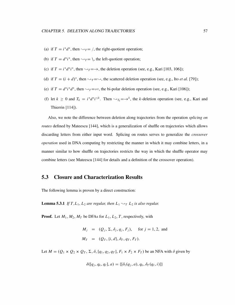
CHAPTER 5. DELETION ALONG TRAJECTORIES 57
(a) if T = i∗d∗, then ;T= /, the right-quotient operation;
(b) if T = d∗i∗, then ;T= \, the left-quotient operation;
(c) if T = i∗d∗i∗, then ;T=→, the deletion operation (see, e.g., Kari [103, 106]);
(d) if T = (i + d)∗, then ;T=;, the scattered deletion operation (see, e.g., Ito et al. [79]);
(e) if T = d∗i∗d∗, then ;T=⇋, the bi-polar deletion operation (see, e.g., Kari [106]);
(f) let k ≥ 0 and Tk = i∗d∗i≤k . Then ;Tk=→k , the k-deletion operation (see, e.g., Kari and
Thierrin [114]).
Also, we note the difference between deletion along trajectories from the operation splicing on
routes defined by Mateescu [144], which is a generalization of shuffle on trajectories which allows
discarding letters from either input word. Splicing on routes serves to generalize the crossover
operation used in DNA computing by restricting the manner in which it may combine letters, in a
manner similar to how shuffle on trajectories restricts the way in which the shuffle operator may
combine letters (see Mateescu [144] for details and a definition of the crossover operation).
5.3 Closure and Characterization Results
The following lemma is proven by a direct construction:
Lemma 5.3.1 If T ,L1, L2 are regular, then L1 ;T L2 is also regular.
Proof. Let M1,M2,MT be DFAs for L1, L2, T , respectively, with
M j = (Q j ,6, δ j , q j , F j ), for j = 1, 2, and
MT = (QT , {i, d}, δT , qT , FT ).
Let M = (Q1 × Q2 × QT ,6, δ, [q1, q2, qT ], F1 × F2 × FT ) be an NFA with δ given by
δ([q j , qk, qℓ], a) = {[δ1(q j , a), qk, δT (qℓ, i)]}
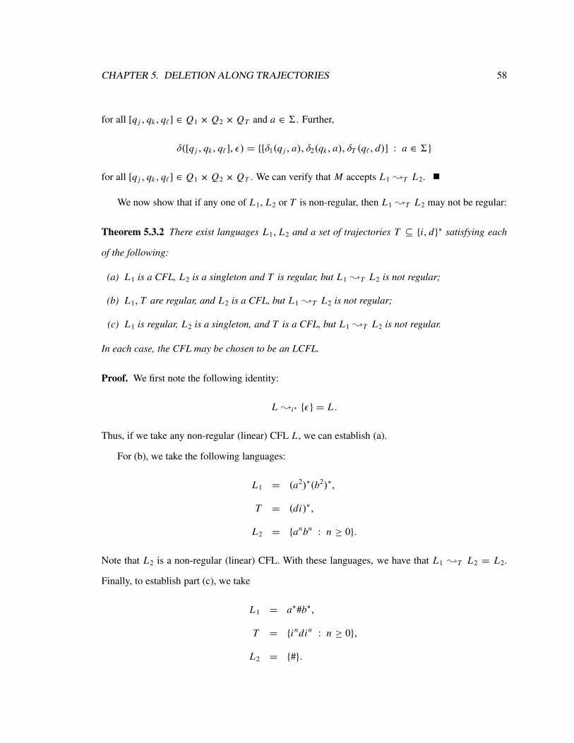
CHAPTER 5. DELETION ALONG TRAJECTORIES 58
for all [q j , qk, qℓ] ∈ Q1 × Q2 × QT and a ∈ 6. Further,
δ([q j , qk, qℓ], ǫ) = {[δ1(q j , a), δ2(qk, a), δT (qℓ, d)] : a ∈ 6}
for all [q j , qk, qℓ] ∈ Q1 × Q2 × QT . We can verify that M accepts L1 ;T L2.
We now show that if any one of L1, L2 or T is non-regular, then L1 ;T L2 may not be regular:
Theorem 5.3.2 There exist languages L1, L2 and a set of trajectories T ⊆ {i, d}∗ satisfying each
of the following:
(a) L1 is a CFL, L2 is a singleton and T is regular, but L1 ;T L2 is not regular;
(b) L1, T are regular, and L2 is a CFL, but L1 ;T L2 is not regular;
(c) L1 is regular, L2 is a singleton, and T is a CFL, but L1 ;T L2 is not regular.
In each case, the CFL may be chosen to be an LCFL.
Proof. We first note the following identity:
L ;i∗ {ǫ} = L .
Thus, if we take any non-regular (linear) CFL L , we can establish (a).
For (b), we take the following languages:
L1 = (a2)∗(b2)∗,
T = (di)∗,
L2 = {anbn : n ≥ 0}.
Note that L2 is a non-regular (linear) CFL. With these languages, we have that L1 ;T L2 = L2.
Finally, to establish part (c), we take
L1 = a∗#b∗,
T = {indin : n ≥ 0},
L2 = {#}.

CHAPTER 5. DELETION ALONG TRAJECTORIES 59
We note that T is a non-regular linear CFL, and that
L1 ;T L2 = {anbn : n ≥ 0}.
This establishes the theorem.
In Section 5.4, we discuss non-regular sets of trajectories which preserve regularity. Recall that
a weak coding is a morphism π : 6∗ → 1∗ such that π(a) ∈ 1 ∪ {ǫ} for all a ∈ 6. We have the
following characterization of deletion along trajectories:
Theorem 5.3.3 Let6 be an alphabet. There exist weak codings ρ1, ρ2, τ, ϕ and a regular language
R such that for all L1, L2 ⊆ 6∗ and all T ⊆ {i, d}∗,
L1 ;T L2 = ϕ(ρ−1
1 (L1) ∩ ρ−12 (L2) ∩ τ−1(T ) ∩ R
).
Proof. Let 6 = {a : a ∈ 6} be a copy of6. Define the morphism ρ1 : (6∪6∪{i, d})∗→ 6∗ as
follows: ρ1(a) = ρ1(a) = a for all a ∈ 6 and ρ1(i) = ρ1(d) = ǫ. Define ρ2 : (6 ∪6 ∪ {i, d})∗→
6∗ as follows: ρ2(a) = a for all a ∈ 6, ρ2(a) = ǫ for all a ∈ 6 and ρ2(d) = ρ2(i) = ǫ.
Define τ : (6 ∪6 ∪{i, d})∗→ {i, d}∗ as follows: τ(a) = τ(a) = ǫ for all a ∈ 6, τ(i) = i and
τ(d) = d. We define ϕ : (6∪6∪{i, d})∗→ 6∗ as ϕ(a) = ǫ for all a ∈ 6, ϕ(a) = a for all a ∈ 6,
and ϕ(i) = ϕ(d) = ǫ. Finally, we note that the result can be proven by letting R = (i6+ d6)∗.
Thus, we have the following corollary:
Corollary 5.3.4 Let C be a cone. Let L1, L2, T be languages such that two are regular and the
third is in C. Then L1 ;T L2 ∈ C.
Note that the closure of cones under quotient with regular sets [68, Thm. 11.3] is a specific
instance of Corollary 5.3.4. Lemma 5.3.1 can also be proven by appealing to Theorem 5.3.3. We
also note that the CFLs are a cone, thus we have the following corollary (a direct construction is
also possible):
Corollary 5.3.5 Let T, L1, L2 be languages such that one is a CFL and the other two are regular
languages. Then L1 ;T L2 is a CFL.

CHAPTER 5. DELETION ALONG TRAJECTORIES 60
The following result shows that if any of the conditions of Corollary 5.3.5 are not met, the result
might not hold:
Theorem 5.3.6 There exist languages L1, L2 and a set of trajectories T ⊆ {i, d}∗ satisfying each
of the following:
(a) L1, L2 are (linear) CFLs and T is regular, but L1 ;T L2 is not a CFL;
(b) L1, T are (linear) CFLs, and L2 is a singleton, but L1 ;T L2 is not a CFL;
(c) L1 is regular, L2, T are (linear) CFLs, but L1 ;T L2 is not a CFL.
Proof. (a) The result is immediate, since it is known (see, e.g., Ginsburg and Spanier [52, Thm.
3.4]) that the CFLs are not closed under right quotient (given by the set of trajectories T = i∗d∗).
The languages described by Ginsburg and Spanier which witness this non-closure are linear CFLs.
(b) Let 6 = {a, b, c, #} and define L1, L2 ⊆ 6∗ and T ⊆ {i, d}∗ by
L1 = {anbn#cm : n,m ≥ 0};
L2 = {#};
T = {i2ndin : n ≥ 0}.
Note that L1, T are indeed linear CFLs. Then we can verify that
L1 ;T L2 = {anbncn : n ≥ 0},
which is not a CFL.
(c) Let 6 = {a, b, c, #}. Then let
L1 = (a2)∗(b2)∗#c∗;
L2 = {anbn# : n ≥ 0};
T = {(di)2ndin : n ≥ 0}.
Then we can verify that L1 ;T L2 = {anbncn : n ≥ 0}, which is not a CFL. This completes the
proof.

CHAPTER 5. DELETION ALONG TRAJECTORIES 61
Note that the CSLs are not a cone, since it is known that they are not closed under arbitrary
morphism (see, e.g., Mateescu and Salomaa [148, Thm. 2.12] for the closure properties of the
CSLs). Thus, Corollary 5.3.4 does not apply to the CSLs. In fact, it is also known that the CSLs are
not closed under (left or right) quotient with regular languages.
5.3.1 Recognizing Deletion Along Trajectories
We now consider the problem of giving a monoid recognizing deletion along trajectories, when the
languages and set of trajectories under consideration are regular. Harju et al. [61] give a monoid
which recognizes L1 T L2 when L1, L2 and T are regular.
For a background on recognition of formal languages by monoids, please consult Pin [164]. A
monoid is a semigroup with unit element. Let L ⊆ 6∗ be a language. We say that a monoid M
recognizes L if there exists a morphism ϕ : 6∗→ M and a subset F ⊆ M such that L = ϕ−1(F).
The following is a characterization of the regular languages due to Kleene (see, e.g., Pin [164,
p. 17]):
Theorem 5.3.7 A language is regular if and only if it is recognized by a finite monoid.
Consider arbitrary regular languages L1, L2 ⊆ 6∗ and T ⊆ {i, d}∗. Then our goal is to construct
a monoid recognizing L1 ;T L2.
Let M1,M2,MT be finite monoids recognizing L1, L2, LT , with morphisms ϕ j : 6∗→ M j for
j = 1, 2, ϕT : {i, d}∗ → MT and subsets F1, F2, FT , respectively.
As in Harju et al. [61], we consider the monoid P(M1 × M2 × MT ) consisting of all subsets
of M1 × M2 × MT . The monoid operation is given by AB = {xy : x ∈ A, y ∈ B} for all
A, B ∈ P(M1 × M2 × MT ), and the product of elements of M1 × M2 × MT is defined component-
wise.
We can now establish that P(M1 × M2 × MT ) recognizes L1 ;T L2. We first define a subset
D ⊆ M1 × M2 × MT which will be useful:
D = {[ϕ1(x), ϕ2(x), ϕT (d|x |)] : x ∈ 6∗}.
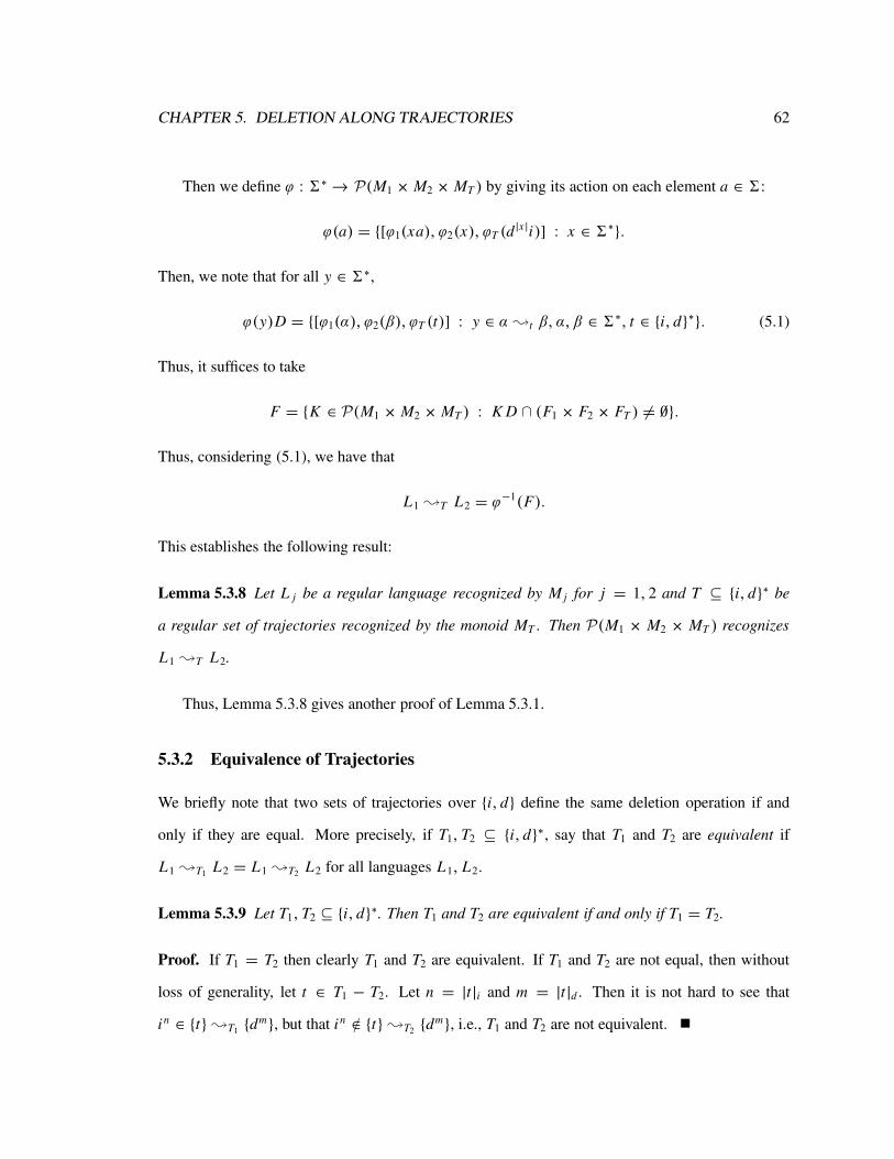
CHAPTER 5. DELETION ALONG TRAJECTORIES 62
Then we define ϕ : 6∗→ P(M1 × M2 × MT ) by giving its action on each element a ∈ 6:
ϕ(a) = {[ϕ1(xa), ϕ2(x), ϕT (d|x |i)] : x ∈ 6∗}.
Then, we note that for all y ∈ 6∗,
ϕ(y)D = {[ϕ1(α), ϕ2(β), ϕT (t)] : y ∈ α ;t β, α, β ∈ 6∗, t ∈ {i, d}∗}. (5.1)
Thus, it suffices to take
F = {K ∈ P(M1 × M2 × MT ) : K D ∩ (F1 × F2 × FT ) 6= ∅}.
Thus, considering (5.1), we have that
L1 ;T L2 = ϕ−1(F).
This establishes the following result:
Lemma 5.3.8 Let L j be a regular language recognized by M j for j = 1, 2 and T ⊆ {i, d}∗ be
a regular set of trajectories recognized by the monoid MT . Then P(M1 × M2 × MT ) recognizes
L1 ;T L2.
Thus, Lemma 5.3.8 gives another proof of Lemma 5.3.1.
5.3.2 Equivalence of Trajectories
We briefly note that two sets of trajectories over {i, d} define the same deletion operation if and
only if they are equal. More precisely, if T1, T2 ⊆ {i, d}∗, say that T1 and T2 are equivalent if
L1 ;T1L2 = L1 ;T2
L2 for all languages L1, L2.
Lemma 5.3.9 Let T1, T2 ⊆ {i, d}∗. Then T1 and T2 are equivalent if and only if T1 = T2.
Proof. If T1 = T2 then clearly T1 and T2 are equivalent. If T1 and T2 are not equal, then without
loss of generality, let t ∈ T1 − T2. Let n = |t|i and m = |t|d . Then it is not hard to see that
in ∈ {t};T1{dm}, but that in /∈ {t};T2
{dm}, i.e., T1 and T2 are not equivalent.

CHAPTER 5. DELETION ALONG TRAJECTORIES 63
Thus, the decidability of the equivalence problem for T1, T2 ⊆ {i, d}∗ is well known. For
instance, it is decidable whether T1, T2 are equivalent if, e.g., T1, T2 are DCFLs, but undecidable if
T1 is regular and T2 is an arbitrary CFL.
5.4 Regularity-Preserving Sets of Trajectories
Consider the following result of Mateescu et al. [147, Thm. 5.1]: if L1 T L2 is regular for all regu-
lar languages L1, L2, then T is regular. This result is clear upon noting that for all T , 0∗ T 1∗ = T .
However, in this section, we note that the same result does not hold if we replace “shuffle
on trajectories” by “deletion along trajectories”. In particular, we demonstrate a class of sets of
trajectories H, which contains non-regular languages, such that for all regular languages R1, R2,
and for all H ∈ H, R1 ;H R2 is regular. We also characterize all H ⊆ i∗d∗ which preserve
regularity (i.e., such that R1 ;H R2 is regular for all regular languages R1, R2), and give some
examples of non-CF trajectories which preserve regularity.
As motivation, we begin with a basic example. Let 6 be an alphabet. Let H = {indn : n ≥ 0}.
Note that
R1 ;H R2 = {x ∈ 6∗ : ∃y ∈ R2 such that xy ∈ R1 and |x| = |y|}.
We can establish directly (by constructing an NFA) that for all regular languages R1, R2 ⊆ 6∗, the
language R1 ;H R2 is regular. However, H is a non-regular CFL.
We remark that R1 ;H R2 is similar to proportional removals studied by Stearns and Hartmanis
[189], Amar and Putzolu [4, 5] Seiferas and McNaughton [180], Kosaraju [120, 121, 122], Kozen
[123], Zhang [205], the author [35], Berstel et al. [17], and others. In particular, we note the case of
12(L), given by
1
2(L) = {x ∈ 6∗ : ∃y ∈ 6∗ such that xy ∈ L and |x| = |y|}.
Thus, 12(L) = L ;H 6∗. The operation 1
2(L) is one of a class of operations which preserve
regularity. Seiferas and McNaughton completely characterize those binary relations r ⊆ N2 such
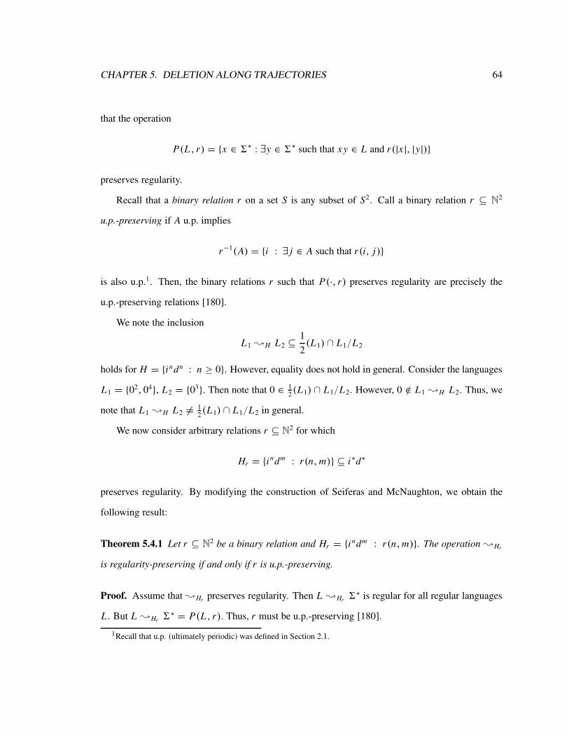
CHAPTER 5. DELETION ALONG TRAJECTORIES 64
that the operation
P(L , r) = {x ∈ 6∗ : ∃y ∈ 6∗ such that xy ∈ L and r(|x|, |y|)}
preserves regularity.
Recall that a binary relation r on a set S is any subset of S2. Call a binary relation r ⊆ N2
u.p.-preserving if A u.p. implies
r−1(A) = {i : ∃ j ∈ A such that r(i, j)}
is also u.p.1. Then, the binary relations r such that P(·, r) preserves regularity are precisely the
u.p.-preserving relations [180].
We note the inclusion
L1 ;H L2 ⊆1
2(L1) ∩ L1/L2
holds for H = {indn : n ≥ 0}. However, equality does not hold in general. Consider the languages
L1 = {02, 04}, L2 = {03}. Then note that 0 ∈ 12(L1) ∩ L1/L2. However, 0 /∈ L1 ;H L2. Thus, we
note that L1 ;H L2 6= 12(L1) ∩ L1/L2 in general.
We now consider arbitrary relations r ⊆ N2 for which
Hr = {indm : r(n,m)} ⊆ i∗d∗
preserves regularity. By modifying the construction of Seiferas and McNaughton, we obtain the
following result:
Theorem 5.4.1 Let r ⊆ N2 be a binary relation and Hr = {indm : r(n,m)}. The operation ;Hr
is regularity-preserving if and only if r is u.p.-preserving.
Proof. Assume that ;Hrpreserves regularity. Then L ;Hr
6∗ is regular for all regular languages
L . But L ;Hr6∗ = P(L , r). Thus, r must be u.p.-preserving [180].
1Recall that u.p. (ultimately periodic) was defined in Section 2.1.

CHAPTER 5. DELETION ALONG TRAJECTORIES 65
For the reverse implication, we modify the construction of Seiferas and McNaughton [180,
Thm. 1]. Let L1, L2 be regular languages. Let M1 = (Q1,6, δ1, q0, F1) be the minimal complete
DFA for L1. Then, for each q ∈ Q1, we let L(q)1 be the language accepted by the DFA M
(q)1 =
(Q1,6, δ1, q0, {q}). Let Rq be the language accepted by the DFA N(q)1 = (Q1,6, δ1, q, F1). Note
that L(q)1 = {w ∈ 6∗ : δ(q0, w) = q} and Rq = {w ∈ 6∗ : δ(q, w) ∈ F1}.
As M1 is complete, 6∗ =⋃q∈Q1L(q)1 . Thus,
L1 ;HrL2 =
⋃
q∈Q1
(L1 ;HrL2) ∩ L
(q)1 .
It suffices to demonstrate that (L1 ;HrL2) ∩ L
(q)1 is regular. But we note that
(L1 ;HrL2) ∩ L
(q)1 = {x ∈ L
(q)1 : ∃y ∈ L2 such that xy ∈ L1 and r(|x|, |y|)}
= {x ∈ L(q)1 : ∃y ∈ (Rq ∩ L2) such that r(|x|, |y|)}
= {x ∈ 6∗ : ∃y ∈ (Rq ∩ L2) such that r(|x|, |y|)} ∩ L(q)1
= {x ∈ 6∗ : |x| ∈ r−1({|y| : y ∈ (Rq ∩ L2)})} ∩ L(q)1 .
It is easy to see that if L is regular, {|y| : y ∈ L} is a u.p. set. As r is u.p.-preserving, r−1({|y| : y ∈
Rq ∩ L2)}) is also u.p.
Note that, in general, L1 ;HrL2 6= P(L1, r) ∩ L1/L2. Consider the following particular
examples of regularity-preserving trajectories:
(a) Consider the relation e = {(n, 2n) : n ≥ 0}. Then He preserves regularity (see, e.g., Zhang
[205, Sect. 3]). However, He is not CF. The set He is, however, a linear conjunctive language
(see Okhotin [160] for the definition of conjunctive and linear conjunctive languages, and for
the proof that He is linear conjunctive).
(b) Consider the relation f = {(n, n!) : n ≥ 0}. Then H f preserves regularity (see again Zhang
[205, Thm. 5.1]). However, H f is not a CFL, nor a linear conjunctive language [160].
Thus, there are non-CF trajectories which preserve regularity. Kozen states that there are even Hr
which preserve regularity but are “highly noncomputable” [123, p. 3].
CHAPTER 5. DELETION ALONG TRAJECTORIES 66
We can extend the class of non-regular sets of trajectories T such that L1 ;T L2 is regular
for all regular languages L1, L2 by considering T such that T ⊆ (d∗i∗)md∗ for some m ≥ 1 (The
choice of T ⊆ (d∗i∗)md∗ rather than, e.g., T ⊆ (i∗d∗)m or T ⊆ (d∗i∗)m is arbitrary. The same
type of formulation and arguments can be applied to these similar types of sets of trajectories).
To consider such non-regular T , it will be advantageous to adopt the notations of Zhang [205] on
boolean matrices. We summarize these notions below; for a full review, the reader may consult the
original paper.
For any finite set Q, let M(Q) denote the set of square Boolean matrices indexed by Q. Let
V(Q) denote the set of Boolean vectors indexed by Q. For an automaton over a set of states Q, we
will associate with it matrices from M(Q) and vectors from V(Q).
In particular, let M = (Q,6, δ, q0, F) be a DFA. Then for each a ∈ 6, let ∇a ∈ M(Q) be
the matrix defined by transitions on a, that is,∇a(q1, q2) = 1 if and only if δ(q1, a) = q2. Let ∇ =∑
a∈6 ∇a (where addition is taken to be Boolean addition, i.e., 0+0 = 0, 0+1 = 1+0 = 1+1 = 1).
Thus, ∇(q1, q2) = 1 if and only if there is some a ∈ 6 such that δ(q1, a) = q2. Note that taking
powers of ∇ yields information on paths of different lengths: for all i ≥ 0, ∇ i(q1, q2) = 1 if and
only if there is a path of length i from q1 to q2.
For any Q ′ ⊆ Q, let IQ ′ ∈ V(Q) be the characteristic vector of Q ′, given by IQ ′(q) = 1 if and
only if q ∈ Q ′. If Q ′ is a singleton q, we denote I{q} by Iq . Note that if Q1, Q2 ⊆ Q and i ≥ 0,
then IQ1· ∇ i · I t
Q2= 1 if and only if there is a path of length i from some state in Q1 to some state
in Q2 (here, I t denotes the transpose of I ).
Call a function f : N → N ultimately periodic with respect to powers of Boolean matrices
[205], abbreviated m.u.p. (for “matrix ultimately periodic”), if, for all square Boolean matrices ∇,
there exist natural numbers e, p (p > 0) such that for all n ≥ e,
∇ f (n) = ∇ f (n+p).
The functions n! and 2n are known to be m.u.p. [205].
Let m ≥ 1. We will define a class of T ⊆ (d∗i∗)md∗ such that for all regular languages R1, R2,

CHAPTER 5. DELETION ALONG TRAJECTORIES 67
R1 ;T R2 is regular. In particular, let m ≥ 1, and let f( j )ℓ : N→ N be a m.u.p. function for each
1 ≤ ℓ ≤ m + 1 and 1 ≤ j ≤ m. Define Xℓ : Nm → N for 1 ≤ ℓ ≤ m + 1 by
Xℓ(n1, n2, . . . , nm) =m∑
j=1
f( j )ℓ (n j ). (5.2)
We will use the abbreviation En = (n1, n2, . . . , nm). Finally, we define
T = {m∏
j=1
(d X j (En)in j )d Xm+1(En) : En = (n1, . . . , nm) ∈ Nm}. (5.3)
The set T satisfies our intuition that the ‘i-portions’ may not interact with each other, but may
interact with any ‘d-portion’ they wish to. Our claim that these T preserve regularity is proven in
the following theorem.
Theorem 5.4.2 Let m ≥ 1, and f( j )ℓ be m.u.p. for 1 ≤ ℓ ≤ m + 1 and 1 ≤ j ≤ m. Let T ⊆
(d∗i∗)md∗ be defined by (5.2) and (5.3). Then for all regular languages R1, R2, the language R1 ;T
R2 is regular.
In this section only, let m = {0, 1, 2, 3, . . . ,m} for any m ≥ 1.
Proof. Let Mi = (Q i ,6, δi , si , Fi ) be a DFA accepting Ri for i = 1, 2. Let M1,2 = (Q1 ×
Q2,6, δ0, [s1, s2], F1 × F2) where δ is given by δ0([q1, q2], a) = (δ1[q1, a], δ2[q2, a]) for all
[q1, q2] ∈ Q1 × Q2 and all a ∈ 6. Note that M1,2 accepts R1 ∩ R2. Let ∇ be the adjacency
matrix for M1,2. For each 1 ≤ j ≤ m and 1 ≤ ℓ ≤ m + 1, let e( j )ℓ and p
( j )ℓ be natural numbers such
that ∇ f( j)ℓ (n) = ∇ f
( j)ℓ (n+p
( j)ℓ ) for all n ≥ e
( j )ℓ .
For all 1 ≤ j ≤ m and 1 ≤ ℓ ≤ m + 1, let g( j )ℓ = e
( j )ℓ + p
( j )ℓ and define the set
M( j, ℓ) = {∇ f( j)ℓ (i) : 0 ≤ i ≤ g
( j )ℓ } × g
(j)ℓ .
We will define an NFA M = (Q,6, δ, S, F) which we claim accepts R1 ;T R2. The NFA
will be nondeterministic, and will also have multiple start states. It is well known that multiple
start states do not affect the regularity of the language accepted (see, e.g., Yu [201, p. 54]); our
presentation is chosen for ease of description.
CHAPTER 5. DELETION ALONG TRAJECTORIES 68
We now proceed with defining M . Our state set Q is given by
Q = m× (m∏
ℓ=1
(
m∏
j=1
M( j, ℓ))× Q31 × Q2)×
m∏
j=1
M( j,m + 1).
Let µ j,ℓ = [∇ f( j)ℓ (0), 0] ∈M( j, ℓ). Our set S of initial states is given by
S = {1} × (m∏
ℓ=1
m∏
j=1
µ j,ℓ × {[q, q] : q ∈ Q1} × Q1 × Q2)×m∏
j=1
µ j,m+1.
To partially motivate this definition, the elements of the form Q31 will represent one path through
M1: the first element will represent our nondeterministic “guess” of where the path starts, the second
state will actually trace the path through M1 (along a portion of our input word) and the third state
represents our guess of where the path will end. Thus, during the course of our computation, the
first and third elements are never changed; only the second is affected by the input word. The first
and third elements are used to verify (once the computation has completed) that our guesses for the
start and finish are correct, and that they correspond (“match up”) with the guessed paths for the
adjacent components. The elements of Q2 will represent our guesses of the intermediate points of
the path through M2; similarly to our guesses in Q1, they will not change through the course of the
computation.
Our set of final states F is given by those states of the form
{m} ×[[
[A( j )ℓ , c
( j )ℓ ]m
j=1q(1)ℓ , q
(2)ℓ , q
(3)ℓ , rℓ
]m
ℓ=1, (A
( j )m+1, c
( j )ℓ )
mj=1
],
where the following conditions are met:
(F-i) for all 1 ≤ ℓ ≤ m, I(q(3)ℓ−1,rℓ−1)
· (∏mj=1 A
( j )ℓ ) · I t
(q(1)ℓ ,rℓ)= 1 (we let q
(3)0 = s1, the start state of M1
and r0 = s2 the start state of M2);
(F-ii) I(q(3)m ,rm )
· (∏mj=1 A
( j )m+1) · I t
F1×F2= 1;
(F-iii) for all 1 ≤ ℓ ≤ m, we have q(2)ℓ = q
(3)ℓ .
We will see that the matrix A( j )ℓ will ensure there is a path of length f
( j )ℓ (n j ) through M1×M2. Thus,
condition (F-i) will ensure that we have a path from our guessed end state of the previous i-portion
CHAPTER 5. DELETION ALONG TRAJECTORIES 69
through to the guessed start state of the next i-portion. This will correspond to the presence of some
word w of length∑m
j=1 f( j )ℓ (n j) which takes us M from the end state of the previous i-portion to
the start of the next i-portion. The condition (F-ii) will ensure that the final d-portion ends in a final
state in both M1 and M2.
Condition (F-iii) verifies that the nondeterministic “guesses” for the end of each i-portion path
is correct.
Finally, we may define the action of δ. We will adopt the convention of Zhang [205] and denote
by 〈c〉ba the quantity
〈c〉ba =
c if c ≤ a;
a + ((c − a) mod b ) otherwise.
Further, to describe the action of δ more easily, we introduce auxiliary functions ϒℓ,α for all
1 ≤ ℓ ≤ m + 1 and 1 ≤ α ≤ m. In particular
ϒℓ,α :
m∏
j=1
M( j, ℓ)→m∏
j=1
M( j, ℓ)
is given by
ϒℓ,α([∇ f( j)ℓ (c
( j)ℓ ), c
( j )ℓ ]m
j=1)
=
[∇ f
( j)ℓ (c
( j)ℓ ), c
( j )ℓ ]α−1
j=1,∇f(α)ℓ (〈c(α)ℓ +1〉p
(α)ℓ
e(α)ℓ
)
, 〈c(α)ℓ + 1〉p(α)ℓ
e(α)ℓ
, [∇ f( j)ℓ (c
( j)ℓ ), c
( j )ℓ ]m
j=α+1
.
Note that ϒℓ,α updates the α-th component, while leaving all other components unchanged.
Then we define δ by
δ([α,[[∇ f
( j)ℓ (c
( j)ℓ ), c
( j )ℓ ]m
j=1, p(1)ℓ , p
(2)ℓ , p
(3)ℓ , rℓ
]m
ℓ=1, [∇ f
( j)m+1(c
( j)m+1), c
( j )m+1]m
j=1
], a)
={[α + β, [ϒℓ,α+β([∇ f
( j)ℓ (c
( j)ℓ ), c
( j )ℓ ]m
j=1), p(1)ℓ , p
(2)ℓ , p
(3)ℓ , rℓ]
α+β−1ℓ=1 ,
ϒα+β,α+β([∇ f( j)α+β (c
( j)α+β ), c
( j )α+β ]m
j=1), p(1)α+β , δ1(p
(2)α+β , a), p
(3)α+β , rα+β
[ϒℓ,α+β([∇ f( j)ℓ (c
( j)ℓ ), c
( j )ℓ ]m
j=1), p(1)ℓ , p
(2)ℓ , p
(3)ℓ , rℓ]
mℓ=α+β+1,
ϒm+1,α+β([∇ f( j)m+1(c
( j)m+1), c
( j )m+1]m
j=1)]
: 0 ≤ β ≤ m − α}.
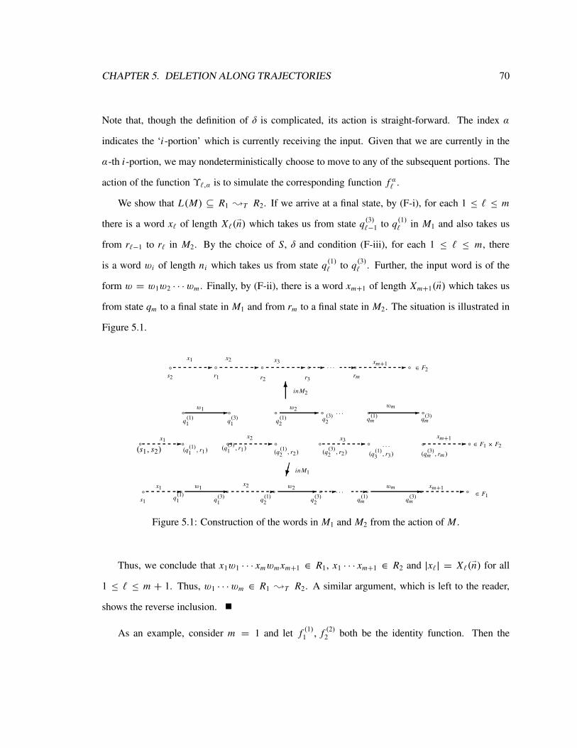
CHAPTER 5. DELETION ALONG TRAJECTORIES 70
Note that, though the definition of δ is complicated, its action is straight-forward. The index α
indicates the ‘i-portion’ which is currently receiving the input. Given that we are currently in the
α-th i-portion, we may nondeterministically choose to move to any of the subsequent portions. The
action of the function ϒℓ,α is to simulate the corresponding function f αℓ .
We show that L(M) ⊆ R1 ;T R2. If we arrive at a final state, by (F-i), for each 1 ≤ ℓ ≤ m
there is a word xℓ of length Xℓ(En) which takes us from state q(3)ℓ−1 to q
(1)ℓ in M1 and also takes us
from rℓ−1 to rℓ in M2. By the choice of S, δ and condition (F-iii), for each 1 ≤ ℓ ≤ m, there
is a word wi of length ni which takes us from state q(1)ℓ to q
(3)ℓ . Further, the input word is of the
form w = w1w2 · · ·wm . Finally, by (F-ii), there is a word xm+1 of length Xm+1(En) which takes us
from state qm to a final state in M1 and from rm to a final state in M2. The situation is illustrated in
Figure 5.1.
x1
s1
--
--
���
6
------
----
aaaaaa
q(1)1
· · ·
· · ·
inM1
inM2
∈ F2rmr3r2
r1s2
xm+1x3
x2x1
xm+1wmw2x2w1
∈ F1q(3)mq
(1)mq
(3)2
q(1)2
q(3)1
a
- -
--- aa a
a aaaaa
a aaaa
aaaaaa
-
a
(q(3)1, r1)
q(3)2
wmw2w1
q(3)mq
(1)mq
(1)2q
(3)1q
(1)1
(q(3)m , rm )
xm+1x3x2
(q(1)3 , r3)
(q(3)2 , r2)(q
(1)2 , r2)
· · ·
· · ·(q(1)1, r1)
x1 ∈ F1 × F2(s1, s2)
-
Figure 5.1: Construction of the words in M1 and M2 from the action of M .
Thus, we conclude that x1w1 · · · xmwmxm+1 ∈ R1, x1 · · · xm+1 ∈ R2 and |xℓ| = Xℓ(En) for all
1 ≤ ℓ ≤ m + 1. Thus, w1 · · ·wm ∈ R1 ;T R2. A similar argument, which is left to the reader,
shows the reverse inclusion.
As an example, consider m = 1 and let f(1)1 , f
(2)2 both be the identity function. Then the

CHAPTER 5. DELETION ALONG TRAJECTORIES 71
conditions of Theorem 5.4.2 are met and T = {dnindn : n ≥ 0}. Consider then that
R1 ;T 6∗ = {x : ∃y, z ∈ 6|x | such that yxz ∈ R1}.
This is the ‘middle-thirds’ operation, which is sometimes used as a challenge problem for under-
graduates in formal language theory (see, e.g., Hopcroft and Ullman [68, Ex. 3.17]). We may
immediately conclude that the regular languages are preserved under the middle-thirds operation.
We note that the condition that (n1, n2, . . . , nm) ∈ Nm in (5.3) can be replaced by the conditions
that, for all 1 ≤ j ≤ m, n j ∈ I j for an arbitrary u.p. set I j ⊆ N. The construction adds considerable
detail to the proof of Theorem 5.4.2, and is omitted. With this extension, we can also consider a
class of examples given by Amar and Putzolu [5], which are equivalent to trajectories of the form
AP(k1, k2, α) = {imk1 dmk2+α : m ≥ 0},
for fixed k1, k2, α ≥ 0 with α < k1 + k2. For any k1, k2, α ≥ 0, we can conclude that the operation
;A preserves regularity, where A = AP(k1, k2, α). This was established by Amar and Putzolu [5]
by means of even linear grammars.
Pin and Sakarovitch use a very general and elegant method to prove that certain operations
preserve regularity [165]. This method can be used to prove that certain operations which can be
modeled by trajectories preserve regularity; it is not known whether the methods developed here
can be extended to cover theses cases. For example, the let Tζ be given by
Tζ = {dnki kdnk : k, n ≥ 0, 2n + 1 is prime}.
Then Pin and Sakarovitch prove that L ;Tζ 6∗ is regular for all regular languages L [165, p. 292]2.
2Note that the definition of Tζ given here matches that given by Pin and Sakarovitch [165]. In a preliminary version
[166], a different deletion operation is defined which can be modeled by a set of trajectories to which Theorem 5.5.1
below can be applied.
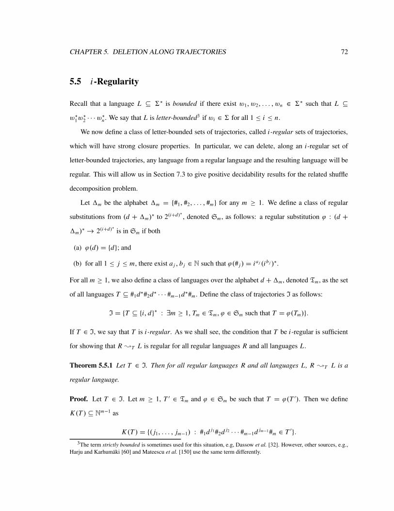
CHAPTER 5. DELETION ALONG TRAJECTORIES 72
5.5 i-Regularity
Recall that a language L ⊆ 6∗ is bounded if there exist w1, w2, . . . , wn ∈ 6∗ such that L ⊆
w∗1w∗2 · · ·w∗n . We say that L is letter-bounded3 if wi ∈ 6 for all 1 ≤ i ≤ n.
We now define a class of letter-bounded sets of trajectories, called i -regular sets of trajectories,
which will have strong closure properties. In particular, we can delete, along an i-regular set of
letter-bounded trajectories, any language from a regular language and the resulting language will be
regular. This will allow us in Section 7.3 to give positive decidability results for the related shuffle
decomposition problem.
Let 1m be the alphabet 1m = {#1, #2, . . . , #m} for any m ≥ 1. We define a class of regular
substitutions from (d + 1m)∗ to 2(i+d)∗ , denoted Sm , as follows: a regular substitution ϕ : (d +
1m)∗→ 2(i+d)∗ is in Sm if both
(a) ϕ(d) = {d}; and
(b) for all 1 ≤ j ≤ m, there exist a j , b j ∈ N such that ϕ(# j ) = ia j (ib j )∗.
For all m ≥ 1, we also define a class of languages over the alphabet d +1m , denoted Tm , as the set
of all languages T ⊆ #1d∗#2d∗ · · · #m−1d∗#m . Define the class of trajectories I as follows:
I = {T ⊆ {i, d}∗ : ∃m ≥ 1, Tm ∈ Tm, ϕ ∈ Sm such that T = ϕ(Tm)}.
If T ∈ I, we say that T is i -regular. As we shall see, the condition that T be i-regular is sufficient
for showing that R ;T L is regular for all regular languages R and all languages L .
Theorem 5.5.1 Let T ∈ I. Then for all regular languages R and all languages L, R ;T L is a
regular language.
Proof. Let T ∈ I. Let m ≥ 1, T ′ ∈ Tm and ϕ ∈ Sm be such that T = ϕ(T ′). Then we define
K (T ) ⊆ Nm−1 as
K (T ) = {( j1, . . . , jm−1) : #1d j1#2d j2 · · · #m−1d jm−1#m ∈ T ′}.3The term strictly bounded is sometimes used for this situation, e.g, Dassow et al. [32]. However, other sources, e.g.,
Harju and Karhumaki [60] and Mateescu et al. [150] use the same term differently.
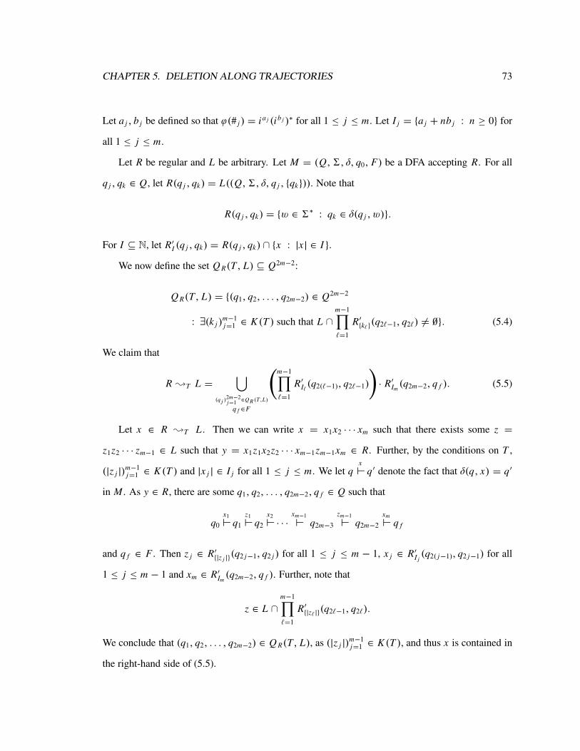
CHAPTER 5. DELETION ALONG TRAJECTORIES 73
Let a j , b j be defined so that ϕ(# j ) = ia j (ib j )∗ for all 1 ≤ j ≤ m. Let I j = {a j + nb j : n ≥ 0} for
all 1 ≤ j ≤ m.
Let R be regular and L be arbitrary. Let M = (Q,6, δ, q0, F) be a DFA accepting R. For all
q j , qk ∈ Q, let R(q j , qk) = L((Q,6, δ, q j , {qk})). Note that
R(q j , qk) = {w ∈ 6∗ : qk ∈ δ(q j , w)}.
For I ⊆ N, let R′I (q j , qk) = R(q j , qk) ∩ {x : |x| ∈ I }.
We now define the set Q R(T, L) ⊆ Q2m−2:
Q R(T, L) = {(q1, q2, . . . , q2m−2) ∈ Q2m−2
: ∃(k j )m−1j=1 ∈ K (T ) such that L ∩
m−1∏
ℓ=1
R′{kℓ}(q2ℓ−1, q2ℓ) 6= ∅}. (5.4)
We claim that
R ;T L =⋃
(q j )2m−2j=1
∈QR (T ,L)
q f ∈F
(m−1∏
ℓ=1
R′Iℓ(q2(ℓ−1), q2ℓ−1)
)· R′Im
(q2m−2, q f ). (5.5)
Let x ∈ R ;T L . Then we can write x = x1x2 · · · xm such that there exists some z =
z1z2 · · · zm−1 ∈ L such that y = x1z1x2z2 · · · xm−1zm−1xm ∈ R. Further, by the conditions on T ,
(|z j |)m−1j=1 ∈ K (T ) and |x j | ∈ I j for all 1 ≤ j ≤ m. We let q
x
⊢ q ′ denote the fact that δ(q, x) = q ′
in M . As y ∈ R, there are some q1, q2, . . . , q2m−2, q f ∈ Q such that
q0
x1⊢ q1
z1⊢ q2
x2⊢ · · ·xm−1
⊢ q2m−3
zm−1
⊢ q2m−2
xm
⊢ q f
and q f ∈ F . Then z j ∈ R′{|z j |}(q2 j−1, q2 j ) for all 1 ≤ j ≤ m − 1, x j ∈ R′I j(q2( j−1), q2 j−1) for all
1 ≤ j ≤ m − 1 and xm ∈ R′Im(q2m−2, q f ). Further, note that
z ∈ L ∩m−1∏
ℓ=1
R′{|zℓ |}(q2ℓ−1, q2ℓ).
We conclude that (q1, q2, . . . , q2m−2) ∈ Q R(T, L), as (|z j |)m−1j=1 ∈ K (T ), and thus x is contained in
the right-hand side of (5.5).
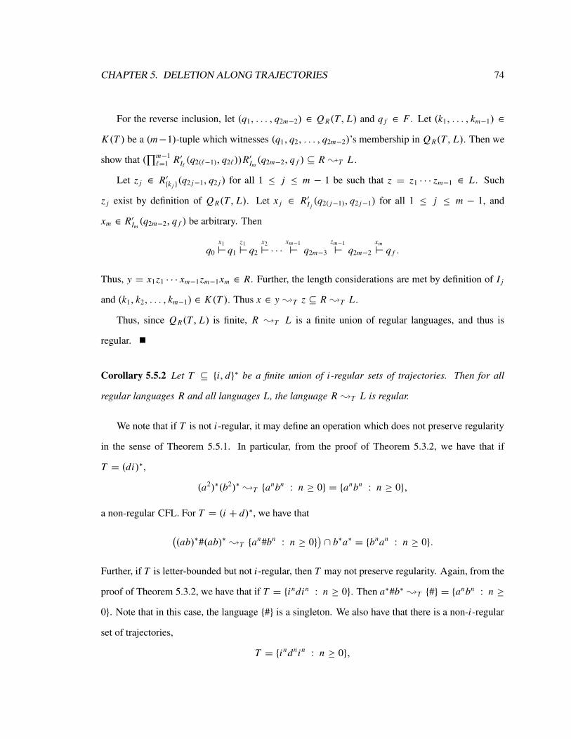
CHAPTER 5. DELETION ALONG TRAJECTORIES 74
For the reverse inclusion, let (q1, . . . , q2m−2) ∈ Q R(T, L) and q f ∈ F . Let (k1, . . . , km−1) ∈
K (T ) be a (m−1)-tuple which witnesses (q1, q2, . . . , q2m−2)’s membership in Q R(T, L). Then we
show that (∏m−1ℓ=1 R′Iℓ (q2(ℓ−1), q2ℓ))R
′Im(q2m−2, q f ) ⊆ R ;T L .
Let z j ∈ R′{k j }(q2 j−1, q2 j ) for all 1 ≤ j ≤ m − 1 be such that z = z1 · · · zm−1 ∈ L . Such
z j exist by definition of Q R(T, L). Let x j ∈ R′I j(q2( j−1), q2 j−1) for all 1 ≤ j ≤ m − 1, and
xm ∈ R′Im(q2m−2, q f ) be arbitrary. Then
q0
x1⊢ q1
z1⊢ q2
x2⊢ · · ·xm−1
⊢ q2m−3
zm−1
⊢ q2m−2
xm
⊢ q f .
Thus, y = x1z1 · · · xm−1zm−1xm ∈ R. Further, the length considerations are met by definition of I j
and (k1, k2, . . . , km−1) ∈ K (T ). Thus x ∈ y ;T z ⊆ R ;T L .
Thus, since Q R(T, L) is finite, R ;T L is a finite union of regular languages, and thus is
regular.
Corollary 5.5.2 Let T ⊆ {i, d}∗ be a finite union of i-regular sets of trajectories. Then for all
regular languages R and all languages L, the language R ;T L is regular.
We note that if T is not i-regular, it may define an operation which does not preserve regularity
in the sense of Theorem 5.5.1. In particular, from the proof of Theorem 5.3.2, we have that if
T = (di)∗,
(a2)∗(b2)∗ ;T {anbn : n ≥ 0} = {anbn : n ≥ 0},
a non-regular CFL. For T = (i + d)∗, we have that
((ab)∗#(ab)∗ ;T {an#bn : n ≥ 0}
)∩ b∗a∗ = {bnan : n ≥ 0}.
Further, if T is letter-bounded but not i-regular, then T may not preserve regularity. Again, from the
proof of Theorem 5.3.2, we have that if T = {indin : n ≥ 0}. Then a∗#b∗ ;T {#} = {anbn : n ≥
0}. Note that in this case, the language {#} is a singleton. We also have that there is a non-i-regular
set of trajectories,
T = {indnin : n ≥ 0},

CHAPTER 5. DELETION ALONG TRAJECTORIES 75
and a regular language R such that R ;T 6∗ is not a regular language. In particular, we have the
following example. Let 6 = {a, b, c} and R = a∗bc∗. Then R ;T 6∗ is not a regular language, as
(R ;T 6∗) ∩ a∗c∗ = {ancn : n ≥ 0}.
As an example of Theorem 5.5.1, consider T = {dnimdn : n,m ≥ 0}. It is easily verified
that T ∈ I (consider T ′ = {#1dn#2dn#3 : n ≥ 0}, and ϕ defined by ϕ(#1) = ϕ(#3) = {ǫ} and
ϕ(#2) = i∗). Thus, the language R ;T L is regular for all regular languages R and all languages
L . For any language L ⊆ 6∗, define sq(L) = {x2 : x ∈ L}. Consider then that
R ;T sq(L) = {w : vwv ∈ R, v ∈ L}.
This precisely defines the middle-quotient operation, which has been investigated by Meduna [153]
for linear CFLs. Let R | L denote the middle quotient of R by L , i.e., R | L = R ;T sq(L). Thus,
we can immediately conclude the following result, which was not considered by Meduna:
Theorem 5.5.3 Given a regular language R and arbitrary language L, the language R|L is regular.
5.6 Filtering and Deletion along Trajectories
Recently, Berstel et al. [17] introduced the concept of filtering. Here we examine the notion of
filtering, and show that it is a particular case of deletion along trajectories.
Given a sequence s ⊆ N, and a word w ∈ 6∗ with w = w1 · · ·wn, wi ∈ 6, the filtering of
w by s is given by w[s] = ws0ws1· · ·wsk
where k is such that sk ≤ n < sk+1. For example, if
s = (1, 2, 4, 7), then abcacb[s] = aba. Filtering is extended monotonically to languages.
For every s ⊆ N, let ωs : N→ {i, d} be given by ωs( j) = i if j ∈ s and ωs( j) = d otherwise4.
Let Ts ⊆ {0, 1}∗ be defined by
Ts = {n∏
j=0
ωs( j) : n ≥ 0}.
Then we clearly have that
L[s] = L ;Ts6∗,
4That is, ωs is the characteristic ω-word of s over {i, d}.
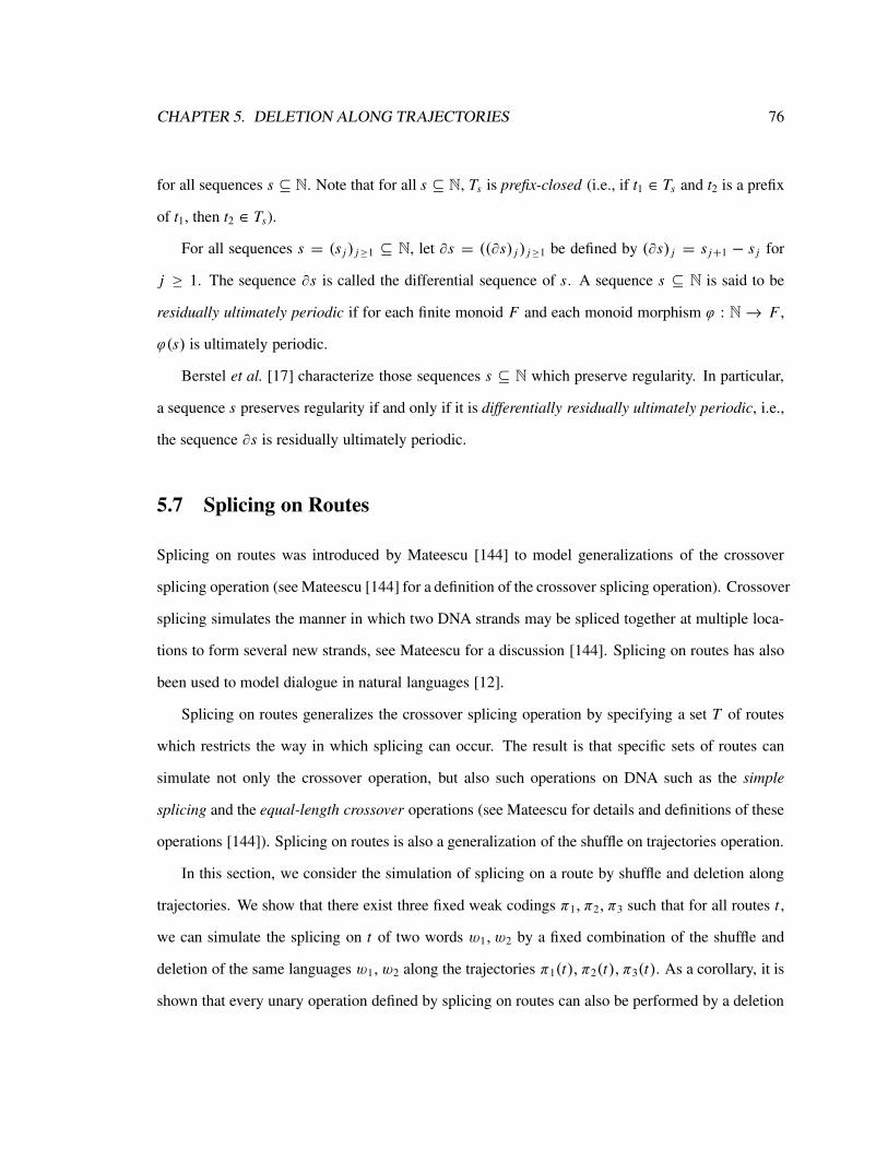
CHAPTER 5. DELETION ALONG TRAJECTORIES 76
for all sequences s ⊆ N. Note that for all s ⊆ N, Ts is prefix-closed (i.e., if t1 ∈ Ts and t2 is a prefix
of t1, then t2 ∈ Ts).
For all sequences s = (s j ) j≥1 ⊆ N, let ∂s = ((∂s) j ) j≥1 be defined by (∂s) j = s j+1 − s j for
j ≥ 1. The sequence ∂s is called the differential sequence of s. A sequence s ⊆ N is said to be
residually ultimately periodic if for each finite monoid F and each monoid morphism ϕ : N→ F ,
ϕ(s) is ultimately periodic.
Berstel et al. [17] characterize those sequences s ⊆ N which preserve regularity. In particular,
a sequence s preserves regularity if and only if it is differentially residually ultimately periodic, i.e.,
the sequence ∂s is residually ultimately periodic.
5.7 Splicing on Routes
Splicing on routes was introduced by Mateescu [144] to model generalizations of the crossover
splicing operation (see Mateescu [144] for a definition of the crossover splicing operation). Crossover
splicing simulates the manner in which two DNA strands may be spliced together at multiple loca-
tions to form several new strands, see Mateescu for a discussion [144]. Splicing on routes has also
been used to model dialogue in natural languages [12].
Splicing on routes generalizes the crossover splicing operation by specifying a set T of routes
which restricts the way in which splicing can occur. The result is that specific sets of routes can
simulate not only the crossover operation, but also such operations on DNA such as the simple
splicing and the equal-length crossover operations (see Mateescu for details and definitions of these
operations [144]). Splicing on routes is also a generalization of the shuffle on trajectories operation.
In this section, we consider the simulation of splicing on a route by shuffle and deletion along
trajectories. We show that there exist three fixed weak codings π1, π2, π3 such that for all routes t ,
we can simulate the splicing on t of two words w1, w2 by a fixed combination of the shuffle and
deletion of the same languages w1, w2 along the trajectories π1(t), π2(t), π3(t). As a corollary, it is
shown that every unary operation defined by splicing on routes can also be performed by a deletion

CHAPTER 5. DELETION ALONG TRAJECTORIES 77
along trajectories.
We define the concept of splicing on routes, and note the difference between deletion along
trajectories from splicing on routes, which allows discarding letters from either input word. In
particular, a route is a word t specified over the alphabet {0, 0, 1, 1}, where, informally, 0, 1 means
insert the letter from the appropriate word, and 0, 1 means discard that letter and continue.
Formally, let x, y ∈ 6∗ and t ∈ {0, 0, 1, 1}∗. We define the splicing of x and y, denoted x ⊲⊳t y,
recursively as follows: if x = ax ′, y = by′ (a, b ∈ 6) and t = ct ′ (c ∈ {0, 0, 1, 1}), then
x ⊲⊳ct ′ y =
a(x ′ ⊲⊳t ′ y) if c = 0;
(x ′ ⊲⊳t ′ y) if c = 0;
b(x ⊲⊳t ′ y′) if c = 1;
(x ⊲⊳t ′ y′) if c = 1.
If x = ax ′ and t = ct ′, where a ∈ 6 and c ∈ {0, 0, 1, 1}, then
x ⊲⊳ct ′ ǫ =
a(x ′ ⊲⊳t ′ ǫ) if c = 0;
(x ′ ⊲⊳t ′ ǫ) if c = 0;
∅ otherwise.
If y = by′ and t = ct ′, where a ∈ 6 and c ∈ {0, 0, 1, 1}, then
ǫ ⊲⊳ct ′ y =
b(ǫ ⊲⊳t ′ y′) if c = 1;
(ǫ ⊲⊳t ′ y′) if c = 1;
∅ otherwise.
We have x ⊲⊳ǫ y = ǫ if {x, y} 6= {ǫ}. Finally, we set ǫ ⊲⊳t ǫ = ǫ if t = ǫ and ∅ otherwise. We
extend ⊲⊳t to sets of trajectories and languages as expected:
x ⊲⊳T y =⋃
t∈T
x ⊲⊳t y ∀T ⊆ {0, 0, 1, 1}∗, x, y ∈ 6∗;
L1 ⊲⊳T L2 =⋃
x∈L1y∈L2
x ⊲⊳T y.
For example, if x = abc, y = cbc and T = {010011, 010011}, then x ⊲⊳T y = {acbcbc, abbc}.
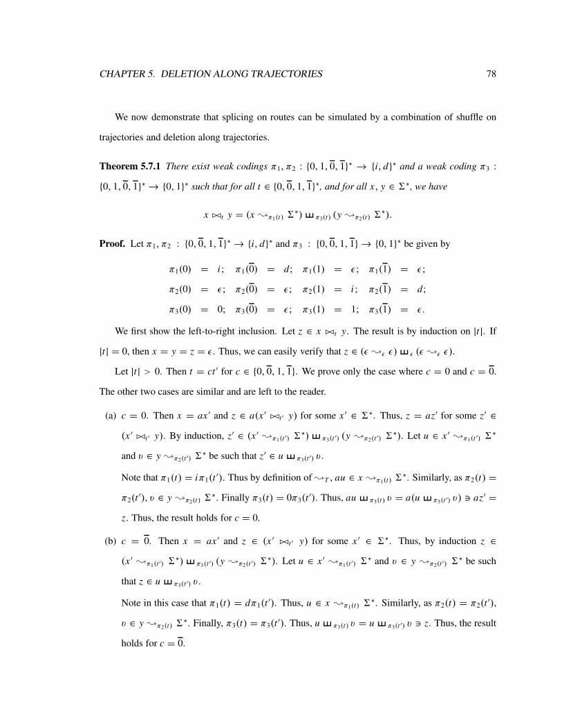
CHAPTER 5. DELETION ALONG TRAJECTORIES 78
We now demonstrate that splicing on routes can be simulated by a combination of shuffle on
trajectories and deletion along trajectories.
Theorem 5.7.1 There exist weak codings π1, π2 : {0, 1, 0, 1}∗ → {i, d}∗ and a weak coding π3 :
{0, 1, 0, 1}∗→ {0, 1}∗ such that for all t ∈ {0, 0, 1, 1}∗, and for all x, y ∈ 6∗, we have
x ⊲⊳t y = (x ;π1(t) 6∗) π3(t) (y ;π2(t) 6
∗).
Proof. Let π1, π2 : {0, 0, 1, 1}∗→ {i, d}∗ and π3 : {0, 0, 1, 1} → {0, 1}∗ be given by
π1(0) = i ; π1(0) = d; π1(1) = ǫ; π1(1) = ǫ;
π2(0) = ǫ; π2(0) = ǫ; π2(1) = i ; π2(1) = d;
π3(0) = 0; π3(0) = ǫ; π3(1) = 1; π3(1) = ǫ.
We first show the left-to-right inclusion. Let z ∈ x ⊲⊳t y. The result is by induction on |t|. If
|t| = 0, then x = y = z = ǫ. Thus, we can easily verify that z ∈ (ǫ ;ǫ ǫ) ǫ (ǫ ;ǫ ǫ).
Let |t| > 0. Then t = ct ′ for c ∈ {0, 0, 1, 1}. We prove only the case where c = 0 and c = 0.
The other two cases are similar and are left to the reader.
(a) c = 0. Then x = ax ′ and z ∈ a(x ′ ⊲⊳t ′ y) for some x ′ ∈ 6∗. Thus, z = az′ for some z′ ∈
(x ′ ⊲⊳t ′ y). By induction, z′ ∈ (x ′ ;π1(t ′) 6∗) π3(t ′) (y ;π2(t ′) 6
∗). Let u ∈ x ′ ;π1(t ′) 6∗
and v ∈ y ;π2(t ′) 6∗ be such that z′ ∈ u π3(t ′) v .
Note that π1(t) = iπ1(t′). Thus by definition of ;T , au ∈ x ;π1(t) 6
∗. Similarly, as π2(t) =
π2(t′), v ∈ y ;π2(t) 6
∗. Finally π3(t) = 0π3(t′). Thus, au π3(t) v = a(u π3(t ′) v) ∋ az′ =
z. Thus, the result holds for c = 0.
(b) c = 0. Then x = ax ′ and z ∈ (x ′ ⊲⊳t ′ y) for some x ′ ∈ 6∗. Thus, by induction z ∈
(x ′ ;π1(t ′) 6∗) π3(t ′) (y ;π2(t ′) 6
∗). Let u ∈ x ′ ;π1(t ′) 6∗ and v ∈ y ;π2(t ′) 6
∗ be such
that z ∈ u π3(t ′) v .
Note in this case that π1(t) = dπ1(t′). Thus, u ∈ x ;π1(t) 6
∗. Similarly, as π2(t) = π2(t′),
v ∈ y ;π2(t) 6∗. Finally, π3(t) = π3(t
′). Thus, u π3(t) v = u π3(t ′) v ∋ z. Thus, the result
holds for c = 0.

CHAPTER 5. DELETION ALONG TRAJECTORIES 79
We now prove the reverse inclusion. Let z ∈ (x ;π1(t) 6∗) π3(t) (y ;π2(t) 6
∗). We show the
result by induction on t . For |t| = 0, t = ǫ. Thus π1(t) = π2(t) = π3(t) = ǫ. By definition of t ,
L1 ǫ L2 is non-empty if and only if ǫ ∈ L1∩ L2, which implies z = ǫ. Thus, ǫ ∈ (x ;ǫ 6∗), and
similarly for y in place of x . By definition of ;t , this implies that x = y = ǫ. Thus, z ∈ x ⊲⊳t y,
by definition. The inclusion is proven for |t| = 0.
Let |t| > 0. Thus, there is some c ∈ {0, 0, 1, 1}, and t ′ ∈ {0, 0, 1, 1}∗ such that t = ct ′. We
distinguish between four cases, for each choice of c in {0, 0, 1, 1}, however, we only prove the cases
c = 0 and c = 0. The other two cases are very similar, and are left to the reader.
(a) c = 0. Note that π1(t) = iπ1(t′), π2(t) = π2(t
′) and π3(t) = 0π3(t′). Let u, v ∈ 6∗ be words
such that u ∈ x ;π1(t) 6∗, v ∈ y ;π2(t) 6
∗ and z ∈ u π3(t) v .
As π3(t) = 0π3(t′), we have, by definition of t , that u = au′, z = az′ and z′ ∈ u′ π3(t ′) v
for some a ∈ 6 and u′, z′ ∈ 6∗. Now, as au′ ∈ x ;iπ1(t ′) 6∗, there exists x ′ ∈ 6∗ such that
x = ax ′ and u′ ∈ x ′ ;π1(t ′) 6∗. Also, note that v ∈ y ;π2(t ′) 6
∗. Thus, combining these
yields that
z′ ∈ (x ′ ;π1(t ′) 6∗) π3(t ′) (y ;π2(t ′) 6
∗).
By induction, z′ ∈ x ′ ⊲⊳t ′ y. Thus,
z = az′ ∈ a(x ′ ⊲⊳t ′ y) = ax ′ ⊲⊳0t ′ y = x ⊲⊳t y.
Thus, the inclusion is proven.
(b) c = 0. Then π1(t) = dπ1(t′), π2(t) = π2(t
′) and π3(t) = π3(t′). Let u, v ∈ 6∗ be such that
u ∈ x ;π1(t) 6∗, v ∈ y ;π2(t) 6
∗ and z ∈ u π3(t) v .
As u ∈ x ;π1(t) 6∗, let u0 ∈ 6∗ be such that u ∈ x ;π1(t) u0. As π1(t) = dπ1(t
′),
there are some b ∈ 6, x ′, u′0 ∈ 6∗ such that x = bx ′, u0 = bu′0 and u ∈ x ′ ;π1(t ′) u′0.
Thus, u ∈ x ′ ;π1(t ′) 6∗. Note that v ∈ y ;π2(t ′) 6
∗. Thus, z ∈ u π3(t ′) v ⊆ (x ′ ;π1(t ′)
6∗) π3(t ′) (y ;π2(t ′) 6∗). By induction, z ∈ x ′ ⊲⊳t ′ y. Thus, we can see that (bx ′ ⊲⊳t y) =
x ′ ⊲⊳t ′ y ∋ z. This proves the inclusion.

CHAPTER 5. DELETION ALONG TRAJECTORIES 80
The result is now proven.
Corollary 5.7.2 There exist weak codings π1, π2 : {0, 1, 0, 1}∗ → {i, d}∗ and π3 : {0, 1, 0, 1}∗ →
{0, 1}∗ such that for all T ⊆ {0, 0, 1, 1}∗ and L1, L2 ⊆ 6∗,
L1 ⊲⊳T L2 =⋃
t∈T
(L1 ;π1(t) 6∗) π3(t) (L2 ;π2(t) 6
∗).
Unfortunately, the identity
L1 ⊲⊳T L2 = (L1 ;π1(T ) 6∗) π3(T ) (L2 ;π2(T ) 6
∗)
does not hold in general, even if L1, L2 are singletons and |T | = 2. For example, if L1 = {ab}, L2 =
{cd} and T = {0011, 0011}, then
L1 ⊲⊳T L2 = {bc, ad};
(L1 ;π1(T ) 6∗) π3(T ) (L2 ;π2(T ) 6
∗) = {ac, ad, bc, bd}.
However, if T is a unary set of routes, by which we mean that T ⊆ {0, 0}∗1∗, then we have the
following result, which is easily established:
Corollary 5.7.3 Let T ⊆ {0, 0}∗1∗. Then for all L ⊆ 6∗,
L ⊲⊳T 6∗ = L ;π1(T ) 6
∗.
We refer the reader to Mateescu [144] for a discussion of unary operations defined by splicing on
routes. As an example, consider that with T = {0n0n
: n ≥ 0}1∗, L ⊲⊳T 6∗ = 1
2(L), where 1
2(L)
was given in Section 5.4.
5.8 Inverse Word Operations
In this section, we show that deletion along trajectories constitutes the inverse of shuffle on trajec-
tories, in the sense introduced by Kari [106].

CHAPTER 5. DELETION ALONG TRAJECTORIES 81
We now define a word operation for our purposes. Given an alphabet 6∗, a word operation is
any binary function ⋄ : (6∗)2 → 26∗. We usually denote a word operation as an infix operator. A
word operation is extended to languages in a monotone way, as we have already seen for shuffle and
deletion along trajectories: given L1, L2 ⊆ 6∗,
L1 ⋄ L2 =⋃
x∈L1y∈L2
x ⋄ y.
Note that unlike Hsiao et al. [69], we do not make any assumptions about the action of ⋄ on ǫ as an
argument.
5.8.1 Left Inverse
Given two binary word operations ⋄, ⋆ : (6∗)2 → 26∗, we say that ⋄ is a left-inverse of ⋆ [106,
Defn. 4.1] if, for all u, v,w ∈ 6∗,
w ∈ u ⋆ v ⇐⇒ u ∈ w ⋄ v.
For instance, the operations of concatenation and right-quotient are left-inverses of each other, as
w = uv iff u ∈ w/v .
Let τ : {0, 1}∗ → {i, d}∗ be the morphism given by τ(0) = i and τ(1) = d. Then we have the
following characterization of left-inverses:
Theorem 5.8.1 Let T ⊆ {0, 1}∗ be a set of trajectories. Then T and ;τ (T ) are left-inverses of
each other.
Proof. We show that for all t ∈ {0, 1}∗, w ∈ u t v ⇐⇒ u ∈ w ;τ (t) v. The proof is by
induction on |w|. For |w| = 0, we have w = ǫ. Thus, by definition of t and ;t , we have that
ǫ ∈ u t v ⇐⇒ u = v = t = ǫ ⇐⇒ u ∈ (ǫ ;τ (t) v).
Let w ∈ 6∗ with |w| > 0 and assume that the result is true for all words shorter than w. Let
w = aw′ for a ∈ 6.

CHAPTER 5. DELETION ALONG TRAJECTORIES 82
First, assume that aw′ ∈ u t v . As |t| = |w|, we have that t 6= ǫ. Let t = et ′ for some
e ∈ {0, 1}. There are two cases:
(a) If e = 0, then we have that u = au′ and that w′ ∈ u′ t ′ v . By induction, u′ ∈ w′ ;τ (t ′) v .
Thus,
w ;τ (t) v = (aw′ ;iτ (t ′) v)
= a(w′ ;τ (t ′) v) ∋ au′ = u.
(b) If e = 1, then we have that v = av ′ and w′ ∈ u t ′ v′. By induction, u ∈ w′ ;τ (t ′) v
′. Thus,
w ;τ (t) v = (aw′ ;dτ (t ′) av ′)
= (w′ ;τ (t ′) v′) ∋ u.
Thus, we have that in both cases u ∈ w ;τ (t) v .
Now, let us assume that u ∈ w ;τ (t) v . As |t| = |τ(t)| = |w| ≥ 1, let t = et ′ for some
e ∈ {0, 1}. We again have two cases:
(a) If e = 0, then τ(e) = i . Then necessarily u = au′, and u′ ∈ w′ ;τ (t ′) v . By induction
w′ ∈ u′ t ′ v . Thus,
u t v = (au′ 0t ′ v)
= a(u′ t ′ v) ∋ aw′ = w.
(b) If e = 1, then τ(e) = d. Then necessarily v = av ′, and u ∈ (w′ ;τ (t ′) v′). By induction,
w′ ∈ u t ′ v′. Thus,
u t v = (u 1t ′ av′)
= a(u t ′ v′) ∋ aw′ = w.
Thus w ∈ u t v . This completes the proof.
We note that Theorem 5.8.1 agrees with the observations of Kari [106, Obs. 4.7].
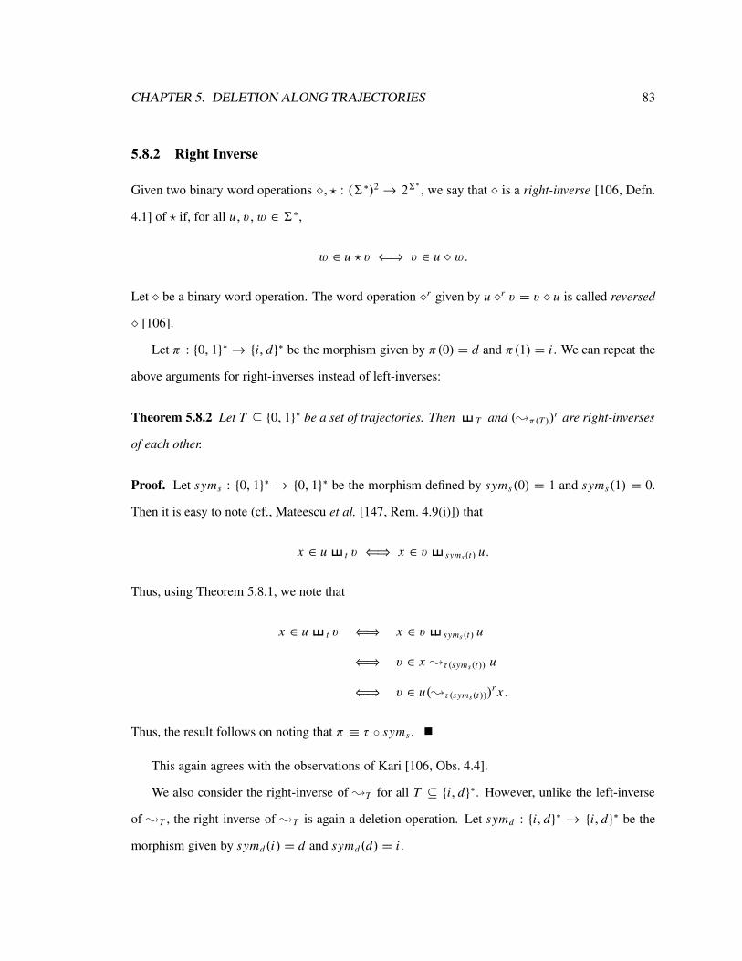
CHAPTER 5. DELETION ALONG TRAJECTORIES 83
5.8.2 Right Inverse
Given two binary word operations ⋄, ⋆ : (6∗)2 → 26∗, we say that ⋄ is a right-inverse [106, Defn.
4.1] of ⋆ if, for all u, v,w ∈ 6∗,
w ∈ u ⋆ v ⇐⇒ v ∈ u ⋄ w.
Let ⋄ be a binary word operation. The word operation ⋄r given by u ⋄r v = v ⋄ u is called reversed
⋄ [106].
Let π : {0, 1}∗ → {i, d}∗ be the morphism given by π(0) = d and π(1) = i . We can repeat the
above arguments for right-inverses instead of left-inverses:
Theorem 5.8.2 Let T ⊆ {0, 1}∗ be a set of trajectories. Then T and (;π(T ))r are right-inverses
of each other.
Proof. Let syms : {0, 1}∗ → {0, 1}∗ be the morphism defined by syms(0) = 1 and syms(1) = 0.
Then it is easy to note (cf., Mateescu et al. [147, Rem. 4.9(i)]) that
x ∈ u t v ⇐⇒ x ∈ v syms(t) u.
Thus, using Theorem 5.8.1, we note that
x ∈ u t v ⇐⇒ x ∈ v syms(t) u
⇐⇒ v ∈ x ;τ (syms(t)) u
⇐⇒ v ∈ u(;τ (syms(t)))r x .
Thus, the result follows on noting that π ≡ τ ◦ syms .
This again agrees with the observations of Kari [106, Obs. 4.4].
We also consider the right-inverse of ;T for all T ⊆ {i, d}∗. However, unlike the left-inverse
of ;T , the right-inverse of ;T is again a deletion operation. Let symd : {i, d}∗ → {i, d}∗ be the
morphism given by symd(i) = d and symd(d) = i .
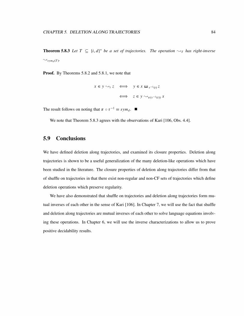
CHAPTER 5. DELETION ALONG TRAJECTORIES 84
Theorem 5.8.3 Let T ⊆ {i, d}∗ be a set of trajectories. The operation ;T has right-inverse
;symd (T ).
Proof. By Theorems 5.8.2 and 5.8.1, we note that
x ∈ y ;t z ⇐⇒ y ∈ x τ−1(t) z
⇐⇒ z ∈ y ;π(τ−1(t)) x
The result follows on noting that π ◦ τ−1 ≡ symd .
We note that Theorem 5.8.3 agrees with the observations of Kari [106, Obs. 4.4].
5.9 Conclusions
We have defined deletion along trajectories, and examined its closure properties. Deletion along
trajectories is shown to be a useful generalization of the many deletion-like operations which have
been studied in the literature. The closure properties of deletion along trajectories differ from that
of shuffle on trajectories in that there exist non-regular and non-CF sets of trajectories which define
deletion operations which preserve regularity.
We have also demonstrated that shuffle on trajectories and deletion along trajectories form mu-
tual inverses of each other in the sense of Kari [106]. In Chapter 7, we will use the fact that shuffle
and deletion along trajectories are mutual inverses of each other to solve language equations involv-
ing these operations. In Chapter 6, we will use the inverse characterizations to allow us to prove
positive decidability results.

Chapter 6
Trajectory-Based Codes
6.1 Introduction
The theory of codes is a fundamental area of formal language theory, with many important applica-
tions. The class of prefix codes is a particularly important subclass of codes, and is fundamentally
linked to the nature of concatenation as the underlying operation. Further research in codes has con-
sidered the subclasses of codes which arise from replacing catenation with other, related operations,
most notably shuffle (the hypercodes) and insertion (the outfix codes).
In this chapter, we generalize these results by considering T -codes. A T -code is any language
L satisfying the equation (L T 6+) ∩ L = ∅. Thus, we consider the natural extension of prefix
codes to all operations defined by shuffle on trajectories, and examine the properties of these classes
of languages.
The idea of studying general classes of codes has received much attention in the literature (see,
e.g., Shyr and Thierrin [186], Jurgensen et al. [99] and Jurgensen and Yu [100]). Further, the
definition of a T -code which we present can also be formulated in dependency theoretic terms (see,
e.g., Jurgensen and Konstantinidis [97] for a survey of dependency theory). Some of the results we
have obtained can be proven by appealing to dependency theory, however, our proofs are simpler in
our restricted situation.
85

CHAPTER 6. TRAJECTORY-BASED CODES 86
In addition, there are works in the literature which consider the problem of defining codes based
on arbitrary binary relations, see, e.g., the work of Jurgensen et al. [99] on codes defined by binary
relations and Shyr and Thierrin [186] for work on so-called strict binary relations. We will see that
we can also view T -codes as anti-chains under the natural binary relation defined by T .
With this research in mind, we nonetheless feel the framework of T -codes is useful in that
it helps us to see results relating to codes defined by shuffle on trajectories in a new way. The
restriction of considering only those codes defined by shuffle on trajectories gives us new insight
into these classes, including prefix-, suffix-, bi(pre)fix-, infix-, outfix-, shuffle- and hyper-codes,
by focusing our attention to classes of codes which are specific enough to allow reasoning on the
associated sets of trajectories, but general enough to encompass all of the above interesting and
well-studied classes of codes.
We also feel that introducing the idea of T -code will allow more unified results to be obtained
on the various classes of codes, since specific conditions on sets of trajectories (i.e., languages)
will be easier to obtain than more general conditions on arbitrary relations. In particular, we have
obtained results which do not appear to have been considered before in the more general framework
of dependency theory or binary relations.
Further, we note that the notion of T -codes is useful elsewhere in the study of iterated shuffle
and deletion along trajectories, for instance, in analyzing the shuffle-base of certain languages. We
examine this relationship in Section 8.9. Finally, the study of T -codes, much like the study of shuffle
on trajectories in general, allows us to examine what assumptions must be made on an operation in
order for certain results to follow. We find that even when these assumptions have been studied in
the literature, the proofs obtained for the specific cases of shuffle on trajectories are often simpler.
We obtain several interesting results on T -codes. We generalize a result relating outfix and
hyper-codes and the notion of (embedding-) convexity to all T -codes. Further, the known closure
properties of shuffle on trajectories allow us to easily conclude positive decidability results for the
problem of determining membership in classes of T -codes (including maximal T -codes), which
were previously determined by ad-hoc constructions in the literature.

CHAPTER 6. TRAJECTORY-BASED CODES 87
We note that recently, a more general concept than T -codes has been independently introduced
by Kari et al. [108], motivated by the bonding of strands of DNA and DNA computing. Their
framework, called bond-free properties, is also a general setting which involves shuffle on trajecto-
ries. Generally, the motivations for our work and those of the work by Kari et al. are different, and
the decidability results which are similar are noted below.
6.2 Definitions
Recall that a non-empty language L is a code if u1u2 · · · um = v1v2 · · · vn where ui , v j ∈ L for
1 ≤ i ≤ m and 1 ≤ j ≤ n implies that n = m and ui = vi for 1 ≤ i ≤ n. For background on codes,
we refer the reader to Berstel and Perrin [18], Jurgensen and Konstantinidis [97] or Shyr [184].
We now come to the main definition of this chapter. Let L ⊆ 6+ be a language. Then, for any
T ⊆ {0, 1}∗, we say that L is a T -code if L is non-empty and (L T 6+) ∩ L = ∅. If 6 is an
alphabet and T ⊆ {0, 1}∗, let PT (6) denote the set of all T -codes over 6. If 6 is understood, we
will denote the set of T -codes over 6 by PT .
There has been much research into the idea of T -codes for particular T ⊆ {0, 1}∗, including
(a) prefix codes, corresponding to T = 0∗1∗ (concatenation);
(b) suffix codes, corresponding to T = 1∗0∗ (anti-catenation);
(c) biprefix (or bifix) codes, corresponding to T = 0∗1∗ + 0∗1∗ (bi-catenation);
(d) outfix and infix codes, corresponding to T = 0∗1∗0∗ (insertion) and T = 1∗0∗1∗, (bi-polar
insertion) respectively;
(e) shuffle-codes, corresponding to bounded sets of trajectories such as
(e-i) T = (0∗1∗)n for fixed n ≥ 1 (prefix codes of index n);
(e-ii) T = (1∗0∗)n for fixed n ≥ 1 (suffix codes of index n);
(e-iii) T = 1∗(0∗1∗)n for fixed n ≥ 1 (infix codes of index n);
(e-iv) T = (0∗1∗)n0∗ for fixed n ≥ 1 (outfix codes of index n);

CHAPTER 6. TRAJECTORY-BASED CODES 88
(f) hypercodes, corresponding to T = (0+ 1)∗ (arbitrary shuffle);
(g) k-codes, corresponding to T = 0∗1∗0≤k (k-catenation, see Kari and Thierrin [114]) for fixed
k ≥ 0; and
(h) for arbitrary k ≥ 1, codes defined by the sets of trajectories P Pk = 0∗ + (0∗1∗)k−10∗1+,
P Sk = 0∗+1+0∗(1∗0∗)k−1, P Ik = 0∗+(1∗0∗)k1+, SIk = 0∗+1+(0∗1∗)k , P Bk = P Pk∪ P Sk
and B Ik = P Ik ∪ SIk , see Long [135], or Ito et al. [77] for P I1, SI1.
For a list of references related to (a)–(f), see Jurgensen and Konstantinidis [97, pp. 549–553]. In
this chapter, we let
H = (0+ 1)∗, (6.1)
P = 0∗1∗, (6.2)
S = 1∗0∗, (6.3)
I = 1∗0∗1∗, (6.4)
O = 0∗1∗0∗, and (6.5)
B = P ∪ S. (6.6)
6.3 General Properties of T -codes
We can give two alternate characterizations of T -codes in terms of the left and right inverses of
shuffle on trajectories. These are given via the morphisms τ, π : {0, 1}∗ → {i, d}∗ defined by
τ(0) = i , τ(1) = d, π(0) = d and π(1) = i . We can easily prove the following two equalities by
appealing to Theorems 5.8.1 and 5.8.2. In particular, we have for all T ⊆ {0, 1}∗, and all 6,
PT (6) = {L ⊆ 6+ : (L ;τ (T ) 6+) ∩ L = ∅}, (6.7)
PT (6) = {L ⊆ 6+ : L ;π(T ) L ⊆ {ǫ}}. (6.8)
For some particular T , these characterizations are well-known, e.g., (6.7) for T = 0∗1∗ is given by
Berstel and Perrin [18, Prop. II.1.1.(ii)].
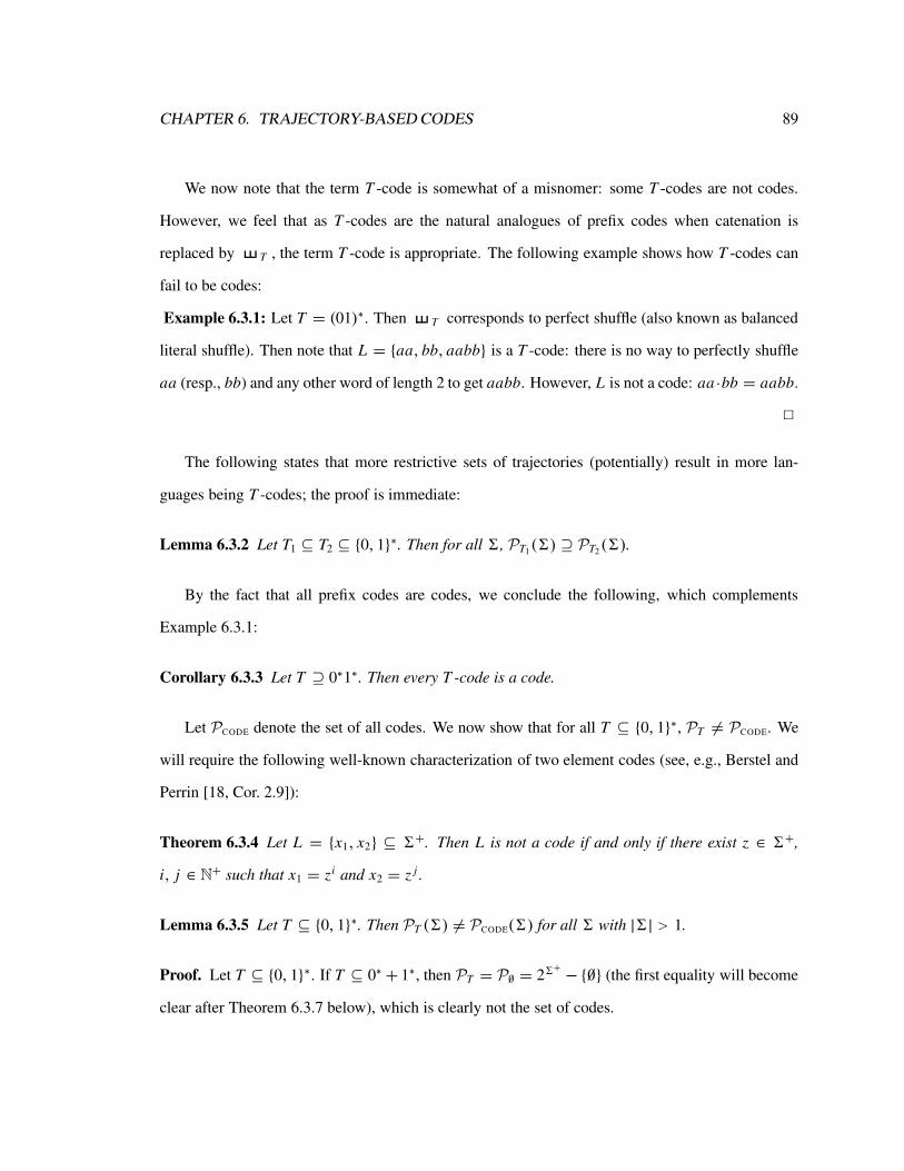
CHAPTER 6. TRAJECTORY-BASED CODES 89
We now note that the term T -code is somewhat of a misnomer: some T -codes are not codes.
However, we feel that as T -codes are the natural analogues of prefix codes when catenation is
replaced by T , the term T -code is appropriate. The following example shows how T -codes can
fail to be codes:
Example 6.3.1: Let T = (01)∗. Then T corresponds to perfect shuffle (also known as balanced
literal shuffle). Then note that L = {aa, bb, aabb} is a T -code: there is no way to perfectly shuffle
aa (resp., bb) and any other word of length 2 to get aabb. However, L is not a code: aa ·bb = aabb.
2
The following states that more restrictive sets of trajectories (potentially) result in more lan-
guages being T -codes; the proof is immediate:
Lemma 6.3.2 Let T1 ⊆ T2 ⊆ {0, 1}∗. Then for all 6, PT1(6) ⊇ PT2
(6).
By the fact that all prefix codes are codes, we conclude the following, which complements
Example 6.3.1:
Corollary 6.3.3 Let T ⊇ 0∗1∗. Then every T -code is a code.
Let PCODE denote the set of all codes. We now show that for all T ⊆ {0, 1}∗, PT 6= PCODE. We
will require the following well-known characterization of two element codes (see, e.g., Berstel and
Perrin [18, Cor. 2.9]):
Theorem 6.3.4 Let L = {x1, x2} ⊆ 6+. Then L is not a code if and only if there exist z ∈ 6+,
i, j ∈ N+ such that x1 = zi and x2 = z j .
Lemma 6.3.5 Let T ⊆ {0, 1}∗. Then PT (6) 6= PCODE(6) for all 6 with |6| > 1.
Proof. Let T ⊆ {0, 1}∗. If T ⊆ 0∗+ 1∗, then PT = P∅ = 26+ −{∅} (the first equality will become
clear after Theorem 6.3.7 below), which is clearly not the set of codes.

CHAPTER 6. TRAJECTORY-BASED CODES 90
Thus, we can assume that there is some t ∈ T with |t|1, |t|0 > 0. Let n = |t|0. Consider that
t ∈ 0nt {0, 1}+. Thus L = {t, 0n} ⊆ {0, 1}+ is not a T -code.
If L is not a code, then t and 0n are powers of the same word, i.e., t ∈ 0∗. This contradicts our
choice of t . Thus, L is a code.
We also observe that PT1∩ PT2
= PT1∪T2. We note that the dual case does not hold. In the
case of PT1∩T2, we have the inclusion PT1
∩ PT2⊆ PT1∩T2
. But of course equality does not hold in
general. For example, with T1 = 0∗1∗ and T2 = 1∗0∗, PT1∩T2= P0∗+1∗ = P∅ = 26
+ − {∅} (the
second equality will be established in Theorem 6.3.7 below). However, PT1∩PT2
= PT1∪T2, the set
of biprefix codes.
We can also ask if T1 ⊂ T2 (⊂ denotes proper inclusion) implies that PT1⊃ PT2
. The answer is
yes, as long as the difference between T2 and T1 contains non-unary words.
Theorem 6.3.6 Let T1 ⊂ T2 be such that (T2 − T1) ∩ 0∗ + 1∗ 6= ∅. Then for all 6 with |6| ≥ 2,
PT1(6) ⊃ PT2
(6).
Proof. Let t ∈ (T2 − T1) ∩ 0∗ + 1∗. Let t0, t1 be defined by t0 = 0|t |0 and t1 = 1|t |1 . Then
note that t0, t1 6= ǫ, by our choice of t . Thus, we have that {t, t0} ⊆ {0, 1}+. We claim that
L t = {t, t0} ∈ PT1− PT2
.
To see that L t /∈ PT2, note that t ∈ t0 t t1. As t ∈ T2 and t1 6= ǫ, L t is not a T2-code. Assume
that L t is not a T1-code. As |t| > |t0|, the only way that L t can fail to be a T1-code is if there exists
x ∈ {0, 1}+ such that t ∈ t0 T1x . By definition, as |t|0 = |t0|, we must have that x = t1 = 1|t |1 .
But t ∈ t0 T1t1 only if t ∈ T1, which is not the case.
Theorem 6.3.7 Let T1 ⊂ T2 and T2−T1 ⊆ 1∗+0∗. Then for all6 with |6| > 1, PT1(6) = PT2
(6).
Proof. Assume, contrary to what we want to prove, that L ⊆ 6+ is a T1-code which is not a T2-
code. As L is not a T2-code, there exist x, z ∈ L , y ∈ 6+ and t ∈ T2 such that z ∈ x t y. As L is
a T1-code, z /∈ x T1y. Thus t /∈ T1. By assumption, this implies that t ∈ 1∗ + 0∗.

CHAPTER 6. TRAJECTORY-BASED CODES 91
If t ∈ 1∗, then by definition of T , z ∈ x t y implies that x = ǫ, contrary to our choice of
L . If t ∈ 0∗, then by definition, y = ǫ, contrary to our choice of y. In either case, we have arrived
at a contradiction.
Thus, we have completely characterized when reducing a set of trajectories corresponds to an
increase in the languages which are T -codes. In particular, we note the following corollary:
Corollary 6.3.8 Let T1, T2 ⊆ {0, 1}∗ be regular sets of trajectories. Then it is decidable whether
PT1= PT2
.
Proof. We note that PT1= PT2
if and only if (T1 − T2) ∪ (T2 − T1) ⊆ 0∗ + 1∗. Since T1, T2 are
regular, so is (T1 − T2) ∪ (T2 − T1), and the inclusion is decidable.
We now examine further questions of decidability.
Lemma 6.3.9 Let T ⊆ {0, 1}∗ be a fixed CF set of trajectories. Then given a regular language L,
it is decidable whether L is a T -code.
Proof. Since L is regular and T is a CFL, L T 6+, and (L T 6
+)∩ L are CFLs. Thus, we can
test whether (L T 6+) ∩ L = ∅, which precisely defines L being a T -code.
This result can also be proved using dependency theory. As every T ⊆ {0, 1}∗ defines a 3-
dependence system, and every context-free T defines a dependence system whose associated sup-
port can be accepted by a 3-tape PDA, the problem of determining membership in PT is decidable;
see Jurgensen and Konstantinidis [97, Sect. 9] for details. Further, Kari et al. [108, Thm. 4.7] estab-
lish a similar decidability result in their framework of bond-free properties. When translated to our
setting, it states that given T, R regular, we can decide if R ∈ PT .
A class of languages C is said to have decidable membership problem if, given L ⊆ 6∗ with
L ∈ C, it is decidable whether x ∈ L for an arbitrary x ∈ 6∗. We have the following positive
decidability result:

CHAPTER 6. TRAJECTORY-BASED CODES 92
Lemma 6.3.10 Let C be a class of languages with decidable membership. Let T ⊆ {0, 1}∗ be a set
of trajectories such that T ∈ C. Then given a finite language F, it is decidable whether F ∈ PT .
Proof. Let F ⊆ 6+ be a finite set. Let n = max{|x| : x ∈ F}. Since membership in T is
decidable, we can test all t ∈ {0, 1}≤n for membership in T . Thus, we can effectively compute
T≤n = T ∩ {0, 1}≤n . It is easily observed that F ∩ (F T≤n L) = F ∩ (F T L) for all L .
Since F, T ≤n,6+ are regular, we can test F ∩ (F T≤n 6+) = ∅. Thus, the result follows.
We conclude with the following method of constructing a T -code from an arbitrary language.
Lemma 6.3.11 Let T ⊆ {0, 1}∗. Let L ⊆ 6+ be a non-empty language. Then L0 = L −
(L T 6+) ∈ PT (6).
Proof. As L0 ⊆ L and T is a monotone operation, (L0 T 6+) ⊆ (L T 6
+). Thus, L0 ∩
(L0 T 6+) ⊆ L0 ∩ (L T 6
+) and L0 ∩ (L T 6+) = ∅ by definition of L0.
The following is proven in exactly the same manner as Lemma 6.3.11:
Lemma 6.3.12 Let T ⊆ {0, 1}∗. Let L ⊆ 6+ be a non-empty language. Then L0 = L − (L ;τ (T )
6+) ∈ PT (6).
6.4 The Binary Relation defined by Trajectories
We can also define T -codes by appealing to a definition based on binary relations. In particular, for
T ⊆ {0, 1}∗, define ωT as follows: for all x, y ∈ 6∗,
x ωT y ⇐⇒ y ∈ x T 6∗.
Then it is clear that L ⊆ 6+ is a T -code if and only if L is an anti-chain under ωT (i.e, x, y ∈ L
and x ωT y implies x = y).
We note that the relation analogous to ωT for infinite words and ω-trajectories was defined by
Kadrie et al. [101], and its properties were briefly investigated. Kadrie et al. do not investigate the
CHAPTER 6. TRAJECTORY-BASED CODES 93
analogous relation with the same amount of detail as below and do not appear to be motivated by
the theory of codes.
We immediately note that if T1, T2 ⊆ {0, 1}∗ are sets of trajectories, there is not necessarily a
set of trajectories T such that ωT = ωT1∩ ωT2
, i.e., such that x ωT y ⇐⇒ (x ωT1y) ∧ (x ωT2
y).
For instance, for P = 0∗1∗ and S = 1∗0∗, the relation ωP ∩ωS is given by ≤d , where x ≤d y if and
only if there exist u, v ∈ 6∗ such that y = xu = vx . This relation cannot be represented by a set of
trajectories:
Lemma 6.4.1 For all T ⊆ {0, 1}∗, ωT 6=≤d .
Proof. Assume that there exists T ⊆ {0, 1}∗ such that ωT =≤d . Consider L0 = {0, 00}. As
0 ≤d 00, we must have that 0 ωT 00. Thus, 00 ∈ 0 T 0 and {01, 10} ∩ T 6= ∅. Thus, without loss
of generality assume that 01 ∈ T . The case 10 ∈ T is similar.
Consider now L1 = {0, 01}. We observe that L1 is an anti-chain under ≤d , i.e., 0 ≤d 01 does
not hold. However, 01 ∈ 0 T 1. Thus, 0 ωT 01, and ωT 6=≤d .
For a discussion of ≤d , see Shyr [184, Ch. 8]. We now recall some of the properties of the
binary relations ωT that will be useful. In what follows, we will refer to T having a property P if
and only if ωT has property P .
6.4.1 Anti-symmetry
Recall that a binary relation ρ is anti-symmetric if x ρ y and y ρ x implies x = y. We note that ωT
always gives an anti-symmetric binary relation:
Lemma 6.4.2 Let T ⊆ {0, 1}∗. The relation ωT is anti-symmetric.
Proof. Let x, y ∈ 6∗ be such that x ωT y ωT x . Then let t1, t2 ∈ T and α, β ∈ 6∗ be such
that x ∈ y t1 α and y ∈ x t2 β. By definition of shuffle on trajectories, |x| = |y| + |α| and
|y| = |x| + |β|. Thus, |α| = |β| = 0, i.e., α = β = ǫ. But now x ∈ y t1 ǫ, which implies that
x = y, again by definition of shuffle on trajectories.

CHAPTER 6. TRAJECTORY-BASED CODES 94
6.4.2 Reflexivity
Recall that a binary relation ρ on 6∗ is reflexive if x ρ x for all x ∈ 6∗.
Lemma 6.4.3 Let T ⊆ {0, 1}∗. Then T is reflexive if and only if 0∗ ⊆ T .
Proof. Let 0∗ ⊆ T . Then x ∈ x 0|x | ǫ, i.e., x ωT x . Thus ωT is reflexive. For the converse, let
x ∈ x T 6∗ for all x ∈ 6∗. Then clearly 0|x | ∈ T for all x ∈ 6∗, which implies 0∗ ⊆ T .
Corollary 6.4.4 Given a CF set T ⊆ {0, 1}∗ of trajectories, it is decidable whether T is reflexive.
Proof. Let T ′ = T ∩ 0∗, which is a unary CFL, and thus regular. In fact, if T is effectively
context-free, then T ′ is effectively regular. We can then test the equality 0∗ = T ′.
6.4.3 Positivity
A binary relation ρ on 6∗ is said to be positive if ǫ ρ x for all x ∈ 6∗.
Lemma 6.4.5 Let T ⊆ {0, 1}∗. Then T is positive if and only if 1∗ ⊆ T .
Proof. Let 1∗ ⊆ T . Then u ∈ ǫ 1|u| u for all u ∈ 6∗, whereby ǫ ωT u, as 1|u| ∈ T . The reverse
implication is similarly established.
Corollary 6.4.6 Given a CF set T ⊆ {0, 1}∗ of trajectories, it is decidable whether T is positive.
6.4.4 ST-Strictness
Shyr and Thierrin [186] define the concept of a strict binary relation. To avoid confusion with the
concept of a strict ordering (see, e.g., Choffrut and Karhumaki [24, Sect. 7.1]), we will call a binary
relation ρ on 6∗ ST-strict if it satisfies the following four properties:
(a) ρ is reflexive;
(b) ρ is positive;

CHAPTER 6. TRAJECTORY-BASED CODES 95
(c) for all u, v ∈ 6∗, u ρ v implies |u| ≤ |v|;
(d) for all u, v ∈ 6∗, u ρ v and |u| = |v| implies u = v .
We now consider T such that ωT is ST-strict. We first note that conditions (c) and (d) are
satisfied by all T . Indeed, if u ωT v , then v ∈ u T 6∗, which implies that |v| ≥ |u|. Further, if
|u| = |v|, then u ωT v implies that v ∈ u T ǫ, which implies that u = v .
Thus, as we already have necessary and sufficient conditions on T being reflexive and positive,
the following results are immediate:
Corollary 6.4.7 Let T ⊆ {0, 1}∗. Then T is ST-strict if and only if 0∗ + 1∗ ⊆ T .
Corollary 6.4.8 Given a CF set T ⊆ {0, 1}∗ of trajectories, it is decidable whether T is ST-strict.
Corollary 6.4.9 Let T1, T2 ⊆ {0, 1}∗ be ST-strict. Then PT1= PT2
if and only if T1 = T2.
6.4.5 Cancellativity
A binary relation ρ on 6∗ is said to be left-cancellative (resp., right-cancellative) if uv ρ ux implies
v ρ x (resp., vu ρ xu implies v ρ x) for all u, v, x ∈ 6∗. The relation ρ is cancellative if it is both
left- and right-cancellative.
Given T ⊆ {0, 1}∗, we define two sets of trajectories, s(T ), p(T ) ⊆ {0, 1}∗, as follows:
p(T ) = {t11 j : t1t2 ∈ T, 0 ≤ j ≤ |t2|},
s(T ) = {1 j t2 : t1t2 ∈ T, 0 ≤ j ≤ |t1|}.
Lemma 6.4.10 Let T ⊆ {0, 1}∗. Then T is left-cancellative (resp., right-cancellative) if s(T ) ⊆ T
(resp., p(T ) ⊆ T ).
Proof. We establish the result for left-cancellativity only; the other case is symmetric. Let s(T ) ⊆
T . Then let u, v, x ∈ 6∗ be such that uvωT ux . Let t ∈ T and α ∈ 6∗ chosen so that ux ∈ uv t α.
Write t = t1t2 and α = α1α2 so that ux ∈ (u t1 α1)(v t2 α2). Let β1, β2 ∈ 6∗ be chosen so that

CHAPTER 6. TRAJECTORY-BASED CODES 96
β1 ∈ u t1 α1, β2 ∈ v t2 α2 and ux = β1β2. As |β1| = |u| + |α1| ≥ |u|, there exists γ ∈ 6∗ such
that uγ = β1 and x = γβ2. Note that |γ | ≤ |β1| = |t1|. Thus,
x ∈ γ (v t2 α2).
Let t3 = 1|γ |t2 ∈ s(T ). By assumption, t3 ∈ T . Further,
x ∈ v t3 γ α2.
We conclude that v ωT x .
Corollary 6.4.11 Let T ⊆ {0, 1}∗. If s(T ) ∪ p(T ) ⊆ T , then T is cancellative.
We now consider a condition of Jurgensen et al. [99]. Say that a binary relation ρ on 6∗ is
leviesque if uv ρ xy implies that u ρ x or v ρ y, for all u, v, x, y ∈ 6∗.
Lemma 6.4.12 Let T ⊆ {0, 1}∗. If s(T ) ∪ p(T ) ⊆ T , then T is leviesque.
Proof. Let rs ωT xy. Then there exist t ∈ T and α ∈ 6∗ such that xy ∈ rs t α. Then there exist
factorizations t = t1t2, α = α1α2 such that xy ∈ (r t1 α1)(s t2 α2). Let β1, β2 ∈ 6∗ be such that
β1 ∈ r t1 α1, β2 ∈ s t2 α2 and xy = β1β2. There are two cases:
(i) If |x| ≥ |β1|, then there exists γ ∈ 6∗ such that x = β1γ and γ y = β2. Note that |γ | ≤
|β2| = |t2|. Consider that x = β1γ ∈ (r t11|γ | α1γ ). As t11|γ | ∈ p(T ) ⊆ T , r ωT x .
(ii) If |x| ≤ |β1|, there exists γ ∈ 6∗ such that xγ = β1 and y = γβ2. Note that |γ | ≤ |β1| = |t1|.
In this case, y = γβ2 ∈ (s 1|γ |t2 γ α2). Thus, as 1|γ |t2 ∈ s(T ) ⊆ T , we have s ωT y.
Thus, rs ωT xy implies (r ωT x) or (s ωT y).
6.4.6 Compatibility
Let ρ be a binary relation on 6∗. Then we say that ρ is left-compatible (resp., right-compatible)
if, for all u, v,w ∈ 6∗, u ρ v implies that wu ρ wv (resp., uw ρ vw). If ρ is both left- and right-
compatible, we say it is compatible.

CHAPTER 6. TRAJECTORY-BASED CODES 97
Lemma 6.4.13 Let T ⊆ {0, 1}∗. Then T is right-compatible (resp., left-compatible) if and only if
T 0∗ ⊆ T (resp., 0∗T ⊆ T ).
Proof. We establish the result for right-compatibility. The result for left-compatibility is symmet-
rical.
Let T 0∗ ⊆ T . Let u, v,w ∈ 6∗ with u ωT v . Then there exist t ∈ T and α ∈ 6∗ such that
v ∈ u t α. As t ′ = t0|w| ∈ T , vw ∈ uw t ′ α. Thus uw ωT vw.
Assume that T 0∗ is not a subset of T . Then there exist t ∈ T and i ∈ N such that t0i /∈ T . Let
j = |t|0 and k = |t|1. Consider that 0 j ωT t , as t ∈ 0 jt 1k . However, 0 j · 0i ωT t · 0i does not
hold, as t0i ∈ 0 j+iT 1k would imply that t0i ∈ T . Thus, T is not right-compatible.
The following corollary is immediate; it is identical to the condition that T 0∗ ∪ 0∗T ⊆ T :
Corollary 6.4.14 Let T ⊆ {0, 1}∗. Then T is compatible if and only if 0∗T 0∗ ⊆ T .
Corollary 6.4.15 Given a regular set T ⊆ {0, 1}∗ of trajectories, it is decidable whether T is (left-
or right-) compatible.
Lemma 6.4.16 Given an LCF set T ⊆ {0, 1}∗ of trajectories, it is undecidable whether T is (left-
or right-) compatible.
Proof. We prove only the case for left-compatibility; the other cases are similar and are left to the
reader. We apply a meta-theorem of Hunt and Rosenkrantz (Theorem 2.5.3). First, we note that
T = {0, 1}∗ is left-compatible.
Let T = {0n1n : n ≥ 0}. We claim that there is no LCF set T ′ ⊆ {0, 1}∗ of trajectories
and trajectory t ∈ {0, 1}+ such that T = T ′/t . Assume that there were such T ′, t . Then as
ǫ ∈ T = T ′/t , we must have t ∈ T ′. As T ′ is left-compatible, we have that 0t ∈ T ′. Thus
0 ∈ T ′/t = T , a contradiction. Thus, the set
{T : ∃ left-compatible LCF T ′ ⊆ {0, 1}∗, t ∈ {0, 1}+ such that T = T ′/t}
is a proper subset of the LCFLs. Therefore, we may apply Theorem 2.5.3, and it is undecidable
whether a given LCF set of trajectories is left-compatible.

CHAPTER 6. TRAJECTORY-BASED CODES 98
Recall the definitions of P, S and O given by (6.2), (6.3) and (6.5). Let PP ,PS,PO be the class
of prefix, suffix and outfix codes. We can conclude the following corollary about positive T which
satisfy compatibility conditions. Parts (a) and (b) of the following result have been established for
all partial orders by Jurgensen et al. [99]; the proofs are immediate in our case:
Corollary 6.4.17 Let T ⊆ {0, 1}∗ be positive. Then the following hold:
(a) if T is left-compatible, then PT ⊆ PP ;
(b) if T is right-compatible, then PT ⊆ PS;
(c) if T is compatible, then PT ⊆ PO .
Furthermore, in each case equality of the classes holds if and only if it holds for the sets of trajec-
tories involved.
Proof. We prove (b); the rest are similar. If T is positive then 1∗ ⊆ T . If T is right compatible,
then T 0∗ ⊆ T . Thus, S = 1∗0∗ ⊆ T . The inclusions thus hold by Lemma 6.3.2; for the equalities,
we note that P, S, O are ST-strict and for each of (a),(b) and (c), T is also ST-strict.
6.4.7 Transitivity
Recall that a binary relation ρ on 6∗ is said to be transitive if x ρ y and y ρ z imply that x ρ z
for all x, y, z ∈ 6∗. We now consider conditions on T which will ensure that ωT is a transitive
relation. Transitivity is often, but not always, a property of the binary relations defining the classic
code classes. For instance, both bi-prefix and outfix codes are defined by binary relations which are
not transitive, and hence not a partial order. We now give necessary and sufficient conditions on a
set T of trajectories defining a transitive binary relation.
First, we define three morphisms we will need. Let D = {x, y, z} and ϕ, σ,ψ : D∗ → {0, 1}∗

CHAPTER 6. TRAJECTORY-BASED CODES 99
be the morphisms given by
ϕ(x) = 0, σ (x) = 0, ψ(x) = 0,
ϕ(y) = 0, σ (y) = 1, ψ(y) = 1,
ϕ(z) = 1, σ (z) = ǫ, ψ(z) = 1.
Note that these morphisms are similar to the substitutions defined by Mateescu et al. [147], whose
purpose is to give necessary and sufficient conditions on a set T of trajectories defining an associa-
tive operation. Indeed, our condition is a weakening of their conditions, which, intuitively, reflects
the fact that any associative operation T defines a transitive binary relation ωT (note, however,
that T = 1∗0∗1∗ is transitive but not associative).
Theorem 6.4.18 Let T ⊆ {0, 1}∗. Then T is transitive if and only if
ψ(ϕ−1(T ) ∩ σ−1(T )) ⊆ T . (6.9)
Proof. (⇐): Let T define a transitive binary relation. Let w ∈ ψ(ϕ−1(T ) ∩ σ−1(T )). Then there
exist t1, t2 ∈ T such that w ∈ ψ(ϕ−1(t1) ∩ σ−1(t2)). Let t ∈ ϕ−1(t1) ∩ σ−1(t2) be chosen so that
w ∈ ψ(t).
Consider t1. Let n ∈ N and αi , βi ∈ N be chosen for 1 ≤ i ≤ n so that
t1 =n∏
i=1
0αi 1βi .
Note that
ϕ−1(t1) =n∏
i=1
(x + y)αi zβi .
As t ∈ ϕ−1(t1) and t ∈ σ−1(t2), by definition of σ , we must have that t2 =∏n
i=1 si for si ∈ {0, 1}∗
satisfying |si | = αi . Thus, we have that |t2| = |t1|0. Furthermore, t ∈ (x p1t2 y p2) t1 z p3 , where
p1 = |t2|0, p2 = |t2|1 and p3 = |t1|1. Consider now that w ∈ ψ(t), so that
w ∈ (0p1t2 1p2) t1 1p3 .
CHAPTER 6. TRAJECTORY-BASED CODES 100
Clearly, 0p1t2 1p2 = t2. Thus, w ∈ t2 t1 1p3 , as well. By definition, we then have that 0p1 ωT
t2 ωT w. By the transitivity of T , 0p1 ωT w, i.e.,
w ∈ 0p1T {0, 1}∗.
Note that |w|1 = p2 + p3 and |w|0 = p1. The only word v over {0, 1} such that w ∈ 0p1T v is
v = 1p2+p3 (regardless of T ). That is, w ∈ 0p1T 1p2+p3 . But from this, we must have that w ∈ T .
Thus, we have that ψ(ϕ−1(T ) ∩ σ−1(T )) ⊆ T .
(⇒): Assume that ψ(ϕ−1(T )∩σ−1(T )) ⊆ T . Let u, v,w ∈ 6∗ be such that uωT v and v ωT w.
We wish to show that u ωT w. Let t1, t2 ∈ T and θ1, θ2 ∈ 6∗ be such that w ∈ v t1 θ1 and
v ∈ u t2 θ2. Thus, w ∈ (u t2 θ2) t1 θ1. Note then that |t1|0 = |t2|. Let n ∈ N and αi , βi ∈ N be
chosen for 1 ≤ i ≤ n so that
t1 =n∏
i=1
0αi 1βi .
Furthermore, let t2 =∏n
i=1 si be so that |si | = αi for all 1 ≤ i ≤ n. For all 1 ≤ i ≤ n, let ηi be the
word obtained from si by replacing 0 with x and 1 with y, i.e., {ηi} = σ−1(si ) ∩ {x, y}∗. Then let
t =n∏
i=1
ηi zβi .
We can verify that ϕ(t) = t1 and σ (t) = t2. Thus, t ∈ ϕ−1(t1) ∩ σ−1(t2). Let t ′ = ψ(t). By
assumption, t ′ ∈ T , and we further note that
t ′ =n∏
i=1
si1βi .
We now define a morphism h : D∗ → {0, 1}∗ given by h(x) = ǫ, h(y) = 0 and h(z) = 1. Let
θ ∈ θ2 h(t) θ1. Then we can verify that w ∈ (u t2 θ2) t1 θ1 ⊆ u t ′ θ ⊆ u T 6∗. Thus,
u ωT w as required.
Remark 6.4.19 As an alternate formulation for Theorem 6.4.18, we note that, for all T ⊆ {0, 1}∗, T
is transitive if and only if T T 1∗ ⊆ T . The reader can verify this by establishing that T T 1∗ =
ψ(ϕ−1(T ) ∩ σ−1(T )) holds for all T ⊆ {0, 1}∗.

CHAPTER 6. TRAJECTORY-BASED CODES 101
Corollary 6.4.20 Given a regular set T ⊆ {0, 1}∗ of trajectories, it is decidable whether T is
transitive.
Proof. Since the regular languages are closed under morphism and inverse morphism, and inclusion
of regular languages is decidable, we can determine whether the inclusion (6.9) holds.
The following decidability result also holds, since we can determine whether T ⊇ 0∗ and (6.9)
hold if T is regular:
Corollary 6.4.21 Given a regular set T ⊆ {0, 1}∗ of trajectories, it is decidable whether ωT is a
partial order.
We now turn to undecidability. We will use PCP, which we defined in Section 2.5.
Theorem 6.4.22 Given a CF set T ⊆ {0, 1}∗ of trajectories, it is undecidable whether T is transi-
tive.
Proof. Let P = (u1, u2, . . . , un; v1, v2, . . . , vn) be a PCP instance. Define
L1 = {01i1 01i2 · · · 01im 0n+11n+1uim uim−1· · · ui1 : m ≥ 1, 1 ≤ i p ≤ n, 1 ≤ p ≤ m};
L2 = {01i1 01i2 · · · 01im 0n+11n+1vim vim−1· · · vi1 : m ≥ 1, 1 ≤ i p ≤ n, 1 ≤ p ≤ m}.
Let K = L1 ∩ L2. It is easy to see that P has a solution if and only if K 6= ∅. Let T = {0, 1}∗ − K .
Thus, P has no solutions if and only if T = {0, 1}∗. It is easily verified that that T is a CFL.
We now show that P has no solutions if and only if T is transitive. If P has no solutions, then
clearly T = {0, 1}∗ is transitive.
Assume that P has a solution. Then there is some word
t = 01i1 01i2 · · · 01im 0n+11n+1uim uim−1· · · ui1 /∈ T .
Note that (L1 ∪ L2) ∩ 02(0 + 1)∗ = ∅, since m ≥ 1, and i p ≥ 1 for all 1 ≤ p ≤ m. Thus, we
have that
t1 = 001i1−101i2 · · · 01im 0n+11n+1uim uim−1· · · ui1 /∈ K ⊆ L1 ∪ L2.

CHAPTER 6. TRAJECTORY-BASED CODES 102
Thus t1 ∈ T . Let α = |t1|0. Note that as n ≥ 1, certainly |x|1 ≥ 2 for all x ∈ L1 ∪ L2. Thus, we
have t2 = 010α−2 ∈ T .
Assume now that T is transitive, contrary to what we want to prove. By (6.9), as t1, t2 ∈ T , we
must have that ψ(ϕ−1(t1) ∩ σ−1(t2)) ⊆ T . But it is easy to verify that t ∈ ψ(ϕ−1(t1) ∩ σ−1(t2)),
which is a contradiction. Thus, T is not transitive.
Therefore P has a solution if and only if T is not transitive, and we conclude that it is undecid-
able whether T is transitive.
Consider, by (6.9), or by direct observation, that if {Ti}i∈I is a family of transitive sets of tra-
jectories, then the set ∩i∈I Ti is also transitive. Thus, we can define the transitive closure of a set T
of trajectories as follows: for all T ⊆ {0, 1}∗, let tr(T ) = {T ′ ⊆ {0, 1}∗ : T ⊆ T ′, T ′ transitive}.
Note that tr(T ) 6= ∅, as {0, 1}∗ ∈ tr(T ) for all T ⊆ {0, 1}∗. Define T as
T =⋂
T ′∈tr(T )
T ′. (6.10)
Then note that T is transitive and is the smallest transitive set of trajectories containing T . The
operation · : 2{0,1}∗ → 2{0,1}
∗is indeed a closure operator (much like the closure operators on sets
of trajectories constructed by Mateescu et al. [147] for, e.g., associativity and commutativity) in
the algebraic sense, since T ⊆ T , and · preserves inclusion and is idempotent. Thus, we can, for
instance, note the following result:
Lemma 6.4.23 If T ⊇ O (= 0∗1∗0∗), then T = H (= {0, 1}∗).
Proof. The result follows, since it is known (and easily observed) that O = H (see, e.g., Ito et
al. [77, Rem. 3.2]).
For particular instances of Lemma 6.4.23, see Thierrin and Yu [193, Prop. 2.3] or Long [136,
Thm. 2.1].
A partial order is said to be a division ordering [24] if it is positive and compatible.
Lemma 6.4.24 Let T ⊆ {0, 1}∗ be a partial order. If T is a division ordering, then T = (0+ 1)∗.

CHAPTER 6. TRAJECTORY-BASED CODES 103
Proof. As T is positive and compatible, then T ⊇ 1∗ and T ⊇ 0∗T 0∗. Thus, T ⊇ O. As T is a
partial order, then T is transitive. Thus, T = T ⊇ O = H . The result follows.
Consider the operator �T : 2{0,1}∗ → 2{0,1}
∗given by
�T (T′) = T ∪ T ′ ∪ ψ(σ−1(T ′) ∩ ϕ−1(T ′)). (6.11)
By definition of �T , any fixed point �T (T0) = T0 contains T and is transitive. Then we have
∅ ⊆ �T (∅) = T ⊆ �2T (T ) ⊆ �3
T (T ) ⊆ · · · ⊆ T .
Since the operations of ǫ-free morphism, inverse morphism, union and intersection are monotone
and continuous [158], �T is monotone and continuous and thus T is the least upper bound of
{�iT (∅)}i≥0. Thus, given T , we can find T by iteratively applying �T to T , and in fact
T =⋃
i≥0
�iT (T ). (6.12)
This observation allows us to construct T , and, for instance, gives us the following result (a similar
result for ω-trajectories is given by Kadrie et al. [101]):
Lemma 6.4.25 There exists a regular set of trajectories T ⊆ {0, 1}∗ such that T is not a CFL.
Proof. Consider T = (01)∗, corresponding to perfect or balanced literal shuffle. Then we note that
T ∩ 01∗ = {012n−1 : n ≥ 1}.
Open Problem 6.4.26 Given T ∈ REG (or T ∈ CF), is it decidable whether T ∈ CF?
6.4.8 Monotonicity
A binary relation ρ on 6∗ is said to be monotone (see, e.g, Ehrenfeucht et al. [47, p. 315]) if x ρ y
and u ρ v implies xu ρ yv for all x, y, u, v ∈ 6∗. Occasionally, the concept of monotonicity is
included as a requirement in compatibility, but we separate the two concepts here for clarity. We
note that monotone here is a condition on T , rather than the monotonicity of the operation T
CHAPTER 6. TRAJECTORY-BASED CODES 104
(i.e., that L1 ⊆ L2, L3 ⊆ L4, and T1 ⊆ T2 imply that L1 T1L3 ⊆ L2 T2
L4), which holds for
all T .
Lemma 6.4.27 Let T ⊆ {0, 1}∗. Then T is monotone if and only if T 2 ⊆ T if and only if T = T+.
Proof. The fact that T 2 ⊆ T if and only if T = T+ is obvious. Thus, we establish that T is
monotone if and only if T 2 ⊆ T .
Assume that T 2 ⊆ T . Let xi ωT yi for i = 1, 2. Let ti ∈ T and αi ∈ 6∗ be chosen so that
yi ∈ xi ti αi for i = 1, 2. Then as t1t2 ∈ T , we have the fact that y1y2 ∈ x1x2 t1t2 α1α2 implies
that x1x2 ωT y1y2. Thus T is monotone.
Assume that T is monotone. Let t1, t2 ∈ T be arbitrary. Let ni = |ti |0 and m i = |ti |1 for
i = 1, 2. Thus, we have that 0ni ωT ti for i = 1, 2. By the monotonicity of T , 0n1+n2 ωT t1t2. Thus,
there exist t ∈ T and α ∈ {0, 1}∗ such that t1t2 ∈ 0n1+n2t α. But it is now clear that α = 1m1+m2
and t = t1t2. Thus t1t2 ∈ T and T 2 ⊆ T .
The following corollary is immediate, since it is decidable whether T+ = T for regular lan-
guages.
Corollary 6.4.28 Given a regular set T of trajectories, it is decidable whether T is monotone.
We also have the following undecidability result:
Lemma 6.4.29 Given an LCF set T ⊆ {0, 1}∗ of trajectories, it is undecidable whether T is mono-
tone.
Proof. We apply Theorem 2.5.3. First, we note that T = {0, 1}∗ is monotone. Further, we note that
the LCF set of trajectories T = {0n1n : n ≥ 0} is not expressible as T = T ′/t for any monotone
T ′ ⊆ {0, 1}∗ and t ∈ {0, 1}+ (Indeed, if this were the case, then as ǫ ∈ T , t ∈ T ′. As T ′ = (T ′)+,
we have that t2, t3 ∈ T ′ and t, t2 ∈ T . But the only way this can happen is if t = ǫ). Thus, we may
apply Theorem 2.5.3. and it is undecidable whether a given LCF set of trajectories is monotone.
CHAPTER 6. TRAJECTORY-BASED CODES 105
We can now consider the monotone closure of a set T of trajectories, much in the same way we
considered the transitive closure in Section 6.4.7. However, we do not need the same level of detail,
since it is clear that the monotone closure of T is T+. Thus, we have the following result:
Lemma 6.4.30 Let T ⊆ {0, 1}∗ be a regular (resp., CF, CS, recursive) set of trajectories. Then the
monotone closure of T is also a regular (resp., CF, CS, recursive) set of trajectories.
Recall that H = {0, 1}∗ and PH corresponds to the set of biprefix codes.
Lemma 6.4.31 Let T ⊆ {0, 1}∗. If T is ST-strict and monotone, then PT = PH .
Proof. Let T be ST-strict and monotone. As T is ST-strict, ǫ, 0, 1 ∈ T . As T is monotone,
{ǫ, 0, 1}+ = H ⊆ T . Thus, T = H and the result follows.
6.4.9 Well-Foundedness
A partial order ρ is said to be well-founded (see, e.g., Choffrut and Karhumaki [24, Sect. 7.1])
if every strictly descending chain under ρ is finite. We note that for relations defined by sets of
trajectories, well-foundedness is implied by partial orders (and even by reflexive binary relations):
Theorem 6.4.32 Let T ⊆ {0, 1}∗ be a partial order. Then ωT is a well-founded partial order.
Proof. Let T be a partial order. Then T is reflexive.
Let {wi}i≥1 be a descending chain, i.e., wi+1 ωT wi for all i ≥ 1. Then |wi+1| ≤ |wi | for all
i ≥ 1. Let K = |w1|. Thus, |wi | ≤ K for all i ≥ 1. Thus, there must exist some j ≥ 1 such
that |w j | = |w j+1|. In particular, this implies that w j = w j+1, and so by the reflexivity of T ,
w j ωT w j+1. Thus, {wi}i≥1 is not an infinite strictly descending chain.
CHAPTER 6. TRAJECTORY-BASED CODES 106
6.5 Transitivity and Bases
Given a closure operator · and a closed set S = S, a base B is a subset B ⊆ S such that B = S
and B is minimal with this property with respect to inclusion. Mateescu et al. note that in gen-
eral, problems relating to the existence and effective constructibility of bases are “very challenging
mathematically [147, p. 30].” Mateescu et al. list several problems relating to bases and associativ-
ity for shuffle on trajectories which, to our knowledge, are still open [147, Prob. 3–6, p. 29]. In this
section, we investigate the problems of bases with respect to transitivity closure, which we studied
in Section 6.4.7.
We will require the following notation. For all n ≥ 1, let ∨n : ({0, 1}n)2 → {0, 1}n be
pointwise ‘OR’. For instance, 0101 ∨4 1100 = 1101. Let ≤(n)∨ be the ordering on the associated
poset, i.e., for all x, y ∈ {0, 1}n , x ≤(n)∨ y if and only if x ∨n y = y.
We now consider the notion of a transitivity-base. Given T ⊆ {0, 1}∗ such that T is transitive,
a set B ⊆ {0, 1}∗ of trajectories is said to be a transitivity-base for T if B ⊆ T , B = T and B
is minimal with respect to inclusion for the above properties (recall that · is the transitive closure
operator defined in Section 6.4.7, cf., (6.10) and (6.12)).
Let 5 : 2{0,1}∗ → 2{0,1}
∗be defined by
5(T ) = ψ(ϕ−1(T − 0∗) ∩ σ−1(T − 0∗)).
Note that by Remark 6.4.19, 5(T ) = (T − 0∗) T−0∗ 1∗. Further, let α : 2{0,1}∗ → 2{0,1}
∗be given
by
α(T ) = T −5(T ).
We now establish that every language has a transitivity-base.
Theorem 6.5.1 Let T ⊆ {0, 1}∗ be a transitive set of trajectories. Then α(T ) is a transitivity-base
for T .
Proof. Clearly, α(T ) ⊆ T . Thus, we first demonstrate that α(T ) = T . Let t ∈ T be arbitrary. We
establish by induction on the length of t that t ∈ α(T ).
CHAPTER 6. TRAJECTORY-BASED CODES 107
For the base case, suppose that t is a trajectory of minimal length in T . Suppose, contrary to
what we want to prove, that t /∈ α(T ) ⊇ α(T ). Then as t /∈ α(T ), t ∈ 5(T ). Let t1, t2 ∈ T − 0∗
be such that t ∈ ψ(ϕ−1(t1) ∩ σ−1(t2)). By definition of ψ, ϕ, σ , there exist n ≥ 1, i j , k j ≥ 0 for
1 ≤ j ≤ n and s j ∈ {0, 1}i j for 1 ≤ j ≤ n such that
t1 =n∏
j=1
0i j 1k j
t2 =n∏
j=1
s j
t =n∏
j=1
s j 1k j .
As∑n
j=1 k j 6= 0, t 6= t2 and |t2| < |t|. As t2 /∈ 0∗, t 6= t1. Now t2 ∈ T and |t2| < |t| contradicts our
choice of t .
Assume that for all t ∈ T with |t| ≤ n, t ∈ α(T ). Let m = min{n′ > n : T ∩{0, 1}n′ 6= ∅}. We
now establish that for all t ∈ T ∩ {0, 1}m, t ∈ α(T ). Let p ≥ 1 and t1, t2, . . . , tp be the trajectories
of length m in T , ordered by ≤(m)∨ . We establish the result by induction.
Let t1 be any trajectory in T of length m which is minimal under ≤(m)∨ . Assume that t1 /∈ α(T ).
Then t1 /∈ α(T ) as well. Let s1, s2 ∈ T − 0∗ be such that t1 ∈ ψ(ϕ−1(s1) ∩ σ−1(s2)). Note that
s1 6= t1, |s1| = |t1| and s1 ≤(m)∨ t1, contradicting our choice of t1. Thus, t1 ∈ α(T ).
Now, let t ∈ T be any word in T of length m, and assume that for all s ∈ T of length m such
that s ≤(m)∨ t , s ∈ α(T ) Assume, contrary to what we want to prove, that t /∈ α(T ). Then again,
t /∈ α(T ) and thus there exist s1, s2 ∈ T − 0∗ such that t ∈ ψ(ϕ−1(s1) ∩ σ−1(s2)). Note that
|s2| < |s1| = |t|, and s1 6= t . Thus, by induction on |t|, s2 ∈ α(T ). By induction on the partial
ordering induced by ≤(m)∨ , s1 ∈ α(T ). By Theorem 6.4.18, as α(T ) is transitive, t ∈ α(T ). Thus,
T ∩ {0, 1}m ⊆ α(T ). Therefore, by induction T ⊆ α(T ) and as · preserves inclusion and T = T (T
is transitive), the reverse inclusion also holds.
Thus, it remains to establish that α(T ) is minimal with respect to inclusions among all T ′ with
T ′ = T . Assume, contrary to what we want to prove, that there exists T ′ ⊆ {0, 1}∗ such that

CHAPTER 6. TRAJECTORY-BASED CODES 108
T ′ ⊂ α(T ), where the inclusion noted is proper, and T ′ = T .
Recall the operator �T defined by (6.11). Let j = min{i : �iT ′(T
′) ∩ (α(T ) − T ′) 6= ∅}.
Clearly j exists, as ∅ 6= (α(T )− T ′) ⊆ T = T ′ = ∪i≥0�iT ′(T
′). Let t ∈ � j
T ′(T′) be arbitrary. We
show that t /∈ α(T )− T ′, contrary to our choice of j . This will give us our contradiction.
Consider that t ∈ � j
T ′(T′) = �
j−1T ′ (T
′) ∪ T ′ ∪ ψ(ϕ−1(�j−1T ′ (T
′)) ∩ σ−1(�j−1T ′ (T
′))). If t ∈
�j−1T ′ (T
′), then by choice of j , t /∈ α(T )− T ′. Also, if t ∈ T ′, then t /∈ α(T )− T ′. Thus, assume
that there exist t1, t2 ∈ � j−1T ′ (T
′) ⊆ T such that t ∈ ψ(ϕ−1(t1) ∩ σ−1(t2)). Note that if t1, t2 /∈ 0∗,
then t ∈ 5(T ). In this case, t /∈ α(T ). Thus, we may assume that t1 ∈ 0∗ or t2 ∈ 0∗.
If t1 ∈ 0∗, then we can see that t = t2 /∈ α(T ) − T ′. Further, if t2 ∈ 0∗, then we see that
t = t1 /∈ α(T )− T ′. Thus, we have established our contradiction, and α(T ) is a transitivity-base for
T .
We have the following corollary:
Corollary 6.5.2 Let T be a finite (resp., regular, context-free, recursive) transitive set of trajecto-
ries. Then T has a finite (resp., regular, co-NP, recursive) transitivity-base.
Proof. The cases when T is finite, regular or recursive are immediate, based on the closure proper-
ties of these classes of languages. We turn to the case when T is a CF set of trajectories. Consider
that
5(T ) = ψ(ϕ−1(T − 0∗) ∩ σ−1(T − 0∗)).
and that α(T ) = T − 5(T ). Note that T − 0∗, ϕ−1(T − 0∗) and σ−1(T − 0∗) are all CFLs.
We claim now that 5(T ) is in NP. To see this, note that ψ is a letter-to-letter morphism (i.e.,
ψ(a) ∈ {0, 1} for all a ∈ {x, y, z}). Thus, to determine if a trajectory t is a member of 5(T ), we
nondeterministically guess a trajectory t1 of the same length as t . We then test whether t ∈ ψ(t1),
and whether t1 ∈ ϕ−1(T − 0∗) ∩ σ−1(T − 0∗). As testing membership in CFLs can be done in
polynomial time, and as t1 is the same length as t , the above is a nondeterministic polynomial-time
algorithm for determining membership in 5(T ). It follows that α(T ) = T −5(T ) is in co-NP.
CHAPTER 6. TRAJECTORY-BASED CODES 109
Example 6.5.3: We give some examples:
(a) let T = 0∗1∗. We can compute that α(T ) = 0∗(ǫ + 1).
(b) If T = (0+ 1)∗, then α(T ) = 0∗(ǫ + 1)0∗.
(c) Let T = {0i12 j 0i : i, j ≥ 0}. Then α(T ) = (00)∗ + {0i110i : i ≥ 0}. Note that T and α(T )
are both context-free.
(d) If T = 1∗0∗1∗, then α(T ) = 0∗ + 10∗ + 0∗1.
2
We now show that the context-free languages are not closed under α. This requires a slightly
more complex construction, which we give now:
Theorem 6.5.4 The context-free languages are not closed under α.
Proof. Let T = {0i1 j : 1 ≤ i ≤ j}∗. We leave it to the reader to verify that T ∈ CF and T is
transitive. Note that T ∩ 0∗ = ∅.
Claim 6.5.5 If t ∈ 5(T ), then 3|t|0 ≤ |t|1.
Let t ∈ 5(T ), and let t1, t2 ∈ T be such that t ∈ t1 t2 1∗. As t1, t2 ∈ T , we have |ti |0 ≤ |ti |1for i = 1, 2. Further, we note that |t1|0 + |t1|1 = |t1| = |t2|0, |t|0 = |t1|0, and |t|1 = |t1|1 + |t2|1.
Thus, we have that
3|t|0 = 3|t1|0 ≤ |t1|1 + 2|t1|0 ≤ |t1|1 + (|t1|0 + |t1|1) ≤ |t1|1 + |t2|0 ≤ |t1|1 + |t2|1 = |t|1.
Thus, the claim is proven. 2
We now return to the proof that α(T ) is not a CFL. Assume, contrary to what what we want to
prove, that α(T ) is a CFL. Then α(T ) ∩ 0+1+0+1+ is also a CFL.
We employ Ogden’s Lemma [68, Lemma 6.2]. Let n be the constant associated with Ogden’s
Lemma. Assume without loss of generality that n ≥ 1. Let t = 0n1n0n15n−1 ∈ T . Note that
|t|0 = 2n and |t|1 = 6n − 1, thus t /∈ 5(T ). Therefore, t ∈ α(T ) ∩ 0+1+0+1+. Let us consider
CHAPTER 6. TRAJECTORY-BASED CODES 110
the first n occurrences of zero as marked. Let t = uvwxy. Then we note that both v, x must occur
within a block of letters of one type, otherwise, we can consider t = uv2wx2 y /∈ 0+1+0+1+. Now,
v or x must contain at least one of the marked letters. Note that if either (a) vwx is entirely contained
in the first block of zeroes or (b) v is contained in the first block of zeroes and x is contained in the
second block of zeroes or the second block of ones, then uv2wx2 y has the form 0n+k1nz for some
word z starting with zero. This word is clearly not in T , thus not in α(T ).
Thus, we must have that v is contained in the first block of zeroes, and x is contained in the first
block of ones. Let v = 0i and x = 1 j for some i, j ≥ 0 with i > 0 and j ≥ 0. We have two cases:
(a) i 6= j . Let k = 0 if i > j and k = 2 if i < j . Then note that n + (k − 1)i > n + (k − 1) j for
this choice of k. Further, uvkwxk y = 0n+(k−1)i 1n+(k−1) j 0n15n−1. Clearly, uvkwxk y /∈ T .
(b) i = j . Note that n ≥ i = j 6= 0. Thus, consider uwy = 0n−i 1n−i 0n15n−1. We claim
that uwy ∈ 5(T ). Consider t1 = 02n−i 12n−i and t2 = 0n−i 1n−i 0n1n02n−i 12n+(i−1). Then
uwy ∈ t1 t2 1∗. It remains to show that t1, t2 ∈ T − 0∗. That t1, t2 /∈ 0∗ is easily observed, as
n 6= 0 and i ≤ n. Clearly, t1 ∈ T . Further, as 2n − i < 2n + (i − 1) for i > 0, t2 ∈ T as well.
Thus, α(T ) is not a CFL, as required.
We briefly discuss the problem of bases for monotone sets of trajectories. Recall that the closure
operator for monotonicity is T+. The problem of finding a base for a monotone set of trajectories is
therefore a classical problem; we refer the reader to Brzozowski [20]. In particular, we note that the
construction µ(T ) = T − T 2 gives a base for a monotone set of trajectories T .
6.6 Convexity and Transitivity
Let T again represent the transitive closure of T . We now examine the relationship between T -codes
and T -codes for arbitrary T ⊆ {0, 1}∗. We call a language L ⊆ 6∗ T -convex if, for all y ∈ 6∗ and
x, z ∈ L , x ωT y and y ωT z implies y ∈ L .
We now characterize when a language is T -convex using shuffle and deletion along trajectories.
CHAPTER 6. TRAJECTORY-BASED CODES 111
Lemma 6.6.1 Let T ⊆ {0, 1}∗. Then L ⊆ 6∗ is T -convex if and only if (L T 6∗) ∩ (L ;τ (T )
6∗) ⊆ L.
Proof. Let L be a T -convex language. Consider an arbitrary word x ∈ (L T 6∗)∩(L ;τ (T ) 6
∗).
Then there exist y1, y2 ∈ L such that x ∈ y1 T 6∗ and x ∈ y2 ;τ (T ) 6
∗. By Lemma 5.8.1, we
have that y2 ∈ x T 6∗. Thus, y1 ωT x ωT y2. By the T -convexity of L , x ∈ L . Thus, the inclusion
is established.
The reverse implication is similar. Let (L T 6∗) ∩ (L ;τ (T ) 6
∗) ⊆ L . Let y1, y2 ∈ L and
x ∈ 6∗ be such that y1 ωT x ωT y2. Then x ∈ y1 T 6∗ and y2 ∈ x T 6
∗. Again, Lemma 5.8.1
implies that x ∈ y2 ;τ (T ) 6∗. Thus, x ∈ L , by our assumed inclusion, and L is T -convex.
Corollary 6.6.2 Let T ⊆ {0, 1}∗ be reflexive. Then L ⊆ 6∗ is T -convex if and only if (L T 6∗)∩
(L ;τ (T ) 6∗) = L.
Proof. We show that if T is reflexive, then for all L ⊆ 6∗,
L ⊆ (L T 6∗) ∩ (L ;τ (T ) 6
∗). (6.13)
If T is reflexive, then 0∗ ⊆ T and (L T 6∗) ⊇ (L 0∗ {ǫ}) = L . Further, if T ⊇ 0∗ then
τ(T ) ⊇ i∗ and (L ;τ (T ) 6∗) ⊇ (L ;i∗ {ǫ}) = L . Thus, we have established (6.13).
We now turn to decidability:
Corollary 6.6.3 Let T ⊆ {0, 1}∗ be a regular set of trajectories. Given a regular language L, it is
decidable whether L is T -convex.
Proof. As L , T are regular, so are L T 6∗, L ;τ (T ) 6
∗ and (L T 6∗) ∩ (L ;τ (T ) 6
∗). Thus,
the inclusion in Lemma 6.6.1 is decidable.
We now turn to our main result of this section:
Theorem 6.6.4 Let 6 be an alphabet and T ⊆ {0, 1}∗. For all languages L ⊆ 6+, the following
two conditions are equivalent:

CHAPTER 6. TRAJECTORY-BASED CODES 112
(i) L is a T -code;
(ii) L is a T -convex T -code.
Proof. (i)⇒ (ii): Let L ⊆ 6+ be a T -code. Then as T ⊆ T , L is a T -code as well. Assume that
u ωT v ωT w, with u, w ∈ L . As T is transitive, by definition, u ωT w. Thus, u = w, as u, w ∈ L .
Now, by the antisymmetry of T , v ωT u and u ωT v imply v = u ∈ L . Thus, L is T -convex.
(ii)⇒ (i): Let L ⊆ 6+ be a T -code, as well as being T -convex.
Recall the operator �T given by (6.11). Let Ti = �iT (T ). Then T = ∪i≥0Ti , by (6.12). We
establish (by induction) that L is a Ti -code for all i ≥ 0. The result will then follow. To see this,
assume L is a Ti -code for all i ≥ 0. Let x, y ∈ L be such that x ωT y. Then there exists t ∈ T such
that y ∈ x t z for some z ∈ 6∗. As t ∈ T , there exists i ≥ 0 such that t ∈ Ti , Thus, x ωTiy and
then x = y, as required.
We now establish by induction on i ≥ 0 that L is a Ti -code. For i = 0, T0 = T . Thus, L is a
T -code by assumption.
Let i > 0 and assume that L is a Ti−1-code. Let x, y ∈ L be chosen so that x ωTiy. Thus,
there exist t ∈ Ti and z ∈ 6∗ such that y ∈ x t z. We have that t ∈ Ti = �T (Ti−1) =
T ∪ Ti−1 ∪ ψ(σ−1(Ti−1) ∩ ϕ−1(Ti−1)). If t ∈ T ∪ Ti−1, then, as y ∈ x t z, by induction x = y.
Consider then the case when t ∈ ψ(σ−1(Ti−1) ∩ ϕ−1(Ti−1)). Let t0, t1 ∈ Ti−1 be such that
t ∈ ψ(ϕ−1(t0) ∩ σ−1(t1)). By definition of ψ, σ, ϕ, we know that we can write
t0 =n∏
k=1
0ik 1 jk
for some n ∈ N and ik, jk ∈ N for all 1 ≤ k ≤ n, as well as t1 =∏n
k=1 sk where |sk | = ik for all
1 ≤ k ≤ n. Further,
t =n∏
k=1
sk1 jk .
As y ∈ x t z, we can write x = ∏nk=1 xk , z = ∏n
k=1 αkβk , where xk, αk, βk ∈ 6∗ satisfy |xk | =
|sk |0, |αk | = |sk |1 and |βk | = jk for all 1 ≤ k ≤ n. Further, let y =∏nk=1 γkβk where γk ∈ xk sk
αk
for all 1 ≤ k ≤ n.

CHAPTER 6. TRAJECTORY-BASED CODES 113
Let α =∏nk=1 αk , β =∏n
k=1 βk and γ = ∏nk=1 γk . Then we note that
y ∈ γ t0 β;
γ ∈ x t1 α.
As t0, t1 ∈ Ti−1 ⊆ T , we conclude that x ωTi−1γ ωTi−1
y, as well as x ωT γ ωT y, and thus γ ∈ L ,
by the T -convexity of L .
Finally, we note that γ ωTi−1y implies that γ = y, as L is a Ti−1-code by induction. Similarly,
x ωTi−1γ implies that γ = x . We conclude that x = y and, since x, y ∈ L were chosen arbitrarily,
L is a Ti -code.
Theorem 6.6.4 was known for the case O = 0∗1∗0∗, which corresponds to outfix codes, see,
e.g., Shyr and Thierrin [185, Prop. 2]. In this case, O = H = (0 + 1)∗, which corresponds to
hypercodes. Theorem 6.6.4 was known to Guo et al. [57, Prop. 2] in a slightly weaker form for
B = 0∗1∗ + 1∗0∗. In this case, B = I = 1∗0∗1∗, and the convexity is with respect to the factor (or
subword) ordering. See also Long [136, Sect. 5] for the case of shuffle codes.
6.7 Closure Properties
We now consider the closure properties of PT .
6.7.1 Closure under Boolean Operations
We note immediately that PT is closed under intersection with arbitrary languages, provided the
intersection is non-empty:
Lemma 6.7.1 Let6 be an alphabet and T ⊆ {0, 1}∗. Let L0 ∈ PT (6) and L1 ⊆ 6+. If L0∩ L1 6=
∅, then L0 ∩ L1 ∈ PT (6).
Further, it is clear that PT is closed under union if and only if T ⊆ 0∗ + 1∗.
CHAPTER 6. TRAJECTORY-BASED CODES 114
Lemma 6.7.2 Let 6 be an alphabet with |6| > 1 and T ⊆ {0, 1}∗. Then PT (6) is closed under
union if and only if T ⊆ 0∗ + 1∗.
Proof. If T ⊆ 0∗+1∗, then PT (6) = 26+−{∅}. Thus, it is clear that PT (6) is closed under union.
If T ∩ 0∗ + 1∗ 6= ∅, then let t ∈ T be such that |t|0, |t|1 6= 0. Let t0 = 0|t |0 . As |t|1 6= 0, t0 6= t .
It suffices to note that {t}, {t0} ∈ PT (6), but that {t, t0} /∈ PT (6).
For completeness, we consider closure of PT (6) under non-empty complement relative to 6+:
Lemma 6.7.3 Let 6 be an alphabet with |6| > 1. Let T ⊆ {0, 1}∗. Then there exists L ∈ PT (6)
such that L ∩6+ 6= ∅ and L ∩6+ /∈ PT (6) if and only if T 6⊆ 0∗ + 1∗.
Proof. If T ⊆ 0∗ + 1∗, then PT (6) = 26+ − {∅}. Assume there exists L ∈ PT (6) such that
L ∩6+ 6= ∅ and L ∩6+ /∈ PT (6) Thus, L ∩6+ /∈ 26+ −{∅}. As L ∩6+ 6= ∅, we must have that
L ∩6+ /∈ 26+
, i.e., L ∩6+ 6⊆ 6+, which is absurd.
If T ∩ 0∗ + 1∗ 6= ∅, then let t ∈ T be such that |t|0, |t|1 6= 0. Let 0, 1 ∈ 6 without loss of
generality.
Let t1 = 1|t |1 and t0 = 0|t |0 . Note that the three trajectories t, t0, t1 are all distinct. We conclude
by noting that L = {t1} ∈ PT (6), but 6+−{t1} ⊇ {t0, t}. Thus, L ∈ PT (6) but L ∩6+ /∈ PT (6).
6.7.2 Closure under Catenation
Theorem 6.7.4 Let T ⊆ {0, 1}∗ be a set of trajectories such that s(T ) ∪ p(T ) ⊆ T . Then PT is
closed under catenation.
Proof. Let L i ∈ PT for i = 1, 2. Assume that
(L1L2 T x) ∩ L1L2 6= ∅
for some x ∈ 6∗. We will demonstrate that x = ǫ. Let αi , βi ∈ L i for i = 1, 2 be such that
β1β2 ∈ α1α2 T x .
CHAPTER 6. TRAJECTORY-BASED CODES 115
Let t ∈ T be such that β1β2 ∈ α1α2 t x . Let x = x1x2 and t = t1t2 be chosen so that β1β2 ∈
(α1 t1 x1)(α2 t2 x2). We distinguish two cases:
(a) |α1| + |x1| ≥ |β1|. Then there exists γ ∈ 6∗ such that
β1γ ∈ α1 t1 x1;
β2 ∈ γ (α2 t2 x2).
Let t ′2 = 1|γ |t2 and x ′2 = γ x2. Then, as |γ | ≤ |t1|, t ′2 ∈ s(T ) ⊆ T and thus β2 ∈ α2 t ′2 x ′2
implies that x ′2 = ǫ. In particular, x2 = γ = ǫ. As γ = ǫ, β1 ∈ α1 t1 x1. Note that
t1 ∈ p(T ) ⊆ T . Thus, L1 a T -code implies that x1 = ǫ and hence x = x1x2 = ǫ.
(b) |α1| + |x1| < |β1|. Let γ ∈ 6+ be such that
β1 ∈ (α1 t1 x1)γ ;
γβ2 ∈ α2 t2 x2.
Let t ′1 = t11|γ | ∈ p(T ) ⊆ T , as |γ | ≤ |t2|, and let x ′1 = x1γ . Then β1 ∈ (α1 t ′1 x ′1). As L1 is
a T -code, x ′1 = ǫ. This contradicts that γ ∈ 6+.
Thus, x = ǫ and L1L2 is a T -code.
We note that Theorem 6.7.4 can also be proven as follows: as p(T ) ∪ s(T ) ⊆ T , T is both
cancellative and leviesque. By Jurgensen et al. [99, Prop. 10], this implies that PT is closed under
catenation.
6.7.3 Closure under Inverse Morphism
We now turn to inverse morphism. Let n ≥ 1. Let T ⊆ (0∗1∗)n be a bounded regular language such
that there exist ai , bi , ci , di for 1 ≤ i ≤ n such that
T =n∏
i=1
0ai (0bi )∗1ci (1di )∗. (6.14)

CHAPTER 6. TRAJECTORY-BASED CODES 116
(We assume throughout that T ⊆ (0∗1∗)n; similar proofs follow if, e.g., T ⊆ (0∗1∗)n0∗). Let
I j = {a j + b j m : m ≥ 0} ∀1 ≤ j ≤ n;
K j = {c j + d j m : m ≥ 0} ∀1 ≤ j ≤ n.
Let I ′j = I j \ {0} for all 1 ≤ j ≤ n.
Let ϕ : 1∗→ 6∗ be a morphism. We define [ϕ], [ϕ−1] : N→ 2N as follows:
[ϕ](m) = {|x| : x ∈ ϕ(6m)};
[ϕ−1](m) = {|x| : x ∈ ϕ−1(6m)}.
We extend these functions naturally to operate on 2N as, e.g., [ϕ](S) =⋃s∈S[ϕ](s).
We now prove a generalization of a result on infix and outfix codes established by Ito et al. [77,
Prop. 6.5].
Theorem 6.7.5 Let T ⊆ (0∗1∗)n be a bounded regular set of trajectories as given by (6.14). Let
ϕ : 1∗→ 6∗ be a morphism satisfying
(a) ∅ 6= [ϕ−1](I j ) ⊆ I j for all 1 ≤ j ≤ n.
(b) there exists j with 1 ≤ j ≤ n such that ∅ 6= [ϕ−1](I ′j ) ⊆ I ′j .
(c) [ϕ](I j ) ⊆ I j for all 1 ≤ j ≤ n.
(d) [ϕ](K j ) ⊆ K j for all 1 ≤ j ≤ n.
Then PT (6) is closed under ϕ−1 if and only if
{|x| : x ∈ ϕ−1(ǫ)}n ∩
n∏
j=1
K j − {0}n = ∅. (6.15)
Proof. Assume that (6.15) fails. Let x j for 1 ≤ j ≤ n be such that x j ∈ ϕ−1(ǫ) and |x j | ∈ K j . By
(6.15), x =∏ni=1 xi 6= ǫ. Let k j = |x j | for 1 ≤ j ≤ n.
By (a), let i j ∈ I j be such that [ϕ−1](i j ) 6= ∅ for all 1 ≤ j ≤ n, and such there exist j0 satisfying
1 ≤ j0 ≤ n, i j0 6= 0 and [ϕ−1](i j0) contains a non-zero element, by (b). Thus, ϕ−1(6i j ) 6= ∅. Let

CHAPTER 6. TRAJECTORY-BASED CODES 117
u j ∈ 6i j be such that there exist v j ∈ ϕ−1(u j ) for all 1 ≤ j ≤ n. As i j0 6= 0, u = ∏nj=1 u j 6= ǫ,
and as we can choose v j0 ∈ ϕ−1(u j0) to be a non-empty word, v = ∏nj=1 v j 6= ǫ. Further, by (a),
|v j | ∈ I j . Let ℓ j = |v j | for 1 ≤ j ≤ n.
Consider t = ∏nj=1 0ℓ j 1k j . As ℓ j ∈ I j and k j ∈ K j , t ∈ T . We now define a T -code L ⊆ 6+
such that ϕ−1(L) is not a T -code.
Consider L = {u} ⊆ 6+. Trivially, L is a T -code. Let w = ∏nj=1 v j x j . Note that ϕ(v) =
ϕ(v1) · · · ϕ(vn) = u1 · · · un = u, and that ϕ(w) = ∏nj=1 ϕ(v j )ϕ(x j ) =
∏nj=1 u j · ǫ = u. Thus,
v,w ∈ ϕ−1(L). Further, v 6= ǫ implies that w 6= ǫ.
The fact that ϕ−1(L) is not a T -code now follows, since w ∈ ϕ−1(L) ∩ (v t x) ⊆ ϕ−1(L) ∩
(ϕ−1(L) T 1+).
For the reverse implication, let L ⊆ 6+ be a T -code such that ϕ−1(L) is not a T -code. Then
there exists t ∈ T , u, v ∈ ϕ−1(L) and x ∈ 1+ such that v ∈ u T x . As ϕ(u), ϕ(v) ∈ L ⊆ 6+,
u, v ∈ 1+.
Consider t = ∏nj=1 0i j 1k j for some i j ∈ I j and k j ∈ K j for 1 ≤ j ≤ n. Then v = ∏n
j=1 u j x j .
for |u j | = i j , |x j | = k j , 1 ≤ j ≤ n. Consider that
ϕ(v) =n∏
i=1
ϕ(u j )ϕ(x j ),
ϕ(u) =n∏
i=1
ϕ(u j ),
ϕ(x) =n∏
i=1
ϕ(x j ).
Let ℓ j = |ϕ(u j )| and m j = |ϕ(x j )| for 1 ≤ j ≤ n. By assumptions (c) and (d), ℓ j ∈ I j and
m j ∈ K j . Thus,
t ′ =n∏
j=1
0ℓ j 1m j ∈ T .
Then we may easily observe that
ϕ(v) ∈ ϕ(u) t ′ ϕ(x).
As ϕ(v), ϕ(u) ∈ L , a T -code, ϕ(x) = ǫ, and, in particular, ϕ(x j ) = ǫ for all 1 ≤ j ≤ n. Thus,
CHAPTER 6. TRAJECTORY-BASED CODES 118
recalling that k j = |x j | and x 6= ǫ, we note that
[k1, · · · , kn] ∈ {|x| : x ∈ ϕ−1(ǫ)}n ∩
n∏
j=1
K j − {0}n .
This completes the proof.
6.7.4 Closure under Reversal
For a word w = w1w2 · · ·wn, where wi ∈ 6, its reversal, denoted wR , is given by wR =
wnwn−1 · · ·w1. If L ⊆ 6∗ is a language, then its reversal is L R = {wR : w ∈ L}. For a
class of languages C, let CR = {L R : L ∈ C}.
Lemma 6.7.6 For all T ⊆ {0, 1}∗, the following equality holds: PT R = P RT .
Proof. It suffices to show that PT R ⊆ P RT .
Let L ∈ PT R . Then we have that L ∩ (L T R 6+) = ∅. Assume that L /∈ P RT and thus
L R /∈ PT . Let x, y ∈ L R, t ∈ T and z ∈ 6+ be such that x ∈ y t z. Then we note (see,
e.g., Mateescu et al. [147, Rem. 4.9(ii)]) that x R ∈ y Rt R z R. But as x R, y R ∈ L , t R ∈ T R , and
z R ∈ 6+, this contradicts that L is a T R-code. Thus, L ∈ P RT .
Corollary 6.7.7 Let T ⊆ {0, 1}∗. Then P RT = PT if and only if T = T R .
6.8 Maximal T -codes
Let T ⊆ {0, 1}∗. We say that L ∈ PT (6) is a maximal T -code if, for all L ′ ∈ PT (6), L ⊆ L ′
implies L = L ′. Denote the set of all maximal T -codes over an alphabet 6 by MT (6). Note
that the alphabet 6 is crucial in the definition of maximality. By Zorn’s Lemma, we can easily
establish that every L ∈ PT (6) is contained in some element of MT (6). Again, the proof is a
specific instance of a result from dependency theory. We may also prove the following result using
dependency theory; the result is also clear in our case:
Lemma 6.8.1 Let T1 ⊆ T2. Then for all 6, MT2(6) ⊆MT1
(6).

CHAPTER 6. TRAJECTORY-BASED CODES 119
6.8.1 Decidability and Maximal T -Codes
Unlike showing that every T -code can be embedded in a maximal T -code, to our knowledge, de-
pendency theory has not addressed the problem of deciding whether a language is a maximal code
under some dependence system. We address this problem for T -codes now. We first require the
following technical lemma, which is interesting in its own right (specific cases were known for,
e.g., prefix codes [18, Prop. 3.1, Thm. 3.3], hypercodes [185, Cor. to Prop. 11], as well as biprefix
and outfix codes [134, Lemmas 3.3 and 3.5]). Let τ : {0, 1}∗ → {i, d}∗ be again given by τ(0) = i
and τ(1) = d.
Lemma 6.8.2 Let T ⊆ {0, 1}∗. Let 6 be an alphabet. For all L ∈ PT (6), L ∈MT (6) if and only
if
L ∪ (L T 6+) ∪ (L ;τ (T ) 6
+) = 6+. (6.16)
Proof. Let L ∈ PT (6) −MT (6). Then there exists x ∈ 6+ such that L ∪ {x} ∈ PT (6), but
x /∈ L . Thus, assume, contrary to what we want to prove, that x ∈ (L T 6+) ∪ (L ;τ (T ) 6
+).
If x ∈ L T 6+, then certainly x ∈ (L ∪ {x}) T 6
+, by the monotonicity of T . But this
contradicts that L ∪ {x} is a T -code.
If x ∈ L ;τ (T ) 6+, then by the monotonicity of ;τ (T ), x ∈ (L ∪ {x}) ;τ (T ) 6
+. But this
contradicts that L ∪ {x} is a T -code, by (6.7). Thus, x /∈ L ∪ (L T 6+) ∪ (L ;τ (T ) 6
+).
For the reverse implication, assume that L ∈MT (6). Then for all x ∈ 6+ with x /∈ L , there
exist y ∈ L , z ∈ 6+ such that either x ∈ y T z or y ∈ x T z. The second membership is
equivalent to x ∈ y ;τ (T ) z. Thus, we have x ∈ (L T 6+) ∪ (L ;τ (T ) 6
+) for all x ∈ 6+ − L .
The result then follows.
Corollary 6.8.3 Let T ⊆ {0, 1}∗ be a regular set of trajectories. Given a regular language L ⊆ 6+,
it is decidable whether L ∈MT (6).
Proof. By Lemma 6.3.9, we can decide whether L ∈ PT (6). If not, then certainly L /∈MT (6).
Otherwise, since T, L are regular, then the languages L , L T 6+, L ;τ (T ) 6
+, as well as L ∪
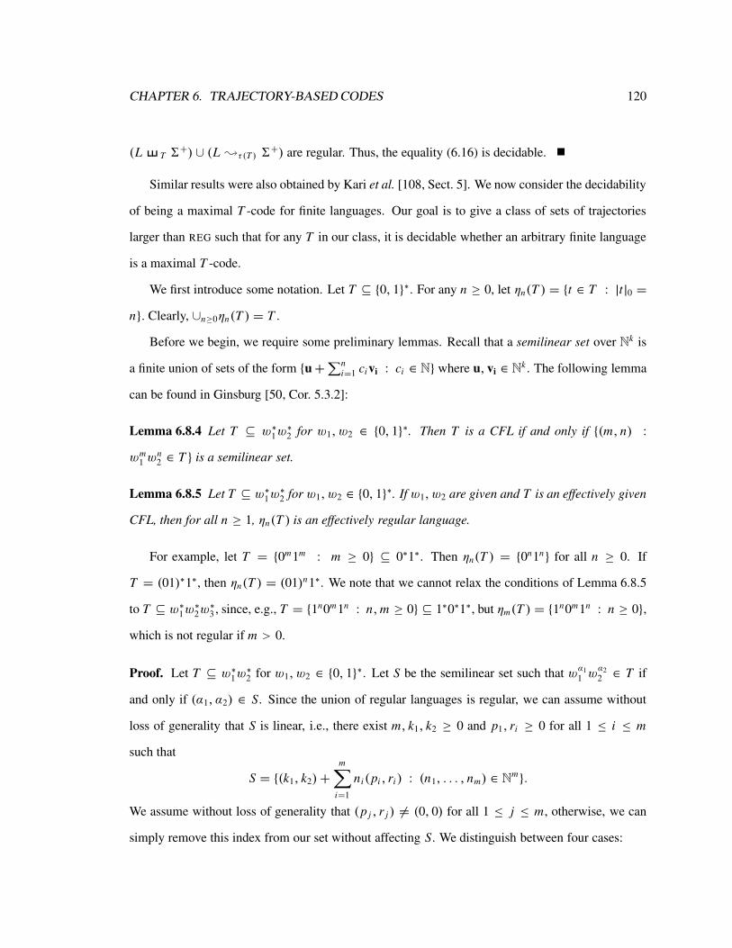
CHAPTER 6. TRAJECTORY-BASED CODES 120
(L T 6+) ∪ (L ;τ (T ) 6
+) are regular. Thus, the equality (6.16) is decidable.
Similar results were also obtained by Kari et al. [108, Sect. 5]. We now consider the decidability
of being a maximal T -code for finite languages. Our goal is to give a class of sets of trajectories
larger than REG such that for any T in our class, it is decidable whether an arbitrary finite language
is a maximal T -code.
We first introduce some notation. Let T ⊆ {0, 1}∗. For any n ≥ 0, let ηn(T ) = {t ∈ T : |t|0 =
n}. Clearly, ∪n≥0ηn(T ) = T .
Before we begin, we require some preliminary lemmas. Recall that a semilinear set over Nk is
a finite union of sets of the form {u+∑ni=1 civi : ci ∈ N} where u, vi ∈ Nk . The following lemma
can be found in Ginsburg [50, Cor. 5.3.2]:
Lemma 6.8.4 Let T ⊆ w∗1w∗2 for w1, w2 ∈ {0, 1}∗. Then T is a CFL if and only if {(m, n) :
wm1 w
n2 ∈ T } is a semilinear set.
Lemma 6.8.5 Let T ⊆ w∗1w∗2 for w1, w2 ∈ {0, 1}∗. If w1, w2 are given and T is an effectively given
CFL, then for all n ≥ 1, ηn(T ) is an effectively regular language.
For example, let T = {0m1m : m ≥ 0} ⊆ 0∗1∗. Then ηn(T ) = {0n1n} for all n ≥ 0. If
T = (01)∗1∗, then ηn(T ) = (01)n1∗. We note that we cannot relax the conditions of Lemma 6.8.5
to T ⊆ w∗1w∗2w∗3 , since, e.g., T = {1n0m1n : n,m ≥ 0} ⊆ 1∗0∗1∗, but ηm(T ) = {1n0m1n : n ≥ 0},
which is not regular if m > 0.
Proof. Let T ⊆ w∗1w∗2 for w1, w2 ∈ {0, 1}∗. Let S be the semilinear set such that wα1
1 wα2
2 ∈ T if
and only if (α1, α2) ∈ S. Since the union of regular languages is regular, we can assume without
loss of generality that S is linear, i.e., there exist m, k1, k2 ≥ 0 and p1, ri ≥ 0 for all 1 ≤ i ≤ m
such that
S = {(k1, k2)+m∑
i=1
ni(pi , ri ) : (n1, . . . , nm) ∈ Nm}.
We assume without loss of generality that (p j , r j ) 6= (0, 0) for all 1 ≤ j ≤ m, otherwise, we can
simply remove this index from our set without affecting S. We distinguish between four cases:

CHAPTER 6. TRAJECTORY-BASED CODES 121
(a) w1w2 ∈ 1∗ + 0∗. In this case, as T is a unary CFL, it is known that T is a regular language.
Thus, so is ηn(T ) = T ∩ (1∗0)n1∗.
(b) w1 ∈ 1∗. By case (a), we can assume that w2 /∈ 1∗, i.e., that |w2|0 6= 0. As w1 ∈ 1∗, there
exists α ≥ 0 such that
T = {1α(k1+∑m
i=1 ni pi )wk2+
∑mi=1 ni ri
2 : (n1, . . . , nm) ∈ Nm}.
Let I ⊆ Nm be defined so that
I = {(n1, . . . , nm) : |w2|0(k2 +m∑
i=1
niri ) = n}.
From this, we can see that
ηn(T ) = {1α(k1+∑m
i=1 ni pi )wk2+
∑mi=1 ni ri
2 : (n1, . . . , nm) ∈ Nm}.
By reordering if necessary, let 0 ≤ m ′ ≤ m be the index such that for all j ≤ m ′, r j 6= 0 and for
all m ′ < j ≤ m, r j = 0. Let ϕ : I → Nm′ be given by ϕ(n1, n2, . . . , nm) = (n1, n2, . . . , nm′).
Note that ϕ−1(ϕ(I )) = I as we have that if (n1, . . . , nm) ∈ I , for all m ′ < j ≤ m,
(n1, n2, . . . , n j−1, n′j , n j+1, . . . , nm) ∈ I
for all n′j ∈ N.
Further, note that ϕ(I ) is finite, since for all (n1, . . . , nm′) ∈ ϕ(I ) and all j ≤ m ′, n j satisfies
n j ≤1
r j
(n
|w2|0− k2
).
Thus, we can conclude that
ηn(T ) ={1α(k1+∑m′
i=1 ni pi )(
m∏
i=m′+1
(1αpi )∗)wk2+
∑m′i=1 ni ri
2
: (n1, . . . , nm′) ∈ ϕ(I )}.
and that ηn(T ) is regular.

CHAPTER 6. TRAJECTORY-BASED CODES 122
(c) w2 ∈ 1∗. Thus, consider that ηn(TR) = ηn(T )
R . As T R ⊆ (wR2 )∗(wR
1 )∗, by (a) or (b), ηn(T
R)
is regular. As the regular languages are closed under reversal, ηn(T ) is regular.
(d) w1, w2 /∈ 1∗. Let I ⊆ Nm be defined by
I ={(n1, . . . , nm) ∈ Nm
: |w1|0(k1 +m∑
i=1
ni pi )+ |w2|0(k2 +m∑
i=1
niri ) = n}.
Note that I is finite, as |w1|0, |w2|0 6= 0 and (pi , ri ) 6= (0, 0) for all 1 ≤ i ≤ m. Further, we
have that
ηn(T ) = {wk1+∑m
i=1 ni pi
1 wk2+
∑mi=1 ni ri
2 : (n1, . . . , nm) ∈ I }.
From this, we note that ηn(T ) is finite.
Thus, ηn(T ) is regular.
We are now ready to give our positive decidability result:
Theorem 6.8.6 Let T ⊆ {0, 1}∗ be a CFL such that T ⊆ w∗1w∗2 for w1, w2 ∈ {0, 1}∗, where w1, w2
are given. If F is a finite set, then we can decide whether F is a maximal T -code. Furthermore, all
constructions are effective.
Proof. Let T ⊆ w∗1w∗2 be a CFL. Let F be our finite set and let ℓ(F) = {|x| : x ∈ F} and
ℓF = max{ℓ : ℓ ∈ ℓ(F)}. First, we note that we can find T≤ℓF = T ∩ {0, 1}≤ℓF , and that
F ;τ (T ) 6+ = F ;τ (T≤ℓF ) 6
+,
which is thus a regular language, since F,6+, τ (T ≤ℓF ) are, as well.
Second, we note that η(T ) = ∪ℓ∈ℓ(F)ηℓ(T ) is a regular language, since ℓ(F) is finite, and ηℓ(T )
is regular by Lemma 6.8.5. Further, we note that
F T 6+ = F η(T )6
+,
which is regular, by the regularity of F,6+ and η(T ).

CHAPTER 6. TRAJECTORY-BASED CODES 123
Thus, we conclude that F∪(F ;τ (T ) 6+)∪(F T 6
+) is a regular language, and thus, we can
determine whether this language is equal to 6+. Thus, by Lemma 6.8.2, we can determine whether
F is a maximal T -code.
6.8.2 Transitivity and Embedding T -codes
Given a class of codes C, and a language L ∈ C of given complexity, there has been much research
into whether or not L can be embedded in (or completed to) a maximal element L ′ ∈ C of the same
complexity, i.e., a maximal code L ′ ∈ C with L ⊆ L ′. Finite and regular languages in these classes
of codes are of particular interest. For instance, we note that every regular code can be completed
to a maximal regular code, while the same is not true for finite codes or finite biprefix codes.
We now show an interesting result on embedding T -codes in maximal T -codes while preserving
complexity. For example, we will show that if T is transitive and regular and L is a regular T -code,
then we can embed L in a maximal T -code which is also regular.
Our construction is a generalization of a result due to Lam [128]. In particular, we define two
transformations on languages. Let T be a set of trajectories and L ⊆ 6+ be a language. Then define
UT (L), VT (L) ⊆ 6+ as
UT (L) = 6+ − (L T 6+ ∪ L ;τ (T ) 6
+);
VT (L) = UT (L)− (UT (L) T 6+).
First, we note the following two properties of UT (L), VT (L):
Lemma 6.8.7 Let T ⊆ {0, 1}∗ be a set of trajectories and L ∈ PT (6). Then L ⊆ UT (L) and
L ⊆ VT (L).
Proof. We establish first that L ⊆ UT (L). Let x ∈ L , but assume that x /∈ UT (L). Then x ∈
L T 6+ or x ∈ L ;τ (T ) 6
+. In the first case, we have L ∩ (L T 6+) 6= ∅, contradicting that L
is a T -code. The second case also contradicts that L is a T -code, since then L∩ (L ;τ (T ) 6+) 6= ∅,
contradicting (6.7).

CHAPTER 6. TRAJECTORY-BASED CODES 124
We now establish L ⊆ VT (L). Assume not, then as L ⊆ UT (L), we must have that L ∩
(UT (L) T 6+) 6= ∅. Assume that y ∈ UT (L), z ∈ 6+ and x ∈ L are chosen so that x ∈ y T z.
Thus y ∈ x ;τ (T ) z ⊆ L ;τ (T ) 6+, contradicting that y ∈ UT (L). Thus, L ⊆ VT (L).
Theorem 6.8.8 Let T ⊆ {0, 1}∗ be transitive. Let 6 be an alphabet. Then for all L ∈ PT (6), the
language VT (L) contains L and VT (L) ∈MT (6).
Proof. By Lemma 6.8.7, L ⊆ VT (L). That VT (L) is a T -code follows from Lemma 6.3.11 applied
to UT (L). Thus, it remains to show that for all z ∈ 6+ − VT (L), VT (L) ∪ {z} is not a T -code.
Let z /∈ VT (L) be arbitrary. We distinguish two cases:
(a) if z /∈ UT (L), then z ∈ (L T 6+) ∪ (L ;τ (T ) 6
+). If z ∈ L T 6+ ⊆ VT (L) T 6
+,
then VT (L) ∪ {z} /∈ PT (6). If z ∈ L ;τ (T ) 6+ ⊆ VT (L) ;τ (T ) 6
+, then again (this time by
(6.7)), VT (L) ∪ {z} /∈ PT (6).
(b) if z ∈ UT (L)− VT (L), then z ∈ UT (L) T 6+. Let y ∈ UT (L) be a shortest word such that
z ∈ y T 6+. We claim that y ∈ VT (L). If this were not the case, then as y ∈ UT (L)−VT (L),
we have that y ∈ UT (L) T 6+, by definition of VT (L). Let y′ ∈ UT (L) be such that
y ∈ y′ T 6+. Thus, we have that y′ωT yωT z. By transitivity of T , y′ωT z, i.e., z ∈ y′ T 6
∗.
As |y′| < |y| < |z|, we certainly have that z ∈ y′ T 6+ in particular. But as |y′| < |y|, this
contradicts our choice of y. Thus, y ∈ VT (L). But y, z ∈ VT (L) ∪ {z} and z ∈ y T 6+
imply that VT (L) ∪ {z} /∈ PT (6).
Thus, VT (L) is a maximal T -code.
There are several consequences of Theorem 6.8.8. We note only one important corollary:
Corollary 6.8.9 Let T ⊆ {0, 1}∗ be transitive and regular. Then every regular (resp., recursive)
T -code is contained in a maximal regular (resp., recursive) T -code.
Corollary 6.8.9 was given for T = 1∗0∗1∗ and regular T -codes by Lam [128, Prop. 3.2]. Further
research into the case when T is not transitive is necessary (for example, the proofs of Zhang
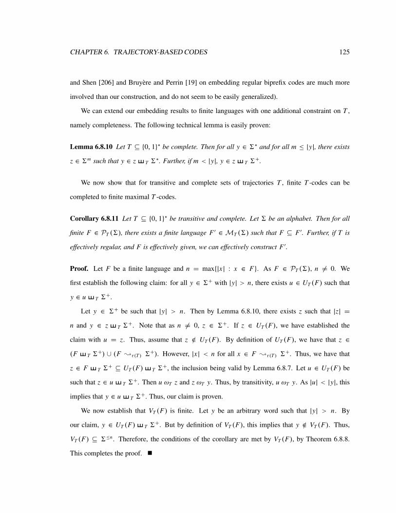
CHAPTER 6. TRAJECTORY-BASED CODES 125
and Shen [206] and Bruyere and Perrin [19] on embedding regular biprefix codes are much more
involved than our construction, and do not seem to be easily generalized).
We can extend our embedding results to finite languages with one additional constraint on T ,
namely completeness. The following technical lemma is easily proven:
Lemma 6.8.10 Let T ⊆ {0, 1}∗ be complete. Then for all y ∈ 6∗ and for all m ≤ |y|, there exists
z ∈ 6m such that y ∈ z T 6∗. Further, if m < |y|, y ∈ z T 6
+.
We now show that for transitive and complete sets of trajectories T , finite T -codes can be
completed to finite maximal T -codes.
Corollary 6.8.11 Let T ⊆ {0, 1}∗ be transitive and complete. Let 6 be an alphabet. Then for all
finite F ∈ PT (6), there exists a finite language F ′ ∈MT (6) such that F ⊆ F ′. Further, if T is
effectively regular, and F is effectively given, we can effectively construct F ′.
Proof. Let F be a finite language and n = max{|x| : x ∈ F}. As F ∈ PT (6), n 6= 0. We
first establish the following claim: for all y ∈ 6+ with |y| > n, there exists u ∈ UT (F) such that
y ∈ u T 6+.
Let y ∈ 6+ be such that |y| > n. Then by Lemma 6.8.10, there exists z such that |z| =
n and y ∈ z T 6+. Note that as n 6= 0, z ∈ 6+. If z ∈ UT (F), we have established the
claim with u = z. Thus, assume that z /∈ UT (F). By definition of UT (F), we have that z ∈
(F T 6+) ∪ (F ;τ (T ) 6
+). However, |x| < n for all x ∈ F ;τ (T ) 6+. Thus, we have that
z ∈ F T 6+ ⊆ UT (F) T 6
+, the inclusion being valid by Lemma 6.8.7. Let u ∈ UT (F) be
such that z ∈ u T 6+. Then u ωT z and z ωT y. Thus, by transitivity, u ωT y. As |u| < |y|, this
implies that y ∈ u T 6+. Thus, our claim is proven.
We now establish that VT (F) is finite. Let y be an arbitrary word such that |y| > n. By
our claim, y ∈ UT (F) T 6+. But by definition of VT (F), this implies that y /∈ VT (F). Thus,
VT (F) ⊆ 6≤n. Therefore, the conditions of the corollary are met by VT (F), by Theorem 6.8.8.
This completes the proof.

CHAPTER 6. TRAJECTORY-BASED CODES 126
In practice, the condition that T be complete is not very restrictive, since natural operations
seem to typically be defined by a complete set of trajectories.
In Section 6.9.3 below, we will give alternate conditions on T that ensure that every finite T -
code can be embedded in a finite maximal T -code. However, this result will be a trivial consequence
of the fact that for such T , all T -codes are finite.
We now show that there exist T which are not transitive, and for which the above results do not
hold. It is known, for example, that there exist finite biprefix codes which cannot be embedded in a
maximal finite biprefix code (see, e.g., Bruyere and Perrin [19, Sect. 3]). We present the following
two examples, as well; in the first case, T is regular but not transitive, and for all regular T -codes
L , L cannot be embedded in any maximal CF T -code. In the second example, T is not complete,
and no finite T -code can be embedded in a maximal finite T -code.
Example 6.8.12: Let T = (01)∗; then T is known as perfect or balanced literal shuffle. Clearly,
T is not transitive. Let6 = {a}. We claim that for all regular languages L ⊆ a∗, L is not a maximal
T -code.
Let L ⊆ a∗ be regular. As L is a unary regular language, it is well-known that L corresponds to
an ultimately periodic set of natural numbers. That is, there exist n0, p ∈ N with p > 0 such that
for all n > n0, an ∈ L if and only if an+p ∈ L .
Let r = min{kp : k ≥ 1, kp > n0}. Then we have two cases:
(a) if ar ∈ L , then a2r ∈ L as well. Thus, as a2r ∈ arT ar , L is not a T -code.
(b) if ar /∈ L , then a2r /∈ L as well. Thus, consider L ∪ {a2r}. If L is a T -code, then as
a2r /∈ L T a+ and L ∩ (a2rT a+) = ∅, we have that L ∪ {a2r} is a T -code as well.
Thus, L is not a maximal T -code.
Thus, there are no regular languages in MT ({a}). Further, since the unary context-free and unary
regular languages coincide, there are no context-free languages in MT ({a}), either. Thus, e.g., the
T -code {a} cannot be embedded in any regular (or context-free) maximal T -code.
We note in passing that one maximal T -code containing {a} is given by L = {acn : n ≥ 1}
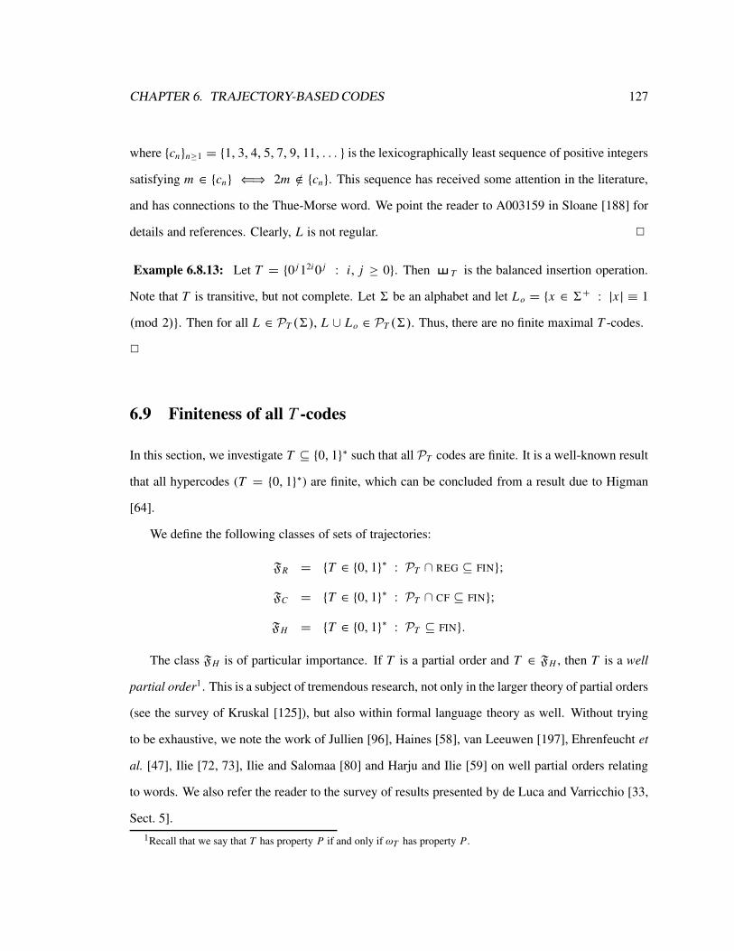
CHAPTER 6. TRAJECTORY-BASED CODES 127
where {cn}n≥1 = {1, 3, 4, 5, 7, 9, 11, . . . } is the lexicographically least sequence of positive integers
satisfying m ∈ {cn} ⇐⇒ 2m /∈ {cn}. This sequence has received some attention in the literature,
and has connections to the Thue-Morse word. We point the reader to A003159 in Sloane [188] for
details and references. Clearly, L is not regular. 2
Example 6.8.13: Let T = {0 j 12i0 j : i, j ≥ 0}. Then T is the balanced insertion operation.
Note that T is transitive, but not complete. Let 6 be an alphabet and let Lo = {x ∈ 6+ : |x| ≡ 1
(mod 2)}. Then for all L ∈ PT (6), L ∪ Lo ∈ PT (6). Thus, there are no finite maximal T -codes.
2
6.9 Finiteness of all T -codes
In this section, we investigate T ⊆ {0, 1}∗ such that all PT codes are finite. It is a well-known result
that all hypercodes (T = {0, 1}∗) are finite, which can be concluded from a result due to Higman
[64].
We define the following classes of sets of trajectories:
FR = {T ∈ {0, 1}∗ : PT ∩ REG ⊆ FIN};
FC = {T ∈ {0, 1}∗ : PT ∩ CF ⊆ FIN};
FH = {T ∈ {0, 1}∗ : PT ⊆ FIN}.
The class FH is of particular importance. If T is a partial order and T ∈ FH , then T is a well
partial order1. This is a subject of tremendous research, not only in the larger theory of partial orders
(see the survey of Kruskal [125]), but also within formal language theory as well. Without trying
to be exhaustive, we note the work of Jullien [96], Haines [58], van Leeuwen [197], Ehrenfeucht et
al. [47], Ilie [72, 73], Ilie and Salomaa [80] and Harju and Ilie [59] on well partial orders relating
to words. We also refer the reader to the survey of results presented by de Luca and Varricchio [33,
Sect. 5].
1Recall that we say that T has property P if and only if ωT has property P.

CHAPTER 6. TRAJECTORY-BASED CODES 128
To begin, we give conditions on T which ensure all regular (or context-free) T -codes are finite.
6.9.1 Finiteness of Regular T -codes
Let T ⊆ {0, 1}∗. Define the insertion behaviour of T , denoted ib(T ), as
ib(T ) = {(n1, n2, n3) ∈ N3 : 0n1 1n2 0n3 ∈ T }.
Say that T is REG-pumping compliant if, for all i, j, k ∈ N ( j > 0), there exists j ′ with 0 ≤ j ′ < j
such that
(i) if j ′ = 0, then ib(T ) ∩ {(i + jm1, jm2, k + jm3) : m1,m3 ≥ 0,m2 > 0} 6= ∅.
(ii) if 1 ≤ j ′ < j , then ib(T )∩ {(i + j ′+ jm1, jm2, k − j ′+ jm3) : m1 ≥ 0,m2,m3 > 0} 6= ∅.
The use of the terminology ‘REG-pumping compliant’ will become clear in the following lemma:
Lemma 6.9.1 Let T ⊆ {0, 1}∗. If T is REG-pumping compliant, then T ∈ FR .
Proof. Let R ∈ REG be an infinite regular language over 6. By the pumping lemma for regular
languages, there exist u, v,w ∈ 6∗ such that v 6= ǫ and uv∗w ⊆ R. Let i = |u|, j = |v| and
k = |w|. Note that j 6= 0. Let j ′ be the natural number implied by the REG-pumping compliance
condition.
If j ′ = 0, then let m1,m2,m3 be chosen so that m1,m3 ≥ 0, m2 > 0 and (i + jm1, jm2, k +
jm3) ∈ ib(T ). Let t = 0i+ jm1 1 jm20k+ jm3 . By definition, t ∈ T . Consider x = uvm1+m3w ∈ R and
y = vm2 . As m2 6= 0 and v 6= ǫ, y 6= ǫ. We note that
x t y ∋ uvm1 · vm2 · vm3w = uvm1+m2+m3w.
Thus, (R T 6+) ∩ R 6= ∅ and R /∈ PT .
If 1 ≤ j ′ < j , let m1 ≥ 0, m2,m3 > 0 be chosen so that
(i + j ′ + jm1, jm2, k − j ′ + jm3) ∈ ib(T ),

CHAPTER 6. TRAJECTORY-BASED CODES 129
and hence t = 0i+ j ′+ jm11 jm20k+( j− j ′)+ j (m3−1) ∈ T . Let v1 ∈ 6∗ be the prefix of v of length j ′ and
let v = v1v2 for some v2 ∈ 6∗.
Consider x = uvm1+m3w ∈ R and y = (v2v1)m2 6= ǫ. Then
x t y ∋ uvm1v1 · v2(v1v2)m2−1v1 · v2v
m3−1w = uvm1+m2+m3w.
Again, (R T 6+)∩ R 6= ∅ and thus R /∈ PT . Thus, PT contains no infinite regular languages.
The condition of being REG-pumping compliant is not very restrictive. Clearly, if T ⊇ 0∗1∗0∗,
then T is REG-pumping compliant (in this case, Lemma 6.9.1 is a corollary of a result on outfix
codes due to Ito et al. [77]). For a broader class of examples, we can consider immune languages.
Lemma 6.9.2 Let T ⊆ {0, 1}∗ be a set of trajectories such that T ∩ 0∗1∗0∗ is REG-immune. Then
T is REG-pumping compliant.
Proof. Let i ≥ 0, j > 0, k ≥ 0 be arbitrary. Consider
T0 = T0(i, j, k) = 0i (0 j )∗(1 j )+(0 j )∗0k .
As T0 is an infinite regular language, T0 is not a subset of T ∩ 0∗1∗0∗. Thus, T0 ∩ (T ∩ 0∗1∗0∗) =
T0 ∩ (T ∪ 0∗1∗0∗) 6= ∅. As T0 ⊆ 0∗1∗0∗, this implies that T0 ∩ T 6= ∅. Thus, there exist m1 ≥ 0,
m2 > 0 and m3 ≥ 0 such that 0i+ jm1 1 jm20k+ jm3 ∈ T , i.e., (i + jm1, jm2, k + jm3) ∈ ib(T ). Thus,
the REG-pumping compliant conditions are met with j ′ = 0.
Next, we show that if T ⊆ 0∗1∗0∗, then REG-pumping compliance is necessary to ensure that
there are no infinite regular languages in PT .
Lemma 6.9.3 Let T ⊆ 0∗1∗0∗ be not REG-pumping compliant. Then PT (6) contains an infinite
regular language for all 6 with |6| ≥ 2.
Proof. Let i, j, k ∈ N be arbitrary such that i ≥ 0, j > 0, k ≥ 0,
ib(T ) ∩ {(i + jm1, jm2, k + jm3) : m1,m3 ≥ 0,m2 > 0} = ∅.

CHAPTER 6. TRAJECTORY-BASED CODES 130
and for all 1 ≤ j ′ < j ,
ib(T ) ∩ {(i + j ′ + jm1, jm2, k − j ′ + jm3) : m1 ≥ 0,m2,m3 > 0} = ∅.
Let a, b ∈ 6 (a 6= b) and R = ai (b j )∗ak . We claim that R ∈ PT (6). Assume not. Then there exist
ℓ1 > ℓ2 ≥ 0 such that
aib jℓ1ak ∈ ai b jℓ2akT z
for some z ∈ {a, b}+. By observation, z = b j (ℓ1−ℓ2). Thus, let t ∈ T be chosen so that
ai b jℓ1ak ∈ ai b jℓ2akt b j (ℓ1−ℓ2).
Then as T ⊆ 0∗1∗0∗, t = 0i+α j+ j ′1 j (ℓ1−ℓ2)0( j− j ′)+(ℓ2−α−1) j+k for some α and j ′ with either 0 ≤ α ≤
ℓ2 and j ′ = 0 or 0 ≤ α < ℓ2−1 and 1 ≤ j ′ < j . If j ′ = 0, then (i+α j, j (ℓ1−ℓ2), k+(ℓ2−α) j) ∈
ib(T ) while if j ′ 6= 0, then (i + j ′ + α j, j (ℓ1 − ℓ2), k − j ′ + (ℓ2 − α) j) ∈ ib(T ), which are both
contradictions.
6.9.2 Finiteness of Context-free T -codes
Let T ⊆ {0, 1}∗. Define the 2–insertion behaviour of T , denoted 2ib(T ), as follows:
2ib(T ) = {(n1, n2, . . . , n5) ∈ N5 : 0n1 1n2 0n3 1n4 0n5 ∈ T }.
We use 2ib(T ) to define the notion of CF-pumping compliance. The idea is the same as REG-
pumping compliance, but with more cases. In particular, say that T is CF-pumping compliant if, for
all i, j1, j2, k, ℓ ∈ N, with j1 + j2 > 0, there exist j ′1, j ′2 ∈ N such that 0 ≤ j ′i < ji for i = 1, 2 and
2ib(T ) ∩ P 6= ∅, where P is defined as follows:
(a) if j ′1 = j ′2 = 0, then
P = {(i + j1α1, j1β, k + j1α2 + j2α3, j2β, ℓ + j2α4)
: αm, β ∈ N, (1 ≤ m ≤ 4), β > 0, α1 + α2 = α3 + α4}.
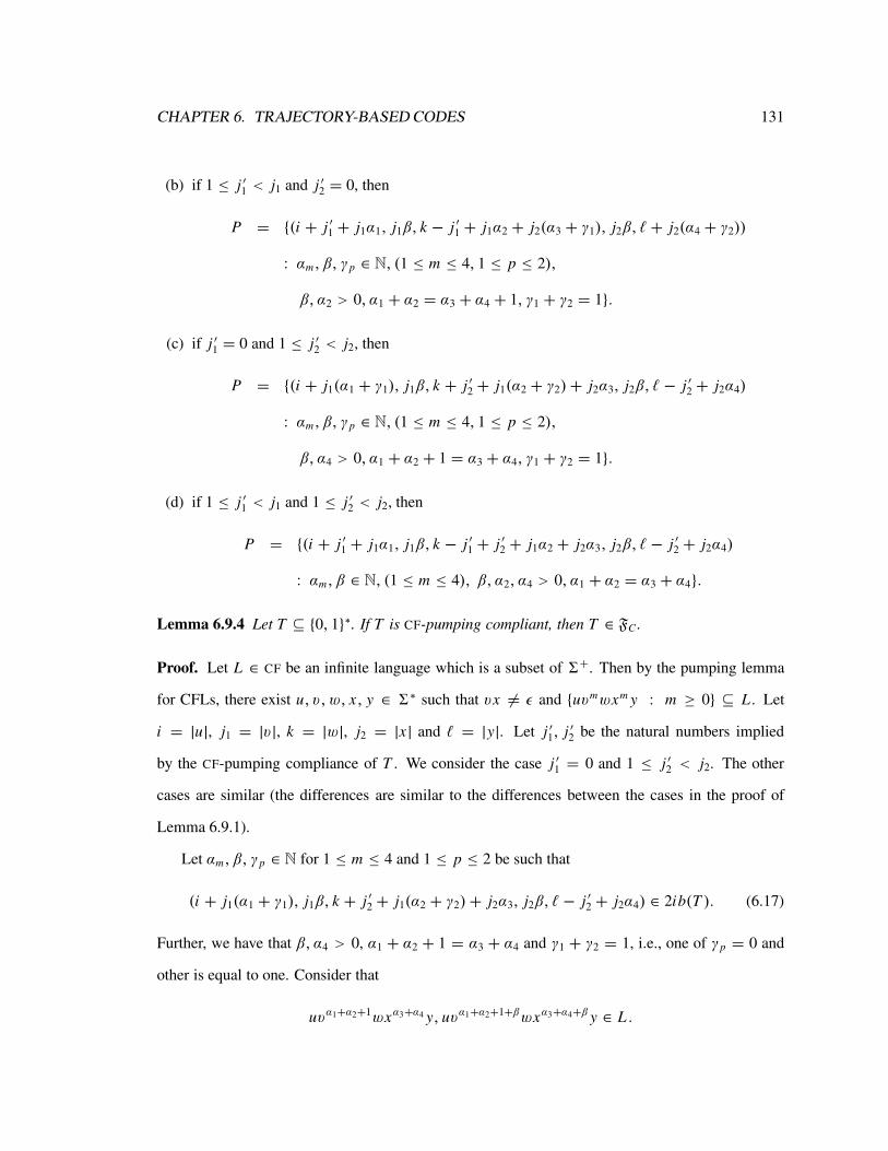
CHAPTER 6. TRAJECTORY-BASED CODES 131
(b) if 1 ≤ j ′1 < j1 and j ′2 = 0, then
P = {(i + j ′1 + j1α1, j1β, k − j ′1 + j1α2 + j2(α3 + γ1), j2β, ℓ+ j2(α4 + γ2))
: αm, β, γp ∈ N, (1 ≤ m ≤ 4, 1 ≤ p ≤ 2),
β, α2 > 0, α1 + α2 = α3 + α4 + 1, γ1 + γ2 = 1}.
(c) if j ′1 = 0 and 1 ≤ j ′2 < j2, then
P = {(i + j1(α1 + γ1), j1β, k + j ′2 + j1(α2 + γ2)+ j2α3, j2β, ℓ − j ′2 + j2α4)
: αm, β, γp ∈ N, (1 ≤ m ≤ 4, 1 ≤ p ≤ 2),
β, α4 > 0, α1 + α2 + 1 = α3 + α4, γ1 + γ2 = 1}.
(d) if 1 ≤ j ′1 < j1 and 1 ≤ j ′2 < j2, then
P = {(i + j ′1 + j1α1, j1β, k − j ′1 + j ′2 + j1α2 + j2α3, j2β, ℓ− j ′2 + j2α4)
: αm, β ∈ N, (1 ≤ m ≤ 4), β, α2, α4 > 0, α1 + α2 = α3 + α4}.
Lemma 6.9.4 Let T ⊆ {0, 1}∗. If T is CF-pumping compliant, then T ∈ FC .
Proof. Let L ∈ CF be an infinite language which is a subset of 6+. Then by the pumping lemma
for CFLs, there exist u, v,w, x, y ∈ 6∗ such that vx 6= ǫ and {uvmwxm y : m ≥ 0} ⊆ L . Let
i = |u|, j1 = |v|, k = |w|, j2 = |x| and ℓ = |y|. Let j ′1, j ′2 be the natural numbers implied
by the CF-pumping compliance of T . We consider the case j ′1 = 0 and 1 ≤ j ′2 < j2. The other
cases are similar (the differences are similar to the differences between the cases in the proof of
Lemma 6.9.1).
Let αm, β, γp ∈ N for 1 ≤ m ≤ 4 and 1 ≤ p ≤ 2 be such that
(i + j1(α1 + γ1), j1β, k + j ′2 + j1(α2 + γ2)+ j2α3, j2β, ℓ− j ′2 + j2α4) ∈ 2ib(T ). (6.17)
Further, we have that β, α4 > 0, α1 + α2 + 1 = α3 + α4 and γ1 + γ2 = 1, i.e., one of γp = 0 and
other is equal to one. Consider that
uvα1+α2+1wxα3+α4 y, uvα1+α2+1+βwxα3+α4+β y ∈ L .

CHAPTER 6. TRAJECTORY-BASED CODES 132
Further, if x = x1x2 where x1, x2 ∈ 6∗ and |x1| = j ′2, then
uvα1+α2+1+βwxα3+α4+β y ∈ z1 · z2 · z3 t vβ(x2x1)
β
where
z1 = uvα1+γ1,
z2 = vα2+γ2wxα3 x1,
z3 = x2xα4−1 y,
t = 0i+ j1(α1+γ1)1 j1β0k+ j ′2+ j1(α2+γ2)+ j2α31 j2β0ℓ− j ′2+ j2α4 .
By (6.17), t ∈ T . Note also that
z1z2z3 = uvα1+α2+1wxα3+α4 y ∈ L .
As vx 6= ǫ and β > 0, vβ(x2x1)β 6= ǫ. Thus, L /∈ PT .
Note that if T ⊇ 0∗1∗0∗1∗0∗ then T satisfies the conditions of Lemma 6.9.4. This instance of
our result is also a corollary of a result due to Thierrin and Yu [193, Prop. 3.3(2)].
6.9.3 Finiteness of T -codes
We now turn to the question of the existence of arbitrary infinite languages in a class of T -codes.
We first show that if T is bounded, then there is an infinite T -code.
Theorem 6.9.5 Let T ⊆ {0, 1}∗ be a bounded set of trajectories. Then for all 6 with |6| > 1,
PT (6) contains an infinite language.
Proof. Let T ⊆ {0, 1}∗ be a bounded language. Then there exist k ≥ 0 and w1, w2, . . . , wk ∈
{0, 1}∗ such that T ⊆ w∗1w∗2 · · ·w∗k . By Lemma 6.3.2, if we can establish that there is an infinite
T ′-code, where T ′ = w∗1 · · ·w∗k , the result will follow. Thus, without loss of generality, we let
T = w∗1w∗2 · · ·w∗k .
CHAPTER 6. TRAJECTORY-BASED CODES 133
If w1 = w2 = · · · = wk = ǫ, then T = {ǫ}, and thus PT (6) = 26+ − {∅}, which clearly
contains an infinite language.
Otherwise, there exists i0 with 1 ≤ i0 ≤ k such that wi0 6= ǫ. For all 1 ≤ i ≤ k, let αi = |wi |.
Let a, b ∈ 6 be distinct letters, and define LT ⊆ {a, b}+ by
LT = {(k∏
i=1
ambαi )am : m ≥ 0}.
We have that LT ⊆ {a, b}+ as αi0 6= 0. We claim LT ∈ PT (6). Assume not. Then there exist
m1,m2 ∈ N with m1 > m2, t ∈ T and z ∈ 6+ such that
(
k∏
i=1
am1 bαi )am1 ∈ (k∏
i=1
am2 bαi )am2t z.
Thus, we have that z = a(k+1)(m1−m2). Further, let ti ∈ {0, 1}∗ for 1 ≤ i ≤ k + 1 be defined so that
t = (k∏
i=1
ti 0αi )tk+1,
where |ti |0 = m2 and |ti |1 = m1−m2 for all 1 ≤ i ≤ k+1. As t ∈ T , there exist ji ∈ N, 1 ≤ i ≤ k,
such that t =∏ki=1 w
jii . Thus, we have that
k∑
i=1
αi ji = (k∑
i=1
|ti | + αi)+ |tk+1|,
and sok∑
i=1
αi ji ≥k∑
i=1
|ti | + αi .
Let ℓ with 1 ≤ ℓ ≤ k be the minimal index such that
ℓ∑
i=1
αi ji ≥ℓ∑
i=1
|ti | + αi . (6.18)
Note that jℓ > 0, since if jℓ = 0, then ℓ − 1 satisfies (6.18) as well, contrary to our choice of ℓ (if
ℓ = 1 and j1 = 0, then |t1| = 0, which is a contradiction to |t1| = m1 > 0).
Let u1 =∏ℓ−1
i=1 ti 0αi , u2 = (
∏ki=ℓ+1 ti 0
αi )tk+1, s1 =∏ℓ−1
i=1 wjii and s2 =
∏ki=ℓ+1 w
jii . Thus, we
have that
u1tℓ0αℓu2 = s1w
jℓℓ s2
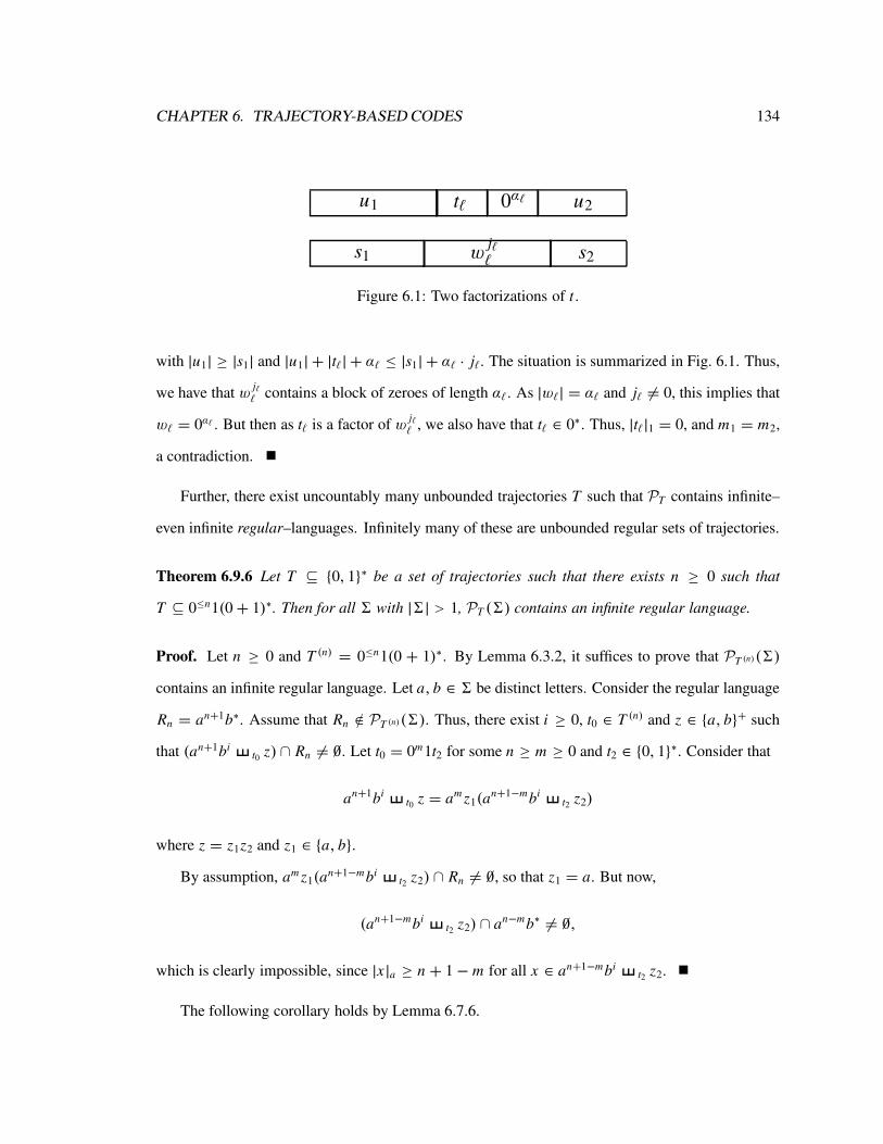
CHAPTER 6. TRAJECTORY-BASED CODES 134
tℓ u20αℓu1
s2wjℓℓs1
Figure 6.1: Two factorizations of t .
with |u1| ≥ |s1| and |u1| + |tℓ| + αℓ ≤ |s1| + αℓ · jℓ. The situation is summarized in Fig. 6.1. Thus,
we have that wjℓℓ contains a block of zeroes of length αℓ. As |wℓ| = αℓ and jℓ 6= 0, this implies that
wℓ = 0αℓ . But then as tℓ is a factor of wjℓℓ , we also have that tℓ ∈ 0∗. Thus, |tℓ|1 = 0, and m1 = m2,
a contradiction.
Further, there exist uncountably many unbounded trajectories T such that PT contains infinite–
even infinite regular–languages. Infinitely many of these are unbounded regular sets of trajectories.
Theorem 6.9.6 Let T ⊆ {0, 1}∗ be a set of trajectories such that there exists n ≥ 0 such that
T ⊆ 0≤n1(0+ 1)∗. Then for all 6 with |6| > 1, PT (6) contains an infinite regular language.
Proof. Let n ≥ 0 and T (n) = 0≤n1(0 + 1)∗. By Lemma 6.3.2, it suffices to prove that PT (n)(6)
contains an infinite regular language. Let a, b ∈ 6 be distinct letters. Consider the regular language
Rn = an+1b∗. Assume that Rn /∈ PT (n)(6). Thus, there exist i ≥ 0, t0 ∈ T (n) and z ∈ {a, b}+ such
that (an+1bit0 z) ∩ Rn 6= ∅. Let t0 = 0m1t2 for some n ≥ m ≥ 0 and t2 ∈ {0, 1}∗. Consider that
an+1bit0 z = am z1(a
n+1−mbit2 z2)
where z = z1z2 and z1 ∈ {a, b}.
By assumption, am z1(an+1−mbi
t2 z2) ∩ Rn 6= ∅, so that z1 = a. But now,
(an+1−mbit2 z2) ∩ an−mb∗ 6= ∅,
which is clearly impossible, since |x|a ≥ n + 1− m for all x ∈ an+1−mbit2 z2.
The following corollary holds by Lemma 6.7.6.
CHAPTER 6. TRAJECTORY-BASED CODES 135
Corollary 6.9.7 Let T ⊆ {0, 1}∗ be a set of trajectories such that there exists n ≥ 0 such that
T ⊆ (0+ 1)∗10≤n . Then for all 6 with |6| > 1, PT (6) contains an infinite regular language.
We now turn to defining sets T of trajectories such that all T -codes are finite. The following
proof is generalized from the case H = (0+ 1)∗ found in, e.g., Lothaire [140] or Conway [28, pp.
63–64].
Lemma 6.9.8 Let n,m ≥ 1 be such that m | n. Let Tn,m = (0n + 1m)∗0≤n−1. Then Tn,m ∈ FH .
Proof. In what follows, let ω = ωTn,m . Assume that there exists an infinite Tn,m-code. Then there
exists an infinite sequence {xi }i≥1 which is ω-free, i.e., i < j implies xi ω x j does not hold. As
Tn,m ⊇ 0∗, ω is reflexive and we have that xi 6= x j for all i > j ≥ 1.
We now choose (using the axiom of choice) a minimal infinite ω-free sequence as follows: let
y1 be the shortest word which begins an infinite ω-free sequence. Let y2 be the shortest word such
that y1, y2 begins an infinite ω-free sequence. We continue in this way. Let {yi}i≥1 be the resulting
sequence. Clearly, {yi}i≥1 is an infinite ω-free sequence.
As ω is reflexive, yi 6= y j for all i > j ≥ 1. Therefore, |yi | ≤ n for only finitely many
i ∈ N. Furthermore, since there are only finitely many words of length n, there exist y ∈ 6n and
{i j } j≥1 ⊆ N such that y is a prefix of yi jfor all j ≥ 1. In particular, for all j ≥ 1, let u j ∈ 6∗ be
the word such that yi j= yu j . Consider the sequence
Y = {y1, y2, y3, · · · , yi1−1, u1, u2, · · · }.
Clearly, as n ≥ 1, |u1| < |yi1 |. Thus, Y is an infinite sequence which comes before {yi}i≥1 in
our ordering of infinite ω-free sequences, and so two words in Y must be comparable under ω. By
assumption, y j1 6 ω y j2 for all 1 ≤ j1 < j2 ≤ i1 − 1. Thus, there are two remaining cases:
(i) there exist 1 ≤ j ≤ i1−1 and k ≥ 1 such that y jωuk . Thus, let t ∈ Tn,m and α ∈ 6∗ be chosen
so that uk ∈ y j t α. Consider t ′ = 1nt ∈ Tn,m . Then yik = yuk ∈ y(y j t α) = y j t ′ yα.
Therefore, y j ω yik . As j ≤ i1 − 1 < ik , this is a contradiction.

CHAPTER 6. TRAJECTORY-BASED CODES 136
(ii) there exist k > ℓ ≥ 1 such that uℓ ω uk . Let α ∈ 6∗ and t ∈ Tn,m be such that uk ∈ uℓ t α.
Consider t ′ = 0nt ∈ Tn,m . Then yik = yuk ∈ y(uℓ t α) = yuℓ t ′ α = yiℓ t ′ α. Thus
yiℓ ω yik . As ℓ < k, this is a contradiction.
We have arrived at a contradiction.
As another class of examples, Ehrenfeucht et al. [47, p. 317] note that {1n, 0}∗ ∈ FH for all
n ≥ 1 (their other results, though elegant and interesting, do not otherwise seem to be applicable to
our situation).
Note that T1,1 = {0, 1}∗. Let Tn = Tn,n . For all 1 ≤ i < j , PTi6= PT j
, as 0i1i ∈ Ti − T j . Thus,
by Lemma 6.3.6, the classes of Ti - and T j -codes are distinct.
Corollary 6.9.9 There are infinitely many T ⊆ {0, 1}∗ which define distinct classes PT satisfying
PT ⊆ FIN.
Further, the following is immediate:
Corollary 6.9.10 Let T ⊆ {0, 1}∗ be such that Tn ⊆ T for some n ≥ 1. Then PT ⊆ FIN.
Ilie [73, Sect. 7.7] also gives a class of partial orders which we may phrase in terms of sets of
trajectories. In particular, define the set of functions
G = {g : N→ N : g(0) = 0 and 1 ≤ g(n) ≤ n for all n ≥ 1}.
Then for all g ∈ G, we define
Tg = {1∗m∏
k=1
(0ik 1∗) : ik ≥ 0 ∀1 ≤ k ≤ m; m = g(
m∑
k=1
ik)}.
We denote the upper limit of a sequence {sn}n≥1 by limn→∞sn . We have the following result
[73, Thm. 7.7.8]:
Theorem 6.9.11 Let g ∈ G. Then Tg ∈ FH ⇐⇒ limn→∞n
g(n)<∞.

CHAPTER 6. TRAJECTORY-BASED CODES 137
6.9.4 Decidability and Finiteness Conditions
We now consider decidability of membership in PT if T satisfies the conditions of the previous
sections. We have the following positive decidability results:
Theorem 6.9.12 Let T be recursive. If T ∈ FR (resp., T ∈ FC , T ∈ FH ) then given a regular
(resp., context-free, context-free) language L, it is decidable whether L ∈ PT .
Proof. We establish the result for T ∈ FC . The case T ∈ FH is an instance of this case and the case
T ∈ FR is very similar. Let T ∈ REC and T ∈ FC . Let L ∈ CF. We first check if L is infinite. If it
is, then certainly L /∈ PT , so we answer no.
If L is finite, then we can effectively find a list of all words in L (consider putting L in Chomsky
Normal Form (CNF); see Hopcroft and Ullman [68] for an introduction to CNF). Let F = L , where
F is some effectively given finite set. Then by Lemma 6.3.10, we can decide whether L = F ∈ PT .
One might hope for an undecidability result of the following type, which would complement
Theorem 6.3.9: for a fixed T ∈ REG (perhaps with some reasonable assumption, e.g., complete-
ness), then it is undecidable, given a CFL L , whether L ∈ PT . Theorem 6.9.12 shows us that we
cannot hope for a simple such result, since we need to restrict ourselves to those T which do not lie
in FC in this case.
6.9.5 Up and Down Sets
Let L ⊆ 6∗ and T ⊆ {0, 1}∗ Define DOWNT (L), UPT (L) as
DOWNT (L) = L ;τ (T ) 6∗;
UPT (L) = L T 6∗.
Our notation roughly follows Harju and Ilie [59], where DOWNT (L) is denoted DOWNωT(L) and
UPT (L) is denoted DOWNω−1T(L).

CHAPTER 6. TRAJECTORY-BASED CODES 138
Our aim in this section is, given T , to characterize the complexity UPT (L) and DOWNT (L) for
arbitrary L . We will have a particular interest in those T ∈ FH which are partial orders. Let F(po)H
denote the class of all trajectories T ∈ FH which are partial orders.
Haines [58] observed that for T = (0+ 1)∗, UPT (L) and DOWNT (L) are regular languages for
all L . There is an elegant generalization of Haines’ result due to Harju and Ilie [59]: If we restrict
our attention to those T ∈ FH which are compatible, then UPT (L) and DOWNT (L) are still regular
languages for all languages L . We recall this in the following result, which is a specific case of a
result due to Harju and Ilie [59, Thm. 6.3]:2
Theorem 6.9.13 Let T ∈ FH be compatible. Let L ⊆ 6∗ be a language. Then UPT (L), DOWNT (L)
are regular languages.
The following corollary is an interesting consequence:
Corollary 6.9.14 Let T ∈ FH satisfy 0∗ ⊆ T ∗. Let L ⊆ 6∗ be a language. Then the languages
UPT ∗(L), DOWNT ∗(L) are regular.
Proof. If 0∗ ⊆ T ∗ then T ∗ is clearly compatible by Corollary 6.4.14. Further, as T ⊆ T ∗, we have
T ∗ ∈ FH . The result now follows by Theorem 6.9.13.
We now consider arbitrary T ∈ F(po)H and seek to characterize the complexity of UPT (L) and
DOWNT (L). By the same proofs as given for H = (0+ 1)∗ (see, e.g., Harrison [62, Sect. 6.6]), we
have the following results:
Lemma 6.9.15 Let T ⊆ F(po)H . Let L ⊆ 6∗. Then
(a) there exists a finite language F ⊆ 6∗ such that UPT (L) = UPT (F).
(b) there exists a finite language G ⊆ 6∗ such that DOWNT (L) = UPT (G).
We now characterize the complexity of UPT (L) and DOWNT (L) for all L , based on the com-
plexity of T :
2Note that what Harju and Ilie call monotone, we call compatible.

CHAPTER 6. TRAJECTORY-BASED CODES 139
Theorem 6.9.16 Let C be a cone. Let T ∈ F(po)H be an element of C. Then for all L ⊆ 6∗,
UPT (L) ∈ C and DOWNT (L) ∈ co-C.
Proof. Let L ⊆ 6∗. Then there exists F ⊆ 6∗ such that UPT (L) = UPT (F) = F T 6∗. By
the closure properties of cones under T , UPT (L) ∈ C. A similar proof shows that DOWNT (L) ∈
co-C.
6.9.6 T -Convexity Revisited
We now turn to the complexity of T -convex languages:
Theorem 6.9.17 Let C be a cone. Let T ∈ F(po)H be an element of C. Then every T -convex language
is an element of C ∧ co-C.
Proof. Let T ∈ F(po)H . As T is a partial order, it is reflexive. Thus, if L is a T -convex language,
we have that L = UPT (L) ∩ DOWNT (L) by Corollary 6.6.2. Thus, by Theorem 6.9.16, the result
follows.
The following corollary is immediate, based on the closure properties of the recursive and reg-
ular languages:
Corollary 6.9.18 Let T ∈ REG (resp., REC) be such that T ∈ F(po)H . If L is a T -convex language,
then L ∈ REG (resp., REC).
Corollary 6.9.18 was known for the case of H = (0+ 1)∗ and L ∈ REG, see Thierrin [192, Cor.
to Prop. 3]. Further, we can also establish the following result:
Theorem 6.9.19 Let T ∈ FH be compatible. Then every T -convex language is regular.
Consider the sets En = {0, 1n}∗. As noted by Ehrenfeucht et al. [47], En ∈ FH . As En = E∗n
and 0∗ ⊆ En , En is compatible. Thus, we have that every En-convex language is regular.
CHAPTER 6. TRAJECTORY-BASED CODES 140
6.10 Conclusions
We have introduced the notion of a T -code, and examined its properties. Many results which are
known in the literature are specific instances of general results on T -codes. However, the notion
of a T -code is not so general as to prevent interesting results from being obtained. We feel that
the framework of T -codes is very suitable for further analysis of the general structure of the many
classes of codes which it generalizes. Further research into this area should prove very useful.
Chapter 7
Language Equations
7.1 Introduction
The study of language equations, that is, the investigation of solutions to systems of equations in
which there are unknowns and fixed language constants, has been the subject of much research
in many varied areas. In this chapter, we seek to unify previous results in the theory of language
equations initially investigated by Kari [106]. The language operations we consider are shuffle and
deletion along trajectories.
We first investigate language equations of the form L1 = X T L2, or L1 = X ;T L2,
where T is a fixed set of trajectories and L1, L2 are fixed languages. Equations of this form have
previously been studied by Kari [106]. However, by the closure properties for shuffle and deletion
on trajectories, we are able to claim positive decidability results when L1, L2 and T are regular.
We also investigate decomposition results for a certain class of trajectories. The problem of
decompositions using shuffle on trajectories was initially suggested by Mateescu et al. [147] as
a possible means of representing complex languages as a combination of simpler languages. For
instance, given a language L , if L = L1 T L2, and if the combined complexity of L1, L2 and
T are less than the complexity of L (for some appropriate measure of complexity) then the triple
[L1, L2, T ] can serve as a more compact representation of the language L . Shuffle decompositions
141

CHAPTER 7. LANGUAGE EQUATIONS 142
for arbitrary shuffle T = (0+1)∗ was studied by Campeanu et al. [21]. When T = 0∗1∗, the decom-
position of languages into prime parts, that is, into languages which cannot be further decomposed,
was studied by Salomaa and Yu [176].
We conclude by investigating systems of equations using shuffle on trajectories. We obtain
preliminary results showing that the invertibility of shuffle on trajectories allows some analysis of
systems of equations rather than simply individual language equations.
Before continuing, we note that the equations we consider in this chapter are known as implicit
language equations by, e.g., Leiss [131, Sect. 2.6.2]. Implicit language equations are of the form
R = ϕ, where R is a fixed language and ϕ is a formula involving constant languages and unknowns
connected by language operations. In contrast, explicit language equations are of the form X = ϕ,
where X is an unknown. We consider some explicit language equations in Section 8.11.
7.2 Solving One-Variable Equations
We begin by examining equations with one unknown. We find positive decidability results in these
cases, provided that the languages involved are regular.
7.2.1 Solving X T L = R and X ;T L = R
The following is a result of Kari [106, Thm. 4.6]:
Theorem 7.2.1 Let L , R be languages over 6 and ⋄, ⋆ be two binary word operations, which are
left-inverses to each other. If the equation X ⋄ L = R has a solution X ⊆ 6∗, then the language
R′ = R ⋆ L
is also a solution of the equation. Moreover, R′ is a superset of all other solutions of the equation.
By Theorem 7.2.1, Theorem 5.8.1 and Lemma 5.3.1, we note the following corollary:
CHAPTER 7. LANGUAGE EQUATIONS 143
Corollary 7.2.2 Let T ⊆ {0, 1}∗. Let T, L , R be regular languages. Then it is decidable whether
the equation X T L = R has a solution X.
The idea is the same as discussed by Kari [106, Thm. 2.3]: we compute R′ given in Theo-
rem 7.2.1, and check whether R′ is a solution to the desired equation. Since all languages involved
are regular and the constructions are effective, we can test for equality of regular languages. Also,
we note the following corollary, which is established in the same manner as Corollary 7.2.2:
Corollary 7.2.3 Let T ⊆ {i, d}∗. Let T, L , R be regular languages. Then it is decidable whether
the equation X ;T L = R has a solution X.
7.2.2 Solving L T X = R and L ;T X = R
The following is also a result of Kari [106, Thm. 4.2]:
Theorem 7.2.4 Let L , R be languages over 6 and ⋄, ⋆ be two binary word operations, which are
right-inverses to each other. If the equation L ⋄ X = R has a solution X ⊆ 6∗, then the language
R′ = L ⋆ R
is also a solution of the equation. Moreover, R′ is a superset of all other solutions of the equation.
Thus, the following result is easily shown, by appealing to Theorem 5.8.2:
Corollary 7.2.5 Let T ⊆ {0, 1}∗. Let T, L , R be regular languages. Then it is decidable whether
the equation L T X = R has a solution X.
We now consider the decidability of solutions to the equation L ;T X = R where T is a fixed
set of trajectories, L , R are regular languages and X is unknown. We have the following result,
which is an immediate corollary of Theorem 5.8.3:
Corollary 7.2.6 Let T ⊆ {i, d}∗. Let T, L , R be regular languages. Then it is decidable whether
the equation L ;T X = R has a solution X.
CHAPTER 7. LANGUAGE EQUATIONS 144
7.2.3 Solving {x} T L = R
In this section, we briefly address the problem of finding solutions to equations of the form
{x} T L = R
where T is a fixed regular set of trajectories, L , R are regular languages, and x is an unknown word.
This is a generalization of the results of Kari [106].
Theorem 7.2.7 Let 6 be an alphabet. Let T ⊆ {0, 1}∗ be a fixed regular set of trajectories. Then
for all regular languages R, L ⊆ 6∗, it is decidable whether there exists a word x ∈ 6∗ such that
{x} T L = R.
Proof. Let r = min{|y| : y ∈ R}. Given a DFA for R, it is clear that we can compute r by
breadth-first search. Then note that |z| = |x| + |y| for all z ∈ x T y (regardless of T ). Thus, it is
clear that if x exists satisfying {x} T L = R, then |x| ≤ r . Our algorithm then simply considers
all words x of length at most r , and checks whether {x} T L = R holds.
7.2.4 Solving {x};T L = R
In this section, we are concerned with decidability of the existence of solutions to the equation
{x};T L = R
where x is a word in6∗, and L , R, T are regular languages. Equations of this form have previously
been considered by Kari [106]. Our constructions generalize those of Kari directly.
We begin with the following technical lemma:
Lemma 7.2.8 Let 6 be an alphabet. Then for all sets of trajectories T ⊆ {i, d}∗, and for all
R, L ⊆ 6∗, the following equality holds:
(R τ−1(T ) L) = {x ∈ 6∗ : {x};T L ⊆ R}.
CHAPTER 7. LANGUAGE EQUATIONS 145
Proof. Let x be a word such that {x} ;T L ⊆ R, and assume, contrary to what we want to prove,
that x ∈ R τ−1(T ) L . Then there exist y ∈ R, z ∈ L and t ∈ τ−1(T ) such that x ∈ y t z. By
Theorem 5.8.1,
y ∈ x ;τ (t) z.
As τ(t) ∈ T , we conclude that y ∈ ({x} ;T L) ∩ R. Thus {x} ;T L ⊆ R does not hold, contrary
to our choice of x . Thus x ∈ (R τ−1(T ) L).
For the reverse inclusion, let x ∈ (R τ−1(T ) L). Further, assume that ({x};T L) ∩ R 6= ∅. In
particular, there exist words z ∈ L and t ∈ T such that
x ;t z ∩ R 6= ∅.
Let y be some word in this intersection. As y ∈ x ;t z, by Theorem 5.8.1, we have that x ∈
y τ−1(t) z. Thus, x ∈ R τ−1(T ) L , contrary to our choice of x . This proves the result.
Thus, we can state the main result of this section:
Theorem 7.2.9 Let 6 be an alphabet. Let T ⊆ {i, d}∗ be an arbitrary regular set of trajectories.
Then the problem “Does there exist a word x such that {x} ;T L = R” is decidable for regular
languages L , R.
Proof. Let L , R be regular languages. We note that if R is infinite, then the answer to our problem
is no; there can only be finitely many deletions along the set of trajectories T from a finite word x .
Thus, assume that R is finite. Then we can construct the following regular language:
P = (R τ−1(T ) L)−⋃
S(R
(S τ−1(T ) L).
Note that ( denotes proper inclusion. We claim that P = {x : {x};T L = R}.
Assume x ∈ P . Then by Lemma 7.2.8, we have that
x ∈ {x : {x};T L ⊆ R}, (7.1)
x /∈ {x : {x};T L ⊆ S ( R}. (7.2)
CHAPTER 7. LANGUAGE EQUATIONS 146
Thus, we must have that {x} ;T L = R, since {x} ;T L is a subset of R, but is not contained in
any proper subset of R.
Similarly, if {x} ;T L = R, then by Lemma 7.2.8, we have that x ∈ (R τ−1(T ) L). But as
{x} ;T L is not contained in any S with S ( R, we have that x /∈ ⋃S(R (S τ−1(T ) L). Thus,
x ∈ P .
Thus, if R is finite, to decide if a word x exists satisfying {x} ;T L = R, we construct P and
test if P 6= ∅. Since P will be regular, this can be done effectively (as we have noted, if R is infinite,
we answer no).
7.3 Decidability of Shuffle Decompositions
Say that a language L has a non-trivial shuffle decomposition with respect to a set of trajectories
T ⊆ {0, 1}∗ if there exist X1, X2 6= {ǫ} such that L = X1 T X2.
In this section, we are concerned with giving a class of sets of trajectories T ⊆ {0, 1}∗ such
that it is decidable, given a regular language R, whether R has a non-trivial shuffle decomposition
with respect to T . For T = (0 + 1)∗, this is an open problem [21, 75]. While we do not settle
this open problem, we establish a unified generalization of the results of Kari and Kari and Thierrin
[105, 106, 114, 117], which leads to a large class of examples of sets of trajectories where the shuffle
decomposition problem is decidable.
Our focus will be on letter-bounded regular sets of trajectories, which we studied in Section 5.5.
We will require the following result of Ginsburg and Spanier [54] on bounded regular languages:
Theorem 7.3.1 Let L ⊆ w∗1w∗2 · · ·w∗n be a regular language. Then there exist N ≥ 1, and
b j,k, c j,k ∈ N for all 1 ≤ j ≤ N and 1 ≤ j ≤ n such that
L =N⋃
j=1
wb j,1
1 (wc j,1
1 )∗ · · ·wb j,nn (w
c j,nn )∗. (7.3)
From results due to Ginsburg and Spanier (see Ginsburg [50, Thm. 5.5.2]) and Szilard et al. [190,
Thm. 2], we have the following result:
CHAPTER 7. LANGUAGE EQUATIONS 147
Corollary 7.3.2 Let L ⊆ 6∗ be a bounded regular language. Then we can effectively compute
w1, . . . , wn ∈ 6∗, N ≥ 1 and b j,k, c j,k ∈ N for all 1 ≤ j ≤ N and 1 ≤ k ≤ n such that (7.3) holds.
We will also require the following observation:
Lemma 7.3.3 Let T ⊆ {i, d}∗ be a letter-bounded regular set of trajectories. Then T is a finite
union of i-regular sets of trajectories.
Proof. Let m ≥ 0 and T ⊆ (i∗d∗)mi∗. Then by Theorem 7.3.1, there exist N ≥ 1, b j,k, c j,k ∈ N
with 1 ≤ j ≤ N and 1 ≤ k ≤ 2m + 1 such that
T =N⋃
j=1
(m∏
k=1
ib j,2k−1(i c j,2k−1)∗db j,2k (dc j,2k )∗)
ib j,2m+1(i c j,2m+1)∗.
Let T j =(∏m
k=1 #k(db j,2k (dc j,2k )∗)
)#m+1 for all 1 ≤ j ≤ N . Let ϕ j be defined by ϕ j (d) = {d} and
ϕ j (#k) = ib j,2k−1(i c j,2k−1)∗ for all 1 ≤ j ≤ m + 1. Then note that T = ⋃Nj=1 ϕ j (T j ). The result thus
holds, as ϕ j (T j ) is i-regular for all 1 ≤ j ≤ N .
We first require a small detour to demonstrate that given a letter-bounded regular set of tra-
jectories, we can compute m such that T ⊆ (i∗d∗)mi∗ (such an m necessarily exists, as is easily
observed).
Lemma 7.3.4 Let T ⊆ {i, d}∗ be a letter-bounded regular set of trajectories. Suppose that T ⊆
w∗1 · · ·w∗n where w j ∈ {i, d}∗, with natural numbers N, b j,k , c j,k with 1 ≤ j ≤ N and 1 ≤ k ≤ n
such that
T =N⋃
j=1
wb j,1
1 (wc j,1
1 )∗ · · ·wb j,nn (w
c j,nn )∗. (7.4)
If wℓ /∈ i∗ + d∗ for some 1 ≤ ℓ ≤ n, then c j,ℓ = 0 for all 1 ≤ j ≤ N.
Proof. Suppose that wℓ /∈ i∗ + d∗ and that there exists j with 1 ≤ j ≤ N and c j,ℓ 6= 0. Then there
exist u, v ∈ {i, d}∗ such that u(wc j,ℓ
ℓ )∗v ⊆ T . Therefore, for any natural number m, we can choose
a word x in T such that more than m blocks of occurrences of i (resp., d) are separated by blocks
of occurrences of d (resp., i). Thus, we cannot have that T ⊆ (i∗d∗)mi∗ for any m and, from this,
we can easily see that T is not letter-bounded.

CHAPTER 7. LANGUAGE EQUATIONS 148
The following observation is also useful:
Fact 7.3.5 Let w = w1 · · ·wn ∈ 6∗ be a word with wi ∈ 6. Then for all i ≥ 0, the following
inclusion holds:
w≤i ⊆ (n∏
i=1
w∗i )i .
In particular, any finite subset of w∗ is letter-bounded.
Theorem 7.3.6 Let T ⊆ {i, d}∗ be a letter-bounded regular set of trajectories. Then we can effec-
tively calculate m ≥ 1 such that T ⊆ (i∗d∗)mi∗.
Proof. As T ⊆ {i, d}∗ is bounded and regular, by Corollary 7.3.2, we can effectively determine
w1, . . . , wn ∈ {i, d}∗ such that T ⊆ w∗1w∗2 · · ·w∗n , N ≥ 1, and b j,k, c j,k for all 1 ≤ j ≤ N and
1 ≤ k ≤ n such that
T =N⋃
j=1
wb j,1
1 (wc j,1
1 )∗ · · ·wb j,nn (w
c j,nn )∗. (7.5)
If w j ∈ i∗ + d∗ for all 1 ≤ j ≤ n, then we can easily find an m to satisfy our conditions.
Suppose w j /∈ i∗ + d∗ for some 1 ≤ j ≤ n. Let S = {j : 1 ≤ j ≤ n, w j ∈ i∗ + d∗}. Then by
Lemma 7.3.4, if k /∈ S then c j,k = 0 for all 1 ≤ j ≤ N .
Thus, we can effectively determine, for all k /∈ S, αk = max{b j,k : 1 ≤ j ≤ N}. Now we note
that, using Fact 7.3.5,
m ≤
∑
j /∈S
α j · |w j |
+ |S| + 2
(the last term reflects the possibility of needing to change an expression of the form T ⊆ (d∗i∗)kd∗
to T ⊆ (i∗d∗)k+1i∗). Thus, we can test, for all m in this range, the resulting (decidable) inclusion
T ⊆ (i∗d∗)mi∗.
We now return to our investigations of shuffle decompositions. We have the following corollary
of Theorem 5.5.1.
Corollary 7.3.7 Let T ⊆ {i, d}∗ be a letter-bounded regular set of trajectories. Then for all regular
languages R, there are only finitely many regular languages L ′ such that L ′ = R ;T L for some

CHAPTER 7. LANGUAGE EQUATIONS 149
language L. Furthermore, given effective constructions for T and R, we can effectively construct a
finite set S of regular languages such that if L ′ = R ;T L for some language L, then L ′ ∈ S .
Proof. Let R be a regular language accepted by a DFA M = (Q,6, δ, q0, F). Let T ⊆ (i∗d∗)mi∗
for some m ≥ 0 be a regular set of trajectories. By Theorem 7.3.6, such an m is computable.
Then by Lemma 7.3.3 and Corollary 7.3.2, there exist n ≥ 0 and Ti ∈ I for 1 ≤ i ≤ n such that
T = ∪ni=1Ti . By (5.5), we know that if Q R(Ti , L) = Q R(Ti , L ′), then R ;Ti
L = R ;TiL ′ for all
1 ≤ i ≤ n.
Note that, for all L ⊆ 6∗ and all 1 ≤ i ≤ n, Q R(Ti , L) ⊆ Q2m . As Q2m is a finite set,
there are only finitely many languages of the form R ;TiL . This set can be obtained by consid-
ering all possible choices of sets Q ′ ⊆ Q2m , and constructing the regular language from (5.5) with
Q ′ = Q R(Ti , L) (duplicates may also then be removed, as we can compare the resulting regular
languages).
Let Si be the finite set of regular languages of the form R ;TiL . As
R ;T L =n⋃
i=1
R ;TiL ,
we have that if L ′ is of the form L ′ = R ;T L , then L ′ = ∪ni=1 L i where L i ∈ Si for all 1 ≤ i ≤ n.
There are again only finitely many languages in {∪ni=1L i : L i ∈ Si }. This establishes the result.
Theorem 7.3.8 Let T ⊆ {0, 1}∗ be a letter-bounded regular set of trajectories. Let R be a regular
language over an alphabet6. Then there exists a natural number n ≥ 1 such that there are n distinct
regular languages Yi with 1 ≤ i ≤ n such that for any L ⊆ 6∗ the following are equivalent:
(a) there exists a solution Y ⊆ 6∗ to the equation L T Y = R;
(b) there exists an index i with 1 ≤ i ≤ n such that L T Yi = R.
The languages Yi can be effectively constructed, given effective constructions for T and R. Further,
if Y is a solution to L T Y = R, then there is some 1 ≤ i ≤ n such that Y ⊆ Yi .

CHAPTER 7. LANGUAGE EQUATIONS 150
Proof. Let T, R be given. Let S1(T, R) be the finite set of languages of the form R ;π(T ) L for
some L ⊆ 6∗. This set is finite and effectively constructible by Corollary 7.3.7. Let S(T, R) =
co-S1(T, R).
Let L be arbitrary. Thus, if L T Y = R, then Y ⊆ X for some X ∈ S(T, R) by Theo-
rems 5.8.2 and 7.2.4, and L T X = R. Further, each language in S(T, R) is regular, by Corol-
lary 7.3.7. Thus, (a) implies (b). The implication (b) implies (a) is trivial.
The symmetric result also holds:
Theorem 7.3.9 Let T ⊆ {0, 1}∗ be a letter-bounded regular set of trajectories. Let R be a regular
language over an alphabet6. Then there exists a natural number n ≥ 1 such that there are n distinct
regular languages Z i with 1 ≤ i ≤ n such that for any L ⊆ 6∗ the following are equivalent:
(a) there exists a solution Z ⊆ 6∗ to the equation Z T L = R;
(b) there exists an index i with 1 ≤ i ≤ n such that Z i T L = R.
The languages Z i can be effectively constructed, given effective constructions for T and R. Further,
if Z is a solution to Z T L = R, then there is some 1 ≤ i ≤ n such that Z ⊆ Z i .
We can now give the main result of this section, which states that the shuffle decomposition
problem is decidable for letter-bounded regular sets of trajectories:
Theorem 7.3.10 Let T ⊆ {0, 1}∗ be a letter-bounded regular set of trajectories. Then given a
regular language R, it is decidable whether there exist X1, X2 such that X1 T X2 = R.
Proof. Let S(T, R) be the set of languages described by Theorem 7.3.8 and, analogously, let
T (T, R) be the set of languages described by Theorem 7.3.9.
We now note the result follows since if X1 T X2 = R has a solution [X1, X2], it also has a
solution in S(T, R) × T (T, R), since T is monotone. Thus, we simply test all the finite (non-
trivial) pairs in S(T, R)× T (T, R) for the desired equality.
CHAPTER 7. LANGUAGE EQUATIONS 151
This result was known for catenation, T = 0∗1∗ (see, e.g., Kari and Thierrin [117]). However,
it also holds for, e.g., the following operations: insertion (0∗1∗0∗), k-insertion (0∗1∗0≤k for fixed
k ≥ 0), and bi-catenation (1∗0∗ + 0∗1∗).
We also note that if the equation X1 T X2 = R has a solution, where R is a regular language
and T is a letter-bounded regular set of trajectories, then the equation also has solution Y1 T Y2 =
R where Y1,Y2 are regular languages. This result is well-known for T = 0∗1∗ (see, e.g., Choffrut
and Karhumaki [25]). For T = (0+ 1)∗, this problem is open [21, Sect. 7].
7.3.1 1-thin sets of trajectories
Recall that a language L is 1-thin if |L ∩6n| ≤ 1 for all n ≥ 0. We now prove that if T ⊆ {0, 1}∗ is
a fixed 1-thin set of trajectories, given a regular language R, it is decidable whether R has a shuffle
decomposition with respect to T .
Define the right-useful solutions to L T X = R as
use(r)T (X ; L) = {x ∈ X : L T x 6= ∅}. (7.6)
The left-useful solutions, denoted use(ℓ)T (X ; L), are defined similarly for the equation X T L = R.
Theorem 7.3.11 Let T ⊆ {0, 1}∗ be a 1-thin regular set of trajectories. Given a regular language
R, it is decidable whether R has a shuffle decomposition with respect to T .
Proof. Let L1 = R ;τ (T ) 6∗ and L2 = R ;π(T ) 6
∗. Then we claim that
∃X1, X2 such that R = X1 T X2 ⇐⇒ L1 T L2 = R. (7.7)
The right-to-left implication is trivial. To prove the reverse implication, we first show that if
X1 T X2 = R, then use(ℓ)T (X1; X2) ⊆ L1 and use
(r)T (X2; X1) ⊆ L2.
We show only that use(ℓ)T (X1; X2) ⊆ L1. The other inclusion is proven similarly. Let x ∈
use(ℓ)T (X1; X2). Then there is some y ∈ X2 such that x T y 6= ∅. As X1 T X2 = R, we must

CHAPTER 7. LANGUAGE EQUATIONS 152
have that z ∈ R for all z ∈ x T y. Thus, by Theorem 5.8.1, x ∈ z ;τ (T ) y ⊆ L1. The inclusion
is proven. Thus,
R = X1 T X2 = use(ℓ)T (X1; X2) T use
(r)T (X2; X1) ⊆ L1 T L2.
To conclude the proof, we need only establish the inclusion L1 T L2 ⊆ R.
Let x ∈ L1. Thus, there exist α ∈ R, β ∈ 6∗ and t ∈ T such that x ∈ α ;t β. Thus,
{α} = x t β. Now, as α ∈ R = X1 T X2, there is some x1 ∈ X1, x2 ∈ X2 and t ′ ∈ T such that
{α} = x1 t ′ x2.
Consider now that |t| = |α| = |t ′|. As T is 1-thin, this implies that t = t ′. Thus,
x t β = x1 t x2,
from which it is clear that x = x1 and x2 = β. Thus, x ∈ X1. A similar argument establishes that
L2 ⊆ X2. Therefore L1 T L2 ⊆ X1 T X2 = R. Thus, we have established that R = L1 T L2
and (7.7) holds. The useful solutions are nontrivial iff L1, L2 6= {ǫ}.
We note that Theorem 7.3.10 and Theorem 7.3.11 do not apply to all sets of trajectories. Thus,
to our knowledge, the question of the decidability of the existence of solutions to R = X1 T X2
for a given regular language R is still open in the following cases (for details on literal and initial
literal shuffle, see Berard [16]):
(a) arbitrary shuffle: T = (0+ 1)∗;
(b) literal shuffle: T = (0∗ + 1∗)(01)∗(0∗ + 1∗);
(c) initial literal shuffle: T = (01)∗(0∗ + 1∗).
7.4 Solving Quadratic Equations
Let T ⊆ {0, 1}∗ be a letter-bounded regular set of trajectories. We can also consider solutions X to
the equation X T X = R, for regular languages R. This is a generalization of a result due to Kari
and Thierrin [114].
CHAPTER 7. LANGUAGE EQUATIONS 153
Theorem 7.4.1 Fix a letter-bounded regular set of trajectories T ⊆ {0, 1}∗. Then it is decidable
whether there exists a solution X to the equation X T X = R for a given regular language R.
Proof. Let S(T, R) be the set of languages described by Theorem 7.3.8, and, analogously, let
T (T, R) be the set of languages described by Theorem 7.3.9.
Assume the equation X T X = R has a solution. Then we claim that it also has a regular
solution. Let X be a language such that X T X = R. Then, in particular, X is a solution to the
equation X T Y = R, where X is fixed and Y is a variable. Thus, by Theorem 7.3.8, there is some
regular language Yi ∈ S(T, R) such that X T Yi = R. Further, X ⊆ Yi . Analogously, considering
the equation X T Yi = R, X ⊆ Z j for some regular language Z j ∈ T (T, R). Thus, X ⊆ Yi ∩ Z j ,
and Z j T Yi = R.
Let X0 = Yi ∩ Z j . Then note that R = X T X ⊆ X0 T X0 ⊆ Z j T Yi = R. The
inclusions follow by the monotonicity of T . Thus, X0 T X0 = R. By construction, X0 is
regular.
Thus, to decide whether there exists X such that X T X = R, we construct the set
U(T, R) = {Yi ∩ Z j : Yi ∈ S(T, R), Z j ∈ T (T, R)},
and test each language for equality. If a solution exists, we answer yes. Otherwise, we answer no.
7.5 Existence of Trajectories
In this section, we consider the following problem: given languages L1, L2 and R, does there exist
a set of trajectories T such that L1 T L2 = R? We prove this to be decidable when L1, L2, R are
regular languages.
Theorem 7.5.1 Let L1, L2, R ⊆ 6∗ be regular languages. Then it is decidable whether there exists
a set T ⊆ {0, 1}∗ of trajectories such that L1 T L2 = R.
CHAPTER 7. LANGUAGE EQUATIONS 154
Proof. Let
T0 = {t ∈ {0, 1}∗ : ∀x ∈ L1, y ∈ L2, x t y ⊆ R}. (7.8)
Note that the following are equivalent definitions of T0:
T0 = {t ∈ {0, 1}∗ : ∀x ∈ L1, y ∈ L2, (x t y 6= ∅ ⇒ x t y ⊆ R)}; (7.9)
T0 = {t ∈ {0, 1}∗ : ∀x ∈ L1 ∩6|t |0, y ∈ L2 ∩6|t |1, (x t y ⊆ R)}. (7.10)
Then we claim that
∃T ⊆ {0, 1}∗ such that (L1 T L2 = R) ⇐⇒ L1 T0L2 = R.
The right-to-left implication is trivial. Assume that there is some T ⊆ {0, 1}∗ such that L1 T L2 =
R. Let t ∈ T . Then for all x ∈ L1 and y ∈ L2, x t y ⊆ L1 T L2 = R. Thus, t ∈ T0 by defini-
tion, and T0 ⊇ T .
Thus, note that R = L1 T L2 ⊆ L1 T0L2. It remains to establish that L1 T0
L2 ⊆ R. But
this is clear from the definition of T0. Thus L1 T0L2 = R and the claim is established.
We now establish that T0 is regular and effectively constructible; to do this, we establish instead
that T0 = {0, 1}∗ − T0 is regular.
Let M j = (Q j ,6, δ j , q j , F j ) be a complete DFA accepting L j for j = 1, 2. Let Mr =
(Qr ,6, δr , qr , Fr ) be a complete DFA accepting R. Define an NFA M = (Q, {0, 1}, δ, q0, F)
where Q = Q1×Q2×Qr , q0 = [q1, q2, qr ], F = F1× F2× (Qr − Fr ), and δ is defined as follows:
δ([q j , qk, qℓ], 0) = {[δ1(q j , a), qk, δr (qℓ, a)] : a ∈ 6} ∀[q j , qk, qℓ] ∈ Q1 × Q2 × Qr ,
δ([q j , qk, qℓ], 1) = {[q j , δ2(qk, a), δr (qℓ, a)] : a ∈ 6} ∀[q j , qk, qℓ] ∈ Q1 × Q2 × Qr .
Then we note that δ has the following property: for all t ∈ {0, 1}∗,
δ([q1, q2, qr ], t) = {[δ(q1, x), δ(q2, y), δ(qr , x t y)] : x, y ∈ 6∗, |x| = |t|0, |y| = |t|1}.
By (7.10), if t ∈ T0 there is some x, y ∈ 6∗ such that x ∈ L1, y ∈ L2, |x| = |t|0, |y| = |t|1 but
x t y ∩ R 6= ∅. This is exactly what is reflected by the choice of F . Thus, L(M) = T0.

CHAPTER 7. LANGUAGE EQUATIONS 155
Thus, as T0 is effectively regular, to determine whether there exists T such that L1 T L2 = R,
we construct T0 and test L1 T0L2 = R.
Note that the proof of Theorem 7.5.1 is similar in theme to the proofs of, e.g., Kari [106, Thm.
4.2, Thm. 4.6]: they each construct a maximal solution to an equation, and that solution is regu-
lar. The maximal solution is then tested as a possible solution to the equation to determine if any
solutions exist. However, unlike the results of Kari, Theorem 7.5.1 does not use the concept of an
inverse operation.
We can also repeat Theorem 7.5.1 for the case of deletion along trajectories. The results are
identical, with the proof following by the substitution of T0 = {t ∈ {i, d}∗ : ∀x ∈ L1, y ∈
L2, x ;t y ⊆ R}. The proof that T0 is regular differs slightly from that above; we leave the
construction to the reader. Thus, we have the following result:
Theorem 7.5.2 Let L1, L2, R ⊆ 6∗ be regular languages. Then it is decidable whether there exists
a set T ⊆ {i, d}∗ of trajectories such that L1 ;T L2 = R.
7.6 Undecidability of One-Variable Equations
We now turn to establishing undecidability results for equations with one unknown. We focus on
the case where one of the remaining languages is an LCFL, and the other is a regular language.
Let 50,51 : {0, 1}∗ → {0, 1}∗ be the projections given by 50(0) = 0,50(1) = ǫ and51(1) =
1,51(0) = ǫ. We say that T ⊆ {0, 1}∗ is left-enabling (resp., right-enabling) if 50(T ) = 0∗ (resp.,
51(T ) = 1∗).
We first show that if a set of trajectories is regular and left- or right-enabling, then it is undecid-
able whether the corresponding equation has a solution:
Theorem 7.6.1 Fix T ⊆ {0, 1}∗ to be a regular set of left-enabling (resp., right-enabling) trajecto-
ries. For a given LCFL L and regular language R, it is undecidable whether or not L T X = R
(resp., X T L = R) has a solution X.

CHAPTER 7. LANGUAGE EQUATIONS 156
Proof. Let T be left-enabling. Let 6 be an alphabet of size at least two and let #, $ /∈ 6. Let
R = (6+ + #+) T $∗. By the closure properties of T , and the fact that T is regular, R is a
regular language. Let L ⊆ 6+ be an arbitrary LCFL and L# = L + #+. Note that L# is an LCFL.
We claim that
L# T X = R has a solution ⇐⇒ L = 6+. (7.11)
This will establish the result, since it is undecidable whether an arbitrary LCFL L ⊆ 6+ satisfies
L = 6+.
First, if L = 6+, then note that X = $∗ is a solution for L# T X = R. Second, assume that
X is a solution for L# T X = R. It is clear that for all X ,
L# T X = R ⇐⇒ L# T use(r)T (X ; L#) = R, (7.12)
where use(r)T (X, L) is defined by (7.6). Thus, we will focus on useful solutions to the equation
L# T X = R.
Now, we note that, assuming that use(r)T (X, L#) is a solution to L# T use
(r)T (X ; L#) = R,
use(r)T (X, L#) cannot contain words with letters from 6, because words in R do not contain words
with both # and letters from 6.
In particular, let x ∈ use(r)T (X, L#) ⊆ X . Then there exists y ∈ L# (in particular, y 6= ǫ) such
that y T x 6= ∅. Consider the word #|y|. As y and #|y| have the same length, we must have that
#|y| T x 6= ∅.
Consider any z ∈ #|y| T x ⊆ L# T X . As |y| 6= 0, |z|# > 0. As L# T X = R, we must
have that z ∈ (6+ + #+) T $∗. Thus, z ∈ (# + $)+, and consequently, x ∈ (# + $)∗. Thus,
use(r)T (X, L#) ⊆ (#+ $)∗.
Let 56 : (6 ∪ {#, $})∗ → 6∗ be the projection onto 6. Now as T is left-enabling, note that
CHAPTER 7. LANGUAGE EQUATIONS 157
56(R) = 6+, by definition of R = (6+ + #+) T $∗. Thus,
6+ = 56(R) = 56(L# T X)
= 56(L# T use(r)T (X, L#)) ⊆ 56(L# T (#+ $)∗)
= 56((L + #+) T (#+ $)∗) = 56((L T (#+ $)∗)+ (#+ T (#+ $)∗))
= 56(L T (#+ $)∗)
= L ⊆ 6+.
The last equality is valid since T is left-enabling, and therefore, for all x ∈ L , there is some j ≥ 0
such that x T ($ + #) j 6= ∅. We conclude that L = 6+, and thus, by (7.11), the result follows.
The proof in the case that T is right-enabling is similar.
Say that a set T ⊆ {0, 1}∗ of trajectories if left-preserving (resp., right-preserving) if T ⊇ 0∗
(resp., T ⊇ 1∗). Note that if T is complete, then it is both left- and right-preserving.
We can give an incomparable result which removes the condition that T must be regular, but
must strengthen the conditions on words in T . Namely, T must be left-preserving rather than left-
enabling:
Theorem 7.6.2 Fix T ⊆ {0, 1}∗ to be a set of left-preserving (resp., right-preserving) trajectories.
Given an LCFL L and a regular language R, it is undecidable whether there exists a language X
such that L T X = R (resp., X T L = R).
Proof. Let T be left-preserving (the proof when T is right-preserving is similar). It is clear that for
all X ,
L T X = R ⇐⇒ L T use(r)T (X ; L) = R.
Thus, we will focus on useful solutions to our equation.
Let 6 be our alphabet and # /∈ 6. Let L ⊆ 6+ be an arbitrary LCFL. Let L# = L + #+. Note
that ǫ 6∈ L# and that L# is an LCFL. We claim that L# T use(r)T (X ; L#) = 6+ + #+ if and only if
L = 6+ and use(r)T (X ; L#) = {ǫ}.

CHAPTER 7. LANGUAGE EQUATIONS 158
First, assume that L = 6+ and use(r)T (X ; L#) = {ǫ}. Then L# = 6+ + #+ and
L# T X = L# T use(r)T (X ; L#)
= (6+ + #+) T {ǫ}
= (6+ + #+),
since T ⊇ 0∗.
Now, assume that L# T use(r)T (X ; L#) = 6+ + #+. Let x ∈ use
(r)T (X ; L#). Then there
exists y ∈ L# (y 6= ǫ) such that y T x 6= ∅. Consider #|y|. As |y| = |#|y||, we must have that
#|y| T x 6= ∅.
For all z ∈ #|y| T x ⊆ L# T use(r)T (X ; L#), as |y| 6= 0, |z|# > 0. Further,
z ∈ L# T use(r)T (X ; L#) = 6+ + #+.
Thus, we must have that z ∈ #+ and that x ∈ #∗. Thus, use(r)T (X ; L#) ⊆ #∗.
We now show that ǫ ∈ use(r)T (X ; L#). As L# T use
(r)T (X ; L#) = 6+ + #+, for all y ∈ 6+,
there exist α ∈ L# and β ∈ use(r)T (X ; L#) ⊆ #∗ such that y ∈ α T β. If β 6= ǫ, then |y|# > 0.
Thus α = y, and β = ǫ ∈ use(r)T (X ; L#). This also demonstrates that 6+ ⊆ L#, which implies that
L = 6+.
It remains to show that use(r)T (X ; L#) = {ǫ}. Let #i ∈ use
(r)T (X ; L#) for some i > 0. Then,
there is some y ∈ L# = 6+ + #+ such that y T #i 6= ∅.
If y ∈ 6+, then for all z ∈ y T #i , |z|6, |z|# > 0, which contradicts that z ∈ 6+ + #+,
since L# T use(r)T (X ; L#) = 6+ + #+. Thus, y ∈ #+. But then let y′ ∈ 6+ be chosen so that
|y| = |y′|. We have that y′ ∈ L# as well. We are thus reduced to the first case with y′ and #i , and
our assumption that #i ∈ use(r)T (X ; L#) is therefore false.
We have established that a (useful) solution to the equation
(L + #+) T X = (6+ + #+)
exists if and only if L = 6+. Therefore, the existence of such solutions must be undecidable.
CHAPTER 7. LANGUAGE EQUATIONS 159
Note that as use(r)T (X ; L#) = {ǫ}, Theorem 7.6.2 remains undecidable even if the required
(useful) language is required to be a singleton.
We also note that if R and L are interchanged in the equations of the statements of Theorem 7.6.2
or Theorem 7.6.1, the corresponding problems are still undecidable. The proofs are trivial, and are
left to the reader.
7.7 Undecidability of Shuffle Decompositions
It has been shown [21] that it is undecidable whether a context-free language has a nontrivial shuffle
decomposition with respect to the set of trajectories {0, 1}∗. Here we extend this result for arbitrary
complete regular sets trajectories.
If T is a complete set of trajectories, then any language L has decompositions L T {ǫ} and
{ǫ} T L . Below we exclude these trivial decompositions; all other decompositions of L are said to
be nontrivial.
Theorem 7.7.1 Let T be any fixed complete regular set of trajectories. For a given context-free
language L it is undecidable whether or not there exist languages X1, X2 6= {ǫ} such that L =
X1 T X2.
Proof. Let P = (u1, . . . , uk ; v1, . . . , vk), k ≥ 1, ui , vi ∈ 6∗, i = 1, . . . , k, be an arbitrary PCP
instance. We construct a context-free language L(P) such that L(P) has a nontrivial decomposition
along the set of trajectories T if and only if the instance P does not have a solution.
Choose � = 6 ∪ {a, b, #, ♭1, ♭2, ♮1, ♮2, $1, $2}, where {a, b, #, ♭1, ♭2, ♮1, ♮2, $1, $2} ∩ 6 = ∅.
Let
L0 =(♭+1 (6 ∪ {a, b, #})∗♮+1 ∪ ♭+2 (6 ∪ {a, b, #})∗♮+2
)T ($+1 ∪ $+2 ). (7.13)
Define
L ′1 = {abi1 · · · abim #uim · · · ui1 #rev(v j1) · · · rev(v jn)#b jn a · · · b j1a
: i1, . . . , im, j1, . . . , jn ∈ {1, . . . , k}, m, n ≥ 1}

CHAPTER 7. LANGUAGE EQUATIONS 160
and let
L1 = L0 − [♭+1 L ′1♮+1 T $+2 ].
Using the fact that T is regular, it is easy to see that a nondeterministic pushdown automaton M
can verify that a given word is not in ♭+1 L ′1♮+1 T $+2 . On input w, using the finite state control M
keeps track of the unique trajectory t (if it exists) such that w ;τ (t) $∗2 ∈ ♭+1 (6 ∪ {a, b, #})∗♮+1 and
w ;π(t) ♭+1 (6 ∪ {a, b, #})∗♮+1 ∈ $∗2. If t 6∈ T , M accepts. Also if t does not exist, M accepts. Using
the stack M can verify that w ;τ (t) $∗2 6∈ ♭+1 L ′1♮+1 by guessing where the word violates the definition
of L ′1. Note that this verification can be interleaved with the computation checking whether t is in
T . Since L0 is regular, it follows that L1 is context-free.
Define
L ′2 = {abi1 · · · abim #w#rev(w)#bim a · · · bi1 a
: w ∈ 6∗, i1, . . . , im ∈ {1, . . . , k}, m ≥ 1}
and let
L2 = L0 − [♭+1 L ′2♮+1 T $+2 ].
As above it is seen that L2 is context-free. It follows that also the language
L(P) = L1 ∪ L2 = L0 − [♭+1 (L′1 ∩ L ′2)♮
+1 T $+2 ] (7.14)
is context-free.
First consider the case where the PCP instance P does not have a solution. Now L ′1 ∩ L ′2 = ∅
and (7.13) gives a nontrivial decomposition for L(P) = L0 along the set of trajectories T .
Secondly, consider the case where the PCP instance P has a solution. This means that there
exists a word
w0 ∈ L ′1 ∩ L ′2. (7.15)
For the sake of contradiction we assume that we can write
L(P) = X1 T X2, (7.16)

CHAPTER 7. LANGUAGE EQUATIONS 161
where X1, X2 6= {ǫ}.
We establish a number of properties that the languages X1 and X2 must necessarily satisfy. We
first claim that it is not possible that
alph(X1) ∩ {♭i , ♮i } 6= ∅ and alph(X2) ∩ {♭ j , ♮ j } 6= ∅ (7.17)
where {i, j} = {1, 2}. If the above relations would hold, then the completeness of T would imply
that X1 T X2 has some word containing a letter from {♭1, ♮1} and a letter from {♭2, ♮2}. This is
impossible since X1 T X2 ⊆ L0.
Let 8 = {♭1, ♭2, ♮1, ♮2}. Since L(P) has both words that contain letters ♭1, ♮1 and words that
contain letters ♭2, ♮2, by (7.17) the only possibility is that all the letters of 8 “come from” one of
the components X1 and X2. We assume in the following that
alph(X2) ∩8 = ∅. (7.18)
This can be done without loss of generality since the other case is completely symmetric (we can
just interchange the letters 0 and 1 in T .)
Next we show that
alph(X2) ∩ (6 ∪ {a, b, #}) = ∅. (7.19)
Let 58 : �∗ → 8∗ be the projection onto 8. Since 58(L(P)) = ♭+1 ♮+1 ∪ ♭+2 ♮+2 and X2 does not
contain any letters of 8, it follows that 58(X1) = ♭+1 ♮+1 ∪ ♭+2 ♮+2 . Thus if (7.19) does not hold, the
completeness of T implies that X1 T X2 contains words where a letter from 6 ∪ {a, b, #} occurs
before a letter from {♭1, ♭2} or after a letter from {♮1, ♮2}. Hence (7.19) holds.
Since X2 6= {ǫ}, the equations (7.18) and (7.19) imply that
alph(X2) ∩ {$1, $2} 6= ∅.
Since L(P) has words with letters $1, other words with letters $2, and no words containing both
letters $1, $2, using again the completeness of T it follows that
alph(X1) ∩ {$1, $2} = ∅. (7.20)

CHAPTER 7. LANGUAGE EQUATIONS 162
Now consider the word w0 ∈ L ′1 ∩ L ′2 given by (7.15). We have ♭iw0♮i T $i ⊆ L i , i = 1, 2,
and let ui ∈ ♭iw0♮i T $i , i = 1, 2, be arbitrary. We can write
ui = xi,1 ti xi,2, such that xi, j ∈ X j , ti ∈ T, i = 1, 2, j = 1, 2.
By (7.18), (7.19) and (7.20) we have
X1 ⊆ (8 ∪6 ∪ {a, b, #})∗ and X2 ⊆ {$1, $2}∗
and hence
xi,1 = ♭iw0♮i , xi,2 = $i , i = 1, 2.
Now x1,1 t1 x2,2 ⊆ X1 T X2. Let η = ♭1w0♮1 t1$2 ∈ x1,1 T x2,2, Then η /∈ L(P) by the
choice of w0 and (7.14). This contradicts (7.16).
In the proof of Theorem 7.7.1, whenever the CFL has a nontrivial decomposition along the set
of trajectories T , it has a decomposition where the component languages are, in fact, regular. This
gives the following result:
Corollary 7.7.2 Let T be any fixed complete regular set of trajectories. For a given context-free
language L it is undecidable whether or not
(a) there exist regular languages X1, X2 6= {ǫ} such that L = X1 T X2.
(b) there exist context-free languages X1, X2 6= {ǫ} such that L = X1 T X2.
7.8 Undecidability of Existence of Trajectories
We now turn to undecidability results for problems involving the existence of a set of trajectories
satisfying a certain equation.
Lemma 7.8.1 Given an LCFL L, it is undecidable whether there exists T ⊆ {0, 1}∗ such that
L T {ǫ} = 6∗ (resp., whether {ǫ} T L = 6∗).

CHAPTER 7. LANGUAGE EQUATIONS 163
Proof. We claim that
∃ T ⊆ {0, 1}∗ such that L T {ǫ} = 6∗ ⇐⇒ L = 6∗.
If L = 6∗, then T = 0∗ satisfies the equation. Assume that there exists T such that L T {ǫ} = 6∗.
Then for all x ∈ 6∗, there exist y ∈ L and t ∈ T such that x ∈ y t ǫ. But this only happens
if x = y and t = 0|x |. Thus, x ∈ L . Therefore, L = 6∗. This establishes the first part of the
lemma. The second follows on noting that T ⊆ {0, 1}∗ satisfies L T {ǫ} = 6∗ iff syms(T )
satisfies {ǫ} syms(T ) L = 6∗.
We will require some additional constructs before proving the remaining case. For a set I ⊆ N,
let 6 I = {x ∈ 6∗ : |x| ∈ I }.
We show the following undecidability result:
Lemma 7.8.2 Given an LCFL L, it is undecidable whether there exists I ⊆ N such that L = 6 I .
Proof. We appeal to Corollary 2.5.4. Let P(L) be true if L = 6 I for some I ⊆ N. Note that P is
non-trivial, as, e.g., P({anbn : n ≥ 0}) does not hold. Further, P(6∗) is true, since 6∗ = 6N in
our notation. Note that P is preserved under quotient, since if L = 6 I and a ∈ 6 is arbitrary, then
L/a = 6 I ′ where I ′ = {x : x + 1 ∈ I }. Thus, we can apply Corollary 2.5.4 and it is undecidable
whether P(L) holds for an arbitrary LCFL L .
We note that a similar undecidability result was proven by Kari and Sosık [112, Lemma 8.1]
for proving undecidability results of the following form: given R1, R2 ∈ REG and L ∈ CF, does
L T R1 = R2 hold? Necessary and sufficient conditions on regular sets of trajectories T such that
the above problem is decidable are given by Kari and Sosık. The related undecidability proof given
by Kari and Sosık uses a reduction from PCP.
Lemma 7.8.3 Given an LCFL L, it is undecidable whether there exists T ⊆ {0, 1}∗ such that
6∗ T {ǫ} = L.
CHAPTER 7. LANGUAGE EQUATIONS 164
Proof. Let L be an LCFL. Then we claim that
∃T ⊆ {0, 1}∗ such that L = 6∗ T {ǫ} ⇐⇒ ∃I ⊆ N such that L = 6 I .
(⇐): If I ⊆ N is such that L = 6 I , then let T = {0}I . Then we can easily see that L = 6∗ T {ǫ}.
(⇒): If T ⊆ {0, 1}∗ exists such that L = 6∗ T {ǫ}, then by definition of shuffle on trajectories,
we can assume without loss of generality that T ⊆ 0∗. Let I = {i : 0i ∈ T }. Then we can see that
L = 6 I . Therefore, since it is undecidable whether L = 6 I , we have established the result.
To summarize, we have established the following result:
Corollary 7.8.4 Given an LCFL L and regular languages R1, R2, it is undecidable whether there
exists T ⊆ {0, 1}∗ such that (a) R1 T R2 = L, (b) R1 T L = R2 or (c) L T R1 = R2.
We now turn to deletion along trajectories.
Lemma 7.8.5 Given an LCFL L, it is undecidable whether there exists T ⊆ {i, d}∗ such that
L ;T {ǫ} = 6∗.
Proof. Let 6 be an alphabet of size at least two, and let L ⊆ 6∗ be an LCFL. Then we can verify
that
∃T ⊆ {i, d}∗ such that L ;T {ǫ} = 6∗ ⇐⇒ L = 6∗, T ⊇ i∗.
The right-to-left implication is easily verified. For the reverse implication, let T ⊆ {i, d}∗ be such
that L ;T {ǫ} = 6∗. Let x ∈ 6∗ be arbitrary. Then there exist y ∈ L and t ∈ T such that
x ∈ y ;t ǫ. By definition, y = x and t = i |x |. From this we can see that L = 6∗ and T ⊇ i∗.
Lemma 7.8.6 Given an LCFL L, it is undecidable whether there exists T ⊆ {i, d}∗ such that
6∗ ;T {ǫ} = L.
Proof. It is easy to verify that
∃T ⊆ {i, d}∗ such that L = 6∗ ;T {ǫ} ⇐⇒ ∃I ⊆ N such that L = 6 I .
CHAPTER 7. LANGUAGE EQUATIONS 165
(⇐): If I ⊆ N is such that L = 6 I , then let T = {i}I . Then we can easily see that L = 6∗ ;T {ǫ}.
(⇒): If T ⊆ {i, d}∗ exists such that L = 6∗ ;T {ǫ}, then by definition of deletion along trajecto-
ries, we can assume without loss of generality that T ⊆ i∗. Let I = {j : i j ∈ T }. Then we can see
that L = 6 I .
Lemma 7.8.7 Given a LCFL L ⊆ {a, b}∗, it is undecidable whether there exists T ⊆ {i, d}∗ such
that (aa + bb)∗ ;T L = (a + b)∗, where {a, b} is a marked copy of {a, b}.
Proof. Let R1 = (aa + bb)∗ and R2 = (a + b)∗. We show that there exists T ⊆ {i, d}∗ such that
R1 ;T L = R2 holds if and only if L = {a, b}∗.
Assume that there exists T ⊆ {i, d}∗ such that R1 ;T L = R2. Let x ∈ R2 be arbitrary. Then
there exist y ∈ R1, z ∈ L and t ∈ T such that x ∈ y ;t z. Let y =∏mi=1 yi yi where yi ∈ {a, b}. As
R2 ⊆ {a, b}∗, and L ⊆ {a, b}∗, we must have that t = (id)m and z = x . Thus, L = {a, b}∗, since x
was chosen arbitrarily in R2.
The converse equality R1 ;T L = R2 with L = {a, b}∗ and T = (id)∗ is easily verified. Thus,
as it is undecidable whether L = {a, b}∗, the result is established.
Thus, we have demonstrated the following result:
Corollary 7.8.8 Given an LCFL L and regular languages R1, R2, it is undecidable whether there
exists T ⊆ {i, d}∗ such that (a) R1 ;T R2 = L, (b) L ;T R1 = R2, or (c) R1 ;T L = R2.
7.9 Systems of Language Equations
The study of language equations is part of the larger study of systems of language equations and
their solutions. In this section, we move from our previous work on the study single language
equations to the study of systems of language equations.
Leiss makes the following strong criticism in his monograph on language equations:
Somewhat related results, for a single equation in a single variable, were reported in
[Kari] [106]; however, this paper restricts the class EXA(CONST; OP, X1, . . . , Xn) in

CHAPTER 7. LANGUAGE EQUATIONS 166
our terminology [the set of all systems of language equations over the alphabet A in
the variables X1, . . . , Xn , with operations from OP and taking constant languages, and
having a solution in, the class of languages CONST] to one where only a single operator
occurs, which, moreover, is assumed invertible with respect to words (not languages).
Effectively, this excludes the standard language equations; the equations considered in
[106] are essentially word equations. Even more damaging for the generality of these
results, only a single equation can be treated at a time, since in order to be able to talk
about (nontrivial) systems of equations, it is necessary to have at least two variables
present in at least one equation. Therefore, this paper does not contribute significantly
toward our goal of establishing a theory of language equations. [131, p. 127]
Leiss does not address the results of Kari and Thierrin [117], which extends the criticized work
of Kari to deal with decomposition of languages via catenation. This is perhaps because these results
only deal with catenation, and not a general set of operations. However the results of Section 7.3
deal with a large class of operations defined by shuffle on trajectories and therefore introduce a
situation where “at least two variables [are] present in at least one equation”. Thus, the results of
Section 7.3 suggest that the framework introduced by Kari [106], and extended by Kari and Thierrin
[117], does represent a valid contribution to the theory of language equations.
In this section, we seek to extend this study of language equations even further and directly
address the criticisms of Leiss by considering systems of equations involving shuffle on trajectories.
We again focus on decidability of the existence of solutions to a system of equations. We feel again
that this shows that the equations considered have merit in the theory of language equations.
We consider systems of equations of the following form. Let n ≥ 1. Let 6 be an alphabet
and R1, . . . , Rn be regular languages over 6. Let X1, . . . , Xm be variables. Further, let Yi,1,Yi,2 ∈
{X1, . . . , Xm} ∪ REG for all 1 ≤ i ≤ n (i.e., Yi, j is either a variable or a regular language over 6).
Let Ti ⊆ {0, 1}∗ for all 1 ≤ i ≤ n be regular sets of trajectories, subject to the condition that if
Yi,1,Yi,2 are both variables, then Ti is letter-bounded. We define our system of equations as follows:
for all 1 ≤ i ≤ n, let Ei be the equation
Ei : Ri = Yi,1 TiYi,2. (7.21)
Our problem then is the following: Given the system of equations Ei for 1 ≤ i ≤ n, does there exist
a solution [X1, . . . , Xm]?

CHAPTER 7. LANGUAGE EQUATIONS 167
Theorem 7.9.1 Let Ei with 1 ≤ i ≤ n be a system of equations as given by (7.21) and the descrip-
tion above. It is decidable whether there exists a solution [X1, . . . , Xm] to the system.
Proof. Let 1 ≤ i ≤ n. Let S(Ti , Ri ) and T (Ti , Ri ) be the sets of languages described by Theo-
rems 7.3.8 and 7.3.9, respectively. For all 1 ≤ i ≤ n and 1 ≤ j ≤ m, define sets V(i)j of languages
as follows:
(a) If Yi,1 = X j and Yi,2 ⊆ 6∗, then V(i)j = {Ri ;τ (Ti ) Yi,2}.
(b) If Yi,1 ⊆ 6∗ and Yi,2 = X j , then V(i)j = {Ri ;π(Ti ) Yi,2}.
(c) If Yi,1 = X j and Yi,2 ∈ {X1, . . . , Xm} − {X j }, then V(i)j = S(Ti , Ri ).
(d) If Yi,1 ∈ {X1, . . . , Xm} − {X j } and Yi,2 = X j , then then V(i)j = T (Ti , Ri ).
(e) If Yi,1 = Yi,2 = X j , then V(i)j = {L1 ∩ L2 : L1 ∈ S(Ti , Ri ), L2 ∈ T (Ti , Ri )}.
(f) If Yi,1,Yi,2 ∈ ({X1, . . . , Xm} − {X j }) ∪ REG, then V(i)j = {6∗}.
For all 1 ≤ j ≤ m, let
V j = {n⋂
i=1
Z (i) : Z (i) ∈ V(i)j }.
Claim 7.9.2 The system Ei (1 ≤ i ≤ n) has a solution [X1, . . . , Xm] iff it has a solution in
∏mj=1 V j (= V1 × V2 × · · · × Vm).
Proof. (⇐): Trivial.
(⇒): Assume there exists a solution [X1, . . . , Xm]. Let 1 ≤ j ≤ m be arbitrary. We show that
as X j is a solution to each of the equations Ei in which X j appears, there is also a language Z j ∈ V j
which is a solution, and X j ⊆ Z j . Let 1 ≤ i ≤ n be chosen so that X j ∈ {Yi,1,Yi,2}. There are five
cases:
(a) X j = Yi,1 and Yi,2 ⊆ 6∗. Then Ei is given by Ri = X j TiYi,2. By Theorems 7.2.1
and 5.8.1, we have that X j ⊆ Ri ;τ (Ti ) Yi,2. Thus, let Z(i)j = Ri ;τ (Ti ) Yi,2. We also have that
Ri = Z(i)j Ti
Yi,2 and that Z(i)j ∈ V
(i)j .
(b) X j = Yi,2 and Yi,1 ⊆ 6∗: similar to case (a).

CHAPTER 7. LANGUAGE EQUATIONS 168
(c) X j = Yi,1 and Yi,2 ∈ {X1, . . . , Xm} − {X j }. Then we have that X j ⊆ Z(i)j for some Z
(i)j ∈ V
(i)j
by Theorem 7.3.8. Further, Ri = Z(i)j Ti
Yi,2.
(d) X j = Yi,2 and Yi,1 ∈ {X1, . . . , Xm} − {X j }. This case is similar to case (c).
(e) X j = Yi,1 = Yi,2. Then Ei is given by Ri = X j TiX j . By the proof of Theorem 7.4.1, we
have that X j ⊆ Z(i)j for some Z
(i)j ∈ V
(i)j . Further, Z
(i)j Ti
Z(i)j = Ri .
Thus, we have that for all 1 ≤ i ≤ n and 1 ≤ j ≤ m, if X j appears in Ei , then X j ⊆ Z(i)j for some
Z(i)j ∈ V
(i)j . Further, replacing X j by Z
(i)j in Ei also yields a solution. If X j does not appear in Ei ,
then Z(i)j = 6∗, and X j ⊆ Z
(i)j . Let
Z j =n⋂
i=1
Z(i)j .
Note that X j ⊆ Z j and that Z j ∈ V j .
We now show that replacing X j with Z j still results in a solution to the system of equations Ei
with 1 ≤ i ≤ n, i.e., that [X1, . . . , X j−1, Z j , X j+1, . . . , Xm] is a solution to the system. Consider
an arbitrary i with 1 ≤ i ≤ n where X j appears in Ei . There are again five cases:
(a) X j = Yi,1 and Yi,2 ⊆ 6∗. Then Ri = X j TiYi,2. By Theorems 7.2.1 and 5.8.1, we have that
Ri = X j TiYi,2 ⊆ Z j Ti
Yi,2
⊆ Z(i)j Ti
Yi,2 = Ri .
The inclusions are due to the monotonicity of Ti. Thus, Z j satisfies Ei .
(b) X j = Yi,2 and Yi,1 ⊆ 6∗: similar to case (a).
(c) X j = Yi,1 and Yi,2 ∈ {X1, . . . , Xm} − {X j }. Let 1 ≤ ℓ ≤ m be chosen so that Xℓ = Y j,2. Then
note that
Ri = X j TiXℓ ⊆ Z j Ti
Xℓ
⊆ Z(i)j Ti
Xℓ = Ri .
The inclusions are again by the monotonicity of Tiand the final equality is due to Theo-
rem 7.3.8. Thus, Z j is a solution to equation Ei .

CHAPTER 7. LANGUAGE EQUATIONS 169
(d) X j = Yi,2 and Yi,1 ∈ {X1, . . . , Xm} − {X j }. This case is similar to case (c).
(e) X j = Yi,1 = Yi,2. Then Ei is given by Ri = X j TiX j . Again, we have that
Ri = X j T jX j ⊆ Z j Ti
Z j
⊆ Z(i)j Ti
Z(i)j = Ri .
Thus, Z j is a solution to Ei .
Thus, we have established that if a solution [X1, . . . , Xm] exists, each X j may be replaced by some
Z j ∈ V j . This establishes the claim.
We now return to our main proof. We know that each set V(i)j is finite and contains only regular
languages, each of which may be effectively constructed. Thus, there are finitely many effectively
regular languages in V j for all 1 ≤ j ≤ m, and the set∏m
j=1 V j consists of finitely many m-tuples
of effectively regular languages. We can test each of these m-tuples for equality. This gives an
effective procedure for determining whether solutions to this systems of equations exist.
We note that the systems we consider cannot be reduced to a single language equation in the
manner of Baader and Narendran [13] (see also Baader and Kusters [11]) since our equations do not
involve an explicit union operation.
We also note that for systems of equations as given by (7.21), if the system has a solution
[X1, . . . , Xm], it also has a solution [Y1, . . . ,Ym] which consists of regular languages. We refer to
the reader to Choffrut and Karhumaki [25] and Polak [167] for a discussion of systems of language
equations involving catenation (T = 0∗1∗), Kleene closure and union.
7.10 Conclusions
In this chapter, we have considered language equations involving shuffle and deletion on trajectories.
Positive decidability results have been obtained when the fixed languages involved in our equations
are regular. When context-free languages are involved, undecidability results have been obtained.
We have also considered systems of equations involving shuffle on trajectories.

CHAPTER 7. LANGUAGE EQUATIONS 170
In particular, we have made progress in the problem posed by shuffle decompositions. The
question of whether a regular language R has a non-trivial shuffle decomposition R = X1 T X2
when T = (0+1)∗ remains open. However, for a substantial and practically significant class of sets
of trajectories–namely, the regular letter-bounded sets of trajectories–we have positively answered
the shuffle decomposition problem.
We have also investigated decidability problems for equations where the unknown is the set of
trajectories. While we have solved the decidability problems for regular languages and LCFLs, the
constructions used are distinct from those in the remainder of this chapter, as they do not explicitly
involve the use of an inverse operation.

Chapter 8
Iteration of Trajectory Operations
8.1 Introduction
Iterated concatenation, known as Kleene closure, is one of the defining operations of regular lan-
guages, and its properties are well known. As is commonly noted, “regular expressions without the
star operator define only finite languages ” [201, p. 77] (others, e.g., Salomaa [175] also express
the same idea). There are many fundamental and deep results in formal language theory related
to Kleene closure: we mention only the study of primitive words and star-height as examples. In
this chapter, we examine iteration of trajectory-based operations, such as iterated (arbitrary) shuffle,
which has been a topic for active research for the past 25 years [55, 85, 86, 87, 88, 93, 170, 182, 198].
We generalize the study of quotients and residuals with respect to an operation, which have
been studied for particular operations by Campeanu et al. [21], Ito et al. [78, 79] and Kari and
Thierrin [115]. We show that the smallest language containing L and closed under shuffle along T
(or deletion along T ) is the (positive) iteration closure of L under T .
We also examine the concepts of shuffle bases and extended shuffle bases. These have been
previously studied by Ito et al. [82], Ito et al. [78, 79], Ito and Silva [80] and Hsiao et al. [69].
These notions are related to the concept of T -codes introduced in Chapter 6.
Some of the work in this chapter has previously appeared in the more general setting of word
171

CHAPTER 8. ITERATION OF TRAJECTORY OPERATIONS 172
operations, as studied by Hsiao et al. [69]. However, we present the results below for several im-
portant reasons. First, the framework on shuffle on trajectories and deletion along trajectories yields
closure properties which do not necessarily hold in the more general setting of word operations.
Further, we have presented our results with slightly modified definitions which we feel are more
natural. These modified definitions allow us to drop certain assumptions which were necessary in
the setting of word operations, and also allow us to make interesting conclusions to the classes of
T -codes which were not done in the more general setting.
8.2 Definitions
We first define the iterated shuffle operations relative to a given set T of trajectories. Let T ⊆ {0, 1}∗
be a set of trajectories. Then, for all languages L ⊆ 6∗ and all i ≥ 0, we define ( T )i(L) as
follows:
( T )0(L) = {ǫ}
( T )1(L) = L
( T )i+1(L) =
(( T )
i(L) T ( T )i (L)
)∪ ( T )
i(L) ∀i ≥ 1. (8.1)
Note that we do not require that T defines an associative operation. Further, we define ( T )∗(L)
and ( T )+(L) as
( T )∗(L) =
⋃
i≥0
( T )i (L);
( T )+(L) =
⋃
i≥1
( T )i (L).
Similarly, we define iterated deletion along a set T of trajectories. Let T ⊆ {i, d}∗ be a set of
trajectories. Then, for all L ⊆ 6∗ and all i ≥ 0, we define (;T )i(L) as follows:
(;T )0(L) = {ǫ};
(;T )1(L) = L;
(;T )i+1(L) =
((;T )
i (L) ;T (;T )i(L)
)∪ (;T )
i(L) ∀i ≥ 1. (8.2)

CHAPTER 8. ITERATION OF TRAJECTORY OPERATIONS 173
We again do not require that T defines an associative operation. Further, we define (;T )∗(L) and
(;T )+(L) as
(;T )∗(L) =
⋃
i≥0
(;T )i (L);
(;T )+(L) =
⋃
i≥1
(;T )i (L).
We also require an auxiliary operation L1[;T ]i L2 which is defined recursively for all i ≥ 0 as
follows:
L1[;T ]0L2 = L1
L1[;T ]i+1 L2 = (L1[;T ]i L2) ;T L2 ∀i ≥ 1.
We then set
L1[;T ]∗L2 =⋃
i≥0
L1[;T ]i L2.
8.3 Iterated Shuffle on Trajectories
We begin our investigation with iterated shuffle on trajectories. We require some preliminary dis-
cussion regarding our definition and an alternate definition. Then we discuss some examples of
iterated shuffle on trajectories before beginning our examination of the operation.
8.3.1 Left-Associativity and a Simplified Definition
Let T ⊆ {0, 1}∗. We say that T is left-associative if, for all α, β, γ ∈ 6∗,
α T (β T γ ) ⊆ (α T β) T γ.
Note that associativity implies left-associativity. Further, we can verify that T = 0∗1∗0∗ (insertion)
is left-associative but not associative. Initial literal shuffle, given by T = (01)∗(0∗+ 1∗), is not left-
associative. Left-associativity is also called left-inclusiveness [69]. Several of the results obtained
CHAPTER 8. ITERATION OF TRAJECTORY OPERATIONS 174
by Hsiao et al. [69] are similar to our results, but must include the condition of left-associativity,
due to a slightly less general definition of iterated operations, given by the recurrence
( T )0X (L) = {ǫ}
( T )1X (L) = L
( T )i+1X (L) = ( T )
iX (L) T L ∀i ≥ 1 (8.3)
instead of (8.1). Definitions (8.1 and (8.3) agree when the operation is left-associative. For example,
our Theorem 8.6.5 in Section 8.6.2 below is given by Hsiao et al. [69] for left-associative word
operations.
We now give a characterization of left-associativity. It is a weakening of the corresponding result
of Mateescu et al. [147] on associativity. Let D = {x, y, z}. Then let τ, σ, ϕ,ψ : D∗ → {0, 1}∗ be
the morphisms given by
σ (x) = 0, τ (x) = 0, ϕ(x) = 0, ψ(x) = ǫ,
σ (y) = 0, τ (y) = 1, ϕ(y) = 1, ψ(y) = 0,
σ (z) = 1, τ (z) = 1, ϕ(z) = ǫ, ψ(z) = 1.
Then the following result follows by the same proof as in Mateescu et al. [147, Prop. 4.7]:
Theorem 8.3.1 Let T ⊆ {0, 1}∗. Then T is left-associative if and only if
τ−1(T ) ∩ ψ−1(T ) ⊆ σ−1(T ) ∩ ϕ−1(T ).
Thus, if T is regular, it is decidable if T is left-associative.
Let ( T )∗X , ( T )
+X be the iterated versions of T defined by (8.3) instead of (8.1), i.e.,
( T )∗X (L) =
⋃
i≥0
( T )iX (L); (8.4)
( T )+X (L) =
⋃
i≥1
( T )iX (L). (8.5)
(8.6)
Again, we note that it is not hard to establish that ( T )∗X (L) = ( T )
∗(L) for all L if T is
left-associative.

CHAPTER 8. ITERATION OF TRAJECTORY OPERATIONS 175
8.3.2 Some examples
We begin by noting the most well-studied iteration operation, that of Kleene closure. If T = 0∗1∗,
then T defines the concatenation operation. Note that T = 0∗1∗ is associative. Thus
(·)∗(L) = L∗ = {w1w2w3 · · ·wn : n ≥ 0, wi ∈ L}.
We note that if L is regular, then L∗ is regular.
If T = (0 + 1)∗, we get the operation of shuffle-closure, which has been well-studied in the
literature (see Gischer [55], Jedrzejowicz [87, 88, 89, 91, 92], Kari and Thierrin [118], Ito et al. [79]
as well as much work in software specification [6, 83, 182, 170]). Let us denote this case by
( )∗(L). We note that ( )∗(L) does not preserve regularity, even if L is a singleton set, as
( )∗({ab}) ∩ a∗b∗ = {anbn : n ≥ 0}.
We also note that the CFLs are not closed under ( )∗, in fact, there exist a finite set F such that
( )∗(F) is not a CFL. Let L = {abc, acb, bac, bca, cab, cba}. Then we can see that
( )∗(L) = {w ∈ {a, b, c}∗ : |w|a = |w|b = |w|c}.
Using a grammar-based argument, Gischer [55] proved that the closure of the regular languages
under ( )∗ is a proper subset of the CSLs. For an LBA-based proof of inclusion, see Jedrzejowicz
[87]. We note that with a simple extension of the result of Jedrzejowicz, we can show that ( T )∗(L) ∈
CS for all T, L ∈ CS with T left-associative.
If T = 0∗1∗0∗, we get the insertion operation, ←. Iterated insertion has been studied by Ito
et al. [78], Kari and Thierrin [118] and Holzer and Lange [67]. Again, we note that (←)∗({ab}) ∩
a∗b∗ = {anbn : n ≥ 0}. Thus, iterated insertion of a singleton can result in non-regular sets.
If T = 0∗1∗ + 1∗0∗, T is the bi-catenation operation (see Shyr and Yu [187] or Hsiao et
al. [69]). Note that L1 T L2 = L1L2 + L2L1. Thus,
( T )2(L) = L2 + L2 = L2
and ( T )∗(L) = L∗. Thus, iterated bi-catenation preserves regularity.

CHAPTER 8. ITERATION OF TRAJECTORY OPERATIONS 176
8.3.3 Iteration and Density
We now turn to examining the relation of the density of a set of trajectories to the closure properties
of its iteration operation. Recall that the density of a language was defined in Section 4.3. We begin
by noting that preserving regularity is incomparable with density of T . We note that T = 0∗1∗
has density O(n), and that the associated operation (Kleene closure) preserves regularity. However,
there exist constant density sets of trajectories whose iteration closure does not preserve regularity,
even when applied to finite sets:
Lemma 8.3.2 Let T = 10∗1. Then pT (n) = 1 but ( T )∗({ab}) = {anbn : n ≥ 0}.
We now show that the set of trajectories in Lemma 8.3.2 can be considered the simplest constant-
density regular set of trajectories which does not preserve regularity, when considering ( T )∗X . In
particular, we show that if T has constant density, then ( T )∗X preserves finiteness unless T ⊇
u(0c)∗v for some u, v ∈ {0, 1}∗ and c ≥ 1.
Lemma 8.3.3 Let T = ∪ki=1uiv
∗i wi for ui , vi , wi ∈ {0, 1}∗ and |vi |1 > 0 for all 1 ≤ i ≤ k. Then
for all finite languages L, ( T )∗X (L) is finite.
Proof. For all 1 ≤ i ≤ k, let βi = |uiwi |1 and ηi = |vi |1 > 0. Let β = max1≤i≤k{βi} and
η = max1≤i≤k{ηi}.
Let 1 ≤ i ≤ k. If, for all x ∈ L , there is no ℓ ≥ 0 such that |x| = βi + ℓηi , then for all X ⊆ 6∗,
X ui v∗i wi
L = ∅. Thus, without loss of generality, we can assume that for each 1 ≤ i ≤ k, there is
some x ∈ L and ℓ ≥ 0 such that |x| = βi + ℓηi , otherwise, we can replace T with
T ′ =⋃
1≤ j≤k
j 6=i
u jv∗jw j .
For all 1 ≤ i ≤ k, let ℓi = max{ℓ ≥ 0 : ∃u ∈ L such that |u| = βi + ℓηi}. Since L is finite, ℓi
exists. Let λ = max1≤i≤k{ℓi}.

CHAPTER 8. ITERATION OF TRAJECTORY OPERATIONS 177
Let x ∈ ( T )∗X (L). We show that the length of x is bounded above by β + λη. As x ∈
( T )∗X (L), either x = ǫ, or there is some y ∈ ( T )
∗X (L) and z ∈ L such that x ∈ y T z. Let
1 ≤ i ≤ k and s ≥ 0 be such that x ∈ y t z where t = uivsiwi .
As ηi 6= 0, |t|1 = βi + sηi > βi + ℓiηi . As |z| = |t|1, we have that s ≤ ℓi by choice of ℓi . Now
|x| = |t| = βi + sηi ≤ βi + ℓiηi ≤ β + λη.
Consider the following particular case of a result due to Szilard et al. [190]:
Lemma 8.3.4 Let L ⊆ 6∗ be a regular language such that pL(n) ∈ O(1). Then L is a finite union
of terms of the form uv∗w for words u, v,w ∈ 6∗.
Then, the following corollary is immediate.
Corollary 8.3.5 Let T ⊆ {0, 1}∗ be a regular set of trajectories such that pT (n) ∈ O(1), and the
closure of the finite languages under ( T )∗X contains an infinite language. Then T ⊇ u(0c)∗v for
some u, v ∈ {0, 1}∗ and c ≥ 1.
We note, however, that if we drop the condition that we use ( T )∗X instead of ( T )
∗, the
result no longer holds. Consider T = (01)∗. Then we have that ( T )∗({ab}) ⊇ {anbn : n ≥ 0}.
We now turn to regular sets of trajectories whose iteration closure contains non-CF languages.
Note that if T = 10∗110∗, ( T )∗X ({abc}) ∩ a∗b∗c∗ = {anbncn : n ≥ 0}. Thus, there is a linear
density regular set of trajectories whose iteration closure of singletons contains non-CF languages.
However, we also have the following example: for T = (01)∗, ( T )∗({abc}) = {a2n
b2nc2n
: n ≥
0}. We summarize the minimal known density of regular languages and regular sets of trajectories
witnessing non-closure properties for iterated shuffle on trajectories in Table 8.1.
8.4 Iterated Deletion
We now consider iterated deletion operations. We first note that the finite languages are closed under
iterated deletion:

CHAPTER 8. ITERATION OF TRAJECTORY OPERATIONS 178
( T )∗ ( T )
∗X
pT (n) pL(n) pT (n) pL(n)
non-regular O(1) O(1) O(1) O(1)
non-CF O(1) O(1) O(n) O(1)
Figure 8.1: Summary of minimum-density regular languages and regular sets of trajectories demon-
strating non-closure properties for iterated shuffle on trajectories.
Lemma 8.4.1 Let L ⊆ 6≤m for some m ≥ 0. Then for all T ⊆ {i, d}∗, (;T )∗(L) ⊆ 6≤m .
Second, we show that an alternate definition will suffice for some operations we will consider
here. This alternate definition will somewhat simplify the results in this section. Call a set of
trajectories T ⊆ {i, d}∗ del-left-preserving if T ⊇ i∗. Consider the following definitions:
(;T )0X (L) = {ǫ}
(;T )1X (L) = L
(;T )i+1X (L) = (;T )
iX (L) ;T ((;T )
iX (L) ∪ {ǫ})∀i ≥ 1 (8.7)
We also define (;T )∗X and (;T )
+X :
(;T )∗X (L) =
⋃
i≥0
(;T )iX (L); (8.8)
(;T )+X (L) =
⋃
i≥1
(;T )iX (L). (8.9)
The following result motivates the above definitions:
Theorem 8.4.2 Let T ⊆ {i, d}∗ be a del-left-preserving set of trajectories. Then for all L ⊆ 6∗,
(;T )∗(L) = (;T )
∗X (L).
Proof. The result is immediate on noting the following two identities, which are obvious from the
definition of ;T :
X ;T (Y + Z) = X ;T Y + X ;T Z ; (8.10)
X ;T {ǫ} = X ;T∩i∗ {ǫ}. (8.11)
CHAPTER 8. ITERATION OF TRAJECTORY OPERATIONS 179
Further, it is clear that X ;i∗ {ǫ} = X .
8.4.1 Iterated Scattered Deletion
In this section, we consider a problem of Ito et al. [79] on iterated scattered deletion1 . Recall that if
T = (0 + 1)∗, we denote ;T by ;. Ito et al. [79] asked whether the regular languages are closed
under (;)+. We show that they are not.
Let k ≥ 2 be arbitrary, and let 6k = {αi , βi , γi , ηi}ki=1. Then we define Lk ⊆ 6∗k as
Lk =k∏
i=1
(αiβi )∗
k∏
i=1
(γiηi )∗ +
k⋃
i=1
βiηi .
We claim that
(;)+(Lk) ∩k∏
i=1
α+i
k∏
i=1
γ +i = {αi11 α
i22 · · · αik
k γi11 γ
i22 · · · γ ik
k : i j ≥ 1}. (8.12)
and that (;)+(Lk) cannot be expressed as the intersection of k − 1 context-free languages.
We first establish (8.12). Let (i1, i2, · · · , ik) ∈ Nk . Then note that
k∏
j=1
αi j
j
k∏
j=1
γi j
j ∈ (· · · (k∏
j=1
(α jβ j )i j
k∏
j=1
(γ jη j )i j )[;]i1β1η1) · · · )[;]ikβkηk .
Intuitively, we delete matching pairs of β j and η j from the word θ = ∏kj=1(α jβ j )
i j∏k
j=1(γ jη j )i j ,
and leave only occurrences of α j and γ j , of which we must necessarily have equal numbers, by
choice of our word θ . This establishes the right-to-left inclusion of (8.12). We now show the
reverse inclusion. First, note that if θ ∈ (;)+(Lk), then we can write θ = x1x2 · · · xk y1y2 · · · yk
where xi ∈ {αi , βi }∗ and yi ∈ {γi , ηi }∗. To prove the left-to-right inclusion of (8.12), we will
establish the following stronger claim:
Claim 8.4.3 Let x1x2 · · · xk y1y2 · · · yk ∈ (;)+(Lk) where xi ∈ {αi , βi}∗ and yi ∈ {γi, ηi }∗ for all
1 ≤ i ≤ k. Then for all 1 ≤ i ≤ k, the following equalities hold:
|xi |αi− |xi |βi
= |yi |γi− |yi |ηi
. (8.13)
1Note: Since this research appeared in Bull. EATCS [36], I have been informed that this problem has been previously
solved; see Ito and Silva [80], where the authors show that there exists a regular language R such that (;)+(R) is not a
CFL. We note that the results here were found independently, and extend those of Ito and Silva.

CHAPTER 8. ITERATION OF TRAJECTORY OPERATIONS 180
Proof. Let z = x1x2 · · · xk y1y2 · · · yk ∈ (;)+(Lk). Then there exists some i ≥ 1 such that
z ∈ (;)i(Lk). The proof is by induction on i . For i = 1, z ∈ Lk . Thus, we see that either
(a) for all 1 ≤ ℓ ≤ k, xℓ = (αℓβℓ) jℓ for some jℓ ≥ 0 and yℓ = (γℓηℓ) j ′ℓ for some j ′ℓ ≥ 0, in which
case |xℓ|αℓ − |xℓ|βℓ = 0 = |yℓ|γℓ − |yℓ|ηℓ ; or
(b) z = βℓηℓ for some 1 ≤ ℓ ≤ k. Thus, |xℓ|αℓ − |xℓ|βℓ = −1 = |yℓ|γℓ − |yℓ|ηℓ and x j = y j = ǫ
for all 1 ≤ j ≤ k with j 6= ℓ.
Thus, the result holds for i = 1.
Assume the claim holds for all natural numbers less than i . Let z ∈ (;)i (Lk). Then there exists
some θ ∈ (;)i−1(Lk) and ζ ∈ (;)i−1(Lk)∪{ǫ} such that z ∈ θ ; ζ . If ζ = ǫ, then z = θ and the
result holds by induction. Thus, let
θ = u1u2 · · · ukv1v2 · · · vk
ζ = s1s2 · · · sk t1t2 · · · tk
with uℓ, sℓ ∈ {αℓ, βℓ}∗ and vℓ, tℓ ∈ {γℓ, ηℓ}∗ for all 1 ≤ ℓ ≤ k. Then note that for all 1 ≤ ℓ ≤ k,
|xℓ|αℓ = |uℓ|αℓ − |sℓ|αℓ ;
|xℓ|βℓ = |uℓ|βℓ − |sℓ|βℓ ;
|yℓ|γℓ = |vℓ|γℓ − |tℓ|γℓ ;
|yℓ|ηℓ = |vℓ|ηℓ − |tℓ|ηℓ .
Thus, by induction, we can easily establish that the desired equalities hold.
We now show that (;)+(Lk) cannot be expressed as the intersection of k − 1 context-free lan-
guages. Let CFk be the class of languages which are expressible as the intersection of k CFLs. The
following lemma is obvious, since the CFLs are closed under intersection with regular languages,
(for further closure properties of CFk , see, e.g., Latta and Wall [129]).
Lemma 8.4.4 CFk is closed under intersection with regular languages.

CHAPTER 8. ITERATION OF TRAJECTORY OPERATIONS 181
We will also require the following lemma:
Lemma 8.4.5 Let L1, L2 ∈ CFk be such that there exist disjoint regular languages R1, R2 such that
L i ⊆ Ri for i = 1, 2. Then L1 ∪ L2 ∈ CFk .
Proof. Let X i ,Yi ∈ CF for 1 ≤ i ≤ k be chosen so that L1 = ∩ki=1 X i and L2 = ∩k
i=1Yi . Then
without loss of generality, we may assume that X j ⊆ R1 and Y j ⊆ R2 for 1 ≤ j ≤ k; if not, we
may replace X i with X i ∩ R1 and Yi with Yi ∩ R2 as necessary. Both intersections are still CFLs.
Thus, note that L1 ∪ L2 = (X1 ∪ Y1)∩ · · · ∩ (Xk ∪ Yk). As X i ∪ Yi ∈ CF, the result immediately
follows.
The following result is due to Liu and Weiner [133, Thm. 8]:
Theorem 8.4.6 Let k ≥ 2. Let L ′′k = {αi11 α
i22 · · · αik
k αi11 α
i22 · · · αik
k : i j ≥ 0}. Then L ′′k ∈ CFk−CFk−1.
However, we prove the following corollary, which will be more useful to us:
Corollary 8.4.7 Let L ′k = {αi11 α
i22 · · · αik
k αi11 α
i22 · · · αik
k : i j ≥ 1}. Then L ′k ∈ CFk − CFk−1.
Proof. The sufficiency of k intersections is obvious, by Lemma 8.4.4. We prove only the necessity
of k intersections. The proof is by induction. For k = 2, the result can be established by the
pumping lemma. Let k > 2 and S ⊂ [k]. Denote by L(S)k the language
L(S)k = {
∏
j∈S
αi j
j
∏
j∈S
αi j
j : i j ≥ 1}.
Further, note that
L(S)k ⊆ (
∏
j∈S
α+j )2.
Let RS = (∏
j∈S α+j )
2. Then note that RS ∩ RS ′ = ∅ for all S, S′ ⊆ [k] (including the possibility
that S = [k]) with S 6= S′. If S ⊂ [k], where the inclusion is proper, then L(S)k ∈ CFk−1.
Assume that L ′k can be expressed as the intersection of k − 1 CFLs. We then note that
L ′′k = L ′k ∪⋃
S([k]
L(S)k .
By Lemma 8.4.5, L ′′k ∈ CFk−1, a contradiction. This completes the proof.
CHAPTER 8. ITERATION OF TRAJECTORY OPERATIONS 182
Thus, we may state our main result:
Theorem 8.4.8 For all k ≥ 2, there exists an O(n2k−1)-density bounded regular language Lk such
that (;)+(Lk) cannot be expressed as the intersection of k − 1 context-free languages.
Proof. Let1k = {γi , αi }ki=1. Let hk : 1∗k → 1∗k be given by hk(αi) = hk(γi) = αi for all 1 ≤ i ≤ k.
Let Dk = (;)+(Lk) and Rk =∏k
i=1 α+i
∏ki=1 γ
+i . If Dk ∈ CFk−1, then Dk ∩ Rk ∈ CFk−1 as well,
by Lemma 8.4.4. We claim that this implies that hk(Dk ∩ Rk) is in CFk−1.
Let X1, X2, . . . , Xk−1 ∈ CF be chosen so that
Dk ∩ Rk = ∩k−1i=1 X i .
The inclusion hk(Dk ∩ Rk) ⊆ ∩k−1i=1 hk(X i ) is easily verified. We now show the reverse inclusion.
First, we may assume without loss of generality that X j ⊆ Rk for all 1 ≤ j ≤ k − 1. If not, let
X ′j = X j∩Rk . By the closure properties of the CFLs, X ′j ∈ CF, and we still have Dk∩Rk = ∩k−1i=1 X ′i .
Let x ∈ ∩k−1i=1 hk(X i). Let yi ∈ X i be such that hk(yi) = x for 1 ≤ i ≤ k − 1. By assumption,
we can write
y j =k∏
i=1
αℓ( j)i
i
k∏
i=1
γm( j)i
i
for some ℓ( j )i ,m
( j )i ≥ 1 for 1 ≤ i ≤ k and 1 ≤ j ≤ k − 1. Thus, by definition of hk ,
hk(y j ) =k∏
i=1
αℓ( j)i
i
k∏
i=1
αm( j)i
i ,
for all 1 ≤ j ≤ k − 1. As hk(y j) = x , for all 1 ≤ j ≤ k − 1, we must have that ℓ( j )i = ℓ
( j ′)i
and m( j )i = m
( j ′)i for 1 ≤ i ≤ k and all 1 ≤ j, j ′ ≤ k − 1. Thus y1 = · · · = yk−1 ∈ ∩k−1
i=1 X i and
x ∈ hk(∩k−1i=1 X i) = hk(Dk ∩ Rk). Therefore, hk(Dk ∩ Rk) = ∩k−1
i=1 hk(X i). As hk(X i ) is a CFL for
all 1 ≤ i ≤ k − 1, hk(Dk ∩ Rk) ∈ CFk−1. But now note that
hk(Dk ∩ Rk) = L ′k,
by (8.12). This contradicts Corollary 8.4.7. Thus, Dk cannot be expressed as the intersection of
k − 1 CFLs.

CHAPTER 8. ITERATION OF TRAJECTORY OPERATIONS 183
We now consider another example of representing non-regular languages by the iterated scat-
tered deletion of a regular language. Let 6 be a copy of 6. Recall that com(u) is the set of all
words which can be obtained by permuting the letters of u, i.e.,
com(u) = {v ∈ 6∗ : ∀a ∈ 6, |u|a = |v|a}.
Theorem 8.4.9 Let L = {uv : u ∈ 6∗, v ∈ com(u)}. Then there exist regular languages R1, R2
such that (;)+(R1) ∩ R2 = L.
Proof. Let 6, 6 be two additional copies of 6. Let R1 = (⋃
a∈6(aa))∗(⋃
a∈6 aa)∗ +⋃a∈6 aa.
Let R2 = 6∗6∗.
We can establish, in the same manner as Theorem 8.4.8, that (;)+(R1) ∩ R2 = L . Again, the
key step is to show that for all x1x2 ∈ (;)+(R1), where x1 ∈ (6 + 6)∗ and x2 ∈ (6 + 6)∗, the
following equality holds for all a ∈ 6:
|x1|a − |x1|a = |x2|a − |x2|a.
This is easily established by induction.
Note that L ∈ CF|6|. To see this, consider the language
La = {wu : w, u ∈ 6∗, |w|a = |u|a}
for all a ∈ 6. Then La ∈ CF, and L = ∩a∈6La. The fact that L ∈ CF|6| is in contrast to the fact
that the language {ww : w ∈ 6∗} is not in CFk for any k ≥ 1, which was established by Wotschke
[200]. Thus, there is a significant difference, in terms of descriptional complexity, between the
language of (marked) squares and the language L of (marked) “Abelian squares”. We refer the
reader to Jedrezejowicz and Szepietowski [93] for a discussion of L versus {ww : w ∈ 6∗} as it
relates to mildly context-sensitive families of languages and iterated shuffle.
We have the following open problem:
Open Problem 8.4.10 For all regular languages R, does there exist a k ≥ 1 such that (;)+(R) ∈
CFk?
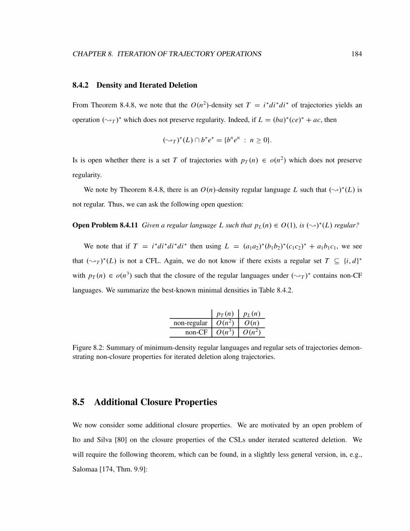
CHAPTER 8. ITERATION OF TRAJECTORY OPERATIONS 184
8.4.2 Density and Iterated Deletion
From Theorem 8.4.8, we note that the O(n2)-density set T = i∗di∗di∗ of trajectories yields an
operation (;T )∗ which does not preserve regularity. Indeed, if L = (ba)∗(ce)∗ + ac, then
(;T )∗(L) ∩ b∗e∗ = {bnen : n ≥ 0}.
Is is open whether there is a set T of trajectories with pT (n) ∈ o(n2) which does not preserve
regularity.
We note by Theorem 8.4.8, there is an O(n)-density regular language L such that (;)∗(L) is
not regular. Thus, we can ask the following open question:
Open Problem 8.4.11 Given a regular language L such that pL(n) ∈ O(1), is (;)∗(L) regular?
We note that if T = i∗di∗di∗di∗ then using L = (a1a2)∗(b1b2)
∗(c1c2)∗ + a1b1c1, we see
that (;T )∗(L) is not a CFL. Again, we do not know if there exists a regular set T ⊆ {i, d}∗
with pT (n) ∈ o(n3) such that the closure of the regular languages under (;T )∗ contains non-CF
languages. We summarize the best-known minimal densities in Table 8.4.2.
pT (n) pL(n)
non-regular O(n2) O(n)
non-CF O(n3) O(n2)
Figure 8.2: Summary of minimum-density regular languages and regular sets of trajectories demon-
strating non-closure properties for iterated deletion along trajectories.
8.5 Additional Closure Properties
We now consider some additional closure properties. We are motivated by an open problem of
Ito and Silva [80] on the closure properties of the CSLs under iterated scattered deletion. We
will require the following theorem, which can be found, in a slightly less general version, in, e.g.,
Salomaa [174, Thm. 9.9]:

CHAPTER 8. ITERATION OF TRAJECTORY OPERATIONS 185
Theorem 8.5.1 Let 6 be an alphabet, and a /∈ 6. Let s ∈ �(log(n)) be any space constructible
function. Then for all L ∈ RE over 6, there exists L ′ ∈ NSPACE(s) such that L ′ ⊆ a∗L and for all
x ∈ L, there exists i ≥ 0 such that ai x ∈ L ′.
For all T ⊆ {i, d}∗, let suff(T ) = {t ∈ {i, d}∗ : ∃t ′ ∈ {i, d}∗ such that t ′t ∈ T }. Our stated
closure property is given below:
Theorem 8.5.2 Let s ∈ �(log(n)) be a space-constructible function. Let d∗i∗ ⊆ T . If there exists
L such that (;suff(T ))+(L) ∈ RE − NSPACE(s), then NSPACE(s) is not closed under (;T )
+.
Proof. Let L ⊆ 6∗ be a language such that (;suff(T ))+(L) ∈ RE − NSPACE(s). Let a /∈ 6
and L0 ⊆ a∗((;suff(T ))
+(L))
be the language in NSPACE(s) described by Theorem 8.5.1. Let
L1 = L0 + a∗. Clearly, L1 ∈ NSPACE(s). We claim that (;T )+(L1) ∩6+ = (;suff(T ))
+(L).
(⊇): Let x ∈ (;suff(T ))+(L). Then there exists j ≥ 0 such that a j x ∈ L1. As a j ∈ L1 and
T ⊇ d∗i∗ ∋ d j i |x |, x ∈ a j x ;T a j ⊆ (;T )+(L1).
(⊆): To prove this inclusion, we prove the stronger claim that
(;T )+(L1) ⊆ a∗(;suff(T ))
∗(L).
Let x ∈ (;T )+(L1). Then there exists j ≥ 1 such that x ∈ (;T )
j (L1). The proof of our claim is
by induction on j .
For j = 1, x ∈ L1 ⊆ a∗(;suff(T ))+(L) + a∗. Thus, the result clearly holds. Let j > 1 and
assume the result holds for all natural numbers less than j . As x ∈ (;T )j (L1), then either x ∈
(;T )j−1(L1), whereby the result clearly holds by induction, or there exist x1, x2 ∈ (;T )
j−1(L1)
and t ∈ T such that x ∈ x1 ;t x2. By induction, xi = aki ui for ki ≥ 0, and ui ∈ (;suff(T ))∗(L), for
i = 1, 2.
There are three cases:
(a) u1, u2 ∈ (;suff(T ))+(L). Then x ∈ x1 ;t x2 implies that t = t1t2 where t1 satisfies |t1| = k1
and |t1|d = k2. Thus, x ∈ ak1−k2(u1 ;t2 u2). Let u ∈ u1 ;t2 u2 be such that x = ak1−k2 u. Then
note that t2 ∈ suff(T ) and thus u ∈ u1 ;t2 u2 ⊆ (;suff(T ))+(L). Thus, x ∈ a∗(;suff(T ))
∗(L).

CHAPTER 8. ITERATION OF TRAJECTORY OPERATIONS 186
(b) u2 = ǫ. Then x2 = ak2 and x1 = ak1 u1 where u1 ∈ (;suff(T ))∗(L1). Then note that necessarily,
x = ak2−k1 u1. Thus, x ∈ a∗(;suff(T ))∗(L1).
(c) u1 = ǫ and u2 ∈ (;T )+(L) such that u2 6= ǫ. Then x1 ;t x2 = ∅.
Thus, we have established that
(;T )+(L1) ∩6+ = (;suff(T ))
+(L). (8.14)
Assume, contrary to what we want to prove, that NSPACE(s) is closed under (;T )+. As L1 ∈
NSPACE(s), (;suff(T ))+(L) ∈ NSPACE(s) by (8.14). This contradicts our choice of L . Thus, we
have established the result.
For scattered deletion, T = (i + d)∗, and thus T = suff(T ). Thus, if CS = NSPACE(n) is closed
under (;)+, then for all L ∈ RE − CS, (;)+(L) ∈ CS. The closure of CS under (;T )+ is an open
problem posed by Ito and Silva [80].
8.6 T -Closure of a Language
We will now investigate the natural problem of, given L , finding the smallest language which is
closed under T and contains L . Classically, it is known that the smallest language containing
L which is closed under concatenation is L+. This question has also been examined by Ito et
al. [78, 79] and Kari and Thierrin [115] for other operations modeled by shuffle on trajectories. We
will require some notions about quotients and residuals, which we discuss first.
8.6.1 Shuffle-T Quotient
Let T ⊆ {0, 1}∗. In this section, we describe the shuffle-T quotient of a language L with respect to
a language L1, and show that if L , L1 and T are regular, the shuffle-T quotient of L1 with respect
to L is again regular.
Let 6 be an alphabet and L ⊆ 6∗. Then the shuffle-T quotient of L with respect to L1, denoted
CHAPTER 8. ITERATION OF TRAJECTORY OPERATIONS 187
sqT (L; L1), is given by
sqT (L; L1) = {x ∈ 6∗ : ∀y ∈ L1, y T x ⊆ L}.
For arbitrary shuffle T = (0+ 1)∗, the shuffle quotient has been examined by Campeanu et al. [21].
Ito et al. have examined (arbitrary) shuffle residual [79], which is given by sqT (L; L) for T =
(0+1)∗ and insertion residual [78], which is given by sqT (L; L) for T = 0∗1∗0∗. Kari and Thierrin
[115] have studied k-insertion residuals, given by sqT (L; L) for T = 0∗1∗0≤k for arbitrary k ≥ 0.
Hsiao et al. [69] consider right residuals for more general word operations. Our main result of this
section is the following:
Theorem 8.6.1 For all L ⊆ 6∗, sqT (L; L1) = (L ;π(T ) L1). Thus, if L , L1, T are regular, so is
sqT (L; L1), and it can be effectively constructed.
Proof. Let x ∈ sqT (L; L1). Assume, contrary to what we want to prove, that x ∈ L ;π(T ) L1.
Thus, there exist t ∈ T , y ∈ L and z ∈ L1 such that x ∈ y ;π(t) z. By Theorem 5.8.2, y ∈ z t x .
As x ∈ sqT (L; L1) and z ∈ L1, z t x ⊆ L . However, y ∈ L , a contradiction.
Let x /∈ sqT (L; L1). Thus, there exists some u ∈ L1 such that u T x ∩ L 6= ∅. Let y be
some word in this intersection, and let t ∈ T be such that y ∈ u t x . Thus by Theorem 5.8.2,
x ∈ y ;π(t) u ⊆ L ;π(T ) L1. Thus, we conclude that sqT (L; L1) ⊆ L ;π(T ) L1.
The fact that the regular languages are effectively closed under deletion along regular trajectories
implies that sqT (L; L1) is a regular language. This completes the proof.
Note that Theorem 8.6.1 gives an alternate proof that if L1, L2 are regular, then the (arbitrary)
shuffle quotient of L1 and L2 is regular (this was originally proven by Campeanu et al. [21, Lemma
4]). Further, Theorem 8.6.1 was proven for L = L1 and T = (0+ 1)∗ by Ito et al. [79, Prop. 2.4],
for L = L1 and T = 0∗1∗0∗ by Ito et al. [78, Prop. 2.3], and for L = L1 and T = 0∗1∗0≤k for fixed
k ≥ 0 by Kari and Thierrin [115, Prop. 2.3]. An equivalent formulation of Theorem 8.6.1 was given
by Hsiao et al. [69, Prop. 30], but without explicitly using the notion of inverse operations. Further,
in their framework of word operations, we cannot conclude any closure properties.
CHAPTER 8. ITERATION OF TRAJECTORY OPERATIONS 188
8.6.2 T -closure
Let rT (L) = sqT (L; L), which we call the shuffle-T residual of L . A language L ⊆ 6∗ such that
L ⊆ rT (L) is said to be shuffle-T closed. Define
CT (L) = {L ′ ⊆ 6∗ : L ⊆ L ′ ⊆ rT (L′)}.
Then CT (L) is the set of all shuffle-T closed languages containing L (CT (L) 6= ∅ as 6∗ ∈ CT (L)).
Further, define
clT (L) =⋂
L ′∈CT (L)
L ′.
Then clT (L) is the smallest T -closed language containing L; we call clT (L) the shuffle-T closure
of L .
Proposition 8.6.2 Let T ⊆ {0, 1}∗. Then L is shuffle-T closed if and only if L T L ⊆ L.
Proof. Let L be shuffle-T closed. Then for all x ∈ L , we have x ∈ rT (L). Thus, for all u ∈ L ,
u T x ⊆ L . Clearly then, L T L ⊆ L .
For the reverse implication, let L T L ⊆ L . Then let x ∈ L; we show x ∈ rT (L). As
L T L ⊆ L , for all y ∈ L , y T x ⊆ L . Thus, by definition, x ∈ rT (L).
Proposition 8.6.2 was noted for scattered deletion by Ito et al. [79], for sequential deletion by
Ito et al. [78] and for k-deletion by Kari and Thierrin [115]. For catenation, a weakened version
of the only-if portion of the result is sometimes given as an easy undergraduate exercise (see, e.g.,
Martin [141, Ex. 2.22]). In the framework of general word operations, a variant of Proposition 8.6.2
is given by Hsiao et al. [69, Prop. 24].
Corollary 8.6.3 Let T ⊆ {0, 1}∗ be a regular set of trajectories. Given a regular language L, it is
decidable whether L is shuffle-T closed.
We now seek to give a characterization of clT (L) for all T ⊆ {0, 1}∗. The following fact is
obvious from the definition of ( T )i :

CHAPTER 8. ITERATION OF TRAJECTORY OPERATIONS 189
Fact 8.6.4 For all L ⊆ 6∗ and all i ≥ 1, ( T )i (L) ⊆ ( T )
i+1(L).
Theorem 8.6.5 Let T ⊆ {0, 1}∗. Then clT (L) = ( T )+(L).
Proof. Note that L = ( T )1(L) ⊆ ( T )
+(L). To show that clT (L) ⊆ ( T )+(L), it suffices
to show that ( T )+(L) is shuffle-T closed. We appeal to Proposition 8.6.2. In particular, we
show that ( T )+(L) T ( T )
+(L) ⊆ ( T )+(L). Let x, y ∈ ( T )
+(L). Then there exist
j, k ≥ 1 such that x ∈ ( T )j (L) and y ∈ ( T )
k(L). Let m = max( j, k). Then clearly
x, y ∈ ( T )m(L). Thus, by definition of ( T )
m(L),
x T y ⊆ ( T )m+1(L) ⊆ ( T )
+(L).
The inclusion is proven.
We now show that ( T )+(L) ⊆ clT (L). Again, the proof is by induction on i : we show
( T )i(L) ⊆ clT (L) for all i ≥ 1.
For i = 1, L ⊆ clT (L) by definition of clT (L). Now let i > 1 and assume the result holds for
all integers less than i . Consider
( T )i(L) =
(( T )
i−1(L) T ( T )i−1(L)
)+ ( T )
i−1(L)
⊆ (clT (L) T clT (L))+ clT (L)
⊆ clT (L)+ clT (L) = clT (L)
where the first inclusion is by induction on i , and the second inclusion is by the fact that clT (L) is
T -closed (by definition of clT (L)), and Proposition 8.6.2.
Theorem 8.6.5 was also proven for sequential insertion by Ito et al. [78, Prop. 2.4], and for
arbitrary shuffle by Ito et al. [79, Prop. 2.6].
Recall that ( T )∗X is the iterated version of T defined by (8.4). As we have stated, it is
not hard to establish that ( T )∗X (L) = ( T )
∗(L) for all L if T is left-associative. Thus, we
can conclude that if T is left-associative, clT (L) = ( T )+X(L) for all L . We now show that the
requirement that T be left-associative is necessary for clT (L) = ( T )+X (L).

CHAPTER 8. ITERATION OF TRAJECTORY OPERATIONS 190
Lemma 8.6.6 There exist a singleton language L and set T of non-left-associative trajectories such
that clT (L) 6= ( T )+X (L).
Proof. We show, in fact, that infinitely many pairs (L , T ) exist satisfying the lemma. Let k ≥ 1,
and Tk = 0∗1∗0≤k . Then Tk= k←, the k-insertion operation, studied by Kari and Thierrin [115].
For each k ≥ 1, we define Lk = {bak}. Then we claim that
clTk(Lk) 6= ( k←)+X (Lk). (8.15)
We establish first that
{biaki : i ≥ 1} ⊆ clTk(Lk).
As Lk ⊆ clTk(Lk), bak ∈ clTk
(Lk). For each i > 1, bak, bi aki ∈ clTk(Lk) imply that bi+1ak(i+1) ∈
bak k← bi aki ⊆ clTk(Lk).
Now, we note that b3(a + b)∗ ∩ ( k←)+X (Lk) = ∅. To see this, note that if x ∈ ( k←)iX (Lk), then
|x| = ki and |x|b = i . We can then prove, by induction, that at most 2 occurrences of b can occur
at the start of any word in (k←)iX(Lk), since k-insertions always happen “close to the right end” of
the word. Thus, we can establish (8.15).
Note that Lemma 8.6.6 corrects an error in Kari and Thierrin [115, Prop. 2.4], where it is claimed
that clTk(L) = ( Tk
)+X (L) for each Tk = 0∗1∗0≤k .
8.6.3 Codes and Shuffle-Closed Languages
We now show that T -codes are shuffle-T closed if and only if they are trivially shuffle-T closed.
Lemma 8.6.7 Let T ⊆ {0, 1}∗. Let L ∈ PT (6). Then L is shuffle-T closed if and only if L T L =
∅.
Proof. If L T L = ∅, then clearly L T L ⊆ L , and L is shuffle-T closed.
Let L ∈ PT (6). Then note that necessarily L ⊆ 6+. Let L be shuffle-T closed. Assume there
exist x, y ∈ L such that x T y 6= ∅. Let z ∈ x T y. Thus, z ∈ L as L is shuffle-T closed.
Therefore, z ∈ L ∩ (L T 6+), contradicting that L is a T -code.
CHAPTER 8. ITERATION OF TRAJECTORY OPERATIONS 191
Corollary 8.6.8 Let T ⊆ {0, 1}∗ be complete. Let L ∈ PT (6). Then L is shuffle-T closed if and
only if L = ∅.
8.7 Deletion Closure of a Language
We now consider the problem of, given a language L , finding the smallest language which contains
L and is closed under ;T .
8.7.1 Del-T Quotient
Let T ⊆ {i, d}∗. In this section, we describe the del-T quotient of a language with respect to a
language L , and show that if L , L1, T are regular, the del-T quotient of L1 with respect to L is
again regular.
We define the set of T -scattered subwords as follows:
scsT (L) = L ;symd (T ) 6∗.
Note that
scsT (L) = {u ∈ 6∗ : ∃v ∈ 6∗ such that u π−1(T ) v ∩ L 6= ∅}.
Further, note that if L , T are regular, then scsT (L) is regular. As examples, note that
(a) when T = i∗d∗i∗, we have scsT (L) = sub(L), the subwords of L (e.g., Ito et al. [78]), given
by
sub(L) = {u ∈ 6∗ : ∃x, y ∈ 6∗ such that xuy ∈ L}.
(b) if T = (i + d)∗, we have that scsT (L) = sps(L), the scattered (or sparse) subwords of L (e.g.,
Ito et al. [79]), given by
sps(L) = {u ∈ 6∗ : ∃v ∈ 6∗ such that u v ∩ L 6= ∅}.

CHAPTER 8. ITERATION OF TRAJECTORY OPERATIONS 192
Let6 be an alphabet and L ⊆ 6∗. Then the deletion-T quotient of L with respect to L1, denoted
dqT (L; L1), is given by
dqT (L; L1) = {x ∈ scsT (L) : ∀y ∈ L1, y ;T x ⊆ L}.
Ito et al. have examined scattered deletion residual [79], which is given by dqT (L; L) for T =
(i + d)∗ and deletion residual [78], which is given by dqT (L; L) for T = i∗d∗i∗. For k ≥ 1, Kari
and Thierrin [115] have studied k-deletion residual, which is given by dqT (L; L) for T = i∗d∗i≤k .
Note that we could also define
dq ′T (L; L1) = {x ∈ 6∗ : ∀y ∈ L1, y ;T x ⊆ L}.
In this case, we get
dq ′T (L; L1) = dqT (L; L1) ∪ scsT (L).
Our main result of the section is the following:
Theorem 8.7.1 For all L ⊆ 6∗, dqT (L; L1) = (L1 ;symd (T ) L) ∩ scsT (L). Thus, if L , L1, T are
regular, so is dqT (L; L1), and it can be effectively constructed.
Proof. Let x ∈ dqT (L; L1). Immediately, we have that x ∈ scsT (L). Assume, contrary to what
we want to prove, that x ∈ L1 ;symd (T ) L . Thus, there exist t ∈ T , y ∈ L and z ∈ L1 such that
x ∈ z ;symd (t) y. By Theorem 5.8.3, y ∈ z ;t x . As x ∈ dqT (L; L1) and z ∈ L1, z ;t x ⊆ L .
However, y ∈ L, a contradiction.
Let x ∈ L1 ;symd (T ) L ∩ scsT (L). Assume, contrary to what we want to prove, that x /∈
dqT (L; L1). As x ∈ scsT (L), this implies that there exists a word y ∈ L1 such that y ;T x∩L 6= ∅.
Let u be some word in this intersection. Thus, there is some t ∈ T such that u ∈ y ;t x . By
Theorem 5.8.3, x ∈ y ;symd (t) u ⊆ L1 ;symd (T ) L. This contradicts our choice of x .
Theorem 8.7.1 was proven by Ito et al. for the cases where L = L1 and T = (i + d)∗ [79, Prop.
4.2] as well as L = L1 and T = i∗d∗i∗ [78, Prop. 3.2]. Theorem 8.7.1 was proven by Kari and
Thierrin [115] for the case of L = L1 and T = i∗d∗i≤k for fixed k ≥ 1.
CHAPTER 8. ITERATION OF TRAJECTORY OPERATIONS 193
8.7.2 T -del-closure
Let T ⊆ {i, d}∗ Let drT (L) = dqT (L; L), which we call the del-T residual of L . A language L
such that L ∩ scsT (L) ⊆ drT (L) is said to be del-T closed.
We first note a class of trajectories for which the annoyance of dealing with scsT (L) is removed.
We call a set T ⊆ {i, d}∗ del-left-preserving with respect to L if i |x | ∈ T for all x ∈ L . Note that if
T is del-left-preserving with respect to every language L then T is del-left-preserving. If symd(T )
is del-left-preserving (with respect to L), we say that T is sym-del-left-preserving (with respect to
L), or sdl-preserving.
Lemma 8.7.2 Let L ⊆ 6∗. If T is sdl-preserving with respect to L, then L ⊆ scsT (L).
Proof. Note in this case that scsT (L) = L ;symd (T ) 6∗ ⊇ L ;symd (T ) {ǫ} = L , as symd(T ) is
del-left-preserving.
Note that if T is sdl-preserving, T ⊇ d∗. This is satisfied by, for example, right- and left-
quotient, and sequential, bi-polar, k- and scattered deletion.
Consider that if L ⊆ scsT (L), then clearly L = scsT (L) ∩ L . This leads to the following
observation:
Proposition 8.7.3 Let T be sdl-preserving with respect to L. Then L is del-T closed if and only if
L ⊆ drT (L).
For defining the T -del-closure of a language, we need the following notation. Define
dCT (L) = {L ′ ⊆ 6∗ : L ⊆ L ′ and L ′ ∩ scsT (L′) ⊆ drT (L
′)}.
Then dCT (L) is the set of all del-T closed languages containing L (dCT (L) 6= ∅ as 6∗ ∈ dCT (L)).
Further, define dclT (L) = ∩L ′∈dCT (L)L′. It is not hard to see that
scsT (dclT (L)) ⊆⋂
L ′∈dCT (L)
scsT (L′), (8.16)

CHAPTER 8. ITERATION OF TRAJECTORY OPERATIONS 194
and that
dclT (L) ∩ scsT (dclT (L)) ⊆⋂
L ′∈dCT (L)
drT (L). (8.17)
With this, we can see that dclT (L) is the smallest T -del-closed language containing L; we call
dclT (L) the del-T closure of L .
Proposition 8.7.4 Let T ⊆ {i, d}∗. Then L is del-T closed if and only if L ;T (L ∩ scsT (L)) ⊆ L.
Proof. The proof is similar to that of Lemma 8.6.2. Let L be del-T closed. Then for all x ∈
L ∩ scsT (L), we have x ∈ drT (L). Thus, for all u ∈ L , u ;T x ⊆ L . Clearly then, L ;T
(L ∩ scsT (L)) ⊆ L .
For the reverse implication, let L ;T (L ∩ scsT (L)) ⊆ L . Consider x ∈ L ∩ scsT (L); we show
x ∈ drT (L). As L ;T (L ∩ scsT (L)) ⊆ L , for all y ∈ L , y ;T x ⊆ L . Thus, by definition, as
x ∈ scsT (L), we also have x ∈ drT (L).
Corollary 8.7.5 Let L ⊆ 6∗. Let T ⊆ {i, d}∗ be sdl-preserving with respect to L. Then L is
del-T -closed if and only if L ; L ⊆ L.
Corollary 8.7.5 was noted by Ito et al. for T = (i + d)∗ [79] and T = i∗d∗i∗ [78]. We can also
generalize an interesting result of Ito et al. [78, 79] and Kari and Thierrin [115, Prop. 3.3]. Call a
set of trajectories T square-enabling if 9(T ) ⊇ {(n, n) : n ≥ 0}.
Lemma 8.7.6 Let T ⊆ {0, 1}∗ be square-enabling, and such that τ(T ) is sdl-preserving. Let L be
a shuffle-T closed language. Then L is del-τ(T ) closed if and only if L = L ;τ (T ) L.
Proof. If L = L ;τ (T ) L , then by Corollary 8.7.5, L is τ(T )-del-closed.
Now, assume that L is τ(T )-del-closed. Again by Corollary 8.7.5, L ⊇ L ;τ (T ) L . Thus, let
x ∈ L . we must show x ∈ L ;τ (T ) L .
As L is shuffle-T closed, x T x ⊆ L . As T is square-enabling, x T x 6= ∅. Thus, let t ∈ T
and y ∈ L be chosen so that y ∈ x t x . By Theorem 5.8.2, x ∈ y ;τ (t) x . Thus, x ∈ L ;τ (T ) L ,
as required.
CHAPTER 8. ITERATION OF TRAJECTORY OPERATIONS 195
Let T ⊆ {i, d}∗. Let L be a language. We now give a characterization of the T -del-closure of a
language L , when T is sdl-preserving.
Fact 8.7.7 For all T ⊆ {i, d}∗ and L ⊆ 6∗, (;T )i(L) ⊆ (;T )
i+1(L).
Theorem 8.7.8 Let L ⊆ 6∗ be a language and T ⊆ {i, d}∗ be sdl-preserving. Then dclT (L) =
(;T )+(L).
Proof. Note that L ⊆ (;T )+(L). Then to show that dclT (L) ⊆ (;T )
+(L), it suffices to show that
(;T )+(L) is del-T closed. We appeal to Corollary 8.7.5. In particular, we show that
(;T )+(L) ;T (;T )
+(L) ⊆ (;T )+(L).
Let u, v ∈ (;T )+(L). Then there exist i, j ≥ 1 such that u ∈ (;T )
i(L) and v ∈ (;T )j (L).
Let k = max(i, j). This implies that u, v ∈ (;T )k(L). Thus, u ; v ⊆ (;T )
k+1(L) by definition
of (;T )k . We conclude that (;T )
+ is del-T closed and thus dclT (L) ⊆ (;T )+(L).
To show the reverse inclusion, we show by induction on i that (;T )i(L) ⊆ dclT (L) for all
i ≥ 1. For i = 1, L ⊆ dclT (L) by definition of dclT (L). Now assume the result holds for all
natural numbers less than i . Consider
(;T )i(L) =
((;T )
i−1(L) ;T (;T )i−1(L)
)+ (;T )
i−1(L);
⊆ (dclT (L) ;T dclT (L))+ dclT (L);
⊆ (dclT (L))+ dclT (L) = dclT (L),
where the first inclusion is by induction on i , and the second inclusion is by Corollary 8.7.5, and the
fact that dclT (L) is T -del-closed.
Theorem 8.7.8 was proven by Ito et al. in the case of scattered [79, Prop. 4.4] and sequential
[78, Prop. 3.4] deletion. Theorem 8.7.8 was proven by Kari and Thierrin [115, Prop. 3.4] for the
case of k-deletion.
We now show that sdl-preservation is necessary in the alternate definition of (;T )+X (L) given
by (8.9):

CHAPTER 8. ITERATION OF TRAJECTORY OPERATIONS 196
Lemma 8.7.9 There exist a set of trajectories T and infinitely many languages L such that T is not
sdl-preserving with respect to L and dclT (L) 6= (;T )+X (L).
Proof. We introduce a rather extreme example of a set T satisfying the conditions. Let T = d∗.
Then note that unless L ⊆ {ǫ}, T is not sdl-preserving with respect to L . Further, note that
L1 ;T L2 =
{ǫ} if L1 ∩ L2 6= ∅.
∅ otherwise.
Then let L be any language such that {ǫ} is properly contained in L . Then L ;T L = {ǫ} and
by induction, we can show that (;T )iX (L) ;T ((;T )
iX (L) + ǫ) = {ǫ}, for all i ≥ 2. Thus,
(;T )+X (L) = {ǫ}. But clearly in this case, dclT (L) 6= {ǫ}, since L ⊆ dclT (L) by definition.
8.8 T -Shuffle Base
We now extend the notion of shuffle base, examined by Ito et al. [78, 79] and Kari and Thierrin
[115]. Let L ⊆ 6+ be a shuffle-T -closed language (the following definitions can be given for
L ⊆ 6∗, as was done by Ito et al. [78, 79] and Kari and Thierrin [115], but we restrict this possibility
to allow for simpler definitions; the results below can also be given for the more complete definitions
of Ito et al. and Kari and Thierrin without much difficulty). The shuffle-T base of L , denoted by
JT (L), is the set of words in L which cannot be expressed as the shuffle along T of words in L .
Thus,
JT (L) = {u ∈ L : u /∈ L T L}.
Proposition 8.8.1 Let T be left-associative and L ⊆ 6+ be shuffle-T closed. Then
L = ( T )+(JT (L)). (8.18)
Proof. As L is shuffle-T closed, L = ( T )+(L). Thus, it suffices to show that ( T )
+(L) =
( T )+(JT (L)). As T is left-associative, we reduce this to showing following equality:
( T )+X (L) = ( T )
+X (JT (L)).

CHAPTER 8. ITERATION OF TRAJECTORY OPERATIONS 197
To see that ( T )+X (JT (L)) ⊆ ( T )
+X (L), we note that JT (L) ⊆ L and ( T )
+X is a monotone
operator, since T is. For the reverse inclusion, let x ∈ ( T )+X (L). Then we note that as ǫ /∈ L ,
if x ∈ ( T )iX (L), then i ≤ |x|. Thus, let hx be the maximum i such that x ∈ ( T )
iX (L). We
prove that x ∈ ( T )+X(JT (L)) by induction on hx .
For hx = 1, x ∈ L and x /∈ ( T )2X (L) = L T L . Thus, by definition, x ∈ JT (L) ⊆
( T )+X (JT (L)). Assume the result holds for all x with hx < h for some h > 1. Let x be a word
such that hx = h. Then x ∈ ( T )hX (L), and there exist y ∈ ( T )
h−1X (L) and z ∈ L such that
x ∈ y T z. By induction, y ∈ ( T )+X (JT (L)). If z ∈ JT (L), we are done. Therefore, assume
that z ∈ L − JT (L). There exist u, v ∈ L such that z = u T v . Thus, x ∈ y T (u T v) ⊆
(y T u) t v , as T is left-associative. But now y ∈ ( T )h−1X (L), u, v ∈ L imply that x ∈
( T )h+1X (L), a contradiction to our choice of x . Thus, z ∈ JT (L) and x ∈ ( T )
+X (JT (L)).
We now demonstrate that if L and T are regular and L is shuffle-T closed, then JT (L) is also
regular.
Lemma 8.8.2 Let T ⊆ {0, 1}∗ be a regular set of trajectories. If L ⊆ 6+ is regular and shuffle-T -
closed, then JT (L) is regular.
Proof. The proof will rely on establishing that
L − JT (L) = L T L . (8.19)
Let x ∈ L − JT (L). Then as x /∈ JT (L), there exist u, v ∈ L such that x ∈ u T v . Thus
x ∈ L T L . Now, let x ∈ L T L . As L is shuffle-T -closed, L T L ⊆ L . Thus x ∈ L . As
x ∈ L T L , x /∈ JT (L) by definition. This establishes (8.19). Now, as L T L , JT (L) ⊆ L , we
have that JT (L) = L − L T L . Since L and L T L are regular, JT (L) is regular.
Lemma 8.8.2 offers alternate proofs of the corresponding results by Ito et al. for scattered dele-
tion [79, Prop. 5.1] and sequential deletion [78, Prop. 5.1], and by Kari and Thierrin for k-insertion
[115, Prop. 2.5].
CHAPTER 8. ITERATION OF TRAJECTORY OPERATIONS 198
8.9 Shuffle-Free Languages
In this section, we consider the notion of shuffle-free languages. This was first examined by Ito et
al. [82]. Hsiao et al. [69, Sect. 5] also considered a similar notion for arbitrary word operations.
We show that for shuffle on trajectories, we can obtain results relating shuffle-free languages and
T -codes.
We adopt the following shorthand:
( T )≥2(L) =
⋃
i≥2
( T )i(L).
Let T ⊆ {0, 1}∗. Then we say that ∅ 6= L ⊆ 6+ is sh-T -free if
( T )≥2(L) ∩ L = ∅.
Thus, L is sh-T -free if, for all u1, u2, . . . , uk ∈ L (k ≥ 2), there is no way to shuffle the u j s together
with T to get a word from L . The concept of sh-T -free is an extension of the corresponding
notion, sh-free, for arbitrary shuffle; this was introduced by Ito et al. [82].
The following lemma will be useful:
Lemma 8.9.1 Let T ⊆ {0, 1}∗. Let L1, L2 be two sh-T -free languages such that ( T )+(L1) =
( T )+(L2). Then L1 = L2.
Proof. Assume not. Let x ∈ L1 − L2, without loss of generality. Since x ∈ L1 ⊆ ( T )+(L1) =
( T )+(L2), either x ∈ L2 or there exist u1, u2 ∈ ( T )
+(L2) such that x ∈ u1 T u2. As x /∈ L2
by assumption, let x ∈ u1 T u2. We now note that u1, u2 ∈ ( T )+(L2) = ( T )
+(L1). Thus,
x ∈ ( T )+(L1) T ( T )
+(L1) ⊆ ( T )≥2(L1). This contradicts that L1 is sh-T -free.
Let L ⊆ 6∗. We say that BT (L) ⊆ L ∩6+ is an extended sh-T -base of L if BT (L) is sh-T -free
and L ∩6+ ⊆ ( T )+(BT (L)).
Lemma 8.9.2 Let T ⊆ {0, 1}∗ and let L ⊆ 6∗. Then the extended sh-T -base of L is unique.

CHAPTER 8. ITERATION OF TRAJECTORY OPERATIONS 199
Proof. Let B1, B2 be two extended sh-T -bases of L .
Let x ∈ B1. Then x 6= ǫ by definition. Further, x ∈ 6+ ∩ L ⊆ ( T )+(B2), by the fact that B2
is an extended-T -base of L . Thus, B1 ⊆ ( T )+(B2), and
( T )+(B1) ⊆ ( T )
+(( T )+(B2)) ⊆ ( T )
+(B2),
where the last inclusion is valid by Theorem 8.6.5. By symmetry, we also have that ( T )+(B2) ⊆
( T )+(B1).
As B1, B2 are sh-T -free, we have that B1 = B2, by Lemma 8.9.1.
We now show that every language has a sh-T -base. Consider the following languages [69, 82]:
B0 = ∅;
Ki = L − ( T )+(
i−1⋃
j=0
H j ); ∀i ≥ 1
Bi = {x : x ∈ Ki and |x| ≤ |y| ∀y ∈ Ki}; ∀i ≥ 1
B =⋃
i≥1
Bi .
Then it is straight-forward to establish that B is a sh-T -base for L (see, e.g., Hsiao et al. [69, Prop.
12]).
There is an interesting relation between extended sh-T -bases and T -codes. This emphasizes the
naturalness of the definition of T -codes.
Lemma 8.9.3 Let T ⊆ {0, 1}∗ be a set of trajectories such that π(T ) is sdl-preserving. If BT (L) is
the extended sh-T -base of any del-π(T ) closed language L, then BT (L) is a T -code.
Proof. Let BT (L) be the extended sh-T -base of L . Suppose BT (L) is not a T -code. Then there exist
u, v ∈ BT (L) ⊆ L such that v ∈ u T w for some w ∈ 6+. By Theorem 5.8.2, w ∈ v ;π(T ) u.
As u, v ∈ L , w ∈ L by Corollary 8.7.5. Thus, w ∈ L ∩ 6+ ⊆ ( T )+(BT (L)). But then
v ∈ u T w ⊆ ( T )≥2(BT (L)). Thus, v ∈ BT (L) ∩ ( T )
≥2(BT (L)), a contradiction.

CHAPTER 8. ITERATION OF TRAJECTORY OPERATIONS 200
Lemma 8.9.3 was established in a slightly weaker form by Ito and Silva [80, Prop. 3.2] for the
case T = (0+ 1)∗. Hsiao et al. [69, Prop. 22] note the result for T = 0∗1∗ + 1∗0∗.
The converse is given in a more general form as follows:
Lemma 8.9.4 Let T ⊆ {0, 1}∗ be a set of trajectories such that π(T ) is sdl-preserving. Let L ∈
PT (L). Then L ∪ {ǫ} is del-π(T ) closed.
Proof. As L ∈ PT (L), L ;π(T ) L ⊆ {ǫ}, by (6.8). Consider that
L ∪ {ǫ};π(T ) L ∪ {ǫ}
= (L ;π(T ) L) ∪ ({ǫ};π(T ) L ∪ {ǫ}) ∪ (L ;π(T ) {ǫ})
⊆ {ǫ} ∪ {ǫ} ∪ L = L ∪ {ǫ}.
Therefore, L ∪ {ǫ} is del-π(T ) closed, by Corollary 8.7.5.
8.10 T -Primitive Words
A word w ∈ 6∗ is said to be primitive if w = uk implies u = w and k = 1. For instance, the
words aab and ababbb are primitive, while aabaab = (aab)2 is not. The concept of primitive
words is one of the most studied in formal language theory, and poses one of the most well-known
of all open problems in formal language theory concerning the complexity of the set of all primitive
words. The concept of a primitive word has been extended from concatenation to insertion and
shuffle by Kari and Thierrin [118] and to arbitrary word operations by Hsiao et al. [69]. In this
section, we consider primitivity with respect to a given shuffle on trajectories operation. We show
that under our general definition of ( T )∗, every word has a T -primitive root. We also consider
analogues of the Lyndon-Schutzenberger Theorems for shuffle on trajectories.
8.10.1 T -Primitivity and T -roots
In this section, we consider primitive words with respect to a set of trajectories. Our definition will
be with respect to our definition of iteration, which will alleviate certain restrictions which were
CHAPTER 8. ITERATION OF TRAJECTORY OPERATIONS 201
imposed by Hsiao et al. [69].
Let T ⊆ {0, 1}∗. Given a word w ∈ 6∗, we say that w is T -primitive if w ∈ ( T )n(u) implies
u = w and n = 1. Let QT (6) be the set of all T -primitive words over an alphabet 6. For all
T ⊆ {0, 1}∗ and w ∈ 6∗, let
T√w = {u ∈ QT (6) : w ∈ ( T )
+(u)}.
We call T√w the set of T -primitive roots of w.
It is well known (see, e.g, Lothaire [140, Prop. 1.3.1]) that every non-empty word has a unique
primitive (i.e., T -primitive for T = 0∗1∗) root, that is, for T = 0∗1∗, | T√w| = 1 for all w ∈ 6+.
Kari and Thierrin [118] note that for T = 0∗1∗0∗, this does not hold, as, e.g., babb, bbab ∈T√(b2a)n+1bn+1 for all n ≥ 1. However, we now note that for all T , every non-empty word has at
least one T -primitive root. We will require the following lemma:
Lemma 8.10.1 Let u ∈ 6∗. Then ( T )+(( T )
+(u)) ⊆ ( T )+(u).
Proof. The proof follows by the fact that ( T )+(u) is shuffle-T closed, by Theorem 8.6.5.
Theorem 8.10.2 Let T ⊆ {0, 1}∗. Let w ∈ 6+. Then | T√w| ≥ 1.
Proof. Let w ∈ 6+ be arbitrary. If w ∈ QT (6), then we are done, as w ∈ T√w. Thus, assume that
w is not T -primitive.
Let w ∈ ( T )i(u) for some u ∈ 6∗ and i ≥ 2. If u is T -primitive, then we are done, as
u ∈ T√w.
Note that |u| < |w| as i ≥ 2. Now, if u is not T -primitive, then u ∈ ( T )j (v) for some
v ∈ 6∗ and j ≥ 2. Note that w ∈ ( T )+(( T )
+(v)) ⊆ ( T )+(v). Thus, if v is T -primitive,
we are done.
Otherwise, as |v| < |u| < |w|, we note that as we continue this process, we eventually reach a
word x such that w ∈ ( T )+(x) and x is T -primitive. This completes the proof.

CHAPTER 8. ITERATION OF TRAJECTORY OPERATIONS 202
8.10.2 Freeness and Uniqueness of T -Primitive Roots
We now turn to uniqueness of T -primitive roots. We will require the notion of a free semigroup, see,
e.g., Shyr [184]. Recall that a semigroup is a set S equipped with an associative binary operation; it
does not necessarily have an identity element. Let M be a semigroup. A non-empty subset B ⊆ M
is said to be a base for M if and only if for all u1, u2, . . . , un, v1, v2, . . . , vm ∈ B, the equality
u1u2 · · · un = v1v2 · · · vm
implies that n = m and ui = vi for all 1 ≤ i ≤ n. Note that6 is a base for6+ as a semigroup under
concatenation. A semigroup M is said to be free if there exists some base B such that B∗ = M (it
can be easily shown that such a base must be unique). Levi [132] gives conditions on a semigroup
being free. Let T be an associative, deterministic set of trajectories. We say that T is free if the
semigroup M = (6+, T ) is free2.
As we will be dealing exclusively with associative sets of trajectories, we will use the operation
( T )+X , which we gave in (8.5).
We first note that, besides concatenation, there exist non-trivial operations which are free. For
instance, the operation of balanced insertion, given by T = {0k12 j 0k : k, j ≥ 0} is both deter-
ministic and associative (see Mateescu et al. [147]) and is free, as is easily verified using Levi’s
conditions.
We now give an open problem concerning freeness:
Open Problem 8.10.3 Given T regular (or context-free), is it decidable whether T is free?
It does not seem that Levi’s conditions are helpful in this regard. Further, consider the following
test: let L = 6+−(6+ T 6+). Test if L is a ∗-T-code (i.e., every word in ( T )
+(L) is uniquely
generated). Then T is free if and only if L is a ∗-T-code.
2We could also easily frame the current discussion in terms of free monoids (i.e., semigroups with identities), and say
that T is free if the monoid M = (6∗, T , ǫ) is free. However, as noted by Mateescu et al. [147, Rem. 4.7], we only
need to require that 0∗ + 1∗ ⊆ T to ensure that ǫ is the identity element for M .

CHAPTER 8. ITERATION OF TRAJECTORY OPERATIONS 203
Since T is regular implies that L is regular, we expect that this would a plausible test for the
freeness of T , since it is decidable whether a regular language is a ∗-code. However, the well-known
algorithm to determine if a regular language is a ∗-code (e.g., Berstel and Perrin [18, Thm. I.3.1])
relies on the fact that 6∗ is a free monoid under concatenation. Thus, it does not seem immediately
possible to generalize this proof to other T ⊆ {0, 1}∗.
Levi’s conditions are occasionally referred to as Levi’s Lemma (see, e.g., Allouche and Shallit
[3, Sect. 1.4]), which can be stated as follows for our purposes:
Lemma 8.10.4 Let T be deterministic, associative and free. Then for all u, v, x, y ∈ 6∗, u T v =
x T y implies that there exists z ∈ 6∗ such that either u = x T z or x = u T z.
Levi’s lemma (with T = 0∗1∗) is necessary for two of the most fundamental and elegant theo-
rems in formal language theory and combinatorics on words, the Lyndon-Schutzenberger Theorems
(see, e.g., Allouche and Shallit [3, Sect. 1.4]):
Theorem 8.10.5 Let x, z ∈ 6+, y ∈ 6∗. Then the following are equivalent:
(a) xy = yz;
(b) there exist u, v ∈ 6∗, e ≥ 0 such that x = uv , z = vu and y = (uv)eu.
Theorem 8.10.6 Let x, y ∈ 6+. Then the following three conditions are equivalent:
(a) xy = yx;
(b) there exist integers i, j > 0 such that x i = y j ;
(c) there exist z ∈ 6+ and integers k, ℓ > 0 such that x = zk and y = zℓ.
We now show that freeness is the essential property in proving a generalization of the Lyndon-
Schutzenberger Theorems for T .
The additional condition necessary to generalize the first Lyndon-Schutzenberger Theorem is
the possession of a unit element (see Mateescu et al. [147, Sect. 4.4]), which is the condition that
0∗ + 1∗ ⊆ T . Thus, if T has a unit element, x ∈ (x T ǫ) ∩ (ǫ T x) for all x ∈ 6∗.

CHAPTER 8. ITERATION OF TRAJECTORY OPERATIONS 204
Theorem 8.10.7 Let T be an associative, deterministic, free set of trajectories with a unit element.
Let x, z ∈ 6+ and y ∈ 6∗ be such that x T y, y T z 6= ∅. Then the following are equivalent:
(a) x T y = y T z;
(b) there exist u, v ∈ 6∗, e ≥ 0 such that
x = u T v,
z = v T u,
y = ( T )eX (u T v) T u.
Proof. ((a) ⇒ (b)): Let x T y = y T z. The proof is by induction on |y|. The base case
for y ∈ 6∗ is |y| = 0. In this case, x = x T ǫ and z = ǫ T z, as x T ǫ, ǫ T z 6= ∅, by
assumption. We conclude that x = z and (b) holds with u = ǫ, v = x = z and e = 0.
Assume the result holds for all words y′ with 0 ≤ |y′| < |y|. Let x T y = y T z. By
Lemma 8.10.4, there exists w ∈ 6∗ such that either x = y T w and z = w T y or y = x T w
and y = w T z.
In the first case, let u = y, v = w and e = 0. Then y = u = ( T )eX (u T v) T u, as T is
ST-strict. Further, x = u T v and z = v T u.
In the second case, we have that x T w = w T z. Note that |w| = |y|−|z| < |y| as z ∈ 6+.
Therefore, by induction, there exist u, v ∈ 6∗ and e ≥ 0 such that x = u T v , z = v T u and
w = ( T )eX (u T v) T u. Note that
y = x T w = (u T v) T ( T )eX (u T v) T u = ( T )
e+1X (u T v) T u,
by the associativity of T . Thus, (b) is satisfied.

CHAPTER 8. ITERATION OF TRAJECTORY OPERATIONS 205
((b)⇒ (a)): Note that
x T y = (u T v) T ( T )eX (u T v) T u
= u T v T (u T v) T · · · T (u T v)︸ ︷︷ ︸e times.
T u
= (u T v) T · · · T (u T v)︸ ︷︷ ︸e times.
T u T v T u
= y T z.
This proves the desired equality.
Call a set T of trajectories concatenation-like if T is deterministic, associative, free, and satisfies
the following property, which we call power-enabling: for all n, k ≥ 0, (kn, n) ∈ 9(T ) ⇒ ((k +
1)n, n) ∈ 9(T ). Note that balanced insertion is power-enabling and hence concatenation-like.
We will require the following proposition, which is easily proven by induction:
Proposition 8.10.8 Let T be associative. Then for all k, ℓ > 0, and all z ∈ 6+,
( T )kX (( T )
ℓX (z)) = ( T )
kℓX (z).
We may now state and prove our second generalized Lyndon-Schutzenberger Theorem:
Theorem 8.10.9 Let T be concatenation-like. Let x, y ∈ 6+ be words such that x T y and
y T x are non-empty. Then the following three conditions are equivalent:
(a) x T y = y T x;
(b) there exist integers i, j > 0 such that ∅ 6= ( T )iX (x) = ( T )
j
X (y);
(c) there exist z ∈ 6+ and k, ℓ > 0 such that x = ( T )kX (z) and y = ( T )
ℓX (z).
Proof. ((a) ⇒ (c)): Assume that x 6= y and ∅ 6= x T y = y T x . We show the result by
induction on |xy|. As x, y ∈ 6+, the base case is |xy| = 2. Thus, x, y ∈ 6. Thus, x T y =
y T x , and T deterministic implies that x = y, contrary to our assumption.
Assume that the result holds for all x, y ∈ 6+ with |xy| < n. Let |xy| = n. Let |x| ≥ |y|.
As x T y = y T x , by Levi’s property, there exists w ∈ 6∗ such that x = y T w. Note that

CHAPTER 8. ITERATION OF TRAJECTORY OPERATIONS 206
y T x = x T y = (y T w) T y = y T (w T y) by the associativity of T . Thus, by the
determinism of T , x = w T y and w T y = y T w.
If w = y, then x = y T y, and (c) follows with z = y and k = 2, ℓ = 1. Thus, assume that
w 6= y.
If |w| = 0, then x = y T w implies that x = y. Again, this contradicts our assumptions on
x, y. Thus, |w| > 0. Note that |wy| = |x| < |xy|. Thus, as w T y = y T w, by induction there
exist z ∈ 6+, k, ℓ > 0 such that w = ( T )kX (z) and y = ( T )
ℓX (z). Thus,
x = ( T )ℓX (z) T ( T )
kX (z).
Thus, x ∈ ( T )+X (z) by the closure of ( T )
+X (z) under T . As T is deterministic, we have that
there is some m > 0 such that x = ( T )mX (z). Thus, (c) is satisfied.
((c) ⇒ (b)): Let z ∈ 6+, k, ℓ > 0 be such that x = ( T )kX (z) and y = ( T )
ℓX (z). Using
Proposition 8.10.8, we note that
( T )ℓX (x) = ( T )
ℓX (( T )
kX (z)) = ( T )
ℓkX (z) = ( T )
kX (( T )
ℓX (z)) = ( T )
kX (y).
By the fact that ( T )kX (z) = x , ((k − 1)|z|, |z|) ∈ 9(T ). Thus, ((ℓ · k − 1)|z|, |z|) ∈ 9(T ) and
both ( T )ℓX (x) and ( T )
kX (y) are non-empty. Thus, (b) is satisfied.
((b)⇒ (a)): Let i, j > 0 be such that ∅ 6= ( T )iX (x) = ( T )
j
X (y). Note that if |x| = |y|, then
|( T )iX (x)| = |( T )
j
X (y)| implies that i = j . Thus, by the determinism of T , x = y and (a)
holds.
Thus, without loss of generality, assume that |x| > |y|. Thus, by the associativity of T ,
x T ( T )i−1X (x) = ( T )
iX (x) = ( T )
j
X (y) = y T ( T )j−1X (y).
(We let ( T )j−1X (y) = ǫ if j = 1, and similarly for x and i .) Thus, by Levi’s property, there exists
some w ∈ 6+ such that x = y T w. Thus,
( T )j
X (y) = ( T )iX (x) = ( T )
iX (y T w).

CHAPTER 8. ITERATION OF TRAJECTORY OPERATIONS 207
Note that
( T )iX (y T w) = (y T w) T (y T w) T · · · T (y T w).︸ ︷︷ ︸
i times
By the determinism of T , ( T )j
X (y) = ( T )iX (y T w) implies that
( T )j−1X (y) = w T ( T )
i−1X (y T w)
⇒ ( T )j−1X (y) T y = w T ( T )
i−1X (y T w) T y
⇒ ( T )j
X (y) = ( T )iX (w T y)
⇒ ( T )iX (y T w) = ( T )
iX (w T y).
By the determinism of T , y T w = w T y. Thus,
x T y = (y T w) T y
= y T (w T y)
= y T x .
Thus, (a) is satisfied, as y 6= x and y T x = x T y 6= ∅.
Our main corollary of the generalized Lyndon-Schutzenberger Theorems concerns the unique-
ness of T -primitive roots:
Corollary 8.10.10 Let T be concatenation-like. Then for all u ∈ 6+, u has a unique T -primitive
root.
Proof. Let u ∈ 6+, and assume that v1, v2 ∈ T√
u. Then as T is concatenation-like, we have
u = ( T )i1(v1) and u = ( T )
i2(v2) for some i1, i2 ≥ 1. Thus, there exist j1, j2 such that
u = ( T )j1X (v1) and u = ( T )
j2X (v2).
By Theorem 8.10.9, there exist z ∈ 6+ and k1, k2 ≥ 1 such that v1 = ( T )k1
X (z) and v2 =
( T )k2X (z). As v1, v2 ∈ QT (6), we must have that k1 = k2 = 1 and z = v1 = v2. Thus, | T
√u| = 1,
as required.
Thus, we see that if T is catenation-like, then each word has a unique T -primitive root. This
applies, e.g., to balanced insertion.

CHAPTER 8. ITERATION OF TRAJECTORY OPERATIONS 208
8.11 Language Equations Revisited
In Chapter 7, we have studied language equations involving shuffle and deletion along trajectories.
In this section, we revisit this topic to consider some equation forms which we did not consider in
Chapter 7.
In particular, we note that all of language equations we have considered have the form
L = X ⋄ Y
where X,Y (and occasionally ⋄) may be unknown, but the language L is always fixed. We recall
that, in the terminology of, e.g., Leiss [131, Sect. 2.6], such equations are called implicit language
equations. In this section, we consider explicit language equations, which we recall are of the
form X = α where X is unknown, and α is an equation involving constants, language operations
(including T ) and unknowns.
Clearly, explicit language equations are of considerable interest; indeed, the fundamental notion
of CFGs is equivalent to explicit systems of language equations of the form X = α where α is an
expression involving catenation and union [10, Sect. 2]. Extensions of the context-free grammar
formalism to capture larger classes of languages via grammars have also been studied, for example,
conjunctive [157] and Boolean [159] grammars, both recently introduced by Okhotin. Explicit
language equations are crucial to both these studies.
Consideration of language equations with unknowns on both sides of the equality sign must
involve some caution, however, especially with regard to our interest thus far in answering ques-
tions such as “is it decidable whether this equation has a solution?” Consider the equation X =
L1 T L2, where L1, L2 are languages and T is a set of trajectories. Clearly, this equation has
a solution X = L1 T L2. Note that this assumes nothing about the complexity of L1, L2 or T .
Other equations possess trivial solutions; X = X T L has a solution X = ∅ regardless of L and
T .
Thus, in this section, our focus will shift somewhat from decidability, which is often trivial, to
characterizations of solutions. Our results will be similar in spirit to Arden’s Lemma (Arden [9],

CHAPTER 8. ITERATION OF TRAJECTORY OPERATIONS 209
cf., Salomaa [173, Ch. 3]) which states that the equation X = X R1+ R2 has a unique solution R∗1 R2
if ǫ /∈ R1. Further, R∗1 R2 is the least solution (by inclusion) of X = X R1 + R2, independent of
R1 (see, e.g., Conway [28, Thm. 3, p. 27]). We will see that such results can be extended to T ,
under certain assumptions on T , and that related equations have similar characterizations.
8.11.1 Arden-like Equations
Our first consideration will be the following equation:
X = X T L1 + L2,
where X is unknown, and L1, L2 are arbitrary languages. In the case where T = 0∗1∗, the char-
acterization of the unique solution of this equation (under the assumption that ǫ /∈ L1) is known
as Arden’s Lemma (however, the identity L2L∗1 = L2L∗1 L1 + L2 was previously known, see, e.g.,
Kleene [119, Eq. (9), p. 24]). We will require some conditions on T in order for a similar result to
hold.
Theorem 8.11.1 Let T ⊆ {0, 1}∗ be left-preserving and associative. Let L1, L2 be arbitrary lan-
guages. The least solution to the equation
X = X T L1 + L2, (8.20)
is the language L2 T ( T )∗(L1).
Proof. As T is associative, it will suffice to establish that the language L2 T ( T )∗X (L1) is the
least solution to (8.20). Recall that ( T )∗X is defined by (8.4).
We first show that L = L2 T ( T )∗X (L1) is a solution to (8.20). We establish the inclusion
L T L1 + L2 ⊆ L , by proving that
L2 ⊆ L2 T ( T )∗X (L1) (8.21)
and that
(L2 T ( T )
iX (L1)
)T L1 ⊆ L2 T ( T )
∗X (L1) (8.22)

CHAPTER 8. ITERATION OF TRAJECTORY OPERATIONS 210
for all i ≥ 0. We note that (8.21) holds since T is left-preserving and ǫ ∈ ( T )∗X (L1). We now
establish (8.22) for all i ≥ 0. Note that for arbitrary i ≥ 0,
(L2 T ( T )iX (L1)) T L1 = L2 T (( T )
iX(L1) T L1)
= L2 T ( T )i+1X (L1)
⊆ L2 T ( T )∗X (L1).
We now establish the inclusion L T L1 + L2 ⊇ L . Let x ∈ L = L2 T ( T )∗X (L1). Then
there exists i ≥ 0 such that x ∈ L2 T ( T )iX (L1). For i = 0, x ∈ L2 T {ǫ} ⊆ L2. Thus,
x ∈ L2 ⊆ L T L1 + L2. Let i > 0. Then
x ∈ L2 T ( T )iX (L1)
= L2 T (( T )i−1X (L1) T L1)
= (L2 T ( T )i−1X (L1)) T L1
⊆ (L2 T ( T )∗X (L1)) T L1 + L2.
Thus, L is a solution to (8.20). We now show that it is the least solution to this equation. Let X0 be
the least solution to (8.20). We show that X0 ⊇ L . First, we note that
X0 = X0 T L1 + L2 ⊇ L2 = L2 T ( T )0X (L1).
Let i ≥ 0. Assume that X0 ⊇ L2 T ( T )iX (L1). Then we have that
X0 ⊇ X0 T L1 ⊇ (L2 T ( T )iX (L1)) T L1
⊇ L2 T (( T )iX (L1) T L1)
⊇ L2 T ( T )i+1X (L1).
Thus, X0 ⊇ L2 T ( T )∗X (L1) = L . This completes the proof.
We can also give the following symmetric result.

CHAPTER 8. ITERATION OF TRAJECTORY OPERATIONS 211
Theorem 8.11.2 Let T ⊆ {0, 1}∗ be right-preserving and associative. Let L1, L2 be arbitrary
languages. Then the least solution to the equation
X = L1 T X + L2, (8.23)
is the language ( T )∗(L1) T L2.
Further results in this area are likely. For instance, Salomaa considers systems of equations of
the form
X i =n∑
j=1
X j L j,i + Ri
for 1 ≤ i ≤ n, and investigates their solutions [173, Ch. 3, Sect. 2]. Systems of this form with
X j T L j,i are clear generalizations (for a single fixed T ⊆ {0, 1}∗), and results can likely be
obtained in the same manner as Theorems 8.11.1 and 8.11.2.
8.11.2 A Language Equation for ( T )+(L)
Due to the conditions placed on T in the previous section, the following question seems natural:
given arbitrary T and L , can we find a language equation for which ( T )+(L) is the minimal
solution? We give this equation in the following theorem:
Theorem 8.11.3 Let T ⊆ {0, 1}∗. For any language L ⊆ 6∗, the least solution to the equation
X = X T X + L (8.24)
is X = ( T )+(L).
Proof. We first show that ( T )+(L) is a solution of (8.24). Consider that
( T )+(L) T ( T )
+(L)+ L ⊆ ( T )+(L)+ L
⊆ ( T )+(L).
The last inclusion is by definition of ( T )+(L) and the first is by Proposition 8.6.2 and Theo-
rem 8.6.5. To prove the reverse inclusion, let x ∈ ( T )+(L). Then there exists i ≥ 1 such that x ∈
CHAPTER 8. ITERATION OF TRAJECTORY OPERATIONS 212
( T )i(L). If i = 1, then x ∈ L ⊆ ( T )
+(L) T ( T )+(L)+ L , and the inclusion holds. As-
sume then that i > 1 and for all y ∈ ( T )j (L) with j < i , y ∈ ( T )
+(L) T ( T )+(L)+ L .
Let x ∈ ( T )i (L). Then by definition, x ∈ ( T )
i−1(L) or x ∈ ( T )i−1(L) T ( T )
i−1(L).
In the first case, the result holds by induction. Otherwise,
x ∈ ( T )i−1(L) T ( T )
i−1(L)
⊆ (( T )+(L) T ( T )
+(L)+ L) T (( T )+(L) T ( T )
+(L)+ L)
⊆ (( T )+(L)+ L) T (( T )
+(L)+ L)
⊆ ( T )+(L) T ( T )
+(L)+ L .
Here, the first inclusion is by induction, the second is by Proposition 8.6.2 and Theorem 8.6.5, and
the third is by the distributivity of ( T )+ over union. Thus,
( T )+(L) = ( T )
+(L) T ( T )+(L)+ L .
Let X0 ⊆ 6∗ be the least solution of (8.24). As ( T )+(L) is a solution of (8.24), X0 ⊆
( T )+(L). It remains to show the reverse inclusion, which is again accomplished by induction,
by showing that ( T )i(L) ⊆ X0 for all i ≥ 1.
For i = 1, L ⊆ L + X0 T X0 = X0. Let i > 1 and assume that ( T )i−1(L) ⊆ X0. Then
note that
X0 = X0 T X0 + L
⊇ X0 T X0
⊇ ( T )i−1(L) T ( T )
i−1(L).
Thus X0 ⊇ ( T )i−1(L) and X0 ⊇ ( T )
i−1(L) T ( T )i−1(L), i.e., X0 ⊇ ( T )
i−1(L) +
( T )i−1(L) T ( T )
i−1(L) = ( T )i(L). This establishes the inclusion. Thus, X0 = ( T )
+(L),
establishing the result.
CHAPTER 8. ITERATION OF TRAJECTORY OPERATIONS 213
8.12 Conclusions
In this chapter, we have considered the iteration of shuffle on trajectory and deletion on trajectory
operations. Our work generalizes previous work by Ito et al. [78, 79] and Kari and Thierrin [115]
on particular shuffle and deletion along trajectories operations. Our work is also similar to that of
Hsiao et al. [69] on iteration of arbitrary word operations. However, by considering a more general
definition of iterated shuffle on trajectories, we are able to overcome some of the conditions imposed
by Hsiao et al. in their study of iterated binary word operations.
After considering iterated shuffle and deletion along trajectories and the closure of languages un-
der shuffle and deletion along trajectories, we have investigated the notions of shuffle base, extended
shuffle base, primitivity and the Lyndon-Schutzenberger Theorems, all considered in trajectory-
based contexts. These notions generalize well to shuffle and deletion along trajectories, and many
key concepts hold. We note that in the context of investigating the Lyndon-Schutzenberger The-
orems, we raise the problem of when T defines a free operation. This fundamental problem
remains open.
Finally, we have returned to the topic of language equations. For explicit equations, the problem
of decidability of the existence of solutions becomes trivial, and we have instead focused on char-
acterizing least solutions to language equations. We have found explicit least solutions for two key
explicit language equations involving T . One generalizes a well-known language equation for
Kleene closure which has been studied for fifty years. The second is a general language equation
formulated so that its least solution is ( T )+(L).
Chapter 9
Conclusions
9.1 Results and Focus
In this thesis, we have examined word operations defined by trajectories, and related problems. Our
focus is on four areas: descriptional complexity, codes, language equations and iterated operations.
Chapter 4 considered the problem of state complexity for shuffle on trajectories. As shuffle on
trajectories defines a very general family of operations on languages, examining the state complexity
of shuffle on trajectories is a challenging problem. The work in Chapter 4 is the first research in
state complexity which does not examine a particular operation, but a class of language operations.
We have seen that the density of the set of trajectories proves useful for characterizing the state
complexity of the resulting shuffle on trajectories operations. We have given upper and lower bounds
on the state complexity of shuffle on trajectories for sets of trajectories which are slender, i.e., sets
of trajectories which only contain a constant number of trajectories for any fixed length. In this
case, we see that there is a substantial advantage over the case where the number of trajectories of
any given length is not restricted.
In Chapter 5, we have introduced the operation of deletion along trajectories. Several natu-
ral deletion-like operations are particular cases of deletion along trajectories, including quotient,
214

CHAPTER 9. CONCLUSIONS 215
scattered deletion and sequential deletion. The most crucial theoretical aspect of deletion along tra-
jectories is that it serves as an inverse to shuffle on trajectories. The closure properties of deletion
along trajectories are different from those of shuffle on trajectories, and we have investigated these
properties. The most interesting property is the similarity between the closure properties of dele-
tion along trajectories and proportional removals. This similarity yields many non-regular sets of
trajectories for which the associated deletion on trajectories operation preserves regularity.
Chapter 6 investigates classes of languages defined by shuffle on trajectories, and their relation
to traditional classes of codes. This investigation has given much insight into the nature of code
classes by shifting the focus from classes of languages to the language-theoretic properties of the
associated sets of trajectories. We have addressed many natural lines of research in the theory of
codes, in particular, questions of maximality, embedding of codes, finiteness properties and the
relationship between convexity of languages and code-theoretic properties. While other general
mechanisms for defining classes of code-like languages have been presented in the literature, we
have found that shuffle on trajectories attains a desirable balance between expressive power on the
one hand and the ability to obtain interesting results on the other. In particular, decidability results
are obtained through the known closure properties of shuffle and deletion along trajectories.
Our consideration of these classes of codes in Chapter 6 has also led naturally to the definition
of a binary relation on the set of all finite words for each set of trajectories. We have investigated
algebraic properties of these binary relations; of particular interest is whether a set of trajectories
defines a transitive binary relation. Decidability of these properties of the binary relation defined by
a set of trajectories are also considered.
As deletion along trajectories constitutes an inverse to shuffle on trajectories, we can therefore
investigate language equations involving both shuffle and deletion along trajectories. This is the
focus of Chapter 7. We have investigated several different equation forms, and have obtained both
positive and negative decidability results for the problem of determining whether an equation pos-
sesses a solution. We have also considered systems of equations with shuffle on trajectories, an
important step in the investigation of language equations involving shuffle on trajectories.

CHAPTER 9. CONCLUSIONS 216
Finally, Chapter 8 has investigated the questions raised by considering iterated versions of shuf-
fle and deletion along trajectories operations. With a very natural definition of iterated shuffle
on trajectories, denoted ( T )+(L), we can give, for all languages L and all sets of trajectories
T ⊆ {0, 1}∗ (resp., all T ⊆ {i, d}∗ with T ⊇ i∗), a characterization of the smallest language con-
taining L and closed under T (resp., ;T ). We have also studied explicit language equations,
i.e., language equations of the form X = α where X is a variable and α is an expression involv-
ing T . This study is a fundamental first step towards developing grammar systems involving
shuffle on trajectories. In our study, we focus on characterization results for elementary explicit
language equations involving shuffle on trajectories. For all T ⊆ {0, 1}∗, we find that the equation
X = X T X + L has least solution ( T )+(L).
9.2 Open Problems
In this section, we survey some of the more interesting open problems we have considered in this
thesis. This is not a complete description of all open problems in this thesis.
Chapter 4 investigated the descriptional complexity of shuffle on trajectories. We concluded
with the following conjecture:
Conjecture 9.2.1 For all T ⊆ {0, 1}∗ with pT (n) ∈ �(2n), there exists L1, L2 such that sc(L1 T L2) =
2�(sc(l1)sc(L2)).
In chapter 6, we investigated T -codes, which are a natural generalization of many classes of
codes. From a theoretical standpoint, the most interesting open problem is characterizing those T
for which all T -codes are finite:
Open Problem 9.2.2 What are necessary and sufficient conditions on a set T ⊆ {0, 1}∗ of trajec-
tories such that PT (6) ⊆ FIN?
In particular, a characterization for Open Problem 9.2.2 which solves the following problem is
of the most interest:

CHAPTER 9. CONCLUSIONS 217
Open Problem 9.2.3 Given a (regular, context-free) set T ⊆ {0, 1}∗ of trajectories, is it decidable
whether PT (6) ⊆ FIN?
One fundamental property of sets of trajectories which we have not resolved is freeness, which
we discussed in Section 8.10.2.
Open Problem 9.2.4 Let T ⊆ {0, 1}∗ be a regular (or context-free) set of trajectories. Is it decid-
able whether the semigroup M = (6∗, T ) is a free semigroup?
There are several open problems concerning iteration of shuffle and deletion on trajectories. The
following problem is easily stated, but a solution does not seem obvious:
Open Problem 9.2.5 For all R ∈ REG, does there exist k ≥ 1 such that (;)+(R) ∈ CFk?
9.3 Further Research Directions
In this section, we examine some research directions which we hope to explore in the future.
9.3.1 Confluence of ωT
Given a transitive, reflexive binary relation ρ on 6∗, we say that a language L ⊆ 6∗ is confluent
with respect to ρ if, for all x, y ∈ L , there exists z ∈ L such that x ρ z and y ρ z.
Ilie [73] has investigated the confluence property for arbitrary binary relations, and examined
decidability problems for specific relations, including the prefix, suffix and factor orders. Investi-
gating the decidability of the confluence problem for arbitrary ωT remains an interesting research
question.

CHAPTER 9. CONCLUSIONS 218
9.3.2 Codes Defined by Multiple Sets of Trajectories
Let n ≥ 1 and Ti ⊆ {0, 1}∗ for 1 ≤ i ≤ n. Define T = {T1, . . . , Tn}. Consider the relation ωT on
6∗ defined by
x ωT y ⇐⇒n∧
i=1
x ωTiy
for all x, y ∈ 6∗. Define PT(6) as the set of all anti-chains under ωT. There has been interest in
PTps(6) for Tps = {0∗1∗, 1∗0∗}, see Jurgensen and Konstantinidis [97, pp. 550–551] for references
and a discussion of this class.
Further, we can define a related class QmT (6) as follows: L ∈ Qm
T (6) if and only if for all L ′ ⊆ L
with |L ′| ≤ m, L ′ ∈ ∪ni=1PTi
(6). For QmT (6), other than Tps, the classes Tio = {0∗1∗0∗, 1∗0∗1∗}
[139], as well as Tk−io = {(1∗0∗)k1∗, (0∗1∗)k0∗} and Tk−ps = {(0∗1∗)k, (1∗0∗)k} for k ≥ 1 (see
Long et al. [138, Defns. 5 and 6] or Long [137]) have received attention.
It is easily established that Q2T(6) = PT(6) and that Qn+i
T (6) = QnT(6) for all T with |T| = n
and for all i ≥ 0. However, other problems related to these classes of languages do not seem to be
so easy. For instance, the decidability of membership in PTps(6) (see Ito et al. [76] or Jurgensen et
al. [98]) relies intrinsically on the nature of the members of Tps. The corresponding problem for Tio
also relies on the nature of the sets of trajectories involved [38]. It appears to be a very challenging
problem to determine the decidability of membership in PT(6) for arbitrary T = {T1, . . . , Tn},
where each Ti is regular. Kari et al. [108, Thm. 4.7] have solved a similar decision problem for
two sets of trajectories in their framework of bond-free property. However, their approach does not
seem to be adaptable to our situation.
9.3.3 Semantic Trajectory-Based Operations
By slightly expanding the notion of a trajectory, we find that trajectory-based operations have sev-
eral interesting applications. Emerging uses of word operations, especially in modeling operations
on strands of DNA, show promise for using shuffle and deletion on trajectories or related trajectory-
based variants. Work has already been conducted in this area by Mateescu [144] and more recently
CHAPTER 9. CONCLUSIONS 219
by Kari et al. [108]. Both of these works focus on using the shuffle on trajectories model to opera-
tions on DNA.
However, there is another approach to adapting the trajectory-based framework to model situ-
ations such as operations on DNA strands. This approach considers what are known as semantic
operations. In the paper which introduced shuffle on trajectories, Mateescu et al. make the following
distinction between syntactic and semantic operations on words:
We introduce and investigate new methods [shuffle on trajectories] to define parallel com-
position of words and languages. These methods are based on syntactic constraints on the
shuffle operations. The constraints are referred to as syntactic constraints since they do not
concern properties of the words that are shuffled, or properties of the letters that occur in
these words.
Instead, the constraints involve the general strategy to switch from one word to another
word. Once such a strategy is defined, the structure of the words that are shuffled does not
play any role.
However, constraints that take into consideration the inner structure of the words that are
shuffled together are referred to as semantic constraints. [147, p. 2]
With the current focus on operations on DNA, we see semantic operations not as a clumsy sib-
ling to syntactic operations, but a challenging area of investigation. We feel that a suitable extension
of the shuffle and deletion along trajectories model would provide much insight into the nature of
semantic operations. A reasonable model exists which shares many similarities to the current shuffle
on trajectories model, but adds sufficient semantic power to encompass many interesting semantic
operations, including those investigated by several authors, including Daley et al. [29, 30, 31], Kari
and Thierrin [116], Kari [107], Mateescu and Salomaa [149], Kudlek and Mateescu [127, 126], de
Simone [34], Chen et al. [23] and many others; Mateescu et al. [146] summarize some of these
semantic operations. We also note the possibility of extending the semantic framework proposed by
Abdelwahed [1, 2], which is a model of combining processes in control of discrete event systems.
Abdelwahed notes that, among others, the concept of shuffle on trajectories is “influential to the
modelling paradigm [1, p. 8]” (called Interacting Discrete Event Systems–IDES) developed in the
thesis.
It remains to be seen which results can be adapted from the syntactic case to the semantic case.

CHAPTER 9. CONCLUSIONS 220
It is clear, however, that generalizations of some results–in particular, the equations considered by
Daley et al. [29, 30]–will yield interesting results relating to bio-informatics.

Bibliography
[1] ABDELWAHED, S. Interacting Discrete Event Systems: Modelling, Verification and Super-
visory Control. PhD thesis, University of Toronto, 2002.
[2] ABDELWAHED, S., AND WONHAM, W. Interacting DES: Modelling and analysis. In 41st
IEEE Conference on Decision and Control (2002), pp. 1175–1180.
[3] ALLOUCHE, J.-P., AND SHALLIT, J. Automatic Sequences: Theory, Applications, General-
izations. Cambridge University Press, 2003.
[4] AMAR, V., AND PUTZOLU, G. On a family of linear grammars. Inf. and Cont. 7 (1964),
283–291.
[5] AMAR, V., AND PUTZOLU, G. Generalizations of regular events. Inf. and Cont. 8 (1965),
56–63.
[6] ARAKI, T., KAGIMASA, T., AND TOKURA, N. Relations of flow languages to Petri net
languages. Theor. Comp. Sci. 15 (1981), 51–75.
[7] ARAKI, T., AND TOKURA, N. Decision problems for regular expressions with shuffle and
shuffle closure operators. Systems, Computers, Controls 12, 6 (1981), 46–50.
[8] ARAKI, T., TOKURA, N., AND KOSAI, S. Shuffle grammars. Systems, Computers, Controls
14, 4 (1983), 37–45.
221

BIBLIOGRAPHY 222
[9] ARDEN, D. Delayed logic and finite state machines. University of Michigan Press, 1960,
pp. 1–35.
[10] AUTEBERT, J.-M., BERSTEL, J., AND BOASSON, L. Context-free languages and pushdown
automata. pp. 111–174. In [171].
[11] BAADER, F., AND KUSTERS, R. Solving linear equations over regular languages. In UNIF
2001: 15th International Workshop on Unification (2001), F. Baader, V. Diekert, C. Tinelli,
and R. Treinen, Eds., pp. 27–31.
[12] BEL-ENGUIX, G., MARTIN-VIDE, C., AND MATEESCU, A. Dialog and splicing on routes.
Romanian Journal of Information Science and Technology 6, 1-2 (2003), 45–59.
[13] BAADER, F., AND NARENDRAN, P. Unification of concept terms in descriptional logics. J.
Symb. Comput. 31 (2001), 277–305.
[14] BALCAZAR, J., DIAZ, J., AND GABARRO, J. Structural Complexity II. Springer, 1990.
[15] BARIL, J.-L., AND VAJNOVSZKI, V. Gray code for derangements. Disc. Appl. Math. 140
(2004), 207–221.
[16] BERARD, B. Literal shuffle. Theor. Comp. Sci. 51 (1987), 281–299.
[17] BERSTEL, J., BOASSON, L., CARTON, O., PETAZZONI, B., AND PIN, J.-E. Operations
preserving recognizable languages. In Fundamentals of Computation Theory (FCT 2003)
(2003), A. Lingas and B. Nilsson, Eds., vol. 2751 of Lecture Notes in Computer Science,
Springer-Verlag, pp. 343–354.
[18] BERSTEL, J., AND PERRIN, D. Theory of Codes. Available at http://www-igm.univ-
mlv.fr/%7Eberstel/LivreCodes/Codes.html, 1996.
[19] BRUYERE, V., AND PERRIN, D. Maximal bifix codes. Theor. Comp. Sci. 218 (1999), 107–
121.

BIBLIOGRAPHY 223
[20] BRZOZOWSKI, J. Roots of star events. J. ACM 14, 3 (1967), 466–477.
[21] CAMPEANU, C., SALOMAA, K., AND VAGVOLGYI, S. Shuffle decompositions of regular
languages. Int. J. Found. Comp. Sci. 13, 6 (2002), 799–816.
[22] CAMPEANU, C., SALOMAA, K., AND YU, S. Tight lower bound for the state complexity
of shuffle of regular languages. J. Automata, Languages and Combinatorics 7, 3 (2002),
303–310.
[23] CHEN, K., FOX, R., AND LYNDON, R. Free differential calculus IV: The quotient groups
of lower central series. Ann. Math., 2nd Ser. 68, 1 (1958), 81–95.
[24] CHOFFRUT, C., AND KARHUMAKI, J. Combinatorics on words. pp. 329–438. In [171].
[25] CHOFFRUT, C., AND KARHUMAKI, J. On Fatou properties of rational languages. In Where
Mathematics, Computer Science, Linguistics and Biology Meet (2000), C. Martin-Vide and
V. Mitrana, Eds., Kluwer, pp. 227–235.
[26] CLERBOUT, M., ROOS, Y., AND RYL, I. Synchronization languages. Theor. Comp. Sci. 215
(1999), 99–121.
[27] CLERBOUT, M., ROOS, Y., AND RYL, I. Synchronization languages and rewriting systems.
Inf. and Comp. 167, 1 (2001), 46–69.
[28] CONWAY, J. Regular Algebra and Finite Machines. Chapman and Hall, 1971.
[29] DALEY, M. Computational Modeling of Genetic Processes in Stichotrichous Ciliates. PhD
thesis, University of Western Ontario, 2003.
[30] DALEY, M., IBARRA, O., AND KARI, L. Closure properties and decision questions of some
language classes under ciliate bio-operations. Theor. Comp. Sci. 306, 1 (2003), 19–38.
[31] DALEY, M., KARI, L., AND MCQUILLAN, I. Families of languages defined by ciliate
bio-operations. Theor. Comp. Sci. 320, 1 (2004), 51–69.
BIBLIOGRAPHY 224
[32] DASSOW, J., MITRANA, V., AND SALOMAA, A. Operations and language generating de-
vices suggested by the genome evolution. Theor. Comp. Sci. 270 (2002), 701–738.
[33] DE LUCA, A., AND VARRICCHIO, S. Regularity and finiteness conditions. pp. 747–810. In
[171].
[34] DE SIMONE, R. Langages infinitaires et produits de mixage. Theor. Comp. Sci. 31 (1984),
83–100.
[35] DOMARATZKI, M. State complexity of proportional removals. J. Automata, Languages and
Combinatorics 7, 4 (2002), 455–468.
[36] DOMARATZKI, M. On iterated scattered deletion. Bull. Eur. Assoc. Theor. Comp. Sci. 80
(2003), 159–161.
[37] DOMARATZKI, M. Deletion along trajectories. Theor. Comp. Sci. 320, 2–3 (2004), 293–313.
[38] DOMARATZKI, M. On the decidability of 2-infix-outfix codes. Tech. Rep. 2004-479, School
of Computing, Queen’s University, 2004.
[39] DOMARATZKI, M. Trajectory-based codes. Acta Inf. 40, 6–7 (2004), 491–527.
[40] DOMARATZKI, M. Trajectory-based embedding relations. Fund. Inf. 59, 4 (2004), 349–363.
[41] DOMARATZKI, M., MATEESCU, A., SALOMAA, K., AND YU, S. Deletion along trajecto-
ries and commutative closure. In Proceedings of WORDS’03: 4th International Conference
on Combinatorics on Words (2003), T. Harju and J. Karhumaki, Eds., pp. 309–319.
[42] DOMARATZKI, M., AND OKHOTIN, A. Representing recursively enumerable languages by
iterated deletion. Theor. Comp. Sci. 314, 3 (2004), 451–457.
[43] DOMARATZKI, M., AND SALOMAA, K. State complexity of shuffle on trajectories. In
Descriptional Complexity of Formal Systems (DCFS) (2002), J. Dassow, M. Hoeberechts,
H. Jurgensen, and D. Wotschke, Eds., pp. 95–109.
BIBLIOGRAPHY 225
[44] DOMARATZKI, M., AND SALOMAA, K. Decidability of trajectory-based equations. To
appear in Mathematical Foundations of Computer Science 2004 (2004).
[45] DOMARATZKI, M., AND SALOMAA, K. Restricted sets of trajectories and decidability
of shuffle decompositions. In Descriptional Complexity of Formal Systems (DCFS 2004)
(2004), L. Ilie and D. Wotschke, Eds., pp. 37–51.
[46] DOMARATZKI, M., AND SALOMAA, K. State complexity of shuffle on trajectories. Ac-
cepted, J. Automata, Languages and Combinatorics 9, 2 (2004).
[47] EHRENFEUCHT, A., HAUSSLER, D., AND ROZENBERG, G. On regularity of context-free
languages. Theor. Comp. Sci. 23 (1983), 311–332.
[48] ELLUL, K. Descriptional complexity measures of regular languages. M.Math thesis, Uni-
versity of Waterloo, 2002.
[49] FLAJOLET, P., AND STEYAERT, J.-M. On sets having only hard subsets. In Automata
Languages and Programming (1974), J. Loeckx, Ed., vol. 14 of Lecture Notes in Computer
Science, Springer-Verlag, pp. 446–457.
[50] GINSBURG, S. The Mathematical Theory of Context-Free Languages. McGraw-Hill, 1966.
[51] GINSBURG, S. Algebraic and Automata-Theoretic Properties of Formal Languages. North-
Holland, 1975.
[52] GINSBURG, S., AND SPANIER, E. Quotients of context-free languages. J. ACM 10, 4 (1963),
487–492.
[53] GINSBURG, S., AND SPANIER, E. Mappings of languages by two-tape devices. J. ACM 12,
3 (1965), 424–434.
[54] GINSBURG, S., AND SPANIER, E. H. Bounded regular sets. Proc. Amer. Math. Soc. 17
(1966), 1043–1049.
BIBLIOGRAPHY 226
[55] GISCHER, J. Shuffle language, Petri nets and context-sensitive grammars. Comm. ACM 24,
9 (1981), 597–605.
[56] GUO, L., SALOMAA, K., AND YU, S. Synchronization expressions and languages. In Proc.
6th IEEE Symposium on Parallel and Distributed Processing (1994), IEEE Computer Society
Press, pp. 257–264.
[57] GUO, Y., SHYR, H., AND THIERRIN, G. E-Convex infix codes. Order 3 (1986), 55–59.
[58] HAINES, L. On free monoids partially ordered by embedding. J. Comb. Th. 6 (1969), 94–98.
[59] HARJU, T., AND ILIE, L. On quasi orders of words and the confluence property. Theor.
Comp. Sci. 200 (1998), 205–224.
[60] HARJU, T., AND KARHUMAKI, J. Morphisms. In Handbook of Formal Languages, Vol. I
(1997), pp. 439–510.
[61] HARJU, T., MATEESCU, A., AND SALOMAA, A. Shuffle on trajectories: The
Schutzenberger product and related operations. In Mathematical Foundations of Computer
Science 1998 (1998), L. Brim, J. Gruska, and J. Zlatuska, Eds., no. 1450 in Lecture Notes in
Computer Science, Springer-Verlag, pp. 503–511.
[62] HARRISON, M. Introduction to Formal Language Theory. Addison-Wesley, 1978.
[63] HAUSLER, D., AND ZEIGER, H. Very special languages and representations of recursively
enumerable languages via computation histories. Inf. and Cont. 47 (1980), 201–212.
[64] HIGMAN, G. Ordering by divisibility in abstract algebras. Proc. London Math. Soc. 2, 3
(1952), 326–336.
BIBLIOGRAPHY 227
[65] HOLZER, M., AND KUTRIB, M. State complexity of basic operations on nondeterministic
finite automata. In Implementation and Application of Automata: 7th International Con-
ference, CIAA 2002 (2003), J.-M. Champarnaud and D. Maurel, Eds., vol. 2608 of Lecture
Notes in Computer Science, Springer-Verlag, pp. 148–157.
[66] HOLZER, M., AND KUTRIB, M. Unary language operations and their nondeterministic state
complexity. In Developments in Language Theory: Sixth International Conference, DLT
2002 (2003), M. Ito and M. Toyama, Eds., vol. 2450 of Lecture Notes in Computer Science,
Springer-Verlag, pp. 162–172.
[67] HOLZER, M., AND LANGE, K.-J. On the complexity of iterated insertions. In New Trends
in Formal Languages (1997), G. Paun and A. Salomaa, Eds., vol. 1218 of Lecture Notes in
Computer Science, Springer-Verlag, pp. 440–453.
[68] HOPCROFT, J. E., AND ULLMAN, J. D. Introduction to Automata Theory, Languages, and
Computation. Addison-Wesley, 1979.
[69] HSIAO, H., HUANG, C., AND YU, S.-S. Word operation closure and primitivity of lan-
guages. J. Universal Comp. Sci. 8, 2 (2002), 243–256.
[70] HUNT, H., AND ROSENKRANTZ, D. Computational parallels between the regular and
context-free languages. SIAM J. Comput. 7 (1978), 99–114.
[71] IGARASHI, A., AND KOBAYASHI, N. Resource usage analysis. ACM SIGPLAN Notices 37,
1 (2002), 331–342.
[72] ILIE, L. Remarks on well quasi orders of words. In Proceedings of the 3rd DLT (1997),
S. Bozapalidis, Ed., pp. 399–411.
[73] ILIE, L. Decision Problems on Orders of Words. PhD thesis, University of Turku, 1998.
BIBLIOGRAPHY 228
[74] IMREH, B., ITO, M., AND KATSURA, M. On shuffle closures of commutative regular
languages. In Combinatorics, Complexity, & Logic (Auckland, 1996) (1997), D. Bridges,
C. Calude, I. Gibbons, S. Reeves, and I. Witten, Eds., Springer, pp. 276–288.
[75] ITO, M. Shuffle decomposition of regular languages. J. Universal Comp. Sci. 8, 2 (2002),
257–259.
[76] ITO, M., JURGENSEN, H., SHYR, H., AND THIERRIN, G. n-prefix-suffix languages. Intl.
J. Comp. Math. 30 (1989), 37–56.
[77] ITO, M., JURGENSEN, H., SHYR, H., AND THIERRIN, G. Outfix and infix codes and related
classes of languages. J. Comp. Sys. Sci. 43 (1991), 484–508.
[78] ITO, M., KARI, L., AND THIERRIN, G. Insertion and deletion closure of languages. Theor.
Comp. Sci. 183 (1997), 3–19.
[79] ITO, M., KARI, L., AND THIERRIN, G. Shuffle and scattered deletion closure of languages.
Theor. Comp. Sci. 245 (2000), 115–133.
[80] ITO, M., AND SILVA, P. Remark on deletions, scattered deletions and related operations on
languages. In Semigroups and Applications (1998), J. Howie and N. Ruskuc, Eds., World
Scientific, pp. 97–105.
[81] ITO, M., AND TANAKA, G. Dense property of initial literal shuffles. Intl. J. Comp. Math.
34 (1990), 161–170.
[82] ITO, M., THIERRIN, G., AND YU, S.-S. Shuffle-closed languages. Publ. Math. Debrecen
48, 3–4 (1996), 317–338.
[83] ITO, T., AND NISHITANI, Y. On universality of concurrent expressions with synchronization
primitives. Theor. Comp. Sci. 19 (1982), 105–115.

BIBLIOGRAPHY 229
[84] IWAMA, K. Unique decomposability of shuffled strings. In Proceedings of the Fifteenth
Annual ACM Symposium on Theory of Computing (1983), D. Johnson et al., Ed., pp. 374–
381.
[85] JANTZEN, M. The power of synchronizing operations on strings. Theor. Comp. Sci. 14
(1981), 127–154.
[86] JANTZEN, M. Extending regular expressions with iterated shuffle. Theor. Comp. Sci. 38
(1985), 223–247.
[87] JEDRZEJOWICZ, J. On the enlargement of the class of regular languages by the shuffle
closure. Inf. Proc. Letters 16 (1983), 51–54.
[88] JEDRZEJOWICZ, J. Nesting of shuffle closure is important. Inf. Proc. Letters 25 (1987),
363–367.
[89] JEDRZEJOWICZ, J. Infinite hierarchy of expressions containing shuffle closure operator. Inf.
Proc. Letters 28, 1 (1988), 33–37.
[90] JEDRZEJOWICZ, J. Infinite hierarchy of shuffle expressions over a finite alphabet. Inf. Proc.
Letters 36, 1 (1990), 13–17.
[91] JEDRZEJOWICZ, J. Undecidability results for shuffle languages. J. Automata, Languages
and Combinatorics 1, 2 (1997), 147–159.
[92] JEDRZEJOWICZ, J. Structural properties of shuffle automata. Grammars 2 (1999), 35–51.
[93] JEDRZEJOWICZ, J., AND SZEPIETOWSKI, A. Shuffle languages are in P. Theor. Comp. Sci.
250 (2001), 31–53.

BIBLIOGRAPHY 230
[94] JIRASEK, J., JIRASKOVA, G., AND SZABARI, A. State Complexity of Concatenation and
Complementation of Regular Languages. In Pre-proceedings of CIAA 2004: Ninth Interna-
tional Conference on Implementations and Applications of Automata (2004), M. Domaratzki,
A. Okhotin, K. Salomaa and S. Yu, Eds., pp. 132–142.
[95] JIRASKOVA, G. State complexity of some operations on regular languages. In Descrip-
tional Complexity of Formal Systems: Fifth International Workshop (2003), E. Csuhaj-Varju,
C. Kintala, D. Wotschke, and G. Vaszil, Eds., pp. 114–125.
[96] JULLIEN, P. Sur un theoreme d’extension dans la theorie des mots. CR Acad. Sc. Paris (Serie
A) 266 (1968), 851–854.
[97] JURGENSEN, H., AND KONSTANTINIDIS, S. Codes. pp. 511–600. In [171].
[98] JURGENSEN, H., SALOMAA, K., AND YU, S. Transducers and the decidability of indepen-
dence in free monoids. Theor. Comp. Sci. 134 (1994), 107–117.
[99] JURGENSEN, H., SHYR, H., AND THIERRIN, G. Codes and compatible partial orders on
free monoids. In Algebra and Order: Proceedings of the First International Symposium on
Ordered Algebraic Structures, Luminy–Marseilles 1984 (1986), S. Wolfenstein, Ed., Helder-
mann Verlag, pp. 323–334.
[100] JURGENSEN, H., AND YU, S. Relations on free monoids, their independent sets, and codes.
Int. J. Comput. Math. 40 (1991), 17–46.
[101] KADRIE, A., DARE, V., THOMAS, D., AND SUBRAMANIAN, K. Algebraic properties of
the shuffle over ω-trajectories. Inf. Proc. Letters 80, 3 (2001), 139–144.
[102] KARI, L. Insertion and deletion of words: Determinism and reversibility. In Mathematical
Foundations of Computer Science 1992 (1992), I. Havel and V. Koubek, Eds., vol. 629 of
Lecture Notes in Computer Science, Springer-Verlag, pp. 315–326.

BIBLIOGRAPHY 231
[103] KARI, L. Generalized derivatives. Fund. Inf. 18 (1993), 27–39.
[104] KARI, L. Insertion operations: Closure properties. Bull. Eur. Assoc. Theor. Comp. Sci. 51
(1993), 181–191.
[105] KARI, L. Deletion operations: Closure properties. Intl. J. Comp. Math. 52 (1994), 23–42.
[106] KARI, L. On language equations with invertible operations. Theor. Comp. Sci. 132 (1994),
129–150.
[107] KARI, L. Power of controlled insertion and deletion. In Results and Trends in Theoretical
Computer Science (1994), J. Karhumaki, H. Maurer, and G. Rozenberg, Eds., vol. 812 of
Lecture Notes in Computer Science, Springer-Verlag, pp. 197–212.
[108] KARI, L., KONSTANTINIDIS, S., AND SOSIK, P. On properties of bond-free DNA lan-
guages. Tech. Rep. 609, Computer Science Department, University of Western Ontario,
2003. Submitted for publication.
[109] KARI, L., KONSTANTINIDIS, S., AND SOSIK, P. Bond-free languages: Formalisms, maxi-
mality and construction methods. Tech. Rep. 2004–001, Saint Mary’s University Department
of Mathematics and Computer Science, 2004. To appear, DNA 10.
[110] KARI, L., KONSTANTINIDIS, S., AND SOSIK, P. Substitutions, trajectories and noisy chan-
nels. In Pre-proceedings of CIAA 2004: Ninth International Conference on Implementations
and Applications of Automata (2004), M. Domaratzki, A. Okhotin, K. Salomaa and S. Yu,
Eds., pp. 154–162.
[111] KARI, L., MATEESCU, A., SALOMAA, A., AND PAUN, G. Deletion sets. Fund. Inf. 19
(1993), 355–370.
[112] KARI, L., AND SOSIK, P. Language deletions on trajectories. Tech. Rep. 606, Computer
Science Department, University of Western Ontario, 2003. Submitted for publication.

BIBLIOGRAPHY 232
[113] KARI, L., AND SOSIK, P. On language equations with deletion. Bull. Eur. Assoc. Theor.
Comp. Sci. 83 (2004), 173–180.
[114] KARI, L., AND THIERRIN, G. k-catenation and applications: k-prefix codes. J. Inf. Opt. Sci.
16, 2 (1995), 263–276.
[115] KARI, L., AND THIERRIN, G. k-insertion and k-deletion closure of languages. Soochow J.
Math 21, 4 (1995), 479–495.
[116] KARI, L., AND THIERRIN, G. Contextual insertions/deletions and computability. Inf. and
Comp. 131 (1996), 47–61.
[117] KARI, L., AND THIERRIN, G. Maximal and minimal solutions to language equations. J.
Comp. Sys. Sci. 53 (1996), 487–496.
[118] KARI, L., AND THIERRIN, G. Word insertions and primitivity. Util. Math. 53 (1998), 49–61.
[119] KLEENE, S. Representation of events in nerve nets and finite automata. In Automata Stud-
ies (1956), C. Shannon and J. McCarthy, Eds., vol. 34 of Annals of Mathematics Studies,
Princeton University Press, pp. 3–41.
[120] KOSARAJU, S. Correction to “Regularity Preserving Functions”. ACM SIGACT News 6, 3
(1974), 22.
[121] KOSARAJU, S. Regularity preserving functions. ACM SIGACT News 6, 2 (1974), 16–17.
[122] KOSARAJU, S. Context-free preserving functions. Math. Sys. Theor. 9, 3 (1975).
[123] KOZEN, D. On regularity-preserving functions. Tech. Rep. TR95-1559, Department of
Computer Science, Cornell University, 1995.
[124] KRISHNAN, P. Automatic synthesis of a subclass of schedulers in timed systems. Theor.
Comp. Sci. 298, 3 (2003), 347–363.

BIBLIOGRAPHY 233
[125] KRUSKAL, J. The theory of well-quasi-ordering: A frequently discovered concept. J. Comb.
Th. (A) 13 (1972), 297–305.
[126] KUDLEK, M., AND MATEESCU, A. On distributed catenation. Theor. Comp. Sci. 180 (1997),
341–352.
[127] KUDLEK, M., AND MATEESCU, A. On mix operation. In New Trends in Formal Languages
(1997), G. Paun and A. Salomaa, Eds., vol. 1218 of Lecture Notes in Computer Science,
Springer-Verlag, pp. 430–439.
[128] LAM, N. Finite maximal infix codes. Semigroup Forum 61 (2000), 346–356.
[129] LATTA, M., AND WALL, R. Intersective context-free languages. In Lenguajes Naturales y
Lenguajes Formalex IX (1993), C. Martin-Vide, Ed., pp. 15–43.
[130] LATTEUX, M., LEGUY, B., AND RATOANDROMANANA, B. The family of one-counter
languages is closed under quotient. Acta. Inf. 22 (1985), 579–588.
[131] LEISS, E. Language Equations. Monographs in Computer Science. Springer, 1999.
[132] LEVI, F. On semigroups. Bull. Calcutta Math. Soc. 36 (1944), 141–146.
[133] LIU, L., AND WEINER, P. An infinite hierarchy of intersections of context-free languages.
Math. Sys. Th. 7, 2 (1973), 185–192.
[134] LONG, D. On nilpotency of the syntactic monoid of a language. In Words, Languages and
Combinatorics II (1992), M. Ito and H. Jurgensen, Eds., World Scientific, pp. 279–293.
[135] LONG, D. On two infinite hierarchies of prefix codes. In Proceedings of the Conference on
Ordered Structures and Algebra of Computer Languages (1993), K. Shum and P. Yuen, Eds.,
World Scientific, pp. 81–90.
[136] LONG, D. k-bifix codes. Rivista di Matematica Pura ed Applicata 15 (1994), 33–55.
BIBLIOGRAPHY 234
[137] LONG, D. Study of Coding Theory and its Application to Cryptography. PhD thesis, City
University of Hong Kong, 2002.
[138] LONG, D., JIA, W., MA, J., AND ZHOU, D. k-p-infix codes and semaphore codes. Disc.
Appl. Math. 109 (2001), 237–252.
[139] LONG, D., MA, J., AND ZHOU, D. Structure of 3-infix-outfix maximal codes. Theor. Comp.
Sci. 188 (1997), 231–240.
[140] LOTHAIRE, M. Combinatorics on Words. Addison-Wesley, 1983.
[141] MARTIN, J. Introduction to Languages and the Theory of Computation (3rd ed.). McGraw-
Hill, 2003.
[142] MARTIN-VIDE, C., MATEESCU, A., ROZENBERG, G., AND SALOMAA, A. Contexts on
trajectories. Intl. J. Comp. Math. 73, 1 (1999), 15–36.
[143] MATEESCU, A. CD grammar systems and trajectories. Acta. Cyb. 13, 2 (1997), 141–157.
[144] MATEESCU, A. Splicing on routes: a framework of DNA computation. In Unconventional
Models of Computation (1998), C. Calude, J. Casti, and M. Dinneen, Eds., Springer, pp. 273–
285.
[145] MATEESCU, A., AND MATEESCU, G. Associative and fair shuffle of ω-words. Tech. Rep.
TUCS-TR-162, University of Turku, 1998.
[146] MATEESCU, A., ROZENBERG, G., AND SALOMAA, A. Syntactic and semantic aspects
of parallelism. In Foundations of Computer Science: Potential–Theory–Cognition (1997),
C. Freksa, M. Jantzen, and R. Valk, Eds., Lecture Notes in Computer Science, Springer-
Verlag, pp. 79–106.
[147] MATEESCU, A., ROZENBERG, G., AND SALOMAA, A. Shuffle on trajectories: Syntactic
constraints. Theor. Comp. Sci. 197 (1998), 1–56.
BIBLIOGRAPHY 235
[148] MATEESCU, A., AND SALOMAA, A. Aspects of classical language theory. pp. 175–246. In
[171].
[149] MATEESCU, A., AND SALOMAA, A. Parallel composition of words with re-entrant symbols.
An. Univ. Bucuresti Mat. Inform. 45, 1 (1996), 71–80.
[150] MATEESCU, A., SALOMAA, A., SALOMAA, K., AND YU, S. On an extension of the Parikh
mapping. Tech. Rep. 364, TUCS, 2000.
[151] MATEESCU, A., SALOMAA, A., AND YU, S. Factorizations of languages and commutativ-
ity conditions. Acta Cyb. 15, 3 (2002), 339–351.
[152] MATEESCU, A., SALOMAA, K., AND YU, S. On fairness of many-dimensional trajectories.
J. Automata, Languages and Combinatorics 5 (2000), 145–157.
[153] MEDUNA, A. Middle quotients of linear languages. Intl. J. Comp. Math. 71 (1999), 319–335.
[154] MORIYA, T., AND YAMASAKI, H. Literal shuffle on ω-languages. Inf. Proc. Letters 59
(1996), 165–168.
[155] NICAUD, C. Average state complexity of operations on unary automata. In Proceedings
of the 24th International Symposium on Mathematical Foundations of Computer Science
(MFCS 1999) (1999), M. Kutylowski, L. Pacholski, and T. Wierzbicki, Eds., vol. 1672 of
Lecture Notes in Computer Science, Springer-Verlag, pp. 230–240.
[156] OGDEN, W., RIDDLE, W., AND ROUNDS, W. Complexity of expressions allowing concur-
rency. In Conference Record of the Fifth Annual ACM Symposium on Principles of Program-
ming Languages (1978), A. Aho and S. Zilles, Eds., pp. 185–194.
[157] OKHOTIN, A. Conjunctive grammars. J. Automata, Languages and Combinatorics 6, 4
(2001), 519–535.
[158] OKHOTIN, A. Personal communication, September 2003.

BIBLIOGRAPHY 236
[159] OKHOTIN, A. Boolean grammars. To appear, Inf. and Comp. (2004).
[160] OKHOTIN, A. On the equivalence of linear conjunctive grammars to trellis automata. RAIRO
Theor. Inf. and Appl. 38, 1 (2004), 69–88.
[161] PARKES, D. Formal Languages and the Word Problem in Groups. PhD thesis, University of
Leicester, 2000.
[162] PARKES, D., AND THOMAS, R. Syntactic monoids and word problems. Arabian Journal
for Science and Engineering (C) 25, 2 (2000), 81–94.
[163] PIGHIZZINI, G., AND SHALLIT, J. Unary language operations, state complexity and Ja-
cobsthal’s function. International Journal of Foundations of Computer Science 13 (2002),
145–159.
[164] PIN, J.-E. Varieties of Formal Languages. Plenum, 1986.
[165] PIN, J.-E., AND SAKAROVITCH, J. Une application de la representation matricielle des
transductions. Theor. Comp. Sci. 35 (1981), 271–293.
[166] PIN, J.-E., AND SAKAROVITCH, J. Some operations and transductions that preserve ratio-
nality. In 6th GI Conference (1983), A. Cremers and H.-P. Kriegel, Eds., vol. 145 of Lecture
Notes in Computer Science, Springer-Verlag, pp. 277–288.
[167] POLAK, L. Syntactic semirings and language equations. In Implementation and Application
of Automata: 7th International Conference (2003), J.-M. Champarnaud and D. Maurel, Eds.,
vol. 2608 of Lecture Notes in Computer Science, Springer-Verlag, pp. 182–193.
[168] PAUN, G., AND SALOMAA, A. Thin and slender languages. Disc. Appl. Math. 61 (1995),
257–270.
[169] RAMESH KUMAR, P., AND RAJAN, A. Expletive languages. Southeast Asian Bulletin of
Mathematics 23 (1998), 187–197.

BIBLIOGRAPHY 237
[170] RIDDLE, W. An approach to software system behaviour description. Comp. Lang. 4 (1979),
29–47.
[171] ROZENBERG, G., AND SALOMAA, A., Eds. Handbook of Formal Languages, Vol. 1.
Springer-Verlag, 1997.
[172] RYL, I., ROOS, Y., AND CLERBOUT, M. Generalized synchronization languages. In
Fundamentals of Computation Theory, 12th International Symposium, (FCT’99) (1999),
G. Ciobanu and G. Paun, Eds., pp. 451–462.
[173] SALOMAA, A. Theory of Automata. Pergamon Press, 1969.
[174] SALOMAA, A. Formal Languages. Academic Press, 1973.
[175] SALOMAA, A. Jewels of Formal Language Theory. Computer Science Press, 1981.
[176] SALOMAA, A., AND YU, S. On the decomposition of finite languages. In Developments in
Language Theory (1999), G. Rozenberg and W. Thomas, Eds., pp. 22–31.
[177] SALOMAA, K., AND YU, S. Synchronization expressions with extended join operation.
Theor. Comp. Sci. 207 (1998), 73–88.
[178] SALOMAA, K., AND YU, S. Synchronization expressions and languages. J. Universal
Comp. Sci. 5 (1999), 610–621.
[179] SANTEAN, L. Six arithmetic-like operation on languages. Cahiers de linguistique theore-
tique et applique 25 (1988), 65–73.
[180] SEIFERAS, J., AND MCNAUGHTON, R. Regularity-preserving relations. Theor. Comp. Sci.
2 (1976), 147–154.
[181] SHALLIT, J. Numeration systems, linear recurrences, and regular sets. Inf. and Comp. 113,
2 (1994), 331–347.
BIBLIOGRAPHY 238
[182] SHAW, A. Software descriptions with flow expressions. IEEE Trans. Soft. Eng. SE-4, 3
(1978), 242–254.
[183] SHOUDAI, T. A P-complete language describable with iterated shuffle. Inf. Proc. Letters 41,
5 (1992), 233–238.
[184] SHYR, H. Free Monoids and Languages. Hon Min Book Company, Taichung, Taiwan, 2001.
[185] SHYR, H., AND THIERRIN, G. Hypercodes. Inf. and Cont. 24, 1 (1974), 45–54.
[186] SHYR, H., AND THIERRIN, G. Codes and binary relations. In Seminaire d’Algebre Paul
Dubreil, Paris 1975–1976 (1977), A. Dold and B. Eckmann, Eds., vol. 586 of Lecture Notes
in Mathematics, Springer-Verlag, pp. 180–188.
[187] SHYR, H., AND YU, S.-S. Bi-catenation and shuffle product of languages. Acta Inf. 35
(1998), 689–707.
[188] SLOANE, N. The On-Line Encyclopedia of Integer Sequences. Published electronically at
http://www.research.att.com/∼njas/sequences, 2004.
[189] STEARNS, R., AND HARTMANIS, J. Regularity preserving modifications of regular expres-
sions. Inf. and Cont. 6, 1 (1963), 55–69.
[190] SZILARD, A., YU, S., ZHANG, K., AND SHALLIT, J. Characterizing regular languages
with polynomial densities. In Mathematical Foundations of Computer Science 1992 (1992),
I. Havel and V. Koubek, Eds., vol. 629 of Lecture Notes in Computer Science, Springer-
Verlag, pp. 494–503.
[191] TANAKA, G. Alternating products of prefix codes. In Second Conference on Automata,
Languages and Programming Systems: Proceedings of the conference held in Salgotarjan,
May 23–26, 1988 (1988), F. Geseg and I. Peak, Eds., pp. 209–213.

BIBLIOGRAPHY 239
[192] THIERRIN, G. Convex languages. In Automata, Languages and Programming, Colloquium,
Paris, France (1972), M. Nivat, Ed., pp. 481–492.
[193] THIERRIN, G., AND YU, S.-S. Shuffle relations and codes. J. Inf. Opt. Sci. 12, 3 (1991),
441–449.
[194] TULLY, E. Expletives in languages and middle units in semigroups. Semigroup Forum 38
(1989), 77–84.
[195] VAJNOVSZKI, V. Gray visiting Motzkins. Acta Inf. 38, 11–12 (2002), 793–811.
[196] VAJNOVSZKI, V. A loopless algorithm for generating the permutations of a multiset. Theor.
Comp. Sci. 307, 2 (2003), 415–431.
[197] VAN LEEUWEN, J. Effective constructions in well-partially ordered free monoids. Disc.
Math. 21 (1978), 237–252.
[198] WARMUTH, M., AND HAUSSLER, D. On the complexity of iterated shuffle. J. Comp. Sys.
Sci. 28 (1984), 345–358.
[199] WOOD, D. A factor theorem for subsets of a free monoid. Inf. and Cont. 21 (1972), 21–26.
[200] WOTSCHKE, D. The boolean closures of deterministic and nondeterministic context-free
languages. In GI Jahrestagung (1973), W. Brauer, Ed., vol. 1 of Lecture Notes in Computer
Science, Springer-Verlag, pp. 113–121.
[201] YU, S. Regular languages. pp. 41–110. In [171].
[202] YU, S. State complexity of the regular languages. J. Automata, Languages and Combina-
torics 6 (2001), 221–234.
[203] YU, S. State complexity of finite and infinite regular languages. Bull. Eur. Assoc. Theor.
Comp. Sci. 76 (2002), 142–152.

BIBLIOGRAPHY 240
[204] YU, S., ZHUANG, Q., AND SALOMAA, K. The state complexities of some basic operations
on regular languages. Theor. Comp. Sci. 125 (1994), 315–328.
[205] ZHANG, G.-Q. Automata, boolean matrices, and ultimate periodicity. Inf. and Comp. 152
(1999), 138–154.
[206] ZHANG, L., AND SHEN, Z. Completion of recognizable bifix codes. Theor. Comp. Sci. 145
(1995), 345–355.
Index
(;T )∗, 173
(;T )+, 173
(;T )∗X , 178
( T )∗, 172
( T )+, 172
( T )∗X , 174
2X , 9
L∗, 9
[;T ]∗, 173
9(·), see Parikh mapping
⇒G , 13
⇒M , 14
⊲⊳T , 77
ǫ, 8
;T , 56
C1 ∩ C2, 17
C1 ∧ C2, 17
| w |a , 10
L , 8
ωT , 92
T√w, 201
x
⊢, 73
wR , see word, reversal
T , 18
ib(T ), see 2-insertion behaviour
alph(·), 10
alphabet, 8
binary relation, 64
anti-symmetric, 93
cancellative, 95
compatible, 96
division ordering, 102
left-cancellative, 95
left-compatible, 96
leviesque, 96
monotone, 103
positive, 94
reflexive, 94
right-cancellative, 95
right-compatible, 96
ST-strict, 94
strict, see binary relation, ST-strict
transitive, 98
241

INDEX 242
u.p.-preserving, 64
well partial order, 127
well-founded, 105
CFk , 180
CFL, see language, context-free (CFL)
clT (L), 188
co-C, 17
code, 87
bifix, see code, biprefix
biprefix, 87
hypercodes, 88
infix, 87
k-code, 88
outfix, 87
prefix, 87
shuffle, 87
suffix, 87
com(·), 10
concatenation, 8
cone, 18
CSL, see language, context-sensitive (CSL)
dclT (L), 194
decidable, see problem, decidable
del-T closure, 194
del-T residual, 193
deletion along trajectories, 56
deletion-T quotient, 192
deterministic finite automata, 10
complete, 11
language accepted by a, 11
DFA, see deterministic finite automata
dqT (L; L1), 192
drT (L), 193
DSPACE(s), 15
DTIME( f ), 15
empty word, see ǫ
extended sh-T -base, 198
filtering, 75
full trio, 18
function
computable, 15
space-constructible, 15
Hunt-Rosenkrantz meta-theorem, 17
ib(T ), see insertion behaviour
immune, see language, immune
insertion behaviour, 128
JT (L), 196
language, 8
C-immune, 18
1-thin, 151

INDEX 243
bounded, 10
code, see code
commutative, 10
complement, 8
complete, 15
context-free (CFL), 13
context-sensitive (CSL), 13
del-T closed, 193
density, 40
hard, 15
letter-bounded, 72
linear context-free (LCFL), 13
prefix-closed, 76
recursive, 14
recursively enumerable (r.e.), 14
regular, 11
sh-T -free, 198
shuffle-T closed, 188
slender, 41
strictly bounded, see language, letter-bounded
T -convex, 110
unbounded, 10
language equation
explicit, 142
implicit, 142
LCFL, see language, linear context-free (CFL)
left quotient, 9
left-inclusiveness, see set of trajectories, left-
associative
left-inverse, see word operation, left-inverse
letter, 8
middle-quotient, 75
monoid, 61
morphism, 9
MT (6), 118
Myhill-Nerode congruence, 12
N, 9
NFA, see nondeterministic finite automata
nondeterministic finite automata, 11
complete, 11
NP, 15
nsc(L), 37
NSPACE(s), 15
NTIME( f ), 15
�T , 103
π(·), 83
P, 15
pL(n), 41
Parikh mapping, 10
power set, 9
predicate, 16
non-trivial, 17

INDEX 244
problem, 16
decidable, 16
undecidable, 16
PT (6), 87
QT (6), 201
quotient, see right quotient
rT (L), 188
r.e., see language, recursively enumerable (r.e.)
reducible, 15
regular expression, 12
right quotient, 9
right-inverse, see word operation, right-inverse
route, 77
sc(L), 37
scsT (L), 191
semigroup, 202
base, 202
free, 202
semilinear set, 120
set of trajectories, 19
i-regular, 72
anti-symmetric, see binary relation, anti-
symmetric
associative, 20
cancellative, see binary relation, cancella-
tive
commutative, 20
compatible, see binary relation, compati-
ble
complete, 20
concatenation-like, 205
del-left-preserving, 178, 193
deterministic, 20
free, 202
left-cancellative, see binary relation, left-
cancellative
left-compatible, see binary relation, left-
compatible
left-enabling, 155
left-inclusiveness, see set of trajectories,
left-associative
left-preserving, 157
leviesque, see binary relation, leviesque
monotone, see binary relation, monotone
positive, see binary relation, positive
power-enabling, 205
reflexive, see binary relation, reflexive
right-cancellative, see binary relation, right-
cancellative
right-compatible, see binary relation, right-
compatible
right-enabling, 155
right-preserving, 157

INDEX 245
sdl-preserving, see set of trajectories, sym-
del-left-preserving
square-enabling, 194
ST-strict, see binary relation, ST-strict
sym-del-left-preserving, 193
transitive, see binary relation, transitive
well partial order, see binary relation, well
partial order
well-founded, see binary relation, well-
founded
sh-T -free, see language, sh-T -free
shuffle, 9
initial literal, 26
literal, 26
shuffle decomposition, 146
shuffle on trajectories, 18
shuffle-T closure, 188
shuffle-T quotient, 186
shuffle-T residual, 188
shuffle-T base, 196
splicing on routes, 77
sqT (L; L1), 187
state complexity, 37
nondeterministic, 37
substitution, 9
regular, 10
symd , 83
syms , 83
τ(·), 81
T -code, 87
maximal, 118
T -convex, see language, T -convex
T -primitive root, 201
T -scattered subwords, 191
TM, see Turing Machine (TM)
trajectory, see set of trajectories
transitivity-base, 106
Turing machine (TM), 14
u.p.-preserving, see binary relation, u.p.-preserving
UkL-index, 41
ultimately periodic (u.p.) set, 9
undecidable, see problem, undecidable
use(ℓ)T (X ; L), 151
use(r)T (X ; L), 151
USL-index, 41
weak coding, 59
word, 8
T -primitive, 201
length, 8
primitive, 200
reversal, 118
word operation, 81
left-inverse, 81
INDEX 246
reversed, 83
right-inverse, 83
Related Documents