Michael Cook - Contributing Author - Practical Predictive Analyticsv2

Practical Predictive Analytics and DecisioningSystems for Medicine

This book is dedicated to the Guest Tutorial Authors,in gratitude for all their expertise and hard work

in providing the central part of this book.

Practical Predictive Analytics andDecisioning Systems for MedicineInformatics Accuracy and Cost-Effectiveness for HealthcareAdministration and Delivery Including Medical Research

AMSTERDAM � BOSTON � HEIDELBERG � LONDON � NEW YORK � OXFORD � PARIS

SAN DIEGO � SAN FRANCISCO � SINGAPORE � SYDNEY � TOKYO

Academic Press is an imprint of Elsevier

Guest Chapter Authors:

Gerard Britton, JD, MS

Eric W. Brown, PhD

John W. Cromwell, MD

Darrell Dean, DO, MPH, CHCQM, FAIHQ

Jacek Jakubowski, PhD

Sven Koch, RN, PhD

Martin S. Kohn, MD, MS, FACEP, FACPE

Leslaw Kulach, MSc

Piotr Murawski, MSc

Chris Papesh, MBA

Vladimir Rastunkov, PhD

Danny W. Stout, PhD

Christopher L. Wasden, EdD

Linda A. Winters-Miner, PhD

Pat S. Bolding, MD

Joseph M. Hilbe, JD, PhD

Mitchell Goldstein, MD

Thomas Hill, PhD

Robert Nisbet, PhD

Nephi Walton, MS, PhD

Gary D. Miner, PhD

Tutorial S

Availability of Hospital Beds for NewlyAdmitted Patients: The Impact ofEnvironmental Services on HospitalThroughputMichael Cook, PhD, CFM

Chapter Outline

Introduction 817

Data Extraction 817

Running the Feature Selection for the EVS Throughput

Tutorial Data Set 818

INTRODUCTION

This tutorial is focused on hospital throughput, and specifically the impact EVS (Environmental Services) depart-

ments have on bed utilization. Bed utilization is a key component of throughput for all in-patient care hospitals. The

goal is to have enough hospital beds available to meet the needs of newly admitted patients. A key constraint is the

ability to quickly clean a room and make it ready for the next patient. This tutorial will focus on the impact of EVS

and their ability to clean rooms to make them ready for the next patients. Central to EVS effectiveness is the ability

to clean rooms within a required timeframe. At the moment a patient is discharged, the clock starts for the EVS

department. The amount of time allotted to EVS for cleaning the rooms depends on the “bed priority” code assigned

by the nurse entering it into the system. There are three codes used: STAT (45 minutes), NEXT (60 minutes), and

NORMAL (120 minutes). Not meeting these timeframes impacts the throughput of the hospital. The data set for

this tutorial represents over 1,600 discharge records for 1 month (January 2013), from a 352-bed hospital located in

Southern California.

DATA EXTRACTION

We begin by extracting a file from electronic medical records. This file is brought into an Excel spreadsheet, where we

begin some preliminary data transformation and then load it into STATISTICA for the analysis. One of the tasks we

did in Excel was create some new variables. Figure S.1 provides an example of creating a new variable to combine the

date field with the time field to make future calculations a little easier. We want to create a new variable that combines

the date field with the associated time field. For example, we want to combine the date field “Bed is Cleaned Date”

with the column “Bed is Cleaned Time” field to create one field to identify the date and time. This was done in .xlsx

file (see Figure S.1).

817Practical Predictive Analytics and Decisioning Systems for Medicine. DOI: http://dx.doi.org/10.1016/B978-0-12-411643-6.00036-3

© 2015 Michael Cook. Published by Elsevier Inc. All rights reserved.

http://dx.doi.org/10.1016/B978-0-12-411643-6.00036-3

RUNNING THE FEATURE SELECTION FOR THE EVS THROUGHPUT TUTORIAL DATA SET

Open the data set. Go to Data Mining, down to the bottom, Data Mining Workspace, and then Click on All Procedures.

Your screen will look like the presentation in Figure S.2.

Click on Data Source and click on the EVS Throughput Tutorial Dataset file, and then on OK. The variable selec-

tion box will come up immediately (Figure S.3).

There are a couple of ways to approach this next step. For this tutorial, close the “Select dependent variables and

predictors” box. Your screen will now look like the display in Figure S.4.

Now choose “Graphs” from the ribbon at the top (right next to the “Data Mining” tab you used before) (Figure S.5).

Once you select Scatterplots, you’ll have the display seen in Figure S.6.

Click OK; then select the variables Total Clean Time, Bed Priority, and Duration of Hospital stay (see Figure S.7).

If it wasn’t evident during data preparation, it’s evident now that there appear to be some non-valid results. We

have negative times for Discharge to Bed is Clean results (Figure S.8). It’s not feasible that a bed was cleaned and

ready for a new admit before the current patient was even discharged. So, data cleaning is appropriate. It is important

to notice that the results of the 3D scatterplot indicate that the Bed Priority is listed as NEXT, NORMAL, and STAT,

but that is not the rank order. STAT is most important, then NEXT, then NORMAL.

To remove the rows with negative processing times, we select the Data tab on the top ribbon, and then Auto Filter.

Click the down arrow in the Discharge Process Time variable and select the Custom option. In the Auto Filter Criteria

dialog box, type in the Expression box V11, 5 0 and then press OK (Figures S.9, S.10).

When you hit OK, you should see the rows with negative or zero values in the Discharge Process Time column

(Figure S.11).

FIGURE S.1 Combine multiple fields to

create a new variable.

FIGURE S.2 Diagram of STATISTICA Data Mining Workspace.

818 PART | 2 Practical Step-by-Step Tutorials and Case Studies

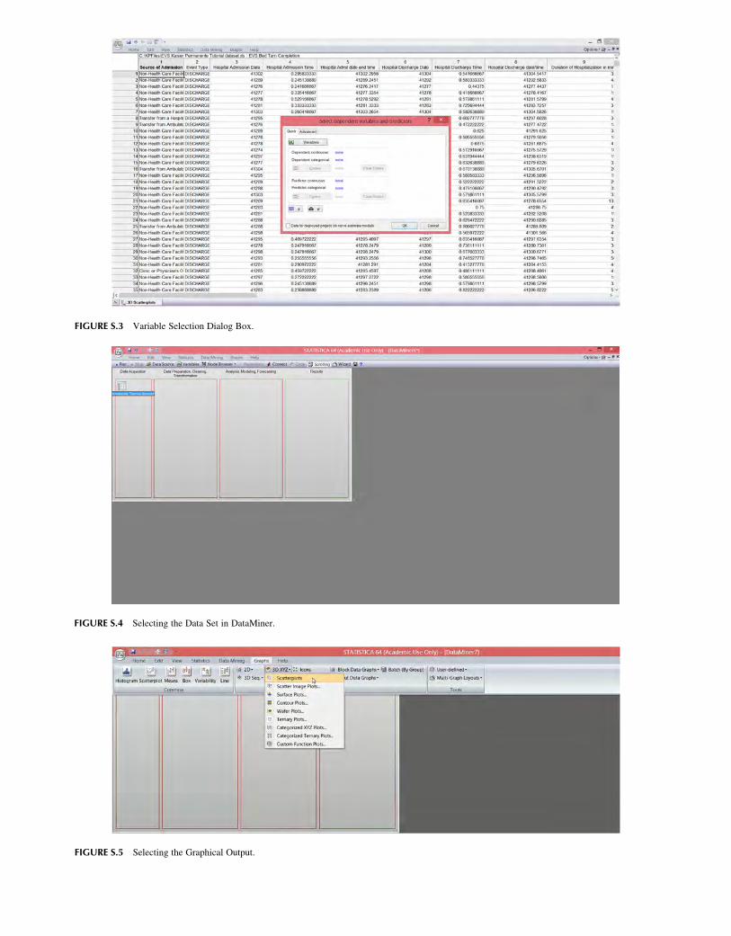
FIGURE S.3 Variable Selection Dialog Box.

FIGURE S.4 Selecting the Data Set in DataMiner.

FIGURE S.5 Selecting the Graphical Output.

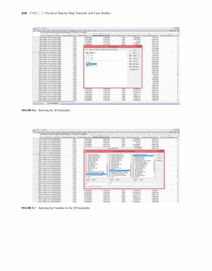
FIGURE S.6 Selecting the 3D Scatterplot.

FIGURE S.7 Selecting the Variables for the 3D Scatterplot.


3D Scatterplot of dept name against bed priority and dischargeto bed is clean (in Minutes) michael cook - EVS throughput

tutorial dataset 31v*1665c

Next

Normal

Stat

Bed priority

–1200–1000–800–600–400–200020040060080010001200140016001800

Discharge to bed is clean (in minutes)

Med_surgTelemetryFmly_ctr_care

Pediatric

ICUDir obs unit

Dept nam

e

FIGURE S.8 Graphical Display of Data Identifies Errors in Dataset.

FIGURE S.9 Auto Filter Criteria � Expression Dialog Box.

Availability of Hospital Beds for Newly Admitted Patients Tutorial | S 821

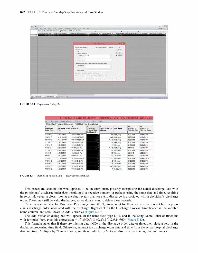
This procedure accounts for what appears to be an entry error, possibly transposing the actual discharge date with

the physicians’ discharge order date, resulting in a negative number, or perhaps using the same date and time, resulting

in zeros. However, a closer look at the data reveals that not every discharge is associated with a physician’s discharge

order. These may still be valid discharges, so we do not want to delete these records.

Create a new variable for Discharge Processing Time (DPT), to account for those records that do not have a phys-

cian’s discharge order associated with the discharge. Right click on the Discharge Process Time header in the variable

name column, and scroll down to Add Variables (Figure S.12).

The Add Variables dialog box will appear. In the name field type DPT, and in the Long Name (label or functions

with formulas) box, type this expression:5 iif(isMD(V11),0,((V8-V12)*24)*60) (Figure S.13).

This formula states that if there are missing data (MD) in the discharge order date or time, then place a zero in the

discharge processing time field. Otherwise, subtract the discharge order date and time from the actual hospital discharge

date and time. Multiply by 24 to get hours, and then multiply by 60 to get discharge processing time in minutes.

FIGURE S.10 Expression Dialog Box.

FIGURE S.11 Results of Filtered Data � Entry Errors Identified.


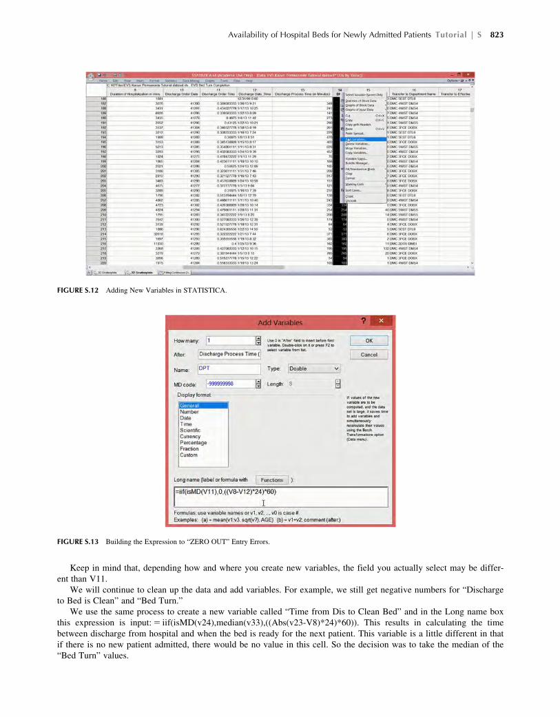
Keep in mind that, depending how and where you create new variables, the field you actually select may be differ-

ent than V11.

We will continue to clean up the data and add variables. For example, we still get negative numbers for “Discharge

to Bed is Clean” and “Bed Turn.”

We use the same process to create a new variable called “Time from Dis to Clean Bed” and in the Long name box

this expression is input:5 iif(isMD(v24),median(v33),((Abs(v23-V8)*24)*60)). This results in calculating the time

between discharge from hospital and when the bed is ready for the next patient. This variable is a little different in that

if there is no new patient admitted, there would be no value in this cell. So the decision was to take the median of the

“Bed Turn” values.

FIGURE S.12 Adding New Variables in STATISTICA.

FIGURE S.13 Building the Expression to “ZERO OUT” Entry Errors.


Rerunning the 3D scatterplot from above (Figure S.8), we see a slightly clearer picture of the distribution of dis-

charge times. By looking at the distribution, there appear to be a few clusters, and a few outliers as well (Figure S.14).

To get a surface plot, from main menu, select the Graphs tab, and then the 3D XYZ button (Figure S.15).

Click on the Variables tab, and then select your variables (Figure S.16).

This surface plot gives a somewhat different, but clearer, picture of the processing times. It appears that when dis-

charge occurs between late evening and the early morning hours, the effective time (the time when all the documenta-

tion is complete) and the discharge processing time (the time when the patient is actually leaving hospital � the famous

“wheelchair” ride) are pretty close together, meaning patients get out of the hospital more quickly when discharged in

the morning. As it gets later into the afternoon and evening hours, the time between the doctor’s order for discharge

and the time the patient actually leaves the hospital increases.

3D Scatterplot of transfer to department name against bed priority andDis to bed cleaned kaiser 33v*1651c

Next

Normal

Stat

Bed priority

–2000

200400

600800

10001200

Dis to bed cleaned

DMC 4WST DMS4

DMC 5EST DTL6

DMC 5WST DMS5

DMC 3FCE DOBX

DMC 3FCW DOBX

DMC 4PED DPEXDMC 2IC2 DICU

DMC 2DOU DMEI

DMC 6WST DTL1

DMC 6EST DTELDMC 4PIC DICPDMC 2IC1 DICU

Transfer to department nam

e

FIGURE S.14 New 3D Scatterplot After Entry Error Cleanup.

FIGURE S.15 Creating Surface Plot in STATISTICA.


As you might suspect, the plot indicates that the discharge processing time appears related to the type of nursing

department as well as the time of the discharge event (Figure S.17).

Additionally, it is interesting to see if there appears to be a relationship between how long it takes between discharge

time and cleaning the room, and if this is impacted by the department. The surface plot in Figure S.18 shows that there

is quite a bit of variation by department and time.

When we want to see which variables have the largest impact, we can do a feature selection. On the main tabs,

select the Data Mining tab, then Feature Selection on the far right (Figures S.19, S.20).

3D Surface plot of discharge process time (in minutes) against dept name andhospital discharge time

Michael cook - EVS throughput tutorial dataset 31v*1646cDischarge process time (in minutes) = Distance weighted least squares

> 750

< 750

< 500

< 250

< 0

Med_surg

Telemetry

Fmly_Ctr_Care

Pediatric

ICU

Dir obs unit

Dept name

4:48:00 AM7:12:00 AM

9:36:00 AM12:00:00 PM

2:24:00 PM4:48:00 PM

7:12:00 PM9:36:00 PM

12:00:00 AM2:24:00 AM

Hospital discharge time

0

1000

2000

3000

4000

5000Discharge process tim

e (in minutes)

FIGURE S.17 3D Surface Plot for Discharge Processing Time Based on Hospital Time and Department Name.

FIGURE S.16 3D Surface Plot Variable Selection.


FIGURE S.19 Feature Selection in STATISTICA.

FIGURE S.20 Feature Selection and Variable Screening.

3D Surface plot of discharge to bed is clean (in minutes) against dept name andhospital discharge time

Michael cook - EVS throughput tutorial dataset 31v*1646cDischarge to bed is clean (in minutes) = Distance weighted least squares

> 800

< 700

< 500

< 300

< 100

Med_surg

Telemetry

Fmly_ctr_care

Pediatric

ICU

Dir obs unit

Dept name

4:48:00 AM12:00:00 AM

4:48:00 AM9:36:00 AM2:24:00 PM

7:12:00 PM12:00:00 AM

4:48:00 AM

Hospital discharge time

0

200

400

600

800

1000

1200

Discharge to bed is clean (in m

inutes)

FIGURE S.18 3D Plot for Discharge Time to Clean Bed based on Hospital Discharge Time and Department Name.


Click on the Variables button and select DPT in the Dependent; continuous column. Then select Predictors; continu-

ous (Bed is Clean Date_Time, bed turns, Discharge to Bed is Clean in minutes, etc.). Then select Transfer to Dept

Name, Source of Admission, and Bed Priority in the Predictors; categorical column (Figures S.21).

From the Feature Selection Results, we will select the Summary: Best k predictors, and the Histogram of importance

for best k predictors (Figure S.22).

It is clear from the graph (Figure S.23) that the department has the largest impact in determining the total discharge

processing time. Although Discharge to Bed is Clean and Bed Turnaround are important for this study, they both occur

after discharge and as such have little impact on discharge processing time, as indicated in this graph. If we rerun the

graph to focus on EVS cleaning times, we would expect to see a somewhat different feature selection graph. We create

a new variable, Hosp_Stay(in hours), to see if there is relationship between how long a patient was in the hospital and

discharge processing times, as well as total cleaning time for EVS.

Once again, we will select a variable in the header of the spreadsheet, right click, and then scroll down to “Add

Variables” (Figure S.24). In the dialog box, change the name to “Hosp_Stay(in hours).” In the “long name” dialog box,

input this formula:5 ((v7-v4)*24). This will compute the time between the admission date and the discharge date. I

used the display format “number” with 0 decimals to show for how many hours a person was in the hospital.

FIGURE S.22 Feature Selection Results � Summary: Best K Predictors.

FIGURE S.21 Feature Selection � Dependent and Predictor Variables.


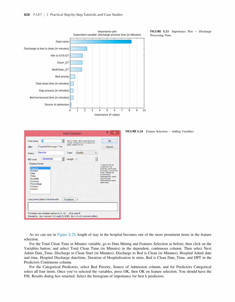
As we can see in Figure S.25, length of stay in the hospital becomes one of the more prominent items in the feature

selection.

For the Total Clean Time in Minutes variable, go to Data Mining and Features Selection as before; then click on the

Variables button, and select Total Clean Time (in Minutes) in the dependent, continuous column. Then select Next

Admit Date_Time, Discharge to Clean Start (in Minutes), Discharge to Bed is Clean (in Minutes), Hospital Admit date

and time, Hospital Discharge date/time, Duration of Hospitalization in mins, Bed is Clean Date_Time, and DPT in the

Predictors Continuous column.

For the Categorical Predictors, select Bed Priority, Source of Admission column, and for Predictors Categorical

select all four items. Once you’ve selected the variables, press OK, then OK on feature selection. You should have the

FSL Results dialog box returned. Select the histogram of importance for best k predictors.

FIGURE S.24 Feature Selection � Adding Variables.

Importance plotDependent variable: Discharge process time (in Minutes)

0 1 2 3 4 5 6 7 8 9 10

Importance (F-value)

Source of admission

Bed turnaround time (in minutes)

Gap process (in minutes)

Total clean time (in minutes)

Bed priority

BedClean_DT

Disch_DT

Xfer to EVS-DT


Dept name

FIGURE S.23 Importance Plot � Discharge

Processing Time.


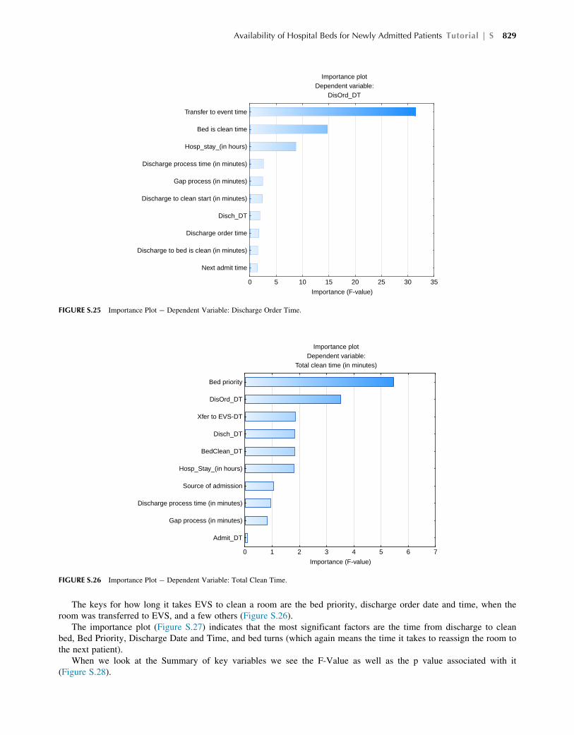
The keys for how long it takes EVS to clean a room are the bed priority, discharge order date and time, when the

room was transferred to EVS, and a few others (Figure S.26).

The importance plot (Figure S.27) indicates that the most significant factors are the time from discharge to clean

bed, Bed Priority, Discharge Date and Time, and bed turns (which again means the time it takes to reassign the room to

the next patient).

When we look at the Summary of key variables we see the F-Value as well as the p value associated with it

(Figure S.28).

Importance plotDependent variable:


0 1 2 3 4 5 6 7


Admit_DT


Discharge process time (in minutes)

Source of admission

Hosp_Stay_(in hours)

BedClean_DT

Disch_DT

Xfer to EVS-DT

DisOrd_DT

Bed priority

FIGURE S.26 Importance Plot � Dependent Variable: Total Clean Time.


DisOrd_DT

0 5 10 15 20 25 30 35


Next admit time


Discharge order time

Disch_DT

Discharge to clean start (in minutes)


Discharge process time (in minutes)

Hosp_stay_(in hours)

Bed is clean time

Transfer to event time

FIGURE S.25 Importance Plot � Dependent Variable: Discharge Order Time.


FIGURE S.28 Summary of Key Values: F and P Values.

FIGURE S.29 Correlation Matrix.



0 1 2 3 4 5 6 7 8


Hospital admit date and time

Source of admission

DPT

Transfer to department name

Bed is clean date_time

Duration of hospitalization in mins

Hospital discharge date/time

Discharge to clean start (in minutes)


Bed turns

Next admit date_time

Discharge date_time

Bed priority

Time from dis to clean bed

FIGURE S.27 Importance Plot � Dependent Variable: Total Clean Time.


Reviewing the correlation matrix helps identify which variables are highly correlated with each other, and therefore

should not be included together. For example, Next Admit date and time is highly correlated (0.999) with Hospital

Discharge Date/Time (Figure S.29). These two variables may be explaining the same phenomenon, and should not both

be used in the analysis.

Overall, it appears that the EVS department has a key role in assisting the hospital with throughput. Important fac-

tors in helping the success of the EVS department are Bed Priority, Hospital Discharge Date, Discharge Order Date and

bed turns and are a focus for further study.

We would need to look at staffing levels, specialists on staff, and other factors to determine why afternoon dis-

charges and specific departments increase the time to leave the hospital. Other key factors are the availability of EVS

attendants to assist in cleaning the rooms and provide a quicker throughput.


Michael Cook - Contributing Author - Practical Predictive Analyticsv2

Documents

phd john

phd christopher

phd danny

phd martin

phd pat

phd gary

bed hospital

date field bed