Michael C. Donohue NIH Public Access Helene Jacqmin-Gadda Mélanie Le ...adni.loni.usc.edu/adni-publications/Donohue_2014_AlzDem.pdf · Estimating long-term multivariate progression

Estimating long-term multivariate progression from short-term data

Michael C. Donohuea, Helene Jacqmin-Gaddab, Mélanie Le Goffb, Ronald G. Thomasa,h, Rema Ramana,h, Anthony C. Gamsta,h, Laurel A. Beckettc, Clifford R. Jack Jrd, Michael W. Weinere, Jean-Francois Dartiguesc, and Paul S. Aiseng for the Alzheimer’s Disease Neuroimaging Initiativeh

aDepartment of Family and Preventive Medicine, Division of Biostatistics and Bioinformatics, University of California San Diego, La Jolla, CA 92093, USA

bINSERM, U897, Biostatistics Department, Bordeaux, F-33076, France

cDepartment of Public Health Sciences, Biostatistics Unit, University of California Davis, Davis, CA 95616, USA

dDepartment of Radiology, Mayo Clinic, Rochester, MN 55902, USA

eCenter for Imaging of Neurodegenerative Diseases, University of California, San Francisco

fINSERM, U897, Aging Department, Bordeaux, F-33076, France

gDepartment of Neuroscience, University of California San Diego, La Jolla, CA 92093, USA

hData used in preparation of this article were obtained from the Alzheimers Disease Neuroimaging Initiative (ADNI) database (http://adni.loni.usc.edu). As such, the investigators within the ADNI contributed to the design and implementation of ADNI and/or provided data but did not participate in analysis or writing of this report. A complete listing of ADNI investigators can be found at: http://adni.loni.usc.edu/wp-content/uploads/how_to_apply/ADNI_Acknowledgement_List.pdf

Abstract

Motivation—Diseases that progress slowly are often studied by observing cohorts at different

stages of disease for short periods of time. The Alzheimer’s Disease Neuroimaging Initiative

(ADNI) follows elders with various degrees of cognitive impairment, from normal to impaired.

The study includes a rich panel of novel cognitive tests, biomarkers, and brain images collected

every six months for up to six years. The relative timing of the observations with respect to

disease pathology is unknown. We propose a general semi-parametric model and iterative

estimation procedure to simultaneously estimate pathologic timing and long-term growth curves.

© 2013 Elsevier Inc. All rights reserved.

Contact: [email protected].

Publisher's Disclaimer: This is a PDF file of an unedited manuscript that has been accepted for publication. As a service to our customers we are providing this early version of the manuscript. The manuscript will undergo copyediting, typesetting, and review of the resulting proof before it is published in its final citable form. Please note that during the production process errorsmaybe discovered which could affect the content, and all legal disclaimers that apply to the journal pertain.

NIH Public AccessAuthor ManuscriptAlzheimers Dement. Author manuscript; available in PMC 2015 October 01.

Published in final edited form as:Alzheimers Dement. 2014 October ; 10(0): S400–S410. doi:10.1016/j.jalz.2013.10.003.

NIH

-PA

Author M

anuscriptN

IH-P

A A

uthor Manuscript

NIH

-PA

Author M

anuscript

http://adni.loni.usc.edu

http://adni.loni.usc.edu/wp-content/uploads/how_to_apply/ADNI_Acknowledgement_List.pdf

http://adni.loni.usc.edu/wp-content/uploads/how_to_apply/ADNI_Acknowledgement_List.pdf

The resulting estimates of long-term progression are fine-tuned using cognitive trajectories

derived from the long-term “Personnes Agées QUID” (PAQUID) study.

Results—We demonstrate with simulations that the method can recover long-term disease trends

from short-term observations. The method also estimates temporal ordering of individuals with

respect to disease pathology, providing subject-specific prognostic estimates of the time until

onset of symptoms. When the method is applied to ADNI data, the estimated growth curves are in

general agreement with prevailing theories of the Alzheimer’s disease cascade. Other datasets with

common outcome measures can be combined using the proposed algorithm.

Availability—Software to fit the model and reproduce results with the statistical software R is

available as the grace package (http://mdonohue.bitbucket.org/grace/). ADNI data can be

downloaded from the Laboratory of NeuroImaging (http://loni.usc.edu).

Keywords

multiple outcomes; semiparametric regression; self modeling regression

1. Introduction

Several methods exist for estimating smooth progression or growth curves from serial

observations of individuals over some biologically common time span. For example,

generalized linear or nonlinear mixed effects models [1] can be used to model height,

weight, or pharmacokinetics over time from some event of interest. The event might be birth

or an intervention. However, we often study diseases that occur over long periods of time by

sampling populations at different stages of disease and taking short-term longitudinal

“snapshots”. Epidemiological studies with biologically heterogeneous subpopulations may

not have an obvious biological event than can serve as a reference “time zero”. Such a “time

zero” is required to fit the standard mixed-effects model. Also, the standard nonlinear

mixed-effects models and software assume similar features on both the subject and

population levels [1, 2, 3]. Short-term follow-up with relatively few observations may

require much simpler subject-level features.

A motivating example is Alzheimers Disease (AD), which is believed to develop decades

before the onset of symptoms. The Alzheimers Disease Neuroimaging Initiative (ADNI,

adni-info.org) has followed volunteers diagnosed as Cognitively Normal (CN), Early and

Late Mild Cognitive Impairment (EMCI and LMCI), and probable mild AD. Maximum

follow-up is up to about 6 years at present and data collection is ongoing. The ADNI battery

includes serial magnetic resonance imaging (MRI) measures of regional brain volumes,

positron emission tomography (PET) measures of brain function and amyloid accumulation,

other biological markers, and clinical and neuropsychological assessment. Time of onset of

dementia, a potential “time zero”, is recorded for subjects with, or transitioning to, dementia,

but these times can be unreliable and subjective. Furthermore, CN and MCI individuals may

not be followed long enough to observe clinical transitions.

Jack et al. [4, 5] proposed a long-term model of the AD pathological cascade, and

specifically hypothesized the trajectory of several key biomarkers over the decades

Donohue et al. Page 2

Alzheimers Dement. Author manuscript; available in PMC 2015 October 01.

NIH

-PA

Author M

anuscriptN

IH-P

A A

uthor Manuscript

NIH

-PA

Author M

anuscript

http://mdonohue.bitbucket.org/grace/

http://loni.usc.edu

http://adni-info.org

preceding the onset of dementia symptoms. The model (Figure 1) proposes that the AD

cascade begins many years prior to the onset of symptoms with amyloid plaque deposition

in the brain followed by neurofibrillary tau tangles; cognitive, clinical and functional decline

are relatively late features of the disease. This hypothesized model is shaping the field of

AD research. Drug development and observational studies have shifted focus to earlier

stages of the disease, selecting subjects not on symptomatic impairment, but on biomarker

signatures. Ideally we would test the hypothesized model by enrolling a large cohort of CN

subjects and collecting biomarkers and cognitive and functional assessments over decades.

The subset who progress to AD could be used to model the long-term biomarker progression

of the disease. Until such a study is conducted, we are limited to analyzing shorter-term

studies, such as ADNI.

Self modeling regression (SEMOR) is an approach for fitting sets of curves under the

assumption of a common shape [6]. A subclass of SEMOR, shape invariant models [7, 8, 9,

10], accommodate unknown location and scale parameters for both the outcome and the

time covariate and model the common shape with regression splines. Kneip and Gasser [6]

relaxed some of the parametric assumptions by using kernel smoothers to estimate the

common shape. Others have modeled the common shape with free-knot regression splines

[11], smoothing splines [12], and penalized splines [13, 14, 15].

To our knowledge, SEMOR has only been applied to datasets in which each subject has

similar follow-up. SEMOR approaches assume a common shape over the population, and

estimate subject-level curves with similar features as the population curve. Our goal is to

estimate population curves over decades of AD progression on an array of outcome

measures; but subject-level data is comprised of at most 9 observations over 6 years. We

propose a SEMOR model with simple linear subject-level effects, while modeling long-term

features with non-parametric monotone smoothing. Subjects are shifted backward or

forward in time according to performance across the panel of outcomes. Long-term

progression curves for the multiple outcomes, and subject-specific random-effects and time

shifts, are iteratively estimated until convergence of the residual sum of squares.

There have been studies of AD progression with long-term follow-up, but these tend to lack

the novel biomarkers of prime interest in early stages of the disease. For instance, the

“Personnes Agees QUID” (PAQUID) study has followed 3,777 French individuals aged 65

years or older studied from 1988 until present [16]. The PAQUID dataset lacks the imaging

and cerebrospinal fluid biomarkers that ADNI collected, but provides invaluable long-term

MMSE trajectories [17]. We can use these trajectories to fine-tune the results of the

algorithm applied to ADNI data, and transform time to represent time-to-dementia-onset.

2. Model assumptions

We assume several outcomes Yij arise over time t, for individual i = 1,…, n and outcome j =

1,… , m, according to:

(1)



NIH

-PA

Author M

anuscriptN

IH-P

A A

uthor Manuscript

NIH

-PA

Author M

anuscript

Furthermore, we assume each gi is a continuously differentiable monotone function, γi have

mean 0 and variance , (α0ij ; α1ij) are bivariate Gaussian with mean 0 and covariance

matrix Σj, and εij(t) are independent Gaussian residual errors with mean 0 and outcome-

specific variance σj. To simplify notation, we think of t as both a covariate and a continuous

valued index. “Short-term” observation time is represented by observed covariate t. In a

panel study like ADNI, t would correspond to the study-time clock. “Long-term”

progression time is represented by t + γi, where γi is the unknown subject-specific time shift.

If subjects aged uniformly, with identical ages at different stages of progression of the

underlying disease features, “long-term” progression time would be the subjects age; in fact,

however, disease manifests at different ages, so this corresponds to an unknown “health-

age”, which may be shifted left or right relative to actual age.

Panel A of Figure 2 depicts simulated data generated according to (1). The logistic function

g1(t) = 1/(1 + exp(−t)), the linear function g2(t) = t/12 + 0:5 and the quadratic g3(t) = (t +

6)2/72 generated the three outcomes. For each of the 100 subjects, we sampled subject-

specific time shifts, γ0, uniformly from the interval −5 to 5. The unshifted observation times

were t = −1, −0.5, 0,0.5,1. The random intercepts and slopes for each subject and outcome

are distributed according to a bivariate Gaussian with mean 0, variance 0.01, and covariance

0.005. The residual variance is also Gaussian with variance 0.01. We chose the different

long-term shapes to test whether our semi-parametric method could recover them without

supervision. The observation times and long-term scatter were chosen to roughly mimic

ADNI. The variance parameters were chosen so that the long-term trends were reasonably

apparent by visual inspection of Panel A of Figure 2.

The long-term trends are obvious in Panel A of Figure 2 because the data are plotted with

the simulated time shifts. However, the time shifts are not observed in data like ADNI.

Rather, the data is observed as in Panel B of Figure 2. The goal of the algorithm proposed in

the next section is to estimate both the time shift parameters and the long-term curves. The

algorithm will leverage the assumption that the long-term trends are monotone and pool

information across outcomes to estimate the subject-specific time shifts.

The restriction that γi, α0ij and α1ij each have mean zero, helps ensure identifiability, i.e. that

the parameters of the model are uniquely determined. Without the random slope term α1ij,

our model is a simplification of the classical Shape Invariant Model (SIM) for each

outcome. The SIM includes two rescaling parameters and two shift parameters. Our model

excludes the SIM rescaling parameters, but includes an additional random slope term.

Without the random slope term, identifiability of our model is established in [6] under the

normalizing condition that shift parameters γi and α0ij have mean zero, which we maintain.

To ensure identifiability in our model with a random slope, α1ij, we simply require the

further restriction that the mean of α1ij is zero. Following [6], the restrictions on the mean of

γi, α0ij and α1ij and the assumption that gj is a continuously differentiable monotone

function for each outcome ensure identifiability.



NIH

-PA

Author M

anuscriptN

IH-P

A A

uthor Manuscript

NIH

-PA

Author M

anuscript

3. The algorithm

The algorithm reduces the high dimensional and complex problem into simpler problems.

Each of the unknown parameters (gj, γi, α) is estimated in turn using the current estimates of

the other parameters. This process is iterated until convergence of the residual sum of

squares (RSS). The algorithm utilizes three different types of partial residuals, using the

language of generalized additive model estimation [18], which we denote , ,

(Table 1). If we assume the model (1) is correct then each of the partial residuals

provides an unbiased estimate of one of the unknown parameters. Specifically, conditional

expectations of the partial residuals are equivalent, or at least approximately equivalent, to

the target parameters (Table 1). We begin the algorithm by initializing γi = 0 and iterating

the following.

1. Given γi, estimate the monotone functions gj by setting α0ij = α1ij = 0 and iterating

the following subroutine.

a.Estimate gj by a monotone smooth of .

b.Estimate α0ij, α1ij by linear mixed-model of . Repeat Steps a and b

until convergence of the RSS for the jth outcome,

.

2. Given current set of gj, set α0ij = α1ij = εij(t) = 0, and estimate each γi with the

average of over all j and t. Repeat Steps 1 and 2 until convergence of the

total residual sum of squares .

Step 1 involves m parallel subroutines for fitting gi and the subject-specific α0ij and α1ij for

each outcome j = 1,…, m. We begin each of the m parallel subroutines by setting α0ij = 0

and α1ij = 0. To estimate gj, we use a monotone B-spline smoother [19] through the scatter

plot of (t + γi, ). This is accomplished using the R package fda [20]. Under the model,

is independently and identically distributed about gj(t), so we need not model within-

subject correlations at this step. To estimate α0ij and α1ij, we minimize by fitting a

linear mixed-effect model of using lme4 [21]. Steps a and b are

repeated with the same γi until convergence of RSSj. The result is m smooth curves, g1 ,…,

gm, and m × n sets of random effects estimates for the m outcomes and n individuals. Plots

of the fits and residuals at each iteration are produced with ggplot2 [22].

In Step 2 we invert the outcome variables and estimate the time shift parameters γi by taking

the average of over all outcomes and times for each individual. This is the only step

that pools data derived from all outcomes at once. To down-weight the influence of more

variable outcomes, one could use a weighted average with weights inversely proportional to

each outcome’s residual variance.



NIH

-PA

Author M

anuscriptN

IH-P

A A

uthor Manuscript

NIH

-PA

Author M

anuscript

4. Simulations

Data simulated as described in Section 2 are depicted in Figure 2. We submitted these data

to the algorithm. Each curve was estimated with the same monotone B-spline smoother with

5 equally spaced knots and 5th degree polynomial splines. The resulting fitted curves are

shown to have good fidelity with the true logistic, linear, and quadratic curves (Panel C).

We also plotted the true simulated time shifts against the estimated time shifts (not shown).

The agreement was not perfect, but as hoped, the regression line through this scatter plot lies

close to the identity line. The residual sum of squares for each of the outcomes converged in

10 iterations to a tolerance of 0.1% of the residual sum of squares. Code to reproduce the

results and an animation demonstrating convergence can be found at http://

mdonohue.bitbucket.org/grace/.

5. ADNI and PAQUID results

Figure 3 shows longitudinal plots of some of the key variables that have been collected over

the course of ADNI. Amyloid plaque accumulation in brain is associated with decreased

CSF and increased Pittsburgh compound B (PiB) and florbetapir uptake on PET. Figure 3

also includes CSF tau and p-tau; FreeSurfer volumetric MRI data for hippocampal, whole

brain, and ventricular volume; fluorodeoxyglucose (FDG) uptake on PET; 13 item

Alzheimers Disease Assessment Scale-Cognitive Sub-scale (ADAS13) including delayed

word recall and number cancellation tasks; Mini Mental State Exam (MMSE); ADCS

Functional Activities Questionnaire (FAQ); Rey Auditory Visual Learning Test (RAVLT),

and the Clinical Dementia Rating Scale Sum-of-Boxes (CDRSB). CSF measures were

collected only on a subset of ADNI volunteers, as evidenced by the relative sparsity of CSF

data. Florbetapir PET imaging and the EMCI cohort were added relatively late in the study.

Additional details on these measures in ADNI are available from adni-info.org.

One of the primary motivations for this work was to derive a data driven version of the

progression curves hypothesized by Jack et al. [4]. The hypothesized figure shows the key

markers of disease progressing on a common vertical scale from normal to abnormal, with

clinical disease stage on the horizontal scale. The percentile scale is a natural choice to attain

a common scale. Therefore, before submitting ADNI measures to our algorithm, we first

transformed them to a percentile scale. Since the diagnostic groups are not equally

represented, we use a weighted percentile transformation. The resulting scale is percentile

normalized to range from 0 (least severe observed value) to 100 (most severe observed

value). Percentiles were calculated using the empirical cumulative distribution function

(ECDF) derived by weighting according to the inverse of the proportion of observations

from each diagnostic category (CN, EMCI, LMCI, AD). For example, in total we observed n = 7,216 MMSE scores from CN (n = 2,094/7,216 = 29.0%), EMCI (n = 979/7,216 = 14.6%),

LMCI (n = 3,074/7,216 = 42.6%), and AD (n = 1,069/7,216 = 14.8%). Because diagnostic

groups are not equally represented, we used the inverse proportions as weights in computing

the ECDF. Table 3 provides the raw values that correspond to the resulting percentiles.



NIH

-PA

Author M

anuscriptN

IH-P

A A

uthor Manuscript

NIH

-PA

Author M

anuscript



ADNI includes many CN, MCI, and even misdiagnosed probable AD who may not have AD

pathology. This is because physicians do not have access to biomarker results at the time of

diagnosis. These subjects do not provide any information about the long-term trends of AD.

Therefore, we applied our algorithm to the subset of N = 388 ADNI participants with some

evidence of abnormal accumulation of amyloid in brain (“Amyloid+”) using published

thresholds for CSF Aβ (192 pg/ml), PiB PET (1.5 standardized uptake value ratio [SUVR] in

region relative to the cerebellum), and florbetapir PET (1.1 SUVR in region relative to the

cerebellum) [23, 24, 25]. The group consisted of n = 100 CN, 137 ECMI, 225 LMCI, and

117 AD; but the algorithm was blind to these diagnostic categorizations. Following the same

approach as the simulation, the B-spline smooths were fitted with 5 equally spaced knots

and 5th degree polynomial splines.

The top of Figure 4a shows the estimated long-term trajectories among Amyloid+ADNI

subjects. Time has been shifted so that time zero represents the time at which the mean

CDRSB score reaches the 80th percentile. The resulting time scale can be interpreted as time

until progression to the worst 20th percentile of CDRSB. To reduce clutter and because it

was very similar to the ADAS13 trajectory, CDRSB is not shown in the middle panel. We

also omit ventricular volume, which tracks closely with hippocampus. The bottom left of

Figure 4a depicts the first derivatives of each curve divided by the standard deviation of its

residuals. The shaded regions in the top panels of Figure 4 depict bootstrap estimates of the

confidence bands. We re-sampled the subjects with replacement and re-applied the

algorithm 100 times. Each re-sampled population contained the same number of subjects as

the observed population. For each time point, we then took the 2.5 and 97.5 percentiles of

the 100 curves as the lower and upper limits.

We also applied the algorithm to the subset of N = 570 ADNI participants who had at least

one Apolipoprotein E e4 allele (Figure 4). This subgroup consisted of n = 92 CN, 85 ECMI,

248 LMCI, and 145 AD; but again the algorithm was blind to the diagnoses. Note that this

group contains many subjects who would be classified as Amyloid-. Utilizing MMSE

trajectories from the PAQUID study, we applied a post-processing step to transform time.

The PAQUID time scale is time to onset of dementia. The ADNI time scale, with estimated

subject-specific time shifts, lacks a pathological anchor. To transform the ADNI time scale

to the PAQUID time to onset, we compose the ADNI MMSE trajectory with the inverse

PAQUID trajectory. That is, if f denotes the estimated MMSE curve from ADNI and g denotes the same from PAQUID, with inverse g−1, we transform ADNI time, t, via the

composition g−1(f (t)). Because PAQUID lacks measures of amyloid burden, we could not

do this transformation with our Amyloid+ analysis.

For comparison, Figure 5 depicts trajectories estimated from those without evidence

Amyloid burden and those without an ApoE ε4 allele. We used the same transformations of

time as described above, in particular using estimated trajectories from PAQUID to calibrate

the ADNI time scale. The Amyloid-group consisted of n = 190 CN, 153 ECMI, 92 LMCI,

and 13 AD; the ApoE ε4 allele non-carrier group consisted of n = 263 CN, 124 ECMI, 219

LMCI, and 75 AD.



NIH

-PA

Author M

anuscriptN

IH-P

A A

uthor Manuscript

NIH

-PA

Author M

anuscript

6. Discussion

Bateman et al. [26] recently produced estimated progression curves over a 50 year span

using data from the Dominantly Inherited Alzheimer’s Network (DIAN). A key feature of

autosomal dominant AD is that the age of onset of symptoms is expected to be close to the

age of onset of the parent. Bateman et al. [26] use the parents’ ages of onset to estimate

long-term disease progression from cross-sectional data from mutation carriers spanning 25

years before, to 10 years after, the parents’ age of onset. In contrast, we have less confidence

about the age of onset in the ADNI population of sporadic AD. Our self modeling regression

approach addresses this limitation of ADNI by simultaneously estimating age of onset and

the progression curves.

Simulations suggest that our iterative algorithm can recover reasonable estimates of the

long-term trajectories from short-term observations. Nonparametric estimation of the

monotone curves allows different shaped curves to emerge without pre-specifying

parametric families. Further simulation studies and analytic development of asymptotic

convergence is warranted. Convergence of estimates of the time shifts will rely in part on

the abundance of outcomes. With only three outcomes used in the simulation, the algorithm

estimated the time shifts surprisingly well.

Jack et al. [4, 5] proposed that all disease markers range from zero (absolutely normal) to

one (absolutely abnormal) and follow sigmoid shapes. Rather than assuming this to be true

and following a parametric approach, we opted to follow a nonparametric monotone

smoothing approach. We chose to apply our algorithm to relatively pathologically

homogenous Amyloid+ and ApoE ε4+ subsets. While restricting to Amyloid+ is ostensibly

assuming that amyloid is the precursor to the AD cascade, we feel that including many

subjects with a low likelihood of AD pathology may lead to distorted trajectories. The ApoE

ε4 allele is the major genetic risk factor for sporadic AD, though roughly one third of

individuals with AD do not carry it.

Our nonparametric approach does not assume sigmoid curves, but rather a very flexible

class of monotone curves. Surprisingly, among Amyloid+ subjects, we found mean CSF Aβ

follows a linear trajectory, while tau, p-tau, and PiB PET follow sigmoid shapes. However,

the sigmoid shapes are flatter than those proposed by [4], and remain within the 40 to 80th

percentile range. Glucose metabolism (FDG PET), hippocampal volume, ventricular

volume, learning, and cognition (ADAS13) all track very close to each other in near linear

trajectories. Function (FAQ) was the final domain to fail following a parabolic trajectory. It

is quite possible that ADNI does not have enough data from later stage dementia, which

might demonstrate the final plateau of a sigmoid. The relative paucity of available

observations at the most severe stage of disease is limitation than will be addressed as the

model is expanded to include additional datasets.

The question of which markers become abnormal first is distinct from the question of which

markers can be efficiently estimated in terms of the signal-to-noise ratio. To explore the

latter question, we provide plots of the first derivatives of curves divided by the residual

standard deviation. Hippocampal volume appears to dominate the other measures across the



NIH

-PA

Author M

anuscriptN

IH-P

A A

uthor Manuscript

NIH

-PA

Author M

anuscript

15 year span in both analyses, with the possible exception of CSF markers. The CSF

markers show some areas of relative high standardized slopes, but these could be due to

scant data and spurious acceleration near the boundaries of observation (bottom Figure 5). In

other cases, the CSF measures are relatively flat which may cause spurious acceleration

depicted in the bell shapes (bottom Figure 4a).

Our approach also does not assume that the mean should attain zero and one. Without this

assumption, our algorithm demonstrates much pathological heterogeneity or measurement

variability, even in the selected Amyloid+ subset. For instance, 15 years prior to reaching

the worst 20th percentile of CDRSB, CSF Aβ ranges between zero and the 80th percentile,

with a mean at about the 20th percentile. Between-subject variability tends to flatten the

mean trajectory, such that most estimated trajectories in Figure 4a do not cover the full

range from zero to one. Assuming the mean attains zero and one may oversimplify the

heterogeneous reality of the disease cascade at the population level.

Perhaps some of the heterogeneity can be explained by diet, lifestyle, education, occupation,

or other covariates related to cognitive reserve. Genetics or family history might also explain

heterogeneity. We plan to investigate these hypotheses in the future by building covariates

into the model, but more data on the earliest phases of the disease will be necessary.

Fortunately, the mixed-model framework we have adopted is well suited to pooling datasets

for meta-analyses. Hierarchical random effects can be used to model within-study as well as

within-subject correlation. Meta-analyses may also help address a key limitation of the

ADNI data, which is the age range of ADNI participants is restricted to 55 to 95 years at

baseline. In fact, across our 15 year span of estimated long-term progression, the mean age

of subjects represented remains in the 70 to 75 year range. Clearly we need to incorporate

data from younger cohorts.

The comparison groups depicted in Figure 5 are difficult to interpret. Note that only n =13

out of 130 (10%) of AD subjects with known amyloid status are classified as Amyloid- and

n = 75 out of 220 (34%) of AD subjects have no ApoE ε4 allele. Also many of the subjects

with mild or no impairment entered into this analysis may never progress. However, we

might interpret the Amyloid-trajectories as a representation of non-Alzheimer’s pathology

which is marked by divergent biomarker signature, including normal CSF and less

pronounced hippocampal atrophy and ventricular expansion. In contrast, the ApoE ε4 non-

carrier group appears to converge toward the ApoE ε4 carrier group as symptom progress.

This apparent convergence is possibly due to the concatenation of subjects without

Alzheimer‘s pathology antecedent to those with Alzheimer’s pathology rather than a true

acceleration of pathology in ApoE ε4 non-carriers.

Our analysis suggests that amyloid PET imaging with florbetapir or PiB may reach

abnormal levels first, followed by CSF tau and p-tau. This is consistent with the view that

PET imaging is the most direct measure of amyloid accumulation in brain (generally

considered to be the inciting event in AD), and suggests a delay before abnormalities are

observed in "downstream" markers of neurodegeneration in the CSF. Learning, glucose

metabolism, hippocampal atrophy, and cognition all follow in close succession. Function is

the last domain to progress to abnormality, as expected. Plots of the adjusted slopes indicate



NIH

-PA

Author M

anuscriptN

IH-P

A A

uthor Manuscript

NIH

-PA

Author M

anuscript

that hippocampal volume assessed by structural MRI provides the most efficient measure of

disease progression across the full span. These observations are consistent with our current

understanding of the disease and paint a picture in general agreement with the [4] model.

Our approach will facilitate analyses utilizing diverse datasets with overlapping measures,

providing a framework for validating models of disease progression.

Finally, our framework provides an approach to assessing the growing body of outcome

data, providing quantitative data to inform still-hypothetical biomarker models. As noted in

an editorial accompanying the revised model from [5, 27], biomarker modeling will be

facilitated by ongoing accrual of data that reduces the gaps in our observations; this applies

to both hypothetical and data-driven efforts.

Acknowledgments

We would like to acknowledge the invaluable contributions of our PAQUID and ADNI collaborators, co-investigators, volunteers, and their families.

Funding: This work was support by a grant (1KL2RR031978) from the National Institutes of Health funded University of California, San Diego Clinical and Translation Research Institute (1UL1RR031980). Data collection and sharing for this project was funded by the Alzheimer’s Disease Neuroimaging Initiative (ADNI) (U01 AG024904). ADNI is funded by the National Institute on Aging, the National Institute of Biomedical Imaging and Bioengineering, and through generous contributions from the following: Abbott; Alzheimers Association; Alzheimers Drug Discovery Foundation; Amorfix Life Sciences Ltd.; AstraZeneca; Bayer HealthCare; BioClin-ica, Inc.; Biogen Idec Inc.; Bristol-Myers Squibb Company; Eisai Inc.; Elan Pharmaceuticals Inc.; Eli Lilly and Company; F. Hoffmann-La Roche Ltd and its affiliated company Genentech, Inc.; GE Healthcare; Innogenetics, N.V.; IXICO Ltd.; Janssen Alzheimer Immunotherapy Research & Development, LLC.; Johnson & Johnson Pharmaceutical Research & Development LLC.; Medpace, Inc.; Merck & Co., Inc.; Meso Scale Diagnostics, LLC.; Novartis Pharmaceuticals Corporation; Pfizer Inc.; Servier; Synarc Inc.; and Takeda Pharmaceutical Company. The Canadian Institutes of Health Research is providing funds to support ADNI clinical sites in Canada. Private sector contributions are facilitated by the Foundation for the National Institutes of Health (www.fnih.org). The grantee organization is the Northern California Institute for Research and Education, and the study is coordinated by the Alzheimer’s Disease Cooperative Study at the University of California, San Diego. The Laboratory for Neuroimaging at the University of Southern California disseminates ADNI data. This research was also supported by NIH grants P30 AG010129 and K01 AG030514. Novartis and IPSEN laboratories, and Conseil Regional dAquitaine fund PAQUID.

References

[1]. Lindstrom MJ, Bates DM. Nonlinear mixed effects models for repeated measures data. Biometrics. 1990; 46:673–687. [PubMed: 2242409]

[2]. Pinheiro, J.; Bates, D.; DebRoy, S.; Sarkar, D.; R Core Team. nlme: Linear and Nonlinear Mixed Effects Models. 2012. R package version 3.1-106

[3]. Pinheiro, JC.; Bates, DM. Mixed-effects models in S and S-PLUS. Springer Verlag; 2000.

[4]. Jack CR, Knopman DS, Jagust WJ, Shaw LM, Aisen PS, Weiner MW, Petersen RC, Trojanowski JQ. Hypothetical model of dynamic biomarkers of the Alzheimer’s pathological cascade. The Lancet Neurology. 2010; 9:119–128. [PubMed: 20083042]

[5]. Jack CR, Knopman DS, Jagust WJ, Petersen RC, Weiner MW, Aisen PS, Shaw LM, Vemuri P, Wiste HJ, Weigand SD, Lesnick TG, Pankratz VS, Donohue MC, Trojanowski JQ. Tracking pathophysiological processes in Alzheimer’s disease: an updated hypothetical model of dynamic biomarkers. The Lancet Neurology. 2013; 12:207–216. [PubMed: 23332364]

[6]. Kneip A, Gasser T. Convergence and consistency results for self-modeling nonlinear regression. The Annals of Statistics. 1988; 16:82–112.

[7]. Lawton WH, Sylvestre EA, Maggio MS. Self modeling nonlinear regression. Technometrics. 1972; 14:513–532.



NIH

-PA

Author M

anuscriptN

IH-P

A A

uthor Manuscript

NIH

-PA

Author M

anuscript

http://www.fnih.org

[8]. Ladd WM, Lindstrom MJ. Self-modeling for two-dimensional response curves. Biometrics. 2000; 56:89–97. [PubMed: 10783781]

[9]. Brumback LC, Lindstrom MJ. Self modeling with flexible, random time transformations. Biometrics. 2004; 60:461–470. [PubMed: 15180672]

[10]. Beath KJ. Infant growth modelling using a shape invariant model with random effects. Statistics in Medicine. 2007; 26:2547–2564. [PubMed: 17061310]

[11]. Lindstrom MJ. Self-modeling with random shift and scale parameters and a free-knot spline shape function. Statistics in Medicine. 1995; 14:2009–2021. [PubMed: 8677401]

[12]. Wang Y, Ke C, Brown MB. Shape-invariant modeling of circadian rhythms with random effects and smoothing spline anova decompositions. Biometrics. 2003; 59:804–812. [PubMed: 14969458]

[13]. Altman N, Villarreal J. Self-modelling regression for longitudinal data with time-invariant covariates. Canadian Journal of Statistics. 2004; 32:251–268.

[14]. Coull BA, Staudenmayer J. Self-modeling regression for multivariate curve data. Statistica Sinica. 2004; 14:695–711.

[15]. Telesca D, Inoue LYT. Bayesian hierarchical curve registration. Journal of the American Statistical Association. 2008; 103:328–339.

[16]. Dartigues JF, Gagnon M, Barberger-Gateau P, Letenneur L, Commenges D, Sauvel C, Michel P, Salamon R. The PAQUID epidemiological program on brain aging. Neuroepidemiology. 1992; 11:8.

[17]. Amieva H, Le Goff M, Millet X, Orgogozo JM, Peres K, Barberger-Gateau P, Jacqmin-Gadda H, Dartigues JF. Prodromal Alzheimer’s disease: Successive emergence of the clinical symptoms. Annals of Neurology. 2008; 64:492–498. [PubMed: 19067364]

[18]. Hastie T, Tibshirani R. Generalized additive models. Statistical Science. 1986; 1:297–310.

[19]. Ramsay JO. Estimating smooth monotone functions. Journal of the Royal Statistical Society. Series B, Statistical Methodology. 1998; 60:365–375.

[20]. Ramsay, JO.; Wickham, H.; Graves, S.; Hooker, G. fda: Functional Data Analysis. 2012. R package version 2.2.8

[21]. Bates, D.; Maechler, M.; Bolker, B. lme4: Linear mixed-effects models using S4 classes. 2012. R package version 0.999999-0

[22]. Wickham, H. ggplot2: elegant graphics for data analysis. Springer New York: 2009.

[23]. Shaw LM, Knapik-Czajka M, Lee VMY, Trojanowski JQ, Vander-stichele H, Clark CM, Aisen P, Petersen R, Blennow K, Soares H, Simon A, Potter W, Lewczuk P, Dean R, Siemers E. Cerebrospinal fluid biomarker signature in Alzheimer’s Disease Neuroimaging Initiative subjects. Annals of Neurology. 2009; 65:403–413. [PubMed: 19296504]

[24]. Jack CR, Lowe VJ, Senjem ML, Weigand SD, Kemp BJ, Shiung MM, Knopman DS, Boeve BF, Klunk WE, Mathis CA, Petersen RC. 11C PiB and structural MRI provide complementary information in imaging of Alzheimer’s disease and amnestic mild cognitive impairment. Brain. 2008; 131:665–680. [PubMed: 18263627]

[25]. Jagust W, Landau S, Shaw L, Trojanowski J, Koeppe R, Reiman E, Foster N, Petersen R, Weiner M, Price J, Mathis C. Relationships between biomarkers in aging and dementia. Neurology. 2009; 73:1193–1199. [PubMed: 19822868]

[26]. Bateman RJ, Xiong C, Benzinger TL, Fagan AM, Goate A, Fox NC, Marcus DS, Cairns NJ, Xie X, Blazey TM, Holtzman DM, San-tacruz A, Buckles V, Oliver A, Moulder K, Aisen PS, Ghetti B, Klunk WE, McDade E, Martins RN, Masters CL, Mayeux R, Ringman JM, Rossor MN, Schofield PR, Sperling RA, Salloway S, Morris JC. Clinical and biomarker changes in dominantly inherited Alzheimer’s disease. New England Journal of Medicine. 2012; 367:795–804. [PubMed: 22784036]

[27]. Frisoni GB, Blennow K. Biomarkers for Alzheimer’s: the sequel of an original model. The Lancet Neurology. 2013; 12:126–128. [PubMed: 23332358]



NIH

-PA

Author M

anuscriptN

IH-P

A A

uthor Manuscript

NIH

-PA

Author M

anuscript

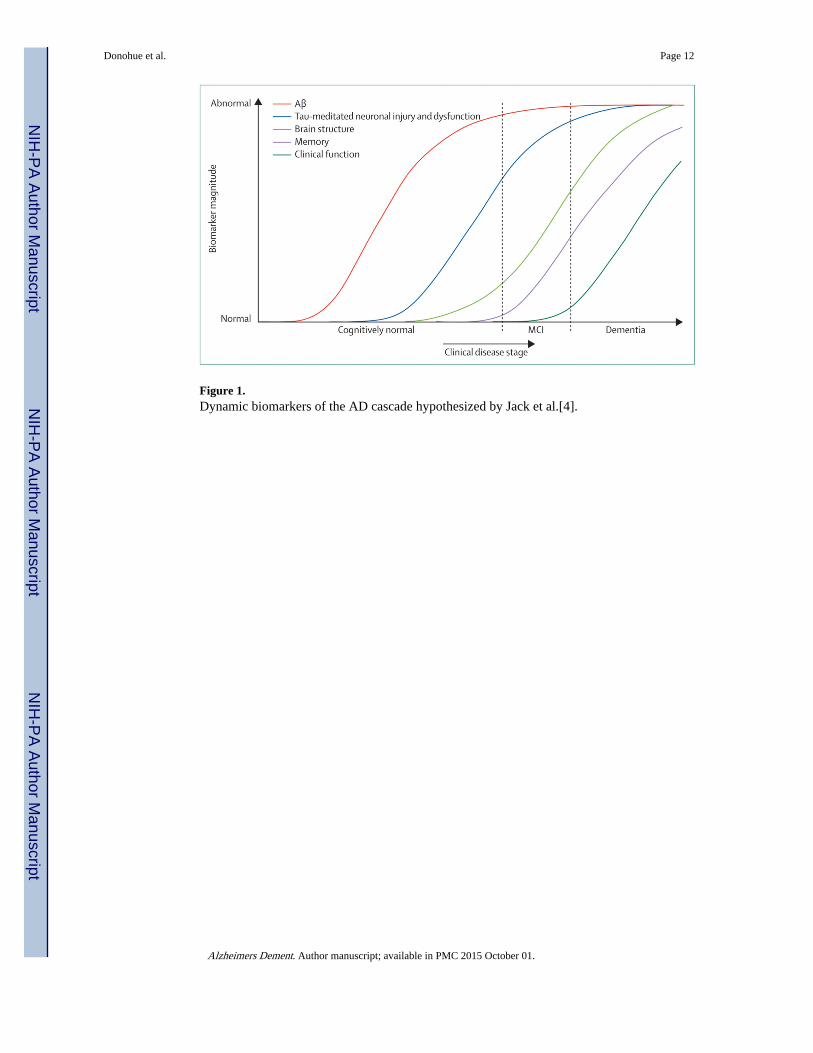
Figure 1. Dynamic biomarkers of the AD cascade hypothesized by Jack et al.[4].



NIH

-PA

Author M

anuscriptN

IH-P

A A

uthor Manuscript

NIH

-PA

Author M

anuscript

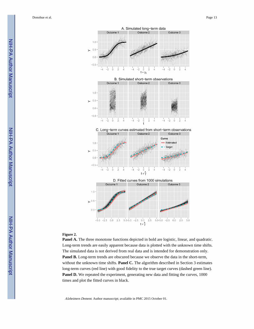
Figure 2. Panel A. The three monotone functions depicted in bold are logistic, linear, and quadratic.

Long-term trends are easily apparent because data is plotted with the unknown time shifts.

The simulated data is not derived from real data and is intended for demonstration only.

Panel B. Long-term trends are obscured because we observe the data in the short-term,

without the unknown time shifts. Panel C. The algorithm described in Section 3 estimates

long-term curves (red line) with good fidelity to the true target curves (dashed green line).

Panel D. We repeated the experiment, generating new data and fitting the curves, 1000

times and plot the fitted curves in black.



NIH

-PA

Author M

anuscriptN

IH-P

A A

uthor Manuscript

NIH

-PA

Author M

anuscript

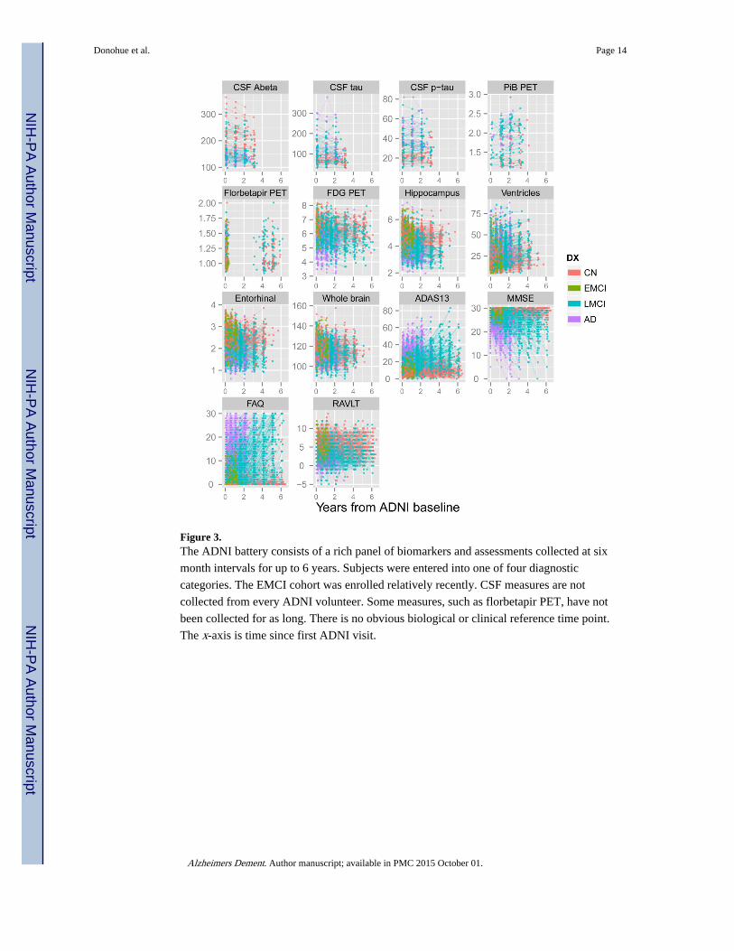
Figure 3. The ADNI battery consists of a rich panel of biomarkers and assessments collected at six

month intervals for up to 6 years. Subjects were entered into one of four diagnostic

categories. The EMCI cohort was enrolled relatively recently. CSF measures are not

collected from every ADNI volunteer. Some measures, such as florbetapir PET, have not

been collected for as long. There is no obvious biological or clinical reference time point.

The x-axis is time since first ADNI visit.



NIH

-PA

Author M

anuscriptN

IH-P

A A

uthor Manuscript

NIH

-PA

Author M

anuscript

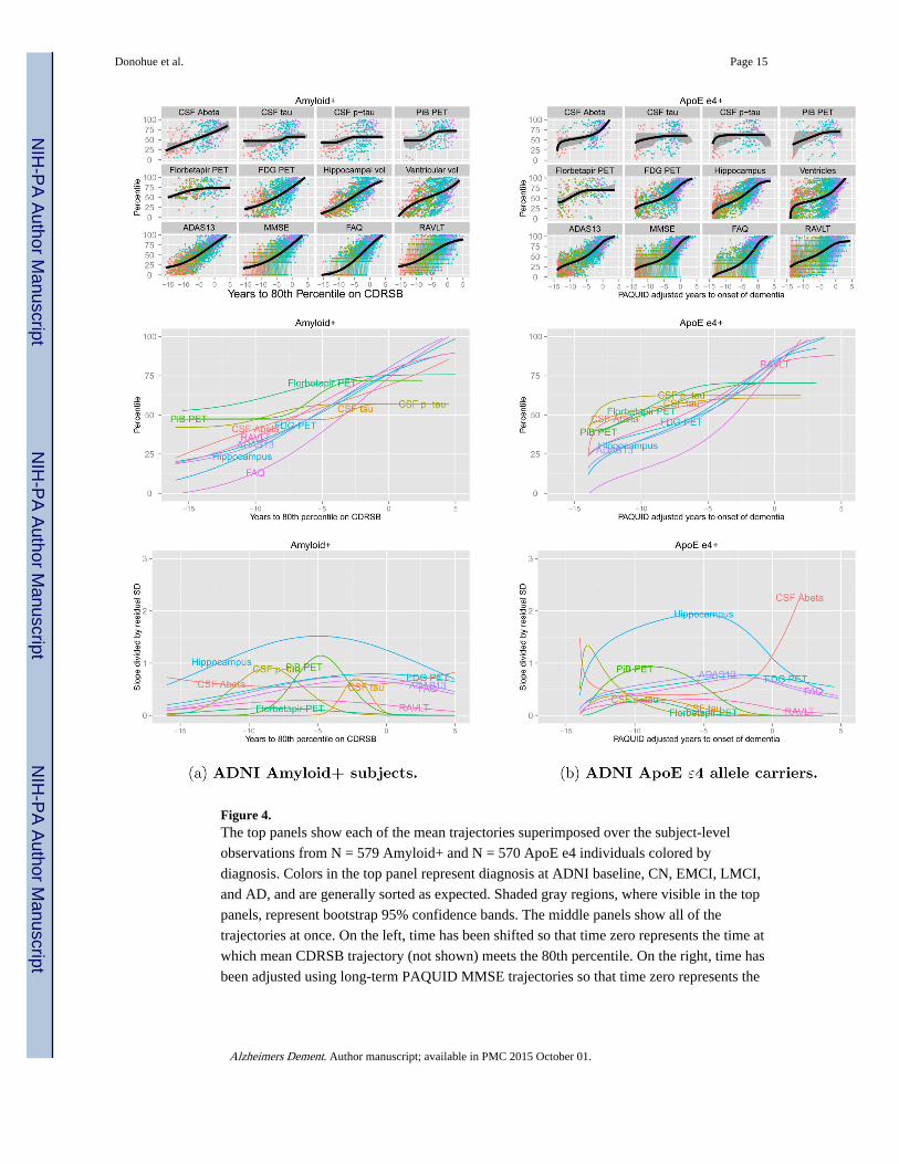
Figure 4. The top panels show each of the mean trajectories superimposed over the subject-level

observations from N = 579 Amyloid+ and N = 570 ApoE e4 individuals colored by

diagnosis. Colors in the top panel represent diagnosis at ADNI baseline, CN, EMCI, LMCI,

and AD, and are generally sorted as expected. Shaded gray regions, where visible in the top

panels, represent bootstrap 95% confidence bands. The middle panels show all of the

trajectories at once. On the left, time has been shifted so that time zero represents the time at

which mean CDRSB trajectory (not shown) meets the 80th percentile. On the right, time has

been adjusted using long-term PAQUID MMSE trajectories so that time zero represents the



NIH

-PA

Author M

anuscriptN

IH-P

A A

uthor Manuscript

NIH

-PA

Author M

anuscript

estimated time to onset of dementia. The bottom panels show rates of change standardized

by residual standard deviation.



NIH

-PA

Author M

anuscriptN

IH-P

A A

uthor Manuscript

NIH

-PA

Author M

anuscript

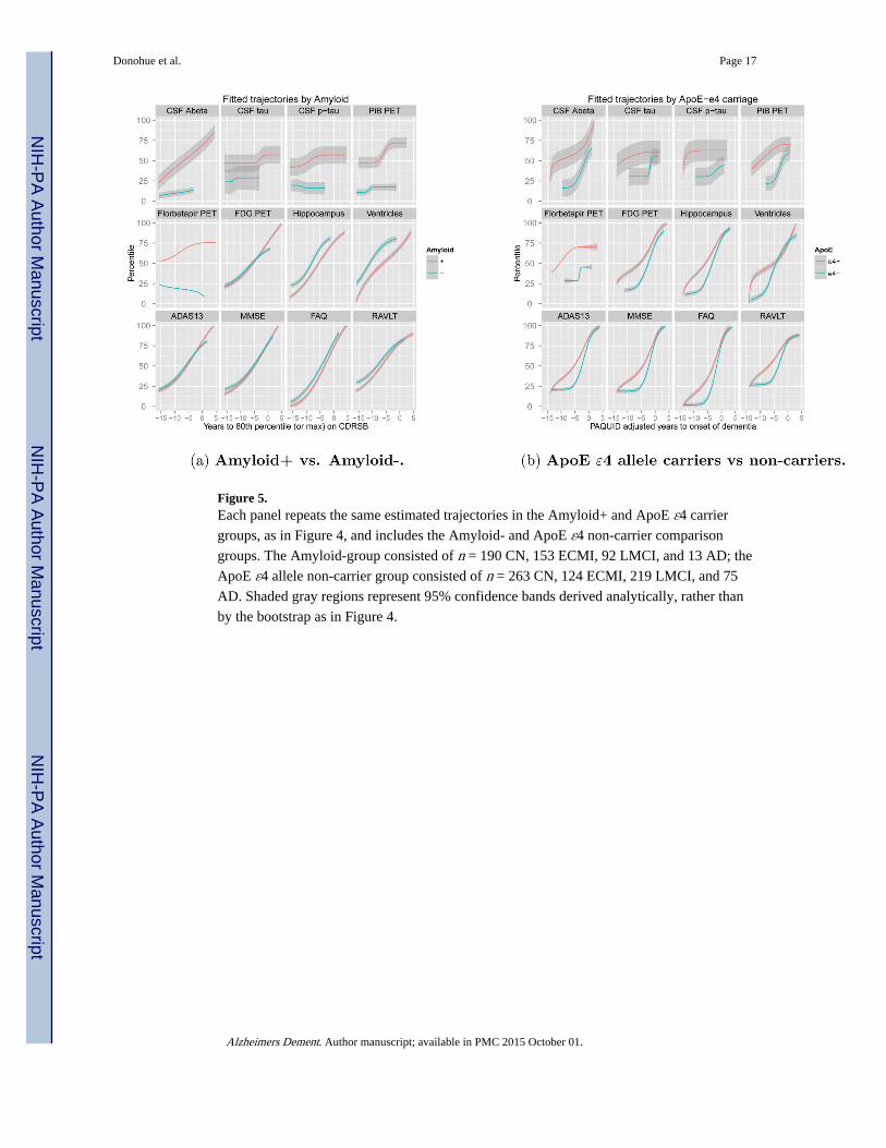
Figure 5. Each panel repeats the same estimated trajectories in the Amyloid+ and ApoE ε4 carrier

groups, as in Figure 4, and includes the Amyloid- and ApoE ε4 non-carrier comparison

groups. The Amyloid-group consisted of n = 190 CN, 153 ECMI, 92 LMCI, and 13 AD; the

ApoE ε4 allele non-carrier group consisted of n = 263 CN, 124 ECMI, 219 LMCI, and 75

AD. Shaded gray regions represent 95% confidence bands derived analytically, rather than

by the bootstrap as in Figure 4.



NIH

-PA

Author M

anuscriptN

IH-P

A A

uthor Manuscript

NIH

-PA

Author M

anuscript

NIH

-PA

Author M

anuscriptN

IH-P

A A

uthor Manuscript

NIH

-PA

Author M

anuscript


Table 1

Partial residuals for each target parameters and their conditional expectations. Target parameters of our model

and the partial residuals we use to estimate each parameter in the iterative algorithm. Under the assumptions of

the model, we see that the conditional expectations of the partial residuals are equivalent to the parameters of

interest. The equivalence is approximate for , since here we integrate over the function . The

approximation is reasonable provided α0ij, α1ij, εij are small and is not too steep.

Partial Residual Conditional Expectation

Long-term smooth curve: gj

Rijg(t) = Yij(t)−α0ij−α1ijt E(Rij

g(t) ∣gj, t,γi) = gj(t+γi)

Subject- & outcome-specific intercept & slope: α0ij , α1ij

Rijα(t) = Yij(t)−gj(t+γi) E(Rij

α(t) ∣α0ij,α1ij, t) =α0ij+α1ijt

Subject-specific time shift: γi

Rijγ(t) = t−gj

−1(Yij(t)) E(Rijγ(t) ∣γi)≈gj

−1(gj(t+γi))− t =γi


NIH

-PA

Author M

anuscriptN

IH-P

A A

uthor Manuscript

NIH

-PA

Author M

anuscript


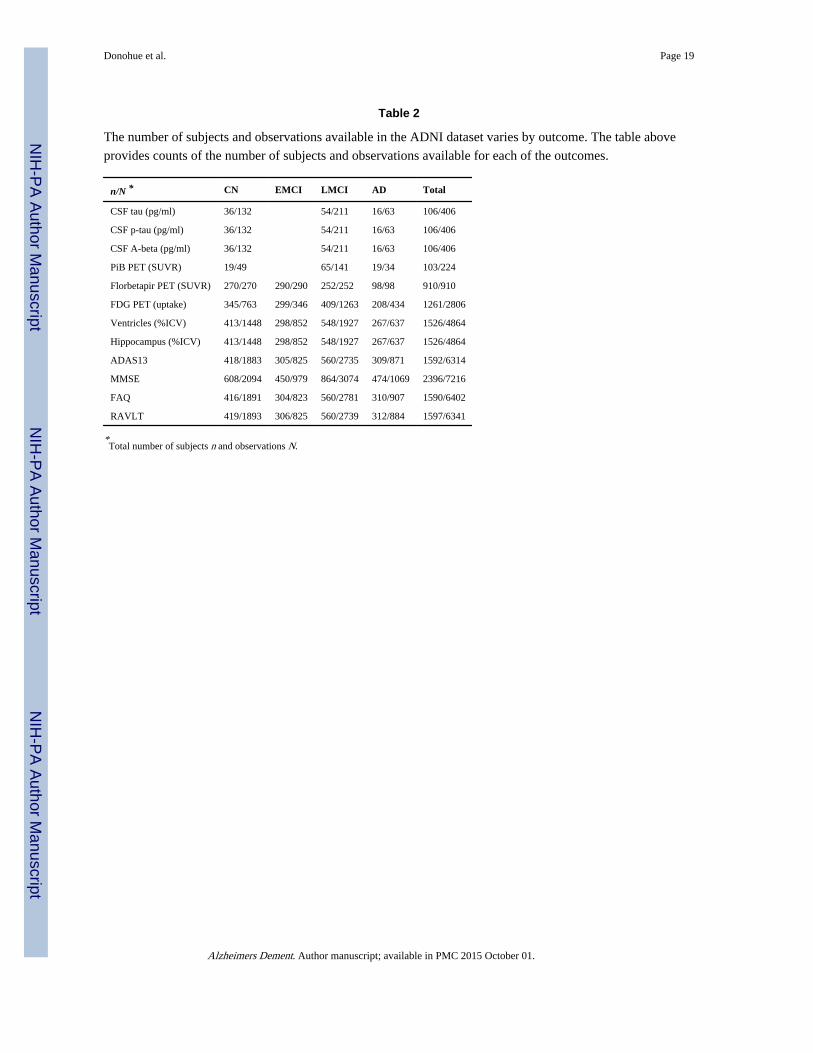
Table 2

The number of subjects and observations available in the ADNI dataset varies by outcome. The table above

provides counts of the number of subjects and observations available for each of the outcomes.

n/N * CN EMCI LMCI AD Total

CSF tau (pg/ml) 36/132 54/211 16/63 106/406

CSF p-tau (pg/ml) 36/132 54/211 16/63 106/406

CSF A-beta (pg/ml) 36/132 54/211 16/63 106/406

PiB PET (SUVR) 19/49 65/141 19/34 103/224

Florbetapir PET (SUVR) 270/270 290/290 252/252 98/98 910/910

FDG PET (uptake) 345/763 299/346 409/1263 208/434 1261/2806

Ventricles (%ICV) 413/1448 298/852 548/1927 267/637 1526/4864

Hippocampus (%ICV) 413/1448 298/852 548/1927 267/637 1526/4864

ADAS13 418/1883 305/825 560/2735 309/871 1592/6314

MMSE 608/2094 450/979 864/3074 474/1069 2396/7216

FAQ 416/1891 304/823 560/2781 310/907 1590/6402

RAVLT 419/1893 306/825 560/2739 312/884 1597/6341

*Total number of subjects n and observations N.


NIH

-PA

Author M

anuscriptN

IH-P

A A

uthor Manuscript

NIH

-PA

Author M

anuscript


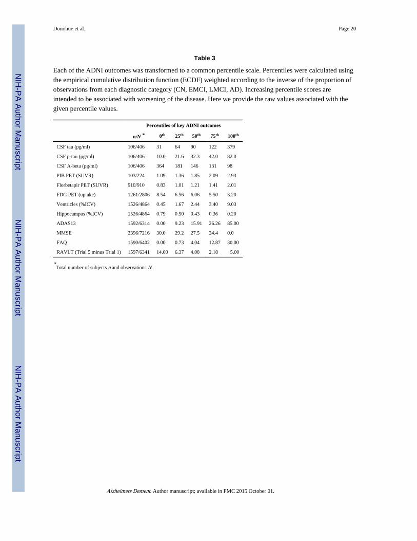
Table 3

Each of the ADNI outcomes was transformed to a common percentile scale. Percentiles were calculated using

the empirical cumulative distribution function (ECDF) weighted according to the inverse of the proportion of

observations from each diagnostic category (CN, EMCI, LMCI, AD). Increasing percentile scores are

intended to be associated with worsening of the disease. Here we provide the raw values associated with the

given percentile values.

Percentiles of key ADNI outcomes

n/N * 0th 25th 50th 75th 100th

CSF tau (pg/ml) 106/406 31 64 90 122 379

CSF p-tau (pg/ml) 106/406 10.0 21.6 32.3 42.0 82.0

CSF A-beta (pg/ml) 106/406 364 181 146 131 98

PIB PET (SUVR) 103/224 1.09 1.36 1.85 2.09 2.93

Florbetapir PET (SUVR) 910/910 0.83 1.01 1.21 1.41 2.01

FDG PET (uptake) 1261/2806 8.54 6.56 6.06 5.50 3.20

Ventricles (%ICV) 1526/4864 0.45 1.67 2.44 3.40 9.03

Hippocampus (%ICV) 1526/4864 0.79 0.50 0.43 0.36 0.20

ADAS13 1592/6314 0.00 9.23 15.91 26.26 85.00

MMSE 2396/7216 30.0 29.2 27.5 24.4 0.0

FAQ 1590/6402 0.00 0.73 4.04 12.87 30.00

RAVLT (Trial 5 minus Trial 1) 1597/6341 14.00 6.37 4.08 2.18 −5.00

*Total number of subjects n and observations N.


Michael C. Donohue NIH Public Access Helene Jacqmin-Gadda Mélanie Le ...adni.loni.usc.edu/adni-publications/Donohue_2014_AlzDem.pdf · Estimating long-term multivariate progression

Documents