Michael A. Akeroyd

Binaural SOUND Creation Toolbox for MATLAB

Michael A. Akeroyd

Department of Neuroscience,

University of Connecticut Health Center,

263 Farmington Avenue,

Farmington, CT 06030, USA.

Laboratory of Experimental Psychology,

School of Biological Sciences,

University of Sussex,

Falmer, Brighton, BN1 9QG, UK.

Chapter 1 Introduction 4

Chapter 1

Introduction

1.1 Preface

This manual describes a MATLAB toolbox for computational modeling of binaural auditory

processing. My goals were (1) to develop MATLAB software for calculating the binaural cross-

correlogram of a sound and for then determining the lateralization of the sound, and (2) to develop

Windows 98 software for displaying and post-processing a binaural cross-correlogram. The toolbox

was written to support my own research but I am making it available in the hope that it may prove

useful.

The manual does not explain either how to use MATLAB or how to do binaural modeling, and

so a familiarity with the concepts of binaural hearing is assumed. I can only offer limited support for

the toolbox, but I will try to mend any bugs that are present and help with its use. Although I use the

toolbox continually, I tend to use the same functions and options and so might not have found any

some bugs (in this sense the toolbox should be regarded as "Beta" code). I will try to incorporate any

suggestions for improvements, changes, or additions to the toolbox or to this manual. I will also try

to—but cannot promise to—answer any questions on binaural modeling that arise out of the use of this

toolbox.

If you find the toolbox useful, I would appreciate it if you would send me an email to

[email protected] I will then put your name onto a mailing list so I can let you know of new

functions, bug corrections, etc.

The toolbox was written whilst I was a MRC Research Fellow at the University of Sussex and

the University of Connecticut Health Center. Any for-profit use or redistribution is prohibited. No

warranty is expressed or implied.

1.2 Hardware/Software requirements

I use this software on a Windows-98 PC running MATLAB 5.11 (specifically version 5.3.1.29215a). It

also works on MATLAB 6 (version 6.0.0.88; release 12); the only known inconsistency is that

mccgramplo2dsqrt does not plot the correlogram properly if either the symbolsize or linewidth

parameters are set to 0. I do not know the degree to which this toolbox will work on earlier versions of

MATLAB or on non-PC platforms. If, however, you find that it does (or does not) work, then I would

appreciate it if you would let me know.

5

With one exception all of the MATLAB functions used in the toolbox are part of the standard release of

MATLAB. The exception is the function hilbert, which computes the Hilbert Transform used in the

envelope-compression algorithm. This function is part of the Signal Processing toolbox, which can be

obtained from the Mathworks.

The display program ccdisplay.exe is a Windows 95/98 executable. It is written in Borland C++

Builder (version 3.0). The source code is available on request from myself.

1.3 Installation

All of the software in the toolbox should be copied into a single directory whose name is then added to

the MATLAB path (see pathdef.m in (on my system) matlab\toolbox\local\). The name of the

directory does not matter so something like "binauraltoolbox" will suffice. The location of the

directory is also immaterial: the only requirement is that it can be accessed by MATLAB.

The Windows program ccdisplay.exe does not require separate installation as all of the libraries it

needs are compiled with it. It should be placed in the same directory as the remainder of the toolbox.

Chapter 2: Overview 6

Chapter 2

Overview of the toolbox

2.1 What is in this manual

Chapters 3-6 are primarily a tutorial in the use of the toolbox. Chapter 3 describes how to make a

bandpass noise. It also describes how to make other signals, and how to plot, play, and save a signal.

Chapter 4 describes how to generate a binaural cross-correlogram. Chapter 5 describes how to apply

frequency or delay weightings to a correlogram, as well as how to use a correlogram to predict the

lateralization of a signal. Chapter 6 describes how to use the Windows program ccdisplay for

displaying and processing a correlogram.

Appendices 1 and 2 outline the various frequency-weighting functions and delay-weighting functions

that are available. Appendix 3 describes the ERB function used to calculate the bandwidth and

frequency spacing of the filters in the gammatone filterbank.

The remainder of this chapter summarizes the functions provided in the toolbox, describes the data

formats used by the functions, and briefly describes the infoflag parameter used in most of the

functions.

2.2 Help

Online help for all the functions can be obtained by typing 'help functioname'. For example, to see

the help page for the function mcreatetone, type:

» help mcreatetone

Further documentation will be found in the comments to the code in each function.

2.3 Functions in the toolbox

The next page lists all the user functions. The other functions in the toolbox are used internally by

these functions.


Signal generators (see Chapter 3)

mcreatetone Dichotic pure tone.

mcreatecomplextone Dichotic complex tone (components defined in an additional text file).

mcreatenoise1 Dichotic bandpass noise (defined by center frequency and bandwidth).

mcreatenoise2 Dichotic bandpass noise (defined by lowpass and highpass cutoff frequencies).

mcreatenoise1rho Interaurally-decorrelated dichotic bandpass noise (defined by c.f. and bandwidth).

mcreatenoise2rho Interaurally-decorrelated dichotic bandpass noise (defined by low/high frequencies).

mcreatehuggins1 Huggins pitch (carrier noise defined by center frequency and bandwidth).

mcreatehuggins2 Huggins pitch (carrier noise defined by lowpass and high-pass cutoff frequencies).

mwavecreate Convert any pre-made signal to the 'wave' format.

Signal processing (see Chapter 3)

mwaveadd Add two ‘wave’ signals.

mwavecat Concatenate two ‘wave’ signals together.

mwaveplay Play a ‘wave’ signal through the PC speakers.

mwavesave Save a ‘wave’ signal as a .wav file.

mwaveplot Plot a ‘wave’ signal.

mfft1side Calculate and plot the FFT of a monaural waveform.

Binaural cross-correlograms (see Chapters 4 and 5)

mcorrelogram Calculate and plot a correlogram of a 'wave' signal.

mccgramdelayweight Apply delay weighting (the p(τ) function) to a correlogram.

mccgramfreqweight Apply frequency weighting to a correlogram.

mccgrampeak Find the location of a peak in the across-frequency average of a correlogram.

mccgramcentroid Find the location of the centroid in the across-frequency average of a correlogram.

mccgramplot4panel Plot a four-panel picture of a correlogram.

mccgramplot3dmesh Plot a correlogram as a 3-dimensional mesh.

mccgramplot3dsurf Plot a correlogram as a 3-dimensional surface.

mccgramplot2dsqrt Plot a correlogram as a 2-dimensional plot (incorporates a square-root transformation of

the correlogram values).

mccgramplotaverage Plot the across-frequency average of a correlogram.

Displaying a correlogram in Windows (see Chapter 6)

mcallccdisplay Display a previously-made correlogram using the Windows program ccdisplay.

ccdisplay.exe A Windows program for displaying and transforming a correlogram.

ERB functions (see Appendix 3)

merb Calculate the ERB at a given center frequency.

mhztoerb Convert a frequency from units of Hz to units of ERB number.

merbtohz Convert a frequency from units of ERB number to units of Hz.


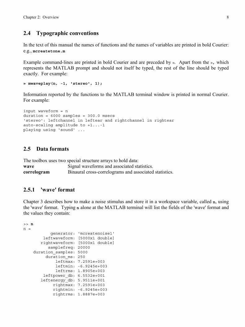
2.4 Typographic conventions

In the text of this manual the names of functions and the names of variables are printed in bold Courier:

e.g., mcreatetone.m

Example command-lines are printed in bold Courier and are preceded by ». Apart from the », which

represents the MATLAB prompt and should not itself be typed, the rest of the line should be typed

exactly. For example:

» mwaveplay(n, -1, 'stereo', 1);

Information reported by the functions to the MATLAB terminal window is printed in normal Courier.

For example:

input waveform = n

duration = 6000 samples = 300.0 msecs

'stereo': leftchannel in leftear and rightchannel in rightear

auto-scaling amplitude to +1...-1

playing using 'sound' ...

2.5 Data formats

The toolbox uses two special structure arrays to hold data:

wave Signal waveforms and associated statistics.

correlogram Binaural cross-correlograms and associated statistics.

2.5.1 'wave' format

Chapter 3 describes how to make a noise stimulus and store it in a workspace variable, called n, using

the 'wave' format. Typing n alone at the MATLAB terminal will list the fields of the 'wave' format and

the values they contain:

>> n

n =

generator: 'mcreatenoise1'

leftwaveform: [5000x1 double]

rightwaveform: [5000x1 double]

samplefreq: 20000

duration_samples: 5000

duration_ms: 250

leftmax: 7.2591e+003

leftmin: -6.9245e+003

leftrms: 1.8905e+003

leftpower_db: 6.5532e+001

leftenergy_db: 5.9511e+001

rightmax: 7.2591e+003

rightmin: -6.9245e+003

rightrms: 1.8887e+003


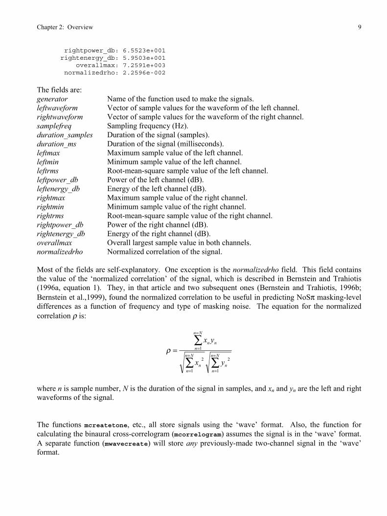
rightpower_db: 6.5523e+001

rightenergy_db: 5.9503e+001

overallmax: 7.2591e+003

normalizedrho: 2.2596e-002

The fields are:

generator Name of the function used to make the signals.

leftwaveform Vector of sample values for the waveform of the left channel.

rightwaveform Vector of sample values for the waveform of the right channel.

samplefreq Sampling frequency (Hz).

duration_samples Duration of the signal (samples).

duration_ms Duration of the signal (milliseconds).

leftmax Maximum sample value of the left channel.

leftmin Minimum sample value of the left channel.

leftrms Root-mean-square sample value of the left channel.

leftpower_db Power of the left channel (dB).

leftenergy_db Energy of the left channel (dB).

rightmax Maximum sample value of the right channel.

rightmin Minimum sample value of the right channel.

rightrms Root-mean-square sample value of the right channel.

rightpower_db Power of the right channel (dB).

rightenergy_db Energy of the right channel (dB).

overallmax Overall largest sample value in both channels.

normalizedrho Normalized correlation of the signal.

Most of the fields are self-explanatory. One exception is the normalizedrho field. This field contains

the value of the ‘normalized correlation’ of the signal, which is described in Bernstein and Trahiotis

(1996a, equation 1). They, in that article and two subsequent ones (Bernstein and Trahiotis, 1996b;

Bernstein et al.,1999), found the normalized correlation to be useful in predicting NoSπ masking-level

differences as a function of frequency and type of masking noise. The equation for the normalized

correlation ρ is:

∑∑

∑=

=

=

=

=

==Nn

n

n

Nn

n

n

Nn

n

nn

yx

yx

1

2

1

2

1ρ

where n is sample number, N is the duration of the signal in samples, and xn and yn are the left and right

waveforms of the signal.

The functions mcreatetone, etc., all store signals using the ‘wave’ format. Also, the function for

calculating the binaural cross-correlogram (mcorrelogram) assumes the signal is in the ‘wave’ format.

A separate function (mwavecreate) will store any previously-made two-channel signal in the ‘wave’

format.


Note that the left and right waveforms are stored in one-dimensional vectors. They can therefore be

manipulated in the same way as any other MATLAB vector. For example, to invert every sample in

the left waveform of a ‘wave’ signal, type:

>> newwaveform = wave1.leftwaveform * -1;

For a second example, to play the left waveform using the MATLAB function soundsc and at the

correct sampling frequency, type:

>> soundsc(wave1.leftwaveform, wave1.samplefreq)

An easy way of converting the transformed waveform to the 'wave' format is to use the mwavecreate

function. For example, to invert the left waveform, type:

>> newwaveform1 = wave1.leftwaveform * -1;

>> wave2 = mwavecreate(newwaveform, wave1.rightwaveform, wave1.samplefreq, 1);

Note that many MATLAB functions can be condensed into one line. For example, the preceding

example is the same as

>> wave2 = mwavecreate(wave1.leftwaveform * -1, wave1.rightwaveform,...

wave1.samplefreq, 1);

2.5.1 'correlogram' format

Chapter 4 describes how to generate the binaural cross-correlogram of a 'wave' signal and store it in a

workspace variable, called cc1, using the 'correlogram' format. Typing cc1 alone at the MATLAB

terminal will list the fields of the 'correlogram' format and the values they contain:

» cc1

cc1 =

title: 'first-level correlogram'

type: 'binauralcorrelogram'

modelname: 'mcorrelogram'

transduction: 'hw'

samplefreq: 20000

mincf: 200

maxcf: 1000

density: 2

nfilters: 21

q: 9.2789e+000

bwmin: 2.4673e+001

mindelay: -3500

maxdelay: 3500

ndelays: 141

freqaxishz: [21x1 double]

freqaxiserb: [21x1 double]

powerleft: [21x1 double]


powerright: [21x1 double]

delayaxis: [1x141 double]

freqweight: 'null'

delayweight: 'null'

data: [21x141 double]

The fields are:

title Title/information on correlogram.

type Type of correlogram (usually ‘binauralcorrelogram’).

modelname Name of function used to create the correlogram.

transduction Name of model for neural transduction.

samplefreq Sampling frequency of the signal (Hz).

mincf Lowest filter frequency in the filterbank (Hz).

maxcf Highest filter frequency in the filterbank (Hz).

density Spacing of filters in the filterbank (filters per ERB).

nfilters Number of filters in the filterbank.

q 'q' factor used in calculating the bandwidth of each filter.

bwmin Minimum-bandwidth factor used in calculating the bandwidth of each filter.

mindelay Smallest (most-negative) internal delay τ used in the correlogram.

maxdelay Largest (most-positive) internal delay τ used in the correlogram.

freqaxishz Vector of the center frequencies of each filter in the filterbank (Hz).

freqaxiserb Vector of the center frequencies of each filter in the filterbank (ERB number).

powerleft Vector of the power in each filter for the left channel.

powerright Vector of the power in each filter for the right channel.

delayaxis Vector of the internal delays τ in the correlogram (µs).

freqweight Whether frequency weighting has been applied or not.

delayweight Whether delay weighting has been applied or not.

data Two-dimensional (frequency x internal delay) matrix of the correlogram values.

The parameters q and bwmin control the bandwidth of the gammatone filters. They, as well as how to

convert filter center frequencies from Hz to ERB number and back again, are described in Appendix 3.

Note that the correlogram itself is stored in the two-dimensional matrix data, which can be transformed

in the same way as any other MATLAB matrix. For example, to square-root every value in the

correlogram, type:

>> newdata = sqrt(cc1.data);

In order to store the transformed data in the 'correlogram' format, first copy the original correlogram, so

preserving all the information in the other fields, and then to copy the transformed data into the data

field directly. For example:

>> cc2 = cc1;

>> cc2.data = sqrt(cc1.data);


2.6 The infoflag parameter

The last parameter of most of the functions is infoflag, whose value determines the amount of

information reported to the MATLAB terminal window. It can take values of 0, 1, or 2:

0 Do not report any information or plot any pictures.

1 Report some information as the function runs. I use this value most of the time as I like to

watch the progress of the functions.

2 In addition to reporting information, also plot figures.

Note that a value of 2 is only meaningful for those functions that can plot pictures, of which the

primary examples are mfft1side and mcorrelogram. Values of 0 and 1 apply to all the functions.

Chapter 3: Generating a signal 13

Chapter 3

Generating a signal

3.1 Dichotic bandpass noise

This part of the tutorial shows how to create a dichotic bandpass noise.

The function mcreatenoise1 will synthesize a dichotic bandpass noise, by first creating two bands of

noise in the spectral domain and then applying an inverse-FFT to create two waveforms. One band of

noise is for the left channel, the other for the right channel. Both bands have the same center

frequency, bandwidth, and duration, but can differ in phase or level so giving an ITD/IPD or an IID.

The full syntax is

outputwave = mcreatenoise1(centerfreq, bandwidth,

spectrumlevelleft, spectrumlevelright, itd, ipd,

duration, gateduration, samplefreq, infoflag);

where the parameters are

centerfreq Center frequency of the passband of the noise (Hz).

bandwidth Bandwidth of the passband of the noise (Hz).

spectrumlevelleft Spectrum level of the left channel of the passband of the noise (dB).

spectrumlevelright Spectrum level of the left channel of the passband of the noise (dB).

itd Interaural time delay (ITD) of the passband of the noise (microseconds).

ipd Interaural phase delay (IPD) of the passband of the noise (degrees).

duration Overall duration (milliseconds).

gateduration Duration of raised-cosine onset/offset gates (milliseconds).


infoflag 1 (report useful information) or 0 (do not report useful information).

For example, typing in this command will create a bandpass noise of 500-Hz center frequency, 400-Hz

bandwidth, 40-dB spectrum level for both channels, 500-µsec ITD, 0° IPD, 300-ms duration, 10-ms

raised-cosine gates, and using a sampling frequency of 20000 Hz. The signal is stored in the

workspace variable n :

>> n = mcreatenoise1(500,400,40,40,500,0,300,10,20000,0);

The last parameter is infoflag. This can be either 0 or 1. If it is equal to 0 then the program runs but

does not report anything to the terminal window (as in the above example). If instead it is equal to 1

then the program reports the following information to the MATLAB terminal window as it runs


(although note that the line numbers in parentheses are not displayed; I added those for this tutorial).

This is shown with the next example command:

>> n = mcreatenoise1(500,400,40,40,500,0,300,10,20000,1);

(1) This is mcreatenoise1.m

(2) creating 6000-point FFT buffer with 20000 sampling rate ...

(3) FFT resolution = 3.33 Hz

(4) center frequency: 500.0 Hz bandwidth: 400 Hz

(5) lowest frequency : 300.0 Hz (rounded to 300.0 Hz)

(6) highest frequency: 700.0 Hz (rounded to 700.0 Hz)

(7) number of FFT components included = 121

(8) creating random real/imag complex pairs ...

(9) inverse ffting for waveform ...

(10) normalizing power ...

(11) getting phase spectrum ...

(12) time-delaying phase spectrum of right channel by 500 usecs ...

(13) phase-shifting phase spectrum of right channel by 0 degs ...

(14) inverse-FFTing left and right channels to get waveforms ...

(15) applying 10.0-ms raised cosine gates ...

(16) setting spectrum level of left channel to 40.0 dB (overall level=66.0 dB)...

(17) setting spectrum level of right channel to 40.0 dB (overall level=66.0 dB)...

(18) transposing left waveform ...

(19) transposing right waveform ...

(20) creating 'wave' structure ...

(21) waveform statistics :

(22) samplingrate = 20000 Hz

(23) power (left, right) = 66.3 dB 66.3 dB

(24) energy (left, right) = 61.1 dB 61.1 dB

(25) maximum (left, right) = 6637.9 6637.9

(26) minimum (left, right) = -7366.0 -7366.0

(27) rms amplitude (left, right) = 2065.0 2063.7

(28) duration = 6000 samples = 300.00 msecs

(29) normalized correlation = 0.0254

(30) storing waveform to workspace as wave structure ..

Line 1 reports the name of the program. Lines 2 and 3 report the size of the buffer used for the FFT.

As MATLAB can perform non-power-of-2 FFTs this buffer is equal to the duration of the noise in

samples. Lines 4-6 report the frequency parameters of the passband of the noise in Hz and when

rounded to the closest FFT frequency (this rounding is necessary as the FFT does not necessarily use

integer-spaced frequencies; in this example the frequencies are spaced at 3.33-Hz steps (see line 3)).

Line 7 reports how many of the FFT components are included in the passband, as both the requested

values and rounded to the closest FFT frequencies. Lines 8-15 report stages in the generation of the

noise. Lines 16-17 report the spectrum and overall levels of the right channels. Lines 18-20 report

further stages in the generation of the noise. Lines 22-29 report some statistics on the noise; note that

the power (line 23) is equal to the requested spectrum level (lines 16/17) in dB plus

10log10(bandwidth), where the value of the bandwidth is in Hz. These values will not be exactly the

same as the requested value as each individual noise is a different random process.

mcreatenoise1 creates a ‘wave’ signal, which contains the left and right waveforms of the signal as

well as a variety of statistics on those waveforms. The components of the structure array can be shown

by typing in the name of the variable (here n) at the MATLAB command line:


» n

n =

generator: 'mcreatenoise1'

leftwaveform: [6000x1 double]

rightwaveform: [6000x1 double]

samplefreq: 20000

duration_samples: 6000

duration_ms: 300

leftmax: 6.6379e+003

leftmin: -7.3660e+003

leftrms: 2.0650e+003

leftpower_db: 6.6298e+001

leftenergy_db: 6.1070e+001

rightmax: 6.6379e+003

rightmin: -7.3660e+003

rightrms: 2.0637e+003

rightpower_db: 6.6293e+001

rightenergy_db: 6.1064e+001

overallmax: 7.3660e+003

normalizedrho: 2.5356e-002

Each field of the 'wave' format is described Section 2.5.1.

3.2 Plotting a 'wave' signal

The left and right waveforms of the noise can be plotted using mwaveplot. The syntax of mwaveplot is

mwaveplot(wave, channelflag, starttime, endtime)


wave Signal to be plotted.

channelflag Whether to plot the left channel, right channel or both channels.

starttime Sample time at which to start plot.

endtime Sample time at which to end plot.

For example, to plot the full waveforms of both channels of n, type:

» mwaveplot(n, 'stereo', -1, -1);

The resulting figure is shown at the top of the next page. The two parameters -1 and -1 mean,

respectively, start the plot at the beginning of the signal and end the plot at the finish of the sound.

The channelflag parameter can take three values (note that the quote marks must be included):

'stereo' Plot both channels.

'left' Plot the left channel only.

'right' Plot the right channel only.


For example, to plot the full waveform of the left channel of n, type:

» mwaveplot(n, 'left', -1, -1);

The resulting figure is shown below.


The duration of the plotted waveforms is controlled by the third and fourth parameters. Their values

define the start time and end time of the plots, with the exception that values of -1 (as used in the above

examples) mean start-plot-at-beginning-of-signal (third parameter) and end-plot-at-finish-of-signal

(fourth parameter). For example, to plot the signal between t = 120 ms and t = 125 ms, type;

» mwaveplot(n, 'stereo', 120, 125);

Note that this plot shows that the right waveform leads the left waveform by 0.5 ms. This is because

the noise n was made with an ITD of 500 µs.

3.3 Playing a 'wave' signal

The function mwaveplay will play a 'wave' signal through the PC speakers. The normal situation is to

play the both channels of the signal at maximum amplitude. For example, to play the noise n, type:

» mwaveplay(n, -1, 'stereo', 1);

input waveform = n




playing using 'sound' ...


The first parameter (here n) is the ‘wave’ signal to be played.

The second parameter (here -1) is a scaling factor that sets the level of the signal. When MATLAB

plays a sound it assumes that the maximum amplitude range of the signal is -1 to +1; any samples with

a value outside this range are clipped. If the second option of mwaveplay is set to –1 then mwaveplay

will automatically scale the signal so that the overallmax field of the ‘wave’ signal is equal to +1. This

is done by dividing all the sample values by overallmax. This value therefore sets the level to be the

maximum without clipping. If instead the value of the second parameter is equal to anything other than

-1 then mwaveplay will divide the sample values by that value and then play the signal. To ensure no

clipping, this number should be large enough so that the resulting values are all in the range –1 to +1.

The third parameter (here 'stereo') is a switch controlling which channels are played. The options

are (again the quote marks must be included):

‘stereo’ Play both channels (as in the above example).

‘swap' Play both channels but with the left and right channels swapped.

‘random’ Use one of ‘stereo’ or ‘swap', chosen at random each time the function is called.

‘left’ Play left channel only.

‘right’ Play right channel only.

For example, to play the left channel only, type:

» mwaveplay(n, -1, 'left', 1);

The fourth parameter (here 1) is infoflag. If it is equal to 1 then the function reports the running

information; if it is equal to 0 then nothing is reported but the function still plays the signal.

3.4 Saving a 'wave' signal

The function mwavesave will save the signal as a .wav file. The syntax is the same as that for

mwaveplay except that an additional parameter specifies the filename. For example:

» mwavesave('sound1.wav', n, -1, 'stereo', 1);

input waveform =




saving to file sound1.wav using 'wavwrite' (16-bit resolution)...

This example will save the 'wave' signal n in the file 'sound1.wav', with automatic setting of the

amplitude range to -1 to +1 and using the 'stereo' option (i.e., both channels). The amplitude scaling

factor (here -1) and the channel switch (here 'stereo') are the same as those described above for

mwaveplay.


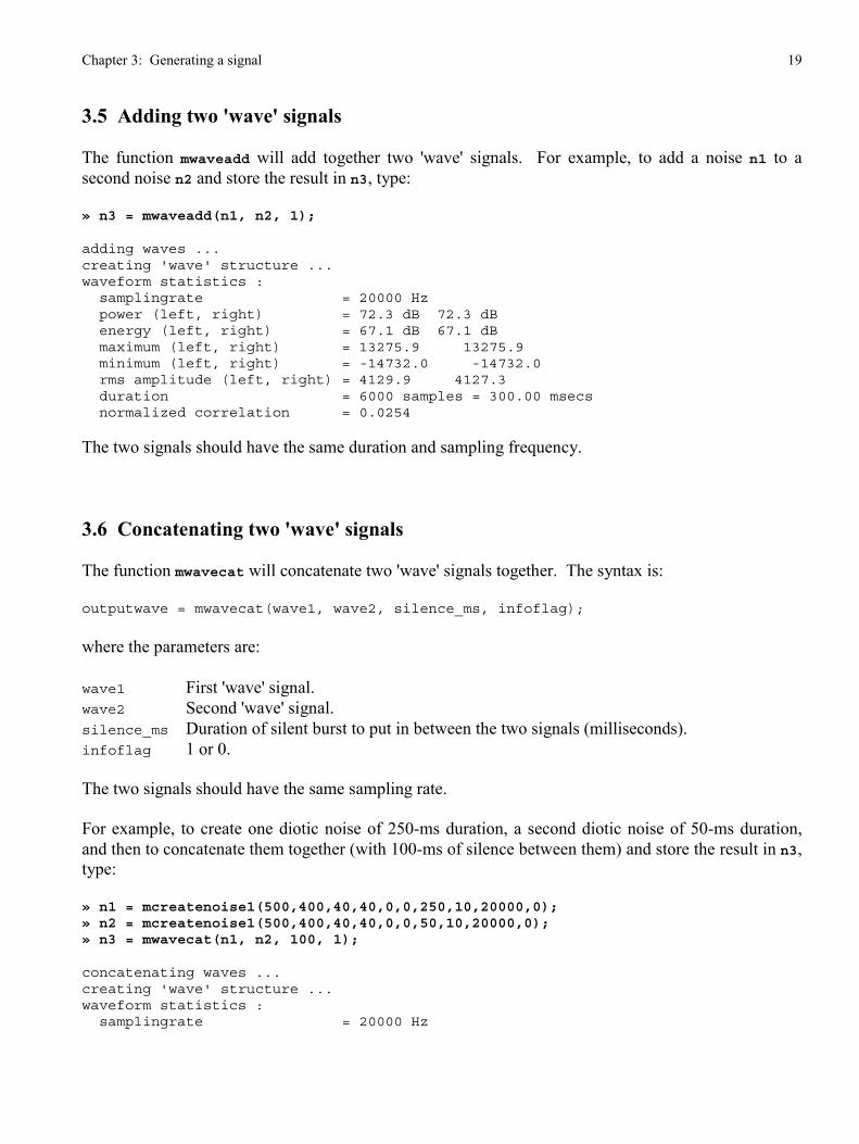
3.5 Adding two 'wave' signals

The function mwaveadd will add together two 'wave' signals. For example, to add a noise n1 to a

second noise n2 and store the result in n3, type:

» n3 = mwaveadd(n1, n2, 1);

adding waves ...

creating 'wave' structure ...

waveform statistics :

samplingrate = 20000 Hz

power (left, right) = 72.3 dB 72.3 dB

energy (left, right) = 67.1 dB 67.1 dB

maximum (left, right) = 13275.9 13275.9

minimum (left, right) = -14732.0 -14732.0

rms amplitude (left, right) = 4129.9 4127.3


normalized correlation = 0.0254

The two signals should have the same duration and sampling frequency.

3.6 Concatenating two 'wave' signals

The function mwavecat will concatenate two 'wave' signals together. The syntax is:

outputwave = mwavecat(wave1, wave2, silence_ms, infoflag);

where the parameters are:

wave1 First 'wave' signal.

wave2 Second 'wave' signal.

silence_ms Duration of silent burst to put in between the two signals (milliseconds).

infoflag 1 or 0.

The two signals should have the same sampling rate.

For example, to create one diotic noise of 250-ms duration, a second diotic noise of 50-ms duration,

and then to concatenate them together (with 100-ms of silence between them) and store the result in n3,

type:

» n1 = mcreatenoise1(500,400,40,40,0,0,250,10,20000,0);

» n2 = mcreatenoise1(500,400,40,40,0,0,50,10,20000,0);

» n3 = mwavecat(n1, n2, 100, 1);

concatenating waves ...

creating 'wave' structure ...

waveform statistics :

samplingrate = 20000 Hz


power (left, right) = 64.5 dB 64.5 dB

energy (left, right) = 60.5 dB 60.5 dB





normalized correlation = 1.0000

The next picture shows the plot of n3 using mwaveplot; note that n3 consists of the 250-ms noise, a

100-ms silent gap, and then the 50-ms noise:

3.7 Other signal-generation functions

3.7.1 Bandpass noises

The function mcreatenoise2 is similar to mcreatenoise1 but the first two parameters specify the

lower and higher cutoff frequencies instead of the center frequency and bandwidth. The other

parameters are the same. The full syntax is

outputwave = mcreatenoise2(lowfrequency, highfrequency,

spectrumlevelleft, spectrumlevelright, itd, ipd,

duration, gateduration, samplefreq, infoflag);


lowfrequency Lower cutoff frequency of the passband of the noise (Hz).


highfrequency Higher cutoff frequency of the passband of the noise (Hz).



itd Interaural time delay (ITD) of the passband of the noise (microseconds).

ipd Interaural phase delay (IPD) of the passband of the noise (degrees).



samplefreq Sampling frequency (Hz)

infoflag 1 or 0.

For example, the noise described in Section 3.1 had a center frequency of 500 Hz and a bandwidth of

400 Hz. The passband therefore extends from 300 Hz to 700 Hz. So, to make this noise using

mcreatenoise2 instead of mcreatenoise1, type:

>> n = mcreatenoise2(300,700,40,40,500,0,300,10,20000,0);

For a second example, to create a diotic noise with a passband from 0 Hz to 1000 Hz, type:

>> n = mcreatenoise2(0,1000,40,40,0,0,300,10,20000,0);

3.7.2 Interaurally-decorrelated bandpass noises

The pair of functions mcreatenoise1rho and mcreatenoise2rho synthesize an interaurally-

decorrelated noise. The interaural correlation ρ (rho) of the noise is specified instead of the ITD or

IPD. The numbers 1 and 2 in the function names are the same as for mcreatenoise1 and

mcreatenoise2: in mcreatenoise1rho the center frequency and bandwidth are specified, and in

mcreatenoise2rho the lower and higher cutoff frequencies are specified.

The full syntax of mcreatenoise1rho is:outputwave = mcreatenoise1rho(centerfreq, bandwidth,

spectrumlevelleft, spectrumlevelright, rho,

duration, gatelength, samplefreq, infoflag)


centerfreq Center frequency of the passband of the noise (Hz).

bandwidth Bandwidth of the passband of the noise (Hz).



rho Interaural correlation of the noise.




infoflag 1 or 0.


The syntax of mcreatenoise2rho is the same but the first two parameters specify the lower and higher

cutoff frequencies.

For example, to create a noise with an interaural correlation of 0.0 (i.e., perfectly uncorrelated, and so

commonly referred to as "Nu"), but whose other parameters are the same as those used in Section 3.1,

type:

>> n = mcreatenoise1rho(500,400,40,40,0,300,10,20000,1);

(1) This is mcreatenoise1rho.m

(2) creating common noise: relative power = 0.00 ...

(3) creating first independent noise: relative power = 1.00 ...

(4) creating second independent noise: relative power = 1.00 ...










(14) normalized correlation = -0.0165


Note that the normalized correlation field (line 14) of the signal is approximately 0; it is not exactly 0.0

because of random fluctuations inherent to all noises.

For a second example, to create the same noise but with an interaural correlation of -1.0 (i.e., a IPD of

π radians, and so commonly referred to as "Nπ"), type:

>> n = mcreatenoise1rho(500,400,40,40,-1,300,10,20000,1);

(1) This is mcreatenoise1rho.m

(2) creating common noise: relative power = 1.00 ...

(3) inverting one channel of common noise to get negative correlation ...

(4) creating first independent noise: relative power = 0.00 ...

(5) creating second independent noise: relative power = 0.00 ...












In this example the normalized correlation is exactly -1.0.


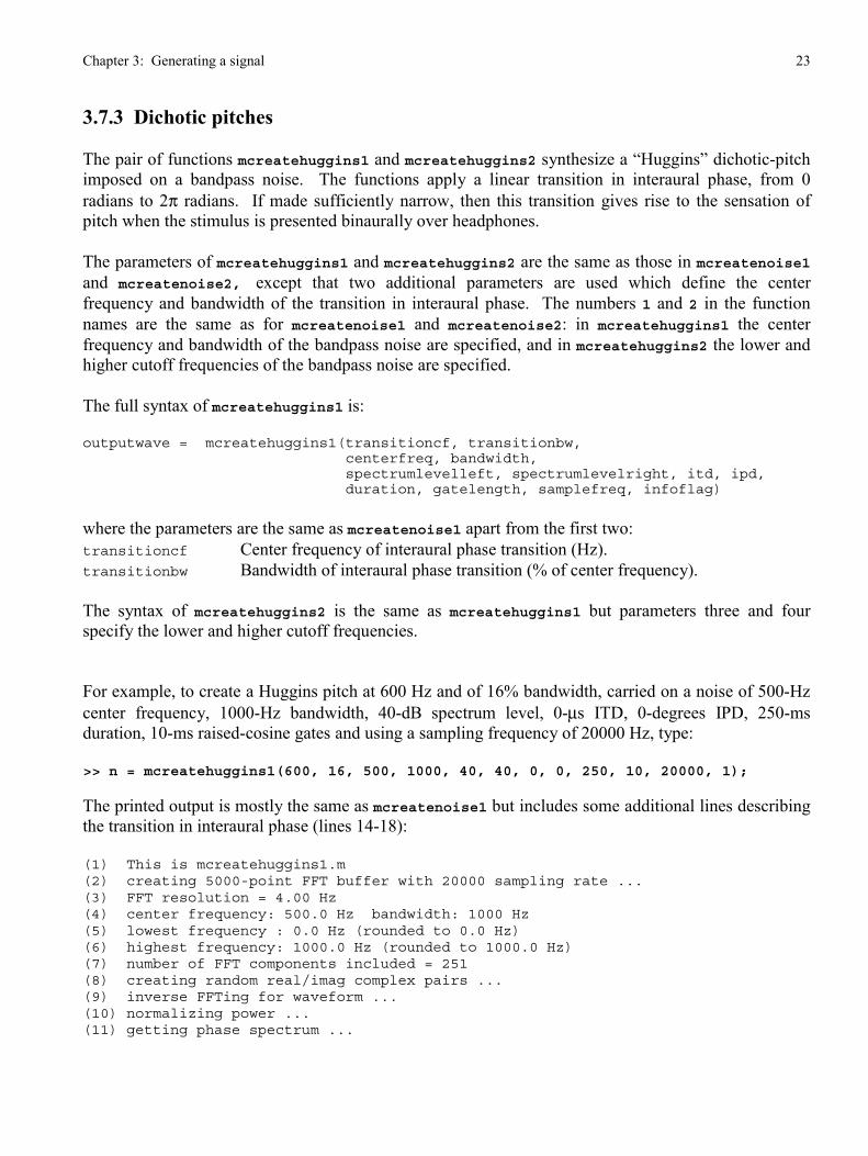
3.7.3 Dichotic pitches

The pair of functions mcreatehuggins1 and mcreatehuggins2 synthesize a “Huggins” dichotic-pitch

imposed on a bandpass noise. The functions apply a linear transition in interaural phase, from 0

radians to 2π radians. If made sufficiently narrow, then this transition gives rise to the sensation of

pitch when the stimulus is presented binaurally over headphones.

The parameters of mcreatehuggins1 and mcreatehuggins2 are the same as those in mcreatenoise1

and mcreatenoise2, except that two additional parameters are used which define the center

frequency and bandwidth of the transition in interaural phase. The numbers 1 and 2 in the function

names are the same as for mcreatenoise1 and mcreatenoise2: in mcreatehuggins1 the center

frequency and bandwidth of the bandpass noise are specified, and in mcreatehuggins2 the lower and

higher cutoff frequencies of the bandpass noise are specified.

The full syntax of mcreatehuggins1 is:

outputwave = mcreatehuggins1(transitioncf, transitionbw, centerfreq, bandwidth, spectrumlevelleft, spectrumlevelright, itd, ipd, duration, gatelength, samplefreq, infoflag)

where the parameters are the same as mcreatenoise1 apart from the first two:

transitioncf Center frequency of interaural phase transition (Hz).

transitionbw Bandwidth of interaural phase transition (% of center frequency).

The syntax of mcreatehuggins2 is the same as mcreatehuggins1 but parameters three and four

specify the lower and higher cutoff frequencies.

For example, to create a Huggins pitch at 600 Hz and of 16% bandwidth, carried on a noise of 500-Hz

center frequency, 1000-Hz bandwidth, 40-dB spectrum level, 0-µs ITD, 0-degrees IPD, 250-ms

duration, 10-ms raised-cosine gates and using a sampling frequency of 20000 Hz, type:

>> n = mcreatehuggins1(600, 16, 500, 1000, 40, 40, 0, 0, 250, 10, 20000, 1);

The printed output is mostly the same as mcreatenoise1 but includes some additional lines describing

the transition in interaural phase (lines 14-18):

(1) This is mcreatehuggins1.m

(2) creating 5000-point FFT buffer with 20000 sampling rate ...

(3) FFT resolution = 4.00 Hz

(4) center frequency: 500.0 Hz bandwidth: 1000 Hz

(5) lowest frequency : 0.0 Hz (rounded to 0.0 Hz)

(6) highest frequency: 1000.0 Hz (rounded to 1000.0 Hz)

(7) number of FFT components included = 251

(8) creating random real/imag complex pairs ...

(9) inverse FFTing for waveform ...

(10) normalizing power ...

(11) getting phase spectrum ...


(12) time-delaying phase spectrum of right channel by 0 usecs ...

(13) phase-shifting phase spectrum of right channel by 0 degs ...

(14) creating 0-2pi phase-shift transition in left channel ...

(15) bottom freq = 552.0 Hz (=0 radians)

(16) middle freq = 600.0 Hz (=pi radians)

(17) top freq = 648.0 Hz (=2pi radians)

(18) range = 96.0 Hz = 24 FFT points)


(20) setting spectrum level of left channel to 40.0 dB (overall level = 70.0 dB)

(21) setting spectrum level of right channel to 40.0 dB (overall level = 70.0 dB)












(33) normalized correlation = 0.8959


3.7.4 Pure tones

The function mcreatetone will synthesize a dichotic pure tone. The syntax is:

outputwave = mcreatetone(freq, powerleft, powerright, itd, ipd,

duration, gatelength, samplefreq, infoflag)


freq Frequency of the tone (Hz).

powerleft Power of the left channel of the tone (dB).

powerright Power of the left channel of the tone (dB).

itd Interaural time delay (ITD) of the tone (microseconds).

ipd Interaural phase delay (IPD) of the tone (degrees).




infoflag 1 or 0.

For example, to create a tone of 750-Hz frequency, 60-dB level for both left and right channels, 500-

µsec ITD, 0° IPD, 300-ms duration, 0-ms raised-cosine gates, and using a sampling frequency of 20000

Hz, type:

>> t = mcreatetone(750,60,60,500,0,300,0,20000,1);


(1) This is mcreatetone.m

(2) frequency =750.0 Hz

(3) itd = 500.0 usecs ipd = 0.0 degs => trueitd: 500.000 usecs

(4) left channel : level = 60.00 dB amplitude = 1414.2 samples

(5) right channel : level = 60.00 dB amplitude = 1414.2 samples

(6) left channel : starting phase (sin) = 0.000 cycles

(7) right channel : starting phase (sin) = 0.375 cycles

(8) creating sinwaves ...














(22) storing waveform in workspace as 'wave' ..

Note that the root-mean-square amplitude of the tone is 1000 (line 19). The maximum sample value is

therefore 1414 (line 17), as, for a pure tone, these values are related by a factor of 2 . Furthermore,

the requested power was 60 dB, which is equal to 20log10(1000).

Also, note that the root-mean-square amplitude is calculated over the full duration of the signal. Thus

it will be smaller if raised-cosine gates are incorporated at the onset and offset of the signal. For

example, if 25-ms gates are used, then the root-mean-square amplitude falls to 946:

>> t = mcreatetone(750,60,60,500,0,300,25,20000,0);

This is mcreatetone.m

...




3.7.5 Complex tones

The function mcreatecomplextone will synthesize a dichotic complex tone. The syntax is

outputwave = mcreatecomplextone(parameterfile, overallgain_db, gatelength_ms,

samplefreq, infoflag)


parameterfile Name of text file defining the components of the complex tone.

overallgain_db Overall gain applied to all components (dB).


gatelength_ms Duration of raised-cosine onset/offset gates applied to each component (msecs).


infoflag 1 or 0.

The text file must specify all the parameters of the components in a special format. The supplied

example is called complextonefile1.txt and is shown next:

% Parameter file for specifying a complex tone% Read by mcreatecomplextone.m%% ordering of values in each line is:% freq Hz% level(left) dB% level(right) dB% phase degrees (assumes 'sin' generator)(-999 is code for random)% starttime msecs% end msecs% itd usecs% ipd degrees%% All lines beginning with '%' are ignored%% This example makes a complex-tone similar to that used by Hill% and Darwin (1996; JASA, 100, 2352-2364): a 1000-ms duration% complex tone with 1500-us ITD but with the 500-Hz component% starting after 400-ms and only lasting for 200 ms% (cf Hill and Darwin, Exp 1)%% Example of MATLAB call:% >> wave1 = mcreatecomplextone('complextonefile1.txt', 0, 20, 20000, 1);%%% version 1.0 (Jan 20th 2001)% MAA Winter 2001%----------------------------------------------------------------

200 60 60 90 0 1000 1500 0300 60 60 90 0 1000 1500 0400 60 60 90 0 1000 1500 0

600 60 60 90 0 1000 1500 0700 60 60 90 0 1000 1500 0800 60 60 90 0 1000 1500 0

500 60 60 90 400 600 1500 0

% the end!


In the text file all lines beginning with % are ignored by the parser in mcreatecomplextone. All other

lines are assumed to specify a separate frequency component. The format of each line is:

frequency power_left power_right startingphase start_time end__time ITD IPD

(Hz) (dB) (dB) (degrees) (ms) (ms) (us) (deg)

Most of the parameters are the same as those used in mcreatetone. The three that are not are:

startingphase The starting phase of each component: 0° corresponds to ‘sin’ phase and 90° to

‘cos’ phase. A value of -999 means that a random starting phase is used.

start_time When to start the component, relative to the start of the signal (ms).

end_time When to end the component, relative to the start of the signal (ms).

Note that (1) the components can be specified in any order and (2) mcreatecomplextone can create

asynchronous components. For example, in the above file complextonefile1.txt, the 500-Hz

component starts after 400 ms and lasts 200 ms. To create this signal, type:

>> t = mcreatecomplextone('complextonefile1.txt', 0, 20, 20000, 1);This is mcreatecomplextone.m

freq (left|right starting phase) (left|right level, gain) itd|ipd start|end times1: 200 Hz (0.000 1.885 rads) (60.00 60.00 +0.00 dB) 1500|0 us|degs start|end = 0 1000 ms

2: 300 Hz (0.000 2.827 rads) (60.00 60.00 +0.00 dB) 1500|0 us|degs start|end = 0 1000 ms3: 400 Hz (0.000 3.770 rads) (60.00 60.00 +0.00 dB) 1500|0 us|degs start|end = 0 1000 ms



transposing left waveform ...transposing right waveform ...

creating 'wave' structure ...waveform statistics :

samplingrate = 20000 Hz power (left, right) = 67.8 dB 67.8 dB

energy (left, right) = 67.8 dB 67.8 dB maximum (left, right) = 8285.6 8285.6

minimum (left, right) = -8285.6 -8285.6 rms amplitude (left, right) = 2454.5 2454.5


normalized correlation = 0.0000storing waveform to workspace as wave structure ..

The asynchronous 500-Hz component generates the change in the waveform visible from 400 to 600

ms shown in the next picture.


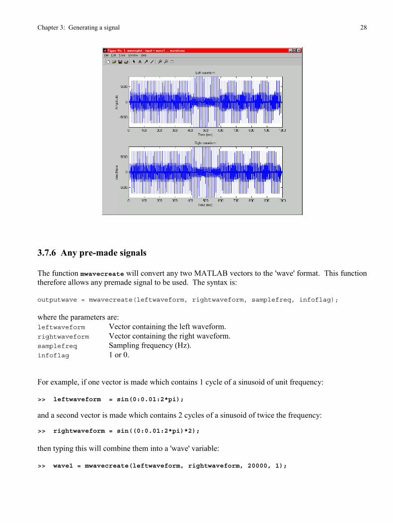
3.7.6 Any pre-made signals

The function mwavecreate will convert any two MATLAB vectors to the 'wave' format. This function

therefore allows any premade signal to be used. The syntax is:

outputwave = mwavecreate(leftwaveform, rightwaveform, samplefreq, infoflag);


leftwaveform Vector containing the left waveform.

rightwaveform Vector containing the right waveform.


infoflag 1 or 0.

For example, if one vector is made which contains 1 cycle of a sinusoid of unit frequency:

>> leftwaveform = sin(0:0.01:2*pi);

and a second vector is made which contains 2 cycles of a sinusoid of twice the frequency:

>> rightwaveform = sin((0:0.01:2*pi)*2);

then typing this will combine them into a 'wave' variable:

>> wave1 = mwavecreate(leftwaveform, rightwaveform, 20000, 1);


which has the unit-frequency sinusoid in the left channel and the twice-frequency sinusoid in the right

channel:

3.8 Obtaining an FFT of a waveform

The function mfft1side will calculate the magnitude and phase spectrum of a waveform. The function

(and the corresponding minversefft1side) are used internally in mcreatenoise1, etc., but is briefly

described here in case it is useful.

To obtain the magnitude and phase spectrum of a waveform, type:

» fftmatrix = mfft1side(wave1.leftwaveform, 20000, 5000, 2);

where the first parameter is the waveform, the second parameter is the sampling frequency, the third is

the number of points in the FFT and the fourth is the value of the infoflag. With an infoflag of 1 or 2

the function reports this:

creating 512-point FFT buffer with FFT resolution = 39.06 Hz

FFTing ...

discarding negative frequencies ...

doubling magnitudes...

scaling by number of points in FFT ...

plotting phase spectrum in figure 1 ...

plotting magnitude spectrum in figure 2 ...

storing answers as 257x3 matrix ...


(257 frequencies = 512/2 + 1 (for 0-Hz component))

If infoflag is set to 2 then two figures are also plotted: figure 1 plots the phase spectrum and figure 2

plots the magnitude spectrum:

The output fftmatrix is a two-dimensional matrix with one row for each frequency in the FFT and

three columns: column 1 contains the value of the frequency (in Hz), column 2 contains the value of

the magnitude spectrum (in linear units not dB), and column 3 contains the phase (in radians).

Note that the first parameter of mfft1side is a waveform vector, not a complete 'wave' signal. This is

because, at the point in mcreatenoise1 at which it is used, only the monaural waveforms are available.

Michael A. Akeroyd

Documents