Lecture Notes on: MFCS: Formal Languages and Automata Christopher M. Poskitt Department of Computer Science University of York Last Updated: June 6, 2012

Welcome message from author
This document is posted to help you gain knowledge. Please leave a comment to let me know what you think about it! Share it to your friends and learn new things together.
Transcript
Lecture Notes on:
MFCS: Formal Languages and Automata
Christopher M. Poskitt
Department of Computer ScienceUniversity of York
Last Updated: June 6, 2012

2
Contents
Introduction 5
Lecture 10 710.1 Recap on NPDAs . . . . . . . . . . . . . . . . . . . . . . . . . . . . . . . . 810.2 Acceptance by Final State versus Empty Stack . . . . . . . . . . . . . . . 1210.3 Context-Free Languages . . . . . . . . . . . . . . . . . . . . . . . . . . . . 1710.4 Transforming a CFG into an NPDA . . . . . . . . . . . . . . . . . . . . . . 2010.5 Summary . . . . . . . . . . . . . . . . . . . . . . . . . . . . . . . . . . . . . 27
Lecture 11 2911.1 Transforming an NPDA into a CFG . . . . . . . . . . . . . . . . . . . . . . 3111.2 Deterministic Pushdown Automata (DPDAs) . . . . . . . . . . . . . . . . 4411.3 Summary . . . . . . . . . . . . . . . . . . . . . . . . . . . . . . . . . . . . . 51
Lecture 12 5312.1 Chomsky Normal Form . . . . . . . . . . . . . . . . . . . . . . . . . . . . 54
12.1.1 Eliminating Useless Symbols . . . . . . . . . . . . . . . . . . . . . 5712.1.2 Eliminating λ-productions . . . . . . . . . . . . . . . . . . . . . . . 5912.1.3 Eliminating Unit Productions . . . . . . . . . . . . . . . . . . . . . 6112.1.4 Transforming CFGs into CNF . . . . . . . . . . . . . . . . . . . . . 64
12.2 Chomsky Hierarchy and Computability Theory . . . . . . . . . . . . . . 6712.3 Summary . . . . . . . . . . . . . . . . . . . . . . . . . . . . . . . . . . . . . 73
Bibliography 75
3

4 CONTENTS
Introduction
These notes are intended to supplement Chris Poskitt’s summer term lectures, deliv-ered as part of the Mathematical Foundations of Computer Science (MFCS) module at theUniversity of York. The lectures focus on nondeterministic pushdown automata (NPDAs)and their relationship with the class of context-free languages, but also covered aredeterministic pushdown automata (DPDAs), grammar simplifications, normal forms, theChomsky hierarchy, and a taster of what is to come in the study of computability the-ory. These notes assume a reasonable understanding of the terminology, notations, andconcepts of the first nine MFCS lectures!
As ever for a mathematical module, the best way of understanding the material inthis course is to put it into practice. The module website, linked to below, contains aplethora of problems (most with sample solutions) via the problem sheets, JFLAP prac-tical sheets, formative tests, and past exam papers. Further exercises can be found inthe recommended text books, [HMU06, Lin06, Coh97].
http://www-module.cs.york.ac.uk/mfcs/fla/
The material and examples in these notes have been drawn from a number of differentsources, but all errors1 are those of the author.
Acknowledgements. Some of the material in these notes is drawn from [HMU06], aswell as the slides and notes of Steve King, who has taught this course at York in previ-ous years. The automata diagrams were drawn in JFLAP, and exported to TikZ formatvia JFlap2TikZ2; the author is grateful to the creators of both tools for saving him froma lot of pain! Finally, the author would like to acknowledge that the presentation ofthese notes was inspired by the course notes of Professor Andrew Pitts, who teaches asimilar course at the University of Cambridge.
Chris Poskitt
1Please get in touch if you spot any. I don’t bite!2See: http://www.ctan.org/pkg/jflap2tikz
5

6 CONTENTS
Lecture 10
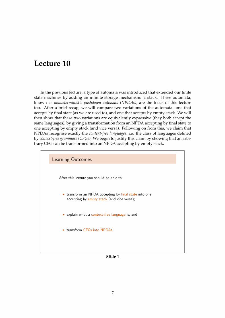
In the previous lecture, a type of automata was introduced that extended our finitestate machines by adding an infinite storage mechanism: a stack. These automata,known as nondeterministic pushdown automata (NPDAs), are the focus of this lecturetoo. After a brief recap, we will compare two variations of the automata: one thataccepts by final state (as we are used to), and one that accepts by empty stack. We willthen show that these two variations are equivalently expressive (they both accept thesame languages), by giving a transformation from an NPDA accepting by final state toone accepting by empty stack (and vice versa). Following on from this, we claim thatNPDAs recognise exactly the context-free languages, i.e. the class of languages definedby context-free grammars (CFGs). We begin to justify this claim by showing that an arbi-trary CFG can be transformed into an NPDA accepting by empty stack.
Learning Outcomes
After this lecture you should be able to:
I transform an NPDA accepting by final state into oneaccepting by empty stack (and vice versa);
I explain what a context-free language is; and
I transform CFGs into NPDAs.
Slide 1
7
8 LECTURE 10.
10.1 Recap on NPDAs
NPDA Recap
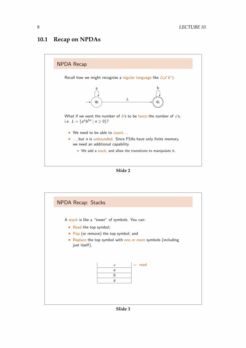
Recall how we might recognise a regular language like L(a∗b∗):
q0 q1
ba
λ
What if we want the number of b’s to be twice the number of a’s,i.e. L = {anb2n | n ≥ 0}?
I We need to be able to count. . .
I . . . but n is unbounded. Since FSAs have only finite memory,we need an additional capability.
I We add a stack, and allow the transitions to manipulate it.
Slide 2
NPDA Recap: Stacks
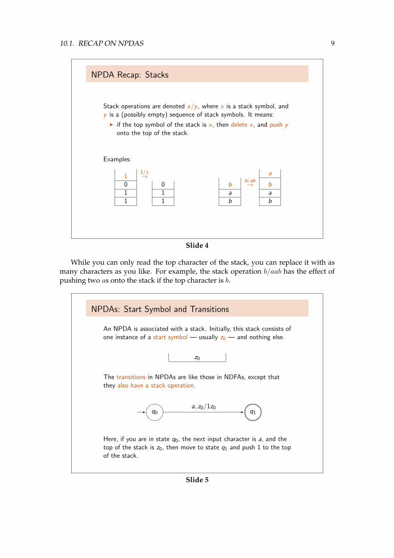
A stack is like a “tower” of symbols. You can:
I Read the top symbol;
I Pop (or remove) the top symbol; and
I Replace the top symbol with one or more symbols (includingjust itself).
a ← readaba
Slide 3
10.1. RECAP ON NPDAS 9
NPDA Recap: Stacks
Stack operations are denoted x/y , where x is a stack symbol, andy is a (possibly empty) sequence of stack symbols. It means:
I if the top symbol of the stack is x , then delete x , and push yonto the top of the stack.
Examples:
11/λ→
0 01 11 1
a
bb/ab→ b
a ab b
Slide 4
While you can only read the top character of the stack, you can replace it with asmany characters as you like. For example, the stack operation b/aab has the effect ofpushing two as onto the stack if the top character is b.
NPDAs: Start Symbol and Transitions
An NPDA is associated with a stack. Initially, this stack consists ofone instance of a start symbol — usually z0 — and nothing else.
z0
The transitions in NPDAs are like those in NDFAs, except thatthey also have a stack operation.
q0 q1a, z0/1z0
Here, if you are in state q0, the next input character is a, and thetop of the stack is z0, then move to state q1 and push 1 to the topof the stack.
Slide 5
10 LECTURE 10.
Sometimes it useful to use a different start symbol to z0. For example, in the trans-formation from CFGs to NPDAs, we take the start symbol of the grammar — S — to bethe start symbol of the stack. In most examples though, what the start symbol actuallyis is irrelevant.
Given a transition label a, x/y, it is helpful to think of a and x as constraints thatmust be satisfied before the transition can be made. That is, if the next input characteris a, and the top of the stack is x, then consume both symbols, follow the transition, andadd y to the stack.
NPDAs: Example
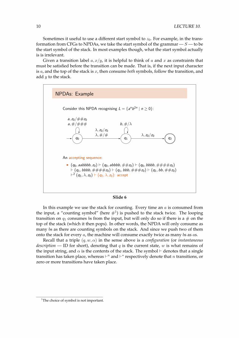
Consider this NPDA recognising L = {anb2n | n ≥ 0}:
q0 q1 q2
b,#/λa, z0/##z0
a,#/###
λ, z0/z0
λ, z0/z0
λ,#/#
An accepting sequence:
I (q0, aabbbb, z0) ` (q0, abbbb,##z0) ` (q0, bbbb,####z0)` (q1, bbbb,####z0) ` (q1, bbb,###z0) ` (q1, bb,##z0)`2 (q1, λ, z0) ` (q2, λ, z0): accept
Slide 6
In this example we use the stack for counting. Every time an a is consumed fromthe input, a “counting symbol” (here #1) is pushed to the stack twice. The loopingtransition on q1 consumes bs from the input, but will only do so if there is a # on thetop of the stack (which it then pops). In other words, the NPDA will only consume asmany bs as there are counting symbols on the stack. And since we push two of themonto the stack for every a, the machine will consume exactly twice as many bs as as.
Recall that a triple (q, w, α) in the sense above is a configuration (or instantaneousdescription — ID for short), denoting that q is the current state, w is what remains ofthe input string, and α is the contents of the stack. The symbol ` denotes that a singletransition has taken place, whereas `n and `∗ respectively denote that n transitions, orzero or more transitions have taken place.
1The choice of symbol is not important.
10.1. RECAP ON NPDAS 11
NPDAs: Formal Definition
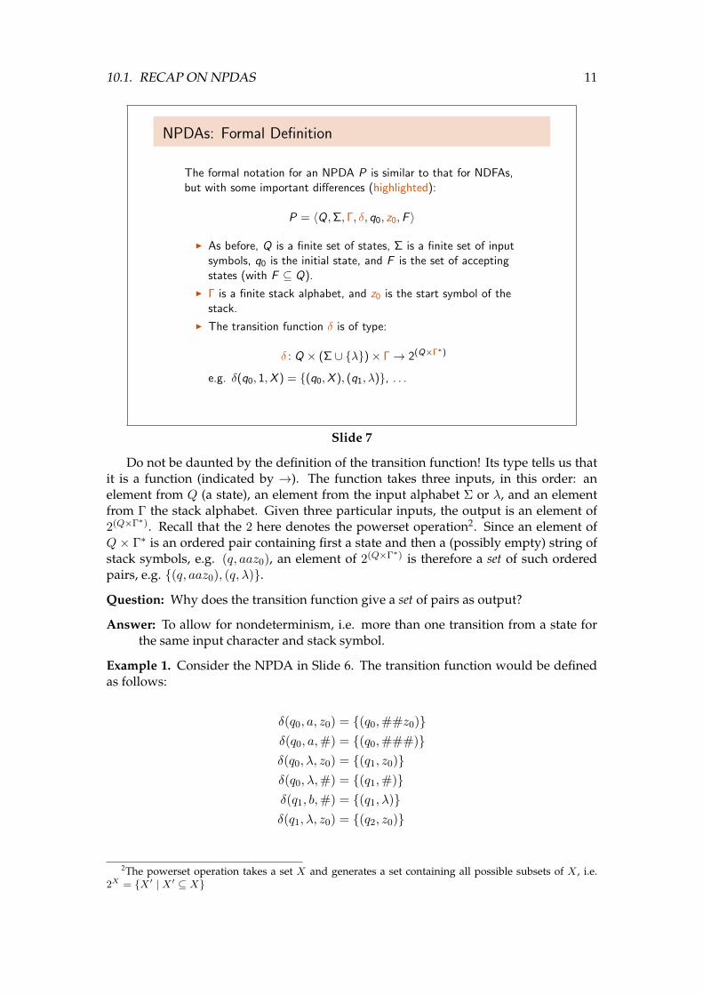
The formal notation for an NPDA P is similar to that for NDFAs,but with some important differences (highlighted):
P = 〈Q,Σ, Γ, δ, q0, z0,F 〉
I As before, Q is a finite set of states, Σ is a finite set of inputsymbols, q0 is the initial state, and F is the set of acceptingstates (with F ⊆ Q).
I Γ is a finite stack alphabet, and z0 is the start symbol of thestack.
I The transition function δ is of type:
δ : Q × (Σ ∪ {λ})× Γ→ 2(Q×Γ∗)
e.g. δ(q0, 1,X ) = {(q0,X ), (q1, λ)}, . . .
Slide 7
Do not be daunted by the definition of the transition function! Its type tells us thatit is a function (indicated by →). The function takes three inputs, in this order: anelement from Q (a state), an element from the input alphabet Σ or λ, and an elementfrom Γ the stack alphabet. Given three particular inputs, the output is an element of2(Q×Γ∗). Recall that the 2 here denotes the powerset operation2. Since an element ofQ × Γ∗ is an ordered pair containing first a state and then a (possibly empty) string ofstack symbols, e.g. (q, aaz0), an element of 2(Q×Γ∗) is therefore a set of such orderedpairs, e.g. {(q, aaz0), (q, λ)}.Question: Why does the transition function give a set of pairs as output?
Answer: To allow for nondeterminism, i.e. more than one transition from a state forthe same input character and stack symbol.
Example 1. Consider the NPDA in Slide 6. The transition function would be definedas follows:
δ(q0, a, z0) = {(q0,##z0)}δ(q0, a,#) = {(q0,###)}δ(q0, λ, z0) = {(q1, z0)}δ(q0, λ,#) = {(q1,#)}δ(q1, b,#) = {(q1, λ)}δ(q1, λ, z0) = {(q2, z0)}
2The powerset operation takes a set X and generates a set containing all possible subsets of X , i.e.2X = {X ′ | X ′ ⊆ X}
12 LECTURE 10.
10.2 Acceptance by Final State versus Empty Stack
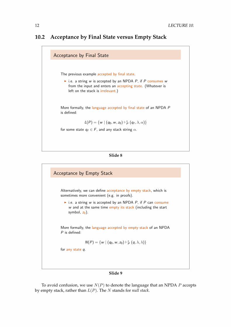
Acceptance by Final State
The previous example accepted by final state.
I i.e. a string w is accepted by an NPDA P, if P consumes wfrom the input and enters an accepting state. (Whatever isleft on the stack is irrelevant.)
More formally, the language accepted by final state of an NPDA Pis defined:
L(P) = {w | (q0,w , z0) `∗P (qf , λ, α)}for some state qf ∈ F , and any stack string α.
Slide 8
Acceptance by Empty Stack
Alternatively, we can define acceptance by empty stack, which issometimes more convenient (e.g. in proofs).
I i.e. a string w is accepted by an NPDA P, if P can consumew and at the same time empty its stack (including the startsymbol, z0).
More formally, the language accepted by empty stack of an NPDAP is defined:
N(P) = {w | (q0,w , z0) `∗P (q, λ, λ)}for any state q.
Slide 9
To avoid confusion, we use N(P ) to denote the language that an NPDA P acceptsby empty stack, rather than L(P ). The N stands for null stack.
10.2. ACCEPTANCE BY FINAL STATE VERSUS EMPTY STACK 13
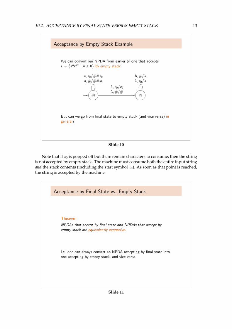
Acceptance by Empty Stack Example
We can convert our NPDA from earlier to one that acceptsL = {anb2n | n ≥ 0} by empty stack:
q0 q1
b,#/λλ, z0/λ
a, z0/##z0
a,#/###
λ, z0/z0
λ,#/#
But can we go from final state to empty stack (and vice versa) ingeneral?
Slide 10
Note that if z0 is popped off but there remain characters to consume, then the stringis not accepted by empty stack. The machine must consume both the entire input stringand the stack contents (including the start symbol z0). As soon as that point is reached,the string is accepted by the machine.
Acceptance by Final State vs. Empty Stack
Theorem
NPDAs that accept by final state and NPDAs that accept byempty stack are equivalently expressive.
i.e. one can always convert an NPDA accepting by final state intoone accepting by empty stack, and vice versa.
Slide 11

14 LECTURE 10.
The theorem in Slide 11 is very useful later in the lecture. We later transform CFGsinto NPDAs that accept by empty stack. What this theorem tells us is that there mustalso be NPDAs accepting by final state for every CFG.
From Final State to Empty Stack
Suppose we have an NPDA PF with start symbol z0 that acceptsby final state.
We can construct an NPDA PN with start symbol x0 that acceptsby empty stack, such that N(PN) = L(PF ).
Slide 12
The transformation in Slide 12 from an NPDA PF accepting by final state to oneaccepting by empty stack is fairly straightforward. The idea is to add λ-transitionsfrom all accepting states of PF , for all symbols in the stack alphabet, to a new state p.This state p cannot be “escaped” from; the only transitions incident to it are loopingones which pop the entire contents of the stack. Finally, to avoid a situation where PFempties the stack without accepting, we add a “marker” x0 on the bottom of the stack,which also serves as the start symbol of the new machine. (We require that the markerx0 is not in the stack alphabet of PF .) A new initial state is added; from this, there isa transition to the original initial state of PF , which pushes the start symbol of PF , z0
onto the stack (and immediately above our marker).
10.2. ACCEPTANCE BY FINAL STATE VERSUS EMPTY STACK 15
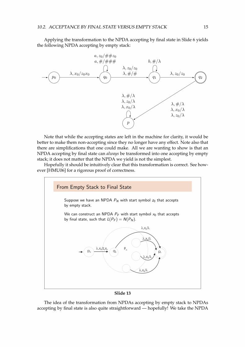
Applying the transformation to the NPDA accepting by final state in Slide 6 yieldsthe following NPDA accepting by empty stack:
q0 q1 q2
p
p0
λ,#/λλ, z0/λλ, x0/λ
λ, x0/z0x0
b,#/λ
λ, z0/z0
λ,#/λλ, x0/λλ, z0/λ
λ, z0/z0
λ,#/#
a, z0/##z0
a,#/###
Note that while the accepting states are left in the machine for clarity, it would bebetter to make them non-accepting since they no longer have any effect. Note also thatthere are simplifications that one could make. All we are wanting to show is that anNPDA accepting by final state can always be transformed into one accepting by emptystack; it does not matter that the NPDA we yield is not the simplest.
Hopefully it should be intuitively clear that this transformation is correct. See how-ever [HMU06] for a rigorous proof of correctness.
From Empty Stack to Final State
Suppose we have an NPDA PN with start symbol z0 that acceptsby empty stack.
We can construct an NPDA PF with start symbol x0 that acceptsby final state, such that L(PF ) = N(PN).
Slide 13
The idea of the transformation from NPDAs accepting by empty stack to NPDAsaccepting by final state is also quite straightforward — hopefully! We take the NPDA
16 LECTURE 10.
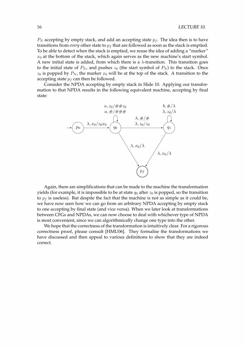
PN accepting by empty stack, and add an accepting state pf . The idea then is to havetransitions from every other state to pf that are followed as soon as the stack is emptied.To be able to detect when the stack is emptied, we reuse the idea of adding a “marker”x0 at the bottom of the stack, which again serves as the new machine’s start symbol.A new initial state is added, from which there is a λ-transition. This transition goesto the initial state of PN , and pushes z0 (the start symbol of PN ) to the stack. Oncez0 is popped by PN , the marker x0 will be at the top of the stack. A transition to theaccepting state pf can then be followed.
Consider the NPDA accepting by empty stack in Slide 10. Applying our transfor-mation to that NPDA results in the following equivalent machine, accepting by finalstate:
q0 q1p0
pf
λ, x0/λ
b,#/λλ, z0/λ
λ, x0/λ
λ,#/#λ, z0/z0λ, x0/z0x0
a, z0/##z0
a,#/###
Again, there are simplifications that can be made to the machine the transformationyields (for example, it is impossible to be at state q0 after z0 is popped, so the transitionto pf is useless). But despite the fact that the machine is not as simple as it could be,we have now seen how we can go from an arbitrary NPDA accepting by empty stackto one accepting by final state (and vice versa). When we later look at transformationsbetween CFGs and NPDAs, we can now choose to deal with whichever type of NPDAis most convenient, since we can algorithmically change one type into the other.
We hope that the correctness of the transformation is intuitively clear. For a rigorouscorrectness proof, please consult [HMU06]. They formalise the transformations wehave discussed and then appeal to various definitions to show that they are indeedcorrect.
10.3. CONTEXT-FREE LANGUAGES 17
10.3 Context-Free Languages
Context-Free Languages
Last term we studied extensively the class of regular languages, i.e.languages accepted by FSAs, generated by regular grammars, ordescribed by regular expressions.
We also studied context-free grammars, which define context-freelanguages, e.g.
S → SS | (S) | λWhy is the above not a regular language?
Slide 14
The grammar denotes the language of balanced parentheses. Since the number ofparentheses allowed is unbounded, counting is required to ensure that they are bal-anced. Finite automata (which recognise the class of regular languages) have strictlyfinite memory, and thus are not able to recognise this language. One could also applythe pumping lemma to show that the language is not regular.
A good question to ask at this stage, is whether there is a relationship betweenCFGs and NPDAs, given that they can respectively define and recognise languagesthat require arbitrary amounts of counting3.
3Though not all! Try writing a CFG or NPDA for L = {anbncn | n ≥ 0}.
18 LECTURE 10.
Context-Free Languages
Question: is there a correspondence between NPDAs andcontext-free languages?
I Yes! CFGs and NPDAs define and accept the same languages.
We will establish this fact by:
1. Showing that CFGs can be transformed into NPDAs; and
2. Showing that NPDAs can be transformed into CFGs.
Slide 15
As you might have expected, there is a correspondence between CFGs and NPDAs.
1. Every language defined by a CFG can be recognised by an NPDA; and
2. Every language recognised by an NPDA can be defined by a CFG.
These languages are known as the context-free languages, and have a number of im-portant applications (e.g. in defining the syntax of programming languages).
The final part of this lecture will focus on the transformation from CFGs to NPDAs.The next lecture will consider the other direction.
10.3. CONTEXT-FREE LANGUAGES 19
Chomsky Hierarchy
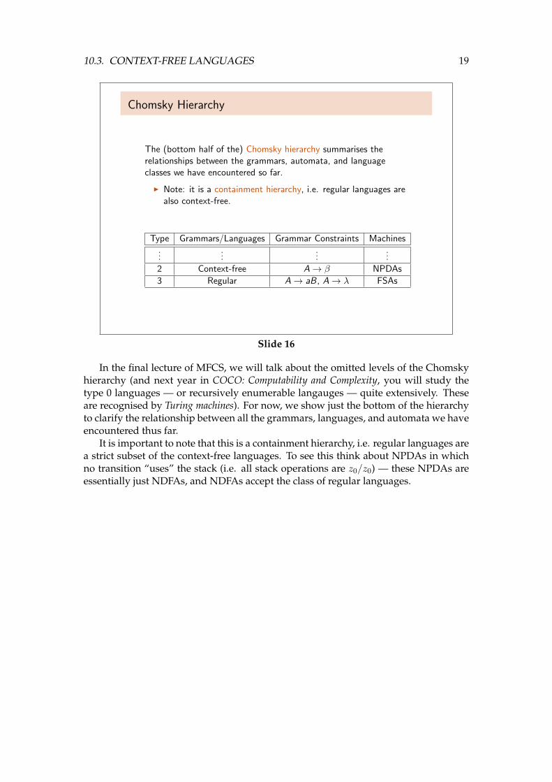
The (bottom half of the) Chomsky hierarchy summarises therelationships between the grammars, automata, and languageclasses we have encountered so far.
I Note: it is a containment hierarchy, i.e. regular languages arealso context-free.
Type Grammars/Languages Grammar Constraints Machines...
......
...
2 Context-free A→ β NPDAs
3 Regular A→ aB, A→ λ FSAs
Slide 16
In the final lecture of MFCS, we will talk about the omitted levels of the Chomskyhierarchy (and next year in COCO: Computability and Complexity, you will study thetype 0 languages — or recursively enumerable langauges — quite extensively. Theseare recognised by Turing machines). For now, we show just the bottom of the hierarchyto clarify the relationship between all the grammars, languages, and automata we haveencountered thus far.
It is important to note that this is a containment hierarchy, i.e. regular languages area strict subset of the context-free languages. To see this think about NPDAs in whichno transition “uses” the stack (i.e. all stack operations are z0/z0) — these NPDAs areessentially just NDFAs, and NDFAs accept the class of regular languages.
20 LECTURE 10.
Chomsky Hierarchy
We’ll discuss the other levels of the Chomsky hierarchy in a laterlecture.
Photo Credit: Duncan Rawlinson
Slide 17
10.4 Transforming a CFG into an NPDA
CFGs can be transformed into NPDAs
Theorem
Given a CFG G , there is an NPDA P accepting by empty stacksuch that N(P) = L(G ).
Slide 18
By the result we talked about earlier in the lecture, there must also be NPDAs ac-cepting by final state for every CFG. Transforming a CFG directly into an NPDA ac-
10.4. TRANSFORMING A CFG INTO AN NPDA 21
cepting by final state is a little more complex however, see for example [Lin06].
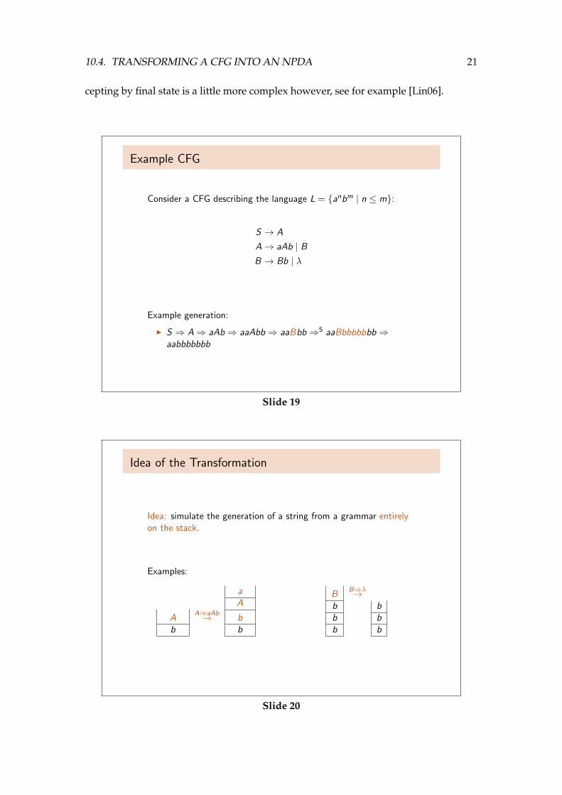
Example CFG
Consider a CFG describing the language L = {anbm | n ≤ m}:
S → A
A→ aAb | B
B → Bb | λ
Example generation:
I S ⇒ A⇒ aAb ⇒ aaAbb ⇒ aaBbb ⇒5 aaBbbbbbbb ⇒aabbbbbbb
Slide 19
Idea of the Transformation
Idea: simulate the generation of a string from a grammar entirelyon the stack.
Examples:
aA
AA⇒aAb→ b
b b
BB⇒λ→
b bb bb b
Slide 20
22 LECTURE 10.
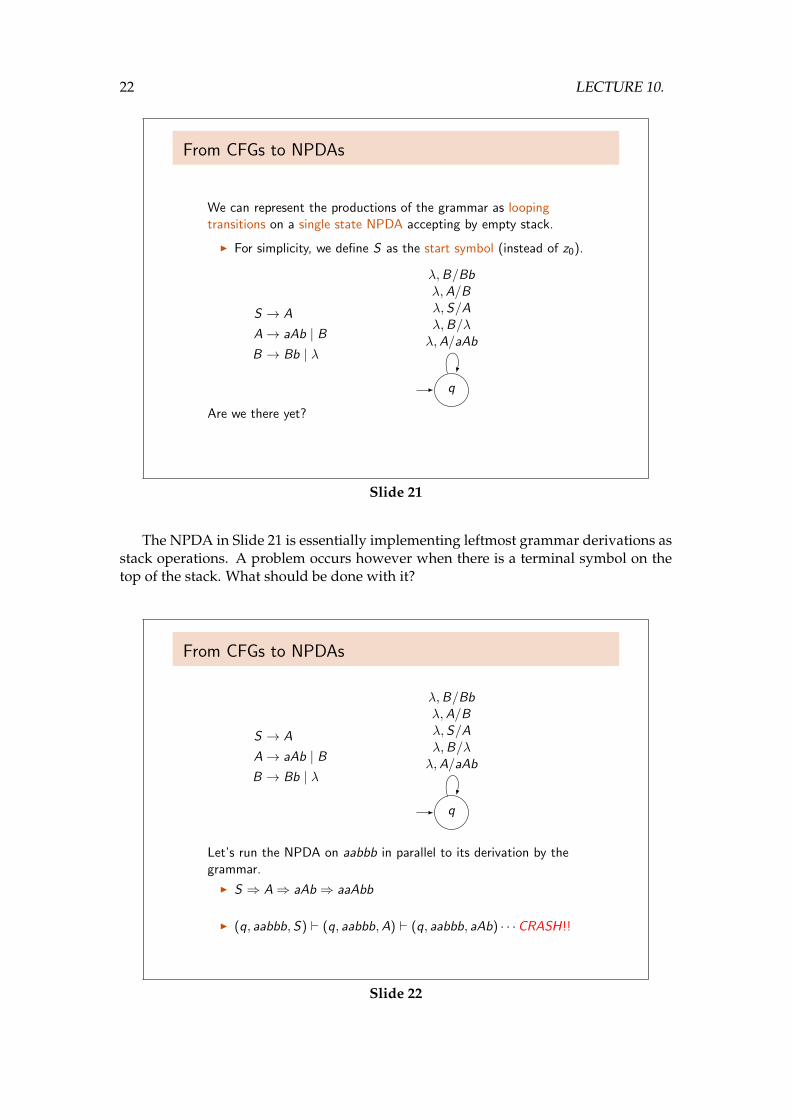
From CFGs to NPDAs
We can represent the productions of the grammar as loopingtransitions on a single state NPDA accepting by empty stack.
I For simplicity, we define S as the start symbol (instead of z0).
S → A
A→ aAb | B
B → Bb | λ
q
λ,B/Bbλ,A/Bλ,S/Aλ,B/λλ,A/aAb
Are we there yet?
Slide 21
The NPDA in Slide 21 is essentially implementing leftmost grammar derivations asstack operations. A problem occurs however when there is a terminal symbol on thetop of the stack. What should be done with it?
From CFGs to NPDAs
S → A
A→ aAb | B
B → Bb | λ
q
λ,B/Bbλ,A/Bλ,S/Aλ,B/λλ,A/aAb
Let’s run the NPDA on aabbb in parallel to its derivation by thegrammar.
I S ⇒ A⇒ aAb ⇒ aaAbb
I (q, aabbb, S) ` (q, aabbb,A) ` (q, aabbb, aAb) · · ·CRASH!!
Slide 22
10.4. TRANSFORMING A CFG INTO AN NPDA 23
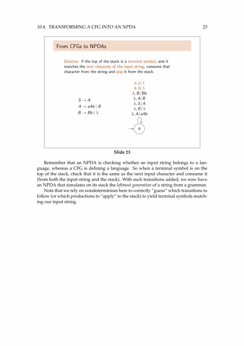
From CFGs to NPDAs
Solution: if the top of the stack is a terminal symbol, and itmatches the next character of the input string, consume thatcharacter from the string and pop it from the stack.
S → A
A→ aAb | B
B → Bb | λ
q
a, a/λb, b/λλ,B/Bbλ,A/Bλ,S/Aλ,B/λλ,A/aAb
Slide 23
Remember that an NPDA is checking whether an input string belongs to a lan-guage, whereas a CFG is defining a language. So when a terminal symbol is on thetop of the stack, check that it is the same as the next input character and consume it(from both the input string and the stack). With such transitions added, we now havean NPDA that simulates on its stack the leftmost generation of a string from a grammar.
Note that we rely on nondeterminism here to correctly “guess” which transitions tofollow (or which productions to “apply” to the stack) to yield terminal symbols match-ing our input string.
24 LECTURE 10.
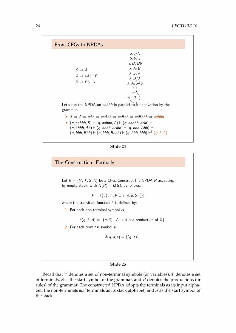
From CFGs to NPDAs
S → A
A→ aAb | B
B → Bb | λ
q
a, a/λb, b/λλ,B/Bbλ,A/Bλ,S/Aλ,B/λλ,A/aAb
Let’s run the NPDA on aabbb in parallel to its derivation by thegrammar.
I S ⇒ A⇒ aAb ⇒ aaAbb ⇒ aaBbb ⇒ aaBbbb ⇒ aabbb
I (q, aabbb, S) ` (q, aabbb,A) ` (q, aabbb, aAb) `(q, abbb,Ab) ` (q, abbb, aAbb) ` (q, bbb,Abb) `(q, bbb,Bbb) ` (q, bbb,Bbbb) ` (q, bbb, bbb) `3 (q, λ, λ)
Slide 24
The Construction: Formally
Let G = 〈V ,T , S ,R〉 be a CFG. Construct the NPDA P acceptingby empty stack, with N(P) = L(G ), as follows:
P = 〈{q},T ,V ∪ T , δ, q,S , {}〉where the transition function δ is defined by:
1. For each non-terminal symbol A,
δ(q, λ,A) = {(q, β) | A→ β is a production of G}2. For each terminal symbol a,
δ(q, a, a) = {(q, λ)}
Slide 25
Recall that V denotes a set of non-terminal symbols (or variables), T denotes a setof terminals, S is the start symbol of the grammar, and R denotes the productions (orrules) of the grammar. The constructed NPDA adopts the terminals as its input alpha-bet, the non-terminals and terminals as its stack alphabet, and S as the start symbol ofthe stack.
10.4. TRANSFORMING A CFG INTO AN NPDA 25
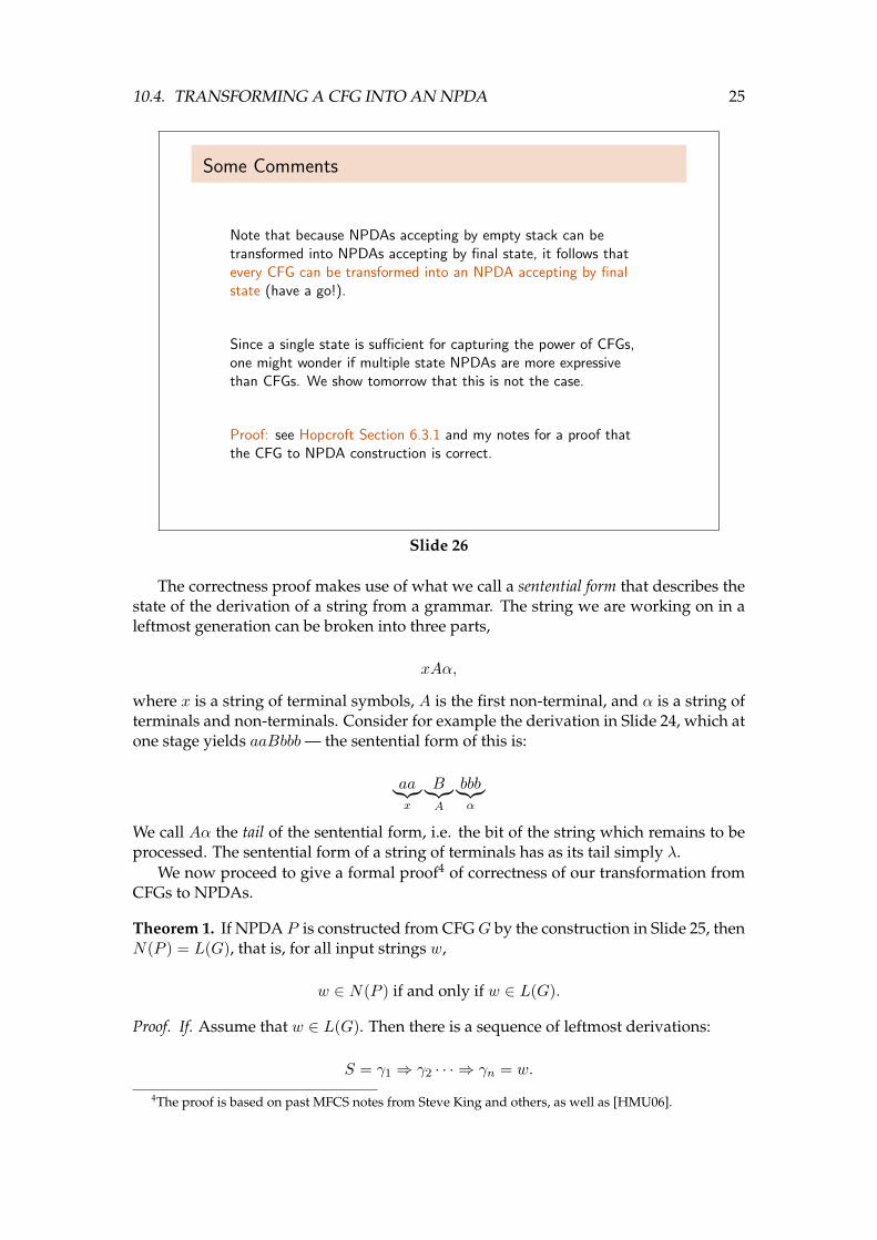
Some Comments
Note that because NPDAs accepting by empty stack can betransformed into NPDAs accepting by final state, it follows thatevery CFG can be transformed into an NPDA accepting by finalstate (have a go!).
Since a single state is sufficient for capturing the power of CFGs,one might wonder if multiple state NPDAs are more expressivethan CFGs. We show tomorrow that this is not the case.
Proof: see Hopcroft Section 6.3.1 and my notes for a proof thatthe CFG to NPDA construction is correct.
Slide 26
The correctness proof makes use of what we call a sentential form that describes thestate of the derivation of a string from a grammar. The string we are working on in aleftmost generation can be broken into three parts,
xAα,
where x is a string of terminal symbols, A is the first non-terminal, and α is a string ofterminals and non-terminals. Consider for example the derivation in Slide 24, which atone stage yields aaBbbb — the sentential form of this is:
aa︸︷︷︸x
B︸︷︷︸A
bbb︸︷︷︸α
We call Aα the tail of the sentential form, i.e. the bit of the string which remains to beprocessed. The sentential form of a string of terminals has as its tail simply λ.
We now proceed to give a formal proof4 of correctness of our transformation fromCFGs to NPDAs.
Theorem 1. If NPDA P is constructed from CFGG by the construction in Slide 25, thenN(P ) = L(G), that is, for all input strings w,
w ∈ N(P ) if and only if w ∈ L(G).
Proof. If. Assume that w ∈ L(G). Then there is a sequence of leftmost derivations:
S = γ1 ⇒ γ2 · · · ⇒ γn = w.
4The proof is based on past MFCS notes from Steve King and others, as well as [HMU06].
26 LECTURE 10.
We show by induction on i that (q, w, S) `∗P (q, yi, αi). Here, w = xiyi, where yi iswhat remains of the input string w after xi has been consumed from the input, and αiis the tail of the sentential form γi = xiαi.
If. Basis. In the base case, i = 1, and γ1 = S. So x1 = λ and y1 = w. Since(q, w, S) `∗ (q, w, S)5, the base case is proved.
If. Induction. Assume that (q, w, S) `∗ (q, yi, αi) and prove that (q, w, S) `∗ (q, yi+1, αi+1).Consider (q, yi, αi). Since αi is a tail, it must begin with a non-terminal, say A,
otherwise the parsing process would have been completed. The application of a pro-duction γi ⇒ γi+1 involves replacingA by one of its “right-hand sides” in the grammardefinition, say β. There are just two possibilities, given the construction of P :
1. We can replace the non-terminal A by β; or
2. We can match any terminals on the top of the stack with the next input symbols.
As a result, we reach the configuration (q, yi+1, αi+1) which represents the next sen-tential form γi+1.
We can complete the “if” part of the proof by noting that αn = λ, because the tail ofγn = w is empty, thus (q, w, S) `∗ (q, λ, λ). And so P accepts w by empty stack.
Only if. Now, we assume that w ∈ N(P ), and show that this implies that w ∈ L(G).We proceed by proving a more general result: if P executes a sequence of moves
that has the net effect of popping a non-terminal A from the top of the stack withoutever goign below A on the stack, then A derives in G whatever input string was con-sumed from the input during this process. That is,
(q, x,A) `∗P (q, λ, λ) implies A⇒∗G x.We prove this by induction on the number of moves taken by P .
Only if. Basis. P takes one move to have the net effect of popping A. The only pos-sibility is that A→ λ is a production of G. In this case x = λ and we know that A⇒ λ.
Only if. Induction. Suppose that P takes n moves with n > 1. The first move mustinvolve replacing a non-terminal using a production, say A → Y1Y2 . . . Yk where eachYi is a non-terminal or terminal. Hence the next n − 1 moves of P must consume xfrom the input and have the net effect of popping each of Y1, Y2, . . . from the stack,one at a time. We can break x into x1x2 . . . xk, where x1 is the portion of the inputconsumed until Y1 is popped off the stack. Then x2 is the next portion of the input thatis consumed while popping Y2 off the stack, and so on.
Formally, (q, xixi+1 . . . xk, Yi) `∗ (q, xi+1 . . . xk, λ) for all i = 1, 2 . . . k. None of thesesequences can be more than n − 1 moves, so the induction hypothesis applies if Yi isa non-terminal. In that case, we can conclude that Yi ⇒∗ xi. If Yi is a terminal, thenthere is exactly one move, and it matches the one symbol of xi against Yi, which are thesame. Again, we conclude Yi ⇒∗ xi (this time in zero steps).
Together, we have the derivations:
5Remember that `∗ indicates zero or more transitions.
10.5. SUMMARY 27
A⇒ Y1Y2 . . . Yk ⇒∗ x1Y2 . . . Yk ⇒∗ · · · ⇒∗ x1x2 . . . xk.
Therefore A⇒∗ x. Hence we have that (q, x,A) `∗P (q, λ, λ) implies A⇒∗G x.To conclude the proof, we let A = S and x = w. Since we assumed at the beginning
that w ∈ N(P ), we know that (q, w, S) `∗ (q, λ, λ). By what we have just provedinductively, we have S ⇒∗ w, i.e. the result that w is in L(G).
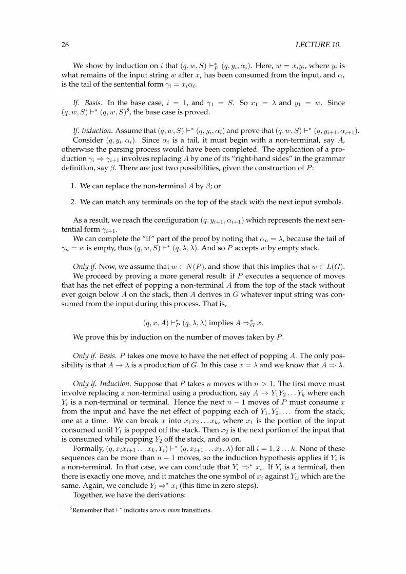
10.5 Summary
Summary
Today we have:
I Reviewed examples of NPDAs and their formal definition.
I Demonstrated how to convert an NPDA accepting by finalstate into one accepting by empty stack (and vice versa).
I Claimed that NPDAs accept the context-free languages, andsummarised within (part of the) Chomsky hierarchy therelationship between languages, grammars, and automata wehave encountered in MFCS so far.
I Studied a transformation from CFGs to NPDAs, proving thatNPDAs are at least as powerful as CFGs.
Slide 27
28 LECTURE 10.
Next Lecture
We will:
I Show that NPDAs can be transformed into CFGs, completingthe proof that NPDAs accept exactly the context-freelanguages.
I Consider deterministic pushdown automata (DPDAs) — canall NPDAs be transformed into DPDAs?
Slide 28
That’s all folks!
Thanks! Questions?
http://www.cs.york.ac.uk/~cposkitt/
Reading: suggest that you study my own notes and Hopcroft Sections
6.1-6.3.1. Linz does not cover acceptance by empty stack (it transforms
CFGs into NPDAs by a similar but different method); Cohen uses a
strange flow chart notation for NPDAs.
Slide 29
Lecture 11
In the previous lecture, we studied two different types of NPDA — one that acceptsby final state, and one that accepts by empty stack — and showed that they were equiv-alently expressive (that is, you can convert one type into the other). We also made theclaim that NPDAs recognise exactly the context-free languages (the languages definedby CFGs). We began to justify this claim by describing a construction from CFGs toNPDAs that accept by empty stack.
A construction from CFGs to NPDAs however only tells us that NPDAs are at leastas powerful than CFGs. To show that NPDAs are no more powerful than CFGs, wemust have a construction from NPDAs to CFGs. Together, these two constructionsshow that NPDAs and CFGs are equivalently expressive, since you can algorithmicallygo from one to the other (and back).
This lecture describes a construction from NPDAs to CFGs. Afterwards, we con-sider pushdown automata that are deterministic (that is, there is never a choice as towhich transition can be followed). It turns out that DPDAs are not as powerful asNPDAs1, but their languages do have some interesting properties.
Slide 1
1This is contrary to the expressive equivalence of DFAs and NDFAs.
29
30 LECTURE 11.
So what happened yesterday?
Yesterday we:
I Reviewed examples of NPDAs and their formal definition.
I Demonstrated how to convert an NPDA accepting by finalstate into one accepting by empty stack (and vice versa).
I Claimed that NPDAs accept the context-free languages, andsummarised within (part of the) Chomsky hierarchy therelationship between languages, grammars, and automata wehave encountered in MFCS so far.
I Studied a transformation from CFGs to NPDAs, proving thatNPDAs are at least as powerful as CFGs.
Slide 2
Learning Outcomes
After this lecture you should be able to:
I transform NPDAs into CFGs;
I define and interpret deterministic pushdown automata(DPDAs);
I identify languages that NPDAs can accept but DPDAscannot; and
I explain the connection between DPDAs and unambiguousCFGs.
Slide 3
11.1. TRANSFORMING AN NPDA INTO A CFG 31
11.1 Transforming an NPDA into a CFG
From NPDAs to CFGs
Problem: given an NPDA P that accepts by empty stack,construct a CFG G such that L(G ) = N(P).
Our construction requires a restriction:
I Each transition in P must increase the stack size by one, ordecrease the stack size by one.
I (Every NPDA can be made to satisfy this property.)
Key Idea: a fundamental event of an NPDA execution is thepopping of a stack symbol. How to represent in a grammar?
Slide 4
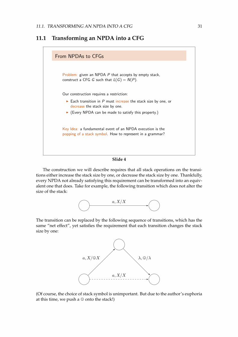
The construction we will describe requires that all stack operations on the transi-tions either increase the stack size by one, or decrease the stack size by one. Thankfully,every NPDA not already satisfying this requirement can be transformed into an equiv-alent one that does. Take for example, the following transition which does not alter thesize of the stack:
a,X/X
The transition can be replaced by the following sequence of transitions, which has thesame “net effect”, yet satisfies the requirement that each transition changes the stacksize by one:
a,X/,X
a,X/X
λ,,/λ
(Of course, the choice of stack symbol is unimportant. But due to the author’s euphoriaat this time, we push a , onto the stack!)
32 LECTURE 11.
The Terminals and Non-Terminals
The terminals of our CFG will simply be the input alphabet Σ.
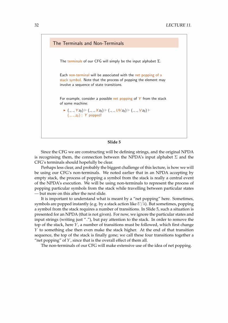
Each non-terminal will be associated with the net popping of astack symbol. Note that the process of popping the element mayinvolve a sequence of state transitions.
For example, consider a possible net popping of Y from the stackof some machine:
I ( , ,Y z0) ` ( , ,Xz0) ` ( , ,UVz0) ` ( , ,Vz0) `( , , z0) : Y popped!
Slide 5
Since the CFG we are constructing will be defining strings, and the original NPDAis recognising them, the connection between the NPDA’s input alphabet Σ and theCFG’s terminals should hopefully be clear.
Perhaps less clear, and probably the biggest challenge of this lecture, is how we willbe using our CFG’s non-terminals. We noted earlier that in an NPDA accepting byempty stack, the process of popping a symbol from the stack is really a central eventof the NPDA’s execution. We will be using non-terminals to represent the process ofpopping particular symbols from the stack while travelling between particular states— but more on this after the next slide.
It is important to understand what is meant by a “net popping” here. Sometimes,symbols are popped instantly (e.g. by a stack action like U/λ). But sometimes, poppinga symbol from the stack requires a number of transitions. In Slide 5, such a situation ispresented for an NPDA (that is not given). For now, we ignore the particular states andinput strings (writing just “ ”), but pay attention to the stack. In order to remove thetop of the stack, here Y , a number of transitions must be followed, which first changeY to something else then even make the stack higher. At the end of that transitionsequence, the top of the stack is finally gone; we call these four transitions together a“net popping” of Y , since that is the overall effect of them all.
The non-terminals of our CFG will make extensive use of the idea of net popping.
11.1. TRANSFORMING AN NPDA INTO A CFG 33
“Net popping” as non-terminals
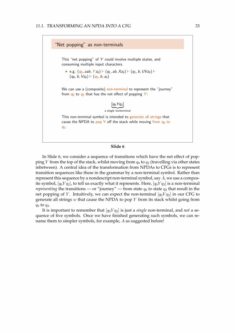
This “net popping” of Y could involve multiple states, andconsuming multiple input characters.
I e.g. (q0, aab,Y z0) ` (q1, ab,Xz0) ` (q1, b,UVz0) `(q0, b,Vz0) ` (q2, b, z0)
We can use a (composite) non-terminal to represent the “journey”from q0 to q2 that has the net effect of popping Y :
[q0Yq2]︸ ︷︷ ︸a single nonterminal
This non-terminal symbol is intended to generate all strings thatcause the NPDA to pop Y off the stack while moving from q0 toq2.
Slide 6
In Slide 6, we consider a sequence of transitions which have the net effect of pop-ping Y from the top of the stack, whilst moving from q0 to q2 (travelling via other statesinbetween). A central idea of the transformation from NPDAs to CFGs is to representtransition sequences like these in the grammar by a non-terminal symbol. Rather thanrepresent this sequence by a nondescript non-terminal symbol, sayA, we use a compos-ite symbol, [q0Y q2], to tell us exactly what it represents. Here, [q0Y q2] is a non-terminalrepresenting the transitions — or “journey” — from state q0 to state q2 that result in thenet popping of Y . Intuitively, we can expect the non-terminal [q0Y q2] in our CFG togenerate all strings w that cause the NPDA to pop Y from its stack whilst going fromq0 to q2.
It is important to remember that [q0Y q2] is just a single non-terminal, and not a se-quence of five symbols. Once we have finished generating such symbols, we can re-name them to simpler symbols, for example, A as suggested before!
34 LECTURE 11.
Defining the Construction
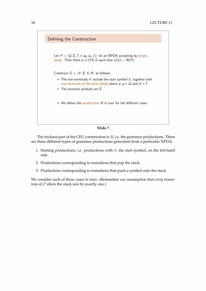
Let P = 〈Q,Σ, Γ, δ, q0, z0, {}〉 be an NPDA accepting by emptystack. Then there is a CFG G such that L(G ) = N(P).
Construct G = 〈V ,Σ,S ,R〉 as follows:
I The non-terminals V include the start symbol S , together withnon-terminals of the form [pXq] where p, q ∈ Q and X ∈ Γ.
I The terminal symbols are Σ.
I We define the productions R in turn for the different cases.
Slide 7
The trickiest part of the CFG construction isR, i.e. the grammar productions. Thereare three different types of grammar productions generated from a particular NPDA:
1. Starting productions, i.e. productions with S, the start symbol, on the left-handside.
2. Productions corresponding to transitions that pop the stack.
3. Productions corresponding to transitions that push a symbol onto the stack.
We consider each of these cases in turn. (Remember our assumption that every transi-tion of P alters the stack size by exactly one.)
11.1. TRANSFORMING AN NPDA INTO A CFG 35
Starting Productions
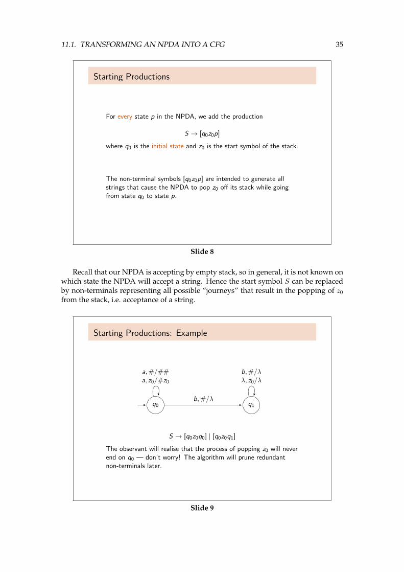
For every state p in the NPDA, we add the production
S → [q0z0p]
where q0 is the initial state and z0 is the start symbol of the stack.
The non-terminal symbols [q0z0p] are intended to generate allstrings that cause the NPDA to pop z0 off its stack while goingfrom state q0 to state p.
Slide 8
Recall that our NPDA is accepting by empty stack, so in general, it is not known onwhich state the NPDA will accept a string. Hence the start symbol S can be replacedby non-terminals representing all possible “journeys” that result in the popping of z0
from the stack, i.e. acceptance of a string.
Starting Productions: Example
q0 q1
b,#/λλ, z0/λ
a,#/##a, z0/#z0
b,#/λ
S → [q0z0q0] | [q0z0q1]
The observant will realise that the process of popping z0 will neverend on q0 — don’t worry! The algorithm will prune redundantnon-terminals later.
Slide 9
36 LECTURE 11.
Here, [q0z0q0] is intended to generate all strings that cause the NPDA to pop z0
from the stack while moving from q0 to q0 (possibly via q1 at some stage); and [q0z0q1]is intended to generate all strings that cause it to pop z0 while moving from q0 to q1.Of course, no string can be accepted while on state q0 since there are no transitions toit that pop z0 from the stack. (The construction aims to be as general as possible, somakes no assumptions about where execution will finish.) For completeness, we keepthe production S → [q0z0q0] in the grammar for the moment, and prune it out towardsthe end with other simplifications.
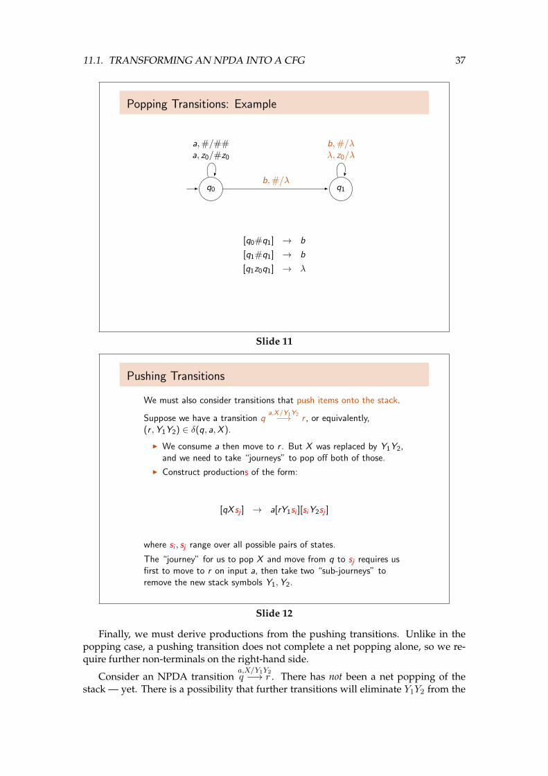
Popping Transitions
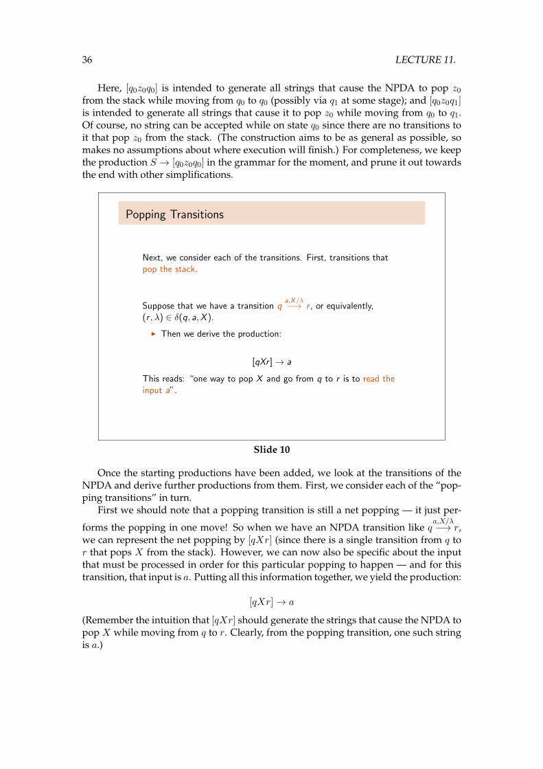
Next, we consider each of the transitions. First, transitions thatpop the stack.
Suppose that we have a transition qa,X/λ−→ r , or equivalently,
(r , λ) ∈ δ(q, a,X ).
I Then we derive the production:
[qXr ]→ a
This reads: “one way to pop X and go from q to r is to read theinput a”.
Slide 10
Once the starting productions have been added, we look at the transitions of theNPDA and derive further productions from them. First, we consider each of the “pop-ping transitions” in turn.
First we should note that a popping transition is still a net popping — it just per-
forms the popping in one move! So when we have an NPDA transition likea,X/λq −→ r,
we can represent the net popping by [qXr] (since there is a single transition from q tor that pops X from the stack). However, we can now also be specific about the inputthat must be processed in order for this particular popping to happen — and for thistransition, that input is a. Putting all this information together, we yield the production:
[qXr]→ a
(Remember the intuition that [qXr] should generate the strings that cause the NPDA topop X while moving from q to r. Clearly, from the popping transition, one such stringis a.)
11.1. TRANSFORMING AN NPDA INTO A CFG 37
Popping Transitions: Example
q0 q1
b,#/λλ, z0/λ
a,#/##a, z0/#z0
b,#/λ
[q0#q1] → b
[q1#q1] → b
[q1z0q1] → λ
Slide 11
Pushing Transitions
We must also consider transitions that push items onto the stack.
Suppose we have a transition qa,X/Y1Y2−→ r , or equivalently,
(r ,Y1Y2) ∈ δ(q, a,X ).
I We consume a then move to r . But X was replaced by Y1Y2,and we need to take “journeys” to pop off both of those.
I Construct productions of the form:
[qXsj ] → a[rY1si ][siY2sj ]
where si , sj range over all possible pairs of states.
The “journey” for us to pop X and move from q to sj requires usfirst to move to r on input a, then take two “sub-journeys” toremove the new stack symbols Y1,Y2.
Slide 12
Finally, we must derive productions from the pushing transitions. Unlike in thepopping case, a pushing transition does not complete a net popping alone, so we re-quire further non-terminals on the right-hand side.
Consider an NPDA transitiona,X/Y1Y2q −→ r . There has not been a net popping of the
stack — yet. There is a possibility that further transitions will eliminate Y1Y2 from the
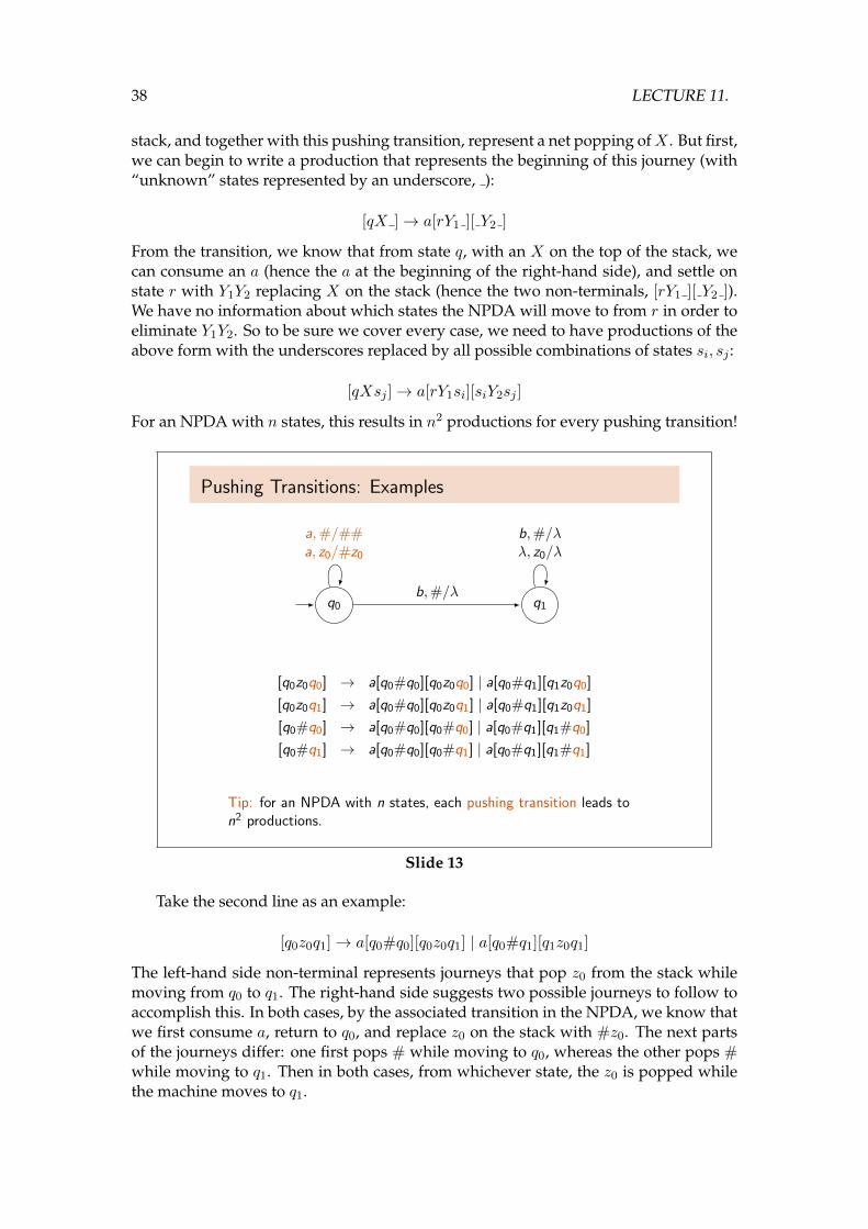
38 LECTURE 11.
stack, and together with this pushing transition, represent a net popping ofX . But first,we can begin to write a production that represents the beginning of this journey (with“unknown” states represented by an underscore, ):
[qX ]→ a[rY1 ][ Y2 ]
From the transition, we know that from state q, with an X on the top of the stack, wecan consume an a (hence the a at the beginning of the right-hand side), and settle onstate r with Y1Y2 replacing X on the stack (hence the two non-terminals, [rY1 ][ Y2 ]).We have no information about which states the NPDA will move to from r in order toeliminate Y1Y2. So to be sure we cover every case, we need to have productions of theabove form with the underscores replaced by all possible combinations of states si, sj :
[qXsj ]→ a[rY1si][siY2sj ]
For an NPDA with n states, this results in n2 productions for every pushing transition!
Pushing Transitions: Examples
q0 q1
b,#/λλ, z0/λ
a,#/##a, z0/#z0
b,#/λ
[q0z0q0] → a[q0#q0][q0z0q0] | a[q0#q1][q1z0q0]
[q0z0q1] → a[q0#q0][q0z0q1] | a[q0#q1][q1z0q1]
[q0#q0] → a[q0#q0][q0#q0] | a[q0#q1][q1#q0]
[q0#q1] → a[q0#q0][q0#q1] | a[q0#q1][q1#q1]
Tip: for an NPDA with n states, each pushing transition leads ton2 productions.
Slide 13
Take the second line as an example:
[q0z0q1]→ a[q0#q0][q0z0q1] | a[q0#q1][q1z0q1]
The left-hand side non-terminal represents journeys that pop z0 from the stack whilemoving from q0 to q1. The right-hand side suggests two possible journeys to follow toaccomplish this. In both cases, by the associated transition in the NPDA, we know thatwe first consume a, return to q0, and replace z0 on the stack with #z0. The next partsof the journeys differ: one first pops # while moving to q0, whereas the other pops #while moving to q1. Then in both cases, from whichever state, the z0 is popped whilethe machine moves to q1.
11.1. TRANSFORMING AN NPDA INTO A CFG 39
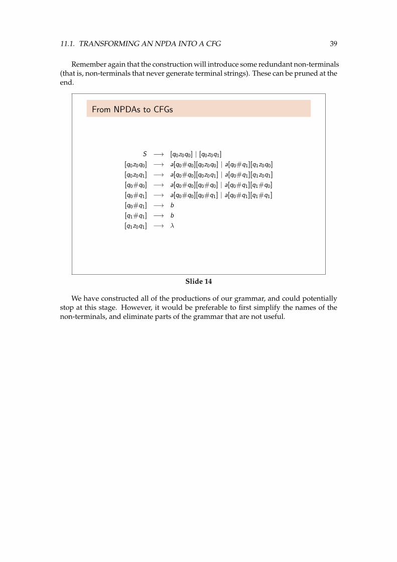
Remember again that the construction will introduce some redundant non-terminals(that is, non-terminals that never generate terminal strings). These can be pruned at theend.
From NPDAs to CFGs
S −→ [q0z0q0] | [q0z0q1]
[q0z0q0] −→ a[q0#q0][q0z0q0] | a[q0#q1][q1z0q0]
[q0z0q1] −→ a[q0#q0][q0z0q1] | a[q0#q1][q1z0q1]
[q0#q0] −→ a[q0#q0][q0#q0] | a[q0#q1][q1#q0]
[q0#q1] −→ a[q0#q0][q0#q1] | a[q0#q1][q1#q1]
[q0#q1] −→ b
[q1#q1] −→ b
[q1z0q1] −→ λ
Slide 14
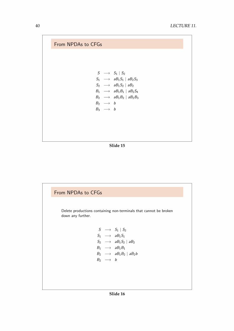
We have constructed all of the productions of our grammar, and could potentiallystop at this stage. However, it would be preferable to first simplify the names of thenon-terminals, and eliminate parts of the grammar that are not useful.
40 LECTURE 11.
From NPDAs to CFGs
S −→ S1 | S2
S1 −→ aB1S1 | aB2S3
S2 −→ aB1S2 | aB2
B1 −→ aB1B1 | aB2S4
B2 −→ aB1B2 | aB2B3
B2 −→ b
B3 −→ b
Slide 15
From NPDAs to CFGs
Delete productions containing non-terminals that cannot be brokendown any further.
S −→ S1 | S2
S1 −→ aB1S1
S2 −→ aB1S2 | aB2
B1 −→ aB1B1
B2 −→ aB1B2 | aB2b
B2 −→ b
Slide 16
11.1. TRANSFORMING AN NPDA INTO A CFG 41
From NPDAs to CFGs
Further simplifications.
S −→ aB
B −→ aBb | b
Slide 17
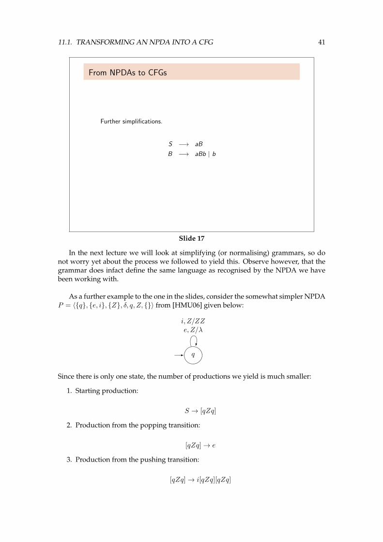
In the next lecture we will look at simplifying (or normalising) grammars, so donot worry yet about the process we followed to yield this. Observe however, that thegrammar does infact define the same language as recognised by the NPDA we havebeen working with.
As a further example to the one in the slides, consider the somewhat simpler NPDAP = 〈{q}, {e, i}, {Z}, δ, q, Z, {}〉 from [HMU06] given below:
q
i, Z/ZZe, Z/λ
Since there is only one state, the number of productions we yield is much smaller:
1. Starting production:
S → [qZq]
2. Production from the popping transition:
[qZq]→ e
3. Production from the pushing transition:
[qZq]→ i[qZq][qZq]
42 LECTURE 11.
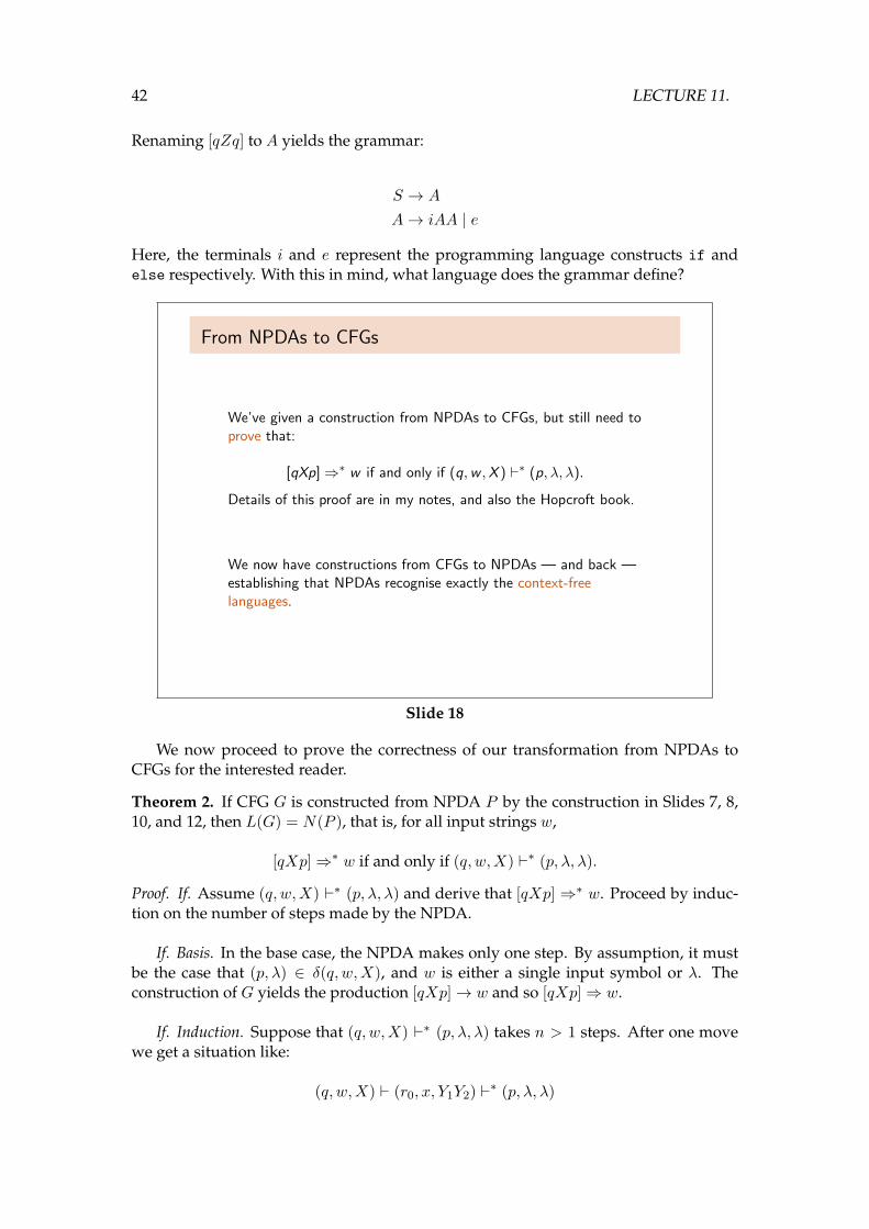
Renaming [qZq] to A yields the grammar:
S → A
A→ iAA | e
Here, the terminals i and e represent the programming language constructs if andelse respectively. With this in mind, what language does the grammar define?
From NPDAs to CFGs
We’ve given a construction from NPDAs to CFGs, but still need toprove that:
[qXp]⇒∗ w if and only if (q,w ,X ) `∗ (p, λ, λ).
Details of this proof are in my notes, and also the Hopcroft book.
We now have constructions from CFGs to NPDAs — and back —establishing that NPDAs recognise exactly the context-freelanguages.
Slide 18
We now proceed to prove the correctness of our transformation from NPDAs toCFGs for the interested reader.
Theorem 2. If CFG G is constructed from NPDA P by the construction in Slides 7, 8,10, and 12, then L(G) = N(P ), that is, for all input strings w,
[qXp]⇒∗ w if and only if (q, w,X) `∗ (p, λ, λ).
Proof. If. Assume (q, w,X) `∗ (p, λ, λ) and derive that [qXp] ⇒∗ w. Proceed by induc-tion on the number of steps made by the NPDA.
If. Basis. In the base case, the NPDA makes only one step. By assumption, it mustbe the case that (p, λ) ∈ δ(q, w,X), and w is either a single input symbol or λ. Theconstruction of G yields the production [qXp]→ w and so [qXp]⇒ w.
If. Induction. Suppose that (q, w,X) `∗ (p, λ, λ) takes n > 1 steps. After one movewe get a situation like:
(q, w,X) ` (r0, x, Y1Y2) `∗ (p, λ, λ)
11.1. TRANSFORMING AN NPDA INTO A CFG 43
where w = ax for a ∈ Σ ∪ {λ}. Therefore, (r0, Y1Y2) ∈ δ(q, a,X). Hence Y1Y2 is beingpushed onto the stack. By construction of G, there is a production (note the consistentrenaming of states in the production of Slide 12 for the purposes of this proof):
[qXr2]→ a[r0Y1r1][r1Y2r2]
where r2 = p and r1 ∈ Q.Each of Y1, Y2 gets popped off in turn, and ri is the state of the NPDA when Yi
is popped off. So we can split x into w1w2, where wi is the input consumed whileYi is popped off, therefore (ri−1, wi, Yi) `∗ (ri, λ, λ) for i = 1, 2. Each of these NPDAcomputations must take fewer than nmoves, so we can apply the induction hypothesis,i.e. [ri−1Yiri]⇒∗ wi. Thus:
[qXr2]⇒ a[r0Y1r1][r1Y2r2]
⇒∗ aw1[r1Y2r2]
⇒∗ aw1w2 = ax = w
Noting that r2 = p, we yield the required result.
Only if. Assume [qXp] ⇒∗ w and derive that (q, w,X) `∗ (p, λ, λ). We proceed byinduction on the number of steps in the derivation.
Only if. Basis. There is one derivation in the base case, so [qXp] → w must bea production. By construction, the only way that this can exist is if there is a transi-tion of P in which X is popped as the NPDA transitions from state q to state p, i.e.(p, λ) ∈ δ(q, a,X) and a = w. Hence (q, w,X) ` (p, λ, λ).
Only if. Induction. Suppose that [qXp] ⇒∗ w takes n > 1 steps. Consider thefirst step of the derivation using the construction of P (note the consistent renaming ofstates in the production of Slide 12 for the purposes of this proof):
[qXr2]⇒ a[r0Y1r1][r1Y2r2]⇒∗ wHere, r2 = p. The production arises because (r0, Y1Y2) ∈ δ(q, a,X). Again, we breakup w so that w = aw1w2 where [ri−1Yiri] ⇒∗ wi for i = 1, 2. By the induction hy-pothesis, we know that (ri−1, wi, Yi) `∗ (ri, λ, λ) and so (r0, w1, Y1) `∗ (r1, λ, λ). By awell-known property of configurations, we can add the string w2 and stack symbol Y2
to yield (r0, w1w2, Y1Y2) `∗ (r1, w2, Y2). Putting this all together we yield:
(q, aw1w2, X) ` (r0, w1w2, Y1Y2)
`∗ (r1, w2, Y2)
`∗ (r2, λ, λ)
Since r2 = p and aw1w2 = w, we have (q, w,X) `∗ (p, λ, λ), the result.
44 LECTURE 11.
11.2 Deterministic Pushdown Automata (DPDAs)
DPDAs
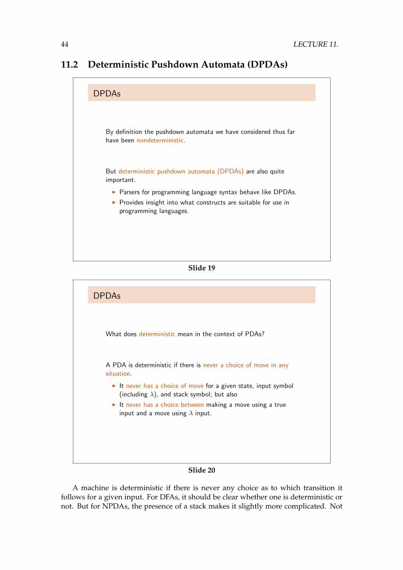
By definition the pushdown automata we have considered thus farhave been nondeterministic.
But deterministic pushdown automata (DPDAs) are also quiteimportant.
I Parsers for programming language syntax behave like DPDAs.
I Provides insight into what constructs are suitable for use inprogramming languages.
Slide 19
DPDAs
What does deterministic mean in the context of PDAs?
A PDA is deterministic if there is never a choice of move in anysituation.
I It never has a choice of move for a given state, input symbol(including λ), and stack symbol; but also
I It never has a choice between making a move using a trueinput and a move using λ input.
Slide 20
A machine is deterministic if there is never any choice as to which transition itfollows for a given input. For DFAs, it should be clear whether one is deterministic ornot. But for NPDAs, the presence of a stack makes it slightly more complicated. Not
11.2. DETERMINISTIC PUSHDOWN AUTOMATA (DPDAS) 45
only must we check that no state has more than one transition away from it with thesame constraints (i.e. requiring the same input symbol and top of stack), but we mustalso check that there is never a choice between consuming a true input character andfollowing a λ-transition.
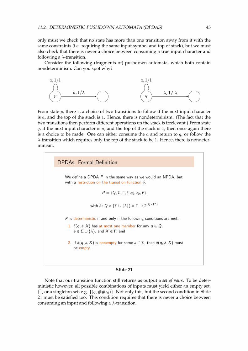
Consider the following (fragments of) pushdown automata, which both containnondeterminism. Can you spot why?
p qλ, 1/ λ
a, 1/1a, 1/1
a, 1/λ
From state p, there is a choice of two transitions to follow if the next input characteris a, and the top of the stack is 1. Hence, there is nondeterminism. (The fact that thetwo transitions then perform different operations on the stack is irrelevant.) From stateq, if the next input character is a, and the top of the stack is 1, then once again thereis a choice to be made. One can either consume the a and return to q, or follow theλ-transition which requires only the top of the stack to be 1. Hence, there is nondeter-minism.
DPDAs: Formal Definition
We define a DPDA P in the same way as we would an NPDA, butwith a restriction on the transition function δ.
P = 〈Q,Σ, Γ, δ, q0, z0,F 〉
with δ : Q × (Σ ∪ {λ})× Γ→ 2(Q×Γ∗)
P is deterministic if and only if the following conditions are met:
1. δ(q, a,X ) has at most one member for any q ∈ Q,a ∈ Σ ∪ {λ}, and X ∈ Γ; and
2. If δ(q, a,X ) is nonempty for some a ∈ Σ, then δ(q, λ,X ) mustbe empty.
Slide 21
Note that our transition function still returns as output a set of pairs. To be deter-ministic however, all possible combinations of inputs must yield either an empty set,{}, or a singleton set, e.g. {(q,##z0)}. Not only this, but the second condition in Slide21 must be satisfied too. This condition requires that there is never a choice betweenconsuming an input and following a λ-transition.
46 LECTURE 11.
Example DPDA
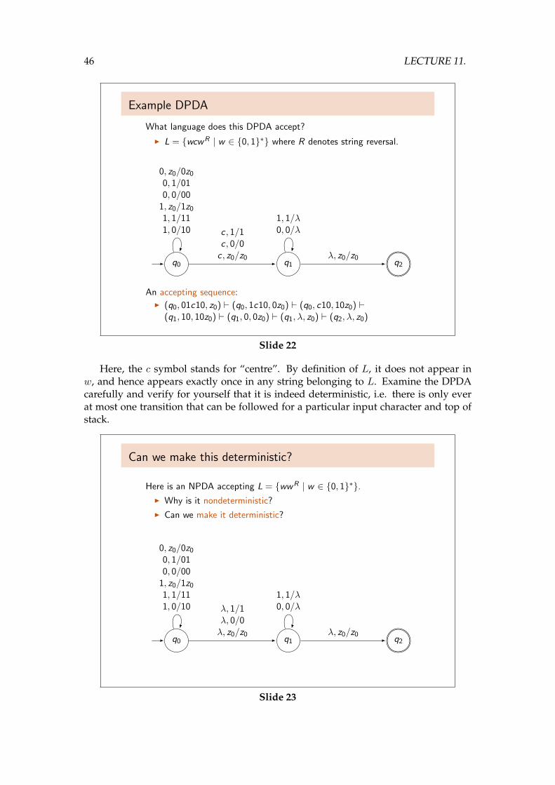
What language does this DPDA accept?
I L = {wcwR | w ∈ {0, 1}∗} where R denotes string reversal.
q0 q1 q2
1, 1/λ0, 0/λ
0, z0/0z0
0, 1/010, 0/00
1, z0/1z0
1, 1/111, 0/10
λ, z0/z0
c , 1/1c , 0/0c , z0/z0
An accepting sequence:I (q0, 01c10, z0) ` (q0, 1c10, 0z0) ` (q0, c10, 10z0) `
(q1, 10, 10z0) ` (q1, 0, 0z0) ` (q1, λ, z0) ` (q2, λ, z0)
Slide 22
Here, the c symbol stands for “centre”. By definition of L, it does not appear inw, and hence appears exactly once in any string belonging to L. Examine the DPDAcarefully and verify for yourself that it is indeed deterministic, i.e. there is only everat most one transition that can be followed for a particular input character and top ofstack.
Can we make this deterministic?
Here is an NPDA accepting L = {wwR | w ∈ {0, 1}∗}.I Why is it nondeterministic?
I Can we make it deterministic?
q0 q1 q2
1, 1/λ0, 0/λ
0, z0/0z0
0, 1/010, 0/00
1, z0/1z0
1, 1/111, 0/10
λ, z0/z0
λ, 1/1λ, 0/0λ, z0/z0
Slide 23
11.2. DETERMINISTIC PUSHDOWN AUTOMATA (DPDAS) 47
The NPDA in Slide 23 must nondeterministically select a transition to follow fromstate q0. Say the next input character is 0, and the top of the stack is 1. Then the ma-
chine must choose between the transitions0,1/01
q0 −→ q0 andλ,1/1
q0 −→ q1, i.e. it must choosebetween consuming a 0 or following a λ-transition. (There are several other configura-tions from which the next transition is chosen nondeterministically.)
Unfortunately, there is no DPDA accepting L = {wwR | w ∈ {0, 1}∗}. A formalproof of this is complex, but we can appeal to intuition. In Slide 22, we had a distinctmarker for the centre of the string. When that DPDA is executing, the moment it seesa c, it knows to start trying to read wR. But the NPDA in Slide 23 has no such centremarker, and so nondeterministically has to “guess” once it has finished reading in wand should start expecting wR. Unless we fixed the length of w (e.g. L5 = {wwR | w ∈{0, 1}∗ ∧ |w| = 5}), there is no way to construct a pushdown automaton that knows tostart expecting wR without using nondeterminism.
The Languages of DPDAs
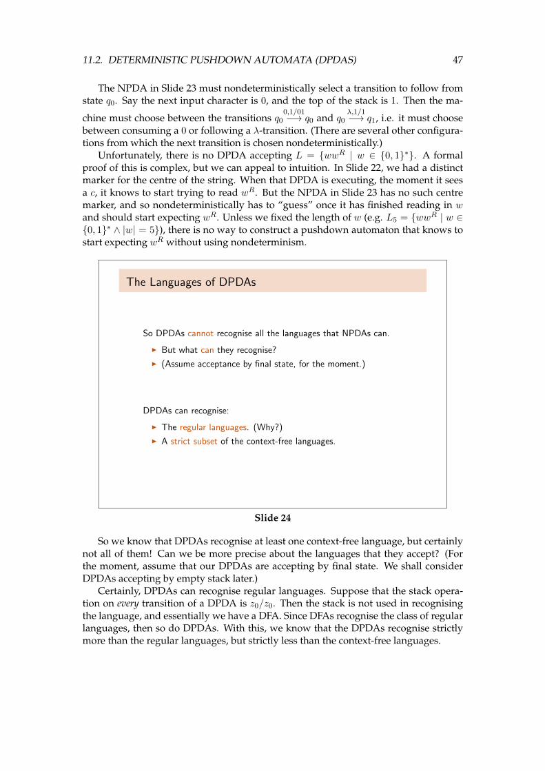
So DPDAs cannot recognise all the languages that NPDAs can.
I But what can they recognise?
I (Assume acceptance by final state, for the moment.)
DPDAs can recognise:
I The regular languages. (Why?)
I A strict subset of the context-free languages.
Slide 24
So we know that DPDAs recognise at least one context-free language, but certainlynot all of them! Can we be more precise about the languages that they accept? (Forthe moment, assume that our DPDAs are accepting by final state. We shall considerDPDAs accepting by empty stack later.)
Certainly, DPDAs can recognise regular languages. Suppose that the stack opera-tion on every transition of a DPDA is z0/z0. Then the stack is not used in recognisingthe language, and essentially we have a DFA. Since DFAs recognise the class of regularlanguages, then so do DPDAs. With this, we know that the DPDAs recognise strictlymore than the regular languages, but strictly less than the context-free languages.
48 LECTURE 11.
DPDAs and Ambiguous Grammars
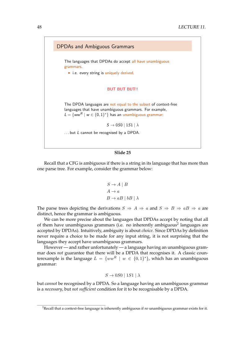
The languages that DPDAs do accept all have unambiguousgrammars.
I i.e. every string is uniquely derived.
BUT BUT BUT!!
The DPDA languages are not equal to the subset of context-freelanguages that have unambiguous grammars. For example,L = {wwR | w ∈ {0, 1}∗} has an unambiguous grammar:
S → 0S0 | 1S1 | λ. . . but L cannot be recognised by a DPDA.
Slide 25
Recall that a CFG is ambiguous if there is a string in its language that has more thanone parse tree. For example, consider the grammar below:
S → A | BA→ a
B → aB | bB | λ
The parse trees depicting the derivations S ⇒ A ⇒ a and S ⇒ B ⇒ aB ⇒ a aredistinct, hence the grammar is ambiguous.
We can be more precise about the languages that DPDAs accept by noting that allof them have unambiguous grammars (i.e. no inherently ambiguous2 languages areaccepted by DPDAs). Intuitively, ambiguity is about choice. Since DPDAs by definitionnever require a choice to be made for any input string, it is not surprising that thelanguages they accept have unambiguous grammars.
However — and rather unfortunately — a language having an unambiguous gram-mar does not guarantee that there will be a DPDA that recognises it. A classic coun-terexample is the language L = {wwR | w ∈ {0, 1}∗}, which has an unambiguousgrammar:
S → 0S0 | 1S1 | λbut cannot be recognised by a DPDA. So a language having an unambiguous grammaris a necessary, but not sufficient condition for it to be recognisable by a DPDA.
2Recall that a context-free language is inherently ambiguous if no unambiguous grammar exists for it.
11.2. DETERMINISTIC PUSHDOWN AUTOMATA (DPDAS) 49
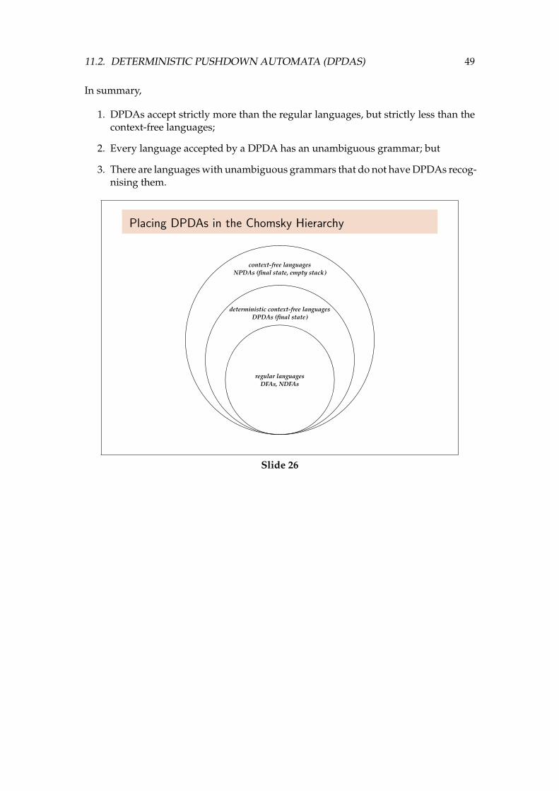
In summary,
1. DPDAs accept strictly more than the regular languages, but strictly less than thecontext-free languages;
2. Every language accepted by a DPDA has an unambiguous grammar; but
3. There are languages with unambiguous grammars that do not have DPDAs recog-nising them.
Placing DPDAs in the Chomsky Hierarchy
regular languagesDFAs, NDFAs
deterministic context-free languagesDPDAs (final state)
context-free languagesNPDAs (final state, empty stack)
Slide 26
50 LECTURE 11.
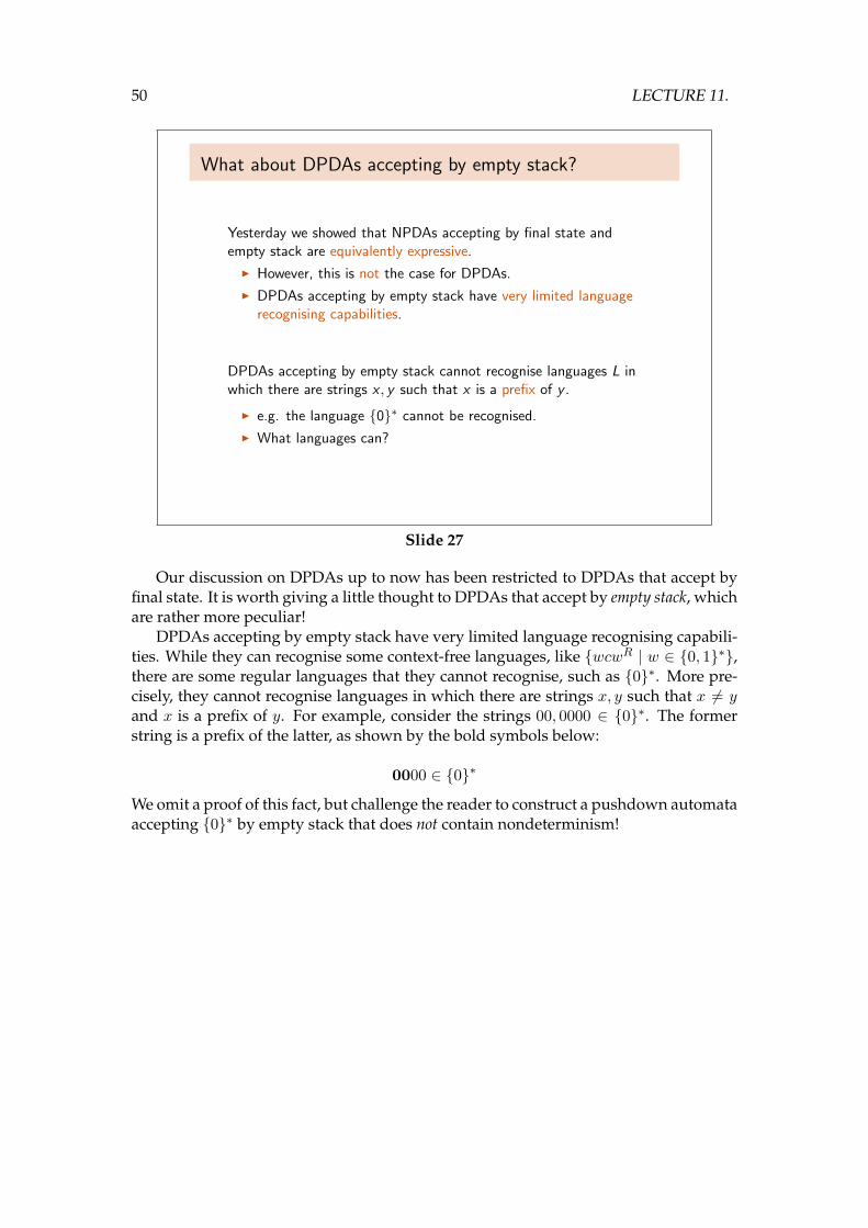
What about DPDAs accepting by empty stack?
Yesterday we showed that NPDAs accepting by final state andempty stack are equivalently expressive.
I However, this is not the case for DPDAs.
I DPDAs accepting by empty stack have very limited languagerecognising capabilities.
DPDAs accepting by empty stack cannot recognise languages L inwhich there are strings x , y such that x is a prefix of y .
I e.g. the language {0}∗ cannot be recognised.
I What languages can?
Slide 27
Our discussion on DPDAs up to now has been restricted to DPDAs that accept byfinal state. It is worth giving a little thought to DPDAs that accept by empty stack, whichare rather more peculiar!
DPDAs accepting by empty stack have very limited language recognising capabili-ties. While they can recognise some context-free languages, like {wcwR | w ∈ {0, 1}∗},there are some regular languages that they cannot recognise, such as {0}∗. More pre-cisely, they cannot recognise languages in which there are strings x, y such that x 6= yand x is a prefix of y. For example, consider the strings 00, 0000 ∈ {0}∗. The formerstring is a prefix of the latter, as shown by the bold symbols below:
0000 ∈ {0}∗
We omit a proof of this fact, but challenge the reader to construct a pushdown automataaccepting {0}∗ by empty stack that does not contain nondeterminism!
11.3. SUMMARY 51
11.3 Summary
Summary
Today we have:
I Discussed the transformation from NPDAs to CFGs.
I Defined DPDAs and contrasted them with NPDAs.
I Seen that DPDAs (accepting by final state) accept a class oflanguages strictly between the regular and context-free.
I Seen that unambiguous grammars are a necessary, but notsufficient condition for a language to be recognised by aDPDA.
I Discussed the limited capabilities of DPDAs accepting byempty stack.
Slide 28
Next Lecture
Next time we will:
I Look at some properties of context-free languages; and
I Discuss grammar simplifications, as well as normal forms (andtheir uses).
Slide 29

52 LECTURE 11.
Lecture 12
In this final lecture, we conclude our study of the context-free languages by lookingat a specific property of them: that is, a context-free language can always be describedby a CFG whose productions are either of the form A → BC or A → a (where A,B,Cdenote non-terminals and a a terminal, as usual). CFGs written in this way are said tobe in Chomsky Normal Form (CNF). We will show how to transform arbitrary CFGs intoCNF, but also explain why this normal form is of interest to us.
In the second part of the lecture, we will discuss what lies beyond the context-freelanguages in the Chomsky hierarchy. We will then take a glimpse into the future, andexplore (albeit very briefly) some of the things you will talk about next year in COCO:Computability and Complexity.
Nearly at the finish line!!
Slide 1
53
54 LECTURE 12.
Learning Outcomes
After this lecture you should be able to:
§ compute the useless symbols, nullable symbols, and unitproductions of CFGs;
§ transform CFGs into Chomsky Normal Form (CNF);
§ explain why CNF is useful;
§ list the levels of the Chomsky hierarchy, characterising theirlanguages by the grammars that define them, and machinesthat accept them;
§ explain the importance of Turing machines to computabilitytheory.
Slide 2
12.1 Chomsky Normal Form
Simplifying CFGs, and Normal Forms
We are going to simplify context-free grammars (CFGs), byshowing they can always be written in some special form — aso-called “normal form”.
It becomes easier to prove facts about context-free languages,since we know their grammars can always be made to conform tothe restrictions of this normal form.
The normal form we will consider today is known as ChomskyNormal Form.
Slide 3
Chomsky Normal Form (CNF) is named after the linguist Noam Chomsky, who firstproposed context-free grammars as a way of describing natural languages. Today a
12.1. CHOMSKY NORMAL FORM 55
Professor (Emeritus) at MIT, he may be more familiar to you through his political ac-tivism.
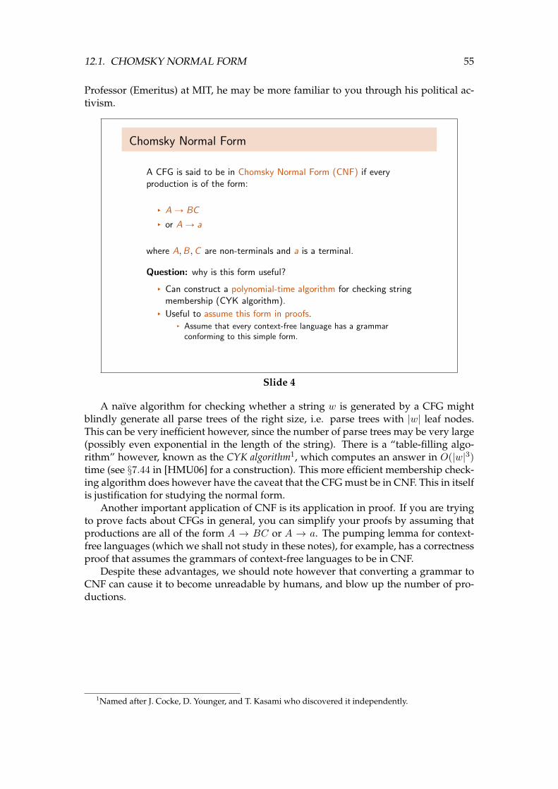
Chomsky Normal Form
A CFG is said to be in Chomsky Normal Form (CNF) if everyproduction is of the form:
§ AÑ BC
§ or AÑ a
where A,B,C are non-terminals and a is a terminal.
Question: why is this form useful?
§ Can construct a polynomial-time algorithm for checking stringmembership (CYK algorithm).
§ Useful to assume this form in proofs.§ Assume that every context-free language has a grammar
conforming to this simple form.
Slide 4
A naı̈ve algorithm for checking whether a string w is generated by a CFG mightblindly generate all parse trees of the right size, i.e. parse trees with |w| leaf nodes.This can be very inefficient however, since the number of parse trees may be very large(possibly even exponential in the length of the string). There is a “table-filling algo-rithm” however, known as the CYK algorithm1, which computes an answer in O(|w|3)time (see §7.44 in [HMU06] for a construction). This more efficient membership check-ing algorithm does however have the caveat that the CFG must be in CNF. This in itselfis justification for studying the normal form.
Another important application of CNF is its application in proof. If you are tryingto prove facts about CFGs in general, you can simplify your proofs by assuming thatproductions are all of the form A → BC or A → a. The pumping lemma for context-free languages (which we shall not study in these notes), for example, has a correctnessproof that assumes the grammars of context-free languages to be in CNF.
Despite these advantages, we should note however that converting a grammar toCNF can cause it to become unreadable by humans, and blow up the number of pro-ductions.
1Named after J. Cocke, D. Younger, and T. Kasami who discovered it independently.
56 LECTURE 12.
Converting CFGs to Chomsky Normal Form
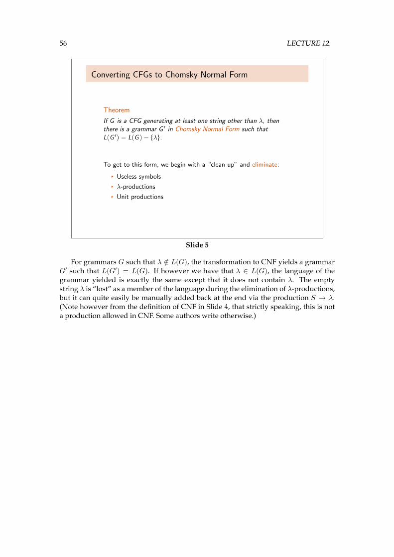
Theorem
If G is a CFG generating at least one string other than λ, thenthere is a grammar G 1 in Chomsky Normal Form such thatLpG 1q “ LpG q ´ tλu.
To get to this form, we begin with a “clean up” and eliminate:
§ Useless symbols
§ λ-productions
§ Unit productions
Slide 5
For grammars G such that λ /∈ L(G), the transformation to CNF yields a grammarG′ such that L(G′) = L(G). If however we have that λ ∈ L(G), the language of thegrammar yielded is exactly the same except that it does not contain λ. The emptystring λ is “lost” as a member of the language during the elimination of λ-productions,but it can quite easily be manually added back at the end via the production S → λ.(Note however from the definition of CNF in Slide 4, that strictly speaking, this is nota production allowed in CNF. Some authors write otherwise.)
12.1. CHOMSKY NORMAL FORM 57
12.1.1 Eliminating Useless Symbols
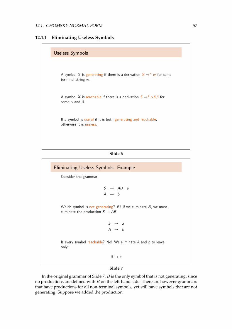
Useless Symbols
A symbol X is generating if there is a derivation X ñ˚ w for someterminal string w .
A symbol X is reachable if there is a derivation S ñ˚ αXβ forsome α and β.
If a symbol is useful if it is both generating and reachable,otherwise it is useless.
Slide 6
Eliminating Useless Symbols: Example
Consider the grammar:
S Ñ AB | aA Ñ b
Which symbol is not generating? B! If we eliminate B, we musteliminate the production S Ñ AB:
S Ñ a
A Ñ b
Is every symbol reachable? No! We eliminate A and b to leaveonly:
S Ñ a
Slide 7
In the original grammar of Slide 7, B is the only symbol that is not generating, sinceno productions are defined with B on the left-hand side. There are however grammarsthat have productions for all non-terminal symbols, yet still have symbols that are notgenerating. Suppose we added the production:
58 LECTURE 12.
B → bB
While we can now apply a production to B, it is still not generating since it will neverderive a string of terminals (i.e. a string in the language of the grammar). Consider forexample the infinite derivation:
S ⇒ AB ⇒ AbB ⇒ AbbB ⇒ AbbbB ⇒ . . .
After removing the production in Slide 7 involving the non-generating symbol B,we are left with a grammar that has a non-reachable symbol, A. Since there is no wayto reach A from the start symbol S, productions with A on the left-hand side will haveno effect on the language of the grammar and can safely be removed.
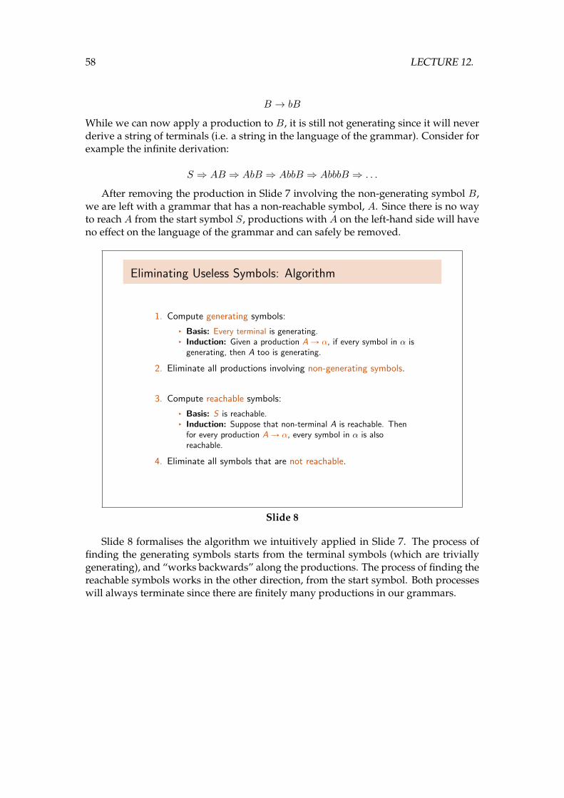
Eliminating Useless Symbols: Algorithm
1. Compute generating symbols:
§ Basis: Every terminal is generating.§ Induction: Given a production AÑ α, if every symbol in α is
generating, then A too is generating.
2. Eliminate all productions involving non-generating symbols.
3. Compute reachable symbols:
§ Basis: S is reachable.§ Induction: Suppose that non-terminal A is reachable. Then
for every production AÑ α, every symbol in α is alsoreachable.
4. Eliminate all symbols that are not reachable.
Slide 8
Slide 8 formalises the algorithm we intuitively applied in Slide 7. The process offinding the generating symbols starts from the terminal symbols (which are triviallygenerating), and “works backwards” along the productions. The process of finding thereachable symbols works in the other direction, from the start symbol. Both processeswill always terminate since there are finitely many productions in our grammars.
12.1. CHOMSKY NORMAL FORM 59
12.1.2 Eliminating λ-productions
λ-productions and Nullable Symbols
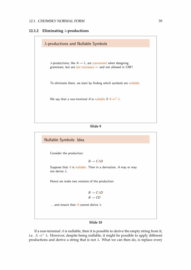
λ-productions, like AÑ λ, are convenient when designinggrammars, but are not necessary — and not allowed in CNF!
To eliminate them, we start by finding which symbols are nullable.
We say that a non-terminal A is nullable if Añ˚ λ.
Slide 9
Nullable Symbols: Idea
Consider the production:
B Ñ CAD
Suppose that A is nullable. Then in a derivation, A may or maynot derive λ.
Hence we make two versions of the production:
B Ñ CAD
B Ñ CD
. . . and ensure that A cannot derive λ.
Slide 10
If a non-terminal A is nullable, then it is possible to derive the empty string from it,i.e. A ⇒∗ λ. However, despite being nullable, it might be possible to apply differentproductions and derive a string that is not λ. What we can then do, is replace every
60 LECTURE 12.
production containing nullable symbols likeAwith new versions that have the nullablesymbols present or absent in all possible combinations. This “captures” the effect of anullable symbol going to λ without the need to have explicit λ-productions.
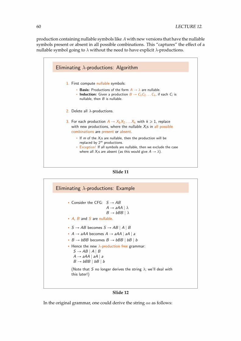
Eliminating λ-productions: Algorithm
1. First compute nullable symbols:
§ Basis: Productions of the form AÑ λ are nullable.§ Induction: Given a production B Ñ C1C2 . . .Ck , if each Ci is
nullable, then B is nullable.
2. Delete all λ-productions.
3. For each production AÑ X1X2 . . .Xk with k ě 1, replacewith new productions, where the nullable Xi s in all possiblecombinations are present or absent.
§ If m of the Xi s are nullable, then the production will bereplaced by 2m productions.
§ Exception! If all symbols are nullable, then we exclude the casewhere all Xi s are absent (as this would give AÑ λ).
Slide 11
Eliminating λ-productions: Example
§ Consider the CFG: S Ñ ABAÑ aAA | λB Ñ bBB | λ
§ A, B and S are nullable.
§ S Ñ AB becomes S Ñ AB | A | B§ AÑ aAA becomes AÑ aAA | aA | a§ B Ñ bBB becomes B Ñ bBB | bB | b§ Hence the new λ-production free grammar:
S Ñ AB | A | BAÑ aAA | aA | aB Ñ bBB | bB | b
(Note that S no longer derives the string λ; we’ll deal withthis later!)
Slide 12
In the original grammar, one could derive the string aa as follows:
12.1. CHOMSKY NORMAL FORM 61
S ⇒ AB ⇒ aAAB ⇒ aAA⇒ aaAAA⇒3 aa
Note that the B eventually derived λ, as did three As towards the end. In the λ-production free grammar of Slide 12, there are additional rules to immediately “cap-ture” the effect of these non-terminals eventually going to λ. We can derive the stringaa as follows:
S ⇒ A⇒ aA⇒ aa
12.1.3 Eliminating Unit Productions
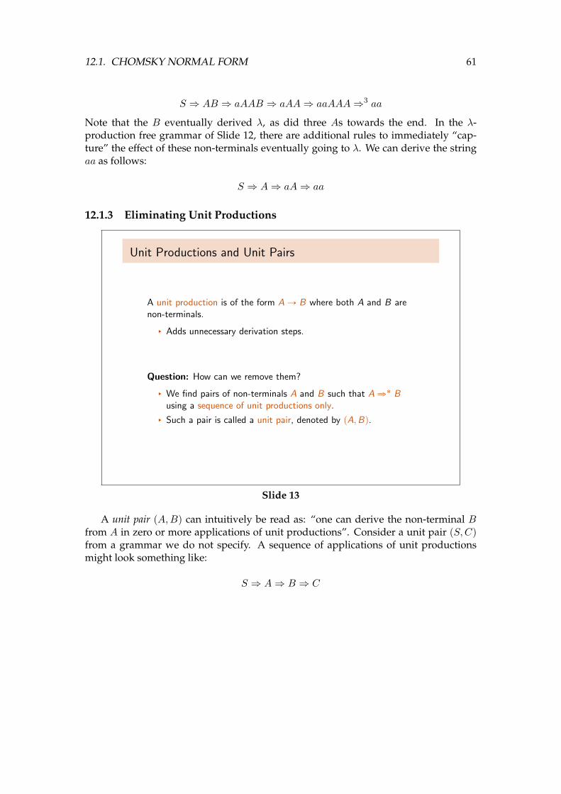
Unit Productions and Unit Pairs
A unit production is of the form AÑ B where both A and B arenon-terminals.
§ Adds unnecessary derivation steps.
Question: How can we remove them?
§ We find pairs of non-terminals A and B such that Añ˚ Busing a sequence of unit productions only.
§ Such a pair is called a unit pair, denoted by pA,Bq.
Slide 13
A unit pair (A,B) can intuitively be read as: “one can derive the non-terminal Bfrom A in zero or more applications of unit productions”. Consider a unit pair (S,C)from a grammar we do not specify. A sequence of applications of unit productionsmight look something like:
S ⇒ A⇒ B ⇒ C
62 LECTURE 12.
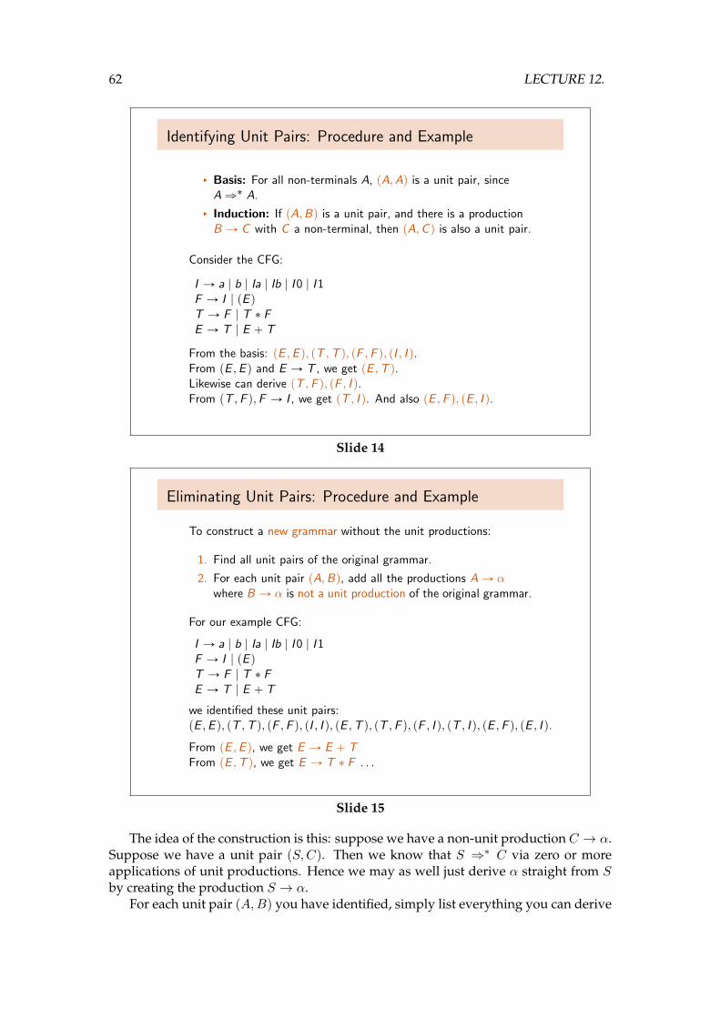
Identifying Unit Pairs: Procedure and Example
§ Basis: For all non-terminals A, pA,Aq is a unit pair, sinceAñ˚ A.
§ Induction: If pA,Bq is a unit pair, and there is a productionB Ñ C with C a non-terminal, then pA,C q is also a unit pair.
Consider the CFG:
I Ñ a | b | Ia | Ib | I0 | I1F Ñ I | pE qT Ñ F | T ˚ FE Ñ T | E ` T
From the basis: pE ,E q, pT ,T q, pF ,F q, pI , I q.From pE ,E q and E Ñ T , we get pE ,T q.Likewise can derive pT ,F q, pF , I q.From pT ,F q,F Ñ I , we get pT , I q. And also pE ,F q, pE , I q.
Slide 14
Eliminating Unit Pairs: Procedure and Example
To construct a new grammar without the unit productions:
1. Find all unit pairs of the original grammar.
2. For each unit pair pA,Bq, add all the productions AÑ αwhere B Ñ α is not a unit production of the original grammar.
For our example CFG:
I Ñ a | b | Ia | Ib | I0 | I1F Ñ I | pE qT Ñ F | T ˚ FE Ñ T | E ` T
we identified these unit pairs:pE ,E q, pT ,T q, pF ,F q, pI , I q, pE ,T q, pT ,F q, pF , I q, pT , I q, pE ,F q, pE , I q.From pE ,E q, we get E Ñ E ` TFrom pE ,T q, we get E Ñ T ˚ F . . .
Slide 15
The idea of the construction is this: suppose we have a non-unit production C → α.Suppose we have a unit pair (S,C). Then we know that S ⇒∗ C via zero or moreapplications of unit productions. Hence we may as well just derive α straight from Sby creating the production S → α.
For each unit pair (A,B) you have identified, simply list everything you can derive
12.1. CHOMSKY NORMAL FORM 63
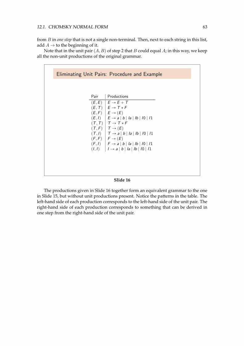
from B in one step that is not a single non-terminal. Then, next to each string in this list,add A→ to the beginning of it.
Note that in the unit pair (A,B) of step 2 that B could equal A; in this way, we keepall the non-unit productions of the original grammar.
Eliminating Unit Pairs: Procedure and Example
Pair Productions
pE ,E q E Ñ E ` TpE ,T q E Ñ T ˚ FpE ,F q E Ñ pE qpE , I q E Ñ a | b | Ia | Ib | I0 | I1pT ,T q T Ñ T ˚ FpT ,F q T Ñ pE qpT , I q T Ñ a | b | Ia | Ib | I0 | I1pF ,F q F Ñ pE qpF , I q F Ñ a | b | Ia | Ib | I0 | I1pI , I q I Ñ a | b | Ia | Ib | I0 | I1
Slide 16
The productions given in Slide 16 together form an equivalent grammar to the onein Slide 15, but without unit productions present. Notice the patterns in the table. Theleft-hand side of each production corresponds to the left-hand side of the unit pair. Theright-hand side of each production corresponds to something that can be derived inone step from the right-hand side of the unit pair.
64 LECTURE 12.
12.1.4 Transforming CFGs into CNF
Transformation to Chomsky Normal Form (CNF)
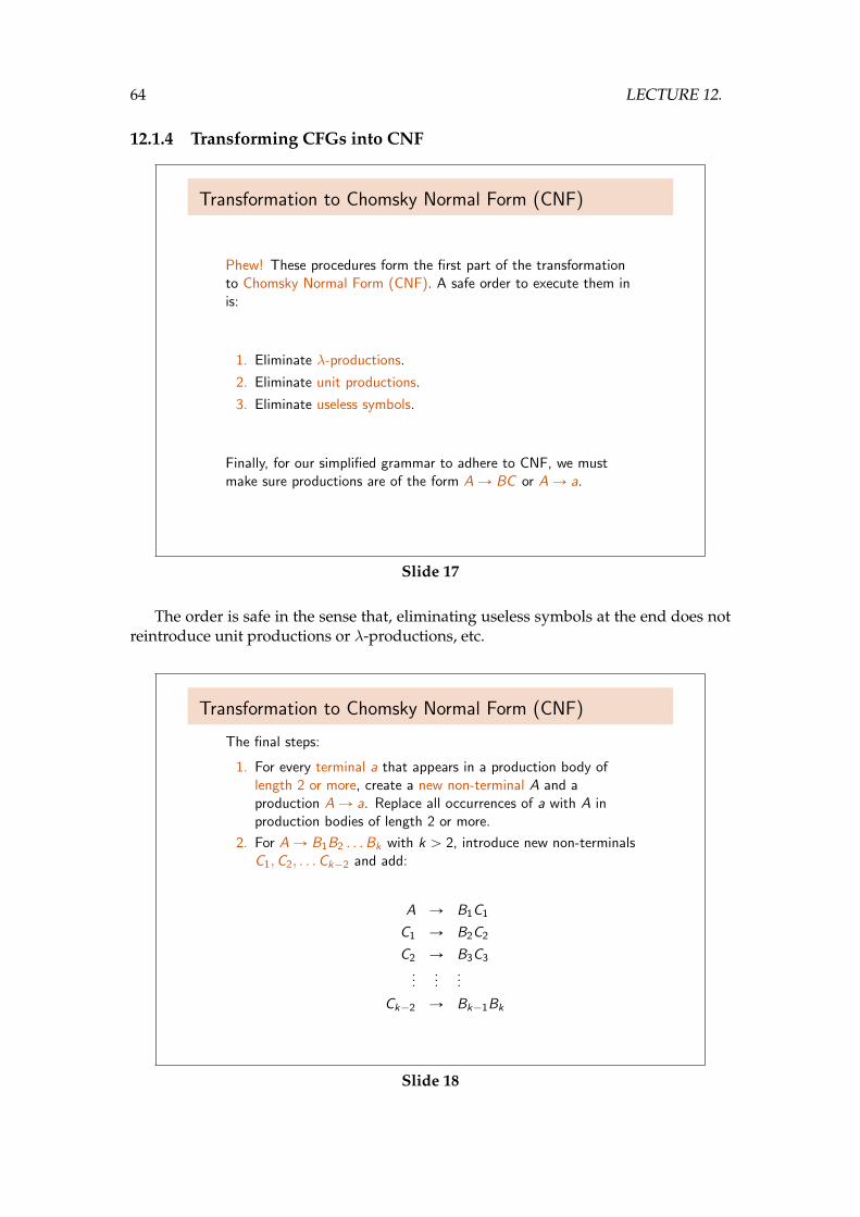
Phew! These procedures form the first part of the transformationto Chomsky Normal Form (CNF). A safe order to execute them inis:
1. Eliminate λ-productions.
2. Eliminate unit productions.
3. Eliminate useless symbols.
Finally, for our simplified grammar to adhere to CNF, we mustmake sure productions are of the form AÑ BC or AÑ a.
Slide 17
The order is safe in the sense that, eliminating useless symbols at the end does notreintroduce unit productions or λ-productions, etc.
Transformation to Chomsky Normal Form (CNF)
The final steps:
1. For every terminal a that appears in a production body oflength 2 or more, create a new non-terminal A and aproduction AÑ a. Replace all occurrences of a with A inproduction bodies of length 2 or more.
2. For AÑ B1B2 . . .Bk with k ą 2, introduce new non-terminalsC1,C2, . . .Ck´2 and add:
A Ñ B1C1
C1 Ñ B2C2
C2 Ñ B3C3
......
...
Ck´2 Ñ Bk´1Bk
Slide 18
12.1. CHOMSKY NORMAL FORM 65
The first step ensures that the right-hand sides of productions with two or moresymbols contain exclusively non-terminal symbols. Any terminal symbols previouslypresent are replaced by fresh non-terminal symbols, which derive exactly the replacedterminals in one derivation step. Thus, terminals only ever appear in productions ofthe form A→ a.
The second step deals with productions such as A → PQRS, i.e. productions withright-hand sides containing more than two non-terminals. These are massaged intoform by creating a series of new non-terminals and productions, in this case:
C1 → QC2
C2 → RS
and finally, by replacing A → PQRS with A → PC1. This trick quickly massagesproductions containing non-terminals on the right-hand sides into the form requiredby CNF.
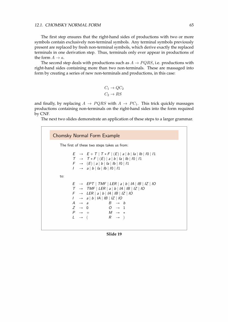
The next two slides demonstrate an application of these steps to a larger grammar.
Chomsky Normal Form Example
The first of these two steps takes us from:
E Ñ E ` T | T ˚ F | pE q | a | b | Ia | Ib | I0 | I1T Ñ T ˚ F | pE q | a | b | Ia | Ib | I0 | I1F Ñ pE q | a | b | Ia | Ib | I0 | I1I Ñ a | b | Ia | Ib | I0 | I1
to:
E Ñ EPT | TMF | LER | a | b | IA | IB | IZ | IOT Ñ TMF | LER | a | b | IA | IB | IZ | IOF Ñ LER | a | b | IA | IB | IZ | IOI Ñ a | b | IA | IB | IZ | IOA Ñ a B Ñ bZ Ñ 0 O Ñ 1P Ñ ` M Ñ ˚L Ñ p R Ñ q
Slide 19
66 LECTURE 12.
Chomsky Normal Form Example
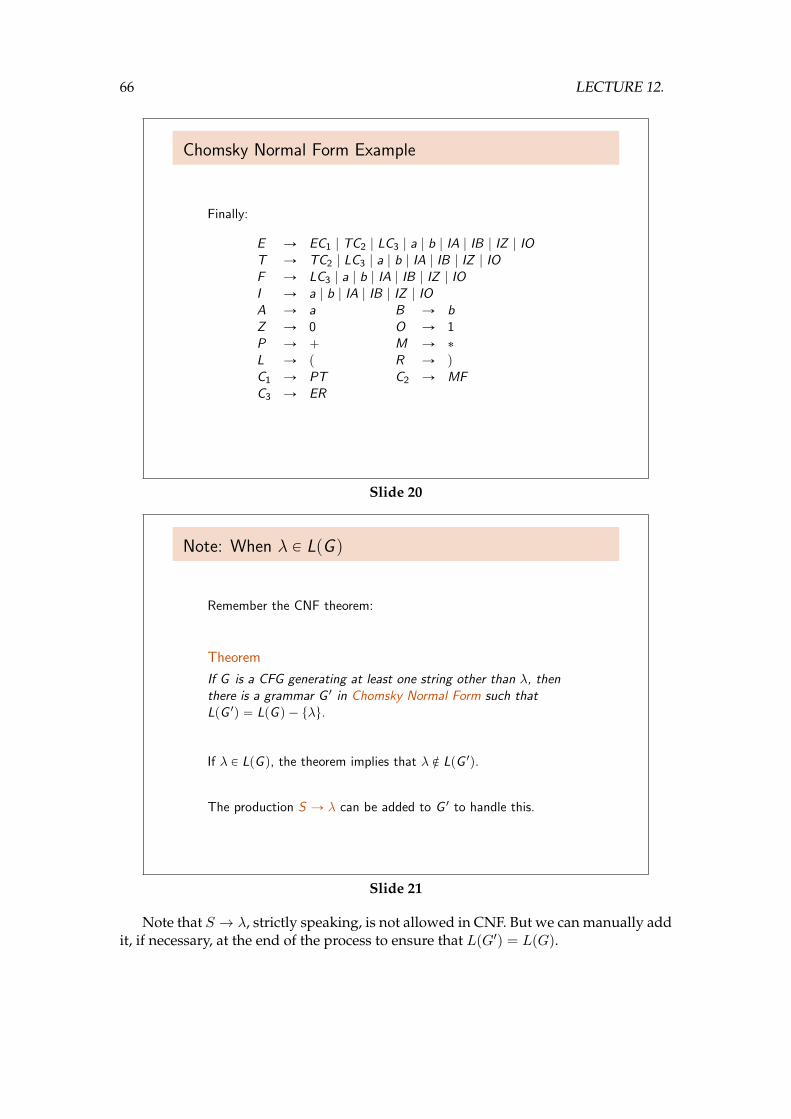
Finally:
E Ñ EC1 | TC2 | LC3 | a | b | IA | IB | IZ | IOT Ñ TC2 | LC3 | a | b | IA | IB | IZ | IOF Ñ LC3 | a | b | IA | IB | IZ | IOI Ñ a | b | IA | IB | IZ | IOA Ñ a B Ñ bZ Ñ 0 O Ñ 1P Ñ ` M Ñ ˚L Ñ p R Ñ qC1 Ñ PT C2 Ñ MFC3 Ñ ER
Slide 20
Note: When λ P LpG q
Remember the CNF theorem:
Theorem
If G is a CFG generating at least one string other than λ, thenthere is a grammar G 1 in Chomsky Normal Form such thatLpG 1q “ LpG q ´ tλu.
If λ P LpG q, the theorem implies that λ R LpG 1q.
The production S Ñ λ can be added to G 1 to handle this.
Slide 21
Note that S → λ, strictly speaking, is not allowed in CNF. But we can manually addit, if necessary, at the end of the process to ensure that L(G′) = L(G).
12.2. CHOMSKY HIERARCHY AND COMPUTABILITY THEORY 67
12.2 Chomsky Hierarchy and Computability Theory
The Chomsky Hierarchy
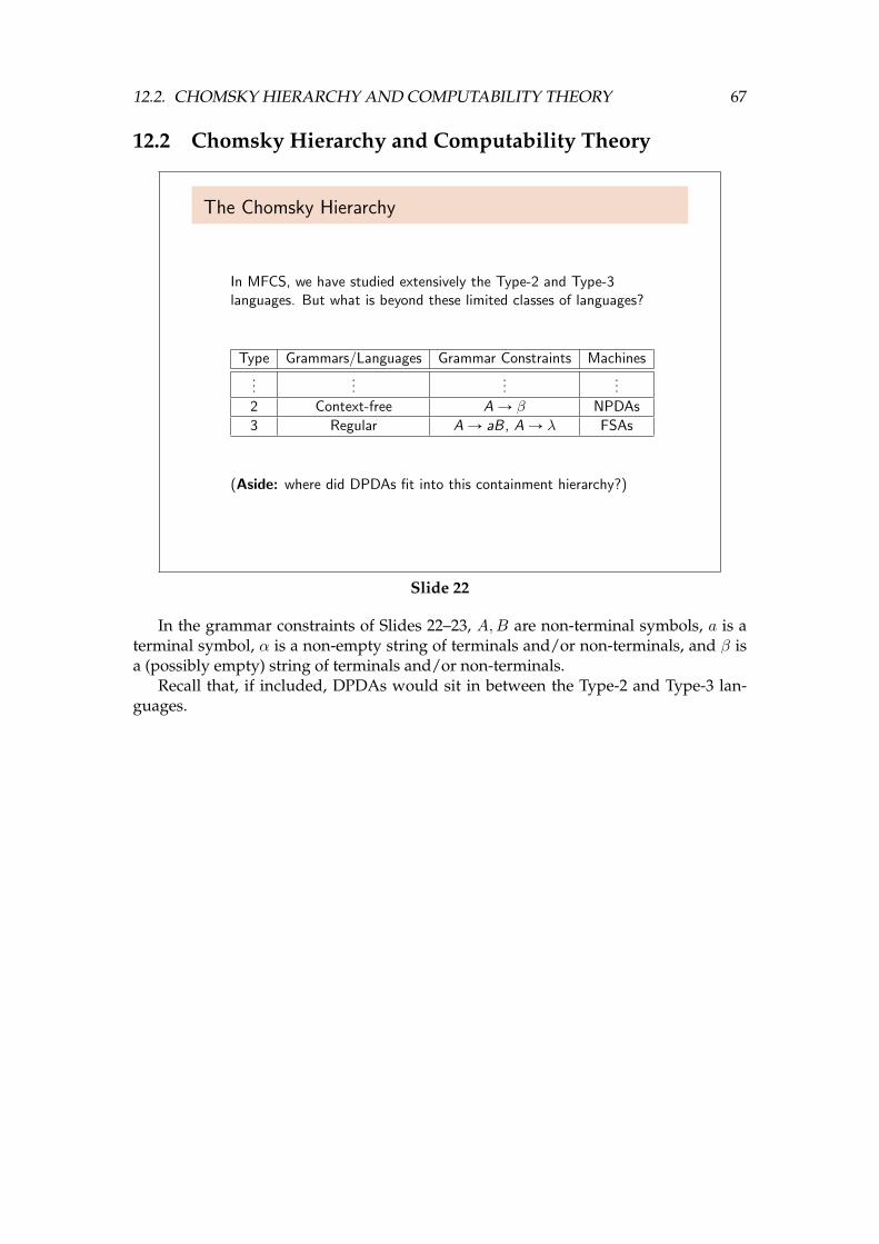
In MFCS, we have studied extensively the Type-2 and Type-3languages. But what is beyond these limited classes of languages?
Type Grammars/Languages Grammar Constraints Machines...
......
...
2 Context-free AÑ β NPDAs
3 Regular AÑ aB, AÑ λ FSAs
(Aside: where did DPDAs fit into this containment hierarchy?)
Slide 22
In the grammar constraints of Slides 22–23, A,B are non-terminal symbols, a is aterminal symbol, α is a non-empty string of terminals and/or non-terminals, and β isa (possibly empty) string of terminals and/or non-terminals.
Recall that, if included, DPDAs would sit in between the Type-2 and Type-3 lan-guages.
68 LECTURE 12.
The Chomsky Hierarchy
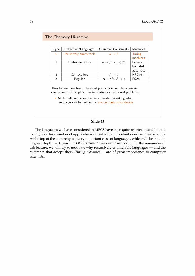
Type Grammars/Languages Grammar Constraints Machines
0 Recursively enumerable αÑ β Turingmachines
1 Context-sensitive αÑ β, |α| ď |β| Linear-boundedautomata
2 Context-free AÑ β NPDAs
3 Regular AÑ aB, AÑ λ FSAs
Thus far we have been interested primarily in simple languageclasses and their applications in relatively constrained problems.
§ At Type-0, we become more interested in asking whatlanguages can be defined by any computational device.
Slide 23
The languages we have considered in MFCS have been quite restricted, and limitedto only a certain number of applications (albeit some important ones, such as parsing).At the top of the hierarchy is a very important class of languages, which will be studiedin great depth next year in COCO: Computability and Complexity. In the remainder ofthis lecture, we will try to motivate why recursively enumerable languages — and theautomata that accept them, Turing machines — are of great importance to computerscientists.
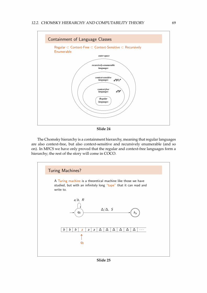
12.2. CHOMSKY HIERARCHY AND COMPUTABILITY THEORY 69
Containment of Language Classes
Regular Ă Context-Free Ă Context-Sensitive Ă RecursivelyEnumerable
nbna
outer-space
c
languages
languages
languages
languages n
context-free nbna
recursively-enumerable
context-sensitive
Regular
Slide 24
The Chomsky hierarchy is a containment hierarchy, meaning that regular languagesare also context-free, but also context-sensitive and recursively enumerable (and soon). In MFCS we have only proved that the regular and context-free languages form ahierarchy; the rest of the story will come in COCO.
Turing Machines?
A Turing machine is a theoretical machine like those we havestudied, but with an infinitely long “tape” that it can read andwrite to.
haq0
a{b, R
∆{∆, S
b b b a a a ∆ ∆ ∆ ∆ ∆ ∆ ¨ ¨ ¨
Ñ
q0
Slide 25
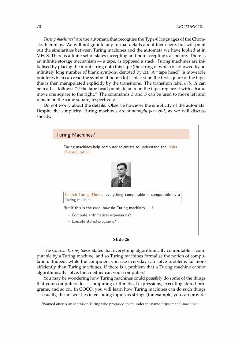
70 LECTURE 12.
Turing machines2 are the automata that recognise the Type-0 languages of the Chom-sky hierarchy. We will not go into any formal details about them here, but will pointout the similarities between Turing machines and the automata we have looked at inMFCS. There is a finite set of states (accepting and non-accepting), as before. There isan infinite storage mechanism — a tape, as opposed a stack. Turing machines are ini-tialised by placing the input string onto this tape (the string of which is followed by aninfinitely long number of blank symbols, denoted by ∆). A “tape head” (a moveablepointer which can read the symbol it points to) is placed on the first square of the tape;this is then manipulated explicitly by the transitions. The transition label a/b, R canbe read as follows: “if the tape head points to an a on the tape, replace it with a b andmove one square to the right.” The commands L and S can be used to move left andremain on the same square, respectively.
Do not worry about the details. Observe however the simplicity of the automata.Despite the simplicity, Turing machines are stunningly powerful, as we will discussshortly.
Turing Machines?
Turing machines help computer scientists to understand the limitsof computation.
Church-Turing Thesis: everything computable is computable by aTuring machine.
But if this is the case, how do Turing machines . . . ?
§ Compute arithmetical expressions?
§ Execute stored programs? . . .
Slide 26
The Church-Turing thesis states that everything algorithmically computable is com-putable by a Turing machine, and so Turing machines formalise the notion of compu-tation. Indeed, while the computers you use everyday can solve problems far moreefficiently than Turing machines, if there is a problem that a Turing machine cannotalgorithmically solve, then neither can your computers!
You may be wondering how Turing machines could possibly do some of the thingsthat your computers do — computing arithmetical expressions, executing stored pro-grams, and so on. In COCO, you will learn how Turing machines can do such things— usually, the answer lies in encoding inputs as strings (for example, you can provide
2Named after Alan Mathison Turing who proposed them under the name “a(utomatic)-machine”.
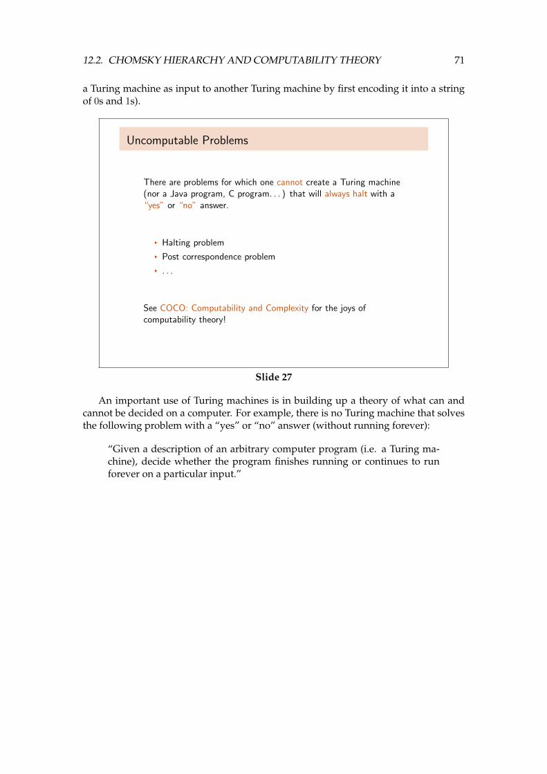
12.2. CHOMSKY HIERARCHY AND COMPUTABILITY THEORY 71
a Turing machine as input to another Turing machine by first encoding it into a stringof 0s and 1s).
Uncomputable Problems
There are problems for which one cannot create a Turing machine(nor a Java program, C program. . . ) that will always halt with a“yes” or “no” answer.
§ Halting problem
§ Post correspondence problem
§ . . .
See COCO: Computability and Complexity for the joys ofcomputability theory!
Slide 27
An important use of Turing machines is in building up a theory of what can andcannot be decided on a computer. For example, there is no Turing machine that solvesthe following problem with a “yes” or “no” answer (without running forever):
“Given a description of an arbitrary computer program (i.e. a Turing ma-chine), decide whether the program finishes running or continues to runforever on a particular input.”
72 LECTURE 12.
Alan Turing Year
A Centenary Celebration of the Life and Work of Alan Turing
http://www.mathcomp.leeds.ac.uk/turing2012/
Slide 28
Alan Turing was born one hundred years ago, and so in 2012 we celebrate hismany contributions to computer science, artificial intelligence, mathematics, biology,and other areas too. His codebreaking work at Bletchley Park during the Second WorldWar is widely acknowledged to have shortened it, and to have potentially saved largenumbers of lives. He is acknowledged as one of Britain’s greatest mathematicians.
While we celebrate his fascinating life and work, we do however acknowledge thetragedy of his death. His life was cut short only a little before his 42nd birthday, whenhe died from cyanide poisoning at home, determined to be suicide. Not long beforethis, he had been prosecuted by the United Kingdom after admitting a homosexual act(which was illegal at the time). He was “treated” with female hormone injections as aform of chemical castration. It was not until 2009 that the British government officiallyapologised for his treatment, after an internet-based campaign.
As a “father” of computer science, it is worth the time to read about Alan Turing’slife. Wikipedia is a good starting point for this:
http://en.wikipedia.org/wiki/Alan_Turing
12.3. SUMMARY 73
12.3 Summary
Summary
Today we have covered:
§ CFG simplifications: useless symbols, λ-productions, unitproductions;
§ How to translate a CFG into Chomsky Normal Form;
§ The (full) Chomsky hierarchy; and
§ Glimpsed into the future: computability theory!
Slide 29
That’s all folks!
Thanks and Good Luck!
http://www.cs.york.ac.uk/~cposkitt/
Reading: my notes; Hopcroft Section 7.1; Linz Sections 6.2 and 11.4.
Slide 30
74 LECTURE 12.
Bibliography
[Coh97] Daniel I.A. Cohen. Introduction to Computer Theory. Wiley, 2nd edition, 1997.
[HMU06] John E. Hopcroft, Rajeev Motwani, and Jeffrey D. Ullman. Introduction toAutomata Theory, Languages, and Computation. Pearson, 3rd edition, 2006.
[Lin06] Peter Linz. An introduction to formal languages and automata. Jones and BartlettPublishers, 4th edition, 2006.
75
Related Documents


