Metric forensics: a multi-level approach for mining volatile graphs

METRICFORENSICS: A Multi-Level Approach for Mining Volatile Graphs∗

Keith Henderson† Tina Eliassi-Rad† Christos Faloutsos‡ Leman Akoglu‡

Lei Li‡ Koji Maruhashi§ B. Aditya Prakash‡ Hanghang Tong‡

Abstract

Advances in data collection and storage capacity have madeit increasingly possible to collect highly volatile graph data foranalysis. Existing graph analysis techniques are not appropriatefor such data, especially in cases where streaming or near-real-time results are required. An example that has drawn signifi-cant research interest is the cyber-security domain, where inter-net communication traces are collected and real-time discovery ofevents, behaviors, patterns, and anomalies is desired. We proposeMETRICFORENSICS, a scalable framework for analysis of volatilegraphs. METRICFORENSICS combines a multi-level “drill down”approach, a collection of user-selected graph metrics, and a col-lection of analysis techniques. At each successive level, more so-phisticated metrics are computed and the graph is viewed at finertemporal resolutions. In this way, METRICFORENSICS scales tohighly volatile graphs by only allocating resources for computa-tionally expensive analysis when an interesting event is discov-ered at a coarser resolution first. We test METRICFORENSICS onthree real-world graphs: an enterprise IP trace, a trace of legit-imate and malicious network traffic from a research institution,and the MIT Reality Mining proximity sensor data. Our largestgraph has ∼3M vertices and ∼32M edges, spanning 4.5 days.The results demonstrate the scalability and capability of METRIC-FORENSICS in analyzing volatile graphs; and highlight four novelphenomena in such graphs: elbows, broken correlations, prolongedspikes, and lightweight stars.

∗This work was performed under the auspices of theU.S. Department of Energy by Lawrence Livermore Na-tional Laboratory under contract No. DE-AC52-07NA27344.LLNL-CONF-432792.†Lawrence Livermore National Laboratory, Livermore, Cal-ifornia, USA, {keith, eliassi}@llnl.gov‡Carnegie Mellon University, Pittsburgh, Pennsylvania,USA, {christos, lakoglu, leili, badityap, htong}@cs.cmu.edu§Fujitsu Laboratories Ltd., Kawasaki, Japan,[email protected]

Copyright 2010 Association for Computing Machinery. ACM acknowl-edges that this contribution was authored or co-authored by an employee,contractor or affiliate of the U.S. Government. As such, the Government re-tains a nonexclusive, royalty-free right to publish or reproduce this article,or to allow others to do so, for Government purposes only.KDD’10, July 25–28, 2010, Washington, DC, USA.Copyright 2010 ACM 978-1-4503-0055-110/07 ...$5.00.

Categories and Subject Descriptors

H.2.8 [Database Applications]: Data mining; E.1 [DataStructures]: Graphs and networks

General Terms

Algorithms, Design, Performance, Experimentation.

Keywords

Graph mining, temporal analysis, volatile graphs

1. Introduction

Given a stream of duration-stamped communication- orcontact-events, how can we find suspicious behaviors, pat-terns, and anomalies in real-time or near real-time? Howcan we do attribution? For example, in a computer commu-nication network, we would like to detect the interval thatwe are under attack, as well as the offending IP address (oraddresses).

We define a “volatile graph” to be a stream of duration-stamped edges (in its simplest form: 〈vsrc, vdst, start time,duration〉), where we assume that there are potentially infi-nite number of nodes, and that edges may appear and dis-appear. Examples of volatile graphs include IP-to-IP com-munication graphs (either at the backbone or at the access-link) as well as physical proximity graphs (e.g., measuredby blue-tooth connections).

This paper introduces METRICFORENSICS which given avolatile graph is able to characterize it and detect interest-ing events at multiple levels (both temporally and topologi-cally). At the global level, METRICFORENSICS computes andmonitors a suite of graph metrics (e.g., the number of activenodes, the first few eigenvalues, their wavelet transforms,etc) at regular intervals. Only when a deviation from usualbehavior is flagged, METRICFORENSICS follows through witha “drill down” approach, where the offending graph is stud-ied at finer temporal and topological resolutions. In partic-ular, flagged sub-graphs (community-level) and even indi-vidual nodes (local-level) are examined using more sophis-ticated and time-consuming metrics and analysis techniques(such as ego-net analysis). Thus, METRICFORENSICS is able

to do attribution of the rare event, while maintaining highprocessing speed.

The contributions of METRICFORENSICS are as follows:

• Effectiveness: METRICFORENSICS spots strange activi-ties, like “elbows” (Section 4.1.1), broken correlations(Section 4.1.2), prolonged spikes (Section 4.1.3), and“lightweight” stars (Section 4.3).

• Scalability: All the components of METRICFORENSICSare carefully chosen to be not only informative, butalso fast to compute (linear on the measures of inter-est).

• Flexibility and generality: The METRICFORENSICS frame-work can easily include other modules in addition tothe ones described, like spectral analysis, PageRank,etc. Moreover, the method can be applied to any typeof volatile graphs (e.g., email/SMS communications).

METRICFORENSICS satisfies the six requirements of anemerging application. They are:1. Requirements for the application: METRICFORENSICS’application is mining of highly volatile graphs representedas streams of duration-stamped edges. This application isuseful in analysis of various communication data (e.g., IPtraffic, phone-calls, blue-tooth connections, twitter feeds, etc).Its requirements are scalability and ability to run in a stream-ing or (near) real-time environment.2. Approach: METRICFORENSICS is a multi-level graph-mining framework, which takes as input a stream of volatilegraphs (represented by duration-stamped edges), constructssummary graphs, and conducts multi-level scalable graphanalysis (such as eigen-value, fractal dimension, and corre-lation analyses). METRICFORENSICS is easily extensible toinclude analysis modules besides the ones presented here.See Figure 1.3. Deployment: METRICFORENSICS has been released tovarious projects within Lawrence Livermore National Lab-oratory. We plan to deploy the system to our governmentsponsors and release the code as open source.4. Evaluation: METRICFORENSICS was evaluated on threereal-world volatile graphs from various domains. Our largestgraph has∼3M vertices and∼32M edges, spanning 4.5 days.The results were verified by inspection of background infor-mation (such as deep packet-capture analysis) and discus-sions with analysts.5. Pragmatic issues: METRICFORENSICS’ framework is de-signed to be scalable (i.e., operate on graphs with millionsof nodes and edges) and run in streaming or (near) real-timeenvironments. See Tables 1 and 2.6. Comparative evaluation: Existing approaches either failin key requirements and functionalities (such as scalability,multi-level graph analysis, and attribution) or can be eas-ily added as a module into METRICFORENSICS’ extendableframework (see Section 2). For example, one of the clos-est systems is Redback [32], which takes a series of graphsand conducts single-level graph analysis. METRICFOREN-SICS and Redback are not directly comparable since Redback(a) puts the burden of discretizing the stream of edges on theuser, (b) it does not conduct multi-level analysis, (c) it is notscalable (the largest graphs reportedly tested on Redbackare hundreds of nodes), and (d) Redback is not open-source.METRICFORENSICS can be used to compare different analy-

sis algorithms such as BGP-Lens [30] and fractal dimensionanalysis (see Section 4.1.3).

The outline of the paper is as follows: Section 1 providesan introduction to this work. Section 2 presents an overviewof the related work. Section 3 describes our proposed frame-work, METRICFORENSICS. Section 4 presents experimentalresults on three real-world volatile graphs. Lastly, Section 5provides some concluding remarks.

2. Background and Related Work

We divide related work into four parts: (1) mining staticgraphs, (2) mining time-evolving graphs, (3) anomaly detec-tion on graphs and finally (4) mining time series.

Mining Static Graphs. This work can be grouped intothree levels. First, on the graph-level, there are discover-ies on the statistical properties of some global metrics (e.g.,degree distribution, diameter, first eigenvalue, etc) of thewhole graph [3, 15, 8, 28]. Next, at the subgraph level, re-search has focused on frequent substructure discovery [35],graph partitioning, and community detection (eg [16]. Fi-nally, at the individual node/edge level, past work includeslink prediction [26], ranking [17], and proximity [33]. Notethat almost all of the previous work deals with only one ofthe three levels, while METRICFORENSICS works on all thelevels in a “drill down” way.

Mining Dynamic Graphs. Most work here has focusedon community evolution [4, 13] and dynamic tensor anal-ysis [31]. Again, most of the above analyze only one of thethree levels (graph level, subgraph level, or node/edge level),and, typically, on a single, fixed time-granularity, in contrastto METRICFORENSICS.

Anomaly Detection on Graphs. Gibbons and Matias [18]proposed a fast method to compute “heavy-hitters” (that is,frequently-occurring items, like source-IP addresses). Lakhinaet al. [24] suggested using entropy to characterize a con-nectivity matrix. Bunke et al. [9] use similar measures tospot differences between connectivity matrices and to reportanomalies when these differences are too high. Additionalwork includes methods based on the minimum descriptionlength (MDL) principle [29, 10], classification-based meth-ods [27], probabilistic measures [14], and spectral methods [21,20]. In OddBall [2], they explicitly focus on the “individual”node-level by examining the 1-step-away ego-networks. Fora comprehensive list, see a recent survey [12]. All such meth-ods can be folded within METRICFORENSICS framework atthe appropriate topological and temporal levels.

Mining Time Series. Related work here includes click-through rate estimation [1] and outlier detection [25]. Again,METRICFORENSICS can naturally incorporate these meth-ods into its framework, such as BGP-Lens [30] for findingpatterns and anomalies in Internet routing updates.

3. METRICFORENSICS

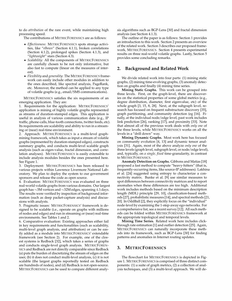
The flowchart for METRICFORENSICS is depicted in Fig-ure 1. METRICFORENSICS is comprised of three distinct com-ponents: (1) a suite of graph metrics, (2) a collection of anal-ysis techniques, and (3) a multi-level approach. We will de-

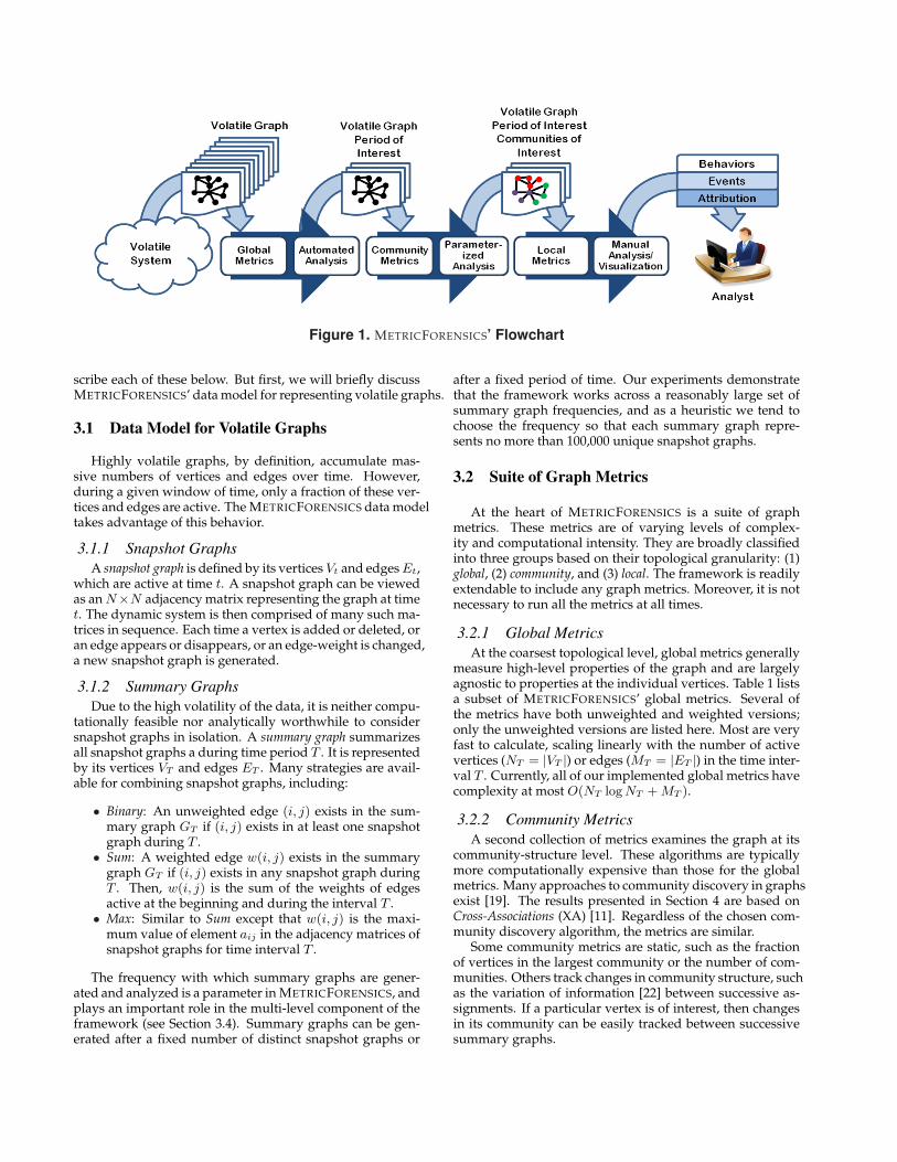
Figure 1. METRICFORENSICS’ Flowchart

scribe each of these below. But first, we will briefly discussMETRICFORENSICS’ data model for representing volatile graphs.

3.1 Data Model for Volatile Graphs

Highly volatile graphs, by definition, accumulate mas-sive numbers of vertices and edges over time. However,during a given window of time, only a fraction of these ver-tices and edges are active. The METRICFORENSICS data modeltakes advantage of this behavior.

3.1.1 Snapshot GraphsA snapshot graph is defined by its vertices Vt and edges Et,

which are active at time t. A snapshot graph can be viewedas an N×N adjacency matrix representing the graph at timet. The dynamic system is then comprised of many such ma-trices in sequence. Each time a vertex is added or deleted, oran edge appears or disappears, or an edge-weight is changed,a new snapshot graph is generated.

3.1.2 Summary GraphsDue to the high volatility of the data, it is neither compu-

tationally feasible nor analytically worthwhile to considersnapshot graphs in isolation. A summary graph summarizesall snapshot graphs a during time period T . It is representedby its vertices VT and edges ET . Many strategies are avail-able for combining snapshot graphs, including:

• Binary: An unweighted edge (i, j) exists in the sum-mary graph GT if (i, j) exists in at least one snapshotgraph during T .

• Sum: A weighted edge w(i, j) exists in the summarygraph GT if (i, j) exists in any snapshot graph duringT . Then, w(i, j) is the sum of the weights of edgesactive at the beginning and during the interval T .

• Max: Similar to Sum except that w(i, j) is the maxi-mum value of element aij in the adjacency matrices ofsnapshot graphs for time interval T .

The frequency with which summary graphs are gener-ated and analyzed is a parameter in METRICFORENSICS, andplays an important role in the multi-level component of theframework (see Section 3.4). Summary graphs can be gen-erated after a fixed number of distinct snapshot graphs or

after a fixed period of time. Our experiments demonstratethat the framework works across a reasonably large set ofsummary graph frequencies, and as a heuristic we tend tochoose the frequency so that each summary graph repre-sents no more than 100,000 unique snapshot graphs.

3.2 Suite of Graph Metrics

At the heart of METRICFORENSICS is a suite of graphmetrics. These metrics are of varying levels of complex-ity and computational intensity. They are broadly classifiedinto three groups based on their topological granularity: (1)global, (2) community, and (3) local. The framework is readilyextendable to include any graph metrics. Moreover, it is notnecessary to run all the metrics at all times.

3.2.1 Global MetricsAt the coarsest topological level, global metrics generally

measure high-level properties of the graph and are largelyagnostic to properties at the individual vertices. Table 1 listsa subset of METRICFORENSICS’ global metrics. Several ofthe metrics have both unweighted and weighted versions;only the unweighted versions are listed here. Most are veryfast to calculate, scaling linearly with the number of activevertices (NT = |VT |) or edges (MT = |ET |) in the time inter-val T . Currently, all of our implemented global metrics havecomplexity at most O(NT log NT + MT ).

3.2.2 Community MetricsA second collection of metrics examines the graph at its

community-structure level. These algorithms are typicallymore computationally expensive than those for the globalmetrics. Many approaches to community discovery in graphsexist [19]. The results presented in Section 4 are based onCross-Associations (XA) [11]. Regardless of the chosen com-munity discovery algorithm, the metrics are similar.

Some community metrics are static, such as the fractionof vertices in the largest community or the number of com-munities. Others track changes in community structure, suchas the variation of information [22] between successive as-signments. If a particular vertex is of interest, then changesin its community can be easily tracked between successivesummary graphs.

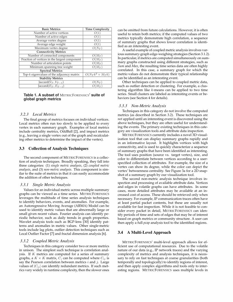
Basic Metrics Time ComplexityNumber of active vertices O(1)Number of active edges O(1)Average vertex degree O(1)Average edge weight O(1)

Maximum vertex degree O(NT )Connectivity Metrics

Number of connected components O(MT )Fraction of vertices in the largest component O(MT )

Number of articulation points O(MT )Minimum spanning tree weight O(MT )

Spectral MetricsTop-k eigenvalues of the adjacency matrix O(NT k2 + MT k)

Stability MetricsJaccard(VT , VT−1) O(NT )Jaccard(ET , ET−1) O(MT )

Table 1. A subset of METRICFORENSICS’ suite ofglobal graph metrics

3.2.3 Local MetricsThe final group of metrics focuses on individual vertices.

Local metrics often run too slowly to be applied to everyvertex in each summary graph. Examples of local metricsinclude centrality metrics, OddBall [2], and impact metrics(e.g., leaving a single vertex out of the graph and recalculat-ing other metrics to determine the impact of the vertex).

3.3 Collection of Analysis Techniques

The second component of METRICFORENSICS is a collec-tion of analysis techniques. Broadly speaking, they fall intothree categories: (1) single metric analysis, (2) coupled metricanalysis, and (3) non-metric analysis. This component is sim-ilar to the suite of metrics in that it can easily accommodatethe addition of other techniques.

3.3.1 Single Metric AnalysisValues for an individual metric across multiple summary

graphs can be viewed as a time series. METRICFORENSICSleverages the multitude of time series analysis techniquesto identify behaviors, events, and anomalies. For example,an Autoregressive Moving Average (ARMA) Model can beused to identify metric values that are abnormally large orsmall given recent values. Fourier analysis can identify pe-riodic behavior, such as daily trends in graph properties.Wavelet analysis tools such as BGP-lens [30] identify pat-terns and anomalies in metric values. Other single-metrictools include lag plots, outlier detection techniques such asLocal Outlier Factor [7] and fractal dimension analysis [6].

3.3.2 Coupled Metric AnalysisTechniques in this category consider two or more metrics

in unison. The simplest such technique is correlation anal-ysis. If K metrics are computed for a series of summarygraphs, a K × K matrix, C, can be computed where Cij issay the Pearson correlation between metrics i and j. Largevalues of |Cij | can identify redundant metrics. If such met-rics vary widely in runtime complexity, then the slower ones

can be omitted from future calculations. However, it is oftenuseful to retain both metrics; if the computed values of twometrics typically demonstrate high correlation, a sequenceof summary graphs that shows lower correlation is identi-fied as an interesting event.

A useful example of coupled metric analysis involves var-ious summary-graph edge-weighing strategies (Section 3.1.2).In particular, if metrics are computed simultaneously on sum-mary graphs constructed using different strategies, such asSum and Max, the resulting time series data are often highlycorrelated. In this case, a summary graph for which themetric-values do not demonstrate their typical relationshipcan be identified as an interesting event.

Other techniques can be applied to coupled metric data,such as outlier detection or clustering. For example, a clus-tering algorithm like k-means can be applied to two timeseries. Small clusters are labeled as interesting events or be-haviors (see Section 4 for details).

3.3.3 Non-Metric AnalysisTechniques in this category do not involve the computed

metrics (as described in Section 3.2). These techniques arenot applied until an interesting event is discovered using theabove techniques, but they are often useful for understand-ing the events. The primary existing techniques in this cate-gory are visualization tools and attribute data inspection.

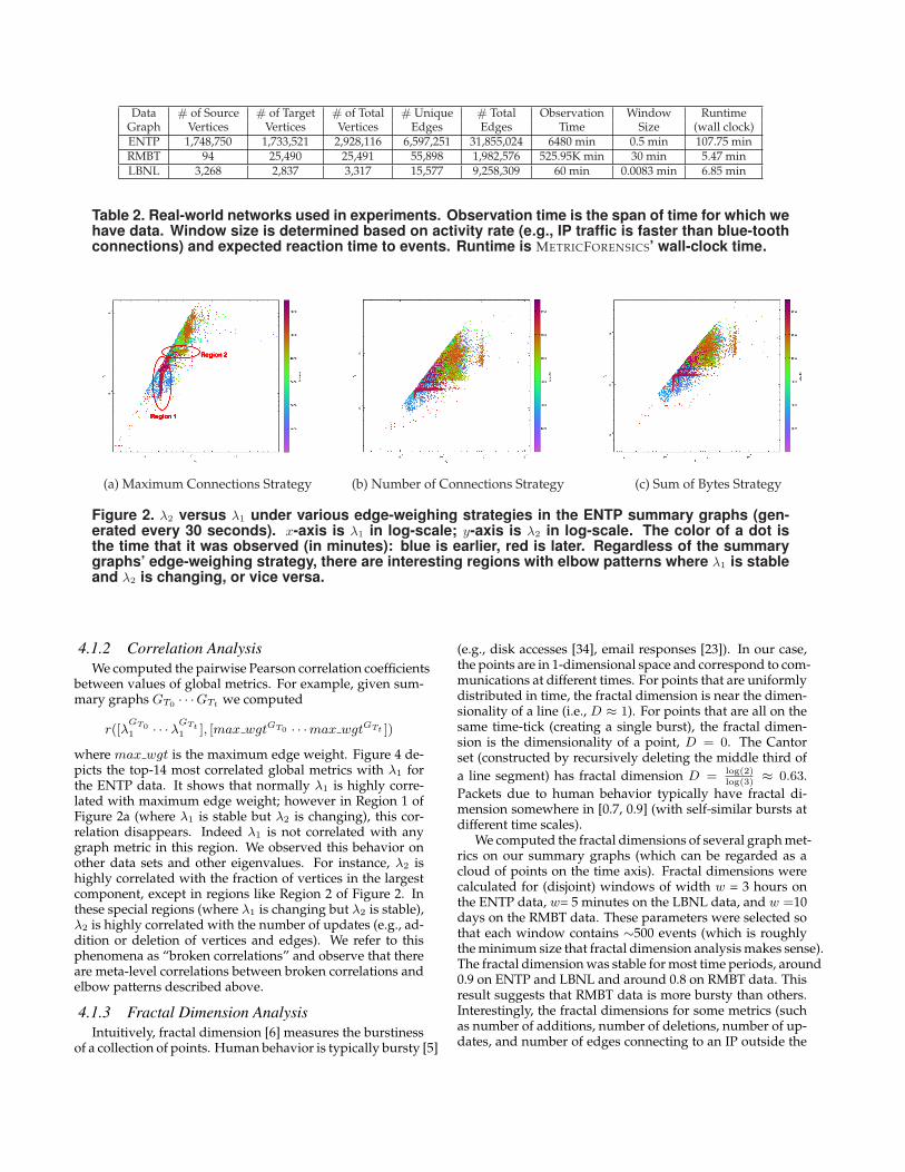
METRICFORENSICS currently includes a novel 3D visual-ization tool that can display summary graphs rapidly andin an informative layout. It highlights vertices with highconnectivity, and is used to quickly characterize a sequenceof summary graphs that have been identified as interesting.The tool uses position (source vs. target vertex), size, andcolor to differentiate between vertices according to a user-specified collection of attributes. For example, the size of avertex can show its degree, while the color can depict thevertex’ betweenness centrality. See Figure 3a for a 2D snap-shot of a summary graph by our visualization tool.

The second non-metric analysis technique involves in-spection and processing of available attribute data. Verticesand edges in volatile graphs can have attributes. In somecases, more detailed attributes may be available at an in-creased cost of access. These should be retrieved only whennecessary. For example, IP communication traces often haveat least partial packet contents, but these are usually notavailable for fast inspection. While it is not feasible to con-sider every packet in detail, METRICFORENSICS can iden-tify periods of time and sets of edges that may be of interestbased on graph metrics or community structure. A user canthen apply a full pcap analysis tool to the identified regions.

3.4 A Multi-Level Approach

METRICFORENSICS’ multi-level approach allows for ef-ficient use of computational resources. Due to the volatilenature of our data (e.g., IP network traces) and the varyingcomplexity of metrics and analysis techniques, it is neces-sary to rely on fast techniques at coarse granularities (bothtemporally and topologically) to identify regions of interest,and then apply complex algorithms and tools only to inter-esting regions. METRICFORENSICS uses multiple levels in

three distinct dimensions: (1) time, (2) topology, and (3) anal-ysis automation.

The general approach involves performing METRICFOREN-SICS’ metrics and analysis multiple times at different levels,starting with the coarsest and becoming finer at each iter-ation. Only those time periods identified as interesting at acoarse level are passed down to be analyzed at the next finerlevel. We generally identify three levels, based on the topo-logical granularity levels (namely, global, community, andlocal). However, METRICFORENSICS supports any numberof levels based on time granularity.

3.4.1 Time GranularityThe temporal scale of METRICFORENSICS can be controlled

in two ways. First, the period of time in which summarygraphs are analyzed can be adjusted. At the coarsest level,METRICFORENSICS operates on all available data, which inmany cases can include streaming data. When an event isdetected, only the relevant portion of the data is examinedat finer levels.1 Second, temporal granularity is adjustedby modifying the interval between summary graphs. Atthe coarsest level, summary graphs are generated less oftenthan in finer levels. This “drill-down” approach is used topinpoint changes in behavior of specific vertices.

3.4.2 Topological GranularityThe axis of refinement here involves which set of graph

metrics are applied. At the coarsest level, only the globaltopology of the graph is considered. Communities and indi-vidual nodes are not generally considered, with the excep-tion of a small number of global statistics that track the iden-tities of high-degree vertices. The global metrics are scalableand can be computed efficiently on each summary graph.When an event is discovered at this level, the period of in-terest is passed to the next (finer) level.

At the finer (regional) level, community-level metrics arecalculated. By identifying communities that exhibit change,METRICFORENSICS can discard many vertices that have notchanged their behavior. This information is subsequentlyused at the finest level of refinement, where local metricsare computed on vertices in the identified communities.

3.4.3 Analysis Automation LevelsThe final difference between levels in METRICFORENSICS

is the selection of analysis techniques. Some techniques,such as ARMA, are fully automated. These can be applied atany refinement level. Other tools and techniques like visu-alization and attribute analysis require user interaction andshould only be applied to small sets of summary graphs.

4. Experiments

We implemented METRICFORENSICS in Java (with someMatlab modules) and ran experiments on a commodity ma-chine Intel Core 2 Duo @2.93GHz with 4Gb of memory. Ourexperiments answer the following questions: (1) Can MET-RICFORENSICS detect interesting events including anomalies?1In a streaming setting, this is accomplished by maintaininga circular buffer that stores a fixed number of recent snap-shot graphs.

(2) Do the discovered interesting events tell us something newabout the nature of volatile graphs? (3) Is METRICFORENSICSscalable and amenable to real-time (or near real-time) execution?

Table 2 lists the graphs used in our experiments. ENTP isIP traffic collected at the perimeter of an enterprise networkover 4.5 days in 2007. RMBT is the MIT Reality Mining’sblue-tooth connections collected over 12 months.2 LBNLis IP traffic collected on an internal enterprise network on2004/12/15 on port #3.3 It includes scanning activities.

4.1 Experiments at the Global Level

We discuss some experiments at the global-level of ourvolatile graphs here. For brevity, we have removed many ofresults (such as our Fourier and wavelet analyses).

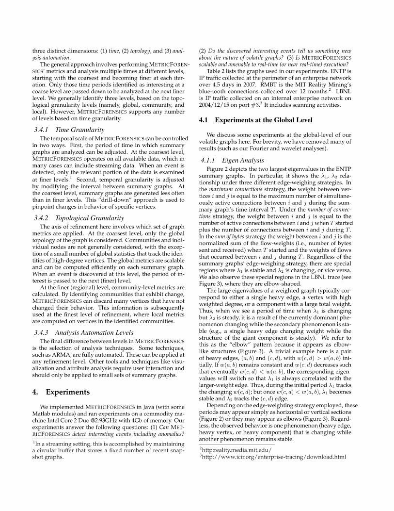
4.1.1 Eigen AnalysisFigure 2 depicts the two largest eigenvalues in the ENTP

summary graphs. In particular, it shows the λ1, λ2 rela-tionship under three different edge-weighing strategies. Inthe maximum connections strategy, the weight between ver-tices i and j is equal to the maximum number of simultane-ously active connections between i and j during the sum-mary graph’s time interval T . Under the number of connec-tions strategy, the weight between i and j is equal to thenumber of active connections between i and j when T startedplus the number of connections between i and j during T .In the sum of bytes strategy the weight between i and j is thenormalized sum of the flow-weights (i.e., number of bytessent and received) when T started and the weights of flowsthat occurred between i and j during T . Regardless of thesummary graphs’ edge-weighing strategy, there are specialregions where λ1 is stable and λ2 is changing, or vice versa.We also observe these special regions in the LBNL trace (seeFigure 3), where they are elbow-shaped.

The large eigenvalues of a weighted graph typically cor-respond to either a single heavy edge, a vertex with highweighted degree, or a component with a large total weight.Thus, when we see a period of time when λ1 is changingbut λ2 is steady, it is a result of the currently dominant phe-nomenon changing while the secondary phenomenon is sta-ble (e.g., a single heavy edge changing weight while thestructure of the giant component is steady). We refer tothis as the “elbow” pattern because it appears as elbow-like structures (Figure 3). A trivial example here is a pairof heavy edges, (a, b) and (c, d), with w(c, d) > w(a, b) ini-tially. If w(a, b) remains constant and w(c, d) decreases suchthat eventually w(c, d) < w(a, b), the corresponding eigen-values will switch so that λ1 is always correlated with thelarger-weight edge. Thus, during the initial period λ1 tracksthe changing w(c, d); but once w(c, d) < w(a, b), λ1 becomesstable and λ2 tracks the (c, d) edge.

Depending on the edge-weighting strategy employed, theseperiods may appear simply as horizontal or vertical sections(Figure 2) or they may appear as elbows (Figure 3). Regard-less, the observed behavior is one phenomenon (heavy edge,heavy vertex, or heavy component) that is changing whileanother phenomenon remains stable.2http:reality.media.mit.edu/3http://www.icir.org/enterprise-tracing/download.html

Data # of Source # of Target # of Total # Unique # Total Observation Window RuntimeGraph Vertices Vertices Vertices Edges Edges Time Size (wall clock)ENTP 1,748,750 1,733,521 2,928,116 6,597,251 31,855,024 6480 min 0.5 min 107.75 minRMBT 94 25,490 25,491 55,898 1,982,576 525.95K min 30 min 5.47 minLBNL 3,268 2,837 3,317 15,577 9,258,309 60 min 0.0083 min 6.85 min

Table 2. Real-world networks used in experiments. Observation time is the span of time for which wehave data. Window size is determined based on activity rate (e.g., IP traffic is faster than blue-toothconnections) and expected reaction time to events. Runtime is METRICFORENSICS’ wall-clock time.

(a) Maximum Connections Strategy (b) Number of Connections Strategy (c) Sum of Bytes Strategy

Figure 2. λ2 versus λ1 under various edge-weighing strategies in the ENTP summary graphs (gen-erated every 30 seconds). x-axis is λ1 in log-scale; y-axis is λ2 in log-scale. The color of a dot isthe time that it was observed (in minutes): blue is earlier, red is later. Regardless of the summarygraphs’ edge-weighing strategy, there are interesting regions with elbow patterns where λ1 is stableand λ2 is changing, or vice versa.

4.1.2 Correlation AnalysisWe computed the pairwise Pearson correlation coefficients

between values of global metrics. For example, given sum-mary graphs GT0 · · ·GTt we computed

r([λGT01 · · ·λGTt

1 ], [max wgtGT0 · · ·max wgtGTt ])

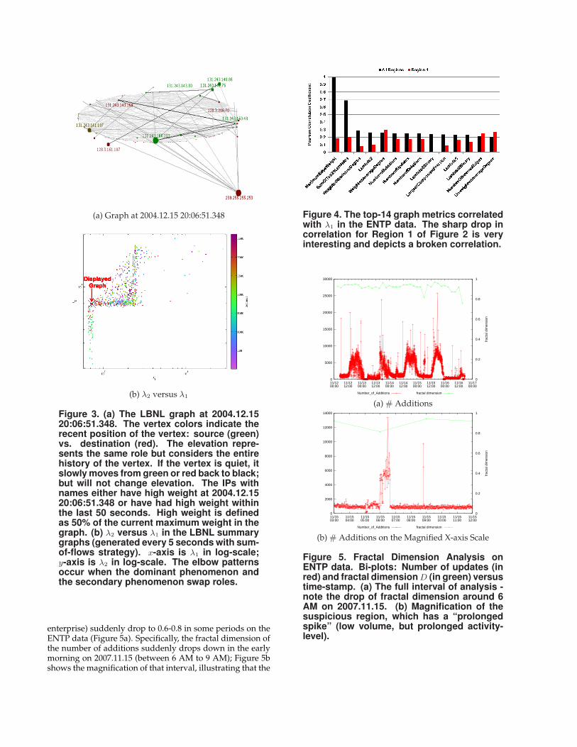
where max wgt is the maximum edge weight. Figure 4 de-picts the top-14 most correlated global metrics with λ1 forthe ENTP data. It shows that normally λ1 is highly corre-lated with maximum edge weight; however in Region 1 ofFigure 2a (where λ1 is stable but λ2 is changing), this cor-relation disappears. Indeed λ1 is not correlated with anygraph metric in this region. We observed this behavior onother data sets and other eigenvalues. For instance, λ2 ishighly correlated with the fraction of vertices in the largestcomponent, except in regions like Region 2 of Figure 2. Inthese special regions (where λ1 is changing but λ2 is stable),λ2 is highly correlated with the number of updates (e.g., ad-dition or deletion of vertices and edges). We refer to thisphenomena as “broken correlations” and observe that thereare meta-level correlations between broken correlations andelbow patterns described above.

4.1.3 Fractal Dimension AnalysisIntuitively, fractal dimension [6] measures the burstiness

of a collection of points. Human behavior is typically bursty [5]

(e.g., disk accesses [34], email responses [23]). In our case,the points are in 1-dimensional space and correspond to com-munications at different times. For points that are uniformlydistributed in time, the fractal dimension is near the dimen-sionality of a line (i.e., D ≈ 1). For points that are all on thesame time-tick (creating a single burst), the fractal dimen-sion is the dimensionality of a point, D = 0. The Cantorset (constructed by recursively deleting the middle third ofa line segment) has fractal dimension D = log(2)

log(3)≈ 0.63.

Packets due to human behavior typically have fractal di-mension somewhere in [0.7, 0.9] (with self-similar bursts atdifferent time scales).

We computed the fractal dimensions of several graph met-rics on our summary graphs (which can be regarded as acloud of points on the time axis). Fractal dimensions werecalculated for (disjoint) windows of width w = 3 hours onthe ENTP data, w= 5 minutes on the LBNL data, and w =10days on the RMBT data. These parameters were selected sothat each window contains ∼500 events (which is roughlythe minimum size that fractal dimension analysis makes sense).The fractal dimension was stable for most time periods, around0.9 on ENTP and LBNL and around 0.8 on RMBT data. Thisresult suggests that RMBT data is more bursty than others.Interestingly, the fractal dimensions for some metrics (suchas number of additions, number of deletions, number of up-dates, and number of edges connecting to an IP outside the

(a) Graph at 2004.12.15 20:06:51.348

(b) λ2 versus λ1

Figure 3. (a) The LBNL graph at 2004.12.1520:06:51.348. The vertex colors indicate therecent position of the vertex: source (green)vs. destination (red). The elevation repre-sents the same role but considers the entirehistory of the vertex. If the vertex is quiet, itslowly moves from green or red back to black;but will not change elevation. The IPs withnames either have high weight at 2004.12.1520:06:51.348 or have had high weight withinthe last 50 seconds. High weight is definedas 50% of the current maximum weight in thegraph. (b) λ2 versus λ1 in the LBNL summarygraphs (generated every 5 seconds with sum-of-flows strategy). x-axis is λ1 in log-scale;y-axis is λ2 in log-scale. The elbow patternsoccur when the dominant phenomenon andthe secondary phenomenon swap roles.

enterprise) suddenly drop to 0.6-0.8 in some periods on theENTP data (Figure 5a). Specifically, the fractal dimension ofthe number of additions suddenly drops down in the earlymorning on 2007.11.15 (between 6 AM to 9 AM); Figure 5bshows the magnification of that interval, illustrating that the

Figure 4. The top-14 graph metrics correlatedwith λ1 in the ENTP data. The sharp drop incorrelation for Region 1 of Figure 2 is veryinteresting and depicts a broken correlation.

0

5000

10000

15000

20000

25000

30000

11/1200:00

11/1212:00

11/1300:00

11/1312:00

11/1400:00

11/1412:00

11/1500:00

11/1512:00

11/1600:00

11/1612:00

11/1700:00

0

0.2

0.4

0.6

0.8

1

frac

tal d

imen

sion

Number_of_Additions fractal dimension

(a) # Additions

0

2000

4000

6000

8000

10000

12000

14000

11/1503:00

11/1504:00

11/1505:00

11/1506:00

11/1507:00

11/1508:00

11/1509:00

11/1510:00

11/1511:00

11/1512:00

0

0.2

0.4

0.6

0.8

1

frac

tal d

imen

sion

Number_of_Additions fractal dimension

(b) # Additions on the Magnified X-axis Scale

Figure 5. Fractal Dimension Analysis onENTP data. Bi-plots: Number of updates (inred) and fractal dimension D (in green) versustime-stamp. (a) The full interval of analysis -note the drop of fractal dimension around 6AM on 2007.11.15. (b) Magnification of thesuspicious region, which has a “prolongedspike” (low volume, but prolonged activity-level).

drop is due to a “prolonged spike”: activity that has low-volume, but persists for a long time. We also observed thisphenomena with wavelet analysis and the BGP-lens pack-age [30]. For brevity, we omit the wavelet analysis.

4.2 Experiments at the Community Level

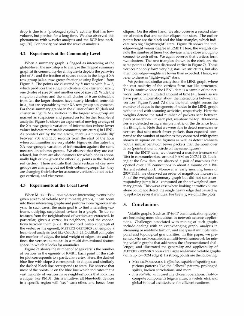
When a summary graph is flagged as interesting at theglobal-level, the next step is to analyze the flagged summarygraph at its community-level. Figure 6a depicts the pairwiseplot of λ1 and the fraction of source nodes in the largest XArow-group (a.k.a. row-group fraction) during Region 1 fromFigure 2. The points are clustered by k-means with k = 8,which produces five singleton clusters, one cluster of size 6,one cluster of size 37, and another one of size 352. While thesingleton clusters and the small cluster of 6 are detectablefrom λ1, the larger clusters have nearly identical centroidsin λ1 but are separable by their XA row-group assignments.For those summary graphs in the cluster of size 37 (dark redcluster in Figure 6a), vertices in the largest row-group aremarked as suspicious and passed on for further local-levelanalysis. Figure 6b shows an exponential moving average ofthe XA row-group’s variation-of-information (where lowervalues indicate more stable community structures) in LBNL.As pointed out by the red arrow, there is a noticeable dipbetween 750 and 1100 seconds from the start of the hourwhen communities are very stable. Figure 6c illustrates theXA row-group’s variation of information against the samemeasure on column groups. We observe that they are cor-related, but there are also instances for which one is abnor-mally high or low given the other (i.e., points in the dashedred circles). These indicate that there vertices whose row-groups are changing but not their column-groups (i.e., theyare changing their behavior as source vertices but not as tar-get vertices), and vice versa.

4.3 Experiments at the Local Level

When METRICFORENSICS detects interesting events in thegiven stream of volatile (or summary) graphs, it can zoominto those interesting graphs and perform more rigorous anal-ysis. In such cases, the main goal is to find interesting (ex-treme, outlying, suspicious) vertices in a graph. To do so,features from the neighborhood of vertices are extracted. Inparticular, given a vertex, its neighbors, and the connec-tions between them (a.k.a. the induced 1-step subgraph ofthe vertex or the egonet), METRICFORENSICS can employ alocal-level analysis tool like OddBall [2]. OddBall computesthe number of edges, the total weight of edges, etc and de-fines the vertices as points in a multi-dimensional featurespace, in which it looks for anomalies.

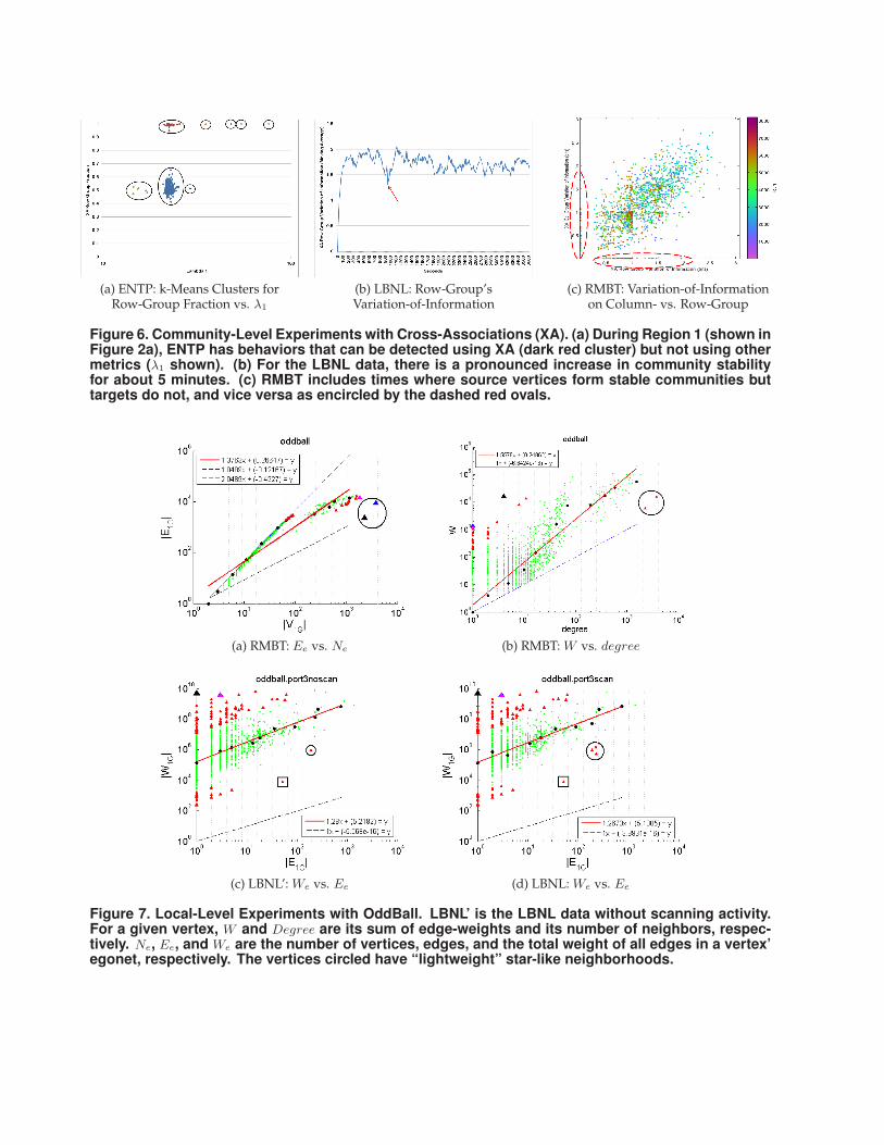
Figure 7a shows the number of edges versus the numberof vertices in the egonets of RMBT. Each point in the scat-ter plot corresponds to a particular vertex. Here, the dashedblue line with slope 2 corresponds to cliques and similarlythe dashed black line corresponds to stars. We observe thatmost of the points lie on the blue line which indicates that avast majority of vertices have neighborhoods that look likea clique. For RMBT, this is intuitive; all blue-tooth devicesin a specific region will “see” each other, and hence form

cliques. On the other hand, we also observe a second clus-ter of nodes that are neither cliques nor stars. The outlierpoints here are the black and the blue triangles, which indi-cate two big “lightweight” stars. Figure 7b shows the totaledge-weight versus degree in RMBT. Here, the weights de-note the number of times two devices where close enough toconnect to each other. We again observe that vertices formtwo clusters. The two triangles shown in the circle are thesame points as the ones discussed earlier in Figure 7a. Thesevertices not only form very big star-like structures, but alsotheir total edge-weights are lower than expected. Hence, werefer to these as “lightweight” stars.

We performed similar analysis on the LBNL graph, wherethe vast majority of the vertices form star-like structures.This is intuitive since the LBNL data is a sample of the net-work traffic over a limited amount of time (≈1 hour), so wehave partial information about the interactions between allvertices. Figure 7c and 7d show the total weight versus thenumber of edges in the egonets of nodes in the LBNL graphwithout and with scanning activities, respectively. Here theweights denote the total number of packets sent betweenpairs of machines. On each plot, we show the top 100 anoma-lies we detected using a simple metric of the distance fromthe fitting line. Note that we were able to detect non-scannervertices that sent much fewer packets than expected com-pared to the number of machines they connected with (pointshown in square on the figures) as well as detect scannerswith a similar behavior: fewer packets than the norm overlinks (points shown in circle on the same figures).

For the ENTP data, we observed a massive increase (of10x) in communications around 9 AM on 2007.11.12. Look-ing at the flow data, we observed a pair of machines thatopened over 10K connections in about a minute on a Bit-Torrent related port. Moreover in early morning hours of2007.11.13, we observed an order of magnitude increase inλ1 of the weighted summary graph but did not see a cor-responding jump in λ1 computed on the unweighted sum-mary graph. This was a case where looking at traffic volumealone could not detect the single heavy edge that caused λ1

to spike for several minutes. For brevity, we omit the plots.

5. Conclusions

Volatile graphs (such as IP-to-IP communication graphs)are becoming more ubiquitous in network science applica-tions. Challenges associated with mining of such graphsinclude dealing with an ever-changing graph, analysis instreaming or real-time fashion, and analysis at multiple tem-poral and topological granularities. In this paper, we pre-sented METRICFORENSICS: a multi-level framework for min-ing volatile graphs that addresses the aforementioned chal-lenges; and illustrated the generality and applicability ofMETRICFORENSICS on several large real-world volatile graphs(with up to∼32M edges). Its strong points are the following:

• METRICFORENSICS is effective, capable of spotting sus-picious patterns like the “elbow” pattern, prolongedspikes, broken correlations, and more.

• It is scalable, with carefully chosen operations, fast-to-compute components (eigenvalues, wavelets, etc), andglobal-to-local architecture, for efficient runtimes.

(a) ENTP: k-Means Clusters for (b) LBNL: Row-Group’s (c) RMBT: Variation-of-InformationRow-Group Fraction vs. λ1 Variation-of-Information on Column- vs. Row-Group

Figure 6. Community-Level Experiments with Cross-Associations (XA). (a) During Region 1 (shown inFigure 2a), ENTP has behaviors that can be detected using XA (dark red cluster) but not using othermetrics (λ1 shown). (b) For the LBNL data, there is a pronounced increase in community stabilityfor about 5 minutes. (c) RMBT includes times where source vertices form stable communities buttargets do not, and vice versa as encircled by the dashed red ovals.

(a) RMBT: Ee vs. Ne (b) RMBT: W vs. degree

(c) LBNL’: We vs. Ee (d) LBNL: We vs. Ee

Figure 7. Local-Level Experiments with OddBall. LBNL’ is the LBNL data without scanning activity.For a given vertex, W and Degree are its sum of edge-weights and its number of neighbors, respec-tively. Ne, Ee, and We are the number of vertices, edges, and the total weight of all edges in a vertex’egonet, respectively. The vertices circled have “lightweight” star-like neighborhoods.

• It is flexible, general and extensible, with room for manymore components, in addition to ones used (fractal anal-ysis, OddBall, wavelets, etc.)

6. References

[1] D. Agarwal, A. Z. Broder, D. Chakrabarti, D. Diklic,V. Josifovski, and M. Sayyadian. Estimating rates ofrare events at multiple resolutions. In KDD, pages16–25, 2007.

[2] L. Akoglu, M. McGlohon, and C. Faloutsos. OddBall:Spotting anomalies in weighted graphs. In PAKDD,2010.

[3] R. Albert, H. Jeong, and A.-L. Barabasi. Diameter ofthe world wide web. Nature, (401):130–131, 1999.

[4] L. Backstrom, D. P. Huttenlocher, J. M. Kleinberg, andX. Lan. Group formation in large social networks:membership, growth, and evolution. In KDD, pages44–54, 2006.

[5] A.-L. Barabasi. The origin of bursts and heavy tails inhuman dynamics. Nature, 435:207–211, 2005.

[6] A. Belussi and C. Faloutsos. Estimating the selectivityof spatial queries using the ‘correlation’ fractaldimension. In VLDB, pages 299–310, 1995.

[7] M. M. Breunig, H.-P. Kriegel, R. T. Ng, and J. Sander.LOF: Identifying density-based local outliers. InSIGMOD, pages 93–104, 2000.

[8] A. Z. Broder, R. Kumar, F. Maghoul, P. Raghavan,S. Rajagopalan, R. Stata, A. Tomkins, and J. L. Wiener.Graph structure in the web. Computer Networks,33(1-6):309–320, 2000.

[9] H. Bunke, P. J. Dickinson, A. Humm, C. Irniger, andM. Kraetzl. Graph sequence visualisation and itsapplication to computer network monitoring andabnormal event detection. In A. Kandel, H. Bunke, andM. Last, editors, Applied Graph Theory in ComputerVision and Pattern Recognition, volume 52 of Studies inComputational Intelligence, pages 227–245. Springer,2007.

[10] D. Chakrabarti. Autopart: Parameter-free graphpartitioning and outlier detection. In PKDD, pages112–124, 2004.

[11] D. Chakrabarti, S. Papadimitriou, D. Modha, andC. Faloutsos. Fully automatic cross-associations. InKDD, pages 79–88, 2004.

[12] V. Chandola, A. Banerjee, and V. Kumar. Anomalydetection: A survey. ACM Comput. Surv., 41(3), 2009.

[13] Y. Chi, X. Song, D. Zhou, K. Hino, and B. L. Tseng.Evolutionary spectral clustering by incorporatingtemporal smoothness. In KDD, pages 153–162, 2007.

[14] W. Eberle and L. B. Holder. Mining for structuralanomalies in graph-based data. In DMIN, 2007.

[15] M. Faloutsos, P. Faloutsos, and C. Faloutsos. Onpower-law relationships of the internet topology. InSIGCOMM, pages 251–262, 1999.

[16] G. Flake, S. Lawrence, C. L. Giles, and F. Coetzee.Self-organization and identification of webcommunities. IEEE Computer, 35(3):66–71, 2002.

[17] F. Geerts, H. Mannila, and E. Terzi. Relationallink-based ranking. In VLDB, pages 552–563, 2004.

[18] P. B. Gibbons and Y. Matias. New sampling-basedsummary statistics for improving approximate queryanswers. In SIGMOD, pages 331–342, 1998.

[19] K. Henderson, T. Eliassi-Rad, S. Papdimitriou, andC. Faloutsos. HCDF: A hybrid community discoveryframework. In SDM, 2010.

[20] S. Hirose, K. Yamanishi, T. Nakata, and R. Fujimaki.Network anomaly detection based on eigen equationcompression. In KDD, pages 1185–1194, 2009.

[21] T. Ide and H. Kashima. Eigenspace-based anomalydetection in computer systems. In KDD, pages440–449, 2004.

[22] B. Karrer, E. Levina, and M. E. J. Newman. Robustnessof community structure in networks. Phys. Rev. E,77(046119), 2008.

[23] J. M. Kleinberg. Bursty and hierarchical structure instreams. In KDD, pages 91–101, 2002.

[24] A. Lakhina, M. Crovella, and C. Diot. Mininganomalies using traffic feature distributions. InSIGCOMM, pages 217–228, 2005.

[25] J.-G. Lee, J. Han, and X. Li. Trajectory outlier detection:A partition-and-detect framework. In ICDE, pages140–149, 2008.

[26] D. Liben-Nowell and J. Kleinberg. The link predictionproblem for social networks. In CIKM, pages 556–559,2003.

[27] C. Liu, X. Yan, H. Yu, J. Han, and P. S. Yu. Miningbehavior graphs for ”backtrace” of noncrashing bugs.In SDM, 2005.

[28] M. E. J. Newman. The structure and function ofcomplex networks. SIAM Review, 45:167–256, 2003.

[29] C. C. Noble and D. J. Cook. Graph-based anomalydetection. In KDD, pages 631–636, 2003.

[30] B. A. Prakash, N. Valler, D. Andersen, M. Faloutsos,and C. Faloutsos. BGP-lens: Patterns and anomalies ininternet routing updates. In KDD, pages 1315–1324,2009.

[31] J. Sun, D. Tao, and C. Faloutsos. Beyond streams andgraphs: dynamic tensor analysis. In KDD, pages374–383, 2006.

[32] V. Syrotiuk, K. Shaukat, Y. Kwon, M. Kraetzl, andJ. Arnold. Application of a network dynamics analysistool to mobile ad hoc networks. In MSWiM, pages36–43, 2006.

[33] H. Tong, C. Faloutsos, and J.-Y. Pan. Random walkwith restart: Fast solutions and applications.Knowledge and Information Systems: An InternationalJournal (KAIS), 14(3):327–346, 2008.

[34] M. Wang, N. H. Chan, S. Papadimitriou, C. Faloutsos,and T. Madhyastha. Data mining meets performanceevaluation: Fast algorithms for modeling burstytraffic. In ICDE, pages 507–516, 2002.

[35] D. Xin, J. Han, X. Yan, and H. Cheng. Miningcompressed frequent-pattern sets. In VLDB, pages709–720, 2005.