Methods for Feature Extraction of an Outcrop using ...

Methods for Feature Extraction of an

Outcrop using Terrestrial LiDAR

Surya Pahal 4390695

Bachelor Thesis

Supervisors: Dr. R.C. Lindenbergh

Dr. J.E.A Storms

Faculty of Civil Engineering and Geosciences

TU Delft 6/7/2018

2

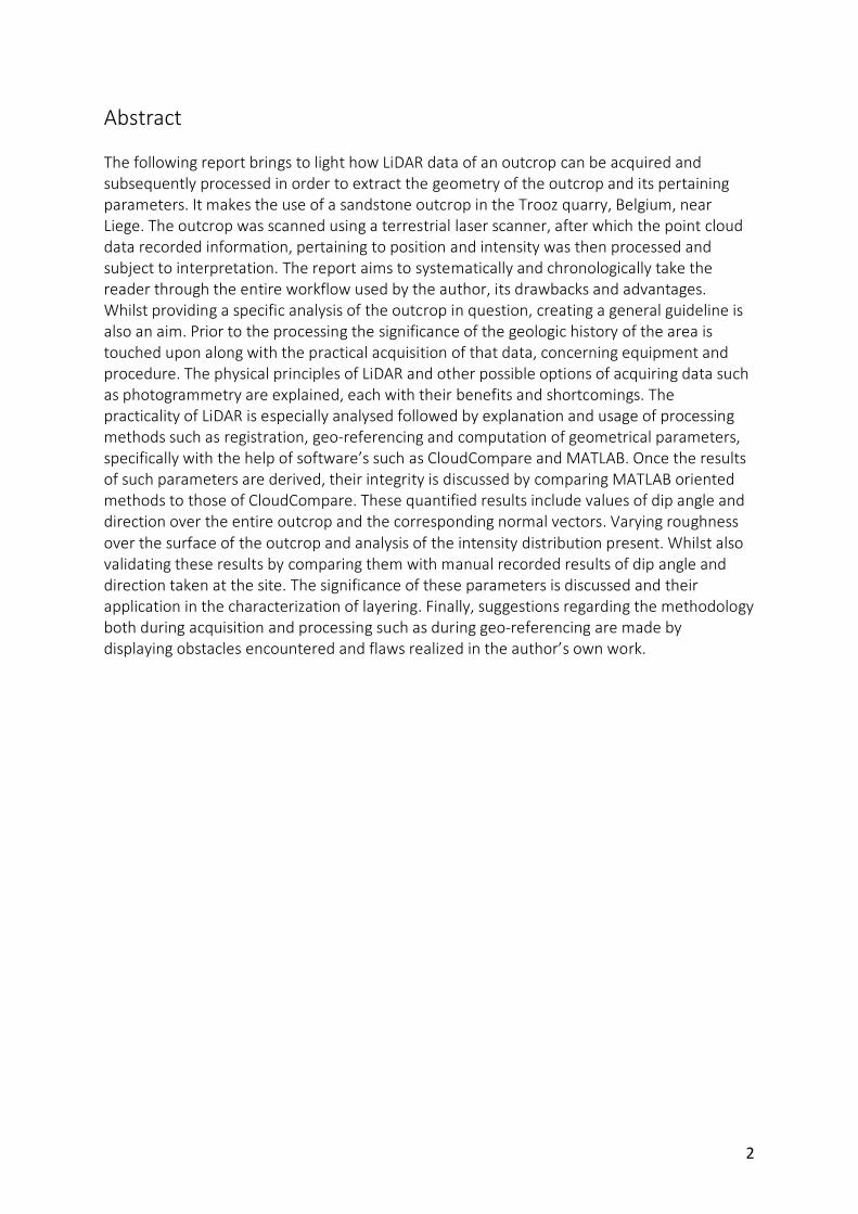
Abstract The following report brings to light how LiDAR data of an outcrop can be acquired and subsequently processed in order to extract the geometry of the outcrop and its pertaining parameters. It makes the use of a sandstone outcrop in the Trooz quarry, Belgium, near Liege. The outcrop was scanned using a terrestrial laser scanner, after which the point cloud data recorded information, pertaining to position and intensity was then processed and subject to interpretation. The report aims to systematically and chronologically take the reader through the entire workflow used by the author, its drawbacks and advantages. Whilst providing a specific analysis of the outcrop in question, creating a general guideline is also an aim. Prior to the processing the significance of the geologic history of the area is touched upon along with the practical acquisition of that data, concerning equipment and procedure. The physical principles of LiDAR and other possible options of acquiring data such as photogrammetry are explained, each with their benefits and shortcomings. The practicality of LiDAR is especially analysed followed by explanation and usage of processing methods such as registration, geo-referencing and computation of geometrical parameters, specifically with the help of software’s such as CloudCompare and MATLAB. Once the results of such parameters are derived, their integrity is discussed by comparing MATLAB oriented methods to those of CloudCompare. These quantified results include values of dip angle and direction over the entire outcrop and the corresponding normal vectors. Varying roughness over the surface of the outcrop and analysis of the intensity distribution present. Whilst also validating these results by comparing them with manual recorded results of dip angle and direction taken at the site. The significance of these parameters is discussed and their application in the characterization of layering. Finally, suggestions regarding the methodology both during acquisition and processing such as during geo-referencing are made by displaying obstacles encountered and flaws realized in the author’s own work.

3

Table of Contents

Chapter 1 ......................................................................................................................................... 5

1.1 Introduction ............................................................................................................................... 5

1.2: Research Questions .................................................................................................................. 6

Chapter 2: Geology and Geometric Parameters ............................................................................ 7

2.1 Geologic Setting and History .................................................................................................... 7

2.2 Sedimentology and Lithology .................................................................................................... 8

2.3 Geometric Parameters ........................................................................................................... 10

Chapter 3: Methods, Equipment and Acquisition of Field Data ................................................. 11

3.1 Theory of Methods ................................................................................................................. 11

LiDAR ............................................................................................................................................. 11

Photogrammetry .......................................................................................................................... 12

3.2 Equipment ............................................................................................................................... 13

3.3 Test Scans ............................................................................................................................... 14

3.4 Acquiring Field Data ............................................................................................................... 16

Chapter 4 Processing and Methodology ..................................................................................... 19

4.1 Alignment and Registration ................................................................................................... 19

4.2 Geo-referencing ...................................................................................................................... 21

4.3 Computation of Normals........................................................................................................ 23

4.4 Orientation and other parameters ........................................................................................ 24

4.5 Conclusions ............................................................................................................................. 28

Chapter 5 Results .......................................................................................................................... 29

5.1 Geo-referencing ...................................................................................................................... 29

5.2 Normals................................................................................................................................... 30

5.3 Orientation.............................................................................................................................. 32

5.4 Roughness ............................................................................................................................... 34

5.5 Intensity .................................................................................................................................. 37

5.6 Discussion ............................................................................................................................... 38

4

Chapter 6 Conclusion and Recommendations ............................................................................ 39

6.1 Conclusions ............................................................................................................................. 39

6.2 Recommendations .................................................................................................................. 40

References ..................................................................................................................................... 41

Appendix ....................................................................................................................................... 42

Guideline to Geo-referencing ....................................................................................................... 42

Kabsch Algorithm Implemented in MATLAB ............................................................................... 43

MATLAB Script .............................................................................................................................. 45

5

Chapter 1

1.1 Introduction Developments in technology for both recording and processing point cloud data have allowed for more efficient and precise virtual analysis of objects. In this instance, the object of interest is a rock outcrop located in a quarry in the municipality of Trooz in Belgium, to the south of Liège. Various methods were used in order to record the point cloud data, however recording data using a terrestrial laser scanner and LiDAR will be specifically focused upon, the process and equipment used. The principles of LiDAR itself, and how it uses the time of flight methodology to calculate coordinates of scanned points, and the types of data it records such as intensity and RGB values will be discussed. Furthermore, how this point cloud data can then be processed and subsequently used to extract certain geometric features using a variety of software’s will also be explained. The outcrop is from the Condroz formation, a primarily sandstone formation from the Paleozoic era, more accurately the late Devonian. The objective was find ways to extract the geometry of the outcrop and model it to find multiple defining parameters characteristic to the outcrop. Such geometric parameters to be extracted include normals, orientations and roughness. The process involved going to the location of the outcrop and scanning it, after which the point cloud data recorded from the scans would have to be processed in order for analysis. The outcrop was also scanned in other ways, such as with pictures from drones, and the DSLR camera in order to model the outcrop with photogrammetry. The applicability and proficiency of these numerous methods is talked about and how they could then be used for cross-referencing and validation of the terrestrial scans. The processing of the LiDAR data and its modelling made the use of multiple software’s such as CloudCompare, Matlab, GoogleEarth and QGIS. The report also goes through how these programmes can be used to extract the previously mentioned features from the created models and how these features are then representative of the outcrop and why. The following report aims to take one through usage of the equipment used in the scanning, such as the targets and the scanner as well as the principles of scanning. The processing that the raw data had to be put through once the scans were complete and how then the geometrical attributes of the outcrop were derived. Simultaneously the quality of these results is discussed and whether these attributes amongst others can be used in order to characterize layering. Finally, conclusions will be drawn and discussed regarding the extracted features and their significance, amidst recommendations regarding the procedure.

6

1.2: Research Questions and Thesis Outline This report hopes to answer the following research questions as thoroughly as possible. Main research question: - How can LiDAR data be processed in order to derive geometrical parameters

of an outcrop? Sub-questions: - How can point cloud data of outcrops be acquired and subsequently processed?

- How can geometrical features of an outcrop be extracted from LiDAR data?

- What are the average values of these parameters for the given outcrop?

- What significance do such features have?

- Which geometrical parameters prove to be representative of the formation and its

layering?

- How can these results be validated?

The report begins introducing the Trooz quarry geology and highlighting important events in its geologic history that have led to its current setting. As well as indicating certain characteristics that may appear in the scans, the most integral being the layering itself and what it comprises of. Followed by the equipment and scanning procedure used in recording the LiDAR data using the Leica ScanStation P40. Whilst also explaining how the ScanStation works itself, its specifications and the principles of light detection and ranging (LiDAR). After delving in the acquisition of the data the subsequent processing using CloudCompare and MATLAB is discussed and how exactly the geometric parameters were extracted and calculated. Following the processing chapter, the results and their integrity are discussed by comparison to manually recorded results, moreover the influence of the processing on the results is talked about. After which there is a concluding chapter in which the drawbacks of certain processes are discussed, and how such steps could have been improved and made more efficient.

7

Chapter 2: Geology and Geometric Parameters

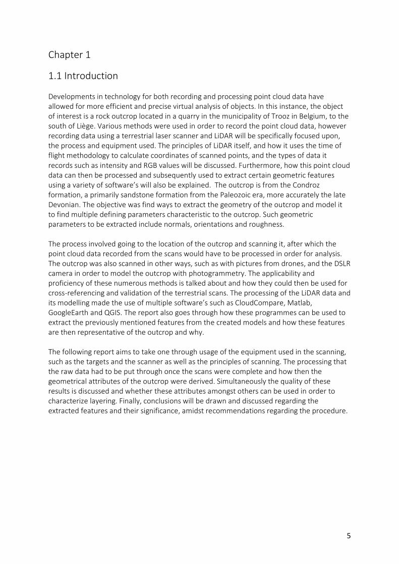
2.1 Geologic Setting and History As mentioned earlier the Condroz sandstone formation is from the late Devonian, to be more exact from the upper Famennian, being a stage in the uppermost Devonian [1]. In Belgium these Famennian outcrops are encountered in five distinct tectonic settings, with the one encountered in Trooz being from the Namur Synclinorium. The early Famennian produced underlying shales (the Famenne shales) after which predominantly sandy sediments were deposited (the Condroz sandstones). Figure 2.11 shows the distribution of sediments from respective eras in Belgium below and to its right, figure 2.12 shows the locations of where the Famennian is encountered.

Figure 2.11 Figure 2.12 In the early Devonian the Caledonian orogeny was coming to end, with the agglomeration of Avalonia, Baltica and Laurentia to form Laurasia or the old red continent. With lower Paleozoic rocks being covered uncomformably in Devonian sediments, however another orogeny was just beginning, the Variscan orogeny, stemming from the collision of Gondwana and Laurasia [2]. With Gondwana approaching from the South in a northward direction, the sea in between the both, the Rhenohercynian basin subsequently closed and led to a compressive setting. Furthermore, the sediments deposited within the basin from the Famennian era were also compressed, leading to a series of faults and extensive tilting. All the prior explains why the Namur synclinorium consists of a succession of synclinal folds. Containing Devonian rocks in a piggyback basin due to orogeneses discussed further on, from sandstone to mica schists after which there are successions of very dark limestones. With the depositional environment gradually becoming shallower from the Devonian towards the Carboniferous due to the compressional setting.

8

2.2 Sedimentology and Lithology All the sediments present in the outcrop originate from the old red continent or Laurasia. To the South of which was the previously mentioned water body called the Rhenohercynian Basin. From which alluvial transport brought and deposited sediments in a delta, carried by the Western Boundary Current (WBC) [12]. The sediments were transported and re-worked and finally deposited in the Condroz shelf area. Consequent of the process mentioned above a wide variety of sedimentation formed, including alluvial, estuarine, lagoonal and shallow marine. The sandstones from the Condroz group were identified as arkosic, meaning that it’s a clastic rock containing about 25 percent feldspar. These sandstones are fine-grained, composed of quartz and feldspars and quite well sorted. Below is figure 2.21, which shows a breakdown of the lithology of the Namur synclinorium and the other encountered Famennian outcrops in Belgium: Figure 2.21

9

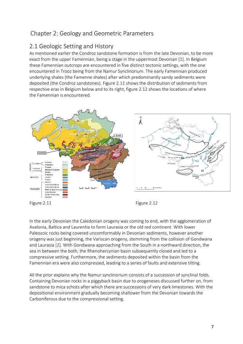
The outcrop showed alternations of layers over its entirety, the alternations were of sandstone (the lighter segments, they appear to be grey on the intensity scale) and shales (which show up as darker layers on the intensity scale). The rising of water levels results in more shales whereas on the other hand shallowing results in a larger amount of sands. The stratigraphic sequence shows shales, followed by large sands, after which there are smaller sands, soils, followed by a deepening resulting in the sequence starting again with shales. At the top of the sequence there are soils, or red beds, which are a sign of the water drying up, severe shallowing. The result is the presence of soils on which vegetation could grow. All the above processes and signs point towards a trans-regressive sequence, which means there is a sequential rise and fall in the sea level causing the previously mentioned repetitive layering. Furthermore, indications of re-working of the sediments can be seen at the ravinement surfaces, showing the boundary of transitional sequences. The ravinement surface is a transgressive, subaqueous erosional surface caused by near shore marine and shoreline erosion associated with sea level rises. The present sequence is one that is coarsening upward, cross bedding can be seen present in the sands as well. Moreover, channelized bands can be seen, specifically with the sands, this can be seen when there is a non-straight or curved boundary of a layer as compared to a straight one. Finally, there is also a huge fault almost in the middle of the outcrop, probably a result of all the orogenic events that have taken place in the general region over time.

Figure 2.22: The outcrop and its layering

10

2.3 Geometric Parameters Strike and dip refer to the orientation or the attitude of a geologic feature and happen to be the first geometric parameters that will be derived from the quarry outcrop. The strike line of a bed, is a line representing the intersection of that feature with a horizontal plane. The dip direction is the azimuth the direction of dip as projected to the horizontal, which happens to be 90 degrees of the strike angle. The dip direction is quite simply the direction in which the bed is dipping, with it ranging from 0 to 360 degrees. On the other hand, the dip angle is the acute angle that the rock surface makes with the horizontal plane and is a measure of how steeply the bed is dipping. The dip angle has a range from 0 to 90 degrees, figure 2.31 provides an accurate representation of the dip direction and angle. However as will be later discussed we will find that in fact, surface normals will have to be found before anything else in order to calculate the orientation parameters. In a three-dimensional case a surface normal is a vector that perpendicular to the tangent plane that the point is placed on. Lastly another parameter hoped to be found is the surface roughness, which is a component of the surface texture. It is quantified by the deviations in the direction of the normal vector of a real surface from its ideal from (a best fitted plane). If these deviations are large the surface is said to be rough, if they are small then the surface is smooth.

Figure 2.31

11

Chapter 3: Methods, Equipment and Acquisition of Field Data

3.1 Theory of Methods

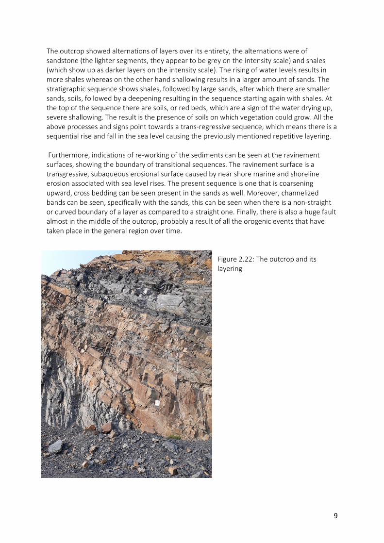
LiDAR The first method to be discussed will be the one this report is primarily concerned with and that is LiDAR. LiDAR is a surveying method that measures distance to a target with a pulsed or continuous laser light and measures the reflected pulses with a sensor, unabbreviated it stands for Light Detection and Ranging [7]. LiDAR was developed in the 1960’s, with it being introduced to terrain mapping in 1970’s since then quality and efficiency of the scanners has progressed significantly. However, the general principle of the sensors remains somewhat the same, the scanners make use of the time of flight methodology. Where the scanner emits a laser pulse or continuous wave and consequently measures and records the reflected energy and the time it takes to return. Differences in laser return times and wavelengths can then be used to make a digital 3D representation of the target in question. Figure 3.11

The pulse is reflected when it hits the surface being measured (the reflector), the objective is to measure the distance between the scanner and the surface and its position. The time of flight methodology allows for this by making a simple calculation, since the time recorded is the two-way travel time, this must be first halved in order to calculate the one-way distance (D) to the object. After which, since the speed of light (C) is known, a simple multiplication of time (T) and speed are made to find the distance to the object. However, an air correction factor (n) must be implemented in reality for a more accurate computation. The formula is a as below:

𝐷 =𝐶𝑛 ×

𝑇2 𝑒𝑞𝑢𝑎𝑡𝑖𝑜𝑛3.11[8]

Furthermore, the co-ordinates of all the data points all recorded relative to the position of the scan station, with it being taken as the origin. As well as this the R, G, B signature of each reflected signal is also stored with the intensity of the signal to produce a more realistic model and provide a more in-depth analysis of the object.

12

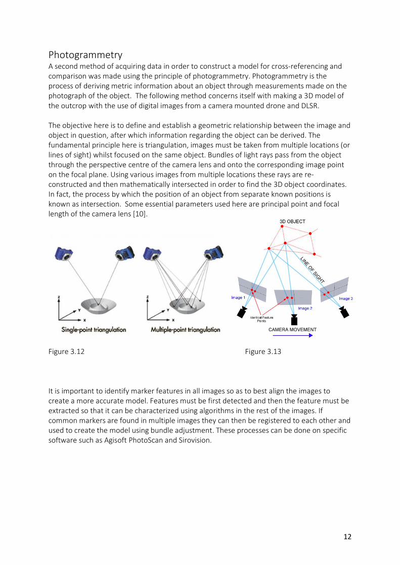
Photogrammetry A second method of acquiring data in order to construct a model for cross-referencing and comparison was made using the principle of photogrammetry. Photogrammetry is the process of deriving metric information about an object through measurements made on the photograph of the object. The following method concerns itself with making a 3D model of the outcrop with the use of digital images from a camera mounted drone and DLSR. The objective here is to define and establish a geometric relationship between the image and object in question, after which information regarding the object can be derived. The fundamental principle here is triangulation, images must be taken from multiple locations (or lines of sight) whilst focused on the same object. Bundles of light rays pass from the object through the perspective centre of the camera lens and onto the corresponding image point on the focal plane. Using various images from multiple locations these rays are re-constructed and then mathematically intersected in order to find the 3D object coordinates. In fact, the process by which the position of an object from separate known positions is known as intersection. Some essential parameters used here are principal point and focal length of the camera lens [10].

Figure 3.12 Figure 3.13 It is important to identify marker features in all images so as to best align the images to create a more accurate model. Features must be first detected and then the feature must be extracted so that it can be characterized using algorithms in the rest of the images. If common markers are found in multiple images they can then be registered to each other and used to create the model using bundle adjustment. These processes can be done on specific software such as Agisoft PhotoScan and Sirovision.

13

3.2 Equipment The primary piece of equipment used in scanning the outcrop was the scanner itself, the Leica ScanStation P40. The P40 is a remarkable piece of equipment as it records the highest quality of 3D data and HDR imaging at an extremely fast scan rate of a million points per second at ranges of up to 270m [9], and having a very large field of view as displayed in figure 3.21:

Figure 3.21 field of view: Vertical 290° Figure 3.22 Horizontal 360° Leica ScanStation P40 Other specifications of the P40 include:

Property Value (Visible Laser) Value (Invisible Laser) Wavelength 658nm 1550nm Beam Divergence (1/e) <1.5mrad <0.23mrad Beam Diameter at front window

<3.5mm (FWHM)

Minimum Range 0.4m Max Range 27m at 34% reflectivity

180m at 18% reflectivity 120m at 18% reflectivity

Range Noise 0.4mm rms at 10m and 0.5mm rms at 50m Table 3.21 [9]

14

The P40 will therefore filter everything out after 270m so as to make sure that all the information it records is accurate. At 270m the data is still quite precise, as there is at most 0.8mm between data points at 10m so at 270m that is 2.16cm between each data point. As well as recording the position of the data points the scanner also records R, G, B values at that point and the subsequent intensity. The intensity being the reflected energy level at each of the data points. The scanner also has an in-built camera so that it can take 360° after the scanning is complete. Other equipment used during scanning included the add-ons for the scanner, such as its height & level adjustable tripod. As well as the batteries for the scanner itself and the targets placed in pre-determined positions so as to aid in aligning multiple scans at a later stage. Furthermore, a GPS coordinate recording device was used for all the targets in order to geo-reference the model, this will be discussed in the theory and methodology chapters. Data was also recorded using secondary methods to be used for validation and verification, this secondary method made the use of a camera mounted drone to take multiple images so as to put them together later using photogrammetry. Simultaneously pictures were also taken of the outcrop from the ground using a DSLR for the same purpose.

3.3 Test Scans Test scans were conducted in order to familiarize with the terrestrial laser scanner and understand the process of acquiring the data. Two preliminary test scans were conducted, first in front of the civil engineering faculty on campus, the second taking place in the botanic gardens in Delft. The focus of the scan in the botanic garden was to successfully scan a treehouse which had been built with a temporary base structure. Four trees had been planted around the treehouse, in hope that at some point in the future these trees would grow and hold up the structure that had been built. The idea was to scan it so that researchers at the university could analyse the current situation of the trees and perhaps check if this was indeed a feasible idea. Below is the first test scan conducted in front of the civil engineering faculty, the scan was done whilst there was a light drizzle in order to see the effect that the rain would have on the scan. The rain ended up barely making a difference to the scan as can be seen in figure 3.31.

Figure 3.31: Point clouds visualized on CloudCompare

15

The next was one of the secondary test scan made in the botanic gardens, five such scans were made after which they would be aligned/registered in order to get a wholesome 3D model of the structure.

Figure 3.32: In the following image the structure was zoomed in on as the abundance of leaves covers the structure and provides a lot of noise. The test scans were helpful in understanding a few essential fundamentals regarding the scanner such as the fact that comprise between resolution of the scan and the duration of it sometimes have to be made. The test scans at the botanic garden took 15 minutes each, with resolution set at 6.3mm at 10m, the sensitivity at high setting, and the max range set 120m, as the scanner was close enough to structure. So, the resolution could be lower as well as the max range, this also conserved time spent taking the scan. However, the sensitivity was kept at high so as to record every signal, even if there were low return signals from poor reflective surfaces. Moreover, many of the features that show in one scan may not be present in another due to position of the scanner in that moment. As the scanner’s position is changes so is its field of view, and certain features may be covered or hidden behind another object, this is known as occlusion. Occlusion can take place in both a vertical and horizontal fashion, to avoid vertical occlusion the scanner should be kept as elevated as possible. Whereas to counteract horizontal occlusion multiple scans are made after which they are aligned/registered to produce 1 main scan with all features present in it, which could have been occluded in individual scans.

16

Figure 3.33: Vertical Occlusion

Figure 4.14: Horizontal Occlusion

3.4 Acquiring Field Data The outcrop was scanned in a quarry in Trooz, Belgium, to the south of Liege. The outcrop is quite big and to minimize the previously mentioned effects of occlusion, three scans were made. Subsequently all the scans were made from different locations covering multiple lines of sight after which the scans could be aligned/registered with one another with the help of 6 targets on the outcrop itself with a few additionally scattered. The outcrop had a roughly a length of 170-180m with a roundabout height of 25m, below is a picture of the quarry, showing the outcrop.

17

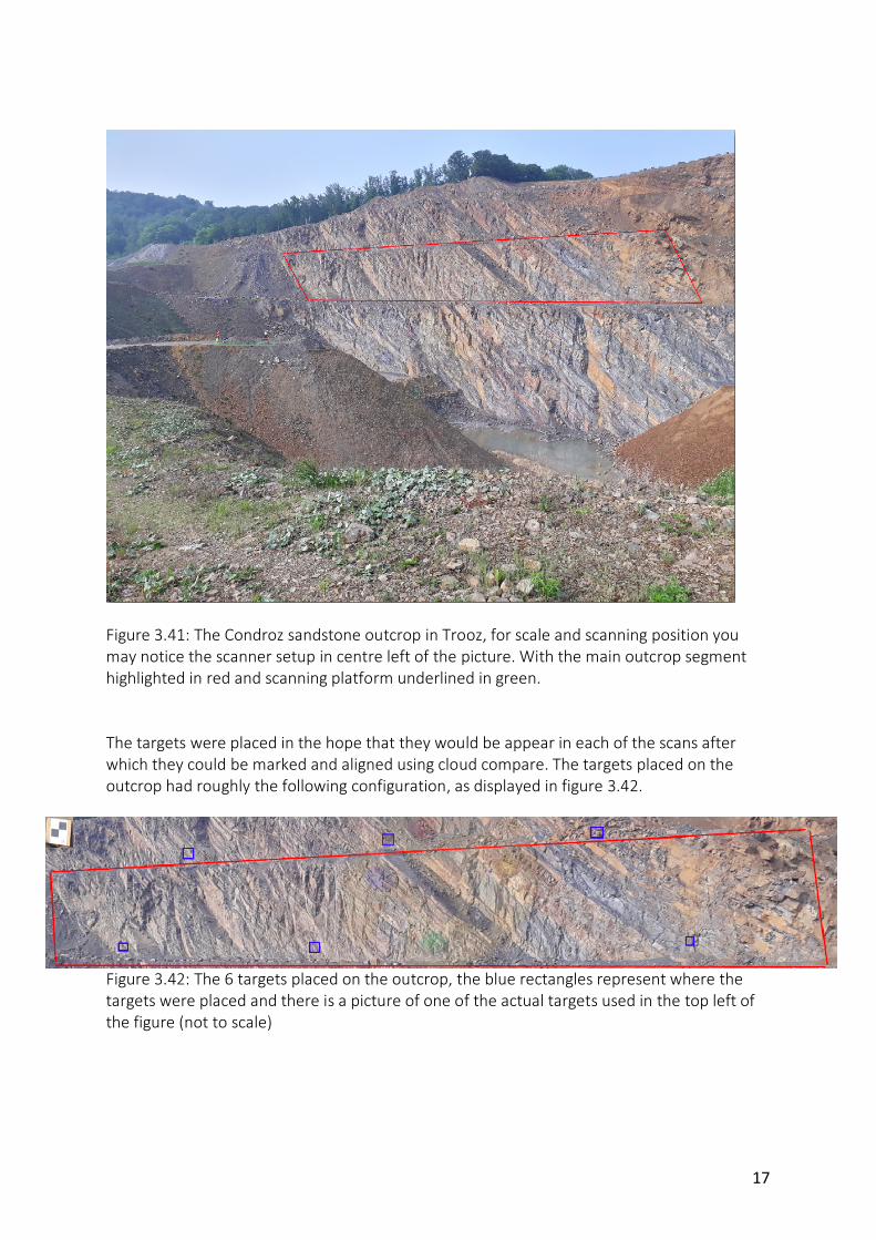
Figure 3.41: The Condroz sandstone outcrop in Trooz, for scale and scanning position you may notice the scanner setup in centre left of the picture. With the main outcrop segment highlighted in red and scanning platform underlined in green. The targets were placed in the hope that they would be appear in each of the scans after which they could be marked and aligned using cloud compare. The targets placed on the outcrop had roughly the following configuration, as displayed in figure 3.42.

Figure 3.42: The 6 targets placed on the outcrop, the blue rectangles represent where the targets were placed and there is a picture of one of the actual targets used in the top left of the figure (not to scale)

18

Figure 3.43: Overall configuration of all targets, the ones placed on the outcrop have been marked in blue and the others marked in red displayed on QGIS

19

Chapter 4 Processing and Methodology The following chapter goes through the processing of the raw data and how certain geometrical parameters were derived using various software’s and methods. Primarily CloudCompare and MATLAB were used in the computation of the parameters, the process began with the registration or alignment of multiple scans. Followed by geo-referencing and filtering of certain unnecessary data and information to further fine tune the model. After which parameters could be calculated beginning with the normals followed by the rest, such as those concerning orientation.

4.1 Alignment and Registration The first step in the processing of the scanned point cloud data, is to align the numerous scans to produce one complete scan or model. This is known as registration, and it means putting all the separate scans (in this case three) into the same co-ordinate system. As when the scans are taken individually they only exist in their own respective co-ordinate systems relative to the scanner itself. The scanner acts as the origin of the individual coordinate systems, so the goal is to put all the scans in to one chosen scans coordinate system, this scan will be known as the master scan. A software known as CloudCompare offers various ways to roughly or finely align point clouds or meshes [14]. To register/align scans with one another, the targets placed in the scanner’s field of view will be used (placed on the outcrop), the point is to identify common features in the scan and align them, therefore aligning the entire scans with one another. The method of registration used for this purpose is alignment via point pair picking and is an inbuilt function in CloudCompare. It lets the user pick several pairs of equivalent points in each cloud in order to register them. While the process is manual it can be relatively fast and quite accurate. In order to see the effect of this alignment, one must have a look at the three separate scans, as shown in figure 4.11, 4.12 & 4.13 Figure 4.11: Scan 1

20

Figure 4.12: Scan 2

Figure 4.13: Scan 3

When you load the scans individually they still exist in segments, in that one individual scan will be of multiple point clouds. A smart move here would be to merge these scans and convert it into one single point cloud, filtering (according to position of the irregular points and unnecessary data) could be applied at this stage however was left till later to be done more accurately in MATLAB. As can be seen the scans were taken from different perspectives and different ranges in terms of field of view, for example scan 3 has the largest field of view hence giving such an elongated point cloud. The first scans aligned with one another were scan 1 & 3, only due to the fact that quality of the scans was much better and that the markers were clearly visible in both scans, so registration was relatively easier. The alignment was done using the previously mentioned method of point pair picking, which meant that the same targets were picked in both scans and simply aligned. A minimum of three targets in both scans was required for this to work, the method required a couple of tries but eventually seemed to work quite well. The registration was evaluated by noticing the continuation of the of the same layering through into the second scan, seeing that it was continuous verified the registration. As well as this the targets used for alignment perfectly overlapped, and the arbitrary targets placed further away from the outcrop had a max error of 5m, seeing this one could say error increases further away from the aligned targets.

21

Figure 4.14: Scan 1 & 3 aligned using point pair picking

After scan 1 and 3 were aligned, next was the registration of scan 2, however scan 2 didn’t turn out so well. As you can tell in the image of scan 2, the point cloud is very scattered and sparse, with only certain parts of the outcrop being scanned successfully. Scan 2’s registration was attempted using the same method as the registration of scan 1 & 3 however this was unsuccessful, as enough markers/targets were not visible in scan 2 for this type of registration. An automatic method to very finely register two entities is the well-known ICP algorithm. ICP stands for iterative closest point, this method allows an input of the amount of iterations and the final RMS difference required. First you pick you aligned point cloud and then your reference one after which the previously mentioned parameters are entered as well as the final overlap required. Following this CloudCompare will try the set number of iterations and find the best fit, unfortunately this method was also unsuccessful, possibility due to the sparsity of the points in the second scan. The alignment would always result in quite a marginal misalignment, as well as this the extra information that scan 2 provided was minimal and so it and its registration with the other scans was omitted. Finally, after all the registration was finalized all the registered scans were merged in order to lock in their alignment.

4.2 Geo-referencing Geo-referencing refers to aligning the common coordinate system that scan 1 and 2 now exist in after registration,0 with the global coordinate system. That is the coordinate system of the master scan had to be transformed in to the global coordinate system, the master scan’s coordinate system is in metres however all relative to the scanner position in the master scan. The aim is convert this into the WGS 84 / UTM Zone 31N, as it would be advisable to keep the coordinate system units in metres for when roughness and other such parameters are computed. Furthermore, this was the specific coordinate system of the Trooz quarry and pretty much the entirety of Belgium allowing for a more appropriate transformation. The Kabsch algorithm was adopted and implemented as code in MATLAB, which was developed by Adriaan van Natijne, a master’s student at the GRS department, the code is available in appendix. The Kabsch algorithm calculates the optimal rotation matrix by minimizing the root mean squared deviation between two paired sets of points. The fed sets of points were the coordinates of the targets in the local scanner coordinates and the other being the coordinates of the same targets by in the global coordinate system (WGS 84/ UTM zone 31N). However, the usage of the algorithm provided quite an error margin due to the fact it would sometimes rotate the scan in an incorrect way even though it still met all the

22

conditions of the algorithm, such as minimizing the RMSD. So, an improvement made was that each of the target’s corresponding coordinates in both sets were tied to each other. So that when the rotation took place each target ended up on its corresponding coordinate and not another. Whilst this made a significant difference, it still wasn’t correct, and the scan was flipped, seemingly mirrored, however just incorrectly rotated. After which certain signs in the transformation matrix were changed in order correctly orient the scan during geo-referencing. It was then realized that the targets being used, in specific the 3 targets placed in the top half of the outcrop seemed to be out of place. As the bottom 3 targets were credible they were used this point forward. After the transformation matrix found by the Kabsch algorithm was implemented there was still a slight error in the orientation of the scan, it’s position however was exactly in the right location after cross-checking on QGIS. In order to fix the remaining error in the orientation a final usage of CloudCompare’s point pair picking registration was used. It was realized that since all three targets being used existed in a line (in the bottom half of the outcrop) allowing for the error that is the scan being flipped. So, it was though a good idea to implement a fourth point from the top half of the outcrop, a set of targets including all 6 on the outcrop in the UTM coordinate system were made to see which one best appeared in the scan. The 4th the target used was from the top half of the outcrop, being the leftmost one. It was aligned with the marked target closest to it, on its left (in red) producing a final RMS value of 7.18, a maximum error in the x direction of 9m and minimum in the z direction of 3m. The following is represented in figure 4.22. Figure 4.22:

The six white spots show where the targets should be, the three lower targets appear in the right place however that is not the case for the upper three, the red highlight shows the position of the only two visible targets in the upper half. Once this issue could be seen, the need for a credible target in the upper half of the outcrop was realized. Or in fact the just another credible target that didn’t lie in the same line as the

23

lower three. As this would easily fix the incorrect flipping of the scan that took place. Finally, the point pair picking was conducted, in two ways however, the first relying only on the three credible lower targets and the second way using one of the discredited upper targets in addition so as to prevent flipping. Seeing the lack in integrity of the upper targets and their utmost important in the alignment, an error in the parameters referring to orientation can be expected. The used code is displayed in the appendix and the outcome of the geo-referencing in the results. As well as this in the appendix a more straightforward and concise methodology template has been given for the process of geo-referencing. Below in table 4.21, the GPS coordinates of the 6 targets on the outcrop are displayed, with credited and discredited ones highlighted.

Target Coordinates X Y Z 1 (bottom left) 691211 5605703 131.8 2 (bottom centre) 691239 5605684 130.8 3 (bottom right) 691294.2 5605650.5 125.7 4 (top left) 691252 5605710 153 5 (top centre) 691278 5605702 153.4 6 (top right) 691302 5605680 152

Table 4.21: Target coordinates, credited targets in blue and discredited in green The Kabsch algorithm method was implemented after attempting numerous other methods unsuccessfully. Such methods included implementing a function that made use of lsqnonlin function in MATLAB to calculate a transformation matrix that could then be applied in CloudCompare, however the error margin generated by this was much too large. As well as this only implementing point pair picking using a manually created point cloud containing the targets in UTM coordinates was also attempted, however to no avail due to a lack in computational power in the used computer.

4.3 Computation of Normals With all the prior processes complete the computation of parameters could then begin, in order to calculate other parameters such as those regarding orientation first the normals had to be calculated. The normals of the outcrop were calculated in to separate ways in order to judge the reliability of CloudCompare’s computation. The first method used to calculate the normals was using CloudCompare itself. To compute normals of a point cloud, it is necessary to estimate the local surface represented by a point and its neighbors. The level of noise and the number/distance of neighbors will change how this surface looks like, which are specifications which can be picked [15]. The user may choose how the local neighbors will be selected. The default neighbor extraction process relies on an octree structure, which was used in this case with an automated recommended calculation for its radius size, being 3.08m. Following this CloudCompare provided a distribution of the normals over the entire outcrop. However, for visualizations the data was assessed on MATLAB and will be presented after the discussion of the second method for normals computation.

24

The second method used was by manual coding and implementation of certain point cloud related functions on MATLAB. The code for the following method is present in the appendix for reference, but before the normals could be calculated there are multiple other steps that had to be done. These steps involved subsampling the data present in CloudCompare so as to decrease its density in order for MATLAB to comfortably handle the amount of data. The point cloud was subsampled with an octree division of 10. After which certain filters based on location were applied to the data so that outlying points (points far from the outcrop and other irregularities in the scan) didn’t influence the distribution of the calculated normals. The normals calculated by MATLAB follow a default procedure as it is a pre-existing function, which relies on 6 neighbouring points to create a plane from which the normals a subsequently computed. Moreover, after the normals were calculated, the ones that were computed in the opposite direction had to be reversed so that they were facing the right way. This alteration of the data was also done in MATLAB, by creating a sensor centre (which was basically the position of the scanner) and creating a condition that flipped only the appropriate normals. The condition stated that if the computed normal were not facing the sensor centre, then and only then would it be flipped/reversed, this corrected all irregularities in the computed normals. After the computation of normals in both ways the results of both could be compared to evaluate the integrity of the CloudCompare calculated normals. Also, the effect on both sets of normals before and after reversal could be assessed. This could be done using a rose diagram, which transforms cartesian coordinates into cylindrical coordinates for a more elaborate visualization of direction in reference to the normals. However, the comparison and assessments will be presented in the results chapter following this one. Another important thing to keep in mind is that all the filtering and subsampling process applied to the data, was applied to all data used in MATLAB and not just the first subsample.

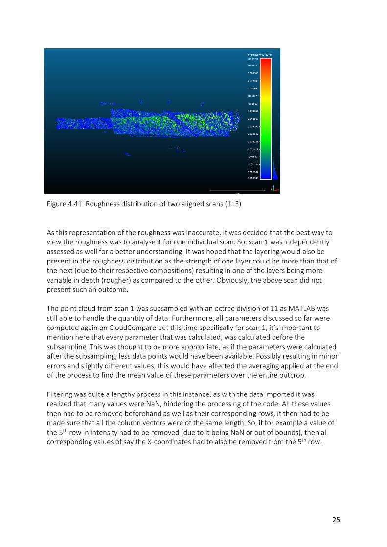
4.4 Orientation and other parameters After the calculation of the normals in CloudCompare the parameters regarding orientation such as dip direction and dip angle could be calculated directly. One can convert the normals of a cloud to two scalar fields, one with the dip value and the other with the dip direction (both in degrees) which resulted in a distribution of both variables over the entire outcrop which could be visualised on CloudCompare. But since certain filtering still needed to be applied, most of the visualizations were done in MATLAB. Following this roughness could also be calculated on CloudCompare, but the issue here was that since the roughness of 2 aligned scans was being calculated, most of the peaks in values of the roughness in the distribution over the outcrop was due to minimal errors in registration of the two scans. The roughness distribution basically outlined the boundaries of the two merged scans and so was not reliable to consider as can be seen in figure 4.41

25

Figure 4.41: Roughness distribution of two aligned scans (1+3) As this representation of the roughness was inaccurate, it was decided that the best way to view the roughness was to analyse it for one individual scan. So, scan 1 was independently assessed as well for a better understanding. It was hoped that the layering would also be present in the roughness distribution as the strength of one layer could be more than that of the next (due to their respective compositions) resulting in one of the layers being more variable in depth (rougher) as compared to the other. Obviously, the above scan did not present such an outcome. The point cloud from scan 1 was subsampled with an octree division of 11 as MATLAB was still able to handle the quantity of data. Furthermore, all parameters discussed so far were computed again on CloudCompare but this time specifically for scan 1, it’s important to mention here that every parameter that was calculated, was calculated before the subsampling. This was thought to be more appropriate, as if the parameters were calculated after the subsampling, less data points would have been available. Possibly resulting in minor errors and slightly different values, this would have affected the averaging applied at the end of the process to find the mean value of these parameters over the entire outcrop. Filtering was quite a lengthy process in this instance, as with the data imported it was realized that many values were NaN, hindering the processing of the code. All these values then had to be removed beforehand as well as their corresponding rows, it then had to be made sure that all the column vectors were of the same length. So, if for example a value of the 5th row in intensity had to be removed (due to it being NaN or out of bounds), then all corresponding values of say the X-coordinates had to also be removed from the 5th row.

26

Figure 4.42: Roughness distribution over Cloud 1 In the figure above the kernel size used was very small, at a size of 0.08m, resulting multiple small planes being fit in order to calculate roughness. Layering can be seen to an extent with the lighter colours representing a greater deviation from the plane, the layers with the greater deviation appear to be the lighter coloured layers in the intensity plots as in figure 5.51. Deviations from the fitted planes are ranging only a couple of centimetres as shown in the colour bar. A larger kernel size may be more appropriate so as to fit a larger plane which will then be applicable for a larger majority of points for the calculation of roughness. As roughness is the distance between a mean plane made according to the specified kernel size and the point under consideration. Below is a distribution of roughness over the entirety of the scan using a kernel size of 40m, which is roughly the size of the outcrop in length.

Figure 4.43: Roughness using a kernel size of 40m

27

Increasing kernel size further results in inconclusive results and so this process was abandoned and instead a profile was attempted to be made. After which a plane could be fit to the model and distances between the points and the fitted plane could then be computed. Roughly the same method as the roughness computation in CloudCompare however manually done. Profiles could be made of the point cloud by using the cross-section available, after which the point cloud was sliced into 30 strips of equal height using CloudCompare’s cross-section function. After a division at the fault was made creating a left segment and right-hand segment of strips so as to exclude the fault from the analysis. 5 clear strips with an abundance in layering were then choses on each side of the strip and individually evaluated by fitting a plane to each and then calculating distances (roughness) to the plane. The clearest strips from each side are present in the results section and their credibility discussed.

28

4.5 Conclusions This chapter proves the multiple ways in which parameters may be calculated and point cloud data processed, obviously with certain methods being preferred in terms accuracy. It also highlights the importance of good, and representative data for processes such as registration to go smoothly. The registration was successful with the exception of scan 2, due to missing targets in the scan and the scan itself being comparatively sparse in points and hence it didn’t provide much additional information anyway. The geo-referencing requires enough well distributed and credible targets to allow for a successful transformation into a global coordinate system. Well distributed to ensure no flipping occurs during the transformation and certainly credible targets in order to ensure the correct output. In the case of this report, geo-referencing was done twice, once with the 4 well spread targets, and once with three in a line, of which the results are displayed in the next chapter. This allows to quantify the error generated due to an uneven spread of targets, this error also propagates into the results of dip direction and angle. The normals calculated were calculated both on MATLAB and CloudCompare to analyse any differences that may exist. Lastly the roughness was analysed in two ways, considering a very large kernel size and a very small one to see which one would result in a distribution most representative of the multiple layers present.

29

Chapter 5 Results The following chapter goes through the subsequent results generated after the due processing of the data. The validity of these results is interpreted and how they are applicable in the analysis of the layering and strata. Moreover, the validity of the process is consequently checked whilst noticing processing affects the resulting values of the parameters.

5.1 Geo-referencing In order to validate the geo-referencing, the point cloud aligned with the targets, post registration was saved as a shapefile. After this it could be opened in QGIS 2.18 as a new vector layer. Once this had been done, the open web-layers plugin had to be used to open maps in the background to check if the point cloud was projected in the correct location so as to verify that the geo-referencing had been done correctly. Since two final geo-referenced models had been made, one dependent on only 3 targets located in the same line in the lower half of the outcrop, and the other using 4 targets, with the three prior and one extra from the top half of the outcrop. Both of them have been visualized on QGIS, not only to validate the positioning but also showing the effect of the flipping of the scan during registration. This phenomenon indicates the utmost importance of good targets that are not only visible in the scan but also well spread so as to assure the correct orientation after geo-referencing.

Figure 5.11: geo-referenced using Figure 5.12: geo-referenced using 4 targets, 3 targets in a line 4th target placed near the top of the outcrop As can be clearly seen in the above two figures, is that they are perfect reversals of each other, they almost seem mirrored. However, they are still located in the same area as the way-points taken and displayed in figure 4.23, thereby validating the geo-referencing, in the sense of the general position of the scan. The figure on the left shows the correct position of scan, although it’s facing the wrong way, this is due to the fact that the targets used for geo-referencing were situated in the same line. Meaning that even though the targets in the scan matched the exact same position of the GPS coordinates of the targets, the entire scan was oriented the wrong way. The scan on the right made use of an extra target situated outside the line of the other 3 targets, resulting in a better geo-referenced system, as you can see its facing the right way. You can tell it’s facing the right way as the bundle of points separate to

30

the main body of the scan represent the position of scanner, and since its situated in front of the rock wall and not behind it, it must be correct. Obviously as previously mentioned since the credibility of the extra target is somewhat questionable so in its subsequent geo-referencing, a slight error is expected.

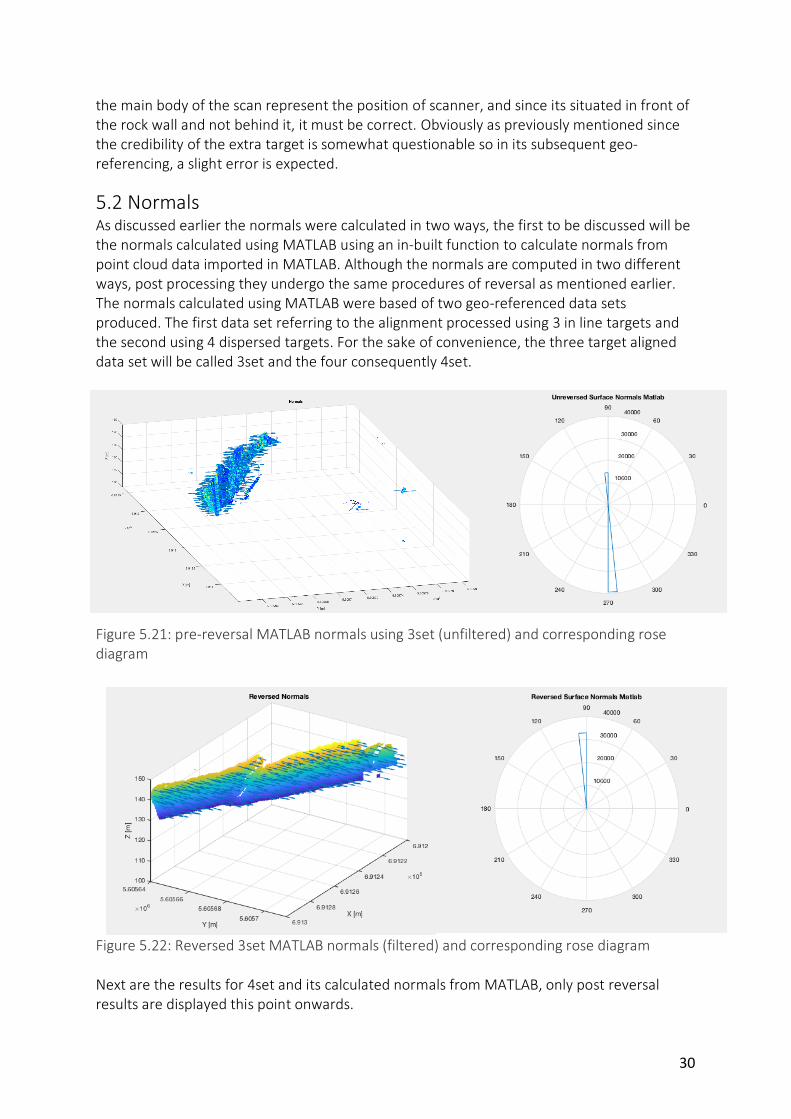
5.2 Normals As discussed earlier the normals were calculated in two ways, the first to be discussed will be the normals calculated using MATLAB using an in-built function to calculate normals from point cloud data imported in MATLAB. Although the normals are computed in two different ways, post processing they undergo the same procedures of reversal as mentioned earlier. The normals calculated using MATLAB were based of two geo-referenced data sets produced. The first data set referring to the alignment processed using 3 in line targets and the second using 4 dispersed targets. For the sake of convenience, the three target aligned data set will be called 3set and the four consequently 4set.

Figure 5.21: pre-reversal MATLAB normals using 3set (unfiltered) and corresponding rose diagram

Figure 5.22: Reversed 3set MATLAB normals (filtered) and corresponding rose diagram Next are the results for 4set and its calculated normals from MATLAB, only post reversal results are displayed this point onwards.

31

Figure 5.23: Reversed MATLAB normals using 4set Now for CloudCompare normals of both 3set and 4set post reversal:

Figure 5.24: CloudCompare normals for 3set (left) and 4set (right) An important thing that can be noticed is that whether it be 3set or 4set CloudCompare normals post reversal are the same, showing that CloudCompare calculates the normals irrespective of the orientation. This may suggest that even though both datasets are finally differently oriented that the calculated dip angle in both is most likely to be the same or with a small error as can be seen in table 5.31 and 5.32. However, in MATLAB’s computation this is not the case although the final directions of the normals after reversal for both datasets are somewhat similar, but there is still a noticeable difference. These differences and their effects can be seen in the subsequent calculation of orientation parameters in the next segment of this chapter.

32

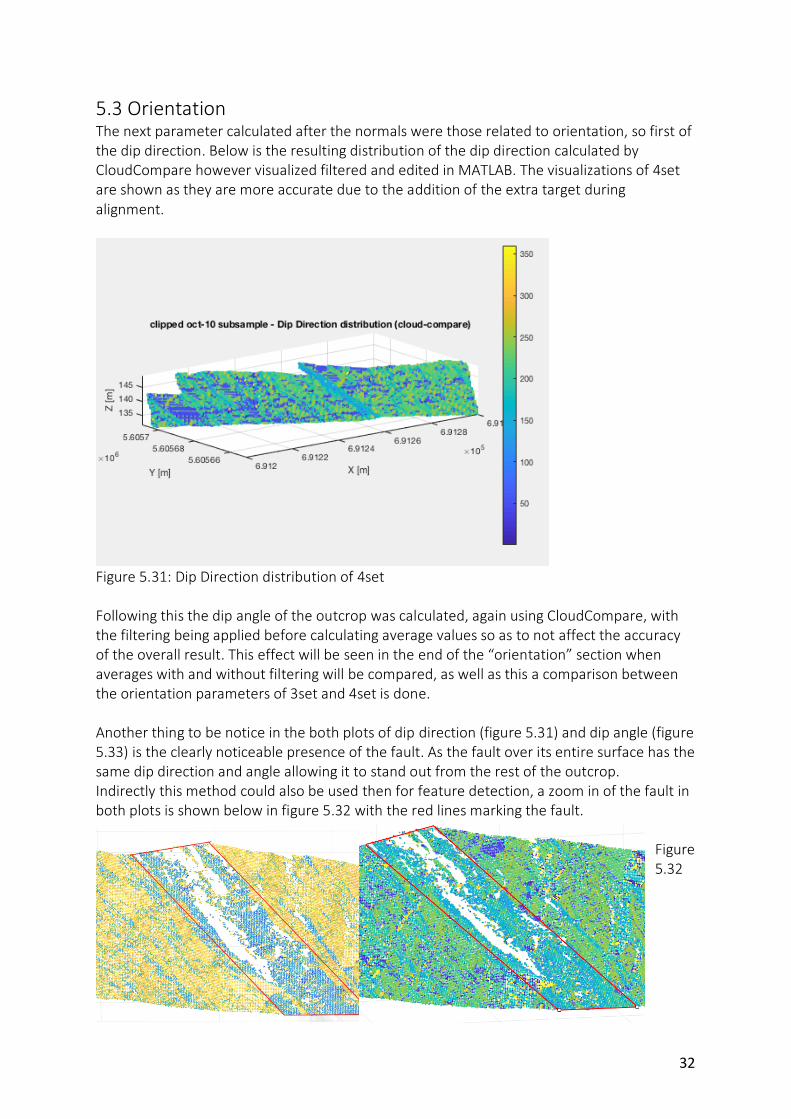
5.3 Orientation The next parameter calculated after the normals were those related to orientation, so first of the dip direction. Below is the resulting distribution of the dip direction calculated by CloudCompare however visualized filtered and edited in MATLAB. The visualizations of 4set are shown as they are more accurate due to the addition of the extra target during alignment.

Figure 5.31: Dip Direction distribution of 4set Following this the dip angle of the outcrop was calculated, again using CloudCompare, with the filtering being applied before calculating average values so as to not affect the accuracy of the overall result. This effect will be seen in the end of the “orientation” section when averages with and without filtering will be compared, as well as this a comparison between the orientation parameters of 3set and 4set is done. Another thing to be notice in the both plots of dip direction (figure 5.31) and dip angle (figure 5.33) is the clearly noticeable presence of the fault. As the fault over its entire surface has the same dip direction and angle allowing it to stand out from the rest of the outcrop. Indirectly this method could also be used then for feature detection, a zoom in of the fault in both plots is shown below in figure 5.32 with the red lines marking the fault.

Figure 5.32

33

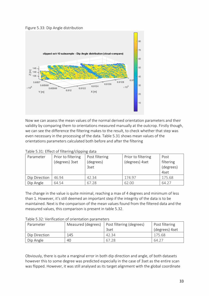
Figure 5.33: Dip Angle distribution

Now we can assess the mean values of the normal derived orientation parameters and their validity by comparing them to orientations measured manually at the outcrop. Firstly though, we can see the difference the filtering makes to the result, to check whether that step was even necessary in the processing of the data. Table 5.31 shows mean values of the orientations parameters calculated both before and after the filtering Table 5.31: Effect of filtering/clipping data

Parameter Prior to filtering (degrees) 3set

Post filtering (degrees) 3set

Prior to filtering (degrees) 4set

Post filtering (degrees) 4set

Dip Direction 46.94 42.34 174.97 175.68 Dip Angle 64.54 67.28 62.00 64.27

The change in the value is quite minimal, reaching a max of 4 degrees and minimum of less than 1. However, it’s still deemed an important step if the integrity of the data is to be maintained. Next is the comparison of the mean values found from the filtered data and the measured values, this comparison is present in table 5.32. Table 5.32: Verification of orientation parameters

Parameter Measured (degrees) Post filtering (degrees) 3set

Post filtering (degrees) 4set

Dip Direction 145 42.34 175.68 Dip Angle 40 67.28 64.27

Obviously, there is quite a marginal error in both dip direction and angle, of both datasets however this to some degree was predicted especially in the case of 3set as the entire scan was flipped. However, it was still analysed as its target alignment with the global coordinate

34

system was more exact even though its oppositely oriented. This may be the reason it’s dip direction is approximately 90 degrees of from its true measure value. Another thing to be noticed, is that as predicted the dip angles of both analysis are the same with a variation of only 3 degrees. Since it has been seen that the dip angle is being calculated irrespective of orientation the analysis of 3set is much more accurate as the targets were matched very closely during geo-referencing, producing a max error in any direction of 1.2m. As well as this the error that can be seen in 4set’s dip direction is due to the fact that one of the used target’s position was not credible and so resulted in a slight mis-alignment with the global coordinate system. This error propagates into the calculation of the dip direction, giving an error of exactly 30 degrees. Another thing to take into account is that there may have been an error in reading the compass during the manual reading resulting in a generation too. As using a compass in the field is quite a crude method, as it depends on whether the surface being used for the reading is actually flat, amongst other things.

5.4 Roughness After the numerous routes tried a visualization of the roughness was finally computed based on the strips of the point cloud data and a manually best fitted plane. The roughness was calculated by calculating the distance from this plane to the point clouds and interpreted as roughness. The best plane was fit using the average dip angle and dip direction found using MATLAB in order to place the plane in roughly the same orientation as the outcrop. With the dip angle being 64 degrees and the dip direction 175 degrees. First a profile of the outcrop was made using cross-sections in CloudCompare, of which an example is displayed below:

Figure 5.41: Profile of one of the segments made to the left of the fault in the outcrop

35

Following this a plane could be fit, after which the distances were calculated using the cloud to cloud/mesh function, below is the same profile from a different angle with the distance to plane distribution over its surface.

Figure 5.42: Distances to plane, over profile of left segment 2 Visualizations were created in CloudCompare as it allowed the possibility to manually draw polylines of the layering and then view them simultaneously with the distribution. In order to see this correlation, it was deemed a good idea to have a look at the right side of the fault as it consists of much bigger and prominent layers, allowing for an easier interpretation. First off, in order to understand the layering there is a visualization of the outcrop based only on the intensity of a profile to the right of the fault. Figure 5.43: Layering the right segment of the outcrop with separation polylines

After this the distribution was projected on the outcrop, with the polylines and one of the strips still in intensity format to provide some reference of the layering whilst comparing it to the roughness of the surface. Figures 5.44 and 5.45 display these results.

36

Figure 5.44: Distance to plane distribution, right wall segment The same method was adopted for the left-hand side segment and its result is in figure 5.45.

Figure 5.45: Distance to plane distribution, left wall segment As in the processing chapter the lighter shade of rock in the intensity plots seemed to show a greater deviation from the fitted plane or was rougher. The hypothesis was that a difference in roughness should be noticed in between the layering due to the difference in composition and hence strength of the layers. The lighter shade of rock, the sandstone appears to be rougher than its darker counterpart, the shales. In some places the described trend is

37

noticeable in both the analysis above in figure 5.45 and figure 4.42, but in other segments of the outcrop completely irregular, there may be numerous reasons for this. The area under question had undergone multiple orogeny’s and therefore was subject to continuous and large amounts of deformations, causing irregularities in the outcrop. This may be a very plausible reason and there are multiple folds and faults in the area, visible in the outcrop as well, for example the giant fault right in the middle of the outcrop is prefect representation. Moreover, since the area in consideration is actually a quarry this would suggest that bulldozers, dynamite and other destructive methods have been used to break the rock of the outcrop resulting in a warped analysis of the outcrop itself. As these destructives methods significantly change the surface geometry of rock, effecting the distance to plane parameter being calculated. Lastly the geometry as such may not be completely representative of the layering, or at least not in the area we are considering, however to firmly decide the cause of these irregularities further research would have to be conducted.

5.5 Intensity As RGB values were not recorded by the scanner the only interpretation of colour available was the intensity. The intensity is the power per unit area transferred by the signal back after reflection from the surface, so can be taken as a parameter in analysing the layering present in the outcrop. The presence of the layering when intensity is set as the scalar field in CloudCompare is clearly visible. However, post filtering it was also interpreted in MATLAB for a clearer view, below is the result.

Figure 5.51: Intensity Distribution Intensity is the parameter in which the layering is most visible, this shows that intensity is definitely representative of the layering present. This is due to the fact that intensity is heavily dependent on the composition and colour of the surface as that is what decide how much energy is absorbed or reflected by it subsequently determining the intensity of the reflected signal. This is why it may seem like a good idea to some type cross plot or false colour image of the outcrop, dependent on more than one parameter, say for example roughness (distance to the plane) and intensity. Moreover, it would be advisable to use a computer with appropriate processing abilities as LiDAR data is extremely dense and whilst its processing multiple crashes could be encountered if not for appropriate computational power.

38

5.6 Discussion The features extracted are representative of the layering present, however the representation could be more accurate if one took a more appropriate example. An example appropriate to the due processing would result in the best analysis. As the results produced from the processes conducted are sensitive to errors, which propagate into the results and subsequently increase. The error produced during geo-referencing using 4set provided a max error horizontally of 9m and vertically 3m. This error then propagates into the mean values of dip direction and angle, producing an error of 30 degrees in dip direction and 24 degrees in dip angle. In the case of 3set the error in geo-referencing produced a max error 1.2m, however since it was flipped it resulted in the dip direction being off by 90 degrees. However, the dip angle calculated had the same error, showing that CloudCompare does indeed calculate dip angle irrespective of the normals as that is the only difference between 3set and 4set. The normals are calculated respective to orientation, and since that differs between 3set and 4set, so do the normals. Roughness as a parameter is less sensitive to error as it less dependent on prior processes. The roughness depends only either the kernel sized used in automated calculation or the plane fitted manual in the case of manual roughness calculation. It is indeed sensitive if the plane fit is inaccurate, as this affects the distance between the points and the plane, ergo roughness values. Intensity is more sensitive to the measurement setup rather than processing the data had to undergo. Intensity is a function of the distance of the scanner to the outcrop and the angle which the scanner makes with its field of view (the incidence angle). But since all the scans were taken from the same location, the effect of this can be ruled out as it is equally present in each scan.

39

Chapter 6 Conclusion and Recommendations

6.1 Conclusions To answer the main research question, there are multiple ways to process LiDAR data in order to extract geometrical parameters of the object in question. What really varies between these methods is the efficiency and the accuracy of them. In this instance the most efficient method and accurate depending on the way it’s done, is using CloudCompare. However, CloudCompare, used in combination with another programming software, such as MATLAB in this case is advisable. Due to its application in visualizations, filtering and manipulation of the data. Visualizations and clipping (filtering) of the data can also be done in CloudCompare although maybe not as accurately as a programming software would allow. Before processing though, there is the task of acquiring data, this is best done using a good quality laser scanner amongst other things. These other things however are just as essential as the scanner itself, they include clear and noticeable targets and a device which can record GPS coordinates (preferably a tool specific for this purpose and not a phone due to a phone’s lapse in judgement). The targets will most definitely be used for registration of separate multiple scans, but can also be used for geo-referencing, which can be seen as another form of registration just with the global coordinate system. The GPS device will be used to measure the coordinates of the scan station itself as well as the used targets for the purpose of geo-referencing. Although the equipment that comes with the scanner is also very important such as the tripod, which is integral for the correct levelling of the scanner. Geometrical features of the outcrop, such as those concerning orientation, normals, roughness, curvature, surface re-construction and more can all be extracted from the data. The only input required is X, Y, Z coordinates of all the points present in the scan, intensity and RGB values are just a bonus and greatly helpful in terms of visualization. All these features can be derived using either CloudCompare or MATLAB, with each producing results in line. Obviously, these results can be brought to have even less of a difference depending on the accuracy with which the processing is conducted. CloudCompare makes use of in-built function for calculating these parameters, quite similarly MATLAB makes use of downloadable pre-made functions for processing point cloud data. Once these values have been found either way, a distribution of these values can be made over the entire outcrop allowing for averages to be found over the whole surface. Such calculated averages are displayed in the chapter prior. Such parameters have immense significance as they can characterize the entire object from both a larger point of view using averages, and a smaller one by analysing and visualizing the distribution of these parameters over the outcrop. In viewing the distribution of such parameters projected on the surface of the outcrop, amongst other things layering can also be observed. No doubt, parameters such as intensity and RGB content are best for this purpose but other variables can also be used as well as combination plots of multiple. Through the duration of this project, the next best parameter representative of layering aside from intensity was found to be the roughness of the surface. In reference to roughness, perhaps this example wasn’t the best, subsequent of its geologic history, but it’s definitely still representative.

40

6.2 Recommendations There is still much room for improvements that could result in a better analysis of the outcrop, such practices in the future should definitely be implemented. For this reason, there is also an attached guideline to geo-referencing in the appendix, due to it being the most complicated and tedious tasks in the processing. One such practice would be being present for the scanning itself and as that without a doubt is definitely helpful. One should only scan representative parts of the outcrop, and place targets themselves so as to best recognize them, and their arrangement in the scans. More importantly as discussed in the processing and results chapters, the need for good targets is integral. Their distribution must also be sparse so as to geo-reference the whole scan and not just one plane or line, giving room to flipping and reversal errors. Lastly, it’s important to tailor make the processing tasks to the outcrop in question to produce an accurate analysis. Outcrops differ in size, composition and features and hence so should their consequent analysis.

41

References [1] Prof.Dr. Eric Groessens. “Le CONDROZ, Une Entité Géographique, Reflet De Son Passé Géologique.” Articles Sur La Géologie, Les Minéraux, Les Fossiles, Les Volcans,..., www.geologie-info.com/articles.php?Article=Condroz. [2] McCann, Tim, and The Geological Society. “The Geology of Central Europe: Precambrian and Palaeozoic.” Google Boeken, Google, 2008, books.google.nl/books?id=BR9FWgu2ps4C. [3]“14.8. Lesson: DEM from LiDAR Data¶.” Working with Projections, QGIS, docs.qgis.org/2.14/en/docs/training_manual/forestry/basic_lidar.html. [4] Portland State. Web.pdx.edu, Portland State. [5] “Processing Lidar Data Using QGIS.” Rstudio-Pubs-Static, Amazonaws, rstudio-pubs-static.s3.amazonaws.com/230154_30a0bbf22e2a49ecbfa1b72b2c7a8f96.html. [6] Bouvlain, Frederic, and Noel Vandenberghe. “An Introduction to the Geology of Belgium and Luxembourg .” Springer.com, Landscapes and Landforms of Belgium and Luxembourg. [7] “Principle of LiDAR.” Www.home.iitk.ac.in, home.iitk.ac.in/~blohani/LiDAR_Tutorial/Principle%20of%20LiDAR.htm.

[8] G. Vosselman and H-G. Maas. Airborne and Terrestrial Laser Scanning. Caithness, Scotland: Whittles Publishing, 2010

[9] Leica ScanSation P40/P30 User Manual. Leica, surveyequipment.com/assets/index/download/id/457/. [10] “Basics of Photogrammetry.” GIS Resources, GIS Resources, 3 Jan. 2014, www.gisresources.com/basic-of-photogrammetry_2/. [11] Walstra, Jan, et al. “Historical Aerial Photographs for Landslide Assessment: Two Case Histories.” Research Gate, Research Gate, www.researchgate.net/figure/The-principles-of-photogrammetry-bundles-of-light-rays-pass-from-object-points-A-and-B_fig1_245378360.

[12] J. Thorez, R. Dreesen, and M. Streel. “Famennian”. In: Geologica Belgica 9.1-2 (2006), pp. 27–45.

[13] “Ravinement Erosion Surface.” STRATA Terminology, www.sepmstrata.org/Terminology.aspx?id=ravinement. [14] GM, Daniel. “Alignment and Registration.” RANSAC Shape Detection (Plugin) - CloudCompareWiki, CloudCompareWiki, www.cloudcompare.org/doc/wiki/index.php?title=Alignment_and_Registration. [15] GM, Daniel. “Normals\Compute.” RANSAC Shape Detection (Plugin) - CloudCompareWiki, CloudCompareWiki, www.cloudcompare.org/doc/wiki/index.php?title=Normals%5CCompute. [16] Schenk, T. “Introduction to Photogrammetry.” Mat.uc.pt, Department of Civil and Environmental Engineering and Geodetic Science The Ohio State University, 2005, www.mat.uc.pt/~gil/downloads/IntroPhoto.pdf. [17] “Pcnormals.” Duration (CDF) Plot - File Exchange - MATLAB Central, Mathworks, 2017, nl.mathworks.com/help/vision/ref/pcnormals.html.

42

Appendix

Guideline to Geo-referencing Geo-referencing is the procedure of aligning the local coordinate system of a scan to the desired global coordinate system. The following takes the reader through instructions for an ideal geo-referencing procedure that produces minimal errors via the use of Kabsch algorithm. The software’s used for this purpose will be MATLAB, QGIS and CloudCompare. To begin with what is required a scan of the object/outcrop in question present in loaded into CloudCompare as a point cloud. This can simply be done by opening the bin file of the scan in question straight into CloudCompare. However, the scan being used must have well dispersed targets present and recognizable in the scan otherwise the following process will produce significant errors. There must be three targets or more present in the scan, the targets must be well spread. That is, they may not be present in one single line, so as to prevent flipping of the scan during the subsequent transformation required for the geo-referencing. The targets placed on the outcrop must have their GPS position recorded by device of the user’s preference. A device specific for recording GPS would be advisable as compared to a mobile phone, in order to ensure the coordinates are accurate and don’t generate too large an error. Finally, once in CloudCompare the user must record the coordinates of the respective targets in scanner’s local coordinate system. Once all of these perquisites have been attained and processes completed the Kabsch algorithm can be used. The Kabsch algorithm makes used of the coordinates of the targets in the global coordinate system and the coordinates of the same targets in the scanners local coordinate system. The algorithm, was coded and developed by Adriaan van Natijne, a master’s student at the GRS department at the TU Delft. The code is present further on in the appendix, the algorithm produces a 4 by 4 matrix containing the required rotation and translation the scan must undergo to exist in the global coordinate system. The code not only calculates the matrix but ensures the corresponding targets are transformed into the correct position and not another targets position, resulting in a flip of the scan. The only input required of the algorithm is the coordinates of the targets in the local system and global in the correct order. After which as output its saves the transformation matrix as a separate file, in the specific case it will save the matrix as trans.txt. Following this the transformation matrix has to be copied and input into the transformation function in CloudCompare, as it is, as CloudCompare also requires a 4 by 4 input. Then simply hit enter, and when the nest pop up box appears, it will be in regard shifting and scaling the transformed scan. To maintain the scan in the correct position and orientation one must click no, however in order to maintain just the orientation yes can be clicked. The code for Kabsch algorithm as developed by Adriaan is below, the input is currently the coordinates of the authors targets for this report.

43

Kabsch Algorithm Implemented in MATLAB % Kabsch algorithm for registration against GCP's % Adriaan van Natijne <[email protected]>, 2018 clear; % GCP's gcp_lidar = [ 64.07615 33.948196 71.420288; ... -126.505432 -131.928497 -89.159653; ... -4.245178 -7.578880 -27.873985]'; gcp_utm= [ 691277.6 691302.5 691239; ... 5605701.7 5605679.8 5605684.4; ... 153.415268 152.02359 130.816406]'; gcp_lidar_b = [104.57554 71.472008 13.50337; ... -75.137375 -89.112091 -114.267639; ... -25.720856 -27.977173 -31.909664]'; gcp_utm_b = [691207.3 691239.0 691294.2; ... 5605702.8 5605684.4 5605650.0; ... 131.801682 130.816406 125.739792]'; %gcp_lidar = [gcp_lidar; gcp_lidar_b]; %gcp_utm = [gcp_utm; gcp_utm_b]; gcp_lidar = gcp_lidar_b; gcp_utm = gcp_utm_b; % Apply translation (centroid at origin) gcp_lidar_0 = gcp_lidar -mean(gcp_lidar, 1); gcp_utm_0 = gcp_utm -mean(gcp_utm, 1); % Remove z gcp_lidar_0(:, 3) = 0; gcp_utm_0(:, 3) = 0; %gcp_lidar_0 = gcp_lidar_0(:, 1:2); %gcp_utm_0 = gcp_utm_0(:, 1:2); figure(1), clf(1); scatter3(gcp_lidar_0(:,1), gcp_lidar_0(:,2), gcp_lidar_0(:,3)); hold on; scatter3(gcp_utm_0(:,1), gcp_utm_0(:,2), gcp_utm_0(:,3)); legend('LiDAR', 'UTM'); % Copy values P = gcp_lidar_0; Q = gcp_utm_0; % Open figure figure(2), clf(2), hold on; scatter3(Q(:,1), Q(:,2), Q(:,3), '*'); % Covariance between points H = P'*Q; % Rotation [U, S, V] = svd(H); d = det(V*U'); R = V*diag([1 1 d])*U';

44

%P = R(:,:,i)*P; % gcp_lidar_1 P = P*R; scatter3(P(:,1), P(:,2), P(:,3)); legend('UTM', 'Fit'); figure(1); scatter3(P(:,1), P(:,2), P(:,3)); figure(1), axis('square'), grid on; figure(2), axis('square'), grid on; % Point connections figure(2); for i=1:size(gcp_utm, 1); plot3([P(i, 1) Q(i, 1)], ... [P(i, 2) Q(i, 2)], ... [P(i, 3) Q(i, 3)]); end; figure(3), clf(3), axis('square'), grid on, hold on; for i=1:size(gcp_utm, 1); plot3([gcp_lidar_0(i, 1) gcp_utm_0(i, 1)], ... [gcp_lidar_0(i, 2) gcp_utm_0(i, 2)], ... [gcp_lidar_0(i, 3) gcp_utm_0(i, 3)]); end; figure(4), clf(4); subplot(121); scatter(gcp_lidar(:, 1), gcp_lidar(:, 2)); subplot(122); scatter(gcp_utm(:, 1), gcp_utm(:, 2)); % Save to CloudCompare R = [R' (mean(gcp_utm, 1) -mean(gcp_lidar, 1))'; 0 0 0 1]; R(3, 3) = 1; dlmwrite('trans.txt', R, 'delimiter', ' ', 'precision', '%.6f');

45

MATLAB Script %%OCT 10 ptcloud=pointCloud([XA, YA, ZA], 'Intensity', IA); figure(1) pcshow(ptcloud, 'MarkerSize', 15) %zlim([100 150]) title('subsampled point-cloud') xlabel('X [m]') ylabel('Y [m]') zlabel('Z [m]') normals=pcnormals(ptcloud); x = XA(1:100:end); y = YA(1:100:end); z = ZA(1:100:end); U=normals(:, 1); V=normals(:, 2); W=normals(:, 3); u=U(1:100:end); v=V(1:100:end); w=W(1:100:end); %% %OCT 10 figure(2) pcshow(ptcloud, 'MarkerSize', 5) zlim([100 150]) title('Normals') xlabel('X [m]') ylabel('Y [m]') zlabel('Z [m]') hold on quiver3(x, y, z, u, v, w); hold off %rose-diagram %convert cartesian coordinates to cylindrical coordinates [TH, R, H]=cart2pol(U, V, W); %TH - theta figure(3) rose(TH, 60) title('Unreversed Surface Normals Matlab') %% %filter out the unnecessary parts of the data set, the sections that give a %poor representation of the model, hence affect averages. Same plots as the %above section will then be made to see how filtering out the data affect %the normal estimated before the reversal are done. %following process to emit all points outside limits of x, y and z so as to %not include inaccuracies in averaging calculations %setting all values outside limits to NaN %this is filtering for the total data set of oct 10 subsampling for i=1:57938 if ZA(i)>149 || ZA(i)<129 ZA(i)=NaN; YA(i)=NaN; XA(i)=NaN; IA(i)=NaN; U(i)=NaN;

46

V(i)=NaN; W(i)=NaN; end if YA(i)>5.60572*(10^6) || YA(i)<5.60564*(10^6) ZA(i)=NaN; YA(i)=NaN; XA(i)=NaN; IA(i)=NaN; U(i)=NaN; V(i)=NaN; W(i)=NaN; end if XA(i)>6.913*(10^5) || XA(i)<6.912*(10^5) ZA(i)=NaN; YA(i)=NaN; XA(i)=NaN; IA(i)=NaN; U(i)=NaN; V(i)=NaN; W(i)=NaN; end end %omittion of all NaN values from all parameters for the original oct 10 %subsample dataset id11=find(isnan(XA)); XA([id11])=[]; id12=find(isnan(YA)); YA([id12])=[]; id13=find(isnan(ZA)); ZA([id13])=[]; id14=find(isnan(IA)); IA([id14])=[]; id15=find(isnan(U)); U([id15])=[]; id16=find(isnan(V)); V([id16])=[]; id17=find(isnan(W)); W([id17])=[]; %% %filtering for points plotted in the pcshow with the normals using quiver (this is done with a section of the oct 10 subsampled data in order to show only a limited number of normal visulaizations to prevent overcrowded graphs) for i=1:580 if z(i)>149 || z(i)<129 z(i)=NaN; y(i)=NaN; x(i)=NaN; u(i)=NaN; v(i)=NaN; w(i)=NaN; end if y(i)>5.60572*(10^6) || y(i)<5.60564*(10^6) z(i)=NaN; y(i)=NaN; x(i)=NaN;

47

u(i)=NaN; v(i)=NaN; w(i)=NaN; end if x(i)>6.913*(10^5) || x(i)<6.912*(10^5) z(i)=NaN; y(i)=NaN; x(i)=NaN; u(i)=NaN; v(i)=NaN; w(i)=NaN; end end %omittion of all NaN values from all parameters for the original oct 10 %subsample dataset id21=find(isnan(x)); x([id21])=[]; id22=find(isnan(y)); y([id22])=[]; id23=find(isnan(z)); z([id23])=[]; id24=find(isnan(u)); u([id24])=[]; id25=find(isnan(v)); v([id25])=[]; id26=find(isnan(w)); w([id25])=[]; %% %OCT 10 %reversal of the points to be plotted not the whole subsampled oct 10 %dataset sensorCenter = [6.913e+05, 5.606e+06, 130.1]; % in X,Y,Z coordinates for k = 1 : numel(x) p1 = sensorCenter - [x(k), y(k), z(k)]; p2 = [u(k), v(k), w(k)]; % Flip the normal vector if it is not pointing towards the sensor angle = atan2(norm(cross(p1, p2)), p1*p2'); if angle > pi/2 || angle < -pi/2 u(k) = -u(k); v(k) = -v(k); w(k) = -w(k); end end figure(4) pcshow([XA,YA,ZA], 'MarkerSize', 5) zlim([100 150]) title('Reversed Normals') xlabel('X [m]') ylabel('Y [m]') zlabel('Z [m]') hold on quiver3(x, y, z, u, v, w); hold off %% %reversal of the whole oct 10 subsampled dataset in order to get an %accurate rose diagram sensorCenter = [6.913e+05, 5.606e+06, 130.1]; % in X,Y,Z coordinates for k = 1 : numel(XA) p1 = sensorCenter - [XA(k), YA(k), ZA(k)];

48

p2 = [U(k), V(k), W(k)]; % Flip the normal vector if it is not pointing towards the sensor angle = atan2(norm(cross(p1, p2)), p1*p2'); if angle > pi/2 || angle < -pi/2 U(k) = -U(k); V(k) = -V(k); W(k) = -W(k); end end %reversed rose-diagram %convert cartesian coordinates to cylindrical coordinates [TH, R, H]=cart2pol(U, V, W); %TH - theta figure(3) rose(TH, 60) title('Reversed Surface Normals Matlab') %% %OCT 9 onwards except for the matlab computed normals %Post Analysis (computations for normals, dip angle, dip direction and roughness done in cloudcompare afterwhich the data was exported to matlab) %RA=str2double(RoughnessAs); %NyA=str2double(Ny); %NxA=str2double(Nx); %IA=str2double(IntensityAs); %DA=str2double(DipAs); %DDA=str2double(DipDAs); ptcloudA=pointCloud([XA, YA, ZA],'Normal' , [NxA, NyA, NzA], 'Intensity', IA); %% figure(6) pcshow([XA, YA, ZA], IA, 'MarkerSize', 15) %zlim([100 150]) title('subsampled point-cloud (oct-9) post computation') xlabel('X [m]') ylabel('Y [m]') zlabel('Z [m]') %hold on %colorbar %hold off %% %need to remove all pre-existing rows with NaNs id331=find(isnan(XA)); id332=find(isnan(YA)); id333=find(isnan(ZA)); id334=find(isnan(IA)); %id335=find(isnan(RA)); id336=find(isnan(DA)); id337=find(isnan(DDA)); id338=find(isnan(NxA)); id339=find(isnan(NyA)); id3310=find(isnan(NzA)); %% %omittion of all NaN values from all parameters XA([id336])=[]; YA([id336])=[]; ZA([id336])=[]; IA([id336])=[]; %RA([id336])=[]; DA([id336])=[]; DDA([id336])=[];

49

NxA([id336])=[]; NyA([id336])=[]; NzA([id336])=[]; XA([id337])=[]; YA([id337])=[]; ZA([id337])=[]; IA([id337])=[]; %RA([id337])=[]; DA([id337])=[]; DDA([id337])=[]; NxA([id337])=[]; NyA([id337])=[]; NzA([id337])=[]; average_dip_angle_unclipped=mean(DA); average_dip_direction_unclipped=mean(DDA); %average_roughness_unclipped=mean(RA); average_intensity_unclipped=mean(IA); %% %following process to emit all points outside limits of x, y and z so as to %not include inaccuracies in averaging calculations %setting all values outside limits to NaN for i=1:57938 if ZA(i)>149 || ZA(i)<131.8 ZA(i)=NaN; YA(i)=NaN; XA(i)=NaN; IA(i)=NaN; %RA(i)=NaN; DDA(i)=NaN; DA(i)=NaN; NxA(i)=NaN; NyA(i)=NaN; NzA(i)=NaN; end if YA(i)>5.60572*(10^6) || YA(i)<5.60564*(10^6) ZA(i)=NaN; YA(i)=NaN; XA(i)=NaN; IA(i)=NaN; %RA(i)=NaN; DDA(i)=NaN; DA(i)=NaN; NxA(i)=NaN; NyA(i)=NaN; NzA(i)=NaN; end if XA(i)>6.913*(10^5) || XA(i)<6.912*(10^5) ZA(i)=NaN; YA(i)=NaN; XA(i)=NaN; IA(i)=NaN; %RA(i)=NaN; DDA(i)=NaN; DA(i)=NaN; NxA(i)=NaN; NyA(i)=NaN;

50

NzA(i)=NaN; end end %% id1=find(isnan(XA)); id2=find(isnan(YA)); id3=find(isnan(ZA)); id4=find(isnan(IA)); %id5=find(isnan(RA)); %RA([id5])=[]; id6=find(isnan(DA)); id7=find(isnan(DDA)); id8=find(isnan(NxA)); id9=find(isnan(NyA)); id10=find(isnan(NzA)); XA([id1])=[]; YA([id2])=[]; ZA([id3])=[]; IA([id4])=[]; %id5=find(isnan(RA)); %RA([id5])=[]; DA([id6])=[]; DDA([id7])=[]; NxA([id8])=[]; NyA([id9])=[]; NzA([id10])=[]; average_dip_angle_clipped=mean(DA); average_dip_direction_clipped=mean(DDA); %average_roughness_clipped=mean(RA); average_intensity_clipped=mean(IA); %% %subsample showing intensity distribution ptcloudA_C=pointCloud([XA, YA, ZA],'Normal' , [NxA, NyA, NzA], 'Intensity', IA); figure(7) pcshow([XA, YA, ZA], IA,'MarkerSize', 15); %zlim([100 150]) title('clipped oct-10 subsample - Intensity distribution') xlabel('X [m]') ylabel('Y [m]') zlabel('Z [m]') %% %subsample showing normals (cloud-compare computed) distribution figure(8) pcshow([XA, YA, ZA], [NxA, NyA, NzA], 'MarkerSize', 15); title('clipped oct-10 subsample - Normals distribution (Cloud-compare) pre-reversal') xlabel('X [m]') ylabel('Y [m]') zlabel('Z [m]') hold on colorbar

51

hold off %rose diagram of normals (cloud-compare) before reversal %convert cartesian coordinates to cylindrical coordinates [TH, R, H]=cart2pol(NxA, NyA, NzA); %TH - theta figure(9) rose(TH, 60) title('Cloud-compare Normals, pre-reversal') %% %Then we need to reverse the incorrect normals although this wont affect %any of the subsequent values of the cloud compare computed parameters %anymore %rversal of normals sensorCenter = [6.913e+05, 5.606e+06, 130.1]; % in X,Y,Z coordinates for k = 1 : numel(XA) p1 = sensorCenter - [XA(k), YA(k), ZA(k)]; p2 = [NxA(k), NyA(k), NzA(k)]; % Flip the normal vector if it is not pointing towards the sensor angle = atan2(norm(cross(p1, p2)), p1*p2'); if angle > pi/2 || angle < -pi/2 NxA(k) = -NxA(k); NyA(k) = -NyA(k); NzA(k) = -NzA(k); end end %rose diagram of cloud-compare normals after reversal for comparison before %reversal and with the matlab computed values of the normals %convert cartesian coordinates to cylindrical coordinates [TH, R, H]=cart2pol(NxA, NyA, NzA); %TH - theta figure(10) rose(TH, 60) title('Cloud-compare Reversed Normals') %% %subsample showing reversed normals (cloud-compare computed) distribution figure(11) pcshow([XA, YA, ZA], [NxA, NyA, NzA], 'MarkerSize', 15); title('clipped oct-9 subsample - Reversed Normals distribution (Cloud-compare)') xlabel('X [m]') ylabel('Y [m]') zlabel('Z [m]') colorbar %% %subsample showing normals (matlab computed) distribution figure (12) pcshow([X, Y, Z], [U, V, W], 'MarkerSize', 15); title('clipped oct-9 subsample - Reversed Normals distribution (Matlab)') xlabel('X [m]') ylabel('Y [m]') zlabel('Z [m]') colorbar %% %dip direction distribution (cloud-compare) figure(13) pcshow([XA, YA, ZA], DDA, 'MarkerSize', 15);

52

title('clipped oct-10 subsample - Dip Direction distribution (cloud-compare)') xlabel('X [m]') ylabel('Y [m]') zlabel('Z [m]') hold on colorbar hold off %% %dip angle distribution (cloud-compare) figure(14) pcshow([XA, YA, ZA], DA, 'MarkerSize', 15); title('clipped oct-10 subsample - Dip Angle distribution (cloud-compare)') xlabel('X [m]') ylabel('Y [m]') zlabel('Z [m]') hold on colorbar hold off %% %roughness distribution (cloud-compare) figure(15) pcshow([XA, YA, ZA], RA, 'MarkerSize', 15); title('clipped oct-9 subsample - Roughness distribution (cloud-compare)') xlabel('X [m]') ylabel('Y [m]') zlabel('Z [m]') %% %the above plots and computations were made using the merged point cloud %data of scan1 and scan3 %however below for maybe a more accurate analysis only scan1 is analyzed, %as allignment to an extent generates noise. This may help us realize to %what extent as well the noise is generated. %the following is a subsample of octree division 11 ptcloudC=pointCloud([C1X, C1Y, C1Z], 'Normal', [CNX, CNY, CNZ], 'Intensity', CI); figure(16) pcshow([C1X, C1Y, C1Z], CI, 'MarkerSize', 15); title('Cloud 1 - subsample OCT 11, Intensity Distribution') xlabel('X [m]') ylabel('Y [m]') zlabel('Z [m]') %% %need to filter out all pre-existing NaN's and the subsequent rows before filtering according to x, %y, z position otherwise all the column vectors are of different sizes %first we locate all the pre-existing NaNs id51=find(isnan(C1X)); id52=find(isnan(C1Y)); id53=find(isnan(C1Z)); id54=find(isnan(CI));

53

id55=find(isnan(CR)); id56=find(isnan(CDA)); id57=find(isnan(CDDA)); id58=find(isnan(CNX)); id59=find(isnan(CNY)); id60=find(isnan(CNZ)); id61=find(isnan(CGC)); %% %Nans were found only in CDDA (id57), CGC (id61), CDA (id56) & CR (id55) %we can then manually erase the NaN rows from all parameters using the 4 %id's in each parameter %for id55 %C1X([id55])=[]; %C1Y([id55])=[]; %C1Z([id55])=[]; %CI([id55])=[]; %CR([id55])=[]; %CDA([id55])=[]; %CDDA([id55])=[]; %CNX([id55])=[]; %CNY([id55])=[]; %CNZ([id55])=[]; %CGC([id55])=[]; %for id56 %C1X([id56])=[]; %C1Y([id56])=[]; %C1Z([id56])=[]; %CI([id56])=[]; %CR([id56])=[]; %CDA([id56])=[]; %CDDA([id56])=[]; %CNX([id56])=[]; %CNY([id56])=[]; %CNZ([id56])=[]; %CGC([id56])=[]; %we only need to use id 57 as it is the largest %for id57 C1X([id57])=[]; C1Y([id57])=[]; C1Z([id57])=[]; CI([id57])=[]; CR([id57])=[]; CDA([id57])=[]; CDDA([id57])=[]; CNX([id57])=[]; CNY([id57])=[]; CNZ([id57])=[]; CGC([id57])=[];

54

%Now we need to filter out the unnecessary data according to x, y, z poistion for i=1:274546 if C1Z(i)>145 || C1Z(i)<132 C1Z(i)=NaN; C1Y(i)=NaN; C1X(i)=NaN; CI(i)=NaN; CR(i)=NaN; CGC(i)=NaN; CDA(i)=NaN; CDDA(i)=NaN; CNZ(i)=NaN; CNY(i)=NaN; CNX(i)=NaN; end if C1Y(i)>21 || abs(C1Y(i))>61 C1Z(i)=NaN; C1Y(i)=NaN; C1X(i)=NaN; CI(i)=NaN; CR(i)=NaN; CGC(i)=NaN; CDA(i)=NaN; CDDA(i)=NaN; CNZ(i)=NaN; CNY(i)=NaN; CNX(i)=NaN; end if C1X(i)>114.893 || C1X(i)<12 C1Z(i)=NaN; C1Y(i)=NaN; C1X(i)=NaN; CI(i)=NaN; CR(i)=NaN; CGC(i)=NaN; CDA(i)=NaN; CDDA(i)=NaN; CNZ(i)=NaN; CNY(i)=NaN; CNX(i)=NaN; end end %% %omittion of all NaN values from all parameters % % only id 41 was used as it is again the largest id41=find(isnan(CGC)); %CGC([id41])=[]; %% %for id41 C1X([id41])=[]; C1Y([id41])=[]; C1Z([id41])=[]; CI([id41])=[]; CR([id41])=[]; CDA([id41])=[]; CDDA([id41])=[]; CNX([id41])=[]; CNY([id41])=[]; CNZ([id41])=[]; CGC([id41])=[]; %%

55

%clipped intensity distribution ptcloudC=pointCloud([C1X, C1Y, C1Z], 'Normal', [CNX, CNY, CNZ], 'Intensity', CI); figure(17) pcshow([C1X, C1Y, C1Z], CI, 'MarkerSize', 15); title('Cloud 1 - subsample OCT 11, Intensity Distribution [CLIPPED]') xlabel('X [m]') ylabel('Y [m]') zlabel('Z [m]') %% %clipped roughness distribution figure(18) pcshow([C1X, C1Y, C1Z], CR, 'MarkerSize', 15); title('Cloud 1 - subsample OCT 11, Roughness Distribution') xlabel('X [m]') ylabel('Y [m]') zlabel('Z [m]') %% %clipped dip angle distrbution figure(19) pcshow([C1X, C1Y, C1Z], CDA, 'MarkerSize', 100); col title('Cloud 1 - subsample OCT 11, Dip Angle Distribution') xlabel('X [m]') ylabel('Y [m]') zlabel('Z [m]') %% %clipped dip direction distrbution figure(19) pcshow([C1X, C1Y, C1Z], CDDA, 'MarkerSize', 70); title('Cloud 1 - subsample OCT 11, Dip Direction Distribution') xlabel('X [m]') ylabel('Y [m]') zlabel('Z [m]') %% %clipped gaussian curvature distrbution figure(19) pcshow([C1X, C1Y, C1Z], CGC, 'MarkerSize', 15); title('Cloud 1 - subsample OCT 11, Gaussian Curvature Distribution') xlabel('X [m]') ylabel('Y [m]') zlabel('Z [m]') %% %clipped normals distrbution figure(19) pcshow([C1X, C1Y, C1Z], [CNZ, CNY, CNZ], 'MarkerSize', 15); title('Cloud 1 - subsample OCT 11, Normals Distribution') xlabel('X [m]') ylabel('Y [m]') zlabel('Z [m]') %% % right segment 0 figure(20) pcshow([RS0X, RS0Y, RS0Z],RS0TAD, 'MarkerSize', 15);

56

title('Right Segment 0') xlabel('X [m]') ylabel('Y [m]') zlabel('Z [m]') hold on colorbar hold off %% % right segment 1 figure(21) pcshow([RS1X, RS1Y, RS1Z],RS1TAD, 'MarkerSize', 15); title('Right Segment 1') xlabel('X [m]') ylabel('Y [m]') zlabel('Z [m]') hold on colorbar hold off %% % right segment 2 figure(22) pcshow([RS2X, RS2Y, RS2Z],RS2TAD, 'MarkerSize', 15); title('Right Segment 2') xlabel('X [m]') ylabel('Y [m]') zlabel('Z [m]') hold on colorbar hold off %% % right segment 3 figure(23) pcshow([RS3X, RS3Y, RS3Z],RS3TAD, 'MarkerSize', 15); title('Right Segment 3') xlabel('X [m]') ylabel('Y [m]') zlabel('Z [m]') hold on colorbar hold off %% % right segment 4 figure(24) pcshow([RS4X, RS4Y, RS4Z],RS4TAD, 'MarkerSize', 15); title('Right Segment 4') xlabel('X [m]') ylabel('Y [m]') zlabel('Z [m]') hold on colorbar hold off %% % left segment 0 figure(25) pcshow([LS0X, LS0Y, LS0Z],LS0TAD, 'MarkerSize', 15); title('Left Segment 0') xlabel('X [m]') ylabel('Y [m]') zlabel('Z [m]') hold on colorbar hold off %%

57

% left segment 1 figure(26) pcshow([LS1X, LS1Y, LS1Z],LS1TAD, 'MarkerSize', 15); title('Left Segment 1') xlabel('X [m]') ylabel('Y [m]') zlabel('Z [m]') hold on colorbar hold off %% % left segment 2 figure(27) pcshow([LS2X, LS2Y, LS2Z],LS2TAD, 'MarkerSize', 15); title('Left Segment 2') xlabel('X [m]') ylabel('Y [m]') zlabel('Z [m]') hold on colorbar hold off %% % left segment 3 figure(28) pcshow([LS3X, LS3Y, LS3Z],LS3TAD, 'MarkerSize', 15); title('Left Segment 3') xlabel('X [m]') ylabel('Y [m]') zlabel('Z [m]') hold on colorbar hold off %% % left segment 4 figure(29) pcshow([LS4X, LS4Y, LS4Z],LS4TAD, 'MarkerSize', 15); title('Left Segment 4') xlabel('X [m]') ylabel('Y [m]') zlabel('Z [m]') hold on colorbar hold off %% %false colour images mixRS4=(RS4I).*(RS4TAD).*(RS4AD); figure(30) pcshow([RS4X, RS4Y, RS4Z],[mixRS4], 'MarkerSize', 15); title('Right Segment 4') xlabel('X [m]') ylabel('Y [m]') zlabel('Z [m]') hold on colorbar hold off figure(31) pcshow([RS4X, RS4Y, RS4Z],[RS4I], 'MarkerSize', 15); title('Right Segment 4') xlabel('X [m]') ylabel('Y [m]') zlabel('Z [m]')

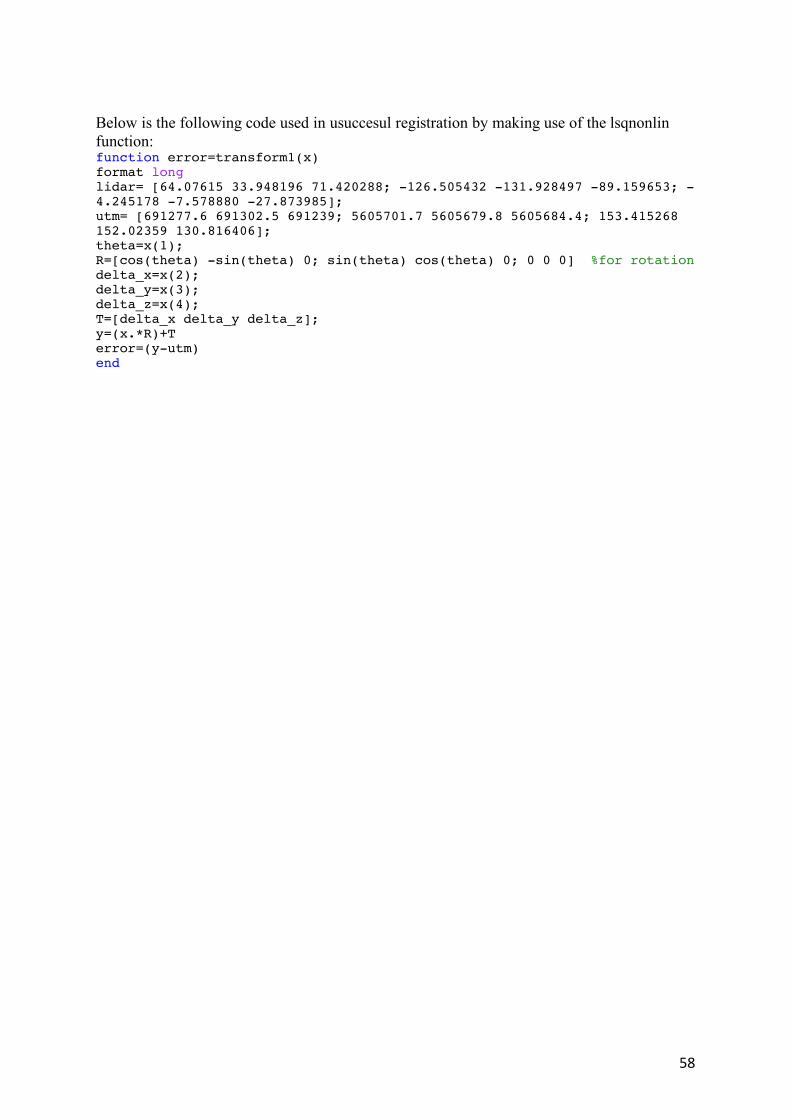
58

Below is the following code used in usuccesul registration by making use of the lsqnonlin function: function error=transform1(x) format long lidar= [64.07615 33.948196 71.420288; -126.505432 -131.928497 -89.159653; -4.245178 -7.578880 -27.873985]; utm= [691277.6 691302.5 691239; 5605701.7 5605679.8 5605684.4; 153.415268 152.02359 130.816406]; theta=x(1); R=[cos(theta) -sin(theta) 0; sin(theta) cos(theta) 0; 0 0 0] %for rotation delta_x=x(2); delta_y=x(3); delta_z=x(4); T=[delta_x delta_y delta_z]; y=(x.*R)+T error=(y-utm) end