Methods for detection of extra-solar planets (exo-planets) · Methods for detection of extra-solar planets (exo-planets): ~500 10? 3 ~100 2? 51 Peg . Folgende Folien basieren auf

Methods for detection

of extra-solar planets (exo-planets):

~500

10?

3 ~100

2?

51 Peg

Folgende Folien basieren auf der

Vorlesung

“Physics of Planetary Systems”

von Prof. Artie Hatzes

(TLS Tautenburg)

Sprache

Language

Literature

Contents:

• Our Solar System from Afar (overview of detection methods)

• Exoplanet discoveries by the transit method

• What the transit light curve tells us

• The Exoplanet population

• Transmission spectroscopy and the Rossiter-McLaughlin effect

• Host Stars

• Secondary Eclipses and phase variations

• Transit timing variations and orbital dynamics

• Brave new worlds By Carole Haswell

Contents:

• Radial Velocities

• Astrometry

• Microlensing

• Transits

• Imaging

• Host Stars

• Brown Dwarfs and Free floating

Planets

• Formation and Evolution

• Interiors and Atmospheres

• The Solar System

Literature

Contributions:

• Radial Velocities

• Exoplanet Transits and Occultations

• Microlensing

• Direct Imaging

• Astrometric Detections

• Planets Around Pulsars

• Statistical Distribution of Exoplanets

• Non-Keplerian Dynamics of Exoplanets

• Tidal Evolution of Exoplanets

• Protoplanetary and Debris Disks

• Terrestrial Planet Formation

• Planet Migration

• Terrestrial Planet Interiors

• Giant Planet Interior Structure and Thermal Evolution

• Giant Planet Atmospheres

• Terrestrial Planet Atmospheres and Biosignatures

• Atmospheric Circulation of Exoplanets

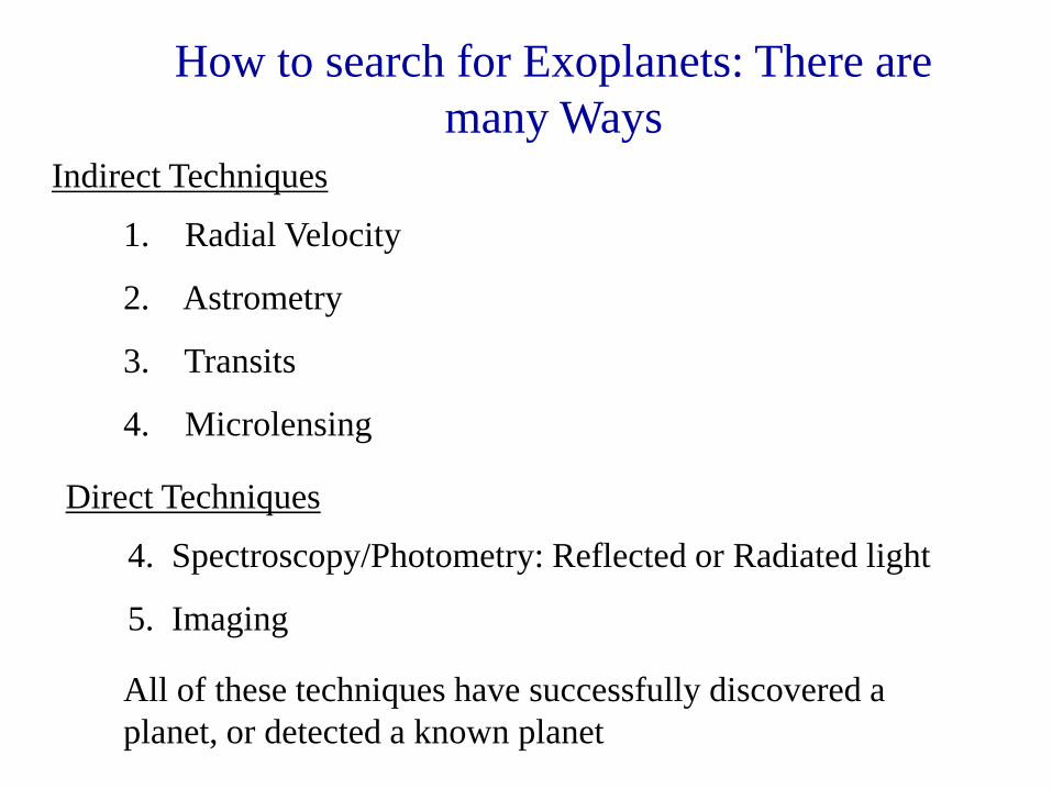
How to search for Exoplanets: There are

many Ways

1. Radial Velocity

2. Astrometry

3. Transits

4. Microlensing

Indirect Techniques

4. Spectroscopy/Photometry: Reflected or Radiated light

5. Imaging

Direct Techniques

All of these techniques have successfully discovered a

planet, or detected a known planet

Radial velocity measurements using the Doppler Wobble

The closer the planet, the higher the velocity amplitude. The

RV method is more sensitive for planets close to the star

(short orbital periods)

Requirements: • Accuracy of better than 10 m/s

• Stability for at least 10 Years

Jupiter: 12 m/s, 11 years

Saturn: 3 m/s, 30 years

Radial Velocity measurements

28.4

P1/3ms2/3

mp sin i Vobs =

Center of mass

2q

2q = 8 mas at a Cen

2q = 1 mas at 10 pcs

Current limits:

1-2 mas (ground)

0.1 mas (HST)

• Since D ~ 1/D can only look

at nearby stars

Astrometric Measurements of Spatial Wobble

m

M

a

D q =

Jupiter only

1 milliarc-seconds for a Star

at 10 parsecs

Microlensing

Methods of Detecting Exoplanets

1. Doppler wobble - Velocity reflex motion of the star due to the planet: 601 planets (107 systems)

2. Transit Method - photometric eclipse due to planet: 1206 planets (357 systems)

3. Astrometry - spatial reflex motion of star due to planet: 0 discoveries, 6 detections of known planets

4. Direct Imaging: 51 planets (1 system)

5. Microlensing – gravitational perturbation by light: 35 planets (2 Systems)

6. Timing variations – changes in the arrival of pulses (pulsars), oscillation frequencies, or time of eclipses (no transit timing variations): 19 planets (4 systems)

A Brief History of Light Deflection

In 1801 Soldner used Newtonian Physics to calculate the deflection of light by

gravity:

A Brief History of Light Deflection

In 1911 Einstein derived:

Einstein in 1911 was only half right !

a = 2 GMּס

c2Rּס

= 0.87 arcsec

In 1916 using General Relativity Einstein derived:

a = 4 GM

c2r

= 1.74 arcsec

Light passing a distance r from object

Factor of 2 due to spatial curvature which is missed if light is treated like particles

Eddington‘s 1919 Eclipse expedition

confirmed Einstein‘s result

Einstein Cross

Einstein Ring

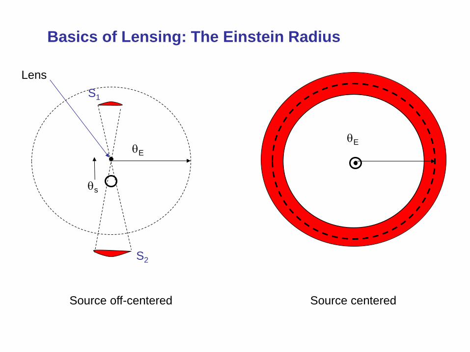
Basics of Lensing: The Einstein Radius

qs

qE

S1

S2

Lens

Source off-centered

qE

Source centered

b = 0

b = q – a(q)

Point lens: magnification of two images m = q

b

dq

db

Typical microlensing events last from a few weeks to a few months

Basics of Lensing: Caustics

source: wikipedia

Caustic: the envelope of light rays reflected or

refracted by a curved surface or object

xc ≈ s + s–1 + 2(cos3f -2 cos f)

s + s–1 – 2(cos2f -2 cos f)2 q

hc ≈ 2 sin3f

s + s–1 – 2(cos2f -2 cos f)2 q

q= mass ratio

s = planet – star separation

For planets q << 1

Analytic solution for planetary caustics

The First: OGLE-235-MOA53

OGLE

alert

Lightcurve close-up & fit (from Bennet)

• Cyan curve is the best fit single lens model

–D2 = 651

• Magenta curve is the best fit model w/ mass fraction e 0.03

–D2 = 323

• 7 days inside caustic = 0.12 tE

–Long for a planet,

–but Dmag = only 20-25%

–as expected for a planet near the Einstein Ring

Caustic Structure Blue and red dots indicate times of observations

Parameters:

tE = 61.6 1.8 days

t0 = 2848.06 0.13 MJD

umin = 0.133 0.003

ap = 1.120 0.007 AU

e = 0.0039 0.007

q = e/(1+ e)

f = 223.8 1.4

t* = 0.059 0.007 days or q*/qE = 0.00096 0.00011

Alternative Models: ap < 1

D2 = 110.4

tE = 75.3 days

t0 = 2850.64

MJD

umin = 0.098

ap = 0.926

e = 0.0117

f = -6.1

t* = 0.036 days

Also planetary!

Microlensing planet detection of a Super Earth?

OGLE-2005-BLG-390

Mass = 2.80 – 10 Mearth

a = 2.0 – 4.1 AU

Best binary

source

q = 7.6 x 10–5 Ratio between planet and star

Let‘s play Devil‘s advocate

• Not all possible models have been exhausted. Only

9 data points define planet

• Source binary model conveniently has a peak in the

data gap

• Source is a G4 III giant star. Giant stars are known

to have spots and pulsations.

• Host star parameters relies on statistics and

galactic models

All derived parameters depend on Bayesian Statistics:

Robert Kraft: „If you have to integrate, you don‘t understand it. If you have to use

statistics, it doesn‘t exist!“

Astrometric Detection of Exoplanets

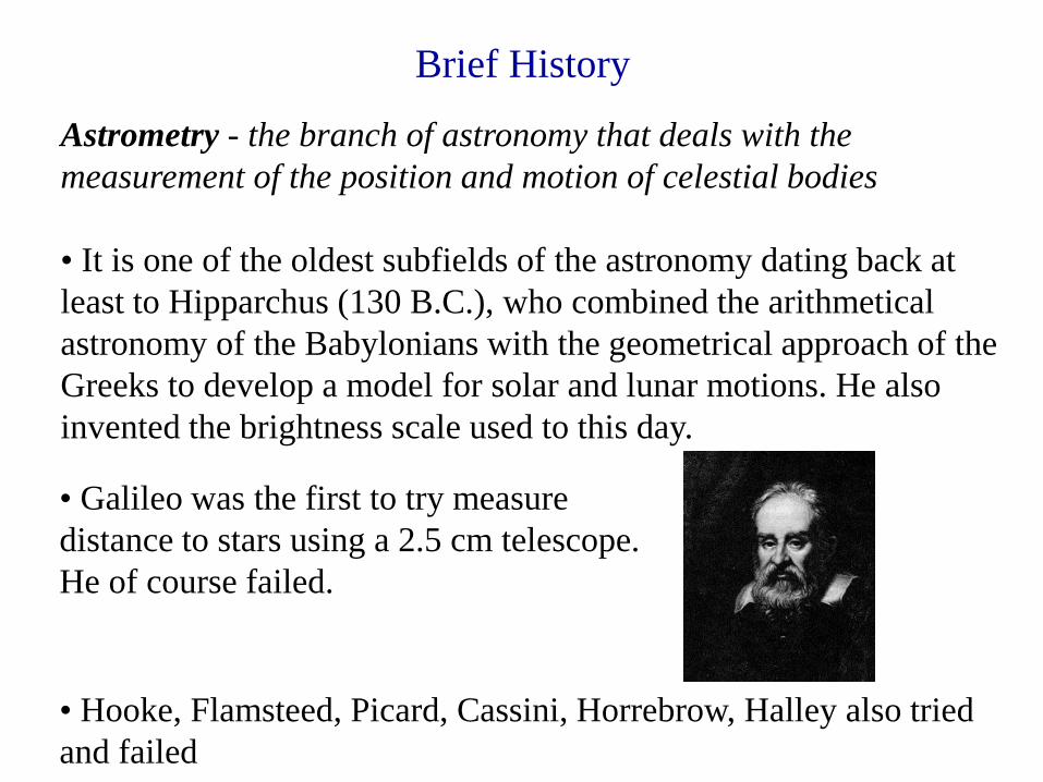
Astrometry - the branch of astronomy that deals with the

measurement of the position and motion of celestial bodies

• It is one of the oldest subfields of the astronomy dating back at

least to Hipparchus (130 B.C.), who combined the arithmetical

astronomy of the Babylonians with the geometrical approach of the

Greeks to develop a model for solar and lunar motions. He also

invented the brightness scale used to this day.

Brief History

• Hooke, Flamsteed, Picard, Cassini, Horrebrow, Halley also tried

and failed

• Galileo was the first to try measure

distance to stars using a 2.5 cm telescope.

He of course failed.

• 1887-1889 Pritchard used photography for astrometric

measurements

• Modern astrometry was founded by

Friedrich Bessel with his Fundamenta

astronomiae, which gave the mean position

of 3222 stars.

• 1838 first stellar parallax (distance) was measured

independently by Bessel (heliometer), Struve (filar micrometer),

and Henderson (meridian circle).

Astrometry: Parallax

Distant stars

1 AU projects to 1 arcsecond at a

distance of 1 pc = 3.26 light years

Astrometry: Parallax

So why did Galileo fail?

d = 1 parsec

q= 1 arcsecond

F f = F/D

D

d = 1/q, d in parsecs, q

in arcseconds

1 parsec = 3.08 ×1018 cm

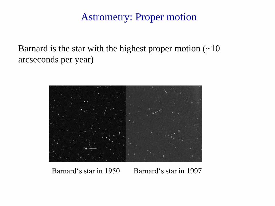
Astrometry: Proper motion

Barnard is the star with the highest proper motion (~10

arcseconds per year)

Barnard‘s star in 1950 Barnard‘s star in 1997

m

M

a

D q =

The astrometric signal is given by:

m = mass of planet

M = mass of star

a = orbital radius

D = distance of star

q = m

M2/3

P2/3

D

Astrometry: Orbital Motion

Note: astrometry is sensitive to companions of

nearby stars with large orbital distances

Radial velocity measurements are distance independent, but

sensitive to companions with small orbital distances

This is in radians. More useful units are

arcseconds (1 radian = 206369 arcseconds) or

milliarcseconds (0.001 arcseconds) = mas

The Space motion of Sirius A and B

Astrometric Detections of Exoplanets

The Challenge:

for a star at a distance of 10 parsecs (=32.6 light years):

Source Displacment (mas)

Jupiter at 1 AU 100

Jupiter at 5 AU 500

Jupiter at 0.05 AU 5

Neptune at 1 AU 6

Earth at 1 AU 0.33

Parallax 100000

Proper motion (/yr) 500000

The Importance of Reference stars

Perfect instrument Perfect instrument at a later time

Reference stars:

1. Define the plate scale

2. Monitor changes in the plate scale (instrumental effects)

3. Give additional measures of your target

Focal „plane“

Detector

Example

Typical plate scale on a 4m telescope (Focal ratio = 13) = 3.82 arcsecs/mm =

0.05 arcsec/pixel (15 mm) = 57 mas/pixel. The displacement of a star at 10

parsecs with a Jupiter-like planet would make a displacement of 1/100 of a

pixel (0.00015 mm)

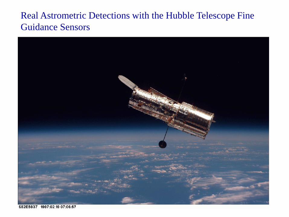
Real Astrometric Detections with the Hubble Telescope Fine

Guidance Sensors

HST uses Narrow Angle Interferometry!

One of our planets is missing: sometimes you need the true mass!

HD 33636 b

P = 2173 d

Msini = 10.2 MJup

B

i = 4 deg → m = 142 MJup

= 0.142 Msun

Bean et al. 2007AJ....134..749B

Gl 876

Vb 10 Control star

Space: The Final Frontier

1. Hipparcos

• 3.5 year mission ending in 1993

• ~100.000 Stars to an accuracy of 7 mas

2. Gaia

• 1.000.000.000 stars

• V-mag 15: 24 mas

• V-mag 20: 200 mas

• Launch 2011 2012

19 December 2013

Number of Expected Planets from GAIA

8000 Giant planet detections

4000 Giant planets with orbital parameters determined

1000 Multiple planet detections

500 Multiple planets with orbital parameters determined

1. Astrometry is the oldest branch of Astronomy

2. It is sensitive to planets at large orbital distances

→ complimentary to radial velocity

3. Gives you the true mass

4. Least successful of all search techniques because

the precision is about a factor of 1000 to large.

5. Will have to await space based missions to have a

real impact

Summary

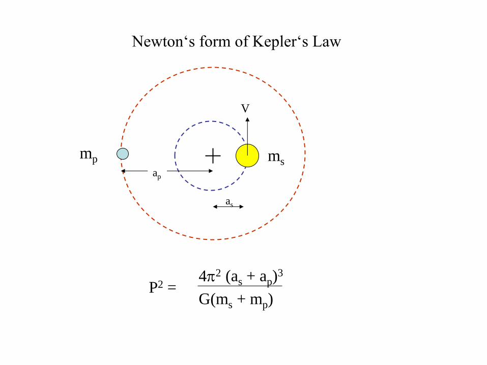
ap

as

V

P2 = 4p2 (as + ap)

3

G(ms + mp)

ms mp

Newton‘s form of Kepler‘s Law

P2 = 4p2 (as + ap)

3

G(ms + mp)

Approximations: ap » as

ms » mp

P2 ≈ 4p2 ap

3

Gms

Circular orbits: V = 2pas

P

„Lever arm“: ms × as = mp × ap

as = mp ap

ms

Solve Kepler‘s law for ap:

ap = P2Gms

4p2 ( )

1/3

… and insert in expression for as and then V for circular

orbits

V = 2p

P(4p2)1/3

mp P2/3 G1/3ms

1/3

V = 0.0075

P1/3ms2/3

mp

= 28.4

P1/3ms2/3

mp

mp in Jupiter

masses

ms in solar masses

P in years

V in m/s

28.4

P1/3ms2/3

mp sin i Vobs =

Planet Mass (MJ) V(m s–1)

Mercury 1.74 × 10–4 0.008

Venus 2.56 × 10–3 0.086

Earth 3.15 × 10–3 0.089

Mars 3.38 × 10–4 0.008

Jupiter 1.0 12.4

Saturn 0.299 2.75

Uranus 0.046 0.297

Neptune 0.054 0.281

Radial Velocity Amplitude of Sun due to Planets in the

Solar System

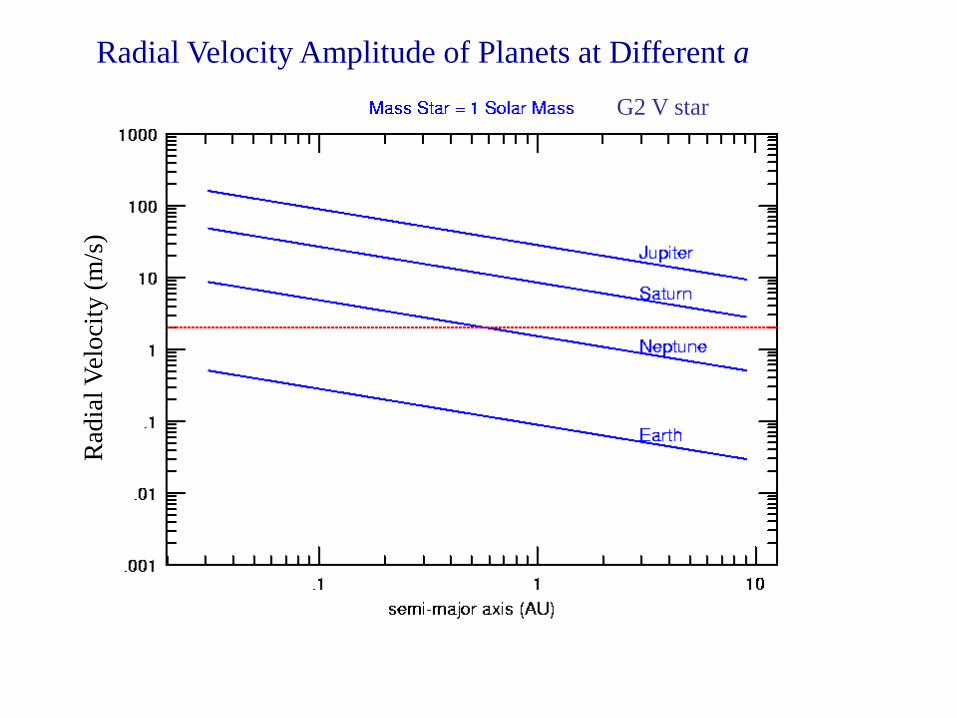
Radial Velocity Amplitude of Planets at Different a

Rad

ial

Vel

oci

ty (

m/s

) G2 V star

Rad

ial

Vel

oci

ty (

m/s

) A0 V star

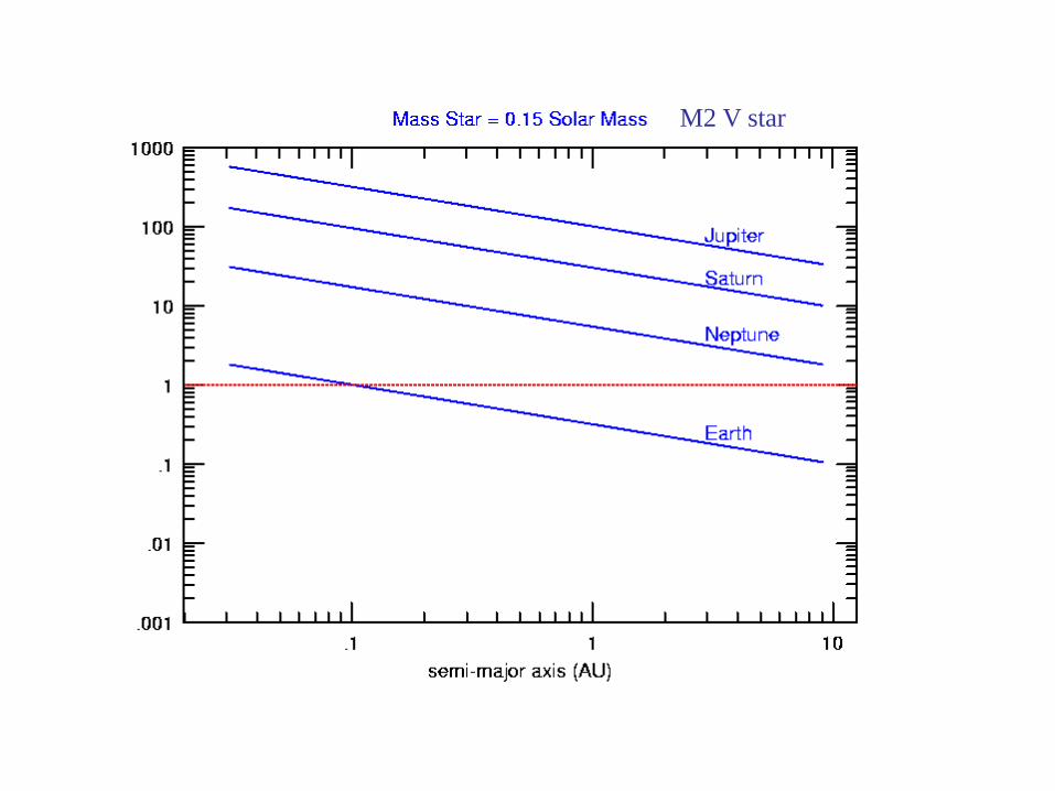
M2 V star

Radial velocity shape as a function of eccentricity:

Radial velocity shape as a function of w, e = 0.7 :

Eccentric orbit can sometimes escape detection:

With poor sampling this star would be considered constant

The Grandfather of Radial Velocity

Planet Detections

Christian Doppler,

Discoverer of the Doppler

effect

Born: 29.11.1803, in Salzburg

Died: 17.03.1853 in Venice

First radial velocity measurement

for a star made on Sirius by Sir

William Higgins in 1868

radialvelocitydemo.htm

Bild: Wikipedia

Measurement of Doppler Shifts

In the non-relativistic case:

l – l0

l0

= Dv

c

We measure Dv by measuring Dl

The Radial Velocity Measurement Error with Time

How did we accomplish this?

Fastest Military

Aircraft (SR-71

Blackbird)

High Speed Train

World Class

Sprinter

Casual Walk

Average Jogger

Including dependence on stellar parameters

v sin i : projected rotational velocity of star in km/s

f(Teff) = factor taking into account line density

f(Teff) ≈ 1 for solar type star

f(Teff) ≈ 3 for A-type star (T = 10000 K, 2 solar masses)

f(Teff) ≈ 0.5 for M-type star (T = 3500, 0.1 solar masses)

s (m/s) ≈ Constant ×(S/N)–1 R–3/2 v sin i

( 2 ) f(Teff) (Dl)–1/2

Traditional method:

Observe your star→

Then your

calibration source→

51 Pegasi b: The Discovery that Shook up

the Field

Discovered by Michel Mayor &

Didier Queloz, 1995

Period = 4,3 Days

Semi-major axis = 0,05 AU (10

Stellar Radii!)

Mass ~ 0,45 MJupiter

51 Peg

Rate of Radial Velocity Planet Discoveries

Eccentricity versus Orbital Distance

Note that there are few highly eccentric orbits close into the star. This

is due to tidal forces which circularizes the orbits quickly.

Butler et al. 2004

McArthur et al. 2004

Santos et al. 2004

Msini = 14-20 MEarth

Classes of planets: Hot Neptunes

Note that the scale on the y-

axes is a factor of 100

smaller than the previous

orbit showing a hot Jupiter

If there are „hot Jupiters“ and „hot Neptunes“ it makes sense that

there are „hot Superearths“

Mass = 7.4 ME P = 0.85 d

CoRoT-7b

Hot Superearths were discovered by space-based transit

searches

Mass = 1.31± 0.25 MEarth (Amplitude = 1.34 m/s)

Period = 8.5 hours

Earth-mass Planet: Kepler 78b

Pepe et al. 2013,

Howard et al. 2013

2.13 AU a

0.2 e

26.2 m/s K

1.76 MJupiter Msini

2.47 Years Period

Planet

18.5 AU a

0.42 ± 0.04 e

1.98 ± 0,08

km/s

K

~ 0.4 ± 0.1 MSun Msini

56.8 ± 5 Years Period

Binary g Cephei

Summary of Exoplanet Properties from RV

Studies

• ~10 % of normal solar-type stars have giant planets

• < 1% of the M dwarfs stars (low mass) have giant planets, but may have

a large population of neptune-mass planets

→ low mass stars have low mass planets, high mass stars have more

planets of higher mass → planet formation may be a steep function of

stellar mass

• 0.5–1% of solar type stars have short period giant plants

• Exoplanets have a wide range of orbital eccentricities (most are not in

circular orbits)

• Massive planets tend to be in eccentric orbits and have large orbital radii

Discovery Space for Exoplanets

R*

a

q

i = 90o+q

sin q = R*/a = |cos i|

Porb = 2p sin i di / 4p = 90-q

90+q

–0.5 cos (90+q) + 0.5 cos(90–q) = sin q

= R*/a for small angles

Transit Probability

a is orbital semi-major axis, and i is the

orbital inclination1

1by definition i = 90 deg is

looking in the orbital plane

Transit Duration

t = 2(R* +Rp)/v

where v is the orbital velocity and i = 90 (transit across disk center)

Exercise left to the audience: Show that the transit

duration for a fixed period is roughly related to the

mean density of the star.

t3 ~ (rmean)–1

For more accurate times need to take into account the

orbital inclination

for i 90o need to replace R* with R:

R2 + d2cos2i = R*2

R = (R*2 – d2 cos2i)1/2

d cos i R*

R

1. First contact with star

2. Planet fully on star

3. Planet starts to exit

4. Last contact with star

Note: for grazing transits there is

no 2nd and 3rd contact

Making contact:

1

2 3

4

Shape of Transit Curves

A real transit light curve is not flat

HST light curve of HD 209458b

To probe limb

darkening in other

stars..

..you can use

transiting planets

At the limb the star has less flux than is expected, thus the planet blocks less light

No limb darkening

transit shape

At different

wavelengths in Ang.

Grazing eclipses/transits These produce a „V-shaped“

transit curve that are more

shallow

Shape of Transit Curves

Planet hunters like to see a flat part on the bottom of the transit

E.g. a field of 10.000 Stars the number of expected transits is:

Ntransits = (10.000)(0.1)(0.01)(0.3) = 3

Probability of right orbit inclination

Frequency of Hot Jupiters

Fraction of stars with suitable radii

So roughly 1 out of 3000 stars will show a transit event due to a

planet. And that is if you have full phase coverage!

CoRoT: looked at 10,000-12,000 stars per field and found on

average 3 Hot Jupiters per field. Similar results for Kepler

Note: Ground-based transit searches are finding hot Jupiters 1 out of

30,000 – 50,000 stars → less efficient than space-based searches

Catching a transiting planet is thus like playing

Lotto. To win in LOTTO you have to

1. Buy lots of tickets → Look at lots of stars

2. Play often → observe as often as you can

The obvious method is to use CCD photometry

(two dimensional detectors) that cover a large

field. You simultaneously record the image of

thousands of stars and measure the light

variations in each.

Light curve for HD 209458

Transit Curve from a 10 cm telescope

Radial Velocity Curve for HD 209458

Period = 3.5 days

M = 0.63 MJup

Transit

phase = 0

Radial Velocity Curve: 3m telescope

False Positives

1. Grazing eclipse by a main sequence star:

One should be able to distinguish

these from the light curve shape and

secondary eclipses, but this is often

difficult with low signal to noise

These are easy to exclude with Radial

Velocity measurements as the

amplitudes should be tens km/s

(2–3 observations)

It looks like a planet, it smells like a planet, but it is not a planet

2. Giant Star eclipsed by main sequence star:

G star

These can easily be excluded using one spectrum to

establish spectral and luminosity class. In principle no

radial velocity measurements are required.

Often a giant star can be known from the transit time.

These are typically several days long!

Giant stars have radii of 10-100 solar radii which

translates into photometric depths of 0.0001 – 0.01 for a

companion like the sun.

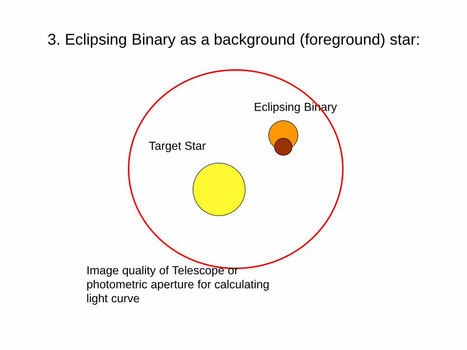
3. Eclipsing Binary as a background (foreground) star:

Eclipsing Binary

Target Star

Image quality of Telescope or

photometric aperture for calculating

light curve

4. Eclipsing binary in orbit around a bright star (hierarchical

triple systems)

Another difficult case. Radial Velocity Measurements of the bright

star will show either long term linear trend no variations if the orbital

period of the eclipsing system around the primary is long. This is

essentialy the same as case 3) but with a bound system

5. Unsuitable transits for Radial Velocity measurements

Transiting planet orbits an early type star with rapid rotation

which makes it impossible to measure the RV variations or

you need lots and lots of measurements.

Depending on the rotational velocity RV measurements are

only possible for stars later than about F3

Period: 9.75

Transit duration: 4.43 hrs

Depth : 0.2%

V = 13.9

Spectral Type: G0IV (1.27 Rsun)

Planet Radius: 5.6 REarth

Photometry: On Target

The Radial Velocity

measurements are

inconclusive. So, how do we

know if this is really a planet.

Note: We have over 30 RV

measurements of this star: 10 Keck

HIRES, 18 HARPS, 3 SOPHIE. In spite

of these, even for V = 13.9 we still do

not have a firm RV detection. This

underlines the difficulty of confirmation

measurements on faint stars.

CoRoT: LRc02_E1_0591

6. Sometimes you do not get a final answer

OGLE

• OGLE: Optical Gravitational Lens Experiment

(http://www.astrouw.edu.pl/~ogle/)

• 1.3m telescope looking into the galactic bulge

• Mosaic of 8 CCDs: 35‘ x 35‘ field

• Typical magnitude: V = 15-19

• Designed for Gravitational Microlensing

• First planet discovered with the transit method

WASP

WASP: Wide Angle Search For Planets (http://www.superwasp.org). Also

known as SuperWASP

• Array of 8 Wide Field Cameras

• Field of View: 7.8o x 7.8o

• 13.7 arcseconds/pixel

• Typical magnitude: V = 9-13

• 86 Planets discovered

• Most successful ground-based transit search program

Another Successful Transit Search Program

• HATNet: Hungarian-made Automated Telescope

(http://www.cfa.harvard.edu/~gbakos/HAT/

• Six 11cm telescopes located at two sites: Arizona and Hawaii

• 8 x 8 square degrees

• 43 Planets discovered

The MEarth Strategy

One star at a time!

The MEarth project

(http://www.cfa.harvard.edu/~zberta/mearth/)

uses 8 identical 40 cm telescopes to search

for terrestrial planets around M dwarfs one

after the other

V- magnitude

Perc

en

t

Stellar Magnitude distribution of Exoplanet

Discoveries

0,00%

5,00%

10,00%

15,00%

20,00%

25,00%

30,00%

35,00%

0.5 4,50 8,50 12,50 16,50

Transits

RV