Methodology underlying the CAPRI model model methodology.pdf · Building up the global data base, which includes areas and market balances for the ... sector data processing may be

Methodology underlying the CAPRI model

2

3

Contents 1 Introduction ....................................................................................................................... 5

2 Position in the agriculture related modeling suite of EUCLIMIT ....................................... 6

2.1 CAPRI ......................................................................................................................... 7

2.2 GLOBIOM ................................................................................................................... 8

2.3 G4M ........................................................................................................................... 8

3 CAPRI database .................................................................................................................. 9

3.1 Improvements in the CAPRI database under EUCLIMIT .......................................... 12

3.1.1 Standard database updates and outlier checking ........................................... 12

3.1.2 Improvement of land use database ................................................................ 12

3.1.3 Full integration of herd size data in all CAPRI modules ................................... 12

4 Baseline Generation ........................................................................................................ 13

4.1 Improvements in the CAPRI baseline procedure under EUCLIMIT ......................... 15

4.1.1 Improved alignment with PRIMES biomass..................................................... 15

4.1.2 Update of EFMA information of fertiliser outlook .......................................... 15

4.1.3 Deepening of linkages to IIASA models ........................................................... 15

4.1.4 Update of MS level expert information ........................................................... 17

5 Simulation mode ............................................................................................................. 17

Annex 1 Activities and items in CAPRI ............................................................................... 20

Annex 2 Animal sector details in CAPRI ............................................................................. 30

Annex 3 Complete area database ..................................................................................... 34

I. Background .................................................................................................................. 34

II. Specific data sources related to land use .................................................................... 35

III. Methodology of data consolidation for the CAPRI Data Base................................. 37

IV. Results ..................................................................................................................... 42

V. Concluding remarks ..................................................................................................... 46

4

5

1 Introduction The Common Agricultural Policy Regional Impact (CAPRI) model is an agricultural sector

model with a focus on Europe (disaggregation into 280 NUTS2 regions, detailed activity data

and coverage of Common Agricultural policies), but embedded in a global market model to

represent bilateral trade between 44 trade regions (countries or country aggregates).

It is the outcome of a series of projects supported by European Commission research funds,

the first one 1996-1999. Operational since more than a decade (1999), it supports decision

making related to the Common Agricultural Policy (CAP) and, due to the development of

environmental indicators, also environmental policies related to agriculture. In the following

we will focus on the elements most relevant to the EUCLIMIT (Development and application

of EU economy-wide climate change mitigation modelling capacity) project whereas the full

documentation is online at http://www.capri-

model.org/docs/capri_documentation_2012.pdf.

The CAPRI outlook systematically merges the information in historical time series with

external projections from other models or independent expert knowledge while imposing

technical consistency. In this application key external information came from the models

PRIMES, GLOBIOM and AGLINK, together with national expert information on specific items.

The key outputs (to GAINS) were the activity data in the livestock sector plus mineral

fertilizer use in the crop sector.

CAPRI and GLOBIOM are both modelling the agricultural sector of EU countries and estimate

the supply and demand of agricultural products as well as emissions from production and

soil. There is thus an overlap of the models in terms of coverage but both have a quite

different orientation and structure. Therefore they complement each other and give the

user additional information when they are applied to the same scenarios.

The methodology report on CAPRI is structured in the following way. Section 2 briefly

presents the general modelling suite as far as it is related to agriculture. Section 3 gives

some details on the database where significant improvements have been achieved under

EUCLIMIT. Section 4 explains the methodology to produce the CAPRI outlook and the

improvements implemented under EUCLIMIT. Section 5 is devoted to “scenario mode” of

CAPRI which has been used under EUCLIMIT to distinguish the “reference run” (with

additional measures) from the “baseline” (only adopted measures). Three annexes complete

this report. The first is a listing of the items available. Annex 2 gives some technical details

on the animal sector of CAPRI that is most important for the role of CAPRI in the EUCLIMIT

modelling chain. Annex 3 finally reports on the efforts to establish a database covering the

complete area of countries. This helped to improve communication between CAPRI and

GLOBIOM under EUCLIMIT.

6

2 Position in the agriculture related modeling suite of

EUCLIMIT To respond to the project tasks regarding emission projections, the models communicate as

shown in Figure 1 below. The macro-economic outlook as well as economic activities and

energy use by sector is captured by GEM-E3 and PRIMES. The biomass component of

PRIMES provides bioenergy related information both to CAPRI and GLOBIOM, ensuring

consistency in bioenergy related assumptions. However, due to the differences between

CAPRI and GLOBIOM, different pieces of information are used as model inputs:

GLOBIOM uses information on various types of bioenergy demand (heat, power, cooking, transport fuels of first and second generation) and biomass production of energy purposes (from crops, forestry, waste items) as lower bounds for the market equilibrium.

CAPRI uses supply and demand of biofuels and the shares of first and second generation production. Furthermore the broad split of first generation agricultural feedstocks (cereals, oilseeds, sugar crop) as well as the areas for lignocellulosic crops are inputs from the PRIMES biomass component.

These differences reflect the endogenous coverage of forestry and lignocellulosic crops in

GLOBIOM. Both models yield results on the complete area allocation and feed back to the

PRIMES biomass components in case of questionable results, for example if a very high

expansion of lignocellulosic crops would have dubious implications for the whole area

allocation in a country.

GLOBIOM projects a long run market equilibrium for key agricultural (and forestry) products

from basic drivers such as GDP, population, food consumption trends, productivity growth. It

is interacting with the G4M model for supply side details on forestry. The CAPRI model uses

these GLOBIOM projections as prior information for its own baseline. This means that they

provide target values for the CAPRI baseline. At the same time CAPRI uses prior information

from the AGLINK baseline, but due to the relative strength of these models the weight of

AGLINK decreases relative to GLOBIOM along a longer-term projection horizon (2030-2050).

The preliminary baseline results of CAPRI and GLOBIOM are compared and in case of

surprising differences a feedback loop of information is initiated.

Relying on a considerable level of technical detail, the forestry and agriculture models may

also supply projections of emissions and removals of GHGs. However, in the EUCLIMIT

modelling suite it is only the LULUCF results from GLOBIOM on carbon releases and

sequestration that enter the final reporting. Non-CO2 emissions from agriculture (and other

sectors) are calculated in GAINS, considering technical abatement options and their cost and

using the agricultural activity information from CAPRI (animal herds, fertiliser use). The

energy related emissions of CO2 are directly provided by PRIMES.

7

Figure 1: Overview of EUCLIMIT model interactions.

Important model characteristics may be summarised as follows, highlighting the differences

and complementarities.

2.1 CAPRI CAPRI (for Common Agricultural Policy Regional Impacts) is a global agricultural sector model

developed at Bonn University with a clear focus on Europe. The main characteristics are:

Global multi commodity model covering about 60 agricultural and processed products and 80 world regions, aggregated to 40 trade regions.

Supply modelling in Europe occurs in more detail (280 NUTS2 regions, potentially disaggregated into 2000 Farm Types) in nonlinear programming models. Both the behavioural function of the global market model as well as the nonlinearities in the European programming models ensure smooth responses to changes in economic incentives.

Partial equilibrium, meaning that non-agricultural sectors are excluded but there are options and experience to link the CAPRI core model to CGEs.

European agricultural land use is represented completely (including fruits, vegetables, wine etc), but some globally relevant crops (e.g. peanuts) and forestry are not modelled.

The livestock sector is represented in great detail including feed requirements (energy, protein, fibre etc.) and young animal herd constraints (Annex A.4.2).

8

CAPRI has a detailed coverage of CAP and agricultural trade policies (including TRQs), relying on the Armington approach for two way international trade.

The model is not designed for stand alone outlook work but incorporates external prior information combined with a statistical analysis of its time series database

It is comparative static and not suitable for very long scenario runs (>2050).

2.2 GLOBIOM The Global Biosphere Management Model (GLOBIOM) has been developed and is used at

the International Institute for Applied Systems Analysis (IIASA). The main characteristics are:

Global land use model covering 53 world regions, including all EU28 Member States. The regional break down can be altered if needed.

The methodology is the same for Europe and other regions. A maximisation of a social welfare function in a linear program simulates the market equilibrium. In small simulation units on the supply side strong specialisation may occur, but the aggregation to countries and larger regions and constraints at the simulation unit level tends to smooth out this feature to some extent.

It is a partial equilibrium model with bottom-up design, not only in a strong disaggregation of supply regions into simulation units but also in the technological detail (detailed representation of cropland management (input and management systems), livestock sector (FAO system classification) and globally consistent GHG accounting)

Substantive experience with linkages to other biophysical and economic models (EPIC, G4M, RUMINANT, PRIMES, POLES etc.)

It covers the major global land-based production sectors (agriculture, forestry, bioenergy, other natural land) and different bioenergy transformation pathways, but some agricultural products (fruits, vegetables, wine etc) are neglected.

Compared to CAPRI less details on agricultural policies as the focus is on global land use issues. Bilateral trade is modelled, but two way trade and TRQs are not explicitly represented.

GLOBIOM is recursive dynamic as e.g. land use changes are transmitted from one period to the other and subject to certain inertia constraints.

The model can relatively easily also be applied for scenarios up to the year 2100 but its short to medium run projections may not capture recent trends, as GLOBIOM does not calibrate its baseline to time series but to an average around the base year (2000). In addition, it is driven by long-term macro-economic driver such as GDP, population growth and productivity changes.

2.3 G4M For the forestry sector, biomass supply is projected by the Global Forestry Model (G4M):

9

Geographically explicit forestry model

Estimates afforestation, deforestation and forest management area and associated emissions and removals per EU Member State

Is calibrated to historic data reported by Member States on afforestation and deforestation and therefore includes policies on these activities. Explicit future targets of forest area development can be included

Informs GLOBIOM about potential wood supply and initial land prices

Receives information from GLOBIOM on the development of wood demand, wood prices and land prices

3 CAPRI database The main characteristics of the CAPRI data base are:

Wherever possible link to harmonised, well documented, official and generally available data sources to ensure acceptance of the data and the possibility of annual updates.

Completeness over time and space. As far as official data sources comprise gaps, suitable algorithms were developed and applied to fill these.

Consistency between the different data (closed market balances, perfect aggregation from lower to higher regional level etc., match of physical and monetary data)

Data are collected at various levels from the global, to the national, and finally regional

(NUTS2) level. A further layer consists of geo-referenced information at the level of clusters

of 1x1 km grid cells which serves as input in the spatial down-scaling part of CAPRI (not used

in EUCLIMIT). Finally in the last CAPRI-RD project a layer of regional CGEs has been

implemented that may be switched on for an analysis of rural development policies (not

used in EUCLIMIT). As it would be impossible to ensure consistency across all regional layers

simultaneously, the process of building up the data base is split in several parts:

Building up the global data base, which includes areas and market balances for the non European regions in the market model (mostly from FAO) and bilateral trade flows.

Building up the European data base at national or Member State level (not only EU but also Norway, Turkey, Western Balkan). It integrates the Economic Accounts data (valued output and input use) with market and farm data, with areas and animal herds (that are currently not covered for non European countries).

Building up the data base at regional or NUTS 2 level, which takes the national data basically as given (for purposes of data consistency), and includes the allocation of inputs across activities and regions as well as consistent areas, herd sizes and yields at regional level.

Given the extent of public intervention in the agricultural sector, policy data complete the database. They are partly CAP instruments like premiums and quotas

10

and partly data on trade policies (Most Favourite Nation Tariffs, Preferential Agreements, Tariff Rate quotas, export subsidies) plus data on domestic market support instruments (market interventions, subsidies to consumption) and rural development policies.

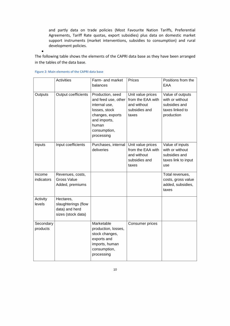
The following table shows the elements of the CAPRI data base as they have been arranged

in the tables of the data base.

Figure 2: Main elements of the CAPRI data base

Activities Farm- and market

balances

Prices Positions from the

EAA

Outputs Output coefficients Production, seed

and feed use, other

internal use,

losses, stock

changes, exports

and imports,

human

consumption,

processing

Unit value prices

from the EAA with

and without

subsidies and

taxes

Value of outputs

with or without

subsidies and

taxes linked to

production

Inputs Input coefficients Purchases, internal

deliveries

Unit value prices

from the EAA with

and without

subsidies and

taxes

Value of inputs

with or without

subsidies and

taxes link to input

use

Income

indicators

Revenues, costs,

Gross Value

Added, premiums

Total revenues,

costs, gross value

added, subsidies,

taxes

Activity

levels

Hectares,

slaughterings (flow

data) and herd

sizes (stock data)

Secondary

products

Marketable

production, losses,

stock changes,

exports and

imports, human

consumption,

processing

Consumer prices

11

In 2012-13 there has been a thorough revision of the CAPRI global database which was

motivated and financed from other projects, mainly to adjust to a different organisation and

data availability from Faostat.

More important for EUCLIMIT are the European data which mostly rely on Eurostat and are

compiled in two major modules, “COCO” (for complete and consistent at the national level)

and “CAPREG” for the CAPRI (NUTS2) regions. The first one, the COCO module for the

national database, is itself composed of two submodules:

COCO1 submodule: This is the major step preparing the bulk of the national database for European countries, one country after the other. It involves three steps: - A data import step that collects a large set of very heterogeneous input files - Including and combining these partly overlapping input data according to a

set of hierarchical overlay criteria, and - Calculating complete and consistent time series while remaining close to the

raw data in an optimisation program. The data import and overlay steps form a bridge between raw data and their final

consolidation step to impose completeness and consistency. The overlay step tries to

tackle gaps in the data in a quite conventional way: If data in the first best source (say a

particular Eurostat table from some domain) are unavailable, look for a second best

source and fill the gaps using a conversion factor to take account of potential differences

in definitions. To process the amount of data needed in a reasonable time this search to

second, third or even fourth best solutions is handled as far as possible in a generic way

where it is checked whether certain data are given and reasonable.

COCO2 submodule: The second COCO module estimates consumer prices and some supplementary data for the feed sector (by-products used as feedstuffs, animal requirements on the MS level, contents and yields of roughage). Both tasks run simultaneously for all countries and build on intermediate results from the COCO1 submodule.

CAPRI is a policy information system regionalised at NUTS 2 level with an emphasis on the

impact of the CAP. The core of the system consists of a regionalized agricultural sector

model using an activity based approach. It is thus necessary to define for each region in the

model, at least for the basis year, the matrix of I/O-coefficients for the different production

activities together with prices for these outputs and inputs. Moreover, for calibration and

validation purposes information concerning land use and livestock numbers is necessary.

The key data are coming from various tables in the REGIO domain of Eurostat on land use,

crop and animal production, and cow milk collection. For some data the Farm Structure

12

Survey (FSS) provides important data to regionalise the national data even though these

data are not available on an annual basis.

3.1 Improvements in the CAPRI database under EUCLIMIT The list of database improvements triggered by EUCLIMIT includes the following points

3.1.1 Standard database updates and outlier checking

A large scale modelling system such as CAPRI requires an extensive database that needs to

be up to date and cleaned from data errors or gaps. Erroneous data are partly cleaned by

automated routines in this context but frequently are also detected only in the process of

analysing results. They are listed in detail in the log of the CAPRI versioning system SVN (e.g.

for revision number 1544, 06.09.2012:” DK: correction of market balances for RICE to ensure

that there is no MAPR”, because processing of paddy rice is zero according to Eurostat in

DK). This maintenance of the database may not be directly related to EUCLIMIT but it is

essential for the functionality of the system (activating the behavioural function for

processing of rice will give an error if there is no input into processing). Updates that have

been directly related to EUCLIMIT include the biofuel data (bioethanol from

http://www.epure.org, biodiesel from http://www.ebb-eu.org).

3.1.2 Improvement of land use database

For better communication with GLOBIOM, but also because this provides a natural

constraint for modelling, the CAPRI database has been extended to cover the whole country

area, see Annex 3.

3.1.3 Full integration of herd size data in all CAPRI modules

Before 2011 CAPRI largely disregarded the statistical information on animal herd sizes, that

is the animals stocks counted at certain survey dates, in favour of the flow data, the

slaughterings per year which were more closely related to meat market balances. An

exception was the treatment of the female breeding herd (cows, sows, ewes, hens).

Nonetheless the conceptual differences caused mapping problems to other modelling

systems that use these animal stock data rather than the flow data, in particular GAINS and

GLOBIOM operated at IIASA. To improve the fit of the databases, CAPRI has included the

herd size data now as well, and where they were inconsistent with the flow data also

reported by Eurostat, has implemented a compromise data set that meets the technical

constraints linking animal herd size, slaughterings per year, process length, daily growth and

final weight). A preliminary implementation for this integration of herd size data into CAPRI

was achieved and rendered operational already in the context of a previous service contract

involving the same consortium (Model based assessment of EU energy and climate change

policies for post-2012 regime, Tender DG ENV.C.5/SER/2009/0036). Under EUCLIMIT this

integration was fully integrated in all CAPRI modules from the feed requirement functions,

the regionalisation step and the baseline modules to fully exploit the potential for additional

13

consistency checks (see http://www.capri-model.org/docs/capri_documentation.pdf, pp 32-

34, 40-41, 47-50, 101-102).

4 Baseline Generation The purpose of a baseline is to serve as a comparison point or comparison time series for

counterfactual analysis. The baseline may be interpreted as a projection in time covering the

most probable future development or the European agricultural sector under the status-quo

policy and including all future changes already foreseen in the current legislation.

Conceptually, the baseline should capture the complex interrelations between technological,

structural and preference changes for agricultural products world-wide in combination with

changes in policies, population and non-agricultural markets. Given the complexity of these

highly interrelated developments, baselines are in most cases not a straight outcome from a

model but developed in conjunction of trend analysis, model runs and expert consultations.

In this process, model parameters such as e.g. elasticities and exogenous assumptions such

as e.g. technological progress captured in yield growth are adjusted in order to achieve

plausible results (as regarded by experts, e.g. European Commission projections). It is almost

unavoidable that the process is somewhat intransparent. Two typical examples are AGLINK

and FAPRI.

As is the case in other agencies, the CAPRI baseline is also fed by external (“expert”)

forecasts, as well by trend forecasts using the CAPRI database. The purpose of these trend

estimates is, on the one hand, to compare expert forecasts with a purely technical

extrapolation of time series and, on the other hand, to provide a ‘safety net’ position in case

no information from external sources is available. The CAPRI module providing projections

for European regions (CAPTRD) operates in several steps:

Step 1 involves independent trends on all series, providing initial forecasts and statistics on the goodness of fit or indirectly on the variability of the series.

Step 2 imposes constraints like identities (e.g. production = area * yield) or technical bounds (like non-negativity or maximum yields) and introduces specific expert information given on the MS level or for specific sectors (like PRIMES for bioenergy).

Step 3 includes expert information on aggregate EU markets. Because this requires some disaggregation to single MS but also because it often the key information steering the outcome, it is treated in a step distinct from (2).

Depending on the aggregation level chosen, the MS result may be disaggregated in subsequent steps to the regional level (NUTS2) or even to the level of farm types.

14

The constrained trends from CAPTRD are simultaneously subject to the consistency

restrictions in steps 2 and 3. Hence they are not independent forecasts for each time series

and the resulting estimator is a system estimator under constraints (e.g. closed area and

market balances). Nonetheless it is to be acknowledged here that even constrained trends

remain mechanical in that they try to respect technological relationships but remain

ignorant about behavioural functions or policy developments1.

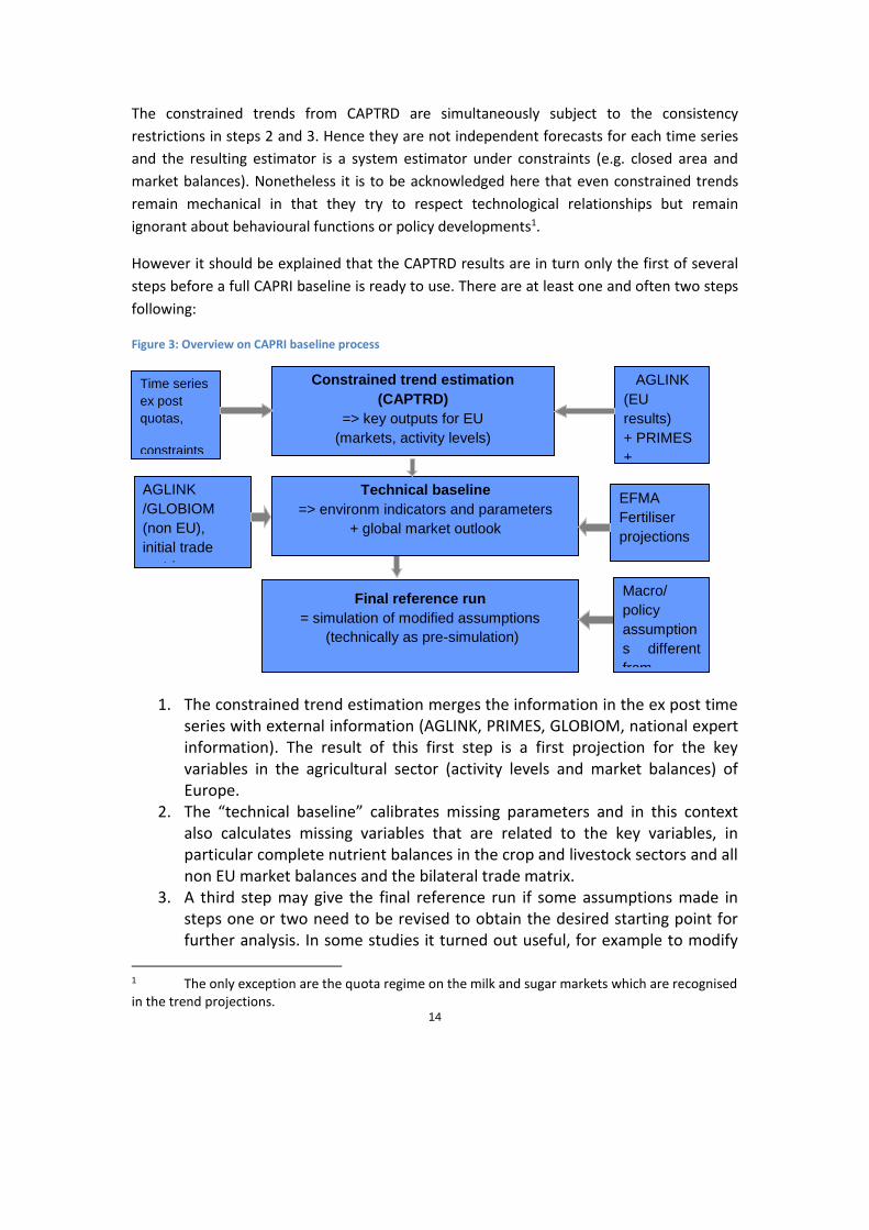
However it should be explained that the CAPTRD results are in turn only the first of several

steps before a full CAPRI baseline is ready to use. There are at least one and often two steps

following:

Figure 3: Overview on CAPRI baseline process

1. The constrained trend estimation merges the information in the ex post time series with external information (AGLINK, PRIMES, GLOBIOM, national expert information). The result of this first step is a first projection for the key variables in the agricultural sector (activity levels and market balances) of Europe.

2. The “technical baseline” calibrates missing parameters and in this context also calculates missing variables that are related to the key variables, in particular complete nutrient balances in the crop and livestock sectors and all non EU market balances and the bilateral trade matrix.

3. A third step may give the final reference run if some assumptions made in steps one or two need to be revised to obtain the desired starting point for further analysis. In some studies it turned out useful, for example to modify

1 The only exception are the quota regime on the milk and sugar markets which are recognised in the trend projections.

Constrained trend estimation

(CAPTRD)

=> key outputs for EU

(markets, activity levels)

AGLINK

(EU

results)

+ PRIMES

+

Time series

ex post

quotas,

constraints

Final reference run

= simulation of modified assumptions

(technically as pre-simulation)

Macro/

policy

assumption

s different

from

Technical baseline

=> environm indicators and parameters

+ global market outlook

EFMA

Fertiliser

projections

AGLINK

/GLOBIOM

(non EU),

initial trade

matrix

15

the macro assumptions of the “agricultural” expert sources (AGLINK, GLOBIOM) but under EUCLIMIT the macro assumptions were aligned with each other.

4.1 Improvements in the CAPRI baseline procedure under EUCLIMIT

4.1.1 Improved alignment with PRIMES biomass

The earlier processing of PRIMES input suffered from some misunderstandings related to the

interpretation of certain items (“Bioheavy”) that have been clarified in the first phase of the

project. Furthermore the new output format offers additional information such as the split

of bioethanol production (rather than only production capacities) according to first and

second generation production which facilitates a better link to CAPRI items.

Communication has also improved relative to ethanol beets where CAPRI has used in earlier

projects the forecasts from industry sources because the PRIMES outputs appeared to be

given in units not commensurate with CAPRI. Some discussion on single country results has

further improved the alignment in the sugar sector.

4.1.2 Update of EFMA information of fertiliser outlook

In some earlier projects there was an intense communication with EFMA representatives

that led to the use of some detailed EFMA projections also in CAPRI, at least for the medium

term horizon. This detailed exchange was very fruitful, but also time consuming such that

the EFMA projections used by CAPRI before the EUCLIMIT project were dating from the 2007

forecasting exercise. In the meantime the published EFMA reporting (see

http://www.fertilizerseurope.com/fileadmin/user_upload/publications/agriculture_publicati

ons/Forecast_2012-final.pdf) has become more complete in terms of single country

information such that it was feasible to update the EFMA forecasts for basically all EU MS

without lengthy communication processes.

However it should be mentioned that beyond 2020, an increasing weight has been given to

the CAPRI internal projection mechanisms as opposed to the EFMA projections (running to

2022 only). These internal mechnisms rely on a stable evolution of parameters describing

farmer’s behaviour, including their habit to apply a certain over-fertilisation above crop

needs, even when acknowledging that a part of organic nutrients are considered not “plant

available” (and thus expected to be lost to the environment).

4.1.3 Deepening of linkages to IIASA models

The key motivation for the extension of the CAPRI land use database to include non-

agricultural land uses was the benefit in projections. While there is some uncertainty how

single land uses might develop in the future (and how they have developed in the past) it is

clear that the sum across all uses must remain constant. Under EUCLIMIT a total area

16

balance has been added therefore to the set of CAPRI constraints used in the initial trend

estimations (CAPTRD step in Figure 3).

Furthermore the consistent “double” accounting in the animal sector in terms of flow data

(slaughterings) and stock data (animal herds counted at some point in time) has also been

extended from the database routines to the projection routines with a few additional

equations.

These adjustments increase the internal consistency of CAPRI projections but they also

support the exchange of respective information between the models. In particular the

GLOBIOM projections on forestry and “other natural land” may be included now as prior

information and indirectly also support the alignment in terms of agricultural areas.

Furthermore there had been a discussion on the various concepts used to represent

productivity gains in the models. It has been clarified that the GLOBIOM approach currently

relies on the idea of neutral technological change. This implies that the input requirements

of all inputs for a kg of milk are decreasing over time by the same percentage due to

technological change. In reality, the number of cows required for a given quantity of milk

also declines, because each cow receives more feed (energy). The reciprocal of the input

requirement in terms of cows, that is the milk produced per cow (a partial factor

productivity), therefore increases historically (and very likely also in the future) at a rate that

exceeds the productivity gain from technological progress (measured by total factor

productivity). The latter is sometimes called the “net productivity” change, whereas the total

change in the milk yield per cow may be called a “gross productivity” change. In GLOBIOM,

only net productivity gains due to increasing feed conversion efficiency (the input

requirements for a kg of milk in terms of feed) are accounted for, but not the additional

productivity gains by changing diets/increasing calorie intake per animal. In other words, the

initial intensity of feed energy per cow is maintained during projections. However, this

approach tends to overestimate total herd numbers compared to reality, if milk yields

change faster than feed efficiency. The clarification of this point led to the conclusion that it

is preferable to remove the GLOBIOM results in terms of animal herds from the input set for

CAPRI and to align instead only the market balance information, including production

quantities.

Finally it is worth mentioning that some technical details to deal with the transition from the

medium run (up to 2020) to the long run (2030 and beyond) have been changed in the

CAPTRD module. It is possible now to phase in the GLOBIOM information already before

2020 if this is useful for common applications. In the end it turned out that for EUCLIMIT it is

not useful to increase the weight for GLOBIOM a lot up to 2020, but the initial discussion

suggested that more flexibility might be needed.

17

In terms of the linkages to GAINS there have been no changes such that the outputs to gains

continue to be

animal herd data (dairy cows, other cattle, pigs fattened, piglets, sows, sheep, hens, other poultry)

dairy cow milk yields including milk directly fed to calves

nitrogen fertiliser use quantities

4.1.4 Update of MS level expert information

In Ireland several analyses have been carried out to assess the feasibility and consequences

of the national “Food harvest 2020” plan (see e.g. from the FAPRI Ireland group

http://www.teagasc.ie/publications/2011/67/67_FoodHarvestEnvironment.pdf), a private

initiative involving both representatives from agriculture as well as from the downstream

food industry and the government. The food harvest 2020 plan includes a target increase for

the volume of milk production from 2009 to 2020 amounting to 50% which is almost twice

the growth that might be expected otherwise. The final EUCLIMIT baseline assumes a

modest effectiveness (25% of the planned impact) which reflects that so far there are no

hard “measures” to support the plan but the creation of several communication platforms,

supporting agencies and so forth with unclear impact. This is somewhat increased compared

to the first implementation (10%) after considering an independent “industry note” of the

dairy sector competitiveness by Rabobank (2012). As a consequence Ireland appears to be

one of the most expansive countries in Europe in terms of milk production.

In addition the MS consultation process also led to some re-specification of the expert

information related to some other countries (AT, NL, LU, HU).

5 Simulation mode The CAPRI global market module breaks down the world into 44 country aggregates or

trading partners, each one (and sometimes regional components within these) featuring

systems of supply, human consumption, feed and processing functions. The parameters of

these functions are derived from elasticities borrowed from other studies and modelling

systems and calibrated to projected quantities and prices in the simulation year. Regularity is

ensured through the choice of the functional form (a normalised quadratic function for feed

and supply and a generalised Leontief expenditure function for human consumption) and

some further restrictions (homogeneity of degree zero in prices, symmetry and correct

curvature). Accordingly, the demand system allows for the calculation of welfare changes for

consumers, processing industry and public sector. Policy instruments in the market module

include bilateral tariffs and tariff rate quotas (TRQs). Intervention purchases and subsidised

18

exports under the World Trade Organisation (WTO) commitment restrictions are explicitly

modelled for the EU 15.

In the market module, special attention is given to the processing of dairy products in the

EU. First, balancing equations for milk fat and protein ensure that these exactly exhaust the

amount of fat and protein contained in the raw milk. The production of processed dairy

products is based on a normalised quadratic function driven by the regional differences

between the market price and the value of its fat and protein content. Then, for consistency,

prices of raw milk are also derived from their fat and protein content valued with fat and

protein prices.

The market module treats bilateral world trade based on the Armington assumption

(Armington, 1969). According to Armington’s theory, the composition of demand from

domestic sales and different import origins responds smoothly to price relatives among

various bilateral trade flows. This allows the model to reflect trade preferences for certain

regions (e.g. Parma or Manchego cheese) and to explain the common feature of trade

statistics that a country may export to another country and in the same period also import

from this trading partner. As many trade policy instruments like TRQs are specific for certain

trading partners, bilateral trade modeling is a precondition for accurate representation of

trade policies.

For European regions the supply side behavioural function in the global market module

approximate the behaviour of country aggregates of regional nonlinear programming

models. In these models regional agricultural supply of annual crops and animal outputs are

given as solutions to a profit maximisation under a limited number of constraints: the land

supply curve, policy restrictions such as sales quotas and set aside obligations and feeding

restrictions based on requirement functions.

The underlying methodology assumes a two stage decision process. In the first stage,

producers determine optimal variable input coefficients per hectare or head (nutrient needs

for crops and animals, seed, plant protection, energy, pharmaceutical inputs, etc.) for given

yields, which are determined exogenously by trend analysis (data from EUROSTAT) and

updated depending on price changes against the baseline. Nutrient requirements enter the

supply models as constraints and all other variable inputs, together with their prices, define

the accounting cost matrix. In the second stage, the profit maximising mix of crop and

animal activities is determined simultaneously with cost minimising feed and fertiliser in the

supply models. Availability of grass and arable land and the presence of quotas impose a

restriction on acreage or production possibilities. Moreover, crop production is influenced

by set aside obligations. Animal requirements (e.g. feed energy and crude protein) are

covered by a cost minimising feeding combination. Fertiliser needs of crops have to be met

by either organic nutrients found in manure (output from animals) or in purchased fertiliser

19

(traded good). A nonlinear cost function covering the effect of all factors not explicitly

handled by restrictions or the accounting costs – such as additional binding resources or

risk - ensures calibration of activity levels and feeding habits in the base year and plausible

reactions of the system. These cost function terms are estimated from ex-post data or

calibrated to exogenous elasticities. Fodder (grass, straw, fodder maize, root crops, silage,

milk from suckler cows or mother goat and sheep) is assumed to be non-tradable, and hence

links animal processes to the crops and regional land availability. All other outputs and

inputs can be sold and purchased at fixed prices. Selling of milk cannot exceed the related

quota, the sugar beet quota regime is modelled by a specific risk component. The use of a

mathematical programming approach has the advantage to directly embed compensation

payments, set-aside obligations, voluntary set-aside and sales quotas, as well as to capture

important relations between agricultural production activities. Not at least, environmental

indicators as NPK balances and output of gases linked to global warming are easily

represented in the system.

The equilibrium in CAPRI is obtained by letting the regional supply and global market

modules iterate with each other. In the first iteration, the regional aggregate programming

models (one for each Nuts 2 region) are solved with prices taken from the baseline. After

being solved, the regional results of these models (crop areas, herd sizes, input/output

coefficients, etc.) are aggregated to the country level, leading to a certain deviation from the

baseline solution, depending on the kind of scenario. Subsequently the supply side

behavioural functions of the market module (for supply and feed demand) are recalibrated

to pass at the given prices through the quantity results from the supply models. The market

module is then solved, yielding new equilibrium producer prices for all regions, including

European countries. These prices are then passed back to the supply models for the

following iteration. At the same time, in between iterations, premiums for activities are

adjusted if ceilings defined in the Common Market Organisations (CMOs) are overshot.

In EUCLIMIT, the difference between the baseline (only adopted measures) and the

reference run (assuming that the renewables targets are met and including the recent

Energy Efficiency Directive) has been treated as a shock to be simulated with the CAPRI

scenario mode. The exogenous shifts were limited to the shifts in the bioenergy sector as

given by the PRIMES biomass component. The variation concerned mainly two types of

variables: The changed production of biofuels (biodiesel and bioethanol) and the

contributions from second generation technologies were modifications for the global market

module. At the same time, the (exogenous) area use for lignocellulosic crops in European

countries has been modified in the regional supply models, assuming that the regional

allocation would not change from the baseline.

20

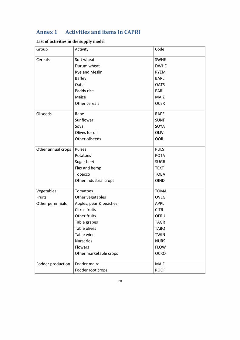
Annex 1 Activities and items in CAPRI

List of activities in the supply model

Group Activity Code

Cereals Soft wheat

Durum wheat

Rye and Meslin

Barley

Oats

Paddy rice

Maize

Other cereals

SWHE

DWHE

RYEM

BARL

OATS

PARI

MAIZ

OCER

Oilseeds Rape

Sunflower

Soya

Olives for oil

Other oilseeds

RAPE

SUNF

SOYA

OLIV

OOIL

Other annual crops Pulses

Potatoes

Sugar beet

Flax and hemp

Tobacco

Other industrial crops

PULS

POTA

SUGB

TEXT

TOBA

OIND

Vegetables

Fruits

Other perennials

Tomatoes

Other vegetables

Apples, pear & peaches

Citrus fruits

Other fruits

Table grapes

Table olives

Table wine

Nurseries

Flowers

Other marketable crops

TOMA

OVEG

APPL

CITR

OFRU

TAGR

TABO

TWIN

NURS

FLOW

OCRO

Fodder production Fodder maize

Fodder root crops

MAIF

ROOF

21

Group Activity Code

Other fodder on arable land

Graze and grazing

OFAR

GRAS

Fallow land and

set-aside

Set-aside idling

Non food production on set-aside

Fallow land

SETA

NONF

FALL

Cattle Dairy cows

Sucker cows

Male adult cattle fattening

Heifers fattening

Heifers raising

Fattening of male calves

Fattening of female calves

Raising of male calves

Raising of female calves

DCOW

SCOW

BULF

HEIF

HEIR

CAMF

CAFF

CAMR

CAFR

Pigs, poultry and

other animals

Pig fattening

Pig breeding

Poultry fattening

Laying hens

Sheep and goat fattening

Sheep and goat for milk

Other animals

PIGF

SOWS

POUF

HENS

SHGF

SHGM

OANI

Land use classes in CAPRI

OART artificial

ARAO (other) arable crops - all arable crops excluding rice and fallow (see also

definition of ARAC below)

PARI paddy rice (already defined)

GRAT temporary grassland (alternative code used for CORINE data, definition

identical to TGRA

FRCT fruit and citrus

22

OLIVGR Olive Groves

VINY vineyard (already defined)

NUPC nursery and permanent crops (Note: the aggregate PERM also includes

flowers and other vegetables

BLWO board leaved wood

COWO coniferous wood

MIWO mixed wood

POEU plantations (wood) and eucalyptus

SHRUNTC shrub land - no tree cover

SHRUTC shrub land - tree cover

GRANTC Grassland - no tree cover

GRATC Grassland - tree cover

FALL fallow land (already defined)

OSPA other sparsely vegetated or bare

INLW inland waters

MARW marine waters

Land use aggregates in CAPRI

OLND other land - shrub, sparsely vegetated or bare

ARAC arable crops

FRUN fruits, nursery and (other) permanent crops

WATER inland or marine waters

23

ARTIF artificial - buildings or roads

OWL other wooded land - shrub or grassland with tree cover (definition to be

discussed)

TWL total wooded land - forest + other wooded land

SHRU shrub land

FORE forest (already defined)

GRAS grassland (already defined)

UAAR utilizable agricultural area (already defined)

ARTO total area - total land and inland waters

ARTM total area including marine waters

CROP crop area - arable and permanent

24

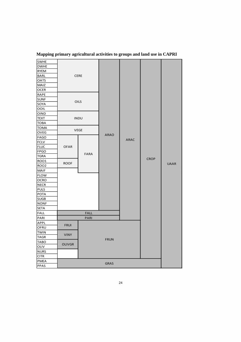
Mapping primary agricultural activities to groups and land use in CAPRI

SWHE

DWHE

RYEM

BARL

OATS

MAIZ

OCER

RAPE

SUNF

SOYA

OOIL

OIND

TEXT

TOBA

TOMA

OVEG

FAGO

FCLV

FLUC

FPGO

TGRA

ROO1

ROO2

MAIF

FLOW

OCRO

NECR

PULS

POTA

SUGB

NONF

SETA

FALL

PARI

APPL

OFRU

TWIN

TAGR

TABO

OLIV

NURS

CITR

PMEA

PPAS

FALL

PARI

CERE

ARAO

ARAC

CROP

UAAR

OILS

INDU

VEGE

OFAR

FARA

ROOF

FRUI

FRUN

GRAS

VINY

OLIVGR

25

Mapping land use classes to aggregates in CAPRI

PARI

ARAC

CROP

UAAR

ARTO ARTM

FALL

ARAO

GRAT

FRCT

FRUN OLIVGR

NUPC

VINY

GRANTC GRAS

GRATC

OART ARTIF

BLWO

FORE TWL

COWO

MIWO

POEU

SHRUTC=OWL

OLND OSPA

SHRUNTC

INLW WATER

MARW

26

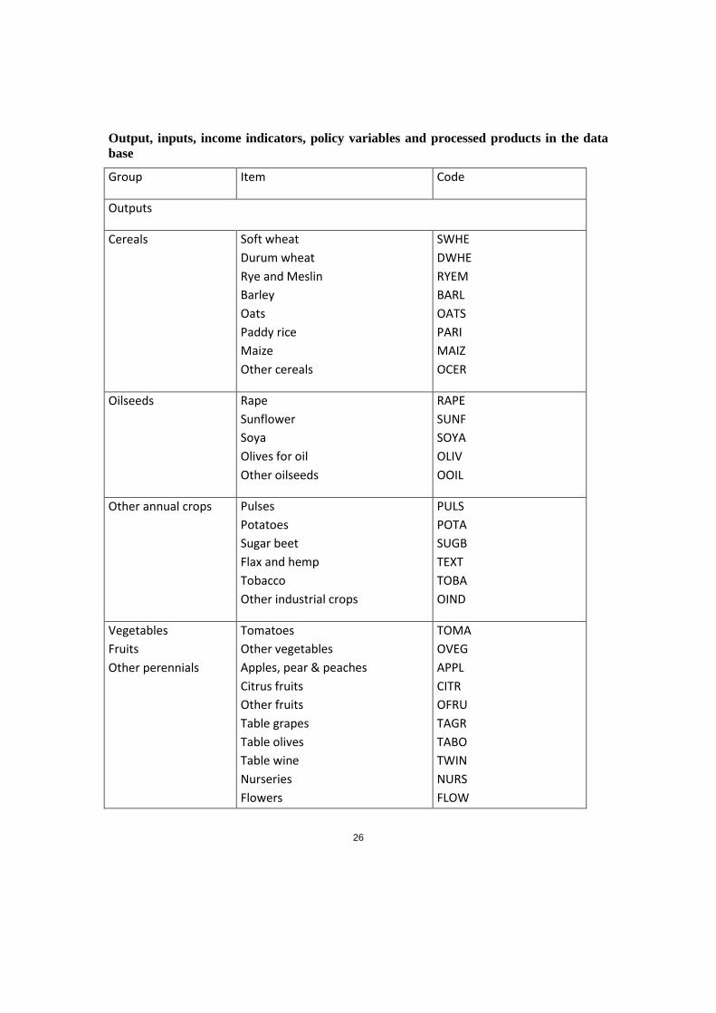
Output, inputs, income indicators, policy variables and processed products in the data

base

Group Item Code

Outputs

Cereals Soft wheat

Durum wheat

Rye and Meslin

Barley

Oats

Paddy rice

Maize

Other cereals

SWHE

DWHE

RYEM

BARL

OATS

PARI

MAIZ

OCER

Oilseeds Rape

Sunflower

Soya

Olives for oil

Other oilseeds

RAPE

SUNF

SOYA

OLIV

OOIL

Other annual crops Pulses

Potatoes

Sugar beet

Flax and hemp

Tobacco

Other industrial crops

PULS

POTA

SUGB

TEXT

TOBA

OIND

Vegetables

Fruits

Other perennials

Tomatoes

Other vegetables

Apples, pear & peaches

Citrus fruits

Other fruits

Table grapes

Table olives

Table wine

Nurseries

Flowers

TOMA

OVEG

APPL

CITR

OFRU

TAGR

TABO

TWIN

NURS

FLOW

27

Group Item Code

Other marketable crops OCRO

Fodder Gras

Fodder maize

Other fodder from arable land

Fodder root crops

Straw

GRAS

MAIF

OFAR

ROOF

STRA

Marketable products

from animal product

Milk from cows

Beef

Pork meat

Sheep and goat meat

Sheep and goat milk

Poultry meat

Other marketable animal products

COMI

BEEF

PORK

SGMT

SGMI

POUM

OANI

Intermediate products

from animal

production

Milk from cows for feeding

Milk from sheep and goat cows for

feeding

Young cows

Young bulls

Young heifers

Young male calves

Young female calves

Piglets

Lambs

Chicken

Nitrogen from manure

Phosphate from manure

Potassium from manure

COMF

SGMF

YCOW

YBUL

YHEI

YCAM

YCAF

YPIG

YLAM

YCHI

MANN

MANP

MANK

Other Output from

EAA

Renting of milk quota

Agricultural services

RQUO

SERO

Inputs

Mineral and organic Nitrogen fertiliser NITF

28

Group Item Code

fertiliser

Seed and plant

protection

Phosphate fertiliser

Potassium fertiliser

Calcium fertiliser

Seed

Plant protection

PHOF

POTF

CAOF

SEED

PLAP

Feedings tuff Feed cereals

Feed rich protein

Feed rich energy

Feed based on milk products

Gras

Fodder maize

Other Feed from arable land

Fodder root crops

Feed other

Straw

FCER

FPRO

FENE

FMIL

FGRA

FMAI

FOFA

FROO

FOTH

FSTRA

Young animal

Other animal specific

inputs

Young cow

Young bull

Young heifer

Young male calf

Young female calf

Piglet

Lamb

Chicken

Pharmaceutical inputs

ICOW

IBUL

IHEI

ICAM

ICAF

IPIG

ILAM

ICHI

IPHA

General inputs Maintennce machinery

Maintennce buildings

Electricity

Heating gas and oil

Fuels

Lubricants

Water

Agricultural services input

Other inputs

REPM

REPB

ELEC

EGAS

EFUL

ELUB

WATR

SERI

INPO

Income indicators Production value

Total input costs

TOOU

TOIN

29

Group Item Code

Gross value added at producer

prices

Gross value added at basic prices

Gross value added at market

prices plus CAP premiums

GVAP

GVAB

MGVA

Activity level Cropped area, slaughtered heads

or herd size

LEVL

Policy variables

Relating to activities

Premium ceiling

Historic yield

Premium per ton historic yield

Set-aside rate

Premium declared below base

area/herd

Premium effectively paid

Premium amount in regulation

Type of premium application

Factor converting PRMR into

PRMD

Ceiling cut factor

PRMC

HSTY

PRET

SETR

PRMD

PRME

PRMR

APPTYPE

APPFACT

CEILCUT

Processed products Rice milled

Molasse

Starch

Sugar

Rape seed oil

Sunflower seed oil

Soya oil

Olive oil

Other oil

Rape seed cake

Sunflower seed cake

Soya cake

Olive cakes

Other cakes

Gluten feed from ethanol

production

Biodiesel

RICE

MOLA

STAR

SUGA

RAPO

SUNO

SOYO

OLIO

OTHO

RAPC

SUNC

SOYC

OLIC

OTHC

GLUE

BIOD

BIOE

30

Group Item Code

Bioethanol

Palm oil

Butter

Skimmed milk powder

Cheese

Fresh milk products

Creams

Concentrated milk

Whole milk powder

Whey powder

Casein and caseinates

Feed rich protein imports or

byproducts

Feed rich energy imports or

byproducts

PLMO

BUTT

SMIP

CHES

FRMI

CREM

COCM

WMIO

WHEP

CASE

FPRI

FENI

Annex 2 Animal sector details in CAPRI Without doubt the animal sector is the most complex topic in the CAPRI regional

programming models because it includes various internal relationships as well as inter-

linkages with the crop sector. Among the former are the various input-output relationships

related to young animals. Figure 4 shows the different cattle activities and the related young

animal products used in the model. Milk cows and suckler cows produce male and female

calves. The relation between male and female calves is estimated ex-post in the “COCO

module” that handles the data consolidation. These calves are assumed to weigh 50 kg at

birth and to be born on the 1st of January. They enter immediately the raising processes for

male and female calves which produce young heifers (300 kg live weight at the end) and

young bulls (335 kg). These raising processing are assumed to take one year, so that calves

born in t enter the processes for male adult fattening, heifers fattening or heifers raising on

the 1st January of the next year t+1. The heifers raising process produces then the young

cows which can be used for replacement or herd size increases in year t+2.

31

Figure 4: The cattle chain

Source: CAPRI Modelling System

Accordingly, each raising and fattening process takes exactly one young animal on the input

side. The raising processes produce exactly one animal on the output side which is one year

older. The output of calves per cow, piglets per sow, lambs per mother sheep or mother

goat is derived ex post, e.g. simultaneously from the number of cows in t-1, the number of

slaughtered bulls and heifers and replaced in t+1 which determine the level of the raising

processes in t and number of slaughtered calves in t. The herd flow models for pig, sheep

and goat and poultry are similar, but less complex, as all interactions happen in the same

year, and no specific raising processes are introduced.

In most cases, all input and output coefficients relating to young animals are estimated in

the database identical at regional and national level, projected by constrained trends and

maintained in the simulations. For slaughter weights a certain regional variation is allowed

in line with stocking densities. In reality farmers may react with changes in final weights to

relative changes in output prices (meat) in relation to input prices (feed, young animals). A

higher price for young animals will tend to increase final weights, as feed has become

comparatively cheaper and vice-versa. In order to introduce more flexibility in the system,

the dairy cow, heifer and bull fattening processes are split up each in two versions that may

substitute against each other in scenarios as shown in the following table.

Beef

Beef

Veal Beef

Beef

Veal

Raising

female

Calves

Fattening

male

Calves

Breeding

Heifers

Milk Cows

Suckler

Cows

Male adult

cattle

High/Low

Fattening

Heifers

High/Low

Fattening

female

Calves

Raising

male

Calves

Raising

female

Calves

Fattening

male

Calves

Breeding

Heifers

Milk Cows

Suckler

Cows

Male adult

cattle

High/Low

Fattening

Heifers

High/Low

Fattening

female

Calves

Raising

male

Calves

Male

Calf

Young

heifer

Young

bull

Young

cow

Female

Calf

Male

Calf

Young

heifer

Young

bull

Young

cow

Female

Calf

32

Table 1 Split up of cattle chain processes in different intensities

Low intensity/final weight High intensity/final weight

Dairy cows (DCOW) DCOL: 75% milk yield of

average, variable inputs

besides feed and young

animals at 75% of average

DCOH: 125% milk yield of

average, variable inputs

besides feed and young

animals at 125% of average

Bull fattening (BULF) BULL: 20% lower meat

output, variable inputs

besides feed and young

animals at 80% of average

BULH: 20% higher meat

output, variable inputs

besides feed and young

animals at 120% of average

Heifers fattening (HEIF) HEIL: 20% lower meat output,

variable inputs besides feed

and young animals at 80% of

average

HEIH: 20% higher meat

output, variable inputs

besides feed and young

animals at 120% of average

For all regions it is assumed that ex post and in the baseline the shares for the high and low

yielding variant (e.g. DCOL, DCOH) are 50% for each. As so far no statistical information on

the distribution of intensities has been used, the category “intensive” has been defined to

represent the upper 50% of the historical and baseline distribution. In scenarios however,

these shares may change in response to incentives.

For fattening activities the process length DAYS, net of any empty days (EDAYS, relevant for

seasonal sheep fattening in Ireland, for example) times the daily growth DAILY should give

the final weight after conversion into live weight with the carcass share carcassSh and

consideration of any starting weight startWgt.

Equation 1 datamaact

BASEDAYSr

Trendmaact

tDAYSr

Trendmaact

tDAILYrmaact

maact

Trendmaact

tyieldr

XXXstartWgt

carcassShX

,

,,

,

,,

,

,,

,

,, /

The process length permits to convert between the CAPRI activity levels for fattening

activities (activity level LEVL = one finished animal per year, flow data) and the animal herds

(HERD) that may be observed in animal countings at some point in time (stock data, used in

GLOBIOM and GAINS).

Equation 2 365/,

,,

,

,,

,

,,

Trendmaact

tDAYSr

Trendmaact

tLEVLr

Trendmaact

tHERDr XXX

The process length is fixed to 365 days for female breeding animals (activities DCOL, DCOH,

SCOW, SOWS, SHGM, HENS) such that the activity level is equal to the herd size there.

33

The input allocation for feed describes which quantities of certain feed aggregates (cereals,

rich protein, rich energy, processed dairy feed, other feed) or single fodder items (fodder

maize, grass, fodder from arable land, straw, raw milk for feeding) are used per animal

activity level.

This input allocation for feed takes into account nutrient requirements of animals, building

upon requirement functions from the animal nutrition literature. In the case of cattle they

have been taken from the IPCC (2006) manual on emissions accounting according to a “tier

2” methodology. For other animals the requirement functions are using other sources and

are typically simpler. The crude protein needs are not only used to steer feed demand but

they also determine the N content of excretions and therefore the fertiliser value of manure,

but also the risk of emissions.

The feed allocation and hence input coefficients for feeding stuff are determined in the

solution of the supply models to ensure that energy and protein requirements cover the

nutrient needs of the animals while respecting maximum and minimum bounds for lysine,

dry matter and fibre intake. Furthermore, ex-post, they also have to be in line with regional

fodder production and total feed demand statistics at the national level, the latter stemming

from market balances. And last but not least, the input coefficients together with feed prices

should lead ex post to reasonable feed cost for the activities.

Historical data do not always meet these consistency relationships. In fact a frequent

problem is that nutrient intake is implausibly exceeding the requirements from the

literature. A certain luxury consumption is perfectly plausible, just reflecting that observed

data usually do not meet the high efficiency laboratory situations in the literature.

Nonetheless without further corrections the measured excess would often attain 50% or

more, at least for protein. A number of remedies have been introduced therefore in CAPRI

to reduce the number of odd cases:

Grass and other fodder yields have been estimated (in COCO already) as a compromise of statistical and expert information (from Alterra, O. Oenema, G. Velthof)

Losses of straw have been permitted to vary according to the surplus situation in the region

A luxury consumption embedded in the sectoral data on feed input and animal products has been steered mainly towards the less intensive (sheep, cattle) activities as opposed to more intensive production chains (pigs, poultry).

This excess „luxury“ consumption is treated as a parameter characterising farmer’s

behaviour, just like the “over-fertilisation parameters” related to fertiliser use. The

requirements from the literature are therefore adjusted (upwards) to permit a balance of

feed use and requirements in the historical period. Subsequently they are maintained in

simulations apart from some moderate gains in feed efficiency over time.

34

Organic fertliser is another link to the crop sector. Given the feed allocation, the nutrient

contents of manure may be calculated. In the historical period the mineral fertiliser use is

also known and allows to calculate the above mentioned parameters characterising nutrient

availability in organic fertilisers and the over-fertilisation on the part of farmers. In the

baseline, prior information for mineral fertiliser use may be available from external

projections (EFMA) or trend extrapolations. This prior information as well as the behavioural

parameters are adjusted to yield consistency in nutrient availability from organic and

mineral fertilisers on the one hand, and nutrient use in the crop sector on the other

(acknowledging gaseous losses).

By contrast in scenarios the behavioural parameters are fixed. Nutrient supply has to be

adjusted to nutrient need that follows from crop yields. Animal activities therefore have

manure as a secondary output, valued at a shadow value that is related to the mineral

fertiliser price. However, in scenarios that constrain emissions directly in the regional supply

models, this value might also become negative.

Annex 3 Complete area database

I. Background Land use data are a surprisingly contentious issue, given that it should be an easy question

to answer how a particular parcel of land is being used. In addition there are several

statistical sources available that provide information on this issue. However, this multitude

of potential statistical sources can be used in different ways to set up a database for

modelling purposes and indeed this choice has been answered in different ways in CAPRI

(for ‘Common Agricultural Policy Regionalised Impact analysis’) and GLOBIOM (for ‘Global

Biosphere Management Model’), two modelling systems that are applied in parallel in

EUCLIMIT, see http://www.euclimit.eu/, (and other) projects2. The differences are mainly

due to the different needs of the systems with GLOBIOM requiring spatially explicit land use

data for certain pixels, but limited to the base year 2000, whereas CAPRI only requires

NUTS2 level data, but these in annual time series back to 1985, if possible. Nonetheless for

joint model application differences in the data base should be small or at least attributable

to clear differences in definitions or procedures. Due to the frequent data exchange with

GLOBIOM it is useful to include in this CAPRI land use documentation also some

comparisons and explanations related to GLOBIOM.

2 Annex 3 draws heavily on Witzke P, Zintl A, Kempen M, Boettcher , Frank S (2013): CAPRI land use documentation (including a comparison with GLOBIOM land use data), Bonn-Laxenburg 2013.

35

II. Specific data sources related to land use While the general problem to establish a complete and consistent database for land use is

similar as in many other areas there are some particularities related to land use:

In general, the cases of conflicting raw data on agricultural variables are rare (for example to take production from Eurostat production statistics or from the market balances) and the different sources do not diverge a lot. This does not hold for land use data: There are often several possible sources and the differences can be large.

Agricultural time series (from Eurostat) are often rather complete and evident statistical breaks are exceptions. Again this does not hold for land use data: Observations are typically given for a few years only or time series show evident breaks.

Whereas many agricultural series show a high volatility (prices, trade, yields, production, single crop areas) land use data for aggregate area categories tend to change only slowly. As a consequence a land use observation for 2010 may have some informational content to assess land use in 1990, whereas such inference would be hazardeous for price or trade data.

The first two points are specific problems, the latter more an additional option that

suggested to modify the typical strategy to establish a consistent and complete database on

time series of land use data. The typical strategy applied in the CAPRI system was to decide

on a reasonable expectation for variables on the basis of a ranking in terms of presumed

data quality and to leave to a mechanical data consolidation procedure only the problem to

resolve inconsistencies between related data (possibly initialised from different sources). So

variables like meat production are initialised preferably with the value from the Eurostat

market balances in CAPRI, but if that was missing, a second best estimate based on the

Eurostat slaughtering statistic is used.

A preferable strategy, adjusted to the multitude of competing sources, possibly on land use

at different points in time, it to consider all of them simultaneously but to define weights

that reflect the presumed quality of these weights. The data sources considered are the

following.

1. Estat_NatLU: Eurostat national land use data (Eurostat table: “apro_cpp_luse”). As these data are annually available since the 80s and give importand land use categories (total area ARTO with inland waters INLW3, arable land ARAC, permanent grassland GRAS, forest land FORE, etc) this would be our preferred source if all series were complete and reliable.

3 See Annex 1 for a complete list of codes.

36

2. Estat_RegLU: Eurostat regional land use data (Eurostat table: “agr_r_landuse”). Inspite of using the same codes as for the national data, the national totals, aggregated from the NUTS2 regions are not always in line with CAPRI_natLU. Furthermore a few categories are missing (no inland waters, no other wooded land). However there are few alternative annual series avaialble to regionalise the national data in a later step of data processing.

3. Estat_LandCov: Eurostat land cover data for 2009 at the MS level. Agricultural land is only distinguished into cropland CROP and grassland GRAS, but 5 nonagricultural areas are neatly aggregating up to the total country (Artificial ARTIF, shrubland (considered similar to “other wooded land” OWL), bare land & wetlands (mapped to “other sparcely vegetated or bare OSPA) and waters WATER.

4. Estat_Envio: Eurostat land cover data from the environment section (table “env_la_luc1”4). Total area is classified into about 40 categories, but data are only given for a number of years (1950, 1970, 1980, 1985, 1990, 1995, 2000) and with many gaps, in particular for the subcategories.

5. Estat_FSS: Eurostat farm structure survey data (table “ef_lu_ovcropaa"). Gives a very detailed and reliable description of agricultural area use, but only for the survey years (1990, 1993, 1995, 1997, 2000, 2003, 2005, 2007). As CAPRI_regLU these data are also used in the subsequent regionalisation steps of the CAPRI data consolidation because NUTS2 data are offered. The main disadvantage for our purposes is the complete lack of nonagricultural data coverage.

6. FAO: Land use data from the resource FAOSTAT domain5 with annual time series on agricultural land use but also some non argicultural area categories (forest, inland waters, other land, total area).

7. MCPFE: Year 2007 version of the Ministerial Conference on the Protection of Forests in Europe C&I database for quantitative indicators. This gives validated data on the forest sector (forest land FORE, other wooded land OWL) and some non forestry data (inland waters INLW, total country area ARTO), but data were only given for 1990, 2000 and 20056.

8. CAPRI_CLC: Corine Land Cover (44 classes, aggregated to the NUTS2 level7 by JRC, Ispra (contact: Sarah Mubareka) for 1990, 2000, 2006. To link the Corine information to the CAPRI land use classes (Table A2) NUTS2 contingency tables8 from Corine to

4 Apparently these data are currently under revision because they are not accessible on the Eurostat website anymore since about June 2012. However they are still accessible (in July 2012) via http://eu22.eu/land-use.2/land-use-by-main-category/. 5 See http://faostat3.fao.org/home/index.html#DOWNLOAD. 6 http://www.foresteurope.org/filestore/foresteurope/Publications/pdf/state_of_europes_forests_2007.pdf. In November 2011 the year 2011 report has beome available, including year 2010 data, but the updated numbers have not yet been used in CAPRI. 7 Data for some countries and years affected by evident problems have been removed. For example the 2006 CLC data only covered parts of Greece, hence are no usable to calculate totals at the MS level. 8 An EU level contingency table and a discussion of problems in assessing the accuracy of CORINE is avaialble at http://agrienv.jrc.ec.europa.eu/publications/pdfs/LUCAS_CORINE.pdf. See also

37

LUCAS categories have been used as a interim step which were provided by JRC Ispra based on LUCAS 2006 and 2009 (new MS) data. This allowed to map the Corine classes (like complex cultivation patterns – “complexCultiv”) to the most probable land cover class from the LUCAS survey (typically for “complexCultiv” => annual crops) which may be aggregated then to the CAPRI land use classes (annual crops[LUCAS] => arable crops[CAPRI], code ARAC). This procedure has many disadvantages, for example, that certain LUCAS categories like “fallow land” are not mapped at all because they are not the most probable matching LUCAS category for any of the Corine classes. But the procedure preserves the original Corine information as much as possible while still yielding transparent rules for mapping to CAPRI.

9. CAPRI_CLC_LUCAS: To acknowledge that the Corine Classes may be mapped to several LUCAS categories they may be multiplied with the “profiles”, giving the distribution of each Corine category according to the LUCAS classes. In the case of the “complexCultiv” area and for the EU level, only 27.6% are be mapped to annual crops, but 5.5% are mapped to “permanent grassland with sparse tree cover”, 35.2% to “permanent grassland without tree cover” and so forth. Currently the Corine data have been used by CAPRI in this transformed form. The transformed Corine data often give the most detailed area coverage and thus assume a role as a kind of fall back information in case that other information is missing.

10. GLOBIOM_CLC: For use in GLOBIOM the Corine data are used in the spatially explicit format. They have been aggregated from the disaggregate pixel information to the country level using a different methodology than used by JRC staff to prepare the NUTS2 tables for CAPRI. Furthermore the mapping to the GLOBIOM area categories relied on other rules than using the most probably LUCAS category. As a consequence the aggregate CLC data from the GLOBIOM database yields different national totals than given by CAPRI_CLC. This illustrates the sensitivity of land use data sets to various methodological issues.

The electronic annex9 to this documentation reproduces the observations from these

sources of “raw data” in the period 1985-2010 for EU27 Member States (Belgium and

Luxembourg aggregated), together with the CAPRI final consolidated results (CAPRIdata) as

well as the land use data from GLOBIOM for year 2000 (GLOBIOMdata).

III. Methodology of data consolidation for the CAPRI Data Base The key procedure of data consolidation applies to all levels (national, regional, global) of

the CAPRI database:

Javier Gallego, Catharina Bamps (2008) Using CORINE land cover and the point survey LUCAS for area estimation, International Journal of Applied Earth Observation and Geoinformation 10 pp 467–475. 9 The excel file “Appendix B.3._land_use_data_docu.xls” collects time series of raw data and results at the MS level for land use aggregates. This excel file is delivered as a separate file along with this report.

38

Collect a possibly large set of heterogeneous input files and map them to the definitions of the system.

Define expected values (“supports”) for each variable (quantities, areas, etc) based on the available “raw data”.

Calculate complete and consistent time series that minimise the distance to the expected values.

Furthermore, the following principles are applied:

Accounting identities – like the identity that production follows from activity levels times yields - constrain the estimation outcome.

Relations between aggregated time series (e.g. total permanent crop area) and single time series are used as additional restrictions in the estimation process.

Bounds for the estimated values based on engineering knowledge or other sources constrain the estimation results

As many time series as technically possible are estimated simultaneously to use the full extent of the informational content of the data constraints (1) and (2).

The first three points neatly conform to the Bayesian Highest Posterior Density (HPD)

approach proposed in Heckelei, Mittelhammer, Britz 2005. The second point, consistent

aggregation to higher levels, is particularly valuable for land use data because the total

country area is typically reported unanimuously in all sources and may be considered one of

the few really “hard” data. Even though the CAPRI land use database will be is mainly used

for its agricultural content, the coverage of total country area is expected to provide a

valuable constraint in the light of different allocations of this total area to land use classes in

the original sources.

The estimation is carried out as part of the CAPRI module “COCO” and the following

explanations heavily draw on http://www.capri-model.org/docs/capri_documentation.pdf,

section 2.2. We may distinguish the following steps:

1. Estimate independent trend lines for the time series. 2. Estimate a Hodrick-Prescott filter using given data where available and otherwise the

trend estimate as input. 3. Define ‘supports’ which are (a) given data, (b) the results from the Hodrick-Prescott filter

times R² plus the last (1-R²) times the average of nearest observations. 4. Specify a ‘standard deviation’ for each data point which is different for given data and

gaps.

Ultimately the concept is a constrained minimisation of normalised least squares:

39

,

2

, , , ,

,2

, , ,

,2

, 1 , , , 1 ,

,2

, , , ,

,

,

(1.1) min ( ) ( )

( )

( ) ( )

max( , ) ) ( )

min( ,

i t

dat dat trd dat

i t i t i t i ty

i t obs

ini ini

i t i t i t

i t obs

hp

i t i t i t i t i t

i t

up up up up

i t i t i t i t

i t

lo lo

i t

wgt y y abs y y

wgt y y s

wgt y y y y s

wgt y y y abs y

wgt y

2

, , ,

,

, , ,

,

) ) ( )

. .(1.2)

(1.3)(1.4)

lo lo

i t i t i t

i t

LO UP

i t i t i t

i t

y y abs y

s ty y y

Accounting identities defined on yIdentity of land use from different sources

where i represents the index of the elements to estimate (e.g. crop production activities or

groups, etc.), t stands for the year, wgtx are weights attached to the different parts of the

objective, and

yi,t = the fitted value for item i, year t

dat

t,iy = the observed data for item i, year t

obs = {(i,t) | dat

t,iy ≠ 0}, the set of data points with nonzero data

trd

t,iy = the trend value of an initial trend line through the given data

ini

t,iy = initial supports for gaps: preliminary Hodrick-Prescott filter result

(from step 2) times R² plus the last (1-R²) times the average of

nearest observations

si,t, (i,t)obs = trd

t,i

ini

t,i sy1.0 , weighted sum of the initial support for gaps and the

standard error of the initialising trend

si,t, (i,t)obs = trd

t,i

dat

t,i sy1.0 , weighted sum of given data and the standard error

of the initialising trend

up

t,i

lo

t,i y,y = ‘soft’ bounds, triggering a high additional penalty if violated

UP

t,i

LO

t,i y,y = ‘hard’ bounds, defining the feasible space

The general weighing of the different terms evidently reflects the acceptability of certain

types of deviations which is lowest ( = 1) for deviations of the fitted value from the HP filter

initialisation as these are considered quite poor, preliminary estimates (derived from

40

independent trends). The weights are 10 times higher for deviations from given data and for

the smoothing HP filter term. Finally there are extra penalty terms for fitted values moving

beyond plausible ‘soft’ bounds up

t,i

lo

t,i y,y . The ‘hard’ bounds UP

t,i

LO

t,i y,y are constraining the

feasible space for a number of solution attempts. However, if it turns out that certain

constraints would persistently preclude feasibility of the data consolidation problem, they

are relaxed in a stepwise fashion, but this widening of bounds is monitored on a parameter

to check.

The denominators used to normalise the different terms are ‘standard deviations’ of the

prior distribution in the framework of a HPD estimation but they are specified in view of

practical considerations. Essentially they provide another weighting for particular (i,t)

deviations depending on their acceptability, but these weights are specific to the particular

data point. All denominators are derived from the variable in question such that they

acknowledge the fact that the means of the time series entering the estimation deviate

considerably. The normalisation hence leads to minimisation of relative deviations instead of

absolute ones which could not be summed in a reasonable way.

It should be mentioned that the above representation of the objective function is a quite

simplified one: It is evident that the above lacks safeguards against division by zero or very

small values which are included in the GAMS code. Furthermore there are different types of

gaps which are not reflected above to avoid clutter (Are there gaps in a series with some

data or is the series empty? Is the mean based on data or estimated from up

t,i

lo

t,i y,y ?)

Equation (1.3) indicates that accountancy restrictions are added. These restrictions can be

balances, aggregation conditions, definitions for processing coefficients and yields etc.

In case of land use there are various sources reporting data on the same item. In technical

terms each of them provides a support for a different variable, say “arable cropland in FAO

definition” and “arable cropland in CAPRI definition”. Equation (1.4) ensures that only a

single definition applies in the consolidated land use database.

Based on this identity all other land related accounting restrictions only have to be checked

for the item “activity level in CAPRI definition”, while the objective functions minimizes

deviation from supports of all sources. Accounting restrictions thus ensure consistency of

crop activities with land use classes and their aggregates (see the annex).

It should also be explained that Equation 1 is not applied simultaneously to the whole

dataset because the optimisation would take too long. Instead it is applied to subsets of

closely related variables:

1. Land use and land balance (Estimation step 1) 2. Crop production (land balance + yields) for all crops simultaneously (Estimation step 2)

41

3. Production, yields, EAA, market balances for groups of animals like “cattle” (Estimation step 3)

4. Crop EAA + market balances for groups of crops, taking production from (1.) as given (Estimation step 4).

This procedure has developed as a path dependent compromise between computation time

and presumed quality. It starts with an estimation of land use in combination with

agricultural land balance. This determines the utilisable agricultural area (UAA) and non-

agricultural land use. Step 2 distributes crop areas within the fixed UAA from step 1 and

estimates crop production and yields. Step 3 only tackles the complete animal sector data

(activities, markets, EAA). The crop production is taken as given, when market balance and

EAA are estimated for the crops and derived processed products (step 4). However, with all

steps completed some final checks may modify the results (e.g. delete tiny activity levels, set

activity level zero if there is no EAA). This may slightly change the UAA as well and and the

accounting identities ensured in steps 1 are not necessarily fulfilled in a strict sence

anymore. Hence a final reconciliation of land use is added for full consistency. The crop

sector data processing may be summarised as follows:

42

Figure 5: Crop sector data consolidation in CAPRI: steps, inputs and outputs

Estimation step 1: consistent) land use area and activity level (coco1_estimc1)

Estimation step 2: (consistent) activity level,

production and yield (coco1_estimc2)

Final reconciliation of land use (coco1_finishlanduse)

Estimation step 4: (consistent) market balance, production value and price

(coco1_estimb)

Land use Area Production and yieldMarket balances,

production value and prices

Activity level

Supports on agricultural

land use

Results on activity level,

production and yield

Results on non

agricultural land use

Results on market balances,

production value and prices

Final consistency check and correction (coco1_finishEAA)

Final results on agricultural

(crop) production

Final results onland use

IV. Results The results are presented in detail in an electronic annex10. Here we will only comment on

two examples, starting with the arable crop area in Denmark, a country that will not be

considered in general as having shaky statistics.

10 The excel file “Appendix B.3._land_use_data_docu.xls” collects time series of raw data and results at the MS level for land use aggregates. This excel file is delivered as a separate file along with this report.

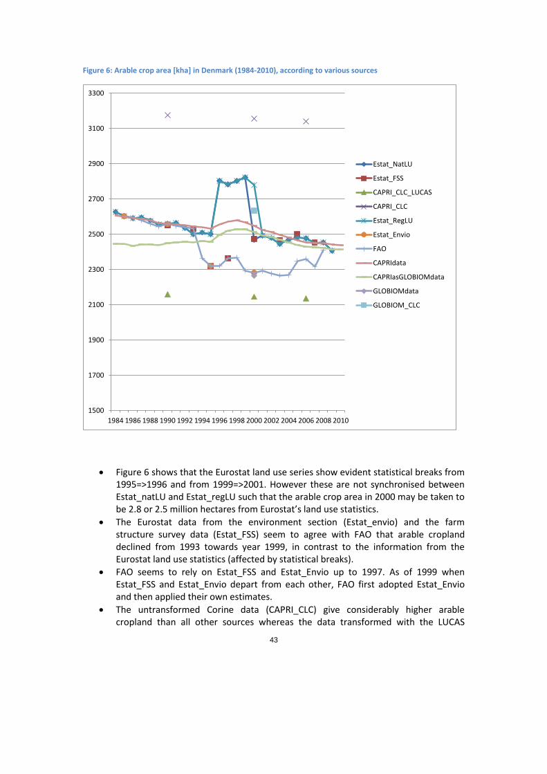
43

Figure 6: Arable crop area [kha] in Denmark (1984-2010), according to various sources

Figure 6 shows that the Eurostat land use series show evident statistical breaks from 1995=>1996 and from 1999=>2001. However these are not synchronised between Estat_natLU and Estat_regLU such that the arable crop area in 2000 may be taken to be 2.8 or 2.5 million hectares from Eurostat’s land use statistics.

The Eurostat data from the environment section (Estat_envio) and the farm structure survey data (Estat_FSS) seem to agree with FAO that arable cropland declined from 1993 towards year 1999, in contrast to the information from the Eurostat land use statistics (affected by statistical breaks).

FAO seems to rely on Estat_FSS and Estat_Envio up to 1997. As of 1999 when Estat_FSS and Estat_Envio depart from each other, FAO first adopted Estat_Envio and then applied their own estimates.

The untransformed Corine data (CAPRI_CLC) give considerably higher arable cropland than all other sources whereas the data transformed with the LUCAS

1500

1700

1900

2100

2300

2500

2700

2900

3100

3300

1984 1986 1988 1990 1992 1994 1996 1998 2000 2002 2004 2006 2008 2010

Estat_NatLU

Estat_FSS

CAPRI_CLC_LUCAS

CAPRI_CLC

Estat_RegLU

Estat_Envio

FAO

CAPRIdata

CAPRIasGLOBIOMdata

GLOBIOMdata

GLOBIOM_CLC

44

contingency table (CAPRI_CLC_LUCAS) seems to be “biased” downwards compared to most other sources. It may be noted that the CORINE data confirm some decline of arable crop area, but the decline is weaker than according to other sources.

The details of data processing matter considerably in Denmark: Whereas the CORINE data used in CAPRI (aggregated by JRC to the NUTS2 level) give an area for arable cropland of NUTS2 data of about 3.2 million ha, the CORINE data aggregated in GLOBIOM from pixel information give only 2.6 million ha (GLOBIOM_CLC).

The consolidated GLOBIOM area (GLOBIOMdata ~ 2.25 million ha) is close to the FAO information and clearly smaller than the CAPRIdata (~ 2.55 million ha) which can be attributed to a smaller crop coverage only to a certain degree. The arable crop aggregate CAPRIasGLOBIOMdata (~ 2.50 million ha) defined from the crop list covered by GLOBIOM is still larger than the area given as GLOBIOMdata, mainly because the GLOBIOM database excludes “unproductive” fodder areas11. In fact this leads in many (but not all) cases to smaller fodder areas (grassland or fodder on arable land) being reported in GLOBIOM than in CAPRI.

The estimated CAPRIdata are evidently “biased upwards” by the information from Estat_natLU and Estat_regLU in the years affected by the break (1996-2000), but the specification seems to ensure a reasonable compromise (in this example). The effect of the Eurostat land use data is unavoidable as these sources are usually the main information to rely on such that the CAPRI data cannot be immune against statistical problems in these sources.

The second example shows a number of remarkable breaks in the statistical information on

grassland in Greece.

The FAO series may be seen to show the most impressive statistical break from 2002 to 2003. It is not evidently derived from other statistical information but in 2005 the FAO number is identical to that from the Eurostat FSS that was related to the FAO information on arable crop area in Denmark in several years as well.

The two annual series offered for land use by Eurostat for grassland (Estat_NatLU and Estat_RegLU) may be observed to drop from the value of 1.789 million ha, invariably given for years before 2000, to much lower values, about 150 kha according to Eurostat’s regional land use statistics and about 275 kha for the national land use data. This information is inconsistent with each other and over time.

11 The GLOBIOM area for „other fodder“ (other than gras and fodder maize) in year 2000 is about 460 kha, whereas the corresponding area is in CAPRI 640 kha.

45

The Eurostat farm structure survey (Estat_FSS) gives a grass land area of 500-800 kha for the survey years, but is likely to cover only the more intensively used grassland areas.

Corine data are given only for 1990 and 2000. They are close to the earlier values reported in NatLU if the Corine data are mapped to the CAPRI land categories using a contingency table between Corine and LUCAS (CAPRI_CLC_LUCAS). Using the Corine data without this transformation gives a considerably higher area of about 3.7 million ha (CAPRI_CLC), almost as high as the older FAO data. The reason is that in Greece it turned out that the important Corine classes “complex cultivation patterns” and “agriculture with natural vegetation” are predominatly identified in LUCAS to be “permanent grassland without tree cover”.

Again it is interesting to note that the methodology to aggregate the CORINE data to the country level matters considerably. The area aggregated from pixels according to the GLOBIOM routines (GLOBIOM_CLC) clearly falls short of the corresponding area mapped to grassland according to the CAPRI rules (CAPRI_CLC). In fact it is also smaller that the NUTS2 value for the CORINE class “natural grassland” as aggregated by the JRC with a different methodology.

Figure 7: Grassland area [kha] in Greece (1984-2010), according to various sources

0

1000

2000

3000

4000

5000

6000

1984 1986 1988 1990 1992 1994 1996 1998 2000 2002 2004 2006 2008 2010

Estat_NatLU

Estat_FSS

CAPRI_CLC_LUCAS

CAPRI_CLC

Estat_RegLU

Estat_LandCov

Estat_Envio

FAO

CAPRIdata

GLOBIOMdata

GLOBIOM_CLC

46

The land cover statistic by Eurostat (Estat_LandCov), unfortunately only given for a single year (2009) gives a value of about 1.6 million ha.

The CAPRI consolidated series may be seen to settle between 1.0 and 1.3 million ha as a compromise of this conflicting raw data information while preserving the stability of grassland that will be considered plausible for this area category.

It is interesting to note that in this case the GLOBIOM area is larger than the CAPRI data and very close to the Eurostat information for this year. So the earlier finding of smaller fodder areas being included in GLOBIOM than in CAPRI does not hold in all cases.

V. Concluding remarks In many cases the CAPRI estimates for a complete area balance of EU countries appears to

be more convincing than single sources that often show unbelievable statistical breaks and

are in conflict with each other.

However this statement is merely confirming that a statistical procedure is able to minimise

the deviations from observations within a given sample (data from various sources). A more

difficult test would be a comparison with an independent, high quality information source

on land use developments over time in one or better several countries. As such information

has not been identified yet, it is difficult to assess whether the CAPRI estimates are

“accurate” or not. Validation of the whole procedure must be considered pending therefore.

A selective comparison with the GLOBIOM database also does not resolve the issue as the

findings are quite heterogeneous.

Documenting the procedure and results in view of potential feedback is therefore one of the

most promising options to achieve further progress in the future.

47