ent Reference Sites ondition n 2 July 2011 Method for the Establishm and Survey of for BioC Versio

Welcome message from author
This document is posted to help you gain knowledge. Please leave a comment to let me know what you think about it! Share it to your friends and learn new things together.
Transcript
ent Reference Sites
ondition
n 2
July 2011
Method for the Establishmand Survey of for BioC
Versio

ISBN 978-1-7423-0916 This work may be cited as: Eyre, T.J., Kelly, A.L., and Neldner, V.J. (2011). Method for the Establishment and Survey of Reference Sites for BioCondition. Version 2.0. Department of Environment and Resource Management (DERM), Biodiversity and Ecological Sciences Unit, Brisbane. Acknowledgements Within the Department of Environment and Resource Management (DERM), the development, testing and improvement of the BioCondition reference site method has been greatly enhanced through contributions by Melinda Laidlaw (reviewed draft), Andrew Franks, Peter Taylor (Figure 9), Tony Bean, Don Butler, Bill McDonald, and Jian Wang. Prepared by:Biodiversity and Ecological Sciences Department of Environment and Resource Management © The State of Queensland (Department of Environment and Resource Management) 2011 Copyright inquiries should be addressed to [email protected] or the Department of Environment and Resource Management, 41 George Street Brisbane QLD 4000 Published by the Queensland Government, July 2011
This publication can be made available in alternative formats (including large print and audiotape) on request for people with a vision impairment. Contact (07) 322 48412 or email <[email protected]> July 2011 #29814

Method for the Establishment and Survey of Reference Sites for BioCondition: Version 2
C ntents o 4
2 6
3 o 6
4 i 7
..........................7
..................................................................................................................8
ta collection.............................................................................................................................................9
22
24
26
..............................29
..............................30
..............................33
Appendix 4: Reference site datasheets .............................................................................................................................35
Appendix 5: Taking Photos................................................................................................................................................37
Appendix 6: Stratifying vegetation .....................................................................................................................................39
Appendix 7: Measuring Tree Height ..................................................................................................................................45
Appendix 8: Life-forms used in BioCondition .....................................................................................................................46
1 Introduction
What is required for the assessment
L cating reference sites
F eld assessment 4.1 When to assess .................................................................................................................
ssment site4.2 Setting up the asse
4.3 Da
5 Deriving Benchmarks from the data
6 References
7 Glossary of terms Appendix 1: Contacts for further information .......................................................................................
Appendix 2: Plant identification guides ................................................................................................
Appendix 3: Using GIS to search for reference sites ...........................................................................
ii
Method for the Establishment and Survey of Reference Sites for BioCondition: Version 2
iii
yout 8
bute 15
17
18
r amounts (as a
ead across the quadrat or distributed in patches. 21
Figure 6: Mapped example showing the extent of RE 12.5.6, where it is the dominant RE in a polygon and where
34
ot photo – try and keep the top of your feet out of the frame and angle th mera
37
hotos – record the bearing or direction of the photo in order to st replicate
photos on subsequent visits. 38
for determining vegetation strata, when not obvious 40
45
eter 45
List of tables Table 1: Site-based attributes that are compared against benchmark values in BioCondition, and hence
measured at reference sites 5
Table 2: Structural formation classes qualified by height 13
List of figures Figure 1: BioCondition reference site area and la
Figure 2: Plot size selection for large tree threshold attri
Figure 3: Median height of the Ecologically Dominant Layer (EDL)
Figure 4: Example of assessing tree canopy cover (%).
Figure 5: Stylised examples of ground cover proportions (DERM 2010). Various ground cove
percentage) can be evenly spr
it is sub-dominant within a local area.
Figure 7: Taking the sp e ca
down as straight as possible
Figure 8: Taking the landscape p assi
Figure 9: Method
Figure 10: Looking through a clinometer
Figure 11: Using a clinom

Method for the Establishment and Survey of Reference Sites for BioCondition: Version 2
1 Introduction
Recent policy demands and expectations have conceptualised vegetation condition as a major cvegetation management, primarily to assist decision making for developmental approvals, inmarket-based investments and demonstration of environmental duty of care (Keith & Gorrod 2Methods to assess vegetation condition are therefore required, with a simple, rapid assessmendesirable, as it facilitates widespread application by a range of users (Andreasen et al. 2001). Acondition assessment tools utilise key attributes or surrogates of biodiversity values that can bethe field (Gibbons & Freudenberger 2006). In Australia, the ‘Habitat Hectares’ approach in V2003) instigated development of similar vegetation condition assessment frameworks such as South Wales (Gibbons et al. 2008), TASVEG in Tasman
omponent of native centive payments,
006; Neldner 2006). t approach highly
ccordingly, most rapidly measured in
ictoria (Parkes et al. BioMetric in New
ia (Michaels 2006) and BioCondition in Queensland (Eyre licy, however they all share
ity; methods to assess eference’ conditions;
stem is refore repeatable
rough to ‘dysfunctional’ c site-based
l Ecosystem (RE). A disturbed sites or from pacts (Michalk and
04). These BOO sites are termed ‘reference sites’.
and will be posted yet been
cted during less than rived by locating and setting up a local reference
measurement
ding of floristic and structural vegetation attributes specifically for the generation of benchmarks for BioCondition. The benchmark data derived using this method is to be used in conjunction with the companion manual: BioCondition – A condition assessment framework for terrestrial biodiversity in Queensland (Eyre et al. 2011). Feedback on the methods is sought and will help improve future versions (See Appendix 1 for contacts).
There are 10 attributes in BioCondition that require benchmarks for the scoring system (Table 1). However, not all attributes require measurement at reference sites. This is because their benchmarks are either effectively zero or scores are qualified in the BioCondition scoring system. Attributes that do not require assessment at reference sites include recruitment of canopy species, non-native plant cover and the attributes relating to landscape context.
et al. 2011). The frameworks vary in accordance with jurisdictional legislation and pofour properties: a set of weighted assessable attributes thought to be important to biodiversthe attributes; comparison against benchmark values based on the same communities under ‘rand a final overall metric or ‘score’ that represents a condition state.
BioCondition is an assessment framework that provides a measure of how well a terrestrial ecosyfunctioning for the maintenance of biodiversity values. It is a site-based, quantitative and theassessment procedure that provides a numeric score along a continuum of ‘functional’ thcondition. The BioCondition score is based on a comparison between measurements of specifiattributes and a benchmark value for each of those attributes, specific to a particular Regionabenchmark value is based on the average or median value obtained from mature and long unBest on Offer (BOO) sites, given few ecosystems are totally free of impacts of threatening imNorton, 1980; Landsberg and Crowley, 20
Benchmarks for REs in Queensland will be derived from quantitative data and expert elicitationon the DERM BioCondition website. However, due to the large number of REs, many have not benchmarked. Where benchmarks are not yet available, or an assessment needs to be conduoptimal conditions, then quantitative benchmark data can be desite. Reference site assessment does require good botanical and habitat assessment skills, and entails and recording of vegetation floristics and structure.
The assessment method detailed in this manual is for the location, establishment and recor
4

Method for the Establishment and Survey of Reference Sites for BioCondition: Version 2
Table 1: Site-based attributes that are compared against benchmark values in BioCondition, and hence ured at reference meas sites
Attribute Measure
Native plant species richness number
Tree canopy cover (%) tage percen
Tree canopy height (m) median
Shrub layer cover (%) percentage
Native perennial grass cover (%) percentage
Large trees number
Coarse woody debris (m) number
Litter cover (%) percentage
BioCondition provides an assessment of the condition of an ecosystem in relation to its functmaintenance of biodiversity values, but will not provide the answer to all your assessment and Practitioners need to evaluate their objectives, as there may be additi
ioning for the monitoring needs.
onal information required in order to meet the vey or monitoring by
pson, E.J. and Dillewaard, H.A. (2005). Methodology for survey and mapping of regional ecosystems and vegetation communities in Queensland. Version 3.1. Department of Environment and Resource Management, Brisbane <www.derm.qld.gov.au>.
Fauna: Eyre, T.J., Ferguson, D. J., Hourigan, C.L., Kelly, A.L., Venz, M.F., Mathieson, M.T., Smith, G. C. (in prep.). Terrestrial Fauna Survey Assessment Guidelines for Queensland.Version 1.0. Department of Environment and Resource Management, Brisbane.
data requirements of their study. If more detailed assessments are required for biodiversity surappropriately skilled operators, then the following methods are recommended:
Flora: Neldner, V.J., Wilson, B.A., Thom
5
Method for the Establishment and Survey of Reference Sites for BioCondition: Version 2
2 What is required for the assessment? s place within a 100 x 50 m area. Ideally you will need:
transect tape
era
res and wire (to peg down tyre) to mark out each end of the transect line (if continual g of site is desired).
ser.
flagging tape
er vary within RE’s according to environmental conditions. Therefore site that occurs close to the area to be assessed and has
, similar climate (same su y etc) and similar natural
eight, canopy cover and species a local reference ar a of comparable vegetation that is known to be remnant, such as a shadeline or road reserve.
As much as practicable, a reference or BOO site should:
be homogenous with regard to RE and condition status
be selected in RE’s with no extensive chemical or mechanical disturbance to the predominant canopy evident on the aerial photograph archive (from 1960s to recent) or on the ground
represent an undisturbed, late mature or BOO of the required RE. That is, the site must have minimal modification through timber harvesting, grazing, fire, erosion, dieback, flood, and/or weed infestation
The assessment take
100 m
50 m transect tape
compass
diameter tape or tree callipers
this current manual
clinometer or hypsometer for measuring tree heights
digital or print film cam
1 m2 quadrat
m2 x star pickets or ty
onitorin
clipboard, pencils and era
pocket calculator
global positioning system (GPS)
plant press for collecting specimens
plant identification guides (see Appendix 2).
3 Locating reference sites
ites is essential to the development of relevant and The appropriate location and establishment of reference seffective benchmarks. Canopy height and covareas to be assessed should be compared with a reference similar environmental conditions, i.e. the same regional ecosystem, vegetation community
bregion), similar landscape conditions (soil, slope, position in the landscape, geologdisturbance (cyclone impacts or fire history). For this reason, field measurements of the h
composition of the area of interest are compared, where possible, to measurements fromea, i.e. a nearby are
6
Method for the Establishment and Survey of Reference Sites for BioCondition: Version 2
be located within a reasonably large (> 5 ha) intact patch of remnant vegetation (to avoid issues of
6 km from permanent water (Fensham and Fairfax
f interest, is to first nal Ecosystem
as digital data from maps and digital data
nting the extent of the RE or the local area from which uld be assessed in the
s are defined at scales bioregions) and a single
polygons).
e forests, and road Queensland le locations
attributes within the of three local reference sites located and measured. It is
preferable that the reference sites are not located proximally, and are established at least 3 km apart to account for ses, particularly in highly fragmented bioregions, it may not be possible within the one reference site, e.g. a recent fire may have impacted upon y species present, but not the number of large trees. It is acceptable to
t provides benchmark data for one or more attributes only. However, it will need to be s that it is a partial reference site only.
Reference site assessment during the peak of summer or following a period of drought is not recommended, as d grass life form
groups. Seasonally, the best time of year for assessment, in the rangelands in particular, is during the growing season of May to June, when plant diversity is generally at its greatest. However, this is a general rule and the appropriate time to assess should be guided by local climate and knowledge.
In regions north of the tropic of Capricorn, site assessment should be conducted after the wet season, ideally between March and May to ensure adequate sampling of ground cover species (Neldner et al. 2004). South of the tropic of Capricorn, site assessment should be generally conducted in May or June following the wetter summer months. An exception would be following an unseasonably wet winter or spring when plant species are flowering.
edge effects)
be located at least 50 m from a roadside, track, or other major disturbance
be remote from artificial water sources e.g. >2008)
exclude areas subject to recent major management change.
An effective strategy for locating reference sites, that best represent a BOO state for the RE olook at the extent remaining of the RE using the latest available Queensland Herbarium Regiomapping. Free RE maps are available as downloadable pdf/printable maps for properties and the Regional Ecosystems area of DERM’s website <www.derm.qld.gov.au>. The hardcopycan be used to produce a map specific for the area represeyou are trying to obtain your local reference sites1 . The applicability of the RE mapping shofield to check if it is relevant at the scale at which the assessment is being conducted. REwhich range from 1:50 000 (e.g. South East Queensland) to 1:100 000 (e.g. rangeland polygon may contain several mapped REs (heterogeneous
Large patches of the RE of interest located in public land reserves such as national parks, statreserves can often represent the RE in an undisturbed or BOO state. In addition, staff from theHerbarium and/or local natural resource managers can often provide information about suitabrepresenting the least disturbed patches remaining of the RE of interest.
To obtain a reasonable representation of the natural variation inherent in vegetation condition geographic range of an RE, there must be a minimum
potential geographic variation. In some cato collect benchmark data for all attributesshrub cover and the number of understoreestablish a reference site thamade clear on the datasheet
4 Field assessment 4.1 When to assess
there is likely to be a reduction in plant diversity during these times, particularly in the forb an
1 If using a Geographic Information System (GIS) to look for reference sites see Appendix 3 for coding to include in a query to pull out the dominant (where >50% of the polygon contains the RE of interest) and subdominant (<50% of polygon) extent of the RE of interest.
7
Method for the Establishment and Survey of Reference Sites for BioCondition: Version 2
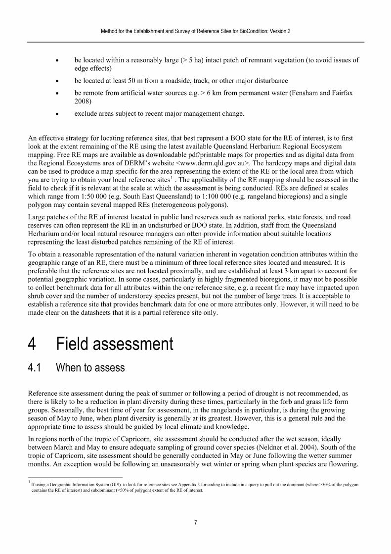
4.2 Setting up the assessment site
ested subplots are e, which constitutes
ot, which is 25 m each ajor disturbance or
be oriented so that ation is recorded at
S) is recommended to record the position of the centre and start points of the transect line in the field. This position should be checked against a 1:100 000 or larger scale topographic map for the area. The altitude recordings on GPS can be inaccurate and are better derived from the topographic map. The use of star pickets, metal tags attached to trees or pegged down tyres at the beginning and end of the 100 m transect will aid in relocating the site for future monitoring.
The assessment site constitutes a 100 m x 50 m nested plot design. The layout of the site and nshown in Figure 1. Demarcation of the reference site is established by positioning a 100 m tapthe centre line of the plot. Flagging tape can be used to identify the outer boundaries of the plside of the centre transect. The plot boundary must be a minimum distance of 50 m from a mdiscontinuity such as a road or disturbed edge. In topographically diverse areas, the plot shouldits long axis follows the contour, or topographic position (e.g. gully, midslope, ridge). Plot locits centre point (the 50 m point along the 100 m transect). A global positioning system (GP
Figure 1: BioCondition reference site area and layout
8

Method for the Establishment and Survey of Reference Sites for BioCondition: Version 2
4.3 Data collection
e used to sample the flo
diameter at breast height (DBH); ction 4.3.1. Site information and disturbance, tree
area.
and >50 cm in
a: records the number of floristic species by lifeform group (Native plant species rea can also be used as a
2 in the Method for Queensland
(5) 1 x 1 m subplots: records Native Perennial Grass cover and Organic Litter cover.
eference site data is provided in Appendix 4. It is important to ensure that the ystem to be sampled. Therefore it may be necessary to reduce the width of the ian ecosystems. In these situations the length of the plot may be increased to
0
4.3.1.1 SitWithin the gdisturbance i
n
cation ther at the start of the ce and bearing from relocation of the plot).
ystem (GPS) ended that GDA94
Plot bearing Refers to the compass bearing or direction the plot is oriented from the start of the transect.
Locality description
Record a general description of where the plot is situated. Include the state forest/national park number and/or name, or a property name or description, the name of the nearest road if applicable and any other information relevant to the locality. Include the tenure of the land parcel on which the plot occurs by reference to the Digital Cadastral Data Base (DCDB) which is maintained by Department of Environment and Resource Management (DERM) <www.derm.qld.gove.au>
Bioregion Record the Queensland bioregion name.
Five sampling areas form the basis for and approach to data collection. A series of subplots arristic, habitat and disturbance components, and are summarised as follows;
>20 or >30 cm(1) 100 x 50 m area: records all potential large trees depending on the tree species, see Large tree sespecies richness and tree canopy height are also assessed in the 100 x 50 m
(2) 100 m transect: records tree and shrub canopy cover.
(3) 50 x 20 m area: records the length of all coarse woody debris >10 cm diameter length.
(4) 50 x 10 m arerichness) for Shrub, Grass, and ‘Forbs and Other’ species. This aSecondary Site for the detailed survey of RE’s if desired following AppendixSurvey and Mapping of Regional Ecosystems and Vegetation Communities in (Neldner et al. 2005).
A datasheet to aid the collection of rplot remains within the regional ecosplot for narrow ecosystems, eg. riparenable the sampling of an adequate area.
4.3.1 1 0 x 50 m assessment area
e information and Disturbance reater 100 x 50 m assessment area assess the site location, general physical characteristics and nformation relevant to the site.
Location a d site information
Plot lo Record three locations, one at a convenient road point, ano100 m central transect and another at the plot centre, the distanthe road to the plot centre and the plot alignment (to aid futureRecord location to the nearest metre using a Global Positioning Sreceiver. Record the datum to which the GPS is set. It is recomm
. or if not available WGS84 is used as the datum
9
Method for the Establishment and Survey of Reference Sites for BioCondition: Version 2
10
nal Ec
description es and density of all
pe (Table 2), as cteristic stratum, or the
(Neldner et al. 2005).
Regional Ecosystem
vegetation unities that are consistently associated with a particular combination of
EDD) is updated ing that you can
ueensland with ailable for over 90
ined by firstly querying REs for the location,
sents. If the description is not a good priate bioregion ecause:
y at 1:100 000 scale, but in scale.
mosaics where, again f scale restraints, a single vegetation polygon is classed as
being a mix of several different vegetation types (and thus REs).
Not all of Queensland has mapping available.
For this reason the regional ecosystem maps should be used as a guide and the habitat description should be detailed enough to enable the classification of the actual community into a single RE.
Regio
Habitat
osystem
Record a detailed description of the site including the key specitree, shrub and ground layers. Aim to include its structural form typer the Queensland Herbarium (BRI) which uses the charalayer that contributes most to overall above-ground biomass
REs were defined by Sattler and Williams (1999) as bioregionalcommgeology, landform and soil. The RE description database (Rregularly and is available on the DERM website along with mappdownload.
A total of 1375 REs are currently defined (REDD v.6.0) in Qmapping updates occurring frequently. RE maps are currently avper cent of Queensland. The RE for the site can be determthe RE mapping and comparing the descriptions of the mapped in order to decide which RE the site reprematch with any of the mapped REs, then check others in the approand land zone. Occasionally the specific RE may not be mapped b
Regional ecosystem mapping is usuallsome cases mapped at 1:25 000
Vegetation mapping often uses the concept ofbecause o

Method for the Establishment and Survey of Reference Sites for BioCondition: Version 2
Land form
itio
ree d in degrees. For d slope as 0 degrees.
Slope aspect Record the compass direction, in degrees, of the downward slope of the plot. For flat areas record a dash (-).
centre point of the plot collect four photos, north, south, east and west, and at the commencement of transect. In addition, spot photos can be useful to capture the variability in ground cover within the five
ce
Disturbance is visually assessed over the whole reference site. These data are not actually required for benchmarking, but it is helpful to have a record of any disturbance if present as information on the current condition of the site at the time of assessment. As outlined earlier, ideally the reference site should have minimal disturbance.
Slope pos n Record the slope position, using codes given on the datasheet.
Slope deg Measure the general slope of the plot using a clinometer and recorflat areas recor
Site photos
At the 50 mthe central1 x 1 m quadrats. See Appendix 5 for description on how to take photos.
Disturban
11
Method for the Establishment and Survey of Reference Sites for BioCondition: Version 2
For each disturbance type a code is used to rank its relative severity (from 0 = no discernible dsevere). Codes are also used to record an estimated time since the last event for each disturba3 years, C: 5-10 years, D: 10-20 years, D: > 20years), and how the disturbance was estimated2 = from historical records, 3 = from informant, 4 = from imagery or mapped source). Assessmshould be considered in the context of impact on the RE’s structure, composition and functionto take into
isturbance to 3 = nce (A: <1 year; B: 1- (1 = visual estimate,
ent of disturbance . Assessment needs
account the capacity of the community to recover after the event – that is, disturbances can appear to be beyond
rt term
Wildfire can be based on
d diameter. Time st-burn regeneration,
rring on ground woody debris which may have fallen since the event, diameter , extent of crown recovery or from the
ping sites such as SIRO Sentinel
ht of fire scars on standing stems.
Burn o reduce fuel loads he nature of these
of this disturbance would rarely be recorded as e ground and
Logging d be the total of all een several logging
Treatment barking or ct harvesting and
aring’ by mechanical means. Standing dead and fallen trees should be examined st height treatment.
paction, presence of s. It will probably not be possible to estimate
n of fencing and stock time since grazing
Non-native plants
Non-native plants include all exotic species, and those declared or assumed to be noxious (e.g. lantana, balloon cotton bush), but not native ‘woody weeds’ such as Dodonaea, Eremophila.
Erosion Record information on erosion seen in the plot, e.g. gully erosion. Erosion outside the plot but in the vicinity should be noted.
Regeneration Record information about regeneration resulting from disturbance e.g. Acacia following wildfire or regrowth following clearing. Detail in notes as required.
Other Specify any other disturbance types noted e.g. dieback, soil disturbance, snig tracks.
severe soon after their occurrence. It is imthe sho
portant to try to gauge how this event will affect the community.
Refers to major previous hot fire disturbance, the severity of whichthe extent of fire scars on standing trees relative to their height ansince such an event can be estimated on the height of any pochagrowth around fire scars on standing live treesaerial photograph or satellite imagery archive or web fire mapNorthern Australian Fire Information (NAFI) website, or the Cwebsite.
Record also the mean heig
Prescribed Refers to the cool, frequent (annual or biennial) burns used tand/or increase grazing potential of the grassy understorey. Tburns dictates that the intensitysevere. However, if the fire regime is too frequent then impact on thshrub layers can be deemed severe.
Record information on past logging events. Severity shoullogging events and time for the latest event. If there have bevents record details in the notes section.
Treatment is defined as the destruction of individual trees by ringpoisoning, in contrast to ‘logging’ of individual trees for produ‘cleclosely for marks indicating past treatment. These can be at wai(ringbarking or axe cuts) or near ground level for basal injection
Grazing Grazing impact can be assessed by the presence of manure, comstock trails, and eaten off grassegrazing severity for older grazing events. However, inspectioinfrastructure in the vicinity may give some indication of theactivity.
12
Method for the Establishment and Survey of Reference Sites for BioCondition: Version 2
13
height
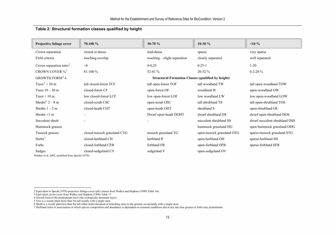
Table 2: Structural formation classes qualified by
Projective foliage cover 70-100 % 30-70 % 10-30 % <10 %
Crown separation ense se very sparse
erlap separ rly separated well separated
atio2 0-0.25 0.25-1 1-20
%3 81-100 % 0.2-20 %
FORM4 ural Forma lified by heigh
forest TCF en-forest TOF tall woodland TW pen-woodland TOW
30 m OF and W dland OW
est LCF rest LOF low woodland LW low open-woodland LOW
8 m C rub OSC tall shrubland TS open-shrubland TOS
2 m closed-heath CHT nd S land OS
- Dwarf open-heath DO bland DS rubland DOS
b land lent shrubland DSS
mock grasses ock grassland n hummock grassland OHG
ock grasses grassland CTG sock grassland TG ssock grassla se-tussock grassland STG
s7 CH bland H erbland OH sparse-herbland SH
closed-forbland CFB forbland FB open-forbland OFB sparse-forbland SFB
Sedges closed-sedgeland CV sedgeland V open-sedgeland OV Neldner et al. 2005, modified from Specht (1970)
closed or d
touching-ov
mid-dense
touching – slight
spar
ation cleaField criteria
Crown separation r <0
CROWN COVER 52-81 % 20-52 %
GROWTH Struct tion Classes (qua t)
Trees5 > 30 m tall closed- tall op tall o
Trees 10 – closed-forest CF open-forest woodl open-woo
Trees < 10 m low closed-for low open-fo
Shrubs6 2 – closed-scrub CS open-sc tall
Shrubs 1 – open-heath OHT shrubla open-shrub
Shrubs <1 m HT dwarf shru
succulent s
dwarf open-sh
Succulent shru - - hrub SS dwarf succu
Hum humm HG ope
Tuss closed-tussock tus open-tu nd OTG spar
Herb closed-herbland her open-h
Forbs
2 Equivalent to Specht (1970) projective foliage cover (pfc) classes from Walker and Hopkins (1990) Table 14a. 3 Equivalent crown cover from Walker and Hopkins (1990) Table 17 4 Growth form of the predominant layer (the ecologically dominant layer). 5 Tree is a woody plant more than 5m tall usually with a single stem. 6 Shrub is a woody plant less than 8m tall either multi-stemmed or branching close to the ground, occasionally with a single stem. 7 Herbland refers to associations in which species composition and abundance is dependant on seasonal conditions and at any one time grasses or forbs may predominate
Method for the Establishment and Survey of Reference Sites for BioCondition: Version 2
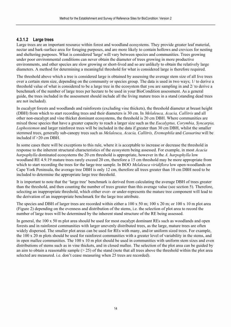
4.3.1.2 Large trees Large trees are an important resource within forest and woodland ecosystems. They providnectar and bark-surface area for foraging purposes, and are more likely to contain holand sheltering purposes. What is considered 'large' will vary between species and communitiunder poor environmental conditions can never obtain the diameter of trees growing in more productive
e greater leaf material, lows and crevices for nesting
es. Trees growing
he relatively large refore required.
size of all live trees o ways; 1/ to derive a in and 2/ to derive a t. As a general
d (standing dead trees
eter at breast height o start recording trees and their diameters is 30 cm. In Melaleuca, Acacia, Callitris and all
re communities are s, Corymbia, Syncarpia,
m DBH, whilst the smaller Casuarina will be
le, where it is acceptable to increase or decrease the threshold in e, in most Acacia ophylla low re appropriate from
In BOO Melaleuca viridiflora low open-woodlands on cm DBH need to be
DBH of trees greater e section 5). Therefore,
mponent will lead to
00 x 10 m plot area a to record the
tructure of the RE being assessed.
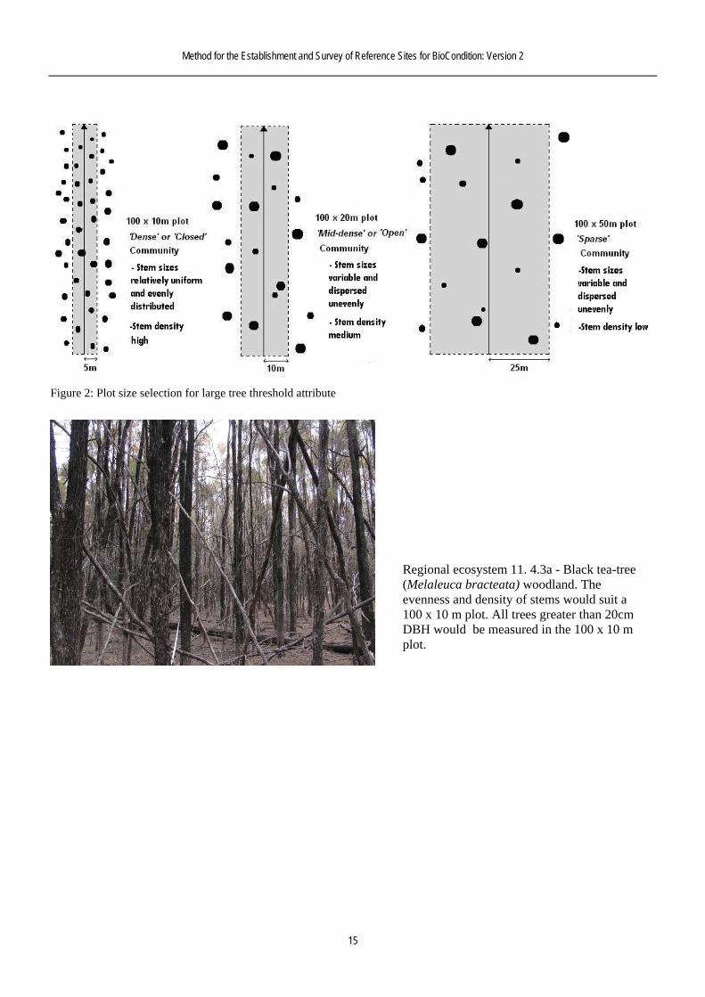
In general, the 100 x 50 m plot area should be used for most eucalypt dominant REs such as woodlands and open forests and in rainforest communities with larger unevenly distributed trees, as the large, mature trees are often widely dispersed. The smaller plot areas can be used for REs with many, and/or uniform sized trees. For example, the 100 x 20 m plots should be used for rainforest communities with a greater level of variability in the stems, and in open mallee communities. The 100 x 10 m plot should be used in communities with uniform stem sizes and even distributions of stems such as in vine thickets, and in closed mallee. The selection of the plot area can be guided by an aim to obtain a reasonable sample (> 25) of the stand (note that all trees above the threshold within the plot area selected are measured. i.e. don’t cease measuring when 25 trees are recorded).
environments, and other species are slow growing or short-lived and so are unlikely to obtain tdiameters. A method for determining a meaningful threshold for what is considered large is the
The threshold above which a tree is considered large is obtained by assessing the average stemover a certain stem size, depending on the community or species group. The data is used in twthreshold value of what is considered to be a large tree in the ecosystem that you are samplingbenchmark of the number of large trees per hectare to be used in your BioCondition assessmenguide, the trees included in the assessment should include all the living mature trees in a stanare not included).
In eucalypt forests and woodlands and rainforests (excluding vine thickets), the threshold diam(DBH) from which tother non-eucalypt and vine thicket dominant ecosystems, the threshold is 20 cm DBH. Whemixed those species that have a greater capacity to reach a larger size such as the EucalyptuLophostemon and larger rainforest trees will be included in the data if greater than 30 cstemmed trees, generally sub-canopy trees such as Melaleuca, Acacia, Callitris, Eremophila and included if >20 cm DBH.
In some cases there will be exceptions to this ruresponse to the inherent structural characteristics of the ecosystem being assessed. For examplharpophylla dominated ecosystems the 20 cm threshold is appropriate, however in the A. harpwoodland RE 4.9.19 mature trees rarely exceed 20 cm, therefore a 15 cm threshold may be mowhich to start recording the trees for the large tree sample. Cape York Peninsula, the average tree DBH is only 12 cm, therefore all trees greater than 10 included to determine the appropriate large tree threshold.
It is important to note that the ‘large tree’ benchmark is derived from calculating the average than the threshold, and then counting the number of trees greater than this average value (seselecting an inappropriate threshold, which either over- or under-represents the mature tree cothe derivation of an inappropriate benchmark for the large tree attribute.
The species and DBH of larger trees are recorded within either a 100 x 50 m; 100 x 20 m; or 1(Figure 2) depending on the evenness and distribution of the stems, i.e. the selection of plot arenumber of large trees will be determined by the inherent stand s
14
Method for the Establishment and Survey of Reference Sites for BioCondition: Version 2
15
Figure 2: Plot size selection for large tree threshold attribute
Regional ecosystem 11. 4.3a - Black tea-tree (Melaleuca bracteata) woodland. The evenness and density of stems would suit a 100 x 10 m plot. All trees greater than 20cm DBH would be measured in the 100 x 10 m plot.
Method for the Establishment and Survey of Reference Sites for BioCondition: Version 2
Regional ecosystem 12.5The unevenness of stem
.13 – Vine forest. sizes and
distribution of stems would suit a 100 x 20 m plot. All trees greater than 20cm DBH would be measured in the 100 x 20 m plot.
11.8.15 – Poplar box ea) woodland. The
m sizes and open random distribution of stems would require a 100 x 50 m plot to assess the large tree attribute.
DBH rees greater than easured in the
Regional ecosystem(Eucalyptus populnunevenness of ste
All 'eucalypt' trees greater than 30cmand all 'non-eucalypt' t20cm DBH would be m100 x 50 m plot.
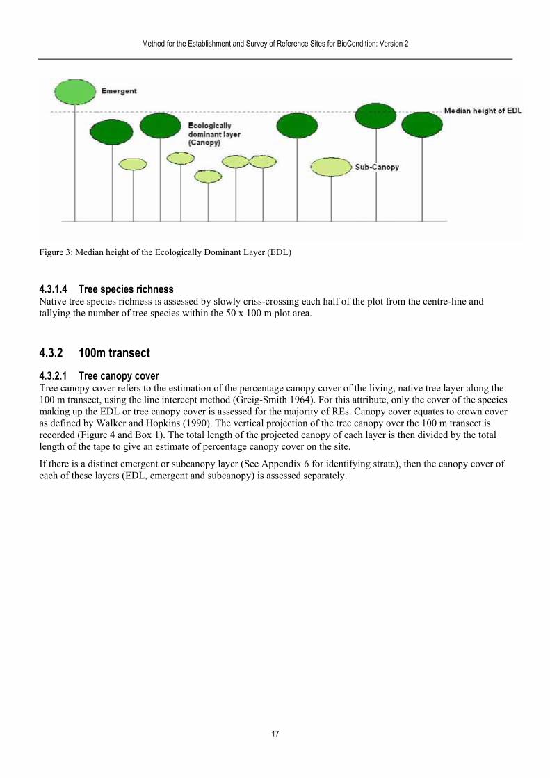
4.3.1.3 Tree canopy height Tree canopy height refers to the median canopy height in metres estimated for trees in the ecolayer (EDL) (canopy layer) (Appendix
logically dominant 6). If there are emergent and/or subcanopy layers present, then median
height of these layers needs to be assessed also. The median canopy height is the height that has 50 per cent of canopy trees larger and smaller than it (Figure 3). The height of woody vegetation is measured from the ground to the tallest live part of the tree (Neldner et al. 2005).
The maximum heights of the crown of at least three trees that are estimated to represent the median canopy height are measured for height, using a hypsometer or clinometer and tape measure (measured to the top of the highest leaves).It is recommended that a clinometer or hypsometer be used if available. When using a clinometer, adjustments are also made for the height of the recorder and any slope in the land surface. A method for assessing tree heights is provided in Appendix 7.
16
Method for the Establishment and Survey of Reference Sites for BioCondition: Version 2
Figure 3: Median height of the Ecologically Dominant Layer (EDL)
s richness Native tree species richness is assessed by slowly criss-crossing each half of the plot from the centre-line and
ree species within the 50 x 100 m plot area.
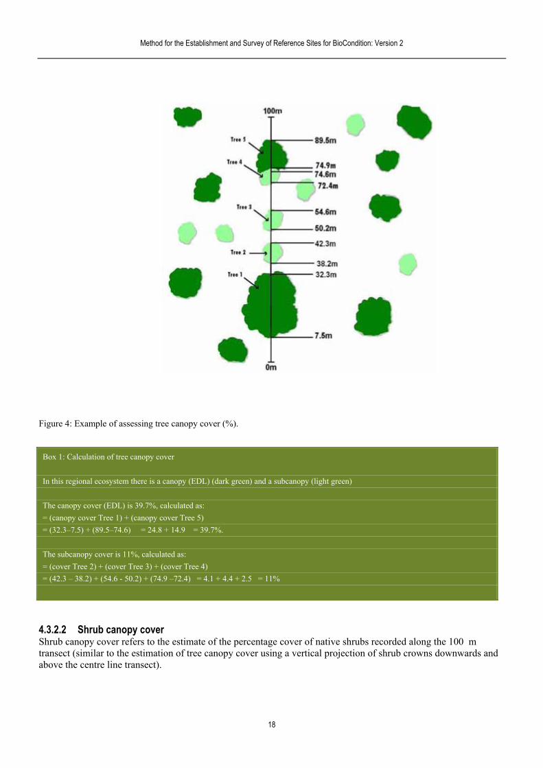
tree layer along the 1964). For this attribute, only the cover of the species
making up the EDL or tree canopy cover is assessed for the majority of REs. Canopy cover equates to crown cover as defined by Walker and Hopkins (1990). The vertical projection of the tree canopy over the 100 m transect is recorded (Figure 4 and Box 1). The total length of the projected canopy of each layer is then divided by the total length of the tape to give an estimate of percentage canopy cover on the site.
If there is a distinct emergent or subcanopy layer (See Appendix 6 for identifying strata), then the canopy cover of each of these layers (EDL, emergent and subcanopy) is assessed separately.
4.3.1.4 Tree specie
tallying the number of t
4.3.2 100m transect
4.3.2.1 Tree canopy cover Tree canopy cover refers to the estimation of the percentage canopy cover of the living, native100 m transect, using the line intercept method (Greig-Smith
17
Method for the Establishment and Survey of Reference Sites for BioCondition: Version 2
anopy cover (%).
Figure 4: Example of assessing tree c
Box 1: Calculation of tree canopy cover
In this regional ecosystem there is a canopy (EDL) (dark green) and a subcanopy (light green)
The canopy cover (EDL) is 39.7%, calculated as:
= (canopy cover Tree 1) + (canopy cover Tree 5)
= (32.3–7.5) + (89.5–74.6) = 24.8 + 14.9 = 39.7%.
The subcanopy cover is 11%, calculated as:
= (cover Tree 2) + (cover Tree 3) + (cover Tree 4)
= (42.3 – 38.2) + (54.6 - 50.2) + (74.9 –72.4) = 4.1 + 4.4 + 2.5 = 11%
4.3.2.2 Shrub canopy cover Shrub canopy cover refers to the estimate of the percentage cover of native shrubs recorded along the 100 m transect (similar to the estimation of tree canopy cover using a vertical projection of shrub crowns downwards and above the centre line transect).
18
Method for the Establishment and Survey of Reference Sites for BioCondition: Version 2
4.3.3 50 x 20 m plot area
, refers to logs or dead ent in contact with the
sholds, regardless of whether they are touching the ground. All CWD within the assessment area are measured to the boundary of the
tare). The total measured value is multiplied by 10 to generate the benchmark and is ctare. Any woody debris smaller than this is included as litter cover.
thin the 50 x 10 m plot. The number of native plant species are assessed into one of four life-form groups, to assist assessment and
ubs, grass, and forbs/other (see Appendix 8 for groupings). Native plant species richness is ee
x 100 m plot.
transect. For
ponents of the ground cover are recorded, to ensure 100 per cent of the ground cover is estimated. Ideally the botanical names of the species observed are recorded, however this is
e observer (for more detailed procedures for recording of floristic data see al ('decreaser') grass
hrubs (< 1m height), he total cover for a
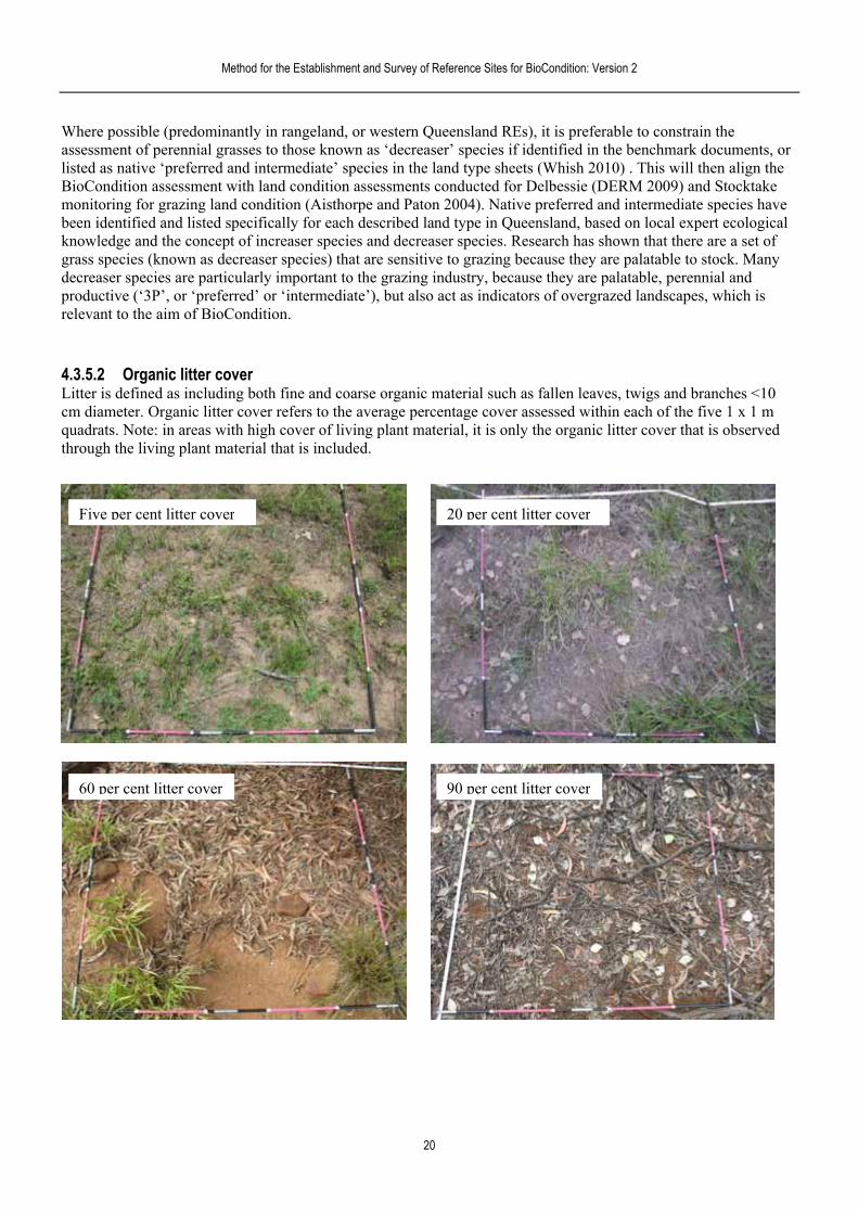
4.3.5.1 Native perennial grass cover Perennial grass cover refers to the average percentage cover of native perennial grasses, assessed within each of the five 1 x 1 m quadrats and averaged to give a benchmark value for the site. The ground cover is measured by a vertical projection downwards of the living and attached plant material. A stylised guide is provided in Figure 5 to help estimate cover percent. This cover equates to the projected foliage cover in Walker and Hopkins (1990). A value for the reference site for each component is obtained by averaging the values from the five sub-plots. The sum of all ground cover components will equal 100 per cent in each subplot.
4.3.3.1 Coarse woody debris Coarse woody debris (CWD), for the purpose of the BioCondition reference site assessmenttimber on the ground that are >10 cm diameter and >0.5 m in length (and more than 80 per cground). Note: branches that are attached to the log, are measured if they meet the size thre
50 x 20 m plot (i.e. 0.1 hecexpressed as metres per he
4.3.4 50 x 10 m plot area
4.3.4.1 Native plant species richness Native plant species richness for shrubs, grass and forbs/other species are recorded wi
benchmarking; trees, shrassessed by slowly walking along each side of the centre-line and tallying the number of species in each of thrlife-forms: shrubs, grasses and forbs/other. NB: Tree species richness is assessed in the 50
4.3.5 1 x 1 m quadrats Ground cover data is recorded from each of the five 1 x 1 m subplots centred along the centralbenchmarking purposes, quantitative data are required only for native perennial grass cover and organic litter cover. However, it is recommended that all com
dependent on the knowledge of thNeldner et al. 2006). The datasheet provides space to record cover estimates for; native perennicover, native other grass cover (if relevant, see below), native forbs and other species, native snon-native grass, non-native forbs and shrubs, litter, rock, bare ground and cryptogams (NB: tquadrat equals 100 per cent).
19
Method for the Establishment and Survey of Reference Sites for BioCondition: Version 2
Where possible (predominantly in rangeland, or western Queensland REs), it is preferable to cassessment of perennial grasses to those known as ‘decreaser’ species if identified in the benclisted as native ‘preferred and intermediate’ species in the land type sheets (Whish 2010) . ThiBioCondition assessment with land condition assessments conducted for Delbessie (DERM 20monitoring for grazing land condition (Aisthorpe and Paton 2004). Native preferred and intebeen identified and listed specifically for each described land type in Queensland, based on loknowledge and the concept of increaser species and decreaser species. Research has showngrass species (known as decre
onstrain the hmark documents, or s will then align the 09) and Stocktake
rmediate species have cal expert ecological
that there are a set of aser species) that are sensitive to grazing because they are palatable to stock. Many
decreaser species are particularly important to the grazing industry, because they are palatable, perennial and rred’ or ‘intermediate’), but also act as indicators of overgrazed landscapes, which is
Litter is defined as including both fine and coarse organic material such as fallen leaves, twigs and branches <10 cm diameter. Organic litter cover refers to the average percentage cover assessed within each of the five 1 x 1 m
h high cover of living only the organic litter cover that is observed through the living plant material that is included.
productive (‘3P’, or ‘preferelevant to the aim of BioCondition.
4.3.5.2 Organic litter cover
quadrats. Note: in areas wit plant material, it is
Five per cent litter cover 20 per cent litter cover
90 per cent litter cover60 per cent litter cover
20

Method for the Establishment and Survey of Reference Sites for BioCondition: Version 2
Figure 5: Stylised examples of ground cover proportions (DERM 2010). Various ground cover amounts (as a percentage) can be evenly spread across the quadrat or distributed in patches.
21
Method for the Establishment and Survey of Reference Sites for BioCondition: Version 2
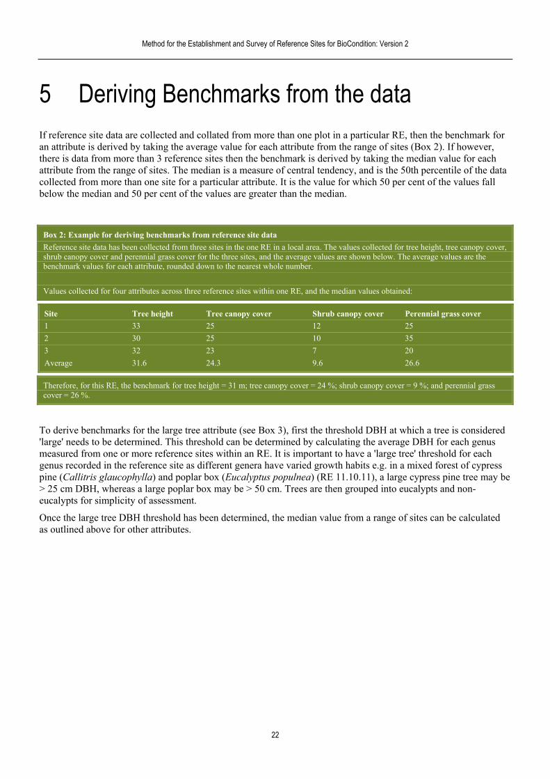
5 Deriving Benchmarks from the data the benchmark for x 2). If however,
ark is derived by taking the median value for each attribute from the range of sites. The median is a measure of central tendency, and is the 50th percentile of the data collected from more than one site for a particular attribute. It is the value for which 50 per cent of the values fall
are greater than the median.
If reference site data are collected and collated from more than one plot in a particular RE, thenan attribute is derived by taking the average value for each attribute from the range of sites (Bothere is data from more than 3 reference sites then the benchm
below the median and 50 per cent of the values
Box 2: Example for deriving benchmarks from reference site data
Reference site data has been collected from three sites in the one RE in a local area. The values collected for tree height, tree canopy cover, shr and perennial grass cover for the th and the average va are shown below. Tub canopy cover ree sites, lues he average values are the benchmark values for each attribute, rounded down to the nea st whole number. re
Values collected for four attributes across three reference sites ithin one RE, and the median values obtained: w
Site Tree height Tree canopy cover Shrub canopy cover Perennial grass cover
1 33 25 12 25
2 30 25 10 35
3 32 23 7 20
Average 31.6 24.3 9.6 26.6
Therefore, for this RE, the benchmark for tree height = 31 m; tree canopy cover = 24 %; shrub canopy cover = 9 %; and perennial grass cover = 26 %.
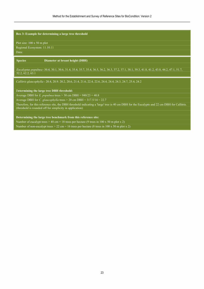
To derive benchmarks for the large tree attribute (see Box 3), first the threshold DBH at whic'large' needs to be determined.
h a tree is considered This threshold can be determined by calculating the average DBH for each genus
measured from one or more reference sites within an RE. It is important to have a 'large tree' threshold for each genus recorded in the reference site as different genera have varied growth habits e.g. in a mixed forest of cypress pine (Callitris glaucophylla) and poplar box (Eucalyptus populnea) (RE 11.10.11), a large cypress pine tree may be > 25 cm DBH, whereas a large poplar box may be > 50 cm. Trees are then grouped into eucalypts and non-eucalypts for simplicity of assessment.
Once the large tree DBH threshold has been determined, the median value from a range of sites can be calculated as outlined above for other attributes.
22
Method for the Establishment and Survey of Reference Sites for BioCondition: Version 2
23
Box 3: Example for determining a large tree threshold
Plot size: 100 x 50 m plot
Regional Ecos tem: 11.10.11 ys
Data:
Species Diameter at breast height (DBH)
Eucalyptus populnea - 30.4, 30.1, 30.6, 31.4, 35.4, 35.7, 35.4, 36.5, 36.2, 36.3, 37.2, 37.1, 38.1, 39.3, 41.8, 41.2, 43.8, 44.2, 47.1, 51.7, 52.2, 62.2, 63.1
Callitris glaucophylla - 20.4, 20.9. 20.2, 20.6, 21.4, 21.6, 22.4, 22.6, 24.4, 24.4, 24.3, 24.7, 25.4, 24.2
Determining the large tree DBH threshold:
Average DBH for E. populnea trees > 30 cm DBH = 940/23 = 40.8
Average DBH for C. glaucophylla trees > 20 cm DBH = 317.5/14 = 22.7
Therefore, for this reference site, the DBH threshold indicating a 'large' tree is 40 cm DBH for the Eucalypts and 22 cm DBH for Callitris. (threshold is rounded off for simplicity in application)
Determining the large tree benchmark from this reference site:
Number of eucalypt trees > 40 cm = 18 trees per hectare (9 trees in 100 x 50 m plot x 2)
Number of non-eucalypt trees > 22 cm = 16 trees per hectare (8 trees in 100 x 50 m plot x 2)
Method for the Establishment and Survey of Reference Sites for BioCondition: Version 2
6 References Abed, T. and Stephens, N.C. (2002). Tree measurement manual for farm foresters - Practicaforesters undertakin
l guidelines for farm g basic inventory in farm forest plantation stands, National Forest Inventory, BRS, Canberra.
ary Industries
lassification and nomenclature. Proc. Linn. Soc. N.S. Wales,
nd Herbarium,
Delbessie Agreement (State Rural eensland Department
and self assessment workbook
VI) (2003). Australian Vegetation nvironment and
erguson D.J., Laidlaw, M.J. and Franks, A.J. (2011) sland. Assessment Manual.
d.
emoteness for grazing relief in Australian arid-lands. Biological
he scale of
A Terrestrial SW Property Vegetation Plan Developer – Operational Manual. NSW
uk, R.J., Thackway, R., and Walker, J. (1990). Vegetation. In Australian Soil and Land Survey Field
Toolkit Version 1.0. Cooperative Research Centre for Tropical Rainforest Ecology and Management. Rainforest CRC, Cairns. <www.rainforest-crc.jcu.edu.au>
Keith, D., and Gorrod, E. (2006). The meanings of vegetation condition. Ecological Management and Restoration 7, S7–S9.
Landsberg, J., and Crowley, G. (2004). Monitoring rangeland biodiversity: Plants as indicators. Austral Ecology 29, 59–77.
Michaels, K. (2006) A Manual for Assessing Vegetation Condition in Tasmania, Version 1.0. Resource Management and Conservation, Department of Primary Industries Water and Environment, Hobart.
Aisthorpe, J., and Paton, C. (2004). Stocktake. Balancing supply and demand. Department of Primand Fisheries, Brisbane.
Andreasen, J.K., O’Neill, R.V., Noss, R., and Slosser, N.C. (2001). Considerations for the development of a terrestrial index of ecological integrity. Ecological Indicators 1, 21–35.
Beadle, N. C. W. & Costin, A. B. (1952). Ecological c77, 61-82.
Bostock, P.D. & Holland, A.E. (eds) (2010). Census of the Queensland Flora 2010. Queensla
Department of Environment and Resource Management, Brisbane.
DERM (Department of Environment and Resource Management) (2009). Leasehold Land Strategy). Guidelines for determining lease land condition. Version 1.1. Quof Environment and Resource Management, Brisbane.
DERM (2010) Delbessie Agreement (State Rural Leasehold Land Strategy)- Lease l(in prep.). Department of Environment and Resource Management, Brisbane.
Executive Steering Committee for Australian Vegetation Information (ESCAAttribute Manual. National Vegetation Information System, Version 6.0, Department of the EHeritage, Canberra.
Eyre T.J., Kelly A.L., Neldner V.J, Wilson B.A., FBioCondition – a condition assessment framework for terrestrial biodiversity in QueenVersion 2.1. Department of Environment and Resource Management, Brisbane, Queenslan
Fensham, R. J., and Fairfax, R. J. (2008). Water-rConservation 141, 1447-1460.
Gibbons, P., and Freudenberger, D. (2006). An overview of methods to assess vegetation condition at tthe site. Ecological Management and Restoration 7, S10-S17.
Gibbons, P., Ayers, D., Seddon, J., Doyle, S., and Briggs, S. (2008). Biometric, Version 2.0.Biodiversity Assessment Tool for the NDepartment of Environment and Climate Change, Canberra.
Greig-Smith, P. (1964). Quantitative Plant Ecology. Butterworths, London.
HnatiHandbook. Third edition. CSIRO publishing, Melbourne, pp. 73-125.
Kanowski, J., and Catterall, C. P. (2006) Monitoring revegetation projects for biodiversity in rainforest landscapes.
24

Method for the Establishment and Survey of Reference Sites for BioCondition: Version 2
25
980). The value of reference areas in the study and management of rangelands.
lletin No. 3.
istic diversity in tropical nd. The Rangeland Journal 26: 190-203.
Queensland.
r survey and mapping of n Queensland.Version 3.1. Environmental Protection Agency,
ional ecosystems.
th edition, CSIRO and
Walker, J., and Hopkins, M.S. (1990). Vegetation. In McDonald, R.C., Isbell, R.F., Speight, J.G., Walker, J., and Hopkins, M.S. (Eds.), Australian Soil and Land Survey Field Handbook. Second edition. Inkata Press, Melbourne, pp. 58–86.
Whish, G. (ed.) (2010). Land types of Queensland. Version 1.3. Department of Employment, Economic Development and Innovation, Brisbane.
Michalk, D.L., and Norton, B.E. (1Australian Rangeland Journal 2: 201–207.
Neldner, V.J. (1984). South Central Queensland. Vegetation Survey of Queensland. Botany BuQueensland Department of Primary Industries, Brisbane.
Neldner, V.J., Kirkwood, A.B. and Collyer, B.S. (2004). Optimum time for sampling floreucalypt woodlands of northern Queensla
Neldner, V.J. (2006). Why is vegetation condition important to government? A case study fromEcological Management and Restoration 7, S5-S7.
Neldner, V.J., Wilson, B.A., Thompson, E.J. and Dillewaard, H.A. (2005). Methodology foregional ecosystems and vegetation communities iBrisbane. <www.derm.qld.gov.au>
Parkes, D., Newell, G., and Cheal, D. (2003). Assessing the quality of native vegetation: The ‘habitat hectares’approach. Ecological Management and Restoration 4, 29–38.
Sattler, P.S and Williams, R.D. (eds) (1999). The conservation status of Queensland’s bioregEnvironmental Protection Agency, Brisbane.
Specht, R.L. (1970) 'Vegetation' in G.W.Leeper (ed), The Australian Environment, 4Melbourne University press, pp. 44-67.
Method for the Establishment and Survey of Reference Sites for BioCondition: Version 2
7 Glossary of terms
k an characteristics e type.
Benchmar A description of a regional ecosystem that represents the mediof a mature and relatively undisturbed ecosystem of the sam
BioCondition The score assigned to the assessed site that indicates its condition relative to the The score can be
egory of 1, 2, 3, or
Score benchmarks set for the regional ecosystem being assessed.
expressed as a percentage, on a scale of zero to one, or as a cat4.
Biodiversity teractions and The diversity of life forms from genes to kingdoms and the inprocesses between.
Canopy ed collectively by the crowns of adjacent trees or shrubs in the us. The canopy usually
The layer formcase of shrublands. It may be continuous or discontinuorefers to the ecological dominant layer.
CORVEG gement Herbarium Queensland Department of Environment and Resource Manadatabase for field data.
Cryptogam pecialized A collective term referring to biological soil crusts, a highly scommunity of cyanobacteria, mosses, and lichens.
Diameter at Breast Heigh(DBH)
measured at 1.3 m. tree from bare earth
ing the diameter.
t the 1.3m mark, ed height (measured in whole 0.1m
described above ce of strangler figs), a reasonable estimate of the
diameter should be made viewing the tree from two different directions. For multiple stems, a diameter is recorded for each stem, when it forks below 1.3m.
t DBH is a measure of the size of the tree and is consistently On sloping ground, DBH is measured on the high side of theground level. Try and ensure that the tape is straight when read
the underside of the On leaning trees, on level ground, 1.3 m is measured fromlean. If a whorl, bump scar or other abnormality occurs ameasure the diameter at a nominatincrements) above the defect. If a representative measure ascannot be taken (e.g.: presen
Dominant species
omass of a A species that contributes most to the overall above-ground biparticular stratum (= predominant species).
EcologDomi
ically nant
(predominanlayer or species (EDL)
egetation biomass,
t)
The EDL contains the greatest amount of above-ground vusually referred to as the canopy layer.
Emergent layer The tallest layer/stratum is regarded as the emergent layer if it does not form the most above-ground biomass, regardless of its canopy cover e.g. poplar box (Eucalyptus populnea) trees above a low woodland of mulga (Acacia aneura).
Eucalypt species
Under BioCondition, a eucalypt species is any species from the following genera: Eucalyptus, Corymbia, Angophora, Lophostemon, Syncarpia, Tristaniopsis, Welchiodendron and Xanthostemon.
26
Method for the Establishment and Survey of Reference Sites for BioCondition: Version 2
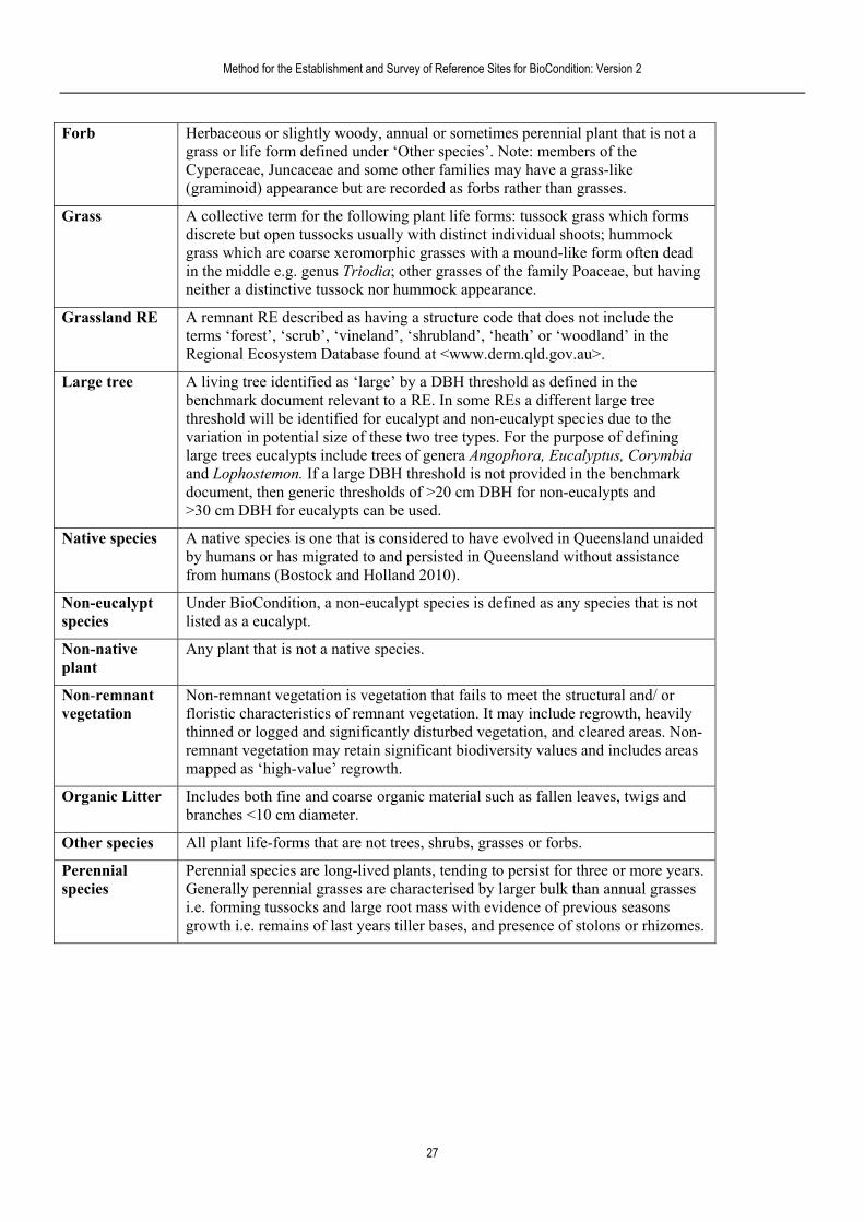
Forb rennial plant that is not a members of the
rass-like grasses.
Herbaceous or slightly woody, annual or sometimes pegrass or life form defined under ‘Other species’. Note:Cyperaceae, Juncaceae and some other families may have a g(graminoid) appearance but are recorded as forbs rather than
Grass ass which forms hummock
like form often dead Poaceae, but having
A collective term for the following plant life forms: tussock grdiscrete but open tussocks usually with distinct individual shoots; grass which are coarse xeromorphic grasses with a mound-in the middle e.g. genus Triodia; other grasses of the familyneither a distinctive tussock nor hummock appearance.
Grassland RE t does not include the woodland’ in the
.au>.
A remnant RE described as having a structure code thaterms ‘forest’, ‘scrub’, ‘vineland’, ‘shrubland’, ‘heath’ or ‘Regional Ecosystem Database found at <www.derm.qld.gov
Large tree ed in the ent large tree
se of defining yptus, Corymbia
H threshold is not provided in the benchmark calypts and
A living tree identified as ‘large’ by a DBH threshold as definbenchmark document relevant to a RE. In some REs a differthreshold will be identified for eucalypt and non-eucalypt species due to the variation in potential size of these two tree types. For the purpolarge trees eucalypts include trees of genera Angophora, Eucaland Lophostemon. If a large DBdocument, then generic thresholds of >20 cm DBH for non-eu>30 cm DBH for eucalypts can be used.
Native specie is considered to have evolved in Queensland unaided by humans or has migrated to and persisted in Queensland without assistance
s A native species is one that
from humans (Bostock and Holland 2010).
Non-eucalyptspecies
es that is not Under BioCondition, a non-eucalypt species is defined as any specilisted as a eucalypt.
Non-native plant
Any plant that is not a native species.
Non-remnanion
to meet the structural and/ or growth, heavily
leared areas. Non-es and includes areas
t Non-remnant vegetation is vegetation that fails vegetat floristic characteristics of remnant vegetation. It may include re
thinned or logged and significantly disturbed vegetation, and cremnant vegetation may retain significant biodiversity valumapped as ‘high-value’ regrowth.
Organic Litter Includes both fine and coarse organic material such as fallen leaves, twigs and branches <10 cm diameter.
Other species All plant life-forms that are not trees, shrubs, grasses or forbs.
Perennial species
Perennial species are long-lived plants, tending to persist for three or more years. Generally perennial grasses are characterised by larger bulk than annual grasses i.e. forming tussocks and large root mass with evidence of previous seasons growth i.e. remains of last years tiller bases, and presence of stolons or rhizomes.
27

Method for the Establishment and Survey of Reference Sites for BioCondition: Version 2
Reference Sit n 'Functional ' e. As not all RE’s will
are meant to On Offer ' for that RE in that area. Data obtained from
of the attributes
e An area that represents an example of a Regional Ecosystem iCondition, i.e. in a relatively undisturbed and mature stathave examples of totally undisturbed states, sites of this kindrepresent the 'BestReference sites will be used to establish benchmarks for each used within BioCondition.
Regional Ecosystem
(1999) as vegetation bioregion that are consistently associated with a particular
descriptions of tion Database at
Regional ecosystems were defined by Sattler and Williamscommunities in a combination of geology, landform and soil. For up to dateregional ecosystems go to the Regional Ecosystem Descrip<www.derm.qld.gov.au>.
(RE)
Remnant vegetation
ct 1999 as map showing
ered (or of concern e Vegetation
mnant vegetation is er than 70 per cent of
reater than 50 per cent of the cover relative to the undisturbed characteristic of the
gional ecosystem maps for most of m.qld.gov.au>.
s can be obtained the same website.
Remnant vegetation is defined in the Vegetation Management Avegetation shown on a regional ecosystem or remnant map. A remnant regional ecosystem is the same as a ‘remnant endangor not of concern) regional ecosystem map’ defined under thManagement Act 1999. Where there are no maps available, redefined as vegetation where the dominant canopy has greatthe height and gheight and cover of that stratum and dominated by speciesvegetation’s undisturbed canopy. Free reQueensland can be obtained from the DERM website <www.derIf RE maps are not available, then remnant vegetation mapfrom
Shrub Woody plant that is multi-stemmed from the base (or within 200 mm from ground level) or if single stemmed, less than 2 m tall.
Shrub canop yer (see y The estimation of the percentage canopy cover of the living shrub lacover Shrub).
Shrub canop anopy height in metres, as estimated for the shrub layer (see Shrub y The median cheight canopy cover).
Stratum A layer in a community produced by the occurrence at approximlevel (height) of an aggregation of plants of the same habit (B1952).
ately the same eadle and Costin
Tree Woody plants, more than 2 m tall with a single stem or branches well above the base.
Tree canopy cover
Refers to the estimation of the percentage canopy cover of the canopy tree layer
Tree canopy height
The median canopy height in metres, as estimated for the canopy tree layer (see Tree canopy cover).
28

Method for the Establishment and Survey of Reference Sites for BioCondition: Version 2
Appendix 1: Contacts for further information
ciences DERM
erbarium Brisbane Botanic Gardens
ong Q 4066
Ph. 07 3896 9834
st
d Ecological Sciences, DERM
isbane Botanic Gardens
Q 4066
Scientist
Biodiversity and Ecological Sciences, DERM
Queensland Herbarium Brisbane Botanic Gardens
Mt Coot-tha Road Toowong Q 4066
Ph. 07 3896 9322
Dr Teresa Eyre, Principal Ecologist
Biodiversity and Ecological S
Queensland H
Mt Coot-tha Road Toow
Annie Kelly, Senior Ecologi
Biodiversity an
Queensland Herbarium Br
Mt Coot-tha Road Toowong
Ph. 07 3896 9878
Dr John Neldner, Chief
29

Method for the Establishment and Survey of Reference Sites for BioCondition: Version 2
30
Appendix 2: Plant identification guides
) (2010). Collecting and Preserving Plant Specimens. Queensland Herbarium, Department of
Brisbane.
eds of Australia. Inkata Press,
Kleinig, D.A. and CSIRO, Australia.
um, Environmental
ide to Eucalyptus, Volume 3. Inkata Press, Sydney.
ersity of Queensland Press,
with corrections 1987).
ent of Primary
Robertson, New South
d.
6) Keys to Cyperaceae, Restionaceae and Juncaceae of Queensland. Queensland Botany Bulletin
, K.A.W. (1979) Native Plants of Queensland, Volume 1. Keith A.W. Williams, North Ipswich.
tive Plants of Queensland, Volume 2. Keith A.W. Williams, North Ipswich.
liams, North Ipswich.
Williams, K.A.W. (1999) Native Plants of Queensland, Volume 4. Keith A.W. Williams, North Ipswich.
Central Queensland
Anderson, E. (2003) Plants of central Queensland, their identification and uses. Department of Primary Industries, Queensland.
Pearson, S. and Pearson, A. (1991) Plants of Central Queensland. The society for Growing Australian Plants, Kangaroo Press, New South Wales.
Meltzer, R. and Plumb, J. (2005) Plants of Capricornia. Capricorn Conservation Council. Queensland.
General plant collecting guidelines
Bean, A.R. (editorEnvironment and Resource Management. www.derm.qld.gov.au
Queensland - general
Andrews, S.B. (1990) Ferns of Queensland. Queensland Department of Primary Industries,
Auld, B.A. and Medd, R.W. (1992) Weeds – An illustrated botanical guide to the weMelbourne, Sydney
Boland, D.J., Brooker, M.I.H., Chippendale, G.M., Hall, N., Hyland, B.P.M., Johnston, R.D., Turner, J.D. (1984) Forest Trees of Australia (Fourth edition revised and enlarged).
Bostock, P.D. and Holland, A.E. (2007) Census of the Queensland Flora. Queensland HerbariProtection Agency, Brisbane.
Brooker, M.I.H. and Kleinig, D.A. (1994) Field Gu
Hacker, J.B. (1990) A Guide to Herbaceous and Shrub Legumes of Queensland. UnivAustralia.
Jones, D.J. and Gray, B. (1988) Climbing Plants of Australia. Reed, Sydney.
Jones, D.J. (1988) Native Orchids of Australia. Reed, Sydney.
Kleinschmidt, H.E. and Johnson, R.W. (1979) Weeds of Queensland (ReprintedQueensland Department of Primary Industries, Brisbane.
Kleinschmidt, H.E., Holland, A. and Simpson, P. (1996)) Suburban Weeds (Third Edition). DepartmIndustries, Queensland.
Low, T. (1991) Wild Herbs of Australia and New Zealand (Revised Edition). Angus &Wales.
Pedley, L. (1987) Acacia in Queensland. Department of Primary Industries, Queenslan
Sharpe, P.R. (198No. 5, Department of Primary Industries, Queensland.
Williams
Williams, K.A.W. (1984) Na
Williams, K.A.W. (1987) Native Plants of Queensland, Volume 3. Keith A.W. Wil
Method for the Establishment and Survey of Reference Sites for BioCondition: Version 2
Southern Queensland
Cunningham, G.M., Mulham, W.E., Milthorpe, P.L. and Leigh, J.H. (1992) Plants of Western New South Wales. Inkata Press, Melbourne, Sydney.
Henry, D.R., Hall, T.J., Jordan, D.J., Milson, J., Schefe, C.M. and Silcock, R.G. (1995) Pasture Plants of Southern
illa, Queensland.
ardens, Sydney.
ardens, Sydney.
ora of New South Wales Volume 3. Royal Botanic Gardens, Sydney.
) Flora of New South Wales Volume 4. Royal Botanic Gardens, Sydney.
Tropical Grassland Society of
South-eastern Australia. Inkata Press, Sydney.
guide to their
field guide to their South Wales.
d Wildflowers of the Parks Association Inc., Noosa Heads.
nsland.
restry Districts. Queensland Forest Service, Brisbane.
ensland Vol. 1. Queensland Department of Primary ane.
d Vol. 2. Queensland Department of Primary
sland Department of Primary
Queensland
Brock, J. (1993) Native Plants of Northern Australia. Reed, Sydney.
Clarkson, J. (2009) A Field Guide to the Eucalypts of the Cape York Peninsula Bioregion. Queensland Government.
Hyland, B.P.M. and Whiffin, T. (1993) Australian Tropical Rain Forest Trees. CSIRO, Australia.
Smith, N.M. (2002) Weeds of the Wet/Dry Tropics of Australia. A Field Guide. Environment Centre NT Inc., Darwin.
Wheeler, J.R., Rye, B.C., Kock, B.L. and Wilson, A.J.G. (1992) Flora of the Kimberley Region. Department of Conservation and Land Management, Western Australia.
Inland Queensland. Department of Primary Industries, Queensland.
Lithgow, G. (1997) 60 Wattles of the Chinchilla and Murilla Shires. Chinch
Harden, G.J. (1990) Flora of New South Wales Volume 1. Royal Botanic G
Harden, G.J. (1991) Flora of New South Wales Volume 2. Royal Botanic G
Harden, G.J. (1992) Fl
Harden, G.J. (1993
Tothill, J.C. and Hacker, J.B. (1996) The Grasses of Southern Queensland, TheAustralian Inc. Queensland.
Southeast Queensland
Floyd, A.G. (1989) Rainforest Trees of Mainland
Harden, G.J., McDonald, W.J.F. and Williams, J.B. (2007) Rainforest Climbing Plants a field identification. Gwen Harden Publishing, New South Wales.
Harden, G.J., McDonald, W.J.F. and Williams, J.B. (2006) Rainforest Trees and Shrubs a identification. Gwen Harden Publishing, New
Harrold, A. (1994) Wildflowers of the Noosa – Cooloola Area. A Introduction to the Trees anWallum, Noosa
Haslam, S. (2004) Noosa’s Native Plants. Noosa Integrated Catchment Association Inc. Quee
Podberscek M. (1991) Field guide to the Eucalypts of the Gympie, Imbil and Maryborough FoTechnical Paper.
Stanley T.D. and Ross E.M. (1983) Flora of south-eastern QueIndustries, Brisb
Stanley T.D. and Ross E.M. (1986) Flora of south-eastern QueenslanIndustries, Brisbane.
Stanley T.D. and Ross E.M. (1989) Flora of south-eastern Queensland Vol. 3. QueenIndustries, Brisbane.
Tame, T. (1992) Acacias of Southeast Australia. Kangaroo Press, Kenthurst.
North
Beasley, J. (2009) Plants of Cape York. The Compact Guide. John Beasley, Cairns.
31

Method for the Establishment and Survey of Reference Sites for BioCondition: Version 2
North West Queensland
Barr, S. (1999) Plants of the Outback. A Field Guide to the Native Plants around Mount Isa. SafetyEnvironment Department, Mount Isa Mines Limited.
, Heal and
ts of North-West Queensland. Department of Primary Industries, Queensland.
stries, Queensland.
West Queensland
dney.
entification in the Arid Zone. Department of Primary Industries, Queensland.
Santos (2003) Field Guide to the common plants of the Cooper Basin (South Australia and Queensland). Santos Ltd. Adelaide, South Australia.
Santos (2007) Field Guide to Trees and Shrubs of Eastern Queensland Oil and Gas Fields. Santos Ltd. Adelaide, South Australia.
Milson, J. (2000) Pasture Plan
Milson, J. (2000) Trees and Shrubs of North-West Queensland. Department of Primary Indu
West and South
Alexander, R. (2005) A field guide to the plants of the channel Country Western Queensland. Channel Landcare Group, Queensland.
Jessop, J. (1981) Flora of Central Australia. The Australian Systematic Botany Society, Reed, Sy
Milson, J. (1995) Plant Id
Moore, P. (2005) A Guide to Plants of Inland Australia. Reed, Sydney.
32

Method for the Establishment and Survey of Reference Sites for BioCondition: Version 2
Appendix 3: Using GIS to search for reference sites Consulting local experts can be the best way to locate suitable Best On Offer (BOO) exampare interested in. The Queensland Herbarium
les of the RE that you ou are working in can
nt, Queensland Parks and conomic Development
condition.
le sites. Data can be -mail to
ional Ecosystem page).
le vegetation ons containing a
der to increase your chances of finding larger patches of your RE of interest it can be useful to make a selection of those polygons that are dominated (>50
community maybe so small that it is worth investigating polygons where the RE is present in less than 50 per cent of the polygon (Sub-
Box 4 and Figure 6).
8 staff who undertook the mapping in the area ybe a useful starting point. Local Department of Environment and Resource ManagemeWildlife Service, Natural Resource Management groups or Department of Employment, Eand Innovation and Employment officers can have also have local knowledge of REs in BOO
Knowing the extent of the RE of interest can also be a useful tool in the location of suitabobtained9 on the Queensland Government Information Service website or by sending an e<[email protected]> (Information on the DERM website on the Reg
Vegetation mapping often uses the concept of mosaics where because of scale restraints, a singpolygon is classed as being a mix of several different vegetation types (and thus REs). Polygmixture of vegetation types are known as heterogeneous polygons. In or
per cent) by the RE of interest. In the case of some RE's however the remaining extent of that
Dominant), in order to find patches of the RE for assessment (e.g.
Box 4 Method for mapping the extent of a Regional Ecosystem where the proportion of the polygon is dominant or sub-dominant.
Using ESRI's GIS software ArcGIS use the 'Selection' drop down menu and 'select by attributes';
For a selection where the RE of interest is Dominant (>50% of polygon of RE of interest) e.g. ("RE1" = '12.5.13' AND "PC1" >= 50) OR ("RE2" = '12.5.13' AND "PC2" >= 50)
Or Sub-Dominant (50% of polygon of RE of interest) e.g. ("RE1" = '12.5.13' AND "PC1" < 50) OR ("RE2" = '12.5.13' AND "PC2" < 50) OR ("RE3" = '12.5.13') OR ("RE4" = '12.5.13') OR ("RE5" = '12.5.13').
8 Queensland Herbarium Brisbane Botanic Gardens
Mt Coot-tha Road Toowong Q 4066 Tel: (07) 3896 9326 9 Charges may apply
33

Method for the Establishment and Survey of Reference Sites for BioCondition: Version 2
Figure 6: Mapped example showing the extent of RE 12.5.6, where it is the dominant RE in a polygon and where it is sub-dominant within a local area.
34
Method for the Establishment and Survey of Reference Sites for BioCondition: Version 2
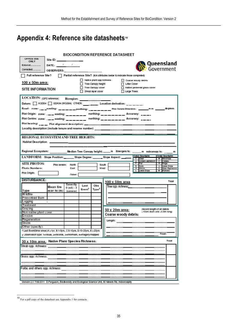
Appendix 4: Reference site datasheets10
10
For a pdf copy of the datasheet see Appendix 1 for contacts.
35

Method for the Establishment and Survey of Reference Sites for BioCondition: Version 2
36

Method for the Establishment and Survey of Reference Sites for BioCondition: Version 2
Appendix 5: Taking Photos (Adapted from Land Manager’s Monitoring Guide Photopoint Monitoring, and Land ManaRural Leasehold Land Self-Assessment Guideline <www.derm.qld.gov.au> and BioCondi
Taking photographs of site features from a fixed point is a great way to keep a permanent visua
37
gement Agreement - tion v 1.6.)
l record of how
mparison to our memories which aren’t nk.
a one square metre locate the same spot
d cover, organic litter and plant species for a standard sized area. Commonly there is great variety in ground cover at any given site, so taking more spot photos will help record this variation. It is important to have a system that allows you to take the spot photos in the same place each time you do an assessment. For example, spot photos could be taken along the transect line where you are doing your ground and litter cover assessments (i.e. 35, 45, 55, 65 and 75 metres).
attributes have changed over time. Photographs can be the most reliable and useful record collected in any monitoring program, as they best represent how things were over time, in coas reliable as we thi
Two photo types are recommended to be taken at each site, each time you do an assessment.
1. The Spot photo
This is a photo taken from head height looking nearly vertically down on a spot marked with frame or quadrat, as shown in Figure 7. You can use the base of your plot centre marker, to reeach time you visit. Spot photos provide a detailed picture of the groun
Figure 7: Taking the spot photo – try and keep the top of your feet out of the frame and angle the camera possible
2. The Landscape photo
The landscape photos are taken of features in the intermediate distance or further to provide anentire site and its surrounds. They illustrate the general condition of the site, showing changes ground layers over time. These site specific landscap
down as straight as
overview of the in tree, shrub and
e photos can also be used to record particular disturbance events such as flood levels and damage or the impacts of a bushfire.
The landscape photo is taken from the plot centre and the origin of the 100m centre line, holding your camera so that the image is taken with a ‘landscape’ perspective – that is where the picture is wider than it is high. Stand next to the plot centre marker (Figure 8), facing south (recommended direction – see ‘photo tips’), and position the horizon so it cuts the photo frame in half (half above the horizon and half below). Then take the photo focusing on infinity. Recording how the photo was lined up or simply taking a copy of the picture with you on future visits will make lining up the shot easier. Alternatively and preferentially, taking a series of plot centre landscape photos in a north, south, east and west direction (with the aid of a compass), allows you to pick up more of the variation across the site and is easy to replicate next time an assessment is done.
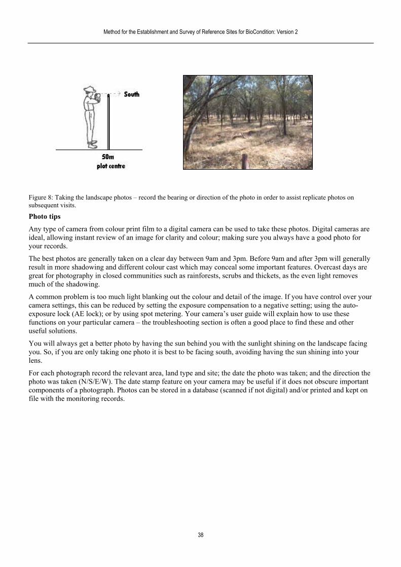
Method for the Establishment and Survey of Reference Sites for BioCondition: Version 2
replicate photos on sits.
tos. Digital cameras are ant review of an image for clarity and colour; making sure you always have a good photo for
d after 3pm will generally tures. Overcast days are
tography in closed communities such as rainforests, scrubs and thickets, as the even light removes
ommon problem is too much light blanking out the colour and detail of the image. If you have control over your ; using the auto-
w to use these these and other
You will always get a better photo by having the sun behind you with the sunlight shining on the landscape facing you. So, if you are only taking one photo it is best to be facing south, avoiding having the sun shining into your lens.
For each photograph record the relevant area, land type and site; the date the photo was taken; and the direction the photo was taken (N/S/E/W). The date stamp feature on your camera may be useful if it does not obscure important components of a photograph. Photos can be stored in a database (scanned if not digital) and/or printed and kept on file with the monitoring records.
Figure 8: Taking the landscape photos – record the bearing or direction of the photo in order to assistsubsequent vi
Photo tips
Any type of camera from colour print film to a digital camera can be used to take these phoideal, allowing instyour records.
The best photos are generally taken on a clear day between 9am and 3pm. Before 9am anresult in more shadowing and different colour cast which may conceal some important feagreat for phomuch of the shadowing.
A ccamera settings, this can be reduced by setting the exposure compensation to a negative settingexposure lock (AE lock); or by using spot metering. Your camera’s user guide will explain hofunctions on your particular camera – the troubleshooting section is often a good place to finduseful solutions.
38
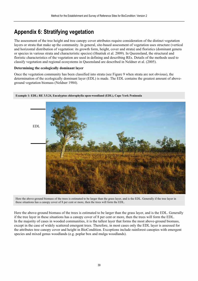
Method for the Establishment and Survey of Reference Sites for BioCondition: Version 2
Appendix 6: Stratifying vegetation The assessment of the tree height and tree canopy cover attributes require consideration of thelayers or strata that make up the community. In general, site-based assessment of vegetationand horizontal distribution of vegetation: its growth form, height, cover and strata) and florisor species in various strata and characteristic species) (Hnatiuk et al. 2009). In Q
distinct vegetation uses structure (vertical tics (dominant genera
ueensland, the structural and n are used in defining and describing REs. Details of the methods used to
(2005).
inant layer
Once the vegetation community has been classified into strata (see Figure 9 when strata are not obvious), the L contains the greatest amount of above-
ground vegetation biomass (Neldner 1984).
floristic characteristics of the vegetatioclassify vegetation and regional ecosystems in Queensland are described in Neldner et al.
Determining the ecologically dom
determination of the ecologically dominant layer (EDL) is made. The ED
Example 1: EDL; RE 3.5.24, Eucalyptus chlorophylla open-woodland (EDL), Cape York Peninsula
EDL
Here the above-ground biomass of the trees is estimated to be larger than the grass layer, and is the EDL. Generally if the tree layer in these situations has a canopy cover of 8 per cent or more, then the trees will form the EDL.
Here the above-ground biomass of the trees is estimated to be larger than the grass layer, and is the EDL. Generally if the tree layer in these situations has a canopy cover of 8 per cent or more, then the trees will form the EDL. In the majority of cases in wooded communities, it is the tallest layer that forms the most above-ground biomass, except in the case of widely scattered emergent trees. Therefore, in most cases only the EDL layer is assessed for the attributes tree canopy cover and height in BioCondition. Exceptions include rainforest canopies with emergent species and mixed genus woodlands (e.g. poplar box and mulga woodlands).
39
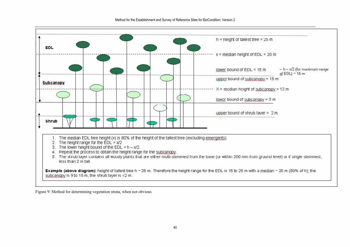
Method for the Establishment and Survey of Reference Sites for BioCondition: Version 2
40
Figure 9: Method for determining vegetation strata, when not obvious
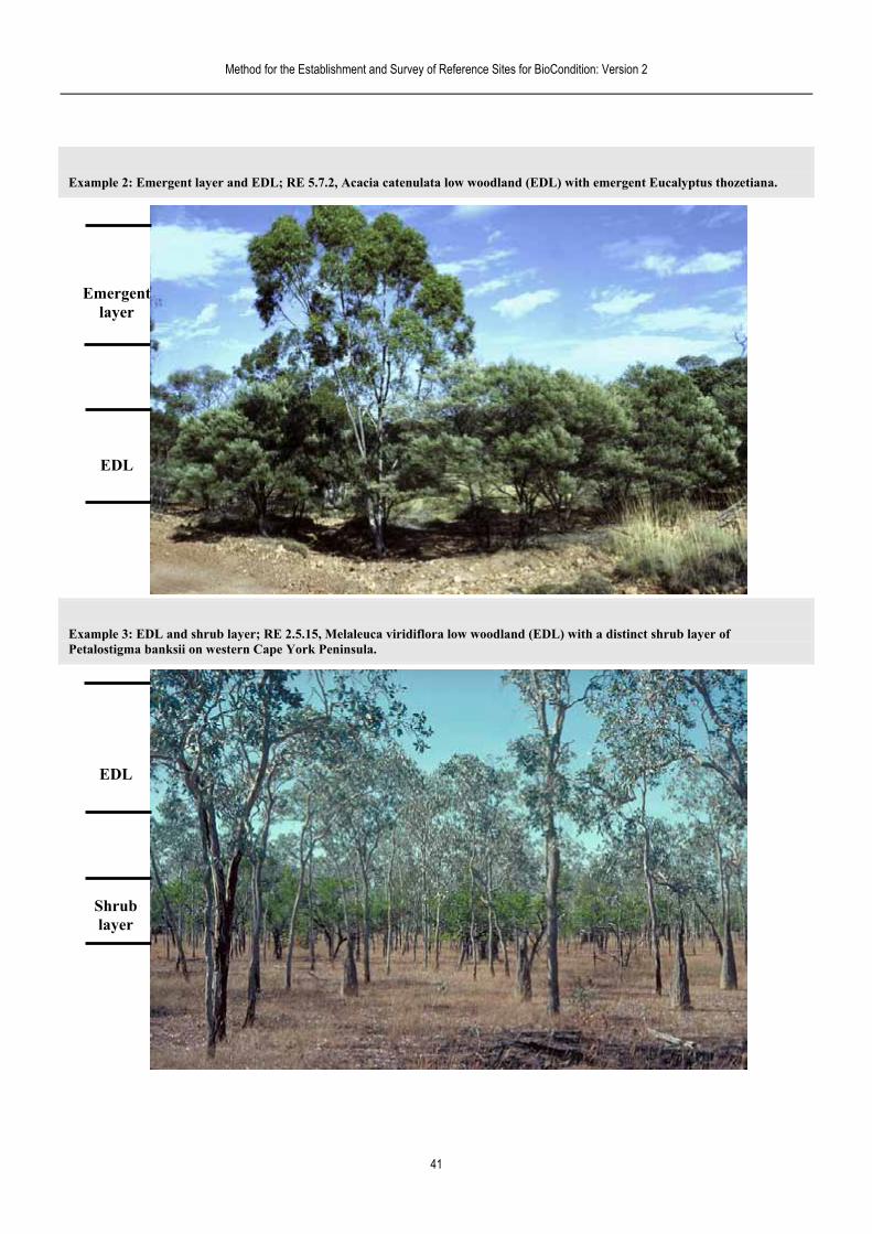
Method for the Establishment and Survey of Reference Sites for BioCondition: Version 2
Example 2: Emergent layer and EDL; RE 5.7.2, Acacia catenulata low woodland (EDL) with emergent Eucalyptus thozetiana.
Emergent layer
EDL
Example 3: EDL and shrub layer; RE 2.5.15, Melaleuca viridiflora low woodland (EDL) with a distinct shrub layer of P gma banksii on western Cape York Peninsula. etalosti
EDL
Shrub layer
41
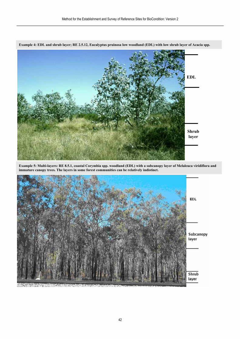
Method for the Establishment and Survey of Reference Sites for BioCondition: Version 2
Example 4: EDL and shrub layer; RE 2.5.12, Eucalyptus pruinosa low woodland (EDL) with low shrub layer of Acacia spp.
EDL
Shrub layer
Example 5: Multi-layers: RE 8.5.1, coastal Corymbia spp. woodland (EDL) with a subcanopy layer of Melaleuca viridiflora and immature canopy trees. The layers in some forest communities can be relatively indistinct.
42

Method for the Establishment and Survey of Reference Sites for BioCondition: Version 2
The impact of disturbance on vegetation structure
While in an undisturbed state, a vegetation community will develop a distinct structure (hethe growth forms of the species present and their abundance. Frequently different species definedifferent layers. However, within an ecosystem the structural attributes (height and cover) will frequentldepending on the environmental conditions at the site (e.g. rainfall and soil depth). Where thnatural (e.g. cyclones, fires or floods) or human disturbance (e.g. clearing or logging), the the vegetation can be significantly altered. At these sites, the development of distinct layers indefinite, and the resultant communities may develop a number of structural outcomes (see situations, it is important to compare the heights and canopy covers of the vegetation atlayers in the benchmark documents. For example, in the RE 6.5.3 Eucalyptus populnea prdistinct but discontinuous canopy (10 - 20 m tall). A lower tree layer (subcanopy) of Acacia
ight and cover) based on and dominate
y vary ere has been significant
structure and floristics of may not occur or be below). In these
the site to the defined edominates forming a
aneura is sometimes present. After disturbance, at least three structures may develop (1) E. populnea woodland with little or no subcanopy, (2) A. aneura woodland with none or only scattered E. populnea emergents, or (3) regenerating woodland of both species. In each structural type it is important to compare the heights and covers of both E. populnea and A. aneura with the layers they dominate in the benchmark site.
RE 6.5.3: Eucalyptus populnea predominates forming a distinct but discontinuous canopy (10 – 20 tall) (EDL). A subcanopy of Acacia aneura is sometimes present.
43
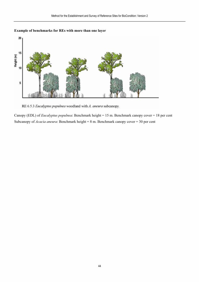
Method for the Establishment and Survey of Reference Sites for BioCondition: Version 2
Example of benchmarks for REs with more than one layer
Canopy (EDL) of Eucalyptus populnea: Benchmark height = 15 m. Benchmark canopy cover = 18 per cent
Subcanopy of Acacia aneura: Benchmark height = 8 m. Benchmark canopy cover = 30 per cent
44
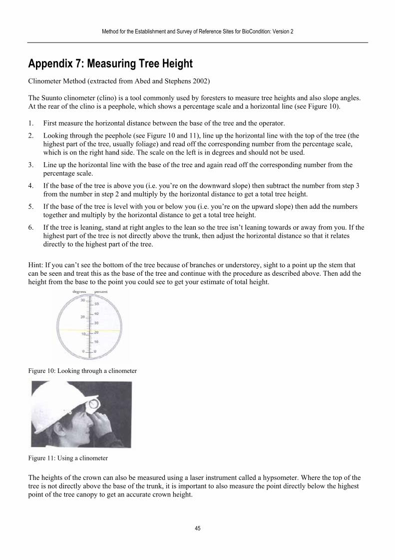
Method for the Establishment and Survey of Reference Sites for BioCondition: Version 2
Appendix 7: Measuring Tree Height
easure tree heights and also slope angles. d a horizontal line (see Figure 10).
the top of the tree (the f the tree, usually foliage) and read off the corresponding number from the percentage scale,
.
corresponding number from the
. umber from step 3 ight.
5. or below you (i.e. you’re on the upward slope) then add the numbers
way from you. If the ust the horizontal distance so that it relates
directly to the highest part of the tree.
Hint: If you can’t see the bottom of the tree because of branches or understorey, sight to a point up the stem that can be seen and treat this as the base of the tree and continue with the procedure as described above. Then add the height from the base to the point you could see to get your estimate of total height.
Clinometer Method (extracted from Abed and Stephens 2002) The Suunto clinometer (clino) is a tool commonly used by foresters to mAt the rear of the clino is a peephole, which shows a percentage scale an 1. First measure the horizontal distance between the base of the tree and the operator.
2. Looking through the peephole (see Figure 10 and 11), line up the horizontal line with highest part owhich is on the right hand side. The scale on the left is in degrees and should not be used
3. Line up the horizontal line with the base of the tree and again read off thepercentage scale.
4 If the base of the tree is above you (i.e. you’re on the downward slope) then subtract the nfrom the number in step 2 and multiply by the horizontal distance to get a total tree he
If the base of the tree is level with you together and multiply by the horizontal distance to get a total tree height.
6. If the tree is leaning, stand at right angles to the lean so the tree isn’t leaning towards or ahighest part of the tree is not directly above the trunk, then adj
Figure 10: Looking through a clinometer
Figure 11: Using a clinometer
The heights of the crown can also be measured using a laser instrument called a hypsometer. Where the top of the tree is not directly above the base of the trunk, it is important to also measure the point directly below the highest point of the tree canopy to get an accurate crown height.
45
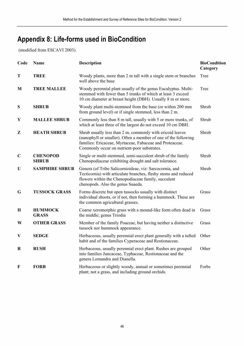
Method for the Establishment and Survey of Reference Sites for BioCondition: Version 2
46
forms used in BioCondition ESCAVI
BioCondition Category
le Tree
MALLEE uc s. Multi-hich at least 3 exceed
lly r more.
Tree
200 mm h .
Shrub
Y MALLEE SHRU h 5 or more trunks, of st do not exceed 10 cm DBH.
Shrub
Z HEATH SHRUB y with ericoid leaves of one following
P eae. rates.
Shrub
family l .
Shrub
U SAMPHIRE SH icornioideae, viz: Sarcocornia, and e reduced
the Chenopodiaceae family, succulent
Shrub
GRASS Grass
H HUMMOCK GRASS
like form often dead in riodia
Grass
ER GRASS eit istinctive e.
Grass
V SEDGE Herbaceous, usually perennial erect plant generally with a tufted habit and of the families Cyperaceae and Restionaceae.
Other
R RUSH Herbaceous, usually perennial erect plant. Rushes are grouped into families Juncaceae, Typhaceae, Restionaceae and the genera Lomandra and Dianella.
Other
F FORB Herbaceous or slightly woody, annual or sometimes perennial plant; not a grass, and including ground orchids.
Forbs
Appendix 8: Life- (modified from 2003).
Code Name Description
T TREE Woody plants, more than 2 m tall with a singwell above the base
stem or branches
M TREE Woody perennial plant usually of the genus Estemmed with fewer than 5 trunks of w
alyptu
10 cm diameter at breast height (DBH). Usua 8 m o
S SHRUB Woody plant multi-stemmed from the base (or within from ground level) or if single stemmed, less t
B Commonly less than 8 m tall, usually witwhich at least three of the large
an 2 m
Shrub usually less than 2 m, commonl(nanophyll or smaller). Often a memberfamilies: Ericaceae, Myrtaceae, Fabaceae andCommonly occur on nutrient-poor subst
of the roteac
C CHENOPOD SHRUB
Single or multi-stemmed, semi-succulent shrub of Chenopodiaceae exhibiting drought and salt to
RUB Genera (of Tribe Sal
the erance
Tecticornia) with articulate branches, fleshy stflowers within
ms and
chenopods. Also the genus Suaeda.
G TUSSOCK Forms discrete but open tussocks usually with distinct individual shoots, or if not, then forming a hummock. These are the common agricultural grasses.
Coarse xeromorphic grass with a mound-the middle; genus T
W OTH Member of the family Poaceae, but having ntussock nor hummock appearanc
her a d
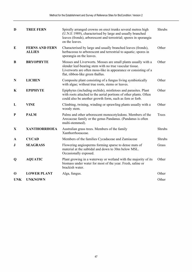
Method for the Establishment and Survey of Reference Sites for BioCondition: Version 2
D TREE FERN ral metres high y branched
spor porangia
Shrubs
E FERNS AND FE by large and usually branched leaves (fronds), u ores in
Other
B BRYOPHYTE orts. Mosses are small plants usually with a ular
n appearance or consisting of a
Other
N LICHEN ymbiotically s.
Other
K EPIPHYTE hytes (including orchids), mistletoes and parasites. Plant he ts. Often
fern or forb.
Other
prawling plants Other
tyledons. M s of the s. (Pand s often
Trees
X XANTHORRHO rass trees. Members of the family Shrubs
A CYCAD ers of the families Cycadaceae and Zamiaceae Shrubs
ering angiosperms forming sparse to dense mats of material at the subtidal and down to 30m below MSL. Occasionally exposed.
Grass
Q AQUATIC Plant growing in a waterway or wetland with the majority of its biomass under water for most of the year. Fresh, saline or brackish water.
Other
O LOWER PLANT Alga, fungus. Other
UNK UNKNOWN Other
Spirally arranged crowns on erect trunks seve(U.N.E 1989), characterised by large and usuallleaves (fronds), arborescent and terrestrial; on the leaves.
RN Characterised
es in s
ALLIES herbaceous to arborescent and terrestrial to aqsporangia on the leaves.
Mosses and Liverw
atic; sp
slender leaf-bearing stem with no true vascLiverworts are often moss-like i
tissue.
flat, ribbon-like green thallus.
Composite plant consisting of a fungus living swith algae; without true roots, stems or leave
Epipwith roots attached to the aerial portions of otcould also be another growth form, such as
r plan
L VINE Climbing, twining, winding or swoody stem.
usually with a
P PALM Palms and other arborescent monoco emberArecaceae family or the genus Pandanumulti-stemmed).
EA Australian g
anus i
Xanthorrhoeaceae.
Memb
J SEAGRASS Flow
47
Related Documents