LAPPEENRANTA UNIVERSITY OF TECHNOLOGY LUT School of Business and Management Industrial Engineering and Management Supply Chain and Operations Management Method selection for demand forecasting Master of Science Thesis Samuli Vaskinen Examiner: Professor Janne Huiskonen Supervisor: M. Eng. Virpi Tikkala 2017

Welcome message from author
This document is posted to help you gain knowledge. Please leave a comment to let me know what you think about it! Share it to your friends and learn new things together.
Transcript

LAPPEENRANTA UNIVERSITY OF TECHNOLOGY
LUT School of Business and Management
Industrial Engineering and Management
Supply Chain and Operations Management
Method selection for demand forecasting
Master of Science Thesis
Samuli Vaskinen
Examiner: Professor Janne Huiskonen
Supervisor: M. Eng. Virpi Tikkala 2017
ABSTRACT
Author: Samuli Vaskinen
Thesis topic: Method selection for demand forecasting
Year: 2017 Place: Hyvinkää
Master’s thesis. Lappeenranta University of Technology, Industrial Engineering
and Management, Supply Chain and Operations Management.
74 pages, 21 figures, 7 tables and 1 appendix
Examiner: professor Janne Huiskonen
Keywords: supply chain, forecasting, forecasting models, method selection,
quantitative forecasting
The purpose of this master’s thesis was to find a systematic way for choosing the
optimal forecasting scheme and to use this method to increase accuracy of
material level demand forecasts in Konecranes.
This thesis is based on literature and earlier research of the topic which is used to
determine a forecast method selection framework. The framework is then used to
find out the optimal forecasting scheme for demand forecasting in two
manufacturing plants. Actual demand data was pulled from SAP and Microsoft
Excel, R and RStudio were the tools used to generate forecasts and calculate
forecast accuracies.
The accuracy of proposed forecasting scheme is also compared to currently used
processes and steps to implement it in ERP are presented.

TIIVISTELMÄ
Tekijä: Samuli Vaskinen
Työn nimi: Metodin valinta kysynnän ennustamisessa
Vuosi: 2017 Paikka: Hyvinkää
Diplomityö. Lappeenrannan teknillinen yliopisto, Tuotantotalous,
Toimitusketjun johtaminen.
74 sivua, 21 kuvaa, 7 taulukkoa ja 1 liite
Tarkastaja: professori Janne Huiskonen
Hakusanat: toimitusketju, ennustaminen, ennustemallit, metodin valinta,
kvantitatiivinen ennustaminen
Tämän diplomityön tavoitteena oli löytää systemaattinen tapa optimaalisen
ennustemallin tai -mallien valintaan ja soveltaa tätä materiaalitason
kysyntäennusteiden tarkkuuden parantamiseen Konecranesillä.
Työ pohjautuu kirjallisuuteen ja aihealueen aiempiin tutkimuksiin, joiden
pohjalta valitun ennustemallin valintametodin avulla kehitettiin optimaalinen
ennustemallien yhdistelmä kahden tuotantolaitoksen kysynnän ennustamiseen.
Kysyntädata kerättiin SAP:sta ja työkaluina ennusteiden generoinnissa ja
ennustetarkkuuksien laskennassa olivat Microsoft Excel, R ja RStudio.
Lopulta luotua ennustemallien yhdistelmää verrattiin yrityksen nykyisin
käyttämiin malleihin ja esitettiin miten se olisi mahdollista ottaa käyttöön ERP-
järjestelmässä.

PREFACE
It has been a long journey to this point in my life, when I am finally about to
graduate. Writing this master’s thesis (as well as my studies as a whole with the
mechanical engineering detour) have taken longer than probably anyone
anticipated.
I wish to thank Konecranes for giving me this opportunity to write my thesis about
an interesting topic and everyone who has contributed to or supported this work in
any way. Especially I want to express my sincere gratitude to Virpi Tikkala and
professor Janne Huiskonen for your invaluable advice and comments while
working on this project as well as all the nudges to keep me writing when I needed
them.
I also want to thank my family and friends for all the support over the years.
Couldn’t have done this without you.
Samuli Vaskinen
Hyvinkää 2017
5
TABLE OF CONTENTS
ABSTRACT ............................................................................................................ 2
TIIVISTELMÄ ........................................................................................................ 3
PREFACE ................................................................................................................ 4
ABBREVIATIONS AND SYMBOLS ................................................................... 7
1 INTRODUCTION ........................................................................................... 9
1.1 Background ............................................................................................... 9
1.2 Research objective and scope ................................................................. 11
1.3 Research methods and structure .............................................................. 12
2 FORECASTING IN SUPPLY CHAIN MANAGEMENT ........................... 13
2.1 Push and pull methods in supply chain management ............................. 15
2.2 Benefits of forecasting ............................................................................ 16
2.3 Demand patterns ..................................................................................... 18
2.4 Dimensions of forecasting ...................................................................... 21
3 FORECASTING METHODS AND METHOD SELECTION ..................... 25
3.1 Qualitative forecasting methods.............................................................. 25
3.2 Quantitative forecasting methods ........................................................... 25
3.2.1 Naïve forecasting ............................................................................. 26
3.2.2 Simple moving average ................................................................... 27
3.2.3 Single exponential smoothing ......................................................... 27
3.2.4 Holt-Winters .................................................................................... 28
3.2.5 Box-Jenkins ..................................................................................... 29
3.2.6 Croston’s method ............................................................................. 30
3.2.7 Boylan-Syntetos ............................................................................... 30
3.3 Forecasting method selection framework ............................................... 31
6
3.4 Categorization of demand ....................................................................... 33
4 MEASURING FORECAST ACCURACY ................................................... 36
4.1 Scale-dependent error metrics ................................................................. 36
4.2 Percentage error metrics.......................................................................... 37
4.3 Relative error metrics .............................................................................. 37
4.4 Scale-free error metrics ........................................................................... 38
5 CASE COMPANY ........................................................................................ 40
5.1 Business areas of Konecranes ................................................................. 40
5.2 Mission, vision and values of Konecranes .............................................. 41
5.3 Markets in which Konecranes operates .................................................. 43
5.4 Products of Konecranes .......................................................................... 44
6 CURRENT FORECASTING PROCESSES IN KONECRANES ................ 46
6.1 Demand-supply balancing ...................................................................... 47
6.2 Statistical forecast ................................................................................... 48
7 COMPARISON OF TIME SERIES MODELS ............................................ 50
7.1 Sample data ............................................................................................. 50
7.2 Forecast accuracy metric selection ......................................................... 54
7.3 Finding the most suitable forecasting methods ....................................... 55
7.4 Accuracy of new scheme compared to current quantitative method ...... 60
7.5 Accuracy of new scheme compared to DSB process .............................. 63
7.6 Implementing new forecast solution ....................................................... 65
8 CONCLUSIONS ........................................................................................... 68
REFERENCES ...................................................................................................... 70
APPENDICES ....................................................................................................... 75

7
ABBREVIATIONS AND SYMBOLS
Abbreviations
AME Americas. One of three Konecranes’ geographical
regions.
APAC Asia-Pacific. One of three Konecranes’ geographical
regions.
BOM Bill of materials
DSB Demand supply balancing
EBIT Earnings before interest and taxes
EMEA Europe, Middle East and Africa. One of three
Konecranes’ geographical regions.
ERP Enterprise resource planning system which integrates
many business functions into one software solution
GMAE Geometric mean absolute error
GMRAE Geometric mean relative absolute error
HML Hämeenlinna
MAE Mean absolute error
MAPE Mean absolute percentage error
MASE Mean absolute scaled error
MdRAE Median relative absolute error
MSE Mean square error
SAP Enterprise resource planning system which integrates
majority of operations into one IT solution.
SCM Supply chain management
SES Single exponential smoothing
SMA Simple moving average
sMAPE Symmetric mean absolute percentage error
SKU Stock keeping unit
SPR Springfield
UoM Unit of measure
8
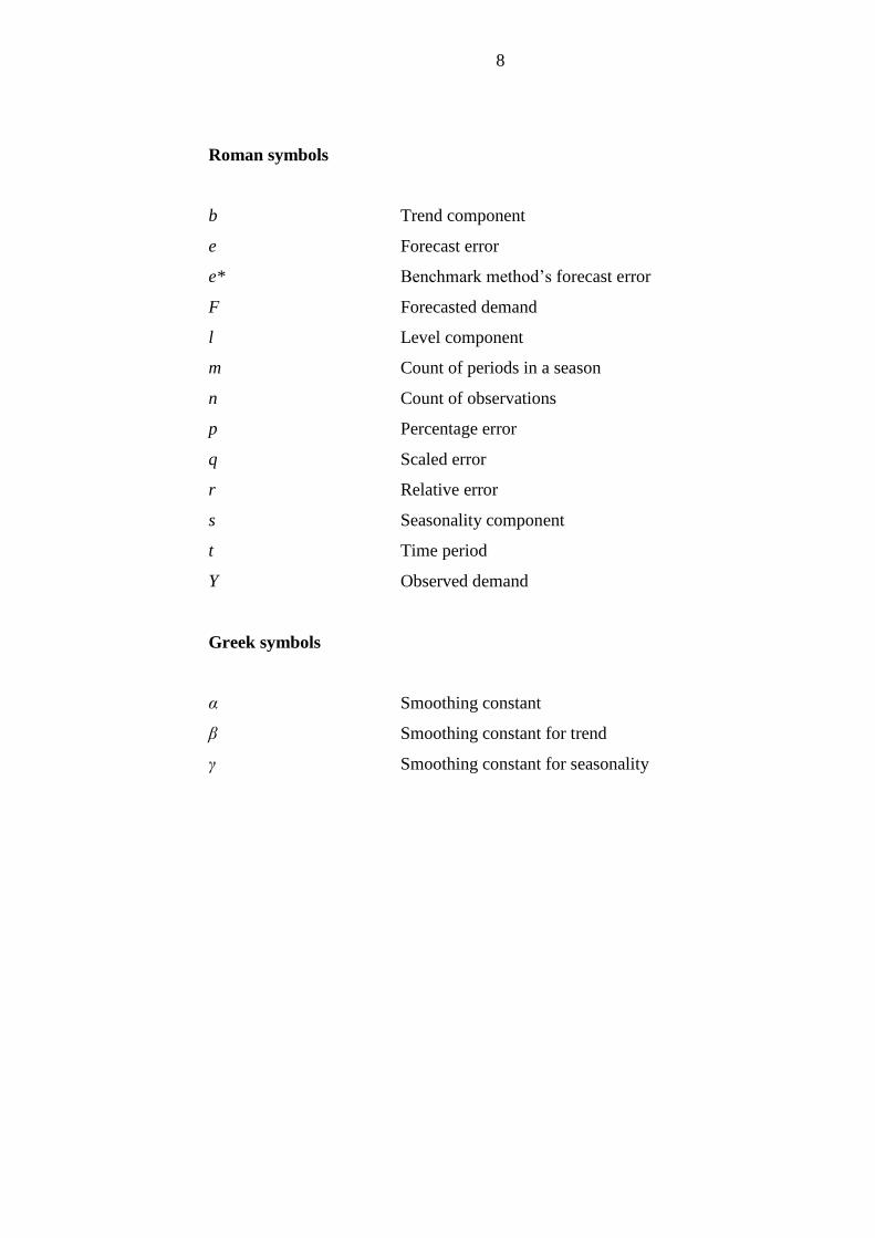
Roman symbols
b Trend component
e Forecast error
e* Benchmark method’s forecast error
F Forecasted demand
l Level component
m Count of periods in a season
n Count of observations
p Percentage error
q Scaled error
r Relative error
s Seasonality component
t Time period
Y Observed demand
Greek symbols
α Smoothing constant
β Smoothing constant for trend
γ Smoothing constant for seasonality
9
1 INTRODUCTION
Forecasting has been used to help decision making for almost as long as there have
been businesses. In short it means creating an estimate of future events that are at
least partially independent of the decisions the company makes. In the beginning
forecasting was mainly used as a managerial tool for budgeting and other high level
decisions but since then more and more detailed forecasts have been the focus of
research. Future demand is not usually known in advance and as a result production
planning and inventory management have to rely on forecasts to be able to fulfill
demand competitively.
1.1 Background
Globalization and other competition increasing developments in the markets during
the last decades has created a need to be able to offer goods to customers with
shorter lead times and with greater customization than before which has increased
the pressure to make operative decisions based on forecasts instead of waiting for
customer orders to start procurement of materials. Increasing forecast accuracy
naturally increases the quality of decisions which base on that forecast and creates
competitive advantage as it enables better utilization of resources and higher
customer satisfaction.
Even though forecasting offers many benefits it does not come without its
limitations. There is always some uncertainty in the future and it is impossible to
predict all events that will occur and affect future demand. When the time horizon
a forecast is created for is increased the accuracy of said forecast usually goes down.
Same can be said about the detail level of a forecast. For example, forecasting
demand on daily level is less accurate than on weekly level or forecasting demand
of material group is usually more accurate than forecasting demand of single
material.

10
Traditionally forecasting research has focused on development of forecasting
techniques especially on time series methods (Fildes & Goodwin, 2007). Time
series techniques aim to predict future demand based on actual past demand using
a set algorithm to statistically extrapolate the data set. Other methods which have
been studied include judgmental reviews of experts, market tests and surveys. Even
with multitude of sophisticated forecasting methods available surveys show that
simple methods are the most often utilized ones in real world scenarios (Tokle &
Krumwiede, 2006).
Fulfilling upcoming demand in an optimal manner which keeps inventory levels as
low as possible without causing stock outs increases the operational performance
in multiple ways. Higher inventory turnover rates lower the capital tied to
inventories and allows it to be utilized in a more profitable manner. Lower
inventories also mean lower inventory carrying costs which directly affects
company’s profits and with accurate forecasts the amount of stocked materials
becoming obsolete due to declining demand can be reduced. Naturally the effects
of these potential benefits become stronger with more accurate forecasts which
should make forecasting one of the cornerstones of inventory optimization
processes.
If forecasts are utilized to their fullest extent they do not benefit just the company
generating them but can also improve performance of whole supply chains. The
company which sells the final goods to end customers has the most information
available to forecast upcoming demand so they should be the one generating
forecasts and sharing their data with the rest of the supply chain. This way the
forecasts are based on real demand data instead of some form of consolidated
demand i.e. orders of bigger batches from component vendors some of which go to
inventories to wait for upcoming end customer needs.

11
1.2 Research objective and scope
This thesis aims to improve Konecranes’ forecasting process with the target of
increasing forecast accuracy in a cost-effective manner. Because the process should
be easily scalable to cover a wide scope of materials, quantitative methods which
are based on available past demand data are the main focus of the research as they
are less labor intensive than qualitative methods which rely on input from
personnel.
Demand forecasts are already used in Konecranes for two purposes. Internally they
are used to determine when material replenishments should be ordered. In practice
this means that reorder points are dynamic results of calculations based on safety
stock values, known upcoming consumption and forecasted demand over material
lead time and thus change as new forecasts are generated.
Information generated by forecasting future demand is also shared with some key
suppliers. By sharing material needs with vendors Konecranes allows them to
optimize their material flows by having better visibility to what Konecranes will be
ordering from them and when. In addition to being able to optimize material flows
the vendors can also utilize the information in their production planning, once again
improving performance. As more and more vendors are given access to the forecast
data it becomes even more valuable to improve forecasting accuracy as much as
possible.
As accurate forecasts offer multiple benefits and aforementioned methods to utilize
forecasts have already been developed and are being actively utilized, the main
objective of this research is on optimizing forecasting accuracy. This is achieved
through answering the following research questions:
• Could another quantitative forecasting method generate more accurate
forecasts than currently used model?
• How should a forecasting scheme be chosen?
12
1.3 Research methods and structure
Research done in this thesis can be divided into three phases. The first phase
consists of literature review about general forecasting theory and benefits, methods
and their classification as well as metrics used for measuring forecast accuracy.
Information in this phase has been gathered from scientific peer reviewed articles
and books which present best practices.
The second phase contains a case study in which multiple forecasts are generated
with the most potential methods. After generating the forecasts their accuracy is
measured to determine the most suitable forecasting scheme. Software solutions
utilized in this study were Microsoft Excel, R and RStudio.
Consumption used for this study is actual usage of materials as it has been saved
into company’s enterprise resource planning system, SAP. Data from 2015 was
used to generate forecast for 2016 consumption. Accuracy of this forecast is then
compared to actual consumption which happened in 2016. This phase also offers
suggestions on which system should be used in the future to have as accurate
forecasts as possible. Also, parameters which affect the outcome of forecasting
models available are considered and optimization possibilities are identified.
Phase three consists of comparison of accuracy between the new forecasting
scheme and current forecasting methods and presents the steps needed to take the
new scheme into use. Also conclusions and some further study possibilities are
considered.
13
2 FORECASTING IN SUPPLY CHAIN MANAGEMENT
There is not just one definition of supply chain but instead multiple descriptions can
be found in the literature with slightly different defining factors. Arnold, Chapman
and Clive (2008) define supply chain as all the processes and actions that are needed
in the production of goods and the delivery of said goods to the end customer.
According to their research, inclusion of recycling or disposal of goods at the end
of their life cycle is also becoming more common as part of the idea of supply chain
(Arnold et al., 2008). Christopher (2005) on the other hand sees supply chains as
networks of organizations which are linked together by either supplier or customer
relationship. All of these organizations are important in creating additional value to
the end customer through refining the end product or offering some service thus
impacting the success of produced goods (Christopher, 2005).
In the end, all of the definitions contain a group of companies, organizations or units
which cooperate to produce goods and bring them available to end customers and
in some cases even recycle or dispose of the goods when they are no longer needed
by the customer. Even a simple supply chain usually contains multiple raw material
suppliers, production facilities, distribution centers, retailers, customers and
logistics service providers. Usually large, globally operating companies have very
complex supply chains which might contain hundreds of organizations.
Members of supply chain can be either internal of external. For example, a company
that manufactures subassemblies in multiple production facilities and assembles
end products in some other facility sees the subassembly supplier as an internal
vendor when looking at the supply chain from the assembling units point of view.

14
Figure 1. A supply chain from one company’s point of view. (Kangas, 2008,
Adapted from Slack, Chambers & Johnston, 2001)
In figure 1 a supply chain is presented from one company’s point of view. All
supply chain members have their own customers and usually there are multiple
levels or tiers of suppliers and customers. (Slack et al., 2001) In this research focus
is on crane factories which for example purchase hoists from internal supplier
which would be considered first tier supplier. This internal supplier in turn
purchases a motor from external supplier which would be considered second tier
supplier from the crane factory’s point of view.
Supply chain management (SCM) is relatively new branch of science which
emerged in the 1950’s. Until that time companies and scientific research had
focused solely on a single entity and its competitive factors. Of course, suppliers
and customers had been observed also before that but the connections to potential
competitive advantages had not been identified nor pursued. With the advent of
supply chain management, the focus has partially shifted to the performance of
whole supply chains and how they can create advantages in competition against
other supply chains. (Fredenhall & Hill, 2001)
15
In practice optimizing the whole supply chain is a difficult task because individual
organizations often try to locally optimize their operations instead of taking the
whole supply chain into account. This leads to suboptimal supply chain
performance and uncoordinated actions which in turn the end customer sees as late
deliveries and increased prices as the cost structure used to produce goods is not as
good as it could be. In the long run, such problems often cause lost customers and
missed sales opportunities which negatively affect all the members of the supply
chain. (Yu, Yan & Cheng, 2001)
2.1 Push and pull methods in supply chain management
There are two approaches to initiating action in a supply chain, push and pull. The
traditional way to manage supply chains was the push method in which goods are
produced (or any other action starts) before an actual customer order has been
received. On markets with scarce competition and steady demand this method
yielded good results as it was able to keep goods available and fulfill customers’
demand for goods which were not customizable. (Christopher, 2007)
The other approach to handle demand in a supply chain is the pull method. The
actions happen reactively after the order has been received and the initial signal to
start production comes from the customer. The emphasis is on the customer and
their need of certain goods. As the competition on many industries has become
fiercer in the last decades and as a result products have become more customizable
and the risk of them becoming obsolete has risen, the pull method has become more
popular and widely applied. (Christopher, 2007)
In reality supply chains usually contain some processes which use the push method
and some processes which utilize the pull method. This combination is used to
counter the negative effects of pull method. In purely pull driven supply chain
delivery times to the customer would often be too long for company to remain
competitive so some of the most time consuming processes, which often have to do
with procurement or part of the production process, are push driven. Because the
16
actual demand is not known when the push processes are executed, they are based
on anticipated customer needs also known as forecasted demand. As the decisions
made in the push processes set constraints to the demand that can be fulfilled
without deviating from designed ways of working, it is valuable for companies to
have accurate forecasts. (Chopra & Meindl, 2007)
2.2 Benefits of forecasting
Forecasting is done on multiple levels in a typical large enterprise. Vollmann et al.
(2005) classify forecasts into strategic business planning, sales and operations
planning and master production scheduling and control based on their level of
detail. Strategic business planning provides data on a rough level to support
strategic decision making. Usually such forecast is done by judgmental methods for
example, expert opinions are used to determine how markets are going to develop,
although it is not unheard of to utilize economic growth models. Output of strategic
business planning is a forecast of total sales on an annual or quarter level with a
horizon of multiple years. The main use of these forecasts is to help management
in making better strategic decisions in high impact matters such as investing into
new production facilities to increase capacity or to enter or withdraw from certain
markets.
Sales and operations planning deals with more detailed questions than strategic
business planning. Forecasting is carried out on product family scope and on weekly
or monthly level and is used to balance sales with production capacity and in some
cases to minimize the costs to fulfill upcoming demand by optimizing production
planning and material replenishments. If the components of the end products are
not too variable, i.e. product is not customizable, raw material needs can also be
predicted based on the forecast generated for sales and operations planning and
material management can be done optimally. (Vollmann et al. 2005)
Master production scheduling and control is the finest level of forecasting
Vollmann et al. (2005) identify and it and it goes to daily or even hourly level. Main
17
usage of these forecasts is in production planning and controlling actual operations
in a facility.
Having accurate forecasts of future material consumption on a raw material level
allows organizations to better optimize their inventories. Naturally basing inventory
parameter calculations on the upcoming demand gives a better chance to be able to
cost-effectively fulfill that demand than basing calculations purely on what would
have been needed to fulfill the past demand, especially in situations when there has
been some shift in end customer’s needs or when a certain product is being replaced
by a new revision.
Even though some studies have questioned the tangible benefits gained from
sharing information of actual demand and forecasts there have been individual
success stories. The more information there is available between the supply chain
members the better the whole chain can operate and the negative effects of material
shortages or limitation in production capacity caused by bullwhip effect can be
mitigated. (Holweg et al., 2005)
However, utilizing available information is not always an easy task and just sharing
that information does not bring any benefits if it does not affect the operations in
any way. In simulation models external collaboration has been shown as a powerful
tool with multiple benefits, most notable of which are improved capacity utilization
and inventory turnover. In practice it has proved to be a much more difficult to
reach the improvements the shared demand visibility brings. The challenges in
utilizing this data usually relate to lack of knowledge or expertise in the area,
distrust into the shared data or contractual limitations. If there is no willingness to
utilize the data on both parties, the benefits will not realize. (Holweg, 2005)
A common problem with forecasting processes is that multiple functions in a
company need forecasts for their own needs and often generate those forecasts
within that business function. This phenomenon known as “island of analysis” leads
to unaligned forecasts and ultimately to unaligned plans between different
18
functions. This phenomenon can often be found in case studies and is caused by
lack of communication between different units. (Mentzer & Moon, 2005)
2.3 Demand patterns
Sometimes there are clearly identifiable characteristics in the past demand. Multiple
forecasting methods have been developed which take these characteristics into
account and at least in theory they should provide more accurate forecasts than
using simpler methods like simple moving average or single exponential
smoothing. However, just because some pattern has repeated in the past, does not
guarantee it to happen again in the future as situations in the market can change
drastically or market might get saturated. Pattern recognition is also used in some
approaches to forecast method selection, one of which is presented later in chapter
3.3.
Sometimes seasonal patterns can be identified in past demand as in figure 2 and it
is possible to utilize a forecasting model that takes seasonal changes in demand into
account to produce more accurate forecasts. For some products, seasonal changes
can be extremely influential and forecasting demand by more traditional methods
would not yield the wanted results. For example, ice cream consumption in Finland
varies highly with seasons because of the weather and how it affects customer
behavior.

19
Figure 2. Seasonal demand example.
In practice, there are two ways seasonality can be accounted for in forecasts:
additive and multiplicative. Which of these methods is more suitable is dependent
upon the situation and should be decided case by case. In cases where the amplitude
of seasonal increase or decrease is independent of the original level of demand
additive method should be used. More often the seasonal fluctuation is proportional
to the non-seasonal demand and multiplicative method leads to better results.
(Winters, 1960)
As with seasonal patterns it is possible to identify trends in demand and utilize that
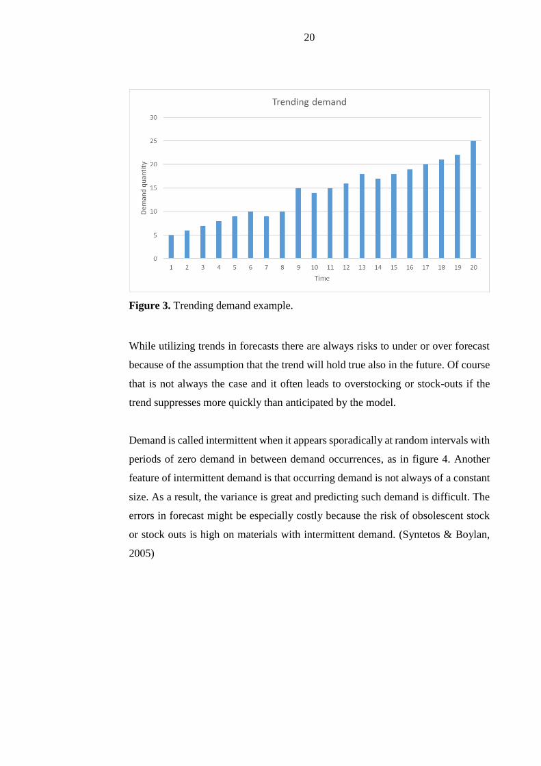
information while generating forecasts. Constantly increasing demand (figure 3),
for example during product ramp ups or with increasing market shares in times of
superior product offering, assuming that the demand keeps increasing and
modifying forecasts accordingly might increase forecast accuracy and reduce stock-
outs. Also for trending demand the forecast model can take the trend into account
in multiple ways. The decision on if the model should handle the trend as ratio,
additive or linear have to be done case by case as one method is not universally
better than the others. (Winters, 1960)
20
Figure 3. Trending demand example.
While utilizing trends in forecasts there are always risks to under or over forecast
because of the assumption that the trend will hold true also in the future. Of course
that is not always the case and it often leads to overstocking or stock-outs if the
trend suppresses more quickly than anticipated by the model.
Demand is called intermittent when it appears sporadically at random intervals with
periods of zero demand in between demand occurrences, as in figure 4. Another
feature of intermittent demand is that occurring demand is not always of a constant
size. As a result, the variance is great and predicting such demand is difficult. The
errors in forecast might be especially costly because the risk of obsolescent stock
or stock outs is high on materials with intermittent demand. (Syntetos & Boylan,
2005)

21
Figure 4. Intermittent demand example.
In practice, single exponential smoothing (SES) and simple moving average (SMA)
are used to forecast intermittent demand but creating methods specifically for
predicting such demand has been the focus of some research. Croston (1972)
presented the current standard for forecasting intermittent demand which is known
as Croston’s method. (Syntetos & Boylan, 2005)
2.4 Dimensions of forecasting
A framework for visualizing supply chain and potential dimensions used in
forecasting concept creation developed by Syntetos et al. (2016) is presented in
figure 5. Their framework has three dimensions: product, time and location. In
practice, all of these dimensions affect the detail level of generated forecasts and
require decision to be made that are independent of forecasting method selection.
Because these affect the detail level of forecasts, the values used for these
dimensions should be chosen based on how the forecast is planned to be utilized.

22
Figure 5. Supply chain structure: a framework. (Syntetos et al., 2016)
Actual demand is realized on order line level i.e. a customer or internal process
requires a certain quantity of particular stock keeping unit (SKU) at a certain time.
The data on this transactional level cannot be used for forecasting purposes and it
must be aggregated before further processing. How this aggregation happens, is
driven by the three dimensions. (Syntetos et al., 2016)
Product dimension determines if all SKUs are handled individually or if some of
these get grouped together. The most used aggregation options regarding products
are single SKUs, product families and all SKUs. As an example, single SKU
forecasts are needed for inventory management while for budgeting it is enough or
even preferable to have forecasts of all SKUs as a single value which contains
everything. Product family detail level is often used for capacity planning as
products from the same product family are often manufactured on the same
production line. (Syntetos et al., 2016)
23
The second dimension, time, deals with the period of time for which the demand is
aggregated into a single value. The usual options are day, week, month, quarter or
year. Selecting period for time aggregation is not usually as straightforward
decision as selecting product dimension. Even if the planned usage is clearly
defined there might be multiple time periods that would be good choices and the
optimal choice might even be one period for one SKU and another for some other
SKU. Especially from inventory management point of view it might be optimal to
forecast consumption of some SKUs on weekly level and some on monthly level
depending on how high and stable their demand is. (Syntetos et al., 2016)
Location dimension is usually the easiest to define and is a clear decision once it is
defined what the forecast will be used for. Once again budgeting or upper
management might not be interested to know details of a single location and
location group might be the correct level of detail. For inventory management
though it is crucial to know in which location the demand is going to actualize.
(Syntetos et al., 2016)
In forecasting and operational literature, it is commonly assumed that the
aggregation level of the utilized data is the same as the needed forecasting output.
However, the degree of aggregation of the source data and output does not have to
match as there are multiple ways to manipulate data to reach the output needed and
it should not be a limiting factor. Instead the level of output aggregation should be
driven by the usage of said forecast. (Syntetos et al., 2016)
In the ideal world, the data used to generate forecasts would always be on the same
detail level than the required output but in reality, that is rarely the case. Syntetos
et al. (2016) identified three cases where the level of detail has to be modified:
• The level of detail needed in the forecast is lower in one or multiple
dimensions than the level of detail in input data. Forecasts can either be
generated on the level of input data and the results aggregated to the wanted
level or the input data can be aggregated before producing forecasts.

24
• The level of detail needed in the forecast is higher than is available in
demand data. In this case forecasts can either be generated on the level of
input data and disaggregated from the result or the input data can be
disaggregated and forecasting carried out on the required detail level.
• The level of detail is higher on some dimension and lower on some
dimension than the source data. This typically requires more finesse in data
manipulation.
(Syntetos et al., 2016)

25
3 FORECASTING METHODS AND METHOD SELECTION
There are many forecasting methods presented in literature. Usually they are
categorized into qualitative and quantitative methods according to what they use as
inputs. One method has not been proved to perform better than others and decision
on what kind of forecasting process and methods should be used has to be done a
case by case basis. The patterns in demand, resources and available data usually
determine what kind of forecasting method is chosen. (Mentzer & Moon, 2005)
3.1 Qualitative forecasting methods
Qualitative methods base their projections on judgment and intuition of key people
who are experts in the area being forecasted. As they are based on opinions they are
prone to being subjective and biased. Even though all forecasting can be considered
judgmental in the sense that method and model selection and parameter definition
is done judgmentally, only methods which wholly rely on judgment as input are
considered to be qualitative. (Wright & Goodwin, 1998)
In cases where no demand history is available for a product (for example during a
new product launch) or when the demand history is considered irrelevant for
predicting future demand, qualitative forecasting is the preferred way to generate
forecasts. But in addition to this qualitative forecasting is widely used on high level
to evaluate budgets. Most used qualitative method is using expert opinions of either
internal experts or external. In practice this means for example asking opinions of
sales department or carrying out a survey for companies in the same industry.
(Armstrong, 2001)
3.2 Quantitative forecasting methods
Quantitative methods are also known as extrapolation methods and that describes
their inner workings quite well. They use purely historical data as input and
extrapolate future demand based on historical figures. Companies usually have
26
historical data available, especially nowadays when enterprise resource planning
(ERP) systems are being utilized by even small companies. Time-series methods
assume that what has happened in the past will happen again in the future and use
a mathematical formula to forecast future demand. More sophisticated systems even
analyze demand history and use an algorithm to select a mathematical model from
multiple options based on that analysis. (Arnold et al. 2008)
Over 70 time-series methods have been developed by researchers and they vary
from extremely simple to rather complicated. The simplest one is to just take last
period’s demand and extrapolate that number as future demand. Other simple but
more widely used methods include simple moving average and single exponential
smoothing. More complex ones analyze past demand and take possible trend or
seasonality into account when generating the forecast. (Mentzer & Moon, 2005)
3.2.1 Naïve forecasting
The simplest forecasting method is called naïve forecasting. In naïve forecasting
method the generated forecast is equal to the last period’s actual demand. If a
forecast is needed for more than one period beyond the current period, it receives
the same value as the previous forecast. Naïve forecast has the potential to change
without limits between periods and it is not widely applied in practice as the values
that change widely every period don’t really support real world operations.
However, forecasts generated by naïve forecasting are often used as a benchmark
in studies that compare different forecasting methods with each other. (Mentzer &
Moon, 2005)
As can be seen in the formula below the mathematical basis in naïve forecasting is
very simple and the method does not have any additional parameters which could
be used to optimize its behavior. Forecasted demand F is equal to the actual demand
Y of the previous period while t denotes time.
𝐹𝑡 = 𝑌𝑡−1 (1)
27
3.2.2 Simple moving average
In simple moving average (SMA) the forecast is the arithmetic mean of predefined
amount of past demand observations. New forecast is generated on every period
change and in that process the oldest observation is dropped out and newest
observation is added to the sample. The results from M1 competition, which pits
different forecasting methods against each other, have shown that simple moving
average is not the most accurate forecasting method. However, due to its simplicity
and familiarity, it has ranked as the most used method in practice. (Ali & Boylan,
2012)
The formula below presents the calculation of simple moving average. In addition
to selecting the method SMA requires a decision to be made on the period based on
which the forecast is generated i.e. how many past observations n should affect the
forecast value. All the observations used for the calculation have the same weight.
𝐹𝑡 =𝑌𝑡−1 + 𝑌𝑡−2 + ⋯ + 𝑌𝑡−𝑛
𝑛 (2)
3.2.3 Single exponential smoothing
Single exponential smoothing (SES) also known as simple exponential smoothing
is an old statistical method first applied to inventory control and demand forecasting
by Brown (1959). The demand observations are weighted and their weight
decreases with age. Single exponential smoothing has an important parameter,
smoothing constant α, which defines how influential older values are compared to
new ones. Low smoothing constant puts more weight to older demand observations
and is slow to react to systematic changes whereas high smoothing constant reacts
faster but is also sensitive to random changes. SES was originally widely adopted
because of its low computational requirements but it has proved to be a robust
method and it still available in most software packages that offer time series based
forecasting functionalities. (Wallström & Segerstedt, 2010)
28
Even though computationally and from data storage point of view SES is not
requiring, in mathematical form, presented below, it is more complex than previous
models. Basically, the forecast generated in the previous period is modified by
observed forecast error in previous period times smoothing constant α.
𝐹𝑡 = 𝐹𝑡−1 + 𝛼(𝑌𝑡−1 − 𝐹𝑡−1) (3)
3.2.4 Holt-Winters
Holt-Winters method (Holt, 1957) is much more complicated model than the
previously mentioned forecasting methods. It does not just smooth or average past
demand but also attempts to take trends and seasonality into account in the forecast.
In practice Holt-Winters forecast consists of three components: level, trend and
seasonal. Level is the base value of the forecast which in practice is calculated
similarly to single exponential smoothing. Trend is also a result of exponential
smoothing i.e. also this component has different weights to different demand
observations in the past and its behavior can be manipulated by smoothing constant.
Seasonal factor is a multiplier derived from seasonal demand patterns in past
demand. (Winters, 1960)
The three components used in Holt-Winters method can be expressed
mathematically by smoothing equations below, where:
• l = level component
• b = trend component
• s = seasonality component
• α = smoothing constant for level
• β = smoothing constant for trend
• γ =smoothing constant for seasonality
• Y = observed demand
• m = periods of the seasonality i.e. number of periods in a season, for
example 12 if periods are months and seasonality is considered to happen
yearly

29
𝑙𝑡−1 = 𝛼(𝑌𝑡−1 − 𝑠𝑡−𝑚) + (1 − 𝛼)(𝑙𝑡−2 + 𝑏𝑡−2) (4)
𝑏𝑡−1 = 𝛽(𝑙𝑡−1 − 𝑙𝑡−2) + (1 − 𝛽)𝑏𝑡−2 (5)
𝑠𝑡−1 = 𝛾(𝑌𝑡−1 − 𝑙𝑡−2 − 𝑏𝑡−2) + (1 − 𝛾)𝑠𝑡−𝑚 (6)
Once the smoothing constants have been chosen, which is usually done
automatically by statistics software, and components have been calculated there are
two options when using Holt-Winters method. Seasonality can be accounted for
either multiplicatively or additively depending on the situation. Forecast formula
for multiplicative method in (7) and additive in (8).
𝐹𝑡 = (𝑙𝑡−1 + 𝑏𝑡−1) ∗ 𝑠𝑡−𝑚 (7)
𝐹𝑡 = 𝑙𝑡−1 + 𝑏𝑡−1 + 𝑠𝑡−𝑚 (8)
3.2.5 Box-Jenkins
Box-Jenkins method is an iterative multistep approach to applying autoregressive
moving average or autoregressive integrated moving average to find the best fitting
model to past values. The first step is to analyze the available data and select a sub-
class of the model that is the most suitable one for the given time series. After a
sub-class of the model has been selected an estimation of optimal parameters is
carried out by utilizing numerical methods to minimize errors. Finally, the selected
model and parameters are evaluated in an attempt to identify areas where the model
could be improved to better fit the available time series. (Box & Jenkins, 1970)
In reality the mathematics behind Box-Jenkins is complex and is usually only
applied in computer software. Fortunately, practically all recent statistical software
packages include Box-Jenkins method in their model selection which allows it to
be used more widely. (Makridakis, Wheelwright & Hyndman, 1998)
30
3.2.6 Croston’s method
Croston (1972) presented a method specifically designed for forecasting materials
with intermittent demand in his paper: Forecasting and Stock Control for
Intermittent Demands. This method derives two-time series from the original data,
one for non-zero demands and another one for inter-demand intervals. Then both
of these new series are independently forecasted using exponential smoothing. Only
one smoothing parameter α is defined and it is used to smooth both series.
(Kourentzes, 2014)
The actual equation used for forecasting in Croston method is presented below.
Forecasted consumption Ft is equal to exponentially smoothed size of non-zero
demands divided by exponentially smoothed inter-demand intervals. The forecast
is updated only when occurs so after periods with zero demand the forecast is equal
to the previous period’s forecast.
𝐹𝑡 =𝑧𝑡
𝑝𝑡 (9)
Since its inception Croston’s method has been the focus of multiple studies (for
example Willemain et al. 1994, Johnston & Boylan, 1996) and has been widely
applied in practice as it is available in several forecasting software packages. Case
studies have shown the method leading to good forecasting accuracy and inventory
performance (for example Willemain at al., 1994, Johnston & Boylan, 1996).
However, Croston’s method has been criticized for its theoretical grounding
(Snyder, 2002, Shenstone & Hyndman, 2005) and for its assumption that inter-
demand intervals and demand volumes are independent (Willemain et al. 1994).
3.2.7 Boylan-Syntetos
In 2001 Syntetos and Boylan proved the bias of Croston’s method and proposed a
new model with a correction to the problem which showed improved accuracy.

31
They used Croston’s method as a basis and approached the accuracy problem from
a mathematical point of view and found two problems. Firstly, Syntetos and Boylan
identified a mistake in the mathematical derivation used to calculate expected
estimate of demand. Secondly, they found a source of bias in Croston’s model and
developed a modification that theoretically should eliminate it. Simulations
presented in their 2001 paper showed this modified model to reach higher forecast
accuracy than original Croston’s method. (Syntetos & Boylan, 2001)
3.3 Forecasting method selection framework
As noted before there are numerous possibilities for generating forecasts and
selecting a method that best suits the needs is not always an easy task. Testing all
available methods is rarely feasible and instead some criteria to select a smaller
subset of them to be tested should be applied. Earlier studies have presented
frameworks for choosing the most potential forecasting methods based on available
data and observed deviation in demand. One of those frameworks, presented as a
decision tree in figure 6, has been created by Sepúlveda-Rojas et al. (2015).
Figure 6. Forecast method decision (Adapted from Sepúlveda-Rojas et al., 2015)

32
The first selection criteria in this framework is availability of data. Formulas used
in quantitative methods require historical consumption data as input so they cannot
be used new materials. Another situation where required data might not be available
is if the company is not keeping records of past consumption.
In the situations where not enough data is available only qualitative methods can be
used. For these cases Sepúlveda-Rojas et al. (2015) suggest the following methods
as options:
• Sales force composition
• Customer and general population survey
• Executive opinion jury
• Delphi method
• Market research
• Test market
• Analog forecast
Aforementioned methods rely more or less on intuition and are subject to biases of
the one generating the forecast (Sepúlveda-Rojas et al., 2015). The main focus of
this thesis is in improving the case company’s automated forecasting process which
has access to past consumption data so these qualitative methods will not be
discussed further.
In cases where data is available Sepúlveda-Rojas et al. (2015) suggest identification
of trends and seasonality as the next step. Depending on if these demand patterns
can be found in the historical data an appropriate model is chosen. This approach
requires setting arbitrary cut-off values on what is considered trending or seasonal
and periodically reanalyzing the data to make sure that the demand has remained
within those limits. If it is identified that a material should be forecasted by a
different method according to the decision tree in figure 6, it has to get reinitialized.
(Sepúlveda-Rojas et al., 2015)

33
3.4 Categorization of demand
All forecasting methods have their own strengths and are best suited for materials
with certain characteristics in the demand. The usual approach to categorization of
demand in software packages that generate forecasts is to arbitrarily categorize
materials based on their demand patterns and base forecast method selection on this
categorization, similarly to the decision tree presented in chapter 6. For example,
cutoff values for number of demand occurrences in a year, standard deviation of the
demand sizes or confidence levels for trend identification may be required as an
input in the system which then categorizes materials into slow movers, intermittent,
lumpy, trending etc. based on the demand history and selected values. (Syntetos,
Boylan, & Croston, 2005)
Syntetos, Boylan and Croston (2005) presented an alternative approach to
categorization which should lead to better forecasting accuracy at the cost of being
more labor or computational intensive. They argue that it is more meaningful to
generate forecasts for all materials by using multiple forecasting methods and
comparing the achieved accuracy to find regions of superior performance. Then
categorization of demand would be done based on these results.
When categorizing materials and finding regions of superior performance there are
almost unlimited number or potential criteria. It is not feasible to try to find some
defining characteristic that could be used for categorization. Instead of testing all
possible characteristics Syntetos et al. (2005) argue that the most meaningful
characterizing variables are coefficient of variation and inter-demand interval and
finding regions of superior performance based on these should be sufficient for
forecasting method selection. (Syntetos, Boylan & Croston, 2005)

34
Figure 7. Demand categorization according to Syntetos et al. (2005): (Adapted
from Syntetos et al. 2005)
Syntetos et al. (2005) categorize demand into four different categories, presented in
figure 6, depending on how often demand occurs and how varying demand volumes
are on those occurrences. In their model presented in the paper the deciding factors
on which category a certain material belongs to are its squared coefficient of
variation and inter-demand intervals found in the series. (Syntetos, Boylan &
Croston, 2005)
Squared coefficient of variation is used to describe how varying the demand
volumes are and inter-demand interval presents if there is demand during all or
nearly all periods. This categorization is pretty intuitive and the logic behind is easy
to understand. It also gives an idea of how easy the material is to accurately forecast
as the more variance there is in the demand the harder forecasting becomes.
The easiest category to handle from material management point of view is the
smooth category. The materials have rather stable demand volumes occurring on

35
practically all periods. As the demand is stable by all metrics SES or even SMA
usually leads to satisfactory forecasting accuracy.
When demand is occurring constantly but with varying volumes Syntetos et al.
(2005) categorize it as erratic. As the demand volumes, might vary significantly the
forecasting difficulty and potential accuracy within this category is not necessarily
good or bad, for some materials forecasted demand might be very close to actual
demand whereas for some materials it might differ significantly.
Usually the metric used to identify intermittent demand is high amount of inter-
demand intervals (for example Croston, 1972) but in this categorization approach
intermittent category requires the material to have stable demand volumes when
demand occurs in addition to having high amount of inter-demand intervals to be
categorized into this box. If also the demand volumes have high variance, then the
material is identified as lumpy. In principle, both of these categories are hard to
forecast and traditional methods such as SMA or SES might not work adequately.
In the practical part of this thesis, all of the quantitative methods except for naïve
method are utilized to find the optimal solution for future forecasting needs. The
categorization of materials based on squared coefficient of variation and inter-
demand interval will be to find the optimal forecasting scheme. In addition to this
the categorization is used to better describe the demand data in chapter 7.1.
36
4 MEASURING FORECAST ACCURACY
Over the years since the advent of forecasting, numerous metrics have been
developed for measuring accuracy of said forecasts. Hyndman and Koehler (2006)
categorizes metrics into four categories based on the logic they are calculated.
4.1 Scale-dependent error metrics
The forecast error e used in scale-dependent error metrics is presented below (10)
as a function of actual demand quantity Y and forecasted demand quantity F.
𝑒𝑡 = 𝑌𝑡 − 𝐹𝑡 (10)
Usually focus is on a longer time horizon so using a forecast error e of a single
period is not feasible and instead errors from multiple periods are combined as mean
or geometric mean. Most used of these are presented in formulas (11), (12) and (13)
below. (Hyndman & Koehler, 2006)
𝑀𝑒𝑎𝑛 𝐴𝑏𝑠𝑜𝑙𝑢𝑡𝑒 𝐸𝑟𝑟𝑜𝑟 (𝑀𝐴𝐸) = 𝑚𝑒𝑎𝑛(|𝑒𝑡|) (11)
𝐺𝑒𝑜𝑚𝑒𝑡𝑟𝑖𝑐 𝑀𝑒𝑎𝑛 𝐴𝑏𝑠𝑜𝑙𝑢𝑡𝑒 𝐸𝑟𝑟𝑜𝑟 (𝐺𝑀𝐴𝐸) = 𝑔𝑚𝑒𝑎𝑛(|𝑒𝑡|) (12)
𝑀𝑒𝑎𝑛 𝑆𝑞𝑢𝑎𝑟𝑒 𝐸𝑟𝑟𝑜𝑟 (𝑀𝑆𝐸) = 𝑚𝑒𝑎𝑛(𝑒𝑡2) (13)
MAE, GMAE and MSE are suitable for measuring accuracy of a single series but
because of their scale dependency they cannot be use for comparing multiple series.
Differences in demand quantities are not accounted for which means in practice
results become extremely skewed if one series contains for example screws with
demand quantities in thousands and another one contains demand of motors with
demand of dozen pieces. (Syntetos & Boylan, 2005)

37
4.2 Percentage error metrics
Several percentage error metrics have been developed to measure forecast accuracy
and they are often the intuitive choice. Main advantages percentage error metrics
have over scale-dependent error metrics are scale independence which allows
multiple data series to be compared and if the error is for example 20 % it is easy
to understand by just that number how accurate the forecast is without needing any
additional information. The most used percentage based metric is mean absolute
percentage error which is defined by below formulas. (Hyndman & Koehler, 2006)
𝑃𝑒𝑟𝑐𝑒𝑛𝑡𝑎𝑔𝑒 𝑒𝑟𝑟𝑜𝑟 (𝑝𝑡) = 100𝑒𝑡/𝑌𝑡 (14)
𝑀𝑒𝑎𝑛 𝑎𝑏𝑠𝑜𝑙𝑢𝑡𝑒 𝑝𝑒𝑟𝑐𝑒𝑛𝑡𝑎𝑔𝑒 𝑒𝑟𝑟𝑜𝑟 (𝑀𝐴𝑃𝐸) = 𝑚𝑒𝑎𝑛(|𝑝𝑡|) (15)
Percentage error metrics have couple notable disadvantages. They cannot be used
for series that contain zero demand periods as that would involve division by zero.
Percentage based error metrics can also lead to extremely skewed view of forecast
accuracy if actual demand is close to zero. MAPE also has the disadvantage of
putting heavier emphasis on positive errors than on negative. Symmetric MAPE
(sMAPE) has been developed as an alternative to MAPE and it solves some
problems MAPE faces. (Makridakis & Hibon, 2000)
𝑆𝑦𝑚𝑚𝑒𝑡𝑟𝑖𝑐 𝑀𝐴𝑃𝐸 (𝑠𝑀𝐴𝑃𝐸) = 𝑚𝑒𝑎𝑛(200|𝑌𝑡 − 𝐹𝑡| / (𝑌𝑡 + 𝐹𝑡)) (16)
However, even sMAPE cannot be used both the forecast and actual demand series
contain zeros. sMAPE might also have both positive and negative values which is
not ideal when interpreting the results (Makridakis & Hibon, 2000)
4.3 Relative error metrics
One of the alternatives to scale-independent metrics are relative error metrics which
directly compare forecast errors obtained by using the method to be tested and some
38
benchmark method. After absolute errors have been calculated for both methods
relative errors can be calculated by below formula where et* is the benchmark
method’s forecast error.
𝑅𝑒𝑙𝑎𝑡𝑖𝑣𝑒 𝑒𝑟𝑟𝑜𝑟 (𝑟𝑡) = 𝑒𝑡 / 𝑒𝑡∗ (17)
The most used benchmark method is the naïve method i.e. the observed demand is
used as the forecast for the period coming after it. Median relative absolute error
and geometric mean relative absolute error presented below have been suggested
by Fildes (1992) and by Armstrong and Collopy (1992) to be used for comparing
forecast accuracy of different methods over multiple series.
𝑀𝑒𝑑𝑖𝑎𝑛 𝑟𝑒𝑙𝑎𝑡𝑖𝑣𝑒 𝑎𝑏𝑠𝑜𝑙𝑢𝑡𝑒 𝑒𝑟𝑟𝑜𝑟 (𝑀𝑑𝑅𝐴𝐸) = 𝑚𝑒𝑑𝑖𝑎𝑛(|𝑟𝑡|) (18)
𝐺𝑒𝑜𝑚𝑒𝑡𝑟𝑖𝑐 𝑚𝑒𝑎𝑛 𝑟𝑒𝑙𝑎𝑡𝑖𝑣𝑒 𝑎𝑏𝑠𝑜𝑙𝑢𝑡𝑒 𝑒𝑟𝑟𝑜𝑟 (𝐺𝑀𝑅𝐴𝐸) = 𝑔𝑚𝑒𝑎𝑛(|𝑟𝑡|) (19)
However, Hyndman and Koehler (2006) note that relative errors cannot be used for
all demand series. If the errors are small as is often the case with intermittent
demand and naïve forecasting as the benchmark method calculating relative error
is impossible because it would once again lead to division by zero.
4.4 Scale-free error metrics
Mean absolute scaled error (MASE) has been proposed as an option which can be
used universally to measure forecast accuracy for all demand series. In MASE the
error is scaled based on in-sample MAE of naïve forecast. Naïve forecast is
generated as one period ahead for all periods in the sample and scaled error q is
calculated according to below formula (5). (Hyndman & Koehler, 2006)
𝑞𝑡 =𝑒𝑡
1𝑛 − 1
∑ |𝑌𝑖 − 𝑌𝑖−1|𝑛𝑖=2
(20)

39
If scaled error is less than one the forecast being measured is more accurate than
naïve forecast generated from previous month’s demand and greater than one if the
forecast is worse than said naïve forecast. As with other measurements error of one
period is not that useful and mean of multiple periods is better for performance
comparison of different forecast methods. Mean absolute scaled error can be
calculated with below formula (6). (Hyndman & Koehler, 2006)
𝑀𝑒𝑎𝑛 𝑎𝑏𝑠𝑜𝑙𝑢𝑡𝑒 𝑠𝑐𝑎𝑙𝑒𝑑 𝑒𝑟𝑟𝑜𝑟 (𝑀𝐴𝑆𝐸) = 𝑚𝑒𝑎𝑛(|𝑞𝑡|) (21)
Mean absolute scaled error will be used in the practical part of this thesis as it is the
only forecast accuracy measure mentioned which can be both calculated for nearly
all materials and compared between different materials. Measuring forecast
accuracy is not as easy as could be assumed but to be able to compare performance
of different forecasting methods a universally applicable metric is needed. Based
on current literature MASE is the closest available.
40
5 CASE COMPANY
Konecranes Plc is a global company focused on designing, manufacturing and
marketing material handling solutions and offering related services. The company
is headquartered in Finland but had sales and service locations in 50 countries in
2016. During the same year reached net sales of over 2 100 million euros and had
11 000 employees. In the beginning of 2017 Konecranes acquired material handling
and port solution businesses of Terex Corporation and as a result key figures are
expected to change significantly in 2017. (Konecranes, 2017)
5.1 Business areas of Konecranes
Konecranes consists of two main business areas: Equipment and Service. Business
area Equipment offers world leading material handling solutions for a wide range
of customers including for example process industries, nuclear sector, container
handling and shipyards. Konecranes markets its product under multiple brands and
in addition to products sold under Konecranes brand their technology can be found
in SWF Krantechnik, Verlinde, R&M, Morris Crane Systems and SANMA Hoists
& Cranes. (Konecranes, 2017)
Konecranes’ product range comprises industrial cranes, workstation lifting systems
and components for these such as wire rope hoists and electric chain hoists. In
addition, Konecranes offers more specialized solutions to certain industries which
have highly characterized needs to their material handling. These include but are
not limited to nuclear cranes, container and bulk handling equipment, shipyard
cranes and lift trucks. The company produces thousands of industrial cranes and
tens of thousands of wire rope hoists, trolleys and electric chain hoists.
(Konecranes, 2017)
As shown in Figure 5, over half of Konecranes’ profits are generated by business
area Service which offers a global service network with specialized maintenance
and modernization capabilities. The extensive services include inspections,

41
preventive maintenance programs, remote and on-call service, repairs, spare parts,
modernizations and consultation for all lifting equipment even for products
originally purchased from competitors. According to current megatrends
Konecranes has been investing into its proprietary internet of things platform called
TRUCONNECT which gathers usage data and abnormal usage alerts and sends
those over the internet to be processed. This data enables Service to identify
maintenance and performance issues preemptively before they cause loss of
productivity or affect safety. (Konecranes, 2017)
Figure 8. Sales and Earnings before interest and taxes (EBIT) in 2016 by business
area. (Konecranes, 2017)
5.2 Mission, vision and values of Konecranes
According to mission statement Konecranes is not just lifting things, but entire
businesses. This means that the company is not just selling and maintaining cranes
and other lifting equipment but offers deeper cooperation to its customers.
Konecranes helps customers in defining their needs and offers them the best
solution to increase the customer’s productivity and profitability. (Konecranes,
2017)
42
The vision of Konecranes is to “know in real time how millions of lifting devices
perform”. Gathering that information allows them to analyze the data around the
clock and make their customers’ operations safer and more productive. This data of
how the cranes are actually used also allows the company in product development
and offering even more suitable replacements when the current equipment reaches
the end of its lifecycle. (Konecranes, 2017)
Values of Konecranes are defined as Trust in People, Total Service Commitment
and Sustained Profitability. Trust in people means that the company wants to be
known for its great people. Responsibilities and career opportunities are also
offered openly to those who have shown they are ready for that. (Konecranes, 2017)
Total service commitment is in the company values to represent that Konecranes
wants to be known for always keeping its promises and servicing customers as well
as possible. On the other hand, Sustained Profitability means that that customer
satisfaction is not chased at the expense of profitability but instead a solution that
benefits both parties is found. (Konecranes, 2017)
Strategy of Konecranes revolves around real time visibility to customer’s
equipment, end to end profitability and shared & harmonized processes. Business
area Service aims to utilize its global service network to service all types and makes
of hoists no matter who manufactured them originally. TRUCONNECT and the
visibility it offers allows them to offer real time care over the whole lifecycle of a
crane and improves safety and productivity of customers’ operations. In business
area Equipment Konecranes sees need based customer offering as key in reaching
high customer satisfaction and profitability. Equipment is offered through direct
and indirect channels to customers utilizing a multi-brand strategy. (Konecranes,
2017)
43
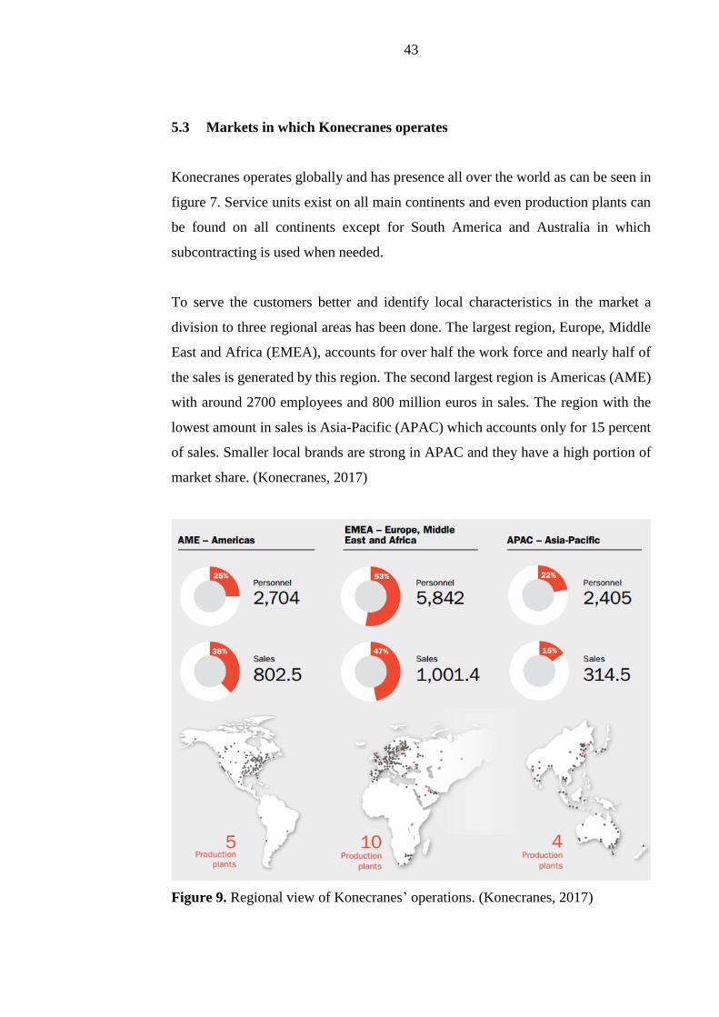
5.3 Markets in which Konecranes operates
Konecranes operates globally and has presence all over the world as can be seen in
figure 7. Service units exist on all main continents and even production plants can
be found on all continents except for South America and Australia in which
subcontracting is used when needed.
To serve the customers better and identify local characteristics in the market a
division to three regional areas has been done. The largest region, Europe, Middle
East and Africa (EMEA), accounts for over half the work force and nearly half of
the sales is generated by this region. The second largest region is Americas (AME)
with around 2700 employees and 800 million euros in sales. The region with the
lowest amount in sales is Asia-Pacific (APAC) which accounts only for 15 percent
of sales. Smaller local brands are strong in APAC and they have a high portion of
market share. (Konecranes, 2017)
Figure 9. Regional view of Konecranes’ operations. (Konecranes, 2017)
44
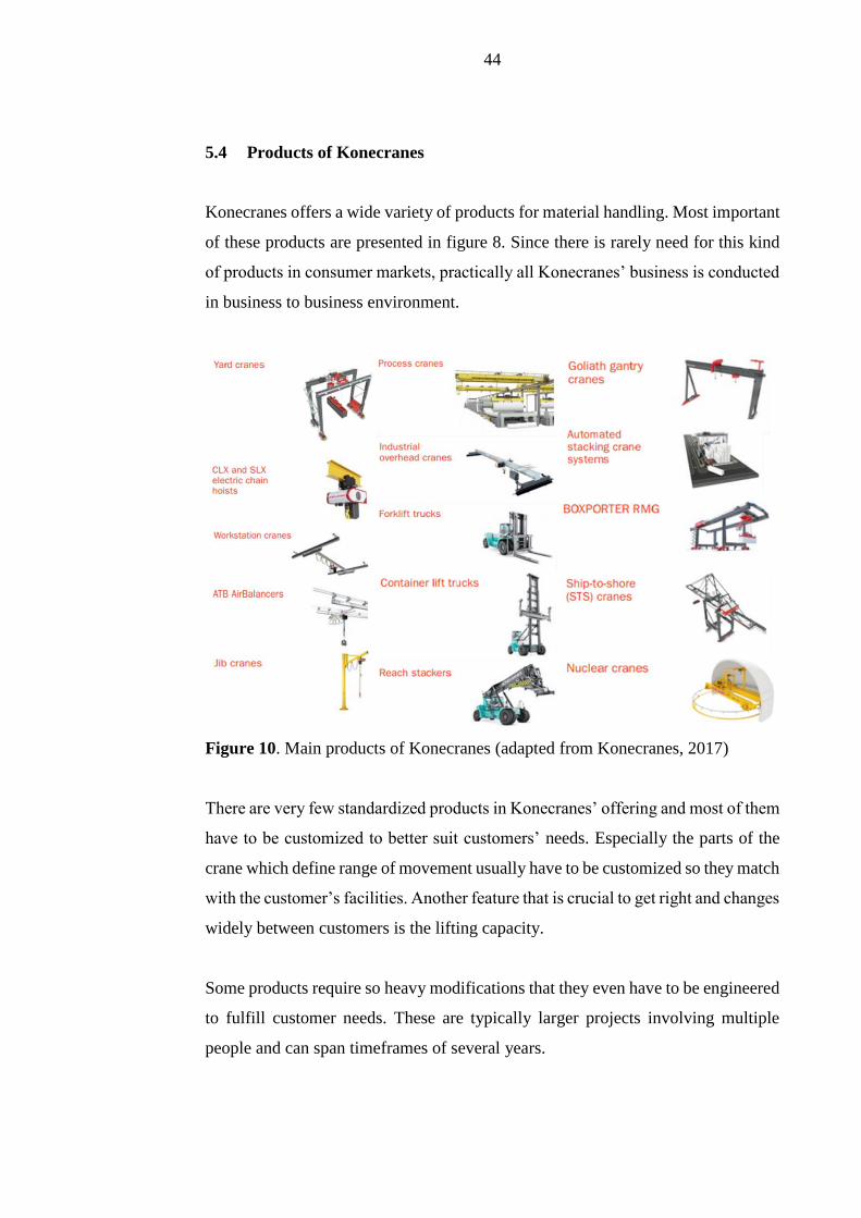
5.4 Products of Konecranes
Konecranes offers a wide variety of products for material handling. Most important
of these products are presented in figure 8. Since there is rarely need for this kind
of products in consumer markets, practically all Konecranes’ business is conducted
in business to business environment.
Figure 10. Main products of Konecranes (adapted from Konecranes, 2017)
There are very few standardized products in Konecranes’ offering and most of them
have to be customized to better suit customers’ needs. Especially the parts of the
crane which define range of movement usually have to be customized so they match
with the customer’s facilities. Another feature that is crucial to get right and changes
widely between customers is the lifting capacity.
Some products require so heavy modifications that they even have to be engineered
to fulfill customer needs. These are typically larger projects involving multiple
people and can span timeframes of several years.

45
Because of all these customizations are needed it is not possible to define one bill
of materials (BOM) for the products. This presents demand forecasting with the
challenge that even if end product demand was known exactly it is not possible to
calculate which materials are needed to fulfill that demand unless all the
characteristics of the final products were known. In reality that is not a realistic
expectation since there is almost an unlimited amount of possible product
variations. Instead historical demand of components is used to extrapolate future
demand on per material basis.
46
6 CURRENT FORECASTING PROCESSES IN
KONECRANES
In the past as Konecranes was using multiple ERP systems there was no defined
forecasting process. The historical consumption data required for material level
forecasting was so fragmented into multiple systems which saved it in different
formats made a global forecasting process not feasible to implement. With SAP
implementation project, a better visibility to all actions going on in the company
was received which has increased potential benefits and attractiveness of
forecasting.
With this new visibility two forecasting processes were implemented. More labor-
intensive demand supply balancing which considers hot offers and expert opinions
from sales function is used for some key products. Because of the resources it
requires there are no plans to get all materials into its scope. To generate forecasts
also for other materials a totally automatic process is needed.
Currently all materials for which demand is forecasted have the forecast data is
generated on weekly level. This level of detail is needed because of the way material
management is set up in SAP. Forecasting materials with high demand volumes on
a monthly level would lead to higher inventories than needed and thus increase
working capital. Reduction of working capital has been one of the main targets for
material management organization for the past years so switching forecasting setup
to a monthly level is not desirable, at least not for all materials.
The horizon for which demand is forecasted is 12 months. Forecasts are not used
only for optimizing the next purchases but for selected materials the forecasted
demand is also shared with the suppliers so they can improve their inventory
management and capacity utilization. Suppliers usually prefer to have forecasts for
as long into the future as possible as long as their accuracy does not decrease
significantly. These longer forecast horizons also give the option for better
47
optimization of order quantities so inventory carrying costs and procurement costs
can be minimized by utilizing methods like economic order quantity.
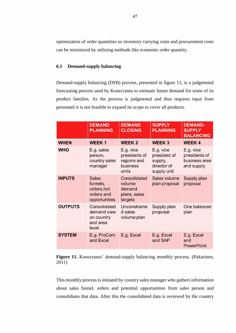
6.1 Demand-supply balancing
Demand-supply balancing (DSB) process, presented in figure 11, is a judgmental
forecasting process used by Konecranes to estimate future demand for some of its
product families. As the process is judgmental and thus requires input from
personnel it is not feasible to expand its scope to cover all products.
Figure 11. Konecranes’ demand-supply balancing monthly process. (Pakarinen,
2011)
This monthly process is initiated by country sales manager who gathers information
about sales funnel, orders and potential opportunities from sales person and
consolidates that data. After this the consolidated data is reviewed by the country
48
sales manager after which it is delivered to the competence center which is
responsible for consolidating the data further and generating sales plan for the
region.
During week two this consolidated sales plan is delivered to the vice president of
regions who links it to monetary sales forecasts. Adjustment proposals might also
be raised at this phase if those are deemed necessary. Finally, this plan is matched
to the sales target volumes and brought to the demand closing meeting in which an
unconstrained sales volume plan is generated.
This unconstrained sales volume plan is then used as an input for supply planning
phase in which it is checked if the factories have the capacity and have materials
available to fulfill the planned sales. In case constraints are found in the supply
chain which prevent fulfillment of the sales plan a modified supply plan proposal
with allocations is generated. This plan is then used in the final stage, demand-
supply balancing. In this final meeting between vice president of the business area,
vice president of supply, chief procurement officer and finance the goal is to reach
a consensus, one balanced plan.
As inventory management requires forecasts on SKU level this balanced plan is not
on a detailed enough and some additional data manipulation is needed to
disaggregate it. Many Konecranes products, even the ones in the scope of DSB, do
not have a fixed bill of materials which could be directly used to calculate material
requirements if end products are known. Instead historical data for the end products
is analyzed and the probabilities of usage for certain material in the selected end
product is calculated and this is used to disaggregate the end product data to
component level.
6.2 Statistical forecast
Currently Konecranes utilizes SAP to generate SKU level forecasts via statistical
method. The model used for all materials has been simple moving average using

49
historical data of the past 13 weeks. Main reason for this choice has been its
simplicity which allows users to easily and quickly understand why it outputs a
certain number. This forecasting process is carried out once a month. However, the
accuracy of this forecasting method has not been measured actively before this
thesis and there have been some discussions about its suitability to this use case and
especially as a blanket solution for all materials.

50
7 COMPARISON OF TIME SERIES MODELS
The current forecasting process used is not as accurate as the company would like
so possibilities for parameter optimization and other models were studied. Selection
criteria for candidates as potential new model was mainly based on the following
characteristics:
• Easily deployable
• Can be automatically run for a wide variety of materials
• Based on best practices presented in literature
• Can be run on a commercially available, actively developed software
solution
7.1 Sample data
Data used for testing different forecasting methods consists of two data sets. One
contains demand data from Hämeenlinna plant and the other from a plant located
in Springfield. As the goal is to find models that can be applied to a wide range of
materials the only scope restriction for materials was annual consumption which
was given minimum value of 3. Main reason for this restriction was to reach a
systematic way to clearing major outliers in accuracy measures. Such small
volumes of demand cannot be reliably forecasted so including them in the data was
not practical from that point of view either.
All the data was obtained from the company’s ERP system, SAP, aggregated on
weekly level; sample of the source data can be seen in appendix I. SAP is relatively
new system in Konecranes and its deployment schedule played a major part in plant
scope selection. Deployments are ongoing and these two plants were among the
first ones to take SAP into use so they had demand data available from 2015 and
2016 which allowed generation of forecasts based on 2015 data and comparing that
to actual demand that happened in 2016.
51
However, this limited history data available also affected the possibility to analyze
if some demand patterns can be identified, namely seasonality, which would require
demand data from multiple years. As the company operates mostly in business to
business markets and mostly serves industrial customers seasonal changes in
demand are practically non-existent and seasonality is not seen as a big factor from
demand forecasting point of view. Based on these reasons, seasonality was not
considered in this study.
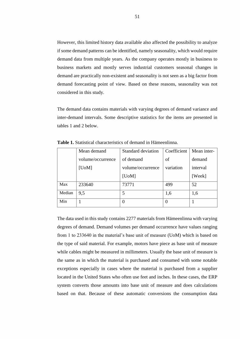
The demand data contains materials with varying degrees of demand variance and
inter-demand intervals. Some descriptive statistics for the items are presented in
tables 1 and 2 below.
Table 1. Statistical characteristics of demand in Hämeenlinna.
Mean demand
volume/occurrence
[UoM]
Standard deviation
of demand
volume/occurrence
[UoM]
Coefficient
of
variation
Mean inter-
demand
interval
[Week]
Max 233640 73771 499 52
Median 9,5 5 1,6 1,6
Min 1 0 0 1
The data used in this study contains 2277 materials from Hämeenlinna with varying
degrees of demand. Demand volumes per demand occurrence have values ranging
from 1 to 233640 in the material’s base unit of measure (UoM) which is based on
the type of said material. For example, motors have piece as base unit of measure
while cables might be measured in millimeters. Usually the base unit of measure is
the same as in which the material is purchased and consumed with some notable
exceptions especially in cases where the material is purchased from a supplier
located in the United States who often use feet and inches. In these cases, the ERP
system converts those amounts into base unit of measure and does calculations
based on that. Because of these automatic conversions the consumption data
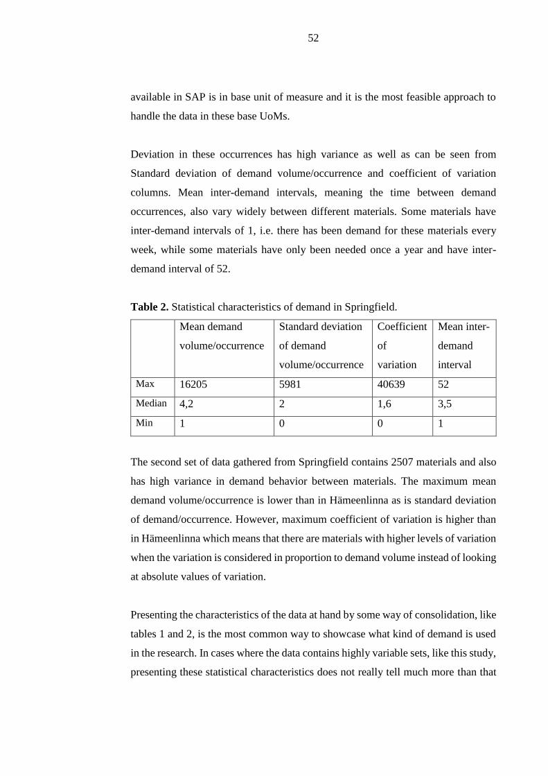
52
available in SAP is in base unit of measure and it is the most feasible approach to
handle the data in these base UoMs.
Deviation in these occurrences has high variance as well as can be seen from
Standard deviation of demand volume/occurrence and coefficient of variation
columns. Mean inter-demand intervals, meaning the time between demand
occurrences, also vary widely between different materials. Some materials have
inter-demand intervals of 1, i.e. there has been demand for these materials every
week, while some materials have only been needed once a year and have inter-
demand interval of 52.
Table 2. Statistical characteristics of demand in Springfield.
Mean demand
volume/occurrence
Standard deviation
of demand
volume/occurrence
Coefficient
of
variation
Mean inter-
demand
interval
Max 16205 5981 40639 52
Median 4,2 2 1,6 3,5
Min 1 0 0 1
The second set of data gathered from Springfield contains 2507 materials and also
has high variance in demand behavior between materials. The maximum mean
demand volume/occurrence is lower than in Hämeenlinna as is standard deviation
of demand/occurrence. However, maximum coefficient of variation is higher than
in Hämeenlinna which means that there are materials with higher levels of variation
when the variation is considered in proportion to demand volume instead of looking
at absolute values of variation.
Presenting the characteristics of the data at hand by some way of consolidation, like
tables 1 and 2, is the most common way to showcase what kind of demand is used
in the research. In cases where the data contains highly variable sets, like this study,
presenting these statistical characteristics does not really tell much more than that

53
there are materials with very different demand patterns. Based on these tables it is
impossible to say how easily or accurately the demand could be forecasted.
To better describe and categorize the demand the categorization scheme presented
by Syntetos et al. (2005) has been utilized with the cut-off values defined by
Kostenko and Hyndman (2006). in their paper. items are divided into four different
categories and presented in a matrix which later had its categorization threshold
values modified by Kostenko and Hyndman (2006). These categorizations
containing the sample sets of this study are presented in figures 11 and 12 below.
Figure 12. Demand categorization of sample materials from Hämeenlinna.
Very small portion, less than 1 percent, of materials used in Hämeenlinna belong to
the smooth category which has traditionally been considered the easiest to forecast
and achieve acceptable accuracy on. Majority of the materials get located to the top
portion of the matrix meaning they have varying demand volumes. Some of these
have demand occurring rather continuously and some have demand occurring only
occasionally.
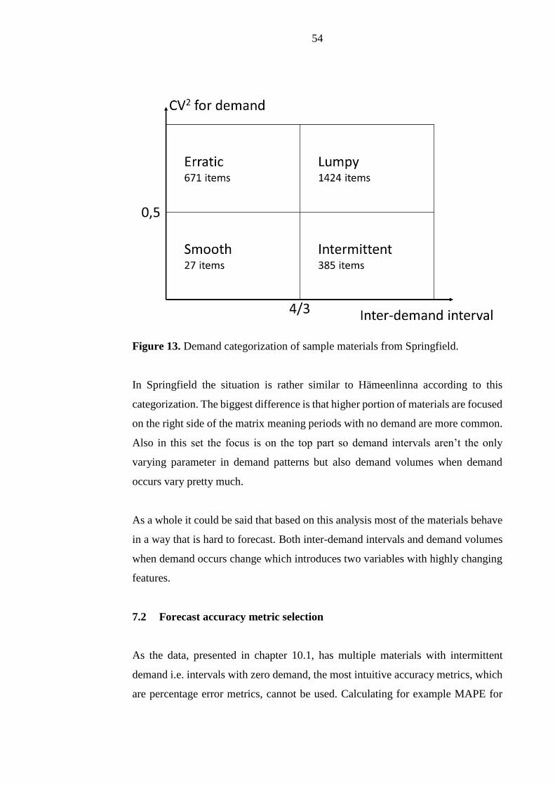
54
Figure 13. Demand categorization of sample materials from Springfield.
In Springfield the situation is rather similar to Hämeenlinna according to this
categorization. The biggest difference is that higher portion of materials are focused
on the right side of the matrix meaning periods with no demand are more common.
Also in this set the focus is on the top part so demand intervals aren’t the only
varying parameter in demand patterns but also demand volumes when demand
occurs vary pretty much.
As a whole it could be said that based on this analysis most of the materials behave
in a way that is hard to forecast. Both inter-demand intervals and demand volumes
when demand occurs change which introduces two variables with highly changing
features.
7.2 Forecast accuracy metric selection
As the data, presented in chapter 10.1, has multiple materials with intermittent
demand i.e. intervals with zero demand, the most intuitive accuracy metrics, which
are percentage error metrics, cannot be used. Calculating for example MAPE for
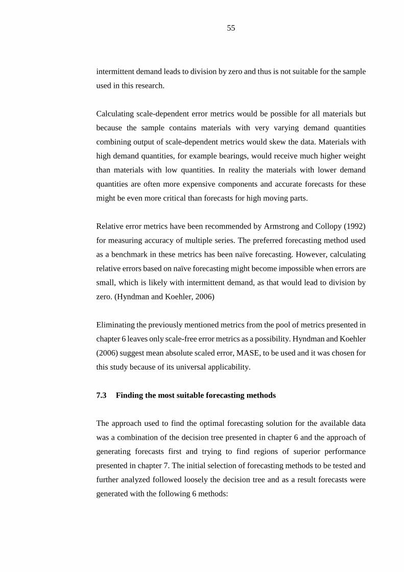
55
intermittent demand leads to division by zero and thus is not suitable for the sample
used in this research.
Calculating scale-dependent error metrics would be possible for all materials but
because the sample contains materials with very varying demand quantities
combining output of scale-dependent metrics would skew the data. Materials with
high demand quantities, for example bearings, would receive much higher weight
than materials with low quantities. In reality the materials with lower demand
quantities are often more expensive components and accurate forecasts for these
might be even more critical than forecasts for high moving parts.
Relative error metrics have been recommended by Armstrong and Collopy (1992)
for measuring accuracy of multiple series. The preferred forecasting method used
as a benchmark in these metrics has been naïve forecasting. However, calculating
relative errors based on naïve forecasting might become impossible when errors are
small, which is likely with intermittent demand, as that would lead to division by
zero. (Hyndman and Koehler, 2006)
Eliminating the previously mentioned metrics from the pool of metrics presented in
chapter 6 leaves only scale-free error metrics as a possibility. Hyndman and Koehler
(2006) suggest mean absolute scaled error, MASE, to be used and it was chosen for
this study because of its universal applicability.
7.3 Finding the most suitable forecasting methods
The approach used to find the optimal forecasting solution for the available data
was a combination of the decision tree presented in chapter 6 and the approach of
generating forecasts first and trying to find regions of superior performance
presented in chapter 7. The initial selection of forecasting methods to be tested and
further analyzed followed loosely the decision tree and as a result forecasts were
generated with the following 6 methods:

56
• Boylan-Syntetos
• Box-Jenkins
• Croston’s method
• Holt-Winters
• Single exponential smoothing
• Simple moving average
Because many of these methods have parameters that affect their outcome a total
of 31 forecasts were generated per data set. As the source data was available from
two different supply units this meant 62 forecasts in total.
For simple moving average, which is mathematically the easiest, forecasting
method the forecasts were generated using Microsoft Excel’s basic functions. The
parameter available to change the behavior of SMA is the time periods used in the
calculation and these were tested from 4 to 52 weeks in 4 week intervals i.e. 4
weeks, 8 weeks, 12 weeks etc.
The other selected forecasting methods, Boylan-Syntetos, Box-Jenkins, Croston’s
method, Holt-Winters and single exponential smoothing, were tested utilizing R
software environment, RStudio and the freely available packages “forecast” and
“tsintermittent” developed by Rob Hyndman and Nikolaos Kourentzes
respectively. For Croston’s method and single exponential smoothing the tested
smoothing parameters ranged from 0,1 to 0,4 with 0,05 intervals. Boylan-Syntetos,
Box-Jenkins and Holt-Winters had their parameters optimized automatically.
As it is not feasible to compare 31 different forecasts at once to try to find regions
of superior performance, the number of forecasts was first limited to one or two
forecasts per forecasting method i.e. the best performing parameters were identified
and selected for further studying. This was done by a four step process. First mean
absolute scaled error was calculated per material for all generated forecasts on 3-,
6- and 12-month forecasting horizons. After this average, median and 99th
percentile were formulated from the MASE values per forecast and forecasting
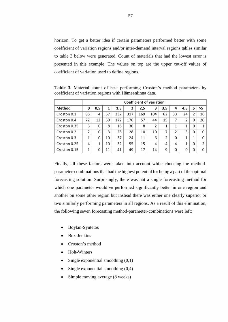
57
horizon. To get a better idea if certain parameters performed better with some
coefficient of variation regions and/or inter-demand interval regions tables similar
to table 3 below were generated. Count of materials that had the lowest error is
presented in this example. The values on top are the upper cut-off values of
coefficient of variation used to define regions.
Table 3. Material count of best performing Croston’s method parameters by
coefficient of variation regions with Hämeenlinna data.
Coefficient of variation
Method 0 0,5 1 1,5 2 2,5 3 3,5 4 4,5 5 >5
Croston 0.1 85 4 57 237 317 169 104 62 33 24 2 16
Croston 0.4 72 12 59 172 176 57 44 15 7 2 0 20
Croston 0.35 3 0 8 16 30 8 2 1 1 1 0 1
Croston 0.2 2 0 3 28 28 10 10 7 2 3 0 0
Croston 0.3 1 0 10 37 24 11 6 2 0 1 1 0
Croston 0.25 4 1 10 32 55 15 4 4 4 1 0 2
Croston 0.15 1 0 11 41 49 17 14 9 0 0 0 0
Finally, all these factors were taken into account while choosing the method-
parameter-combinations that had the highest potential for being a part of the optimal
forecasting solution. Surprisingly, there was not a single forecasting method for
which one parameter would’ve performed significantly better in one region and
another on some other region but instead there was either one clearly superior or
two similarly performing parameters in all regions. As a result of this elimination,
the following seven forecasting method-parameter-combinations were left:
• Boylan-Syntetos
• Box-Jenkins
• Croston’s method
• Holt-Winters
• Single exponential smoothing (0,1)
• Single exponential smoothing (0,4)
• Simple moving average (8 weeks)
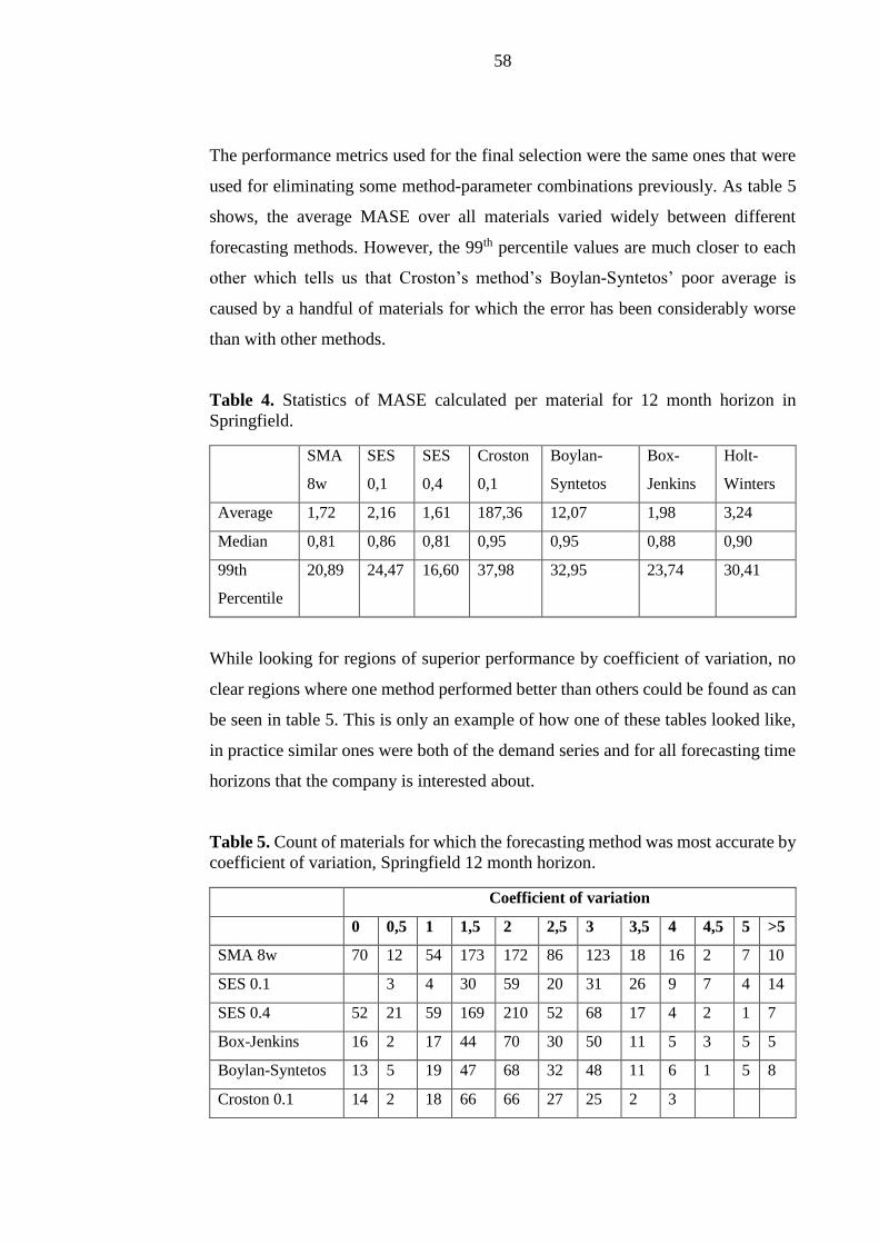
58
The performance metrics used for the final selection were the same ones that were
used for eliminating some method-parameter combinations previously. As table 5
shows, the average MASE over all materials varied widely between different
forecasting methods. However, the 99th percentile values are much closer to each
other which tells us that Croston’s method’s Boylan-Syntetos’ poor average is
caused by a handful of materials for which the error has been considerably worse
than with other methods.
Table 4. Statistics of MASE calculated per material for 12 month horizon in
Springfield.
SMA
8w
SES
0,1
SES
0,4
Croston
0,1
Boylan-
Syntetos
Box-
Jenkins
Holt-
Winters
Average 1,72 2,16 1,61 187,36 12,07 1,98 3,24
Median 0,81 0,86 0,81 0,95 0,95 0,88 0,90
99th
Percentile
20,89 24,47 16,60 37,98 32,95 23,74 30,41
While looking for regions of superior performance by coefficient of variation, no
clear regions where one method performed better than others could be found as can
be seen in table 5. This is only an example of how one of these tables looked like,
in practice similar ones were both of the demand series and for all forecasting time
horizons that the company is interested about.
Table 5. Count of materials for which the forecasting method was most accurate by
coefficient of variation, Springfield 12 month horizon.
Coefficient of variation
0 0,5 1 1,5 2 2,5 3 3,5 4 4,5 5 >5
SMA 8w 70 12 54 173 172 86 123 18 16 2 7 10
SES 0.1
3 4 30 59 20 31 26 9 7 4 14
SES 0.4 52 21 59 169 210 52 68 17 4 2 1 7
Box-Jenkins 16 2 17 44 70 30 50 11 5 3 5 5
Boylan-Syntetos 13 5 19 47 68 32 48 11 6 1 5 8
Croston 0.1 14 2 18 66 66 27 25 2 3
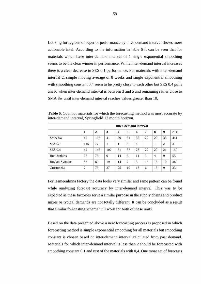
59
Looking for regions of superior performance by inter-demand interval shows more
actionable intel. According to the information in table 6 it can be seen that for
materials which have inter-demand interval of 1 single exponential smoothing
seems to be the clear winner in performance. While inter-demand interval increases
there is a clear decrease in SES 0,1 performance. For materials with inter-demand
interval 2, simple moving average of 8 weeks and single exponential smoothing
with smoothing constant 0,4 seem to be pretty close to each other but SES 0,4 pulls
ahead when inter-demand interval is between 3 and 5 and remaining rather close to
SMA 8w until inter-demand interval reaches values greater than 10.
Table 6. Count of materials for which the forecasting method was most accurate by
inter-demand interval, Springfield 12 month horizon.
Inter-demand interval
1 2 3 4 5 6 7 8 9 >10
SMA 8w 42 167 41 59 31 36 22 20 35 441
SES 0.1 115 77 1 1 3 4
1 2 3
SES 0.4 42 146 107 81 37 28 22 29 21 149
Box-Jenkins 67 78 9 14 6 11 5 4 9 55
Boylan-Syntetos 57 89 19 14 7 3 13 13 10 38
Croston 0.1 7 75 27 25 10 18 6 13 9 33
For Hämeenlinna factory the data looks very similar and same pattern can be found
while analyzing forecast accuracy by inter-demand interval. This was to be
expected as these factories serve a similar purpose in the supply chains and product
mixes or typical demands are not totally different. It can be concluded as a result
that similar forecasting scheme will work for both of these units.
Based on the data presented above a new forecasting process is proposed in which
forecasting method is simple exponential smoothing for all materials but smoothing
constant is chosen based on inter-demand interval calculated from past demand.
Materials for which inter-demand interval is less than 2 should be forecasted with
smoothing constant 0,1 and rest of the materials with 0,4. One more set of forecasts
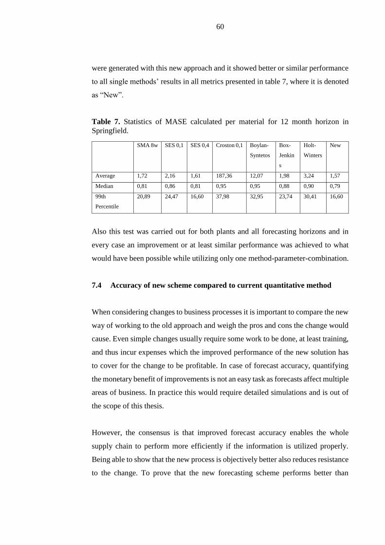
60
were generated with this new approach and it showed better or similar performance
to all single methods’ results in all metrics presented in table 7, where it is denoted
as “New”.
Table 7. Statistics of MASE calculated per material for 12 month horizon in
Springfield.
SMA 8w SES 0,1 SES 0,4 Croston 0,1 Boylan-
Syntetos
Box-
Jenkin
s
Holt-
Winters
New
Average 1,72 2,16 1,61 187,36 12,07 1,98 3,24 1,57
Median 0,81 0,86 0,81 0,95 0,95 0,88 0,90 0,79
99th
Percentile
20,89 24,47 16,60 37,98 32,95 23,74 30,41 16,60
Also this test was carried out for both plants and all forecasting horizons and in
every case an improvement or at least similar performance was achieved to what
would have been possible while utilizing only one method-parameter-combination.
7.4 Accuracy of new scheme compared to current quantitative method
When considering changes to business processes it is important to compare the new
way of working to the old approach and weigh the pros and cons the change would
cause. Even simple changes usually require some work to be done, at least training,
and thus incur expenses which the improved performance of the new solution has
to cover for the change to be profitable. In case of forecast accuracy, quantifying
the monetary benefit of improvements is not an easy task as forecasts affect multiple
areas of business. In practice this would require detailed simulations and is out of
the scope of this thesis.
However, the consensus is that improved forecast accuracy enables the whole
supply chain to perform more efficiently if the information is utilized properly.
Being able to show that the new process is objectively better also reduces resistance
to the change. To prove that the new forecasting scheme performs better than

61
current methods, average, median and 99th percentile of mean absolute scaled errors
(MASE) of materials were calculated.
First MASE was determined per material and average of these error values across
all materials was calculated. These averages are presented in figure 14 in 3, 6 and
12 month forecasting horizons. Two leftmost columns in every time horizon present
average MASE in Springfield and two rightmost columns present same values in
Hämeenlinna. As can be seen in the figure below, the average MASE in
Hämeenlinna decreases to less than half of current values with the new forecasting
scheme in all forecasting horizons. In Springfield the improvement is not as drastic
but clearly noticeable at 18 percent.
Figure 14. Average MASE with old and new quantitative methods.
Similarly calculated median of mean absolute scaled error values across all
materials can be seen in figure 15. While looking at medians, the performance of
new scheme and current method are much closer to each other. However, this
statistic also shows the new scheme to achieve higher accuracy in both these plants
at all forecasting horizons.
1,9
5
1,9
4
1,9
4
1,6
1
1,5
9
1,5
7
3,9
1
3,9
5
3,9
7
1,6
3
1,6
5
1,6
6
3 M O N T H 6 M O N T H 1 2 M O N T H
SPR old AVG SPR new AVG HML old AVG HML new AVG

62
Figure 15. Median MASE with old and new quantitative methods.
While looking at worst case scenarios of forecast accuracy i.e. 99th percentile
MASEs, there is a clear improvement in accuracy. With this metric, presented in
figure 16, even the new scheme has high levels of error for some materials but
compared to current solution its error is clearly lower.
Figure 16. 99th percentile MASE with old and new quantitative methods.
0,9
3
0,8
9
0,8
30,8
8
0,8
5
0,7
9
0,8
0
0,8
2
0,8
0
0,7
6
0,7
9
0,7
7
3 M O N T H 6 M O N T H 1 2 M O N T H
SPR old median SPR new median HML old median HML new median
22
,48
23
,02
23
,52
16
,74
16
,42
16
,60
21
,54
22
,47
22
,28
11
,62
12
,40
12
,67
3 M O N T H 6 M O N T H 1 2 M O N T H
SPR old 99th percentile SPR new 99th percentile
HML old 99th percentile HML new 99th percentile
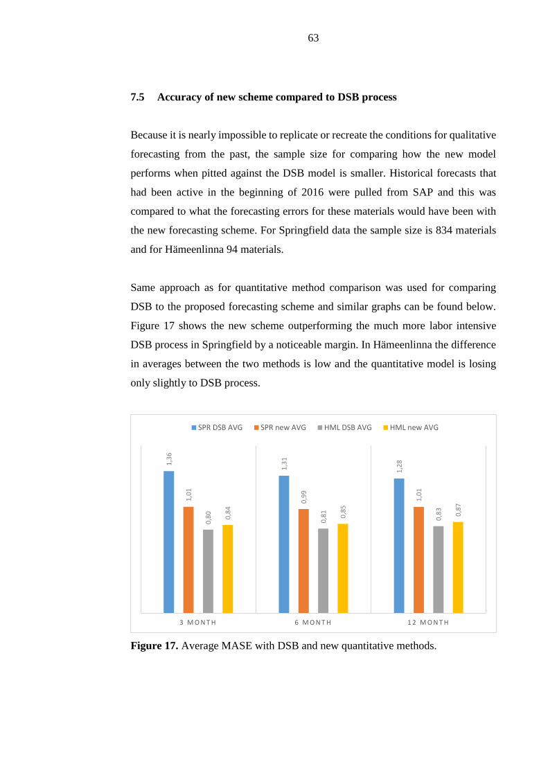
63
7.5 Accuracy of new scheme compared to DSB process
Because it is nearly impossible to replicate or recreate the conditions for qualitative
forecasting from the past, the sample size for comparing how the new model
performs when pitted against the DSB model is smaller. Historical forecasts that
had been active in the beginning of 2016 were pulled from SAP and this was
compared to what the forecasting errors for these materials would have been with
the new forecasting scheme. For Springfield data the sample size is 834 materials
and for Hämeenlinna 94 materials.
Same approach as for quantitative method comparison was used for comparing
DSB to the proposed forecasting scheme and similar graphs can be found below.
Figure 17 shows the new scheme outperforming the much more labor intensive
DSB process in Springfield by a noticeable margin. In Hämeenlinna the difference
in averages between the two methods is low and the quantitative model is losing
only slightly to DSB process.
Figure 17. Average MASE with DSB and new quantitative methods.
1,3
6
1,3
1
1,2
8
1,0
1
0,9
9
1,0
1
0,8
0
0,8
1
0,8
3
0,8
4
0,8
5
0,8
7
3 M O N T H 6 M O N T H 1 2 M O N T H
SPR DSB AVG SPR new AVG HML DSB AVG HML new AVG

64
Figure 18 shows the median across the materials. From this point of view the picture
is very similar to averages. In Springfield the new scheme leads to lower errors than
DSB process and in Hämeenlinna its error is only slightly higher. All forecasting
horizons show similar differences in performance.
Figure 18. Median MASE with DSB and new quantitative methods.
While looking at the worst case scenarios of mean absolute scaled errors in figure
19, the story stays the same. Proposed new forecasting scheme outperforms DSB at
all time horizons in Springfield and only loses slightly in Hämeenlinna. Based on
these results it would be justifiable to question the benefits of DSB process and if
the very slight accuracy improvement it generates in Hämeenlinna is worth all the
additional resources required by the process especially when it is taken into account
that the quantitative method can be totally automated.
1,0
9
1,1
0
1,1
0
0,8
7
0,8
1
0,8
1
0,7
2
0,7
4
0,7
6
0,7
4
0,7
5
0,7
6
3 M O N T H 6 M O N T H 1 2 M O N T H
SPR DSB median SPR new median HML DSB median HML new median

65
Figure 19. SPR 99th percentile, HML 95th percentile MASE with DSB and new
quantitative methods.
7.6 Implementing new forecast solution
In SAP forecasting behavior is managed per material by values input into material
master data. There are multiple fields which affect forecast generation, these are
shown in figure 20. Most important of these values is forecast model which defines
what method is used for the calculation. SAP offers only a limited amount of
options for this but single exponential smoothing, which is the only one needed for
the proposed forecasting scheme, is one of them.
Due to single exponential smoothing’s availability in SAP without any additional
work or modules needed, it is easy to implement the new forecasting scheme. As
the new scheme requires utilizing two different smoothing constants, a mass update
for all the materials cannot be done. Instead inter-demand intervals should be
calculated for the materials and based on those results either 0,1 or 0,4 should be
chosen as smoothing constant, or alpha factor as it is known in SAP.
5,2
6
4,8
7
4,7
0
3,7
6
3,3
9
3,4
8
1,2
8
1,3
2
1,3
1
1,3
3
1,3
6
1,2
7
3 M O N T H 6 M O N T H 1 2 M O N T H
SPR DSB 99th percentile SPR new 99th percentile
HML DSB 95th percentile HML new 95th percentile
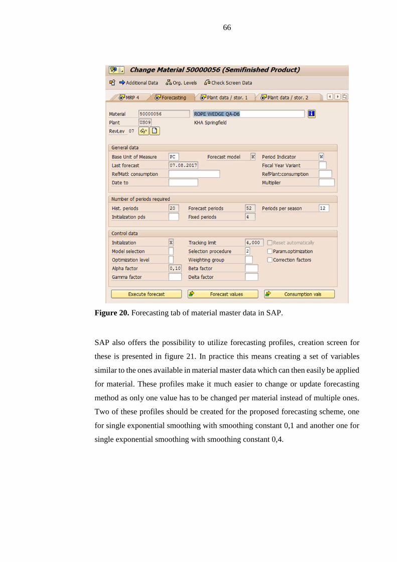
66
Figure 20. Forecasting tab of material master data in SAP.
SAP also offers the possibility to utilize forecasting profiles, creation screen for
these is presented in figure 21. In practice this means creating a set of variables
similar to the ones available in material master data which can then easily be applied
for material. These profiles make it much easier to change or update forecasting
method as only one value has to be changed per material instead of multiple ones.
Two of these profiles should be created for the proposed forecasting scheme, one
for single exponential smoothing with smoothing constant 0,1 and another one for
single exponential smoothing with smoothing constant 0,4.

67
Figure 21. Forecast profile creation screen in SAP.
Even though the initial implementation of this solution is easy, choosing the correct
parameters once is not enough. Demand of materials changes over time and
naturally their inter-demand interval does not remain constant either. There should
be periodic recalculations of inter-demand intervals and updates of forecast profiles
when necessary, for example once a quarter.
68
8 CONCLUSIONS
The main purpose of this thesis was to find out the forecasting methods which
would produce the most accurate demand forecasts without needing much
resources. This meant looking into quantitative forecasting methods and what
criteria or process should be used to choose the ones that yield the best results.
Based on literature over 70 different quantitative methods have been developed
over the years and which of these performs the best is dependent on how the demand
behaves.
Usually materials’ past demand is analyzed first and the materials are categorized
to some predefined number of subsets which are then assigned to be forecast by a
certain method. This categorization is based on manually input cutoff values of
characterizing parameters like inter-demand interval or coefficient of variation.
However, with this approach forecast accuracy is not necessarily as good as it could
be. Instead, the approach used in this thesis relies on generating forecasts with
multiple methods, calculating their accuracies and trying to find regions of
superiority i.e. some characteristics in demand for which a certain forecasting
method has the best performance.
Based on all the generated forecasts and analyzing them, a forecasting scheme
consisting of single exponential smoothing with smoothing constant 0,1 for
materials with inter-demand interval of two or less and smoothing constant 0,4 for
rest of the materials is proposed as the optimal solution. This result contradicts with
typical literature where Croston’s method, or lately Boylan-Syntetos method, has
been proposed as best practice to forecast intermittent demand. However, both of
those methods were part of the study and the proposed solution had better accuracy
with this demand data.
The proposed solution was also shown to outperform current quantitative method
utilized by Konecranes while also being easy to implement in SAP. The most
surprising result of the thesis was the new scheme’s better or just slightly worse

69
performance against the DSB process depending on plant and metric used. DSB
process is much more labor intensive and has already been the topic of other
master’s theses. Based on this it would be reasonable to consider if it is worth it to
keep utilizing it or if it can be improved further.
For future research the optimal level of detail on which forecasts are being
generated should be studied. Closer collaboration with suppliers and understanding
what level of detail would be best for optimizing their production and material
management could also yield positive results. Of course machine learning and
artificial intelligence with the ever increasing amount of data are likely to have
drastic effects in this field and research regarding their application to optimize
forecasts would be warranted.

70
REFERENCES
Ali, M. M. & Boylan, J. E. 2012. On the effect of non-optimal forecasting method
on supply chain downstream demand. IMA Journal of Management Mathematics.
Vol. 23. pp. 81-98.
Arnold, T. J. R., Chapman, S. N. & Clive, L. M. 2008. Introduction to materials
management. Pearson/Prentice Hall.
Armstrong, J. S. & Collopy, F. 1992. Error measures for generalizing about
forecasting methods. International Journal of Forecasting. Vol. 8. pp. 69-80.
Armstrong, J. S. 2001. Principles of Forecasting: A Handbook for Researchers and
Practitioners. Kluwer Academic Publishers.
Box, G. E. P. & Jenkins, G. M. 1970. Time series analysis: Forecasting and control.
Holden-Day.
Brown, R. G. 1959. Statistical Forecasting for Inventory Control. McGraw-Hill.
Chopra, S., Meindl, P. 2007. Supply Chain Management: Strategy, Planning and
Operation. 3. edition. Upper Saddle River/Prentice Hall. 536 p.
Christopher, M. 2005. Logistics and supply chain management: Creating value-
adding networks. 3. edition. Pearson Education. 298 p.
Christopher, M. 2007. Transforming the Supply chain into a Demand Chain.
Cranfield, Cranfield School of Management. Presentation.
Croston, J. D. 1972. Forecasting and stock control for intermittent demands.
Operational Research Quarterly. Vol. 23. pp. 289-304.
71
Fildes, R. 1992. The evaluation of extrapolative forecasting methods. International
Journal of Forecasting. Vol. 8. pp. 81-98.
Fildes, R. & Goodwin, P. 2007. Against your better judgment? How organizations
improve their use of management judgment in forecasting. Interfaces. Vol. 37. pp.
570-576.
Fredendall, L.W., Hill, E. 2001. Basics of Supply Chain Management. CRC Press
LLC. 237 p.
Holt, C. C. 1957. Forecasting trends and seasonals by exponentially weighted
averages. Carnegie Institute of Technology, Pittsburgh ONR memorandum no. 52.
Holweg, M., Disney, S., Holmström, J. & Småros, J. 2005. Supply Chain
Collaboration: Making Sense of the Strategy Continuum. European Management
Journal. Vol. 23. pp. 170-181.
Hyndman, R. J. & Koehler, A. B. 2006. Another look at forecast-accuracy metrics
for intermittent demand. The International Journal of Applied Forecasting. Vol. 4
pp. 43-46.
Johnston, F. R. & Boylan, J. E. 1996. Forecasting for items with intermittent
demand. Journal of Operational Research Society. Vol. 47. pp. 113-121.
Kangas, E. 2008. Balancing Demand and Supply in the Global Industrial Crane
Components Supply Chain. Master of Science Thesis. 114 p.
Konecranes. 2017. Konecranes Annual Report 2016.
Kostenko, A. V. & Hyndman, R. J. 2006. A note on the categorization of demand
patterns. Journal of Operational Research Society. Vol. 57. pp. 1256-1257.

72
Kourentzes, N. 2014. On intermittent demand model optimisation and selection.
International Journal of Production Economics. Vol. 156. pp. 180-190.
Makridakis, S., Wheelwright, S. C., & Hyndman, R. J. 1998. Forecasting: methods
and applications. John Wiley & Sons.
Makridakis, S. G. & Hibon, M. 2000. The M3-competition: Results, conclusions
and implications. International Journal of Forecasting. Vol. 16. pp. 451-476.
Mentzer, J. T. & Moon, M. A. 2005. Sales Forecasting Management: A demand
Management Approach. 2. edition. Thousand Oaks.
Pakarinen, P. 2011. Generating the basis of business performance management in
demand-supply planning. Master of Science Thesis. 93 p.
Sepúlveda-Rojas, J. P., Rojas, F., Valdés-González, H. & Martín, M. S. 2015.
Forecasting Models Selection Mechanism for Supply Chain Demand Estimation.
Procedia Computer Science. Vol. 55. pp. 1060-1068.
Shenstone, L. & Hyndman, R. J. 2005. Stochastic models underlying Croston’s
method for intermittent demand forecasting. Journal of Forecasting. Vol. 24. pp.
389-402.
Slack, N., Chambers, S., Johnston, R. 2001. Operations Management. 3. edition.
Harlow/Prentice Hall. 765 p.
Snyder, R. 2002. Forecasting sales of slow and fast moving inventories. European
Journal of Operational Research. Vol. 140. pp. 684-699.
Syntetos, A. A. & Boylan, J. E. 2001. On the bias of intermittent demand estimates.
International Journal of Production Economics. Vol. 71. pp. 457-466.

73
Syntetos, A. A. & Boylan, J. E. 2005. The accuracy of intermittent demand
estimates. International Journal of Forecasting. Vol. 21. pp. 303-314.
Syntetos, A. A., Boylan, J. E. & Croston, J. D. 2005. On the categorization of
demand patterns. Journal of the Operational Research Society. Vol. 56. pp. 495-
503.
Syntetos, A. A., Badai, Z., Boylan, J. E., Kolassa, S. & Nikolopoulos, K. 2016.
Supply chain forecasting: Theory, practice, their gap and the future. European
Journal of Operational Research. Vol. 252. pp. 1-26.
Tokle, J. & Krumwiede, D. 2006. An overview of Forecasting Error among
International Manufacturers. Journal of International Business Research. Vol. 5. pp.
97-105.
Vollmann, T. E., Berry, W. L., Whybark D. C., Jacobs, F. R. 2005. Manufacturing
Planning and Control Systems for Supply Chain Management. McGraw-Hill. 598
p.
Yu, Z., Yan, H., Cheng, E. 2001. Benefits of information sharing with supply chain
partnerships. Industrial Management & Data Systems. Vol. 101. pp. 114–119.
Wallström, P. & Segerstedt, A. 2010. Evaluation of forecasting error measurements
and techniques for intermittent demand. International Journal of Production
Economics. Vol. 128. pp. 625-636.
Willemain, T. R., Smart, C. N., Shockor, J. H. & DeSautels, P.A. 1994. Forecasting
intermittent demand in manufacturing: A comparative evaluation of Croston’s
method. International Journal of Forecasting. Vol. 10. pp. 529-538
Winters, P. R. 1960. Forecasting sales by exponentially weighted moving averages.
Management Science. Vol. 6. pp. 324-342.

74
Wright, G. & Goodwin, P. 1998. Forecasting With Judgment, 1. edition. John Wiley
& Sons Ltd.
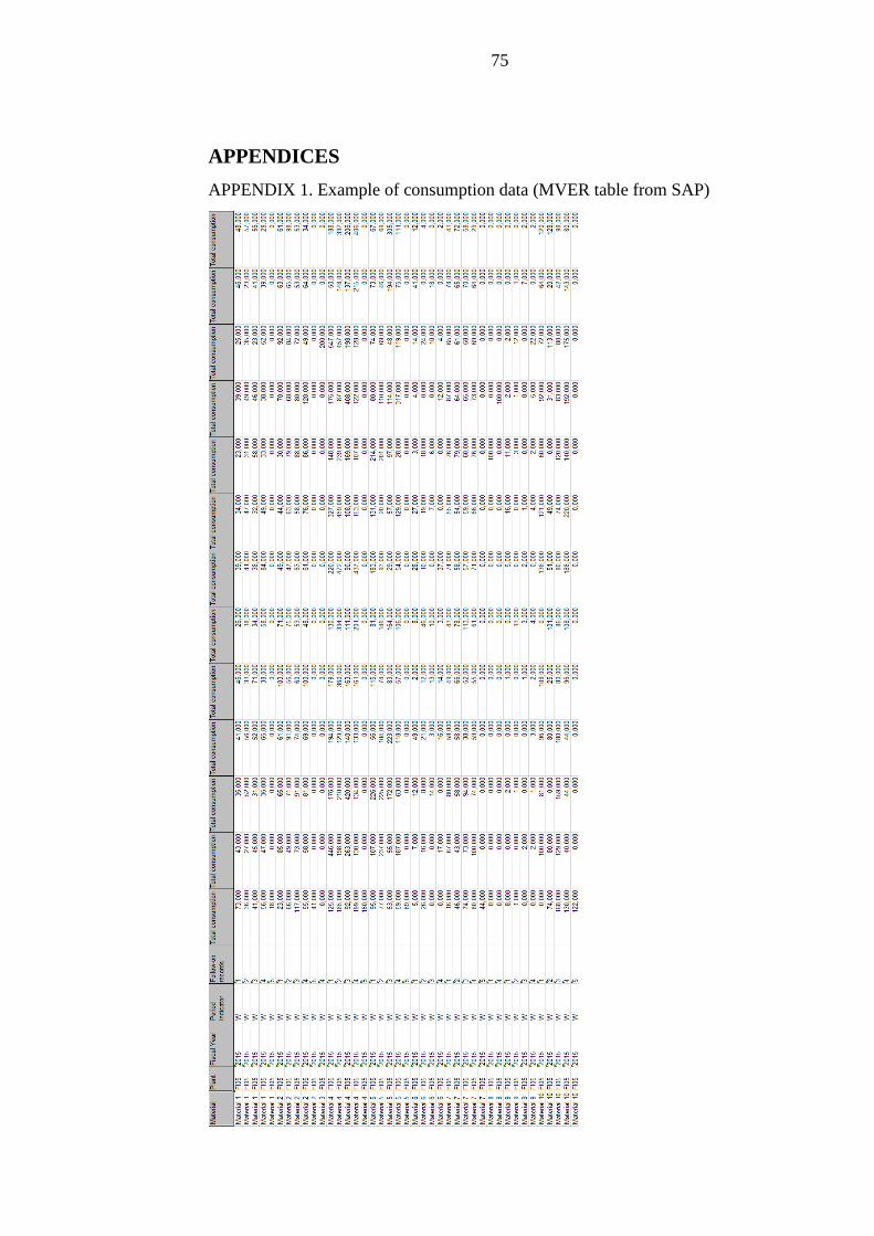
75
APPENDICES
APPENDIX 1. Example of consumption data (MVER table from SAP)
Related Documents