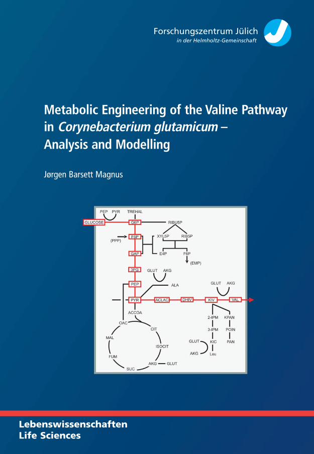
Lebenswissenschaften Life Sciences Metabolic Engineering of the Valine Pathway in Corynebacterium glutamicum – Analysis and Modelling Jørgen Barsett Magnus

Welcome message from author
This document is posted to help you gain knowledge. Please leave a comment to let me know what you think about it! Share it to your friends and learn new things together.
Transcript
LebenswissenschaftenLife Sciences
Band / Volume 38ISBN 978-3-89336-499-2 38
Leb
en
swis
sen
sch
aft
en
Life
Sci
en
ces
Jørg
en
Bars
ett
Mag
nu
sM
etab
olic
Eng
inee
ring
of
the
Valin
e Pa
thw
ay
LebenswissenschaftenLife Sciences
�������������� �������������������� �����������
�������������� �������������������� �����������
Metabolic Engineering of the Valine Pathwayin Corynebacterium glutamicum –Analysis and Modelling
Jørgen Barsett Magnus
Dr.-Ing. Jørgen Barsett Magnus studied Mathematics and Chemistry atthe University of Oslo and Chemical Engineering at the University ofManchester, Institute of Science and Technology (UMIST). He wrote hisMaster thesis at the Institute of Biochemical Engineering at the University ofStuttgart under the supervision of Klaus Mauch and Prof. Matthias Reuss.
In his thesis “Metabolic Engineering of the Valine Pathway in Corynebac-terium glutamicum – Analysis and Modelling” the functionality and dynamicsof the intracellular reaction network in C. glutamicum is investigated byusing metabolite concentration measurements, mathematical modelling,metabolic control analysis and thermodynamics.

Schriften des Forschungszentrums JülichReihe Lebenswissenschaften / Life Sciences Band / Volume 38

Forschungszentrum Jülich GmbHInstitut für Biotechnologie 2
Metabolic Engineering of the Valine Pathwayin Corynebacterium glutamicum –Analysis and Modelling
Jørgen Barsett Magnus
Schriften des Forschungszentrums JülichReihe Lebenswissenschaften / Life Sciences Band / Volume 38
ISSN 1433-5549 ISBN 978-3-89336-499-2
Bibliographic information published by Die Deutsche Nationalbibliothek.The Deutsche Bibliothek lists this publication in the DeutscheNationalbibliografie; detailed bibliographic data are available on theInternet <http://dnb.ddb.de>.
Publisher and Forschungszentrum Jülich GmbHDistributor: Zentralbibliothek, Verlag
52425 JülichPhone +49 (0)2461 61-5368 · Fax +49 (0)2461 61-6103E-Mail: [email protected]: http://www.fz-juelich.de/zb
Cover Design: Grafische Medien, Forschungszentrum Jülich GmbH
Printer: Grafische Medien, Forschungszentrum Jülich GmbH
Copyright: Forschungszentrum Jülich 2007
Schriften des Forschungszentrums JülichReihe Lebenswissenschaften /Life Sciences Band /Volume 38
D 93 (Diss., Stuttgart, Univ., 2007)
ISSN 1433-5549ISBN 978-3-89336-499-2
Neither this book nor any part of it may be reproduced or transmitted in any form or by any means, electronic or mechanical, including photocopying, microfilming, and recording, or by any information storage and retrieval system, without permission in writing from the publisher.

The whole is more than the sum of its parts.
Aristotle (in Metaphysics, 336 - 323 B.C)

v
Acknowledgements
The presented work was carried out at the Research Centre Jülich at the Institute of Biotechnology 2 in the Fermentation Technology group. The work was funded by the Deutsche Forschungsgemeinschaft, through the DFG grant TA241/3-2.
I would like to express my appreciation to all those who have supported and taken part of the research reported in this thesis. In particular, I am indebted to Prof. C. Wandrey for accepting me as a PhD student at the Institute of Biotechnology 2, for providing the excellent working conditions there and for the help with the scientific work. Furthermore I would like to thank Prof. M. Reuss for acting as thesis supervisor and for the cooperation with the Institute of Biochemical Engineering at the University of Stuttgart. I am also very grateful to PD Dr.-Ing. habil. R. Takors who, as Head of the Fermentation Group in Jülich, was my direct supervisor and provided me with much inspiration and vital scientific input for my work. Without his support the results reported in this thesis could not have been achieved. I would like to thank Dr. M Oldiges for his help and advice on the chemical analysis and for his review of my thesis. Many thanks to K. Mauch for the cooperation in developing the whole cell model and for his helpful advice on metabolic modelling. Klaus Mauch was also the person who inspired me to enter this field in the first place. Prof. W. Wiechert and Dr. M. Haunschild are thanked for the cooperation within the DFG bioinformatics project and for providing the program MMT2. Dr. L. Eggeling provided the strain that was investigated and gave valuable advice on biological issues for which I am very grateful. Dr. H. D. Narres is thanked for the cooperation on the measurements on the mass spectrometer. Many thanks to my diploma students D. Hollwedel and G. Schmidt and to all the members of the Fermentation Group in Jülich. Finally, and most importantly, I would like to thank Isabel for her enormous support and patience.
Jørgen Barsett Magnus,Frankfurt am Main, Germany

vii
Summary
The functionality of the intracellular reaction network in a Corynebacterium glutamicumvaline production strain was investigated with special focus on the valine / leucine biosynthesis pathway. The aim was to gain a quantitative understanding of the behaviour of the reaction network. The methods required to do so were developed, and enzyme targets for the further optimisation of the investigated strain were identified.
The intracellular metabolite concentrations were observed during a transient state by performing a glucose stimulus experiment. A mathematical model describing the in vivo reaction dynamics of the valine / leucine pathway was developed and a metabolic control analysis was performed based on the data from the stimulus experiment and the dynamic model. The thermodynamic driving forces in the valine / leucine pathway were analysed.
The optimal procedure for the stimulus experiment with respect to obtaining a useful data set for the modelling and analysis was identified. Samples were taken at sub-second intervals and the concentrations of 26 metabolites from the valine / leucine pathway and the central metabolism were measured. A very fast response to the stimulus was observed in most intracellular metabolites with for example a 3-fold increase in the pyruvate concentration within one second. The connectivities of the metabolites around the ketoisovalerate branchpoint were investigated using a time series analysis. The difference in metabolite levels and stimulus reaction at two different physiological states was demonstrated.
The kinetic model consisted of a system of differential equations defined by setting up material balances on the metabolites. Splines were used to represent the unbalanced metabolites in the reaction system and the reaction rate equations were defined using linlog kinetics. The model can simulate the concentrations and fluxes in the valine and leucine pathway accurately during the transient state. The implementation of a model selection criterion based on the second law of thermodynamics was demonstrated to be essential for the identification of realistic and unique models. Large differences between the enzyme properties determined in vitro and those determined in vivo by the model were observed with the in vivo maximal rates being almost an order of magnitude larger than the in vitro maximal rates. The transamination of ketoisovalerate to valine is carried out mainly by the Transaminase B enzyme with the Transaminase C enzyme playing a minor role. The availability of the cofactors NADP and NADPH has only modest influence on the flux through the valine pathway while the influence of NAD and NADH on the flux through the leucine pathway is negligible.
Other, alternative methods of setting up a kinetic model were also investigated. The alternative models included a mechanistic model of the valine / leucine pathway and a large linlog model of the whole metabolism of the strain. The mechanistic model was not capable of simulating the measured concentrations due to the limitations of its elasticities. The instability of the whole cell model made it inappropriate for a metabolic control analysis and further interpretation. However, the simulation of the whole metabolism of the strain provides a proof of concept for the whole cell modelling approach and shows in which direction metabolic modelling will develop in the future.
Both data driven and model based methods were used to analyse the control hierarchy in the valine / leucine pathway. In addition, predictions of the effect of changes in the enzyme levels were made based on the model. In an optimisation study the enzyme levels were optimised with respect to the valine flux. Based on the acquired understanding of the behaviour of the reaction network the following targets for further strain development were identified:
viii
1. Overexpression of the valine translocase 2. Implementation of an inhibition resistant AHAS enzyme and possibly further
overexpression.3. Removal of the overexpression of the gene coding for DHAD on the plasmid to
save the cell the burden of overproducing this enzyme which has negligible influence on the valine flux.
4. Modification of the central carbon metabolism to increase pyruvate availability.
The identification of the targets for strain development demonstrates the usefulness of a kinetic model in metabolic engineering and in the general understanding of metabolic control.
The concentration data and the kinetic model were used to analyse the thermodynamic driving force, i.e. the reaction affinity, in the valine / leucine pathway. The concept of a reaction resistance was introduced to relate the driving force to reaction rate in analogy with Ohm’s law. This provides a new angle of analysing metabolic networks. A correlation between enzyme level and reaction resistance was found, but a number of other factors also influence the resistance. The linear relation between reaction rate and affinity which apply for uni-uni reactions can not be assumed to be valid for bi-bi reactions operating far from equilibrium. This is demonstrated through theoretical considerations and confirmed by experimental observations. Thus the assumption of linearity can not be used to analyse metabolic systems. The reaction resistance must therefore be considered a system variable. The theory of metabolic control analysis was extended to include also the reaction potential and the reaction resistance. Reactions far from equilibrium are controlled almost entirely through the changes in the resistance while reactions closer to equilibrium are also affected by changes in the affinity. The reaction system is kept stable through a high degree of self-organisation.
ix
INDEX
1 Introduction ......................................................................................11.1 The Cellular Reaction System................................................................................ 1 1.2 Metabolomics ......................................................................................................... 3 1.3 Modelling and Simulation...................................................................................... 4 1.4 Metabolic Control Analysis ................................................................................... 5 1.5 Thermodynamic Analysis ...................................................................................... 5 1.6 Objective ................................................................................................................ 6 1.7 Structure of the Thesis............................................................................................ 8
2 Materials............................................................................................92.1 Strain ...................................................................................................................... 9 2.2 Cultivation medium.............................................................................................. 10 2.3 Rapid sampling apparatus .................................................................................... 10 2.4 Analytical devices ................................................................................................ 11
2.4.1 Analysis of the fermentation broth................................................................... 11 2.4.2 Mass spectrometry............................................................................................ 12
2.5 Modelling Software.............................................................................................. 16 2.5.1 Metabolic Modelling Tool 2 (MMT2) ............................................................. 16 2.5.2 Gepasi............................................................................................................... 17 2.5.3 Jarnac................................................................................................................ 18 2.5.4 In-Silico Discovery .......................................................................................... 18 2.5.5 Comparison of modelling software .................................................................. 18
3 Experimental Methods...................................................................213.1 Cultivation............................................................................................................ 21 3.2 Glucose stimulus experiment ............................................................................... 21 3.3 Cell disruption and metabolite extraction ............................................................ 22 3.4 Chemical Analysis of the Intracellular Metabolites ............................................. 22
4 Theoretical methods ......................................................................274.1 Time series analysis ............................................................................................. 27 4.2 Kinetic modelling................................................................................................. 28
4.2.1 Model Set Up ................................................................................................... 28 4.2.2 Reaction rate expressions ................................................................................. 31 4.2.3 Parameter Fitting .............................................................................................. 33 4.2.4 Estimation of the Parameter Covariance Matrix .............................................. 33 4.2.5 The Thermodynamic Model Constraint ........................................................... 34 4.2.6 Stability Analysis ............................................................................................. 35 4.2.7 Spline approximation ....................................................................................... 36
4.3 Metabolic Control Analysis ................................................................................. 39 4.3.1 Data Driven Analysis ....................................................................................... 39 4.3.2 Model Based Control Analysis ........................................................................ 40
4.4 Thermodynamic Analysis .................................................................................... 45 4.4.1 Introduction to the thermodynamic analysis of metabolic networks ............... 45
5 Metabolomics .................................................................................495.1 The glucose stimulus experiment ......................................................................... 49
x
5.1.1 The establishment of the extraction method .................................................... 49 5.1.2 Criteria for the fermentation............................................................................. 49 5.1.3 Identification of the optimal procedure for the experiment ............................. 50
5.2 The intracellular response to the stimulus............................................................ 51 5.3 The response in the pantothenate pathway........................................................... 56 5.4 Comparison of two different physiological states................................................ 58
6 Modelling and Simulation..............................................................616.1 Model performance .............................................................................................. 61 6.2 Model parameters ................................................................................................. 65 6.3 The thermodynamic modelling constraint............................................................ 68 6.4 The stability of the linlog model .......................................................................... 69
7 Metabolic Control Analysis ...........................................................717.1 Enzyme state ........................................................................................................ 71 7.2 The Pool Efflux Capacity ..................................................................................... 72 7.3 The control and response coefficients .................................................................. 73 7.4 Model predictions................................................................................................. 74 7.5 Optimisation of enzyme levels ............................................................................. 76 7.6 Comparison of the different methods................................................................... 77 7.7 Identification of target enzymes for strain optimisation ...................................... 79
8 Thermodynamic Analysis..............................................................818.1 The concept of the thermodynamic resistance ..................................................... 81 8.2 The thermodynamics of the system at steady state .............................................. 82 8.3 The relationship between the reaction rate and the affinity ................................. 85
8.3.1 Thermokinetic expressions............................................................................... 85 8.3.2 The variation of reaction rate with affinity ...................................................... 87 8.3.3 A short discussion of the main conclusions in section 8.3............................... 89
8.4 The control of the thermodynamic forces and resistances ................................... 89 8.4.1 The MCA of the thermodynamic functions affinity and resistance ................. 89 8.4.2 The control of the affinity and the resistance in the valine pathway................ 93 8.4.3 A short discussion of the main conclusions in section 8.4............................... 94
9 Alternative modelling approaches................................................979.1 A mechanistic model of the valine / leucine pathway.......................................... 97
9.1.1 Definition of the mechanistic model ................................................................ 97 9.1.2 Simulation results with the mechanistic model.............................................. 101
9.2 Whole cell modelling ......................................................................................... 104 9.2.1 The process of developing a whole cell model for C. glutamicum ................ 104 9.2.2 The definition of the stoichiometry................................................................ 105 9.2.3 Steady state metabolic flux analysis and topological analysis ....................... 109 9.2.4 Simulation results ........................................................................................... 111 9.2.5 Stability analysis ............................................................................................ 114 9.2.6 Discussion of the whole cell modelling approach.......................................... 116
10 Conclusion....................................................................................11911 References....................................................................................125Appendix A: Medium Composition...........................................................................141Appendix B: Synthesis of alpha acetolactate...........................................................145
xi
Appendix C: The data for the optimal stimulus experiment .....................................147Appendix D: Source code for the time-lagged correlation analysis..........................151Appendix E: The complete parameter correlation matrix for the linlog model..........155Appendix F: The source code of the spline program JMSpline................................157Appendix G: Stability Analysis of Dynamic Models..................................................161Appendix H: The compounds and reactions in the whole cell model.......................167

xiii
Figure Index
Figure 1–1: The cell as a chemical reactor................................................................................ 1 Figure 1–2: General procedure of the investigation.................................................................. 7 Figure 2–1: The genetic modifications in the isoleucine, valine and pantothenic acid
pathways applied in the Corynebacterium glutamicum strain.. ......................................... 9 Figure 2–2: Picture of the stimulus and rapid sampling apparatus. ........................................ 10 Figure 2–3: The procedure of a stimulus experiment with rapid sampling. ........................... 11 Figure 2–4: The principle of electrospray ionisation.. ............................................................ 13 Figure 2–5: The triple quadrupole mass spectrometer. ........................................................... 14 Figure 2–6: The structure of the -cyclodextrin columns. ...................................................... 15 Figure 2–7: The skeleton of the M3L document showing the main elements. ....................... 17 Figure 2–8: The graphical user interface of In-Silico Discovery.. .......................................... 19 Figure 3–1: The chromatogram for the measurements on the ThermoFinnigan mass
spectrometer. .................................................................................................................... 26 Figure 3–2: The chromatogram for the measurements on the mass spectrometer from Applied
Bioscience. ....................................................................................................................... 26 Figure 4–1: Illustration of the time-lagged correlation analysis method. ............................... 27 Figure 4–2: The reaction network of the valine and leucine anabolic pathways. ................... 29 Figure 4–3: Example of the spline coefficients on XML format as printed out by the spline
program. ........................................................................................................................... 38 Figure 4–4: The graphical user interface of the spline program. ............................................ 39 Figure 5–1: The intracellular pyruvate time course in the two preliminary experiments used
to establish the experimental procedure. .......................................................................... 50 Figure 5–2: The fermentation run for the optimal experiment. Left:...................................... 51 Figure 5–3: The reaction sequence in the glycolysis and the response to the glucose stimulus
in the EMP pathway. ........................................................................................................ 52 Figure 5–4: The reaction sequence in the valine pathway and the response to the glucose
stimulus. ........................................................................................................................... 54 Figure 5–5: The reaction sequence in the leucine pathway and the response to the glucose
stimulus. ........................................................................................................................... 55 Figure 5–6: The time course of Ketopantoate......................................................................... 56 Figure 5–7: The KIV branch point.......................................................................................... 57 Figure 5–8: The correlations of valine, KPan and 2-IPM with KIV at different time lags..... 57 Figure 5–9: Comparison of the response to the glucose stimulus for a culture adapted to
growth under glucose limitation and for a culture at the end of the exponential growth phase................................................................................................................................. 60
Figure 6–1: The simulation of the intracellular metabolites in the valine pathway (lines) and the measurements that were used to fit the parameters in the model (dots)..................... 62
Figure 6–2: The simulation of the intracellular metabolites in the leucine pathway (lines) and the measurements that were used to fit the parameters in the model (dots)..................... 63
Figure 6–3: The spline representation of the independent metabolites (lines) and the measurements from which the splines were calculated (dots). ........................................ 64
Figure 6–4: The time course of the simulated fluxes in the valine and leucine pathway. ...... 65 Figure 6–5: The cumulative frequency distribution of the parameter correlations................. 68 Figure 6–6: The simulations of a model where Transaminase C is the dominating enzyme in
the transamination reaction. ............................................................................................. 69 Figure 7–1: The Pool Efflux Capacities of the enzymes in the valine pathway. .................... 72 Figure 7–2: Flux control coefficients for the enzymes in the valine and leucine pathway with
respect to valine flux. ....................................................................................................... 73
xiv
Figure 7–3: Model predictions of the change in valine flux that would result from changingan enzyme level by a factor 2........................................................................................... 75
Figure 7–4: The optimal distribution of enzyme levels yielding the maximal flux of valine under the constraints given in section 4.3.2. .................................................................... 77
Figure 8–1: The fall of Gibbs energy, or total chemical potential, through the valine pathway........................................................................................................................................... 83
Figure 8–2: The reaction network of the valine and leucine pathways with the reaction resistances at steady state. ................................................................................................ 85
Figure 8–3: The reaction rate dependence on the affinity....................................................... 87 Figure 8–4: The variation of the intracellular reaction rates with affinity for the AHAS
reaction and the BCAAT reaction forming valine. .......................................................... 88 Figure 9–1: The simulated time courses of the metabolites in the valine pathway by the
mechanistic model for the two best fitting parameter sets. ............................................ 101 Figure 9–2: Overview of the stoichiometric model. ............................................................. 107 Figure 9–3: Illustration of the reactions of the two glucose uptake system as well as the
glycolysis and pentose phosphate pathway. ................................................................... 108 Figure 9–4: The simulation time courses for the 16 identified parameter sets displayed with a
different colour for each parameter set. ......................................................................... 112 Figure 9–5: The cumulative frequency distribution of the absolute values of the elasticities in
the whole cell model. ..................................................................................................... 113
Figure C 1: The response to the glucose stimulus in the EMP pathway and in the nucleotides ATP, ADP and AMP...................................................................................................... 147
Figure C 2: The response to the glucose stimulus in the valine and the leucine pathway.... 148 Figure C 3: The response to the glucose stimulus in 6-phosphoglycerate, in the sum of the
pentose-5-phosphates (intermediates of the PPP pathway) and in the nucleotides NAD and NADP as well as in the amino acids isoleucine, alanine and glutamate and in -ketoglutarate. .................................................................................................................. 149
Figure C 4: The response in the ketopantoate concentration to the glucose stimulus. ......... 150
xv
Table Index
Table 2–1: HPLC gradient with 12 mM ammoniumacetate and methanol used for the Nucleodex -OH column. ................................................................................................ 15
Table 2–2: HPLC gradient with 10 mM tributylamin + acidic acid (pH = 7) and methanol used for the phenomenex column..................................................................................... 16
Table 3–1; The method specific parameters for the measurements on the triple quadrupole mass spectrometer from ThermoFinnigan and from Applied Bioscience........................ 23
Table 3–2: The measured metabolites with their parent and product ions in MS/MS mode and the applied collision energy for fragmentation as measured on the ThermoFinnigan mass spectrometer with the -cyclodextrin chromatography column. ..................................... 24
Table 3–3: The measured metabolites with their parent and product ions in MS/MS mode and the applied collision energy for fragmentation as measured on the Applied Bioscience mass spectrometer with the phenyl phase chromatography column. ............................... 25
Table 4–1: The reactions in the valine and leucine pathway and the inhibitors included in the model as well as the standard Gibbs free energy of reaction (aqueous) at the biological standard state ( Gr
°’). ....................................................................................................... 29 Table 4–2: The mass balance equations for the linlog model of the valine / leucine pathway
according to the stoichiometry given in Table 4-1........................................................... 31 Table 5–1: The correlation maxima of valine, 2-IPM and KPan with KIV and the time-lags at
which they occur. ............................................................................................................. 57Table 6–1: The metabolite concentrations at the reference state. ........................................... 61 Table 6–2: The values of the model parameters...................................................................... 66 Table 6–3: The correlations between the parameters corresponding to the different reactants
and effectors in the AHAS and AHAIR reaction (Extract of the full correlation matrix found in Appendix E). ...................................................................................................... 67
Table 7–1: The intracellular concentrations of the substrates of the different enzymes compared to the respective Michaelis-Menten constants................................................. 71
Table 7–2: Response coefficients giving a measure for the response in valine flux to changes in the external metabolites................................................................................................ 74
Table 8–1: The steady state concentrations, Gibbs energies of formation and the chemical potential for the metabolites participating in the valine / leucine pathway...................... 82
Table 8–2: The reaction stoichiometry and standard affinities for the reactions, A°’ as well as the affinities, A, calculated at the steady state conditions of the system.......................... 84
Table 8–3: The affinity and resistance elasticities of the AHAS reaction with respect to pyruvate, acetolactate and valine. .................................................................................... 93
Table 8–4: The affinity and resistance elasticities for the BCAAT reaction with respect to glutamate, ketoisovalerate, -ketoglutarate and valine.................................................... 93
Table 8–5: The affinity and resistance control coefficients as well as the -elasticity and the self-organising term for the reactions in the valine pathway. .......................................... 94
Table 9–1: Excerpt of Table H-2 showing the synthesis reactions of the amino acids aspartate, asparagine, lysine, methionine and threonine. ............................................... 106
Table 9–2: The conserved moieties in the whole cell model. The abbreviations are explained in Appendix H in Table H-1........................................................................................... 110
Table 9–3: Summary of the topological analysis of the whole cell model. .......................... 110 Table 9–4: The parameters and elasticities for the reactions in the valine pathway for the
whole cell model and for the small model of the valine / leucine pathway. .................. 113 Table 9–5: The number of zero and positive eigenvalues of the model for the 16 parameter
sets. ................................................................................................................................. 116
xvi
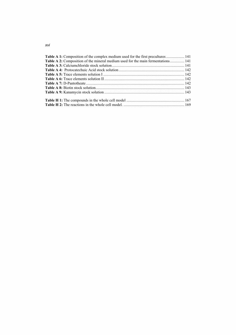
Table A 1: Composition of the complex medium used for the first precultures ................... 141 Table A 2: Composition of the mineral medium used for the main fermentations............... 141 Table A 3: Calciumchloride stock solution........................................................................... 141 Table A 4: Protocatechuic Acid stock solution .................................................................... 142 Table A 5: Trace elements solution I .................................................................................... 142 Table A 6: Trace elements solution II ................................................................................... 142 Table A 7: D-Pantotheate ...................................................................................................... 142 Table A 8: Biotin stock solution............................................................................................ 143 Table A 9: Kanamycin stock solution ................................................................................... 143
Table H 1: The compounds in the whole cell model ............................................................ 167 Table H 2: The reactions in the whole cell model. ............................................................... 169
xvii
Notation
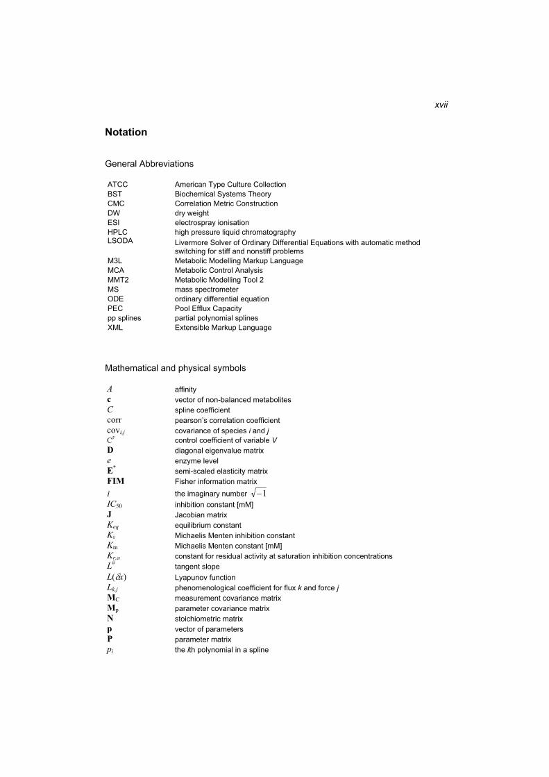
General Abbreviations
ATCC American Type Culture Collection BST Biochemical Systems Theory CMC Correlation Metric Construction DW dry weight ESI electrospray ionisation HPLC high pressure liquid chromatography LSODA Livermore Solver of Ordinary Differential Equations with automatic method
switching for stiff and nonstiff problems M3L Metabolic Modelling Markup Language MCA Metabolic Control Analysis MMT2 Metabolic Modelling Tool 2 MS mass spectrometer ODE ordinary differential equation PEC Pool Efflux Capacity pp splines partial polynomial splines XML Extensible Markup Language
Mathematical and physical symbols
A affinityc vector of non-balanced metabolites C spline coefficient corr pearson’s correlation coefficient covi,j covariance of species i and jCV control coefficient of variable VD diagonal eigenvalue matrix e enzyme level E* semi-scaled elasticity matrix FIM Fisher information matrix i the imaginary number 1IC50 inhibition constant [mM] J Jacobian matrix Keq equilibrium constant Ki Michaelis Menten inhibition constant Km Michaelis Menten constant [mM] Kr,a constant for residual activity at saturation inhibition concentrations L# tangent slope L( x) Lyapunov function Lk,j phenomenological coefficient for flux k and force jMC measurement covariance matrix Mp parameter covariance matrix N stoichiometric matrix p vector of parameters P parameter matrix pi the ith polynomial in a spline
xviii
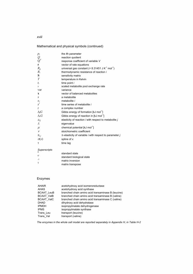
Mathematical and physical symbols (continued)
pi the ith parameter Q reaction quotient QV response coefficient of variable Vr vector of rate equations Rg universal gas constant (= 8.31451 J K-1 mol-1)Ri thermodynamic resistance of reaction iS sensitivity matrix T temperature in Kelvin ti time point iv scaled metabolite pool exchange rate var variance x vector of balanced metabolites x a metabolite xi metabolite ixi time series of metabolite iz a complex number
fG Gibbs energy of formation [kJ mol-1]rG Gibbs energy of reaction in [kJ mol-1]i,j elasticity of reaction i with respect to metabolite j
eigenvalue chemical potential [kJ mol-1]stoichiometric coefficient
i,j -elasticity of variable i with respect to parameter j(x) spline of x
time lag
Superscripts0 standard state 0’ standard biological state -1 matrix inversion T matrix transpose
Enzymes
AHAIR acetohydroxy acid isomeroreductase AHAS acetohydroxy acid synthase BCAAT_LeuB branched chain amino acid transaminase B (leucine) BCAAT_ValB branched chain amino acid transaminase B (valine) BCAAT_ValC branched chain amino acid transaminase C (valine) DHAD dihydroxy acid dehydratase IPMDH isopropylmalate dehydrogenase IPMS isopropylmalate synthase Trans_Leu transport (leucine) Trans_Val transport (valine)
The enzymes in the whole cell model are reported separately in Appendix H, in Table H-2
xix
Metabolites
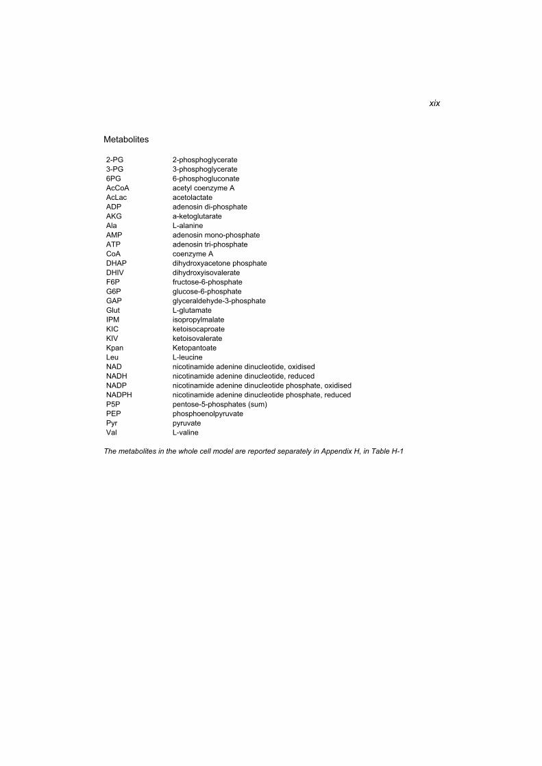
2-PG 2-phosphoglycerate 3-PG 3-phosphoglycerate 6PG 6-phosphogluconate AcCoA acetyl coenzyme A AcLac acetolactate ADP adenosin di-phosphate AKG a-ketoglutarate Ala L-alanine AMP adenosin mono-phosphate ATP adenosin tri-phosphate CoA coenzyme A DHAP dihydroxyacetone phosphate DHIV dihydroxyisovalerate F6P fructose-6-phosphate G6P glucose-6-phosphate GAP glyceraldehyde-3-phosphate Glut L-glutamate IPM isopropylmalate KIC ketoisocaproate KIV ketoisovalerate Kpan Ketopantoate Leu L-leucine NAD nicotinamide adenine dinucleotide, oxidised NADH nicotinamide adenine dinucleotide, reduced NADP nicotinamide adenine dinucleotide phosphate, oxidised NADPH nicotinamide adenine dinucleotide phosphate, reduced P5P pentose-5-phosphates (sum) PEP phosphoenolpyruvate Pyr pyruvate Val L-valine
The metabolites in the whole cell model are reported separately in Appendix H, in Table H-1

1 Introduction 1
1 Introduction
1.1 The Cellular Reaction System
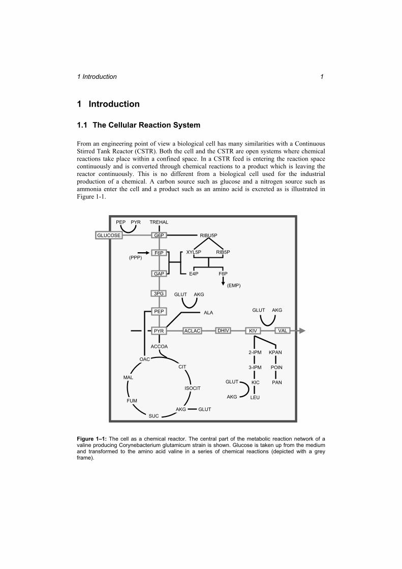
From an engineering point of view a biological cell has many similarities with a Continuous Stirred Tank Reactor (CSTR). Both the cell and the CSTR are open systems where chemical reactions take place within a confined space. In a CSTR feed is entering the reaction space continuously and is converted through chemical reactions to a product which is leaving the reactor continuously. This is no different from a biological cell used for the industrial production of a chemical. A carbon source such as glucose and a nitrogen source such as ammonia enter the cell and a product such as an amino acid is excreted as is illustrated in Figure 1-1.
GLUCOSE RIBU5P
XYL5P RIB5P
E4P F6P
G6P
3PG
PEP
TREHAL
AKGSUC
FUM
MAL
OAC
ISOCIT
CIT
ACCOA
ACLAC DHIV KIV VAL
GLUT AKG
GLUT
AKG
3-IPM
KPAN
POIN
LEU
2-IPM
KIC PAN
ALA
GLUT AKG
F6P
GAP
PYR
(EMP)
(PPP)
PEP PYR
GLUT
GLUCOSE RIBU5P
XYL5P RIB5P
E4P F6P
G6P
3PG
PEP
TREHAL
AKGSUC
FUM
MAL
OAC
ISOCIT
CIT
ACCOA
ACLAC DHIV KIV VAL
GLUT AKG
GLUT
AKG
3-IPM
KPAN
POIN
LEU
2-IPM
KIC PAN
ALA
GLUT AKG
F6P
GAP
PYR
(EMP)
(PPP)
PEP PYR
GLUT
Figure 1–1: The cell as a chemical reactor. The central part of the metabolic reaction network of a valine producing Corynebacterium glutamicum strain is shown. Glucose is taken up from the medium and transformed to the amino acid valine in a series of chemical reactions (depicted with a grey frame).
1 Introduction 2
The difference between a cell and a CSTR lies first of all in the complexity of the reaction system. A bacterial cell contains several hundred different chemical species (metabolites) that react with each other through a reaction network where each metabolite may take part in many different reactions. Each reaction is catalysed by an enzyme which is specific to that reaction. The activity of the enzymes, and therefore the reaction rates, are regulated through allosteric effects so also metabolites that are not reaction partners in a reaction can influence the reaction rate. It is therefore not so useful to think of metabolism as a number of independent reactions, rather it is a highly interconnected reaction network of metabolites that interact in a complex manner. The complexity, in combination with the often poor observability of the intracellular concentrations, sets additional requirements to the analysis of a cellular reaction system. However, within applications in industrial biotechnology the cell can be thought of as a complex chemical reactor.
In order to understand the reaction network that constitutes cellular metabolism, it must be analysed as a system. Detailed knowledge of the individual parts of the metabolic system is in itself not enough, the information must also be integrated to explain the behaviour of the system since all parts interact with each other. This line of thought has gained increasing recognition in recent years and has led to the birth of Systems Biology. Systems Biology is a new scientific field which attempts to utilise all available data on genes, proteins and biochemical reactions in order to unravel the logic that underlie cellular processes. Leroy Hood, the president of the Institute of Systems Biology in Seattle has defined Systems Biology as “... the science of discovering, modelling, understanding and ultimately engineering at the molecular level the dynamic relationship between the biological molecules that define living organisms” (www.systemsbiology.org). Systems Biology takes a holistic approach rather than the reductionist approach often taken in molecular biology. The idea of holistic thinking can be applied to all fields of science and goes back to Aristotle who, in his work Metaphysics, states that “the whole is more than the sum of its parts”. The fundamental idea in Systems Biology is that “the cell is more than the sum of its genes, enzymes and metabolites”.
Understanding the reaction systems in cells is important not only in providing insight into the biology of cells in general, but is also central in the field of Metabolic Engineering. This discipline deals with the improvement of cellular activities by manipulation of enzymatic, transport and regulatory functions of the cell with the use of recombinant DNA technology (Bailey, 1991). The methods of Metabolic Engineering are often applied in order to increase the productivity of industrial production strains or to introduce new pathways in microorganisms with the aim of producing novel metabolites. Manipulation of metabolic systems was traditionally achieved through random mutation and selection and in this way the productivity of for instance the Penicillium chrysogenum strains used for penicillin production was increased more than 500 times from that of the original strains (Nielsen, 1998). While this approach of trial and error has proved to be fruitful, it is relatively labour intensive and slow, and may lead to an accumulation of unwanted mutations. With the rapid development of recombinant DNA technology, it became possible to introduce specific, targeted changes to the genome and the discipline of Metabolic Engineering emerged. However, given the high degree of complexity in metabolic systems it is seldom intuitively clear which genetic alterations will provide the desired change in phenotype. Thus there is a need for rigorous methods in order to obtain the detailed understanding required.
In the presented work a recombinant Corynebacterium glutamicum strain for the production of valine is used as a model organism. Corynebacterium glutamicum is an aerobic gram-positive bacterium widely used for the industrial production of amino acids, especially glutamate and lysine (Eggeling and Sahm, 1999; de Graaf, 2000). Its metabolism has therefore been the subject of extensive research (Sahm et al., 2000) and its complete genome has been sequenced (Kalinowski et al., 2003). Besides glutamate and lysine, valine also
1.2 Metabolomics 3
represents a commercially interesting product with applications in the cosmetic and pharmaceutical industry. The annual world production of valine in 2001 was about 500 tons (Eggeling et al., 2001).
1.2 Metabolomics
The importance of metabolomics in the quantitative understanding of biological systems has gained increasing recognition in recent years and metabolomics is now acknowledged as a key technology in Systems Biology (Weckwerth, 2003). Since the intracellular concentrations are the variables of biological reaction networks, accurate measurements of these concentrations are essential. In particular, the observation of how the intracellular concentrations change in response to changes in the extracellular environment can provide an understanding of the reaction system and give insight into the functionality of the enzymes in the cell. Such data may be interpreted directly using statistical methods, or they may form the experimental basis of a mathematical model of the metabolism.
With the continuous improvement of accurate analytical devices such as mass spectrometers, the field of metabolomics has developed rapidly. Even so, metabolomics is still in its early phase of development. Only a relatively small proportion of the 600 – 700 metabolites present in a Corynebacterium glutamicum cell grown on minimal medium can be quantified with reasonable accuracy (Strelkov et al. 2004). The pentose phosphate pathway intermediate erythrose-4-phosphate (E4P), for instance, is the precursor of the aromatic amino acids and is therefore a central metabolite in the metabolism, but to date this metabolite proves difficult to measure due to its chemical instability (Williams et al., 1980; Ruijter and Visser, 1999). A method for measuring this metabolite was developed at the Research Centre Jülich recently. However, the limited number of metabolites that can be accurately measured is a restricting factor in setting up kinetic models.
A technique referred to as a stimulus-response experiment (Oldiges and Takors, 2005) or a pulse experiment (Theobald et al., 1993 and 1997; Weuster-Botz, 1997) provides data particularly useful for the identification of kinetic models of the metabolism (Oldiges and Takors, 2005). The concentration of an extracellular metabolite, typically glucose, is rapidly increased in the culture and the response in the cells is measured by collecting samples using a rapid sampling technique with immediate quenching of the metabolism and subsequent extraction and chemical analysis of the intracellular metabolite concentrations. In this way the metabolism in the cell is shifted away from its steady state, and time series of the intracellular metabolite concentrations during the transient state are obtained. The quality and usefulness of the data depends on the state of the bacterial culture at the time of the glucose addition and thus on the fermentation preceding the experiment.
The valine / leucine pathway is particularly suitable for this type of investigations because it can be expected that the glucose stimulus will have a strong effect on the valine / leucine pathway leading to large changes in the concentrations of the pathway intermediates. Glucose is taken up by the phosphotransferase system which converts one molecule of phosphoenol-pyruvat to pyruvate for every glucose molecule that passes the membrane. The glucose stimulus will therefore have a direct effect on the pyruvate concentration. Since the valine / leucine pathway starts with two pyruvate molecules condensing to form one acetolactate molecule, the first intermediate in the pathway, acetolactate should be particularly sensitive to changes in the pyruvate concentration and thus to the glucose stimulus.
1 Introduction 4
1.3 Modelling and Simulation
Given the complexity of metabolic reaction networks a mathematical model is clearly an essential tool in order to understand the network as a system (Bailey, 1998; Wiechert, 2002). Once a model describing the reaction kinetics and the intracellular metabolite concentrations of the metabolic network is established, the complexity becomes manageable and the network can be understood at a new level. An adequate kinetic model can be used not only to analyse the control hierarchy in the reaction system at the enzyme level, but can also give quantitative predictions of the change in fluxes and concentrations following a change in an enzyme activity. Thus mathematical modelling has become one of the most important techniques in Metabolic Engineering (Nielsen, 1998).
Several structured kinetic models of in-vivo metabolic networks describing the metabolite dynamics at the enzyme level have been developed during the last decade. These studies include the penicillin pathway in Penicillium chrysogenum (Pissara et al., 1996), glycolysis and the pentose phosphate pathway in Saccharomyces cerevisiae (Rizzi et al., 1997 and Vaseghi et al., 1999), the lysine pathway in Corynebacterium glutamicum (Yang et al., 1999), the central carbon metabolism in Escherichia coli (Chassagnole et al., 2002) and many others (Olivier and Snoep, 2004).
Although many enzymes have undergone extensive investigation in-vitro, there is little data available in literature on the in-vivo kinetic properties since the exact in-vivo conditions are difficult or even impossible to reproduce in-vitro. Kinetic constants such as Michaelis - Menten constants found in-vitro for instance can not be assumed to be valid for the in-vivo conditions (Wright and Kelly, 1981; Teusink et al., 2000), because they are normally measured at different a pH, different ion concentrations, and without the influence of the many other species present in the cytosol. Therefore, model-based analysis is an appropriate way to extract mechanistic understanding of experimental observations of the intracellular metabolite concentrations ultimately aiming at the understanding of the in-vivo kinetics. Kinetic modelling can be seen as a complex in-vivo enzyme study where many enzymes are investigated simultaneously and where their function as parts of a reaction system is analysed.
In a kinetic model each modelled reaction rate must be assigned a rate equation. These are most commonly based on the enzyme reaction mechanism. Recently a non-mechanistic rate equation, the so-called linlog kinetic equation, was suggested used for metabolic modelling (Hatzimanikatis et al., 1996 and 1998; Hatzimanikatis and Bailey, 1997; Visser and Heijnen, 2003). This type of kinetic equation is based only on the stoichiometry and the allosteric regulation of the enzyme so the information about the order at which the substrates and products bind to and leave from the enzyme is lost. However, it was demonstrated that this type of kinetics was able to describe the dynamics of metabolic pathways well, and that it was also suitable for design. (Visser et al., 2004a). An advantage of the linlog approach is that fewer parameters are required in the model, and that the parameters are easy to interpret.
A kinetic model should be set up according to the experimental data available for model identification. One could argue that a model should not contain any metabolites or reactions for which there are no experimental data available to verify the simulated concentrations or to fit the parameters of the reaction rates. Also, including metabolites that have not been measured increases the parameter space of the model without increasing the empirical basis, which can result in a loss of accuracy and predictive power. However, excluding central metabolites means that one misses feedforward or feedback effects resulting from the stoichiometry and the regulatory structure of the network. The modeller is therefore forced to make a compromise and must build the model he considers most relevant taking the network under study, the available measurements and the intended purpose of the model into account.
1.4 Metabolic Control Analysis 5
1.4 Metabolic Control Analysis
The cell controls its intracellular metabolite concentrations and fluxes by regulating the rates of the reactions in the cell. The activities of the enzymes catalysing the reactions in the network are controlled at the metabolome level through inhibition and activation effects. In addition the transcription and translation of the genome for the synthesis of new enzymes is controlled through various regulation mechanisms. These intricate control mechanisms make it possible for the cell for example to adapt its metabolism to a wide range of extracellular conditions, to grow on different energy sources, to coordinate the synthesis of all 20 amino acids as required for protein assembly and to avoid an uncontrolled rise or fall of intracellular metabolite concentrations which would be damaging to the cell. The theoretical framework that is used to analyse this control structure in a quantitative manner is referred to as Metabolic Control Analysis (MCA). Through MCA an understanding of the control of the system as a whole can be obtained, something which can not be achieved by analysing the system components separately. Since the enzymes with the highest control of a flux will be the target enzymes in a metabolic engineering project, MCA is one of the most important techniques in the analytical part of metabolic engineering.
The theory of MCA was developed by Kacser and Burns (1973) and Heinrich and Rapoport (1974). Later, a common nomenclature was agreed on which has been the standard since then (Burns et al., 1985). By using sensitivity analysis MCA provides a measure for the extent of control that the system parameters have on the fluxes and metabolite concentrations in the network. In this way the level of control that a specific enzyme activity has on the flux through the entire pathway can be obtained. The strength of MCA lies in its ability to analyse the global properties of the reaction system. Furthermore, the conclusions of MCA are quantitative, i.e. rather than the qualitative conclusions typically reached by more intuitive approaches, MCA gives a quantitative description of how the control is distributed on the various system components and parameters.
The analysis of an intracellular reaction network requires information on the in-vivo functionality of the participating enzymes. Some knowledge, on for example reaction mechanisms, can be obtained by in-vitro enzyme studies, but in general some type of in-vivo experimental data must be available.
1.5 Thermodynamic Analysis
The simplicity and fundamental nature of thermodynamics makes it a universally applicable theory with a great power of explaining physical phenomena. This was recognised for example by Albert Einstein who referred to thermodynamics as “… the only physical theory of universal content concerning which I am convinced that, within the framework of applicability of its basic concepts, it will never be overthrown” (Einstein, 1949). Thermodynamics therefore has a great potential as a method of analysing cellular reaction networks which are both complex and difficult to observe. In particular, thermodynamics can contribute to the understanding of how a metabolic network functions as a system. As such, thermodynamics becomes an important tool for metabolic engineering.
A biological cell is a prime example of an open thermodynamic system where mass and energy can flow over the system boundary. The branch of thermodynamics dealing with open systems is called non-equilibrium thermodynamics since such systems will contain non-zero thermodynamic forces and will therefore not be at equilibrium. Non-equilibrium thermodynamics was developed from classical thermodynamics and focuses primarily on the entropy production in irreversible processes. The first step in developing the theory of non-
1 Introduction 6
equilibrium thermodynamics was taken by Lars Onsager when he published his reciprocal relations in irreversible processes (Onsager, 1930 and 1931). Later the theory was developed further by Ilya Prigogine with the analysis of dissipative structures (Prigogine and Lefever, 1968). Both Onsager and Prigogine received the Nobel Prize in chemistry for their contributions (Onsager in 1968 and Prigogine in 1977).
In some of the more recent publications various aspects of metabolic networks are investigated by applying thermodynamic principles. Examples include the feasibility analysis of biochemical pathways based on the Gibbs free energy of the reactions (Mavrovouniotis 1993 and 1996), the combination of an energy balance with the traditional material balances in a metabolic flux analysis (Beard et al., 2002 and 2004), the inclusion of thermodynamic considerations in metabolic network analysis (Schilling et al., 2000; Holzhütter 2004; Hatzimanikatis et al., 2005), metabolic control analysis based on a thermokinetic description of the reaction rates (Nielsen 1997) and the inclusion of thermodynamic constraints in the development of kinetic models (Magnus et al., 2006). Qian and Beard also suggested a link between the level of gene expression and the ratio of flux to Gibbs free energy of reaction (Qian et al., 2003) and provided a more general thermodynamic formalism for the study of biochemical reaction networks (Qian and Beard 2005). Thermodynamic principles were applied in the investigation of real systems such as the pathways for penicillin production in Penicillium chrysogenum (de Noronha Pissarra and Nielsen 1997), the complete E. colimetabolism (Beard et al., 2002) and the regulation and control structure in hepatocyte metabolism (Beard and Qian 2005).
1.6 Objective
In the presented thesis the intracellular reaction network of the valine synthesis pathway in a recombinant Corynebacterium glutamicum is analysed and modelled. Special focus is set on the valine / leucine biosynthesis pathway. The overall aim is to gain a systemic understanding of the dynamic behaviour of this reaction system and to develop the general methods required for such investigations. In this respect the investigation follows the holistic philosophy of Systems Biology. The investigation also aims to use the acquired understanding to identify the target enzymes for further strain optimisation and therefore constitutes the analytical part of a metabolic engineering project of this strain. It is the first time that such an investigation has been carried out for the valine / leucine pathway.
It should be noted that the investigation analyses the reaction system on the metabolome level. The analysis of the genome, the transcriptome and the proteome is not part of the investigation presented here.
More specifically the part aims are formulated as follows:
Metabolomics:
- To establish the optimal experimental procedure for a glucose stimulus experiment with respect to obtaining a useful data set for the modelling and further analysis.
- To monitor the intracellular concentrations in the valine / leucine pathway and the central metabolism during the transient state following a glucose stimulus experiment.
- To investigate the applicability of a statistical method (a time series analysis) to analyse the connectivities of the metabolites in the network based on the measured metabolite time courses.
- To compare the effect of a glucose stimulus on the cell at two different physiological states.
1.6 Objective 7
Modelling and simulation:
- To establish a kinetic model that describes the reaction dynamics of the valine / leucine pathway.
- To develop further methods for dynamic modelling of metabolic reaction networks. - To test the applicability of mechanistic and linlog reaction rate equations for dynamic
models.- To develop a whole cell model of the Corynebacterium glutamicum strain and test the
whole cell modelling approach with the metabolome data.
Metabolic Control Analysis:
- To investigate the control hierarchy in the valine / leucine pathway and obtain quantitative measures for control by using the classical theory of MCA as well as other data driven and model based methods.
- To identify the target enzymes for the further strain optimisation.
Thermodynamic analysis:
- To analyse the role of the thermodynamic forces in metabolic reaction networks and to establish the required methods based on the principles of non-equilibrium thermodynamics.
Metabolomics
Quantitative description of metabolism and flux control
Identification of targets for strain optimisation
Thermodynamicanalysis
Metabolic ControlAnalysis
Modelling andsimulation
1. Observation
2. Interpretation
3. Understanding
4. Application
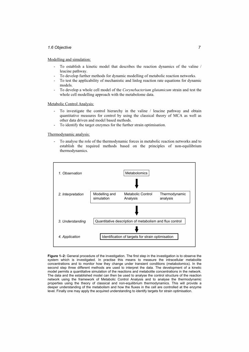
Figure 1–2: General procedure of the investigation. The first step in the investigation is to observe the system which is investigated. In practise this means to measure the intracellular metabolite concentrations and to monitor how they change under transient conditions (metabolomics). In the second step three different methods are used to interpret the data. The development of a kinetic model permits a quantitative simulation of the reactions and metabolite concentrations in the network. The data and the established model can then be used to analyse the control structure of the reaction network using the framework of Metabolic Control Analysis and to analyse the thermodynamic properties using the theory of classical and non-equilibrium thermodynamics. This will provide a deeper understanding of the metabolism and how the fluxes in the cell are controlled at the enzyme level. Finally one may apply the acquired understanding to identify targets for strain optimisation.
1 Introduction 8
1.7 Structure of the Thesis
There are four central topics in this study. These are: Metabolomics, Modelling and Simulation, Metabolic Control Analysis and Thermodynamic Analysis. Methods from these disciplines are used to achieve the overall aim of the thesis as explained in Figure 1-2. Each of the four disciplines builds on each other and is part of an integrated study.
In Chapter 2 the materials used in the investigation are described. Chapter 3 and 4 present the experimental and theoretical methods and also describe how these methods were used within the investigation. Chapters 5, 6, 7 and 8 then presents the results achieved within Metabolomics, Modelling and Simulation, Metabolic Control Analysis and Thermodynamic Analysis respectively.
During the course of the investigation several modelling strategies were used for the development of the model. The optimal model with respect to the overall aim turned out to be a linlog model of the valine and leucine synthesis pathways. This model is presented as the main result in the modelling and simulation part in Chapter 6. In Chapter 9 two other models, namely a mechanistic model of the valine / leucine pathways and a model of the whole metabolism of Corynebacterium glutamicum, are presented.
Each of the chapters 5 – 9 present the results and also give a discussion of these within each of the sub topics. In Chapter 10 a general, overall discussion and conclusion of the results is given as well as an outlook on what results can be achieved in the future.
2 Materials 9
2 Materials
2.1 Strain
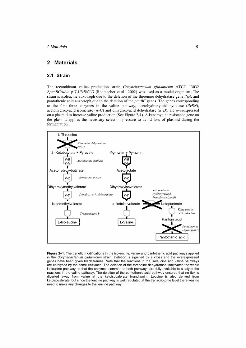
The recombinant valine production strain Corynebacterium glutamicum ATCC 13032 panBC ilvA pJC1ilvBNCD (Radmacher et al., 2002) was used as a model organism. The
strain is isoleucine auxotroph due to the deletion of the threonine dehydratase gene ilvA, and pantothenic acid auxotroph due to the deletion of the panBC genes. The genes corresponding to the first three enzymes in the valine pathway, acetohydroxyacid synthase (ilvBN), acetohydroxyacid isomerase (ilvC) and dihydroxyacid dehydratase (ilvD), are overexpressed on a plasmid to increase valine production (See Figure 2-1). A kanamycine resistance gene on the plasmid applies the necessary selection pressure to avoid loss of plasmid during the fermentation.
Figure 2–1: The genetic modifications in the isoleucine, valine and pantothenic acid pathways applied in the Corynebacterium glutamicum strain. Deletion is signified by a cross and the overexpressed genes have been given black frames. Note that the reactions in the isoleucine and valine pathways are catalysed by the same enzymes. The deletion of the threonine dehydratase inactivates the whole isoleucine pathway so that the enzymes common to both pathways are fully available to catalyse the reactions in the valine pathway. The deletion of the pantothenic acid pathway ensures that no flux is diverted away from valine at the ketoisovalerate branchpoint. Leucine is also derived from ketoisovalerate, but since the leucine pathway is well regulated at the transcriptome level there was no need to make any changes to the leucine pathway.
L-Isoleucine
L-Threonine
2- Ketobutyrate + Pyruvate
Acetohydroxybutyrate
Dihydroxymethylvalerate
Ketomethylvalerate
ilvA
ilvBilvN
ilvC
ilvD
Pyruvate + Pyruvate
Acetolactate
Dihydroxyisovalerate
ketoisovalerate
ilvBilvN
ilvC
ilvD
Acetolactate synthase
Isomeroreductase
Dihydroxyacid dehydratase
L-Valine
Transaminase B
Threonine dehydratase(ilvA)
panB Ketopantoate
Pantoin acid
Pantothenic acid
panC
KetopantoateHydroxymethylTransferase (panB)
Ketopantoinacid reductase
PantothenateLigase (panC)
2 Materials 10
2.2 Cultivation medium
A complex medium based on yeast extract (LB-medium) was used for the precultures. For the main fermentations the mineral medium CGXII (Keilhauer et al., 1993) was used. Supplementary trace elements were added according to Weuster-Botz et al. (1997). In addition, the medium contained 0.24 mg/l pantothenic acid, 0.144 g/l isoleucine and 25 mg/l of the antibiotic kanamycine. The exact composition of the different media is listed in Table A1 and A2 in Appendix A. Antifoam S289 from Sigma was used to control foam formation.
2.3 Rapid sampling apparatus
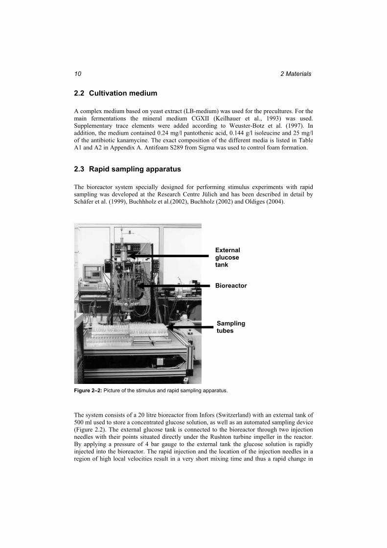
The bioreactor system specially designed for performing stimulus experiments with rapid sampling was developed at the Research Centre Jülich and has been described in detail by Schäfer et al. (1999), Buchhholz et al.(2002), Buchholz (2002) and Oldiges (2004).
Figure 2–2: Picture of the stimulus and rapid sampling apparatus.
The system consists of a 20 litre bioreactor from Infors (Switzerland) with an external tank of 500 ml used to store a concentrated glucose solution, as well as an automated sampling device (Figure 2.2). The external glucose tank is connected to the bioreactor through two injection needles with their points situated directly under the Rushton turbine impeller in the reactor. By applying a pressure of 4 bar gauge to the external tank the glucose solution is rapidly injected into the bioreactor. The rapid injection and the location of the injection needles in a region of high local velocities result in a very short mixing time and thus a rapid change in
Bioreactor
Samplingtubes
Externalglucosetank
2.4 Analytical devices 11
glucose concentration in the bioreactor. In the experiments described in this thesis the working volume was 7 litres and 50 ml of a 500 g/l glucose solution was injected to stimulate the metabolism. Under these conditions the 90 % mixing time in the bioreactor was 650 ms (Buchholz et al. 2002) and an increase in glucose concentration of 3.5 g/l was achieved.
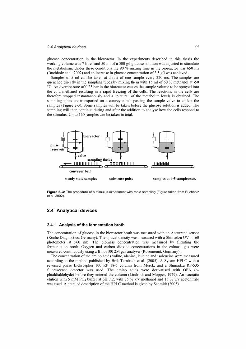
Samples of 5 ml can be taken at a rate of one sample every 220 ms. The samples are quenched directly in the sampling tubes by mixing them with 15 ml of 60 % methanol at -50 °C. An overpressure of 0.23 bar in the bioreactor causes the sample volume to be sprayed into the cold methanol resulting in a rapid freezing of the cells. The reactions in the cells are therefore stopped instantaneously and a “picture” of the metabolite levels is obtained. The sampling tubes are transported on a conveyor belt passing the sample valve to collect the samples (Figure 2-3). Some samples will be taken before the glucose solution is added. The sampling will then continue during and after the addition to analyse how the cells respond to the stimulus. Up to 160 samples can be taken in total.
Figure 2–3: The procedure of a stimulus experiment with rapid sampling (Figure taken from Buchholz et al. 2002).
2.4 Analytical devices
2.4.1 Analysis of the fermentation broth
The concentration of glucose in the bioreactor broth was measured with an Accutrend sensor (Roche Diagnostics, Germany). The optical density was measured with a Shimadzu UV – 160 photometer at 560 nm. The biomass concentration was measured by filtrating the fermentation broth. Oxygen and carbon dioxide concentrations in the exhaust gas were measured continuously using a Binos100 2M gas analyser (Rosemount, Germany).
The concentration of the amino acids valine, alanine, leucine and isoleucine were measured according to the method published by Brik Ternbach et al. (2005). A Sycam HPLC with a reversed phase Lichrospher 100 RP 18-5 column from Merck, and a Shimadzu RF-535 fluorescence detector was used. The amino acids were derivatised with OPA (o-phtaldialdehyde) before they entered the column (Lindroth and Mopper, 1979). An isocratic elution with 5 mM PO4 buffer at pH 7.2, with 35 % v/v methanol and 15 % v/v acetonitrile was used. A detailed description of the HPLC method is given by Schmidt (2005).
2 Materials 12
The organic acids lactate, acetate, a-ketoglutarate and ketoisovalerate were measured using an Aminex HPX-87H column (Biorad, Germany) eluted at 40°C with 0.2 M H2SO4 with detection by UV adsorption at 215 nm.
2.4.2 Mass spectrometry
Ion trap MS The apparatus consisted of an HPLC connected to a single quadrupole ion trap mass spectrometer. The MS part consisted of a LCQ Thermoquest mass spectrometer with an electrospray ionisation (ESI) ion source. The HPLC apparatus was from Gynkotek/Dionex and consisted of an ASI100-T Dionex programmable autosampler, an M480 Gynkotek gradient/elution pump run at 25°C and a UVD Dionex diode array detector capable of UV measurements at wavelengths between 200 and 595 nm. The software Chromeleon 6.4 (Dionex) and Excalibur 1.3 (ThermoFinnigan) were used for controlling, data acquisition and data evaluation for the HPLC and the MS parts respectively. A syringe connected to the MS allowed manual direct injection of sample when this was required.
The apparatus was run according to a method developed by Buchholz (Buchholz et al., 2001; Buchholz, 2002). The sample flow rate entering the MS was 40 l/min. Additional methanol was added directly to the ionisation chamber using a separate HPLC pump at a rate of 25 l/min. Nitrogen was provided by a 2000-40 Jun-Air oil free air compressor with an ECO-Inert ESP2 DWT membrane filtration unit and used as sheath and auxiliary gas in the mass spectrometer. Helium was used as collision gas in the ion trap.
Triple quadrupole MS from ThermoFinnigan An Agilent 1100 HPLC from Agilent Technologies was used in connection with the triple quadrupole TSQ Quantum mass spectrometer with ESI ionisation source from ThermoFinnigan. The HPLC device had a programmable HTC Pal autosampler from CTC Analytics. The software Excalibur (ThermoFinnigan) was used for controlling, data acquisition and data evaluation.
The sample flow rate was 100 l/min. Nitrogen was provided by the same type of equipment as for the ion trap MS and used as sheath and auxiliary gas. The temperature of the capillary was 375°C and the voltage used in the ionisation was 4.0 kV. The collision gas was Argon.
Triple quadrupole MS from Applied Bioscience The system consisted of an Agilent 1100 HPLC system including a programmable autosampler from Agilent Technologies in connection with the 4000 Q Trap triple quadropole mass spectrometer from Applied Biosystems. The software Analyst (Applied Biosystems) was used for controlling, data aquisition and data evaluation.
The sample flow rate was 200 l/min. Nitrogen was used as curtain and collision gas. Air was used as auxiliary gas. The temperature of the capillary was 600 °C and the ionisation voltage was 4.5 kV.
A Short Discussion of the Principles of Mass Spectrometry A brief description of the most central parts of the mass spectrometers used in this thesis is given in the following. A more thorough treatment of these subjects is given by Buchholz (2002) and Oldiges (2005).
The first step in the mass spectrometer is the ionisation of the analytes. Electrospray ionisation (ESI) was used for all mass spectrometers. The principle of ESI is shown in Figure 2-4. The solution containing the analytes enters the ionisation chamber through a needle of about 0.1 mm diameter. It is then sprayed into the electrical field in the ionisation chamber and fine droplets are formed. The droplets contain the analytes as positive or negative ions according to the direction of the electrical field. As the solvent in the droplets evaporate, the
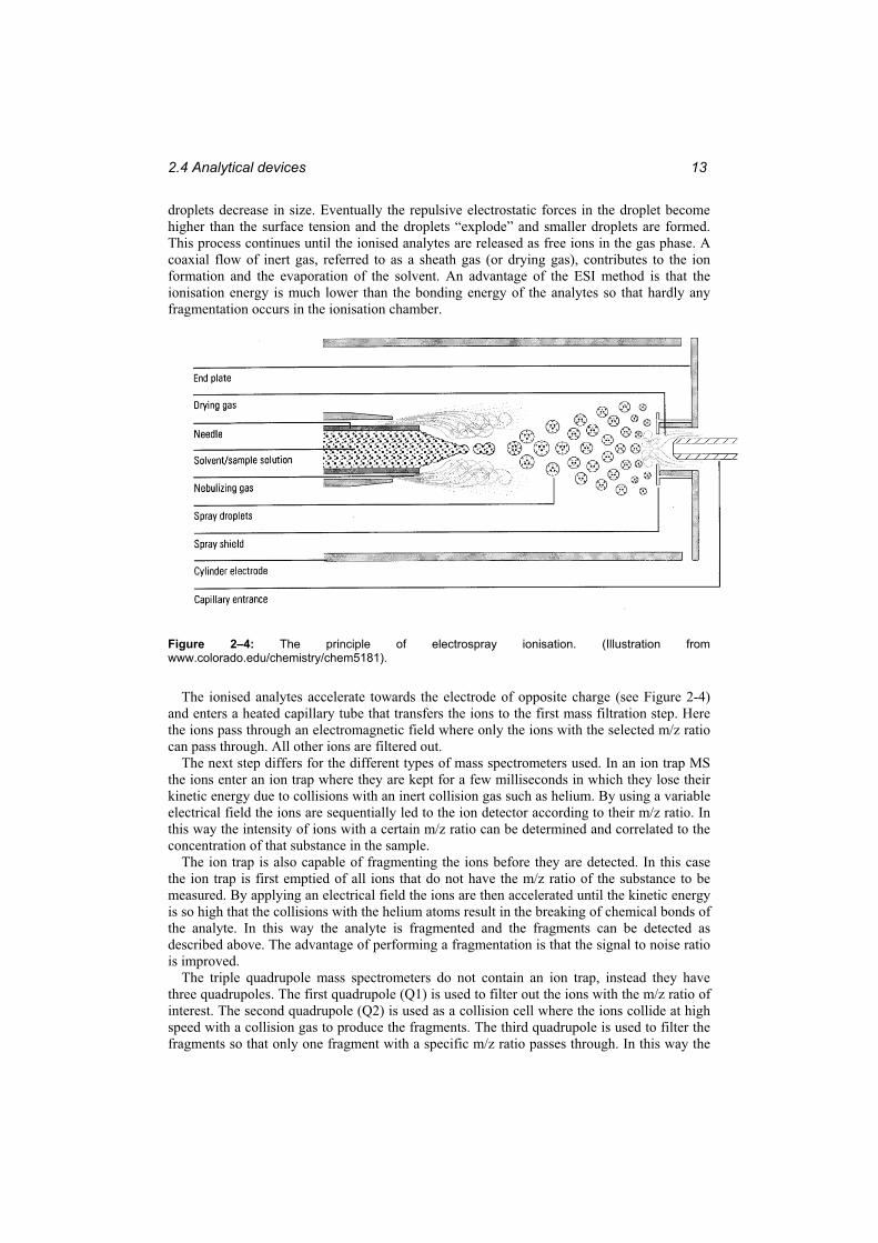
2.4 Analytical devices 13
droplets decrease in size. Eventually the repulsive electrostatic forces in the droplet become higher than the surface tension and the droplets “explode” and smaller droplets are formed. This process continues until the ionised analytes are released as free ions in the gas phase. A coaxial flow of inert gas, referred to as a sheath gas (or drying gas), contributes to the ion formation and the evaporation of the solvent. An advantage of the ESI method is that the ionisation energy is much lower than the bonding energy of the analytes so that hardly any fragmentation occurs in the ionisation chamber.
Figure 2–4: The principle of electrospray ionisation. (Illustration from www.colorado.edu/chemistry/chem5181).
The ionised analytes accelerate towards the electrode of opposite charge (see Figure 2-4) and enters a heated capillary tube that transfers the ions to the first mass filtration step. Here the ions pass through an electromagnetic field where only the ions with the selected m/z ratio can pass through. All other ions are filtered out.
The next step differs for the different types of mass spectrometers used. In an ion trap MS the ions enter an ion trap where they are kept for a few milliseconds in which they lose their kinetic energy due to collisions with an inert collision gas such as helium. By using a variable electrical field the ions are sequentially led to the ion detector according to their m/z ratio. In this way the intensity of ions with a certain m/z ratio can be determined and correlated to the concentration of that substance in the sample.
The ion trap is also capable of fragmenting the ions before they are detected. In this case the ion trap is first emptied of all ions that do not have the m/z ratio of the substance to be measured. By applying an electrical field the ions are then accelerated until the kinetic energy is so high that the collisions with the helium atoms result in the breaking of chemical bonds of the analyte. In this way the analyte is fragmented and the fragments can be detected as described above. The advantage of performing a fragmentation is that the signal to noise ratio is improved.
The triple quadrupole mass spectrometers do not contain an ion trap, instead they have three quadrupoles. The first quadrupole (Q1) is used to filter out the ions with the m/z ratio of interest. The second quadrupole (Q2) is used as a collision cell where the ions collide at high speed with a collision gas to produce the fragments. The third quadrupole is used to filter the fragments so that only one fragment with a specific m/z ratio passes through. In this way the
2 Materials 14
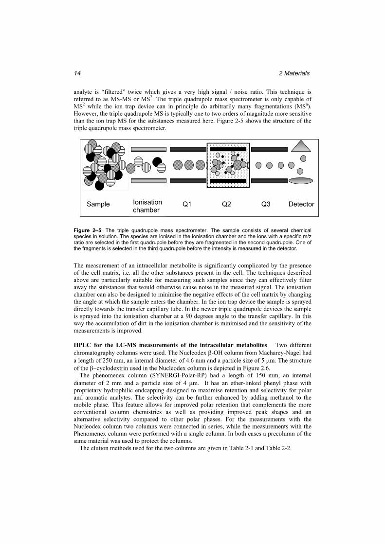
analyte is “filtered” twice which gives a very high signal / noise ratio. This technique is referred to as MS-MS or MS2. The triple quadrupole mass spectrometer is only capable of MS2 while the ion trap device can in principle do arbitrarily many fragmentations (MSn). However, the triple quadrupole MS is typically one to two orders of magnitude more sensitive than the ion trap MS for the substances measured here. Figure 2-5 shows the structure of the triple quadrupole mass spectrometer.
Figure 2–5: The triple quadrupole mass spectrometer. The sample consists of several chemical species in solution. The species are ionised in the ionisation chamber and the ions with a specific m/z ratio are selected in the first quadrupole before they are fragmented in the second quadrupole. One of the fragments is selected in the third quadrupole before the intensity is measured in the detector.
The measurement of an intracellular metabolite is significantly complicated by the presence of the cell matrix, i.e. all the other substances present in the cell. The techniques described above are particularly suitable for measuring such samples since they can effectively filter away the substances that would otherwise cause noise in the measured signal. The ionisation chamber can also be designed to minimise the negative effects of the cell matrix by changing the angle at which the sample enters the chamber. In the ion trap device the sample is sprayed directly towards the transfer capillary tube. In the newer triple quadrupole devices the sample is sprayed into the ionisation chamber at a 90 degrees angle to the transfer capillary. In this way the accumulation of dirt in the ionisation chamber is minimised and the sensitivity of the measurements is improved.
HPLC for the LC-MS measurements of the intracellular metabolites Two different chromatography columns were used. The Nucleodex -OH column from Macharey-Nagel had a length of 250 mm, an internal diameter of 4.6 mm and a particle size of 5 m. The structure of the cyclodextrin used in the Nucleodex column is depicted in Figure 2.6.
The phenomenex column (SYNERGI-Polar-RP) had a length of 150 mm, an internal diameter of 2 mm and a particle size of 4 m. It has an ether-linked phenyl phase with proprietary hydrophilic endcapping designed to maximise retention and selectivity for polar and aromatic analytes. The selectivity can be further enhanced by adding methanol to the mobile phase. This feature allows for improved polar retention that complements the more conventional column chemistries as well as providing improved peak shapes and an alternative selectivity compared to other polar phases. For the measurements with the Nucleodex column two columns were connected in series, while the measurements with the Phenomenex column were performed with a single column. In both cases a precolumn of the same material was used to protect the columns.
The elution methods used for the two columns are given in Table 2-1 and Table 2-2.
Q0 Q1 Q2 Q3Ionisationchamber
Q1 Q2 Q3 DetectorSample
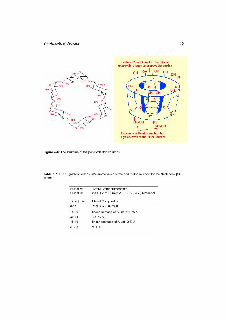
2.4 Analytical devices 15
Figure 2–6: The structure of the -cyclodextrin columns.
Table 2–1: HPLC gradient with 12 mM ammoniumacetate and methanol used for the Nucleodex -OHcolumn.
Eluent A: 12mM Ammoniumacetate Eluent B: 20 % ( v/ v ) Eluent A + 80 % ( v/ v ) Methanol
Time [ min ] Eluent Composition
0-14 2 % A and 98 % B
15-29 linear increase of A until 100 % A 30-44 100 % A 45-46 linear decrease of A until 2 % A
47-60 2 % A
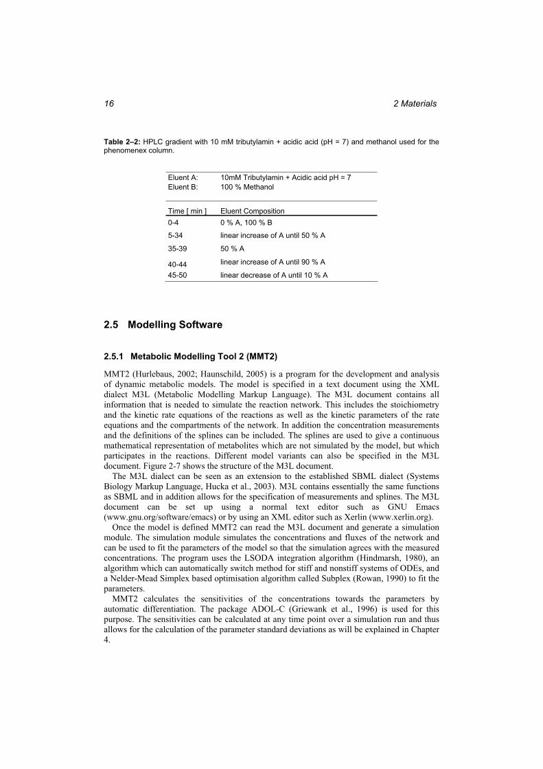
2 Materials 16
Table 2–2: HPLC gradient with 10 mM tributylamin + acidic acid (pH = 7) and methanol used for the phenomenex column.
Eluent A: 10mM Tributylamin + Acidic acid pH = 7 Eluent B: 100 % Methanol
Time [ min ] Eluent Composition 0-4 0 % A, 100 % B
5-34 linear increase of A until 50 % A
35-39 50 % A
40-44 linear increase of A until 90 % A
45-50 linear decrease of A until 10 % A
2.5 Modelling Software
2.5.1 Metabolic Modelling Tool 2 (MMT2)
MMT2 (Hurlebaus, 2002; Haunschild, 2005) is a program for the development and analysis of dynamic metabolic models. The model is specified in a text document using the XML dialect M3L (Metabolic Modelling Markup Language). The M3L document contains all information that is needed to simulate the reaction network. This includes the stoichiometry and the kinetic rate equations of the reactions as well as the kinetic parameters of the rate equations and the compartments of the network. In addition the concentration measurements and the definitions of the splines can be included. The splines are used to give a continuous mathematical representation of metabolites which are not simulated by the model, but which participates in the reactions. Different model variants can also be specified in the M3L document. Figure 2-7 shows the structure of the M3L document.
The M3L dialect can be seen as an extension to the established SBML dialect (Systems Biology Markup Language, Hucka et al., 2003). M3L contains essentially the same functions as SBML and in addition allows for the specification of measurements and splines. The M3L document can be set up using a normal text editor such as GNU Emacs (www.gnu.org/software/emacs) or by using an XML editor such as Xerlin (www.xerlin.org).
Once the model is defined MMT2 can read the M3L document and generate a simulation module. The simulation module simulates the concentrations and fluxes of the network and can be used to fit the parameters of the model so that the simulation agrees with the measured concentrations. The program uses the LSODA integration algorithm (Hindmarsh, 1980), an algorithm which can automatically switch method for stiff and nonstiff systems of ODEs, and a Nelder-Mead Simplex based optimisation algorithm called Subplex (Rowan, 1990) to fit the parameters.
MMT2 calculates the sensitivities of the concentrations towards the parameters by automatic differentiation. The package ADOL-C (Griewank et al., 1996) is used for this purpose. The sensitivities can be calculated at any time point over a simulation run and thus allows for the calculation of the parameter standard deviations as will be explained in Chapter 4.
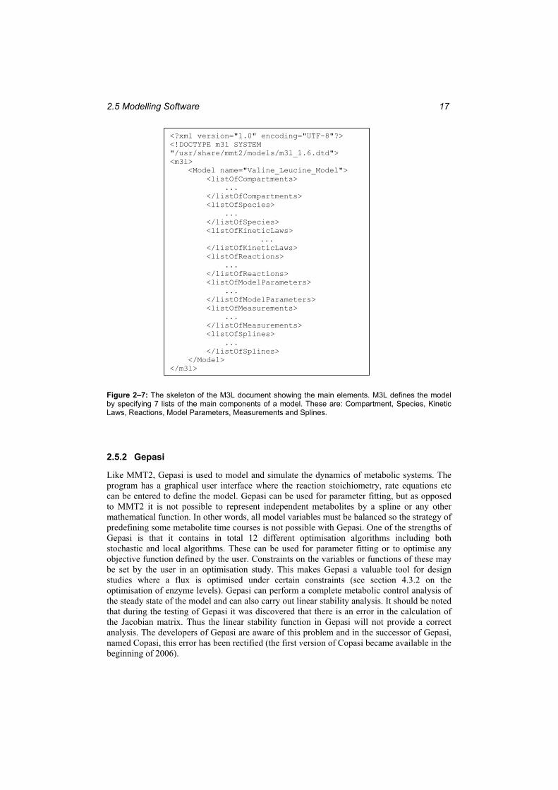
2.5 Modelling Software 17
Figure 2–7: The skeleton of the M3L document showing the main elements. M3L defines the model by specifying 7 lists of the main components of a model. These are: Compartment, Species, Kinetic Laws, Reactions, Model Parameters, Measurements and Splines.
2.5.2 Gepasi
Like MMT2, Gepasi is used to model and simulate the dynamics of metabolic systems. The program has a graphical user interface where the reaction stoichiometry, rate equations etc can be entered to define the model. Gepasi can be used for parameter fitting, but as opposed to MMT2 it is not possible to represent independent metabolites by a spline or any other mathematical function. In other words, all model variables must be balanced so the strategy of predefining some metabolite time courses is not possible with Gepasi. One of the strengths of Gepasi is that it contains in total 12 different optimisation algorithms including both stochastic and local algorithms. These can be used for parameter fitting or to optimise any objective function defined by the user. Constraints on the variables or functions of these may be set by the user in an optimisation study. This makes Gepasi a valuable tool for design studies where a flux is optimised under certain constraints (see section 4.3.2 on the optimisation of enzyme levels). Gepasi can perform a complete metabolic control analysis of the steady state of the model and can also carry out linear stability analysis. It should be noted that during the testing of Gepasi it was discovered that there is an error in the calculation of the Jacobian matrix. Thus the linear stability function in Gepasi will not provide a correct analysis. The developers of Gepasi are aware of this problem and in the successor of Gepasi, named Copasi, this error has been rectified (the first version of Copasi became available in the beginning of 2006).
<?xml version="1.0" encoding="UTF-8"?> <!DOCTYPE m3l SYSTEM "/usr/share/mmt2/models/m3l_1.6.dtd"><m3l> <Model name="Valine_Leucine_Model"> <listOfCompartments> ... </listOfCompartments> <listOfSpecies> ... </listOfSpecies> <listOfKineticLaws>
... </listOfKineticLaws> <listOfReactions> ... </listOfReactions> <listOfModelParameters> ... </listOfModelParameters> <listOfMeasurements> ... </listOfMeasurements> <listOfSplines> ... </listOfSplines> </Model> </m3l>
2 Materials 18
2.5.3 Jarnac
Jarnac is another simulation tool for metabolic models. Jarnac differs from Gepasi and MMT2 in that it supports a scripting language which allows users to directly interact with the computational engine. This makes Jarnac a very flexible tool which can be adapted to suit the needs of the user. The Jarnac language is similar to the Basic language and supports typical constructs such as for loops, conditionals, while/do and repeat/until. Jarnac has several built in functions such as dynamic simulation, steady state analysis, stability analysis, operators for matrix algebra as well as a full metabolic control analysis. Jarnac has no optimisation algorithms implemented and can not perform parameter fitting.
2.5.4 In-Silico Discovery
In-Silico Discovery is a graphically oriented program for developing and interpreting metabolic models. It is designed to be a general metabolic engineering tool and integrates many of the techniques used in the analytical part of metabolic engineering. It provides methods for model set up, topological analysis, metabolic flux analysis and dynamic simulation. The dynamic model is generated automatically from the stoichiometry of the reactions defined by the user. The dynamic model is set up using linlog equations for all reactions. It is not possible for the user to define the rate equations himself, thus only linlog models can be modelled with In-Silico Discovery. The program is intended to handle large models, i.e. models with more than 100 reactions. It uses evolutionary algorithms from the package JavaEvA (www-ra.informatik.uni-tuebingen.de/software/JavaEvA) and parallel computing for the parameter fitting.
The main advantage of In-Silico Discovery is its many tools for organising, structuring and validating the information in a model. This makes it particularly suitable for large scale modelling. A screen shot of the graphical user interface is given in Figure 2-8.
2.5.5 Comparison of the modelling software
MMT2, Gepasi and Jarnac were used for the development and interpretation of the model of the valine / leucine pathway. In general one can say that MMT2 is the optimal tool for model development and error analysis while Gepasi and Jarnac are better for the interpretation of the developed model. Gepasi is ideal for enzyme optimisation studies while Jarnac can be used for stability analysis and for calculating quantities which are not standard in systems biology such as the control coefficients of the thermodynamic properties which are introduced in Chapter 8. Both Gepasi and Jarnac can be used for classical metabolic control analysis. In-Silico Discovery is the most suitable program for large metabolic models and contains the most functions for the analysis and interpretation of developed models.
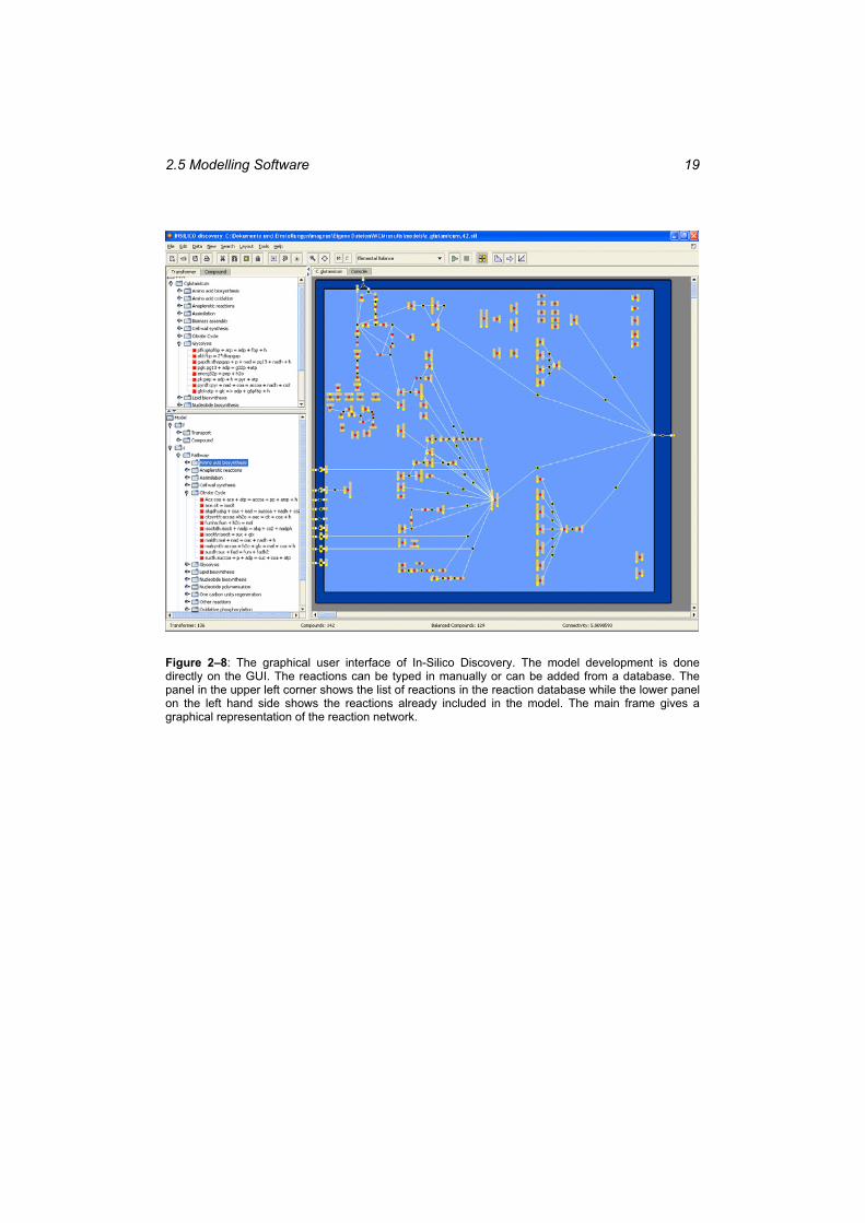
2.5 Modelling Software 19
Figure 2–8: The graphical user interface of In-Silico Discovery. The model development is done directly on the GUI. The reactions can be typed in manually or can be added from a database. The panel in the upper left corner shows the list of reactions in the reaction database while the lower panel on the left hand side shows the reactions already included in the model. The main frame gives a graphical representation of the reaction network.

2 Materials 20
3 Experimental Methods 21
3 Experimental Methods The glucose stimulus experiments were the central part of the experimental work. The aim was to obtain a data set of time series of intracellular metabolite concentrations which would be useful for the identification of the kinetic model and for the further data driven analysis. Some preliminary experiments were required to establish the growth pattern of the strain, the different disruption methods and the quenching method. In total three complete stimulus experiments were then performed under different experimental conditions. This was necessary in order to find the procedure that would yield the optimal data set.
3.1 Cultivation
The preculture for the fermentation was done in two steps. In the first step the strain was grown on complex medium based on yeast extract. The second preculture was performed on mineral medium and inoculated with 2 % of the first preculture. The main fermentation, also on mineral medium, was inoculated with 10 % of the second preculture. The strain was then grown in batch fermentation mode in the 20 l bioreactor with a working volume of 7 l. The correlation between growth and isoleucine consumption had been established in the preliminary fermentations with this strain. Thus, isoleucine depletion could be avoided by injecting further isoleucine at three different time points according to the biomass in the bioreactor. The culture was therefore never at isoleucine limitation. The airflow to the bioreactor was kept at 2 l/min and the pH was controlled at 7.6 by addition of 25 % ammonia. The partial pressure of oxygen was kept at 30 % of the saturation pressure by regulating the stirrer speed. Small amounts of antifoam were added during the fermentation. Oxygen and carbon dioxide concentrations in the exhaust gas were measured continuously. Samples of the fermentation broth were analysed for glucose and biomass concentration as well as the concentrations of the amino acids valine, isoleucine, leucine and alanine.
3.2 Glucose stimulus experiment
The glucose concentration and the partial pressure of dissolved oxygen in the bioreactor (pO2)were monitored closely to determine the exact point of glucose depletion, i.e. the point where the glucose concentration in the bioreactor reaches zero. This enabled the experimenter to time the addition of the glucose stimulus to the glucose depletion. Three stimulus experiments were carried out with different fermentation strategies. The identification of the optimal strategy is one of the significant experimental results and is reported in Chapter 5.
The rapid sampling apparatus described in the materials section was used to perform the stimulus experiment. 50 ml of a 500 g/l glucose solution was rapidly injected into the bioreactor by applying a pressure of 4 bar gauge. The glucose concentration in the bioreactor increased from 0 to 3.5 g/l which is far above most of the half saturation constants for the pts system reported in literature (Lengeler et a. 1999, Ferenci 1996, Postma et al. 1993). 47 samples of the fermentation broth were taken at a rate of 2.3 samples per second. The sampling was started 4 seconds before the glucose addition in order to analyse both the concentrations before the glucose addition as well as under the transient concentrations after the stimulus. The high frequency of the sampling was necessary to observe the rapid changes in the intracellular metabolite concentrations which are known to have turnover rates in the sub second range (de Koning and van Dam, 1992).
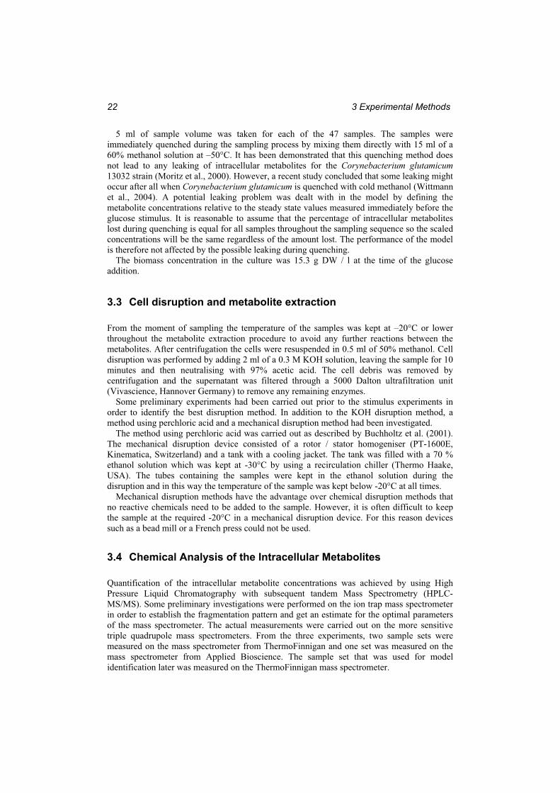
3 Experimental Methods 22
5 ml of sample volume was taken for each of the 47 samples. The samples were immediately quenched during the sampling process by mixing them directly with 15 ml of a 60% methanol solution at –50°C. It has been demonstrated that this quenching method does not lead to any leaking of intracellular metabolites for the Corynebacterium glutamicum13032 strain (Moritz et al., 2000). However, a recent study concluded that some leaking might occur after all when Corynebacterium glutamicum is quenched with cold methanol (Wittmann et al., 2004). A potential leaking problem was dealt with in the model by defining the metabolite concentrations relative to the steady state values measured immediately before the glucose stimulus. It is reasonable to assume that the percentage of intracellular metabolites lost during quenching is equal for all samples throughout the sampling sequence so the scaled concentrations will be the same regardless of the amount lost. The performance of the model is therefore not affected by the possible leaking during quenching.
The biomass concentration in the culture was 15.3 g DW / l at the time of the glucose addition.
3.3 Cell disruption and metabolite extraction
From the moment of sampling the temperature of the samples was kept at –20°C or lower throughout the metabolite extraction procedure to avoid any further reactions between the metabolites. After centrifugation the cells were resuspended in 0.5 ml of 50% methanol. Cell disruption was performed by adding 2 ml of a 0.3 M KOH solution, leaving the sample for 10 minutes and then neutralising with 97% acetic acid. The cell debris was removed by centrifugation and the supernatant was filtered through a 5000 Dalton ultrafiltration unit (Vivascience, Hannover Germany) to remove any remaining enzymes.
Some preliminary experiments had been carried out prior to the stimulus experiments in order to identify the best disruption method. In addition to the KOH disruption method, a method using perchloric acid and a mechanical disruption method had been investigated.
The method using perchloric acid was carried out as described by Buchholtz et al. (2001). The mechanical disruption device consisted of a rotor / stator homogeniser (PT-1600E, Kinematica, Switzerland) and a tank with a cooling jacket. The tank was filled with a 70 % ethanol solution which was kept at -30°C by using a recirculation chiller (Thermo Haake, USA). The tubes containing the samples were kept in the ethanol solution during the disruption and in this way the temperature of the sample was kept below -20°C at all times.
Mechanical disruption methods have the advantage over chemical disruption methods that no reactive chemicals need to be added to the sample. However, it is often difficult to keep the sample at the required -20°C in a mechanical disruption device. For this reason devices such as a bead mill or a French press could not be used.
3.4 Chemical Analysis of the Intracellular Metabolites
Quantification of the intracellular metabolite concentrations was achieved by using High Pressure Liquid Chromatography with subsequent tandem Mass Spectrometry (HPLC-MS/MS). Some preliminary investigations were performed on the ion trap mass spectrometer in order to establish the fragmentation pattern and get an estimate for the optimal parameters of the mass spectrometer. The actual measurements were carried out on the more sensitive triple quadrupole mass spectrometers. From the three experiments, two sample sets were measured on the mass spectrometer from ThermoFinnigan and one set was measured on the mass spectrometer from Applied Bioscience. The sample set that was used for model identification later was measured on the ThermoFinnigan mass spectrometer.
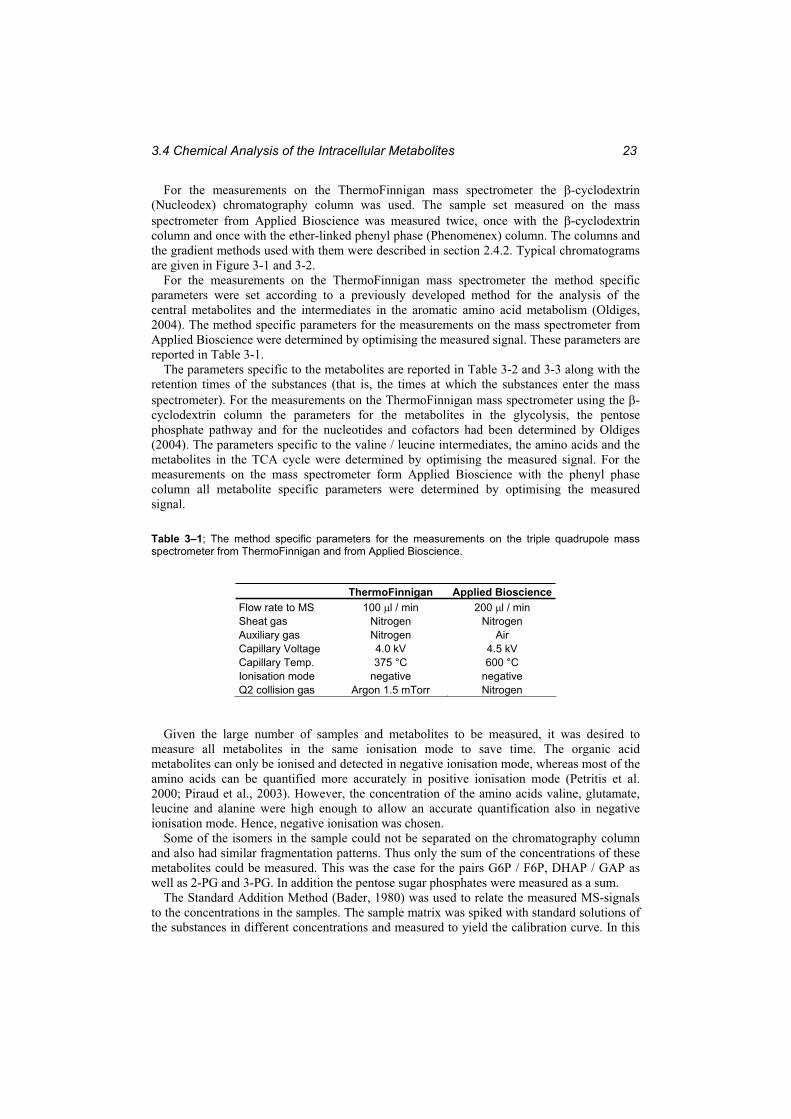
3.4 Chemical Analysis of the Intracellular Metabolites 23
For the measurements on the ThermoFinnigan mass spectrometer the -cyclodextrin(Nucleodex) chromatography column was used. The sample set measured on the mass spectrometer from Applied Bioscience was measured twice, once with the -cyclodextrincolumn and once with the ether-linked phenyl phase (Phenomenex) column. The columns and the gradient methods used with them were described in section 2.4.2. Typical chromatograms are given in Figure 3-1 and 3-2.
For the measurements on the ThermoFinnigan mass spectrometer the method specific parameters were set according to a previously developed method for the analysis of the central metabolites and the intermediates in the aromatic amino acid metabolism (Oldiges, 2004). The method specific parameters for the measurements on the mass spectrometer from Applied Bioscience were determined by optimising the measured signal. These parameters are reported in Table 3-1.
The parameters specific to the metabolites are reported in Table 3-2 and 3-3 along with the retention times of the substances (that is, the times at which the substances enter the mass spectrometer). For the measurements on the ThermoFinnigan mass spectrometer using the -cyclodextrin column the parameters for the metabolites in the glycolysis, the pentose phosphate pathway and for the nucleotides and cofactors had been determined by Oldiges (2004). The parameters specific to the valine / leucine intermediates, the amino acids and the metabolites in the TCA cycle were determined by optimising the measured signal. For the measurements on the mass spectrometer form Applied Bioscience with the phenyl phase column all metabolite specific parameters were determined by optimising the measured signal.
Table 3–1; The method specific parameters for the measurements on the triple quadrupole mass spectrometer from ThermoFinnigan and from Applied Bioscience.
ThermoFinnigan Applied Bioscience Flow rate to MS 100 l / min 200 l / min Sheat gas Nitrogen Nitrogen Auxiliary gas Nitrogen Air Capillary Voltage 4.0 kV 4.5 kV Capillary Temp. 375 °C 600 °C Ionisation mode negative negative Q2 collision gas Argon 1.5 mTorr Nitrogen
Given the large number of samples and metabolites to be measured, it was desired to measure all metabolites in the same ionisation mode to save time. The organic acid metabolites can only be ionised and detected in negative ionisation mode, whereas most of the amino acids can be quantified more accurately in positive ionisation mode (Petritis et al. 2000; Piraud et al., 2003). However, the concentration of the amino acids valine, glutamate, leucine and alanine were high enough to allow an accurate quantification also in negative ionisation mode. Hence, negative ionisation was chosen.
Some of the isomers in the sample could not be separated on the chromatography column and also had similar fragmentation patterns. Thus only the sum of the concentrations of these metabolites could be measured. This was the case for the pairs G6P / F6P, DHAP / GAP as well as 2-PG and 3-PG. In addition the pentose sugar phosphates were measured as a sum.
The Standard Addition Method (Bader, 1980) was used to relate the measured MS-signals to the concentrations in the samples. The sample matrix was spiked with standard solutions of the substances in different concentrations and measured to yield the calibration curve. In this
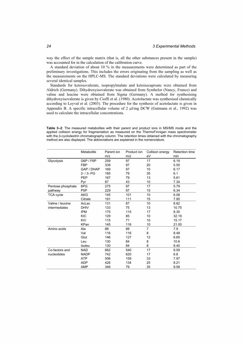
3 Experimental Methods 24
way the effect of the sample matrix (that is, all the other substances present in the sample) was accounted for in the calculation of the calibration curve.
A standard deviation of about 10 % in the measurements were determined as part of the preliminary investigations. This includes the errors originating from the sampling as well as the measurements on the HPLC-MS. The standard deviations were calculated by measuring several identical samples.
Standards for ketoisovalerate, isopropylmalate and ketoisocaproate were obtained from Aldrich (Germany). Dihydroxyisovalerate was obtained from Synthelor (Nancy, France) and valine and leucine were obtained from Sigma (Germany). A method for synthesising dihydroxyisovalerate is given by Cioffi et al. (1980). Acetolactate was synthesised chemically according to Leyval et al. (2003). The procedure for the synthesis of acetolactate is given in Appendix B. A specific intracellular volume of 2 l/mg DCW (Gutmann et al., 1992) was used to calculate the intracellular concentrations.
Table 3–2: The measured metabolites with their parent and product ions in MS/MS mode and the applied collision energy for fragmentation as measured on the ThermoFinnigan mass spectrometer with the -cyclodextrin chromatography column. The retention times obtained with the chromatography method are also displayed. The abbreviations are explained in the nomenclature.
Metabolite Parent ion Product ion Collison energy Retention time m/z m/z eV min Glycolysis G6P / F6P 259 97 17 6.19 FBP 339 97 20 5.55 GAP / DHAP 169 97 10 6.17 2- / 3- PG 185 79 35 6.1 PEP 167 79 13 5.61 Pyr 87 43 10 7.34 Pentose phosphate 6PG 275 97 17 5.79 pathway P5P 229 97 15 6.34 TCA cycle AKG 145 101 10 6.08 Citrate 191 111 15 7.95 Valine / leucine AcLac 131 87 10 8.82 intermediates DHIV 133 75 13 10.75 IPM 175 115 17 8.35 KIC 129 85 10 32.19 KIV 115 71 10 15.17 KPan 145 116 10 21.00 Amino acids Ala 88 88 7 7.9 Val 116 116 8 8.48 Glut 146 127 12 6.65 Leu 130 84 8 10.6 Isoleu 130 84 8 9.45 Co-factors and NAD 662 540 17 9.59 nucleotides NADP 742 620 17 6.8 ATP 506 159 33 7.97 ADP 426 134 25 8.21 AMP 346 79 35 9.58
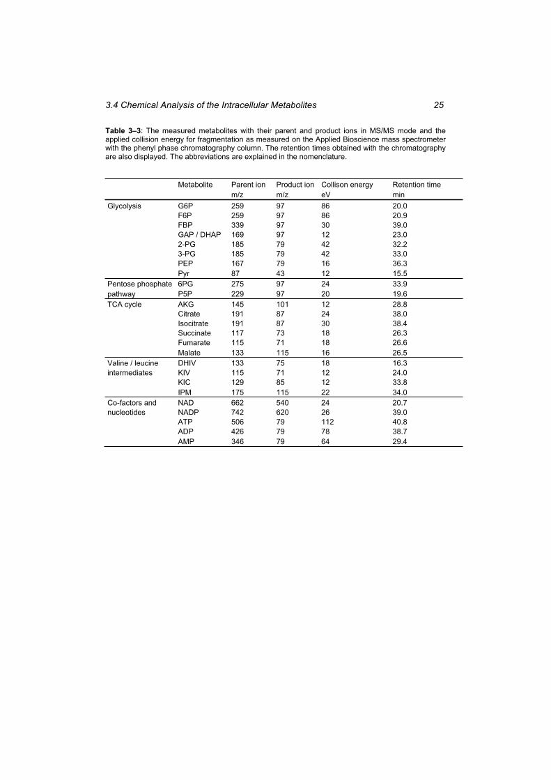
3.4 Chemical Analysis of the Intracellular Metabolites 25
Table 3–3: The measured metabolites with their parent and product ions in MS/MS mode and the applied collision energy for fragmentation as measured on the Applied Bioscience mass spectrometer with the phenyl phase chromatography column. The retention times obtained with the chromatography are also displayed. The abbreviations are explained in the nomenclature.
Metabolite Parent ion Product ion Collison energy Retention time m/z m/z eV min Glycolysis G6P 259 97 86 20.0 F6P 259 97 86 20.9 FBP 339 97 30 39.0 GAP / DHAP 169 97 12 23.0 2-PG 185 79 42 32.2 3-PG 185 79 42 33.0 PEP 167 79 16 36.3 Pyr 87 43 12 15.5 Pentose phosphate 6PG 275 97 24 33.9 pathway P5P 229 97 20 19.6 TCA cycle AKG 145 101 12 28.8 Citrate 191 87 24 38.0 Isocitrate 191 87 30 38.4 Succinate 117 73 18 26.3 Fumarate 115 71 18 26.6 Malate 133 115 16 26.5 Valine / leucine DHIV 133 75 18 16.3 intermediates KIV 115 71 12 24.0 KIC 129 85 12 33.8 IPM 175 115 22 34.0 Co-factors and NAD 662 540 24 20.7 nucleotides NADP 742 620 26 39.0 ATP 506 79 112 40.8 ADP 426 79 78 38.7 AMP 346 79 64 29.4
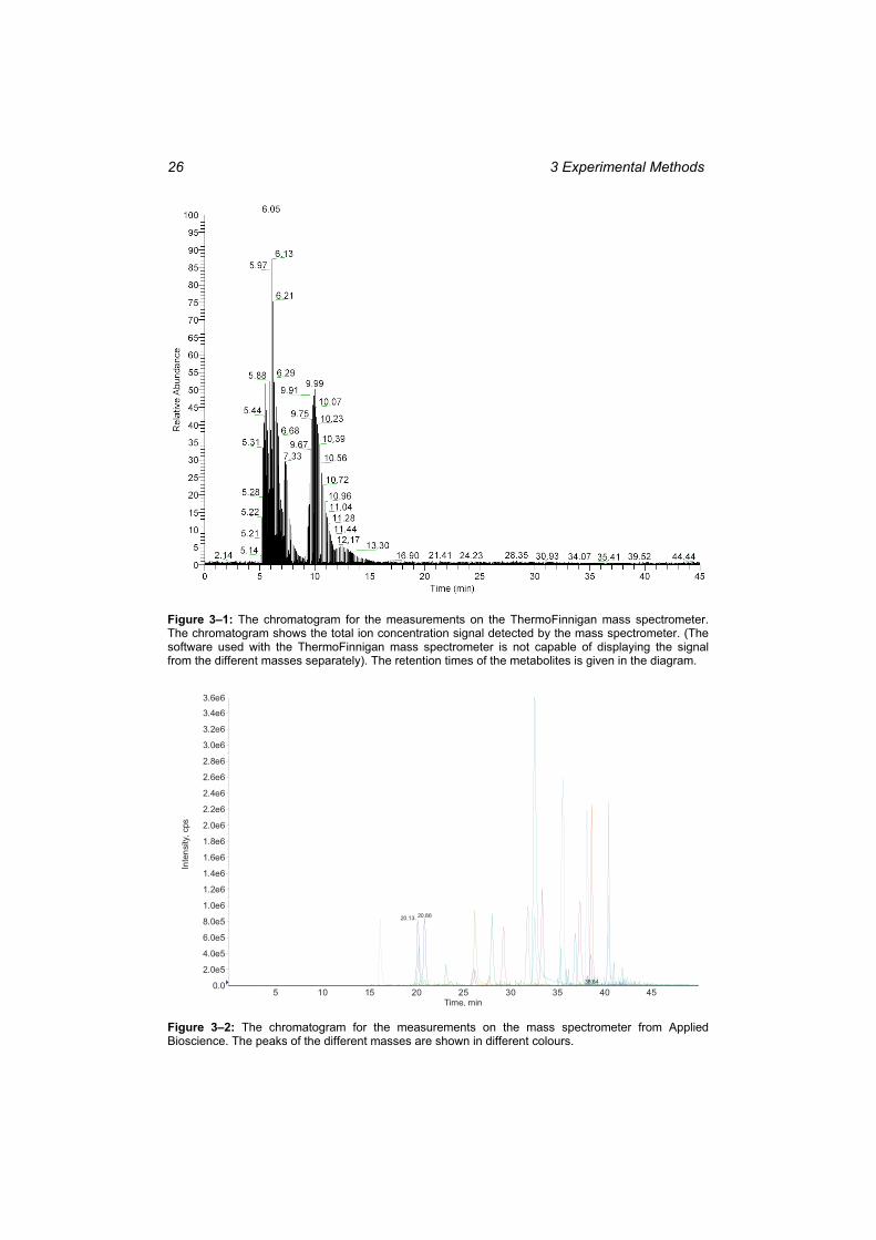
3 Experimental Methods 26
Figure 3–1: The chromatogram for the measurements on the ThermoFinnigan mass spectrometer. The chromatogram shows the total ion concentration signal detected by the mass spectrometer. (The software used with the ThermoFinnigan mass spectrometer is not capable of displaying the signal from the different masses separately). The retention times of the metabolites is given in the diagram.
Figure 3–2: The chromatogram for the measurements on the mass spectrometer from Applied Bioscience. The peaks of the different masses are shown in different colours.
5 10 15 20 25 30 35 40 45Time, min
0.0
2.0e5
4.0e5
6.0e5
8.0e5
1.0e6
1.2e6
1.4e6
1.6e6
1.8e6
2.0e6
2.2e6
2.4e6
2.6e6
2.8e6
3.0e6
3.2e6
3.4e6
3.6e6
Inte
nsity
, cps
20.8620.13
38.64
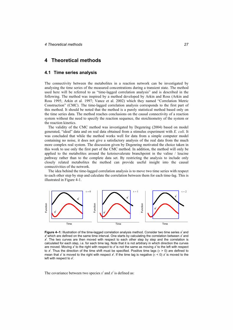
4 Theoretical methods 27
4 Theoretical methods
4.1 Time series analysis
The connectivity between the metabolites in a reaction network can be investigated by analysing the time series of the measured concentrations during a transient state. The method used here will be referred to as “time-lagged correlation analysis” and is described in the following. The method was inspired by a method developed by Arkin and Ross (Arkin and Ross 1995; Arkin et al. 1997; Vance et al. 2002) which they named “Correlation Metric Construction” (CMC). The time-lagged correlation analysis corresponds to the first part of this method. It should be noted that the method is a purely statistical method based only on the time series data. The method reaches conclusions on the causal connectivity of a reaction system without the need to specify the reaction sequence, the stoichiometry of the system or the reaction kinetics.
The validity of the CMC method was investigated by Degenring (2004) based on model generated, “ideal” data and on real data obtained from a stimulus experiment with E. coli. It was concluded that while the method works well for data from a simple computer model containing no noise, it does not give a satisfactory analysis of the real data from the much more complex real system. The discussion given by Degenring motivated the choice taken in this work to use only the first part of the CMC method. In addition, the method will only be applied to the metabolites around the ketoisovalerate branchpoint in the valine / leucine pathway rather than to the complete data set. By restricting the analysis to include only closely related metabolites the method can provide useful insight into the causal connectivities of the network.
The idea behind the time-lagged correlation analysis is to move two time series with respect to each other step by step and calculate the correlation between them for each time-lag. This is illustrated in Figure 4-1.
xjFunc
tion
Time
xi xi
xjFunc
tion
Time
xj
Func
tion
Time
xi
Figure 4–1: Illustration of the time-lagged correlation analysis method. Consider two time series xi and xj which are defined on the same time interval. One starts by calculating the correlation between xi and xj. The two curves are then moved with respect to each other step by step and the correlation is calculated for each step, i.e. for each time lag. Note that it is not arbitrary in which direction the curves are moved. Moving xi to the right with respect to xj is not the same as moving xi to the left with respect to xj. Thus the direction of the time shift must be specified. Positive time lags ( > 0) are defined to mean that xi is moved to the right with respect xj. If the time lag is negative ( < 0) xi is moved to the left with respect to xj.
The covariance between two species xi and xj is defined as:
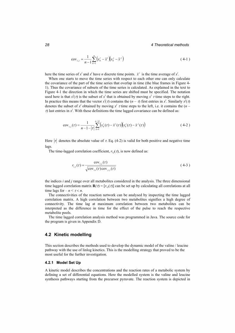
4 Theoretical methods 28
n
k
jjk
iikji xxxx
n 1, 1
1cov ( 4-1 )
here the time series of xi and xj have n discrete time points. ix is the time average of xi.When one starts to move the time series with respect to each other one can only calculate
the covariance of the part of the time series that overlap in time (the blue frames in Figure 4-1). Thus the covariance of subsets of the time series is calculated. As explained in the text to Figure 4-1 the direction in which the time series are shifted must be specified. The notation used here is that xi( ) is the subset of xi that is obtained by moving xi time steps to the right. In practice this means that the vector xi( ) contains the (n – ) first entries in xi. Similarly xj( )denotes the subset of xj obtained by moving xj time steps to the left, i.e. it contains the (n – ) last entries in xj. With these definitions the time lagged covariance can be defined as:
n
k
jjk
iikji xxxx
n 1, )()()()(
11)(cov ( 4-2 )
Here denotes the absolute value of . Eq. (4-2) is valid for both positive and negative time lags.
The time-lagged correlation coefficient, ri,j( ), is now defined as:
)(cov)(cov
)(cov)(
,,
,,
jjii
jijir ( 4-3 )
the indices i and j range over all metabolites considered in the analysis. The three dimensional time lagged correlation matrix R( ) = [ri,j( )] can be set up by calculating all correlations at all time lags for – n < n.
The connectivities of the reaction network can be analysed by inspecting the time lagged correlation matrix. A high correlation between two metabolites signifies a high degree of connectivity. The time lag at maximum correlation between two metabolites can be interpreted as the difference in time for the effect of the pulse to reach the respective metabolite pools.
The time lagged correlation analysis method was programmed in Java. The source code for the program is given in Appendix D.
4.2 Kinetic modelling
This section describes the methods used to develop the dynamic model of the valine / leucine pathway with the use of linlog kinetics. This is the modelling strategy that proved to be the most useful for the further investigation.
4.2.1 Model Set Up
A kinetic model describes the concentrations and the reaction rates of a metabolic system by defining a set of differential equations. Here the modelled system is the valine and leucine synthesis pathways starting from the precursor pyruvate. The reaction system is depicted in
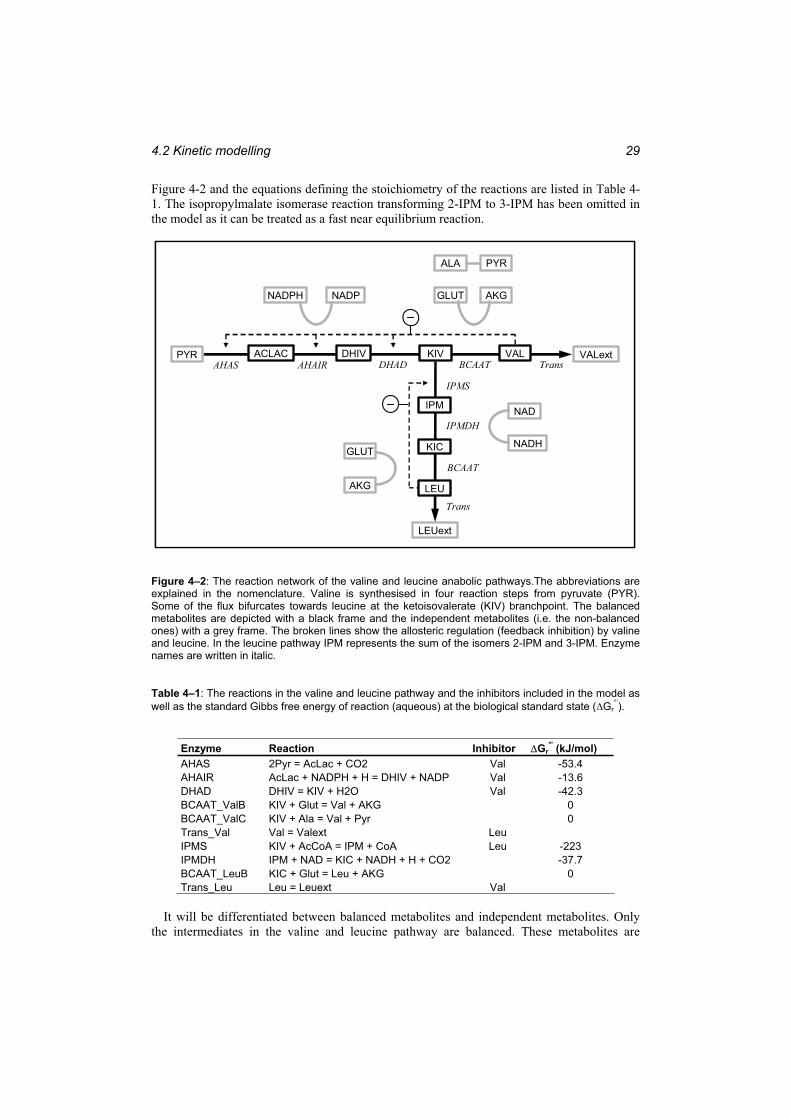
4.2 Kinetic modelling 29
Figure 4-2 and the equations defining the stoichiometry of the reactions are listed in Table 4-1. The isopropylmalate isomerase reaction transforming 2-IPM to 3-IPM has been omitted in the model as it can be treated as a fast near equilibrium reaction.
ACLAC DHIV KIV VAL
GLUT AKG
GLUT
AKG
PYR VALext
NAD
NADH
NADPH NADP
LEUext
ALA PYR
AHAS AHAIR DHAD
LEU
KIC
IPM
BCAAT Trans
IPMS
IPMDH
BCAAT
Trans
ACLAC DHIV KIV VAL
GLUT AKG
GLUT
AKG
PYR VALext
NAD
NADH
NADPH NADP
LEUext
ALA PYR
AHAS AHAIR DHAD
LEU
KIC
IPM
BCAAT Trans
IPMS
IPMDH
BCAAT
Trans
Figure 4–2: The reaction network of the valine and leucine anabolic pathways.The abbreviations are explained in the nomenclature. Valine is synthesised in four reaction steps from pyruvate (PYR). Some of the flux bifurcates towards leucine at the ketoisovalerate (KIV) branchpoint. The balanced metabolites are depicted with a black frame and the independent metabolites (i.e. the non-balanced ones) with a grey frame. The broken lines show the allosteric regulation (feedback inhibition) by valine and leucine. In the leucine pathway IPM represents the sum of the isomers 2-IPM and 3-IPM. Enzyme names are written in italic.
Table 4–1: The reactions in the valine and leucine pathway and the inhibitors included in the model as well as the standard Gibbs free energy of reaction (aqueous) at the biological standard state ( Gr
°’).
Enzyme Reaction Inhibitor Gr°' (kJ/mol)
AHAS 2Pyr = AcLac + CO2 Val -53.4 AHAIR AcLac + NADPH + H = DHIV + NADP Val -13.6 DHAD DHIV = KIV + H2O Val -42.3 BCAAT_ValB KIV + Glut = Val + AKG 0 BCAAT_ValC KIV + Ala = Val + Pyr 0 Trans_Val Val = Valext Leu IPMS KIV + AcCoA = IPM + CoA Leu -223 IPMDH IPM + NAD = KIC + NADH + H + CO2 -37.7 BCAAT_LeuB KIC + Glut = Leu + AKG 0 Trans_Leu Leu = Leuext Val
It will be differentiated between balanced metabolites and independent metabolites. Only the intermediates in the valine and leucine pathway are balanced. These metabolites are
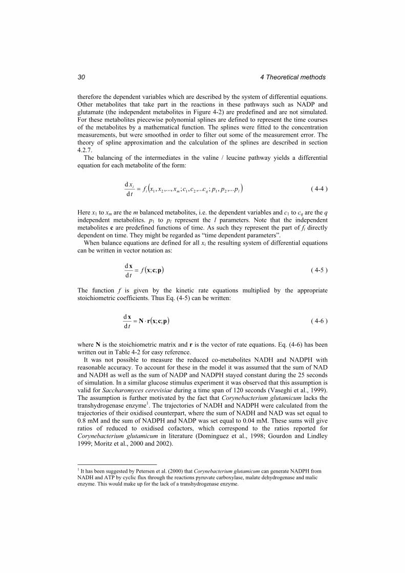
4 Theoretical methods 30
therefore the dependent variables which are described by the system of differential equations. Other metabolites that take part in the reactions in these pathways such as NADP and glutamate (the independent metabolites in Figure 4-2) are predefined and are not simulated. For these metabolites piecewise polynomial splines are defined to represent the time courses of the metabolites by a mathematical function. The splines were fitted to the concentration measurements, but were smoothed in order to filter out some of the measurement error. The theory of spline approximation and the calculation of the splines are described in section 4.2.7.
The balancing of the intermediates in the valine / leucine pathway yields a differential equation for each metabolite of the form:
lqmii pppcccxxxf
tx
,...,;,...,;,...,,d
d212121 ( 4-4 )
Here x1 to xm are the m balanced metabolites, i.e. the dependent variables and c1 to cq are the qindependent metabolites. p1 to pl represent the l parameters. Note that the independent metabolites c are predefined functions of time. As such they represent the part of fi directly dependent on time. They might be regarded as “time dependent parameters”.
When balance equations are defined for all xi the resulting system of differential equations can be written in vector notation as:
pcxx ;;dd f
t ( 4-5 )
The function f is given by the kinetic rate equations multiplied by the appropriate stoichiometric coefficients. Thus Eq. (4-5) can be written:
pcxrNx ;;dd
t ( 4-6 )
where N is the stoichiometric matrix and r is the vector of rate equations. Eq. (4-6) has been written out in Table 4-2 for easy reference.
It was not possible to measure the reduced co-metabolites NADH and NADPH with reasonable accuracy. To account for these in the model it was assumed that the sum of NAD and NADH as well as the sum of NADP and NADPH stayed constant during the 25 seconds of simulation. In a similar glucose stimulus experiment it was observed that this assumption is valid for Saccharomyces cerevisiae during a time span of 120 seconds (Vaseghi et al., 1999). The assumption is further motivated by the fact that Corynebacterium glutamicum lacks the transhydrogenase enzyme1. The trajectories of NADH and NADPH were calculated from the trajectories of their oxidised counterpart, where the sum of NADH and NAD was set equal to 0.8 mM and the sum of NADPH and NADP was set equal to 0.04 mM. These sums will give ratios of reduced to oxidised cofactors, which correspond to the ratios reported for Corynebacterium glutamicum in literature (Dominguez et al., 1998; Gourdon and Lindley 1999; Moritz et al., 2000 and 2002).
1 It has been suggested by Petersen et al. (2000) that Corynebacterium glutamicum can generate NADPH from NADH and ATP by cyclic flux through the reactions pyruvate carboxylase, malate dehydrogenase and malic enzyme. This would make up for the lack of a transhydrogenase enzyme.
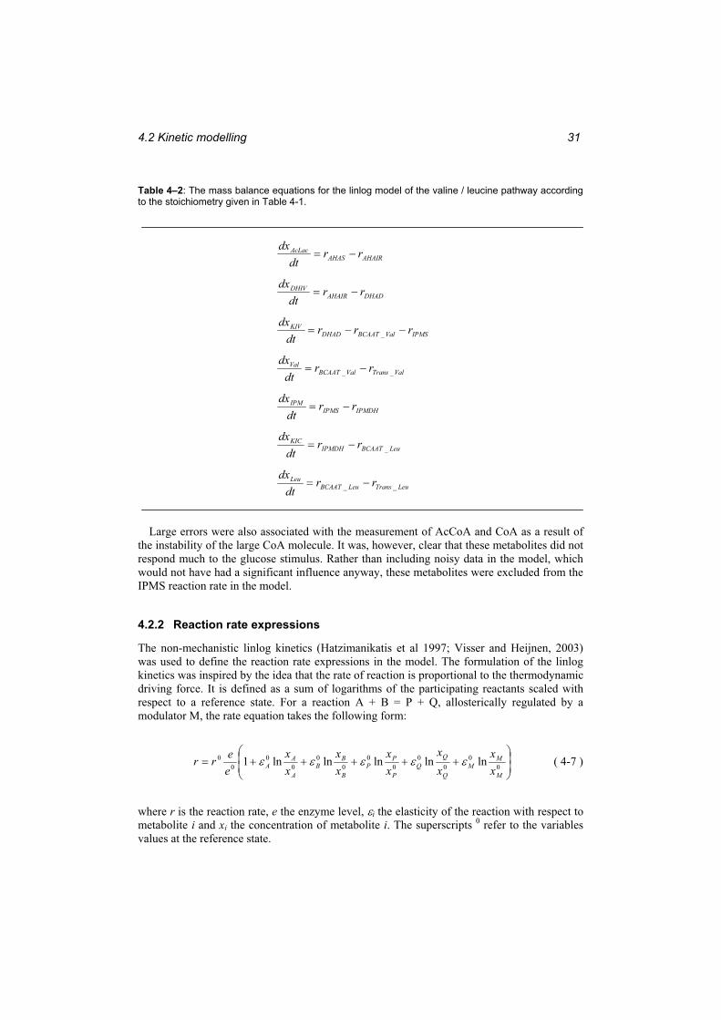
4.2 Kinetic modelling 31
Table 4–2: The mass balance equations for the linlog model of the valine / leucine pathway according to the stoichiometry given in Table 4-1.
Large errors were also associated with the measurement of AcCoA and CoA as a result of the instability of the large CoA molecule. It was, however, clear that these metabolites did not respond much to the glucose stimulus. Rather than including noisy data in the model, which would not have had a significant influence anyway, these metabolites were excluded from the IPMS reaction rate in the model.
4.2.2 Reaction rate expressions
The non-mechanistic linlog kinetics (Hatzimanikatis et al 1997; Visser and Heijnen, 2003) was used to define the reaction rate expressions in the model. The formulation of the linlog kinetics was inspired by the idea that the rate of reaction is proportional to the thermodynamic driving force. It is defined as a sum of logarithms of the participating reactants scaled with respect to a reference state. For a reaction A + B = P + Q, allosterically regulated by a modulator M, the rate equation takes the following form:
00
00
00
00
00
00 lnlnlnlnln1
M
MM
Q
P
PP
B
BB
A
AA x
xxx
xx
xx
xx
eerr ( 4-7 )
where r is the reaction rate, e the enzyme level, i the elasticity of the reaction with respect to metabolite i and xi the concentration of metabolite i. The superscripts 0 refer to the variables values at the reference state.
AHAIRAHASAcLac rrdt
dx
DHADAHAIRDHIV rrdt
dx
IPMSValBCAATDHADKIV rrr
dtdx
_
ValTransValBCAATVal rr
dtdx
__
IPMDHIPMSIPM rr
dtdx
LeuBCAATIPMDHKIC rr
dtdx
_
LeuTransLeuBCAATLeu rr
dtdx
__
4 Theoretical methods 32
The elasticity of a reaction is a property often discussed within the framework of Biochemical Systems Theory (BST) and Metabolic Control Analysis (MCA). The theory of MCA is described in more detail in Chapter 4.3. Since the elasticity of a reaction is one of the parameters of the linlog equation its definition is introduced here. It is defined as the scaled local partial derivative of the reaction rate with respect to a metabolite:
j
i
i
jji x
rrx
, ( 4-8 )
An advantage of formulating the linlog kinetic with respect to a reference state as in Eq. (4-7) is that the parameters equal the enzyme elasticities at the reference state which makes a direct interpretation of the parameters possible. (The reader who needs to be convinced of this may differentiate Eq. (4-7) with respect to xA. By multiplying the result with the scaling factor
00 vxA and setting e and Ax equal to their reference values e0 and 0Ax the answer should be
0A .)For the parameter fitting of the model it is useful to apply the formulation:
000000
0 lnlnlnlnlnM
M
Q
Q
P
P
B
B
A
A
xxm
xx
qxxp
xxb
xxar
eer ( 4-9 )
Eq. (4-9) is identical to Eq. (4-7) except that r0 has been multiplied into the parenthesis. As a result the parameters are now the semi-scaled elasticities evaluated at the reference state:
00A
AA x
xrxa , 00
BB
B xxrxb , etc ( 4-10 )
It is most convenient to choose the steady state as the reference state so that the r0 and x0
parameters are the steady state flux and concentrations respectively. The advantage is that information about the steady state can then be included in the model. In a reaction sequence the r0 parameter for each reaction will depend on each other according to the stoichiometry of the reactions. Thus in the reaction network presented here only the steady state excretion rates of valine and leucine are needed to determine the r0 parameters for all the reactions. In the general case, the steady state fluxes can be determined by a flux analysis. This leaves only the parameters a, b, p, q and m to be determined through parameter fitting. Notice also that by scaling the metabolite concentrations by the steady state concentrations, the influence on the model of a possible leaking problem during quenching of the samples has been eliminated as discussed under Experimental Methods in section 3-2.
The enzyme level e is assumed to be constant during the 25 seconds that are simulated so the ratio e/e0 = 1. This is a fundamental assumption in modelling the reaction dynamics at the enzyme level since one otherwise would have to include gene transcription in the model as well.
Inhibitors were included in the rate equations according to published enzyme studies (Leyval et al., 2003). Valine and leucine are actively transported over the cell membrane by the same protein (Kennerknecht et al., 2002) and are thus competing substrates for this protein. This effect can be included in a linlog model by defining leucine as an inhibitor to the valine transport rate and valine as an inhibitor to the leucine transport rate. The inhibitors are listed in Table 4-1.
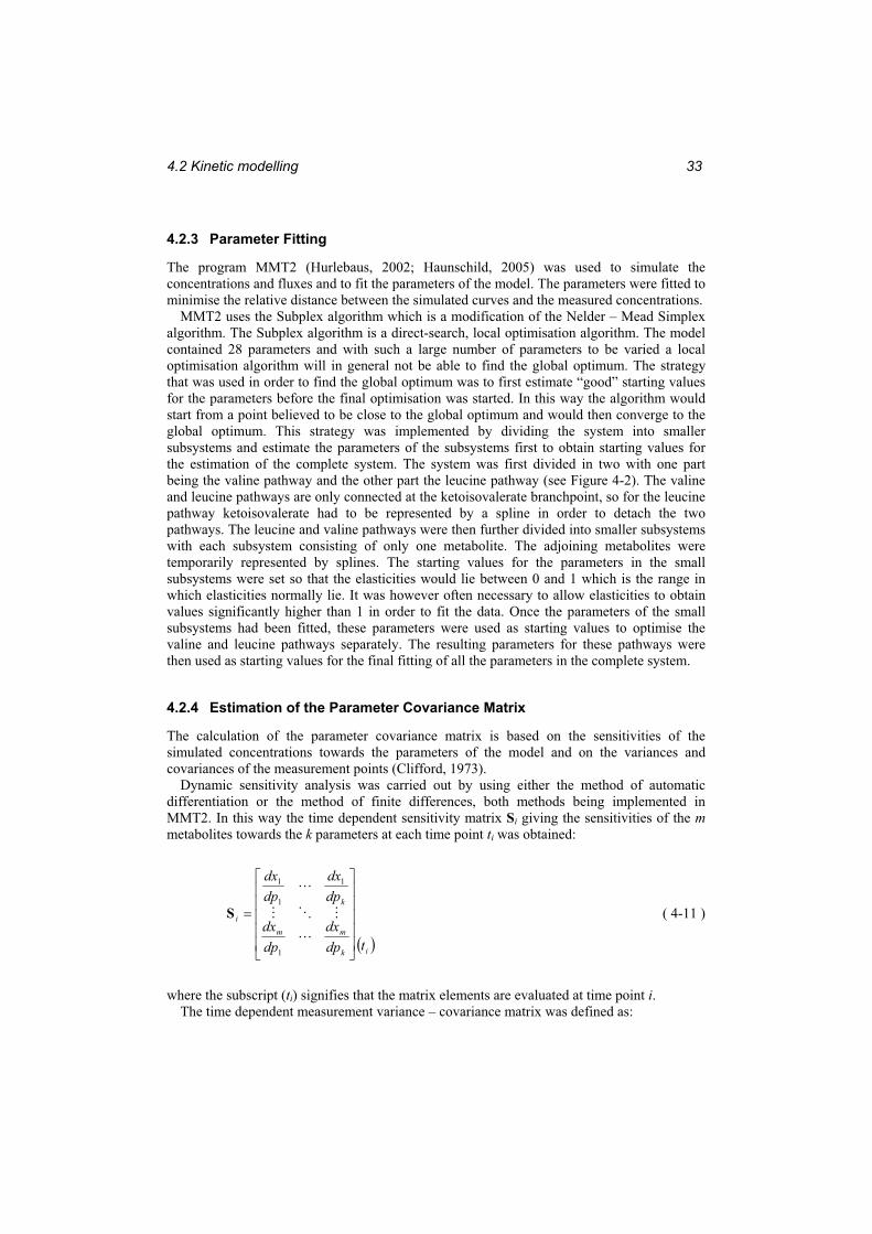
4.2 Kinetic modelling 33
4.2.3 Parameter Fitting
The program MMT2 (Hurlebaus, 2002; Haunschild, 2005) was used to simulate the concentrations and fluxes and to fit the parameters of the model. The parameters were fitted to minimise the relative distance between the simulated curves and the measured concentrations.
MMT2 uses the Subplex algorithm which is a modification of the Nelder – Mead Simplex algorithm. The Subplex algorithm is a direct-search, local optimisation algorithm. The model contained 28 parameters and with such a large number of parameters to be varied a local optimisation algorithm will in general not be able to find the global optimum. The strategy that was used in order to find the global optimum was to first estimate “good” starting values for the parameters before the final optimisation was started. In this way the algorithm would start from a point believed to be close to the global optimum and would then converge to the global optimum. This strategy was implemented by dividing the system into smaller subsystems and estimate the parameters of the subsystems first to obtain starting values for the estimation of the complete system. The system was first divided in two with one part being the valine pathway and the other part the leucine pathway (see Figure 4-2). The valine and leucine pathways are only connected at the ketoisovalerate branchpoint, so for the leucine pathway ketoisovalerate had to be represented by a spline in order to detach the two pathways. The leucine and valine pathways were then further divided into smaller subsystems with each subsystem consisting of only one metabolite. The adjoining metabolites were temporarily represented by splines. The starting values for the parameters in the small subsystems were set so that the elasticities would lie between 0 and 1 which is the range in which elasticities normally lie. It was however often necessary to allow elasticities to obtain values significantly higher than 1 in order to fit the data. Once the parameters of the small subsystems had been fitted, these parameters were used as starting values to optimise the valine and leucine pathways separately. The resulting parameters for these pathways were then used as starting values for the final fitting of all the parameters in the complete system.
4.2.4 Estimation of the Parameter Covariance Matrix
The calculation of the parameter covariance matrix is based on the sensitivities of the simulated concentrations towards the parameters of the model and on the variances and covariances of the measurement points (Clifford, 1973).
Dynamic sensitivity analysis was carried out by using either the method of automatic differentiation or the method of finite differences, both methods being implemented in MMT2. In this way the time dependent sensitivity matrix Si giving the sensitivities of the mmetabolites towards the k parameters at each time point ti was obtained:
ik
mm
k
i
tdpdx
dpdx
dpdx
dpdx
1
1
1
1
S ( 4-11 )
where the subscript (ti) signifies that the matrix elements are evaluated at time point i.The time dependent measurement variance – covariance matrix was defined as:
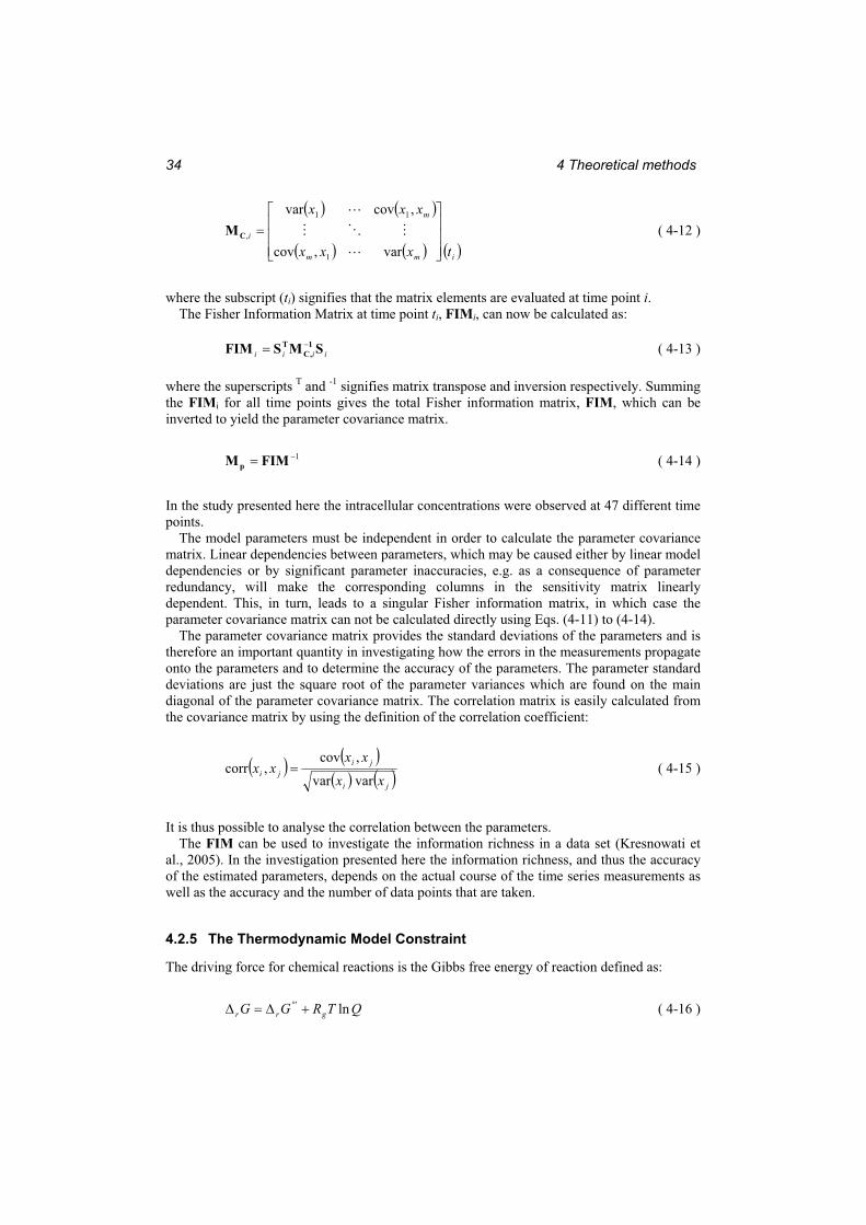
4 Theoretical methods 34
imm
m
i
txxx
xxx
var,cov
,covvar
1
11
,CM ( 4-12 )
where the subscript (ti) signifies that the matrix elements are evaluated at time point i.The Fisher Information Matrix at time point ti, FIMi, can now be calculated as:
iiii SMSFIM 1,C
T ( 4-13 )
where the superscripts T and -1 signifies matrix transpose and inversion respectively. Summing the FIMi for all time points gives the total Fisher information matrix, FIM, which can be inverted to yield the parameter covariance matrix.
1FIMMp ( 4-14 )
In the study presented here the intracellular concentrations were observed at 47 different time points.
The model parameters must be independent in order to calculate the parameter covariance matrix. Linear dependencies between parameters, which may be caused either by linear model dependencies or by significant parameter inaccuracies, e.g. as a consequence of parameter redundancy, will make the corresponding columns in the sensitivity matrix linearly dependent. This, in turn, leads to a singular Fisher information matrix, in which case the parameter covariance matrix can not be calculated directly using Eqs. (4-11) to (4-14).
The parameter covariance matrix provides the standard deviations of the parameters and is therefore an important quantity in investigating how the errors in the measurements propagate onto the parameters and to determine the accuracy of the parameters. The parameter standard deviations are just the square root of the parameter variances which are found on the main diagonal of the parameter covariance matrix. The correlation matrix is easily calculated from the covariance matrix by using the definition of the correlation coefficient:
ji
jiji xx
xxxx
varvar
,cov,corr ( 4-15 )
It is thus possible to analyse the correlation between the parameters. The FIM can be used to investigate the information richness in a data set (Kresnowati et
al., 2005). In the investigation presented here the information richness, and thus the accuracy of the estimated parameters, depends on the actual course of the time series measurements as well as the accuracy and the number of data points that are taken.
4.2.5 The Thermodynamic Model Constraint
The driving force for chemical reactions is the Gibbs free energy of reaction defined as:
QTRGG grr ln' ( 4-16 )
4.2 Kinetic modelling 35
where rG°’ is the Gibbs energy of reaction at the biological standard state. The biological standard state is the same as the standard state normally defined for chemical reactions (atmospheric pressure, temperature at 25 °C) except that the reference pH value is 7. The standard concentrations are 1 M for all reactants except for H2O which has a standard concentration of 55.5 M (that of pure water) and for H+ and OH- which have standard concentrations of 10-7 M. Rg is the universal gas constant, T is the temperature in Kelvin and the reaction quotient, Q, is defined as the activities of the products divided by the activities of the substrates. It is assumed here that all activity coefficients equal 1, so Q is calculated as the concentrations of products divided by the concentrations of substrates. So far no intracellular metabolite activity measurements have been carried out, so there is no information on the activity coefficients in literature. Setting these to 1 is probably a reasonable approximation since the concentrations of the metabolites are relatively low and the activity coefficients approach 1 as the concentration approach 0.
The direction of spontaneous change at constant temperature and pressure is towards lower values of the Gibbs energy so rG must always be negative. rG is a function of the concentrations of the metabolites so it will change throughout a simulation, however, the following constraint must always apply:
0i
ir
rG
( 4-17 )
Including this criterion in the model identification process ensures that all the simulated reaction rates always go in the direction towards lower Gibbs energy which is an important consideration in establishing realistic models. The constraint applies to all reaction rates ri at all time points and it thus greatly reduces the parameter space in which the optimal parameters are sought.
The Gibbs free energy of formation of the relevant metabolites at the biological standard state was calculated by the group contribution method according to Mavrovouniotis (Mavrovoniotis, 1990; 1991). The standard Gibbs energy of reaction (reported in Table 4-1) can then be calculated from the Gibbs energies of formation.
4.2.6 Stability Analysis
The analysis of the stability of the steady state is an important aspect for the further interpretation of dynamic models. Only if the model has a stable steady state can a sensitivity analysis of its variables be performed. Thus a model must be stable in order to be used for metabolic control analysis.
The stability criterion The stability of a system is analysed by examining the Jacobian matrix. For a system of ODEs as defined in Eq. (4-5) the Jacobian is the matrix of partial derivatives of f:
m
mm
m
xf
xf
xf
xf
1
1
1
1
J ( 4-18 )
4 Theoretical methods 36
A general criterion for the stability of a state was formulated by Lyapunov (Kondepudi and Prigogine, 1998). Using Lyapunov’s theory in combination with linear stability analysis gives the criterion for stability:
Theorem: Stability criterion
Thus, the stability is evaluated by calculating the eigenvalues of the Jacobian of the system of ODEs. The issue of stability of mathematical models is common in all engineering disciplines and the theorem above is well known. The derivation of the stability criterion and the description of Lyapunov’s theory have therefore been put in Appendix G.
A conjugate pair of complex eigenvalues2 signifies that the system is able to oscillate. If a zero eigenvalue is found, the test gives no conclusion on the stability.
4.2.7 Spline approximation
A time series of discrete data points can be interpolated by fitting a polynomial or some other mathematical function to the data. However, in many cases one single function defined over the whole time interval will not give an adequate representation of the data. Different strategies have therefore been developed to obtain an accurate continuous mathematical representation of discrete data. Piecewise polynomial splines (pp-splines) represent one of the most common interpolation methods. Rather than defining one polynomial over the entire time interval this method defines different polynomials on subintervals resulting in a much more flexible mathematical form.
Consider a time series of n discrete data points g(t1), g(t2), … , g(tn) defined on a time interval [a, b] with a = t1 < t2 < ... < tn = b. [a, b] is divided into subintervals where, in the case of pp-splines, each subinterval is the distance between two consecutive time points. Polynomials are then defined on each subinterval. The division of [a, b] in subintervals is referred to as the mesh of the spline. Thus on the ith subinterval [ti, ti+1] the polynomial has the form:
11,)( 10
1, niandttxfortxCxp ii
k
j
jijii ( 4-19 )
where k is the degree of the polynomial and Ci,j is the polynomial coefficient corresponding to the term of degree j. The spline (x) is defined as:
2 A complex number z is a number on the form z = a + ib where a is the real part of z and ib is the imaginary part with i being the imaginary number 1 . In the case where b equals 0, z is just a real number. Complex numbers occur in the general solution of algebraic equations. A polynomial of degree n has exactly n roots where some of the roots may be complex numbers. This theorem is know as the fundamental theorem of algebra and was proved by the german mathematician Carl Friedrich Gauss in 1799. In the solution of algebraic equations the complex roots will occur as conjugated pairs, i.e. if a + ib is a solution to the equation then a - ib will also be a solution (Lindstrøm, 1995). Since the calculation of the eigenvalues of a matrix is essentially the solution of an algebraic equation, a square matrix of dimension n will have n eigenvalues where the complex eigenvalues occur as conjugated pairs.
A steady state is stable if, and only if, the eigenvalues of the associated Jacobian matrix all have negative real parts.
4.2 Kinetic modelling 37
],[
),[),[
)(
)()(
)(
1
32
21
1
2
1
nnn ttx
ttxttx
xp
xpxp
x ( 4-20 )
the coefficients Ci,j are set so that the polynomial pi(x) satisfies the conditions:
)(
)()(
)(
)(
)()(
)(
11
1
1'
1
1
11
1'
1
iki
ii
i
i
iki
ii
ii
ii
tp
tptgtg
tp
tptptp
( 4-21 )
In other words, at its end points, pi(x) agrees with the data points g(t) and the first k-1derivatives equal the derivatives of the adjacent polynomials at the mesh nodes. Thus the spline (x) of degree k is (k – 1) times continuously differentiable in all time points. For a spline of degree 3 for instance (a cubic spline) this means that the first and second derivatives are continuous at the mesh nodes.
The polynomial coefficients Ci,j are determined by solving a system of linear equations which are set up from the conditions stated in Eq. (4-21). A detailed description of this procedure will not be given here, but can be found for example in the book by de Boor (1978). It should however be noted that a spline of degree k has in total (k+1)*n coefficients. The conditions in Eq. (4-21) result in (k+1)*n – k + 1 equations so one must set (k – 1) additional conditions in order to obtain a unique solution for the polynomial coefficients. This is done by specifying the conditions at the end points of the spline. For a cubic spline (k = 3) two boundary conditions must be set. It is common to set 0)()( ''
1''
ntt . In this case the spline is referred to as a natural spline.
For measurement data containing noise the spline representation does not necessarily have to go exactly through each data point since these might contain errors. Rather, the spline should be an approximating curve representing the complete set of data. Thus, instead of having an interpolating spline a “smooth” spline going near the measurement points can be calculated. This is done by constructing a spline that minimises the following expression:
nt
t
n
i i
ii dxxaw
ttga
1
)()1()()( ''
1
2
( 4-22 )
where wi is the weight of data point i and a is the smoothing factor. Minimisation of (4-22) establishes a compromise between the desire to stay close to the data and the desire to obtain a smooth curve. By assigning weights to the data points one may allow a stronger deviation from the data points where a large error is suspected. The weights wi should be set equal to the variances of the data points. The condition that (4-22) is minimised now replaces the condition that the spline goes through every data point. The implementation of this criterion is described by de Boor (1978).
It should be noted that pp-splines are not the only type of splines that can be used. Another common type is the B-spline which has some numerical advantages over pp-splines (Hayes,
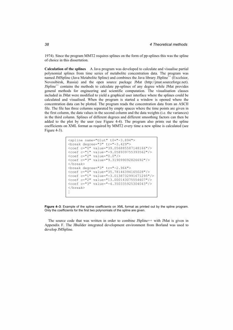
4 Theoretical methods 38
1974). Since the program MMT2 requires splines on the form of pp-splines this was the spline of choice in this dissertation.
Calculation of the splines A Java program was developed to calculate and visualise partial polynomial splines from time series of metabolite concentration data. The program was named JMSpline (Java Metabolite Spline) and combines the Java library JSpline++ (Excelsior, Novosibirsk, Russia) and the open source package JMat (http://jmat.sourceforge.net).JSpline++ contains the methods to calculate pp-splines of any degree while JMat provides general methods for engineering and scientific computation. The visualisation classes included in JMat were modified to yield a graphical user interface where the splines could be calculated and visualised. When the program is started a window is opened where the concentration data can be plotted. The program reads the concentration data from an ASCII file. The file has three columns separated by empty spaces where the time points are given in the first column, the data values in the second column and the data weights (i.e. the variances) in the third column. Splines of different degrees and different smoothing factors can then be added to the plot by the user (see Figure 4-4). The program also prints out the spline coefficients on XML format as required by MMT2 every time a new spline is calculated (see Figure 4-3).
Figure 4–3: Example of the spline coefficients on XML format as printed out by the spline program. Only the coefficients for the first two polynomials of the spline are given.
The source code that was written in order to combine JSpline++ with JMat is given in Appendix F. The JBuilder integrated development environment from Borland was used to develop JMSpline.
<spline name="Glut" t0="-3.894"> <break degree="3" tr="-3.429"> <coef c="0" value="39.056885587148166"/> <coef c="1" value="-9.058939755393562"/> <coef c="2" value="0.0"/> <coef c="3" value="9.319099092826692"/> </break><break degree="3" tr="-2.964"> <coef c="0" value="35.78146394165028"/> <coef c="1" value="-3.0138732991671295"/><coef c="2" value="13.000143075554607"/> <coef c="3" value="-4.350335925304043"/> </break>
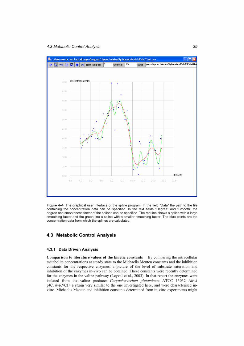
4.3 Metabolic Control Analysis 39
Figure 4–4: The graphical user interface of the spline program. In the field “Data” the path to the file containing the concentration data can be specified. In the text fields “Degree” and “Smooth” the degree and smoothness factor of the splines can be specified. The red line shows a spline with a large smoothing factor and the green line a spline with a smaller smoothing factor. The blue points are the concentration data from which the splines are calculated.
4.3 Metabolic Control Analysis
4.3.1 Data Driven Analysis
Comparison to literature values of the kinetic constants By comparing the intracellular metabolite concentrations at steady state to the Michaelis Menten constants and the inhibition constants for the respective enzymes, a picture of the level of substrate saturation and inhibition of the enzymes in-vivo can be obtained. These constants were recently determined for the enzymes in the valine pathway (Leyval et al., 2003). In that report the enzymes were isolated from the valine producer Corynebacterium glutamicum ATCC 13032 ilvApJC1ilvBNCD, a strain very similar to the one investigated here, and were characterised in-vitro. Michaelis Menten and inhibition constants determined from in-vitro experiments might

4 Theoretical methods 40
not be valid for the in-vivo conditions (Wright and Kelly, 1981; Teusink et al., 2000). However, when there are orders of magnitude of difference between the in-vitro constants and the respective concentration levels, one can draw some general conclusions.
The Pool Efflux Capacity The Pool Efflux Capacity (PEC) is a measure of an enzyme’s capacity to turn substrates into products at a given system state. The criterion was defined and applied to the aromatic amino acid pathway by Oldiges et al. (2004). The calculation procedure is purely data driven and aims to shed light on the control structure of the investigated pathway without the need to develop complex kinetic models. Time series of metabolite concentrations form the basis of this method. Scaled metabolite pool exchange rates are calculated as:
dttdx
xv i
SSii
)(1
,
( 4-23 )
where xi,SS is the concentration of metabolite i at steady state. The Pool Efflux Capacity is defined as the maximal relative efflux rate of a pool, i.e. the largest negative value of vi in Eq. (4-23) over a certain time period. In a linear reaction sequence the PEC value of a metabolite pool gives a measure of how fast the enzyme directly downstream of the pool is able to convert the substrates into products. Strictly, only net conversion rates of the metabolite pools are analysed so the method qualifies as an easy-to-apply quantitative guess giving approximations to the level of control in a linear pathway. A high capacity suggests that the enzyme has little control of the flux through the pathway since the enzyme will then be able to restore the system to steady state quickly. A low capacity signifies a high level of control. The PEC values are related to the enzyme elasticities defined in Eq. 4-8, in that an enzyme with high elasticities will in general have a high PEC and vice versa.
It should be noted that the PEC values do not necessarily sum up to 1 unless they have been scaled. As many PEC-values can be calculated as metabolite pools that are observed experimentally. Both characteristics differ from typical MCA approaches as will be demonstrated in the following chapters.
4.3.2 Model Based Control Analysis
The theoretical framework of MCA MCA uses sensitivity analysis to quantify the level of control that a system parameter (such as an enzyme level) has on a variable (such as a flux). The global and local coefficients used in MCA are defined here (Burns et al., 1985). A complete description of the theory can be found in the original papers (Kacser and Burns, 1973; Heinrich and Rapoport, 1974) or in one of the more recent reviews (Fell, 1992; Liao and Delgado, 1993; Visser and Heijnen, 2002).
The control coefficients are total derivatives which describe the global scaled sensitivity of a variable Vi towards a system parameter, pj:
j
i
i
jVji p
VVp
dd
C , ( 4-24 )
Control coefficients give a measure for the control that a parameter has on a certain variable at the system state considered.
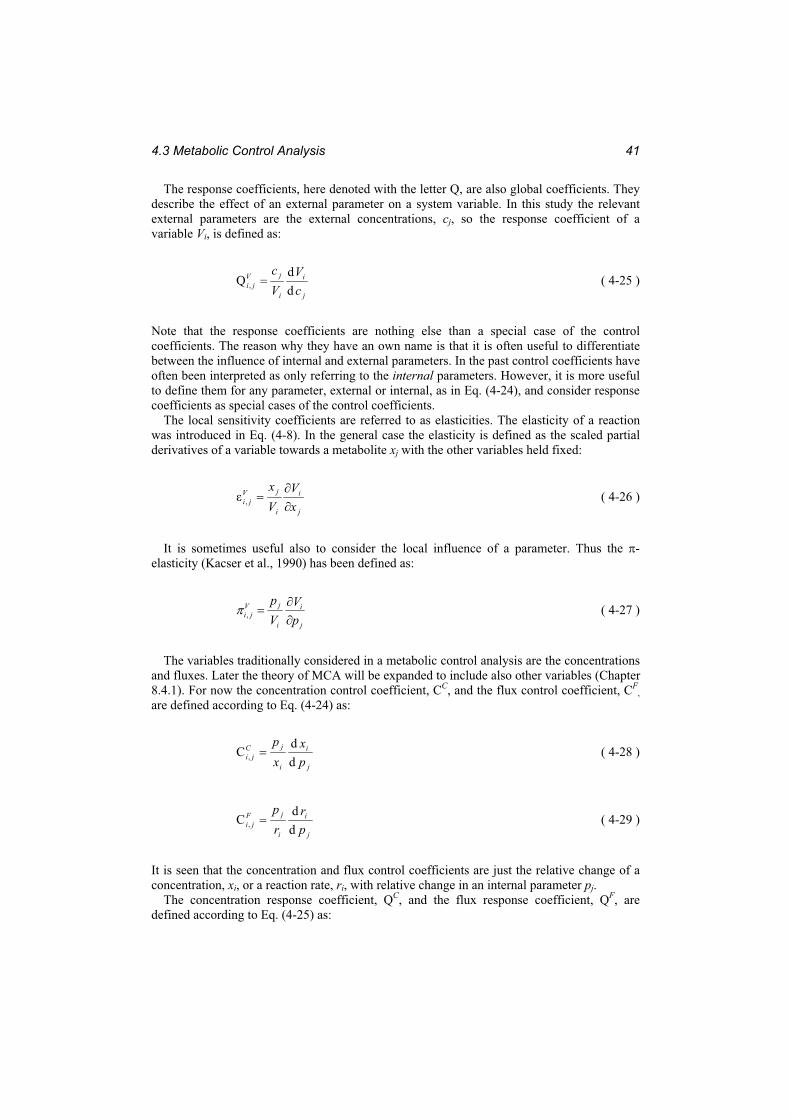
4.3 Metabolic Control Analysis 41
The response coefficients, here denoted with the letter Q, are also global coefficients. They describe the effect of an external parameter on a system variable. In this study the relevant external parameters are the external concentrations, cj, so the response coefficient of a variable Vi, is defined as:
j
i
i
jVji c
VVc
dd
Q , ( 4-25 )
Note that the response coefficients are nothing else than a special case of the control coefficients. The reason why they have an own name is that it is often useful to differentiate between the influence of internal and external parameters. In the past control coefficients have often been interpreted as only referring to the internal parameters. However, it is more useful to define them for any parameter, external or internal, as in Eq. (4-24), and consider response coefficients as special cases of the control coefficients.
The local sensitivity coefficients are referred to as elasticities. The elasticity of a reaction was introduced in Eq. (4-8). In the general case the elasticity is defined as the scaled partial derivatives of a variable towards a metabolite xj with the other variables held fixed:
j
i
i
jVji x
VVx
, ( 4-26 )
It is sometimes useful also to consider the local influence of a parameter. Thus the -elasticity (Kacser et al., 1990) has been defined as:
j
i
i
jVji p
VVp
, ( 4-27 )
The variables traditionally considered in a metabolic control analysis are the concentrations and fluxes. Later the theory of MCA will be expanded to include also other variables (Chapter 8.4.1). For now the concentration control coefficient, CC, and the flux control coefficient, CF
,are defined according to Eq. (4-24) as:
j
i
i
jCji p
xxp
dd
C , ( 4-28 )
j
i
i
jFji p
rrp
dd
C , ( 4-29 )
It is seen that the concentration and flux control coefficients are just the relative change of a concentration, xi, or a reaction rate, ri, with relative change in an internal parameter pj.
The concentration response coefficient, QC, and the flux response coefficient, QF, are defined according to Eq. (4-25) as:
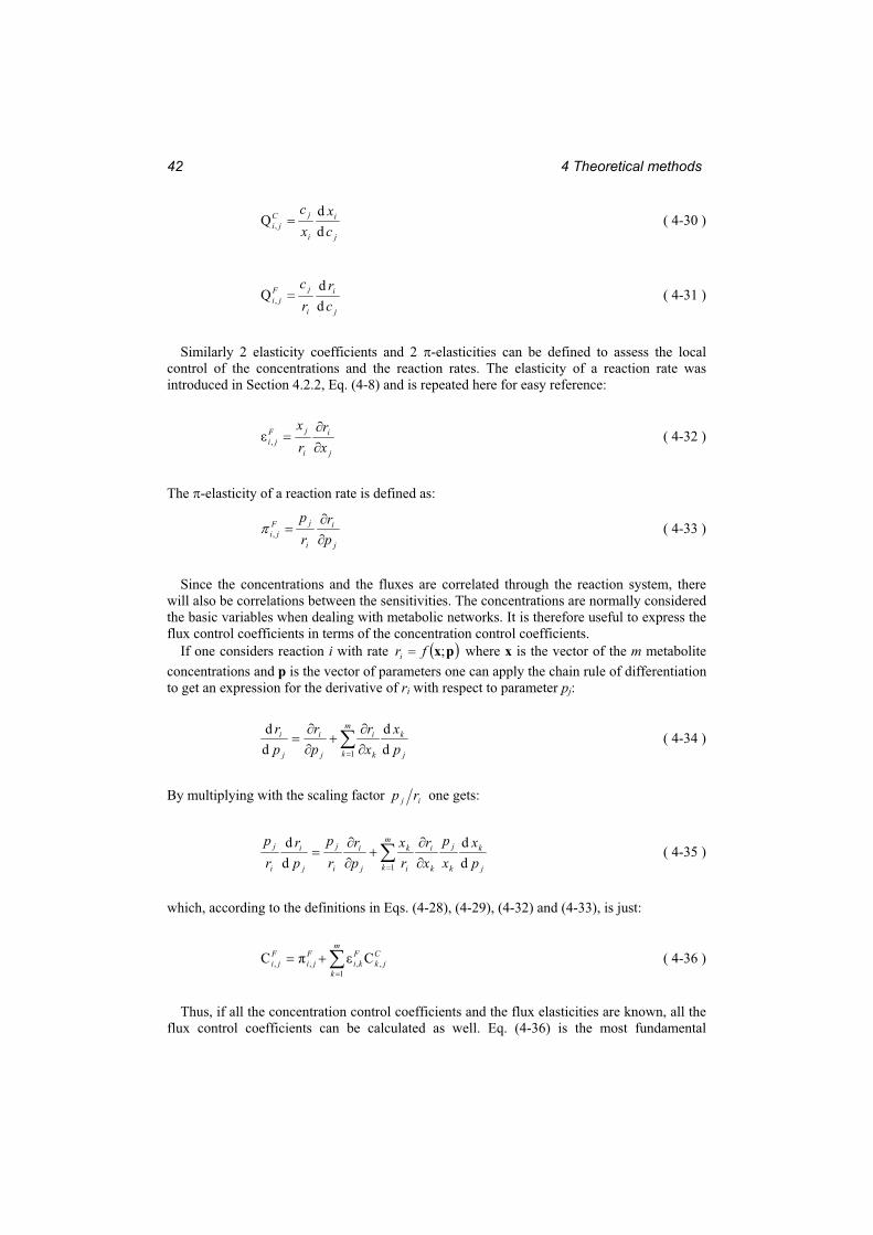
4 Theoretical methods 42
j
i
i
jCji c
xxc
dd
Q , ( 4-30 )
j
i
i
jFji c
rrc
dd
Q , ( 4-31 )
Similarly 2 elasticity coefficients and 2 -elasticities can be defined to assess the local control of the concentrations and the reaction rates. The elasticity of a reaction rate was introduced in Section 4.2.2, Eq. (4-8) and is repeated here for easy reference:
j
i
i
jFji x
rrx
, ( 4-32 )
The -elasticity of a reaction rate is defined as:
j
i
i
jFji p
rrp
, ( 4-33 )
Since the concentrations and the fluxes are correlated through the reaction system, there will also be correlations between the sensitivities. The concentrations are normally considered the basic variables when dealing with metabolic networks. It is therefore useful to express the flux control coefficients in terms of the concentration control coefficients.
If one considers reaction i with rate px;fri where x is the vector of the m metabolite concentrations and p is the vector of parameters one can apply the chain rule of differentiation to get an expression for the derivative of ri with respect to parameter pj:
m
k j
k
k
i
j
i
j
i
px
xr
pr
pr
1 dd
dd
( 4-34 )
By multiplying with the scaling factor ij rp one gets:
m
k j
k
k
j
k
i
i
k
j
i
i
j
j
i
i
j
px
xp
xr
rx
pr
rp
pr
rp
1 dd
dd
( 4-35 )
which, according to the definitions in Eqs. (4-28), (4-29), (4-32) and (4-33), is just:
m
k
Cjk
Fki
Fji
Fji
1,,,, CC ( 4-36 )
Thus, if all the concentration control coefficients and the flux elasticities are known, all the flux control coefficients can be calculated as well. Eq. (4-36) is the most fundamental
4.3 Metabolic Control Analysis 43
equation in MCA because it is a general formulation of the summation and connectivity theorems (Stephanopoulos et al. 1998). The flux summation theorem says that with respect to the enzyme levels the flux control coefficients for a specific flux must sum up to 1:
n
i
FiC
11 ( 4-37 )
The flux control connectivity theorem expresses the relationship between the flux control coefficients and the elasticities:
n
i
Fji
FiC
1, 0 ( 4-38 )
It is important to recognise that the control and response coefficients are total differentials, which means that the global effect of the parameter change taking all system variables into account is evaluated. Both coefficients are dependent on the state of the system and do not in general change linearly with parameter. The control coefficients calculated at one system state can therefore not be used to predict the change in flux resulting from a finite change in parameter. However, the control coefficients are useful to elucidate the control hierarchy in the reaction system at a specific state and also give a good indication of which enzymes should be considered for manipulation.
The flux control coefficients with respect to the enzyme levels are normally the most important coefficients in a metabolic engineering study since the enzyme levels are the parameters which can be changed by the use of DNA technology. In some cases it is interesting to also calculate control coefficients to evaluate the influence of the substrate affinity, the product affinity and inhibitor affinity. For a mechanistic model this could be achieved by calculating the flux control coefficients with respect to the Michaelis Menten constants, Km, and the inhibition constants, Ki. For a linlog model these constants are not part of the model parameters and such an analysis is therefore not possible with a linlog model. However, this is only a minor drawback to the linlog approach since changes to the Km and the Ki constants are difficult to implement in practice anyway.
For the purpose of finding the target enzymes for a further optimisation of the strain all coefficients will be calculated with respect to the valine excretion rate in order to analyse the influence and control that the different system parameters have on the strains ability to produce valine. By comparing the flux control coefficients to each other the distribution of control of the enzymes in the pathway is evaluated. The response coefficients are calculated for all external metabolites to investigate how the availability of the different co-metabolites affects the valine excretion rate. The metabolic network simulation programs Jarnac (Sauro et al., 2003) and Gepasi (Mendes 1993; 1997) were used to calculate flux and response coefficients at steady state.
Model Prediction The model is further used to predict the changes in valine flux resulting from some of the possible genetic alterations suggested by the MCA. By doing these in-silico changes an estimate of how the strain would be affected in a real experiment can be obtained and the applicability of MCA in the identification of target enzymes can be investigated. Only changes which realistically can be implemented in the real cell are considered. Jarnac (Sauro et al., 2003) and Gepasi (Mendes, 1993; 1997) were used to calculate the model predictions of the change in valine excretion rate.
4 Theoretical methods 44
Optimisation of Enzyme Levels In an optimisation study, the enzyme activities in the valine / leucine pathway were optimised to obtain the maximum valine excretion rate. The external metabolites in the system were fixed at their steady state levels during the optimisation. The simulated annealing optimisation algorithm (Kirkpatrick et al., 1983) as implemented in Gepasi (Mendes et al., 1998) was used. This algorithm is slow, but gives a higher probability of finding the global optimum than most other optimisation algorithms. In the system optimised here only 7 system parameters were varied so the computation time was acceptable also with this algorithm.
4 constraints were set for the parameter optimisation. The first ensures that the total enzyme concentration is kept at a constant level. This is formulated as:
neen
i i
i
10 ( 4-39 )
where e/e0 is the enzyme activity relative to the reference state and n is the number of enzymes considered.
The second constraint allows only modest changes in the metabolite levels in order to avoid influence on the gene expression and other secondary effects. This homeostatic constraint is formulated as:
1.011
0
0m
i i
ii
xxx
m ( 4-40 )
where m is the number of metabolites and xi is the concentration of metabolite i and the superscript 0 refers to the reference state. The constraint ensures that the average change in metabolite level is less than 10 %. These first two constraints were applied by Mauch et al. (2001) to optimise the ethanol production in yeast, by Visser et al. (2004a) in a design study of the primary metabolism of Escherichia coli and by Schmid et al. (2004) in the optimisation of tryptophan production in Escherichia coli. Their importance in the design of metabolic system was discussed in more detail in the respective publications. The homeostasis constraint was first suggested by Kacser and Acerenza (1993) and also discussed by Thomas and Fell (1996) and applied by Stephanopoulos and Simpson (1997) in a theoretical study.
The third constraint ensures that the second law of thermodynamics is not violated. This constraint is identical to the thermodynamic constraint used for the model development and is described in more detail in Section 4.2.5. The optimised fluxes are not allowed to conflict with Eq. (4-17).
The fourth constraint sets the essential requirement that the optimal enzyme levels result in a stable steady state. The steady state is stable if and only if all the eigenvalues of the associated Jacobian matrix have negative real parts (Kondepudi and Prigogine 1998). In the model investigated here this constraint did not significantly limit the search for the optimal parameters as the model structure ensures stability for most choices of enzyme levels. However, in the general case the stability constraint is important since it is not given that dynamic models are stable.
Finally it is not desired to have a strain that consumes leucine so negative fluxes of leucine excretion were not allowed.
4.4 Thermodynamic Analysis 45
4.4 Thermodynamic Analysis
4.4.1 Introduction to the thermodynamic analysis of metabolic networks
As stated in the introduction, the role of the thermodynamic driving forces for the reactions in metabolic networks will be analysed. The driving force for a chemical reaction is referred to as the reaction affinity, A, and was defined by De Donder (De Donder 1927; De Donder and van Rysselberghe 1936):
iiiA ( 4-41 )
Here i is the stoichiometric coefficient of substance i, defined to be positive for products and negative for reactants and i is the chemical potential of component i. Thus the affinity is just the negative difference in chemical potential of the reactants and products i.e. the negative of Gibbs free energy of reaction, Gr. There is, however, a conceptual difference between A and
Gr; Gibbs free energy is used in the context of equilibrium states whereas the affinity is central in non-equilibrium thermodynamics.
Since A is just the negative of Gr it can be calculated in the same manner that Gr is calculated (see Section 4.2.5 Eq. (4-16)). Thus, for a reaction with m reacting species A is given by:
m
kkkg xTRAA
1
' ln ( 4-42 )
Here A°’ is the standard affinity at the biological standard state where the reference pH is 7 (see Section 4.2.5 for the definition of the thermodynamic biological standard state). xk is the concentration of metabolite k participating in the reaction and the stoichiometric coefficients
k are defined positive for products and negative for reactants. As noted earlier the activities should be used instead of the concentrations, but setting the activity coefficients equal to 1 is probably a good approximation for the dilute concentrations in the cell. Rg is the universal gas constant and T the temperature in Kelvin.
A°’ is calculated from the standard chemical potentials, °’ according to the definition in Eq. (4-41):
iiiA '' ( 4-43 )
The chemical potential of a substance is just the molar Gibbs energy and it is common in practical calculations to set the standard chemical potentials, °’, equal to the Gibbs energy of formation, Gf
°’. A°’ can therefore be calculated directly from Eq. (4-43) by using literature values for Gf
°’.Furthermore, the chemical potential, , of a species i in a mixture at any concentration can
be calculated from:
igii xTR ln' ( 4-44 )
4 Theoretical methods 46
This equation is found in textbooks on physical chemistry, for example in the book by Atkins (1998). xi is the concentration of metabolite i measured in mole/l.
At equilibrium the affinity is zero so it follows from Eq. (4-42) that
eqg KTRA ln' ( 4-45 )
where Keq is the equilibrium constant. When A°’ is known, Keq is easily calculated by rewriting Eq. (4-45) as:
TRA
eqgeK
'
( 4-46 )
Cellular metabolism is an open system which continuously exchanges matter and energy with the surroundings. The reactions in the cells are therefore never at equilibrium, instead a non-equilibrium steady state is reached where the fluxes and concentrations do not change with time. Classical thermodynamics deals primarily with equilibrium situations and has therefore been extended to the non-equilibrium state by the work of Onsager (1931), Prigogine (1961) and others to deal with the many non-equilibrium real systems as described in the Introduction.
Here it will be differentiated between near-equilibrium states and far-from-equilibrium states according to a criterion stated by Caplan (1971). A reaction is near equilibrium when
1TR
A
g
( 4-47 )
Here Rg is the universal gas constant and T the temperature in Kelvin. For near-equilibrium reactions the flux is proportional to the forces driving it, i.e. the
phenomenological relations are valid. A flux Jk is then given by:
jjjkk ALJ , ( 4-48 )
where Lk,j are the phenomenological coefficients and Aj are the different forces driving it. Eq. (4-48) is analogous to other common relations between flow and force such as Fick’s law of diffusion, Poisseseuile’s law for fluid flow, Fourier’s law of heat conduction and Ohm’s law for flow of electric current.
Biochemical reactions can generally not be assumed to be near equilibrium so the phenomenological relations can not be assumed to be valid. However, a linear relation between force and flux has often been observed experimentally for example for the processes of oxidative phosphorylation (Rottenberg 1973 and 1979; Stucki 1980). Rottenberg (1973) and van der Meer et al. (1980) suggested that this was due to the mechanism of enzyme catalysed reactions and demonstrated that the mechanism of the uni-uni Michaelis Menten kinetics implies a near linear relation between rate and affinity within a certain affinity range. This was also discussed by Westerhoff and van Dam (1987).
4.4 Thermodynamic Analysis 47
A further investigation of the relationship between rate and affinity is important in establishing a theoretical basis for the application of thermodynamic analysis to biochemical systems. If the phenomenological relations can be demonstrated to hold also at states far from equilibrium it will significantly simplify the analysis. Onsager’s reciprocal relations (Onsager 1931) would then be valid and could be used for example to investigate the degree of coupling between the reactions. Furthermore, it would promote the use of network thermodynamics (Mikulecky 2001) where the reaction network is analysed in the same way that electrical circuits are analysed, the advantage being that the entire body of electrical network theory can be applied. The analogy between biochemical networks and electrical circuits is fairly obvious. Kirchhoff’s first and second laws for electrical circuits, for example, correspond to the material and energy balances used in metabolic flux analysis.
Far-from-equilibrium systems may be unstable (Prigogine and Lefever, 1968), i.e. they may not have a uniquely defined steady state and may display chaotic behaviour such as concentration oscillations or propagating waves. It is therefore not obvious that metabolic networks are stable even under constant extracellular conditions. However, living cells are clearly stable systems, as they can maintain their function also under varying extracellular conditions. When the phenomenological relations apply, the system will always have a stable state (Kondepudi and Prigogine 1998). The investigation of the linearity between rate and force in biochemical reaction networks will therefore provide a deeper insight into the stability of these systems.
When analysing the behaviour of complex dynamic systems one often distinguishes between central control and self-organising of the system. Examples of this are found in many real systems. In an ecosystem the population of rabbits and foxes will adjust themselves to each other through self-organising. When a certain number of foxes and rabbits are hunted each year (by humans), this is central control. A business company functions according to how the workers perform and how they interact and cooperate (self-organisation), but also according to the decisions that are made by the board of directors (central control).
In a cell, the division of the control of the metabolism into central control and self-organising is obvious. Central control is achieved through the transcription of the different genes and translation of the corresponding mRNAs. The cell regulates its fluxes by adjusting the enzyme levels. Self-organisation (or post-translational control) results from the interactions of the metabolites in the network with the enzymes catalysing the reactions. The steady state reached by the system depends on the complex reaction mechanisms of enzymes where allosteric effects from metabolites not participating in the reaction may play a role. Feedback inhibition is an important part of the self-organising of metabolic networks. The observed fluxes in a cell are the result of the combination of central control and self-organisation.
Using the framework of metabolic control analysis one can assess the level of central control and self-organising. This is particularly useful in analysing the role of the thermodynamic forces in the control of metabolic networks. It will be shown in Chapter 8 how the theoretical framework of MCA can be extended to include also the thermodynamic properties. In this way quantitative measures of control can be obtained for the thermodynamic properties in the same way that is done for the fluxes and concentrations.

4 Theoretical methods 48
5 Metabolomics 49
5 Metabolomics As pointed out in the introduction, accurate data of the concentrations of the intracellular metabolites was the starting point for the analysis of the metabolic network reported in this work. The glucose stimulus experiment was performed to obtain concentration time series of the metabolites during a transient state. These formed the experimental basis of the kinetic model as well as of the metabolic control analysis and the thermodynamic analysis. The experimental results are reported in this chapter with the focus set on the experiment which yielded the optimal data set for the further modelling and analysis.
5.1 The glucose stimulus experiment
5.1.1 The establishment of the extraction method
The most suitable method of cell disruption and metabolite extraction was established prior to the stimulus experiments. Two chemical extraction methods using either KOH or perchloric acid (HClO4) as well as a mechanical disruption method using the rotor / stator homogenisator described in Section 3.3 were tested. The extraction efficiency of the three different methods was evaluated by performing repetitive extraction cycles on the same sample and measuring the amount of intracellular metabolites that could be extracted for each cycle. In this way it was established that from the total amount of an intracellular metabolite present in the cell, 92 % could be extracted with the KOH method after one extraction cycle. The perchloric acid disruption method, which has frequently been used in similar investigations (Buchholz et al., 2001), could extract 88 % of the amount of the metabolites, but led to larger standard deviations in the analytical measurements. The KOH disruption also had the advantage that acid sensitive metabolites would not be affected by the disruption procedure. The levels of NAD and NADP were equal within measurement error for the two chemical disruption methods whereas NADH and NADPH could not be quantified with either method.
The mechanical disruption method using the rotor / stator homogeniser could only extract 42 % of the metabolites when operated at -20 °C and this method was therefore not investigated further. Other mechanical disruption devices such as bead mills or french presses could not be operated at -20 °C and were therefore not interesting for these experiments.
5.1.2 Criteria for the fermentation
The fermentation and the stimulus-response experiment must be carefully designed to yield a useful data set. Large changes in the metabolite concentrations are desired to provide a good experimental basis for the fitting of the model parameters and to obtain a wide range of validity of the model. Thus, the following two criteria for the setup of the fermentation were formulated: The physiological state of the culture at the time of the stimulus-response experiment should be chosen such that, (i) the results are readily transferable to the production conditions and (ii) the stimulus has a strong effect on the intracellular pools resulting in large deflections in the concentrations.
Criterion (ii) ensures that an information-rich data set is obtained. The biomass specific valine excretion rate of this strain is at its highest during the
exponential growth phase, so according to criterion (i), the investigation should be relevant to this state. However, the cells must be limited in their glucose supply immediately before the glucose addition to ensure sufficient glucose input stimulation, so the exponential growth
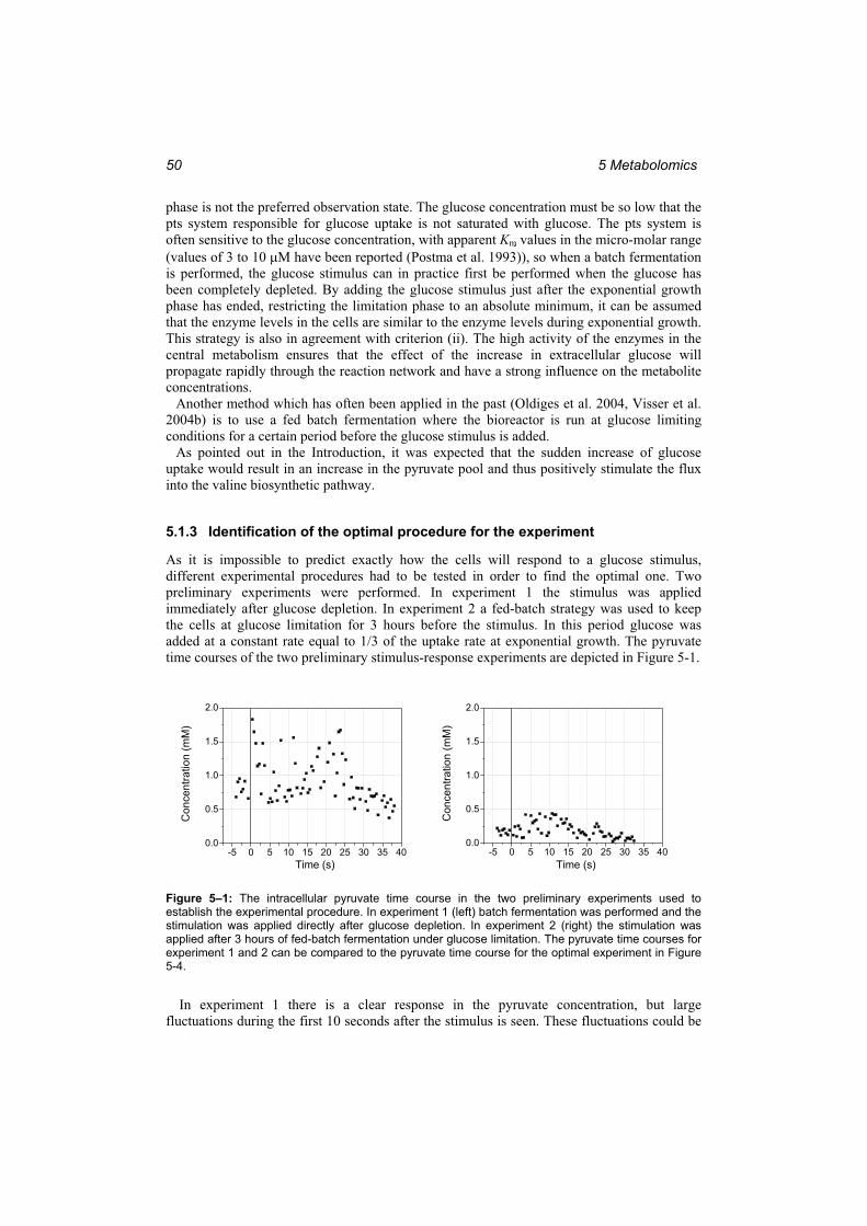
5 Metabolomics 50
phase is not the preferred observation state. The glucose concentration must be so low that the pts system responsible for glucose uptake is not saturated with glucose. The pts system is often sensitive to the glucose concentration, with apparent Km values in the micro-molar range (values of 3 to 10 M have been reported (Postma et al. 1993)), so when a batch fermentation is performed, the glucose stimulus can in practice first be performed when the glucose has been completely depleted. By adding the glucose stimulus just after the exponential growth phase has ended, restricting the limitation phase to an absolute minimum, it can be assumed that the enzyme levels in the cells are similar to the enzyme levels during exponential growth. This strategy is also in agreement with criterion (ii). The high activity of the enzymes in the central metabolism ensures that the effect of the increase in extracellular glucose will propagate rapidly through the reaction network and have a strong influence on the metabolite concentrations.
Another method which has often been applied in the past (Oldiges et al. 2004, Visser et al. 2004b) is to use a fed batch fermentation where the bioreactor is run at glucose limiting conditions for a certain period before the glucose stimulus is added.
As pointed out in the Introduction, it was expected that the sudden increase of glucose uptake would result in an increase in the pyruvate pool and thus positively stimulate the flux into the valine biosynthetic pathway.
5.1.3 Identification of the optimal procedure for the experiment
As it is impossible to predict exactly how the cells will respond to a glucose stimulus, different experimental procedures had to be tested in order to find the optimal one. Two preliminary experiments were performed. In experiment 1 the stimulus was applied immediately after glucose depletion. In experiment 2 a fed-batch strategy was used to keep the cells at glucose limitation for 3 hours before the stimulus. In this period glucose was added at a constant rate equal to 1/3 of the uptake rate at exponential growth. The pyruvate time courses of the two preliminary stimulus-response experiments are depicted in Figure 5-1.
-5 0 5 10 15 20 25 30 35 400.0
0.5
1.0
1.5
2.0
Con
cent
ratio
n (m
M)
Time (s)-5 0 5 10 15 20 25 30 35 40
0.0
0.5
1.0
1.5
2.0
Con
cent
ratio
n (m
M)
Time (s)
Figure 5–1: The intracellular pyruvate time course in the two preliminary experiments used to establish the experimental procedure. In experiment 1 (left) batch fermentation was performed and the stimulation was applied directly after glucose depletion. In experiment 2 (right) the stimulation was applied after 3 hours of fed-batch fermentation under glucose limitation. The pyruvate time courses for experiment 1 and 2 can be compared to the pyruvate time course for the optimal experiment in Figure 5-4.
In experiment 1 there is a clear response in the pyruvate concentration, but large fluctuations during the first 10 seconds after the stimulus is seen. These fluctuations could be
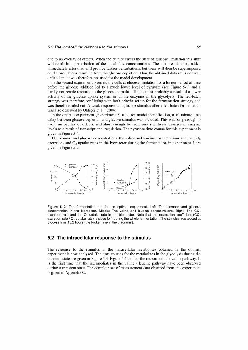
5.2 The intracellular response to the stimulus 51
due to an overlay of effects. When the culture enters the state of glucose limitation this shiftwill result in a perturbation of the metabolite concentrations. The glucose stimulus, added immediately after that, will provide further perturbations, but these will then be superimposed on the oscillations resulting from the glucose depletion. Thus the obtained data set is not well defined and it was therefore not used for the model development.
In the second experiment, keeping the cells at glucose limitation for a longer period of time before the glucose addition led to a much lower level of pyruvate (see Figure 5-1) and a hardly noticeable response to the glucose stimulus. This is most probably a result of a lower activity of the glucose uptake system or of the enzymes in the glycolysis. The fed-batch strategy was therefore conflicting with both criteria set up for the fermentation strategy and was therefore ruled out. A weak response to a glucose stimulus after a fed-batch fermentation was also observed by Oldiges et al. (2004).
In the optimal experiment (Experiment 3) used for model identification, a 10-minute time delay between glucose depletion and glucose stimulus was included. This was long enough to avoid an overlay of effects, and short enough to avoid any significant changes in enzyme levels as a result of transcriptional regulation. The pyruvate time course for this experiment is given in Figure 5-4.
The biomass and glucose concentrations, the valine and leucine concentrations and the CO2excretion- and O2 uptake rates in the bioreactor during the fermentation in experiment 3 are given in Figure 5-2.
0 2 4 6 8 10 12 140
10
20
30
40 glucose
biom
ass
dry
wei
ght,
g/l
gluc
ose,
g/l
fermentation time, h
0
4
8
12
16 biomass
0 2 4 6 8 10 12 140
20
40
60
80
0.0
0.5
1.0
1.5
2.0
2.5
L-valine
conc
netra
tion
L-le
ucin
e, m
M
conc
netra
tion
L-va
line,
mM
fermentation time, h
L-leucine
0 2 4 6 8 10 12 140
1
2
3
4
5
6
CO
2 and
O2, m
mol
/min
fermentation time, h
CO2
O2
Figure 5–2: The fermentation run for the optimal experiment. Left: The biomass and glucose concentration in the bioreactor. Middle: The valine and leucine concentrations. Right: The CO2excretion rate and the O2 uptake rate in the bioreactor. Note that the respiration coefficient (CO2excretion rate / O2 uptake rate) is close to 1 during the whole fermentation. The stimulus was added at process time 13.2 hours (the broken line in the diagrams).
5.2 The intracellular response to the stimulus
The response to the stimulus in the intracellular metabolites obtained in the optimal experiment is now analysed. The time courses for the metabolites in the glycolysis during the transient state are given in Figure 5.3. Figure 5.4 depicts the response in the valine pathway. It is the first time that the intermediates in the valine / leucine pathway have been observed during a transient state. The complete set of measurement data obtained from this experiment is given in Appendix C.
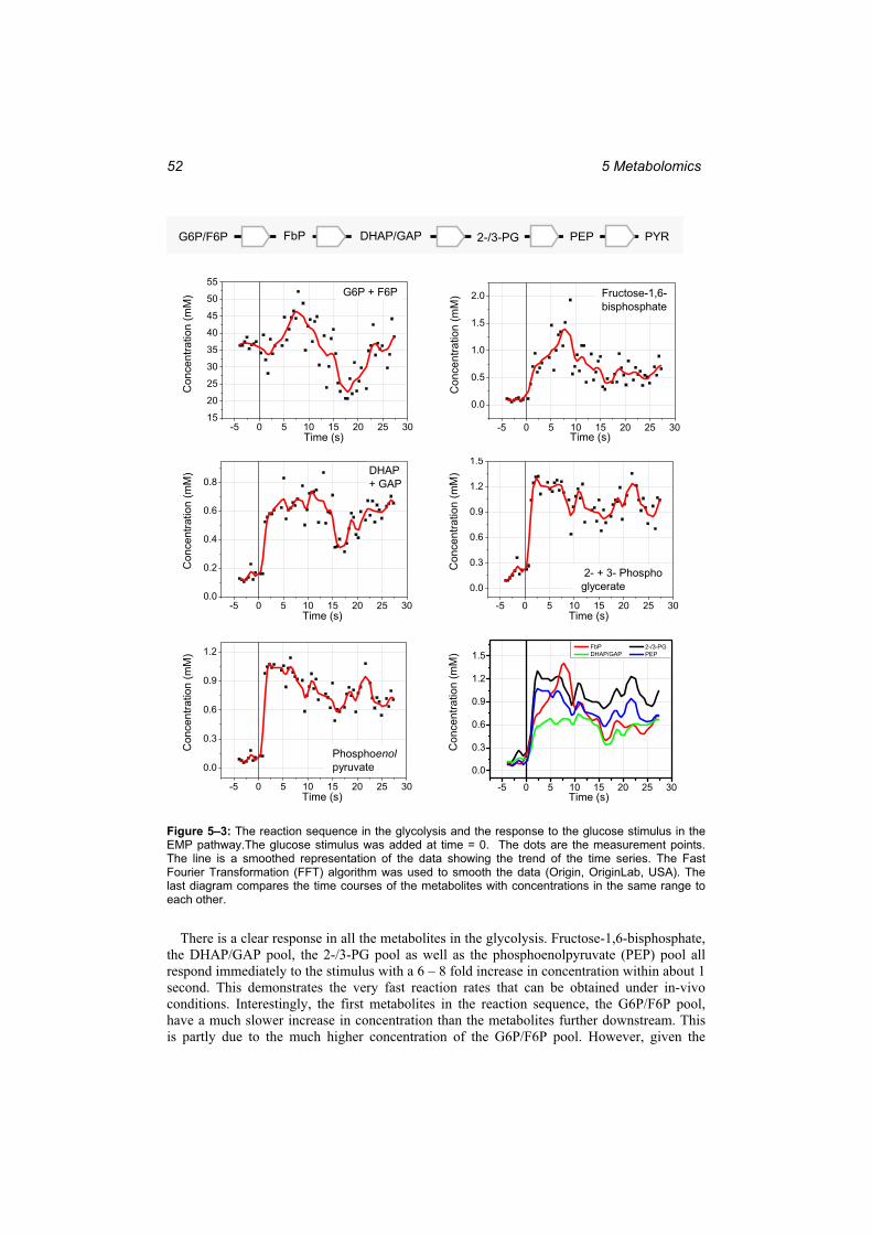
5 Metabolomics 52
G6P/F6P FbP DHAP/GAP PEP PYR2-/3-PGG6P/F6P FbP DHAP/GAP PEP PYR2-/3-PG
-5 0 5 10 15 20 25 3015
20
25
30
35
40
45
50
55
Con
cent
ratio
n (m
M)
Time (s)
G6P + F6P
-5 0 5 10 15 20 25 30
0.0
0.5
1.0
1.5
2.0
Con
cent
ratio
n (m
M)
Time (s)
Fructose-1,6-bisphosphate
-5 0 5 10 15 20 25 300.0
0.2
0.4
0.6
0.8
Con
cent
ratio
n (m
M)
Time (s)
DHAP+ GAP
-5 0 5 10 15 20 25 30
0.0
0.3
0.6
0.9
1.2
1.5C
once
ntra
tion
(mM
)
Time (s)
2- + 3- Phosphoglycerate
-5 0 5 10 15 20 25 30
0.0
0.3
0.6
0.9
1.2
Con
cent
ratio
n (m
M)
Time (s)
Phosphoenolpyruvate
-5 0 5 10 15 20 25 30
0.0
0.3
0.6
0.9
1.2
1.5 2-/3-PG PEP
Con
cent
ratio
n (m
M)
Time (s)
FbP DHAP/GAP
Figure 5–3: The reaction sequence in the glycolysis and the response to the glucose stimulus in the EMP pathway.The glucose stimulus was added at time = 0. The dots are the measurement points. The line is a smoothed representation of the data showing the trend of the time series. The Fast Fourier Transformation (FFT) algorithm was used to smooth the data (Origin, OriginLab, USA). The last diagram compares the time courses of the metabolites with concentrations in the same range to each other.
There is a clear response in all the metabolites in the glycolysis. Fructose-1,6-bisphosphate, the DHAP/GAP pool, the 2-/3-PG pool as well as the phosphoenolpyruvate (PEP) pool all respond immediately to the stimulus with a 6 – 8 fold increase in concentration within about 1 second. This demonstrates the very fast reaction rates that can be obtained under in-vivo conditions. Interestingly, the first metabolites in the reaction sequence, the G6P/F6P pool, have a much slower increase in concentration than the metabolites further downstream. This is partly due to the much higher concentration of the G6P/F6P pool. However, given the
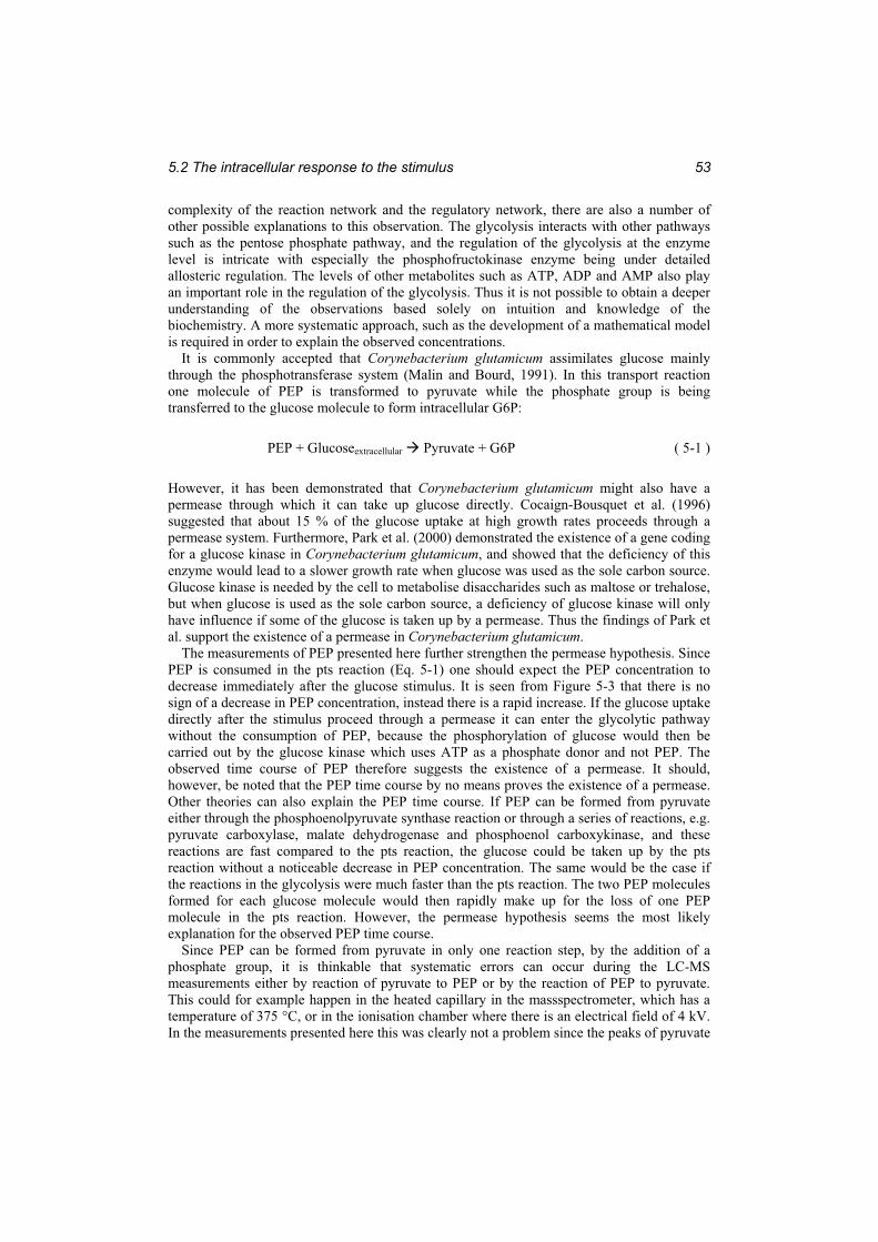
5.2 The intracellular response to the stimulus 53
complexity of the reaction network and the regulatory network, there are also a number of other possible explanations to this observation. The glycolysis interacts with other pathways such as the pentose phosphate pathway, and the regulation of the glycolysis at the enzyme level is intricate with especially the phosphofructokinase enzyme being under detailed allosteric regulation. The levels of other metabolites such as ATP, ADP and AMP also play an important role in the regulation of the glycolysis. Thus it is not possible to obtain a deeper understanding of the observations based solely on intuition and knowledge of the biochemistry. A more systematic approach, such as the development of a mathematical model is required in order to explain the observed concentrations.
It is commonly accepted that Corynebacterium glutamicum assimilates glucose mainly through the phosphotransferase system (Malin and Bourd, 1991). In this transport reaction one molecule of PEP is transformed to pyruvate while the phosphate group is being transferred to the glucose molecule to form intracellular G6P:
PEP + Glucoseextracellular Pyruvate + G6P ( 5-1 )
However, it has been demonstrated that Corynebacterium glutamicum might also have a permease through which it can take up glucose directly. Cocaign-Bousquet et al. (1996) suggested that about 15 % of the glucose uptake at high growth rates proceeds through a permease system. Furthermore, Park et al. (2000) demonstrated the existence of a gene coding for a glucose kinase in Corynebacterium glutamicum, and showed that the deficiency of this enzyme would lead to a slower growth rate when glucose was used as the sole carbon source. Glucose kinase is needed by the cell to metabolise disaccharides such as maltose or trehalose, but when glucose is used as the sole carbon source, a deficiency of glucose kinase will only have influence if some of the glucose is taken up by a permease. Thus the findings of Park et al. support the existence of a permease in Corynebacterium glutamicum.
The measurements of PEP presented here further strengthen the permease hypothesis. Since PEP is consumed in the pts reaction (Eq. 5-1) one should expect the PEP concentration to decrease immediately after the glucose stimulus. It is seen from Figure 5-3 that there is no sign of a decrease in PEP concentration, instead there is a rapid increase. If the glucose uptake directly after the stimulus proceed through a permease it can enter the glycolytic pathway without the consumption of PEP, because the phosphorylation of glucose would then be carried out by the glucose kinase which uses ATP as a phosphate donor and not PEP. The observed time course of PEP therefore suggests the existence of a permease. It should, however, be noted that the PEP time course by no means proves the existence of a permease. Other theories can also explain the PEP time course. If PEP can be formed from pyruvate either through the phosphoenolpyruvate synthase reaction or through a series of reactions, e.g. pyruvate carboxylase, malate dehydrogenase and phosphoenol carboxykinase, and these reactions are fast compared to the pts reaction, the glucose could be taken up by the pts reaction without a noticeable decrease in PEP concentration. The same would be the case if the reactions in the glycolysis were much faster than the pts reaction. The two PEP molecules formed for each glucose molecule would then rapidly make up for the loss of one PEP molecule in the pts reaction. However, the permease hypothesis seems the most likely explanation for the observed PEP time course.
Since PEP can be formed from pyruvate in only one reaction step, by the addition of a phosphate group, it is thinkable that systematic errors can occur during the LC-MS measurements either by reaction of pyruvate to PEP or by the reaction of PEP to pyruvate. This could for example happen in the heated capillary in the massspectrometer, which has a temperature of 375 °C, or in the ionisation chamber where there is an electrical field of 4 kV. In the measurements presented here this was clearly not a problem since the peaks of pyruvate
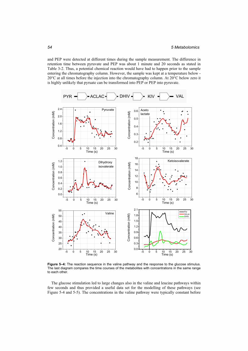
5 Metabolomics 54
and PEP were detected at different times during the sample measurement. The difference in retention time between pyruvate and PEP was about 1 minute and 20 seconds as stated in Table 3-2. Thus, a potential chemical reaction would have had to happen prior to the sample entering the chromatography column. However, the sample was kept at a temperature below -20°C at all times before the injection into the chromatography column. At 20°C below zero it is highly unlikely that pyruate can be transformed into PEP or PEP into pyruvate.
-5 0 5 10 15 20 25 300.4
0.8
1.2
1.6
2.0
2.4
Con
cent
ratio
n (m
M)
Time (s)
Pyruvate
-5 0 5 10 15 20 25 30
0.2
0.3
0.4
0.5
0.6
Con
cent
ratio
n (m
M)
Time (s)
Acetolactate
-5 0 5 10 15 20 25 30
0.0
0.2
0.4
0.6
0.8
1.0
1.2
Con
cent
ratio
n (m
M)
Time (s)
Dihydroxyisovalerate
-5 0 5 10 15 20 25 30
6
8
10
12
14
16
18
Con
cent
ratio
n (m
M)
Time (s)
Ketoisovalerate
-5 0 5 10 15 20 25 3020
25
30
35
40
45
50
55
Con
cent
ratio
n (m
M)
Time (s)
Valine
-5 0 5 10 15 20 25 300.0
0.3
0.6
0.9
1.2
1.5
1.8
2.1
Con
cent
ratio
n (m
M)
Time (s)
Pyr AcLac DHIV
Figure 5–4: The reaction sequence in the valine pathway and the response to the glucose stimulus. The last diagram compares the time courses of the metabolites with concentrations in the same range to each other.
The glucose stimulation led to large changes also in the valine and leucine pathways within few seconds and thus provided a useful data set for the modelling of these pathways (see Figure 5-4 and 5-5). The concentrations in the valine pathway were typically constant before
PYR ACLAC DHIV KIV VALPYR ACLAC DHIV KIV VAL
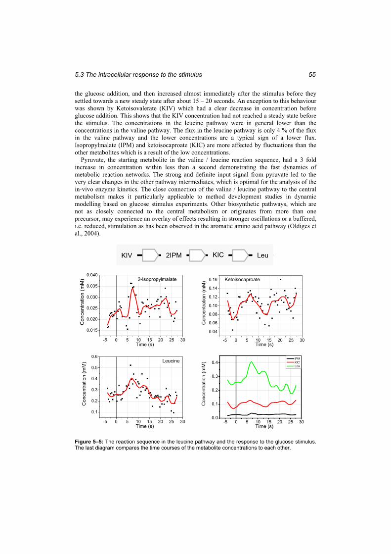
5.3 The intracellular response to the stimulus 55
the glucose addition, and then increased almost immediately after the stimulus before they settled towards a new steady state after about 15 – 20 seconds. An exception to this behaviour was shown by Ketoisovalerate (KIV) which had a clear decrease in concentration before glucose addition. This shows that the KIV concentration had not reached a steady state before the stimulus. The concentrations in the leucine pathway were in general lower than the concentrations in the valine pathway. The flux in the leucine pathway is only 4 % of the flux in the valine pathway and the lower concentrations are a typical sign of a lower flux. Isopropylmalate (IPM) and ketoisocaproate (KIC) are more affected by fluctuations than the other metabolites which is a result of the low concentrations.
Pyruvate, the starting metabolite in the valine / leucine reaction sequence, had a 3 fold increase in concentration within less than a second demonstrating the fast dynamics of metabolic reaction networks. The strong and definite input signal from pyruvate led to the very clear changes in the other pathway intermediates, which is optimal for the analysis of the in-vivo enzyme kinetics. The close connection of the valine / leucine pathway to the central metabolism makes it particularly applicable to method development studies in dynamic modelling based on glucose stimulus experiments. Other biosynthetic pathways, which are not as closely connected to the central metabolism or originates from more than one precursor, may experience an overlay of effects resulting in stronger oscillations or a buffered, i.e. reduced, stimulation as has been observed in the aromatic amino acid pathway (Oldiges et al., 2004).
KIV 2IPM KIC Leu
-5 0 5 10 15 20 25 30
0.015
0.020
0.025
0.030
0.035
0.040
Con
cent
ratio
n (m
M)
Time (s)
2-Isopropylmalate
-5 0 5 10 15 20 25 30
0.04
0.06
0.08
0.10
0.12
0.14
0.16
Con
cent
ratio
n (m
M)
Time (s)
Ketoisocaproate
-5 0 5 10 15 20 25 30
0.1
0.2
0.3
0.4
0.5
0.6
Con
cent
ratio
n (m
M)
Time (s)
Leucine
-5 0 5 10 15 20 25 300.0
0.1
0.2
0.3
0.4
Con
cent
ratio
n (m
M)
Time (s)
IPM KIC Leu
Figure 5–5: The reaction sequence in the leucine pathway and the response to the glucose stimulus. The last diagram compares the time courses of the metabolite concentrations to each other.
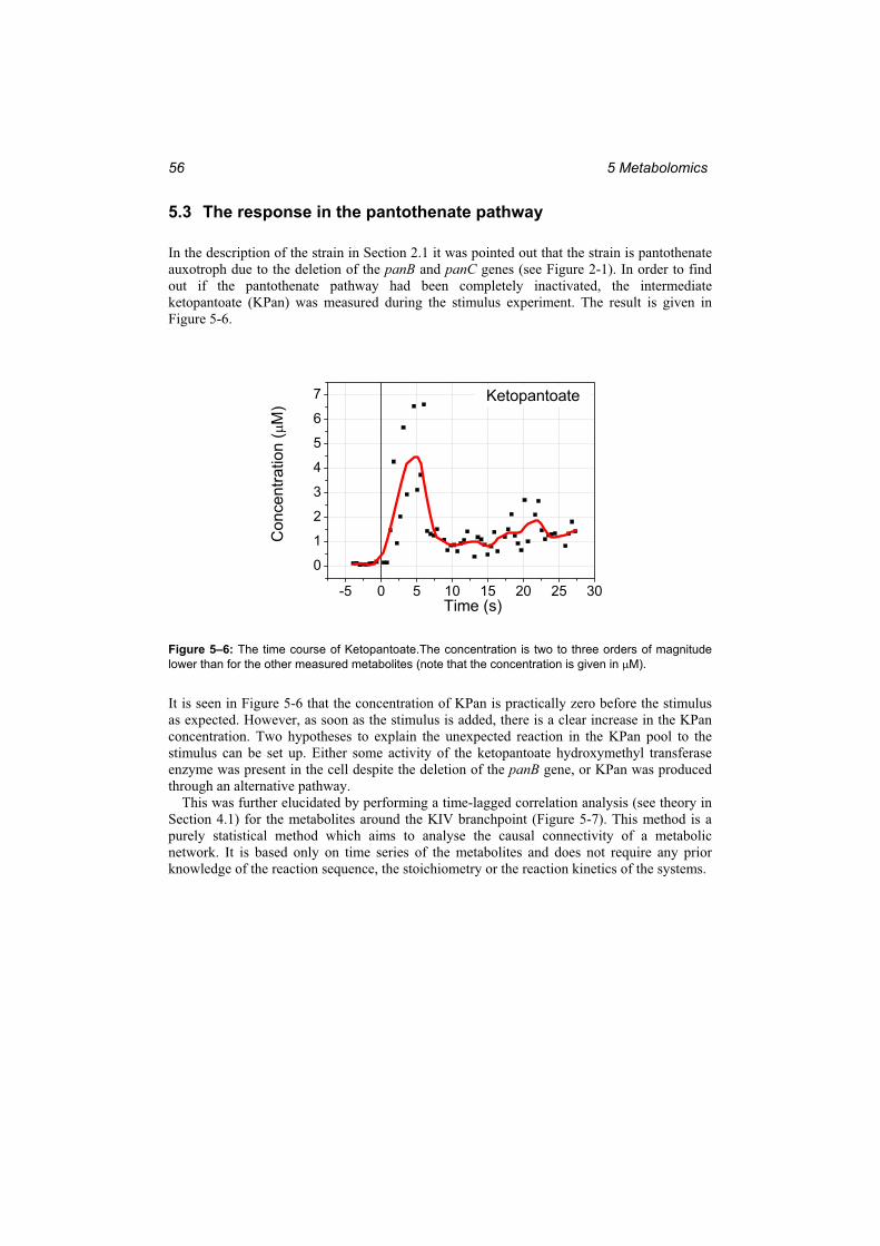
5 Metabolomics 56
5.3 The response in the pantothenate pathway
In the description of the strain in Section 2.1 it was pointed out that the strain is pantothenate auxotroph due to the deletion of the panB and panC genes (see Figure 2-1). In order to find out if the pantothenate pathway had been completely inactivated, the intermediate ketopantoate (KPan) was measured during the stimulus experiment. The result is given in Figure 5-6.
-5 0 5 10 15 20 25 30
0
1
2
3
4
5
6
7
Con
cent
ratio
n (
M)
Time (s)
Ketopantoate
Figure 5–6: The time course of Ketopantoate.The concentration is two to three orders of magnitude lower than for the other measured metabolites (note that the concentration is given in M).
It is seen in Figure 5-6 that the concentration of KPan is practically zero before the stimulus as expected. However, as soon as the stimulus is added, there is a clear increase in the KPan concentration. Two hypotheses to explain the unexpected reaction in the KPan pool to the stimulus can be set up. Either some activity of the ketopantoate hydroxymethyl transferase enzyme was present in the cell despite the deletion of the panB gene, or KPan was produced through an alternative pathway.
This was further elucidated by performing a time-lagged correlation analysis (see theory in Section 4.1) for the metabolites around the KIV branchpoint (Figure 5-7). This method is a purely statistical method which aims to analyse the causal connectivity of a metabolic network. It is based only on time series of the metabolites and does not require any prior knowledge of the reaction sequence, the stoichiometry or the reaction kinetics of the systems.
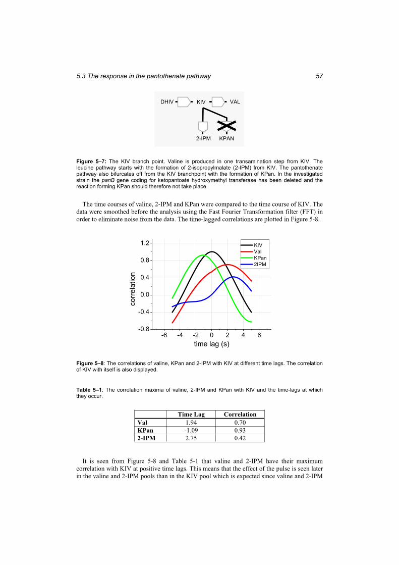
5.3 The response in the pantothenate pathway 57
2-IPM
DHIV KIV VAL
KPAN
Figure 5–7: The KIV branch point. Valine is produced in one transamination step from KIV. The leucine pathway starts with the formation of 2-isopropylmalate (2-IPM) from KIV. The pantothenate pathway also bifurcates off from the KIV branchpoint with the formation of KPan. In the investigated strain the panB gene coding for ketopantoate hydroxymethyl transferase has been deleted and the reaction forming KPan should therefore not take place.
The time courses of valine, 2-IPM and KPan were compared to the time course of KIV. The data were smoothed before the analysis using the Fast Fourier Transformation filter (FFT) in order to eliminate noise from the data. The time-lagged correlations are plotted in Figure 5-8.
-6 -4 -2 0 2 4 6-0.8
-0.4
0.0
0.4
0.8
1.2
corr
elat
ion
time lag (s)
KIV Val KPan 2IPM
Figure 5–8: The correlations of valine, KPan and 2-IPM with KIV at different time lags. The correlation of KIV with itself is also displayed.
Table 5–1: The correlation maxima of valine, 2-IPM and KPan with KIV and the time-lags at which they occur.
Time Lag CorrelationVal 1.94 0.70 KPan -1.09 0.93 2-IPM 2.75 0.42
It is seen from Figure 5-8 and Table 5-1 that valine and 2-IPM have their maximum correlation with KIV at positive time lags. This means that the effect of the pulse is seen later in the valine and 2-IPM pools than in the KIV pool which is expected since valine and 2-IPM
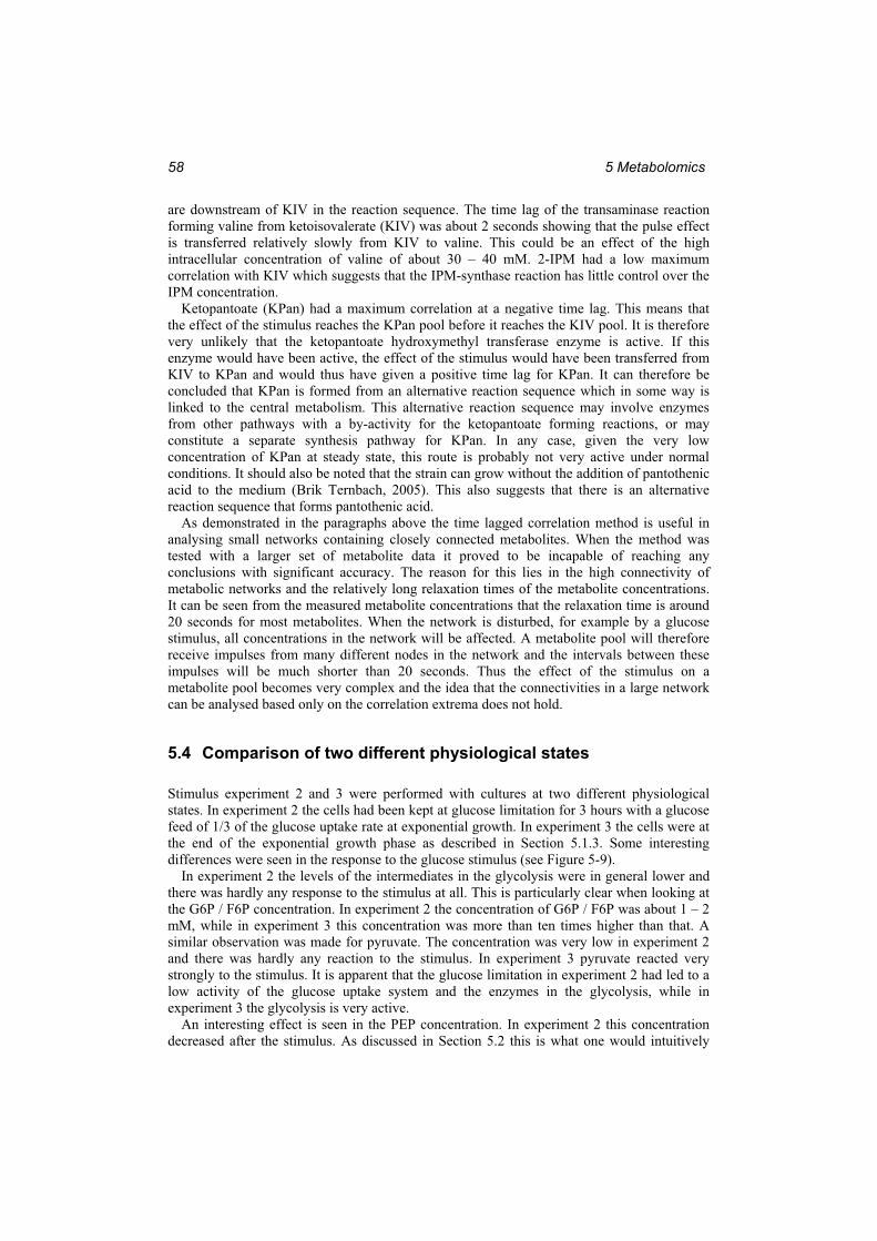
5 Metabolomics 58
are downstream of KIV in the reaction sequence. The time lag of the transaminase reaction forming valine from ketoisovalerate (KIV) was about 2 seconds showing that the pulse effect is transferred relatively slowly from KIV to valine. This could be an effect of the high intracellular concentration of valine of about 30 – 40 mM. 2-IPM had a low maximum correlation with KIV which suggests that the IPM-synthase reaction has little control over the IPM concentration.
Ketopantoate (KPan) had a maximum correlation at a negative time lag. This means that the effect of the stimulus reaches the KPan pool before it reaches the KIV pool. It is therefore very unlikely that the ketopantoate hydroxymethyl transferase enzyme is active. If this enzyme would have been active, the effect of the stimulus would have been transferred from KIV to KPan and would thus have given a positive time lag for KPan. It can therefore be concluded that KPan is formed from an alternative reaction sequence which in some way is linked to the central metabolism. This alternative reaction sequence may involve enzymes from other pathways with a by-activity for the ketopantoate forming reactions, or may constitute a separate synthesis pathway for KPan. In any case, given the very low concentration of KPan at steady state, this route is probably not very active under normal conditions. It should also be noted that the strain can grow without the addition of pantothenic acid to the medium (Brik Ternbach, 2005). This also suggests that there is an alternative reaction sequence that forms pantothenic acid.
As demonstrated in the paragraphs above the time lagged correlation method is useful in analysing small networks containing closely connected metabolites. When the method was tested with a larger set of metabolite data it proved to be incapable of reaching any conclusions with significant accuracy. The reason for this lies in the high connectivity of metabolic networks and the relatively long relaxation times of the metabolite concentrations. It can be seen from the measured metabolite concentrations that the relaxation time is around 20 seconds for most metabolites. When the network is disturbed, for example by a glucose stimulus, all concentrations in the network will be affected. A metabolite pool will therefore receive impulses from many different nodes in the network and the intervals between these impulses will be much shorter than 20 seconds. Thus the effect of the stimulus on a metabolite pool becomes very complex and the idea that the connectivities in a large network can be analysed based only on the correlation extrema does not hold.
5.4 Comparison of two different physiological states
Stimulus experiment 2 and 3 were performed with cultures at two different physiological states. In experiment 2 the cells had been kept at glucose limitation for 3 hours with a glucose feed of 1/3 of the glucose uptake rate at exponential growth. In experiment 3 the cells were at the end of the exponential growth phase as described in Section 5.1.3. Some interesting differences were seen in the response to the glucose stimulus (see Figure 5-9).
In experiment 2 the levels of the intermediates in the glycolysis were in general lower and there was hardly any response to the stimulus at all. This is particularly clear when looking at the G6P / F6P concentration. In experiment 2 the concentration of G6P / F6P was about 1 – 2 mM, while in experiment 3 this concentration was more than ten times higher than that. A similar observation was made for pyruvate. The concentration was very low in experiment 2 and there was hardly any reaction to the stimulus. In experiment 3 pyruvate reacted very strongly to the stimulus. It is apparent that the glucose limitation in experiment 2 had led to a low activity of the glucose uptake system and the enzymes in the glycolysis, while in experiment 3 the glycolysis is very active.
An interesting effect is seen in the PEP concentration. In experiment 2 this concentration decreased after the stimulus. As discussed in Section 5.2 this is what one would intuitively
5.4 Comparison of two different physiological states 59
expect since PEP is consumed in the pts reaction. In experiment 2 the activity of the glycolysis was low enough for the decrease in PEP to occur. Later, at about 10 seconds after the stimulus, an increase in PEP concentration is seen. In experiment 3, on the other hand, there is a rapid increase in PEP concentration immediately after the stimulus. It was suggested in section 5.2 that the PEP increase at exponential growth was due to the existence of a glucose permease. The PEP time course in experiment 2 clearly shows that the permease is not active at glucose limiting conditions and that the pts system is the dominating glucose uptake system at this condition. If Corynebacterium glutamicum has a glucose permease it is only active when there is a good availability of glucose.
The concentration of AMP was higher in experiment 2 signifying a lower energy level of the cell due to the glucose limitation. The qualitative reaction in the AMP pool was similar for both experiments.
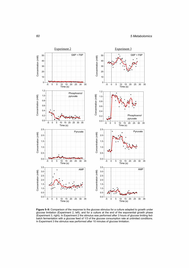
5 Metabolomics 60
Experiment 2 Experiment 3
-5 0 5 10 15 20 25 30 350
10
20
30
40
50
Con
cent
ratio
n (m
M)
Time (s)
G6P + F6P
-5 0 5 10 15 20 25 30 350
10
20
30
40
50
Con
cent
ratio
n (m
M)
Time (s)
G6P + F6P
-5 0 5 10 15 20 25 30 350.0
0.2
0.4
0.6
0.8
1.0
1.2
Con
cent
ratio
n (m
M)
Time (s)
Phosphoenolpyruvate
-5 0 5 10 15 20 25 30 350.0
0.2
0.4
0.6
0.8
1.0
1.2
Con
cent
ratio
n (m
M)
Time (s)
Phosphoenolpyruvate
-5 0 5 10 15 20 25 30 350.0
0.5
1.0
1.5
2.0
2.5
Con
cent
ratio
n (m
M)
Time (s)
Pyruvate
-5 0 5 10 15 20 25 30 350.0
0.5
1.0
1.5
2.0
2.5
Con
cent
ratio
n (m
M)
Time (s)
Pyruvate
-5 0 5 10 15 20 25 30 350.0
0.5
1.0
1.5
2.0
2.5
3.0
3.5
Con
cent
ratio
n (m
M)
Time (s)
AMP
-5 0 5 10 15 20 25 30 350.0
0.5
1.0
1.5
2.0
2.5
3.0
3.5
Con
cent
rato
in (m
M)
Time (s)
AMP
Figure 5–9: Comparison of the response to the glucose stimulus for a culture adapted to growth under glucose limitation (Experiment 2, left), and for a culture at the end of the exponential growth phase (Experiment 3, right). In Experiment 2 the stimulus was performed after 3 hours of glucose limiting fed-batch fermentation with a glucose feed of 1/3 of the glucose consumption rate at unlimited conditions. In Experiment 3 the stimulus was performed after 10 minutes of glucose limitation.
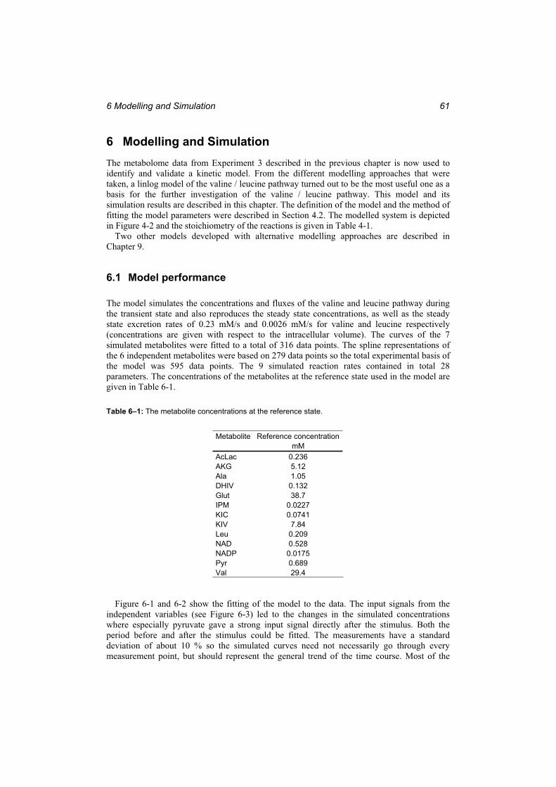
6 Modelling and Simulation 61
6 Modelling and Simulation The metabolome data from Experiment 3 described in the previous chapter is now used to identify and validate a kinetic model. From the different modelling approaches that were taken, a linlog model of the valine / leucine pathway turned out to be the most useful one as a basis for the further investigation of the valine / leucine pathway. This model and its simulation results are described in this chapter. The definition of the model and the method of fitting the model parameters were described in Section 4.2. The modelled system is depicted in Figure 4-2 and the stoichiometry of the reactions is given in Table 4-1.
Two other models developed with alternative modelling approaches are described in Chapter 9.
6.1 Model performance
The model simulates the concentrations and fluxes of the valine and leucine pathway during the transient state and also reproduces the steady state concentrations, as well as the steady state excretion rates of 0.23 mM/s and 0.0026 mM/s for valine and leucine respectively (concentrations are given with respect to the intracellular volume). The curves of the 7 simulated metabolites were fitted to a total of 316 data points. The spline representations of the 6 independent metabolites were based on 279 data points so the total experimental basis of the model was 595 data points. The 9 simulated reaction rates contained in total 28 parameters. The concentrations of the metabolites at the reference state used in the model are given in Table 6-1.
Table 6–1: The metabolite concentrations at the reference state.
Metabolite Reference concentration mM AcLac 0.236 AKG 5.12 Ala 1.05 DHIV 0.132 Glut 38.7 IPM 0.0227 KIC 0.0741 KIV 7.84 Leu 0.209 NAD 0.528 NADP 0.0175 Pyr 0.689 Val 29.4
Figure 6-1 and 6-2 show the fitting of the model to the data. The input signals from the independent variables (see Figure 6-3) led to the changes in the simulated concentrations where especially pyruvate gave a strong input signal directly after the stimulus. Both the period before and after the stimulus could be fitted. The measurements have a standard deviation of about 10 % so the simulated curves need not necessarily go through every measurement point, but should represent the general trend of the time course. Most of the
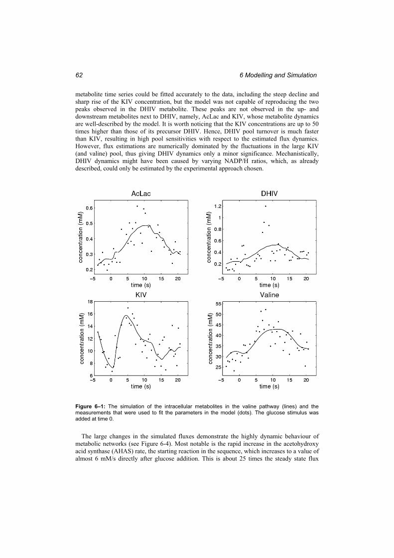
6 Modelling and Simulation 62
metabolite time series could be fitted accurately to the data, including the steep decline and sharp rise of the KIV concentration, but the model was not capable of reproducing the two peaks observed in the DHIV metabolite. These peaks are not observed in the up- and downstream metabolites next to DHIV, namely, AcLac and KIV, whose metabolite dynamics are well-described by the model. It is worth noticing that the KIV concentrations are up to 50 times higher than those of its precursor DHIV. Hence, DHIV pool turnover is much faster than KIV, resulting in high pool sensitivities with respect to the estimated flux dynamics. However, flux estimations are numerically dominated by the fluctuations in the large KIV (and valine) pool, thus giving DHIV dynamics only a minor significance. Mechanistically, DHIV dynamics might have been caused by varying NADP/H ratios, which, as already described, could only be estimated by the experimental approach chosen.
Figure 6–1: The simulation of the intracellular metabolites in the valine pathway (lines) and the measurements that were used to fit the parameters in the model (dots). The glucose stimulus was added at time 0.
The large changes in the simulated fluxes demonstrate the highly dynamic behaviour of metabolic networks (see Figure 6-4). Most notable is the rapid increase in the acetohydroxy acid synthase (AHAS) rate, the starting reaction in the sequence, which increases to a value of almost 6 mM/s directly after glucose addition. This is about 25 times the steady state flux
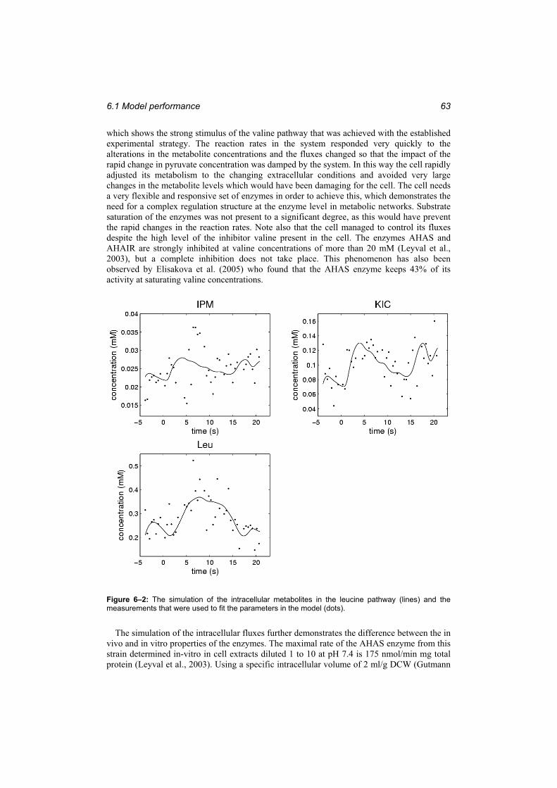
6.1 Model performance 63
which shows the strong stimulus of the valine pathway that was achieved with the established experimental strategy. The reaction rates in the system responded very quickly to thealterations in the metabolite concentrations and the fluxes changed so that the impact of the rapid change in pyruvate concentration was damped by the system. In this way the cell rapidly adjusted its metabolism to the changing extracellular conditions and avoided very large changes in the metabolite levels which would have been damaging for the cell. The cell needs a very flexible and responsive set of enzymes in order to achieve this, which demonstrates the need for a complex regulation structure at the enzyme level in metabolic networks. Substrate saturation of the enzymes was not present to a significant degree, as this would have prevent the rapid changes in the reaction rates. Note also that the cell managed to control its fluxes despite the high level of the inhibitor valine present in the cell. The enzymes AHAS and AHAIR are strongly inhibited at valine concentrations of more than 20 mM (Leyval et al., 2003), but a complete inhibition does not take place. This phenomenon has also been observed by Elisakova et al. (2005) who found that the AHAS enzyme keeps 43% of its activity at saturating valine concentrations.
Figure 6–2: The simulation of the intracellular metabolites in the leucine pathway (lines) and the measurements that were used to fit the parameters in the model (dots).
The simulation of the intracellular fluxes further demonstrates the difference between the in vivo and in vitro properties of the enzymes. The maximal rate of the AHAS enzyme from this strain determined in-vitro in cell extracts diluted 1 to 10 at pH 7.4 is 175 nmol/min mg total protein (Leyval et al., 2003). Using a specific intracellular volume of 2 ml/g DCW (Gutmann
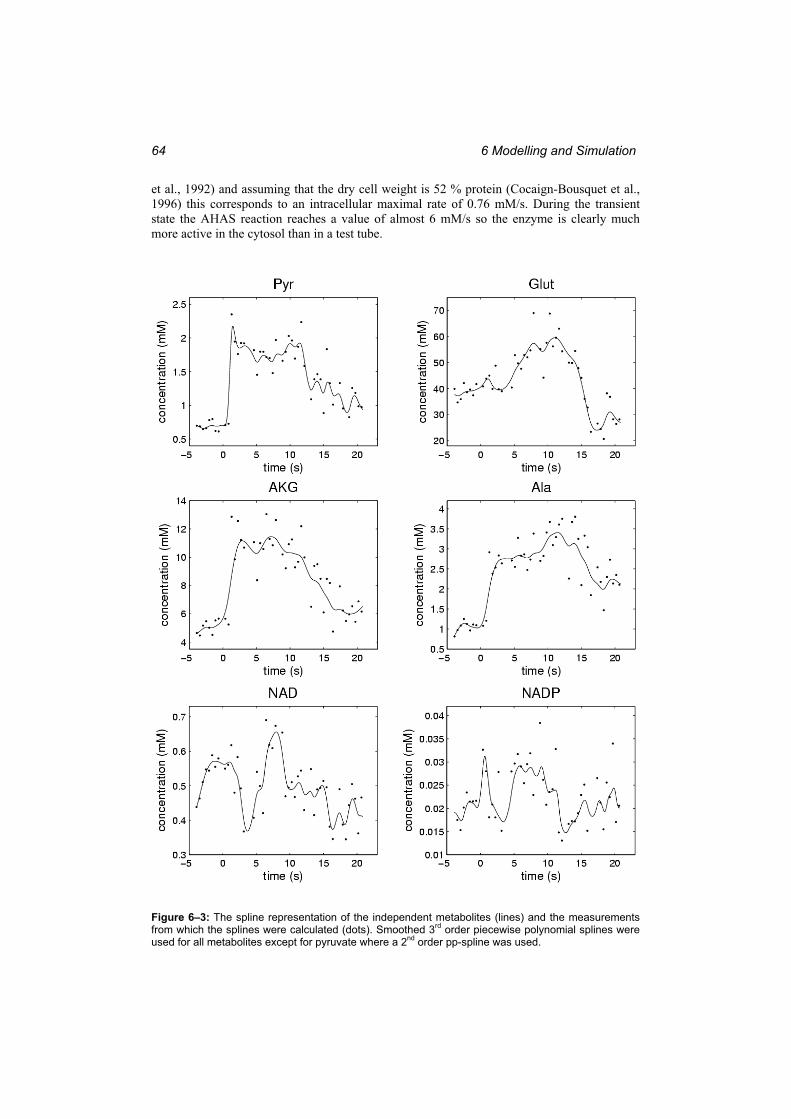
6 Modelling and Simulation 64
et al., 1992) and assuming that the dry cell weight is 52 % protein (Cocaign-Bousquet et al., 1996) this corresponds to an intracellular maximal rate of 0.76 mM/s. During the transient state the AHAS reaction reaches a value of almost 6 mM/s so the enzyme is clearly much more active in the cytosol than in a test tube.
Figure 6–3: The spline representation of the independent metabolites (lines) and the measurements from which the splines were calculated (dots). Smoothed 3rd order piecewise polynomial splines were used for all metabolites except for pyruvate where a 2nd order pp-spline was used.
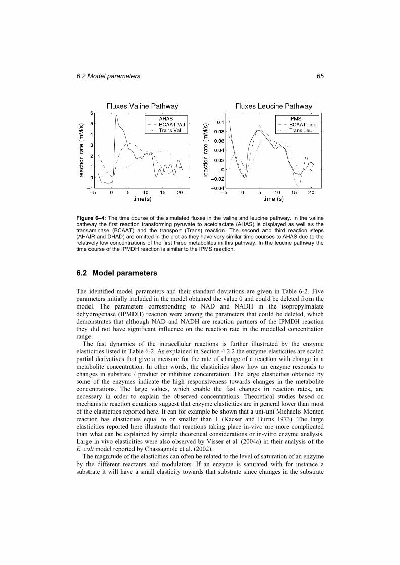
6.2 Model parameters 65
Figure 6–4: The time course of the simulated fluxes in the valine and leucine pathway. In the valine pathway the first reaction transforming pyruvate to acetolactate (AHAS) is displayed as well as the transaminase (BCAAT) and the transport (Trans) reaction. The second and third reaction steps (AHAIR and DHAD) are omitted in the plot as they have very similar time courses to AHAS due to the relatively low concentrations of the first three metabolites in this pathway. In the leucine pathway the time course of the IPMDH reaction is similar to the IPMS reaction.
6.2 Model parameters
The identified model parameters and their standard deviations are given in Table 6-2. Five parameters initially included in the model obtained the value 0 and could be deleted from the model. The parameters corresponding to NAD and NADH in the isopropylmalate dehydrogenase (IPMDH) reaction were among the parameters that could be deleted, which demonstrates that although NAD and NADH are reaction partners of the IPMDH reaction they did not have significant influence on the reaction rate in the modelled concentration range.
The fast dynamics of the intracellular reactions is further illustrated by the enzyme elasticities listed in Table 6-2. As explained in Section 4.2.2 the enzyme elasticities are scaled partial derivatives that give a measure for the rate of change of a reaction with change in a metabolite concentration. In other words, the elasticities show how an enzyme responds to changes in substrate / product or inhibitor concentration. The large elasticities obtained by some of the enzymes indicate the high responsiveness towards changes in the metabolite concentrations. The large values, which enable the fast changes in reaction rates, are necessary in order to explain the observed concentrations. Theoretical studies based on mechanistic reaction equations suggest that enzyme elasticities are in general lower than most of the elasticities reported here. It can for example be shown that a uni-uni Michaelis Menten reaction has elasticities equal to or smaller than 1 (Kacser and Burns 1973). The large elasticities reported here illustrate that reactions taking place in-vivo are more complicated than what can be explained by simple theoretical considerations or in-vitro enzyme analysis. Large in-vivo-elasticities were also observed by Visser et al. (2004a) in their analysis of the E. coli model reported by Chassagnole et al. (2002).
The magnitude of the elasticities can often be related to the level of saturation of an enzyme by the different reactants and modulators. If an enzyme is saturated with for instance a substrate it will have a small elasticity towards that substrate since changes in the substrate
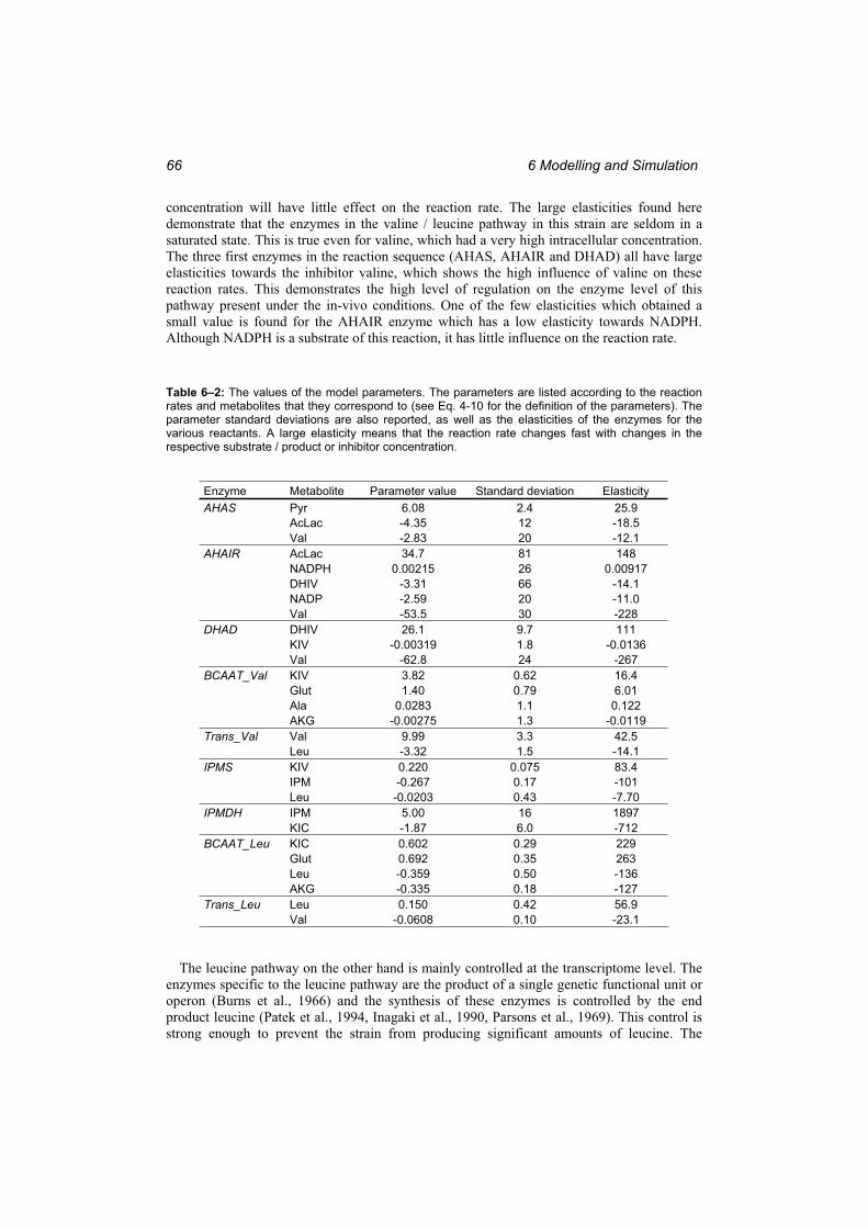
6 Modelling and Simulation 66
concentration will have little effect on the reaction rate. The large elasticities found here demonstrate that the enzymes in the valine / leucine pathway in this strain are seldom in a saturated state. This is true even for valine, which had a very high intracellular concentration. The three first enzymes in the reaction sequence (AHAS, AHAIR and DHAD) all have large elasticities towards the inhibitor valine, which shows the high influence of valine on these reaction rates. This demonstrates the high level of regulation on the enzyme level of this pathway present under the in-vivo conditions. One of the few elasticities which obtained a small value is found for the AHAIR enzyme which has a low elasticity towards NADPH. Although NADPH is a substrate of this reaction, it has little influence on the reaction rate.
Table 6–2: The values of the model parameters. The parameters are listed according to the reaction rates and metabolites that they correspond to (see Eq. 4-10 for the definition of the parameters). The parameter standard deviations are also reported, as well as the elasticities of the enzymes for the various reactants. A large elasticity means that the reaction rate changes fast with changes in the respective substrate / product or inhibitor concentration.
Enzyme Metabolite Parameter value Standard deviation Elasticity AHAS Pyr 6.08 2.4 25.9
AcLac -4.35 12 -18.5 Val -2.83 20 -12.1
AHAIR AcLac 34.7 81 148 NADPH 0.00215 26 0.00917 DHIV -3.31 66 -14.1 NADP -2.59 20 -11.0 Val -53.5 30 -228
DHAD DHIV 26.1 9.7 111 KIV -0.00319 1.8 -0.0136 Val -62.8 24 -267
BCAAT_Val KIV 3.82 0.62 16.4 Glut 1.40 0.79 6.01 Ala 0.0283 1.1 0.122 AKG -0.00275 1.3 -0.0119
Trans_Val Val 9.99 3.3 42.5 Leu -3.32 1.5 -14.1
IPMS KIV 0.220 0.075 83.4 IPM -0.267 0.17 -101 Leu -0.0203 0.43 -7.70
IPMDH IPM 5.00 16 1897 KIC -1.87 6.0 -712
BCAAT_Leu KIC 0.602 0.29 229 Glut 0.692 0.35 263 Leu -0.359 0.50 -136 AKG -0.335 0.18 -127
Trans_Leu Leu 0.150 0.42 56.9 Val -0.0608 0.10 -23.1
The leucine pathway on the other hand is mainly controlled at the transcriptome level. The enzymes specific to the leucine pathway are the product of a single genetic functional unit or operon (Burns et al., 1966) and the synthesis of these enzymes is controlled by the end product leucine (Patek et al., 1994, Inagaki et al., 1990, Parsons et al., 1969). This control is strong enough to prevent the strain from producing significant amounts of leucine. The
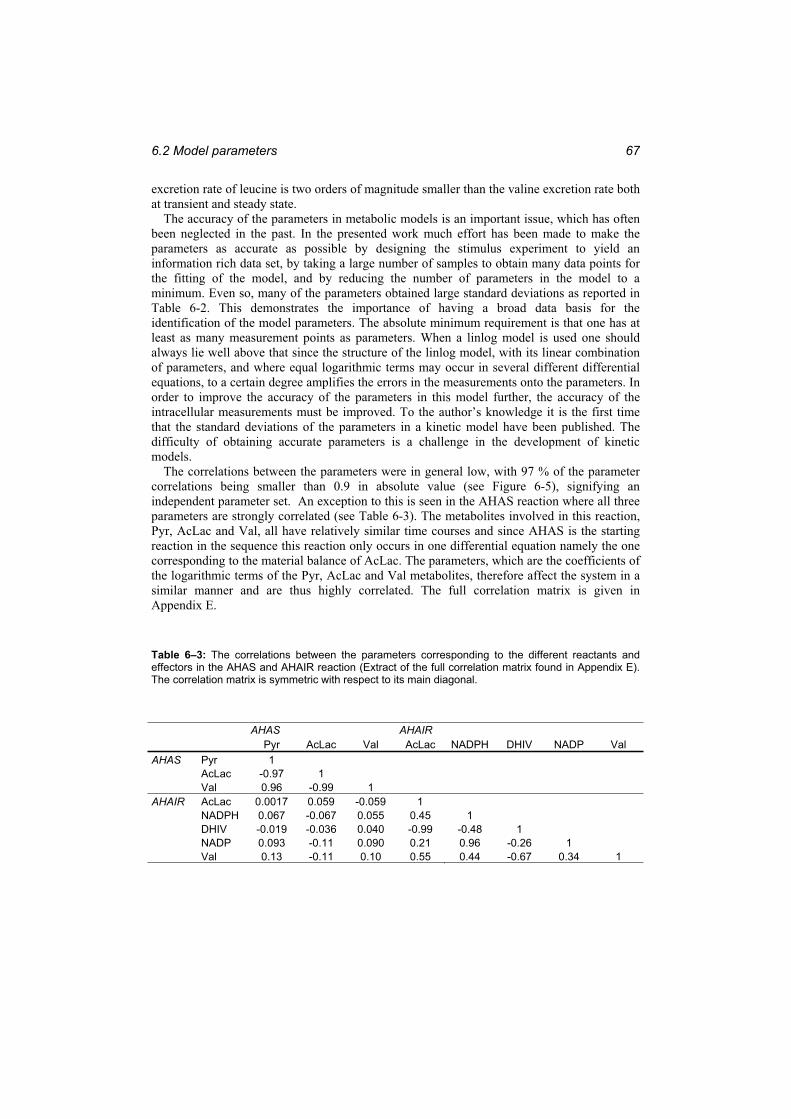
6.2 Model parameters 67
excretion rate of leucine is two orders of magnitude smaller than the valine excretion rate both at transient and steady state.
The accuracy of the parameters in metabolic models is an important issue, which has often been neglected in the past. In the presented work much effort has been made to make the parameters as accurate as possible by designing the stimulus experiment to yield an information rich data set, by taking a large number of samples to obtain many data points for the fitting of the model, and by reducing the number of parameters in the model to a minimum. Even so, many of the parameters obtained large standard deviations as reported in Table 6-2. This demonstrates the importance of having a broad data basis for the identification of the model parameters. The absolute minimum requirement is that one has at least as many measurement points as parameters. When a linlog model is used one should always lie well above that since the structure of the linlog model, with its linear combination of parameters, and where equal logarithmic terms may occur in several different differential equations, to a certain degree amplifies the errors in the measurements onto the parameters. In order to improve the accuracy of the parameters in this model further, the accuracy of the intracellular measurements must be improved. To the author’s knowledge it is the first time that the standard deviations of the parameters in a kinetic model have been published. The difficulty of obtaining accurate parameters is a challenge in the development of kinetic models.
The correlations between the parameters were in general low, with 97 % of the parameter correlations being smaller than 0.9 in absolute value (see Figure 6-5), signifying an independent parameter set. An exception to this is seen in the AHAS reaction where all three parameters are strongly correlated (see Table 6-3). The metabolites involved in this reaction, Pyr, AcLac and Val, all have relatively similar time courses and since AHAS is the starting reaction in the sequence this reaction only occurs in one differential equation namely the one corresponding to the material balance of AcLac. The parameters, which are the coefficients of the logarithmic terms of the Pyr, AcLac and Val metabolites, therefore affect the system in a similar manner and are thus highly correlated. The full correlation matrix is given in Appendix E.
Table 6–3: The correlations between the parameters corresponding to the different reactants and effectors in the AHAS and AHAIR reaction (Extract of the full correlation matrix found in Appendix E). The correlation matrix is symmetric with respect to its main diagonal.
AHAS AHAIR Pyr AcLac Val AcLac NADPH DHIV NADP Val AHAS Pyr 1
AcLac -0.97 1 Val 0.96 -0.99 1
AHAIR AcLac 0.0017 0.059 -0.059 1 NADPH 0.067 -0.067 0.055 0.45 1 DHIV -0.019 -0.036 0.040 -0.99 -0.48 1 NADP 0.093 -0.11 0.090 0.21 0.96 -0.26 1 Val 0.13 -0.11 0.10 0.55 0.44 -0.67 0.34 1
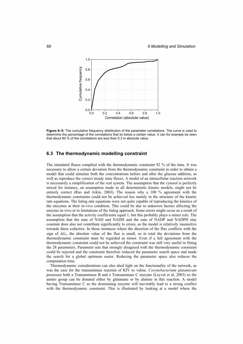
6 Modelling and Simulation 68
0.0 0.2 0.4 0.6 0.8 1.00.0
0.2
0.4
0.6
0.8
1.0
Cum
ulat
ive
frequ
ency
Correlation (absolute value)
Figure 6–5: The cumulative frequency distribution of the parameter correlations. The curve is used to determine the percentage of the correlations that lie below a certain value. It can for example be seen that about 80 % of the correlations are less than 0.3 in absolute value.
6.3 The thermodynamic modelling constraint
The simulated fluxes complied with the thermodynamic constraint 92 % of the time. It was necessary to allow a certain deviation from the thermodynamic constraint in order to obtain a model that could simulate both the concentrations before and after the glucose addition, as well as reproduce the correct steady state fluxes. A model of an intracellular reaction network is necessarily a simplification of the real system. The assumption that the cytosol is perfectly mixed for instance, an assumption made in all deterministic kinetic models, might not be entirely correct (Rao and Arkin, 2003). The reason why a 100 % agreement with the thermodynamic constraints could not be achieved lies mainly in the structure of the kinetic rate equations. The linlog rate equations were not quite capable of reproducing the kinetics of the enzymes at their in-vivo condition. This could be due to unknown factors affecting the enzyme in-vivo or to limitations of the linlog approach. Some errors might occur as a result of the assumption that the activity coefficients equal 1, but this probably plays a minor role. The assumption that the sum of NAD and NADH and the sum of NADP and NADPH stay constant does also not contribute significantly to errors, as the model is relatively insensitive towards these cofactors. In those instances where the direction of the flux conflicts with the sign of Gr, the absolute value of the flux is small, so in total the deviations from the thermodynamic constraint must be regarded as minor. Even if a full agreement with the thermodynamic constraint could not be achieved the constraint was still very useful in fitting the 28 parameters. Parameter sets that strongly disagreed with the thermodynamic constraint could be rejected and the constraint therefore reduced the parameter search space and made the search for a global optimum easier. Reducing the parameter space also reduces the computation time.
Thermodynamic considerations can also shed light on the functionality of the network, as was the case for the transaminase reaction of KIV to valine. Corynebacterium glutamicum possesses both a Transaminase B and a Transaminase C enzyme (Leyval et al, 2003) so the amino group can be donated either by glutamate or by alanine in this reaction. A model having Transaminase C as the dominating enzyme will inevitably lead to a strong conflict with the thermodynamic constraint. This is illustrated by looking at a model where the

6.4 The stability of the linlog model 69
transaminase reaction is catalysed mainly by Transaminase C (Figure 6-6). The fitting of the simulated concentrations to the measured data is just as good in this model as in the final one (compare the fitting of valine in Figure 6-6 to the fitting of valine given in Figure 6-1), and the model can also reproduce the steady state concentrations and the steady state fluxes. However, during the transient state the fluxes agree with the thermodynamic constraint in only 41 % of the simulated time and the model must therefore be rejected. This shows the importance of considering the thermodynamics when developing realistic models. The thermodynamic constraint makes it possible to arrive at the conclusion that Transaminase B is the dominating enzyme. This confirms the findings of previous investigations based on enzyme studies of this strain (Eggeling et al., 1987; Radmacher et al., 2002; Leyval et al., 2003).
As discussed above several “optimal” parameter sets may exist for a complex kinetic model, i.e. there is not always a unique solution when only the fit to the measured data is considered. In order to identify a unique parameter set additional constraints must be included. In this context the thermodynamic constraint is an essential tool for the identification of realistic and unique kinetic models.
When including the thermodynamic constraint in the fitting, the same optimal parameter set was always found when starting from different random initial parameters. It can therefore be concluded that the identified parameter set is unique and that the model is as realistic as it is possible to achieve with the method used.
Figure 6–6: The simulations of a model where Transaminase C is the dominating enzyme in the transamination reaction. The fluxes (left) comply with the thermodynamic constraint in only 41 % of the time during the transient state. The model is therefore rejected despite the fact that the simulated concentrations fit the measurements well as illustrated by the valine simulation (right).
6.4 The stability of the linlog model
An important criterion for the establishment of a useful model is that it is stable. The stability of a model can be investigated by analysing the Jacobian matrix of the system of ODEs. The Jacobian for the system presented here was fully ranked, so all eigenvalues were non-zero. The Jacobian is given in Eq. (6-1) and the corresponding eigenvalues are 269.2541,
206.4190, 105.5035, 10.6383, 1.084, 0.3242 0.4780i,0.3242 + 0.4780i. As was demonstrated in Section 4.2.6 and in Appendix G the system
is stable if, and only if, all the eigenvalues of the Jacobian have negative real parts. Since this was the case here one can conclude that the system will always return to the steady state after
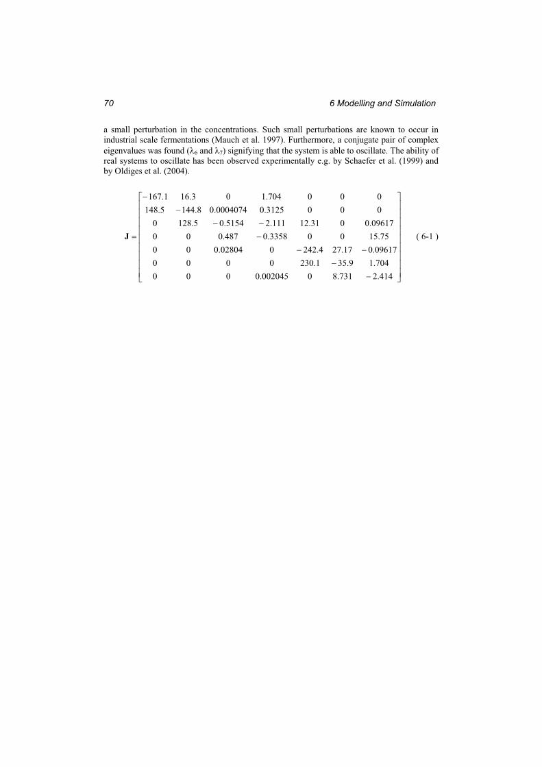
6 Modelling and Simulation 70
a small perturbation in the concentrations. Such small perturbations are known to occur in industrial scale fermentations (Mauch et al. 1997). Furthermore, a conjugate pair of complex eigenvalues was found ( and ) signifying that the system is able to oscillate. The ability of real systems to oscillate has been observed experimentally e.g. by Schaefer et al. (1999) and by Oldiges et al. (2004).
414.2731.80002045.0000704.19.351.230000009617.017.274.242002804.000
75.15003358.0487.00009617.0031.12111.25154.05.1280
0003125.00004074.08.1445.148000704.103.161.167
J ( 6-1 )
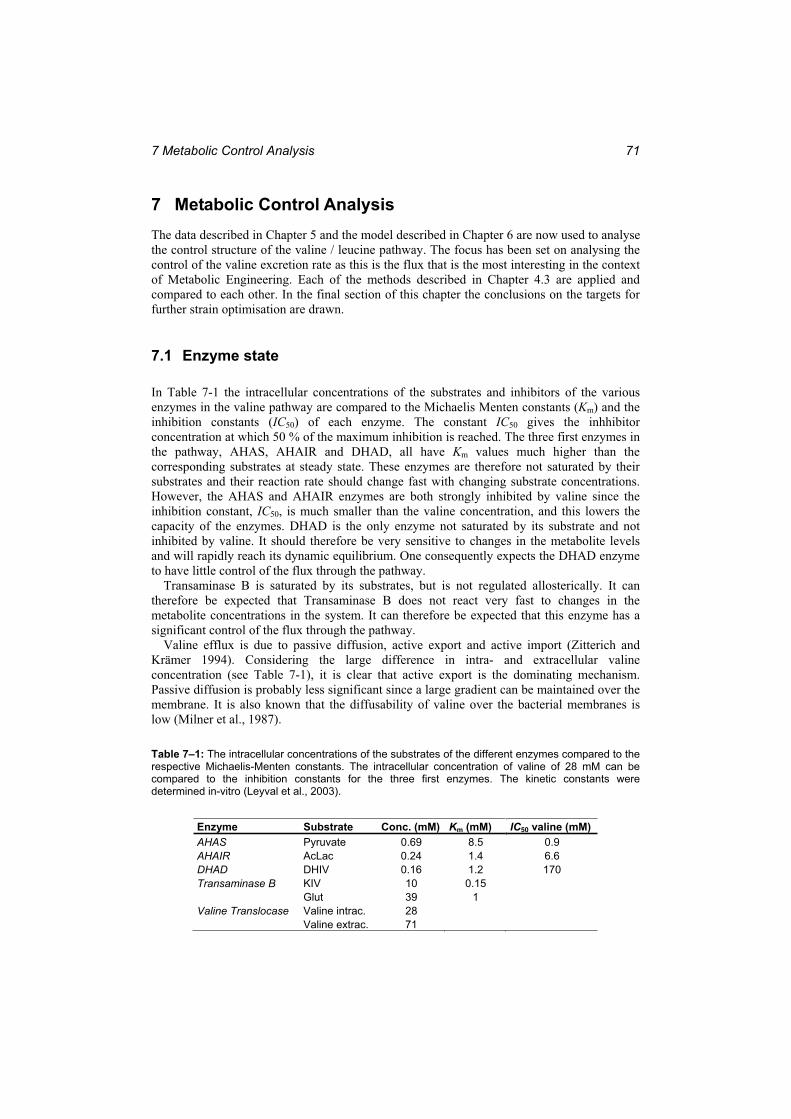
7 Metabolic Control Analysis 71
7 Metabolic Control Analysis The data described in Chapter 5 and the model described in Chapter 6 are now used to analyse the control structure of the valine / leucine pathway. The focus has been set on analysing the control of the valine excretion rate as this is the flux that is the most interesting in the context of Metabolic Engineering. Each of the methods described in Chapter 4.3 are applied and compared to each other. In the final section of this chapter the conclusions on the targets for further strain optimisation are drawn.
7.1 Enzyme state
In Table 7-1 the intracellular concentrations of the substrates and inhibitors of the various enzymes in the valine pathway are compared to the Michaelis Menten constants (Km) and the inhibition constants (IC50) of each enzyme. The constant IC50 gives the inhhibitor concentration at which 50 % of the maximum inhibition is reached. The three first enzymes in the pathway, AHAS, AHAIR and DHAD, all have Km values much higher than the corresponding substrates at steady state. These enzymes are therefore not saturated by their substrates and their reaction rate should change fast with changing substrate concentrations. However, the AHAS and AHAIR enzymes are both strongly inhibited by valine since the inhibition constant, IC50, is much smaller than the valine concentration, and this lowers the capacity of the enzymes. DHAD is the only enzyme not saturated by its substrate and not inhibited by valine. It should therefore be very sensitive to changes in the metabolite levels and will rapidly reach its dynamic equilibrium. One consequently expects the DHAD enzyme to have little control of the flux through the pathway.
Transaminase B is saturated by its substrates, but is not regulated allosterically. It can therefore be expected that Transaminase B does not react very fast to changes in the metabolite concentrations in the system. It can therefore be expected that this enzyme has a significant control of the flux through the pathway.
Valine efflux is due to passive diffusion, active export and active import (Zitterich and Krämer 1994). Considering the large difference in intra- and extracellular valine concentration (see Table 7-1), it is clear that active export is the dominating mechanism. Passive diffusion is probably less significant since a large gradient can be maintained over the membrane. It is also known that the diffusability of valine over the bacterial membranes is low (Milner et al., 1987).
Table 7–1: The intracellular concentrations of the substrates of the different enzymes compared to the respective Michaelis-Menten constants. The intracellular concentration of valine of 28 mM can be compared to the inhibition constants for the three first enzymes. The kinetic constants were determined in-vitro (Leyval et al., 2003).
Enzyme Substrate Conc. (mM) Km (mM) IC50 valine (mM) AHAS Pyruvate 0.69 8.5 0.9 AHAIR AcLac 0.24 1.4 6.6 DHAD DHIV 0.16 1.2 170 Transaminase B KIV 10 0.15 Glut 39 1 Valine Translocase Valine intrac. 28 Valine extrac. 71
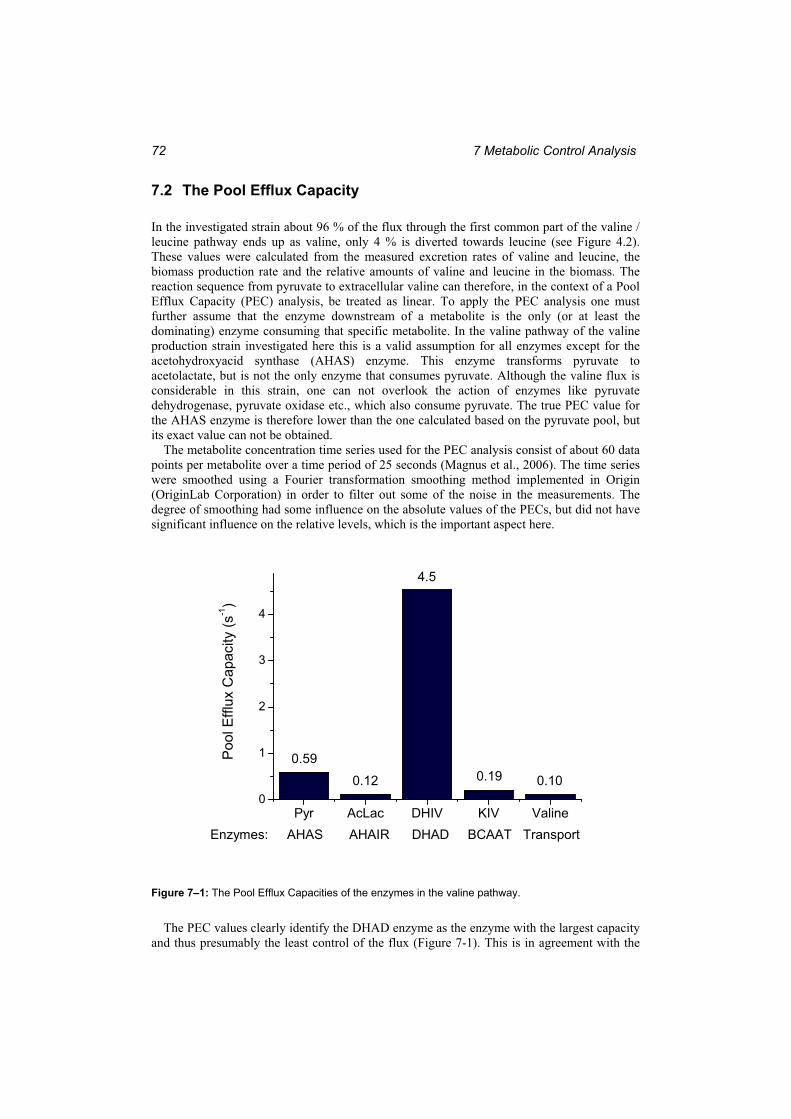
7 Metabolic Control Analysis 72
7.2 The Pool Efflux Capacity
In the investigated strain about 96 % of the flux through the first common part of the valine / leucine pathway ends up as valine, only 4 % is diverted towards leucine (see Figure 4.2). These values were calculated from the measured excretion rates of valine and leucine, the biomass production rate and the relative amounts of valine and leucine in the biomass. The reaction sequence from pyruvate to extracellular valine can therefore, in the context of a Pool Efflux Capacity (PEC) analysis, be treated as linear. To apply the PEC analysis one must further assume that the enzyme downstream of a metabolite is the only (or at least the dominating) enzyme consuming that specific metabolite. In the valine pathway of the valine production strain investigated here this is a valid assumption for all enzymes except for the acetohydroxyacid synthase (AHAS) enzyme. This enzyme transforms pyruvate to acetolactate, but is not the only enzyme that consumes pyruvate. Although the valine flux is considerable in this strain, one can not overlook the action of enzymes like pyruvate dehydrogenase, pyruvate oxidase etc., which also consume pyruvate. The true PEC value for the AHAS enzyme is therefore lower than the one calculated based on the pyruvate pool, but its exact value can not be obtained.
The metabolite concentration time series used for the PEC analysis consist of about 60 data points per metabolite over a time period of 25 seconds (Magnus et al., 2006). The time series were smoothed using a Fourier transformation smoothing method implemented in Origin (OriginLab Corporation) in order to filter out some of the noise in the measurements. The degree of smoothing had some influence on the absolute values of the PECs, but did not have significant influence on the relative levels, which is the important aspect here.
Pyr AcLac DHIV KIV Valine0
1
2
3
4
0.590.190.12 0.10
4.5
Enzymes: AHAS AHAIR DHAD BCAAT Transport
Poo
l Effl
ux C
apac
ity (s
-1)
Figure 7–1: The Pool Efflux Capacities of the enzymes in the valine pathway.
The PEC values clearly identify the DHAD enzyme as the enzyme with the largest capacity and thus presumably the least control of the flux (Figure 7-1). This is in agreement with the
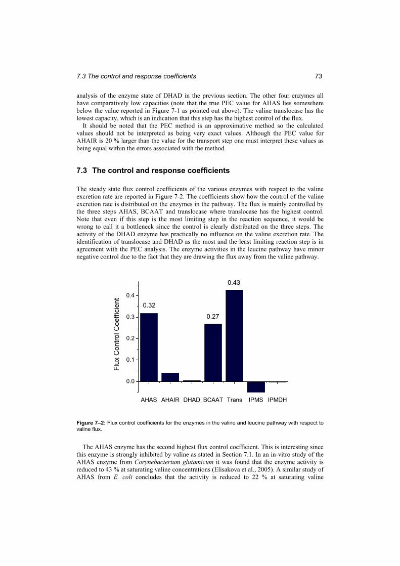
7.3 The control and response coefficients 73
analysis of the enzyme state of DHAD in the previous section. The other four enzymes all have comparatively low capacities (note that the true PEC value for AHAS lies somewhere below the value reported in Figure 7-1 as pointed out above). The valine translocase has the lowest capacity, which is an indication that this step has the highest control of the flux.
It should be noted that the PEC method is an approximative method so the calculated values should not be interpreted as being very exact values. Although the PEC value for AHAIR is 20 % larger than the value for the transport step one must interpret these values as being equal within the errors associated with the method.
7.3 The control and response coefficients
The steady state flux control coefficients of the various enzymes with respect to the valine excretion rate are reported in Figure 7-2. The coefficients show how the control of the valine excretion rate is distributed on the enzymes in the pathway. The flux is mainly controlled by the three steps AHAS, BCAAT and translocase where translocase has the highest control. Note that even if this step is the most limiting step in the reaction sequence, it would be wrong to call it a bottleneck since the control is clearly distributed on the three steps. The activity of the DHAD enzyme has practically no influence on the valine excretion rate. The identification of translocase and DHAD as the most and the least limiting reaction step is in agreement with the PEC analysis. The enzyme activities in the leucine pathway have minor negative control due to the fact that they are drawing the flux away from the valine pathway.
AHAS AHAIR DHAD BCAAT Trans IPMS IPMDH
0.0
0.1
0.2
0.3
0.4
0.32
0.27
Flux
Con
trol C
oeffi
cien
t
0.43
Figure 7–2: Flux control coefficients for the enzymes in the valine and leucine pathway with respect to valine flux.
The AHAS enzyme has the second highest flux control coefficient. This is interesting since this enzyme is strongly inhibited by valine as stated in Section 7.1. In an in-vitro study of the AHAS enzyme from Corynebacterium glutamicum it was found that the enzyme activity is reduced to 43 % at saturating valine concentrations (Elisakova et al., 2005). A similar study of AHAS from E. coli concludes that the activity is reduced to 22 % at saturating valine
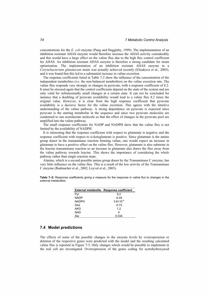
7 Metabolic Control Analysis 74
concentrations for the E. coli enzyme (Pang and Duggleby, 1999). The implementation of an inhibition resistant AHAS enzyme would therefore increase the AHAS activity considerably and this would have a large effect on the valine flux due to the high flux control coefficient for AHAS. An inhibition resistant AHAS enzyme is therefore a strong candidate for strain optimisation. The implementation of an inhibition resistant AHAS enzyme in a Corynebacterium glutamicum strain was actually achieved recently (Elisakova et al., 2005), and it was found that this led to a substantial increase in valine excretion.
The response coefficients listed in Table 7-2 show the influence of the concentration of the independent metabolites (i.e. the non-balanced metabolites) on the valine excretion rate. The valine flux responds very strongly to changes in pyruvate, with a response coefficient of 8.2. It must be stressed again that the control coefficients depend on the state of the system and are only valid for infinitesimally small changes at a certain state. It can not be concluded for instance that a doubling of pyruvate availability would lead to a valine flux 8.2 times the original value. However, it is clear from the high response coefficient that pyruvate availability is a decisive factor for the valine excretion. This agrees with the intuitive understanding of the valine pathway. A strong dependence on pyruvate is expected since pyruvate is the starting metabolite in the sequence and since two pyruvate molecules are condensed to one acetolactate molecule so that the effect of changes in the pyruvate pool are amplified into the valine pathway.
The small response coefficients for NADP and NADPH show that the valine flux is not limited by the availability of NADPH.
It is interesting that the response coefficient with respect to glutamate is negative and the response coefficient with respect to -ketoglutarate is positive. Since glutamate is the amino group donor in the transaminase reaction forming valine, one would expect an increase in glutamate to have a positive effect on the valine flux. However, glutamate is also substrate in the leucine transaminase reaction so an increase in glutamate also draws the flux away from the valine pathway towards leucine. This shows the importance of considering the whole pathway rather than single reaction steps.
Alanine, which is a second possible amino group donor by the Transaminase C enzyme, has very little influence on the valine flux. This is a result of the low activity of the Transaminase C enzyme (Radmacher et al., 2002; Leyval et al., 2003).
Table 7–2: Response coefficients giving a measure for the response in valine flux to changes in the external metabolites.
External metabolite Response coefficient Pyr 8.2 NADP -0.44 NADPH 3.6×10⁻⁴
Glut -0.72 AKG 1.2 NAD 0 Ala 0.034
7.4 Model predictions
The effects of some of the possible changes to the enzyme levels by overexpression or deletion of the respective genes were predicted with the model and the resulting calculated valine flux is reported in Figure 7-3. Only changes which would be possible to implement in the real cell are investigated. Overexpression of the genes coding for acetohydroxyacid
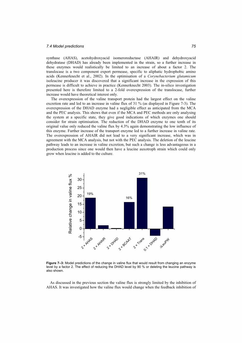
7.4 Model predictions 75
synthase (AHAS), acetohydroxyacid isomeroreductase (AHAIR) and dehydroxyacid dehydratase (DHAD) has already been implemented in the strain, so a further increase in these enzymes would realistically be limited to an increase of about a factor 2. The translocase is a two component export permease, specific to aliphatic hydrophobic amino acids (Kennerknecht et al., 2002). In the optimisation of a Corynebacterium glutamicumisoleucine producer it was discovered that a significant increase in the expression of this permease is difficult to achieve in practice (Kennerknecht 2003). The in-silico investigation presented here is therefore limited to a 2-fold overexpression of the translocase, further increase would have theoretical interest only.
The overexpression of the valine transport protein had the largest effect on the valine excretion rate and led to an increase in valine flux of 31 % (as displayed in Figure 7-3). The overexpression of the DHAD enzyme had a negligible effect as anticipated from the MCA and the PEC analysis. This shows that even if the MCA and PEC methods are only analysing the system at a specific state, they give good indications of which enzymes one should consider for strain optimisation. The reduction of the DHAD enzyme to one tenth of its original value only reduced the valine flux by 4.3% again demonstrating the low influence of this enzyme. Further increase of the transport enzyme led to a further increase in valine rate. The overexpression of AHAIR did not lead to a very significant increase, which was in agreement with the MCA analysis, but not with the PEC analysis. The deletion of the leucine pathway leads to an increase in valine excretion, but such a change is less advantageous in a production process since one would then have a leucine auxotroph strain which could only grow when leucine is added to the culture.
2 × AHAS
2 × AHAIR
2 × DHAD
2 × BCAAT
2 × Tran
s
0.1× D
HAD
LeuP
W-5
0
5
10
15
20
25
30
Rel
ativ
e ch
ange
in v
alin
e flu
x %
19%16%
31%
Figure 7–3: Model predictions of the change in valine flux that would result from changing an enzyme level by a factor 2. The effect of reducing the DHAD level by 90 % or deleting the leucine pathway is also shown.
As discussed in the previous section the valine flux is strongly limited by the inhibition of AHAS. It was investigated how the valine flux would change when the feedback inhibition of
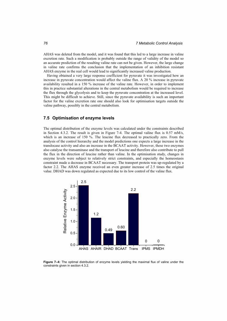
7 Metabolic Control Analysis 76
AHAS was deleted from the model, and it was found that this led to a large increase in valine excretion rate. Such a modification is probably outside the range of validity of the model so an accurate prediction of the resulting valine rate can not be given. However, the large change in valine rate confirms the conclusion that the implementation of an inhibition resistant AHAS enzyme in the real cell would lead to significantly increased valine production.
Having obtained a very large response coefficient for pyruvate it was investigated how an increase in pyruvate concentration would affect the valine flux. A 20 % increase in pyruvate availability resulted in a 150 % increase of the valine rate. However, in order to implement this in practice substantial alterations in the central metabolism would be required to increase the flux through the glycolysis and to keep the pyruvate concentration at the increased level. This might be difficult to achieve. Still, since the pyruvate availability is such an important factor for the valine excretion rate one should also look for optimisation targets outside the valine pathway, possibly in the central metabolism.
7.5 Optimisation of enzyme levels
The optimal distribution of the enzyme levels was calculated under the constraints described in Section 4.3.2. The result is given in Figure 7-4. The optimal valine flux is 0.57 mM/s, which is an increase of 150 %. The leucine flux decreased to practically zero. From the analysis of the control hierarchy and the model predictions one expects a large increase in the translocase activity and also an increase in the BCAAT activity. However, these two enzymes also catalyse the transaminase and the transport of leucine and therefore also contribute to pull the flux in the direction of leucine rather than valine. In the optimisation study, changes in enzyme levels were subject to relatively strict constraints, and especially the homeostasis constraint made a decrease in BCAAT necessary. The transport protein was up-regulated by a factor 2.2. The AHAS enzyme received an even greater increase of 2.5 times the original value. DHAD was down regulated as expected due to its low control of the valine flux.
AHAS AHAIR DHAD BCAAT Trans IPMS IPMDH0.0
0.5
1.0
1.5
2.0
2.5
0 0
2.2
0.600.49
1.2
Rel
ativ
e E
nzym
e A
ctiv
ity
2.5
Figure 7–4: The optimal distribution of enzyme levels yielding the maximal flux of valine under the constraints given in section 4.3.2.
7.6 Comparison of the different methods 77
The optimisation of valine flux yielded a very specific distribution of enzyme levels, which would not be possible to implement with the specified accuracy in a real cell. The calculated optimum is therefore a theoretical optimum, which shows the maximum of what can be achieved subject to the specified constraints and the distribution of the enzymes yielding this maximum. This is valuable information in identifying the target enzymes for manipulation in a practical application.
7.6 Comparison of the different methods
The different methods used are in good agreement and give a clear picture of the control hierarchy in the valine pathway. The control coefficients and the PEC analysis both identify DHAD as the least limiting enzyme and the translocase system as the most limiting step in the reaction sequence. This is confirmed by the calculation of the effect that finite changes in these enzyme activities would have on the valine excretion rate and by the optimisation of the enzyme activities. In the investigation presented here the flux control coefficients provided correct indications of which enzymes should be considered for strain optimisation. In addition to the translocase, the AHAS enzyme and the BCAAT enzyme had significant control.
The distribution of control as analysed by the flux control coefficients can be understood intuitively. The AHAS enzyme is the enzyme diverting the flux away from the central carbon metabolism and into the valine / leucine pathway so it is not surprising that this enzyme has significant control of the valine excretion rate. The translocase is responsible for actually excreting valine and also decreases the valine concentration which has a strong inhibitory effect on the AHAS enzyme. The IPMS enzyme diverts flux away from the valine pathway so this enzyme has a negative influence on the valine excretion rate. The role of the BCAAT enzyme in the control hierarchy is not intuitively clear since this enzyme pulls the flux towards both valine and leucine at the same time. A systemic approach is needed to gain further insight. The model based metabolic control analysis presented here showed that an increase in BCAAT activity leads to an increase in valine flux. Through the control coefficients it was possible to obtain quantitative measures for the influence of each enzyme by analysing the reaction system as a whole.
The identification of the exporting translocase as the most promising target for strain optimisation is analogous to an investigation of a Corynebacterium glutamicum isoleucine producer where export was identified as the most limiting step (Morbach et al., 1996; Sahm et al., 1999). The translocase encoded by the brnE and brnF genes (Kennerknecht et al., 2002) is the permease which is responsible for the export of both valine and isoleucine and it is the most limiting factor in the production of both of these amino acids. That the export system of an amino acid is not capable of coping with high export fluxes is not surprising since bacteria do not need to excrete primary metabolites in high amounts under normal conditions and would therefore not need a powerful export system. It has been demonstrated that the overexpression of this translocase poses some practical difficulties (Kennerknecht, 2003). If the permease activity can not be significantly increased by recombinant DNA technology, this might be achieved through fermentation technology. Keeping the extracellular concentration of valine low during a production phase will ease the excretion of valine since the translocase would then not have to pump against such a high concentration gradient and since passive diffusion of valine back into the cell would be less.
The strong feedback regulation of the pathway through the AHAS enzyme was demonstrated in Section 7.3 and 7.4 and AHAS can be seen as the main regulatory enzyme of the valine pathway. It is important to realise that the regulatory enzymes are not necessarily the most controlling enzyme. A regulatory enzyme is an enzyme having a regulatory function
7 Metabolic Control Analysis 78
through its capacity to undergo a change in catalytic activity by allosteric mechanisms or by covalent modification (Lehninger et al., 1993). The degree of metabolic control exercised by an enzyme is quantified by the control coefficients and refers to the effect that a change of an enzyme level will have on the metabolic fluxes and concentrations. It was pointed out already in the first paper on MCA by Kacser and Burns (1973) that a regulatory enzyme will typically have little control because the regulation mechanism contributes to lowering the flux control coefficient. An extensive discussion of this issue was published by Hofmeyr and Cornish-Bowden (1991). This is in fact one of the most important results of Metabolic Control Analysis because it contradicts the intuitive understanding of metabolic engineering. It seems logic that in order to increase the flux through a pathway one must increase the activity of the regulating enzyme. The work of Kacser and Burns shows that this is not necessarily the case. In the presented work this point is confirmed. AHAS is the regulating enzyme, but it is not the most controlling enzyme. AHAIR also has a regulatory function, but has a very low flux control coefficient. These results emphasise the necessity of differentiating between metabolic regulation and metabolic control. It should be noted that in this investigation the flux control coefficient for AHAS is unusually high for an enzyme with a strong regulatory function.
There was a strong correlation between the flux control coefficients and the PEC values of the enzymes. Enzymes with high PEC values had little control and vice versa. The valine transport step had the highest control and the lowest PEC, and the DHAD enzyme had the least control and the highest PEC. Note that this correlation is not true for the AHAIR enzyme, which has a low PEC, but little control of the flux. This shows that the PEC values will not always be exact measures for control. However, since the main conclusions on the most and the least limiting enzymes agree with the MCA analysis, it can be concluded that the PEC analysis is a useful method to get a first estimate of the control hierarchy in a metabolic network. Its great advantage is its simple calculation procedure, which does not require a kinetic model.
From the definition of elasticity and PEC it is clear that large elasticities will in general lead to large PECs. Although there are exceptions to this correlation, it can be seen as the underlying reason for the connection between flux control coefficients and PECs. Large elasticities are associated with low flux control coefficients (Stephanopoulus et al., 1998) so large PECs will in general result in low flux control coefficients and vice versa. The analysis of the DHAD enzyme gives an example of this. This enzyme has a particularly high elasticity towards its substrate DHIV which result in a high PEC value and a low flux control coefficient. These high elasticities occur as a result of the enzyme being neither saturated by its substrates nor inhibited by its inhibitor. The enzyme is thus able to react quickly to changes in metabolite concentrations. By using the different methods reported here one can not only analyse the enzymes’ place in the control hierarchy of the pathway, but also obtain some understanding of the causes of their level of control.
When doing a model based MCA or using a model to predict the changes in flux as a result of alterations in the enzyme levels one must consider the range of validity of the model. The model applied here simulates the valine / leucine pathway so only the control hierarchy within that pathway is examined. By limiting the model to a part of the full metabolic reaction network present in a real cell, some of the interactions between the valine / leucine pathway and the rest of the metabolism are lost. The model considers the influence of the independent metabolites on the valine / leucine pathway, but does not include the influence of the metabolites in the valine pathway on the independent metabolites. The predictions made by a part model are therefore not 100% accurate unless one is able to keep the independent metabolites at their initial level after a change in e.g. enzyme activity. However, for modest changes in flux the model gives useful estimates of the expected changes in phenotype.
7.7 Identification of target enzymes for strain optimisation 79
7.7 Identification of target enzymes for strain optimisation
Based on the acquired understanding of the control of the valine and leucine pathway as discussed in this chapter the following suggestions for the further optimisation of the valine production strain are made:
1. Overexpression of translocase. 2. Implementation of an inhibition resistant AHAS enzyme and possibly further
overexpression.3. Removal of the overexpression of the gene coding for DHAD on the plasmid to save
the cell the burden of overproducing this enzyme which has negligible influence on the valine flux.
4. Modification of the central carbon metabolism to increase pyruvate availability.
The other modifications already applied to the strain (the deletion of the threonine dehydratase enzyme, the deletion of the two enzymes in the pantothenic acid pathway and the overexpression of AHAS and AHAIR) should be kept as they are.

7 Metabolic Control Analysis 80
8 Thermodynamic Analysis 81
8 Thermodynamic Analysis The influence of the thermodynamic forces on the reactions in the valine / leucine pathway is now analysed. The analysis is based on the measured intracellular metabolite concentrations and on the intracellular reaction rates obtained from the dynamic model described in Chapter 6. Central to the analysis is the concept of reaction affinity and reaction resistance. First the system at its steady state composition will be analysed, before the relationship between reaction rate and affinity is investigated. Finally the theory of metabolic control analysis is extended to include also the thermodynamic properties, and this theory is used to analyse the control of the thermodynamic forces in the reaction network.
8.1 The concept of the thermodynamic resistance
In Section 4.4.1 the reaction affinity, A, was defined. The affinity is the thermodynamic reaction potential and the driving force for chemical reactions. The relation between rate and affinity will here be described by introducing a reaction resistance, R, in analogy with Ohms law. For an uncoupled reaction, where only one force drives the reaction, the reaction rate can be expressed as:
i
ii R
Ar ( 8-1 )
In the general case it can not be assumed that R is constant with affinity so it must be treated as a system variable rather than a parameter. However, as mentioned in Section 4.4.1, the reaction rate is proportional to the affinity in near-equilibrium situations so for these cases the resistance can be treated as a constant. In addition, it has been observed experimentally that in some cases the reaction rate will be proportional to the affinity also for reactions operating far from equilibrium.
The observed rate of an enzyme catalysed reaction depends on several elementary steps including the diffusion and adsorption / desorption of the participating compounds to and from the enzyme as well as the rate of transformation at the catalytic site. The catalytic activity is determined by enzyme concentration, substrate and product saturation levels, activation or inhibition effects from other metabolites, substrate competition, the presence of metal ions in the cytosol and covalent modification of the enzyme itself yielding an active and an inactive form. It is impossible to determine the exact influence of all these factors in-vivoso they are summarised in the quantity R which can be considered a function of the enzyme state showing the resistance to the driving force. The definition of a reaction resistance allows the reaction rate to be expressed as a function of only two variables A and R as seen in Eq. (8-1). When the reaction rate and affinity are known, the resistance can be calculated from Eq. (8-1).
It should be noted that the thermodynamic resistances are not measures for flux control and should not be confused with the flux control coefficients as these are different concepts. The resistances are used to describe a reaction system in terms of the thermodynamic potentials. They are properties of an enzyme at a specific system state and can be considered a system parameter or a system variable. The flux control coefficients are derivatives of a system variable, namely the flux, and show how the variable changes in response to an alteration in a system parameter.
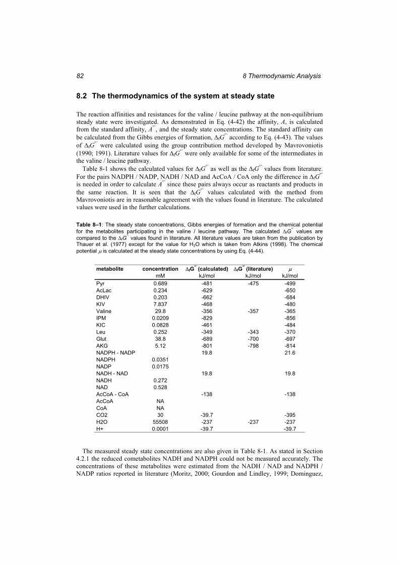
8 Thermodynamic Analysis 82
8.2 The thermodynamics of the system at steady state
The reaction affinities and resistances for the valine / leucine pathway at the non-equilibrium steady state were investigated. As demonstrated in Eq. (4-42) the affinity, A, is calculated from the standard affinity, A°’, and the steady state concentrations. The standard affinity can be calculated from the Gibbs energies of formation, fG°’ according to Eq. (4-43). The values of fG°’ were calculated using the group contribution method developed by Mavrovoniotis (1990; 1991). Literature values for fG°’ were only available for some of the intermediates in the valine / leucine pathway.
Table 8-1 shows the calculated values for fG°’ as well as the fG°’ values from literature. For the pairs NADPH / NADP, NADH / NAD and AcCoA / CoA only the difference in fG°’
is needed in order to calculate A°’ since these pairs always occur as reactants and products in the same reaction. It is seen that the fG°’ values calculated with the method from Mavrovoniotis are in reasonable agreement with the values found in literature. The calculated values were used in the further calculations.
Table 8–1: The steady state concentrations, Gibbs energies of formation and the chemical potential for the metabolites participating in the valine / leucine pathway. The calculated fG°’ values are compared to the fG°’ values found in literature. All literature values are taken from the publication by Thauer et al. (1977) except for the value for H2O which is taken from Atkins (1998). The chemical potential is calculated at the steady state concentrations by using Eq. (4-44).
metabolite concentration fG°' (calculated) fG°' (literature) mM kJ/mol kJ/mol kJ/mol
Pyr 0.689 -481 -475 -499 AcLac 0.234 -629 -650 DHIV 0.203 -662 -684 KIV 7.837 -468 -480 Valine 29.8 -356 -357 -365 IPM 0.0209 -829 -856 KIC 0.0828 -461 -484 Leu 0.252 -349 -343 -370 Glut 38.8 -689 -700 -697 AKG 5.12 -801 -798 -814 NADPH - NADP 19.8 21.6 NADPH 0.0351 NADP 0.0175 NADH - NAD 19.8 19.8 NADH 0.272 NAD 0.528 AcCoA - CoA -138 -138 AcCoA NA CoA NA CO2 30 -39.7 -395 H2O 55508 -237 -237 -237 H+ 0.0001 -39.7 -39.7
The measured steady state concentrations are also given in Table 8-1. As stated in Section 4.2.1 the reduced cometabolites NADH and NADPH could not be measured accurately. The concentrations of these metabolites were estimated from the NADH / NAD and NADPH / NADP ratios reported in literature (Moritz, 2000; Gourdon and Lindley, 1999; Dominguez,
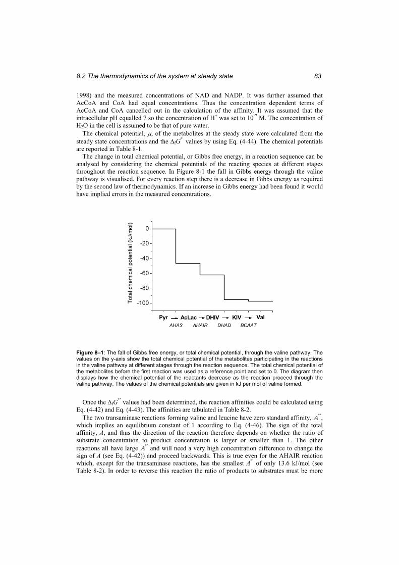
8.2 The thermodynamics of the system at steady state 83
1998) and the measured concentrations of NAD and NADP. It was further assumed that AcCoA and CoA had equal concentrations. Thus the concentration dependent terms of AcCoA and CoA cancelled out in the calculation of the affinity. It was assumed that the intracellular pH equalled 7 so the concentration of H+ was set to 10-7 M. The concentration of H2O in the cell is assumed to be that of pure water.
The chemical potential, , of the metabolites at the steady state were calculated from the steady state concentrations and the fG°’ values by using Eq. (4-44). The chemical potentials are reported in Table 8-1.
The change in total chemical potential, or Gibbs free energy, in a reaction sequence can be analysed by considering the chemical potentials of the reacting species at different stages throughout the reaction sequence. In Figure 8-1 the fall in Gibbs energy through the valine pathway is visualised. For every reaction step there is a decrease in Gibbs energy as required by the second law of thermodynamics. If an increase in Gibbs energy had been found it would have implied errors in the measured concentrations.
AHAS AHAIR DHAD BCAAT
-100
-80
-60
-40
-20
0
ValKIVDHIVAcLac
Tota
l che
mic
al p
oten
tial (
kJ/m
ol)
Pyr
Figure 8–1: The fall of Gibbs free energy, or total chemical potential, through the valine pathway. The values on the y-axis show the total chemical potential of the metabolites participating in the reactions in the valine pathway at different stages through the reaction sequence. The total chemical potential of the metabolites before the first reaction was used as a reference point and set to 0. The diagram then displays how the chemical potential of the reactants decrease as the reaction proceed through the valine pathway. The values of the chemical potentials are given in kJ per mol of valine formed.
Once the fG°’ values had been determined, the reaction affinities could be calculated using Eq. (4-42) and Eq. (4-43). The affinities are tabulated in Table 8-2.
The two transaminase reactions forming valine and leucine have zero standard affinity, °’,which implies an equilibrium constant of 1 according to Eq. (4-46). The sign of the total affinity, A, and thus the direction of the reaction therefore depends on whether the ratio of substrate concentration to product concentration is larger or smaller than 1. The other reactions all have large °’ and will need a very high concentration difference to change the sign of A (see Eq. (4-42)) and proceed backwards. This is true even for the AHAIR reaction which, except for the transaminase reactions, has the smallest A°’ of only 13.6 kJ/mol (see Table 8-2). In order to reverse this reaction the ratio of products to substrates must be more
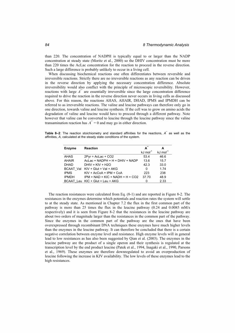
8 Thermodynamic Analysis 84
than 220. The concentration of NADPH is typically equal to or larger than the NADP concentration at steady state (Moritz et al., 2000) so the DHIV concentration must be more than 220 times the AcLac concentration for the reaction to proceed in the reverse direction. Such a large difference is probably unlikely to occur in a living cell.
When discussing biochemical reactions one often differentiates between reversible and irreversible reactions. Strictly there are no irreversible reactions as any reaction can be driven in the reverse direction by applying the necessary concentration difference. Absolute irreversibility would also conflict with the principle of microscopic reversibility. However, reactions with large A°’ are essentially irreversible since the large concentration difference required to drive the reaction in the reverse direction never occurs in living cells as discussed above. For this reason, the reactions AHAS, AHAIR, DHAD, IPMS and IPMDH can be referred to as irreversible reactions. The valine and leucine pathways can therefore only go in one direction, towards valine and leucine synthesis. If the cell was to grow on amino acids the degradation of valine and leucine would have to proceed through a different pathway. Note however that valine can be converted to leucine through the leucine pathway since the valine transamination reaction has °’ = 0 and may go in either direction.
Table 8–2: The reaction stoichiometry and standard affinities for the reactions, A°’ as well as the affinities, A, calculated at the steady state conditions of the system.
Enzyme Reaction A°' A kJ mol-1 kJ mol-1
AHAS 2Pyr = AcLac + CO2 53.4 46.6 AHAIR AcLac + NADPH + H = DHIV + NADP 13.6 15.7 DHAD DHIV = KIV + H2O 42.3 33.0 BCAAT_Val KIV + Glut = Val + AKG 0 1.74 IPMS KIV + AcCoA = IPM + CoA 223 238 IPMDH IPM + NAD = KIC + NADH + H + CO2 37.70 48.9 BCAAT_Leu KIC + Glut = Leu + AKG 0 2.33
The reaction resistances were calculated from Eq. (8-1) and are reported in Figure 8-2. The resistances in the enzymes determine which potentials and reaction rates the system will settle to at the steady state. As mentioned in Chapter 7.2 the flux in the first common part of the pathway is more than 25 times the flux in the leucine pathway (0.24 and 0.0085 mM/s respectively) and it is seen from Figure 8-2 that the resistances in the leucine pathway are about two orders of magnitude larger than the resistances in the common part of the pathway. Since the enzymes in the common part of the pathway are the ones that have been overexpressed through recombinant DNA techniques these enzymes have much higher levels than the enzymes in the leucine pathway. It can therefore be concluded that there is a certain negative correlation between enzyme level and resistance. High enzyme levels will in general lead to low resistances as has also been suggested by Qian et al. (2003). The enzymes in the leucine pathway are the product of a single operon and their synthesis is regulated at the transcription level by the end product leucine (Patek et al., 1994, Inagaki et al., 1990, Parsons et al., 1969). These enzymes are therefore downregulated to avoid an overproduction of leucine following the increase in KIV availability. The low levels of these enzymes lead to the high resistances.
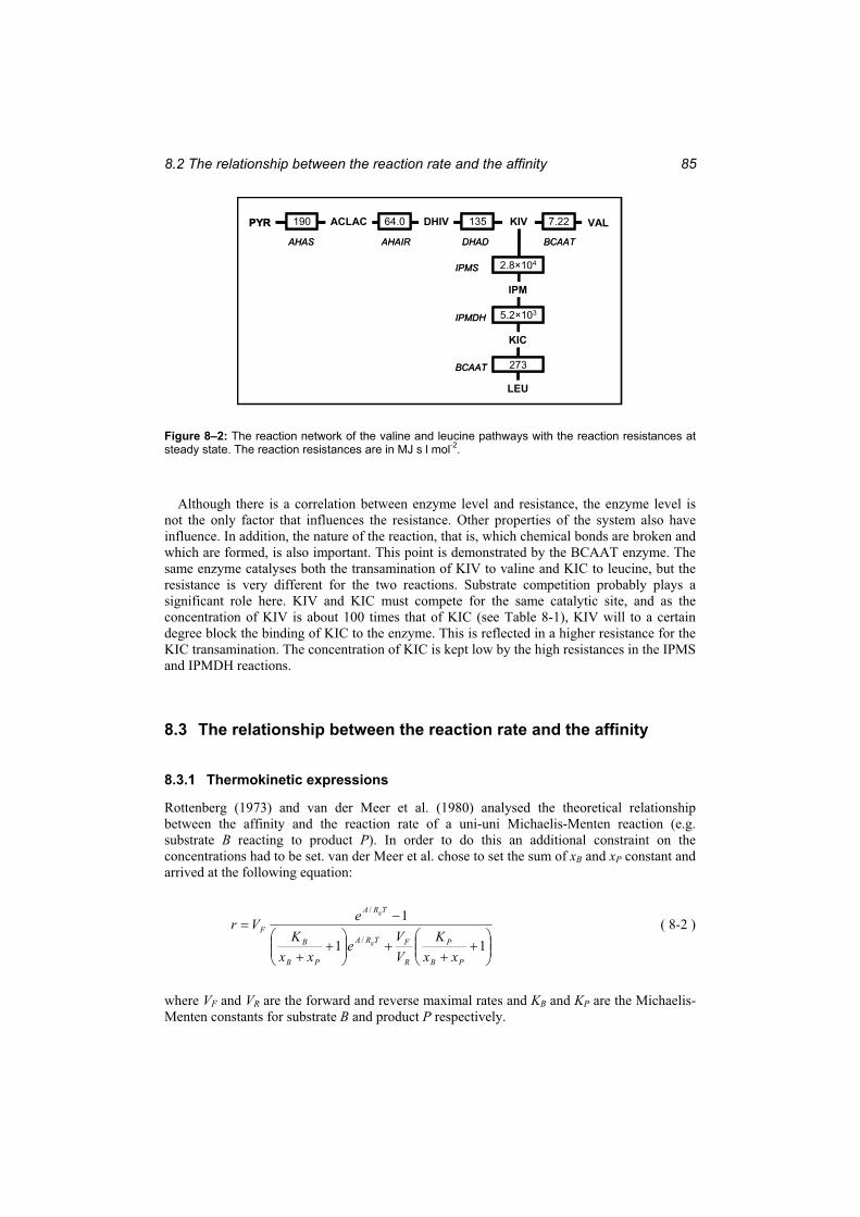
8.2 The relationship between the reaction rate and the affinity 85
ACLAC DHIV KIV VALPYR
AHAS AHAIR DHAD
LEU
KIC
IPM
BCAAT
IPMS
IPMDH
BCAAT
190
5.2×10³
64.0 135 7.22
2.8×10⁴
273
ACLAC DHIV KIV VALPYR
AHAS AHAIR DHAD
LEU
KIC
IPM
BCAAT
IPMS
IPMDH
BCAAT
190
5.2×10³
64.0 135 7.22
2.8×10⁴
273
Figure 8–2: The reaction network of the valine and leucine pathways with the reaction resistances at steady state. The reaction resistances are in MJ s l mol-2.
Although there is a correlation between enzyme level and resistance, the enzyme level is not the only factor that influences the resistance. Other properties of the system also have influence. In addition, the nature of the reaction, that is, which chemical bonds are broken and which are formed, is also important. This point is demonstrated by the BCAAT enzyme. The same enzyme catalyses both the transamination of KIV to valine and KIC to leucine, but the resistance is very different for the two reactions. Substrate competition probably plays a significant role here. KIV and KIC must compete for the same catalytic site, and as the concentration of KIV is about 100 times that of KIC (see Table 8-1), KIV will to a certain degree block the binding of KIC to the enzyme. This is reflected in a higher resistance for the KIC transamination. The concentration of KIC is kept low by the high resistances in the IPMS and IPMDH reactions.
8.3 The relationship between the reaction rate and the affinity
8.3.1 Thermokinetic expressions
Rottenberg (1973) and van der Meer et al. (1980) analysed the theoretical relationship between the affinity and the reaction rate of a uni-uni Michaelis-Menten reaction (e.g. substrate B reacting to product P). In order to do this an additional constraint on the concentrations had to be set. van der Meer et al. chose to set the sum of xB and xP constant and arrived at the following equation:
11
1/
/
PB
P
R
FTRA
PB
B
TRA
F
xxK
VVe
xxK
eVrg
g
( 8-2 )
where VF and VR are the forward and reverse maximal rates and KB and KP are the Michaelis-Menten constants for substrate B and product P respectively.
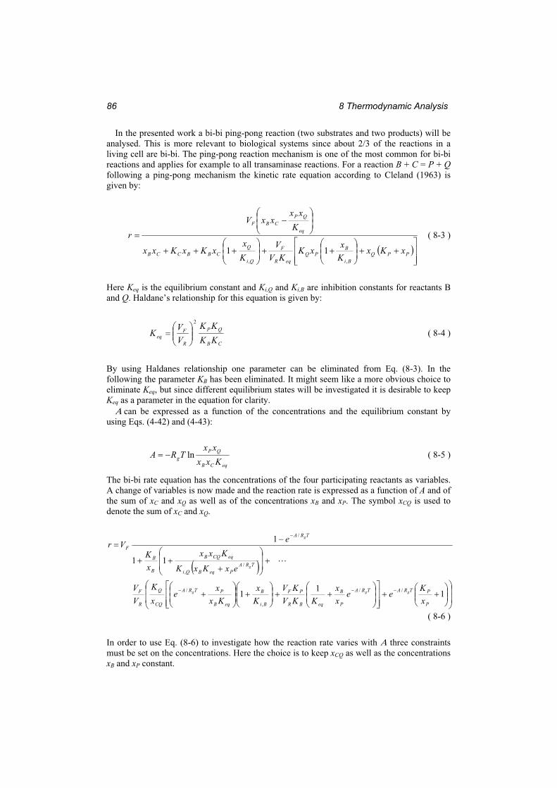
8 Thermodynamic Analysis 86
In the presented work a bi-bi ping-pong reaction (two substrates and two products) will be analysed. This is more relevant to biological systems since about 2/3 of the reactions in a living cell are bi-bi. The ping-pong reaction mechanism is one of the most common for bi-bi reactions and applies for example to all transaminase reactions. For a reaction B + C = P + Qfollowing a ping-pong mechanism the kinetic rate equation according to Cleland (1963) is given by:
PPQBi
BPQ
eqR
F
Qi
QCBBCCB
eq
QPCBF
xKxKxxK
KVV
Kx
xKxKxx
Kxx
xxVr
,,
11
( 8-3 )
Here Keq is the equilibrium constant and Ki,Q and Ki,B are inhibition constants for reactants Band Q. Haldane’s relationship for this equation is given by:
CB
QP
R
Feq KK
KKVVK
2
( 8-4 )
By using Haldanes relationship one parameter can be eliminated from Eq. (8-3). In the following the parameter KB has been eliminated. It might seem like a more obvious choice to eliminate Keq, but since different equilibrium states will be investigated it is desirable to keep Keq as a parameter in the equation for clarity.
can be expressed as a function of the concentrations and the equilibrium constant by using Eqs. (4-42) and (4-43):
eqCB
QPg Kxx
xxTRA ln ( 8-5 )
The bi-bi rate equation has the concentrations of the four participating reactants as variables. A change of variables is now made and the reaction rate is expressed as a function of A and of the sum of xC and xQ as well as of the concentrations xB and xP. The symbol xCQ is used to denote the sum of xC and xQ.
111
11
1
//
,
/
/,
/
P
PTRATRA
P
B
eqBR
PF
Bi
B
eqB
PTRA
CQ
Q
R
F
TRAPeqBQi
eqCQB
B
B
TRA
F
xK
eexx
KKVKV
Kx
Kxx
exK
VV
exKxK
KxxxK
eVr
ggg
g
g
( 8-6 )
In order to use Eq. (8-6) to investigate how the reaction rate varies with three constraints must be set on the concentrations. Here the choice is to keep xCQ as well as the concentrations xB and xP constant.
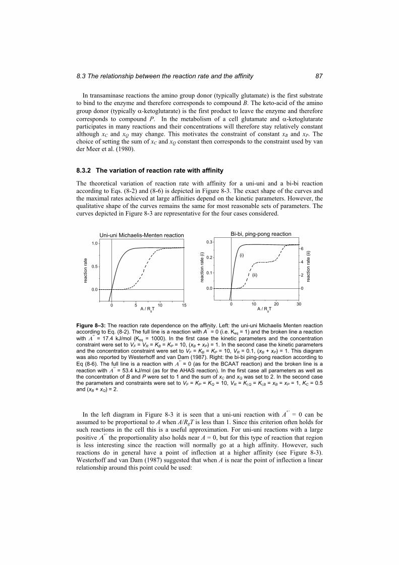
8.3 The relationship between the reaction rate and the affinity 87
In transaminase reactions the amino group donor (typically glutamate) is the first substrate to bind to the enzyme and therefore corresponds to compound B. The keto-acid of the amino group donor (typically -ketoglutarate) is the first product to leave the enzyme and therefore corresponds to compound P. In the metabolism of a cell glutamate and -ketoglutarate participates in many reactions and their concentrations will therefore stay relatively constant although xC and xQ may change. This motivates the constraint of constant xB and xP. The choice of setting the sum of xC and xQ constant then corresponds to the constraint used by van der Meer et al. (1980).
8.3.2 The variation of reaction rate with affinity
The theoretical variation of reaction rate with affinity for a uni-uni and a bi-bi reaction according to Eqs. (8-2) and (8-6) is depicted in Figure 8-3. The exact shape of the curves and the maximal rates achieved at large affinities depend on the kinetic parameters. However, the qualitative shape of the curves remains the same for most reasonable sets of parameters. The curves depicted in Figure 8-3 are representative for the four cases considered.
0 5 10 15
0.0
0.5
1.0
reac
tion
rate
A / RgT
Uni-uni Michaelis-Menten reaction
0 10 20 30
0.0
0.1
0.2
0.3
0
2
4
6
(ii)
reac
tion
rate
(ii)
reac
tion
rate
(i)
A / RgT
(i)
Bi-bi, ping-pong reaction
Figure 8–3: The reaction rate dependence on the affinity. Left: the uni-uni Michaelis Menten reaction according to Eq. (8-2). The full line is a reaction with A°’ = 0 (i.e. Keq = 1) and the broken line a reaction with °’ = 17.4 kJ/mol (Keq = 1000). In the first case the kinetic parameters and the concentration constraint were set to VF = VR = KB = KP = 10, (xB + xP) = 1. In the second case the kinetic parameters and the concentration constraint were set to VF = KB = KP = 10, VR = 0.1, (xB + xP) = 1. This diagram was also reported by Westerhoff and van Dam (1987). Right: the bi-bi ping-pong reaction according to Eq (8-6). The full line is a reaction with °’ = 0 (as for the BCAAT reaction) and the broken line is a reaction with °’ = 53.4 kJ/mol (as for the AHAS reaction). In the first case all parameters as well as the concentration of B and P were set to 1 and the sum of xC and xQ was set to 2. In the second case the parameters and constraints were set to VF = KP = KQ = 10, VR = Ki,Q = Ki,B = xB = xP = 1, KC = 0.5 and (xB + xQ) = 2.
In the left diagram in Figure 8-3 it is seen that a uni-uni reaction with A°’ = 0 can be assumed to be proportional to A when A/RgT is less than 1. Since this criterion often holds for such reactions in the cell this is a useful approximation. For uni-uni reactions with a large positive °’ the proportionality also holds near A = 0, but for this type of reaction that region is less interesting since the reaction will normally go at a high affinity. However, such reactions do in general have a point of inflection at a higher affinity (see Figure 8-3). Westerhoff and van Dam (1987) suggested that when A is near the point of inflection a linear relationship around this point could be used:
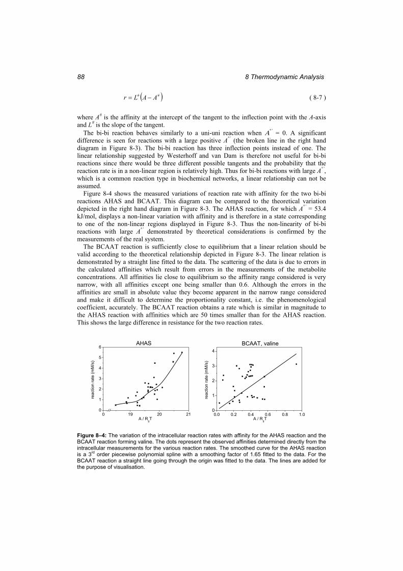
8 Thermodynamic Analysis 88
## AALr ( 8-7 )
where A# is the affinity at the intercept of the tangent to the inflection point with the A-axis and L# is the slope of the tangent.
The bi-bi reaction behaves similarly to a uni-uni reaction when °’ = 0. A significant difference is seen for reactions with a large positive A°’ (the broken line in the right hand diagram in Figure 8-3). The bi-bi reaction has three inflection points instead of one. The linear relationship suggested by Westerhoff and van Dam is therefore not useful for bi-bi reactions since there would be three different possible tangents and the probability that the reaction rate is in a non-linear region is relatively high. Thus for bi-bi reactions with large A°’,which is a common reaction type in biochemical networks, a linear relationship can not be assumed.
Figure 8-4 shows the measured variations of reaction rate with affinity for the two bi-bi reactions AHAS and BCAAT. This diagram can be compared to the theoretical variation depicted in the right hand diagram in Figure 8-3. The AHAS reaction, for which A°’ = 53.4 kJ/mol, displays a non-linear variation with affinity and is therefore in a state corresponding to one of the non-linear regions displayed in Figure 8-3. Thus the non-linearity of bi-bi reactions with large A°’ demonstrated by theoretical considerations is confirmed by the measurements of the real system.
The BCAAT reaction is sufficiently close to equilibrium that a linear relation should be valid according to the theoretical relationship depicted in Figure 8-3. The linear relation is demonstrated by a straight line fitted to the data. The scattering of the data is due to errors in the calculated affinities which result from errors in the measurements of the metabolite concentrations. All affinities lie close to equilibrium so the affinity range considered is very narrow, with all affinities except one being smaller than 0.6. Although the errors in the affinities are small in absolute value they become apparent in the narrow range considered and make it difficult to determine the proportionality constant, i.e. the phenomenological coefficient, accurately. The BCAAT reaction obtains a rate which is similar in magnitude to the AHAS reaction with affinities which are 50 times smaller than for the AHAS reaction. This shows the large difference in resistance for the two reaction rates.
0 19 20 210
1
2
3
4
5
6
reac
tion
rate
(mM
/s)
A / RgT
AHAS
0.0 0.2 0.4 0.6 0.8 1.00
1
2
3
4
reac
tion
rate
(mM
/s)
A / RgT
BCAAT, valine
Figure 8–4: The variation of the intracellular reaction rates with affinity for the AHAS reaction and the BCAAT reaction forming valine. The dots represent the observed affinities determined directly from the intracellular measurements for the various reaction rates. The smoothed curve for the AHAS reaction is a 3rd order piecewise polynomial spline with a smoothing factor of 1.65 fitted to the data. For the BCAAT reaction a straight line going through the origin was fitted to the data. The lines are added for the purpose of visualisation.
8.4 The control of the thermodynamic forces and resistances 89
As described in section 8.2, reactions with large A°’ will need a very large concentration difference in order to go in the reverse direction. It is seen from Figure 8-3 that even when such reactions are pushed in the reverse direction they will obtain very small rates in that direction. This is implied through the Haldane relationship. In addition to the concentrations of the reactants, it is the kinetic constants that directly decide the reaction rate. The reverse reaction rate of a bi-bi reaction will be small when VF, KP and KQ are large and when VR, KBand KC are small. According to the Haldane relationship the following relation holds:
CB
QP
R
Feq
RTA
KKKK
VVKe
2/'
( 8-8 )
By inspecting Eq. (8-8) it is seen that a large A°’ implies that VF, KP and KQ are large and that VR, KB and KC are small. Thus, by the Haldane relationship, a large A°’ implies small reverse reaction rates.
It was concluded in section 8.2 that the reactions AHAS, AHAIR, DHAD, IPMS and IPMDH are irreversible due to their large A°’. The consideration of the Haldane relationship provides further evidence of this conclusion. Even if these reactions could be pushed in the reverse direction they would obtain negligibly small reaction rates.
8.3.3 A short discussion of the main conclusions in section 8.3
The thermokinetic rate equation for a ping-pong, bi-bi reaction was derived. This equation was used to give a theoretical proof that for a bi-bi reaction operating far from equilibrium it can generally not be assumed that the reaction rate is proportional to the thermodynamic driving force. Close to equilibrium this assumption is valid. The theoretical analysis was confirmed by the experimental data.
As discussed in section 4.4.1 the question of linearity is important in the establishment of a theoretical basis for the thermodynamic analysis of biochemical systems. It has been suggested in several publications that the reaction mechanism of enzymes implies a linear relationship also at far from equilibrium conditions. However, these publications only considered a uni-uni reaction. Through the analysis of a bi-bi reaction presented here it was demonstrated that the conclusion of linearity is wrong.
8.4 The control of the thermodynamic forces and resistances
8.4.1 The MCA of the thermodynamic functions affinity and resistance
The classical theory of MCA analysing the control of the concentrations and fluxes in metabolic networks was described in Section 4.3.2. The theory will here be expanded to evaluate also the control of the affinity and the resistance.
Control coefficients can be defined for the affinity and the resistance according to Eq. (4-24) in Section 4.3.2 as:
j
i
i
jAji p
AAp
dd
C , ( 8-9 )
8 Thermodynamic Analysis 90
j
i
i
jRji p
RRp
dd
C , ( 8-10 )
Similarly, response coefficients can be defined for the affinity and the resistance according to Eq. (4-25).
j
i
i
jAji c
AAc
dd
Q , ( 8-11 )
j
i
i
jRji c
RRc
dd
Q , ( 8-12 )
The local coefficients with respect to the metabolites, i.e. the elasticities, are defined according to Eq. (4-26):
j
i
i
jAji x
AAx
, ( 8-13 )
j
i
i
jRji x
RRx
, ( 8-14 )
The - elasticities are defined according to Eq. (4-27) as:
j
i
i
jAji p
AAp
, ( 8-15 )
j
i
i
jRji p
RRp
, ( 8-16 )
Note that an expression for the elasticity of A can be obtained easily by using Eq. (4-42) in combination with Eq. (8-13).
i
jgAji A
TR, ( 8-17 )
j is here the stoichiometric coefficient of metabolite j, Rg is the universal gas constant and Tis the temperature in Kelvin. The affinity does not depend directly on any kinetic parameters and the - elasticity of A will therefore equal zero for all parameters considered here. In some special cases it might be useful to consider the temperature a parameter or even to consider
8.4 The control of the thermodynamic forces and resistances 91
the stoichiometric coefficients parameters (e.g. in the analysis of oxidative phosphorylation) in which cases one could calculate a - elasticity for A. However, in the work presented here only the kinetic parameters and the enzyme levels are treated as system parameters.
In Section 4.3.2 it was demonstrated how the flux control coefficients depend on the concentration control coefficients and the flux elasticities (Eq. 4-36). The same argument is applied here to show how the affinity and resistance control coefficients depend on the concentration control coefficients. The affinity is a function of the concentrations only, while the resistance is a function of the concentrations and the kinetic parameters. Consider reaction i with resistance px;fRi where x is the vector of the m metabolite concentrations and pis the vector of parameters. By applying the chain rule of differentiation an expression for the derivative of Ri with respect to parameter pj can be obtained:
m
k j
k
k
i
j
i
j
i
px
xR
pR
pR
1 dd
dd
( 8-18 )
multiplication with the scaling factor ij Rp on both sides gives:
m
k j
k
k
j
k
i
i
k
j
i
i
j
j
i
i
j
px
xp
xR
Rx
pR
Rp
pR
Rp
1 dd
dd
( 8-19 )
which according to the definitions in Eqs. (4-28), (8-10), (8-14) and (8-15) is:
m
k
Cjk
Rki
Rji
Rji
1,,,, CC ( 8-20 )
Following the same procedure for the affinity, the affinity control coefficient is given by
m
k
Cjkk
i
gAji A
TR
1,, CC ( 8-21 )
The affinity control coefficient gets a simpler expression since the A equals zero and Eq. (8-17) can be used to include the general expression for A.
Looking at Eq. (8-20) it is seen that the resistance control coefficient can be divided into two terms; the -elasticity and the sum of the -elasticities multiplied by the concentration control coeffients:
m
k
Cjk
Rki
Rji
Rji
1,,,, CC ( 8-20 )
direct effects / central control indirect effects / self-organising
The R-elasticity was defined in Eq. (8-16) and is the change in resistance with parameter when all other variables are held constant. The R-elasticity is therefore a measure of the
8 Thermodynamic Analysis 92
direct effect that the change in parameter has on the resistance. The change in parameter might also lead to changes in the concentrations as well, which in turn might also influence the resistance by for example changing the substrate and product saturation level. These indirect effects are given by the second term in Eq. (8-20). Note that if the resistance is insensitive towards changes in the concentrations, i.e. if all the R equal zero, the resistance is only affected by the direct effects, in which case the analysis will be simplified. In cases where the parameter is not directly influencing the reaction the R-elasticity will be zero and only the indirect effects will apply.
In Section 4.4.1 it was pointed out that the control of dynamic systems can be divided into central control and self-organising. These two terms correspond to the direct effects and the indirect effects respectively. The great benefit of Eq. (8-20) is that it gives quantitative measures for central control and self-organising. By considering Eq. (8-20) one can assess to which degree a system is controlled through central control and to which degree it is controlled through self-organising. In the cell central control is exercised through gene transcription and translation which may lead to a change in an enzyme level. Self-organising is the result of the reaction system adapting itself to the changed enzyme level according to the thermodynamic forces in the system and the kinetic properties of the enzymes.
Two further useful relationships between the elasticity and control coefficients of the different variables can be derived from the definition of resistance. The resistance is given by:
i
ii r
AR ( 8-22 )
By taking the total differentials of both sides of Eq. (8-22) with respect to parameter pj the following expression is obtained:
j
i
i
i
j
i
ij
i
pr
rA
pA
rpR
dd
dd1
dd
2 ( 8-23 )
Multiplying both sides of Eq. (8-23) with ij Rp and using the definition of R in Eq. (8-22) to simplify the expression, Eq. (8-23) becomes:
j
i
i
j
j
i
i
j
j
i
i
j
pr
rp
pA
Ap
pR
Rp
dd
dd
dd
( 8-24 )
which, according to the definitions of the control coefficients in Eqs. (4-29), (8-9) and (8-10), is just:
Fji
Aji
Rji CCC ,,, ( 8-25 )
By using the same strategy the analogous equation can be derived for the resistance elasticity:
Fji
Aji
Rji ,,, ( 8-26 )

8.4 The control of the thermodynamic forces and resistances 93
As was demonstrated in Section 4.3.2 all flux control coefficients can be calculated if all the concentration control coefficients and all the flux elasticities are known. It is seen that by using Eq. (8-20), (8-21), (8-25) and (8-26) all the affinity and resistance control coefficients can be calculated as well from the concentration control coefficients and the flux elasticities.
8.4.2 The control of the affinity and the resistance in the valine pathway
The elasticities of the affinities and resistances for the AHAS and the valine BCAAT reactions are listed in Table 8-3 and 8-4. By comparing the values of the As and the Rs the role of the affinity and resistance in the control of the reaction rate can be investigated since the F (the reaction rate elasticity) is just A minus R according to Eq (8-26).
Table 8–3: The affinity and resistance elasticities of the AHAS reaction with respect to pyruvate, acetolactate and valine.
A R
Pyr 0.108 -25.8 AcLac 0.0541 18.5 Val 0 12.1
Table 8–4: The affinity and resistance elasticities for the BCAAT reaction with respect to glutamate, ketoisovalerate, -ketoglutarate and valine.
A R
Glut 1.45 -4.56 KIV 1.45 -15.0 AKG -1.45 -1.44 Val -1.45 -1.45
It is seen from Table 8-3 that for the AHAS reaction the resistances are very sensitive to the concentration of the substrate pyruvate and the product acetolactate while the affinity is almost insensitive to changes in these concentrations. For the BCAAT a different picture is seen (Table 8-4). The resistance elasticities for the substrates and products are much smaller and the affinity elasticities are comparable to the resistance elasticities. This illustrates a general point. Reactions far from equilibrium (such as the AHAS reaction) are controlled almost entirely through the reaction resistances, i.e. through the properties of the enzymes. For reactions closer to equilibrium (such as the BCAAT reaction) the reaction rate is also controlled through the affinity, a quantity not directly dependent on the enzyme properties.
This point is further illustrated by the control coefficients in Table 8-5 where it is seen that the AHAS affinity is much less sensitive to changes in the enzyme levels than the resistance. For the BCAAT reaction the affinity control coefficient is in the same range as the resistance control coefficient. The important conclusion here is that, in general, the closer to equilibrium a reaction is, the more the reaction rate is controlled through the affinity.
The discussion above gives an understanding of why metabolic reaction networks are stable. For reactions far from equilibrium the enzyme properties, which have developed through evolution, ensure a stable state. For reactions close to equilibrium the affinity plays a more important role. However, close to equilibrium the reaction rate varies linearly with
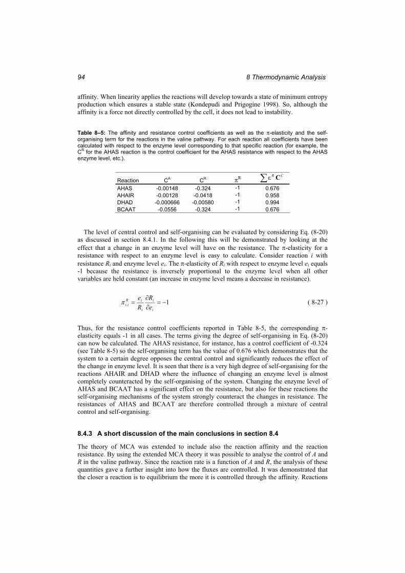
8 Thermodynamic Analysis 94
affinity. When linearity applies the reactions will develop towards a state of minimum entropy production which ensures a stable state (Kondepudi and Prigogine 1998). So, although the affinity is a force not directly controlled by the cell, it does not lead to instability.
Table 8–5: The affinity and resistance control coefficients as well as the -elasticity and the self-organising term for the reactions in the valine pathway. For each reaction all coefficients have been calculated with respect to the enzyme level corresponding to that specific reaction (for example, the CR for the AHAS reaction is the control coefficient for the AHAS resistance with respect to the AHAS enzyme level, etc.).
Reaction CA CR R CR CAHAS -0.00148 -0.324 -1 0.676AHAIR -0.00128 -0.0418 -1 0.958DHAD -0.000666 -0.00580 -1 0.994BCAAT -0.0556 -0.324 -1 0.676
The level of central control and self-organising can be evaluated by considering Eq. (8-20) as discussed in section 8.4.1. In the following this will be demonstrated by looking at the effect that a change in an enzyme level will have on the resistance. The -elasticity for a resistance with respect to an enzyme level is easy to calculate. Consider reaction i with resistance Ri and enzyme level ei. The -elasticity of Ri with respect to enzyme level ei equals-1 because the resistance is inversely proportional to the enzyme level when all other variables are held constant (an increase in enzyme level means a decrease in resistance).
1,i
i
i
iRii e
RRe
( 8-27 )
Thus, for the resistance control coefficients reported in Table 8-5, the corresponding -elasticity equals -1 in all cases. The terms giving the degree of self-organising in Eq. (8-20) can now be calculated. The AHAS resistance, for instance, has a control coefficient of -0.324 (see Table 8-5) so the self-organising term has the value of 0.676 which demonstrates that the system to a certain degree opposes the central control and significantly reduces the effect of the change in enzyme level. It is seen that there is a very high degree of self-organising for the reactions AHAIR and DHAD where the influence of changing an enzyme level is almost completely counteracted by the self-organising of the system. Changing the enzyme level of AHAS and BCAAT has a significant effect on the resistance, but also for these reactions the self-organising mechanisms of the system strongly counteract the changes in resistance. The resistances of AHAS and BCAAT are therefore controlled through a mixture of central control and self-organising.
8.4.3 A short discussion of the main conclusions in section 8.4
The theory of MCA was extended to include also the reaction affinity and the reaction resistance. By using the extended MCA theory it was possible to analyse the control of A and R in the valine pathway. Since the reaction rate is a function of A and R, the analysis of these quantities gave a further insight into how the fluxes are controlled. It was demonstrated that the closer a reaction is to equilibrium the more it is controlled through the affinity. Reactions
8.4 The control of the thermodynamic forces and resistances 95
far from equilibrium are controlled mostly through the resistance. This provided an explanation of why cellular reaction networks are stable systems.
It was further demonstrated how quantitative measures for the central control and the self-organising effects in metabolic networks can be defined and calculated. These concepts give a new and deeper insight into the control of such systems since they evaluate to which degree the reaction system controls itself and to which degree the cell controls the reaction rates through transcription and translation of its genes.

8 Thermodynamic Analysis 96
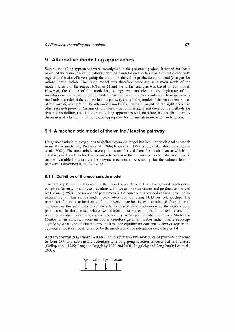
9 Alternative modelling approaches 97
9 Alternative modelling approaches Several modelling approaches were investigated in the presented project. It turned out that a model of the valine / leucine pathway defined using linlog kinetics was the best choice with regards to the aim of investigating the control of the valine production and identify targets for rational optimisation. The linlog model was therefore presented as a main result of the modelling part of the project (Chapter 6) and the further analysis was based on this model. However, the choice of this modelling strategy was not clear at the beginning of the investigation and other modelling strategies were therefore also considered. These included a mechanistic model of the valine / leucine pathway and a linlog model of the entire metabolism of the investigated strain. The alternative modelling strategies might be the right choice in other research projects. An aim of this thesis was to investigate and develop the methods for dynamic modelling, and the other modelling approaches will, therefore, be described here. A discussion of why they were not found appropriate for the investigation will also be given.
9.1 A mechanistic model of the valine / leucine pathway
Using mechanistic rate equations to define a dynamic model has been the traditional approach in metabolic modelling (Pissara et al., 1996; Rizzi et al., 1997; Yang et al., 1999; Chassagnole et al., 2002). The mechanistic rate equations are derived from the mechanism at which the substrates and products bind to and are released from the enzyme. A mechanistic model based on the available literature on the enzyme mechanisms was set up for the valine / leucine pathway as described in the following.
9.1.1 Definition of the mechanistic model
The rate equations implemented in the model were derived from the general mechanistic equations for enzyme catalysed reactions with two or more substrates and products as derived by Cleland (1963). The number of parameters in the equations is reduced as far as possible by eliminating all linearly dependent parameters and by using Haldanes relationship. The parameter for the maximal rate of the reverse reaction Vr was eliminated from all rate equations as this parameter can always be expressed as a combination of the other kinetic parameters. In those cases where two kinetic constants can be summarised as one, the resulting constant is no longer a mechanistically meaningful constant such as a Michaelis-Menten or an inhibition constant and is therefore given a number rather than a subscript signifying what type of kinetic constant it is. The equilibrium constant is always kept in the equation since it can be determined by thermodynamic considerations (see Chapter 4.4).
Acetohydroxyacid synthase (AHAS) In this reaction two molecules of pyruvate condense to form CO2 and acetolactate according to a ping pong reaction as described in literature (Gollop et al., 1989; Pang and Duggleby 1999 and 2001, Duggleby and Pang 2000; Lee et al., 2002):
Pyr CO2 Pyr AcLac
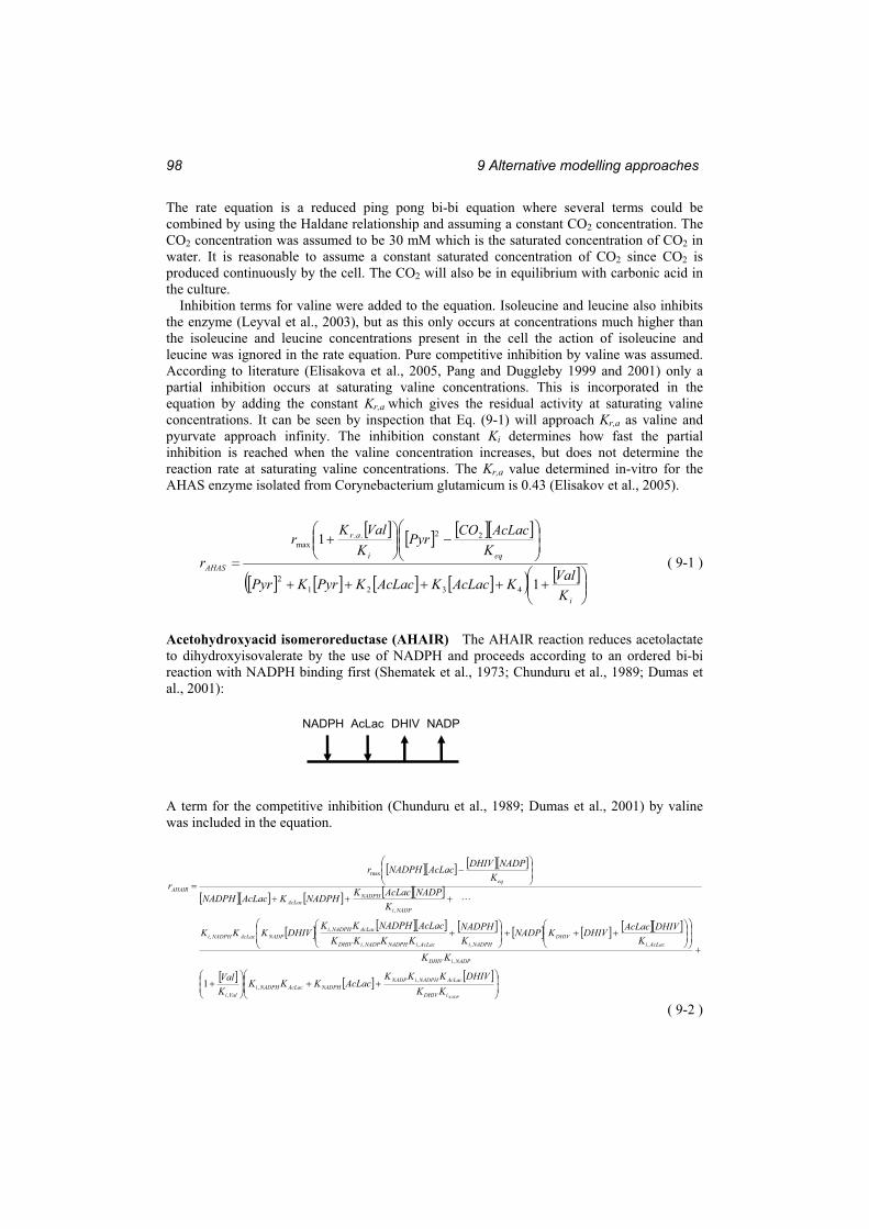
9 Alternative modelling approaches98
The rate equation is a reduced ping pong bi-bi equation where several terms could be combined by using the Haldane relationship and assuming a constant CO2 concentration. The CO2 concentration was assumed to be 30 mM which is the saturated concentration of CO2 in water. It is reasonable to assume a constant saturated concentration of CO2 since CO2 is produced continuously by the cell. The CO2 will also be in equilibrium with carbonic acid in the culture.
Inhibition terms for valine were added to the equation. Isoleucine and leucine also inhibits the enzyme (Leyval et al., 2003), but as this only occurs at concentrations much higher than the isoleucine and leucine concentrations present in the cell the action of isoleucine and leucine was ignored in the rate equation. Pure competitive inhibition by valine was assumed. According to literature (Elisakova et al., 2005, Pang and Duggleby 1999 and 2001) only a partial inhibition occurs at saturating valine concentrations. This is incorporated in the equation by adding the constant Kr,a which gives the residual activity at saturating valine concentrations. It can be seen by inspection that Eq. (9-1) will approach Kr,a as valine and pyurvate approach infinity. The inhibition constant Ki determines how fast the partial inhibition is reached when the valine concentration increases, but does not determine the reaction rate at saturating valine concentrations. The Kr,a value determined in-vitro for the AHAS enzyme isolated from Corynebacterium glutamicum is 0.43 (Elisakov et al., 2005).
i
eqi
ar
AHAS
KValKAcLacKAcLacKPyrKPyr
KAcLacCOPyr
KValK
rr
1
1
43212
22..max
( 9-1 )
Acetohydroxyacid isomeroreductase (AHAIR) The AHAIR reaction reduces acetolactate to dihydroxyisovalerate by the use of NADPH and proceeds according to an ordered bi-bi reaction with NADPH binding first (Shematek et al., 1973; Chunduru et al., 1989; Dumas et al., 2001):
A term for the competitive inhibition (Chunduru et al., 1989; Dumas et al., 2001) by valine was included in the equation.
NADPiDHIV
AcLacNADPHiNADPNADPHAcLacNADPHi
Vali
NADPiDHIV
AcLaciDHIV
NADPHiAcLaciNADPHNADPiDHIV
AcLacNADPHiNADPAcLacNADPHi
NADPi
NADPHAcLac
eqAHAIR
KKDHIVKKK
AcLacKKKKVal
KK
KDHIVAcLacDHIVKNADP
KNADPH
KKKKAcLacNADPHKK
DHIVKKK
KNADPAcLacKNADPHKAcLacNADPH
KNADPDHIVAcLacNADPHr
r
,,
,
,
,,,,
,,
,
max
1
( 9-2 )
NADPH AcLac DHIV NADP
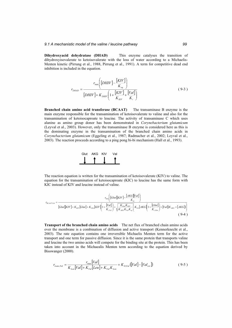
9.1 A mechanistic model of the valine / leucine pathway 99
Dihydroxyacid dehydratase (DHAD) This enzyme catalyses the transition of dihydroxyisovalerate to ketoisovalerate with the loss of water according to a Michaelis-Menten kinetic (Pirrung et al., 1988, Pirrung et al., 1991). A term for competitive dead end inhibition is included in the equation.
iKIVDHIV
eqDHAD
KVal
KKIVKDHIV
KKIVDHIVr
r1
max
( 9-3 )
Branched chain amino acid transferase (BCAAT) The transaminase B enzyme is the main enzyme responsible for the transamination of ketoisovalerate to valine and also for the transamination of ketoisocaproate to leucine. The activity of transaminase C which uses alanine as amino group donor has been demonstrated in Corynebacterium glutamicum(Leyval et al., 2003). However, only the transaminase B enzyme is considered here as this is the dominating enzyme in the transamination of the branched chain amino acids in Corynebacterium glutamicum (Eggeling et al., 1987; Radmacher et al., 2002; Leyval et al., 2003). The reaction proceeds according to a ping pong bi-bi mechanism (Hall et al., 1993).
The reaction equation is written for the transamination of ketoisovalerate (KIV) to valine. The equation for the transamination of ketoisocaproate (KIC) to leucine has the same form with KIC instead of KIV and leucine instead of valine.
AKGKValKGlutAKGK
KKKKK
KValKIVKGlutKKIVGlut
KValAKGKIVGlutr
r
AKGGluti
ValeqValAKG
KIVGlut
ValiGlutKIV
eqValBCAAT
,,
max
,
11
( 9-4 )
Transport of the branched chain amino acids The net flux of branched chain amino acids over the membrane is a combination of diffusion and active transport (Kennerknecht et al., 2003). The rate equation contains one irreversible Michaelis Menten term for the active transport and one term for passive diffusion. Since it is the same protein that transports valine and leucine the two amino acids will compete for the binding site at the protein. This has been taken into account in the Michaealis Menten term according to the equation derived by Bisswanger (2000).
extValDLeuValValLeu
Valtrans ValValKKKLeuKValK
Valrr ,
max, ( 9-5 )
Glut AKG KIV Val
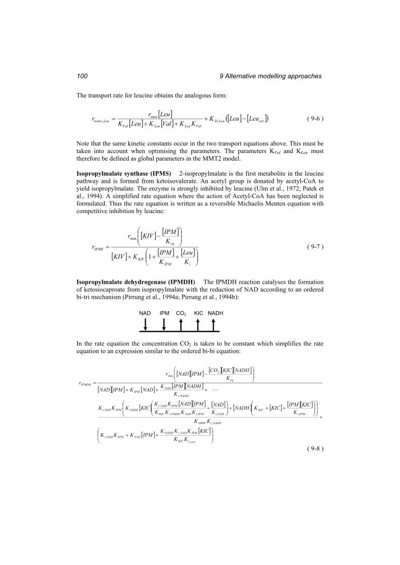
9 Alternative modelling approaches100
The transport rate for leucine obtains the analogous form:
extLeuDValLeuLeuVal
Leutrans LeuLeuKKKValKLeuK
Leurr ,
max, ( 9-6 )
Note that the same kinetic constants occur in the two transport equations above. This must be taken into account when optimising the parameters. The parameters KVal and KLeu must therefore be defined as global parameters in the MMT2 model.
Isopropylmalate synthase (IPMS) 2-isopropylmalate is the first metabolite in the leucine pathway and is formed from ketoisovalerate. An acetyl group is donated by acetyl-CoA to yield isopropylmalate. The enzyme is strongly inhibited by leucine (Ulm et al., 1972; Patek et al., 1994). A simplified rate equation where the action of Acetyl-CoA has been neglected is formulated. Thus the rate equation is written as a reversible Michaelis Menten equation with competitive inhibition by leucine:
iIPMKIV
eqIPMS
KLeu
KIPMKKIV
KIPMKIVr
r1
max
( 9-7 )
Isopropylmalate dehydrogenase (IPMDH) The IPMDH reaction catalyses the formation of ketosiocaproate from isopropylmalate with the reduction of NAD according to an ordered bi-tri mechanism (Pirrung et al., 1994a; Pirrung et al., 1994b):
In the rate equation the concentration CO2 is taken to be constant which simplifies the rate equation to an expression similar to the ordered bi-bi equation:
NADHiKIC
IPMNADiNADHNADIPMNADi
NADPiDHIV
IPMiKIC
NADiIPMiNADNADHiKIC
IPMNADiNADHIPMNADi
NADHi
NADIPM
eqIPMDH
KKKICKKK
IPMKKK
KK
KKICIPMKICKNADH
KNAD
KKKKIPMNADKK
KICKKK
KNADHIPMK
NADKIPMNAD
KNADHKICCO
IPMNADr
r
,,
,
,,,,
,,
,
2max
( 9-8 )
NAD IPM CO2 KIC NADH

9.1 A mechanistic model of the valine / leucine pathway 101
9.1.2 Simulation results with the mechanistic model
The parameters of the kinetic model were fitted with the MMT2 software using the same optimisation strategy as was used for the linlog model (see Section 4.2.3). The equilibrium constants Keq were calculated from the Gibbs free energies (see Eq. (4-46)). Information about the steady state fluxes was used to identify the rmax values so that only the K – parameters had to be fitted. In Figure 9-1 the time courses of the two best models that could be fitted is presented. It is seen that the model could not reproduce the measurements as well as the linlog model (see Figure 6-1). Especially the simulation of the KIV and the valine time course did not give a satisfactory fit to the data. This is surprising at first since the mechanistic model has more parameters than the linlog model and therefore should be easier to fit to the measurements. The mechanistic model contains 43 independent parameters as compared to the 28 parameters in the linlog model.
Figure 9–1: The simulated time courses of the metabolites in the valine pathway by the mechanistic model for the two best fitting parameter sets.
The reason why the mechanistic model is more difficult to fit lies in the structure of the rate equations. The linlog structure sets no boundaries on the elasticities that can be obtained for the system (the definition of elasticities is given in Eq. (4-8)). By varying the parameters of a linlog model any elasticity can be obtained. For the mechanistic model the rate equations sets
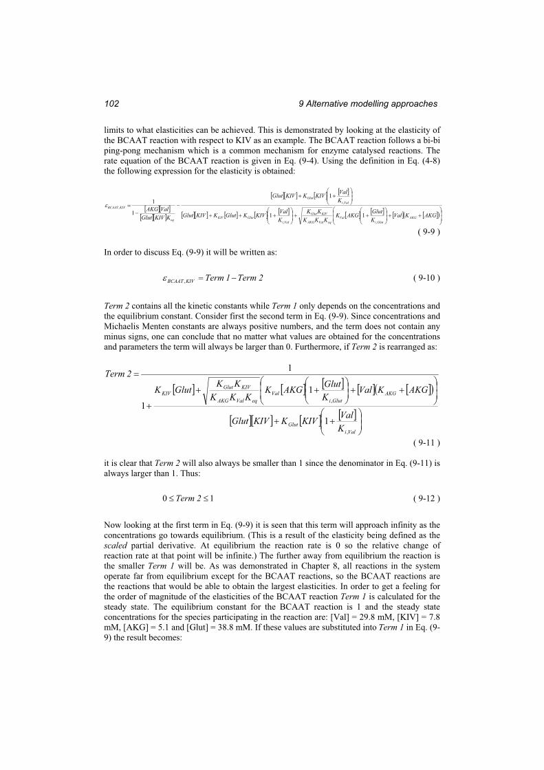
9 Alternative modelling approaches102
limits to what elasticities can be achieved. This is demonstrated by looking at the elasticity of the BCAAT reaction with respect to KIV as an example. The BCAAT reaction follows a bi-bi ping-pong mechanism which is a common mechanism for enzyme catalysed reactions. The rate equation of the BCAAT reaction is given in Eq. (9-4). Using the definition in Eq. (4-8) the following expression for the elasticity is obtained:
AKGKValKGlutAKGK
KKKKK
KValKIVKGlutKKIVGlut
KValKIVKKIVGlut
KKIVGlutValAKG
AKGGluti
ValeqValAKG
KIVGlut
ValiGlutKIV
ValiGlut
eq
KIVBCAAT
,,
,,
11
1
1
1
( 9-9 )
In order to discuss Eq. (9-9) it will be written as:
2Term1TermKIVBCAAT , ( 9-10 )
Term 2 contains all the kinetic constants while Term 1 only depends on the concentrations and the equilibrium constant. Consider first the second term in Eq. (9-9). Since concentrations and Michaelis Menten constants are always positive numbers, and the term does not contain any minus signs, one can conclude that no matter what values are obtained for the concentrations and parameters the term will always be larger than 0. Furthermore, if Term 2 is rearranged as:
ValiGlut
AKGGluti
ValeqValAKG
KIVGlutKIV
KValKIVKKIVGlut
AKGKValKGlutAKGK
KKKKKGlutK
2Term
,
,
1
1
1
1
( 9-11 )
it is clear that Term 2 will also always be smaller than 1 since the denominator in Eq. (9-11) is always larger than 1. Thus:
10 2Term ( 9-12 )
Now looking at the first term in Eq. (9-9) it is seen that this term will approach infinity as the concentrations go towards equilibrium. (This is a result of the elasticity being defined as the scaled partial derivative. At equilibrium the reaction rate is 0 so the relative change of reaction rate at that point will be infinite.) The further away from equilibrium the reaction is the smaller Term 1 will be. As was demonstrated in Chapter 8, all reactions in the system operate far from equilibrium except for the BCAAT reactions, so the BCAAT reactions are the reactions that would be able to obtain the largest elasticities. In order to get a feeling for the order of magnitude of the elasticities of the BCAAT reaction Term 1 is calculated for the steady state. The equilibrium constant for the BCAAT reaction is 1 and the steady state concentrations for the species participating in the reaction are: [Val] = 29.8 mM, [KIV] = 7.8 mM, [AKG] = 5.1 and [Glut] = 38.8 mM. If these values are substituted into Term 1 in Eq. (9-9) the result becomes:
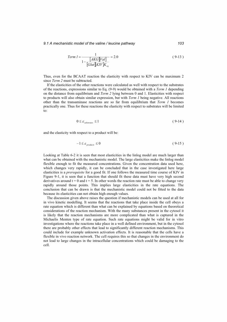
9.1 A mechanistic model of the valine / leucine pathway 103
0.21
1
eqKKIVGlutValAKG
1Term ( 9-13 )
Thus, even for the BCAAT reaction the elasticity with respect to KIV can be maximum 2 since Term 2 must be subtracted.
If the elasticities of the other reactions were calculated as well with respect to the substrates of the reactions, expressions similar to Eq. (9-9) would be obtained with a Term 1 depending on the distance from equilibrium and Term 2 lying between 0 and 1. Elasticities with respect to products will also obtain similar expression, but with Term 1 being negative. All reactions other than the transaminase reactions are so far from equilibrium that Term 1 becomes practically one. Thus for these reactions the elasticity with respect to substrates will be limited to:
10 substrates ( 9-14 )
and the elasticity with respect to a product will be:
01 products ( 9-15 )
Looking at Table 6-2 it is seen that most elasticities in the linlog model are much larger than what can be obtained with the mechanistic model. The large elasticities make the linlog model flexible enough to fit the measured concentrations. Given the concentration data used here, which changes very rapidly, it can be concluded that in the case investigated here large elasticities is a prerequisite for a good fit. If one follows the measured time course of KIV in Figure 9-1, it is seen that a function that should fit these data must have very high second derivatives around t = 0 and t = 5. In other words the reaction rate must be able to change very rapidly around those points. This implies large elasticities in the rate equations. The conclusion that can be drawn is that the mechanistic model could not be fitted to the data because its elasticities can not obtain high enough values.
The discussion given above raises the question if mechanistic models can be used at all for in vivo kinetic modelling. It seems that the reactions that take place inside the cell obeys a rate equation which is different than what can be explained by equations based on theoretical considerations of the reaction mechanism. With the many substances present in the cytosol it is likely that the reaction mechanisms are more complicated than what is captured in the Michaelis Menten type of rate equation. Such rate equations might be valid for in vitro investigations where the reactions take place in a well defined environment, but in the cytosol there are probably other effects that lead to significantly different reaction mechanisms. This could include for example unknown activation effects. It is reasonable that the cells have a flexible in vivo reaction network. The cell requires this so that changes in the environment do not lead to large changes in the intracellular concentrations which could be damaging to the cell.
9 Alternative modelling approaches104
9.2 Whole cell modelling
The linlog model presented in Chapter 6 simulates only the intermediates in the valine and leucine pathway. In order to include the influence of other metabolites such as glutamate and NADPH on the reactions, these non-balanced metabolites were represented by splines and used as input to the simulation.
A different approach is the whole cell modelling approach where the entire metabolism of the cell is modelled. All reactions involved in transforming nutrients to biomass and products must be specified. The model will therefore necessarily contain a large number of metabolites and reactions. Only the extracellular metabolites must then be defined as input to the model.
The ability to model the complete metabolism of cells has been a goal in Systems Biology and Metabolic Engineering for several years and has led to large research projects such as the E-Cell project (Tomita, 2001). However, the modelling of large networks has different requirements and potential problems than the modelling of small networks. A critical issue is the amount of experimental data that is needed for model identification. Another obvious challenge is the fitting of the parameters which becomes an increasingly difficult task when the model becomes larger since the parameter search space increases exponentially with number of model parameters. It is therefore not given that the global optimum can be found.
A whole cell kinetic model was developed to provide a proof of concept for the whole cell modelling of the investigated Corynebacterium glutamicum strain. The aim was to find out if the measured metabolite concentrations could be simulated accurately with a whole cell model and to identify potential problems associated with the whole cell modelling approach.
9.2.1 The process of developing a whole cell model for C. glutamicum
The whole cell model was set up using the software In-Silico Discovery. The model uses linlog kinetics for all rate equations.
The development of a whole cell linlog model consists essentially of 3 steps. First the stoichiometry of all reactions in the network and the modulation effects are defined. In-Silico Discovery can then automatically generate the required linlog equations based on the stoichiometry and modulations. The second step is to carry out a steady state flux analysis based on the measured uptake and excretion rates. The “r0” parameters in the linlog rate equations (see section 4.2.2) are set equal to the steady state fluxes. Finally the kinetic parameters of the model are fitted so that the simulated time courses agree with the metabolite measurements. The time series of all 26 measured metabolites were used to fit the parameters. Thus the data basis consisted of in total 1500 data points. The model contained 690 parameters. The parameter fitting was performed on the computer cluster at the Institute of Biochemical Engineering, University of Stuttgart using the evolutionary optimisation algorithm from the JavaEvA package developed at the University of Tübingen.
The stoichiometric reaction network included the following reactions: Uptake and excretion reactions, glycolysis, the pentose phosphate pathway, the TCA cycle, anaplerotic reactions, oxidative phosphorylation and one-carbon-units regeneration as well as the biosynthesis of peptidoglycan, nucleic acids, fatty acids and all amino acids and the polymerisation of these metabolites to macromolecules. Only reactions confirmed in literature to be active in Corynebacterium glutamicum were included in the model. Each compound in the model was defined with chemical formula and charge. This information was used to carry out element and charge balances on the reactions to check their consistency. The element and charge balances are an important tool to eliminate errors in the stoichiometry.
Furthermore, all reaction rate modulations, i.e. activation and inhibition effects, were specified for the reactions according to published literature. For many enzymes no published
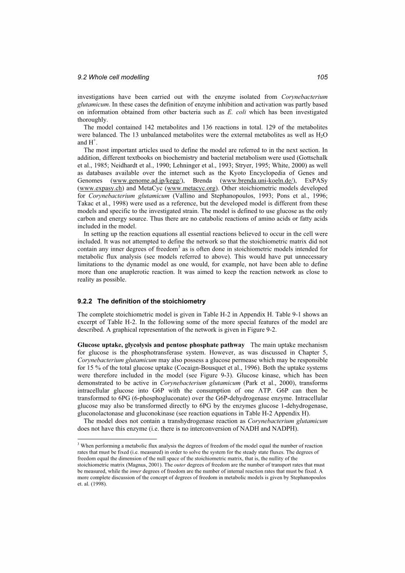
9.2 Whole cell modelling 105
investigations have been carried out with the enzyme isolated from Corynebacteriumglutamicum. In these cases the definition of enzyme inhibition and activation was partly based on information obtained from other bacteria such as E. coli which has been investigated thoroughly.
The model contained 142 metabolites and 136 reactions in total. 129 of the metabolites were balanced. The 13 unbalanced metabolites were the external metabolites as well as H2Oand H+.
The most important articles used to define the model are referred to in the next section. In addition, different textbooks on biochemistry and bacterial metabolism were used (Gottschalk et al., 1985; Neidhardt et al., 1990; Lehninger et al., 1993; Stryer, 1995; White, 2000) as well as databases available over the internet such as the Kyoto Encyclopedia of Genes and Genomes (www.genome.ad.jp/kegg/), Brenda (www.brenda.uni-koeln.de/), ExPASy (www.expasy.ch) and MetaCyc (www.metacyc.org). Other stoichiometric models developed for Corynebacterium glutamicum (Vallino and Stephanopoulos, 1993; Pons et al., 1996; Takac et al., 1998) were used as a reference, but the developed model is different from these models and specific to the investigated strain. The model is defined to use glucose as the only carbon and energy source. Thus there are no catabolic reactions of amino acids or fatty acids included in the model.
In setting up the reaction equations all essential reactions believed to occur in the cell were included. It was not attempted to define the network so that the stoichiometric matrix did not contain any inner degrees of freedom3 as is often done in stoichiometric models intended for metabolic flux analysis (see models referred to above). This would have put unnecessary limitations to the dynamic model as one would, for example, not have been able to define more than one anaplerotic reaction. It was aimed to keep the reaction network as close to reality as possible.
9.2.2 The definition of the stoichiometry
The complete stoichiometric model is given in Table H-2 in Appendix H. Table 9-1 shows an excerpt of Table H-2. In the following some of the more special features of the model are described. A graphical representation of the network is given in Figure 9-2.
Glucose uptake, glycolysis and pentose phosphate pathway The main uptake mechanism for glucose is the phosphotransferase system. However, as was discussed in Chapter 5, Corynebacterium glutamicum may also possess a glucose permease which may be responsible for 15 % of the total glucose uptake (Cocaign-Bousquet et al., 1996). Both the uptake systems were therefore included in the model (see Figure 9-3). Glucose kinase, which has been demonstrated to be active in Corynebacterium glutamicum (Park et al., 2000), transforms intracellular glucose into G6P with the consumption of one ATP. G6P can then be transformed to 6PG (6-phosphogluconate) over the G6P-dehydrogenase enzyme. Intracellular glucose may also be transformed directly to 6PG by the enzymes glucose 1-dehydrogenase, gluconolactonase and gluconokinase (see reaction equations in Table H-2 Appendix H).
The model does not contain a transhydrogenase reaction as Corynebacterium glutamicumdoes not have this enzyme (i.e. there is no interconversion of NADH and NADPH). 3 When performing a metabolic flux analysis the degrees of freedom of the model equal the number of reaction rates that must be fixed (i.e. measured) in order to solve the system for the steady state fluxes. The degrees of freedom equal the dimension of the null space of the stoichiometric matrix, that is, the nullity of the stoichiometric matrix (Magnus, 2001). The outer degrees of freedom are the number of transport rates that must be measured, while the inner degrees of freedom are the number of internal reaction rates that must be fixed. A more complete discussion of the concept of degrees of freedom in metabolic models is given by Stephanopoulos et. al. (1998).
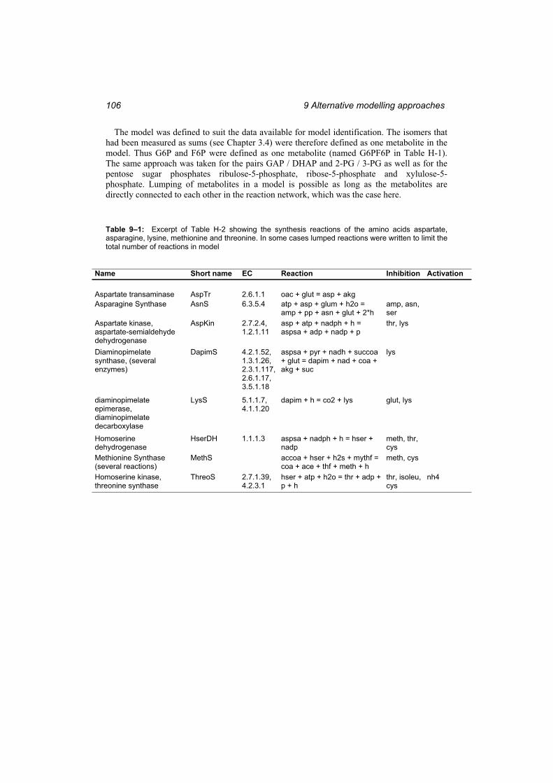
9 Alternative modelling approaches106
The model was defined to suit the data available for model identification. The isomers that had been measured as sums (see Chapter 3.4) were therefore defined as one metabolite in the model. Thus G6P and F6P were defined as one metabolite (named G6PF6P in Table H-1). The same approach was taken for the pairs GAP / DHAP and 2-PG / 3-PG as well as for the pentose sugar phosphates ribulose-5-phosphate, ribose-5-phosphate and xylulose-5-phosphate. Lumping of metabolites in a model is possible as long as the metabolites are directly connected to each other in the reaction network, which was the case here.
Table 9–1: Excerpt of Table H-2 showing the synthesis reactions of the amino acids aspartate, asparagine, lysine, methionine and threonine. In some cases lumped reactions were written to limit the total number of reactions in model
Name Short name EC Reaction Inhibition Activation Aspartate transaminase AspTr 2.6.1.1 oac + glut = asp + akg Asparagine Synthase AsnS 6.3.5.4 atp + asp + glum + h2o =
amp + pp + asn + glut + 2*h amp, asn, ser
Aspartate kinase, aspartate-semialdehyde dehydrogenase
AspKin 2.7.2.4, 1.2.1.11
asp + atp + nadph + h = aspsa + adp + nadp + p
thr, lys
Diaminopimelate synthase, (several enzymes)
DapimS 4.2.1.52, 1.3.1.26,2.3.1.117,2.6.1.17,3.5.1.18
aspsa + pyr + nadh + succoa + glut = dapim + nad + coa + akg + suc
lys
diaminopimelate epimerase, diaminopimelate decarboxylase
LysS 5.1.1.7, 4.1.1.20
dapim + h = co2 + lys glut, lys
Homoserine dehydrogenase
HserDH 1.1.1.3 aspsa + nadph + h = hser + nadp
meth, thr, cys
Methionine Synthase (several reactions)
MethS accoa + hser + h2s + mythf = coa + ace + thf + meth + h
meth, cys
Homoserine kinase, threonine synthase
ThreoS 2.7.1.39, 4.2.3.1
hser + atp + h2o = thr + adp + p + h
thr, isoleu, cys
nh4
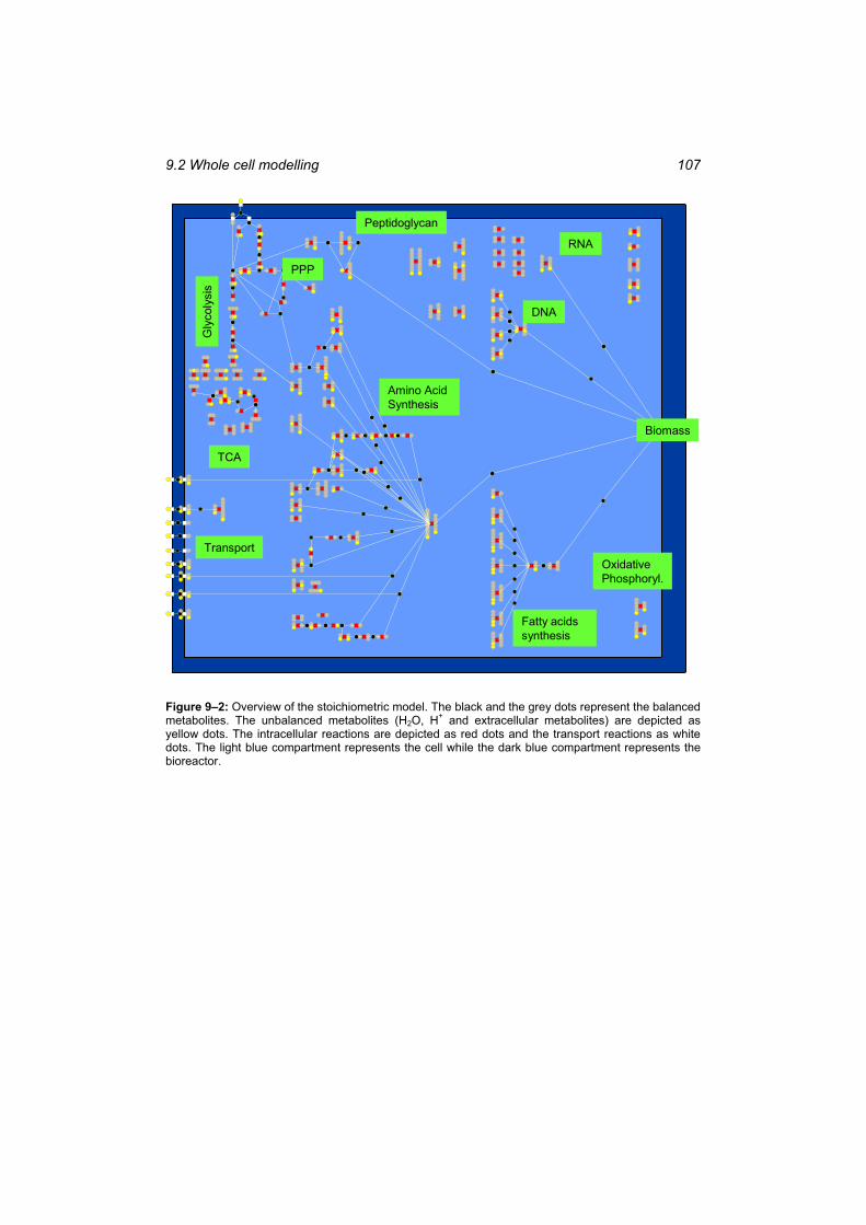
9.2 Whole cell modelling 107
TCA
Gly
coly
sis
Amino Acid Synthesis
DNA
RNA
Peptidoglycan
Fatty acids synthesis
Biomass
OxidativePhosphoryl.
Transport
PPP
Figure 9–2: Overview of the stoichiometric model. The black and the grey dots represent the balanced metabolites. The unbalanced metabolites (H2O, H+ and extracellular metabolites) are depicted as yellow dots. The intracellular reactions are depicted as red dots and the transport reactions as white dots. The light blue compartment represents the cell while the dark blue compartment represents the bioreactor.
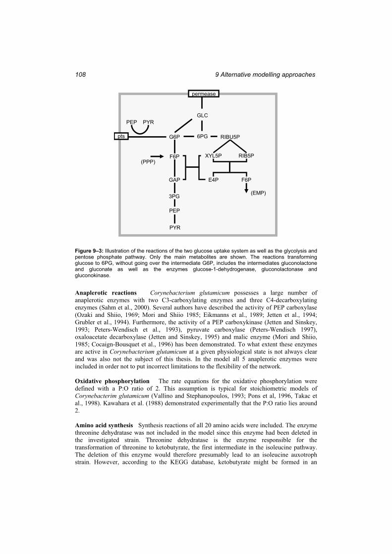
9 Alternative modelling approaches108
pts RIBU5P
XYL5P RIB5P
E4P F6P
G6P
3PG
PEP
F6P
GAP
(EMP)
(PPP)
PEP PYRGLC
permease
PYR
6PG
Figure 9–3: Illustration of the reactions of the two glucose uptake system as well as the glycolysis and pentose phosphate pathway. Only the main metabolites are shown. The reactions transforming glucose to 6PG, without going over the intermediate G6P, includes the intermediates gluconolactone and gluconate as well as the enzymes glucose-1-dehydrogenase, gluconolactonase and gluconokinase.
Anaplerotic reactions Corynebacterium glutamicum possesses a large number of anaplerotic enzymes with two C3-carboxylating enzymes and three C4-decarboxylating enzymes (Sahm et al., 2000). Several authors have described the activity of PEP carboxylase (Ozaki and Shiio, 1969; Mori and Shiio 1985; Eikmanns et al., 1989; Jetten et al., 1994; Grubler et al., 1994). Furthermore, the activity of a PEP carboxykinase (Jetten and Sinskey, 1993; Peters-Wendisch et al., 1993), pyruvate carboxylase (Peters-Wendisch 1997), oxaloacetate decarboxylase (Jetten and Sinskey, 1995) and malic enzyme (Mori and Shiio, 1985; Cocaign-Bousquet et al., 1996) has been demonstrated. To what extent these enzymes are active in Corynebacterium glutamicum at a given physiological state is not always clear and was also not the subject of this thesis. In the model all 5 anaplerotic enzymes were included in order not to put incorrect limitations to the flexibility of the network.
Oxidative phosphorylation The rate equations for the oxidative phosphorylation were defined with a P:O ratio of 2. This assumption is typical for stoichiometric models of Corynebacterim glutamicum (Vallino and Stephanopoulos, 1993; Pons et al, 1996, Takac et al., 1998). Kawahara et al. (1988) demonstrated experimentally that the P:O ratio lies around 2.
Amino acid synthesis Synthesis reactions of all 20 amino acids were included. The enzyme threonine dehydratase was not included in the model since this enzyme had been deleted in the investigated strain. Threonine dehydratase is the enzyme responsible for the transformation of threonine to ketobutyrate, the first intermediate in the isoleucine pathway. The deletion of this enzyme would therefore presumably lead to an isoleucine auxotroph strain. However, according to the KEGG database, ketobutyrate might be formed in an
9.2 Whole cell modelling 109
alternative pathway from homoserine over the cystathionine -synthase enzyme (metB). In preliminary experiments the intracellular concentration of KBut at steady state was measured to 0.7 mM and it was observed that the strain could also grow without isoleucine. This strongly suggests the existence of the alternative ketobutyrate pathway in the investigated strain. In the investigation of another recombinant Corynebacterium glutamicum strain Kromer et al. (2006) also concluded that this alternative pathway was active. The synthesis reaction of ketobutyrate from homoserine was therefore included in the model.
Lipid biosynthesis Lipids are built from glycerol-3-phosphate, serine and fatty acids. The fatty acid composition was taken from Jang et al. (1997). Other publications specifying the fatty acid composition of corynebacteria give similar values as Jang et al. (Collins et al., 1982; Chevalier et al., 1992). The amount of energy in the form of phosphate groups (e.g. from ATP) for the lipid assembly was included in the protein assembly equation according to Neidhardt (1990). Lehninger et al. (1993) specified the types of phosphorylated nucleotides needed.
Protein biosynthesis The amino acid composition of the protein in mole % was as follows (Cocaign-Bousquet et al. 1996): alanine, 16.4; arginine, 4.3; aspartate, 4.2; asparagine, 4.2; cysteine, 0.023; glutamate, 11; glutamine, 11; glycine, 7.8; histidine, 1.4; isoleucine, 4.0; leucine, 5.9; lysine, 3.9; methionine, 1.1; phenylalanine, 2.8; proline, 3.3; serine, 6.0; threonine, 6.1; tryptophane, 0.023; tyrosine, 1.7; valine, 5.9. The amount of energy in the form of phosphate groups for the protein assembly was included in the protein assembly equation according to Neidhardt (1990). Lehninger et al. (1993) specified the types of phosphorylated nucleotides needed.
RNA and DNA assembly The average nucleotide composition of RNA and DNA in E. coli was used in the model (Neidhardt et al., 1990). The energy requirement for assembly was given by Neidhardt et al. (1993).
Biomass assembly The dry biomass composition in weight % was specified by Cocaign-Bousquet et al. (1996) as: 52 % protein, 5% RNA, 1% DNA, 13% lipids and 19% cell wall components. The way to incorporate biomass production in the model was to define biomass as a metabolite that is excreted from the cell. One biomass unit was defined to be a molecule with a molecular mass of 192 000 g/mol. The biomass elemental composition resulting from the macromolecular composition specified above was: C0.518H0.070O0.260N0.139P0.013S0.0007.
The molecular mass of a biomass molecule in the model can be set to any value. 192 000 g/mol resulted from the choice of defining a DNA molecule as a helix consisting of 100 nucleotides. With a biomass molecule containing 1 % w/w DNA the resulting molecular mass is 192 000 g/mol.
9.2.3 Steady state metabolic flux analysis and topological analysis
It will be assumed here that the reader is familiar with the concept of steady state metabolic flux analysis based on metabolite balances and the different terms and expression used within this area. An introduction to metabolic flux analysis is given by Stephanopoulos et al. (1998).
The stoichiometric model had been defined to include all significant reactions that could take place in the cell in order to make the reaction network as realistic as possible. This led to a model with in total 7 inner degrees of freedom. The 5 anaplerotic reactions resulted in 4 inner degrees of freedom. The two glucose uptake systems and the possibility for glucose to enter the pentose phosphate pathway either over G6P or over gluconolactone resulted in two more. The inclusion of the glyoxylate shunt in the TCA cycle gave rise to one additional
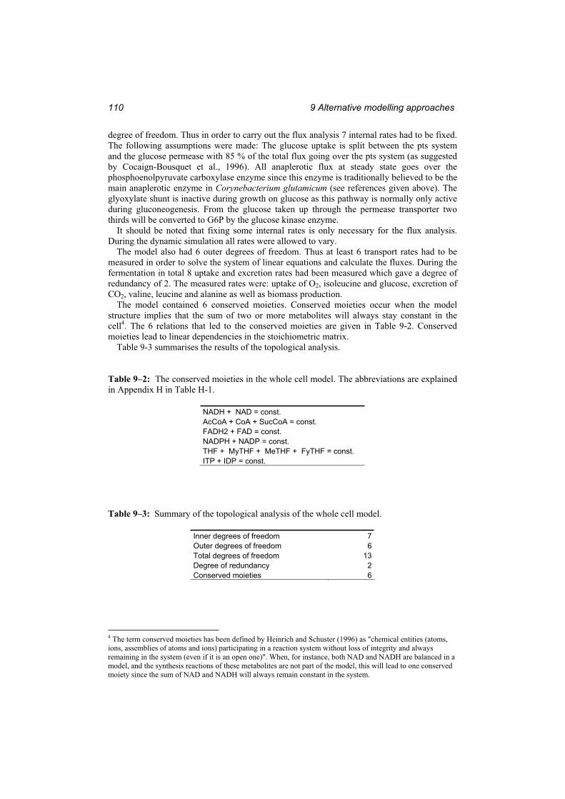
9 Alternative modelling approaches110
degree of freedom. Thus in order to carry out the flux analysis 7 internal rates had to be fixed. The following assumptions were made: The glucose uptake is split between the pts system and the glucose permease with 85 % of the total flux going over the pts system (as suggested by Cocaign-Bousquet et al., 1996). All anaplerotic flux at steady state goes over the phosphoenolpyruvate carboxylase enzyme since this enzyme is traditionally believed to be the main anaplerotic enzyme in Corynebacterium glutamicum (see references given above). The glyoxylate shunt is inactive during growth on glucose as this pathway is normally only active during gluconeogenesis. From the glucose taken up through the permease transporter two thirds will be converted to G6P by the glucose kinase enzyme.
It should be noted that fixing some internal rates is only necessary for the flux analysis. During the dynamic simulation all rates were allowed to vary.
The model also had 6 outer degrees of freedom. Thus at least 6 transport rates had to be measured in order to solve the system of linear equations and calculate the fluxes. During the fermentation in total 8 uptake and excretion rates had been measured which gave a degree of redundancy of 2. The measured rates were: uptake of O2, isoleucine and glucose, excretion of CO2, valine, leucine and alanine as well as biomass production.
The model contained 6 conserved moieties. Conserved moieties occur when the model structure implies that the sum of two or more metabolites will always stay constant in the cell4. The 6 relations that led to the conserved moieties are given in Table 9-2. Conserved moieties lead to linear dependencies in the stoichiometric matrix.
Table 9-3 summarises the results of the topological analysis.
Table 9–2: The conserved moieties in the whole cell model. The abbreviations are explained in Appendix H in Table H-1.
NADH + NAD = const. AcCoA + CoA + SucCoA = const. FADH2 + FAD = const. NADPH + NADP = const. THF + MyTHF + MeTHF + FyTHF = const. ITP + IDP = const.
Table 9–3: Summary of the topological analysis of the whole cell model.
Inner degrees of freedom 7Outer degrees of freedom 6Total degrees of freedom 13Degree of redundancy 2Conserved moieties 6
4 The term conserved moieties has been defined by Heinrich and Schuster (1996) as "chemical entities (atoms, ions, assemblies of atoms and ions) participating in a reaction system without loss of integrity and always remaining in the system (even if it is an open one)". When, for instance, both NAD and NADH are balanced in a model, and the synthesis reactions of these metabolites are not part of the model, this will lead to one conserved moiety since the sum of NAD and NADH will always remain constant in the system.
9.2 Whole cell modelling 111
9.2.4 Simulation results
In total 16 parameter sets were fitted for the model. The simulated time courses of all metabolites for all parameter sets are given in Figure 9-4. It is seen that for the measured metabolites the different parameter sets give very similar time courses and the goodness of fit is comparable for all parameter sets. For the metabolites for which no measurements are available there are large quantitative differences, as is seen for example in serine (ser_c) or in glutamine (glum_c). This demonstrates the need for more metabolite data in order to identify the correct parameter set. It should, however, be noted that most of the simulated time courses are qualitatively similar, that is, they follow the same trend. Thus, some mechanistic understanding could be extracted based only on the available measurements.
The simulated curves fit well with most of the measured concentrations. In the glycolysis all metabolites fitted well except the sum of G6P and F6P (the metabolite named G6PF6P in Figure 9-4). The sharp rise directly after the stimulus which is seen in all metabolites in the glycolysis downstream of F6P could be simulated correctly. Also the nucleotides ATP, ADP and AMP as well as NAD and NADP obtained good fits. These metabolites participate in many reactions and it is interesting that they could all be simulated accurately by the model.
For the metabolites glutamate, valine, ketoisovalerate and G6PF6P the dynamic changes in concentration could not be reproduced by the model. These metabolites all have much higher concentrations than the other measured metabolites. Glutamate for instance has a concentration of 40 – 50 mM. This is typically two orders of magnitude more than most of the other metabolites.
In the valine pathway, both KIV and valine obtained poor fits. These are the two metabolites in the valine / leucine pathway with the highest values, about 10 mM and 30 mM respectively. Although the other metabolites in the pathway (Pyr, AcLac, DHIV, IPM, KIC and Leu) could be fitted well, the fit for the pathway seen as a whole is unsatisfactory.
In order to simulate the large metabolite pools the reaction rates must be able to change fast because the change in the metabolite concentration is much higher than the flux at steady state. Thus, large elasticities in the rate expressions are required to simulate the large pools. The need for large elasticities in a kinetic model was also discussed in Chapter 9.1.
Figure 9-5 shows the cumulative frequency distribution of the elasticities in the whole cell model. 70 % of the elasticities had absolute values smaller than 20 and 95 % of the elasticities had absolute values smaller than 1000. In Table 9-4 the parameter values and elasticities for the whole cell model are compared to the values for the small model of the valine / leucine pathway presented in Chapter 6. The values for the valine pathway are shown. It is seen that the elasticities in the small model are two to three orders of magnitude larger than the elasticities in the whole cell model. The low elasticities in the whole cell model were the underlying reason why the large metabolite pools could not be fitted.
The parameter values (and thus the elasticities) were not limited upwards during the parameter fitting. It is reasonable to believe that a better fit could have been found with larger parameter values. The fact that these better fitting parameter sets were not found could indicate that the algorithm used for optimisation got stuck in a local optimum and therefore did not find the global optimum. It must be recognised that the optimisation of a model with 690 parameters is a very difficult task since the parameter search space then has 690 dimensions. Although the evolutionary algorithm is a global, stochastic method, there is no guarantee that the global optimum is found.
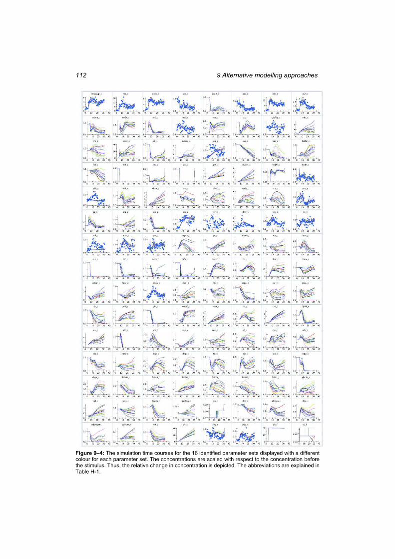
9 Alternative modelling approaches112
Figure 9–4: The simulation time courses for the 16 identified parameter sets displayed with a different colour for each parameter set. The concentrations are scaled with respect to the concentration before the stimulus. Thus, the relative change in concentration is depicted. The abbreviations are explained in Table H-1.
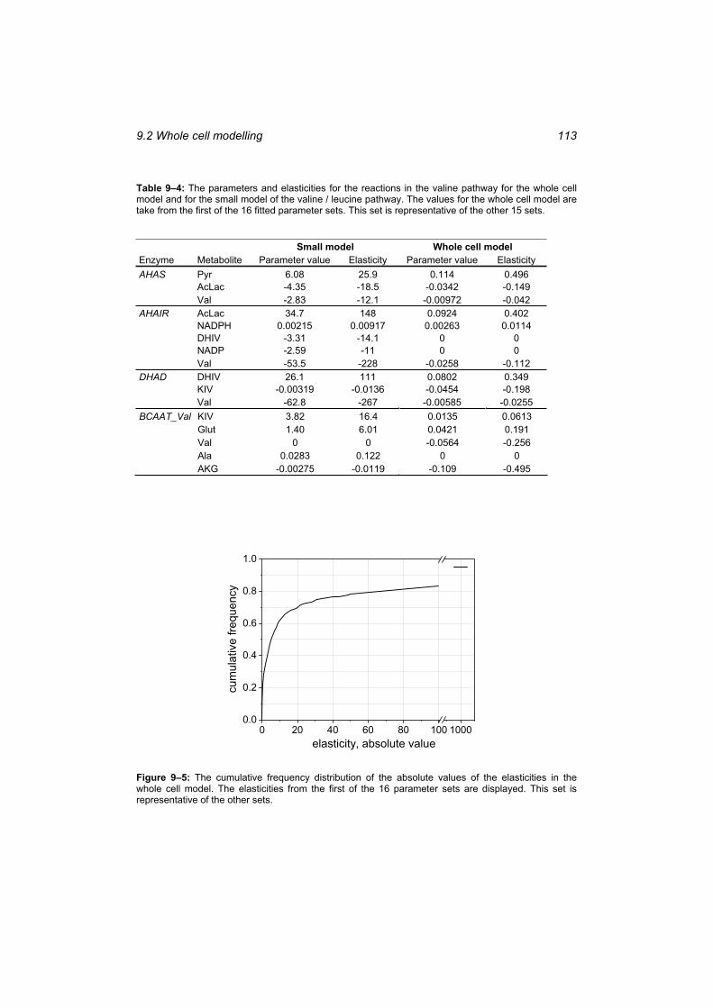
9.2 Whole cell modelling 113
Table 9–4: The parameters and elasticities for the reactions in the valine pathway for the whole cell model and for the small model of the valine / leucine pathway. The values for the whole cell model are take from the first of the 16 fitted parameter sets. This set is representative of the other 15 sets.
Small model Whole cell model Enzyme Metabolite Parameter value Elasticity Parameter value Elasticity AHAS Pyr 6.08 25.9 0.114 0.496
AcLac -4.35 -18.5 -0.0342 -0.149 Val -2.83 -12.1 -0.00972 -0.042
AHAIR AcLac 34.7 148 0.0924 0.402 NADPH 0.00215 0.00917 0.00263 0.0114 DHIV -3.31 -14.1 0 0 NADP -2.59 -11 0 0 Val -53.5 -228 -0.0258 -0.112
DHAD DHIV 26.1 111 0.0802 0.349 KIV -0.00319 -0.0136 -0.0454 -0.198 Val -62.8 -267 -0.00585 -0.0255
BCAAT_Val KIV 3.82 16.4 0.0135 0.0613 Glut 1.40 6.01 0.0421 0.191 Val 0 0 -0.0564 -0.256 Ala 0.0283 0.122 0 0 AKG -0.00275 -0.0119 -0.109 -0.495
0 20 40 60 80 100 10000.0
0.2
0.4
0.6
0.8
1.0
cum
ulat
ive
frequ
ency
elasticity, absolute value
Figure 9–5: The cumulative frequency distribution of the absolute values of the elasticities in the whole cell model. The elasticities from the first of the 16 parameter sets are displayed. This set is representative of the other sets.
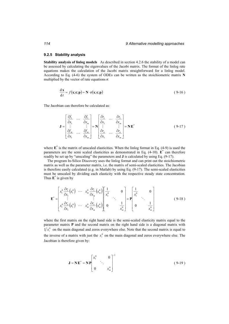
9 Alternative modelling approaches114
9.2.5 Stability analysis
Stability analysis of linlog models As described in section 4.2.6 the stability of a model can be assessed by calculating the eigenvalues of the Jacobi matrix. The format of the linlog rate equations makes the calculation of the Jacobi matrix straightforward for a linlog model. According to Eq. (4-6) the system of ODEs can be written as the stoichiometric matrix Nmultiplied by the vector of rate equations r:
pcxrNpcxx ;;;;dd f
t ( 9-16 )
The Jacobian can therefore be calculated as:
*
1
1
1
1
1
1
1
1
ENNJ
m
nn
m
m
mm
m
xr
xr
xr
xr
xf
xf
xf
xf
( 9-17 )
where E* is the matrix of unscaled elasticities. When the linlog format in Eq. (4-9) is used the parameters are the semi scaled elasticities as demonstrated in Eq. (4-10). E* can therefore readily be set up by “unscaling” the parameters and J is calculated by using Eq. (9-17).
The program In-Silico Discovery uses the linlog format and can print out the stoichiometric matrix as well as the parameter matrix, i.e. the matrix of semi-scaled elasticities. The Jacobian is therefore easily calculated (e.g. in Matlab) by using Eq. (9-17). The semi-scaled elasticities must be unscaled by dividing each elasticity with the respective steady state concentration. Thus E* is given by
0
01
0
01
0001
1
01
01001
1
101
*
10
01
10
01
mmm
m
nm
n
mm
m
x
x
x
x
xxrxx
xrx
xxrxx
xrx
PE ( 9-18 )
where the first matrix on the right hand side is the semi-scaled elasticity matrix equal to the parameter matrix P and the second matrix on the right hand side is a diagonal matrix with
01 ix on the main diagonal and zeros everywhere else. Note that the second matrix is equal to the inverse of a matrix with just the 0
ix on the main diagonal and zeros everywhere else. The Jacobian is therefore given by:
1
0
01
*
0
0
mx
xPNENJ ( 9-19 )
9.2 Whole cell modelling 115
In Eq. (9-19) the parameter matrix must be written with the columns corresponding to the metabolites and the rows corresponding to the reaction rates. In-Silico Discovery prints out this matrix the other way around, i.e. with the columns corresponding to the reactions and the rows corresponding to the metabolites. The matrix from In-Silico Discovery must therefore be transposed before Eq. (9-19) can be used.
The fact that the Jacobian is just the stoichiometric matrix times the unscaled elasticity matrix (according to Eq. (9-17)) has an important implication. If the stoichiometric matrix contains linearly dependent rows, the Jacobian will also have linearly dependent rows. The linear dependencies in the rows in N will be transferred to J so that J contains at least the same number of linear dependencies as N. A square matrix with linearly dependent rows will have as many zero eigenvalues as there are linear dependencies. Thus, it can be concluded that the Jacobian matrix will have at least as many zero eigenvalues as there are linearly dependent rows in N.
Linear dependencies in the Jacobian matrix can also originate from the elasticity matrix. If the elasticity matrix contains linearly dependent columns the Jacobian matrix will also contain linearly dependent columns as can be seen by inspection of Eq. 9-17. In the presented model the glucose stimulus was simulated by including a glucose feed to the fermenter, which at time = 0 increased rapidly in the same way that happens for the real system (see section 3.2). The glucose feed is a predefined rate and is therefore not correlated to any of the metabolites in the model. The elasticities of the glucose feed rate with respect to the metabolite concentrations are therefore all equal to zero. In other words, the column in the elasticity matrix corresponding to the glucose feed rate contains only zero elements. A zero vector is linearly dependent to any other vector according to the definition of linear dependent vectors (see the textbook on linear algebra by Fraleigh and Beauregard, 1995), so the zero column in E* implies that one further linear dependency is added to J. Thus, the inclusion of the glucose feed in the model leads to one more zero eigenvalue in J.
The important conclusion that can be drawn from the discussion in the preceding paragraphs is stated as follows:
As stated in Section 4.2.6 a zero eigenvalue gives no conclusion on the stability of the model. It does not prove that the model is unstable, neither does it prove that it is stable.
The stability of the developed model A stability analysis of the 16 models was performed by calculating the eigenvalues of the Jacobian matrices for all parameter sets. The model is stable if, and only if, all the real parts of the eigenvalues are negative (Section 4.2.6). Zero eigenvalues give no conclusion on the stability. Table 9-5 summarises the eigenvalue calculations.
It is seen in Table 9-5 that all 16 models have 7 zero eigenvalues. These result from the 6 conserved moieties of the model (see Table 9-3), as well as the zero elasticities of the glucose feed as discussed above.
A linlog model with a stoichiometric matrix containing linearly dependent rows or an elasticity matrix containing linearly dependent columns will have a Jacobian with one or more zero eigenvalues.
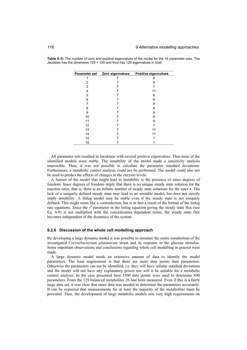
9 Alternative modelling approaches116
Table 9–5: The number of zero and positive eigenvalues of the model for the 16 parameter sets. The Jacobian has the dimension 129 × 129 and thus has 129 eigenvalues in total.
Parameter set Zero eigenvalues Positive eigenvalues 1 7 9 2 7 6 3 7 7 4 7 11 5 7 6 6 7 6 7 7 8 8 7 8 9 7 9 10 7 9 11 7 9 12 7 7 13 7 11 14 7 11 15 7 7 16 7 7
All parameter sets resulted in Jacobians with several positive eigenvalues. Thus none of the identified models were stable. The instability of the model made a sensitivity analysis impossible. Thus, it was not possible to calculate the parameter standard deviations. Furthermore, a metabolic control analysis could not be performed. The model could also not be used to predict the effects of changes in the enzyme levels.
A feature of the model that might lead to instability is the presence of inner degrees of freedom. Inner degrees of freedom imply that there is no unique steady state solution for the reaction rates, that is, there is an infinite number of steady state solutions for the rates r. The lack of a uniquely defined steady state may lead to an unstable model, but does not strictly imply instability. A linlog model may be stable even if the steady state is not uniquely defined. This might seem like a contradiction, but is in fact a result of the format of the linlog rate equations. Since the r0 parameter in the linlog equation giving the steady state flux (see Eq. 4-9) is not multiplied with the concentration dependent terms, the steady state flux becomes independent of the dynamics of the system.
9.2.6 Discussion of the whole cell modelling approach
By developing a large dynamic model it was possible to simulate the entire metabolism of the investigated Corynebacterium glutamicum strain and its response to the glucose stimulus. Some important observations and conclusions regarding whole cell modelling in general were made.
A large dynamic model needs an extensive amount of data to identify the model parameters. The least requirement is that there are more data points than parameters. Otherwise the parameters can not be identified, i.e. they will have infinite standard deviations and the model will not have any explanatory power nor will it be suitable for a metabolic control analysis. In the case presented here 1500 data points were used to determine 690 parameters. From the 129 balanced metabolites 26 had been measured. Even if this is a fairly large data set, it was clear that more data was needed to determine the parameters accurately. It can be expected that measurements for at least the majority of the metabolites must be provided. Thus, the development of large metabolic models sets very high requirements on
9.2 Whole cell modelling 117
the data that must be available for model identification. Although the field of metabolomics is developing fast, a limiting factor for whole cell modelling is still the availability of metabolite concentration data.
The fitting of the parameters becomes an increasingly difficult task when the model becomes larger. From the 16 identified parameter sets, none had converged to the same optimum. The 16 different optima that were found were probably all local optima. This demonstrates how difficult it is to find the global optimum when the parameter search space is large. Furthermore, as noted in Section 9.2.4, the fit for KIV and valine was not satisfactory. This was clearly due to the parameter fitting since good fits could be found with the small model (Chapter 6).
One way to decrease the parameter search space is to impose more constraints on the parameters. Implementing the thermodynamic constraint (Section 4.2.5) will already decrease the search space considerably and ease the search for the global optimum.
Another strategy would be to set starting values which are believed to lie in the vicinity of the optimal parameter values before the fitting of the whole model is started. As described in Section 4.2.3 this can be done by dividing the model into part-models and fit the parameters of the part-models first. The fitted parameters for the part-models are then used as starting values to fit the parameters of the whole model.
The evolutionary optimisation algorithm used for the parameter fitting is a global algorithm which also has the advantage that the computation can be run in parallel on several computers simultaneously. It is therefore well suited to fit the parameters of a whole cell model. However, there are also other global algorithms, such as the simulated annealing algorithm, which may give a higher probability of finding the global optimum. It should be noted that the simulated annealing algorithm is much slower than an evolutionary algorithm.
While small models are seldom unstable, the stability of large models is not given, as was demonstrated for the whole cell model developed here. Stability is an important issue because only stable models can be used for metabolic engineering purposes such as metabolic control analysis or in-silico design. Based on the experience drawn from the development of the Corynebacterium glutamicum model it is recommended to reduce the number of linear dependencies in the stoichiometric matrix as much as possible to avoid the zero eigenvalues in the Jacobian matrix. In practise this would mean that the model should be set up without conserved moieties. The linear dependency resulting from the feed is more difficult to avoid.
A further measure to avoid instability would be to define the model without inner degrees of freedom. However, this is controversial because the model would then be limited with respect to what reactions can be included. For instance, only one anaplerotic reaction could be included in the model. It has been demonstrated that several anaplerotic reactions are active simultaneously in Corynebacterium glutamicum (Petersen, 2000).
One way to avoid the parameter sets leading to unstable models could be to include the stability of the model as a criterion in the parameter fitting. This would imply that the eigenvalues of the Jacobian are computed for every simulation run, which would increase the computation time. It would, however, decrease the parameter search space which would increase the probability of finding the global optimum.
A well defined whole cell model has some advantages over a small model. A small model must necessarily define some metabolites as independent variables which means that the model can not capture all the interactions between the modelled pathway and the other reactions in the cell. As an example, the model of the valine / leucine pathway presented in Chapter 6 can analyse the influence of glutamate on the valine pathway, but can not analyse the influence of the valine pathway on the glutamate concentration. This puts some restrictions on the applicability of a small model for making predictions of changes in flux after a change in enzyme level. However, the development of a whole cell model is a complicated process and especially the availability of measurement data is a decisive factor.

9 Alternative modelling approaches118
With the rapid development of metabolomics it can be expected that well-defined whole cell models can be established in the future. The model presented here provides a proof of concept for the whole cell modelling approach for a Corynebacterium glutamicum strain.
10 Conclusion 119
10 Conclusion The main objective of the investigation was to analyse the dynamic behaviour of the intracellular reaction network in a Corynebacterium glutamicum strain. This objective was achieved by using different techniques from the areas of Metabolomics, Modelling and Simulation, Metabolic Control Analysis and Thermodynamic Analysis. The different methods build on each other and are part of an integrated study.
Metabolomics The measurements of the intracellular concentrations provided the experimental data which formed the basis of the further investigation. The experimental procedure was developed according to the guidelines that the experiment should be relevant to the production conditions, and that the stimulus should have a large impact on the intracellular concentrations. As it is impossible to predict the exact effect that a glucose stimulus will have on a culture, different procedures had to be tested. The optimal procedure within the context of the investigation was a batch fermentation with a time delay of 10 minutes between glucose depletion and glucose addition.
The dynamic changes in the concentrations of 26 metabolites from the central metabolism and the valine / leucine pathway were monitored over a time interval of 35 seconds. Samples were taken every 440 milliseconds before and after the glucose stimulus. A very rapid response was seen in the metabolites in the glycolysis demonstrating the fast reaction kinetics in this pathway. In the valine / leucine pathway a mixture of effects was seen resulting from the interactions with the other metabolites in the network. It is the first time that the transient behaviour of the valine / leucine pathway has been observed.
Some conclusions could be reached based on a direct interpretation of the measured concentration time series. Several authors have suggested the existence of a glucose permease in Corynebacterium glutamicum, but until now no proof of this has been presented. The measured time series of PEP (phosphoenolpyruvate) supports the permease theory. Furthermore, by using time series analysis, the unexpected response in the ketopantoate concentration could be analysed. It was demonstrated that ketopantoate is not formed from KIV by the ketopantoate-hydroxymethyl transferase enzyme, but through some other alternative pathway. It was also concluded that the time series analysis is useful only for small networks containing closely connected metabolites. For larger networks the method can not reach any conclusion with significant accuracy.
The comparison of two different stimulus experiments demonstrated the difference in intracellular concentrations at different physiological states. At glucose limitation the concentrations of the metabolites in the glycolysis were lower than at exponential growth as a result of the lower activity of the glucose uptake system and the glycolysis. The AMP concentration was higher at glucose limitation signifying a lower energy level of the cell. The response in the PEP concentration to the stimulus at glucose limitation suggests that different mechanisms of glucose uptake are active at different physiological states.
Modelling and Simulation A dynamic model of the valine / leucine pathway was developed based on the intracellular concentration data. The model gives a quantitative description of the concentrations and fluxes in the cell. In this way the model explains the functionality of the pathway and the interactions between the metabolites can be analysed. The simulated concentrations fitted well with the measured data. The simulated fluxes changed very rapidly directly after the glucose stimulus which shows the strong impulse that the pathway had received and also the high responsiveness of the reactions in the pathway. Feedback inhibition by valine plays an important role in the regulation of the pathway, but a complete inhibition is not reached.
10 Conclusion 120
The model simulation demonstrated the fast dynamics of intracellular networks where reactions may obtain much larger rates than what can be achieved in an in vitro experiment. It can be concluded that there is a large difference between the in vivo enzyme properties and the enzyme properties determined in vitro. The limited validity of in vitro enzyme properties for in vivo investigations is an important fact that must be taken into consideration in the study of intracellular reactions.
The development of the model further demonstrated that high elasticities are present under in vivo conditions. The only way to explain the measured concentrations was to allow high elasticities in the model. The identified large elasticities are another indication that in vivo reaction mechanisms are more complicated than what can be analysed by in vitro investigations or by theoretical considerations.
Further methods for the general modelling of dynamic networks were developed. Most importantly it was demonstrated that including the second law of thermodynamics as a criterion in the fitting of the parameters is essential in order to establish realistic models and identify a unique parameter set. The thermodynamic criterion can be used to eliminate false models and may also provide further insight into the metabolism of the cell. Thus by using the themodynamic criterion Transaminase B was identified as the main enzyme in the transamination of ketoisovalerate to valine.
It was further shown how the parameter standard deviations and the correlations can be calculated. The necessity of having a large data set in order to obtain accurate parameters was demonstrated. Calculating the parameter correlations enables the modeller to eliminate redundant parameters.
The stability of a model must always be assessed since only stable models can be used for a metabolic control analysis.
Metabolic Control Analysis The control hierarchy in the valine / leucine pathway was evaluated by performing a complete metabolic control analysis. It was demonstrated how different methods, based either on the kinetic model or directly on the experimental data, can be employed to assess the control. The different methods were in general in good agreement and gave a clear picture of the control in the valine / leucine pathway.
By comparing the steady state concentrations to the respective Michaelis-Menten and inhibition constants the enzyme state at the in-vivo conditions can be elucidated. A PEC analysis is also a completely data driven method and for the first time a PEC analysis was compared to a set of flux control coefficients. The similar conclusions reached with the two methods showed that even if the PEC analysis is approximate in nature it gives good indications of the degree of control.
The flux control coefficients, which were calculated from the kinetic model, give the most detailed analysis of the control of the pathway. These are therefore the most important quantities to consider when the targets for further strain optimisation are identified. It was also shown how predictions of the change in valine flux following an alteration in enzyme level can be made, and how these predictions are important in the rational design of a production strain. In an optimisation study of the enzyme levels it was found that the flux through the valine pathway could theoretically be increased by 150 % with the optimal enzyme levels. The optimisation study was subject to certain constraints on the concentrations and enzyme levels.
In the publications describing the theoretical framework of metabolic control analysis it is often emphasised that the control is normally distributed on several enzymes and that the idea of a bottleneck enzyme is seldom correct. The investigation presented here illustrates this point. The control was mainly distributed on the acetohydroxyacid synthase enzyme, the branched chain amino acid transaminase and the exporting translocase.
10 Conclusion 121
The calculation of the response coefficients demonstrated that the availability of pyruvate has substantial influence on the valine flux while the co-metabolites are less important.
Based on the acquired understanding of metabolic control in the valine / leucine pathway clear targets for further strain optimisation were identified. This was one of the main objectives in the thesis. The identified targets are listed in Section 7.7.
Thermodynamics The introduction of the concept of the reaction resistance provides a new angle to the analysis of metabolic reaction networks. While metabolic flux is traditionally analysed by looking at metabolite concentrations and enzyme levels, the paradigm is now shifted to consider the thermodynamic driving force and the resistance to this force in analogy with Ohm’s law. The cell adjusts its reaction resistances in order to direct the flux as required by the cell’s need for biomass precursors. The thermodynamic theory presented in this work provides a new way of describing metabolic reaction networks quantitatively, as well as analysing its control and stability, and therefore constitutes an alternative to kinetic models. The fundamental difference is that the system is analysed in terms of its forces rather than its matter.
At the steady state of the system large resistances were found in the leucine pathway as a result of the transcriptional regulation of the enzyme levels. The resistances in the valine pathway were smaller due to the overexpression of the enzymes in this pathway. As a result large fluxes were obtained in the valine pathway while the fluxes in the leucine pathway were comparatively small.
The reversibility of the reactions can be elucidated by looking at the standard thermodynamic potentials and it was found that the first three reactions in the valine pathway and the first two reactions in the leucine pathway are essentially irreversible.
It has been suggested in literature that there is a linear relationship between affinity and rate for enzyme catalysed reactions due to the reaction mechanism of enzymes. It was demonstrated here both by theoretical considerations and experimental measurements that this is not true for bi-bi reactions operating far from equilibrium. The majority of the reactions in the cell will fall within this category so it is concluded that a metabolic reaction network can not be analysed by assuming a linear relationship between affinity and rate. The reaction resistance must therefore be considered a system variable.
The theoretical framework of Metabolic Control Analysis was extended to include also control coefficients for the thermodynamic properties affinity and resistance. The extended theory allows an investigation of the control and stability of reaction networks in terms of the thermodynamic forces. By considering the elasticities and control coefficients of the affinity and the resistance it was demonstrated that reactions operating far from equilibrium are controlled almost entirely through the changes in the resistances i.e. through the enzyme properties. In this case the enzyme properties, which were developed through evolution, provide the stability of the system. Reactions operating closer to equilibrium are also controlled through the affinity. For these reactions the linear relationship between rate and affinity will ensure stability. Metabolic reaction systems have a high degree of self-organisation, i.e. when the system is perturbed by a change in a parameter it will have a strong tendency to return to a state close to the original one.
The investigation of the thermodynamic forces in the valine / leucine pathway was based on the concentration measurements and the intracellular reaction rate obtained from the kinetic model.
Alternative models Two alternative modelling approaches were investigated. These included a mechanistic model of the valine / leucine pathway based on the enzyme mechanisms reported in literature and a whole cell model comprising the entire metabolism of Corynebacterium glutamicum.
10 Conclusion 122
The mechanistic model simulated the same reaction network as the linlog model that was presented as the main result for the modelling part in Chapter 6. It can be argued that a mechanistic model is in some regards more correct than a linlog model because the reaction kinetics are based on the mechanism at which the substrates, products and inhibitors bind to, and are released from, the enzyme. The parameters of a mechanistic model are the Michaelis-Menten constants (Km) and inhibition constants (Ki), which are established concepts in enzymology. Although a mechanistic model will normally contain more parameters than the corresponding linlog model, an advantage of the mechanistic models is that Km and Ki values determined in vitro can often be found in literature, and these values can serve as starting values for the parameter fitting.
The mechanistic model developed here was not capable of giving a satisfactory simulation of the measured concentrations of ketoisovalerate and valine. It was demonstrated that the structure of mechanistic rate equations implies a limitation in the elasticities that can be achieved with a mechanistic model. The elasticities will typically be limited to a value between 0 and 1. This was the reason why the model could not be fitted to the data. The measurement data, with rapidly changing intracellular concentrations, imply that the model must have much larger elasticities. Thus the measurement data were not compatible with the mechanistic equations. This is an import result because it raises the question whether or not the mechanistic equations, i.e. the Michaelis-Menten type of equations, are valid under in vivo conditions. From the investigation reported here it must be concluded that this is not so. The in vivo reactions have a more complex and flexible reaction mechanism than what can be described with the traditional Michaelis-Menten type of equations. This is one of the main conclusions in the presented work and is supported by results obtained in the other parts of the investigation as well. The metabolite concentrations reported in chapter 5 demonstrate that many metabolite time courses have a high second derivative which suggests that the elasticities of the reactions must be high. In chapter 6 large elasticities in the valine / leucine pathway was found by developing a linlog model. The development of the whole cell model in section 9.2 also demonstrated the need for large elasticities. As noted above, the large elasticities are not compatible with Michaelis Menten kinetics.
A proof of concept for the whole-cell modelling approach was established by setting up a model of Corynebacterium glutamicum containing 136 reactions and 142 metabolites. It was demonstrated that the model could simulate the whole metabolic network of the cell. Until now, no whole cell dynamic models of any organism have been published. (The company Insilico Biotechnology has developed whole cell dynamic models, but these have not yet been published).
Some general conclusions were reached regarding the whole cell modelling approach. A large data set with measurement data for at least the majority of the modelled concentrations must be used to identify the parameters. The availability of metabolome data is the limiting factor in the development of whole cell models. Furthermore, the model stability is a critical issue for whole cell models. A whole cell model should be defined without conserved moieties since these may make the model unstable. The identification of the model parameters is a complex task due to the large amount of parameters that must be fitted simultaneously, and finding the global optimum can be difficult. The developed model could not reproduce the large metabolite pool due to the low elasticities that were fitted or the model. A parameter set with higher elasticities could have provided a better fit.
Overall conclusion The presented thesis demonstrates how the techniques of Metabolomics, Modelling and Simulation, Metabolic Control Analysis and Thermodynamics can be integrated to provide a metabolic engineering study. The different methods were developed further and used to analyse the dynamic behaviour of the metabolic reaction network in Corynebacterium glutamicum. Special focus was set on the valine / leucine
10 Conclusion 123
pathway. The methods build on each other and provide an integrate study. The strategy of the investigation was to first observe the metabolism and set up a mathematical model describing the system, and then apply the methods of metabolic control analysis and non-equilibrium thermodynamics to interpret the observations and the model. The insight into the metabolism of the cell acquired in this way was used to identify specific targets for further strain optimisation. As such the investigation covered the whole analytical part of a metabolic engineering project.
The investigation followed the holistic thinking of Systems Biology. The fundamental idea was to gain an understanding of how the reaction network operated as a system. The kinetic model captures the functionality of the modelled network and therefore makes it possible to analyse how the metabolites in the network interact. Metabolic Control Analysis and non-equilibrium Thermodynamics are also methods which take a systemic approach and were used here to extract quantitative measures for the systemic properties from the model. The presented thesis therefore demonstrates the great usefulness of a kinetic model in Systems Biology.
The most fundamental work in the investigation was the monitoring of the intracellular metabolite concentrations. All further analysis did ultimately build on this data. This highlights the importance of metabolomics. In order to investigate a metabolic reaction network it is essential to be able to observe the metabolic concentrations.
Outlook At some point in the foreseeable future researchers will succeed in developing a mathematical model that integrates the genome, transcriptome, proteome and metabolome level in order to simulate a whole life cycle of a living cell. This will provide a new understanding of life and will have an enormous impact on research in medicine, plant science and industrial biotechnology. An important step in this direction is the development of a whole cell model at the metabolome level as presented here. With the rapid development of metabolomics, data sets large enough for the identification of such models will soon be available.
In industrial biotechnology the modelling of bioreactors is important in deciding on the optimal feeding and harvesting strategy for large fermentation plants. The integration of a macrokinetic model with an in vivo kinetic model would provide much more detailed and reliable simulations of the bioreactor than what can be achieved with a traditional macrokinetic model. The in vivo kinetic models have been developed to a level that enables the creation of such a hybrid model. No such models have yet been published although these models have a great potential of optimising industrial scale bioreactors.
Non-equilibrium thermodynamics remains an active field of research in physical chemistry and it can be expected that further progress will be made in this area. The fundamental nature of thermodynamics makes it an ideal theory to analyse the complex reaction network of the cell. The full theoretical potential of biothermodynamics applied to intracellular reaction networks has not been realised. The analysis of the rate of entropy production in cellular systems for example, could provide a new understanding of the control of such systems. The increasing availability of metabolome data will enable the theory to be used to analyse real systems.

124
11 References 125
11 References
Arkin A, Ross, J. 1995. Statistical Construction of Chemical Reaction Mechanisms from Measured Time-Series. J. Phys. Chem. 99:970-979.
Arkin A, Ross, J. 1997. A Test Case of Correlation Metric Construction of a Reaction Pathway from Measurements. Science 277:1275-1279.
Atkins, PW. 1998. Physical chemistry. Oxford. Oxford University Press.
Bader M. 1980. A systematic approach to standard addition methods in instrumental analysis. J. Chem. Education 57(1):703-706.
Bailey JE. 1991. Towards a science of metabolic engineering. Science 252(5013):1668-1675.
Bailey JE. 1998. Mathematical modelling and analysis in biochemical engineering: Past accomplishments and future opportunities. Biotechnol. Prog 14(1):8-20.
Beard DA, Liang, S., Qian, H. 2002. Energy balance for analysis of complex metabolic networks. Biophys. J. 83:79-86.
Beard DA, Babson, E., Curtis, E., Qian, H. 2004. Thermodynamic constraints for biochemical networks. J. Theor. Biol. 228:327-333.
Beard DA, Qian, H. 2005. Thermodynamic-based computational profiling of cellular regulatory control in hepatocyte metabolism. J. Physiol. Endocrinol. Metab. 288:633-644.
Bisswanger H. 2000. Enzymkinetik. Weinheim: Wiley.
Brik Ternbach, M. 2005. Model based process development of fed-batch processes: L-valine production of Corynebacterium glutamicum. PhD-thesis. University of Aachen.
Brik Ternbach M, Bollman, C., Wandrey, C., Takors, R. 2005. Application of model discriminating experimental design for modelling and development of a fermentative fed-batch L-valine production process. Biotechnol Bioeng 91(3):356-368.
11 References 126
Buchholz A, Takors, R. Wandrey, C. 2001. Quantification of intracellular metabolites in Escherichia coli K12 using liquid chromatographic-electrospray ionization tandem mass spectrometric techniques. Anal. Biochem. 295(2):129-137.
Buchholz AK. 2002. Quantifizierung intracellulärer Metabolitdynamiken zur Untersuchung mikrobieller Netzwerke. [PhD Thesis]: Univ. of Bonn.
Bucholz A, Hurlebaus, J., Wandrey, C., Takors, R. 2002. Metabolomics: quantification of intracellular metabolite dynamics. Biom. Eng 19(1):5-15.
Burns RO, Calvo, J., Margolin, P., Umbarger, H. E. 1966. Expression of leucine operon. J. Bacteriol. 91(4):1570-1576.
Burns JA, Cornish-Bowden, A., Groen, A. K., Heinrich, R., Kacser, H., Porteous, J. W., Rapoport, S. M., Rapoport, T. A., Stucki, J. W., Tager, J. M., Wanders, R. J. A., Westerhoff, H. V. 1985. Control analysis of metabolic systems. Trends Biochem. Sci. 10:16.
Caplan SR. 1971. Nonequilibrium thermodynamics and its application to bioenergetics. 1-79 p.
Chassagnole C, Noisommit-Rizzi, N., Schmid, J. W., Mauch, K., Reuss, M. 2002. Dynamic modeling of the Central Carbon Metabolism of Escherichia coli. Biotechnol. Bioeng 79(1):53-73.
Chevalier J, Pommier, M. T., Cremieux, A., Michel, G. 1992. Fatty acid and mycolic acid composition fo JK and D2 corynebacteria. System. Appl. Microbiol. 15:336-339.
Chohnan S, Izawa, H., Nishihara, H., Takamura, Y. 1998. Changes in size of intracellular pools of Coenzyme A and its thioesters in Escherichia coli K-12 cells to various carbon sources and stresses. Biosci. Biotechnol. Biochem. 62(6):1122-1128.
Chunduru SK, Mrachko, G. T., Calvo, K. C. 1989. Mechanism of ketol acid reductoisomerase - steady state analysis and metal ion requirement. Biochemistry. 28:486-493.
Cioffi EA, Shaw, K. J., Bailey, W. F., Berg, C. M. 1980. Improved synthesis of sodium salt of DL-a,b-dihydroxyisovaleric
acid. Anal. Biochem. 104:485-488.
Cleland WW. 1963. The kinetics of enzyme-catalyzed reactions with two or more substrates or products. Biochim. et Biophys. acta 67:104-137.
11 References 127
Clifford AA. 1973. Multivariate error analysis. Essex: Applied Science Publishers ltd.
Cocaign-Bousquet M, Guyonvarch, A., Lindley, N. 1996. Growth rate dependent modulation of carbon flux through central metabolism and the kinetic consequences for glucose limited chemostat cultures of Corynebacterium glutamicum. Appl. Environ. Microbiol 62(2):429-436.
Collins MD, Goodfellow, M., Minnikin, D. E. 1982. Fatty acid composition of some mycolic acid-containing coryneform bacteria. J. General Microbiol. 128:2503-2509.
de Boor C. 1978. A practical guide to splines. New York: Springer-Verlag.
De Donder T. 1927. L'Affinité. Paris: Gauthiers-Villars.
De Donder T, van Rysselberghe, P. 1936. Affinity. Menlo Park CA: Stanford University Press.
de Graaf AA. 2000. Flux analysis of Corynebacterium glutamcum. In: Schügerl K, Bellgardt K. H., editor. Bioreaction Engineering. Berlin: Springer. p 506-555.
de Koning W, van Dam, K. 1992. A method for the determination of changes of glycolytic metabolites in yeast on a subsecond time scale using extraction at neutral pH. Anal. Biochem 204(1):118-123.
de Noronha Pissarra P, Nielsen, J. 1997. Thermodynamics of metabolic pathways for penicillin production: Analysis of thermodynamic feasibility and free energy changes during fed-batch cultivation. Biotechnol. Prog. 13:156-165.
Degenring D. 2004. Erstellung und Validierung mechanistischer Modelle für den mikrobiellen Stofwechsel zur Auswertung von Substrat-Puls-Experimenten. [PhD thesis]: Univ. of Rostock Germany.
Dominguez H, Rollin, H., Guyonvarch. A., Guerqzuin-Kern, J. L., Cocaign-Bousquet, M., Lindley, N. D. 1998. Carbon-flux distribution in the central metabolic pathways of Corynebacterium glutamicum during growth on fructose. Eur. J. Biochem 254(1):96-102.
Duggleby RG, Pang, S. S. 2000. Acetohydroxyacid synthase. J. Biochem. Mol. Biol. 33(1):1-36.
Dumas R, Biou, V., Halgnd, F., Douce, R., Duggleby, R. G. 2001. Enzymology, structure and dynamics of acetohydroxy acid isomeroreductase. Acc. Chem. Res. 34:399-408.
Easterby JS. 1981. A generalized theory of the transition time for sequential enzyme reactions. Biochem J 199(1):155-161.
11 References 128
Eggeling I, Cordes, C., Eggeling, L., Sahm, H. 1987. Regulation of acetohydroxy acid synthase in Corynebacterium glutamicum during fermentation of -ketobutyrate to L-isoleucine. Appl. Microbiol. Biotechnol 25(4):346-351.
Eggeling L, Sahm, H. 1999. L-glutamate and L-lysine: traditional products with impetuous developments. Appl. Microbiol Biotechnol 52(2):146-153.
Eggeling L, Pfefferle, W., Sahm, H. 2001. Amino acids. In: Ratledge CK, B., editor. Basic Biotechnology: Cambridge University Press. p 281-303.
Eikmanns BJ, Follettie, M. T., Griot, M. U., Sinskey, A. J. 1989. The phosphoenolpyruvate carboxylase gene of Corynebacterium glutamicum: molecular cloning, nucleotide sequence and expression. Mo. Gen. Genet. 218:330-339.
Einstein A. 1949. Autobiographical notes. In: Schlipp PA, editor. Albert Einstein: Philosopher-Scientist. Evanston.
Elisakova V, Patek, M., Holatko, J., Nesvera, J., Leyval, D., Goergen, J. L., Delaunay, S. 2005. Feedback-resistant acetohydroxy acid synthase increases valine production in Corynebacterium glutamicum. Appl. Environ. Microbiol 71(1):207-213.
Fell DA. 1992. Metabolic control analysis: a survey of its theoretical and experimental development. Biochem. J. 286:313-330.
Ferenci T. 1996. Adaptation to life at micromolar nutrition levels: the regulation of Escherichia coli glucose transport by endoinduction and cAMP. FEMS Microbiol Rev 18:301-317.
Fraleigh JB, Beauregard, R. A. 1995. Linear algebra. Reading: Addison-Wesley Publishing Company.
Gollop N, Damri, B., Barak, Z., Chipman, D. M. 1989. Kinetics and mechanism of acetohydroxy acid synthase isozyme III from Escherichia coli. Biochemistry. 28:6310-6317.
Gottschalk G. 1985. Bacterial Metabolism. Heidelberg: Springer.
Gourdon P, Lindley, N. D. 1999. Metabolic analysis of glutamate production by Corynebacterium glutamicum. Metab. Eng 1(3):224-231.
Griewank A, Juedes D, Utke J. 1996. ADOL-C: a package for the automatic differentiation of algorithms written in C/C++. ACM Trans. Math. Softw. 22(2):131-167.
11 References 129
Grubler M, Park, S. M., Jetten, M., Stephanopoulos, G. and Sinskey, A. J. 1994. Effects if phosphoenolpyruvate carboxylase deficiency on metabolism and lysin production in Corynebacterium glutamicum. Appl. Microbiol. Biotechnol. 40:857-863.
Gutmann M, Hoischen, C., Krämer, R. 1992. Carrier-mediated glutamate secretion by Corynebacterium glutamicum under biotin limitation. Biochem. Biophys. Acta 1112(1):115-123.
Hall TR, Wallin, R., Reinhart, G. D., Hutson, S. M. 1993. Branched chain aminotransferase isozymes - purification and characterization of the rat brain isoenzyme. J. Biol. Chem. 268(5):3092-3098.
Hatzimanikatis V, Floudas, C.A., Bailey, J.E. 1996. Analysis and design of metablic reaction networks via mixed-integer linear optimization. AICHE J. 42:1277-1292.
Hatzimanikatis V, Bailey, J.E. 1997. Effects of spatiotemporal variations on metabolic control: approximate analysis using (log) linear kinetic models. Biotechnol. Bioeng. 54(2):91-104.
Hatzimanikatis V, Emmerling, M., Sauer, U., Bailey, J.E. 1998. Application of mathematical tools for metabolic design of microbial ethanol production. Biotechnol. Bioeng. 58:154-161.
Hatzimanikatis V, Li C., Ionita, J. A., Henry, C. S., Jankowski, M. D., Broadbelt, L. J. 2005. Exploring the diversity of complex metabolic networks. Bioinformatics 21(8):1603-1609.
Haunschild MD, Freisleben, B., Takors, R., Wiechert, W. 2005. Investigating the dynamic behaviour of biochemical networks using model families. Bioinformatics 21(8):1617-1625.
Hayes JG. 1974. Numerical methods for curve and surface fitting. Bulletin / Institute of mathematics and its application. 10:144-152.
Heinrich R, Rapoport, T. A. 1974. A linear steady-state treatment of enzymatic chains. General properties, control and effector strength. Eur. J. Biochem. 42:89-95.
Heinrich R, Schuster, S. 1996. The Regulation of Cellular Systems. New York. Chapman & Hall
Hindmarsh AC. 1980. LSODE and LSODI, two new initial value ordinary differential equation solvers. ACM-SIGNUM Newsletter 15:10-11.
11 References 130
Hofmeyr, J.H.S., Cornish-Bowden, A. 1991. Quantitative assessment of regulation in metabolic systems. Eur. J. Biochem. 200: 223-236.
Holzhütter H-G. 2004. The principle of flux minimization and its application to estimate stationary fluxes in metabolic networks. Eur. J. Biochem. 271:2905-2922.
Hurlebaus J, Buchholz, A., Alt, W., Wiechert, W., Takors, R. 2002. MMT - a pathway modeling tool applied to data from rapid sampling experiments. In Silico Biology 2(4):467-484.
Inagaki K, Kawaguchi, H., Kuwata, Y., Sugio, T., Tanaka, H., Tano, T. 1990. Cloning and expression of the Thiobacillus ferrooxydans 3-isopopylmalate dehydrogenase gene in Escherichia coli. J. Fermentation Bioeng 70(2):71-74.
J. H. Hofmeyr HK, K. J. van der Merwe. 1986. Metabolic control analysis of moiety-conserved cycles. Eur J Biochem 155(3)::631-641.
Jang KH, Pierotti, D., Kemp, G. W., Best, G. R., Britz, M. L. 1997. Mycolic acid composition of Corynebacterium glutamicum and its cell surface mutants: effects of growth with glycine and isonicotinic acid hydrazide. Microbiol. 143:3209-3221.
Jetten MSM, Sinskey, A. J. 1993. Characterization of phosphoenolpyruvate carboxykinase from Corynebacterium glutamicum. FEMS Microbiol. Lett. 111:183-188.
Jetten MSM, Pitoc, G. A., Follettie, M. T., Sinskey, A. J. 1994. Regulation of phospho(enol)-pyruvate- and oxaloacetate converting enzymes in Corynebacterium glutamicum. Appl. Microbiol. Biotechnol. 41:47-52.
Jetten MSM, Follettie, M. T., Sinskey, A. J. 1995. Effect of different levels of aspartokinase on the lysine production of Corynebacterium glutamicum. Appl. Microbiol. Biotechnol. 43(1):76-82.
Kacser H, Burns, J. A. 1973. The control of flux. Symp. Soc. Exp. Biol. 27:65-104.
Kacser H, Sauro, H. M., Acerenza, L. 1990. Enzyme-enzyme interactions and control analysis. 1. The case of non-additivity: monomer-oligomer associations. Eur. J. Biochem. 187:481-491.
Kacser H, Acerenza, L. 1993. A universal method of achieving increases in metabolite production. Eur. J. Biochem. 216:361-367.
11 References 131
Kalinowski J, Bathe, B., Bartels, D., Bischoff, N., Bott, M., Burkovski, A., Dusch, N., Eggeling, L., Eikmanns, B. J., Gaigalat, L., Goesmann, A., Hartmann, M., Huthmacher, K., Kraemer R., Linke, B., McHardy, A. C., Meyer, F., Möckel B., Pfefferle, W., Pühler, A., Rey, D. A., Rueckert, C., Rupp, O., Sahm, H., Wendisch, V. F., Wiergraebe, I., Tauch, A. 2003. The complete Corynebacterium glutamicum ATCC 13032 genome sequence and its impact on the production of L-aspartate derived amino acids and vitamins. J. Biotechnol 104(1-3):5-25.
Kawahara Y, Tanaka, T., Ikeda, S., Sone, N. 1988. Coupling sites of the respiratory chain of Brevibacterium lactofermentum. Agric. Biol. Chem. 52:1979-1983.
Keilhauer C, Eggeling, L., Sahm, H. 1993. Isoleucine synthesis in Corynebacterium glutamicum: molecular analysis of the ilvB-ilvN-ilvC operon. J. Bacteriol. 175(17):5595-5603.
Kennerknecht N, Sahm, H., Yen, M. R. Patek, M., Saier, M. H., Eggeling, L. 2002. Export of L-isoleucine from Corynebacterium glutamicum: a two gene encoded member of a new translocator family. J. Bacteriol. 184(14):3947-3956.
Kennerknecht, N., 2003. Untersuchungen zum Export verzweigtkettiger Aminosäuren in Corynebacterium glutamicum. PhD-thesis. University of Düsseldorf.
Kirkpatrick, S., Gelatt, Jr., C.D., Vecchi, M.P., 1983. Optimization by simulated annealing. Science. 4598 (220): 671-680.
Kondepudi D P, I. 1998. Modern thermodynamics from heat engines to dissipative structures. Chichester: Wiley.
Kresnowati MTAP, van Winden, W. A., Heijnen, J. J. 2005. Determination of elasticities, concentration and flux control coefficients from transient metabolite data using linlog kinetics. Metab. Eng 7:142-153.
Kromer JO, Heinzle, E., Schroder, H. Wittmann, C. 2006. Accumulation of homolanthionine and activation of a novel pathway for isoleucine biosynthesis in Corynebacterium glutamicum McbR deletion strains. J. Bacteriol. 188(2):609-618.
Lee BW, Choi, J. D., Yoon, M. Y. 2002. Steady-state kinetics of the recombinant acetohydroxy acid synthase from tobacco. Bull. Korean Chem. Soc. 23(5):765-768.
Lehninger AL, Nelson, D. L., Cox, M. M. 1993. Principles of Biochemistry. New York: Worth Publishers.
11 References 132
Lengeler JW, Drews, G. Schlegel H.G. 1999. Biology of Procaryotes. Stuttgart, New York: Thieme.
Leyval D, Uy, D., Delaunay, S., Goergen, J. L., Engasser J. M. 2003. Characterisation of the enzyme activities involved in the valine biosynthesis pathway in a valine producing strain of Corynebacterium glutamicum. J. Biotechnol 104(1-3):241-252.
Liao JC, Delgado, J. 1993. Advances in metabolic control analysis. Biotechnol. Prog. 9:221-233.
Lindroth P. MK. 1979. High performance liquid chromatographic determination of subpicomole amounts of amino acids by precolumn derivatisation with o-pthaldialdehyde. Anal. Chem. 51(11):1667-1674.
Lindstrøm. T. 1995. Kalkulus. Oslo. Universitetsforlaget AS.
Magnus JB, Hollwedel, D., Oldiges, M., Takors, R. 2006. Monitoring and Modelling of the Reaction Dynamics in the Valine/Leucine Synthesis Pathway Corynebacterium glutamicum. Biotechnol. Prog. 22(4):1071-1083.
Magnus JB. 2001. Model based analysis of fluxes in large metabolic networks. Diploma thesis. University of Stuttgart.
Malin gM, Bourd, G. I. 1991. Phosphotransferase-dependent glucose transport in Corynebacterium glutamicum. J. Appl. Bacteriol. 71:517-523.
Mauch K, Arnold, S., Reuss, M. 1997. Dynamic sensitivity analysis for metabolic systems. Chem. Eng. Science. 52(15):2589-2598.
Mauch, K., Buziol, S., Schmid, J., Reuss, M., 2001. Computer-aided design of metabolic networks. In: AIChE Symposium Series. Chemical Process Control-6 Conference, Tucson, Arizona.
Mavrovouniotis ML. 1990. Group contributions for estimating standard Gibbs energies of formation of biochemical compounds in aqueous solution. Biotechnol. Bioeng 36(10):1070-1082.
Mavrovouniotis ML. 1991. Estimation of standard Gibbs energy changes of biotransformations. J. Biol. Chem 266(2):14440-14445.
11 References 133
Mavrovouniotis ML. 1993. Identification of localized and distributed bottlenecks in metabolic pathways. Proc Int Conf Intell Syst Mol Biol 1:275-283.
Mavrovouniotis ML. 1996. Duality theory for thermodynamic bottlenecks in bioreaction pathways. Chem. eng. science 51(9):1495-1507.
Mendes P. 1993 Oct. GEPASI: a software package for modelling the dynamics, steady states and control of biochemical and other systems. Computer Applications in the Biosciences 9(5):563-571.
Mendes P. 1997. Biochemistry by numbers: simulation of biochemical pathways with Gepasi 3. TRENDS IN BIOCHEMICAL SCIENCES 22(9):361-363.
Mendes, P. Kell, D.B., 1998. Non-linear optimization of biochemical pathways: applications to metabolic engineering and parameter estimation. Bioinformatics 14: 869-883.
Mikulecky DC. 2001. Network thermodynamics and complexity: a transition to relational systems theory. Comp. and Chem. 25:369-391.
Milner, J.L., Vink, B., Wood, J.M., 1987. Transmembrane amino acid flux n bacterial cells. CRC Crit. Rev. Biotechnol. 5: 1-48.
Morbach, S., Sahm, H., Eggeling, L., 1996. L-Isoleucine production with Corynebacterium glutamicum: further flux increase and limitation of export. Appl. Environ. Microbiol. 62 (12): 4345-4351.
Mori M, Shiio, I. 1985. Purification and some properties of phosphoenolpyruvate carboxylase from Brevibacterium flavium and its aspartate overproducing mutant. J. Biochem. 97:1119-1128.
Moritz B, Striegel, K., de Graaf, A. A., Sahm, H. 2000. Kinetic properties of the glucose-6-phosphate and 6-phosphogluconate dehydrogenases from Corynebacterium glutamicum and their application for predicting pentose phosphate pathway flux in vivo. Eur. J. Biochem 267(12):3442-3452.
Moritz B, Striegel, K., de Graaf, A. A., Sahm, H. 2002. Changes of pentose phosphate pathway flux in vivo in Corynebacterium glutamicum during leucine-limited batch cultivation as determined from intracellular metabolite concentration measurements. Metab. Eng 4(4):295-305.
Neidhardt FC, Ingraham, J. L., Schaechter, M. 1990. Physiology of the bacterial cell: A molecular approach. Sunderland, Massachusetts: Sinauer Associates Inc.
11 References 134
Nielsen J. 1997. Metabolic control analysis of biopchemical pathways based on a thermokinetic description of reaction rates. Biochem. J. 321:133-138.
Nielsen J. 1998. Metabolic engineering: Techniques for analysis of targets for genetic manipulations. Biotechnol. Bioeng 58(2-3):125-132.
Oldiges M, Kunze, M., Degenring, D., Sprenger, G. A., Takors, R. 2004. Stimulation, monitoring and analysis of pathway dynamics by metabolic profiling in the aromatic amino acid pathway. Biotechnol. Prog 20(6):1623-1633.
Oldiges M. 2004. Metabolomanalyse zur Untersuchung der Dynamik im Aromatenbiosyntheseweg in L-Phenylalanin Produzenten von Escherichia coli [PhD-thesis]: University of Bonn.
Oldiges M, Takors, R. 2005. Applying metabolic profiling techniques for stimulus-response experiments: chances and pitfalls. Adv. Biochem. Eng. Biotechnol 92:173-196.
Olivier BG, Snoep, J. L. 2004. Web-based kinetic modelling using JWS Online. Bioinformatics 20(13):2143-2144.
Onsager L. 1931. Reciprocal relations in irreversible processes. Physical Reviews 37:405-426.
Ozaki H, Shiio, I. 1969. Regulation of the TCA and glyoxylate cycles in Brevibacterium glutamicum. J. Biochem. 66:297-311.
Pang SS, Duggleby, R., G. 1999. Expression, purification, characterisation and reconstitution of the large and small subunit of yeast acetohydroxyacid synthase. Biochemistry. 38:5222-5231.
Pang SS, Duggleby, R., G. 2001. Regulation of yeast acetohydroxyacid synthase by valine and ATP. Biochem. J. 357:749-757.
Park SY, Kim, H. K., Yoo, S. K., Oh, T. K. Lee, J. K. 2000. Characterisation of glk, a gene coding for glucose kinase of Corynebacterium glutamicum. FEMS Microbiol. Lett. 188:209-215.
Parsons SJ, Burns, R. O. 1969. Purification and properties of beta-isopropylmalate dehydrogenase. J. Biol. Chem 244(4):996-1003.
11 References 135
Patek M, Krumbach, K., Eggeling, L., Sahm, H. 1994. Leucine synthesis in Corynebacterium glutamicum: Enzyme activities, structure of leuA, and effect of leuA inactivation on lysine synthesis. Appl. Env. Microb 60(1):133-140.
Peters-Wendisch PG, Eikmanns, B. J., Thierbach, G., Bachmann, B., Sahm, H. 1993. Phosphoenolpyruvate carboxylase in Corynebacterium glutamicum is dispensible for growth and lysine production. FEMS Microbiol. Lett. 112:269-274.
Peters-Wendisch PG, Wendisch, V. F., Paul, S., Eikmanns, B. J., Sahm, H. 1997. Pyruvate carboxylase as an anaplerotic enzyme in Corynebacterium glutamicum. Microbiol. 143:1095-1103.
Petersen S, de Graaf, A. A., Eggeling, L., Möllney, M., Wiechert, W., Sahm, H. 2000. In vivoquantification of parallel and bidirectional Fluxes in the anaplerosis of Corynebacteriumglutamicum. J. Biol. Chem. 275(17):35932-35941.
Petritis K, Chaimbault, P., Elfakir, C., Dreux, M. 2000. Parameter optimization for the analysis of underivatized protein amino acids by liquid chromatography and ionspray tandem mass spectrometry. J. Chromatogr. A 896:253-263.
Piraud M, Vianey-Saban, C., Petritis, K., Elfakir, C., Steghens, J. P., Morla, A., Bouchu, D. 2003. ESI-MS/MS analysis of underivatised amino acids: a new tool for the diagnosis of inherited disorders of amino acid metabolism. Fragmentation study of 79 molecules of biological interest in positive and negative ionisation mode. Rapid Commun. Mass Spectrom 17(12):1297-1311.
Pirrung MC, Ha, H. J., Holmes, C. P. 1989. Purification and inhibition of spinach a,b-dihydroxyacid dehydratase. J. Org. Chem. 54:1543-1548.
Pirrung MC, Holmes, C. P., Horowitz, D. M., Nunn, D. S. 1991. Mechanism and stereochemistry of a,b-dihydroxyacid dehydratase. J. Am. Chem. Soc. 113:1020-1025.
Pirrung MC, Han, H., Nunn, D. S. 1994a. Kinetic mechanism and reaction pathway of Thermus thermophilus isopropylmalate dehydrogenase. J. Org. Chem. 59:2423-2429.
Pirrung MC, Han, H., Ludwig, R. T. 1994b. Inhibitors of Thermus thermophilus isopropylmalate dehydrogenase. J. Org. Chem. 59:2430-2436.
Pissara PD, Nielsen, J., Bazin, M., 1996. Pathway kinetics and metabolic control analysis of a high-yielding strain of Penicillium chryogenum during fed batch cultivations. 1996. Pathway kinetics and metabolic control analysis of a high-yielding strain of Penicillium chryogenum during fed batch cultivations. Biotechnol. Bioeng 51(2):168-176.
11 References 136
Pons A, Dussap, C. G., Pequignot, C., Gros, J. B. 1996. Metabolic flux distribution in Corynebacterium melassecola ATCC 17965 for varoius carbon sources. Biotechnol. Bioeng. 51:177-189.
Postma PW, Lengeler, J.W., Jacobson G.R. 1993. Phosphoenolpyruvate: Carbohydrate phosphotransferase systems of bacteria. Microbiol Rev. 57:543-594.
Prigogine I. 1961. Introduction to thermodynamics of irreversible processes. New York: Interscience Publishers, Wiley.
Prigogine I, Lefever, R. 1968. Symmetry breaking instabilities in dissipative systems. II. J. Chem. Phys. 48(4):1695-1700.
Qian H, Beard, D. A., Liang, S-d. 2003. Stoichiometric network theory for nonequilibrium biochemical systems. Eur. J. Biochem. 270:415-421.
Qian H, Beard, D. A. 2005. Thermodynamics of stoichiometric biochemical netowrks in living systems far from equilibrium. Biophys. Chem. 114:213-220.
Radmacher E, Vaitsikova, A., Burger, U., Krumbach, K., Sahm, H., Eggeling, L. 2002. Linking central metabolism with increased pathway flux: L-Valine accumulation by Corynebacterium glutamicum. Appl. Environ. Microbiol 65(5):2246-2250.
Rao, C. V., Arkin, A. P. 2003. Stochastic chemical kinetics and the quasi-steady-state assumption: Aüülication to the Gillespie algorithm. J. Chem. Phys. 118 (11), 4999-5010.
Reder C. 1988. Metabolic control theory: a structural approach. J Theor Biol 135(2):175-201.
Rizzi M, Baltes, M., Theobald, U., Reuss, M. 1997. In vivo analysis of metabolic dynamics in Saccharomyces cerevisiae: II. Mathematical model. Biotechnol. Bioeng 55(4):592-608.
Rottenberg H. 1973. The thermodynamic description of enzyme-catalysed reactions. The linear relation between the reaction rate and the affinity. Biophys. J. 13:503-511.
Rottenberg H. 1979. Non-equilibrium thermodynamics of energy conversion in bioenergetics. Biochim. et Biophys. acta 549:225-253.
Rowan T. 1990. Functional stability analysis of numerical algorithms [PhD thesis]. Austin: University of Texas.
11 References 137
Ruijter GJG, Visser, J. 1999. Characterization of Aspergillus niger phosphoglucose isomerase. Use for quantitative determination of erythrose 4-phosphate. Biochimie 81(3):267-272.
Sahm, H., Eggeling, L., Morbach, S., 1999. Construction of L-isoleucine overproducing strains of Corynebacterium glutamicum. Naturwissenschaften 86: 33-38.
Sahm H, Eggeling, L., de Graaf, A. A. 2000. Pathway Analysis and Metabolic Engineering in Corynebacterium glutamicum. Biol. Chem. 381:899-910.
Sauro HM, Hucka, M., Finney, A., Wellock, C., Bolouri, H., Doyle, J., Kitano, H. 2003. Next generation simulation tools: The systems biology workbench and BioSPICE integration. OMICS 7(4):355-372.
Schaefer U, Boos, W., Takors, R., Weuster-Botz, D. 1999. Automated sampling device for monitoring intracellular metabolite dynamics. Anal. Biochem 270(1):88-96.
Schilling CH, Letscher, D., Palsson, B., Ø. 2000. Theory for the systemic definition of metabolic pathways and their use in interpreting metabolic function from a pathway-oriented perspective. J. theor. Biol. 203:229-248.
Schmid J.W., Mauch, K., Reuss, M., Gilles, E.D., Kremling, A., 2004. Metabolioc design based on a coupled gene expression-metabolic network model of tryptophan production in Escherichia coli. Metab. Eng. 6: 364-377.
Schuster S, Klamt S, Weckwerth W, Moldenhauer F, Pfeiffer T. 2002. Use of network analysis of metabolic systems in bioengineering. Bioprocess and Biosystems Engineering 24(6):363-372.
Shematek EM, Arfin, S. M., Diven, W. F. 1973. A kinetic study of alpha-acetohydroxy acid isomeroreductase from Salmonella typhimurium. Arch. Biochm. Biophys 158:132-138.
Stephanopoulos G. 1999. Metabolic Fluxes and Metabolic Engineering. metabolic engineering 1.
Stephanopoulos G. N. Aristidou, A. A., Nielsen, J. 1998. Metabolic Engineering, Principles and Methodologies. San Diego: Academic Press.
Stephanopoulos, G., Simpson, T. W., 1997. Flux amplification in complex metabolic networks. Chem. Eng. Science. 52 (15): 2607-2627.
11 References 138
Strelkov S, Elstermann, M., Schomburg, D. 2004. Comprehensive analysis of metabolites in Corynebacterium glutamicum by gas chromatography/mass spectrometry. Biol. Chem 385(9):853-861.
Stryer L. 1995. Biochemistry. New York: W. H. Freeman and Company.
Stucki JW. 1980. The optimal efficiency and the economic degrees of coupling of oxidative phosphorylation. Eur. J. Biochem. 109:269-283.
Takac S, Cali, G., Mavituna, F., Dervakos, G. 1998. Metabolic flux distribution for the optimised production of L-glutamate. Enz. Microb. Tech. 23:286-300.
Thauer, KR, Jungermann, K, Decker, K. 1977. Energy conservation in chemotrophic anaerobic bacteria. Bacteriol. Rev. 41(1):100-180.
Teusink B, Passarge, J., Reijenga, C. A., Esgalhado, E., van der Weijden, C. C., Schepper, M., Walsh, M. C., Bakker, B. M., van Dam, K., Westerhoff H. V., Snoep, J. L. 2000. Can yeast glycolysis be understood in terms of in vitro kinetics of the constituent enzymes? Testing biochemistry. Eur. J. Biochem 267(17):5313-5329.
Theobald U, Mailinger, W., Reuss, M., Rizzi, M. 1993. In vivo analysis of glucose- induced fast changes in yeast adenine nucleotide pool applying a rapid sampling technique. Anal. Biochem 214(1):31-37.
Theobald U, Mailinger, W., Baltes, M., Rizzi, M., Reuss, M. 1997. In vivo analysis of metabolic dynamics in Saccharomyces cerevisiae. 1. Experimental observations. Biotechol. Bioeng 55(2):305-316.
Thomas, S., Fell, D.A. 1996. Design of metabolic control for large flux changes. J. theor. Biol. 182: 285-298.
Tomita, M. 2001. Whole-cell simulation: a grand challenge of the 21st century. Trends Biotechnol. 19(6):205-210.
Ulm EH, Böhme, R., Kohlhaw, G. 1972. a-isopropylmalate synthase from yeast: purification, kinetic studies and effect of ligands on stability. J. Bacteriol. 110(3):1118-1126.
Vallino JJ, Stephanopoulos, G. 1993. Metabolic flux distributions in Corynebacterium glutamicum during growth and lysine overproduction. Biotechnol. Bioeng. 41:633-646.
11 References 139
Vallino JJ, Stephanopoulos G. 1994. Carbon Flux Distributions at the Glucose-6-Phosphate Branch Point in Corynebacterium-Glutamicum During Lysine Overproduction. Biotechnology Progress 10(3):327-334.
van der Meer R, Westerhoff, H. V., van Dam, K. 1980. Linear relation between rate and thermodynamic force in enzyme-catalysed reactions. Biochim. et Biophys. acta 591:488-493.
Vance W, Arkin, A., Ross, J. 2002. Determination of causal connectivites of species in reaction networks. Proc Natl. Acad. Sci. USA. 99(9):5816-5821.
Vaseghi S, Baumeister A., Rizzi, M., Reuss, M. 1999. In vivo dynamics of the pentose phosphate pathway in Saccharomyces cerevisiae. Metab. Eng 1(2):128-140.
Visser D, Heijnen, J. J. 2002. The mathematics of metabolic control analysis revisited. Metab. Eng. 4:114-123.
Visser D, Heijnen, J. J. 2003. Dynamic simulation and metabolic re-design of a branched pathway using linlog kinetics. Metab. Eng 5(3):164-176.
Visser D, Schmid J. W., Mauch, K., Reuss, M., Heijnen J. J. 2004a. Optimal re-design of primary metabolism in Escherichia coli using linlog kinetics. Metab. Eng 6(4):378-390.
Visser D, van Zuylen G. A., van Dam, J. C., Eman, M. R., Pröll, A., Ras, C., Wu, L., van Gulik, W. M., Heijnen, J. J. Analysis of the in vivo kinetics of glycolysis in aerobic Saccharomyces cerevisiae by application of glucose and ethanol pulses. 2004b. Biotechnol. Bioeng. 88(2):157-167
Weckwerth W. 2003. Metabolomics in systems biology. Annu. Rev. Plant. Biol. 54:669-689.
Westerhoff H, van Dam, K. 1987. Thermodynamics and control of biological free-energy transduction. Amsterdam: Elsevier.
Westerhoff, H.V., Groen, A.K., Wanders, R.J.A., 1984. Modern theories of metabolic control and their application. Bioscience Reports 4: 1-22.
Weuster-Botz D. 1997. Sampling tube device for monitoring intracellular metabolite dynamics. Anal. Biochem 246(2):225-233.
Weuster-Botz D, Kelle, R., Frantzen, M., Wandrey, C. 1997. Substrate controlled fed-batch production of L-lysine with Corynebacterium glutamicum. Biotechnol. Prog 13(4):387-393.
11 References 140
White D. 2000. The Physiology and Biochemistry of Prokaryotes. Oxford: Oxford University Press Inc.
Wiechert W. 2002. Modeling and simulation: tools for metabolic engineering. J. Biotechnol 94(1):37-63.
Williams JF, Blackmore, P. F., Duke C. C., MacLeod, J. K. 1980. Fact, uncertainty and speculation concerning the biochemistry of D-erythrose-4-phosphate and its metabolic roles. Int. J. Biochem 12(3):339-344.
Wittmann C, Krömer, J.O., Kiefer, P., Binz, T., Heinzle, E. 2004. Impact of the cold shock phenomenon on quatification of intracellular metabolites in bacteria. Anal. Biochem 327:135-139.
Wright BE, Kelly, P. J. 1981. Kinetic models of metabolism in intact cells, tissues and organisms. Curr. Top. Cell. Regul 19:103-158.
Yang C, Hua, Q., Shimizu, K. 1999. Development of a kinetic model for L-lysine biosynthesis in Corynebacterium glutamicum and its application to metabolic control analysis. J. Biosc. Bioeng 88(4):393-403.
Zitterich, S., Krämer, R., 1994. Quantitative discrimination of carrier-mediated excretion of isoleucine from uptake and diffusion in Corynebacterium glutamicum.
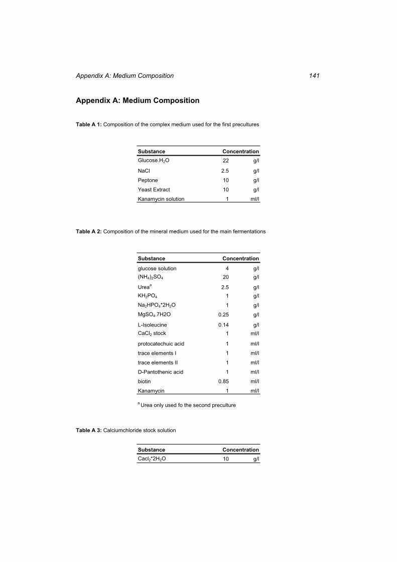
Appendix A: Medium Composition 141
Appendix A: Medium Composition
Table A 1: Composition of the complex medium used for the first precultures
Substance ConcentrationGlucose.H2O 22 g/l
NaCl 2.5 g/l
Peptone 10 g/l
Yeast Extract 10 g/l
Kanamycin solution 1 ml/l
Table A 2: Composition of the mineral medium used for the main fermentations
Substance Concentration
glucose solution 4 g/l(NH4)2SO4 20 g/l
Ureaa 2.5 g/lKH2PO4 1 g/l
Na2HPO4*2H2O 1 g/l
MgSO4.7H2O 0.25 g/l
L-Isoleucine 0.14 g/lCaCl2 stock 1 ml/l
protocatechuic acid 1 ml/l
trace elements I 1 ml/l
trace elements II 1 ml/l
D-Pantothenic acid 1 ml/l
biotin 0.85 ml/l
Kanamycin 1 ml/l
a Urea only used fo the second preculture
Table A 3: Calciumchloride stock solution
Substance ConcentrationCacl2*2H2O 10 g/l
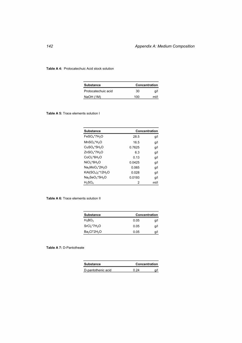
Appendix A: Medium Composition 142
Table A 4: Protocatechuic Acid stock solution
Substance Concentration
Protocatechuic acid 30 g/l
NaOH (1M) 100 ml/l
Table A 5: Trace elements solution I
Substance ConcentrationFeSO4*7H2O 28.5 g/l
MnSO4*H2O 16.5 g/lCuSO4*5H2O 0.7625 g/lZnSO4*7H2O 6.3 g/lCoCl2*6H2O 0.13 g/lNiCl2*6H2O 0.0425 g/lNa2MoO4*2H2O 0.065 g/lKAl(SO4)2*12H2O 0.028 g/lNa2SeO3*5H2O 0.0193 g/lH2SO4 2 ml/l
Table A 6: Trace elements solution II
Substance ConcentrationH3BO3 0.05 g/l
SrCl2*7H2O 0.05 g/l
Ba2Cl*2H2O 0.05 g/l
Table A 7: D-Pantotheate
Substance Concentration
D-pantothenic acid 0.24 g/l
Appendix A: Medium Composition 143
Table A 8: Biotin stock solution
Substance Concentration
biotin 1 g/l
Table A 9: Kanamycin stock solution
Substance Concentration
Kanamycinsulphate 25 g/l

144
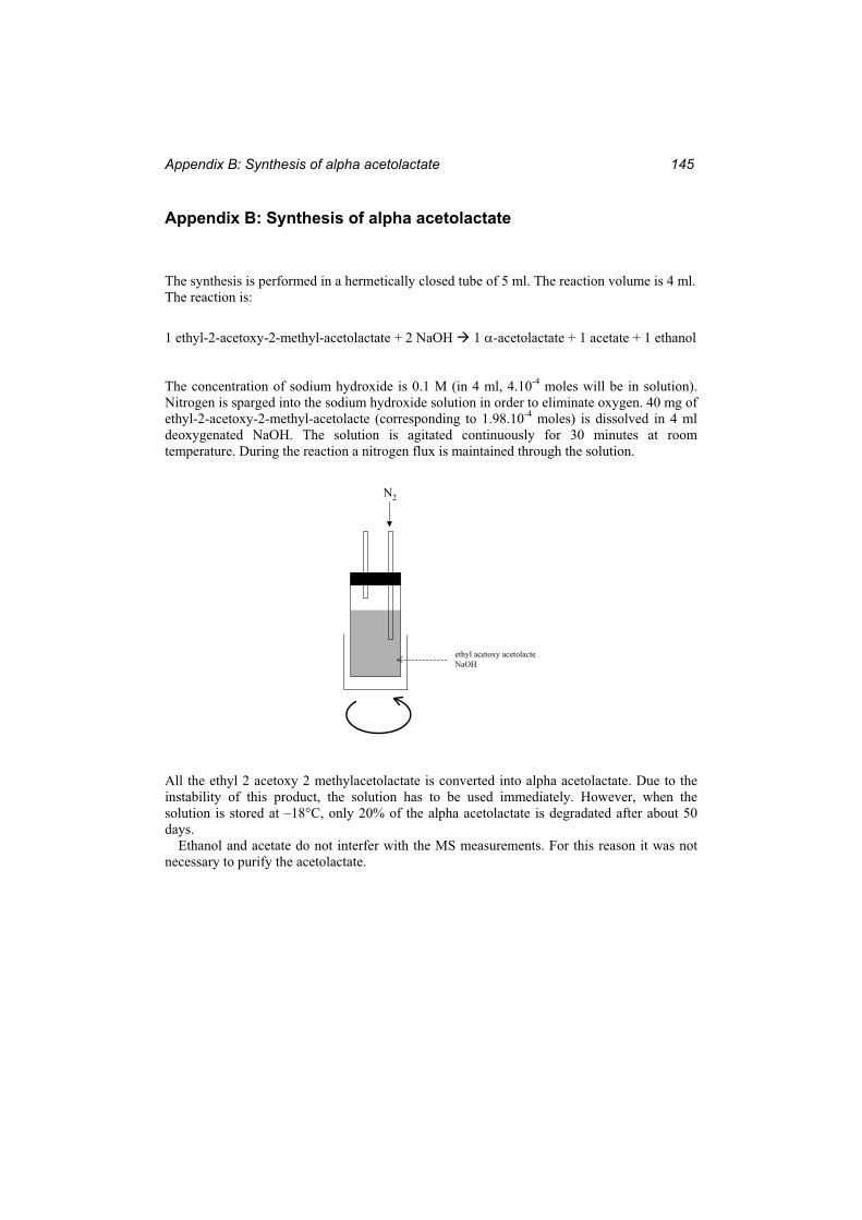
Appendix B: Synthesis of alpha acetolactate 145
Appendix B: Synthesis of alpha acetolactate
The synthesis is performed in a hermetically closed tube of 5 ml. The reaction volume is 4 ml. The reaction is:
1 ethyl-2-acetoxy-2-methyl-acetolactate + 2 NaOH 1 -acetolactate + 1 acetate + 1 ethanol
The concentration of sodium hydroxide is 0.1 M (in 4 ml, 4.10-4 moles will be in solution). Nitrogen is sparged into the sodium hydroxide solution in order to eliminate oxygen. 40 mg of ethyl-2-acetoxy-2-methyl-acetolacte (corresponding to 1.98.10-4 moles) is dissolved in 4 ml deoxygenated NaOH. The solution is agitated continuously for 30 minutes at room temperature. During the reaction a nitrogen flux is maintained through the solution.
All the ethyl 2 acetoxy 2 methylacetolactate is converted into alpha acetolactate. Due to the instability of this product, the solution has to be used immediately. However, when the solution is stored at –18°C, only 20% of the alpha acetolactate is degradated after about 50 days.
Ethanol and acetate do not interfer with the MS measurements. For this reason it was not necessary to purify the acetolactate.
N2
ethyl acetoxy acetolacteNaOH

146
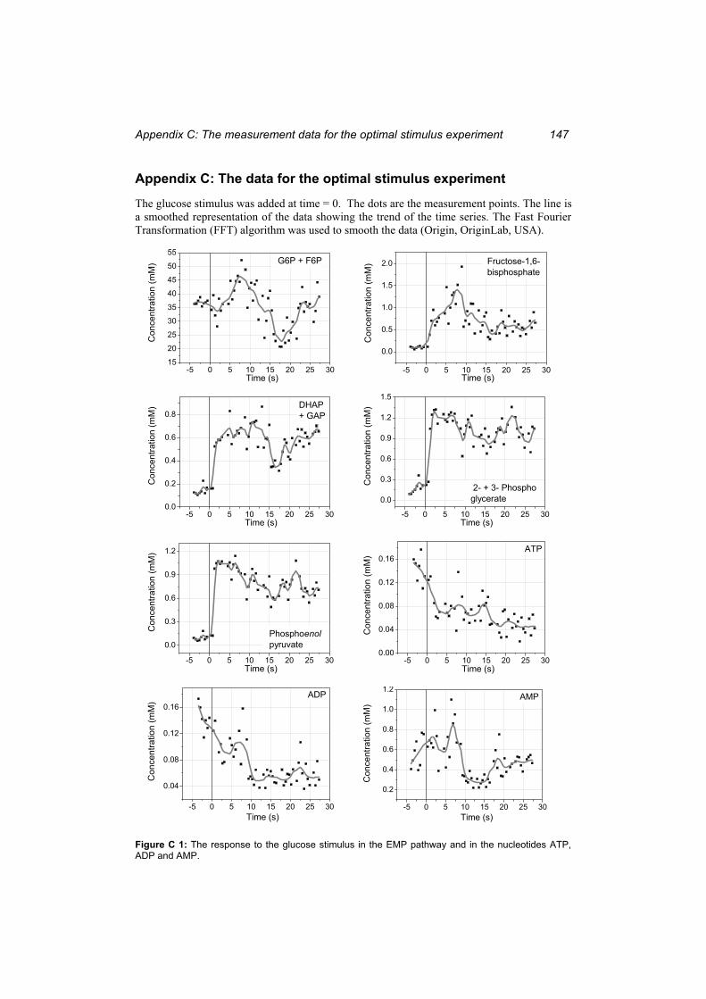
Appendix C: The measurement data for the optimal stimulus experiment 147
Appendix C: The data for the optimal stimulus experiment
The glucose stimulus was added at time = 0. The dots are the measurement points. The line is a smoothed representation of the data showing the trend of the time series. The Fast Fourier Transformation (FFT) algorithm was used to smooth the data (Origin, OriginLab, USA).
-5 0 5 10 15 20 25 3015
20
25
30
35
40
45
50
55
Con
cent
ratio
n (m
M)
Time (s)
G6P + F6P
-5 0 5 10 15 20 25 30
0.0
0.5
1.0
1.5
2.0
Con
cent
ratio
n (m
M)
Time (s)
Fructose-1,6-bisphosphate
-5 0 5 10 15 20 25 300.0
0.2
0.4
0.6
0.8
Con
cent
ratio
n (m
M)
Time (s)
DHAP+ GAP
-5 0 5 10 15 20 25 30
0.0
0.3
0.6
0.9
1.2
1.5
Con
cent
ratio
n (m
M)
Time (s)
2- + 3- Phosphoglycerate
-5 0 5 10 15 20 25 30
0.0
0.3
0.6
0.9
1.2
Con
cent
ratio
n (m
M)
Time (s)
Phosphoenolpyruvate
-5 0 5 10 15 20 25 300.00
0.04
0.08
0.12
0.16
Con
cent
ratio
n (m
M)
Time (s)
ATP
-5 0 5 10 15 20 25 30
0.04
0.08
0.12
0.16
Con
cent
ratio
n (m
M)
Time (s)
ADP
-5 0 5 10 15 20 25 30
0.2
0.4
0.6
0.8
1.0
1.2
Con
cent
ratio
n (m
M)
Time (s)
AMP
Figure C 1: The response to the glucose stimulus in the EMP pathway and in the nucleotides ATP, ADP and AMP.
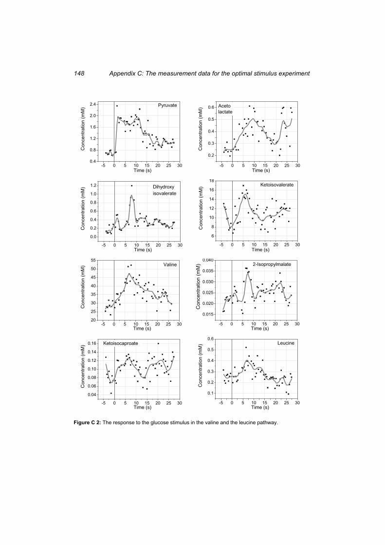
Appendix C: The measurement data for the optimal stimulus experiment 148
-5 0 5 10 15 20 25 300.4
0.8
1.2
1.6
2.0
2.4
Con
cent
ratio
n (m
M)
Time (s)
Pyruvate
-5 0 5 10 15 20 25 30
0.2
0.3
0.4
0.5
0.6
Con
cent
ratio
n (m
M)
Time (s)
Acetolactate
-5 0 5 10 15 20 25 30
0.0
0.2
0.4
0.6
0.8
1.0
1.2
Con
cent
ratio
n (m
M)
Time (s)
Dihydroxyisovalerate
-5 0 5 10 15 20 25 30
6
8
10
12
14
16
18
Con
cent
ratio
n (m
M)
Time (s)
Ketoisovalerate
-5 0 5 10 15 20 25 3020
25
30
35
40
45
50
55
Con
cent
ratio
n (m
M)
Time (s)
Valine
-5 0 5 10 15 20 25 30
0.015
0.020
0.025
0.030
0.035
0.040
Con
cent
ratio
n (m
M)
Time (s)
2-Isopropylmalate
-5 0 5 10 15 20 25 30
0.04
0.06
0.08
0.10
0.12
0.14
0.16
Con
cent
ratio
n (m
M)
Time (s)
Ketoisocaproate
-5 0 5 10 15 20 25 30
0.1
0.2
0.3
0.4
0.5
0.6
Con
cent
ratio
n (m
M)
Time (s)
Leucine
Figure C 2: The response to the glucose stimulus in the valine and the leucine pathway.
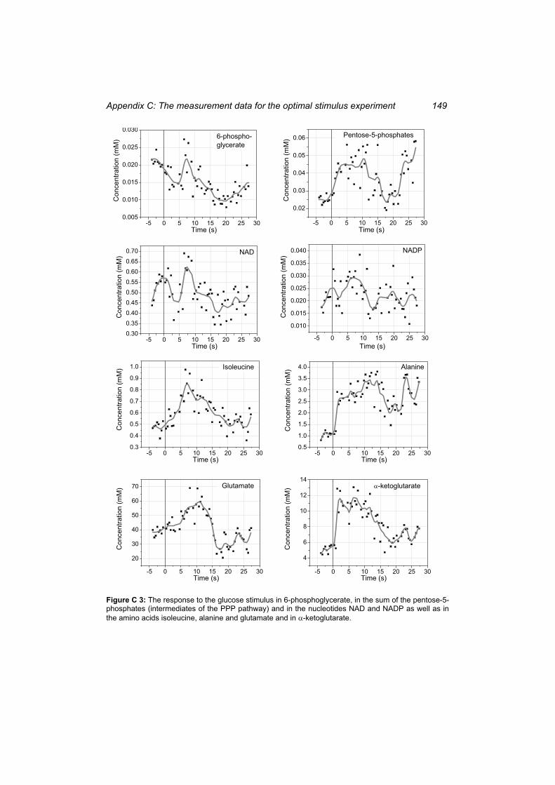
Appendix C: The measurement data for the optimal stimulus experiment 149
-5 0 5 10 15 20 25 300.005
0.010
0.015
0.020
0.025
0.030
Con
cent
ratio
n (m
M)
Time (s)
6-phospho-glycerate
-5 0 5 10 15 20 25 30
0.02
0.03
0.04
0.05
0.06
Con
cent
ratio
n (m
M)
Time (s)
Pentose-5-phosphates
-5 0 5 10 15 20 25 300.300.350.400.450.500.550.600.650.70
Con
cent
ratio
n (m
M)
Time (s)
NAD
-5 0 5 10 15 20 25 30
0.010
0.015
0.020
0.025
0.030
0.035
0.040
Con
cent
ratio
n (m
M)
Time (s)
NADP
-5 0 5 10 15 20 25 300.3
0.4
0.5
0.6
0.7
0.8
0.9
1.0
Con
cent
ratio
n (m
M)
Time (s)
Isoleucine
-5 0 5 10 15 20 25 300.5
1.0
1.5
2.0
2.5
3.0
3.5
4.0
Con
cent
ratio
n (m
M)
Time (s)
Alanine
-5 0 5 10 15 20 25 30
20
30
40
50
60
70
Con
cent
ratio
n (m
M)
Time (s)
Glutamate
-5 0 5 10 15 20 25 30
4
6
8
10
12
14
Con
cent
ratio
n (m
M)
Time (s)
-ketoglutarate
Figure C 3: The response to the glucose stimulus in 6-phosphoglycerate, in the sum of the pentose-5-phosphates (intermediates of the PPP pathway) and in the nucleotides NAD and NADP as well as in the amino acids isoleucine, alanine and glutamate and in -ketoglutarate.
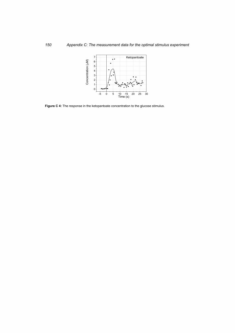
Appendix C: The measurement data for the optimal stimulus experiment 150
-5 0 5 10 15 20 25 30
0
1
2
3
4
5
6
7
Con
cent
ratio
n (
M)
Time (s)
Ketopantoate
Figure C 4: The response in the ketopantoate concentration to the glucose stimulus.
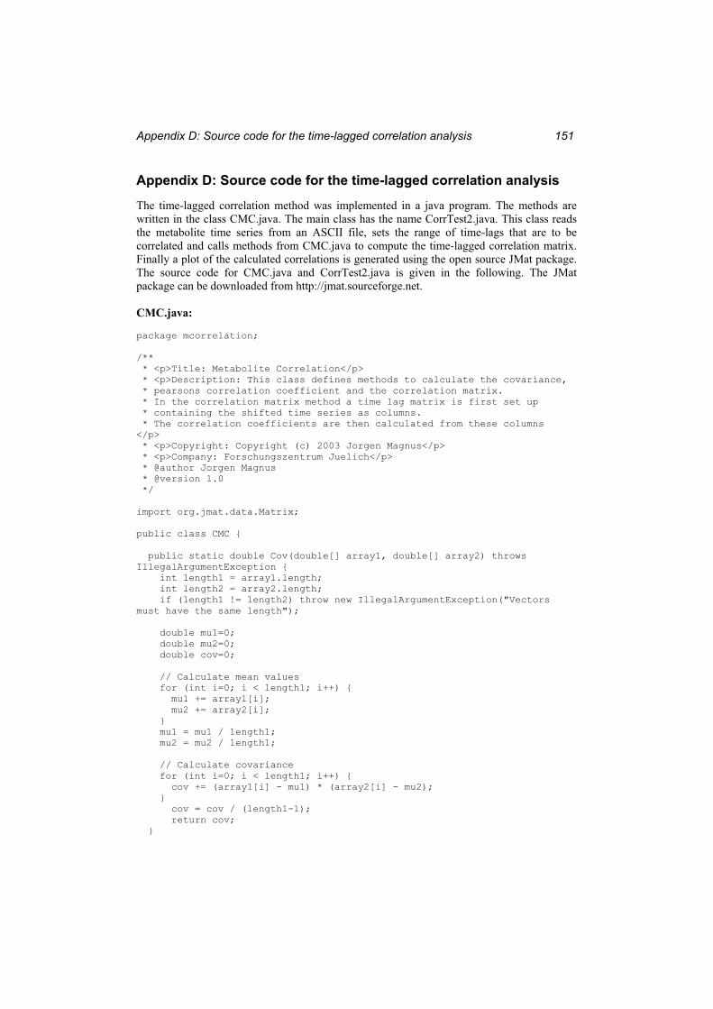
Appendix D: Source code for the time-lagged correlation analysis 151
Appendix D: Source code for the time-lagged correlation analysis
The time-lagged correlation method was implemented in a java program. The methods are written in the class CMC.java. The main class has the name CorrTest2.java. This class reads the metabolite time series from an ASCII file, sets the range of time-lags that are to be correlated and calls methods from CMC.java to compute the time-lagged correlation matrix. Finally a plot of the calculated correlations is generated using the open source JMat package. The source code for CMC.java and CorrTest2.java is given in the following. The JMat package can be downloaded from http://jmat.sourceforge.net.
CMC.java:
package mcorrelation;
/** * <p>Title: Metabolite Correlation</p> * <p>Description: This class defines methods to calculate the covariance, * pearsons correlation coefficient and the correlation matrix. * In the correlation matrix method a time lag matrix is first set up * containing the shifted time series as columns. * The correlation coefficients are then calculated from these columns</p> * <p>Copyright: Copyright (c) 2003 Jorgen Magnus</p> * <p>Company: Forschungszentrum Juelich</p> * @author Jorgen Magnus * @version 1.0 */
import org.jmat.data.Matrix;
public class CMC {
public static double Cov(double[] array1, double[] array2) throws IllegalArgumentException { int length1 = array1.length; int length2 = array2.length; if (length1 != length2) throw new IllegalArgumentException("Vectors must have the same length");
double mu1=0; double mu2=0; double cov=0;
// Calculate mean values for (int i=0; i < length1; i++) { mu1 += array1[i]; mu2 += array2[i]; } mu1 = mu1 / length1; mu2 = mu2 / length1;
// Calculate covariance for (int i=0; i < length1; i++) { cov += (array1[i] - mu1) * (array2[i] - mu2); } cov = cov / (length1-1); return cov; }
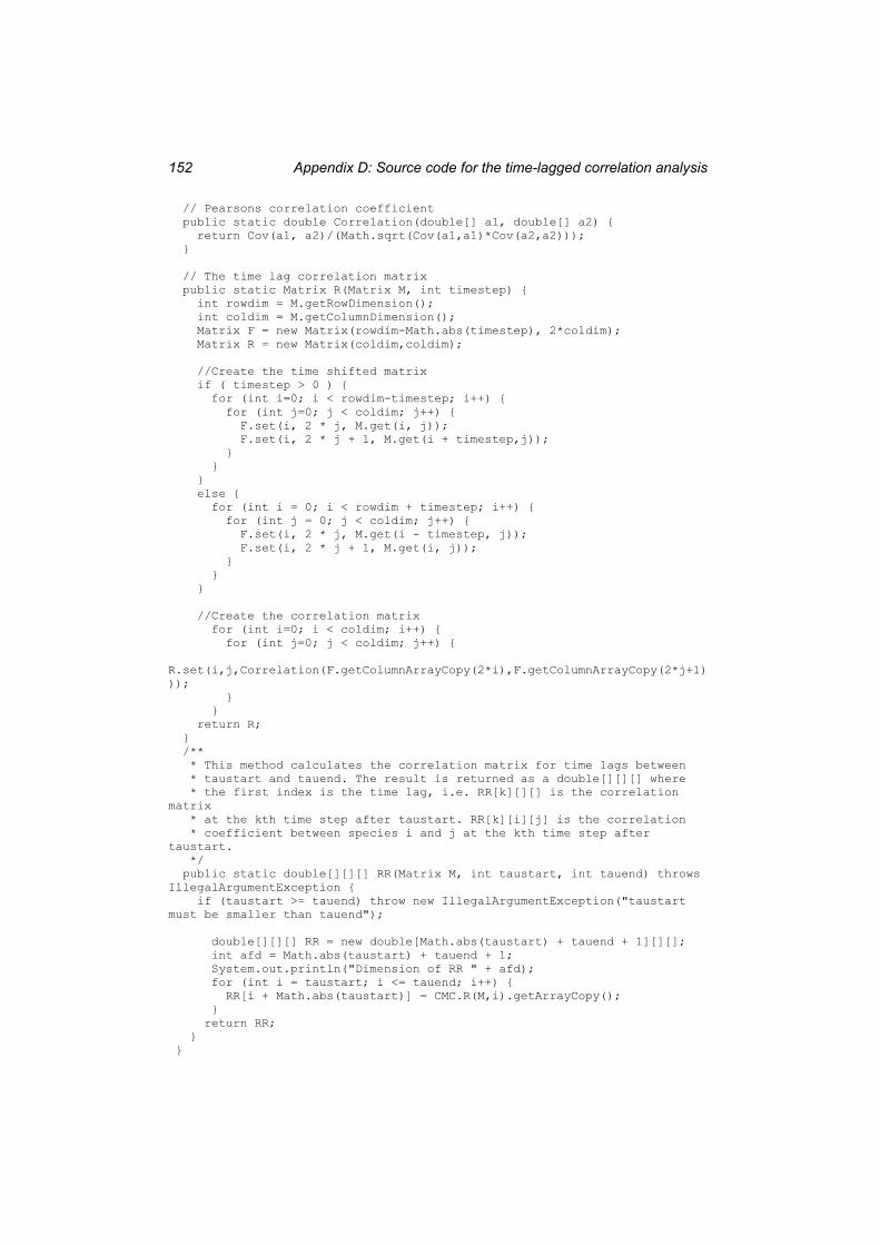
Appendix D: Source code for the time-lagged correlation analysis 152
// Pearsons correlation coefficient public static double Correlation(double[] a1, double[] a2) { return Cov(a1, a2)/(Math.sqrt(Cov(a1,a1)*Cov(a2,a2))); }
// The time lag correlation matrix public static Matrix R(Matrix M, int timestep) { int rowdim = M.getRowDimension(); int coldim = M.getColumnDimension(); Matrix F = new Matrix(rowdim-Math.abs(timestep), 2*coldim); Matrix R = new Matrix(coldim,coldim);
//Create the time shifted matrix if ( timestep > 0 ) { for (int i=0; i < rowdim-timestep; i++) { for (int j=0; j < coldim; j++) { F.set(i, 2 * j, M.get(i, j)); F.set(i, 2 * j + 1, M.get(i + timestep,j)); } } } else { for (int i = 0; i < rowdim + timestep; i++) { for (int j = 0; j < coldim; j++) { F.set(i, 2 * j, M.get(i - timestep, j)); F.set(i, 2 * j + 1, M.get(i, j)); } } }
//Create the correlation matrix for (int i=0; i < coldim; i++) { for (int j=0; j < coldim; j++) {
R.set(i,j,Correlation(F.getColumnArrayCopy(2*i),F.getColumnArrayCopy(2*j+1))); } } return R; } /** * This method calculates the correlation matrix for time lags between * taustart and tauend. The result is returned as a double[][][] where * the first index is the time lag, i.e. RR[k][][] is the correlation matrix * at the kth time step after taustart. RR[k][i][j] is the correlation * coefficient between species i and j at the kth time step after taustart. */ public static double[][][] RR(Matrix M, int taustart, int tauend) throws IllegalArgumentException { if (taustart >= tauend) throw new IllegalArgumentException("taustart must be smaller than tauend");
double[][][] RR = new double[Math.abs(taustart) + tauend + 1][][]; int afd = Math.abs(taustart) + tauend + 1; System.out.println("Dimension of RR " + afd); for (int i = taustart; i <= tauend; i++) { RR[i + Math.abs(taustart)] = CMC.R(M,i).getArrayCopy(); } return RR; } }
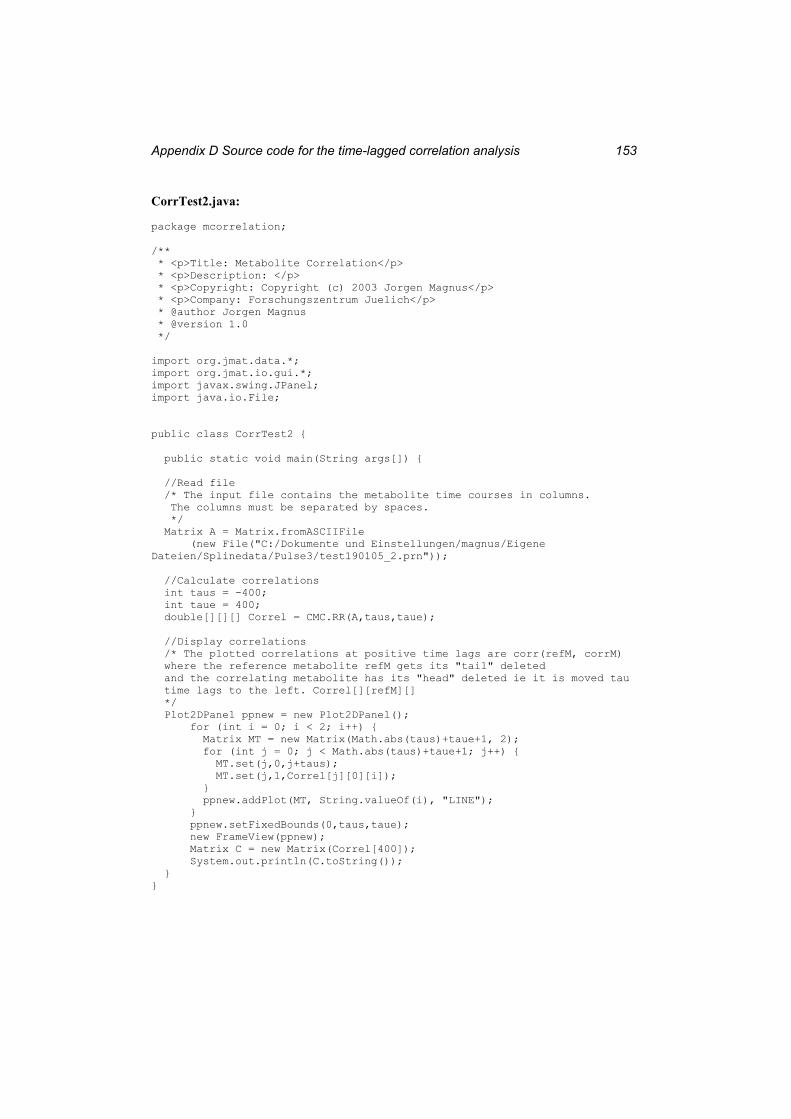
Appendix D Source code for the time-lagged correlation analysis 153
CorrTest2.java:
package mcorrelation;
/** * <p>Title: Metabolite Correlation</p> * <p>Description: </p> * <p>Copyright: Copyright (c) 2003 Jorgen Magnus</p> * <p>Company: Forschungszentrum Juelich</p> * @author Jorgen Magnus * @version 1.0 */
import org.jmat.data.*; import org.jmat.io.gui.*; import javax.swing.JPanel; import java.io.File;
public class CorrTest2 {
public static void main(String args[]) {
//Read file /* The input file contains the metabolite time courses in columns. The columns must be separated by spaces. */ Matrix A = Matrix.fromASCIIFile (new File("C:/Dokumente und Einstellungen/magnus/Eigene Dateien/Splinedata/Pulse3/test190105_2.prn"));
//Calculate correlations int taus = -400; int taue = 400; double[][][] Correl = CMC.RR(A,taus,taue);
//Display correlations /* The plotted correlations at positive time lags are corr(refM, corrM) where the reference metabolite refM gets its "tail" deleted and the correlating metabolite has its "head" deleted ie it is moved tau time lags to the left. Correl[][refM][] */ Plot2DPanel ppnew = new Plot2DPanel(); for (int i = 0; i < 2; i++) { Matrix MT = new Matrix(Math.abs(taus)+taue+1, 2); for (int j = 0; j < Math.abs(taus)+taue+1; j++) { MT.set(j,0,j+taus); MT.set(j,1,Correl[j][0][i]); } ppnew.addPlot(MT, String.valueOf(i), "LINE"); } ppnew.setFixedBounds(0,taus,taue); new FrameView(ppnew); Matrix C = new Matrix(Correl[400]); System.out.println(C.toString()); } }
Appendix D Source code for the time-lagged correlation analysis 154
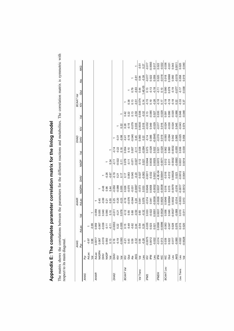
App
endi
x E:
The
com
plet
e pa
ram
eter
cor
rela
tion
mat
rix fo
r the
linl
og m
odel
The
mat
rix s
how
s th
e co
rrel
atio
ns b
etw
een
the
para
met
ers
for
the
diff
eren
t rea
ctio
ns a
nd m
etab
olite
s. Th
e co
rrel
atio
n m
atrix
is s
ymm
etric
with
re
spec
t to
its m
ain
diag
onal
.
A
HA
S
AH
AIR
D
HA
D
BC
AA
T V
al
Pyr
A
cLac
V
al
AcL
ac
NA
DP
H
DH
IV
NA
DP
V
al
DH
IV
KIV
V
al
KIV
G
lut
Ala
A
KG
A
HA
SP
yr
1
A
cLac
-0
.97
1
Val
0.
96
-0.9
9 1
AH
AIR
AcL
ac
0.00
17
0.05
9 -0
.059
1
N
AD
PH
0.
067
-0.0
67
0.05
5 0.
45
1
D
HIV
-0
.019
-0
.036
0.
040
-0.9
9 -0
.48
1
NA
DP
0.
093
-0.1
1 0.
090
0.21
0.
96
-0.2
6 1
Val
0.
13
-0.1
1 0.
10
0.55
0.
44
-0.6
7 0.
34
1
DH
AD
DH
IV
0.16
-0
.005
3 -0
.011
0.
25
-0.0
50
-0.1
9 -0
.11
-0.1
4 1
KIV
-0
.19
0.22
-0
.21
-0.2
0 -0
.088
0.
21
-0.0
22
-0.2
2 -0
.31
1
Val
-0
.093
-0
.055
0.
078
-0.2
3 0.
055
0.17
0.
11
0.18
-0
.98
0.22
1
BC
AA
T V
al
KIV
-0
.21
0.15
-0
.12
-0.1
9 0.
026
0.17
0.
078
0.05
4 -0
.41
0.28
0.
42
1
Glu
t 0.
43
-0.4
9 0.
55
-0.0
76
-0.0
70
0.06
3 -0
.11
0.10
-0
.16
-0.1
5 0.
22
0.38
1
Ala
0.
59
-0.6
2 0.
68
-0.0
44
-0.0
31
0.04
5 -0
.071
0.
057
-0.0
40
-0.0
79
0.13
0.
13
0.79
1
A
KG
-0
.32
0.44
-0
.50
0.24
-0
.009
7 -0
.20
-0.0
27
-0.1
1 0.
45
0.03
5 -0
.50
-0.5
1 -0
.83
-0.8
1 1
Val
Tra
ns
Val
0.
56
-0.5
4 0.
60
0.04
1 -0
.073
-0
.027
-0
.12
0.03
8 0.
060
0.00
30
0.03
6 -0
.074
0.
44
0.84
-0
.51
Leu
-0.2
6 0.
29
-0.3
2 0.
076
0.03
3 -0
.063
0.
021
-0.0
94
0.22
0.
016
-0.3
2 0.
14
1.4E
-05
-0.3
9 0.
27
IPM
S
KIV
-0
.007
5 -0
.035
0.
033
-0.0
14
0.00
49
-0.0
011
0.00
44
0.07
3 -0
.14
-0.0
32
0.13
-0
.15
0.13
-0
.017
-0
.017
IP
M
0.00
12
0.02
3 -0
.022
0.
041
0.00
58
-0.0
32
0.00
30
-0.0
28
0.08
6 0.
049
-0.0
85
0.19
-0
.13
0.02
2 -0
.009
3 Le
u -0
.022
0.
021
0.00
51
-0.0
039
-0.0
032
0.00
21
0.00
25
0.02
2 -0
.004
5 -0
.029
0.
027
-0.2
6 -0
.18
0.05
9 0.
017
IPM
DH
IP
M
-0.0
14
0.00
98
0.00
31
-0.0
026
0.00
37
-4.3
E-0
4 0.
0072
0.
021
-0.0
19
-0.0
17
0.03
0 -0
.18
-0.1
1 0.
020
0.02
2 K
IC
0.01
3 -0
.009
6 -0
.002
4 0.
0025
-0
.003
8 0.
0004
1 -0
.007
1 -0
.020
0.
019
0.01
6 -0
.029
0.
17
0.10
-0
.018
-0
.022
B
CA
AT
Leu
KIC
0.
039
-0.0
63
0.05
6 0.
0049
0.
016
-0.0
16
0.01
2 0.
062
-0.0
93
-0.0
24
0.09
1 -0
.18
0.09
0 0.
018
-0.0
36
Glu
t 0.
022
-0.0
47
0.04
0 0.
0009
40.
015
-0.0
12
0.01
1 0.
060
-0.0
94
-0.0
30
0.09
0 -0
.18
0.07
8 0.
0068
-0
.031
Le
u -0
.017
0.
028
-0.0
027
0.00
32
-0.0
079
0.00
025
-0.0
032
-0.0
032
0.04
2 -0
.024
-0
.020
-0
.18
-0.1
9 0.
050
0.04
3 A
KG
-0
.060
0.
076
-0.0
69
-0.0
14
-0.0
16
0.02
3 -0
.008
3 -0
.055
0.
065
0.04
5 -0
.066
0.
22
-0.0
77
-0.0
19
0.00
11
Leu
Tran
s Le
u -0
.022
0.
015
0.01
0 -0
.003
3 -0
.001
7 -0
.001
2 0.
0031
0.
036
-0.0
25
-0.0
43
0.04
6 -0
.33
-0.1
7 0.
058
0.02
0
Val
-0
.002
8 0.
020
-0.0
11
0.01
3 -0
.001
2 -0
.004
1 0.
0014
-0
.030
0.
058
0.07
4 -0
.048
0.
37
-0.0
38
0.01
9 -0
.040
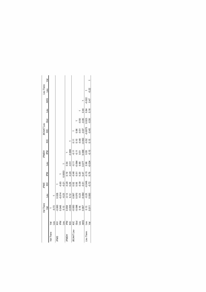
V
al T
rans
IP
MS
IP
MD
H
B
CA
AT
Leu
Leu
Tran
s
V
al
Leu
KIV
IP
M
Leu
IPM
K
IC
KIC
G
lut
Leu
AK
G
Leu
Val
V
al T
rans
V
al
1
Le
u -0
.73
1
IPM
S
KIV
-0
.060
0.
028
1
IP
M
0.04
8 -0
.014
-0
.93
1
Leu
0.13
-0
.23
-0.2
1 0.
0053
1
IPM
DH
IP
M
0.05
9 -0
.13
-0.2
9 0.
19
0.54
1
K
IC
-0.0
55
0.12
0.
29
-0.2
0 -0
.51
-0.9
99
1
B
CA
AT
Leu
KIC
-0
.083
0.
067
0.52
-0
.46
-0.1
1 -0
.11
0.11
1
G
lut
-0.0
96
0.07
0 0.
55
-0.5
1 -0
.084
-0
.11
0.10
0.
98
1
Le
u 0.
16
-0.2
3 -0
.39
0.20
0.
89
0.51
-0
.48
-0.5
1 -0
.50
1
AK
G
0.06
7 -0
.064
-0
.51
0.47
0.
077
0.09
6 -0
.093
-0
.97
-0.9
5 0.
44
1
Le
u Tr
ans
Leu
0.13
-0
.25
-0.0
49
-0.1
5 0.
98
0.55
-0
.52
-0.0
075
0.02
3 0.
84
-0.0
22
1
V
al
0.01
1 0.
093
-0.7
2 0.
79
-0.0
34
-0.1
5 0.
15
-0.4
5 -0
.50
0.16
0.
47
-0.2
2 1
Appendix F: The source code of the spline program JMSpline 157
Appendix F: The source code of the spline program JMSpline.
The class Spline01.java contains the main method. This class opens a panel using the Plot2DPanel.java class from the JMat package where the concentration data are plotted. The panel contains a toolbar which has been extended to also include three new text fields where the path to the ASCII file containing the concentration data, the spline degree and the smoothing factor can be specified. A button to remove splines from the plot was also included. The toolbar was extended by making additions to the JMat class PlotToolBar.java. When the user presses enter in one of the text fields, the program calls the method addSpline() which is written into the PlotPanel.java class contained in the JMat package. The method addSpline() reads the ASCII file containing the concentration data, as well as the contents of the text fields on the tool bar, and calculates a spline by using the JSpline++ library. The spline is plotted in the panel and the spline coefficients are printed out on XML format. The source code for Spline01.java and for the method addSpline() as well as the additions to PlotToolBar.java are given below:
Spline01.java :
package org.jmat.test; /** * <p>Title: <JMSpline/p> * <p>Description: </p> * <p>Copyright: Copyright (c) 2003 Jorgen Magnus * <p>Company: Forschungszentrum Juelich * @Jorgen Magnus * @version 1.0 */ import java.io.File; import org.jmat.data.Matrix; import org.jmat.io.gui.Plot2DPanel; import org.jmat.io.gui.FrameView; public class Spline01 { String filename;
Plot2DPanel p2Dp;
public Spline01(String filename) { Matrix A = Matrix.fromASCIIFile(new File(filename)); Matrix Data = A.getColumns(0,1); p2Dp = new Plot2DPanel(Data, filename , "SCATTER"); p2Dp.setFixedBounds(0,-5,30); p2Dp.setFixedBounds(1, Data.getColumn(1).min().toDouble(), Data.getColumn(1).max().toDouble());
new FrameView(filename, p2Dp); p2Dp.setName(filename); }
public static void main(String args[]) { new Spline01("C:/Dokumente und Einstellungen/magnus/
Eigene Dateien/Splinedata/Puls2/Puls2Glut.prn"); } }
Appendix F: The source code of the spline program JMSpline 158
The method addSpline() as implemented in PlotPanel.java:
//Method add spline to plot public void addSpline() throws CalculatingException {
// get input from textfields int degree = Integer.parseInt(toolBar.splinedegree.getText()); double smoothpara =
Double.parseDouble(toolBar.smoothingparameter.getText()); String theWeights = toolBar.weightsfile.getText();
//Get the data values and the weights Plot plt = (Plot) plots.get(0);
double[] themesh = plt.getDatas().getColumnArrayCopy(0); double[] thedata = plt.getDatas().getColumnArrayCopy(1); double[] weights = Matrix.fromASCIIFile(new
File(theWeights)).getColumnArrayCopy(2);
//Create the spline Spline spl;
int order; if((degree%2) == 0) {
spl = PEvenSplineCreator.createSpline(1+degree/2, themesh, thedata,smoothpara, weights);
} else { spl = POddSplineCreator.createSpline((1+degree)/2, themesh,
thedata,smoothpara, weights); }
//Print out spline coefficients (SF is the scaling factor) int numberofcoeff = spl.vector().length; double SF = (themesh[themesh.length-1]-themesh[0])/(themesh.length-1);
System.out.println("SF " + SF);
System.out.println("coefficients on the form p(x)=a0 + a1(x-x0) +a2(x-x0)^2 ...");
System.out.println("<spline name=\"spline\" t0=\"" + themesh[0] + "\">");
for (int i=0; i < themesh.length-1; i++) { System.out.println("<break degree=\"" + degree + "\" tr=\"" + themesh[i+1] + "\">");
for (int j=0; j<degree + 1; j++) { System.out.println("<coef c=\"" + j + "\" value=\"" + spl.vector().get(j+(degree+1)*i)/Math.pow(SF,(j+(degree+1)*i)%
( degree+1)) + "\"/>"); } System.out.println("</break>"); //System.out.println(i + ": " + spl.vector().get(i)/(Math.pow(SF,i%3))); } System.out.println("</spline>");
int numberofvalues = 120; double startpoint = themesh[0]; double endpoint = themesh[themesh.length-1]; double stepsize = (endpoint-startpoint)/(numberofvalues-1);
Matrix splinevalues = new Matrix(numberofvalues,2);
// The spline values are set in a matrix for (int i=0; i < numberofvalues; i++) {
splinevalues.set(i,0,startpoint + stepsize*i); // Set x values
Appendix F: The source code of the spline program JMSpline 159
splinevalues.set(i,1,spl.value(startpoint + stepsize*i)); //set y values }
Matrix Data = plt.getDatas(); this.addPlot(splinevalues, "The Spline","LINE"); this.setFixedBounds(0,-5,30);this.setFixedBounds(1, Data.getColumn(1).min().toDouble() ,
Data.getColumn(1).max().toDouble());
//Calculate the average before pulse: double sum = 0; int index = 0; for(int i = 0; i < Data.getRowDimension(); i++) { if (Data.get(i,0) <= 0) {
sum += Data.get(i,1); }
else { index = i;
break; } }
double average = sum/index; System.out.println("Average: " + average); System.out.println("Data points before pulse: " + index);
Additions to PlotToolBar.java
protected JButton buttonRemove;public TextField smoothingparameter = new TextField("0.2", 6 ); public TextField splinedegree = new TextField("2", 4); public TextField weightsfile = new TextField( " " , 40); protected Label smoothlabel = new Label("Smooth:"); protected Label weightslabel = new Label("Data:"); protected Label splinedegreelabel = new Label("Degree:");
buttonRemove = new JButton("Rem"); buttonRemove.setToolTipText("Remove old spline");
buttonRemove.addActionListener(new ActionListener() { public void actionPerformed(ActionEvent e) {
plotPanel.removePlot(1); } });
smoothingparameter.addActionListener(new ActionListener() { public void actionPerformed(ActionEvent e) { try {
plotPanel.addSpline(); }
catch (ru.sscc.util.CalculatingException e1) {e1.printStackTrace(); } } });
splinedegree.addActionListener(new ActionListener(){ public void actionPerformed(ActionEvent e) { try {
plotPanel.addSpline(); }
Appendix F: The source code of the spline program JMSpline 160
catch (ru.sscc.util.CalculatingException e1) {e1.printStackTrace(); } } });
weightsfile.addActionListener(new ActionListener() { public void actionPerformed(ActionEvent e) {
weightsfile.setText(plotPanel.getName()); } });
add(buttonRemove, null); add(splinedegreelabel); add(splinedegree); add(smoothlabel); add(smoothingparameter); add(weightslabel); add(weightsfile);
Appendix G: Stability Analysis of Dynamic Models 161
Appendix G: Stability Analysis of Dynamic Models
In the following the condition for the stability of a steady state of a dynamic model is obtained using Lyapunov’s stability criterion (Kondepudi and Prigogine, 1998) and linear stability analysis. In order to do this the concepts of eigenvectors and eigenvalues of a square matrix are needed so a brief introduction to these concepts is given first.
Eigenvectors and eigenvalues of square matrices Eigenvectors and eigenvalues are defined as follows:
Definition: Eigenvalues and eigenvectors
The eigenvalues and eigenvectors have the following useful property (Fraleigh and Beauregard, 1995):
Theorem: Matrix summary of eigenvalues of A
The theorem above is easily proved by using the definition of eigenvalues and eigenvectors. If the matrix C is invertible it can be used to diagonalise A, i.e.:
C-1AC = D ( G-1 )
Conversely, also provided that C is invertible:
A = CDC-1 ( G-2 )
C will be invertible if and only if A has n independent eigenvectors.
Linear stability analysis and Lyapunov’s criterion for stability Consider a system of differential equations as defined in Eq. (4-5). Suppose the system has a steady state given by:
Let A be an n × n matrix. A scalar is an eigenvalue of A if there is a nonzero column vector v in n-space such that Av = v. The vector v is then an eigenvector of Acorresponding to
Let A be an n × n matrix and let n be (possibly complex) scalars and v1, v2,. . . , vn be nonzero vectors in n-space. Let C be the n × n matrix having vj as jth column vector, and let D be the diagonal matrix with n on its main diagonal and zeros everywhere else
n0
0
2
1
D
Then AC = CD if and only if n are eigenvalues of A and vj is an eigenvector of A corresponding to j for j = 1, 2, . . . , n.
Appendix G: Stability Analysis of Dynamic Models 162
0);;(dd 00 pcxx f
t ( G-3 )
where the superscript 0 refers to the steady state concentration values. When analysing the steady state the independent metabolite concentrations, c0, are considered to stay constant so they can be included in the parameter vector. An extended parameter vector pcp 0# is therefore defined so that Eq. (G-3) can be written as:
0);(dd #0 pxx f
t ( G-4 )
The stability of this steady state is analysed by looking at what happens after a small perturbation x. A positive function L( x) is defined in the space spanned by x. L( x) can be thought of as a distance between the perturbed and the steady state and is referred to as the Lyapunov function. If this distance between the steady state x0 and the perturbed state (x0 + x) decreases steadily with time after the perturbation the steady state is stable. Lyapunov’s
criterion for stability therefore becomes:
0xL 0dt
dL x ( G-5 )
Suppose now that the stationary state x0 is perturbed by x = The metabolite concentrations will then be given by:
txx 0 ( G-6 )
The time evolution of metabolite xi is given by:
#00
;d
dpxi
ii ft
x ( G-7 )
By doing a Taylor expansion of fi around xi0 fi can be expressed as:
m
jj
j
iii x
fff
0
#0#0 ;);( pxpx ( G-8 )
The subscript 0 on the partial derivatives indicates that they are evaluated at the stationary state x0. The higher order terms in the Taylor polynomial can be neglected since is small and one therefore only needs to consider the linear terms (hence linear stability analysis). If the relation
ttx
tx iiii
dd
dd
dd 00
( G-9 )
Appendix G: Stability Analysis of Dynamic Models 163
is used Eq. (G-7) and (G-8) can be combined to get
m
jj
j
ii
ii
xf
ftt
x
0
#00
;d
dd
dpx ( G-10 )
Since by definition
0;d
d #00
pxft
xi
i ( G-11 )
Eq. (G-10) reduces to
m
jj
j
ii
xf
dtd
0
( G-12 )
Thus i(t) can be expressed as a linear combination of partial derivatives of f. Eq. (G-12) written in matrix notation for all i becomes:
Jtd
d ( G-13 )
J is the matrix of partial derivatives of f often referred to as the Jacobian:
m
mm
m
xf
xf
xf
xf
1
1
1
1
J ( G-14 )
where the partial derivatives are evaluated at x0.If the eigenvectors of J are independent Eq. (G-2) can be used to obtain a general solution
of Eq. (G-13). The m × m matrix J has m eigenvalues and eigenvectors. Let D be the diagonal matrix of the eigenvalues of J:
m
2
1
D ( G-15 )
and C be the matrix made up of the eigenvectors v of J where vj is the jth column in C
Appendix G: Stability Analysis of Dynamic Models 164
|||
|||
21 mvvvC ( G-16 )
According to Eq. (G-2) J can be expressed as:
J = CDC-1 ( G-17 )
Substituting for J in Eq. (G-13) the differential of becomes:
CDC 1
dd
t ( G-18 )
Define now a dummy variable
y = C-1 ( G-19 )so that Eq. (G-18) can be written as
Dyytd
d ( G-20 )
Since D is a diagonal matrix the system of differential equations in Eq. (G-20) can be readily solved. For each yi one gets:
iii y
ty
dd
( G-21 )
which has the general solution:
tii
iekty ( G-22 )
where ki is a scalar. In vector notation for all yi:
tm
t
t
mek
ekek
2
1
2
1
y ( G-23 )
can now be substituted back in again using Eq. (G-19) to get the general solution of Eq. (G-13):
Appendix G: Stability Analysis of Dynamic Models 165
tm
t
t
m
i
ek
ekek
22
1
C ( G-24 )
With the general solution for the time evolution of the perturbation , a conclusion on the stability of the steady state can now be arrived at. According to Lyapunov’s theory the stability depends on whether the perturbation will grow or decay with time. It is seen from Eq. (G-24) that the only time dependent terms are the exponentials. Thus the stability of the system depends only on the eigenvalues of the Jacobian matrix. If one or more of the eigenvalues have a positive real part the associated solutions will grow exponentially. The stability criterion can therefore be formulated as:
Theorem: Stability criterion A steady state is stable if, and only if, the eigenvalues of the associated Jacobian matrix all have negative real parts.

Appendix G: Stability Analysis of Dynamic Models 166
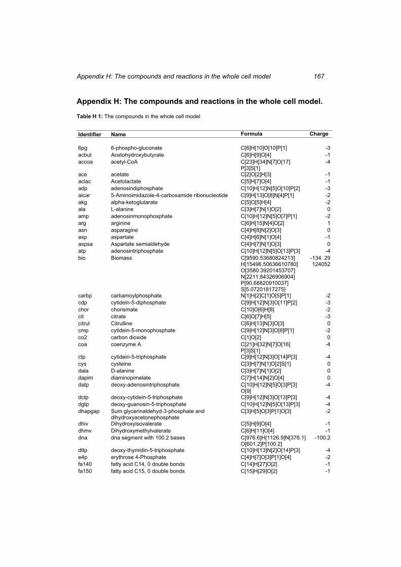
Appendix H: The compounds and reactions in the whole cell model 167
Appendix H: The compounds and reactions in the whole cell model.
Table H 1: The compounds in the whole cell model
Identifier Name Formula Charge
6pg 6-phospho-gluconate C[6]H[10]O[10]P[1] -3acbut Acetohydroxybutyrate C[6]H[9]O[4] -1accoa acetyl-CoA C[23]H[34]N[7]O[17]
P[3]S[1]-4
ace acetate C[2]O[2]H[3] -1aclac Acetolactate C[5]H[7]O[4] -1adp adenosindiphosphate C[10]H[12]N[5]O[10]P[2] -3aicar 5-Aminoimidazole-4-carboxamide ribonucleotide C[9]H[13]O[8]N[4]P[1] -2akg alpha-ketoglutarate C[5]O[5]H[4] -2ala L-alanine C[3]H[7]N[1]O[2] 0amp adenosinmonophosphate C[10]H[12]N[5]O[7]P[1] -2arg arginine C[6]H[15]N[4]O[2] 1asn asparagine C[4]H[8]N[2]O[3] 0asp aspartate C[4]H[6]N[1]O[4] -1aspsa Aspartate semialdehyde C[4]H[7]N[1]O[3] 0atp adenosintriphosphate C[10]H[12]N[5]O[13]P[3] -4bio Biomass C[9590.53680824213]
H[15496.50636610780] O[3580.39201453707] N[2211.84326906904] P[90.68820910037] S[5.07201817275]
-134. 29124052
carbp carbamoylphosphate N[1]H[2]C[1]O[5]P[1] -2cdp cytidein-5-diphosphate C[9]H[12]N[3]O[11]P[2] -3chor chorismate C[10]O[6]H[8] -2cit citrate C[6]O[7]H[5] -3citrul Citrulline C[6]H[13]N[3]O[3] 0cmp cytidein-5-monophosphate C[9]H[12]N[3]O[8]P[1] -2co2 carbon dioxide C[1]O[2] 0coa coenzyme A C[21]H[32]N[7]O[16]
P[3]S[1]-4
ctp cytidein-5-triphosphate C[9]H[12]N[3]O[14]P[3] -4cys cysteine C[3]H[7]N[1]O[2]S[1] 0dala D-alanine C[3]H[7]N[1]O[2] 0dapim diaminopimelate C[7]H[14]N[2]O[4] 0datp deoxy-adenosintriphosphate C[10]H[12]N[5]O[3]P[3]
O[9]-4
dctp deoxy-cytidein-5-triphosphate C[9]H[12]N[3]O[13]P[3] -4dgtp deoxy-guanosin-5-triphosphate C[10]H[12]N[5]O[13]P[3] -4dhapgap Sum glycerinaldehyd-3-phosphate and
dihydroxyacetonephosphate C[3]H[5]O[3]P[1]O[3] -2
dhiv Dihydroxyisovalerate C[5]H[9]O[4] -1dhmv Dihydroxymethylvalerate C[6]H[11]O[4] -1dna dna segment with 100.2 bases C[976.6]H[1126.9]N[376.1]
O[601.2]P[100.2] -100.2
dttp deoxy-thymidin-5-triphosphate C[10]H[13]N[2]O[14]P[3] -4e4p erythrose 4-Phosphate C[4]H[7]O[3]P[1]O[4] -2fa140 fatty acid C14, 0 double bonds C[14]H[27]O[2] -1fa150 fatty acid C15, 0 double bonds C[15]H[29]O[2] -1
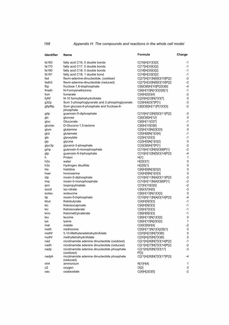
Appendix H: The compounds and reactions in the whole cell model 168
Identifier Name Formula Charge fa160 fatty acid C16, 0 double bonds C[16]H[31]O[2] -1fa170 fatty acid C17, 0 double bonds C[17]H[33]O[2] -1fa180 fatty acid C18, 0 double bonds C[18]H[35]O[2] -1fa181 fatty acid C18, 1 double bond C[18]H[33]O[2] -1fad flavin-adenine-dinucleotide, (oxidised C[27]H[31]N[9]O[15]P[2] -2fadh2 flavin-adenine-dinucleotide (reduced) C[27]H[33]N[9]O[15]P[2] -2fbp fructose-1,6-bisphosphate C[6]O[6]H[10]P[2]O[6] -4fmeth N-Formylmethionine C[6]H[10]N[1]O[3]S[1] -1fum fumarate C[4]H[2]O[4] -2fythf N-10 formyltetrahydrofolate C[20]H[23]N[7]O[7] 0g32p Sum 3-phosphoglycerate and 2-phosphoglycerate C[3]H[4]O[7]P[1] -3g6pf6p Sum glucose-6-phosphate and fructose-6-
phosphate C[6]O[6]H[11]P[1]O[3] -2
gdp guanosin-5-diphosphate C[10]H[12]N[5]O[11]P[2] -3glc glucose C[6]O[6]H[12] 0gluc Gluconate C[6]H[11]O[7] -1gluclac D-Glucono-1,5-lactone C[6]H[10]O[6] 0glum glutamine C[5]H[10]N[2]O[3] 0glut glutamate C[5]H[8]N[1]O[4] -1glx glyoxylate C[2]H[1]O[3] -1gly glycine C[2]H[5]N[1]O[2] 0glyc3p glycerol-3-phosphate C[3]O[6]H[7]P[1] -2gmp guanosin-5-monophosphate C[10]H[12]N[5]O[8]P[1] -2gtp guanosin-5-triphosphate C[10]H[12]N[5]O[14]P[3] -4h Proton H[1] 1h2o water H[2]O[1] 0h2s Hydrogen disulfide H[2]S[1] 0his histidine C[6]H[9]N[3]O[2] 0hser homoserine C[4]H[9]N[1]O[3] 0idp inosin-5-diphosphate C[10]H[11]N[4]O[11]P[2] -3imp inosin-5-monophosphate C[10]H[11]N[4]O[8]P[1] -2ipm Isopropylmalate C[7]H[10]O[5] -2isocit iso-citrate C[6]O[7]H[5] -3isoleu isoleucine C[6]H[13]N[1]O[2] 0itp inosin-5-triphosphate C[10]H[11]N[4]O[14]P[3] -4kbut Ketobutyrate C[4]H[5]O[3] -1kic Ketoisocaproate C[6]H[9]O[3] -1kiv Ketoisovalerate C[5]H[7]O[3] -1kmv Ketomethylvalerate C[6]H[9]O[3] -1leu leucine C[6]H[13]N[1]O[2] 0lys lysine C[6]H[15]N[2]O[2] 1mal malate C[4]O[5]H[4] -2meth methionine C[5]H[11]N[1]O[2]S[1] 0methf 5,10-Methylenetetrahydrofolate C[20]H[23]N[7]O[6] 0mythf methyltetrahydrofolate C[20]H[25]N[7]O[6] 0nad nicotinamide adenine dinucleotide (oxidized) C[21]H[26]N[7]O[14]P[2] -1nadh nicotinamide adenine dinucleotide (reduced) C[21]H[27]N[7]O[14]P[2] -2nadp nicotinamide adenine dinucleotide phosphate
(oxidized) C[21]H[25]N[7]O[17] P[3]
-3
nadph nicotinamide adenine dinucleotide phosphate (reduced)
C[21]H[26]N[7]O[17]P[3] -4
nh4 ammonium N[1]H[4] 1o2 oxygen O[2] 0oac oxalacetate C[4]H[2]O[5] -2
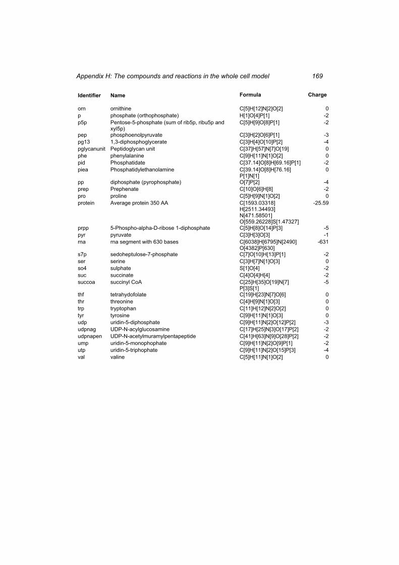
Appendix H: The compounds and reactions in the whole cell model 169
Identifier Name Formula Charge orn ornithine C[5]H[12]N[2]O[2] 0p phosphate (orthophosphate) H[1]O[4]P[1] -2p5p Pentose-5-phosphate (sum of rib5p, ribu5p and
xyl5p) C[5]H[9]O[8]P[1] -2
pep phosphoenolpyruvate C[3]H[2]O[6]P[1] -3pg13 1,3-diphosphoglycerate C[3]H[4]O[10]P[2] -4pglycanunit Peptidoglycan unit C[37]H[57]N[7]O[19] 0phe phenylalanine C[9]H[11]N[1]O[2] 0pid Phosphatidate C[37.14]O[8]H[69.16]P[1] -2piea Phosphatidylethanolamine C[39.14]O[8]H[76.16]
P[1]N[1]0
pp diphosphate (pyrophosphate) O[7]P[2] -4prep Prephenate C[10]O[6]H[8] -2pro proline C[5]H[9]N[1]O[2] 0protein Average protein 350 AA C[1593.03318]
H[2511.34493] N[471.58501] O[559.26228]S[1.47327]
-25.59
prpp 5-Phospho-alpha-D-ribose 1-diphosphate C[5]H[8]O[14]P[3] -5pyr pyruvate C[3]H[3]O[3] -1rna rna segment with 630 bases C[6038]H[6795]N[2490]
O[4382]P[630] -631
s7p sedoheptulose-7-phosphate C[7]O[10]H[13]P[1] -2ser serine C[3]H[7]N[1]O[3] 0so4 sulphate S[1]O[4] -2suc succinate C[4]O[4]H[4] -2succoa succinyl CoA C[25]H[35]O[19]N[7]
P[3]S[1]-5
thf tetrahydofolate C[19]H[23]N[7]O[6] 0thr threonine C[4]H[9]N[1]O[3] 0trp tryptophan C[11]H[12]N[2]O[2] 0tyr tyrosine C[9]H[11]N[1]O[3] 0udp uridin-5-diphosphate C[9]H[11]N[2]O[12]P[2] -3udpnag UDP-N-acylglucosamine C[17]H[25]N[3]O[17]P[2] -2udpnapen UDP-N-acetylmuramylpentapeptide C[41]H[63]N[9]O[28]P[2] -2ump uridin-5-monophophate C[9]H[11]N[2]O[9]P[1] -2utp uridin-5-triphophate C[9]H[11]N[2]O[15]P[3] -4val valine C[5]H[11]N[1]O[2] 0
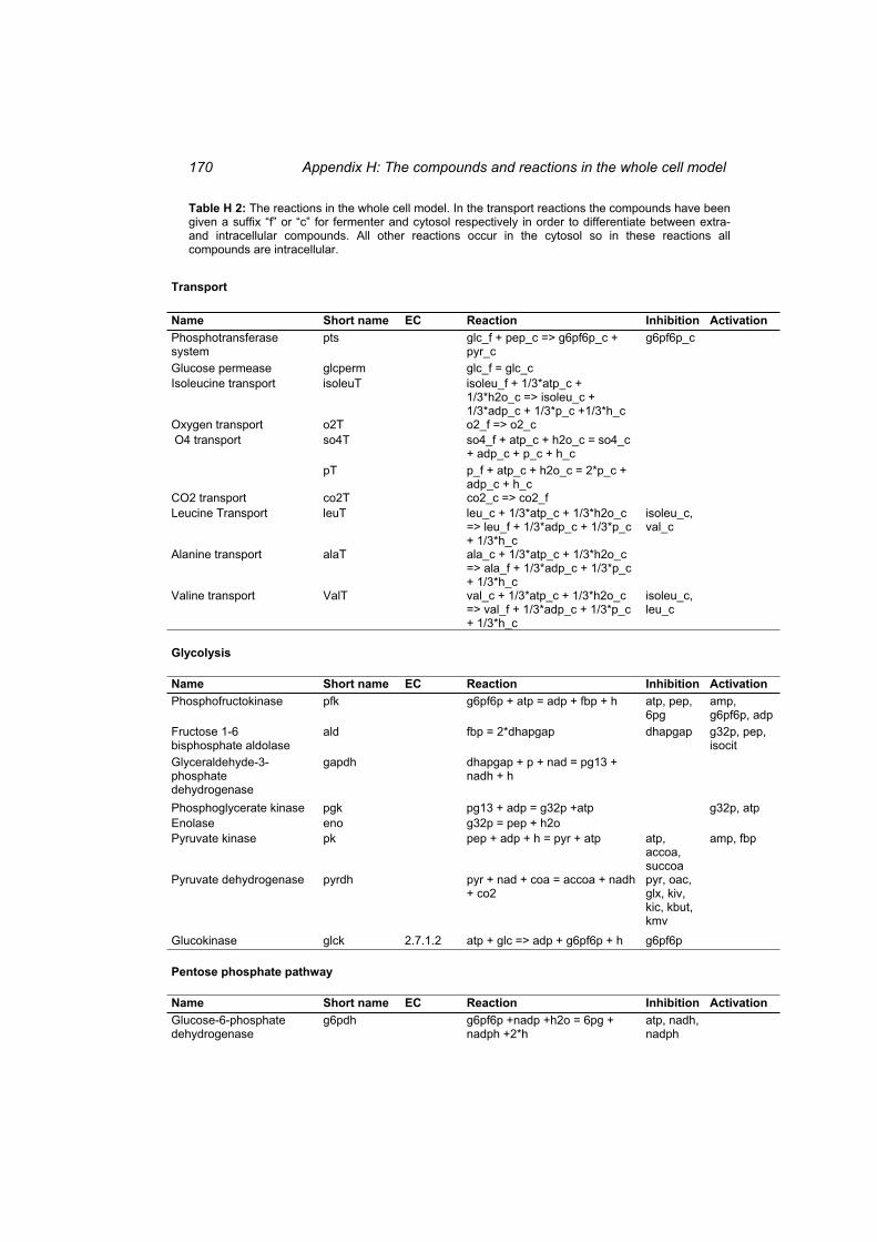
Appendix H: The compounds and reactions in the whole cell model 170
Table H 2: The reactions in the whole cell model. In the transport reactions the compounds have been given a suffix “f” or “c” for fermenter and cytosol respectively in order to differentiate between extra- and intracellular compounds. All other reactions occur in the cytosol so in these reactions all compounds are intracellular.
Transport Name Short name EC Reaction Inhibition Activation Phosphotransferase system
pts glc_f + pep_c => g6pf6p_c + pyr_c
g6pf6p_c
Glucose permease glcperm glc_f = glc_c Isoleucine transport isoleuT isoleu_f + 1/3*atp_c +
1/3*h2o_c => isoleu_c + 1/3*adp_c + 1/3*p_c +1/3*h_c
Oxygen transport o2T o2_f => o2_c O4 transport so4T so4_f + atp_c + h2o_c = so4_c
+ adp_c + p_c + h_c pT p_f + atp_c + h2o_c = 2*p_c +
adp_c + h_c CO2 transport co2T co2_c => co2_f Leucine Transport leuT leu_c + 1/3*atp_c + 1/3*h2o_c
=> leu_f + 1/3*adp_c + 1/3*p_c + 1/3*h_c
isoleu_c, val_c
Alanine transport alaT ala_c + 1/3*atp_c + 1/3*h2o_c => ala_f + 1/3*adp_c + 1/3*p_c + 1/3*h_c
Valine transport ValT val_c + 1/3*atp_c + 1/3*h2o_c => val_f + 1/3*adp_c + 1/3*p_c + 1/3*h_c
isoleu_c, leu_c
Glycolysis Name Short name EC Reaction Inhibition Activation Phosphofructokinase pfk g6pf6p + atp = adp + fbp + h atp, pep,
6pgamp,g6pf6p, adp
Fructose 1-6 bisphosphate aldolase
ald fbp = 2*dhapgap dhapgap g32p, pep, isocit
Glyceraldehyde-3-phosphate dehydrogenase
gapdh dhapgap + p + nad = pg13 + nadh + h
Phosphoglycerate kinase pgk pg13 + adp = g32p +atp g32p, atp Enolase eno g32p = pep + h2o Pyruvate kinase pk pep + adp + h = pyr + atp atp,
accoa,succoa
amp, fbp
Pyruvate dehydrogenase pyrdh pyr + nad + coa = accoa + nadh + co2
pyr, oac, glx, kiv, kic, kbut, kmv
Glucokinase glck 2.7.1.2 atp + glc => adp + g6pf6p + h g6pf6p Pentose phosphate pathway Name Short name EC Reaction Inhibition Activation Glucose-6-phosphate dehydrogenase
g6pdh g6pf6p +nadp +h2o = 6pg + nadph +2*h
atp, nadh, nadph
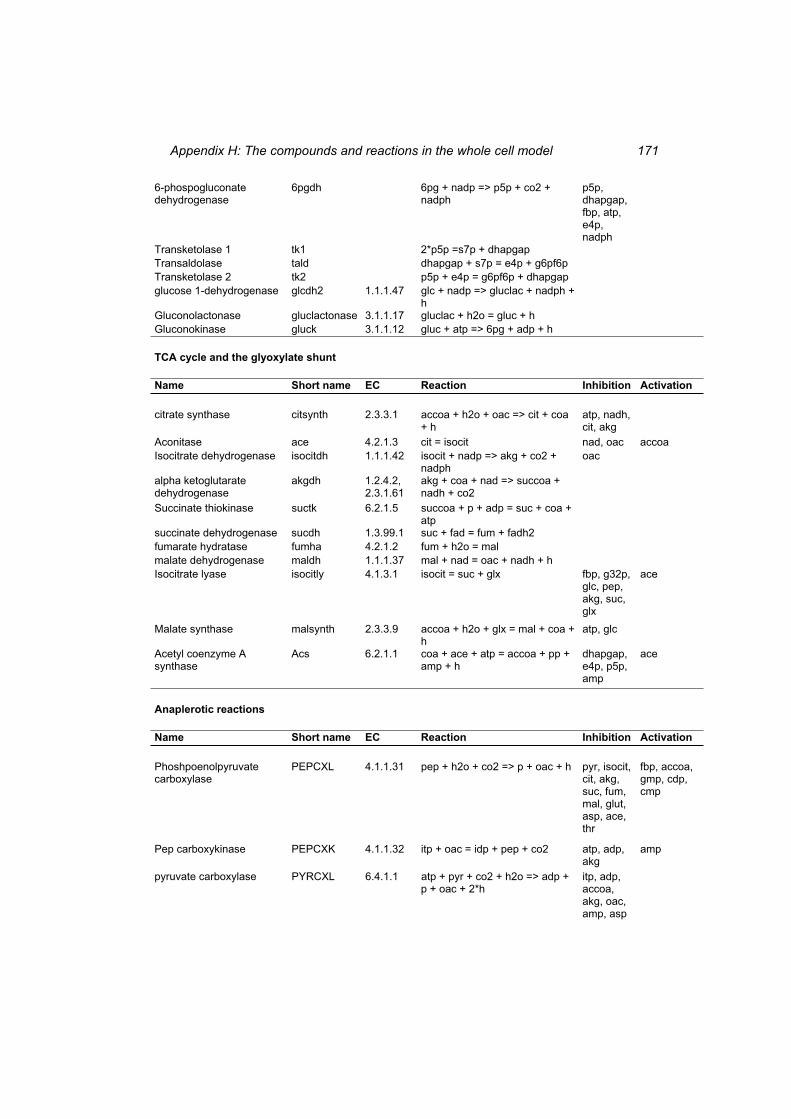
Appendix H: The compounds and reactions in the whole cell model 171
6-phospogluconate dehydrogenase
6pgdh 6pg + nadp => p5p + co2 + nadph
p5p,dhapgap, fbp, atp, e4p,nadph
Transketolase 1 tk1 2*p5p =s7p + dhapgap Transaldolase tald dhapgap + s7p = e4p + g6pf6p Transketolase 2 tk2 p5p + e4p = g6pf6p + dhapgap glucose 1-dehydrogenase glcdh2 1.1.1.47 glc + nadp => gluclac + nadph +
hGluconolactonase gluclactonase 3.1.1.17 gluclac + h2o = gluc + h Gluconokinase gluck 3.1.1.12 gluc + atp => 6pg + adp + h TCA cycle and the glyoxylate shunt
Name Short name EC Reaction Inhibition Activation citrate synthase citsynth 2.3.3.1 accoa + h2o + oac => cit + coa
+ h atp, nadh, cit, akg
Aconitase ace 4.2.1.3 cit = isocit nad, oac accoa Isocitrate dehydrogenase isocitdh 1.1.1.42 isocit + nadp => akg + co2 +
nadph oac
alpha ketoglutarate dehydrogenase
akgdh 1.2.4.2, 2.3.1.61
akg + coa + nad => succoa + nadh + co2
Succinate thiokinase suctk 6.2.1.5 succoa + p + adp = suc + coa + atp
succinate dehydrogenase sucdh 1.3.99.1 suc + fad = fum + fadh2 fumarate hydratase fumha 4.2.1.2 fum + h2o = mal malate dehydrogenase maldh 1.1.1.37 mal + nad = oac + nadh + h Isocitrate lyase isocitly 4.1.3.1 isocit = suc + glx fbp, g32p,
glc, pep, akg, suc, glx
ace
Malate synthase malsynth 2.3.3.9 accoa + h2o + glx = mal + coa + h
atp, glc
Acetyl coenzyme A synthase
Acs 6.2.1.1 coa + ace + atp = accoa + pp + amp + h
dhapgap, e4p, p5p, amp
ace
Anaplerotic reactions
Name Short name EC Reaction Inhibition Activation Phoshpoenolpyruvate carboxylase
PEPCXL 4.1.1.31 pep + h2o + co2 => p + oac + h pyr, isocit, cit, akg, suc, fum, mal, glut, asp, ace, thr
fbp, accoa, gmp, cdp, cmp
Pep carboxykinase PEPCXK 4.1.1.32 itp + oac = idp + pep + co2 atp, adp, akg
amp
pyruvate carboxylase PYRCXL 6.4.1.1 atp + pyr + co2 + h2o => adp + p + oac + 2*h
itp, adp, accoa,akg, oac, amp, asp
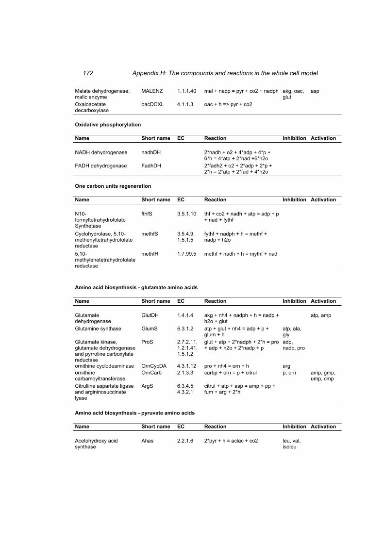
Appendix H: The compounds and reactions in the whole cell model 172
Malate dehydrogenase, malic enzyme
MALENZ 1.1.1.40 mal + nadp = pyr + co2 + nadph akg, oac, glut
asp
Oxaloacetate decarboxylase
oacDCXL 4.1.1.3 oac + h => pyr + co2
Oxidative phosphorylation
Name Short name EC Reaction Inhibition Activation NADH dehydrogenase nadhDH 2*nadh + o2 + 4*adp + 4*p +
6*h = 4*atp + 2*nad +6*h2o FADH dehydrogenase FadhDH 2*fadh2 + o2 + 2*adp + 2*p +
2*h = 2*atp + 2*fad + 4*h2o One carbon units regeneration
Name Short name EC Reaction Inhibition Activation N10-formyltetrahydrofolate Synthetase
fthfS 3.5.1.10 thf + co2 + nadh + atp = adp + p + nad + fythf
Cyclohydrolase, 5,10-methenyltetrahydrofolate reductase
methfS 3.5.4.9, 1.5.1.5
fythf + nadph + h = methf + nadp + h2o
5,10-methylenetetrahydrofolate reductase
methfR 1.7.99.5 methf + nadh + h = mythf + nad
Amino acid biosynthesis - glutamate amino acids
Name Short name EC Reaction Inhibition Activation Glutamatedehydrogenase
GlutDH 1.4.1.4 akg + nh4 + nadph + h = nadp + h2o + glut
atp, amp
Glutamine synthase GlumS 6.3.1.2 atp + glut + nh4 = adp + p + glum + h
atp, ala, gly
Glutamate kinase, glutamate dehydrogenase and pyrroline carboxylate reductase
ProS 2.7.2.11, 1.2.1.41,1.5.1.2
glut + atp + 2*nadph + 2*h = pro + adp + h2o + 2*nadp + p
adp,nadp, pro
ornithine cyclodeaminase OrnCycDA 4.3.1.12 pro + nh4 = orn + h arg ornithine carbamoyltransferase
OrnCarb 2.1.3.3 carbp + orn = p + citrul p, orn amp, gmp, ump, cmp
Citrulline aspartate ligase and argininosuccinate lyase
ArgS 6.3.4.5, 4.3.2.1
citrul + atp + asp = amp + pp + fum + arg + 2*h
Amino acid biosynthesis - pyruvate amino acids
Name Short name EC Reaction Inhibition Activation Acetohydroxy acid synthase
Ahas 2.2.1.6 2*pyr + h = aclac + co2 leu, val, isoleu
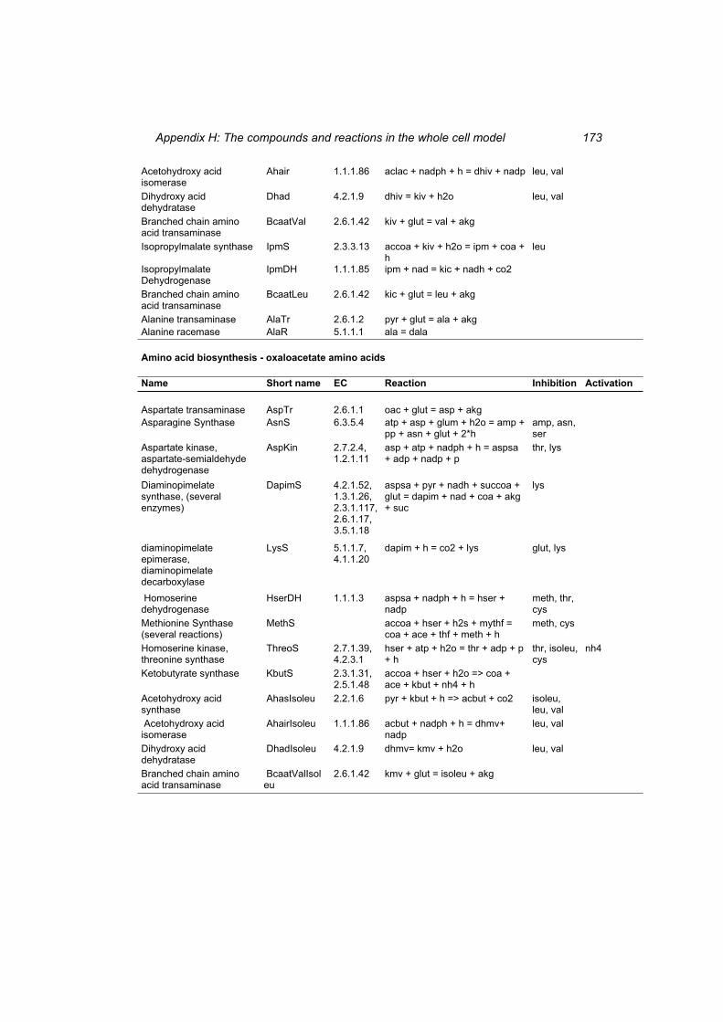
Appendix H: The compounds and reactions in the whole cell model 173
Acetohydroxy acid isomerase
Ahair 1.1.1.86 aclac + nadph + h = dhiv + nadp leu, val
Dihydroxy acid dehydratase
Dhad 4.2.1.9 dhiv = kiv + h2o leu, val
Branched chain amino acid transaminase
BcaatVal 2.6.1.42 kiv + glut = val + akg
Isopropylmalate synthase IpmS 2.3.3.13 accoa + kiv + h2o = ipm + coa + h
leu
Isopropylmalate Dehydrogenase
IpmDH 1.1.1.85 ipm + nad = kic + nadh + co2
Branched chain amino acid transaminase
BcaatLeu 2.6.1.42 kic + glut = leu + akg
Alanine transaminase AlaTr 2.6.1.2 pyr + glut = ala + akg Alanine racemase AlaR 5.1.1.1 ala = dala Amino acid biosynthesis - oxaloacetate amino acids
Name Short name EC Reaction Inhibition Activation Aspartate transaminase AspTr 2.6.1.1 oac + glut = asp + akg Asparagine Synthase AsnS 6.3.5.4 atp + asp + glum + h2o = amp +
pp + asn + glut + 2*h amp, asn, ser
Aspartate kinase, aspartate-semialdehyde dehydrogenase
AspKin 2.7.2.4, 1.2.1.11
asp + atp + nadph + h = aspsa + adp + nadp + p
thr, lys
Diaminopimelate synthase, (several enzymes)
DapimS 4.2.1.52, 1.3.1.26,2.3.1.117,2.6.1.17,3.5.1.18
aspsa + pyr + nadh + succoa + glut = dapim + nad + coa + akg + suc
lys
diaminopimelate epimerase, diaminopimelate decarboxylase
LysS 5.1.1.7, 4.1.1.20
dapim + h = co2 + lys glut, lys
Homoserine dehydrogenase
HserDH 1.1.1.3 aspsa + nadph + h = hser + nadp
meth, thr, cys
Methionine Synthase (several reactions)
MethS accoa + hser + h2s + mythf = coa + ace + thf + meth + h
meth, cys
Homoserine kinase, threonine synthase
ThreoS 2.7.1.39, 4.2.3.1
hser + atp + h2o = thr + adp + p + h
thr, isoleu, cys
nh4
Ketobutyrate synthase KbutS 2.3.1.31, 2.5.1.48
accoa + hser + h2o => coa + ace + kbut + nh4 + h
Acetohydroxy acid synthase
AhasIsoleu 2.2.1.6 pyr + kbut + h => acbut + co2 isoleu, leu, val
Acetohydroxy acid isomerase
AhairIsoleu 1.1.1.86 acbut + nadph + h = dhmv+ nadp
leu, val
Dihydroxy acid dehydratase
DhadIsoleu 4.2.1.9 dhmv= kmv + h2o leu, val
Branched chain amino acid transaminase
BcaatValIsol eu
2.6.1.42 kmv + glut = isoleu + akg
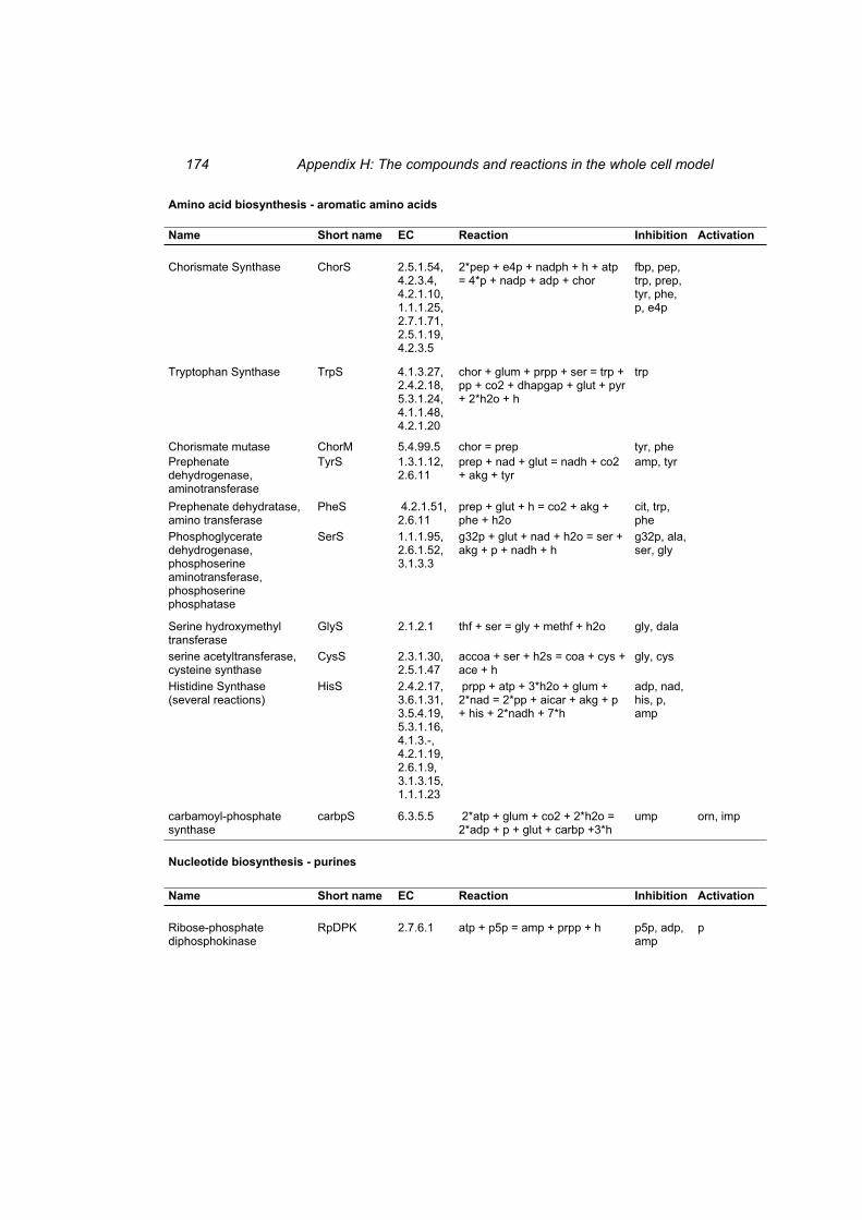
Appendix H: The compounds and reactions in the whole cell model 174
Amino acid biosynthesis - aromatic amino acids
Name Short name EC Reaction Inhibition Activation Chorismate Synthase ChorS 2.5.1.54,
4.2.3.4,4.2.1.10,1.1.1.25,2.7.1.71,2.5.1.19,4.2.3.5
2*pep + e4p + nadph + h + atp = 4*p + nadp + adp + chor
fbp, pep, trp, prep, tyr, phe, p, e4p
Tryptophan Synthase TrpS 4.1.3.27, 2.4.2.18,5.3.1.24,4.1.1.48,4.2.1.20
chor + glum + prpp + ser = trp + pp + co2 + dhapgap + glut + pyr + 2*h2o + h
trp
Chorismate mutase ChorM 5.4.99.5 chor = prep tyr, phe Prephenate dehydrogenase, aminotransferase
TyrS 1.3.1.12, 2.6.11
prep + nad + glut = nadh + co2 + akg + tyr
amp, tyr
Prephenate dehydratase, amino transferase
PheS 4.2.1.51, 2.6.11
prep + glut + h = co2 + akg + phe + h2o
cit, trp, phe
Phosphoglycerate dehydrogenase, phosphoserine aminotransferase, phosphoserine phosphatase
SerS 1.1.1.95, 2.6.1.52,3.1.3.3
g32p + glut + nad + h2o = ser + akg + p + nadh + h
g32p, ala, ser, gly
Serine hydroxymethyl transferase
GlyS 2.1.2.1 thf + ser = gly + methf + h2o gly, dala
serine acetyltransferase, cysteine synthase
CysS 2.3.1.30, 2.5.1.47
accoa + ser + h2s = coa + cys + ace + h
gly, cys
Histidine Synthase (several reactions)
HisS 2.4.2.17, 3.6.1.31,3.5.4.19,5.3.1.16,4.1.3.-,4.2.1.19,2.6.1.9,3.1.3.15,1.1.1.23
prpp + atp + 3*h2o + glum + 2*nad = 2*pp + aicar + akg + p + his + 2*nadh + 7*h
adp, nad, his, p, amp
carbamoyl-phosphate synthase
carbpS 6.3.5.5 2*atp + glum + co2 + 2*h2o = 2*adp + p + glut + carbp +3*h
ump orn, imp
Nucleotide biosynthesis - purines
Name Short name EC Reaction Inhibition Activation Ribose-phosphate diphosphokinase
RpDPK 2.7.6.1 atp + p5p = amp + prpp + h p5p, adp, amp
p
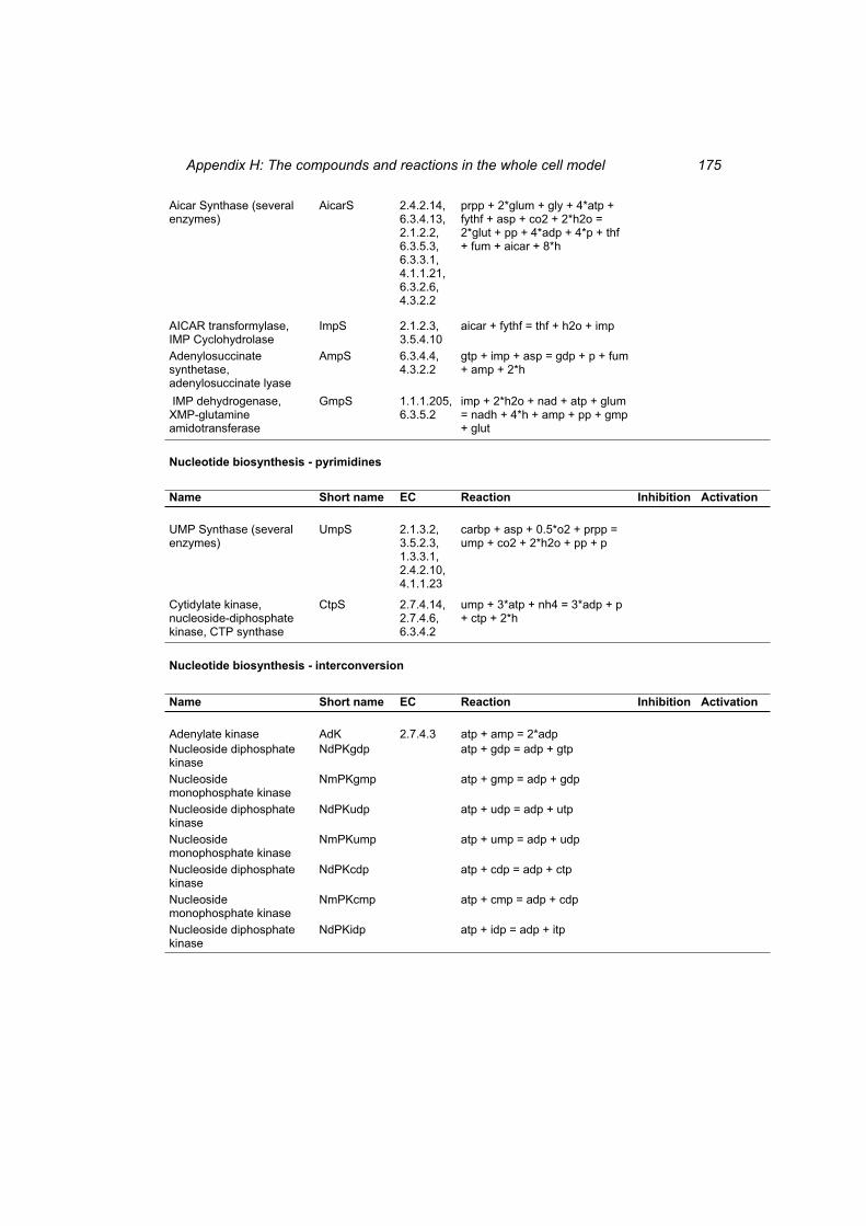
Appendix H: The compounds and reactions in the whole cell model 175
Aicar Synthase (several enzymes)
AicarS 2.4.2.14, 6.3.4.13,2.1.2.2,6.3.5.3,6.3.3.1,4.1.1.21,6.3.2.6,4.3.2.2
prpp + 2*glum + gly + 4*atp + fythf + asp + co2 + 2*h2o = 2*glut + pp + 4*adp + 4*p + thf + fum + aicar + 8*h
AICAR transformylase, IMP Cyclohydrolase
ImpS 2.1.2.3, 3.5.4.10
aicar + fythf = thf + h2o + imp
Adenylosuccinate synthetase, adenylosuccinate lyase
AmpS 6.3.4.4, 4.3.2.2
gtp + imp + asp = gdp + p + fum + amp + 2*h
IMP dehydrogenase, XMP-glutamine amidotransferase
GmpS 1.1.1.205, 6.3.5.2
imp + 2*h2o + nad + atp + glum = nadh + 4*h + amp + pp + gmp + glut
Nucleotide biosynthesis - pyrimidines
Name Short name EC Reaction Inhibition Activation UMP Synthase (several enzymes)
UmpS 2.1.3.2, 3.5.2.3,1.3.3.1,2.4.2.10,4.1.1.23
carbp + asp + 0.5*o2 + prpp = ump + co2 + 2*h2o + pp + p
Cytidylate kinase, nucleoside-diphosphate kinase, CTP synthase
CtpS 2.7.4.14, 2.7.4.6,6.3.4.2
ump + 3*atp + nh4 = 3*adp + p + ctp + 2*h
Nucleotide biosynthesis - interconversion
Name Short name EC Reaction Inhibition Activation Adenylate kinase AdK 2.7.4.3 atp + amp = 2*adp Nucleoside diphosphate kinase
NdPKgdp atp + gdp = adp + gtp
Nucleoside monophosphate kinase
NmPKgmp atp + gmp = adp + gdp
Nucleoside diphosphate kinase
NdPKudp atp + udp = adp + utp
Nucleoside monophosphate kinase
NmPKump atp + ump = adp + udp
Nucleoside diphosphate kinase
NdPKcdp atp + cdp = adp + ctp
Nucleoside monophosphate kinase
NmPKcmp atp + cmp = adp + cdp
Nucleoside diphosphate kinase
NdPKidp atp + idp = adp + itp
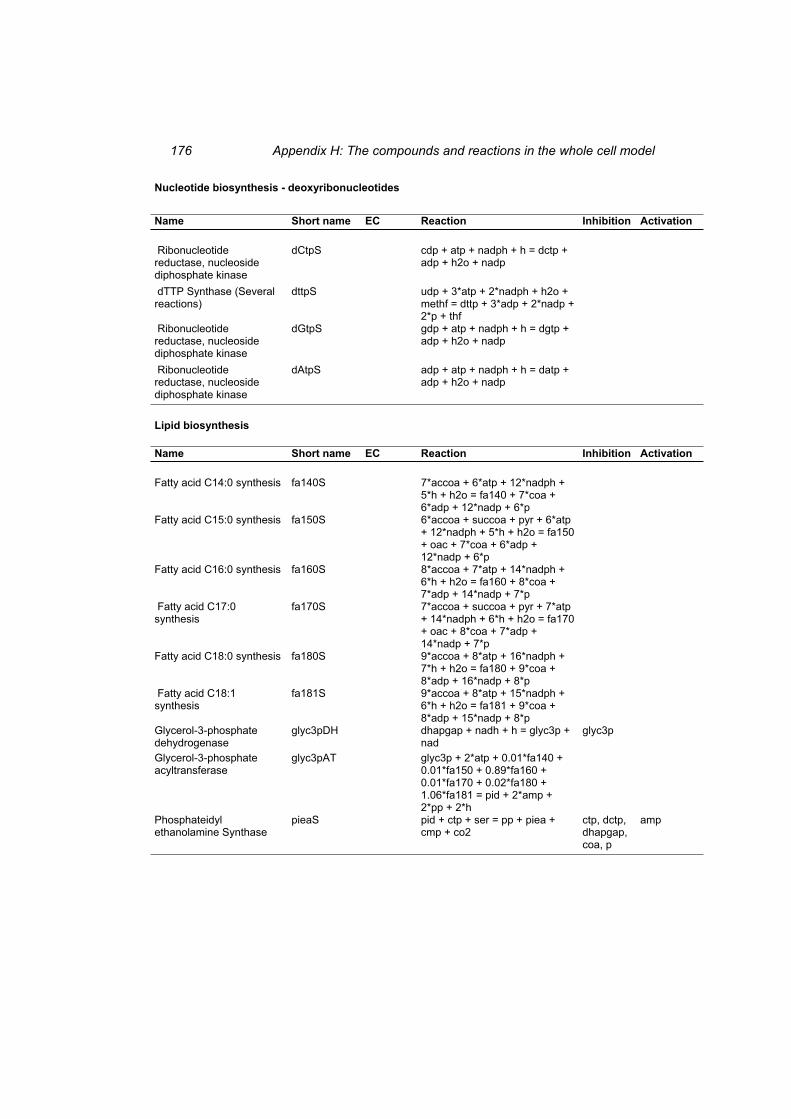
Appendix H: The compounds and reactions in the whole cell model 176
Nucleotide biosynthesis - deoxyribonucleotides
Name Short name EC Reaction Inhibition Activation Ribonucleotide reductase, nucleoside diphosphate kinase
dCtpS cdp + atp + nadph + h = dctp + adp + h2o + nadp
dTTP Synthase (Several reactions)
dttpS udp + 3*atp + 2*nadph + h2o + methf = dttp + 3*adp + 2*nadp + 2*p + thf
Ribonucleotide reductase, nucleoside diphosphate kinase
dGtpS gdp + atp + nadph + h = dgtp + adp + h2o + nadp
Ribonucleotide reductase, nucleoside diphosphate kinase
dAtpS adp + atp + nadph + h = datp + adp + h2o + nadp
Lipid biosynthesis
Name Short name EC Reaction Inhibition Activation Fatty acid C14:0 synthesis fa140S 7*accoa + 6*atp + 12*nadph +
5*h + h2o = fa140 + 7*coa + 6*adp + 12*nadp + 6*p
Fatty acid C15:0 synthesis fa150S 6*accoa + succoa + pyr + 6*atp + 12*nadph + 5*h + h2o = fa150 + oac + 7*coa + 6*adp + 12*nadp + 6*p
Fatty acid C16:0 synthesis fa160S 8*accoa + 7*atp + 14*nadph + 6*h + h2o = fa160 + 8*coa + 7*adp + 14*nadp + 7*p
Fatty acid C17:0 synthesis
fa170S 7*accoa + succoa + pyr + 7*atp + 14*nadph + 6*h + h2o = fa170 + oac + 8*coa + 7*adp + 14*nadp + 7*p
Fatty acid C18:0 synthesis fa180S 9*accoa + 8*atp + 16*nadph + 7*h + h2o = fa180 + 9*coa + 8*adp + 16*nadp + 8*p
Fatty acid C18:1 synthesis
fa181S 9*accoa + 8*atp + 15*nadph + 6*h + h2o = fa181 + 9*coa + 8*adp + 15*nadp + 8*p
Glycerol-3-phosphate dehydrogenase
glyc3pDH dhapgap + nadh + h = glyc3p + nad
glyc3p
Glycerol-3-phosphate acyltransferase
glyc3pAT glyc3p + 2*atp + 0.01*fa140 + 0.01*fa150 + 0.89*fa160 + 0.01*fa170 + 0.02*fa180 + 1.06*fa181 = pid + 2*amp + 2*pp + 2*h
Phosphateidyl ethanolamine Synthase
pieaS pid + ctp + ser = pp + piea + cmp + co2
ctp, dctp, dhapgap, coa, p
amp
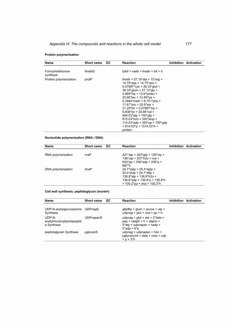
Appendix H: The compounds and reactions in the whole cell model 177
Protein polymerisation
Name Short name EC Reaction Inhibition Activation Formylmethionine synthese
fmethS fythf + meth = fmeth + thf + h
Protein polymerisation protP fmeth + 57.18*ala + 15*arg + 14.75*asp + 14.75*asn + 0.07887*cys + 38.33*glut + 38.33*glum + 27.13*gly + 4.969*his + 13.8*isoleu + 20.66*leu + 13.49*lys + 0.3944*meth + 9.701*phe + 11.67*pro + 20.9*ser + 21.29*thr + 0.07887*trp + 5.836*tyr + 20.66*val + 464.03*atp + 700*gtp + 815.03*h2o = 350*amp + 114.03*adp + 350*pp + 700*gdp + 814.03*p + 1514.03*h + protein
Nucleotide polymerisation (RNA / DNA)
Name Short name EC Reaction Inhibition Activation RNA polymerisation rnaP 421*atp + 203*gtp + 126*ctp +
136*utp + 257*h2o = rna + 630*pp + 256*adp + 256*p + 887*h
DNA polymerisation dnaP 24.7*datp + 25.4*dgtp + 25.4*dctp + 24.7*dttp + 136.8*atp + 136.8*h2o = 136.8*adp + 136.8*p + 136.8*h + 100.2*pp + dna + 100.2*h
Cell wall synthesis; peptidoglycan (murein)
Name Short name EC Reaction Inhibition Activation UDP-N-acetylglucosamine Synthase
UDPnagS g6pf6p + glum + accoa + utp = udpnag + glut + coa + pp + h
UDP-N-acetylmuramylpentapeptide Synthase
UDPnapenS udpnag + glut + ala + 2*dala + pep + nadph + h + dapim + 5*atp = udpnapen + nadp + 5*adp + 6*p
peptidoglycan Synthase pglycanS udpnag + udpnapen + h2o = pglycanunit + dala + ump + udp + p + 3*h
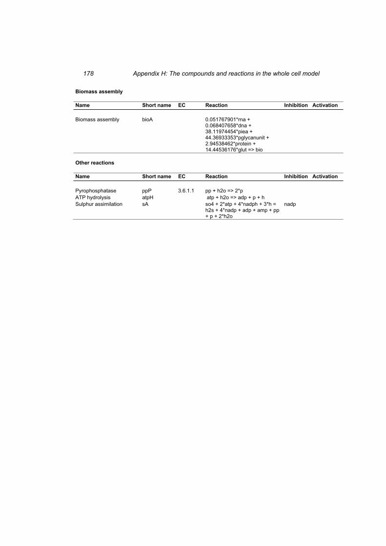
Appendix H: The compounds and reactions in the whole cell model 178
Biomass assembly
Name Short name EC Reaction Inhibition Activation Biomass assembly bioA 0.051767901*rna +
0.068407658*dna + 38.11974454*piea + 44.36933353*pglycanunit + 2.94538462*protein + 14.44536176*glut => bio
Other reactions
Name Short name EC Reaction Inhibition Activation Pyrophosphatase ppP 3.6.1.1 pp + h2o => 2*p ATP hydrolysis atpH atp + h2o => adp + p + h Sulphur assimilation sA so4 + 2*atp + 4*nadph + 3*h =
h2s + 4*nadp + adp + amp + pp + p + 2*h2o
nadp
Schriften des Forschungszentrums Jülich Reihe Lebenswissenschaften / Life Sciences
1. Toxizitätsprüfungen in Zellkulturen für eine Vorhersage der akuten Toxizität (LD50) zur Einsparung von Tierversuchen von W. Halle (1998), 92 Seiten ISBN: 978-3-89336-221-9
2. Die Rolle der Reaktionstechnik in der mikrobiellen Verfahrensentwicklung von D. Weuster-Botz (1999), II, 320 Seiten ISBN: 978-3-89336-245-5
3. Cell Culture Models as Alternatives to Animal Experimentation for the Testing of Neuroprotective Compounds in Stroke Research Practical Handbook of Methods edited by A. J. Carter, H. Kettenmann (1999), 144 pages ISBN: 978-3-89336-250-9
4. Action and Visuo-Spatial Attention Neurobiological Bases and Disorders Book of Abstracts collected by P. H. Weiss (2000), XIV, 56 pages ISBN: 978-3-89336-272-1
5. Genomweite Genexpressionsanalysen mit DNA-Chips zur Charakte-risierung des Glucose-Überflussmetabolismus von Escherichia coli von T. Polen (2003), 100 Seiten ISBN: 978-3-89336-337-7
6. Auslegung des Detektorsystems für einen hochauflösenden Positronen-Emissions-Tomographen mit hoher Sensitivität von U. Heinrichs (2003), IV, 238 Seiten ISBN: 978-3-89336-340-7
7. Biological Principles Applied to Technical Asymmetric Catalysis by A. Liese (2003), VI, 206 pages ISBN: 978-3-89336-344-5
8. ���������������� ��-Zusatzes für einen hochauflösenden Positronen-Emissions-Tomographen: Beispiel für ein multimodales bildgebendes System von M. Khodaverdi (2004), III, 162 Seiten ISBN: 978-3-89336-360-5
9. Bioprocess Development for the Generation of Monocyte-Derived Dendritic Cells: Applicability in Breast Cancer Immunotherapy by H.R. Bohnenkamp (2004), XLII, 128 pages ISBN: 978-3-89336-364-3
Schriften des Forschungszentrums Jülich Reihe Lebenswissenschaften / Life Sciences
10. Regulation der clp-Genexpression durch ClgR und Definition des ClgR-Regulons aus Corynebacterium glutamicum von S. Engels (2004), V, 125 Seiten ISBN: 978-3-89336-379-7
11. Metabolomanalyse zur Untersuchung der Dynamik im Aromaten-biosyntheseweg in L–Phenylalanin Produzenten von Escherichia coli von M. Oldiges (2005), XVI, 181 Seiten ISBN: 978-3-89336-380-3
12. Identifizierung und Charakterisierung eines Transkriptionsregulators der Aconitase von Corynebacterium glutamicum von A. Krug (2005), VI, 122 Seiten ISBN: 978-3-89336-382-7
13. Prozessentwicklung der elektroenzymatischen Sulfoxidation mit Chloroperoxidase von S. Lütz (2005), XIV, 178 Seiten ISBN: 978-3-89336-387-2
14. Export von Proteinen mit Zwillingsarginin-Signalsequenzen über den Tat-Weg in Escherichia coli von P. J. Kreutzenbeck (2005), 118 Seiten ISBN: 978-3-89336-388-9
15. Untersuchungen zur Fettsäure- und Zellwandsynthese sowie zur Glutamatbildung mit Corynebacterium glutamicum von E. Radmacher (2005), 130 Seiten ISBN: 978-3-89336-389-6
16. Monomodale und multimodale Registrierung von autoradiographischen und histologischen Bilddaten von A. Vieten (2005), 116 Seiten ISBN: 978-3-89336-390-2
17. Biosynthese von Phosphonaten: Charakterisierung des rekombinanten Enzyms Phosphonopyruvat-Decarboxylase aus Streptomyces viridochromogenes Tü494 von S. Johnen (2005), 128 Seiten ISBN: 978-3-89336-400-8
18. Ex-vivo Generierung von neutrophilen Zellen zur Prävention und Therapie der Sepsis von R. Herbold (2005), 202 Seiten ISBN: 978-3-89336-407-7
Schriften des Forschungszentrums Jülich Reihe Lebenswissenschaften / Life Sciences
19. Entwicklung eines Donor/Akzeptor-Konzeptes für die asymmetrische Synthese unsymmetrischer Benzoine mit Hilfe ThDP-abhängiger Enzyme von P. Dünkelmann (2005), 222 Seiten ISBN: 978-3-89336-408-4
20. Analyse der Bindungsspezifität der humanen Lck-SH3-Domäne anhand artifizieller und physiologischer Peptid-Liganden und strukturelle Charakterisierung dieser Peptide im Komplex mit SH3-Domänen von T. T. Tran (2005), 155 Seiten ISBN: 978-3-89336-412-1
21. Modeling Based Process Development of Fed-Batch Bioprocesses: L-Valine Production by Corynebacterium glutamicum by M. Brik Ternbach (2005), 202 pages ISBN: 978-3-89336-413-8
22. Charakterisierung der Ausscheidung von L-Glutamat bei Corynebacterium glutamicum von K. C. Stansen (2005), 151 Seiten ISBN: 978-3-89336-416-9
23. Metabolic and Bioprocess Engineering – a Fruitful Symbiosis by R.Takors (2005), 399 pages ISBN: 978-3-89336-420-6
24. Reaktionstechnische Untersuchungen zur enzymatischen de novo Synthese von GDP- -L-Fucose und der in situ Fucosylierung von Oligosacchariden von C. Hoh (2005), 240 Seiten ISBN: 978-3-89336-423-7
25. Humane Primärzellen als Feederzellen für die Kokultur mit hämatopoetischen Stammzellen aus Nabelschnurblut von A. S. Magin (2006), 206 Seiten ISBN: 978-3-89336-424-4
26. Vergleichende Analyse der Sec- und Tat-abhängigen sekretorischen Proteingewinnung mit Gram-positiven Bakterien als Wirtsorganismen von D. Meißner (2006), 140 Seiten ISBN: 978-3-89336-427-5
27. Energie- und Redoxstoffwechsel von Corynebacterium glutamicum von A. Kabus (2006), VI, 115 Seiten ISBN: 978-3-89336-439-8
28. NMR-Lösungsstruktur der humanen Hck SH3-Domäne im Komplex mit einem artifiziellen, hochaffinen Peptid-Liganden von H. Schmidt (2006), XII, 115 Seiten ISBN: 978-3-89336-441-1
Schriften des Forschungszentrums Jülich Reihe Lebenswissenschaften / Life Sciences
29. Entwicklung und Untersuchung eines Verfahrens zur integrierten Aufreinigung von Plasmid DNA mittels wässriger Zweiphasenextraktion von A. Frerix (2006), VII, 127 Seiten ISBN: 978-3-89336-442-8
30. Advanced Methods in Multiplexing Multi-Pinhole Imaging Design and Implementation of a High-Resolution and High-Sensitivity Small-Animal SPECT Imaging System by C. Lackas (2006), XX, 176 pages ISBN: 978-3-89336-451-0
31. Enantioselektive C-C Knüpfung mit Enzymen Charakterisierung und reaktionstechnische Bearbeitung der Benzaldehydlyase aus Pseudomonas fluorescens Biovar I von T. Stillger (2006), XIV, 146 Seiten ISBN: 978-3-89336-457-2
32. Echtzeitsystem für Phasenrücksetzanalysen und Neuro-Rückkopplungen am MEG von H. Rongen (2006), 176 Seiten ISBN: 978-3-89336-461-9
33. Analyse des Mechanismus der Phosphatregulation in Corynebacterium glutamicum von U. Sorger-Herrmann (2006), 117 Seiten ISBN: 978-3-89336-466-4
34. Enantioselective Reduction of Hydrophobic Keto Compounds in Multiphase Bioreactor by M. Villela Filho (2007), XVI, 196 pages ISBN: 978-3-89336-470-1
35. Untersuchung der Sec2-abhängigen Proteintranslokation in nicht-pathogenen Gram-positiven Bakterien von M. Caspers (2007), 164 Seiten ISBN: 978-3-89336-488-6
36. Regulation der Phosphatmangelgene von Corynebacterium glutamicum durch das Zweikomponenten-System PhoRS von S. Schaaf (2007), VI, 114 Seiten ISBN: 978-3-89336-496-1
37. Bioprozessentwicklung und in-situ Produktgewinnung von trans-Cyclohexadien-Derivaten von R. Bujnicki (2007), II, VIII, 163 Seiten ISBN: 978-3-89336-498-5
Schriften des Forschungszentrums Jülich Reihe Lebenswissenschaften / Life Sciences
38. Metabolic Engineering of the Valine Pathway in Corynebacterium glutamicum – Analysis and Modelling by J. B. Magnus (2007), XIX, 178 pages ISBN: 978-3-89336-499-2
LebenswissenschaftenLife Sciences
Band / Volume 38ISBN 978-3-89336-499-2 38
Leb
en
swis
sen
sch
aft
en
Life
Sci
en
ces
Jørg
en
Bars
ett
Mag
nu
sM
etab
olic
Eng
inee
ring
of
the
Valin
e Pa
thw
ay
LebenswissenschaftenLife Sciences
�������������� �������������������� �����������
�������������� �������������������� �����������
Metabolic Engineering of the Valine Pathwayin Corynebacterium glutamicum –Analysis and Modelling
Jørgen Barsett Magnus
Dr.-Ing. Jørgen Barsett Magnus studied Mathematics and Chemistry atthe University of Oslo and Chemical Engineering at the University ofManchester, Institute of Science and Technology (UMIST). He wrote hisMaster thesis at the Institute of Biochemical Engineering at the University ofStuttgart under the supervision of Klaus Mauch and Prof. Matthias Reuss.
In his thesis “Metabolic Engineering of the Valine Pathway in Corynebac-terium glutamicum – Analysis and Modelling” the functionality and dynamicsof the intracellular reaction network in C. glutamicum is investigated byusing metabolite concentration measurements, mathematical modelling,metabolic control analysis and thermodynamics.
Related Documents