Mesoscale simulation of spherulite growth during polymer crystallization by use of a cellular automaton

Acta Materialia 52 (2004) 2653–2664

www.actamat-journals.com

Mesoscale simulation of spherulite growth duringpolymer crystallization by use of a cellular automaton

D. Raabe *

Max-Planck-Institut f€ur Eisenforschung, Max-Planck-Str. 1, D€usseldorf 40237, Germany

Received 10 June 2003; received in revised form 26 January 2004; accepted 11 February 2004

Available online 16 March 2004

Abstract

The paper introduces a 3D cellular automaton model for the spatial and crystallographic prediction of spherulite growth phe-

nomena in polymers at the mesoscopic scale. The automaton is discrete in time, real space, and orientation space. The kinetics is

formulated according to the Hoffman–Lauritzen secondary surface nucleation and growth theory for spherulite expansion. It is used

to calculate the switching probability of each grid point as a function of its previous state and the state of the neighboring grid

points. The actual switching decision is made by evaluating the local switching probability using a Monte Carlo step. The growth

rule is scaled by the ratio of the local and the maximum interface energies, the local and maximum occurring Gibbs free energy of

transformation, the local and maximum occurring temperature, and by the spacing of the grid points. The use of experimental input

data provides a real time and space scale.

� 2004 Acta materialia Inc. Published by Elsevier Ltd. All rights reserved.

Keywords: Simulation; Texture; Polymer; Crystallization; Spherulite growth; Microstructure; Transformation; Avrami

1. Motivation for introducing a cellular automaton model

for spherulite growth

1.1. Basics of cellular microstructure automata

Cellular automata are algorithms that describe the

spatial and temporal evolution of complex systems byapplying local switching rules to the discrete cells of a

regular lattice [1]. Each cell is characterized in terms of

state variables which assume one out of a finite set of

states (such as crystalline or amorphous), but continu-

ous variable states are admissible as well (e.g., crystal

orientation) [2]. The opening state of an automaton is

defined by mapping the initial distribution of the values

of the chosen state variables onto the lattice. The dy-namical evolution of the automaton takes place through

the synchronous application of switching rules acting on

the state of each cell. These rules determine the state of a

lattice point as a function of its previous state and the

* Tel.: +49-211-679-2278; fax: +49-211-679-2333.

E-mail address: [email protected] (D. Raabe).

1359-6454/$30.00 � 2004 Acta materialia Inc. Published by Elsevier Ltd. Al

doi:10.1016/j.actamat.2004.02.013

state of the neighboring sites. The number, arrangement,

and range of the neighbor sites used by the switching

rule for calculating a state switch determines the range

of the interaction and the local shape of the areas which

evolve. After each discrete time interval the values of the

state variables are updated for all lattice points in syn-

chrony mapping the new (or unchanged) values assignedto them through the local rules. Owing to these features,

cellular automata provide a discrete method of simu-

lating the evolution of complex dynamical systems

which contain large numbers of similar components on

the basis of their local interactions. The basic rational of

cellular automata is to try to describe the evolution of

complex systems by simulating them on the basis of the

elementary dynamics of the interacting constituentsfollowing simple generic rules. In other words, the cel-

lular automaton approach pursues the goal to let the

global complexity of dynamical systems emerge by the

repeated interaction of local rules.

The cellular automaton method presented in this

paper is a tool for predicting microstructure, kinetics,

and texture of crystallizing polymers. It is formulated on

l rights reserved.

2654 D. Raabe / Acta Materialia 52 (2004) 2653–2664

the basis of a scaled version of the Hoffman–Lauritzen

rate theory for spherulite growth in partially crystalline

polymers and tracks the growth and impingement of

such spheres at the mesoscopic scale on a real time basis.

The major advantage of a discrete kinetic mesoscalemethod for the simulation of polymer crystallization

is that it considers material heterogeneity in terms of

crystallography, energy, and temperature, as opposed to

classical statistical approaches which are based on the

assumption of material homogeneity [2].

1.2. Cellular automaton models in physical metallurgy

Areas where microstructure-based cellular automa-

ton models have been successfully introduced are pri-

marily in the domain of physical metallurgy. Important

examples are static primary recrystallization and re-

covery [2–9], formation of dendritic grain structures in

solidification processes [10–13], as well as related nu-

cleation and coarsening phenomena [14–16]. Overviews

on cellular automata for materials and metallurgicalapplications are given in [2,17].

1.3. Previous models for polymer crystallization

Earlier approaches to the modeling of crystallization

processes in polymers were suggested and discussed in

detail by various groups. For instance Koscher and

Fulchiron [18] studied the influence of shear on poly-propylene crystallization experimentally and in terms of a

kinetic model for crystallization under quiescent condi-

tions. Their approachwas based on a classical topological

Avrami–Johnson–Mehl–Kolmogorov (AJMK) model

for isothermal conditions and on corresponding modifi-

cations such as those of Nakamura et al. [19] and Ozawa

[20] for non-isothermal conditions. The authors found in

part excellent agreement between these predictions andtheir own experimental data. For predicting crystalliza-

tion kinetics under shear conditions the authors used a

AJMK model in conjunction with a formulation for the

number of activated nuclei under the influence of shear.

The latter part of the approach was based on an earlier

study of Eder et al. [21,22] who expressed the number of

activated nuclei as a function of the square of the shear

rate which provides a possibility to predict the thicknessof thread-like precursors. A related approach was pub-

lished byHieber [23] who used theNakamura equation to

establish a direct relation between the Avrami and the

Ozawa crystallization rate constants.

AJMK-based transformation models have been ap-

plied to polymers with great success to cases where their

underlying assumptions of material homogeneity are

reasonably fulfilled [18–23]. It is, however, likely thatfurther progress in understanding and tailoring polymer

microstructures can be made by the introduction of

automaton models which are designed to cope with

more realistic boundary conditions by taking material

heterogeneity into account [24]. Important cases where

the application of cellular automata is conceivable in the

field of polymer crystallization are heterogeneous

spherulite formation and growth; heterogeneous topol-ogies and size distributions of spherulites; topological

and crystallographic effects arising from additives for

heterogeneous nucleation; lateral heterogeneity of the

crystallographic texture; overall crystallization kinetics

under complicated boundary conditions; reduction of

the spherulite size; randomization of the crystallo-

graphic texture; as well as effects arising from impurities

and temperature gradients.

2. Basic design of the cellular automaton model and

treatment of the crystallographic texture

The model for the mesoscale prediction of spherulite

growth in polymers is designed as a 3D cellular au-

tomaton model with a probabilistic switching rule. It isdiscrete in time, real space, and crystallographic orien-

tation space. It is defined on a cubic lattice considering

the three nearest neighbor shells for the calculation of

cell switches. The kinetics is formulated on the basis of

the Hoffman–Lauritzen rate theory for spherulite

growth. It is used to calculate the switching probability

of each grid point as a function of its previous state and

the state of the neighboring grid points. The actual de-cision about a switching event is made by evaluating the

local switching probability using a Monte Carlo step.

The growth rule is scaled by the ratio of the local and

the maximum possible interface properties, the local and

maximum occurring Gibbs free energy of transforma-

tion, the local and maximum occurring temperature,

and by the spacing of the grid points. The use of ex-

perimental input data allows one to make predictions ona real time and space scale. The transformation rule is

scalable to any mesh size and to any spectrum of in-

terface and transformation data. The state update of all

grid points is made in synchrony.

Independent variables of the automaton are time tand space x ¼ ðx1; x2; x3Þ. Space is discretized into an

array of cubic cells. The state of each cell is character-

ized in terms of the dependent field variables. These arethe temperature field, the phase state (amorphous matrix

or partially crystalline spherulite), the transformation

and interface energies, the crystallographic orientation

distribution of the crystalline nuclei f ðhÞ ¼ f ðhÞðu1;/;u2Þ, and the crystallographic orientation distri-

bution f ðgÞ ¼ f ðgÞðu1;/;u2Þ of one spherulite, where hand g are orientation matrices and u1;/;u2 are Euler

angles. The introduction of two variable fields for thetexture, h and g, deserves a more detailed explanation:

When analyzing crystallographic textures of partially

crystalline polymers it is useful to distinguish between

D. Raabe / Acta Materialia 52 (2004) 2653–2664 2655

different orientational scales. These are defined, first, by

the sample coordinate system; second, by the coordinate

system of the crystalline nuclei (where the incipient

crystal orientation is created by the direction of the

alignment of the first lamellae in case of homogeneousnucleation or by epitaxy effects in case of heterogeneous

nucleation); third, by the intrinsic helix angle of the

single lamellae according to the chain conformation;

and fourth, by the complete orientation distribution

function of one partially crystalline spherulite (Figs. 1

and 2). The latter orientation distribution function is

characterized by the orientational degrees of freedom

provided by the lamella helix angle as well as by orien-tational branching creating a complete orientation dis-

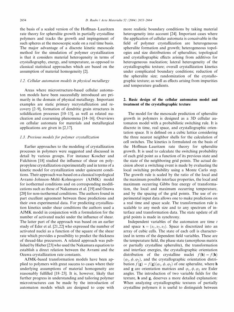
Fig. 1. Reference systems for polymer textures (polyethylene as an example

defined by normal, transverse, and longitudinal direction of the macroscopi

defined by the crystallographic orientation of the primary nucleus or by the

cleating agent. Finally, owing to the extensive branching of their internal c

entation but an orientation distribution. Further rotational degrees of fr

single lamella scale due to the molecular conformation of the constituent m

polyethylene).

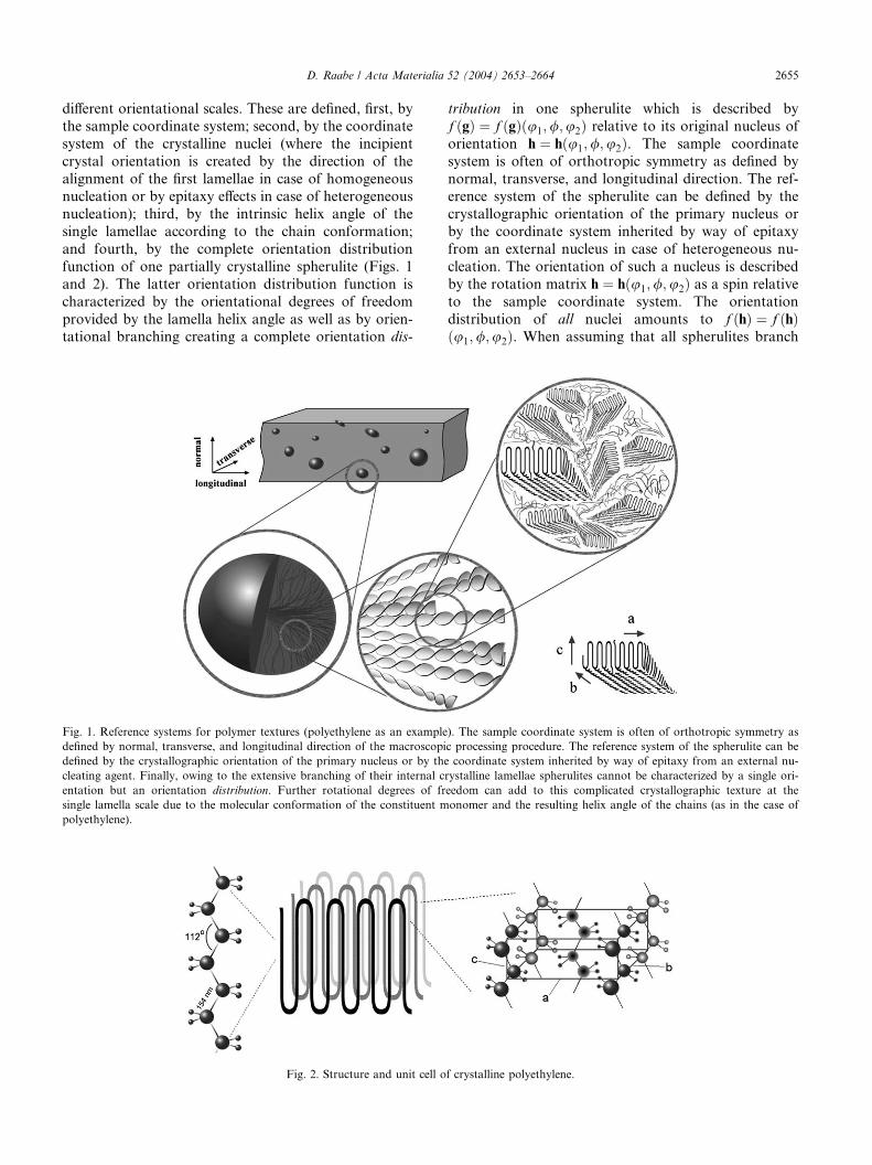
Fig. 2. Structure and unit cell o

tribution in one spherulite which is described by

f ðgÞ ¼ f ðgÞðu1;/;u2Þ relative to its original nucleus of

orientation h ¼ hðu1;/;u2Þ. The sample coordinate

system is often of orthotropic symmetry as defined by

normal, transverse, and longitudinal direction. The ref-erence system of the spherulite can be defined by the

crystallographic orientation of the primary nucleus or

by the coordinate system inherited by way of epitaxy

from an external nucleus in case of heterogeneous nu-

cleation. The orientation of such a nucleus is described

by the rotation matrix h ¼ hðu1;/;u2Þ as a spin relative

to the sample coordinate system. The orientation

distribution of all nuclei amounts to f ðhÞ ¼ f ðhÞðu1;/;u2Þ. When assuming that all spherulites branch

). The sample coordinate system is often of orthotropic symmetry as

c processing procedure. The reference system of the spherulite can be

coordinate system inherited by way of epitaxy from an external nu-

rystalline lamellae spherulites cannot be characterized by a single ori-

eedom can add to this complicated crystallographic texture at the

onomer and the resulting helix angle of the chains (as in the case of

f crystalline polyethylene.

2656 D. Raabe / Acta Materialia 52 (2004) 2653–2664

in a similar fashion, leading to a single-spherulite tex-

ture, f ðgÞ ¼ f ðgÞðu1;/;u2Þ, the total orientation

distribution of a bulk polymer can then be calculated

according to f ðhÞ � f ðgÞ.The current simulation takes a mesoscopic view at

this multi-scale problem, i.e., it does not provide a ge-

neric simulation of the texture evolution of a single

spherulite but includes only the orientation distribution

f ðhÞ ¼ f ðhÞðu1;/;u2Þ of the texture of the nuclei.

The driving force is the Gibbs free energy Gt per swit-

ched cell associated with the transformation. The starting

data, i.e., the mapping of the amorphous state, the tem-

perature field, and the spatial distribution of the Gibbsfree energy, must be provided by experiment or theory.

The kinetics of the automaton result from changes in

the state of the cells which are hereafter referred to as

cell switches. They occur in accord with a switching rule

which determines the individual switching probability of

each cell as a function of its previous state and the state

of its neighbor cells. The switching rule used in the

simulations discussed below is designed for the simula-tion of static crystallization of a quiescent supercooled

amorphous matrix. It reflects that the state of a non-

crystallized cell belonging to an amorphous region may

change due to the expansion of a crystallizing neighbor

spherulite which grows according to the local tempera-

ture, Gibbs free energy associated with that transfor-

mation, and interface properties. If such an expanding

spherulite sweeps a non-crystallized cell, the energy ofthat cell changes and a new orientation distribution is

assigned to it, namely that of the growing neighbor

spherulite.

3. Basic rate equation for spherulitic growth

In 1957 Keller [25] reported that polyethylene formedchainfolded lamellar crystals from solution. This dis-

covery was followed by the confirmation of the gener-

ality of this morphology, namely, that lamellar crystals

form upon crystallization, both from the solution and

from the melt [26] for a wide variety of polymers.

Most theories of polymer crystallization go back to

the work of Turnbull and Fisher [27] in which the rate of

nucleation is formulated in terms of the product of twoBoltzmann expressions, one quantifying the mobility of

the growth interface in terms of the activation energy for

motion, the other one involving the energy for second-

ary nucleation on existing crystalline lamellae. On the

basis of this pioneering work Hoffman and Lauritzen

developed a more detailed rate equation for spherulite

growth under consideration of secondary surface nu-

cleation [28]. Overviews on spherulite growth kineticswere given by Keller [29], Hoffman et al. [30], Snyder

and Marand [31,32], Hoffman and Miller [33], and Long

et al. [34].

The rate equation by Hoffman and Lauritzen is used

as a basis for the formulation of the switching rule of the

cellular automaton model. It describes growth interface

motion in terms of lateral and forward molecule align-

ment and disalignment processes at a homogeneousplanar portion of an interface segment between a semi-

crystalline spherulite and the amorphous matrix mate-

rial. It is important to note that the Hoffman and

Lauritzen rate theory is a coarse-grained formulation

which homogenizes over two rather independent sets of

very anisotropic mechanisms, namely, secondary nu-

cleation on the lateral surface of the growing lamellae

(creating strong lateral, i.e., out-of-plane volume ex-pansion and new texture components) and lamella

growth (creating essentially two-dimensional, i.e., in-

plane expansion and texture continuation). Although

the two basic ingredients of this rate formulation are

individually of a highly anisotropic character the overall

spherulite equation is typically used in an isotropic

form. The basic rate equation is

_x ¼ _xp exp

�� Q�

RðT � T1Þ

�exp

�� Kg

TDT

�; ð1Þ

where _x is the velocity vector of the interface between

the spherulite and the supercooled amorphous matrix,_xp is the pre-exponential velocity vector, DT the super-

cooling defined by DT ¼ T 0m � T , where T 0

m is the equi-librium melting point (valid for a very large crystal

formed from fully extended chains, no effect of free

surfaces), Q� is the activation energy for viscous mole-

cule flow or, respectively, attachment of the chain to the

crystalline surface, T1 is the temperature below which

all viscous flow stops (glass transition temperature,

temperature at which the viscosity exceeds the value of

1013 Ns/m2), Kg the secondary nucleation exponentand T the absolute temperature of the (computer)

experiment.

According to Hoffman and Lauritzen [28,30,33], the

exponent Kg amounts to

Kg ¼nbrreT 0

m

kBDGf

; ð2Þ

where kB is the Boltzmann constant, n a constant which

equals 4 for growth regimes I and III and 2 for growth

regime II [33,35], b is the thickness of a crystalline lattice

cell in growth direction (see Figs. 1 and 2), r is the free

energy per area for the interface between the lateral

surface and the supercooled melt, re is the free energyper area for the interface between the fold surface where

the molecule chains fold back or emerge from the la-

mella and the supercooled melt, and DGf is the Gibbs

free energy of fusion at the crystallization temperature

which is approximated by DGf � ðDHfDT Þ=Tm [28,

30,33].

The different growth regimes, I (shallow quench

regime), II (deep quench regime), and III (very deep

D. Raabe / Acta Materialia 52 (2004) 2653–2664 2657

quench regime), were discussed by Hoffman and Miller

[33] in the sense that within regime I of spherulite

growth the expansion of the spherulite is dominated by

weak secondary nucleation and preferred forward la-

mellae growth. Nucleation is in this regime dominatedby the formation of few single surface nuclei which are

referred to as stems. It is assumed that when one stem is

nucleated the entire new layer is almost instantaneously

completed relative to the nucleation rate. In regime II

the two rates are comparable. Regime II is the normal

condition for spherulitic growth. It has a weaker DTdependence than regime I. In regime III nucleation of

many nuclei occurs leading to disordered crystal growth.Nucleation is in this regime more important than

growth.

According to the work of Hoffman and Miller [33] the

pre-exponential velocity vector for an interface between

a spherulite and the supercooled amorphous matrix can

be modeled according to

_xp ¼ nN0bJ‘u

kBTbr

�� kBT2brþ abDGf

�; ð3Þ

where N0 is the number of initial stems, soon to be in-

volved in the first stem deposition process, n the unit

normal vector of the respective interface segment, and ‘uthe monomer length. J amounts to

J ¼ 1nz

kBTh

� �; ð4Þ

where 1 is a constant for the molecular friction experi-

enced by the chain as it is reeled onto the growth in-

terface, nz the number of molecular repeat units in the

chain, and h the Planck constant. The fraction kBT=hcan be interpreted as a frequency pre-factor. The pre-

exponential velocity vector can then be written

_xp ¼ nN0b1‘unz

kBTh

� �kBTbr

�� kBT2brþ abDGf

�ð5Þ

yielding a Hoffman–Lauritzen–Miller type version [33]of a velocity-rate vector equation for spherulite growth

under consideration of secondary nucleation

_x ¼ nN0b1‘unz

kBTh

� �kBTbr

�� kBT2brþ abDGf

�

� exp

�� Q�

R T � T1ð Þ

�exp

�� nbrreT 0

m

kBTDTDGf

�: ð6Þ

4. Using rate theory as a basis for the automaton model

4.1. Mapping the rate equation on a cellular automaton

mesh

For dealing with competing state changes affectingthe same lattice cell in a cellular automaton, the statis-

tical rate equation can be rendered into a probabilistic

analogue which allows one to calculate switching

probabilities for the states of the cellular automaton

cells [2]. For this purpose, the rate equation is separated

into a non-Boltzmann part, _x0, which depends com-

paratively weakly on temperature, and a Boltzmannpart, w, which depends exponentially on temperature

_x ¼ _x0w

¼ nN0b1‘unz

kBTh

� �kBTbr

�� kBT2brþ abDGf

�

� exp

�� Q�

R T � T1ð Þ

�exp

�� nbrreT 0

m

kBTDTDGf

�

with _x0 ¼ nN0b1‘unz

kBTh

� �kBTbr

�� kBT2brþ abDGf

�

and w ¼ exp

�� Q�

RðT � T1Þ

�exp

�� nbrreT 0

m

kBTDTDGf

�:

ð7Þ

The Boltzmann factors, w, represent the probability for

cell switches. According to this equation non-vanishing

switching probabilities occur for cells with different

temperatures and/or transformation energies. The au-

tomaton considers the first, second (2D), and third (3D)

neighbor shell for the calculation of the switchingprobability acting on a cell. The local value of the

switching probability may in principal depend on the

crystallographic character of the interfaces entering via

the interface energies in the secondary nucleation term.

The current simulation does, however, not account for

this potential source of anisotropy but assumes constant

values for the interface energies of the lateral and of the

fold interface.

4.2. The scaled and normalized switching probability

The cellular automaton is usually applied to starting

data which have a spatial resolution far above the

atomic scale. This means that the automaton grid may

have some mesh size km � b. If a moving boundary

segment sweeps a cell, the spherulite thus grows (orshrinks) by k3m rather than b3. Since the net velocity of

an interface segment (between a partially crystalline

spherulite and the amorphous matrix) must be inde-

pendent of the imposed value of km, an increase of the

jump width must lead to a corresponding decrease of the

grid attack frequency, i.e. to an increase of the charac-

teristic time step, and vice versa. For obtaining a scale-

independent interface velocity, the grid frequency mustbe chosen in a way to ensure that the attempted switch

of a cell of length km occurs with a frequency much

below the atomic attack frequency which attempts to

switch a cell of length b. Mapping the rate equation on

such an imposed grid which is characterized by an ex-

ternal scaling length (lattice parameter of the mesh) kmleads to the equation

2658 D. Raabe / Acta Materialia 52 (2004) 2653–2664

_x ¼ _x0w ¼ nðkmmÞw

with m ¼ N0b1km‘unz

kBTh

� �kBTbr

�� kBT2brþ abDGf

�; ð8Þ

where m is the eigenfrequency of the chosen mesh char-

acterized by the scaling length km.The eigenfrequency given by this equation represents

the attack frequency which is valid for one particular

interface with constant self-reproducing properties

moving in a constant temperature field. In order to in-

troduce the possibility of a whole spectrum of interfaceproperties (due to temperature fields and intrinsic in-

terface energy anisotropy) in one simulation it is nec-

essary to normalize this equation by a general grid

attack frequency m0 which is common to all interfaces in

the system rendering the above equation into

_x ¼ _x0w ¼ nkmm0mm0

� �w ¼ _x0

mm0

� �w ¼ _x0w; ð9Þ

where the normalized switching probability amounts

to

w ¼ mm0

� �exp

�� Q�

RðT � T1Þ

�exp

�� nbrreT 0

m

kBTDTDGf

�

¼ N0b1m0km‘unz

kBTh

� �kBTbr

�� kBT2brþ abDGf

�

� exp

�� Q�

RðT � T1Þ

�exp

�� nbrreT 0

m

kBTDTDGf

�: ð10Þ

The value of the normalization or grid attack frequency

m0 can be identified by using the plausible assumption

that the maximum occurring switching probability

cannot assume a state above one

wmax ¼ N0b1m0km‘unz

kBTmax

h

� �kBTmax

brmin

�� kBTmax

2brmin þ abDGf

�

� exp

�� Q�

R Tmax � T1ð Þ

�

� exp

�� nbrminre;minT 0

m

kBTmaxDTmaxDGf;max

�6

!

1; ð11Þ

where Tmax is the maximum occurring temperature in the

system, DTmax the maximum occurring supercooling,rmin the minimum occurring lateral interface energy (for

instance in cases where a crystallographic orientation

dependence of the interface energy exists), DGf;max the

maximum Gibbs free transformation energy which de-

pends on the local temperature, i.e. DGf ;max �ðDHDTmaxÞ=T 0

m, and re;min the minimum occurring fold

interface energy.

With wmax ¼ 1 in the above equation one obtains thenormalization frequency, mmin

0 , as a function of the upper

bound input data.

mmin0 ¼ N0b1

km‘unz

kBTmax

h

� �kBTmax

brmin

�� kBTmax

2brmin þ abDGf

�

� exp

�� Q�

R Tmax � T1ð Þ

�

� exp

�� nbrminre;minT 0

m

kBTmaxDTmaxDGf ;max

�: ð12Þ

This frequency must only be calculated once per simu-

lation. It normalizes all other switching processes.

Inserting this basic attack frequency of the grid into

Eq. (10) yields an expression for calculating the local

values of the switching probability as a function of

temperature and energy

wlocal¼ TlocalTmax

� � kBTlocalbrlocal

� kBTlocal2brlocalþabDGf ;local

h ikBTmax

brmin� kBTmax

2brminþabDGf ;max

h i�exp

�� Q�

R

� �1

Tlocal�T1ð Þ

��� 1

Tmax�T1ð Þ

���

�exp

�� nbT 0

m

kB

� �rlocalre;local

TlocalDTlocalDGf;local

��

� rminre;min

TmaxDTmaxDGf;max

���: ð13Þ

This expression is the central switching equation of the

algorithm. The cellular automaton generally works in

such a way that an existing (expanding) spherulite in-

fects its neighbor cells at a rate or respectively proba-

bility which is determined by Eq. (13). This means that

wherever a partially crystalline spherulite has the topo-

logical possibility to expand into an amorphous neigh-bor cell the automaton rule uses Eq. (13) to quantify the

probability of that cell switch using the local state var-

iable data which characterize the two neighboring cells.

Eq. (13) reveals that local switching probabilities on

the basis of rate theory can be quantified in terms of

the ratio of the local and the maximum temperature and

the corresponding ratio of the interface properties. The

probability of the fastest occurring interface segment torealize a cell switch is exactly equal to 1. The above

equation also shows that the mesh size of the automaton

does not influence the switching probability but only the

time step elapsing during an attempted switch. The

characteristic time constant of the simulation Dt is

1=mmin0 .

In this context, the local switching probability can

also be regarded as the ratio of the distances that can beswept by the local interface and the interface with

maximum velocity, or as the number of time steps the

local interface needs to wait before crossing the en-

countered neighbor cell [6]. This reformulates the same

underlying problem, namely, that interfaces with dif-

ferent velocities cannot switch the state of the automa-

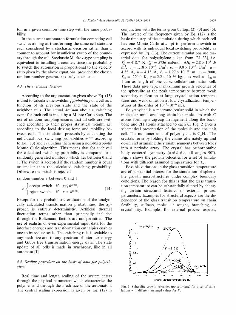
Fig. 3. Spherulite growth velocities (polyethylene) for a set of simu-

lations with different assumed values for T1.

D. Raabe / Acta Materialia 52 (2004) 2653–2664 2659

ton in a given common time step with the same proba-

bility.

In the current automaton formulation competing cell

switches aiming at transforming the same cell state are

each considered by a stochastic decision rather than acounter to account for insufficient sweep of the bound-

ary through the cell. Stochastic Markov-type sampling is

equivalent to installing a counter, since the probability

to switch the automaton is proportional to the velocity

ratio given by the above equations, provided the chosen

random number generator is truly stochastic.

4.3. The switching decision

According to the argumentation given above Eq. (13)

is used to calculate the switching probability of a cell as a

function of its previous state and the state of the

neighbor cells. The actual decision about a switching

event for each cell is made by a Monte Carlo step. The

use of random sampling ensures that all cells are swit-

ched according to their proper statistical weight, i.e.according to the local driving force and mobility be-

tween cells. The simulation proceeds by calculating the

individual local switching probabilities wlocal according

to Eq. (13) and evaluating them using a non-Metropolis

Monte Carlo algorithm. This means that for each cell

the calculated switching probability is compared to a

randomly generated number r which lies between 0 and

1. The switch is accepted if the random number is equalor smaller than the calculated switching probability.

Otherwise the switch is rejected

random number r between 0 and 1

� accept switch if r6 wlocal;

reject switch if r > wlocal:

(ð14Þ

Except for the probabilistic evaluation of the analyti-

cally calculated transformation probabilities, the ap-

proach is entirely deterministic. Artificial thermal

fluctuation terms other than principally included

through the Boltzmann factors are not permitted. The

use of realistic or even experimental input data for the

interface energies and transformation enthalpies enables

one to introduce scale. The switching rule is scalable toany mesh size and to any spectrum of interface energy

and Gibbs free transformation energy data. The state

update of all cells is made in synchrony, like in all

automata [1].

4.4. Scaling procedure on the basis of data for polyeth-

ylene

Real time and length scaling of the system enters

through the physical parameters which characterize the

polymer and through the mesh size of the automaton.

The central scaling expression is given by Eq. (12) in

conjunction with the terms given by Eqs. (2), (3) and (5).

The inverse of the frequency given by Eq. (12) is the

basic time step of the simulation during which each cell

has one Monte Carlo attempt to perform a switch in

accord with its individual local switching probability asexpressed by Eq. (13). The current simulations use ma-

terial data for polyethylene taken from [31–33], i.e.

T 0m ¼ 418:7 K, Q� ¼ 5736 cal/mol, DHf ¼ 2:8� 108 J/

m3, r ¼ 1:18� 10�2 J/m2, re ¼ 9:0� 10�2 J/m2, a ¼4:55 �A, b ¼ 4:15 �A, ‘u ¼ 1:27� 10�10 m, nz ¼ 2000,

T1 ¼ 220:0 K, 1 ¼ 2:2� 10�12 kg s, as well as km ¼1 lm as length of one cubic cellular automaton cell.

These data give typical maximum growth velocities ofthe spherulite at the peak temperature between weak

secondary nucleation at large crystallization tempera-

tures and weak diffusion at low crystallization temper-

atures of the order of 10�7–10�6 m/s.

Polyethylene is a macromolecular solid in which the

molecular units are long chain-like molecules with C

atoms forming a zig-zag arrangement along the back-

bone and 2H atoms attached to each C. Fig. 2 gives aschematical presentation of the molecule and the unit

cell. The monomer unit of polyethylene is C2H4. The

crystals form by folding the chains alternately up and

down and arranging the straight segments between folds

into a periodic array. The crystal has orthorhombic

body centered symmetry (a 6¼ b 6¼ c, all angles 90�).Fig. 3 shows the growth velocities for a set of simula-

tions with different assumed temperatures for T1.Possible variations in the glass transition temperature

are of substantial interest for the simulation of spheru-

lite growth microstructures under complex boundary

conditions. The reason for this is that the glass transi-

tion temperature can be substantially altered by chang-

ing certain structural features or external process

parameters. Examples for structural aspects are the de-

pendence of the glass transition temperature on chainflexibility, stiffness, molecular weight, branching, or

crystallinity. Examples for external process aspects,

2660 D. Raabe / Acta Materialia 52 (2004) 2653–2664

which in part drastically influence the aforementioned

structural state of the material, are accumulated elastic–

plastic deformation, externally imposed shear rates, or

the hydrostatic pressure.

4.5. Nucleation criteria

Two phenomenological approaches were used in the

simulations to treat nucleation, namely site-saturated

heterogeneous nucleation and constant homogeneous

nucleation. The calculations with site-saturated nucle-

ation condition were based on the assumption of ex-

ternal heterogeneous nucleation sites such as provided att ¼ 0 s by small impurities or nucleating agent particles.

The calculations with constant thermal nucleation were

conducted using the nucleation rate equation of Hoff-

man et al. [28,30].

5. Simulation results and discussion

5.1. Kinetics and spherulite structure for site-saturated

conditions

This section presents some 3D simulation results for

spherulite growth under the assumption of site-saturated

nucleation conditions using a cellular automaton with

10 million lattice cells. These standard conditions are

chosen to study the reliability of the new method withrespect to the kinetic exponents (comparison with the

analytical Avrami–Johnson–Mehl–Kolmogorov solu-

tion), to lattice effects (spatial discreteness), to topology,

and to statistics.

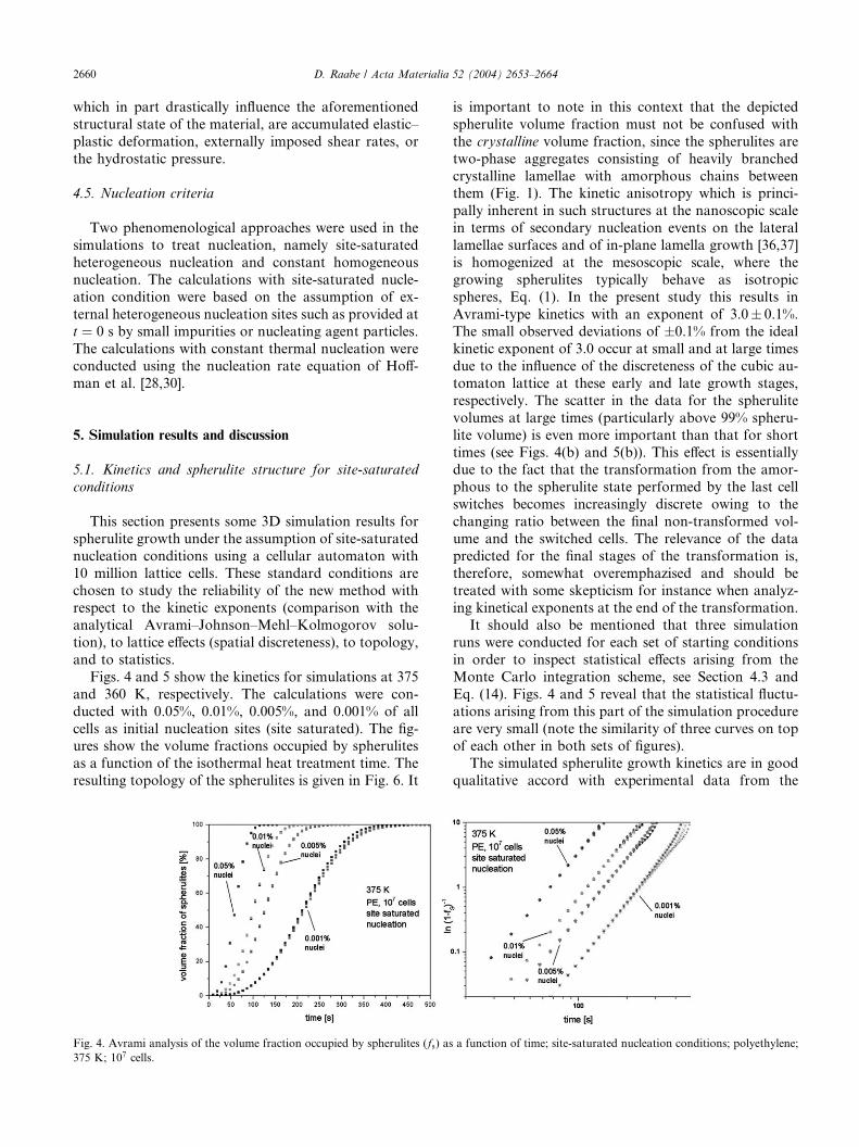
Figs. 4 and 5 show the kinetics for simulations at 375

and 360 K, respectively. The calculations were con-

ducted with 0.05%, 0.01%, 0.005%, and 0.001% of all

cells as initial nucleation sites (site saturated). The fig-ures show the volume fractions occupied by spherulites

as a function of the isothermal heat treatment time. The

resulting topology of the spherulites is given in Fig. 6. It

Fig. 4. Avrami analysis of the volume fraction occupied by spherulites (fs) as375 K; 107 cells.

is important to note in this context that the depicted

spherulite volume fraction must not be confused with

the crystalline volume fraction, since the spherulites are

two-phase aggregates consisting of heavily branched

crystalline lamellae with amorphous chains betweenthem (Fig. 1). The kinetic anisotropy which is princi-

pally inherent in such structures at the nanoscopic scale

in terms of secondary nucleation events on the lateral

lamellae surfaces and of in-plane lamella growth [36,37]

is homogenized at the mesoscopic scale, where the

growing spherulites typically behave as isotropic

spheres, Eq. (1). In the present study this results in

Avrami-type kinetics with an exponent of 3.0� 0.1%.The small observed deviations of �0.1% from the ideal

kinetic exponent of 3.0 occur at small and at large times

due to the influence of the discreteness of the cubic au-

tomaton lattice at these early and late growth stages,

respectively. The scatter in the data for the spherulite

volumes at large times (particularly above 99% spheru-

lite volume) is even more important than that for short

times (see Figs. 4(b) and 5(b)). This effect is essentiallydue to the fact that the transformation from the amor-

phous to the spherulite state performed by the last cell

switches becomes increasingly discrete owing to the

changing ratio between the final non-transformed vol-

ume and the switched cells. The relevance of the data

predicted for the final stages of the transformation is,

therefore, somewhat overemphazised and should be

treated with some skepticism for instance when analyz-ing kinetical exponents at the end of the transformation.

It should also be mentioned that three simulation

runs were conducted for each set of starting conditions

in order to inspect statistical effects arising from the

Monte Carlo integration scheme, see Section 4.3 and

Eq. (14). Figs. 4 and 5 reveal that the statistical fluctu-

ations arising from this part of the simulation procedure

are very small (note the similarity of three curves on topof each other in both sets of figures).

The simulated spherulite growth kinetics are in good

qualitative accord with experimental data from the

a function of time; site-saturated nucleation conditions; polyethylene;

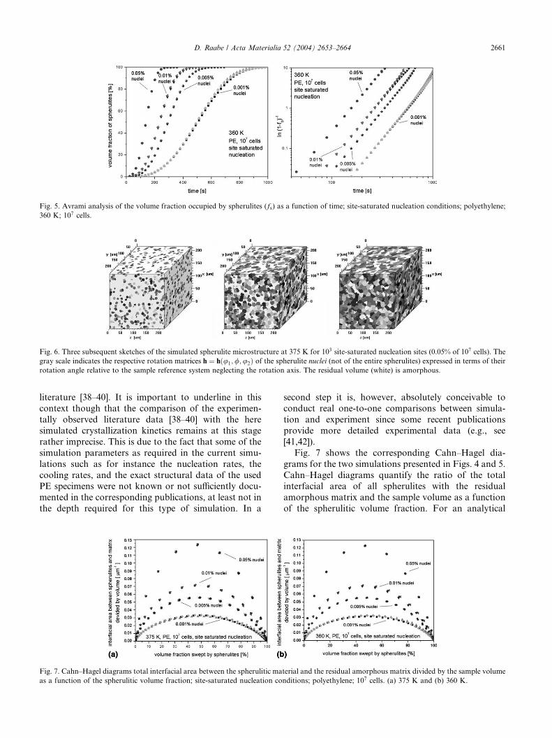
Fig. 5. Avrami analysis of the volume fraction occupied by spherulites (fs) as a function of time; site-saturated nucleation conditions; polyethylene;

360 K; 107 cells.

Fig. 6. Three subsequent sketches of the simulated spherulite microstructure at 375 K for 103 site-saturated nucleation sites (0.05% of 107 cells). The

gray scale indicates the respective rotation matrices h ¼ hðu1;/;u2Þ of the spherulite nuclei (not of the entire spherulites) expressed in terms of their

rotation angle relative to the sample reference system neglecting the rotation axis. The residual volume (white) is amorphous.

D. Raabe / Acta Materialia 52 (2004) 2653–2664 2661

literature [38–40]. It is important to underline in this

context though that the comparison of the experimen-

tally observed literature data [38–40] with the here

simulated crystallization kinetics remains at this stage

rather imprecise. This is due to the fact that some of the

simulation parameters as required in the current simu-

lations such as for instance the nucleation rates, the

cooling rates, and the exact structural data of the usedPE specimens were not known or not sufficiently docu-

mented in the corresponding publications, at least not in

the depth required for this type of simulation. In a

Fig. 7. Cahn–Hagel diagrams total interfacial area between the spherulitic ma

as a function of the spherulitic volume fraction; site-saturated nucleation co

second step it is, however, absolutely conceivable to

conduct real one-to-one comparisons between simula-

tion and experiment since some recent publications

provide more detailed experimental data (e.g., see

[41,42]).

Fig. 7 shows the corresponding Cahn–Hagel dia-

grams for the two simulations presented in Figs. 4 and 5.

Cahn–Hagel diagrams quantify the ratio of the totalinterfacial area of all spherulites with the residual

amorphous matrix and the sample volume as a function

of the spherulitic volume fraction. For an analytical

terial and the residual amorphous matrix divided by the sample volume

nditions; polyethylene; 107 cells. (a) 375 K and (b) 360 K.

2662 D. Raabe / Acta Materialia 52 (2004) 2653–2664

Avrami-type case and site-saturated conditions this

curve assumes a maximum at 50% spherulite growth

which is well fulfilled for the present simulations.

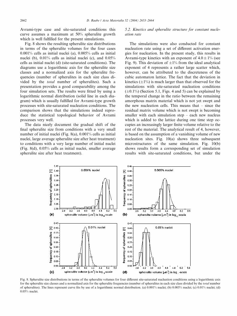
Fig. 8 shows the resulting spherulite size distributions

in terms of the spherulite volumes for the four cases0.001% cells as initial nuclei (a), 0.005% cells as initial

nuclei (b), 0.01% cells as initial nuclei (c), and 0.05%

cells as initial nuclei (d) (site-saturated conditions). The

diagrams use a logarithmic axis for the spherulite size

classes and a normalized axis for the spherulite fre-

quencies (number of spherulites in each size class di-

vided by the total number of spherulites). Such a

presentation provides a good comparability among thefour simulation sets. The results were fitted by using a

logarithmic normal distribution (solid line in each dia-

gram) which is usually fulfilled for Avrami-type growth

processes with site-saturated nucleation conditions. The

comparison shows that the simulations indeed repro-

duce the statistical topological behavior of Avrami

processes very well.

The data nicely document the gradual shift of thefinal spherulite size from conditions with a very small

number of initial nuclei (Fig. 8(a), 0.001% cells as initial

nuclei, large average spherulite size after heat treatment)

to conditions with a very large number of initial nuclei

(Fig. 8(d), 0.05% cells as initial nuclei, smaller average

spherulite size after heat treatment).

Fig. 8. Spherulite size distributions in terms of the spherulite volumes for fou

for the spherulite size classes and a normalized axis for the spherulite frequenc

of spherulites). The lines represent curve fits by use of a logarithmic normal

0.05% nuclei.

5.2. Kinetics and spherulite structure for constant nucle-

ation rate

The simulations were also conducted for constant

nucleation rate using a set of different activation ener-gies for nucleation. In the present study, this results in

Avrami-type kinetics with an exponent of 4.0� 1% (see

Fig. 9). This deviation of �1% from the ideal analytical

exponent of 4 represents a rather large scatter which,

however, can be attributed to the discreteness of the

cubic automaton lattice. The fact that the deviation in

kinetics (�1%) is much larger than that observed for the

simulations with site-saturated nucleation conditions(�0.1%) (Section 5.1, Figs. 4 and 5) can be explained by

the temporal change in the ratio between the remaining

amorphous matrix material which is not yet swept and

the new nucleation cells. This means that – since the

residual matrix volume which is not swept is becoming

smaller with each simulation step – each new nucleus

which is added to the lattice during one time step oc-

cupies an increasingly larger finite volume relative to therest of the material. The analytical result of 4, however,

is based on the assumption of a vanishing volume of new

nucleation sites. Fig. 10(a) shows three subsequent

microstructures of the same simulation. Fig. 10(b)

shows results form a corresponding set of simulation

results with site-saturated conditions, but under the

r different site-saturated nucleation conditions using a logarithmic axis

ies (number of spherulites in each size class divided by the total number

distribution. (a) 0.001% nuclei; (b) 0.005% nuclei; (c) 0.01% nuclei; (d)

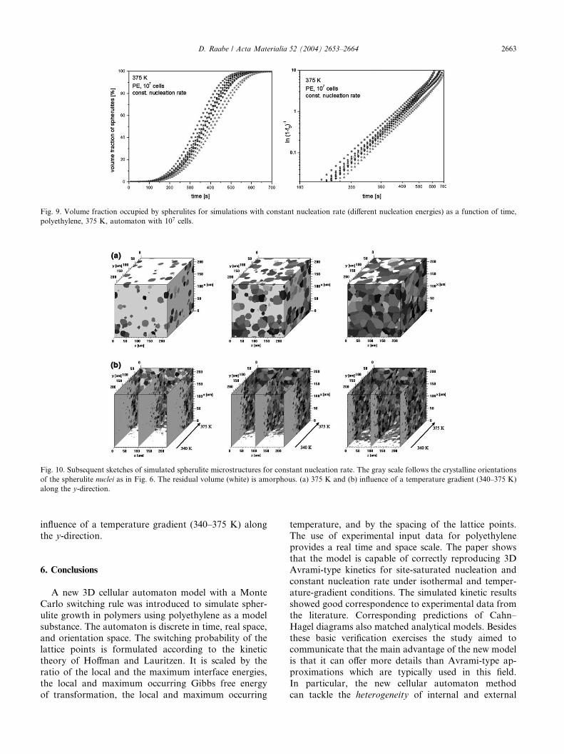
Fig. 9. Volume fraction occupied by spherulites for simulations with constant nucleation rate (different nucleation energies) as a function of time,

polyethylene, 375 K, automaton with 107 cells.

Fig. 10. Subsequent sketches of simulated spherulite microstructures for constant nucleation rate. The gray scale follows the crystalline orientations

of the spherulite nuclei as in Fig. 6. The residual volume (white) is amorphous. (a) 375 K and (b) influence of a temperature gradient (340–375 K)

along the y-direction.

D. Raabe / Acta Materialia 52 (2004) 2653–2664 2663

influence of a temperature gradient (340–375 K) along

the y-direction.

6. Conclusions

A new 3D cellular automaton model with a Monte

Carlo switching rule was introduced to simulate spher-

ulite growth in polymers using polyethylene as a model

substance. The automaton is discrete in time, real space,

and orientation space. The switching probability of thelattice points is formulated according to the kinetic

theory of Hoffman and Lauritzen. It is scaled by the

ratio of the local and the maximum interface energies,

the local and maximum occurring Gibbs free energy

of transformation, the local and maximum occurring

temperature, and by the spacing of the lattice points.

The use of experimental input data for polyethylene

provides a real time and space scale. The paper showsthat the model is capable of correctly reproducing 3D

Avrami-type kinetics for site-saturated nucleation and

constant nucleation rate under isothermal and temper-

ature-gradient conditions. The simulated kinetic results

showed good correspondence to experimental data from

the literature. Corresponding predictions of Cahn–

Hagel diagrams also matched analytical models. Besides

these basic verification exercises the study aimed tocommunicate that the main advantage of the new model

is that it can offer more details than Avrami-type ap-

proximations which are typically used in this field.

In particular, the new cellular automaton method

can tackle the heterogeneity of internal and external

2664 D. Raabe / Acta Materialia 52 (2004) 2653–2664

boundary and starting conditions which is not possible

for Avrami-models because they are statistical in nature.

The new automaton approach can for instance predict

intricate spherulite topologies, kinetic details, and crys-

tallographic textures in homogeneous or heterogeneousfields (the paper gives an example of spherulite growth

in a temperature gradient field). Furthermore, it can be

coupled to forming and processing models making use

of local rather than only global boundary conditions.

References

[1] von Neumann J. The general and logical theory of automata.

1963. In: Aspray W, Burks A, editors. Papers of John von

Neumann on Computing and Computer Theory. The Charles

Babbage Institute Reprint Series for the History of Computing,

vol. 12. MIT Press; 1987.

[2] Raabe D. Ann Rev Mater Res 2002;32:53.

[3] Hesselbarth HW, G€obel IR. Acta Metall 1991;39:2135.

[4] Pezzee CE, Dunand DC. Acta Metall 1994;42:1509.

[5] Davies CHJ. Scri Metall Mater 1995;33:1139.

[6] Marx V, Reher F, Gottstein G. Acta Mater 1998;47:1219.

[7] Raabe D. Philos Mag A 1999;79:2339.

[8] Raabe D, Becker R. Model Simul Mater Sci Eng 2000;8:445.

[9] Janssens KGF. Model Simul Mater Sci Eng 2003;11:157.

[10] Cortie MB. Metall Trans B 1993;24:1045.

[11] Brown SGR, Williams T, Spittle JA. Acta Metall 1994;42:2893.

[12] Gandin CA, Rappaz M. Acta Metall 1997;45:2187.

[13] Gandin CA, Desbiolles JL, Thevoz PA. Metall Mater Trans A

1999;30:3153.

[14] Spittle JA, Brown SGR. Acta Metall 1994;42:1811.

[15] Geiger J, Roosz A, Barkoczy P. Acta Mater 2001;49:623.

[16] Young MJ, Davies CHJ. Scri Mater 1999;41:697.

[17] Raabe D. Computational materials science. Weinheim: Wiley-

VCH; 1998.

[18] Koscher E, Fulchiron R. Polymer 2002;43:6931.

[19] Nakamura K, Watanabe K, Katayama K, Amano T. J Appl

Polym Sci 1972;16:1077.

[20] Ozawa T. Polymer 1971;12:150.

[21] Eder G, Janeschitz-Kriegl H. In: Cahn RW, Haasen P, Kramer

EJ, editors. Processing of polymers. Meijer HEH, editor. Mater

Sci Technol, vol. 18. VCH; 1997. p. 269 [chapter 5].

[22] Eder G, Janeschitz-Kriegl H, Krobath G. Progr Colloid Polym Sci

1989;80:1.

[23] Hieber CA. Polymer 1995;36:1455.

[24] Michaeli W, Hoffmann S, Cramer A, Dilthey U, Brandenburg A,

Kretschmer M. Adv Eng Mater 2003;5:133.

[25] Keller A. Philos Mag 1957;2:1171.

[26] Toda A, Keller A. Colloid Polym Sci 1993;271:328.

[27] Turnbull D, Fisher JC. J Chem Phys 1949;17:71.

[28] Lauritzen JI, Hoffman JD. J Res Natl Bur Stand 1960;64:73.

[29] Keller A. Rep Progr Phys 1968;31:623.

[30] Hoffman JD, Davis GT, Lauritzen JI. In: Hanney NB, editor.

Treatise of solid state chemistry. New York: Plenum Press; 1976.

p. 497 [chapter 7].

[31] Snyder CR, Marand H, Mansfield ML. Macromolecules

1996;29:7508.

[32] Snyder CR, Marand H. Macromolecules 1997;30:2759.

[33] Hoffman JD, Miller RL. Polymer 1997;38:3151.

[34] Long Y, Shanks RA, Stachurki ZH. Progr Polym Sci 1995;20:

651.

[35] Point JJ, Janimak JJ. J Cryst Growth 1993;131:501.

[36] Hobbs JK, Humphris ADL, Miles MJ. Macromolecules

2001;34:5508.

[37] Hobbs JK, McMaster TJ, Miles MJ, Barham PJ. Polymer

2001;39:2437.

[38] Cooper M, Manley RSJ. Macromolecules 1975;8:219.

[39] Leung WM, Manley RSJ, Panaras AR. Macromolecules

1985;18:760.

[40] Ergoz E, Fatou JG, Mandelkern L. Macromolecules 1972;5:

147.

[41] Supaphol P, Spruiell JE. J Appl Polym Sci 2002;86:1009.

[42] Zhu X, Li Y, Yan D, Fang Y. Polymer 2001;42:9217.