1 RESEARCH ARTICLE 10.1002/2014JC009820 Mesoscale eddy variability in the southern extension of the East Madagascar Current: Seasonal cycle, energy conversion terms, and eddy mean properties 2 Issufo Halo 1,2 , Pierrick Penven 3 , Bj€ orn Backeberg 1,2,4 , Isabelle Ansorge 2 , Frank Shillington 1,2 , 3 and Raymond Roman 2 4 1 Nansen-Tutu Centre for Marine Environmental Research, University of Cape Town, Cape Town, South Africa, 5 2 Department of Oceanography, MA-RE, University of Cape Town, Cape Town, South Africa, 3 LMI ICEMASA, Laboratoire de 6 Physique des Oc eans, Ifremer, UMR 6523, CNRS/IFREMER/IRD/UBO, Plouzan e, France, 4 Nansen Environmental and Remote 7 Sensing Centre, Bergen, Norway 8 Abstract In this study, we used more than 17 years of satellite altimetry observations and output from 9 an ocean model to investigate the mesoscale eddy variability and forcing mechanisms to the south of 10 Madagascar. Analysis of energy conversion terms in the model has shown seasonality on eddy formation, 11 both by barotropic and baroclinic instabilities: maximum in winter (JJA) and minimum in summer (DJF). The 12 eddies were mainly formed in the upper ocean (0–300 m) and at intermediate depths (800–2000 m) by bar- 13 otropic and baroclinic instabilities, respectively. The former dominated in the southeastern margin of Mada- 14 gascar, and the latter to the southwest, where the South-East Madagascar Current (SEMC) separates from 15 the continental shelf. Seasonality of the eddy formation appeared linked with the seasonal intensification of 16 the SEMC. The energy conversion terms indicated that the eddies have a significant contribution to the 17 large-scale circulation, but not being persistent throughout the year, occurring mainly during the fall season 18 (MAM). Eddy demography from altimetry and model provided information on eddy preferential sites for 19 birth, annual occurrence (6–13 per year), eddy mean diameter (124–178 km), mean amplitude (9–28 cm), 20 life-time (90–183 days), and maximum traveling distances (325–1052 km). Eddies formed to the southwest 21 of Madagascar exhibited distinct characteristics from those formed in the southeast. Nevertheless, all eddies 22 were highly nonlinear, suggesting that they are potential vectors of connectivity between Madagascar and 23 Africa. This may have a significant impact on the ecology of this region. 24 25 26 1. Introduction 27 The present description of the circulation in the southwest Indian Ocean, to the south of the Mozambique 28 Channel and the Madagascar Island is that sketched in Figure F1 1a. It involves two poleward western bound- 29 ary flows, the Agulhas Current (AC) at the southeast coast of South Africa, transporting 70 Sv (1Sv 5 10 6 m 30 s 23 ) in the upper 2000 m depth [Donohue et al., 2000; Lutjeharms, 2006], and the South-East Madagascar 31 Current (SEMC) at the southeast coast of Madagascar, carrying variable quantities 22 Sv in the upper 32 1500 m depth [Schott et al., 1988; Schott and McCreary, 2001], or larger 32–37 Sv [Nauw et al., 2008]. The 33 SEMC is a narrow current (width 120 km) with typical velocities of 1.1 m s 21 [Nauw et al., 2008], and 34 derives its waters from the westward South Equatorial Current (SEC) that splits between 17 S and 20 S at 35 the east coast of Madagascar [Lutjeharms et al., 1981, 2000; Chapman et al., 2003]. Direct observations of the 36 velocity field from a ship-mounted and lowered ADCP across four hydrographic sections perpendicular to 37 the SEMC, revealed the presence of an equatorward East Madagascar Undercurrent (EMUC), carrying 2.8 38 Sv [Nauw et al., 2008]. This undercurrent propagates at intermediate depths below the SEMC, and its core is 39 centered between 1100 and 1800 m depth [Nauw et al., 2008]. Another large-scale oceanographic feature 40 present in the region is the shallow northeastward South Indian Ocean Countercurrent (SICC) [Siedler et al., 41 2006; Palastanga et al., 2007]. It is located offshore of the SEMC, and transports 10 Sv in the upper 800 m 42 depth [Siedler et al., 2006] above SEC, along the 25 S latitude band [Palastanga et al., 2007]. 43 The AC and SEMC are separated by the Mozambique Basin (Figure 1a), and this region is characterized 44 by intense mesoscale activity (Figure 1b). Large cyclonic and anticyclonic eddies [Lutjeharms, 1988; Key Points: Two-distinct regions of enhanced mesoscale activity to the south of Madagascar Southwest (southeast) region dominated by baroclinic (barotropic) instability Eddies have potential to trap and transport material from Madagascar to Africa Correspondence to: I. Halo, [email protected] Citation: Halo, I., P. Penven, B. Backeberg, I. Ansorge, F. Shillington, and R. Roman (2014), Mesoscale eddy variability in the southern extension of the East Madagascar Current: Seasonal cycle, energy conversion terms, and eddy mean properties, J. Geophys. Res. Oceans, 119, doi:10.1002/ 2014JC009820. Received 16 JAN 2014 Accepted 10 SEP 2014 Accepted article online 18 SEP 2014 This is an open access article under the terms of the Creative Commons Attribution-NonCommercial-NoDerivs License, which permits use and distribution in any medium, provided the original work is properly cited, the use is non-commercial and no modifications or adaptations are made. HALO ET AL. V C 2014. The Authors. 1 Journal of Geophysical Research: Oceans PUBLICATIONS J_ID: JGRC Customer A_ID: JGRC20914 Cadmus Art: JGRC20914 Ed. Ref. No.: 2014JC009820RR Date: 23-September-14 Stage: Page: 1 ID: pachiyappanm Time: 20:15 I Path: //xinchnasjn/01Journals/Wiley/3b2/JGRC/Vol00000/140359/APPFile/JW-JGRC140359

Welcome message from author
This document is posted to help you gain knowledge. Please leave a comment to let me know what you think about it! Share it to your friends and learn new things together.
Transcript
1RESEARCH ARTICLE10.1002/2014JC009820
Mesoscale eddy variability in the southern extension of the
East Madagascar Current: Seasonal cycle, energy conversion
terms, and eddy mean properties
2Issufo Halo1,2, Pierrick Penven3, Bj€orn Backeberg1,2,4, Isabelle Ansorge2, Frank Shillington1,2,
3and Raymond Roman2
41Nansen-Tutu Centre for Marine Environmental Research, University of Cape Town, Cape Town, South Africa,
52Department of Oceanography, MA-RE, University of Cape Town, Cape Town, South Africa, 3LMI ICEMASA, Laboratoire de
6Physique des Oc�eans, Ifremer, UMR 6523, CNRS/IFREMER/IRD/UBO, Plouzan�e, France, 4Nansen Environmental and Remote
7Sensing Centre, Bergen, Norway
8Abstract In this study, we used more than 17 years of satellite altimetry observations and output from
9an ocean model to investigate the mesoscale eddy variability and forcing mechanisms to the south of
10Madagascar. Analysis of energy conversion terms in the model has shown seasonality on eddy formation,
11both by barotropic and baroclinic instabilities: maximum in winter (JJA) and minimum in summer (DJF). The
12eddies were mainly formed in the upper ocean (0–300 m) and at intermediate depths (800–2000 m) by bar-
13otropic and baroclinic instabilities, respectively. The former dominated in the southeastern margin of Mada-
14gascar, and the latter to the southwest, where the South-East Madagascar Current (SEMC) separates from
15the continental shelf. Seasonality of the eddy formation appeared linked with the seasonal intensification of
16the SEMC. The energy conversion terms indicated that the eddies have a significant contribution to the
17large-scale circulation, but not being persistent throughout the year, occurring mainly during the fall season
18(MAM). Eddy demography from altimetry and model provided information on eddy preferential sites for
19birth, annual occurrence (6–13 per year), eddy mean diameter (124–178 km), mean amplitude (9–28 cm),
20life-time (90–183 days), and maximum traveling distances (325–1052 km). Eddies formed to the southwest
21of Madagascar exhibited distinct characteristics from those formed in the southeast. Nevertheless, all eddies
22were highly nonlinear, suggesting that they are potential vectors of connectivity between Madagascar and
23
Africa. This may have a significant impact on the ecology of this region.
24
25
261. Introduction
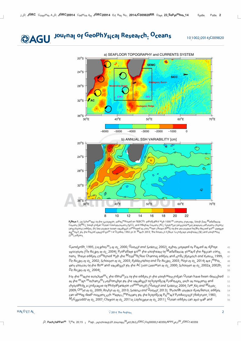
27The present description of the circulation in the southwest Indian Ocean, to the south of the Mozambique
28Channel and the Madagascar Island is that sketched in Figure F11a. It involves two poleward western bound-
29ary flows, the Agulhas Current (AC) at the southeast coast of South Africa, transporting �70 Sv (1Sv5 106 m
30s23) in the upper 2000 m depth [Donohue et al., 2000; Lutjeharms, 2006], and the South-East Madagascar
31Current (SEMC) at the southeast coast of Madagascar, carrying variable quantities �22 Sv in the upper
321500 m depth [Schott et al., 1988; Schott and McCreary, 2001], or larger �32–37 Sv [Nauw et al., 2008]. The
33SEMC is a narrow current (width �120 km) with typical velocities of �1.1 m s21 [Nauw et al., 2008], and
34derives its waters from the westward South Equatorial Current (SEC) that splits between 17�S and 20�S at
35the east coast of Madagascar [Lutjeharms et al., 1981, 2000; Chapman et al., 2003]. Direct observations of the
36velocity field from a ship-mounted and lowered ADCP across four hydrographic sections perpendicular to
37the SEMC, revealed the presence of an equatorward East Madagascar Undercurrent (EMUC), carrying �2.8
38Sv [Nauw et al., 2008]. This undercurrent propagates at intermediate depths below the SEMC, and its core is
39centered between 1100 and 1800 m depth [Nauw et al., 2008]. Another large-scale oceanographic feature
40present in the region is the shallow northeastward South Indian Ocean Countercurrent (SICC) [Siedler et al.,
412006; Palastanga et al., 2007]. It is located offshore of the SEMC, and transports �10 Sv in the upper 800 m
42depth [Siedler et al., 2006] above SEC, along the 25�S latitude band [Palastanga et al., 2007].
43The AC and SEMC are separated by the Mozambique Basin (Figure 1a), and this region is characterized
44by intense mesoscale activity (Figure 1b). Large cyclonic and anticyclonic eddies [Lutjeharms, 1988;
Key Points:
� Two-distinct regions of enhanced
mesoscale activity to the south of
Madagascar
� Southwest (southeast) region
dominated by baroclinic (barotropic)
instability
� Eddies have potential to trap and
transport material from Madagascar
to Africa
Correspondence to:
I. Halo,
Citation:
Halo, I., P. Penven, B. Backeberg, I.
Ansorge, F. Shillington, and R. Roman
(2014), Mesoscale eddy variability in
the southern extension of the East
Madagascar Current: Seasonal cycle,
energy conversion terms, and eddy
mean properties, J. Geophys. Res.
Oceans, 119, doi:10.1002/
2014JC009820.
Received 16 JAN 2014
Accepted 10 SEP 2014
Accepted article online 18 SEP 2014
This is an open access article under the
terms of the Creative Commons
Attribution-NonCommercial-NoDerivs
License, which permits use and
distribution in any medium, provided
the original work is properly cited, the
use is non-commercial and no
modifications or adaptations are
made.
HALO ET AL. VC 2014. The Authors. 1
Journal of Geophysical Research: Oceans
PUBLICATIONS
J_ID: JGRC Customer A_ID: JGRC20914 Cadmus Art: JGRC20914 Ed. Ref. No.: 2014JC009820RR Date: 23-September-14 Stage: Page: 1
ID: pachiyappanm Time: 20:15 I Path: //xinchnasjn/01Journals/Wiley/3b2/JGRC/Vol00000/140359/APPFile/JW-JGRC140359
45Gr€undlingh, 1995; Lutjeharms et al., 2000; Quartly and Srokosz, 2002], either isolated or paired as dipole
46structures [De Ruijter et al., 2004], propagate from the southeast of Madagascar toward the African conti-
47nent. These eddies combined with the Mozambique Channel eddies and rings [Biastoch and Krauss, 1999;
48De Ruijter et al., 2002; Schouten et al., 2003; Ridderinkhof and De Ruijter, 2003; Halo et al., 2014] are impor-
49tant sources of the flow and variability for the AC [van Leeuwen et al., 2000; Schouten et al., 2002a, 2002b;
50De Ruijter et al., 2004].
51For the marine ecosystems, the dynamics of the eddies in the southwest Indian Ocean have been described
52as the main mechanisms responsible for the variability of biological properties, such as nutrients and
53chlorophyll-a (indicative of phytoplankton community) [Quartly and Srokosz, 2004; Tew-Kai and Marsac,
542009; Omta et al., 2009; Roshin et al., 2010; Srokosz and Quartly, 2013]. Through surface divergence, eddies
55can upwell deep nutrient-rich waters important for the biological primary productivity [Robinson, 1983;
56McGillicuddy et al., 2007; Chelton et al., 2011a; Lathuiliere et al., 2011]. Ocean eddies can also trap and
Figure 1. (a) Schematic of the circulation, superimposed on GEBCO1 topography with 1000 m contour intervals. South-East Madagascar
Current (SEMC), South Indian Ocean Countercurrent (SICC), and Agulhas Current (AC). Clockwise (anticlockwise) features represent cyclonic
(anticyclonic) eddies. (b) Sea surface ocean variability computed as root mean square (RMS) of the sea surface height derived from satellite
altimetry, for the period starting from 14 October 1992 to 31 March 2010. The boxes in Figure 1a indicate southeast (SE) and southwest
(SW) regions.
J_ID: JGRC Customer A_ID: JGRC20914 Cadmus Art: JGRC20914 Ed. Ref. No.: 2014JC009820RR Date: 23-September-14 Stage: Page: 2
ID: pachiyappanm Time: 20:15 I Path: //xinchnasjn/01Journals/Wiley/3b2/JGRC/Vol00000/140359/APPFile/JW-JGRC140359
Journal of Geophysical Research: Oceans 10.1002/2014JC009820
HALO ET AL. VC 2014. The Authors. 2
57transport organic and inorganic materials over long distances [Robinson, 1983; Provenzale, 1999; Thorpe,
582007; Chelton et al., 2011b]. In line with these facts, it is thought that the eddies generated in the SEMC are
59potential vectors of connectivity of the marine fauna between Madagascar and KwaZulu-Natal, east coast of
60South Africa (M. Roberts, personal communication). AQ1A scientific research project termed ‘‘SuitCase’’ is
61ongoing with the aims to investigate the ecological linkages between the southeast of Madagascar and the
62east coast of South Africa (http://www.seaworld.org.za/research/entry/the-suitcase-project-eddies-as-poten-
63tial-vectors-of-connectivity-between-ma). In this study, we provide corroborative evidence based on long-
64term satellite altimetric observation and model output that suggests such connectivity occurs, especially by
65the cyclonic eddy features.
66Due to the paucity of in situ data, and an intense eddy field, the description of the circulation in this region
67is very complex, poorly understood, and to-date remains a subject of different interpretations: some arguing
68that the termination of the SEMC is a straight throughflow, as a main tributary to the Agulhas Current
69proper [Gr€undlingh, 1985; Tomczak and Godfrey, 1994; Quartly and Srokosz, 2004], while others suggest that
70it retroflects [Lutjeharms and Roberts, 1988; Lutjeharms, 1988; Quartly et al., 2006]. Later analysis of altimetry
71data and model output by Siedler et al. [2009], inferred that the flow pattern is composed by two main
72regimes: in one regime the SEMC flows mostly westward, closer to the southern Madagascar continental
73slope, where it originates a cyclonic recirculation, with cyclonic eddies being formed at the inshore edge of
74the flow. On the other hand, the second regime is characterized by the SEMC at the south of the Island
75propagating mostly south-westward direction, away from the Madagascar slope, and sheds an anticyclonic
76loop recirculation, which favors a retroflection of the SEMC. However, a more recent work suggests that
77none of these regimes are supported by hydrographic data, and neither retroflection of the SEMC nor con-
78tribution of the SEMC toward the SICC occurs [Ridderinkhof et al., 2013]. Here on the basis of model output,
79we infer that there is a significant contribution of the SEC toward SICC, induced by mesoscale eddy activity
80but not sustained throughout the year.
81While some studies have provided important information about the characteristics of the eddies formed in
82this region, such as mean size, amplitude, propagation speed [De Ruijter et al., 2004; Quartly et al., 2006; Sie-
83dler et al., 2009], yet detailed information in connection with their demographic properties at different
84scales is missing. Identification and tracking of eddies to study their demography is a complex process.
85Quartly and Srokosz [2002] used an automatic eddy detection method based on identification of SST
86anomalies greater than 0.4�C for anticyclones and smaller than20.4� for cyclones, within a 200 km box.
87The method can be sensitive to the threshold value of the SST anomaly. It can lose accuracy in the case of
88weak SST gradients. Quartly et al. [2006] used a second algorithm, based on the work of Isern-Fontanet et al.
89[2006]. This method is also sensitive to the choice of the threshold value for the vorticity field. De Ruijter
90et al. [2004] have used an empirical approach to follow in time and space eddies by visually identifying sur-
91face field of sea level anomalies from satellite altimetry (1995–2000). Their statistics of the dipole structures
92have shown that about four eddies per year were generated in the south of Madagascar: the eddies radii
93ranged from 50 to 200 km, both cyclones and anticyclones, and their amplitudes span from 0.21 to 0.48 cm,
94and propagation speeds varied between 5 and 10 cm s21. A manual eddy tracking can be sensitive to
95human subjectivity. Therefore, in this study we apply a robust automatic algorithm to assess more accu-
96rately detailed eddy characteristics.
97While two-distinct modes of variability differentiates the southeast from the southwest region of Madagas-
98car [Matano et al., 1999], little is known about property difference in eddy characteristics between these
99two regions. Therefore, in combination with altimetry observations, output from an eddy simulating
100regional ocean model is used to investigate such property difference. Furthermore, in situ data used here
101provide basic estimates of two cyclonic eddy structures on either sides of the southern Madagascar shelf,
102and the characteristics of the SEMC at 25�S. Thus, this study provides complementary information that
103enhances the present knowledge of eddy variability in this region. This is granted by both a longer altimetry
104time series (�20 year record) and improved skills of the algorithms to identify and track eddies [Chelton
105et al., 2011b; Halo et al., 2014].
106This paper is structured as follows: section 2 describes the observations and model used. Section 3 presents
107the validation of the model. Section 4 assesses the mechanisms of eddy formation and section 5 describes
108the eddy tracking algorithm. The results and discussion are presented in section 6. The main findings are
109summarized in section 7.
J_ID: JGRC Customer A_ID: JGRC20914 Cadmus Art: JGRC20914 Ed. Ref. No.: 2014JC009820RR Date: 23-September-14 Stage: Page: 3
ID: pachiyappanm Time: 20:15 I Path: //xinchnasjn/01Journals/Wiley/3b2/JGRC/Vol00000/140359/APPFile/JW-JGRC140359
Journal of Geophysical Research: Oceans 10.1002/2014JC009820
HALO ET AL. VC 2014. The Authors. 3
1102. Model and Observational Data
111In combination with altimetry and in situ data, we used the CNES-CLS09 product, and drifter data to validate
112the model field.
1132.1. Altimetry Data
114To make an assessment of the observed eddy variability and properties, we used gridded maps of absolute
115dynamic topography, which combines sea level anomaly observations merged from satellites Jason-1, Envi-
116sat, GFO, ERS-1, ERS-2, and Topex/Poseidon with the CNES-CLS09 mean dynamic topography (MDT). The
117altimetry data used here spans from 14 October 1992 to 31 March 2010. The product is globally gridded at
1181/4� 3 1/4� , every 7 days [Ducet et al., 2000], produced by Ssalto/Duacs and distributed globally by AVISO,
119with support from CNES. The data set is suitable to study the mesoscale ocean variability in the region south
120of Madagascar, where the first internal Rossby radius of deformation ranges from 60 km in the north to
12140 km in the south [Chelton et al., 1998].
1222.2. CNES-CLS09 Data
123To evaluate the model ocean current fields, we used the CNES-CLS09 data set [Rio et al., 2011], which represents
124surface geostrophic mean circulation. The data set is a global estimation of MDT, gridded at 1/4� 3 1/4�,
125computed from combination of the Gravity Recovery and Climate Experiment mission (GRACE), altimetric
126measurements, and oceanographic in situ data from 1993 to 2008, which includes all hydrographic profiles
127from Argo floats array [Rio et al., 2011]. The product is known to resolve stronger gradients in western
128boundary currents, being in better agreement with independent in situ observations, than other MDT esti-
129mates [Rio et al., 2011]. The data set is distributed by the French CNES-CLS.
1302.3. Hydrographic Data From the ASCLME Cruise
131To evaluate the model eddy vertical structure, we used in situ data from the first multidiscipline cruise of
132the Agulhas Somali Current Large Marine Ecosystem (ASCLME) project, carried out in August and Septem-
133ber 2008, on board of the r/v Fridtjof Nansen [Krakstad et al., 2008]. The vessel was equipped with a ship-
134mounted RD instruments 150 kHz ADCP which was used to obtain vertical profiles of current speed and
135direction in the upper layer (�300 m), and a Seabird 911plus CTD plus to obtain vertical profiles of tempera-
136ture, salinity, and oxygen at a maximum cast depth of 3000 m. The ADCP data used were 20 min ensembles
137with a depth bin length of 4 m. Navigation was provided by a Seapath DGPS system. Relating ADCP cur-
138rents to geostrophic velocities is somewhat complicated as ADCP currents include ageostrophic flows such
139as drift currents, tides, and internal waves or inertial oscillations. Donohue and Toole [2003] showed tidal
140influences of around 5 cm/s in southeast of Madagascar and in the Mozambique Channel. To remove baro-
141tropic tidal component, we used the tidal estimate provided by the OSU inverse tidal model, TPX08-atlas
142(http:volkov.oce.orst.edu/tides/tpxo8_atlas.html). Here we only used data collected in two transects
143because they intersected important oceanographic features of interest in this study: a cyclonic eddy at
14425�30S on the southwest coast of Madagascar, and a cyclonic eddy interacting with the SEMC at 25�S on
145the southeast coast.
1462.4. Drifter Data
147In combination with satellite altimetry to validate the model derived mesoscale activity, we also used
148quality-controlled velocity fields from satellite tracked surface drifting buoys [Niiler et al., 1995; Hansen and
149Poulain, 1996], from the Global Drifters Program. The drifters are drogued at 15 m depth following the
150mixed-layer currents [Lumpkin and Flament, 2007]. The velocity fields are derived at 6 hourly intervals using
151a 12 h centered differences of the interpolated positions [Lumpkin and Flament, 2013]. The data are known
152to allow a better spatial resolution of seasonal variations and ocean current fields [Lumpkin and Flament,
1532013]. The drifter measurements used here span from 1992 to 2012. During this period, a total of 215
154drifters entered in the region of study (20�E–70�E and 20�S–36�S), and were reinterpolated daily on a
1551/2� 3 1/2� grid.
1562.5. ROMS Model
157Model output provides a regular spatial and temporal sampling of the variables throughout the ocean col-
158umn at a desirable resolution, thus it allows for a more detailed study of eddies [Kurian et al., 2011; Chelton
159et al., 2011b]. Because of few in situ observations available in the region and limitation of satellite altimetry
J_ID: JGRC Customer A_ID: JGRC20914 Cadmus Art: JGRC20914 Ed. Ref. No.: 2014JC009820RR Date: 23-September-14 Stage: Page: 4
ID: pachiyappanm Time: 20:15 I Path: //xinchnasjn/01Journals/Wiley/3b2/JGRC/Vol00000/140359/APPFile/JW-JGRC140359
Journal of Geophysical Research: Oceans 10.1002/2014JC009820
HALO ET AL. VC 2014. The Authors. 4
160data only at sea surface, we used also model derived data to give insight on the mechanisms of eddy forma-
161tion in the water column. In fact, the assessment of eddy forcing mechanisms through energy transfer
162requires a vertical integration of the flow field components [Marchesiello et al., 2003]. Therefore, here we
163used the output from the South-West Indian Ocean Model (SWIM) configuration, which has been shown to
164provide a good representation of the main oceanographic features (hydrographic properties, mean circula-
165tion, the seasonal cycle, and the eddy variability) in the Mozambique Channel [Halo et al., 2014], and in the
166southwest Indian Ocean as a whole [Halo, 2012]. SWIM is based on the Regional Ocean Modelling Systems
167(ROMS) [Shchepetkin and McWilliams, 2005], and the configuration domain extends from 0�E to 77.5�E, and
168from 3�S to 47.5�S. It is forced at the surface by 1/2� 3 1/2� gridded climatological fields from COADS05
169[Da Silva et al., 1994], and at the lateral boundaries by 1� 3 1� gridded climatology from WOA05 [Conkright
170et al., 2002]. At the bottom, it uses the higher resolution topography from General Bathymetric Chart of the
171Oceans GEBCO1 [Carpine-Lancre et al., 2003]. The configuration runs at 1/5� horizontal grid resolution, with
17245-vertical sigma-layers, for 10 years. It has been spun-up for 3 years and the output is averaged at 2 day
173time steps. In this study, the ability of the model to reproduce the oceanographic features of the region
174south of Madagascar is further demonstrated in the next section. However, a detailed description and vali-
175dation of SWIM is presented by Halo [2012].
1763. Model Validation
177The ability of the model to reproduce the observed regional oceanographic features of the circulation is
178evaluated against formerly described observational data. Some published materials, such as that by Dono-
179hue and Toole [2003], Siedler et al. [2006], and Nauw et al. [2008] have been also used.
30oE 40
oE 50
oE 60
oE 70
oE
36oS
32oS
28oS
24oS
20oS
a) SSH [m] − CNES−CLS09
30oE 40
oE 50
oE 60
oE 70
oE
36oS
32oS
28oS
24oS
20oS
b) SSH [m] − SWIM
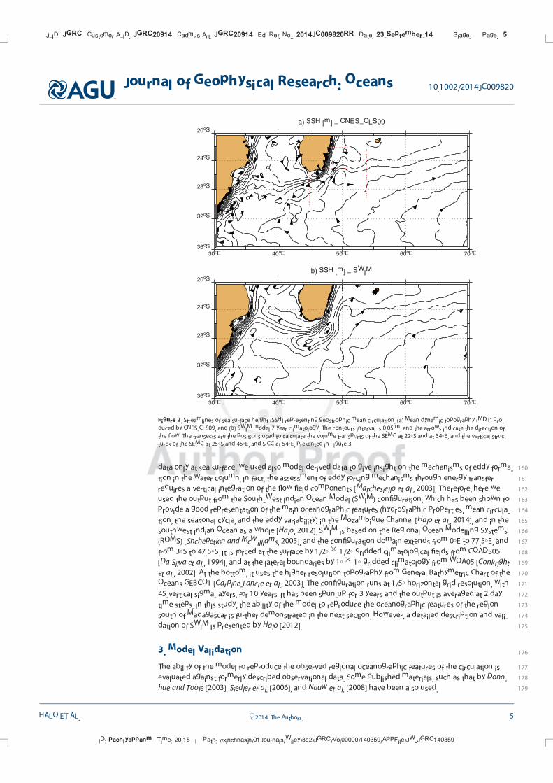
Figure 2. Streamlines of sea surface height (SSH) representing geostrophic mean circulation. (a) Mean dynamic topography (MDT) pro-
duced by CNES-CLS09, and (b) SWIM model 7 year climatology. The contours interval is 0.05 m, and the arrows indicate the direction of
the flow. The transects are the positions used to calculate the volume transports of the SEMC at 22�S and at 54�E, and the vertical struc-
tures of the SEMC at 25�S and 45�E, and SICC at 54�E, presented in Figure 3.
J_ID: JGRC Customer A_ID: JGRC20914 Cadmus Art: JGRC20914 Ed. Ref. No.: 2014JC009820RR Date: 23-September-14 Stage: Page: 5
ID: pachiyappanm Time: 20:15 I Path: //xinchnasjn/01Journals/Wiley/3b2/JGRC/Vol00000/140359/APPFile/JW-JGRC140359
Journal of Geophysical Research: Oceans 10.1002/2014JC009820
HALO ET AL. VC 2014. The Authors. 5
1803.1. Surface Geostrophic Mean Circulation
181Figure F22 shows streamlines of SSH (with 0.05 m contours interval) used as proxy for geostrophic mean
182ocean circulation. Figure 2a was derived from CNES-CLS09 data set and Figure 2b from the SWIM model,
183with stream arrows indicating the direction of flow. Similarities on the patterns of the streamlines in the
184model and observation are an indicative of convergency of results, which suggests that the model is reason-
185ably accurate. Similar features to be noticed (one may find more informative to compare it with Figure 1a)
186are: the presence of the SEMC at the southeast coast of Madagascar; and offshore of the SEMC the presence
187of the SICC flowing northeastward between 28�S and 24�S, which is consistent with results from Siedler
188et al. [2006] and Palastanga et al. [2007]. On reaching the southern tip of Madagascar, it is evident patterns
189of cyclonic recirculation inshore and anticyclonic recirculation offshore of the SEMC, which is in agreement
190with hydrographic observations by De Ruijter et al. [2004]. It is also evident that the flow from the South of
191Madagascar and the Mozambique Channel is sources of the Agulhas Current, furthering agreeing with the
192studies by Stramma and Lutjeharms [1997] and Lutjeharms [2006]. However, some differences between the
193model and observations are obvious, especially directly south of Madagascar, at the offshore edge of the
194SEMC, where the model (Figure 2b) shows stronger anticyclonic recirculation which appears to suggest a
195retroflection of the SEMC, that feeds the SICC as proposed by Siedler et al. [2009]. Note also that the model
196appears to reproduce a relatively weaker SEMC, and a stronger boundary flow at the African continent,
197between 28�S and 24�S (Figure 2b). The reason for such behavior is not clear. However, one has to bear in
198mind that the CNES-CLS09 product is known to reproduce stronger gradients of western boundary mean
199flows [Rio et al., 2011]. Stronger gradients produced by the model between 28�S and 24�S could be associ-
200ated to localized intense eddy activity (evident at the Delagoa Bight), which impacts the averaged field by
201producing a northward offshore component mostly depicted in Figure 2b.
Longitude [oE]
De
pth
[m
]
a) V (m s−1
) at −25o S SWIM
−0.5−0.45−0.4−0.35−0.3−0.25−0.2−0.15
−0.1
−0.05
0
0 0
0
0
0
0 0
0
0
0.05
0.05
0.05
0.05
0.1
0.1
0.15
0.15
0.2
0.2
0.25
0.25
0.3
0
0 0
0
0
47.5 48 48.5 49 49.5 50
−4000
−3000
−2000
−1000
0
−0.5
0
0.5
Latitude [oS]
De
pth
[m
]
b) U (m s−1
) at 45o E SWIM
−0.4−0.35
−0.3
−0.25
−0.2
−0.1
5
−0.1 −
0.1
−0.05
−0.0
5
−0.0
5
0
0
0
0
0
0
0
0
0 0
0
0
0
0
0
0
0
0
0.05
0.10.15
−32 −31 −30 −29 −28 −27 −26−2500
−2000
−1500
−1000
−500
0
−0.5
0
0.5
−29 −28 −27 −26 −25 −24 −23 −22−1500
−1000
−500
0
Latitude [oS]
De
pth
[m
]
c) U (m s−1
) at 54o E SWIM
0
0 000
0
0
0.050.1
−0.5
0
0.5
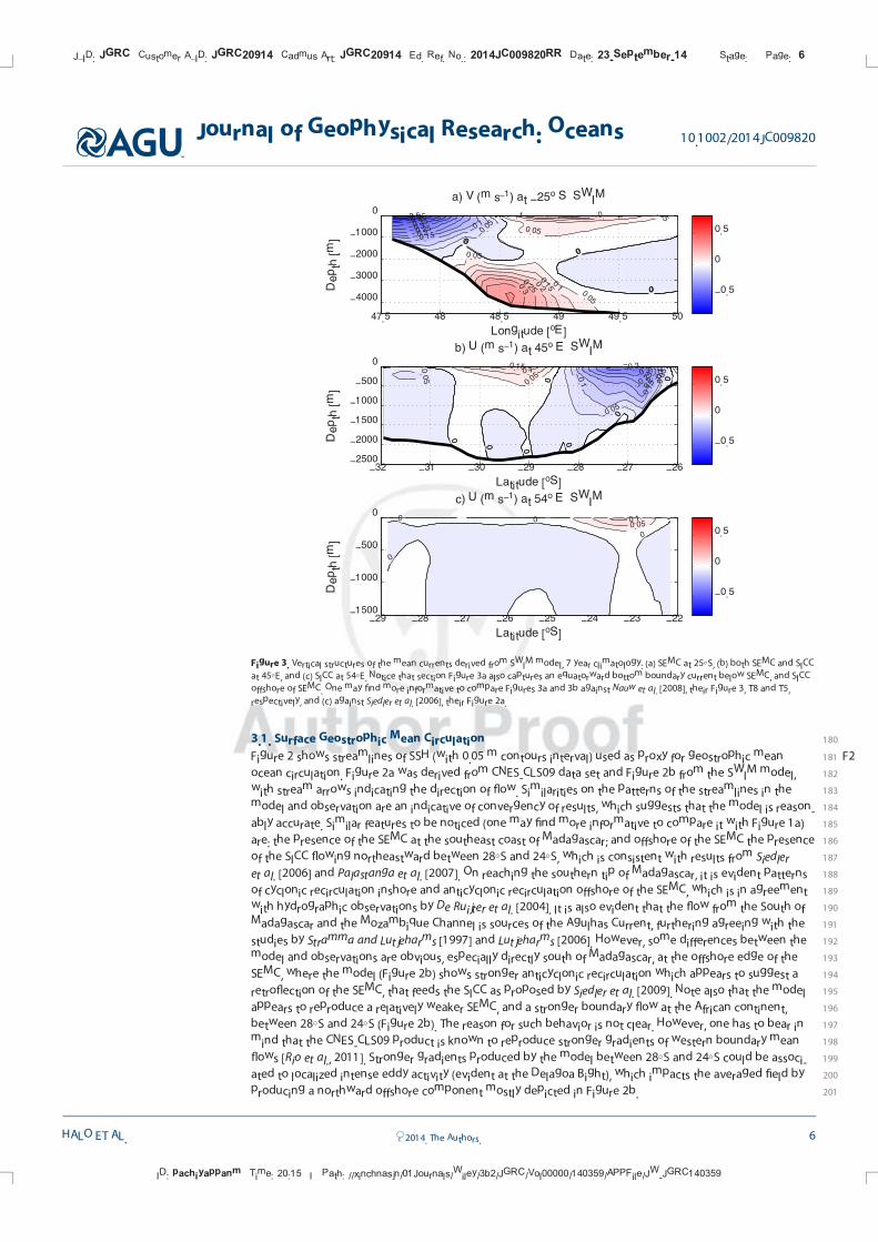
Figure 3. Vertical structures of the mean currents derived from SWIM model, 7 year climatology: (a) SEMC at 25�S, (b) both SEMC and SICC
at 45�E, and (c) SICC at 54�E. Notice that section Figure 3a also captures an equatorward bottom boundary current below SEMC, and SICC
offshore of SEMC. One may find more informative to compare Figures 3a and 3b against Nauw et al. [2008], their Figure 3, T8 and T5,
respectively, and (c) against Siedler et al. [2006], their Figure 2a.
J_ID: JGRC Customer A_ID: JGRC20914 Cadmus Art: JGRC20914 Ed. Ref. No.: 2014JC009820RR Date: 23-September-14 Stage: Page: 6
ID: pachiyappanm Time: 20:15 I Path: //xinchnasjn/01Journals/Wiley/3b2/JGRC/Vol00000/140359/APPFile/JW-JGRC140359
Journal of Geophysical Research: Oceans 10.1002/2014JC009820
HALO ET AL. VC 2014. The Authors. 6
2023.2. Vertical Structure of the SEMC and SICC
203Figure 3 shows model derived vertical structures of the mean currents system dominating the circulation in
204the region. Figure 3a was computed along 25�S, between 47.5�E and 50�E, across the meridional extension
205of the SEMC (see Figure 2a for reference). Its top left corner shows the SEMC clinging to the southern Mada-
206gascar continental slope. It penetrates �1800 m deep, and extends zonally offshore toward 48.5�E (being
207slightly larger than �100 km). This size magnitude is within the range of the typical width of the SEMC,
208known to vary from 100 to 200 km, as shown by hydrographic measurements [Schott et al., 1988; Donohue
209and Toole, 2003]. Notice also that the width of �100 km of the SEMC is apparent in the ASCLME cruise data
210shown in Figure F55, which was also measured at 25�S. The model SEMC is surface intensified, with maximum
211velocities slightly above 0.7 m s21, which is in good agreement with the intensity of 80 cm s21 estimated
212from in situ observations by Donohue and Toole [2003] and Nauw et al. [2008] at the same location. The
213model vertical extension of the SEMC at 25�S is deeper than that presented by Nauw et al. [2008] for the
214same latitude. However, other sections by Nauw et al. [2008] made slightly to the south of 25�S (see their
215Figure 2, transect T6), also shows the SEMC extending as deep as �1500 m (see their Figure 3, transect T6).
216The vertical structure of the SEMC observed through isopycnal perturbations of the neutral density field in
217the ASCLME cruise data, also suggests a vertical extension of the SEMC toward �1500 m depth (Figure 5d),
218which corroborates the model estimates.
219Offshore of the SEMC, to the east of �48.5�E (Figure 3a), it was evident that there is a northward mean flow,
220with velocities �0.05 m s21 penetrating to about 1000 m deep, but its main core with maximum velocity of
221�0.3 m s21 was confined to the upper 300 m. Similar characteristics were also observed by Nauw et al.
222[2008], and appear to be linked with the flow of the SICC. Figure 3a also shows a northward flow below the
223SEMC, extending from 2000 m to the seafloor, and its maximum core was about 0.35 m s21, at the continen-
224tal rise, between 3500 and 4000 m. The location of this northward flow is in agreement with the deep west-
225ern boundary current along the east coast of Madagascar identified by Donohue and Toole [2003]. Nauw et al.
226[2008] have reported the presence of a northward flow below the SEMC, at intermediate depths, and termed
227it the East Madagascar Undercurrent (EMUC). The observed EMUC by Nauw et al. [2008] at 25�S has its core
228between 1000 and 1500 m, and lies over a steep continental slope. This is not evident in the model. This
229could be associated with the poor representation of the continental slope due to relatively coarse grid resolu-
230tion (1/5�) of the model (it is instructive to compare Figure 3a with Nauw et al. [2008], their Figure 3, T8).
231Figure 3b shows the vertical structure of the zonal mean flow at 45�E, from the Madagascar shelf to 30�S
232(Figure 2a for locations). The model also has been able to capture both the SEMC and SICC. Here the SEMC
233has a vertical extension of about 1000 m, maximum surface velocities of �0.4 m s21, and is confined to the
234north of �28�S. In contrast, the SICC has a maximum vertical extension of only �500 m, and maximum sur-
235face velocities of �0.15 m s21. While there is good agreement in general between the model and observa-
236tions for the geographical location and vertical structures of the SEMC and SICC at 45�E, the model appears
237to under-estimate the magnitudes of their maximum intensity by �50%, when comparing it against hydro-
238graphic observations by Nauw et al. [2008] made at the same longitudinal position (see their Figure 3, T5).
239The vertical structure of the zonal extension of the SICC at 54�E, between 22�S and 29�S (Figure 3c), is com-
240parable with the 1995 high resolution meridional hydrographic section from the World Ocean Circulation
241Experiment (WOCE) by Siedler et al. [2006] (their Figure 2, 54�E). At this position, SWIM captured the SICC,
242with its main core centered between 23�S and 24.5�S, confined to the upper 300 m (consistent with WOCE
243measurements, and findings by Siedler et al. [2006] and Palastanga et al. [2007]).
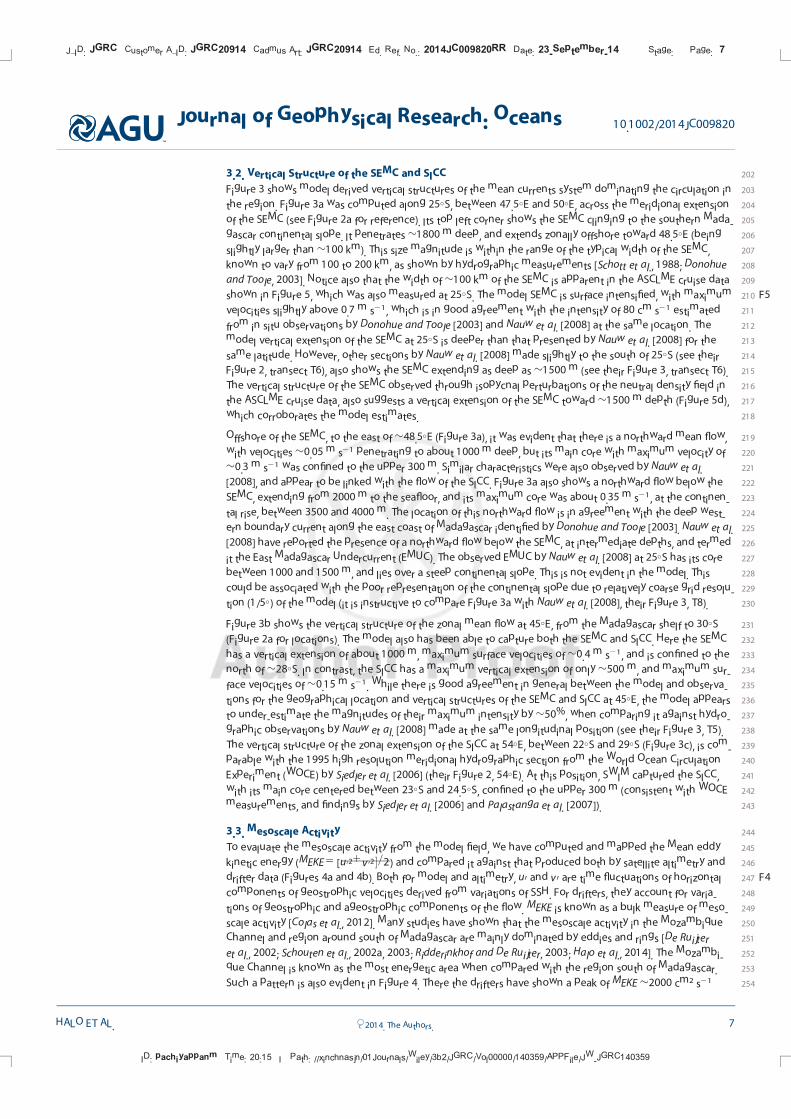
2443.3. Mesoscale Activity
245To evaluate the mesoscale activity from the model field, we have computed and mapped the Mean eddy
246kinetic energy (MEKE5 [u021v
02�=2) and compared it against that produced both by satellite altimetry and
247drifter data (Figures F44a and 4b). Both for model and altimetry, u0 and v0 are time fluctuations of horizontal
248components of geostrophic velocities derived from variations of SSH. For drifters, they account for varia-
249tions of geostrophic and ageostrophic components of the flow. MEKE is known as a bulk measure of meso-
250scale activity [Colas et al., 2012]. Many studies have shown that the mesoscale activity in the Mozambique
251Channel and region around south of Madagascar are mainly dominated by eddies and rings [De Ruijter
252et al., 2002; Schouten et al., 2002a, 2003; Ridderinkhof and De Ruijter, 2003; Halo et al., 2014]. The Mozambi-
253que Channel is known as the most energetic area when compared with the region south of Madagascar.
254Such a pattern is also evident in Figure 4. There the drifters have shown a peak of MEKE �2000 cm2 s21
J_ID: JGRC Customer A_ID: JGRC20914 Cadmus Art: JGRC20914 Ed. Ref. No.: 2014JC009820RR Date: 23-September-14 Stage: Page: 7
ID: pachiyappanm Time: 20:15 I Path: //xinchnasjn/01Journals/Wiley/3b2/JGRC/Vol00000/140359/APPFile/JW-JGRC140359
Journal of Geophysical Research: Oceans 10.1002/2014JC009820
HALO ET AL. VC 2014. The Authors. 7
255(Figure 4a), while altimetry has shown
256a peak �1400 cm2 s21 (Figure 4b) and
257model �1600 cm2 s21 (Figure 4c).
258South of Madagascar and along the
259southeastern African margin, both
260drifters and model produce peak val-
261ues of about 1000 cm2 s21 and
2621200 cm2 s21, respectively, whereas
263altimetry only reaches a peak of
264�800 cm2 s21 to the southwest of
265Madagascar, failing to produce the
266energetic field in the vicinity of the
267Agulhas Current. While in general all
268data sets agree with regard to their
269spatial distributions, the model
270appears to under-estimate the energy
271levels when compared against drifters,
272but over-estimates the altimetry. This
273is not a surprising result, as altimetric
274geostrophic velocities are known to
275under-estimate the ocean currents by
276about 30% [Ternon et al., 2014]. Proc-
277essing of the altimetry data set
278requires grid interpolations and filter-
279ing of SSH field [Chelton et al., 2011b],
280thus reducing its local value. Drifters
281account for both geostrophic and
282ageostrophic components of the
283ocean currents. Recent analysis of the
284cyclogeostrophic balance in the
285Mozambique Channel has demon-
286strated that the main cause for the dif-
287ferences observed between altimetry
288and drifter EKE is associated with the
289omission of centrifugal acceleration in
290the geostrophic relation [Penven et al.,
2912014].
292
293
2943.3.1. Eddy Density Structure
295Figure 5 shows eddy field at two hydrographic transects during the ASCLME cruise in the southwest of
296Madagascar at 25�30S, in 26 and 27 August 2008, and in the southeast at 25�S, in 10 September 2008. In
297these sections, the flow has been integrated vertically in the upper 300 m of the water column. Altimetric
298maps of weekly sea level anomalies correspondent to the dates of the cruise were superimposed on the
299observed data. Thus, a clear pattern emerges: a strong cyclonic eddy is responsible for the clockwise rever-
300sal of the flow on the southwest transect close to Madagascar coast. The surface signal of this eddy appears
301to have a width greater than 200 km diameter. The expression of the SLA seems to under-estimate the
302diameter compared to the cruise data, likely due to interpolations in time and space, and processing of the
303satellite data. Nevertheless, there is good agreement between the two data sets. The pattern observed on
304the southeast coast shows a strong poleward flow along the Madagascar coast, the SEMC, and at its off-
305shore edge an intense equatorward flow associated with a strong cyclonic eddy. The width of the observed
306current is slightly greater than 100 km, fairly consistent with other hydrographic data [Schott et al., 1988].
307Because the ASCLME cruise track did not extend far offshore, the eddy was partly sampled, hence little can
308be inferred about its size. Bearing in mind that here the flow field is also dominated by the SICC [Palastanga
30oE 40
oE 50
oE 60
oE 70
oE
36oS
32oS
28oS
24oS
20oS
a) MEKE [cm2 s
−2] − DRIFTERS
30oE 40
oE 50
oE 60
oE 70
oE
36oS
32oS
28oS
24oS
20oS
b) MEKE [cm2 s
−2] − AVISO
30oE 40
oE 50
oE 60
oE 70
oE
36oS
32oS
28oS
24oS
20oS
c) MEKE [cm2 s
−2] − SWIM
0 200 400 600 800 1000 1200 1400 1600 1800 2000
Figure 4. Surface mean eddy kinetic energy (MEKE). (a) Based on 215 drifters from
1992 to July 2012, (b) based on satellite altimetry from October 1992 to March
2010, and (c) Based on SWIM model 7 year climatology.
J_ID: JGRC Customer A_ID: JGRC20914 Cadmus Art: JGRC20914 Ed. Ref. No.: 2014JC009820RR Date: 23-September-14 Stage: Page: 8
ID: pachiyappanm Time: 20:15 I Path: //xinchnasjn/01Journals/Wiley/3b2/JGRC/Vol00000/140359/APPFile/JW-JGRC140359
Journal of Geophysical Research: Oceans 10.1002/2014JC009820
HALO ET AL. VC 2014. The Authors. 8
309et al., 2007], the eddy mean flow interaction could have an influence on the observed pattern. Interestingly,
310the pattern produced here (Figure 5) resembles that observed in hydrographic measurements by Donohue
311and Toole [2003] (see their Figure F99), and the ACSEX cruise data presented by Nauw et al. [2006] (see their
312Figure F66), exactly at 25�S. The in situ observed eddy in the southwest transect showed a strong shoaling of
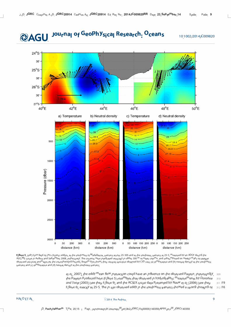
Figure 5. (top) Flow field of two cyclonic eddies, at the southwest of Madagascar, transect across 25�30S and at the southeast, transect at 25�S, measured by an ADCP during the
ASCLME cruise in August and September 2008, respectively. The currents were integrated vertically in upper 300 m of water column, and superimposed on weekly maps of satellite
observed sea level anomalies for the corresponding periods. Bottom plot shows their vertical structure obtained by CTD cast: (a) temperature and (b) neutral density at the southwest
transect and (c) temperature and (d) neutral density at the southeast transect.
J_ID: JGRC Customer A_ID: JGRC20914 Cadmus Art: JGRC20914 Ed. Ref. No.: 2014JC009820RR Date: 23-September-14 Stage: Page: 9
ID: pachiyappanm Time: 20:15 I Path: //xinchnasjn/01Journals/Wiley/3b2/JGRC/Vol00000/140359/APPFile/JW-JGRC140359
Journal of Geophysical Research: Oceans 10.1002/2014JC009820
HALO ET AL. VC 2014. The Authors. 9
313the isotherms, upwelling cooler deep waters to the subsurface layers. The maximum observed temperature
314at the sea surface was about 22�C (Figure 5a). Its density structure (Figure 5b) has shown stronger perturba-
315tions of the isopycnals between 500 and 2000 m, suggesting stronger eddy activity at subsurface layers.
316Horizontally, its core was centered about 200 km offshore. The transect in the southeast showed relatively
317warmer waters at the sea surface of about 24�C (Figure 5c), confined inshore (less than 150 km from the
318coast), suggesting a propagation of warm tropical waters by the SEMC. Further offshore, between 200 and
319250 km, the shoaling of the isotherms was associated with a cyclonic eddy which caused upwelling. The
320transition depth from perturbed to flat isopycnals near 1500 m deep (Figure 5d) adjacent to the continental
321slope, sheds light on the vertical extension of the SEMC. Little can be inferred about the structure of the
322cyclonic eddy at the eastern margin of the SEMC (Figure 5d) because the transect only partly sampled the
323eddy field. Nevertheless, a radius greater than 150 km can still be observed.
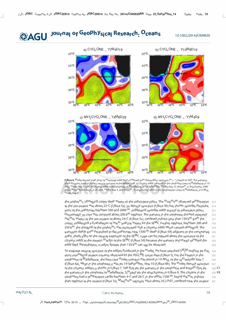
324To evaluate vertical structure of the eddies produced in the model, we have searched SWIM outputs for pat-
325terns resembling surface currents observed by the ASCLME cruise data (Figure 5). For the pattern in the
326southwest of Madagascar, the best case model scenario was found in 19 April, of the climatology year 7
327(Figure 6a), while in the southeast it was for 19 September, year 10 (Figure 6b). The model density structure
328of the cyclonic eddies is shown in Figure F77. Top plot for the transect in the southwest and bottom plot for
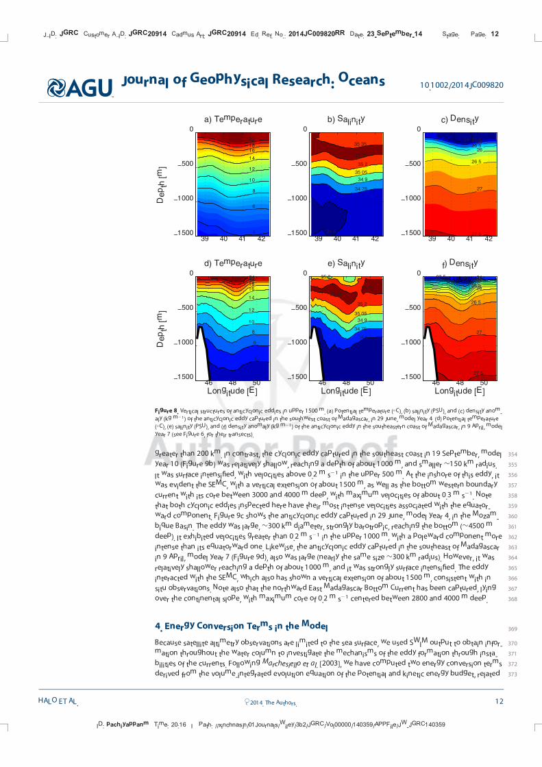
329the transect in the southeast of Madagascar. Similarly for the anticyclones in Figure F88. The cyclone in the
330southwest had a temperature range between 4�C and 26�C in the upper 1500 m, being warmer inshore
331than offshore at the surface (Figure 7a). Maximum salinities were about 35.2 PSU, confined near the surface
36oE 38
oE 40
oE 42
oE 44
oE 46
oE
30oS
28oS
26oS
24oS
22oS
a) CYCLONE − Y7M4D19
44oE 46
oE 48
oE 50
oE 52
oE 54
oE
30oS
28oS
26oS
24oS
22oS
b) CYCLONE − Y10M9D19
44oE 46
oE 48
oE 50
oE 52
oE 54
oE
30oS
28oS
26oS
24oS
22oS
d) ANTICYCLONE − Y7M4D9
36oE 38
oE 40
oE 42
oE 44
oE 46
oE
30oS
28oS
26oS
24oS
22oS
c) ANTICYCLONE − Y4M6D29
Figure 6. Model derived snap-shots of mesoscale eddy field computed from geostrophic velocities (m s21), based on SSH. The transects
show positions used to inspect vertical structure of the eddies. (top, a) Cyclonic eddy captured in the southwest coast of Madagascar in 19
April, model year 7; (top, b) cyclonic eddy in the southeast of Madagascar, in 19 September, model year 10. (bottom, c) Anticyclonic eddy
in the Mozambique Basin, in 29 June, model year 4, and (bottom, d) anticyclonic eddy in the southeastern coast of Madagascar, in 9 April,
model year 7.
J_ID: JGRC Customer A_ID: JGRC20914 Cadmus Art: JGRC20914 Ed. Ref. No.: 2014JC009820RR Date: 23-September-14 Stage: Page: 10
ID: pachiyappanm Time: 20:15 I Path: //xinchnasjn/01Journals/Wiley/3b2/JGRC/Vol00000/140359/APPFile/JW-JGRC140359
Journal of Geophysical Research: Oceans 10.1002/2014JC009820
HALO ET AL. VC 2014. The Authors. 10
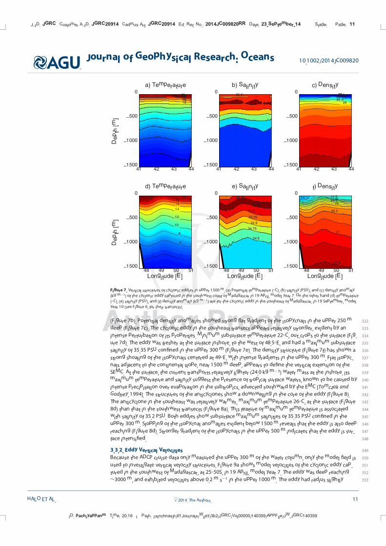
332(Figure 7b). Potential density anomalies showed strong flat gradient of the isopycnals in the upper 250 m
333deep (Figure 7c). The cyclonic eddy in the southeast transect appears relatively stronger, evident by an
334intense perturbation of its properties. Minimum subsurface temperature 22�C, out-crops to the surface (Fig-
335ure 7d). The eddy was fresher at the surface inshore, to the west of 48.5�E, and had a maximum subsurface
336salinity of 35.35 PSU confined in the upper 300 m (Figure 7e). The density structure (Figure 7f) has shown a
337strong shoaling of the isopycnals centered at 49�E, with intense gradients in the upper 300 m. Flat isopyc-
338nals adjacent to the continental slope, near 1500 m deep, appears to define the vertical extension of the
339SEMC. At the surface, the current transports relatively lighter (24.0 kg m23) water mass at the inshore. Its
340maximum temperature and salinity suggest the presence of tropical surface waters, known to be caused by
341intense precipitation over evaporation in the subtropics, advected southward by the EMC [Tomczak and
342Godfrey, 1994]. The structures of the anticyclones show a downwelling in the core of the eddy (Figure 8).
343The anticyclone in the southeast was relatively warmer, maximum temperature 26�C, at the surface (Figure
3448d) than that in the southwest transects (Figure 8a). This feature of maximum temperature is associated
345with salinity of 35.2 PSU. Both eddies show subsurface maximum salinities of 35.35 PSU confined in the
346upper 300 m. Slopping of the isopycnal anomalies evident below 1500 m reveals that the eddy is also deep
347reaching (Figure 8d). Stronger gradient of the isopycnals in the upper 500 m indicates that the eddy is sur-
348face intensified.
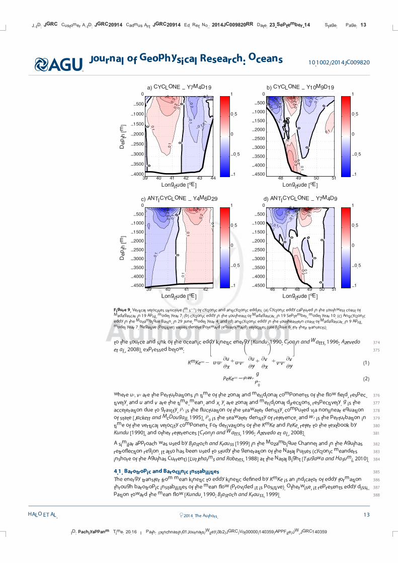
3493.3.2. Eddy Vertical Velocities
350Because the ADCP cruise data only measured the upper 300 m of the water column, only the model field is
351used to investigate vertical velocity structures. Figure 9a shows model velocities of the cyclonic eddy cap-
352tured in the southwest of Madagascar, at 25�50S, in 19 April, model year 7. The eddy was deep reaching
353�3000 m, and exhibited velocities above 0.2 m s21 in the upper 1000 m. The eddy had radius slightly
161820222426
Depth
[m
]
a) Temperature
41 42 43 44−1500
−1000
−500
0 35.2
35
b) Salinity
41 42 43 44−1500
−1000
−500
0 2323.52424.52525.526
c) Density
41 42 43 44−1500
−1000
−500
0
4
6
8
10
12
14
16182022 22
Depth
[m
]
d) Temperature
Longitude [E]48 49 50 51
−1500
−1000
−500
0
34.6
34.75
34.9
35.05
35.2
35.35
35.35
Longitude [E]
e) Salinity
48 49 50 51−1500
−1000
−500
024 24.5
2525.526
26.5
27
27.5
f) Density
Longitude [E]48 49 50 51
−1500
−1000
−500
0
Figure 7. Vertical structures of cyclonic eddies in upper 1500 m. (a) Potential temperature (�C), (b) salinity (PSU), and (c) density anomaly
(kg m21) of the cyclonic eddy captured in the southwest coast of Madagascar in 19 April, model year 7. On the other hand (d) temperature
(�C), (e) salinity (PSU), and (f) density anomaly (kg m21) are for the cyclonic eddy in the southeast of Madagascar, in 19 September, model
year 10 (see Figure 6, for their transects).
J_ID: JGRC Customer A_ID: JGRC20914 Cadmus Art: JGRC20914 Ed. Ref. No.: 2014JC009820RR Date: 23-September-14 Stage: Page: 11
ID: pachiyappanm Time: 20:16 I Path: //xinchnasjn/01Journals/Wiley/3b2/JGRC/Vol00000/140359/APPFile/JW-JGRC140359
Journal of Geophysical Research: Oceans 10.1002/2014JC009820
HALO ET AL. VC 2014. The Authors. 11
354greater than 200 km. In contrast, the cyclonic eddy captured in the southeast coast in 19 September, model
355year 10 (Figure 9b) was relatively shallow, reaching a depth of about 1000 m, and smaller �150 km radius.
356It was surface intensified, with velocities above 0.2 m s21 in the upper 500 m. At the inshore of this eddy, it
357was evident the SEMC, with a vertical extension of about 1500 m, as well as the bottom western boundary
358current with its core between 3000 and 4000 m deep, with maximum velocities of about 0.3 m s21. Note
359that both cyclonic eddies inspected here have their most intense velocities associated with the equator-
360ward component. Figure 9c shows the anticyclonic eddy captured in 29 June, model year 4, in the Mozam-
361bique Basin. The eddy was large, �300 km diameter, strongly barotropic, reaching the bottom (�4500 m
362deep). It exhibited velocities greater than 0.2 m s21 in the upper 1000 m, with a poleward component more
363intense than its equatorward one. Likewise, the anticyclonic eddy captured in the southeast of Madagascar
364in 9 April, model year 7 (Figure 9d), also was large (nearly the same size �300 km radius). However, it was
365relatively shallower reaching a depth of about 1000 m, and it was strongly surface intensified. The eddy
366interacted with the SEMC, which also has shown a vertical extension of about 1500 m, consistent with in
367situ observations. Note also that the northward East Madagascar Bottom Current has been captured, lying
368over the continental slope, with maximum core of 0.2 m s21 centered between 2800 and 4000 m deep.
3694. Energy Conversion Terms in the Model
370Because satellite altimetry observations are limited to the sea surface, we used SWIM output to obtain infor-
371mation throughout the water column to investigate the mechanisms of the eddy formation through insta-
372bilities of the currents. Following Marchesiello et al. [2003], we have computed two energy conversion terms
373derived from the volume-integrated evolution equation of the potential and kinetic energy budget, related
4
6
8
10
12
14
16182022
Depth
[m
]
a) Temperature
39 40 41 42−1500
−1000
−500
0
34.6
34.75
34.9
35.05
35.2
35.35
35.35
b) Salinity
39 40 41 42−1500
−1000
−500
0
24 24.52525.5
26
26.5
27
27 5
c) Density
39 40 41 42−1500
−1000
−500
0
4
6
8
10
12
14
161820222426
Depth
[m
]
d) Temperature
Longitude [E]46 48 50
−1500
−1000
−500
0
34.6
34.75
34.9
35.05
35.2
35.2
35.35
35.35
Longitude [E]
e) Salinity
46 48 50−1500
−1000
−500
02323.5 24
24.52525.5
26
26.5
27
27.5
f) Density
Longitude [E]46 48 50
−1500
−1000
−500
0
Figure 8. Vertical structures of anticyclonic eddies in upper 1500 m. (a) Potential temperature (�C), (b) salinity (PSU), and (c) density anom-
aly (kg m21) of the anticyclonic eddy captured in the southwest coast of Madagascar, in 29 June, model year 4. (d) Potential temperature
(�C), (e) salinity (PSU), and (f) density anomaly (kg m21) of the anticyclonic eddy in the southeastern coast of Madagascar, in 9 April, model
year 7 (see Figure 6, for their transects).
J_ID: JGRC Customer A_ID: JGRC20914 Cadmus Art: JGRC20914 Ed. Ref. No.: 2014JC009820RR Date: 23-September-14 Stage: Page: 12
ID: pachiyappanm Time: 20:16 I Path: //xinchnasjn/01Journals/Wiley/3b2/JGRC/Vol00000/140359/APPFile/JW-JGRC140359
Journal of Geophysical Research: Oceans 10.1002/2014JC009820
HALO ET AL. VC 2014. The Authors. 12
374to the source and sink of the oceanic eddy kinetic energy [Kundu, 1990; Cronin and Watts, 1996; Azevedo
375et al., 2008], expressed below:
KmKe52 u0u
0 @�u
@x1u
0v
0 @�u
@y1@�v
@x
� �
1v0v
0 @�v
@y
� �
(1)
PeKe52q0w
0 g
q0(2)
376where u0; v0 are the perturbations in time of the zonal and meridional components of the flow field, respec-
377tively, and �u and �v are the time-mean, and x, y, are zonal and meridional directions, respectively. g is the
378acceleration due to gravity, q0 is the fluctuation of the seawater density, computed via nonlinear equation
379of state [Jackett and McDougall, 1995], q0 is the seawater density of reference, and w0 is the perturbation in
380time of the vertical velocity component. For derivations of the KmKe and PeKe, refer to the textbook by
381Kundu [1990], and other references [Cronin and Watts, 1996; Azevedo et al., 2008].
382A similar approach was used by Biastoch and Krauss [1999] in the Mozambique Channel and in the Agulhas
383retroflection region. It also has been used to study the generation of the Natal Pulses (cyclonic meanders
384inshore of the Agulhas Current) [Lutjeharms and Roberts, 1988] at the Natal Bight [Tsugawa and Hasumi, 2010].
3854.1. Barotropic and Baroclinic Instabilities
386The energy transfer from mean kinetic to eddy kinetic defined by KmKe is an indicator of eddy formation
387through barotropic instabilities of the mean flow (provided it is positive). Otherwise, it represents eddy dissi-
388pation toward the mean flow [Kundu, 1990; Biastoch and Krauss, 1999].
Longitude [oE]
Depth
[m
]
a) CYCLONE − Y7M4D19
−0.2
−0.2
−0.1
−0.1
−0.1
−0.1
00
0
00
0
00
0
00
0
0.1
0.1
0.1
0.2
0.3
0.4
00
0
00
039 40 41 42 43 44
−4000
−3500
−3000
−2500
−2000
−1500
−1000
−500
0
−1
−0.5
0
0.5
1
Longitude [oE]
b) CYCLONE − Y10M9D19
−0.5
−0.4
−0.3
−0.2 −
0.2
−0.1 −
0.1 −0.10
00
0
0
0
0
0
00
0
0
0
0
0.1
0.1
0.1
0.1
0.2
0.2
0.3
0.3
0.4
0
00
0
0
0
0
48 49 50 51−4500
−4000
−3500
−3000
−2500
−2000
−1500
−1000
−500
0
−1
−0.5
0
0.5
1
Longitude [oE]
Depth
[m
]
c) ANTICYCLONE − Y4M6D29
−0.5
−0.4
−0.3
−0.2
−0.1
−0.1
0
0
0
0
0.1
0.1
0.1
0.2
0.30.4
0
0
39 40 41 42−4500
−4000
−3500
−3000
−2500
−2000
−1500
−1000
−500
0
−1
−0.5
0
0.5
1
Longitude [oE]
d) ANTICYCLONE − Y7M4D9−0.5−0.4−0.3
−0.2
−0.1
−0.1
0
0
0
00
0
0
0
0
0
00
0
0
0.1
0.1
0.2
0.20.
30.40.51
0
0
0
00
0
0
46 47 48 49 50 51−4500
−4000
−3500
−3000
−2500
−2000
−1500
−1000
−500
0
−1
−0.5
0
0.5
1
Figure 9. Vertical velocities structure (m s21) of cyclonic and anticyclonic eddies. (a) Cyclonic eddy captured in the southwest coast of
Madagascar in 19 April, model year 7; (b) cyclonic eddy in the southeast of Madagascar, in 19 September, model year 10. (c) Anticyclonic
eddy in the Mozambique Basin, in 29 June, model year 4, and (d) anticyclonic eddy in the southeastern coast of Madagascar, in 9 April,
model year 7. Negative (positive) values denote poleward (equatorward) velocities (see Figure 6, for their transects).
J_ID: JGRC Customer A_ID: JGRC20914 Cadmus Art: JGRC20914 Ed. Ref. No.: 2014JC009820RR Date: 23-September-14 Stage: Page: 13
ID: pachiyappanm Time: 20:16 I Path: //xinchnasjn/01Journals/Wiley/3b2/JGRC/Vol00000/140359/APPFile/JW-JGRC140359
Journal of Geophysical Research: Oceans 10.1002/2014JC009820
HALO ET AL. VC 2014. The Authors. 13
389The other transfer term defined by PeKe describes the conversion of energy from eddy potential to eddy
390kinetic ‘‘buoyancy production’’ [Kundu, 1990; Marchesiello et al., 2003]. It represents the work performed by
391turbulent buoyancy forces on the vertical stratification, leading to changes in potential energy [Cushman-
392Roisin and Beckers, 2009]. It is known as the second phase of baroclinic instability [Kundu, 1990; Cronin and
393Watts, 1996; Marchesiello et al., 2003; Azevedo et al., 2008].
394The work of the local winds has been regarded less important for the mesoscale variability of this region
395[Lutjeharms and Machu, 2000], therefore here it is neglected.
3965. Eddy Detection and Tracking Algorithm
397The algorithm used to detect and track eddies combines both geometrical and dynamical properties of the
398flow field [Halo, 2012; Halo et al., 2014]. A geostrophic eddy is regarded as an instantaneous flow field iden-
399tified simultaneously by closed contours of sea surface height (SSH) [Chelton et al., 2011b], and a negative
400Okubo-Weiss parameter [Isern-Fontanet et al., 2006; Chelton et al., 2007]. The Okubo-Weiss parameter
401[Okubo, 1970; Weiss, 1991] is defined as:
W5S2n1S2s2n2 (3)
402where
Sn5@u
@x2@v
@y(4)
Ss5@v
@x1@u
@y(5)
n5@v
@x2@u
@y(6)
403Sn and Ss are the normal and shear components of strain tensor, respectively, n is the vertical component of
404relative vorticity, u and v are the geostrophic velocity components in x and y, respectively, derived from alti-
405metric SSH:
u52g@½SSH�
f@y; v5
g@½SSH�
f@x(7)
406g is the acceleration due to gravity, and f is the Coriolis parameter.
407To minimize the subjectivity on the identification of the eddies, the algorithm is designed with a minimum
408tunable parameters: the intervals between the closed contours, set to 2 cm, and the maximum closed loop
409of SSH to exclude gyre-scale features, set to 600 km. The threshold value for W is 0. Two passes of the Han-
410ning filter has been applied over W field to minimize the grid-scale noise, common in Wmethods [Chelton
411et al., 2011b; Souza et al., 2011]. As demonstrated by Halo [2012] and Halo et al. [2014], this hybrid method
412is more robust than using the closed contours method and the Okubo-Weiss criteria independently. The
413eddies are tracked with reference to their centers, following the method proposed by Penven et al. [2005],
414where an eddy retains its identity between two consecutive time steps when a generalized distance in a
415nondimensional property space is minimum.
4166. Results and Discussions
417The findings of the present study are presented and discussed below. These mainly include: the role of sea-
418sonality on eddy activity; the eddy generation processes, their seasonal cycle and spatial variability; the
419interaction of the eddies with the large-scale ocean currents in the region; the eddy demography and their
420mean properties.
4216.1. Impact of Seasonality on Altimetry MEKE
422To assess the overall impact of seasonal variations on the mesoscale activity, we have computed and
423mapped MEKE with and without seasonality included in the data set (Figure F1010). Seasonality was removed
424by obtaining the anomaly from seasonal average [Marchesiello et al., 2003; Penven et al., 2005]. When sea-
425sonality was included in the data set there were two regions of enhanced MEKE located to the southeast
J_ID: JGRC Customer A_ID: JGRC20914 Cadmus Art: JGRC20914 Ed. Ref. No.: 2014JC009820RR Date: 23-September-14 Stage: Page: 14
ID: pachiyappanm Time: 20:16 I Path: //xinchnasjn/01Journals/Wiley/3b2/JGRC/Vol00000/140359/APPFile/JW-JGRC140359
Journal of Geophysical Research: Oceans 10.1002/2014JC009820
HALO ET AL. VC 2014. The Authors. 14
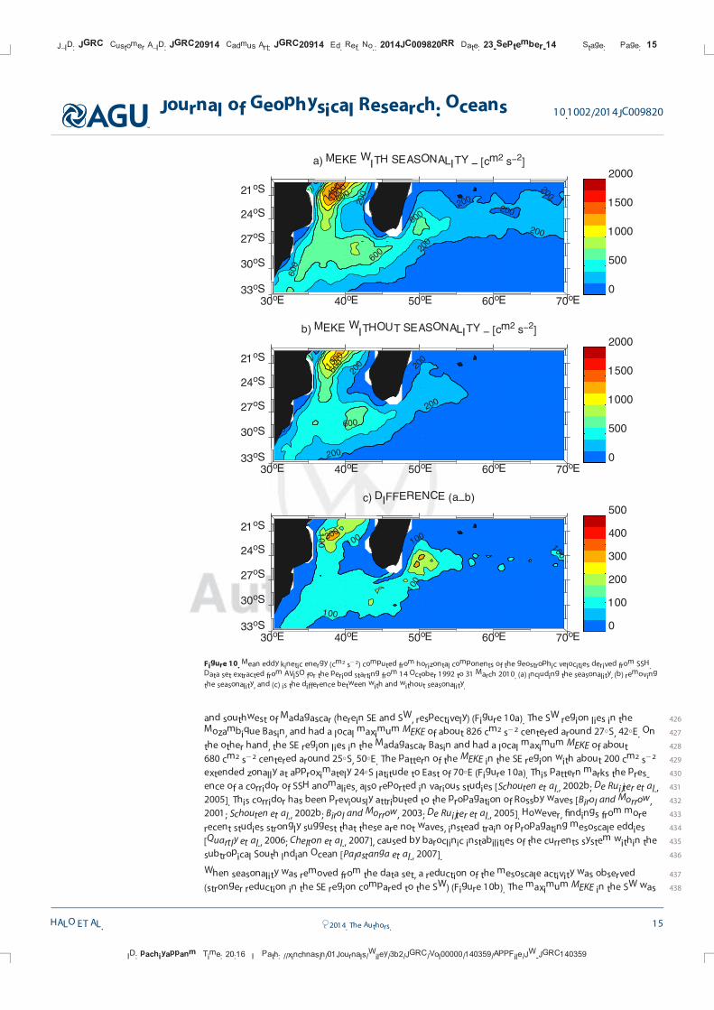
426and southwest of Madagascar (herein SE and SW, respectively) (Figure 10a). The SW region lies in the
427Mozambique Basin, and had a local maximum MEKE of about 826 cm2 s22 centered around 27�S, 42�E. On
428the other hand, the SE region lies in the Madagascar Basin and had a local maximum MEKE of about
429680 cm2 s22 centered around 25�S, 50�E. The pattern of the MEKE in the SE region with about 200 cm2 s22
430extended zonally at approximately 24�S latitude to East of 70�E (Figure 10a). This pattern marks the pres-
431ence of a corridor of SSH anomalies, also reported in various studies [Schouten et al., 2002b; De Ruijter et al.,
4322005]. This corridor has been previously attributed to the propagation of Rossby waves [Birol and Morrow,
4332001; Schouten et al., 2002b; Birol and Morrow, 2003; De Ruijter et al., 2005]. However, findings from more
434recent studies strongly suggest that these are not waves, instead train of propagating mesoscale eddies
435[Quartly et al., 2006; Chelton et al., 2007], caused by baroclinic instabilities of the currents system within the
436subtropical South Indian Ocean [Palastanga et al., 2007].
437When seasonality was removed from the data set, a reduction of the mesoscale activity was observed
438(stronger reduction in the SE region compared to the SW) (Figure 10b). The maximum MEKE in the SW was
200
200
200
200
200
200
600 600
600
600
1000
1400
a) MEKE WITH SEASONALITY − [cm2 s
−2]
30oE 40
oE 50
oE 60
oE 70
oE
33oS
30oS
27oS
24oS
21oS
0
500
1000
1500
2000
200
200 20
0
200
200
600
600
1000
b) MEKE WITHOUT SEASONALITY − [cm2 s
−2]
30oE 40
oE 50
oE 60
oE 70
oE
33oS
30oS
27oS
24oS
21oS
0
500
1000
1500
2000
100 100
100
100
100
100
300
c) DIFFERENCE (a−b)
30oE 40
oE 50
oE 60
oE 70
oE
33oS
30oS
27oS
24oS
21oS
0
100
200
300
400
500
Figure 10. Mean eddy kinetic energy (cm2 s22) computed from horizontal components of the geostrophic velocities derived from SSH.
Data set extracted from AVISO for the period starting from 14 October 1992 to 31 March 2010. (a) Including the seasonality, (b) removing
the seasonality, and (c) is the difference between with and without seasonality.
J_ID: JGRC Customer A_ID: JGRC20914 Cadmus Art: JGRC20914 Ed. Ref. No.: 2014JC009820RR Date: 23-September-14 Stage: Page: 15
ID: pachiyappanm Time: 20:16 I Path: //xinchnasjn/01Journals/Wiley/3b2/JGRC/Vol00000/140359/APPFile/JW-JGRC140359
Journal of Geophysical Research: Oceans 10.1002/2014JC009820
HALO ET AL. VC 2014. The Authors. 15
439about 676 cm2 s22 centered around 27�S, 42�E, and in the SE a maximum of about 384 cm2 s22 was cen-
440tered around 25�S, 50�E. In this case, the pattern of the MEKE was confined to the west of about 55�E (Fig-
441ure 10b). The difference between the MEKE with and without seasonality was calculated (Figure 10c). It
442indicates an overall impact of seasonal variations on the mean currents that accounts for 18% and 44% of
443the mesoscale activity in the SW and SE regions, respectively. By removing the seasonality (Figure 10b), the
444bulk effects of seasonal variations of the mean currents on the mesoscale activity are filtered out. The MEKE
445is influenced by variabilities at extraseasonal time scales. At these time scales, the subtropical eddy-corridor
446extended only to the west of about 55�E. This may suggest that the seasonal variations of the mean cur-
447rents are strongly linked with variability produced in the far east Indian Ocean. The peak of MEKE observed
448near 24�S, 50�E (Figure 10a) suggests a local enhancement. Enhancement of eddy activity in this region has
449been attributed to the interaction of the arriving eddies from the east Indian Ocean [Quartly et al., 2006; Pal-
450astanga et al., 2007] with the SEMC at the southeastern slope of Madagascar [Siedler et al., 2009]. In the
451Mozambique Basin, the local maximum MEKE observed near 27�S, 42�E (Figure 10a) is relatively stronger
452than that observed in the Madagascar Basin (near 25�S, 50�E). In the latter region, the seasonality accounts
453for only 18% of the maximum MEKE, while in the former region it accounts for 44%. This indicates that a
454great deal of variability produced in the Mozambique Basin overwhelms that produced at seasonal time
455scales. The Mozambique and the Madagascar Basins are separated by the Madagascar Ridge, a prominent
456topographic feature rising up to about 2000 m depth (Figure 1a). It is thought that this bathymetric feature
457affects the mesoscale eddy variability observed in this region [Quartly and Srokosz, 2004], and is responsible
458for the two-distinct modes of variability to the west and east of 45�E [Matano et al., 1999, 2002]. De Ruijter
459et al. [2004] using LADCP measurements collected during the Agulhas Current Source Experiment cruise,
460combined with altimetric measurements observed a regular formation of mesoscale dipole eddies in this
461region. The period of enhanced formation of these dipoles coincided with the negative phase of the Indian
462Ocean Dipoles (IOD) and El-Nin~o Southern-Oscillation (ENSO) cycles [De Ruijter et al., 2004], which are phe-
463nomena at extraseasonal time scales.
464In the next section, we investigate the dominant eddy forcing mechanisms through current instabilities,
465their seasonal cycle and geographical distribution.
4666.2. Model Derived Barotropic and Baroclinic Instabilities, Their Seasonal Cycle
467To study the barotropic (KmKe) versus baroclinic (PeKe) contribution in the eddy formation, vertical profiles
468of the energy conversion terms within the region of enhanced mesoscale variability (39�E–51�E and 32�S–
46923�S, Figure 10a) were inspected for different seasons of the year: December–February (DJF), March–May
470(MAM), June–August (JJA), and September–November (SON). The seasons used here are in agreement with
471the criteria used by Lutjeharms et al. [2000], where DJF is representative of summer season, MAM is for fall,
472JJA is for winter and SON for spring.
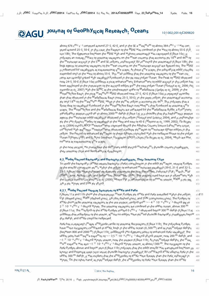
4736.2.1. Model Derived Vertical Structures of KmKe and PeKe
474Figures F1111a and 11b show the characteristic mean-profiles for KmKe and PeKe averaged within the region.
475DJF (dotted lines), MAM (dashed lines), JJA (dot-dashed lines), and SON (continuous lines). The profiles of
476KmKe show large seasonal variations at the sea surface, ranging from �24 3 1028 cm2 s23 during fall to
47723 1028 cm2 s23 during winter. The seasonal variations are confined to the upper ocean, above 300 m
478(Figure 11a). The merging of the KmKe profiles toward 0 cm2 s23 observed below 300 m depth (Figure 11a)
479suggests that regardless of the season, almost no eddies were formed through barotropic instabilities below
480this depth, and KmKe could be neglected.
481PeKe has a relatively smaller amplitude range of seasonal fluctuations (Figure 11b). The individual profiles
482have more oscillations compared to KmKe, both in the upper ocean (0–500 m) and at intermediate depths
483(between 800 and 2000 m) (Figure 11b), suggesting two different layers of enhanced PeKe variability. The
484upper layer had maxima extremes of �23.5 3 1028 cm2 s23 during spring season, near 200 m depth, and
485�1 3 1028 cm2 s23 during winter season, near the surface (Figure 11b). At intermediate depths, the maxi-
486mum extreme was also �13 1028 cm2 s23 during winter season, at about 1300 m. The oscillation of the
487PeKe profiles above and below zero (Figure 11b) indicates that the eddy energy was transferred between its
488kinetic and potential state (vice versa) through baroclinic instability. By comparing KmKe against PeKe in the
489upper 300 m depth, it was evident that the amplitudes of KmKe were greater than the PeKe, especially in
490winter. On the other hand, at intermediate depth, the amplitudes of PeKe were greater than the KmKe
J_ID: JGRC Customer A_ID: JGRC20914 Cadmus Art: JGRC20914 Ed. Ref. No.: 2014JC009820RR Date: 23-September-14 Stage: Page: 16
ID: pachiyappanm Time: 20:16 I Path: //xinchnasjn/01Journals/Wiley/3b2/JGRC/Vol00000/140359/APPFile/JW-JGRC140359
Journal of Geophysical Research: Oceans 10.1002/2014JC009820
HALO ET AL. VC 2014. The Authors. 16
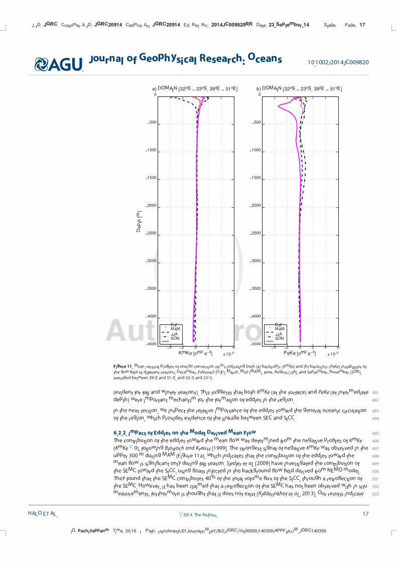
491(evident for fall and winter seasons). This suggests that both KmKe (at the surface) and PeKe (at intermediate
492depth) were important mechanism for the formation of eddies in the region.
493In the next section, we inspect the relative importance of the eddies toward the general oceanic circulation
494of the region, which provides evidence of the linkage between SEC and SICC.
4956.2.2. Impact of Eddies on the Model Derived Mean Flow
496The contribution of the eddies toward the mean flow was determined from the negative profiles of KmKe
497(KmKe< 0), following Biastoch and Krauss [1999]. The strongest signal of negative KmKe was observed in the
498upper 300 m during MAM (Figure 11a), which indicates that the contribution of the eddies toward the
499mean flow is significant only during fall season. Siedler et al. [2009] have investigated the contribution of
500the SEMC toward the SICC, using floats injected in the background flow field derived from NEMO model.
501They found that the SEMC contributes 40% of the total volume flux of the SICC, through a retroflection of
502the SEMC. However, it has been claimed that a retroflection of the SEMC has not been observed with in situ
503measurements, furthermore is thought that it does not exist [Ridderinkhof et al., 2013]. Our results indicate
−4 −2 0 2 4 6
x 10−8
−4500
−4000
−3500
−3000
−2500
−2000
−1500
−1000
−500
0
a) DOMAIN [32oS − 23
oS, 39
oE − 51
oE]
Depth
[m
]
KmKe [cm2 s
−3]
DJFMAMJJASON
−4 −2 0 2 4 6
x 10−8
−4500
−4000
−3500
−3000
−2500
−2000
−1500
−1000
−500
0
b) DOMAIN [32oS − 23
oS, 39
oE − 51
oE]
PeKe [cm2 s
−3]
DJFMAMJJASON
Figure 11. Mean-vertical profiles of energy conversion terms indicating both (a) barotropic (KmKe) and (b) baroclinic (PeKe) instabilities of
the flow field at different seasons: December–February (DJF), March–May (MAM), June–August (JJA), and September–November (SON),
averaged between 39�E and 51�E, and 32�S and 23�S.
J_ID: JGRC Customer A_ID: JGRC20914 Cadmus Art: JGRC20914 Ed. Ref. No.: 2014JC009820RR Date: 23-September-14 Stage: Page: 17
ID: pachiyappanm Time: 20:16 I Path: //xinchnasjn/01Journals/Wiley/3b2/JGRC/Vol00000/140359/APPFile/JW-JGRC140359
Journal of Geophysical Research: Oceans 10.1002/2014JC009820
HALO ET AL. VC 2014. The Authors. 17
504that the connection between SEMC and SICC is likely to be established through the shedding of anticyclonic
505eddies. This conclusion would be consistent with a nonpersistent retroflection of the SEMC, stated by
506Quartly et al. [2006]. A small contribution from the eddies toward the mean flow was also observed below
5073500 m depth, for all seasons (Figure 11a). This may suggest a marginal, but persistent contribution of the
508eddies toward the deep currents.
509To diagnose the geographical focus of eddy formation through current instabilities, spatial maps of eddy
510conversion terms were prepared and are presented in the next section.
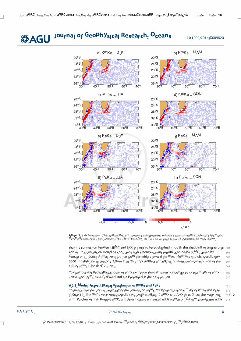
5116.2.3. Model Derived Spatial Distribution of KmKe and PeKe
512To investigate the spatial variability of the conversion terms, we plotted seasonal maps of KmKe and PeKe
513(Figure F1212). The maps were constructed by vertically integrating KmKe and PeKe throughout the water col-
514umn. Patches of high positive KmKe and PeKe indicate enhanced eddy formation. Otherwise indicates eddy
30oE 40
oE 50
oE 60
oE 70
oE
36oS
32oS
28oS
24oS
20oS
a) KmKe − DJF
30oE 40
oE 50
oE 60
oE 70
oE
36oS
32oS
28oS
24oS
20oS
b) KmKe − MAM
30oE 40
oE 50
oE 60
oE 70
oE
36oS
32oS
28oS
24oS
20oS
c) KmKe − JJA
30oE 40
oE 50
oE 60
oE 70
oE
36oS
32oS
28oS
24oS
20oS
d) KmKe − SON
30oE 40
oE 50
oE 60
oE 70
oE
36oS
32oS
28oS
24oS
20oS
e) PeKe − DJF
30oE 40
oE 50
oE 60
oE 70
oE
36oS
32oS
28oS
24oS
20oS
f) PeKe − MAM
30oE 40
oE 50
oE 60
oE 70
oE
36oS
32oS
28oS
24oS
20oS
g) PeKe − JJA
30oE 40
oE 50
oE 60
oE 70
oE
36oS
32oS
28oS
24oS
20oS
h) PeKe − SON
−1.5 −1 −0.5 0 0.5 1 1.5
x 10−4
Figure 12. Eddy generation by barotropic (KmKe) and baroclinic instabilities (PeKe) in different seasons: December–February (DJF), March–
May (MAM), June–August (JJA), and September–November (SON). The maps are vertically integrated throughout the water column.
J_ID: JGRC Customer A_ID: JGRC20914 Cadmus Art: JGRC20914 Ed. Ref. No.: 2014JC009820RR Date: 23-September-14 Stage: Page: 18
ID: pachiyappanm Time: 20:16 I Path: //xinchnasjn/01Journals/Wiley/3b2/JGRC/Vol00000/140359/APPFile/JW-JGRC140359
Journal of Geophysical Research: Oceans 10.1002/2014JC009820
HALO ET AL. VC 2014. The Authors. 18
515dissipation toward the mean kinetic energy and toward the eddy potential energy, respectively. Regions of
516enhanced eddy formation were found near the southern coast of Madagascar throughout the year. KmKe
517dominates to the southeast of Madagascar (Figures 12a–12d), and PeKe on the southwest (Figures 12e–
51812h). The strongest KmKe in the region was observed along the African coast, stretching from the Mozambi-
519que Channel toward the Agulhas Current region (Figures 12a–12d). This pattern is consistent with the altim-
520etry derived MEKE (Figure 10). Along the SEMC the strongest signal of KmKe was mostly located near the
521Madagascar continental shelf, at the southeastern sector of the island, suggesting strong shear production
522in the SEMC. This is not a surprising result. In this region, patches of KmKe are located where a great-deal of
523mesoscale disturbances occurs when the SEMC approaches the southeastern edge of Madagascar continen-
524tal shelf [Lutjeharms, 1988; Lutjeharms and Machu, 2000; De Ruijter et al., 2004; Siedler et al., 2009]. De Ruijter
525et al. [2004] found that such disturbances of the flow field have the potential for causing an anticyclonic
526recirculation and a possible localized retroflection of the SEMC, which may favor the formation of anticy-
527clonic eddies. Results from our numerical model suggest that these anticyclonic eddies are formed through
528the transfer of kinetic energy from the mean component to eddying component, shear production in the
529southward flowing SEMC. In the southwest of Madagascar, eddy formation appears to be driven by both
530barotropic and baroclinic instabilities of the westward propagating SEMC, after it has past the southern tip
531of Madagascar (Figure 12). It is likely that some eddies are formed through coastline and topographic
532effects.
533The maps of PeKe highlight local enhancement of eddy formation between the southern tip of Madagascar
534continental shelf and the Madagascar Ridge (the outflow region of the SEMC), throughout the seasons, lying
535in the northeastern sector of the Mozambique Basin, between 26�S and 20�S (Figures 12e–12f). Along the
536African continent, the signals of PeKe stretching from the Mozambique Channel toward the Agulhas Current
537region are noisy and rather difficult to interpret. However, it is evident that negative PeKe dominated on the
538continental shelf, while positive PeKe appeared to dominate slightly off-shelf, suggesting that the continen-
539tal shelf in this region may also contribute for the dissipation of eddy kinetic energy toward its potential
540form. This pattern of dissipation at the western boundary is consistent with Zhai et al. [2010] (see their Fig-
541ure 3), which appears to be the main region of eddy dissipation in the Indian Ocean.
542An interesting feature appears when comparing KmKe (Figures 12a–12d) against PeKe (Figures 12e–12h) for
543each corresponding season. The respective distribution of PeKe and KmKe structures located at the outflow
544region of the SEMC, and on the western flank of the Madagascar Ridge, near 44�E, 28�S, indicates that baro-
545clinic instabilities dominated to the north of 28�S, relatively closer to the Madagascar shelf, while barotropic
546instabilities dominated to the south of that latitude. This pattern was consistent throughout the seasons.
547Strongly positive and negative patches of PeKe are located at the outflow of the SEMC (Figures 12e–12h).
548Similar structures, but for an instantaneous flow field was observed and investigated in the Cape Verde
549Frontal Zone, using in situ measurements from a moored current meter and numerical solution from an iso-
550pycnal coordinate model [Erasmi et al., 1998]. The results infer that such patterns are produced when pass-
551ing eddies induce a vertical displacement of the isopycnals and a disturbance of the vertical velocity field.
552They also suggest that cyclonic eddies moving through a less disturbed background flow, it is expected
553that a large positive PeKe will be located at the leading edge of the eddy, and a large negative PeKe at the
554back. The opposite will be observed in case of an anticyclonic eddy [Erasmi et al., 1998]. In our case, the
555direction of propagation of the eddies generated in the outflow of the SEMC is mainly southwestward. The
556large negative patches of PeKe of the time-averaged field (Figures 12e–12h), located to the south of the pos-
557itive patches, arguably would suggest a predominant propagation of anticyclonic eddies. Notwithstanding,
558De Ruijter et al. [2004] and Ridderinkhof et al. [2013] have found that the anticyclonic part of the dipole struc-
559ture formed in this region is generally the first to form over its cyclonic counter-part.
560In the next section, we investigate the relationship between the eddy forcing mechanisms and the intensity
561of the dominant large-scale circulation feature, thus providing evidence of the drivers of the eddy
562variability.
5636.3. Relating Model Derived Seasonal Cycle of KmKe and PeKe With Volume Transport of the SEMC
564To infer possible mechanisms related with the seasonal variability on the eddy formation, we have quanti-
565fied the mean of the energy conversion terms in the upper 1000 m of the water column for different sea-
566sons and compared against the corresponding volume transports. The energy conversion terms were
J_ID: JGRC Customer A_ID: JGRC20914 Cadmus Art: JGRC20914 Ed. Ref. No.: 2014JC009820RR Date: 23-September-14 Stage: Page: 19
ID: pachiyappanm Time: 20:16 I Path: //xinchnasjn/01Journals/Wiley/3b2/JGRC/Vol00000/140359/APPFile/JW-JGRC140359
Journal of Geophysical Research: Oceans 10.1002/2014JC009820
HALO ET AL. VC 2014. The Authors. 19
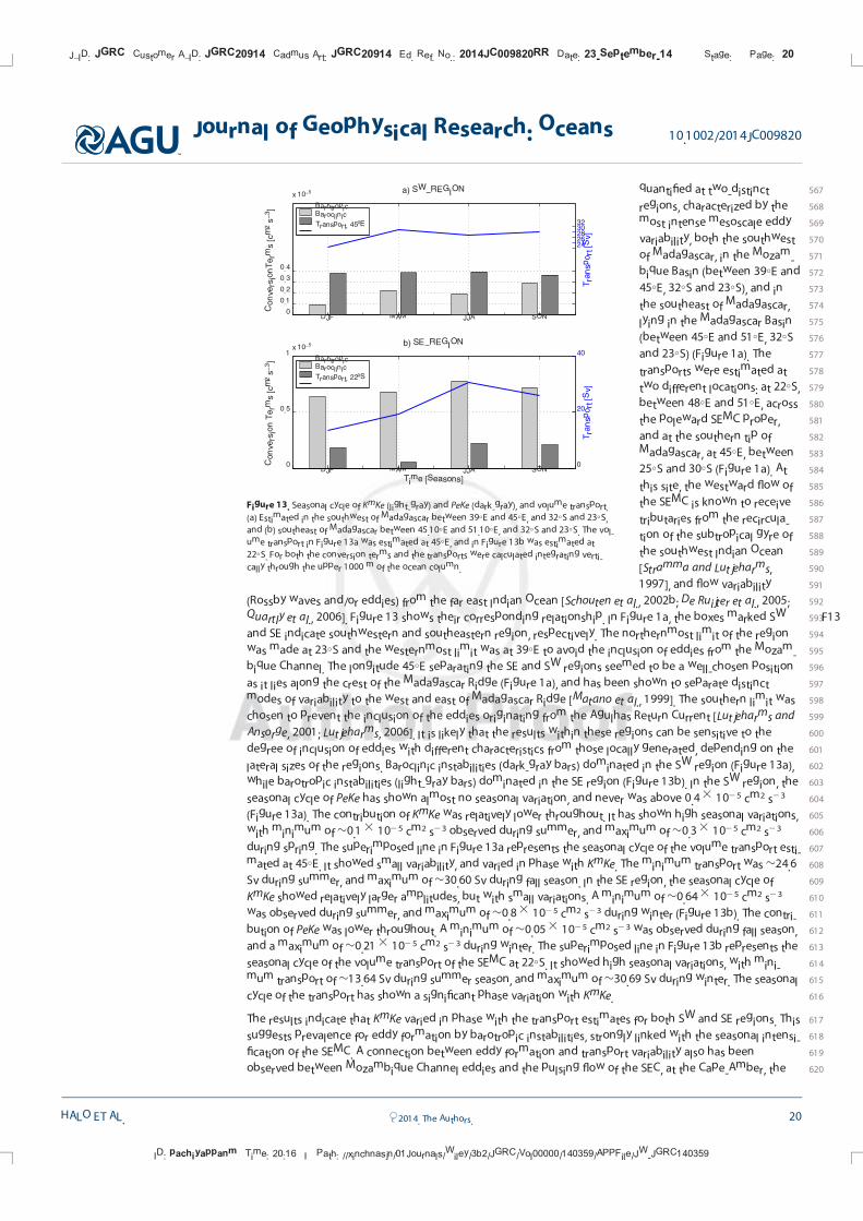
567quantified at two-distinct
568regions, characterized by the
569most intense mesoscale eddy
570variability, both the southwest
571of Madagascar, in the Mozam-
572bique Basin (between 39�E and
57345�E, 32�S and 23�S), and in
574the southeast of Madagascar,
575lying in the Madagascar Basin
576(between 45�E and 51�E, 32�S
577and 23�S) (Figure 1a). The
578transports were estimated at
579two different locations: at 22�S,
580between 48�E and 51�E, across
581the poleward SEMC proper,
582and at the southern tip of
583Madagascar, at 45�E, between
58425�S and 30�S (Figure 1a). At
585this site, the westward flow of
586the SEMC is known to receive
587tributaries from the recircula-
588tion of the subtropical gyre of
589the southwest Indian Ocean
590[Stramma and Lutjeharms,
5911997], and flow variability
592(Rossby waves and/or eddies) from the far east Indian Ocean [Schouten et al., 2002b; De Ruijter et al., 2005;
593Quartly et al., 2006]. Figure F1313 shows their corresponding relationship. In Figure 1a, the boxes marked SW
594and SE indicate southwestern and southeastern region, respectively. The northernmost limit of the region
595was made at 23�S and the westernmost limit was at 39�E to avoid the inclusion of eddies from the Mozam-
596bique Channel. The longitude 45�E separating the SE and SW regions seemed to be a well-chosen position
597as it lies along the crest of the Madagascar Ridge (Figure 1a), and has been shown to separate distinct
598modes of variability to the west and east of Madagascar Ridge [Matano et al., 1999]. The southern limit was
599chosen to prevent the inclusion of the eddies originating from the Agulhas Return Current [Lutjeharms and
600Ansorge, 2001; Lutjeharms, 2006]. It is likely that the results within these regions can be sensitive to the
601degree of inclusion of eddies with different characteristics from those locally generated, depending on the
602lateral sizes of the regions. Baroclinic instabilities (dark-gray bars) dominated in the SW region (Figure 13a),
603while barotropic instabilities (light-gray bars) dominated in the SE region (Figure 13b). In the SW region, the
604seasonal cycle of PeKe has shown almost no seasonal variation, and never was above 0.4 3 1025 cm2 s23
605(Figure 13a). The contribution of KmKe was relatively lower throughout. It has shown high seasonal variations,
606with minimum of �0.13 1025 cm2 s23 observed during summer, and maximum of �0.33 1025 cm2 s23
607during spring. The superimposed line in Figure 13a represents the seasonal cycle of the volume transport esti-
608mated at 45�E. It showed small variability, and varied in phase with KmKe. The minimum transport was �24.6
609Sv during summer, and maximum of �30.60 Sv during fall season. In the SE region, the seasonal cycle of
610KmKe showed relatively larger amplitudes, but with small variations. A minimum of �0.643 1025 cm2 s23
611was observed during summer, and maximum of �0.83 1025 cm2 s23 during winter (Figure 13b). The contri-
612bution of PeKe was lower throughout. A minimum of �0.053 1025 cm2 s23 was observed during fall season,
613and a maximum of �0.213 1025 cm2 s23 during winter. The superimposed line in Figure 13b represents the
614seasonal cycle of the volume transport of the SEMC at 22�S. It showed high seasonal variations, with mini-
615mum transport of �13.64 Sv during summer season, and maximum of �30.69 Sv during winter. The seasonal
616cycle of the transport has shown a significant phase variation with KmKe.
617The results indicate that KmKe varied in phase with the transport estimates for both SW and SE regions. This
618suggests prevalence for eddy formation by barotropic instabilities, strongly linked with the seasonal intensi-
619fication of the SEMC. A connection between eddy formation and transport variability also has been
620observed between Mozambique Channel eddies and the pulsing flow of the SEC, at the Cape-Amber, the
DJF MAM JJA SON0
0.5
1x 10
−5
Time [Seasons]
Convers
ion T
erm
s [cm
2 s
−3]
b) SE−REGION
BarotropicBaroclinic
Transport, 22oS
0
20
40
Tra
nsport
[S
v]
DJF MAM JJA SON0
0.1
0.2
0.3
0.4
x 10−5
Convers
ionT
erm
s [cm
2 s
−3]
a) SW−REGION
BarotropicBaroclinic
Transport, 45oE
2426283032
Tra
nsport
[S
v]
Figure 13. Seasonal cycle of KmKe (light-gray) and PeKe (dark-gray), and volume transport.
(a) Estimated in the southwest of Madagascar between 39�E and 45�E, and 32�S and 23�S,
and (b) southeast of Madagascar between 45.10�E and 51.10�E, and 32�S and 23�S. The vol-
ume transport in Figure 13a was estimated at 45�E, and in Figure 13b was estimated at
22�S. For both the conversion terms and the transports were calculated integrating verti-
cally through the upper 1000 m of the ocean column.
J_ID: JGRC Customer A_ID: JGRC20914 Cadmus Art: JGRC20914 Ed. Ref. No.: 2014JC009820RR Date: 23-September-14 Stage: Page: 20
ID: pachiyappanm Time: 20:16 I Path: //xinchnasjn/01Journals/Wiley/3b2/JGRC/Vol00000/140359/APPFile/JW-JGRC140359
Journal of Geophysical Research: Oceans 10.1002/2014JC009820
HALO ET AL. VC 2014. The Authors. 20
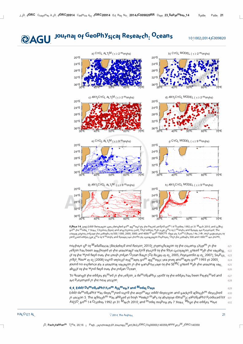
621northern tip of Madagascar [Backeberg and Reason, 2010]. Intensification of the currents system in the
622region has been attributed to the seasonally varying forcing of the gyre circulation, linked with the variabili-
623ty of the wind field over the south Indian Ocean Basin [De Ruijter et al., 2005; Palastanga et al., 2007]. Surpris-
624ingly, Nauw et al. [2008] using velocity estimates from altimetric sea level anomalies from 1993 to 2005,
625found no evidence for a seasonal variation in the transport rate of the SEMC linked with the seasonal vari-
626ability of the wind field over the Indian Ocean.
627To quantify the eddies formed in the region, a demographic study of the eddies has been performed and
628are presented in the next section.
6296.4. Eddy Demography From Altimetry and Model Data
630Eddy demography was determined using the automatic eddy detection and tracking algorithm described
631in section 5. The algorithm was applied to both weekly maps of absolute dynamic topography produced by
632AVISO, from 14 October 1992 to 31 March 2010, and model outputs for 7 years. While the eddies were
30oE 40
oE 50
oE 60
oE 70
oE
36oS
32oS
28oS
24oS
20oS
c) ANTICYCL ALTIM ( τ ≥ 2 months)
30oE 40
oE 50
oE 60
oE 70
oE
36oS
32oS
28oS
24oS
20oS
g) ANTICYCL ALTIM ( τ ≥ 9 months)
30oE 40
oE 50
oE 60
oE 70
oE
36oS
32oS
28oS
24oS
20oS
a) CYCL ALTIM ( τ ≥ 2 months)
30oE 40
oE 50
oE 60
oE 70
oE
36oS
32oS
28oS
24oS
20oS
e) CYCL ALTIM ( τ ≥ 9 months)
30oE 40
oE 50
oE 60
oE 70
oE
36oS
32oS
28oS
24oS
20oS
d) ANTICYCL MODEL ( τ ≥ 2 months)
30oE 40
oE 50
oE 60
oE 70
oE
36oS
32oS
28oS
24oS
20oS
h) ANTICYCL MODEL ( τ ≥ 9 months)
30oE 40
oE 50
oE 60
oE 70
oE
36oS
32oS
28oS
24oS
20oS
b) CYCL MODEL ( τ ≥ 2 months)
30oE 40
oE 50
oE 60
oE 70
oE
36oS
32oS
28oS
24oS
20oS
f) CYCL MODEL ( τ ≥ 9 months)
Figure 14. (left) Eddy generation sites identified from altimetry for the period ranging from 14 October 1992 to 31 March 2010, and (right)
from the model, 7 years. Cyclones (blue) and anticyclones (red). Only eddies with a life-time of 2 months and greater are presented. The
coastal isolines indicate the isobaths of 500, 1000, 2000, 3000, and 4000 m from GEBCO1 data set. From Figures 14e–14h, only trajectories of
long-lived eddies (life-time of 9 months and greater) are shown for visualization purposes. Only the isobaths 500 and 1000 m are shown.
J_ID: JGRC Customer A_ID: JGRC20914 Cadmus Art: JGRC20914 Ed. Ref. No.: 2014JC009820RR Date: 23-September-14 Stage: Page: 21
ID: pachiyappanm Time: 20:16 I Path: //xinchnasjn/01Journals/Wiley/3b2/JGRC/Vol00000/140359/APPFile/JW-JGRC140359
Journal of Geophysical Research: Oceans 10.1002/2014JC009820
HALO ET AL. VC 2014. The Authors. 21
633identified in the whole domain (Figures F1414a–14d), the analysis of the statistical census and mean properties
634(occurrence, kinetic energy, diameter, amplitude, vorticity, life-time, maximum traveling distance, polarity,
635and nonlinearity) were limited to the regions of most intense variability, SW and SE (Figure 1a for
636reference).
6376.4.1. Eddy Birth
638Figures 14a, 14c and 14b, 14d show generation sites of all cyclonic and anticyclonic eddies with a life-time
639of 2 months and greater (s � 60 days) in the altimetry and model data, respectively. Looking at the spatial
640distribution of the generation sites in both products, it is evident that both cyclonic and anticyclonic eddies
641were generated almost everywhere. In fact, it is now known that mesoscale eddies are ubiquitous features
642in the ocean [Chelton et al., 2007, 2011b]. Nevertheless, it is also observed in the two data sets a preferential
643tendency for cyclonic eddies to be formed directly south and southwest of Madagascar coast, near the con-
644tinental shelf (Figures 14a and 14b), while the anticyclonic eddies generally formed slightly farther offshore
645(Figures 14c and 14d). The generation of cyclonic eddies near to the coast was also observed to the south
646of the La-Reunion Island (�22�S, 55�E), and over the African continental shelf, near the Delagoa Bight
647(�26�S, 33�E). Within the Mozambique Channel, to the north of �24�S, both cyclones and anticyclones
648appear to be generated mostly in the eastern boundary. It is interesting to see that the model also feature
649this pattern remarkably well, giving us further confidence in the model. The occurrence of eddies near
650Madagascar and the African coast, over the Mozambican shelf (Figures 14e–14h), is an indicative of conti-
651nental boundary effects. In the southwestern Madagascar shelf (Figure 14e, near 26.5�S, 43.5�E), the distri-
652bution of cyclonic eddy formation sites is in agreement with the description of the flow found in recent
653literature [De Ruijter et al., 2004; Siedler et al., 2009; Ridderinkhof et al., 2013]. These studies have suggested
654that an occlusion of a cyclonic recirculation from the SEMC, near the southwestern sector of the Madagascar
655shelf triggers cyclonic eddies, by friction between the landward edge of the SEMC with the shelf. On the
656other hand, the seaward edge of the SEMC becomes unstable, leading to an anticyclonic recirculation, even-
657tually triggering anticyclonic eddies, which may form a part of a dipole structure [De Ruijter et al., 2004],
658hence explaining the presence for the site of anticyclonic eddy formation, here observed in both products
659directly south and southwest of Madagascar. Whereas along the eastern margin of the African continent,
660over Mozambican shelf, the generation of cyclonic eddies is in agreement with the Delagoa Bight eddies
661described by Lutjeharms and da Silva [1988], known to be formed by interaction of the flow from the
662Mozambique Channel, with the continental slope [Lutjeharms and da Silva, 1988; Lamont et al., 2010]. The
663anticyclonic eddy formation along the southeastern margin of Madagascar near 28�S appears to be related
664to the interaction of the SEMC with the local topography (Madagascar Ridge), perhaps during the period
665when the SEMC is mostly poleward oriented as proposed by Siedler et al. [2009]. On the other hand, the
666generation site at 24�S could be related to the interaction between the SEMC with the incoming variability
667signals from the Indian Ocean, along the eddy-corridor [Quartly et al., 2006] (see Figure 1b). These patterns
668are also evident in altimetry (Figure 14g) and model (Figure 14h).
669Caution is required when comparing the maps of energy conversion terms by KmKe and PeKe presented
670in Figure 12 against the eddy birth sites identified by the eddy detection scheme used here as shown in
671Figure 14. The latter shows generation sites almost everywhere, while the former shows KmKe and PeKe at
672localized positions. Both model and observations clearly show that for some places, high clusters of eddy
673birth sites are located where strong signals of KmKe and/or PeKe cooccurs (e.g., along the southeastern
674coast of Madagascar, also around the southern tip of Madagascar). On the other hand, there are also clus-
675ters of high birth positions where no signals of KmKe and/or PeKe are enhanced (e.g., clusters of cyclonic
676eddies along the southwestern margin of Madagascar, between 26�S and 24�S). Such an apparent dis-
677crepancy should be interpreted carefully: the energy transfer terms being vertically integrated, they will
678be significant for eddies generated with a sufficient vertical extension. The eddy detection being done on
679the surface pressure field (the SSH), it does not discriminate between structures purely at the surface and
680those with a larger vertical extension. This is probably why there is a better correspondence with the
681long-lived eddies (a structure with a larger spatial extension should be able to keep its coherence for a
682longer time).
6836.4.2. Eddy Census
684For the entire period of altimetry used here (14 October 1992 to 31 March 2010), the eddy detection
685scheme in the SW region identified a total of 394 eddies. About 58% of these were cyclones and 42% were
J_ID: JGRC Customer A_ID: JGRC20914 Cadmus Art: JGRC20914 Ed. Ref. No.: 2014JC009820RR Date: 23-September-14 Stage: Page: 22
ID: pachiyappanm Time: 20:16 I Path: //xinchnasjn/01Journals/Wiley/3b2/JGRC/Vol00000/140359/APPFile/JW-JGRC140359
Journal of Geophysical Research: Oceans 10.1002/2014JC009820
HALO ET AL. VC 2014. The Authors. 22
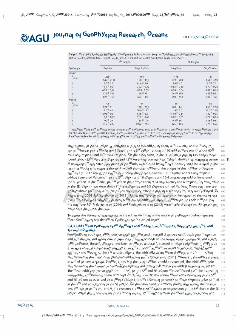
686anticyclones. In the SE region, it identified a total of 356 eddies, of about 49% cyclonic and 51% anticy-
687clonic. Whereas in the model (for 7 years), in the SW region, a total of 106 eddies were found: about 60%
688were anticyclones and 40% were cyclones. On the other hand, in the SE region, a total of 145 eddies were
689found, about 55% were anticyclones and 45% were their counter-part. Table T11 shows their statistical census
690N. Relatively smaller quantities found in the model as opposed by altimetry product could be related to the
691fact that model time series is shorter. Dividing the total number of the eddies by the number of years in
692altimetry (�17.47 years), the estimates suggest that there are about 13.1 cyclonic and 9.4 anticyclonic
693eddies generated per annum in the SW region, and 10 cyclonic and 10.4 anticyclonic eddies generated in
694the SE region. In the model, for SW region there were about 9.14 anticyclones and 6 cyclones per year, while
695in the SE region there were about 11.4 anticyclones and 9.3 cyclones formed per year. These estimates are
696slightly above from that reported in previous studies, where a total of 4–6 eddies per year are proposed [De
697Ruijter et al., 2004; Ridderinkhof et al., 2013]. Higher estimates in our case could be related to the use of rela-
698tively more precise algorithms to identify mesoscale eddy structures. It is important to keep in mind that
699the estimates by De Ruijter et al. [2004] and Ridderinkhof et al. [2013] were made specially for dipole-eddies,
700while here that is not the case.
701To assess the general characteristics of the eddies dominating the region an inspection of their relevant
702mean geometrical and dynamical properties are presented below.
7036.4.3. Eddy Mean Properties From Altimetry and Model: Size, Amplitude, Vorticity, Life-Time, and704Traveling Distance
705Knowledge of eddy size, amplitude, vorticity, life-time, and traveling distances can provide information on
706eddies behavior, and allows one to infer their implication both on the overall ocean circulation, and ecosys-
707tems response. These properties have been estimated and are presented in Table 1 (diameter �L, amplitude
708�g, relative vorticity �f, planetary vorticity �f , life-time �s , and maximum traveling distance �k), derived from
709altimetry and model, for the SW and SE regions. The eddy equivalent mean diameter (�L523ffiffiffiffiffiffiffiffiffiffiffiffiffiffiffiffiffi
P
S=Npp
)
710was defined as the mean of all identified eddies per frame [Souza et al., 2011]. Where S is the eddy’s surface,
711assumed to have a circular geometry, and N is the total number of eddies detected. The eddy amplitude
712was defined as the difference between the highest and lowest SSH within the eddy [Chelton et al., 2011b].
713The mean eddy relative vorticity (�n5P
n=N), for the SW and SE regions was computed from the horizontal
714geostrophic components of the flow field: n5@v=@x2@u=@y. The annual mean eddy properties in the SW
715and SE regions as observed by altimetry (Table 1) shows a general tendency for more cyclones to be formed
716in the SW and anticyclones in the SE region. On the other hand, the model shows anticyclonic dominance
717everywhere. In terms of �L and �g, the cyclones are more comparable to anticyclones in the SW than in the SE
718region. Again this is not present in the model results. Symmetry between the mean sizes of cyclones and
Table 1. Mean Eddy Properties Estimated in Two-Different Regions Around South of Madagascar, Southwest Region, SW: 39�E–45�E
and 32�S–23�S, and Southeast Region, SE: 45.10�E–51.10�E and 32�S–23�S (See Figure 1a for Reference)a
Properties
SW Region SE Region
Cyclones Anticyclones Cyclones Anticyclones
AVISO
Neddies 229 165 175 181
L 1456 21.0 1506 33.0 1396 28.0 1546 32.0
g 15.06 7.0 15.06 8.0 9.06 4.0 12.06 7.0
f 21.16 0.3 0.926 0.22 20.836 0.39 0.796 0.28
f 26.93 60.64 26.9560.55 26.946 0.64 26.826 0.65
s 1766 105 1266 85 1636 109 1426 93
k 8276 457 6176 437 5506 418 5856 460
MODEL
Neddies 42 64 65 80
L 1246 11 1786 26.0 1206 14 1666 22.0
g 9.06 4.0 28.06 18.0 96 5.0 22.06 12.0
f 20.936 0.3 1.166 0.2 21.106 0.34 1.206 0.35
f 26.76 0.62 26.876 0.66 26.826 0.65 26.796 0.65
s 906 29 1836 104 1446 54 1536 94
k 4156 229 10526 744 3256 195 7776 659
aEstimates made from altimetric eddies detected from 14 October 1992 to 31 March 2010, and model output (7 years). Neddies is the
number of eddies, L (km) is eddy diameter, g (cm) is eddy amplitude, f (31026 s21) is the relative vorticity, f (31025 s21) is Coriolis
parameter within the eddy, s (day) is eddy life-time, and k (km) is the maximum eddy traveling distance.
J_ID: JGRC Customer A_ID: JGRC20914 Cadmus Art: JGRC20914 Ed. Ref. No.: 2014JC009820RR Date: 23-September-14 Stage: Page: 23
ID: pachiyappanm Time: 20:16 I Path: //xinchnasjn/01Journals/Wiley/3b2/JGRC/Vol00000/140359/APPFile/JW-JGRC140359
Journal of Geophysical Research: Oceans 10.1002/2014JC009820
HALO ET AL. VC 2014. The Authors. 23
719anticyclones in the SW region also has been observed by De Ruijter et al. [2004] and Ridderinkhof et al.
720[2013]. The estimates shown in Table 1 indicate that the model slightly over-estimates the size of the anticy-
721clones, while under-estimating the cyclones. It also greatly over-estimates the amplitude of the anticy-
722clones. Over-estimation of the eddies amplitudes could be associated to the fact that the model over-
723estimates the variability of SSH in this region, as demonstrated in our previous study [Halo et al., 2014].
724While over-estimating the eddy-size presented in Table 1, one should keep in mind that in situ observation
725made in this region have shown that the eddies radii in the region varies from 50 to 250 km [De Ruijter
726et al., 2004]. The swirling velocities of the eddy observed during the ASCLME at the southwest coast of
727Madagascar, around 25�30S (Figure 5), also can give an idea of the size of the eddy. These observations sug-
728gest that the eddies presented here (Table 1), are within the expected range. Altimetric results presented in
729Table 1 have shown that cyclonic eddies formed in the SW region have stronger vorticity, live longer, and
730travel longer distances from their origin than any other mesoscale coherent structure inspected. However,
731the model failed to reproduce that pattern, while attributing such properties to the anticyclones. Neverthe-
732less, these results indicate that the eddies in the SW region hold distinct properties from those in the SE. It
733is tempting to relate such differences to the different modes of variability which are known to dominate
734these regions, namely, seasonal wind forcings to the west of the Madagascar Ridge, and current variability
735to the east [Matano et al., 1999].
7366.4.4. Eddy Tracks
737Figures 14e–14g show the trajectories of cyclonic and anticyclonic eddies derived from the altimetry and
738model data. The dots represent their generation sites and the tracks their pathways. Only long-lived eddies
739(s � 9 months) are presented for visualization purpose. For this time scale, there are more long-lived eddies
740in the altimetry (Figures 14e and 14g), than in the model (Figures 14f and 14h). In altimetry there are more
741long-lived cyclones than anticyclones, while the opposite is observed in the model. From the altimetry,
742many of the long-lived cyclonic eddies formed directly south of the southern tip of Madagascar (Figure
74314e), made their way toward the southeastern coast of the African continent. This indicates that connectiv-
744ity between Madagascar and Africa does exist. Whereas for anticyclones (Figure 14g), such connectivity still
745exist, but is not vigorous at this time scale. In the model, such time scale favors more anticyclones (Figure
74614h) than cyclones (Figure 14f). For both products, the long-lived anticyclonic eddies were formed only to
747the east of �45�E, in the Madagascar and Mascarene Basins. These eddies propagate predominantly west-
748ward, with a slightly northwestward orientation for anticyclones (Figure 14g). Westward propagation of
749eddies with a slight meridional deflections (poleward for cyclones and equatorward for anticyclones) is in
750agreement with a previous study in the region [De Ruijter et al., 2004], (see their Figure 9). These trajectories
751are consistent with theories of geostrophic ocean turbulence [McWilliams and Flierl, 1979; Chelton et al.,
7522007], and have been observed in various ocean basins [Morrow et al., 2004]. Eddies meridional deflections
753have been attributed to a combined effect of the planetary vorticity gradient and eddy self-advection
754[McWilliams and Flierl, 1979; Cushman-Roisin, 1994]. Altimetric cyclones and anticyclones have been
755deflected poleward at the continental boundary, in the southeastern coast of Madagascar. In coastal zones,
756meridional deflections are known to be associated with background boundary currents [Chelton et al.,
7572011b]. In our case, the SEMC and the AC may play a significant role. From the model, at the time scale (s �
7589 months), none eddy from the east Indian Ocean was able to reach the Madagascar coast. They dissipate
759near 60�E (Figures 14f and 14h). In the Mozambique Basin, eddies have followed a southwestward trajecto-
760ries, with cyclones having a stronger poleward orientation than anticyclones. Again, it is also evident a
761northwestward propagation of the anticyclones from altimetry (Figure 14g) and model (Figure 14h). On
762reaching the African continent at �24–25�S, they seem to be advected poleward along the path of the
763eddies and rings coming from the Mozambique Channel, which are known to propagate parallel to the
764coast toward the Agulhas Current [De Ruijter et al., 2002; Schouten et al., 2003; Ridderinkhof and De Ruijter,
7652003; Halo et al., 2014].
7666.4.5. Eddy-Density and Energy Distribution
767Figures F1515a–15d shows the distribution of the total number of eddies (in %) with s � 60 day, identified in
768the SW and SE regions, in the altimetry data set (from 14 October 1992 to 31 March 2010), and model out-
769put (for 7 years). They are distributed as function of their radii, clustered at 10 km intervals. The correspond-
770ing eddy kinetic energy integrated across their surface is shown from Figures 15e–15h. For the altimetry,
771cyclonic eddies are represented by white bars and anticyclonic eddies by black. Whereas in the model,
772cyclones are light-gray bars, and anticyclones are dark-gray. Eddies with radii smaller than 40 km are
J_ID: JGRC Customer A_ID: JGRC20914 Cadmus Art: JGRC20914 Ed. Ref. No.: 2014JC009820RR Date: 23-September-14 Stage: Page: 24
ID: pachiyappanm Time: 20:16 I Path: //xinchnasjn/01Journals/Wiley/3b2/JGRC/Vol00000/140359/APPFile/JW-JGRC140359
Journal of Geophysical Research: Oceans 10.1002/2014JC009820
HALO ET AL. VC 2014. The Authors. 24
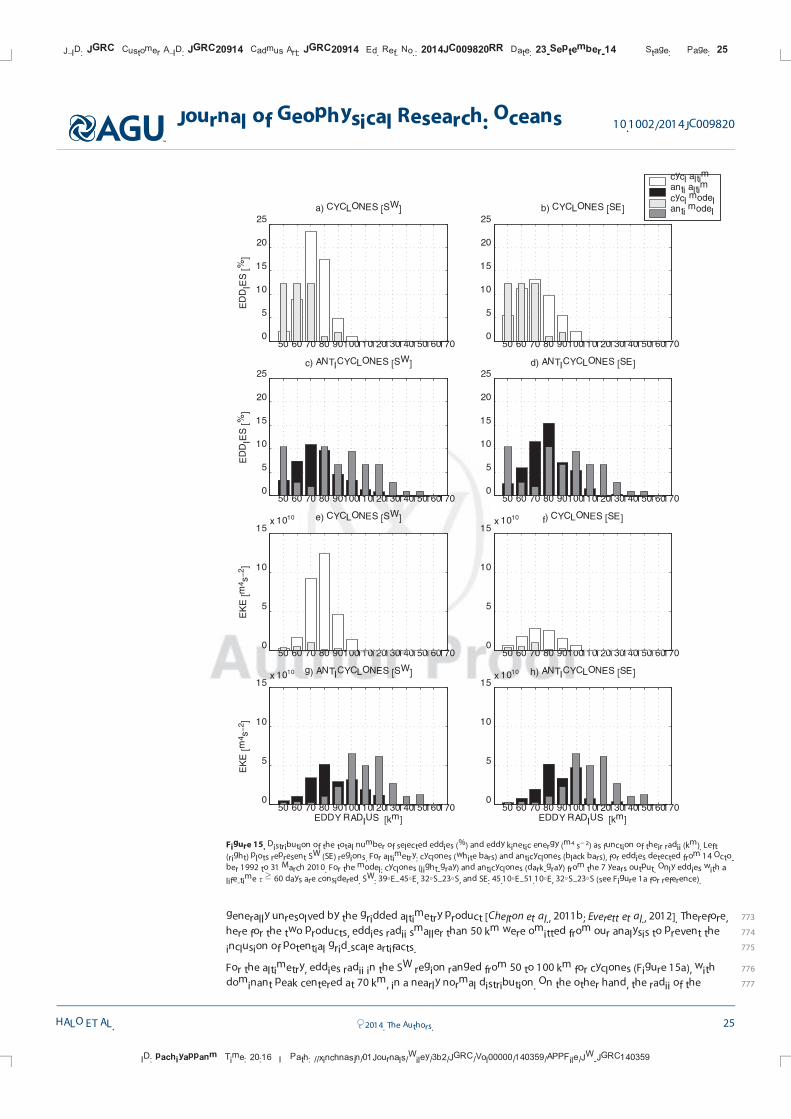
773generally unresolved by the gridded altimetry product [Chelton et al., 2011b; Everett et al., 2012]. Therefore,
774here for the two products, eddies radii smaller than 50 km were omitted from our analysis to prevent the
775inclusion of potential grid-scale artifacts.
776For the altimetry, eddies radii in the SW region ranged from 50 to 100 km for cyclones (Figure 15a), with
777dominant peak centered at 70 km, in a nearly normal distribution. On the other hand, the radii of the
50 60 70 80 901001101201301401501601700
5
10
15
20
25b) CYCLONES [SE]
cycl altimanti altimcycl modelanti model
50 60 70 80 901001101201301401501601700
5
10
15
20
25d) ANTICYCLONES [SE]
50 60 70 80 901001101201301401501601700
5
10
15x 10
10 f) CYCLONES [SE]
50 60 70 80 901001101201301401501601700
5
10
15x 10
10
EDDY RADIUS [km]
h) ANTICYCLONES [SE]
50 60 70 80 901001101201301401501601700
5
10
15
20
25a) CYCLONES [SW]
ED
DIE
S [
%]
50 60 70 80 901001101201301401501601700
5
10
15
20
25c) ANTICYCLONES [SW]
ED
DIE
S [
%]
50 60 70 80 901001101201301401501601700
5
10
15x 10
10 e) CYCLONES [SW]
EK
E [
m4s
−2]
50 60 70 80 901001101201301401501601700
5
10
15x 10
10
EDDY RADIUS [km]
g) ANTICYCLONES [SW]
EK
E [
m4s
−2]
Figure 15. Distribution of the total number of selected eddies (%) and eddy kinetic energy (m4 s22) as function of their radii (km). Left
(right) plots represent SW (SE) regions. For altimetry: cyclones (white bars) and anticyclones (black bars), for eddies detected from 14 Octo-
ber 1992 to 31 March 2010. For the model: cyclones (light-gray) and anticyclones (dark-gray) from the 7 years output. Only eddies with a
life-time s � 60 days are considered. SW: 39�E–45�E, 32�S–23�S, and SE: 45.10�E–51.10�E, 32�S–23�S (see Figure 1a for reference).
J_ID: JGRC Customer A_ID: JGRC20914 Cadmus Art: JGRC20914 Ed. Ref. No.: 2014JC009820RR Date: 23-September-14 Stage: Page: 25
ID: pachiyappanm Time: 20:16 I Path: //xinchnasjn/01Journals/Wiley/3b2/JGRC/Vol00000/140359/APPFile/JW-JGRC140359
Journal of Geophysical Research: Oceans 10.1002/2014JC009820
HALO ET AL. VC 2014. The Authors. 25
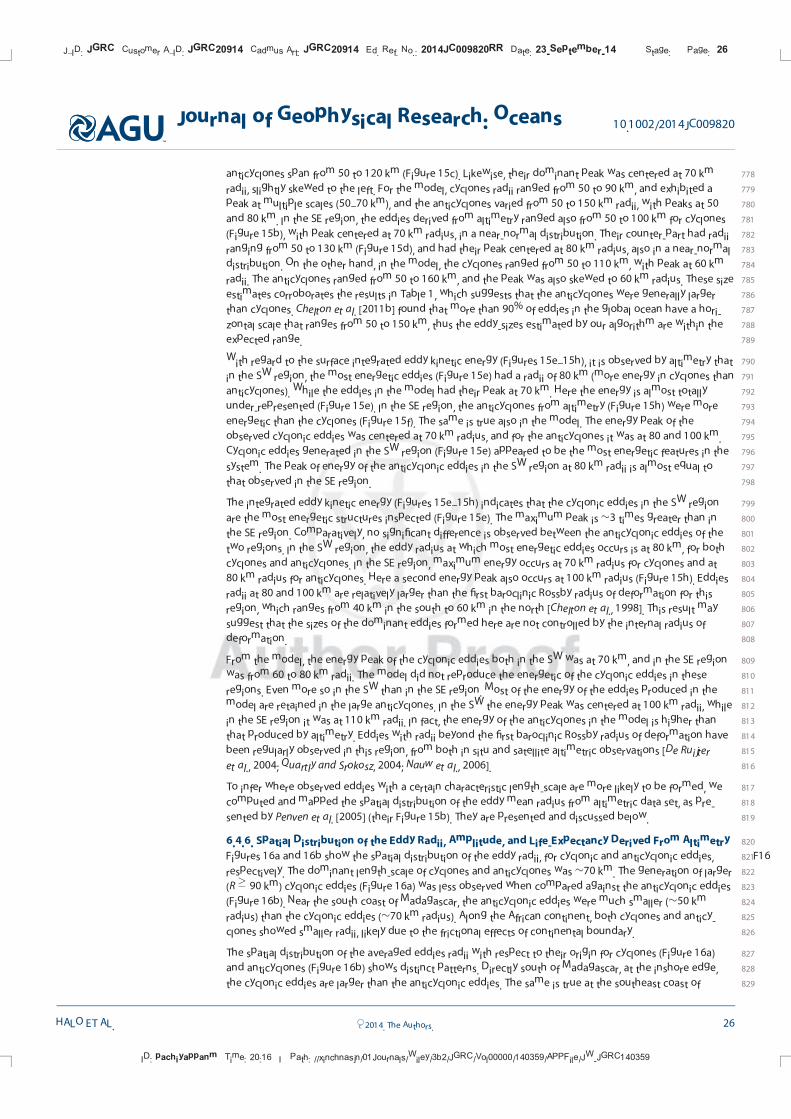
778anticyclones span from 50 to 120 km (Figure 15c). Likewise, their dominant peak was centered at 70 km
779radii, slightly skewed to the left. For the model, cyclones radii ranged from 50 to 90 km, and exhibited a
780peak at multiple scales (50–70 km), and the anticyclones varied from 50 to 150 km radii, with peaks at 50
781and 80 km. In the SE region, the eddies derived from altimetry ranged also from 50 to 100 km for cyclones
782(Figure 15b), with peak centered at 70 km radius, in a near-normal distribution. Their counter-part had radii
783ranging from 50 to 130 km (Figure 15d), and had their peak centered at 80 km radius, also in a near-normal
784distribution. On the other hand, in the model, the cyclones ranged from 50 to 110 km, with peak at 60 km
785radii. The anticyclones ranged from 50 to 160 km, and the peak was also skewed to 60 km radius. These size
786estimates corroborates the results in Table 1, which suggests that the anticyclones were generally larger
787than cyclones. Chelton et al. [2011b] found that more than 90% of eddies in the global ocean have a hori-
788zontal scale that ranges from 50 to 150 km, thus the eddy-sizes estimated by our algorithm are within the
789expected range.
790With regard to the surface integrated eddy kinetic energy (Figures 15e–15h), it is observed by altimetry that
791in the SW region, the most energetic eddies (Figure 15e) had a radii of 80 km (more energy in cyclones than
792anticyclones). While the eddies in the model had their peak at 70 km. Here the energy is almost totally
793under-represented (Figure 15e). In the SE region, the anticyclones from altimetry (Figure 15h) were more
794energetic than the cyclones (Figure 15f). The same is true also in the model. The energy peak of the
795observed cyclonic eddies was centered at 70 km radius, and for the anticyclones it was at 80 and 100 km.
796Cyclonic eddies generated in the SW region (Figure 15e) appeared to be the most energetic features in the
797system. The peak of energy of the anticyclonic eddies in the SW region at 80 km radii is almost equal to
798that observed in the SE region.
799The integrated eddy kinetic energy (Figures 15e–15h) indicates that the cyclonic eddies in the SW region
800are the most energetic structures inspected (Figure 15e). The maximum peak is �3 times greater than in
801the SE region. Comparatively, no significant difference is observed between the anticyclonic eddies of the
802two regions. In the SW region, the eddy radius at which most energetic eddies occurs is at 80 km, for both
803cyclones and anticyclones. In the SE region, maximum energy occurs at 70 km radius for cyclones and at
80480 km radius for anticyclones. Here a second energy peak also occurs at 100 km radius (Figure 15h). Eddies
805radii at 80 and 100 km are relatively larger than the first baroclinic Rossby radius of deformation for this
806region, which ranges from 40 km in the south to 60 km in the north [Chelton et al., 1998]. This result may
807suggest that the sizes of the dominant eddies formed here are not controlled by the internal radius of
808deformation.
809From the model, the energy peak of the cyclonic eddies both in the SW was at 70 km, and in the SE region
810was from 60 to 80 km radii. The model did not reproduce the energetic of the cyclonic eddies in these
811regions. Even more so in the SW than in the SE region. Most of the energy of the eddies produced in the
812model are retained in the large anticyclones. In the SW the energy peak was centered at 100 km radii, while
813in the SE region it was at 110 km radii. In fact, the energy of the anticyclones in the model is higher than
814that produced by altimetry. Eddies with radii beyond the first baroclinic Rossby radius of deformation have
815been regularly observed in this region, from both in situ and satellite altimetric observations [De Ruijter
816et al., 2004; Quartly and Srokosz, 2004; Nauw et al., 2006].
817To infer where observed eddies with a certain characteristic length-scale are more likely to be formed, we
818computed and mapped the spatial distribution of the eddy mean radius from altimetric data set, as pre-
819sented by Penven et al. [2005] (their Figure 15b). They are presented and discussed below.
8206.4.6. Spatial Distribution of the Eddy Radii, Amplitude, and Life-Expectancy Derived From Altimetry
821Figures F1616a and 16b show the spatial distribution of the eddy radii, for cyclonic and anticyclonic eddies,
822respectively. The dominant length-scale of cyclones and anticyclones was �70 km. The generation of larger
823(R � 90 km) cyclonic eddies (Figure 16a) was less observed when compared against the anticyclonic eddies
824(Figure 16b). Near the south coast of Madagascar, the anticyclonic eddies were much smaller (�50 km
825radius) than the cyclonic eddies (�70 km radius). Along the African continent, both cyclones and anticy-
826clones showed smaller radii, likely due to the frictional effects of continental boundary.
827The spatial distribution of the averaged eddies radii with respect to their origin for cyclones (Figure 16a)
828and anticyclones (Figure 16b) shows distinct patterns. Directly south of Madagascar, at the inshore edge,
829the cyclonic eddies are larger than the anticyclonic eddies. The same is true at the southeast coast of
J_ID: JGRC Customer A_ID: JGRC20914 Cadmus Art: JGRC20914 Ed. Ref. No.: 2014JC009820RR Date: 23-September-14 Stage: Page: 26
ID: pachiyappanm Time: 20:16 I Path: //xinchnasjn/01Journals/Wiley/3b2/JGRC/Vol00000/140359/APPFile/JW-JGRC140359
Journal of Geophysical Research: Oceans 10.1002/2014JC009820
HALO ET AL. VC 2014. The Authors. 26

830Madagascar. However, the opposite is observed further offshore. This may suggest a larger sensitivity for
831dissipation of the anticyclones by frictional effects with the continental boundaries. Their life-expectancy
832also corroborates further this conclusion (Figures 16e and 16f). Another distinct pattern is a general tend-
833ency for the eddies to decrease in size from the south of Madagascar toward the southeastern African
834coast. From geostrophic oceanic turbulence, such a poleward meridional decrease of the eddies horizon-
835tal scale is expected to occur, since the deformation radius decreases with the increasing latitude [Chelton
836et al., 1998, 2007].
837Similar analysis also made for the spatial distribution of the eddy mean amplitude, for cyclonic and anticy-
838clonic eddies, as presented by Everett et al. [2012] for the Tasman sea (see their Figures 1c and 1d), is shown
839in Figures 16c and 16d, respectively. Comparing these maps against their corresponding plots (Figures 16a
840and 16b), a consistent pattern is observed: the position of the highest mean amplitude (�over 30 cm) of
841the cyclonic eddies coincided with the location of largest radius (�over 90 km, near 27�S, 43�E). The same is
842true for the anticyclonic eddies, with exception for those formed around the eastern parts of the domain
843(�24�S, 53�E), where the largest anticyclonic eddies (Figure 16b) had smaller amplitudes (�10 cm,
844Figure 16d).
50
50
5050
70
70
7070
70
70
70
70
70
70
70
70
70
70
70
70
70
70
70
70
70
70
70
70
90
30oE 36
oE 42
oE 48
oE 54
oE
30oS
27oS
24oS
21oS
a) CYCLONIC RADIUS [km]
50
50
50
70
70
70
70
70
70
70
70
70
70
70
70
70
70
70
70
70
70
70
70
70
70
70
90
90
90
90
9090
90
90
90
90
90
90
9090
90
90
30oE 36
oE 42
oE 48
oE 54
oE
30oS
27oS
24oS
21oS
b) ANTICYCLONIC RADIUS [km]
50 60 70 80 90 100
10
10
10 10
10
10
10
10
10
10
10
10
10
10
10
10
10
10
10
10
10
10
10
10
10
10
10
10
10
10
10
10
20 20
20
20
20
20
20
20
20
20
20
20
20
20
20
20
20
3030
30oE 36
oE 42
oE 48
oE 54
oE
30oS
27oS
24oS
21oS
c) CYCLONIC AMPLITUDE [cm]
10
10
10
10
10
10 10
10
10 10
1010
10
10
10
1010
10
10
10
10
10
10
10
10
10
10
10 10
20
20
20
20
20
20
20
20
20
20
20
20
2020
2020
20
20
30
30
30
30
30
30
30
30
30
40
40
30oE 36
oE 42
oE 48
oE 54
oE
30oS
27oS
24oS
21oS
d) ANTICYCLONIC AMPLITUDE [cm]
0 10 20 30 40 50
120
120
120 120
120
120
120
120
120
120
120
120
120
120
120
120
120
12
0
120
120
120
120
120
1201
20
120
120
120
120
120
120
120
120
120
120
120
240
240
240
240240
240
240
240
240
240
240
360360
30oE 36
oE 42
oE 48
oE 54
oE
30oS
27oS
24oS
21oS
e) CYCLONIC LIFETIME [days]
120
120
120
120
120
120
120
120
120
120
120
120
120
120
120
120
120
120
120
120
120
120
120
120
120
120
120
120
120
120120 240
240
240
240
240240240
360
30oE 36
oE 42
oE 48
oE 54
oE
30oS
27oS
24oS
21oS
f) ANTICYCLONIC LIFETIME [days]
0 50 100 150 200 250 300 350 400 450 500
Figure 16. Spatial distribution of the mean eddy radius (km), mean amplitude (cm), and mean time of eddy permanence (days), with
regard to their generation site. Altimetric eddies detected from 14 October 1992 to 31 March 2010. Left plots show cyclonic eddies and
right plots anticyclonic.
J_ID: JGRC Customer A_ID: JGRC20914 Cadmus Art: JGRC20914 Ed. Ref. No.: 2014JC009820RR Date: 23-September-14 Stage: Page: 27
ID: pachiyappanm Time: 20:16 I Path: //xinchnasjn/01Journals/Wiley/3b2/JGRC/Vol00000/140359/APPFile/JW-JGRC140359
Journal of Geophysical Research: Oceans 10.1002/2014JC009820
HALO ET AL. VC 2014. The Authors. 27
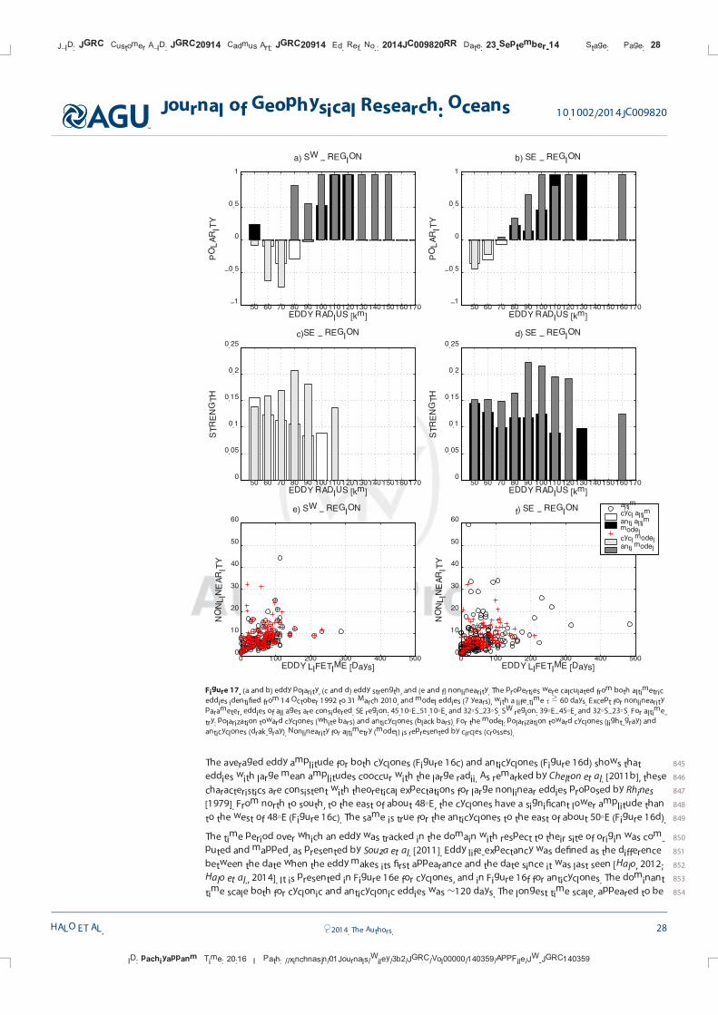
845The averaged eddy amplitude for both cyclones (Figure 16c) and anticyclones (Figure 16d) shows that
846eddies with large mean amplitudes cooccur with the large radii. As remarked by Chelton et al. [2011b], these
847characteristics are consistent with theoretical expectations for large nonlinear eddies proposed by Rhines
848[1979]. From north to south, to the east of about 48�E, the cyclones have a significant lower amplitude than
849to the west of 48�E (Figure 16c). The same is true for the anticyclones to the east of about 50�E (Figure 16d).
850The time period over which an eddy was tracked in the domain with respect to their site of origin was com-
851puted and mapped, as presented by Souza et al. [2011]. Eddy life-expectancy was defined as the difference
852between the date when the eddy makes its first appearance and the date since it was last seen [Halo, 2012;
853Halo et al., 2014]. It is presented in Figure 16e for cyclones, and in Figure 16f for anticyclones. The dominant
854time scale both for cyclonic and anticyclonic eddies was �120 days. The longest time scale, appeared to be
50 60 70 80 90 100 110 120 130 140 150 160 170−1
−0.5
0
0.5
1
PO
LA
RIT
Y
EDDY RADIUS [km]
b) SE − REGION
0 100 200 300 400 5000
10
20
30
40
50
60
NO
NLIN
EA
RIT
Y
EDDY LIFETIME [Days]
f) SE − REGION altimcycl altimanti altimmodelcycl modelanti model
50 60 70 80 90 100 110 120 130 140 150 160 1700
0.05
0.1
0.15
0.2
0.25
ST
RE
NG
TH
EDDY RADIUS [km]
c)SE − REGION
50 60 70 80 90 100 110 120 130 140 150 160 1700
0.05
0.1
0.15
0.2
0.25
EDDY RADIUS [km]
ST
RE
NG
TH
d) SE − REGION
50 60 70 80 90 100 110 120 130 140 150 160 170−1
−0.5
0
0.5
1
PO
LA
RIT
Y
EDDY RADIUS [km]
a) SW − REGION
0 100 200 300 400 5000
10
20
30
40
50
60
NO
NLIN
EA
RIT
Y
EDDY LIFETIME [Days]
e) SW − REGION
Figure 17. (a and b) eddy polarity, (c and d) eddy strength, and (e and f) nonlinearity. The properties were calculated from both altimetric
eddies identified from 14 October 1992 to 31 March 2010, and model eddies (7 years), with a life-time s � 60 days. Except for nonlinearity
parameter, eddies of all ages are considered. SE region: 45.10�E–51.10�E, and 32�S–23�S. SW region: 39�E–45�E, and 32�S–23�S. For altime-
try: polarization toward cyclones (white bars) and anticyclones (black bars). For the model: polarization toward cyclones (light-gray) and
anticyclones (drak-gray). Nonlinearity for altimetry (model) is represented by circles (crosses).
J_ID: JGRC Customer A_ID: JGRC20914 Cadmus Art: JGRC20914 Ed. Ref. No.: 2014JC009820RR Date: 23-September-14 Stage: Page: 28
ID: pachiyappanm Time: 20:16 I Path: //xinchnasjn/01Journals/Wiley/3b2/JGRC/Vol00000/140359/APPFile/JW-JGRC140359
Journal of Geophysical Research: Oceans 10.1002/2014JC009820
HALO ET AL. VC 2014. The Authors. 28
855associated with eddies that formed to the southeast of the Madagascar Basin, between �32�S and 27�S,
856and 48�E and 53�E.
857Eddy life-time is shown in Figures 16e and 16f. Eddies formed in the eastern parts of the domain have a lon-
858ger life-expectancy. In the western parts, a significant eddy-shelf and eddy-eddy interactions are known to
859occur [De Ruijter et al., 2004], these may enhance their weakening and dissipation. This result indicates that
860the eddy amplitude is not the sole factor that determines the longevity of an eddy, as has been inferred by
861Chelton et al. [2011b]. Cyclonic eddies (Figure 16e) generated near the Madagascar coast have a longer life-
862expectancy than the anticyclones (Figure 16f).
863To determine the dominant eddy type in the SW and SE of Madagascar, and infer their potential role on the
864marine connectivity between Madagascar and Africa, relevant dynamical eddy properties are discussed
865below.
8666.4.7. Eddy Polarity, Strength, and Nonlinearity From Altimetry and Model
867Figures F1717a and 17b show the eddy polarity for the SW and SE regions, respectively, as function of their
868radii, clustered into 10 km intervals, based on altimetry observations and model output. For altimetry cyclo-
869nes are represented by white bars and anticyclones by black bars. For the model, cyclones are light-gray
870bars and anticyclones by dark-gray bars. Eddy polarity provides useful information about the length-scale at
871which cyclonic eddies are prevalent over anticyclonic eddies [Chelton et al., 2011b]. Following Kurian et al.
872[2011], eddy polarity was defined as ðNa2NcÞ=ðNa1NcÞ, where Na and Nc are the total numbers of anticy-
873clonic and cyclonic eddies, respectively.
874From altimetry product in the SW region, there were eight bands of polarization (Figure 17a). The eddies
875were polarized toward the cyclones between 60 and 90 km radii, accounting for 50% of the all observed
876bands. Prevalence of anticyclones occurred at 50 km, and between 100 and 120 km radii, accounting for
877the other 50%. This result arguably could indicate that a dipolar coherent mesoscale structure is favored to
878occur in the SW region. Prevalence of cyclonic eddies occurs at smaller-scales, and anticyclonic eddies at
879larger-scales, except at 50 km. For the SE region (Figure 17b), there were also eight bands of polarization.
880Prevalence toward cyclones occurred at radii between 50 and 70 km, accounting for 37.5% of all observed
881bands. The polarization toward anticyclones ranged from 80 to 130 km, accounting for 62.5%. This indicates
882a tendency for anticyclones at large-scale to dominate over the cyclones in the SE region.
883In order to infer the tendency for dominance of large anticyclones over the cyclones, we have inspected
884the strength of the eddies formed within this region. Here following Kurian et al. [2011] and Liang et al.
885[2012], eddy strength was defined as the ratio between the absolute relative vorticity averaged within the
886eddy, normalized by the planetary vorticity jf=f j. Figures 17c and 17d show their distribution as function of
887cyclonic and anticyclonic radii. Cyclonic eddies were stronger than the anticyclonic at smaller-scale (R �
88870 km), while the opposite was observed at larger-scales.
889From the model product in the SW region (Figure 17a), there were 11 bands of polarization. Cyclones
890polarization ranged from 50 to 70 km radii, while anticyclones were from 80 to 150 km. In the SE region
891(Figure 17b), cyclones were between 50 and 60 km, and anticyclones span from 70 to 160 km. In general,
892the model shows a strong preference for anticyclonic formation at both intermediate (70–80 km) and
893larger (�80 km) horizontal scales, while cyclones at smaller-scales. Inspection of their strength in the SE
894region has shown a tendency for cyclones to reach their maximum strength at 80 km (Figure 17c) and
895anticyclones at 90 km radii (Figure 17d). The asymmetry between cyclones and anticyclones has been
896observed in in situ measurements, laboratory experiments, as well as in numerical model solutions [McWil-
897liams, 1985; Graves et al., 2006; Perret et al., 2006, 2011]. However, theoretical explanations for this asym-
898metry remain an ongoing study, suggesting different controlling mechanisms [Cushman-Roisin and Tang,
8991990; Willett et al., 2006; Graves et al., 2006; Perret et al., 2006, 2011]. Because the eddies in our study are
900not wind forced, rather they form through current instabilities, interpretations linked to the wind activity
901are not considered here. The eddies in the SE region are mostly formed through barotropic instabilities of
902the SEMC in the upper ocean, and baroclinic instabilities at intermediate depths (Figure 11). Possible
903explanation for the observed asymmetry here is made through inspections of the eddy strength, which
904measure their robustness. For altimetry, our analysis of the eddy strength in the SE shows a considerable
905weakening of the cyclones while increasing radii (Figure 17c). Under such weakening regime, the preva-
906lence of the large anticyclones over cyclones could be associated to the tendency for weakening of the
J_ID: JGRC Customer A_ID: JGRC20914 Cadmus Art: JGRC20914 Ed. Ref. No.: 2014JC009820RR Date: 23-September-14 Stage: Page: 29
ID: pachiyappanm Time: 20:16 I Path: //xinchnasjn/01Journals/Wiley/3b2/JGRC/Vol00000/140359/APPFile/JW-JGRC140359
Journal of Geophysical Research: Oceans 10.1002/2014JC009820
HALO ET AL. VC 2014. The Authors. 29
907large cyclonic structures, probably induced by the background flow [Perret et al., 2011]. Similar process
908also has been reported in the northeastern tropical Pacific [Liang et al., 2012]. However, in the model,
909such pattern can only be observed for cyclonic eddies with radii larger than 70 km. From 50 to 80 km they
910increase in strength, then they decrease. It is likely that other processes (not mentioned here) are also
911playing an important role.
912To investigate the ability of the eddies to trap materials, we have inspected the nonlinearity parameter of
913eddies of all ages in the SW and SE regions, both for altimetry and model output. Following Chelton et al.
914[2007, 2011b], eddy nonlinearity parameter was defined as the ratio between the eddy rotational velocity
915and their propagation speed (u=c). For u=c> 1 implies that the eddies are nonlinear, thus are able to trap
916material in their core [Chelton et al., 2011b; Kurian et al., 2011]. Figures 17e and 17f show the distribution of
917the eddy nonlinearity as function of their life-time, as observed by altimetry (circle-symbols) and model out-
918put (cross-symbols). For altimetry product in both regions the eddies were highly nonlinear (by 99.16% in
919SE and by 100% in SW region). In the SW region the peak of nonlinearity was �44.2, observed within the
920eddies with a life-time slightly greater than 100 days (relatively old-age), implying that their evolutionary
921history may play an important role. Whereas in the SE region the peak was �59.3, for eddies with a life-time
922of �30 days (relatively young-age), implying that their generation history may play an important role. In the
923SW region cyclonic eddies were the most abundant, had strongest relative vorticity, were most energetic,
924were longest-lived and traveled longest distances, suggesting that they are most effective structures to trap
925materials in their core and transport for long distances, evidently from Madagascar toward the African conti-
926nent. For the model, both in SW and SE region, all eddies were by 100% highly nonlinear, and have shown
927a general preference to reach their maximum peak at relatively young age �30 days. Eddies measured in
928situ in this region by De Ruijter et al. [2004] also have shown to carry their water characteristics as they
929drifted away. Global inspection of mesoscale eddies by Chelton et al. [2007] has shown that the vast major-
930ity of eddies in the ocean are nonlinear. Especially, so outside the tropical band between 20�N and 20�S,
931with preferential tendency for cyclones in the southern hemisphere and anticyclones in the northern [Chel-
932ton et al., 2011b].
9337. Conclusion
934The region to the south of Madagascar has high levels of mesoscale eddy variability. Based on altimetric
935observations, two-regions have been characterized with distinctly different mesoscale activity and eddy
936characteristics. The mesoscale activity in the region to the southeast of Madagascar (SE) is strongly
937impacted by seasonal variability. In this region, satellite altimetry indicates that the overall impact of the
938seasonality accounts for �44% of the maximum kinetic energy, while in the southwest region (SW) it is only
939slightly affected (�18%).
940Analysis of energy conversion terms in the model output throughout the water column indicates that there
941is seasonality on eddy formation, both by barotropic and baroclinic instabilities: maximum in winter (JJA)
942and minimum in summer (DJF). The eddies are mainly formed in the upper ocean (0–300 m) by barotropic
943instability and at intermediate depths (800–2000 m) by baroclinic instability. Barotropic instability domi-
944nates to the southeast of Madagascar and baroclinic instability to the southwest. A significant phase varia-
945tion was found between the model derived seasonal cycle of the volume transport of the SEMC and
946barotropic instabilities, indicating that the surface eddy formation is strongly modulated by the seasonal
947intensification of the background flow. Another important conclusion based in the model is that the eddies
948have a significant contribution to the large-scale circulation, but not persistent throughout the year, occur-
949ring mainly during the fall season (MAM).
950The use of an automatic algorithm to identify and track eddies with a reasonable accuracy allowed to access
951a wider range of eddy properties in altimetry and model data, providing information of their preferential
952sites of birth, annual occurrence (6–13 per year), eddy mean diameter (124–178 km), mean amplitude (9–
95328 cm), eddy mean life-time (90–183 days), and maximum traveling distances (325–1052 km). It also
954allowed to access preferential eddy scales for polarization, being cyclones favored at small-scale, and anticy-
955clones at large-scale.
956Both model and observations have shown that nearly all eddies to the south of Madagascar were highly
957nonlinear and are potential vectors of connectivity between Madagascar and Africa.
J_ID: JGRC Customer A_ID: JGRC20914 Cadmus Art: JGRC20914 Ed. Ref. No.: 2014JC009820RR Date: 23-September-14 Stage: Page: 30
ID: pachiyappanm Time: 20:16 I Path: //xinchnasjn/01Journals/Wiley/3b2/JGRC/Vol00000/140359/APPFile/JW-JGRC140359
Journal of Geophysical Research: Oceans 10.1002/2014JC009820
HALO ET AL. VC 2014. The Authors. 30
958Both satellite and model have shown that eddies formed around the south of Madagascar escaped the
959study area moving toward the Agulhas Current (Figures 14e, 14g, and 14h). Considering that they have lived
960longer than 9 months, if they reach the Agulhas retroflection region as some studies suggest, then it could
961be expected an inter-ocean exchange of biological communities between Indian and Atlantic oceans. A
962study aiming to understand the impact of such connectivity in the ecosystems would be worth to be
963considered.
964
965References966Azevedo, J. L. L., L. R. de Oliveira, J. F. A. de Sousa, I. D. Soares, and M. M. Mata (2008), Os Processos de Convers~ao de Energ�ıas nos Oceanos,967uma Revis~ao do Diagrama de Lorenz, Rev. Bras. Geophys., 26, 153–172.968Backeberg, B. C., and C. Reason (2010), A connection between the South Equatorial Current north of Madagascar and Mozambique Chan-969nel, Geophys. Res. Lett., 37, L04604, doi:10.1029/2009GL041950.970Backeberg, B. C., P. Penven, and M. Rouault (2012), Impact of intensified Indian Ocean winds on mesoscale variability in the Agulhas sys-971tem, Nat. Clim. Change, 2, 608–612, doi:10.1038/NCLIMATE1587. AQ2972Beal, L. M., W. P. M. De Ruijter, A. Biastoch, R. Zahn, and SCOR/WCRP/IAPSO Working Group 136 (2011), On the role of the Agulhas System973in ocean circulation and climate, Nature, 472, 429–436, doi:10.1038/nature09983.974Biastoch, A., and W. Krauss (1999), The role of mesoscale eddies in the source regions of the Agulhas Current, J. Phys. Oceanogr., 29, 2303–9752317.976Biastoch, A., J. R. E. Lutjeharms, C. W. B€oning, and M. Scheinert (2008a), Mesoscale perturbations control inter-ocean exchange South of977Africa, Geophys. Res. Lett., 35, L20602, doi:10.1029/2008GL035132.978Biastoch, A., C. W. B€oning, and J. R. E. Lutjeharms (2008b), Agulhas leakage dynamics affects decadal variability in Atlantic overturning cir-979culation, Nature, 456, 489–492, doi:10.1038/nature07426.980Birol, F., and R. Morrow (2001), Sources of the baroclinic waves in the Indian Ocean, J. Geophys. Res., 106, 9145–9160.981Birol, F., and R. Morrow (2003), Separation of quasi-semiannual Rossby waves from the eastern boundary of the Indian Ocean, J. Mar. Res.,98261, 707–723, doi:10.1357/002224003322981110.983Carpine-Lancre, J., R. Fisher, B. Harper, P. Hunter, M. Jones, A. Kerr, A. Laughton, S. Ritchie, D. Scott, and M. Whitmarsh (2003), The 100-Year984Story of the General Bathymetric Chart of the Oceans, vol. 5, 149 pp., GITC bv, Lammer, Netherlands.985Chapman, P., S. F. DiMarco, R. E. Davis, and A. C. Coward (2003), Flow at intermediate depths around Madagascar based on ALACE float tra-986jectories, Deep Sea Res., Part II, 50, 1957–1986.987Chelton, D. B., R. A. deSzoeke, M. G. Schlax, K. E. Naggar, and N. Siwertz (1998), Geographical variability of the first-baroclinic Rossby radius988of deformation, J. Phys. Oceanogr., 28, 433–460.989Chelton, D. B., M. G. Schlax, R. M. Samelson, and R. A. Szoeke (2007), Global observations of large oceanic eddies, Geophys. Res. Lett., 34,990L15606, doi:10.1029/2007GL030812.991Chelton, D. B., P. Gaube, M. G. Schlax, J. J. Early, and R. M. Samelson (2011a), The influence of nonlinear mesoscale eddies on near surface992oceanic chlorophyll, Science, 334, 328–332, doi:10.1126/science.1208897.993Chelton, D. B., M. G. Schlax, and R. M. Samelson (2011b), Global observations of nonlinear mesoscale eddies, Prog. Oceanogr., 91, 167–216,994doi:10.1016/j.pocean.2011.01.002.995Colas, F., J. C. McWilliams, X. Capet, and J. Kurian (2012), Heat balance and eddies in the Peru-Chile current system, Clim. Dyn., 39, 509–529,996doi:10.1007/s00382-011-1170-6.997Conkright, M. E., R. A. Locarnini, H. E. Garcia, T. D. O’Brien, T. P. Boyer, C. Stephens, and J. I. Antonov (2002), World Ocean Atlas 2001: Objec-998tive analyses, data statistics, and figures, CD-ROM documentation, technical report, Natl. Oceanogr. Data Center, Silver Spring, Md. AQ3999Cronin, M., and D. R. Watts (1996), Eddy-mean flow interaction in the gulf stream at 68�W. Part 1: Eddy energetics, J. Phys. Oceanogr., 26,10002107–2131.1001Cushman-Roisin, B. (1994), Introduction to Geophysical Fluid Dynamics, 320 pp., Prentice Hall, New York.1002Cushman-Roisin, B., and B. Tang (1990), Geostrophic turbulence and emergence of eddies beyond the radius of deformation, J. Phys. Oce-1003anogr., 20, 97–113.1004Cushman-Roisin, B., and J.-M. Beckers (2009), Introduction to Geophysical Fluid Dynamics. Physical and Numerical Aspects, 777 pp., Academic,1005Thayer Sch. of Eng. Dartmouth College, Hanover, N. H.1006Da Silva, A. M., C. C. Young, and S. Levitus (1994), Atlas of surface marine data 1994, vol. 1, algorithms and procedures, technical report,1007U.S. Dep. of Commer., NOAA. AQ41008De Ruijter, W. P. M., A. Biastoch, S. S. Drijfhout, J. R. E. Lutjeharms, R. P. Matano, T. Pichevin, P. J. van Leeuwen, and W. Weijer (1999), Indian-1009Atlantic interocean exchange: Dynamics, estimation and impact, J. Geophys. Res., 104, 20,885–20,910.1010De Ruijter, W. P. M., H. Ridderinkhof, J. R. E. Lutjeharms, M. W. Schouten, and C. Veth (2002), Observations of the flow in the Mozambique1011Channel, Geophys. Res. Lett., 29(10), doi:10.1029/2001GL013714.1012De Ruijter, W. P. M., H. M. van Aken, E. J. Beier, J. R. E. Lutjeharms, R. P. Matano, and M. W. Schouten (2004), Eddies and dipoles around1013South Madagascar: Formation, pathways and large-scale impact, Deep Sea Res., Part I, 51, 383–400, doi:10.1016/j.dsr.2003.10.011.1014De Ruijter, W. P. M., H. Ridderinkhof, and M. W. Schouten (2005), Variability of the southwest Indian Ocean, Philos. Trans. R. Soc. A, 363, 63–101576.1016Donohue, K. A., and J. M. Toole (2003), A near synoptic survey of the SouthWest Indian Ocean, Deep Sea Res., Part II, 50, 1893–1931.1017Donohue, K. A., E. Firing, and L. Beal (2000), Comparison of three velocity sections of the Agulhas Current and Agulhas Undercurrent, J.1018Geophys. Res., 105, 585–593.1019Ducet, N., P. Y. Le Traon, and G. Reverdin (2000), Global high-resolution mapping of ocean circulation from TOPEX/Poseidon and ERS-11020and -2, J. Geophys. Res., 105, 19,477–19,498.1021Erasmi, W., G. Siedler, and R. Onken (1998), Energy conversion in the Cape Verde Frontal Zone, J. Geophys. Res., 103, 21,469–21,479.1022Everett, J. D., M. E. Baird, P. R. Oke, and I. M. Suthers (2012), An avenue of eddies: Quantifying the biophysical properties of mesoscale1023eddies in the Tasman Sea, Geophys. Res. Lett., 39, L16608, doi:10.1029/2012GL053091.1024Graves, L. P., J. C. McWilliams, and M. T. Montgomery (2006), Vortex evolution due to straining: A mechanism for dominance of interior anti-1025cyclones, Geophys. Astrophys. Fluid Dyn., 100(3), 151–183.1026Gr€undlingh, M. L. (1985), Features of the circulation in the Mozambique Basin in 1981, J. Mar. Res., 43, 779–792.
Acknowledgments
The authors gratefully acknowledge
the funding from the IRD research
grant, and the Nansen-Tutu Centre
(NTC) for Marine Environmental
Research at the Oceanography
department, University of Cape Town,
supported by the Nansen Scientific
Society. The altimetry data set was
provided by the SSALTO/DUACS, CNES,
AVISO. Special acknowledgment to
Johnny Johannessen for hosting me at
NERSC (Bergen, Norway) where most
of this paper was written.
J_ID: JGRC Customer A_ID: JGRC20914 Cadmus Art: JGRC20914 Ed. Ref. No.: 2014JC009820RR Date: 23-September-14 Stage: Page: 31
ID: pachiyappanm Time: 20:16 I Path: //xinchnasjn/01Journals/Wiley/3b2/JGRC/Vol00000/140359/APPFile/JW-JGRC140359
Journal of Geophysical Research: Oceans 10.1002/2014JC009820
HALO ET AL. VC 2014. The Authors. 31
1027Gr€undlingh, M. L. (1995), Tracking eddies in the southeast Atlantic and southwest Indian Oceans with TOPEX-POSEIDON, J. Geophys. Res.,1028100, 24,977–24,986.1029Halo, I. (2012), The Mozambique Channel eddies: Characteristics and mechanisms of formation, PhD thesis, Univ. of Cape Town, Cape1030Town.1031Halo, I., B. Backeberg, P. Penven, I. Ansorge, C. Reason, and J. E. Ullgren (2014), Eddy properties in the Mozambique Channel: A comparison1032between observations and two numerical ocean circulation models, Deep Sea Res., Part II, 100, 38–53, doi:10.1016/j.dsr2.2013.10.015.1033Hansen, D. V., and P. Poulain (1996), Quality control and interpolation of WOCE/TOGA drifter data, J. Atmos. Oceanic Technol., 13,1034900–909.1035Isern-Fontanet, J., E. Garcia-Ladona, and J. Font (2006), Vortices of the Mediterranean Sea: An altimetric perspective, J. Phys. Oceanogr., 36,103687–103.1037Jackett, D. R., and T. J. McDougall (1995), Minimal adjustment of hydrostatic profiles to achieve static stability, J. Atmos. Oceanic Technol.,103812, 381–389.1039Krakstad, J. O., S. Mehl, R. Roman, J. Escobar-Porras, J. Stapley, B. Flynn, M. Olsen, and I. M. Beck (2008), East Madagascar Current ecosystem1040survey, technical report, Inst. of Mar. Res., Bergen, Norway. AQ51041Kundu, P. K. (1990), Fluid Mechanics, vol. 1, 638 pp., Academic, San Diego, Calif.1042Kurian, J., F. Colas, X. Capet, J. C. McWilliams, and D. B. Chelton (2011), Eddy properties in the California Current System, J. Geophys. Res.,1043116, C08027, doi:10.1029/2010JC006895.1044Lamont, T., M. J. Roberts, R. G. Barlow, T. Morris, and M. A. vander Berg (2010), Circulation patterns in the Delagoa Bight, Mozambique, and1045the influence of deep ocean eddies, Afr. J. Mar. Sci., 32, 553–562.1046Lathuiliere, C., M. Levy, and V. Echevin (2011), Impact of eddy-driven vertical fluxes on phytoplankton abundance in the euphotic layer, J.1047Plankton Res., 33, 827–831, doi:10.1093/plankt/fbq131.1048Liang, J., J. C. McWilliams, J. Kurian, F. Colas, P. Wang, and Y. Uchiyama (2012), Mesoscale variability in the northern tropical Pacific: Forcing1049mechanisms and eddy properties, J. Geophys. Res., 117, C07003, doi:10.1029/2012JC008008.1050Lumpkin, R., and P. J. Flament (2007), Extent and energetics of the Hawaiian Lee Countercurrent, Oceanogr. Soc., 26, 58–65.1051Lumpkin, R., and P. J. Flament (2013), Extent and energetics of the Hawaiian lee countercurrent, Oceanogr. Soc., 26, 58–65.1052Lutjeharms, J. R. E. (1988), On the role of the East Madagascar Current as a source of the Agulhas Current, S. Afr. J. Sci., 84, 236–238.1053Lutjeharms, J. R. E. (2006), The Agulhas Current, vol. 1, 329 pp., Springer, Berlin.1054Lutjeharms, J. R. E., and A. J. da Silva (1988), The Delagoa Bight eddy, Deep Sea Res., Part A, 35, 619–634.1055Lutjeharms, J. R. E., and H. R. Roberts (1988), The Natal Pulse: An extreme transient on the Agulhas Current, J. Geophys. Res., 93, 631–645.1056Lutjeharms, J. R. E., and E. Machu (2000), An upwelling cell inshore of the East Madagascar Current, Deep Sea Res., Part I, 47, 2405–2411.1057Lutjeharms, J. R. E., and I. Ansorge (2001), The Agulhas Return Current, J. Mar. Syst., 30, 115–138.1058Lutjeharms, J. R. E., N. D. Bang, and C. P. Duncan (1981), Characteristics of the currents east and south of Madagascar, Deep Sea Res., Part A,105928, 879–899.1060Lutjeharms, J. R. E., P. M. Wedepohl, and J. M. Meeuwis (2000), On the surface drift of the East Madagascar and the Mozambique Currents,1061S. Afr. J. Sci., 96, 141–147.1062Marchesiello, P., J. C. McWilliams, and A. Shchepetkin (2003), Equilibrium structure and dynamics of the California Current System, J. Phys.1063Oceanogr., 33, 753–783.1064Matano, R. P., C. G. Simionato, and P. T. Strub (1999), Modeling the wind-driven variability of the South Indian Ocean, J. Phys. Oceanogr., 29,1065217–230.1066Matano, R. P., E. J. Beier, P. T. Strub, and R. Tokmakian (2002), Large-scale forcing of the Agulhas variability: The seasonal cycle, J. Phys. Oce-1067anogr., 32, 1228–1241.1068McGillicuddy, J. D., et al. (2007), Eddy/wind interaction stimulate extraordinary mid-ocean plankton blooms, Science, 316, 1021–1026.1069McWilliams, J. C. (1985), Submesoscale, coherent vortices in the ocean, Rev. Geophys., 23, 165–182.1070McWilliams, J. C., and G. R. Flierl (1979), On evolution of isolated non-linear vortices, Dyn. Atmos. Oceans, 5, 43–66.1071Morrow, R., F. Birol, D. Griffin, and J. Sudre (2004), Divergent pathways of cyclonic and anticyclonic eddies, Geophys. Res. Lett., 31, L24311,1072doi:10.1029/2004GL020974.1073Nauw, J. J., H. M. van Aken, J. R. E. Lutjeharms, and W. P. M. D. Ruijter (2006), Intrathermocline eddies in the Southern Indian Ocean, J. Geo-1074phys. Res., 111, C03006, doi:10.1029/2005JC002917.1075Nauw, J. J., H. M. van Aken, A. Webb, J. R. E. Lutjeharms, and W. P. M. D. Ruijter (2008), Observations of the southern East Madagascar Cur-1076rent and Undercurrent and Countercurrent system, J. Geophys. Res., 113, C08006, doi:10.1029/2007JC004639.1077Niiler, P. P., A. Sybrandy, K. Bi, P. Poulain, and D. Bitterman (1995), Measurements of the water-following capability of Holey-sock and TRIS-1078TAR drifters, Deep Sea Res., Part I, 42, 1951–1964.1079Okubo, W. (1970), Horizontal dispersion of floatable particles in the vicinity of velocity singularities such as convergencies, Deep Sea Res.1080Oceanogr. Abstr., 17, 445–454.1081Omta, A. W., J. Llido, V. Garcon, S. A. L. M. Kooijman, and H. A. Dijkstra (2009), The interpretation of satellite chlorophyll observations: The1082case of the Mozambique Channel, Deep Sea Res., Part I, 56, 974–988, doi:10.1016/j.dsr.2009.01.011.1083Palastanga, V., P. J. van Leeuwen, M. W. Schouten, and W. P. M. D. Ruijter (2007), Flow structure and variability in the subtropical Indian1084Ocean: Instability of the South Indian Ocean Countercurrent, J. Geophys. Res., 112, C01001, doi:10.1029/2005JC003395.1085Penven, P., V. �Echevin, J. Pasapera, F. Colas, and J. Tam (2005), Average circulation, seasonal cycle and mesoscale dynamics of the Peru Cur-1086rent System: A modeling approach, J. Geophys. Res., 110, C10021, doi:10.1029/2005JC002945.1087Penven, P., J. R. E. Lutjeharms, and P. Florenchie (2006), Madagascar: A pacemaker for the Agulhas Current system?, Geophys. Res. Lett., 33,1088L17609, doi:10.1029/2006GL026854.1089Penven, P., I. Halo, S. Pous, and L. Mari�e (2014), Cyclogeostrophic balance in the Mozambique Channel, J. Geophys. Res., Oceans, 119, 1054–10901067, doi:10.1002/2013JC009528.1091Perret, G., A. Stegner, and M. Farge (2006), Cyclonic-anticyclonic asymmetry of large-scale wakes in the laboratory, Phys. Fluids, 18, 036603.1092Perret, G., T. Dubos, and A. Stegner (2011), How large-scale and cyclogeostrophic barotropic instabilities favor the formation of anticyclonic1093vortices in the ocean, J. Phys. Oceanogr., 41, 303–328, doi:10.1175/2010JPO4362.1.1094Provenzale, A. (1999), Transport by coherent barotropic vortices, Annu. Rev. Fluid Mech., 31, 55–93.1095Quartly, G. D., and M. A. Srokosz (2002), SST observations of the Agulhas and East Madagascar retroflections by TRMM microwave imager,1096J. Phys. Oceanogr., 32, 1585–1592.1097Quartly, G. D., and M. A. Srokosz (2004), Eddies in the southern Mozambique Channel, Deep Sea Res., Part II, 51, 69–83, doi:10.1098/1098rsta.2002.1108.
J_ID: JGRC Customer A_ID: JGRC20914 Cadmus Art: JGRC20914 Ed. Ref. No.: 2014JC009820RR Date: 23-September-14 Stage: Page: 32
ID: pachiyappanm Time: 20:16 I Path: //xinchnasjn/01Journals/Wiley/3b2/JGRC/Vol00000/140359/APPFile/JW-JGRC140359
Journal of Geophysical Research: Oceans 10.1002/2014JC009820
HALO ET AL. VC 2014. The Authors. 32
1099Quartly, G. D., J. J. H. Buck, M. A. Srokosz, and A. C. Coward (2006), Eddies around Madagascar—The Retroflection re-considered, J. Mar.1100Syst., 63, 115–129, doi:10.1016/j.jmarsys.2006.06.001.1101Rhines, P. B. (1979), Geostrophic turbulence, Annu. Rev. Fluid Mech., 11, 401–441.1102Ridderinkhof, H., and W. P. M. De Ruijter (2003), Moored current observations in the Mozambique Channel, Deep Sea Res., Part II, 50, 1933–11031955, doi:10.1016/S0967-0645(03)00041-9.1104Ridderinkhof, W., D. Le Bars, A. S. von der Heydt, and W. P. M. De Ruijter (2013), Dipoles of the South-east Madagascar Current, Geophys.1105Res. Lett., 40, 558–562, doi:10.1002/GRL.50157.1106Rio, M. H., S. Guinehut, and G. Larnicol (2011), The new CNES-CLS09 global mean dynamic topography computed from the combination of1107GRACE data, altimetry and in-situ measurements, J. Geophys. Res., 116, C07018, doi:10.1029/2010JC006505.1108Robinson, A. R. (1983), Eddies in Marine Science, 644 pp., Springer. AQ61109Roshin, P. R., N. P. Benny, and D. Pushpadas (2010), Oceanic and atmospheric influences on the variability of phytoplankton bloom in the1110Southwestern Indian Ocean, J. Mar. Syst., 82, 217–229, doi:10.1016/j.jmarsys.2010.05.009.1111Schott, F. A., and J. P. McCreary (2001), The Monsoon circulation of the Indian Ocean, Prog. Oceanogr., 51, 1–123.1112Schott, F. A., M. Fieux, J. Kindle, J. Swallow, and R. Zantopp (1988), The boundary currents east and north of Madagascar. 2: Direct measure-1113ments and model comparisons, J. Geophys. Res., 93, 4963–4974.1114Schouten, M. W., W. P. M. De Ruijter, and P. J. van Leeuwen (2002a), Upstream control of Agulhas ring shedding, J. Geophys. Res., 107(C8),11153109, doi:10.1029/2001JC000804.1116Schouten, M. W., W. P. M. De Ruijter, P. J. van Leeuwen, and H. A. Dijkstra (2002b), An oceanic teleconnection between the equatorial and1117southern Indian Ocean, Geophys. Res. Lett., 29(16), 1812, doi:10.1029/2001GL014542.1118Schouten, M. W., W. P. M. De Ruijter, P. J. van Leeuwen, and H. Ridderinkhof (2003), Eddies and variability in the Mozambique Channel,1119Deep Sea Res., Part II, 50, 1987–2003, doi:10.1016/S0967-0645(03)00042-0.1120Shchepetkin, A. F., and J. C. McWilliams (2005), The regional oceanic modeling system (ROMS): A split-explicit, free-surface, topography-1121following-coordinate oceanic model, Ocean Modell., 9, 347–404, doi:10.1016/j.ocemod.2004.08.002.1122Siedler, G., M. Rouault, and J. R. E. Lutjeharms (2006), Structures and origin of the subtropical South Indian Ocean, Geophys. Res. Lett., 33,1123L24609, doi:10.1029/2006GL027399.1124Siedler, G., M. Rouault, A. Biastoch, B. Backeberg, C. J. C. Reason, and J. R. E. Lutjeharms (2009), Modes of the southern extension of the East1125Madagascar Current, J. Geophys. Res., 114, C01005, doi:10.1029/2008JC004921.1126Souza, J. M. A. C., C. de Boyer Montegut, and P. Y. Le Traon (2011), Comparison between three implementations of automatic identification1127algorithms for the qualification and characterization of mesoscale eddies in the South Atlantic Ocean, Ocean Sci., 7, 317–334, doi:112810.5194/os-7-317-2011.1129Srokosz, M. A., and G. D. Quartly (2013), The Madagascar Bloom: A serendipitous study, J. Geophys. Res., 118, 14–25, doi:10.1029/11302012JC008339.1131Stramma, L., and J. R. E. Lutjeharms (1997), The flow field of the subtropical gyre in the South Indian Ocean into the Southeast Atlantic1132Ocean: A case study, J. Geophys. Res., 99, 14,053–14,070.1133Ternon, J.-F., M. J. Roberts, T. Morris, L. Hancke, and B. Backeberg (2014), In situ measured current structures of the eddy field in the1134Mozambique Channel, Deep Sea Res., Part II, 100, 10–26, doi:10.1016/j.dsr2.2013.10.013.1135Tew-Kai, E., and F. Marsac (2009), Patterns of variability of sea surface chlorophyll in the Mozambique Channel: A quantitative approach, J.1136Mar. Syst., 77, 77–88, doi:10.1016/j.jmarsys.2008.11.007.1137Thorpe, S. A. (2007), An Introduction to Ocean Turbulence, vol. 1, 240 pp., Cambridge Univ. Press, Cambridge, U. K.1138Tomczak, M., and J. S. Godfrey (1994), Regional oceanography: An introduction, Bull. Am. Meteorol. Soc., 2, 390.1139Tsugawa, M., and H. Hasumi (2010), Generation and growth mechanism of the natal pulse, J. Phys. Oceanogr., 40, 1597–1612.1140van Leeuwen, P. J., W. P. M. De Ruijter, and J. R. E. Lutjeharms (2000), Natal Pulses and the formation of Agulhas rings, J. Geophys. Res., 105,11416425–6436.1142Weijer, W., W. P. M. De Ruijter, H. A. Dijkstra, and P. J. van Leeuwen (1999), Impact of interbasin exchange on the Atlantic overturning circu-1143lation, J. Phys. Oceanogr., 29, 2266–2284.1144Weiss, J. (1991), The dynamics of enstrophy transfer in two-dimensional hydrodynamics, Physica D, 48, 273–294.1145Willett, C. S., R. R. Leben, and M. F. Lavin (2006), Eddies and tropical instability waves in the eastern tropical Pacific: A review, Prog. Ocean-1146ogr., 69, 218–238.1147Zhai, X., H. L. Johnson, and D. P. Marshall (2010), Significant sink of ocean-eddy energy near western boundaries, Nat. Geosci., 3, 607–612,1148doi:10.1038/NGEO943.
1149
J_ID: JGRC Customer A_ID: JGRC20914 Cadmus Art: JGRC20914 Ed. Ref. No.: 2014JC009820RR Date: 23-September-14 Stage: Page: 33
ID: pachiyappanm Time: 20:16 I Path: //xinchnasjn/01Journals/Wiley/3b2/JGRC/Vol00000/140359/APPFile/JW-JGRC140359
Journal of Geophysical Research: Oceans 10.1002/2014JC009820
HALO ET AL. VC 2014. The Authors. 33
Related Documents