Notes on Nodal Analysis, Prof. Mack Grady, June 4, 2007 Definitions Node: A point or set of points at the same potential that have at least two branches connected to them. Branch: A circuit element that connects nodes. Major Node: A node with three or more branches connected to it. Super Node: Two major nodes with an ideal voltage source between them. Reference Node: The node to which all other node potentials are r eferenced. The r elative voltage of the reference node is zero. Solution Procedure 1. Draw a neat circuit diagram and try to eliminate as many branch crossings as possible. 2. Choose a reference node. All other node voltages will be referenced to it. Ideally, it should be the node with the most branches connected to it, so that the number of terms in the admittance matrix is minimal. 3. If the circuit contains voltage sources, do either of the following: • Convert them to current sources (if they have series impedances) • Create super nodes by encircling the corresponding end nodes of each voltage source. 4. Assign a number to every major node (except the reference node) that is not part of a super node (N1 of these). 5. Assign a number to either end (but not both ends) of every super node that does not touch the reference node (N2 of these) 6. Apply KCL to every numbered node from Step 4 (N1 equations) 7. Apply KCL to every numbered super node from Step 5 (N2 equations) 8. The dimension of the problem is now N1 + N2. Solve the set of linear equations for the node voltages. At this point, the circuit has been “solved.” 9. Using your results, check KCL for at least one node to make sure that your currents sum to zero. 9. Use Ohm’s Law, KCL, and the voltage divider principle to find other node voltages, branch currents, and powers as needed. EE411, Fall2011, Week2, Page 1 of 31

Welcome message from author
This document is posted to help you gain knowledge. Please leave a comment to let me know what you think about it! Share it to your friends and learn new things together.
Transcript

7/30/2019 Mesh Analysis, Nodal Analysis
http://slidepdf.com/reader/full/mesh-analysis-nodal-analysis 1/31
Notes on Nodal Analysis, Prof. Mack Grady, June 4, 2007
Definitions
Node: A point or set of points at the same potential that have at least two branches
connected to them.
Branch: A circuit element that connects nodes.
Major Node: A node with three or more branches connected to it.
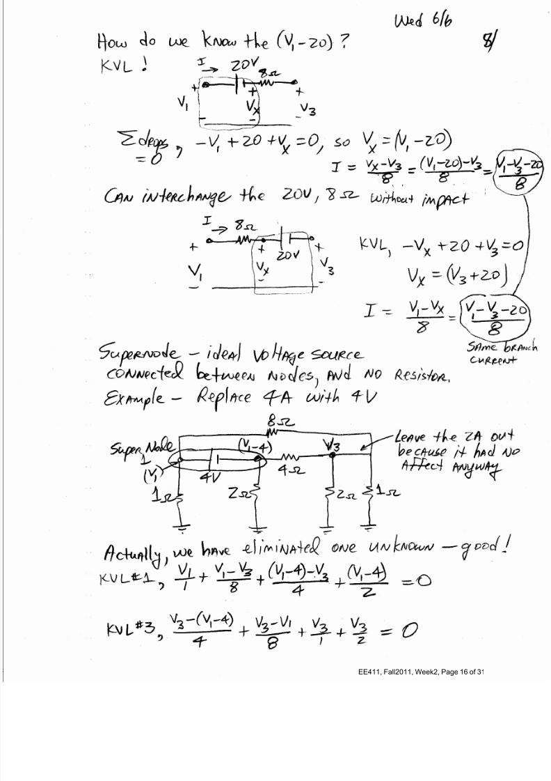
Super Node: Two major nodes with an ideal voltage source between them.
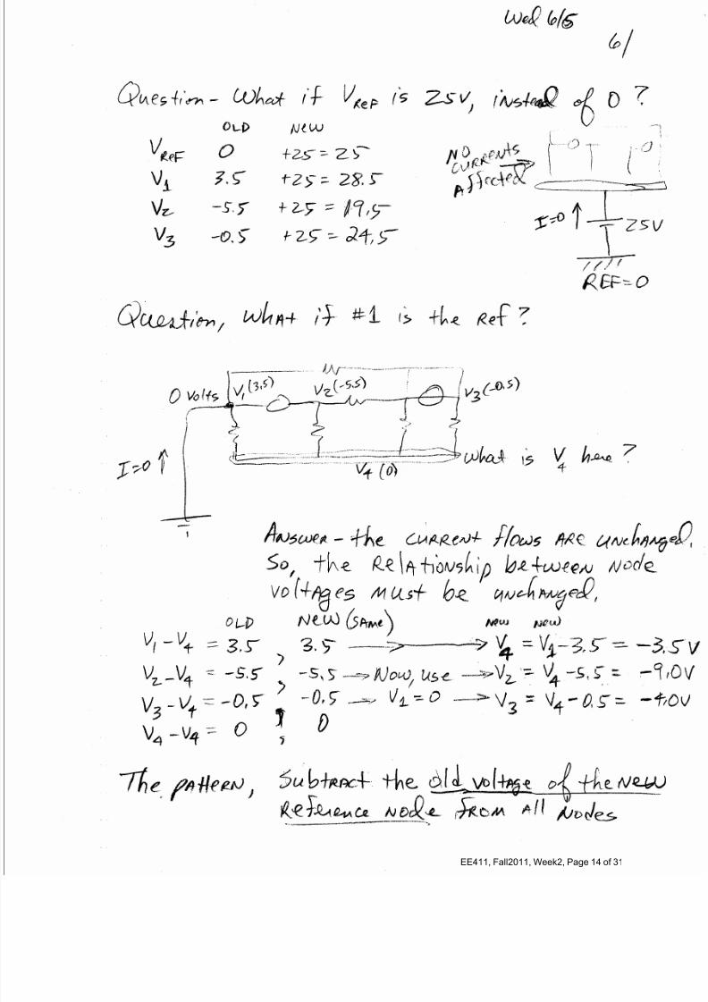
Reference Node: The node to which all other node potentials are referenced. The relativevoltage of the reference node is zero.
Solution Procedure
1. Draw a neat circuit diagram and try to eliminate as many branch crossings as possible.
2. Choose a reference node. All other node voltages will be referenced to it. Ideally, itshould be the node with the most branches connected to it, so that the number of terms in
the admittance matrix is minimal.
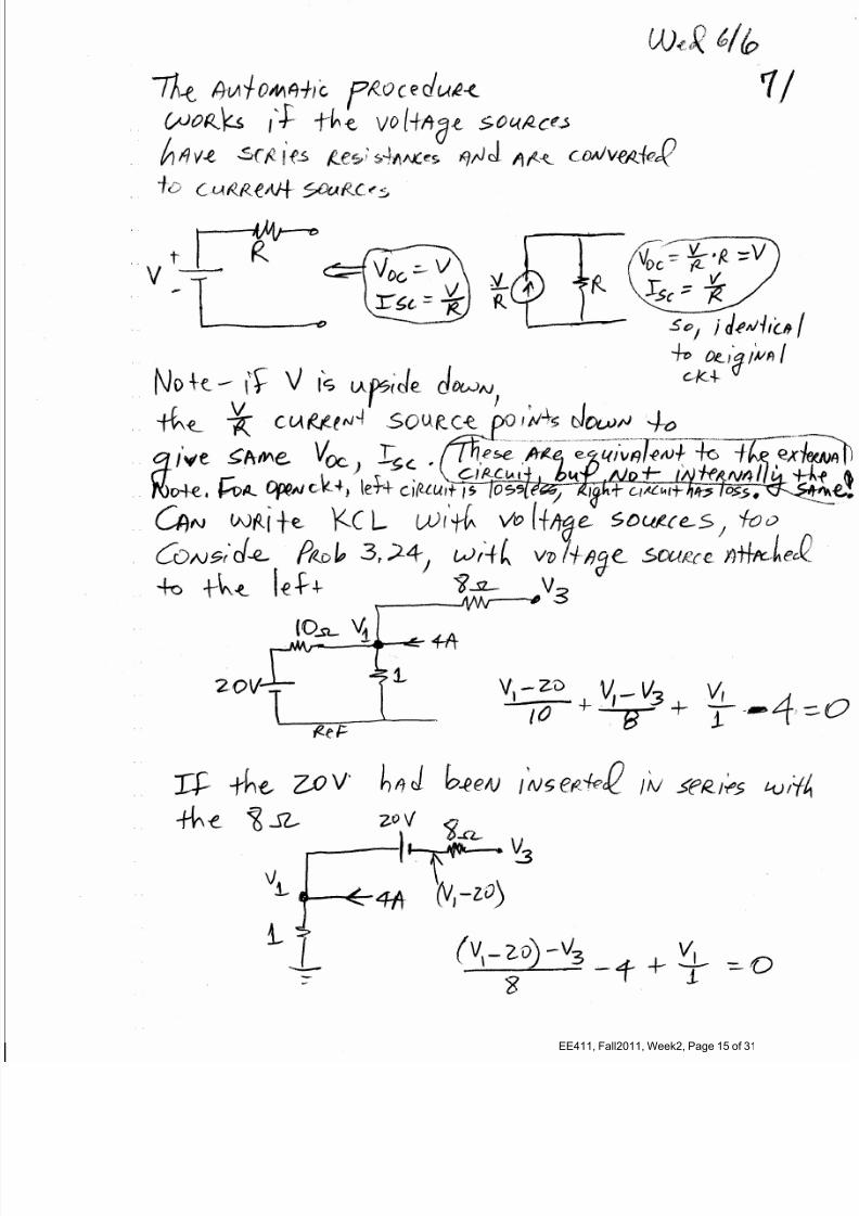
3. If the circuit contains voltage sources, do either of the following:
• Convert them to current sources (if they have series impedances)
• Create super nodes by encircling the corresponding end nodes of each voltage source.
4. Assign a number to every major node (except the reference node) that is not part of asuper node (N1 of these).
5. Assign a number to either end (but not both ends) of every super node that does not touch
the reference node (N2 of these)
6. Apply KCL to every numbered node from Step 4 (N1 equations)
7. Apply KCL to every numbered super node from Step 5 (N2 equations)
8. The dimension of the problem is now N1 + N2. Solve the set of linear equations for the
node voltages. At this point, the circuit has been “solved.”
9. Using your results, check KCL for at least one node to make sure that your currents sum
to zero.
9. Use Ohm’s Law, KCL, and the voltage divider principle to find other node voltages,
branch currents, and powers as needed.
EE411, Fall2011, Week2, Page 1 of 31

7/30/2019 Mesh Analysis, Nodal Analysis
http://slidepdf.com/reader/full/mesh-analysis-nodal-analysis 2/31
Notes on Mesh Analysis, Prof. Mack Grady, June 4, 2007
Definitions
Branch: A circuit element that connects nodes
Planar Network: A network whose circuit diagram can be drawn on a plane in such a
manner that no branches pass over or under other branches
Loop: A closed path
Mesh: A loop that is the only loop passing through at least one branch
Solution Procedure
1. Draw a neat circuit diagram and make sure that the circuit is planar (if not
planar, then the circuit is not a candidate for mesh analysis)
2.
If the circuit contains current sources, do either of the following:
A. Convert them to voltage sources (if they have internal impedances), or B. Create super meshes by making sure in Step 3 that two (and not more than
two) meshes pass through each current source. SM super meshes.
3. Draw clockwise mesh currents, where each one passes through at least one
new branch. M meshes.
4. Apply KVL for every mesh that is not part of a super mesh (M – 2SM
equations)
5. For meshes that form super meshes, apply KVL to the portion of the loop
formed by the two meshes that does not pass through the current source (SM
equations)
6. For each super mesh, write an equation that relates the corresponding mesh
currents to the current source (SM equations)
7. The dimension of the problem is now M. Solve the set of M linear equations
for the mesh currents. At this point, the network has been “solved.”
8. Using your results, check KVL around at least one mesh to make sure that the
net voltage drop is zero.
9. Use Ohm’s law, loop currents, KVL, KCL and the voltage divider principle to
find node voltages, branch currents, and powers as needed.
EE411, Fall2011, Week2, Page 2 of 31

7/30/2019 Mesh Analysis, Nodal Analysis
http://slidepdf.com/reader/full/mesh-analysis-nodal-analysis 3/31
Grady, Admittance Matrix and the Nodal Method, June 2007, Page 1
Building the Admittance Matrix
Most power system networks are analyzed by first forming the admittance matrix. The
admittance matrix is based upon Kirchhoff's current law (KCL), and it is easily formed and very
sparse for most large networks.
Consider the three-bus network shown in Figure that has five branch impedances and one current
source.
1 2 3
ZE
ZA
ZB
ZC
ZDI3
Figure 1. Three-Bus Network
Applying KCL at the three independent nodes yields the following equations for the bus voltages
(with respect to ground):
At bus 1, 0211 =−
+ A E Z
V V
Z
V ,
At bus 2, 032122 =−
+−
+C A B Z
V V
Z
V V
Z
V ,
At bus 3, 3233
I Z
V V
Z
V
C D
=−
+ .
Collecting terms and writing the equations in matrix form yields
⎥⎥
⎥
⎦
⎤
⎢⎢
⎢
⎣
⎡
=
⎥⎥
⎥
⎦
⎤
⎢⎢
⎢
⎣
⎡
⎥⎥⎥⎥
⎥⎥⎥
⎦
⎤
⎢⎢⎢⎢
⎢⎢⎢
⎣
⎡
+−
−++−
−+
332
1
0
0
1110
11111
0111
I V
V
V
Z Z Z
Z Z Z Z Z
Z Z Z
DC C
C C B A A
A A E
,
or in matrix form,
I YV = ,
EE411, Fall2011, Week2, Page 3 of 31

7/30/2019 Mesh Analysis, Nodal Analysis
http://slidepdf.com/reader/full/mesh-analysis-nodal-analysis 4/31
Grady, Admittance Matrix and the Nodal Method, June 2007, Page 2
where Y is the admittance matrix, V is a vector of bus voltages (with respect to ground), and I is a
vector of current injections.
Voltage sources, if present, can be converted to current sources using the usual network rules. If
a bus has a zero-impedance voltage source attached to it, then the bus voltage is already known,
and the dimension of the problem is reduced by one.
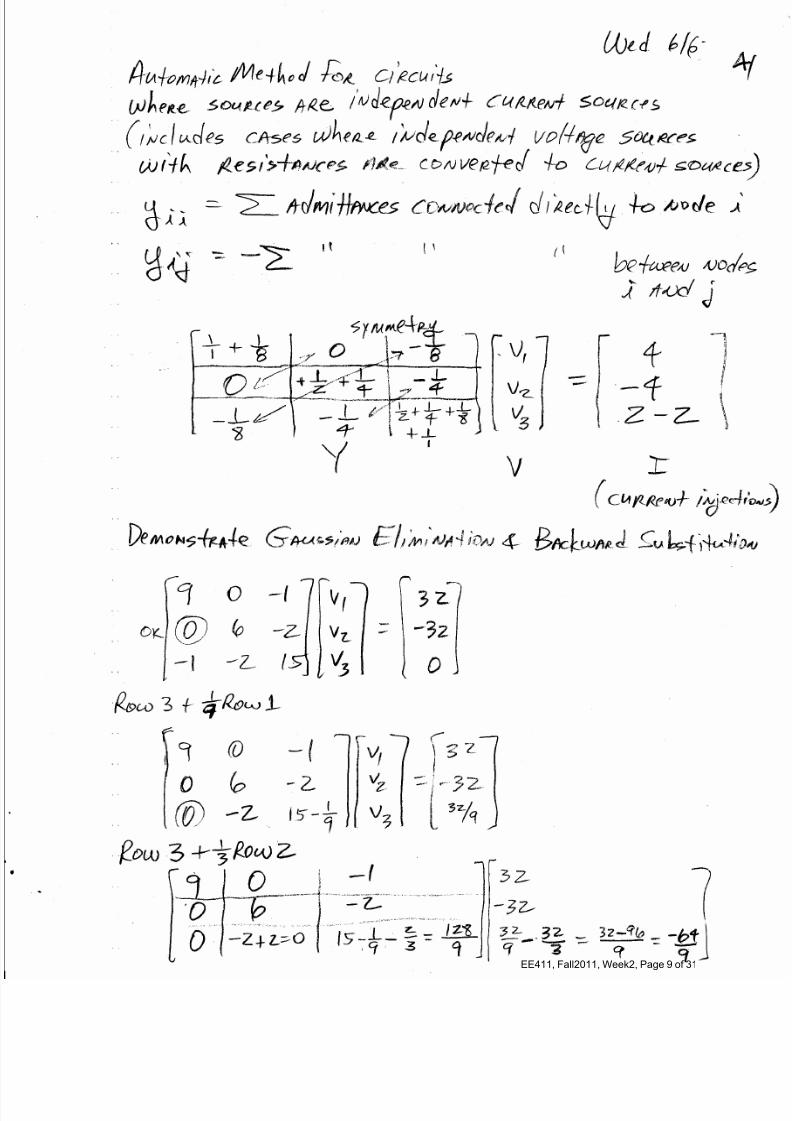
A simple observation of the structure of the above admittance matrix leads to the following rule
for building Y :
1. The diagonal terms of Y contain the sum of all branch admittances connected directly to the
corresponding bus.
2. The off-diagonal elements of Y contain the negative sum of all branch admittances connected
directly between the corresponding busses.
EE411, Fall2011, Week2, Page 4 of 31
7/30/2019 Mesh Analysis, Nodal Analysis
http://slidepdf.com/reader/full/mesh-analysis-nodal-analysis 5/31
Grady, Admittance Matrix and the Nodal Method, June 2007, Page 3
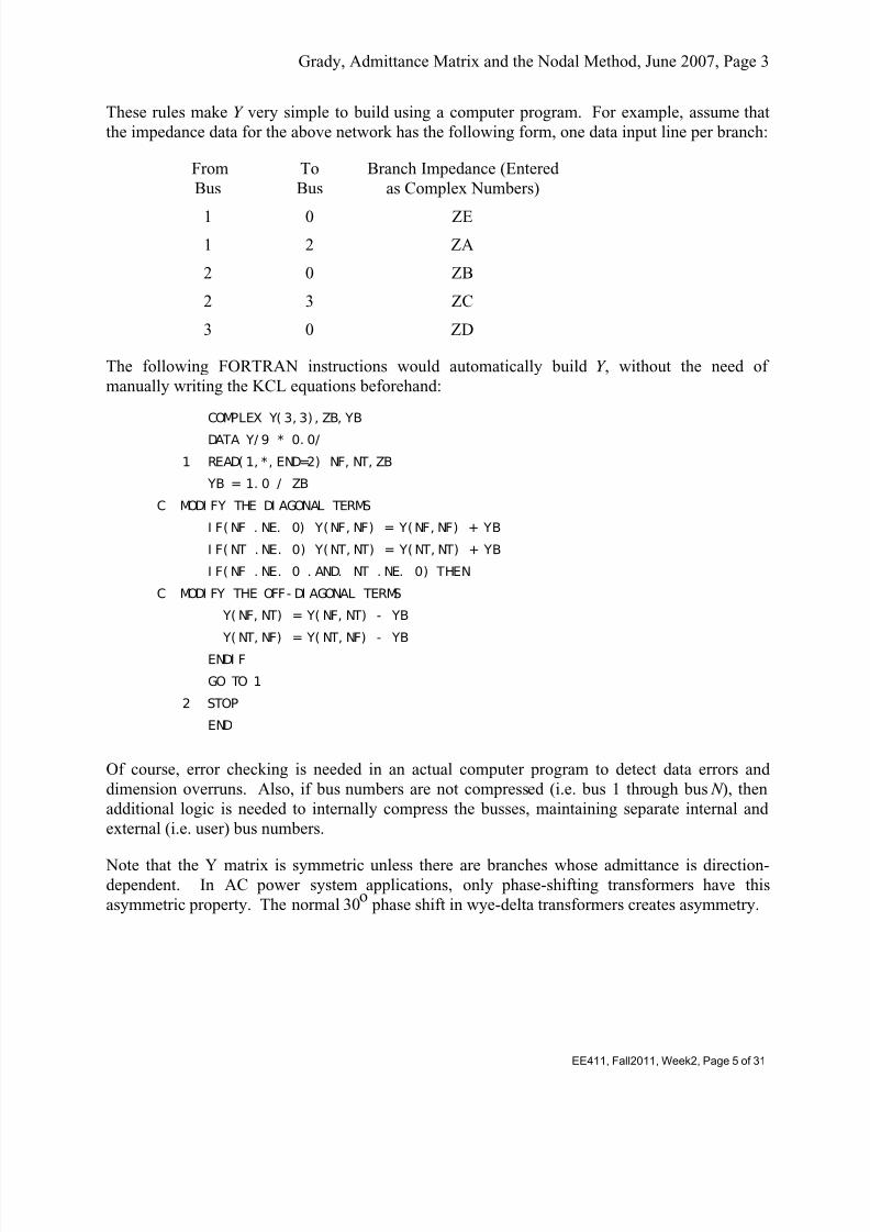
These rules make Y very simple to build using a computer program. For example, assume that
the impedance data for the above network has the following form, one data input line per branch:
From To Branch Impedance (Entered
Bus Bus as Complex Numbers)
1 0 ZE
1 2 ZA
2 0 ZB
2 3 ZC
3 0 ZD
The following FORTRAN instructions would automatically build Y , without the need of
manually writing the KCL equations beforehand:
COMPLEX Y( 3, 3) , ZB, YB
DATA Y/ 9 * 0. 0/
1 READ( 1, *, END=2) NF, NT, ZB
YB = 1. 0 / ZB
C MODI FY THE DI AGONAL TERMS
I F( NF . NE. 0) Y(NF, NF) = Y(NF, NF) + YB
I F( NT . NE. 0) Y(NT, NT) = Y( NT, NT) + YB
I F( NF . NE. 0 . AND. NT . NE. 0) THEN
C MODI FY THE OFF- DI AGONAL TERMS
Y( NF, NT) = Y( NF, NT) - YB
Y( NT, NF) = Y( NT, NF) - YB
ENDI F
GO TO 1
2 STOP
END
Of course, error checking is needed in an actual computer program to detect data errors and
dimension overruns. Also, if bus numbers are not compressed (i.e. bus 1 through bus N ), then
additional logic is needed to internally compress the busses, maintaining separate internal and
external (i.e. user) bus numbers.
Note that the Y matrix is symmetric unless there are branches whose admittance is direction-dependent. In AC power system applications, only phase-shifting transformers have this
asymmetric property. The normal 30o
phase shift in wye-delta transformers creates asymmetry.
EE411, Fall2011, Week2, Page 5 of 31
7/30/2019 Mesh Analysis, Nodal Analysis
http://slidepdf.com/reader/full/mesh-analysis-nodal-analysis 6/31
EE411, Fall2011, Week2, Page 6 of 31
7/30/2019 Mesh Analysis, Nodal Analysis
http://slidepdf.com/reader/full/mesh-analysis-nodal-analysis 7/31
EE411, Fall2011, Week2, Page 7 of 31
7/30/2019 Mesh Analysis, Nodal Analysis
http://slidepdf.com/reader/full/mesh-analysis-nodal-analysis 8/31
EE411, Fall2011, Week2, Page 8 of 31
7/30/2019 Mesh Analysis, Nodal Analysis
http://slidepdf.com/reader/full/mesh-analysis-nodal-analysis 9/31
EE411, Fall2011, Week2, Page 9 of 31
7/30/2019 Mesh Analysis, Nodal Analysis
http://slidepdf.com/reader/full/mesh-analysis-nodal-analysis 10/31
EE411, Fall2011, Week2, Page 10 of 31
7/30/2019 Mesh Analysis, Nodal Analysis
http://slidepdf.com/reader/full/mesh-analysis-nodal-analysis 11/31
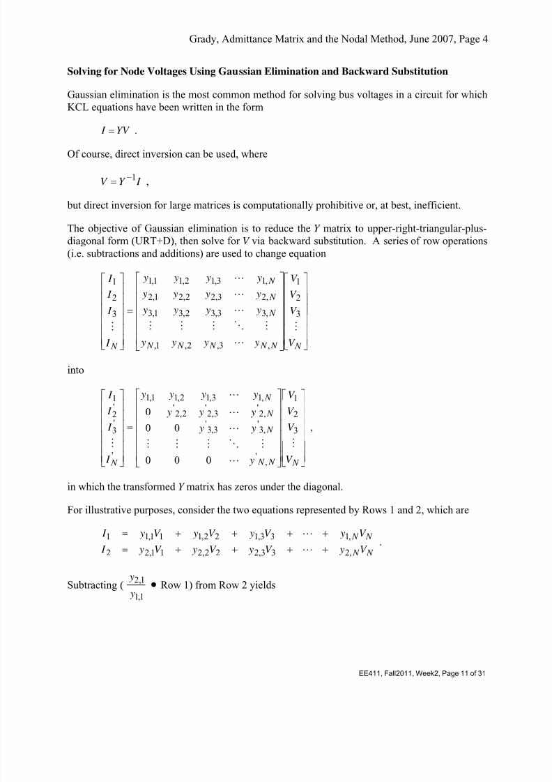
Grady, Admittance Matrix and the Nodal Method, June 2007, Page 4
Solving for Node Voltages Using Gaussian Elimination and Backward Substitution
Gaussian elimination is the most common method for solving bus voltages in a circuit for which
KCL equations have been written in the form
YV I = .
Of course, direct inversion can be used, where
I Y V 1−= ,
but direct inversion for large matrices is computationally prohibitive or, at best, inefficient.
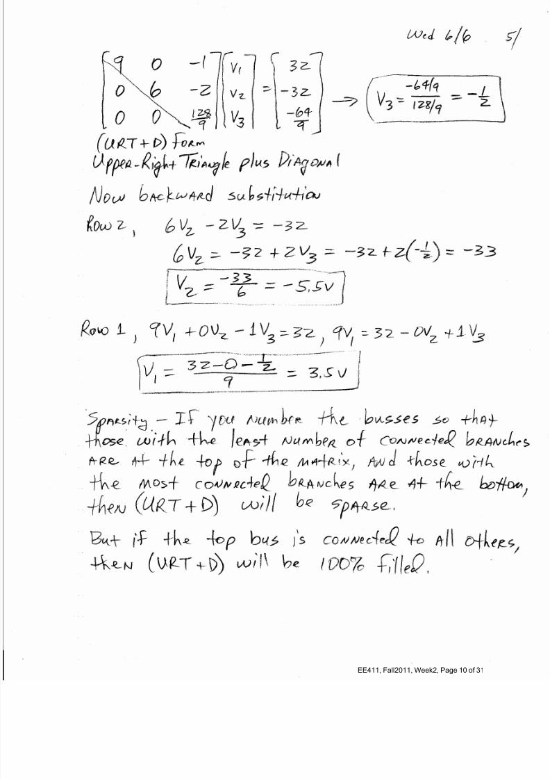
The objective of Gaussian elimination is to reduce the Y matrix to upper-right-triangular-plus-
diagonal form (URT+D), then solve for V via backward substitution. A series of row operations
(i.e. subtractions and additions) are used to change equation
⎥⎥⎥⎥⎥⎥
⎦
⎤
⎢⎢⎢⎢⎢⎢
⎣
⎡
⎥⎥⎥⎥⎥⎥
⎦
⎤
⎢⎢⎢⎢⎢⎢
⎣
⎡
=
⎥⎥⎥⎥⎥⎥
⎦
⎤
⎢⎢⎢⎢⎢⎢
⎣
⎡
N N N N N N
N
N
N
N V
V
V
V
y y y y
y y y y
y y y y
y y y y
I
I
I
I
M
L
MOMMM
L
L
L
M
3
2
1
,3,2,1,
,33,32,31,3
,23,22,21,2
,13,12,11,1
3
2
1
into
⎥⎥⎥⎥⎥⎥
⎦
⎤
⎢⎢⎢⎢⎢⎢
⎣
⎡
⎥⎥⎥⎥⎥⎥
⎦
⎤
⎢⎢⎢⎢⎢⎢
⎣
⎡
=
⎥⎥⎥⎥⎥⎥
⎦
⎤
⎢⎢⎢⎢⎢⎢
⎣
⎡
N N N
N
N
N
N V
V
V
V
y
y y
y y y
y y y y
I
I
I
I
M
L
MOMMM
L
L
L
M
3
2
1
,'
,3'
3,3'
,2'3,2'2,2'
,13,12,11,1
'
'3
'2
1
000
00
0,
in which the transformed Y matrix has zeros under the diagonal.
For illustrative purposes, consider the two equations represented by Rows 1 and 2, which are
N N
N N
V yV yV yV y I
V yV yV yV y I
,233,222,211,22
,133,122,111,11
++++=
++++=
L
L.
Subtracting (1,1
1,2
y
y • Row 1) from Row 2 yields
EE411, Fall2011, Week2, Page 11 of 31
7/30/2019 Mesh Analysis, Nodal Analysis
http://slidepdf.com/reader/full/mesh-analysis-nodal-analysis 12/31
Grady, Admittance Matrix and the Nodal Method, June 2007, Page 5
N N N
N N
V y y
y yV y
y
y yV y
y
y yV y
y
y y I
y
y I
V yV yV yV y I
⎟⎟
⎠
⎞
⎜⎜
⎝
⎛ −++
⎟⎟
⎠
⎞
⎜⎜
⎝
⎛ −+
⎟⎟
⎠
⎞
⎜⎜
⎝
⎛ −+
⎟⎟
⎠
⎞
⎜⎜
⎝
⎛ −=−
++++=
,11,1
1,2,233,1
1,1
1,23,222,1
1,1
1,22,211,1
1,1
1,21,21
1,1
1,22
,133,122,111,11
L
L.
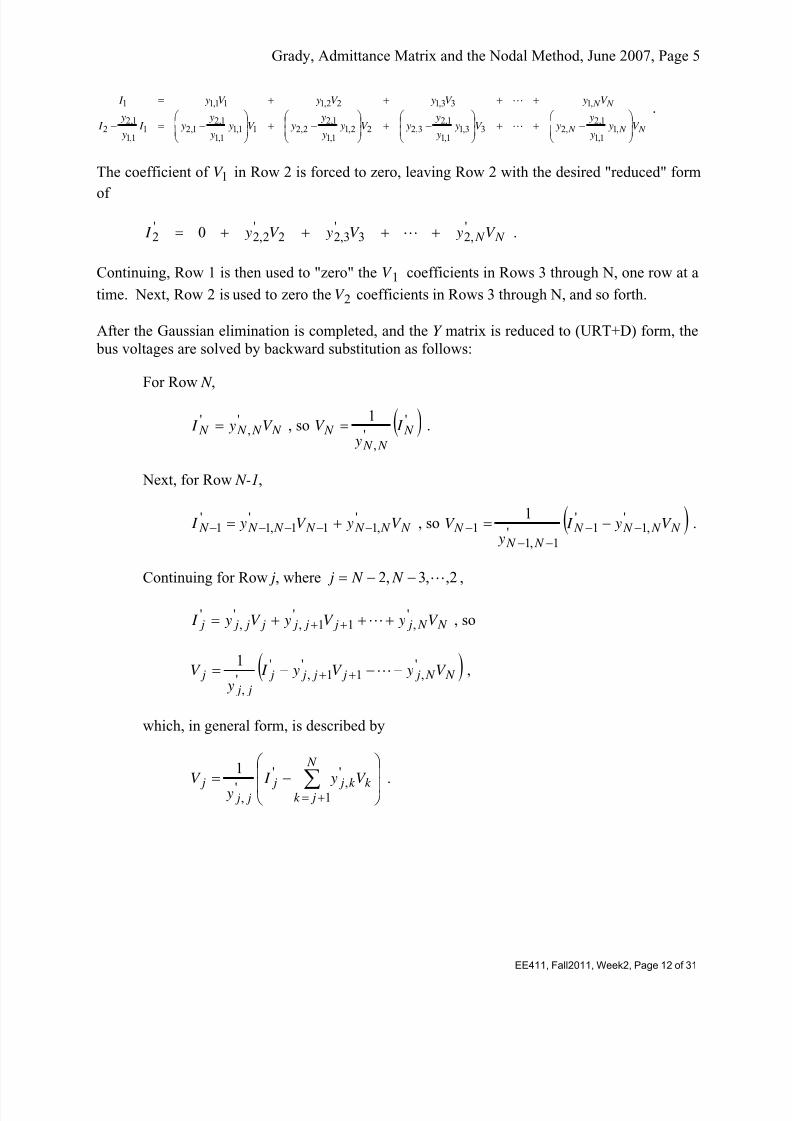
The coefficient of 1V in Row 2 is forced to zero, leaving Row 2 with the desired "reduced" form
of
N N V yV yV y I ',23
'3,22
'2,2
'2 0 ++++= L .
Continuing, Row 1 is then used to "zero" the 1V coefficients in Rows 3 through N, one row at a
time. Next, Row 2 is used to zero the 2V coefficients in Rows 3 through N, and so forth.
After the Gaussian elimination is completed, and the Y matrix is reduced to (URT+D) form, the
bus voltages are solved by backward substitution as follows:
For Row N ,
N N N N V y I '
,' = , so ( )'
',
1 N
N N
N I y
V = .
Next, for Row N-1,
N N N N N N N V yV y I '
,11'
1,1'
1 −−−−− += , so ( ) N N N N
N N
N V y I y
V '
,1'
1'1,1
11
−−−−
− −= .
Continuing for Row j, where 2,,3,2 L−−= N N j ,
N N j j j j j j j j V yV yV y I ',1
'1,
',
' +++= ++ L , so
( ) N N j j j j j
j j
j V yV y I y
V ',1
'1,
'
',
1
−−−= ++ L ,
which, in general form, is described by
⎟
⎟
⎠
⎞
⎜
⎜
⎝
⎛ −=
∑+=k k j
N
jk j
j j j V y I yV
'
,1
'
',
1
.
EE411, Fall2011, Week2, Page 12 of 31
7/30/2019 Mesh Analysis, Nodal Analysis
http://slidepdf.com/reader/full/mesh-analysis-nodal-analysis 13/31
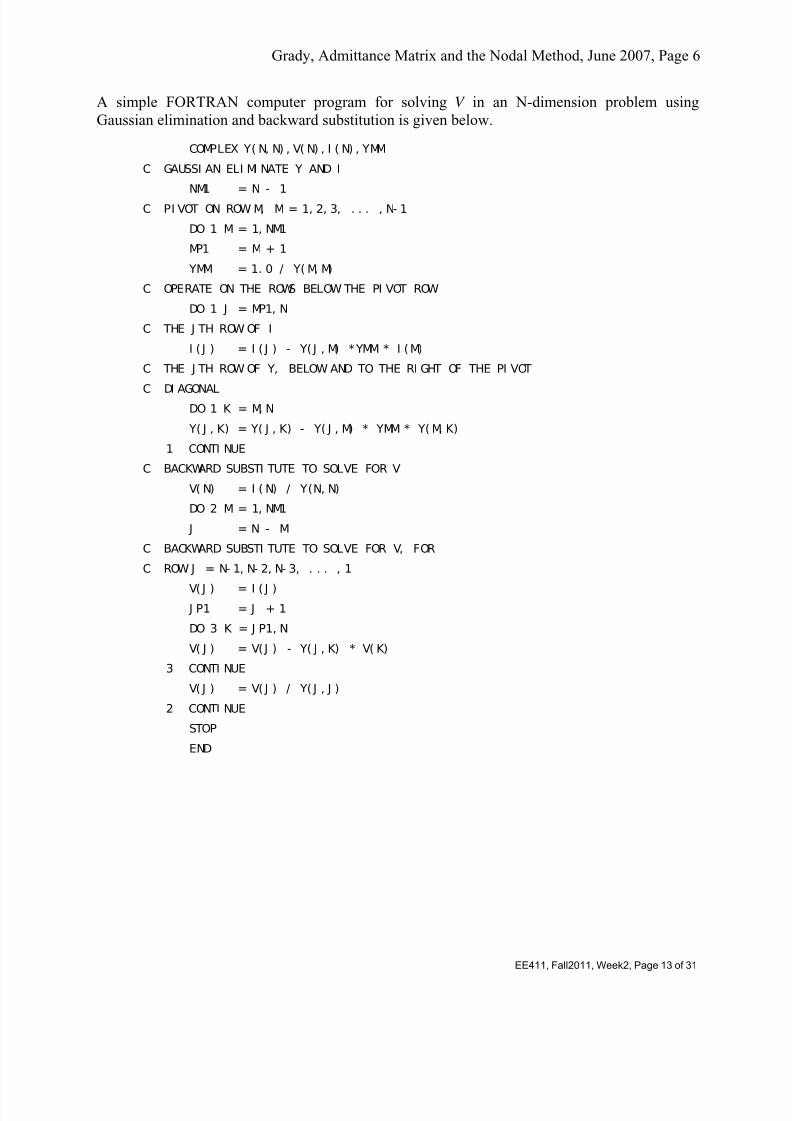
Grady, Admittance Matrix and the Nodal Method, June 2007, Page 6
A simple FORTRAN computer program for solving V in an N-dimension problem using
Gaussian elimination and backward substitution is given below.
COMPLEX Y( N, N) , V( N) , I ( N) , YMM
C GAUSSI AN ELI MI NATE Y AND I
NM1 = N - 1
C PI VOT ON ROW M, M = 1, 2, 3, . . . , N- 1
DO 1 M = 1, NM1
MP1 = M + 1
YMM = 1. 0 / Y( M, M)
C OPERATE ON THE ROWS BELOW THE PI VOT ROW
DO 1 J = MP1, N
C THE J TH ROW OF I
I ( J ) = I ( J ) - Y( J , M) *YMM * I (M)
C THE J TH ROW OF Y, BELOW AND TO THE RI GHT OF THE PI VOT
C DI AGONALDO 1 K = M, N
Y( J , K) = Y( J , K) - Y( J , M) * YMM * Y( M, K)
1 CONTI NUE
C BACKWARD SUBSTI TUTE TO SOLVE FOR V
V( N) = I ( N) / Y(N, N)
DO 2 M = 1, NM1
J = N - M
C BACKWARD SUBSTI TUTE TO SOLVE FOR V, FOR
C ROW J = N- 1, N- 2, N- 3, . . . , 1
V( J ) = I ( J )
J P1 = J + 1
DO 3 K = J P1, N
V( J ) = V( J ) - Y( J , K) * V( K)
3 CONTI NUE
V( J ) = V( J ) / Y( J , J )
2 CONTI NUE
STOP
END
EE411, Fall2011, Week2, Page 13 of 31
7/30/2019 Mesh Analysis, Nodal Analysis
http://slidepdf.com/reader/full/mesh-analysis-nodal-analysis 14/31
EE411, Fall2011, Week2, Page 14 of 31
7/30/2019 Mesh Analysis, Nodal Analysis
http://slidepdf.com/reader/full/mesh-analysis-nodal-analysis 15/31
EE411, Fall2011, Week2, Page 15 of 31
7/30/2019 Mesh Analysis, Nodal Analysis
http://slidepdf.com/reader/full/mesh-analysis-nodal-analysis 16/31
EE411, Fall2011, Week2, Page 16 of 31
7/30/2019 Mesh Analysis, Nodal Analysis
http://slidepdf.com/reader/full/mesh-analysis-nodal-analysis 17/31
EE411, Fall2011, Week2, Page 17 of 31
7/30/2019 Mesh Analysis, Nodal Analysis
http://slidepdf.com/reader/full/mesh-analysis-nodal-analysis 18/31
EE411, Fall2011, Week2, Page 18 of 31
7/30/2019 Mesh Analysis, Nodal Analysis
http://slidepdf.com/reader/full/mesh-analysis-nodal-analysis 19/31
EE411, Fall2011, Week2, Page 19 of 31
7/30/2019 Mesh Analysis, Nodal Analysis
http://slidepdf.com/reader/full/mesh-analysis-nodal-analysis 20/31
EE411, Fall2011, Week2, Page 20 of 31
7/30/2019 Mesh Analysis, Nodal Analysis
http://slidepdf.com/reader/full/mesh-analysis-nodal-analysis 21/31
EE411, Fall2011, Week2, Page 21 of 31
7/30/2019 Mesh Analysis, Nodal Analysis
http://slidepdf.com/reader/full/mesh-analysis-nodal-analysis 22/31
EE411, Fall2011, Week2, Page 22 of 31
7/30/2019 Mesh Analysis, Nodal Analysis
http://slidepdf.com/reader/full/mesh-analysis-nodal-analysis 23/31
EE411, Fall2011, Week2, Page 23 of 31
7/30/2019 Mesh Analysis, Nodal Analysis
http://slidepdf.com/reader/full/mesh-analysis-nodal-analysis 24/31
EE411, Fall2011, Week2, Page 24 of 31
7/30/2019 Mesh Analysis, Nodal Analysis
http://slidepdf.com/reader/full/mesh-analysis-nodal-analysis 25/31
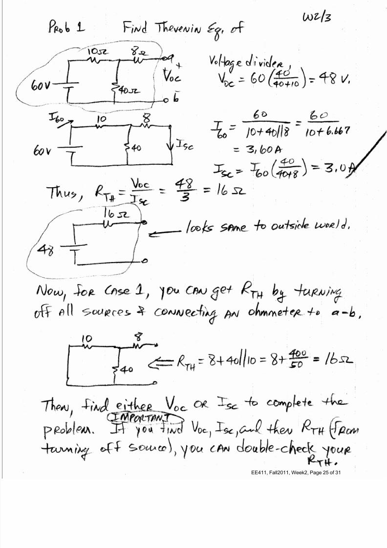
EE411, Fall2011, Week2, Page 25 of 31
7/30/2019 Mesh Analysis, Nodal Analysis
http://slidepdf.com/reader/full/mesh-analysis-nodal-analysis 26/31
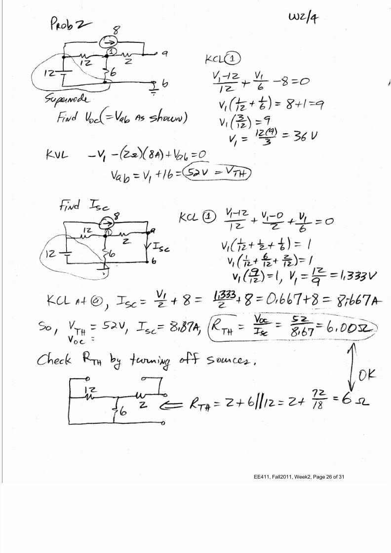
EE411, Fall2011, Week2, Page 26 of 31
7/30/2019 Mesh Analysis, Nodal Analysis
http://slidepdf.com/reader/full/mesh-analysis-nodal-analysis 27/31
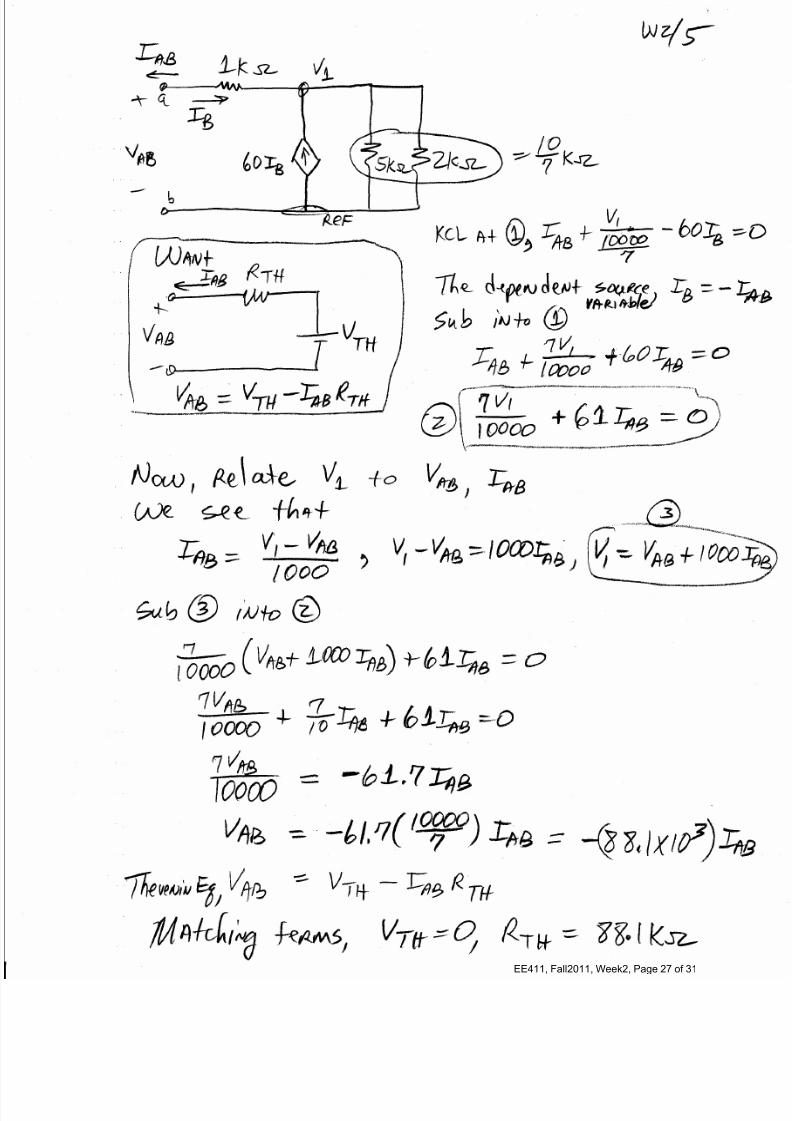
EE411, Fall2011, Week2, Page 27 of 31
7/30/2019 Mesh Analysis, Nodal Analysis
http://slidepdf.com/reader/full/mesh-analysis-nodal-analysis 28/31
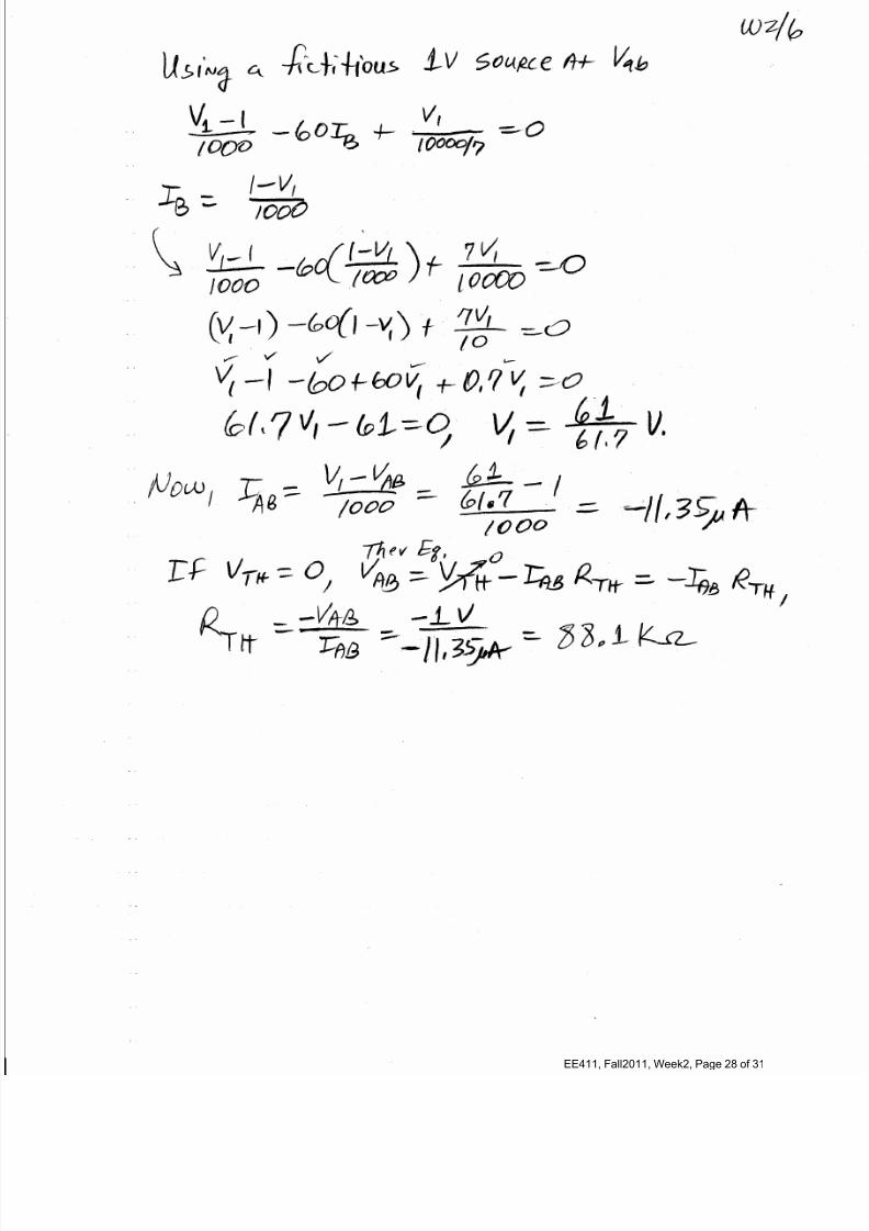
EE411, Fall2011, Week2, Page 28 of 31
7/30/2019 Mesh Analysis, Nodal Analysis
http://slidepdf.com/reader/full/mesh-analysis-nodal-analysis 29/31
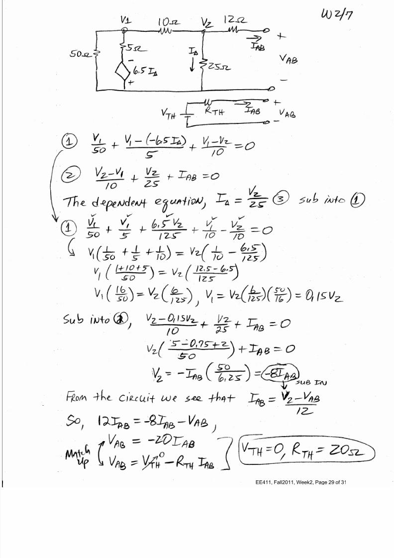
EE411, Fall2011, Week2, Page 29 of 31
7/30/2019 Mesh Analysis, Nodal Analysis
http://slidepdf.com/reader/full/mesh-analysis-nodal-analysis 30/31
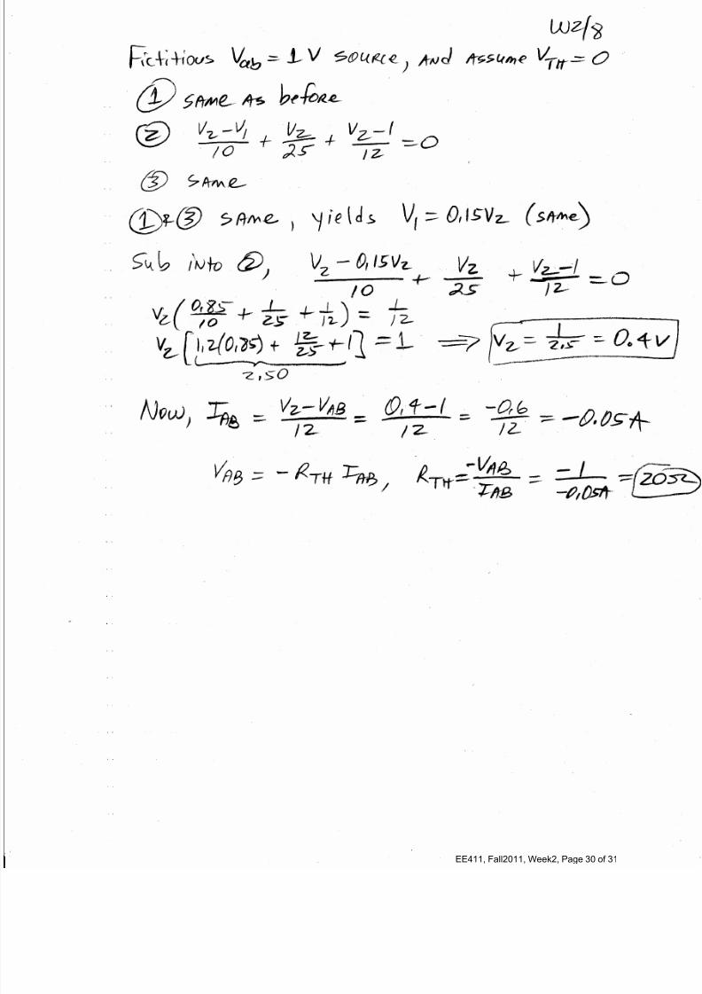
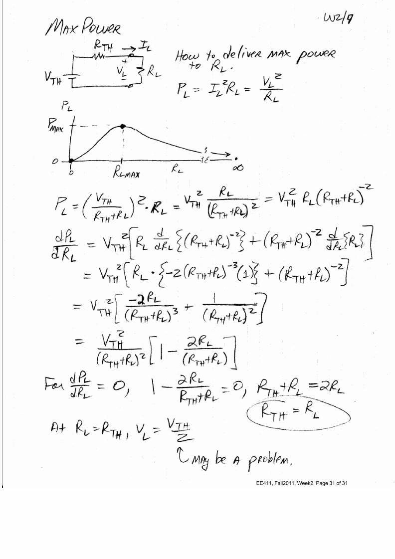
EE411, Fall2011, Week2, Page 30 of 31
7/30/2019 Mesh Analysis, Nodal Analysis
http://slidepdf.com/reader/full/mesh-analysis-nodal-analysis 31/31
Related Documents