MERRIMAC – HIGH-PERFORMANCE AND HIGHLY-EFFICIENT SCIENTIFIC COMPUTING WITH STREAMS A DISSERTATION SUBMITTED TO THE DEPARTMENT OF ELECTRICAL ENGINEERING AND THE COMMITTEE ON GRADUATE STUDIES OF STANFORD UNIVERSITY IN PARTIAL FULFILLMENT OF THE REQUIREMENTS FOR THE DEGREE OF DOCTOR OF PHILOSOPHY Mattan Erez May 2007

Welcome message from author
This document is posted to help you gain knowledge. Please leave a comment to let me know what you think about it! Share it to your friends and learn new things together.
Transcript
MERRIMAC – HIGH-PERFORMANCE AND HIGHLY-EFFICIENT
SCIENTIFIC COMPUTING WITH STREAMS
A DISSERTATION
SUBMITTED TO THE DEPARTMENT OF ELECTRICAL ENGINEERING
AND THE COMMITTEE ON GRADUATE STUDIES
OF STANFORD UNIVERSITY
IN PARTIAL FULFILLMENT OF THE REQUIREMENTS
FOR THE DEGREE OF
DOCTOR OF PHILOSOPHY
Mattan Erez
May 2007

c© Copyright by Mattan Erez 2007
All Rights Reserved
ii

I certify that I have read this dissertation and that, in my opinion, it is fully
adequate in scope and quality as a dissertation for the degree of Doctor of
Philosophy.
(William J. Dally) Principal Adviser
I certify that I have read this dissertation and that, in my opinion, it is fully
adequate in scope and quality as a dissertation for the degree of Doctor of
Philosophy.
(Patrick M. Hanrahan)
I certify that I have read this dissertation and that, in my opinion, it is fully
adequate in scope and quality as a dissertation for the degree of Doctor of
Philosophy.
(Mendel Rosenblum)
Approved for the University Committee on Graduate Studies.
iii

iv
Abstract
Advances in VLSI technology have made the raw ingredients for computation plentiful.
Large numbers of fast functional units and large amounts of memory and bandwidth can
be made efficient in terms of chip area, cost, and energy, however, high-performance com-
puters realize only a small fraction of VLSI’s potential. This dissertation describes the
Merrimac streaming supercomputer architecture and system. Merrimac has an integrated
view of the applications, software system, compiler, and architecture. We will show how
this approach leads to over an order of magnitude gains in performance per unit cost, unit
power, and unit floor-space for scientific applications when compared to common scien-
tific computers designed around clusters of commodity general-purpose processors. The
dissertation discusses Merrimac’s stream architecture, the mapping of scientific codes to
effectively run on the stream architecture, and system issues in the Merrimac supercom-
puter.
The stream architecture is designed to take advantage of the properties of modern
semiconductor technology — very high bandwidth over short distances and very high
transistor counts, but limited global on-chip and off-chip bandwidths — and match them
with the characteristics of scientific codes — large amounts of parallelism and access
locality. Organizing the computation into streams and exploiting the resulting locality
using a register hierarchy enables a stream architecture to reduce the memory bandwidth
required by representative computations by an order of magnitude or more. Hence a
processing node with a fixed memory bandwidth (which is expensive) can support an order
of magnitude more arithmetic units (which are inexpensive). Because each node has much
greater performance (128 double-precision GFLOP/s) than a conventional microprocessor,
a streaming supercomputer can achieve a given level of performance with fewer nodes,
reducing costs, simplifying system management, and increasing reliability.
v

Acknowledgments
During my years in Stanford my technical writing skills developed significantly, unfor-
tunately, the same cannot be said for more sentimental genres. Below is my unworthy
attempt to acknowledge and thank those who have made my time at Stanford possible,
rewarding, exciting, and fun.
First and foremost I would like to thank my adviser Bill Dally. Bill’s tremendous
support and encouragement were only exceeded by the inspiration and opportunities he
gave me. Bill facilitated my studies at Stanford from even before I arrived, let me help plan
and teach two new classes, and always gave me the freedom to pursue both my research
and extra curricular interests while (mostly) keeping me focused on my thesis. Most
importantly, Bill gave me the chance to be deeply involved in the broad and collaborative
Merrimac project.
I was very lucky that I was able to collaborate and interact with several of Stanford’s
remarkable faculty members as part of my thesis and the Merrimac project. I particularly
want to thank Pat Hanrahan and Mendel Rosenblum for the continuous feedback they
have provided on my research and the final thoughtful comments on this dissertation. Pat
and Mendel, as well as Eric Darve and Alex Aiken, taught me much and always offered
fresh perspectives and insight that broadened and deepened my knowledge.
I want to give special thanks to Ronny Ronen, Uri Weiser, and Adi Yoaz. They gave
me a great start in my career in computer architecture and provided careful and extensive
guidance and help over the years.
This dissertation represents a small part of the effort that was put into the Merrimac
project and I would like to acknowledge the amazing students and researchers with whom
I collaborated. The Merrimac team included Jung Ho Ahn, Nuwan Jayasena, Abhishek
Das, Timothy J. Knight, Francois Labonte, Jayanth Gummaraju, Ben Serebrin, Ujval
Kapasi, Binu Mathew, and Ian Buck. I want to particularly thank Jung Ho Ahn, Jayanth
vi

Gummaraju , and Abhishek Das, with whom I worked most closely, for their thoughts and
relentless infrastructure support. Timothy J. Barth, Massimiliano Fatica, Frank Ham, and
Alan Wray of the Center for Integrated Turbulence Research provided priceless expertise
and showed infinite patience while developing applications for Merrimac.
In my time at Stanford, I had the pleasure to work with many other wonderful fellow
students outside the scope of my dissertation research. I especially want to thank the
members of the CVA group and those of the Sequoia project. Recently, I had the pleasure
to participate in the ambitious efforts of Kayvon Fatahlian, Timothy J. Knight, Mike
Houston, Jiyoung Park, Manman Ren, Larkhoon Lim, and Abhishek Das on the Sequoia
project. Earlier, I spent many rewarding and fun hours with Sarah Harris and Kelly Shaw,
learned much about streaming from Ujval Kapasi, Brucek Khailany, John Owens, Peter
Mattson, and Scott Rixner, and got a taste of a wide range of other research topics from
Brian Towles, Patrick Chiang, Andrew Chang, Arjun Singh, Amit Gupta, Paul Hartke,
John Kim, Li-Shiuan Peh, Edward Lee, David Black-Schaffer, Oren Kerem, and James
Balfour.
I am grateful to the assistance I got over the years from Shelley Russell, Pamela Elliott,
Wanda Washington, and Jane Klickman, and to the funding agencies that supported
my graduate career at Stanford, including the Department of Energy (under the ASCI
Alliances Program, contract LLNL-B523583), the Defense Advanced Research Projects
Agency (under the Polymorphous Computing Architectures Project, contract F29601-00-
2-0085), and the Nvidia Fellowship Program.
In addition to the friends I met through research, I also want to deeply thank the rest
of my friends. Those in Israel who made me feel like I I had never left home whenever
I went for visit, and those at Stanford who have gave me a new home and sustained
me with a slew of rituals (Thursday parties, afternoon coffee, Sunday basketball, movie
nights, . . .): Wariya Keatpadungkul, Assaf Yeheskelly, Eilon Brenner, Zvi Kons, Dror
Levin, Ido Milstein, Galia Arad-Blum, Eran Barzilai, Shahar Wilner, Dana Porat, Luis
Sentis, Vincent Vanhoucke, Onn Brandman, Ofer Levi, Ulrich Barnhoefer, Ira Wygant, Uri
Lerner, Nurit Jugend, Rachel Kolodny, Saharon Rosset, Eran Segal, Yuval Nov, Matteo
Slanina, Cesar Sanchez, Teresa Madrid, Magnus Sandberg, Adela Ben-Yakar, Laurence
Melloul, Minja Trjkla, Oren Shneorson, Noam Sobel, Guy Peled, Bay Thongthepairot, Mor
Naaman, Tonya Putnam, Relly Brandman, Calist Friedman, Miki Lustig, Yonit Lustig,
Vivian Ganitsky, and Joyce Noah-Vanhoucke.
vii
Above all I thank my family without whom my years at Stanford would have been
both impossible and meaningless. my parents, Lipa and Mia Erez, and my sister, Mor
Peleg, gave me a wonderful education, set me off on the academic path, encouraged me
in all my choices and made my endeavors possible and simple. My brother in law, Alex
Peleg, who introduced me to the field of computer architecture and my nephew and nieces,
Tal, Adi, and Yael Peleg, whom I followed to Stanford. My love for them has without a
doubt been the single most critical contributor to my success.
viii

Contents
Abstract v
Acknowledgments vi
1 Introduction 1
1.1 Contributions . . . . . . . . . . . . . . . . . . . . . . . . . . . . . . . . . . . 2
1.2 Detailed Thesis Roadmap and Summary . . . . . . . . . . . . . . . . . . . . 3
1.2.1 Background . . . . . . . . . . . . . . . . . . . . . . . . . . . . . . . . 3
1.2.2 Merrimac Architecture . . . . . . . . . . . . . . . . . . . . . . . . . . 3
1.2.3 Streaming Scientific Applications . . . . . . . . . . . . . . . . . . . . 5
1.2.4 Unstructured and Irregular Algorithms . . . . . . . . . . . . . . . . 5
1.2.5 Fault Tolerance . . . . . . . . . . . . . . . . . . . . . . . . . . . . . . 6
1.2.6 Conclusions . . . . . . . . . . . . . . . . . . . . . . . . . . . . . . . . 6
2 Background 7
2.1 Scientific Applications . . . . . . . . . . . . . . . . . . . . . . . . . . . . . . 7
2.1.1 Numerical Methods . . . . . . . . . . . . . . . . . . . . . . . . . . . 8
2.1.2 Parallelism . . . . . . . . . . . . . . . . . . . . . . . . . . . . . . . . 10
2.1.3 Locality and Arithmetic Intensity . . . . . . . . . . . . . . . . . . . . 11
2.1.4 Control . . . . . . . . . . . . . . . . . . . . . . . . . . . . . . . . . . 12
2.1.5 Data Access . . . . . . . . . . . . . . . . . . . . . . . . . . . . . . . . 13
2.1.6 Scientific Computing Usage Model . . . . . . . . . . . . . . . . . . . 13
2.2 VLSI Technology . . . . . . . . . . . . . . . . . . . . . . . . . . . . . . . . . 13
2.2.1 Logic Scaling . . . . . . . . . . . . . . . . . . . . . . . . . . . . . . . 14
2.2.2 Bandwidth Scaling . . . . . . . . . . . . . . . . . . . . . . . . . . . . 14
ix
2.2.3 Latency scaling . . . . . . . . . . . . . . . . . . . . . . . . . . . . . . 15
2.2.4 VLSI Reliability . . . . . . . . . . . . . . . . . . . . . . . . . . . . . 16
2.2.5 Summary . . . . . . . . . . . . . . . . . . . . . . . . . . . . . . . . . 16
2.3 Trends in Supercomputers . . . . . . . . . . . . . . . . . . . . . . . . . . . . 17
2.4 Models and Architectures . . . . . . . . . . . . . . . . . . . . . . . . . . . . 19
2.4.1 The von Neumann Model and the General Purpose Processor . . . . 20
2.4.2 Vector Processing . . . . . . . . . . . . . . . . . . . . . . . . . . . . 24
2.4.3 The Stream Execution Model and Stream Processors . . . . . . . . . 24
2.4.4 Summary and Comparison . . . . . . . . . . . . . . . . . . . . . . . 28
3 Merrimac 30
3.1 Instruction Set Architecture . . . . . . . . . . . . . . . . . . . . . . . . . . . 32
3.1.1 Stream Instructions . . . . . . . . . . . . . . . . . . . . . . . . . . . 33
3.1.2 Kernel Instructions . . . . . . . . . . . . . . . . . . . . . . . . . . . . 38
3.1.3 Memory Model . . . . . . . . . . . . . . . . . . . . . . . . . . . . . . 39
3.1.4 Exception and Floating Point Models . . . . . . . . . . . . . . . . . 44
3.2 Processor Architecture . . . . . . . . . . . . . . . . . . . . . . . . . . . . . . 47
3.2.1 Scalar Core . . . . . . . . . . . . . . . . . . . . . . . . . . . . . . . . 47
3.2.2 Stream Controller . . . . . . . . . . . . . . . . . . . . . . . . . . . . 48
3.2.3 Stream Unit Overview . . . . . . . . . . . . . . . . . . . . . . . . . . 51
3.2.4 Compute Cluster . . . . . . . . . . . . . . . . . . . . . . . . . . . . . 53
3.2.5 Stream Register File . . . . . . . . . . . . . . . . . . . . . . . . . . . 60
3.2.6 Inter-Cluster Switch . . . . . . . . . . . . . . . . . . . . . . . . . . . 64
3.2.7 Micro-controller . . . . . . . . . . . . . . . . . . . . . . . . . . . . . 67
3.2.8 Memory System . . . . . . . . . . . . . . . . . . . . . . . . . . . . . 70
3.3 System Architecture . . . . . . . . . . . . . . . . . . . . . . . . . . . . . . . 72
3.3.1 Input/Output and Storage . . . . . . . . . . . . . . . . . . . . . . . 73
3.3.2 Synchronization and Signals . . . . . . . . . . . . . . . . . . . . . . . 74
3.3.3 Resource Sharing . . . . . . . . . . . . . . . . . . . . . . . . . . . . . 74
3.4 Area, Power, and Cost Estimates . . . . . . . . . . . . . . . . . . . . . . . . 74
3.4.1 Area and Power . . . . . . . . . . . . . . . . . . . . . . . . . . . . . 75
3.4.2 Cost Estimate . . . . . . . . . . . . . . . . . . . . . . . . . . . . . . 81
3.5 Discussion . . . . . . . . . . . . . . . . . . . . . . . . . . . . . . . . . . . . . 83
x

3.5.1 Architecture Comparison . . . . . . . . . . . . . . . . . . . . . . . . 83
3.5.2 System Considerations . . . . . . . . . . . . . . . . . . . . . . . . . . 92
3.5.3 Software Aspects . . . . . . . . . . . . . . . . . . . . . . . . . . . . . 94
4 Streaming Scientific Applications 96
4.1 Merrimac Benchmark Suite . . . . . . . . . . . . . . . . . . . . . . . . . . . 97
4.1.1 CONV2D . . . . . . . . . . . . . . . . . . . . . . . . . . . . . . . . . 98
4.1.2 MATMUL . . . . . . . . . . . . . . . . . . . . . . . . . . . . . . . . . 99
4.1.3 FFT3D . . . . . . . . . . . . . . . . . . . . . . . . . . . . . . . . . . 103
4.1.4 StreamFLO . . . . . . . . . . . . . . . . . . . . . . . . . . . . . . . . 105
4.1.5 StreamFEM . . . . . . . . . . . . . . . . . . . . . . . . . . . . . . . . 108
4.1.6 StreamCDP . . . . . . . . . . . . . . . . . . . . . . . . . . . . . . . . 111
4.1.7 StreamMD . . . . . . . . . . . . . . . . . . . . . . . . . . . . . . . . 114
4.1.8 StreamSPAS . . . . . . . . . . . . . . . . . . . . . . . . . . . . . . . 117
4.2 Merrimac Software System . . . . . . . . . . . . . . . . . . . . . . . . . . . 118
4.2.1 Macrocode, Microcode, and KernelC . . . . . . . . . . . . . . . . . . 119
4.2.2 StreamC . . . . . . . . . . . . . . . . . . . . . . . . . . . . . . . . . . 119
4.2.3 Brook . . . . . . . . . . . . . . . . . . . . . . . . . . . . . . . . . . . 120
4.3 Evaluation . . . . . . . . . . . . . . . . . . . . . . . . . . . . . . . . . . . . . 123
4.3.1 Arithmetic Intensity . . . . . . . . . . . . . . . . . . . . . . . . . . . 123
4.3.2 Sustained Performance . . . . . . . . . . . . . . . . . . . . . . . . . . 125
4.3.3 Locality Hierarchy . . . . . . . . . . . . . . . . . . . . . . . . . . . . 128
5 Unstructured and Irregular Algorithms 130
5.1 Framework for Unstructured Applications . . . . . . . . . . . . . . . . . . . 131
5.1.1 Application Parameter Space . . . . . . . . . . . . . . . . . . . . . . 131
5.2 Exploiting Locality and Parallelism . . . . . . . . . . . . . . . . . . . . . . . 136
5.2.1 Localization . . . . . . . . . . . . . . . . . . . . . . . . . . . . . . . . 136
5.2.2 Parallelization . . . . . . . . . . . . . . . . . . . . . . . . . . . . . . 143
5.3 Evaluation . . . . . . . . . . . . . . . . . . . . . . . . . . . . . . . . . . . . . 147
5.3.1 Compute Evaluation . . . . . . . . . . . . . . . . . . . . . . . . . . . 147
5.3.2 Storage Hierarchy Evaluation . . . . . . . . . . . . . . . . . . . . . . 150
5.3.3 Sensitivity Analysis . . . . . . . . . . . . . . . . . . . . . . . . . . . 152
5.3.4 Performance Impact of MIMD Execution . . . . . . . . . . . . . . . 154
xi
5.4 Discussion and Related Work . . . . . . . . . . . . . . . . . . . . . . . . . . 155
6 Fault Tolerance 158
6.1 Overview of Fault Tolerance Techniques . . . . . . . . . . . . . . . . . . . . 160
6.1.1 Software Techniques . . . . . . . . . . . . . . . . . . . . . . . . . . . 160
6.1.2 Hardware Techniques . . . . . . . . . . . . . . . . . . . . . . . . . . 162
6.1.3 Fault Tolerance for Superscalar Architectures . . . . . . . . . . . . . 163
6.2 Merrimac Processor Fault Tolerance . . . . . . . . . . . . . . . . . . . . . . 164
6.2.1 Fault Susceptibility . . . . . . . . . . . . . . . . . . . . . . . . . . . . 165
6.2.2 Fault-Tolerance Scheme . . . . . . . . . . . . . . . . . . . . . . . . . 166
6.2.3 Recovery from Faults . . . . . . . . . . . . . . . . . . . . . . . . . . 174
6.3 Evaluation . . . . . . . . . . . . . . . . . . . . . . . . . . . . . . . . . . . . . 180
6.3.1 Methodology . . . . . . . . . . . . . . . . . . . . . . . . . . . . . . . 181
6.3.2 Matrix Multiplication . . . . . . . . . . . . . . . . . . . . . . . . . . 182
6.3.3 StreamMD . . . . . . . . . . . . . . . . . . . . . . . . . . . . . . . . 183
6.3.4 StreamFEM . . . . . . . . . . . . . . . . . . . . . . . . . . . . . . . . 184
6.4 Discussion . . . . . . . . . . . . . . . . . . . . . . . . . . . . . . . . . . . . . 185
7 Conclusions 187
7.1 Future Work . . . . . . . . . . . . . . . . . . . . . . . . . . . . . . . . . . . 189
7.1.1 Computation and Communication Tradeoffs . . . . . . . . . . . . . . 189
7.1.2 State and Latency Hiding Tradeoffs . . . . . . . . . . . . . . . . . . 190
7.1.3 Multi-Processor Merrimac Systems . . . . . . . . . . . . . . . . . . . 192
A Glossary 193
Bibliography 195
xii
List of Tables
2.1 Definition of mesh types. . . . . . . . . . . . . . . . . . . . . . . . . . . . . . 10
2.2 Modern supercomputer processor families . . . . . . . . . . . . . . . . . . . 17
3.1 Stream register file parameters . . . . . . . . . . . . . . . . . . . . . . . . . 61
3.2 Kernel Software Pipeline Operation Squash Conditions. . . . . . . . . . . . 70
3.3 Summary of area and power estimates . . . . . . . . . . . . . . . . . . . . . 75
3.4 Area and power model parameters . . . . . . . . . . . . . . . . . . . . . . . 77
3.5 Rough per-node budget . . . . . . . . . . . . . . . . . . . . . . . . . . . . . 82
3.6 Merrimac and Cell performance parameters. . . . . . . . . . . . . . . . . . . 87
3.7 Key parameter comparison of three GPP cores and Merrimac . . . . . . . . 91
3.8 Key parameter comparison of special-purpose cores and Merrimac . . . . . 92
4.1 Merrimac evaluation benchmark suite. . . . . . . . . . . . . . . . . . . . . . 97
4.2 Expected best arithmetic intensity values for StreamFEM . . . . . . . . . . 112
4.3 Merrimac arithmetic intensity evaluation . . . . . . . . . . . . . . . . . . . . 125
4.4 Merrimac performance evaluation summary . . . . . . . . . . . . . . . . . . 126
4.5 FFT3D performance compassion . . . . . . . . . . . . . . . . . . . . . . . . 127
4.6 Merrimac evaluation locality summary . . . . . . . . . . . . . . . . . . . . . 128
5.1 Properties of the unstructured and irregular Merrimac benchmarks . . . . . 133
5.2 Machine parameters for evaluation of unstructured mapping . . . . . . . . . 147
6.1 Area and AVF of Merrimac components . . . . . . . . . . . . . . . . . . . . 166
6.2 Expected SER contribution with no fault tolerance . . . . . . . . . . . . . . 166
6.3 Stream execution unit fault detection performance and overhead . . . . . . 172
6.4 Summary of fault-detection schemes. . . . . . . . . . . . . . . . . . . . . . . 173
xiii

6.5 Evaluation of MATMUL under the five reliability schemes. . . . . . . . . . 182
6.6 Evaluation of StreamMD under the four applicable reliability schemes. . . . 183
6.7 Evaluation of StreamFEM under the four applicable reliability schemes. . . 184
7.1 Summary of Merrimac advantages over Pentium 4. . . . . . . . . . . . . . . 188
xiv
List of Figures
2.1 Illustration of mesh types. . . . . . . . . . . . . . . . . . . . . . . . . . . . . 10
2.2 Computational phases limit TLP and locality . . . . . . . . . . . . . . . . . 11
2.3 Sketch of canonical general-purpose, vector, and stream processors . . . . . 23
2.4 Stream flow graph . . . . . . . . . . . . . . . . . . . . . . . . . . . . . . . . 27
3.1 Stream level software controlled latency hiding . . . . . . . . . . . . . . . . 32
3.2 Example usage of stream instructions . . . . . . . . . . . . . . . . . . . . . 34
3.3 Stream memory operation access modes . . . . . . . . . . . . . . . . . . . . 36
3.4 Kernel VLIW instruction format. . . . . . . . . . . . . . . . . . . . . . . . . 38
3.5 Mapping virtual addresses to physical addresses. . . . . . . . . . . . . . . . 41
3.6 Components of the Merrimac Processor . . . . . . . . . . . . . . . . . . . . 47
3.7 Stream controller block diagram. . . . . . . . . . . . . . . . . . . . . . . . . 49
3.8 The locality hierarchy of the Merrimac processor . . . . . . . . . . . . . . . 52
3.9 Internal organization of a compute cluster. . . . . . . . . . . . . . . . . . . . 54
3.10 MULADD local register file organization. . . . . . . . . . . . . . . . . . . . 55
3.11 Accelerator unit for iterative operations (ITER). . . . . . . . . . . . . . . . 58
3.12 Stream register file organization . . . . . . . . . . . . . . . . . . . . . . . . . 62
3.13 Inter-cluster data network . . . . . . . . . . . . . . . . . . . . . . . . . . . . 65
3.14 Micro-controller architecture . . . . . . . . . . . . . . . . . . . . . . . . . . 68
3.15 Kernel Software Pipelining State Diagram . . . . . . . . . . . . . . . . . . . 70
3.16 2PFLOP/s Merrimac system . . . . . . . . . . . . . . . . . . . . . . . . . . 73
3.17 Floorplan of the Merrimac processor . . . . . . . . . . . . . . . . . . . . . . 76
3.18 Floor-plan of Merrimac’s compute cluster. . . . . . . . . . . . . . . . . . . . 80
4.1 Numerical algorithm and blocking of CONV2D. . . . . . . . . . . . . . . . . 99
4.2 Straightforward and optimized CONV2D kernel pseudocode. . . . . . . . . 100
xv
4.3 Numerical algorithm and blocking of MATMUL. . . . . . . . . . . . . . . . 102
4.4 Depiction of MATMUL hierarchical blocking . . . . . . . . . . . . . . . . . 103
4.5 Blocking of FFT3D in three dimensions . . . . . . . . . . . . . . . . . . . . 104
4.6 Restriction and relaxation in multigrid acceleration. . . . . . . . . . . . . . 105
4.7 Stencil operators for ∆T and flux computations in StreamFLO. . . . . . . . 106
4.8 Stencil operators for restriction and prolongation in StreamFLO. . . . . . . 107
4.9 General structure of StreamFLO code. . . . . . . . . . . . . . . . . . . . . . 108
4.10 Producer-consumer locality in StreamFLO. . . . . . . . . . . . . . . . . . . 109
4.11 Structure of StreamFEM computation. . . . . . . . . . . . . . . . . . . . . . 110
4.12 Pseudocode for StreamFEM. . . . . . . . . . . . . . . . . . . . . . . . . . . 111
4.13 Sample CDP mesh . . . . . . . . . . . . . . . . . . . . . . . . . . . . . . . . 113
4.14 Pseudocode for StreamCDP structure. . . . . . . . . . . . . . . . . . . . . . 114
4.15 Adaptive mesh refinement on CDP mesh . . . . . . . . . . . . . . . . . . . . 115
4.16 Pseudocode for StreamMD. . . . . . . . . . . . . . . . . . . . . . . . . . . . 117
4.17 StreamSPAS CSR storage format. . . . . . . . . . . . . . . . . . . . . . . . 118
4.18 StreamSPAS algorithm pseudocode. . . . . . . . . . . . . . . . . . . . . . . 118
4.19 Overall plan for optimizing Brook compiler. . . . . . . . . . . . . . . . . . . 124
5.1 Pseudocode for canonical unstructured irregular computation . . . . . . . . 132
5.2 Neighbor per node distributions of irregular unstructured mesh datasets . . 134
5.3 Pseudocode for nDR processing . . . . . . . . . . . . . . . . . . . . . . . . . 137
5.4 Pseudocode for DR processing . . . . . . . . . . . . . . . . . . . . . . . . . . 139
5.5 Pseudocode for DR algorithm . . . . . . . . . . . . . . . . . . . . . . . . . . 140
5.6 Locality in the unstructured FEM and CDP datasets . . . . . . . . . . . . . 141
5.7 Locality in the unstructured CDP and MD datasets . . . . . . . . . . . . . 142
5.8 Overhead of PAD irregular parallelization scheme . . . . . . . . . . . . . . . 144
5.9 Pseudocode for COND parallelization method . . . . . . . . . . . . . . . . . 146
5.10 Computation cycle evaluation of unstructured benchmarks . . . . . . . . . . 148
5.11 Performance of unstructured codes with realistic memory system . . . . . . 151
5.12 Performance impact of localization increasing reordering . . . . . . . . . . . 153
5.13 Computation cycle count for StreamMD PAD technique . . . . . . . . . . . 154
6.1 SER contribution breakdown, before and after ECC on large arrays. . . . . 168
6.2 SER contribution breakdown, with ECC only and with logic as well. . . . . 170
xvi

6.3 Mirrored cluster hardware arrangement. . . . . . . . . . . . . . . . . . . . . 171
6.4 0-order piecewise approximation of the reliability function. . . . . . . . . . . 177
6.5 Expected slowdown sensitivity to the MTBF . . . . . . . . . . . . . . . . . 179
6.6 Expected slowdown sensitivity to the checkpoint interval . . . . . . . . . . . 180
6.7 Expected slowdown due to hard faults. . . . . . . . . . . . . . . . . . . . . . 181
xvii

xviii

Chapter 1
Introduction
Most scientific computers today are designed using general purpose processors . A typical
system is a cluster of general purpose processors (GPPs) and an interconnection network
for communication between the GPPs. The appeal of such designs is that little, if any,
processor architecture development and VLSI chip design are necessary. Examples range
from systems that rely entirely on custom, off the shelf parts (COTS) [147], through sys-
tems with COTS processors and custom interconnect [36, 162], to systems with a custom
processor based on an existing GPP architecture [98]. The downside of the COTS philos-
ophy is that the priority of the GPP architecture and design are not scientific applications
and algorithms, leading to 1− 2 orders of magnitude gaps in the price/performance, pow-
er/performance, and floor-space/performance of the system compared to the potential of
a tailored architecture and processor, as detailed in Chapters 2–3.
The potential of VLSI stems from the large number of devices that can be placed on
a single chip. In 90nm technology, for example, over 200 of 64-bit floating point units
(FPUs) fit on an economical 12 × 12mm die. The limit on exploiting this potential for
inexpensive computation is bandwidth. Sustaining operand and instruction throughput
to a very large number of functional units is challenging because bandwidth on modern
technology quickly decreases with the distance information must traverse [38, 67]. This
challenge is not met by current GPP designs, which provide at most 4 − 8 64-bit floating
point units in 90mm [55, 157, 7] and are not even presented with the challenge.
GPPs target the von Neumann execution model, which emphasizes the need for low
1
2 CHAPTER 1. INTRODUCTION
data access latency. Therefore, GPP architectures dedicate significant resources to opti-
mize the execution of sequential code and focus on reducing latency as opposed to maxi-
mizing throughput. As a result, only a small number of FPUs are feasible within a given
hardware and power budget.
Scientific applications, on the other hand, are, for the most part, inherently parallel at
both the algorithm and the code implementation levels. An architecture that can exploit
these software characteristics and match them with the strengths of modern VLSI stand
to gain a significant advantage over current scientific computing systems.
This dissertation explores the suitability of the stream architecture model for scientific
computing. Stream processors rely on inherent application parallelism and locality and
exploit them with a large number of FPUs and a deep and rich locality hierarchy. We ex-
tend and tune the architecture for the properties and usage models of scientific computing
in general, and physical modeling in particular. We also estimate the cost of the hardware,
develop a methodology and framework for mapping scientific modeling applications onto
our architecture, measure application performance through simulation, and demonstrate
an order of magnitude or more improvement in cost/performance, and nearly two orders
of magnitude improvements in power/performance and floor-space/performance metrics.
1.1 Contributions
The primary contributions of this dissertation to the field of computer architecture are as
follows:
1. We demonstrate the effectiveness of the stream architecture model for scientific com-
puting and physical modeling and show over an order of magnitude or more im-
provement in cost/performance, and nearly two orders of magnitude improvements
in power/performance and floor-space/performance metrics.
2. We develop a streaming scientific computing architecture that is tuned to the us-
age models of scientific applications and is scalable, high-performance, and highly-
efficient. This includes developing a novel high-throughput arithmetic architecture
that accelerates common complex divide and square root computations and can
handle exceptions without compromising performance.
3. We analyze the features and characteristics of a range of representative physical

1.2. DETAILED THESIS ROADMAP AND SUMMARY 3
modeling applications and develop a methodology and framework for mapping them
onto the stream architecture. The constructs span a large range of properties such as
regular and irregular control flow, structured and unstructured data structures, and
varying degree of arithmetic intensity (the ratio of arithmetic to global bandwidth).
4. We explore the implication of utilizing the highly-efficient stream processor as the
core of the design on system issues such as fault tolerance and develop mechanisms
that combine both software and hardware techniques to ensure acceptable correct-
ness of the application execution.
1.2 Detailed Thesis Roadmap and Summary
1.2.1 Background
In Chapter 2 we provide background on scientific computing systems, modern VLSI tech-
nology, scientific applications, and programming and execution models.
We describe the underlying scientific computation that inspired the applications chosen
for Merrimac including the numerical methods and critical application properties. We
discuss the type and amount of parallelism that is common to scientific applications, the
degree of locality and arithmetic intensity they have, the regularity and irregularity of
control, the style of data access, and the typical throughput-oriented usage model.
We then summarize the properties and scaling of modern VLSI fabrication technology
and identify parallelism, locality, and latency tolerance as the critical aspects that must
be addressed for efficient high performance. We follow by exploring recent trends in su-
percomputers, where a vast majority of systems are based on commodity general-purpose
processor architectures.
We conclude the chapter with a detailed discussion of execution and programming
models and how they affect and interact with the hardware architecture. Specifically, we
discuss the von Neumann model and general-purpose processors, the vector extension of
this model, and the stream execution model and stream processor architecture.
1.2.2 Merrimac Architecture
Chapter 3 describes the processor, system, and instruction-set architectures of the Mer-
rimac Streaming Supercomputer, estimates processor area and power costs, and makes
4 CHAPTER 1. INTRODUCTION
comparisons to alternative architectures.
Merrimac is a stream processor that is specifically tuned to the properties and needs
of scientific applications. Merrimac relies on the stream execution model, where a stream
program exposes the large amounts of data parallelism available in scientific algorithms,
as well as multiple levels of locality. The Merrimac processor exploits the parallelism to
operate a large number of functional units and to hide the long latencies of memory op-
erations. The stream architecture also lowers the required memory and global bandwidth
by capturing short term producer-consumer locality, such as the locality present within a
function call, in local register files (LRF) and long term producer-consumer locality in a
large stream register file (SRF), potentially raising the application’s arithmetic intensity.
A single Merrimac chip is organized as an array of 16 data-parallel compute clusters,
a streaming memory system, an integrated network interface, and a scalar processor for
running control code. Each compute cluster consists of a set of 4 fully pipelined 64-bit
multiply-add FPUs, a set of LRFs totaling 768 words per cluster, and a bank of the SRF
with 8KWords, or 1MB of SRF for the entire chip. The LRFs are connected to individual
arithmetic units over short wires providing very high bandwidth, and the SRF is aligned
with clusters of functional units so that it only requires local communication as well. We
estimate the Merrimac processor chip to be 145mm2 in a 90nm CMOS process, achieve a
peak performance of 128GFLOP/s at the planned 1GHz operating frequency, and dissipate
approximately 65W using a standard-cell tool chain. A Merrimac system is scalable up
to a 2PFLOP/s 16, 384-node supercomputer.
Another important piece enabling Merrimac’s high performance and efficiency is the
streaming memory system. A single stream memory operation transfers an entire stream,
which is typically many thousands of words long, between memory and the SRF. Mer-
rimac supports both strided access patterns and gathers/scatters through the use of the
stream address generators. The memory system provides high-bandwidth access to a sin-
gle global address space for up to 16, 384 nodes, including all scalar and stream execution
units. Each Merrimac chip has a 32KWords cache with a bandwidth of 8 words per cy-
cle (64GB/s), and directly interfaces with the node’s external DRAM and network. The
2GB of external DRAM is composed of 8 Rambus XDR-DRAM channels providing a
peak bandwidth of 64GB/s and roughly 16GB/s, or 2 words per cycle, of random access
bandwidth. Remote addresses are translated in hardware to network requests, and single
word accesses are made via the interconnection network. The flexibility of the addressing

1.2. DETAILED THESIS ROADMAP AND SUMMARY 5
modes, and the single-word remote memory access capability simplifies the software and
eliminates the costly pack/unpack routines common to many parallel architectures. The
Merrimac memory system also supports floating-point and integer streaming scatter-add
atomic read-modify-write operations across multiple nodes at full cache bandwidth.
1.2.3 Streaming Scientific Applications
In Chapter 4 we focus on the applications. We explain how to construct a streaming sci-
entific application in general, present the Merrimac benchmark suite and discuss how each
program is mapped to the Merrimac hardware, describe the Merrimac software system,
and evaluate benchmark performance.
The Merrimac benchmark suite is composed of 8 programs that were chosen to rep-
resent the type of complex multi-physics computations performed in the Stanford Center
for Integrated Turbulence Simulation. In addition to being inspired by actual scientific
codes, the benchmarks span a large range of the properties described in Chapter 2.
We discuss the mapping of the codes with regular control in detail in this chapter and
deffer the in-depth discussion of irregular codes to Chapter 5. We describe the numerical
algorithm and properties of each benchmark, including developing models for the expected
arithmetic intensity. We follow up by collecting execution results using the cycle-accurate
Merrimac simulator.
The overall results show that the benchmark programs utilize the Merrimac hardware
features well, and most achieve a significant (greater than 35%) fraction of peak perfor-
mance. When possible, we give a direct comparison of Merrimac to a state of the art
general purpose processor, and show speedup factors greater than 15 over a 3.6GHz Intel
Pentium 4.
1.2.4 Unstructured and Irregular Algorithms
Chapter 5 examines the execution and mapping of unstructured and irregular mesh and
graph codes. Unstructured mesh and graph applications are an important class of numeri-
cal algorithms used in the scientific computing domain, which are particularly challenging
for stream architectures. These codes have irregular structures where nodes have a vari-
able number of neighbors, resulting in irregular memory access patterns and irregular
control. We study four representative sub-classes of irregular algorithms, including finite-
element and finite-volume methods for modeling physical systems, direct methods for

6 CHAPTER 1. INTRODUCTION
n-body problems, and computations involving sparse algebra. We propose a framework
for representing the diverse characteristics of these algorithms, and demonstrate it using
one representative application from each sub-class. We then develop techniques for map-
ping the applications onto a stream processor, placing emphasis on data-localization and
parallelizations.
1.2.5 Fault Tolerance
In Chapter 6 we look at the growing problem of processor reliability. As device scales
shrink, higher transistor counts are available while soft-errors, even in logic, become a
major concern. Stream processors exploit the large number of FPUs possible with modern
VLSI processes and, therefore, their reliability properties differ significantly from control-
intensive general-purpose processors. The main goal of the proposed schemes for Merrimac
is to conserve the critical and costly off-chip bandwidth and on-chip storage resources,
while maintaining high peak and sustained performance. We achieve this by allowing for
reconfigurability and relying on programmer input. The processor is either run at full
peak performance employing software fault-tolerance methods, or reduced performance
with hardware redundancy. We present several methods, analyze the properties and costs
of the methods in general, and examine three case studies in detail.
1.2.6 Conclusions
Finally, Chapter 7 concludes the dissertation and briefly describes avenues of potential
future research based on the new insights gained.

Chapter 2
Background
Since the early days of computing scientific applications have pushed the edge of both
hardware and software technology. This chapter provides background on scientific ap-
plications, properties of modern semi-conductor VLSI processes, and current trends in
scientific computing platforms. The discrepancy between modern VLSI properties and
current platforms motivates a new architecture that takes greater advantage of the char-
acteristics of the applications to achieve orders of magnitude improvements in performance
per unit cost and unit power.
2.1 Scientific Applications
The applications used in this thesis are inspired by the complex physical modeling prob-
lems that are the focus of the Center for Integrated Turbulence Simulations (CITS). CITS
is a multidisciplinary organization established in July 1997 at Stanford University to de-
velop advanced numerical simulation methodologies that will enable a new paradigm for
the design of complex, large-scale systems in which turbulence plays a controlling role.
CITS is supported by the Department of Energy (DOE) under its Advanced Simulation
and Computing (ASC), and is currently concentrating on a comprehensive simulation of
gas turbine engines. The codes being developed span a large range of numerical methods
and execution properties and address problems in computational fluid dynamics (CFD),
molecular dynamics (MD), and linear algebra operations. An introduction to the proper-
ties of this type of application is given below, and a more comprehensive discussion appears
in Chapter 4. We will summarize the numerical methods used and then briefly describe
7
8 CHAPTER 2. BACKGROUND
four categories of application execution properties that will be important to understand
and motivate the Merrimac architecture. These properties relate to parallelism, control,
data access, and locality. Locality can be expressed as arithmetic intensity, which is the
ratio between the number of floating point operations performed by the application and
the number of words that must be transferred to and from external DRAM.
2.1.1 Numerical Methods
The task of the scientific applications discussed in the context of this thesis relates to
the problem of modeling an evolving physical system. There are two basic ways of rep-
resenting systems: particles and fields. In a particle based system, the forces acting on
each particle due to interactions with the system are directly computed and applied by
solving a system of ordinary differential equations (ODEs). In a system represented with
fields, a set of partial differential equations (PDEs) is solved to determine how the system
evolves. Algorithms that use a combination of both particle and field methods will not
be discussed. An introduction to the various methods discussed here is available in basic
scientific computing and numerical analysis literature (e.g., [62]).
2.1.1.1 Particle Methods
A typical example of a particle method is a n-body simulation, which is a system com-
posed of interacting particles that obey Newton’s laws of motion. The forces that the
particles exert on each other depend on the modeling problem. For example, in molecular
dynamics the forces include long range electrostatic forces, medium range van der Waals
forces, and short range molecular bonds. All forces in a Newtonian system follow the
superposition principle, which states that the contribution of a given particle to the total
force is independent of all other particles. Therefore, particle methods typically follow
three computational phases:
1. Compute partial forces acting on each particle based on the current time step posi-
tions of all interacting particles. Partial forces can be computed in parallel because
of superposition.
2. Perform a reduction of the partial forces into the total force for each particle. Re-
duction operations can also be performed in parallel.
2.1. SCIENTIFIC APPLICATIONS 9
3. Update each particle’s state variables (e.g., position and velocity) based on current
values and computed forces and advance the time step.
2.1.1.2 Field Based Methods
In order to represent and solve the PDEs associated with a system represented as a field,
the space must be discretized. This is done using a geometric mesh that approximates
the system with interpolation performed for values that are not at mesh nodes. The mesh
is formed by polyhedral elements, which share vertices and faces. A mesh can be either
structured, unstructured, or block structured, as well as regular or irregular as defined in
Table 2.1 and illustrated in Figure 2.1. The formulation of the PDEs on the mesh typically
follows a finite difference method, finite volume method (FVM), or finite element method
(FEM). Two of the applications described in detail in Chapter 4 are FVM and FEM codes.
Regardless of the formulation method used, the solution to the PDEs is computed using
either an explicit or an implicit scheme.
With an explicit scheme, which performs integration forward in time, the solution is
computed iteratively across time steps and only information from a local neighborhood of
each element is used. As with particle methods, the contribution of each element or node
to the field is independent of other elements and the superposition principle applies. A
typical computation proceeds as follows:
1. Process all nodes by gathering values from neighboring nodes and updating the
current node. This can be done in parallel because of superposition.
2. Apply a parallel reduction to the contributions from neighboring nodes.
3. Potentially repeat steps 1 and 2 for multiple variables and to maintain conservation
laws.
4. Update values and advance to next time step. Each node can be processed indepen-
dently and in parallel.
Implicit schemes involve solving the set of PDEs at every time step of the application,
integrating both forward and backward in time simultaneously. This typically enables
coarser time steps, but requires global transformations, such as matrix inversion using
linear algebra operators, spectral schemes, or multi-grid acceleration. Parallel implemen-
tations exist for all the transformations above, and Chapter 4 discusses example codes.

10 CHAPTER 2. BACKGROUND
regular all elements in the mesh are geometrically and topologically identical asin a Cartesian mesh
irregular element geometry is arbitrary
structured all elements in mesh are topologically identical (structured meshes arecommonly synonymous with regular meshes)
unstructured arbitrary mesh element topology
block structured mesh is composed out of blocks of structured sub-meshes
Table 2.1: Definition of mesh types.
structured-regular structured-irregular unstructured block unstructured
Figure 2.1: Illustration of mesh types.
2.1.2 Parallelism
As discussed above, scientific modeling applications have a large degree of parallelism as
the bulk of the computation on each element in the dataset can be performed indepen-
dently. This type of parallelism is known as data-level parallelism (DLP) and is inherent
to the data being processed. In the numerical methods used in CITS applications DLP
scales with the size of the dataset and is the dominant form of parallelism in the code.
However, other forms of parallelism can also be exploited.
Instruction-level parallelism (ILP) is fine-grained parallelism between arithmetic op-
erations within the computation of a single data element. Explicit method scientific ap-
plications tend to have 10− 50 arithmetic instructions that can be executed concurrently
because of the complex functions that implement the physical model. We found that
the building blocks of implicit methods tend to have only minimal amounts of ILP (see
Chapter 4).
Task-level parallelism is coarse-grained parallelism between different types of compu-
tation functions. TLP is most typically exploited as pipeline parallelism, where the output
of one task is used as direct input to a second task. We found TLP to be very limited in
scientific applications and restricted to different phases of computation. A computational
phase is defined as the processing of the entire dataset with a global synchronization point
at the end of the phase (Figure 2.2). Due to the phase restriction on TLP it cannot be

2.1. SCIENTIFIC APPLICATIONS 11
phase0 phase0
phase0 phase0
phase0 reduce
phase1
phase1sync
phase1
phase1 sync
phase2 phase2
phase2
phase2 reduce
phase3
phase3sync
phase3
phase3 sync
phase3
Figure 2.2: Computational phases limit TLP by requiring a global synchronization point.Tasks from different phases cannot be run concurrently, limiting TLP to 5, even thoughthere are 14 different tasks that could have been pipelined. The global communicationrequired for synchronization also restricts long term producer-consumer locality.
exploited for concurrent operations in the scientific applications we examined. Additional
details are provided in Chapter 4 in the context of the Merrimac benchmark suite.
2.1.3 Locality and Arithmetic Intensity
Locality in computer architecture is classified into spatial and temporal forms. Spatial
locality refers to the likelihood that two pieces of data that are close to one another in the
memory address space will both be accessed within a short period of time. Spatial locality
affects the performance of the memory system and depends on the exact layout of the data
in the virtual memory space as well as the mapping of virtual memory addresses to physical
locations. It is therefore a property of a hardware and software system implementation
more than a characteristic of the numerical algorithm.
An application displays temporal locality if a piece of data is accessed multiple times
within a certain time period. Temporal locality is either a value being reused in multiple
arithmetic operations, or producer-consumer locality in which a value is produced by one
operation and consumed by a second operation within a short time interval.
With the exception of sparse linear algebra (see Section 4.1.8), all applications we
studied display significant temporal locality. Data is reused when computing interactions
between particles and between mesh elements (see Chapter 5) and in dense algebra and
Fourier transform calculations (see Chapter 4). Abundant short term producer-consumer

12 CHAPTER 2. BACKGROUND
locality is available between individual arithmetic operations due to the complex compu-
tation performed on every data element. This short term locality is also referred to as
kernel locality. Long term producer-consumer locality is limited due to the computational
phases, which require a global reduction that breaks locality as depicted in Figure 2.2.
Locality can be increased by using domain decomposition methods, as discussed in Sub-
section 5.2.1.
2.1.3.1 Arithmetic Intensity
Arithmetic intensity is an important property that determines whether the application is
bandwidth bound or compute bound. It is defined as the number of arithmetic operations
that is performed for each data word that must be transferred between any two storage
hierarchy levels (e.g., ratio of operations to loads and stores to registers and ratio of com-
putation to off-chip to on-chip memory data transfers). We typically refer to arithmetic
intensity as the ratio between arithmetic operations and words transferred between on-
chip and off-chip memory. When arithmetic intensity is high the application is compute
bound and is not limited by bandwidth between storage levels.
Arithmetic intensity is closely related to temporal locality. When temporal locality is
high, either due to reuse or producer-consumer locality, a small number of words crosses
hierarchy levels and arithmetic intensity is high as well. As with spatial locality, arithmetic
intensity is a property of the system and depends on the implementation, storage capacity,
and the degree to which temporal locality is exploited. Chapter 3 details how the Merrimac
stream processor provides architectural support for efficient utilization of locality leading
to high arithmetic intensity and area and power efficient high performance.
2.1.4 Control
Control flow in scientific applications is structured and composed of conditional statements
and loops. These control structures can be classified into regular control, which depends
on the algorithm structure and is independent of the data being processed, and irregular
control that depends on the data being processed.
We observe that conditional structures are regular or can be treated as regular due to
their granularity. In our applications, conditional IF statements tend to be either very
fine grained and govern a few arithmetic operations, or very coarse grained and affect
the execution of entire computational phases. Fine-grained statements can be if converted
2.2. VLSI TECHNOLOGY 13
(predicated) to non-conditional code that follows both execution paths, and coarse-grained
control can simply be treated dynamically with little affect on the software and hardware
systems (see Chapter 4).
With regard to loops, structured mesh codes and dense linear operators rely entirely
on FOR loops and exhibit regular control. Unstructured mesh codes and complex particle
methods, on the other hand, feature WHILE loops and irregular control. A detailed discus-
sion of regular and irregular looping appears in Chapter 4 and Chapter 5 respectively.
2.1.5 Data Access
Similarly to the control aspects, data access can be structured or unstructured. Structured
data access patterns are determined by the algorithm and are independent of the data
being processed, while unstructured data access is data dependent. Chapter 3 details
Merrimac’s hardware mechanisms for dealing with both access types, and Chapters 4 and
5 show how applications utilize the hardware mechanisms.
2.1.6 Scientific Computing Usage Model
Scientific computing, for the most part, relies on expert programmers that write throughput-
oriented codes. A user running a scientific application is typically guaranteed exclusive
use of physical resources encompassing hundreds or thousands of compute nodes for a long
duration (hours to weeks). Therefore, correctness of execution is critical and strong fault
tolerance, as well as efficient exception handling are a must. Additionally, most scien-
tific algorithms rely on high precision arithmetic of at least a double 64-bit floating point
operations with denormalization support as specified by the IEEE 754 standard [72].
Because expert programmers are involved system designers have some freedom in
choosing memory consistency models and some form of relaxed consistency is assumed.
However, emphasis is still placed on programmer productivity and hardware support for
communication, synchronization, and memory namespace management is important and
will be discussed in greater detail in Chapter 3.
2.2 VLSI Technology
Modern VLSI fabrication processes continue to scale at a steady rate, allowing for large
increases in potential arithmetic performance. For example, within a span of less about 15

14 CHAPTER 2. BACKGROUND
years the size of a 64-bit floating point unit (FPU) has decreased from ≈ 20mm2 in the 1989
custom designed, state of the art Intel i860 processor to ≈ 0.5mm2 in today’s commodity
90nm technology with a standard cell ASIC design. Instead of a single FPU consuming
much of the die area, hundreds of FPUs can be placed on a 12mm×12mm chip that can be
economically manufactured for $100. Even at a conservative operating frequency of 1GHz
a 90nm processor can achieve a cost of 64-bit floating-point arithmetic of less than $0.50
per GFLOP/s. The challenges is maintaining the operand and instruction throughput
required to keep such a large number of FPUs busy, in the face of smaller logic and a
growing number of functional units, decreasing global bandwidth, and increasing latency.
2.2.1 Logic Scaling
The already low cost of arithmetic is decreasing rapidly as technology improves. We
characterize VLSI CMOS technology by its minimum feature size, or the minimal drawn
gate length of transistors – L. Historical trends and future projections show that L
decreases at about 14% per year [148]. The cost of a GFLOP/s of arithmetic scales as L3
and hence decreases at a rate of about 35% per year [38]. Every five years, L is halved,
four times as many FPUs fit on a chip of a given area, and they operate twice as fast,
giving a total of eight times the performance for the same cost. Of equal importance, the
switching energy also scales as L3 so every five years, we get eight times the arithmetic
performance for the same power. In order to utilize the increase in potential performance,
the applications that run on the system must display enough parallelism to keep the FPUs
In order to keep the large number of FPUs busy. As explained above in Subsection 2.1,
demanding scientific applications have significant parallelism that scales with the dataset
being processed.
2.2.2 Bandwidth Scaling
Global bandwidth, not arithmetic is the factor limiting the performance and dominating
the power of modern processors. The cost of bandwidth grows at least linearly with
distance in terms of both availability and power [38, 67]. To explain the reasons, we use
a technology insensitive measure for wire length and express distances in units of tracks.
One track (or 1χ) is the minimum distance between two minimum width wires on a chip.
In 90nm technology, 1χ ≈ 315nm, and χ scales at roughly the same rate at L. Because
wires and logic change together, the performance improvement, in terms of both energy

2.2. VLSI TECHNOLOGY 15
and bandwidth, of a scaled local wire (fixed χ) is equivalent to the improvements in logic
performance. However, when looking at a fixed physical wire length (growing in terms
of χ), available relative bandwidth decreases and power consumption increases. Stated
differently, we can put ten times as many 10nχ wires on a chip as we can 10n+1χ wires,
mainly because of routing and repeater constraints. Just as importantly, moving a bit of
information over a 10nχ wire takes only 110
ththe energy as moving a bit over a 10n+1χ wire,
as energy requirements are proportional to wire capacitance and grows roughly linearly
with length. In a 90nm technology, for example, transporting the three 64-bit operands for
a 50pJ floating point operation over global 3× 10⁴χ wires consumes about 320pJ, 6 times
the energy required to perform the operation. In contrast, transporting these operands
on local wires with an average length of 3 × 10²χ takes only 3pJ, and the movement is
dominated by the energy cost of the arithmetic operation. In a future 45nm technology,
the local wire will still be 3× 10²χ, but the same physical length of global wires will grow
by a factor of two increasing its relative energy cost and reducing its relative bandwidth.
The disparity in power and bandwidth is even greater for off-chip communication, because
the number of pins available on a chip does not scale with VLSI technology and the power
required for transmission scales slower than on-chip power. As a result of the relative
decrease in global and off-chip bandwidth, locality in the application must be extensively
exploited to increase arithmetic intensity and limit the global communication required to
perform the arithmetic computation.
2.2.3 Latency scaling
Another important scaling trend is the increase in latency for global communication when
measured in clock cycles. Processor clock frequency also scales with technology at 17% per
year, but the delay of long wires, both on-chip and off-chip is roughly constant. Therefore,
longer and longer latencies must be tolerated in order to maintain peak performance. This
problem is particularly taxing for DRAM latencies, which today measure hundreds of clock
cycles for direct accesses, and thousands of cycles for remote accesses across a multi-node
system. Tolerating latency is thus a critical part of any modern architecture and can be
achieved through a combination of exploiting locality and parallelism. Locality can be
utilized to decrease the distance operands travel and reduce latency, while parallelism can
be used to hide data access time with useful arithmetic work.

16 CHAPTER 2. BACKGROUND
2.2.4 VLSI Reliability
While the advances and scaling of VLSI technology described above allow for much higher
performance levels on a single chip, the same physical trends lead to an increase in the sus-
ceptibility of the chips to faults and failures. In particular, soft errors, which are transient
faults caused by noise or radiation are of increasing concern. The higher susceptibility
to soft errors is the result of an increase in the number of devices on each chip that can
be affected and the likelihood that radiation or noise can cause a change in the intended
processor state. As the dimensions of the devices shrink, the charge required to change a
state decreases quadratically, significantly increasing the chance of an error to occur. As
reported in [149] this phenomenon is particularly visible in logic circuits with suscepti-
bility rates increasing exponentially over the last few VLSI technology generations. The
growing problem of soft errors in logic circuits on a chip is compounded in the case of
compute-intensive processors such as Merrimac by the fact that a large portion of the die
area is dedicated to functional units.
2.2.5 Summary
Modern VLSI technology enables unprecedented levels of performance on a single chip, but
places strong demands on exploiting locality and parallelism available at the application
level:
• Parallelism is necessary to provide operations for tens to hundreds of FPUs on a
single chip and many thousands of FPUs on a large scale supercomputer.
• Locality is critical to raise the arithmetic intensity and bridge the gap between the
large operand and instruction throughput required by the many functional units
(≈ 10TB/s today) with available global on-chip and off-chip bandwidth (≈ 10 −100GBytes/s).
• A combination of locality and parallelism is needed to tolerate long data access
latencies and maintain high utilization of the FPUs.
When an architecture is designed to exploit these characteristics of the application
domain it targets, it can achieve very high absolute performance with efficiency. For
example, the modern R580 graphic processor of the ATI 1900XTX [10] relies on the
characteristics of the rendering applications to achieve over 370GFLOP/s (32-bit non
2.3. TRENDS IN SUPERCOMPUTERS 17
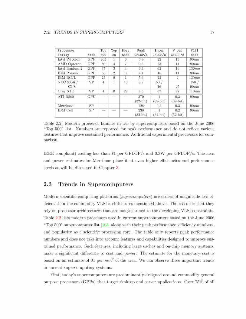
Processor Top Top Best Peak $ per W per VLSI
Family Arch 500 20 Rank GFLOP/s GFLOP/s GFLOP/s Node
Intel P4 Xeon GPP 265 1 6 6.8 22 13 90nm
AMD Opteron GPP 80 4 7 9.6 23 11 90nm
Intel Itanium 2 GPP 37 3 4 6.4 62 16 130nm
IBM Power5 GPP 35 2 3 4.4 15 11 90nm
IBM BG/L GPP 25 9 1 5.6 22 2 130nm
NEC SX-6 / VP 4 1 10 8 / 50 / 150 /SX-8 16 25 90nm
Cray X1E VP 4 0 22 4.5 67 27 110nm
ATI R580 GPU — — — 370 1 0.3 90nm
(32-bit) (32-bit) (32-bit)
Merrimac SP — — — 128 1.1 0.3 90nm
IBM Cell SP — — — 230 1 0.2 90nm
(32-bit) (32-bit) (32-bit)
Table 2.2: Modern processor families in use by supercomputers based on the June 2006“Top 500” list. Numbers are reported for peak performance and do not reflect variousfeatures that improve sustained performance. Additional experimental processors for com-parison.
IEEE compliant) costing less than $1 per GFLOP/s and 0.3W per GFLOP/s. The area
and power estimates for Merrimac place it at even higher efficiencies and performance
levels as will be discussed in Chapter 3.
2.3 Trends in Supercomputers
Modern scientific computing platforms (supercomputers) are orders of magnitude less ef-
ficient than the commodity VLSI architectures mentioned above. The reason is that they
rely on processor architectures that are not yet tuned to the developing VLSI constraints.
Table 2.2 lists modern processors used in current supercomputers based on the June 2006
“Top 500” supercomputer list [163] along with their peak performance, efficiency numbers,
and popularity as a scientific processing core. The table only reports peak performance
numbers and does not take into account features and capabilities designed to improve sus-
tained performance. Such features, including large caches and on-chip memory systems,
make a significant difference to cost and power. The estimate for the monetary cost is
based on an estimate of $1 per mm2 of die area. We can observe three important trends
in current supercomputing systems.
First, today’s supercomputers are predominantly designed around commodity general
purpose processors (GPPs) that target desktop and server applications. Over 75% of all

18 CHAPTER 2. BACKGROUND
systems use an Intel Xeon [73, 145], AMD Opteron [7, 145], or IBM Power5/PPC970
processor [71]. Contemporary GPP architectures are unable to use more than a few
arithmetic units because they are designed for applications with limited parallelism and
are hindered by a low bandwidth memory system. Their main goal is to provide high
performance for mostly serial code that is highly sensitive to memory latency and not
bandwidth. This is in contrast to the need to exploit parallelism and locality as discussed
above in Section 2.2.
Second, vector processors are not very popular in supercomputers and only the NEC
Earth Simulator, which is based on the 0.15µm SX-6 processor [90], breaks into the top 20
fastest systems at number 10. The main reason is that vector processors have not adapted
to the shifts in VLSI costs similarly to GPPs. The SX-6 and SX-8 processors [116] still pro-
vide formidable memory bandwidth (32GBytes/s) enabling high sustained performance.
The Cray X1E [35, 127] is only used in 4 of the Top500 systems.
Third, power consumption is starting to play a dominant role in supercomputer de-
sign. The custom BlueGene/L processor [21], which is based on the embedded low-power
PowerPC-440 core, is used in nine of the twenty fastest systems including numbers one
and two. As shown in Table 2.2, this processor is 5 times more efficient in performance
per unit power than its competitors. However, its power consumption still exceeds that
of architectures that are tuned for today’s VLSI characteristics by an order of magnitude.
Because current supercomputers under-utilize VLSI resources, many thousands of
nodes are required to achieve the desired performance levels. For example, the fastest
computer today is a IBM BlueGene/L system with 65, 536 processing nodes with a peak
of only 367TFLOP/s, whereas a more effective use of VLSI can yield similar performance
with only about 2, 048 nodes. A high node count places pressure on power, cooling, and
system engineering. These factors dominate system cost today and significantly increase
cost of ownership. Therefore, tailoring the architecture to the scientific computing do-
main and utilizing VLSI resources effectively can yield orders of magnitude improvement
in cost. The next chapter explore one such design, the Merrimac Streaming Supercom-
puter, and provides estimates of Merrimac’s cost and a discussion of cost of ownership
and comparisons to alternative architectures.
2.4. MODELS AND ARCHITECTURES 19
2.4 Execution Models, Programming Models, and Archi-
tectures
To sustain high performance on current VLSI processor technology an architecture must
be able to utilize multiple FPUs concurrently and maintain a high operand bandwidth
to the FPUs by exploiting parallelism and locality (locality refers to spatial, temporal,
and producer-consumer reuse). Parallelism is used to ensure enough operations can be
concurrently executed on the FPUs and also to tolerate data transfer and operation laten-
cies by overlapping computations and communication. Locality is needed to enable high
bandwidth data supply by allowing efficient wire placement and to reduce latencies and
power consumption by communicating over short distances as much as possible.
GPPs, vector processor (VP), and stream processors (SP) are high-performance archi-
tectures, but each is tuned for a different execution model. The execution model defines
an abstract interface between software and hardware, including control over operation ex-
ecution and placement and movement of operands and state. The GPPs support the von
Neumann execution model, which is ideal for control-intensive codes. VPs use a vector
extension of the von Neumann execution model and put greater emphasis on DLP. SPs
are optimized for stream processing and require large amounts of DLP.
Note that many processors can execute more than one execution model, yet their
hardware is particularly well suited for one specific model. Additionally, the choice of
programming model can be independent of the target execution model and the compiler
is responsible for appropriate output. However, current compiler technology limits the
flexibility of matching a programming model to multiple execution models. Similarly to
an execution model, a programming model is an abstract interface between the programmer
and the software system and allows the user to communicate information on data, control,
locality, and parallelism.
All three, von Neumann, vector, and stream execution models can support multiple
threads of control. A discussion of the implications of multiple control threads on the
architectures is left for future work. An execution model that does not require a control
thread is the dataflow execution model [43, 126]. No system today uses the dataflow
model, but the WaveScalar [159] academic project is attempting to apply dataflow to
conventional programming models.
In the rest of the section we present the three programming models and describe the
20 CHAPTER 2. BACKGROUND
general traits of the main architectures designed specifically for each execution model, the
GPP (Subsection 2.4.1), vector processor (Subsection 2.4.2), and the Stream Processor
(Subsection 2.4.3). We also summarize the similarities and differences in Subsection 2.4.4.
2.4.1 The von Neumann Model and the General Purpose Processor
The von Neumann execution model is interpreted today as a sequence of state-transition
operations that process single words of data [13]. The implications are that each opera-
tion must wait for all previous operations to complete before it can semantically execute
and that single-word granularity accesses are prevalent leading to the von Neumann bot-
tleneck. This execution model is ideal for control-intensive code and has been adopted
and optimized for by GPP hardware. To achieve high performance, GPPs have complex
and expensive hardware structures to dynamically overcome this bottleneck and allow for
concurrent operations and multi-word accesses. In addition, because of the state-changing
semantics, GPPs dedicate hardware resources to maintaining low-latency data access in
the form of multi-level cache hierarchies.
Common examples of GPPs are the x86 architecture from Intel [73] and AMD [7],
PowerPC from IBM [71], and Intel’s Itanium [157] (see Table 2.2).
2.4.1.1 General Purpose Processor Software
GPPs most typically execute code expressed in a single-word imperative language such
as C or Java following the von Neumann style and compiled to a general-purpose scalar
instruction set architecture (scalar ISA) implementing the von Neumann execution model.
Modern scalar ISAs includes two mechanisms for naming data: a small number of registers
allocated by the compiler for arithmetic instruction operands, and a single global memory
addressed with single words or bytes. Because of the fine granularity of operations ex-
pressed in the source language the compiler operates on single instructions within a data
flow graph (DFG) or basic blocks of instructions in a control flow graph (CFG) This style
of programming and compilation is well suited to codes with arbitrary control structures,
and is a natural way to represent general-purpose control-intensive code. However, the
resulting low-level abstraction, lack of structure, and most importantly the narrow scope
of the scalar ISA, limits current commercial compilers to produce executables that contain
only small amounts of parallelism and locality. For the most part, hardware has to extract
additional locality and parallelism dynamically.

2.4. MODELS AND ARCHITECTURES 21
Two recent trends in GPP architectures are extending the scalar ISA with wide words
for short-vector arithmetic [129, 6, 113, 160] and allowing software to control some hard-
ware caching mechanisms through prefetch, allocation, and invalidation hints. These new
features, aimed at compute-intensive codes, are a small step towards alleviating the bot-
tlenecks through software by increasing granularity to a few words (typically 16-byte short
vectors, or two double-precision floating point numbers, for arithmetic and 64-byte cache
line control). However, taking advantage of these features is limited to a relatively small
number of applications, due to the limitations of the imperative programming model. Au-
tomatic analysis is currently limited to for loops that have compile-time constant bounds
and where all memory accesses are an affine expression of loop induction variables [102].
Alternative programming models for GPPs that can, to a degree, take advantage
of the coarser-grained ISA operations include cache oblivious algorithms [53, 54] that
better utilize the cache hierarchy, and domain specific libraries. Libraries may either be
specialized to a specific processor (e.g., Intel Math Kernel Library [74]) or automatically
tuned via a domain-specific heuristic search (e.g., ATLAS [169] and FFTW [52]).
A more flexible and extensive methodology to delegate more responsibility to software
is the stream execution model, which can also be applied to GPPs [58].
2.4.1.2 General Purpose Processor Hardware
A canonical GPP hardware architecture consisting of an execution core with a control
unit, multiple FPUs, a central register file, and a memory hierarchy with multiple levels
of cache and a performance enhancing hardware prefetcher is depicted in Figure 2.3(a).
Modern GPPs contain numerous other support structures, which are described in detail
in [64].
The controller is responsible for sequentially fetching instructions according to the or-
der encoded in the executable. The controller then extracts parallelism from the sequence
of instructions by forming and analyzing a data flow graph (DFG) in hardware. This is
done by dynamically allocating hardware registers1 to data items named by the compiler
using the instruction set registers, and tracking and resolving dependencies between in-
structions. The register renaming and dynamic scheduling hardware significantly increase
the processor’s complexity and instruction execution overheads. Moreover, a typical basic
1Compiler based register allocation is used mostly as an efficient way to communicate the DFG to thehardware
22 CHAPTER 2. BACKGROUND
block does not contain enough parallelism to utilize all the FPUs and tolerate the pipeline
and data access latencies, requiring the control to fetch instruction beyond branch points
in the code. Often, instructions being fetched are dependent on a conditional branch whose
condition has not yet been determined requiring the processor to speculate on the value
of the conditional [153]. Supporting speculative execution leads to complex and expensive
hardware structures, such as a branch predictor and reorder buffer, and achieves greater
performance at the expense of lower area and power efficiencies. Additional complexity is
added to the controller to enable multiple instruction fetches on every cycle even though
the von Neumann model allows for any instruction to affect the instruction flow follow-
ing it [34, 128]. Speculative execution and dynamic scheduling also allow the hardware
to tolerate moderate data access and pipeline parallelism with the minimal parallelism
exported by the scalar ISA and compiler.
Because the hardware can only hide moderate latencies with useful dynamically ex-
tracted parallel computation and because global memory accesses can have immediate
affect on subsequent instructions, great emphasis is placed on hardware structures that
minimize data access latencies. The storage hierarchy of the GPP is designed to achieve
exactly this latency minimization goal. At the lowest level of the storage hierarchy are
the central register file and the complex pipeline bypass networks. While hardware dy-
namically allocates the physical registers, it can currently only rename registers already
allocated by the compiler. Due to scalar ISA encoding restrictions, the compiler is only
able to name a small number of registers, leading to an increased pressure on the memory
system to reduce latency. To do this, the memory system is composed of multiple levels of
cache memories where latency increases as the cache size grows larger. Caches rely on the
empirical property of applications that values that have been recently accessed in mem-
ory will be accessed again with high probability (temporal locality), and that consecutive
memory addresses tend to be accessed together (spatial locality). Therefore, a small cache
memory can provide data for a majority of the memory operations in the application with
low latency. When an access misses in the low-latency first level cache, additional, larger,
on-chip caches are used to bridge the latency gap to memory even further. These empirical
locality properties are true for most control intensive code that accesses a limited working
set of data. For compute and data intensive applications additional hardware mechanisms
and software techniques are often used. A hardware prefetcher attempts to predict what
memory locations will be accessed before the memory instruction is actually executed. The

2.4. MODELS AND ARCHITECTURES 23
prefetcher requests the predicted locations from off-chip memory and places the values in
the on-chip cache. If the prediction is both timely and correct, the memory access latency
is completely hidden from the load instruction. A typical hardware prefetcher consists of
a state machine to track recent memory requests and to control a simple functional unit
that computes future predicted addresses, the functional unit, and miss status holding
registers (MSHRs) [93] for efficiently communicating with the off-chip memory controller.
...
DR
AM
prefetcher
L1L2L2
controllercontroller
inst. cacheinst. cache
(a) GPP
L2 ... ...
Prefetcher
Prefetcher
DR
AM
DR
AM
controllercontroller
inst. cacheinst. cache
LD/S
T
(b) VP
SR
F ... ...
DM
AD
MA
DR
AM
DR
AM
controllercontroller
inst. storeinst. store
(c) SP
Figure 2.3: Sketch of canonical general-purpose, vector, and stream processors highlighting
their similarities and differences. Each hardware component is shaded according to the
degree of hardware control complexity (darker indicates greater hardware involvement),
as summarized in Subsection 2.4.4.
24 CHAPTER 2. BACKGROUND
Modern processors often contain multiple cores on the same die, but the discussion
above holds for each individual core. Another trend in GPPs is the support of multiple
concurrent threads on a single core, which also does not alter the basic description above.
2.4.2 Vector Processing
In addition to having capabilities similar to GPPs, vector processors can execute long-
vector instructions that apply the same primitive operation to a sequence of values, which
have been packed into a single very wide data word (typically 32 or 64 double-precision
floating point numbers) [141, 35, 90, 116, 92]. The primitive operations include integer
and floating point arithmetic, as well as memory loads and stores. Thus, the vector
execution model is a simple extension to the von Neumann model with the granularity of
an operation extended from acting on a single numerical value to a fixed-length vector.
As shown in Table 2.2, the Cray X1 [35] and NEC SX-6 [90] and SX-8 [116] are in use
today.
However, with memory latencies reaching hundreds of cycles and with single chip
processing capabilities of hundreds of concurrent FPUs, the control granularity of a 32−64
element vector is insufficient to overcome the von Neumann bottleneck leading to increased
hardware complexity as with the scalar GPP. Figure 2.3(b) depicts the major components
of a vector processor and shows the similarity with a GPP (Figure 2.3(a)). Just like GPPs,
VPs today devote significant hardware resources to dynamically extract parallelism and
to increase the architectural register space by hardware register renaming. To keep the
FPUs busy, the controller must run ahead and issue vector memory instructions to keep
the memory pipeline full, while at the same time providing enough state for the vectors in
the form of physical vector registers. Much of the complication is the result of the limits
of the execution model and the ISA.
The programming model for a vector processor is also similar to a GPP with short-
vector and prefetch extensions. A vectorizing compiler [170] is typically employed, re-
quiring the affine restrictions on the code, or a specialized domain-specific library can be
used.
2.4.3 The Stream Execution Model and Stream Processors
The stream execution model, in its generalized form, executes complex kernel operations
on collections of data elements referred to as streams. Increasing the granularity of control
2.4. MODELS AND ARCHITECTURES 25
and data transfer allows for less complex and more power and area efficient hardware, but
requires more effort from the software system and programmer.
Stream processors were first introduced with the Imagine processor [136] in 1998.
As common with such a relatively new architecture, several architectures with differing
characteristics have emerged, including the Sony/Toshiba/IBM Cell Broadband Engine
(Cell) [130], the ClearSpeed CSX600 [31], as well as Imagine and Merrimac. Addition-
ally, programmable graphics processors (GPUs) can also be classified as a type of stream
processor based on their execution model. This section discusses characteristics common
to all the processors above that stem from the stream execution model, while Section 3.5
provides specific comparisons with Merrimac.
2.4.3.1 Stream Processing Software
Stream processors are specifically designed to run compute-intensive applications with
limited and structured control and large amounts of data level parallelism (DLP). To
make efficient use of on-chip resources and limited power envelopes, SPs rely on software
to provide coarse-grained bulk operations and eliminate the need to dynamically extract
fine-grained parallelism and locality with complex hardware. In contrast to von Neumann
style programs which are represented by a CFG of basic blocks, a stream program is
expressed as a stream flow graph (SFG) and compiled at this higher granularity of complex
kernel operations (nodes) and structured data transfers (edges) as shown in Figure 2.4.
The figure describes the SFG of an n-body particle method, which interacts each of the
n particles in the system (a central particle) with particles that are close enough to affect
its trajectory (the neighbor particles). Kernels expose a level of locality (kernel locality)
as all accesses made by a kernel refer to data that is local to the kernel or that is passed
to the kernel in the form of a stream. The streams that connect kernels express producer-
consumer locality, as one kernel consumes the output of a kernel it is connected to, shown
by the time-stepping kernel consuming the forces produced by the interaction kernel.
In its strict form, a stream program is limited to a synchronous data flow graph [19].
An SDF is a restricted form of data flow where all rates of production, consumption,
and computation are known statically and where nodes represent complex kernel compu-
tations and edges represent sequences of data elements flowing between the kernels. A
compiler can perform rigorous analysis on an SDF graph to automatically generate code

26 CHAPTER 2. BACKGROUND
that explicitly expresses parallelism and locality and statically manages concurrency, la-
tency tolerance, and state allocation [25, 161]. The key properties of the strict stream
code represented by an SDF are large amounts of parallelism, structured and predictable
control, and data transfers that can be determined well in advance of actual data con-
sumption. A simple SDF version of the n-body method example of Figure 2.4 assumes
that all particles are close enough to interact and the interaction kernel reads the position
of all (n− 1) neighbor particles for each central particle position to produce a single force
value. Its rates are therefore (incentral = 1, inneighbor = n − 1, out = 1). The rate of all
streams of the timestep kernel are 1.
The same properties can be expressed and exploited through a more flexible and general
stream programming style that essentially treats a stream as a sequence of blocks as
opposed to a sequence of elements and relies on the programmer to explicitly express
parallelism [88]. In the n-body example, instead of the kernel computing the interaction
of a single particle with all other particles, the kernel now processes an entire block of
central particles and a block of neighbor particles. The kernel has the flexibility to reuse
position values if they appear in the neighbor lists of multiple central particles. In addition,
the read and write rates of the streams need not be fixed and each particle may have a
different number of neighbors. This variable rate property is impossible to express in
strict SDF. The greater flexibility and expressiveness of this gather, compute, scatter
style of generalized stream programming is not based on a solid theoretical foundation as
SDF, but experimental compilation and hardware systems have successfully implemented
it [107, 83, 37].
The stream ISA for the generalized stream execution model consists of coarse- and
medium-grained stream (block) instruction for bulk data transfers and kernels, as well
as fine-grained instructions within kernels that express ILP. Additionally, the stream ISA
provides a rich set of namespaces to support a hierarchy of storage and locality (locality
hierarchy) composed of at least two levels including on-chip local memory namespace
and off-chip memory addresses. Additionally, for efficiency and performance reasons a
namespace of kernel registers is desirable. In this way, the stream execution model allows
software to explicitly express parallelism, latency tolerance, and locality and alleviate
hardware from the responsibility of discovering them. Section 4.1 discusses how streaming
scientific applications utilize the stream model to express these critical properties.

2.4. MODELS AND ARCHITECTURES 27
particle positions
in DRAMtime (n)
particle velocities
in DRAMtime (n)
particle velocities
in DRAM
time (n+1)
particle positions
in DRAM
time (n+1)
particle velocities
in DRAM
time (n+1)
particle positions
in DRAM
time (n+1)
neighborpositions
centralpositions
centralvelocities
centralpositions
centralvelocities
centralforces
interactionkernel
interactionkernel
timestepkernel
timestepkernel
Figure 2.4: Stream flow graph of a n2 n-body particle method. Shaded nodes repre-sent computational kernels, clear boxes represent locations in off-chip memory, and edgesare streams representing stream load/store operations and producer-consumer localitybetween kernels.
2.4.3.2 Stream Processing Hardware
A stream processor, in contrast to a modern GPP, contains much more efficient and less
complex structures. Relying on large amounts of parallel computation, structured and
predictable control, and memory accesses performed in coarse granularity, the software
system is able to bear much of the complexity required to manage concurrency, locality,
and latency tolerance as discussed in the previous subsection. The canonical architecture
presented in Figure 2.3(c), includes minimal control consisting of fetching medium- and
coarse-grained instructions and executing them directly on the many FPUs. For efficiency
and increased locality, the FPUs are partitioned into multiple processing elements (PEs),
also referred to as execution clusters, and the register files are distributed amongst the
FPUs within a PE. Static scheduling is used whenever possible in order to limit dynamic
control to a minimum. To enable a static compiler to deal with the intricacies of scheduling
the execution pipeline, execution latencies of all instructions must be, to a large degree,
analyzable at compile time. To achieve this, a SP decouples the nondeterministic off-
chip accesses from the execution pipeline by only allowing the FPUs to access explicitly
software managed on-chip local memory. This local memory (commonly referred to as a
local store or stream register file) serves as a staging area for the bulk stream memory
operations, making all FPU memory reference latencies predictable. External memory

28 CHAPTER 2. BACKGROUND
accesses are performed by stream load/store units, which asynchronously execute the
coarse-grained bulk memory operations of the stream model. The stream load/store units
are analogous to asynchronous direct memory access (DMA) units. Delegating memory
accesses to the stream load/store units significantly simplifies the memory system when
compared to a GPP. Using the local memories as a buffer for the asynchronous bulk
memory operations, transfers the responsibility of latency tolerance from hardware to
software. As a result, the hardware structures are designed to maximize bandwidth rather
than minimize latencies. For example, deeper DRAM command scheduling windows can
be used to better utilize DRAM bandwidth at the expense of increased DRAM access
latency [137]. Additionally, the local memory increases the compiler managed on-chip
namespace allowing for greater static control over locality and register allocation and
reducing off-chip bandwidth demands.
Chapter 3 presents the Merrimac architecture and discusses streaming hardware in
greater detail.
2.4.4 Summary and Comparison
The main differences between the GPP, VP, and SP architectures stem from the granular-
ity of operation and degree of structure present in the von Neumann and stream execution
models, where the vector execution model as seen as an extension to von Neumann. The
fine granularity and immediate causality of the state changing von Neumann operations
lead to architectures that must be able to extract parallelism and locality dynamically
as well as minimize latencies. The stream model, in contrast, deals with coarse-grained,
and possibly hierarchical bulk block transfers and kernel operations leading to hardware
optimized for throughput processing. The GPP contains complex control units includ-
ing speculative execution support with large branch predictors and dynamic scheduling,
while the SP relies on static compiler scheduling and minimal hardware control. A VP is
somewhere in between the two with some, but not enough, parallelism exposed in DLP
vectors. A GPP implicitly maps off-chip memory addresses to on-chip cache locations
requiring complex associative structures and limiting the degree of software control. A
VP uses the implicit mapping into caches, but can additionally rely on vector memory
operations to gather vectors of words. However, a large number of vector operations is
required to load the data leading to hardware control complexity. A SP, on the other
hand, provides a hierarchy of explicit namespaces and delegates allocation and scheduling
2.4. MODELS AND ARCHITECTURES 29
to software. Both GPPs and SPs rely on asynchronous DMAs for hiding long DRAM
latencies on compute and data intensive codes, but the GPP uses a predictive hardware
prefetcher as opposed to the software controlled stream load/store units of the SP. A VP
has limited architectural asynchronous transfers in the form of vector loads and stores,
but requires hardware control to be able to cover long memory latencies. Finally, there are
large differences in terms of the software systems. The GPP handles arbitrarily complex
code and can strives to execute minimally optimized code well. Conversely, SPs and VPs,
rely on algorithm and program restructuring by the programmer and highly optimizing
compilers.

Chapter 3
Merrimac
Merrimac is a scientific supercomputer designed to deliver high performance in a cost
effective manner scaling efficiently from a $2K 128GFLOP/s workstation configuration
to a $20M 2PFLOP/s configuration with 16K nodes. The high level of performance
and economy are achieved by matching the strengths of modern VLSI technology to the
properties and characteristics of scientific applications. Merrimac relies on the stream
execution model, which places greater responsibility on software than the conventional
von Neumann model, allowing efficient and high-performance hardware.
As discussed in Section 2.2, hundreds of FPUs can be placed on an economically sized
chip making arithmetic almost free. Device scaling of future fabrication processes will
make the relative cost of arithmetic even lower. On the other hand, the number of in-
put/output pins available on a chip does not scale with fabrication technology making
bandwidth the critical resource. Thus, the problem faced by architects is supplying a
large number of functional units with data to perform useful computation. Merrimac
employs a stream processor architecture to achieve this goal. The Merrimac processor
architecture is heavily influenced by the Imagine processor [136], and a comparison of the
two is provided in Subsection 3.5.1.1. The Merrimac processor uses a hierarchy of locality
and storage resources of increasing bandwidth including a stream cache, stream register
file (SRF) and clustered execution units fed by local register files (LRFs) to simultane-
ously improve data parallelism while conserving bandwidth. The resultant architecture
has a peak performance of 128GFLOP/s per node at 1GHz in a 90nm process and can
execute both coarse-grained stream instructions and fine-grained scalar operations and
kernel arithmetic. The Merrimac processor integrates the 128GFLOP/s stream unit, a
30
31
scalar core to execute scalar instructions and control, and a throughput oriented stream
memory subsystem that directly interfaces with local DRAM and the global intercon-
nection network. The Merrimac system contains up to 16K nodes, where each node is
composed of a Merrimac processor, local node DRAM memory, and a port to the global
interconnection network.
Applications for Merrimac are written in a high-level language and compiled to the
stream execution model. The current Merrimac software system is described in Section 4.2.
The compiler performs two different decompositions. In the domain decomposition step,
data streams are partitioned into pieces that are assigned to the local memory on individual
nodes. However, all nodes share a single global address space and can access memory
anywhere in the system. Thus domain decomposition is an optimization for improving
locality and bandwidth and any reasonable decomposition is possible as long as the data
fits in node memory and the workload is balanced. The second decomposition involves
partitioning the application code into a scalar program with stream instructions and a
set of kernels according to the stream execution model. The scalar code is compiled
into a scalar processor binary with embedded coarse-grained stream instructions and each
of the stream kernels is compiled into microcode. The domain decomposed data and
program binaries are loaded into node local memories and the scalar processors at each
node commence execution.
Coarse-grained stream loads and stores in the scalar program initiate data transfer be-
tween global memory and a node’s stream register file. The memory system is optimized
for throughput and can handle both strided loads and stores and indexed gathers and
scatters in hardware. The memory system is designed for parallel execution and supports
atomic read-modify-write stream operations including the scatter-add primitive for super-
position type reductions [2]. Additionally, if the data is not resident in the node’s local
DRAM, the memory system hardware autonomously transfers the data over the global
interconnection network. Kernel instructions in the scalar program cause the stream
execution unit to start running a previously loaded kernel binary. Kernel execution is
controlled by a micro-controller unit and proceeds in a SIMD manner with all clusters in
the same node progressing in lockstep. Data transfers between various levels of the on-chip
memory hierarchy including the stream register file, stream buffers and local register files
are controlled from the microcode. As kernel execution progresses, the scalar program
continues to load more data into the stream register file and save output streams to main

32 CHAPTER 3. MERRIMAC
memory, hiding memory access latencies with useful computation (Figure 3.1). The scalar
core also handles global synchronization primitives such as barriers. Multiprogramming
is supported by the use of segment registers which protect memory regions of individual
programs from each other.
load
cen
tral
s 0
load
nei
ghbo
rs0
load
vel
ociti
es0
inte
ract
0
times
tep 0
stor
e ce
ntra
ls0
stor
e ve
loci
ties 0
load
cen
tral
s 1
load
nei
ghbo
rs1
load
vel
ociti
es1
inte
ract
1
times
tep 1
stor
e ce
ntra
ls1
stor
e ve
loci
ties 1
load
cen
tral
s 2
load
nei
ghbo
rs2
load
vel
ociti
es2
inte
ract
2
Figure 3.1: Stream level software controlled latency hiding. The software pipeline of thestream instructions corresponding to the blocked n-body SFG of Figure 2.4.
Section 3.1 summarizes Merrimac’s instruction set architecture (ISA) and philosophy,
Section 3.2 details the Merrimac processor architecture, and Section 3.3 describes the
Merrimac system. Details of the fault tolerance and reliability schemes will be described
in Chapter 6. We estimate Merrimac’s die area, power consumption, and cost in Sec-
tion 3.4 and discuss related architectures and the implications of Merrimac’s design on
the hardware and software systems in Section 3.5.
3.1 Instruction Set Architecture
The Merrimac processor and system are designed specifically for the stream execution
model. This is reflected in the instruction set architecture (ISA), which stresses through-
put and a hierarchy of control and locality. The hierarchical nature of the stream execution
model and its coarse-grained stream instructions are also central to the memory and ex-
ception models, which are described in Subsection 3.1.3 and Subsection 3.1.4 respectively.
The Merrimac ISA has three types of instructions corresponding to the stream execu-
tion model:

3.1. INSTRUCTION SET ARCHITECTURE 33
• Scalar instructions that execute on the scalar core and are used for non-streaming
portions of the application code and for flow control. These instructions include the
standard scalar ISA, as well as instructions for interfacing with the stream unit.
• Stream instructions that include setting stream related architectural registers and
state, invoking kernels, and executing stream memory operations.
• Kernel instructions that are executed while running a kernel on the compute
clusters and micro-controller. Kernel instructions are at a lower level of the con-
trol hierarchy than stream instructions, and a single stream kernel instruction, for
example, may control the execution of many thousands of kernel instructions.
Any standard scalar ISA (MIPS, PowerPC, x86) is suitable for Merrimac’s scalar ISA
with the addition of instructions to interface with the stream unit (Subsection 3.2.1).
3.1.1 Stream Instructions
Stream instructions are embedded within the scalar instruction stream and are used to
control the stream unit, issue stream memory operations, initiate and control kernel ex-
ecution, and manipulate stream unit state. The stream instructions are communicated
by the scalar core to the stream controller to allow their execution to be decoupled from
scalar execution. The stream controller accepts instructions from the scalar core interface
and autonomously schedules them to the appropriate streaming resource. Along with the
instruction, the scalar core also sends encoded dependency information of the instruction
on preceding stream instructions, alleviating the need to dynamically track dependencies
in hardware. The stream controller uses the dependencies and a scoreboard mechanism to
dynamically schedule the out of order execution of stream instructions on 4 resources it
controls: an address generators (AG) in the memory subsystem for running stream mem-
ory instructions, the micro-controller which sequences kernels, a cache controller, and the
stream controller itself.
The stream instructions fall into three categories: operations that control the stream
controller, stream memory operations, and kernel control operations. Figure 3.2 shows
how to use the stream instructions to implement the n-body example of Figure 2.4 with
the software pipeline depicted in Figure 3.1, and the paragraphs below describe the in-
structions in detail.
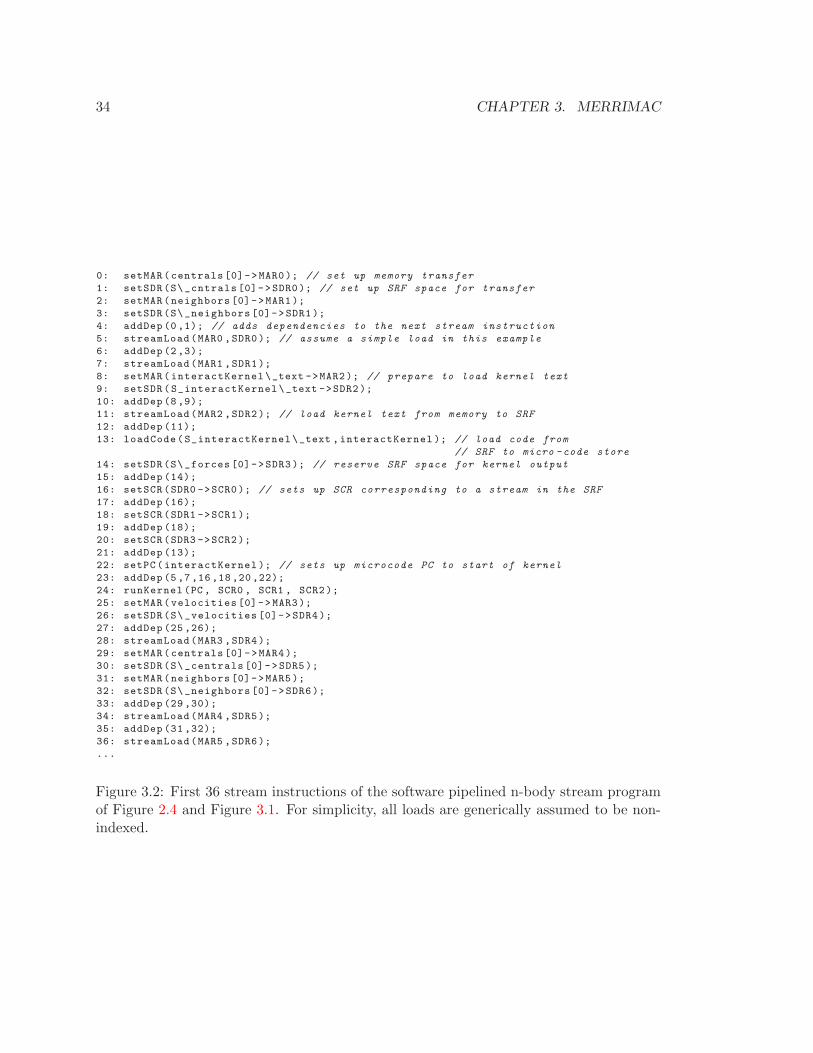
34 CHAPTER 3. MERRIMAC
0: setMAR(centrals [0]->MAR0); // set up memory transfer
1: setSDR(S\_cntrals [0]->SDR0); // set up SRF space for transfer
2: setMAR(neighbors [0]->MAR1);
3: setSDR(S\_neighbors [0]->SDR1);
4: addDep (0,1); // adds dependencies to the next stream instruction
5: streamLoad(MAR0 ,SDR0); // assume a simple load in this example
6: addDep (2,3);
7: streamLoad(MAR1 ,SDR1);
8: setMAR(interactKernel\_text ->MAR2); // prepare to load kernel text
9: setSDR(S_interactKernel\_text ->SDR2);
10: addDep (8,9);
11: streamLoad(MAR2 ,SDR2); // load kernel text from memory to SRF
12: addDep (11);
13: loadCode(S_interactKernel\_text ,interactKernel ); // load code from
// SRF to micro -code store
14: setSDR(S\_forces [0]->SDR3); // reserve SRF space for kernel output
15: addDep (14);
16: setSCR(SDR0 ->SCR0); // sets up SCR corresponding to a stream in the SRF
17: addDep (16);
18: setSCR(SDR1 ->SCR1);
19: addDep (18);
20: setSCR(SDR3 ->SCR2);
21: addDep (13);
22: setPC(interactKernel ); // sets up microcode PC to start of kernel
23: addDep (5,7,16,18,20,22);
24: runKernel(PC , SCR0 , SCR1 , SCR2);
25: setMAR(velocities [0]->MAR3);
26: setSDR(S\_velocities [0]->SDR4);
27: addDep (25 ,26);
28: streamLoad(MAR3 ,SDR4);
29: setMAR(centrals [0]->MAR4);
30: setSDR(S\_centrals [0]->SDR5);
31: setMAR(neighbors [0]->MAR5);
32: setSDR(S\_neighbors [0]->SDR6);
33: addDep (29 ,30);
34: streamLoad(MAR4 ,SDR5);
35: addDep (31 ,32);
36: streamLoad(MAR5 ,SDR6);
...
Figure 3.2: First 36 stream instructions of the software pipelined n-body stream programof Figure 2.4 and Figure 3.1. For simplicity, all loads are generically assumed to be non-indexed.

3.1. INSTRUCTION SET ARCHITECTURE 35
Stream Controller Operations
The instructions in this category do not actually perform a stream operation, but rather
control the way the stream controller handles other stream instructions:
1. Instructions for setting dependencies between stream instructions. The addDep
instruction sets scoreboard state for the immediately following stream instruction to
be dependent on the scoreboard locations specified in the addDep operation.
2. Instructions for removing stream instructions that have not yet started. These in-
structions are not common and are only used when stream-level software speculation
is used. This case does not appear in the example of Figure 3.2.
Stream Memory Operations
Merrimac can issue strided memory reads and writes, indexed reads and writes, and
various flavors of these operations which include one of the following operations: integer
increment, integer add, and floating-point addition. All access modes are record based
and the hardware aligns individual records to be contiguous in a SRF lane. A SRF lane
is a portion of the SRF that is aligned with an execution cluster. Figure 3.3 depicts the
access modes and alignment:
Strided Access
A strided access is a systematic memory reference pattern. The strided access is described
by four parameters, the base virtual address (base), the record length (recLen), and the
stride (stride), which is the distance in words between consecutive records in the stream.
A strided load, for example, reads recLen consecutive words starting at virtual memory
address base and writes the words to the first lane of the SRF. The second lane also
receives recLen consecutive words, but the starting address is base + stride. This process
repeats, appending records to each lane for the entire stream length.
Gather/Scatter Access
The gather/scatter access mode uses an stream of indices to generate record accesses as
opposed to the systematic pattern of a strided access. The indices are read from the SRF,
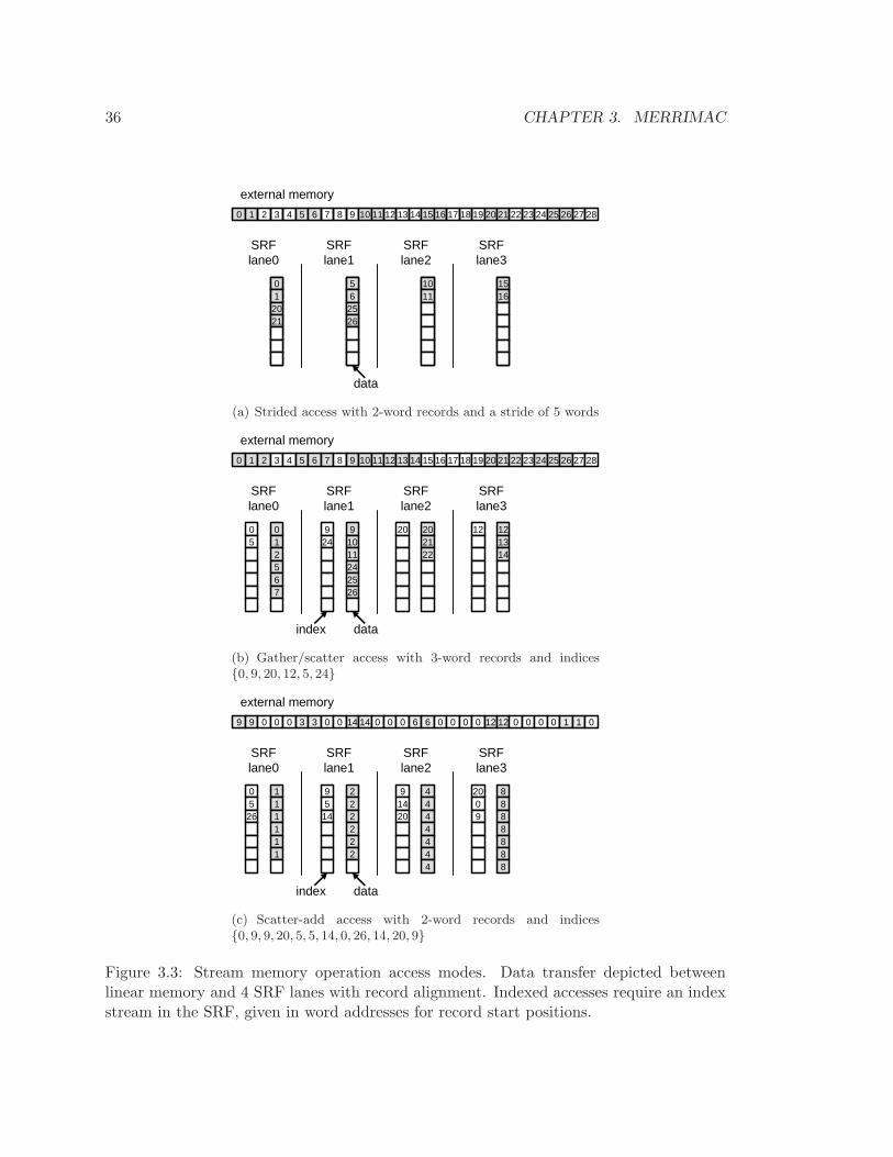
36 CHAPTER 3. MERRIMAC
0 1 2 3 4 5 6 7 8 9 10 11 12 13 14 15 16 17 18 19 20 21 22 23 24 25 26 27 28
01
2021
01
2021
56
2526
56
2526
10111011
15161516
external memory
SRFlane0
SRFlane1
SRFlane2
SRFlane3
data
(a) Strided access with 2-word records and a stride of 5 words
0 1 2 3 4 5 6 7 8 9 10 11 12 13 14 15 16 17 18 19 20 21 22 23 24 25 26 27 28
012567
91011242526
202122
121314
05
924
20 12
external memory
SRFlane0
SRFlane1
SRFlane2
SRFlane3
index data
(b) Gather/scatter access with 3-word records and indices{0, 9, 20, 12, 5, 24}
9 9 0 0 0 3 3 0 0 14 14 0 0 0 6 6 0 0 0 0 12 12 0 0 0 0 1 1 0
111111
222222
4 805
26
95
14
91420
2009
444444
888888
external memory
SRFlane0
SRFlane1
SRFlane2
SRFlane3
index data
(c) Scatter-add access with 2-word records and indices{0, 9, 9, 20, 5, 5, 14, 0, 26, 14, 20, 9}
Figure 3.3: Stream memory operation access modes. Data transfer depicted betweenlinear memory and 4 SRF lanes with record alignment. Indexed accesses require an indexstream in the SRF, given in word addresses for record start positions.
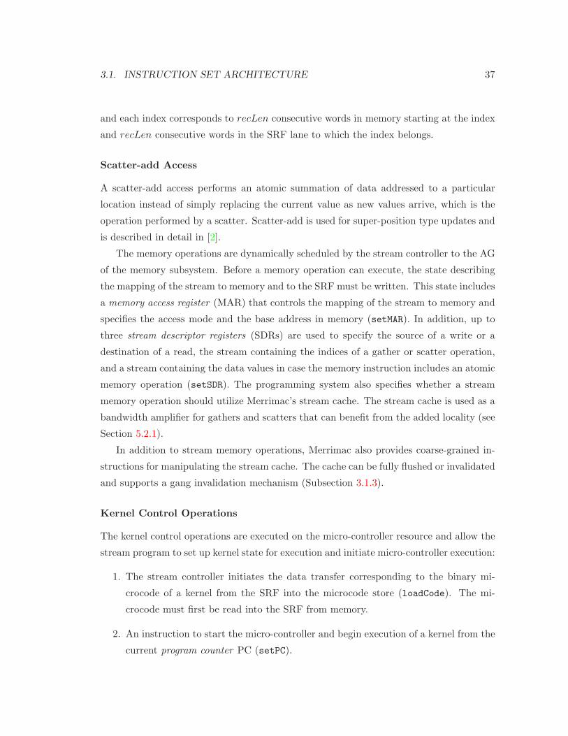
3.1. INSTRUCTION SET ARCHITECTURE 37
and each index corresponds to recLen consecutive words in memory starting at the index
and recLen consecutive words in the SRF lane to which the index belongs.
Scatter-add Access
A scatter-add access performs an atomic summation of data addressed to a particular
location instead of simply replacing the current value as new values arrive, which is the
operation performed by a scatter. Scatter-add is used for super-position type updates and
is described in detail in [2].
The memory operations are dynamically scheduled by the stream controller to the AG
of the memory subsystem. Before a memory operation can execute, the state describing
the mapping of the stream to memory and to the SRF must be written. This state includes
a memory access register (MAR) that controls the mapping of the stream to memory and
specifies the access mode and the base address in memory (setMAR). In addition, up to
three stream descriptor registers (SDRs) are used to specify the source of a write or a
destination of a read, the stream containing the indices of a gather or scatter operation,
and a stream containing the data values in case the memory instruction includes an atomic
memory operation (setSDR). The programming system also specifies whether a stream
memory operation should utilize Merrimac’s stream cache. The stream cache is used as a
bandwidth amplifier for gathers and scatters that can benefit from the added locality (see
Section 5.2.1).
In addition to stream memory operations, Merrimac also provides coarse-grained in-
structions for manipulating the stream cache. The cache can be fully flushed or invalidated
and supports a gang invalidation mechanism (Subsection 3.1.3).
Kernel Control Operations
The kernel control operations are executed on the micro-controller resource and allow the
stream program to set up kernel state for execution and initiate micro-controller execution:
1. The stream controller initiates the data transfer corresponding to the binary mi-
crocode of a kernel from the SRF into the microcode store (loadCode). The mi-
crocode must first be read into the SRF from memory.
2. An instruction to start the micro-controller and begin execution of a kernel from the
current program counter PC (setPC).
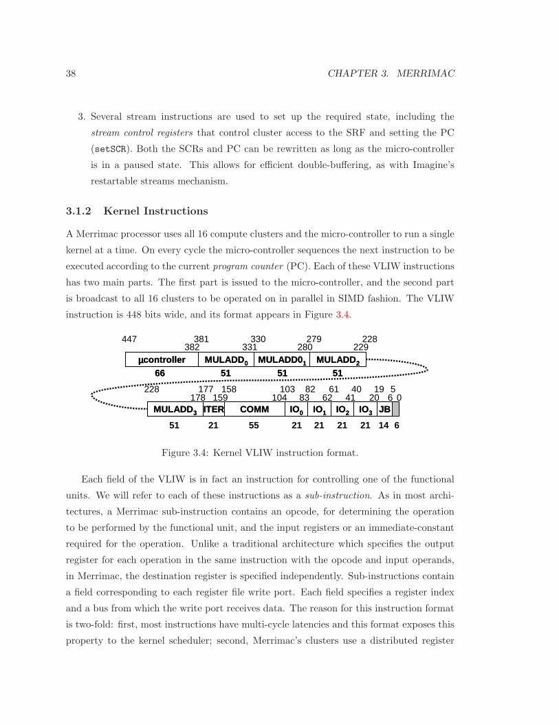
38 CHAPTER 3. MERRIMAC
3. Several stream instructions are used to set up the required state, including the
stream control registers that control cluster access to the SRF and setting the PC
(setSCR). Both the SCRs and PC can be rewritten as long as the micro-controller
is in a paused state. This allows for efficient double-buffering, as with Imagine’s
restartable streams mechanism.
3.1.2 Kernel Instructions
A Merrimac processor uses all 16 compute clusters and the micro-controller to run a single
kernel at a time. On every cycle the micro-controller sequences the next instruction to be
executed according to the current program counter (PC). Each of these VLIW instructions
has two main parts. The first part is issued to the micro-controller, and the second part
is broadcast to all 16 clusters to be operated on in parallel in SIMD fashion. The VLIW
instruction is 448 bits wide, and its format appears in Figure 3.4.
µµµµcontroller MULADD 0 MULADD0 1 MULADD 2µµµµcontroller MULADD 0 MULADD0 1 MULADD 2
ITER COMM IO0MULADD 3 JBIO1 IO2 IO3ITER COMM IO0MULADD 3 JBIO1 IO2 IO3
66 51 51 5166 51 51 51
51 21 55 21 21 21 21 14 6
382 331 280 229381 330 279 228447
178 159 104 83 62 41 20 6 0177 158 103 82 61 40 19 5228
Figure 3.4: Kernel VLIW instruction format.
Each field of the VLIW is in fact an instruction for controlling one of the functional
units. We will refer to each of these instructions as a sub-instruction. As in most archi-
tectures, a Merrimac sub-instruction contains an opcode, for determining the operation
to be performed by the functional unit, and the input registers or an immediate-constant
required for the operation. Unlike a traditional architecture which specifies the output
register for each operation in the same instruction with the opcode and input operands,
in Merrimac, the destination register is specified independently. Sub-instructions contain
a field corresponding to each register file write port. Each field specifies a register index
and a bus from which the write port receives data. The reason for this instruction format
is two-fold: first, most instructions have multi-cycle latencies and this format exposes this
property to the kernel scheduler; second, Merrimac’s clusters use a distributed register

3.1. INSTRUCTION SET ARCHITECTURE 39
file architecture to lower area and power overheads. Each of the 13 register file write
ports, 4 SRF data words, and 4 SRF addresses can be written to by 15 producers on the
intra-cluster switch: 4 MULADD units, 1 ITER unit, 1 COMM unit, 1 JB unit, and 4
data-words and 4 valid flags returned by the INOUT units for SRF data. For a detailed
description of the register file organization, please see Subsection 3.2.4.
Merrimac provides hardware support for efficient software-pipelined (SWP) loops within
kernels. The micro-controller, which is responsible for instruction issue, squashes oper-
ations that affect state changes while priming or draining the software pipeline. This is
done by tagging register writes and INOUT operations with the stage of the software
pipeline they are scheduled in. The micro-controller tracks the iteration number of the
loop and combines this information with the stage tag of each state-changing operation in
order to potentially suppress the instructions effect. In each LRF, register 0 is hard coded
to the value 0 and writes to it are ignored. The micro-controller squashes register writes
by converting the destination register to 0. INOUT operations are squashed by replacing
the opcode with a NOP.
3.1.3 Memory Model
Merrimac supports a flat memory space with hardware assisted software coherency. In line
with the stream execution model, the memory model and architecture take advantage of
the coarse granularity of the stream memory operations to efficiently implement the global
address space. Instead of dynamic and fine-grained demand-paging common to GPPs,
Merrimac utilizes a coarse-grained control segmentation scheme to map virtual addresses
to physical node addresses enabling high-throughput translation of memory addresses into
network requests by the memory unit. Merrimac’s consistency and coherency models also
rely on the stream granularity of memory operations, permitting high throughput without
the need of costly fine-grained hardware coherence. Thus, Merrimac can be economically
scaled up to a 16K node configuration.
Memory Segmentation
Merrimac uses a segment level protection scheme to allow multiple jobs to be run simulta-
neously without the overhead associated with TLBs and paged memory. The segmentation
system also interleaves addresses across nodes in a programmable manner. Segments can
be interleaved with a granularity ranging from one word to the entire segment in powers

40 CHAPTER 3. MERRIMAC
of two. The system translates 64-bit virtual addresses into 64-bit physical addresses via a
set of segment registers. Each segment register specifies the segment length, the subset of
nodes over which the segment is mapped, the interleave (striping) factor for the segment,
and the cache state of the segment. The segmentation translation is performed within the
memory unit using the five most significant bits of a virtual address.
Figure 3.5 illustrates the mapping process. The process is summarized below and is
followed by an example.
• The SegNum field of the virtual address is used to index into the segment register
file and select the segment register for performing the translation.
• The SegAddr field of the virtual address is simply the contiguous virtual address
within the segment.
• The n0 and n1 fields of the segment register determine the striping of the SegAddr
virtual address across the nodes in the segment. n0 is the starting bit of SegAddr
that determines the mapping onto nodes, such that the nodes are interleaved in a
granularity of 2n0 . n1 is the ending bit. Therefore, there are 2n1−n0 nodes in the
segment. Note that n0 ≥ 2 to ensure that cache lines are not split between node
stripes. Bits 0− (n0 − 1) of SegAddr determine the least significant bits of the offset
within a node in the segment, bits n0 − (n1 − 1) are the node number within the
segment, and bits n1 − (35 + n1 − n0) correspond to the most significant bits of the
address offset.
• The node to which the virtual address is referring is calculated by adding NodeBase,
the start of the contiguous range of nodes in the segment, to NodeOff.
• The absolute physical address (PhysAddr) within the determined node (Node) is
computed by adding PhysOff to PhysBase.
• The physical address must fall within the segment memory range in the node, namely
PhysBase to PhysBase + 2PhysLen − 1. Note that the base physical address (Phys-
Base) must be an integer multiple of the segment size.
Within each segment, the virtual addresses (SegAddr) are contiguous and run from 0 up
to 2PhysLen+x−1, where x = n1−n0 and 2x is the number of nodes in the segment. Phys-
ically, however, due to the way the virtual addresses are converted to physical addresses,
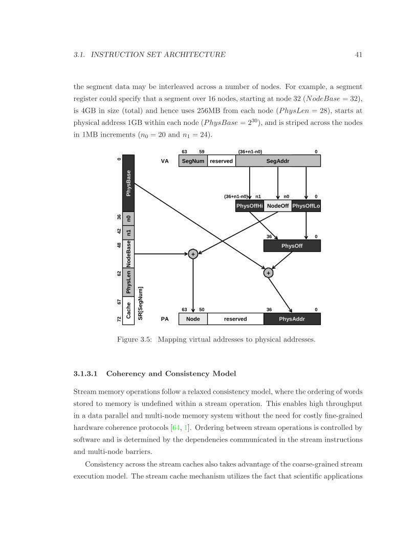
3.1. INSTRUCTION SET ARCHITECTURE 41
the segment data may be interleaved across a number of nodes. For example, a segment
register could specify that a segment over 16 nodes, starting at node 32 (NodeBase = 32),
is 4GB in size (total) and hence uses 256MB from each node (PhysLen = 28), starts at
physical address 1GB within each node (PhysBase = 230), and is striped across the nodes
in 1MB increments (n0 = 20 and n1 = 24).
SegAddrVA reservedSegNum
Phy
sBas
en1
n0N
odeB
ase
Phy
sLen
Cac
he
PhysOffHi NodeOff PhysOffLo
PhysOff
PhysAddrreservedNode
+
+
PASR
[Seg
Num
]
0
0
0
050
n0n1
5963 (36+n1-n0)
(36+n1-n0)
36
3663
036
4248
6267
72
Figure 3.5: Mapping virtual addresses to physical addresses.
3.1.3.1 Coherency and Consistency Model
Stream memory operations follow a relaxed consistency model, where the ordering of words
stored to memory is undefined within a stream operation. This enables high throughput
in a data parallel and multi-node memory system without the need for costly fine-grained
hardware coherence protocols [64, 1]. Ordering between stream operations is controlled by
software and is determined by the dependencies communicated in the stream instructions
and multi-node barriers.
Consistency across the stream caches also takes advantage of the coarse-grained stream
execution model. The stream cache mechanism utilizes the fact that scientific applications

42 CHAPTER 3. MERRIMAC
operate in computational phases (Chapter 4). Hence, each memory location serves as
either an input, an output, or as a reduction target within a given phase and is read-only,
write-only, or uses an atomic read-modify-write stream memory operation. Therefore, the
stream cache does not perform any fine-grained hardware coherence operations. Instead,
the cache can distinguish between cacheable and uncacheable properties associated with a
segment or stream memory operation; it is up to the software system to use these cacheable
properties in a safe manner utilizing explicit bulk invalidate and flush operations.
The stream cache supports explicit flush and invalidate instructions at a stream gran-
ularity. This is implemented via 4 valid bits in each stream cache line (the line is valid
if any of the valid bits are set). Because the stream cache serves as a bandwidth ampli-
fier for a typically small number of stream operations with irregular locality properties, 4
valid bits are sufficient. In each MAR there is an entry specifying whether the stream is
memory-uncacheable or network-uncacheable (or both/neither), and another entry speci-
fying which stream cache valid bit to use. If the memory-uncacheable flag is set, then any
data whose address is in the node’s local memory will not be cached, and if the network-
uncacheable flag is set, then any data whose address is in a remote node (i.e., over the
network) will not be cached. The stream cache is placed in front of the local memory and
the network interface and satisfies requests from the local stream units, the local scalar
core, and remote nodes (via the network interface). The source of the memory requests is
not a factor in the stream-uncacheable properties.
An invalidate operation on a cached stream is cheap as it simply sets the associated
valid bit line to zero, while a flush is expensive (as is usually the case) because the cache
must be traversed to write dirty data back to memory.
When the stream unit requests a memory word, the request is first checked in the local
node’s stream cache and satisfied from there in the case of a cache hit. In the case of a
stream cache miss, the request is sent to the home node of the memory word determined
by the segment mapping. That node, in turn, will check its stream cache before reading
the word from its main memory.
For example, consider data that is initially private on a node and later becomes read-
only from multiple nodes. In the first phase, the node on which the data resides will mark
the address range memory-cacheable and all other nodes will set the range to network-
uncacheable. This ensures that the node on which the data is private will have exclusive
cached access and all other nodes will not cache stale data. In the second phase, all

3.1. INSTRUCTION SET ARCHITECTURE 43
nodes mark the range as network-cacheable and are free to make cached copies of the data
because it will not be modified by any node.
Scalar Cache Coherency and Consistency
The Merrimac design minimizes modifications to off-the-shelf scalar core architectures.
Therefore, the L1 cache (and L2 cache, if there is one) are accessible to the scalar processor
alone, and not accessible to the stream units or other nodes. Hence, unlike the stream
cache, the scalar cache does not need bits for segment or stream identification. The scalar
memory consistency and coherence models are as relaxed and inexpensive as possible. The
only additional requirement of the scalar cache hierarchy is that the scalar core support
uncacheable memory segments defined by the segment registers. This may be achieved
by adding logic to check segment registers or by using the non-cacheable bit found in the
page table and TLB of modern GPPs.
The scalar cache needs to support an explicit flush command, but it is not required to
perform any coherence operations. It is up to software to use the cacheable/uncacheable
segment properties in a safe manner. The scalar cache does not see remote memory
requests to its node since these go directly to the stream memory system. If multiple
scalar processors use shared variables to communicate, then these variables should be
placed in segments that are both memory- and network-uncacheable, and the memory
addresses corresponding to the variables must be explicitly flushed before the first shared
use. This guarantees that the node to which the variable is local in memory does not
cache a stale copy (memory-uncacheable), as well as no stale copies on nodes that must
traverse the network to access the variable (network-uncacheable).
Even though the stream units cannot see the scalar cache, the converse is not true.
The scalar processor can see the stream caches, and if a local reference misses in the scalar
cache then it may be satisfied by the stream cache rather than accessing main memory.
However, scalar references which miss in the stream cache will not cause a line to be read
into it.
The scalar processor should have a node memory barrier or fence instruction similar
to the SYNC instruction of the MIPS II ISA [80]. The compiler may use this instruc-
tion when it needs to guarantee the order of scalar memory instructions. The memory
barrier instruction prevents new loads and stores from being issued until all the currently
outstanding memory references from the scalar processor have completed.
44 CHAPTER 3. MERRIMAC
The scalar processor is required to provide the following two consistency guarantees.
1. After a node memory barrier, all outstanding scalar accesses from that node will
have been committed.
2. Multiple scalar accesses from a given scalar processor to the same memory address
in its home node will exhibit sequential consistency. There are no guarantees with
respect to the ordering of accesses to different addresses or to/from different proces-
sors.
3.1.4 Exception and Floating Point Models
Merrimac’s exception and floating point models are designed to economically support
high-throughput execution while meeting user requirements based on the IEEE 754 stan-
dard [72] and common GPP exception models. Merrimac follows the lead of high-performa-
nce short-vector extensions of GPPs (e.g., SSE [160] and Altivec [113]) in terms of floating
point precision and rounding and exceptions in scalar and control code. However, the
floating point and memory exception model leverages the stream execution model and
does not require fine-grained interrupts.
3.1.4.1 Floating Point Model
Merrimac supports double-precision IEEE 754 numbers including denormalized numbers,
infinities, zeros, and NaNs. Extended double-precision is only used within the MULADD
pipeline between the multiply and addition of a fused multiply-add.
Merrimac does not follow the standard regarding divide and square-root operations, as
it does not provide dedicated hardware for these functions. Binary to decimal conversions
and remainders are supported in software only, and are not guaranteed to be exactly
rounded.
IEEE 754 specifies 4 rounding modes: round to nearest even, round to zero, round
to +∞, and round to −∞. Moreover, the standard permits the program to change the
rounding mode at run-time. Merrimac only provides rounding to nearest even, as this
is the most commonly used mode and also because this mode offers superior numerical
precision [65].
3.1. INSTRUCTION SET ARCHITECTURE 45
3.1.4.2 Exception Model
Merrimac’s control unit is responsible for handling all exceptions. The scalar core follows
current GPP exception and interrupt models for non-streaming scalar portions of the
code and control operations it executes. Exceptions from the stream and memory units
are reported to the stream controller and can communicated to the scalar core via polling
or maskable interrupts.
Merrimac may perform over 161 operations that can raise an exception every cycle
(128 FP operations on the 4 MULADD units, 16 ITER FP operations, 1 micro-controller
operation, 8 address translations, 8 atomic read-modify-write FP additions, and fault-
detection exceptions as discussed in Chapter 6). Implementing a precise exception model
that may interrupt kernel and program execution on each of these operations is infeasible
and will degrade performance, particularly if the controller masks the particular exception
raised. Merrimac takes advantage of the stream execution model and treats all stream op-
erations as atomic operations with regards to exceptions. Thus, exception related control
is coarse-grained and scalable.
The exception model meets user requirements for exception handling and recovery
without the need of precise exceptions. For example, precise exceptions are not a require-
ment of the IEEE 754 standard. Instead, the standard specifies that each instruction with
an exception raise a flag, and suggests that software should be able to trap on it and
recover. In Merrimac, the exception unit tracks exceptions raised by the individual func-
tional units and records the first occurrence of each exception type for a running stream
instruction (kernel or memory). Before a stream operation completes, the exception unit
raises an exception interrupt flag to the scalar core if an exception occurred. The scalar
core retrieves the exception information, which contains the precise point during execu-
tion that caused the exception. Since software controls all inputs to stream instructions,
the kernel or memory operation can be immediately re-executed up to the point of the
exception to emulate precise exception handling with hardware and software cooperation.
Exceptions in Kernels
Kernels may raise exceptions related to the micro-controller or the FPUs. The micro-
controller may encounter ill-formed VLIW instructions or branches and will pause its
execution and signal the exception unit. The FPUs may raise FP exceptions based on

46 CHAPTER 3. MERRIMAC
IEEE 754 as follows:
• Invalid – This flag is raised when an invalid result is generated producing a NaN.
• Divide by Zero (DVBZ) – raised when 10 is executed on the ITER unit (SFINV(0)).
The result returned by the ITER unit in this case is always a +∞.
• Overflow – raised when an addition, subtraction, multiplication, or fused multiply-
add results in a number that is larger than the maximum representable using double-
precision. In addition to raising the overflow flag, the result returned is +∞.
• Underflow – raised when a computation result is smaller than the minimum repre-
sentable number using denormalized form of double-precision. The result returned
is a ±0. Merrimac only raises the underflow exception flag when a denormalized
number underflows, not when gradual underflow begins.
The inexact exception type of IEEE 754 is not supported. Similar to the case of the
less common rounding modes, it is most often used for interval arithmetic.
Also, the Merrimac hardware does not pass any parameters to the trap handler as
specified by IEEE 754, and software must recover based on the exact exception point
information in the exception unit. This information consists of the exception type, PC,
uCR values, and FPU ID of the first occurrence of the exception and allows for precise
reconstruction of the exception instruction based on the unchanged kernel input streams.
Exceptions in Memory Operations
Memory operations may raise exception flags under two conditions: a) an address is
requested that is outside the specified segment (segment violation) or b) a floating-point
exception occurs. When exceptions occur, the stream element number of the first address
that caused the exception is stored in the exception unit for the appropriate exception
type. In the case of an FP exception, the ID of the FPU that faulted (one of the 8 FPUs in
the atomic-memory-operation units) is also recorded. Once the memory operation finishes
execution, software can check the exception register and recover the precise state prior to
the exception.
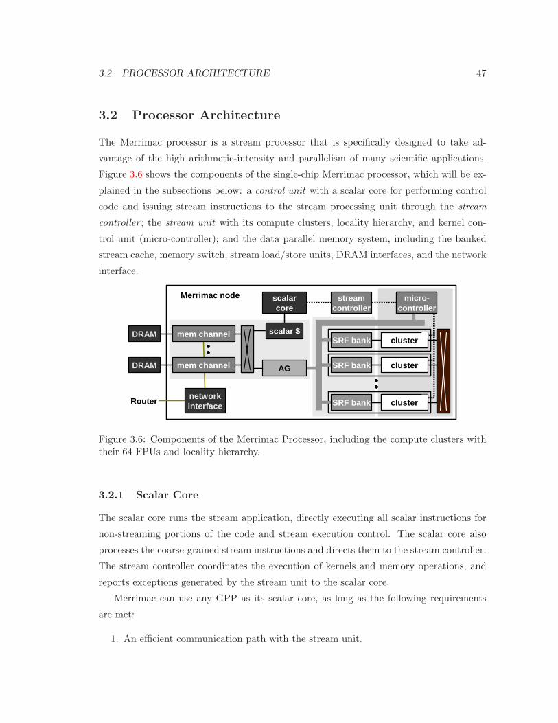
3.2. PROCESSOR ARCHITECTURE 47
3.2 Processor Architecture
The Merrimac processor is a stream processor that is specifically designed to take ad-
vantage of the high arithmetic-intensity and parallelism of many scientific applications.
Figure 3.6 shows the components of the single-chip Merrimac processor, which will be ex-
plained in the subsections below: a control unit with a scalar core for performing control
code and issuing stream instructions to the stream processing unit through the stream
controller ; the stream unit with its compute clusters, locality hierarchy, and kernel con-
trol unit (micro-controller); and the data parallel memory system, including the banked
stream cache, memory switch, stream load/store units, DRAM interfaces, and the network
interface.
Merrimac node streamcontroller
DRAM
DRAM
clustercluster
cluster
clustercluster
SRF bank
SRF bank
SRF banknetworkinterface
micro-controller
micro-controller
AG
scalar $
scalarcore
mem channel
mem channel
Router
Figure 3.6: Components of the Merrimac Processor, including the compute clusters withtheir 64 FPUs and locality hierarchy.
3.2.1 Scalar Core
The scalar core runs the stream application, directly executing all scalar instructions for
non-streaming portions of the code and stream execution control. The scalar core also
processes the coarse-grained stream instructions and directs them to the stream controller.
The stream controller coordinates the execution of kernels and memory operations, and
reports exceptions generated by the stream unit to the scalar core.
Merrimac can use any GPP as its scalar core, as long as the following requirements
are met:
1. An efficient communication path with the stream unit.
48 CHAPTER 3. MERRIMAC
2. Relaxed memory consistency with a mechanism for implementing a single-processor
memory barrier.
3. A way to specify certain memory sections as uncacheable, such as through page table
definitions.
4. 64-bit support along with 64-bit memory addresses.
The MIPS20Kc core [110] meets all the above requirements, with the COP2 interface
used for communicating with the stream controller and stream unit.
The scalar core execution is decoupled from the stream unit by the stream controller
to allow for maximal concurrency.
3.2.2 Stream Controller
The stream controller unit in Merrimac is responsible for accepting stream instructions
from the scalar processor, and issuing them to the stream functional units (address gen-
erators and compute clusters) satisfying dependencies among the instructions. Its goal
is to decouple the execution of stream instructions from scalar instructions. To achieve
this goal the main element of the stream controller is the instruction queue which holds
stream instructions and issues them once the resources they require are free and their
dependencies have cleared. Since many of the dependencies among stream instructions
require analysis of memory ranges and the knowledge of the stream schedule (including
SRF allocation), the dependencies are explicitly expressed by the scalar processor. As a
result the stream scheduler need not perform complex dynamic dependency tracking as in
a GPP. The architecture of the stream controller is shown in Figure 3.7.
3.2.2.1 Scalar/Stream Interface Registers
These registers constitute the interface between the scalar processor and the stream pro-
cessor. This document uses the MIPS COP2 interface as an example and the scalar/stream
interface registers are implemented as COP2 registers, but the actual interface that will
be used depends on what the selected scalar core supports. Only the STRINST register is
writable from the scalar core and is used to send a stream instruction to the stream unit.
The other registers are read-only from the scalar core and supply status information: The
uCR register is used to hold a value read from the micro-controller within the stream unit;

3.2
.P
RO
CE
SSO
RA
RC
HIT
EC
TU
RE
49
Cluster
15
Issue Unit
AG
0
SC
R
(3)
MS
CR
(1)
W r i t e S C R
W r i t e M S C R
G O
AG
1
SC
R
(3)
MS
CR
(1)
W r i t e S C R
W r i t e M S C R
G O
Stream
C
ache
G O ( S . C a c h e O p )
MA
R
(16) S
DR
(64)
Microcontroller
PC
uCode
SC
R
(1)
W r i t e P C
W r i t e S C R
G O ( U C O p )
R e a d / W r i t e u C R
uCR
(64)
Cluster
0
SC
R
(12) S
CR
(12)
W r i t e S C R
D o n e
D o n e
D o n e
P A U S E
R e a d y
E x c e p t i o n
E x c e p t i o n
E x c e p t i o n
E x c e p t i o n
E x c e p t i o n
Instruction Queue
and S
coreboard
S t r e a m i n s t r . t o i s s u e
Scalar/S
tream Interface R
egisters
S t r e a m i n s t r .
Scalar P
rocessor
S c o r e b o a r d s t a t u s
SC
R
(12)
SC
RB
RD
S
(1)
Exception
Unit
SC
RB
RD
C
(1) A
GID
(2)
ST
RIN
ST
(1)
A G I D ( x 2 )
u C R v a l u e
Stream
Controller
Exception R
egisters (15)
uCR
(1)
Figu
re3.7:
Stream
controller
blo
ckdiagram
.
50 CHAPTER 3. MERRIMAC
SCRBRDS and SCRBRDC convey the instruction queue and scoreboard described below;
and the exception registers hold exception information as discussed in Section 3.1.
3.2.2.2 Instruction Queue and Scoreboard
The stream controller sequences stream instructions according to two criteria: the avail-
ability of resources on the Merrimac chip, and the program dependencies which must be
obeyed between the instructions, as specified by the scalar core. Thus, an instruction can
be issued once all of its program dependencies have been satisfied and all of its required
resources are free. The main part of this out-of-order queue is the dynamic instruction
scoreboard, which both holds the stream instructions and dynamically resolves dependen-
cies for issue. Each of the 64 entries of the scoreboard holds a 128-bit stream instruction,
its resource requirements (5 bits), and the start-dependency and completion-dependency
bit-masks, which are 64 bits each, one bit for each scoreboard entry. The hardware also
maintains the completed and issued registers, which have a bit corresponding to the com-
pletion and start of each of the 64 instructions in the scoreboard. The scoreboard also has
several buses used to broadcast start and completion status of instructions, as well as the
priority encoder which selects among all instructions ready to issue.
The out-of-order issue logic dynamically resolves all dependencies by way of the score-
board mechanism. The scoreboard tracks all instruction issue and completion and updates
the ready-status of each remaining instruction in the scoreboard. In order to perform
the status update the scoreboard must know which other instructions each instruction
is dependent on; this is done using the slot number in the scoreboard, by which de-
pendencies between instructions are explicit based on the instructions’ slots within the
scoreboard. Each scoreboard entry has two dependency fields associated with it, one
for start-dependencies and the second for completion-dependencies. All dependencies are
explicitly expressed by the scalar unit using the instruction queue slot number.
3.2.2.3 Issue Unit
This unit accepts a single stream instruction that is ready to be issued from the scoreboard.
It is responsible for executing all stream instructions except those that deal with the
scoreboard, which are executed directly by the scoreboard unit. At most one stream
instruction is in issue at any time, and the issue unit takes several cycles to issue a stream

3.2. PROCESSOR ARCHITECTURE 51
instruction. It implements a state machine which sets the appropriate control signals on
consecutive cycles.
Issuing a stream instruction entails writing the appropriate values into the control
registers of the stream or memory units. To issue a kernel to the stream unit, the stream
controller must set all the stream control registers (SCRs) to specify the kernel input and
output streams in the SRF and the program counter (PC) register in the micro-controller
to determine the kernel starting instruction. For memory operations, the DMA SCR
and memory stream control register (MSCR, which contains information for the DMA
instruction) must be set. Once all information has been communicated, the GO signal to
a block kicks off the operation in that block.
When a stream instruction completes, the unit on which it executed asserts the READY
signal updating the scoreboard and instruction queue and releasing any dependent in-
structions for execution.
3.2.2.4 Exception Unit
This unit, is actually distributed over the chip despite the fact that it is shown as a single
box in the diagram. It collects exception information from the various blocks and makes
it available to the scalar core via the scalar/stream interface registers. The exception
information is discussed in Section 3.1.
3.2.3 Stream Unit Overview
Figure 3.8 shows the locality hierarchy of the Merrimac processor, which is mostly imple-
mented within the stream unit and described in detail below. The stream unit consists of
an array of 16 clusters, each with a set of 4 64-bit multiply-accumulate (MADD) FPUs
and supporting functional units. The FPUs are directly connected to a set of local reg-
ister files (LRFs) totaling 768 words per cluster connected with the intra-cluster switch.
Each cluster also contains a bank of the stream register file (SRF) of 8KWords, or 1MB of
SRF for the entire chip. The clusters are connected to one another with the inter-cluster
switch and to the data parallel memory system with the memory switch. Note that with
each level of the locality hierarchy the capacity and wire length increases while bandwidth
drops. For example, the LRFs use 100χ wires and can supply nearly 4TBytes/s of band-
width from ∼ 64KB of storage, while the SRF can hold 1MB but requires 1000χ wires
and can only sustain 512GBytes/s.
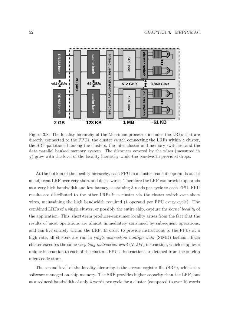
52 CHAPTER 3. MERRIMAC
~61 KB
cluster switch
cluster switch
SR
F lane
SR
F lane
1 MB
3,840 GB/s512 GB/s
Inter-cluster and mem
ory switches
cache bankcache bank
DR
AM
bankD
RA
M bank
I/O pins
128 KB2 GB
64 GB/s<64 GB/s
Figure 3.8: The locality hierarchy of the Merrimac processor includes the LRFs that aredirectly connected to the FPUs, the cluster switch connecting the LRFs within a cluster,the SRF partitioned among the clusters, the inter-cluster and memory switches, and thedata parallel banked memory system. The distances covered by the wires (measured inχ) grow with the level of the locality hierarchy while the bandwidth provided drops.
At the bottom of the locality hierarchy, each FPU in a cluster reads its operands out of
an adjacent LRF over very short and dense wires. Therefore the LRF can provide operands
at a very high bandwidth and low latency, sustaining 3 reads per cycle to each FPU. FPU
results are distributed to the other LRFs in a cluster via the cluster switch over short
wires, maintaining the high bandwidth required (1 operand per FPU every cycle). The
combined LRFs of a single cluster, or possibly the entire chip, capture the kernel locality of
the application. This short-term producer-consumer locality arises from the fact that the
results of most operations are almost immediately consumed by subsequent operations,
and can live entirely within the LRF. In order to provide instructions to the FPUs at a
high rate, all clusters are run in single instruction multiple data (SIMD) fashion. Each
cluster executes the same very long instruction word (VLIW) instruction, which supplies a
unique instruction to each of the cluster’s FPUs. Instructions are fetched from the on-chip
micro-code store.
The second level of the locality hierarchy is the stream register file (SRF), which is a
software managed on-chip memory. The SRF provides higher capacity than the LRF, but
at a reduced bandwidth of only 4 words per cycle for a cluster (compared to over 16 words

3.2. PROCESSOR ARCHITECTURE 53
per cycle on the LRFs). The SRF serves two purposes: capturing inter-kernel, long-term
producer-consumer locality and serving as a data staging area for memory. Long-term
producer-consumer locality is similar to kernel locality but cannot be captured within the
limited capacity LRF. The second, and perhaps more important, role of the SRF is to
serve as a staging area for memory data transfers and allow the software to hide long
memory latencies. An entire stream is transferred between the SRF and the memory with
a single instruction. These stream memory operations generate a large number of memory
references to fill the very deep pipeline between processor and memory, allowing memory
bandwidth to be maintained in the presence of latency. FPUs are kept busy by overlapping
the execution of arithmetic kernels with these stream memory operations. In addition,
the SRF serves as a buffer between the unpredictable latencies of the memory system and
interconnect, and the deterministic scheduling of the execution clusters. While the SRF
is similar in size to a cache, SRF accesses are much less expensive than cache accesses
because they are aligned and do not require a tag lookup. Each cluster accesses its own
bank of the SRF over the short wires of the cluster switch. In contrast, accessing a cache
requires a global communication over long wires that span the entire chip.
The final level of the locality hierarchy is the inter-cluster switch which provides a
mechanism for communication between the clusters, and interfaces with the memory sys-
tem which is described in the following subsection.
3.2.4 Compute Cluster
The compute engine of the Merrimac stream processor consists of a set of 16 arithmetic
clusters operated in a SIMD manner by a micro-controller unit. The same wide instruction
word is broadcast to each of the 16 clusters. Individual functional units within a cluster
have their own slots within the instruction word and thus may execute different operations,
but, corresponding functional units in all clusters execute the same operation. Clusters
receive data from the stream register file, apply a kernel to the data and send results back
to the stream register file. It is possible to transfer data between clusters via an inter-
cluster switch. Clusters are not connected directly to the stream register file. Rather,
they are decoupled from the stream register file by means of stream buffers which act
as intermediaries that perform rate matching and help arbitrate and automate stream
transfers. Both the stream register file and the stream buffers are distributed structures
composed of 16 banks each. Each bank is paired with a cluster. Remember, that

54 CHAPTER 3. MERRIMAC
cluster along with its associated stream register file and stream buffer banks is referred
to as a lane. Details of stream transfers may be found in Subsection 3.2.5. This section
concentrates on the architecture of a cluster and its connections to its lane. Figure 3.9
shows the internal organization of a cluster.
646464
+x
LRF_0
646464 6464
+
x
LRF_4
64
It
Intra-cluster Switch
646464
+x
LRF_1
646464 444
+x
LRF_2
646464 646464
+x
LRF_3
6444
25
Addr_0
252525
Addr_0
25
Addr_1
252525
Addr_1
25
Addr_2
252525
Addr_2
25
Addr_3
252525
Addr_3
Inter-clusterSwitch
xLRF5
1164
64
6464 6464
JB
12 xCondstate
1717 111
11 16
CondNetwork
55
sb_fifos
LRF6
LRF7
2x2
xCOMM
64
64 64
In/Out_0
1 646464 646464
In/Out_0
11 64 64
In/Out_1
1 646464 646464
In/Out_1
11 64 64
In/Out_2
1 646464 646464
In/Out_2
11 64 64
In/Out_3
1 646464 646464
In/Out_3
11
Figure 3.9: Internal organization of a compute cluster.
A cluster consists of four fused multiply-add (MULADD) units, an iterative unit
(ITER), a communication unit (COMM) and a jukebox (JB) unit. The JB unit is log-
ically a single unit shared by all clusters. For performance, it is physically distributed
across all the clusters. Each port on each local register file has a corresponding slot in
the VLIW micro-instruction that is supplied by the micro-controller (Subsection 3.2.7).
Thus, reads and writes to every port are statically controlled on a cycle by cycle basis by
the micro-code compiler.
3.2.4.1 MULADD Units
Each MULADD unit is a fully pipelined, 3-input, 1-output, 64-bit floating point and
integer unit that performs variations of fused multiply-add as well as logic and comparison
operations. The MULADD unit has the ability to compute the quantities: A × B + C,
A×B −C, and −A×B + C. The operands may be in IEEE 754 floating-point format or
in signed or unsigned integer formats. Other than fused multiply-add, the third operand
is also used in conditional selects for predicated execution.
The local register file of a MULADD unit is depicted in Figure 3.9 as logically having
two write and three read ports. For reasons of area efficiency this register file is internally

3.2. PROCESSOR ARCHITECTURE 55
composed of three register files each with 32 64-bit words, one read port and one write
port. The organization of a MULADD unit’s LRF is shown in Figure 3.10. The three read
ports supply operands to the MULADD unit through a 3×3 switch, thus reading operands
from any of the three register files. Because of the LRF organization, no two operands
for any instruction may be stored in the same single-ported register file. During register
allocation, the compiler ensures that the three operands of an instruction are stored in
separate internal register files. Some variables may need to be duplicated for this purpose.
Similarly, the write ports are attached to the intra-cluster switch via a 2× 3 switch. We
found that 2 write ports are sufficient for efficient VLIW scheduling and allow us to keep
the VLIW micro-instruction to 448 bits. While adding a third write port to each register
file does not have significant area overhead on the cluster area, an additional machine
word (64 bits) will be added to each VLIW micro-instruction.
LRF a
LRF a
LRF a
2×3 switch
3×3 switch
+
x
64
64
64
64
64 64
64
64 64
64
64
Figure 3.10: MULADD local register file organization.
3.2.4.2 ITER Functional Unit
The iterative function acceleration unit is a fully pipelined unit designed to accelerate the
iterative computation of floating-point reciprocal and reciprocal square-root. The oper-
ation of the ITER unit consists of looking up an 8-bit approximation of the function to
be computed in a dedicated ROM and expanding it to a 27 bit approximation which can
then be used to compute a full precision result in a single Newton-Raphson iteration per-
formed on the regular MULADD units. The foundation for this unit is Albert Liddicoat’s
work [101, 100].
The basis for accelerating the iterative operation are the generalization of the Newton
Raphson iteration method and the utilization of low-precision multipliers. For example,
to calculate a reciprocal value 1b, the (i+1)th iteration is computed by Xi+1 = Xi(2−bXi)

56 CHAPTER 3. MERRIMAC
and X0 is an initial approximation, typically from a lookup table. Equations 3.1–3.4 show
the effect of chaining two iterations into a single expression. Looking at the form of this
equation, we can generalize the Newton Raphson method to a kth order approximation
as: Xi+1 = Xi
(
1 + (1 − bXi) + (1 − bXi)2 + · · · + (1 − bXi)
k)
. We use a second order
Newton Raphson to take an approximate 8-bit seed to a roughly 27-bit precision value.
The sizes of the tables and precision are based on the reported values in [100].
Xi+2 = Xi+1(2 − bXi+1) (3.1)
= (Xi (2 − bXi) (2 − Xi (2 − bXi))) (3.2)
= Xi
(
4 − 2bXi + 4 (bXi)2 − (bXi)
3)
(3.3)
= Xi
(
1 + (1 − bXi) + (1 − bXi)2)
(3.4)
Because X0 is an approximation of the inverse of b, the first 7 bits of their products are
guaranteed to be 0, which reduces the size of the multiplier. The squaring and cubing units
are much smaller than full multipliers because of the fact that the same two numbers are
multiplied by each other. Also because we are multiplying fractions, the least significant
bits are not very important. Of course they could potentially all be ones and generate a
carry that would cause an additional bit, but we can tolerate up to 0.5 bits of error. We
will use that to cut off whole columns from the partial products that we have to calculate
in the squaring and cubing units. A full explanation of the cost saving due to the low
precision multipliers is given in [101, 100].
Similarly to the calculation of the inverse, the second order approximation of 1√b,
can be written as Y = Y0
(
1 + 12 (1 − bX0) + 3
8 (1 − bX0)2 + 5
16 (1 − bX0)3)
, with Y0 the
initial approximation of 1√b
and X0 the approximation of 1b. Please see [100] for a detailed
derivation. The final Newton Raphson iteration for calculating the full double precision
number is given by Yi+1 = 12Yi(3 − bYi
2).
The internal structure of the unit is shown in Figure 3.11 and is described below. The
sign of the output is carried over from the input . The path of the exponent is simple, in
the case of an inverse square root operation, it is shifted right by one to divide it by 2.
Then for both cases this result is negated.
The lookup table uses the 8 most significant bits of the fraction (not the implicit leading
1). The table provides the approximates of both the inverse and inverse square root with
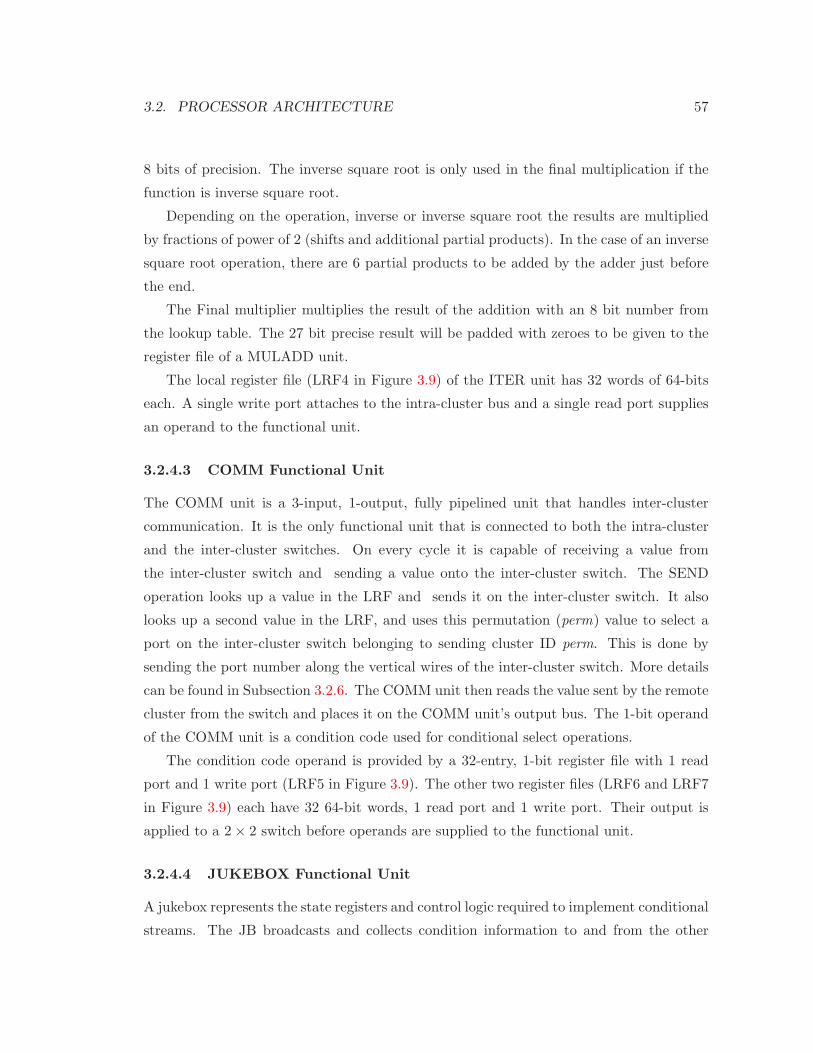
3.2. PROCESSOR ARCHITECTURE 57
8 bits of precision. The inverse square root is only used in the final multiplication if the
function is inverse square root.
Depending on the operation, inverse or inverse square root the results are multiplied
by fractions of power of 2 (shifts and additional partial products). In the case of an inverse
square root operation, there are 6 partial products to be added by the adder just before
the end.
The Final multiplier multiplies the result of the addition with an 8 bit number from
the lookup table. The 27 bit precise result will be padded with zeroes to be given to the
register file of a MULADD unit.
The local register file (LRF4 in Figure 3.9) of the ITER unit has 32 words of 64-bits
each. A single write port attaches to the intra-cluster bus and a single read port supplies
an operand to the functional unit.
3.2.4.3 COMM Functional Unit
The COMM unit is a 3-input, 1-output, fully pipelined unit that handles inter-cluster
communication. It is the only functional unit that is connected to both the intra-cluster
and the inter-cluster switches. On every cycle it is capable of receiving a value from
the inter-cluster switch and sending a value onto the inter-cluster switch. The SEND
operation looks up a value in the LRF and sends it on the inter-cluster switch. It also
looks up a second value in the LRF, and uses this permutation (perm) value to select a
port on the inter-cluster switch belonging to sending cluster ID perm. This is done by
sending the port number along the vertical wires of the inter-cluster switch. More details
can be found in Subsection 3.2.6. The COMM unit then reads the value sent by the remote
cluster from the switch and places it on the COMM unit’s output bus. The 1-bit operand
of the COMM unit is a condition code used for conditional select operations.
The condition code operand is provided by a 32-entry, 1-bit register file with 1 read
port and 1 write port (LRF5 in Figure 3.9). The other two register files (LRF6 and LRF7
in Figure 3.9) each have 32 64-bit words, 1 read port and 1 write port. Their output is
applied to a 2 × 2 switch before operands are supplied to the functional unit.
3.2.4.4 JUKEBOX Functional Unit
A jukebox represents the state registers and control logic required to implement conditional
streams. The JB broadcasts and collects condition information to and from the other
58 CHAPTER 3. MERRIMAC
1 - B*X 0
B_sig
X 0 1/B 8 53
46 (first 7 bits garanteed to be 0, because X 0 1/B)
Truncated squaring unit
Truncated cubing unit
Op 1/x: *1
Op 1/sqrt: *3/8
Op 1/x: *1
Op 1/sqrt: *5/16
Op 1/x: *1
Op 1/sqrt: *1/2
+ 1
*
8
Function approximate
B_exp
12
>> Op == 1/sqrt
0-x
Lookup table in: 8
out: 2x 8 bits
8
12 Out_exp
27 Out_sig
Figure 3.11: Accelerator unit for iterative operations (ITER).

3.2. PROCESSOR ARCHITECTURE 59
arithmetic clusters and based on this information computes whether the cluster it is on
must access its SRF and what port of the inter-cluster network to use to obtain the data.
Details on the JB unit can be found in [81, 86].
3.2.4.5 INOUT Functional Units
The INOUT units are not physical function units, rather, they represent the interface
between the clusters and the SRF. Each cluster has four INOUT units that connect intra-
cluster switch ports to the SRF. There are two kinds of ports from the intra-cluster switch
to the SRF: data input/output ports (DINOUTs) and address output ports (AOUTs).
A DINOUT port consists of an input port from the SRF to the intra-cluster switch
and an output port from the intra-cluster switch to the SRF. The Merrimac architecture
supports several types of stream accesses from the clusters:
1. Sequential streams: these are typically setup by the stream controller before kernel
execution starts, and require only data read/writes over the DINOUTS. No AOUT
ops are required.
2. Cluster-indexed streams: these are explicitly indexed by the clusters, and require
AOUT ops to be issued prior to the corresponding DINOUT ops.
3. Conditional streams: these streams allow clusters to selectively inhibit stream access
at the level of individual records based on dynamically computed conditions.
A kernel may contain up to 12 concurrently active streams, and the SRF is capable of
managing as many streams. However, intra-cluster switch bandwidth limitations constrain
the number of DINOUTs and AOUTs per cluster to 4 of each. DINOUT 0 interfaces with
streams 0, 4, and 8. Similarly, DINOUT 1, 2, and 3 interface with streams (1, 5, and 9),
(2, 6, and 10), and (3, 7, and 11). The 4 AOUTs correspond to the 12 streams in the same
manner. In addition, all 4 AOUT ports also connect to a special address port in the SRF
sub-block used for cross-lane stream accesses. While each DINOUT and each AOUT may
perform an operation every cycle, only one of the streams connected to each unit may be
accessed at a time.
The next subsection provides further details about the cluster/SRF interface, stream
operations, stream types, and other SRF-related resources.

60 CHAPTER 3. MERRIMAC
3.2.4.6 Intra-cluster Switch and Register Files
The intra-cluster switch enables communications between the various functional units
within a cluster. It connects 15 data producers (7 functional units and 4 DINOUT data
words along with 4 valid flags from the stream-buffers) to 21 data consumers (13 LRF
write ports, 4 DINOUT links to stream buffers, and 4 AOUT links to address FIFOs). It
is input-switched, meaning that the output from each functional unit goes on a dedicated
bus. The consumers of data then select one of the dedicated buses. The micro-instruction
word contains slots for every write port on every LRF. Each slot specifies a register index
and a source for the input. The register writes are predicated in hardware depending
on the state of a software pipelined loop and based on which stage of the loop the write
belongs to. Based on this information, the micro-controller is able to squash writes during
the priming and draining of the software pipeline (Subsection 3.2.7).
3.2.5 Stream Register File
The Merrimac architecture is designed around the concept of streaming, and data trans-
fers are grouped into sequences of data records called streams. The stream register file
(SRF) serves as the source or destination for all stream transfers. Input data streams
are transferred from memory to the SRF. Compute clusters operate on streams in the
SRF and write their results to the SRF. Output streams are written back from the SRF
to memory. In addition, microcode instruction sequences are also transferred as streams
from memory to the SRF, and then from the SRF to the microcode store. Table 3.1 lists
some key parameters of the SRF. We only provide a brief description of Merrimac’s SRF
here, and a complete explanation and full details of the SRF can be found in [78].
A stream is read-only or write-only for the entire duration of a single transfer. The same
stream may, however, be read and written during different transfers (e.g. a stream written
by a kernel or a memory load may be read by one or more subsequent kernels). Data
structures that require reads and writes during a single kernel execution are supported
via scratch pad accesses from the clusters, but sustain lower aggregate bandwidth than
read-only and write-only streams. Attributes of a stream transfer such as its direction
(read or write), address range in the SRF, addressing method etc. are controlled by the
cluster SCRs (stream control registers).
The SRF may store an arbitrary number of streams subject to the following constraints:

3.2. PROCESSOR ARCHITECTURE 61
Word size 64 bits
Capacity 128K words (1MB)
Peak bandwidth 64 words per SRF cycle
Table 3.1: Stream register file parameters
1. Total storage occupied by all streams is limited to the total capacity of the SRF.
2. Each stream must start on a 64-word block boundary.
In addition, a maximum of 16 streams can be active (i.e. being accessed) concurrently.
The 16 concurrently active streams supported by the SRF are described below.
12 Cluster streams: These streams transfer data between the SRF and the compute
clusters.
1 Microcode stream: This stream transfers microcode from the SRF to the microcode
store.
1 Memory Data Stream: This stream is used for transferring data between the SRF
and memory.
1 Memory Index Stream: This stream provides offsets for address calculation during
gather and scatter operations from/to memory.
1 Memory Op Value Stream: This stream provides operands for computations per-
formed in the memory system during scatter-add transfers (see Subsection 3.2.8).
Figure 3.12 shows the high level organization of the SRF and related components. The
SRF has a capacity of 128 KWords and is organized as 16 banks with each bank associated
with a single compute cluster. A compute cluster along with its associated SRF bank will
be referred to as a lane. The stream buffers (SBs) interface the clusters, microcode store,
and the memory system with the SRF. Like the SRF, the 12 cluster stream buffers are
also organized as banks. Each of the 12 cluster stream buffers thus has one bank that
belongs in each lane.
A stream buffer is the physical embodiment of an active stream, i.e., there is a one
to one mapping between SBs and the 16 active streams. Access to the SRF is time-
multiplexed among the SBs, providing the abstraction of sustaining up to 16 concurrent

62 CHAPTER 3. MERRIMAC
streams. The SBs provide the hardware interface and rate matching between the SRF and
client units – the clusters, the memory system, and the microcode store.
SB 18
SB 12
. . .
SB 12
Bank 15Bank 0
. . .
SRF
To memory system & microcode store
Write data: 64b x 64Read data: 64b x 64
SB 11
SB 0 ...
Write data: 4 x 64bAddr: 4 x 13b
Read data: 4 x 64b
To Cluster 0
SB 11
SB 0 ...
Write data: 4 x 64bAddr: 4 x 13b
Read data: 4 x 64b
To Cluster 15
. . .
SB 18
SB 12
. . .
SB 12
SB 18
SB 12
. . .
SB 12
Bank 15Bank 0
. . .
SRF
To memory system & microcode store
Write data: 64b x 64Read data: 64b x 64
SB 11
SB 0 ...
Write data: 4 x 64bAddr: 4 x 13b
Read data: 4 x 64b
To Cluster 0
SB 11
SB 0 ...SB 11
SB 0 ...
Write data: 4 x 64bAddr: 4 x 13b
Read data: 4 x 64b
To Cluster 0
SB 11
SB 0 ...
Write data: 4 x 64bAddr: 4 x 13b
Read data: 4 x 64b
To Cluster 15
SB 11
SB 0 ...SB 11
SB 0 ...
Write data: 4 x 64bAddr: 4 x 13b
Read data: 4 x 64b
To Cluster 15
. . .SB 0
SB 4
SB 8
SB 1
SB 5
SB 9
INOUT 0
INOUT 1
SB 2
SB 6
SB 10
SB 3
SB 7
SB 11
INOUT 2
INOUT 3
SB 0
SB 4
SB 8
SB 1
SB 5
SB 9
INOUT 0
INOUT 1
SB 0
SB 4
SB 8
SB 1
SB 5
SB 9
INOUT 0
INOUT 1
SB 2
SB 6
SB 10
SB 3
SB 7
SB 11
INOUT 2
INOUT 3
SB 2
SB 6
SB 10
SB 3
SB 7
SB 11
INOUT 2
INOUT 3
Figure 3.12: Stream register file organization
The memory and microcode streams connect the memory unit and the micro-controller
to the SRF. They perform block transfers of 64 words per cycle in or out of the SRF (4
contiguous words from each lane starting at the same address in all SRF banks), and
are always accessed sequentially in lock-step across all lanes. Therefore the addresses
for accessing these streams are generated by a single global counter associated with each
stream called a Stream Control Register (SCR).
The 12 cluster streams interface the compute clusters with the SRF. While all 12
streams can be concurrently active during a kernel’s execution, only a maximum of 4 can
be accessed on any given cycle due to bandwidth constraints in the intra-cluster network.
3.2. PROCESSOR ARCHITECTURE 63
Each of these streams is read-only or write-only and conforms to one of the following
access types for the duration of an entire kernel execution. A more detailed discussions of
each type of access can be found in [78].
In-lane Block-indexed Access (Sequential Access) In block-indexed access
mode, SRF access is performed at the granularity of 4 contiguous words in each lane.
These are typically used for stream accesses where each cluster sequentially accesses
the portion of stream data mapped to its local bank of the SRF. Addresses for these
accesses are generated by counters in each lane.
In-Lane Word-indexed Access SRF access for this mode is performed at the gran-
ularity of 1 word in each lane per access per stream. These are typically used for
non-sequential accesses with the access orders specified by explicit addresses (indices
in to the SRF) issued from the compute clusters. Address computation is performed
in the clusters by user code. However, a cluster is limited to accessing the portion
of stream data that is mapped to its local SRF bank. Multiple word-indexed ac-
cesses may take place within a single SRF bank simultaneously if they do not cause
sub-bank conflicts.
Cross-Lane Word-indexed Access Like in-lane word-indexed access mode, cross-lane
accesses also use addresses computed by the cluster. Unlike in-lane access mode,
the computed addresses may target any bank in the SRF. Cross-lane accesses may
proceed concurrently with in-lane word-indexed accesses if they do not result in sub-
bank conflicts. Due to bandwidth constraints, the throughput of cross-lane indexed
streams is limited to 1 word per cycle per lane. Cross-lane access is only supported
for read streams.
Conditional Access These are in-lane block or word indexed streams that are accessed
based on condition codes computed dynamically and independently in each lane.
Each cluster specifies a condition code with the access,and the read/write opera-
tions are only performed for clusters whose condition code is true. There are two
variations of conditional streams. Globally conditional streams (only supported for
block indexed streams) access the stream data interleaved across lanes in strictly se-
quential order. Due to interleaving, on any given access, the lanes that contain the
64 CHAPTER 3. MERRIMAC
sequentially next data in stream order may not necessarily match up with the clus-
ters with valid condition codes. To access the correct data, communication across
lane boundaries is required. However, since conditional access is only supported for
in-lane access, globally conditional accesses are implemented as two separate oper-
ations – an in-lane conditional access and a cross-lane communication. Lane-wise
conditional streams conditionally access data mapped to the bank of the SRF within
the lane without requiring any data communication across lanes.
Scratch Pad Access Scratch pad access mode is similar to in-lane word-indexed access
except that it supports data structures that are read/write (“scratch pad” data)
within a kernel whereas all other cluster streams are either read-only or write-only.
This type of access is only supported on streams 10 and 11. During scratch pad reads
on stream 10, the write buffer associated with stream 11 is checked for pending writes
to the location being read, so as to avoid reading stale data. Streams 10 and 11 may
be used as regular in-lane block or word indexed streams in kernels that do not
require scratch pad accesses.
3.2.6 Inter-Cluster Switch
The switch consists of independent data, address, and condition networks. The data net-
work is used for two types of operations: register-to-register inter-cluster communications
and data returns of cross-lane SRF accesses. The address network is used for communi-
cating indices for cross-lane SRF access. The condition network is used for broadcasting
condition codes across the entire processor (all lanes and/or the micro-controller). All
buses in the networks use parity checks to detect single-bit errors.
3.2.6.1 Data Network
The data network supports all permutations of one-to-one and one-to-many communica-
tions among the compute clusters and the micro-controller as long as no cluster or the
micro-controller consumes or generates more than one word of data at a time. A block
diagram of the network is shown in Figure 3.13. Values to be communicated are written
to the horizontal buses in the figure and results are read from the vertical buses. This
inter-cluster switch configuration is based on [86].

3.2. PROCESSOR ARCHITECTURE 65
During a communication event, each cluster writes to its dedicated write bus (hori-
zontal buses in the figure). A cluster that requires access to the data written out by a
particular cluster must set the appropriate cross-points in the network to make the data
available on its dedicated read bus (vertical buses in the figure).
Cluster 0
Cluster 15
5x64b
4x64b
Micro-controller
4x64b
5x64b
Figure 3.13: Inter-cluster data network
The data network is used for statically scheduled register-to-register inter-cluster com-
munications and data returns of cross-lane indexed SRF accesses. The inter-cluster com-
munication operations are statically scheduled and do not cause any contention on the
network (i.e. each cluster is guaranteed to generate and consume at most one data word
during these operations). During cross-lane stream data returns also the communication
pattern is guaranteed to not cause contention [78]. However, it is possible for an inter-
cluster communication and a cross-lane SRF data return to be attempted on the same
66 CHAPTER 3. MERRIMAC
cycle. In such cases, inter-cluster communications receive higher priority since they usu-
ally complete in a fixed latency in the static schedule. Starvation of SRF data returns
may lead to clusters being stalled, providing a back-pressure mechanism under high data
network utilization.
3.2.6.2 Address Network
The address network is used for communicating addresses during cross-lane indexed SRF
accesses. The dimensionality and general layout of the address network is similar to the
data network, but there is no connection to/from the micro-controller. In addition, the
data width of this network is 19 bits (18-bit SRF index + valid bit) and unlike in the data
switch, simultaneous requests are not guaranteed to be conflict free.
The upper 4 bits of a cross-lane SRF index identifies the target lane, and is used
for routing in the network. Requests are placed on horizontal wires similar to the data
network shown in figure 3.13. During the first cycle after being issued, requests traverse
the horizontal wires and arbitrate for the vertical wires. This arbitration is performed
separately (and locally) in each set of 4 horizontal buses. During the next cycle, requests
that were granted vertical wires in the previous cycle arbitrate to resolve conflicts among
the local arbitration decisions of the previous cycle. Results of this second arbitration
are communicated back to the horizontal-to-vertical cross points that performed the first
arbitration. Requests that succeed both arbitrations are communicated to the target lane.
During the next cycle, the overall status of the original requests is communicated to the
requesting clusters. This status information consists of two bits: whether the request
made by the cluster succeeded, and whether any valid requests were attempted in the
cycle to which the status corresponds (status information corresponds to requests issued 3
cycles back). The second bit allows each cluster to track when to expect data returns for
its requests since all cross-lane accesses proceed in lock step once they leave the address
network.
Address requests that fail arbitration are buffered in the network and are re-attempted
the next cycle. This requires 8 requests worth of storage at each of the 4×4 cross points in
the network (including pipeline storage). Due to limited buffering in the address network,
a cluster that receives a request failure signal on a particular cycle may not issue a new
address request during that cycle (i.e. it may drive the horizontal wires speculatively, but
should not update internal state to represent a sent request). It is possible for clusters to
3.2. PROCESSOR ARCHITECTURE 67
receive request success/failure signals corresponding to cycles in which no requests were
made since earlier requests may have been buffered in the network and reattempted.
3.2.6.3 Condition Network
Several operations, such as conditional streams and loops based on cross-lane conditional
state, require the communication of a condition code from each cluster to all lanes and
the micro-controller. A set of dedicated condition code broadcast buses (one per cluster)
is provided for this purpose. AT any given time, each cluster may write its condition code
bus and read all the condition codes. The micro-controller does not generate a condition
code, but is able to read all broadcast codes.
3.2.7 Micro-controller
The micro-controller is responsible for controlling the execution of the microprograms
executed on the arithmetic clusters. The same micro-instruction is issued to all the clus-
ters simultaneously by the micro-controller. Hence, the execution of the clusters occurs
in lockstep, in SIMD fashion. During microprogram execution the micro-controller also
responds to certain fields in the microcode instruction word of the currently executing mi-
croprogram. The micro-controller is a small, and fairly simple component of the Merrimac
processor, however, it is responsible for kernel execution and is important in understand-
ing the operation of the compute clusters. The functions of the micro-controller are listed
below and a block diagram is depicted in Figure 3.14.
1. Handle communications between the compute clusters and the stream controller.
2. Sequence the micro-instructions that comprise a kernel.
3. Squash state changing operations (register writes and INOUT operations) to cor-
rectly prime and drain software pipelined loops.
Communication with Other Units
The micro-controller and stream controller exchange data via the shared uCRs since both
units own read and write ports to this register file. The micro-controller can pause exe-
cution (conditionally or unconditionally) for synchronizing with the stream controller and

68 CHAPTER 3. MERRIMAC
ALU
2:1 MUX
uCR
Stream Controller
IMM COMM
COMM_CL
COMMC
2:1 MUX
Adder
PC
IMM 1
Fetch and Decode,
SWP Logic
Stream Controller
IMM
Microcode Store
From SRF
Stream Controller
r e s t
a r t
s t a
l l
16
Stall signal from each cluster
Control signals and modified cluster
instructions
To clusters
OUT BUS
COMM BUS
COMMC BUS
PC BUS
2:1 MUX
SCR (12)
Stream Controller
IMM
Figure 3.14: Micro-controller architecture
scalar code. Once the micro-controller is paused, the stream controller can safely update
uCRs or the PC and then restart the micro-controller.
The inter-cluster data switch enables the micro-controller to broadcast a 64-bit word to
the clusters every cycle. This is done by asserting the comm en bit in the micro-controller
sub-instruction format, which enables the COMM unit to read the output of the micro-
controller’s ALU off the OUT BUS and send it to the inter-cluster data switch. On any cycle
when the COMM unit is enabled, the comm cl field indicates which data source on the
inter-cluster data switch should be read. There are 17 possible data sources including 16
clusters and the micro-controller. The selected value will then be placed on the COMM
unit’s output bus. In addition, the value on the inter-cluster conditions network can be
written into the lower 16 bits of a uCR (regardless of the value of comm en).
Instruction Sequencing
The chief function of the micro-controller is to sequence the VLIW instructions to the
clusters and handle SWP loops and other control flow. For control flow, the micro-
controller has an integer-only ALU that can execute a variety of compare operations
for testing branch conditions.
Since the PC needs to be updated every cycle, a special functional unit (PC-unit) is

3.2. PROCESSOR ARCHITECTURE 69
in charge of this task. Unless the micro-controller is stalled, the PC-unit will implicitly
add a value to the PC on each cycle. The value added is 1, unless one of the jump or
loop instructions is issued. Only relative jumps are supported in which case the offset
is supplied by the immediate constant field of the instruction. The PC-unit can also
overwrite the current value of the PC with a value set by the SC.
In addition to simply sequencing instructions, the micro-controller also provides hard-
ware support for software pipelined loops in the kernels. The SWP unit contains a state-
machine that governs the priming and draining of software pipelined loops. The SWP
unit is reset just before a loop starts and the maximum number of stages in the software
pipeline is set by software. The micro-controller executes the loop branch until the SWP
is fully drained (even after the loop continuation test fails for the first time). Every it-
eration updates the stage counter of the SWP unit, incrementing it while looping, and
decrementing it while draining. The stage counter is used along with the stage field asso-
ciated with each write port’s micro-code field to suppress register writes that should not
be executed while priming or draining the SWP.
Figure 3.15 illustrates the SWP state diagram used by the micro-controller to deter-
mine whether to squash operations. The micro-controller moves from one state to the
next after seeing either a loop start or loop branch instruction and testing the relevant
condition. When in the LOOPING or DRAINING state, the microcontroller will squash
certain operations based on the current SWP stage.
In order to do this, the micro-controller inspects all operations before issue. Each
operation is associated with a stage number. When in the LOOPING state, an operation
will be squashed if its associated op stage value is greater than the current value of stage,
and when in the DRAINING state, an operation will be squashed if op stage ≤ stage;
this is summarized in table 3.2. The squashing is accomplished by the microcontroller
modifying the instruction that it broadcasts to the clusters; to squash register writes, the
register number to write is turned into a zero, as register 0 is hardwired to 0 in the cluster
LRFs. To squash an INOUT or JB operation, the opcode is turned into a NOP. Note that
there can be no nested loops within a software pipelined loop, regardless of whether the
nested loop is pipelined or not.
Each of the VLIW instructions issued has two main parts. The first part is issued to
the micro-controller, and the second part is broadcast to all 16 clusters to be operated
on in parallel in SIMD fashion. The VLIW instruction is 448 bits wide and controls all

70 CHAPTER 3. MERRIMAC
LOOPING
Loop prime and/or steady state
DRAINING
NOT LOOPING
LOOPB(stage < max_stage) stage++ select IMM in PC adder MUX
STARTL stage = 0 set max_stage
LOOPB(loop cond false) stage = 0 select IMM in PC adder MUX
LOOPB(loop cond true) stage++ select IMM in PC adder MUX
LOOPB(stage == max_stage) select 1 in PC adder MUX
Figure 3.15: Kernel Software Pipelining State Diagram
SWP State Op Squash ConditionLOOPING op stage > stage
DRAINING op stage ≤ stage
Table 3.2: Kernel Software Pipeline Operation Squash Conditions.
aspects of cluster execution including the functional units, LRFs, INOUT units, and the
intra-cluster switch.
3.2.8 Memory System
The memory system of Merrimac is designed to support efficient stream memory oper-
ations. A single stream memory operation transfers an entire stream, which is typically
many thousands of words long, between memory and the SRF amortizing the long memory
latencies. Merrimac supports both strided access patterns and gathers/scatters through

3.2. PROCESSOR ARCHITECTURE 71
the use of the stream address generators. Each processor chip has an address generator,
which produces up to 8 single-word addresses every cycle. The address generators take a
base address in memory for the stream, and either a fixed stride and record-length or a
pointer to a stream of indices in the SRF. The memory system provides high-bandwidth
access to a single global address space for up to 16K nodes including all scalar and stream
execution units. Each Merrimac chip has a 32KWords cache with a bandwidth of 8 words
per cycle (64GBytes/s), and directly interfaces with the node’s external DRAM and net-
work. The 2GB of external DRAM is composed of 8 Rambus XDR modules [45] providing
a peak bandwidth of 64GB/s and roughly 16GB/s, or 2 words per cycle, of random access
bandwidth. Remote addresses are translated in hardware to network requests, and single
word accesses are made via the interconnection network. The flexibility of the addressing
modes, and the single-word remote memory access capability simplifies the software and
eliminates the costly pack/unpack routines common to many parallel architecture. The
Merrimac memory system also supports floating-point and integer streaming read-modify-
write operations across multiple nodes at full cache bandwidth.
The five responsibilities of the on-chip memory system are briefly summarized below.
Details and analysis are available in related work as specified.
1. The memory system is responsible for executing stream memory operations, generat-
ing single-word requests for each stream element record. This is done by the address
generator, which execute stream memory operations issued by the stream-controller.
The AG takes operands in the form of stream and memory descriptors, and generate
individual word requests for an entire stream memory operation over many cycles.
The requests of a single element record are aligned to a single SRF lane using a set
of buffers. The AG can produce 8 requests per cycle to match the memory system’s
bandwidth of 1 processed request per cycle on each bank. The address generator
function follows that of Imagine [135].
2. The memory system performs address translation for implementing Merrimac’s seg-
mented memory. Both the scalar unit and address generator access the segment
registers performing virtual to physical address translation on all requests coming
from the scalar cache or address generators. Once a request passes address trans-
lation it proceeds through a bank input switch, which routes the requests coming
from the scalar unit, AG, and from remote nodes to the appropriate bank based on
72 CHAPTER 3. MERRIMAC
the physical address.
3. It ensures atomicity of stream read-modify-write operations. The atomic memory
unit is first on the path of a request arriving at a bank from the bank input switch,
and the first unit for data returned from DRAM. Its operation is explained in [2].
4. It services memory requests through the stream cache, and controls the node’s XDR
DRAM modules. If a reference hits in the stream cache it is serviced out of the bank
and returned to the requester. If the request does not hit in the stream cache it is sent
down to the DRAM controllers if the physical address is local to the node, or to the
network interface to be sent as a remote request to another node. Requests returning
from DRAM (data and acknowledgment) are combined with those returning from the
network. The DRAM controllers aggressively reorder memory requests to maximize
throughput on modern DRAM architectures [137, 3]. Additional details on the
implementation of Merrimac’s data parallel memory system, including arbitration
and deadlock avoidance will appear in a separate document.
5. The memory system interfaces with the interconnection network, converting local
requests to remote nodes into network packets. As mentioned above, each network
interface can form a network packet for requests to remote data that miss in the
stream cache. These packets are sent to the remote node where they are processed
and data or an acknowledgment is returned.
3.3 System Architecture
This dissertation focuses on the Merrimac processor and on mapping scientific applications
to its stream architecture. However, Merrimac’s processor architecture is heavily influ-
enced by the supercomputing usage model. In this section we briefly sketch the Merrimac
supercomputer to place the processor architecture in context.
Merrimac is scalable from a single-node 128GFLOP/s workstation to a 16, 384 node
2PFLOP/s supercomputer spanning 32 cabinets. The key technology enabling this scal-
ability is the streaming memory system with its global address space and the high-
bandwidth interconnection network described below. As with the rest of the Merrimac
design, the network does not rely on future technology and can be built using current com-
ponents and custom chips. In fact, the Cray Black Widow system uses an interconnection

3.3. SYSTEM ARCHITECTURE 73
network with similar properties [146].
8 xXDR-DRAM
2GB
StreamProcessor
64 FPU128 GFLOPS
On-Board Network
Intra-Cabinet NetworkE/OO/E
Inter-Cabinet Network
Bisection 24TBytes/s
64GBytes/s
20GBytes/s32+32 pairs
48GBytes/s128+128 pairs
6” Teradyne GbX
768GBytes/s2K+2K links
Ribbon Fiber
Backplane
Board
Node
Node2
Node16
Board 32
Board 216 Nodes1K FPUs2TFLOPS
32GB
Backplane 232 Boards512 Nodes32K FPUs64TFLOPS
1TB
Backplane 32
Figure 3.16: A 2PFLOP/s Merrimac system uses a high-radix interconnection network.
Figure 3.16 illustrates a fully-configured Merrimac system with 16K processor nodes.
The organization is hierarchical, and is composed of nodes, boards, and backplanes (cab-
inets). Each node includes the Merrimac processor and its 8 XDR DRAM modules. A
single Merrimac board contains 16 nodes totaling a peak performance of 2TFLOP/s with
a capacity of 32GB of memory. Each board provides two high-radix router chips. The
router chips interconnect the 16 processors providing flat memory bandwidth on board
of 20GB/s per node, as well as providing a gateway to the inter-board interconnection
network. The network uses a five-stage folded-Clos [32] network.1 and is similar to the
high-radix interconnection network of the Cray Blackwidow [146]. 32 boards are pack-
aged in a single cabinet with backplane routing, and 32 cabinets form the fully-configured
system.
3.3.1 Input/Output and Storage
We envision a parallel file system hosted in separate cabinets as the input/output and
storage systems of Merrimac. The high-radix interconnect topology can support additional
1This topology is sometimes called a Fat Tree [99].
74 CHAPTER 3. MERRIMAC
storage nodes and cabinets, thus input/output will be virtualized as part of the global
address space.
3.3.2 Synchronization and Signals
Merrimac does not have a dedicated signaling and barrier synchronization network as
found in the Cray T3D [85] or IBM BlueGene/L [98]. Instead, we use the interconnection
network and the memory subsystem to support full synchronization and signals by way of
named split barriers. These barriers are named with a virtual address and can be signaled
and waited upon using separate operations to allow for overlap of computation and barrier
communication. Our current implementation uses the atomic memory unit to implement
the barrier mechanism.
3.3.3 Resource Sharing
The throughput-oriented batch usage model of scientific computing allows us to dedicate
the system to a single running application and not require context switching. If multiple
users wish to share a large configuration, Merrimac supports a spatial partitioning of the
system as opposed to time multiplexing. The memory segmentation scheme allows power-
of-two subdivisions of the system with hardware guaranteed protection that is managed
by the privileged operating system instructions for setting the segment registers.
3.4 Area, Power, and Cost Estimates
This section presents the die area, power, and cost estimates for the Merrimac proces-
sor and system. The Merrimac processor architecture is specified in detail but the pro-
cessor has not been designed and fabricated. Therefor, processor area and power are
estimated based on the architectural components using previously established method-
ology [86, 89] and measurements of similar components on existing silicon as described
in Subsection 3.4.1. Using the area estimates and system configuration we calculate the
approximate costs of a Merrimac system in Subsection 3.4.2.

3.4. AREA, POWER, AND COST ESTIMATES 75
3.4.1 Area and Power
We take the following approach to estimate the area and power of the Merrimac processor.
We evaluate each of Merrimac’s hardware components separately and design floor-plans for
individual components and the entire processor. When possible we use measurements from
existing silicon and scale them to Merrimac’s 90nm technology as necessary. For other
units or blocks we follow the VLSI area and power estimation methodology developed for
the Imagine stream processor in [86, 89] and VLSI parameters detailed in [148]. Merrimac
shares many architectural and design features with Imagine. We assume a 90nm VLSI
technology in an ASIC flow targeting a frequency of 1GHz.
Table 3.3 lists the components of Merrimac, their area and power estimates, and the
method used to derive the estimate, and Figure 3.17 depicts the Merrimac floorplan based
on the area estimates of the components.
Component Count Subcomponent Count Area Power Method
chip 1 144.9 mm2 68.5W mixed
cluster 16 4.3mm2 2.4W mixed
switch 1 0.4mm2 0.05W estimate
SRF 1 1.3mm2 0.3W estimate
MULADD + LRF 4 0.6mm2 0.5W mixed
ITER + LRF 1 0.1mm2 0.1W mixed
micro-controller 1 3.5mm2 1.7W estimate
inter-clusterswitch 1 7.6mm
2 0.8W estimate
memorysubsystem 1 55.6mm
2 20.0W mixed
AG 1 4.6mm2 0.1W estimate
channel 8 1.2mm2 0.3W estimate
DRAM interface 8 3.3mm2 10.8W silicon
network 1 14.9mm2 6.8W silicon
scalar core 1 9.6mm2 1.1W silicon
clock network 1 6.6W silicon
Table 3.3: Summary of the area and power estimates for the Merrimac processor.
Before presenting the detailed area and energy estimates we list the building blocks of
the models used in Table 3.4. We use technology independent units for length, area, and
energy and give their values for 90nm VLSI technology in the table [148]. χ is a VLSI
technology independent unit of distance measured as the minimal distance between two
wires on the chip and is also referred to as a track. A grid is a technology independent
unit of area that is equal to 1χ2. Energy is measured in units of Ew, where 1Ew is the
energy required to propagate a signal over a single wire track. The values in the table

76 CHAPTER 3. MERRIMAC
DRAM Interface
Ne
two
rk In
terfa
ce
Me
mo
ry
Ch
an
ne
lSc
ala
r Pro
ce
ssor
AG µµµµctrl
cluster cluster cluster cluster
cluster cluster cluster cluster
cluster cluster cluster cluster
cluster cluster cluster cluster
DRAM Interface
Ne
two
rk In
terfa
ce
Me
mo
ry
Ch
an
ne
lSc
ala
r Pro
ce
ssor
AG µµµµctrl
cluster cluster cluster cluster
cluster cluster cluster cluster
cluster cluster cluster cluster
cluster cluster cluster cluster
12.0mm
12.1mm
Figure 3.17: Floorplan of the Merrimac processor chip measuring 12mm ×12.1mm.
are derived from the Imagine processor as reported in [86] scaled to the 64-bit datapath
of Merrimac. The energy for a traversal of the intra-cluster switch is calculated from the
wire lengths.
3.4.1.1 Compute Cluster
The compute cluster is described in detail in Subsection 3.2.4 on page 53. It is composed
of seven functional units (four MULADD FPUs, the ITER inverse and inverse square root
accelerator, the JUKEBOX, and the COMM unit) and their associated LRFs, an SRF
lane with its 12 stream buffers, the intra-cluster switch, and a small amount of control
logic including the four INOUT units for accessing the SBs.
Intra-Cluster Switch
The intra-cluster switch connect the outputs of the seven functional units and the four
INOUT units to the LRF input ports. It is organized as a linear switch that spans the
width of the cluster and has a height that can support the 11 connection points at 64 bits
each (see Figure 3.9 on page 54). It’s area is therefore given as Ai = (Xcχ × (11 · 64)χ).

3.4. AREA, POWER, AND COST ESTIMATES 77
Param Description Value
χ minimal distance between two wires 315nm
Ar area of single bit of a 1-read, 1-write portregister file
128χ2 (latch based)
As area of single SRAM bit with amortizedperipheral circuitry
18χ2
Xc width of a compute cluster derived below
Ew energy required to propagate a signal overa 1χ wire
5.51 × 10⁻¹⁷J
EF energy of single multiply-add FPU oper-ation (not including inputs)
8 × 10⁶Ew
Er read or write energy of one 64-bit register 5.9 × 10⁵Ew
Es read or write energy of one SRAM bit(need to scale by total SRAM size)
8.7Ew
α estimate of switching activity factor of allcircuits
0.3
Wl number of words in SRF lane 4
bW bits per word varies
Ai area of intra-cluster switch
AS area of SRF
ASB area of stream buffer
AM area of MULADD
AI area of ITER
Aµ area of micro-controller
Aµc area of micro-code store
Asw area of inter-cluster switch
Ei energy of intra-cluster switch
ES energy of SRF
ESB energy of stream buffer
EM energy of MULADD
EI energy of ITER
Eµ energy of micro-controller
Eµc energy of micro-code store
Eb energy of micro-code broadcast network
Pc power of cluster
Pµ power of micro-controller
Psw power of inter-cluster switch
Table 3.4: Area of cluster building blocks and energy of basic cluster operations.
78 CHAPTER 3. MERRIMAC
The switch is directly controlled by the VLIW instruction and its energy consumption
is dominated by the capacitance of the wires: Ei = α · 64 · 11 · (Xc + 11 · 64).
SRF Lane
The SRF lane is dominated by the SRAM arrays and the SBs and.
Based on the measurements of [86], SRAM designs in 90nm, the detailed analysis of
Merrimac’s indexed SRF structure of [78], and the overhead of ECC for reliability (see
Chapter 6), we estimate the area of the SRF array within a cluster at 108χ2.
As explained in Section 3.2.5 and in [78], each of the 12 SBs stores 2 SRF lines, or 8
64-bit words, as well as address information (17 bits) for implementing indexed access to
the entire SRF address space. The SB is implemented as a register FIFO, and its area is
ASB = 12 · 8 · (64 + 17)Ar = 107χ2.
The energy of an SRF access consists of reading or writing the bits to the SRAM array
(including 8 extra bits per word for ECC), as well as the energy of accessing the SBs:
ES = Wl · (64 + 8) · Es + 2 · α · Er = 4.9 × 10⁶Ew.
MULADD
The MULADD unit is a standard 64-bit FPU/ALU and its area and energy are dominated
by the FP multiplier, which is similar in design to Imagine’s 32-bit multiplier. Therefore,
we estimate the MULADD unit to be 2800χ×1754χ, given Imagine’s multiplier measured
area of 1400χ × 877χ [86] and scaling from 32 to 64 bits. The energy for a MULADD
operation is listed in Table 3.4 and is based on the Imagine implementation.
The LRF architecture associated with the MULADD is also described in Subsec-
tion 3.2.4. The LRF has three 32-entry, 64-bit, 1-read/1-write port register files, a 2 × 3
64-bit input switch, and a 3 × 3 64-bit output switch. The area of the three register files
is roughly Ar · 64 · 32 · 3, where Ar = 128χ2 [86]. An ideal VLSI layout aligns the bits of
the register files with the datapath of the FPU. With this layout, the area of the 2 input
and 3 output switches can be neglected. Therefore, the area of the LRF is(
7.9 × 10⁵χ2)
and its width is equal to that of the MULADD FPU (2800χ).
The LRF energy consumption estimate is based on the fact that each MULADD can
read three values and produce one result, therefore EM = EF + α · 4 · Er = 7.1 × 10⁵Ew.
3.4. AREA, POWER, AND COST ESTIMATES 79
ITER
The iterative unit is much simpler than the MULADD FPU. Its microarchitecture is
described in Subsection 3.2.4.2. Based on this design we use a very rough estimate equating
the ITER unit with Imagine’s FP multiplier at 877χ×1400χ. The ITER LRF is composed
of two 32-entry, 64-bit, 1-read/1-write port register files, and two 2 × 2 64-bit switches.
As with the MULADD unit, the LRF is aligned with the ITER datapath and has an area
of(
Ar · 64 · 32 · 2 = 5.2 × 10⁵χ2)
with a width of 877χ.
Assuming the energy of an ITER operation scales similarly to its area compared to
the MULADD, then EI = 0.25 · EF + α · 3 · Er = 2.5 × 10⁶Ew.
JUKEBOX and COMM
Based on the Imagine implementation, both the JUKEBOX and COMM unit contain a
small amount of logic and their area and energy are negligible.
Overall Cluster Area and Power
We designed a floor-plan for the Merrimac compute cluster based on the estimates given
above. As seen in Figure 3.18, each compute cluster is estimated at 6500χ × 7000χ or
4.5mm2.
The power of the cluster is calculated by evaluating the frequency at which each
component is activated and multiplying by the component’s energy requirement. As an
upper bound, we assume that all cluster components operate on every clock cycle, and do
not account for clock gating or lower switching activity factors due to functional unit idle
cycles. Therefore, Pc = (4 · EM + EI + ES + Ei)Ew · 109Hz = 2.2W .
3.4.1.2 Micro-controller
The micro-controller has four main components: the ALU and datapath logic, the uCR
and SCR register files, the microcode store, and the VLIW broadcast network to deliver
instructions to the compute clusters. However, the small register file and datapath are
negligible in terms of area and power compared to the very large microcode store and
instruction broadcast network.
The microcode store is a SRAM array of 4 096 448-bit instruction words and ECC of
an additional 56 bits for reliability. It’s area is Aµc = As · 4096 · (448 + 56) = 3.5mm2 and
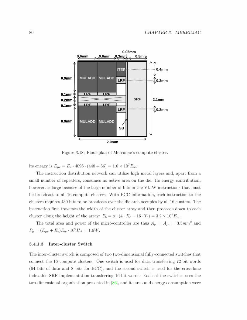
80 CHAPTER 3. MERRIMAC
SRFSRF
0.9mm
0.9mm
0.2mm
0.1mm
0.1mm
0.9mm
0.9mm
0.2mm
0.1mm
0.1mm
2.1mm
0.4mm
0.2mm
0.2mm
MULADD MULADD
MULADD MULADD
LRF LRF
LRF LRF
LRF
LRF
ITER
SB
0.6mm 0.6mm 0.3mm 0.5mm0.05mm
2.0mm
Figure 3.18: Floor-plan of Merrimac’s compute cluster.
its energy is Eµc = Es · 4096 · (448 + 56) = 1.6 × 10⁷Ew.
The instruction distribution network can utilize high metal layers and, apart from a
small number of repeaters, consumes no active area on the die. Its energy contribution,
however, is large because of the large number of bits in the VLIW instructions that must
be broadcast to all 16 compute clusters. With ECC information, each instruction to the
clusters requires 430 bits to be broadcast over the die area occupies by all 16 clusters. The
instruction first traverses the width of the cluster array and then proceeds down to each
cluster along the height of the array: Eb = α · (4 · Xc + 16 · Yc) = 3.2 × 10⁷Ew.
The total area and power of the micro-controller are thus Aµ = Aµc = 3.5mm2 and
Pµ = (Eµc + Eb)Ew · 109Hz = 1.6W .
3.4.1.3 Inter-cluster Switch
The inter-cluster switch is composed of two two-dimensional fully-connected switches that
connect the 16 compute clusters. One switch is used for data transferring 72-bit words
(64 bits of data and 8 bits for ECC), and the second switch is used for the cross-lane
indexable SRF implementation transferring 16-bit words. Each of the switches uses the
two-dimensional organization presented in [86], and its area and energy consumption were

3.4. AREA, POWER, AND COST ESTIMATES 81
shown to be(
W · 16 ·√
16 · (bW ·√
16 + 2 · (Xc + Yc))
and(
bW · 16 ·√
16 · (Xc + Yc))
.
Using the bit widths of the two switches the total area and power of the two switches
is Asw = 7.6mm2 and Psw = 0.8W .
3.4.1.4 Memory Subsystem
The details of Merrimac’s memory system are not the focus of this thesis. We therefore
only summarize the key area and power parameters of the main components of the memory
subsystem in Table 3.3 on page 75. The area and power requirements of the address
generator, atomic memory unit, cache banks, buffers, and registers were estimated using
the same model and techniques presented above. The area of the DRAM and network
interfaces was estimated based on measurements made on the 90nm Cell chip. Cell uses
the same XDR DRAM parts as Merrimac and its network also uses high-speed serial links.
We do not have power measurements for the external interfaces and roughly estimate them
at 18W . Merrimac’s total off-chip bandwidth is 17.6GB/s (117GB/s for DRAM with ECC
and 20 + 2.5 + 20 + 2.5GB/s for the network with address words and ECC). At about
15mW per 1Gb/s of bandwidth, which is possible with high-speed serial links, the external
interface power is 10.8W for memory and 6.8W for the network.
3.4.1.5 Scalar Core
The area and power of the scalar core are the numbers given in the MIPS20Kc documen-
tation [110] scaled to Merrimac’s 90nm process technology.
Clock Network
The clock network consumes little active die area as it is implemented in high metal layers.
The power consumption associated with the clocks is estimated based on the clock network
of Imagine, which accounted for 11% of Imagine’s power consumption.
3.4.2 Cost Estimate
Table 3.5 shows the estimated cost of a streaming supercomputer. The processor and
router chip are modest-sized ASICs in 1000-pin flip-chip BGA packages that are expected
to cost $200 each in moderate quantities of thousands of chips. DRAM Modules are pro-
jected to cost $50 each for XDR DRAM, making memory, at $400 the largest single cost

82 CHAPTER 3. MERRIMAC
Item Cost($) Per-node cost ($)
Processor Chip 200 200
Router Chip 200 69
DRAM Module 50 400
Board 1000 63
Router Board 1000 2
Backplane 5000 10
Global Router Board 5000 5
Power 2 200
Per Node Cost 949
$/GFLOPS (128/Node) 8
$/M-GUPS (250/Node) 4
Table 3.5: Rough per-node budget; parts cost only, does not include I/O.
item. Board and backplane costs, including connectors, capacitors, regulators, and other
components is amortized over the 16 nodes on each board and the 512 nodes in each back-
plane. The router board and global router board costs reflect the costs of the intra-cabinet
and inter-cabinet networks respectively. Supplying and removing power costs about $2
per W or about $200 per 100W node (processor, memory, and routing). Overall cost is
less than $1000 per node, which translates into $7.8 per GFLOP of peak performance and
$4 per M-GUPS. GUPS, or global updates per second, is a measure of global unstructured
memory bandwidth. It is the number of single-word read-modify-write operations a ma-
chine can perform to memory locations randomly selected from over the entire address
space.
The ratios between arithmetic rate, memory bandwidth, and memory capacity on Mer-
rimac are balanced based on cost and utility so that the last dollar spent on each returns
the same incremental improvement in performance. This balancing by diminishing returns
gives ratios quite different from the common approach of fixing the ratio of GFLOP/s to
GB of memory irrespective of cost. If we took the standard, fixed-ratio approach with
Merrimac, we would have to provide 128GB of memory (costing about $50K) for each $200
processor chip making our processor to memory cost ratio 1 : 250. If one needs 128GB of
memory, it is more efficient to provide 64 nodes, even if the additional processors are not
required as their cost is small compared to the memory.
3.5. DISCUSSION 83
3.5 Discussion
Merrimac uses a stream architecture that is specifically tuned for scientific computing.
This section discusses the design choices and unique architecture of Merrimac in the con-
text of other processors in Subsection 3.5.1. We also discuss the implications of Merri-
mac’s design on system cost and design (Subsection 3.5.2) and on the software systems
and applications (Subsection 3.5.3. The key motive of the discussion of Merrimac’s effi-
cient architecture is hardware–software cooperation enabled by the coarse-grained stream
execution model and the throughput-oriented nature of scientific computing.
3.5.1 Architecture Comparison
In this subsection we compare Merrimac’s architecture and design with other stream
processors and vector processors, as well as with general-purpose processors that are
commonly used in scientific computers. Subsection 3.5.1.1 focuses on a comparing and
contrasting Merrimac from the Imagine processor, on which Merrimac’s architecture is
based. Subsection 3.5.1.2 looks at the recent Cell Broadband Engine processor from Sony,
Toshiba, and IBM, which we classify as a commercial stream processor. Subsection 3.5.1.3
gives a brief comparison of Merrimac and vector processors, and Subsection 3.5.1.4 eval-
uates several commercially available processor cores that use the same 90nm VLSI tech-
nology node as Merrimac.
3.5.1.1 Imagine
Merrimac’s architecture is heavily influenced by that of the Imagine processor. Imagine
introduced a form of the generalized stream execution model with software explicitly
expressing data-level parallelism, and a two-tiered hierarchy of locality and control in the
form of kernels and streams [136, 82, 107, 83]. The Imagine project also developed the
stream architecture for the stream execution model. The Imagine stream architecture
includes the same basic components used in Merrimac [136, 135]: a stream controller
that interfaces with an off-chip host processor and coordinates the execution of coarse-
grained stream instructions; a micro-controller for issuing SIMD-VLIW instructions to
compute clusters; the locality hierarchy consisting of the software-controlled distributed
LRFs [138, 108], a SRF with sequential access only, a data-only inter-cluster switch, and
off-chip DRAM; and a memory subsystem that supports strided and indexed record-based

84 CHAPTER 3. MERRIMAC
stream operations and DRAM access reordering for increased throughput [137].
Despite the same architectural principles the difference in application domains — me-
dia processing for Imagine [123, 122, 124] and scientific computing for Merrimac — leads
to significant changes in the architecture and design choices. Additionally, the 90nm VLSI
process for Merrimac also enables greater integration than the 0.18/0.15µm process used
for the Imagine implementation [87]. The main differences are listed and explained below.
Massive Parallelism and Reliability
While Imagine explored stream processors for the first time, Merrimac targets massively-
parallel, large-scale scientific computing. We therefore placed emphasis on designing and
implementing a single global address space with scalable, high-performance synchroniza-
tion mechanisms and coherency and consistency models.
The global address space model is implemented with the segment register mecha-
nisms. Segment registers, as opposed to dynamic paging, permit a high-, and predictable-
throughput hardware implementation for virtual to physical address translation. The
translation includes determining what node a piece of data resides on and issuing remote
requests through the integrated network interface. In contrast, Imagine’s interconnection
network is source routed and does not provide the flexibility required to implement the
global address space.
Our consistency and coherency model is tuned for streaming scientific codes and ex-
poses explicit mechanisms for coarse-grained coherence and consistency. Eliminating the
need for fine-grained coherency and strict consistency reduces hardware costs and allows
Merrimac to economically scale to very large systems of up to 16K processors. Imagine
does not support a shared address space between nodes, and a memory consistency model
was not a focus of the project because the host system did not share physical memory
with the stream unit.
The scatter-add mechanism developed in Merrimac is inspired by the super-position
principle that is a basis for many physical modeling scientific codes. Scatter-add is key to
eliminating the need for many synchronization steps and fine-grained coherence [2], and
also enables efficient barrier mechanisms in software.
Operating a large number of Merrimac processors in a modern VLSI process raises
concerns on the reliability of the results. As will be discussed in Chapter 6, achieving
correct execution for a large-scale scientific computation on Merrimac requires careful

3.5. DISCUSSION 85
attention to reliability and fault-tolerance of the system. Thus, fault tolerance is a design
requirement for Merrimac and Chapter 6 discusses the mechanisms used in detail. The
Imagine project did not address reliability and fault-tolerance issues.
Indexable SRF and Streams of Blocks
Imagine’s SRF could only be accessed sequentially along a data stream. This design point
was motivated by the restricted-stream characteristic of most media applications, and is
optimal in terms of area and power as all accesses to the SRF are for entire SRF lines. In
contrast, Merrimac’s SRF supports both sequential and arbitrarily indexed access. The
SRF provides higher bandwidth and lower energy or sequential accesses, but with an
hardware area overhead of 11% [77] enables greater flexibility through indexing.
The added flexibility allows us to generalize the stream model even further than done
in Imagine. In Imagine’s model, there are two levels of streams: streams of data blocks
are processed in to and out of the SRF by stream memory operations, and each block is
processed as a stream by kernel operations. In Merrimac, the second level of sequential
stream access within a kernel is an optimization only and the computation can access
the data blocks freely. This is used to more efficiently execute unstructured and irregular
codes that are common in scientific applications (see Chapter 5).
Arithmetic for Scientific Applications
Imagine’s arithmetic clusters were tuned based on the characteristics of media applications.
Each cluster contained three adders and two multipliers, each for 32-bit single-precision
floating point, as well as a dedicated divide/square-root unit. This organization is not
suitable for scientific computing and we opted for a different functional unit mix that
is enabled by the more advanced VLSI process used for Merrimac. Each of the clusters
in Merrimac has four fused multiply-add 64-bit FPUs. Additionally, we opted not to
include a dedicated divider because we found that with such an organization application
performance is limited by divide/square-root throughput. Instead, we developed a fully
pipelined functional unit for accelerating iterative operations based on the divider design
of [100].
Scientific applications have stringent demands for accuracy and correctness of the
results, and hence, detecting exceptions during computation is critical. We developed
an exception model for Merrimac that leverages the hierarchical control of the stream

86 CHAPTER 3. MERRIMAC
execution model enabling high-throughput, yet accurate and timely detection of arithmetic
and other execution exceptions.
Higher Integration Degree
Merrimac’s 90nm VLSI process target permitted us to integrate the scalar control core
into the same die as the stream unit. Additionally, Merrimac supports higher memory
and network bandwidths than Imagine, which are critical for high-performance scientific
applications.
In contrast to Imagine, Merrimac’s integrated scalar core shares the memory system
with the stream unit and required the development of the memory consistency scheme
presented in Subsection 3.1.3.
3.5.1.2 Cell
The Cell Broadband Engine Processor (Cell) from Sony, Toshiba, and IBM [130, 70] was
designed as the CPU of the Sony PlayStation 3 game console. Cell, which was announced
roughly four years after the initial design of Merrimac, shares many architectural char-
acteristics and the streaming “philosophy” with Merrimac. Like Merrimac, Cell has an
exposed and explicitly software controlled locality hierarchy and delegates the discovery
and expression of parallelism and latency tolerance entirely to software. However, Cell’s
target application domain presents different demands on the implementation leading to
markedly different design choices.
The Cell processor contains an integrate scalar PowerPC core with first and second level
caches (PPE, or Power processing element, in Cell literature), 8 PEs (SPEs, or synergistic
processing elements), external XDR DRAM and I/O interfaces, and a ring interconnection
network to connect the components (EIB, or element interconnect bus). Each PE has a
256KB local memory shared for both data and instructions, 128 short-vector registers of
128 bits each, one short-vector MULADD FPU that can operate on 4 32-bit words, one
short-vector load/store and permute unit that can only access the local registers and the
local memory in a granularity of 128 bits, an instruction sequencer, and a DMA unit.
The following paragraphs compare and contrast the Cell and Merrimac processors’
locality hierarchy, instruction supply, parallelism mechanisms, and the DMA and memory
subsystem architecture.

3.5. DISCUSSION 87
Parameter Merrimac Cell
clock frequency 1GHz 3.2GHz
FP precision 64-bit 32-bit
Peak performance 128GFLOP/s 205GFLOP/s
Peak memory BW 8Words/cycle 8Words/cycle
local memory capacity 128KWords + 512KWords4K kernel instructions shared data∼ 128KWords in Cell and instructions
local registers capacity ∼ 8KWords 4KWords
Table 3.6: Merrimac and Cell performance parameters.
Locality Hierarchy
The greatest similarity between the two architectures is in the locality hierarchy of a
throughput-oriented off-chip memory system, a global interconnect, a partitioned local
memory that is aligned with the PEs, and local register files. Table 3.6 summarizes the
performance and locality hierarchy characteristics of two processors. Cell offers nearly
twice the peak performance of Merrimac in terms of FP operations per second, but for 32-
bit single precision FP only. To support higher peak arithmetic performance, Cell provides
about twice the local memory capacity (in terms of words), when adjusted for the shared
instruction and data local memory of cell (see explanation below). However Merrimac
has a richer local register set with twice the capacity for exploiting kernel locality and
reducing demand on the local memory.
Instruction Supply
Merrimac uses a flexible SIMD-VLIW instruction set, with a single, micro-controller se-
quencing instructions and broadcasting VLIW instructions to all compute clusters. The
instructions are stored in a dedicated microcode store. Cell, on the other hand, provides
an instruction sequencer for each of the 8 PEs, which fetches short-vector instructions
from the shared data/instruction local memory. Cell’s multiple instruction sequencers are
necessary for the gaming environment because multiple real-time tasks must be supported
simultaneously. Merrimac’s SIMD organization is tuned for throughput, and is well suited
even for irregular scientific computation (see Chapter 5).
The advantages of the Merrimac implementation are the area-efficient instruction stor-
age and sequencing. Merrimac requires only a single sequencer and a single 448-bit in-
struction to operate all 64 MULADD FPUs, all load/store operations to the SRF, all
88 CHAPTER 3. MERRIMAC
data movement operations, and kernel control operations. In contrast, one 32-bit Cell in-
struction is only capable of performing a single type of functionality, such as a short-vector
operation on 4 words (arithmetic, load/store, or data movement) and kernel control. Thus,
a single Merrimac kernel instruction is equivalent to 64 Cell instructions (one FPU, one
load/store, one data permutation, and one control instruction in each of the 16 clusters).
Parallelism Mechanisms
Both Cell and Merrimac heavily exploit explicitly expressed ILP, DLP, and TLP. ILP
is used as pipeline parallelism to hide execution latencies within a PE or cluster and to
operate the multiple functional units within a cluster concurrently. In both systems, it
is the compiler’s responsibility to statically schedule instructions to effectively expose the
ILP. Looking at the execution pipeline depths and resources, Merrimac requires a greater
degree of ILP for optimal performance with roughly 24 MULADD instructions in flight in
each cluster, compared to Cell’s 7 concurrent FP MULADD instructions. To support this
greater parallelism, Merrimac provides a larger capacity LRF than Cell.
DLP is the most abundant form of parallelism in both game and scientific applications.
Cell and Merrimac utilize DLP directly with SIMD operations. Cell uses a restrictive 4-
word short-vector SIMD implementation, while Merrimac provides flexible 16-wide SIMD
support that simplifies programming of irregular and unstructured codes (Chapter 5) in
comparison to short vectors. Both systems also allow the software system to convert DLP
to ILP and TLP through loop unrolling, software pipelining, and domain decomposition
techniques.
The main TLP mechanism in Merrimac is the concurrent processing of kernels and
stream memory operations for latency hiding. In addition to asynchronous DMA opera-
tions, Cell also provides multiple sequencers for true multiple-instruction,
multiple-data (MIMD) control. This style of control is a requirement of the target gaming
applications of Cell, but as discussed in Chapter 5, does nor provide much of a performance
benefit for Merrimac’s applications. It is important to note that Cell’s DMA engines are
directly controlled by the PEs, whereas Merrimac’s memory subsystem is autonomous
from the compute clusters and the stream controller provides efficient synchronization.

3.5. DISCUSSION 89
Memory Subsystem
The external interface of both Merrimac and Cell uses XDR DRAM modules, and both
systems provide equivalent bandwidth of 8Words/cycle. DRAM accesses are only possible
through the scalar core cache hierarchy and explicit, software controlled, asynchronous
DMA operations.
Merrimac’s DMA operations are the flexible stream memory operations are described
in detail in Section 3.1. The stream controller issues the stream memory operations that
execute on the centralized AG. The AG generates single-word requests and the memory
controller reorders and aggregates requests to maximize DRAM throughput. The memory
subsystem also collects data loaded from DRAM and aligns the data with the appropriate
SRF lane reducing the need of data movement instructions within kernels.
DMA operations in Cell are independently issued from all 8 PEs and cannot refer to
single 32-bit words. Instead, each DMA command must load at least 16 bytes (4 words)
from memory on 16-byte aligned addresses [70]. This restriction on access granular-
ity prevents true gather/scatter support. Furthermore, for optimal DRAM throughput,
DMA accesses from must from multiple PEs must be coordinated to account for the 16
banks of the memory subsystem and must refer to at least 128 consecutive bytes and
aligned on 128-byte boundaries [30]. These restrictions add significant complexity to the
applications and require careful consideration of vector alignment to the 4-wide short vec-
tors [48]. Additionally, PE instruction bandwidth is consumed by preparing and issuing
DMA commands, and each command refers to a contiguous block in memory.2 However,
the flexibility of issuing DMA requests from within a kernel permits algorithms that are
not feasible with Merrimac’s long control loop of DMA operations that must pass through
the scalar core and stream controller. One example of such an algorithm is a software cache
implementation that can be used for ray tracing. Another advantage of Cell’s multiple-
DMA design point is its inherent modularity and scalability when compared to Merrimac’s
centrally controlled memory subsystem.
3.5.1.3 Vector Processors
A general comparison between stream processors, including Merrimac, and vector proces-
sors is presented in Subsection 2.4.2 and is summarized below.
2Multiple DMA commands can be chained together to reduce synchronization overhead.

90 CHAPTER 3. MERRIMAC
Stream processors share with vector processors, like the Cray1 through Cray X1 [141,
35], the ability to hide latency, amortize instruction overhead, and expose data parallelism
by operating on large aggregates of data. In a similar manner, a stream processor, such
as Merrimac, hides memory latency by fetching a stream of records with a single stream
load instruction. A kernel is performed on one or more streams of records in the stream
register file (SRF) with a single operate instruction. This both amortizes the overhead of
the operate instruction and exposes data parallelism.
Stream processors extend the capabilities of vector processors by adding a layer to
the register hierarchy, and adding a layer of instruction sequencing that enables them to
operate in record (rather than operation) order. The functions of the vector register file
(VRF) of a vector processor is split between the local register files (LRFs) and the stream
register file (SRF) of a stream processor. The LRFs stage data between ALU operations
to exploit fine-grained producer-consumer locality (sometimes called kernel locality). To
support a large number of ALUs, they have a very high aggregate bandwidth. Because
they exploit only kernel locality, their capacity can be modest, a few thousand words -
about the same size as a modern VRF. The stream register file (SRF) of a stream processor
stages data to and from memory and stages data to and from the LRFs to exploit coarse-
grained (sometimes called outer-loop) producer-consumer locality. Because it is relieved
of the task of forwarding data to/from the ALUs, its bandwidth is modest (an order of
magnitude less than the LRFs) which makes it economical to build SRFs large enough to
exploit coarse-grained locality.
3.5.1.4 General Purpose Processors
Section 2.4 compared stream processors and general purpose processors in general terms.
In this subsection we look at top-of-the line commercial GPPs used in supercomputers,
that are fabricated in the same 90nm VLSI technology node that Merrimac is designed
for.
Based on the analysis of the Top500 supercomputer list presented in Section 2.3, we
chose to look at the Intel Pentium 4 Prescott, the AMD 8xx series dual-core Opteron,
and the IBM PPC970FX cores. Table 3.7 lists key parameters of the above architectures,
as well as Merrimac’s. The area of the components of the GPPs were estimated based
on measurements made on die photos of the cores. Note that the circuit technology
used differs between the implementations. For example, the Intel Prescott core uses a
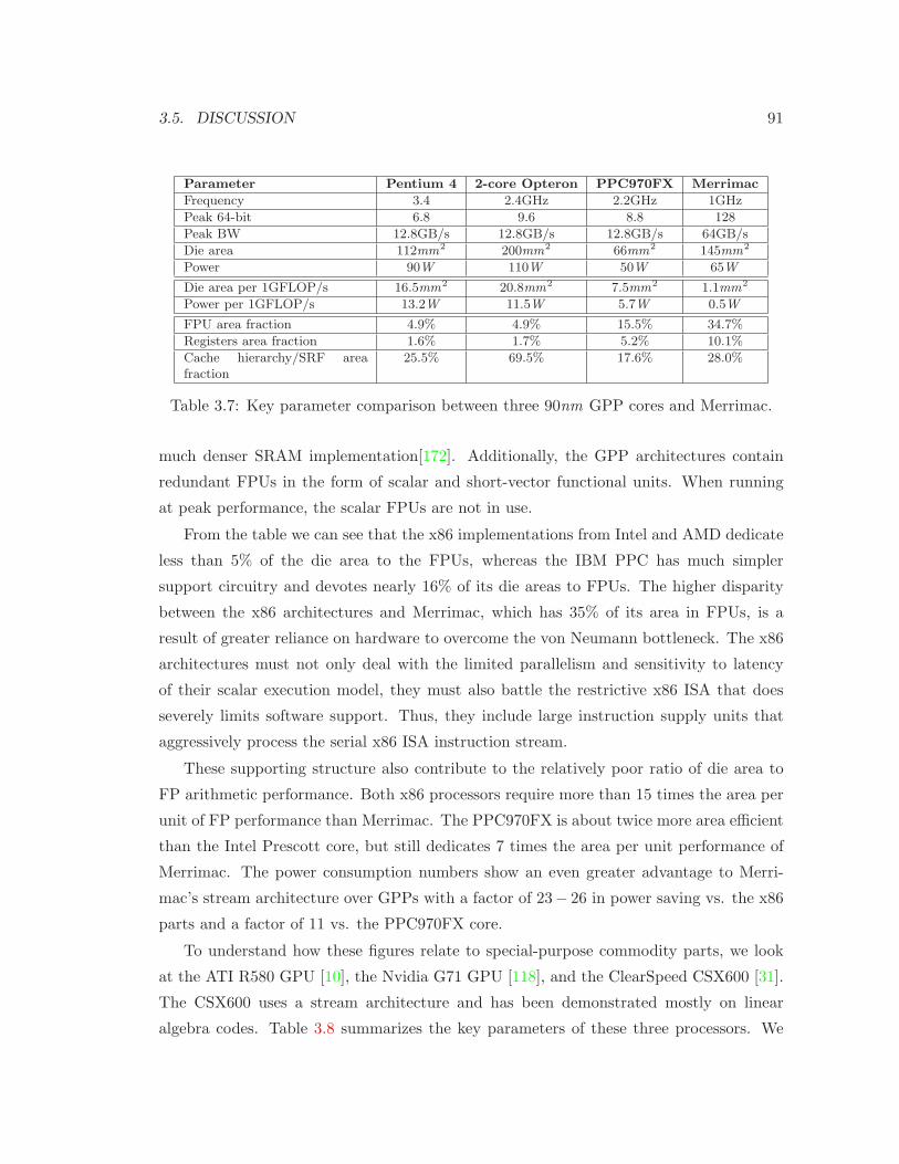
3.5. DISCUSSION 91
Parameter Pentium 4 2-core Opteron PPC970FX Merrimac
Frequency 3.4 2.4GHz 2.2GHz 1GHz
Peak 64-bit 6.8 9.6 8.8 128
Peak BW 12.8GB/s 12.8GB/s 12.8GB/s 64GB/s
Die area 112mm2 200mm
2 66mm2 145mm
2
Power 90W 110W 50W 65W
Die area per 1GFLOP/s 16.5mm2 20.8mm
2 7.5mm2 1.1mm
2
Power per 1GFLOP/s 13.2W 11.5W 5.7W 0.5W
FPU area fraction 4.9% 4.9% 15.5% 34.7%
Registers area fraction 1.6% 1.7% 5.2% 10.1%
Cache hierarchy/SRF areafraction
25.5% 69.5% 17.6% 28.0%
Table 3.7: Key parameter comparison between three 90nm GPP cores and Merrimac.
much denser SRAM implementation[172]. Additionally, the GPP architectures contain
redundant FPUs in the form of scalar and short-vector functional units. When running
at peak performance, the scalar FPUs are not in use.
From the table we can see that the x86 implementations from Intel and AMD dedicate
less than 5% of the die area to the FPUs, whereas the IBM PPC has much simpler
support circuitry and devotes nearly 16% of its die areas to FPUs. The higher disparity
between the x86 architectures and Merrimac, which has 35% of its area in FPUs, is a
result of greater reliance on hardware to overcome the von Neumann bottleneck. The x86
architectures must not only deal with the limited parallelism and sensitivity to latency
of their scalar execution model, they must also battle the restrictive x86 ISA that does
severely limits software support. Thus, they include large instruction supply units that
aggressively process the serial x86 ISA instruction stream.
These supporting structure also contribute to the relatively poor ratio of die area to
FP arithmetic performance. Both x86 processors require more than 15 times the area per
unit of FP performance than Merrimac. The PPC970FX is about twice more area efficient
than the Intel Prescott core, but still dedicates 7 times the area per unit performance of
Merrimac. The power consumption numbers show an even greater advantage to Merri-
mac’s stream architecture over GPPs with a factor of 23− 26 in power saving vs. the x86
parts and a factor of 11 vs. the PPC970FX core.
To understand how these figures relate to special-purpose commodity parts, we look
at the ATI R580 GPU [10], the Nvidia G71 GPU [118], and the ClearSpeed CSX600 [31].
The CSX600 uses a stream architecture and has been demonstrated mostly on linear
algebra codes. Table 3.8 summarizes the key parameters of these three processors. We

92 CHAPTER 3. MERRIMAC
Parameter R580 G71 CSX600 Merrimac
Frequency 250MHz 650MHz 650MHz 1GHz
Peak GFLOP/s 375 (32-bit) 330 (32-bit) 96/25 (64-bit) 128 (64-bit)
Peak BW 49.6GB/s 56.3GB/s 3.2GB/s 64GB/s
Die area 352mm2 196mm
2 145mm2
Power ≈ 100W 10W 65W
Die area per 1GFLOP/s 1.1mm2 1.7mm
2 1.1mm2
Power per 1GFLOP/s 0.3W 0.1/0.4W 0.5W
Table 3.8: Key parameter comparison between three 90nm special-purpose cores andMerrimac. Note that the ClearSpeed reports the CSX600 performance at 25GFLOP/ssustained on dense matrix-matrix multiply and we use both numbers above.
can see that Merrimac’s programmable stream architecture matches well with commercial
special-purpose VLSI implementations, whereas the GPP implementations are about an
order of magnitude worse in both power and area utilization.
3.5.2 System Considerations
The Merrimac processor is designed as a building block for an economically scalable sci-
entific computer, from a 128GFLOP/s single-node workstation to a 2PFLOP/s supercom-
puter. This goal influenced many design decisions and the impact is summarized below.
Compute Density and System Cost
Merrimac delivers very high performance per unit die area and unit power. As a result,
a smaller number of processors is required to achieve a desired level of performance and
the processors can be tightly packed. This leads to a compound effect on both the initial
cost and the operational cost of the system.
Power consumption is one of the largest and most costly problems facing large system
designs today. The power density of modern systems stresses cooling and power-supply
systems and significantly contributes to both initial cost and operational cost. Cooling
and supplying power, of course, require more energy than the energy being consumed by
the computation, and thus, reducing energy demands has a compound positive effect on
cost. Merrimac increases computational efficiency while achieving the high performance
levels expected from a supercomputer.
Another important factor affecting costs is the physical size of the system. Due to
electrical, physical, and power restrictions, only a limited number of processors can be

3.5. DISCUSSION 93
packaged into a system cabinet. Typically, at most 32 boards fit within a single cabinet,
providing power consumption is lower than about 30KW. Merrimac is designed to match
these packaging restrictions, and one cabinet provides 64TFLOP/s of performance at an
estimated 25KW of power. For comparison, Merrimac is almost 6 times more efficient in
compute floor-space utilization than the custom-designed IBM BlueGene/L (5.7TFLOP/s
with 32 boards at 20KW per cabinet), and is over 80 times better than the Sandia Red
Storm Cray XT3 system, which is based on AMD Opteron processors. All three systems
are designed with a 90nm VLSI process for large scale supercomputing.
The number of nodes and cabinets also directly impacts the cost and complexity of
the interconnection network. The smaller the number of nodes, the fewer cables that are
necessary and the lower the cost. The cabling cost of a multi-cabinet interconnection net-
work dominates all other networking aspects, and thus Merrimac’s advantage in compute
density significantly reduces system cost.
Merrimac’s cost of $8 per 1GFLOP/s of performance is very low by supercomputer
standards. must For example, in 2004, Sandia National Lab acquired the Red Storm
system for a reported $90M contract. Red Storm is a Cray XT3 Opteron based system,
that delivers a peak performance of 41.2TFLOP/s. Conservatively assuming a 50% profit
margin,3 and that half of the system cost is in the file storage system and physical facil-
ities, Red Storm still comes out at about 500 per 1GFLOP/s. The IBM BlueGene/L at
Lawrence Livermore National Lab, most likely cost upwards of $100M. BlueGene/L uses
a custom-designed processor to lower overall system cost and power consumption. With
similar assumptions about costs as for Red Storm, BlueGene/L performance costs roughly
$70 per 1GFLOP/s. By better matching VLSI and application characteristics, Merrimac
is able to deliver much higher value at $8 per 1GFLOP/s compute performance.
Scalable Memory Model
To assist efficient and effective implementations of complex scientific algorithms, Merrimac
provides a single global memory address space that can be accessed in single-word granu-
larity by software. Typical architectures balk at such a design because of the non-scalable
costs associated with fine-grained cache coherency, memory consistency, and address trans-
lation.
Merrimac provides economically scalable mechanisms to address these issues. Segment
3Supercopmuter profit margins are often in the single percentage points.

94 CHAPTER 3. MERRIMAC
registers are used to streamline address translation, and replace dynamic paging with soft-
ware controlled physical address mapping. The memory consistency model is flexible, and
again, transfers responsibility to software by providing memory fence operations only when
necessary. Finally, coherency is not performed at the granularity of single words. Instead,
software has explicit and precise control of the caching behavior, thus limiting coherence
requirements to a subset of the total memory accesses. Furthermore, the coarse-grained
stream model enables software initiated coherence operations that are implemented by the
stream cache bulk invalidate and flush mechanisms.
Reliability
The Merrimac processor dedicates a large fraction of its die area to FPUs and arithmetic
logic. This change in ratios also significantly affects the soft-error fault propensity of
the chip. We have taken great care in designing Merrimac to be able to tolerate soft-
errors in the computation and in state in an efficient and economical fashion. The fault
tolerance mechanisms take advantage of the throughput-oriented usage model of scientific
computing and the coarse-grained stream execution model to allow software and hardware
to cooperate in guaranteeing correctness. The details are presented in Chapter 6.
3.5.3 Software Aspects
Locality Implications
The stream programming model is designed for architectures that include the distinct
SRF address space and advocates a gather–compute–scatter style, where overall execution
is broken down into computational strips as with the strip-mining technique [104]. How-
ever, requiring all data that an inner-loop computation accesses to be gathered ahead of
the computation poses a problem for irregular accesses of unstructured mesh algorithms
because the working set depends on the connectivity data. We explore different methods
for performing the localization step required for stream processing and their affect on the
computation in Chapter 5. Additional complexity relates to the tradeoffs of indexed vs.
sequential access to the SRF, and whether cross-lane accesses are employed.
The locality and control hierarchy of Merrimac require software to carefully orchestrate
data movement in the presence of exceptions. As with any processor, software is responsi-
ble for handling exceptions raised by the hardware. In Merrimac, however, software is also
3.5. DISCUSSION 95
responsible for maintaining pre-exception state as the hardware does not provide precise
exceptions (Subsection 3.1.4).
Memory System Implications
Utilizing the memory system for scientific applications is made simple by the stream
programming model and the global address space. However, software must still consider
the tradeoff involved in utilizing the stream cache, and managing cache coherency. Care
must be taken in allocating space in the cache to only those accesses that can benefit from
this type of dynamic locality. We discuss this in greater detail and evaluate performance
tradeoffs in Chapter 5. Additionally, the hardware assist for caching behavior and bulk
invalidation must be appropriately operated by the software system. Another important
impact of the memory system is the sensitivity of achieved DRAM throughput to the
access pattern presented by the application. This issue is addresses in [3] and is beyond
the scope of this dissertation.
Parallelism Implications
The strong reliance of stream processors on SIMD execution for parallelism poses problems
for irregular unstructured computation. We cannot simply map an irregular computation
as it requires different control paths for different nodes in the dataset. We address this
issue in Chapter 5.
Chapter 4
Streaming Scientific Applications
As described in Chapter 2, most scientific application have abundant DLP and locality,
which are the necessary characteristics for efficient stream processing. In order to cast an
application into the streaming style, it must be converted into a gather–compute–scatter
form. In the gather phase, all data required for the next compute phase is localized into
the SRF. Once all the data has been loaded to on-chip state, the compute stage performs
the arithmetic operations and produces all data within the SRF. Further, once all data
from the localized data, and any intermediate results, have been processed, the results are
written back off-chip in the scatter phase. For efficient execution, the steps are pipelined
such that the computation phase can hide the latency of the communication phases.
This type of transformation is common in scientific computing, where many applica-
tions are designed to also run on distributed memory computers. For such machines, a
domain decomposition is performed on the data and computation to assign a portion of
each to every node on the system. This is similar to the localization step, but the granular-
ity is typically much greater in traditional systems. The SRF in Merrimac is 128KWords
total, and only 8KWords in each compute cluster, whereas compute nodes in distributed
memory machines often contain several GB of memory. The smaller granularity, also
results in more data movement operations in Merrimac. Other critical considerations due
to Merrimac’s unique architecture are mapping to the relaxed SIMD control of the clus-
ters and taking advantage of the hardware acceleration for sequential SRF accesses and
low-cost inter-cluster communication.
In Section 4.1 we present the Merrimac benchmark suite, and discuss the general
mapping of both structured and unstructured applications to Merrimac along the lines of
96
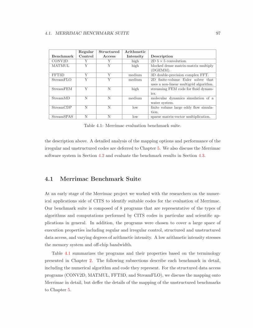
4.1. MERRIMAC BENCHMARK SUITE 97
Regular Structured ArithmeticBenchmark Control Access Intensity Description
CONV2D Y Y high 2D 5 × 5 convolution.
MATMUL Y Y high blocked dense matrix-matrix multiply(DGEMM).
FFT3D Y Y medium 3D double-precision complex FFT.
StreamFLO Y Y medium 2D finite-volume Euler solver thatuses a non-linear multigrid algorithm.
StreamFEM Y N high streaming FEM code for fluid dynam-ics.
StreamMD N N medium molecular dynamics simulation of awater system.
StreamCDP N N low finite volume large eddy flow simula-tion.
StreamSPAS N N low sparse matrix-vector multiplication.
Table 4.1: Merrimac evaluation benchmark suite.
the description above. A detailed analysis of the mapping options and performance of the
irregular and unstructured codes are deferred to Chapter 5. We also discuss the Merrimac
software system in Section 4.2 and evaluate the benchmark results in Section 4.3.
4.1 Merrimac Benchmark Suite
At an early stage of the Merrimac project we worked with the researchers on the numer-
ical applications side of CITS to identify suitable codes for the evaluation of Merrimac.
Our benchmark suite is composed of 8 programs that are representative of the types of
algorithms and computations performed by CITS codes in particular and scientific ap-
plications in general. In addition, the programs were chosen to cover a large space of
execution properties including regular and irregular control, structured and unstructured
data access, and varying degrees of arithmetic intensity. A low arithmetic intensity stresses
the memory system and off-chip bandwidth.
Table 4.1 summarizes the programs and their properties based on the terminology
presented in Chapter 2. The following subsections describe each benchmark in detail,
including the numerical algorithm and code they represent. For the structured data access
programs (CONV2D, MATMUL, FFT3D, and StreamFLO), we discuss the mapping onto
Merrimac in detail, but deffer the details of the mapping of the unstructured benchmarks
to Chapter 5.

98 CHAPTER 4. STREAMING SCIENTIFIC APPLICATIONS
4.1.1 CONV2D
The CONV2D benchmark performs a two-dimensional convolution of a 2052× 2052 input
array with a 5×5 stencil using halo boundary conditions. Halo boundary conditions imply
that the output array is 2048 × 2048 elements. Each element is a single double-precision
floating point number. Pseudocode for the CONV2D numerical algorithm appears in
Figure 4.1(a). We will use N and W to describe the CONV2D algorithm, with N = 2048
and W = 5.
Convolution with a stencil (kernel) of weights is a common operation in many struc-
tured finite-volume and finite-difference scientific codes, and forms the basic operation of
the StreamFLO application described in Subsection 4.1.4. The input size was chosen to be
large enough to represent realistic problems, where enough strips are processed to achieve
steady state behavior. The size of the stencil was inspired by the StreamFLO scientific
application.
The arithmetic intensity of the inner-most loop is only 23 (two input words and one
output word for a multiply and an add). However, when looking at the entire computation,(
N2W 22)
operations are performed for(
(N + W − 1)2 + W 2 + N2)
words of input and
output. Therefore the optimal arithmetic intensity is(
αopt ≃ W 2)
when N ≫ W .
Stripping the CONV2D algorithm is straightforward, with each strip being a rectan-
gular domain of the input array (Figure 4.1(b)). Apart from overlaps between strips, each
input is read once, and the arithmetic intensity remains close to optimal:(
α =2BxByW 2
(Bx+W−1)(By+W−1)+W 2+BxBy≃ W 2
)
.
It is possible to reduce the number of words read from memory by storing the overlap
regions in the SRF or communicating them between clusters with the inter-cluster switch.
However, the 8KWords capacity of each SRF lane allows for blocks that are much larger
than W and the overhead of replicating overlap elements on block boundaries is very low.
For example, with a 32× 32 block in each cluster αestimate = 22, and is high enough such
that CONV2D should be compute bound on Merrimac.
Using the indexable SRF, we can directly implement the kernel using the inner for
loops of the numerical algorithm in Figure 4.1(a). However, the SRF hardware is opti-
mized for sequential access. To take advantage of this hardware acceleration (higher SRF
throughput and auto-increment access mode), our optimized kernel processes each row
of the input sequentially in each cluster. (W − 1) temporary streams, which hold par-
tial sums for previously processed rows, are also accessed sequentially. The partial sum

4.1. MERRIMAC BENCHMARK SUITE 99
N = 2048;
W = 5;
double Ain[N+W-1][N+W-1];
double Aout[N][N]; // initialize to 0.0
double Aw[W][W];
conv2d (&Ain , &Aout , &Aw , N, W) {
for (i=0; i<N; i++) {
for (j=0; j<N; j++) {
for (k=0; k<W; k++) {
for (l=0; l<W; l++) {
Aout[i][j] += Ain[i+k][j+l]*Aw[k][l];
}
}
}
}
}
(a) CONV2D numerical algorithm.
// variables declared as above
BX = 512; // sample block size
BY = 32;
for (i=0; i<N; i+=BY) {
for (j=0; j<N; j+=BX) {
conv2d (&Ain[i][j], &Aout[i][j], &Aw , N, W);
// note that conv2d above accesses Ain[i:i+BY+W -1][j:j+BX+w -1]
}
}
(b) CONV2D blocking.
Figure 4.1: Numerical algorithm and blocking of CONV2D.
streams are reused for each new input row by setting the starting position with the index-
able SRF mechanism. Additionally, registers are used for each row of the stencil, instead
of indexed SRF accesses. The optimized kernel computes 50 arithmetic operations, while
making 4 sequential accesses, 2 index calculations, and 4 register transfers and is compute
bound on Merrimac. The two kernel implementations are shown in Figure 4.2.
4.1.2 MATMUL
MATMUL performs a dense double-precision matrix-matrix multiplication of two 512×512
matrices (Figure 4.3(a)), which is essentially the level-3 BLAS DGEMM routine. As with
CONV2D, the matrices sizes were chosen to significantly exceed the size of the SRF, thus
being representative of much larger problems while not requiring unduly large simulation
times. Dense matrix multiplication is common to many codes, and is also the basic
operation of the LINPACK benchmarks.
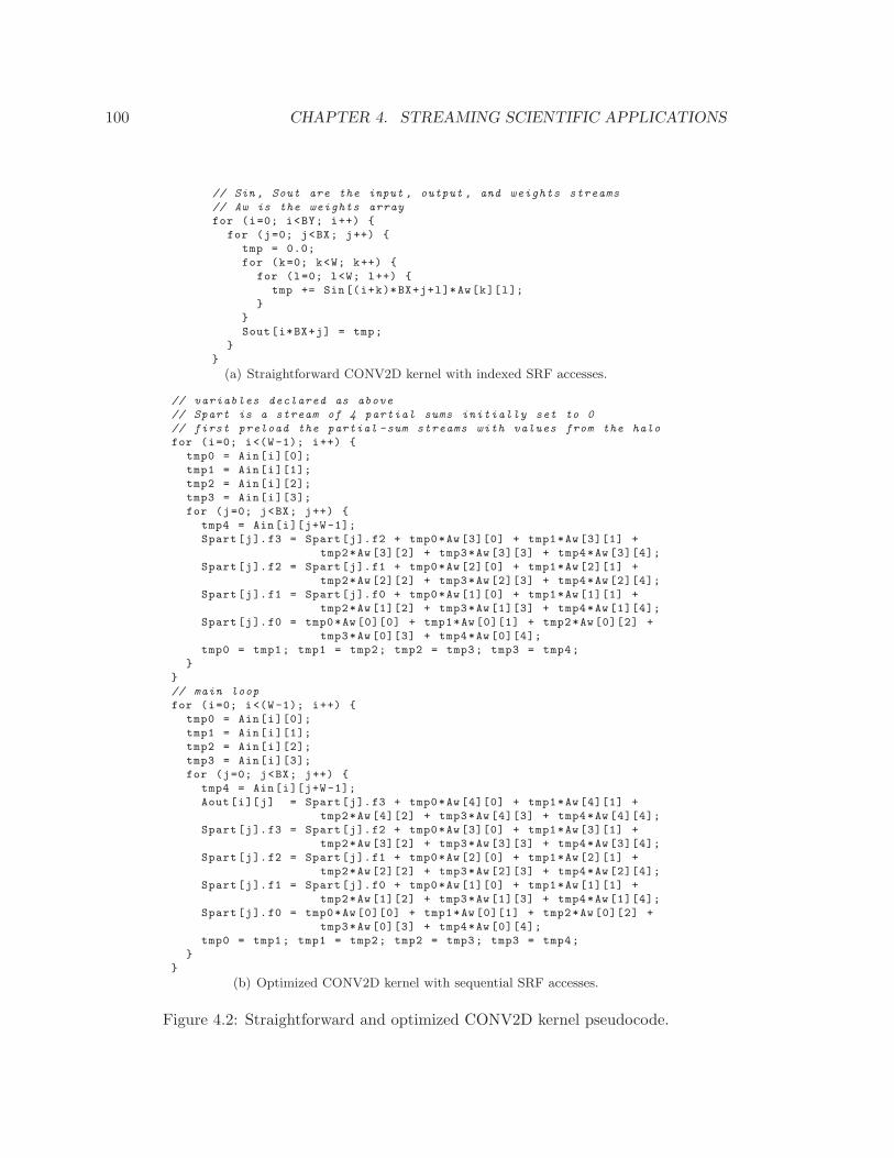
100 CHAPTER 4. STREAMING SCIENTIFIC APPLICATIONS
// Sin , Sout are the input , output , and weights streams
// Aw is the weights array
for (i=0; i<BY; i++) {
for (j=0; j<BX; j++) {
tmp = 0.0;
for (k=0; k<W; k++) {
for (l=0; l<W; l++) {
tmp += Sin[(i+k)*BX+j+l]*Aw[k][l];
}
}
Sout[i*BX+j] = tmp;
}
}
(a) Straightforward CONV2D kernel with indexed SRF accesses.
// variables declared as above
// Spart is a stream of 4 partial sums initially set to 0
// first preload the partial -sum streams with values from the halo
for (i=0; i<(W-1); i++) {
tmp0 = Ain[i][0];
tmp1 = Ain[i][1];
tmp2 = Ain[i][2];
tmp3 = Ain[i][3];
for (j=0; j<BX; j++) {
tmp4 = Ain[i][j+W-1];
Spart[j].f3 = Spart[j].f2 + tmp0*Aw [3][0] + tmp1*Aw [3][1] +
tmp2*Aw [3][2] + tmp3*Aw [3][3] + tmp4*Aw [3][4];
Spart[j].f2 = Spart[j].f1 + tmp0*Aw [2][0] + tmp1*Aw [2][1] +
tmp2*Aw [2][2] + tmp3*Aw [2][3] + tmp4*Aw [2][4];
Spart[j].f1 = Spart[j].f0 + tmp0*Aw [1][0] + tmp1*Aw [1][1] +
tmp2*Aw [1][2] + tmp3*Aw [1][3] + tmp4*Aw [1][4];
Spart[j].f0 = tmp0*Aw [0][0] + tmp1*Aw [0][1] + tmp2*Aw [0][2] +
tmp3*Aw [0][3] + tmp4*Aw [0][4];
tmp0 = tmp1; tmp1 = tmp2; tmp2 = tmp3; tmp3 = tmp4;
}
}
// main loop
for (i=0; i<(W-1); i++) {
tmp0 = Ain[i][0];
tmp1 = Ain[i][1];
tmp2 = Ain[i][2];
tmp3 = Ain[i][3];
for (j=0; j<BX; j++) {
tmp4 = Ain[i][j+W-1];
Aout[i][j] = Spart[j].f3 + tmp0*Aw [4][0] + tmp1*Aw [4][1] +
tmp2*Aw [4][2] + tmp3*Aw [4][3] + tmp4*Aw [4][4];
Spart[j].f3 = Spart[j].f2 + tmp0*Aw [3][0] + tmp1*Aw [3][1] +
tmp2*Aw [3][2] + tmp3*Aw [3][3] + tmp4*Aw [3][4];
Spart[j].f2 = Spart[j].f1 + tmp0*Aw [2][0] + tmp1*Aw [2][1] +
tmp2*Aw [2][2] + tmp3*Aw [2][3] + tmp4*Aw [2][4];
Spart[j].f1 = Spart[j].f0 + tmp0*Aw [1][0] + tmp1*Aw [1][1] +
tmp2*Aw [1][2] + tmp3*Aw [1][3] + tmp4*Aw [1][4];
Spart[j].f0 = tmp0*Aw [0][0] + tmp1*Aw [0][1] + tmp2*Aw [0][2] +
tmp3*Aw [0][3] + tmp4*Aw [0][4];
tmp0 = tmp1; tmp1 = tmp2; tmp2 = tmp3; tmp3 = tmp4;
}
}
(b) Optimized CONV2D kernel with sequential SRF accesses.
Figure 4.2: Straightforward and optimized CONV2D kernel pseudocode.

4.1. MERRIMAC BENCHMARK SUITE 101
To take full advantage of Merrimac’s locality hierarchy and functional units, we use a
hierarchical blocking scheme. The first level of blocking is from memory into the SRF, and
the second level between the SRF and the LRF. The computation also takes advantage of
inter-cluster communication to utilize all SRF lanes for a single shared block.
The first level of blocking is designed to efficiently take advantage of the SRF space.
Without loss of generality we will discuss using square (BSRF × BSRF ) submatrices with
square (N × N) input matrices, and N divisible by BSRF . Each submatrix Cij of the
solution is computed by summing(
NBSRF
)
products of
(BSRF × BSRF ) submatrices of A and B as shown in Equation 4.1 and Figures 4.3(b)–
4.4(a). Therefore, each submatrix of C requires writing the (BSRF × BSRF ) output and
processing of the A and B submatrices products, leading to an the arithmetic intensity
derived in Equations 4.2–4.3. Arithmetic intensity is directly proportional to the block
size, and BSRF must be chosen so as to not exceed the SRF size while providing state
for pipelined execution. The value of BSRF also depends on the second level of blocking
described below.
Cij =
NBSRF∑
k=0
AikBkj (4.1)
α =N
BSRF2B3
SRF
NBSRF
2B2SRF + B2
SRF
(4.2)
α ≃ BSRF (4.3)
Blocking the computation of each the submatrices products exploits inter-cluster com-
munication and fully utilizes the four MULADD units in each cluster. As shown in Fig-
ure 4.4(b), each of the submatrices is divided into BLRF ×BLRF chunks. Chunks of each
Aik submatrix are assigned to clusters by rows. Corresponding chunks of Cij also follow
the by-row allocation to clusters. On each iteration of the kernel, each cluster reads a
chunk from Aik in parallel. Each cluster also reads values from Bkj and broadcasts the
values to all other clusters. The combined values from all clusters form the same chunk of
the Bkj submatrix in all clusters. The kernel then proceeds to perform a matrix-matrix
product of the A and B chunks, and adds the result to the current value of the C chunk.
After an entire column of Bkj is processed, the kernel proceeds to the next column using

102 CHAPTER 4. STREAMING SCIENTIFIC APPLICATIONS
the same Aik submatrix by restarting, or resetting the starting index of the Aik stream
using the indexable SRF mechanism. Figure 4.3(c) presents the pseudocode of the kernel
computation.
N = 512;
double A[N][N];
double B[N][N];
double C[N][N];
matmul (&A, &B, &C) {
for (i=0; i<N; i++) {
for (j=0; j<N; j++) {
C[i][j] = 0.0;
for (k=0; k<N; k++) {
C[i][j] += A[i][k]*B[k][j];
}
}
}
}
(a) MATMUL numerical algorithm.
B_SRF = 32; // block size is B_SRF x B_SRF
for (i=0; i<N; i+=B) {
for (j=0; j<N; j+=B) {
reset(C[i][j], B); // set B_SRFxB_SRF submatrix to 0.0 starting at C[i][j]
for (k=0; k<N; k+=B) {
matmul(A[i][k], B[k][j], C[i][j], B_SRF ); // matmul won ’t reset C sub -block
}
}
}
(b) Blocking of MATMUL into SRF.
for (n=0; n<B_SRF/B_LRF; n++) {
read_chunk(C[n], C_chunk ); // reads chunk in each clusters
for (m=0; m<B_SRF/B_LRF; m++) {
read_chunk(A[m], A_chunk ); // reads chunk in each clusters
broadcast(B[m][n], B_chunk ); // reads one word in each cluster and
// broadcasts to form chunk
matmul(A_chunk , B_chunk , C_chunk , B_LRF ); // matmul will not reset C sub -block
}
}
(c) MATMUL kernel.
Figure 4.3: Numerical algorithm and blocking of MATMUL.
The computation of every chunk requires, in each cluster,(
2B3LRF
)
arithmetic op-
erations,(
B2LRF
)
broadcast operations, and
(
B2LRF +
B2
LRF
Nclust
)
SRF reads (Nclust is the
number of clusters – 16 in Merrimac). In addition,(
B2LRF
)
SRF reads and(
B2LRF
)
SRF
writes are needed to reduce the chunk of the C matrix once for every row of the Aik sub-
matrix. Merrimac has 4 MULADD units, can read or write 4 words from or to the SRF

4.1. MERRIMAC BENCHMARK SUITE 103
and can perform 1 broadcast operation on every cycle. Therefore, setting (BLRF = 4) will
saturate all these resources in the main part of the kernel loop.
Given Merrimac’s SRF size, we set (BSRF = 64) resulting in (αestimated = 64), which
is enough to prevent the memory system from becoming the bottleneck in MATMUL.
B1
B2
B3
A3A1A0
BAC
A2C0 B0
(a) Blocking of MATMUL into SRF
BkjA ikCij
Cijln
clust 0
clust 1
clust 2
clust 3
clust 0
clust 1
clust 2
clust 3
broadcast
Aiklm Bkj
mn
(b) Blocking of MATMUL into LRF
7654
111098
15141312
lll
lll
lll
lll
lll
llll
llll
llll
BkjnmA ik
lmCijln
l 3l 210
l
l
l
(c) Computation on chunks within kernel, numbers above rep-resent the cluster from which the element value was read
Figure 4.4: Depiction of MATMUL hierarchical blocking: blocking into SRF, blockinginto the LRFs, and utilization of indexable SRF to restart blocks of A and inter-clusterswitch to broadcast chunks of B.
4.1.3 FFT3D
The FFT3D benchmark computes a (128 × 128 × 128) three-dimensional decimation-in-
time complex FFT with double-precision numbers. FFT3D represents spectral methods
that use this algorithm as part of the numerical calculation.
The calculation is performed as three single-dimensional 128 point FFTs applied in
succession. Each phase applies 1282 single-dimensional FFTs to each row along a plane,

104 CHAPTER 4. STREAMING SCIENTIFIC APPLICATIONS
where an entire row is computed in a single cluster. The blocking strategy and phases
are depicted in Figure 4.5. The first phase processes FFTs along the X-dimension in
blocks of the Y Z plane with stripping along the Y -dimension across clusters. The second
phase performs the FFTs of the Y -dimension, with stripping along the X-dimension across
clusters. Because the memory subsystem interleaves accesses from the clusters, stripping in
the X dimension increases locality in the DRAM access and improves performance [30, 3].
The final stage computes the Z-dimension FFTs, and again stripping is along the X
dimension.
x
yz
x
yz
cluster 0
cluster 15
cluster 0
cluster 15
cluster 0 cluster 15cluster 0 cluster 15x y z
cluster 0 cluster 15z
cluster 0 cluster 15
Figure 4.5: Blocking of FFT3D in three dimensions. The dotted line represents a singleblock, with the allocation of rows to clusters within each plane.
The optimal arithmetic intensity of a three-dimensional FFT can be attained if the
entire dataset can fit in on-chip memory. The number of computations is equal to that of
standard FFT (5N log2 N), and each of the N = n3 elements requires two words of input
and two words of output, one for the real part and a second for the imaginary part of each
complex number. Thus for the (128 × 128 × 128) FFT, the optimal arithmetic intensity
is:(
αopt = 5(n3)log2n3
4n3 = 26.25)
.
The arithmetic intensity of the blocked algorithm is lower, as the data must be entirely
read and written in each of the three phases. No additional computation is required in the
blocked version and the arithmetic intensity is equal in all three phases, and in each single-
dimensional FFT. Within a phase, each FFT requires calculating (5n log2 n) arithmetic
operations (n = 128), reading 2n words (complex values), and writing 2n words. We
precompute all twiddle factors and store them in the SRF and LRFs. For the 128-point
FFT, the arithmetic intensity is therefore:

4.1. MERRIMAC BENCHMARK SUITE 105
(
αestimate = 5n log2 n4n
= 8.8)
4.1.4 StreamFLO
StreamFLO is a finite volume two-dimensional Euler solver that uses a non-linear multigrid
acceleration algorithm. StreamFLO is the most complex of the Merrimac benchmark and
is a complete code representative of typical computational fluid dynamics applications. It
is based on the original FORTRAN code of FLO82 [75, 76], which developed an approach
that is used in many industrial and research applications. The StreamFLO code was
developed by Massimiliano Fatica (Stanford CITS) for Merrimac using Brook.
The StreamFLO algorithm and implementation is described in detail in [49]. The code
is a cell-centered finite-volume solver for the set of five Euler PDEs in conservative form.
The solver uses explicit time stepping with a five-stage Runge-Kutta integration scheme.
The key characteristic of the code is the multigrid acceleration, which involves restriction
and prolongation operations for transferring the data from a fine mesh to a coarser one
and from a coarse mesh to a finer mesh respectively (Figure 4.6). Each restriction step
reduces the size of the grid computation by a factor of 2 in each dimension, or a factor of
4 in the two-dimensional StreamFLO.
compute
compute
compute
compute
restrict
restrict
restrict prolong
prolong
prolong
2×2
4×4
8×8
16×16
Figure 4.6: Restriction and relaxation in multigrid acceleration.
The general structure of the StreamFLO algorithm is give as pseudocode in Figure 4.9.
Each timestep consists of a multigrid V-cycle, a loop of coarsening steps and computation
(restriction), followed by a loop of refinement steps (prolongation). For each level during
the coarsening phase, the time step duration to use is calculated based on the current
state followed by the calculation of the convective and dissipative fluxes and explicit time

106 CHAPTER 4. STREAMING SCIENTIFIC APPLICATIONS
first iteration of kernel loop
second iteration of kernel loop
(a) Five-element stencil for convective flux and ∆t com-putation
first iteration of kernel loop
second iteration of kernel loop
(b) Nine-element stencil for dissipative flux computationon fine grid
Figure 4.7: Stencil operators for ∆T and flux computations in StreamFLO.
integration. The time step and convective flux are calculated using a five-element cross-
shaped stencil (Figure 4.7). The dissipative flux uses a nine-element cross on the finest
grid, and a five-element one on all coarser grids as with the convective flux calculation.
These computations are very similar to CONV2D, but each point requires several arith-
metic operations, including divides and square-roots. The StreamFLO implementation
is not as optimized as CONV2D and each stencil access requires an index calculation.
This overhead is small compared to the large number of arithmetic operations performed.
Each stencil computation uses halo boundary conditions on the horizontal dimension and
periodic boundary conditions on the vertical dimension. Setting up the boundary con-
ditions requires copying data from memory to the SRF along with the main grid. After
the fluxes are computed, the solution is updated. Then, the solution and residuals are
transferred to a coarser grid with the restriction operator. Restriction uses a four-element
square stencil, with no overlaps between neighboring stencils, on the finer grid to produce

4.1. MERRIMAC BENCHMARK SUITE 107
first iteration of kernel loop
second iteration of kernel loop
(a) Restriction operator with no stencil overlaps.
first iteration of kernel loop
second iteration of kernel loop
third iteration of kernel loop
(b) Prolongation operator with stencil overlaps.
Figure 4.8: Stencil operators for restriction and prolongation in StreamFLO.
a single element of the coarser grid (Figure 4.8(a)). After the coarsest level is reached,
the solution is transferred back into the finer grid in several prolongation operations. The
prolongation uses a four-element stencil, with overlaps, on the coarser grid to produce four
elements of the finer grid (Figure 4.8(b)).
StreamFLO is written in Brook and was processed with automatic tools and not hand
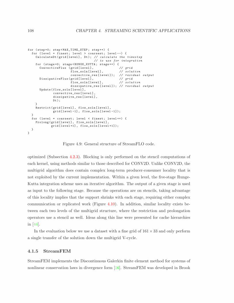
108 CHAPTER 4. STREAMING SCIENTIFIC APPLICATIONS
for (step =0; step <MAX_TIME_STEP ; step ++) {
for (level = finest; level > coarsest; level --) {
CalculateDt(grid[level], Dt); // calculate the timestep
// to use for integration
for (stage =0; stage <RUNGE_KUTTA; stage ++) {
ConvectiveFlux (grid[level], // grid
flow_soln[level], // solution
convective_res[level ]); // residual output
DissipativeFlux (grid[level], // grid
flow_soln[level], // solution
dissipative_res [level ]); // residual output
Update(flow_soln[level],
convective_res[level],
dissipative_res [level],
Dt);
}
Restrict(grid[level], flow_soln[level],
grid[level -1], flow_soln[level -1]);
}
for (level = coarsest; level < finest; level ++) {
Prolong(grid[level], flow_soln[level],
grid[level +1], flow_soln[level +1]);
}
}
Figure 4.9: General structure of StreamFLO code.
optimized (Subsection 4.2.3). Blocking is only performed on the stencil computations of
each kernel, using methods similar to those described for CONV2D. Unlike CONV2D, the
multigrid algorithm does contain complex long-term producer-consumer locality that is
not exploited by the current implementation. Within a given level, the five-stage Runge-
Kutta integration scheme uses an iterative algorithm. The output of a given stage is used
as input to the following stage. Because the operations are on stencils, taking advantage
of this locality implies that the support shrinks with each stage, requiring either complex
communication or replicated work (Figure 4.10). In addition, similar locality exists be-
tween each two levels of the multigrid structure, where the restriction and prolongation
operators use a stencil as well. Ideas along this line were presented for cache hierarchies
in [44].
In the evaluation below we use a dataset with a fine grid of 161× 33 and only perform
a single transfer of the solution down the multigrid V-cycle.
4.1.5 StreamFEM
StreamFEM implements the Discontinuous Galerkin finite element method for systems of
nonlinear conservation laws in divergence form [16]. StreamFEM was developed in Brook

4.1. MERRIMAC BENCHMARK SUITE 109
stage 0
stage 1
stage 2
stencil
Figure 4.10: Producer-consumer locality in StreamFLO.
and C by Timothy J. Barth (NASA Ames). This code represents finite element methods,
which are an important category of scientific applications in general, and computational
fluid dynamics in particular.
The algorithm uses a three-dimensional unstructured mesh with irregular memory
accesses. Our current implementation is for tetrahedral elements only, leading to regular
control because all elements have exactly 4 neighbors. The structure of the code is depicted
in Figure 4.11 and presented as pseudocode in Figure 4.12. The execution consists of
two phases within each timestep. The first phase processes all faces in the system by
gathering the data of the two elements that define each face, and calculates the fluxes
across each face. The fluxes are scattered to memory followed by a global synchronization
step to ensure all memory locations have been updated. The second phase gathers the
flux information of the faces neighboring each element and updates the element values
and solution. The timestep is then advanced using a first-order Runge-Kutta explicit
integrator and all elements updated in memory. A second synchronization operation is
needed before processing faces of the next timestep iteration.
The actual computation of the fluxes, elements, and solution is parameterizable in
StreamFEM. The system can be configured as solving simple advection equations (1 PDE),
the Euler flow equations (5 PDEs), and magnetohydrodynamics (MHD) that requires 8
PDEs. Additionally, the interpolation of values from the control points of the elements
and faces can be varied between a constant interpolation with a single degree of free-
dom (DOF), linear interpolation (4 DOFs), quadratic interpolation (10 DOFs), and cubic
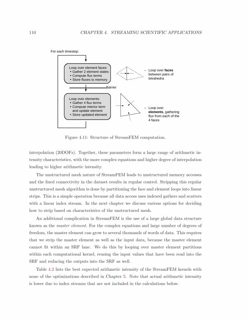
110 CHAPTER 4. STREAMING SCIENTIFIC APPLICATIONS
– Loop over facesbetween pairs of tetrahedra
– Loop over elements, gathering flux from each of the 4 faces
Loop over element faces:� Gather 2 element states� Compute flux terms� Store fluxes to memory
Loop over elements:� Gather 4 flux terms� Compute interior term
and update element� Store updated element
For each timestep:
Barrier
Figure 4.11: Structure of StreamFEM computation.
interpolation (20DOFs). Together, these parameters form a large range of arithmetic in-
tensity characteristics, with the more complex equations and higher degree of interpolation
leading to higher arithmetic intensity.
The unstructured mesh nature of StreamFEM leads to unstructured memory accesses
and the fixed connectivity in the dataset results in regular control. Stripping this regular
unstructured mesh algorithm is done by partitioning the face and element loops into linear
strips. This is a simple operation because all data access uses indexed gathers and scatters
with a linear index stream. In the next chapter we discuss various options for deciding
how to strip based on characteristics of the unstructured mesh.
An additional complication in StreamFEM is the use of a large global data structure
known as the master element. For the complex equations and large number of degrees of
freedom, the master element can grow to several thousands of words of data. This requires
that we strip the master element as well as the input data, because the master element
cannot fit within an SRF lane. We do this by looping over master element partitions
within each computational kernel, reusing the input values that have been read into the
SRF and reducing the outputs into the SRF as well.
Table 4.2 lists the best expected arithmetic intensity of the StreamFEM kernels with
none of the optimizations described in Chapter 5. Note that actual arithmetic intensity
is lower due to index streams that are not included in the calculations below.

4.1. MERRIMAC BENCHMARK SUITE 111
for {timestep =0; timesteps <MAX_STEP; timestep ++) {
// face phase
for (face =0; face <NUM_FACES; face ++) {
// gather cell data for the two cell neighbors
// of the face
GatherFluxState (elements[face_Relements[face]],
elements[face_Lelements[face]],
right_element ,
left_element );
// compute the fluxes on the face
ComputeFlux(right_element , left_element ,
faces[face], Rflux , Lflux );
// scatter fluxes to memory for element phase
fluxes [2* face]= Rflux;
fluxes [2* face +1]= Lflux;
}
barrier (); // previous loop is streaming , need to make
// sure all scattered data is in memory
// element loop
for (element =0; element <NUM_ELEMENTS; element ++) {
// gather fluxes on the 4 faces of each cell
GatherCell(fluxes[elements_face0[element ]],
fluxes[elements_face1[element ]],
fluxes[elements_face2[element ]],
fluxes[elements_face3[element ]],
residual );
// compute cell values
ComputeCellInterior (elements[element], residual );
// time integration
AdvanceCell(elements[element], residual , solution[element ]);
}
}
Figure 4.12: Pseudocode for StreamFEM.
We have a single dataset for StreamFEM with 9 664 nodes and 20 080 neighbors and
we only evaluate the Euler-linear and MHD-linear configurations. Configurations with
constant interpolation are not particularly interesting from a scientific code perspective,
and higher orders of interpolation result in a configuration that is dominated by the
ComputeCellInterior kernel and have very high arithmetic intensity. This combination
makes StreamFEM less balanced in terms of memory and compute and less interesting
to analyze and stress Merrimac. As will be discussed in Section 4.3, even with lower
arithmetic intensity of linear interpolation, the performance of StreamFEM is very high.
4.1.6 StreamCDP
StreamCDP solves the transport advective equation for large eddy simulations (LES)
using a finite volume method [131]. We evaluate the second-order WENO (Weighted

112 CHAPTER 4. STREAMING SCIENTIFIC APPLICATIONS
Arithmetic RelativeEquation Interpolation Kernel Intensity # Ops
Euler
GatherFluxState 4.7 10%ComputeFlux 13.4 18%
linear GatherCell 7.9 10%ComputeCellInterior 63.6 61%AdvanceCell 1.3 2%Overall 44.0 100%
GatherFluxState 12.5 12%ComputeFlux 54.5 8%
quadratic GatherCell 23.0 11%ComputeCellInterior 157.5 68%AdvanceCell 1.3 1%Overall 115.3 100%
GatherFluxState 30.2 8%ComputeFlux 124.6 3%
cubic GatherCell 57.5 7%ComputeCellInterior 684.5 82%AdvanceCell 1.3 0%Overall 570.4 100%
MHD
GatherFluxState 4.7 8%ComputeFlux 30.2 17%
linear GatherCell 8.3 7%ComputeCellInterior 87.8 65%AdvanceCell 1.3 1%Overall 63.1 100%
GatherFluxState 12.6 10%ComputeFlux 70.5 9%
quadratic GatherCell 23.5 10%ComputeCellInterior 195.6 71%AdvanceCell 1.3 1%Overall 147.9 100%
GatherFluxState 30.3 7%ComputeFlux 161.1 3%
cubic GatherCell 58.3 7%ComputeCellInterior 811.1 84%AdvanceCell 1.3 0%Overall 688.8 100%
Table 4.2: Expected best arithmetic intensity values for StreamFEM. Values are give forall five kernels and six equation type and interpolation degree combinations. The fractionof number of operations field refers to the number of operations performed during theexecution of StreamFEM for a given kernel as a fraction of the total number of operationsexecuted.
Essentially Non-Oscillatory) [103] component of the solver that uses an unstructured mesh.
Our datasets contain a variety of polyhedral elements with varying number of neighbors
leading to irregular control (Figure 4.13). This code represents a general FVM solver with a
irregular control and unstructured data accesses. Such codes are common in computational
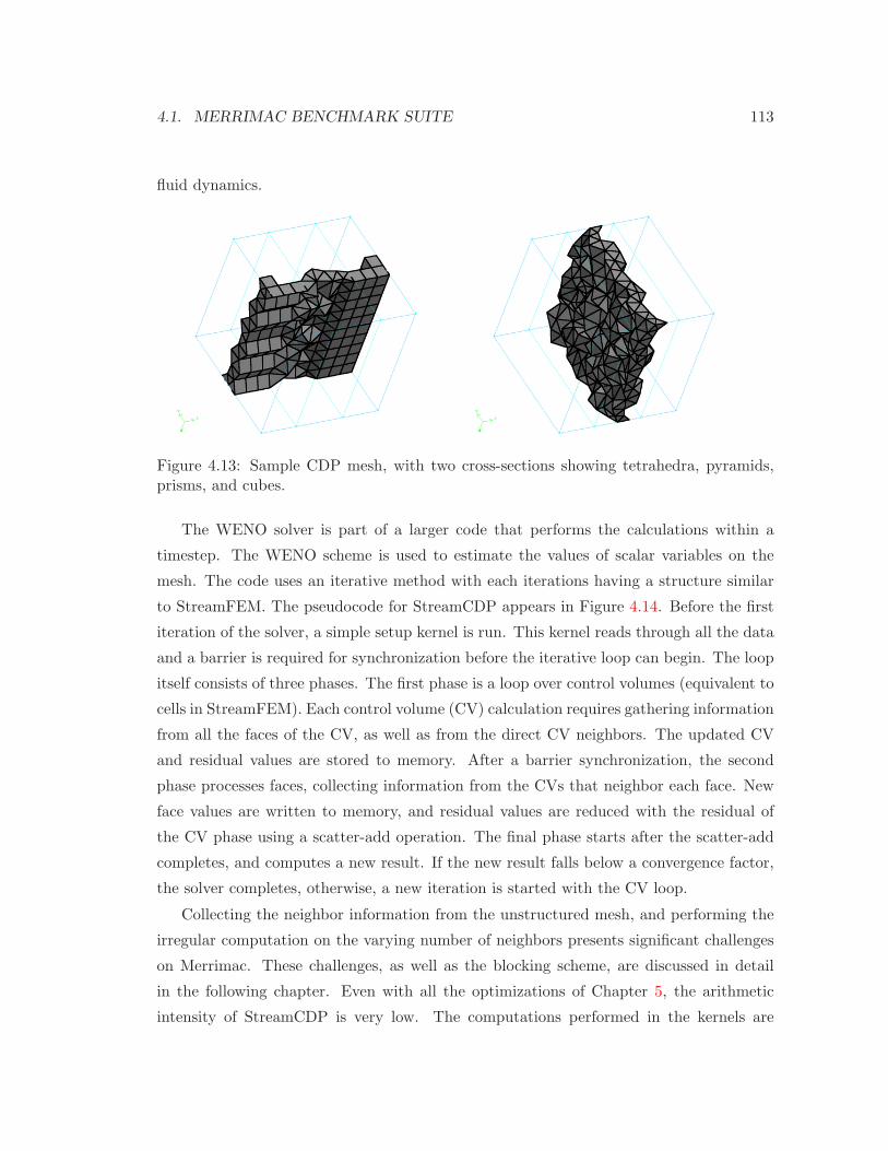
4.1. MERRIMAC BENCHMARK SUITE 113
fluid dynamics.
Figure 4.13: Sample CDP mesh, with two cross-sections showing tetrahedra, pyramids,prisms, and cubes.
The WENO solver is part of a larger code that performs the calculations within a
timestep. The WENO scheme is used to estimate the values of scalar variables on the
mesh. The code uses an iterative method with each iterations having a structure similar
to StreamFEM. The pseudocode for StreamCDP appears in Figure 4.14. Before the first
iteration of the solver, a simple setup kernel is run. This kernel reads through all the data
and a barrier is required for synchronization before the iterative loop can begin. The loop
itself consists of three phases. The first phase is a loop over control volumes (equivalent to
cells in StreamFEM). Each control volume (CV) calculation requires gathering information
from all the faces of the CV, as well as from the direct CV neighbors. The updated CV
and residual values are stored to memory. After a barrier synchronization, the second
phase processes faces, collecting information from the CVs that neighbor each face. New
face values are written to memory, and residual values are reduced with the residual of
the CV phase using a scatter-add operation. The final phase starts after the scatter-add
completes, and computes a new result. If the new result falls below a convergence factor,
the solver completes, otherwise, a new iteration is started with the CV loop.
Collecting the neighbor information from the unstructured mesh, and performing the
irregular computation on the varying number of neighbors presents significant challenges
on Merrimac. These challenges, as well as the blocking scheme, are discussed in detail
in the following chapter. Even with all the optimizations of Chapter 5, the arithmetic
intensity of StreamCDP is very low. The computations performed in the kernels are
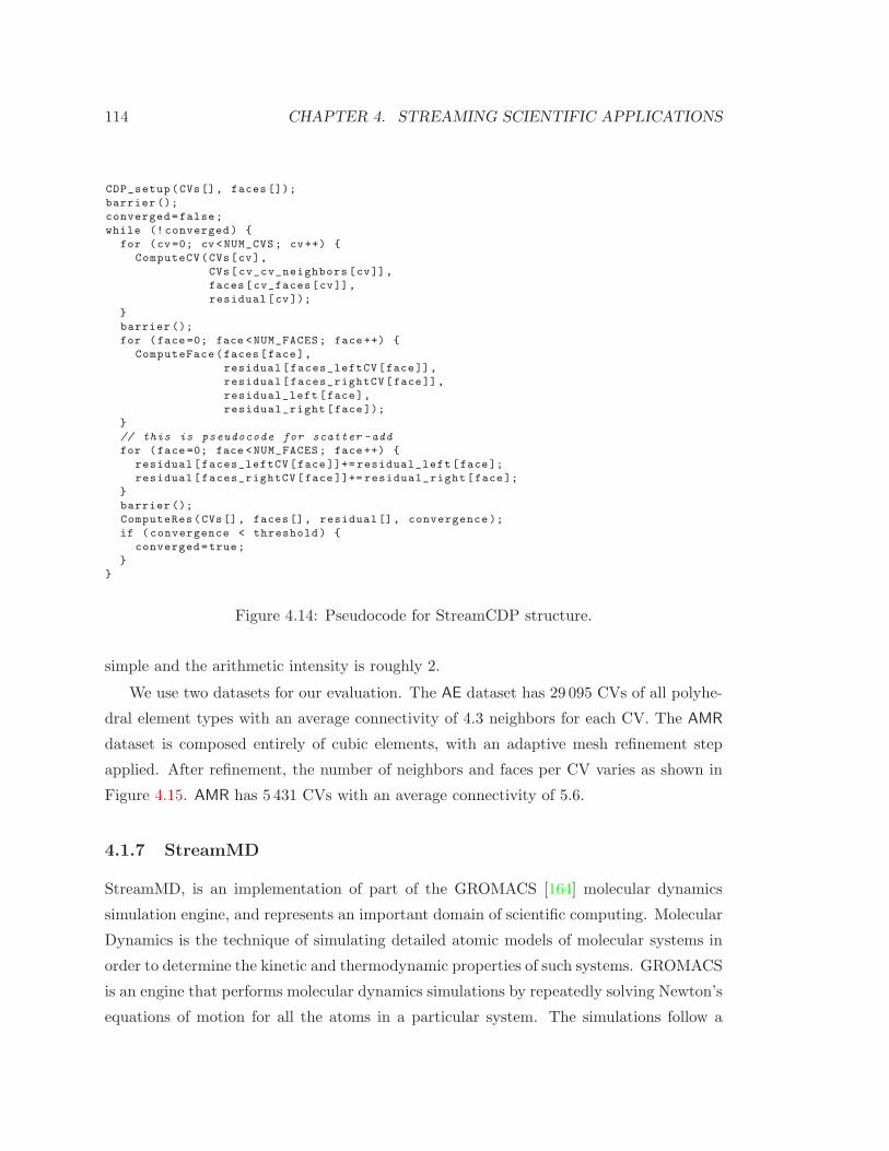
114 CHAPTER 4. STREAMING SCIENTIFIC APPLICATIONS
CDP_setup(CVs[], faces []);
barrier ();
converged=false;
while (! converged) {
for (cv=0; cv <NUM_CVS; cv++) {
ComputeCV(CVs[cv],
CVs[cv_cv_neighbors [cv]],
faces[cv_faces[cv]],
residual[cv]);
}
barrier ();
for (face =0; face <NUM_FACES; face ++) {
ComputeFace(faces[face],
residual[faces_leftCV[face]],
residual[faces_rightCV [face]],
residual_left [face],
residual_right[face ]);
}
// this is pseudocode for scatter -add
for (face =0; face <NUM_FACES; face ++) {
residual[faces_leftCV[face ]]+= residual_left [face];
residual[faces_rightCV [face ]]+= residual_right[face];
}
barrier ();
ComputeRes(CVs[], faces[], residual[], convergence );
if (convergence < threshold) {
converged=true;
}
}
Figure 4.14: Pseudocode for StreamCDP structure.
simple and the arithmetic intensity is roughly 2.
We use two datasets for our evaluation. The AE dataset has 29 095 CVs of all polyhe-
dral element types with an average connectivity of 4.3 neighbors for each CV. The AMR
dataset is composed entirely of cubic elements, with an adaptive mesh refinement step
applied. After refinement, the number of neighbors and faces per CV varies as shown in
Figure 4.15. AMR has 5 431 CVs with an average connectivity of 5.6.
4.1.7 StreamMD
StreamMD, is an implementation of part of the GROMACS [164] molecular dynamics
simulation engine, and represents an important domain of scientific computing. Molecular
Dynamics is the technique of simulating detailed atomic models of molecular systems in
order to determine the kinetic and thermodynamic properties of such systems. GROMACS
is an engine that performs molecular dynamics simulations by repeatedly solving Newton’s
equations of motion for all the atoms in a particular system. The simulations follow a

4.1. MERRIMAC BENCHMARK SUITE 115
Figure 4.15: Adaptive mesh refinement on cubic CDP mesh leading to variable number ofneighbors. The central CV on the left has 5 neighbors, but after the left-most element isrefined, the central CV (shown on the right) has 8 neighbors.
discrete timescale, and are used to compute various observables of interest. Often, such
simulations are used to design new materials or study biological molecules such as proteins,
DNA. When simulating the latter, it is common to surround those molecules with a large
number of water molecules. In that case, a significant portion of the calculation is spent
calculating long ranged interactions between water molecules and between the protein and
the surrounding water molecules.
GROMACS is highly optimized to take advantage of mechanisms found in commercial
high-end processors including hand optimized loops using SSE, 3DNow!, and Altivec in-
structions. One of the numerical method employed by GROMACS for long ranged forces
uses a cut-off distance approximation. All interactions between particles which are at
a distance greater than rc are approximated as exerting no force. This approximation
limits the number of interactions calculated for the system from O(n2) to O(n), where
each particle (we will refer to this as the central particle) only interacts with a small
number of neighboring particles. The list of neighbors for each particle is calculated in
scalar-code and passed to the stream program through memory along with the particle
positions. The overhead of the neighbor list is kept to a minimum by only generating it
once every several time-steps. The accuracy of the calculation is maintained by artificially
increasing the cutoff distance beyond what is strictly required by the physics. StreamMD
is an implementation of this phase of the GROMACS algorithm for Merrimac. A more
in-depth discussion of our implementation appears in [47].
Since the Merrimac system integrates a conventional scalar processor with a stream

116 CHAPTER 4. STREAMING SCIENTIFIC APPLICATIONS
unit it offers a simple path for porting an application. Most of the application can initially
be run on the scalar processor and only the time consuming computations are streamed.
StreamMD performs the force calculation of GROMACS using Merrimac’s highly parallel
hardware. The current implementation computes the force interaction of water molecules
and is intended to interface with the rest of GROMACS through Merrimac’s global shared
memory addressing.
The streaming portion of StreamMD consists of a single kernel performing the inter-
actions. The interacting particles are not single atoms but entire water molecules. Each
kernel iteration processes a molecule and one of its neighboring molecules, and computes
the non-bonded interaction force between all atom pairs (Equation 4.4). The first term
contributes to Coulomb interaction, where 14πǫ0
is the electric conversion factor. The sec-
ond term contributes to Lennard-Jones interaction, where C12 and C6 depend on which
particle types constitute the pair.
Vnb =∑
i,j
[
1
4πǫ0
qiqj
rij+
(
C12
r12ij
− C6
r6ij
)]
(4.4)
GROMACS provides the configuration data consisting of a position array containing
nine coordinates for each molecule (because we are using water molecules these are the
coordinates for each of the three atoms), the central molecule indices stream i central
(one element per molecule), and the neighboring molecules indices stream i neighbor
(one element per interaction). These streams index into the position input array and the
force output array. These data are loaded through memory, so that the stream unit can
be used as a coprocessor for the time-intensive force computation portion of the program.
The basic flow of StreamMD is summarized below, and given as pseudocode in Fig-
ure 4.16.
1. Gather the positions of the interacting molecules into the SRF using Merrimac’s
hardware gather mechanism.
2. Run the force computation kernel over all interactions, reading the required data
from the predictable SRF. The kernel’s output is a stream of partial-forces and a
stream of indices which maps each force to a molecule. Those partial forces are
subsequently reduced to form the complete force acting on each atom.
3. Reduce the partial forces. This is achieved using Merrimac’s scatter-add feature.
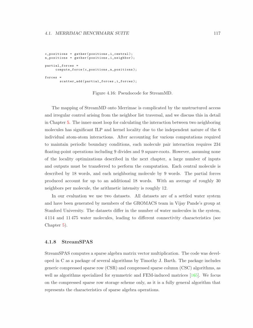
4.1. MERRIMAC BENCHMARK SUITE 117
c_positions = gather(positions ,i_central );
n_positions = gather(positions ,i_neighbor );
partial_forces =
compute_force (c_positions ,n_positions );
forces =
scatter_add(partial_forces ,i_forces );
Figure 4.16: Pseudocode for StreamMD.
The mapping of StreamMD onto Merrimac is complicated by the unstructured access
and irregular control arising from the neighbor list traversal, and we discuss this in detail
in Chapter 5. The inner-most loop for calculating the interaction between two neighboring
molecules has significant ILP and kernel locality due to the independent nature of the 6
individual atom-atom interactions. After accounting for various computations required
to maintain periodic boundary conditions, each molecule pair interaction requires 234
floating-point operations including 9 divides and 9 square-roots. However, assuming none
of the locality optimizations described in the next chapter, a large number of inputs
and outputs must be transferred to perform the computation. Each central molecule is
described by 18 words, and each neighboring molecule by 9 words. The partial forces
produced account for up to an additional 18 words. With an average of roughly 30
neighbors per molecule, the arithmetic intensity is roughly 12.
In our evaluation we use two datasets. All datasets are of a settled water system
and have been generated by members of the GROMACS team in Vijay Pande’s group at
Stanford University. The datasets differ in the number of water molecules in the system,
4 114 and 11 475 water molecules, leading to different connectivity characteristics (see
Chapter 5).
4.1.8 StreamSPAS
StreamSPAS computes a sparse algebra matrix vector multiplication. The code was devel-
oped in C as a package of several algorithms by Timothy J. Barth. The package includes
generic compressed sparse row (CSR) and compressed sparse column (CSC) algorithms, as
well as algorithms specialized for symmetric and FEM-induced matrices [165]. We focus
on the compressed sparse row storage scheme only, as it is a fully general algorithm that
represents the characteristics of sparse algebra operations.

118 CHAPTER 4. STREAMING SCIENTIFIC APPLICATIONS
The CSR storage format is depicted in Figure 4.17. The sparse matrix is stored using
three dense arrays. Array A stores all non-zero values of the matrix, array JA sores the
column positions corresponding to the non-zero elements, and array IA points to the row
starting positions in the first two arrays. This storage format is, in fact, a graph format,
with IA and JA defining the adjacency matrix of the graph. Looked at this way, the CSR
matrix-vector multiply is an unstructured, irregular mesh algorithm similar to StreamMD
and StreamCDP. The matrix rows act as nodes in the mesh and the matrix and vector
values are neighbors. The algorithm for CSR in StreamSPAS is shown in Figure 4.18, and
the mapping to Merrimac is discussed in Chapter 5.
A02 A04 A05
A10 A16
A22 A23 A24
A30 A32 A33 A34 A37
A02 A04 A05 A10 A16 A22 A23 A24 A30 A32 A33 A34 A37
2 4 5 0 6 2 3 4 0 2 3 4 7
0 3 5 8 13IA
JA
A
Figure 4.17: StreamSPAS CSR storage format.
for (int row=0; row <NUM_ROWS; row ++) {
result[row ]=0.0;
for (col=IA[row]; col <IA[row +1]; col ++) {
result[row] += A[JA[col ]]* vect[JA[col ]];
}
}
Figure 4.18: StreamSPAS algorithm pseudocode.
4.2 Merrimac Software System
Over the course of the Merrimac project we developed and used several software systems
and compilers. This section describes these efforts from low-level to high-level.
4.2. MERRIMAC SOFTWARE SYSTEM 119
4.2.1 Macrocode, Microcode, and KernelC
The lowest level programming tools for Merrimac use macrocode and microcode interfaces.
Macrocode uses C++ classes and methods that correspond to Merrimac’s stream instruc-
tions (Subsection 3.1.1), which are executed on the scalar core to issue coarse-grained
stream memory operations and kernels. The direct mapping of macrocode to instructions
in the stream ISA allows for precise control over execution and performance. Because of
this precision, all of the applications for Merrimac, except for StreamFLO, were eventually
ported to macrocode for optimal performance. As will be discussed later in this section,
this port was relatively simple because the applications were written for the stream exe-
cution model of Merrimac, which is represented exactly by macrocode programs.
Microcode is a similar low-level interface that corresponds to the cluster’s kernel ISA
(Subsection 3.1.2). Due to the complexity of scheduling kernel instructions onto the ex-
posed communication VLIW substrate of the compute clusters, we did not program any of
Merrimac’s benchmarks at this low level. Instead we relied on a powerful optimizing kernel
compiler that accepts kernels written in the KernelC language as input. The compiler is
an extension of the kernel scheduler developed in the Imagine project [108]. Merrimac’s
version of KernelC extends that of Imagine [107] to support fused MULADD instructions,
acceleration for iterative operations, and indexed access to the SRF (both in-lane and
cross-lane).
4.2.2 StreamC
StreamC is a mid-level stream language that is under active development. It was origi-
nally developed for Imagine [107] as a more user-friendly interface than macrocode and
supported compiler analyses and optimizations. The StreamC compiler performs stream
scheduling [82], which includes automatic space-time allocation of streams in the SRF, in-
troduces stream memory operations, and statically schedules stream memory operations
and kernels. It outputs code that directly translates to Merrimac stream instructions. The
compiler has access to machine parameters and uses a performance model to effectively
search through the large space of SRF allocation,
The stream scheduling capabilities of the StreamC compiler proved invaluable in the
Imagine project. The automatic analysis simplified programming, and the optimizations
improved performance when compared to macrocode implementations of the codes [107,
120 CHAPTER 4. STREAMING SCIENTIFIC APPLICATIONS
121, 122]. Based on this experience we chose StreamC as out first programming system
Merrimac and adapted the Imagine StreamC compiler to Merrimac’s ISA. Over time, we
found that StreamC did not meet all of our requirements, in terms of transparency of the
performance model exposed to the user and the actual performance of the generated code.
To enable the current implementation of the automatic stream scheduling optimiza-
tions, the StreamC language implements a more restrictive stream execution model than
that of Merrimac. StreamC assumes that all streams are accessed sequentially, as is
common in the media application domain targeted by Imagine. In contrast, Merrimac
uses streams of blocks, where accesses within a block can be data dependent. While the
StreamC interface can be used for describing blocks as well as streams, but care must be
taken to ensure that the StreamC compiler does not re-allocate the dynamically indexed
blocks in the SRF while the data is still live. For example, the StreamC compiler may
insert spill and fill stream memory instructions during SRF allocation. If all streams are
accessed sequentially the compiler can ensure that the appropriate section of the stream
is resident in the SRF before it is accessed. If the stream is indexed, however, spilling
parts of the stream without programmer knowledge can result in invalid SRF accesses and
incorrect data. In the programming style inspired by Merrimac’s execution model, the
programmer explicitly expresses the blocking of the algorithm, whereas in StreamC, the
compiler attempts to automatically strip-mine and schedule the code.
While in some cases, the compiler could automatically strip-mine and software pipeline
the program, at the time that we developed the Merrimac benchmarks these capabilities
were not fully developed. Additionally, the complex heuristics used by the compiler for
allocating SRF resources required us to tweak the program to achieve the desired per-
formance goals. Because we used a programming style that directly reflects Merrimac’s
generalized stream execution model, we had already blocked the programs, and applying
software-pipelined scheduling was mechanical with the simple control flow of Merrimac’s
scientific programs. Therefore, we decided to directly use macrocode and avoid the opaque
optimizations of stream scheduling.
4.2.3 Brook
While StreamC was developed for Imagine as a replacement to low-level macrocode, the
Brook language was developed as an abstract and portable stream language. We developed
Brook specifically for scientific applications, but strived to maintain a level of abstraction

4.2. MERRIMAC SOFTWARE SYSTEM 121
that will not tie it down to a specific platform. Brook was developed from the start both
as the language of choice for Merrimac benchmarks and as a software system targeting
programmable GPUs [24, 23].
The Brook execution model and language [22] refer to computational kernels that
are applied to streams, which are unordered collections of data elements that serve. A
stream is used to express DLP, and a kernel applied to a stream can potentially process
all the stream elements in parallel. Kernels can only use a subset of C and can only
reference arguments passed to the kernel and locally declared kernel variables. Stream
arguments to kernels are presented to the kernels as single elements, and kernels do not
retain any state other than explicitly expressed reductions. These unordered streams and
kernels, in conjunction with the ability to perform reductions, allow the programmer to
effectively express DLP. Additionally, kernels operating on streams capture the ideas of
kernel locality, producer-consumer locality, and a two-level locality hierarchy of off-chip
memory and an on-chip SRF. To ensure locality, streams in Brook do not refer to a specific
memory location.
Given the above restrictions on stream allocation and access to stream elements in
kernels, Brook offers a variety of stream manipulation operators for scientific comput-
ing. First, Brook streams can be assigned multi-dimensional rectangular shapes. Second,
the streams can be modified with stream operators, including multi-dimensional stencils,
multi-dimensional groups, gathers/scatters, and atomic stream memory operations such as
scatter-add. These features of Brook are similar to SDF languages, but Brook breaks away
from such restrictions with the availability of variable output streams and data-dependent
stream operators.
Brook is designed as an extension to C. However, many scientific codes are written in
Fortran. To enable smoother and simpler porting of Fortran legacy codes to the stream
execution model, Alan Wray (NASA Ames) and Massimiliano Fatica (Stanford, CITS)
developed BrookTRAN as a Fortran based syntax of Brook.
Both StreamFLO and StreamFEM were originally coded in Brook and we developed
a set of tools to attempt an optimizing Brook compiler for Merrimac. Our overall plan for
the Brook compiler is presented in Figure 4.19. The compilation process consists of front-
end parsing, global optimizations, and code generation. The plan was to use the stream
virtual machine (SVM) [95] as an intermediate representation for the global optimizations
and to interface with StreamC or macrocode and KernelC to perform the code generation.

122 CHAPTER 4. STREAMING SCIENTIFIC APPLICATIONS
Our first version of the compiler was based on metacompilation [46]. A metacompiler
framework was developed to parse Brook code [29], and we implemented several of the
global passes. The output of this compiler was StreamC and KernelC code that was
automatically compiled by the StreamC compiler and kernel scheduler to Merrimac. The
metacompiler framework limited us to local patter-matching style optimizations. We
developed several passes that converted Brooks multi-dimensional stream shape, stencil,
and group operators to Brook, and were able to fully compile the StreamFLO application.
However, we were unable to perform the complex analyses required for high performance
within the metacompiler.
We then started developing a Brook compiler based on the Open64 framework [120].
We completed front-end work on the Brook and BrookTRAN parsers, but did not imple-
ment any of the optimizations, because of parallel work on a Brook compiler at Reservoir
Labs. We discontinued work on out Open64-based compiler and collaborated with Reser-
voir on the R-Stream compiler. During that time, we continued to develop codes for
Merrimac directly in StreamC, macrocode, and KernelC, bypassing the use of Brook.
Eventually, we completely abandoned Brook as a language for Merrimac, although the
GPU variant has become popular for developing applications on modern programmable
GPUs. The reasons for this decision related to three important characteristics of Brook.
First, Brook’s programming model only allows the user to express a single dimension of
data parallelism, because all elements of a stream can be processed in parallel and because
kernels and streams cannot be nested. This limitation on expressibility was recognized
early in the development of Brook but proved more restrictive than we had originally
anticipated.
Second, the use of non-nested kernels and streams also limits the programmer to ex-
pressing only three levels of locality: streams which exist in the memory namespace,
short-term kernel locality within the stateless Brook kernels, and producer-consumer lo-
cality expressed as streams connecting two kernels. While this abstraction is sufficient for
GPUs and a single Merrimac node, the rich hierarchies of full supercomputers may require
greater expressibility for optimal performance.
Finally, Brook relied on sophisticated compiler analysis because the programmer does
not express blocking and does not directly control on-chip state. These concepts must be
garnered from the Brook code by understanding and analyzing the use of stream operators.
This type of compiler analysis proved intractable for the complex data access patterns and
4.3. EVALUATION 123
irregular control of many of the Merrimac benchmarks.
While we have successfully developed programs for Merrimac, the use of Merrimac
specific low-level tools renders our implementation non-portable. Sequoia [48] is a recent
project that attempts to overcome Brook’s limitations while providing for portability and
allowing for explicit user-directed optimizations. The key insight that enables Sequoia to
do that is that the algorithm and programmer must explicitly address the hierarchical
nature of locality, bandwidth, and control on modern and emerging systems.
4.3 Evaluation
In this section we evaluate the Merrimac architecture with the benchmarks described
earlier in this chapter. We perform the analysis using a cycle-accurate simulator for
Merrimac’s stream architecture and memory system, including DRAM timing. With the
exception of StreamFLO, all the benchmarks are written in the streaming style with
macrocode and KernelC, and fully optimized with the KernelC compiler. The simulations
use the parameters of Merrimac as described in Chapter 3. StreamFLO was written
in an early version of Brook and compiled with the Brook metacompiler to StreamC
and KernelC. The code was not hand optimized, and was also not maintained as the
Merrimac software system and simulator evolved. As a result, the StreamFLO numbers
use a different machine configuration with a more limited memory system that has a
peak throughput of 38.4GB/s. Additionally, not all measurements could be made on the
StreamFLO code.
The subsections below present the results and analyze them in terms of arithmetic
intensity, sustained performance, and utilization of the locality hierarchy. For the un-
structured and irregular benchmarks, the best performing version described in the next
chapter are used. When counting operations, we only count only those operations that
are defined by the algorithm and dividing by the total run time of each benchmark. In-
verse and inverse square-root instructions count as a single operation. Index arithmetic,
conditionals, and other non-algorithmic operations are not counted.
4.3.1 Arithmetic Intensity
Table 4.3 summarizes the estimates for the arithmetic intensity of the benchmarks per-
formed in Section 4.1, as well as the arithmetic intensity measured through simulation.

124 CHAPTER 4. STREAMING SCIENTIFIC APPLICATIONS
Frontend Metacompiler
Global Compilation Phase
Expand Stream Operators
Reduction Optimization
Persistent Storage Management
Conditional Conversion
Split/Merge Kernels
Split Records
Data Partitioning
Task Partitioning
Synchronization
Stream Scheduling
Strip-mining
Software Pipelining
SRF Allocation
Operation Ordering
S t r
e a m
V i r t
u a l M
a c h i
n e
Code Generation Intercluster
Communication
Loop Optimization
Communication Scheduling
Register Allocation
Brook Code
SSS Code
Figure 4.19: Overall plan for optimizing Brook compiler.
The arithmetic intensity is measured as the ratio of the number of algorithmic floating-
point operations (see above) to the number of words transferred to and from the memory
system.
The highly regular CONV2D and MATMUL show a close match between the actual
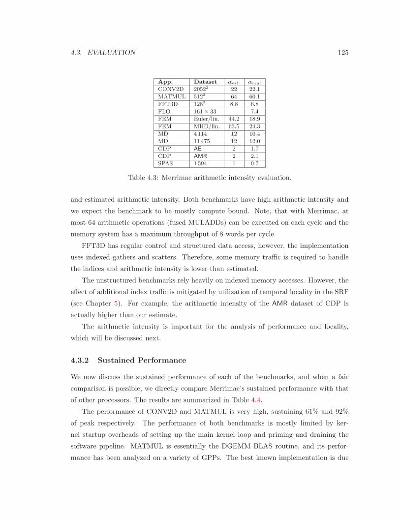
4.3. EVALUATION 125
App. Dataset αest. αreal
CONV2D 20522 22 22.1
MATMUL 5122 64 60.1
FFT3D 1283 8.8 6.8
FLO 161 × 33 7.4
FEM Euler/lin. 44.2 18.9
FEM MHD/lin. 63.5 24.3
MD 4114 12 10.4
MD 11 475 12 12.0
CDP AE 2 1.7
CDP AMR 2 2.1
SPAS 1 594 1 0.7
Table 4.3: Merrimac arithmetic intensity evaluation.
and estimated arithmetic intensity. Both benchmarks have high arithmetic intensity and
we expect the benchmark to be mostly compute bound. Note, that with Merrimac, at
most 64 arithmetic operations (fused MULADDs) can be executed on each cycle and the
memory system has a maximum throughput of 8 words per cycle.
FFT3D has regular control and structured data access, however, the implementation
uses indexed gathers and scatters. Therefore, some memory traffic is required to handle
the indices and arithmetic intensity is lower than estimated.
The unstructured benchmarks rely heavily on indexed memory accesses. However, the
effect of additional index traffic is mitigated by utilization of temporal locality in the SRF
(see Chapter 5). For example, the arithmetic intensity of the AMR dataset of CDP is
actually higher than our estimate.
The arithmetic intensity is important for the analysis of performance and locality,
which will be discussed next.
4.3.2 Sustained Performance
We now discuss the sustained performance of each of the benchmarks, and when a fair
comparison is possible, we directly compare Merrimac’s sustained performance with that
of other processors. The results are summarized in Table 4.4.
The performance of CONV2D and MATMUL is very high, sustaining 61% and 92%
of peak respectively. The performance of both benchmarks is mostly limited by ker-
nel startup overheads of setting up the main kernel loop and priming and draining the
software pipeline. MATMUL is essentially the DGEMM BLAS routine, and its perfor-
mance has been analyzed on a variety of GPPs. The best known implementation is due
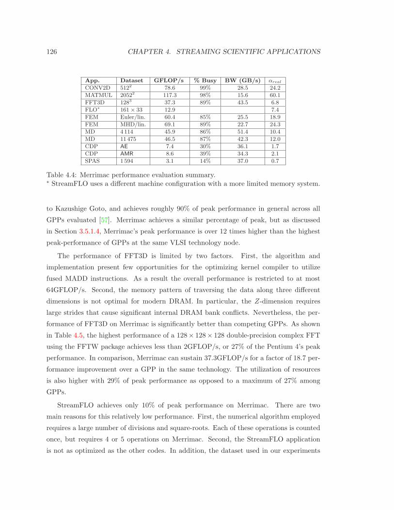
126 CHAPTER 4. STREAMING SCIENTIFIC APPLICATIONS
App. Dataset GFLOP/s % Busy BW (GB/s) αreal
CONV2D 5122 78.6 99% 28.5 24.2
MATMUL 20522 117.3 98% 15.6 60.1
FFT3D 1283 37.3 89% 43.5 6.8
FLO∗ 161 × 33 12.9 7.4
FEM Euler/lin. 60.4 85% 25.5 18.9
FEM MHD/lin. 69.1 89% 22.7 24.3
MD 4114 45.9 86% 51.4 10.4
MD 11 475 46.5 87% 42.3 12.0
CDP AE 7.4 30% 36.1 1.7
CDP AMR 8.6 39% 34.3 2.1
SPAS 1 594 3.1 14% 37.0 0.7
Table 4.4: Merrimac performance evaluation summary.∗ StreamFLO uses a different machine configuration with a more limited memory system.
to Kazushige Goto, and achieves roughly 90% of peak performance in general across all
GPPs evaluated [57]. Merrimac achieves a similar percentage of peak, but as discussed
in Section 3.5.1.4, Merrimac’s peak performance is over 12 times higher than the highest
peak-performance of GPPs at the same VLSI technology node.
The performance of FFT3D is limited by two factors. First, the algorithm and
implementation present few opportunities for the optimizing kernel compiler to utilize
fused MADD instructions. As a result the overall performance is restricted to at most
64GFLOP/s. Second, the memory pattern of traversing the data along three different
dimensions is not optimal for modern DRAM. In particular, the Z-dimension requires
large strides that cause significant internal DRAM bank conflicts. Nevertheless, the per-
formance of FFT3D on Merrimac is significantly better than competing GPPs. As shown
in Table 4.5, the highest performance of a 128× 128× 128 double-precision complex FFT
using the FFTW package achieves less than 2GFLOP/s, or 27% of the Pentium 4’s peak
performance. In comparison, Merrimac can sustain 37.3GFLOP/s for a factor of 18.7 per-
formance improvement over a GPP in the same technology. The utilization of resources
is also higher with 29% of peak performance as opposed to a maximum of 27% among
GPPs.
StreamFLO achieves only 10% of peak performance on Merrimac. There are two
main reasons for this relatively low performance. First, the numerical algorithm employed
requires a large number of divisions and square-roots. Each of these operations is counted
once, but requires 4 or 5 operations on Merrimac. Second, the StreamFLO application
is not as optimized as the other codes. In addition, the dataset used in our experiments
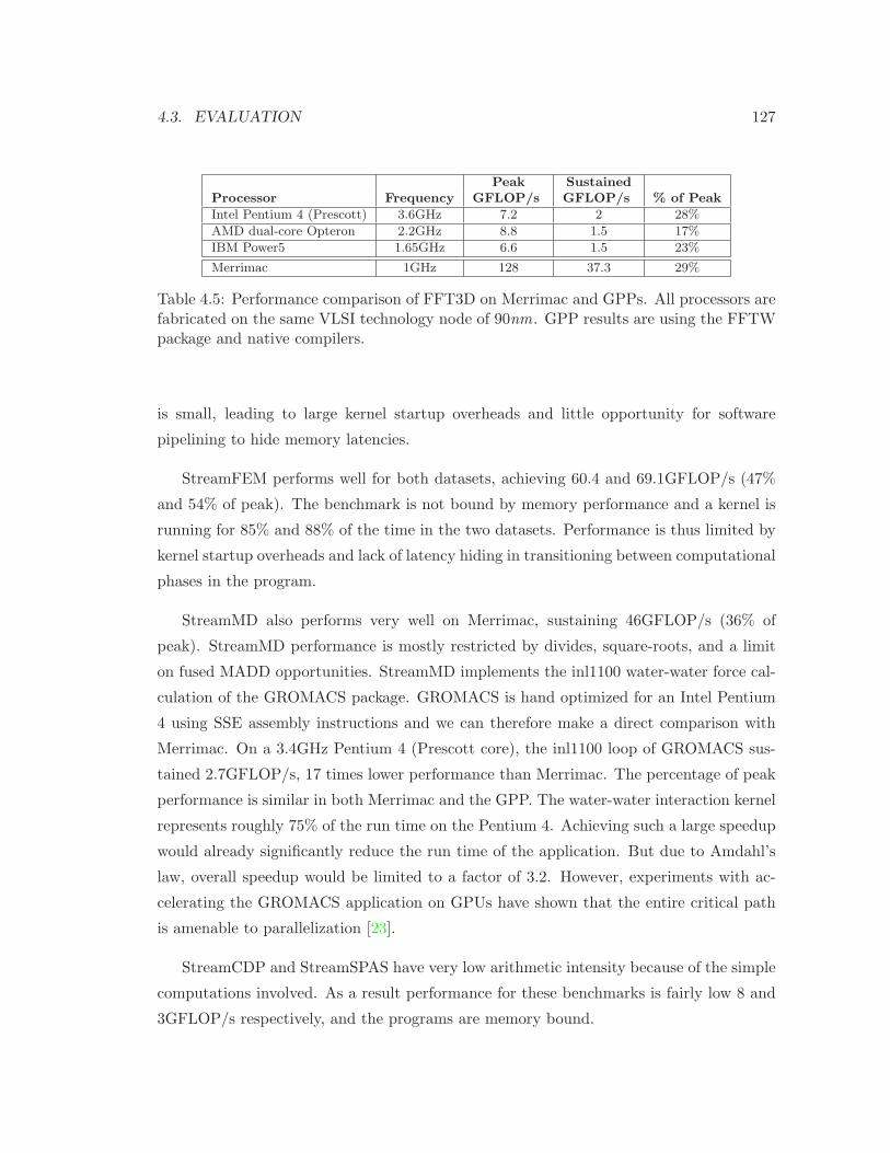
4.3. EVALUATION 127
Peak SustainedProcessor Frequency GFLOP/s GFLOP/s % of Peak
Intel Pentium 4 (Prescott) 3.6GHz 7.2 2 28%
AMD dual-core Opteron 2.2GHz 8.8 1.5 17%
IBM Power5 1.65GHz 6.6 1.5 23%
Merrimac 1GHz 128 37.3 29%
Table 4.5: Performance comparison of FFT3D on Merrimac and GPPs. All processors arefabricated on the same VLSI technology node of 90nm. GPP results are using the FFTWpackage and native compilers.
is small, leading to large kernel startup overheads and little opportunity for software
pipelining to hide memory latencies.
StreamFEM performs well for both datasets, achieving 60.4 and 69.1GFLOP/s (47%
and 54% of peak). The benchmark is not bound by memory performance and a kernel is
running for 85% and 88% of the time in the two datasets. Performance is thus limited by
kernel startup overheads and lack of latency hiding in transitioning between computational
phases in the program.
StreamMD also performs very well on Merrimac, sustaining 46GFLOP/s (36% of
peak). StreamMD performance is mostly restricted by divides, square-roots, and a limit
on fused MADD opportunities. StreamMD implements the inl1100 water-water force cal-
culation of the GROMACS package. GROMACS is hand optimized for an Intel Pentium
4 using SSE assembly instructions and we can therefore make a direct comparison with
Merrimac. On a 3.4GHz Pentium 4 (Prescott core), the inl1100 loop of GROMACS sus-
tained 2.7GFLOP/s, 17 times lower performance than Merrimac. The percentage of peak
performance is similar in both Merrimac and the GPP. The water-water interaction kernel
represents roughly 75% of the run time on the Pentium 4. Achieving such a large speedup
would already significantly reduce the run time of the application. But due to Amdahl’s
law, overall speedup would be limited to a factor of 3.2. However, experiments with ac-
celerating the GROMACS application on GPUs have shown that the entire critical path
is amenable to parallelization [23].
StreamCDP and StreamSPAS have very low arithmetic intensity because of the simple
computations involved. As a result performance for these benchmarks is fairly low 8 and
3GFLOP/s respectively, and the programs are memory bound.
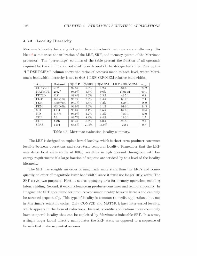
128 CHAPTER 4. STREAMING SCIENTIFIC APPLICATIONS
4.3.3 Locality Hierarchy
Merrimac’s locality hierarchy is key to the architecture’s performance and efficiency. Ta-
ble 4.6 summarizes the utilization of the LRF, SRF, and memory system of the Merrimac
processor. The “percentage” columns of the table present the fraction of all operands
required by the computation satisfied by each level of the storage hierarchy. Finally, the
“LRF:SRF:MEM” column shows the ratios of accesses made at each level, where Merri-
mac’s bandwidth hierarchy is set to 64:8:1 LRF:SRF:MEM relative bandwidths.
App. Dataset %LRF %SRF %MEM LRF:SRF:MEM αreal
CONV2D 5122 92.8% 6.0% 1.2% 84:6:1 24.2
MATMUL 20522 93.9% 5.6% 0.6% 178:11:1 60.1
FFT3D 1283 88.6% 9.0% 2.3% 43:5:1 6.8
FLO∗ 161 × 33 95.7% 2.9% 1.4% 68:2:1 7.4
FEM Euler/lin. 93.3% 5.5% 1.2% 82:5:1 18.9
FEM MHD/lin. 93.9% 5.0% 1.1% 91:6:1 24.3
MD 4 114 95.5% 3.1% 1.5% 67:3:1 10.4
MD 11 475 95.9% 2.7% 1.3% 74:3:1 12.0
CDP AE 82.7% 8.9% 8.4% 12:2:1 1.7
CDP AMR 86.4% 8.6% 5.0% 20:3:1 2.1
SPAS 1 594 63.5% 21.6% 14.9% 7:2:1 0.7
Table 4.6: Merrimac evaluation locality summary.
The LRF is designed to exploit kernel locality, which is short-term producer-consumer
locality between operations and short-term temporal locality. Remember that the LRF
uses dense local wires (order of 100χ), resulting in high operand throughput with low
energy requirements if a large fraction of requests are serviced by this level of the locality
hierarchy.
The SRF has roughly an order of magnitude more state than the LRFs and conse-
quently an order of magnitude lower bandwidth, since it must use longer 103χ wires. The
SRF serves two purposes. First, it acts as a staging area for memory operations enabling
latency hiding. Second, it exploits long-term producer-consumer and temporal locality. In
Imagine, the SRF specialized for producer-consumer locality between kernels and can only
be accessed sequentially. This type of locality is common to media applications, but not
in Merrimac’s scientific codes. Only CONV2D and MATMUL have inter-kernel locality,
which appears in the form of reductions. Instead, scientific applications more commonly
have temporal locality that can be exploited by Merrimac’s indexable SRF. In a sense,
a single larger kernel directly manipulates the SRF state, as opposed to a sequence of
kernels that make sequential accesses.

4.3. EVALUATION 129
CONV2D, MATMUL, FFT3D, StreamFLO, StreamMD, and StreamFEM all have
significant arithmetic intensity, presenting large amounts of kernel locality. Roughly 90%
of references in these benchmarks are satisfied from the LRF. The SRF, in these programs,
is used to provide 3 − 9% of the values, while no more than roughly 2% of requests reach
the memory system.
While StreamCDP has low arithmetic intensity and low kernel locality, the benchmark
still utilizes the SRF for temporal locality, and no more than 8.4% of requests are serviced
by the memory system.
StreamSPAS is an extreme case, where the arithmetic intensity is under 1. As a result,
the memory system is heavily taxed and must handle nearly 15% of the operands.
Chapter 5
Unstructured and Irregular
Algorithms
Merrimac achieves its efficiency and high performance advantage over GPPs by relying on
the highly parallel compute clusters, hardware structures that are tuned for minimal data-
dependent control, and the explicitly software managed storage hierarchy that is optimized
for sequential access. Regular, structured codes map well to this set of characteristics,
however, mapping irregular or unstructured computations from the scientific computing
domain presents significant challenges.
In this chapter we focus on mapping the irregular control and data access of unstruc-
tured mesh and graph algorithms to Merrimac. There is a rich body of research on exe-
cuting irregular applications on a variety of architectures [50, 26, 94, 51, 20, 91, 143, 142].
We draw from this prior work, adapt it, and evaluate new techniques in the context of the
unique properties of Merrimac.
First, Merrimac has an explicitly software managed storage hierarchy that requires
data to be localized to the SRF before computation can take place. The localization step
is challenging for unstructured mesh applications because the neighborhoods of nodes in
the mesh cannot be expressed as simple expressions and are data dependent.
Second, computation must be parallelized onto the compute clusters featuring limited
hardware support for data-dependent branching and tightly coupled VLIW and LRF con-
trol. However, the irregular control of the computation does not map directly onto this
compute substrate and must be regularized to some degree.
We propose a framework for representing the properties of irregular unstructured mesh
130

5.1. FRAMEWORK FOR UNSTRUCTURED APPLICATIONS 131
and graph applications in the context of Merrimac and stream processing in Section 5.1.
Based on this framework we then develop both a methodology and techniques for mapping
irregular applications onto Merrimac. We focus on localization and parallelization and de-
scribing the tradeoffs involved based on application properties (Section 5.2). We evaluate
the performance of the mapping schemes on our unstructured and irregular benchmarks
(StreamFEM, StreamMD, StreamCDP, and StreamSPAS), and draw conclusions on the
benefits of Merrimac’s hardware mechanisms (Section 5.3). We also situate the constraints
on mapping presented by stream architectures in the context of prior work (Section 5.4).
5.1 Framework for Unstructured Mesh and Graph Applica-
tions
Many scientific modeling applications contain irregular computation on unstructured mesh
or graph data. The unstructured data is a result of efficient representations of complex
physical systems. For example, the algorithm used in StreamMD uses neighbor lists to
approximate an O(n2) calculation as O(n). Irregularity in computation and data accesses
is a result of the graph structures used to represent the physical system model, and the
spatial dependence of the model on the topology. In this section we develop a framework
for representing such irregular computation applications and characterize their fundamen-
tal properties. We explore the StreamFEM, StreamCDP, StreamMD, and StreamSPAS
application, which represent applications from the FEM, FVM, direct n-body, and sparse
algebra domains.
A canonical irregular unstructured application consists of potentially multiple phases
that process the nodes and neighbors in the graph representing the data and computation,
as shown in Figure 5.1(a). Typically, scientific computation is strip-mined [104] – par-
titioned into subcomputations that each processes a portion of the data (Figure 5.1(b)).
The amount of computation and data accesses required for the processing functions, as
well as the connectivity properties of the graph affect how an algorithm should be mapped
to stream processors.
5.1.1 Application Parameter Space
Table 5.1 summarizes the properties of the applications. The properties are discussed in
detail in the following subsections. For StreamFEM and StreamCDP, we separate the

132 CHAPTER 5. UNSTRUCTURED AND IRREGULAR ALGORITHMS
for (i=0; i<num_nodes; i++) {
process_node(nodes[i]);
for (j=neighbor_starts [i]; j<neighbor_starts [i+1]; j++) {
process_neighbor(neighbors[neighbor_list [j]]);
}
}
(a) Canonical unstructured irregular computation.
for (s=0; s<num_strips; s++) {
for (i=node_starts[s]; i<node_starts[s+1]; i++) {
process_node(nodes[i]);
for (j=neighbor_starts [i]; j<neighbor_starts [i+1]; j++) {
process_neighbor(neighbors[neighbor_list [j]]);
}
}
}
(b) Stripmined unstructured irregular computation.
Figure 5.1: Pseudocode for canonical unstructured irregular computation and its strip-mined version.
properties of the element (CV) loop and face loop. We also describe the properties of
both the Euler-linear and MHD-linear StreamFEM configurations. In addition to the two
datasets of StreamCDP and StreamMD described in the previous chapter, we also present
properties for larger datasets, for which simulation times were unreasonably high. For
StreamCDP, we add a dataset representing the Pratt & Whitney PW6000 jet turbine
engine with 1, 278, 374 CVs, and for StreamMD a dataset with 57, 556 water molecules.
5.1.1.1 Mesh Connectivity Degree and Variability
The connectivity degree, i.e., the number of neighbors of each node, is an important metric
which affects the locality of data access, the amount of communication, and the style
of implementation on a stream architecture. A high connectivity degree tends to place
greater pressure on the processor’s communication and on-chip storage resources, because
data for all neighbors must be read in advance before processing a node when using the
stream execution model. A large number of neighbors also deemphasizes the arithmetic
properties of the node processing (columns 5 and 7 in Table 5.1). The applications based
on element meshes have a low degree, whereas n-body and sparse algebra tend to have a
large number of average neighbors. StreamMD in particular has a very large number of
potential neighbors, where over 20% of nodes have more than 40 neighbors and over 5%
of nodes have more than 80 neighbors.
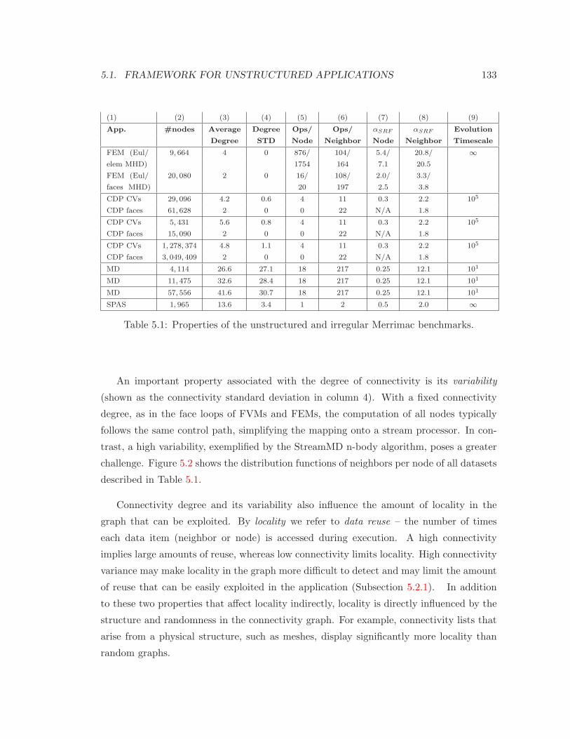
5.1. FRAMEWORK FOR UNSTRUCTURED APPLICATIONS 133
(1) (2) (3) (4) (5) (6) (7) (8) (9)
App. #nodes Average Degree Ops/ Ops/ αSRF αSRF Evolution
Degree STD Node Neighbor Node Neighbor Timescale
FEM (Eul/ 9, 664 4 0 876/ 104/ 5.4/ 20.8/ ∞elem MHD) 1754 164 7.1 20.5
FEM (Eul/ 20, 080 2 0 16/ 108/ 2.0/ 3.3/
faces MHD) 20 197 2.5 3.8
CDP CVs 29, 096 4.2 0.6 4 11 0.3 2.2 105
CDP faces 61, 628 2 0 0 22 N/A 1.8
CDP CVs 5, 431 5.6 0.8 4 11 0.3 2.2 105
CDP faces 15, 090 2 0 0 22 N/A 1.8
CDP CVs 1, 278, 374 4.8 1.1 4 11 0.3 2.2 105
CDP faces 3, 049, 409 2 0 0 22 N/A 1.8
MD 4, 114 26.6 27.1 18 217 0.25 12.1 101
MD 11, 475 32.6 28.4 18 217 0.25 12.1 101
MD 57, 556 41.6 30.7 18 217 0.25 12.1 101
SPAS 1, 965 13.6 3.4 1 2 0.5 2.0 ∞
Table 5.1: Properties of the unstructured and irregular Merrimac benchmarks.
An important property associated with the degree of connectivity is its variability
(shown as the connectivity standard deviation in column 4). With a fixed connectivity
degree, as in the face loops of FVMs and FEMs, the computation of all nodes typically
follows the same control path, simplifying the mapping onto a stream processor. In con-
trast, a high variability, exemplified by the StreamMD n-body algorithm, poses a greater
challenge. Figure 5.2 shows the distribution functions of neighbors per node of all datasets
described in Table 5.1.
Connectivity degree and its variability also influence the amount of locality in the
graph that can be exploited. By locality we refer to data reuse – the number of times
each data item (neighbor or node) is accessed during execution. A high connectivity
implies large amounts of reuse, whereas low connectivity limits locality. High connectivity
variance may make locality in the graph more difficult to detect and may limit the amount
of reuse that can be easily exploited in the application (Subsection 5.2.1). In addition
to these two properties that affect locality indirectly, locality is directly influenced by the
structure and randomness in the connectivity graph. For example, connectivity lists that
arise from a physical structure, such as meshes, display significantly more locality than
random graphs.

134 CHAPTER 5. UNSTRUCTURED AND IRREGULAR ALGORITHMS
0%
10%
20%
30%
40%
50%
60%
70%
80%
1 2 3 4 5 6
(a) StreamCDP, AE, 29, 096 nodes.
0%
10%
20%
30%
40%
50%
60%
70%
1 2 3 4 5 6 7 8
(b) StreamCDP, AMR, 5, 431 nodes.
0%
5%
10%
15%
20%
25%
30%
35%
40%
45%
50%
1 2 3 4 5 6
(c) StreamCDP, PW6000, 1, 278, 374nodes.
0%
2%
4%
6%
8%
10%
12%
1 12 23 34 45 56 67 78 89 100 111 122
(d) StreamMD, 4, 114 nodes.
0%
1%
2%
3%
4%
5%
6%
7%
8%
9%
1 11 21 31 41 51 61 71 81 91 101 111 121
(e) StreamMD, 11, 475 nodes.
0%
1%
2%
3%
4%
5%
6%
1 12 23 34 45 56 67 78 89 100 111 122 133
(f) StreamMD, 57, 556 nodes.
0%
2%
4%
6%
8%
10%
12%
14%
16%
1 3 5 7 9 11 13 15 17 19 21 23
(g) StreamSPAS, 1, 965 nodes.
Figure 5.2: Neighbor per node distributions of irregular unstructured mesh datasets.

5.1. FRAMEWORK FOR UNSTRUCTURED APPLICATIONS 135
5.1.1.2 Arithmetic Intensity
We represent the computational properties of the application inner loops using four pa-
rameters: the number of arithmetic operations performed on each individual node and
neighbor (process node and process neighbor in Figure 5.1 and columns 5–6 in Ta-
ble 5.1); and the kernel-to-SRF arithmetic intensity – the ratio between arithmetic oper-
ations and the number of input and output words required to compute them in the loop
(columns 7–8).
Computations with a low operation count often do not utilize the many functional
units of a stream processor well because compiler techniques, such as software pipelining
and loop unrolling [96], are hindered by the irregularity of control and data-dependent
loop bounds seen in the canonical pseudocode representation (see also Section 5.3.1). A
low arithmetic intensity also reduces inner loop execution performance as it is limited
by on-chip memory bandwidth. Additionally, applications with low arithmetic intensity
may require sophisticated software mapping techniques or hardware structures to reduce
off-chip bandwidth demands and avoid stalls while waiting on off-chip memory.
For some applications, arithmetic intensity and operation counts are higher if more
accurate physical modeling algorithms, which are more computationally demanding, are
used. For example in StreamFEM, a higher order interpolation could be used.
5.1.1.3 Runtime Properties
A final property of unstructured mesh and graph applications is the rate at which the
connectivity graph evolves in relation to the algorithm time steps (column 9 of Table 5.1).
While some benchmarks, such as StreamFEM and StreamSPAS have a fixed connectivity,
other benchmarks evolve their graph structure over time. For example, StreamCDP may
occasionally applies an adaptive mesh refinement technique to account for changes in the
physical model, and StreamMD (GROMACS) recomputes the molecule interaction list
every several (∼ 10) time steps.
Graph evolution on a small time scale implies that only minimal preprocessing of the
connectivity graph is possible without negatively impacting the application performance.

136 CHAPTER 5. UNSTRUCTURED AND IRREGULAR ALGORITHMS
5.2 Exploiting Locality and Parallelism
The stream execution model requires the distinct SRF address space and advocates a
gather–compute–scatter style, where overall execution is broken down into computational
strips as with the strip-mining technique [104]. A prototypical example of a strip-mined
program is shown Figure 5.1(b). However, requiring all data that an inner-loop computa-
tion accesses to be gathered ahead of the computation poses a problem for the irregular
accesses of unstructured mesh algorithms. Additional complexity relates to the tradeoffs
of indexed vs. sequential access to the SRF, whether cross-lane accesses are employed,
and tradeoffs relating to SRF and stream cache sizes. We explore different methods for
performing the localization step and their effect on the computation in Subsection 5.2.1.
The strong reliance of stream processors on SIMD execution for parallelism poses
problems for irregular unstructured computation. We cannot simply map the computation
of Figure 5.1 as it requires different control paths for different nodes as the number of
neighbors per node varies. We discuss how to address this issue in stream processors in
Subsection 5.2.2 and mention alternative MIMD architectures as well.
5.2.1 Localization
Merrimac restricts all heavy computation to kernels executing on the compute clusters.
Kernels cannot make arbitrary memory references, but rather must access the SRF local
memory. Unlike GPPs, the local memories have distinct name-spaces; as a result localiza-
tion implies that data elements must be renamed to the local SRF address space. This is
similar to the requirements of distributed memory parallel systems, although the granu-
larity of control and degree of runtime overhead that can be tolerated is much lower in the
case of Merrimac because of the relatively small size of the SRF (8KWords per cluster).
The renaming process entails re-writing the neighbor-list pointers to local memory
addresses in a processing step separate from the actual computation. This process is
similar to the inspector–executor model [143, 91], where the program is run in two phases.
The first phase inspects the execution of all control code and collects all references that
must be made in order to perform the actual computation in the executor phase. While
renaming is performed, additional optimizations can be applied. We first describe the
basic localization scheme that has minimal preprocessing overhead and can be performed
statically without knowledge of the connectivity. We then discuss an optimization that

5.2. EXPLOITING LOCALITY AND PARALLELISM 137
removes duplicate elements referred to by the neighbor list. Removing duplicates has two
main benefits: reducing the required off-chip bandwidth as data reads are not repeated,
and improving utilization of on-chip memory by eliminating copies of neighbor elements
leading to longer computational strips.
5.2.1.1 Basic Renaming
With non-duplicate-removal renaming (nDR), each element of the neighbor list is assigned
a unique location in the SRF. This amounts to dereferencing the neighbor-list pointers
as they are transferred into the SRF. As a result, duplicate entries may be allocated for
a neighbor that is shared between several nodes and is referred to multiple times in the
neighbor lists. The computational inner loop processes the neighbor data in order out of
the SRF as shown in Figure 5.3. The number of neighbor data elements transferred and
stored in the SRF is equal to the total length of the neighbor list.
for (s=0; s<num_strips; s++) {
strip_neighbor_start = neighbor_starts [node_starts[s]];
strip_num_neighbors = neighbor_starts [node_starts[s+1]] -
neighbor_starts [node_starts[s]];
// localize data (gather performed by
// the memory system)
for (i=0; i<strip_num_neighbors ; i++) {
local_nl[i] = neighbor_data [neighbor_list [strip_neighbor_starts +i]];
}
for (i=0; i< (node_starts[i+1]- node_starts[s]); i++) {
local_nodes[i] = node_data[i+node_starts[s]];
}
for (i=0; i< (node_starts[i+1]- node_starts[s]); i++) {
local_nn[i] = neighbors_per_node [i+node_starts[s]];
}
// process from local memory
for (i=0; i< (node_starts[i+1]- node_starts[s]); i++) {
n_ptr =0; // current location in local_nl
process_node(local_nodes[i]);
for (j=0; j<local_nn[i]; j++) {
process_neighbor(local_nl[n_ptr ++]);
}
}
}
Figure 5.3: Pseudocode for nDR processing (local prefix refers to data that has beenlocalized to cluster).
The main advantage of this scheme is that its implementation is independent of the
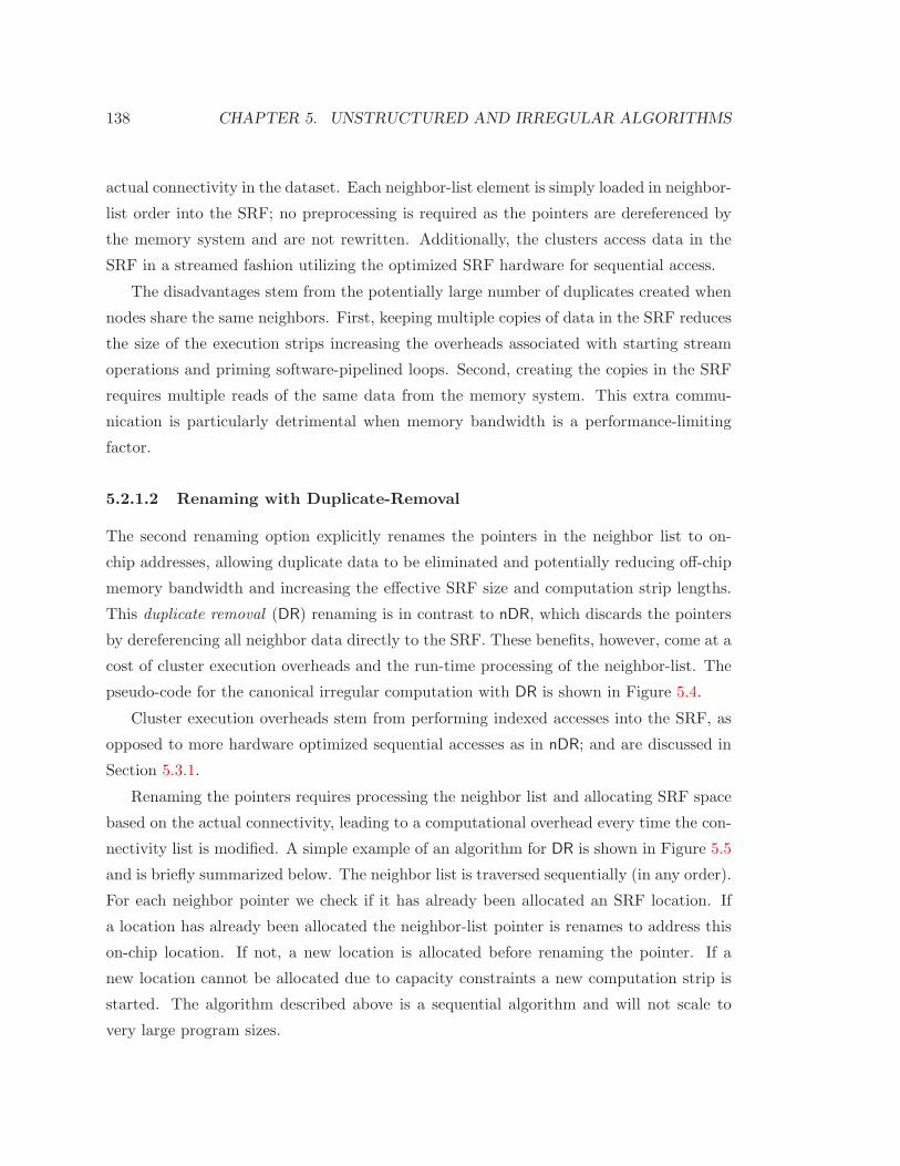
138 CHAPTER 5. UNSTRUCTURED AND IRREGULAR ALGORITHMS
actual connectivity in the dataset. Each neighbor-list element is simply loaded in neighbor-
list order into the SRF; no preprocessing is required as the pointers are dereferenced by
the memory system and are not rewritten. Additionally, the clusters access data in the
SRF in a streamed fashion utilizing the optimized SRF hardware for sequential access.
The disadvantages stem from the potentially large number of duplicates created when
nodes share the same neighbors. First, keeping multiple copies of data in the SRF reduces
the size of the execution strips increasing the overheads associated with starting stream
operations and priming software-pipelined loops. Second, creating the copies in the SRF
requires multiple reads of the same data from the memory system. This extra commu-
nication is particularly detrimental when memory bandwidth is a performance-limiting
factor.
5.2.1.2 Renaming with Duplicate-Removal
The second renaming option explicitly renames the pointers in the neighbor list to on-
chip addresses, allowing duplicate data to be eliminated and potentially reducing off-chip
memory bandwidth and increasing the effective SRF size and computation strip lengths.
This duplicate removal (DR) renaming is in contrast to nDR, which discards the pointers
by dereferencing all neighbor data directly to the SRF. These benefits, however, come at a
cost of cluster execution overheads and the run-time processing of the neighbor-list. The
pseudo-code for the canonical irregular computation with DR is shown in Figure 5.4.
Cluster execution overheads stem from performing indexed accesses into the SRF, as
opposed to more hardware optimized sequential accesses as in nDR; and are discussed in
Section 5.3.1.
Renaming the pointers requires processing the neighbor list and allocating SRF space
based on the actual connectivity, leading to a computational overhead every time the con-
nectivity list is modified. A simple example of an algorithm for DR is shown in Figure 5.5
and is briefly summarized below. The neighbor list is traversed sequentially (in any order).
For each neighbor pointer we check if it has already been allocated an SRF location. If
a location has already been allocated the neighbor-list pointer is renames to address this
on-chip location. If not, a new location is allocated before renaming the pointer. If a
new location cannot be allocated due to capacity constraints a new computation strip is
started. The algorithm described above is a sequential algorithm and will not scale to
very large program sizes.

5.2. EXPLOITING LOCALITY AND PARALLELISM 139
The efficiency of the DR method, in terms of reducing SRF space usage and off-chip
bandwidth, depends on the mesh locality properties. If the mesh has high locality and
a high connectivity degree large amounts of neighbor storage can be removed. On the
other hand if the connectivity or locality are very low, there is little to be gained by
removing duplicates and this mapping option should not be chosen due to the increased
preprocessing and execution overheads (see Section 5.3.2).
Figures 5.6–5.7 presents the locality available in the unstructured mesh datasets used
in this study as a function of available local memory space. We do not present results
for StreamSPAS because the vector in our dataset is small, and all possible locality is
exploited. In each figure, the horizontal axis is the number of neighbor elements that
// remove duplicates
// reads neighbor list and produces
// duplicate removed data (DR_data), the rewritten pointers (DR_nl),
// and the associated stripping information
DR(neighbor_list , output_DR_nl , output_DR_data , output_DR_starts );
// see next figure for sample pseudocode for DR()
for (s=0; s<num_strips; s++) {
strip_neighbor_start = neighbor_starts [node_starts[s]];
strip_num_neighbors = neighbor_starts [node_starts[s+1]] -
neighbor_starts [node_starts[s]];
// localize data (gather performed by
// the memory system)
for (i=0; i<strip_num_neighbors ; i++) {
local_DR_nl[i] = output_DR_nl[neighbor_list [strip_neighbor_starts +i]];
}
for (i=0; i< (node_starts[i+1]- node_starts[s]); i++) {
local_nodes[i] = node_data[i+node_starts[s]];
}
for (i=0; i< (node_starts[i+1]- node_starts[s]); i++) {
local_nn[i] = neighbors_per_node [i+node_starts[s]];
}
for (i=0; i<( output_DR_starts[s+1]- output_DR_starts[s]) {
local_DR_data [i] = output_DR_data[i+output_DR_starts[s];
}
// process from local memory
for (i=0; i< (node_starts[i+1]- node_starts[s]); i++) {
n_ptr =0; // current location in local_nl
process_node(local_nodes[i]);
for (j=0; j<local_nn[i]; j++) {
process_neighbor(local_DR_data [local_DR_nl[n_ptr ++]]);
}
}
}
Figure 5.4: Pseudocode for DR processing (local prefix refers to data that has beenlocalized to the cluster).
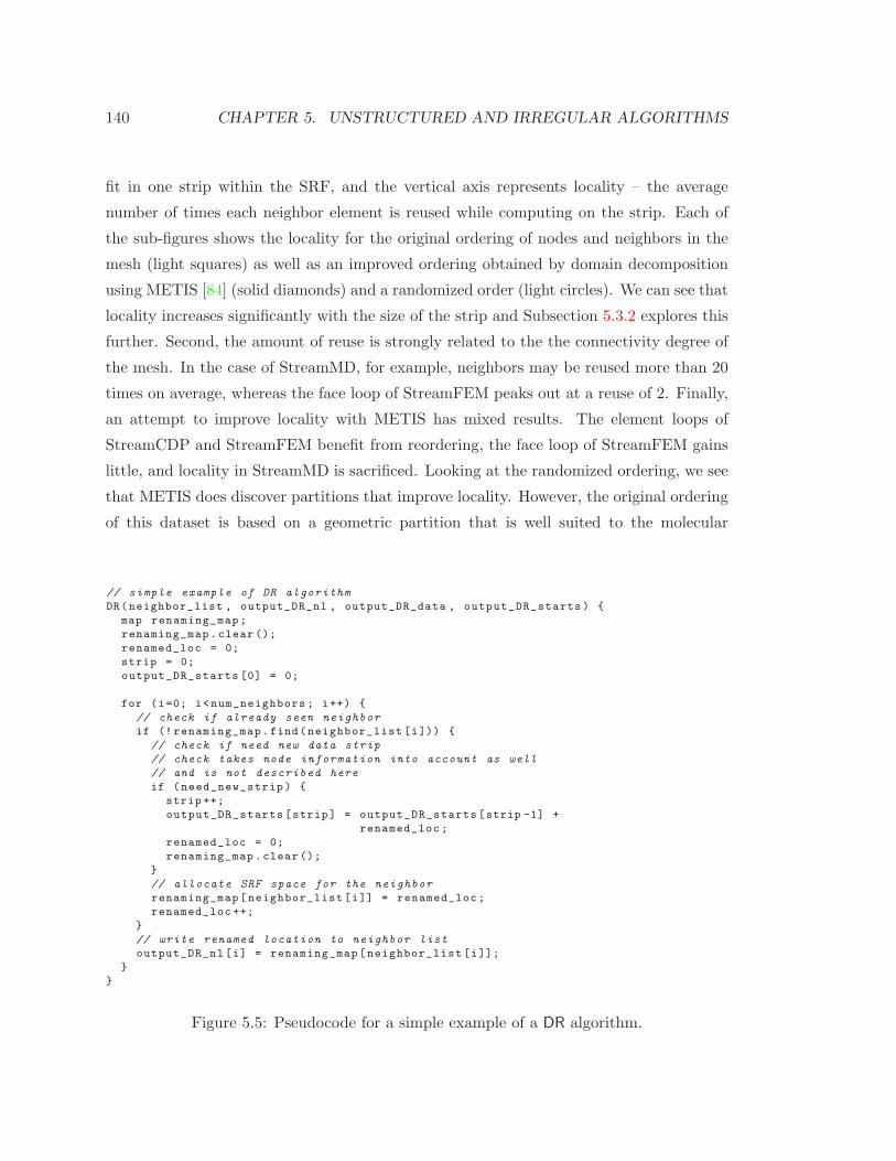
140 CHAPTER 5. UNSTRUCTURED AND IRREGULAR ALGORITHMS
fit in one strip within the SRF, and the vertical axis represents locality – the average
number of times each neighbor element is reused while computing on the strip. Each of
the sub-figures shows the locality for the original ordering of nodes and neighbors in the
mesh (light squares) as well as an improved ordering obtained by domain decomposition
using METIS [84] (solid diamonds) and a randomized order (light circles). We can see that
locality increases significantly with the size of the strip and Subsection 5.3.2 explores this
further. Second, the amount of reuse is strongly related to the the connectivity degree of
the mesh. In the case of StreamMD, for example, neighbors may be reused more than 20
times on average, whereas the face loop of StreamFEM peaks out at a reuse of 2. Finally,
an attempt to improve locality with METIS has mixed results. The element loops of
StreamCDP and StreamFEM benefit from reordering, the face loop of StreamFEM gains
little, and locality in StreamMD is sacrificed. Looking at the randomized ordering, we see
that METIS does discover partitions that improve locality. However, the original ordering
of this dataset is based on a geometric partition that is well suited to the molecular
// simple example of DR algorithm
DR(neighbor_list , output_DR_nl , output_DR_data , output_DR_starts) {
map renaming_map;
renaming_map.clear ();
renamed_loc = 0;
strip = 0;
output_DR_starts [0] = 0;
for (i=0; i<num_neighbors ; i++) {
// check if already seen neighbor
if (! renaming_map.find(neighbor_list [i])) {
// check if need new data strip
// check takes node information into account as well
// and is not described here
if (need_new_strip) {
strip ++;
output_DR_starts[strip] = output_DR_starts[strip -1] +
renamed_loc;
renamed_loc = 0;
renaming_map.clear ();
}
// allocate SRF space for the neighbor
renaming_map[neighbor_list [i]] = renamed_loc;
renamed_loc ++;
}
// write renamed location to neighbor list
output_DR_nl[i] = renaming_map[neighbor_list [i]];
}
}
Figure 5.5: Pseudocode for a simple example of a DR algorithm.
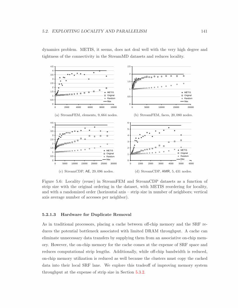
5.2. EXPLOITING LOCALITY AND PARALLELISM 141
dynamics problem. METIS, it seems, does not deal well with the very high degree and
tightness of the connectivity in the StreamMD datasets and reduces locality.
0
0.5
1
1.5
2
2.5
3
3.5
4
4.5
0 2000 4000 6000 8000 10000
METISOriginalRandomMax
(a) StreamFEM, elements, 9, 664 nodes.
0
0.5
1
1.5
2
2.5
0 5000 10000 15000 20000
METISOriginalRandomMax
(b) StreamFEM, faces, 20, 080 nodes.
0
0.5
1
1.5
2
2.5
3
3.5
4
4.5
0 5000 10000 15000 20000 25000 30000
METISOriginalRandomMax
(c) StreamCDP, AE, 29, 096 nodes.
0
1
2
3
4
5
6
0 1000 2000 3000 4000 5000 6000
METISOriginalRandomMax
(d) StreamCDP, AMR, 5, 431 nodes.
Figure 5.6: Locality (reuse) in StreamFEM and StreamCDP datasets as a function ofstrip size with the original ordering in the dataset, with METIS reordering for locality,and with a randomized order (horizontal axis – strip size in number of neighbors; verticalaxis average number of accesses per neighbor).
5.2.1.3 Hardware for Duplicate Removal
As in traditional processors, placing a cache between off-chip memory and the SRF re-
duces the potential bottleneck associated with limited DRAM throughput. A cache can
eliminate unnecessary data transfers by supplying them from an associative on-chip mem-
ory. However, the on-chip memory for the cache comes at the expense of SRF space and
reduces computational strip lengths. Additionally, while off-chip bandwidth is reduced,
on-chip memory utilization is reduced as well because the clusters must copy the cached
data into their local SRF lane. We explore this tradeoff of improving memory system
throughput at the expense of strip size in Section 5.3.2.
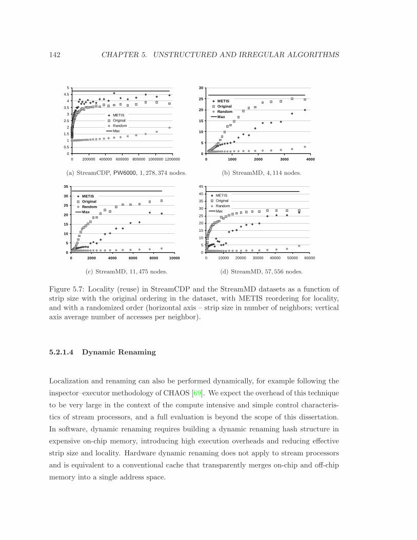
142 CHAPTER 5. UNSTRUCTURED AND IRREGULAR ALGORITHMS
0
0.5
1
1.5
2
2.5
3
3.5
4
4.5
5
0 200000 400000 600000 800000 1000000 1200000
METISOriginalRandomMax
(a) StreamCDP, PW6000, 1, 278, 374 nodes.
0
5
10
15
20
25
30
0 1000 2000 3000 4000
METISOriginalRandomMax
(b) StreamMD, 4, 114 nodes.
0
5
10
15
20
25
30
35
0 2000 4000 6000 8000 10000
METISOriginalRandomMax
(c) StreamMD, 11, 475 nodes.
0
5
10
15
20
25
30
35
40
45
0 10000 20000 30000 40000 50000 60000
METISOriginalRandomMax
(d) StreamMD, 57, 556 nodes.
Figure 5.7: Locality (reuse) in StreamCDP and the StreamMD datasets as a function ofstrip size with the original ordering in the dataset, with METIS reordering for locality,and with a randomized order (horizontal axis – strip size in number of neighbors; verticalaxis average number of accesses per neighbor).
5.2.1.4 Dynamic Renaming
Localization and renaming can also be performed dynamically, for example following the
inspector–executor methodology of CHAOS [69]. We expect the overhead of this technique
to be very large in the context of the compute intensive and simple control characteris-
tics of stream processors, and a full evaluation is beyond the scope of this dissertation.
In software, dynamic renaming requires building a dynamic renaming hash structure in
expensive on-chip memory, introducing high execution overheads and reducing effective
strip size and locality. Hardware dynamic renaming does not apply to stream processors
and is equivalent to a conventional cache that transparently merges on-chip and off-chip
memory into a single address space.

5.2. EXPLOITING LOCALITY AND PARALLELISM 143
5.2.2 Parallelization
To fully utilize a stream processor the computation must be parallelized to take advan-
tage of the multiple clusters. An irregular application poses tradeoffs with regards to both
hardware and software of a streaming system. Below is a description of the classes of map-
pings that can be used to parallelize an irregular mesh computation on a stream processor.
The assumptions are that the execution model is a data-parallel single program multiple
data (SPMD) model, where all clusters are dedicated to the same computational task.
In our applications, a global reduction operation occurs between different computational
tasks, preventing more flexible execution models. The broad classes detailed below can be
combined with one another to provide hybrid mapping implementations, but evaluating
these options is beyond the scope of this dissertation.
We classify hardware into three broad categories: SIMD with sequential stream ac-
cesses only, SIMD with a conditional stream access mode [81] or with relaxed SRF accesses
as in Merrimac, and MIMD capable hardware.
5.2.2.1 SIMD Sequential Mapping
This is the most efficient hardware category, where the same instruction sequence is broad-
cast to all clusters and the local memory is tuned for sequential access. To utilize this
type of restricted execution and address mode architecture requires that the irregular
computation of our benchmarks be regularized. This can be achieved using two general
techniques.
The connectivity sort (SORT) method sorts the nodes based on their connectivity
degree into lists of fixed degree. Computation can then proceed in a regular fashion
handling one fixed-connectivity list at a time. This technique is conceptually very simple
and potentially incurs no execution overhead, but has several key drawbacks. First, sorting
is a computationally expensive process and leads to large preprocessing overheads, or even
dynamic processing if the mesh changes during the application run time. Second, sorting
into individual fixed-connectivity lists may result in many short lists leading to increased
inner loop startup overheads. Third, sorting requires a reordering that may impact the
locality within a strip and conflict with a locality-increasing domain decomposition.
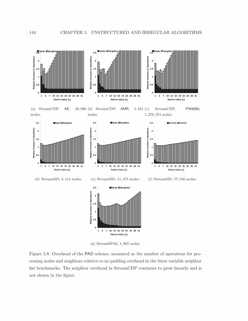
144 CHAPTER 5. UNSTRUCTURED AND IRREGULAR ALGORITHMS
0
0.5
1
1.5
2
2.5
1 4 7 10 13 16 19 22 25 28 31
Pad-to Value (L)
Rel
ativ
e In
crea
se in
Ope
ratio
ns
Node Neighbor
(a) StreamCDP, AE, 29, 096
nodes.
0
0.5
1
1.5
2
2.5
1 4 7 10 13 16 19 22 25 28 31
Pad-to Value (L)
Rel
ativ
e In
crea
se in
Ope
ratio
ns
Node Neighbor
(b) StreamCDP, AMR, 5, 431
nodes.
0
0.5
1
1.5
2
2.5
1 4 7 10 13 16 19 22 25 28 31
Pad-to Value (L)
Rel
ativ
e In
crea
se in
Ope
ratio
ns
Node Neighbor
(c) StreamCDP, PW6000,
1, 278, 374 nodes.
0
0.5
1
1.5
2
2.5
1 4 7 10 13 16 19 22 25 28 31
Pad-to Value (L)
Rel
ativ
e In
crea
se in
Ope
ratio
ns
Node Neighbor
(d) StreamMD, 4, 114 nodes.
0
0.5
1
1.5
2
2.5
1 4 7 10 13 16 19 22 25 28 31
Pad-to Value (L)
Rel
ativ
e In
crea
se in
Ope
ratio
ns
Node Neighbor
(e) StreamMD, 11, 475 nodes.
0
0.5
1
1.5
2
2.5
1 4 7 10 13 16 19 22 25 28 31
Pad-to Value (L)
Rel
ativ
e In
crea
se in
Ope
ratio
ns
Series1 Series2
(f) StreamMD, 57, 556 nodes.
0
0.5
1
1.5
2
2.5
1 4 7 10 13 16 19 22 25 28 31
Pad-to Value (L)
Rel
ativ
e In
crea
se in
Ope
ratio
ns
Node Neighbor
(g) StreamSPAS, 1, 965 nodes.
Figure 5.8: Overhead of the PAD scheme, measured as the number of operations for pro-
cessing nodes and neighbors relative to no padding overhead in the three variable neighbor
list benchmarks. The neighbor overhead in StreamCDP continues to grow linearly and is
not shown in the figure.
5.2. EXPLOITING LOCALITY AND PARALLELISM 145
The fixed padding (PAD) technique regularizes the computation by ensuring all neigh-
bor lists conform to a predetermined fixed length. Nodes whose neighbor list is shorter
than the fixed length L are padded with dummy neighbors, whereas nodes whose list
is longer than L are split into multiple length-L lists. Splitting a node entails replicat-
ing its data, computing separately on each replica, and then reducing the results. This
technique is described in detail for StreamMD in [47], and also in work related to vector
architectures. The advantage of this scheme is its suitability for efficient hardware and
low preprocessing overhead. The disadvantages include wasted computation on dummy
neighbors and the extra work involved in replicating and reducing node data. Figure 5.8
shows the relative increase in the number of node neighbor operations (including reduc-
tions) with several fixed-length padding values for StreamMD, the StreamCDP element
loop, and StreamSPAS, which have variable number of neighbors. The overhead is the ra-
tio of the number of operations required for the computation with padding to the minimal
operation count, and is separated into overhead for processing replicated nodes and that
of processing dummy neighbors. Note, that an increase in execution time is not linearly
proportional to the increase in operation count, as apparent in the execution results in
Subsection 5.3.3. The arithmetic intensity of the node and neighbor sections of the code
lead to different execution overheads for each computation (see the application properties
in Table 5.1).
It is possible to combine these techniques. For example, the connectivity list can be
sorted into bins and then the list of each node padded up to the bin value, however, the
evaluation of hybrid techniques is beyond the scope of this paper.
5.2.2.2 SIMD with Conditional or Relaxed SRF Access
A simple extension to a pure sequential access SIMD stream architecture is the addition
of a conditional access mechanism. The basis of this mechanism is to allow the clusters to
access their local memories in unison, but not necessarily advance in the stream, i.e., the
next access to the stream may read the same values as the previous access independently in
each cluster. Such a mechanism can be implemented as discussed in [81]. In our evaluation
we use an alternative implementation based on indexable SRF.
With conditional access (COND), the node computation of Figure 5.1 can be modified
to support SIMD execution as shown in Figure 5.9. The key idea is that the processing of
the node is folded into the inner loop that processes neighbors, but executed conditionally,

146 CHAPTER 5. UNSTRUCTURED AND IRREGULAR ALGORITHMS
as suggested in [5]. The overhead of conditionally executing the node portion of the com-
putation for every neighbor is typically low, as reported in Table 5.1 and the performance
impact with Merrimac is analyzed in Subsection 5.3.1.
i = 0;
neighbors_left = 0;
for (j=0; i<num_neighbors ; j++) {
if (neighbors_left == 0) {
process_node(nodes[i]);
neighbors_left = neighbor_starts [i+1] -
neighbor_starts [i];
i++;
}
process_neighbor(neighbors[neighbor_list [j]]);
neighbors_left --;
}
Figure 5.9: Pseudocode for COND parallelization method.
An additional overhead is related to load balancing. Each cluster is responsible for
processing a subset of the nodes in each computational strip, but the amount of work
varies with the number of neighbors. This leads to imbalance, where all clusters must
idle, waiting for the cluster with the largest number of neighbors to process in the strip
to complete. Load balancing techniques have been studied in the past, and the solutions
and research presented are applicable to Merrimac as well.
5.2.2.3 MIMD Mapping
With MIMD style execution, the basic node computation of Figure 5.1 can be implemented
directly in parallel, and synchronization between clusters need only occur on strip or phase
boundaries. This results in an execution that is very similar to SIMD with conditional
access without the overhead of performing node-related instructions in the inner loop.
Similarly to the COND method, the load must be balanced between clusters to ensure
optimal performance. If the MIMD capabilities extend to the memory system, however,
the granularity of imbalance can be at the level of processing the entire dataset, as opposed
to at the strip level as with COND.
To support true MIMD execution, the hardware must provide multiple instruction
sequencers. These additional structures reduce both the area and energy efficiency of the
design. A quantitative analysis of this area/feature tradeoff is left for future work, but we
bound the maximal advantage of MIMD over SIMD in Subsection 5.3.1.
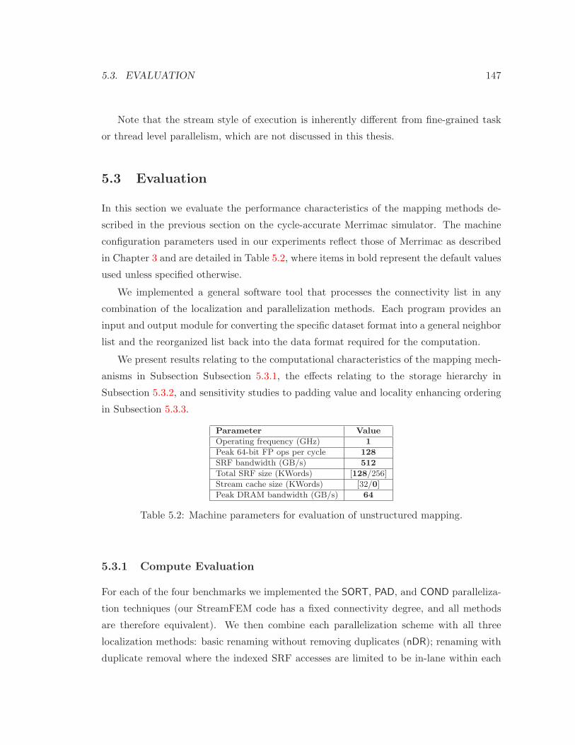
5.3. EVALUATION 147
Note that the stream style of execution is inherently different from fine-grained task
or thread level parallelism, which are not discussed in this thesis.
5.3 Evaluation
In this section we evaluate the performance characteristics of the mapping methods de-
scribed in the previous section on the cycle-accurate Merrimac simulator. The machine
configuration parameters used in our experiments reflect those of Merrimac as described
in Chapter 3 and are detailed in Table 5.2, where items in bold represent the default values
used unless specified otherwise.
We implemented a general software tool that processes the connectivity list in any
combination of the localization and parallelization methods. Each program provides an
input and output module for converting the specific dataset format into a general neighbor
list and the reorganized list back into the data format required for the computation.
We present results relating to the computational characteristics of the mapping mech-
anisms in Subsection Subsection 5.3.1, the effects relating to the storage hierarchy in
Subsection 5.3.2, and sensitivity studies to padding value and locality enhancing ordering
in Subsection 5.3.3.
Parameter Value
Operating frequency (GHz) 1
Peak 64-bit FP ops per cycle 128
SRF bandwidth (GB/s) 512
Total SRF size (KWords) [128/256]
Stream cache size (KWords) [32/0]
Peak DRAM bandwidth (GB/s) 64
Table 5.2: Machine parameters for evaluation of unstructured mapping.
5.3.1 Compute Evaluation
For each of the four benchmarks we implemented the SORT, PAD, and COND paralleliza-
tion techniques (our StreamFEM code has a fixed connectivity degree, and all methods
are therefore equivalent). We then combine each parallelization scheme with all three
localization methods: basic renaming without removing duplicates (nDR); renaming with
duplicate removal where the indexed SRF accesses are limited to be in-lane within each

148 CHAPTER 5. UNSTRUCTURED AND IRREGULAR ALGORITHMS
Figure 5.10: Computation cycle simulation results for all mapping variants across the fourbenchmarks. Execution cycles measured with perfect off-chip memory and normalized tothe nDR IL COND variant of each benchmark (lower is better).
cluster (DR IL); and duplicate removal with dynamic accesses across SRF lanes with inter-
cluster communication (DR XL).
To isolate the computational properties of the variants from dependence on the memory
system, Figure 5.10 shows the number of computation cycles in the benchmarks normal-
ized to the nDR IL COND variant of each benchmark and dataset combination (lower bars
indicate higher performance). Computation cycles are equivalent to running the bench-
mark with a perfect off-chip memory system that can supply all data with zero latency.
Remember, that in a stream processor the clusters cannot directly access off-chip mem-
ory, and all aspects relating to SRF access and inter-cluster communication are faithfully
modeled. We explain the results of the figure in the paragraphs below. With the exception
of StreamMD, we use the baseline Merrimac configuration with a 256KB stream cache, a
1MB SRF, and no locality-increasing reordering. For StreamMD, we increase the SRF size
to 8MB to account for a minor deficiency in our implementation of the SORT technique.
With SORT, in StreamMD some nodes have over 130 neighbors, whereas others have only
a single neighbor. We only implemented a simple SRF allocation policy that provides
enough SRF space for the maximal number of neighbors and maximal number of nodes
at the same time. In the case of StreamMD, this allocation policy requires a large SRF.
In this subsection we only look at computation cycles, which are not significantly affected
by this increase in SRF size (under 1% difference in measured computation cycles).

5.3. EVALUATION 149
Parallelization Compute Properties
We will first describe the left-most (solid) group of bars for each program-dataset, which
show the computation time of the nDR variants. StreamFEM has a fixed connectivity, and
all parallelization techniques are equivalent. StreamCDP and StreamSPAS have a very
small number of operations applied to each neighbor, and as a result the COND technique
significantly reduces performance as the extra operations are relatively numerous (see
Table 5.1). Additionally, the conditional within the inner loop introduces a loop-carried
dependency and severely restricts compiler scheduling optimizations. This results in the
factor of 6 compute time difference seen in StreamSPAS. StreamMD, on the other hand,
has a large number of inner loop operations and the overhead of the extra conditional
operations in COND is lower than the overhead of dummy computations in PAD.
The SORT technique has the least amount of computation performed because there
is no overhead associated with either padding or conditionals. However, the computation
cycles are also affected by the kernel startup costs, which are greater for SORT than with
the other techniques. With SORT, each connectivity degree requires at least one kernel
invocation. This has a strong effect on the execution of StreamSPAS, where there are
many connectivity bins with very few nodes, as shown in the distributions of Figure 5.2.
More evidence is also seen in the difference in the computation cycle behavior of the
4, 114 and 11, 475 datasets of StreamMD. As shown in Figure 5.2, 4, 114 has many more
connectivity bins with a very small number of nodes compared to 11, 475. As a result,
SORT is much less effective in the 4, 114 case and only improves performance by 1% over
COND. In comparison the performance difference is 18% with the 11, 475 dataset.
Duplicate-Removal Compute Properties
Renaming while removing duplicates relies on indexing into the SRF, which is less efficient
than sequential access. In-lane indexing inserts index-computation operations that are not
required for sequential access, and cross-lane indexing has an additional runtime penalty
due to dynamic conflicts of multiple requests to a single SRF lane.
In StreamSPAS and StreamCDP, the inner loop of the kernel contains few instructions
and the additional overhead of indexing significantly increases the number of computa-
tion cycles. For example, DR IL PAD is 1.6 and DR XL PAD is 2.6 times worse than
nDR IL PAD in the case of StreamSPAS. In StreamCDP, DR IL SORT and DR XL SORT

150 CHAPTER 5. UNSTRUCTURED AND IRREGULAR ALGORITHMS
are worse than nDR IL SORT by a factor of 1.4 and 2.2 respectively. The behavior of PAD
is different for the AE and AMR dataset of StreamCDP. The reason for this difference is
the difference in the padding values. In AMR we pad each node to 6 neighbors, whereas
AE is only padded to 4. Therefore, AE has a higher relative overhead. In contrast to
the short loops of StreamCDP and StreamSPAS, StreamMD and StreamFEM have high
arithmetic intensity. As a result, adding in-lane indexing increases the computation cycles
by about 13% for StreamMD and less than 5% in StreamFEM.
Another interesting observation relates to the amount of locality captured by the
DR XL technique. In StreamCDP, StreamSPAS, and StreamFEM, increasing the amount
of available state to the entire SRF, significantly increases the amount of locality ex-
ploited. Therefore, a large number of nodes attempt to access the same SRF lane dynami-
cally, increasing the overhead of cross-lane access. Using cross-lane indexing increases the
computation cycle count by over 70% in StreamCDP, more than 150% in StreamSPAS,
and almost 50% in the case of StreamFEM. In StreamMD, on the other hand, dynamic
conflicts are a smaller concern and increase computation cycles by about 30%.
Despite the higher computation cycle count, the next subsection shows that overall
application run time can be significantly improved by employing duplicate removal once
realistic memory system performance is accounted for.
5.3.2 Storage Hierarchy Evaluation
Figure 5.11 shows the execution time of the benchmarks with Merrimac’s realistic, 64GB/s
peak, memory system. We show the number for the best performing parallelized variant
in each program with nDR, DR IL, and DR XL options, normalized to the benchmark
runtime of nDR on a configuration that includes a stream cache (lower bars indicate
higher performance). We also explore two storage hierarchy configurations for analyzing
the tradeoffs of using a stream cache or increasing strip sizes: cache is the Merrimac
default configuration of Chapter 3, which uses a 1MB SRF backed up by a 256KB cache;
and nocache does not use a cache and dedicates 2MB of on-chip memory to the SRF (SRF
size must be a power of 2).
In StreamCDP, we can see a clear advantage to increasing the strip size in all map-
ping variants, even when duplicates are not removed in software. StreamCDP has low
arithmetic intensity (Table 5.1) and is limited by the memory system, therefore removing
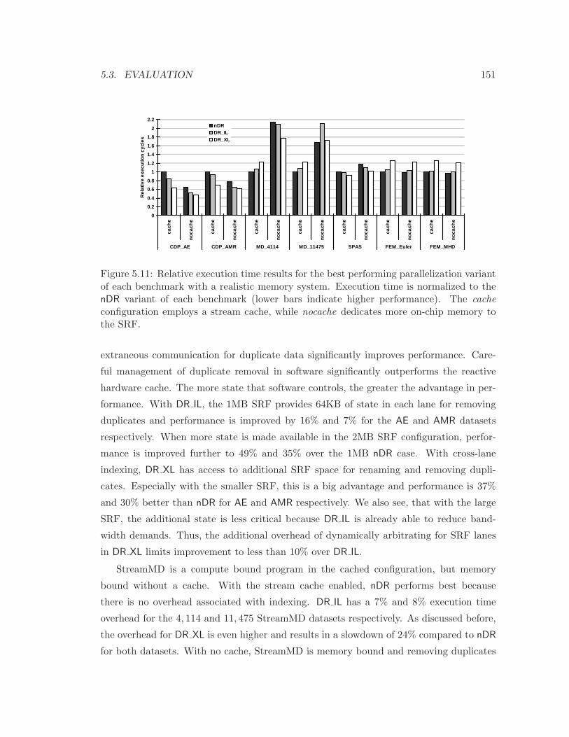
5.3. EVALUATION 151
0
0.2
0.4
0.6
0.8
1
1.2
1.4
1.6
1.8
2
2.2
cach
e
noca
che
cach
e
noca
che
cach
e
noca
che
cach
e
noca
che
cach
e
noca
che
cach
e
noca
che
cach
e
noca
che
CDP_AE CDP_AMR MD_4114 MD_11475 SPAS FEM_Euler FEM_MHD
Rel
ativ
e ex
ecut
ion
cycl
es
nDRDR_ILDR_XL
Figure 5.11: Relative execution time results for the best performing parallelization variantof each benchmark with a realistic memory system. Execution time is normalized to thenDR variant of each benchmark (lower bars indicate higher performance). The cacheconfiguration employs a stream cache, while nocache dedicates more on-chip memory tothe SRF.
extraneous communication for duplicate data significantly improves performance. Care-
ful management of duplicate removal in software significantly outperforms the reactive
hardware cache. The more state that software controls, the greater the advantage in per-
formance. With DR IL, the 1MB SRF provides 64KB of state in each lane for removing
duplicates and performance is improved by 16% and 7% for the AE and AMR datasets
respectively. When more state is made available in the 2MB SRF configuration, perfor-
mance is improved further to 49% and 35% over the 1MB nDR case. With cross-lane
indexing, DR XL has access to additional SRF space for renaming and removing dupli-
cates. Especially with the smaller SRF, this is a big advantage and performance is 37%
and 30% better than nDR for AE and AMR respectively. We also see, that with the large
SRF, the additional state is less critical because DR IL is already able to reduce band-
width demands. Thus, the additional overhead of dynamically arbitrating for SRF lanes
in DR XL limits improvement to less than 10% over DR IL.
StreamMD is a compute bound program in the cached configuration, but memory
bound without a cache. With the stream cache enabled, nDR performs best because
there is no overhead associated with indexing. DR IL has a 7% and 8% execution time
overhead for the 4, 114 and 11, 475 StreamMD datasets respectively. As discussed before,
the overhead for DR XL is even higher and results in a slowdown of 24% compared to nDR
for both datasets. With no cache, StreamMD is memory bound and removing duplicates

152 CHAPTER 5. UNSTRUCTURED AND IRREGULAR ALGORITHMS
can improve performance. With the nDR technique, performance is degraded by a factor
of 2.1 for 4, 114 and 1.7 for 11, 475. The difference can be attributed to the different
connectivity properties presented by the two datasets. The behavior of DR IL and DR XL
is similar for both datasets. DR IL is unable to utilize much locality due to the large
amount of state required to expose locality in StreamMD (see Figure 5.7) and as a result
performance is a factor of 2.1 worse than nDR with a cache. DR XL is able to exploit
locality and improves performance by 16% over DR IL. For the 4, 114 dataset, this is a
77% slowdown vs. cached nDR, and 73% slowdown in the case of 11, 475.
While there is a 17% performance advantage to using a cache for nDR variant of
StreamSPAS, the software duplicate-removal methods match the performance of a cached
configuration without the additional hardware complexity of a reactive stream cache.
StreamFEM has little reuse and hence benefits minimally from duplicate removal in
either hardware or software. The computation overhead of DR XL decreases performance
by 21 − 25% for both StreamFEM configurations.
5.3.3 Sensitivity Analysis
As shown in Subsection 5.2.1.2, reordering the nodes and neighbors in the connectivity list
using domain decomposition techniques can increase the amount of reuse within a given
strip size (StreamCDP and StreamFEM). Figure 5.12 explores the effects of reordering
on performance, where bars labeled with M use METIS and those labeled with noM do
not. We make three observations regarding the effects of using METIS on application
performance.
First, using METIS to increase locality significantly improves the performance of the
cached configurations in StreamCDP, with the best performing cached configuration out-
performing the best non-cached configuration by 18% and 23% for AE and AMR respec-
tively. On the other hand, the non-cached configurations consistently outperform the
cached configuration with StreamFEM, due to the increased strip size and reduced kernel
startup overheads.
Second, regardless of the availability of a cache, METIS always improves the perfor-
mance of the DR IL scheme. This is because METIS exposes greater locality that can
be exploited by the limited SRF state within each lane. In fact, with METIS enabled,
DR IL can outperform DR XL by (−1) − 10%, whereas without METIS DR IL trails the
performance of DR XL by 5 − 33%.
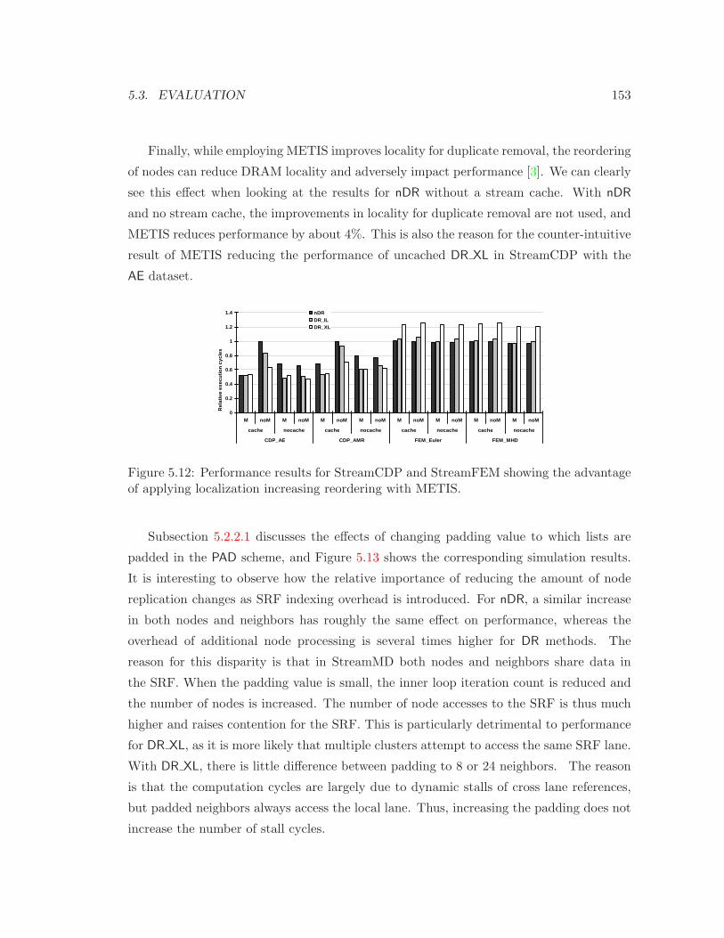
5.3. EVALUATION 153
Finally, while employing METIS improves locality for duplicate removal, the reordering
of nodes can reduce DRAM locality and adversely impact performance [3]. We can clearly
see this effect when looking at the results for nDR without a stream cache. With nDR
and no stream cache, the improvements in locality for duplicate removal are not used, and
METIS reduces performance by about 4%. This is also the reason for the counter-intuitive
result of METIS reducing the performance of uncached DR XL in StreamCDP with the
AE dataset.
0
0.2
0.4
0.6
0.8
1
1.2
1.4
M noM M noM M noM M noM M noM M noM M noM M noM
cache nocache cache nocache cache nocache cache nocache
CDP_AE CDP_AMR FEM_Euler FEM_MHD
Rel
ativ
e ex
ecut
ion
cycl
es
nDRDR_ILDR_XL
Figure 5.12: Performance results for StreamCDP and StreamFEM showing the advantageof applying localization increasing reordering with METIS.
Subsection 5.2.2.1 discusses the effects of changing padding value to which lists are
padded in the PAD scheme, and Figure 5.13 shows the corresponding simulation results.
It is interesting to observe how the relative importance of reducing the amount of node
replication changes as SRF indexing overhead is introduced. For nDR, a similar increase
in both nodes and neighbors has roughly the same effect on performance, whereas the
overhead of additional node processing is several times higher for DR methods. The
reason for this disparity is that in StreamMD both nodes and neighbors share data in
the SRF. When the padding value is small, the inner loop iteration count is reduced and
the number of nodes is increased. The number of node accesses to the SRF is thus much
higher and raises contention for the SRF. This is particularly detrimental to performance
for DR XL, as it is more likely that multiple clusters attempt to access the same SRF lane.
With DR XL, there is little difference between padding to 8 or 24 neighbors. The reason
is that the computation cycles are largely due to dynamic stalls of cross lane references,
but padded neighbors always access the local lane. Thus, increasing the padding does not
increase the number of stall cycles.
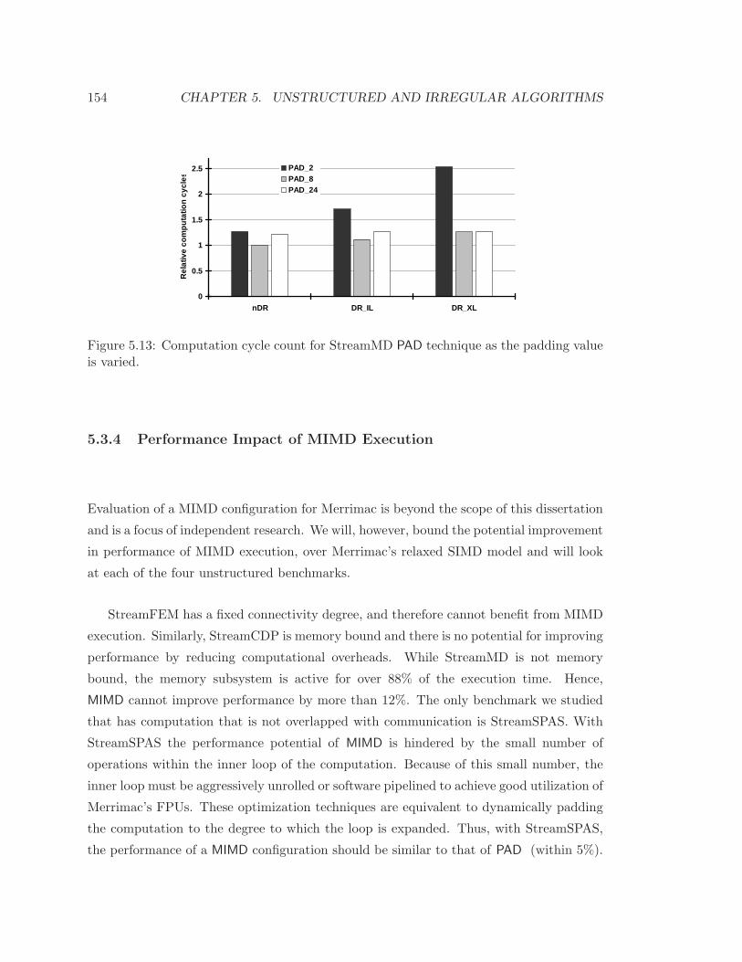
154 CHAPTER 5. UNSTRUCTURED AND IRREGULAR ALGORITHMS
0
0.5
1
1.5
2
2.5
nDR DR_IL DR_XL
Rel
ativ
e co
mpu
tatio
n cy
cles
PAD_2PAD_8PAD_24
Figure 5.13: Computation cycle count for StreamMD PAD technique as the padding valueis varied.
5.3.4 Performance Impact of MIMD Execution
Evaluation of a MIMD configuration for Merrimac is beyond the scope of this dissertation
and is a focus of independent research. We will, however, bound the potential improvement
in performance of MIMD execution, over Merrimac’s relaxed SIMD model and will look
at each of the four unstructured benchmarks.
StreamFEM has a fixed connectivity degree, and therefore cannot benefit from MIMD
execution. Similarly, StreamCDP is memory bound and there is no potential for improving
performance by reducing computational overheads. While StreamMD is not memory
bound, the memory subsystem is active for over 88% of the execution time. Hence,
MIMD cannot improve performance by more than 12%. The only benchmark we studied
that has computation that is not overlapped with communication is StreamSPAS. With
StreamSPAS the performance potential of MIMD is hindered by the small number of
operations within the inner loop of the computation. Because of this small number, the
inner loop must be aggressively unrolled or software pipelined to achieve good utilization of
Merrimac’s FPUs. These optimization techniques are equivalent to dynamically padding
the computation to the degree to which the loop is expanded. Thus, with StreamSPAS,
the performance of a MIMD configuration should be similar to that of PAD (within 5%).

5.4. DISCUSSION AND RELATED WORK 155
5.4 Discussion and Related Work
A large body of research exists on mapping irregular scientific applications to a wide
variety of architectures including: distributed memory systems built from COTS such as
Beowulf clusters [156] and grid computing [27]; shared memory multiprocessors (e.g., [97]);
vector processors (e.g., [141, 90]); and more exotic specialized architectures such as the
Monsoon dataflow machine [125].
In this section we discuss our contributions in the context of the research on the above
mentioned systems, which we classify into two main categories: research on optimizing
and enabling global communication in multiprocessor systems; and work on dealing with
irregular control in SIMD architectures.
Unstructured Communication in Multiprocessors
Multi-processor systems benefit from, and in the case of distributed memory architectures
require data localization into each processor’s DRAM. Additionally, work must be dis-
tributed across all processors. Several runtime systems (e.g., CHAOS [69]) and languages
(e.g., UPC [28], Titanium [173], and ZPL [41]) have been developed to address the chal-
lenge of efficient data communication and work partitioning with the large memories and
coarse granularity of multi-processor systems. These systems often use inspector–executor
methods [69, 158, 40] or data speculation [33] to hide data communication time on rela-
tively low-bandwidth connectivities. They also employ MIMD/SPMD methods (e.g., [66])
to partition work and load balance across full processor systems.
We deal with similar issues in data locality and work parallelization but in the context
of the storage hierarchy and the constrained execution fabric of a stream processor. The
problem we address is at a much smaller granularity of both control and storage sizes, as
opposed to large scale multiple processor systems. Therefore, even though some concepts
developed for large-scale systems could be applied to stream processors the techniques
cannot be used directly because the tradeoffs in bandwidths and memory usage are quite
different.
We use a domain decomposition technique to reorder memory accesses and extract
greater locality. In general, domain decomposition frameworks (such as METIS [84],
CHACO [63], and JOSTLE [166]) are used both to improve localization and balance
load across multiple processors. In the context of the tightly integrated PEs of a stream

156 CHAPTER 5. UNSTRUCTURED AND IRREGULAR ALGORITHMS
processor, sophisticated load balancing is not required, but we envision that multi-node
streaming systems will take advantage of domain decomposition for this purpose as well.
Automatically localizing data has been a topic of active research in the compiler com-
munity [59, 60, 102]. By examining the computation loops and the data access patterns the
compiler can potentially rearrange computation using loop transformations (e.g, fission,
permutation, tiling) or change data layout through data transformations (e.g., padding,
transpose) to improve locality and reduce communication. These techniques could be in-
corporated into an optimizing stream compiler to automate several techniques that were
discussed in this chapter.
Irregular Execution on SIMD Architectures
Merrimac relies on SIMD execution in the clusters and faces similar challenges with ex-
ecuting irregular applications as other SIMD machines. To the best of our knowledge
previous related work has focused on either completely general frameworks for executing
irregular codes, at a cost in performance, or on algorithm-specific solutions outside of a
generalized framework. Our work combines multiple techniques that have been used in
the past in different contexts into a single framework that is applicable to a large range of
unstructured and irregular scientific applications. We give a detailed performance evalu-
ation of such codes on Merrimac and stream processors in general. We also address and
evaluate localization methods to the restricted on-chip SRF of stream processors, an issue
that was not discussed in prior work.
A review of specific implementations of regular and irregular applications on both
SIMD and MIMD systems is given in [50]. The paper also provides a taxonomy of par-
allel applications and the suitability of various algorithms to SIMD or MIMD. However,
only restricted SIMD machines are evaluated that do not support Merrimac’s generalized
stream execution model and relaxed SIMD execution. Examples of specific implementa-
tions include ideas similar to SORT and PAD have been used for sparse linear algebra on
vector machines and for molecular dynamics on SIMD architectures. The ELL [142] for-
mat for sparse matrices is equivalent to PAD, where each row of storage contains as many
elements as the row with the most non-zeros in the matrix. The JAD sparse format [142]
and CSR with permutation [39] are variants of our SORT technique. The same molecular
dynamics algorithm used in StreamMD has also been implemented for the SIMD Quadrics
computer [17] using a technique that is a combination of PAD and SORT at the algorithmic
5.4. DISCUSSION AND RELATED WORK 157
level [139], similar to the ideas presented in [47].
General frameworks for handling irregular control on SIMD processors include tech-
niques for converting control conditionals into data dependencies [5]. An overview of an
important class of conditional techniques in vector processors, vector masking, is given
in [154].
Another general solution to executing irregular control on SIMD machines is to emulate
MIMD execution through interpretation (e.g., [144, 150]). The idea is that all SIMD
processing elements emulate a processor pipeline, and the irregular application is compiled
to this virtual ISA. Since emulation is done in software, the virtual ISA can be application
specific and include coarse-grained operations that are free of irregular control. Note that
this technique only works on architectures that provide independent memory addressing
to each processing element.
Finally, frameworks based on prefix-sum operations have also been used to implement
irregular applications on data parallel systems [20]. We use Merrimac’s scatter-add mecha-
nism, which is a form of prefix-sum as well. However, implementing an entire algorithm in
prefix-sum form requires significant restructuring and incurs heavy overheads compared
to our direct implementation using the PAD, COND, or SORT techniques and software
tool.

Chapter 6
Fault Tolerance
Merrimac utilizes advanced 90nm semiconductor technology that allows high performance
levels on a single chip. At the same time, the ever-shrinking device dimensions and voltages
have given rise to an increased problem of soft errors, which are transient faults caused
by noise or radiation [149]. In a system such as Merrimac, with up to 16, 384 processors,
these errors must be dealt with not only at a system level, for which a large body of work
exists [151], but also at the single-processor level. As VLSI process dimensions shrink even
further, from Merrimac’s 90nm to future technologies, transient faults will become an even
more serious problem. In this chapter we explore these trends of increased performance
and the need for greater reliability in the case of Merrimac. Merrimac belongs to a
new class of architectures that are compute-intensive and achieve high performance by
reducing dynamic control, providing a large number of programmable functional units, and
exposing low-level hardware communication to the programming system. These features
differ significantly from modern general-purpose processors and offer opportunities for
novel fault-tolerance schemes.
In this chapter we will focus on soft-error fault-tolerance techniques within the Merri-
mac processor, as the details for other fault types and full system reliability follow common
practice and the large knowledge base developed over many years of dealing with reliable
high-performance computers. For the most part Merrimac follows a dynamic redundancy
approach to fault-tolerance, and relies on robust fault-detection followed by re-execution
for fault-correction. Therefore, the discussion concentrates on fault-detection methods,
and only briefly touches on the mechanism for recovery. Strong fault-detection capabili-
ties are particularly important and difficult for compute-intensive processors. The reason
158

159
is that a vast majority of instructions are data manipulation instructions and do not affect
program control or make off-chip memory references. These types of instructions are not
likely to lead to a catastrophic failure, where a violation is easy to detect (e.g., a segmen-
tation fault), but rather remain a silent error that corrupts the computed result without
producing a warning [114]. This is in contrast to control-intensive high-performance GPPs
where a fault will many times quickly lead to a catastrophic failure, and other times be
squashed in the speculative pipeline without even affecting the architectural state of the
machine [167].
In order to detect soft-errors in execution, some degree of redundancy must be in-
troduced in either hardware, software, or both. Building redundant hardware increases
cost which adversely affects peak performance as the additional units consume die area
that could have been used otherwise. Redundant instruction execution, on the other
hand, places greater demands on the execution and bandwidth resources possibly leading
to degraded sustained performance when a large number of redundant instructions are
introduced.
The Merrimac reliability scheme uses a careful balance of hardware and software redun-
dancy to ensure that the most vital resources are not squandered. For compute-intensive
architectures such as Merrimac, careful management of the locality hierarchy is crucial
for achieving high utilization of the large number of arithmetic units available. There-
fore, the fault-tolerance mechanisms stress conservation of the critical resources in this
respect – off-chip bandwidth and on-chip memory capacity. These two resources are often
responsible for limiting application performance (see Chapter 4).
Careful attention is also paid to the amount of hardware overheads incurred in sup-
porting fault-tolerance. Certain application classes contain information that allows sanity
checks or algorithmic based techniques to be used to ensure correct execution with mini-
mal performance impact and no additional hardware. In such cases, all available execution
resources may be applied towards improving performance without loss of reliability. For
other application classes, however, transient fault detection requires redundant execution.
Therefore, the Merrimac system allows the programmer and/or the programming system
to reconfigure the degree of hardware redundancy support depending on the availability
of application-specific, efficient, software fault-detection methods.
Our analysis shows that in Merrimac’s current 90nm technology, ECC protection of
large arrays is enough to achieve reasonable failure rates and requires a small overhead
160 CHAPTER 6. FAULT TOLERANCE
of only about 3% in chip area. However, in a future 50nm technology, using the same
architectural unit mix, the computational clusters and interfaces will require coverage as
well. Our proposed schemes will have 4−11% area overheads, but the ability to reconfigure
the level of redundancy allows applications which can effectively be protected in software
to suffer only small performance degradations.
Section 6.1 describes existing fault-detection methods and the degree in which they are
suitable for Merrimac. Section 6.2 explores fault-tolerance specifically for Merrimac and
provides a general analysis of costs and performance, while a detailed treatment of case-
studies highlighting the interplay between software and hardware techniques is presented
in Section 6.3.
6.1 Overview of Fault Tolerance Techniques
In this section we will describe existing techniques relating to soft-error fault detection.
The failure mechanisms here are energetic particle strikes that cause hole-electron pairs
to be generated, effectively injecting a momentary (< 1ns) pulse of current into a circuit
node. Our fault model of this is a transient 1-cycle flip of a single bit in the circuit,
which is also applicable in the case of supply noise briefly affecting a circuit’s voltage
level. For more detail, and for a discussion of the general fault-tolerance problem we refer
the interested reader to [151] and [149].
As mentioned in the introduction fault-detection techniques can broadly be classified
into software and hardware. We will briefly describe the main methods in each category
as well as their strengths, weaknesses, and suitability for Merrimac. Note that many of
the recently reported hardware techniques have been developed in the context of multi-
threaded and multi-core GPPs and are not well-suited for compute-intensive architectures
as discussed in Subsection 6.1.3.
6.1.1 Software Techniques
Software techniques range from algorithm specific modifications for fault-tolerance, through
techniques relying on program structure and sanity of results, to full instruction replica-
tion.

6.1. OVERVIEW OF FAULT TOLERANCE TECHNIQUES 161
6.1.1.1 Algorithmic Based Fault Tolerance (ABFT)
Algorithmic-based checking allows for cost-effective fault tolerance by embedding a tai-
lored checking, and possibly correcting, scheme within the algorithm to be performed. It
relies on a modified form of the algorithm that operates on redundancy encoded data, and
that can decode the results to check for errors that might have occurred during execution.
Since the redundancy coding is tailored to a specific algorithm various trade-offs between
accuracy and cost can be made by the user [14, 4]. Therein also lies this technique’s
main weakness, as it is not applicable to arbitrary programs and requires time-consuming
algorithm development. In the case of linear algorithms amenable to compiler analysis,
an automatic technique for ABFT synthesis was introduced in [14]. ABFT enabled algo-
rithms have been developed for various applications including linear algebra operations
such as matrix multiply [68, 15] and QR decomposition [132] as well as the compiler
synthesis approach mentioned above, FFT [79], and multi-grid methods [111]. A full de-
scription of the actual ABFT techniques is beyond the scope of this dissertation, but we
do discuss the specific case of dense matrix-matrix multiply in Subsection 6.3.2. It should
be mentioned that the finite precision of actual computations adds some complication to
these algorithms, but can be dealt with in the majority of cases.
ABFT methods only apply to the actual computation and not control code, or data
movement operations. This however fits well with the overall design of the Merrimac fault
tolerance schemes as will be explained in Section 6.2, as it allows for efficient software
fault-detection in conjunction with hardware detection when software algorithms are not
available.
6.1.1.2 Assertion and Sanity-Based Fault Detection
A less systematic approach to software fault detection, which still relies on specific knowl-
edge of the algorithm and program, is to have the programmer annotate the code with
assertions and invariants [9, 106, 134]. Although it is difficult to analyze the effectiveness
of this technique in the general case, it has been shown to provide high error-coverage at
very low cost.
An interesting specific case of an assertion is to specify a few sanity checks and make
sure the result of the computation is reasonable. An example might be to check whether
energy is conserved in a physical system simulation. This technique is very simple to
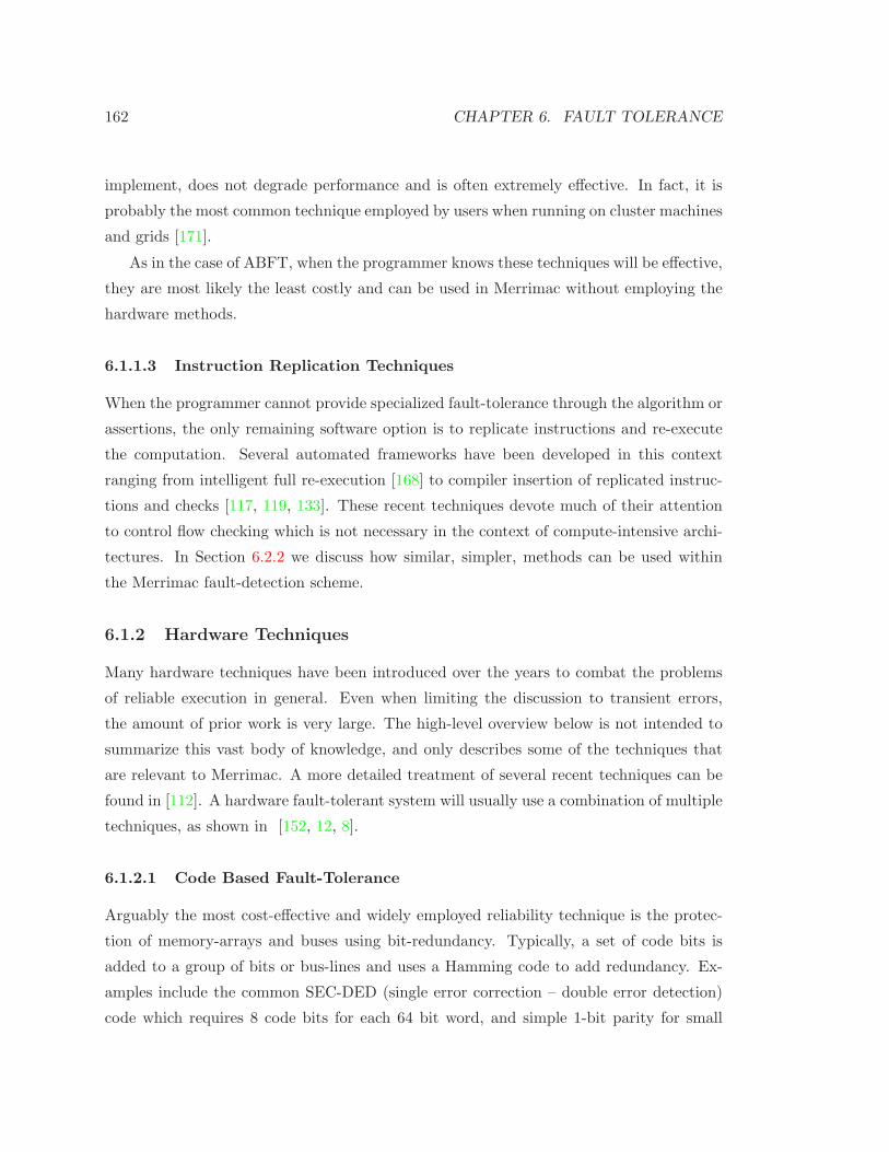
162 CHAPTER 6. FAULT TOLERANCE
implement, does not degrade performance and is often extremely effective. In fact, it is
probably the most common technique employed by users when running on cluster machines
and grids [171].
As in the case of ABFT, when the programmer knows these techniques will be effective,
they are most likely the least costly and can be used in Merrimac without employing the
hardware methods.
6.1.1.3 Instruction Replication Techniques
When the programmer cannot provide specialized fault-tolerance through the algorithm or
assertions, the only remaining software option is to replicate instructions and re-execute
the computation. Several automated frameworks have been developed in this context
ranging from intelligent full re-execution [168] to compiler insertion of replicated instruc-
tions and checks [117, 119, 133]. These recent techniques devote much of their attention
to control flow checking which is not necessary in the context of compute-intensive archi-
tectures. In Section 6.2.2 we discuss how similar, simpler, methods can be used within
the Merrimac fault-detection scheme.
6.1.2 Hardware Techniques
Many hardware techniques have been introduced over the years to combat the problems
of reliable execution in general. Even when limiting the discussion to transient errors,
the amount of prior work is very large. The high-level overview below is not intended to
summarize this vast body of knowledge, and only describes some of the techniques that
are relevant to Merrimac. A more detailed treatment of several recent techniques can be
found in [112]. A hardware fault-tolerant system will usually use a combination of multiple
techniques, as shown in [152, 12, 8].
6.1.2.1 Code Based Fault-Tolerance
Arguably the most cost-effective and widely employed reliability technique is the protec-
tion of memory-arrays and buses using bit-redundancy. Typically, a set of code bits is
added to a group of bits or bus-lines and uses a Hamming code to add redundancy. Ex-
amples include the common SEC-DED (single error correction – double error detection)
code which requires 8 code bits for each 64 bit word, and simple 1-bit parity for small

6.1. OVERVIEW OF FAULT TOLERANCE TECHNIQUES 163
arrays and buses.
Merrimac’s stream unit uses an SEC-DED code to protect the SRF, cache, microcode
store and global chip buses (Subsection 6.2.2.1).
6.1.2.2 Fault Tolerant Circuits
Fault-tolerance and redundancy can be introduced at design-time with little effect on the
overall architecture. These techniques are attractive when dealing with small parts of the
design, or when some amount of redundancy is already present for other reasons (one
example is scan-chains that are used for testing) [112]. This type of circuit is sometimes
referred to as a hardened circuit as many were originally designed for high-radiation en-
vironments. Most commonly, these designs use latches based on multiple flip-flops and
possibly special logic circuits with built-in verification. To the best of our knowledge,
hardened designs typically require roughly twice the area and a longer clock-cycle than
an equivalent conventional circuit [61, 105]. As we do not have a design of Merrimac at
this point, we do not employ circuit level techniques. Such techniques may be applicable
to Merrimac’s external interfaces as mentioned in Subsection 6.2.2.3.
6.1.2.3 Replication of Hardware Units
Instead of replication at a circuit-level, entire structures can be replicated in the architec-
ture or micro-architecture. This option is very useful when dealing with structures that
consume modest die area, or are not visible to software. Good examples of employing these
techniques are presented in [152, 12]. In Merrimac hardware replication is enabled through
reconfigurability and a software-hardware hybrid approach (see Subsection 6.2.2.2).
6.1.3 Fault Tolerance for Superscalar Architectures
The Merrimac processor includes a scalar control-processor core, which can use some of
the recently developed fault-tolerance techniques aimed at superscalar processors. We
briefly reference a few such options and explain why they are not an appropriate choice
for the compute-intensive stream unit.
[11] suggests that a simple checker module can be used to detect errors in execu-
tion. Further analyses show that the hardware costs are modest and that performance
degradation is low. While a promising design point for complex modern control-intensive

164 CHAPTER 6. FAULT TOLERANCE
superscalar processors, this method is not applicable to compute-intensive architectures.
The reason is that the main computational engine is in essence as simple as the sug-
gested checker, and the overall scheme closely resembles full hardware replication of a
large portion of the processor.
A different set of techniques relies on the fact that control-intensive processor execution
resources are often idle, and utilize them for time-redundant execution that can be initiated
by the micro-architecture [140]. In compute-intensive processors, resources are rarely idle
and these schemes are not directly applicable.
Another fault-tolerance option is to concurrently run two (or more) copies of the
program/thread on a chip multi-processor. Again, hardware can be introduced to reduce
software overhead for initiation and comparison [56]. Efficient comparison is an important
issue [155] and its optimizations may apply to the scalar portion of the Merrimac processor.
6.2 Merrimac Processor Fault Tolerance
In this section we detail the Merrimac fault-tolerance and detection mechanisms and
perform a general analysis related to fault susceptibility, hardware costs, and impact on
performance. A more detailed treatment of these analyses for specific case-studies appears
in Section 6.3.
An overarching goal of the Merrimac architecture is to achieve high utilization of
scarce resources such as off-chip bandwidth and on-chip memory capacity. These priori-
ties pervade the fault-tolerance mechanisms of Merrimac as well. As with other aspects of
Merrimac’s design, the fault-tolerance scheme also takes advantage of the stream execu-
tion model with its coarse-grained operations. Hardware fault-tolerance mechanisms are
favored where they can be supported without incurring high area overheads and eliminate
potential performance or bandwidth bottlenecks. Where hardware mechanisms are costly,
the flexibility to trade off performance and reliability is provided, particularly in cases
where algorithmic/sanity techniques may be possible with low overheads.
We will first examine the fault susceptibility of the baseline architecture, and proceed
by describing and discussing various options for fault-detection and recovery in Merrimac
based on a dynamic redundancy scheme. ECC is used to enable large arrays and buses to
mask a single fault (Subsection 6.2.2.1), but if two or more faults occur in a single word,
or when an error is caught during execution in the compute clusters (Subsection 6.2.2.2),
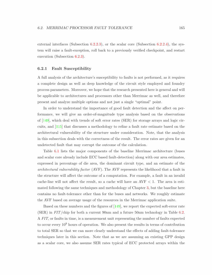
6.2. MERRIMAC PROCESSOR FAULT TOLERANCE 165
external interfaces (Subsection 6.2.2.3), or the scalar core (Subsection 6.2.2.4), the sys-
tem will raise a fault-exception, roll back to a previously verified checkpoint, and restart
execution (Subsection 6.2.3).
6.2.1 Fault Susceptibility
A full analysis of the architecture’s susceptibility to faults is not performed, as it requires
a complete design as well as deep knowledge of the circuit style employed and foundry
process parameters. Moreover, we hope that the research presented here is general and will
be applicable to architectures and processors other than Merrimac as well, and therefore
present and analyze multiple options and not just a single “optimal” point.
In order to understand the importance of good fault detection and the affect on per-
formance, we will give an order-of-magnitude type analysis based on the observations
of [149], which deal with trends of soft error rates (SER) for storage arrays and logic cir-
cuits, and [115] that discusses a methodology to refine a fault rate estimate based on the
architectural vulnerability of the structure under consideration. Note, that the analysis
in this subsection deals with the correctness of the result. The error rates are given for an
undetected fault that may corrupt the outcome of the calculation.
Table 6.1 lists the major components of the baseline Merrimac architecture (buses
and scalar core already include ECC based fault-detection) along with our area estimates,
expressed in percentage of die area, the dominant circuit type, and an estimate of the
architectural vulnerability factor (AVF). The AVF represents the likelihood that a fault in
the structure will affect the outcome of a computation. For example, a fault in an invalid
cache-line will not affect the result, so a cache will have an AVF < 1. The area is esti-
mated following the same techniques and methodology of Chapter 3, but the baseline here
contains no fault-tolerance other than for the buses and networks. We roughly estimate
the AVF based on average usage of the resources in the Merrimac application suite.
Based on these numbers and the figures of [149], we report the expected soft-error rate
(SER) in FIT/chip for both a current 90nm and a future 50nm technology in Table 6.2.
A FIT, or faults in time, is a measurement unit representing the number of faults expected
to occur every 109 hours of operation. We also present the results in terms of contribution
to total SER so that we can more clearly understand the effects of adding fault-tolerance
techniques later in this section. Note that as we are assuming an existing GPP design
as a scalar core, we also assume SER rates typical of ECC protected arrays within the
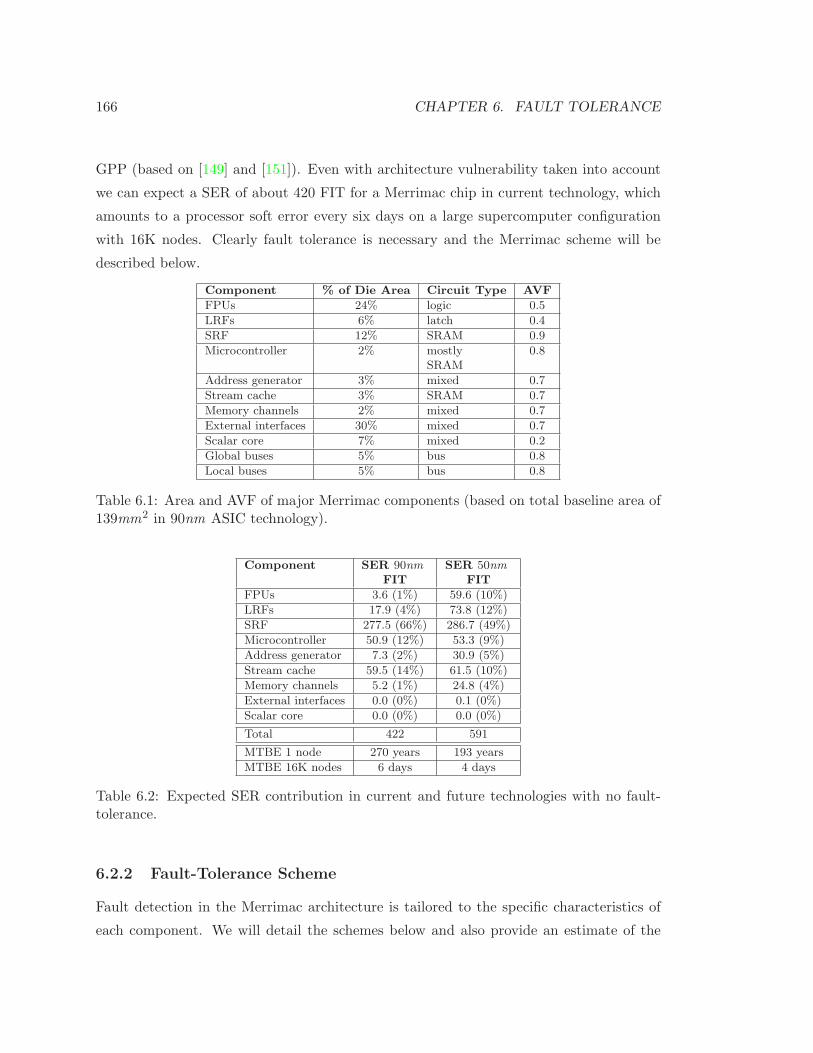
166 CHAPTER 6. FAULT TOLERANCE
GPP (based on [149] and [151]). Even with architecture vulnerability taken into account
we can expect a SER of about 420 FIT for a Merrimac chip in current technology, which
amounts to a processor soft error every six days on a large supercomputer configuration
with 16K nodes. Clearly fault tolerance is necessary and the Merrimac scheme will be
described below.
Component % of Die Area Circuit Type AVF
FPUs 24% logic 0.5
LRFs 6% latch 0.4
SRF 12% SRAM 0.9
Microcontroller 2% mostly 0.8SRAM
Address generator 3% mixed 0.7
Stream cache 3% SRAM 0.7
Memory channels 2% mixed 0.7
External interfaces 30% mixed 0.7
Scalar core 7% mixed 0.2
Global buses 5% bus 0.8
Local buses 5% bus 0.8
Table 6.1: Area and AVF of major Merrimac components (based on total baseline area of139mm2 in 90nm ASIC technology).
Component SER 90nm SER 50nm
FIT FIT
FPUs 3.6 (1%) 59.6 (10%)
LRFs 17.9 (4%) 73.8 (12%)
SRF 277.5 (66%) 286.7 (49%)
Microcontroller 50.9 (12%) 53.3 (9%)
Address generator 7.3 (2%) 30.9 (5%)
Stream cache 59.5 (14%) 61.5 (10%)
Memory channels 5.2 (1%) 24.8 (4%)
External interfaces 0.0 (0%) 0.1 (0%)
Scalar core 0.0 (0%) 0.0 (0%)
Total 422 591
MTBE 1 node 270 years 193 years
MTBE 16K nodes 6 days 4 days
Table 6.2: Expected SER contribution in current and future technologies with no fault-tolerance.
6.2.2 Fault-Tolerance Scheme
Fault detection in the Merrimac architecture is tailored to the specific characteristics of
each component. We will detail the schemes below and also provide an estimate of the

6.2. MERRIMAC PROCESSOR FAULT TOLERANCE 167
hardware costs and impact on performance.
6.2.2.1 On-Chip Arrays and Buses
As can be seen in Table 6.2 large SRAM arrays are the main contributor to SER. Following
standard practices we use SEC-DED ECC codes based fault-tolerance on all large arrays
and buses. This includes the SRF, micro-code store, cache, and global chip buses such as
the inter-cluster and memory switches. ECC techniques reduce the expected SER of these
structure by a factor of 100 to over 1000. Exact analysis of the numbers is not performed,
and we will approximate the reduction in SER factor as 1000, based on [151]. The area
overhead of SEC-DED ECC is due to the added storage of the codes (8 bits per 64-bit
word) and minimal area overhead for the decoders. The area overhead of ECC is thus
roughly 12%.
There is little to no performance impact as error-detection can proceed concurrently
with data movement.
Although this area cost is not negligible, we are not aware of any more cost-effective
mechanism for protecting these large arrays, and therefore require that ECC be used at
all times. After adding ECC to the SRF and the stream cache, for example, their SER
contribution drops from 80% to 1.1% in 90nm technology, and the drop is even more
dramatic in future processes. Figure 6.1 shows the breakdown of SER contribution before
and after ECC is applied. After ECC on the large arrays, the total SER in 90nm is 34, or
a mean time between errors (MTBE) of almost 11 weeks on a 16K processor system. In
50nm, however, the MTBE is less than 2 weeks.
6.2.2.2 Stream Execution Unit Fault Detection
After protecting large arrays with ECC, the compute clusters are responsible for over
60% of the SER. In addition, we estimate that the stream execution unit, excluding
the ECC protected SRF, occupies 30% of the Merrimac processor die area. Therefore,
replicating any significant portion of these resources leads to high area overheads, reducing
the amount of compute clusters that can be accommodated on a fixed sized die. Such an
overhead is particularly wasteful in cases where algorithmic fault detection techniques can
be applied. Therefore, we explore a range of software-only and software/hardware hybrid
techniques that can be selectively applied only in cases where algorithmic approaches are
not applicable, and high reliability is desired. These techniques are discussed below.
168 CHAPTER 6. FAULT TOLERANCE
MicroController, 50.9
MemChannel, 5.2
Interfaces, 0.0
ScalarCore, 0.1SRF, 277.5
FPU, 3.6
StreamCache, 59.5
AG, 7.3
LRF, 17.9
(a) No FT, 90nm, SER = 422 FIT
MicroController, 0.0
MemChannel, 0.2
Interfaces, 0.0
ScalarCore, 0.0
SRF, 0.0
FPU, 0.1
StreamCache, 0.0
AG, 0.2
LRF, 0.5
(b) ECC, 90nm, SER = 34 FIT
MicroController, 53.3
MemChannel, 24.8
Interfaces, 0.1
ScalarCore, 0.0
SRF, 286.8
FPU, 59.6
StreamCache, 61.5
AG, 30.9
LRF, 73.8
(c) No FT, 50nm, SER = 591 FIT
MicroController, 0.8
MemChannel, 24.2
Interfaces, 0.1
ScalarCore, 1.4
LRF, 72.1 AG, 30.2
StreamCache, 0.1
FPU, 58.2
SRF, 0.3
(d) ECC, 50nm, SER = 187 FIT
Figure 6.1: SER contribution breakdown, before and after ECC on large arrays.
We would like to emphasize that even if the LRF contribution were reduced using ECC
or parity (a technique which may reduce the operating frequency and adds a significant
amount of encoding/decoding logic), cluster logic will still account for roughly 80% of the
SER. In a 90nm system, with parity on the LRFs the SER would drop to a relatively
low 4FIT, or 1.6 years of error free execution on a fully configured 16K-node Merrimac.
However, the overall SER of a future chip without protecting logic will still be 65 FIT
(90% from logic), equivalent to only less than 6 contiguous weeks of correct execution on
a fully configured Merrimac supercomputer, just from soft faults in the processor chips.
Therefore, we should look at techniques which are able to detect faults in both registers
and logic.
We propose multiple techniques below, all of which effectively check for errors by
performing the computation twice and comparing results at a granularity of either SRF
or memory writes. Again, a full analysis of the SER reduction is beyond our means at
this time, but based on a simple model given in [151] we estimate that this dual-modular
redundancy approach with fine-grained checking should reduce SER by at least a factor of
1000, providing more than enough protection for this hardware unit, and bringing the chip

6.2. MERRIMAC PROCESSOR FAULT TOLERANCE 169
SER to 0.9 FIT in 90nm and 7.4 FIT in 50nm (8 and 1 years of MTBE respectively for a
16K-node system). Unlike ECC on the memory arrays and buses which is able to correct
single bit errors, faults detected in cluster logic are handled via the rollback technique
described in Subsection 6.2.3. Figure 6.2 shows the impact of protecting logic on SER
compared to ECC on large arrays.
Full Program Re-execution (FPR)
A straight-forward software-only technique is to execute entire applications twice and
compare the final results. The main appeal of this technique is that it requires no changes
to hardware or application binaries. However, effective system throughput for applications
that require checking is reduced by more than half due to time spent in re-execution and
result comparison.
Instruction Replication (IR)
An alternative software-only technique is to insert instructions at compile time to perform
each computation twice and compare results. Unlike full program re-execution, this tech-
nique requires different versions of binaries for full throughput execution and fault-tolerant
execution modes. However, it has several advantages over full program re-execution. First,
since scalar code and memory accesses are already protected through other mechanisms,
redundant instructions need only be inserted in kernel code. Second, memory accesses
are performed only once since only the computation is replicated. Third, on multiple-
issue architectures, unused issue slots can be used to perform redundant computation and
checking, reducing execution time relative to full program re-execution. However, the ap-
plications targeted by Merrimac have abundant parallelism, resulting in very high issue
slot utilization. Therefore, on Merrimac, this technique results in essentially doubling
kernel execution time. In addition, replicated computation within the instruction stream
increases register pressure and instruction storage capacity requirements potentially lead-
ing to hardware overheads as well.
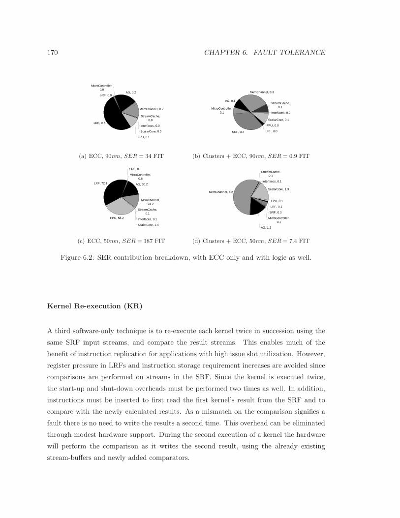
170 CHAPTER 6. FAULT TOLERANCE
MicroController, 0.0
MemChannel, 0.2
Interfaces, 0.0
ScalarCore, 0.0
SRF, 0.0
FPU, 0.1
StreamCache, 0.0
AG, 0.2
LRF, 0.5
(a) ECC, 90nm, SER = 34 FIT
MicroController, 0.1
MemChannel, 0.3
Interfaces, 0.0
ScalarCore, 0.1
LRF, 0.0
AG, 0.1StreamCache,
0.1
FPU, 0.0
SRF, 0.3
(b) Clusters + ECC, 90nm, SER = 0.9 FIT
MicroController, 0.8
MemChannel, 24.2
Interfaces, 0.1
ScalarCore, 1.4
LRF, 72.1 AG, 30.2
StreamCache, 0.1
FPU, 58.2
SRF, 0.3
(c) ECC, 50nm, SER = 187 FIT
MicroController, 0.1
MemChannel, 4.2
Interfaces, 0.1
ScalarCore, 1.3
LRF, 0.1
AG, 1.2
StreamCache, 0.1
FPU, 0.1
SRF, 0.3
(d) Clusters + ECC, 50nm, SER = 7.4 FIT
Figure 6.2: SER contribution breakdown, with ECC only and with logic as well.
Kernel Re-execution (KR)
A third software-only technique is to re-execute each kernel twice in succession using the
same SRF input streams, and compare the result streams. This enables much of the
benefit of instruction replication for applications with high issue slot utilization. However,
register pressure in LRFs and instruction storage requirement increases are avoided since
comparisons are performed on streams in the SRF. Since the kernel is executed twice,
the start-up and shut-down overheads must be performed two times as well. In addition,
instructions must be inserted to first read the first kernel’s result from the SRF and to
compare with the newly calculated results. As a mismatch on the comparison signifies a
fault there is no need to write the results a second time. This overhead can be eliminated
through modest hardware support. During the second execution of a kernel the hardware
will perform the comparison as it writes the second result, using the already existing
stream-buffers and newly added comparators.
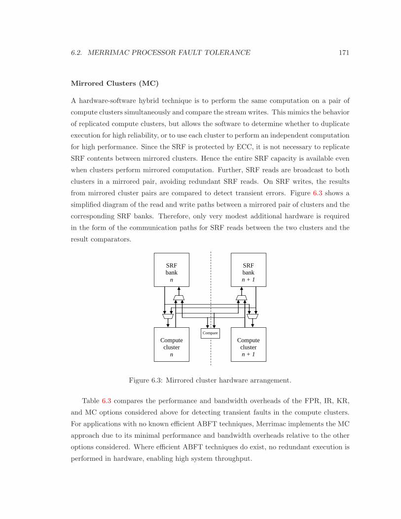
6.2. MERRIMAC PROCESSOR FAULT TOLERANCE 171
Mirrored Clusters (MC)
A hardware-software hybrid technique is to perform the same computation on a pair of
compute clusters simultaneously and compare the stream writes. This mimics the behavior
of replicated compute clusters, but allows the software to determine whether to duplicate
execution for high reliability, or to use each cluster to perform an independent computation
for high performance. Since the SRF is protected by ECC, it is not necessary to replicate
SRF contents between mirrored clusters. Hence the entire SRF capacity is available even
when clusters perform mirrored computation. Further, SRF reads are broadcast to both
clusters in a mirrored pair, avoiding redundant SRF reads. On SRF writes, the results
from mirrored cluster pairs are compared to detect transient errors. Figure 6.3 shows a
simplified diagram of the read and write paths between a mirrored pair of clusters and the
corresponding SRF banks. Therefore, only very modest additional hardware is required
in the form of the communication paths for SRF reads between the two clusters and the
result comparators.
SRF bank
n
Compare
SRF bank n + 1
Compute cluster
n
Compute
cluster n + 1
Figure 6.3: Mirrored cluster hardware arrangement.
Table 6.3 compares the performance and bandwidth overheads of the FPR, IR, KR,
and MC options considered above for detecting transient faults in the compute clusters.
For applications with no known efficient ABFT techniques, Merrimac implements the MC
approach due to its minimal performance and bandwidth overheads relative to the other
options considered. Where efficient ABFT techniques do exist, no redundant execution is
performed in hardware, enabling high system throughput.
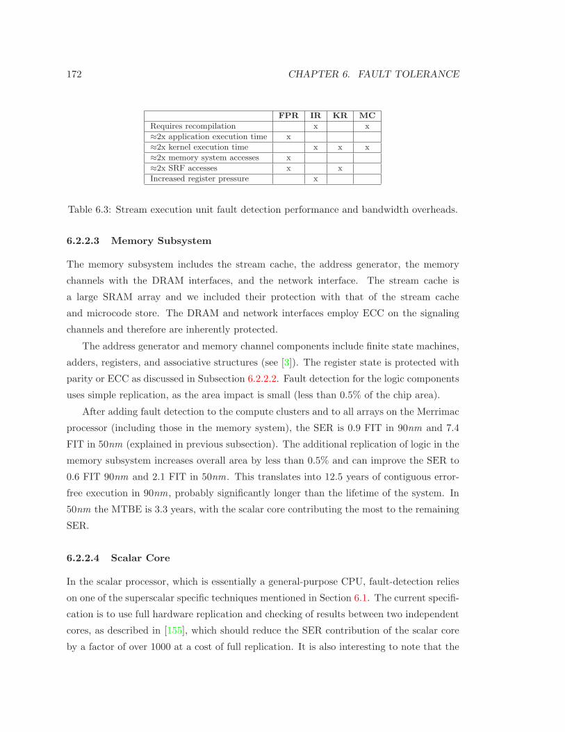
172 CHAPTER 6. FAULT TOLERANCE
FPR IR KR MC
Requires recompilation x x
≈2x application execution time x
≈2x kernel execution time x x x
≈2x memory system accesses x
≈2x SRF accesses x x
Increased register pressure x
Table 6.3: Stream execution unit fault detection performance and bandwidth overheads.
6.2.2.3 Memory Subsystem
The memory subsystem includes the stream cache, the address generator, the memory
channels with the DRAM interfaces, and the network interface. The stream cache is
a large SRAM array and we included their protection with that of the stream cache
and microcode store. The DRAM and network interfaces employ ECC on the signaling
channels and therefore are inherently protected.
The address generator and memory channel components include finite state machines,
adders, registers, and associative structures (see [3]). The register state is protected with
parity or ECC as discussed in Subsection 6.2.2.2. Fault detection for the logic components
uses simple replication, as the area impact is small (less than 0.5% of the chip area).
After adding fault detection to the compute clusters and to all arrays on the Merrimac
processor (including those in the memory system), the SER is 0.9 FIT in 90nm and 7.4
FIT in 50nm (explained in previous subsection). The additional replication of logic in the
memory subsystem increases overall area by less than 0.5% and can improve the SER to
0.6 FIT 90nm and 2.1 FIT in 50nm. This translates into 12.5 years of contiguous error-
free execution in 90nm, probably significantly longer than the lifetime of the system. In
50nm the MTBE is 3.3 years, with the scalar core contributing the most to the remaining
SER.
6.2.2.4 Scalar Core
In the scalar processor, which is essentially a general-purpose CPU, fault-detection relies
on one of the superscalar specific techniques mentioned in Section 6.1. The current specifi-
cation is to use full hardware replication and checking of results between two independent
cores, as described in [155], which should reduce the SER contribution of the scalar core
by a factor of over 1000 at a cost of full replication. It is also interesting to note that the

6.2. MERRIMAC PROCESSOR FAULT TOLERANCE 173
scalar core occupies a small portion of the total chip area, and therefore does not greatly
contribute to the overall SER. It may be possible to use less expensive software-based
techniques with no hardware replication to protect it, provided the slowdown in the con-
trol processor does not dramatically reduce the performance of the stream unit under its
control.
6.2.2.5 Summary of Fault-Detection Scheme
Table 6.4 summarizes the estimated expected SER reduction, as well as area and per-
formance overheads of the techniques described above. Each line in the table represents
adding a technique to the design and the cumulative increase in area compared to the
baseline described in Subsection 6.2.1.
Adding ECC to all arrays (including the LRFs and registers within the address genera-
tor and memory channels) is the most cost-effective way to increase fault-tolerance. With
an area overhead of 3.2% the SER is reduced by two orders of magnitude down to 4 FIT
in 90nm, technology. However, this method will not be sufficient in future technologies,
where we still expect an SER of 65 FIT arising mostly from logic. The focus of this chapter
is on fault-tolerance for the compute clusters, and we see that with practically no area
over-head we are able to improve SER by close to an additional 80% in 90nm and 90% in
50nm over ECC alone. The final two methods at our disposal are hardware replication in
the memory subsystem and scalar unit.
Technique Total Cumulative Performance SER MTBE SER MTBEArea Area Impact 90nm (16K nodes) 50nm (16K nodes)(mm
2) Overhead (FIT) 90nm (FIT) 50nm
Baseline 139 0% N/A 422 6 days 643 4 daysECC on 143 2.3% minimal 34 11 weeks 187 2 weeksSRAM arraysECC on 144 3.2% ∼ 1.5× kernel 4 1.6 years 65 6 weeksall arrays exec. timeIR/KR/MC 145 4.0% ∼ 2× kernel 1 8 years 7 1 year
exec. timeInterfaces 145 4.2% none 0.6 12 years 2 3.3 yearsScalar 154 11% none 0.4 16 years 0.7 9.5 yearsredundancy
Table 6.4: Summary of fault-detection schemes.

174 CHAPTER 6. FAULT TOLERANCE
6.2.3 Recovery from Faults
The above techniques are aimed at detecting the occurrence of transient faults. Once a
fault is detected, the system must recover to a pre-fault state. The ECC protecting the
memories are capable of correcting single bit errors, and hence do not require system-level
recovery. However, on all other detectable faults, including multi-bit failures in storage
arrays, recovery uses the checkpoint-restart scheme. Periodically, the system state is
backed up on non-volatile storage. Once a fault is detected, the system state is restored
from the last correct checkpoint. This technique is commonly used in scientific computing
because of the batch usage model. The applications do not require an interactive real-time
response, and checkpoint-restart can be used with no additional hardware and with only
a small effect on overall application runtime.
In Subsection 6.2.3.1 we develop a set of equations for the optimal checkpoint interval
and expected performance degradation. We then explore the expected slowdown given
Merrimac system parameters and show that a checkpoint interval of several hours results
in less than 5% application slowdown (Subsection 6.2.3.2).
6.2.3.1 Slowdown Equations
We will use the following notation while developing the slowdown equation. System pa-
rameters appear in bold and will be discussed in the next subsection.
Tcp – checkpoint duration
∆tcp – checkpoint interval
Tcp−1 – time to restore a checkpoint and restart
T – program runtime
T0 – runtime on a perfect system
S – slowdown
t – current time
tF – time of failure occurrence
ncp – number of checkpoints performed
nf – number of failures
∆tfi– duration between failure i and i − 1
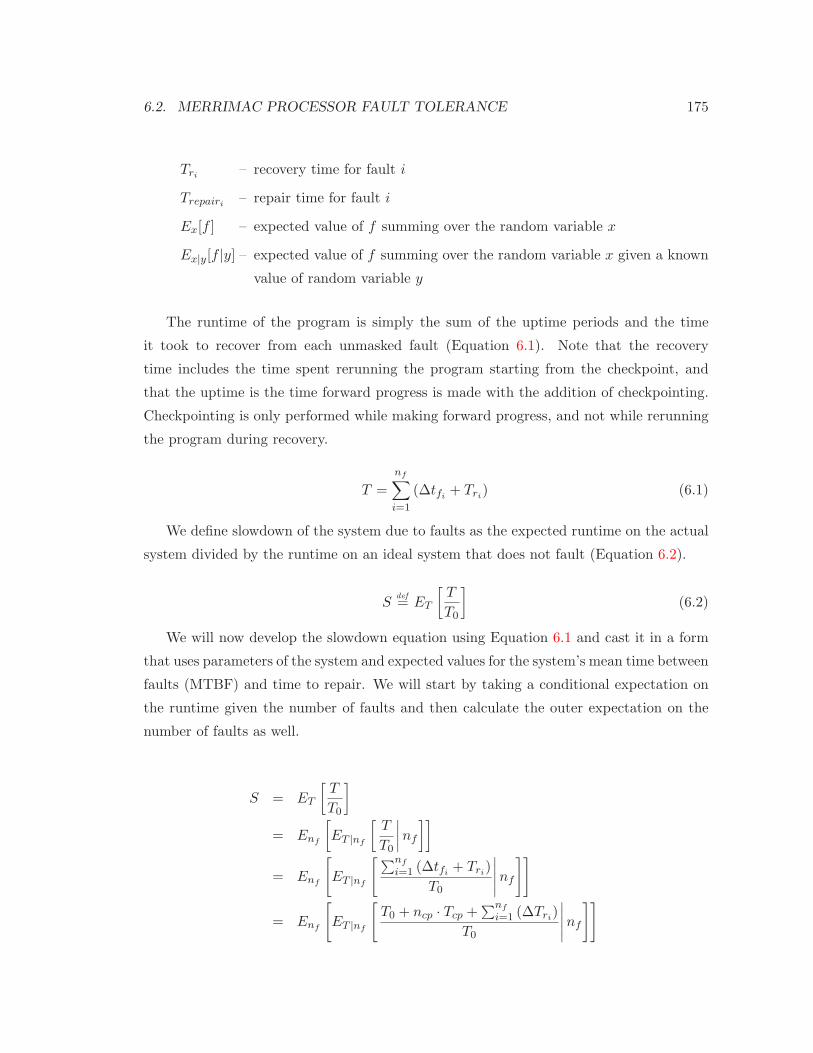
6.2. MERRIMAC PROCESSOR FAULT TOLERANCE 175
Tri– recovery time for fault i
Trepairi– repair time for fault i
Ex[f ] – expected value of f summing over the random variable x
Ex|y[f |y] – expected value of f summing over the random variable x given a known
value of random variable y
The runtime of the program is simply the sum of the uptime periods and the time
it took to recover from each unmasked fault (Equation 6.1). Note that the recovery
time includes the time spent rerunning the program starting from the checkpoint, and
that the uptime is the time forward progress is made with the addition of checkpointing.
Checkpointing is only performed while making forward progress, and not while rerunning
the program during recovery.
T =
nf∑
i=1
(∆tfi+ Tri
) (6.1)
We define slowdown of the system due to faults as the expected runtime on the actual
system divided by the runtime on an ideal system that does not fault (Equation 6.2).
Sdef= ET
[
T
T0
]
(6.2)
We will now develop the slowdown equation using Equation 6.1 and cast it in a form
that uses parameters of the system and expected values for the system’s mean time between
faults (MTBF) and time to repair. We will start by taking a conditional expectation on
the runtime given the number of faults and then calculate the outer expectation on the
number of faults as well.
S = ET
[
T
T0
]
= Enf
[
ET |nf
[
T
T0
∣
∣
∣
∣
nf
]]
= Enf
[
ET |nf
[
∑nf
i=1 (∆tfi+ Tri
)
T0
∣
∣
∣
∣
∣
nf
]]
= Enf
[
ET |nf
[
T0 + ncp · Tcp +∑nf
i=1 (∆Tri)
T0
∣
∣
∣
∣
∣
nf
]]

176 CHAPTER 6. FAULT TOLERANCE
= Enf
ET |nf
T0 +T0
∆tcp· Tcp +
nf∑
i=1
(∆Tri)
T0
∣
∣
∣
∣
∣
∣
∣
∣
∣
∣
∣
nf
=Tcp
∆tcp+ 1 + Enf
[
nf ·ET |nf
[Tr|nf ]
T0
]
=Tcp
∆tcp+ 1 + E [Tr] · E
[
nf
T0
]
=Tcp
∆tcp+ 1 + E [Tr] · E
[
T
T0· 1
E [∆tf ]
]
=Tcp
∆tcp+ 1 + S
E [Tr]
E [∆tf ]
=
(
Tcp
∆tcp+ 1
)(
1 − E[Tr]
E[∆Tf ]
)−1
(6.3)
Now we need to express the expected recovery time (E[Tr]) in terms of the parameters
of the system. The recovery time is composed of the time it takes to repair the fault,
the time it takes to restore from a checkpoint and restart the system, and the time spent
rerunning the part of the program between the last checkpoint and the time the fault
occurred (Equation 6.4).
E[Tr] = E[Trepair] + E[∆trerun] + Tcp−1 (6.4)
Now we will express the rerun time in terms of known quantities of the system (Equa-
tion 6.5).
E[∆trerun] =
ncp−1∑
i=0
((Pr {i∆tcp ≤ tF < (i + 1)∆tcp} ·
E [tF − i∆tcp|i∆tcp ≤ t < (i + 1) ∆tcp]) +
(Pr {i∆tcp ≤ tF < (i∆tcp + Tcp)} ·
E [tF − i∆tcp|i∆tcp ≤ tF < (i∆tcp + Tcp)]))
Even using the simple and common assumption of a Poisson process for faults (which
leads to an exponential distribution on ∆tf ) the expected rerun-time is not simple to

6.2. MERRIMAC PROCESSOR FAULT TOLERANCE 177
calculate. To simplify the calculation we will make the following assumptions:
1. Probability of fault while checkpointing is negligible.
2. Probability of fault while restoring a checkpoint is negligible.
3. Repair time is constant (assumes there is always a ready spare to replace the faulting
board)
The result of these assumptions is that we can provide a simple upper bound for the
expected time spent rerunning the program (Equation 6.5). To arrive at this bound we
will use a 0-order piece-wise approximation of the reliability function (∆tf ) at checkpoint
intervals. This means that the failure distribution is uniform across each checkpoint
interval (Figure 6.2.3.1).
Figure 6.4: 0-order piecewise approximation of the reliability function.
Using this approximation and assumptions 1 and 2, we can rewrite Equation 6.5 as:
E[∆trerun] <=
ncp−1∑
i=0
(Pr {i∆tcp ≤ tF < (i + 1) ∆tcp} ·
E [tF − i∆tcp|i∆tcp ≤ t < (i + 1)∆tcp])
=
ncp−1∑
i=0
(
Pr {i∆tcp ≤ tF < (i + 1)∆tcp} ·∆tcp
2
)
=∆tcp
2·
ncp−1∑
i=0
(Pr {i∆tcp ≤ tF < (i + 1)∆tcp})
=∆tcp
2· 1
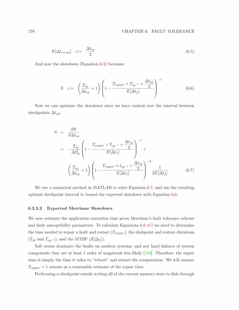
178 CHAPTER 6. FAULT TOLERANCE
E[∆trerun] <=∆tcp
2(6.5)
And now the slowdown (Equation 6.3) becomes:
S <=
(
Tcp
∆tcp+ 1
)
1 −Trepair + Tcp−1 +
∆tcp
2E[∆tf ]
−1
(6.6)
Now we can optimize the slowdown since we have control over the interval between
checkpoints ∆tcp:
0 =∂S
∂∆tcp
= − Tcp
∆t2cp
1 −Trepair + Tcp−1 +
∆tcp
2E[∆tf ]
−1
+
(
Tcp
∆tcp+ 1
)
1 −Trepair + tcp−1 +
∆tcp
2E[∆tf ]
−2
1
2E[∆tf ](6.7)
We use a numerical method in MATLAB to solve Equation 6.7, and use the resulting
optimal checkpoint interval to bound the expected slowdown with Equation 6.6.
6.2.3.2 Expected Merrimac Slowdown
We now estimate the application execution time given Merrimac’s fault tolerance scheme
and fault susceptibility parameters. To calculate Equations 6.6–6.7 we need to determine
the time needed to repair a fault and restart (Trepair), the chekpoint and restore durations
(Tcp and Tcp−1), and the MTBF (E[∆f ]).
Soft errors dominate the faults on modern systems, and not hard failures of system
components that are at least 1 order of magnitude less likely [109]. Therefore, the repair
time is simply the time it takes to “reboot” and restart the computation. We will assume
Trepair = 1 minute as a reasonable estimate of the repair time.
Performing a checkpoint entails writing all of the current memory state to disk through

6.2. MERRIMAC PROCESSOR FAULT TOLERANCE 179
the I/O channels of the system. On systems with local disks, the checkpoint duration is
typically less than a minute, while on systems with centralized storage checkpointing can
take up to 10 minutes. Figure 6.5 shows the expected slowdown, with Trepair = 1 minute,
across a range of MTBF and Tcp values. If the MTBF is less than 100 hours, it is desirable
to have low Tcp and use local disks to store checkpoints. On the other hand, if the MTBF
is large, even with global checkpoint storage the expected slowdown is less than 5%.
1
1.02
1.04
1.06
1.08
1.1
1.12
1.14
0 100 200 300 400
MTBF [hours]
Slo
wdo
wn
Tcp=1 sec.Tcp=10 sec.Tcp=1 min.Tcp=10 min.
Figure 6.5: Expected slowdown sensitivity to the MTBF. A fully configured Merrimacsupercomputer has an MTBF of 20 hours.
The Merrimac supercomputer is composed of processor, router, and DRAM chips,
as well as mechanical components and power supplies. The fault rate of the non-VLSI
components is low, because they are not subject to soft errors. The Merrimac processor
has a fault rate of roughly 75FIT. The fault rate for Merrimac is higher than the MTBE
discussed in Subsection 6.2.1, because detected but uncorrected errors in the SRAM arrays
still require restoring a checkpoint. We assume a similar SER for the interconnection
network components. For DRAM, we use previously published results [18, 109, 42] and
estimate that a single DRAM chip has a SER of 140FIT for a detected but uncorrected
error. Each Merrimac processor requires 16 DRAM chips, and thus the MTBF for the
Merrimac system is 3, 120 FIT per node, or a MTBF of 20 hours for 16K processor.
Using Equations 6.6–6.7, with the parameters above, the expected application perfor-
mance degradation is 4.4% for a checkpoing duration of 1 minute and an optimal check-
point interval of 0.8 hours (48 minutes). Figure 6.6 shows the sensitivity of the expected
slowdown on the checkpoint interval. For a slowdown of less than 5% the checkpoint

180 CHAPTER 6. FAULT TOLERANCE
interval must be lower than 1.3 hours.
1.0
1.1
1.1
0.3 0.8 1.3 1.8 2.3 2.8
∆∆∆∆ T_cp [hours]
Slo
wdo
wn
1.0
1.1
1.1
0.3 0.8 1.3 1.8 2.3 2.8
∆∆∆∆ T_cp [hours]
Slo
wdo
wn
Figure 6.6: Expected slowdown sensitivity to the checkpoint interval. ∆Tcp is varied froma factor of about 0.3 to 3.0 away from the optimal interval. This figure is plotted for theestimated values of a 16K-node Merrimac with an MTBF of 20 hours and a checkpointtime (Tcp) of 1 minute.
Finally, we look at the mechanism for recovery from hard faults of system components.
Figure 6.7 shows the effects of varying the recovery time from 1 minute to 5 hours, across
a range of hard-fault MTBFs. We expect Merrimac’s hard-fault MTBF to be one order
of magnitude higher than the soft-error MTBF, or roughly 250 hours. Even with a 5 hour
repair time, the performance degradation due to hard faults is only 3%. Therefore, it is
not necessary to include hot spares in the system design.
6.3 Evaluation
To demonstrate the trade-offs involved we now evaluate the techniques discussed in the
previous section on three case study applications. The first example is of dense matrix-
matrix multiplication that can employ a very efficient algorithmic based fault tolerance
technique [68]. The second is StreamMD that has more dynamic behavior and for which
no ABFT technique has been developed. Finally, we also discuss StreamFEM that cannot
employ ABFT and presents different execution characteristics than StreamMD. Together,
these three case studies cover a large range of attributes and allow us to fully explore the
tradeoffs in applying our fault-detection techniques.
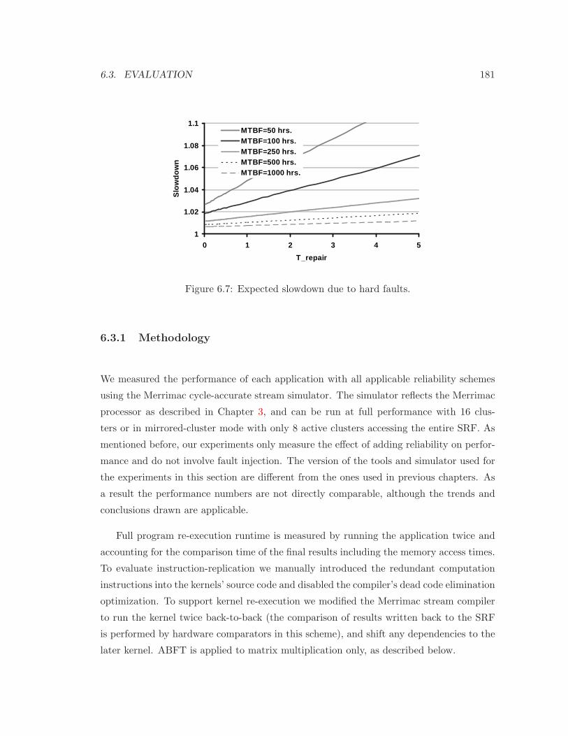
6.3. EVALUATION 181
1
1.02
1.04
1.06
1.08
1.1
0 1 2 3 4 5
T_repair
Slo
wdo
wn
MTBF=50 hrs.MTBF=100 hrs.MTBF=250 hrs.MTBF=500 hrs.MTBF=1000 hrs.
Figure 6.7: Expected slowdown due to hard faults.
6.3.1 Methodology
We measured the performance of each application with all applicable reliability schemes
using the Merrimac cycle-accurate stream simulator. The simulator reflects the Merrimac
processor as described in Chapter 3, and can be run at full performance with 16 clus-
ters or in mirrored-cluster mode with only 8 active clusters accessing the entire SRF. As
mentioned before, our experiments only measure the effect of adding reliability on perfor-
mance and do not involve fault injection. The version of the tools and simulator used for
the experiments in this section are different from the ones used in previous chapters. As
a result the performance numbers are not directly comparable, although the trends and
conclusions drawn are applicable.
Full program re-execution runtime is measured by running the application twice and
accounting for the comparison time of the final results including the memory access times.
To evaluate instruction-replication we manually introduced the redundant computation
instructions into the kernels’ source code and disabled the compiler’s dead code elimination
optimization. To support kernel re-execution we modified the Merrimac stream compiler
to run the kernel twice back-to-back (the comparison of results written back to the SRF
is performed by hardware comparators in this scheme), and shift any dependencies to the
later kernel. ABFT is applied to matrix multiplication only, as described below.

182 CHAPTER 6. FAULT TOLERANCE
6.3.2 Matrix Multiplication
Our matrix multiplication example consists of multiplying two dense matrices A and B
of sizes (304 × 512) and (512 × 384) to form the result matrix C of size (304 × 384).
The matrices sizes were chosen to be large enough to exceed the size of the SRF, thus
being representative of much larger matrices while not requiring unduly large simulation
times on the cycle accurate simulator. The computation was hierarchically blocked to take
advantage of locality at both the SRF and LRF levels, as well as utilize Merrimac’s inter-
cluster communication. The full details of this implementation are not described in this
dissertation. The resulting code is just memory system limited on Merrimac, and achieves
over 80% of Merrimac’s 128GFLOP/s only accounting for actual matrix computation
instructions.
Our ABFT implementation of matrix multiplication follows the ideas discussed in [68]
and uses a simple column checksum. As we process a block of the A matrix in the SRF
we compute the sum of each of its columns. This checksum row is then multiplied with
the block of the B matrix and stored back to the SRF. Once an entire block of the result
matrix C is computed in the SRF we run a kernel that computes the column sums of
the C matrix block and compares them against the multiplied checksum row. Due to
the linearity of matrix multiplication, any difference in the results indicates an erroneous
computation and a fault exception can be raised.
Scheme Normalized Register InstructionRuntime Pressure Pressure
Baseline 1.00 17 117
FPR 2.09 17 117
IR 2.51 52 258
KR 1.77 17 117
MC 1.76 17 117
ABFT 1.03 22 255
Table 6.5: Evaluation of MATMUL under the five reliability schemes.
Table 6.5 summarizes the results for matrix multiplication. The runtime is given rela-
tive to the baseline implementation that does not use any of the stream unit fault-detection
mechanisms. The register-pressure column lists the maximum number of registers in a
single LRF required to run each variant, and the instruction-pressure column shows the
number of instructions that need to be present in the micro-code store.
As expected, FPR, the simplest fault-detection method, has a large impact on runtime

6.3. EVALUATION 183
requiring a full re-execution with an additional 10% increase due to the final comparison.
The poor performance of the IR software scheme, which has a slowdown of about 20%
compared even to FPR, is the result of the large number of comparisons that were added
to the compute kernel and the fact that the baseline kernel fully utilized all the available
multiply-add units. Moreover, IR requires over two times as many instructions in the
kernel and increases the register requirements in a single LRF by a similar factor.
Both the KR and MC approaches essentially double the computation only without
increasing register or instruction pressure and rely on comparators in hardware. As the
baseline implementation is memory bandwidth limited on Merrimac, the additional com-
putations fill the idle execution slots resulting in a speedup of 18% over naive FPR. The
small difference of 1% in runtime in favor of MC over KR is due to the necessity of doubling
the small kernel overhead in the KR scheme.
Finally ABFT is clearly superior for matrix multiplication, and requires only a small
overhead of 3% to achieve fault detection. While the increase in code size is significant
(a factor of almost 2.2), the total size is still small and easily fits within Merrimac’s
instruction store.
6.3.3 StreamMD
Unlike matrix multiplication, force calculation in molecular dynamics displays dynamic
behavior and non-linear computations and we are not aware of any ABFT technique
that is applicable to it. We use the nDR IL COND variant of StreamMD, the Merrimac
implementation of the GROMACS ([164]) water-water force calculation as an example of
such an application.
Scheme Normalized Register InstructionRuntime Pressure Pressure
Baseline 1.00 27 170
FPR 2.01 27 170
IR 1.85 47 328
KR 1.90 27 170
MC 1.88 27 170
Table 6.6: Evaluation of StreamMD under the four applicable reliability schemes.
Table 6.6 lists our results for StreamMD, and follows the format of Table 6.5 described
in the previous subsection.
The force calculation requires significant computation and a large input set, yet only

184 CHAPTER 6. FAULT TOLERANCE
produces a small number of values as a result (the total force on each atom in the system).
Therefore, FPR has little overhead for comparison and requires 2.01× the runtime of the
baseline case. Another differentiation point from matrix-multiply is that the molecular
dynamics application is not as memory limited as the MATMUL version used in this chap-
ter. This makes FPR a more attractive alternative, where the best performing reliability
technique is only 8% faster.
While IR did not perform well in the case of matrix multiplication, it is the most
efficient technique applicable to molecular dynamics. The reason is that the structure
of the computation is such that there is significant slack in kernel schedule and not all
instruction slots are filled during kernel execution (as in matrix multiplication). As a result
some of the additional instructions required to duplicate the computation and perform
the comparison can be scheduled in the empty slots leading to a kernel that requires less
than twice the execution time of the baseline kernel. This is not the case for the KR
and MC schemes, which fully double the execution time the main kernel loop, trailing
the performance of IR by 3% and 2% respectively. However, achieving this speedup
requires increasing the number of registers in each LRF and roughly doubling the kernels
instruction count.
The performance difference between the KR and MC techniques is again quite low, at
1% due to the small overhead of priming the kernel software pipelined main loop.
6.3.4 StreamFEM
As a third case study, we chose the Euler-quadratic variant of StreamFEM. This variant
includes kernels with large startup overheads allowing us to explore another point in the
tradeoff space.
Scheme Normalized Register InstructionRuntime Pressure Pressure
Baseline 1.00 88 1907
FPR 2.05 88 1907
IR 1.48 172 3588
KR 1.52 88 1907
MC 1.40 88 1907
Table 6.7: Evaluation of StreamFEM under the four applicable reliability schemes.
Table 6.7 lists our results for StreamFEM, and follows the format of Table 6.5 and
Table 6.6 described in the previous subsections.

6.4. DISCUSSION 185
The most striking difference about the Euler-quadratic variant of StreamFEM is the
very large kernels and the number of registers required. The kernel is over 10 times larger
than MATMUL and nearly exhausts all available registers on Merrimac (requiring 88
registers). While IR performed well, improving the runtime by 38% over FPR, the register
pressure exceeds the available register space due to the increased state of instruction
replication. Similarly, the microcode store is barely large enough to hold the kernels after
replicating all instructions.
Another interesting feature of this configuration of StreamFEM is that a few of the
kernels have significant startup overheads. This limits the effectiveness of KR, which is
2% slower than IR and 8.5% slower than the MC approach.
The combination of a large amount of state, high instruction count, densely scheduled
kernels, and high-startup overhead leads to the reconfigurable hardware MC scheme to
outperform the software techniques. MC is 6% faster than IR – the best software approach
for this application.
6.4 Discussion
The three case studies presented above span diverse characteristics in the trade-off space.
Matrix multiplication shows the power of applying an ABFT technique, but also rep-
resents applications with a relatively high overhead for final-result comparison, memory
bandwidth limited applications (with this particular dataset and version of the tools),
very tight kernel schedules, and low kernel startup overheads. Molecular dynamics on the
other hand, requires very few comparisons of its final result, is not memory limited, and
has kernels with significant scheduling slack. Finally, like StreamMD, StreamFEM also
requires few final comparisons and is not memory limited. However, StreamFEM has a
high instruction count, large register state requirements, and significant kernel startup
overheads. We can draw a few interesting observations from these characteristics.
The most obvious observation is that ABFT techniques should be applied when possi-
ble. While not all cases will be as efficient as dense matrix multiplication, we expect that
ABFT will almost always offer better performance than other schemes, possibly requiring
modifications to the input set of the application. One exception to this general rule is
applications that are extremely memory bandwidth limited, for which even doubling the
computation will not change the total runtime.

186 CHAPTER 6. FAULT TOLERANCE
Another interesting point is that kernels that do not have a very tight schedule offer
the opportunity to hide much of the cost of instruction replication. This matches with
many observations of using this technique with conventional CPUs, which usually display
significant idle execution slots.
Finally, the stream execution model of Merrimac enables the KR and MC techniques
that are not available to GPPs. Because Merrimac uses hierarchical control of all compute
and on-chip storage resources, software can guarantee that no unchecked result is commit-
ted to visible off-chip state. This is not the case with cache-based GPPs that have control
granularity of single instructions and writes of individual words to off-chip memory. In
MATMUL and StreamMD, the kernel startup overheads are low, and therefore KR is
almost as efficient as MC. The small amount of additional hardware required to enable
MC execution (a local switch between the SRF lanes of each cluster pair), is, however,
more attractive for StreamFEM with its high kernel overheads.

Chapter 7
Conclusions
This dissertation presents and evaluates the architecture of the Merrimac Streaming Su-
percomputer. Merrimac demonstrates that the streaming execution and architectural
model is very effective for scientific computing and achieves significant improvements in
performance per unit die area, performance per unit energy, performance per unit cost,
and performance per unit floor space. Merrimac is tuned for scientific computing and relies
on the abundant parallelism and locality of the applications as well as the throughput-
oriented usage model. The key to Merrimac’s efficiency is a hierarchical architecture in
both storage and control. The explicitly managed locality hierarchy of storage allows
software to make optimal use of scarce on-chip state and global bandwidth resources.
The control hierarchy overcomes the von Neumann bottleneck, which limits the perfor-
mance of general-purpose processors, and allows Merrimac to efficiently operate a very
large number of functional units and a throughput-oriented memory system. In conjunc-
tion with the high throughput execution and memory architecture, Merrimac provides
throughout-oriented programming, arithmetic, exception handling, and memory models
to make effective use of the capable hardware. Merrimac also places emphasis on a scal-
able system design and fault-tolerance mechanisms. The paragraphs below summarize the
main contributions and are followed by discussion of possible future work.
We developed and detailed the architecture of Merrimac in Chapter 3 and summarized
our performance evaluation in Chapter 4. As discussed in Section 2.3, general-purpose
processors dominate the supercomputing market today. Table 7.1 summarizes the advan-
tages of Merrimac over a representative GPP, the Intel 3.6GHz Pentium 4 (Prescott core).
187

188 CHAPTER 7. CONCLUSIONS
Looking at the peak performance numbers, Merrimac has a factor of 18 greater perfor-
mance per processor, Merrimac also has an advantage of 25 times higher energy efficiency
per unit performance, and a 14 times better cost/performance ratio. These advantages
are achieved despite the fact that our estimates for Merrimac are based on an ASIC design
flow as opposed to the full-custom design of the Pentium 4. Table 7.1 also directly com-
pares the four applications for which we have an optimized version for both Merrimac and
the Pentium 4. With the exception of the memory bound StreamSPAS application, Mer-
rimac maintains its performance, power/performance, and cost/performance advantages
over the GPP expected from the peak values.
Application Metric (sustained) Merrimac Pentium 4 Improvement
peakGFLOP/s 128 7.2 17.8W/GFLOP/s 0.5 12.5 24.6$/GFLOP/s 1.1 15.6 13.7
MATMULGFLOP/s 117 6.6 17.7W/GFLOP/s 0.6 13.6 24.5$/GFLOP/s 1.2 16.9 13.7
FFT3DGFLOP/s 37 2.0 18.7W/GFLOP/s 1.8 45.5 25.9$/GFLOP/s 3.9 56.6 14.4
StreamMDGFLOP/s 46 2.5 16.1W/GFLOP/s 1.4 31.5 22.3$/GFLOP/s 3.2 39.2 12.4
StreamSPASGFLOP/s 3.1 0.5 6.0W/GFLOP/s 21.0 174.2 8.3$/GFLOP/s 46.8 216.8 4.6
Table 7.1: Summary of Merrimac advantages over Pentium 4.
In addition to the advantages expected for a single processor, the Merrimac system is
designed to economically scale in terms of both performance per unit cost and performance
per unit floor-space. As discussed in Subsection 3.5.2, we estimate Merrimac, which can
be built using widely available 90nm technology, to have an order of magnitude higher
peak performance than the current fastest supercomputer. At the same time, we expect
the system cost to be 9 times lower per unit performance than the custom designed
BlueGene/L and to require a factor of 6 less floor space. When comparing to the COTS-
based Red Storm computer, Merrimac’s advantage is a factor of 64 in cost/performance
and over 80 times better in terms of performance per unit floor space.
To support this scalability, Merrimac relies on the stream execution model and the
properties of scientific applications and places greater responsibility on software. The
7.1. FUTURE WORK 189
memory model provides minimal and efficient hardware mechanisms for software con-
trolled consistency and coherency. Similarly the fault tolerance mechanisms match the
usage model of scientific computing and provide low-overhead reconfigurable hardware
mechanisms. The software system and user can decide whether to rely on hardware
fault detection, at reduced peak performance, or delegate the responsibility to a software
method that can utilize the full performance potential of Merrimac.
Finally, we showed how to map a variety of scientific applications, inspired by the com-
plex multi-physics modeling applications of the Center for Integrated Turbulence Simula-
tion at Stanford University, onto Merrimac. To do so, we developed a general framework
and software tools to execute challenging unstructured mesh and graph applications, which
feature irregular control and unstructured memory access patterns on stream processors.
7.1 Future Work
The Merrimac architecture is designed for scientific computing, with the driving applica-
tions centered around the fluid and molecular dynamics applications of CITS. Looking at
a wider range of numerical methods may lead to several interesting research directions as
described below. Additionally, this dissertation focuses on the Merrimac processor itself,
and future work should evaluate the scalability to multi-processor systems.
7.1.1 Computation and Communication Tradeoffs
As semiconductor technology continues to scale on-chip devices at a higher rate than off-
chip bandwidth, increasing locality by recomputing values instead of fetching them from
memory becomes a meaningful optimization. Performance can potentially be improved
by increasing the arithmetic intensity, either trading off the addition of numerically un-
necessary computation for a reduction in memory bandwidth requirements, or by taking
advantage of the ample compute resources to implement more accurate physical models
that will require an overall smaller number of timesteps or mesh elements. While locality
is a crucial consideration, parallelism must also be increased to allow the concurrent use
of the growing number of functional units on a chip and in the system.
An example of the first tradeoff is the register blocking optimizations applied to sparse
matrix vector multiplication described in [165]. Instead of multiplying individual matrix
and vector elements, the matrix is divided into dense blocks. This reduces the information
190 CHAPTER 7. CONCLUSIONS
stored and communicated for the sparse format and increases kernel locality. At the same
time, the dense blocks may contain zeros, increasing the amount of work performed. This
scheme works particularly well for sparse matrices generated from finite element meshes,
where the dense submatrices correspond to the mesh elements. A similar tradeoff in the
case of StreamMD is discussed in [47].
StreamFEM provides a good example of the second tradeoff. The higher order in-
terpolation functions and more complex physical modeling equations require significantly
more computation and have a higher arithmetic intensity (Subsection 4.1.5).
An avenue for future research is to generalize these examples and form a theoretical
framework and programming model for reasoning about and addressing the performance-
critical aspects of locality and parallelism. With future architectures, minimizing opera-
tion count or memory footprint will not yield the most optimal algorithms and implemen-
tations.
7.1.2 State and Latency Hiding Tradeoffs
Achieving high performance in modern systems requires mitigating the detrimental effects
of increasing latencies for fetching data from off-chip, due to both the high access latency
and low bandwidth relative to on-chip storage. In general, this can be done by exploiting
locality to reduce access latency and utilizing parallelism to hide the latency with useful
computation.
Merrimac provides minimalistic and efficient hardware mechanisms and relies on the
structured gather–compute–scatter stream execution model to mitigate the effects of la-
tency. Intra- and inter-kernel producer-consumer localities reduce the number of off-chip
accesses, and the coarse-grained stream memory operations and kernels allow software to
tolerate latency with parallelism. The applications considered in this dissertation fit the
stream execution and programming model well. Even the irregular applications still fea-
ture a clear gather-compute-scatter structure, with the gathers and scatters being mostly
independent from the actual computation. The reason for this behavior is that the data
structures used are static and the traversal order is predetermined with respect to the
stream code.
Not all applications, however, have this simplifying characteristic. For example, algo-
rithms that use geometric acceleration structures, such as ray tracing and the Barnes-Hut
n-body method, have much tighter dependence between computation and data access. In

7.1. FUTURE WORK 191
essence, a chain of computation and communication is formed when computation must be
performed in order to determine the data structure traversal, and data must be accessed
in order to perform this computation.
It is possible to streamify this type of data access and computation interdependence
with a breadth-first approach utilizing a work queue. The work queue maintains pending
computations, and when each computation is executed it generates a data access and
places the next computation that depends on this access onto the tail of the work queue.
If enough parallelism exists in the application, the work queue is deep enough to hide the
latency of the memory accesses. This is typically the case with challenging applications
and is true for both Barnes-Hut and ray tracing, which utilize millions of particles and
rays respectively. The drawback of the work queue solution is that the work queue must
be deep enough to hide the worst-case access latency. This results in long streams of
computation–communication chain links that must be stored as continuations.
A non-streaming approach to mitigating the access latency and achieving high perfor-
mance is to utilize parallelism with multiple threads of control instead of coarse-grained
stream operations. With the threaded method, a computation–communication chain is
processed depth first, with the assumption that most data accesses will be to on-chip mem-
ory as in the case of a cache with a high hit-rate. Threads exploit the dynamic locality of
the acceleration structure using caches. When an access results in off-chip communication,
the entire state of the thread must be stored on-chip and the state of a different restored
restored to continue its execution. If enough threads are kept live, the off-chip latency
can be tolerated. Unlike the streaming, breadth-first technique, in which stream lengths
and on-chip storage requirements are determined by the worst-case latency, the number
of live threads can be tuned for the common case of a cache hit.
To summarize, we compare the main advantages and drawbacks of the streaming and
threaded style. With the streaming style, on-chip storage resources are directly controlled
by a kernel, and continuations consist of minimal state that must be stored as communica-
tion between kernels. This approach is ideal in situations where locality can be determined
ahead of execution and kernels and streams tuned can be to exploit it. The threaded style,
on the other hand, can easily exploit dynamic locality, which cannot be determined prior
to execution. However, when locality is predetermined threads cannot utilize the locality
as efficiently streams. The reason is that on-chip resources must be partitioned between

192 CHAPTER 7. CONCLUSIONS
live threads because each thread follows an independent control path. In particular, reg-
ister resources must be dedicated to all active threads, and thread continuations for live
threads must consist of the entire thread state, as opposed to the minimal storage required
by streams.
As future work, it would be interesting to quantitatively explore these tradeoffs and
form a framework for systematically choosing the appropriate latency tolerance mecha-
nism.
7.1.3 Multi-Processor Merrimac Systems
The Merrimac processor presented in this dissertation is designed from the ground up to
be the basis of large scale parallel systems. The architecture is tuned for a throughput-
oriented usage model and the hierarchical stream execution model. Merrimac features
coarse-grained hardware mechanisms to control virtual to physical memory mapping,
stream cache coherence, memory consistency, and exception handling. However, we have
only evaluated a single-processor system that does not take advantage of these techniques.
Appendix A
Glossary
χ VLSI process independent unit representing the minimal metal pitch.
Arithmetic intensity (α) The ratio of arithmetic to global bandwidth.
CFD Computational fluid dynamics.
DLP Data-level parallelism.
DR Duplicate-removal scheme for dealing with irregular and unstructured applications.
FEM Finite element method.
FFT Fast fourier transform.
FIT Faults in time unit representing the number of faults expected to occur every 109
hours of operation.
FPU Floating point unit.
FT Fault tolerance.
FVM Finite volume method.
GBytes/s 109 bytes transferred per second.
GFLOP/s 109 floating point operations per second.
GPP General purpose processor.
193

194 APPENDIX A. GLOSSARY
IL In-lane SRF access.
ILP Instruction-level parallelism.
ISA Instruction set architecture.
lane The portion of the SRF that is aligned with a cluster.
LRF Local register file.
MAR Memory access register for describing mapping between streams and memory ad-
dress spaces.
MD Molecular dynamics.
MIMD Multiple instruction multiple data.
nDR No-duplicate-removal scheme for dealing with irregular and unstructured applica-
tions.
SB Stream buffer.
SDR Stream descriptor register describing a stream in the SRF.
SIMD Single instruction single data.
SP Stream Processor.
SRF Stream register file.
TLP Task-level parallelism.
VLSI Very large scale integration.
VP Vector processor.
XL Cross-lane SRF access.
Bibliography
[1] A. Agarwal, R. Simoni, J. Hennessy, and M. Horowitz. An evaluation of direc-
tory schemes for cache coherence. In ISCA ’88: Proceedings of the 15th Annual
International Symposium on Computer architecture, pages 280–298, 1988.
[2] J. H. Ahn, M. Erez, and W. J. Dally. Scatter-add in data parallel architectures.
In Proceedings of the Symposium on High Performance Computer Architecture (Ac-
cepted), Feb. 2005.
[3] J. H. Ahn, M. Erez, and W. J. Dally. The design space of data-parallel memory
systems. In SC’06, November 2006.
[4] A. Al-Yamani, N. Oh, and E. McCluskey. Performance evaluation of checksum-based
abft. In 16th IEEE International Symposium on Defect and Fault Tolerance in VLSI
Systems (DFT’01), San Francisco, California, USA, October 2001.
[5] J. R. Allen, K. Kennedy, C. Porterfield, and J. Warren. Conversion of control de-
pendence to data dependence. In Proceedings of the 10th ACM SIGACT-SIGPLAN
symposium on Principles of programming languages, pages 177–189, 1983.
[6] AMD, One AMD Place, P.O. Box 3453, Sunnyvale, California, USA. 3DNow! Tech-
nology Manual, Mar. 2000. Order number 21928G/0.
[7] AMD. AMD Opteron processor family. http://www.amd.com/us-
en/Processors/ProductInformation/0,,30 118 8825,00.html, 2006.
[8] H. Ando, Y. Yoshida, A. Inoue, I. Sugiyama, T. Asakawa, K. Morita, T. Muta,
T. Motokurumada, S. Okada, H. Yamashita, Y. Satsukawa, A. Konmoto, R. Ya-
mashita, and H. Sugiyama. A 1.3GHz fifth generation SPARC64 microprocessor. In
195

196 BIBLIOGRAPHY
DAC ’03: Proceedings of the 40th conference on Design automation, pages 702–705,
2003.
[9] D. M. Andrews. Using executable assertions for testing and fault tolerance. In 9th
Fault-Tolerance Computing Symposium, Madison, Wisconsin, USA, June 1979.
[10] ATI. Radeon X1900 Series. http://www.ati.com/products/RadeonX1900/ in-
dex.html, 2005.
[11] T. M. Austin. DIVA: a reliable substrate for deep submicron microarchitecture
design. In MICRO 32: Proceedings of the 32nd annual ACM/IEEE international
symposium on Microarchitecture, pages 196–207, 1999.
[12] A. Avizienis, G. C. Gilley, F. P. Mathur, D. A. Rennels, J. A. Rohr, and D. K. Rubin.
The STAR (Self Testing And Repairing) computer: an investigation of the theory
and practice of fault-tolerant computer design. IEEE Trans. Comput., C-20(11),
November 1971.
[13] J. Backus. Can programming be liberated from the von neumann style? Commu-
nications of the ACM, 21(8):613–641, August 1978.
[14] V. Balasubramanian and P. Banerjee. Compiler-assisted synthesis of algorithm-
based checking in multiprocessors. IEEE Transactions on Computers, 39(4):436–
446, 1990.
[15] P. Banerjee, J. T. Rahmeh, C. Stunkel, V. S. Nair, K. Roy, V. Balasubramanian,
and J. A. Abraham. Algorithm-based fault tolerance on a hypercube multiprocessor.
IEEE Transactions on Computers, 39(9):1132–1145, 1990.
[16] T. Barth. Simplified discontinuous Galerkin methods for systems of conservation
laws with convex extension. In Cockburn, Karniadakis, and Shu, editors, Discontin-
uous Galerkin Methods, volume 11 of Lecture Notes in Computational Science and
Engineering. Springer-Verlag, Heidelberg, 1999.
[17] C. Battista, S. Cabasino, F. Marazano, P. S. Paolucci, J. Pech, F. Rapuano,
R. Sarno, G. M. Todesco, M. Torelli, W. Tross, and P. Vicini. The APE-100 com-
puter: (I) the architecture. International Journal of High Speed Computing, 5:637,
1993.
BIBLIOGRAPHY 197
[18] R. C. Baumann. Radiation-induced soft errors in advanced semiconductor tech-
nologies. Device and Materials Reliability, IEEE Transactions on, 5(3):305–316,
September 2005.
[19] S. S. Bhattacharyya, P. K. Murthy, and E. A. Lee. Software Synthesis from Dataflow
Graphs. Kluwer Academic Press, Norwell, MA, 1996.
[20] G. E. Blelloch. Vector Models for Data-Parallel Computing. MIT Press, Cambridge,
Massachusetts, USA, 1990.
[21] A. A. Bright, R. A. Haring, M. B. Dombrowa, M. Ohmacht, D. Hoenicke, S. Singh,
J. A. Marcella, R. F. Lembach, S. M. Douskey, M. R. Ellavsky, C. G. Zoellin, and
A. Gara. Blue Gene/L compute chip: Synthesis, timing, and physical design. IBM
Journal of Research and Development, 49(2), March 2005.
[22] I. Buck. Brook specification v0.2. October 2003.
[23] I. Buck. Stream computing on graphics hardware. PhD thesis, Stanford University,
Stanford, CA, USA, 2005. Adviser-Pat Hanrahan.
[24] I. Buck, T. Foley, D. Horn, J. Sugerman, K. Fatahalian, M. Houston, and P. Hanra-
han. Brook for GPUs: stream computing on graphics hardware. ACM Transactions
on Graphics, 23(3):777–786, 2004.
[25] J. Buck, S. Ha, E. A. Lee, and D. G. Messerschmitt. Ptolemy: a framework for
simulating and prototyping heterogeneous systems. Readings in hardware/software
co-design, pages 527–543, 2002.
[26] R. Buyya. High performance cluster computing: Architectures and systems, volume
1. Prentice Hall PTR, 82:327–350, 1999.
[27] R. Buyya, D. Abramson, and J. Giddy. A Case for Economy Grid Architecture
for Service-Oriented Grid Computing. In 10th IEEE International Heterogeneous
Computing Workshop, 2001.
[28] W. W. Carlson, J. M. Draper, D. E. Culler, K. Yelick, E. Brooks, and K. Warren.
Introduction to UPC and language specification. University of California-Berkeley
Technical Report: CCS-TR-99-157, 1999.
198 BIBLIOGRAPHY
[29] B. Chelf. Brook metacompilation. SSS Internal Document, 2002.
[30] A. Chow, G. Fossum, and D. Brokenshire. A programming example: Large FFT on
the Cell Broadband Engine, 2005.
[31] ClearSpeed. CSX600 Datasheet. http://www.clearspeed.com/down-
loads/CSX600Processor.pdf, 2005.
[32] C. Clos. A study of non-blocking switching networks. Bell System Technical Journal,
32:406–424, 1953.
[33] L. Codrescu, D. Wills, and J. Meindl. Architecture of the Atlas chip-multiprocessor:
Dynamically parallelizing irregular applications. IEEE Transactions on Computer,
January 2001.
[34] T. M. Conte, K. N. Menezes, P. M. Mills, and B. A. Patel. Optimization of instruc-
tion fetch mechanisms for high issue rates. In ISCA, pages 333–344, 1995.
[35] Cray. Cray X1TMSystem Overview, 2002.
[36] Cray Inc. Cray xd1 supercomputer. http://www.cray.com/products/xd1/index.html,
2005.
[37] W. J. Dally, P. Hanrahan, M. Erez, T. J. Knight, F. Labonte, J.-H. A., N. Jayasena,
U. J. Kapasi, A. Das, J. Gummaraju, and I. Buck. Merrimac: Supercomputing with
streams. In SC’03, Phoenix, Arizona, November 2003.
[38] W. J. Dally and W. Poulton. Digital Systems Engineering. Cambridge University
Press, 1998.
[39] E. F. D’Azevedo, M. R. Fahey, and R. T. Mills. Vectorized sparse matrix multiply for
compressed row storage format. In proceedings of the 2005 International Conference
on Computational Science (ICCS’05), pages 99–106, May 2005.
[40] S. J. Deitz, B. L. Chamberlain, S.-E. Choi, and L. Snyder. The design and im-
plementation of a parallel array operator for the arbitrary remapping of data. In
PPoPP ’03: Proceedings of the ninth ACM SIGPLAN symposium on Principles and
practice of parallel programming, pages 155–166, 2003.

BIBLIOGRAPHY 199
[41] S. J. Deitz, B. L. Chamberlain, and L. Snyder. Abstractions for dynamic data
distribution. In Ninth International Workshop on High-Level Parallel Programming
Models and Supportive Environments, pages 42–51. IEEE Computer Society, 2004.
[42] T. J. Dell. A white paper on the benefits of chipkill-correct ecc for pc server main
memory. http://www-03.ibm.com/servers/eserver/pseries/campaigns/chipkill.pdf,
November 1997.
[43] J. B. Dennis. A preliminary architecture for a basic dataflow processor. In Proceed-
ings of the International Symposium on Computer Architecture, January 1976.
[44] C. C. Douglas, J. Hu, M. Iskandarani, M. Kowarschik, U. Rude, and C. Weiss.
Maximizing cache memory usage for multigrid algorithms. In Multiphase Flows and
Transport in Porous Media: State of the Art, pages 124–137. Springer, Berlin, 2000.
[45] ELPIDA Memory Inc. 512M bits XDRTM DRAM, 2005. http://
www.elpida.com/pdfs/E0643E20.pdf.
[46] D. R. Engler. Interface compilation: Steps toward compiling program interfaces as
languages. IEEE Trans. Softw. Eng., 25(3):387–400, 1999.
[47] M. Erez, J. Ahn, A. Garg, W. J. Dally, and E. Darve. Analysis and performance
results of a molecular modeling application on Merrimac. In SC’04, Pittsburgh,
Pennsylvaniva, November 2004.
[48] K. Fatahalian, T. J. Knight, M. Houston, M. E. D. R. Horn, L. Leem, J. Y. Park,
M. Ren, A. Aiken, W. J. Dally, and P. Hanrahan. Sequoia: Programming the
memory hierarchy. In SC’06, November 2006.
[49] M. Fatica, A. Jameson, and J. J. Alonso. Streamflo: an euler solver for stream-
ing architectures. In IAA Paper 2004-1090, 42nd Aerospace Sciences Meeting and
Exhibit Conference, Reno, Nevada, USA, January 2004.
[50] G. C. Fox. What have we learnt from using real parallel machines to solve real
problems? In Proceedings of the third conference on Hypercube concurrent computers
and applications, pages 897–955, 1988.
[51] G. C. Fox, R. D. Williams, and P. C. Messina. Parallel Computing Works! Morgan
Kaufmann, 1994.

200 BIBLIOGRAPHY
[52] M. Frigo. A fast Fourier transform compiler. In Proc. 1999 ACM SIGPLAN Conf.
on Programming Language Design and Implementation, pages 169–180, May 1999.
[53] M. Frigo, C. E. Leiserson, H. Prokop, and S. Ramachandran. Cache-oblivious algo-
rithms. In FOCS ’99: Proceedings of the 40th Annual Symposium on Foundations
of Computer Science, page 285, New York, New York, 1999.
[54] M. Frigo and V. Strumpen. Cache oblivious stencil computations. In ICS ’05:
Proceedings of the 19th annual international conference on Supercomputing, pages
361–366, New York, NY, USA, 2005. ACM Press.
[55] P. N. Glaskowsky. IBM’s PPC970 becomes Apple’s G5. Microprocessor Report, July
7, 2003.
[56] M. Gomaa, C. Scarbrough, T. N. Vijaykumar, and I. Pomeranz. Transient-fault
recovery for chip multiprocessors. In ISCA ’03: Proceedings of the 30th annual
international symposium on Computer architecture, pages 98–109, 2003.
[57] K. Goto and R. A. van de Geijn. Anatomy of high-performance matrix multiplica-
tion. submitted to ACM Transactions on Mathematical Software, 2006.
[58] J. Gummaraju and M. Rosenblum. Stream programming on general-purpose pro-
cessors. In MICRO 38: Proceedings of the 38th annual ACM/IEEE international
symposium on Microarchitecture, November 2005.
[59] M. Guo. Automatic parallelization and optimization for irregular scientic applica-
tions. In 18th International Parallel and Distributed Processing Symposium, 2005.
[60] H. Han, G. Rivera, and C. Tseng. Software support for improving locality in scientic
codes. In Compilers for Parallel Computation, 2000.
[61] P. Hazucha, T. Karnik, S. W. B. Bloechel, J. T. J. Maiz, K. Soumyanath, G. Dermer,
S. Narendra, V. De, and S. Borkar. Measurements and analysis of SER tolerant
latch in a 90 nm dual-Vt CMOS process. In 2003 IEEE Custom Integrated Circuits
Conference, pages 617–620, September 2003.
[62] M. T. Heath. SCIENTIFIC COMPUTING: An Introductory Survey. McGraw-Hill,
New York, 2nd edition, 2002.
BIBLIOGRAPHY 201
[63] B. Hendrickson and R. Leland. The Chaco user’s guide — version 2.0. Technical
report, Sandia National Laboratories, Technical Report SAND94-2692, 1994.
[64] J. L. Hennessy and D. A. Patterson. Computer Architecture: A Quantitative Ap-
proach. Morgan Kaufmann, 3rd edition, 2003.
[65] N. J. Higham. Accuracy and Stability of Numerical Algorithms. Society for Industrial
and Applied Mathematics, Philadelphia, PA, USA, second edition, 2002.
[66] J. Hippold and G. Runger. Task pool teams for implementing irregular algorithms
on clusters of SMPs. In Parallel and Distributed Processing Symposium, 2003.
[67] R. Ho, K. W. Mai, and M. A. Horowitz. The future of wires. Proc. of the IEEE,
89(4):14–25, April 2001.
[68] K. H. Huang and J. A. Abraham. Algorithm-based fault tolerance for matrix oper-
ations. IEEE Trans. Comput., C-33:518–528, 1984.
[69] Y. S. Hwang, B. Moon, S. D. Sharma, R. Ponnusamy, R. Das, and J. H. Saltz. Run-
time and language support for compiling adaptive irregular programs on distributed-
memory machines. Softw. Pract. Exper., 25(6):597–621, 1995.
[70] IBM. Cell broadband engine architecture, August 8 2005.
[71] IBM. IBM PowerPC 970FX microprocessor design guide. Document SA14-
970FXDG, August 2005.
[72] IEEE Task P754. ANSI/IEEE 754-1985, Standard for Binary Floating-Point Arith-
metic. IEEE, Aug. 12 1985.
[73] Intel. 64-bit Intel Xeon processor with 2MB L2 cache datasheet. Document Number:
306249-002, September 2005.
[74] Intel. Math kernel library. http://www.intel.com/software/products/mkl, 2005.
[75] A. Jameson. Analysis and design of numerical schemes for gas dynamics 1. artificial
diffusion, upwind biasing, limiters and their effects on accuracy and multigrid conver-
gence. International Journal of Computational Fluid Dynamics, Volume 4:171–218,
1995.
202 BIBLIOGRAPHY
[76] A. Jameson. Analysis and design of numerical schemes for gas dynamics 2. artificial
diffusion and discrete shock structure. International Journal of Computational Fluid
Dynamics, Volume 5:1–38, 1995.
[77] N. Jayasena, M. Erez, J. H. Ahn, and W. J. Dally. Stream register files with indexed
access. In Proceedings of the Tenth International Symposium on High Performance
Computer Architecture, Madrid, Spain, February 2004.
[78] N. S. Jayasena. Memory hierarchy design for stream computing. PhD thesis, Stanford
University, Stanford, CA, USA, 2005. Adviser-William J. Dally.
[79] J.-Y. Jou and J. A. Abraham. Fault-tolerant FFT networks. IEEE Trans. Comput.,
37(5):548–561, 1988.
[80] G. Kane. MIPS RISC Architecture. Prentice Hall, 2nd edition, 1991.
[81] U. Kapasi, W. Dally, S. Rixner, P. Mattson, J. Owens, and B. Khailany. Efficient con-
ditional operations for data-parallel architectures. Proc. of the Annual IEEE/ACM
International Symposium on Microarchitecture, pages 159–170, December 2000.
[82] U. J. Kapasi, P. Mattson, W. J. Dally, J. D. Owens, and B. Towles. Stream schedul-
ing. In Proceedings of the 3rd Workshop on Media and Streaming Processors, pages
101–106, 2001.
[83] U. J. Kapasi, S. Rixner, W. J. Dally, B. Khailany, J. H. Ahn, P. Mattson, and J. D.
Owens. Programmable stream processors. IEEE Computer, August 2003.
[84] G. Karypis and V. Kumar. A Fast and High Quality Multilevel Scheme for Par-
titioning Irregular Graphs. SIAM Journal on Scientific Computing, 20(1):359–392,
1998.
[85] R. Kessler and J. Schwarzmeier. Cray T3D: a new dimension for Cray Research.
In Proc. of the IEEE Computer Society International Conferrence (COMPCON),
pages 176–182, February 1993.
[86] B. Khailany. The VLSI Implementation and Evaluation of Area- and Energy-
Efficient Streaming Media Processors. PhD thesis, Stanford University, June 2003.
BIBLIOGRAPHY 203
[87] B. Khailany, W. J. Dally, A. Chang, U. J. Kapasi, J. Namkoong, and B. Towles.
VLSI design and verification of the Imagine processor. In Proceedings of the IEEE
International Conference on Computer Design, pages 289–294, September 2002.
[88] B. Khailany, W. J. Dally, S. Rixner, U. J. Kapasi, P. Mattson, J. Namkoong, J. D.
Owens, B. Towles, and A. Chang. Imagine: Media processing with streams. IEEE
Micro, pages 35–46, March/April 2001.
[89] B. Khailany, W. J. Dally, S. Rixner, U. J. Kapasi, J. D. Owen, and B. Towles.
Exploring the VLSI scalability of stream processors. In Proceedings of the Ninth
Symposium on High Performance Computer Architecture, pages 153–164, Anaheim,
California, USA, February 2003.
[90] K. Kitagawa, S. Tagaya, Y. Hagihara, and Y. Kanoh. A hardware overview of SX-6
and SX-7 supercomputer. NEC Research and Development, 44(1):27, January 2003.
[91] C. Koelbel and P. Mehrotra. Compiling Global Name-Space Parallel Loops for
Distributed Execution. IEEE Trans. Parallel Distrib. Syst., 2(4):440–451, 1991.
[92] C. Kozyrakis, J. Gebis, D. Martin, S. Williams, I. Mavroidis, S. Pope, D. Jones,
D. Patterson, , and K. Yelick. Vector IRAM: A media-oriented vector processor
with embedded DRAM. In Hot Chips 12, Stanford, CA, August 2000.
[93] D. Kroft. Lockup-free instruction fetch/prefetch cache organization. In ISCA ’81:
Proceedings of the 8th annual symposium on Computer Architecture, pages 81–87,
1981.
[94] V. Kumar, A. Grama, A. Gupta, and G. Karypis. Introduction to parallel comput-
ing: design and analysis of algorithms. Benjamin-Cummings Publishing Co., Inc.
Redwood City, CA, USA, 1994.
[95] F. Labonte, P. Mattson, I. Buck, C. Kozyrakis, and M. Horowitz. The stream virtual
machine. In Proceedings of the 2004 International Conference on Parallel Architec-
tures and Compilation Techniques, Antibes Juan-les-pins, France, September 2004.
[96] M. Lam. Software pipelining: an effective scheduling technique for VLIW machines.
In Proceedings of the ACM SIGPLAN 1988 conference on Programming Language
design and Implementation, pages 318–328, 1988.
204 BIBLIOGRAPHY
[97] J. Laudon and D. Lenoski. The SGI Origin: A ccNUMA highly scalable server. In
Proceedings of the 24th Annual International Symposium on Computer Architecture,
1997.
[98] Lawrence Livermore National Lab. BlueGene/L.
http://www.llnl.gov/ASC/platforms/bluegenel/, 2005.
[99] C. E. Leiserson. Fat-trees: Universal networks for hardware efficient supercomput-
ing. IEEE Transactions on Computers, 34(10):892–901, October 1985.
[100] A. A. Liddicoat. High-Performance Arithmetic for Division and the Elementary
Fucntions. PhD thesis, Stanford University, 2002.
[101] A. A. Liddicoat and M. J. Flynn. High-performance floating point divide. In Pro-
ceedings of the Euromicro Symposium on Digital System Design, pages 354–361,
September 2001.
[102] A. W. Lim and M. S. Lam. Maximizing parallelism and minimizing synchronization
with affine transforms. In Proceedings of the Annual Symposium on Principles of
Programming Languages, 1997.
[103] X.-D. Liu, S. Osher, and T. Chan. Weighted essentially non-oscillatory schemes.
Journal of Computational Physics, 115(1):200–212, 1994.
[104] D. B. Loveman. Program improvement by source to source transformation. In
Proceedings of the 3rd ACM SIGACT-SIGPLAN symposium on Principles on pro-
gramming languages, pages 140–152, 1976.
[105] D. Lunardini, B. Narasimham, V. Ramachandran, V. Srinivasan, R. D. Schrimpf,
and W. H. Robinson. A performance comparison between hardened-by-design and
conventional-design standard cells. In 2004 Workshop on Radiation Effects on
Components and Systems, Radiation Hardening Techniques and New Developments,
September 2004.
[106] A. Mahmood, D. J. Lu, and E. J. McCluskey. Concurrent fault detection using a
watchdog processor and assertions. In 1983 International Test Conference, pages
622–628, Philadelphia, Pennsylvania, USA, October 1983.

BIBLIOGRAPHY 205
[107] P. Mattson. A Programming System for the Imagine Media Processor. PhD thesis,
Stanford University, 2002.
[108] P. Mattson, W. J. Dally, S. Rixner, U. J. Kapasi, and J. D. Owens. Communication
scheduling. In Proceedings of the ninth international conference on Architectural
support for programming languages and operating systems, pages 82–92, 2000.
[109] Micron. Module MTBF. Technical Report TN-04-45, Micron Technologies, 1997.
[110] MIPS Technologies. MIPS64 20Kc Core, 2004.
http://www.mips.com/ProductCatalog/P MIPS6420KcCore.
[111] A. Mishra and P. Banerjee. An algorithm-based error detection scheme for the
multigrid method. IEEE Trans. Comput., 52(9):1089–1099, 2003.
[112] S. Mitra, N. Seifert, M. Zhang, Q. Shi, and K. S. Kim. Robust system design with
built-in soft-error resilience. Computer, 38(2):43–52, 2005.
[113] Motorola Inc. AltiVec Technology Programming Interface Manual. Motorola, 1999.
[114] S. S. Mukherjee, J. Emer, and S. K. Reinhardt. The soft error problem: An ar-
chitectural perspective. In Eleventh International Symposium on High-Performance
Computer Architecture (HPCA-11), San Francisco, California, February 2005.
[115] S. S. Mukherjee, C. Weaver, J. Emer, S. K. Reinhardt, and T. Austin. A sys-
tematic methodology to compute the architectural vulnerability factors for a high-
performance microprocessor. In MICRO 36: Proceedings of the 36th Annual
IEEE/ACM International Symposium on Microarchitecture, page 29, 2003.
[116] NEC. SX-8 vector supercomputer. http://www.nec.com.au/products
detail.aspx?view=145, 2006.
[117] B. Nicolescu, R. Velazco, M. Sonza-Reorda, M. Rebaudengo, and M. Violante. A
software fault tolerance method for safety-critical systems: Effectiveness and draw-
backs. In SBCCI ’02: Proceedings of the 15th symposium on Integrated circuits and
systems design, 2002.
[118] NVIDIA. GeForce 7900 GPUs. http://www.nvidia.com/page/geforce 7900.html,
2006.
206 BIBLIOGRAPHY
[119] N. Oh, S. Mitra, and E. J. McCluskey. Ed4i: Error detection by diverse data and
duplicated instructions. IEEE Trans. Comput., 51(2):180–199, 2002.
[120] Open64. Open64 compiler, 2004. http://sourceforge.net/projects/open64/.
[121] J. D. Owens. Computer Graphics on a Stream Architecture. PhD thesis, Stanford
University, November 2002.
[122] J. D. Owens, W. J. Dally, U. J. Kapasi, S. Rixner, P. Mattson, and B. Mowery.
Polygon rendering on a stream architecture. In HWWS ’00: Proceedings of the
ACM SIGGRAPH/EUROGRAPHICS workshop on Graphics hardware, pages 23–
32, 2000.
[123] J. D. Owens, U. J. Kapasi, P. Mattson, B. Towles, B. Serebrin, S. Rixner, and
W. J. Dally. Media processing applications on the Imagine stream processor. In
Proceedings of the IEEE International Conference on Computer Design, pages 295–
302, sep 2002.
[124] J. D. Owens, B. Khailany, B. Towles, and W. J. Dally. Comparing reyes and OpenGL
on a stream architecture. In HWWS ’02: Proceedings of the ACM SIGGRAPH/EU-
ROGRAPHICS conference on Graphics hardware, pages 47–56, 2002.
[125] G. Papadopoulos and D. Culler. Monsoon: an explicit token-store architecture.
ACM SIGARCH Computer Architecture News, 18(3):82–91, 1990.
[126] G. M. Papadopoulos and D. E. Culler. Monsoon: an explicit token-store architecture.
SIGARCH Comput. Archit. News, 18(3a):82–91, 1990.
[127] G. Pautsch. Thermal challenges in the next generation of supercomputers. CoolCon,
May 2005.
[128] A. Peleg and U. Weiser. Dynamic flow instruction cache memory organized around
trace segments independent of virtual address line. U.S. Patent Number 5,381,533,
Intel Corporation, 1994.
[129] A. Peleg and U. Weiser. MMX technology extension to the Intel architecture. IEEE
Micro, 16(4):42–50, 1996.

BIBLIOGRAPHY 207
[130] D. Pham, S. Asano, M. Bolliger, M. N. Day, H. P. Hofstee, C. Johns, J. Kahle,
A. Kameyama, J. Keaty, Y. Masubuchi, M. Riley, D. Shippy, D. Stasiak, M. Suzuoki,
M. Wang, J. Warnock, S. Weitzel, D. Wendel, T. Yamazaki, and K. Yazawa. The
design and implementation of a first-generation CELL processor. In Proceedings of
the IEEE International Solid-State Circuits Conference, pages 184–185, February
2005.
[131] D. I. Pullin and D. J. Hill. Computational methods for shock-driven turbulence and
les of the richtmyer-meshkov instability. USNCCM, 2003.
[132] A. L. N. Reddy and P. Banerjee. Algorithm-based fault detection for signal process-
ing applications. IEEE Trans. Comput., 39(10):1304–1308, 1990.
[133] G. A. Reis, J. Chang, N. Vachharajani, R. Rangan, and D. I. August. SWIFT:
software implemented fault tolerance. In CGO ’05: Proceedings of the International
Symposium on Code Generation and Optimization (CGO’05), pages 243–254, 2005.
[134] M. Z. Rela, H. Madeira, and J. G. Silva. Experimental evaluation of the fail-silent
behaviour in programs with consistency checks. In FTCS ’96: Proceedings of the
The Twenty-Sixth Annual International Symposium on Fault-Tolerant Computing,
page 394, 1996.
[135] S. Rixner. Stream processor architecture. Kluwer Academic Publishers, Norwell,
MA, USA, 2002.
[136] S. Rixner, W. J. Dally, U. J. Kapasi, B. Khailany, A. Lopez-Lagunas, P. R. Matt-
son, and J. D. Owens. A bandwidth-efficient architecture for media processing. In
Proceedings of the 31st Annual IEEE/ACM International Symposium on Microar-
chitecture, Dallas, TX, November 1998.
[137] S. Rixner, W. J. Dally, U. J. Kapasi, P. Mattson, and J. D. Owens. Memory access
scheduling. In Proceedings of the 27th Annual International Symposium on Computer
Architecture, June 2000.
[138] S. Rixner, W. J. Dally, B. Khailany, P. Mattson, U. J. Kapasi, and J. D. Owens.
Register organization for media processing. In Proceedings of the 6th International
Symposium on High Performance Computer Architecture, Toulouse, France, January
2000.
208 BIBLIOGRAPHY
[139] D. Roccatano, R. Bizzarri, G. Chillemi, N. Sanna, and A. D. Nola. Development of
a parallel molecular dynamics code on SIMD computers: Algorithm for use of pair
list criterion. Journal of Computational Chemistry, 19(7):685–694, 1998.
[140] E. Rotenberg. AR-SMT: a microarchitectural approach to fault tolerance in micro-
processors. In FTCS ’99: Proceedings of the Twenty-Ninth Annual International
Symposium on Fault-Tolerant Computing, page 84, 1999.
[141] R. M. Russell. The Cray-1 computer system. Communications of the ACM, 21(1):63–
72, 1978.
[142] Y. Saad. Iterative Methods for Sparse Linear Systems. 2nd edition, January 2000.
[143] J. H. Salz, R. Mirchandaney, and K. Crowley. Run-Time Parallelization and Schedul-
ing of Loops. IEEE Trans. Comput., 40(5):603–612, 1991.
[144] P. Sanders. Efficient emulation of MIMD behavior on SIMD machines. Technical
Report iratr-1995-29, 1995.
[145] sandpile.org. The world’s leading source for pure technical x86 processor information.
http://www.sandpile.org, 2006.
[146] S. Scott, D. Abts, J. Kim, and W. J. Dally. The BlackWidow high-radix clos net-
work. In ISCA ’06: Proceedings of the 33rd International Symposium on Computer
Architecture, pages 16–28, 2006.
[147] M. Seager. Thunder. http://www.llnl.gov/linux/thunder/, 2004.
[148] Semiconductor Industry Association. The International Technology Roadmap for
Semiconductors, 2001 Edition.
[149] P. Shivakumar, M. Kistler, S. W. Keckler, D. Burger, and L. Alvisi. Modeling the
effect of technology trends on the soft error rate of combinational logic. In DSN
’02: Proceedings of the 2002 International Conference on Dependable Systems and
Networks, pages 389–398, 2002.
[150] W. Shu and M.-Y. Wu. Asynchronous problems on SIMD parallel computers. IEEE
Transactions on Parallel and Distributed Systems, 06(7):704–713, 1995.

BIBLIOGRAPHY 209
[151] D. P. Siewiorek and R. S. Swarz. Reliable computer systems (3rd ed.): design and
evaluation. A. K. Peters, Ltd., Natick, MA, USA, 1998.
[152] T. J. Slegel, R. M. A. III, M. A. Check, B. C. Giamei, B. W. Krumm, C. A.
Krygowski, W. H. Li, J. S. Liptay, J. D. MacDougall, T. J. McPherson, J. A. Navarro,
E. M. Schwarz, K. Shum, and C. F. Webb. IBM’s S/390 G5 microprocessor design.
IEEE Micro, 19(2):12–23, 1999.
[153] J. E. Smith. A study of branch prediction strategies. In ISCA ’81: Proceedings of
the 8th annual symposium on Computer Architecture, pages 135–148, 1981.
[154] J. E. Smith, G. Faanes, and R. Sugumar. Vector instruction set support for condi-
tional operations. In Proceedings of the 27th Annual International Symposium on
Computer Architecture, pages 260–269, June 2000.
[155] J. C. Smolens, B. T. Gold, J. Kim, B. Falsafi, J. C. Hoe, and A. G. Nowatzyk.
Fingerprinting: bounding soft-error detection latency and bandwidth. In ASPLOS-
XI: Proceedings of the 11th international conference on Architectural support for
programming languages and operating systems, pages 224–234, 2004.
[156] T. Sterling, D. Savarese, D. J. Becker, J. E. Dorband, U. A. Ranawake, and C. V.
Packer. BEOWULF: A parallel workstation for scientific computation. In Pro-
ceedings of the 24th International Conference on Parallel Processing, pages I:11–14,
1995.
[157] J. Stinson and S. Rusu. A 1.5ghz third generation itanium 2 processor. In DAC ’03:
Proceedings of the 40th conference on Design automation, pages 706–709, 2003.
[158] J. Su and K. Yelick. Automatic support for irregular computations in a high-level
language. In 19th International Parallel and Distributed Processing Symposium,
2005.
[159] S. Swanson, K. Michelson, A. Schwerin, and M. Oskin. WaveScalar. In MICRO 36:
Proceedings of the 36th annual IEEE/ACM International Symposium on Microar-
chitecture, page 291, 2003.
[160] S. T. Thakkar and T. Huff. The Internet Streaming SIMD Extensions. Intel Tech-
nology Journal, Q2:8, May 1999.

210 BIBLIOGRAPHY
[161] W. Thies, M. Karczmarek, and S. P. Amarasinghe. StreamIt: a language for stream-
ing applications. In Proceedings of the 11th International Conference on Compiler
Construction, pages 179–196, April 2002.
[162] J. L. Tomkins and W. J. Camp. Red storm.
http://www.cs.sandia.gov/platforms/RedStorm.html, 2006.
[163] Univ. of Mannheim, Univ. of Tennessee, and NERSC/LBNL.
27th Edition of TOP500 List of World’s Fastest Supercomputers.
http://www.top500.org/lists/2006/06/100, June 2006.
[164] D. van der Spoel, A. R. van Buuren, E. Apol, P. J. Meulenhoff, D. P. Tieleman, A. L.
T. M. Sijbers, B. Hess, K. A. Feenstra, E. Lindahl, R. van Drunen, and H. J. C.
Berendsen. Gromacs User Manual version 3.1. Nijenborgh 4, 9747 AG Groningen,
The Netherlands. Internet: http://www.gromacs.org, 2001.
[165] R. Vuduc, J. W. Demmel, K. A. Yelick, S. Kamil, R. Nishtala, and B. Lee. Per-
formance optimizations and bounds for sparse matrix-vector multiply. In SC’02,
page 26, 2002.
[166] C. Walshaw, M. Cross, S. Johnson, and M. Everett. JOSTLE: Partitioning of un-
structured meshes for massively parallel machines. In N. Satofuka, J. Periaux, and
A. Ecer, editors, Parallel Computational Fluid Dynamics: New Algorithms and Ap-
plications, pages 273–280. Elsevier, Amsterdam, 1995.
[167] N. J. Wang, J. Quek, T. M. Rafacz, and S. J. patel. Characterizing the effects of
transient faults on a high-performance processor pipeline. In DSN ’04: Proceedings of
the 2004 International Conference on Dependable Systems and Networks (DSN’04),
page 61, 2004.
[168] J. H. Wensley, M. W. Green, K. N. Levitt, and R. E. Shostak. The design, analysis,
and verification of the SIFT fault tolerant system. In ICSE ’76: Proceedings of the
2nd international conference on Software engineering, pages 458–469, 1976.
[169] R. C. Whaley, A. Petitet, and J. J. Dongarra. Automated empirical optimization of
software and the ATLAS project. Parallel Computing, 27(1–2):3–35, 2001.

BIBLIOGRAPHY 211
[170] M. J. Wolfe. Optimizing Supercompilers for Supercomputers. MIT Press, Cambridge,
MA, USA, 1990.
[171] J. M. Wozniak, A. Striegel, D. Salyers, and J. A. Izaguirre. GIPSE: Streamlining
the management of simulation on the grid. In ANSS ’05: Proceedings of the 38th
Annual Symposium on Simulation, pages 130–137, 2005.
[172] Y. Ye, M. Khellah, D. Somasekhar, A. Farhang, and V. De. A 6-GHz 16-kB L1 cache
in a 100-nm dual-VT technology using a bitline leakage reduction (BLR) technique.
IEEE Journal of Solid-State Circuits, 38(5):839–842, May 2003.
[173] K. Yelick, L. Semenzato, G. Pike, C. Miyamoto, B. Liblit, A. Krishnamurthy, P. Hil-
finger, S. Graham, D. Gay, P. Colella, and A. Aiken. Titanium: A high-performance
Java dialect. In ACM 1998 Workshop on Java for High-Performance Network Com-
puting, Stanford, California, 1998.
Related Documents