Merging active and passive data sets in traveltime tomography

Geophysical Prospecting, 2008, 56, 555–573 doi:10.1111/j.1365-2478.2007.00687.x

Merging active and passive data sets in traveltime tomography: Thecase study of Campi Flegrei caldera (Southern Italy)

Jean Battaglia1∗, Aldo Zollo1, Jean Virieux2 and Dario Dello Iacono1

1Dipartimento di Scienze Fisiche, Universita degli Studi di Napoli Federico II, Via Coroglio 156, 80124 Naples, Italy, and 2UMR GeosciencesAzur, 250 Rue A. Einstein, 06560 Valbonne, France

Received July 2007, revision accepted November 2007

ABSTRACTWe propose a strategy for merging both active and passive data sets in linearizedtomographic inversion. We illustrate this in the reconstruction of 3D images of acomplex volcanic structure, the Campi Flegrei caldera, located in the vicinity of thecity of Naples, southern Italy. The caldera is occasionally the site of significant unrestscharacterized by large ground uplifts and seismicity. The P and S velocity modelsof the caldera structure are obtained by a tomographic inversion based on traveltimes recorded during two distinct experiments. The first data set is composed of 606earthquakes recorded in 1984 and the second set is composed of recordings for 1528shots produced during the SERAPIS experiment in 2001. The tomographic inversion isperformed using an improved method based on an accurate finite-difference traveltimecomputation and a simultaneous inversion of both velocity models and earthquakelocations. In order to determine the adequate inversion parameters and relative dataweighting factors, we perform massive synthetic simulations allowing one to mergethe two types of data optimally. The proper merging provides high resolution velocitymodels, which allow one to reliably retrieve velocity anomalies over a large part of thetomography area. The obtained images confirm the presence of a high P velocity ringin the southern part of the bay of Pozzuoli and extends its trace inland as comparedto previous results. This annular anomaly represents the buried trace of the rim ofthe Campi Flegrei caldera. Its shape at 1.5 km depth is in good agreement with thelocation of hydrothermalized lava inferred by gravimetric data modelling. The Vp/Vsmodel confirms the presence of two characteristic features. At about 1 km depth avery high Vp/Vs anomaly is observed below the town of Pozzuoli and is interpretedas due to the presence of rocks that contain fluids in the liquid phase. A low Vp/Vsbody extending at about 3–4 km depth below a large part of the caldera is interpretedas the top of formations that are enriched in gas under supercritical conditions.

I N T R O D U C T I O N

Background

The Campi Flegrei caldera is located west of the city of Naplesin a highly populated area. It is a nested calderic system, which

∗Now at: Laboratoire Magmas et Volcans, Universite Blaise Pas-cal, CNRS, 5, rue Kessler, 63038, Clermont-Ferrand, France. E-mail:[email protected]

is assumed to be mostly the result of two explosive events: theCampanian Ignimbrite eruption (37 ka) and the NeapolitanTuff eruption (12 ka) (Scandone et al. 1991; Orsi, de Vita andDi Vito 1996). The calderic structure contains in its perime-ter many craters, mainly monogenic tuff cones and tuff rings,which are the result of more recent eruptions, including theMonte Nuovo which was the site of the last eruption in 1538(Di Vito et al. 1987).

The caldera is strongly affected by bradyseismic activ-ity, which is characterized by large-scale vertical ground

C© 2008 European Association of Geoscientists & Engineers 555

brought to you by COREView metadata, citation and similar papers at core.ac.uk

provided by Earth-prints Repository

https://core.ac.uk/display/41149138?utm_source=pdf&utm_medium=banner&utm_campaign=pdf-decoration-v1

556 J. Battaglia et al.

deformations, whose magnitude is unsurpassed anywhere inthe world (Newhall and Dzurizin 1988). The two most recentepisodes of large and rapid ground uplift occurred in 1970-72 and 1982-84. They led to a cumulative maximum uplift ofabout 3.5 metres in the town of Pozzuoli (Orsi et al. 1999) andwere accompanied by swarms of earthquakes and increaseddegassing. The 1982-1984 bradyseismic crisis led to an upliftof about 1.8 metres (Barberi et al. 1984) and was accompa-nied by more than 15,000 earthquakes. Part of this seismicityis used in the present tomographic study. The bradyseismiccrises are superimposed over long-term secular subsidence andsince the 1982-84 crisis, the floor of the caldera is subsidingwith an average rate of about 5 cm/yr, accompanied by almostno seismicity. Several minor uplift events of a few centimetres,accompanied by swarms of low-magnitude earthquakes, wereobserved in 1989, 1994 and 2000 (Gaeta et al. 2003). Recentresults (Troise et al. 2007) indicate a renewed ground upliftsince November 2004, leading to about 4 cm of uplift up tothe end of October 2006.

The source of the bradyseismic activity is still a matter ofdebate. Two main types of sources have been considered toexplain the deformations: the intrusion of new magma intoa magma chamber (Berrino et al. 1984; Dvorak and Berrino1991) and the migration of fluid and/or the pressure increaseinto a hydrothermal reservoir (Bonafede 1991; Bonafede andMazzanti 1998; Gaeta et al. 1998). The second may possiblybe caused by a deeper intrusion of magma. A hybrid sourceinvolving both hydrothermal and magmatic components hasrecently been proposed by Gottsmann, Rymer and Berrino(2006). Nevertheless, modelling of ground deformations indi-cate that any of the possible sources responsible for uplift orsubsidence has to be located between 1.5 and 5.5 km depth.The presence of two different sources, with different depthsand shapes, has been proposed by Battaglia et al. (2006) toexplain the uplift and subsidence.

Seismic tomography at Campi Flegrei

Local earthquake tomography is an efficient tool to obtaininformation on the underground structure of an active areavia the assessment of its 3D P and S velocity structures (Akiand Lee 1976; Crosson 1976). The Campi Flegrei caldera hasalready been the target of several tomographic studies basedon various sets of data. Aster and Meyer (1988) used 228events recorded by a temporary network of the University ofWisconsin-Madison, USA during the end of the 1982–1984bradyseismic crisis to get both Vp and Vs velocity models.

Vanorio et al. (2005) used an upgraded data set composed of462 events recorded during the same period, with re-picked ar-rival times for the University of Wisconsin-Madison networkcomplemented with arrival times from the analogue networkof the Osservatorio Vesuviano. More recently, data from activeexperiment SERAPIS have been used by Zollo et al. (2003) andJudenherc and Zollo (2004) to obtain P velocity structures ofthe Bay of Naples and Bay of Pozzuoli. Chiarabba and Moretti(2006) used subsets of both active and passive data sets men-tioned previously to obtain Vp and Vp/Vs 3D models of theBay of Pozzuoli.

The different existing tomographic works provide variousvelocity models for Campi Flegrei depending on the data setand technique which was used. We propose a strategy for theconstruction of a unique velocity model which satisfies bothpassive and active data sets: data from earthquakes recorded in1984 as well as data from the more recent shots of the SERAPISexperiment. After presenting the different data sets which weused, we examine the effect of merging these sets which havevery different characteristics and quantities. We then searchfor the optimal tomographic parameters and finally presentthe resolution tests and tomographic results.

D ATA

The reconstruction of P and S velocity models of the CampiFlegrei caldera structure is based on a linearized tomographicinversion. Considered traveltimes come from two distinct ex-periments (Fig. 1).

Passive data

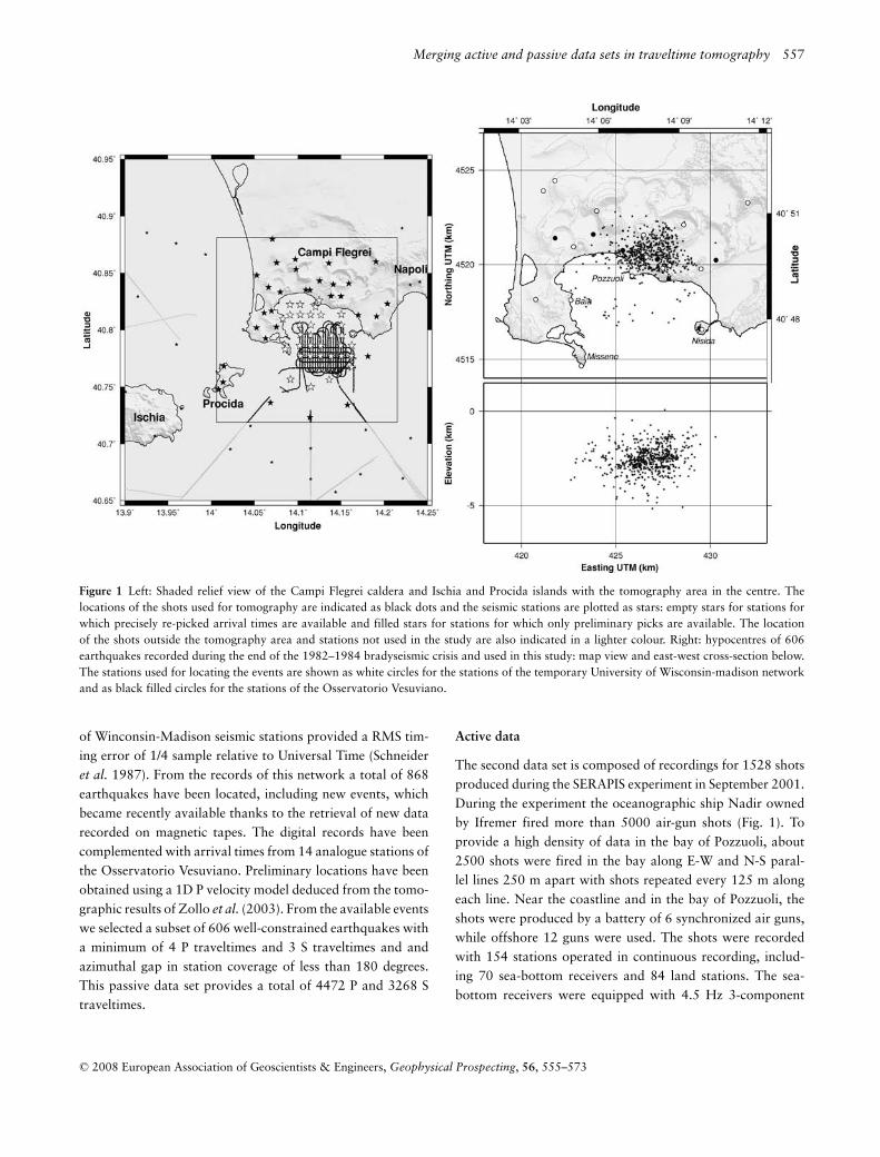
The first data set is composed of 606 earthquakes recordedin 1984 during the end of the last bradyseismic crisis, whichoccurred in 1982–1984. The events were recorded by a tem-porary digital network composed of 13 3-component stations,which were installed on 16 sites from mid-January to the endof April 1984. This network was operated by the Universityof Wisconsin-Madison in collaboration with the OsservatorioVesuviano to complement the 25 analogue stations operatedby the Osservatorio Vesuviano and AGIP (Azienda GeneraleItaliana). Each digital station recorded data in triggered modeon a stand-alone basis with a sampling frequency of 100 or200 Hz. The stations were equipped with 3-component 1 HzGeotech S-13 and Hall-Sears HS-10-1 geophones. Timing wasobtained from a 13.6 kHz Omega receiver and the applicationof a timing-correction process developed for the University

C© 2008 European Association of Geoscientists & Engineers, Geophysical Prospecting, 56, 555–573

Merging active and passive data sets in traveltime tomography 557

Figure 1 Left: Shaded relief view of the Campi Flegrei caldera and Ischia and Procida islands with the tomography area in the centre. Thelocations of the shots used for tomography are indicated as black dots and the seismic stations are plotted as stars: empty stars for stations forwhich precisely re-picked arrival times are available and filled stars for stations for which only preliminary picks are available. The locationof the shots outside the tomography area and stations not used in the study are also indicated in a lighter colour. Right: hypocentres of 606earthquakes recorded during the end of the 1982–1984 bradyseismic crisis and used in this study: map view and east-west cross-section below.The stations used for locating the events are shown as white circles for the stations of the temporary University of Wisconsin-madison networkand as black filled circles for the stations of the Osservatorio Vesuviano.

of Winconsin-Madison seismic stations provided a RMS tim-ing error of 1/4 sample relative to Universal Time (Schneideret al. 1987). From the records of this network a total of 868earthquakes have been located, including new events, whichbecame recently available thanks to the retrieval of new datarecorded on magnetic tapes. The digital records have beencomplemented with arrival times from 14 analogue stations ofthe Osservatorio Vesuviano. Preliminary locations have beenobtained using a 1D P velocity model deduced from the tomo-graphic results of Zollo et al. (2003). From the available eventswe selected a subset of 606 well-constrained earthquakes witha minimum of 4 P traveltimes and 3 S traveltimes and andazimuthal gap in station coverage of less than 180 degrees.This passive data set provides a total of 4472 P and 3268 Straveltimes.

Active data

The second data set is composed of recordings for 1528 shotsproduced during the SERAPIS experiment in September 2001.During the experiment the oceanographic ship Nadir ownedby Ifremer fired more than 5000 air-gun shots (Fig. 1). Toprovide a high density of data in the bay of Pozzuoli, about2500 shots were fired in the bay along E-W and N-S paral-lel lines 250 m apart with shots repeated every 125 m alongeach line. Near the coastline and in the bay of Pozzuoli, theshots were produced by a battery of 6 synchronized air guns,while offshore 12 guns were used. The shots were recordedwith 154 stations operated in continuous recording, includ-ing 70 sea-bottom receivers and 84 land stations. The sea-bottom receivers were equipped with 4.5 Hz 3-component



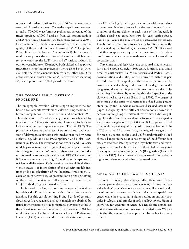
sensors and on-land stations included 66 3-component sen-sors and 18 vertical sensors. The entire experiment produceda total of 700,000 waveforms. A preliminary screening of thetraces provided 65,000 P arrivals from sea-bottom stationsand 25,000 from on-land stations (Judenherc and Zollo 2004).Later, a subset of the data was reprocessed to improve thequality of the arrival times which provided 36,254 re-pickedP traveltimes (Dello Iacono et al. submitted). In the presentwork we only consider a subset of the entire available dataset, as we only use the 1,528 shots and 67 stations included inour tomographic area. We merged both picked and re-pickedtraveltimes, choosing in preference the re-picked ones whenavailable and complementing them with the other ones. Ouractive data set includes a total of 55,123 traveltimes including36,195 re-picked and 18,928 picked traveltimes.

T H E T O M O G R A P H I C I N V E R S I O NP R O C E D U R E

The tomographic inversion is done using an improved methodbased on an accurate traveltime calculation using the finite dif-ference computation scheme of Podvin and Lecomte (1991).Three dimensional P and S velocity models are obtained byinverting P and S first arrival times simultaneously for both ve-locity models and earthquake locations (Thurber 1992). Theprocedure is iterative and at each iteration a linearized inver-sion of delayed traveltimes is performed as proposed by manyauthors (e.g. Aki and Lee 1976; Spakman and Nolet 1988;Benz et al. 1996). The inversion is done with P and S velocitymodels parametrized as 3D grids of regularly spaced nodes.According to our station/source configuration, we considerin this work a tomographic volume of 18∗18∗9 km starting0.5 km above sea level (Fig. 1) with a node spacing of0.5 km in all directions. Each iteration can be subdivided into4 main stages: (1) interpolation of the velocity models intofiner grids and calculation of the theoretical traveltimes, (2)calculation of derivatives, (3) preconditioning and smoothingof the derivative matrix and (4) inversion by means of theLSQR method (Paige and Saunders 1982).

The forward problem of traveltime computation is doneby solving the Eikonal equation with a finite differences al-gorithm. For this calculation fine P and S grids of constantslowness cells are required and such models are obtained bytrilinear interpolation of the tomographic inversion grids. Inthe present case we use fine grids with a spacing of 0.1 kmin all directions. The finite difference scheme of Podvin andLecomte (1991) is well suited for the calculation of precise

traveltimes in highly heterogeneous media with large veloc-ity contrasts. It allows for each station to obtain a first es-timation of the traveltimes at each node of the fine grid. Itis then possible to trace back rays for each station-sourcepair by following the gradient of the estimated traveltimes.Finally, precise traveltimes are calculated by integration of theslowness along the traced rays. Latorre et al. (2004) showedthat this computation improves the precision of the calcu-lated traveltimes as compared to those calculated by wavefrontreconstruction.

Traveltime partial derivatives are computed simultaneouslyfor P and S slowness fields, hypocentre locations and origintimes of earthquakes (Le Meur, Virieux and Podvin 1997).Normalization and scaling of the derivative matrix is per-formed to control the quality of the retrieved parameters. Toensure numerical stability and to control the degree of modelroughness, the system is preconditioned and smoothed. Thesmoothing is achieved by requiring that the Laplacian of theslowness field must vanish (Benz et al. 1996). The degree ofsmoothing in the different directions is defined using param-eters Lx, Ly and Lz, whose values are discussed later in thispaper. The quality of the different observations is taken intoaccount by weighting the different traveltimes. Initial weight-ing of the different data was done as follows: for earthquakeswe assigned weights of 1.0, 0.5, 0.2 and 0.1 for picked arrivaltimes with respective quality (hypo71 software; Lee and Lahr1975) 0, 1, 2 and 3 and for shots, we assigned a weight of 1.0for precisely re-picked shots and 0.6 for preliminarily pickedshots. Changes in the relative weighting of the different datasets are discussed later by means of synthetic tests and tomo-graphic runs. Finally, the inversion of the scaled and weightedlinear system was done using the LSQR algorithm (Page andSaunders 1982). The inversion was regularized using a damp-ing factor whose optimal value is discussed later.

M E R G I N G O F T H E T W O S E T S O F D ATA

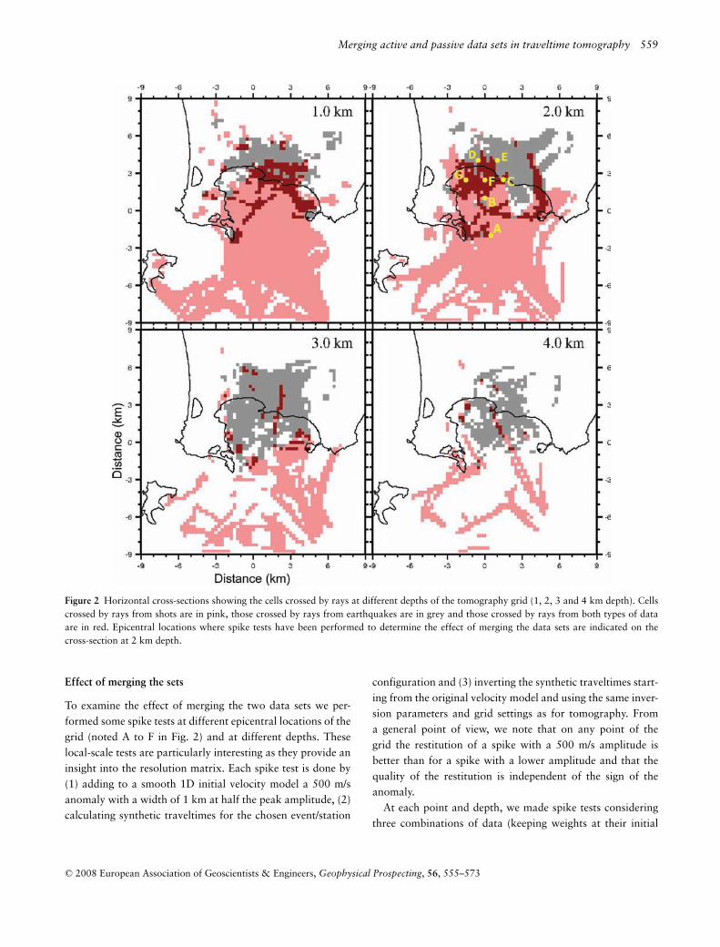
The joint inversion problem is especially difficult since the ac-tive and passive data sets are complementary: the first one pro-vides both Vp and Vs velocity models, as well as earthquakelocations but has a lower resolution and a limited spatial cov-erage, while the second has a higher resolution but only pro-vides P velocity and samples mostly shallow layers. Figure 2shows the ray coverage provided by each set and emphasizesthat the two sets overlap only over a limited area. We alsonote that the amounts of rays provided by each set are verydifferent.



Figure 2 Horizontal cross-sections showing the cells crossed by rays at different depths of the tomography grid (1, 2, 3 and 4 km depth). Cellscrossed by rays from shots are in pink, those crossed by rays from earthquakes are in grey and those crossed by rays from both types of dataare in red. Epicentral locations where spike tests have been performed to determine the effect of merging the data sets are indicated on thecross-section at 2 km depth.

Effect of merging the sets

To examine the effect of merging the two data sets we per-formed some spike tests at different epicentral locations of thegrid (noted A to F in Fig. 2) and at different depths. Theselocal-scale tests are particularly interesting as they provide aninsight into the resolution matrix. Each spike test is done by(1) adding to a smooth 1D initial velocity model a 500 m/sanomaly with a width of 1 km at half the peak amplitude, (2)calculating synthetic traveltimes for the chosen event/station

configuration and (3) inverting the synthetic traveltimes start-ing from the original velocity model and using the same inver-sion parameters and grid settings as for tomography. Froma general point of view, we note that on any point of thegrid the restitution of a spike with a 500 m/s amplitude isbetter than for a spike with a lower amplitude and that thequality of the restitution is independent of the sign of theanomaly.

At each point and depth, we made spike tests consideringthree combinations of data (keeping weights at their initial



-6

-5

-4

-3

-2

-1

0

1

Depth

(km

)

0 500 1000 1500 2000 2500

Amplitude (m/s)

pt "B"

P vel.

-6

-5

-4

-3

-2

-1

0

1

Depth

(km

)

0 500 1000 1500 2000 2500

Amplitude (m/s)

pt "E"

P vel.

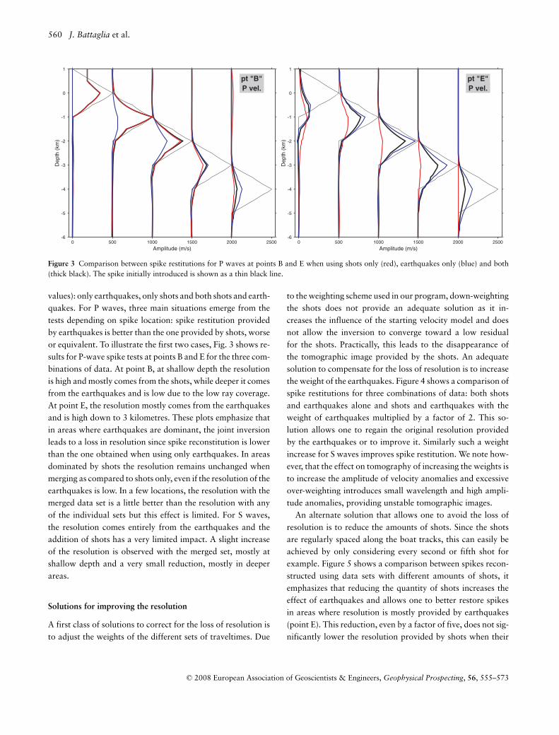
Figure 3 Comparison between spike restitutions for P waves at points B and E when using shots only (red), earthquakes only (blue) and both(thick black). The spike initially introduced is shown as a thin black line.

values): only earthquakes, only shots and both shots and earth-quakes. For P waves, three main situations emerge from thetests depending on spike location: spike restitution providedby earthquakes is better than the one provided by shots, worseor equivalent. To illustrate the first two cases, Fig. 3 shows re-sults for P-wave spike tests at points B and E for the three com-binations of data. At point B, at shallow depth the resolutionis high and mostly comes from the shots, while deeper it comesfrom the earthquakes and is low due to the low ray coverage.At point E, the resolution mostly comes from the earthquakesand is high down to 3 kilometres. These plots emphasize thatin areas where earthquakes are dominant, the joint inversionleads to a loss in resolution since spike reconstitution is lowerthan the one obtained when using only earthquakes. In areasdominated by shots the resolution remains unchanged whenmerging as compared to shots only, even if the resolution of theearthquakes is low. In a few locations, the resolution with themerged data set is a little better than the resolution with anyof the individual sets but this effect is limited. For S waves,the resolution comes entirely from the earthquakes and theaddition of shots has a very limited impact. A slight increaseof the resolution is observed with the merged set, mostly atshallow depth and a very small reduction, mostly in deeperareas.

Solutions for improving the resolution

A first class of solutions to correct for the loss of resolution isto adjust the weights of the different sets of traveltimes. Due

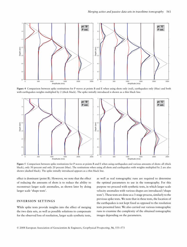
to the weighting scheme used in our program, down-weightingthe shots does not provide an adequate solution as it in-creases the influence of the starting velocity model and doesnot allow the inversion to converge toward a low residualfor the shots. Practically, this leads to the disappearance ofthe tomographic image provided by the shots. An adequatesolution to compensate for the loss of resolution is to increasethe weight of the earthquakes. Figure 4 shows a comparison ofspike restitutions for three combinations of data: both shotsand earthquakes alone and shots and earthquakes with theweight of earthquakes multiplied by a factor of 2. This so-lution allows one to regain the original resolution providedby the earthquakes or to improve it. Similarly such a weightincrease for S waves improves spike restitution. We note how-ever, that the effect on tomography of increasing the weights isto increase the amplitude of velocity anomalies and excessiveover-weighting introduces small wavelength and high ampli-tude anomalies, providing unstable tomographic images.

An alternate solution that allows one to avoid the loss ofresolution is to reduce the amounts of shots. Since the shotsare regularly spaced along the boat tracks, this can easily beachieved by only considering every second or fifth shot forexample. Figure 5 shows a comparison between spikes recon-structed using data sets with different amounts of shots, itemphasizes that reducing the quantity of shots increases theeffect of earthquakes and allows one to better restore spikesin areas where resolution is mostly provided by earthquakes(point E). This reduction, even by a factor of five, does not sig-nificantly lower the resolution provided by shots when their



-6

-5

-4

-3

-2

-1

0

1

Depth

(km

)

0 500 1000 1500 2000 2500

Amplitude (m/s)

pt "B"

P vel.

-6

-5

-4

-3

-2

-1

0

1

Depth

(km

)

0 500 1000 1500 2000 2500

Amplitude (m/s)

pt "E"

P vel.

Figure 4 Comparison between spike restitutions for P waves at points B and E when using shots only (red), earthquakes only (blue) and bothwith earthquakes weights multiplied by 2 (thick black). The spike initially introduced is shown as a thin black line.

-6

-5

-4

-3

-2

-1

0

1

Depth

(km

)

0 500 1000 1500 2000 2500

Amplitude (m/s)

pt "B"

P vel.

-6

-5

-4

-3

-2

-1

0

1

Depth

(km

)

0 500 1000 1500 2000 2500

Amplitude (m/s)

pt "E"

P vel.

Figure 5 Comparison between spike restitutions for P waves at points B and E when using earthquakes and various amounts of shots: all (thickblack), only 50 percent and only 20 percent (blue). The restitutions when using all shots and earthquakes with weights multiplied by 2 are alsoshown (dashed black). The spike initially introduced appears as a thin black line.

effect is dominant (point B). However, we note that the effectof reducing the amounts of shots is to reduce the ability toreconstruct larger scale anomalies, as shown later by doinglarger scale ‘shape tests’.

I N V E R S I O N S E T T I N G S

While spike tests provide insights into the effect of mergingthe two data sets, as well as possible solutions to compensatefor the observed loss of resolution, larger scale synthetic tests,

as well as real tomographic runs are required to determinethe optimal parameters to use in the tomography. For thispurpose we proceed with synthetic tests, in which larger scalevelocity anomalies with various shapes are introduced (‘shapetests’). These tests are done as a 3-stage process, similarly to theprevious spike tests. We note that in these tests, the location ofthe earthquakes is not kept fixed as opposed to the resolutiontests presented later. We also carried out various tomographicruns to examine the complexity of the obtained tomographicimages depending on the parameters.



-8

-4

0

4

8D

ista

nce (

km

)

-8 -4 0 4 8Distance (km)

T02

Figure 6 Shape of the input anomaly for test T02, P and S waves(shapes for tests T01 and T03 are shown in Fig. 9).

Once the size of the inversion cells is fixed, the main param-eters that have an influence on the tomographic results are thesmoothing coefficients Lx, Ly and Lz, which control the pre-conditioning of the matrix of traveltime delays, the dampingfactor DAMP, which regulates the LSQR inversion and, in thepresent case, the increase in the weight of the earthquakes (Pand S waves) and the amounts of shots that we used. In thepresent work, we consider homogeneous smoothing in all di-rections and take the same value for Lx, Ly and Lz, which wenote LX later on. To determine the proper parameters to usefor tomography, we first compare the quality of recomposedsynthetic anomalies when using different values. We presenthere results for three different shape tests that cover variousareas of the tomographic grid:

0 0.2 0.4 0.6 0.8 1

Damping

0.9

1

1.1

1.2

1.3

1.4

No

rma

lize

d a

vera

ge

err

or

eqks*1

eqks*2

eqks*4

eqks*6

0 0.2 0.4 0.6 0.8 1

Damping

0.6

0.7

0.8

0.9

1

Ave

rag

e n

orm

aliz

ed

err

or

Test T02 P waves LX=0.3

eqks*1

eqks*2

eqks*4

eqks*6

0 0.2 0.4 0.6 0.8 1

Damping

0.6

0.7

0.8

0.9

1

Ave

rag

e n

orm

aliz

ed

err

or

Test T02 S waves LX=0.3

eqks*1

eqks*2

eqks*4

eqks*6

Figure 7 Mean error rates for test T01 P waves and test T02 P and S waves as a function of the damping. Each symbol represents the averageof the absolute value of the difference between the introduced velocity anomaly and the one restored. This average is calculated over all nodesbetween 0 and 4 km b.s.l..

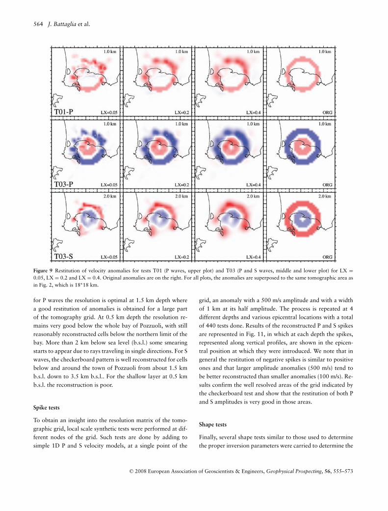
� Test T01: an annular anomaly with a 100 m/s amplitudeadded at each depth in the periphery of the tomographygrid to the P velocity model (Fig. 9).

� Test T02: a 100 m/s anomaly shaped like a cross added inthe centre of the grid at each depth to both P and S velocitymodels (Fig. 6).

� Test T03: two annular anomalies with opposite signs addedat each depth. For the P model, the internal anomaly is+150 m/s and the external −200 m/s; for the S model, theinside anomaly is −150 m/s and external +200 m/s (Fig. 9).To simplify the analysis of the results, we represent each

synthetic test by its average error, which is defined as the aver-age of the absolute value of the difference between the intro-duced and the reproduced anomaly. This error is calculatedover all the nodes between 0 and 4 km below sea level, whichis the best resolved part of grid. We normalize the obtainedvalues to the average amount of anomaly introduced initially.Figure 7 shows results obtained for tests T01 and T02 forvarious values of the damping and for various multiplicativefactors applied to the weight of the earthquakes. The resultssuggest that appropriate values for damping are in the rangebetween 0.3 and 0.5. The choice of the multiplicative factorfor the weight of the earthquakes is more problematic, as itseffect appears to depend on the location of the anomaly: for Pwaves, increasing the weights increases the mean error for testT01 and decreases it significantly for test T02. A satisfactorycompromise for P waves is found by multiplying the weight ofearthquakes by two, as this also compensates for the loss inresolution caused by data merging. For S waves, synthetic testssuggest a better reproduction of the anomalies with increas-ing weight without providing an uppermost boundary for thevalue to use.



To help constraining the choice of the P and S multiplica-tive factors, we take into account another criterion which isthe simplicity of the obtained velocity models when doing thetomography. Indeed, a major effect of increasing the weightof the earthquakes (P and S waves) is to increase the com-plexity of the obtained velocity models by introducing higheramplitude, small wavelength anomalies. It is well known thatin tomography it is generally possible to find a whole classof models, instead of a single model, which fits equally wellthe observations (Monteiller et al. 2005). The choice of thebest model in that class is done by choosing the result with thelower degree of freedom (Akaike 1974; Tarantola and Valette1982). For this purpose we examine the variance of the P andS velocity models and Vp/Vs ratio obtained with various mul-tiplicative factors and examine the corresponding residuals forP and S traveltimes. For P-waves, results indicate that a goodchoice is found with weights multiplied by two, which is ingood agreement with results suggested by the above synthetictests. For S-waves, however, increasing weights leads to a re-duction of the individual rms for S-waves in general but alsoto an increase of the variance of the Vp/Vs model in particu-lar. Solutions that do not imply a substantial increase of thevariance for the final velocity models are found for S-weightsmultiplied by up to 4.

In a similar way to Fig. 7, Fig. 8 shows the effect of reducingthe amounts of shots. Despite the fact that such a reductionallows one to avoid the loss of resolution according to spiketests, the results for shape tests indicate that it leads to a sig-nificant reduction in the ability to reproduce anomalies in theperipheral area of the grid (test T01), where the resolutioncomes mostly from the shots. For more central anomalies (testT02), the reduction leads to few changes. In general, however,the effect of increasing the earthquakes weight by a factor oftwo brings significantly better results. Combining earthquakes

0 0.2 0.4 0.6 0.8 1

Damping

0.8

1

1.2

1.4

1.6

1.8

2

2.2

2.4

Ave

rage n

orm

aliz

ed e

rror

eqks*1 100%

eqks*2 100%

eqks*1 50%

eqks*1 20%

0 0.2 0.4 0.6 0.8 1

Damping

0.7

0.8

0.9

1

Ave

rage n

orm

aliz

ed e

rror

Test 02 P Waves LX=0.3

eqks*1 100%

eqks*2 100%

eqks*1 50%

eqks*1 20%

0 0.2 0.4 0.6 0.8 1

Damping

0.6

0.7

0.8

0.9

1

1.1

Ave

rage n

orm

aliz

ed e

rror

Test 02 S Waves LX=0.3

eqks*1 100%

eqks*2 100%

eqks*1 50%

eqks*1 20%

Figure 8 Mean error rates for test T01 P waves and test T02 P and S waves as a function of the damping when taking into account variousquantities of shots. Each symbol represents the average error calculated over all nodes between 0 and 4 km b.s.l..

weight increase and reduction of shots leads to inappropriatesolutions in a similar way to over-weighting the earthquakes.This indicates that the weight increase is only permitted by thestabilizing effect brought about by the large amount of shotstraveltimes.

Finally, to determine a proper value to use for the smoothingcoefficients we proceed with visual inspections of the recom-posed anomalies. Figure 9 shows results for tests with variousvalues of LX. The images indicate that appropriate values forLX are in the range 0.2 to 0.3. Lower values lead to the ap-pearance of small-scale asperities and larger values provideblurred images.

R E S O L U T I O N T E S T S

In order to identify the well resolved areas of the tomographicimages, we performed several synthetic tests on a global scale(checkerboard and shape tests) as well as on a local scale (spiketests). All tests are done in a similar way to the tests used todetermine the effect of merging the passive and active data sets,except that the position of the sources is kept constant duringthe inversion of synthetic traveltimes. Tests are carried outwith the same station-event configuration as for tomographyand with the same inversion parameters and grid settings (gridsize, origin and spacing).

Checkerboard test

A checkerboard test was first performed to obtain a globalview of the resolution for both P and S waves. This test isdone by adding a grid of positive and negative anomalies withsizes of 2 km in all directions and with an amplitude of ±50m/s to simple one dimension P and S velocity models. Figure 10shows the restitution of the anomalies with areas not sampledby any ray shown in lighter colours. The test indicates that



Figure 9 Restitution of velocity anomalies for tests T01 (P waves, upper plot) and T03 (P and S waves, middle and lower plot) for LX =0.05, LX = 0.2 and LX = 0.4. Original anomalies are on the right. For all plots, the anomalies are superposed to the same tomographic area asin Fig. 2, which is 18∗18 km.

for P waves the resolution is optimal at 1.5 km depth wherea good restitution of anomalies is obtained for a large partof the tomography grid. At 0.5 km depth the resolution re-mains very good below the whole bay of Pozzuoli, with stillreasonably reconstructed cells below the northern limit of thebay. More than 2 km below sea level (b.s.l.) some smearingstarts to appear due to rays traveling in single directions. For Swaves, the checkerboard pattern is well reconstructed for cellsbelow and around the town of Pozzuoli from about 1.5 kmb.s.l. down to 3.5 km b.s.l.. For the shallow layer at 0.5 kmb.s.l. the reconstruction is poor.

Spike tests

To obtain an insight into the resolution matrix of the tomo-graphic grid, local scale synthetic tests were performed at dif-ferent nodes of the grid. Such tests are done by adding tosimple 1D P and S velocity models, at a single point of the

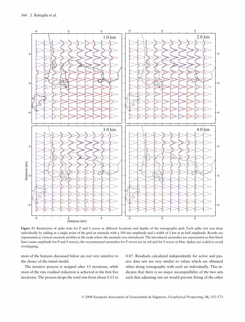
grid, an anomaly with a 500 m/s amplitude and with a widthof 1 km at its half amplitude. The process is repeated at 4different depths and various epicentral locations with a totalof 440 tests done. Results of the reconstructed P and S spikesare represented in Fig. 11, in which at each depth the spikes,represented along vertical profiles, are shown in the epicen-tral position at which they were introduced. We note that ingeneral the restitution of negative spikes is similar to positiveones and that larger amplitude anomalies (500 m/s) tend tobe better reconstructed than smaller anomalies (100 m/s). Re-sults confirm the well resolved areas of the grid indicated bythe checkerboard test and show that the restitution of both Pand S amplitudes is very good in those areas.

Shape tests

Finally, several shape tests similar to those used to determinethe proper inversion parameters were carried to determine the



Figure 10 Results for a checkerboard test with 2∗2∗2 km cells with ±50 m/s anomalies added to P (left) and S (right) velocities.

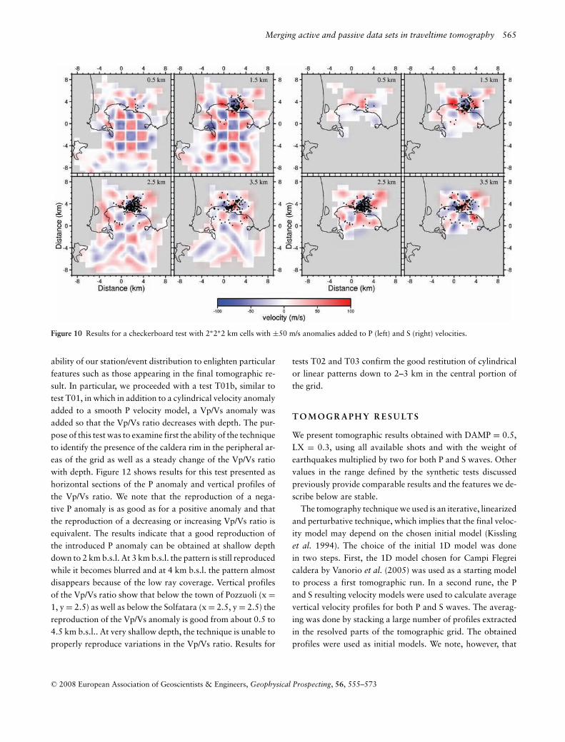
ability of our station/event distribution to enlighten particularfeatures such as those appearing in the final tomographic re-sult. In particular, we proceeded with a test T01b, similar totest T01, in which in addition to a cylindrical velocity anomalyadded to a smooth P velocity model, a Vp/Vs anomaly wasadded so that the Vp/Vs ratio decreases with depth. The pur-pose of this test was to examine first the ability of the techniqueto identify the presence of the caldera rim in the peripheral ar-eas of the grid as well as a steady change of the Vp/Vs ratiowith depth. Figure 12 shows results for this test presented ashorizontal sections of the P anomaly and vertical profiles ofthe Vp/Vs ratio. We note that the reproduction of a nega-tive P anomaly is as good as for a positive anomaly and thatthe reproduction of a decreasing or increasing Vp/Vs ratio isequivalent. The results indicate that a good reproduction ofthe introduced P anomaly can be obtained at shallow depthdown to 2 km b.s.l. At 3 km b.s.l. the pattern is still reproducedwhile it becomes blurred and at 4 km b.s.l. the pattern almostdisappears because of the low ray coverage. Vertical profilesof the Vp/Vs ratio show that below the town of Pozzuoli (x =1, y = 2.5) as well as below the Solfatara (x = 2.5, y = 2.5) thereproduction of the Vp/Vs anomaly is good from about 0.5 to4.5 km b.s.l.. At very shallow depth, the technique is unable toproperly reproduce variations in the Vp/Vs ratio. Results for

tests T02 and T03 confirm the good restitution of cylindricalor linear patterns down to 2–3 km in the central portion ofthe grid.

T O M O G R A P H Y R E S U LT S

We present tomographic results obtained with DAMP = 0.5,LX = 0.3, using all available shots and with the weight ofearthquakes multiplied by two for both P and S waves. Othervalues in the range defined by the synthetic tests discussedpreviously provide comparable results and the features we de-scribe below are stable.

The tomography technique we used is an iterative, linearizedand perturbative technique, which implies that the final veloc-ity model may depend on the chosen initial model (Kisslinget al. 1994). The choice of the initial 1D model was donein two steps. First, the 1D model chosen for Campi Flegreicaldera by Vanorio et al. (2005) was used as a starting modelto process a first tomographic run. In a second rune, the Pand S resulting velocity models were used to calculate averagevertical velocity profiles for both P and S waves. The averag-ing was done by stacking a large number of profiles extractedin the resolved parts of the tomographic grid. The obtainedprofiles were used as initial models. We note, however, that



-4

0

4

-4 0 4

1.0 km

-4

0

4

-4 0 4

2.0 km

-4

0

4

Dis

tan

ce

(km

)

-4 0 4Distance (km)

3.0 km

-4

0

4

-4 0 4

4.0 km

Figure 11 Restitution of spike tests for P and S waves at different locations and depths of the tomography grid. Each spike test was doneindividually by adding at a single point of the grid an anomaly with a 500 m/s amplitude and a width of 1 km at its half amplitude. Results arerepresented as vertical anomaly profiles at the node where the anomaly was introduced. The introduced anomalies are represented as thin blacklines (same amplitude for P and S waves), the reconstructed anomalies for P waves are in red and for S waves in blue. Spikes are scaled to avoidoverlapping.

most of the features discussed below are not very sensitive tothe choice of the initial model.

The iterative process is stopped after 15 iterations, whilemost of the rms residual reduction is achieved in the first fiveiterations. The process drops the total rms from about 0.15 to

0.07. Residuals calculated independently for active and pas-sive data sets are very similar to values which are obtainedwhen doing tomography with each set individually. This in-dicates that there is no major incompatibility of the two setssuch that adjusting one set would prevent fitting of the other



Figure 12 Results for synthetic test T01b showing the reconstruction of the P anomaly at different depths (left) and 2 vertical profiles showingthe reconstruction (blue) of the Vp/Vs anomaly (black).

one. The obtained 3D velocity models, as well as earthquakeslocations are shown in Figs 13 to 15. Cells not sampled by anyray are shown in lighter colours.

P velocity model

Figure 13 shows the obtained final P velocity model presentedas horizontal cross-sections. The most characteristic featurethat emerges is the presence of a ring-shaped high P veloc-ity anomaly, which is particularly clear around 1.5 km b.s.l..Our results confirm the presence of this ring in the southernpart of the bay of Pozzuoli, as previously observed by Zolloet al. (2003) and Judenherc and Zollo (2004) but also extendits trace inland along the western border of the bay and lessclearly along the eastern border below and north of the islandof Nisida. At 1.5 km depth, no clear trace of the ring con-tinuation is observed in the northern part of the grid, whilesynthetic tests suggests an annular anomaly could be recon-structed there if present in the resolved part of the tomographyarea (Fig. 12). The structure which is defined by our resultshas a diameter of about 8–12 km at 1.5 b.s.l.. We note thatat this depth, the shape of the ring is in good agreement withthe location of hydrothermalized lava inferred by gravimet-

ric data modeling (Fig. 16). In total, the trace of the ring canbe seen from about 0.5 km b.s.l. down to about 2.5–3.0 km.At 3 km depth its trace is, however, less clear and appearsas a lower velocity zone surrounded by higher velocity struc-tures, including on the northern side, with a diameter of about6 km.

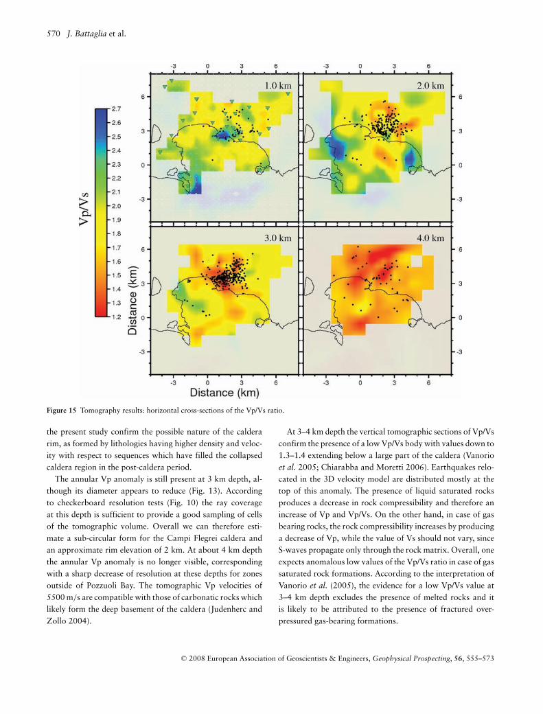
Vp/Vs model

The obtained Vp/Vs model presents several interesting fea-tures (Figures 14 and 15). The Vp/Vs East-West cross sectionat y = 2.5 (Fig. 14), which passes below the town of Pozzuoli,outlines the presence of a very high Vp/Vs anomaly locatedat about 1 km b.s.l. below the town as observed previouslyby Aster and Meyer (1988) and Vanorio et al. (2005). Thisanomaly has values up to 2.7, with a lateral extent of about1 to 2 km. According to synthetic tests, the uppermost ex-tent of the anomaly is poorly constrained and near the surfacethe ratio depends strongly on the value of the initial velocitymodel. We also note an extension of the high Vp/Vs anomalytoward the Solfatara area (horizontal cross-section at 2 kmdepth in Fig. 15). The amplitude and size of this secondaryanomaly is sensitive to the weight of the S waves used in the



Figure 13 Tomography results: horizontal sections of the P velocity model.

inversion. The results presented in this paper favour the choiceof a smooth Vp/Vs model by using S weights multiplied by afactor of 2 while the use of a factor of 4 tends to increase theroughness of the model and increases the size and amplitudeof this anomaly. Horizontal cross-sections of the Vp/Vs ratio(Fig. 15) confirm the presence of a low Vp/Vs body extend-ing at about 3–4 km depth below a large part of the calderawith values down to 1.3–1.4. The upper limit of this structurehowever, is not smooth according to the vertical cross-sectionin Fig. 14.

Earthquake locations

Finally, looking at the position of the relocated earthquakes inthe 3D final velocity structure, we note that the events appeargenerally more clustered than according to the initial loca-tions. Horizontal cross-sections (Fig. 13) show that most ofthe events found inland below the Pozzuoli area are roughlyaligned along an SW-NE elongated pattern, most clear at about3 km depth. Most of the seismicity is found at the upper limit

and above the low Vp/Vs body located at about 3–4 km depth.We also note an interesting feature that appears on the verti-cal cross-section in Fig. 15, which shows that the earthquakesdefine a 45 degree dipping plane below which most of themare found and above which is located the high Vp/Vs shallowanomaly.

D I S C U S S I O N

Our tomographic results outline several characteristic featuresthat can be interpreted in terms of the previous studies done inthe Campi Flegrei area. Previous results obtained from gravi-metric, seismic activity, and drilled-rock sampling analysesconducted in Pozzuoli Bay and on land have been used forgeological interpretation of Vp and Vp/Vs anomalies on thebasis that the P and S velocity distribution and their Vp/Vsratio can be associated with the elastic characteristics of rocksunder investigation and with the physic state of the pore fluid.

By analysing the horizontal sections of the P-velocity modelin Fig. 13, we observe at about 1 km depth an arc-like positive



Figure 14 Tomography results: East-West cross-section at y=2500 of the Vp/Vs ratio.

anomaly, which extends from Capo Miseno in the West to theIsland of Nisida in the East, with velocity values around 3500-4000 m/s as compared to values of 2500–3000 m/s for sedi-ments filling the inner region of the Pozzuoli Bay. At approxi-mately the same depth an anomalous high value of the Vp/Vsratio is observed on the vertical cross-section, passing belowthe town of Pozzuoli (Fig. 14). According to Zollo et al. (2003)and Judenherc and Zollo (2004), we suggest that the annularvelocity anomaly represents the buried trace of the southernrim of the Campi Flegrei caldera. The relatively high velocitiesof rocks forming the rim could be related to the presence oflava or tuff with inter-bedded lava according to stratigraphicand sonic logs inferred from deep boreholes (AGIP 1987). De-posits filling the inner bay area are instead characterized byrelatively low Vp and high Vp/Vs values, which can be the ev-idence for a thick brine rock sedimentary layer (Vanorio et al.

2005). Recently, Dello Iacono et al. (submitted) analysed theP-to-P and P-to-S phases reflected from a very shallow seismicdiscontinuity at 500–700 m depth, detected by the seismic re-flection analysis of data from a recent 3D active seismic survey(SERAPIS 2001). The move-out velocity analysis and stack ofthe P-P and P-S reflections at the layer bottom allowed themto estimate relatively high Vp/Vs values (3.5 ± 0.6). Based

on theoretical rock physical modelling of the Vp/Vs ratio asa function of porosity, the authors conclude that the shallowlayer is likely formed by incoherent, water saturated, volcanicand marine sediments that filled Pozzuoli Bay during the post-caldera activity.

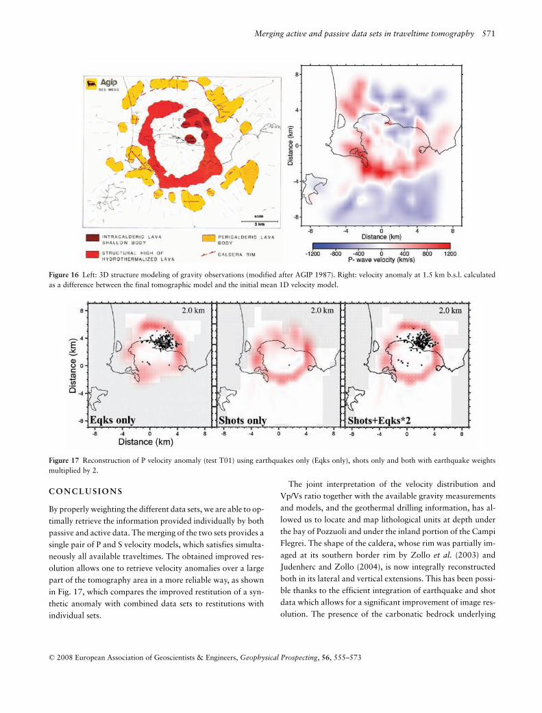
The buried caldera rim is well visible, also at greater depthsfrom the obtained tomographic model. The section at 1.5 kmdepth (Fig. 13) allows one to roughly estimate a diameter of10 km of the annular high Vp anomaly with a thicknessof about 1 km. By comparing the tomographic image withBouguer anomaly maps, based on data acquired in the earlyeighties (AGIP 1987; Barberi et al. 1991; Florio et al. 1999;Capuano and Achauer 2003) one can find a good correlationbetween the geometry and position of the velocity anomalyand the positive gravity anomaly, which has been attributedto the presence of hydrothermalized lava formations (Fig. 16),detected in Mofete wells at about 1 km depth. More recently,Tramelli et al. (2006) applied the scattering imaging method tocoda waves of earthquake seismograms and were able to iden-tify at 1–2 km depth the caldera border, behaving as a strongseismic signal scatterer with areas having the largest scatter-ing coefficient nearly corresponding to the high Vp anomaly ofthis study. The mentioned observations along with results from



Figure 15 Tomography results: horizontal cross-sections of the Vp/Vs ratio.

the present study confirm the possible nature of the calderarim, as formed by lithologies having higher density and veloc-ity with respect to sequences which have filled the collapsedcaldera region in the post-caldera period.

The annular Vp anomaly is still present at 3 km depth, al-though its diameter appears to reduce (Fig. 13). Accordingto checkerboard resolution tests (Fig. 10) the ray coverageat this depth is sufficient to provide a good sampling of cellsof the tomographic volume. Overall we can therefore esti-mate a sub-circular form for the Campi Flegrei caldera andan approximate rim elevation of 2 km. At about 4 km depththe annular Vp anomaly is no longer visible, correspondingwith a sharp decrease of resolution at these depths for zonesoutside of Pozzuoli Bay. The tomographic Vp velocities of5500 m/s are compatible with those of carbonatic rocks whichlikely form the deep basement of the caldera (Judenherc andZollo 2004).

At 3–4 km depth the vertical tomographic sections of Vp/Vsconfirm the presence of a low Vp/Vs body with values down to1.3–1.4 extending below a large part of the caldera (Vanorioet al. 2005; Chiarabba and Moretti 2006). Earthquakes relo-cated in the 3D velocity model are distributed mostly at thetop of this anomaly. The presence of liquid saturated rocksproduces a decrease in rock compressibility and therefore anincrease of Vp and Vp/Vs. On the other hand, in case of gasbearing rocks, the rock compressibility increases by producinga decrease of Vp, while the value of Vs should not vary, sinceS-waves propagate only through the rock matrix. Overall, oneexpects anomalous low values of the Vp/Vs ratio in case of gassaturated rock formations. According to the interpretation ofVanorio et al. (2005), the evidence for a low Vp/Vs value at3–4 km depth excludes the presence of melted rocks and itis likely to be attributed to the presence of fractured over-pressured gas-bearing formations.



Figure 16 Left: 3D structure modeling of gravity observations (modified after AGIP 1987). Right: velocity anomaly at 1.5 km b.s.l. calculatedas a difference between the final tomographic model and the initial mean 1D velocity model.

Figure 17 Reconstruction of P velocity anomaly (test T01) using earthquakes only (Eqks only), shots only and both with earthquake weightsmultiplied by 2.

C O N C L U S I O N S

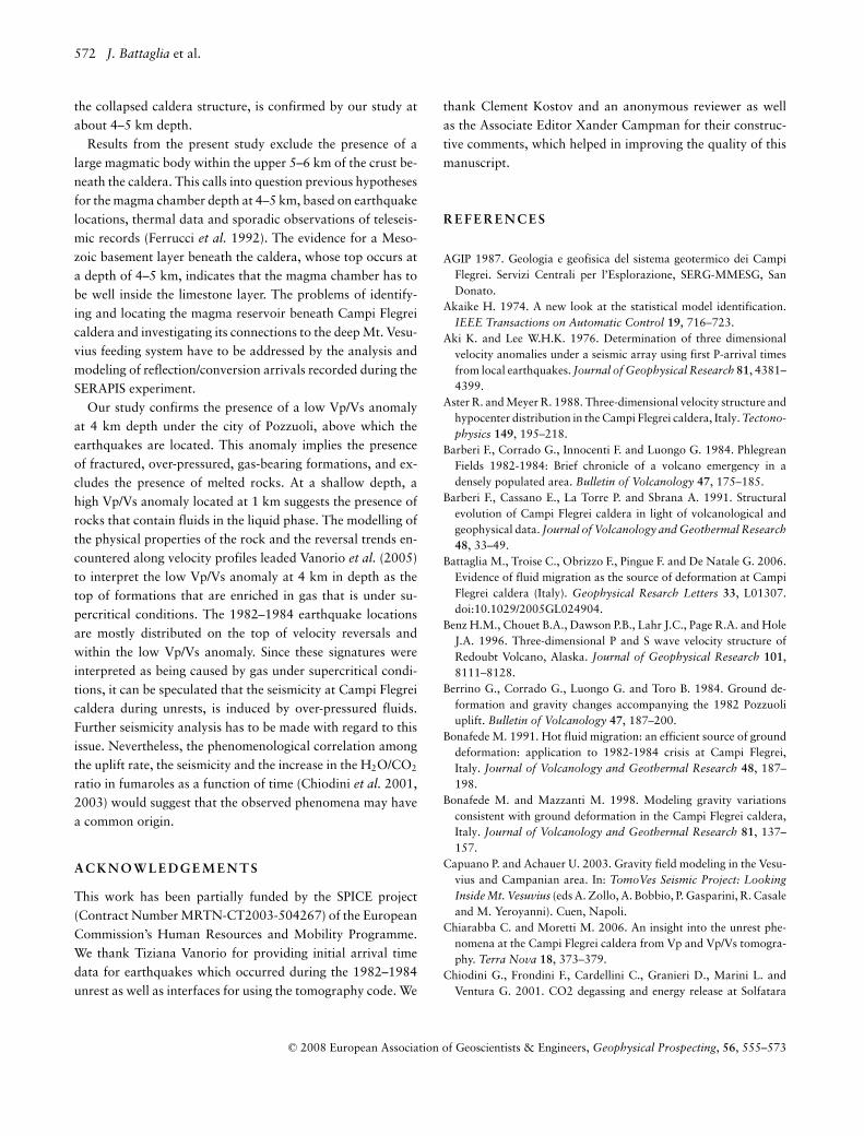
By properly weighting the different data sets, we are able to op-timally retrieve the information provided individually by bothpassive and active data. The merging of the two sets provides asingle pair of P and S velocity models, which satisfies simulta-neously all available traveltimes. The obtained improved res-olution allows one to retrieve velocity anomalies over a largepart of the tomography area in a more reliable way, as shownin Fig. 17, which compares the improved restitution of a syn-thetic anomaly with combined data sets to restitutions withindividual sets.

The joint interpretation of the velocity distribution andVp/Vs ratio together with the available gravity measurementsand models, and the geothermal drilling information, has al-lowed us to locate and map lithological units at depth underthe bay of Pozzuoli and under the inland portion of the CampiFlegrei. The shape of the caldera, whose rim was partially im-aged at its southern border rim by Zollo et al. (2003) andJudenherc and Zollo (2004), is now integrally reconstructedboth in its lateral and vertical extensions. This has been possi-ble thanks to the efficient integration of earthquake and shotdata which allows for a significant improvement of image res-olution. The presence of the carbonatic bedrock underlying



the collapsed caldera structure, is confirmed by our study atabout 4–5 km depth.

Results from the present study exclude the presence of alarge magmatic body within the upper 5–6 km of the crust be-neath the caldera. This calls into question previous hypothesesfor the magma chamber depth at 4–5 km, based on earthquakelocations, thermal data and sporadic observations of teleseis-mic records (Ferrucci et al. 1992). The evidence for a Meso-zoic basement layer beneath the caldera, whose top occurs ata depth of 4–5 km, indicates that the magma chamber has tobe well inside the limestone layer. The problems of identify-ing and locating the magma reservoir beneath Campi Flegreicaldera and investigating its connections to the deep Mt. Vesu-vius feeding system have to be addressed by the analysis andmodeling of reflection/conversion arrivals recorded during theSERAPIS experiment.

Our study confirms the presence of a low Vp/Vs anomalyat 4 km depth under the city of Pozzuoli, above which theearthquakes are located. This anomaly implies the presenceof fractured, over-pressured, gas-bearing formations, and ex-cludes the presence of melted rocks. At a shallow depth, ahigh Vp/Vs anomaly located at 1 km suggests the presence ofrocks that contain fluids in the liquid phase. The modelling ofthe physical properties of the rock and the reversal trends en-countered along velocity profiles leaded Vanorio et al. (2005)to interpret the low Vp/Vs anomaly at 4 km in depth as thetop of formations that are enriched in gas that is under su-percritical conditions. The 1982–1984 earthquake locationsare mostly distributed on the top of velocity reversals andwithin the low Vp/Vs anomaly. Since these signatures wereinterpreted as being caused by gas under supercritical condi-tions, it can be speculated that the seismicity at Campi Flegreicaldera during unrests, is induced by over-pressured fluids.Further seismicity analysis has to be made with regard to thisissue. Nevertheless, the phenomenological correlation amongthe uplift rate, the seismicity and the increase in the H2O/CO2

ratio in fumaroles as a function of time (Chiodini et al. 2001,2003) would suggest that the observed phenomena may havea common origin.

A C K N O W L E D G E M E N T S

This work has been partially funded by the SPICE project(Contract Number MRTN-CT2003-504267) of the EuropeanCommission’s Human Resources and Mobility Programme.We thank Tiziana Vanorio for providing initial arrival timedata for earthquakes which occurred during the 1982–1984unrest as well as interfaces for using the tomography code. We

thank Clement Kostov and an anonymous reviewer as wellas the Associate Editor Xander Campman for their construc-tive comments, which helped in improving the quality of thismanuscript.

R E F E R E N C E S

AGIP 1987. Geologia e geofisica del sistema geotermico dei CampiFlegrei. Servizi Centrali per l’Esplorazione, SERG-MMESG, SanDonato.

Akaike H. 1974. A new look at the statistical model identification.IEEE Transactions on Automatic Control 19, 716–723.

Aki K. and Lee W.H.K. 1976. Determination of three dimensionalvelocity anomalies under a seismic array using first P-arrival timesfrom local earthquakes. Journal of Geophysical Research 81, 4381–4399.

Aster R. and Meyer R. 1988. Three-dimensional velocity structure andhypocenter distribution in the Campi Flegrei caldera, Italy. Tectono-physics 149, 195–218.

Barberi F., Corrado G., Innocenti F. and Luongo G. 1984. PhlegreanFields 1982-1984: Brief chronicle of a volcano emergency in adensely populated area. Bulletin of Volcanology 47, 175–185.

Barberi F., Cassano E., La Torre P. and Sbrana A. 1991. Structuralevolution of Campi Flegrei caldera in light of volcanological andgeophysical data. Journal of Volcanology and Geothermal Research48, 33–49.

Battaglia M., Troise C., Obrizzo F., Pingue F. and De Natale G. 2006.Evidence of fluid migration as the source of deformation at CampiFlegrei caldera (Italy). Geophysical Resarch Letters 33, L01307.doi:10.1029/2005GL024904.

Benz H.M., Chouet B.A., Dawson P.B., Lahr J.C., Page R.A. and HoleJ.A. 1996. Three-dimensional P and S wave velocity structure ofRedoubt Volcano, Alaska. Journal of Geophysical Research 101,8111–8128.

Berrino G., Corrado G., Luongo G. and Toro B. 1984. Ground de-formation and gravity changes accompanying the 1982 Pozzuoliuplift. Bulletin of Volcanology 47, 187–200.

Bonafede M. 1991. Hot fluid migration: an efficient source of grounddeformation: application to 1982-1984 crisis at Campi Flegrei,Italy. Journal of Volcanology and Geothermal Research 48, 187–198.

Bonafede M. and Mazzanti M. 1998. Modeling gravity variationsconsistent with ground deformation in the Campi Flegrei caldera,Italy. Journal of Volcanology and Geothermal Research 81, 137–157.

Capuano P. and Achauer U. 2003. Gravity field modeling in the Vesu-vius and Campanian area. In: TomoVes Seismic Project: LookingInside Mt. Vesuvius (eds A. Zollo, A. Bobbio, P. Gasparini, R. Casaleand M. Yeroyanni). Cuen, Napoli.

Chiarabba C. and Moretti M. 2006. An insight into the unrest phe-nomena at the Campi Flegrei caldera from Vp and Vp/Vs tomogra-phy. Terra Nova 18, 373–379.

Chiodini G., Frondini F., Cardellini C., Granieri D., Marini L. andVentura G. 2001. CO2 degassing and energy release at Solfatara



volcano, Campi Flegrei, Italy. Journal of Geophysical Research 106,16213–16222.

Chiodini G., Todesco M., Caliro S., Del Gaudio C., Macedonio G.and Russo M. 2003. Magma degassing as a trigger of bradyseismicevents: The case of Phlegrean Fields (Italy). Geophysical ResearchLetters 30, 1434. doi:10.1029/2002GL016790.

Crosson R. 1976. Crustal structure modeling of earthquake data. 1.Simultaneous least square estimation of hypocenter and velocityparameters. Journal of Geophysical Research 81, 3036–3046.

Dello Iacono D., Zollo A., Vassallo M., Vanorio T. and JudenhercS. 2007. Seismic image and rock properties of the very shallowstructure of Campi Flegrei caldera (southern Italy). Bulletin of Vol-canology, submitted.

Di Vito M.A., Lirer L., Mastrolorenzo G. and Rolandi G. 1987. TheMonte Nuovo eruption (Campi Flegrei, Italy). Bulletin of Volcanol-ogy 49, 608–615.

Dvorak J.J. and Berrino G. 1991. Recent ground movement and seis-mic activity in Campi Flegrei, Southern Italy: episodic growth of aresurgent dome. Journal of Geophysical Research 96, 2309–2323.

Ferrucci F., Hirn A., de Natale G., Virieux J. and Mirabile L. 1992.P-SV conversions at a shallow boundary beneath Campi Flegreicaldera (Italy) - Evidence for the magma chamber. Journal of Geo-physical Research 97, 15351–15359.

Florio G., Fedi M., Cella F. and Rapolla A. 1999. The CampanianPlain and Campi Flegrei: structural setting from potential field data.Journal of Volcanology and Geothermal Research 91, 361–379.

Gaeta S.G., De Natale G., Peluso F., Mastrolorenzo G., CastagnoloD., Troise C., Pingue F., Mita G. and Rossano S. 1998. Genesis andevolution of unrest episodes at Campi Flegrei caldera: the role ofthermal fluid-dynamical processes in the geothermal system. Jour-nal of Geophysical Research 103, 20921–20933.

Gaeta F.S., Peluso F., Arienzo I., Castagnolo D., De Natale G., MilanoG., Albanese C. and Mita D.G. 2003. A physical appraisal of anew aspect of bradyseism: The miniuplifts. Journal of GeophysicalResearch 33, 2363. doi:10.1029/2002JB001913.

Gottsman, J., Rymer H. and Berrino G. 2006. Unrest at the Campi Fle-grei caldera (Italy): A critical evaluation of source parameters fromgeodetic data inversion. Journal of Volcanology and GeothermalResearch 150, 132–145.

Judenherc S. and Zollo A. 2004. The Bay of Naples (Southern Italy):Constraints on the volcanic structures inferred from a dense seismicsurvey. Journal of Geophysical Research 33, B10312.

Kissling E., Ellsworth W. L., Eberhart-Phillips D. and Kradolfer U.1994. Initial reference models in local earthquake tomography.Journal of Geophysical Research 99, 19635–19646.

Latorre D., Virieux J., Monfret T., Monteiller V., Vanorio T., Got J.-L.and Lyon-Caen H. 2004. A new seismic tomography of Aigion area(Gulf of Corinth-Greece) from a 1991 dataset. Geophysical JournalInternational 159, 1013–1031.

Le Meur H., Virieux J. and Podvin P. 1997. Seismic tomography of theGulf of Corinth: A comparison of methods. Annales Geophysicae40, 1–25.

Lee W.H.K. and Lahr J.C. 1975. HYPO71 (revised): A computer pro-gram for determining hypocenter, magnitude, and first motion pat-tern of local earthquakes. US Geological Survey Open File Report75–311.

Monteiller V. 2005. Tomographie al’aide de decalages temporelsd’ondes sismiques P : developpements methodologiques et appli-cations. PhD thesis, Universite de Savoie.

Newhall C.G. and Dzurizin D. 1988. Historical unrest at largecalderas of the world. US Geological Survey Bulletin 33,1108.

Orsi G., de Vito S. and Di Vito M. 1996. The restless, resurgent CampiFlegrei nested caldera (Italy): Constraints on its evolution and con-figuration. Journal of Volcanology and Geothermal Research 74,179–214.

Orsi G., Civetta L., Del Gaudio C., de Vita S., Di Vito M.A., IsaiaR., Petrazzuoli S.M., Ricciardi G.P. and Ricco C. 1999. Short-termground deformations and seismicity in the resurgent Campi Flegreicaldera (Italy): An example of active block-resurgence in a denselypopulated area. Journal of Volcanology and Geothermal Research91, 415–451.

Paige C.C. and Saunders M.A. 1982. LSQR: An algorithm for sparselinear equations and sparse least squares. ACM Transactions onMathematical Software 8, 43–71.

Podvin P. and Lecomte I. 1991. Finite difference computation of trav-eltimes in very contrasted velocity models: A massively parallel ap-proach and its associated tools. Geophysical Journal International105, 271–284.

Scandone R., Bellucci F., Lirer L. and Rolandi G. 1991. The structureof the Campanian plain and the activity of the Napolitan volcanoes.Journal of Volcanology and Geothermal Research 48, 1–31.

Schneider J., Aster R., Powell L. and Meyer R. 1987. Timing ofportable seismographs from Omega navigational signals. Bulletinof the Seismological Society of America 77, 1457–1478.

Spakman W. and Nolet G. 1988. Imaging algorithms, accuracy andresolution. In: Mathematical GeophysicsM (ed.N. Vlaar), pp. 155–187. Springer.

Tarantola A. and Valette B. 1982. Generalized nonlinear inverse prob-lems solved using the least-squares criterion. Reviews of Geophysicsand Space Physics 20, 219–232.

Thurber C.H. 1992. Hypocenter-velocity structure coupling in localearthquake tomography. Physics of the Earth and Planetary Interi-ors 75, 55–62.

Tramelli A., Del Pezzo E., Bianco F. and Boschi E. 2006. 3D scatteringimage of the Campi Flegrei caldera (Southern Italy). Physics of theEarth and Planetary Interiors 155, 269–280.

Troise C., De Natale G., Pingue F., Obrizzo F., De Martino P.,Tammaro U. and Boschi E. 2007. Renewed ground uplift atCampi Flegrei caldera (Italy): New insight on magmatic pro-cesses and forecast. Geophysical Research Letters 33, L03301.doi:10.1029/2006GL028545.

Vanorio T., Virieux J., Capuano P. and Russo G. 2005. Three-dimensional seismic tomography from P wave and S wave mi-croearthquake traveltimes and rock physics characterization ofthe Campi Flegrei Caldera. Journal of Geophysical Research 33,B03201. doi:10.1029/2004GL003102.

Zollo A., Judenherc S., Auger E., D’Auria L., Virieux J., Capuano P.,Chiarabba C., de Franco R., Makris J., Michelini A. and Musac-chio G. 2003. Evidence for the buried rim of Campi Flegrei calderafrom 3-d active seismic imaging. Geophysical Research Letters 33.doi:10.1029/2003GL018173.


Merging active and passive data sets in traveltime tomography

Documents