Mercury cycling and species mass balances in four North American lakes

lable at ScienceDirect

Environmental Pollution 157 (2009) 452–462

Contents lists avai

Environmental Pollution

journal homepage: www.elsevier .com/locate/envpol

Mercury cycling and species mass balances in four North American lakes

Asif Qureshi, Matthew MacLeod*, Martin Scheringer, Konrad HungerbuhlerSafety and Environmental Technology Group, Institute for Chemical and Bioengineering, ETH Zurich, CH-8093 Zurich, Switzerland

A mass balance model for mercury is applied to four lake ecosystems t

a r t i c l e i n f o

Article history:Received 7 February 2008Received in revised form 3 September 2008Accepted 14 September 2008

Keywords:Multimedia modelMercury species mass balanceUncertainty analysisSpecies interconversion

* Corresponding author. Tel.: þ41 446323171; fax:E-mail address: [email protected] (M. MacLe

0269-7491/$ – see front matter � 2008 Elsevier Ltd.doi:10.1016/j.envpol.2008.09.023

a b s t r a c t

A mass balance model for mercury based on the fugacity concept is applied to Lake Superior, LakeMichigan, Onondaga Lake and Little Rock Lake to evaluate model performance, analyze cycling of threemercury species groups (elemental, divalent and methyl mercury), and identify important processes thatdetermine the source-to-concentration relationship of the three mercury species groups in these lakes.This model application to four disparate ecosystems is an extension of previous applications of fugacity-based models describing mercury cycling. The model performs satisfactorily following site-specificparameterization, and provides an estimate of minimum rates of species interconversion that comparewell with literature. Volatilization and sediment burial are the main processes removing mercury fromthe lakes, and uncertainty analyses indicate that air–water exchange of elemental mercury and water–sediment exchange of divalent mercury attached to particles are influential in governing mercuryconcentrations in water. Any new model application or field campaign to quantify mercury cycling ina lake should consider these processes as important.

� 2008 Elsevier Ltd. All rights reserved.

1. Introduction

Consumption of fish contaminated with methyl mercury is oneof the most important routes of exposure to mercury, which canhave potential neurological and cardiovascular consequences.Mercury contamination of aquatic systems can be caused by directemissions to water or by deposition of mercury from the atmo-sphere. Once in the aquatic system, mercury can be interconvertedbetween three species groups, elemental mercury (Hg(0)), divalentmercury and its compounds (collectively denoted as Hg(II) in thispaper), and methylated mercury (denoted as MeHg, but includingboth monomethyl and dimethyl mercury). The rates of intercon-version between these species groups depend on both biotic andabiotic factors. For example, elemental mercury can be formed inlake water through photoreduction of divalent mercury in thepresence of humic substances (Amyot et al., 1994). Elementalmercury can be oxidized to divalent mercury in water in the pres-ence of ions such as chloride (Amyot et al., 1997a; Yamamoto, 1996).Finally, the rate of conversion of divalent mercury to methylmercury is dependent on a combination of factors such as watermicrobiology, temperature, pH, organic matter, redox conditions,

þ41 446321189.od).

All rights reserved.

sulfide concentration and salinity, as reviewed by Ullrich et al.(2001). The three species groups have very different behavior inlake systems. Elemental mercury is volatile and has a tendencyto escape from sediments or water to the atmosphere; once inthe atmosphere, Hg(0) can undergo long-range transport andbe distributed over the whole globe. Divalent mercury can bestrongly sorbed to sediments, or can be converted to elementalmercury or methyl mercury; methyl mercury is toxic and highlybioaccumulative.

A full understanding of mercury cycling in an aquatic system canonly be achieved by quantitatively considering the sources, inter-conversions, partitioning, and sinks of all three species groups.Mass balance models, such as the kinetics-based models of TetraTech Inc. (1996) and Knightes (2008) or the fugacity-based modelsof Diamond et al. (2000), MacLeod et al. (2005) and Ethier et al.(2008) have demonstrated the ability to quantitatively account forthe three mercury species. However, to satisfactorily apply suchmodels to real world cases, a variety of site-specific data is required.Kinetics-based models require knowledge of kinetic parameters todetermine mercury interconversion rates, which are oftenunavailable or highly uncertain (Ethier et al., 2008). Therefore, toapply these models, in addition to observational data on concen-trations of mercury, generally more data or experiments arerequired. Fugacity-based models, on the other hand, have beensuccessfully applied to some environmental systems with the use of

A. Qureshi et al. / Environmental Pollution 157 (2009) 452–462 453

only observational data on mercury concentrations as proxies forkinetic information on interconversion rates. Therefore, fugacity-based models are an attractive means to analyze mercury cyclingand species interconversion in environmental systems.

Of the three fugacity-based models, the model of Diamond et al.(2000) has undergone further development (Gandhi et al., 2007),and the newest version requires rate kinetics information. Themodels of MacLeod et al. (2005) and Ethier et al. (2008) maintaina model structure that does not require kinetic information, buthave thus far been applied to only one environmental system ineach case. Both models have essentially the same model structure;if the ability of either of these models to successfully describemercury cycling in more than one ecosystem can be demonstrated,this will render these models more credible to the research andregulatory community.

In this paper, we apply the fugacity-based mass balance modelof MacLeod et al. (2005), which previously gave satisfactory resultsfor the San Francisco Bay Area, to four disparate lake ecosystems(Lake Superior, Lake Michigan, Onondaga Lake and Little RockLake). The objectives of this research are as follows:

(i) To test the performance of the model by evaluating modelresults against measured concentrations of total mercury and ofHg(0), Hg(II), and MeHg in the four lakes, thereby establishing themodel’s ability to describe lake ecosystems with a range ofbiogeochemical characteristics.

(ii) To obtain quantitative mass balances for mercury cycling ineach of the lakes, and to determine the major sources, sinks andfate determining processes.

inter

inter

inter

sedimentationand diffusion

sedi

advection

advection

AIR

WATER

SEDIMENT

dry and wetdeposition,diffusion

Fig. 1. Model environment illustrating the loadings, transport processes, species interconvedifferent compartments) and loss processes of mercury and its three species.

(iii) To conduct Monte Carlo uncertainty analyses to determinethe model input parameters that contribute most to uncertainty inmercury concentrations. These parameters represent processesthat limit our understanding of mercury cycling, and thus can beimportant in guiding further experimental and modeling research.

The four lakes were selected because sufficient data on lakeproperties, mercury concentrations in air, water and sediments,and mercury loadings were available to support application of themodel and allow for model evaluation. In addition, these lakes alsorepresent a wide range of physical and biogeochemical properties,and mercury contamination history. Lakes Superior and Michiganare two very large lakes whose mercury inputs are dominated byatmospheric deposition, Onondaga Lake is a small lake witha history of direct input of mercury, and Little Rock Lake is an evensmaller lake with a history of experimental manipulation. Thus, weassess the performance of the model when applied to differentecosystems, with the goal of determining the amount of site-specific information that is needed for the model to worksatisfactorily.

2. Methods

2.1. Model description

We have applied the model to calculate steady-state mass balances of mercuryin a system consisting of air over the lake, lake water and lake sediments (Fig. 1). Theinputs to the model are lake properties, mercury loading rates, and ratios of mercuryspecies concentrations in air, water and sediments. The output is a quantitativeaccounting of mass fluxes of all three forms of mercury in the lake, and concen-trations in air, water and sediment that can be compared to monitoring data.

conversion

specified atmosphericconcentrations

conversion

conversion

specified water loadings

specifiedgroundwaterloadings

volatilization

resuspension,diffusion

ment burial

specifiedadvection

specified advection

rsion processes (i.e. rate of appearance or disappearance of Hg(0), Hg(II) and MeHg in

A. Qureshi et al. / Environmental Pollution 157 (2009) 452–462454

An important set of input parameters to the model is the ratios of concentrationsof the three mercury species groups in each phase. These ‘‘speciation coefficients’’can be viewed as analogues to partition coefficients: partition coefficients describethe distribution of a particular species group between available phases; speciationcoefficients describe the distribution of mercury species groups relative to oneanother in each phase. In our model, speciation coefficients are assumed to beconstant. This assumption will be valid when either (i) the rate of interconversion ofmercury between the three species groups is fast relative to their rate of transport inand out of the environmental compartment under consideration, or (ii) when thesystem is near steady-state conditions. An advantage of using speciation coefficientsis that we avoid the necessity of specifying rate constants for species interconver-sions as model input parameters. This approach of using speciation coefficients wasoriginally proposed by Toose and Mackay (2004) for modeling multi-speciespollutants such as mercury.

The model computes mass balances of all three mercury species groups, and theminimum net rates of formation or destruction of each of the mercury speciesgroups that are required to close the mass balance. These net rates are an estimate ofthe whole-lake minimum species interconversions and are not based on any labo-ratory or in situ determination. If the model provides a reasonable description of thesystem, the actual field interconversion rates will not be lower than these model-estimated values. This is because the model computed rates are a net value ofreversible reactions; the actual rates of reactions could be higher (e.g. 1 kg/y� 0 kg/y¼ 1 kg/y, and also 4 kg/y� 3 kg/y¼ 1 kg/y). We also compare the estimatedminimum equivalent rate constants for species interconversion determined fromour modeling with rate constants reported in literature in order to evaluate themodel results.

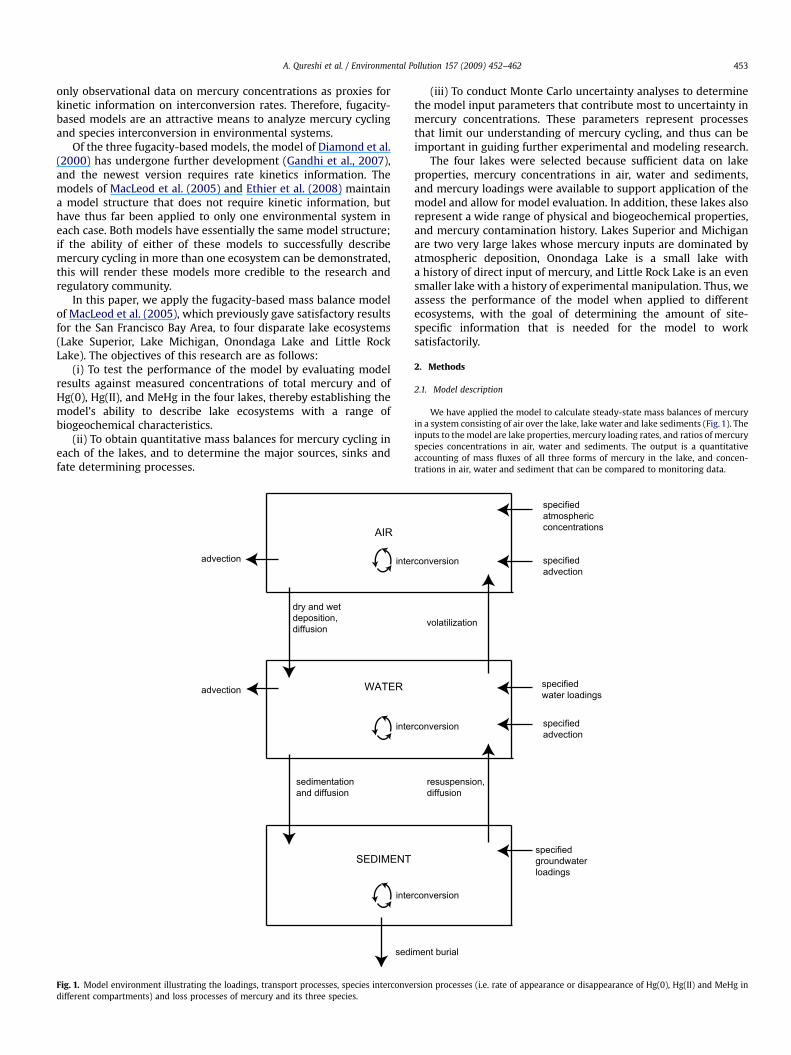
2.2. Model application

A flow sheet describing the procedure of application and evaluation of themodel is shown in Fig. 2. For all four lakes, measurements of concentrations ofmercury species in air, water and sediments have been gathered from the literatureand used to estimate partition and speciation coefficients that are used as initialinputs to the model. Site-specific values are listed in Tables 1 and 2. Speciationcoefficients in air were assigned default generic values of Hg(II)/Hg(0)¼ 0, andMeHg/Hg(0)¼ 10�6 for all systems (MacLeod et al., 2005). Using the initial param-eterization, the model is run and calculated mercury concentrations in air, water andsediments are compared with available monitoring data. At this stage, somerefinements can be made in the input data to optimize the agreement betweenobserved and modeled values; however, a condition is that the input values that areadjusted should remain within the range reported in literature. The final steady-state model output provides a quantitative description of fluxes between environ-mental compartments and inventories in each compartment for all three speciesgroups and total mercury (THg). These mass balances can be used as a basis toevaluate mercury sources, cycling and sinks in the system.

2.3. Uncertainty analysis

We perform Monte Carlo uncertainty analysis to estimate uncertainty in modeloutputs due to combined uncertainty and variability in model inputs. In this analysiswe assume that possible values of inputs are lognormally distributed, and thatvariance in input parameters is uncorrelated (MacLeod et al., 2002, 2005). Modeloutputs, with the exception of interconversion rates, cannot assume negative values.Therefore, their distributions are skewed towards the positive number space, and

MASS BAL

Refine estimatrange of speciacoefficients, loabudget.

MODEL OUT

Individual spe

Net species i

INTERPRE

LAKE PROPERTIES ANDTRANSPORTPARAMETERS

Area

Water depthActive sedimentdepth

Suspended andsediment solidsconcentrations

Sediment depositionSedimentresuspensionAdvectivethroughflow

8. Diffusive transfercoefficients

MERCURYSPECIATION ANDPARTITIONINGPROPERTIES

Measured speciationcoefficients(Hg(II):Hg(0),MeHg:Hg(0))

Measured partitioncoefficients

Mercury concetra-tions in airLoadings to waterLoadings tosedimentsfrom groundwater

INITIAL PARAMETERIZATION OF MODEL

3.

1.LOADING ESTIMATES

5.

6.

7.

2.

3.

1.

4.

2.

1.

2.

Fig. 2. Procedure for application and evaluat

thus assumed to be lognormally distributed (Limpert et al., 2001). For intercon-version rates, the distribution of possible values can be both negative and positive;hence a normal distribution is assumed for these values. For all lognormal distri-butions, we express variance as confidence factors (CF), where 95% of possible valueslie in the range between the median multiplied by the CF and the median divided bythe CF (MacLeod et al., 2002). For each Monte Carlo analysis 5000 individual modelcalculations were performed, which was found to provide stable results for outputCFs.

2.4. Site descriptions and mercury sources

Physical characteristics, estimated mercury loadings, and mercury partitioningand speciation properties used in the model that are specific to the four lakes areprovided in Tables 1–4. In cases where speciation coefficients for only one phase ofa bulk compartment were available (e.g. the dissolved or particulate phase of thebulk water compartment), speciation coefficients in the other phase were estimatedfrom the known speciation coefficients and species–specific partition coefficients.Table 5 shows model input parameters that are common to all four lakes. We collectdata from literature and interpret it to represent conditions in each lake as a whole.The data include values from the late 1980s to the late 1990s, to correspond withavailable loading estimates. Additional lake-specific information is given in thefollowing paragraphs.

2.4.1. Lake SuperiorLake Superior is the largest lake in the world by surface area, 82,100 km2

(Rolfhus et al., 2003), and has the largest volume among the Great Lakes. LakeSuperior is dimictic, meaning the water column is stratified in summer and winter,but usually turns over and mixes vertically in both the fall and the spring. It hasa mean depth of 147 m (Rolfhus et al., 2003) and a mean hydraulic residence time of200 years (Quinn, 1992).

The Lake Superior basin has a low population density, but past industrialactivities likely released mercury to the lake. These activities included chlor-alkaliproduction and gold and silver mining (Rossmann, 1999). According to Kerfoot andNriagu (1999), about 25% of Canadian gold production came from the northern rimof Lake Superior in the period 1989–1999. Current mercury sources to the lake,however, are likely dominated by atmospheric deposition (Rolfhus et al., 2003).

2.4.2. Lake MichiganLake Michigan is the largest freshwater lake in the United States. It has a surface

area of 58,016 km2 (Eadie, 1997), a mean depth of 85 m and a hydraulic residencetime of 62 years (Quinn, 1992). The southern tip of the lake is heavily urbanized andindustrialized; the cities of Chicago and Milwaukee are on the lake. Lake Michigan isdimictic; it usually turns over in December and early April (McCormick andPazdalski, 1993).

Lake Michigan receives mercury loading from atmospheric deposition and toa lesser extent by tributary inflow (Table 4). Our estimated tributary loading is takenfrom the Lake Michigan Mass Balance study, (http://www.epa.gov/glnpo/lmmb/, lastvisited May 14, 2007).

2.4.3. Onondaga LakeOnondaga Lake is located in the urban area of Syracuse, New York, USA. It has

a surface area of 11.7 km2 (Gbondo-Tugbawa and Driscoll, 1998), mean depth of 12 m(Jacobs et al., 1995) and an average hydraulic residence time of 107 days (Kim et al.,2004). Onondaga Lake is hypereutrophic and has received direct discharges from an

ANCE MODEL

Are predicted concen-trations in satisfactoryagreement withobserved concentra-tions?

Yes

Noes, within observedtion and partitiondings, and sediment

PUTS + UNCERTAINTY ANALYSIS

Ranges of predicted concentrations in air, water and sediments

cies mass balances Total mercury mass balance

nterconversion rates

TATION OF MODEL OUTPUTS

ion of the Mercury Mass Balance Model.

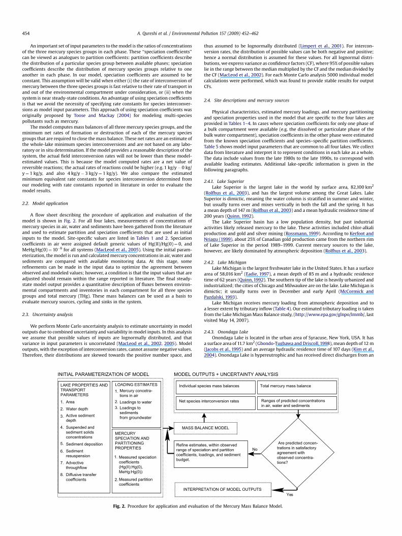
Table 1Lake-specific mercury speciation coefficients (CF).

Lake Water (dissolved phase) Sediment (solid phase)a

Hg(II):Hg(0) MeHg:Hg(0) Hg(II):Hg(0) MeHg:Hg(0)

Superior 21b (3) 0.22b (5) 5000b (3.4) 10b (3.4)Michigan 9c (2) 0.5c (2) 2850d (4) 10d (4)Onondaga 176e (4.9) 41e (5.6) 2500f (1.35) 10f (1.35)Little Rock 66g (2.5) 12g (6.1) 777h (2.2) 10h (1.5)

CF¼ confidence factors.a In all cases, only the ratio THg:MeHg was available in literature. From this ratio,

the ratio Hg(II):MeHg was estimated. Since no Hg(0) contents in sediment solidswere reported in any of the studies, MeHg:Hg(0) was assumed to be 10:1. This wasbased on the statement of Cossa and Gobeil (2000) that no elemental mercury wasdetectable in sediment cores. The Hg(II):Hg(0) ratio was calculated by multiplyingthe Hg(II):MeHg ratio with MeHg:Hg(0) ratio.

b Estimated from Rolfhus et al. (2003).c Estimated from Mason and Sullivan (1997).d Rossmann et al. (2001).e Estimated from Bloom and Effler (1990).f Estimated from Henry et al. (1995).g Estimated from Watras et al. (1994).h Estimated from Watras et al. (1996).

A. Qureshi et al. / Environmental Pollution 157 (2009) 452–462 455

alkali manufacturer (Effler and Perkins, 1987). The lake is normally dimictic,however, it did not experience spring turnover in 7 of the 18 years between 1968 and1986 (Effler and Perkins, 1987).

Total direct discharges of mercury from the chlor-alkali factory to OnondagaLake are estimated to be about 75,000 kg for the period 1946–1970 (Bloom andEffler, 1990) and it is alleged that illegal dumping continued until 1988 from anotherfacility (http://www.onlakepartners.org/ppdf/p1508a.pdf, last visited April 03,2007). However, extensive action has been taken over the past several years toreduce mercury loadings to the lake, and mercury loading to the lake is nowdominated by tributary inflows (Table 4).

2.4.4. Little Rock Lake treatment basinLittle Rock Lake is a remote seepage lake situated in the North Highland Lake

district in Vilas County, Wisconsin, USA. The lake was divided into two basins; thefirst basin (called the treatment basin) was physically separated from the rest of lake(called the reference basin) by a vinyl curtain. The treatment basin was subjected toexperimental acidification, followed by natural recovery (Brezonik et al., 1993). Inthis work, we consider only the treatment basin of the lake because complete datarequired for our modeling was available for this part only. The basin has a uniquehistory of mercury biogeochemistry as it was experimentally acidified, and thusprovides an extreme example that tests the flexibility of the model approach.

The treatment basin has a small surface area of 0.098 km2 and a mean depth of3.8 m (Hurley et al., 1994). The basin is dimictic and the hypolimnion is reported tobecome anoxic during stratification. We refer to the treatment basin as ‘‘Little RockLake’’ in the remainder of the paper.

Mercury loadings to Little Rock Lake are exclusively from atmospheric deposi-tion (Table 4). The data used to estimate speciation coefficients and partition coef-ficients are gathered from experiments conducted in the lake between 1988 and1992 (Watras et al., 1994). In Little Rock Lake, seasonal hypolimnic THg and MeHgconcentrations were more than 100 times greater than epilimnitic concentrations.Therefore, for consistency with whole-lake average concentrations described by themodel, the hypolimnitic concentrations were weighted by volume and seasonbefore the speciation coefficients for the lake were calculated.

Table 2Lake-specific mercury partition coefficients (CF).

Lake Suspended solids–water (dimensionless)

Hg(0)a Hg(II) MeHg

Superior 3.0� 104 (1.5) 7.04� 104,b (1.5) 7.04� 105,b (1Michigan 3.0� 104 (1.5) 5.5� 105,c (1.4) 5.5� 105,c (1.4Onondaga 3.0� 104 (1.5) 4.07� 105,f (2.2) 4.3� 105,f (2.2Little Rock 3.0� 104 (1.5) 6.9� 104,h (6.3) 8.8� 104,h (12

CF¼ confidence factors.a Dimensionless partition coefficients for Hg(0) are taken from MacLeod et al. (2005)b Estimated from Rolfhus et al. (2003).c Estimated from Mason and Sullivan (1997).d Selected from the reported range by Lyon et al. (1997), 1.37�104 to 2.38� 106 for Hg

water and sediment concentrations. Confidence factors assigned a generic value of 3.e Confidence factors assigned a generic value of 3.f Estimated from Bloom and Effler (1990).g Uncertainty in parameters (expressed as confidence factors) assumed to be same ash Estimated from Watras et al. (1994).

3. Results and discussions

3.1. Model performance, lake mercury mass balances, andinfluential parameters

Comparisons of modeled mercury concentrations with ranges ofmeasured data, steady-state mercury distribution and fluxes, andthe important input parameters identified in the Monte Carlouncertainty analyses are shown in Figs. 3–6. The good agreementsbetween measurements and model in Figs. 3A, 4A, 5A and 6A arenot evidence of predictive capabilities of the model, but ratherdemonstrate that the model provides a description of mercury ineach lake that is consistent with observations. The information thatis gained in this modeling exercise and that goes beyond themeasurement data, is the quantitative description of mercuryfluxes between air, water and sediment and between differentspecies groups, and the identification of influential input parame-ters. Parameters influential in the four lakes considered here willlikely be influential for other lakes as well, and indicate importantmercury fate processes. Note that the fluxes and interconversionrates are calculated by the model on a molar basis, but for easyinterpretation we present them on a mass basis (Figs. 3B, 4B, 5B and6B). Below we analyze the model performance, mercury fluxes anduncertainty analysis results for each lake separately.

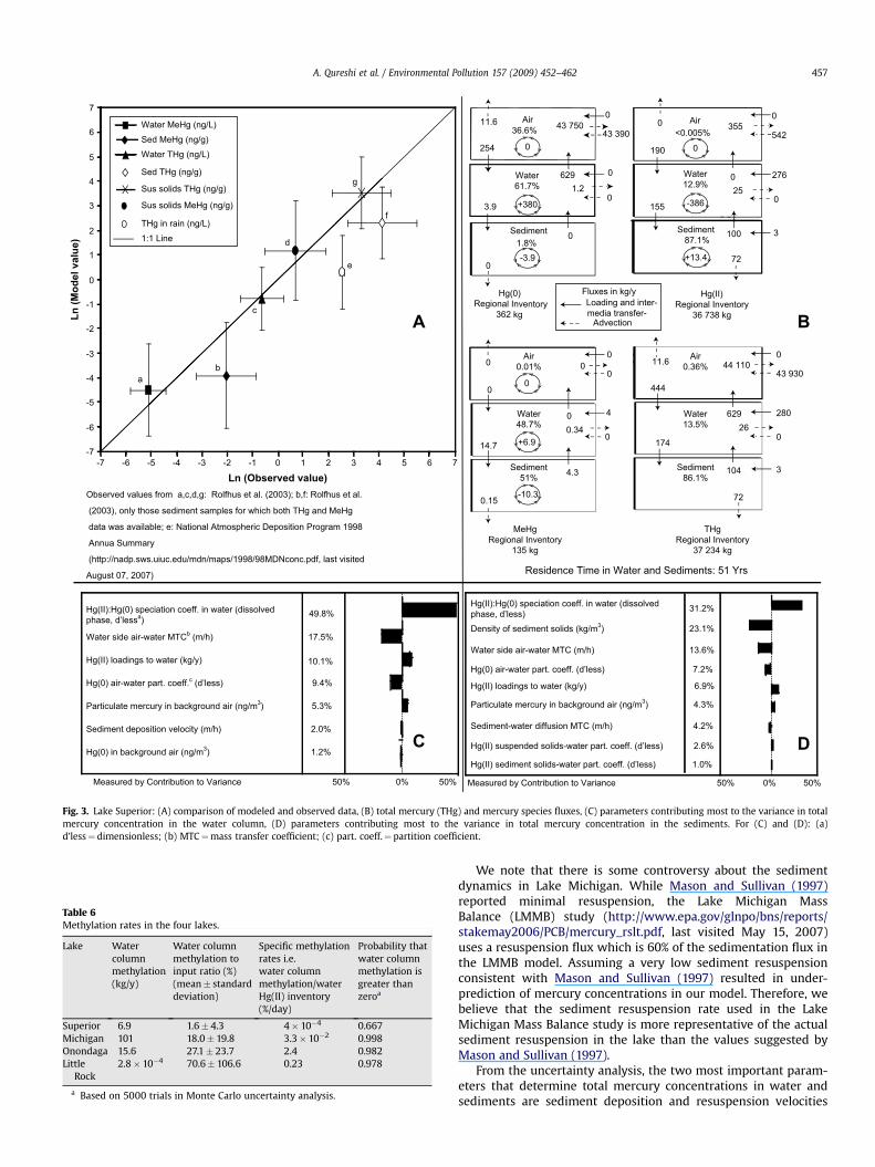
3.1.1. Lake SuperiorModeled mercury concentrations are generally in good agree-

ment with those observed in the field (Fig. 3A). However, steady-statesediment concentrations calculated by the model are under-estimated relative to values reported by Rolfhus et al. (2003). It ispossible that this discrepancy is attributable to mercury measure-ments being made near historical sources of mercury (Rolfhus et al.,2003), or due to the surface enrichment of sediment mercury (Fabbriet al., 2001), which is not described in the model. Further, modeledmercury concentrations in rain are also underestimated. The modeldoes not take into account the conversion of elemental mercury todivalent mercury in air. However, it has been reported that as much as1%/h of elemental mercury can be oxidized in the aqueous phase byozone under lab conditions (see review by Schroeder et al. (1991)).Thus, substantial conversion of elemental mercury to divalentmercury in rain over Lake Superior is possible (Schroeder et al.,1991;Hall, 1995). Accordingly, conversion of Hg(0) to Hg(II) in the atmo-sphere may explain our underestimation of mercury concentrationsin rain (Fig. 3A). Alternatively, or additionally, this underestimationcould also be due to non-accounting for scavenging of elementalmercury by rain (Van Loon et al., 2001).

Lake sediments are estimated to be the largest reservoir of totalmercury, while methyl mercury is evenly distributed between the

Sediment solids–water (dimensionless)

Hg(0)a Hg(II) MeHg

.5) 2.0� 104 (1.5) 1.92� 104,b (1.5) 7.44� 102b (1.5)) 2.0� 104 (1.5) 1.92� 104,d (3)e 2.0� 104d (3)e

) 2.0� 104 (1.5) 1.92� 106,d (2.2)f 2.0� 104c (2.2)g

.6) 2.0� 104 (1.5) 1.19� 103,h (2.4) 1.8� 103d (3)

and their confidence factors are assumed to be equal to 1.5.

(II) and 1.56�103 to 2.64�105 for MeHg, to achieve good agreement with reported

in suspended solids–water partition coefficients for the same lake.

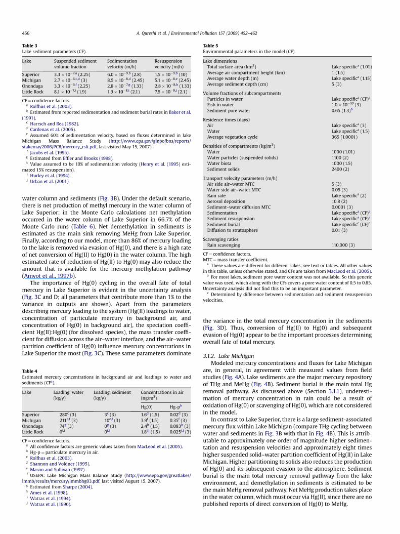
Table 3Lake sediment parameters (CF).

Lake Suspended sedimentvolume fraction

Sedimentationvelocity (m/h)

Resuspensionvelocity (m/h)

Superior 3.3� 10�7,a (2.25) 6.0� 10�9,b (2.8) 1.5� 10�9,b (10)Michigan 2.7� 10�6,c,d (3) 8.5� 10�8,d (2.45) 5.1� 10�8,e (2.45)Onondaga 3.3� 10�6,f (2.25) 2.8� 10�7,g (1.33) 2.8� 10�8,h (1.33)Little Rock 8.1� 10�7,i (1.9) 1.9� 10�8,i (2.1) 7.5� 10�9,j (2.1)

CF¼ confidence factors.a Rolfhus et al. (2003).b Estimated from reported sedimentation and sediment burial rates in Baker et al.

(1991).c Harrsch and Rea (1982).d Cardenas et al. (2005).e Assumed 60% of sedimentation velocity, based on fluxes determined in lake

Michigan Mass Balance Study (http://www.epa.gov/glnpo/bns/reports/stakemay2006/PCB/mercury_rslt.pdf, last visited May 15, 2007).

f Jacobs et al. (1995).g Estimated from Effler and Brooks (1998).h Value assumed to be 10% of sedimentation velocity (Henry et al. (1995) esti-

mated 15% resuspension).i Hurley et al. (1994).j Urban et al. (2001).

Table 5Environmental parameters in the model (CF).

Lake dimensionsTotal surface area (km2) Lake specifica (1.01)Average air compartment height (km) 1 (1.5)Average water depth (m) Lake specifica (1.15)Average sediment depth (cm) 5 (3)

Volume fractions of subcompartmentsParticles in water Lake specifica (CF)a

Fish in water 1.0� 10�10 (3)Sediment pore water 0.65 (1.3)b

Residence times (days)Air Lake specifica (3)Water Lake specifica (1.5)Average vegetation cycle 365 (1.0001)

Densities of compartments (kg/m3)Water 1000 (1.01)Water particles (suspended solids) 1100 (2)Water biota 1000 (1.5)Sediment solids 2400 (2)

Transport velocity parameters (m/h)Air side air–water MTC 5 (3)Water side air–water MTC 0.05 (3)Rain rate Lake specifica (2)Aerosol deposition 10.8 (2)Sediment–water diffusion MTC 0.0001 (3)Sedimentation Lake specifica (CF)a

Sediment resuspension Lake specifica (CF)a

Sediment burial Lake specificc (CF)c

Diffusion to stratosphere 0.01 (3)

Scavenging ratiosRain scavenging 110,000 (3)

CF¼ confidence factors.MTC¼mass transfer coefficient.

a These values are different for different lakes; see text or tables. All other valuesin this table, unless otherwise stated, and CFs are taken from MacLeod et al. (2005).

b For most lakes, sediment pore water content was not available. So this genericvalue was used, which along with the CFs covers a pore water content of 0.5 to 0.85.Uncertainty analysis did not find this to be an important parameter.

c Determined by difference between sedimentation and sediment resuspensionvelocities.

A. Qureshi et al. / Environmental Pollution 157 (2009) 452–462456

water column and sediments (Fig. 3B). Under the default scenario,there is net production of methyl mercury in the water column ofLake Superior; in the Monte Carlo calculations net methylationoccurred in the water column of Lake Superior in 66.7% of theMonte Carlo runs (Table 6). Net demethylation in sediments isestimated as the main sink removing MeHg from Lake Superior.Finally, according to our model, more than 86% of mercury loadingto the lake is removed via evasion of Hg(0), and there is a high rateof net conversion of Hg(II) to Hg(0) in the water column. The highestimated rate of reduction of Hg(II) to Hg(0) may also reduce theamount that is available for the mercury methylation pathway(Amyot et al., 1997b).

The importance of Hg(0) cycling in the overall fate of totalmercury in Lake Superior is evident in the uncertainty analysis(Fig. 3C and D; all parameters that contribute more than 1% to thevariance in outputs are shown). Apart from the parametersdescribing mercury loading to the system (Hg(II) loadings to water,concentration of particulate mercury in background air, andconcentration of Hg(0) in background air), the speciation coeffi-cient Hg(II):Hg(0) (for dissolved species), the mass transfer coeffi-cient for diffusion across the air–water interface, and the air–waterpartition coefficient of Hg(0) influence mercury concentrations inLake Superior the most (Fig. 3C). These same parameters dominate

Table 4Estimated mercury concentrations in background air and loadings to water andsediments (CFa).

Lake Loading, water(kg/y)

Loading, sediment(kg/y)

Concentrations in air(ng/m3)

Hg(0) Hg-pb

Superior 280c (3) 3c (3) 1.6d (1.5) 0.02d (3)Michigan 211e,f (3) 10e,f (3) 3.9f (1.5) 0.35f (3)Onondaga 74g (3) 0g (3) 2.4h (1.5) 0.083h (3)Little Rock 0i,j 0i,j 1.8i,j (1.5) 0.025i,j (3)

CF¼ confidence factors.a All confidence factors are generic values taken from MacLeod et al. (2005).b Hg-p¼ particulate mercury in air.c Rolfhus et al. (2003).d Shannon and Voldner (1995).e Mason and Sullivan (1997).f USEPA: Lake Michigan Mass Balance Study (http://www.epa.gov/greatlakes/

lmmb/results/mercury/lmmbhg03.pdf, last visited August 15, 2007).g Estimated from Sharpe (2004).h Ames et al. (1998).i Watras et al. (1994).j Watras et al. (1996).

the variance in the total mercury concentration in the sediments(Fig. 3D). Thus, conversion of Hg(II) to Hg(0) and subsequentevasion of Hg(0) appear to be the important processes determiningoverall fate of total mercury.

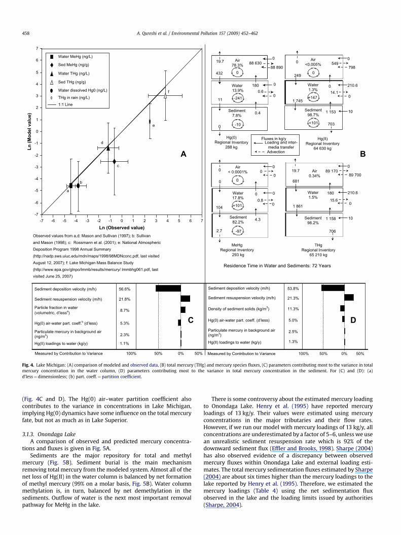
3.1.2. Lake MichiganModeled mercury concentrations and fluxes for Lake Michigan

are, in general, in agreement with measured values from fieldstudies (Fig. 4A). Lake sediments are the major mercury repositoryof THg and MeHg (Fig. 4B). Sediment burial is the main total Hgremoval pathway. As discussed above (Section 3.1.1), underesti-mation of mercury concentration in rain could be a result ofoxidation of Hg(0) or scavenging of Hg(0), which are not consideredin the model.

In contrast to Lake Superior, there is a large sediment-associatedmercury flux within Lake Michigan (compare THg cycling betweenwater and sediments in Fig. 3B with that in Fig. 4B). This is attrib-utable to approximately one order of magnitude higher sedimen-tation and resuspension velocities and approximately eight timeshigher suspended solid–water partition coefficient of Hg(II) in LakeMichigan. Higher partitioning to solids also reduces the productionof Hg(0) and its subsequent evasion to the atmosphere. Sedimentburial is the main total mercury removal pathway from the lakeenvironment, and demethylation in sediments is estimated to bethe main MeHg removal pathway. Net MeHg production takes placein the water column, which must occur via Hg(II), since there are nopublished reports of direct conversion of Hg(0) to MeHg.

Hg(0) Regional Inventory

362 kg

Hg(II)Regional Inventory

36 738 kg

MeHgRegional Inventory

135 kg

Fluxes in kg/y Loading and inter-

media transfer-Advection

THgRegional Inventory

37 234 kg

Air0.36%

Water13.5%

Sediment86.1%

0

43 93044 11011.6

444

629 280

026

174

104

72

3

0

+134

Air<0.005%

Water12.9%

Sediment 87.1%

0

542 3550

190

0 276

25

155

100

72

3

Air0.01%

Water48.7%

Sediment51%

0

000

0

0 4

00.34

14.7

4.3

0.15

+6.9

0

0

0

Water61.7%

11.6

6291.2

3.9

Air36.6%

0

43 39043 750

254

Residence Time in Water and Sediments: 51 Yrs

+380

0

0

-10.3

0

-386

+13.4

Sediment1.8%

0

0-3.9

Hg(II):Hg(0) speciation coeff. in water (dissolvedphase, d’lessa)

49.8%

Water side air-water MTCb (m/h) 17.5%

Hg(II) loadings to water (kg/y) 10.1%

Hg(0) air-water part. coeff.c (d’less) 9.4%

Particulate mercury in background air (ng/m3) 5.3%

Sediment deposition velocity (m/h) 2.0%

Hg(0) in background air (ng/m3) 1.2%

50% 0% Measured by Contribution to VarianceMeasured by Contribution to Variance

Observed values from a,c,d,g: Rolfhus et al. (2003); b,f: Rolfhus et al.

(2003), only those sediment samples for which both THg and MeHg

data was available; e: National Atmospheric Deposition Program 1998

Annua Summary

(http://nadp.sws.uiuc.edu/mdn/maps/1998/98MDNconc.pdf, last visited

August 07, 2007)

Hg(II):Hg(0) speciation coeff. in water (dissolvedphase, d’less) 31.2%

Density of sediment solids (kg/m3) 23.1%

Water side air-water MTC (m/h) 13.6%

Hg(II) loadings to water (kg/y) 6.9%

Hg(0) air-water part. coeff. (d’less) 7.2%

Particulate mercury in background air (ng/m3) 4.3%

Sediment-water diffusion MTC (m/h) 4.2%

Hg(II) suspended solids-water part. coeff. (d’less) 2.6%

50% 0% 50%

1.0%Hg(II) sediment solids-water part. coeff. (d’less)

-7

-6

-5

-4

-3

-2

-1

0

1

2

3

4

5

6

7

-7 -6 -5 -4 -3 -2 -1 0 1 2 3 5 6 7

Ln (Observed value)

Ln

(M

od

el v

alu

e)

Water MeHg (ng/L)Sed MeHg (ng/g)Water THg (ng/L)

Sed THg (ng/g)

Sus solids THg (ng/g)

Sus solids MeHg (ng/g)

1:1 LineTHg in rain (ng/L)

ab

c

d

e

f

g

50%

C D

4

A B

Fig. 3. Lake Superior: (A) comparison of modeled and observed data, (B) total mercury (THg) and mercury species fluxes, (C) parameters contributing most to the variance in totalmercury concentration in the water column, (D) parameters contributing most to the variance in total mercury concentration in the sediments. For (C) and (D): (a)d’less¼ dimensionless; (b) MTC¼mass transfer coefficient; (c) part. coeff.¼ partition coefficient.

Table 6Methylation rates in the four lakes.

Lake Watercolumnmethylation(kg/y)

Water columnmethylation toinput ratio (%)(mean� standarddeviation)

Specific methylationrates i.e.water columnmethylation/waterHg(II) inventory(%/day)

Probability thatwater columnmethylation isgreater thanzeroa

Superior 6.9 1.6� 4.3 4� 10�4 0.667Michigan 101 18.0� 19.8 3.3� 10�2 0.998Onondaga 15.6 27.1� 23.7 2.4 0.982Little

Rock2.8� 10�4 70.6� 106.6 0.23 0.978

a Based on 5000 trials in Monte Carlo uncertainty analysis.

A. Qureshi et al. / Environmental Pollution 157 (2009) 452–462 457

We note that there is some controversy about the sedimentdynamics in Lake Michigan. While Mason and Sullivan (1997)reported minimal resuspension, the Lake Michigan MassBalance (LMMB) study (http://www.epa.gov/glnpo/bns/reports/stakemay2006/PCB/mercury_rslt.pdf, last visited May 15, 2007)uses a resuspension flux which is 60% of the sedimentation flux inthe LMMB model. Assuming a very low sediment resuspensionconsistent with Mason and Sullivan (1997) resulted in under-prediction of mercury concentrations in our model. Therefore, webelieve that the sediment resuspension rate used in the LakeMichigan Mass Balance study is more representative of the actualsediment resuspension in the lake than the values suggested byMason and Sullivan (1997).

From the uncertainty analysis, the two most important param-eters that determine total mercury concentrations in water andsediments are sediment deposition and resuspension velocities

Observed values from a,d: Mason and Sullivan (1997); b: Sullivanand Mason (1998); c: Rossmann et al. (2001); e: National AtmosphericDeposition Program 1998 Annual Summary (http://nadp.sws.uiuc.edu/mdn/maps/1998/98MDNconc.pdf, last visited August 12, 2007); f: Lake Michigan Mass Balance Study(http://www.epa.gov/glnpo/lmmb/results/mercury/ lmmbhg061.pdf, last visited June 25, 2007)

Hg(0)Regional Inventory

288 kg

Hg(II)Regional Inventory

64 630 kg

MeHgRegional Inventory

293 kg

Fluxes in kg/yLoading and inter-

media transfer Advection

THgRegional Inventory

65 210 kg

Air0.34%

Water1.5%

Sediment98.2%

0

89 70089 17019.7

681

180 210.6

015.6

1 861

1 158

706

10

0

+134

Air<0.005%

Water1.3%

Sediment98.7%

0

798 5490

249

0 210.6

14.1

1 745

1 153

703

+147

10

Air< 0.0001%

Water17.8%

Sediment82.2%

0

000

0

0 0

00.8

104

4.3

2.7

0

0

0

Water 13.9%

19.7

1800.6

11

Air78.3%

0

88 890 88 630

432

Residence Time in Water and Sediments: 72 Years

-241

0

+101

0

+101

-97

Sediment7.8% 0.4

0 -10

0

Sediment deposition velocity (m/h) 53.8%

Sediment resuspension velocity (m/h) 21.3%

Density of sediment solids (kg/m3) 11.3%

Hg(0) air-water part. coeff. (d’less) 5.0%

Particulate mercury in background air(ng/m3)

2.5%

Hg(II) loadings to water (kg/y) 1.3%

100% 50% 50%Measured by Contribution to Variance

Sediment deposition velocity (m/h) 56.6%

Sediment resuspension velocity (m/h) 21.8%

Particle fraction in water (volumetric, d’lessa) 8.7%

Hg(0) air-water part. coeff.b (d’less) 5.3%

Particulate mercury in background air(ng/m3) 2.3%

Hg(II) loadings to water (kg/y) 1.1%

100% 50% 0% 50%Measured by Contribution to Variance

-7

-6

-5

-4

-3

-2

-1

0

1

2

3

4

5

6

7

-7 -6 -5 -4 -3 -2 -1 0 1 2 3 4 5 6 7

Ln (Observed value)

Ln

(M

od

el v

alu

e)

Water MeHg (ng/L)

Sed MeHg (ng/g)

Water THg (ng/L)

Sed THg (ng/g)

Water dissolved Hg0 (ng/L)

1:1 Line

THg in rain (ng/L)

a

b

c

d

e

f

A B

C D

0%

Fig. 4. Lake Michigan: (A) comparison of modeled and observed data, (B) total mercury (THg) and mercury species fluxes, (C) parameters contributing most to the variance in totalmercury concentration in the water column, (D) parameters contributing most to the variance in total mercury concentration in the sediment. For (C) and (D): (a)d’less¼ dimensionless; (b) part. coeff.¼ partition coefficient.

A. Qureshi et al. / Environmental Pollution 157 (2009) 452–462458

(Fig. 4C and D). The Hg(0) air–water partition coefficient alsocontributes to the variance in concentrations in Lake Michigan,implying Hg(0) dynamics have some influence on the total mercuryfate, but not as much as in Lake Superior.

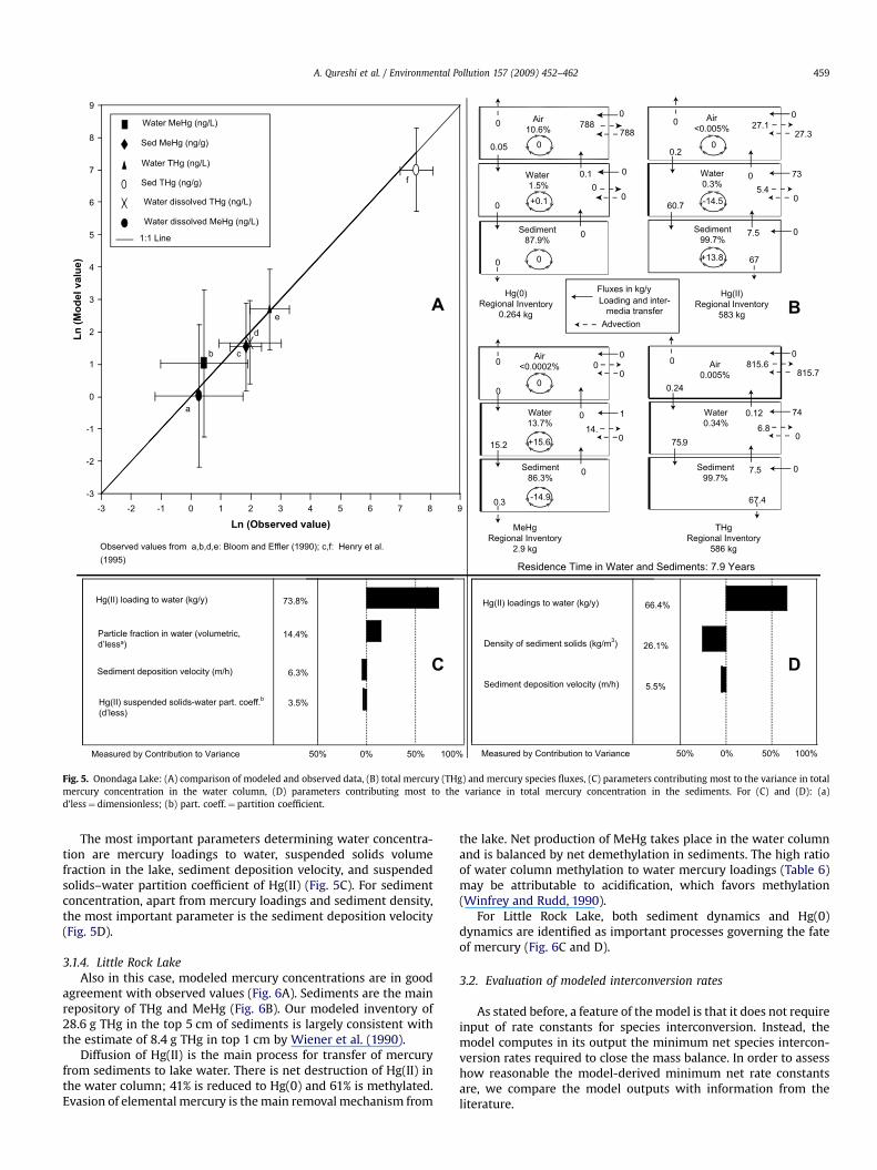
3.1.3. Onondaga LakeA comparison of observed and predicted mercury concentra-

tions and fluxes is given in Fig. 5A.Sediments are the major repository for total and methyl

mercury (Fig. 5B). Sediment burial is the main mechanismremoving total mercury from the modeled system. Almost all of thenet loss of Hg(II) in the water column is balanced by net formationof methyl mercury (99% on a molar basis, Fig. 5B). Water columnmethylation is, in turn, balanced by net demethylation in thesediments. Outflow of water is the next most important removalpathway for MeHg in the lake.

There is some controversy about the estimated mercury loadingto Onondaga Lake. Henry et al. (1995) have reported mercuryloadings of 13 kg/y. Their values were estimated using mercuryconcentrations in the major tributaries and their flow rates.However, if we run our model with mercury loadings of 13 kg/y, allconcentrations are underestimated by a factor of 5–6, unless we usean unrealistic sediment resuspension rate which is 92% of thedownward sediment flux (Effler and Brooks, 1998). Sharpe (2004)has also observed evidence of a discrepancy between observedmercury fluxes within Onondaga Lake and external loading esti-mates. The total mercury sedimentation fluxes estimated by Sharpe(2004) are about six times higher than the mercury loadings to thelake reported by Henry et al. (1995). Therefore, we estimated themercury loadings (Table 4) using the net sedimentation fluxobserved in the lake and the loading limits issued by authorities(Sharpe, 2004).

Observed values from a,b,d,e: Bloom and Effler (1990); c,f: Henry et al. (1995)

Hg(0)Regional Inventory

0.264 kg

Hg(II)Regional Inventory

583 kg

MeHgRegional Inventory

2.9 kg

Fluxes in kg/yLoading and inter-

media transferAdvection

THgRegional Inventory

586 kg

Air0.005%

Water0.34%

Sediment99.7%

0

815.7815.60

0.24

0.12 74

06.8

75.9

7.5

67.4

0

0

+134

Air<0.005%

Water0.3%

Sediment99.7%

0

27.3 27.10

0.2

0 73

5.4

60.7

7.5

67

0

Air<0.0002%

Water13.7%

Sediment86.3%

0

000

0

0 1

0 14.

15.2

0

0.3

+15.6

0

0

0

Water 1.5%

0

0.10

0

Air10.6%

0

788788

0.05

Residence Time in Water and Sediments: 7.9 Years

0

+0.1

0

-14.9

0

-14.5

+13.8

Sediment87.9%

0

0 0

Hg(II) loading to water (kg/y) 73.8%

Particle fraction in water (volumetric, d’lessa)

14.4%

Sediment deposition velocity (m/h) 6.3%

Hg(II) suspended solids-water part. coeff.b(d’less)

3.5%

100%50% 0% 50%Measured by Contribution to Variance

Hg(II) loadings to water (kg/y) 66.4%

Density of sediment solids (kg/m3) 26.1%

Sediment deposition velocity (m/h) 5.5%

100%50% 0% 50%Measured by Contribution to Variance

-3

-2

-1

0

1

2

3

4

5

6

7

8

9

-3 -2 -1 0 1 2 3 4 5 6 7 8 9

Ln

(M

od

el valu

e)

Water MeHg (ng/L)

Sed MeHg (ng/g)

Water THg (ng/L)

Sed THg (ng/g)

Water dissolved THg (ng/L)

Water dissolved MeHg (ng/L)

1:1 Line

Ln (Observed value)

a

b c

d

e

f

C D

BA

Fig. 5. Onondaga Lake: (A) comparison of modeled and observed data, (B) total mercury (THg) and mercury species fluxes, (C) parameters contributing most to the variance in totalmercury concentration in the water column, (D) parameters contributing most to the variance in total mercury concentration in the sediments. For (C) and (D): (a)d’less¼ dimensionless; (b) part. coeff.¼ partition coefficient.

A. Qureshi et al. / Environmental Pollution 157 (2009) 452–462 459

The most important parameters determining water concentra-tion are mercury loadings to water, suspended solids volumefraction in the lake, sediment deposition velocity, and suspendedsolids–water partition coefficient of Hg(II) (Fig. 5C). For sedimentconcentration, apart from mercury loadings and sediment density,the most important parameter is the sediment deposition velocity(Fig. 5D).

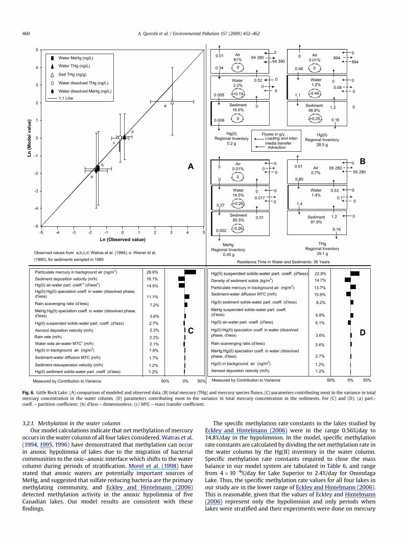
3.1.4. Little Rock LakeAlso in this case, modeled mercury concentrations are in good

agreement with observed values (Fig. 6A). Sediments are the mainrepository of THg and MeHg (Fig. 6B). Our modeled inventory of28.6 g THg in the top 5 cm of sediments is largely consistent withthe estimate of 8.4 g THg in top 1 cm by Wiener et al. (1990).

Diffusion of Hg(II) is the main process for transfer of mercuryfrom sediments to lake water. There is net destruction of Hg(II) inthe water column; 41% is reduced to Hg(0) and 61% is methylated.Evasion of elemental mercury is the main removal mechanism from

the lake. Net production of MeHg takes place in the water columnand is balanced by net demethylation in sediments. The high ratioof water column methylation to water mercury loadings (Table 6)may be attributable to acidification, which favors methylation(Winfrey and Rudd, 1990).

For Little Rock Lake, both sediment dynamics and Hg(0)dynamics are identified as important processes governing the fateof mercury (Fig. 6C and D).

3.2. Evaluation of modeled interconversion rates

As stated before, a feature of the model is that it does not requireinput of rate constants for species interconversion. Instead, themodel computes in its output the minimum net species intercon-version rates required to close the mass balance. In order to assesshow reasonable the model-derived minimum net rate constantsare, we compare the model outputs with information from theliterature.

Hg(0)Regional Inventory

0.2 g

Hg(II)Regional Inventory

28.5 g

Fluxes in g/yLoading and inter-media transfer

Advection

THgRegional Inventory

29.1 g

Air0.7%

Water1.4%

Sediment97.9%

0

65 28065 2800.01

0.80

0.53 0

0 0.1

1.4

1.2

0.16

0

0

+134

Air0.01%

Water1.2%

Sediment98.8%

0

8948940

0.46

0 0

0.08

1.1

1.2

0.16

0

Air0.01%

Water14.5%

Sediment85.5%

0

000

0

0 0

00.017

0.27

0.01

0.002

0

0

Water 2.2%

0.01

0.520

0.008 +0.19

Air81%

0

64 39064 390

0.34 0

Residence Time in Water and Sediments: 36 Years

-0.46

+0.25

0

+0.28

-0.26

Sediment16.6%

0

0.008 0

0

Water MeHg (ng/L)

Water THg (ng/L)

Sed THg (ng/g)

Water dissolved THg (ng/L)

Water dissolved MeHg (ng/L)

1:1 Line

Observed values from a,b,c,d: Watras et al. (1994); e: Wiener et al. (1990), for sediments sampled in 1985

-5

-4

-3

-2

-1

0

1

2

3

4

5

-5 -4 -3 -2 -1 0 1 2 3 4 5

Ln (Observed value)

Ln

(M

od

el v

alu

e)

a

b

c

d

e

28.6%16.1%

14.5%

11.1%

7.2%

3.6%

2.7%2.3%

2.2%2.1%1.8%

1.7%

1.2%1.2%

50% 0% 50%

Particulate mercury in background air (ng/m3) Sediment deposition velocity (m/h)Hg(0) air-water part. coeff.a (d’lessb)Hg(II):Hg(0) speciation coeff. in water (dissolved phase,d’less)

Rain scavenging ratio (d’less)

MeHg:Hg(0) speciation coeff. in water (dissolved phase, d’less)

Hg(II) suspended solids-water part. coeff. (d’less)

Aerosol depositon velocity (m/h)Rain rate (m/h)Water side air-water MTCc (m/h)Hg(0) in background air (ng/m3)

Sediment-water diffusion MTC (m/h)

Sediment resuspension velocity (m/h)Hg(II) sediment solids-water part. coeff. (d’less)

50% 0% 50%

22.9%14.7%

13.7%10.9%

8.2%

6.8%

6.1%

3.6%

3.4%

2.7%

1.2%1.2%

Hg(II) suspended solids-water part. coeff. (d’less)Density of sediment solids (kg/m3)

Particulate mercury in background air (ng/m3)Sediment-water diffusion MTC (m/h)

Hg(II) sediment solids-water part. coeff. (d’less)

MeHg suspended solids-water part. coeff. (d’less)

Hg(0) air-water part. coeff. (d’less)

Hg(II):Hg(0) speciation coeff. in water (dissolved phase, d’less)

Rain scavenging ratio (d’less)

MeHg:Hg(0) speciation coeff. in water (dissolvedphase, d’less)

Hg(0) in background air (ng/m3)

Aerosol depositon velocity (m/h)

Measured by Contribution to Variance Measured by Contribution to Variance

MeHgRegional Inventory

0.45 g

AB

DC

Fig. 6. Little Rock Lake: (A) comparison of modeled and observed data, (B) total mercury (THg) and mercury species fluxes, (C) parameters contributing most to the variance in totalmercury concentration in the water column, (D) parameters contributing most to the variance in total mercury concentration in the sediments. For (C) and (D): (a) part.-coeff.¼ partition coefficient; (b) d’less¼ dimensionless; (c) MTC¼mass transfer coefficient.

A. Qureshi et al. / Environmental Pollution 157 (2009) 452–462460

3.2.1. Methylation in the water columnOur model calculations indicate that net methylation of mercury

occurs in the water column of all four lakes considered. Watras et al.(1994, 1995, 1996) have demonstrated that methylation can occurin anoxic hypolimnia of lakes due to the migration of bacterialcommunities to the oxic–anoxic interface which shifts to the watercolumn during periods of stratification. Morel et al. (1998) havestated that anoxic waters are potentially important sources ofMeHg, and suggested that sulfate reducing bacteria are the primarymethylating community, and Eckley and Hintelmann (2006)detected methylation activity in the anoxic hypolimnia of fiveCanadian lakes. Our model results are consistent with thesefindings.

The specific methylation rate constants in the lakes studied byEckley and Hintelmann (2006) were in the range 0.56%/day to14.8%/day in the hypolimnion. In the model, specific methylationrate constants are calculated by dividing the net methylation rate inthe water column by the Hg(II) inventory in the water column.Specific methylation rate constants required to close the massbalance in our model system are tabulated in Table 6, and rangefrom 4�10�4%/day for Lake Superior to 2.4%/day for OnondagaLake. Thus, the specific methylation rate values for all four lakes inour study are in the lower range of Eckley and Hintelmann (2006).This is reasonable, given that the values of Eckley and Hintelmann(2006) represent only the hypolimnion and only periods whenlakes were stratified and their experiments were done on mercury

A. Qureshi et al. / Environmental Pollution 157 (2009) 452–462 461

tracers which might be more bioavailable, whereas our results arereported as yearly and whole-lake averages and represent a lowerbound of possible values.

While it has been suggested that high MeHg concentrations inthe hypolimnion can also result from MeHg diffusion from sedi-ments to water (Eckley and Hintelmann, 2006), our model resultsindicate that on a whole-lake basis diffusion of MeHg from sedi-ments to the water column is much less important than watercolumn production.

3.2.2. Demethylation in sedimentsNet methylation or demethylation depends on the respective

rate constants and on the amount of available substrate. Mathe-matically, if m is the methylation rate constant and d is the deme-thylation rate constant, and if the inventories of Hg(II) and MeHg insediments are SHg(II) and SMeHg, then net methylation will beobserved if:

m$SHgðIIÞ > d$SMeHg (1)

or,

SHgðIIÞSMeHg

>dm

(2)

Therefore the ratio of inventories of Hg(II) and MeHg must begreater than d/m, if net methylation is to be observed in the sedi-ments. Given that not all Hg(II) is bioavailable for methylation butmost of the MeHg is bioavailable for demethylation (Hintelmannet al., 2000), the required ratio will likely have to be higher than d/m.

Hintelmann et al. (2000) reported rate constants for demethy-lation in sediments that were higher than the methylation rateconstant by a factor of 390 (¼ d/m) for ambient concentrations(Hintelmann et al., 2000), and by a factor of 33–40 for tracerconcentrations (Hintelmann et al., 2000). From these values, weinfer that in natural settings, if the ratio of inventories of Hg(II) andMeHg is of the order of 390 or more, one may expect net methyl-ation in sediments. If the ratio is lower than about 390, one mayexpect net demethylation in sediments. We note that 390 is justone value, and this cut-off value will be different in differentecosystems. Nevertheless, we use this as a benchmark to compareagainst our model results: the ratios of inventory of Hg(II) toinventory of MeHg in sediments for the four lakes in our work arebetween 73 and 464. These values are of the same order as inHintelmann et al. (2000). Thus, our range of Hg(II):MeHg inventoryis in the range in which demethylation in sediments can beexpected, and the modeled rates of demethylation appear to bereasonable.

3.3. Data gaps and future research needs

3.3.1. Methylation and demethylationAll papers on mercury methylation cited in this section (Eckley

and Hintelmann, 2006; Watras et al., 1994, 1995, 1996) stress theimportance of stratification in influencing methylation activity.Methylation even ceases to exist after turnover (Eckley and Hin-telmann, 2006). Thus methylation activity is highly variable, bothspatially (vertically in the water column, as a result of stratifica-tion), and temporally (seasonally). Therefore, future modeling andfield research should be conducted considering this seasonal andspatial variability.

A more detailed analysis of mercury methylation would bepossible in a model which is temporally resolved and explicitlydescribes the formation of stratified layers; however, this is beyondthe scope of this study. A refined version of the current modelwould consist of two water compartments, epilimnion and

hypolimnion, with adequate parameterizations for turbulent anddiffusive exchange velocities between the two compartments.

In field campaigns, measurements of depth profiles of methylmercury with as much temporal resolution as possible wouldprovide valuable information for both calibration and evaluation.More research that quantifies methylation or demethylation rateconstants under ambient conditions should also be undertaken toproperly understand the net methylation potential of water andsediments.

3.3.2. Lake Superior vs. Lake MichiganOur model results suggest that there is net Hg(0) production in

Lake Superior but net Hg(0) loss in Lake Michigan. Differences incalculated species interconversions in the two lakes are largelyattributable to the speciation coefficients used as input to themodel. The Hg(0):Hg(II) speciation coefficients for Lake Superiorand Lake Michigan are derived from limited data (Rolfhus et al.,2003; Mason and Sullivan, 1997, respectively) which may notaccurately represent the whole-lake averages. Our Monte Carlouncertainty analysis indicates that, within the framework ofthis model, we cannot confidently distinguish between theHg(II) 4 Hg(0) conversion processes in these lakes; more seasonaland depth-resolved data from both lakes would be needed.

4. Conclusions

We have demonstrated that the model performs well whenapplied to four different lake ecosystems. In addition, we haveidentified the main mercury removal processes and that accuratedescription of Hg(0) volatilization and Hg(II) sediment dynamicswill generally be important to support modeling of mercury cyclingand fate in lakes. The model also gives first estimates of mercuryinterconversion in lakes without necessitating specification ofkinetic parameters, and is helpful in identifying data gaps andguiding future research.

However, we agree with Knightes and Ambrose (2007) thatprocess-based models such as the one applied here cannot yetpredict mercury concentrations at a regional scale without site-specific calibration and evaluation against monitoring data.Continued fundamental research and additional experience drawnfrom case-studies of well-characterized systems may eventuallymake it possible to apply the models in a predictive fashion.

Acknowledgements

The study was funded by the Swiss Federal Office for the Envi-ronment (Bundesamt fur Umwelt, BAFU). We also thank Dr. C.T.Driscoll for providing us with a copy of the thesis of Mr. C. Sharpe.

References

Ames, M., Gullu, G., Olmez, I., 1998. Atmospheric mercury in the vapor phase, and infine and coarse particulate phase matter at Perch River, New York. AtmosphericEnvironment 32, 865–872.

Amyot, M., Mierle, G., Lean, D.R.S., McQueen, D.J., 1994. Sunlight-induced formationof dissolved gaseous mercury in lake waters. Environmental Science andTechnology 28, 2366–2371.

Amyot, M., Gill, G.A., Morel, F.M.M., 1997a. Production and loss of dissolved gaseousmercury in coastal seawater. Environmental Science and Technology 31, 3603–3611.

Amyot, M., Mierle, G., Lean, D.R.S., McQueen, D.J., 1997b. Effect of solar radiation onthe formation of dissolved gaseous mercury in temperate lakes. Geochimica etCosmochimica Acta 61, 975–987.

Baker, J.E., Eisenreich, S.J., Eadie, B.J., 1991. Sediment trap fluxes and benthic recy-cling of organic carbon, polycyclic aromatic hydrocarbons, and poly-chlorobiphenyl congeners in Lake Superior. Environmental Science andTechnology 25, 500–509.

Bloom, N.S., Effler, S.W., 1990. Seasonal variability in the mercury speciation ofOnondaga Lake (New York). Water, Air, and Soil Pollution 53, 251–265.

Brezonik, P.L., Eaton, J.G., Frost, T.M., Garrison, P.J., Kratz, T.K., Mach, C.E.,McCormick, J.H., Perry, J.A., Rose, W.A., Sampson, C.J., Shelley, B.C.L., Swenson, W.A.,

A. Qureshi et al. / Environmental Pollution 157 (2009) 452–462462

Webster, K.E., 1993. Experimental acidification of Little Rock Lake, Wisconsin:chemical and biological changes over the pH range 6.1 to 4.7. Canadian Journal ofFisheries and Aquatic Sciences 50, 1101–1121.

Cardenas, M.P., Schwab, D.J., Eadie, B.J., Hawley, N., Lesht, B.M., 2005. Sedimenttransport model validation in Lake Michigan. Journal of Great Lakes Research31, 373–385.

Cossa, D., Gobeil, C., 2000. Mercury speciation in the lower St. Lawrence Estuary.Canadian Journal of Fisheries and Aquatic Sciences 57 (S1), 138–147.

Diamond, M., Ganapathy, M., Peterson, S., Mach, C., 2000. Mercury dynamics in theLahonton Reservoir, Nevada: application of the QWASI fugacity/aquivalencemultispecies model. Water, Air, and Soil Pollution 117, 133–156.

Eadie, B.J., 1997. Probing particle processes in Lake Michigan using sediment traps.Water, Air, and Soil Pollution 99, 133–139.

Eckley, C.S., Hintelmann, H., 2006. Determination of mercury methylation potentialsin the water column of lakes across Canada. Science of the Total Environment368, 111–125.

Effler, S.W., Perkins, M.G., 1987. Failure of spring turnover in Onondaga Lake, NY,USA. Water, Air, and Soil Pollution 34, 285–291.

Effler, S.W., Brooks, C.M., 1998. Dry weight deposition in polluted Onondaga Lake,New York, USA. Water, Air, and Soil Pollution 103, 389–404.

Ethier, A.L.M., Mackay, D., Toose-Reid, L.K., O’Driscoll, N.J., Scheuhammer, A.M.,Lean, D.R.S., 2008. The development and application of a mass balance modelfor mercury (total, elemental and methyl) using data from a Remote Lake (BigDam West, Nova Scotia, Canada) and the multi-species multiplier method.Applied Geochemistry 23, 467–481.

Fabbri, D., Gabianelli, G., Locatelli, C., Lubrano, D., Trombini, C., Vassura, I., 2001.Distribution of mercury and other heavy metals in core sediments of thenorthern Adriatic Sea. Water, Air, and Soil Pollution 129, 143–153.

Gandhi, N., Bhavsar, S.P., Diamond, M.L., Kuwabara, J.S., Marvin-DiPasquale, M.,Krabbenhoft, D.P., 2007. Development of a mercury speciation, fate, and bioticuptake (BIOTRANSPEC) model: application to Lahontan Reservoir (Nevada,USA). Environmental Toxicology and Chemistry 26, 2260–2273.

Gbondo-Tugbawa, S., Driscoll, C.T., 1998. Application of the regional mercury cyclingmodel (RMCM) to predict the fate and remediation of mercury in OnondagaLake, New York. Water, Air, and Soil Pollution 105, 417–426.

Hall, B., 1995. The gas phase oxidation of elemental mercury by ozone. Water, Air,and Soil Pollution 80, 301–315.

Harrsch, E.C., Rea, D.K., 1982. Composition and distribution of suspended sedimentsin Lake Michigan during summer stratification. Environmental Geology 4, 87–98.

Henry, E.A., Dodge-Murphy, L.J., Bigham, G.N., Klein, S.M., Gilmour, C.C., 1995. Totalmercury and methylmercury mass balance in an alkaline, hypereutrophic urbanlake (Onondaga Lake, NY). Water, Air, and Soil Pollution 80, 509–517.

Hintelmann, H., Keppel-Jones, K., Evans, R.D., 2000. Constants of mercury methyl-ation and demethylation rates in sediments and comparison of tracer andambient mercury availability. Environmental Toxicology and Chemistry 19,2204–2211.

Hurley, J.P., Watras, C.J., Bloom, N.S.,1994. Distribution and flux of particulate mercuryin four stratified seepage lakes. In: Watras, C.J., Huckabee, J.W. (Eds.), MercuryPollution: Integration and Synthesis. Lewis Publishers, MI, USA, pp. 69–82.

Jacobs, L.A., Klein, S.M., Henry, E.A., 1995. Mercury cycling in the water column ofa seasonally anoxic urban lake (Onondaga Lake, NY). Water, Air, and SoilPollution 80, 553–562.

Kerfoot, W.C., Nriagu, J.O., 1999. Copper mining, copper cycling and mercury in theLake Superior ecosystem: an introduction. Journal of Great Lakes Research 25,594–598.

Kim, D., Wang, Q., Sorial, G.A., Dionysiou, D.D., Timberlake, D., 2004. A modelapproach for evaluating effects of remedial actions on mercury speciation andtransport in a lake system. Science of the Total Environment 327, 1–15.

Knightes, C.D., 2008. Development and test application of a screening-levelmercury fate model and tool for evaluating wildlife exposure for surface waterswith mercury-contaminated sediments (SERAFM). Environmental Modelingand Software 23, 495–510.

Knightes, C.D., Ambrose Jr., R.B., 2007. Evaluating regional predictive capacity ofa process-based mercury exposure model, regional-mercury cycling model,applied to 91 Vermont and New Hampshire lakes and ponds, USA. Environ-mental Toxicology and Chemistry 26, 807–815.

Limpert, E., Stahel, W.A., Abbt, M., 2001. Log-normal distribution across thesciences: keys and clues. Bioscience 51, 341–352.

Lyon, B.F., Ambrose, R., Rice, G., Maxwell, C.J., 1997. Calculation of soil–water andbenthic sediment partition coefficients for mercury. Chemosphere 35, 791–808.

MacLeod, M., McKone, T.E., Mackay, D., 2005. A mass balance for mercury in the SanFrancisco Bay Area. Environmental Science and Technology 39, 6721–6729.

MacLeod, M., Fraser, A.J., Mackay, D., 2002. Evaluating and expressing the propa-gation of uncertainty in chemical fate and bioaccumulation models. Environ-mental Toxicology and Chemistry 21, 700–709.

Mason, R.P., Sullivan, K.A., 1997. Mercury in Lake Michigan. Environmental Scienceand Technology 31, 942–947.

McCormick, M.J., Pazdalski, J.D., 1993. Monitoring midlake water temperature insouthern Lake Michigan for climate change studies. Climatic Change 25, 119–125.

Morel, F.M.M., Kraepiel, A.M.L., Amyot, M., 1998. The chemical cycle andbioaccumulation of mercury. Annual Review of Ecology and Systematics 29,543–566.

Quinn, F.H., 1992. Hydraulic residence times for the Laurentian great lakes. Journalof Great Lakes Research 18, 22–28.

Rolfhus, K.R., Sakamoto, H.E., Cleckner, L.B., Stoor, R.W., Babiarz, C.L., Back, R.C.,Manolopoulos, H., Hurley, J.P., 2003. Distribution and fluxes of total andmethylmercury in Lake Superior. Environmental Science and Technology 37,865–872.

Rossmann, R., 1999. Horizontal and vertical distributions of mercury in 1983 LakeSuperior sediments with estimates of storage and mass flux. Journal of GreatLakes Research 25, 683–696.

Rossmann, R., Rygwelski, K.R., Filkins, J.C., 2001. Methyl mercury in Lake Michigansediments. In: Abstracts From the 44th Conference on Great Lakes Research,June 10–14, Green Bay, WI, U.S.A.

Schroeder, W.H., Yarwood, G., Niki, H., 1991. Transformation processes involvingmercury species in the atmosphere – results from a literature survey. Water, Air,and Soil Pollution 56, 653–666.

Sharpe, C., 2004. Mercury Dynamics of Onondaga Lake and Adjacent Wetlands. M.S.thesis, Syracuse University, Syracuse, Ny, U.S.A., 131 p.

Shannon, J.D., Voldner, E.C., 1995. Modeling atmospheric concentrations of mercuryand deposition to the Great Lakes. Atmospheric Environment 29, 1649–1661.

Sullivan, K.A., Mason, R.P., 1998. The concentration and distribution of mercury inLake Michigan. Science of the Total Environment 213, 213–228.

Tetra Tech Inc., 1996. Regional Mercury Cycling Model: a Model for Mercury Cyclingin Lakes (R-MCM Version 1.0b Beta). Tetra Tech Inc., Lafayette, CA.

Toose, L.K., Mackay, D., 2004. Adaptation of fugacity models to treat speciatingchemicals with constant species concentration ratios. Environmental Scienceand Technology 38, 4619–4626.

Ullrich, S.M., Tanton, T.W., Abdrashitova, S.A., 2001. Mercury in the aquaticenvironment: a review of factors affecting methylation. Critical Reviews inEnvironmental Science and Technology 31, 241–293.

Urban, N.R., Sampson, C.J., Brezonik, P.L., Baker, L.A., 2001. Sulfur cycling in thewater column of Little Rock Lake, Wisconsin. Biogeochemistry 52, 41–77.

Van Loon, L.L., Mader, E.A., Scott, S.L., 2001. Sulfite stabilization and reduction of theaqueous mercuric ion: kinetic determination of sequential formation constants.Journal of Physical Chemistry A 105, 3190–3195.

Watras, C.J., Bloom, N.S., Hudson, R.J.M., Gherini, S., Munson, R., Claas, S.A.,Morrison, K.A., Hurley, J., Wiener, J.G., Fitzgerald, W.F., Mason, R.P., Vandal, G.,Powell, D., Rada, R., Rislov, L., Winfrey, M., Elder, J., Krabbenhoft, D., Andren, W.,Babiarz, C., Porcella, D.B., Huckabee, J.W., 1994. Sources and fates of mercuryand methylmercury in Wisconsin lakes. In: Watras, C.J., Huckabee, J.W. (Eds.),Mercury Pollution: Integration and Synthesis. Lewis Publishers, MI, USA, pp.153–177.

Watras, C.J., Bloom, N.S., Claas, S.A., Morrison, K.A., Gilmour, C.C., Craig, S.R., 1995.Methylmercury production in the anoxic hypolimnion of a dimictic seepagelake. Water, Air, and Soil Pollution 80, 735–745.

Watras, C.J., Morrison, K.A., Back, R.C., 1996. Mass balance studies of mercury andmethylmercury in small temperate/boreal lakes of the northern hemisphere. In:Baeyens, W.R.G., Ebinghaus, R., Vasiliev, O.F. (Eds.), Global and Regional MercuryCycles: Sources, Fluxes and Mass Balances. Kluwer Academic Publishers,Dordrecht, Netherlands, pp. 329–358.

Wiener, J.G., Fitzgerald, W.F., Watras, C.J., Rada, R.G., 1990. Partitioning andbioavailability of mercury in an experimentally acidified Wisconsin lake.Environmental Toxicology and Chemistry 9, 909–918.

Winfrey, M.R., Rudd, J.W.M., 1990. Environmental factors affecting the formation ofmethylmercury in low pH lakes. Environmental Toxicology and Chemistry 9,853–869.

Yamamoto, M., 1996. Stimulation of elemental mercury oxidation in the presence ofchloride ion in aquatic environments. Chemosphere 32, 1217–1224.