Mercator Ocean Quarterly Newsletter #31– October 2008 – Page 1 GIP Mercator Ocean Quarterly Newsletter Editorial – October 2008 Greetings to all, The Global Ocean Data Assimilation Experiment (GODAE) final symposium will be held in Nice in November 12-15 2008. This project has been a precursor to a world wide experiment to demonstrate the feasibility of global ocean observing systems using state of the art assimilation techniques. Today, several teams are working on operational ocean systems to provide forecast and description of the ocean, using increasingly complex assimilation schemes and high resolution models. As we saw in the last newsletter, these systems have reached the coast and routinely provide real time ocean forecast. But they need input information for their boundaries and initialisation fields, from regional, basin wide or global configurations. This month, the Newsletter is dedicated to global ocean systems resulting from the GODAE project. In the first news feature, a review of the GODAE achievements in ocean observing systems is made by Le Traon et al. In a second introduction paper, Pierre Bahurel provides a “Global view on MyOcean” where he introduces the special ongoing efforts to improve products and services to users. Four systems from three countries (U.S., France and Japan) are then presented, showing a variety of developments, model resolutions and assimilation schemes that are all facing the same challenges: to describe, understand and forecast the world ocean. The first contribution is from Chassignet et Hurlburt and is dedicated to the U.S. HYCOM 1/12° global configuration. Menemenlis et al. will then tell us how useful the ECCO2 system is in understanding and estimating ocean processes. Legalloudec et al. follow with the 1/12° Mercator g lobal model and its ability to represent the mesoscale activity. Finally, Kamachi et al. will present the MRI global systems, including two nesting configurations dedicated to several applications from climate variability to boundary forcing or ocean weather. The next newsletter will be published in January 2009 and dedicated to the Mediterranean Sea. We wish you a pleasant reading.

Welcome message from author
This document is posted to help you gain knowledge. Please leave a comment to let me know what you think about it! Share it to your friends and learn new things together.
Transcript
Mercator Ocean Quarterly Newsletter #31– October 2008 – Page 1
GIP Mercator Ocean
Quarterly Newsletter
Editorial – October 2008
Greetings to all,
The Global Ocean Data Assimilation Experiment (GODAE) final symposium will be held in Nice in November 12-15 2008. This
project has been a precursor to a world wide experiment to demonstrate the feasibility of global ocean observing systems using
state of the art assimilation techniques. Today, several teams are working on operational ocean systems to provide forecast and
description of the ocean, using increasingly complex assimilation schemes and high resolution models. As we saw in the last
newsletter, these systems have reached the coast and routinely provide real time ocean forecast. But they need input information
for their boundaries and initialisation fields, from regional, basin wide or global configurations.
This month, the Newsletter is dedicated to global ocean systems resulting from the GODAE project.
In the first news feature, a review of the GODAE achievements in ocean observing systems is made by Le Traon et al. In a
second introduction paper, Pierre Bahurel provides a “Global view on MyOcean” where he introduces the special ongoing efforts
to improve products and services to users.
Four systems from three countries (U.S., France and Japan) are then presented, showing a variety of developments, model
resolutions and assimilation schemes that are all facing the same challenges: to describe, understand and forecast the world
ocean. The first contribution is from Chassignet et Hurlburt and is dedicated to the U.S. HYCOM 1/12° global configuration.
Menemenlis et al. will then tell us how useful the ECCO2 system is in understanding and estimating ocean processes.
Legalloudec et al. follow with the 1/12° Mercator g lobal model and its ability to represent the mesoscale activity. Finally, Kamachi
et al. will present the MRI global systems, including two nesting configurations dedicated to several applications from climate
variability to boundary forcing or ocean weather.
The next newsletter will be published in January 2009 and dedicated to the Mediterranean Sea.
We wish you a pleasant reading.
Mercator Ocean Quarterly Newsletter #31– October 2008 – Page 2
GIP Mercator Ocean
Contents
UGODAE Oceanview: from an experiment towards a long-term Ocean Analysis and Forecasting International
Program U ........................................................................................................................................................... 3
By Pierre Yves Le Traon, Mike Bell, Eric Dombrowsky, Andreas Schiller, Kirsten Wilmer-Becker
UA Global View on MyOcean U .............................................................................................................................. 4
By Pierre Bahurel
UOcean U.S. GODAE: Global Ocean Prediction with the HYbrid Coordinate Ocean Model (HYCOM)U .................. 5
By Eric P. Chassignet and Harley E. Hurlburt
UECCO2: High Resolution Global Ocean and Sea Ice Data SynthesisU ................................................................. 13
By Dimitris Menemenlis, Jean-Michel Campin, Patrick Heimbach, Chris Hill, Tong Lee, An Nguyen, Michael Schodlok and Hong
Zhang
USimulation of Meso-Scale Eddies in the Mercator Global Ocean High Resolution ModelU ............................... 22
By Olivier Le Galloudec, Romain Bourdallé Badie, Yann Drillet, Corinne Derval and Clément Bricaud
UOcean Data Assimilation and Prediction system in JM and MRIU ..................................................................... 31
By Masafumi Kamachi, Yosuke Fujii, Norihisa Usui, Shiroh Ishizaki, Satoshi Matsumoto and Hiroyuki Tsujino
UNotebookU ....................................................................................................................................................... 42
Mercator Ocean Quarterly Newsletter #31 – October 2008 – Page 3
GODAE Oceanview: From an experiment towards a long term Ocean Analysis and Forecasting International P rogram
GODAE Oceanview: from an experiment towards a long- term Ocean Analysis and Forecasting International Program By Pierre Yves Le Traon 1, Mike Bell 2, Eric Dombrowsky 3, Andreas Schiller 4, Kirsten Wilmer-
Becker 2 1 Ifremer Brest, Technopole Brest-Iroise, BP70, 29280 Plouzané cedex 2 Met Office, Exeter, UK 3 Mercator Ocean, 8-10 rue Hermès, Toulouse, France 4 CAWCR-CSIRO, Hobart, Tasmania, Australia
Over the past 10 years, GODAE through its International GODAE Steering Team (IGST) has coordinated and facilitated the
development of global and regional ocean forecasting systems and has made excellent progress. It has been demonstrated that
global ocean data assimilation is feasible and GODAE has made important contributions to the establishment of an effective and
efficient infrastructure for global operational oceanography that includes the required observing systems, data assembly and
processing centers, modeling and data assimilation centers and data and product servers. GODAE as an experiment will end in
2008. Its final symposium (Nice, November 12-15, 2008) will provide an opportunity to review the key achievements of the last 10
years. The symposium will also discuss the future of operational ocean analysis and forecasting and proposals for its international
coordination. Main issues are summarized hereafter.
Although there are still major challenges to face, global operational oceanography now needs to transition from a demonstration to
a permanent and sustained capability. Most GODAE groups have or are now transitioning towards operational or pre-operational
status. GODAE systems are also evolving to satisfy new requirements (e.g. for coastal zone and ecosystem monitoring and
forecasting, climate monitoring) and must benefit from scientific advances in ocean modeling and data assimilation.
In order to ensure the required long-term international collaboration and cooperation on these issues, it is thus proposed to set up
an international program on ocean analysis and forecasting systems called GODAE OceanView. Through its science team,
GODAE OceanView would provide international coordination and leadership in:
• The development and scientific testing of the next generation of ocean analysis and forecasting systems, covering bio-
geochemical and eco-systems as well as physical oceanography, and extending from the open ocean into the shelf sea
and coastal waters.
• The exploitation of this capability in other applications (weather forecasting, seasonal and decadal prediction, climate
change detection and its coastal impacts, etc).
• The assessment of the contribution of the various components of the observing system and scientific guidance for
improved design and implementation of the ocean observing system.
GODAE OceanView science team will provide a forum where the main operational and research institutions involved in global
ocean analysis and forecasting can develop collaborations and international coordination of their activities. It will include scientists
from the main operational systems as well as scientific experts on specific fields (e.g. observation, modeling, data assimilation)
and representatives of key observing systems. Some of the GODAE OceanView objectives will be pursued through a number of
Task Teams (e.g. Intercomparison and Validation, Observing System Evaluation, Coastal Ocean and Shelf Seas, Marine
Ecosystem Monitoring and Prediction). These teams will address specific topics of particular importance to GODAE OceanView
usually in collaboration with international research programs (e.g. OOPC, CLIVAR, IMBER, WCRP). Operational aspects related
to product harmonization and standardization and links with JCOMM will be carried out by the JCOMM ET-OOFS.
To summarize, operational oceanography faces many challenges with time scales ranging from weather to climate. It is inherently
an international issue, requiring broad collaboration to span the global oceans. GODAE OceanView will promote the development
of ocean modelling and assimilation in a consistent framework to optimize mutual progress and benefit. It will also promote the
associated exploitation of improved ocean analyses and forecasts and provide a means to assess the relative contributions of and
requirements for observing systems. GODAE OceanView detailed objectives and links with international research programs must
now be discussed with the wider community. The GODAE final symposium will be a major opportunity for starting such an
interaction.
Mercator Ocean Quarterly Newsletter #31 – October 2008 – Page 4
A Global View on MyOcean
A Global View on MyOcean By Pierre Bahurel 1
1 Mercator Ocean, 8-10 rue Hermes, Parc technologique du canal, 31520 Ramonville st Agne (MyOcean coordinator) Numerical global models have now joined satellites and in situ instruments to reinforce their ocean watch mission all around the
planet. They form together a powerful brigade to monitor the ocean state, describe its real time situation anywhere, and forecast
its short-term evolutions. They deliver a new and global view on the ocean.
“One planet, one ocean”, as it is declared these days on the frontpage of the International Oceanographic Commission (IOC)
website. It sounds like an invitation to join efforts all around the world for a better depiction of the ocean. It sounds like an
injunction to act collectively to increase our knowledge and respect of our ocean planet. During the past ten years, the
international “Global Ocean Data Assimilation Experiment (GODAE)” conducted with IOC has been a first answer to this
challenge, and lead to a major step forward in operational oceanography. It has lead to the emergence of a reliable, continuous,
real-time, 3D and global capacity in ocean monitoring and forecasting. World-leading teams (amongst with the Japanese, US and
French teams presenting their global ocean capacities in this newsletter) have joined effort and motivation to set up a new
international network of operational oceanography centres.
Europe has undoubtedly taken an important role in the development of this modern operational oceanography. Born with
successful national projects at the end of the 90’s (such as Mercator in France) now linked together and cross-fertilized through
European projects from ESA or the Commission, the European capacity for ocean monitoring and forecasting has reached the
point where the demonstration is over, and the service activated. This is what “MyOcean” is about.
MyOcean is the European service for ocean monitoring and forecasting, the marine component of the “Kopernikus” European
program for a global monitoring of environment & security. The mission is straight-forward: offer the best information available on
the state of the global ocean and European regional seas for the benefit of any citizen, decision-maker, or downstream service
provider requiring it. To serve a user community as wide as the marine application sectors, the MyOcean focus has been clearly
set on the common denominator data requested for all users: a “core” information on the ocean provided by the European Marine
“Core” Service.
Mercator Ocean is the coordinator of this new European service.
The MyOcean project will start in the first days of 2009, and the MyOcean service will open in the following months.
The FP7 project that provides for the 3 years coming (2009-2011) the European Union framework to set-up this new service
gathers with Mercator Océan 60 partners, all the major operational oceanography centres, all maritime member states from UE,
and the best skills in Europe for this challenge. This consortium is composed of old companions of the GODAE years, but half of it
is formed by new teams from other countries or communities in Europe.
MyOcean is built indeed on the strong belief that sharing data and knowledge increases the value of the information service.
That’s why connections with other initiatives in the world – on the model invented by GODAE – are priorities for the MyOcean
European team to build this new view on our global ocean.
Mercator Ocean Quarterly Newsletter #31 – October 2008 – Page 5
Ocean U.S. GODAE: Global Ocean Prediction with the Hybrid Coordinate Ocean Model
Ocean U.S. GODAE: Global Ocean Prediction with the HYbrid Coordinate Ocean Model (HYCOM) By Eric P. Chassignet 1 and Harley E. Hurlburt 2
1 COAPS, Florida State University,Tallahassee, FL, USA 2 Naval Research Laboratory, Stennis Space Center, MS, USA
Introduction
During the past 5-10 years, a broad partnership of institutions has been collaborating in developing and demonstrating the
performance and application of eddy-resolving, real-time global and basin-scale ocean prediction systems using the HYbrid
Coordinate Ocean Model (HYCOM). These systems have been or are in the process of being transitioned for operational use by the
U.S. Navy at the Naval Oceanographic Office (NAVOCEANO), Stennis Space Center, MS, and by the National Oceanic and
Atmospheric Administration (NOAA) at the National Centers for Environmental Prediction (NCEP), Washington, D.C. The systems
run efficiently on a variety of massively parallel computers and include sophisticated, but relatively inexpensive, data assimilation
techniques for assimilation of satellite altimeter sea surface height and sea surface temperature as well as in-situ temperature,
salinity, and float displacement. The partnership represents a broad spectrum of the oceanographic community, bringing together
academia, federal agencies, and industry/commercial entities, spanning modeling, data assimilation, data management and serving,
observational capabilities, and application of HYCOM prediction system outputs. All participating institutions were committed and
the collaborative partnership provided an opportunity to leverage and accelerate the efforts of existing and planned projects,
consequently producing a high quality product that should collectively better serve a wider range of users than would the individual
projects.
The HYCOM partnership is a U.S. component of the international Global Ocean Data Assimilation Experiment (GODAE). GODAE is
a coordinated international effort envisioning “a global system of observations, communications, modeling, and assimilation that will
deliver regular, comprehensive information on the state of the oceans, in a way that will promote and engender wide utility and
availability of this resource for maximum benefit to the community” (see Chassignet and Verron (2006) for a review). Navy
applications, NOAA applications such as maritime safety, fisheries, the offshore industry, and management of shelf/coastal areas
are among the expected beneficiaries of the HYCOM ocean prediction systems (Hhttp://www.hycom.orgH). More specifically, the
precise knowledge and prediction of ocean mesoscale features is used by Navy, NOAA, the oil industry, and fisheries for an optimal
use of their resources. Examples are optimal ship and submarine routing, search and rescue, oil spill drift application, monitoring of
the open ocean ecosystems, fisheries management, short range coupled atmosphere-ocean forecasts, forecast of the coastal and
near-shore environment, etc…
Background
Numerical modeling studies over the past several decades have demonstrated progress in both model architecture and the
availability of computational resources for the scientific community. Perhaps the most noticeable aspect of this progression has
been the evolution from simulations on coarse-resolution horizontal/vertical grids outlining basins of simplified geometry and
bathymetry and forced by idealized stresses, to fine-resolution simulations incorporating realistic coastal definition and bottom
topography, forced by observational data on relatively short time scales. The choice of the vertical coordinate system in an ocean
model however remains one of the most important aspects of its design. In practice, the representation and parameterization of the
processes not resolved by the model grid are often directly linked to the vertical coordinate choice (Griffies et al., 2000). Oceanic
general circulation models traditionally represent the vertical in a series of discrete intervals in either a depth, density, or terrain-
following unit. Because none of the three main vertical coordinates (depth, density, and terrain-following) provide universal
optimality, it is natural to envision a hybrid approach that combines the best features of each vertical coordinate. Isopycnic (density-
tracking) layers work best for modeling the deep stratified ocean, levels at constant fixed depth or pressure are best to use to
provide high vertical resolution near the surface within the mixed layer, and terrain-following levels are often the best choice for
modeling shallow coastal regions. In HYCOM, the optimal vertical coordinate distribution of the three vertical coordinate types is
chosen at every time step. The default configuration of HYCOM is isopycnic in the open stratified ocean, but makes a dynamically
smooth transition to terrain-following coordinates in shallow coastal regions and to fixed pressure-level coordinates in the surface
mixed layer and/or unstratified seas. In doing so, the model takes advantage of the different coordinate types in optimally simulating
coastal and open-ocean circulation features (Chassignet et al., 2006, 2007). A user-chosen option allows specification of the vertical
coordinate separation that controls the transition among the three coordinate systems. The assignment of additional coordinate
surfaces to the oceanic mixed layer also allows the straightforward implementation of multiple vertical mixing turbulence closure
schemes (Halliwell, 2004). The choice of the vertical mixing parameterization is also of importance in areas of strong entrainment,
such as overflows.
Mercator Ocean Quarterly Newsletter #31 – October 2008 – Page 6
Ocean U.S. GODAE: Global Ocean Prediction with the Hybrid Coordinate Ocean Model
Data assimilation is essential for ocean prediction because (a) many ocean phenomena are due to nonlinear processes (i.e., flow
instabilities) and thus are not a deterministic response to atmospheric forcing, (b) errors exist in the atmospheric forcing, and (c)
ocean models are imperfect, including limitations in numerical algorithms and in resolution. Most of the information about the ocean
surface’s space-time variability is obtained remotely from instruments aboard satellites [Sea Surface Height (SSH) and Sea Surface
Temperature (SST)], but these observations are insufficient for specifying the subsurface variability. Vertical profiles from
expendable bathythermographs (XBT), conductivity-temperature-depth (CTD) profilers, and profiling floats (e.g., Argo, which
measures temperature and salinity in the upper 2000 m of the ocean) provide another substantial source of data. Even together,
these data sets are insufficient to determine the state of the ocean completely, so it is necessary to exploit prior knowledge in the
form of statistics determined from past observations as well as our present understanding of ocean dynamics. By combining all of
these observations through data assimilation into an ocean model, it is possible to produce a dynamically consistent depiction of the
ocean. However, in order to have any predictive capabilities, it is extremely important that the freely evolving ocean model (i.e., non-
data-assimilative model) has skill in representing ocean features of interest.
To properly assimilate the SSH anomalies determined from satellite altimeter data, the oceanic mean SSH over the altimeter
observation period must be provided. In this mean, it is essential that the mean current systems and associated SSH fronts be
accurately represented (position, amplitude, and sharpness). Unfortunately, the earth’s geoid is not presently known with sufficient
accuracy for this purpose, and coarse hydrographic climatologies (~0.5º-1º horizontal resolution) cannot provide the spatial
resolution necessary when assimilating SSH in an eddy-resolving model (horizontal grid spacing of 1/10º or finer). At these scales of
interest, it is essential to have the observed means of boundary currents and associated fronts sharply defined (Hurlburt et al.,
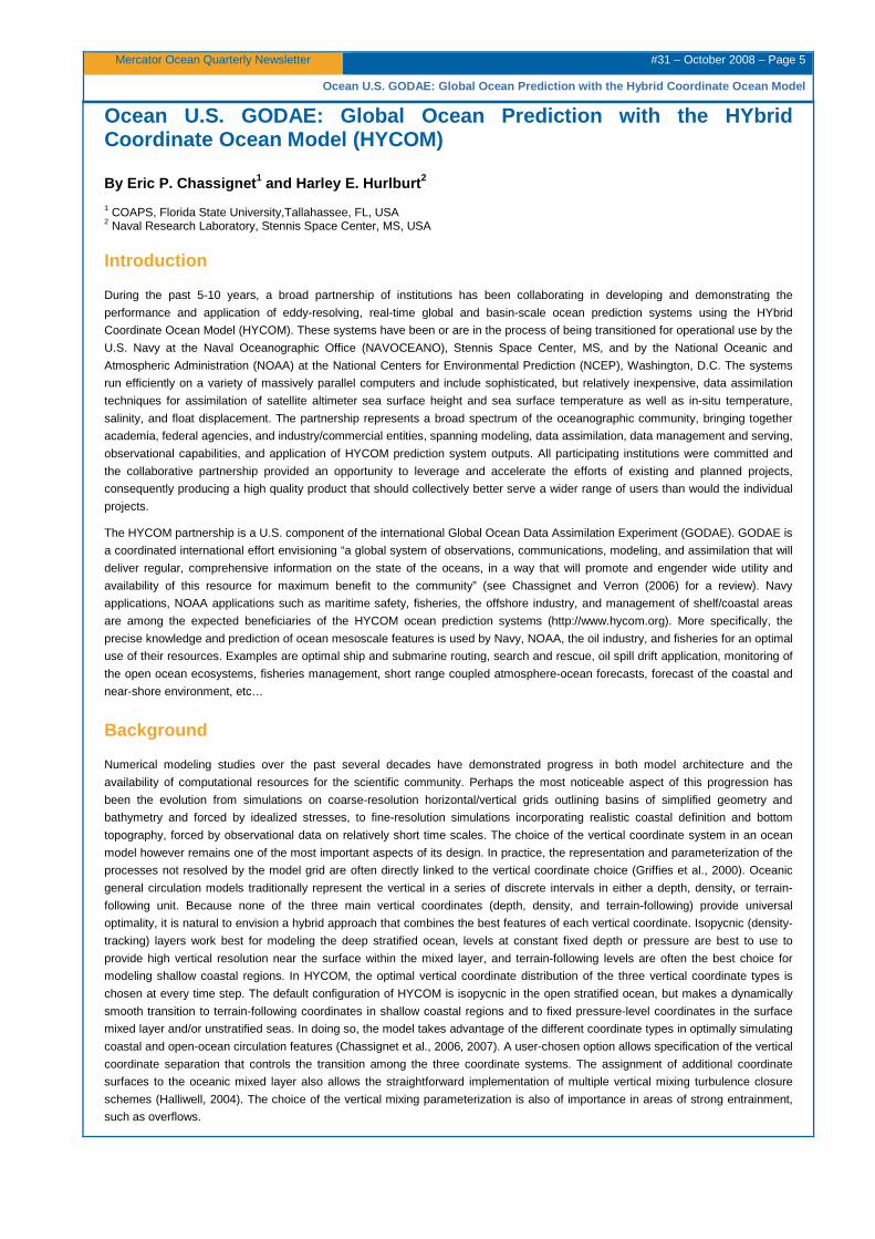
2008). Figure 1 shows the climatological mean derived on a 0.5º grid using surface drifters by Maximenko and Niiler (2005) as well
as the mean currently used in the Navy global HYCOM prediction system (see following section for details). The HYCOM mean was
constructed as follows: a 5-year mean sea surface height field from a non-data assimilative 1/12º global HYCOM run was compared
to available climatologies and a rubber-sheeting technique (Carnes et al., 1996) was used to modify the model mean in two regions,
the Gulf Stream and the Kuroshio, where the western boundary extensions were not well represented and where an accurate frontal
location is crucial for ocean prediction. Rubber-sheeting consists of a suite of computer programs specifically designed to operate
on SSH fields, overlay contours from a reference field, and move masses of water in an elastic way (hence rubber-sheeting).
Mercator Ocean Quarterly Newsletter #31 – October 2008 – Page 7
Ocean U.S. GODAE: Global Ocean Prediction with the Hybrid Coordinate Ocean Model
Figure 1
Mean SSH (in cm) derived from surface drifters (Maximenko and Niiler, 2005) (top panel) and from a non-data assimilative HYCOM
run corrected in the Gulf Stream and Kuroshio regions using a rubber-sheeting technique (bottom panel). The RMS difference
between the two fields is 9.2 cm
The HYCOM Ocean Prediction Systems (Hhttp://www.hycom.orgH) Two systems are in the process of being evaluated for operational use by the U.S. Navy at the Naval Oceanographic Office
(NAVOCEANO), Stennis Space Center, MS, and by the National Oceanic and Atmospheric Administration (NOAA) at the National
Centers for Environmental Prediction (NCEP), Washington, D.C.
The first system is the NOAA Real Time Ocean Forecast System for the Atlantic (RTOFS). The Atlantic domain spans 25°S to 76°N
with a horizontal resolution varying from 4 km near the U.S. coastline to 20 km near the African coast. The system is run daily with
one-day nowcasts and five-day forecasts. Prior to June 2007, only the sea surface temperature was assimilated. In June 2007,
NOAA implemented the 3D-Var data assimilation of i) sea surface temperature and sea surface height (JASON and GFO), ii)
temperature and salinity profile assimilation (ARGO, CTD, moorings, etc.), and iii) GOES data. The model outputs are available at
Hhttp://polar.ncep.noaa.gov/ofs/H.
The second system is the pre-operational global U.S. Navy nowcast/forecast system using the 1/12º global HYCOM (6.5 km grid
spacing on average, 3.5 km grid spacing at North Pole, and 32 vertical hybrid layers), which has been running in near real-time
since December 2006 and in real-time since February 2007. The current ice model is thermodynamic (energy loan), but it will soon
include more physics as it is upgraded to PIPS (based on the Los Alamos CICE ice model). The model is currently running daily on
Mercator Ocean Quarterly Newsletter #31 – October 2008 – Page 8
Ocean U.S. GODAE: Global Ocean Prediction with the Hybrid Coordinate Ocean Model
379 processors on the IBM Power 5+ at the Naval Oceanographic Office using a part of the operational allocation on the machine.
The daily run (U.S. Navy requirement) consists of a 5 day hindcast and a 5 day forecast and takes about ~15 wall clock hours. The
system assimilates sea surface height (Envisat, GFO, and Jason-1), ii) sea surface temperature (all available satellite and in-situ
sources), iii) all available in-situ temperature and salinity profile (ARGO, CTD, moorings, etc.), and iv) SSM/I sea ice concentration.
The three-dimensional multivariate optimum interpolation Navy Coupled Ocean Data Assimilation (NCODA) (Cummings, 2005)
system is the assimilation technique. The NCODA horizontal correlations are multivariate in geopotential and velocity, thereby
permitting adjustments (increments) to the mass fields to be correlated with adjustments to the flow fields. The velocity adjustments
are in geostrophic balance with the geopotential increments, and the geopotential increments are in hydrostatic agreement with the
temperature and salinity increments. Either the Cooper and Haines (1996) technique or synthetic temperature and salinity profiles
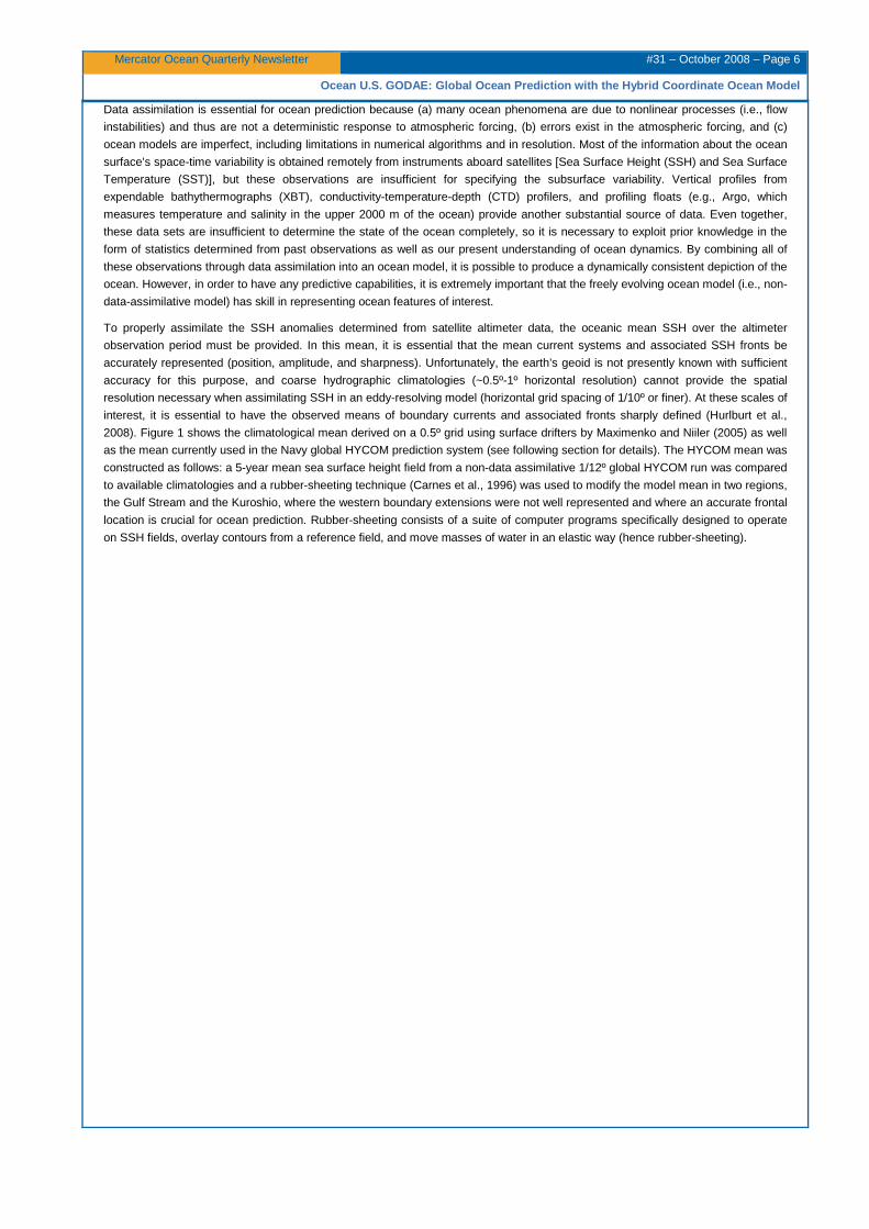
(Fox et al., 2002) can be used for downward projection of SSH and SST. An example of forecast performance is shown in Figure 2.
Figure 2
Verification of 30-day ocean forecasts: median SSH anomaly correlation vs. forecast length in comparison with the verifying analysis
for the global HYCOM over the world ocean and five subregions. The red curves verify forecasts using operational atmospheric
forcing, which reverts toward climatology after five days. The green curves verify “forecasts” with analysis quality forcing for the
duration and the blue curves verify forecasts of persistence (i.e. no change from the initial state). The plots show median statistics
over twenty 30-day HYCOM forecasts initialized during January 2004 - December 2005, a period when data from three nadir-beam
altimeters, Envisat, GFO and Jason-1, were assimilated
The model outputs from the hindcast experiment are available through the HYCOM consortium web page, Hhttp://www.hycom.orgH. A
validation of the results is underway using independent data with a focus on the large scale circulation features, sea surface height
variability, eddy kinetic energy, mixed layer depth, vertical profiles of temperature and salinity, sea surface temperature and coastal
sea levels. Figure 3 and 4 show some examples for the Gulf Stream region while Figure 5 documents the performance of HYCOM
in representing the mixed layer depth. HYCOM is also an active participant in the international GODAE comparison of global ocean
forecasting systems.
Mercator Ocean Quarterly Newsletter #31 – October 2008 – Page 9
Ocean U.S. GODAE: Global Ocean Prediction with the Hybrid Coordinate Ocean Model
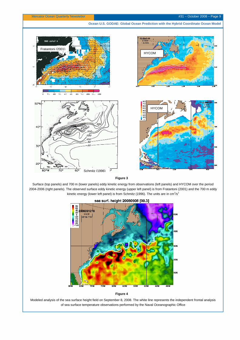
Figure 3
Surface (top panels) and 700 m (lower panels) eddy kinetic energy from observations (left panels) and HYCOM over the period
2004-2006 (right panels). The observed surface eddy kinetic energy (upper left panel) is from Fratantoni (2001) and the 700 m eddy
kinetic energy (lower left panel) is from Schmitz (1996). The units are in cm2/s2
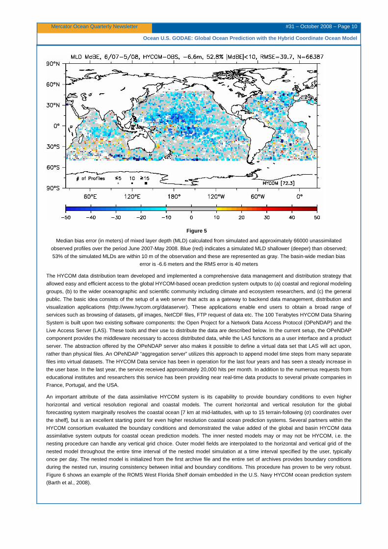
Figure 4
Modeled analysis of the sea surface height field on September 8, 2008. The white line represents the independent frontal analysis
of sea surface temperature observations performed by the Naval Oceanographic Office
HYCOM
HYCOM
Schmitz (1996)
Fratantoni (2001)
Mercator Ocean Quarterly Newsletter #31 – October 2008 – Page 10
Ocean U.S. GODAE: Global Ocean Prediction with the Hybrid Coordinate Ocean Model
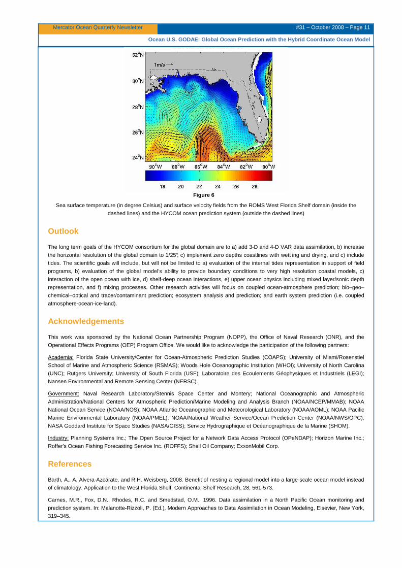
Figure 5
Median bias error (in meters) of mixed layer depth (MLD) calculated from simulated and approximately 66000 unassimilated
observed profiles over the period June 2007-May 2008. Blue (red) indicates a simulated MLD shallower (deeper) than observed;
53% of the simulated MLDs are within 10 m of the observation and these are represented as gray. The basin-wide median bias
error is -6.6 meters and the RMS error is 40 meters
The HYCOM data distribution team developed and implemented a comprehensive data management and distribution strategy that
allowed easy and efficient access to the global HYCOM-based ocean prediction system outputs to (a) coastal and regional modeling
groups, (b) to the wider oceanographic and scientific community including climate and ecosystem researchers, and (c) the general
public. The basic idea consists of the setup of a web server that acts as a gateway to backend data management, distribution and
visualization applications (Hhttp://www.hycom.org/dataserverH). These applications enable end users to obtain a broad range of
services such as browsing of datasets, gif images, NetCDF files, FTP request of data etc. The 100 Terabytes HYCOM Data Sharing
System is built upon two existing software components: the Open Project for a Network Data Access Protocol (OPeNDAP) and the
Live Access Server (LAS). These tools and their use to distribute the data are described below. In the current setup, the OPeNDAP
component provides the middleware necessary to access distributed data, while the LAS functions as a user interface and a product
server. The abstraction offered by the OPeNDAP server also makes it possible to define a virtual data set that LAS will act upon,
rather than physical files. An OPeNDAP “aggregation server” utilizes this approach to append model time steps from many separate
files into virtual datasets. The HYCOM Data service has been in operation for the last four years and has seen a steady increase in
the user base. In the last year, the service received approximately 20,000 hits per month. In addition to the numerous requests from
educational institutes and researchers this service has been providing near real-time data products to several private companies in
France, Portugal, and the USA.
An important attribute of the data assimilative HYCOM system is its capability to provide boundary conditions to even higher
horizontal and vertical resolution regional and coastal models. The current horizontal and vertical resolution for the global
forecasting system marginally resolves the coastal ocean [7 km at mid-latitudes, with up to 15 terrain-following (σ) coordinates over
the shelf], but is an excellent starting point for even higher resolution coastal ocean prediction systems. Several partners within the
HYCOM consortium evaluated the boundary conditions and demonstrated the value added of the global and basin HYCOM data
assimilative system outputs for coastal ocean prediction models. The inner nested models may or may not be HYCOM, i.e. the
nesting procedure can handle any vertical grid choice. Outer model fields are interpolated to the horizontal and vertical grid of the
nested model throughout the entire time interval of the nested model simulation at a time interval specified by the user, typically
once per day. The nested model is initialized from the first archive file and the entire set of archives provides boundary conditions
during the nested run, insuring consistency between initial and boundary conditions. This procedure has proven to be very robust.
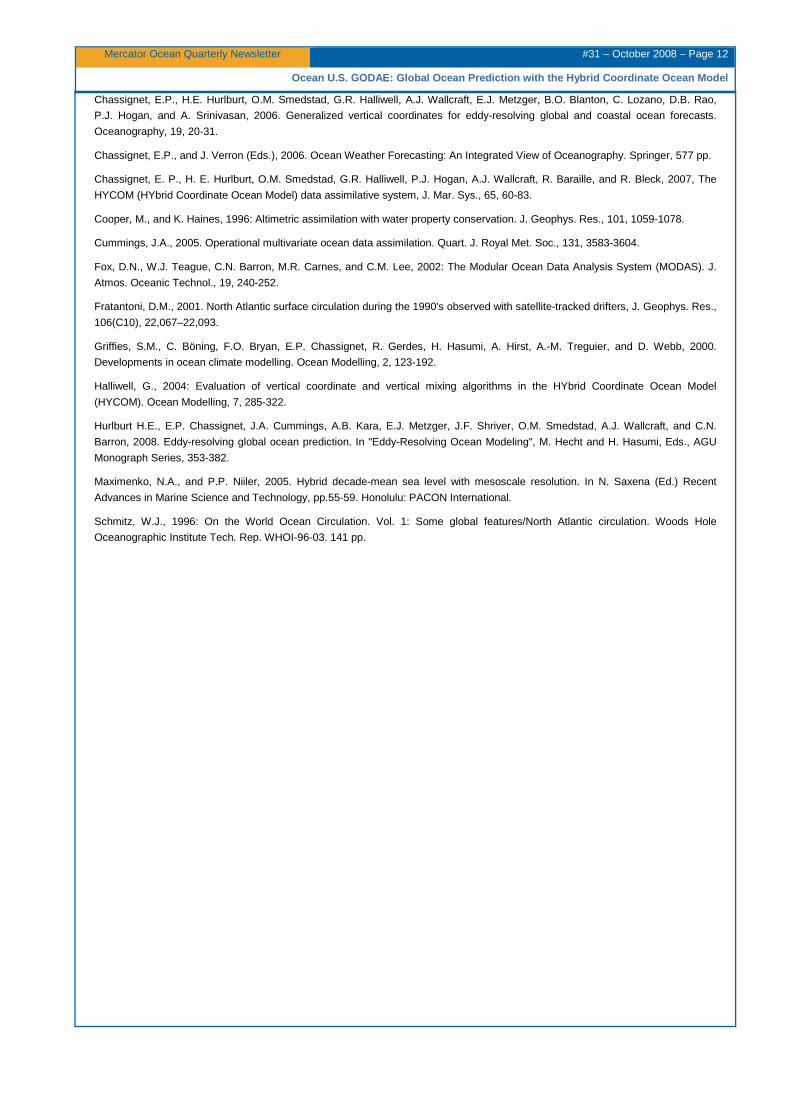
Figure 6 shows an example of the ROMS West Florida Shelf domain embedded in the U.S. Navy HYCOM ocean prediction system
(Barth et al., 2008).
Mercator Ocean Quarterly Newsletter #31 – October 2008 – Page 11
Ocean U.S. GODAE: Global Ocean Prediction with the Hybrid Coordinate Ocean Model
Figure 6
Sea surface temperature (in degree Celsius) and surface velocity fields from the ROMS West Florida Shelf domain (inside the
dashed lines) and the HYCOM ocean prediction system (outside the dashed lines)
Outlook
The long term goals of the HYCOM consortium for the global domain are to a) add 3-D and 4-D VAR data assimilation, b) increase
the horizontal resolution of the global domain to 1/25°, c) implement zero depths coastlines with wett ing and drying, and c) include
tides. The scientific goals will include, but will not be limited to a) evaluation of the internal tides representation in support of field
programs, b) evaluation of the global model’s ability to provide boundary conditions to very high resolution coastal models, c)
interaction of the open ocean with ice, d) shelf-deep ocean interactions, e) upper ocean physics including mixed layer/sonic depth
representation, and f) mixing processes. Other research activities will focus on coupled ocean-atmosphere prediction; bio–geo–
chemical–optical and tracer/contaminant prediction; ecosystem analysis and prediction; and earth system prediction (i.e. coupled
atmosphere-ocean-ice-land).
Acknowledgements
This work was sponsored by the National Ocean Partnership Program (NOPP), the Office of Naval Research (ONR), and the
Operational Effects Programs (OEP) Program Office. We would like to acknowledge the participation of the following partners:
UAcademia:U Florida State University/Center for Ocean-Atmospheric Prediction Studies (COAPS); University of Miami/Rosenstiel
School of Marine and Atmospheric Science (RSMAS); Woods Hole Oceanographic Institution (WHOI); University of North Carolina
(UNC); Rutgers University; University of South Florida (USF); Laboratoire des Ecoulements Géophysiques et Industriels (LEGI);
Nansen Environmental and Remote Sensing Center (NERSC).
UGovernment:U Naval Research Laboratory/Stennis Space Center and Montery; National Oceanographic and Atmospheric
Administration/National Centers for Atmospheric Prediction/Marine Modeling and Analysis Branch (NOAA/NCEP/MMAB); NOAA
National Ocean Service (NOAA/NOS); NOAA Atlantic Oceanographic and Meteorological Laboratory (NOAA/AOML); NOAA Pacific
Marine Environmental Laboratory (NOAA/PMEL); NOAA/National Weather Service/Ocean Prediction Center (NOAA/NWS/OPC);
NASA Goddard Institute for Space Studies (NASA/GISS); Service Hydrographique et Océanographique de la Marine (SHOM).
UIndustry:U Planning Systems Inc.; The Open Source Project for a Network Data Access Protocol (OPeNDAP); Horizon Marine Inc.;
Roffer's Ocean Fishing Forecasting Service Inc. (ROFFS); Shell Oil Company; ExxonMobil Corp.
References
Barth, A., A. Alvera-Azcárate, and R.H. Weisberg, 2008. Benefit of nesting a regional model into a large-scale ocean model instead
of climatology. Application to the West Florida Shelf. Continental Shelf Research, 28, 561-573.
Carnes, M.R., Fox, D.N., Rhodes, R.C. and Smedstad, O.M., 1996. Data assimilation in a North Pacific Ocean monitoring and
prediction system. In: Malanotte-Rizzoli, P. (Ed.), Modern Approaches to Data Assimilation in Ocean Modeling, Elsevier, New York,
319–345.
Mercator Ocean Quarterly Newsletter #31 – October 2008 – Page 12
Ocean U.S. GODAE: Global Ocean Prediction with the Hybrid Coordinate Ocean Model
Chassignet, E.P., H.E. Hurlburt, O.M. Smedstad, G.R. Halliwell, A.J. Wallcraft, E.J. Metzger, B.O. Blanton, C. Lozano, D.B. Rao,
P.J. Hogan, and A. Srinivasan, 2006. Generalized vertical coordinates for eddy-resolving global and coastal ocean forecasts.
Oceanography, 19, 20-31.
Chassignet, E.P., and J. Verron (Eds.), 2006. Ocean Weather Forecasting: An Integrated View of Oceanography. Springer, 577 pp.
Chassignet, E. P., H. E. Hurlburt, O.M. Smedstad, G.R. Halliwell, P.J. Hogan, A.J. Wallcraft, R. Baraille, and R. Bleck, 2007, The
HYCOM (HYbrid Coordinate Ocean Model) data assimilative system, J. Mar. Sys., 65, 60-83.
Cooper, M., and K. Haines, 1996: Altimetric assimilation with water property conservation. J. Geophys. Res., 101, 1059-1078.
Cummings, J.A., 2005. Operational multivariate ocean data assimilation. Quart. J. Royal Met. Soc., 131, 3583-3604.
Fox, D.N., W.J. Teague, C.N. Barron, M.R. Carnes, and C.M. Lee, 2002: The Modular Ocean Data Analysis System (MODAS). J.
Atmos. Oceanic Technol., 19, 240-252.
Fratantoni, D.M., 2001. North Atlantic surface circulation during the 1990's observed with satellite-tracked drifters, J. Geophys. Res.,
106(C10), 22,067–22,093.
Griffies, S.M., C. Böning, F.O. Bryan, E.P. Chassignet, R. Gerdes, H. Hasumi, A. Hirst, A.-M. Treguier, and D. Webb, 2000.
Developments in ocean climate modelling. Ocean Modelling, 2, 123-192.
Halliwell, G., 2004: Evaluation of vertical coordinate and vertical mixing algorithms in the HYbrid Coordinate Ocean Model
(HYCOM). Ocean Modelling, 7, 285-322.
Hurlburt H.E., E.P. Chassignet, J.A. Cummings, A.B. Kara, E.J. Metzger, J.F. Shriver, O.M. Smedstad, A.J. Wallcraft, and C.N.
Barron, 2008. Eddy-resolving global ocean prediction. In "Eddy-Resolving Ocean Modeling", M. Hecht and H. Hasumi, Eds., AGU
Monograph Series, 353-382.
Maximenko, N.A., and P.P. Niiler, 2005. Hybrid decade-mean sea level with mesoscale resolution. In N. Saxena (Ed.) Recent
Advances in Marine Science and Technology, pp.55-59. Honolulu: PACON International.
Schmitz, W.J., 1996: On the World Ocean Circulation. Vol. 1: Some global features/North Atlantic circulation. Woods Hole
Oceanographic Institute Tech. Rep. WHOI-96-03. 141 pp.
Mercator Ocean Quarterly Newsletter #31 – October 2008 – Page 13
ECCO2: High Resolution Global Ocean and Sea Ice Dat a Synthesis
ECCO2: High Resolution Global Ocean and Sea Ice Dat a Synthesis By Dimitris Menemenlis 1, Jean-Michel Campin 2, Patrick Heimbach 2, Chris Hill 2, Tong Lee 1, An
Nguyen 1, Michael Schodlok 1, and Hong Zhang 1
1 Jet Propulsion Laboratory, California Institute of Technology, Pasadena, USA 2 Massachusetts Institute of Technology, Cambridge, USA
Abstract
The Estimating the Circulation and Climate of the Ocean (ECCO) project was established in 1998 as part of the World Ocean
Circulation Experiment (WOCE) with the goal of combining a general circulation model (GCM) with diverse observations in order
to produce a quantitative depiction of the time-evolving global ocean state. Such combinations, also known as data assimilation,
are important because available remotely sensed and in-situ observations are sparse and incomplete compared to the scales
and properties of ocean circulation. These combinations also provide rigorous consistency tests for models and for data. In
contrast to numerical weather prediction that also combines models and data, ECCO estimates are physically consistent; in
particular, ECCO estimates do not contain discontinuities when and where data are ingested. First generation ECCO solutions
are available and widely used for numerous science applications but the coarse horizontal grid spacing and the lack of Arctic
Ocean and of sea ice of these first-generation solutions limits their ability to describe the real ocean. To address these
shortcomings, the follow-on ECCO, Phase II (ECCO2) project aims to produce a best-possible, global, time-evolving synthesis
of most available ocean and sea-ice data at a resolution that admits ocean eddies. A first ECCO2 synthesis for the period 1992–
2007 has been obtained using a Green's Function approach (Menemenlis, et al., 2005a) to estimate initial temperature and
salinity conditions, surface boundary conditions, and several empirical ocean and sea ice model parameters. Data constraints
include altimetry, gravity, drifter, hydrography, and observations of sea-ice. A large complement of high-frequency and high-
resolution diagnostics has been saved; these diagnostics are made available to the scientific community via ftp and OPeNDAP
servers at Hhttp://ecco2.orgH. This note provides a brief overview of this first ECCO2 synthesis and of some early science
applications.
Introduction
Physically consistent estimates of ocean circulation constrained by in situ and remotely sensed observations, as produced by
the ECCO project, have now become routinely available and are being applied to myriad scientific applications (Wunsch and
Heimbach, 2007). The coarse horizontal grid spacing of current-generation ECCO solutions, however, is a severe limitation on
their ability to describe the real ocean, for example, mesoscale eddies, flow over narrow sills, boundary currents, and regions of
deep convection and of restratification. Despite the very great progress made toward parameterizing sub-grid scale processes,
some problems remain intractable through this route. First, eddy parameterizations are not based upon completely fundamental
principles and they fail to adequately account for known anisotropies in their fluxes. Everything we know about eddies suggests
that their property fluxes can accumulate in the ocean, changing it measurably and importantly from what it would be if eddies
were absent. That is, the long-wavelength, low-frequency features characterizing climate are controlled in part by eddy fluxes.
Second, studies have shown that horizontal grid-spacing of order 2 km is required to resolve restratification processes, in which
stratified fluid in the periphery of the convection patch is drawn over the surface, allowing the convected fluid to be `swallowed'
by the ocean. If restratification is not represented adequately, then the water-mass properties of the modeled ocean deteriorate
over time, there are model drifts, and the attendant air-sea fluxes become compromised and have to be `corrected'.
Restratification of mixed layers is a ubiquitous feature of the ocean but is particularly important in strong frontal regions and in
regions of deep-water formation. Third, scalar property transports (heat, fresh water, carbon, oxygen, etc.) are of central interest
for climate studies and in the ocean, narrow western and eastern boundary currents make major contributions; these boundary
currents are not parameterizable and, until they are resolved, there will always be doubts that the ocean model is carrying their
property transports realistically. Ultimately, water mass properties in the ocean are important to climate and climate change. In
the abyssal ocean, the inability to resolve major topographic features, e.g., fracture zones and sills, leads to systematic errors in
the movement of deep-water masses with consequences, for example, on the accuracy of computation of carbon uptake.
Another limitation of current-generation ECCO solutions is that they exclude the Arctic Ocean and that they lack an interactive
sea-ice model. This restricts the use of satellite data over ice-covered regions and the usefulness of current-generation
solutions for describing and studying high-latitude processes. Coupled ocean and sea ice state estimation is an integral
component of the ECCO2 project. The inclusion of an interactive sea-ice model provides for more realistic surface boundary
conditions in Polar Regions and allows the model to be constrained by satellite observations over ice-covered oceans. The sea-
ice model also provides the ability to estimate the time-evolving sea-ice thickness distribution and to quantify the role of sea-ice
in the global ocean circulation. Improved representation of high-latitude processes will enhance hindcasting and forecasting
Mercator Ocean Quarterly Newsletter #31 – October 2008 – Page 14
ECCO2: High Resolution Global Ocean and Sea Ice Dat a Synthesis
capability, both of which are needed for climate-change studies, for the design of in-situ measurement campaigns, and for
operational purposes, e.g., navigation, drilling activity, wildlife behavior, and dispersion of pollutants. Improved representation of
high-latitude processes is also a crucial requirement for reducing uncertainty in predictions of the climate response to prescribed
increases in greenhouse gases and in predictions of how the oceanic sink for greenhouse gases might change in the future in
response to a changing climate.
Model description
ECCO2 data syntheses are obtained by least squares fit of a global full-depth-ocean and sea-ice configuration of the
Massachusetts Institute of Technology general circulation model (MITgcm; Marshall et al., 1997) to the available satellite and in-
situ data. The computational demands of rigorous ocean state estimation, aka data assimilation, are enormous. Depending on
the method and on the approximations that are used, the computational cost of state estimation is several dozen to several
thousand times more expensive than integrating a model without state estimation. This has limited the resolution of first-
generation ECCO solutions to horizontal grid spacing of order 1 degree (except at the Equator where meridional grid spacing is
1/3-degree in one of the solutions). First-generation solutions also exclude the Arctic Ocean and lack an interactive sea-ice
model, which restricts the utilization of satellite data over Polar Regions. Therefore, a necessary condition for a next generation
synthesis is an efficient truly global model and significant computational resources.
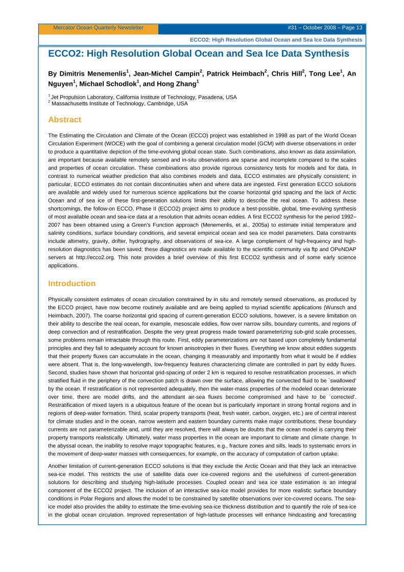
Figure 1
Cubed-sphere ocean model configuration. The figure shows simulated near-surface (15-m) ocean-current speed and sea-ice
cover from an unconstrained eddy-permitting integration. Color scale ranges from 0 to 0.5 m/s. Simulated sea-ice is shown as
an opaque, white cover. The thin blue line is passive radiometer observations of sea-ice extent (15% concentration).
Landmasses and ice shelves are overlain with NASA satellite imagery
A first, global ECCO2 solution was obtained on the MITgcm model configuration, which is described in Menemenlis et al.
(2005b) and depicted on Figure 1. A cube-sphere grid projection is employed, which permits relatively even grid spacing
throughout the domain and which avoids polar singularities (Adcroft et al., 2004). Each face of the cube comprises 510 by 510
grid cells for a mean horizontal grid spacing of 18 km; this is inadequate for fully resolving the processes discussed in the
introduction but it is the best that can be achieved at the moment with available computational resources. The model has 50
vertical levels ranging in thickness from 10 m near the surface to approximately 450 m at a maximum model depth of 6150 m.
Bathymetry is from the S2004 (W. Smith, unpublished) blend of Smith and Sandwell (1997) and of General Bathymetric Charts
of the Oceans (GEBCO) one arc-minute bathymetric grid. The partial-cell formulation of Adcroft et al. (1997), which permits
accurate representation of the bathymetry, is used. The model is integrated in a volume-conserving configuration using a finite
volume discretization with C-grid staggering of the prognostic variables. The ocean model is coupled to a sea-ice model that
computes ice thickness, ice concentration, and snow cover as per Zhang et al. (1998) and that simulates a viscous-plastic
Mercator Ocean Quarterly Newsletter #31 – October 2008 – Page 15
ECCO2: High Resolution Global Ocean and Sea Ice Dat a Synthesis
rheology using an efficient parallel implementation of the Zhang and Hibler (1997) solver. Inclusion of sea-ice provides for more
realistic surface boundary conditions in Polar Regions and allows the system to be constrained by polar satellite observations.
The sea-ice model also permits estimation of the time-evolving sea-ice thickness distribution.
Estimation approaches
The first high-resolution global-ocean and sea-ice data synthesis was obtained for the period 1992-2007 by calibrating a small
number of control variables using a Green’s function approach (Menemenlis, et al., 2005a). The control parameters include
initial temperature and salinity conditions, atmospheric surface boundary conditions, background vertical diffusivity, critical
Richardson numbers for the Large et al. (1994) KPP scheme, air-ocean, ice-ocean, air-ice drag coefficients, ice/ocean/snow
albedo coefficients, bottom drag, and vertical viscosity. Data constraints include sea level anomaly from altimeter data, time-
mean sea level from Maximenko and Niiler (2005), sea surface temperature from GHRSST-PP, temperature and salinity profiles
from WOCE, TAO, ARGO, XBT, etc., sea ice concentration from passive microwave data, sea ice motion from radiometers,
QuikSCAT, and RGPS, and sea ice thickness from ULS.
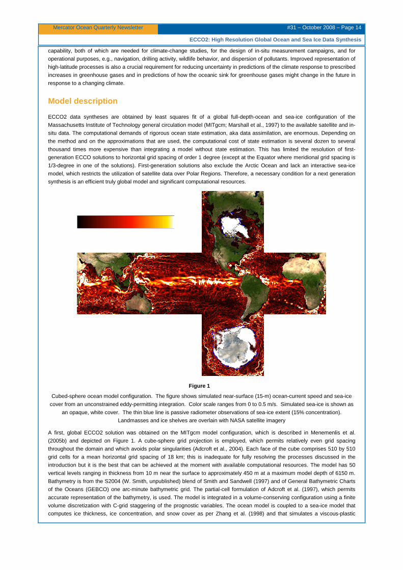
Figure 2
Sensitivity maps of sea-ice export through Fram Strait during December 1995 to changes in ice thickness at any point in the
domain 1, 2, 3, and 4 years prior. The dominant pattern reflects the advective pathways of sea-ice through the Arctic
(Heimbach, 2008)
Mercator Ocean Quarterly Newsletter #31 – October 2008 – Page 16
ECCO2: High Resolution Global Ocean and Sea Ice Dat a Synthesis
In parallel with the Green’s function optimization, work is underway towards adjoint-method optimization on the same grid. One
objective of the MITgcm ocean and sea-ice model development effort has been to provide the capability for automatic
generation of the adjoint model from up-to-date versions of the MITgcm, which is invaluable for ocean state estimation. A major
milestone was reached recently with the completion of an adjoint of the full-fledged dynamic/thermodynamic MITgcm sea-ice
component. The coupled ocean/sea-ice adjoint now yields stable and physically meaningful adjoint sensitivities or Lagrange
multipliers. By way of example, Figure 2 depicts sensitivity maps of sea-ice export through Fram Strait during December 1995 to
changes in ice thickness at any point in the domain 1, 2, 3, and 4 years prior (Heimbach, 2008). The dominant pattern reflects
the advective pathways of sea-ice through the Arctic. In general terms, points furthest away from Fram Strait are connected to
Fram Strait export by faster advective time scales. Time-varying Lagrange multipliers for many other variables, including sea-ice
(concentration, thickness, salinity, and velocity), snow (thickness and velocity), ocean (temperature, salinity, and velocity),
atmospheric forcing (surface air temperature, specific humidity, precipitation, and wind velocity), and internal model parameters
(vertical diffusivity, and bottom drag) are available, and are being analyzed to understand main causes of sea-ice variability.
Mazloff (2008) demonstrated the feasibility of high-resolution adjoint-based state estimation on a regional scale. At this point a
preliminary solution (based on 22 iterations) of a 1/6-degree Southern Ocean State Estimate (SOSE) covering the years 2005
and 2006 is available and is being analyzed both in-house and by other research groups. Almost all of the data employed in the
first-generation ECCO efforts have been utilized with major emphasis on the satellite altimetry, the Argo profiles, and satellite
Sea Surface Temperature (SST). Given the success of this regional, eddy resolving, adjoint-based state estimation effort and of
the sea-ice sensitivity experiments, we are currently attempting an adjoint-method optimization on the global, cubed-sphere
ocean and sea ice model configuration as a way to increase the number of control variables relative to the existing Green’s
function optimization.
In related work, the ECCO2 project is contributing to the development of an open-source Automatic Differentiation (AD) tool
called OpenAD. Much effort over the last year has gone into generating efficient adjoint code for the MITgcm that can be applied
for large-scale applications. After demonstrating that OpenAD can handle a simplified configuration of the MITgcm we are now
in a position to adjoint a global coarse-resolution MITgcm configuration (including the GM/Redi eddy parameterization scheme),
which has been a workhorse setup for various adjoint sensitivity studies. It is noteworthy to report that the availability of an
adjoint model based on a different AD tool has enabled us to trace a bug in the current "production" AD tool TAF. This is just
one aspect of the advantages of having an independent AD tool at our disposal. A major breakthrough is the implementation of
a hierarchical checkpointing algorithm, without which adjoint integrations would have been limited to a few days. Using OpenAD,
we have conducted a 100-year adjoint integration to compute transient sensitivities of Atlantic meridional heat transport.
A first ECCO2 synthesis
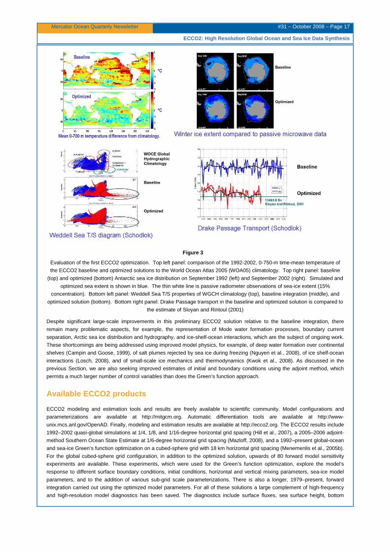
The specific objective of the first ECCO2 optimization was to reduce large-scale biases and drifts of the model relative to
observations. Figure 3 displays some of the large-scale biases that were present in the baseline integration and the equivalent
fields from the optimized solution, demonstrating significant improvements of the optimized solution relative to the baseline
integration. Specifically, the top left panel compares the 1992-2002, 0-750-m time-mean temperature of the ECCO2 baseline
and optimized solutions to the World Ocean Atlas 2005 (WOA05) climatology. The baseline simulation exhibits a global warm
bias of up to 3° C, which is not present in the opt imized solution. The top right panel shows baseline (top) and optimized
(bottom) Antarctic sea ice distribution on September 1992 (left) and September 2002 (right). Simulated sea is shown in blue.
The thin white line is passive radiometer observations of sea-ice extent (15% concentration). The problematic open-water winter
polynyas in the Ross and Weddell Seas, which appear in the baseline integration, are no longer present in the optimized
solution. The bottom left panel shows Weddell Sea T/S properties of the WGCH climatology (top), of the baseline integration
(middle), and of the optimized solution (bottom). The optimized Weddell Sea T/S properties are considerably closer to the
observations compared to the baseline integration. The bottom right panel shows Drake Passage transport in the baseline and
optimized solutions, which can be compared to the estimate of Sloyan and Rintoul (2001). The Drake Passage transport in the
baseline integration is 35 Sv too strong compared to the Sloyan and Rintoul (2001) estimate while that of the optimized solution
is much more realistic due, in part, to a much-improved Southern Ocean hydrography.
Mercator Ocean Quarterly Newsletter #31 – October 2008 – Page 17
ECCO2: High Resolution Global Ocean and Sea Ice Dat a Synthesis
Figure 3
Evaluation of the first ECCO2 optimization. Top left panel: comparison of the 1992-2002, 0-750-m time-mean temperature of
the ECCO2 baseline and optimized solutions to the World Ocean Atlas 2005 (WOA05) climatology. Top right panel: baseline
(top) and optimized (bottom) Antarctic sea ice distribution on September 1992 (left) and September 2002 (right). Simulated and
optimized sea extent is shown in blue. The thin white line is passive radiometer observations of sea-ice extent (15%
concentration). Bottom left panel: Weddell Sea T/S properties of WGCH climatology (top), baseline integration (middle), and
optimized solution (bottom). Bottom right panel: Drake Passage transport in the baseline and optimized solution is compared to
the estimate of Sloyan and Rintoul (2001)
Despite significant large-scale improvements in this preliminary ECCO2 solution relative to the baseline integration, there
remain many problematic aspects, for example, the representation of Mode water formation processes, boundary current
separation, Arctic sea ice distribution and hydrography, and ice-shelf-ocean interactions, which are the subject of ongoing work.
These shortcomings are being addressed using improved model physics, for example, of deep water formation over continental
shelves (Campin and Goose, 1999), of salt plumes rejected by sea ice during freezing (Nguyen et al., 2008), of ice shelf-ocean
interactions (Losch, 2008), and of small-scale ice mechanics and thermodynamics (Kwok et al., 2008). As discussed in the
previous Section, we are also seeking improved estimates of initial and boundary conditions using the adjoint method, which
permits a much larger number of control variables than does the Green’s function approach.
Available ECCO2 products
ECCO2 modeling and estimation tools and results are freely available to scientific community. Model configurations and
parameterizations are available at Hhttp://mitgcm.orgH. Automatic differentiation tools are available at Hhttp://www-
unix.mcs.anl.gov/OpenADH. Finally, modeling and estimation results are available at Hhttp://ecco2.orgH. The ECCO2 results include
1992–2002 quasi-global simulations at 1/4, 1/8, and 1/16-degree horizontal grid spacing (Hill et al., 2007), a 2005–2006 adjoint-
method Southern Ocean State Estimate at 1/6-degree horizontal grid spacing (Mazloff, 2008), and a 1992–present global-ocean
and sea-ice Green’s function optimization on a cubed-sphere grid with 18 km horizontal grid spacing (Menemenlis et al., 2005b).
For the global cubed-sphere grid configuration, in addition to the optimized solution, upwards of 80 forward model sensitivity
experiments are available. These experiments, which were used for the Green’s function optimization, explore the model’s
response to different surface boundary conditions, initial conditions, horizontal and vertical mixing parameters, sea-ice model
parameters, and to the addition of various sub-grid scale parameterizations. There is also a longer, 1979–present, forward
integration carried out using the optimized model parameters. For all of these solutions a large complement of high-frequency
and high-resolution model diagnostics has been saved. The diagnostics include surface fluxes, sea surface height, bottom
Mercator Ocean Quarterly Newsletter #31 – October 2008 – Page 18
ECCO2: High Resolution Global Ocean and Sea Ice Dat a Synthesis
pressure, mixed and mixing layer depths, sea-ice thickness, concentration, salinity, ocean temperature, density, velocity and
eddy transports of mass, temperature, and salt. A large portion of these diagnostics (~100 TB) is readily available online via ftp,
http, and OPeNDAP servers. The complete diagnostics are stored on tapes at the NASA Advanced Supercomputing (NAS) and
are made available upon request.
Early science applications
This section lists some early science applications of the ECCO2 products. A first set of applications concerns improved error
estimates and eddy parameterizations for coarser-resolution ocean simulations and estimations. Forget and Wunsch (2007)
used hydrographic data and an early ECCO2 simulation to estimate global hydrographic variability and data weights in oceanic
state estimates. Ponte et al. (2007) used altimeter data and an early ECCO2 simulation for spatial mapping of time-variable
errors in Jason-1 and TOPEX/POSEIDON sea surface height measurements. ECCO2 high-resolution simulations have also
been used to inform the model parameterization of sub-grid scale processes (Fox-Kemper and Menemenlis, 2008; Danabasoglu
et al., 2008).
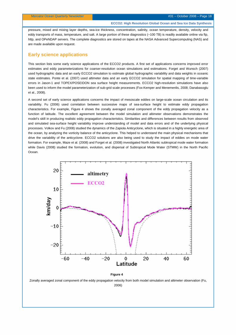
A second set of early science applications concerns the impact of mesoscale eddies on large-scale ocean circulation and its
variability. Fu (2006) used correlation between successive maps of sea-surface height to estimate eddy propagation
characteristics. For example, Figure 4 shows the zonally averaged zonal component of the eddy propagation velocity as a
function of latitude. The excellent agreement between the model simulation and altimeter observations demonstrates the
model’s skill in producing realistic eddy propagation characteristics. Similarities and differences between results from observed
and simulated sea-surface height variability improve understanding of model and data errors and of the underlying physical
processes. Volkov and Fu (2008) studied the dynamics of the Zapiola Anticyclone, which is situated in a highly energetic area of
the ocean, by analyzing the vorticity balance of the anticyclone. This helped to understand the main physical mechanisms that
drive the variability of the anticyclone. ECCO2 solutions are also being used to study the impact of eddies on mode water
formation. For example, Maze et al. (2008) and Forget et al. (2008) investigated North Atlantic subtropical mode water formation
while Davis (2008) studied the formation, evolution, and dispersal of Subtropical Mode Water (STMW) in the North Pacific
Ocean.
Figure 4
Zonally averaged zonal component of the eddy propagation velocity from both model simulation and altimeter observation (Fu,
2006)
Mercator Ocean Quarterly Newsletter #31 – October 2008 – Page 19
ECCO2: High Resolution Global Ocean and Sea Ice Dat a Synthesis
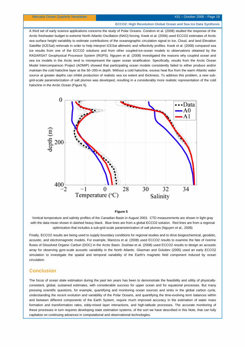
A third set of early science applications concerns the study of Polar Oceans. Condron et al. (2008) studied the response of the
Arctic freshwater budget to extreme North Atlantic Oscillation (NAO) forcing. Kwok et al. (2006) used ECCO2 estimates of Arctic
sea surface height variability to estimate contributions of the oceanographic circulation signal to Ice, Cloud, and land Elevation
Satellite (ICESat) retrievals in order to help interpret ICESat altimetric and reflectivity profiles. Kwok et al. (2008) compared sea
ice results from one of the ECCO2 solutions and from other coupled-ice-ocean models to observations obtained by the
RADARSAT Geophysical Processor System (RGPS). Nguyen et al. (2008) investigated the reasons why coupled ocean and
sea ice models in the Arctic tend to misrepresent the upper ocean stratification. Specifically, results from the Arctic Ocean
Model Intercomparison Project (AOMIP) showed that participating ocean models consistently failed to either produce and/or
maintain the cold halocline layer at the 50–200-m depth. Without a cold halocline, excess heat flux from the warm Atlantic water
source at greater depths can inhibit production of realistic sea ice extent and thickness. To address this problem, a new sub-
grid-scale parameterization of salt plumes was developed, resulting in a considerably more realistic representation of the cold
halocline in the Arctic Ocean (Figure 5).
Figure 5
Vertical temperature and salinity profiles of the Canadian Basin in August 2003. CTD measurements are shown in light gray
with the data mean shown in dashed heavy black. Blue lines are from a global ECCO2 solution. Red lines are from a regional
optimization that includes a sub-grid-scale parameterization of salt plumes (Nguyen et al., 2008)
Finally, ECCO2 results are being used to supply boundary conditions for regional studies and to drive biogeochemical, geodetic,
acoustic, and electromagnetic models. For example, Manizza et al. (2008) used ECCO2 results to examine the fate of riverine
fluxes of Dissolved Organic Carbon (DOC) in the Arctic Basin. Dushaw et al. (2008) used ECCO2 results to design an acoustic
array for observing gyre-scale acoustic variability in the North Atlantic. Glazman and Golubev (2005) used an early ECCO2
simulation to investigate the spatial and temporal variability of the Earth's magnetic field component induced by ocean
circulation.
Conclusion
The focus of ocean state estimation during the past ten years has been to demonstrate the feasibility and utility of physically-
consistent, global, sustained estimates, with considerable success for upper ocean and for equatorial processes. But many
pressing scientific questions, for example, quantifying and monitoring ocean sources and sinks in the global carbon cycle,
understanding the recent evolution and variability of the Polar Oceans, and quantifying the time-evolving term balances within
and between different components of the Earth System, require much improved accuracy in the estimation of water mass
formation and transformation rates, eddy-mixed layer interactions, and high-latitude processes. The accurate monitoring of
these processes in turn requires developing state estimation systems, of the sort we have described in this Note, that can fully
capitalize on continuing advances in computational and observational technologies.
Mercator Ocean Quarterly Newsletter #31 – October 2008 – Page 20
ECCO2: High Resolution Global Ocean and Sea Ice Dat a Synthesis
Acknowledgements
ECCO2 is a contribution to the NASA Modeling, Analysis, and Prediction (MAP) program. We gratefully acknowledge
computational resources and support from the NASA Advanced Supercomputing (NAS) Division and from the Jet Propulsion
Laboratory (JPL) Supercomputing and Visualization Facility (SVF).
References
Adcroft, A., C. Hill, and J. Marshall, 1997: Representation of topography by shaved cells in a height coordinate ocean model.
Mon. Weather Rev., 125, 2293–2315.
Adcroft, A., J. Campin, C. Hill and J. Marshall, 2004: Implementation of an atmosphere-ocean general circulation model on the
expanded spherical cube. Mon. Wea. Rev., 132, 2845–2863.
Campin, J.-M., and H. Goosse, 1999: A parameterization of density downsloping flow for a coarse resolution ocean model in z-
coordinate. Tellus, 51A, 412–430.
Condron, A., P. Winsor, C. Hill and D. Menemenlis, 2008: Response of the Arctic freshwater budget to extreme NAO forcing. J.
Climate, submitted.
Danabasoglu, G., R. Ferrari, and J. McWilliams, 2008: Sensitivity of an ocean general circulation model to a parameterization of
near-surface eddy fluxes. J. Climate, 21, 1192–1208.
Davis, X., 2008: Numerical and theoretical investigations of North Pacific Subtropical Mode Water with implications to Pacific
climate variability. Ph.D. thesis, University of Rhode Island, Kingston, RI.
Dushaw, B., P. Worcester, R. Andrew, B. Howe, J. Mercer, R. Spindel, B. Cornuelle, M. Dzieciuch, W. Munk, T. Birdsall, K.
Metzger, D. Menemenlis, and C. Wunsch, 2008: A decade of acoustic thermometry in the North Pacific Ocean: using long-range
acoustic travel times to test gyre-scale temperature variability derived from other observations and ocean models. J. Geophys.
Res., submitted.
Forget, G. and C. Wunsch, 2007: Global hydrographic variability and the data weights in oceanic state estimates. J. Phys.
Oceanogr., 37, 1997–2008.
Forget, G., Maze, G., Buckley, M and Marshall, J. (2008): Quantitative and dynamical analysis of EDW formation using a model-
data synthesis. J. Phys. Oceanogr., submitted.
Fox-Kemper, B., and D. Menemenlis, 2008: Can Large Eddy Simulation Techniques Improve Mesoscale Rich Ocean Models?
Ocean Modeling in an Eddying Regime, ed. Matthew Hecht & Hiroyasu Hasumi, American Geophysical Union, 319–338.
Fu, L.-L., 2006: Pathways of eddies in the South Atlantic revealed from satellite altimeter observations, Geophysical Research
Letters, 33, L14610.
Glazman, R. and Y. Golubev, 2005: Variability of the ocean-induced magnetic field predicted at sea surface and at satellite
altitudes. J. Geophys. Res., 110, C12011.
Heimbach, P., 2008: The MITgcm/ECCO adjoint modeling infrastructure. CLIVAR Exchanges, 44, 13-17.
Hill, C., D. Menemenlis, B. Ciotti, and C. Henze, 2007: Investigating solution convergence in a global ocean model using a
2048-processor cluster of distributed shared memory machines. Scientific Programming, 12, 107–115.
Kwok, R., G. Cunningham, H. Zwally, and D. Yi, 2006. ICESat over Arctic sea ice: Interpretation of altimetric and reflectivity
profiles. J. Geophys. Res., 111, C06006.
Kwok, R., E. Hunke, W. Maslowski, D. Menemenlis, and J. Zhang, 2008: Variability of
sea ice simulations assessed with RGPS kinematics. J. Geophys. Res., in press.
Large, W., J. McWilliams, and S. Doney, 1994: Oceanic vertical mixing: a review and a model with a nonlocal boundary layer
parameterization. Rev. Geophysics, 32, 363–403.
Losch, M., 2008: Modeling ice shelf cavities in a z coordinate ocean general circulation model. J. Geophys. Res., 113, C08043.
Manizza, M., M. Follows, S. Dutkiewicz, J. McClelland, D. Menemenlis, C. Hill, and J. Peterson, 2008: Modeling transport, fate,
and lifetime of riverine DOC in the Arctic Ocean, Global Biogeochem. Cycles, submitted.
Marshall, J., A. Adcroft, C. Hill, L. Perelman, and C. Heisey, 1997: A finite volume, incompressible Navier-Stokes model for
studies of the ocean on parallel computers. J. Geophys. Res., 102, 5753–5766.
Mercator Ocean Quarterly Newsletter #31 – October 2008 – Page 21
ECCO2: High Resolution Global Ocean and Sea Ice Dat a Synthesis
Maximenko, N., and P. Niiler, 2005: Hybrid decade-mean global sea level with mesoscale resolution. In Recent Advances in
Marine Science and Technology, Saxena, N., Ed., PACON International, Honolulu, 55–59.
Maze, G., G. Forget, M. Buckley and J. Marshall, 2008: Using transformation and formation maps to study water mass
transformation: a case study of North Atlantic Eighteen Degree Water. J. Phys. Oceanogr., submitted.
Mazloff, M., 2008: The Southern Ocean meridional overturning circulation as diagnosed from an eddy permitting state estimate.
Ph.D. thesis, Massachusetts Institute of Technology and the Woods Hole Oceanographic Institution, Cambridge, MA.
Menemenlis, D., I. Fukumori, and T. Lee, 2005a: Using Green's functions to calibrate an ocean general circulation model. Mon.
Weather Rev., 133, 1224–1240.
Menemenlis, D., C. Hill, A. Adcroft, J. Campin, B. Cheng, B. Ciotti, I. Fukumori, A. Koehl, P. Heimbach, C. Henze, T. Lee, D.
Stammer, J. Taft, and J. Zhang, 2005b: NASA supercomputer improves prospects for ocean climate research. Eos, 86, 89–96.
Nguyen, A., D. Menemenlis, and R. Kwok, 2008: Improved modeling of the Arctic halocline with a sub-grid-scale brine rejection
parameterization. J. Geophys. Res., submitted.
Ponte, R. M., C. Wunsch, and D. Stammer, 2007: Spatial mapping of time-variable errors in Jason-1 and TOPEX/POSEIDON
sea surface height measurements. J. Atmos. Ocean. Technol., 24, 1078–1085.
Sloyan, B., and S. Rintoul, 2001: Circulation, renewal, and modification of Antarctic Mode and Intermediate Water, J. Phys.
Oceanogr., 31, 1005–1030.
Smith, W., and D. Sandwell, 1997: Global sea floor topography from satellite altimetry and ship depth soundings. Science, 277,
1956–1962.
Volkov, D. and L.-L. Fu, 2008: The role of vorticity fluxes in the dynamics of the Zapiola Anticyclone. Geophys. Res. Lett.,
submitted.
Wunsch, C., and P. Heimbach, 2007: Practical global ocean state estimation. Physica D, 230, 197–208.
Zhang, J., and W. Hibler, 1997: On an efficient numerical method for modeling sea ice dynamics. J. Geophys. Res., 102, 8691–
8702.
Zhang, J., W. Hibler, M. Steele, and D. Rothrock, 1998: Arctic ice-ocean modeling with and without climate restoring. J. Phys.
Oceanogr., 28, 191–217.
Mercator Ocean Quarterly Newsletter #31– October 2008 – Page 22
Simulation of Meso-Scale Eddies in the Mercator Glo bal Ocean High Resolution Model
Simulation of Meso-Scale Eddies in the Mercator Glo bal Ocean High Resolution Model By Olivier Le Galloudec 1, Romain Bourdallé Badie 2, Yann Drillet 1, Corinne Derval 2 and Clément
Bricaud 1
1 Mercator Ocean, 8-10 rue Hermes, Parc technologique du canal, 31520 Ramonville st Agne 2 CERFACS, 42 avenue Gustave Coriolis, 31057 Toulouse cedex 01
Abstract
The simulation of ocean eddies in the global high resolution ORCA12 model is compared to altimetric observations. At the
global scale, the eddy kinetic energy (EKE) of the eddy resolving global ocean model is close to the eddy kinetic energy
computed from the geostrophic velocity deduced from altimetric maps. Even if the model is generally overestimating the EKE,
the main patterns corresponding to main meso-scale activity areas are well reproduced in term of intensity and geographical
position. We have chosen to study particularly six regions relevant of the World Ocean : the Leeuwing Current and the
Mozambique Channel for the Indian Ocean, the Alaska current and the Kuroshio for the Pacific Ocean and the Sargasso Sea
and the Aghulas Current for Atlantic Ocean. In all these regions, the number of eddy simulated by the model is in good
agreement with satellite data. The other result is the high significant correlation between the temporal evolution of the number of
cyclonic (and anticyclonic) eddies for the model and observations. The higher correlations (0.8, and more) are found in the
Leeuwing Current for cyclonic eddies, in the Kuroshio and in the Sargasso Sea for the both kind of eddies.
Introduction
Mercator Océan is developing a new global high resolution ocean forecasting system which will be the global component of the
European MyOcean project. In this paper, study focuses on the validation and on the representation of ocean eddies in the first
interannual simulation realized with the global high resolution ocean model. Results are compared to altimetry data which allow
both a good representation of the ocean meso-scale activity and tracking of eddy structures like it is mentioned in Aviso web site
(http://www.aviso.oceanobs.com/en/applications/ocean/meso-scale-circulation/altimetry-on-eddies-tracks/index.html). As it is the
first time that a model allows us to follow eddies in all the world oceans, a brief review of the main ocean eddy formation areas
is described by comparison between a “virtual” ocean simulated by the model and the “real” ocean observed by altimetric
satellites. In a first part, the model configuration is described. In the second one, the eddy detection algorithm is presented and
in the last section, results in 6 areas are commented.
Numerical model: description and validation
The eddy resolving Mercator Océan 1/12° OGCM (here after called ORCA12) is based on NEMO code [Madec, et al., 1998].
The global grid is a quasi isotropic tripolar ORCA grid [Madec and Imbard, 1996], with resolution from 9.3 km at equator to 1.8
km at high latitudes. The vertical coordinates are z-levels with partial cells parameterization [Barnier, et al., 2006].The vertical
resolution is based on 50 levels with layer thickness ranging from 1 m at the surface to 450 m at the bottom. A free surface that
filters high frequency features is used for the surface boundary condition [Roullet and Madec, 2000]. The closure of the turbulent
equation is a turbulent kinetic energy mixing parameterization (1.5 closure scheme). The TVD advection scheme is combined to
an enstrophy and energy conserving scheme for the tracer fields [Lévy, et al., 2001; Barnier, et al., 2006; Arakawa and Lamb,
1980]. The lateral diffusion on the tracers (125 m2.s-1) is ruled by an isopycnal laplacian operator and a horizontal bilaplacian is
used for the lateral diffusion on momentum (-1.25e10 m2.s-2). The global bathymetry is processed from a combination of
ETOPO2v2 bathymetry and GEBCO for the Hudson Bay. Monthly climatological runoffs, from the Dai&Trenberth database, are
prescribed [Dai and Trenberth, 2003; Bourdalle-Badie and Treguier, 2006]. The 99 major rivers are spread at mouth and others
runoffs are applied as coastal, particularly, along the Antarctic [Jacobs, et al., 1992]. The model is initialised with the recent
version of Levitus climatology [Boyer, et al., 2005]. This simulation is forced by the CLIO bulk formulae [Goosse, et al., 2001]
using ECMWF analyses from 1999 to 2006. The last 4 simulated years (2002-2006) have been chosen as a significant period to
realise statistics and to spin up the surface layer in the ocean. The ORCA12 simulation has been performed on Mercator-Océan
SGI computer.
The data base used in this study to validate the ocean meso-scale activity simulated by ORCA12 model, is based on AVISO
altimetry [Le Traon, et al., 1998] which contains weekly maps of the global sea level anomaly and the associated geostrophic
velocity. The horizontal resolution of these maps is 1/3° which allows a representation of the main me so-scale eddies, except
the smaller one. This point will be discussed in the following parts.
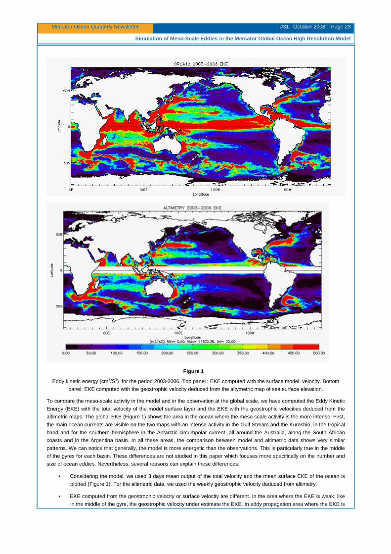
Mercator Ocean Quarterly Newsletter #31– October 2008 – Page 23
Simulation of Meso-Scale Eddies in the Mercator Glo bal Ocean High Resolution Model
Figure 1
Eddy kinetic energy (cm2/S2) for the period 2003-2006. Top panel : EKE computed with the surface model velocity. Bottom
panel: EKE computed with the geostrophic velocity deduced from the altymetric map of sea surface elevation.
To compare the meso-scale activity in the model and in the observation at the global scale, we have computed the Eddy Kinetic
Energy (EKE) with the total velocity of the model surface layer and the EKE with the geostrophic velocities deduced from the
altimetric maps. The global EKE (Figure 1) shows the area in the ocean where the meso-scale activity is the more intense. First,
the main ocean currents are visible on the two maps with an intense activity in the Gulf Stream and the Kuroshio, in the tropical
band and for the southern hemisphere in the Antarctic circumpolar current, all around the Australia, along the South African
coasts and in the Argentina basin. In all these areas, the comparison between model and altimetric data shows very similar
patterns. We can notice that generally, the model is more energetic than the observations. This is particularly true in the middle
of the gyres for each basin. These differences are not studied in this paper which focuses more specifically on the number and
size of ocean eddies. Nevertheless, several reasons can explain these differences:
• Considering the model, we used 3 days mean output of the total velocity and the mean surface EKE of the ocean is
plotted (Figure 1). For the altimetric data, we used the weekly geostrophic velocity deduced from altimetry.
• EKE computed from the geostrophic velocity or surface velocity are different. In the area where the EKE is weak, like
in the middle of the gyre, the geostrophic velocity under estimate the EKE. In eddy propagation area where the EKE is
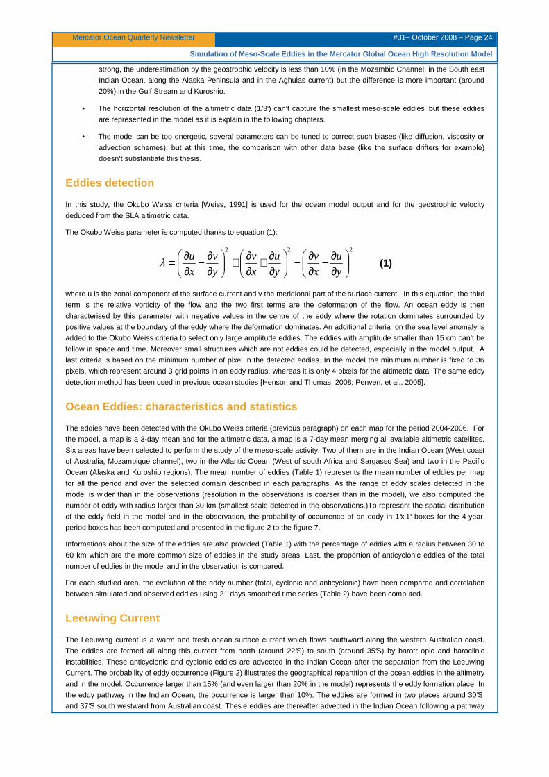
Mercator Ocean Quarterly Newsletter #31– October 2008 – Page 24
Simulation of Meso-Scale Eddies in the Mercator Global Ocean High Resolution Model
strong, the underestimation by the geostrophic velocity is less than 10% (in the Mozambic Channel, in the South east
Indian Ocean, along the Alaska Peninsula and in the Aghulas current) but the difference is more important (around
20%) in the Gulf Stream and Kuroshio.
• The horizontal resolution of the altimetric data (1/3°) can’t capture the smallest meso-scale eddies but these eddies
are represented in the model as it is explain in the following chapters.
• The model can be too energetic, several parameters can be tuned to correct such biases (like diffusion, viscosity or
advection schemes), but at this time, the comparison with other data base (like the surface drifters for example)
doesn’t substantiate this thesis.
Eddies detection
In this study, the Okubo Weiss criteria [Weiss, 1991] is used for the ocean model output and for the geostrophic velocity
deduced from the SLA altimetric data.
The Okubo Weiss parameter is computed thanks to equation (1):
222
∂∂−
∂∂−
∂∂+
∂∂+
∂∂−
∂∂=
y
u
x
v
y
u
x
v
y
v
x
uλ (1)
where u is the zonal component of the surface current and v the meridional part of the surface current. In this equation, the third
term is the relative vorticity of the flow and the two first terms are the deformation of the flow. An ocean eddy is then
characterised by this parameter with negative values in the centre of the eddy where the rotation dominates surrounded by
positive values at the boundary of the eddy where the deformation dominates. An additional criteria on the sea level anomaly is
added to the Okubo Weiss criteria to select only large amplitude eddies. The eddies with amplitude smaller than 15 cm can’t be
follow in space and time. Moreover small structures which are not eddies could be detected, especially in the model output. A
last criteria is based on the minimum number of pixel in the detected eddies. In the model the minimum number is fixed to 36
pixels, which represent around 3 grid points in an eddy radius, whereas it is only 4 pixels for the altimetric data. The same eddy
detection method has been used in previous ocean studies [Henson and Thomas, 2008; Penven, et al., 2005].
Ocean Eddies: characteristics and statistics
The eddies have been detected with the Okubo Weiss criteria (previous paragraph) on each map for the period 2004-2006. For
the model, a map is a 3-day mean and for the altimetric data, a map is a 7-day mean merging all available altimetric satellites.
Six areas have been selected to perform the study of the meso-scale activity. Two of them are in the Indian Ocean (West coast
of Australia, Mozambique channel), two in the Atlantic Ocean (West of south Africa and Sargasso Sea) and two in the Pacific
Ocean (Alaska and Kuroshio regions). The mean number of eddies (Table 1) represents the mean number of eddies per map
for all the period and over the selected domain described in each paragraphs. As the range of eddy scales detected in the
model is wider than in the observations (resolution in the observations is coarser than in the model), we also computed the
number of eddy with radius larger than 30 km (smallest scale detected in the observations.)To represent the spatial distribution
of the eddy field in the model and in the observation, the probability of occurrence of an eddy in 1°x 1° boxes for the 4-year
period boxes has been computed and presented in the figure 2 to the figure 7.
Informations about the size of the eddies are also provided (Table 1) with the percentage of eddies with a radius between 30 to
60 km which are the more common size of eddies in the study areas. Last, the proportion of anticyclonic eddies of the total
number of eddies in the model and in the observation is compared.
For each studied area, the evolution of the eddy number (total, cyclonic and anticyclonic) have been compared and correlation
between simulated and observed eddies using 21 days smoothed time series (Table 2) have been computed.
Leeuwing Current
The Leeuwing current is a warm and fresh ocean surface current which flows southward along the western Australian coast.
The eddies are formed all along this current from north (around 22°S) to south (around 35°S) by barotr opic and baroclinic
instabilities. These anticyclonic and cyclonic eddies are advected in the Indian Ocean after the separation from the Leeuwing
Current. The probability of eddy occurrence (Figure 2) illustrates the geographical repartition of the ocean eddies in the altimetry
and in the model. Occurrence larger than 15% (and even larger than 20% in the model) represents the eddy formation place. In
the eddy pathway in the Indian Ocean, the occurrence is larger than 10%. The eddies are formed in two places around 30°S
and 37°S south westward from Australian coast. Thes e eddies are thereafter advected in the Indian Ocean following a pathway
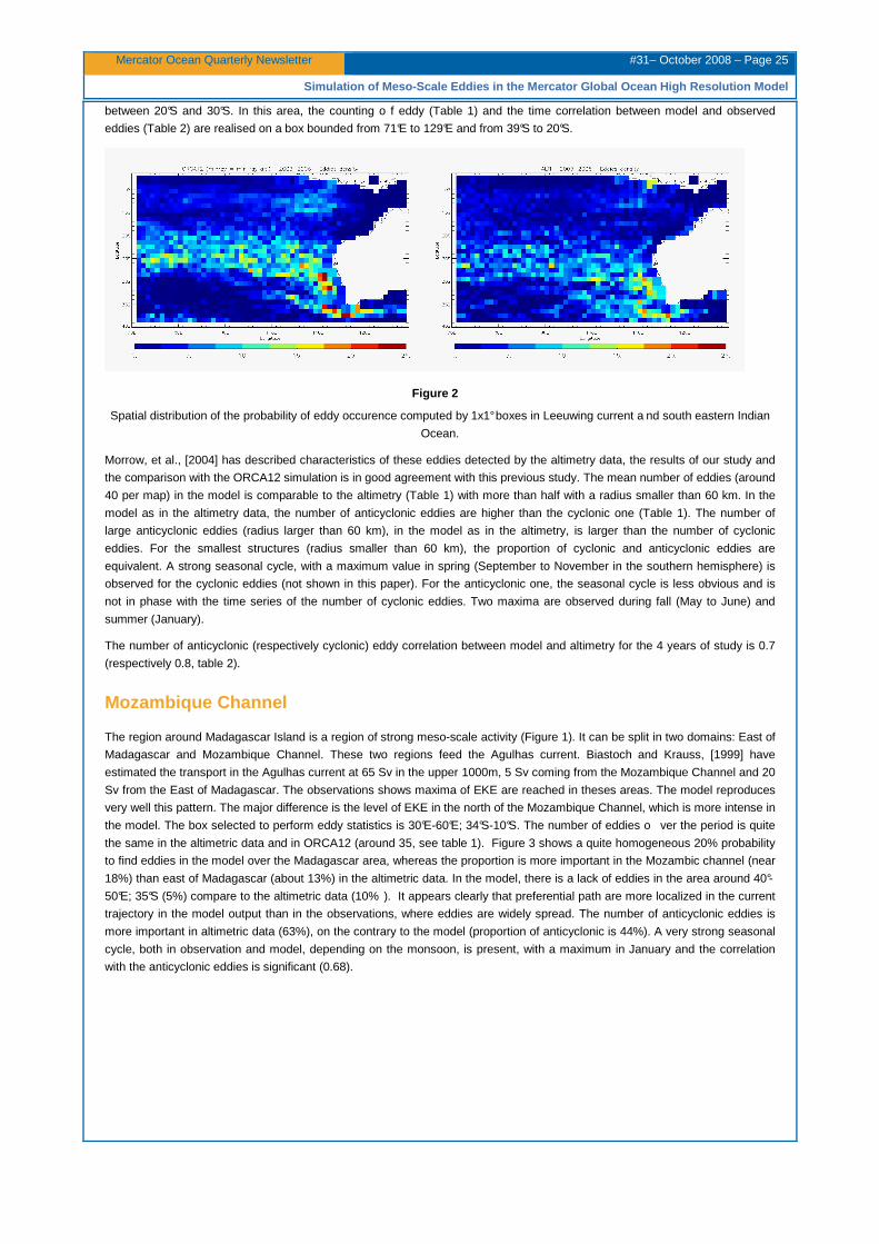
Mercator Ocean Quarterly Newsletter #31– October 2008 – Page 25
Simulation of Meso-Scale Eddies in the Mercator Glo bal Ocean High Resolution Model
between 20°S and 30°S. In this area, the counting o f eddy (Table 1) and the time correlation between model and observed
eddies (Table 2) are realised on a box bounded from 71°E to 129°E and from 39°S to 20°S.
Figure 2
Spatial distribution of the probability of eddy occurence computed by 1x1° boxes in Leeuwing current a nd south eastern Indian
Ocean.
Morrow, et al., [2004] has described characteristics of these eddies detected by the altimetry data, the results of our study and
the comparison with the ORCA12 simulation is in good agreement with this previous study. The mean number of eddies (around
40 per map) in the model is comparable to the altimetry (Table 1) with more than half with a radius smaller than 60 km. In the
model as in the altimetry data, the number of anticyclonic eddies are higher than the cyclonic one (Table 1). The number of
large anticyclonic eddies (radius larger than 60 km), in the model as in the altimetry, is larger than the number of cyclonic
eddies. For the smallest structures (radius smaller than 60 km), the proportion of cyclonic and anticyclonic eddies are
equivalent. A strong seasonal cycle, with a maximum value in spring (September to November in the southern hemisphere) is
observed for the cyclonic eddies (not shown in this paper). For the anticyclonic one, the seasonal cycle is less obvious and is
not in phase with the time series of the number of cyclonic eddies. Two maxima are observed during fall (May to June) and
summer (January).
The number of anticyclonic (respectively cyclonic) eddy correlation between model and altimetry for the 4 years of study is 0.7
(respectively 0.8, table 2).
Mozambique Channel
The region around Madagascar Island is a region of strong meso-scale activity (Figure 1). It can be split in two domains: East of
Madagascar and Mozambique Channel. These two regions feed the Agulhas current. Biastoch and Krauss, [1999] have
estimated the transport in the Agulhas current at 65 Sv in the upper 1000m, 5 Sv coming from the Mozambique Channel and 20
Sv from the East of Madagascar. The observations shows maxima of EKE are reached in theses areas. The model reproduces
very well this pattern. The major difference is the level of EKE in the north of the Mozambique Channel, which is more intense in
the model. The box selected to perform eddy statistics is 30°E-60°E; 34°S-10°S. The number of eddies o ver the period is quite
the same in the altimetric data and in ORCA12 (around 35, see table 1). Figure 3 shows a quite homogeneous 20% probability
to find eddies in the model over the Madagascar area, whereas the proportion is more important in the Mozambic channel (near
18%) than east of Madagascar (about 13%) in the altimetric data. In the model, there is a lack of eddies in the area around 40°-
50°E; 35°S (5%) compare to the altimetric data (10% ). It appears clearly that preferential path are more localized in the current
trajectory in the model output than in the observations, where eddies are widely spread. The number of anticyclonic eddies is
more important in altimetric data (63%), on the contrary to the model (proportion of anticyclonic is 44%). A very strong seasonal
cycle, both in observation and model, depending on the monsoon, is present, with a maximum in January and the correlation
with the anticyclonic eddies is significant (0.68).
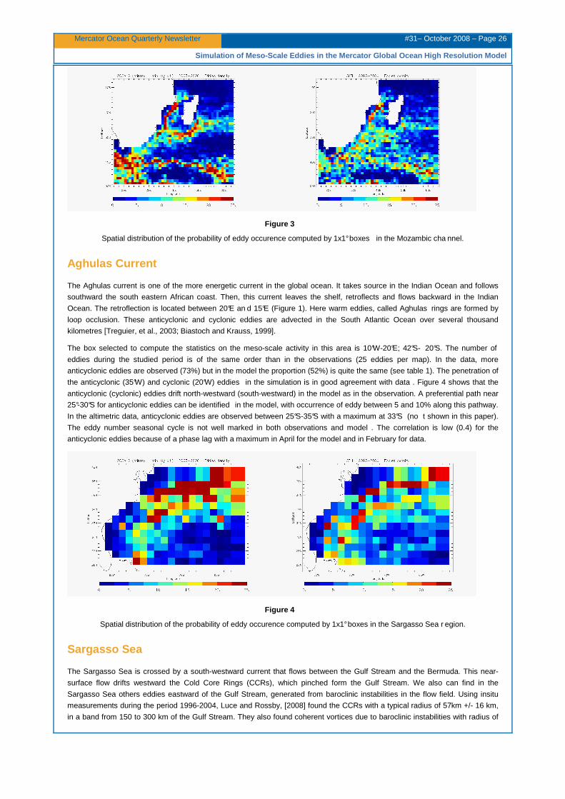
Mercator Ocean Quarterly Newsletter #31– October 2008 – Page 26
Simulation of Meso-Scale Eddies in the Mercator Glo bal Ocean High Resolution Model
Figure 3
Spatial distribution of the probability of eddy occurence computed by 1x1° boxes in the Mozambic cha nnel.
Aghulas Current
The Aghulas current is one of the more energetic current in the global ocean. It takes source in the Indian Ocean and follows
southward the south eastern African coast. Then, this current leaves the shelf, retroflects and flows backward in the Indian
Ocean. The retroflection is located between 20°E an d 15°E (Figure 1). Here warm eddies, called Aghulas rings are formed by
loop occlusion. These anticyclonic and cyclonic eddies are advected in the South Atlantic Ocean over several thousand
kilometres [Treguier, et al., 2003; Biastoch and Krauss, 1999].
The box selected to compute the statistics on the meso-scale activity in this area is 10°W-20°E; 42°S- 20°S. The number of
eddies during the studied period is of the same order than in the observations (25 eddies per map). In the data, more
anticyclonic eddies are observed (73%) but in the model the proportion (52%) is quite the same (see table 1). The penetration of
the anticyclonic (35°W) and cyclonic (20°W) eddies in the simulation is in good agreement with data . Figure 4 shows that the
anticyclonic (cyclonic) eddies drift north-westward (south-westward) in the model as in the observation. A preferential path near
25°-30°S for anticyclonic eddies can be identified in the model, with occurrence of eddy between 5 and 10% along this pathway.
In the altimetric data, anticyclonic eddies are observed between 25°S-35°S with a maximum at 33°S (no t shown in this paper).
The eddy number seasonal cycle is not well marked in both observations and model . The correlation is low (0.4) for the
anticyclonic eddies because of a phase lag with a maximum in April for the model and in February for data.
Figure 4
Spatial distribution of the probability of eddy occurence computed by 1x1° boxes in the Sargasso Sea r egion.
Sargasso Sea
The Sargasso Sea is crossed by a south-westward current that flows between the Gulf Stream and the Bermuda. This near-
surface flow drifts westward the Cold Core Rings (CCRs), which pinched form the Gulf Stream. We also can find in the
Sargasso Sea others eddies eastward of the Gulf Stream, generated from baroclinic instabilities in the flow field. Using insitu
measurements during the period 1996-2004, Luce and Rossby, [2008] found the CCRs with a typical radius of 57km +/- 16 km,
in a band from 150 to 300 km of the Gulf Stream. They also found coherent vortices due to baroclinic instabilities with radius of
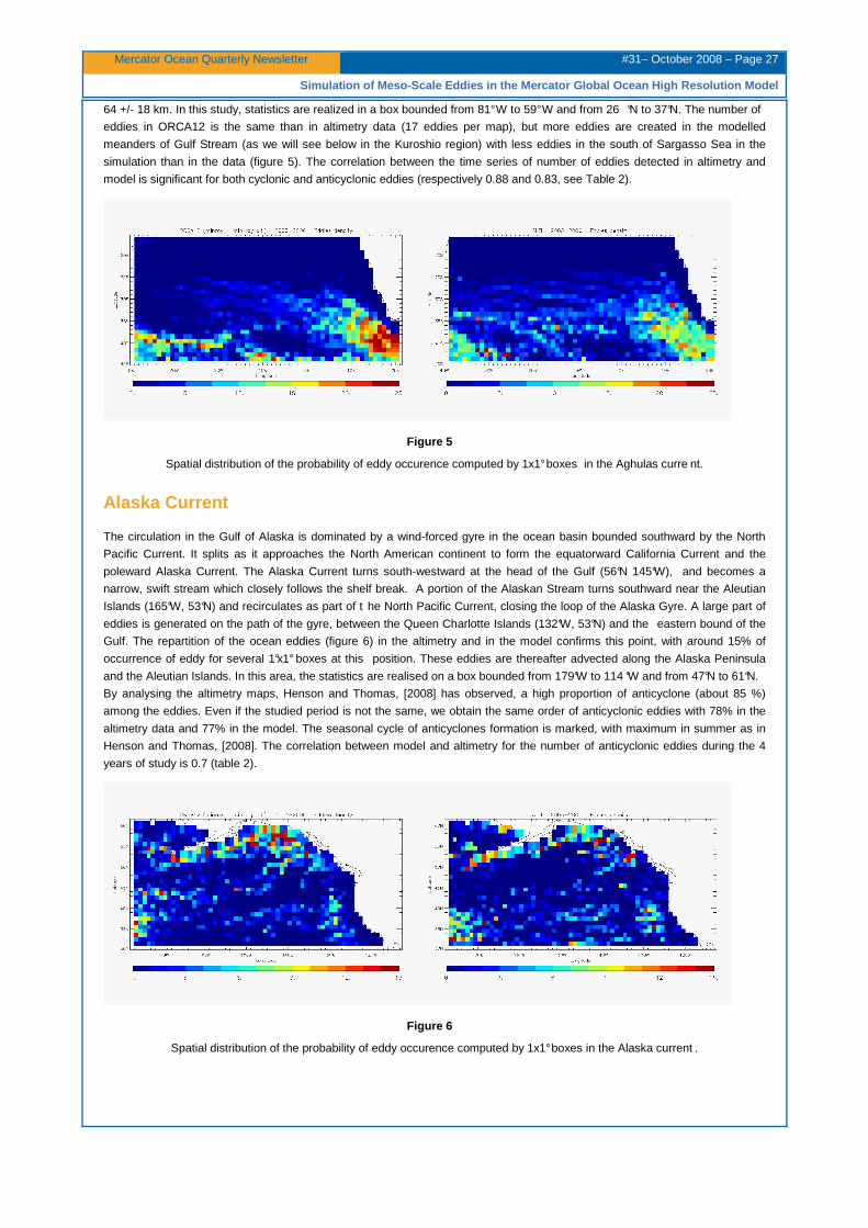
Mercator Ocean Quarterly Newsletter #31– October 2008 – Page 27
Simulation of Meso-Scale Eddies in the Mercator Glo bal Ocean High Resolution Model
64 +/- 18 km. In this study, statistics are realized in a box bounded from 81° W to 59° W and from 26 °N to 37°N. The number of
eddies in ORCA12 is the same than in altimetry data (17 eddies per map), but more eddies are created in the modelled
meanders of Gulf Stream (as we will see below in the Kuroshio region) with less eddies in the south of Sargasso Sea in the
simulation than in the data (figure 5). The correlation between the time series of number of eddies detected in altimetry and
model is significant for both cyclonic and anticyclonic eddies (respectively 0.88 and 0.83, see Table 2).
Figure 5
Spatial distribution of the probability of eddy occurence computed by 1x1° boxes in the Aghulas curre nt.
Alaska Current
The circulation in the Gulf of Alaska is dominated by a wind-forced gyre in the ocean basin bounded southward by the North
Pacific Current. It splits as it approaches the North American continent to form the equatorward California Current and the
poleward Alaska Current. The Alaska Current turns south-westward at the head of the Gulf (56°N 145°W), and becomes a
narrow, swift stream which closely follows the shelf break. A portion of the Alaskan Stream turns southward near the Aleutian
Islands (165°W, 53°N) and recirculates as part of t he North Pacific Current, closing the loop of the Alaska Gyre. A large part of
eddies is generated on the path of the gyre, between the Queen Charlotte Islands (132°W, 53°N) and the eastern bound of the
Gulf. The repartition of the ocean eddies (figure 6) in the altimetry and in the model confirms this point, with around 15% of
occurrence of eddy for several 1°x1° boxes at this position. These eddies are thereafter advected along the Alaska Peninsula
and the Aleutian Islands. In this area, the statistics are realised on a box bounded from 179°W to 114 °W and from 47°N to 61°N.
By analysing the altimetry maps, Henson and Thomas, [2008] has observed, a high proportion of anticyclone (about 85 %)
among the eddies. Even if the studied period is not the same, we obtain the same order of anticyclonic eddies with 78% in the
altimetry data and 77% in the model. The seasonal cycle of anticyclones formation is marked, with maximum in summer as in
Henson and Thomas, [2008]. The correlation between model and altimetry for the number of anticyclonic eddies during the 4
years of study is 0.7 (table 2).
Figure 6
Spatial distribution of the probability of eddy occurence computed by 1x1° boxes in the Alaska current .
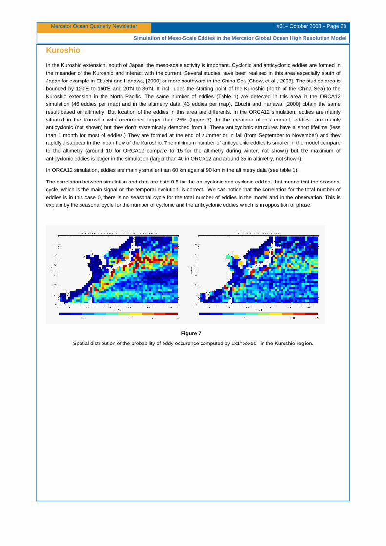
Mercator Ocean Quarterly Newsletter #31– October 2008 – Page 28
Simulation of Meso-Scale Eddies in the Mercator Glo bal Ocean High Resolution Model
Kuroshio
In the Kuroshio extension, south of Japan, the meso-scale activity is important. Cyclonic and anticyclonic eddies are formed in
the meander of the Kuroshio and interact with the current. Several studies have been realised in this area especially south of
Japan for example in Ebuchi and Hanawa, [2000] or more southward in the China Sea [Chow, et al., 2008]. The studied area is
bounded by 120°E to 160°E and 20°N to 36°N. It incl udes the starting point of the Kuroshio (north of the China Sea) to the
Kuroshio extension in the North Pacific. The same number of eddies (Table 1) are detected in this area in the ORCA12
simulation (46 eddies per map) and in the altimetry data (43 eddies per map), Ebuchi and Hanawa, [2000] obtain the same
result based on altimetry. But location of the eddies in this area are differents. In the ORCA12 simulation, eddies are mainly
situated in the Kuroshio with occurrence larger than 25% (figure 7). In the meander of this current, eddies are mainly
anticyclonic (not shown) but they don’t systemically detached from it. These anticyclonic structures have a short lifetime (less
than 1 month for most of eddies.) They are formed at the end of summer or in fall (from September to November) and they
rapidly disappear in the mean flow of the Kuroshio. The minimum number of anticyclonic eddies is smaller in the model compare
to the altimetry (around 10 for ORCA12 compare to 15 for the altimetry during winter, not shown) but the maximum of
anticyclonic eddies is larger in the simulation (larger than 40 in ORCA12 and around 35 in altimetry, not shown).
In ORCA12 simulation, eddies are mainly smaller than 60 km against 90 km in the altimetry data (see table 1).
The correlation between simulation and data are both 0.8 for the anticyclonic and cyclonic eddies, that means that the seasonal
cycle, which is the main signal on the temporal evolution, is correct. We can notice that the correlation for the total number of
eddies is in this case 0, there is no seasonal cycle for the total number of eddies in the model and in the observation. This is
explain by the seasonal cycle for the number of cyclonic and the anticyclonic eddies which is in opposition of phase.
Figure 7
Spatial distribution of the probability of eddy occurence computed by 1x1° boxes in the Kuroshio reg ion.
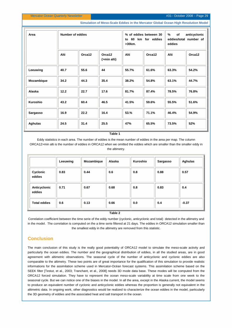
Mercator Ocean Quarterly Newsletter #31– October 2008 – Page 29
Simulation of Meso-Scale Eddies in the Mercator Glo bal Ocean High Resolution Model
Area Number of eddies % of eddies between 30
to 60 km for eddies
>30km.
% of anticyclonic
eddies/total number of
eddies
Alti Orca12 Orca12 (>min alti)
Alti Orca12 Alti Orca12
Leeuwing 40.7 55.6 44 55.7% 61.6% 63.3% 54.2%
Mozambique 34.2 44.3 35.4 38.2% 54.8% 63.1% 44.7%
Alaska 12.2 22.7 17.6 81.7% 87.4% 78.5% 76.8%
Kuroshio 43.2 60.4 46.5 41.5% 59.6% 55.5% 51.6%
Sargasso 16.9 22.2 16.4 53.% 71.1% 46.4% 54.9%
Aghulas 24.5 31.4 25.5 47% 65.5% 73.5% 52%
Table 1
Eddy statistics in each area. The number of eddies is the mean number of eddies in the area per map. The column
ORCA12>min alti is the number of eddies in ORCA12 when we omitted the eddies which are smaller than the smaller eddy in
the altimetry.
Leeuwing Mozambique Alaska Kuroshio Sargasso Aghul as
Cyclonic eddies
0.83 0.44 0.6 0.8 0.88 0.57
Anticyclonic
eddies
0.71 0.67 0.68 0.8 0.83 0.4
Total eddies 0.6 0.13 0.66 0.0 0.4 -0.37
Table 2
Correlation coefficient between the time serie of the eddy number (cyclonic, anticyclonic and total) detected in the altimetry and
in the model. The correlation is computed on the a time serie filtered at 21 days. The eddies in ORCA12 simulation smaller than
the smallest eddy in the altimetry are removed from this statistic.
Conclusion
The main conclusion of this study is the really good potentiality of ORCA12 model to simulate the meso-scale activity and
particularly the ocean eddies. The number and the geographical distribution of eddies, in all the studied areas, are in good
agreement with altimetric observations. The seasonal cycle of the number of anticyclonic and cyclonic eddies are also
comparable to the altimetry. These two points are of great importance for the qualification of this simulation to provide realistic
informations for the assimilation scheme used in Mercator-Océan forecast systems. This assimilation scheme based on the
SEEK filter [Testut, et al., 2003; Tranchant, et al., 2008] needs 3D mode data base. These modes will be computed from the
ORCA12 forced simulation. They have to represent the ocean meso-scale variability at time scale from one week to the
seasonal cycle. But we can notice one of the biases in the model. In all the area, except in the Alaska current, the model seems
to produce an equivalent number of cyclonic and anticyclonic eddies whereas the proportion is generally not equivalent in the
altimetric data. In ongoing work, other diagnostics would be realized to characterize the ocean eddies in the model, particularly
the 3D geometry of eddies and the associated heat and salt transport in the ocean.
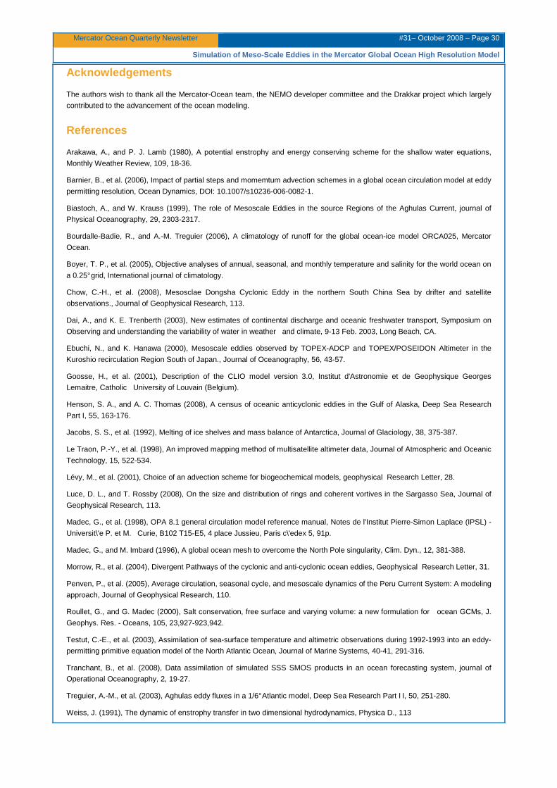
Mercator Ocean Quarterly Newsletter #31– October 2008 – Page 30
Simulation of Meso-Scale Eddies in the Mercator Glo bal Ocean High Resolution Model
Acknowledgements
The authors wish to thank all the Mercator-Ocean team, the NEMO developer committee and the Drakkar project which largely
contributed to the advancement of the ocean modeling.
References
Arakawa, A., and P. J. Lamb (1980), A potential enstrophy and energy conserving scheme for the shallow water equations,
Monthly Weather Review, 109, 18-36.
Barnier, B., et al. (2006), Impact of partial steps and momemtum advection schemes in a global ocean circulation model at eddy
permitting resolution, Ocean Dynamics, DOI: 10.1007/s10236-006-0082-1.
Biastoch, A., and W. Krauss (1999), The role of Mesoscale Eddies in the source Regions of the Aghulas Current, journal of
Physical Oceanography, 29, 2303-2317.
Bourdalle-Badie, R., and A.-M. Treguier (2006), A climatology of runoff for the global ocean-ice model ORCA025, Mercator
Ocean.
Boyer, T. P., et al. (2005), Objective analyses of annual, seasonal, and monthly temperature and salinity for the world ocean on
a 0.25° grid, International journal of climatology.
Chow, C.-H., et al. (2008), Mesosclae Dongsha Cyclonic Eddy in the northern South China Sea by drifter and satellite
observations., Journal of Geophysical Research, 113.
Dai, A., and K. E. Trenberth (2003), New estimates of continental discharge and oceanic freshwater transport, Symposium on
Observing and understanding the variability of water in weather and climate, 9-13 Feb. 2003, Long Beach, CA.
Ebuchi, N., and K. Hanawa (2000), Mesoscale eddies observed by TOPEX-ADCP and TOPEX/POSEIDON Altimeter in the
Kuroshio recirculation Region South of Japan., Journal of Oceanography, 56, 43-57.
Goosse, H., et al. (2001), Description of the CLIO model version 3.0, Institut d'Astronomie et de Geophysique Georges
Lemaitre, Catholic University of Louvain (Belgium).
Henson, S. A., and A. C. Thomas (2008), A census of oceanic anticyclonic eddies in the Gulf of Alaska, Deep Sea Research
Part I, 55, 163-176.
Jacobs, S. S., et al. (1992), Melting of ice shelves and mass balance of Antarctica, Journal of Glaciology, 38, 375-387.
Le Traon, P.-Y., et al. (1998), An improved mapping method of multisatellite altimeter data, Journal of Atmospheric and Oceanic
Technology, 15, 522-534.
Lévy, M., et al. (2001), Choice of an advection scheme for biogeochemical models, geophysical Research Letter, 28.
Luce, D. L., and T. Rossby (2008), On the size and distribution of rings and coherent vortives in the Sargasso Sea, Journal of
Geophysical Research, 113.
Madec, G., et al. (1998), OPA 8.1 general circulation model reference manual, Notes de l'Institut Pierre-Simon Laplace (IPSL) -
Universit\'e P. et M. Curie, B102 T15-E5, 4 place Jussieu, Paris c\'edex 5, 91p.
Madec, G., and M. Imbard (1996), A global ocean mesh to overcome the North Pole singularity, Clim. Dyn., 12, 381-388.
Morrow, R., et al. (2004), Divergent Pathways of the cyclonic and anti-cyclonic ocean eddies, Geophysical Research Letter, 31.
Penven, P., et al. (2005), Average circulation, seasonal cycle, and mesoscale dynamics of the Peru Current System: A modeling
approach, Journal of Geophysical Research, 110.
Roullet, G., and G. Madec (2000), Salt conservation, free surface and varying volume: a new formulation for ocean GCMs, J.
Geophys. Res. - Oceans, 105, 23,927-923,942.
Testut, C.-E., et al. (2003), Assimilation of sea-surface temperature and altimetric observations during 1992-1993 into an eddy-
permitting primitive equation model of the North Atlantic Ocean, Journal of Marine Systems, 40-41, 291-316.
Tranchant, B., et al. (2008), Data assimilation of simulated SSS SMOS products in an ocean forecasting system, journal of
Operational Oceanography, 2, 19-27.
Treguier, A.-M., et al. (2003), Aghulas eddy fluxes in a 1/6° Atlantic model, Deep Sea Research Part I I, 50, 251-280.
Weiss, J. (1991), The dynamic of enstrophy transfer in two dimensional hydrodynamics, Physica D., 113
Mercator Ocean Quarterly Newsletter #31– October 2008 – Page 31
Ocean Data Assimilation and Prediction system in JM and MRI
Ocean Data Assimilation and Prediction system in JM and MRI By: Masafumi Kamachi, Yosuke Fujii, Norihisa Usui, Shiroh Ishizaki, Satoshi Matsumoto and
Hiroyuki Tsujino
Meteorological Research Institute, Japan Meteorological Agency
Abstract
Ocean data assimilation/prediction systems MOVE/MRI.COM are introduced. The systems have been developed in
Meteorological Research Institute, and been operated in Japan Meteorological Agency. The operation is for ocean state
estimation and prediction of ocean weather (mesoscale) and of seasonal to interannual (e.g., ElNino) phenomenon. This report
shows briefly the structure of ocean model, assimilation method and some examples of ocean state (velocity and water mass)
and prediction of the Kuroshio path. Future perspective is also briefly stated.
Introduction
The Meteorological Research Institute (MRI) Multivariate Ocean Variational Estimation (MOVE/MRI.COM). Systems have been
developed for research system to study mesoscale phenomenon, climate variability and for the operational ocean data
assimilation system in Japan Meteorological Agency (JMA).
The MOVE/MRI.COM systems have three components: the global (MOVE/MRI.COM-G), North Pacific (MOVE/MRI.COM-NP)
and Western North Pacific (MOVE/MRI.COM-WNP) systems (Usui et al., 2006a). The aims of MOVE/MRI.COM-G are the
initialization of MRI coupled GCM for seasonal-interannual forecasting and analysis/reanalysis project, which is related to
CLIVAR/GSOP project. The period of the analysis/reanalysis product is 1948 to 2007. The aims of MOVE/MRI.COM-NP and -
WNP are the initialization of ocean forecast in the North pacific (especially around Japan) and analysis/reanalysis, which period
is 1993-2007 and which is related to GODAE project. Information about the systems and recent publications are given in the
MRI homepage Hhttp://www.mri-jma.go.jp/Dep/oc/oc.htmlH. Here we introduce the system’s configurations and some
demonstration results.
MOVE/MRI.COM
MOVE/MRI.COM systems are composed of OGCMs and a variational analysis scheme which synthesizes the observed
information (i.e., temperature, salinity and sea surface height) together with the OGCMs.
Model
The numerical code for the OGCMs used in the MOVE/MRI.COM system is the MRI community ocean model (MRI.COM).
MRI.COM has been developed in JMA/MRI and is independent of any other popular OGCM code (Ishikawa et al. 2005, Tsujino
et al., 2006). It is a multilevel model code that solves the primitive equations under the hydrostatic and Boussinesq
approximations. The vertical coordinate is a terrain following-depth (σ−z) hybrid, i.e., the levels near the surface follow the
surface topography. It enables us to adopt a fine vertical resolution near the surface because it prevents the uppermost layer
from vanishing during integration when the free surface variation is explicitly solved. For momentum advection, MRI.COM uses
the generalized enstrophy-preserving scheme with the Takano–Oonishi scheme, which contains the concept of diagonally
upward/downward mass momentum fluxes along a sloping bottom (Ishizaki and Motoi, 1999).
The OGCM used in MOVE/MRI.COM-G is a model with a global domain (model G) for climate variability. On the other hand, for
ocean weather, MOVE/MRI.COM employs two models, namely the North Pacific and western North Pacific models (models NP
and WNP). Model WNP is nested into model NP, i.e., the boundary conditions for the western, eastern, and southern
boundaries in model WNP are passed from model NP (one-way nesting). Daily outputs from model NP are linearly interpolated
both in time and space to replace boundary data of model WNP at every time step.
The domain of model G extends from 75°S to 75°N glo bally. The grid spacing in the zonal direction is 1° and that in the
meridional direction is 0.3° within 5°S–5°N, 1° pol eward of 15°S and 15°N and gradually changed from 0 .3° to 1° in the
transition regions (i.e. 5°S-15°S, 5°N-15°N). There are 50 levels in vertical. The bottom topography is based on ETOPO5. The
northern boundary is closed. The isopycnal diffusion (Redi, 1982) and the isopycnal thickness diffusion (Gent and McWilliams,
1990; hereafter GM), the background coefficients for vertical diffusion by Tsujino et al. (2000), the harmonic viscosity with the
parameterization of Smagorinsky (1963, hereafter SMA63), and the level-2.5 turbulent closure scheme of Mellor and Yamada
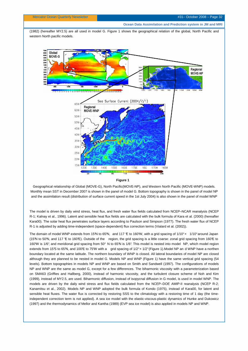
Mercator Ocean Quarterly Newsletter #31– October 2008 – Page 32
Ocean Data Assimilation and Prediction system in JM and MRI
(1982) (hereafter MY2.5) are all used in model G. Figure 1 shows the geographical relation of the global, North Pacific and
western North pacific models.
Figure 1
Geographical relationship of Global (MOVE-G), North Pacific(MOVE-NP), and Western North Pacific (MOVE-WNP) models.
Monthly mean SST in December 2007 is shown in the panel of model G. Bottom topography is shown in the panel of model NP
and the assimilation result (distribution of surface current speed in the 1st July 2004) is also shown in the panel of model WNP
The model is driven by daily wind stress, heat flux, and fresh water flux fields calculated from NCEP–NCAR reanalysis (NCEP
R-1; Kalnay et al., 1996). Latent and sensible heat flux fields are calculated with the bulk formula of Kara et al. (2000) (hereafter
Kara00). The solar heat flux penetrates surface layers according to Paulson and Simpson (1977). The fresh water flux of NCEP
R-1 is adjusted by adding time-independent (space-dependent) flux correction terms (Vialard et al. (2002)).
The domain of model WNP extends from 15°N to 65°N, and 117 °E to 160°W, with a grid spacing of 1/10° × 1/10° around Japan
(15°N to 50°N, and 117 °E to 160°E). Outside of the region, the grid spacing is a little coarse: zonal grid spacing from 160°E to
160°W is 1/6°, and meridional grid spacing from 50° N to 65°N is 1/6°. This model is nested into model NP, which model region
extends from 15°S to 65°N, and 100°E to 75°W with a grid spacing of 1/2° × 1/2° (Figure 1).Model NP an d WNP have a northen
boundary located at the same latitude. The northern boundary of WNP is closed. All lateral boundaries of model NP are closed
although they are planned to be nested in model G. Models NP and WNP (Figure 1) have the same vertical grid spacing (54
levels). Bottom topographies in models NP and WNP are based on Smith and Sandwell (1997). The configurations of models
NP and WNP are the same as model G, except for a few differences. The biharmonic viscosity with a parameterization based
on SMA63 (Griffies and Hallberg, 2000), instead of harmonic viscosity, and the turbulent closure scheme of Noh and Kim
(1999), instead of MY2.5, are used. Biharmonic diffusion, instead of isopycnal diffusion in G model, is used in model WNP. The
models are driven by the daily wind stress and flux fields calculated from the NCEP–DOE AMIP-II reanalysis (NCEP R-2;
Kanamitsu et al., 2002). Models NP and WNP adopted the bulk formula of Kondo (1975), instead of Kara00, for latent and
sensible heat fluxes. The water flux is corrected by restoring SSS to the climatology with a restoring time of 1 day (the time-
independent correction term is not applied). A sea ice model with the elastic-viscous-plastic dynamics of Hunke and Dukowicz
(1997) and the thermodynamics of Mellor and Kantha (1989) (EVP sea ice model) is also applied in models NP and WNP.
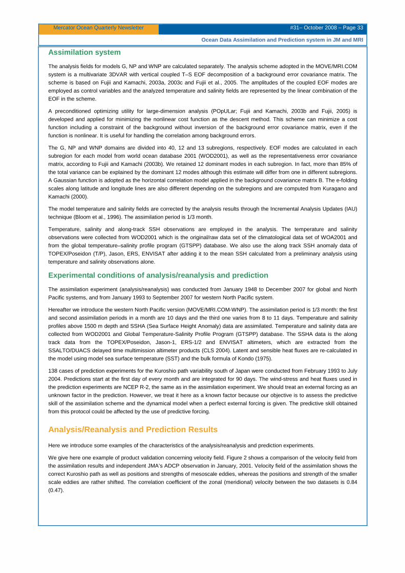
Mercator Ocean Quarterly Newsletter #31– October 2008 – Page 33
Ocean Data Assimilation and Prediction system in JM and MRI
Assimilation system
The analysis fields for models G, NP and WNP are calculated separately. The analysis scheme adopted in the MOVE/MRI.COM
system is a multivariate 3DVAR with vertical coupled T–S EOF decomposition of a background error covariance matrix. The
scheme is based on Fujii and Kamachi, 2003a, 2003c and Fujii et al., 2005. The amplitudes of the coupled EOF modes are
employed as control variables and the analyzed temperature and salinity fields are represented by the linear combination of the
EOF in the scheme.
A preconditioned optimizing utility for large-dimension analysis (POpULar; Fujii and Kamachi, 2003b and Fujii, 2005) is
developed and applied for minimizing the nonlinear cost function as the descent method. This scheme can minimize a cost
function including a constraint of the background without inversion of the background error covariance matrix, even if the
function is nonlinear. It is useful for handling the correlation among background errors.
The G, NP and WNP domains are divided into 40, 12 and 13 subregions, respectively. EOF modes are calculated in each
subregion for each model from world ocean database 2001 (WOD2001), as well as the representativeness error covariance
matrix, according to Fujii and Kamachi (2003b). We retained 12 dominant modes in each subregion. In fact, more than 85% of
the total variance can be explained by the dominant 12 modes although this estimate will differ from one in different subregions.
A Gaussian function is adopted as the horizontal correlation model applied in the background covariance matrix B. The e-folding
scales along latitude and longitude lines are also different depending on the subregions and are computed from Kuragano and
Kamachi (2000).
The model temperature and salinity fields are corrected by the analysis results through the Incremental Analysis Updates (IAU)
technique (Bloom et al., 1996). The assimilation period is 1/3 month.
Temperature, salinity and along-track SSH observations are employed in the analysis. The temperature and salinity
observations were collected from WOD2001 which is the original/raw data set of the climatological data set of WOA2001 and
from the global temperature–salinity profile program (GTSPP) database. We also use the along track SSH anomaly data of
TOPEX/Poseidon (T/P), Jason, ERS, ENVISAT after adding it to the mean SSH calculated from a preliminary analysis using
temperature and salinity observations alone.
Experimental conditions of analysis/reanalysis and prediction
The assimilation experiment (analysis/reanalysis) was conducted from January 1948 to December 2007 for global and North
Pacific systems, and from January 1993 to September 2007 for western North Pacific system.
Hereafter we introduce the western North Pacific version (MOVE/MRI.COM-WNP). The assimilation period is 1/3 month: the first
and second assimilation periods in a month are 10 days and the third one varies from 8 to 11 days. Temperature and salinity
profiles above 1500 m depth and SSHA (Sea Surface Height Anomaly) data are assimilated. Temperature and salinity data are
collected from WOD2001 and Global Temperature-Salinity Profile Program (GTSPP) database. The SSHA data is the along
track data from the TOPEX/Poseidon, Jason-1, ERS-1/2 and ENVISAT altimeters, which are extracted from the
SSALTO/DUACS delayed time multimission altimeter products (CLS 2004). Latent and sensible heat fluxes are re-calculated in
the model using model sea surface temperature (SST) and the bulk formula of Kondo (1975).
138 cases of prediction experiments for the Kuroshio path variability south of Japan were conducted from February 1993 to July
2004. Predictions start at the first day of every month and are integrated for 90 days. The wind-stress and heat fluxes used in
the prediction experiments are NCEP R-2, the same as in the assimilation experiment. We should treat an external forcing as an
unknown factor in the prediction. However, we treat it here as a known factor because our objective is to assess the predictive
skill of the assimilation scheme and the dynamical model when a perfect external forcing is given. The predictive skill obtained
from this protocol could be affected by the use of predictive forcing.
Analysis/Reanalysis and Prediction Results
Here we introduce some examples of the characteristics of the analysis/reanalysis and prediction experiments.
We give here one example of product validation concerning velocity field. Figure 2 shows a comparison of the velocity field from
the assimilation results and independent JMA’s ADCP observation in January, 2001. Velocity field of the assimilation shows the
correct Kuroshio path as well as positions and strengths of mesoscale eddies, whereas the positions and strength of the smaller
scale eddies are rather shifted. The correlation coefficient of the zonal (meridional) velocity between the two datasets is 0.84
(0.47).
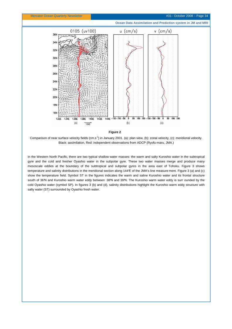
Mercator Ocean Quarterly Newsletter #31– October 2008 – Page 34
Ocean Data Assimilation and Prediction system in JM and MRI
Figure 2
Comparison of near surface velocity fields (cm.s-1) in January 2001. (a): plan view, (b): zonal velocity, (c): meridional velocity.
Black: assimilation, Red: independent observations from ADCP (Ryofu-maru, JMA.)
In the Western North Pacific, there are two typical shallow water masses: the warm and salty Kuroshio water in the subtropical
gyre and the cold and fresher Oyashio water in the subpolar gyre. These two water masses merge and produce many
mesoscale eddies at the boundary of the subtropical and subpolar gyres in the area east of Tohoku. Figure 3 shows
temperature and salinity distributions in the meridional section along 144°E of the JMA’s line measure ment. Figure 3 (a) and (c)
show the temperature field. Symbol ST in the figures indicates the warm and saline Kuroshio water and its frontal structure
south of 36°N and Kuroshio warm water eddy between 38°N and 39°N. The Kuroshio warm water eddy is surr ounded by the
cold Oyashio water (symbol SP). In figures 3 (b) and (d), salinity distributions highlight the Kuroshio warm eddy structure with
salty water (ST) surrounded by Oyashio fresh water.
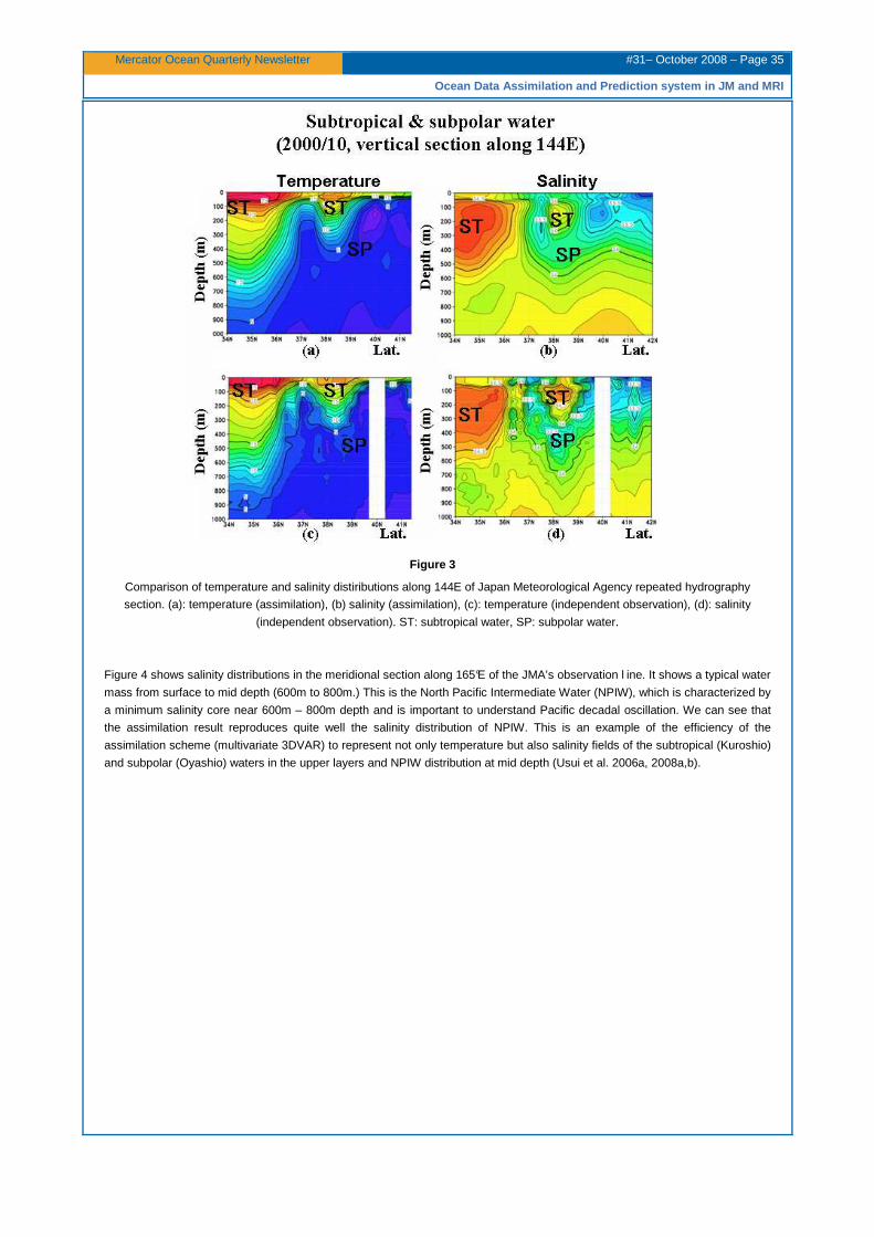
Mercator Ocean Quarterly Newsletter #31– October 2008 – Page 35
Ocean Data Assimilation and Prediction system in JM and MRI
Figure 3
Comparison of temperature and salinity distiributions along 144E of Japan Meteorological Agency repeated hydrography
section. (a): temperature (assimilation), (b) salinity (assimilation), (c): temperature (independent observation), (d): salinity
(independent observation). ST: subtropical water, SP: subpolar water.
Figure 4 shows salinity distributions in the meridional section along 165°E of the JMA’s observation l ine. It shows a typical water
mass from surface to mid depth (600m to 800m.) This is the North Pacific Intermediate Water (NPIW), which is characterized by
a minimum salinity core near 600m – 800m depth and is important to understand Pacific decadal oscillation. We can see that
the assimilation result reproduces quite well the salinity distribution of NPIW. This is an example of the efficiency of the
assimilation scheme (multivariate 3DVAR) to represent not only temperature but also salinity fields of the subtropical (Kuroshio)
and subpolar (Oyashio) waters in the upper layers and NPIW distribution at mid depth (Usui et al. 2006a, 2008a,b).
Mercator Ocean Quarterly Newsletter #31– October 2008 – Page 36
Ocean Data Assimilation and Prediction system in JM and MRI
Figure 4
Salinity distribution along 165E (Japan Meteorological Agency repeated hydrography section). (a): assimilation, (b): JMA
independent observation. The both panels (a) and (b) show composite distributions of salinity. Observation/assimilation period is
in September (April), 2000 in each left (right)-half of the panels.
Mean water mass property (temperature and salinity) along JMA’s hydrographic observation lines around Japan are also
examined. Figure 5 shows JMA’s observation lines of the repeated hydrography. Figure 6 shows the climatological mean water
mass property calculated from the assimilation of the JMA’s observed data into MOVE/MRI.COM-WNP. Though the JMA’s
observation data are assimilated (i.e., not independent data), the assimilation (analysis/reanalysis) results gives a good
representation of the mean water masses along almost all lines. Some sections have a larger bias. PH line (figure 5) in the
subtropical-subpolar boundary region along 41.5°N h as the largest bias. This is difficult to reproduce the ocean state/water
mass into this area even if the water masses of the Kuroshio and Oyashio are well recovered (figure 3). PM line in the Japan
Sea shows also large bias near the bottom. The structures, variations and trend (which is related to climate change) are
examined with each water mass in the Pacific. It explains the causes of the variation, propagation path and changes of water
property in formation regions and relation with the atmospheric conditions. It is an on-going study (see Matsumoto et al., 2008).
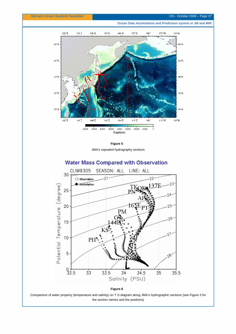
Mercator Ocean Quarterly Newsletter #31– October 2008 – Page 37
Ocean Data Assimilation and Prediction system in JM and MRI
Figure 5
JMA’s repeated hydrography sections
Figure 6
Comparison of water property (temperature and salinity) on T-S diagram along JMA’s hydrographic sections (see Figure 3 for
the section names and the positions)
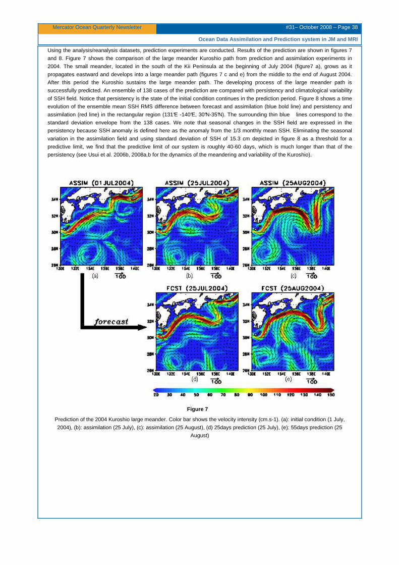
Mercator Ocean Quarterly Newsletter #31– October 2008 – Page 38
Ocean Data Assimilation and Prediction system in JM and MRI
Using the analysis/reanalysis datasets, prediction experiments are conducted. Results of the prediction are shown in figures 7
and 8. Figure 7 shows the comparison of the large meander Kuroshio path from prediction and assimilation experiments in
2004. The small meander, located in the south of the Kii Peninsula at the beginning of July 2004 (figure7 a), grows as it
propagates eastward and develops into a large meander path (figures 7 c and e) from the middle to the end of August 2004.
After this period the Kuroshio sustains the large meander path. The developing process of the large meander path is
successfully predicted. An ensemble of 138 cases of the prediction are compared with persistency and climatological variability
of SSH field. Notice that persistency is the state of the initial condition continues in the prediction period. Figure 8 shows a time
evolution of the ensemble mean SSH RMS difference between forecast and assimilation (blue bold line) and persistency and
assimilation (red line) in the rectangular region (131°E -140°E, 30°N-35°N). The surrounding thin blue lines correspond to the
standard deviation envelope from the 138 cases. We note that seasonal changes in the SSH field are expressed in the
persistency because SSH anomaly is defined here as the anomaly from the 1/3 monthly mean SSH. Eliminating the seasonal
variation in the assimilation field and using standard deviation of SSH of 15.3 cm depicted in figure 8 as a threshold for a
predictive limit, we find that the predictive limit of our system is roughly 40-60 days, which is much longer than that of the
persistency (see Usui et al. 2006b, 2008a,b for the dynamics of the meandering and variability of the Kuroshio).
Figure 7
Prediction of the 2004 Kuroshio large meander. Color bar shows the velocity intensity (cm.s-1). (a): initial condition (1 July,
2004), (b): assimilation (25 July), (c): assimilation (25 August), (d) 25days prediction (25 July), (e): 55days prediction (25
August)
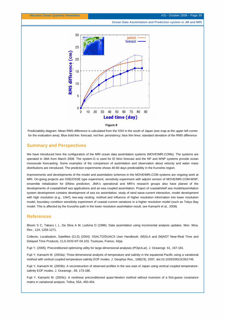
Mercator Ocean Quarterly Newsletter #31– October 2008 – Page 39
Ocean Data Assimilation and Prediction system in JM and MRI
Figure 8
Predictability diagram. Mean RMS difference is calculated from the SSH in the south of Japan (see map at the upper left corner
for the evaluation area). Blue bold line: forecast; red line: persistency; blue thin lines: standard deviation of the RMS difference
Summary and Perspectives
We have introduced here the configuration of the MRI ocean data assimilation systems (MOVE/MRI.COMs). The systems are
operated in JMA from March 2008. The system-G is used for El Nino forecast and the NP and WNP systems provide ocean
mesoscale forecasting. Some examples of the comparison of assimilation and observation about velocity and water mass
distributions are introduced. The prediction experiments shows 40-60 days predictability in the Kuroshio region.
Improvements and developments of the model and assimilation schemes in the MOVE/MRI.COM systems are ongoing work at
MRI. On-going projects are OSE/OSSE type experiment, sensitivity experiment with adjoint version of MOVE/MRI.COM-WNP,
ensemble initialization for ElNino prediction. JMA’s operational and MRI’s research groups also have planed of the
developments of coastal/shelf sea applications and air-sea coupled assimilation. Project of coastal/shelf sea model/assimilation
system development contains development of sea ice assimilation, study of wind wave-current interaction, model development
with high resolution (e.g., 1/64°), two-way nesting method and influence of higher resolution information into lower resolution
model, boundary condition sensitivity experiment of coastal current variations in a higher resolution model (such as Tokyo Bay
model. This is affected by the Kuroshio path in the lower resolution assimilation result, see Kamachi et al., 2008).
References
Bloom S C, Takacs L L, Da Silva A M, Ledvina D (1996): Data assimilation using incremental analysis updates. Mon. Wea.
Rev., 124, 1256-1271.
Collecte, Localisation, Satellites (CLS) (2004): SSALTO/DUACS User Handbook: (M)SLA and (M)ADT Near-Real Time and
Delayed Time Products, CLS-DOS-NT-04.103, Toulouse, France, 42pp.
Fujii Y. (2005): Preconditioned optimizing utility for large-dimensional analyses (POpULar). J. Oceanogr. 61, 167-181.
Fujii Y, Kamachi M. (2003a): Three-dimensional analysis of temperature and salinity in the equatorial Pacific using a variational
method with vertical coupled temperature-salinity EOF modes. J. Geophys Res., 108(C9), 3297, doi:10.1029/2002JC001745.
Fujii Y, Kamachi M. (2003b): A reconstruction of observed profiles in the sea east of Japan using vertical coupled temperature-
salinity EOF modes. J. Oceanogr., 59, 173-186.
Fujii Y, Kamachi M. (2003c): A nonlinear preconditioned quasi-Newton method without inversion of a first-guess covariance
matrix in variational analysis. Tellus, 55A, 450-454.
Mercator Ocean Quarterly Newsletter #31– October 2008 – Page 40
Ocean Data Assimilation and Prediction system in JM and MRI
Fujii Y, Ishizaki S, Kamachi M. (2005): Application of nonlinear constraints in a three-dimensional variational ocean analysis. J.
Oceanogr., 61, 655-662.
Gent, P. R., McWilliams, J. C. (1990): Isopycnal mixing in ocean circulation models. J. Phys. Oceanogr. 20, 150-155.
Griffies SM, Hallberg RW., (2000): Biharmonic friction with a Smagorinsky-like viscosity for use in large-scale eddy-permitting
ocean models. Mon. Wea Rev., 128, 2935-2946.
Hunke, E. C. and Dukowicz, J. K. (1997): An elastic-viscous-plastic model for sea ice dynamics. J. Phys. Oceanogr. 27, 1849-
1867.
Ishikawa I, Tsujino H, Hirabara M, Nakano H, Yasuda T, Ishizaki H. (2005): Meteorological Research Institute Community
Ocean Model (MRI.COM) Manual. Technical Reports of the Meteorological Research Institute, No.47 (in Japanese).
Ishizaki H, Motoi T. (1999): Reevaluation of the Takano-Oonishi schemes for momentum advection on bottom relief in ocean
models. J. Atmos Oceanic Technol., 16, 1994-2010.
Kalnay, E., Kanamitsu, M., Kistler, R., Collins, W., Deaven, D., Gandin, L., Iredell, M., Saha, S., White, G., Woollen, J., Zhu, Y.,
Chelliah, M., Ebisuzaki, W., Higgins, W., Janowiak, J., Mo, K. C., Ropelewski, C., Wang, J., Leetmaa, A., Reynolds, R., Roy, J.,
Dennis, J. (1996): The NCEP/NCAR 40-year reanalysis project. Bull. Amer. Meteorol. Soc. 77, 437-471.
Kamachi, M. P. DeMey, F. Davidson, Y.-H. Kim, J.-M. Lellouche, C. Rowley, D. Storkey, K. Thompson, and J.-H. Yoon (2008):
Regional High Resolution Analyses and Forecasts at the Mesoscale. In the Proceedings of the Final GODAE Symposium, Nice,
France.
Kanamitsu M, Ebisuzaki W, Woollen J, Yang S-K, Hnilo JJ, Fiorino M, Potter GL (2002): NCEP-DOE AMIP-II reanalysis(R-2).
Bull. Amer Meteor Soc., 83, 1631-1643.
Kara, A. B., Rochford, P. A., Hurlburt H. E. (2000): Efficient and accurate bulk parameterizations of air-sea fluxes for use in
general circulation models. J. Atmos. Ocean Tech. 17, 1421-1438.
Kondo J. (1975): Air-sea bulk transfer coefficients in diabatic conditions. Bound.-Layer Meteorol., 9, 91-112.
Kuragano T, Kamachi M. (2000): Global statistical space-time scales of oceanic variability estimated from the
TOPEX/POSEIDON altimetry data. J. Geophys. Res., 105, 955-974.
Matsumoto S., T. Nakano, Y. Fujii, T. Yasuda and M. Kamachi (2008): Mid-depth Freshening and Ocean Climate examined
from Water Mass Variabilities in the Ocean Reanalyses (in preparation).
Mellor, G. L., Yamada T. (1982): Developement of a turbulence closure model for geophysical fluid problems. Rev. Geophys.
Space Phys. 20, 851-875.
Mellor GL, Kantha L (1989): An ice-ocean coupled model. J. Geophys. Res., 94, 10937-10954.
Noh Y, Kim H-J (1999): Simulations of temperature and turbulence structure of the oceanic boundary layer with the improved
near-surface processes. J. Geophys. Res., 104, 15621-15634.
Paulson, C. A., Simpson, J. J. (1977): Irradiance measurements in the upper ocean. J. Phys. Oceanogr. 7, 952-956.
Redi, M. H. (1982): Oceanic isopycnal mixing by coordinate rotation. J. Phys. Oceanogr. 12, 1154-1158.
Smagorinsky, J. (1963): General circulation experiments with the primitive equations: I. The basic experiment. Mon. Wea. Rev.
91, 99-164.
Smith WHF, Sandwell DT (1997): Global sea floor topography from satellite altimetry and ship depth soundings. Science, 277,
1956-1962.
Tsujino, H., Hasumi, H., Suginohara, N. (2000): Deep pacific circulation controlled by vertical diffusivity at the lower thermocline
depth. J. Phys. Oceanogr. 30, 2853-2865.
Tsujino H, Usui N, Nakano H (2006): Dynamics of Kuroshio path variations in a high-resolution GCM. J. Geophys Res., 111 ,
C11001, doi:10.1029/ 2005JC003118
Usui N., S. Ishizaki, Y. Fujii, H. Tsujino, T. Yasuda and M. Kamachi (2006a): Meteorological Research Institute Multivariate
Ocean Variational Estimation (MOVE) System: Some Early Results. Adv. Space Res., vol. 37, 806-822.
Usui, N., H. Tsujino, Y. Fujii, M. Kamachi (2006b): Short-range prediction experiments of the Kuroshio path variabilities south of
Japan. Ocean Dynamics, vol.56, 607-623, DOI 10.1007/s10236-006-0084-z

Mercator Ocean Quarterly Newsletter #31– October 2008 – Page 41
Ocean Data Assimilation and Prediction system in JM and MRI
Usui, N., H. Tsujino, Y. Fujii, M. Kamachi (2008a): Generation of a trigger meander for the 2004 Kuroshio large meander. J.
Geophys. Res. 113, C01012, doi:10.1029/2007JC004266.
Usui, N., H. Tsujino, H. Nakano, and Y. Fujii (2008b): Formation process of the Kuroshio large meander in 2004. J. Geophys.
Res. (in press)
Vialard, J., Delecluse, P., Menkes, C. (2002): A modeling study of salinity variability and its effect in the tropical Pacific Ocean
during the 1993-1999 period. J. Geophys. Res. 107, 8005, doi:10.1029/000758.
Mercator Ocean Quarterly Newsletter #31 – October 2008 – Page 42
Notebook
0BNotebook
Editorial Board:
Hélène Etienne
Secretary:
Monique Gasc
Articles:
GODAE Oceanview: from an experiment towards a long-
term Ocean Analysis and Forecasting International
Program
By Pierre Yves Le Traon, Mike Bell, Eric Dombrowsky ,
Andreas Schiller,Kirsten Wilmer-Becker
A Global View on My Ocean
By Pierre Bahurel
Ocean U.S. GODAE: Global Ocean Prediction with the HYbrid Coordinate Ocean Model (HYCOM)
By Eric P. Chassignet and Harley E. Hurlburt
ECCO2: High Resolution Global Ocean and Sea Ice Dat a Synthesis
By Dimitris Menemenlis, Jean-Michel Campin, Patrick
Heimbach, Chris Hill, Tong Lee, An Nguyen, Michael Schodlok and Hong Zhang
Simulation of Meso-Scale Eddies in the Mercator Glo bal
Ocean High Resolution Model
By Olivier Le Galloudec, Romain Bourdallé Badie, Y ann
Drillet, Corinne Derval and Clément Bricaud
Ocean Data Assimilation and Prediction system in JM and MRI
By Masafumi Kamachi, Yosuke Fujii, Norihisa Usui, S hiroh
Ishizaki, Satoshi Matsumoto and Hiroyuki Tsujino
Contact :
Please send us your comments to the following e-mail address: [email protected]
Next issue: January 2009
Related Documents


