MEng Thesis STRUCTURAL COMPONENTS IN LOCALISED FIRES

MEng Thesis

STRUCTURAL COMPONENTSIN LOCALISED FIRES

by

Federico Annoni

s0953471

(Submitted April 25, 2014)

Supervisor: Dr Stephen Welch

Second Reader: Dr Ricky Carvel

Contents

Declaration v

Abstract vi

Introduction 1

1 Literature Review 10

1.1 Technical References . . . . . . . . . . . . . . . . . . . . . . . . . . . . . . 10

1.2 Experimental Results . . . . . . . . . . . . . . . . . . . . . . . . . . . . . . 11

1.3 Previous Numerical Investigations . . . . . . . . . . . . . . . . . . . . . . . 12

1.4 Analytical Methods for Localised Fires . . . . . . . . . . . . . . . . . . . . . 13

1.5 CFD Guidelines . . . . . . . . . . . . . . . . . . . . . . . . . . . . . . . . . . 13

2 Empirical Correlations and Design Codes 14

2.1 Eurocode 1 . . . . . . . . . . . . . . . . . . . . . . . . . . . . . . . . . . . . 14

2.2 SFPE . . . . . . . . . . . . . . . . . . . . . . . . . . . . . . . . . . . . . . . 16

2.3 Results . . . . . . . . . . . . . . . . . . . . . . . . . . . . . . . . . . . . . . 17

3 SOFIE CFD Numerical Investigation 22

3.1 Model Description . . . . . . . . . . . . . . . . . . . . . . . . . . . . . . . . 22

3.2 Results . . . . . . . . . . . . . . . . . . . . . . . . . . . . . . . . . . . . . . 23

4 FDS Baseline Model 26

4.1 Computational Domain . . . . . . . . . . . . . . . . . . . . . . . . . . . . . . 26

4.1.1 Mesh Stretching . . . . . . . . . . . . . . . . . . . . . . . . . . . . . 28

i

4.2 Boundary Conditions . . . . . . . . . . . . . . . . . . . . . . . . . . . . . . . 31

4.3 Obstructions . . . . . . . . . . . . . . . . . . . . . . . . . . . . . . . . . . . 31

4.4 Fuel Properties . . . . . . . . . . . . . . . . . . . . . . . . . . . . . . . . . . 32

4.5 Burner . . . . . . . . . . . . . . . . . . . . . . . . . . . . . . . . . . . . . . . 33

4.6 Material Properties . . . . . . . . . . . . . . . . . . . . . . . . . . . . . . . . 34

4.6.1 Density . . . . . . . . . . . . . . . . . . . . . . . . . . . . . . . . . . 34

4.6.2 Specific Heat Capacity . . . . . . . . . . . . . . . . . . . . . . . . . . 34

4.6.3 Thermal Conductivity . . . . . . . . . . . . . . . . . . . . . . . . . . 35

4.6.4 Material Thickness . . . . . . . . . . . . . . . . . . . . . . . . . . . . 36

4.6.5 Emissivity . . . . . . . . . . . . . . . . . . . . . . . . . . . . . . . . . 36

4.7 Heat Flux Output Quantities . . . . . . . . . . . . . . . . . . . . . . . . . . . 37

4.7.1 Radiative Heat Flux . . . . . . . . . . . . . . . . . . . . . . . . . . . 37

4.7.2 Convective Heat Flux . . . . . . . . . . . . . . . . . . . . . . . . . . 38

4.7.3 Net Heat Flux . . . . . . . . . . . . . . . . . . . . . . . . . . . . . . . 38

4.7.4 Incident Heat Flux . . . . . . . . . . . . . . . . . . . . . . . . . . . . 39

4.7.5 Heat Flux Gauges . . . . . . . . . . . . . . . . . . . . . . . . . . . . 39

4.7.6 Comparison of the Heat Flux Output Quantities . . . . . . . . . . . . 41

4.8 Temperature Output Quantities . . . . . . . . . . . . . . . . . . . . . . . . . 41

4.8.1 Wall Temperature . . . . . . . . . . . . . . . . . . . . . . . . . . . . . 42

4.8.2 Adiabatic Surface Temperature . . . . . . . . . . . . . . . . . . . . . 43

4.8.3 Gas Temperature . . . . . . . . . . . . . . . . . . . . . . . . . . . . . 44

4.8.4 Thermocouples . . . . . . . . . . . . . . . . . . . . . . . . . . . . . . 45

4.8.5 Comparison of the Temperature Output Quantities . . . . . . . . . . 46

4.9 MPI Potential Use . . . . . . . . . . . . . . . . . . . . . . . . . . . . . . . . 46

4.10 Symmetry . . . . . . . . . . . . . . . . . . . . . . . . . . . . . . . . . . . . . 47

4.11 OpenMP . . . . . . . . . . . . . . . . . . . . . . . . . . . . . . . . . . . . . . 47

5 Sensitivity Study 50

5.1 Grid Resolution . . . . . . . . . . . . . . . . . . . . . . . . . . . . . . . . . . 54

5.1.1 Characteristic Fire Diameter D* . . . . . . . . . . . . . . . . . . . . . 54

ii

5.1.2 FDS Model Changes . . . . . . . . . . . . . . . . . . . . . . . . . . . 56

5.1.3 Results . . . . . . . . . . . . . . . . . . . . . . . . . . . . . . . . . . 57

5.1.4 Computational Time Considerations . . . . . . . . . . . . . . . . . . 67

5.2 Beam Thickness . . . . . . . . . . . . . . . . . . . . . . . . . . . . . . . . . 67

5.2.1 Thin Obstructions . . . . . . . . . . . . . . . . . . . . . . . . . . . . 67

5.2.2 Results: Thin vs Thick Obstacles . . . . . . . . . . . . . . . . . . . 70

5.3 Radiation . . . . . . . . . . . . . . . . . . . . . . . . . . . . . . . . . . . . . 76

5.3.1 RTE Discretization . . . . . . . . . . . . . . . . . . . . . . . . . . . . 76

5.3.2 Results: Number of Solid Angles Study . . . . . . . . . . . . . . . . 77

5.3.3 Wide Band Model . . . . . . . . . . . . . . . . . . . . . . . . . . . . 82

5.3.4 Results: Wide Band Model Study . . . . . . . . . . . . . . . . . . . . 84

5.3.5 Radiative Fraction . . . . . . . . . . . . . . . . . . . . . . . . . . . . 89

5.3.6 Results: Radiative Fraction Study . . . . . . . . . . . . . . . . . . . . 91

5.3.7 Maximum HRRPUV . . . . . . . . . . . . . . . . . . . . . . . . . . . 96

5.3.8 Results: Maximum HRRPUV . . . . . . . . . . . . . . . . . . . . . . 97

5.4 Convection . . . . . . . . . . . . . . . . . . . . . . . . . . . . . . . . . . . . 101

5.4.1 Results: Radiative and Convective Heat Fluxes . . . . . . . . . . . . 104

5.5 Soot Yield . . . . . . . . . . . . . . . . . . . . . . . . . . . . . . . . . . . . . 108

5.5.1 Results: Soot Yield Study . . . . . . . . . . . . . . . . . . . . . . . . 109

5.6 Turbulence Resolution . . . . . . . . . . . . . . . . . . . . . . . . . . . . . . 114

5.7 HRRPUV and Integrated Intensity Distribution . . . . . . . . . . . . . . . . . 116

5.8 LES Parameters . . . . . . . . . . . . . . . . . . . . . . . . . . . . . . . . . 118

6 Conclusions 121

A Risk Assessment 129

B Baseline Model Input File (95 kW) 130

C Output Analysis 137

C.1 Plots of the DEVC Output (95 kW test) . . . . . . . . . . . . . . . . . . . . . 139

iii

D Baseline Model Complete Results 144

D.1 95 kW test . . . . . . . . . . . . . . . . . . . . . . . . . . . . . . . . . . . . . 144

D.2 160 kW test . . . . . . . . . . . . . . . . . . . . . . . . . . . . . . . . . . . . 148

E Recorded Computational Times 152

iv

Declaration

All sentences or passages quoted in this project dissertation from other people’s work

have been specifically acknowledged in the bibliography. I understand that failure to do

this amounts to plagiarism and will be considered grounds for failure in this module and

the degree examination as a whole.

Name:

Signed:

Date:

v

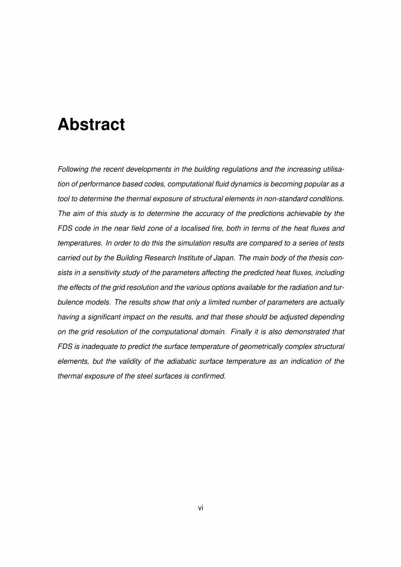
Abstract

Following the recent developments in the building regulations and the increasing utilisa-

tion of performance based codes, computational fluid dynamics is becoming popular as a

tool to determine the thermal exposure of structural elements in non-standard conditions.

The aim of this study is to determine the accuracy of the predictions achievable by the

FDS code in the near field zone of a localised fire, both in terms of the heat fluxes and

temperatures. In order to do this the simulation results are compared to a series of tests

carried out by the Building Research Institute of Japan. The main body of the thesis con-

sists in a sensitivity study of the parameters affecting the predicted heat fluxes, including

the effects of the grid resolution and the various options available for the radiation and tur-

bulence models. The results show that only a limited number of parameters are actually

having a significant impact on the results, and that these should be adjusted depending

on the grid resolution of the computational domain. Finally it is also demonstrated that

FDS is inadequate to predict the surface temperature of geometrically complex structural

elements, but the validity of the adiabatic surface temperature as an indication of the

thermal exposure of the steel surfaces is confirmed.

vi

Introduction

Localised fires

By definition, every fire should be considered as a localised fire before flash-over occurs

in the compartment. This is explicitly stated in Eurocode 1 and alternative methods are

prescribed for situations “where flash-over is unlikely to occur”[4]

.

The objective of the thesis is to validate the CFD code FDS against a series of ex-

periments reproducing a fire with constant heat release rate in well ventilated conditions.

The floor and the ceiling constitute the only boundaries in the compartment and in such

conditions flash-over conditions cannot be reached. Therefore the thermal exposure re-

mains constant for a long period of time and this will have a very different effect on the

structural elements in the compartment compared to fast growing fires.

This is the reason why Computational Fluid Dynamics is often used for modelling

purposes when the conditions are unclear and a distinction between localised and fully

developed fires is not possible.

Performance Based Approach to Design

Performance based regulations allow to use alternative methods to the prescriptive de-

sign codes developed for standard buildings and fire scenarios. However, in order to be

accepted by regulatory authorities, the alternative methods need to be valid and reliable.

This of course applies to all the CFD codes developed in the last decades and it explains

the necessity of rigorous validation studies.

1

CFD models can be divided into three categories:

• RANS

The acronym RANS stands for Reynolds-averaged form of the Navier-Stokes equa-

tions. This model can be used to describe complex geometries and can include a

large number of parameters.

RANS models were developed as “statistically time-averaged equations that de-

scribe the principle of mass, momentum, energy and species conservation”[15]

.

Because of this averaging procedure large eddy transport coefficients are required

or equations approximating turbulence have to be added (such as the two-equation

k − ε turbulence model)

• LES

Large Eddy Simulation models are computationally much more expensive than

RANS and became more popular for engineering applications only when the com-

putational power of personal computers started to increase.

This technique is capable of describing the turbulent mixing of the gaseous fuel

and combustion products with the atmosphere, which determines the burning rate

in most fires and controls the spread of smoke and hot gases.

However, because LES uses spatial averaging (or filtering), not all the turbulent

eddies are large enough to be calculated. This means that the mesh chosen for

a simulation determines the size of the eddies that are resolvable and therefore

smaller eddies are modelled using an approximated sub-grid model. This process

is called low-pass filtering and reduces the computational cost of the simulation.

• DNS

Direct Numerical Simulations reproduce the flow field structure by exactly simulating

the fluctuations of all turbulent properties without any additional turbulence model.

That means that the whole range of spatial and temporal scales of the turbulence

must be resolved in the computational mesh.

The computational cost of DNS is very high and its widespread use in fire safety

engineering is currently unrealistic.

2

In this project we used exclusively the popular LES code developed by NIST called FDS

(Fire Dynamics Simulator). Many alternatives are available in commerce, for example

Ansys CFX and STAR-CCM+. Another popular open source alternative is OpenFOAM.

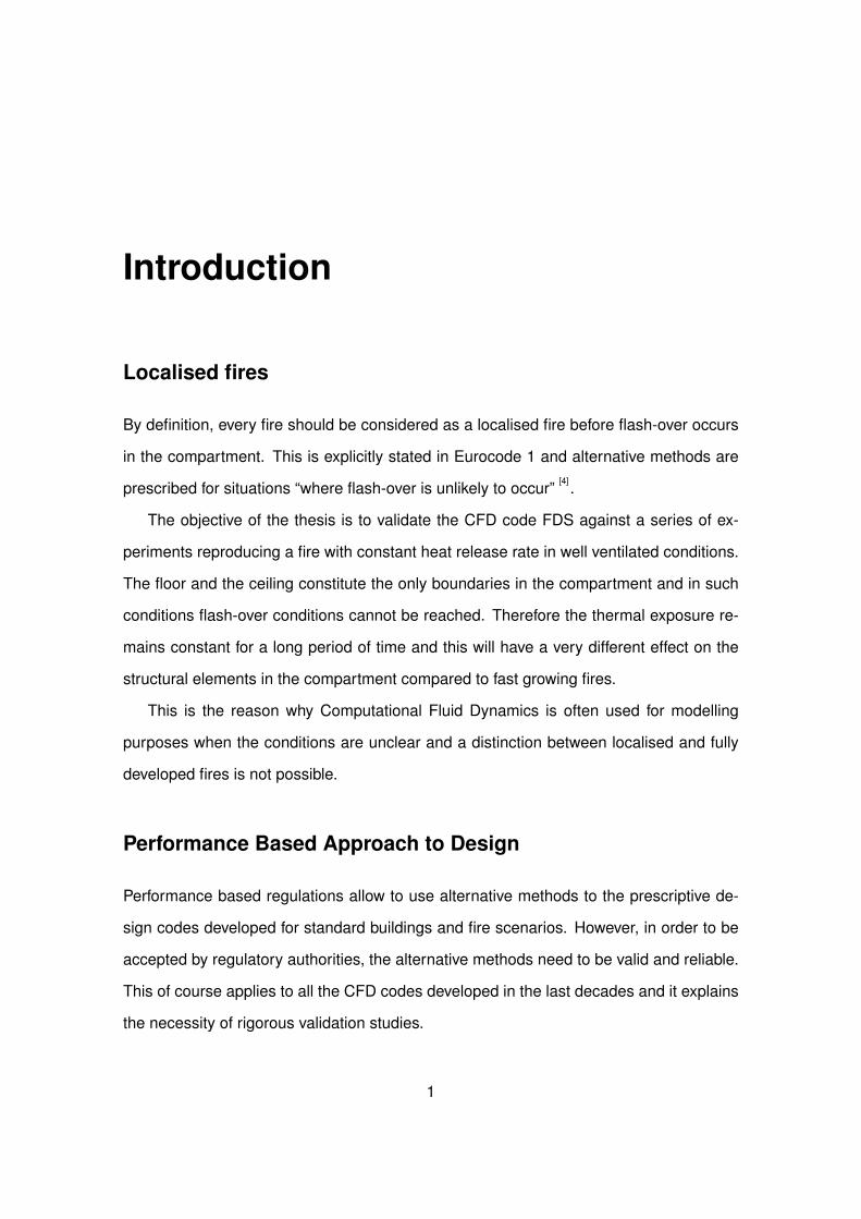
Experiment Description

The main objective of the thesis is to model and simulate the experiments carried out at

the Building Research Institute (BRI) of Japan in 1996. The experimental setup and the

results obtained are presented in a paper titled “Experimental and Numerical Study on the

Behaviour of a Steel Beam under Ceiling Exposed to a Localised Fire” by A. Pchelintstev,

Y. Hasemi, T. Wakamatsu, Y. Yokobayashi. Full-scale experiments were conducted by

the same organisation in 2003[29]

, but our priority is to study the small-scale tests first,

and compare the results to the previous numerical studies available to us.

Figure 1: Experimental layout

Experimental Apparatus

The setup reproduces a typical steel beam and ceiling system. The experiment is scaled

down to a third of typical dimensions for steel frames and the conditions can be compared

3

to the ones of a car catching fire under a steel beam in an open and well ventilated car

park. The experimental apparatus[10]

includes:

• Burner

The burners used propane as the fuel and the flame can be assumed to be uniform.

Complete combustion was also assumed. Two types of burners were used: one

has a circular area with 0.5 m diameter, the other is square and the diameter (of the

interior circle) is 1m.

• Steel beam

The steel beam is 3.6m long and it is held by two steel columns at each end. The

width of the section is equal to 75 mm, the depth is 150 mm, the web thickness is 5

mm and the flanges are 6 mm thick. The beam is not insulated.

• Ceiling

The flat ceiling in the experiment was constructed using two perlite boards 1.83m

wide and 3.60m long. The total thickness of the ceiling is 24 mm (each board is 12

mm thick) and steel reinforcement was used to ensure its stability.

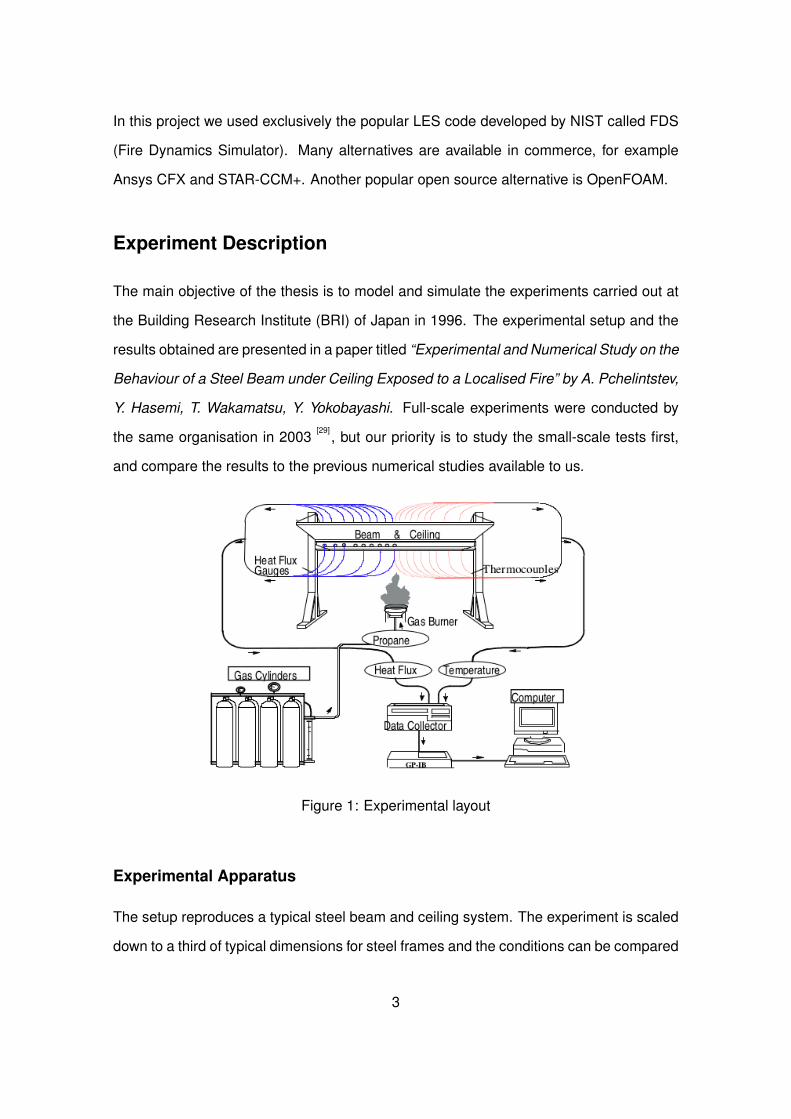
• Heat flux gauges

Heat flux gauges are placed on the left half of the beam at regular intervals starting

from the stagnation point. At each of these locations, one gauge is placed on the

upper flange, one on the web, one on the top surface of the lower flange and on the

lower side. They are water-cooled Schmidt-Boelter gauges (the temperature can be

assumed to be constant at 55°C) and were installed by drilling into the steel beam.

• Thermocouples

The thermocouples were placed on the right side of the beam and their location is

symmetrical to the one of the heat flux gauges but the temperature on the upper

side of the lower flange however was not measured. The devices are K-type ther-

mocouples, with a diameter of 0.2 mm, and were embedded 0.5 mm into the steel

surface.

4

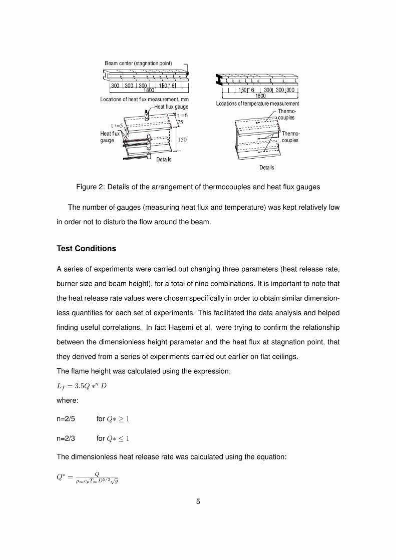
Figure 2: Details of the arrangement of thermocouples and heat flux gauges

The number of gauges (measuring heat flux and temperature) was kept relatively low

in order not to disturb the flow around the beam.

Test Conditions

A series of experiments were carried out changing three parameters (heat release rate,

burner size and beam height), for a total of nine combinations. It is important to note that

the heat release rate values were chosen specifically in order to obtain similar dimension-

less quantities for each set of experiments. This facilitated the data analysis and helped

finding useful correlations. In fact Hasemi et al. were trying to confirm the relationship

between the dimensionless height parameter and the heat flux at stagnation point, that

they derived from a series of experiments carried out earlier on flat ceilings.

The flame height was calculated using the expression:

Lf = 3.5Q ∗n D

where:

n=2/5 for Q∗ ≥ 1

n=2/3 for Q∗ ≤ 1

The dimensionless heat release rate was calculated using the equation:

Q∗ =.Q

ρ∞cpT∞D5/2√g

5

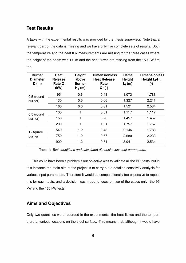
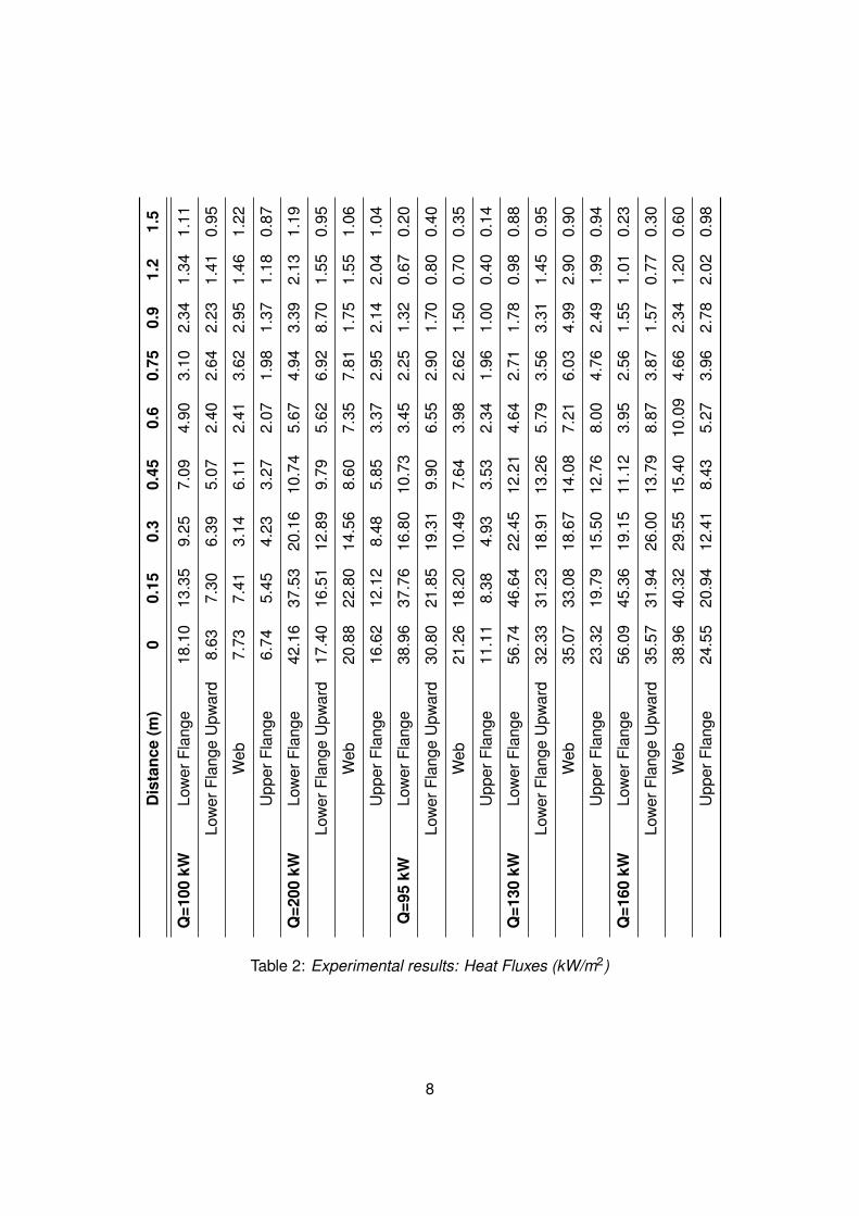
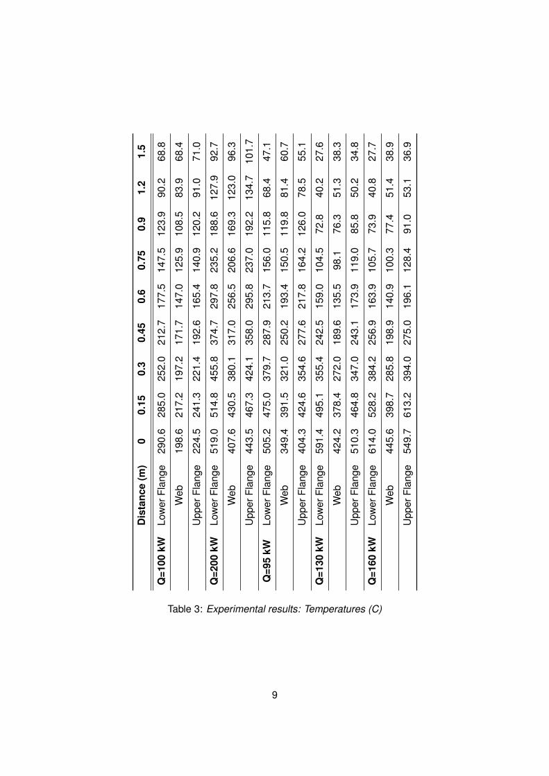
Test Results

A table with the experimental results was provided by the thesis supervisor. Note that a

relevant part of the data is missing and we have only five complete sets of results. Both

the temperature and the heat flux measurements are missing for the three cases where

the height of the beam was 1.2 m and the heat fluxes are missing from the 150 kW fire

too.

BurnerDiameter

D (m)

HeatReleaseRate Q(kW)

HeightaboveBurnerHb (m)

DimensionlessHeat Release

RateQ* (-)

FlameHeightLf (m)

DimensionlessHeight Lf/Hb

(-)

0.5 (roundburner)

95 0.6 0.48 1.073 1.788

130 0.6 0.66 1.327 2.211

160 0.6 0.81 1.521 2.534

0.5 (roundburner)

100 1 0.51 1.117 1.117

150 1 0.76 1.457 1.457

200 1 1.01 1.757 1.757

1 (squareburner)

540 1.2 0.48 2.146 1.788

750 1.2 0.67 2.680 2.233

900 1.2 0.81 3.041 2.534

Table 1: Test conditions and calculated dimensionless test parameters.

This could have been a problem if our objective was to validate all the BRI tests, but in

this instance the main aim of the project is to carry out a detailed sensitivity analysis for

various input parameters. Therefore it would be computationally too expensive to repeat

this for each tests, and a decision was made to focus on two of the cases only: the 95

kW and the 160 kW tests

Aims and Objectives

Only two quantities were recorded in the experiments: the heat fluxes and the temper-

ature at various locations on the steel surface. This means that, although it would have

6

been important to investigate the results of FDS in the gas phase, we are limited to the

following two problems:

• HEAT FLUX DISTRIBUTION

The heat fluxes measured by the gauges in the experiment can be compared di-

rectly to the simulation results by using the ’HEAT FLUX GAUGE’ output quantity.

Also, because the gauges are water cooled, the heat fluxes measured at these

points are decoupled and independent from the temperature of the steel surface.

This is critical because it allows us to eliminate (almost completely) the systematic

error caused by the one-dimensional heat conduction model used by FDS in the

solid phase.

• SURFACE TEMPERATURE OF THE STEEL

FDS in not capable of taking into account the lateral heat conduction within the

beam. A Finite Element Analysis would usually take care of this aspect of the prob-

lem, once the CFD code successfully estimated the thermal environment and the

gas temperatures surrounding the structural member. However it is important to

determine the level of accuracy achievable using FDS, since this could be used to

estimate the temperature of steel elements in design situations . Finally, alternative

quantities defining the surface temperature will be studied. In particular the Adia-

batic Surface Temperature became recently more popular as a way to define the

thermal exposure a structural member is exposed to.

7

Dis

tanc

e(m

)0

0.15

0.3

0.45

0.6

0.75

0.9

1.2

1.5

Q=1

00kW

Low

erFl

ange

18.1

013

.35

9.25

7.09

4.90

3.10

2.34

1.34

1.11

Low

erFl

ange

Upw

ard

8.63

7.30

6.39

5.07

2.40

2.64

2.23

1.41

0.95

Web

7.73

7.41

3.14

6.11

2.41

3.62

2.95

1.46

1.22

Upp

erFl

ange

6.74

5.45

4.23

3.27

2.07

1.98

1.37

1.18

0.87

Q=2

00kW

Low

erFl

ange

42.1

637

.53

20.1

610

.74

5.67

4.94

3.39

2.13

1.19

Low

erFl

ange

Upw

ard

17.4

016

.51

12.8

99.

795.

626.

928.

701.

550.

95

Web

20.8

822

.80

14.5

68.

607.

357.

811.

751.

551.

06

Upp

erFl

ange

16.6

212

.12

8.48

5.85

3.37

2.95

2.14

2.04

1.04

Q=9

5kW

Low

erFl

ange

38.9

637

.76

16.8

010

.73

3.45

2.25

1.32

0.67

0.20

Low

erFl

ange

Upw

ard

30.8

021

.85

19.3

19.

906.

552.

901.

700.

800.

40

Web

21.2

618

.20

10.4

97.

643.

982.

621.

500.

700.

35

Upp

erFl

ange

11.1

18.

384.

933.

532.

341.

961.

000.

400.

14

Q=1

30kW

Low

erFl

ange

56.7

446

.64

22.4

512

.21

4.64

2.71

1.78

0.98

0.88

Low

erFl

ange

Upw

ard

32.3

331

.23

18.9

113

.26

5.79

3.56

3.31

1.45

0.95

Web

35.0

733

.08

18.6

714

.08

7.21

6.03

4.99

2.90

0.90

Upp

erFl

ange

23.3

219

.79

15.5

012

.76

8.00

4.76

2.49

1.99

0.94

Q=1

60kW

Low

erFl

ange

56.0

945

.36

19.1

511

.12

3.95

2.56

1.55

1.01

0.23

Low

erFl

ange

Upw

ard

35.5

731

.94

26.0

013

.79

8.87

3.87

1.57

0.77

0.30

Web

38.9

640

.32

29.5

515

.40

10.0

94.

662.

341.

200.

60

Upp

erFl

ange

24.5

520

.94

12.4

18.

435.

273.

962.

782.

020.

98

Table 2: Experimental results: Heat Fluxes (kW/m2)

8

Dis

tanc

e(m

)0

0.15

0.3

0.45

0.6

0.75

0.9

1.2

1.5

Q=1

00kW

Low

erFl

ange

290.

628

5.0

252.

021

2.7

177.

514

7.5

123.

990

.268

.8

Web

198.

621

7.2

197.

217

1.7

147.

012

5.9

108.

583

.968

.4

Upp

erFl

ange

224.

524

1.3

221.

419

2.6

165.

414

0.9

120.

291

.071

.0

Q=2

00kW

Low

erFl

ange

519.

051

4.8

455.

837

4.7

297.

823

5.2

188.

612

7.9

92.7

Web

407.

643

0.5

380.

131

7.0

256.

520

6.6

169.

312

3.0

96.3

Upp

erFl

ange

443.

546

7.3

424.

135

8.0

295.

823

7.0

192.

213

4.7

101.

7

Q=9

5kW

Low

erFl

ange

505.

247

5.0

379.

728

7.9

213.

715

6.0

115.

868

.447

.1

Web

349.

439

1.5

321.

025

0.2

193.

415

0.5

119.

881

.460

.7

Upp

erFl

ange

404.

342

4.6

354.

627

7.6

217.

816

4.2

126.

078

.555

.1

Q=1

30kW

Low

erFl

ange

591.

449

5.1

355.

424

2.5

159.

010

4.5

72.8

40.2

27.6

Web

424.

237

8.4

272.

018

9.6

135.

598

.176

.351

.338

.3

Upp

erFl

ange

510.

346

4.8

347.

024

3.1

173.

911

9.0

85.8

50.2

34.8

Q=1

60kW

Low

erFl

ange

614.

052

8.2

384.

225

6.9

163.

910

5.7

73.9

40.8

27.7

Web

445.

639

8.7

285.

819

8.9

140.

910

0.3

77.4

51.4

38.9

Upp

erFl

ange

549.

761

3.2

394.

027

5.0

196.

112

8.4

91.0

53.1

36.9

Table 3: Experimental results: Temperatures (C)

9

Chapter 1

Literature Review

For a series of reasons, including the time required to familiarise with FDS and develop

a preliminarry model, the first simulation results were obtained relatively late. Therefore

most of the reading list is taken up by the FDS documentation and by similar FDS studies.

For clarity we can divide the literature review into five main sections.

1.1 Technical References

On the FDS official web page various manuals can be downloaded[5, 20, 18, 22, 21, 19]

. In our

case the most important are:

• FDS Technical Reference Guide Volume 1: Mathematical Model

This manual contains the explanations of the mathematical models and the algo-

rithms used by FDS. It was particularly important to understand the radiation model

and the turbulence model.

• FDS Technical Reference Guide Volume 3: Validation Guide

This guide provides a very large number of validation cases and explains the re-

search methodology for each case. Most of the cases are related to compartment

fires or the fire dynamics of burning plumes.

• FDS Technical Reference Guide Volume 4: Configuration Manual

This manual was extremely useful to solve a number of technical problems, such

10

as the software installation, running parallel calculations and other IT issues.

• FDS User Guide

This was by far the document that was used the most. This guide contains ev-

erything that is required to write an FDS input file, it explains the most common

parameters significance and describes the issues related to each of them.

In addition to these:

• The FDS discussion group on Google is a valuable source of information and con-

tains a large number of resolved issues and clarifications to the manuals. It also

allows to contact directly the developers.

• A reduced version of the User’s Manual was used at the beginning of the project.

This guide, written by E. Gissi, is titled "An Introduction to Fire Simulation with FDS

and Smokeview" and was particularly useful for the baseline model construction,

thanks to the large number of examples and summary tables.

1.2 Experimental Results

• The experimental conditions are presented in “Experimental and Numerical Study

on the Behaviour of a Steel Beam under Ceiling Exposed to a Localised Fire” by

Hasemi, Pchelintstev, Wakamatsu and Yokobayashi. The same authors carried

out a series of similar experiments using a real-scale set up but these were not

considered in this thesis.

• Two NIST publications about the calibration of thermocouples and heat flux gauges[27] [24]

were used to attempt an estimation of the experimental uncertainties, ignored

by Hasemi et al. in their study. However, due to the lack of test records, this study

was abandoned.

11

1.3 Previous Numerical Investigations

This section can be ulteriorly divided into two parts, depending on the CFD codes used

in each case: The most relevant studies that used RANS modelling are:

• "Numerical Prediction of Heat Transfer to a Steel Beam in a Fire" by Welch and

Pchelintsev[30]

, describing the results obtained by simulating the BRI tests using

the SOFIE CFD code.

• The BRE report[14]

, published in 2000, titled “The Development and Validation of a

CFD-based Engineering Methodology for Evaluating Thermal Action on Steel and

Composite Structures” contains additional information about the study above.

The most relevant studies that used FDS are:

• “Thermal Behavior of a Steel Beam Exposed to a Localized Fire – Numerical Sim-

ulation and Comparison with Experimental Results” by Zhang and Li. The report

describes the results obtained using FDS 5, to model Hasemi’s tests. The details

of the sensitivity study are missing and only one case (100 kW) is presented[33]

.

• “Experiments and Modeling of Structural Steel Elements Exposed to Fire”, pub-

lished by NIST, is a report of the investigations carried out after the World Trade

Center Disaster. The model of the steel trusses in the towers is particularly relevant[9]

, and offered many suggestions for our study.

• Numerous other publications[8, 3, 34, 35]

, for example “Simulating the behavior of re-

strained steel beams to flame impingement from localized-fires” by Zhang, Usmani

and Li, are interested in the same problem, but the focus of the study is on the Finite

Element Analysis based on the CFD results. The main objective of these studies is

to predict the mechanical behaviour of the steel beam.

12

1.4 Analytical Methods for Localised Fires

• The basic equations used to describe the fire plumes behaviour are presented in

“An Introduction to Fire Dynamics” by Drysdale. Also, the book was a valid refer-

ence for most of the fire dynamics issues encountered during the thesis

• Eurocode 1 provides an analytical model to estimate the heat fluxes and the tem-

perature of structural members in localised fires[4]

• An alternative but similar method is given in the SFPE Handbook of Fire Protection

Engineering[16]

.

• An interesting analytic technique using the Adiabatic Surface Temperature pre-

dicted by FDS to estimate the actual temperature of the steel is proposed by Zhang,

Li and Wang in the paper titled “Using Adiabatic Surface Temperature for Thermal

Calculation of Steel Members Exposed to Localized Fires”. In this regard, it is also

useful to consider Wilkström’s study on the conceptual development of the adiabatic

surface temperature[32]

.

1.5 CFD Guidelines

Finally other papers tried to evaluate the potential impact of FDS and other CFD applica-

tions on performance based engineering solutions: The most important were:

• "Fire Modelling with Computational Fluid Dynamics” by Kumar

• "An Introduction to the use of Fire Modelling" by Chitty

• “Global Modelling of Structures in Fire” by Gillie

13

Chapter 2

Empirical Correlations and Design

Codes

2.1 Eurocode 1

Computational Fluid Dynamics modelling is mentioned in Eurocode 1, but no specific

guidelines are indicated. Instead, for localised fire scenarios, the design codes suggest

the use of some simple empirical correlations. Incidentally these equations are derived

from a series of experiments conducted by Hasemi, studying the impingement of flames

on a flat ceiling.

Figure 2.1: Diagram of the EC1 model

14

A spreadsheet was prepared, based on this model, and the calculations were carried

out for two of the tests (the 95 kW and 160 kW one) considering only the lower flange of

the beam. The procedure is:

1. Calculate two non-dimensional heat release rates in terms of the fire source diam-

eter D and the beam height H:

Q∗H = Q/(1.11× 106H2.5)

Q∗D = Q/(1.11× 106D2.5)

2. Calculate the horizontal flame length Lh

Lh = (2.9H(Q∗H)0.33)−H

3. Calculate the virtual heat source z′

z′ = 2.4D(Q∗2/5D −Q∗2/3D ) if Q∗D < 1

z′ = 2.4D(Q∗2/5D −Q∗2/3D ) if Q∗D ≥ 1

4. Calculate the parameter y for each measurement point, based on the horizontal

distance r from the stagnation point:

y =r +H + z′

Lh +H + z′

5. Calculate the incident heat flux.q′′inc (in kW/m2) :

.q′′inc = 100 if y ≤ 0.3

.q′′inc = 136.3− 121y if 0.3 < y < 1

.q′′inc = 15y−3.7 if y ≥ 1

6. Calculate the net heat flux.q′′net:

.q′′net =

.q′′inc − hc(Tw − 20)− Φεmεfσ[(Tw + 273)4 − 2934]

15

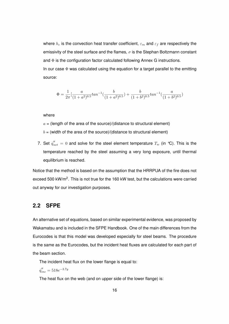
where hc is the convection heat transfer coefficient, εm and εf are respectively the

emissivity of the steel surface and the flames, σ is the Stephan Boltzmann constant

and Φ is the configuration factor calculated following Annex G instructions.

In our case Φ was calculated using the equation for a target parallel to the emitting

source:

Φ =1

2π[

a

(1 + a2)0.5tan−1(

b

(1 + a2)0.5) +

b

(1 + b2)0.5tan−1(

a

(1 + b2)0.5)

where

a = (length of the area of the source)/(distance to structural element)

b = (width of the area of the source)/(distance to structural element)

7. Set.q′′net = 0 and solve for the steel element temperature Tw (in °C). This is the

temperature reached by the steel assuming a very long exposure, until thermal

equilibrium is reached.

Notice that the method is based on the assumption that the HRRPUA of the fire does not

exceed 500 kW/m2. This is not true for the 160 kW test, but the calculations were carried

out anyway for our investigation purposes.

2.2 SFPE

An alternative set of equations, based on similar experimental evidence, was proposed by

Wakamatsu and is included in the SFPE Handbook. One of the main differences from the

Eurocodes is that this model was developed especially for steel beams. The procedure

is the same as the Eurocodes, but the incident heat fluxes are calculated for each part of

the beam section.

The incident heat flux on the lower flange is equal to:.q′′inc = 518e−3.7y

The heat flux on the web (and on upper side of the lower flange) is:

16

.q′′inc = 148.1e−2.75y

And lastly, the heat flux on lower side of the upper flange is:.q′′inc = 100.5e−2.85y

2.3 Results

In the following graphs we can see the different results obtained using the EC1 and the

SFPE models and their level of accuracy. The results are limited to the lower side of the

lower flange due to the fact that the EC1 model was developed for flat ceilings only. For

this reason, the EC1 results should be more conservative, and this is confirmed by the

graphs.

Before looking at the figures however we must consider that:

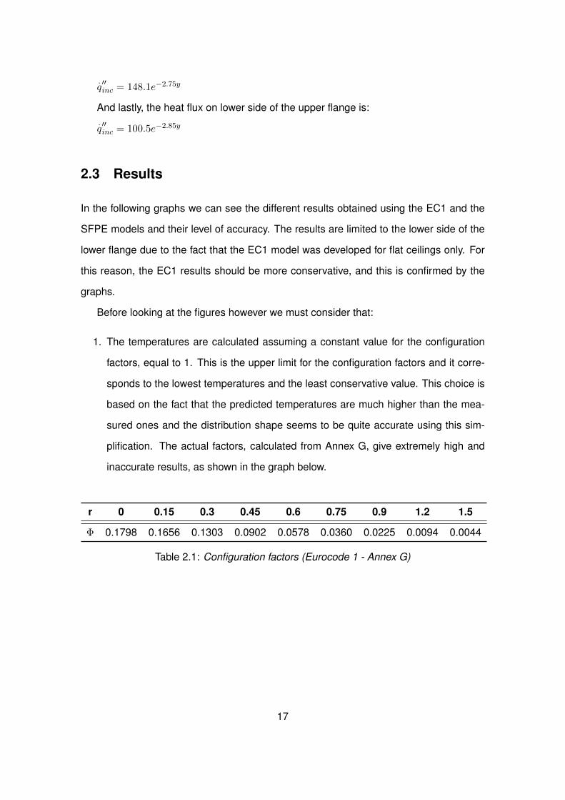
1. The temperatures are calculated assuming a constant value for the configuration

factors, equal to 1. This is the upper limit for the configuration factors and it corre-

sponds to the lowest temperatures and the least conservative value. This choice is

based on the fact that the predicted temperatures are much higher than the mea-

sured ones and the distribution shape seems to be quite accurate using this sim-

plification. The actual factors, calculated from Annex G, give extremely high and

inaccurate results, as shown in the graph below.

r 0 0.15 0.3 0.45 0.6 0.75 0.9 1.2 1.5

Φ 0.1798 0.1656 0.1303 0.0902 0.0578 0.0360 0.0225 0.0094 0.0044

Table 2.1: Configuration factors (Eurocode 1 - Annex G)

17

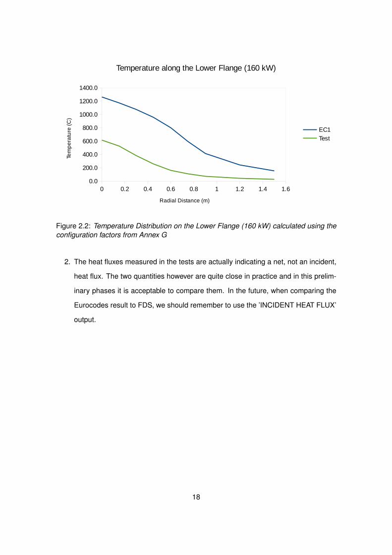
Figure 2.2: Temperature Distribution on the Lower Flange (160 kW) calculated using theconfiguration factors from Annex G

2. The heat fluxes measured in the tests are actually indicating a net, not an incident,

heat flux. The two quantities however are quite close in practice and in this prelim-

inary phases it is acceptable to compare them. In the future, when comparing the

Eurocodes result to FDS, we should remember to use the ’INCIDENT HEAT FLUX’

output.

18

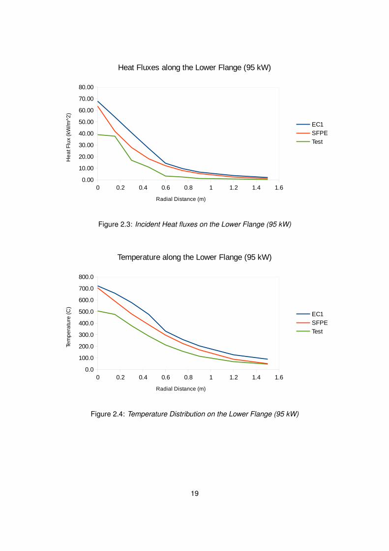
Figure 2.3: Incident Heat fluxes on the Lower Flange (95 kW)

Figure 2.4: Temperature Distribution on the Lower Flange (95 kW)

19

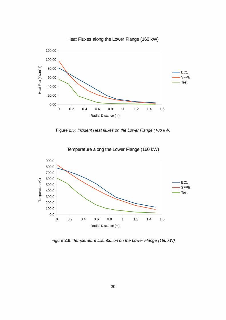
Figure 2.5: Incident Heat fluxes on the Lower Flange (160 kW)

Figure 2.6: Temperature Distribution on the Lower Flange (160 kW)

20

Parameter Value Units

T∞ 20 C

T∞ 293 K

εsteel 0.9 -

εfire 1 -

h 25 W/m2K

σ 5.67E-008 W/m2K

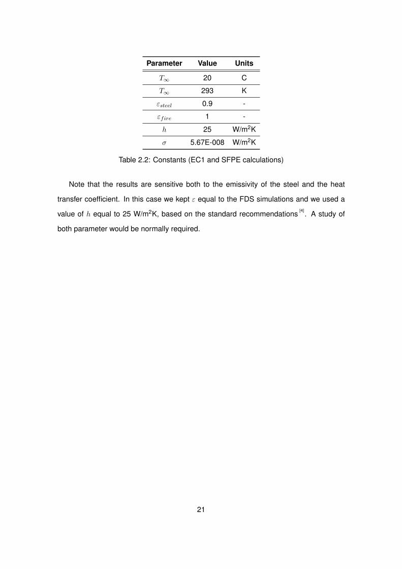
Table 2.2: Constants (EC1 and SFPE calculations)

Note that the results are sensitive both to the emissivity of the steel and the heat

transfer coefficient. In this case we kept ε equal to the FDS simulations and we used a

value of h equal to 25 W/m2K, based on the standard recommendations[4]

. A study of

both parameter would be normally required.

21

Chapter 3

SOFIE CFD Numerical Investigation

3.1 Model Description

In 1997 Welch and Pchelintsev carried out a study in order to validate the SOFIE CFD

code (developed within the BRE group) using Hasemi’s experimental data.

The study was one of the most important references throughout the whole project, in

part because of the level of detail, in part due to the availability of the results and the role

of Dr. Stephen Welch as the thesis supervisor, but most importantly it was used to define

the research methodology.

The study can be divided into three parts: the construction of the model (which can

be called the baseline model), a sensitivity analysis of the numerical parameters affecting

the results, and the discussion of the results compared to the experimental data. The

structure of our thesis is the same, and our sensitivity study is also based on the SOFIE

CFD one. Even though the two models are very different with respect to the numerical

methods used to solve the transport and the radiation equations, the parameters that can

be defined by the user are very similar and fall into three main categories:

• Grid Resolution

• Radiation Model

• Turbulence Model

22

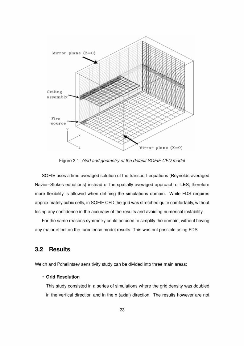
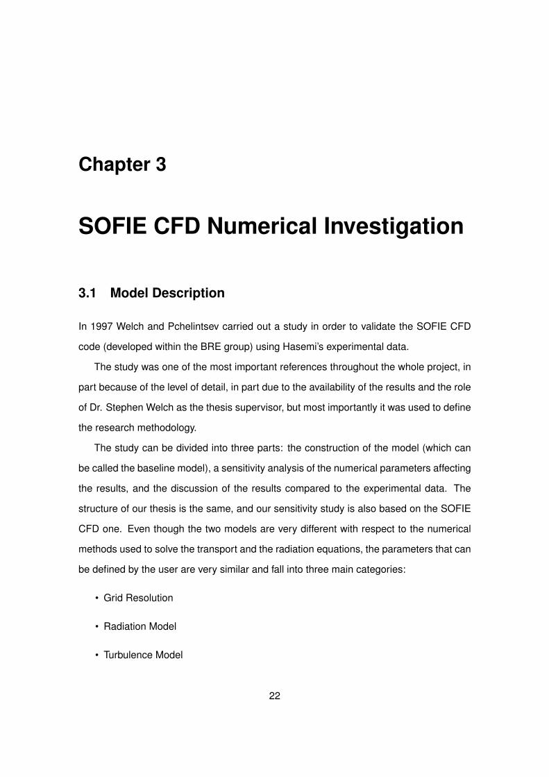
Figure 3.1: Grid and geometry of the default SOFIE CFD model

SOFIE uses a time averaged solution of the transport equations (Reynolds-averaged

Navier–Stokes equations) instead of the spatially averaged approach of LES, therefore

more flexibility is allowed when defining the simulations domain. While FDS requires

approximately cubic cells, in SOFIE CFD the grid was stretched quite comfortably, without

losing any confidence in the accuracy of the results and avoiding numerical instability.

For the same reasons symmetry could be used to simplify the domain, without having

any major effect on the turbulence model results. This was not possible using FDS.

3.2 Results

Welch and Pchelintsev sensitivity study can be divided into three main areas:

• Grid Resolution

This study consisted in a series of simulations where the grid density was doubled

in the vertical direction and in the x (axial) direction. The results however are not

23

presented in the publications.

• Radiation Model

This was the most extended part of the study. The main parameters analysed are

the number of solid angles and the number of polar angles used by the RTE solver.

The parameters defining the "mixed grey gas model” used by SOFIE were also

studied in detail.

The results of the sensitivity analysis show that the impact of the RTE discretization

and the modified absorption coefficients was minor.

• Turbulence Model

A series of simulations were run in order to show the effects of the Schmidt-Prandtl

number in the viscosity equation. Additionally the eddy break-up equation param-

eters were studied and various other variations were tested, including the Rodi

centerline corrections and Bilger’s additional density factor.

Because of the nature of the fire source and its simplicity, the study of the combustion

model parameters was ignored.

Figure 3.2: 95 kW test: SOFIE CFD predicted heat fluxes (Lower Flange Downwards)

24

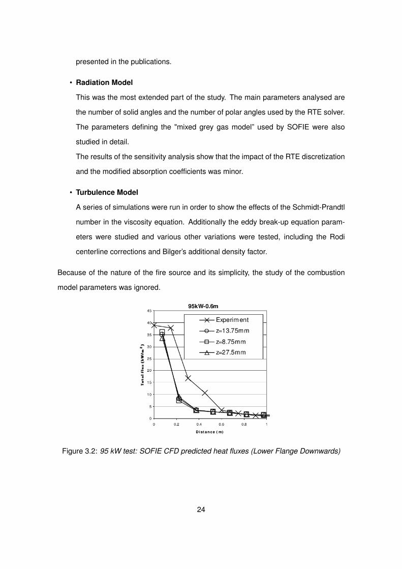
Figure 3.3: 160 kW test: SOFIE CFD predicted heat fluxes (Lower Flange Downwards)

The plots above show the results obtained for the 95 kW and the 160 kW tests. The

different curves on the graphs refer to the heat fluxes predicted at three different locations

across the lower flange.

Finally note that the temperatures were estimated by using a separate FE analysis

that used the CFD results as boundary conditions for the three dimensional model of the

beam. Interestingly the results are similar to the AST distribution predicted by FDS.

25

Chapter 4

FDS Baseline Model

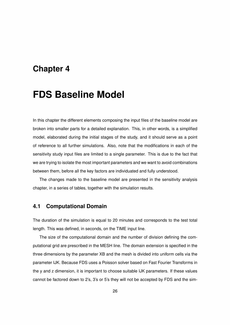
In this chapter the different elements composing the input files of the baseline model are

broken into smaller parts for a detailed explanation. This, in other words, is a simplified

model, elaborated during the initial stages of the study, and it should serve as a point

of reference to all further simulations. Also, note that the modifications in each of the

sensitivity study input files are limited to a single parameter. This is due to the fact that

we are trying to isolate the most important parameters and we want to avoid combinations

between them, before all the key factors are individuated and fully understood.

The changes made to the baseline model are presented in the sensitivity analysis

chapter, in a series of tables, together with the simulation results.

4.1 Computational Domain

The duration of the simulation is equal to 20 minutes and corresponds to the test total

length. This was defined, in seconds, on the TIME input line.

The size of the computational domain and the number of division defining the com-

putational grid are prescribed in the MESH line. The domain extension is specified in the

three dimensions by the parameter XB and the mesh is divided into uniform cells via the

parameter IJK. Because FDS uses a Poisson solver based on Fast Fourier Transforms in

the y and z dimension, it is important to choose suitable IJK parameters. If these values

cannot be factored down to 2’s, 3’s or 5’s they will not be accepted by FDS and the sim-

26

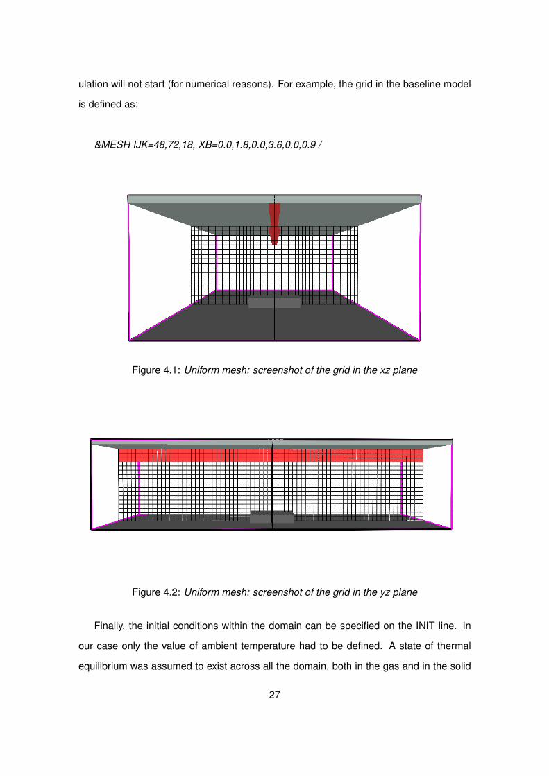
ulation will not start (for numerical reasons). For example, the grid in the baseline model

is defined as:

&MESH IJK=48,72,18, XB=0.0,1.8,0.0,3.6,0.0,0.9 /

Figure 4.1: Uniform mesh: screenshot of the grid in the xz plane

Figure 4.2: Uniform mesh: screenshot of the grid in the yz plane

Finally, the initial conditions within the domain can be specified on the INIT line. In

our case only the value of ambient temperature had to be defined. A state of thermal

equilibrium was assumed to exist across all the domain, both in the gas and in the solid

27

phase. The temperature, as in the rest of the input file, is specified in Celsius degrees.

4.1.1 Mesh Stretching

FDS is provided with a function capable of stretching the cell dimensions in the mesh.

This allows to obtain a much higher resolution in a particular region of the computational

domain, without incurring in the computational cost increase that we would observe using

a finer uniform mesh across the entire domain. Also, the cells can be stretched in two

different modes, using two different functions:

• a piecewise linear linear mesh transformation

• a polynomial mesh transformation

The idea to use one of these options first came up during the literature review, in the ear-

lier stages of the project, and it was motivated by the fact that both Welch and Ptelinchev

in their RANS model[30]

, and Zhang and Li[33]

, in their FDS model, used some sort of

mesh stretching in order to improve the computational efficiency of the simulations.

First, we attempted to use the linear mesh transformation, but we observed that:

1. the simulations often stopped running because of numerical instability. This tend to

occurr almost at the same when the simulations were re-run, but the cause was not

identified.

2. centering and matching the mesh exactly to the beam geometry was more difficult

than expected, and usually caused large and unphysical deformations.

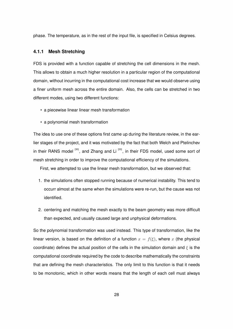
So the polynomial transformation was used instead. This type of transformation, like the

linear version, is based on the definition of a function x = f(ξ), where x (the physical

coordinate) defines the actual position of the cells in the simulation domain and ξ is the

computational coordinate required by the code to describe mathematically the constraints

that are defining the mesh characteristics. The only limit to this function is that it needs

to be monotonic, which in other words means that the length of each cell must always

28

be a positive number, non equal to zero. The graph below shows an example of the

relationship between these two parameters.

Figure 4.3: Polynomial Mesh Transformation: Physical Coordinate (x) VS ComputationalCoordinate (ξ)

Similarly to this case, in our simulation we defined the transformation so that the

length of the cells was halved in the center of the domain, using the following lines after

the MESH line:

&TRNX IDERIV=1, CC=0.9, PC=0.5 /

&TRNX IDERIV=2, CC=0.9, PC=0.0 /

&TRNY IDERIV=1, CC=1.8, PC=0.5 /

&TRNY IDERIV=2, CC=1.8, PC=0.0 /

Finally, it is important to note that the number of cells is not exactly the same com-

pared to the baseline model. The reason of this is that in the third dimension z the cells

cannot and should not be stretched. They cannot be stretched because FDS supports

this function only for two dimensions and they should not be stretched because the nat-

ural phenomena of burning plume, should be resolved as accurately as possible in this

direction.

29

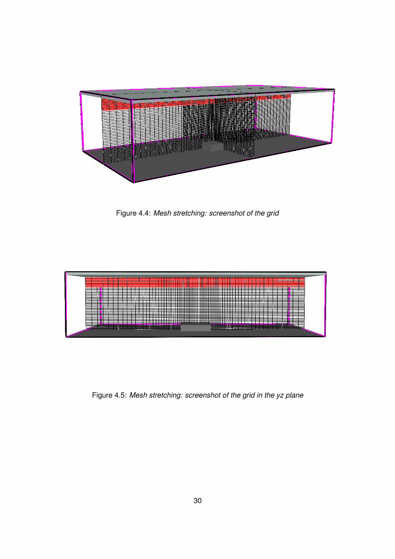
Figure 4.4: Mesh stretching: screenshot of the grid

Figure 4.5: Mesh stretching: screenshot of the grid in the yz plane

30

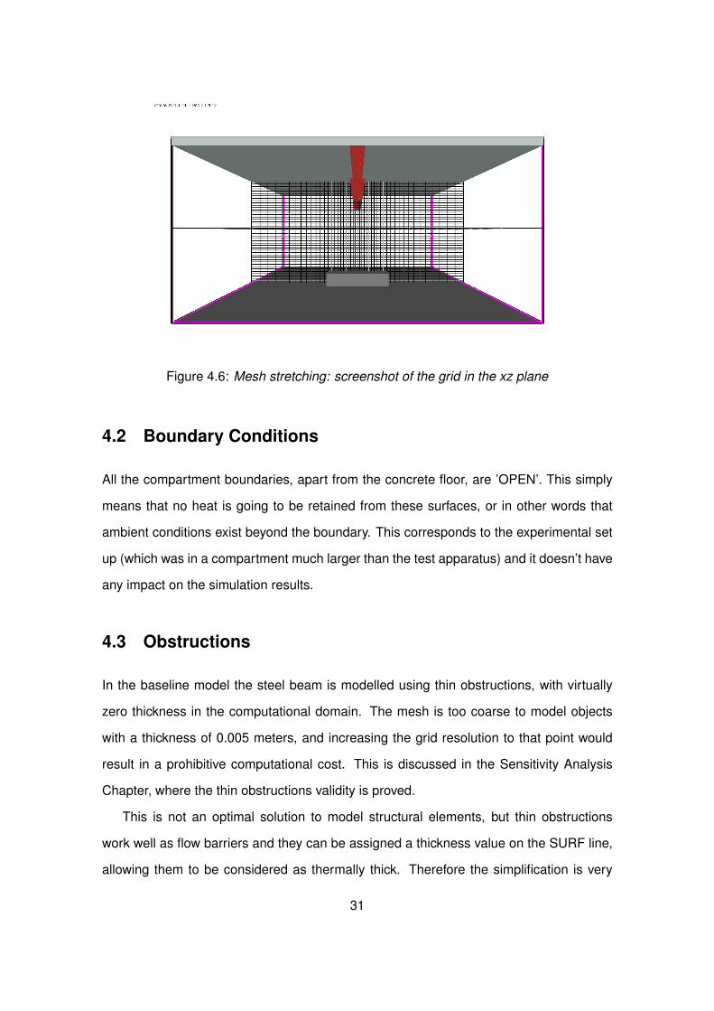
Figure 4.6: Mesh stretching: screenshot of the grid in the xz plane

4.2 Boundary Conditions

All the compartment boundaries, apart from the concrete floor, are ’OPEN’. This simply

means that no heat is going to be retained from these surfaces, or in other words that

ambient conditions exist beyond the boundary. This corresponds to the experimental set

up (which was in a compartment much larger than the test apparatus) and it doesn’t have

any impact on the simulation results.

4.3 Obstructions

In the baseline model the steel beam is modelled using thin obstructions, with virtually

zero thickness in the computational domain. The mesh is too coarse to model objects

with a thickness of 0.005 meters, and increasing the grid resolution to that point would

result in a prohibitive computational cost. This is discussed in the Sensitivity Analysis

Chapter, where the thin obstructions validity is proved.

This is not an optimal solution to model structural elements, but thin obstructions

work well as flow barriers and they can be assigned a thickness value on the SURF line,

allowing them to be considered as thermally thick. Therefore the simplification is very

31

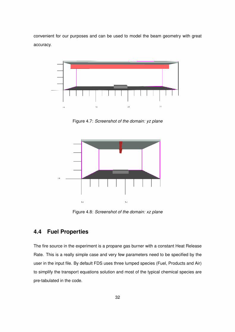
convenient for our purposes and can be used to model the beam geometry with great

accuracy.

Figure 4.7: Screenshot of the domain: yz plane

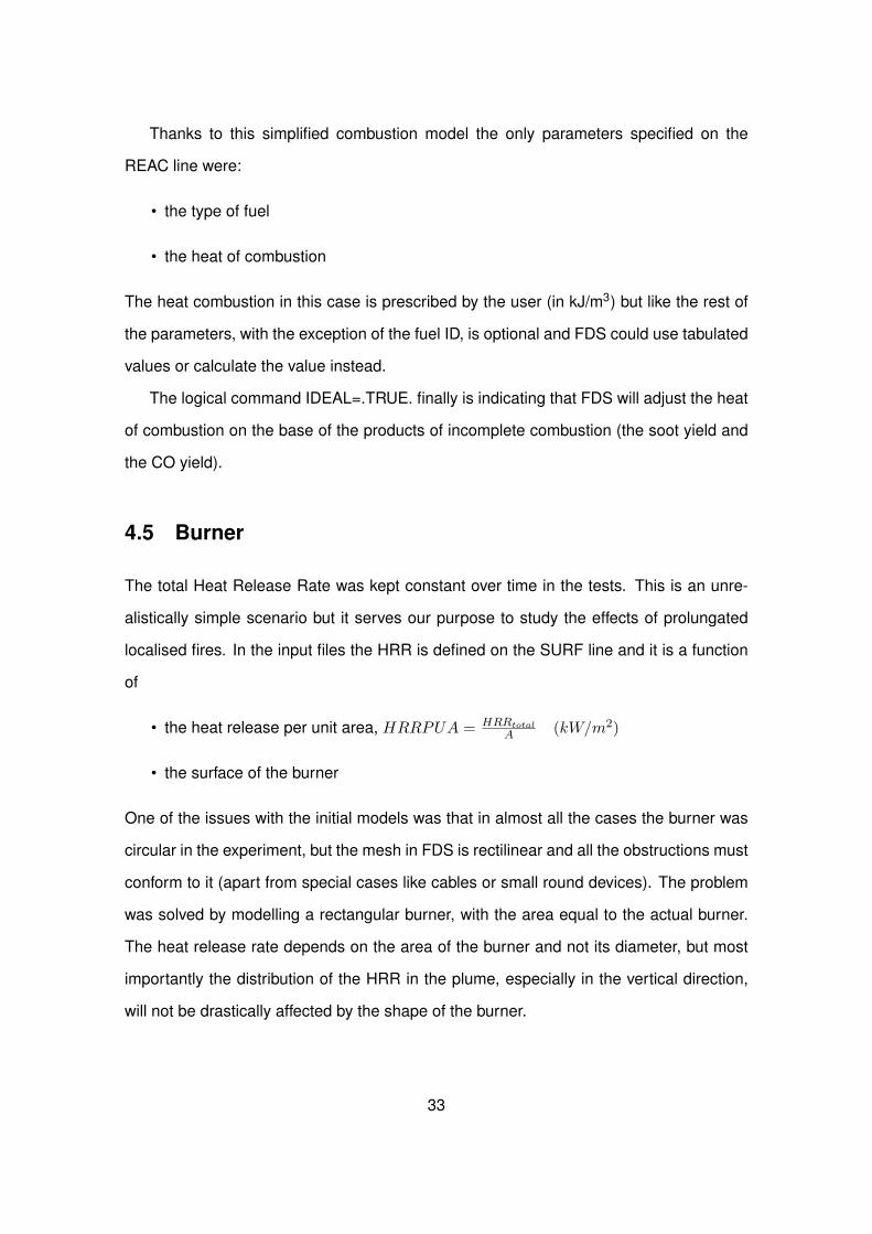
Figure 4.8: Screenshot of the domain: xz plane

4.4 Fuel Properties

The fire source in the experiment is a propane gas burner with a constant Heat Release

Rate. This is a really simple case and very few parameters need to be specified by the

user in the input file. By default FDS uses three lumped species (Fuel, Products and Air)

to simplify the transport equations solution and most of the typical chemical species are

pre-tabulated in the code.

32

Thanks to this simplified combustion model the only parameters specified on the

REAC line were:

• the type of fuel

• the heat of combustion

The heat combustion in this case is prescribed by the user (in kJ/m3) but like the rest of

the parameters, with the exception of the fuel ID, is optional and FDS could use tabulated

values or calculate the value instead.

The logical command IDEAL=.TRUE. finally is indicating that FDS will adjust the heat

of combustion on the base of the products of incomplete combustion (the soot yield and

the CO yield).

4.5 Burner

The total Heat Release Rate was kept constant over time in the tests. This is an unre-

alistically simple scenario but it serves our purpose to study the effects of prolungated

localised fires. In the input files the HRR is defined on the SURF line and it is a function

of

• the heat release per unit area, HRRPUA = HRRtotalA (kW/m2)

• the surface of the burner

One of the issues with the initial models was that in almost all the cases the burner was

circular in the experiment, but the mesh in FDS is rectilinear and all the obstructions must

conform to it (apart from special cases like cables or small round devices). The problem

was solved by modelling a rectangular burner, with the area equal to the actual burner.

The heat release rate depends on the area of the burner and not its diameter, but most

importantly the distribution of the HRR in the plume, especially in the vertical direction,

will not be drastically affected by the shape of the burner.

33

Note that the burner is raised from the floor (by at least the height of two cells). This

should improve the accuracy of the model, facilitate the air entrainment in the burning

plume and simulate the turbulent conditions at the edges of the burner.

4.6 Material Properties

The material properties required for our simulation were all specified in the report “Nu-

merical Prediction of Heat Transfer to a Steel Beam in a Fire” by Welch and Pchelinstev.

The materials to be included in the computational domain are only three:

• Steel

• Concrete

• Perlite

4.6.1 Density

The density is expressed in kg/m3 in FDS. The values used in our simulations are:

ρsteel = 7850 kg/m3

ρperlite = 789 kg/m3

ρconcrete = 2800 kg/m3

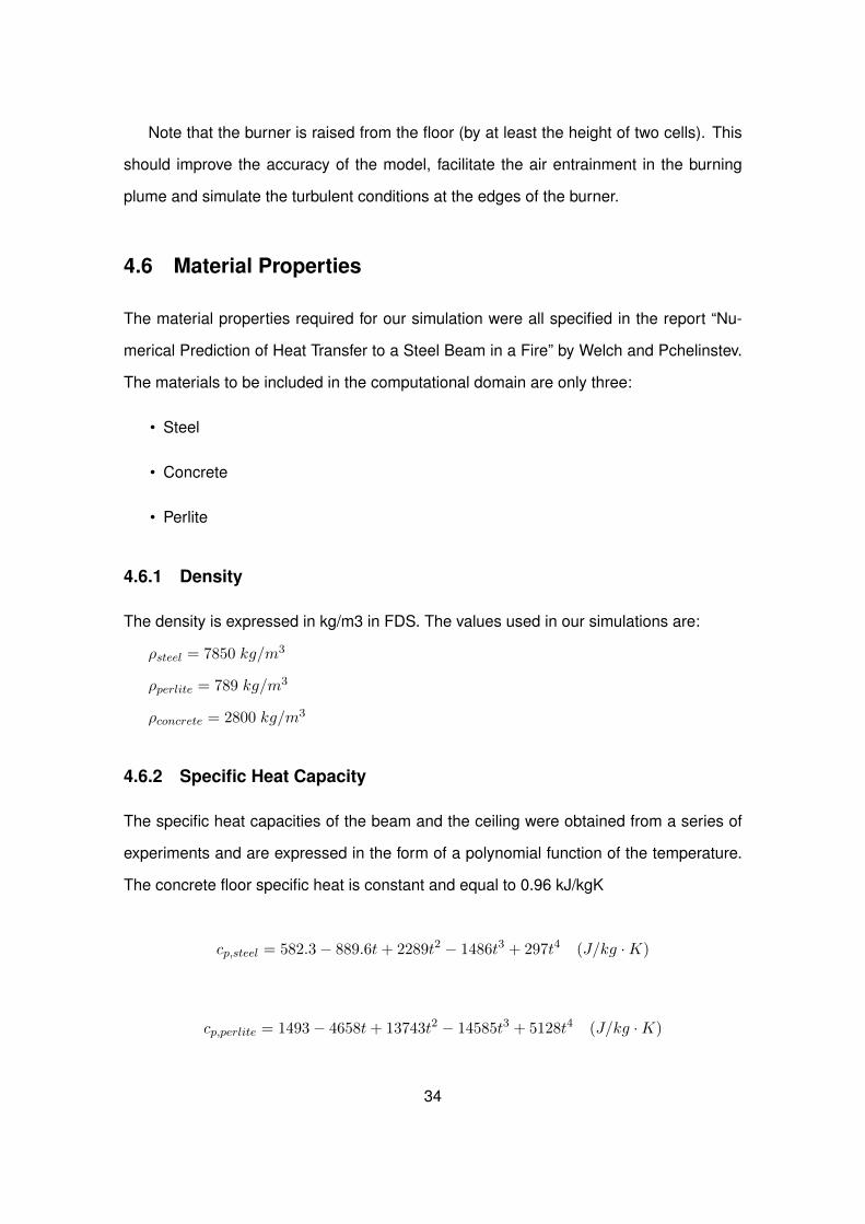
4.6.2 Specific Heat Capacity

The specific heat capacities of the beam and the ceiling were obtained from a series of

experiments and are expressed in the form of a polynomial function of the temperature.

The concrete floor specific heat is constant and equal to 0.96 kJ/kgK

cp,steel = 582.3− 889.6t+ 2289t2 − 1486t3 + 297t4 (J/kg ·K)

cp,perlite = 1493− 4658t+ 13743t2 − 14585t3 + 5128t4 (J/kg ·K)

34

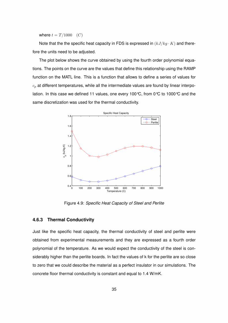
where t = T/1000 (C)

Note that the the specific heat capacity in FDS is expressed in (kJ/kg ·K) and there-

fore the units need to be adjusted.

The plot below shows the curve obtained by using the fourth order polynomial equa-

tions. The points on the curve are the values that define this relationship using the RAMP

function on the MATL line. This is a function that allows to define a series of values for

cp at different temperatures, while all the intermediate values are found by linear interpo-

lation. In this case we defined 11 values, one every 100°C, from 0°C to 1000°C and the

same discretization was used for the thermal conductivity.

0 100 200 300 400 500 600 700 800 900 10000.4

0.6

0.8

1

1.2

1.4

1.6

1.8Specific Heat Capacity

Temperature (C)

cp (

kJ/k

g.K

)

Steel

Perlite

Figure 4.9: Specific Heat Capacity of Steel and Perlite

4.6.3 Thermal Conductivity

Just like the specific heat capacity, the thermal conductivity of steel and perlite were

obtained from experimental measurements and they are expressed as a fourth order

polynomial of the temperature. As we would expect the conductivity of the steel is con-

siderably higher than the perlite boards. In fact the values of k for the perlite are so close

to zero that we could describe the material as a perfect insulator in our simulations. The

concrete floor thermal conductivity is constant and equal to 1.4 W/mK.

35

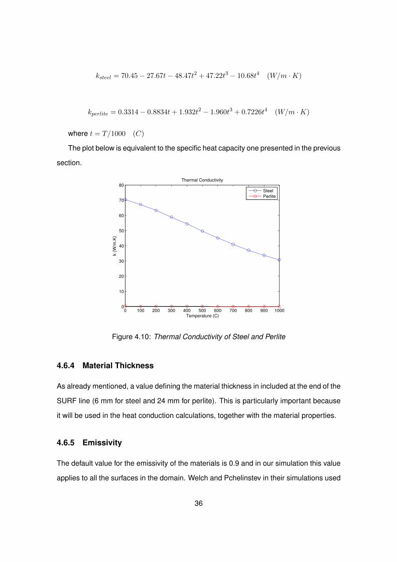
ksteel = 70.45− 27.67t− 48.47t2 + 47.22t3 − 10.68t4 (W/m ·K)

kperlite = 0.3314− 0.8834t+ 1.932t2 − 1.960t3 + 0.7226t4 (W/m ·K)

where t = T/1000 (C)

The plot below is equivalent to the specific heat capacity one presented in the previous

section.

0 100 200 300 400 500 600 700 800 900 10000

10

20

30

40

50

60

70

80Thermal Conductivity

Temperature (C)

k (

W/m

.K)

Steel

Perlite

Figure 4.10: Thermal Conductivity of Steel and Perlite

4.6.4 Material Thickness

As already mentioned, a value defining the material thickness in included at the end of the

SURF line (6 mm for steel and 24 mm for perlite). This is particularly important because

it will be used in the heat conduction calculations, together with the material properties.

4.6.5 Emissivity

The default value for the emissivity of the materials is 0.9 and in our simulation this value

applies to all the surfaces in the domain. Welch and Pchelinstev in their simulations used

36

a different value (0.8) for the lower flange of the beam but, since this choice was not

motivated, we decided to keep the default value at this location.

This is also the most likely choice in a normal design situation, where experimental

measurements and observations are not available.

4.7 Heat Flux Output Quantities

A range of different DEVC output quantities was tested before it was proven the the ’HEAT

FLUX GAUGE’ option was the optimal choice for our simulations. In total five different

quantities were used in our simulations:

• ’RADIATIVE HEAT FLUX’

• ’CONVECTIVE HEAT FLUX’

• ’NET HEAT FLUX’

• ’INCIDENT HEAT FLUX’

• ’HEAT FLUX GAUGE’

Other output quantities, such as the ’RADIOMETER’ or the ’RADIATIVE HEAT FLUX

GAS’ were ignored since they do not correspond in any way to the experimental proce-

dure.

4.7.1 Radiative Heat Flux

The definition of this quantity is essential to understand and derive the rest of options for

the heat flux output. The Radiative Heat Flux can be defined as the difference between

the incoming, or absorbed, thermal rays and the outgoing, or reflected, radiations:

.q′′rad =

.q′′rad,in −

.q′′rad,out

The amount of incoming energy is calculated by FDS radiation model and it takes into

account all the cells (or reflecting surfaces) in the domain emitting thermal radiations and

37

the intensity field resulting from the angles discretization process.

On the other hand, the amount of energy being reflected depends on the properties

of the target and its temperature Tw, and can be defined as the product of the black body

radiation of the target times the emissivity of the target. Therefore the equation becomes:

.q′′rad =

.q′′rad,in − εσT 4

w

Note that this relationship will be used repeatedly in the following sections in order to

derive or simplify other expressions.

4.7.2 Convective Heat Flux

By definition the convective heat flux is directly proportional to the difference between the

temperature of the gas in contact with the target and the target temperature itself. The

proportionality coefficient is called Heat Transfer Coefficient or h.

.q′′conv = h (Tgas − Tw)

In practice this quantity, together with the Radiative Heat Flux, was used to investigate

the respective impact of radiation and convection on the predicted heat fluxes.

4.7.3 Net Heat Flux

The Net Heat Flux is simply defined as the sum of the radiative heat flux and the convec-

tive heat flux at the device location. It can also be called Total Net Heat Flux and it can

be calculated as:

.q′′net =

.q′′rad +

.q′′conv

∴.q′′net =


w + h (Tgas − Tw)

This quantity was only used during the preliminary stages of the project, in order to

38

confirm that the heat flux gauge option was the optimal choice for our simulations.

4.7.4 Incident Heat Flux

The Incident Heat Flux quantity in FDS is only taking into account the incoming radiations

and convection, assuming that all the radiations energy is absorbed and none of it is

reflected.

.q′′inc =

.q′′rad,in

ε+

.q′′conv

Similarly to the Net Heat Flux, this quantity was only used to prove the accuracy of

the heat flux gauge output results.

4.7.5 Heat Flux Gauges

Thanks to the fact that the gauges were kept at the constant temperature of 55°C using

a water cooling system, the heat flux measurements can be decoupled from the surface

temperature. This is extremely useful for our simulations because the FDS capabilities

are very limited in the solid phase, and the predicted temperatures are expected to be

considerably different from the measured values.

Therefore, using the ‘GAUGE HEAT FLUX’ output quantity in the FDS model, the

simulation results can be compared directly to the experimental data, and the radiative

heat flux error due to the target temperature is eliminated. In practice the only adjust-

ment required consists in specifying the gauge temperature Tgauge via the parameter

’GAUGE_TEMPERATURE’ on the PROP line.

The equation used to calculate the heat flux for a gauge with fixed temperature can

be written as:

.q′′gauge =

.q′′rad

ε+

.q′′conv + σ

(T 4w − T 4

gauge

)+ h (Tw − Tgauge)

This expression is based on the assumption that the heat fluxes recorded are account-

ing for the incoming radiations, the reflected radiations and convection. And therefore the

39

two terms σ(T 4w − T 4

gauge

)and h (Tw − Tgauge) are used to cancel out the quantity Tw from

the equation:

.q′′gauge =

.q′′rad,in

ε−

.q′′rad,out

ε+ σ

(T 4w − T 4

gauge

)+

.q′′conv + h (Tw − Tgauge)

∴.q′′gauge =

.q′′rad,in

ε− σT 4

w + σ(T 4w − T 4

gauge

)+ h (Tgas − Tw) + h (Tw − Tgauge)

∴.q′′gauge =

.q′′rad,in

ε− σT 4

gauge + h (Tgas − Tgauge)

By carrying out this simplification, notice that the term Tw has been completely re-

moved and now the reflected radiations (second term) and convection (third term) are all

expressed in terms of the gauge temperature Tgauge, and the incoming radiations do not

depend on the properties of the target anyways.

The only issue is that this cannot avoid the fact that we are introducing an error in the

convection term due to the convective heat transfer. The flow velocity and gas tempera-

ture that are used to estimate the heat transfer coefficient come from the numerical model

and it can’t be proved that they match the experimental conditions. This uncertainty is

really difficult to quantify, but convection was typically a minor contributor to the total heat

flux that the gauges recorded, as shown in Section 5.4, and therefore this issue can be

ignored. Experimental measurements of the gas temperature and velocity in the proxim-

ity of the steel beam would allow to check the discrepancies between the simulations and

the physical tests, but these were completely ignored by BRI Japan.

40

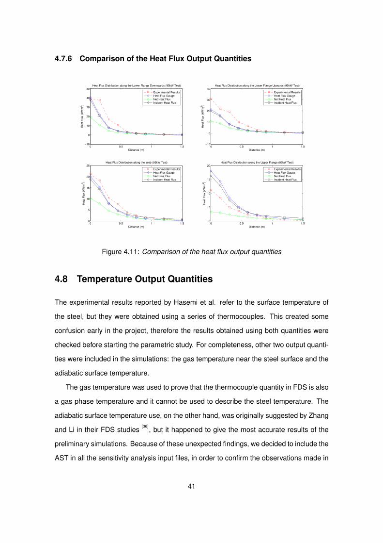
4.7.6 Comparison of the Heat Flux Output Quantities

0 0.5 1 1.5−10

0

10

20

30

40

50Heat Flux Distribution along the Lower Flange Downwards (95kW Test)

Distance (m)

He

at

Flu

x (

kW

/m2)

Experimental Results

Heat Flux Gauge

Net Heat Flux

Incident Heat Flux

0 0.5 1 1.5−10

0

10

20

30

40Heat Flux Distribution along the Lower Flange Upwards (95kW Test)

Distance (m)

He

at

Flu

x (

kW

/m2)


Heat Flux Gauge

Net Heat Flux

Incident Heat Flux

0 0.5 1 1.50

5

10

15

20

25Heat Flux Distribution along the Web (95kW Test)

Distance (m)

He

at

Flu

x (

kW

/m2)


Heat Flux Gauge

Net Heat Flux

Incident Heat Flux

0 0.5 1 1.50

5

10

15

20Heat Flux Distribution along the Upper Flange (95kW Test)

Distance (m)

He

at

Flu

x (

kW

/m2)


Heat Flux Gauge

Net Heat Flux

Incident Heat Flux

Figure 4.11: Comparison of the heat flux output quantities

4.8 Temperature Output Quantities

The experimental results reported by Hasemi et al. refer to the surface temperature of

the steel, but they were obtained using a series of thermocouples. This created some

confusion early in the project, therefore the results obtained using both quantities were

checked before starting the parametric study. For completeness, other two output quanti-

ties were included in the simulations: the gas temperature near the steel surface and the

adiabatic surface temperature.

The gas temperature was used to prove that the thermocouple quantity in FDS is also

a gas phase temperature and it cannot be used to describe the steel temperature. The

adiabatic surface temperature use, on the other hand, was originally suggested by Zhang

and Li in their FDS studies[36]

, but it happened to give the most accurate results of the

preliminary simulations. Because of these unexpected findings, we decided to include the

AST in all the sensitivity analysis input files, in order to confirm the observations made in

41

the preliminary simulations and prove the validity of this quantity as a representation of

the thermal environment surrounding the steel beam.

In summary the four different temperatures measured at the devices locations in the

FDS model were:

• ’WALL TEMPERATURE’

• ’ADIABATIC SURFACE TEMPERATURE’

• ’GAS TEMPERATURE’

• ’THERMOCOUPLE’

4.8.1 Wall Temperature

The output quantity called ’WALL TEMPERATURE’ represents the superficial tempera-

ture of the steel. In FDS the heat conduction through the steel is calculated using a simple

one dimensional model, so the heat transfer and the heat losses can only be modelled in

one direction: from the surface into the beam.

For each solid surface in contact with the hot gases, FDS creates a grid (or a series

of nodes) in order to solve the heat conduction equation numerically. As a rule of thumb

the dimensions of the cells in the grid used by the solver must be smaller than√k/ρc,

but this can modified on the SURF line if required.

Also, note that FDS does not distinguish between thermally thin and thermally thick

materials, but the calculations are based uniquely on the material properties specified by

the user, in particular the thermal inertia kρc.

Therefore in our baseline model FDS will proceed as follows:

1. Because the steel obstructions have no thickness in the computational domain, a

single node will be created in each cell where the solid is in contact with the gases.

Note that if a steel sheet is exposed on both sides FDS will create two nodes, one

for each side.

2. Each of these nodes will represent a thickness equal to the value prescribed on the

steel SURF line (t = 0.006 m)

42

3. The heat conduction calculations are performed by taking into account the density

ρ, the conductivity k and the specific heat c of the steel.

This means that the steel sheets, which are thin and conductive, will be essentially ther-

mally thin and therefore the thermal gradients within the beam will be ignored. Of course,

this is in contrast with the actual heat conduction in the beam, and it will result in the

surface temperature predictions depending solely on the local gas temperatures. Only a

finite element simulation, where the boundary conditions are imported from FDS, could

correctly predict the effects of the lateral heat conduction in all three dimensions (along

the length of the beam and between the different parts of the cross section). Therefore,

if we have to analyse the temperature of complex structural elements in FDS, we should

use alternative quantities or indicators, like the net heat fluxes.q′′net or the adiabatic surface

temperature TAST .

4.8.2 Adiabatic Surface Temperature

The Adiabatic Surface Temperature is an indicator of the thermal environment the struc-

tural element is exposed to. This quantity was first proposed by the Swedish researcher

Ulf Wickström and it was created with the objective of solving the issue of interfacing fire

models with structural models[31]

.

Our simulations are in fact a clear evidence of this issue: the fire model is rather

complex and the gas phase results are quite accurate, but in the solid phase the heat

conduction model is too approximate to be acceptable and the results have to be trans-

ferred to a FE software for a proper thermal and structural analysis.

The AST is derived from the net heat flux equation. By definition:

.q′′net =


w + h (Tgas − Tw) = ε(.q′′inc − σT 4

w) + h (Tgas − Tw)

So if we assume that the material is ideally a perfectly insulated, the total net heat

flux must be equal to zero (because by definition both the radiative and the convective

heat fluxes will no longer exist on the surfaces of a perfect insulator). And substituting the

43

actual temperature of the steel Tw with this new conceptual temperature TAST , gives:

ε(.q′′inc − σT 4

AST ) + h (Tgas − TAST ) = 0

or, if we consider again the formula for the net heat flux

ε(.q′′inc − σT 4

AST ) + h (Tgas − TAST ) = ε(.q′′inc − σT 4

w) + h (Tgas − Tw)

which, being rearranged, can be written as:

.q′′net = εσ(T 4

AST − T 4w) + h (TAST − Tw)

This is the equation used by FDS to find the AST. Interestingly, this expression is

similar to the equation used in Eurocode 1 to calculate the heat transfer to structural

elements, where TAST is replaced by the standard fire temperature Tf .

.q′′net = Φεmεfσ[(Tf + 273)4 − (Tw + 273)4] + h(Tgas − Tw)

Therefore it would be legitimate to consider this quantity as a conservative estimate

of the temperature of the steel.

However, notice that the Adiabatic Surface Temperature is an indicator of the heat

transfer to a solid, and does not represent the actual temperature of the steel (because

it is based on the assumption that the thermal conductivity k is infinitely small, unlike

steel). This could create some confusion but, in our case, we can consider TAST as

the temperature reached by the steel in steady state conditions without any lateral heat

conduction, assuming that no heat can be lost to the environment from the surface.

4.8.3 Gas Temperature

The ’GAS TEMPERATURE’ quantity is simply the spatially averaged temperature of the

gases in the cell touching the device surface. This temperature is calculated by default in

FDS and it only needs to be copied in the output csv file.

44

4.8.4 Thermocouples

In FDS the ’THERMOCOUPLE’ devices give a measurement of the gas temperature, but

they adjust the value based on the properties of the thermocouple bead. This results in a

slight lag between the gas temperature and the thermocouple, and the bead temperature

can be found by solving the following formula for TTC

ρTCcTCdTTCdt

= εTC(U

4− σT 4

TC) + h(Tgas − TTC) = 0

where

ρTC is the density of the thermocouple bead

cTC is the specific heat of the bead

εTC is the emissivity of the bead (0.85 by default)

Also, note that the heat transfer coefficient h depends on the diameter of the bead DTC ,

since h = k·NuDTC

. The properties of the thermocouple can be modified, but the default

diameter is equal to 1 mm and the material properties are based on nickel (as for common

k-type thermocouples).

This quantity does not correctly represent the test measurements. The experimental

data in our possession refer to the surface temperature of the steel, and they are not a

measurement of the local gas temperature around the beam. This is precisely what the

thermocouples do in FDS.

45

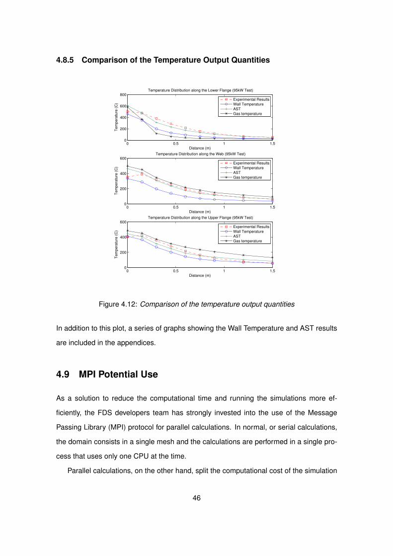
4.8.5 Comparison of the Temperature Output Quantities

0 0.5 1 1.50

200

400

600

800Temperature Distribution along the Lower Flange (95kW Test)

Distance (m)

Te

mp

era

ture

(C

)


Wall Temperature

AST

Gas temperature

0 0.5 1 1.50

200

400

600Temperature Distribution along the Web (95kW Test)

Distance (m)

Te

mp

era

ture

(C

)


Wall Temperature

AST

Gas temperature

0 0.5 1 1.50

200

400

600Temperature Distribution along the Upper Flange (95kW Test)

Distance (m)

Te

mp

era

ture

(C

)


Wall Temperature

AST

Gas temperature

Figure 4.12: Comparison of the temperature output quantities

In addition to this plot, a series of graphs showing the Wall Temperature and AST results

are included in the appendices.

4.9 MPI Potential Use

As a solution to reduce the computational time and running the simulations more ef-

ficiently, the FDS developers team has strongly invested into the use of the Message

Passing Library (MPI) protocol for parallel calculations. In normal, or serial calculations,

the domain consists in a single mesh and the calculations are performed in a single pro-

cess that uses only one CPU at the time.

Parallel calculations, on the other hand, split the computational cost of the simulation

46

by dividing the domain into multiple meshes (of similar size) and by carrying out these

separated processes simultaneously. This allows to optimise the CPU usage and enables

the use of computer clusters or supercomputers, but the method has some limits in terms

of the accuracy of the results.

For example the User’s Manual strongly advise not to divide a single burning plume

between two or more separate meshes. MPI is a communication protocol that allows the

separate processes to transfer information between each other but part of the informa-

tion is always lost, in particular in the case of the turbulence model and radiation model

results.

4.10 Symmetry

The size of the domain, and therefore the computational cost of the simulations, could be

reduced to a quarter of the baseline model using two ’MIRROR’ vents as axis of symmetry

in the x and y direction. This solution was used by Welch and Ptelinchev for their RANS

model[30]

, but there are many issues when the same simplification is applied to a LES

model.

In a RANS model every burning plume is symmetric about its axis because the model

uses a time-averaged solution of the transport equations and turbulence is simply applied

to the results using a simplified model. In LES instead the solutions are not time averaged

and turbulence is a key component of the model, being included in the transport equations

and in the combustion process. For this reason, the FDS manual clearly states that

a ’MIRROR’ boundary used as an axis of symmetry along the centerline of the plume

should always be avoided for a turbulent plume.

4.11 OpenMP

OpenMP (or Open Multi Processing) is a protocol similar to the Message Passing Inter-

face discussed earlier, but instead of dividing the domain into multiple meshes, it enables

the use of all the CPUs available to perform the calculations for a single mesh. This

47

greatly improves the efficiency of the simulations, but due to the very high number of

simulations required by our sensitivity study we preferred to run different simulations si-

multaneously, using all the available processors in a similar way.

48

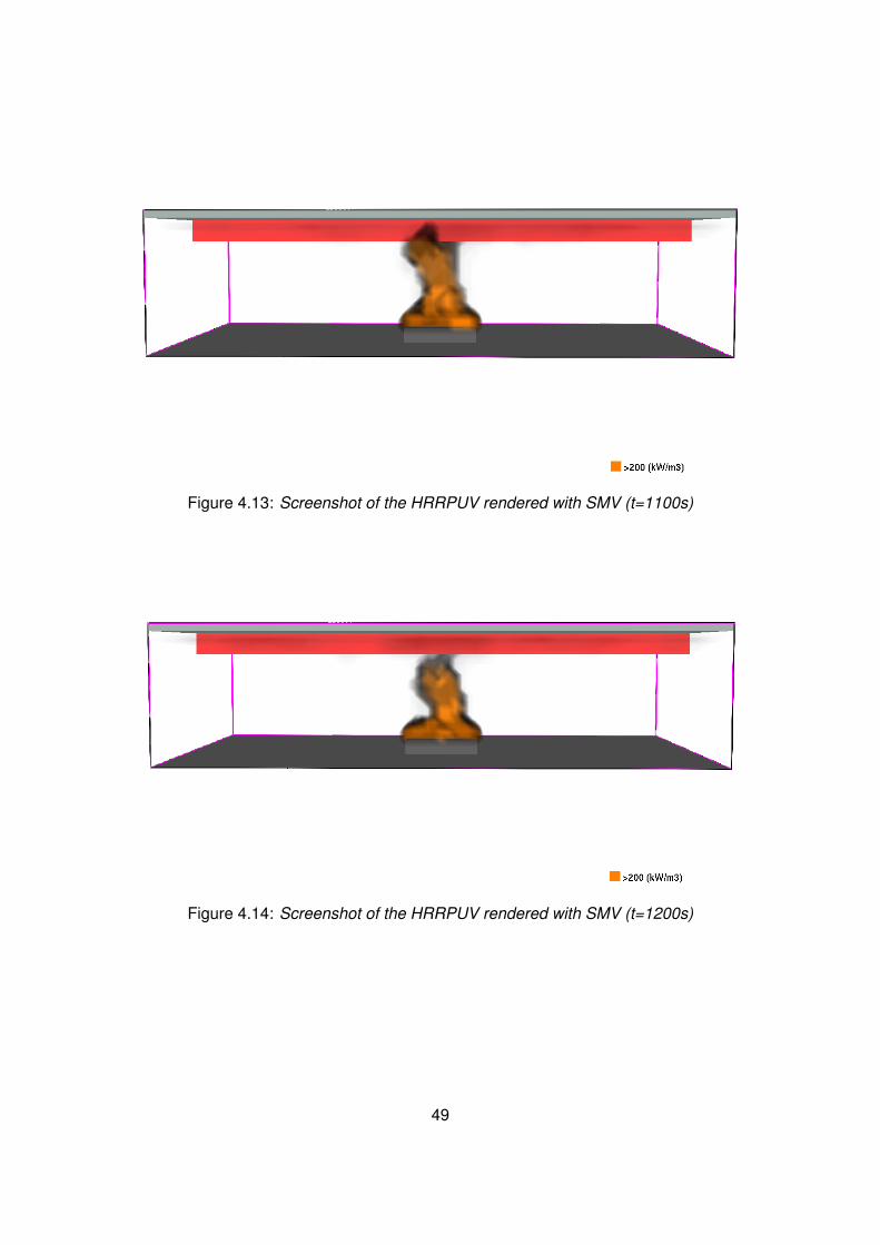
Figure 4.13: Screenshot of the HRRPUV rendered with SMV (t=1100s)

Figure 4.14: Screenshot of the HRRPUV rendered with SMV (t=1200s)

49

Chapter 5

Sensitivity Study

Introduction

The main body of this research project will focus on a variety of input parameters and

their effect on the output of the FDS model. This is commonly called sensitivity analysis

and its main objectives and aims are:

• Increasing our understanding of the Fire Dynamics Simulator

• Testing the model robustness and its capabilities in practical design situations

• Defining the impact of different variables on the model output and assess their va-

lidity by comparison to experimental results

The computational cost for a detailed sensitivity study for each of the tests was relatively

high, considering our means and objectives. Therefore only two of the experiments have

been fully analysed in this section: the 95 kW and the 160 kW cases. The domain of these

two tests is identical and the only difference is the heat release rate quantity. Thanks to

this the input files preparation was extremely easy.

Using two models instead of a single one is very important for the validity of our

study. Each set of experimental data is in fact subject to some level of uncertainty, and

the fact that the FDS predictions are compared to multiple cases immediately increases

the importance of our study and the confidence in the results obtained, without having

50

to force the simulation results to “converge” to a particular correlation, derived from the

experiments. Each case should be validated individually, if possible.

Finally note that in this chapter we are only presenting the heat flux distribution results.

The reasons are two:

• FDS is only capable of solving the one dimensional heat conduction from the sur-

face into the beam. In our case though, the lateral heat conduction within the beam

and the heat conduction across the section cannot be ignored and therefore the

temperature results will be incorrect.

• The heat flux gauges measurements are virtually insensitive to the temperature of

the beam. The gauges temperature is assumed to be constant at 55 °C, both in the

physical experiments and in the numerical simulation, therefore no correction to the

data is required .

FDS 5 and FDS 6 Simulations

Most of the simulations in the preliminary stages of the project were carried out using

FDS 5, but a system update of the School of Engineering Linux machines forced us to

update to the latest version of the software in late March. This is a great opportunity to

test the new features of FDS 6 and clearly goes in the direction of any future research in

this area. FDS 6 is fully supported, stable, complete with full documentation and it carries

all the corrections developed from the validation cases throughout the years.

The following list summarizes where the two versions of FDS were respectively used.

(More information is given in each section)

• The bulk of the Grid Sensitivity Analysis was carried out using FDS 5.5.3. Two tests

were also run in FDS 6, in order to compare the them to the FDS 5 results and to

serve as a baseline case for the rest of the input parameters sensitivity studies.

• The effect of the thin and the thick representations of the beam geometry was stud-

ied using FDS 5.5.3

51

• The radiation parameters sensitivity study was carried out using FDS 6.0.1 only.

• All the remaining studies were carried out using FDS 6.0.1.

FDS 6.0.1 New Features

Compared to FDS 5.5.3, which was the last official release of the software, the new

version of FDS has some important new features. The most notable ones, considering

the nature of our simulations, are:

• Improved numerical stability.

• Numerous bugs fixed (e.g. particle tracking algorithm)

• New scalar transport schemes are introduced in order to achieve more accurate

results in terms of species concentrations and temperature distribution.

• The default hydrodynamic turbulence model has changed to The Deardoff model.

The Dynamic Smagorinsky and the Vreman models are also available. The new

algorithms should achieve a better resolution of turbulence for relatively coarse

meshes.

• Baroclinic torque is set as default

• Improved combustion model. The user can define custom gas mixtures and chem-

ical mechanisms can be also prescribed.

• Turbulent mixing is now based on a partially-stirred batch reactor model

• Possibility to take into account the soot deposition on surfaces

• The narrow-band model RadCal has been improved by including more fuel species

and the possibility to customize them

• A correction factor(C) is applied to the radiation intensity term in the near field zone.

This factor ensures that the prescribed value of the radiative fraction is maintained

when the total heat release is considered, instead of directly multiplying the heat

release rate per unit volume.

(q′′′) to the radiative fraction (χr).

52

• Statistics (RMS, correlation coefficients and covariance) are available for the de-

vices output.

Experimental Uncertainties

Defining some values for the experiments uncertainties is essential for our study. The

conclusions of the sensitivity analysis will be based on the comparison between the BRI

test recorded quantities and the numerical predictions obtained using FDS. If the experi-

mental error can be quantified, then the predictions accuracy can be easily measured and

the simulation results can be deemed acceptable or not. Unfortunately all the publications

by BRI Japan[10]

completely ignore this aspect of the experiments, and no indication is

given about the calibration and uncertainty measurement of the heat flux gauges and

thermocouples. In the following sections we will assume that these uncertainties can be

ignored and so all the plots presented do not include error bars for the experimental data.

This assumption is based on the fact that the BRI Japan team must have analysed the

measurements and averaged them in order to eliminate noise and minor fluctuations in

the data. Surely a value of the standard deviation must have been specified, but it was

probably considered to be irrelevant and was not included in any of the reports available

to us.

More information about the devices, their calibration and the resulting uncertainties is

available on the NIST website or other alternative standards, such as the Annual Book of

ASTM Standards. Some of the NIST publications, such as “The Calibration of Thermo-

couples and Thermocouple Materials”, “Assessment of Uncertainties of Thermocouple

Calibrations at NIST” and “Heat-Flux Sensor Calibration”, would be useful to find an esti-

mate for the experimental uncertainties[27, 24]

. This goes beyond the scope of our research

project, but it must definitely be considered in the case of future experiments and valida-

tion cases.

Finally, note that where uncertainties and error bars were introduced they are related

to the FDS output quantities. For more details see the section dedicated to the output

devices in the previous chapter.

53

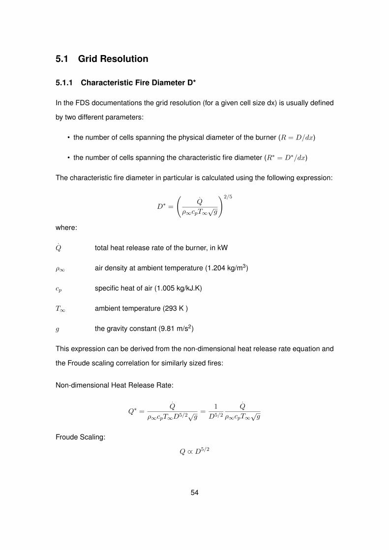
5.1 Grid Resolution

5.1.1 Characteristic Fire Diameter D*

In the FDS documentations the grid resolution (for a given cell size dx) is usually defined

by two different parameters:

• the number of cells spanning the physical diameter of the burner (R = D/dx)

• the number of cells spanning the characteristic fire diameter (R∗ = D∗/dx)

The characteristic fire diameter in particular is calculated using the following expression:

D∗ =

( .Q

ρ∞cpT∞√g

)2/5

where:

.Q total heat release rate of the burner, in kW

ρ∞ air density at ambient temperature (1.204 kg/m3)

cp specific heat of air (1.005 kg/kJ.K)

T∞ ambient temperature (293 K )

g the gravity constant (9.81 m/s2)

This expression can be derived from the non-dimensional heat release rate equation and

the Froude scaling correlation for similarly sized fires:

Non-dimensional Heat Release Rate:

Q∗ =

.Q

ρ∞cpT∞D5/2√g=

1

D5/2

.Q

ρ∞cpT∞√g

Froude Scaling:

Q ∝ D5/2

54

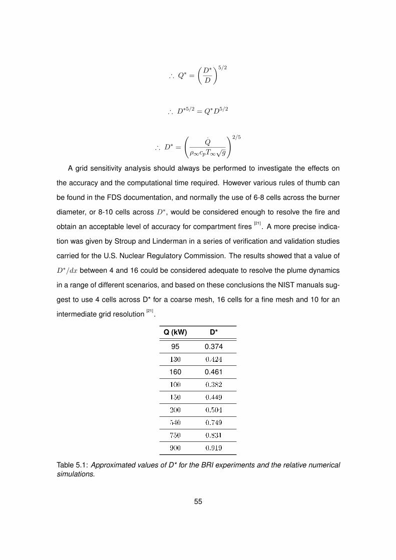
∴ Q∗ =

(D∗

D

)5/2

∴ D∗5/2 = Q∗D5/2

∴ D∗ =

( .Q

ρ∞cpT∞√g

)2/5

A grid sensitivity analysis should always be performed to investigate the effects on

the accuracy and the computational time required. However various rules of thumb can

be found in the FDS documentation, and normally the use of 6-8 cells across the burner

diameter, or 8-10 cells across D∗, would be considered enough to resolve the fire and

obtain an acceptable level of accuracy for compartment fires[21]

. A more precise indica-

tion was given by Stroup and Linderman in a series of verification and validation studies

carried for the U.S. Nuclear Regulatory Commission. The results showed that a value of

D∗/dx between 4 and 16 could be considered adequate to resolve the plume dynamics

in a range of different scenarios, and based on these conclusions the NIST manuals sug-

gest to use 4 cells across D* for a coarse mesh, 16 cells for a fine mesh and 10 for an

intermediate grid resolution[21]

.

Q (kW) D*

95 0.374

130 0.424

160 0.461

100 0.382

150 0.449

200 0.504

540 0.749

750 0.831

900 0.919

Table 5.1: Approximated values of D* for the BRI experiments and the relative numericalsimulations.

55

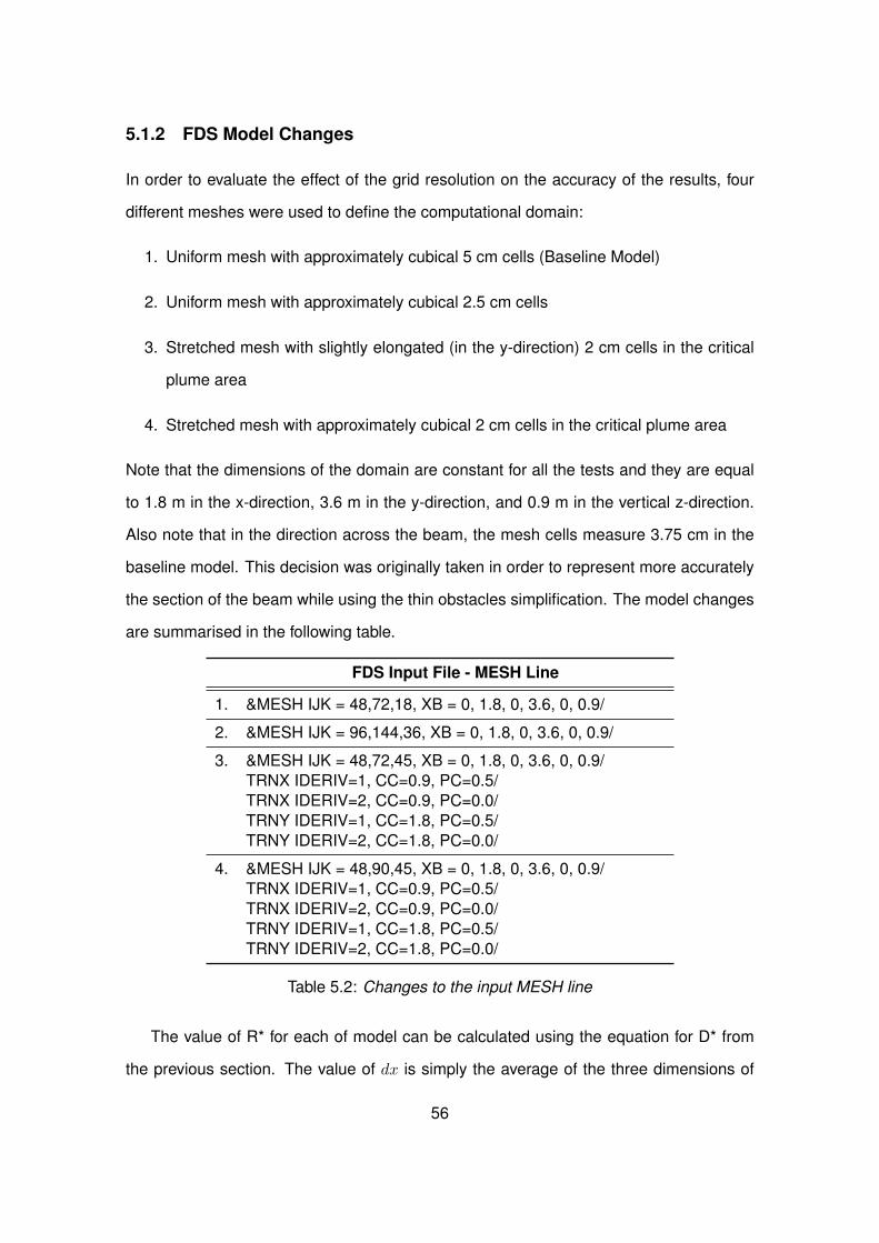
5.1.2 FDS Model Changes

In order to evaluate the effect of the grid resolution on the accuracy of the results, four

different meshes were used to define the computational domain:

1. Uniform mesh with approximately cubical 5 cm cells (Baseline Model)

2. Uniform mesh with approximately cubical 2.5 cm cells

3. Stretched mesh with slightly elongated (in the y-direction) 2 cm cells in the critical

plume area

4. Stretched mesh with approximately cubical 2 cm cells in the critical plume area

Note that the dimensions of the domain are constant for all the tests and they are equal

to 1.8 m in the x-direction, 3.6 m in the y-direction, and 0.9 m in the vertical z-direction.

Also note that in the direction across the beam, the mesh cells measure 3.75 cm in the

baseline model. This decision was originally taken in order to represent more accurately

the section of the beam while using the thin obstacles simplification. The model changes

are summarised in the following table.

FDS Input File - MESH Line

1. &MESH IJK = 48,72,18, XB = 0, 1.8, 0, 3.6, 0, 0.9/

2. &MESH IJK = 96,144,36, XB = 0, 1.8, 0, 3.6, 0, 0.9/

3. &MESH IJK = 48,72,45, XB = 0, 1.8, 0, 3.6, 0, 0.9/TRNX IDERIV=1, CC=0.9, PC=0.5/TRNX IDERIV=2, CC=0.9, PC=0.0/TRNY IDERIV=1, CC=1.8, PC=0.5/TRNY IDERIV=2, CC=1.8, PC=0.0/

4. &MESH IJK = 48,90,45, XB = 0, 1.8, 0, 3.6, 0, 0.9/TRNX IDERIV=1, CC=0.9, PC=0.5/TRNX IDERIV=2, CC=0.9, PC=0.0/TRNY IDERIV=1, CC=1.8, PC=0.5/TRNY IDERIV=2, CC=1.8, PC=0.0/

Table 5.2: Changes to the input MESH line

The value of R* for each of model can be calculated using the equation for D* from

the previous section. The value of dx is simply the average of the three dimensions of

56

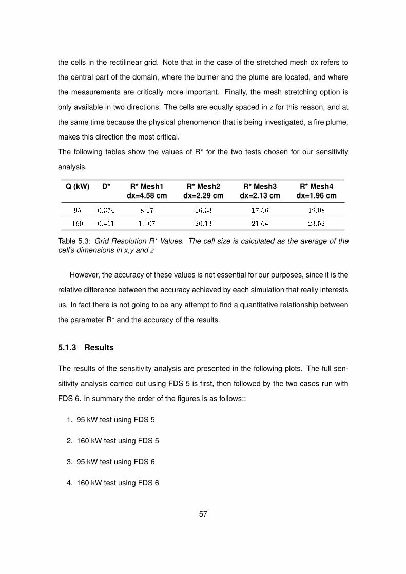
the cells in the rectilinear grid. Note that in the case of the stretched mesh dx refers to

the central part of the domain, where the burner and the plume are located, and where

the measurements are critically more important. Finally, the mesh stretching option is

only available in two directions. The cells are equally spaced in z for this reason, and at

the same time because the physical phenomenon that is being investigated, a fire plume,

makes this direction the most critical.

The following tables show the values of R* for the two tests chosen for our sensitivity

analysis.

Q (kW) D* R* Mesh1dx=4.58 cm

R* Mesh2dx=2.29 cm

R* Mesh3dx=2.13 cm

R* Mesh4dx=1.96 cm

95 0.374 8.17 16.33 17.56 19.08

160 0.461 10.07 20.13 21.64 23.52

Table 5.3: Grid Resolution R* Values. The cell size is calculated as the average of thecell’s dimensions in x,y and z

However, the accuracy of these values is not essential for our purposes, since it is the

relative difference between the accuracy achieved by each simulation that really interests

us. In fact there is not going to be any attempt to find a quantitative relationship between

the parameter R* and the accuracy of the results.

5.1.3 Results

The results of the sensitivity analysis are presented in the following plots. The full sen-

sitivity analysis carried out using FDS 5 is first, then followed by the two cases run with

FDS 6. In summary the order of the figures is as follows::

1. 95 kW test using FDS 5




57

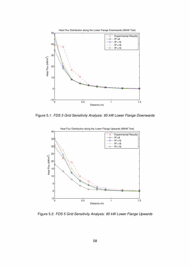
0 0.5 1 1.5−10

0

10

20

30

40


Distance (m)

Heat F

lux (

kW

/m2)


R*=8

R*=16

R*=18

R*=19

Figure 5.1: FDS 5 Grid Sensitivity Analysis: 95 kW Lower Flange Downwards

0 0.5 1 1.5−5

0

5

10

15

20

25

30

35


Distance (m)

Heat F

lux (

kW

/m2)


R*=8

R*=16

R*=18

R*=19

Figure 5.2: FDS 5 Grid Sensitivity Analysis: 95 kW Lower Flange Upwards

58

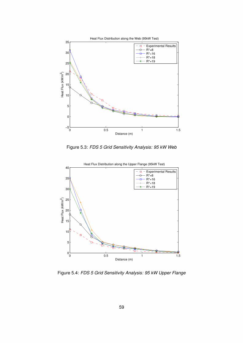
0 0.5 1 1.5−5

0

5

10

15

20

25

30


Distance (m)

Heat F

lux (

kW

/m2)


R*=8

R*=16

R*=18

R*=19

Figure 5.3: FDS 5 Grid Sensitivity Analysis: 95 kW Web

0 0.5 1 1.50

5

10

15

20

25

30

35


Distance (m)

Heat F

lux (

kW

/m2)


R*=8

R*=16

R*=18

R*=19

Figure 5.4: FDS 5 Grid Sensitivity Analysis: 95 kW Upper Flange

59

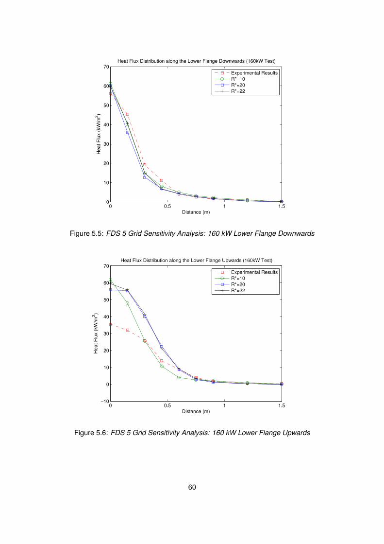
0 0.5 1 1.50

10

20

30

40

50

60


Distance (m)

Heat F

lux (

kW

/m2)


R*=10

R*=20

R*=22


0 0.5 1 1.5−10

0

10

20

30

40

50

60


Distance (m)

Heat F

lux (

kW

/m2)


R*=10

R*=20

R*=22


60

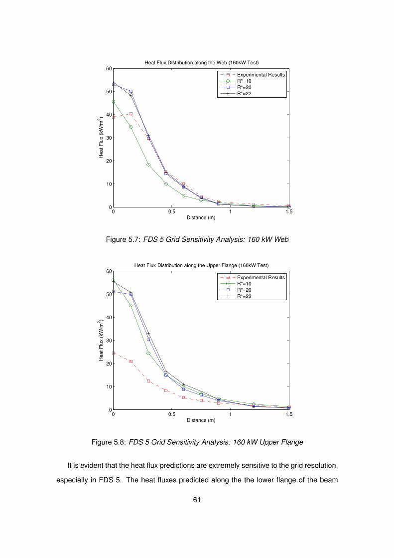
0 0.5 1 1.50

10

20

30

40

50


Distance (m)

Heat F

lux (

kW

/m2)


R*=10

R*=20

R*=22


0 0.5 1 1.50

10

20

30

40

50


Distance (m)

Heat F

lux (

kW

/m2)


R*=10

R*=20

R*=22


It is evident that the heat flux predictions are extremely sensitive to the grid resolution,

especially in FDS 5. The heat fluxes predicted along the the lower flange of the beam

61

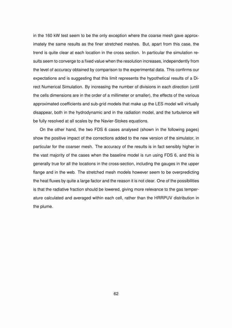
in the 160 kW test seem to be the only exception where the coarse mesh gave approx-

imately the same results as the finer stretched meshes. But, apart from this case, the

trend is quite clear at each location in the cross section. In particular the simulation re-

sults seem to converge to a fixed value when the resolution increases, independently from

the level of accuracy obtained by comparison to the experimental data. This confirms our

expectations and is suggesting that this limit represents the hypothetical results of a Di-

rect Numerical Simulation. By increasing the number of divisions in each direction (until

the cells dimensions are in the order of a millimeter or smaller), the effects of the various

approximated coefficients and sub-grid models that make up the LES model will virtually

disappear, both in the hydrodynamic and in the radiation model, and the turbulence will

be fully resolved at all scales by the Navier-Stokes equations.

On the other hand, the two FDS 6 cases analysed (shown in the following pages)

show the positive impact of the corrections added to the new version of the simulator, in

particular for the coarser mesh. The accuracy of the results is in fact sensibly higher in

the vast majority of the cases when the baseline model is run using FDS 6, and this is

generally true for all the locations in the cross-section, including the gauges in the upper

flange and in the web. The stretched mesh models however seem to be overpredicting

the heat fluxes by quite a large factor and the reason it is not clear. One of the possibilities

is that the radiative fraction should be lowered, giving more relevance to the gas temper-

ature calculated and averaged within each cell, rather than the HRRPUV distribution in

the plume.

62

0 0.5 1 1.5−10

0

10

20

30

40


Distance (m)

Heat F

lux (

kW

/m2)


R* = 8

R* = 18


0 0.5 1 1.5−5

0

5

10

15

20

25

30

35


Distance (m)

Heat F

lux (

kW

/m2)


R* = 8

R* = 18


63

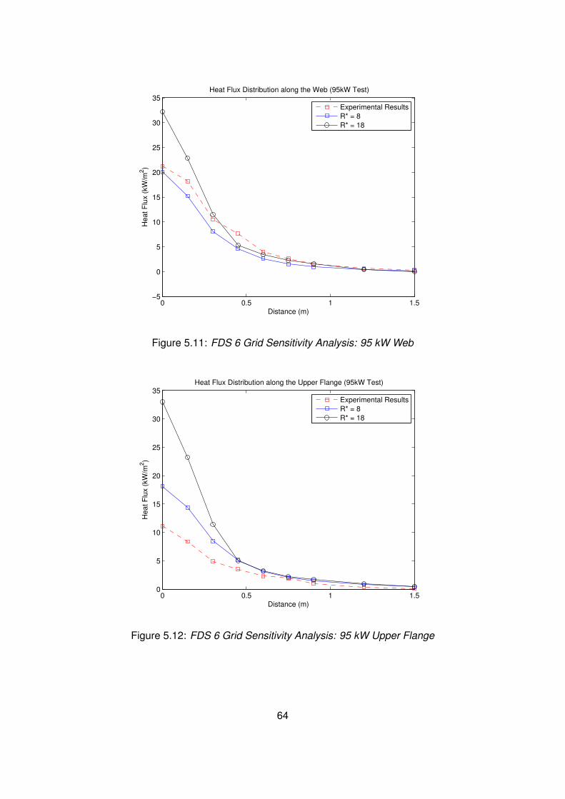
0 0.5 1 1.5−5

0

5

10

15

20

25

30


Distance (m)

Heat F

lux (

kW

/m2)


R* = 8

R* = 18


0 0.5 1 1.50

5

10

15

20

25

30


Distance (m)

Heat F

lux (

kW

/m2)


R* = 8

R* = 18


64

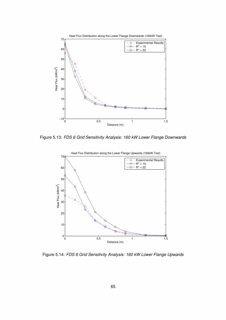
0 0.5 1 1.5−10

0

10

20

30

40

50

60


Distance (m)

Heat F

lux (

kW

/m2)


R* = 10

R* = 22


0 0.5 1 1.50

10

20

30

40

50

60


Distance (m)

Heat F

lux (

kW

/m2)


R* = 10

R* = 22


65

0 0.5 1 1.50

10

20

30

40

50

60


Distance (m)

Heat F

lux (

kW

/m2)


R* = 10

R* = 22


0 0.5 1 1.50

10

20

30

40

50

60


Distance (m)

Heat F

lux (

kW

/m2)


R* = 10

R* = 22


66

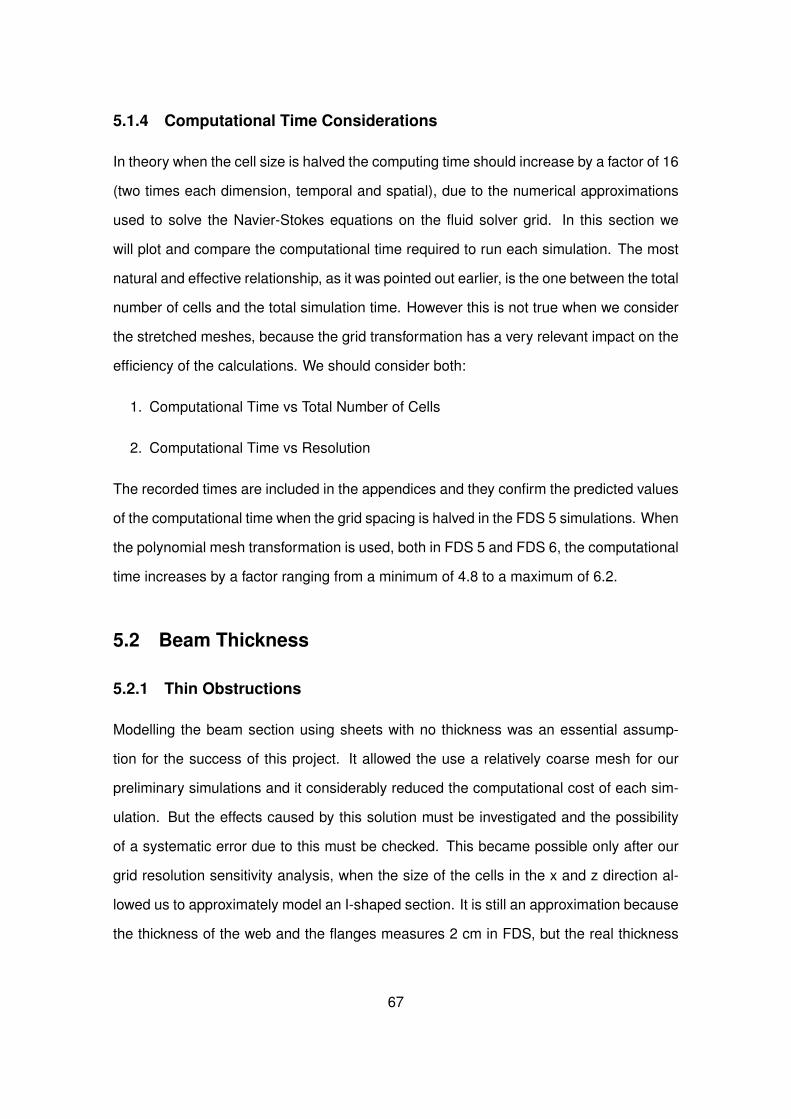
5.1.4 Computational Time Considerations

In theory when the cell size is halved the computing time should increase by a factor of 16

(two times each dimension, temporal and spatial), due to the numerical approximations

used to solve the Navier-Stokes equations on the fluid solver grid. In this section we

will plot and compare the computational time required to run each simulation. The most

natural and effective relationship, as it was pointed out earlier, is the one between the total

number of cells and the total simulation time. However this is not true when we consider

the stretched meshes, because the grid transformation has a very relevant impact on the

efficiency of the calculations. We should consider both:

1. Computational Time vs Total Number of Cells

2. Computational Time vs Resolution

The recorded times are included in the appendices and they confirm the predicted values

of the computational time when the grid spacing is halved in the FDS 5 simulations. When

the polynomial mesh transformation is used, both in FDS 5 and FDS 6, the computational

time increases by a factor ranging from a minimum of 4.8 to a maximum of 6.2.

5.2 Beam Thickness

5.2.1 Thin Obstructions

Modelling the beam section using sheets with no thickness was an essential assump-

tion for the success of this project. It allowed the use a relatively coarse mesh for our

preliminary simulations and it considerably reduced the computational cost of each sim-

ulation. But the effects caused by this solution must be investigated and the possibility

of a systematic error due to this must be checked. This became possible only after our

grid resolution sensitivity analysis, when the size of the cells in the x and z direction al-

lowed us to approximately model an I-shaped section. It is still an approximation because

the thickness of the web and the flanges measures 2 cm in FDS, but the real thickness

67

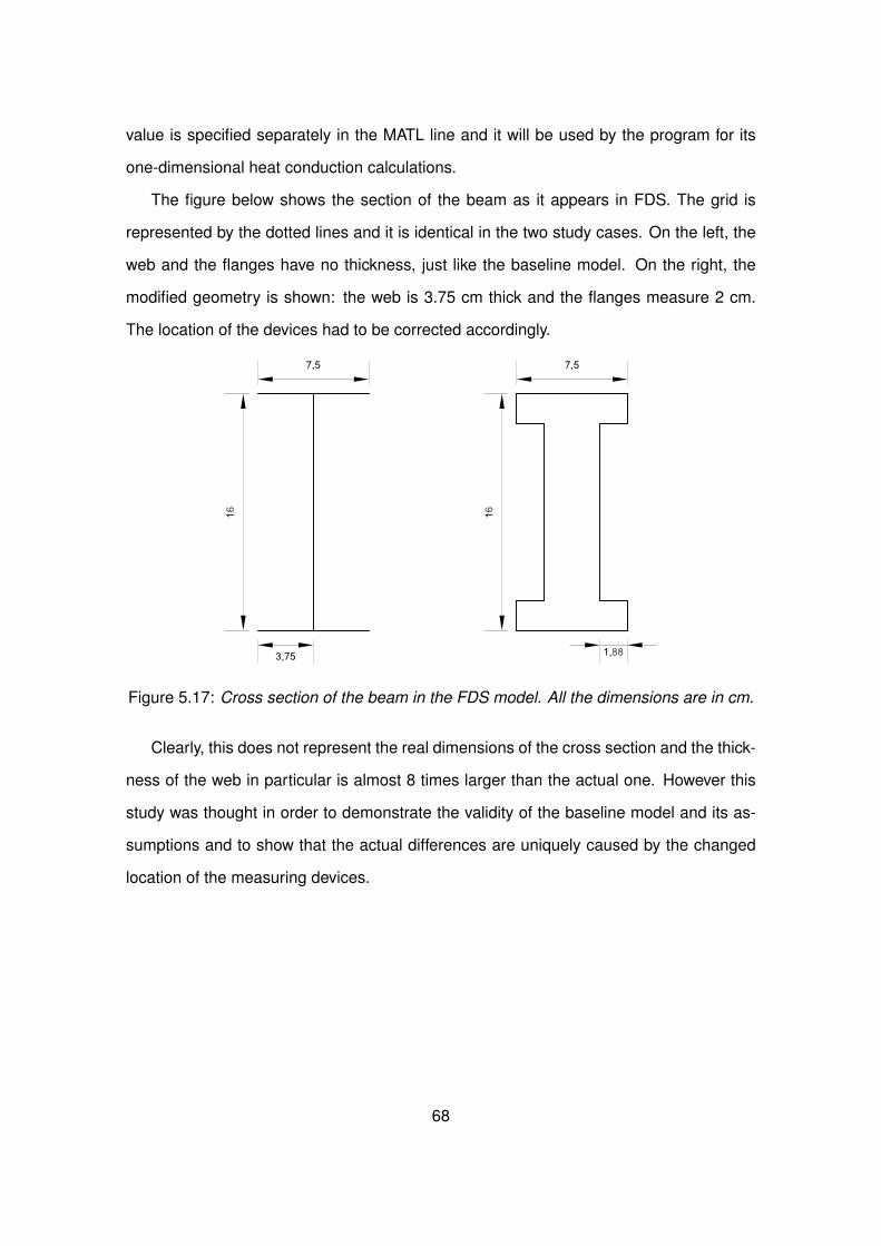
value is specified separately in the MATL line and it will be used by the program for its

one-dimensional heat conduction calculations.

The figure below shows the section of the beam as it appears in FDS. The grid is

represented by the dotted lines and it is identical in the two study cases. On the left, the

web and the flanges have no thickness, just like the baseline model. On the right, the

modified geometry is shown: the web is 3.75 cm thick and the flanges measure 2 cm.

The location of the devices had to be corrected accordingly.

Figure 5.17: Cross section of the beam in the FDS model. All the dimensions are in cm.

Clearly, this does not represent the real dimensions of the cross section and the thick-

ness of the web in particular is almost 8 times larger than the actual one. However this

study was thought in order to demonstrate the validity of the baseline model and its as-

sumptions and to show that the actual differences are uniquely caused by the changed

location of the measuring devices.

68

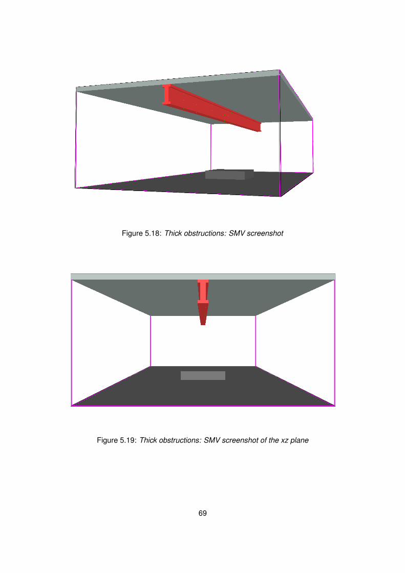
Figure 5.18: Thick obstructions: SMV screenshot

Figure 5.19: Thick obstructions: SMV screenshot of the xz plane

69

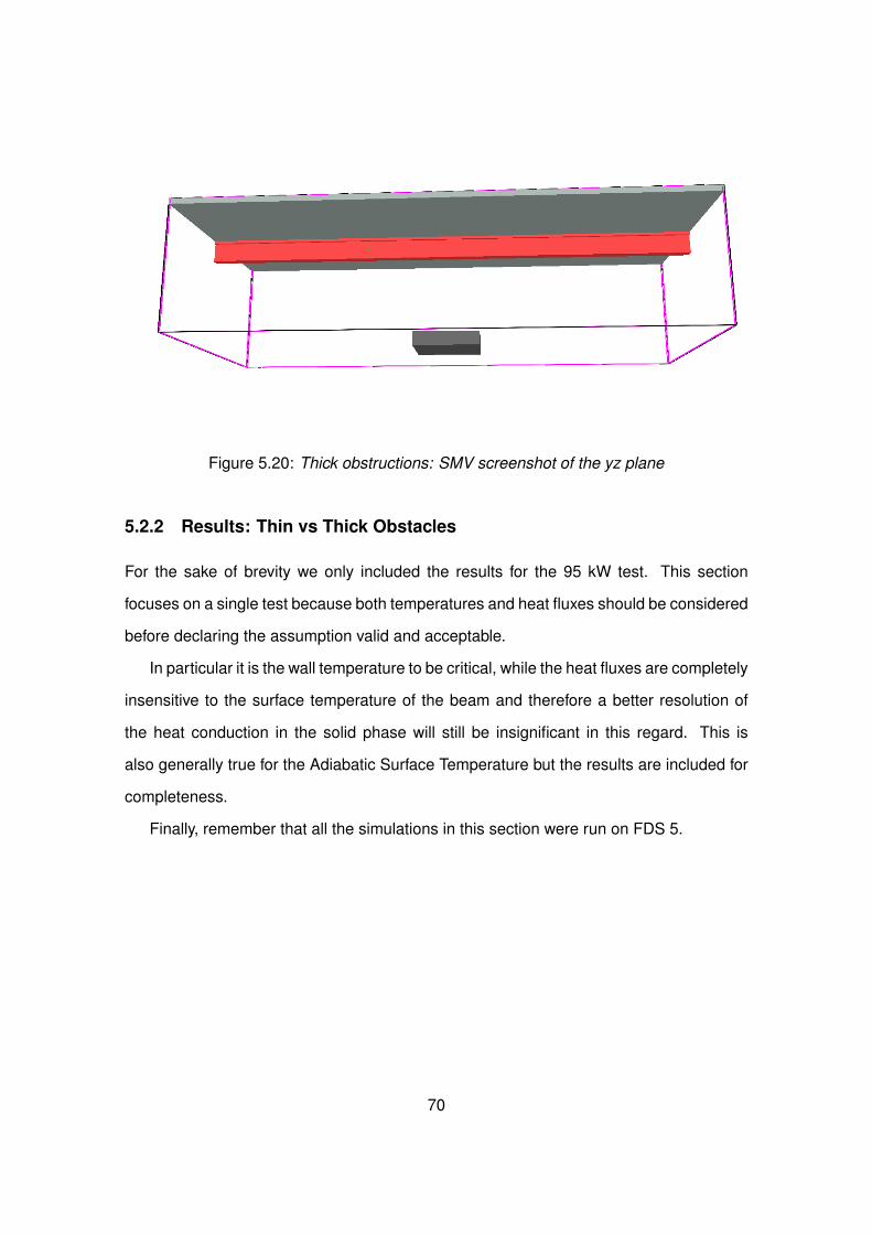
Figure 5.20: Thick obstructions: SMV screenshot of the yz plane

5.2.2 Results: Thin vs Thick Obstacles

For the sake of brevity we only included the results for the 95 kW test. This section

focuses on a single test because both temperatures and heat fluxes should be considered

before declaring the assumption valid and acceptable.

In particular it is the wall temperature to be critical, while the heat fluxes are completely

insensitive to the surface temperature of the beam and therefore a better resolution of

the heat conduction in the solid phase will still be insignificant in this regard. This is

also generally true for the Adiabatic Surface Temperature but the results are included for

completeness.

Finally, remember that all the simulations in this section were run on FDS 5.

70

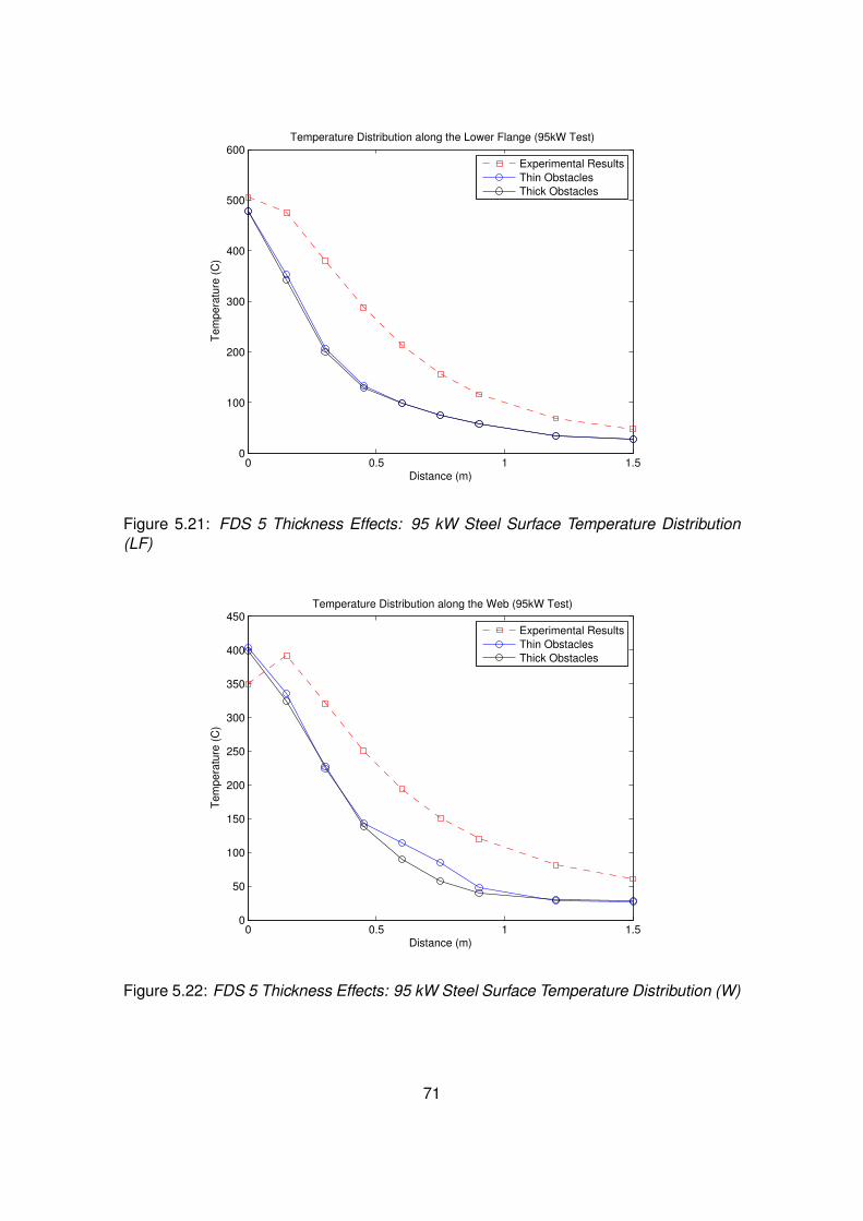
0 0.5 1 1.50

100

200

300

400

500


Distance (m)

Tem

pera

ture

(C

)


Thin Obstacles

Thick Obstacles

Figure 5.21: FDS 5 Thickness Effects: 95 kW Steel Surface Temperature Distribution(LF)

0 0.5 1 1.50

50

100

150

200

250

300

350

400


Distance (m)

Tem

pera

ture

(C

)


Thin Obstacles

Thick Obstacles

Figure 5.22: FDS 5 Thickness Effects: 95 kW Steel Surface Temperature Distribution (W)

71

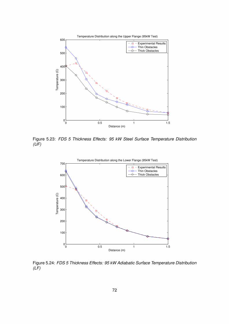
0 0.5 1 1.50

100

200

300

400

500


Distance (m)

Tem

pera

ture

(C

)


Thin Obstacles

Thick Obstacles

Figure 5.23: FDS 5 Thickness Effects: 95 kW Steel Surface Temperature Distribution(UF)

0 0.5 1 1.50

100

200

300

400

500

600


Distance (m)

Tem

pera

ture

(C

)


Thin Obstacles

Thick Obstacles

Figure 5.24: FDS 5 Thickness Effects: 95 kW Adiabatic Surface Temperature Distribution(LF)

72

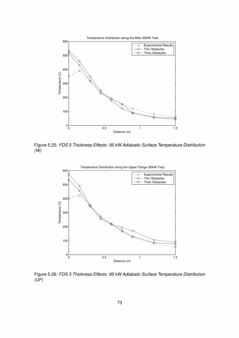
0 0.5 1 1.50

100

200

300

400

500


Distance (m)

Tem

pera

ture

(C

)


Thin Obstacles

Thick Obstacles

Figure 5.25: FDS 5 Thickness Effects: 95 kW Adiabatic Surface Temperature Distribution(W)

0 0.5 1 1.50

100

200

300

400

500


Distance (m)

Tem

pera

ture

(C

)


Thin Obstacles

Thick Obstacles

Figure 5.26: FDS 5 Thickness Effects: 95 kW Adiabatic Surface Temperature Distribution(UF)

73

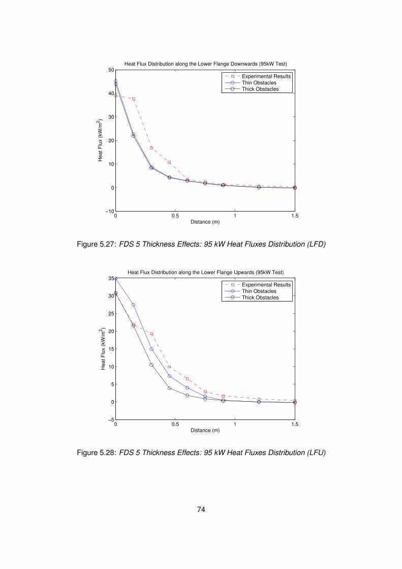
0 0.5 1 1.5−10

0

10

20

30

40


Distance (m)

Heat F

lux (

kW

/m2)


Thin Obstacles

Thick Obstacles

Figure 5.27: FDS 5 Thickness Effects: 95 kW Heat Fluxes Distribution (LFD)

0 0.5 1 1.5−5

0

5

10

15

20

25

30


Distance (m)

Heat F

lux (

kW

/m2)


Thin Obstacles

Thick Obstacles

Figure 5.28: FDS 5 Thickness Effects: 95 kW Heat Fluxes Distribution (LFU)

74

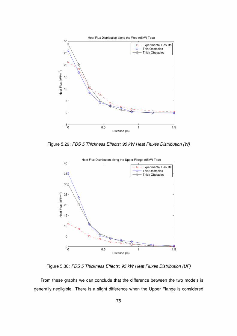
0 0.5 1 1.5−5

0

5

10

15

20

25


Distance (m)

Heat F

lux (

kW

/m2)


Thin Obstacles

Thick Obstacles

Figure 5.29: FDS 5 Thickness Effects: 95 kW Heat Fluxes Distribution (W)

0 0.5 1 1.50

5

10

15

20

25

30

35


Distance (m)

Heat F

lux (

kW

/m2)


Thin Obstacles

Thick Obstacles

Figure 5.30: FDS 5 Thickness Effects: 95 kW Heat Fluxes Distribution (UF)

From these graphs we can conclude that the difference between the two models is

generally negligible. There is a slight difference when the Upper Flange is considered

75

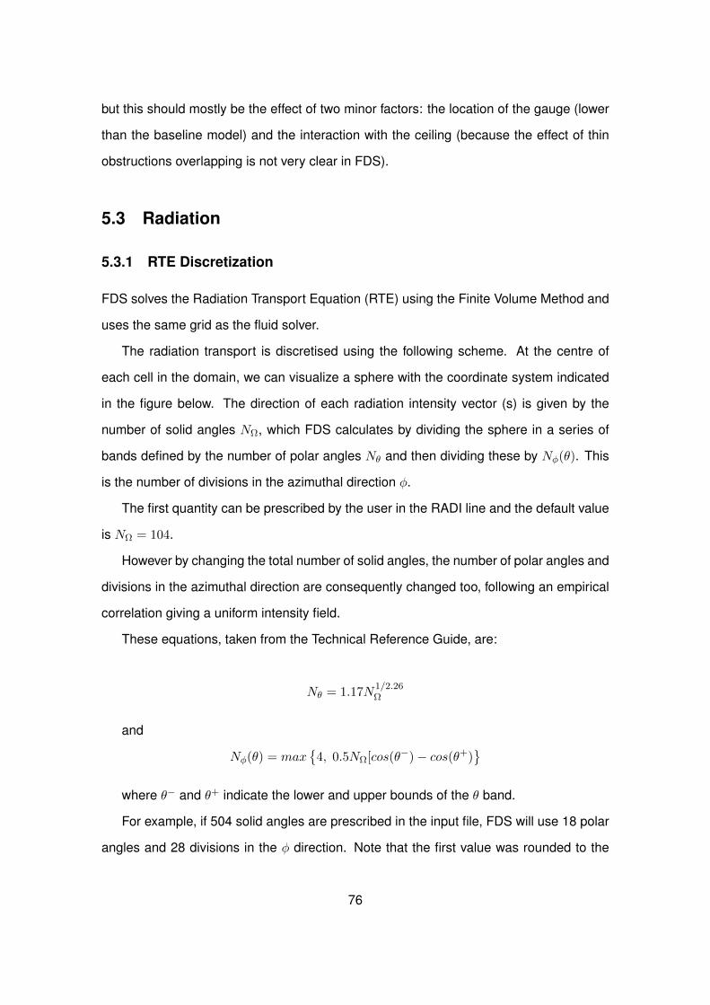
but this should mostly be the effect of two minor factors: the location of the gauge (lower

than the baseline model) and the interaction with the ceiling (because the effect of thin

obstructions overlapping is not very clear in FDS).

5.3 Radiation

5.3.1 RTE Discretization

FDS solves the Radiation Transport Equation (RTE) using the Finite Volume Method and

uses the same grid as the fluid solver.

The radiation transport is discretised using the following scheme. At the centre of

each cell in the domain, we can visualize a sphere with the coordinate system indicated

in the figure below. The direction of each radiation intensity vector (s) is given by the

number of solid angles NΩ, which FDS calculates by dividing the sphere in a series of

bands defined by the number of polar angles Nθ and then dividing these by Nφ(θ). This

is the number of divisions in the azimuthal direction φ.

The first quantity can be prescribed by the user in the RADI line and the default value

is NΩ = 104.

However by changing the total number of solid angles, the number of polar angles and

divisions in the azimuthal direction are consequently changed too, following an empirical

correlation giving a uniform intensity field.

These equations, taken from the Technical Reference Guide, are:

Nθ = 1.17N1/2.26Ω

and

Nφ(θ) = max

4, 0.5NΩ[cos(θ−)− cos(θ+)

where θ− and θ+ indicate the lower and upper bounds of the θ band.

For example, if 504 solid angles are prescribed in the input file, FDS will use 18 polar

angles and 28 divisions in the φ direction. Note that the first value was rounded to the

76

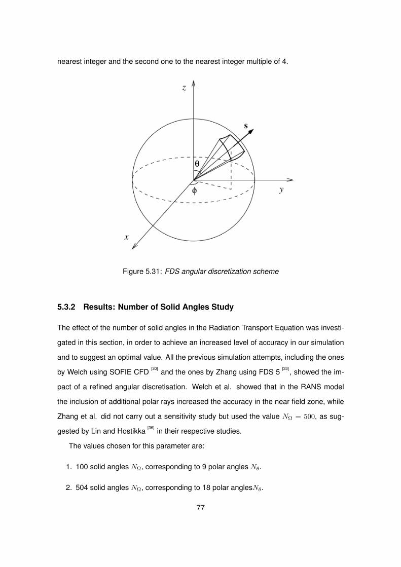
nearest integer and the second one to the nearest integer multiple of 4.

Figure 5.31: FDS angular discretization scheme

5.3.2 Results: Number of Solid Angles Study

The effect of the number of solid angles in the Radiation Transport Equation was investi-

gated in this section, in order to achieve an increased level of accuracy in our simulation

and to suggest an optimal value. All the previous simulation attempts, including the ones

by Welch using SOFIE CFD[30]

and the ones by Zhang using FDS 5[33]

, showed the im-

pact of a refined angular discretisation. Welch et al. showed that in the RANS model

the inclusion of additional polar rays increased the accuracy in the near field zone, while

Zhang et al. did not carry out a sensitivity study but used the value NΩ = 500, as sug-

gested by Lin and Hostikka[36]

in their respective studies.

The values chosen for this parameter are:

1. 100 solid angles NΩ, corresponding to 9 polar angles Nθ.

2. 504 solid angles NΩ, corresponding to 18 polar anglesNθ.

77

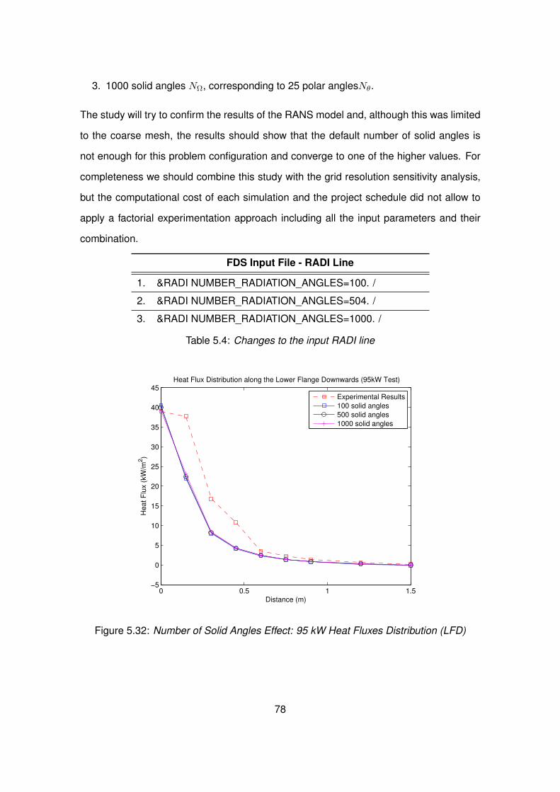
3. 1000 solid angles NΩ, corresponding to 25 polar anglesNθ.

The study will try to confirm the results of the RANS model and, although this was limited

to the coarse mesh, the results should show that the default number of solid angles is

not enough for this problem configuration and converge to one of the higher values. For

completeness we should combine this study with the grid resolution sensitivity analysis,

but the computational cost of each simulation and the project schedule did not allow to

apply a factorial experimentation approach including all the input parameters and their

combination.

FDS Input File - RADI Line

1. &RADI NUMBER_RADIATION_ANGLES=100. /



Table 5.4: Changes to the input RADI line

0 0.5 1 1.5−5

0

5

10

15

20

25

30

35

40


Distance (m)

Heat F

lux (

kW

/m2)


100 solid angles

500 solid angles

1000 solid angles

Figure 5.32: Number of Solid Angles Effect: 95 kW Heat Fluxes Distribution (LFD)

78

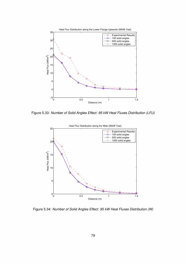
0 0.5 1 1.5−5

0

5

10

15

20

25

30


Distance (m)

Heat F

lux (

kW

/m2)


100 solid angles

500 solid angles

1000 solid angles

Figure 5.33: Number of Solid Angles Effect: 95 kW Heat Fluxes Distribution (LFU)

0 0.5 1 1.50

5

10

15

20


Distance (m)

Heat F

lux (

kW

/m2)


100 solid angles

500 solid angles

1000 solid angles

Figure 5.34: Number of Solid Angles Effect: 95 kW Heat Fluxes Distribution (W)

79

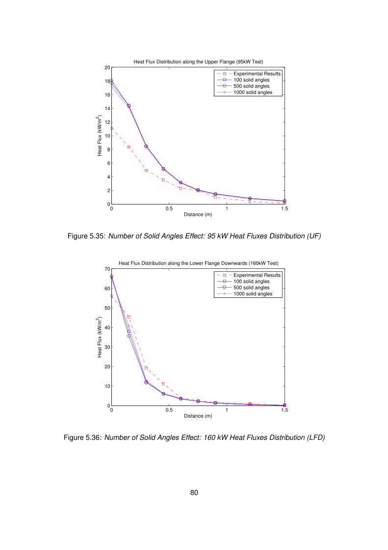
0 0.5 1 1.50

2

4

6

8

10

12

14

16

18


Distance (m)

Heat F

lux (

kW

/m2)


100 solid angles

500 solid angles

1000 solid angles

Figure 5.35: Number of Solid Angles Effect: 95 kW Heat Fluxes Distribution (UF)

0 0.5 1 1.50

10

20

30

40

50

60


Distance (m)

Heat F

lux (

kW

/m2)


100 solid angles

500 solid angles

1000 solid angles

Figure 5.36: Number of Solid Angles Effect: 160 kW Heat Fluxes Distribution (LFD)

80

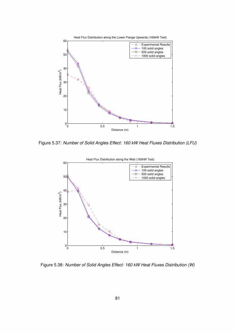
0 0.5 1 1.50

10

20

30

40

50


Distance (m)

Heat F

lux (

kW

/m2)


100 solid angles

500 solid angles

1000 solid angles

Figure 5.37: Number of Solid Angles Effect: 160 kW Heat Fluxes Distribution (LFU)

0 0.5 1 1.50

10

20

30

40

50


Distance (m)

Heat F

lux (

kW

/m2)


100 solid angles

500 solid angles

1000 solid angles

Figure 5.38: Number of Solid Angles Effect: 160 kW Heat Fluxes Distribution (W)

81

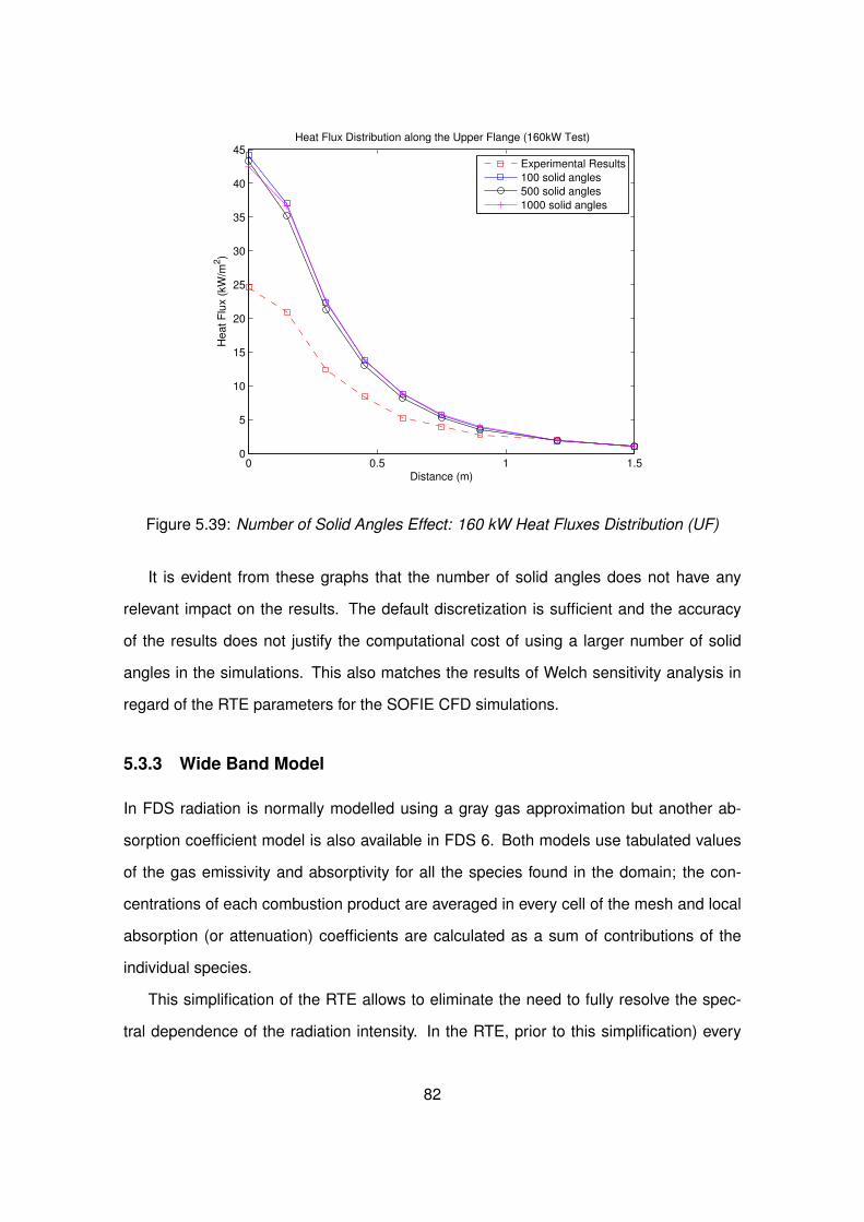
0 0.5 1 1.50

5

10

15

20

25

30

35

40


Distance (m)

Heat F

lux (

kW

/m2)


100 solid angles

500 solid angles

1000 solid angles

Figure 5.39: Number of Solid Angles Effect: 160 kW Heat Fluxes Distribution (UF)

It is evident from these graphs that the number of solid angles does not have any

relevant impact on the results. The default discretization is sufficient and the accuracy

of the results does not justify the computational cost of using a larger number of solid

angles in the simulations. This also matches the results of Welch sensitivity analysis in

regard of the RTE parameters for the SOFIE CFD simulations.

5.3.3 Wide Band Model

In FDS radiation is normally modelled using a gray gas approximation but another ab-

sorption coefficient model is also available in FDS 6. Both models use tabulated values

of the gas emissivity and absorptivity for all the species found in the domain; the con-

centrations of each combustion product are averaged in every cell of the mesh and local

absorption (or attenuation) coefficients are calculated as a sum of contributions of the

individual species.

This simplification of the RTE allows to eliminate the need to fully resolve the spec-

tral dependence of the radiation intensity. In the RTE, prior to this simplification) every

82

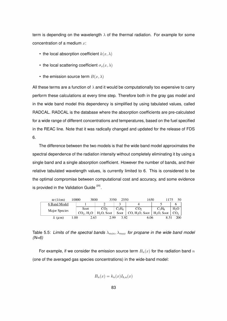
term is depending on the wavelength λ of the thermal radiation. For example for some

concentration of a medium x:

• the local absorption coefficient k(x, λ)

• the local scattering coefficient σs(x, λ)

• the emission source term B(x, λ)

All these terms are a function of λ and it would be computationally too expensive to carry

perform these calculations at every time step. Therefore both in the gray gas model and

in the wide band model this dependency is simplified by using tabulated values, called

RADCAL. RADCAL is the database where the absorption coefficients are pre-calculated

for a wide range of different concentrations and temperatures, based on the fuel specified

in the REAC line. Note that it was radically changed and updated for the release of FDS

6.

The difference between the two models is that the wide band model approximates the

spectral dependence of the radiation intensity without completely eliminating it by using a

single band and a single absorption coefficient. However the number of bands, and their

relative tabulated wavelength values, is currently limited to 6. This is considered to be

the optimal compromise between computational cost and accuracy, and some evidence

is provided in the Validation Guide[20]

.

Table 5.5: Limits of the spectral bands λmin, λmax for propane in the wide band model(N=6)

For example, if we consider the emission source term Bn(x) for the radiation band n

(one of the averaged gas species concentrations) in the wide-band model:

Bn(x) = kn(x)Ib,n(x)

83

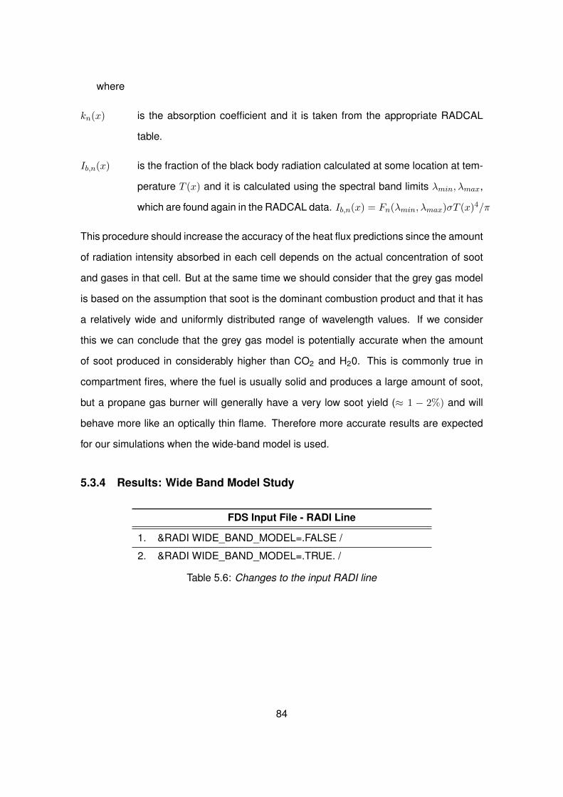
where

kn(x) is the absorption coefficient and it is taken from the appropriate RADCAL

table.

Ib,n(x) is the fraction of the black body radiation calculated at some location at tem-

perature T (x) and it is calculated using the spectral band limits λmin, λmax,

which are found again in the RADCAL data. Ib,n(x) = Fn(λmin, λmax)σT (x)4/π

This procedure should increase the accuracy of the heat flux predictions since the amount

of radiation intensity absorbed in each cell depends on the actual concentration of soot

and gases in that cell. But at the same time we should consider that the grey gas model

is based on the assumption that soot is the dominant combustion product and that it has

a relatively wide and uniformly distributed range of wavelength values. If we consider

this we can conclude that the grey gas model is potentially accurate when the amount

of soot produced in considerably higher than CO2 and H20. This is commonly true in

compartment fires, where the fuel is usually solid and produces a large amount of soot,

but a propane gas burner will generally have a very low soot yield (≈ 1 − 2%) and will

behave more like an optically thin flame. Therefore more accurate results are expected

for our simulations when the wide-band model is used.

5.3.4 Results: Wide Band Model Study


1. &RADI WIDE_BAND_MODEL=.FALSE /

2. &RADI WIDE_BAND_MODEL=.TRUE. /


84

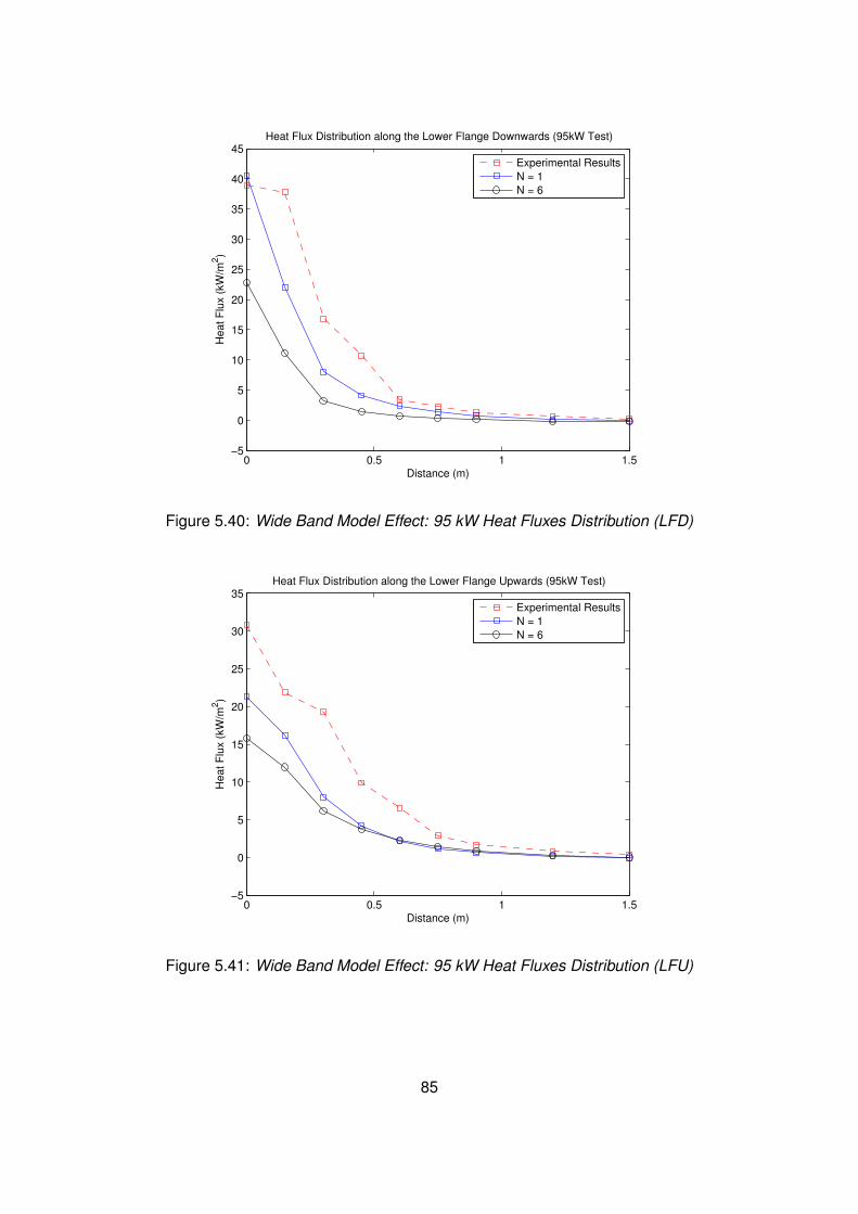
0 0.5 1 1.5−5

0

5

10

15

20

25

30

35

40


Distance (m)

Heat F

lux (

kW

/m2)


N = 1

N = 6

Figure 5.40: Wide Band Model Effect: 95 kW Heat Fluxes Distribution (LFD)

0 0.5 1 1.5−5

0

5

10

15

20

25

30


Distance (m)

Heat F

lux (

kW

/m2)


N = 1

N = 6

Figure 5.41: Wide Band Model Effect: 95 kW Heat Fluxes Distribution (LFU)

85

0 0.5 1 1.50

5

10

15

20


Distance (m)

Heat F

lux (

kW

/m2)


N = 1

N = 6

Figure 5.42: Wide Band Model Effect: 95 kW Heat Fluxes Distribution (W)

0 0.5 1 1.50

2

4

6

8

10

12

14

16

18


Distance (m)

Heat F

lux (

kW

/m2)


N = 1

N = 6

Figure 5.43: Wide Band Model Effect: 95 kW Heat Fluxes Distribution (UF)

86

0 0.5 1 1.5−10

0

10

20

30

40

50

60


Distance (m)

Heat F

lux (

kW

/m2)


N = 1

N = 6

Figure 5.44: Wide Band Model Effect: 160 kW Heat Fluxes Distribution (LFD)

0 0.5 1 1.50

10

20

30

40

50


Distance (m)

Heat F

lux (

kW

/m2)


N = 1

N = 6

Figure 5.45: Wide Band Model Effect: 160 kW Heat Fluxes Distribution (LFU)

87

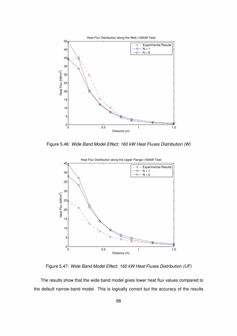
0 0.5 1 1.50

5

10

15

20

25

30

35

40

45


Distance (m)

Heat F

lux (

kW

/m2)


N = 1

N = 6

Figure 5.46: Wide Band Model Effect: 160 kW Heat Fluxes Distribution (W)

0 0.5 1 1.50

5

10

15

20

25

30

35

40


Distance (m)

Heat F

lux (

kW

/m2)


N = 1

N = 6

Figure 5.47: Wide Band Model Effect: 160 kW Heat Fluxes Distribution (UF)

The results show that the wide band model gives lower heat flux values compared to

the default narrow band model. This is logically correct but the accuracy of the results

88

is considerably worse in our case. Possibly, by combining in the same simulation the

wide band model (giving lower heat fluxes) to a finer grid (giving higher heat fluxes), the

accuracy of the results could improve significantly.

Interestingly, the shape of the distribution improves slightly when the wide band model

is used, in particular in the stagnation point area. This could solve the issue of the con-

stant overprediction of the heat fluxes at stagnation point, but a finer mesh is required for

this analysis.

5.3.5 Radiative Fraction

Approximately one third (30-40%) of the energy created by the propane combustion takes

the form of thermal radiation. In order to make sure that this ratio is respected in the sim-

ulation FDS needs a radiative fraction to be prescribed in the input file. The radiative

fraction χr indicates the fraction of energy radiated from the combustion region, but the

general definition of the term instead specifies that χr is a fraction of the total Heat Re-

lease Rate. This is particularly important because there is no proof that this proportion is

conserved locally, and therefore that χr can be applied as a factor to all the cells in the

combustion region, like FDS 5 used to do.

Based on this second definition and a series of validation cases, the FDS team de-

veloped a method to correct the emission source term, in order to obtain more accurate

results in the near field zone. The heat fluxes on targets far from the flaming region are

usually well predicted by FDS, since the emission source term based on the fourth-power

of the gas temperature is dominant and it is basically equivalent to the values calculated

by using a point source assumption. On the other hand, where the plume impinges on

the steel beam, approximately 0.5 m away from stagnation point in our simulations, FDS

seems to fail predicting the incident heat fluxes with an acceptable level of accuracy. The

preliminary simulations results, using FDS 5, clearly show that the heat fluxes in this re-

gion are quite heavily under-predicted, and sometimes they do not even reach half of the

values measured in the experiments.

This can be quite easily explained for FDS 5, as the following equations to calculate

89

the emission term:

• kIb(x) = kσT (x)4/π in the cells where HRRPUV is equal to zero, or where the

temperature dominates the results over the HRRPUV

• and kIb(x) = χr.

q′′′/4π in the cells in the combustion region (where HRRPUV > 0)

By assuming that the radiative fraction can be directly applied to the heat release rate

locally in each cell the results are not balanced and the the rest of the plume is completely

ignored when we consider a single cell. This means that, because of the spatial averaging

employed by FDS, the approximations of the model in terms of T (x) and HRRPUV have a

direct impact on the incident flux measured by the FDS devices. And this is considerably

more relevant noting that the radiation intensity depends on T (x)4.

For this reason the FDS team developed and implemented a new method to take into

account the whole plume region and to balance out local inaccuracies. This method uses

a correction factor C, with the constraint C ≥ 1, in the cells where the heat release rate

per unit volume is non-zero. Therefore the emission term Ib becomes:

Ib(x) = CσT (x)4

π

where the corrective factor C is calculated as:

C =

∑HRRPUV >0(χr

.q′′′

+ kijkUijk)dV∑HRRPUV >0(4kijkσT

4ijk)dV

Thanks to this modification the radiative fraction proportion to the total heat release

rate is conserved, but χr is not applied directly to the heat produced in the cells. The

results should therefore be more accurate in our simulations, just by using FDS 6 and

keeping the same grid resolution.

Also, note that if the radiative fraction is set to zero, the thermal radiation is based

on the source temperature T (x) and the absorption coefficient k everywhere. This is

true both for FDS 5 and FDS 6 and it can be useful because it eliminates some of the

effects due to an incorrect distribution of the HRRPUV, which is highly probable in our

simulations considering the limits of the LES method and the grid resolution adopted.

90

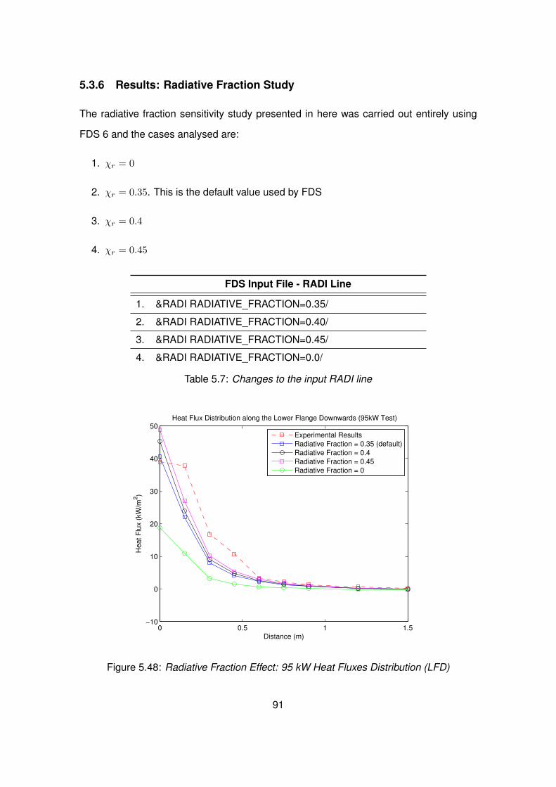
5.3.6 Results: Radiative Fraction Study

The radiative fraction sensitivity study presented in here was carried out entirely using

FDS 6 and the cases analysed are:

1. χr = 0

2. χr = 0.35. This is the default value used by FDS

3. χr = 0.4

4. χr = 0.45


1. &RADI RADIATIVE_FRACTION=0.35/





0 0.5 1 1.5−10

0

10

20

30

40


Distance (m)

Heat F

lux (

kW

/m2)


Radiative Fraction = 0.35 (default)

Radiative Fraction = 0.4


Radiative Fraction = 0

Figure 5.48: Radiative Fraction Effect: 95 kW Heat Fluxes Distribution (LFD)

91

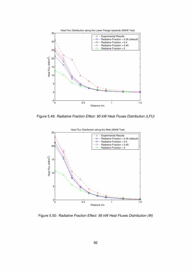
0 0.5 1 1.5−5

0

5

10

15

20

25

30


Distance (m)

Heat F

lux (

kW

/m2)






Figure 5.49: Radiative Fraction Effect: 95 kW Heat Fluxes Distribution (LFU)

0 0.5 1 1.50

5

10

15

20


Distance (m)

Heat F

lux (

kW

/m2)






Figure 5.50: Radiative Fraction Effect: 95 kW Heat Fluxes Distribution (W)

92

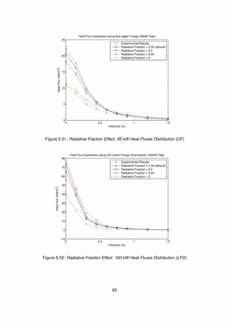
0 0.5 1 1.50

5

10

15

20


Distance (m)

Heat F

lux (

kW

/m2)






Figure 5.51: Radiative Fraction Effect: 95 kW Heat Fluxes Distribution (UF)

0 0.5 1 1.5−10

0

10

20

30

40

50

60

70


Distance (m)

Heat F

lux (

kW

/m2)






Figure 5.52: Radiative Fraction Effect: 160 kW Heat Fluxes Distribution (LFD)

93

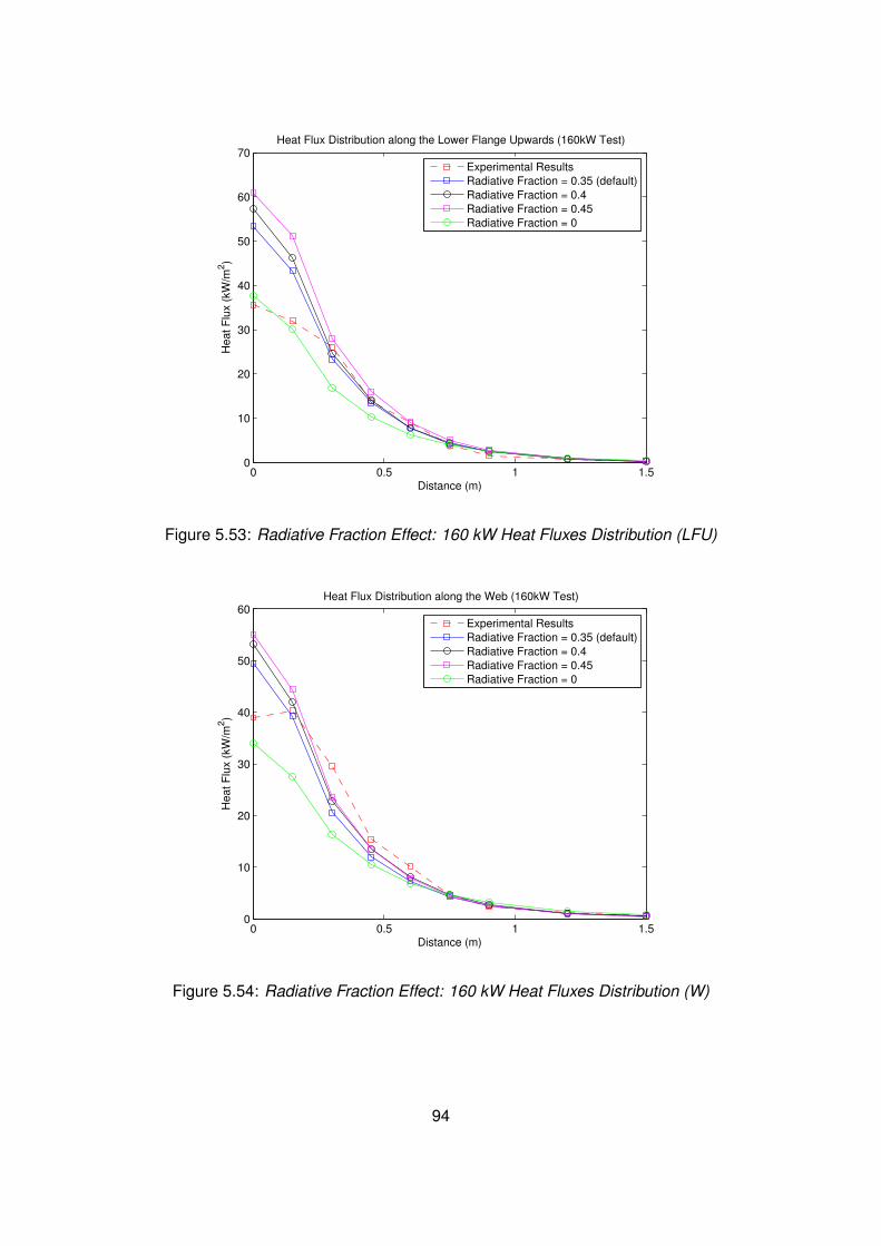
0 0.5 1 1.50

10

20

30

40

50

60


Distance (m)

Heat F

lux (

kW

/m2)






Figure 5.53: Radiative Fraction Effect: 160 kW Heat Fluxes Distribution (LFU)

0 0.5 1 1.50

10

20

30

40

50


Distance (m)

Heat F

lux (

kW

/m2)






Figure 5.54: Radiative Fraction Effect: 160 kW Heat Fluxes Distribution (W)

94

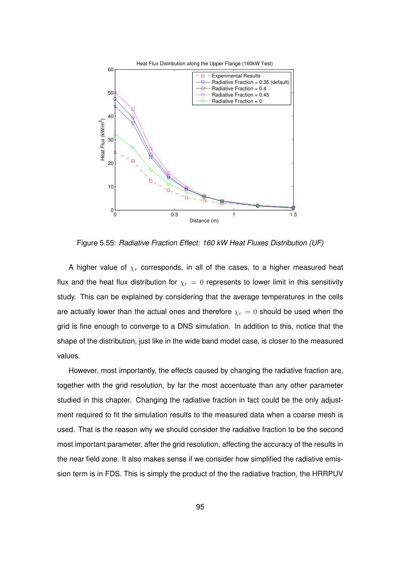
0 0.5 1 1.50

10

20

30

40

50


Distance (m)

Heat F

lux (

kW

/m2)






Figure 5.55: Radiative Fraction Effect: 160 kW Heat Fluxes Distribution (UF)

A higher value of χr corresponds, in all of the cases, to a higher measured heat

flux and the heat flux distribution for χr = 0 represents to lower limit in this sensitivity

study. This can be explained by considering that the average temperatures in the cells

are actually lower than the actual ones and therefore χr = 0 should be used when the

grid is fine enough to converge to a DNS simulation. In addition to this, notice that the

shape of the distribution, just like in the wide band model case, is closer to the measured

values.

However, most importantly, the effects caused by changing the radiative fraction are,

together with the grid resolution, by far the most accentuate than any other parameter

studied in this chapter. Changing the radiative fraction in fact could be the only adjust-

ment required to fit the simulation results to the measured data when a coarse mesh is

used. That is the reason why we should consider the radiative fraction to be the second

most important parameter, after the grid resolution, affecting the accuracy of the results in

the near field zone. It also makes sense if we consider how simplified the radiative emis-

sion term is in FDS. This is simply the product of the the radiative fraction, the HRRPUV

95

calculated from the fuel and oxygen concentration in each cell, and the absorption co-

efficient based on the soot and gas species concentration. Clearly the impact on the

measured heat fluxes will be major.

5.3.7 Maximum HRRPUV

There is a final factor to be taken into account when we consider the radiation intensity.

In order to improve the numerical stability of the model for very coarse meshes, the

FDS developers set a limit to the spatially averaged value of HRRPUV. This is not a

physical limit and it can be one of the causes of the inaccuracies of the radiative heat flux

distribution, especially when the grid resolution is increased.

Also, note that these values are based on the assumption that the fire non-dimensional

HRR Q∗ ≥ 1. This is not true for any of the tests carried out by BRI Japan, except for the

200 kW case, where Q∗ = 1.02. For example the 95 kW test has a dimensionless HRR

Q∗ = 0.48 and in the 160 kW case Q∗ = 0.82.

The value of the limit (in FDS 6) is given by the equation:

HRRPUVmax =200

dx+ 2500 kW/m3

where 200 kW/m2 is the maximum heat release rate per unit area allowed in the

cell, 2500 kW/m3 is the maximum average heat release per unit area, and dx is the

characteristic cell size.

All this values however can be modified by the user on the REAC line of the input file

through the parameters HRRPUA_SHEET (kW/m2) and HRRPUV_AVERAGE (kW/m3).

By choosing really high values we can eliminate this artificial limit to the HRRPUV and

potentially “fix” the emission term in the lower section of the plume. And this in theory

should results in more accurate predictions in the near field zone.

Finally note that FDS 6 already showed some improvement compared to FDS 5.

In the older version of the simulator, the default value of HRRPUVmaxwas simply 2500

kW/m3and the equation shown above was only used for DNS.

96

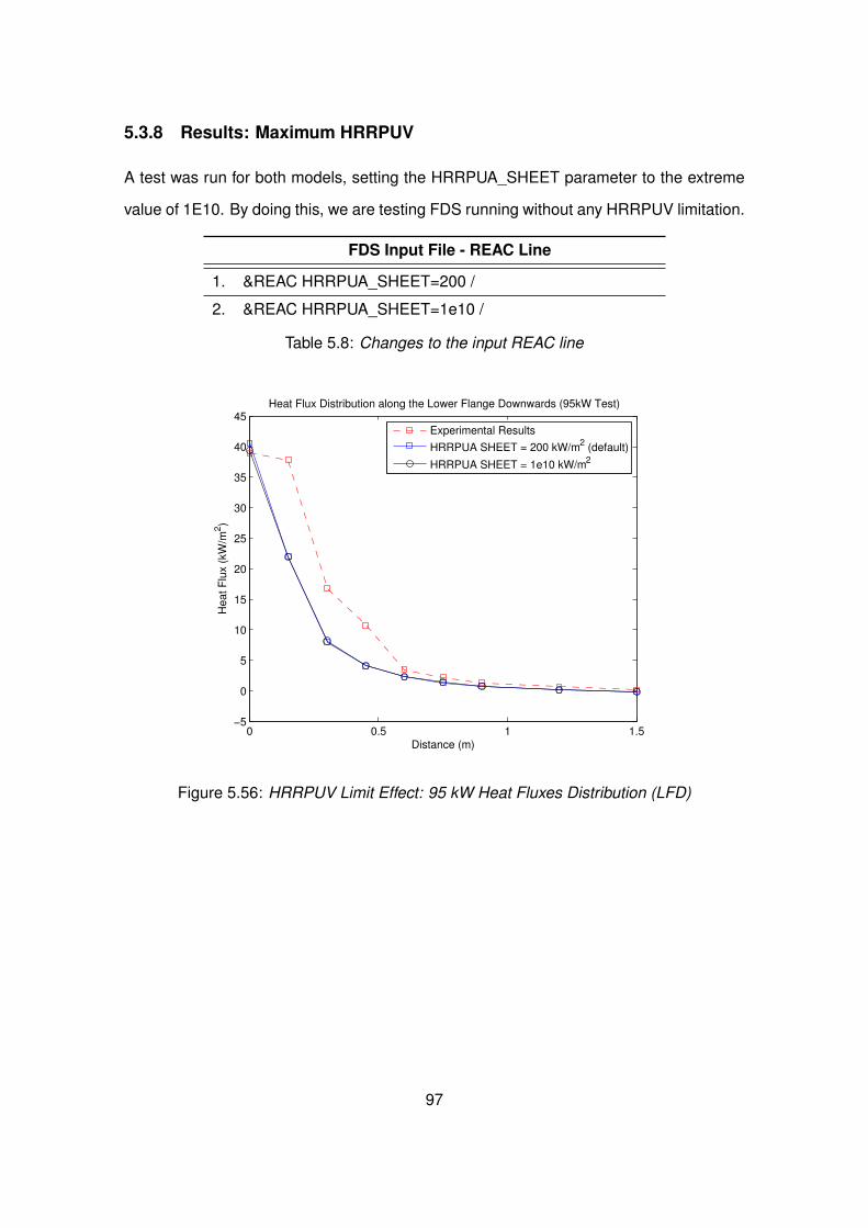
5.3.8 Results: Maximum HRRPUV

A test was run for both models, setting the HRRPUA_SHEET parameter to the extreme

value of 1E10. By doing this, we are testing FDS running without any HRRPUV limitation.

FDS Input File - REAC Line

1. &REAC HRRPUA_SHEET=200 /

2. &REAC HRRPUA_SHEET=1e10 /

Table 5.8: Changes to the input REAC line

0 0.5 1 1.5−5

0

5

10

15

20

25

30

35

40


Distance (m)

Heat F

lux (

kW

/m2)


HRRPUA SHEET = 200 kW/m2 (default)

HRRPUA SHEET = 1e10 kW/m2

Figure 5.56: HRRPUV Limit Effect: 95 kW Heat Fluxes Distribution (LFD)

97

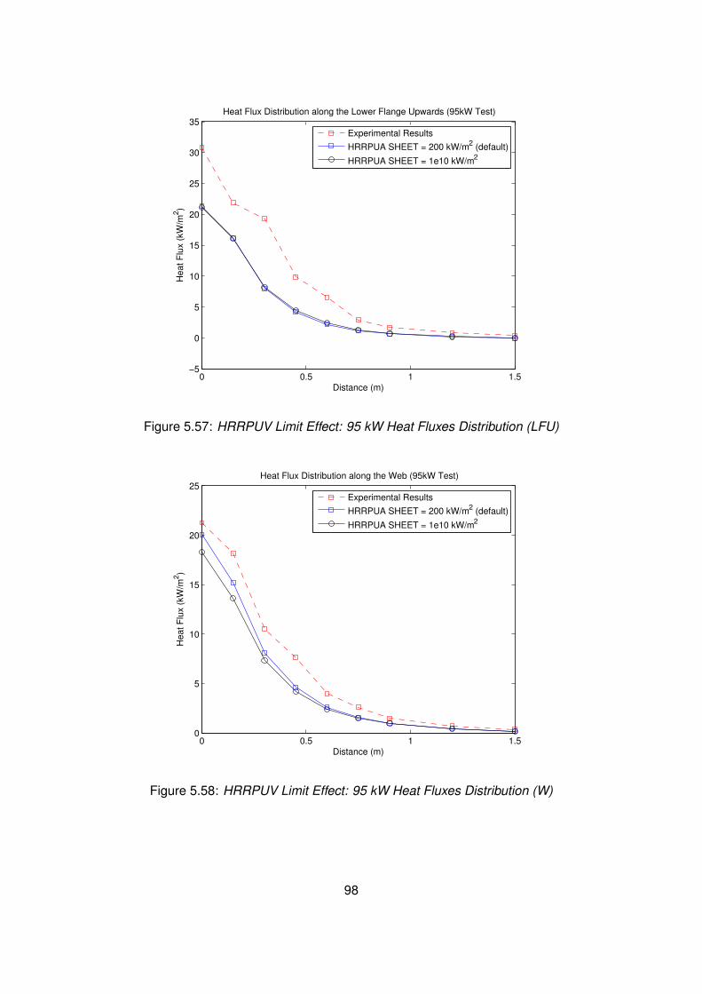
0 0.5 1 1.5−5

0

5

10

15

20

25

30


Distance (m)

Heat F

lux (

kW

/m2)




Figure 5.57: HRRPUV Limit Effect: 95 kW Heat Fluxes Distribution (LFU)

0 0.5 1 1.50

5

10

15

20


Distance (m)

Heat F

lux (

kW

/m2)




Figure 5.58: HRRPUV Limit Effect: 95 kW Heat Fluxes Distribution (W)

98

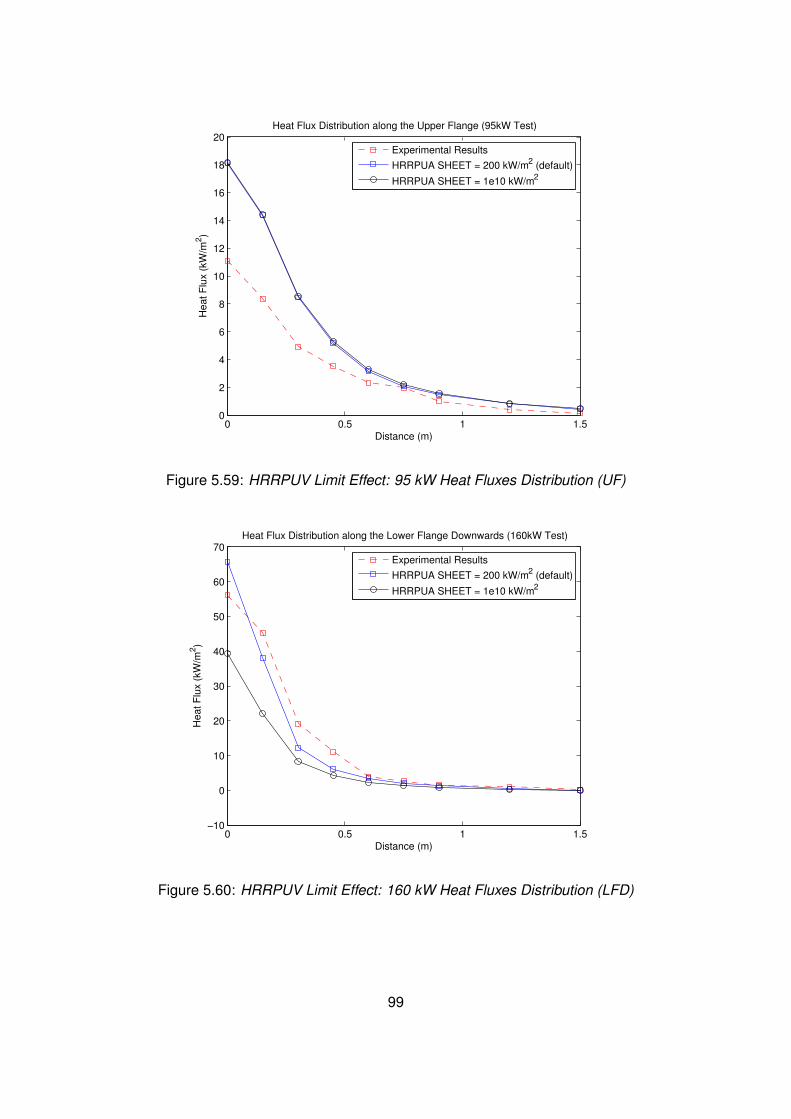
0 0.5 1 1.50

2

4

6

8

10

12

14

16

18


Distance (m)

Heat F

lux (

kW

/m2)




Figure 5.59: HRRPUV Limit Effect: 95 kW Heat Fluxes Distribution (UF)

0 0.5 1 1.5−10

0

10

20

30

40

50

60


Distance (m)

Heat F

lux (

kW

/m2)




Figure 5.60: HRRPUV Limit Effect: 160 kW Heat Fluxes Distribution (LFD)

99

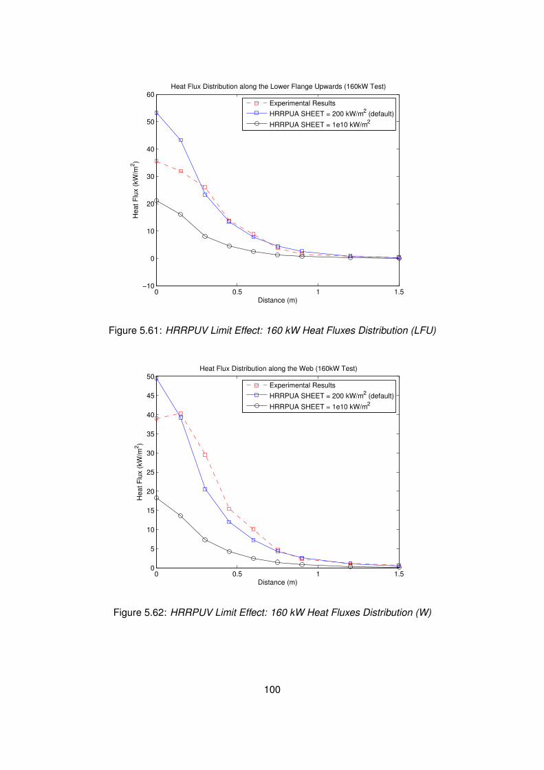
0 0.5 1 1.5−10

0

10

20

30

40

50


Distance (m)

Heat F

lux (

kW

/m2)




Figure 5.61: HRRPUV Limit Effect: 160 kW Heat Fluxes Distribution (LFU)

0 0.5 1 1.50

5

10

15

20

25

30

35

40

45


Distance (m)

Heat F

lux (

kW

/m2)




Figure 5.62: HRRPUV Limit Effect: 160 kW Heat Fluxes Distribution (W)

100

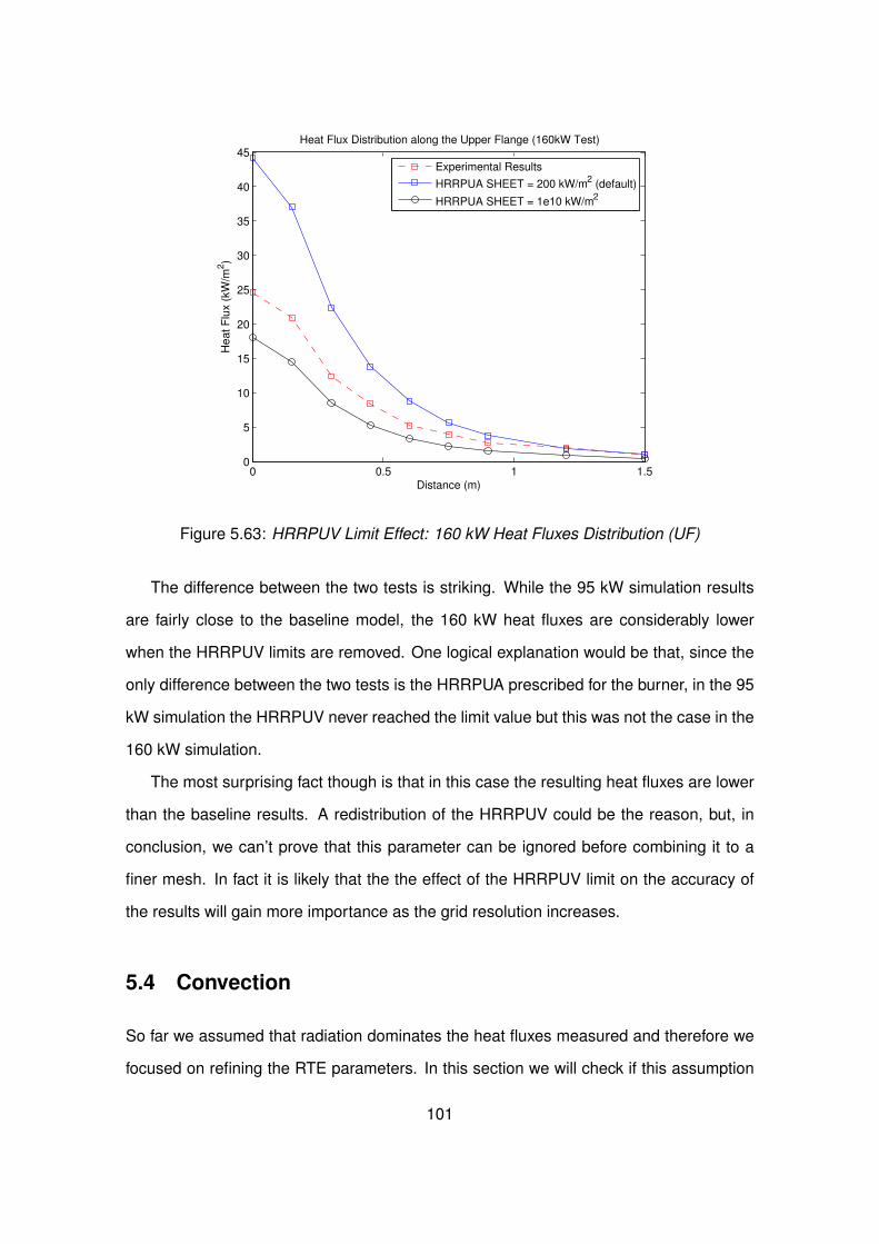
0 0.5 1 1.50

5

10

15

20

25

30

35

40


Distance (m)

Heat F

lux (

kW

/m2)




Figure 5.63: HRRPUV Limit Effect: 160 kW Heat Fluxes Distribution (UF)

The difference between the two tests is striking. While the 95 kW simulation results

are fairly close to the baseline model, the 160 kW heat fluxes are considerably lower

when the HRRPUV limits are removed. One logical explanation would be that, since the

only difference between the two tests is the HRRPUA prescribed for the burner, in the 95

kW simulation the HRRPUV never reached the limit value but this was not the case in the

160 kW simulation.

The most surprising fact though is that in this case the resulting heat fluxes are lower

than the baseline results. A redistribution of the HRRPUV could be the reason, but, in

conclusion, we can’t prove that this parameter can be ignored before combining it to a

finer mesh. In fact it is likely that the the effect of the HRRPUV limit on the accuracy of

the results will gain more importance as the grid resolution increases.

5.4 Convection

So far we assumed that radiation dominates the heat fluxes measured and therefore we

focused on refining the RTE parameters. In this section we will check if this assumption

101

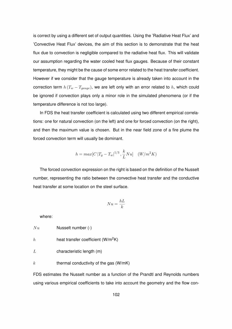
is correct by using a different set of output quantities. Using the ’Radiative Heat Flux’ and

’Convective Heat Flux’ devices, the aim of this section is to demonstrate that the heat

flux due to convection is negligible compared to the radiative heat flux. This will validate

our assumption regarding the water cooled heat flux gauges. Because of their constant

temperature, they might be the cause of some error related to the heat transfer coefficient.

However if we consider that the gauge temperature is already taken into account in the

correction term h (Tw − Tgauge), we are left only with an error related to h, which could

be ignored if convection plays only a minor role in the simulated phenomena (or if the

temperature difference is not too large).

In FDS the heat transfer coefficient is calculated using two different empirical correla-

tions: one for natural convection (on the left) and one for forced convection (on the right),

and then the maximum value is chosen. But in the near field zone of a fire plume the

forced convection term will usually be dominant.

h = max[C |Tg − Tw|1/3 ,k

LNu] (W/m2K)

The forced convection expression on the right is based on the definition of the Nusselt

number, representing the ratio between the convective heat transfer and the conductive

heat transfer at some location on the steel surface.

Nu =hL

k

where:

Nu Nusselt number (-)

h heat transfer coefficient (W/m2K)

L characteristic length (m)

k thermal conductivity of the gas (W/mK)

FDS estimates the Nusselt number as a function of the Prandtl and Reynolds numbers

using various empirical coefficients to take into account the geometry and the flow con-

102

ditions for each particular case. For example if we consider convection to a flat surface,

the Nusselt number will be given by

Nu = 0.037Re0.8Pr0.3

with

Pr ≈ 0.7

and

Re =ρ |u|Lµ

where:

ρ density of the gas (kg/m3)

u near wall gas velocity

L characteristic length (m)

µ dynamic viscosity (kg/ms)

More details can be found in the Technical Reference Guide, Section 7.1.2.

In conclusion, we are expecting a really low convective heat flux in the lower flange

and in the upper flange, because these are directly exposed to the fire source, but the

effect of convection could be critical in less exposed areas such as the lower half of the

web.

103

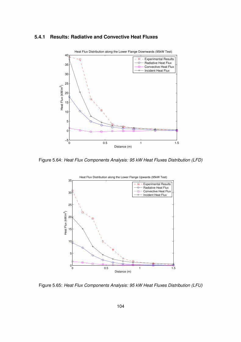
5.4.1 Results: Radiative and Convective Heat Fluxes

0 0.5 1 1.5−5

0

5

10

15

20

25

30

35


Distance (m)

Heat F

lux (

kW

/m2)


Radiative Heat Flux

Convective Heat Flux

Incident Heat Flux

Figure 5.64: Heat Flux Components Analysis: 95 kW Heat Fluxes Distribution (LFD)

0 0.5 1 1.50

5

10

15

20

25

30


Distance (m)

He

at

Flu

x (

kW

/m2)


Radiative Heat Flux


Incident Heat Flux

Figure 5.65: Heat Flux Components Analysis: 95 kW Heat Fluxes Distribution (LFU)

104

0 0.5 1 1.50

5

10

15

20

25Heat Flux Distribution along the Web (95kW Test))

Distance (m)

Heat F

lux (

kW

/m2)


Radiative Heat Flux


Incident Heat Flux

Figure 5.66: Heat Flux Components Analysis: 95 kW Heat Fluxes Distribution (W)

0 0.5 1 1.5−2

0

2

4

6

8

10

12

14

16

18Heat Flux Distribution along the Upper Flange (95kW Test))

Distance (m)

He

at

Flu

x (

kW

/m2)


Radiative Heat Flux


Incident Heat Flux

Figure 5.67: Heat Flux Components Analysis: 95 kW Heat Fluxes Distribution (UF)

105

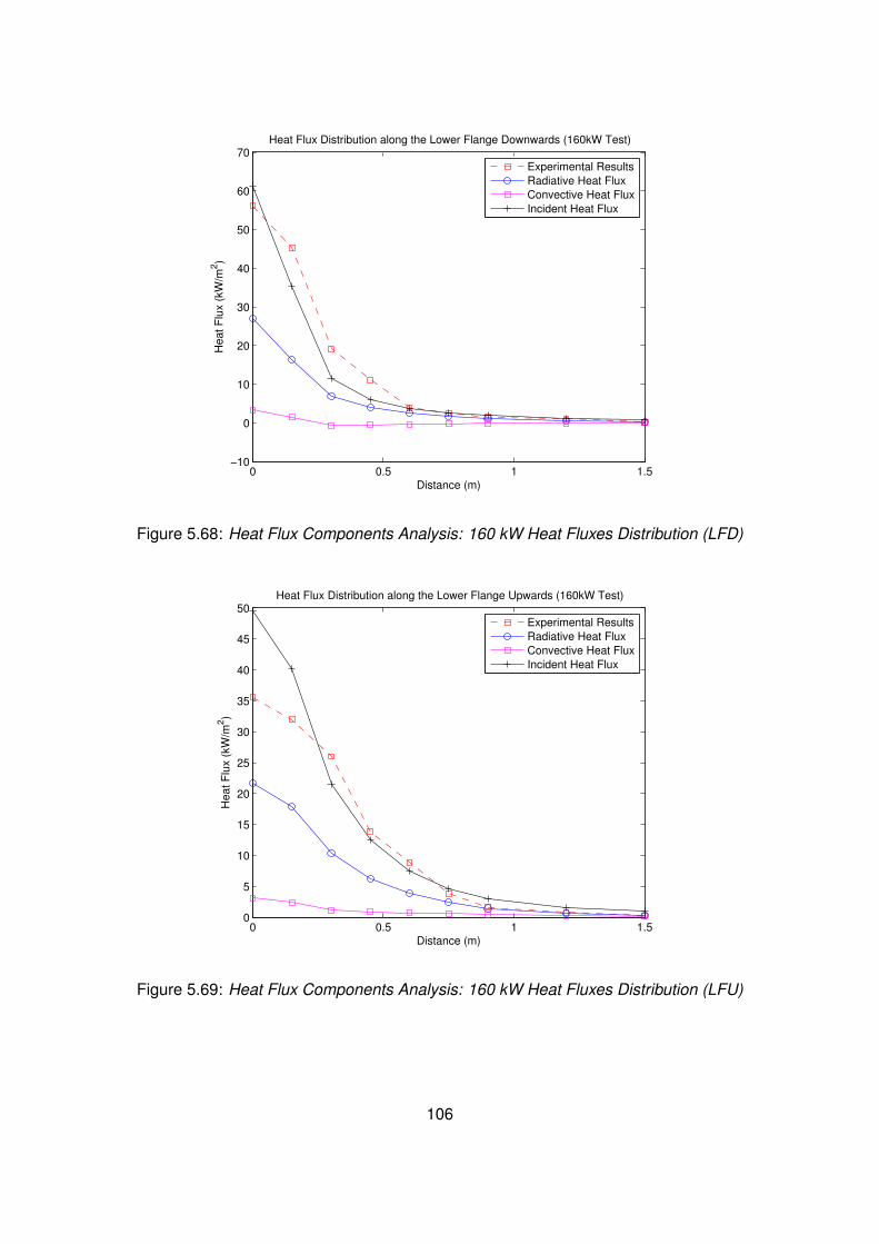
0 0.5 1 1.5−10

0

10

20

30

40

50

60


Distance (m)

Heat F

lux (

kW

/m2)


Radiative Heat Flux


Incident Heat Flux

Figure 5.68: Heat Flux Components Analysis: 160 kW Heat Fluxes Distribution (LFD)

0 0.5 1 1.50

5

10

15

20

25

30

35

40

45


Distance (m)

Heat F

lux (

kW

/m2)


Radiative Heat Flux


Incident Heat Flux

Figure 5.69: Heat Flux Components Analysis: 160 kW Heat Fluxes Distribution (LFU)

106

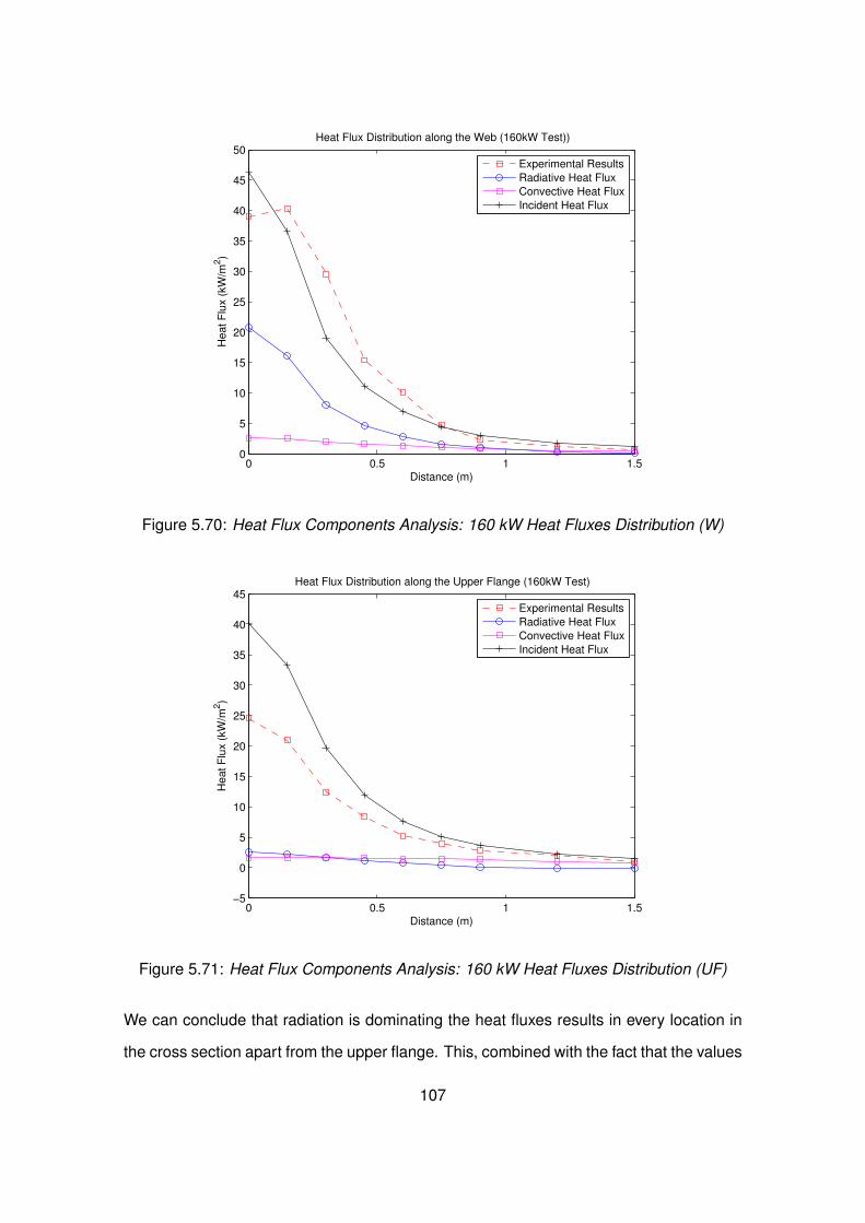
0 0.5 1 1.50

5

10

15

20

25

30

35

40

45

50Heat Flux Distribution along the Web (160kW Test))

Distance (m)

Heat F

lux (

kW

/m2)


Radiative Heat Flux


Incident Heat Flux

Figure 5.70: Heat Flux Components Analysis: 160 kW Heat Fluxes Distribution (W)

0 0.5 1 1.5−5

0

5

10

15

20

25

30

35

40


Distance (m)

Heat F

lux (

kW

/m2)


Radiative Heat Flux


Incident Heat Flux

Figure 5.71: Heat Flux Components Analysis: 160 kW Heat Fluxes Distribution (UF)

We can conclude that radiation is dominating the heat fluxes results in every location in

the cross section apart from the upper flange. This, combined with the fact that the values

107

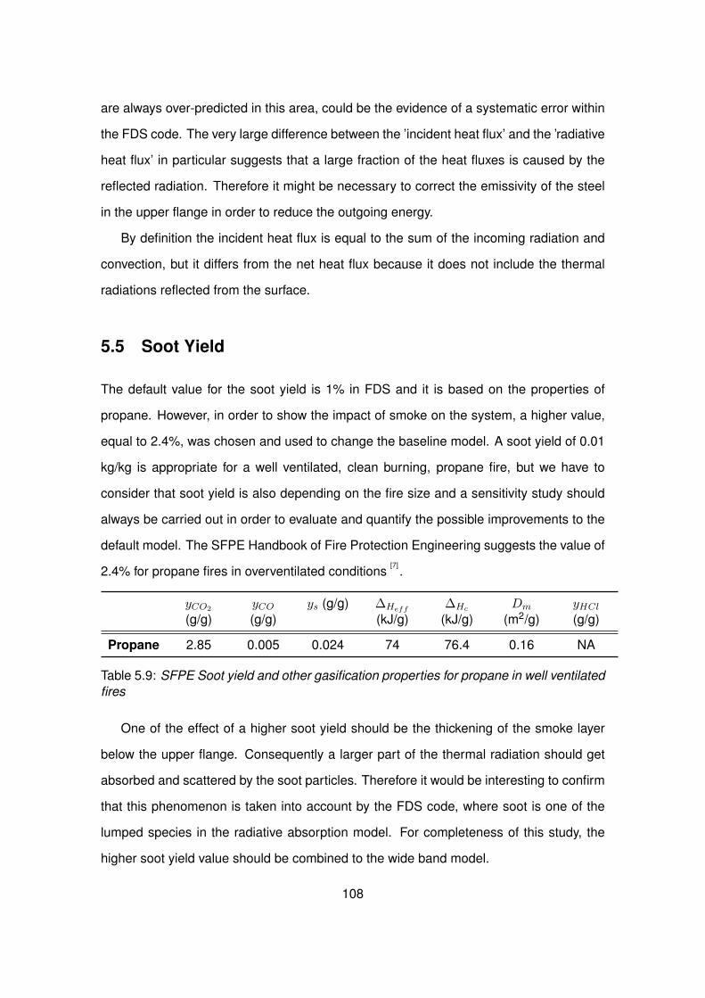
are always over-predicted in this area, could be the evidence of a systematic error within

the FDS code. The very large difference between the ’incident heat flux’ and the ’radiative

heat flux’ in particular suggests that a large fraction of the heat fluxes is caused by the

reflected radiation. Therefore it might be necessary to correct the emissivity of the steel

in the upper flange in order to reduce the outgoing energy.

By definition the incident heat flux is equal to the sum of the incoming radiation and

convection, but it differs from the net heat flux because it does not include the thermal

radiations reflected from the surface.

5.5 Soot Yield

The default value for the soot yield is 1% in FDS and it is based on the properties of

propane. However, in order to show the impact of smoke on the system, a higher value,

equal to 2.4%, was chosen and used to change the baseline model. A soot yield of 0.01

kg/kg is appropriate for a well ventilated, clean burning, propane fire, but we have to

consider that soot yield is also depending on the fire size and a sensitivity study should

always be carried out in order to evaluate and quantify the possible improvements to the

default model. The SFPE Handbook of Fire Protection Engineering suggests the value of

2.4% for propane fires in overventilated conditions[7]

.

yCO2

(g/g)yCO(g/g)

ys (g/g) ∆Heff

(kJ/g)∆Hc

(kJ/g)Dm

(m2/g)yHCl(g/g)

Propane 2.85 0.005 0.024 74 76.4 0.16 NA

Table 5.9: SFPE Soot yield and other gasification properties for propane in well ventilatedfires

One of the effect of a higher soot yield should be the thickening of the smoke layer

below the upper flange. Consequently a larger part of the thermal radiation should get

absorbed and scattered by the soot particles. Therefore it would be interesting to confirm

that this phenomenon is taken into account by the FDS code, where soot is one of the

lumped species in the radiative absorption model. For completeness of this study, the

higher soot yield value should be combined to the wide band model.

108

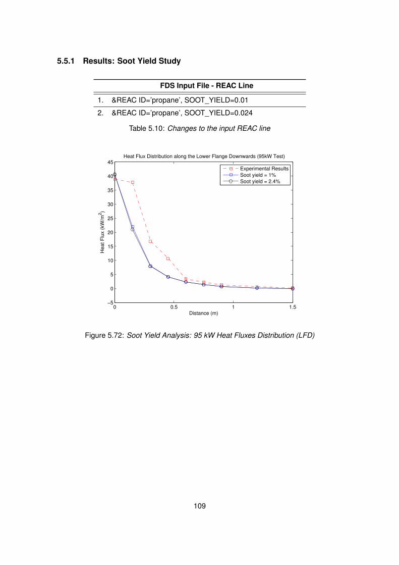
5.5.1 Results: Soot Yield Study

FDS Input File - REAC Line

1. &REAC ID=’propane’, SOOT_YIELD=0.01

2. &REAC ID=’propane’, SOOT_YIELD=0.024

Table 5.10: Changes to the input REAC line

0 0.5 1 1.5−5

0

5

10

15

20

25

30

35

40


Distance (m)

Heat F

lux (

kW

/m2)


Soot yield = 1%

Soot yield = 2.4%

Figure 5.72: Soot Yield Analysis: 95 kW Heat Fluxes Distribution (LFD)

109

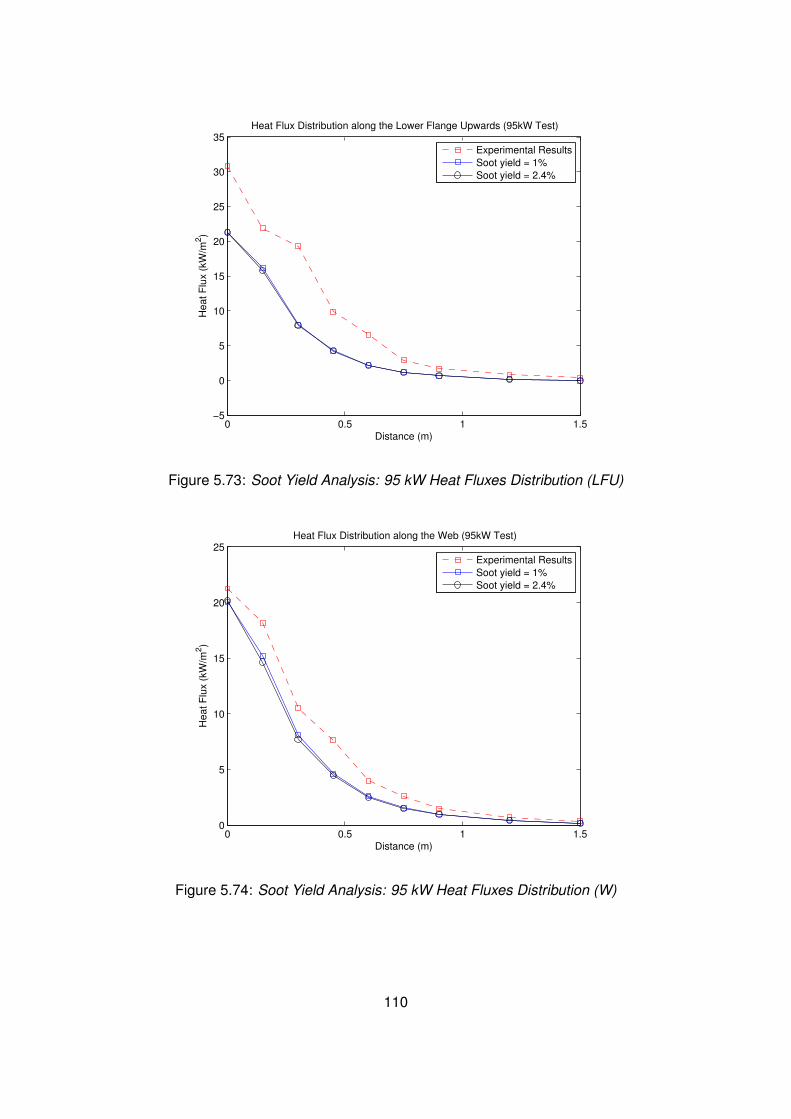
0 0.5 1 1.5−5

0

5

10

15

20

25

30


Distance (m)

Heat F

lux (

kW

/m2)


Soot yield = 1%

Soot yield = 2.4%

Figure 5.73: Soot Yield Analysis: 95 kW Heat Fluxes Distribution (LFU)

0 0.5 1 1.50

5

10

15

20


Distance (m)

Heat F

lux (

kW

/m2)


Soot yield = 1%

Soot yield = 2.4%

Figure 5.74: Soot Yield Analysis: 95 kW Heat Fluxes Distribution (W)

110

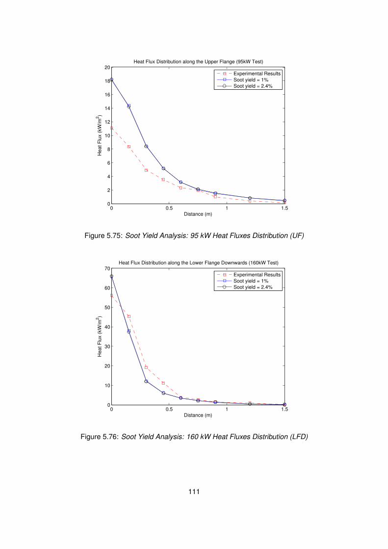
0 0.5 1 1.50

2

4

6

8

10

12

14

16

18


Distance (m)

Heat F

lux (

kW

/m2)


Soot yield = 1%

Soot yield = 2.4%

Figure 5.75: Soot Yield Analysis: 95 kW Heat Fluxes Distribution (UF)

0 0.5 1 1.50

10

20

30

40

50

60


Distance (m)

Heat F

lux (

kW

/m2)


Soot yield = 1%

Soot yield = 2.4%

Figure 5.76: Soot Yield Analysis: 160 kW Heat Fluxes Distribution (LFD)

111

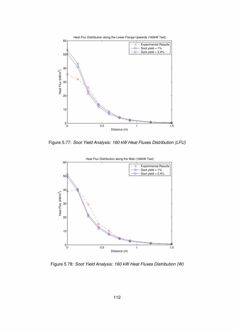
0 0.5 1 1.50

10

20

30

40

50


Distance (m)

Heat F

lux (

kW

/m2)


Soot yield = 1%

Soot yield = 2.4%

Figure 5.77: Soot Yield Analysis: 160 kW Heat Fluxes Distribution (LFU)

0 0.5 1 1.50

10

20

30

40

50


Distance (m)

Heat F

lux (

kW

/m2)


Soot yield = 1%

Soot yield = 2.4%

Figure 5.78: Soot Yield Analysis: 160 kW Heat Fluxes Distribution (W)

112

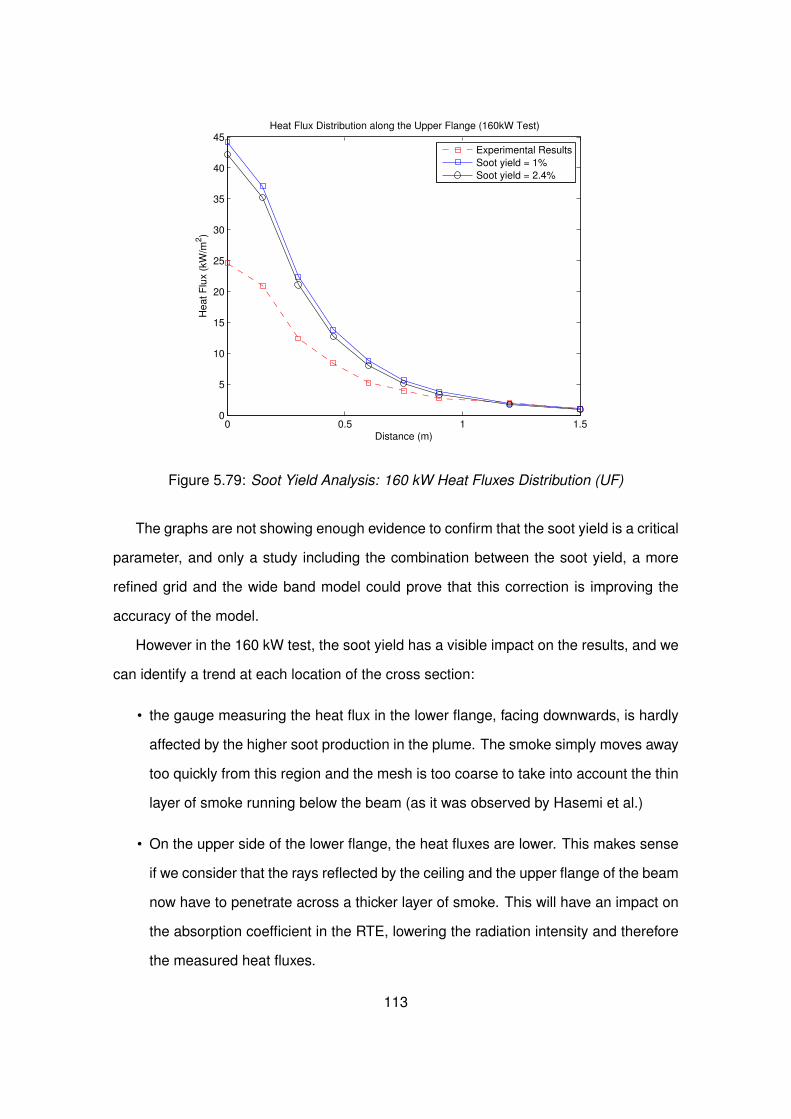
0 0.5 1 1.50

5

10

15

20

25

30

35

40


Distance (m)

Heat F

lux (

kW

/m2)


Soot yield = 1%

Soot yield = 2.4%

Figure 5.79: Soot Yield Analysis: 160 kW Heat Fluxes Distribution (UF)

The graphs are not showing enough evidence to confirm that the soot yield is a critical

parameter, and only a study including the combination between the soot yield, a more

refined grid and the wide band model could prove that this correction is improving the

accuracy of the model.

However in the 160 kW test, the soot yield has a visible impact on the results, and we

can identify a trend at each location of the cross section:

• the gauge measuring the heat flux in the lower flange, facing downwards, is hardly

affected by the higher soot production in the plume. The smoke simply moves away

too quickly from this region and the mesh is too coarse to take into account the thin

layer of smoke running below the beam (as it was observed by Hasemi et al.)

• On the upper side of the lower flange, the heat fluxes are lower. This makes sense

if we consider that the rays reflected by the ceiling and the upper flange of the beam

now have to penetrate across a thicker layer of smoke. This will have an impact on

the absorption coefficient in the RTE, lowering the radiation intensity and therefore

the measured heat fluxes.

113

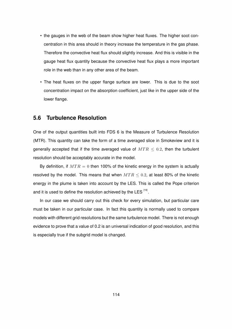
• the gauges in the web of the beam show higher heat fluxes. The higher soot con-

centration in this area should in theory increase the temperature in the gas phase.

Therefore the convective heat flux should slightly increase. And this is visible in the

gauge heat flux quantity because the convective heat flux plays a more important

role in the web than in any other area of the beam.

• The heat fluxes on the upper flange surface are lower. This is due to the soot

concentration impact on the absorption coefficient, just like in the upper side of the

lower flange.

5.6 Turbulence Resolution

One of the output quantities built into FDS 6 is the Measure of Turbulence Resolution

(MTR). This quantity can take the form of a time averaged slice in Smokeview and it is

generally accepted that if the time averaged value of MTR ≤ 0.2, then the turbulent

resolution should be acceptably accurate in the model.

By definition, if MTR = 0 then 100% of the kinetic energy in the system is actually

resolved by the model. This means that when MTR ≤ 0.2, at least 80% of the kinetic

energy in the plume is taken into account by the LES. This is called the Pope criterion

and it is used to define the resolution achieved by the LES[19]

.

In our case we should carry out this check for every simulation, but particular care

must be taken in our particular case. In fact this quantity is normally used to compare

models with different grid resolutions but the same turbulence model. There is not enough

evidence to prove that a value of 0.2 is an universal indication of good resolution, and this

is especially true if the subgrid model is changed.

114

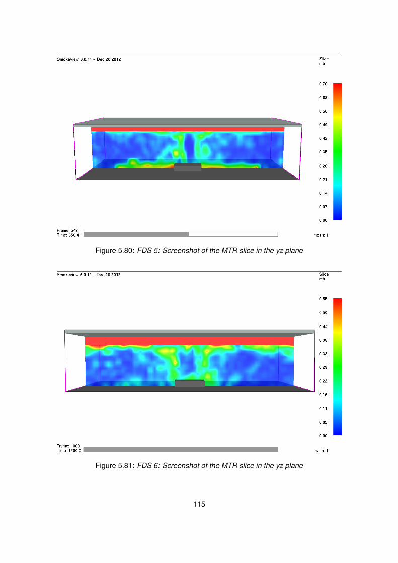
Figure 5.80: FDS 5: Screenshot of the MTR slice in the yz plane

Figure 5.81: FDS 6: Screenshot of the MTR slice in the yz plane

115

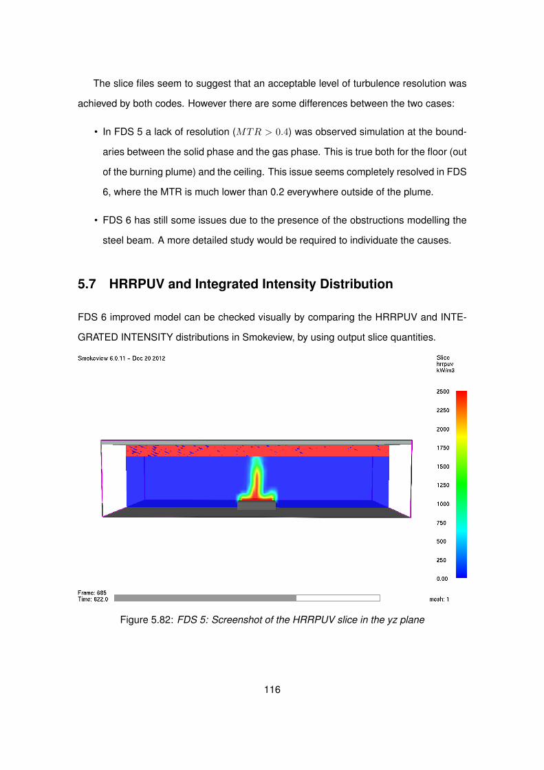
The slice files seem to suggest that an acceptable level of turbulence resolution was

achieved by both codes. However there are some differences between the two cases:

• In FDS 5 a lack of resolution (MTR > 0.4) was observed simulation at the bound-

aries between the solid phase and the gas phase. This is true both for the floor (out

of the burning plume) and the ceiling. This issue seems completely resolved in FDS

6, where the MTR is much lower than 0.2 everywhere outside of the plume.

• FDS 6 has still some issues due to the presence of the obstructions modelling the

steel beam. A more detailed study would be required to individuate the causes.

5.7 HRRPUV and Integrated Intensity Distribution

FDS 6 improved model can be checked visually by comparing the HRRPUV and INTE-

GRATED INTENSITY distributions in Smokeview, by using output slice quantities.

Figure 5.82: FDS 5: Screenshot of the HRRPUV slice in the yz plane

116

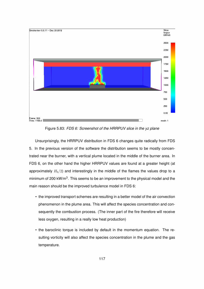
Figure 5.83: FDS 6: Screenshot of the HRRPUV slice in the yz plane

Unsurprisingly, the HRRPUV distribution in FDS 6 changes quite radically from FDS

5. In the previous version of the software the distribution seems to be mostly concen-

trated near the burner, with a vertical plume located in the middle of the burner area. In

FDS 6, on the other hand the higher HRRPUV values are found at a greater height (at

approximately Hb/2) and interestingly in the middle of the flames the values drop to a

minimum of 200 kW/m3. This seems to be an improvement to the physical model and the

main reason should be the improved turbulence model in FDS 6:

• the improved transport schemes are resulting in a better model of the air convection

phenomenon in the plume area. This will affect the species concentration and con-

sequently the combustion process. (The inner part of the fire therefore will receive

less oxygen, resulting in a really low heat production)

• the baroclinic torque is included by default in the momentum equation. The re-

sulting vorticity will also affect the species concentration in the plume and the gas

temperature.

117

• the new turbulence model is achieving a better resolution of turbulence in coarse

meshes. Turbulent mixing is also an important factor that has been revised in FDS

6.

The heat fluxes measured by the devices however indicate that, for relatively coarse

meshes like this, the model has been significantly improved. In particular the improve-

ments in the near field zone heat fluxes, which are a function of the HRRPUV, could be

an important factor for the success of LES in performance based design situations.

5.8 LES Parameters

One of the most important features of FDS, compared to RANS, is the capability to model

turbulence and eddy formation within the computational grid. In order to describe these

phenomena, FDS needs to estimate three diffusive parameters in every cell of the do-

main:

• the thermal conductivity (kt)

• the mass diffusivity (Dt)

• the turbulent viscosity (µt)

These parameters are then applied to the transport equations for mass, momentum and

energy through the hydrodynamic model algorithms and they can easily be overlooked by

FDS users with little fire modelling experience. However, if we ignore the mathematical

implementation in the code, we will notice that originally the calculations are based on

empirical observations and quite rough assumptions, that can be modified on the MISC

line of the input file.

The thermal conductivity(kt) and the material diffusivityDt , for example, are assumed

to be a function of the viscosity and some constant values of the Schmidt number and

the Prandtl number (two dimensionless parameters defining the mass diffusivity and the

thermal diffusivity respectively).

118

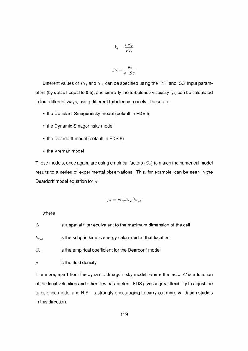
kt =µtcpPrt

Dt =µt

ρ · Sct

Different values of Prt and Sct can be specified using the ’PR’ and ’SC’ input param-

eters (by default equal to 0.5), and similarly the turbulence viscosity (µ) can be calculated

in four different ways, using different turbulence models. These are:

• the Constant Smagorinsky model (default in FDS 5)

• the Dynamic Smagorinsky model

• the Deardorff model (default in FDS 6)

• the Vreman model

These models, once again, are using empirical factors (Cv) to match the numerical model

results to a series of experimental observations. This, for example, can be seen in the

Deardorff model equation for µ:

µt = ρCv∆√ksgs

where

∆ is a spatial filter equivalent to the maximum dimension of the cell

ksgs is the subgrid kinetic energy calculated at that location

Cv is the empirical coefficient for the Deardorff model

ρ is the fluid density

Therefore, apart from the dynamic Smagorinsky model, where the factor C is a function

of the local velocities and other flow parameters, FDS gives a great flexibility to adjust the

turbulence model and NIST is strongly encouraging to carry out more validation studies

in this direction.

119

In conclusion, it would be interesting to compare the results obtained using different

turbulence models, changing the Pr and Sc numbers and the empirical coefficients used

to calculate the thermal diffusivity and viscosity parameters. The main reason is because

these modifications will most likely change the turbulent mixing process (spatially and

temporally), and consequently this could have an impact on the HRRPUV distribution

and on the thermal radiations emission source. This, of course, has also a direct impact

on the accuracy of the heat fluxes in our simulations.

120

Chapter 6

Conclusions

Sensitivity Study Conclusions

The objective of the sensitivity study discussed in the previous chapter was to define a lim-

ited number of parameters, critically affecting the accuracy of the simulations. Amongst

all, only four parameters had a significant impact on the results:

1. Grid resolution

In general when the grid resolution increases, the predicted heat fluxes increase

considerably in the near field zone, resulting in an improved level of accuracy. This

is due to a simultaneous improvement in the resolution of the combustion, the radia-

tion, the hydrodynamic and the turbulence phenomena, which practically translates

in a more accurate prediction of the HRRPUV distribution. As we expect, the results

seem to converge to a limit value when R* is large enough, and we can identify this

limit with the hypothetical results of a Direct Numerical Simulation.

2. Maximum HRRPUV limit

The impact of this parameter depends mostly on the fire size and the grid resolution

of each model. It gives more accurate results when a coarse mesh is used, because

the spatially averaged temperatures are critically more inaccurate in this case, but

this limit should be removed when performing simulations

3. Radiative fraction

121

Similarly to the HRRPUV limit, this quantity is useful when the grid resolution is

relatively low and the emission source term is simply calculated as a fraction of

the HRRPUV in each cell in the flaming region. This simplification however doesn’t

hold when the cell dimensions are small enough to allow a relatively accurate pre-

diction of the local temperatures, and should be completely ignored in case of DNS

calculations.

4. Absorption band model

The steep gradient and the general overprediction of the heat fluxes near the stag-

nation point seem to be less pronounced when the wide band model is employed.

This is due to the fact that the absorption coefficients dependence on the gas tem-

peratures is included into the model and results in lower values of the predicted

heat fluxes. Although this seems a regression from the baseline model, it is likely

to be compensated by the use of a finer grid.

It is important to notice that all the effects can be explained logically from the equations at

the base of the FDS model and therefore we might expect certain results when combining

the different parameters. This is explained in detail in the next section.

Finally, the optional turbulence models available in the FDS codes, and the constants

defining them, are expected to be critical too but there was not enough time to investigate

the effects of each of them. This should be included if the same problem is studied again

in the future.

Suggestions for Further Research

There are three possible developments for this study:

1. Improving the accuracy of the simulations while keeping a limit to the computational

cost. This would be the direct continuation of this thesis and should be intended as

a study of the FDS capabilities in practical design situations. It should consist in a

larger number of simulations, compared to a wider and more meaningful range of

experimental data, and it should study all the possible combinations between the

122

critical parameters highlighted in this thesis[17, 23]

. The results should be shared with

the FDS community and included in the official validation guide.

2. Improving the accuracy of the results without a set limit to the computational cost.

In this case the aim would be to perform a series of direct numerical simulations (or

large-eddy simulations with extremely high grid resolution) and test the FDS code

in this context. High-performance computing will be necessary to run this type of

simulations, and this will be technically the most challenging aspect of the project.

3. Using finite element analysis to correctly predict the steel temperature and me-

chanical response of the beam. This sort of analysis is more concerned with the

structural aspects of localised fires and should be based on the previous simulation

attempts described in the literature review. It would also be interesting to develop

the use of the AST quantity

Guidelines for the Practical Use of FDS

The first recommendation is to use the latest version of the code available, study the doc-

umentation and interact directly with the developers on the dedicated discussion group.

Secondarily, in the context of this specific problem, we proved the validity of a series

of practical strategies to simplify the computational model, without affecting the accuracy

of the results:

• Thin obstructions can be used to model the steel beam when the mesh is too coarse

compared to the geometry of the section. This type of obstructions work correctly

as flow barriers but they can be problematic for the solid phase heat conduction

model.

• Mesh stretching can be useful to increase the grid resolution in the critical areas of

the domain, such as the burning plume in our simulations, without incurring in the

computational cost of a uniform finer mesh.

123

• When analysing complex structural elements, the Adiabatic Surface Temperature

quantity should be preferred to the Wall Temperature. The simple one-dimensional

heat conduction model used by FDS is completely incorrect when the heat transfer

within the beam is critical in all three dimensions. Also, the AST is more more

conservative and it can be used to define the boundary conditions in a finite element

model of the beam.

Finally, it is important to notice that for a complete study of all the phenomena involved

in this type of scenarios, measurements of the temperatures and the flow field conditions

are just as critical as the measurements on the steel surface.

124

Bibliography

[1] Richard Chitty. An Introduction to the Use of Fire Modelling. BRE Digest, page 8,

2010.

[2] D Drysdale. An introduction to fire dynamics. Wiley, 2nd editio edition, 2011.

[3] M.M.S. Dwaikat and V.K.R. Kodur. A performance based methodology for fire design

of restrained steel beams. Journal of Constructional Steel Research, 67(3):510–524,

March 2011.

[4] BS EN. 1-2: 2002 Eurocode 1: Actions on structures Part 1-2: General actions

Actions on structures exposed to fire. British Standards, 2013.

[5] GP Forney and KB McGrattan. User’s guide for Smokeview version 5-A tool for

visualizing fire dynamics simulation data. NIST Special Publication, 2008.

[6] M Gillie. Global modelling of structures in fire. 2009.

[7] D. Gottuk, C. Mealy, and Jason Floyd. Smoke Transport and FDS Validation. Fire

Safety Science, 9:129–140, 2008.

[8] Zhang Guo-wei, Zhu Guo-qing, and Huang Li-li. Temperature development in steel

members exposed to localized fire in large enclosure. Safety Science, 62:319–325,

February 2014.

[9] A Hamins and EL Johnsson. Federal Building and Fire Safety Investigation of the

World Trade Center Disaster: Experiments and Modeling of Structural Steel Ele-

ments Exposed to Fire. NIST. 2007.

125

[10] Y Hasemi and Y Yokobashi. Modelling of Heating Mechanism and Thermal Re-

sponse of Structural Components Exposed to Localized Fires: A new application

of diffusion flame. Thirteenth Meeting of the UJ NR Panel on Fire Research and

Safety, 1996.

[11] G Heskestad. SFPE Handbook of Fire Protection Engineering, chapter Fire Plumes,

Flame Height and Air Entrainment. National Fire Protection Association, 2002.

[12] D. Kamikawa, Y. Hasemi, Takashi Wakarnatsu, and K. Kagiya. Experimental Flame

Heat Transfer Correlations For A Steel Column Adjacent To And Surrounded By A

Pool Fire. Fire Safety Science, 7:989–1000, 2003.

[13] Matti Kokkala. Experimental Study Of Heat Transfer To Ceiling From An Impinging

Diffusion Flame. Fire Safety Science, 3:261–270, 1991.

[14] S Kumar, S Welch, SD Miles, and LG Cajot. Natural Fire Safety Concept-The de-

velopment and validation of a CFD-based engineering methodology for evaluating

thermal action on steel and Composite Structures. 2005.

[15] Suresh Kumar. Fire Modelling with Computational Fluid Dynamics. BRE Digest DG

511, page 12, 2009.

[16] BY Lattimer. Heat Fluxes from Fires to Surfaces, SFPE handbook of fire protection

engineering. Society of Fire Protection Engineers, 2002.

[17] LM Lye. Design of Experiments in Civil Engineering: Are we still in the 1920s. . . . the

Canadian Society for Civil Engineering, . . . , 2002.

[18] KB McGrattan, S Hostikka, and JE Floyd. Fire Dynamics Simulator (Version 5),

Technical Reference Guide: Mathematical Model. NIST Special Publication, 2004.

[19] KB McGrattan, S Hostikka, R McDermott, JE Floyd, C Weinschenk, and K Over-

holt. Fire Dynamics Simulator, Technical Reference Guide, Volume 1: Mathematical

Model. NIST Special Publication 1018, 2013.

126

[20] KB McGrattan, S Hostikka, R McDermott, JE Floyd, C Weinschenk, and K Overholt.

Fire Dynamics Simulator Technical Reference Guide Volume 3 : Validation. NIST

Special Publication 1018, 3, 2013.

[21] KB McGrattan, S Hostikka, R McDermott, JE Floyd, C Weinschenk, and K Overholt.

Fire Dynamics Simulator, User’s Guide. NIST Special Publication 1019, 2013.

[22] KB McGrattan and B Klein. Fire Dynamics Simulator (Version 5), User’s Guide. NIST

special Publication, 2008.

[23] DC Montgomery. Design and analysis of experiments. 2008.

[24] AV Murthy, BK Tsai, and CE Gibson. Calibration of high heat flux sensors at NIST.

1997.

[25] A Pchelintsev, T Hasemi, T Wakamatsu, and Y Yokobayashi. Experimental and

Numerical Study on the Behavior of a Localized Steel Beam Under Ceiling Exposed

to a Localized Fire. Fire Safety Science, Proceedings of the Seventh International

Symposium, 1997.

[26] JG Quintiere. Fundamentals of fire phenomena. 2006.

[27] D Ripple, GW Burns, and MG Scroger. Assessment of uncertainties of thermocouple

calibrations at NIST. 1994.

[28] JL Torero and T Steinhaus. Applications of Computer Modelling to Fire Safety De-

sign. 2004.

[29] T Wakamatsu, Y Hasemi, K Kagiya, and D Kamikawa. Heating Mechanism of Un-

protected Steel Beam Installed beneath Ceiling and Exposed to a Localized Fire:

Verification using the real-scale experiment. Proc. 7th IAFSS Symp., Worcester,

2002.

[30] Stephen Welch and A. Pchelintsev. Numerical prediction of heat transfer to a steel

beam in a fire. 1997.

127

[31] U. Wickström. Adiabatic Surface Temperature and the Plate Thermometer for Calcu-

lating Heat Transfer and Controlling Fire Resistance Furnaces. Fire Safety Science,

9:1227–1238, 2008.

[32] U Wickström, D Duthinh, and KB McGrattan. Adiabatic surface temperature for

calculating heat transfer to fire exposed structures. Proceedings of the Eleventh

International Interflam Conference, 2007.

[33] C Zhang and G Li. Thermal behavior of a steel beam exposed to a localized fire,

Numerical simulation and comparison with eExperimental Results. Journal of Struc-

tural Fire Engineering, 2009.

[34] Chao Zhang, John L. Gross, and Therese P. McAllister. Lateral torsional buckling

of steel W-beams subjected to localized fires. Journal of Constructional Steel Re-

search, 88:330–338, September 2013.

[35] Chao Zhang, Guo Qiang Li, and Asif Usmani. Simulating the behavior of restrained

steel beams to flame impingement from localized-fires. Journal of Constructional

Steel Research, 83:156–165, April 2013.

[36] Chao Zhang, Guo-Qiang Li, and Ruolin Wang. Using adiabatic surface temperature

for thermal calculation of steel members exposed to localized fires. International

Journal of Steel Structures, 13(3):547–556, October 2013.

128

Appendix A

Risk Assessment

Description of

Hazard

Probability

(1 to 10)

Severity

(1 to 10)

Initial Risk

(Probability x

Severity)

Mitigation Measures Residual Risk

(Result of

mitigations)

Corruption/Storage

problems of the

project files

3 7 21 Back up data frequently

on alternative storage

systems

3x2=6

Strain injury and

back pain due to

prolongated periods

of work

6 3 18 Take regular breaks and

ensure that the posture

is correct while working

2x2=4

Eye strain and

headaches due to

long exposure to

computer screen

4 4 16 Use adequate

illumination and screen

settings. Take regular

breaks

2x1=2

Power disruption

and Computer

crash

2 4 8 Maintain software and

hardware of the

dedicated machine.

Save the work regularly

1x3=3

129

Appendix B

Baseline Model Input File (95 kW)

Note that the HRRPUA parameter on the SURF line is the only difference between the

95 kW and the 160 kW tests.

&HEAD CHID=’6_95kW_0p6m’, TITLE=’Baseline model’ /

T_END=1200./

&MESH IJK=48,72,18, XB=0.0,1.8,0.0,3.6,0.0,0.9 /

XB=0.0,1.8,0.0,3.6,0.0,0.9, TEMPERATURE=20. /

&REAC ID=’propane’, SOOT_YIELD=0.01, C=3., H=8.,

HEAT_OF_COMBUSTION=46460., IDEAL=.TRUE. /

&MISC SURF_DEFAULT=’concrete’ / &MATL ID=’concrete’,

SPECIFIC_HEAT=0.96, CONDUCTIVITY=1.4, DENSITY=2800. /

&SURF ID=’concrete’, RGB=77,77,77, MATL_ID=’concrete’, THICKNESS=0.5 /

&MATL ID=’steel’, SPECIFIC_HEAT_RAMP=’c_steel’,

CONDUCTIVITY_RAMP=’k_steel’, DENSITY=7850. /

&RAMP ID=’c_steel’, T=20., F=0.57 /

&RAMP ID=’c_steel’, T=120., F=0.51 /

&RAMP ID=’c_steel’, T=220., F=0.48 /

&RAMP ID=’c_steel’, T=320., F=0.49 /

&RAMP ID=’c_steel’, T=420., F=0.51 /

&RAMP ID=’c_steel’, T=520., F=0.55 /

&RAMP ID=’c_steel’, T=620., F=0.60 /

&RAMP ID=’c_steel’, T=720., F=0.65 /

&RAMP ID=’c_steel’, T=820., F=0.71 /

&RAMP ID=’c_steel’, T=920., F=0.76 /

&RAMP ID=’c_steel’, T=1000., F=0.79 /

130

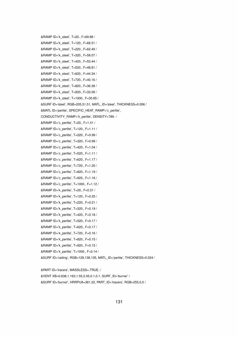
&RAMP ID=’k_steel’, T=20., F=69.88 /

&RAMP ID=’k_steel’, T=120., F=66.51 /

&RAMP ID=’k_steel’, T=220., F=62.49 /

&RAMP ID=’k_steel’, T=320., F=58.07 /

&RAMP ID=’k_steel’, T=420., F=53.44 /

&RAMP ID=’k_steel’, T=520., F=48.81 /

&RAMP ID=’k_steel’, T=620., F=44.34 /

&RAMP ID=’k_steel’, T=720., F=40.16 /

&RAMP ID=’k_steel’, T=820., F=36.38 /

&RAMP ID=’k_steel’, T=920., F=33.09 /

&RAMP ID=’k_steel’, T=1000., F=30.85 /

&SURF ID=’steel’, RGB=205,51,51, MATL_ID=’steel’, THICKNESS=0.006 /

&MATL ID=’perlite’, SPECIFIC_HEAT_RAMP=’c_perlite’,

CONDUCTIVITY_RAMP=’k_perlite’, DENSITY=789. /

&RAMP ID=’c_perlite’, T=20., F=1.41 /











&RAMP ID=’k_perlite’, T=20., F=0.31 /











&SURF ID=’ceiling’, RGB=128,138,135, MATL_ID=’perlite’, THICKNESS=0.024 /

&PART ID=’tracers’, MASSLESS=.TRUE. /

&VENT XB=0.638,1.163,1.55,2.05,0.1,0.1, SURF_ID=’burner’ /

&SURF ID=’burner’, HRRPUA=361.22, PART_ID=’tracers’, RGB=255,0,0 /

131

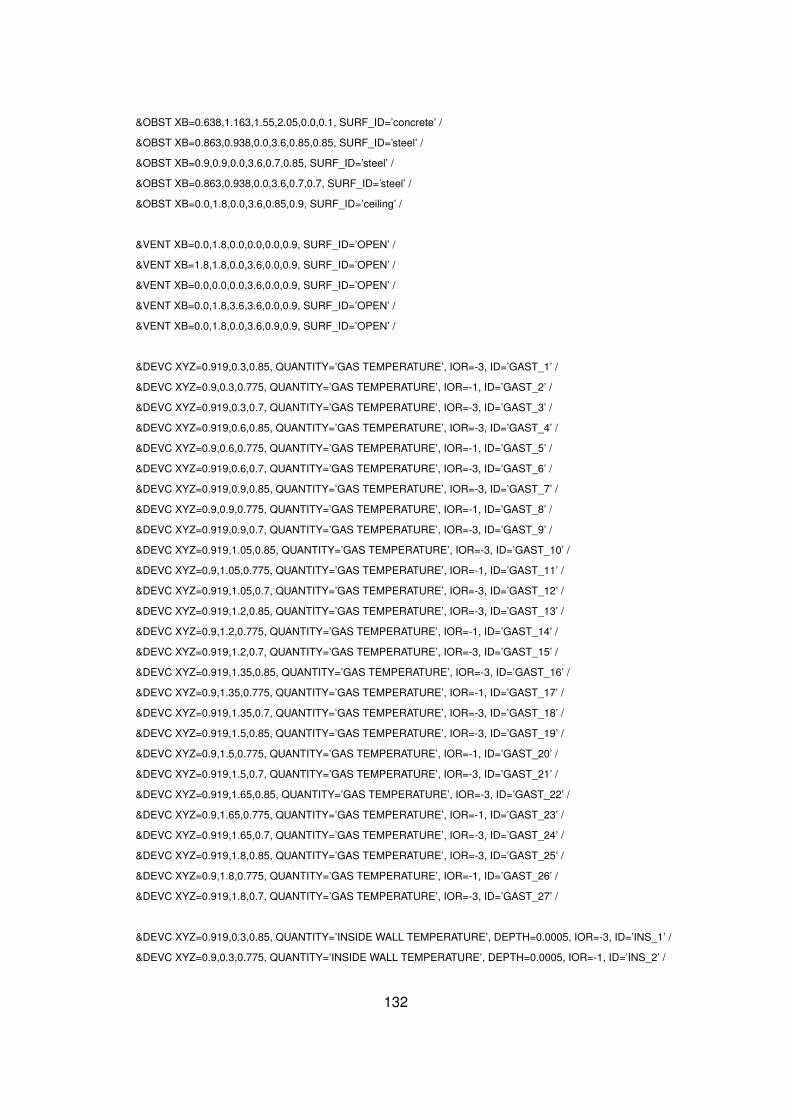
&OBST XB=0.638,1.163,1.55,2.05,0.0,0.1, SURF_ID=’concrete’ /

&OBST XB=0.863,0.938,0.0,3.6,0.85,0.85, SURF_ID=’steel’ /



&OBST XB=0.0,1.8,0.0,3.6,0.85,0.9, SURF_ID=’ceiling’ /

&VENT XB=0.0,1.8,0.0,0.0,0.0,0.9, SURF_ID=’OPEN’ /





&DEVC XYZ=0.919,0.3,0.85, QUANTITY=’GAS TEMPERATURE’, IOR=-3, ID=’GAST_1’ /



























&DEVC XYZ=0.919,0.3,0.85, QUANTITY=’INSIDE WALL TEMPERATURE’, DEPTH=0.0005, IOR=-3, ID=’INS_1’ /


132








&DEVC XYZ=0.919,1.05,0.85,QUANTITY=’INSIDE WALL TEMPERATURE’, DEPTH=0.0005, IOR=-3, ID=’INS_10’/






&DEVC XYZ=0.919,1.35,0.85, QUANTITY=’INSIDE WALL TEMPERATURE’, DEPTH=0.0005,IOR=-3,ID=’INS_16’ /



&DEVC XYZ=0.919,1.5,0.85, QUANTITY=’INSIDE WALL TEMPERATURE’, DEPTH=0.0005, IOR=-3,ID=’INS_19’ /



&DEVC XYZ=0.919,1.65,0.85, QUANTITY=’INSIDE WALL TEMPERATURE’, DEPTH=0.0005,IOR=-3,ID=’INS_22’ /



&DEVC XYZ=0.919,1.8,0.85, QUANTITY=’INSIDE WALL TEMPERATURE’, DEPTH=0.0005, IOR=-3, ID=’INSI_25’ /



&DEVC XYZ=0.919,0.3,0.85, QUANTITY=’ADIABATIC SURFACE TEMPERATURE’, IOR=-3, ID=’AST_1’ /
















133












HEAT FLUX

&PROP ID=’GAUG_T’,GAUGE_TEMPERATURE=55 /

&DEVC XYZ=0.9,0.3,0.775, QUANTITY=’GAUGE HEAT FLUX’, IOR=-1, ID=’gauge1’, PROP_ID=’GAUG_T’ /


&DEVC XYZ=0.919,0.3,0.7, QUANTITY=’GAUGE HEAT FLUX’, IOR=3, ID=’gauge3’, PROP_ID=’GAUG_T’ /


























134









&DEVC XYZ=0.9,0.3,0.775, QUANTITY=’NET HEAT FLUX’, IOR=-1, ID=’NET_1’ /


&DEVC XYZ=0.919,0.3,0.7, QUANTITY=’NET HEAT FLUX’, IOR=3, ID=’NET_3’ /






&DEVC XYZ=0.9,0.9,0.775, QUANTITY=’NET HEAT FLUX’, IOR=-1, ID=’NET_9’, /

























135




&DEVC XYZ=0.9,0.3,0.775, QUANTITY=’INCIDENT HEAT FLUX’, IOR=-1, ID=’INCIDENT_1’ /


&DEVC XYZ=0.919,0.3,0.7, QUANTITY=’INCIDENT HEAT FLUX’, IOR=3, ID=’INCIDENT_3’ /






&DEVC XYZ=0.9,0.9,0.775, QUANTITY=’INCIDENT HEAT FLUX’, IOR=-1, ID=’INCIDENT_9’, /




























&TAIL /

136

Appendix C

Output Analysis

All the results of the FDS simulations were analysed and plotted using MATLAB. The main

issue encountered was due to the fact that the procedure used to define the experimental

results was not specified in the publications available to us. However we know that the

measurements represent the temperature and the heat fluxes after 20 minutes from the

test start. And we can assume that the heat fluxes recorded were smoothed, in order

to take into account the lag between the gas and the solid phases, and to eliminate the

effect of noises and minor fluctuations in the readings.

For these reasons, we attempted to use a moving average or the equivalent method

of averaging the last chosen number of terms. First, we tried to use a 30 seconds moving

average but this solution did not eliminate the minor fluctuations caused by the absence

of symmetry in FDS. Therefore, throughout the whole thesis, we used the average of

the last 100 seconds of the simulations. This is equivalent to the use of a 100-seconds

moving average, but it was much simpler to implement in the matlab scripts. Using this

method we can also calculate the standard deviation of the last 100 seconds, and insert

errorbars in the validation plots.

137

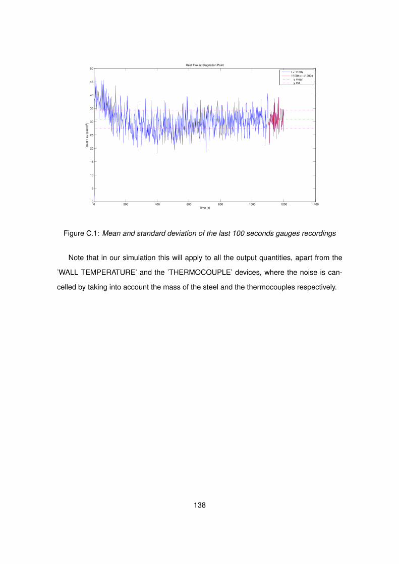
0 200 400 600 800 1000 1200 14000

5

10

15

20

25

30

35

40

45

50

Time (s)

He

at

Flu

x (

kW

/m2)

Heat Flux at Stagnation Point

t < 1100s

1100s< t <1200s

y mean

y std

Figure C.1: Mean and standard deviation of the last 100 seconds gauges recordings

Note that in our simulation this will apply to all the output quantities, apart from the

’WALL TEMPERATURE’ and the ’THERMOCOUPLE’ devices, where the noise is can-

celled by taking into account the mass of the steel and the thermocouples respectively.

138

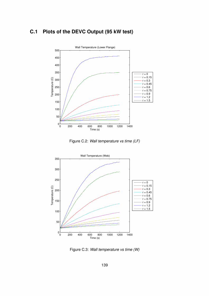
C.1 Plots of the DEVC Output (95 kW test)

0 200 400 600 800 1000 1200 14000

50

100

150

200

250

300

350

400

450

500Wall Temperature (Lower Flange)

Time (s)

Tem

pera

ture

(C

)

r = 0

r = 0.15

r = 0.3

r = 0.45

r = 0.6

r = 0.75

r = 0.9

r = 1.2

r = 1.5

Figure C.2: Wall temperature vs time (LF)

0 200 400 600 800 1000 1200 14000

50

100

150

200

250

300

350Wall Temperature (Web)

Time (s)

Tem

pera

ture

(C

)

r = 0

r = 0.15

r = 0.3

r = 0.45

r = 0.6

r = 0.75

r = 0.9

r = 1.2

r = 1.5

Figure C.3: Wall temperature vs time (W)

139

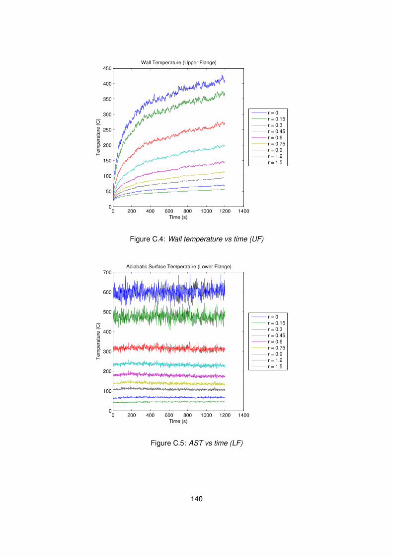
0 200 400 600 800 1000 1200 14000

50

100

150

200

250

300

350

400

450Wall Temperature (Upper Flange)

Time (s)

Tem

pera

ture

(C

)

r = 0

r = 0.15

r = 0.3

r = 0.45

r = 0.6

r = 0.75

r = 0.9

r = 1.2

r = 1.5

Figure C.4: Wall temperature vs time (UF)

0 200 400 600 800 1000 1200 14000

100

200

300

400

500

600

700Adiabatic Surface Temperature (Lower Flange)

Time (s)

Tem

pera

ture

(C

)

r = 0

r = 0.15

r = 0.3

r = 0.45

r = 0.6

r = 0.75

r = 0.9

r = 1.2

r = 1.5

Figure C.5: AST vs time (LF)

140

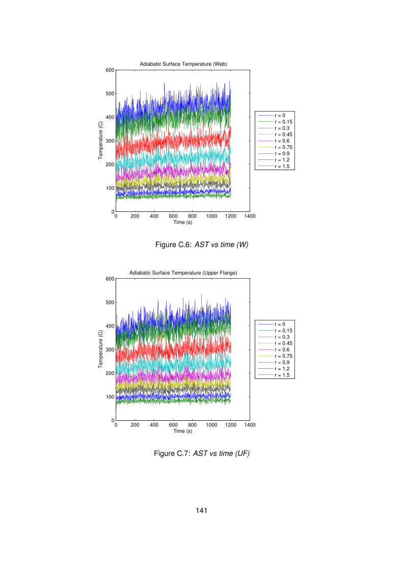
0 200 400 600 800 1000 1200 14000

100

200

300

400

500

600Adiabatic Surface Temperature (Web)

Time (s)

Tem

pera

ture

(C

)

r = 0

r = 0.15

r = 0.3

r = 0.45

r = 0.6

r = 0.75

r = 0.9

r = 1.2

r = 1.5

Figure C.6: AST vs time (W)

0 200 400 600 800 1000 1200 14000

100

200

300

400

500

600Adiabatic Surface Temperature (Upper Flange)

Time (s)

Tem

pera

ture

(C

)

r = 0

r = 0.15

r = 0.3

r = 0.45

r = 0.6

r = 0.75

r = 0.9

r = 1.2

r = 1.5

Figure C.7: AST vs time (UF)

141

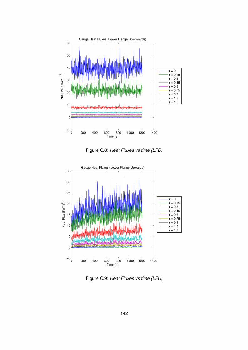
0 200 400 600 800 1000 1200 1400−10

0

10

20

30

40

50

60Gauge Heat Fluxes (Lower Flange Downwards)

Time (s)

Heat F

lux (

kW

/m2)

r = 0

r = 0.15

r = 0.3

r = 0.45

r = 0.6

r = 0.75

r = 0.9

r = 1.2

r = 1.5

Figure C.8: Heat Fluxes vs time (LFD)

0 200 400 600 800 1000 1200 1400−5

0

5

10

15

20

25

30

35Gauge Heat Fluxes (Lower Flange Upwards)

Time (s)

Heat F

lux (

kW

/m2)

r = 0

r = 0.15

r = 0.3

r = 0.45

r = 0.6

r = 0.75

r = 0.9

r = 1.2

r = 1.5

Figure C.9: Heat Fluxes vs time (LFU)

142

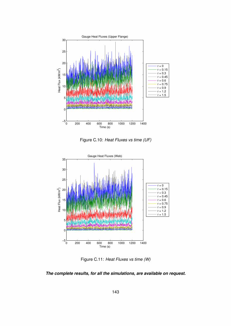
0 200 400 600 800 1000 1200 1400−5

0

5

10

15

20

25

30Gauge Heat Fluxes (Upper Flange)

Time (s)

Heat F

lux (

kW

/m2)

r = 0

r = 0.15

r = 0.3

r = 0.45

r = 0.6

r = 0.75

r = 0.9

r = 1.2

r = 1.5

Figure C.10: Heat Fluxes vs time (UF)

0 200 400 600 800 1000 1200 1400−5

0

5

10

15

20

25

30

35Gauge Heat Fluxes (Web)

Time (s)

Heat F

lux (

kW

/m2)

r = 0

r = 0.15

r = 0.3

r = 0.45

r = 0.6

r = 0.75

r = 0.9

r = 1.2

r = 1.5

Figure C.11: Heat Fluxes vs time (W)

The complete results, for all the simulations, are available on request.

143

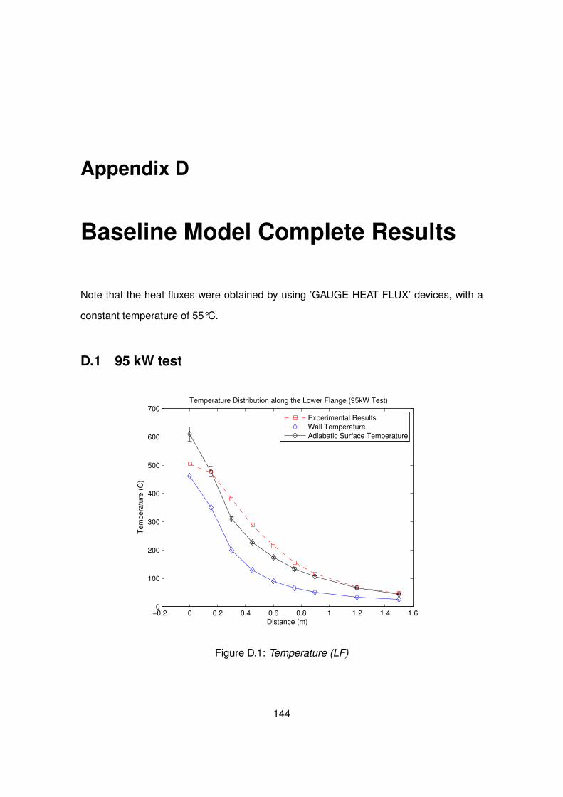
Appendix D

Baseline Model Complete Results

Note that the heat fluxes were obtained by using ’GAUGE HEAT FLUX’ devices, with a

constant temperature of 55°C.

D.1 95 kW test

−0.2 0 0.2 0.4 0.6 0.8 1 1.2 1.4 1.60

100

200

300

400

500

600


Distance (m)

Tem

pera

ture

(C

)


Wall Temperature

Adiabatic Surface Temperature

Figure D.1: Temperature (LF)

144

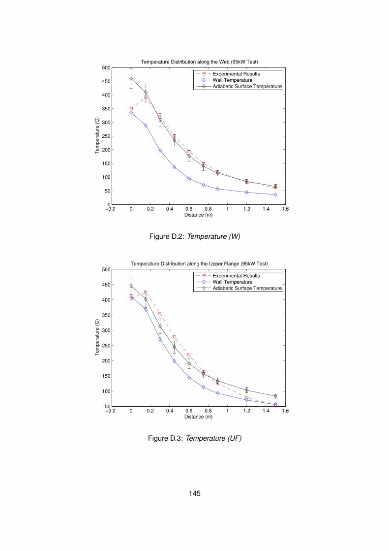
−0.2 0 0.2 0.4 0.6 0.8 1 1.2 1.4 1.60

50

100

150

200

250

300

350

400

450


Distance (m)

Tem

pera

ture

(C

)


Wall Temperature


Figure D.2: Temperature (W)

−0.2 0 0.2 0.4 0.6 0.8 1 1.2 1.4 1.650

100

150

200

250

300

350

400

450


Distance (m)

Tem

pera

ture

(C

)


Wall Temperature


Figure D.3: Temperature (UF)

145

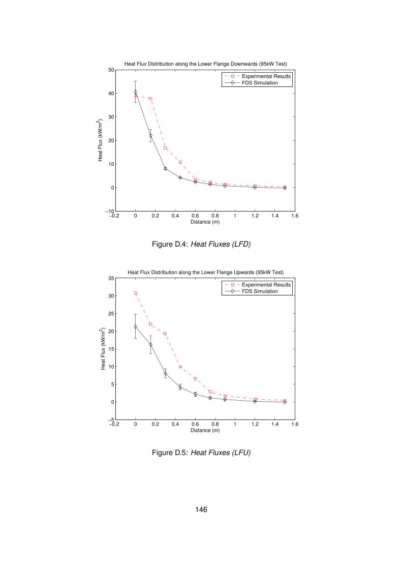
−0.2 0 0.2 0.4 0.6 0.8 1 1.2 1.4 1.6−10

0

10

20

30

40


Distance (m)

Heat F

lux (

kW

/m2)


FDS Simulation

Figure D.4: Heat Fluxes (LFD)

−0.2 0 0.2 0.4 0.6 0.8 1 1.2 1.4 1.6−5

0

5

10

15

20

25

30


Distance (m)

Heat F

lux (

kW

/m2)


FDS Simulation

Figure D.5: Heat Fluxes (LFU)

146

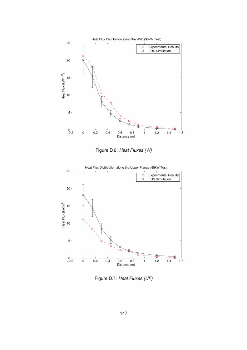
−0.2 0 0.2 0.4 0.6 0.8 1 1.2 1.4 1.60

5

10

15

20


Distance (m)

Heat F

lux (

kW

/m2)


FDS Simulation

Figure D.6: Heat Fluxes (W)

−0.2 0 0.2 0.4 0.6 0.8 1 1.2 1.4 1.60

5

10

15

20


Distance (m)

Heat F

lux (

kW

/m2)


FDS Simulation

Figure D.7: Heat Fluxes (UF)

147

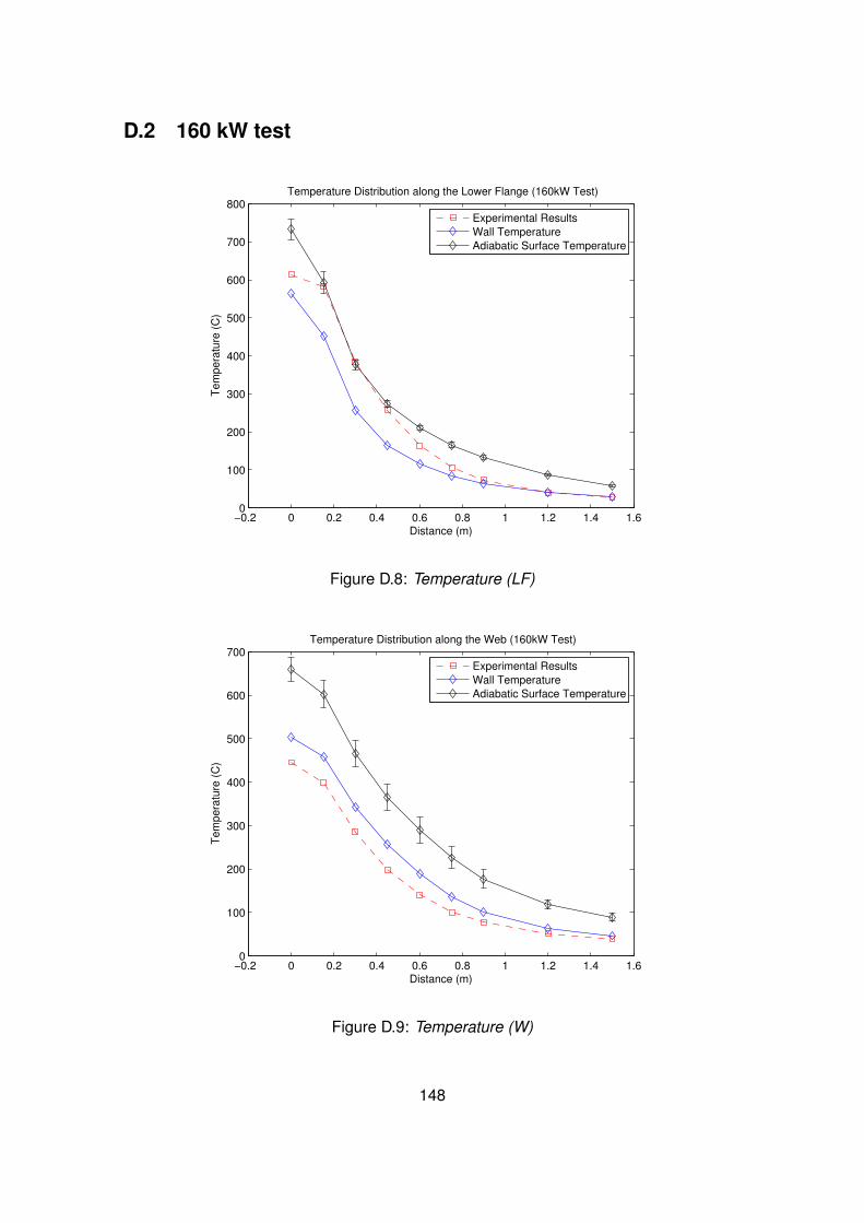
D.2 160 kW test

−0.2 0 0.2 0.4 0.6 0.8 1 1.2 1.4 1.60

100

200

300

400

500

600

700


Distance (m)

Tem

pera

ture

(C

)


Wall Temperature


Figure D.8: Temperature (LF)

−0.2 0 0.2 0.4 0.6 0.8 1 1.2 1.4 1.60

100

200

300

400

500

600


Distance (m)

Tem

pera

ture

(C

)


Wall Temperature


Figure D.9: Temperature (W)

148

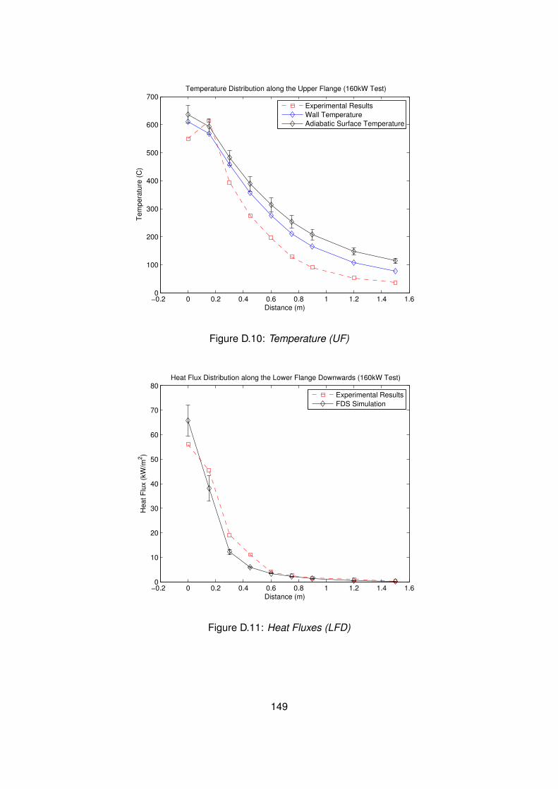
−0.2 0 0.2 0.4 0.6 0.8 1 1.2 1.4 1.60

100

200

300

400

500

600


Distance (m)

Tem

pera

ture

(C

)


Wall Temperature


Figure D.10: Temperature (UF)

−0.2 0 0.2 0.4 0.6 0.8 1 1.2 1.4 1.60

10

20

30

40

50

60

70


Distance (m)

Heat F

lux (

kW

/m2)


FDS Simulation

Figure D.11: Heat Fluxes (LFD)

149

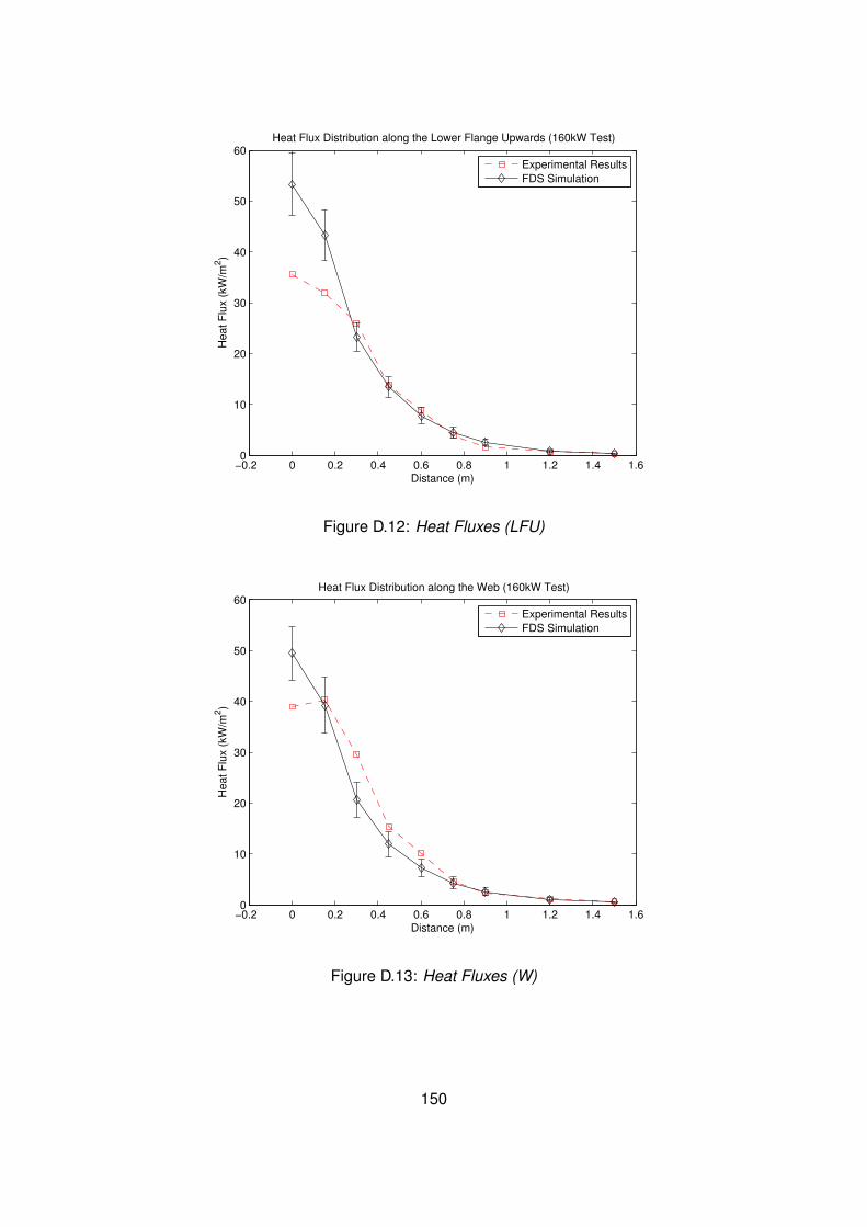
−0.2 0 0.2 0.4 0.6 0.8 1 1.2 1.4 1.60

10

20

30

40

50


Distance (m)

Heat F

lux (

kW

/m2)


FDS Simulation

Figure D.12: Heat Fluxes (LFU)

−0.2 0 0.2 0.4 0.6 0.8 1 1.2 1.4 1.60

10

20

30

40

50


Distance (m)

Heat F

lux (

kW

/m2)


FDS Simulation

Figure D.13: Heat Fluxes (W)

150

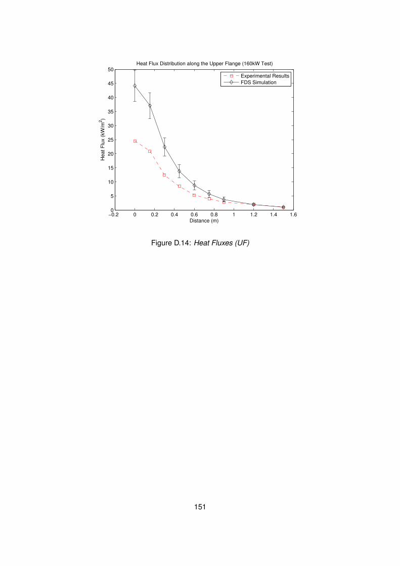
−0.2 0 0.2 0.4 0.6 0.8 1 1.2 1.4 1.60

5

10

15

20

25

30

35

40

45


Distance (m)

Heat F

lux (

kW

/m2)


FDS Simulation

Figure D.14: Heat Fluxes (UF)

151

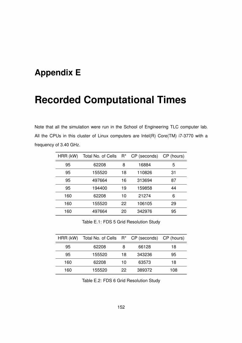
Appendix E

Recorded Computational Times

Note that all the simulation were run in the School of Engineering TLC computer lab.

All the CPUs in this cluster of Linux computers are Intel(R) Core(TM) i7-3770 with a

frequency of 3.40 GHz.

HRR (kW) Total No. of Cells R* CP (seconds) CP (hours)

95 62208 8 16884 5

95 155520 18 110826 31

95 497664 16 313694 87

95 194400 19 159858 44

160 62208 10 21274 6

160 155520 22 106105 29

160 497664 20 342976 95

Table E.1: FDS 5 Grid Resolution Study

HRR (kW) Total No. of Cells R* CP (seconds) CP (hours)

95 62208 8 66128 18

95 155520 18 343236 95

160 62208 10 63573 18

160 155520 22 389372 108

Table E.2: FDS 6 Grid Resolution Study

152

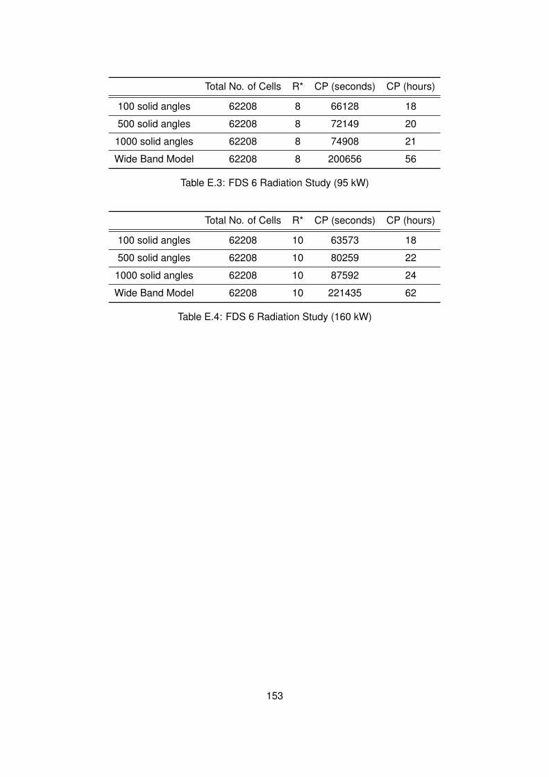
Total No. of Cells R* CP (seconds) CP (hours)

100 solid angles 62208 8 66128 18

500 solid angles 62208 8 72149 20

1000 solid angles 62208 8 74908 21

Wide Band Model 62208 8 200656 56

Table E.3: FDS 6 Radiation Study (95 kW)

Total No. of Cells R* CP (seconds) CP (hours)

100 solid angles 62208 10 63573 18

500 solid angles 62208 10 80259 22

1000 solid angles 62208 10 87592 24

Wide Band Model 62208 10 221435 62

Table E.4: FDS 6 Radiation Study (160 kW)

153

MEng Thesis STRUCTURAL COMPONENTS IN LOCALISED FIRES

Documents