Membrane Potential Fluctuations Determine the Precision of Spike Timing and Synchronous Activity: A Model Study

Membrane potential fluctuations determine the precision ofspike timing and synchronous activity : a model study

Kretzberg, Jutta; Egelhaaf, Martin; Warzecha, Anne-KathrinKretzberg, Jutta; Egelhaaf, Martin; Warzecha, Anne-Kathrin

Suggested CitationKretzberg, Jutta ; Egelhaaf, Martin ; Warzecha, Anne-Kathrin (2001) Membrane potentialfluctuations determine the precision of spike timing and synchronous activity : a model study.Journal of computational neuroscience, 10(1), pp. 79-97

Posted at BiPrints Repository, Bielefeld University.http://repositories.ub.uni-bielefeld.de/biprints/volltexte/2006/84

Membrane potential fluctuations determine the precision ofspike timing and synchronous activity

Abstract

It is much debated on what time scale information is encoded by neuronal spike activity. With aphenomenological model that transforms time-dependent membrane potential fluctuations intospike trains, we investigate constraints for the timing of spikes and for synchronous activity ofneurons with common input. The model of spike generation has a variable threshold thatdepends on the time elapsed since the previous action potential and on the precedingmembrane potential changes. To ensure that the model operates in a biologically meaningfulrange, the model was adjusted to fit the responses of a fly visual interneuron to motion stimuli.The dependence of spike timing on the membrane potential dynamics was analyzed. Fastmembrane potential fluctuations are needed to trigger spikes with a high temporal precision.Slow fluctuations lead to spike activity with a rate about proportional to the membranepotential. Thus, for a given level of stochastic input, the frequency range of membranepotential fluctuations induced by a stimulus determines whether a neuron can use a rate codeor a temporal code. The relationship between the steepness of membrane potentialfluctuations and the timing of spikes has also implications for synchronous activity in neuronswith common input. Fast membrane potential changes must be shared by the neurons toproduce synchronous activity.

Journal of Computational Neuroscience 10, 79–97, 2001

c© 2001 Kluwer Academic Publishers. Manufactured in The Netherlands.

Membrane Potential Fluctuations Determine the Precision of Spike Timing

and Synchronous Activity: A Model Study

JUTTA KRETZBERG, MARTIN EGELHAAF AND ANNE-KATHRIN WARZECHA

Lehrstuhl fur Neurobiologie, Fakultat fur Biologie, Universitat Bielefeld, Postfach 10 01 31,

D-33501 Bielefeld, Germany

[email protected]

Received February 23, 2000; Revised August 9, 2000; Accepted August 24, 2000

Action Editor: Christof Koch

Abstract. It is much debated on what time scale information is encoded by neuronal spike activity. With a

phenomenological model that transforms time-dependent membrane potential fluctuations into spike trains, we

investigate constraints for the timing of spikes and for synchronous activity of neurons with common input. The

model of spike generation has a variable threshold that depends on the time elapsed since the previous action

potential and on the preceding membrane potential changes. To ensure that the model operates in a biologically

meaningful range, the model was adjusted to fit the responses of a fly visual interneuron to motion stimuli. The

dependence of spike timing on the membrane potential dynamics was analyzed. Fast membrane potential fluctuations

are needed to trigger spikes with a high temporal precision. Slow fluctuations lead to spike activity with a rate

about proportional to the membrane potential. Thus, for a given level of stochastic input, the frequency range

of membrane potential fluctuations induced by a stimulus determines whether a neuron can use a rate code or a

temporal code. The relationship between the steepness of membrane potential fluctuations and the timing of spikes

has also implications for synchronous activity in neurons with common input. Fast membrane potential changes

must be shared by the neurons to produce synchronous activity.

Keywords: spike mechanism, model, spike timing, synchronization, reliability, neural coding

1. Introduction

Spike generation appears to be precise, since in many

systems spikes occur synchronized in pairs of neurons

on a millisecond timescale (e.g., Alonso et al., 1996;

Brivanlou et al., 1998; Warzecha et al., 1998; Lampl

et al., 1999; Bair, 1999; Usrey and Reid, 1999). More-

over, spikes have been found to be tightly time-locked

to fast fluctuations of the membrane potential (Mainen

and Sejnowski, 1995; Haag and Borst, 1996; Stevens

and Zador, 1998; Zador, 1998).

Despite the precision of the spike-generation mech-

anism, spikes in sensory neurons couple to stimuli on

a broad range of time scales, depending on the sensory

modality and the computational task of the neuron.

One extreme are neurons in the auditory and in the

electrosensory system that show a precision in spike

timing in the millisecond or even submillisecond range

(Carr and Friedmann, 1999). In contrast, in the visual

system spikes are often found to time-lock to stimuli on

a coarser scale (e.g., Buracas et al., 1998; Bair, 1999).

For instance, broad-band white-noise velocity fluctua-

tions lead, on average, to a precision in the order of only

tens of milliseconds (Warzecha et al., 1998). Nonethe-

less, a higher precision may be achieved under special

stimulus conditions. In motion-sensitive visual neu-

rons rapid displacements of the stimulus pattern may

lead to a time-locking of spikes in the millisecond range

80 Kretzberg, Egelhaaf and Warzecha

(de Ruyter van Steveninck and Bialek, 1988, 1995;

Warzecha and Egelhaaf, 2000). On the basis of the

experimental results on the time-locking of spikes to

sensory stimuli, it has been concluded that a high pre-

cision is possible only if the stimuli induce sufficiently

rapid depolarizations of the membrane potential. Oth-

erwise, the exact timing of spikes has been proposed to

be essentially determined by membrane potential noise

(Warzecha et al., 1998).

With a dynamic threshold model of spike genera-

tion we tested this hypothesis by analyzing the con-

straints that are imposed on the time-locking of spikes

to membrane potential fluctuations and on correlated

spike activity in pairs of cells. In our simulations we

took only correlated spike activity into account, which

is elicited by common synaptic input rather than by di-

rect synaptic interactions between the neurons. Unlike

other studies analyzing the dependence of correlated

activity on synaptic input (e.g., Shadlen and Newsome,

1998; Ritz and Sejnowski, 1997), we investigated the

relation between the membrane potential of a neuron

and its spike output. To tune our model the membrane

potential dynamics was taken from intracellular record-

ings of postsynaptic potentials of a fly motion-sensitive

neuron that responds with graded membrane potential

changes to motion stimuli even in its output terminal.

The model output was compared to experimental data

from a spiking neuron with functionally similar prop-

erties. Since identified motion-sensitive neurons in the

fly are well amenable to electrophysiological analysis,

the fly has been used previously to investigate the neu-

ronal processing of motion information and its reliabil-

ity (Hausen, 1981; Bialek and Rieke, 1992; Egelhaaf

and Warzecha, 1999).

By modeling the transformation of membrane poten-

tial fluctuations into sequences of spikes, we answer the

following questions: What characteristics of the mem-

brane potential and, in particular, what aspects of its

dynamics determine the timing of spikes? To what ex-

tent do the postsynaptic potentials of two cells have to

correspond to one another to cause synchronized spike

activity?

2. Methods

To investigate the determinants of the timing of spikes

we used a phenomenological threshold model that

transforms the time-dependent membrane potential

into a sequence of spikes. For each time step a variable

threshold was calculated and compared to the actual

membrane potential to determine whether a spike was

generated.

To tune the model and to compare the model output

with experimentally determined spike trains, the mem-

brane potential dynamics was taken from experimental

data. For systematic analyses sinusoidal membrane

potential fluctuations were used. To simulate many ex-

perimental trials with the same stimulus (such as a vi-

sual motion stimulus or current injection), a stochastic

component that differed for each trial was superim-

posed onto the deterministic component of the mem-

brane potential fluctuations (Fig. 1). The deterministic

component is given by the mean time-dependent mem-

brane potential fluctuations evoked by a given stimulus.

The stochastic component accounts for the variability

of neuronal responses.

All our analyses are based on the assumption that

the stochastic response component adds linearly to the

deterministic component. We are currently investigat-

ing whether this assumption applies to motion-sensitive

neurons in the fly (Warzecha et al., 2000) since for

retinal ganglion cells model simulations indicate the

opposite (Levine, 1998).

2.1. Dynamical Threshold Model

of Spike Generation

The model of spike generation consists of a variable

threshold θ(ti ) that is compared with the membrane

potential U (ti ). A spike is generated if θ(ti ) < U (ti ).

The spike threshold was calculated for each time step

ti according to the equation

θ(ti ) =

{

∞ if s ≤ γ ref

θ0 + η(s) + ρ(ti ) if s > γ ref,

where ti is the actual time step, s is the time elapsed

since the previous spike, γ ref is the absolute refractory

period, θ0 is the constant basis threshold,

η(s) =η0

s − γ ref

is the influence of the relative refractoriness with

weight constant η0, and

ρ(ti ) = −ρ0

T·

T∑

j=1

1

j· (U (ti ) − U (ti− j ))

is the influence of the membrane potential changes

Precision of Spike Timing and Synchronous Activity 81

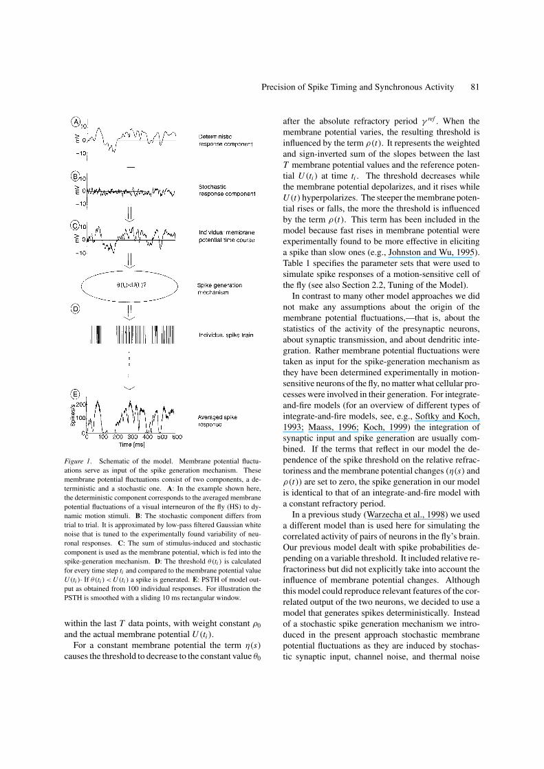
Figure 1. Schematic of the model. Membrane potential fluctu-

ations serve as input of the spike generation mechanism. These

membrane potential fluctuations consist of two components, a de-

terministic and a stochastic one. A: In the example shown here,

the deterministic component corresponds to the averaged membrane

potential fluctuations of a visual interneuron of the fly (HS) to dy-

namic motion stimuli. B: The stochastic component differs from

trial to trial. It is approximated by low-pass filtered Gaussian white

noise that is tuned to the experimentally found variability of neu-

ronal responses. C: The sum of stimulus-induced and stochastic

component is used as the membrane potential, which is fed into the

spike-generation mechanism. D: The threshold θ(ti ) is calculated

for every time step ti and compared to the membrane potential value

U (ti )· If θ(ti ) < U (ti ) a spike is generated. E: PSTH of model out-

put as obtained from 100 individual responses. For illustration the

PSTH is smoothed with a sliding 10 ms rectangular window.

within the last T data points, with weight constant ρ0

and the actual membrane potential U (ti ).

For a constant membrane potential the term η(s)

causes the threshold to decrease to the constant value θ0

after the absolute refractory period γ ref . When the

membrane potential varies, the resulting threshold is

influenced by the term ρ(t). It represents the weighted

and sign-inverted sum of the slopes between the last

T membrane potential values and the reference poten-

tial U (ti ) at time ti . The threshold decreases while

the membrane potential depolarizes, and it rises while

U (t) hyperpolarizes. The steeper the membrane poten-

tial rises or falls, the more the threshold is influenced

by the term ρ(t). This term has been included in the

model because fast rises in membrane potential were

experimentally found to be more effective in eliciting

a spike than slow ones (e.g., Johnston and Wu, 1995).

Table 1 specifies the parameter sets that were used to

simulate spike responses of a motion-sensitive cell of

the fly (see also Section 2.2, Tuning of the Model).

In contrast to many other model approaches we did

not make any assumptions about the origin of the

membrane potential fluctuations,—that is, about the

statistics of the activity of the presynaptic neurons,

about synaptic transmission, and about dendritic inte-

gration. Rather membrane potential fluctuations were

taken as input for the spike-generation mechanism as

they have been determined experimentally in motion-

sensitive neurons of the fly, no matter what cellular pro-

cesses were involved in their generation. For integrate-

and-fire models (for an overview of different types of

integrate-and-fire models, see, e.g., Softky and Koch,

1993; Maass, 1996; Koch, 1999) the integration of

synaptic input and spike generation are usually com-

bined. If the terms that reflect in our model the de-

pendence of the spike threshold on the relative refrac-

toriness and the membrane potential changes (η(s) and

ρ(t)) are set to zero, the spike generation in our model

is identical to that of an integrate-and-fire model with

a constant refractory period.

In a previous study (Warzecha et al., 1998) we used

a different model than is used here for simulating the

correlated activity of pairs of neurons in the fly’s brain.

Our previous model dealt with spike probabilities de-

pending on a variable threshold. It included relative re-

fractoriness but did not explicitly take into account the

influence of membrane potential changes. Although

this model could reproduce relevant features of the cor-

related output of the two neurons, we decided to use a

model that generates spikes deterministically. Instead

of a stochastic spike generation mechanism we intro-

duced in the present approach stochastic membrane

potential fluctuations as they are induced by stochas-

tic synaptic input, channel noise, and thermal noise

82 Kretzberg, Egelhaaf and Warzecha

Table 1. Ranges for tested parameter values and examples for parameter sets that fit all

criteria to simulate the H1-cell. Parameter set number 1 was used as standard parameter set.

θ0 (mV) γ ref (ms) η0 (ms·mV) ρ0 T

Tested range −2–5 0–2 0–60 0–200 0–40 (corresp. ≈ 15 ms)

Set 1 1 2 20 3.75 3 (corresp. ≈ 1 ms)

Set 2 0 0 40 3 3 (corresp. ≈ 1 ms)

Set 3 3 1 20 9 6 (corresp. ≈ 2 ms)

Set 4 1 1 30 7.5 12 (corresp. ≈ 4 ms)

Set 5 0.5 0.5 25 0 0

(see, e.g., Manwani and Koch, 1999a, 1999b). Ion

channel stochasticity may contribute significantly to

the variability of spike timing (e.g., Schneidman et

al., 1998; White et al., 2000). Nevertheless, there is

evidence that in many situations the stochastic nature

of the mechanisms underlying spike generation con-

tributes much less to the variability in the timing of

spikes than membrane potential fluctuations that are

conveyed to a neuron by its synaptic input but are not

locked to its sensory input (see Mainen and Sejnowski,

1995; Zador, 1998; Stevens and Zador, 1998). There-

fore, a deterministic model is appropriate for our ana-

lyzes.

The model simulations and all evaluation routines

were implemented in Matlab 5.3 (The MathWorks

Inc.). A temporal resolution of 2.7 kHz was used for

the model of spike generation.

2.2. Tuning of the Model

To find appropriate parameter values, we compared the

simulation results directly with experimentally deter-

mined spike trains of the H1-cell, a motion-sensitive

visual interneuron of the fly (Hausen, 1981). The

visual system of the fly is well suited for our analysis

because it contains at the same level of information-

processing spiking neurons (such as the H1-cell) as

well as neurons that respond with graded membrane

potential changes (such as the HS-cells) even in the neu-

ronal output region. These graded membrane potential

changes mainly reflect the integrated postsynaptic po-

tentials of the cell’s many retinotopically organized in-

puts.

The H1-neuron receives similar retinotopic input and

is assumed to respond with graded membrane poten-

tial changes in a similar way as the HS-cells when

the activity is recorded intracellularly in its dendritic

tree. Since intracellular recordings of the H1-neuron

are very difficult because of the small diameter of all

of the H1-cell’s dendritic branches, the graded mem-

brane potential changes of the HS-cells were used as a

substitute for those of the H1-cell and fed as input into

the spike-generation mechanism. To use the membrane

potential of the HS-cell has also the advantage that it

is less influenced by active processes than the one of

the H1-cell. Therefore, it better reflects the integrated

postsynaptic potential.

To substitute the postsynaptic potential of the H1-

cell by that of the HS-cell is justified because both

types of neurons show functionally similar properties

without having direct synaptic connections with each

other (for review, see Egelhaaf and Warzecha, 1999).

For instance, for a wide range of motion stimuli the

time course of the stimulus-induced response compo-

nent of HS-cells, as obtained by averaging over many

responses to repeated stimulus presentations (Fig. 2A),

is very similar to the stimulus-induced responses of the

H1-neuron as reflected in its peri-stimulus-time his-

togram (PSTH, Fig. 2B). The relation between mem-

brane potential changes in the HS-neuron and spike

timing in the H1-cell was further characterized by

the spike-triggered average of the membrane potential

(Fig. 2C).

This analysis was done for responses obtained from

double recordings of the HS-cell and the H1-cell. Re-

sponses were correlated with each other that were

either simultaneously recorded or randomly assorted

(shuffled). Both spike-triggered averages are charac-

terized by a fairly broad and large peak, suggesting that

the neuronal responses are time-locked to the motion

stimulus on a timescale of some tens of milliseconds.

The difference between these two spike-triggered av-

erages (Fig. 2D) indicates that, on a finer timescale,

both neurons also share parts of their input signals that

are not deterministically coupled to the stimulus but

vary from trial to trial. It should be noted that the re-

sponse traces of the HS-cells had to be sign inverted for

Precision of Spike Timing and Synchronous Activity 83

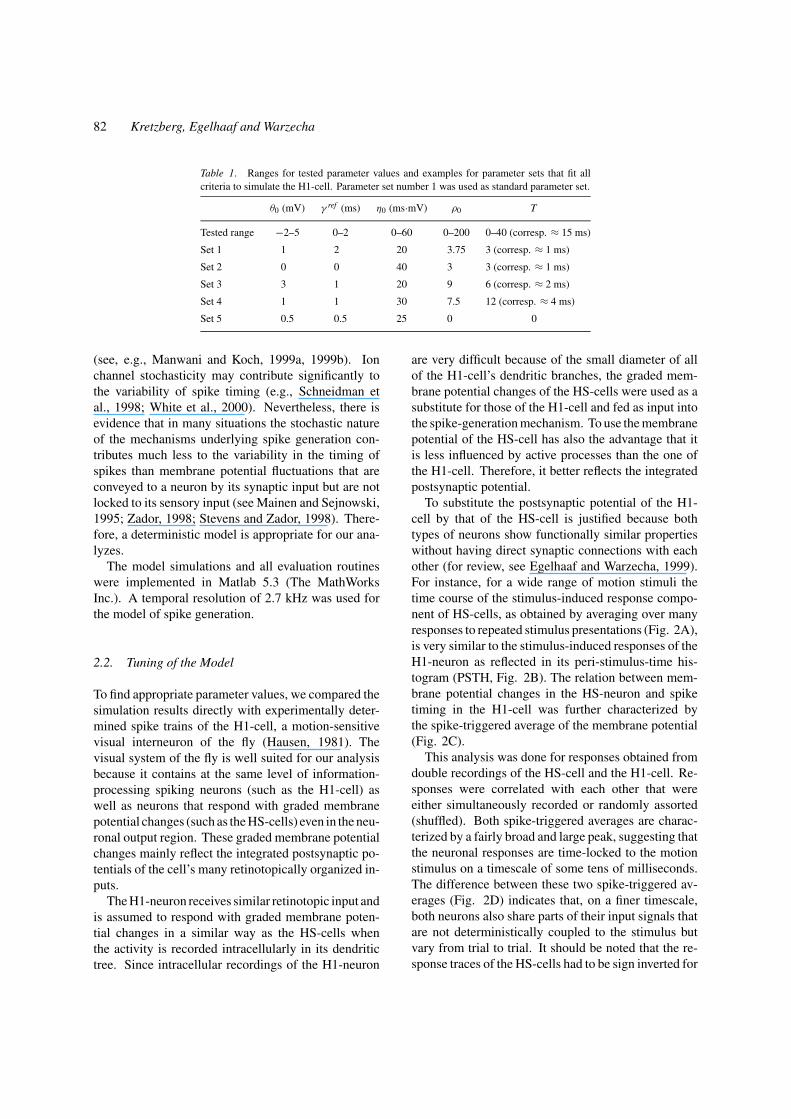
Figure 2. Comparison of the membrane potential of an HS-cell

and the spike activity of the H1-cell. The activity of both neurons

was recorded during stimulation with lowpass-filtered white-noise

velocity fluctuations. The resting potential of the HS-cell was set

to zero and the membrane potential was sign-inverted to account for

the opposite preferred directions of the HS-cell and the H1-cell. A,

B: Average time course of the membrane potential of the HS-cell

and of the spike activity of the H1-cell to identical motion stimuli.

The mean responses to 100 stimulus presentations for each cell were

smoothed with a sliding rectangular window of 10 ms width. Stim-

ulus conditions were the same as in Warzecha et al. (1998, Fig. 3).

The membrane potential of the HS-cell and the spike activity of the

H1-cell show a very similar time course. Recordings of the HS-cell

and the H1-cell were performed in different animals. C: Mean mem-

brane potential of an HS-cell triggered at time 0 with the spikes of

the H1-cell obtained from a double recording of both cells with 49

stimulus presentations. The analyzed time interval lasted for 3.1 s.

The mean spike activity within this interval was 85 spikes/s. Spike-

triggered averages are shown for simultaneously recorded responses

(solid line) and for the same response traces that were assorted in

shuffled order so that response traces were combined that were not

measured simulateneously (dashed line). D: Difference between

the spike-triggered mean membrane potential of the simultaneously

recorded and the shuffled responses. Same data as those shown in C.

comparison with the spike response of the H1-cell and

when feeding them into the model cell because the

H1-and the HS-cells have opposite preferred directions.

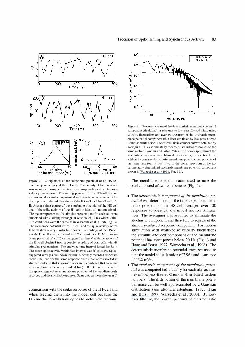
Figure 3. Power spectrum of the deterministic membrane potential

component (thick line) in response to low-pass-filtered white-noise

velocity fluctuations and average spectrum of the stochastic mem-

brane potential component (thin line) simulated by low-pass-filtered

Gaussian white noise. The deterministic component was obtained by

averaging 100 experimentally recorded individual responses to the

same motion stimulus and lasted 2.96 s. The power spectrum of the

stochastic component was obtained by averaging the spectra of 100

artificially generated stochastic membrane potential components of

the same duration. It was fitted to the power spectrum of the ex-

perimentally determined stochastic membrane potential component

shown in Warzecha et al. (1998, Fig. 3D).

The membrane potential traces used to tune the

model consisted of two components (Fig. 1):

• The deterministic component of the membrane po-

tential was determined as the time-dependent mem-

brane potential of the HS-cell averaged over 100

responses to identical dynamical motion stimula-

tion. The averaging was assumed to eliminate the

stochastic component and therefore to represent the

stimulus-induced response component. For motion

stimulation with white-noise velocity fluctuations

the stimulus-induced component of the membrane

potential has most power below 20 Hz (Fig. 3 and

Haag and Borst, 1997; Warzecha et al., 1998). The

deterministic membrane potential trace we used to

tune the model had a duration of 2.96 s and a variance

of 13.2 mV2.

• The stochastic component of the membrane poten-

tial was computed individually for each trial as a se-

ries of lowpass-filtered Gaussian distributed random

numbers. The distribution of the membrane poten-

tial noise can be well approximated by a Gaussian

distribution (see also Hengstenberg, 1982; Haag

and Borst, 1997; Warzecha et al., 2000). By low-

pass filtering the power spectrum of the stochastic

84 Kretzberg, Egelhaaf and Warzecha

component was fitted to the power spectrum of

the experimentally determined membrane potential

noise of an HS-cell recorded during white-noise

velocity stimulation (Fig. 3 and Warzecha et al.,

1998). We used a second-order lowpass filter with

equal time constants of 1.6 ms. The variance of the

stochastic component was set to 2.8 mV2 in accor-

dance with experimental data. The stochastic com-

ponent of the membrane potential has considerably

more power at frequencies above 40 Hz than the

stimulus-induced deterministic component (Fig. 3

and Warzecha et al., 1998).

The deterministic and the stochastic components of the

membrane potential were added and then fed into the

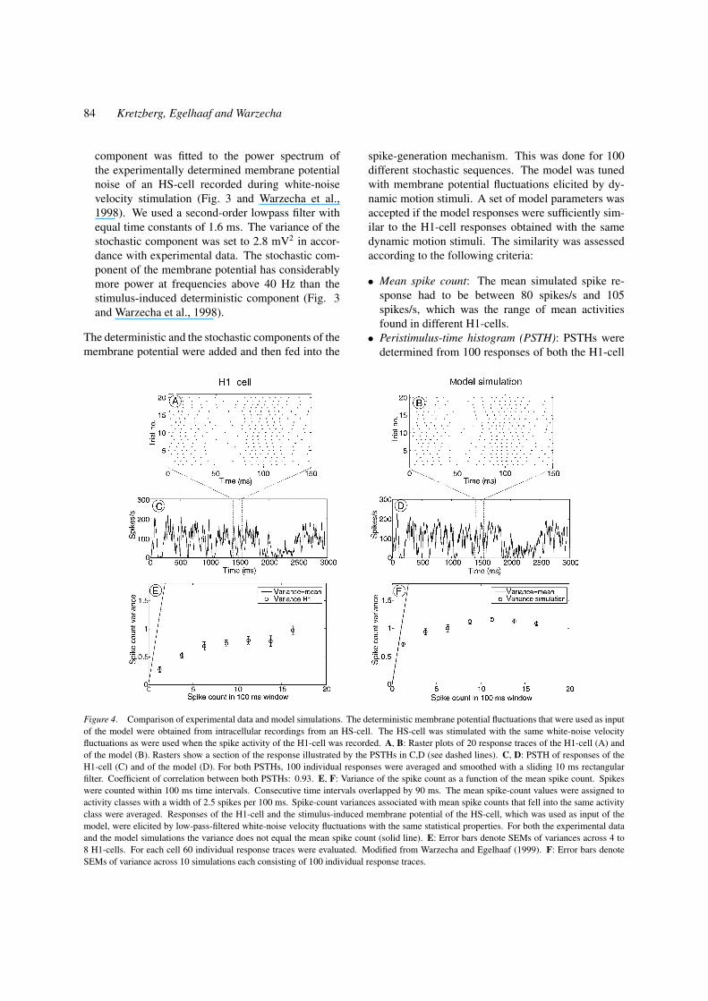
Figure 4. Comparison of experimental data and model simulations. The deterministic membrane potential fluctuations that were used as input

of the model were obtained from intracellular recordings from an HS-cell. The HS-cell was stimulated with the same white-noise velocity

fluctuations as were used when the spike activity of the H1-cell was recorded. A, B: Raster plots of 20 response traces of the H1-cell (A) and

of the model (B). Rasters show a section of the response illustrated by the PSTHs in C,D (see dashed lines). C, D: PSTH of responses of the

H1-cell (C) and of the model (D). For both PSTHs, 100 individual responses were averaged and smoothed with a sliding 10 ms rectangular

filter. Coefficient of correlation between both PSTHs: 0.93. E, F: Variance of the spike count as a function of the mean spike count. Spikes

were counted within 100 ms time intervals. Consecutive time intervals overlapped by 90 ms. The mean spike-count values were assigned to

activity classes with a width of 2.5 spikes per 100 ms. Spike-count variances associated with mean spike counts that fell into the same activity

class were averaged. Responses of the H1-cell and the stimulus-induced membrane potential of the HS-cell, which was used as input of the

model, were elicited by low-pass-filtered white-noise velocity fluctuations with the same statistical properties. For both the experimental data

and the model simulations the variance does not equal the mean spike count (solid line). E: Error bars denote SEMs of variances across 4 to

8 H1-cells. For each cell 60 individual response traces were evaluated. Modified from Warzecha and Egelhaaf (1999). F: Error bars denote

SEMs of variance across 10 simulations each consisting of 100 individual response traces.

spike-generation mechanism. This was done for 100

different stochastic sequences. The model was tuned

with membrane potential fluctuations elicited by dy-

namic motion stimuli. A set of model parameters was

accepted if the model responses were sufficiently sim-

ilar to the H1-cell responses obtained with the same

dynamic motion stimuli. The similarity was assessed

according to the following criteria:

• Mean spike count: The mean simulated spike re-

sponse had to be between 80 spikes/s and 105

spikes/s, which was the range of mean activities

found in different H1-cells.

• Peristimulus-time histogram (PSTH): PSTHs were

determined from 100 responses of both the H1-cell

Precision of Spike Timing and Synchronous Activity 85

and the model cell and smoothed with a 10 ms rectan-

gular filter (Fig. 4C and D). To quantify the similar-

ity of their time courses, the correlation coefficient of

the smoothed PSTHs was calculated. In accordance

to the similarity of PSTHs of H1-cells in different

preparations, the correlation coefficient had to reach

a value of at least 0.92.

• Activity distribution: The mean spike count within

time windows of 100 ms duration was determined

for the entire spike train (see Fig. 4E and F). Adja-

cent time windows overlapped by 90 ms. The indi-

vidual spike count values were assigned to activity

classes with a width of 2.5 spikes per 100 ms, and

the probability of each activity class was determined.

According to experimental data, model parameters

were accepted if the model responses satisfied the

following criteria: (1) between 1% and 17% of the

spike count values had to be in the lowest activity

class (0 to 2.5 spikes/100 ms); (2) the activity class

that occurred most frequently had to be in the range

between 8 spikes/100 ms and 15 spikes/100 ms; (3)

between 23% and 30% of the spike count values had

to be in the most frequently occurring activity class.

• Interspike-interval histogram: The most frequently

observed interspike interval had to be between 5 and

8 ms. The frequency of its occurrence had to be

between 4% and 10% of all interspike intervals. In-

terspike intervals were evaluated with a precision of

0.37 ms.

A systematic search was perfomed with equidistant pa-

rameter values for all possible combinations of val-

ues within the whole physiologically plausible param-

eter range (see Table 1). Within the parameter ranges

that revealed partly acceptable simulation results, the

search was continued with finer subdivisions of the pa-

rameter values. Five different parameter sets that sat-

isfied all criteria were chosen for further model anal-

ysis (Table 1, sets 1–5). They led to qualitatively the

same results. For all figures shown in this article, the

standard parameter set 1 was used. In parameter set

5, membrane potential changes are not taken explic-

itly into account for determining the spike threshold

(ρ(t) = 0).

2.3. Simulation of Spike Timing and Synchronous

Activity in Pairs of Cells

Two analyses were performed to investigate the pre-

requisites of precise spike timing and synchronized ac-

tivity between pairs of cells. For the analysis of the

dependence of spike timing on the membrane potential

dynamics the input consisted of two components:

• A sinusoidally fluctuating deterministic input with

variable frequency between 1 Hz and 100 Hz and a

physiolologically plausible amplitude of 5.1 mV;

• A stochastic component with the shape of its power

spectrum fitting that of the HS-cell under white-noise

velocity stimulation (see Section 2.2, Tuning of the

Model) and with the same or half of its variance.

For analyzing the dependence of spike synchronization

on the amount of common input the input of pairs of

model cells consisted of three components:

• The deterministic component of the membrane po-

tential of the HS-cell obtained during dynamical

motion stimulation (see Section 2.2, Tuning of the

Model) (this component was common to both cells);

• A stochastic component that was shared by both cells

and that represents common input that is not deter-

ministically induced by the stimulus;

• A stochastic component that was statistically inde-

pendent for both cells simulating intrinsic noise of

the cell and all input that is not shared by both cells.

The power spectrum and the variance of the total

stochastic component 〈S2tot〉 consisting of the common

and the independent component were fitted to that de-

termined for the HS-cell (see Section 2.2, Tuning of

the Model). To estimate the influence of the common

stochastic input on the extent of correlated activity,

the relative size of the two stochastic components was

varied keeping the shape of their power spectrum unal-

tered. Each stochastic component was generated sepa-

rately as described above. The common and the inde-

pendent stochastic component were scaled to have the

variances 〈S2c 〉 and 〈S2

i 〉, respectively, with

⟨

S2c

⟩

+⟨

S2i

⟩

=⟨

S2tot

⟩

= const

—that is, the total variance was held constant at the ex-

perimentally determined value. The common stochas-

tic input will be given as a relative measure (C). C is

calculated as the percentage of the standard deviation

of the common stochastic component relative to the

sum of the standard deviations of the common and the

independent stochastic components:

C = 100 ·

√

⟨

S2c

⟩

√

⟨

S2i 〉 +

√

⟨

S2c

⟩

.

86 Kretzberg, Egelhaaf and Warzecha

To quantify the similarity of individual spike trains,

cross-correlograms were calculated that were normal-

ized to the respective autocorrelograms, so that for

identical spike trains a value of 1.0 is obtained at zero

lag. The height of the correlation peak was defined as

the relative frequency of coincidences above the chance

level of spike coincidences in the two cells. The chance

level was calculated on the basis of the mean activity of

both cells. Note that the subtraction of the chance level

causes the maximum correlation height to be smaller

than 1 even for identical spike trains. The correlation

width was calculated at half-maximum height above

chance level. All cross-correlations were computed

with a temporal resolution of 1.1 ms as it was used for

the corresponding experimental data.

It has been argued that the cross-correlogram of re-

sponses to repeated presentations of the same stimulus

is no valid measure to quantify the precision with which

spikes time-lock to the stimulus. Rather, the precision

of time-locking should be quantified by deconvolution

of the cross-correlogram by the corresponding autocor-

relogram of the responses (de Ruyter van Steveninck

et al., 2000). However, the resulting autocorrelogram

of the spike jitter distribution indicates a high precision

of time-locking of spikes to the stimulus, only if the

spike jitter is considerably smaller than half the inter-

spike interval. The spike jitter is given by the variable

timing of spikes in different trials relative to a given

instant of time. If, for instance, spikes are generated at

an average rate of 200 spikes/s, the mean interspike in-

terval is 5 ms. In this case a jitter in the timing of spikes

of only a few milliseconds would be an immediate con-

sequence of the relatively high spike rate without indi-

cating that the spikes are precisely time-locked to the

stimulus. The cross-correlogram of responses elicited

by repeated presentation of the same stimulus would

then be rather flat. In contrast, if spikes, on average,

lock to stimuli with a spike jitter smaller than about

half the interspike interval, this precision will show

up in a narrow peak of the cross-correlogram. There-

fore, cross-correlograms will be used in the present

analysis to quantify the similarity of spike trains and,

thus, the time-locking of spikes to sensory stimulation.

It should be noted that cross-correlograms are only a

measure of the overall precision and that a broad cross-

correlogram does not exclude that part of the spikes are

generated with a high precision at certain phases of a

stimulus trace (Warzecha and Egelhaaf, 2000).

Moreover, cross-correlograms will be used to quan-

tify synchronized spike activity of pairs of neurons.

It has been argued that this method is questionable if

the width of the correlograms are in the same order of

magnitude as the peak width of the autocorrelogram of

the PSTHs (Brody, 1999). In our simulations as well

as in our experimental results (Warzecha et al., 1998)

this is not the case. The simultaneously elicited spike

activity is synchronized on a time scale of single mil-

liseconds, while the covariation of the cell’s activities

induced by the stimulus concerns a time scale of some

tens of milliseconds. This can be seen in the PSTHs

as well as the shuffled cross-correlogram of spike re-

sponses that show a broad (∼30 ms) and flat peak. In

contrast, the peak of the cross-correlogram of simul-

taneously recorded spike responses is narrow (∼2 ms)

and high (Warzecha et al., 1998; Figs. 2 and 7 in this

article).

3. Results

3.1. Comparison of Model Simulations

and Experimental Results

The spike-generation model reproduces characteristic

response features of the fly motion-sensitive H1-cell,

when it is fed with membrane potential fluctuations as

were determined experimentally in a neuron with sim-

ilar response properties (an HS-cell). Various sets of

model parameters (Table 1) were found to meet the

criteria for accepting the model responses as an ade-

quate fit to the corresponding neuronal responses (see

Section 2, Methods). For some parameter sets mem-

brane potential changes did not explicitly affect the

spike threshold because the term ρ(t) was set to zero

(ρ0 = 0 or T = 0; see set 5 in Table 1). It has not

been possible to fit model responses to experimental

data when the relative refractory period η0 was set

to 0. In this case the interspike-interval histograms

had a sharp peak that was much larger than was found

experimentally. Thus, the criteria employed to tune the

model to response properties of the H1-cell of the fly

could not be satisfied with a constant threshold as it is

used in standard integrate-and-fire models.

The close correspondence of the experimentally de-

termined and the simulated data is illustrated in Fig. 4

for three response features. The PSTH of the model

responses was found to be very similar to the PSTH

determined from the responses of the H1-cell to the

same white-noise velocity fluctuations that elicited

the membrane potential used as deterministic input to

the model (Fig. 4C and D). Judged by the correlation

Precision of Spike Timing and Synchronous Activity 87

coefficient (see Section 2, Methods) both PSTHs were

as similar as PSTHs of different H1-cells.

The model does not only account for the cellular

responses as averaged over many stimulus presenta-

tions. For individual spike trains it is impossible to

tell whether they represent the output of the model

or of the H1-cell (Fig. 4A and B). The model also

reproduces the variability of the neuronal responses

as quantified by the across-trial variance of the spike

count. It should be noted that the model has not been

adjusted to fit the experimentally determined variance

of neuronal responses. In Fig. 4E and F the mean

spike count variance determined within time windows

of 100 ms from responses to dynamic velocity stim-

ulation is plotted versus the mean spike count deter-

mined within the corresponding time windows. For

both, the H1-neuron and the model, the variance does

not increase much with increasing mean spike count for

large parts of the cells’ activity range (for details con-

cerning the experiments, see Warzecha and Egelhaaf,

1999; for a detailed analysis of spike count variances of

the H1-cell and model responses, see Warzecha et al.,

2000). Hence, for levels of stochastic membrane po-

tential fluctuations as found in intracellular recordings

of fly motion-sensitive neurons the spike count vari-

ance remains much smaller than the mean spike count.

Although this finding is not restricted to fly motion-

sensitive neurons (see e.g., Berry et al., 1997), it is

by no means trivial, given the fact that the variance of

many neurons was found to increase about linearly with

the mean activity (e.g., Tolhurst et al., 1983; Vogels

et al., 1989; Britten et al., 1993).

Hence, although only the averaged time course of the

spike response and the interspike interval histogram

were included into the parameter evaluation (see

Section 2, Methods), the model is also capable of re-

producing the variability of responses of a fly motion-

sensitive neuron. Therefore, we used the model to

analyze general aspects of the time-locking of action

potentials to membrane potential fluctuations and the

correlated activity of pairs of nerve cells.

3.2. Dependence of Spike Timing on the Membrane

Potential Dynamics

We analyzed systematically how the dynamics of

membrane potential fluctuations influences the pre-

cision of spike generation. For this purpose, sinu-

soidal membrane potential fluctuations were used as

the deterministic component instead of the stimulus-

induced responses obtained from real neurons. The

sinusoidal deterministic membrane potential fluctua-

tions were superimposed with stochastic fluctuations

that differed for each trial. The shape of the power

spectrum of the stochastic fluctuations was fitted to the

one determined experimentally for white-noise veloc-

ity stimulation (see Section 2, Methods, and Fig. 3).

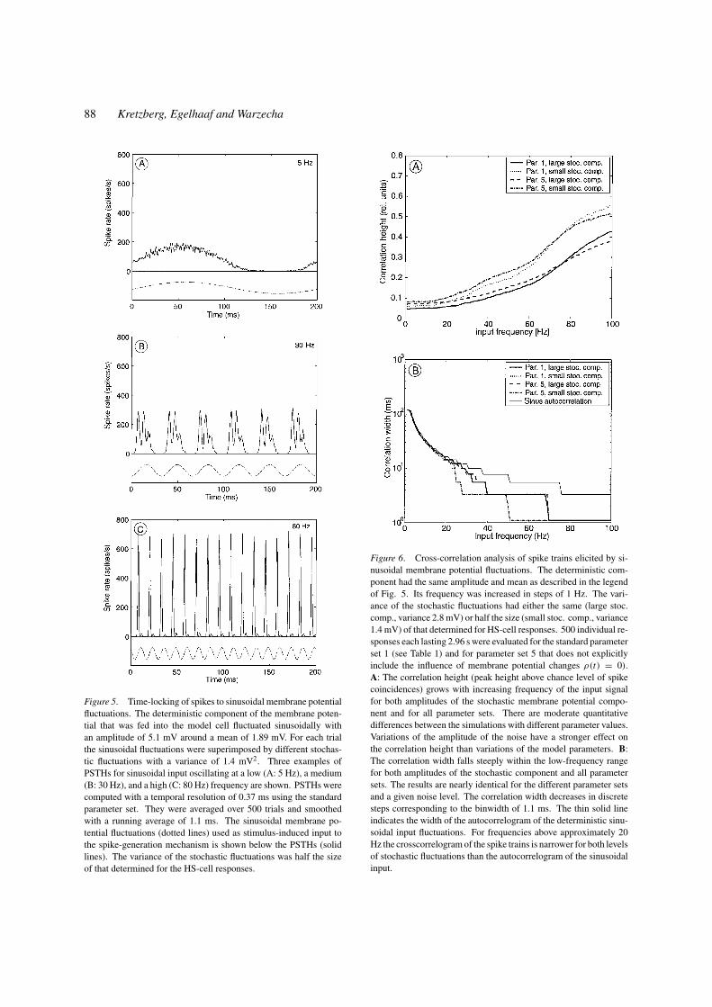
The PSTH of the simulated cell obtained with a 5

Hz input is virtually sinusoidal except for clipping at

low rates and, thus, resembles strongly the determin-

istic input (Fig. 5A). A spike can be generated at any

time when the membrane potential is sufficiently depo-

larized. The probability for eliciting a spike increases

with increasing depolarization of the cell. The spikes

do not time-lock on a millisecond timescale to the sinu-

soidal input at this frequency. Rather, the exact timing

of spikes depends on the stochastic membrane poten-

tial changes. For such low input frequencies the spike

rate is basically proportional to the deterministic mem-

brane potential which is fed into the spike generation

mechanism. For a 30 Hz input (Fig. 5B) the PSTH

is no longer sinusoidally modulated but shows several

short peaks during each depolarization phase. The in-

dividual spikes begin to phase-lock to the sinusoidal

fluctuations of the deterministic membrane potential

component. Fluctuations of the input at 80 Hz cause

a very precise time-locking of spikes. Accordingly,

the resulting PSTH shows sharp peaks (Fig. 5C). Ad-

ditional small peaks in the PSTH indicate that a sec-

ond spike is occasionally generated within one cycle.

For higher frequencies the small peaks disappear and

only one spike is generated for each cycle with a jitter

below one millisecond. If the input frequency is high

enough to cause peaks in the PSTH, the first and largest

peak occurs for each depolarization phase before the

maximum of the depolarization is reached indicating a

phase shift between the spike rate and the deterministic

sinusoidal input.

For a quantitative analysis of the temporal precision

of spike timing, we calculated the cross-correlogram of

individual spike trains. For this analysis two different

parameter sets and two levels of the stochastic compo-

nent were used (see legend of Fig. 6). The height of

the cross-correlogram above the chance level of spike

coincidences and the width of the correlogram at

half height were used as measures of the similarity

of individual spike trains and, thus, of the precision

with which the spikes time-lock to the determinis-

tic membrane potential component. For both levels

88 Kretzberg, Egelhaaf and Warzecha

Figure 5. Time-locking of spikes to sinusoidal membrane potential

fluctuations. The deterministic component of the membrane poten-

tial that was fed into the model cell fluctuated sinusoidally with

an amplitude of 5.1 mV around a mean of 1.89 mV. For each trial

the sinusoidal fluctuations were superimposed by different stochas-

tic fluctuations with a variance of 1.4 mV2. Three examples of

PSTHs for sinusoidal input oscillating at a low (A: 5 Hz), a medium

(B: 30 Hz), and a high (C: 80 Hz) frequency are shown. PSTHs were

computed with a temporal resolution of 0.37 ms using the standard

parameter set. They were averaged over 500 trials and smoothed

with a running average of 1.1 ms. The sinusoidal membrane po-

tential fluctuations (dotted lines) used as stimulus-induced input to

the spike-generation mechanism is shown below the PSTHs (solid

lines). The variance of the stochastic fluctuations was half the size

of that determined for the HS-cell responses.

Figure 6. Cross-correlation analysis of spike trains elicited by si-

nusoidal membrane potential fluctuations. The deterministic com-

ponent had the same amplitude and mean as described in the legend

of Fig. 5. Its frequency was increased in steps of 1 Hz. The vari-

ance of the stochastic fluctuations had either the same (large stoc.

comp., variance 2.8 mV) or half the size (small stoc. comp., variance

1.4 mV) of that determined for HS-cell responses. 500 individual re-

sponses each lasting 2.96 s were evaluated for the standard parameter

set 1 (see Table 1) and for parameter set 5 that does not explicitly

include the influence of membrane potential changes ρ(t) = 0).

A: The correlation height (peak height above chance level of spike

coincidences) grows with increasing frequency of the input signal

for both amplitudes of the stochastic membrane potential compo-

nent and for all parameter sets. There are moderate quantitative

differences between the simulations with different parameter values.

Variations of the amplitude of the noise have a stronger effect on

the correlation height than variations of the model parameters. B:

The correlation width falls steeply within the low-frequency range

for both amplitudes of the stochastic component and all parameter

sets. The results are nearly identical for the different parameter sets

and a given noise level. The correlation width decreases in discrete

steps corresponding to the binwidth of 1.1 ms. The thin solid line

indicates the width of the autocorrelogram of the deterministic sinu-

soidal input fluctuations. For frequencies above approximately 20

Hz the crosscorrelogram of the spike trains is narrower for both levels

of stochastic fluctuations than the autocorrelogram of the sinusoidal

input.

Precision of Spike Timing and Synchronous Activity 89

of the stochastic component, the height and width of

the cross-correlogram depend on the frequency of the

deterministic membrane potential fluctuations: The

correlation height increases with increasing input

frequency (Fig. 6A), whereas the correlation width

decreases (Fig. 6B). To assess the precision of time-

locking of spikes to the membrane potential fluctua-

tions, the width of the correlation peak of the spike

trains was compared to the width of the autocorrelo-

gram of the corresponding sinusoidal membrane po-

tential fluctuations (Fig. 6B). For frequencies below

approximately 20 Hz the width of the spike correlo-

grams and the sinus autocorrelogram are essentially

the same. This similarity indicates that the spike rate

follows the membrane potential changes and individual

spikes do not time-lock to a given phase. In contrast,

for higher frequencies the correlation width of the sim-

ulated spike trains becomes smaller than the width of

the autocorrelation of the sinusoidal input. Hence, for

frequencies above 20 Hz spikes are time-locked more

precisely to the input fluctuations than would be ex-

pected if the instantaneous spike rate were proportional

to the instantaneous membrane potential.

The exact values of correlation height and width de-

pend on the size of the stochastic membrane potential

fluctuations that are superimposed on the sinusoidal in-

put (Fig. 6). For increasing size of the stochastic com-

ponent, higher frequencies of the deterministic mem-

brane potential fluctuations are needed to obtain a given

correlation height and width. Nevertheless, the depen-

dence between input frequency and correlation height

and width are qualitatively the same for different sizes

of the stochastic membrane potential component. The

correlation between spike trains elicited by the same

sinusoidal input superimposed by different stochastic

components with the same statistical properties is also

influenced by the shape of the power spectrum of the

stochastic component and by the amplitude of the si-

nusoidal input. These effects have not been analyzed

systematically in the present study.

How robust are these conclusions with respect to

variations of the model parameters? Changes in the

parameters that determine the refractory period (γ ref

and η0) affect the shape of the correlogram of spike

responses to a sinusoidal membrane potential input

much more than changes in the other model parameters.

Due to the fact that the refractory period interacts with

the periodicity of the deterministic input, the shape of

the correlogram depends on the refractory period in a

complex manner. In contrast, correlation height and

width do not depend much on those parameters that

determine the dependence of the spike threshold on the

membrane potential changes (T and ρ0; compare data

obtained with parameter sets 1 and 5 in Fig. 6). For

frequencies below approximately 75 Hz the correlation

height is slightly larger, when the membrane potential

changes do not explicitly influence the spike thresh-

old (parameter set 5). For frequencies above about 75

Hz this relationship reverses (Fig. 6A). This reversal

is plausible as spikes are expected to time-lock even

better to fast membrane potentials when the influence

of membrane potential changes is explicitly modeled

(parameter set 1) than when it is not (parameter set 5).

Since for the low-frequency input all fast membrane

potential changes are stochastic, this feature of param-

eter set 1 reduces the correlation height compared to

parameter set 5. However, in the high-frequency range

spikes can time-lock to the deterministic input more

precisely when the fast membrane potential changes

influence the spike threshold explicitly. Therefore, for

deterministic input with sufficiently high frequencies

the correlation height is larger for parameter set 1 than

for parameter set 5. The correlation width was virtually

not affected by the parameter changes (Fig. 6B). For

neurons with a realistic amount of stochastic membrane

potential fluctuations it can be concluded that indepen-

dent of the parameter choice relatively fast membrane

potential changes are necessary to time-lock spikes pre-

cisely. This result is in accordance with a previous

conclusion based on experimental data on fly motion-

sensitive neurons (Warzecha et al., 1998).

3.3. Dependence of Spike Synchronization

on the Amount of Common Input

So far the model has been used to simulate spike trains

elicited in a neuron by repetitive identical stimulation

superimposed by noise. Successive spike trains simu-

lated by using the same deterministic membrane poten-

tial fluctuations but different stochastic response com-

ponents can also be interpreted as spike trains elicited

simultaneously in neurons with identical properties that

share parts of their input signals. As in many other sys-

tems (see Section 1, Introduction), two spiking neurons

in the fly motion pathway (H1 and H2) generate a large

proportion of their spikes synchronously (Warzecha

et al., 1998). These motion-sensitive interneurons are

thought to receive their input signals from largely the

same population of presynaptic elements. An example

90 Kretzberg, Egelhaaf and Warzecha

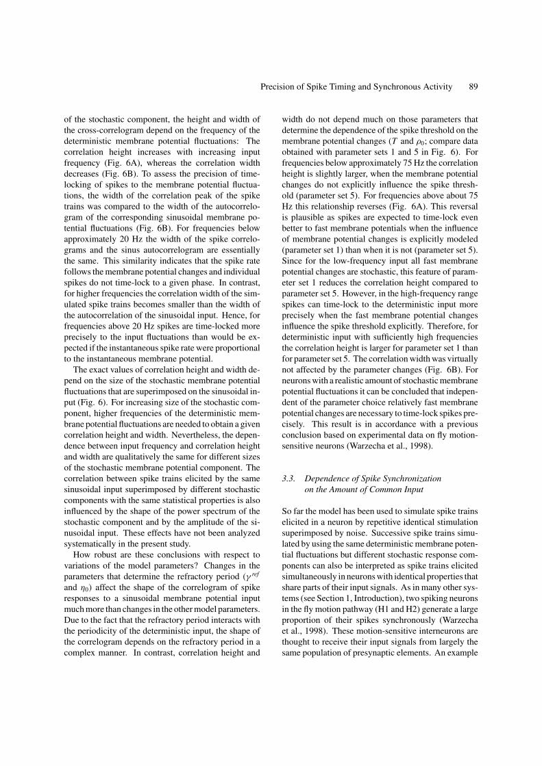
Figure 7. Cross-correlograms of simultaneously recorded and sim-

ulated neurons. Zero level indicates level of random coincidences of

spikes. A: Cross-correlogram of simultaneously recorded responses

of the H1-cell and the H2-cell to white-noise velocity fluctuations.

30 responses each lasting 3.1 s were used (modified from Warzecha

et al., 1998). B: Cross-correlogram of responses of two identical

model neurons. The input to the model cells consisted of the stimulus-

induced membrane potential obtained from an HS-cell that was su-

perimposed by stochastic fluctuations with the variance (2.8 mV2)

and the power spectrum fitted to experimental data (see Section 2,

Methods). The stochastic input consisted of two components, one

common to both neurons and one component that was generated in-

dependently for both neurons. The variance of both stochastic com-

ponents was identical (C = 50% common stochastic input). 30 pairs

of simulated spike trains each lasting 2.96 s were evaluated.

for a cross-correlogram of their spike trains is given

in Fig. 7A. The sharp peak in the cross-correlogram

can be reproduced by two model cells with identical

properties (Fig. 7B).

The model enables us to analyze which aspects of

the spike-generation mechanism are important deter-

minants of spike synchronization in pairs of cells and

to investigate how the temporal precision of spike gen-

eration depends on the composition of the input signals.

In the first step of the analysis, two cells with identical

parameters were simulated. Both cells shared as deter-

ministic component the same stimulus-induced mem-

brane potential as obtained from a fly motion-sensitive

neuron during motion stimulation with white-noise ve-

locity fluctuations. The stochastic component of the

membrane potential consisted of two parts—one part

common to both cells, the other one statistically in-

dependent for each cell (see Section 2, Methods). The

relative size of these stochastic components was varied,

while the variance of the total stochastic input was kept

constant. The power spectra of the stochastic compo-

nents were the same (except for a linear scale factor) but

different from that of the deterministic component. In

particular, the stochastic components contained more

power at high frequencies than the deterministic com-

ponent (see Section 2, Methods, and Fig. 3). The sim-

ilarity of spike trains of pairs of neurons was quanti-

fied by cross-correlation analysis. When spike trains

are simultaneously recorded, the height of the cross-

correlogram at t = 0 above the chance level of spike co-

incidences can indicate the amount of synchronous ac-

tivity. The width at half-height is taken to quantify the

temporal precision. The correlogram peak is small and

very broad if there is no common stochastic input to the

two simulated cells and the only common membrane

potential changes are stimulus-induced (Fig. 8). The

width of the cross-correlogram decreases (Fig. 8A) and

its height increases (Fig. 8B) with increasing percent-

age C of common stochastic input. The correlation

width falls steeply until the common stochastic input

reaches 50%. For larger common stochastic input the

correlation has a narrow peak that indicates spike syn-

chronization on a millisecond timescale. The correla-

tion height rises only slightly as long as the independent

part is predominant. Only when the common stochas-

tic component gets larger than the independent one, the

correlation height rises steeply and reaches its maxi-

mum for 100% common input. A qualitatively simi-

lar result was obtained with a reduced version of our

model in which the threshold was kept constant apart

from an absolute refractory period (data not shown) as

well as with integrate-and-fire units that share part of

their input consisting of Poisson spike trains (Ritz and

Sejnowski, 1997; Shadlen and Newsome, 1998).

To analyze the role of different model parameters

for the correlation between the spike trains of two

identical model neurons the parameters were varied

Precision of Spike Timing and Synchronous Activity 91

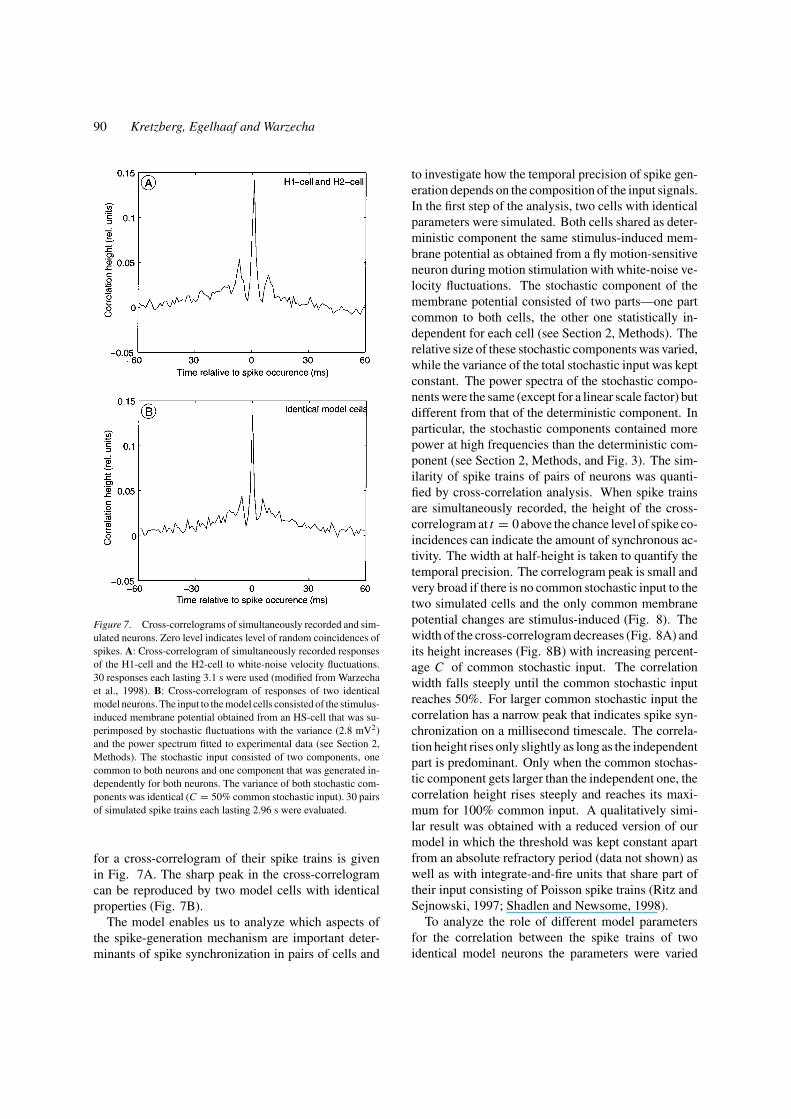
Figure 8. Correlated activity of pairs of neurons depends on the percentage of common stochastic input. The input common to two identical

model neurons consisted of the deterministic membrane potential component and a stochastic component that was identical for both neurons but

different from trial to trial. In addition, each model neuron was fed with stochastic membrane potential fluctuations generated independently

from those of the other neuron. The proportion of common and independent stochastic input (see Section 2, Methods) was varied while the total

variance of the input was held constant. The stochastic component of the input had more power than the deterministic component for frequencies

above about 30 Hz. 10 simulations were evaluated, each consisting of 100 responses of 2.96 s duration. The results of all simulations were

averaged. A, B: The correlation width decreases and the correlation height grows with increasing percentage C of the common stochastic input.

The correlation height must stay below 1 because it is calculated as the height above the chance level of spike coincidences. Error bars in A

denote SEMs of correlation widths of 10 simulations. The SEMs of correlation heights are smaller than the range covered by the symbols. C, D:

Comparison of correlation heights for pairs of identical model cells with different parameter values. The circles are a detail of B calculated with

parameter set 1. The other symbols indicate the outcome of simulations using the same parameter set except for ρ0 in C and T in D. Triangles

show simulations in which membrane potential changes are not taken into account in determining the spike threshold (ρ(t) = 0). C: For a

given percentage of common stochastic input the correlation height is largest when changes in the membrane potential are allowed to affect the

threshold most strongly. D: Highest correlation peaks were obtained for short integration times. As in C the correlations are smallest when the

influence of membrane potential changes is not explicitly taken into account (triangles).

systematically. Only two of the five model parame-

ters were found to influence the correlation in a no-

ticeable way. In contrast to the findings obtained with

sinusoidally fluctuating input, parameters determining

the refractoriness do not much influence the correla-

tion. Instead, enlarging the weight ρ0 with which mem-

brane potential changes affect spike threshold increases

the correlation height (Fig. 8C). For higher values of

ρ0 than those used in Fig. 8C the correlation height

increases even further. The correlation height is largest

for short time windows T within which the membrane

potential changes are determined (Fig. 8D). When

the membrane potential changes are not taken into ac-

count (T = 0 or ρ0 = 0), the correlation height for a

given amount of common input is smaller than for the

standard model (compare triangles and circles in Fig.

8C and D). For longer integration times T than those

employed in Fig. 8D the correlation height decreases,

92 Kretzberg, Egelhaaf and Warzecha

approaching the values obtained for T = 0. Neverthe-

less, the dependence of the correlation height on the

percentage of common stochastic input stays qualita-

tively the same for all parameter sets.

So far, we used the same parameters to simulate two

neurons. However, most biological neurons exhibiting

synchronized spike activity are unlikely to be identi-

cal. When any of the model parameters differed for

the two simulated neurons, the correlation height de-

creased for a given percentage of the common stochas-

tic membrane potential. This implies that for neurons

simulated with different parameter sets a larger per-

centage of common stochastic input is needed than for

identical model neurons to obtain a given correlation

height and width. Especially for simulations without

influence of the membrane potential changes on the

spike threshold (T = 0 or ρ0 = 0), the relative size of

the common stochastic input must be increased con-

siderably to maintain a given correlation height. These

findings imply that the level of common noise that is

needed to explain synchronized activity of pairs of neu-

rons is underestimated if the estimation is based on

model cells simulated with the same parameter set. As

has been shown above, the degree of synchronization

found in a pair of fly motion-sensitive neurons (H1 and

H2) can be reproduced by a pair of identical model cells

when they share 50% of their stochastic input (Fig. 7).

The real level of common stochastic input can be ex-

pected to be much larger because both neurons have

divergent characteristic properties (such as mean spike

rates differing by a factor of 2 to 3) and thus require

different parameter sets to account for these proper-

ties. For any parameter set chosen to fit the different

average spike activities of H1 and H2, at least 65%

common stochastic input was needed to obtain cross-

correlograms with a height and width similar to the

experimental data. For several parameter sets correla-

tion peaks were small and broad even when the total

stochastic component was common to both cells.

4. Discussion

The variability of spike trains and the time-locking

of spikes to membrane potential fluctuations has been

simulated with a time-dependent threshold model of

spike generation. It has been shown that spikes are

mainly time-locked to rapid depolarizations of the

membrane potential rather than to its slowly changing

components. This characteristic of spike generation

will be discussed with respect to (1) the features of the

model of spike generation that are responsible for it

and (2) its functional consequences for the synchro-

nization of spikes in neurons with common input and

for the encoding of time-dependent sensory stimuli.

4.1. Relevant Features of the Model

of Spike Generation

The time-dependent threshold model of spike genera-

tion proposed in the present study is a phenomenolog-

ical model with parameters adjusted to fit the spike

responses of a fly motion-sensitive neuron. Spike

activity in fly motion-sensitive neurons has already

been simulated by different model approaches ranging

from special versions of the integrate-and-fire model

(Mastebroek, 1974; Gestri et al., 1980) to a single-

compartment Hodgkin-Huxley type neuron (Haag et

al., 1999). None of these models was appropriate

for our purposes. Whereas the models of Maste-

broek (1974) and Gestri et al. (1980) were developed

to account for general statistical properties of aver-

aged spike trains, we wanted to explain the timing

of individual spikes. In Hodgkin-Huxley type models

currents serve as input to the spike-generation mecha-

nism, whereas we wanted to feed the spike-generation

mechanism with membrane potential changes elicited

by dynamic motion stimuli because these, rather than

the corresponding currents, are available for fly motion-

sensitive neurons from electrophysiological experi-

ments.

To account for the variability of spike trains as it

arises due to random background synaptic activity and

stochastic opening and closing of ion channels and to

a lesser extent to thermal noise (Manwani and Koch,

1999a, 1999b), a stochastic component must be in-

cluded into any spike-generation model. We added

stochastic fluctuations to the deterministic component

of the membrane potential (see also Reich et al., 1998).

An implicit assumption of this approach was that noise

is independent of the stimulus. This assumption does

not necessarily hold for real neurons. A recent study

revealed that the stochastic membrane potential com-

ponent in the H1-neuron of the fly may depend on the

stimulus conditions (Warzecha et al., 2000). Although

the implications of this finding for the mechanism of

spike generation need further investigations, the quali-

tative results of our model study do not critically depend

on the assumption of stimulus-independent noise.

There are further possibilities to introduce sto-

chasticity. In some models the membrane potential

Precision of Spike Timing and Synchronous Activity 93

determines at each instant of time the probability for

eliciting a spike. In this way the stochastic nature of

spike generation is simulated (e.g., Gerstner and van

Hemmen, 1992; Heck et al., 1993; Warzecha et al.,

1998). In other models a stochastically changing spike

threshold was used (e.g., Mastebroek, 1974; Reich

et al., 1997). Formally, the same output spike trains are

obtained when stochastic fluctuations are added to the

threshold or to the membrane potential because the dif-

ference between the actual threshold and the membrane

potential determines whether or not a spike is gener-

ated. We used stochastic membrane potential fluctua-

tions and a deterministic (but time-varying) threshold

(e.g., Cecchi et al., 2000) because there is evidence

that the spike-generation process does not represent the

main source of variability of neural activity (Mainen

and Sejnowski, 1995; Zador, 1998; Stevens and Zador,

1998). For integrate-and-fire units the threshold is of-

ten assumed to be constant, and a stochastic spike out-

put is obtained by using stochastic spike trains as input

(e.g., Shadlen and Newsome, 1998; Koch, 1999).

The relative refractory period is an absolute neces-

sity in our spike-generation model to explain the spike

responses of fly motion-sensitive neurons. Since the

relative refractory period is a well established prop-

erty of spike generation (e.g., Kandel et al., 1995), it is

not surprising that it was explicitly taken into account

in many phenomenological models of spike generation

(e.g., Mastebroek, 1974; Eckhorn et al., 1990; Gerstner

and van Hemmen, 1992; Heck et al., 1993). In con-

trast, in the Hodgkin-Huxley model of spike-generation

(Hodgkin and Huxley, 1952) refractoriness is not an ex-

plicit model parameter but derives from the dynamics

of the spike mechanism itself.

It is well established that fast depolarizing currents

injected into a neuron trigger a spike at more nega-

tive voltage values than do slowly depolarizing currents

(e.g., Johnston and Wu, 1995). This fundamental fea-

ture of spike generation is reflected in the experimental

finding that spikes couple to rapid membrane potential

fluctuations more reliably than to less transient ones

(Mainen and Sejnowski, 1995; Haag and Borst, 1996;

Reich et al., 1997; Mechler et al., 1998; Warzecha et

al., 1998). Moreover, the timing of spikes could be pre-

dicted better if the time derivative of the membrane po-

tential, rather than the actual membrane potential itself,

is assumed to determine the spike threshold (Ebbing-

haus et al., 1997). These results are consistent with the

phase advance of the peak in the PSTH with respect

to sinusoidal membrane potential fluctuations (Fig. 5)

and the increased phase locking of spikes to higher

frequencies (Fig. 6). With phenomenological models

of spike generation, a more precise coupling to rapid

membrane potential fluctuations than to slow ones is

obtained even if the spike threshold is not explicitly in-

fluenced by membrane potential changes (Fig. 6; see

also Cecchi et al., 2000). Nonetheless, as was shown by

the present model simulations the explicit influence of

membrane potential changes on spike threshold influ-

ences the precision of time-locking of individual spikes

to the synaptic input of the cell. In particular, if the

membrane potential dynamics affects the spike thresh-

old, a smaller amount of common stochastic input is

needed to explain synchronous spike activity than when

the spike threshold is not affected in this way.

4.2. Significance of Fast Membrane

Potential Fluctuations

A large part of the membrane potential fluctuations of a

neuron is due to its synaptic input (Calvin and Stevens,

1968). Spikes tend to time-lock to the fast rather than to

the slow components of these fluctuations (see above).

Such fast membrane potential changes may be tightly

time-locked to changes in sensory stimuli, or they may

be unrelated to the temporal properties of the stimu-

lus. How well spikes couple to a sensory stimulus de-

pends on the proportion of the amplitudes and on the

frequency composition of the stimulus-induced and of

the stochastic membrane potential component. Only if

the amplitude of the stimulus-induced component ex-

ceeds the stochastic component in a sufficiently high-

frequency range can spikes be time-locked precisely to

the stimulus. Nevertheless, synchronized spike activ-

ity can appear even if the stimulus does not determine

the exact timing of spikes (e.g., Usrey et al., 1998;

Usrey and Reid, 1999; Warzecha et al., 1998). Hence,

rapid membrane potential fluctuations in different neu-

rons that have their origin in a source common to these

neurons may lead to synchronized spike activity re-

gardless of whether the rapid fluctuations are induced

by the stimulus or whether they are unrelated to it.

Accordingly, it cannot be concluded from the occur-

rence of spike synchronization that this synchroniza-

tion is important for the computations a neuronal sys-

tem performs. Instead, it has to be analyzed for the re-

spective system whether synchronized activity is used

by neurons at the next processing stage and whether the

exact timing of spikes plays a functional role to encode

sensory stimuli.

94 Kretzberg, Egelhaaf and Warzecha

4.2.1. Dependence of Spike Timing on Sensory Stimu-

lation. On what time scale spikes of sensory neurons

are coupled to sensory stimuli is constrained by the

temporal properties of the underlying stimulus-induced

membrane potential fluctuations and, thus, by the tem-

poral properties of the respective stimulus. This time

scale can range over several orders of magnitude de-

pending on the system under consideration. For in-

stance, in the electrosensory system of electric fish

phase-coding neurons are known that fire one spike

phase-locked with very little temporal jitter to each

cycle of the electric organ discharge (Heiligenberg,

1991; Kawasaki, 1997). In the auditory system, in-

teraural time differences are used to localize sound

sources. This task can be solved only if very precise

phase-locking of the individual spikes to the arrival

times of the sound at the two ears is guaranteed (Carr

and Friedmann, 1999). In contrast, spikes of motion-

sensitive neurons in visual systems usually lock to mo-

tion stimuli on a coarser timescale. This is because

high-frequency changes in the direction of motion are

attenuated as a consequence of motion computations

(e.g., Egelhaaf and Borst, 1993). Due to these compu-

tational constraints, mainly relatively low frequencies

(up to 20 to 40Hz) dominate the stimulus-induced re-

sponses of motion-sensitive neurons—for example, in

the monkey and the fly when activated with broad-band

velocity fluctuations (Bair and Koch, 1996; Haag and

Borst, 1997, 1998; Warzecha et al., 1998). For the

fly it was shown that for these stimulus conditions the

power of the stochastic membrane potential component

exceeds the power of the deterministic fluctuations for

frequencies above about 30 Hz. Hence most spikes of

the motion-sensitive H1-cell were concluded to time-

lock with a millisecond precision to the fast stochastic

rather than to the stimulus-induced response compo-

nent (Warzecha et al., 1998).

The dynamical properties of the stimulus-induced

response component need to be qualified because they

were obtained with artificially generated stimuli that

may differ from natural stimuli in their amplitude and

their frequency composition. Both of these aspects

may influence the power spectrum of the stimulus-

induced response component and thus the precision

with which spikes can couple to the visual stimu-

lus. In specific behavioral situations the retinal im-

age velocities that are encountered by flies can as-

sume very large values (e.g., Land and Collett, 1974;

Wagner, 1986). In contrast to a recent hypothesis

(de Ruyter van Steveninck et al., 2000), the response

amplitude of motion-sensitive neurons in a variety of

species (Pollen et al., 1978; Wolf-Oberhollenzer and

Kirschfeld, 1990; Lisberger and Movshon, 1999) in-

cluding the fly (Hausen, 1982; Maddess and Laughlin

1985, Egelhaaf and Reichardt, 1987) does not scale

proportionally to stimulus velocity. In particular, dur-

ing white-noise velocity stimulation as used in the

present account (such as Figs. 2 and 3) the membrane

potential of fly motion-sensitive neurons de- and hy-

perpolarized by about 10 mV. Much larger response

amplitudes cannot be elicited close to the output re-

gion of the motion-sensitive neurons in the fly’s brain

by any visual motion stimulation. Therefore, it seems

unlikely that due to the large amplitude of the retinal

image velocities that occur in certain behavioral situa-

tions, the stimulus-induced component will exceed the

stochastic component in the high-frequency range.

The frequency composition of the stimulus (when an

animal is confronted with a behaviorally relevant sit-

uation) largely depends on the animal’s behavior. For

instance, if a fly tries to fly straight and to stabilize its

flight course against disturbances, the retinal velocity

was found in behavioral studies in a flight simulator to

change only relatively slowly (Warzecha and Egelhaaf,

1996). The resulting membrane potential changes are

not fast enough to time-lock spikes with a millisec-

ond precision (Warzecha and Egelhaaf, 1997). On the

other hand, during very fast saccade-like body turns

(see, e.g., van Hateren and Schilstra, 1999; Schilstra

and van Hateren, 1999), transient image displacements

may occur that elicit postsynaptic membrane potentials

fast enough to time-lock spikes precisely (Warzecha

and Egelhaaf, 2000; de Ruyter van Steveninck et al.,

2000). In conclusion, it very much depends on the stim-

ulus conditions and thus on the behavioral context as

well as the biophysical, and computational constraints,

on what time scale spikes time-lock to sensory stimuli

under natural conditions.

4.2.2. Implications for Neural Coding. Our results

hint at a novel perspective with respect to the apparent

antagonism between rate code and time code (see, e.g.,

Shadlen and Newsome, 1994; Softky, 1995). On the

one hand, spikes time-lock precisely to high-frequency

membrane potential fluctuations. Their timing is then

more precise than the underlying membrane potential

dynamics,—that is, the spike rate is not proportional to

the membrane potential as is the case for slow mem-

brane potential changes (Fig. 5). Hence, fast depo-

larizations of the cell are a prerequisite for a code that

Precision of Spike Timing and Synchronous Activity 95

transmits information by the exact timing of individ-

ual spikes and for synchronizing the activity of neu-

rons with common input on a fine timescale. On the

other hand, slow stimulus-induced membrane potential

changes determine the probability of spike timing only

on a coarse time scale, at least if these are superimposed

by noise. Hence, slowly changing stimuli on their own

do not synchronize the activity of neurons that share

parts of their inputs. Instead, such stimuli are encoded

by the spike rate, whereas the exact timing of the indi-

vidual spikes is determined by fast stochastic processes.

However, these two kinds of coding are not strictly sep-

arate since rate coding may turn into time coding and

vice versa, when the dynamics of the membrane poten-

tial fluctuations changes. Accordingly, the relevance of

spike timing for encoding a stimulus is not a question

that can be answered with yes or no. To what extent the

timing of individual spikes matters rather depends on

the dynamics of the membrane potential changes of the

investigated neuron that are induced by the stimulus,

on the one hand, and the stochastic membrane potential

component, on the other hand.

Acknowledgments

We thank our coworkers R. Kern, H. Krapp, R. Kurtz,

and J.P. Lindemann for reading and discussing the

manuscript. The detailed constructive comments of

two anonymous referees are gratefully acknowledged.

This study was supported by a grant of the Studi-

enstiftung des deutschen Volkes to J.K. and by the

DFG.

References

Alonso JM, Usrey W, Reid R (1996) Precisely correlated firing in

cells of the lateral geniculate nucleus. Nature 383:815–819.

Bair W (1999) Spike timing in the mammalian visual system. Curr.

Opin. Neurobiol. 9:447–453.

Bair W, Koch C (1996) Temporal precision of spike trains in extras-

triate cortex of the behaving macaque monkey. Neural Comput.

8:1185–1202.

Berry MJ, Warland DK, Meister M (1997) The structure and preci-

sion of retinal spike trains. PNAS, USA 94:5411–5416.

Bialek W, Rieke F (1992) Reliability and information transmission

in spiking neurons. TINS 15:428–434.

Britten K, Shadlen M, Newsome W, Movshon J (1993) Responses

of neurons in macaque MT to stochastic motion signals. Vis. Neu-

rosci. 10:1157–1169.

Brivanlou I, Warland D, Meister M (1998) Mechanisms of concerted

firing among retinal ganglion cells. Neuron 20:527–539.

Brody C (1999) Correlations without synchrony. Neural Comput.

11:1537–1551.

Buracas G, Zador A, DeWeese M, Albright T (1998) Efficient dis-

crimination of temporal patterns by motion-sensitive neurons in

primate visual cortex. Neuron 20:956–969.

Calvin W, Stevens C (1968) Synaptic noise and other sources of

randomness in motoneuron interspike intervals. J. Neurophysiol.

31:574–587.

Carr C, Friedmann M (1999) Evolution of time coding systems.

Neural Comput. 11:1–20.

Cecchi G, Sigman M, Alonso JM, Martinez L, Chialvo D, Magnasco

M (2000) Noise in neurons is message-dependent. Proc. Natl.

Acad. Sci. USA 97:5557–5561.

de Ruyter van Steveninck R, Bialek W (1988) Real-time performance

of a movement-sensitive neuron in the blowfly visual system: Cod-

ing and information transfer in short spike sequences. Proc. R. Soc.

Lond. B 234:379–414.

de Ruyter van Steveninck R, Bialek W (1995) Reliability and sta-

tistical efficiency of a blowfly movement sensitive neuron. Phil.

Trans. R. Soc. Lond. B 348:321–340.

de Ruyter van Steveninck R, Borst A, Bialek W (2000) Real-time

encoding of motion: Answerable questions and questionable an-

swers from the fly’s visual system. In: Zanker JM, Zeil J, eds.

Visual Motion. Springer, Heidelberg (in press).

Ebbinghaus C, Diesmann M, Rotter S, Aertsen A (1997) The neu-

ral firing threshold: Can I help U? In: Elsner N, Wassle H,

eds. Gottingen Neurobiology Report 1997. Proceedings of the

25th Gottingen Neurobiology Conference 1997. Thieme, Stuttgart

p. 624.

Eckhorn R, Reitboeck H, Arndt M, Dicke P (1990) Feature link-

ing via synchronization among distributed assemblies: Simula-

tions of results from cat visual cortex. Neural Comput. 2:293–

307.

Egelhaaf M, Borst A (1993) Movement detection in arthropods.

In: Miles FA, Wallman J, eds. Visual Motion and Its Role in the

Stabilization of Gaze. Elsevier, Amsterdam. pp. 53–77.

Egelhaaf M, Reichardt W (1987) Dynamic response properties of

movement detectors: Theoretical analysis and electrophysiolog-

ical investigation in the fly system of the fly. Biol. Cybern. 56:

69–87.

Egelhaaf M, Warzecha, A-K (1999) Encoding of motion in real time

by the fly visual system. Curr. Opin. Neurobiol. 9:454–460.

Gerstner W, van Hemmen L (1992) Associative memory in a network

of “spiking” neurons. Network 3:139–164.

Gestri G, Mastebroek H, Zaagman W (1980) Stochastic constancy,

variability and adaptation of spike generation: Performance of a

giant neuron in the visual system of the fly. Biol. Cybern. 38:31–

40.

Haag J, Borst A (1996) Amplifications of high-frequency synaptic

inputs by active dendritic membrane processes. Nature 379:639–

641.

Haag J, Borst A (1997) Encoding of visual motion information and

reliability in spiking and graded potential neurons. J. Neurosci.

17:4809–4819.

Haag J, Borst A (1998) Active membrane properties and signal

encoding in graded potential neurons. J. Neurosci. 18:7972–

7986.

Haag J, Vermeulen A, Borst A (1999) The intrinsic electrophysiolog-

ical characteristics of fly lobula plate tangential cells: III. Visual

response properties. J. Comp. Neurosci. 7:213–234.

96 Kretzberg, Egelhaaf and Warzecha

Hausen K (1981) Monocular and binocular computation of mo-

tion in the lobula plate of the fly. Verh. Dtsch. Zool. Ges. 74:49–

70.

Hausen K (1982) Motion sensitive interneurons in the optomotor sys-

tem of the fly. II. The horizontal cells: Receptive field organization

and response characteristics. Biol. Cybern. 46:67–79.

Heck D, Rotter S, Aertsen A (1993) Spike generation in corti-

cal neurons: Probabilistic threshold function shows intrinsic and

long-lasting dynamics. In: Aertsen A, ed. Brain Theory. Elsevier,

Amsterdam. pp. 241–249.

Heiligenberg W (1991) Neural Nets in Electric Fish. MIT Press,

Cambridge, MA.

Hengstenberg R (1982) Common visual response properties of giant

vertical cells in the lobula plate of the blowfly Calliphora. J. Comp.

Physiol. 149:179–193.

Hodgkin A, Huxley A (1952) A quantitative description of ion cur-

rents and its applications to conduction and excitation in nerve

membranes. J. Physiol. (London) 117:500–544.

Johnston D, Wu SS (1995) Foundations of Cellular Neurophysiology.

MIT Press, Cambridge, MA.

Kandel E, Schwartz J, Jessell T (1995) Essentials of neural science

and behavior. Appleton & Lange, Norwalk, CT.

Kawasaki M (1997) Sensory hyperacuity in the jamming avoidance

response of weakly electric fish. Curr. Opin. Neurobiol. 7:473–

479.

Koch C (1999) Biophysics of Computation: Information Processing

in Single Neurons. Oxford University Press, New York.

Lampl I, Reichova I, Ferster D (1999) Synchronous membrane po-

tential fluctuations in neurons of the cat visual cortex. Neuron

22:361–374.

Land MF, Collet TS (1974) Chasing behaviour of houseflys (Fannia

caicularis). J. Comp. Physiol. 89:331–357.

Levine M (1998) Models for the cross-correlation between retinal

ganglion cells. Biol. Cybern. 79:367–376.

Lisberger SG, Movshon JA (1999) Visual motion analysis for pursuit

eye movements in area MT of macaque monkeys. J. Neurophysiol.

19:2224–2246.

Maass W (1996) Networks of spiking neurons: The third generation

of neural network models. Neur Networks 10:1659–1671.

Maddess T, Laughlin SB (1985) Adaptation of the motion-sensitive

neuron H1 is generated locally and governed by contrast frequency.

Proc. R. Soc. Lond. B 225:251–275.

Mainen Z, Sejnowski T (1995) Reliability of spike timing in neocor-

tical neurons. Science 268:1503–1506.

Manwani A, Koch C (1999a) Detecting and estimating signals in

noisy cable structures: I. Neuronal noise sources. Neural Comput.

11:1797–1829.

Manwani A, Koch C (1999b) Detecting and estimating signals in

noisy cable structures: II. Information theoretical analysis. Neural

Comput. 11:1831–1873.

Mastebroek H (1974) Stochastic structure of neural activity in the

visual system of the blowfly. Ph.D. thesis, Rijksuniversiteit te

Groningen.

Mechler F, Victor JD, Purpura KP, Shapley R (1998) Robust temporal

coding of contrast by V1 neurons for transient but not for steady-

state stimuli. J. Neurosci. 18:6583–6598.

Pollen DA, Andrews BW, Feldon SE (1978) Spatial frequency se-

lectivity of periodic complex cells in the visual cortex of the cat.

Vis. Res. 18:665–682.

Reich D, Victor J, Knight B (1998) The power ratio and the interval

map: Spiking models and extracellular recordings. J. Neurosci.

18:10090–10104.

Reich D, Victor J, Kneight B, Ozaki T, Kaplan E (1997) Response

variability and timing precision of neuronal spike trains in vivo. J.

Neurophysiol. 77:2836–2841.

Ritz R, Sejnowski T (1997) Correlation coding in stochastic neu-

ral networks. In: Gerstner W, Germona A, Hasler M, Nicaud

J-D, eds. Proceedings ICANW 97. Springer, Heidelberg, pp. 79–

84.

Schilstra C, Hateren JH van (1999) Blowfly flight and optic flow. I.

Thorax kinematics and flight dynamics. J. Exp. Biol. 202:1481–

1490.

Schneidman E, Freedman B, Segev I (1998) Ion channel stochasticity

may be critical in determining the reliability and precision of spike

timing. Neural Comput. 10:1679–1703.

Shadlen M, Newsome W (1994) Noise, neural codes and cortical

organization. Curr. Opin. Neurobiol. 4:569–579.

Shadlen M, Newsome W (1998) The variable discharge of cortical

neurons: Implications for connectivity, computation, and infor-

mation coding. J. Neurosci. 18:3870–3896.

Softky W (1995) Simple codes versus efficient codes. Curr. Opin.

Neurobiol. 5:239–247.

Softky W, Koch C (1993) The highly irregular firing of cortical cells

is inconsistent with temporal integration of random epsps. J. Neu-

rosci. 13:334–350.

Stevens C, Zador A (1998) Input synchrony and the irregular firing

of cortical neurons. Nature Neurosci 1:210–217.

Tolhurst D, Movshon JA, Dean A (1983) The statistical reliability

of signals in single neurons in cat and monkey visual cortex. Vis.

Res. 23:775–785.

Usrey WM, Reid RC (1999) Synchronous activity in the visual sys-

tem. Ann. Rev. Physiol 61:435–456.

Usrey WM, Reppas JB, Reid RC (1998) Paired-spike interactions

and synaptic efficacy of retinal inputs to the thalamus. Nature

395:384–387.

van Hateren JH, Schilstra C (1999) Blowfly flight and optic flow.

II. Head movements during flight. J. Exp. Biol. 202:1491–

1500.

Vogels R, Spileers W, Orban G (1989) The response variability of stri-

ate cortical neurons in behaving monkey. Exp. Brain. Res. 77:432–

436.

Wagner H (1986) Flight performance and visual control of flight of

the free flying housefly (Musca domestica L.) II. Pursuit of targets.

Phil. Trans. R. Soc. Lond. B 312:553–579.

Warzecha AK, Egelhaaf M (1996) Intrinsic properties of bio-

logical motion detectors prevent the optomotor control system

from getting unstable. Phil. Trans. R. Soc. Lond. B 351:1579–

1591.

Warzecha AK, Egelhaaf M (1997) How reliably does a neuron in the

visual motion pathway of the fly encode behaviourally relevant

information? Eur. J. Neurosci. 9:1365–1374.

Warzecha AK, Egelhaaf M (1999) Variability in spike trains

during constant and dynamic stimulation. Science 283:1927–

1930.

Warzecha AK, Egelhaaf M (2000) Neuronal encoding of visual

motion in real-time In: Zanker JM, Zeil J, eds. Visual Motion.

Springer, Heidelberg (in press).

Warzecha AK, Kretzberg J, Egelhaaf M (1998) Temporal precision of

the encoding of motion information by visual interneurons. Curr.

Biol. 8:359–368.

Precision of Spike Timing and Synchronous Activity 97

Warzecha AK, Kretzberg J, Egelhaaf M (2000) Reliability of a fly

motion sensitive neuron depends on stimulus parameters. J. Neu-

rosci. 20:8886–8896.

White JA, Rubinstein JT, Kay AR (2000) Channel noise in neurons.

Trends Neurosci. 23:131–137.

Wolf-Oberhollenzer F, Kirschfeld K (1990) Temporal frequency

dependence in motion-sensitive neurons of the accessory optic

system of the pigeon. Naturwiss. 77:296–298.

Zador A (1998) Impact of synaptic unreliability on the information

transmitted by spiking neurons. J. Neurophysiol. 79:1219–1229.