Meep Download Release notes F AQ Meep manual Introduction Installation Tutorial Reference C++ Tutorial C++ Reference Acknowledgements License and Copyright Meep T utorial From AbInitio In this page, we'll go through a couple of simple examples that illustrate the process of computing fields, transmission/reflection spectra, and resonant modes in Meep. All of the examples here are two-dimensional calculations, simply because they ar e quicker than 3d computations and they illustrate most of the essential features, but of course Meep can d o similar calculations in 3d. This tutorial uses the libctl/Scheme scripting interface to Meep, which is what we expect most users to employ most of the time. There is also a C++ interface that may give additional flexibility in some situations; that is described in the C++ tutorial. In order to convert the HDF5 output files of Meep into images of the fields and so on, this tutorial uses our free h5utils programs. (Y ou could also use any other program, such as Matlab (http://www .mathworks.com/access/helpd esk/help/techdoc/ref/hdf5read.html) , that supports reading HDF5 files.) Contents 1 The ctl file 2 Fields in a waveguide 2.1 A straight waveguide 2.2 A 90° bend 2.2.1 Output tips and tricks 3 Transmission spectrum around a waveguide bend 4 Modes of a ring resonator 4.1 Exploiting symmetry 5 More examples 6 Editors and ctl The ctl file The use of Meep revol ves around the control file, abbreviated "ctl" and typically called something like foo.ctl (although you can use any file name you wish). The ctl file specifies the geometry you wish to stud y, the current sources, the outputs computed, and everything else specific to y our calculation. Rather than a flat, inflexible file format, however, the ctl file is actually written in a scripting language. This means that it can b e everything from a simple sequence of commands setting the geometry, etcetera, to a full-fledged program with us er input, loops, and anything else that you might need. Don't worry , though—simple things are simple (you don't need to be a Real Programmer (http://catb.org/esr/jar gon/html/R/Real-Programmer.html) ), and even there you will appreciate the flexibility that a scripting language gives you. (e.g. you can input things in any order, without regard for whites pace, insert comments where you please, omit things when reasonable defaults are available...) The ctl file is actually implemented on top of the libctl library, a set of utilities that are in turn built on top of the Scheme language. Thus, there are three sources of possible commands and syntax for a ctl file: Scheme, a powerful and beautiful programming language developed at MIT , which has a particularly simple syntax: all statements are of the form (function arguments...). We run Scheme under the GNU Guile interpreter (designed to be plugged into programs as a scripting and extension language). Y ou don't

Welcome message from author
This document is posted to help you gain knowledge. Please leave a comment to let me know what you think about it! Share it to your friends and learn new things together.
Transcript

7/18/2019 Meep Tutorial - AbInitio.pdf
http://slidepdf.com/reader/full/meep-tutorial-abinitiopdf 1/15
Meep
Download
Release notes
FAQ
Meep manual
IntroductionInstallation
Tutorial
Reference
C++ Tutorial
C++ Reference
Acknowledgements
License and Copyright
Meep Tutorial
om AbInitio
his page, we'll go through a couple of simple examples that illustrate the process of
mputing fields, transmission/reflection spectra, and resonant modes in Meep. All of themples here are two-dimensional calculations, simply because they are quicker than 3d
mputations and they illustrate most of the essential features, but of course Meep can doilar calculations in 3d.
s tutorial uses the libctl/Scheme scripting interface to Meep, which is what we expect
st users to employ most of the time. There is also a C++ interface that may give
itional flexibility in some situations; that is described in the C++ tutorial.
rder to convert the HDF5 output files of Meep into images of the fields and so on, this
rial uses our free h5utils programs. (You could also use any other program, such as
lab (http://www.mathworks.com/access/helpdesk/help/techdoc/ref/hdf5read.html) ,
supports reading HDF5 files.)
ontents
1 The ctl file
2 Fields in a waveguide
2.1 A straight waveguide2.2 A 90° bend
2.2.1 Output tips and tricks
3 Transmission spectrum around a waveguide bend4 Modes of a ring resonator
4.1 Exploiting symmetry
5 More examples
6 Editors and ctl
he ctl file
use of Meep revolves around the control file, abbreviated "ctl" and typically called something like foo.ctlhough you can use any file name you wish). The ctl file specifies the geometry you wish to study, the current
rces, the outputs computed, and everything else specific to your calculation. Rather than a flat, inflexible file
mat, however, the ctl file is actually written in a scripting language. This means that it can be everything from a
ple sequence of commands setting the geometry, etcetera, to a full-fledged program with user input, loops, and
thing else that you might need.
n't worry, though—simple things are simple (you don't need to be a Real Programmer
p://catb.org/esr/jargon/html/R/Real-Programmer.html) ), and even there you will appreciate the flexibility that a
pting language gives you. (e.g. you can input things in any order, without regard for whitespace, insert
mments where you please, omit things when reasonable defaults are available...)
ctl file is actually implemented on top of the libctl library, a set of utilities that are in turn built on top of the
eme language. Thus, there are three sources of possible commands and syntax for a ctl file:
Scheme, a powerful and beautiful programming language developed at MIT, which has a particularly simple
syntax: all statements are of the form (function arguments...). We run Scheme under the GNU
Guile interpreter (designed to be plugged into programs as a scripting and extension language). You don't

7/18/2019 Meep Tutorial - AbInitio.pdf
http://slidepdf.com/reader/full/meep-tutorial-abinitiopdf 2/15
need to know much Scheme for a basic ctl file, but it is always there if you need it; you can learn more about
it from these Guile and Scheme links.
libctl, a library that we built on top of Guile to simplify communication between Scheme and scientificcomputation software. libctl sets the basic tone of the interface and defines a number of useful functions
(such as multi-variable optimization, numeric integration, and so on). See the libctl manual pages.
Meep itself, which defines all the interface features that are specific to FDTD calculations. This manual is
primarily focused on documenting these features.
his point, please take a moment to leaf through the libctl tutorial to get a feel for the basic style of the interface,
ore we get to the Meep-specific stuff below. (If you've used MPB, all of this stuff should already be familiar,
ough Meep is somewhat more complex because it can perform a wider variety of computations.)
ay, let's continue with our tutorial. The Meep program is normally invoked by running something like the
owing at the Unix command-line (herein denoted by the unix% prompt):
x% meep foo.ctl >& foo.out
ch reads the ctl file foo.ctl and executes it, saving the output to the file foo.out. However, if you invoke
ep with no arguments, you are dropped into an interactive mode in which you can type commands and see their
ults immediately. If you do that now, you can paste in the commands from the tutorial as you follow it and see
at they do.
elds in a waveguide
our first example, let's examine the field pattern excited by a localized CW source in a waveguide— first
ight, then bent. Our waveguide will have (non-dispersive) and width 1. That is, we pick units of
gth so that the width is 1, and define everything in terms of that (see also units in meep).
traight waveguide
ore we define the structure, however, we have to define the computational cell. We're going to put a source at
end and watch it propagate down the waveguide in the x direction, so let's use a cell of length 16 in the x
ction to give it some distance to propagate. In the y direction, we just need enough room so that the boundaries
ow) don't affect the waveguide mode; let's give it a size of 8. We now specify these sizes in our ctl file via theometry-lattice variable:
t! geometry-lattice (make lattice (size 16 8 no-size)))
e name geometry-lattice comes from MPB, where it can be used to define a more general periodicce. Although Meep supports periodic structures, it is less general than MPB in that affine grids are not
ported.) set! is a Scheme command to set the value of an input variable. The last no-size parameter says
the computational cell has no size in the z direction, i.e. it is two-dimensional.
w, we can add the waveguide. Most commonly, the structure is specified by a list of geometric objects, stored
he geometry variable. Here, we do:
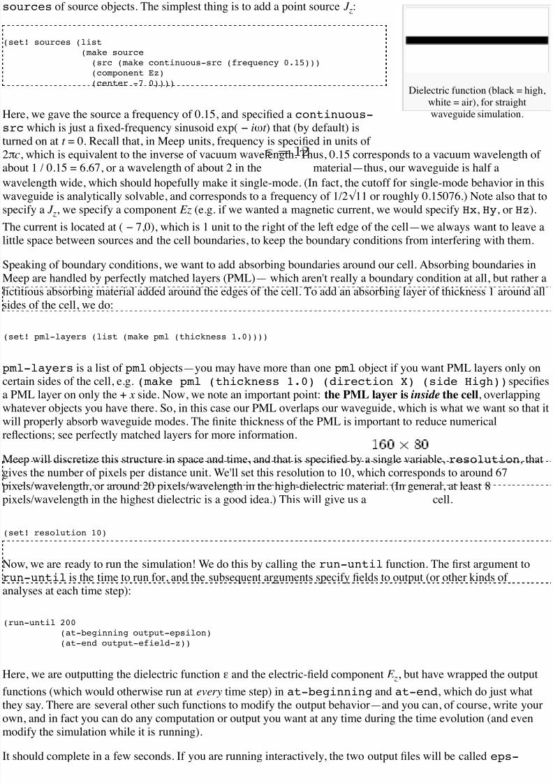
t! geometry (list(make block (center 0 0) (size infinity 1 infinity)
(material (make dielectric (epsilon 12))))))
waveguide is specified by a block (parallelepiped) of size , with !=12, centered at (0,0) (the
ter of the computational cell). By default, any place where there are no objects there is air (!=1), although this
be changed by setting the default-material variable. The resulting structure is shown at right.
w that we have the structure, we need to specify the current sources, which is specified as a list called
7/18/2019 Meep Tutorial - AbInitio.pdf
http://slidepdf.com/reader/full/meep-tutorial-abinitiopdf 3/15
Dielectric function (black = high,
white = air), for straight
waveguide simulation.
urces of source objects. The simplest thing is to add a point source J z:
t! sources (list(make source(src (make continuous-src (frequency 0.15)))(component Ez)(center -7 0))))
e, we gave the source a frequency of 0.15, and specified a continuous-c which is just a fixed-frequency sinusoid exp( " i#t ) that (by default) is
ed on at t = 0. Recall that, in Meep units, frequency is specified in units of , which is equivalent to the inverse of vacuum wavelength. Thus, 0.15 corresponds to a vacuum wavelength of ut 1 / 0.15 = 6.67, or a wavelength of about 2 in the material—thus, our waveguide is half a
velength wide, which should hopefully make it single-mode. (In fact, the cutoff for single-mode behavior in this
veguide is analytically solvable, and corresponds to a frequency of 1/2 % 11 or roughly 0.15076.) Note also that to
cify a J z, we specify a component Ez (e.g. if we wanted a magnetic current, we would specify Hx, Hy, or Hz).
current is located at ( " 7,0), which is 1 unit to the right of the left edge of the cell—we always want to leave a
e space between sources and the cell boundaries, to keep the boundary conditions from interfering with them.
aking of boundary conditions, we want to add absorbing boundaries around our cell. Absorbing boundaries in
ep are handled by perfectly matched layers (PML)— which aren't really a boundary condition at all, but rather atious absorbing material added around the edges of the cell. To add an absorbing layer of thickness 1 around all
s of the cell, we do:
t! pml-layers (list (make pml (thickness 1.0))))
l-layers is a list of pml objects—you may have more than one pml object if you want PML layers only onain sides of the cell, e.g. (make pml (thickness 1.0) (direction X) (side High)) specifies
ML layer on only the + x side. Now, we note an important point: the PML layer is inside the cell, overlapping
atever objects you have there. So, in this case our PML overlaps our waveguide, which is what we want so that itproperly absorb waveguide modes. The finite thickness of the PML is important to reduce numerical
ections; see perfectly matched layers for more information.
ep will discretize this structure in space and time, and that is specified by a single variable, resolution, that
es the number of pixels per distance unit. We'll set this resolution to 10, which corresponds to around 67
els/wavelength, or around 20 pixels/wavelength in the high-dielectric material. (In general, at least 8
els/wavelength in the highest dielectric is a good idea.) This will give us a cell.
t! resolution 10)
w, we are ready to run the simulation! We do this by calling the run-until function. The first argument ton-until is the time to run for, and the subsequent arguments specify fields to output (or other kinds of
lyses at each time step):
n-until 200(at-beginning output-epsilon)(at-end output-efield-z))
e, we are outputting the dielectric function ! and the electric-field component E z, but have wrapped the output
ctions (which would otherwise run at every time step) in at-beginning and at-end, which do just what
y say. There are several other such functions to modify the output behavior—and you can, of course, write your
n, and in fact you can do any computation or output you want at any time during the time evolution (and even
dify the simulation while it is running).
hould complete in a few seconds. If you are running interactively, the two output files will be called eps-
7/18/2019 Meep Tutorial - AbInitio.pdf
http://slidepdf.com/reader/full/meep-tutorial-abinitiopdf 4/15
0000.00.h5 and ez-000200.00.h5 (notice that the file names include the time at which they were
put). If we were running a tutorial.ctl file, then the outputs will be tutorial-eps-000000.00.h5tutorial-ez-000200.00.h5. In any case, we can now analyze and visualize these files with a wideety of programs that support the HDF5 format, including our own h5utils, and in particular the h5topnggram to convert them to PNG images.
x% h5topng -S3 eps-000000.00.h5
s will create eps-000000.00.png, where the -S3 increases the image scale by 3 (so that it is around 450
els wide, in this case). In fact, precisely this command is what created the dielectric image above. Much moreresting, however, are the fields:
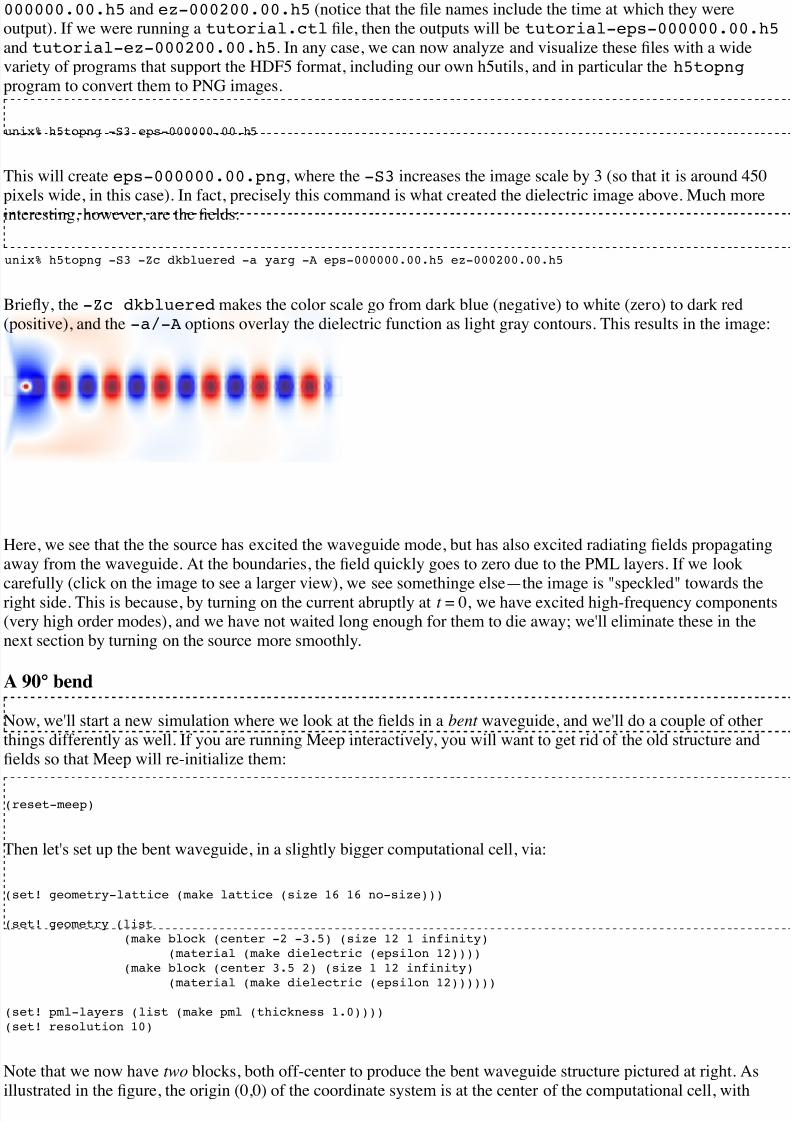
x% h5topng -S3 -Zc dkbluered -a yarg -A eps-000000.00.h5 ez-000200.00.h5
efly, the -Zc dkbluered makes the color scale go from dark blue (negative) to white (zero) to dark red
sitive), and the -a/-A options overlay the dielectric function as light gray contours. This results in the image:
e, we see that the the source has excited the waveguide mode, but has also excited radiating fields propagating
y from the waveguide. At the boundaries, the field quickly goes to zero due to the PML layers. If we look
efully (click on the image to see a larger view), we see somethinge else—the image is "speckled" towards thet side. This is because, by turning on the current abruptly at t = 0, we have excited high-frequency componentsy high order modes), and we have not waited long enough for them to die away; we'll eliminate these in the
t section by turning on the source more smoothly.
90° bend
w, we'll start a new simulation where we look at the fields in a bent waveguide, and we'll do a couple of other
gs differently as well. If you are running Meep interactively, you will want to get rid of the old structure and
ds so that Meep will re-initialize them:
set-meep)
n let's set up the bent waveguide, in a slightly bigger computational cell, via:
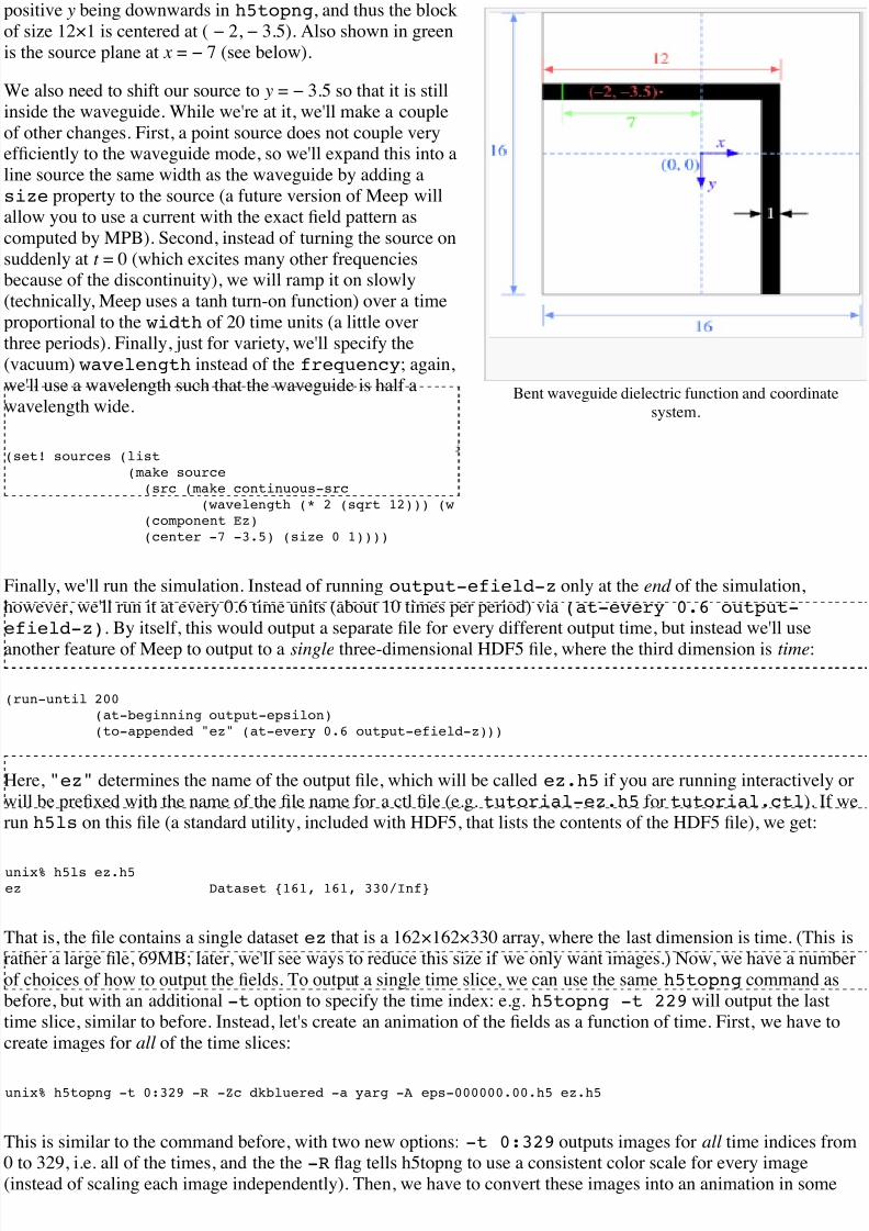
t! geometry-lattice (make lattice (size 16 16 no-size)))
t! geometry (list(make block (center -2 -3.5) (size 12 1 infinity)
(material (make dielectric (epsilon 12))))(make block (center 3.5 2) (size 1 12 infinity)
(material (make dielectric (epsilon 12))))))
t! pml-layers (list (make pml (thickness 1.0))))t! resolution 10)
e that we now have two blocks, both off-center to produce the bent waveguide structure pictured at right. As
strated in the figure, the origin (0,0) of the coordinate system is at the center of the computational cell, with
7/18/2019 Meep Tutorial - AbInitio.pdf
http://slidepdf.com/reader/full/meep-tutorial-abinitiopdf 5/15
Bent waveguide dielectric function and coordinate
system.
itive y being downwards in h5topng, and thus the block
ize 12&1 is centered at ( " 2, " 3.5). Also shown in green
he source plane at x = " 7 (see below).
also need to shift our source to y = " 3.5 so that it is still
de the waveguide. While we're at it, we'll make a couple
ther changes. First, a point source does not couple veryciently to the waveguide mode, so we'll expand this into a
source the same width as the waveguide by adding a
ze property to the source (a future version of Meep will
w you to use a current with the exact field pattern asmputed by MPB). Second, instead of turning the source on
denly at t = 0 (which excites many other frequenciesause of the discontinuity), we will ramp it on slowly
hnically, Meep uses a tanh turn-on function) over a time
portional to the width of 20 time units (a little over
e periods). Finally, just for variety, we'll specify the
cuum) wavelength instead of the frequency; again,
l use a wavelength such that the waveguide is half a
velength wide.
ally, we'll run the simulation. Instead of running output-efield-z only at the end of the simulation,
wever, we'll run it at every 0.6 time units (about 10 times per period) via (at-every 0.6 output-ield-z). By itself, this would output a separate file for every different output time, but instead we'll use
ther feature of Meep to output to a single three-dimensional HDF5 file, where the third dimension is time:
n-until 200(at-beginning output-epsilon)(to-appended "ez" (at-every 0.6 output-efield-z)))
e, "ez" determines the name of the output file, which will be called ez.h5 if you are running interactively or
be prefixed with the name of the file name for a ctl file (e.g. tutorial-ez.h5 for tutorial.ctl). If weh5ls on this file (a standard utility, included with HDF5, that lists the contents of the HDF5 file), we get:
x% h5ls ez.h5Dataset {161, 161, 330/Inf}
t is, the file contains a single dataset ez that is a 162&162&330 array, where the last dimension is time. (This is
er a large file, 69MB; later, we'll see ways to reduce this size if we only want images.) Now, we have a number
hoices of how to output the fields. To output a single time slice, we can use the same h5topng command as
ore, but with an additional -t option to specify the time index: e.g. h5topng -t 229 will output the last
e slice, similar to before. Instead, let's create an animation of the fields as a function of time. First, we have to
ate images for all of the time slices:
x% h5topng -t 0:329 -R -Zc dkbluered -a yarg -A eps-000000.00.h5 ez.h5
s is similar to the command before, with two new options: -t 0:329 outputs images for all time indices from329, i.e. all of the times, and the the -R flag tells h5topng to use a consistent color scale for every image
tead of scaling each image independently). Then, we have to convert these images into an animation in some
t! sources (list(make source(src (make continuous-src
(wavelength (* 2 (sqrt 12))) (w(component Ez)(center -7 -3.5) (size 0 1))))

7/18/2019 Meep Tutorial - AbInitio.pdf
http://slidepdf.com/reader/full/meep-tutorial-abinitiopdf 6/15
x by time
slice of bent
waveguide
(vertical =
time).
mat. For this, we'll use the free ImageMagick convert program (although there is other software that will do
trick as well).
x% convert ez.t*.png ez.gif
e, we are using an animated GIF format for the output, which is not the most efficient animation format (e.g.mpg, for MPEG format, would be better), but it is unfortunately the only format supported by this Wiki
ware. This results in the following animation :
clear that the transmission around the bend is rather low for this frequency and structure—
h large reflection and large radiation loss are clearly visible. Moreover, since we operating arebarely below the cutoff for single-mode behavior, we are able to excite a second leaky mode
r the waveguide bend, whose second-order mode pattern (superimposed with the fundamental
de) is apparent in the animation. At right, we show a field snapshot from a simulation with a
er cell along the y direction, in which you can see that the second-order leaky mode decays
y, leaving us with the fundamental mode propagating downward.
ead of doing an animation, another interesting possibility is to make an image from ae. Here is the y = " 3.5 slice, which gives us an image of the fields in the first waveguide
nch as a function of time.
x% h5topng -0y -35 -Zc dkbluered ez.h5
e, the -0y -35 specifies the y = " 3.5 slice, where we have multiplied by 10 (our resolution)et the pixel coordinate.
tput tips and tricks
ove, we outputted the full 2d data slice at every 0.6 time units, resulting in a 69MB file. This is not too bad byay's standards, but you can imagine how big the output file would get if we were doing a 3d simulation, or even
rger 2d simulation—one can easily generate gigabytes of files, which is not only wasteful but is also slow.
ead, it is possible to output more efficiently if you know what you want to look at.
create the movie above, all we really need are the images corresponding to each time. Images can be stored
ch more efficiently than raw arrays of numbers—to exploit this fact, Meep allows you to output PNG images
ead of HDF5 files. In particular, instead of output-efield-z as above, we can use (output-png EzZc dkbluered"), where Ez is the component to output and the "-Zc dkbluered" are options for
topng (which is the program that is actually used to create the image files). That is:
n-until 200 (at-every 0.6 (output-png Ez "-Zc bluered")))
output a PNG file file every 0.6 time units, which can then be combined with convert as above to create a

7/18/2019 Meep Tutorial - AbInitio.pdf
http://slidepdf.com/reader/full/meep-tutorial-abinitiopdf 7/15
vie. The movie will be similar to the one before, but not identical because of how the color scale is determined.
ore, we used the -R option to make h5topng use a uniform color scale for all images, based on the
imum/maximum field values over all time steps. That is not possible, here, because we output an image beforewing the field values at future time steps. Thus, what output-png does is to set its color scale based on the
imum/maximum field values from all past times—therefore, the color scale will slowly "ramp up" as the source
s on.
above command outputs zillions of .png files, and it is somewhat annoying to have them clutter up our
ctory. Instead, we can use the following command before run-until:
e-output-directory)
s will put all of the output files (.h5, .png, etcetera) into a newly-created subdirectory, called by default
lename -out/ if our ctl file is filename .ctl.
at if we want to output an slice, as above? To do this, we only really wanted the values at y = " 3.5, and
efore we can exploit another powerful Meep output feature—Meep allows us to output only a subset of the
mputational cell. This is done using the in-volume function, which (like at-every and to-appended) is
ther function that modifies the behavior of other output functions. In particular, we can do:
un-until 200(to-appended "ez-slice"(at-every 0.6
(in-volume (volume (center 0 -3.5) (size 16 0))output-efield-z))))
first argument to in-volume is a volume, specified by (volume (center ...) (size ...)),
ch applies to all of the nested output functions. (Note that to-appended, at-every, and in-volume aremulative regardless of what order you put them in.) This creates the output file ez-slice.h5 which contains a
aset of size 162&330 corresponding to the desired slice.
ansmission spectrum around a waveguide bend
ove, we computed the field patterns for light propagating around a waveguide bend. While this is pretty, theults are not quantitatively satisfying. We'd like to know exactly how much power makes it around the bend, how
ch is reflected, and how much is radiated away. How can we do this?
basic principles were described in the Meep introduction; please re-read that section if you have forgotten.ically, we'll tell Meep to keep track of the fields and their Fourier transforms in a certain region, and from this
mpute the flux of electromagnetic energy as a function of #. Moreover, we'll get an entire spectrum of the
smission in a single run, by Fourier-transforming the response to a short pulse. However, in order to normalizetransmission (to get transmission as a fraction of incident power), we'll have to do two runs, one with and one
hout a bend.
s control file will be more complicated than before, so you'll definitely want it as a separate file rather than
ng it interactively. See the bend-flux.ctl file included with Meep in its examples/ directory.
ove, we hard-coded all of the parameters like the cell size, the waveguide width, etcetera. For serious work,
wever, this is inefficient—we often want to explore many different values of such parameters. For example, we
y want to change the size of the cell, so we'll define it as:
fine-param sx 16) ; size of cell in X directionfine-param sy 32) ; size of cell in Y directiont! geometry-lattice (make lattice (size sx sy no-size)))
tice that a semicolon ";" begins a comment, which is ignored by Meep.) define-param is a libctl feature to

7/18/2019 Meep Tutorial - AbInitio.pdf
http://slidepdf.com/reader/full/meep-tutorial-abinitiopdf 8/15
ne variables that can be overridden from the command line. We could now do meep sx=17 tut-wvg-nd-trans.ctl to change the X size to 17, without editing the ctl file, for example. We'll also define a couple
arameters to set the width of the waveguide and the "padding" between it and the edge of the computational:
fine-param pad 4) ; padding distance between waveguide and cell edgefine-param w 1) ; width of waveguide
rder to define the waveguide positions, etcetera, we will now have to use arithmetic. For example, the y center
he horizontal waveguide will be given by -0.5 * (sy - w - 2*pad). At least, that is what theression would look like in C; in Scheme, the syntax for 1 + 2 is (+ 1 2), and so on, so we will define the
ical and horizontal waveguide centers as:
fine wvg-ycen (* -0.5 (- sy w (* 2 pad)))) ; y center of horiz. wvgfine wvg-xcen (* 0.5 (- sx w (* 2 pad)))) ; x center of vert. wvg
w, we have to make the geometry, as before. This time, however, we really want two geometries: the bend, and
a straight waveguide for normalization. We could do this with two separate ctl files, but that is annoying.ead, we'll define a parameter no-bend? which is true for the straight-waveguide case and false for the
d.
fine-param no-bend? false) ; if true, have straight waveguide, not bend
w, we define the geometry via two cases, with an if statement—the Scheme syntax is (if predicate? if-ue if-false ).
t! geometry(if no-bend?
(list
(make block(center 0 wvg-ycen)(size infinity w infinity)(material (make dielectric (epsilon 12)))))
(list(make block(center (* -0.5 pad) wvg-ycen)(size (- sx pad) w infinity)(material (make dielectric (epsilon 12))))
(make block(center wvg-xcen (* 0.5 pad))(size w (- sy pad) infinity)(material (make dielectric (epsilon 12)))))))
s, if no-bend? is true we make a single block for a straight waveguide, and otherwise we make two blocks
a bent waveguide.
source is now a gaussian-src instead of a continuous-src, parameterized by a center frequency and a
uency width (the width of the Gaussian spectrum), which we'll define via define-param as usual.
fine-param fcen 0.15) ; pulse center frequencyfine-param df 0.1) ; pulse width (in frequency)t! sources (list
(make source(src (make gaussian-src (frequency fcen) (fwidth df)))(component Ez)(center (+ 1 (* -0.5 sx)) wvg-ycen)(size 0 w))))
ice how we're using our parameters like wvg-ycen and w: if we change the dimensions, everythign will now
7/18/2019 Meep Tutorial - AbInitio.pdf
http://slidepdf.com/reader/full/meep-tutorial-abinitiopdf 9/15
t automatically. The boundary conditions and resolution are set as before, except that now we'll use set-ram! so that we can override the resolution from the command line.:
t! pml-layers (list (make pml (thickness 1.0))))t-param! resolution 10)
ally, we have to specify where we want Meep to compute the flux spectra, and at what frequencies. (This mustdone after specifying the geometry, sources, resolution, etcetera, because all of the field parameters are
alized when flux planes are created.)
fine-param nfreq 100) ; number of frequencies at which to compute fluxfine trans ; transmitted flux
(add-flux fcen df nfreq(if no-bend?
(make flux-region(center (- (/ sx 2) 1.5) wvg-ycen) (size 0 (* w 2)))
(make flux-region(center wvg-xcen (- (/ sy 2) 1.5)) (size (* w 2) 0)))))
fine refl ; reflected flux(add-flux fcen df nfreq
(make flux-region(center (+ (* -0.5 sx) 1.5) wvg-ycen) (size 0 (* w 2)))))
compute the fluxes through a line segment twice the width of the waveguide, located at the beginning or end of
waveguide. (Note that the flux lines are separated by 1 from the boundary of the cell, so that they do not lie
hin the absorbing PML regions.) Again, there are two cases: the transmitted flux is either computed at the right
he bottom of the computational cell, depending on whether the waveguide is straight or bent.
e, the fluxes will be computed for 100 (nfreq) frequencies centered on fcen, from fcen-df/2 to
en+df/2. That is, we only compute fluxes for frequencies within our pulse bandwidth. This is important
ause, to far outside the pulse bandwidth, the spectral power is so low that numerical errors make the computed
es useless.
w, as described in the Meep introduction, computing reflection spectra is a bit tricky because we need to separate
incident and reflected fields. We do this in Meep by saving the Fourier-transformed fields from the
malization run (no-bend?=true), and loading them, negated , before the other runs. The latter subtracts therier-transformed incident fields from the Fourier transforms of the scattered fields; logically, we might subtract
e after the run, but it turns out to be more convenient to subtract the incident fields first and then accumulate the
rier transform. All of this is accomplished with two commands, save-flux (after the normalization run) and
ad-minus-flux (before the other runs). We can call them as follows:
(not no-bend?) (load-minus-flux "refl-flux" refl))
n-sources+ 500 (at-beginning output-epsilon))no-bend? (save-flux "refl-flux" refl))
s uses a file called refl-flux.h5, or actually bend-flux-refl-flux.h5 (the ctl file name is used as a
fix) to store/load the Fourier transformed fields in the flux planes. The (run-sources+ 500) runs the
ulation until the Gaussian source has turned off (which is done automatically once it has decayed for a fewdard deviations), plus an additional 500 time units.
y do we keep running after the source has turned off? Because we must give the pulse time to propagatempletely across the cell. Moreover, the time required is a bit tricky to predict when you have complex structures,
ause there might be resonant phenomena that allow the source to bounce around for a long time. Therefore, it is
venient to specify the run time in a different way: instead of using a fixed time, we require that the | E z |2 at the
of the waveguide must have decayed by a given amount (e.g. 1/1000) from its peak value. We can do this via:
n-sources+top-when-fields-decayed 50 Ez

7/18/2019 Meep Tutorial - AbInitio.pdf
http://slidepdf.com/reader/full/meep-tutorial-abinitiopdf 10/15
(if no-bend?(vector3 (- (/ sx 2) 1.5) wvg-ycen)(vector3 wvg-xcen (- (/ sy 2) 1.5)))
1e-3))
op-when-fields-decayed takes four arguments: (stop-when-fields-decayed dT component
decay-by ). What it does is, after the sources have turned off, it keeps running for an additional dT time
s every time the given |component|2 at the given point has not decayed by at least decay-by from its peak
ue for all times within the previous dT. In this case, dT=50, the component is E z, the point is at the center of the
plane at the end of the waveguide, and decay-by=0.001. So, it keeps running for an additional 50 time
s until the square amplitude has decayed by 1/1000 from its peak: this should be sufficient to ensure that the
rier transforms have converged.
ally, we have to output the flux values:
splay-fluxes trans refl)
s prints a series of outputs like:
x1:, 0.1, 7.91772317108475e-7, -3.16449591437196e-7x1:, 0.101010101010101, 1.18410865137737e-6, -4.85527604203706e-7x1:, 0.102020202020202, 1.77218779386503e-6, -7.37944901819701e-7x1:, 0.103030303030303, 2.63090852112034e-6, -1.11118350510327e-6x1:, ...
s is comma-delimited data, which can easily be imported into any spreadsheet or plotting program (e.g. Matlab):
first column is the frequency, the second is the transmitted power, and the third is the reflected power.
w, we need to run the simulation twice, once with no-bend?=true and once with no-bend?=false (the
ault):
x% meep no-bend?=true bend-flux.ctl | tee bend0.outx% meep bend-flux.ctl | tee bend.out
e tee command is a useful Unix command that saves the output to a file and displays it on the screen, so that
can see what is going on as it runs.) Then, we should pull out the flux1 lines into a separate file to import them
our plotting program:
x% grep flux1: bend0.out > bend0.datx% grep flux1: bend.out > bend.dat
w, we import them to Matlab (using its dlmread command), and plot the results:

7/18/2019 Meep Tutorial - AbInitio.pdf
http://slidepdf.com/reader/full/meep-tutorial-abinitiopdf 11/15
at are we plotting here? The transmission is the transmitted flux (second column of bend.dat) divided by the
dent flux (second column of bend0.dat), to give us the fraction of power transmitted. The reflection is the
ected flux (third column of bend.dat) divided by the incident flux (second column of bend0.dat); we alsoe to multiply by " 1 because all fluxes in Meep are computed in the positive-coordinate direction by default, and
want the flux in the " x direction. Finally, the loss is simply 1 - transmission - reflection.
should also check whether our data is converged, by increasing the resolution and cell size and seeing by how
ch the numbers change. In this case, we'll just try doubling the cell size:
x% meep sx=32 sy=64 no-bend?=true bend-flux.ctl |tee bend0-big.outx% meep sx=32 sy=64 bend-flux.ctl |tee bend-big.out
ain, we must run both simulations in order to get the normalization right. The results are included in the plot
ve as dotted lines—you can see that the numbers have changed slightly for transmission and loss, probably
mming from interference between light radiated directly from the source and light propagating around the
veguide. To be really confident, we should probably run the simulation again with an even bigger cell, but we'llit enough for this tutorial.
odes of a ring resonator
described in the Meep introduction, another common task for FDTD simulation is to find the resonant modes—
uencies and decay rates—of some electromagnetic cavity structure. (You might want to read that introduction
in to recall the basic computational strategy.) Here, we will show how this works for perhaps the simplest
mple of a dielectric cavity: a ring resonator, which is simply a waveguide bent into a circle. (This can be alsond in the examples/ring.ctl file included with Meep.) In fact, since this structure has cylindrical
mmetry, we can simulate it much more efficiently by using cylindrical coordinates, but for illustration here we'll
use an ordinary 2d simulation.
before, we'll define some parameters to describe the geometry, so that we can easily change the structure:
fine-param n 3.4) ; index of waveguide

7/18/2019 Meep Tutorial - AbInitio.pdf
http://slidepdf.com/reader/full/meep-tutorial-abinitiopdf 12/15
fine-param w 1) ; width of waveguidefine-param r 1) ; inner radius of ring
fine-param pad 4) ; padding between waveguide and edge of PMLfine-param dpml 2) ; thickness of PML
fine sxy (* 2 (+ r w pad dpml))) ; cell sizet! geometry-lattice (make lattice (size sxy sxy no-size)))
w do we make a circular waveguide? So far, we've only seen block objects, but Meep also lets you specify
nders, spheres, ellipsoids, and cones, as well as user-specified dielectric functions. In this case, we'll use two
linder objects, one inside the other:
t! geometry (list(make cylinder (center 0 0) (height infinity)
(radius (+ r w)) (material (make dielectric (index n))))(make cylinder (center 0 0) (height infinity)
(radius r) (material air))))
t! pml-layers (list (make pml (thickness dpml))))t-param! resolution 10)
er objects in the geometry list take precedence over (lie "on top of") earlier objects, so the second air () cylinder cuts a circular hole out of the larger cylinder, leaving a ring of width w.
w, we don't know the frequency of the mode(s) ahead of time, so we'll just hit the structure with a broad
ussian pulse to excite all of the (TM polarized) modes in a chosen bandwidth:
fine-param fcen 0.15) ; pulse center frequencyfine-param df 0.1) ; pulse width (in frequency)t! sources (list
(make source(src (make gaussian-src (frequency fcen) (fwidth df)))(component Ez) (center (+ r 0.1) 0))))
ally, we are ready to run the simulation. The basic idea is to run until the sources are finished, and then to run for
me additional period of time. In that additional period, we'll perform some signal-processing on the fields at soment with harminv to identify the frequencies and decay rates of the modes that were excited:
n-sources+ 300(at-beginning output-epsilon)(after-sources (harminv Ez (vector3 (+ r 0.1)) fcen df)))
signal-processing is performed by the harminv function, which takes four arguments: the field componente Ez) and position (here (r + 0.1,0)) to analyze, and a frequency range given by a center frequency and
dwidth (here, the same as the source pulse). Note that we wrap harminv in (after-sources ...), since
only want to analyze the frequencies in the source-free system (the presence of a source will distort the
lysis). At the end of the run, harminv prints a series of lines (beginning with harminv0:, to make it easy toep for) listing the frequencies it found:
re are six columns (in addition to the label), comma-delimited for easy import into other programs. The
aning of these columns is as follows. Harminv analyzes the fields f (t ) at the given point, and expresses this as a
m of modes (in the specified bandwidth):
minv0:, frequency, imag. freq., Q, |amp|, amplitude, errorminv0:, 0.118101575043663, -7.31885828253851e-4, 80.683059081382, 0.00341388964904578, -0.003050229052minv0:, 0.147162555528154, -2.32636643253225e-4, 316.29272471914, 0.0286457663908165, 0.01931278820164minv0:, 0.175246750722663, -5.22349801171605e-5, 1677.48461212767, 0.00721133215656089, -8.12770506086
7/18/2019 Meep Tutorial - AbInitio.pdf
http://slidepdf.com/reader/full/meep-tutorial-abinitiopdf 13/15
complex amplitudes an and complex frequencies #n. The six columns relate to these quantities. The first column
he real part of #n, expressed in our usual 2$ c units, and the second column is the imaginary part—a negative
ginary part corresponds to an exponential decay. This decay rate, for a cavity, is more often expressed as a
ensionless "lifetime" Q, defined by:
s the number of optical periods for the energy to decay by exp( " 2$ ), and 1 / Q is the fractional bandwidth at
-maximum of the resonance peak in Fourier domain.) This Q is the third column of the output. The fourth and
h columns are the absolute value | an | and complex amplitudes an. The last column is a crude measure of the
r in the frequency (both real and imaginary)...if the error is much larger than the imaginary part, for example,
n you can't trust the Q to be accurate. Note: this error is only the uncertainty in the signal processing, and tells
nothing about the errors from finite resolution, finite cell size, and so on!
interesting question is how long should we run the simulation, after the sources are turned off, in order to
lyze the frequencies. With traditional Fourier analysis, the time would be proportional to the frequencyolution required, but with harminv the time is much shorter. Here, for example, there are three modes. The last
a Q of 1677, which means that the mode decays for about 2000 periods or about 2000/0.175 = 104 time units.
have only analyzed it for about 300 time units, however, and the estimated uncertainty in the frequency is 10 " 7
h an actual error of about 10 " 6, from below)! In general, you need to increase the run time to get more
uracy, and to find very high Q values, but not by much—in our own work, we have successfully found Q = 109
des by analyzing only 200 periods.
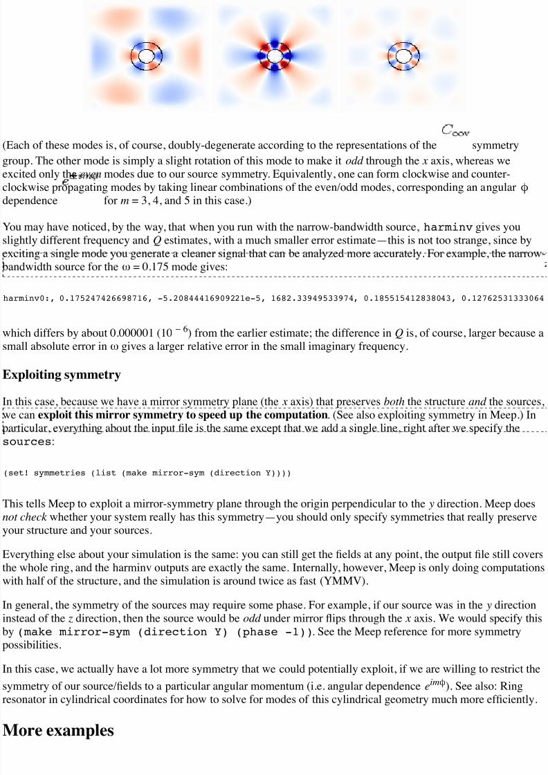
his case, we found three modes in the specified bandwith, at frequencies of 0.118, 0.147, and 0.175, with
esponding Q values of 81, 316, and 1677. (As was shown by Marcatilli in 1969, the Q of a ring resonatoreases exponentially with the product of # and ring radius.) Now, suppose that we want to actually see the field
erns of these modes. No problem: we just re-run the simulation with a narrow-band source around each mode
output the field at the end.
articular, to output the field at the end we might add an (at-end output-efield-z) argument to our
n-sources+ function, but this is problematic: we might be unlucky and output at a time when the E z field is
ost zero (i.e. when all of the energy is in the magnetic field), in which case the picture will be deceptive. Instead,
he end of the run we'll output 20 field snapshots over a whole period 1/fcen by appending the command:
n-until (/ 1 fcen) (at-every (/ 1 fcen 20) output-efield-z))
w, we can get our modes just by running e.g.:
x% meep fcen=0.118 df=0.01 ring.ctl
er each one of these commands, we'll convert the fields into PNG images and thence into an animated GIF (as
h the bend movie, above), via:
x% h5topng -RZc dkbluered -C ring-eps-000000.00.h5 ring-ez-*.h5x% convert ring-ez-*.png ring-ez-0.118.gif
resulting animations for (from left to right) 0.118, 0.147, and 0.175, are below, in which you can clearly see the
ating fields that produce the losses:
7/18/2019 Meep Tutorial - AbInitio.pdf
http://slidepdf.com/reader/full/meep-tutorial-abinitiopdf 14/15
ch of these modes is, of course, doubly-degenerate according to the representations of the symmetry
up. The other mode is simply a slight rotation of this mode to make it odd through the x axis, whereas we
ited only the even modes due to our source symmetry. Equivalently, one can form clockwise and counter-
ckwise propagating modes by taking linear combinations of the even/odd modes, corresponding an angular 'endence for m = 3, 4, and 5 in this case.)
may have noticed, by the way, that when you run with the narrow-bandwidth source, harminv gives you
htly different frequency and Q estimates, with a much smaller error estimate—this is not too strange, since by
iting a single mode you generate a cleaner signal that can be analyzed more accurately. For example, the narrow-
dwidth source for the # = 0.175 mode gives:
ch differs by about 0.000001 (10 " 6) from the earlier estimate; the difference in Q is, of course, larger because a
ll absolute error in # gives a larger relative error in the small imaginary frequency.
ploiting symmetry
his case, because we have a mirror symmetry plane (the x axis) that preserves both the structure and the sources,can exploit this mirror symmetry to speed up the computation. (See also exploiting symmetry in Meep.) Inicular, everything about the input file is the same except that we add a single line, right after we specify the
urces:
t! symmetries (list (make mirror-sym (direction Y))))
s tells Meep to exploit a mirror-symmetry plane through the origin perpendicular to the y direction. Meep does
check whether your system really has this symmetry—you should only specify symmetries that really preserve
r structure and your sources.
rything else about your simulation is the same: you can still get the fields at any point, the output file still covers
whole ring, and the harminv outputs are exactly the same. Internally, however, Meep is only doing computations
h half of the structure, and the simulation is around twice as fast (YMMV).
eneral, the symmetry of the sources may require some phase. For example, if our source was in the y direction
ead of the z direction, then the source would be odd under mirror flips through the x axis. We would specify this
(make mirror-sym (direction Y) (phase -1)). See the Meep reference for more symmetry
sibilities.
his case, we actually have a lot more symmetry that we could potentially exploit, if we are willing to restrict the
mmetry of our source/fields to a particular angular momentum (i.e. angular dependence eim'). See also: Ring
onator in cylindrical coordinates for how to solve for modes of this cylindrical geometry much more efficiently.
ore examples
minv0:, 0.175247426698716, -5.20844416909221e-5, 1682.33949533974, 0.185515412838043, 0.12762531333064

7/18/2019 Meep Tutorial - AbInitio.pdf
http://slidepdf.com/reader/full/meep-tutorial-abinitiopdf 15/15
examples above suffice to illustrate the most basic features of Meep. However, there are many more advanced
ures that have not been demonstrated here. So, we hope to add, over time, a sequence of examples that exhibit
re complicated structures and computational techniques. The ones we have so far are listed below.
ou have a good example you would like to share, feel free to register for a user name and log in, and then add a
to a new page for your example below. (Please prefix the link with "Meep Tutorial/". Simple examples
strating a specific concept are preferred.)
Meep Tutorial/Ring resonator in cylindrical coordinates
Meep Tutorial/Band diagram, resonant modes, and transmission in a holey waveguide
Meep Tutorial/Third harmonic generation (Kerr nonlinearity)Meep Tutorial/Material dispersion
Meep Tutorial/Local density of states (Purcell enhancement)
Meep Tutorial/Optical forces (Maxwell stress tensor)
ditors and ctl
useful to have emacs use its scheme-mode for editing ctl files, so that hitting tab indents nicely, and so on.acs does this automatically for files ending with ".scm "; to do it for files ending with ".ctl" as well, add the
owing lines to your ~/.emacs file:
(assoc "\\.ctl" auto-mode-alist)nil
nconc auto-mode-alist '(("\\.ctl" . scheme-mode))))
identally, emacs scripts are written in "elisp," a language closely related to Scheme.)
ou don't use emacs (or derivatives such as Aquamacs), it would be good to find another editor that supports a
eme mode. For example, jEdit (http://www.jedit.org/) is a free/open-source cross-platform editor with Scheme-
tax support. Another option is GNU gedit (http://projects.gnome.org/gedit/) (for GNU/Linux and Unix); in fact,
Hessam Moosavi Mehr has donated a hilighting mode for Meep/MPB (http://github.com/hessammehr/meepmpb-hlight) that specially highlights the Meep/MPB keywords.
rieved from "http://ab-initio.mit.edu/wiki/index.php/Meep_Tutorial"
egories: Meep | Meep examples
This page was last modified 05:19, 29 September 2012.This page has been accessed 294,122 times.Privacy policyAbout AbInitioDisclaimers
Related Documents


