Medical Image Understanding and Analysis 2003

The University of Sheffield

10-11 July 2003

Medical Image Understandingand Analysis 2003

Proceedings of

Medical Image Understanding and Analysis 2003 Proceedings of the seventh Annual Conference The University of Sheffield 10-11 July 2003 Edited by: David Barber Sponsored by: British Machine Vision Association, British Institute of Radiology and Institute of Physics and Engineering in Medicine.

David Barber Department of Medical Physics and Clinical Engineering The Royal Hallamshire Hospital Sheffield Teaching Hospitals NHS Trust Sheffield S10 2JF U.K. ISBN 1 901725 22 7 Apart from any fair dealing for the purposes of research or private study, or criticism or review, as permitted under the Copyright, Designs and Patents act 1988, this publication may only be reproduced, stored or transmitted, in any form or by any means, with the prior permission in writing of the publishers, or in the case of reprographic reproduction in accordance with the terms of licences issued by the Copyright Licensing Agency. Enquiries outside those terms should be sent to the publishers. ©BMVA 2003 The use of registered names, trademarks, etc. in this publication does not imply, even in the absence of a specific statement, that such names are exempt from the relevant laws and regulations and therefore free for general use. The publisher makes no representation, express or implied, with regard to accuracy of the information in this book and cannot accept any legal responsibility for any error or omission that may be made. Printed and bound in the United Kingdom by the University of Sheffield.

Medical Image Understanding and Analysis 2003 Organiser and Chair David Barber Department of Medical Physics and Clinical Engineering

Sheffield Teaching Hospitals NHS Trust Steering Committee E Berry University of Leeds, IPEM JM Brady University of Oxford, RAE JS Fleming Southampton General Hospital, BIR DJ Hawkes Kings College, London CJ Taylor University of Manchester, BMVA Programme Committee SR Arridge University College, London S Astley University of Manchester J Bamber Institute of Cancer Research & Royal Marsden NHS Trust DC Barber Sheffield Teaching Hospitals NHS Trust E Berry University of Leeds A Bhalerao University of Warwick A Bulpitt University of Leeds JM Brady University of Oxford J Byrne Radcliffe Infirmary, Oxford E Claridge University of Birmingham A Colchester University of Kent JS Fleming Southampton General Hospital J Hajnal Imperial College, London DJ Hawkes Kings College, London AS Houston Royal Hospital Haslar, Portsmouth Hospitals NHS Trust CJ Taylor University of Manchester A Todd_Pokropek University College, London P Undrill University of Aberdeen R Zwiggelaar University of East Anglia

Foreward This is the seventh in a series of annual scientific and technical meetings designed to provide a UK forum for discussion and dissemination of research in medical image understanding and analysis. The meeting has been sponsored by three professional organisations representing the disciplines active in this area, namely the British Machine Vision Association (BMVA), the British Institute of Radiology (BIR) and the Institute of Physics and Engineering in Medicine (IPEM). We are grateful for their support, which contributes significantly to the success of MIUA. The use of mathematical techniques and computers to help in the interpretation and quantification of medical images has a history which spans several decades. Computer processing of images is usually time consuming and until fairly recently this represented a limit on what processing could be done in a clinically useful time. With the increased computational power now available this restriction is being relaxed. In addition, the determination of the Department of Health to introduce full electronic management of patient data through the Integrated Care Record, and the fact that a key component of this will be digital image management, means that digital medical images will rapidly become widespread throughout healthcare, raising hopes and expectations that software tools for aiding in diagnosis and therapy will become available as digital imaging technology comes on-line. The scientific and engineering community seeks to develop such tools, the clinical community seeks to use them clinically. An important aim of MIUA is to bring these communities together to encourage and facilitate the use of medical image understanding and analysis. If effective progress is to be made each community needs to understand the limits and constraints under which the other is working, and how these are best circumvented, as well as together working towards the benefits that medical image analysis can bring to patients. The range and quality of submissions continues to be high. Each paper submitted to MIUA2003 was reviewed by three members of the programme committee and feedback was provided to the authors. Most reviewers reviewed 10 papers and ranked them. The results of this ranking were used to compute a robust average rank and these values were used by the Programme Committee to select 24 papers for oral submission and 28 for poster presentation. These proceedings contain all 52 accepted papers. The submission, reviewing and selection processes were facilitated by the CAWS conference management software package developed and operated by Imaging Science and Biomedical Engineering (ISBE) at the University of Manchester. This system has proved invaluable for conference administration and special thanks are due to Mike Rogers at ISBE for providing help and technical support in the use of CAWS for MIUA2003. Although MIUA frequently has contributions from outside the UK it continues primarily to be a forum for distributing research results generated within the UK. It is a particularly friendly forum for students or young researcher making their first presentations and MIUA2003 is no exception to this. Producing proceedings prior to a meeting poses some difficulties, but I believe it is useful to be able to refer to papers both before and after their presentation. I am grateful to all authors for getting their camera ready copy to me on time, for preparing their papers in the correct format and for keeping to length. This has made my task much easier than it might have been. I am grateful to my colleagues in Sheffield for the help they have given to organising MIUA2003 and to the staff of the University of Sheffield for facilitating the conference. I am especially grateful to the help Margaret Beckett has given in administering the conference. David Barber July 2003

Table of Contents Page Session 1: Models A Statistical Model of Texture for Medical Image Synthesis and Analysis 1

CJ Rose and CJ Taylor, University of Manchester Improving Appearance Model Matching Using Local Structure 5

IM Scott, TF Cootes and CJ Taylor, University of Manchester Multi-resolution transportation for the detection of mammographic asymmetry 9

M Board and S Astley, University of Manchester Session 2: Classification Combining rCBF SPECT images obtained from different centres in a composite normal atlas 13

AS Houston, SMA Hoffmann, L Sanders, DRR White, L Bolt, JS Fleming, MA Macleod and PM Kemp, Royal Hospital Haslar, Gosport

Separating Normal and Disease Groups using Regional Cerebral Blood Flow 17 MLJ Scott, NA Thacker and AJ Lacey, University of Manchester

Classification of White Matter Tract Shapes from DTI without Registration 21 PG Batchelor, F Calamante, D Atkinson, D Tournier, DLG Hill, R Blythe and A Connelly, King’s College, London

Session 3: Image Registration Automatic registration of retinal images 25

A Sabate-Cequier, JF Boyce, M Dumskyj, M Himaga, D Usher, TH Williamson and SS Nussey, St George’s Hospital, London

Delineation of the prostate capsule in 3D Trans Rectal Ultrasound images using 29 image registration

S Mehta, DC Barber, E van Beek, JM Wild and FC Hamdy, University of Sheffield 2D/3D Registration Using Shape From Shading Information in Application to Endoscope 33

F Deligianni, A Chung and G-Z Yang, Imperial College, London A new method for Validation of Non-Rigid Registration 37

PP Wyatt and JA Noble, University of Oxford Session 4: Posters 1 Skin Lesion Classification Using Curvature of Skin Pattern 41

Z She and PJ Fish, University of Wales Registration of ultrasound breast images acquired from a conical geometry 45

JA Shipley, FA Duck and BT Thomas, Royal United Hospital, Bath Colour normalisation of retinal images 49

KA Goatman, AD Whitwam, A Manivannan, JA Olson and PF Sharp, University of Aberdeen

Nonlinear fusion for enhancing Digitally Subtracted Angiograms 53 RJ King, M Petrou, K Wells and D Johnson, University of Surrey

Characterising pattern asymmetry in pigmented skin lesions 57 E Claridge, J Powell and A Orun, University of Birmingham

Automatic Construction of Statistical Shape Models for Protein Spot Analysis 61 in Electrophoresis Gels

M Rogers, J Graham and RP Tonge, University of Manchester Modelling an average planar shape 65

J-G Kim and JA Noble, University of Oxford

Corresponding Locations of Knee Articular Cartilage Thickness Measurements by 69 Modelling the Underlying Bone.

TG Williams, CJ Taylor, Z Gao and JC Waterton, University of Manchester Statistical Shape Modelling of the Levator Ani 73

S-L Lee, P Horkaew, A Darzi and G-Z Yang, Imperial College, London An active contour model to segment foetal cardiac ultrasound data 77

I Dindoyal, T Lambrou, J Deng, CF Ruff, AD Linney and A Todd-Pokropek, University College, London

Automated assessment of digital fundus image quality using detected vessel area 81 DB Usher, M Himaga, MJ Dumskyj, JF Boyce, A Sabate-Cequier, TH Williamson, E Mensah, EM Kohner, SS Nussey and J Marshall, St George’s Hospital, London

3D Markov Random Field Binary Texture Model: Preliminary Results 85 L Blot and R Zwiggelaar, University of East Anglia

The work of Reading Mammograms and the Implications for Computer-Aided 89 Detection Systems

M Hartswood, R Procter, M Rouncefield, R Slack and J Soutter, University of Edinburgh Automatic generation of Regions of Interest for Radionuclide Renograms 93

DC Barber, Sheffield Teaching Hospitals, Sheffield Session 5: Morphology Investigation of Shape Changes in the Lateral Ventricles Associated with Schizophrenia : 97 A Morphometric Study Using a Three-Dimensional Point Distribution Model

K Babalola, J Graham, L Kopala and R Vandorpe, University of Manchester A Non-Euclidean Metric for the Classification of Variations in Medical Images 101

C Twining and S Marsland, University of Manchester An evaluation of deformation-based morphometry in the developing human brain 105 and detection of volumetric changes associated with preterm birth

JP Boardman, K Bhatia, S Counsell, J Allsop, O Kapellou, MA Rutherford, AD Edwards, JV Hajnal and D Rueckert, Imperial College, London

Session 6: MR Developments Image-based ghost reduction of amplitude discontinuities in k-space by method 109 of generalised projections (MGP)

KJ Lee, MN Paley, JM Wild, DC Barber, ID Wilkinson and PD Griffiths, University of Sheffield

Automatic Planning of the Acquisition of Cardiac MR Images 113 C Jackson, M Robson, J Francis and JA Noble, University of Oxford

Inter-subject Comparison of Brain Connectivity using Diffusion-Tensor 117 Magnetic Resonance Imaging

PA Cook and DC Alexander, University College, London

Session 7: Posters 2 Segmentation of Dermatoscopic Images by Iterative Segmentation Algorithm 121

MI Rajab, MS Woolfson and SP Morgan, University of Nottingham Segmentation of Mammograms Using a Weighted Gaussian Mixture Model 125 and Hidden Markov Random Field

K Bovis and S Singh, University of Exeter Prostate Segmentation: A Comparative Study 129

Y Zhu, R Zwiggelaar and S Williams, University of East Anglia Histological parametric maps of the human ocular fundus: preliminary results 133

F Orihuela-Espina, E Claridge and SJ Preece, University of Birmingham

Texture Segmentation in Mammograms 137 R Zwiggelaar, L Blot, D Raba and ERE Denton, University of East Anglia

Thick Emulsion Holography and Medical Tomography 141 P Thompson and G Saxby, Doncaster Royal Infirmary

Imaging the Pigments of Human Skin with a Technique which is Invariant to 145 Changes in Surface Geometry and Intensity of Illuminating Light

S Preece, S Cotton and E Claridge, University of Birmingham Computer Based System for Acquisition and Analysis of Nailfold Capillary Images 149

PD Allen, VF Hillier, T Moore, ME Anderson, CJ Taylor and AL Herrick, University of Manchester

A Novel Method for Simulating Soft Tissue Deformation 153 MA ElHelw, A Chung and G-Z Yang, Imperial College, London

Using autostereoscopic displays as a complementary visual aid to the surgical stereo 157 microscope in Augmented Reality surgery

RJ Lapeer, AC Tan, G Alusi and A Linney, University of East Anglia Automatic Capillary Measurement 161

K Feng, PD Allen, T Moore, AL Herrick and CJ Taylor, University of Manchester Fast 3D Mean Shift Filter applied to CT Images 165

GF Dominguez, H Bischof, R Beichel and F Leberl, Graz University of Technology, Austria Fine grading of colorectal biopsy images using colour texture analysis 169

JK Shuttleworth, AG Todman, RNG Naguib, BM Newman and MK Bennett, University of Coventry

Enhanced display of pulmonary embolism in simultaneous dual isotope 173 ventilation/perfusion planar scintigraphy

CJ Reid, S Misson, JS Fleming, L Sawyer, SA Hoffmann and N Nagaraj, Southampton General Hospital, Southampton

Session 8: Segmentation Analysis of Total Hip Replacements Using Active Ellipses 177

S Kerrigan, S McKenna, IW Ricketts and C Wigderowitz, University of Dundee An Automated Algorithm for Breast Background Segmentation 181

S Petroudi and M Brady, University of Oxford An Artificially Evolved Vision System for Segmenting Skin Lesion images 185

ME Roberts and E Claridge, University of Birmingham Segmentation of cardiac MR images using a 4D probabilistic atlas and the EM algorithm 189

M Lorenzo-Valdes, GI Sanchez-Ortiz, R Mohiaddin and D Rueckert, Imperial College, London

Session 9: Motion and Reconstruction Motion Trajectories For Ultrasound Displacement Quantification 193

JD Revell, M Mirmehdi and D McNally, University of Bristol Dealing with cardiovascular motion for strain imaging in the liver 197

AF Kolen and JC Bamber, Royal Marsden NHS Trust, Sutton Fourier Snakes for the Reconstruction of Massively Undersampled MRI 201

AMS Silver, I Kastanis, DLG Hill and SR Arridge, Guy’s Hospital, London Volume reconstruction from sparse 3D ultrasonography. 205

MJ Goodling, S Kennedy and JA Noble, University of Oxford

A Statistical Model of Texture for Medical Image Synthesis andAnalysis

C. J. Rose∗ and C. J. Taylor

Imaging Science and Biomedical Engineering,University of Manchester, UK

Abstract. We address the problem of building generative statistical models of the appearance of highly variablemedical images, in particular mammograms. We treat appearance as a texture that can vary over the imageplane. We present a model motivated by one of the most successful algorithms in the texture synthesis literature.Our approach has significant advantages over existing methods: it can learn from very large data sets, does notneed to assume spatial ergodicity and can be used for synthesis and analysis. We present early results in theform of synthetic images.

1 Introduction

We are interested in building generative statistical models of the appearance of highly variable medical images,for use in model-based interpretation. In particular, we are interested in digitised x-ray mammograms and thedetection of abnormal features which can indicate cancer. Breast cancer is a significant health issue in the westernworld. In the period 2001-2002, 39,000 British women were diagnosed with breast cancer [1]; a national breastscreening programme has been running for several years. Due to the nature of the imaging process and anatomicaldifferences between women, mammograms exhibit high variability, both between and within patients. Manualplacement of the breast by the radiographer results in variation in image content. There is significant variationin anatomy: the number of ducts in one woman’s breast may differ from another. Because of the large scale andlimited effectiveness of x-ray mammography [2] there has been considerable interest in Computer Aided Detection(CADe). Conventionally, mammography has been treated as a pattern recognition task, where a classifier is trainedon examples of normal and abnormal descriptors extracted from training images [3]. Conventional approaches toCADe do not attempt to explain image content, choosing instead to use ad hoc descriptors that seem to capturevarious characteristics of abnormal signs in mammograms. Most significantly, although breast cancer is a majorcause of death in women, cancers are extremely rare in screening mammography. Therefore, detecting signs ofabnormality should ideally be treated as a novelty detection, rather than classification, task [4].

Statistical model-based approaches such as [5] have been applied successfully to many image interpretation tasks.Such methods rely on establishing correspondences across a set of training images. Due to the variability inmammograms described above, establishing such correspondences is extremely difficult, if not impossible. Wepropose an alternative approach, considering mammographic appearance to be a spatially variable texture – i.e.local appearance is treated as a texture, which can vary over the image plane. A statistical model-based approachenables us to explain and account for variation in a principled way, regardless of its origin. We aim to buildgenerative models of pathology-free mammograms and approach image interpretation as a novelty detection task.We have developed a generative statistical model of texture which we describe in this paper. We present earlyresults in the form of synthetic images.

2 Background

In [6], Efros and Leung describe a novel non-parametric method of synthesising new textures from a sampleimage, motivated by [7] (which is closely related to [8]). Their method assumes that an empty image is seededwith a section taken from a sample image; they call this the seed image. They select a pixel which neighbours theboundary of the seed in order to fill it with an appropriate value. A square window is extracted around this pixel.Some of the extracted window elements contain pixels from the seed and the remaining elements contain blankpixels. The authors define a similarity measure which allows them to compare the extracted window with all suchwindows in the sample image, taking account of the blank (missing) elements in the extracted window. Using thesimilarity measure, a small set of candidate windows is selected from the sample image. One of these windowsis chosen at random, and its centre pixel is placed into the seed image to fill the selected pixel. This process isrepeated until all pixels in the seed image are filled. Although the algorithm is simple, it produces some of the

∗[email protected]

best results in the literature. The method has been applied to simple textures, natural images and images of textwith convincing results. In [9], Efros and Freeman address one of the main problems of [6]: synthesis is slowbecause for each pixel synthesised, a comparison has to be made between the extracted window and all windowsin the sample image. They address this problem by synthesising the texture in a patch-by-patch process rather thanpixel-by-pixel: they partially overlap whole windows with the growing texture and merge the edges of the windowto fit the image being synthesised. This results in much faster synthesis at a little cost in the quality of the synthetictextures. Other methods, for example those presented in [10–12] use wavelets to accomplish texture synthesis andmodelling; in particular, the methods in [10, 11] are among the best in the literature.

Most methods in the literature rely on the assumption of spatial ergodicity (i.e. invariance of texture statisticsacross the image plane). The methods presented in [7, 8, 11, 12] consider learning from training sets, but none ofthem consider learning from very large data sets. Our approach, presented in the next section, was motivated bythe work of Efros and Leung [6], and can be considered as an extension to [7] and [8]. It can also be viewed as aunification of [6] and [9] within a statistical framework. Our contribution is to unify two state-of-the-art algorithmsfor texture synthesis within a principled statistical framework that enables image analysis. We have addressed theproblem of learning from large training sets. Furthermore, we have developed a model which does not need toassume spatial ergodicity, as do most methods in the literature

3 Method

We assume a training set of digitised images. For each image in the training set, we extract a square window ofpixel values around each pixel (the centre pixel), and treat each window as a vector, as in [6]. We want to modelthe distribution of points in this vector space. For all but the most powerful computers, directly modelling thisdistribution is computationally difficult due to the dimensionality of the data and the size of the training set.

3.1 Modelling the Data

The first step in our approach is to build a parametric model of the data. We have chosen to use the k-meansclustering algorithm [13] (also described in [14]) to build a Gaussian mixture model (GMM) of the distribution;the parameter k is the number of components in the mixture. Automatic selection of the number of componentsneeded to best model a distribution is an open research question, and so we choose k based upon experience usingthe model. To deal with very large training sets, we adopt a ‘divide and conquer’ approach to clustering [15] (alsodescribed in [14]). We divide the training data randomly into subsets, each of which can be clustered in memory.We perform clustering on each of these subsets using the k-means algorithm. Each clustering then contributesa representative set of data points from each cluster to form a central pool of data. The number of data pointscontributed from a particular cluster is proportional to the probability of that cluster and is such that the final dataset can be clustered in available memory. The final model of patch pdf is:

p(x) =

k∑

i=1

p(i)p(x|i) . (1)

where x is a point in our vector space, i indexes the model components, k is the number of components in ourmodel and p(x|i) ∼ N(µi, Σi), where µi is the mean vector for the i-th component and Σi is the covariancematrix for the i-th component. Given this model, we can perform image synthesis and, ultimately, analysis.

3.2 Image Synthesis

We assume a model of texture built as described above. As in [6], we form a seed image and extract a windowaround a pixel neighbouring the seed. We treat the window as a vector, x, where some elements are known (i.e.they contain pixel values sampled from the seed) and some elements are unknown (i.e. they contain blank pixelsfrom the seed). We want to be able to sample a pixel value from our model that is consistent with what we haveobserved. To do this we first marginalise the model over the dimensions of x that are unknown (except the centrepixel). For a multivariate Gaussian this is achieved by ‘crossing out’ the rows and columns of the covariance matrixthat correspond to the dimensions we are marginalising over, doing likewise with the mean vector. We perform thisprocess on each component of the model. We then condition the marginal distribution on the dimensions of x weknow. For a multivariate Gaussian, this can be achieved by computing a new mean vector and covariance matrix.

Let us partition x as [x1 x2]T where x1 corresponds to the dimensions that we do not know and x2 corresponds to

the dimensions we do know. (We want to determine the distribution of the centre pixel values given measurementsfor some elements in the sampled window. After marginalisation, x1 corresponds to the centre pixel.) We partitionthe mean vector and covariance matrix of each component as:

µ =

[

µ1

µ2

]

, Σ =

[

Σ11Σ12

Σ21Σ22

]

. (2)

where µ1

corresponds to the unknown dimensions and µ2

corresponds to the known dimensions; similarly for thepartitioned covariance matrix. The conditioned mean vector and covariance matrix are computed by [16]:

µ′ = µ

1+ Σ12Σ

−1

22(x2 − µ

2), Σ

′ = Σ11 − Σ12Σ−1

22Σ21 . (3)

We perform this process on each component of the model. To complete the computation of the conditional distri-bution, we need to update the the mixing proportions. This is easily achieved using Bayes’ theorem:

p(i|x2) =p(x2|i)p(i)

p(x2)∝ p(x2|i)p(i) . (4)

where the p(x2|i) is computed by marginalising each component over the known dimensions, as described above.(The distribution of the centre pixel values is a univariate distribution and not a multivariate distribution as thenotation in (3) implies, but we present the general method for completeness.) The model of the distribution ofpossible centre pixel values is:

p(x1) =

k∑

i=1

p(i|x2)p(x1|i) (5)

where x1 is the centre pixel and p(x1|i) ∼ N(µ′

i, Σ′

i) (a univariate distribution). Once we have computed (5), we

sample from it, setting the pixel being considered to the sampled value. Sampling from (5) is achieved by choosingone of the clusters using p(i|x2) and then sampling from the p(x1|i) corresponding to the chosen component. Aftersampling the pixel value for the current pixel, we move on to another pixel neighbouring the (growing) seed andrepeat the process of marginalisation, conditioning and sampling until the entire seed image has been populated.The approach to synthesis described above is analogous to the non-parametric approach of [6]. By skipping themarginalisation step (sampling all remaining pixels in the window), our approach can be considered analogous tothe non-parametric approach of [9]. Most methods in the literature rely on the assumption of spatial ergodicity (i.e.invariance of texture statistics across the image plane); our model makes no such assumption. We can explicitlyinclude spatial information in the training vectors to build a texture model that captures textural variability over theimage plane. We can then condition the model on such information during synthesis and analysis.

4 Results

We have evaluated our approach by producing synthetic textures and making qualitative judgements. Quantitativeevaluation of results is notably absent from the texture synthesis and modelling literature; quantifying the generalityand specificity of our models will form part of our future research. Figure 1 shows training and synthetic imagesfrom two of our models. The first model was built from 10 patches taken from pathology-free mammograms inthe DDSM [17]. The second model was built from the four Asphalt images in the MeasTex database. No spatialinformation was included in the models. Qualitatively, our results are comparable to those produced by the bestmethods in the literature, such as [6] for the image classes being considered. It is difficult to make comparisonsbetween our results and those of other methods in the literature because our method allows us to use a large trainingset while others [6,9,11] are limited to a single sample image. While [7,8,10] could be trained using data extractedfrom more than one image, the results they present are generated from a limited training set, most likely a singleimage. Although [12] presents a sophisticated model which is trained using a reasonably large data set, we arguethat our synthetic images are more convincing.

(a) (b) (c) (d)

Figure 1. Mammographic textures: A training patch (a) and a synthetic patch (b). MeasTex Asphalt textures: Atraining patch (c) and a synthetic patch (d).

5 Conclusions

We have described an approach to texture modelling for synthesis and analysis of digitised mammograms and otherclasses of medical image. We have unified two state of the art algorithms for texture synthesis within a principledstatistical framework that enables image analysis. We have also addressed the problem of learning from largetraining sets. Furthermore, we have developed a model which does not need to assume spatial ergodicity, unlikemost methods in the literature. Our results indicate that this approach is successful at modelling such textures.Current work focuses on the use of dimensionality reduction techniques such as PCA [18] to improve clusteringaccuracy and increase synthesis speed. Our ultimate aim is to model entire, pathology-free mammograms in orderto perform abnormality detection as a novelty detection task.

References

1. “Breakthrough Breast Cancer Annual Review 2001-2002.” http://www.breakthrough.org.uk/. AccessedMarch 20 2003.

2. P. T. Huynh, A. Jarolimek & S. Daye. “The False-Negative Mammogram.” Radiographics 18(5), pp. 1137–1154, 1998.3. D. Brzakovic, X. M. Luo & P. Brzakovic. “An Approach to Automated Detection of Tumors in Mammograms.” IEEE

Transactions on Medical Imaging 9(3), September 1990.4. L. Tarassenko, P. Hayton, N. Cerneaz et al. “Novelty Detection for the Identification of Masses in Mammograms.” In 4th

IEE International Conference on Artificial Neural Networks, pp. 442–447. Cambridge, UK, 1995.5. T. F. Cootes, G. Edwards & C. Taylor. “Active Appearance Models.” In H. Burkhardt & B. Neumann (editors), European

Conference on Computer Vision 1998, volume 2, pp. 484–498. Springer, 1998.6. A. A. Efros & T. K. Leung. “Texture Synthesis by Non-Parametric Sampling.” In IEEE International Conference on

Computer Vision (ICCV 99). Corfu, Greece, 1999.7. K. Popat & R. Picard. “Novel Cluster-Based Probability Model for Texture Synthesis, Classification, and Compression.”

In SPIE Visual Communications and Image Processing. Boston, USA, November 1993.8. J. Grim & M. Haindl. “A Discrete Mixtures Colour Texture Model.” In Texture 2002, The 2nd Intl. Workshop on Texture

Analysis and Synthesis. Copenhagen, Denmark, 2002.9. A. A. Efros & W. T. Freeman. “Image Quilting for Texture Synthesis and Transfer.” In SIGGRAPH 01. Los Angeles, USA,

August 2001.10. J. Portilla & E. P. Simoncelli. “A Parametric Texture Model based on Joint Statistics of Complex Wavelet Coefficients.”

International Journal of Computer Vision 40(1), pp. 49–71, October 2000.11. J. S. De Bonet & P. Viola. “A Non-Parametric Multi-Scale Statistical Model for Natural Images.” Advances in Neural

Information Processing 10, 1997.12. C. Spence, L. Parra & P. Sajda. “Detection, Synthesis and Compression in Mammographic Image Analysis with a Hier-

archical Image Probability Model.” In L. Staib (editor), IEEE Workshop on Mathematical Methods in Biomedical ImageAnalysis. 2001.

13. J. McQueen. “Some Methods for Classification and Analysis of Multivariate Observations.” In 5th Berkeley Symposiumon Mathematical Statistics and Probability. 1967.

14. A. K. Jain, M. N. Murty & P. J. Flynn. “Data Clustering: A Review.” ACM Computing Surveys 31(3), September 1999.15. M. N. Murty & G. Krishna. “A Computationally Efficient Technique for Data-Clustering.” Pattern Recognition 12,

pp. 153–158, 1980.16. R. A. Johnson & D. W. Wichern. Applied Multivariate Statistical Analysis. Prentice-Hall, fifth edition, 2002.17. M. Heath, K. W. Bowyer & D. Kopans. “Current State of the Digital Database for Screening Mammography.” In Digital

Mammography: Fourth International Workshop on Digital Mammography, pp. 457–460. Kluwer Academic Publishers,Nijmegen, The Netherlands, 1998.

18. I. Jolliffe. Principal Component Analysis. Springer Series in Statistics. Springer Verlag, New York, second edition, 2002.

Improving Appearance Model Matching Using Local Structure

I.M. Scott∗, T.F. Cootes, C.J. TaylorImaging Science and Biomedical Engineering, University of Manchester.

Abstract. We show how non-linear representations of local image structure can be used to improve the perfor-mance of model matching algorithms in medical image analysis tasks. Rather than represent image structureusing intensity values, we use measures that indicate the reliability of a set of local image feature detector out-puts. These features are image edges, corners, and gradients. Detector outputs in flat, noisy regions tend to beignored whereas those near strong structure are favoured. We demonstrate that combinations of these featuresgive more reliable matching between models and new images than modelling image intensity alone. We alsoshow that the approach is robust to non-linear changes in contrast, such as those found in multi-modal imaging.

1 Introduction

This paper builds on Cootes’set al. [1] work on constructing statistical appearance models and matching them tonew images using the Active Appearance Model (AAM) search algorithm. We want to use a representation ofimage structure that discriminates in favour of a reliable comparison between image and model, and is invariant tothe sorts of global transformation that may occur. For example, statistical appearance models commonly representimage texture by a vector of pixel intensities, linearly normalised so as to be invariant to global contrast andbrightness. Nevertheless, such models tend to be sensitive to imaging parameters, biological variability, etc.

An obvious alternative to modelling the intensity values directly is to record the local image gradient in eachdirection at each pixel. Although this yields more information at each pixel, and at first glance might seem tofavour informative edge regions over flatter, less informative regions, it is only a linear transformation of theoriginal intensity data. Since building our models involves applying a linear Principal Component Analysis (PCA)to the samples, the resulting model will be almost identical to one built from raw intensities.

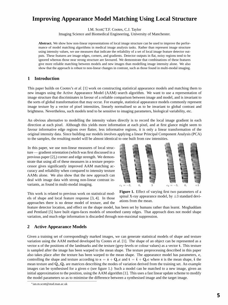
In this paper, we use non-linear measures of local struc-

c1 = −3, 0, 3 c2 = −3, 0, +3

Figure 1. Effect of varying first two parameters of aspinal X-ray appearance model, by±3 standard devi-ations from the mean.

ture — gradient orientation (which was first discussed in aprevious paper [2],) corner and edge strength. We demon-strate that using all of these measures in a texture prepro-cessor gives significantly improved AAM matching ac-curacy and reliability when compared to intensity textureAAMs alone. We also show that the new approach candeal with image data with strong non-linear contrast in-variants, as found in multi-modal imaging.

This work is related to previous work on statistical mod-els of shape and local feature response [3, 4]. In thoseapproaches there is no dense model of texture, and thefeature detector location, and effect on the shape model, has been set by humans rather than learnt. Moghaddamand Pentland [5] have built eigen-faces models of smoothed canny edges. That approach does not model shapevariation, and much edge information is discarded through non-maximal suppression.

2 Active Appearance Models

Given a training set of correspondingly marked images, we can generate statistical models of shape and texturevariation using the AAM method developed by Cooteset al. [1]. The shape of an object can be represented as avectors of the positions of the landmarks and the texture (grey-levels or colour values) as a vectort. This textureis sampled after the image has been warped to the mean shape. The texture preprocessing described in this paperalso takes place after the texture has been warped to the mean shape. The appearance model has parameters,c,controlling the shape and texture according tos = s + Qsc andt = t + Qtc wheres is the mean shape,t themean texture andQs,Qt are matrices describing the modes of variation derived from the training set. An exampleimages can be synthesised for a givenc (see figure 1.) Such a model can be matched to a new image, given aninitial approximation to the position, using the AAM algorithm [1]. This uses a fast linear update scheme to modifythe model parameters so as to minimise the difference between a synthesised image and the target image.∗[email protected]

αααα

ββββ

strongedges

strongcorners

flatareas

Figure 2. How α andβ relateto cornerness and edgeness.

αααα

ββββ

θedgeness e

cornerness c

2θ

Figure 3. Making cornerness independent of edgenessby doubling angle from axis.

In this paper, rather than just recording the intensities at each pixel, we record a local structure tuple. It is usefulto think about the rest of this work as usingtexture preprocessorswhich take an input image, and non-linearlyproduce an image of tuples representing various aspects of local structure. When sampling the image to producea texture vector for a model, instead of samplingn image intensity values from the original image, we sample allthe values from eachm-tuple atn sample locations, to produce a texture vector of lengthnm.

3 Local Structure Detectors

As noted earlier, the texture preprocessor needs to be non-linear to make a significant difference to a linear PCA-based model. If we restrict the choice of preprocessor to those whose magnitude reflects the strength of responseof a local feature detector, then it would be useful to transform this magnitudem into a reliability measure. Wehave chosen to use sigmoid function for this non-linear transformf(x) = m

m+m wherem is the mean of the featureresponse magnitudesm over all samples. This function has the effect of limiting very large responses, preventingthem from dominating the image. Any response significantly above the mean gives similar output. Also, anyresponse significantly below the mean gives approximately zero output. This output behaves like the probabilityof there being a real local structure feature at that location.

The first local structure descriptor with which we have experimented is gradient orientation. Early work on non-linear gradient orientation is described in [2]. We calculate the image gradientg = (gx gy)T at each point givinga 2-tuple texture image for 2-d input images. The magnitude|g| can be transformed using the sigmoid function,while preserving the direction. This is followed by the non-linear normalisation step to give(gx gy)T /(|g|+ |g|)

We had observed that image corners were sometimes badly matched by gradient and intensity AAMs. Cornersare well known as reliable features for corresponding multiple images, and in applications such as morphometryaccurate corner location is important in diagnosis.

Harris and Stephens [6] describe how to build a corner detector. They construct a local texture descriptor bycalculating the Euclidean distance, or sum of square differences between a patch (of an imageI,) and itself as oneis scanned over the other. This local image difference energyE is zero at the patch origin, and rises faster forstronger textures. To enforce locality and the consideration of only small shifts, they added a Gaussian windoww(u, v),and then made a first order approximation;

E(x, y) =∑u,v

w(u, v)[x ∂I

∂u (x, y) + y ∂I∂v (x, y) + O(x2, y2)

]2 ≈ Ax2 + 2Cxy + By2 = (x y)M(x y)T

wherew(u, v) = exp−(u2 − v2)/2σ2, A(x, y) =[

∂I∂u

]2 ⊗ w, etc. The eigenvaluesα,β of M = ( A CC B )

characterise the rate of change of the sum of squared differences function as its moves from the patch origin. Sinceα andβ are the principle rates of change, they are invariant to rotation. Without loss of generality, the eigenvaluescan be rearranged so thatα >= β. The local texture at each point in the image can be described by these twovalues. As shown in figure 2, low values ofα andβ imply a flat image region. A high value ofα and low value ofβ imply an edge. High values of bothα andβ imply a corner.

At this point Harris and Stephens identified individual image corners by looking for local maxima indetM −k[trM]2. We leave their approach here, except to note that useful measures derived fromα andβ can be foundwithout actually performing an eigenvector decomposition, e.g.det(M) = AB−C2. For our purposes, it would beuseful to have independent descriptors of edgeness and cornerness. To forceα andβ into an independent form, we

take the vector(α β)T and double the angle from theα axis, as in figure 3. It is possible to calculate the cornerness,r, and edgeness,e, defined this way, without explicitly having to calculate an eigenvector decomposition. Notethate is independent of edge direction unlike the gradient measure, and so may describe additional structure.

r = 2AB − 2C2 e = (A + B)√

(A−B)2 + 4C2

These values are then normalised using the sigmoid transform, and combined to produce a texture preprocessor.

4 Experiments

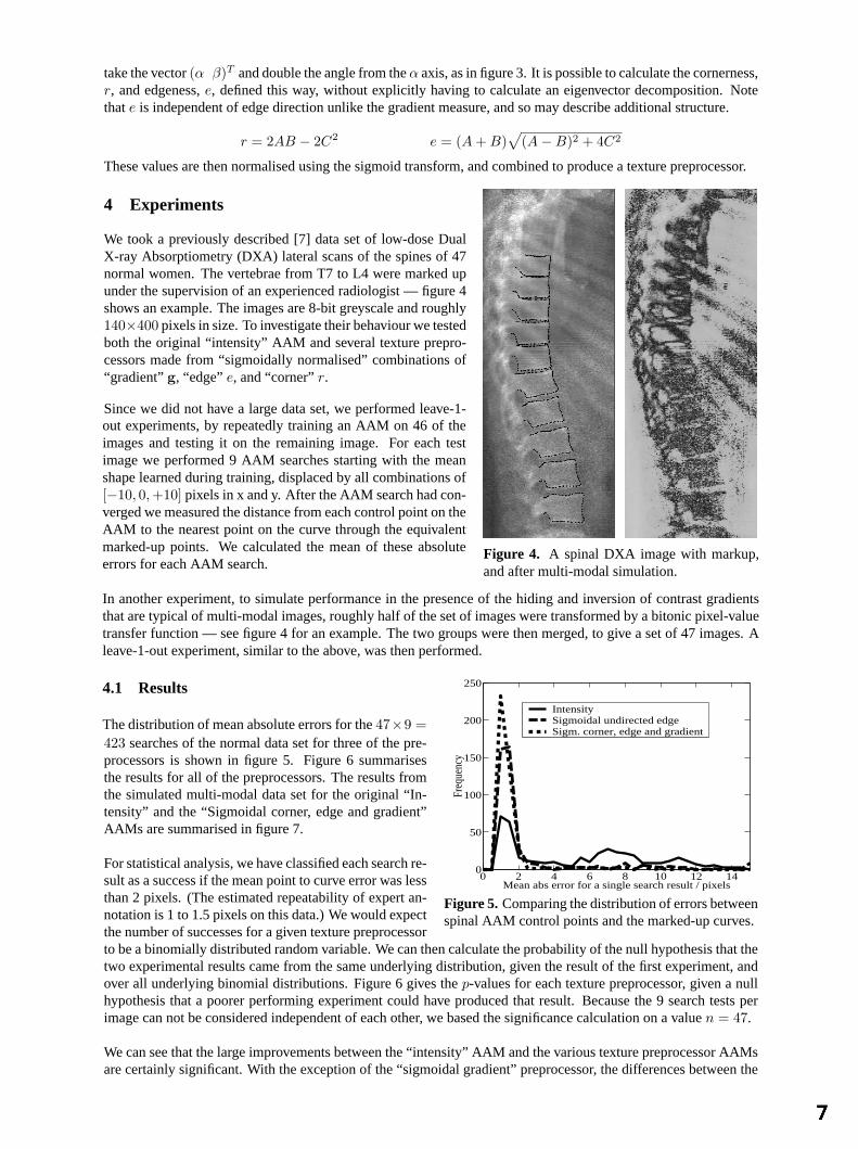
We took a previously described [7] data set of low-dose DualX-ray Absorptiometry (DXA) lateral scans of the spines of 47normal women. The vertebrae from T7 to L4 were marked upunder the supervision of an experienced radiologist — figure 4shows an example. The images are 8-bit greyscale and roughly140×400 pixels in size. To investigate their behaviour we testedboth the original “intensity” AAM and several texture prepro-cessors made from “sigmoidally normalised” combinations of“gradient”g, “edge”e, and “corner”r.

Since we did not have a large data set, we performed leave-1-

Figure 4. A spinal DXA image with markup,and after multi-modal simulation.

out experiments, by repeatedly training an AAM on 46 of theimages and testing it on the remaining image. For each testimage we performed 9 AAM searches starting with the meanshape learned during training, displaced by all combinations of[−10, 0, +10] pixels in x and y. After the AAM search had con-verged we measured the distance from each control point on theAAM to the nearest point on the curve through the equivalentmarked-up points. We calculated the mean of these absoluteerrors for each AAM search.

In another experiment, to simulate performance in the presence of the hiding and inversion of contrast gradientsthat are typical of multi-modal images, roughly half of the set of images were transformed by a bitonic pixel-valuetransfer function — see figure 4 for an example. The two groups were then merged, to give a set of 47 images. Aleave-1-out experiment, similar to the above, was then performed.

4.1 Results

The distribution of mean absolute errors for the47×9 =

0 2 4 6 8 10 12 140

50

100

150

200

250

Freq

uenc

y

Mean abs error for a single search result / pixels

Intensity Sigmoidal undirected edge Sigm. corner, edge and gradient

Figure 5. Comparing the distribution of errors betweenspinal AAM control points and the marked-up curves.

423 searches of the normal data set for three of the pre-processors is shown in figure 5. Figure 6 summarisesthe results for all of the preprocessors. The results fromthe simulated multi-modal data set for the original “In-tensity” and the “Sigmoidal corner, edge and gradient”AAMs are summarised in figure 7.

For statistical analysis, we have classified each search re-sult as a success if the mean point to curve error was lessthan 2 pixels. (The estimated repeatability of expert an-notation is 1 to 1.5 pixels on this data.) We would expectthe number of successes for a given texture preprocessorto be a binomially distributed random variable. We can then calculate the probability of the null hypothesis that thetwo experimental results came from the same underlying distribution, given the result of the first experiment, andover all underlying binomial distributions. Figure 6 gives thep-values for each texture preprocessor, given a nullhypothesis that a poorer performing experiment could have produced that result. Because the 9 search tests perimage can not be considered independent of each other, we based the significance calculation on a valuen = 47.

We can see that the large improvements between the “intensity” AAM and the various texture preprocessor AAMsare certainly significant. With the exception of the “sigmoidal gradient” preprocessor, the differences between the

Figure 6. Comparing the point-to-curve errors (in pixels) for different spinal AAM texture preprocessors, includingthe probabilities (p-values) that an experiment could be a random result of a worse performing spinal experiment.

Texture Preprocessor Point-Curve error Searches − log10 p-value given base resultmean std 90%-ile <2 pixels 35% 40% 75% 80% 81% 82% 85%

Intensity 5.4 3.8 11.0 35%

Sigmoidal gradient 5.1 4.0 10.8 40% 0.5

Sigmoidal corner 2.6 2.7 7.5 75% 4.7 3.9

Sigmoidal corner and gradient 2.1 2.2 1.2 80% 5.6 4.8 0.6

Sigmoidal corner and edge† 2.2 2.6 4.8 81% 6.1 5.3 0.8 0.5

Sigmoidal edge† 2.4 3.1 6.5 82% 6.1 5.3 0.8 0.5 0.4

Sigmoidal edge and gradient 1.9 2.1 4.6 85% 6.7 5.8 0.9 0.6 0.5 0.5

Sigm. corner, edge, and gradient 1.5 1.4 1.8 92% 9.5 8.5 2.2 1.7 1.4 1.4 1.2† Note that the fraction of successful results is rounded down to the next lowest multiple of1/n for p-value calculation, causingtwo rows with slightly dissimilar success rates to have identicalp-values.

various texture preprocessors are not significant at theα = 0.01 level.

5 Discussion and Conclusion

We have shown that using descriptions of local struc-

Figure 7. Comparing the point-to-curve errors (in pixels)for simulated multi-modal spinal images

Texture Preprocessor Point-Curve error Searchesmean std 90%-ile <2 pixels

Intensity 9.5 6.1 16.0 7%

Sigm. corner, edge,and gradient

3.4 3.8 9.3 60%

ture for the texture model of an AAM significantlyimproves the accuracy and reliability of AAM search.Furthermore, the local structure descriptors are lessdependent on global or sub-global contrast effectscaused by differing imaging parameters. The simu-lated multi-modal spinal image experiment shows that the “intensity” AAM needs to devote so much variance toit’s texture model to cope, that it fails to learn any useful information about the images. Comparing the results forthe “Sigmoidal corner, edge and gradient” preprocessor in figures 6 and 7 shows that the severe image corruptionhas a relatively small effect on a local structure AAM.

Using all the sigmoidally-normalised local structure descriptors gives the best results. This suggests that it may beadvantageous to add more local structure descriptors, including parameterised families of descriptors, e.g. differ-ential Gaussian invariants or complex wavelets.

We can see from figure 6 that the “sigmoidal edge” local structure descriptor is responsible for the majority of theimprovement, while the “sigmoidal gradient” detector shows no significant improvement. In experiments on facialAAMs [2], the “sigmoidal gradient” detector shows large improvements over the ordinary “intensity” AAM. Inthis paper we have shown that providing the AAM training algorithm with all of the local structure descriptors, itcan learn which descriptors are most useful, and adjust the importance of each descriptor on a pixel by pixel basisto get optimum performance.

Acknowledgements

We would like to thank Prof. Judith Adams and Martin Roberts for the data and useful discussions.

References

1. T. Cootes, G. Edwards & C.J.Taylor. “Active appearance models.”IEEE Transactions on Pattern Matching and MachineIntelligence23(6), pp. 681–885, 2001.

2. T. Cootes & C. Taylor. “On representing edge structure for model matching.” InCVPR, volume 1, pp. 1114–1119. 2001.3. M. Lades, J. Vorbruggen, J. Buhmann et al. “Distortion invariant object recognition in the dynamic link architecture.”IEEE

Transactions On Computers42(3), pp. 300–311, 1993.4. S. J. McKenna, S. Gong, R. P. Wrtz et al. “Tracking facial feature points with gabor wavelets and shape models.” In

International Conference on Audio-Video Based Biometric Person Authentication, pp. 35–43. 1997.5. B. Moghaddam & A. Pentland. “Probabilistic visual learning for object representation.”IEEE Transactions on Pattern

Matching and Machine Intelligence19(7), pp. 696–710, 1997.6. C. Harris & M. Stephens. “A combined corner and edge detector.” InAlvey Vision Conference, pp. 147–151. 1988.7. P. P. Smyth, C. J. Taylor & J. E. Adams. “Vertebral shape: Automatic measurement with active shape models.”Radiology

211, pp. 571–578, 1999.

Multi-resolution transportation for the detection of mammographic asymmetry

Michael Board* and Sue Astley

Division of Imaging Science and Biomedical Engineering, University of Manchester, M13 9PT, UK

Abstract. We are developing a method of comparing left-breast and right-breast mammographic images with the aim of identifying asymmetries caused by malignancy. Our approach uses a novel multi-resolution transportation algorithm to measure image similarity. This efficient algorithm permits the processing of high resolution images for which a standard linear programming solution to the transportation algorithm would be infeasible. Initial results are presented which demonstrate the potential of the method to aid the detection of abnormal asymmetry.

1 Introduction

Computer aided detection (CAD) systems have been developed to aid radiologists searching for abnormalities in digitised mammograms. In these systems, computer vision algorithms detect potentially abnormal areas in the images. The attention of the radiologist is drawn to the most suspicious areas of the original films by prompts presented as markers superimposed on low resolution versions of the images. There is evidence that, provided the prompts are sufficiently accurate, this approach can improve human detection performance.

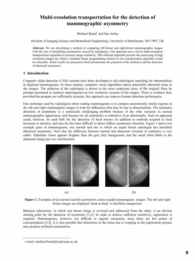
One technique used by radiologists when reading mammograms is to compare anatomically similar regions in the left and right mammogram images to look for differences that may be due to abnormalities. The automatic detection of asymmetry is a technically challenging problem because of the wide variation in normal mammographic appearance, and because not all asymmetry is indicative of an abnormality. Such an approach could, however, be used both for the detection of focal masses (in addition to methods targeted at local increases in density), and also for the more difficult to detect diffuse asymmetric densities. Figure 1 shows two example pairs of mammograms, one normal and one in which an expert breast radiologist has identified abnormal asymmetry. Note that the difference between normal and abnormal variation in symmetry is very subtle. Glandular tissue appears brighter than the grey fatty background, and the small white blobs in the abnormal image pair are calcifications.

(a) (b)

Figure 1. Examples of (a) normal and (b) asymmetric cranio-caudal mammogram images. The left and right breast images are displayed ‘back-to-back’ to facilitate comparison.

Bilateral subtraction, in which one breast image is reversed and subtracted from the other, is an obvious starting point for the detection of asymmetry [1,2]. In order to achieve sufficient sensitivity, registration is required. Mammograms, however, are difficult to register accurately, since there are few points of correspondence [3,4]. It is also possible that distortions in the tissue due to warping in the registration process may produce artificial asymmetries.

* e-mail: [email protected]

The approach described by Miller [5] differs from other published methods in that no registration took place and the comparison was made on the basis of measuring the cost of transporting the grey level values in one breast image to the other. With this approach, any slight misalignment of the images or difference in size between the breasts resulted in a pattern of movement that was easily distinguished from patterns generated by more sinister differences in breast density. One of the main limitations of Miller’s technique is that, for practical reasons, it was applied only to very low resolution images (regions of approximately 20 by 30 pixels). At such a low resolution small or subtle abnormalities may be overlooked. The technique classified cases as normal or abnormal but did not result in the output of a precise location of any suspected abnormality. It was suggested that this could be achieved by searching for clusters of long journeys in the transportation results.

The aim of the work described in this paper is to build on Miller’s work, which produced promising early results (despite the low resolution it gave a sensitivity of 74%), and to develop an efficient method of comparing bilateral mammograms. Ultimately, the objective of our research is to produce a prompting algorithm for asymmetries which will be sensitive, specific and efficient.

2 The transportation algorithm

The transportation problem is the problem of distributing goods from warehouses to markets at minimum cost [6]. The problem can be solved using linear programming to give the optimal set of journeys and a total minimum cost. The transportation algorithm is commonly applied to logistics and telecommunications, and more recently it has found use in image-based applications. Applied to images, the transportation takes place from a source to a destination image. We treat the source image as a map of warehouse locations in which the pixel intensities represent the goods. The destination image is our image of markets; the cost of moving a unit of intensity is the distance it must travel to satisfy the demand. Thus the total cost of efficiently distributing the pixel intensities from the source image to the destination image gives us some measure of the similarity between the two images. In mammographic imaging, the transportation algorithm has previously been used to compare image signatures [7] as a means of detecting asymmetry between left and right breasts [5], and to evaluate the efficacy of prompting algorithms [8].

To solve the transportation problem it is formulated as a linear programming problem, and it is most commonly solved by use of a simplex solver [9]. More recently, interior points methods have been applied and these may be more efficient, especially in the case of large scale problems [10]. Using a simplex algorithm from the Numerical Algorithms Group (NAG) [11], the problem scales badly with increasing image size. Figure 2 shows the time to compare two images plotted against the number of constraints applied, which is equal to the total number of non-zero pixels in both images.

0

10000

20000

30000

40000

50000

0 2000 4000 6000

No. constraints

Tim

e to

run

(s)

NAG

Figure 2. Time to solve transportation problem using the NAG simplex algorithm vs the number of constraints

3 Multi-resolution transportation

In mammographic imaging many of the features of interest are small or subtle, and digital images used for analysis are often processed at high spatial resolution (typically 50 microns per pixel). For the transportation algorithm to be applied to images at a resolution where all the detail required is present, a more efficient transportation method is required. One approach to reducing the size of the problem is to place restrictions on the transportation, so that not all of the possible journeys are permitted. If each pixel in the source image is only allowed to transport its intensity to a sub-set of pixels in the destination image, this can drastically reduce

both the size of the problem and the time taken to solve it. The pixels should be restricted to move only to ‘likely’ destinations – considering every pixel in the destination image is unnecessary and computationally costly.

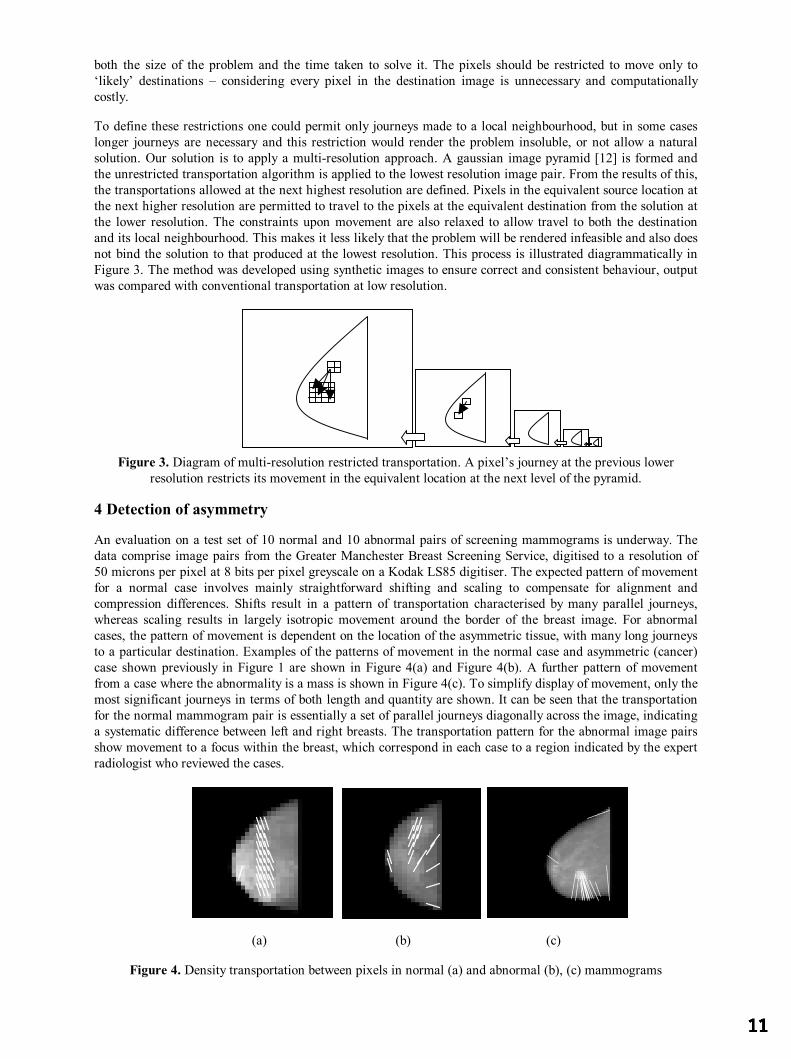
To define these restrictions one could permit only journeys made to a local neighbourhood, but in some cases longer journeys are necessary and this restriction would render the problem insoluble, or not allow a natural solution. Our solution is to apply a multi-resolution approach. A gaussian image pyramid [12] is formed and the unrestricted transportation algorithm is applied to the lowest resolution image pair. From the results of this, the transportations allowed at the next highest resolution are defined. Pixels in the equivalent source location at the next higher resolution are permitted to travel to the pixels at the equivalent destination from the solution at the lower resolution. The constraints upon movement are also relaxed to allow travel to both the destination and its local neighbourhood. This makes it less likely that the problem will be rendered infeasible and also does not bind the solution to that produced at the lowest resolution. This process is illustrated diagrammatically in Figure 3. The method was developed using synthetic images to ensure correct and consistent behaviour, output was compared with conventional transportation at low resolution.

Figure 3. Diagram of multi-resolution restricted transportation. A pixel’s journey at the previous lower resolution restricts its movement in the equivalent location at the next level of the pyramid.

4 Detection of asymmetry

An evaluation on a test set of 10 normal and 10 abnormal pairs of screening mammograms is underway. The data comprise image pairs from the Greater Manchester Breast Screening Service, digitised to a resolution of 50 microns per pixel at 8 bits per pixel greyscale on a Kodak LS85 digitiser. The expected pattern of movement for a normal case involves mainly straightforward shifting and scaling to compensate for alignment and compression differences. Shifts result in a pattern of transportation characterised by many parallel journeys, whereas scaling results in largely isotropic movement around the border of the breast image. For abnormal cases, the pattern of movement is dependent on the location of the asymmetric tissue, with many long journeys to a particular destination. Examples of the patterns of movement in the normal case and asymmetric (cancer) case shown previously in Figure 1 are shown in Figure 4(a) and Figure 4(b). A further pattern of movement from a case where the abnormality is a mass is shown in Figure 4(c). To simplify display of movement, only the most significant journeys in terms of both length and quantity are shown. It can be seen that the transportation for the normal mammogram pair is essentially a set of parallel journeys diagonally across the image, indicating a systematic difference between left and right breasts. The transportation pattern for the abnormal image pairs show movement to a focus within the breast, which correspond in each case to a region indicated by the expert radiologist who reviewed the cases.

(a) (b) (c)

Figure 4. Density transportation between pixels in normal (a) and abnormal (b), (c) mammograms

5 Discussion and further work

We have described a novel, efficient transportation-based technique for the bilateral comparison of mammograms. The initial results are promising, and an evaluation based on clinical data is currently in progress. Results show significant computational improvement with timings for a given step up to 30 times faster than conventional methods, allowing higher resolution images to be processed than previously.

Miller segmented the glandular tissue from the mammograms before comparing image pairs, having showed that the shape differences in glandular discs allowed classification by radiologists. Hence segmenting or enhancing the glandular disc may improve results further. Segmentation also has the advantage of reducing the size of the images to be processed, thus further reducing computational expense.

Our work will now proceed with statistical analysis of journey clusters to form a prompting system based on focal regions within the breast to which significant transportations are made. Regions which contribute most to the overall transportation cost of the image pair can be considered as candidate abnormalities. Further work will examine the extent of normal variability to improve specificity. Ultimately, the algorithm could be included in a prompting system, as asymmetry is one of the most subjective signs which radiologists are required to detect.

This technique may have other applications, both in mammography and in other medical imaging modalities in which bilateral or temporal differences are important. For example, multi-resolution transportation could be used to look for changes over time in slow growing lesions, or to investigate changes in clusters of calcifications with a view to identifying potential malignancy.

Acknowledgements

We are grateful for support from the EPSRC for Michael Board’s PhD studentship, and from Dr Caroline Boggis of the Greater Manchester Breast Screening Service for providing the clinical images.

References

1. M.L. Giger, P. Lu, Z. Huo et al.: “CAD in Digital Mammography: Computerized Detection and Classification of Masses” In: Digital Mammography, Elsevier Science, pp281-287, 1994

2. N. Karssemeijer, G.T. Brake : “Combining single view features and asymmetry for detection of mass lesions” In Digital Mammography, Nijmegen, Kluwer Academic Publishers, pp95-102, 1998

3. K. Marias, J.M. Brady, R.P. Highnam, et al.: “Registration and matching of temporal mammograms for detecting abnormalities”. In: Medical Imaging Understanding and Analysis 1999

4. S.J Caulkin, S. Astley, : “Sites of Occurrence of Malignancies on Mammograms”. In Digital Mammography, Nijmegen, Kluwer Academic Publishers, pp279-282, 1998

5. P. Miller, & S. Astley : “Automated Detection of Mammographic Asymmetry Using Anatomical Features” In: International Journal of Pattern Recognition and Artificial Intelligence. 7(6), pp1461-1476, 1993

6. F.L. Hitchcock. “The distribution of a product from several sources to numerous localities” Journal of Mathematical Physics 20: pp224-230, 1941

7. A.S Holmes, C.J. Taylor, : “Computer-Aided Diagnosis: An Improved Metric Space for Pixel Signatures” In: IWDM 2000 pp226-232

8. M. Board, S. Astley, : “A new method for optimising and evaluating mammographic detection algorithms“ In Digital Mammography, Springer-Verlag, pp257-261, 2002

9. A. Ravindram, D.T.Philips & J.J.Solberg. “Operations research: principles and practice” John Wiley & Sons, 2nd Edition, 1987

10. L. Portugal, F. Bastos, J. Judice, et al. : “An Investigation of Interior-Point Algorithms for the Linear Transportation Problem In: SIAM Journal of Scientific Computing 17(5), pp1202-1223, 1996

11. Numerical Algorithms Group. : http://www.nag.co.uk/numeric/numerical_libraries.asp 12. A. Rosenfeld : “Multi-resolution image processing and analysis” Springer-Verlag, 1984

Combining rCBF SPECT images obtained from different centres in a composite normal atlas

A S Houstona, S M A Hoffmannc, L Sandersa, D R R Whitea, L Boltc, J S Flemingc, M A Macleodb and P M Kemp d

aDepartment of Medical Physics and bDepartment of Nuclear Medicine, Royal Hospital Haslar, Gosport, UK and cDepartment of Medical Physics and Bioengineering and dDepartment of Nuclear Medicine, Southampton General

Hospital, UK

Abstract. An attempt is made to produce a normal rCBF SPECT atlas, using images obtained from normal control subjects at two centres. Several registration methods are first tested using images from one centre and it is shown that a non-linear approach is necessary. On this basis, non-linear SPM registration is adopted and applied to the images from both centres, using one of the images as a reference. The resulting images are normalised to total counts and the mean and SD images, together with the first ten eigenimages, are extracted. The composite atlas provides good ‘nearest normal’ fits to images in the data set from both centres and to an abnormal image obtained at one of the centres. The results are comparable with those obtained using the corresponding local atlas and much better than those obtained using the corresponding remote atlas.

1 Introduction With a growing requirement for standardisation in healthcare for image acquisition and processing techniques, it is entirely possible that national or international computerised normal atlases can be developed for different imaging procedures. The use of normal atlases in medical imaging, particularly with regards to brain imaging in SPECT and PET, has, so far, generally been restricted to a single site using a single imaging device. A problem that persists is whether normal image sets obtained under different conditions at different centres are in any way transportable and whether they can somehow be combined in a single normal atlas. At present, this problem is compounded by the fact that image acquisition and processing techniques are inconsistent from site to site. This paper attempts to create a single normal atlas for regional cerebral blood flow (rCBF) SPECT images obtained from normal subjects at two centres – Royal Hospital Haslar and Southampton General Hospital.

Several methods have been suggested for using information from a set of normal images to analyse images of patients, including statistical parametric mapping (SPM) [1] and the use of normal eigenimages to create ‘nearest normal’ fits to new images [2,3]. For the purposes of this paper, the latter approach will be adopted, although an alternative approach using SPM is currently under investigation. The use of eigenimages, highlighting major variations within the image set, allows us to examine whether or not images obtained from different centres can realistically be combined in this way

2 Materials and Methods Fifty rCBF SPECT images were obtained from normal volunteers at the Royal Hospital Haslar and a further 24 images were obtained from normal volunteers at Southampton General Hospital. Exclusion criteria at both sites included previous head injury with loss of consciousness; history of neurological or psychiatric disease; participation or past participation in boxing and undersea diving; and pregnancy.

Of the 50 normal subjects imaged at Haslar, 25 were male and 25 female with an overall age range of 18-79. The mean age and SD were 38 and 16 in the male group and 38 and 15 in the female group. Of the 24 normal subjects imaged at Southampton, 11 were male and 13 female with an overall age range of 40-96. The mean age and SD were 68 and 17 in the male group and 67 and 12 in the female group. Clearly, as well as procedural differences between the groups in the acquisition and processing of the images, there is also an obvious age mismatch.

The image acquisition procedure at Haslar was as follows. Patients are injected, while lying down, with 500MBq 99mTc-HMPAO in a room with subdued lighting. The acquisition is performed within 30 minutes of the injection on an ADAC Vertex dual-headed gamma camera, using LEHR collimators. The camera heads are rotated through 180° using a circular orbit at a radius of 20 cm that is consistent among subjects and 64 planar images of 45 seconds each are acquired within a 128x128 matrix. The zoom is set at 2.19 giving a pixel size of 1.42mm. The reconstruction is performed on a Pegasys workstation and uses Pegasys filtered back-projection with a Butterworth filter (order: 10; cut-off: 0.17). Attenuation correction of 0.12 cm-1 is achieved using the iterative Chang method with an ellipse outline set for a typical slice. The resultant images, which were 128 transaxial slices of 128 x 128 matrix size, are not reoriented prior to analysis.

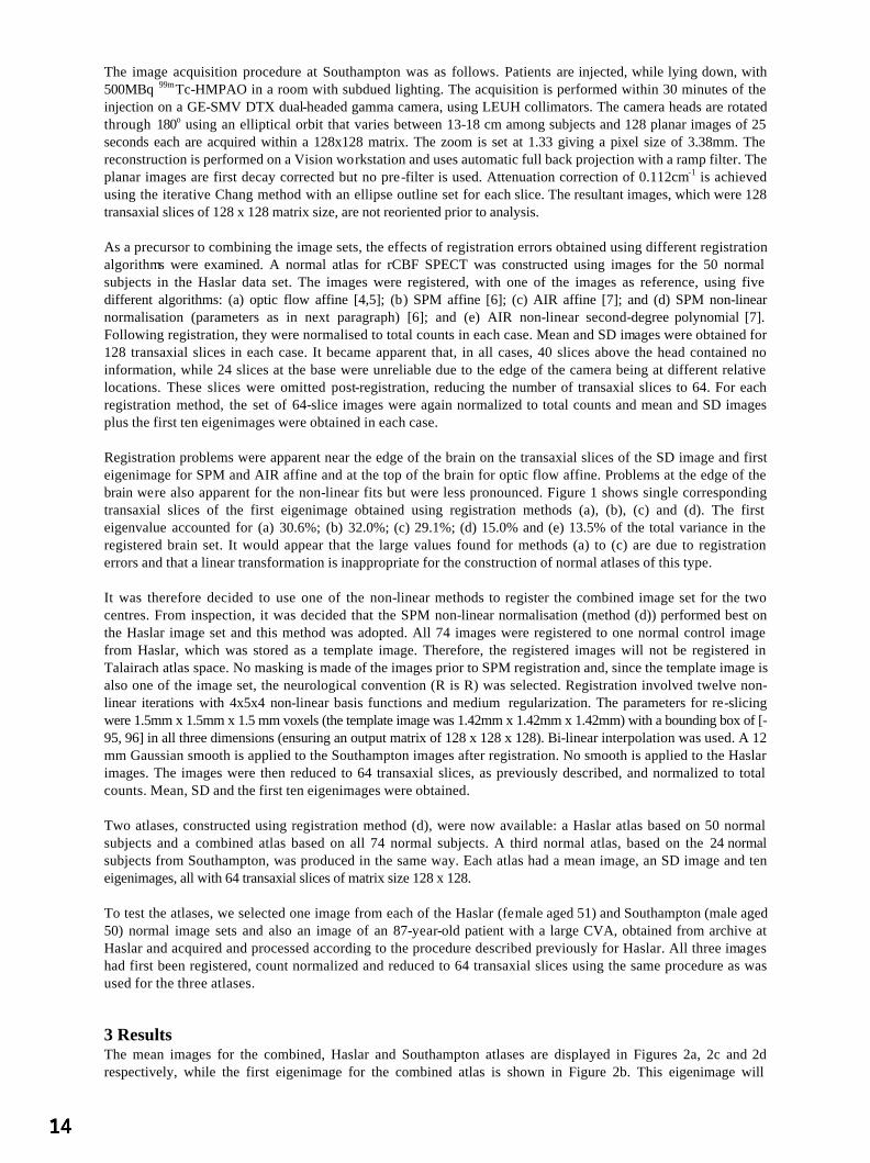
The image acquisition procedure at Southampton was as follows. Patients are injected, while lying down, with 500MBq 99mTc-HMPAO in a room with subdued lighting. The acquisition is performed within 30 minutes of the injection on a GE-SMV DTX dual-headed gamma camera, using LEUH collimators. The camera heads are rotated through 180o using an elliptical orbit that varies between 13-18 cm among subjects and 128 planar images of 25 seconds each are acquired within a 128x128 matrix. The zoom is set at 1.33 giving a pixel size of 3.38mm. The reconstruction is performed on a Vision workstation and uses automatic full back projection with a ramp filter. The planar images are first decay corrected but no pre-filter is used. Attenuation correction of 0.112cm-1 is achieved using the iterative Chang method with an ellipse outline set for each slice. The resultant images, which were 128 transaxial slices of 128 x 128 matrix size, are not reoriented prior to analysis. As a precursor to combining the image sets, the effects of registration errors obtained using different registration algorithms were examined. A normal atlas for rCBF SPECT was constructed using images for the 50 normal subjects in the Haslar data set. The images were registered, with one of the images as reference, using five different algorithms: (a) optic flow affine [4,5]; (b) SPM affine [6]; (c) AIR affine [7]; and (d) SPM non-linear normalisation (parameters as in next paragraph) [6]; and (e) AIR non-linear second-degree polynomial [7]. Following registration, they were normalised to total counts in each case. Mean and SD images were obtained for 128 transaxial slices in each case. It became apparent that, in all cases, 40 slices above the head contained no information, while 24 slices at the base were unreliable due to the edge of the camera being at different relative locations. These slices were omitted post-registration, reducing the number of transaxial slices to 64. For each registration method, the set of 64-slice images were again normalized to total counts and mean and SD images plus the first ten eigenimages were obtained in each case. Registration problems were apparent near the edge of the brain on the transaxial slices of the SD image and first eigenimage for SPM and AIR affine and at the top of the brain for optic flow affine. Problems at the edge of the brain were also apparent for the non-linear fits but were less pronounced. Figure 1 shows single corresponding transaxial slices of the first eigenimage obtained using registration methods (a), (b), (c) and (d). The first eigenvalue accounted for (a) 30.6%; (b) 32.0%; (c) 29.1%; (d) 15.0% and (e) 13.5% of the total variance in the registered brain set. It would appear that the large values found for methods (a) to (c) are due to registration errors and that a linear transformation is inappropriate for the construction of normal atlases of this type. It was therefore decided to use one of the non-linear methods to register the combined image set for the two centres. From inspection, it was decided that the SPM non-linear normalisation (method (d)) performed best on the Haslar image set and this method was adopted. All 74 images were registered to one normal control image from Haslar, which was stored as a template image. Therefore, the registered images will not be registered in Talairach atlas space. No masking is made of the images prior to SPM registration and, since the template image is also one of the image set, the neurological convention (R is R) was selected. Registration involved twelve non-linear iterations with 4x5x4 non-linear basis functions and medium regularization. The parameters for re-slicing were 1.5mm x 1.5mm x 1.5 mm voxels (the template image was 1.42mm x 1.42mm x 1.42mm) with a bounding box of [-95, 96] in all three dimensions (ensuring an output matrix of 128 x 128 x 128). Bi-linear interpolation was used. A 12 mm Gaussian smooth is applied to the Southampton images after registration. No smooth is applied to the Haslar images. The images were then reduced to 64 transaxial slices, as previously described, and normalized to total counts. Mean, SD and the first ten eigenimages were obtained. Two atlases, constructed using registration method (d), were now available: a Haslar atlas based on 50 normal subjects and a combined atlas based on all 74 normal subjects. A third normal atlas, based on the 24 normal subjects from Southampton, was produced in the same way. Each atlas had a mean image, an SD image and ten eigenimages, all with 64 transaxial slices of matrix size 128 x 128. To test the atlases, we selected one image from each of the Haslar (female aged 51) and Southampton (male aged 50) normal image sets and also an image of an 87-year-old patient with a large CVA, obtained from archive at Haslar and acquired and processed according to the procedure described previously for Haslar. All three images had first been registered, count normalized and reduced to 64 transaxial slices using the same procedure as was used for the three atlases.

3 Results The mean images for the combined, Haslar and Southampton atlases are displayed in Figures 2a, 2c and 2d respectively, while the first eigenimage for the combined atlas is shown in Figure 2b. This eigenimage will

represent the greatest normal variation in the image set and should contain mainly differences between the two image sets. The eigenvalues corresponding to the first ten eigenimages for the three atlases are shown in Table 1.

Eigenvalues Atlas No. of studies

1 2 3 4 5 6 7 8 9 10

Combined 74 0.280 0.092 0.051 0.037 0.028 0.025 0.021 0.021 0.018 0.018 Haslar 50 0.150 0.073 0.053 0.041 0.034 0.030 0.029 0.028 0.025 0.023 Southampton 24 0.184 0.142 0.094 0.085 0.054 0.053 0.047 0.038 0.034 0.032

It became apparent that, in all cases, the eigenvalues tend to level out after the fourth eigenvalue. For this reason four eigenimages were used in the construction of ‘nearest normal’ images in each case. Coefficients of the eigenimages were constrained to be within ±3 times the SD for corresponding coefficients in the normal image set, thus constraining the effect of the eigenimages.

In Figure 3, single corresponding transaxial slices are shown for the selected Haslar normal control and ‘nearest normal’ fits obtained from the combined atlas, the Haslar atlas and the Southampton atlas. Figures 4 and 5 show similar configurations for the selected Southampton normal control and the abnormal Haslar patient respectively.

4 Discussion and Conclusion From Figures 3, 4 and 5 it is seen that good ‘nearest normal’ fits are obtained from the combined and local normal atlases but not from the normal atlas obtained at the remote site. It is also apparent from Table 1 that combining normal image sets from different centres does not necessarily involve the use of an increased number of eigenimages. This suggests that the construction of composite normal atlases from a number of centres is viable. In this case, the images obtained from the two centres were quite different with the Southampton images appearing much smoother than the Haslar images. It should be stated that Southampton use this smooth image for statistical analysis only and a different image for viewing, while Haslar use the same image for both purposes. Future work will involve using SPM and Talairach atlas space to compare images from the two centres. It is also planned to include a third centre in future analyses.

References

1. K.J. Friston, A.P. Holmes, K.J. Worsley, J-B. Poline, C.D. Frith & R.S.J. Frackowiak “Statistical parametric maps in functional imaging: a general linear approach”, Human Brain Mapping 1, pp 214-220, 1994.

2. A.S. Houston, P.M. Kemp & M.A. Macleod “A method for assessing the significance of abnormalities in HMPAO brain SPECT images”, J Nucl Med 35, pp 239-244, 1994.

3. A.S. Houston, P.M. Kemp, M.A. Macleod, J.R. Francis, H.A. Colohan & H.P. Matthews “Use of the significance image to determine patterns of cortical blood flow abnormality in pathological and at-risk groups”, J Nucl Med 39, pp 425-430, 1998.

4. D.C. Barber “Registration of low resolution images”, Phys Med Biol 37, pp 1485-1498, 1992. 5. D.C. Barber, W.B. Tindale, E Hunt, A. Mayes & H.J. Sagar “Automatic registration of SPECT images as an alternative

to immobilization in neuroactivation studies”, Phys Med Biol 40, pp 449-463, 1995. 6. J. Ashburner & K.J. Friston “Spatial transformation of images” In SPM short course notes , chapter2, Wellcome

Department of Cognitive Neurology, 1997. 7. R.P. Woods, S.R. Cherry & J.C. Mazziotta “Rapid automated algorithm for aligning and reslicing PET images” J Comput

Assist Tomogr 16, 620-633, 1992.

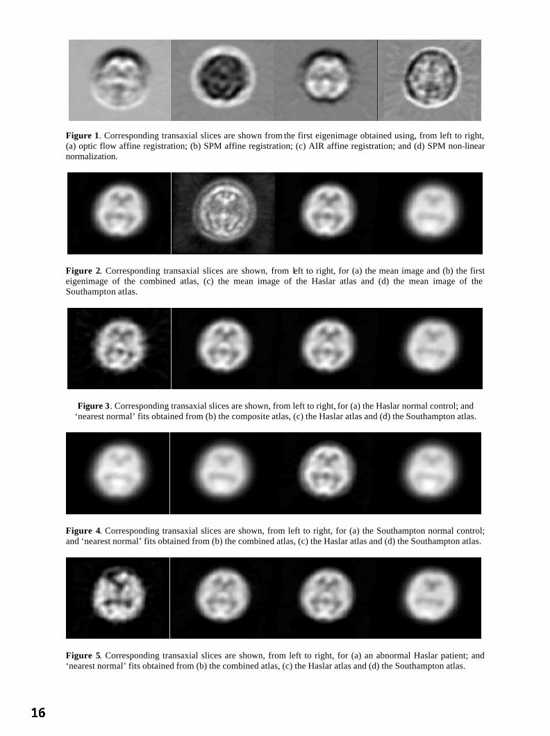
Figure 1. Corresponding transaxial slices are shown from the first eigenimage obtained using, from left to right, (a) optic flow affine registration; (b) SPM affine registration; (c) AIR affine registration; and (d) SPM non-linear normalization.

Figure 2. Corresponding transaxial slices are shown, from left to right, for (a) the mean image and (b) the first eigenimage of the combined atlas, (c) the mean image of the Haslar atlas and (d) the mean image of the Southampton atlas.

Figure 3. Corresponding transaxial slices are shown, from left to right, for (a) the Haslar normal control; and ‘nearest normal’ fits obtained from (b) the composite atlas, (c) the Haslar atlas and (d) the Southampton atlas.

Figure 4. Corresponding transaxial slices are shown, from left to right, for (a) the Southampton normal control; and ‘nearest normal’ fits obtained from (b) the combined atlas, (c) the Haslar atlas and (d) the Southampton atlas.

Figure 5. Corresponding transaxial slices are shown, from left to right, for (a) an abnormal Haslar patient; and ‘nearest normal’ fits obtained from (b) the combined atlas, (c) the Haslar atlas and (d) the Southampton atlas.

Separating Normal and Disease Groups using Regional CerebralBlood Flow

MariettaL. J.Scott,Neil A. Thacker, Anthony J.Lacey

ImagingScienceandBiomedicalImaging,Universityof Manchester

Abstract.Thispaperdescribesresearchexploring theproblemsassociatedwith interpretingregionalbloodflow measure-mentsin thebrain. We investigatea methodfor separatingnormalsfrom thosewith cerebraldiseases,wherethediseaseis causedby, or hasresultedin, alteredcerebralhaemodynamics.Cerebralperfusionmapsaredi-videdinto 10 vascularterritories.Thevariancescaledmeanvaluesfrom eachregion areusedto determine10principle axesof the normaldata. We demonstratethat normalvariability in theseaxesis large,but that ourtechniqueis capableof detectingmeasurableperturbationsin cerebralhaemodynamics.It is alsopossibletolocalisediseasegroupswith known vascularchangewithin a portionof thenormalspace.

1 Introduction

Measurementof cerebralbloodflow hasimportantactualandpotentialclinical utility, particularlyin diseasessuchascarotidstenosis,stroke andAlzheimer’s dementia.DynamicT2* susceptibilitycontrastenhancedMagneticResonanceImaging (DSCE-MRI) can be usedto observe the passageof a bolus of Gd-DTPA contrastagentthroughthebrainvasculatureandhenceeffectively imagebloodflow. Fromthecontrastconcentrationtimecourseof thefirst passof thebolusthroughthebrain,it is possibleto determinethevolumeandmeantime of arrival ofcontrastagentin avoxel [1]. Conventionalapproachesto perfusionmeasurementbasedupondeconvolutionof thesignal from a voxel by somearterial input function (eg, [2] [3]) make too many invalid assumptionsto providemeaningfulestimatesof blood flow [4]. We have previously shown [5], using the ideaof bolus tracking, thatparametricimagemapsof CerebralBlood Volume(CBV) andTime to Mean(TTM) canbeusedto calculatetheNetCerebralBloodFlow (NCBF)acrossavoxel. Netflow is implicitly assumedto benegligible in methodologiesbasedupondeconvolution,althoughwebelieveit to dominateatthemillimetreimagingscalesof MRI. Thesuccessof our approachfundamentallyreliesupontheability to obtainnearisotropicvoxel dimensionsin orderthat thevelocitycomponentof flow canbecomputedfrom TTM mapsusingspatialdifferentiation.Thistechniqueprovidesa uniqueopportunityto determinedirectionalestimatesof blood flow at all locationsin brain tissue. Suchdataprovidesgreatpotentialfor the analysisof blood flow in disease.Although this is a novel technique,in [1] wedemonstratethat normaldataagreeswith both a physiologicalmodelandflow valuesderived usingalternativetechniques.However, regardlessof thephysiologicalmeaningof thesemeasures,the truevalueof the techniquecanonly befoundby testingits diagnosticpower.

Thispaperdescribesaninvestigationinto theutility of usingour measuresof bloodflow in separatingnormalanddiseasegroups. To demonstratesuchutility, we must fulfill two criteria. First, that we canquantify changeinnormalsaboveandbeyondthatof normalvariationandmeasurementaccuracy. Secondly, thatnormalanddiseasegroupswith known cerebralvascularabnormalitieswill separatein the measurementspace.If thesecriteria aremet,themethodcanbeappliedto datasetsin orderto confirmor disputehypothesesof vascularabnormality. Theapproachwehavetakenis todividetheNCBFandTTM imagemapsintovascularterritories[6]. Wehaverestrictedourselves to oneplaneof datathroughthe brain at an anatomicallevel at which it is relatively straightfowardto identify vascularterritories. Correlationsbetweenthe flow valuesfor eachregion are identifiedby PrincipleComponentsAnalysis(PCA), giving us the major modesof variationof the data;a spacein which normalanddiseasegroupsareexpectedto separate.

2 Methods

Subject data: Table1 outlinesthegroupsof subjectdata,chosento illustratetheutility of our technique.As wellasthenormalgroups,we have a groupof patientswith carotidstenoses(all had

70%occlusionin at leastone

carotidartery),whowereimagedbeforeandafteracarotidendarterectomy(aproceduredesignedto improvebloodflow in arteries)in orderto investigatewhetherwe canquantifya changein flow dueto theintervention.Patientswith Alzheimer’s dementiatypically show hypoperfusionof partsof the temporalandparietallobes[7], so thisgroupshouldseparatefrom thenormalgroups.Finally, we have a groupof patientswith amnesticmild cognitive

Table 1. Subjectsgroups,numbers,meanageandranges

SubjectGroup Number MeanAge Std.Dev RangeNormal 60 73.05 5.81 61-87

MemoryPoor 34 73.24 5.23 63-85Alzheimer’s 9 61.56 6.15 54-72

CarotidStenosis 5 70.60 - 63-80

Figure 1. The vascularterritories overlaid on a T2* map. L/R =Left/Right, A/M/PCAT = Anterior/Middle/PosteriorCerebralArterialTerritories,A/PWT = Anterior/PosteriorWatershedTerritories

RACATLACAT

RAWTLAWT

LPCAT RPCAT

RPWTLPWT

RMCATLMCAT

impairment[8] (“memorypoor”), apossibleprecursorto Alzheimer’s,for whichthereis atentativehypothesisthattheremaybeanunderlyingvascularcause[9]. All subjectsunderwentaPRESTO [10] scan(TR=28ms,TE=20ms,FA=10 , voxel size= 1.79 1.79 3.5mm).

Vascular Territories: As weareinterestedin detectinglocalisedvascularinbalancesin bloodflow, it is expedientto divide the brain into vascularterritoriesbasedon the supply of blood to theseregions. We have devised amethodfor separatingthebrain,at thelevel of theupperborderof thethird ventricleinto 10classicallydefined[6]vascularterritories.Arterial regionsarethosedirectlyservedby theanterior, middleandposteriorcerebralarteries(observersleft andright); the watershedregions(anteriorandposterior)arethosein between.An active shapemodeldefiningcontrolpointsis fitted to arepresentativeT2* imageusinga linearaffine transformandtheregionsaredefinedaccordingto thesepoints(fig. 1). The vascularterritoriesareoverlaid on the mapsof interest(thelog(NCBF)or TTM maps)andthemeanandstandarderrorof thepixel valuesin eachof the10regionscalculated.

Standardising the data: Thedistribution of NCBF valuesis highly skeweddueto the few high flow andmanylow flow vesselsin a slice. A logarithmictransformis thereforeappliedto the datain orderto make the distri-bution conformmorecloselyto a Gaussiandistribution. TheTTM mapdistributionsdo approximatea Gaussiandistribution,andthenumbersagainareabsolutebut thedatahasnofixedorigin dueto variationsbetweensubjectsin injection time andboluspassage.In order to compareregionsbetweensubjects,we subtractthe meanpixelvaluefor thewholesliceso that thedistribution of valuesis centredaroundzero. Note thatwhenlooking at dis-easegroups,globaldelaysaffecting thewholesliceequallywill not bedetected.For eachsubjectandmaptype(ie, log(NCBF)or TTM), we have two 10D vectors;onecontainingthemeanvaluesfor the10 regions,theothercontainingthestandarderroron themeanof eachregion. PCA requireshomogenousmeasurementerrorsacrossthe input vectorspace,so in orderto comparethe meanpixel valuesof the differentregionsusingPCA, all theregionalvaluesneedto have the samestatisticalscaling;ie, all the regionsshouldhave unit variance.To obtainthe scalefactors,we take theaverageof the regionalstandarderrorsover all of thenormaldata. Becauseof thehemisphericsymmetryof thedata,we canaveragethescalefactorsfor theleft andright regionsandusethesameweightsfor both left andright regions. Thereis no reasonto believe that thereshouldbe any differencein theability to accuratelymeasurethemeanbetweentheleft andright regionsof thebrain.Hereweuseonly thenormaldatato createthescalefactors.

To transformthe datainto a form suitablefor PCA, we producea Covariancematrix of the scaleddatafor theNormalsubjects.TheCovariancematrix allows usto quantifythecorrelationsin flow betweenall of thevascular

Table 2. CorrelationMatrix for weightedNormalNCBFdata.Bold indicatesvaluesreferencedin textRegions RACAT RAWT RMCAT RPWT RPCAT LPCAT LPWT LMCAT LAWT LACATRACAT 1.0 - - - - - - - - -RAWT 0.72 1.0 - - - - - - - -RMCAT 0.53 0.59 1.0 - - - - - - -RPWT 0.23 0.57 0.50 1.0 - - - - - -RPCAT 0.46 0.57 0.63 0.42 1.0 - - - - -LPCAT 0.48 0.57 0.71 0.54 0.69 1.0 - - - -LPWT 0.33 0.39 0.44 0.61 0.49 0.63 1.0 - - -LMCAT 0.60 0.61 0.78 0.61 0.65 0.70 0.54 1.0 - -LAWT 0.60 0.88 0.63 0.62 0.63 0.62 0.37 0.75 1.0 -LACAT 0.56 0.76 0.62 0.46 0.56 0.49 0.28 0.66 0.77 1.0

Dat

a in

2nd

eig

enve

ctor

-14-

12-1

0 -

8 -

6 -

4 -

2 0

2 4

6 8

10

12

Data in 1st eigenvector

-40 -30 -20 -10 0 10 20 30 40

(a) log(NCBF)

Dat

a in

2nd

eig

enve

ctor

-50

-40

-30

-20

-10

0 1

0 2

0 3

0

Data in 1st eigenvector

-40 -30 -20 -10 0 10 20 30 40

(b) TTM

Figure 2. Plot of datain 1stand2ndeigenvectorspacefor log(NCBF)andTTM data, = normals, = carotidstenosis,linesindicatedirectionof movementafterwideningof arteries,thick endof line indicatespost-operative,

= Alzheimer’s,+ = memorypoor

regions(seetable2). Thegreatestcorrelationsareseenbetweentheleft andright anteriorwatershedterritoriesandthe left andright middlecerebralarterialterritories. The fact that thereis goodagreementbetweensymmetricalregionsis acorollaryof thefactthatthephysiologicalprocessesinvolvedin NCBFformationaresymmetric.Thereis alsoa high correlationbetweenthe left anteriorwatershedterritory andbothadjacentregions(the left anteriorand middle cerebralarterial territories). This may be due to the fact that both of the left middle and anteriorcerebralarteries(indirectly) feedthewatershedregion, but mayalsobedueto a misplacementof theboundariesbetweentheseregions.With 10 regions,thereis a reasonablechancethatany oneregionwill behighly correlatedwith another. However, the fact that the greatestcorrelationsoccurbetweensymmetricalterritories,wherethereis no confoundingboundarybetweenthem, and that thesecorrelationsare an averageover the whole trainingsetsuggeststhat the correlationsrepresentthe true physiology. SingularValueDecomposition(SVD) is usedtoperformPCAon theCovariancematrixandgivesus10 eigenvectorsandcorrespondingeigenvalues.

3 Results

We transformall of the datainto the eigenvectorspace.The first two principle axes(eigenvectors)accountforthegreatestvariationin thenormaldata.Resultsfor thelog(NCBF)andTTM datain thetransformedeigenvectorspacefor all subjectgroupsareshown in figures2aand2b.

For thecarotidstenosispatients(linkedby linespre-andpost-operatively in thefigures)therearesignificantmea-surablechangespost-operatively in bothlog(NCBF)andTTM for mostpatients,bearingin mind theeigenvectoraxes representthe standarderror space. The directionof changeis unimportanthere,the main point is that aperturbationin thecerebralbloodsupplyhasproduceda measurablechange.We would not necessarilyexpectallpatientsto respondin the samemanner, particularlyafter sucha major operation.Examinationof the normals,memorypoorandAlzheimer’s subjectsin thefirst two componentsof eigenvectorspacefor both the log(NCBF)andTTM shows that thedatais dominatedby normalvariation,andthat thereis no clearseparationbetweenanyof thegroups.Distributionsof datain theremainingcomponentsof eigenvectorspacearesimilarandnot reportedhere.Despitethelackof separation,theAlzheimer’spatientsdo form adistinctclusterat theedgeof theboundaryof thenormalsubjectsin the log(NCBF)caseandhave a significantlydifferentmean(at thep=0.05significancelevel) from thenormalsin the1steigenvectorspace(p=0.014).Alzheimer’sdementiaappearsto haveasystematicvascularcomponent.TheAlzheimer’s groupis youngerthantheothergroupsbut thereis no evidenceto suggestthatwhatwe areseeingis purelyanage-relatedeffect, asthey do not directly correlatewith similar age-matchednormals.Thereappearsto beno differencebetweenthenormalsandmemorypoorsubjects(p=0.84andp=0.58for 1stand2ndeigenvectors).

The mechanismsof the diseasesalsoallows us to hypothesizeon the utility of the technique.Carotidstenosispatientshave animpedimentto flow in oneor moreof themajorbrainfeedingarteries.We would expectregions

suppliedby thesearteriesto be fed slightly later than unimpededregions, either becausethe occlusionslowsthe blood, or becausethe region is fed by collateralflow. An occlusionwould thereforecausea large changein the TTM acrossthe brain. Wideningof the arterieswould result in a returnto normalTTM values. This isindeedshown in fig. 1(b). By contrast,in termsof vasculardisease,Alzheimer’sdementiais at themicrovascularlevel [11], wherewe expectto seelocalisedchangesin flow, ratherthana consistentalterationin TTM. Again,this is seenin 1(a);thereis a consistenttrendin thelog(NCBF)caseandtheAlzheimer’spatientsshow nochangefrom normalityin theTTM case(p=0.13andp=0.55for 1stand2ndeigenvectors).

4 Conclusions

Thispaperdescribesapreliminarystudyin theanalysisof regionalnetflow variablesfrom dynamicsusceptibilitycontrastenhancedMRI. Having takenappropriateaccountof statisticalvariability in ourdata,theresultsfrom thenormalsandcarotidstenosispatientssuggestthat therearesignificant,measurabledifferenceswithin thenormalgroup.Subjectswith Alzheimer’sdementiahavegrouplevel variationswhichcauseasystematicshift in thegroupdistribution with respectto thenormalgroupbut do not causechangesoutsidethenormalobservablerange.Thisis an importantfinding as it suggeststhat it might not be physiologicallypossibleto exist outsidenormalflowboundariesand thereforewe would never expect to seea clearseparationin the log(NCBF) eigenvectorspacebetweennormalanddiseasegroups.This techniqueasit standsis unableto separatediseasegroupsfrom anormalgroup. However, we have successfullylocalisedthe Alzheimer’s patientsto a portion of the normalspace. Intermsof thememorypoorindividuals,they overlapthenormalgroupwell anddo not localisein thesamemannerasthe Alzheimer’s patients,so we cannotconfirm the role of a vascularcomponentin this disorder. The utilityof thedifferentflow maps(log(NCBF)or TTM) is dependentuponthediseaseunderinvestigation.TTM imagemapsaremorelikely to beusefulwhenlooking at macrovasculardisease,log(NCBF) mapswill be moreusefulfor small-vesseldisease.Althoughregionalmeasurementsof netflow show promisetherearemany areaswhichstill requireattention.In particular, thelargedegreeof variability of flow patternsin normalscouldbein partdueto aninability to enforceanequivalentphysiologicalstatebetweenindividualswhenscanning.In futurework weintendto investigatemorerigorouscontrolstrategiesbeforeandduringacquisition.In addition,althoughthisworksetsabenchmarkfor whatwecancurrentlyachieve,thereis still muchto bedonewith regardto analysisof wholevolumesof dataandalsoalternative analysistechniques(including non-linearmethods)for the identificationofcorrelatedchangesbetweengroups.Bothof theseissuesarenow areasof ongoingresearch.

5 Acknowledgements

Work onthispaperwassupportedby agrantfrom theWellcomeTrust.Thanksto Dr. G.Riding,Dr. R.C.Baldwin,Prof. A. JacksonandProf P. Rabbittfor useof thesubjectdata.

References

1. N. A. Thacker, M. L. J.Scott& A. Jackson.“Can dynamicsusceptibilitycontrastmagneticresonanceimagingperfusiondatabeanalyzedusinga modelbasedon directionalflow?” J. Magn. Reson. Imaging 17(2), pp.241–255,February2003.

2. L. Ostergaard,R. M. Weisskoff, D. A. Chesleret al. “High resolutionmeasurementof cerebralbloodflow usingintravas-culartracerboluspassages.partI: Mathematicalapproachandstatisticalanalysis.” Magn. Reson. Med. 36(5), pp.715–725,Nov 1996.

3. K. A. Rempp,G. Brix, F. Wenzet al. “Quantificationof regionalcerebralbloodflow andvolumewith dynamicsuscepti-bility contrast-enhancedMR imaging.” Radiology 193(3), pp.637–641,Dec1994.

4. N. A. Thacker, X. P. Zhu, M. Nazarpooret al. “A new approachfor the estimationof MTT in boluspassageperfusiontechniques.” In Proc. MIUA. BMVA, London,July2000.

5. N. A. Thacker, M. L. J.Scott,D. L. Buckley et al. “A new methodfor thequantitative calculationof netbloodflow usingT2* susceptibilityimaging.” In Proc. ISMRM. Hawaii, 2002.

6. T. B. Moller & E. Reif. Pocket Atlas of Cross-Sectional Anatomy CT and MRI, volume1; Head,Neck,SpineandJoints.Theime,1994.

7. K. Lobotesis,J. D. Fenwick,A. Phippset al. “Occipital hypoperfusionon SPECTin dementiawith lewy bodiesbut notAD.” Neurol. 56, pp.643–649,2001.

8. R.C. Petersen,G. E. Smith,S.C.Waringetal. “Mild cognitive impairment- clinical characterizationandoutcome.” Arch.Neurol. 56, pp.303–308,March1999.

9. J.H. Naish,R.C.Baldwin,S.Jeffriesetal. “Analysisof cerebralflow in patientswith latelife depression.” In Proc. MIUA,volume6, pp.41–44.BMVA, 2001.

10. G. Liu, G. Sobering,J. Duyn et al. “A functionalMRI techniquecombiningprinciplesof echo-shiftingwith a train ofobservations(PRESTO).” Magn. Reson. Med. 30, pp.764–768,1993.

11. E. Farkas& P. G. M. Luiten. “Cerebralmicrovascularpathologyin agingandalzheimer’s disease.” Prog. Neurobiol. 64,pp.575–611,2001.

Classificationof White Matt er Tract Shapesfr om DTI WithoutRegistration

P. G. Batchelor, F. Calamante,D. Atkinson, , D. Tournier, D. L. G. Hill, R. Blyth, A. Connelly,

[email protected]

1 Intr oduction

Currentlythefinal output of DiffusionTensorMRI is thecalculationof fibretracts( [1,2]). Thetractsaresupposedto bea fair representationof axonalconnectionsin thebrain. Here,we usethephrase’final output’ in thesensethatnothingfurther is extractedoutof thefibres,andthey areusuallysimplydisplayed, leadingto thecriticismthattheir clinical useis limited. Clinically, theanisotropiesof thetensorscanbedisplayedusinga colour scheme,butthis informationis justat thevoxel level, andnotabouthow voxelsareconnected[3]. Weproposehereaparticularuseof mathematicaltools from thegeometry of curves. Theseallow statementsto bemadeabout theshapesofcurves thatareindependent of theirspatialposition, thusby definition, about theshapespaceof thecurves. Futureapplications might include thequantification of normal andabnormal shapes,the classificationof differentfibretracts,the characterisationof tractsthat passcloseto eachotherandidentificationof functionally similar brainregions by examining the endpointsof tractswith similar shapes.We candefinea norm on the setof shapesof curves,andthuswe have the necessaryingredientsfor statistics.We notethat Basserhasalreadymentionedusingcurve invariantsin [4], andthey have beenusedimplicitly to stopfibreswhenthey became abnormal [2].Furthermore,Ding et al. have recentlyproposeda method to groupfibresby bundles,andreport curvatureandtorsionvalues [5]. Here,however, we make a more systematicuseof theseinvariants. We propose that usingthe fundamentaltheoremof thegeometry of spacecurvesis a more rigorousway to classifycurves into bundlesof similar shapes.By factoring out irrelevant parameterssuchasspatiallocationandglobal scale,we areableto definea shapespacefor fibre tracts. Thesetoolswill allow intersubject comparisonof individual curves. Wealsoextend thegeometryto therelativespatialconfigurationsof curves,describingfor example how spatialcurveswind aroundeachother, usingquantititieslike theLink, andtheWritheof apairof curves.Someof thetechniquesareinspiredfrom DNA andpolymer folding analyses[6–8]. We construct simulationsdemonstratingthemethod,andapplythis method to in vivo datasets.

2 Method

MR diffusiondataon two healthyvolunteerswereacquiredusinga 1.5TSiemensVision systemon two separateoccasions. Thescansconsistedof a multi-slice (60 contiguousslices)diffusion-weightedsequencewith 20 uni-formly distributeddirections(numberof averages=1)and3 nondiffusion-weightedimages( [9]). Theacquisitionwasperformedtwice on onevolunteer, resultingin threedatasets,labeleda1anda2for thesamevolunteer, andbfor theothervolunteer.

Fibertracking wasperformedusingastreamlinesalgorithm( [1,10]). Fibretractsaremathematically describedasnon-closedspatialcurves,written where is thelength of thecurve. If thecurve is reparametrisedby arc-length , thenthe derivative with respectto , is a constant‘speed’ with "! . Fromthis it follows that the acceleration, # %$ '& is perpendicular to the speedvector. In this parametri-sation,the magnitude of the accelerationis the curvature # and its direction is $ . The binormal vector( ) *+$ completes a right handed trihedron, the Frenetframe[11]. The variationof this frameisentirelydescribedby thecurvature,andanother quantity, the torsion , - of thecurve. As eachof , $ ,

(are

normal, theirderivative is perpendicularto theirown direction, for example as( *.$ , ( * $ is always

perpendicularto , thusparallelto $ , andthecoefficient (/ $0 , is thetorsion.Thecurvature describes howmucha curve turns inside the planeof its speedandacceleration, the torsionthe speedat which it getsout ofthis plane. The curvatureandtorsioncanbeshown to be independentof theparametrisations, i.e. depend onlyon the shapeof the curve. The fundamentaltheoremof spacecurvestheoryis that the reciprocal holds: givenparticular curvatureandtorsionfunctions,thereis, upto rigid motion,only onecurvewith thesamecurvatureandtorsion.Thiscurvecanbereconstructedby integrationof theFrenet-Serret equations[11]. This theoremprovidesuswith a complete tool to classifyshapesof fibre tracts. We definetheshapeof a curve asanequivalenceclassof curvesunder theequivalenceof rigid body motions,anddenote theshapeof curve by 1 . The fundamental2

P. G.Batchelor(EPSRCGrantnoGR/N04867) D. Atkinson,(EPSRCFellowshipAF/001381)andD. L. G.Hill areat theImagingSciencesDivision, King’s College, Guy’s Campus,LondonSE19RT, F. Calamante, D. Tournier, R. Blyth andA. Connelly areat the Radiology andPhysicsUnit, Instituteof Child Health,UniversityCollegeLondon.Contactauthor: D. L. G.Hill, ImagingSciencesDivision,5thfloor ThomasGuy House,King’s CollegeLondon,Guy’s Campus,LondonSE19RT, 3 derek.hill,phil ipp.batchelor4 @kcl.ac.uk

tool to classifyobjectsis to haveadistancefunction ontheseobjects,andthetheoremallowsusto doexactly that:any distanceon a pair of functions will generatea distanceon shapes.The simplest,andmoststraightforward

is the 65 norm 7 % 98:; 5 =<9> 8? # 8- A@B# 5 - C 5ED , 8F- A@+, 5 - C 5 G7 -;H 8%I 5 where the curvesarescaledto

unit length. Having a distancefunctionon shapes,we candefinethemeanshapeof a set 81KJCJJ MLN astheoneminimisingthesumof squareddistancesto the KO s (oneof thepossibledefinitionsof themean). Doingthiswegetameancurvatureandtorsion, whichwecanintegrateto getarepresentationof themeanshape.For asetof curves8PCJCJJCML we definethemeanshapeastheonecorresponding to Q#RTS"# OVU9W Q,XYS O , OVUPW where # O and , O arethecurvaturesof the PO (scaledto a unit length,using FOVU O ). Thischoiceof meanis somewhatarbitrary, but usingit consistentlyis sufficient for our application. In this way, we obtainstatisticson the setof shapeswithout thedifficulty of registration, andfor example, cananalyseandcomparecorresponding fibresacrossindividuals,(seetheexamplesin Fig. 1). Wecouldthenfor examplegroup curvestogetherby thresholding ontheirshapedistance.Bundlesof CurvesAnother aspectof interestfor mutliple fibres,is how theirgeometry interacts.In threedimen-sions,thegeometricalinteraction betweencurvesis relatively complicated,asonecurvecantwist, or wraparoundanother. We proposeheretools for thequantification of sucha relation. For two curves 8 and 5 , we considerconfigurations,i.e. pairs 8 5 equivalentunderrigid body motion. TheLink of apair is definedas

[Z\% 8 5 !]K^R_`ba\_`Vc Md 8 - * Md5 fe g h ;8P- A@ 5 fe 8 - @ 5 fe 7 - _G`bai_G`Vc locf 8 - 5 e %G7 - 7 e 7 e

(theprime meansderivative with respectto theparameter - , which is not requiredhereto bearc-length) andtheWrithe of a curve shapeis definedas jlk % 1 m EZ\g P1 . Theseareusedin molecularbiology to studyDNAribbonsandpolymershape[6–8,12]. Thesequantitiesareagainrigid bodyinvariants.Computation In practice,thecomputationis done by fitting cubicsplinesandresamplingat 1000 (which makescomparisonsmorepractical)pointsthroughevery setof curve points. Thederivativesarecomputedby symbolicdifferentiationof thesplinecurves. Thetorsioninvolvesthird derivatives,andFig. 1 suggeststhat for example amedianfiltering of the torsionimprove robustness(although thereconstructedcurve doesnot seemto have beenaffected). Theintegration is straightforwardsummation.

3 Results

As afirst example,we illustratehow wecanreconstruct ameanshapewithoutregistration. Westartwith thecurvein Fig. 1 a),with curvature ! Dongprqsft for t in u ^ , andconstant torsion.We construct artificial perturbationsbycreating50 copiesof thecurve,by randomrigid bodytransformationandadditionof a perturbation, seeFig. 1 b).Fromthese,we computetheaveragecurvatureandtorsion(Figs.1c,e)andusingthesewe canreconstruct a curvesimilar to theoriginal (Fig. 1 f) by integrationof theFrenet-Serret equations.

Curve Classification We thusdefinea shapespaceof curves,andclassifycurve shapesusingthis spacewithits metric. Shapesof interestcouldbe,among others,—straightlines( #v w ,v ), —circular lines(#v const,,x , —helicoidallines( # and , const),—’U’-shapedcurves( # piecewiseconstant,,x ). Seefor example thetractsin [13], asexamplesof shapesof clinical tracts.

Thecorticospinalfibre tracts(CST)werecomputed for eachdatasetusinga streamlinesalgorithm startingfromsimilar seedregions (a1: 53 tracks,a2: 15 tracks,b: 10 tracks). Note that no registrationwas required, andthat thenumberof tractsin eachbundle weredifferent. Thecomputedshapedistancesbetweenmean shapesare7 fy ! 1z 6!9| J K !~ , 7 yuz EY!9 J ]F]N | , 7 fyGuGy !96! wJ | ] . SeeFig. 2 for plotsof thecurvaturesandtorsionsof themeanshapes.

We alsotracked the cross-pontinefibres(CPF),andcomputed the link betweena pair of fibresin the CST, andbetweenonefibre in the CST andonein the CPF(see2 c) andd)). TheCST-CST link was-0.0378,while theCST-CPFonewas0.5013.

4 Discussion

We have demonstratedtechniquesthatmight beusedfor theclassificationandcomparisonof fibre shapes,or insummary, ashapespaceof fibretracks.With thesetoolsonecan,for example,usecurvatureandtorsionto quantifyfibre geometry. We havealsointroduceda method to studytherelativeshapesof multiple fibres,andin particular

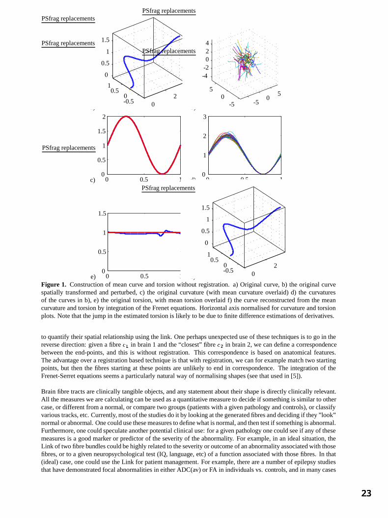
a)

PSfragreplacements

02

-0.50

0.51

0

0.5

1

1.5

b)

PSfragreplacements

-50

5

-50

5

-4-2024

c)

PSfragreplacements

0 0.5 10

0.5

1

1.5

2

d)

PSfragreplacements

0 0.5 10

1

2

3

e)

PSfragreplacements

0 0.5 10

0.5

1

1.5

f)

PSfragreplacements

02

-0.50

0.51

0

0.5

1

1.5

Figure 1. Constructionof meancurve andtorsionwithout registration. a) Original curve, b) the original curvespatially transformedandperturbed,c) the original curvature (with meancurvatureoverlaid) d) the curvaturesof the curvesin b), e) the original torsion,with meantorsionoverlaid f) the curve reconstructedfrom the meancurvatureandtorsionby integrationof theFrenetequations. Horizontal axisnormalisedfor curvatureandtorsionplots.Notethatthejumpin theestimatedtorsionis likely to bedueto finite differenceestimationsof derivatives.

to quantify their spatialrelationship usingthelink. Oneperhapsunexpecteduseof thesetechniquesis to go in thereversedirection: givena fibre 8 in brain1 andthe“closest”fibre 5 in brain2, we candefinea correspondencebetweenthe end-points, and this is without registration. This correspondence is basedon anatomical features.Theadvantageovera registrationbasedtechniqueis thatwith registration, wecanfor example matchtwo startingpoints,but thenthe fibresstartingat thesepoints areunlikely to endin correspondence. The integration of theFrenet-Serret equationsseemsa particularly natural wayof normalisingshapes(seethatusedin [5]).

Brain fibre tractsareclinically tangible objects,andany statementabout their shapeis directlyclinically relevant.All themeasureswearecalculatingcanbeusedasaquantitativemeasureto decide if something is similar to othercase,or differentfrom anormal, or comparetwo groups (patients with agivenpathology andcontrols),or classifyvarioustracks,etc.Currently, mostof thestudiesdoit by looking atthegeneratedfibresanddeciding if they ”look”normal orabnormal. Onecouldusethesemeasurestodefinewhatis normal, andthentestif something is abnormal.Furthermore,onecouldspeculateanotherpotential clinical use:for agiven pathology onecouldseeif any of thesemeasuresis a good marker or predictor of theseverity of theabnormality. For example, in an idealsituation,theLink of two fibrebundlescouldbehighly relatedto theseverity or outcomeof anabnormalityassociatedwith thosefibres,or to a given neuropsychological test(IQ, language, etc)of a function associatedwith thosefibres. In that(ideal)case,onecouldusetheLink for patientmanagement.For example, therearea numberof epilepsystudiesthathavedemonstratedfocalabnormalitiesin eitherADC(av) or FA in individualsvs. controls,andin many cases

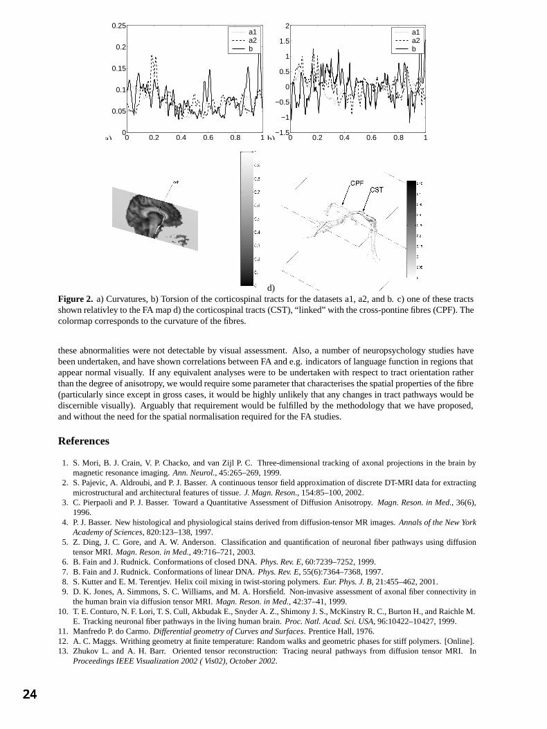
a) 0 0.2 0.4 0.6 0.8 10

0.05

0.1

0.15

0.2

0.25a1a2b

b) 0 0.2 0.4 0.6 0.8 1−1.5

−1

−0.5

0

0.5

1

1.5

2a1a2b

c) d)Figure 2. a) Curvatures,b) Torsionof thecorticospinal tractsfor thedatasetsa1,a2,andb. c) oneof thesetractsshown relativley to theFA mapd) thecorticospinaltracts(CST),“link ed” with thecross-pontinefibres(CPF).Thecolormapcorrespondsto thecurvatureof thefibres.

theseabnormalitieswerenot detectable by visual assessment.Also, a number of neuropsychology studieshavebeenundertaken,andhaveshown correlationsbetweenFA ande.g.indicators of languagefunction in regions thatappearnormal visually. If any equivalentanalyseswereto beundertakenwith respectto tractorientationratherthanthedegreeof anisotropy, wewouldrequire someparameterthatcharacterisesthespatialpropertiesof thefibre(particularly sinceexcept in grosscases,it would behighly unlikely thatany changesin tractpathways would bediscernible visually). Arguably that requirementwould be fulfilled by the methodology that we have proposed,andwithout theneedfor thespatialnormalisationrequiredfor theFA studies.

References

1. S. Mori, B. J. Crain, V. P. Chacko, andvan Zijl P. C. Three-dimensional trackingof axonalprojectionsin the brain bymagneticresonanceimaging.Ann. Neurol., 45:265–269,1999.

2. S.Pajevic, A. Aldroubi, andP. J.Basser. A continuoustensorfield approximationof discreteDT-MRI datafor extractingmicrostructuralandarchitecturalfeaturesof tissue.J. Magn. Reson., 154:85–100,2002.

3. C. PierpaoliandP. J. Basser. Toward a Quantitative Assessmentof Diffusion Anisotropy. Magn. Reson. in Med., 36(6),1996.

4. P. J.Basser. New histologicalandphysiological stainsderivedfrom diffusion-tensor MR images.Annals of the New YorkAcademy of Sciences, 820:123–138,1997.

5. Z. Ding, J. C. Gore,andA. W. Anderson. Classificationandquantificationof neuronal fiber pathways usingdiffusiontensorMRI. Magn. Reson. in Med., 49:716–721,2003.

6. B. Fain andJ.Rudnick.Conformationsof closedDNA. Phys. Rev. E, 60:7239–7252, 1999.7. B. Fain andJ.Rudnick.Conformationsof linearDNA. Phys. Rev. E, 55(6):7364–7368, 1997.8. S.KutterandE. M. Terentjev. Helix coil mixing in twist-storingpolymers.Eur. Phys. J. B, 21:455–462,2001.9. D. K. Jones,A. Simmons,S. C. Williams, andM. A. Horsfield. Non-invasive assessmentof axonal fiber connectivity in

thehumanbrainvia diffusiontensorMRI. Magn. Reson. in Med., 42:37–41,1999.10. T. E.Conturo,N. F. Lori, T. S.Cull, AkbudakE.,SnyderA. Z., Shimony J.S.,McKinstry R.C.,BurtonH., andRaichleM.

E. Trackingneuronal fiber pathwaysin theliving humanbrain. Proc. Natl. Acad. Sci. USA, 96:10422–10427,1999.11. ManfredoP. do Carmo.Differential geometry of Curves and Surfaces. PrenticeHall, 1976.12. A. C. Maggs. Writhing geometryatfinite temperature:Random walksandgeometricphasesfor stiff polymers.[Online].13. Zhukov L. and A. H. Barr. Orientedtensorreconstruction:Tracing neuralpathways from diffusion tensorMRI. In

Proceedings IEEE Visualization 2002 ( Vis02), October 2002.

Automatic registration of retinal images

Anna Sabate-Cequierab , James F Boyceb, Martin Dumskyjc, Mitsutoshi Himagab, David Ushera,Thomas H Williamsond, Stephen S Nusseya

aDepartment of Oncology, Gastroenterology, Endocrinology and Metabolism, St George’s HospitalMedical School, London, UK, bDepartment of Physics, King’s College London, Strand, London, UK,

cDepartment of Endocrinology, Royal Free Hospital, London, UK, dDepartment of Ophthalmology,St Thomas’ Hospital, London, UK

Abstract. This paper describes a system to automatically register temporal retinal images. The aim was toregister two retinal images of the same region at different times in order to to measure changes potentiallyassociated with diabetic retinopathy (DR). The method used landmarks automatically detected from the bloodvessel structure. The curvature of the retina was taken into account by applying thin-plate splines algorithm tothe images. Subtraction of the two registered images reveals changes between them. Results of the applicationof the system to a set of pairs selected from a diabetic retinopathy screening program are presented. Evaluationof the system was achieved using visual inspection by an experienced clinician and by the error measuredagainst manually selected anatomical landmarks.

1 Introduction

Registration of two images requires an interpolation function that maps one image into the other. Applied toretinal images, the curvature of the retina generates a complexity in finding a good interpolation. Temporal retinalregistration would allow a direct comparison of pixels in order to detect pathological changes. Diabetic retinopathy(DR) is the most common cause of blindness in the working age population of the developed world, treatment isavailable if the condition is detected in the early stages [1]. The aim of screening is to detect pathological lesionsthat appear on the retina during a pre-symptomatic stage of the disease. Temporal retinal registration would allowto track the development of the disease. The aim was to evaluate the progression of diabetic retinopathy in the eye.

An algorithm for temporal registration or retinal images was proposed by Zana et al [2], using a Bayesian Houghtransform based on point correspondence. Can et al [3] presented a hierarchical algorithm to construct a mosaicfrom images of the retina, comprising translation, affine and quadratic approximations and using landmarks be-longing to the blood vessel structure. Matsopoulos et al [4] presented a method for automatic retinal registration,using Genetic Algorithms with an affine or bilinear interpolation. Besl et al [5] proposed a method to register3-D shapes based on the iterative closest point algorithm. Bookstein [6] developed a thin-plate spline algorithmto model curved surfaces, using a non-linear function to interpolate two sets of point-correspondence landmarksmodelled by a warp surface. A method for mosaicing two retinal images has been reported previously [7]. Themethod used two images of the same eye taken at a single examination, one macular and one nasal view, andmerged them. A linear interpolation method was followed by a non-linear interpolation algorithm. Manual selec-tion of landmarks was required. The use of thin-plate splines [6] applied to model the deformity of the retina anda final weighted average of the two combined images demonstrated accurate registrations.

This paper presents an automatic method for temporal retinal registration. The method is based on the mosaicretinal images method previously presented [7] applied for temporal registration. In addition, the method automat-ically detects a set of landmarks from both blood vessel structures of the image pair, with no previous knowledge ofany correspondence between them. The landmarks are initially detected from the bifurcations of the blood vesselstructure, and along all the vasculature structure after linear approximation. When the registration is complete, thefinal registered images are then combined and subtracted. The importance of the subtracted result is to evaluatethe potential differences between the images taken at different times.

2 Method

The images used in this work comprised pairs of fundus images of the same region of the eye,

macular centredfield of view, captured at different times. One image of the pair, the object image, is geometrically transformed tomap onto the other image, the reference image.Author for correspondence, anna.sabate james.boyce @kcl.ac.uk

The images were first pre-processed to equalise contrast and illumination levels [8]. The main elements of theretina were detected, the optic disc [9] and the blood vessel structure [10], being significant features to be used forthe registration technique. The blood vessel structure was then thinned to a width of one pixel by a skeletonizationalgorithm [11]. Landmark points belonging to the bifurcations of the blood vessels were automatically detected byusing the skeletonized vasculature structure and a set of rules was established to reduce the number to select validpoints, producing two sets of landmark points per image pair. The size of each of the two landmark points set perpair may be different, as no prior knowledge of any existing correspondence between the landmarks was assumed.

The registration method consisted of a Euclidean interpolation followed by a non-linear interpolation. An affinetransformation may be decomposed into components of translation, rotation, magnification and shear. Previousobservations led to reducing the affine transformation to components of translation and rotation, as there wasno significant change in magnification or shear [7], yielding a Euclidean transformation. As translation may besignificant, this first transformation was necessary in order to achieve the next stage of corresponding points search.A point-correspondence search was performed based on closest distance. A correlation was then applied to furthervalidate the correspondences between the two sets of landmark points.

In order to increase the number of corresponding landmark points a further search was performed through theskeleton of the vasculature structure using cross-correlation applied to a small window around potential landmarkcorrespondences. A threshold correlation value and a parameter based on the distances between any existinglandmark points were used to select new corresponding points. Given these two larger corresponding landmarksets, a non-linear algorithm, thin-plate splines [6], was used to interpolate the two landmark sets and then appliedto the object image. This algorithm was able to model the curvature of the retina, and thereby produce a goodregistration result which minimises the error, the Euclidean distance between corresponding landmarks.

The different parameter sets used to refine the initial landmark points and to increase the number of correspondingpoints in the registration method as described above produced four solutions per image pair. A performancemeasure based on the maximum number of pixels in the overlapping area of the two blood vessel structures of theregistered images was used to select the optimum of the four solutions. The images were then combined in order tovisually assess the accuracy of the overlapping area. In addition, the images were subtracted to display and furtheranalyse potential changes between the two images.

3 Evaluation

The images used in this work were acquired using a Topcon TRC-NW5S non-mydriatic digital fundus camera,producing RGB colour images of 570 x 570 pixels, covering a

centred macular field of view and saved in

JPEG format. Image pairs comprised the same region of the eye taken at different times. Nineteen pairs wererandomly selected for this experiment.

In order to assess the performance of the system, validation techniques suggested by Woods [12] were used.The validation and evaluation of the system consisted of measuring the performance of the landmarks and thefinal registered images. The registered images were evaluated by visual inspection [12] by an expert clinician.The performance of the registration method was measured by evaluation against anatomical landmarks manuallyselected by an experienced technician [12]. Visual inspection consisted of visually analysing the registered images,concentrating on the accuracy of the matching of the vessel structure in the overlapping area. Each pair registeredwas considered as approved or rejected. The evaluation against anatomically corresponding landmarks consistedof measuring the error, the mean of all the Euclidean distances between the corresponding landmarks of eachpair of registered images. The error was calculated by initially selecting corresponding anatomical landmarks andapplying the previously calculated registration interpolation function to the corresponding landmarks. These twoerror measures enabled us to assess the performance of the registration.

4 Results

The visual inspection undertaken on the overlapping area of the registered images resulted in seventeen out ofnineteen pairs being successfully registered and two presenting an unsuccessful registration, producing a 89.5%success rate. One unsuccessful image pair was of a very poor quality and presented a very small area of bloodvessels due to cataract in the eye, therefore the small number of landmarks detected was not suficient for theregistration process. The other image pair presented a good registration over the entire image, except on the top

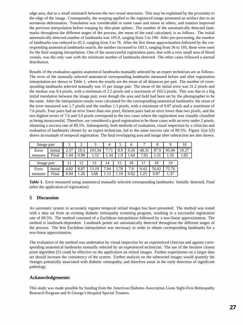
edge area, due to a small mismatch between the two vessel structures. This may be explained by the proximity tothe edge of the image. Consequently, the warping applied to the registered image presented an artifact due to anerroneous deformation. Translation was considerable in some cases and minor in others, and rotation improvedthe previous interpolation before warping by thin-plate splines. The number of the automatically detected land-marks throughout the different stages of the process, the mean of the total calculated, is as follows. The initialautomatically detected number of landmarks was 105.9, ranging from 3 to 196. After pre-processing, the numberof landmarks was reduced to 45.2, ranging from 3 to 78. After the first linear approximation followed by the cor-responding anatomical landmarks search, the number increased to 143.5, ranging from 36 to 193, these were usedfor the final warping interpolation. One of the unsuccessful registration pairs, that with a very small area of bloodvessels, was the only case with the minimum number of landmarks detected. The other cases followed a normaldistribution.

Results of the evaluation against anatomical landmarks manually selected by an expert technician are as follows.The error of the manually selected anatomical corresponding landmarks measured before and after registrationinterpolation are shown in Table 1, where the results are the mean of all distances per pair. The number of corre-sponding landmarks selected manually was 15 per image pair. The mean of the initial error was 31.2 pixels andthe median was 9.4 pixels, with a minimum of 2.5 pixels and a maximum of 103.5 pixels. This was due to a biginitial translation between the image pair, even though the area and field had been set by the photographer to bethe same. After the interpolation results were calculated for the corresponding anatomical landmarks: the mean ofthe error measured was 1.7 pixels and the median 1.3 pixels, with a minimum of 0.87 pixels and a maximum of7.6 pixels. Four pairs had an error lower than one pixel, thirteen pairs had an error lower than two pixels, and thetwo highest errors of 7.6 and 3.6 pixels correspond to the two cases where the registration was visually classifiedas being unsuccessful. Therefore, we considered a good registration to be those cases with an error under 2 pixels,obtaining a success rate of 89.5%. Subsequently, both methods of evaluation, visual inspection by a clinician andevaluation of landmarks chosen by an expert technician, led to the same success rate of 89.5%. Figure 1(a)-1(f)shows an example of temporal registration. The final overlapping area and image after subtraction are also shown.

Image pair 1 2 3 4 5 6 7 8 9 10

Error Initial 2.57 10.3 103.54 7.71 8.9 9.26 48.35 87.9 95.06 10.27measure Final 1.44 0.98 1.52 1.34 1.9 1.64 7.65 1.31 1.35 1.02

Image pair 11 12 13 14 15 16 17 18 19

Error Initial 4.82 8.87 13.19 7.94 5.78 7.0 9.43 76.02 75.76measure Final 0.94 1.26 3.68 1.13 1.19 0.92 1.25 0.87 1.37

Table 1. Error measured using anatomical manually selected corresponding landmarks: Initially detected, Final(after the application of registration)

5 Discussion

An automatic system to accurately register temporal retinal images has been presented. The method was testedwith a data set from an existing diabetic retinopathy screening program, resulting in a successful registrationrate of 89.5%. The method consisted of a Euclidean interpolation followed by a non-linear approximation. Themethod is landmark-dependent. Landmark points are automatically detected throughout the different stages ofthe process. The first Euclidean interpolation was necessary in order to obtain corresponding landmarks for anon-linear approximation.

The evaluation of the method was undertaken by visual inspection by an experienced clinician and against corre-sponding anatomical landmarks manually selected by an experienced technician. The use of the iterative closestpoint algorithm [5] could be effective on the application on retinal images. Further experiments on a larger dataset should increase the consistency of the system. Further analysis on the subtracted images would quantify thechanges potentially associated with diabetic retinopathy, and therefore assist in the early detection of significantpathology.

Acknowledgements

This study was made possible by funding from the American Diabetes Association Lions Sight-First RetinopathyResearch Program and St George’s Hospital Special Trustees.

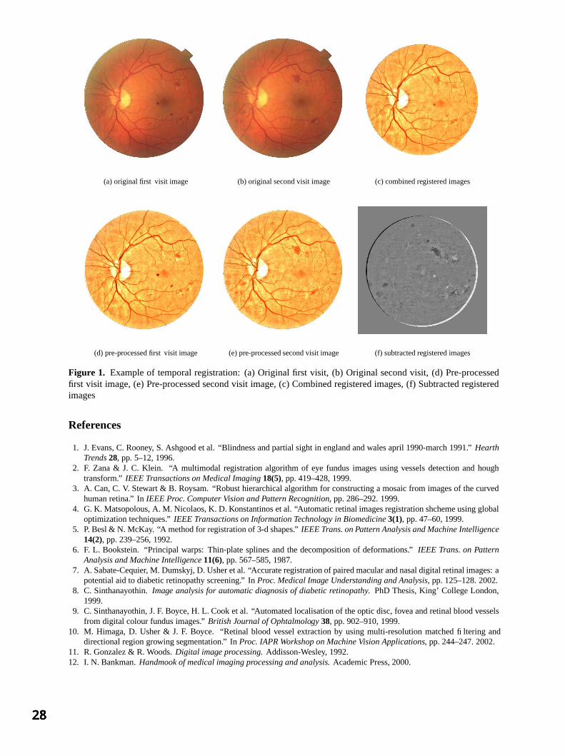
(a) original first visit image (b) original second visit image (c) combined registered images

(d) pre-processed first visit image (e) pre-processed second visit image (f) subtracted registered images

Figure 1. Example of temporal registration: (a) Original first visit, (b) Original second visit, (d) Pre-processedfirst visit image, (e) Pre-processed second visit image, (c) Combined registered images, (f) Subtracted registeredimages

References

1. J. Evans, C. Rooney, S. Ashgood et al. “Blindness and partial sight in england and wales april 1990-march 1991.” HearthTrends 28, pp. 5–12, 1996.

2. F. Zana & J. C. Klein. “A multimodal registration algorithm of eye fundus images using vessels detection and houghtransform.” IEEE Transactions on Medical Imaging 18(5), pp. 419–428, 1999.

3. A. Can, C. V. Stewart & B. Roysam. “Robust hierarchical algorithm for constructing a mosaic from images of the curvedhuman retina.” In IEEE Proc. Computer Vision and Pattern Recognition, pp. 286–292. 1999.

4. G. K. Matsopolous, A. M. Nicolaos, K. D. Konstantinos et al. “Automatic retinal images registration shcheme using globaloptimization techniques.” IEEE Transactions on Information Technology in Biomedicine 3(1), pp. 47–60, 1999.

5. P. Besl & N. McKay. “A method for registration of 3-d shapes.” IEEE Trans. on Pattern Analysis and Machine Intelligence14(2), pp. 239–256, 1992.

6. F. L. Bookstein. “Principal warps: Thin-plate splines and the decomposition of deformations.” IEEE Trans. on PatternAnalysis and Machine Intelligence 11(6), pp. 567–585, 1987.

7. A. Sabate-Cequier, M. Dumskyj, D. Usher et al. “Accurate registration of paired macular and nasal digital retinal images: apotential aid to diabetic retinopathy screening.” In Proc. Medical Image Understanding and Analysis, pp. 125–128. 2002.

8. C. Sinthanayothin. Image analysis for automatic diagnosis of diabetic retinopathy. PhD Thesis, King’ College London,1999.

9. C. Sinthanayothin, J. F. Boyce, H. L. Cook et al. “Automated localisation of the optic disc, fovea and retinal blood vesselsfrom digital colour fundus images.” British Journal of Ophtalmology 38, pp. 902–910, 1999.

10. M. Himaga, D. Usher & J. F. Boyce. “Retinal blood vessel extraction by using multi-resolution matched filtering anddirectional region growing segmentation.” In Proc. IAPR Workshop on Machine Vision Applications, pp. 244–247. 2002.

11. R. Gonzalez & R. Woods. Digital image processing. Addisson-Wesley, 1992.12. I. N. Bankman. Handmook of medical imaging processing and analysis. Academic Press, 2000.

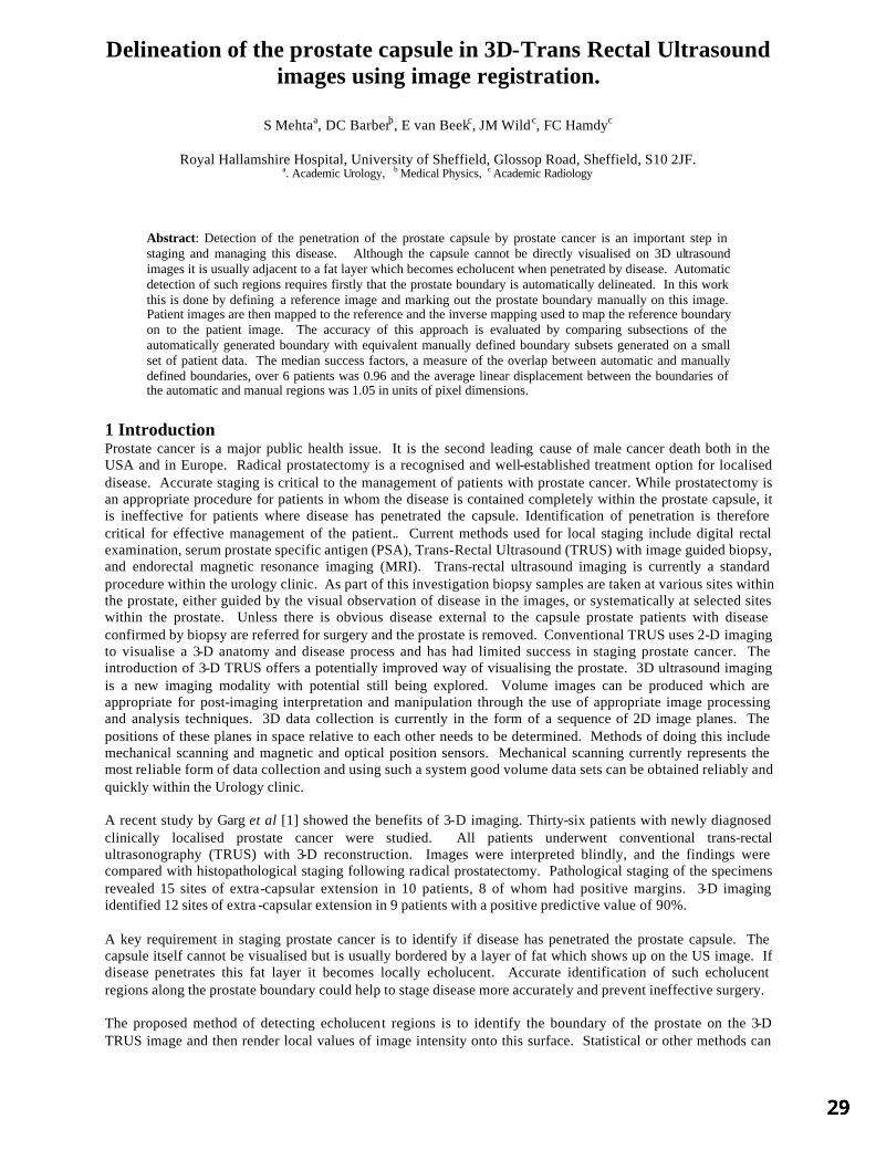
Delineation of the prostate capsule in 3D-Trans Rectal Ultrasound images using image registration.

S Mehtaa, DC Barberb, E van Beekc, JM Wildc, FC Hamdyc

Royal Hallamshire Hospital, University of Sheffield, Glossop Road, Sheffield, S10 2JF. a. Academic Urology, b Medical Physics, c Academic Radiology

Abstract: Detection of the penetration of the prostate capsule by prostate cancer is an important step in staging and managing this disease. Although the capsule cannot be directly visualised on 3D ultrasound images it is usually adjacent to a fat layer which becomes echolucent when penetrated by disease. Automatic detection of such regions requires firstly that the prostate boundary is automatically delineated. In this work this is done by defining a reference image and marking out the prostate boundary manually on this image. Patient images are then mapped to the reference and the inverse mapping used to map the reference boundary on to the patient image. The accuracy of this approach is evaluated by comparing subsections of the automatically generated boundary with equivalent manually defined boundary subsets generated on a small set of patient data. The median success factors, a measure of the overlap between automatic and manually defined boundaries, over 6 patients was 0.96 and the average linear displacement between the boundaries of the automatic and manual regions was 1.05 in units of pixel dimensions.

1 Introduction Prostate cancer is a major public health issue. It is the second leading cause of male cancer death both in the USA and in Europe. Radical prostatectomy is a recognised and well-established treatment option for localised disease. Accurate staging is critical to the management of patients with prostate cancer. While prostatectomy is an appropriate procedure for patients in whom the disease is contained completely within the prostate capsule, it is ineffective for patients where disease has penetrated the capsule. Identification of penetration is therefore critical for effective management of the patient.. Current methods used for local staging include digital rectal examination, serum prostate specific antigen (PSA), Trans-Rectal Ultrasound (TRUS) with image guided biopsy, and endorectal magnetic resonance imaging (MRI). Trans-rectal ultrasound imaging is currently a standard procedure within the urology clinic. As part of this investigation biopsy samples are taken at various sites within the prostate, either guided by the visual observation of disease in the images, or systematically at selected sites within the prostate. Unless there is obvious disease external to the capsule prostate patients with disease confirmed by biopsy are referred for surgery and the prostate is removed. Conventional TRUS uses 2-D imaging to visualise a 3-D anatomy and disease process and has had limited success in staging prostate cancer. The introduction of 3-D TRUS offers a potentially improved way of visualising the prostate. 3D ultrasound imaging is a new imaging modality with potential still being explored. Volume images can be produced which are appropriate for post-imaging interpretation and manipulation through the use of appropriate image processing and analysis techniques. 3D data collection is currently in the form of a sequence of 2D image planes. The positions of these planes in space relative to each other needs to be determined. Methods of doing this include mechanical scanning and magnetic and optical position sensors. Mechanical scanning currently represents the most reliable form of data collection and using such a system good volume data sets can be obtained reliably and quickly within the Urology clinic. A recent study by Garg et al [1] showed the benefits of 3-D imaging. Thirty-six patients with newly diagnosed clinically localised prostate cancer were studied. All patients underwent conventional trans-rectal ultrasonography (TRUS) with 3-D reconstruction. Images were interpreted blindly, and the findings were compared with histopathological staging following radical prostatectomy. Pathological staging of the specimens revealed 15 sites of extra-capsular extension in 10 patients, 8 of whom had positive margins. 3-D imaging identified 12 sites of extra -capsular extension in 9 patients with a positive predictive value of 90%. A key requirement in staging prostate cancer is to identify if disease has penetrated the prostate capsule. The capsule itself cannot be visualised but is usually bordered by a layer of fat which shows up on the US image. If disease penetrates this fat layer it becomes locally echolucent. Accurate identification of such echolucent regions along the prostate boundary could help to stage disease more accurately and prevent ineffective surgery. The proposed method of detecting echolucent regions is to identify the boundary of the prostate on the 3-D TRUS image and then render local values of image intensity onto this surface. Statistical or other methods can

be used to identify regions of abnormal intensity. To do this numerically the boundary of the prostate needs to be delineated. Manual identification and delineation of the prostate boundary is not feasible for routine clinical work. This paper describes a method being developed to locate the 3D prostate boundary automatically using image registration. Houston et al [2] proposed the use of 3D registration to delineate the boundary of 3D radionuclide cardiac studies. In their work the mapping function was an affine function, based on a previously published approach by Barber et al [3] for 3D image registration of brain radionuclide data. In both these cases the affine transform was adequate. However, registration of 3D-TRUS images of the prostate requires a non-linear mapping. Non-linear methods have been proposed using global basis functions (Friston et al [4], Barber [5]) but there are significant computational and other advantages in using local basis functions (Vemuri et al, [6]). Image registration has not been widely applied to ultrasound images because of the limited availability of 3D image data but Shields [7] investigated its use in removing motion effects when imaging the carotid artery though the cardiac cycle. 2 Methods Six patients with proven prostate cancer without evidence of extra-capsular involvement were imaged using a Brüel and Kjæ 2102 ultrasound scanner with 3D imaging capability. Image data was transferred to a workstation for analysis. The data consisted of an angular sequence of 2D images, typically of dimensions 55 x 30 mm (pixel dimensions 0.13 x 0.13 mm) over an angle which could be selected by the user but was typically 125o. The angular spacing between images was 0.3o. Scanning took 20 seconds per data set. Data was stored for analysis in raw form without conversion from angular to Cartesian co-ordinates, but could be converted to Cartesian form for display purposes. Data was analysed in raw form. For the purpose of image registration data at high resolution is not required and so the image data in raw form is packed by summing 4 x 4 x 4 voxels to form a single voxel. The voxel dimensions are then 0.52 x 0.52 mm by 1.2o. Once the mappings have been determined they can be applied to images of the original resolution, although this was not done here.

Figure 1a shows a cross section through a 3-D scan of a prostate. Figure 1b shows the image data in raw form. The image is noisy and in many images the prostate border is poorly defined. The method used to identify the prostate boundary is to first construct a reference image, define a 3-D boundary on this image and then use image registration to map the boundary image to the patient image. A 3-D image registration algorithm (see Appendix for brief details) is first used to construct the reference image. A suitable patient image is chosen as a reference and the images from the remaining subjects registered to this reference image. The mean of the registered images is then computed and this is used as the reference image. A third cycle can be run if required

but this usually produces few further changes. Figure 2a shows the reference image generated in this way from 6

Figure 1. (a) Data in Cartesian form. (b) Data in raw form

Figure 2 (a) The reference image (b) The reference boundary

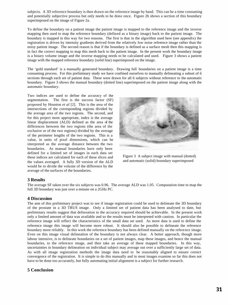
subjects. A 3D reference boundary is then drawn on the reference image by hand. This can be a time consuming and potentially subjective process but only needs to be done once. Figure 2b shows a section of this boundary superimposed on the image of Figure 2a. To define the boundary on a patient image the patient image is mapped to the reference image and the inverse mapping then used to map the reference boundary (defined as a binary image) back to the patient image. The boundary is mapped in this way for two reasons. The first is that in the algorithm used here (see appendix) the registration is driven by intensity gradients derived from the relatively low noise reference image rather than the noisy patient image. The second reason is that if the boundary is defined as a surface mesh then this mapping is in fact the correct mapping to map this mesh back to the patient image. In the present work the boundary image is a binary volume image and the inverse mapping needs to be calculated and used. Figure 3 shows a patient image with the mapped reference boundary (solid line) superimposed on the image. The ‘gold standard’ is a manually generated boundary. Drawing full boundaries on a patient image is a time consuming process. For this preliminary study we have confined ourselves to manually delineating a subset of 6 sections through each set of patient data. These were drawn for all 6 subjects without reference to the automatic boundary. Figure 3 shows the manual boundary (dotted line) superimposed on the patient image along with the automatic boundary. Two indices are used to define the accuracy of the segmentation. The first is the success factor (SF) proposed by Houston et al [2]. This is the area of the intersections of the corresponding regions divided by the average area of the two regions. The second, and for this project more appropriate, index is the average linear displacement (ALD) defined as the area of the differences between the two regions (the area of the exclusive or of the two regions) divided by the average of the perimeter lengths of the two regions. This is a value, in units of pixel dimensions, which can be interpreted as the average distance between the two boundaries. As manual boundaries have only been defined for a limited set of images in each data set these indices are calculated for each of these slices and the values averaged. A fully 3D version of the ALD would be to divide the volume of the difference by the average of the surfaces of the boundaries. 3 Results The average SF taken over the six subjects was 0.96. The average ALD was 1.05. Computation time to map the full 3D boundary was just over a minute on a 2GHz PC. 4 Discussion The aim of this preliminary project was to see if image registration could be used to delineate the 3D boundary of the prostate in a 3D TRUS image. Only a limited set of patient data has been analysed to date, but preliminary results suggest that delineation to the accuracy required should be achievable. In the present work only a limited amount of data was available and so the results must be interpreted with caution. In particular the reference image will reflect the characteristics of the small data set used. As more data is used to define the reference image this image will become more robust. It should also be possible to delineate the reference boundary more reliably. In this work the reference boundary has been defined manually on the reference image. Even on this image visual delineation of the boundary is not always clear. A better approach, though more labour intensive, is to delineate boundaries on a set of patient images, map these images, and hence the manual boundaries, to the reference image, and then take an average of these mapped boundaries. In this way, uncertainties in boundary delineation on individual subject may average out over a sufficiently large set of data. As with all image registration methods the image data need to be reasonably aligned to ensure correct convergence of the registration. It is simple to do this manually and in most images examine so far this does not have to be done too accurately, but fully automating initial alignment is a subject for further research. 5 Conclusion

Figure 3 A subject image with manual (dotted) and automatic (solid) boundary superimposed

Automatic delineation of the prostate boundary on 3D TRUS images seems feasible and could become a useful tool in the staging of prostate cancer. The method proposed is fully generic in that the domain specific knowledge required, the reference image and reference boundary, is independent of the computational algorithm used, and therefore the method should be applicable to other situations where 3D object boundaries are required. References 1. S Garg, B Fortling, F C Hamdy . 1999 Staging of prostate cancer using 3-dimensional transrectal ultrasound images: a

pilot study . J Urol , 162:1318-1321. 2. A S Houston, D White, W F D Sampson, M Mcleod and J Pilkington. 1998 An assessment of two methods for

generation automatic regions of interest. Nucl. Med. Commun 19:1005-1016. 3. D C Barber, W B Tindale, E Hunt, A Mayes and H J Sagar. 1995 Automatic registrationof SPECT images as an

alternative 4. to immobilisation in neuroactivation studies . Phys Med Biol. 40:449-463. 5. K J Friston, J Ashburn, C D Frith, J-B Poline, J D Heather and R S J Frackowiak 1995 Spatial registration and

normalisation of images. Human Brain Mapping 2 165-189. 6. D C Barber 1999 Efficient nonlinear registration of 3D images using high order co-ordinate transfer functions Journal

of Medical Engineering & Technology. 23:5 157-168 7. Vemuri B C, Huang S, Sahni S, Leonard C M, Mohr C, Gilmore R and Fitzimmons J 1998 An efficient motion

estimator with application to medical image registration. Medical Image Analysis 2 79-98 8. K Shields, D C Barber and S B Sherriff. 1993 Image registration for the investigation of atherosclerotic plaque

movement. In: Lecture notes in Computer Science 687. Information processing in Medical Imaging. H.H Barrett, A.F Gmitro (eds.) Springer-Verlag 438-458

Appendix

The aim of registration is to map an image m(x,y,z), the moved image, to an image f(x,y,z), the fixed image. We assume that such a mapping is possible in that there is a one-to-one mapping which converts m(x,y,z to f(x,y,z) such that the intensity values completely match (in the absence of noise). Then the moved and fixed images can be related by

where ∆x(x,y,z), ∆y(x,y,z) and ∆z(x,y,z) together constitute the mapping function. We modify the above equation by adding an extra term

which deals with the residual differences between the two images. In this form, the mapping function (including the ∆s(x,y,z) term) is clearly non-unique. However, if smoothness constraints are imposed on the mapping functions unique solutions are possible. One such constraint is to expand the mapping functions in terms of a set of basis functions φi(x,y). We can show that, for images close together

)z,y,x(szm

zf)z,y,x(z

21

ym

yf)z,y,x(y

21

xm

xf)z,y,x(x

21)z,y,x(m)z,y,x(f ∆−

∂∂+

∂∂∆+

∂∂+

∂∂∆+

∂∂+

∂∂∆=− (1)

and by expanding the components of the mapping function in terms of basis functions φi(x,y,z)

∑∑∑∑ φ−

∂∂+

∂∂φ+

∂∂+

∂∂φ+

∂∂+

∂∂φ=−

iallisi

iallizi

ialliyi

iallixi )z,y,x(a

zm

zf)z,y,x(a

21

ym

yf)z,y,x(a

21

xm

xf)z,y,x(a

21)z,y,x(m)z,y,x(f

which can be solved for the parameters a. Additional smoothing constraints in terms of minimising the magnitude of the Laplacian of the mapping function can also be added. The basis functions used in this work are local bilinear functions. Inclusion of the ∆s(x,y,z) without constraint results in a trivial solution in that ∆s(x,y,z) can be set to f – m. However, consider equation 1. The difference between f and m is made up of contributions from four terms. If each of these terms contributes equal amounts to the differences between f and m then since the gradients are relatively non-smooth functions ∆x and ∆y will be smoother than ∆s. The smoothest way of accounting for the difference between f and m is as far as possible to utilise the first two terms and then evoke ∆s when all else fails. This is what appears to happen in practice. The Laplacian smoothness constraint is not shown in the above analysis but is added in the context of solving the a in the usual way. The mapping functions are computed using image data within a registration region around the prostate.

)z,y,x(f))z,y,x(zz),z,y,x(yy),z,y,x(xx(m =∆+∆+∆+

)z,y,x(f)z,y,x(s))z,y,x(zz),z,y,x(yy),z,y,x(xx(m =∆−∆+∆+∆+

2D/3D Registration Using Shape From Shading Information in Application to Endoscope

Fani Deligianni, Adrian Chung and Guang-Zhong Yang

1Royal Society/Wolfson Foundation Image Computing Laboratory,

Imperial College of Science, London, UK

Abstract. This paper presents a new pq-space based 2D/3D registration method for camera pose estimation in tracking endoscope images. The proposed technique involves the extraction of surface normals for each pixel of the video images by using a linear shape-from-shading algorithm that is derived from the unique camera/lighting constrains of the endoscopes. We show how to use the derived pq-space distribution to match to that of the 3D tomographic model, and demonstrate the accuracy of the proposed method by using an electro-magnetic tracker and a specially constructed airway phantom. Comparison to existing intensity-based techniques has also been made, which highlights the major strength of the proposed method in its robustness against illumination and tissue deformation.

1 Methods

The basic process of the proposed technique is based on the following major steps: the extraction of surface normals for each pixel of the video images by using a linear local shape-from-shading algorithm derived from the unique camera/lighting constrains of the endoscopes; extraction of the p-q components of the 3D tomographic model by direct z-buffer differentiation; and the construction of a similarity measure based on angular deviations of the p-q vectors derived from 2D and 3D data sets. For this study, a p-q vector is defined as ( ) ( )yzxzqp ∂∂∂∂= ,, which represents the rate of change in depth along the x and y directions.

1.1 Shape From Shading for Endoscope Images

Shape from shading is a classical problem in computer vision that has been well established by the pioneering work of Horn [12-14]. It addresses the problem of extracting both surface and relative depth information from a single image. However, his main analysis is based on the assumption that the angle between the viewing vector V and the Z-axis, α , is negligible when the object size is small compared to its distance from the camera. In the case of endoscope images, both the camera and the light source are close to the object and the direction of the illuminating light coincides with the axis of the camera, thus no assumption can be made on α being negligible and lighting being uniform. Furthermore, the intensity of the image is also affected from the distance between the surface point and the light source. Rashid in [15] modelled this dependency by adding one more factor, which was a monotonically decreasing function ( )rf between the surface point and the light source. Therefore, the

image irradiance, E ,can be formulated as:

( ) ( ) ( ) ( )rfiyxsyx ⋅⋅⋅=Ε cos,, 0 ρ (1)

where 0s is a constant related to the camera, ρ is the surface albedo and ( )icos is the angle between the incident

light ray and the surface normal [ ]1,, −= qpn . Within the context of this study, our main interest is focused on estimating the normal vectors but not to reconstruct the whole surface. Therefore, the above technique was adapted because it can approximate well the gradient vectors p-q by using a linear local shape-from-shading algorithm. It has been proved that under the assumptions of light source being close to the viewer and surface being smooth and Lambertian, the following two linear equations with unknown p, q components can be written as:

fd301,ajchung,[email protected]

=+⋅+⋅=+⋅+⋅

00

20202

10101

CqBpACqBpA

where

( ) ( )( )

( )( )

( ) ( )( )

⋅+++⋅=⋅−++⋅+⋅−=⋅⋅−⋅++⋅−=

⋅+++⋅=⋅⋅−⋅++⋅−=⋅−++⋅+⋅−=

02

02

02

20

20

2002

0002

02

02

02

02

01

0002

02

01

20

20

2001

31313

313131

313

yyxRCyyxRyByxxyxRA

xyxRCyxyyxRBxyxRxA

y

y

y

x

x

x

(2)

In the above equation, EER xx = and EER yy = are the normalized partial derivatives of the image intensities,

E is the intensity of the pixel under consideration and 0x and 0y are the normalized image plane coordinates.

1.2 Extraction of p-q components from the 3D model

The extraction of the p-q components from the 3D model is relatively straightforward as for tomographic images the exact surface representation is known. Since xzp ∂∂= and yzq ∂∂= , differentiation of the z-buffer for the

rendered 3D surface will result in the required p-q distribution, which also elegantly avoids the tasks of occlusion detection. The effect of perspective projection has been taken into account during the rendering stage. The perspective projection parameters have been defined in order to match those of the video camera.

1.3 Similarity Measure

One would expect to use the angle between the surface normals extracted from shape-from-shading and those from the 3D model for constructing a minimization problem for 2D/3D registration. This, however, is not possible because the p-q vectors in the shape-from-shading algorithm have been scaled. The similarity measure used in this paper depends on the p-q components alone and the cross correlation between the two p-q distribution are used.

Analytically, for each pixel of the video frame, a p-q vector corresponding to ( ) [ ]Tjijiimg qpjin ,, ,, = was

calculated by using the linear shade-from-shading algorithm shown above. Similarly, for the current pose of the

rendered 3D model, the corresponding p-q vectors ( ) [ ]TjijiD qpjin ,,3 ,, ′′= for all rendered pixels were also

extracted by differentiating the z-buffer. The similarity of the two images was determined by evaluating the dot product of corresponding p-q vectors:

( ) ( )( ) ( ) ( )( ) ( )jinjin

jinjinjinjin

imgD

imgDimgD

,,

,,,,,

3

33

⋅

⋅=ϕ (3)

By applying a weighting factor that is proportional to the norm of Dn3 , the above equation can be reduced to

( ) ( )( ) ( ) ( )( )jin

jinjinjinjin

img

imgDimgDw

,

,,,,,

33

⋅=ϕ (4)

By incorporating the mean angular difference and the associated standard deviations (σ) of wϕ , the following

similarity function can be derived

( ) ( )( )∑ ∑ ∑ ∑ ⋅−⋅

=

DWw n

S

31

1

ϕσϕ

(5)

By minimizing Equation (5), the optimum pose of the camera for the video image can be determined. The reason for introducing a weighting factor for Equation (3) is due to the fact that p-q estimation from the 3D model is more accurate than that of the shape-from-shading algorithm, as it is not affected factors such as surface texture, illumination, or surface reflective properties. The weighting factor therefore reduces the potentia l impact of erroneous p-q values from the shape-from-shading algorithm and improves the overall robustness of the registration process.

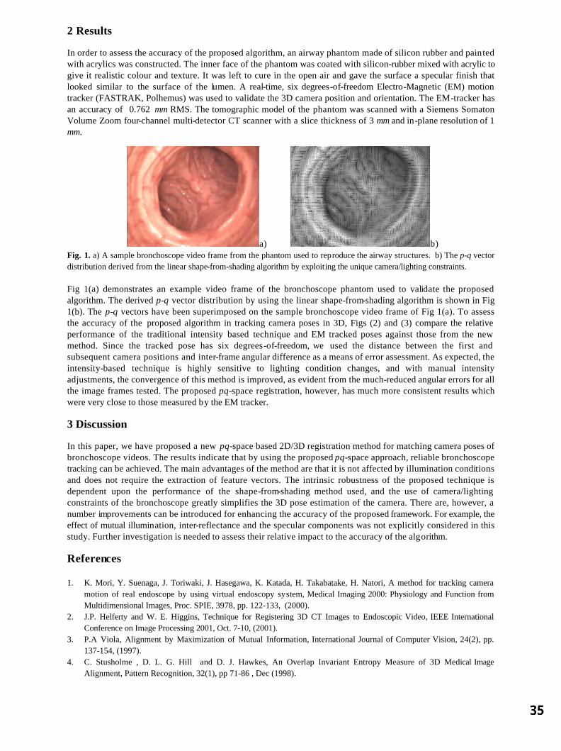
2 Results

In order to assess the accuracy of the proposed algorithm, an airway phantom made of silicon rubber and painted with acrylics was constructed. The inner face of the phantom was coated with silicon-rubber mixed with acrylic to give it realistic colour and texture. It was left to cure in the open air and gave the surface a specular finish that looked similar to the surface of the lumen. A real-time, six degrees-of-freedom Electro-Magnetic (EM) motion tracker (FASTRAK, Polhemus) was used to validate the 3D camera position and orientation. The EM-tracker has an accuracy of 0.762 mm RMS. The tomographic model of the phantom was scanned with a Siemens Somaton Volume Zoom four-channel multi-detector CT scanner with a slice thickness of 3 mm and in-plane resolution of 1 mm.

a) b) Fig. 1. a) A sample bronchoscope video frame from the phantom used to reproduce the airway structures. b) The p-q vector distribution derived from the linear shape-from-shading algorithm by exploiting the unique camera/lighting constraints. Fig 1(a) demonstrates an example video frame of the bronchoscope phantom used to validate the proposed algorithm. The derived p-q vector distribution by using the linear shape-from-shading algorithm is shown in Fig 1(b). The p-q vectors have been superimposed on the sample bronchoscope video frame of Fig 1(a). To assess the accuracy of the proposed algorithm in tracking camera poses in 3D, Figs (2) and (3) compare the relative performance of the traditional intensity based technique and EM tracked poses against those from the new method. Since the tracked pose has six degrees-of-freedom, we used the distance between the first and subsequent camera positions and inter-frame angular difference as a means of error assessment. As expected, the intensity-based technique is highly sensitive to lighting condition changes, and with manual intensity adjustments, the convergence of this method is improved, as evident from the much-reduced angular errors for all the image frames tested. The proposed pq-space registration, however, has much more consistent results which were very close to those measured by the EM tracker.

3 Discussion

In this paper, we have proposed a new pq-space based 2D/3D registration method for matching camera poses of bronchoscope videos. The results indicate that by using the proposed pq-space approach, reliable bronchoscope tracking can be achieved. The main advantages of the method are that it is not affected by illumination conditions and does not require the extraction of feature vectors. The intrinsic robustness of the proposed technique is dependent upon the performance of the shape-from-shading method used, and the use of camera/lighting constraints of the bronchoscope greatly simplifies the 3D pose estimation of the camera. There are, however, a number improvements can be introduced for enhancing the accuracy of the proposed framework. For example, the effect of mutual illumination, inter-reflectance and the specular components was not explicitly considered in this study. Further investigation is needed to assess their relative impact to the accuracy of the algorithm.

References 1. K. Mori, Y. Suenaga, J. Toriwaki, J. Hasegawa, K. Katada, H. Takabatake, H. Natori, A method for tracking camera

motion of real endoscope by using virtual endoscopy system, Medical Imaging 2000: Physiology and Function from Multidimensional Images, Proc. SPIE, 3978, pp. 122-133, (2000).

2. J.P. Helferty and W. E. Higgins, Technique for Registering 3D CT Images to Endoscopic Video, IEEE International Conference on Image Processing 2001, Oct. 7-10, (2001).

3. P.A Viola, Alignment by Maximization of Mutual Information, International Journal of Computer Vision, 24(2), pp. 137-154, (1997).

4. C. Stusholme , D. L. G. Hill and D. J. Hawkes, An Overlap Invariant Entropy Measure of 3D Medical Image Alignment, Pattern Recognition, 32(1), pp 71-86 , Dec (1998).

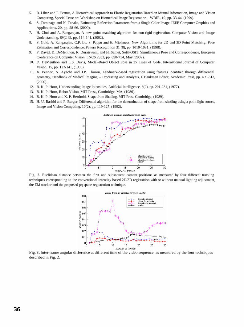
5. B. Likar and F. Pernus, A Hierarchical Approach to Elastic Registration Based on Mutual Information, Image and Vision Computing, Special Issue on: Workshop on Biomedical Image Registration – WBIR, 19, pp. 33-44, (1999).

6. S. Tominaga and N. Tanaka, Estimating Reflection Parameters from a Single Color Image, IEEE Computer Graphics and Applications, 20, pp. 58-66, (2000).

7. H. Chui and A. Rangarajan, A new point-matching algorithm for non-rigid registration, Computer Vision and Image Understanding, 89(2-3), pp. 114-141, (2002).

8. S. Gold, A. Rangarajan, C.P. Lu, S. Pappu and E. Mjolsness, New Algorithms for 2D and 3D Point Matching: Pose Estimation and Correspondence, Pattern Recognition 31 (8), pp. 1019-1031, (1998).

9. P. David, D. DeMenthon, R. Duraiswami and H. Samet, SoftPOSIT: Simultaneous Pose and Correspondence, European Conference on Computer Vision, LNCS 2352, pp. 698-714, May (2002).

10. D. DeMenthon and L.S. Davis, Model-Based Object Pose in 25 Lines of Code, International Journal of Computer Vision, 15, pp. 123-141, (1995).

11. X. Pennec, N. Ayache and J.P. Thirion, Landmark-based registration using features identified through differential geometry, Handbook of Medical Imaging – Processing and Analysis, I. Bankman Editor, Academic Press, pp. 499-513, (2000).

12. B. K. P. Horn, Understanding Image Intensities, Artificial Intelligence, 8(2), pp. 201-231, (1977). 13. B. K. P. Horn, Robot Vision, MIT Press, Cambridge, MA, (1986). 14. B. K. P. Horn and K. P. Berthold, Shape from Shading, MIT Press Cambridge, (1989). 15. H. U. Rashid and P. Burger, Differential algorithm for the determination of shape from shading using a point light source,

Image and Vision Computing, 10(2), pp. 119-127, (1992).

Fig. 2. Euclidean distance between the first and subsequent camera positions as measured by four different tracking techniques corresponding to the conventional intensity based 2D/3D registration with or without manual lighting adjustment, the EM tracker and the proposed pq space registration technique.

Fig. 3. Inter-frame angular difference at different time of the video sequence, as measured by the four techniques described in Fig. 2.

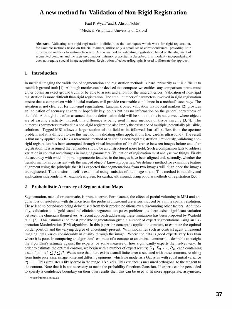
A new method for Validation of Non-Rigid Registration

Paul P. Wyattaand J. Alison Noblea

a Medical Vision Lab, University of Oxford

Abstract. Validating non-rigid registration is difficult as the techniques which work for rigid registration,for example methods based on fiducial markers, utilise only a small set of correspondences; providing littleinformation on the deformation elsewhere. A new method for validating registration, based on the alignment ofsegmented contours and the registered images’ intrinsic properties is described. It is modality independent anddoes not require special image acquisition. Registration of echocardiographs is used to illustrate the approach.

1 Introduction

In medical imaging the validation of segmentation and registration methods is hard, primarily as it is difficult toestablish ground truth [1]. Although metrics can be devised that compare two entities, any comparison metric musteither obtain an exact ground truth, or be able to assess and allow for the inherent errors. Validation of non-rigidregistration is more difficult than rigid registration. The small number of parameters involved in rigid registrationensure that a comparison with fiducial markers will provide reasonable confidence in a method’s accuracy. Thesituation is not clear cut for non-rigid registration. Landmark based validation via fiducial markers [2] providesan indication of accuracy at certain, hopefully key, points but has no information on the general correctness ofthe field. Although it is often assumed that the deformation field will be smooth, this is not correct where objectsare of varying elasticity. Indeed, this difference is being used in new methods of tissue imaging [3, 4]. Thenumerous parameters involved in a non-rigid registration also imply the existence of multiple, potentially plausible,solutions. Tagged-MRI allows a larger section of the field to be followed, but still suffers from the apertureproblem and it is difficult to use this method in validating other applications (i.e. cardiac ultrasound). The resultis that many applications lack a reasonable method of validating non-rigid registration. Previously, validating non-rigid registration has been attempted through visual inspection of the difference between images before and afterregistration. It is assumed the remainder should be an unstructured noise field. Such a comparison fails to addressvariation in contrast and changes in imaging parameters. Validation of registration must analyse two things. Firstlythe accuracy with which important geometric features in the images have been aligned and, secondly, whether thetransformation is consistent with the imaged objects’ known properties. We define a method for examining featurealignment using the principle that it is expected that segmentations from two images will align once the imagesare registered. The transform itself is examined using statistics of the image strain. This method is modality andapplication independent. An example is given, for cardiac ultrasound, using popular methods of registration [5,6].

2 Probabilistic Accuracy of Segmentation Maps

Segmentation, manual or automatic, is prone to error. For instance, the effect of partial voluming in MRI and an-gular loss of resolution with distance from the probe in ultrasound are errors induced by a finite spatial resolution.These lead to boundaries being delocalised from their precise positions even discounting other factors. Addition-ally, validation to a ‘gold-standard’ clinician segmentation poses problems, as there exists significant variationbetween the clinicians themselves. A recent approach addressing these limitations has been proposed by Warfieldet al [7]. This estimates the most probable segmentation given a number of expert segmentations using an Ex-pectation Maximization (EM) algorithm. In this paper the concept is applied to contours, to estimate the optimalborder position and the varying degree of uncertainty present. With modalities such as contrast agent ultrasoundimaging, data varies considerably in quality through the image. Where the data is good experts vary less thanwhere it is poor. In comparing an algorithm’s estimate of a contour to an optimal contour it is desirable to weightthe algorithm’s estimate against the experts’ by some measure of how significantly experts themselves vary. Inorder to estimate the optimal contour, we begin with a number of expert results; D 1;D2; ;DR, each containinga set of points 1 j J . We assume that there exists a small finite error associated with these contours, resultingfrom finite pixel size, image noise and differing opinions, which we model as a Gaussian with equal initial variance2i = 1. This simulates a likely error in the range3 pixels. This variance is measured orthogonal to the tangent to

the contour. Note that it is not necessary to make the probability functions Gaussian. If experts can be persuadedto specify a confidence boundary on their own results then this can be used to fit more appropriate, assymetric,

[email protected]

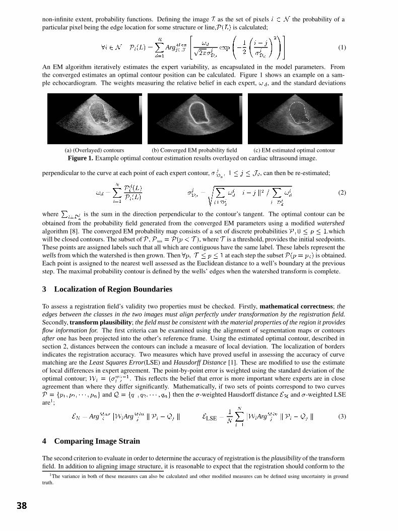
non-infinite extent, probability functions. Defining the image I as the set of pixels i 2 N the probability of aparticular pixel being the edge location for some structure or line,P(L) is calculated;

8i 2 N Pi(L) =RXd=1

ArgMaxj2J

24 !dp

2jDd

exp

0@1

2

i j

jDd

!21A35 (1)

An EM algorithm iteratively estimates the expert variability, as encapsulated in the model parameters. Fromthe converged estimates an optimal contour position can be calculated. Figure 1 shows an example on a sam-ple echocardiogram. The weights measuring the relative belief in each expert, ! d, and the standard deviations

(a) (Overlayed) contours (b) Converged EM probability field (c) EM estimated optimal contourFigure 1. Example optimal contour estimation results overlayed on cardiac ultrasound image.

perpendicular to the curve at each point of each expert contour, jDd

; 1 j Jd, can then be re-estimated;

!d =

NXi=1

Pdi (L)

Pi(L)

jDd

=

sXi?D

j

d

!id k i j k2 =

Xi?D

j

d

!id (2)

whereP

i?Dj

d

is the sum in the direction perpendicular to the contour’s tangent. The optimal contour can beobtained from the probability field generated from the converged EM parameters using a modified watershedalgorithm [8]. The converged EM probability map consists of a set of discrete probabilities P ; 0 p 1.whichwill be closed contours. The subset ofP , Pmin = P(p < T ), where T is a threshold, provides the initial seedpoints.These points are assigned labels such that all which are contiguous have the same label. These labels represent thewells from which the watershed is then grown. Then 8p; T p 1 at each step the subset P(p = p i) is obtained.Each point is assigned to the nearest well assessed as the Euclidean distance to a well’s boundary at the previousstep. The maximal probability contour is defined by the wells’ edges when the watershed transform is complete.

3 Localization of Region Boundaries

To assess a registration field’s validity two properties must be checked. Firstly, mathematical correctness; theedges between the classes in the two images must align perfectly under transformation by the registration field.Secondly, transform plausibility; the field must be consistent with the material properties of the region it providesflow information for. The first criteria can be examined using the alignment of segmentation maps or contoursafter one has been projected into the other’s reference frame. Using the estimated optimal contour, described insection 2, distances between the contours can include a measure of local deviation. The localization of bordersindicates the registration accuracy. Two measures which have proved useful in assessing the accuracy of curvematching are the Least Squares Error(LSE) and Hausdorff Distance [1]. These are modified to use the estimateof local differences in expert agreement. The point-by-point error is weighted using the standard deviation of theoptimal contour; Wi = (opt

i )1. This reflects the belief that error is more important where experts are in closeagreement than where they differ significantly. Mathematically, if two sets of points correspond to two curvesP = fp1; p2; ; png and Q = fq1; q2; ; qng then the -weighted Hausdorff distance EH and -weighted LSEare1;

EH = ArgMaxi

WiArgMinj k Pi Qj k

ELSE =1

N

NXi=1

WiArgMinj k Pi Qj k

(3)

4 Comparing Image Strain

The second criterion to evaluate in order to determine the accuracy of registration is the plausibility of the transformfield. In addition to aligning image structure, it is reasonable to expect that the registration should conform to the

1The variance in both of these measures can also be calculated and other modified measures can be defined using uncertainty in groundtruth.

properties of the materials whose deformation it represents. In practise such conformity is difficult to measure.Properties of biological structures exhibit significant variation with age, health and sex of an individual as well astissue orientation within a structure, even though in-vitro values may be reasonably well known from biopsies [4].Solutions estimated from Finite Element Methods [3] vary according to the boundary conditions and element shapeused. Therefore, although we would like to be able to validate the transform field directly it is currently impracticalto do so. Instead, the registered images can be used. In principle, Iff the transform is correct then there will be nostrain between the reference image and an image registered to it. The caveat is that the imaging modalities mustbe capable of responding to the same structural information; i.e. bone, muscle, skin etc... The plausibility can beassessed using a hypothesis test to compare an estimate of the distribution of image strain to the predicted straindistribution. Strain, @x

@t, is closely related to the local change in phase, 4, ( @x

@t= 4

2); it is this observation

which underlies strain imaging [9]. Image phase is a strong indicator of structure and may be estimated using theMonogenic Signal [10]. Using this representation, an image I may be analysed using a bandpass filter,f BP , andgeneralized Hilbert transform iu

juj. Theoretically, any centre frequency may be specified for fBP , though as the

registered image has been obtained using bicubic spline interpolation on the intensity, it is sensible to restrict thefilter to frequencies below half the image width/height owing to the low-pass effect of this. Applying the Riesztransform and denoting the two orthogonal filtered components obtained by A x + nx; Ay + ny, where nx(y) isnoise, the phase is obtained;

tan =

Ay + ny

Ax + nx

=

I fBP u2juj

I fBP u1juj

!(4)

In addition to estimating the strain in the images, from phase information, it is necessary to predict the straindistribution that would result for an accurate registration. If all structure is correctly aligned (the goal) then strainwill take a distribution solely dependent upon the noise properties of the imaging modality and tissues beingimaged. Consider the case of isotropic Gaussian noise, with variance 2

n. The signal componentsAx+nx; Ay+ny

will form a 2D Gaussian distribution with mean = [Ax; Ay]. The phase can be shown to be the following pdf;

Pr() =1

22ne

1

22n

sin

cos

TA2x AxAy

AxAy A2y

sin

cos

Z 1

0

e

1

22n

x

Ax+Ay tan

1+tan2

2dx

For Ax; Ay such that Ax+Ay tan1+tan2

3 the integral evaluates top2. The phase pdf is then a Gaussian, with

variance (A2x + A

2y)

2n . The slight difficulty is that the variance is not constant, but depends upon A x; Ay which

we can only estimate. Note that, as Ax; Ay ! 0 the distribution tends to white noise and the phase is dependentsolely on the noise. As such, validation of plausibility through strain is restricted to points with significant energy.The noise variance (2n) can be estimated as the local variance of the difference between the reference imageand itself after median filtering. The phase difference can then be normalized using estimates of A x; Ay and n;yielding the test distributionN (0; 1).

Using the estimates of image phase and the predicted strain distribution from the noise analysis, plausibility is ex-amined through a one tailed hypothesis test using the 2 statistic [11]. Accepting the hypothesis that the estimateddistribution agrees with the theoretic indicates an acceptable level of plausibility for the transform. The RandomVariable x is assumed to be N (; ). Under hypothesisH0 : = 0 the test statistic q will be 2(n), where n isthe number of data points. To accept H0 at confidence level (1 ) the inequality of equation 5 must be true. Fora confidence level of 95%, z0:05 = 1:645."

q =Xi

xi

0

2#<

21(n)

1

2(z1 +

p2n 1)2

; n 50 (5)

5 Results

The proposed method was applied to the validation of ultrasound registration fields. Two registration criteriawere used, the Correlation Ratio [5] and Normalized Mutual Information [6]. A set of candidate matches wereregularized using MAP estimation with an isotropic prior. A dense field was fitted using a standard isotropic cubicB-spline. Intensity interpolation was also performed using a cubic B-spline. Segmentation of the endocardiumfor 2 long and 1 short axis cardiac ultrasound sequence(s) ( 60 images) was performed by 3 experts and 1individual familiar with cardiac imaging. These 4 contours were amalgamated into a single optimal estimate forthe endocardium as described in section 2. Experts opinions were given, arbitrarily, 3 times the weighting of a

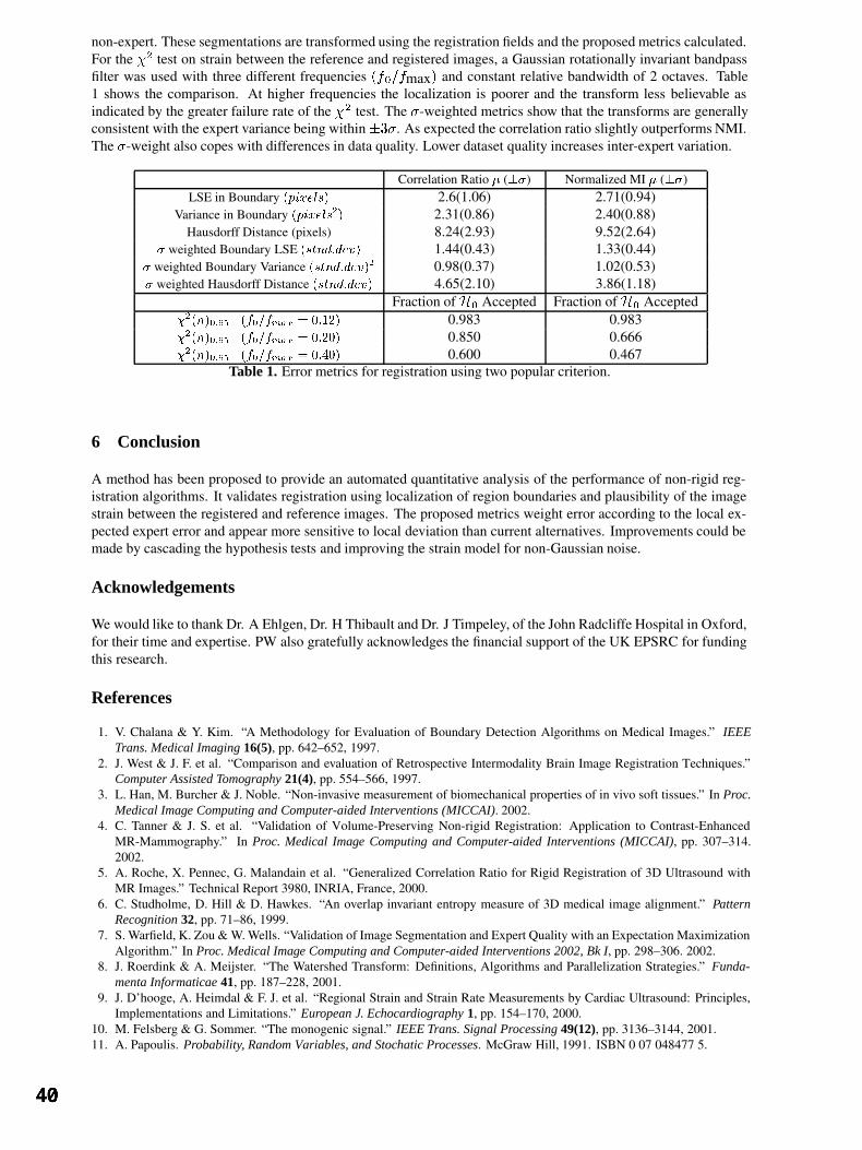
non-expert. These segmentations are transformed using the registration fields and the proposed metrics calculated.For the 2 test on strain between the reference and registered images, a Gaussian rotationally invariant bandpassfilter was used with three different frequencies (f0=fmax) and constant relative bandwidth of 2 octaves. Table1 shows the comparison. At higher frequencies the localization is poorer and the transform less believable asindicated by the greater failure rate of the 2 test. The -weighted metrics show that the transforms are generallyconsistent with the expert variance being within3. As expected the correlation ratio slightly outperforms NMI.The -weight also copes with differences in data quality. Lower dataset quality increases inter-expert variation.

Correlation Ratio () Normalized MI ()LSE in Boundary (pixels) 2.6(1.06) 2.71(0.94)

Variance in Boundary (pixels2) 2.31(0.86) 2.40(0.88)Hausdorff Distance (pixels) 8.24(2.93) 9.52(2.64)

weighted Boundary LSE (stnd:dev) 1.44(0.43) 1.33(0.44) weighted Boundary Variance (stnd:dev)2 0.98(0.37) 1.02(0.53) weighted Hausdorff Distance (stnd:dev) 4.65(2.10) 3.86(1.18)

Fraction of H0 Accepted Fraction of H0 Accepted2(n)0:95 (f0=fmax

= 0:12) 0.983 0.9832(n)0:95 (f0=fmax

= 0:20) 0.850 0.6662(n)0:95 (f0=fmax

= 0:40) 0.600 0.467Table 1. Error metrics for registration using two popular criterion.

6 Conclusion

A method has been proposed to provide an automated quantitative analysis of the performance of non-rigid reg-istration algorithms. It validates registration using localization of region boundaries and plausibility of the imagestrain between the registered and reference images. The proposed metrics weight error according to the local ex-pected expert error and appear more sensitive to local deviation than current alternatives. Improvements could bemade by cascading the hypothesis tests and improving the strain model for non-Gaussian noise.

Acknowledgements

We would like to thank Dr. A Ehlgen, Dr. H Thibault and Dr. J Timpeley, of the John Radcliffe Hospital in Oxford,for their time and expertise. PW also gratefully acknowledges the financial support of the UK EPSRC for fundingthis research.

References

1. V. Chalana & Y. Kim. “A Methodology for Evaluation of Boundary Detection Algorithms on Medical Images.” IEEETrans. Medical Imaging 16(5), pp. 642–652, 1997.

2. J. West & J. F. et al. “Comparison and evaluation of Retrospective Intermodality Brain Image Registration Techniques.”Computer Assisted Tomography 21(4), pp. 554–566, 1997.

3. L. Han, M. Burcher & J. Noble. “Non-invasive measurement of biomechanical properties of in vivo soft tissues.” In Proc.Medical Image Computing and Computer-aided Interventions (MICCAI). 2002.

4. C. Tanner & J. S. et al. “Validation of Volume-Preserving Non-rigid Registration: Application to Contrast-EnhancedMR-Mammography.” In Proc. Medical Image Computing and Computer-aided Interventions (MICCAI), pp. 307–314.2002.

5. A. Roche, X. Pennec, G. Malandain et al. “Generalized Correlation Ratio for Rigid Registration of 3D Ultrasound withMR Images.” Technical Report 3980, INRIA, France, 2000.

6. C. Studholme, D. Hill & D. Hawkes. “An overlap invariant entropy measure of 3D medical image alignment.” PatternRecognition 32, pp. 71–86, 1999.

7. S. Warfield, K. Zou & W. Wells. “Validation of Image Segmentation and Expert Quality with an Expectation MaximizationAlgorithm.” In Proc. Medical Image Computing and Computer-aided Interventions 2002, Bk I, pp. 298–306. 2002.

8. J. Roerdink & A. Meijster. “The Watershed Transform: Definitions, Algorithms and Parallelization Strategies.” Funda-menta Informaticae 41, pp. 187–228, 2001.

9. J. D’hooge, A. Heimdal & F. J. et al. “Regional Strain and Strain Rate Measurements by Cardiac Ultrasound: Principles,Implementations and Limitations.” European J. Echocardiography 1, pp. 154–170, 2000.

10. M. Felsberg & G. Sommer. “The monogenic signal.” IEEE Trans. Signal Processing 49(12), pp. 3136–3144, 2001.11. A. Papoulis. Probability, Random Variables, and Stochatic Processes. McGraw Hill, 1991. ISBN 0 07 048477 5.

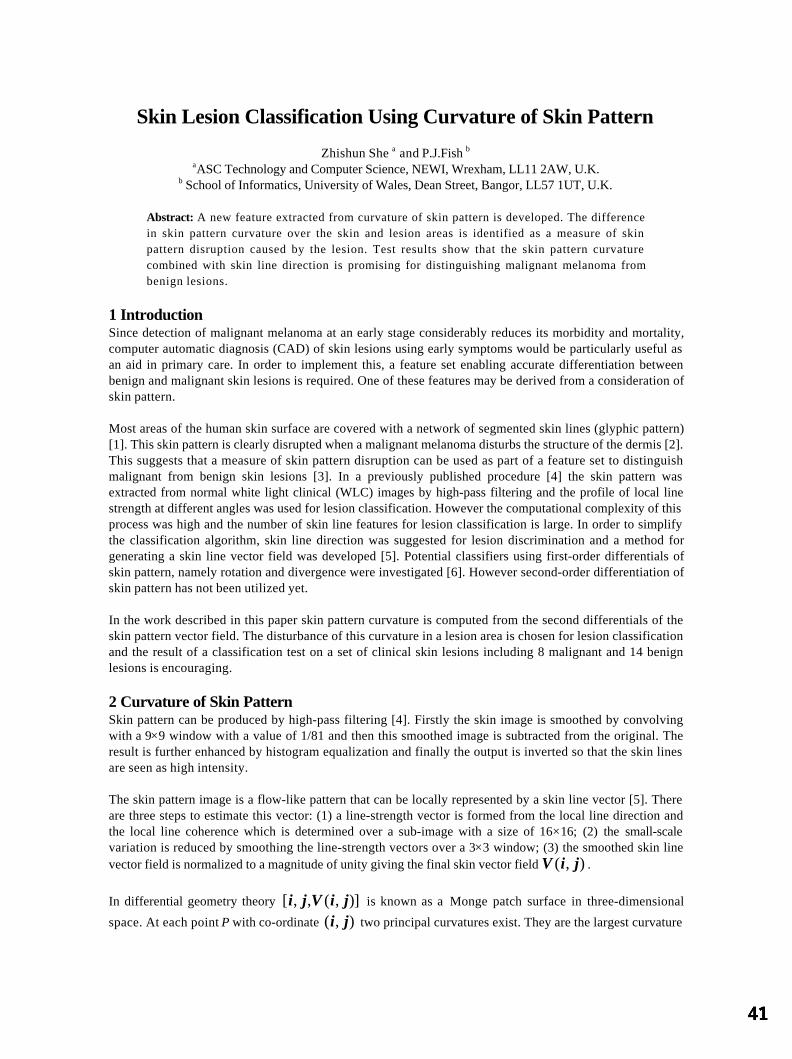
Skin Lesion Classification Using Curvature of Skin Pattern

Zhishun She a and P.J.Fish baASC Technology and Computer Science, NEWI, Wrexham, LL11 2AW, U.K.

b School of Informatics, University of Wales, Dean Street, Bangor, LL57 1UT, U.K.

Abstract: A new feature extracted from curvature of skin pattern is developed. The differencein skin pattern curvature over the skin and lesion areas is identified as a measure of skinpattern disruption caused by the lesion. Test results show that the skin pattern curvaturecombined with skin line direction is promising for distinguishing malignant melanoma frombenign lesions.

1 IntroductionSince detection of malignant melanoma at an early stage considerably reduces its morbidity and mortality,computer automatic diagnosis (CAD) of skin lesions using early symptoms would be particularly useful asan aid in primary care. In order to implement this, a feature set enabling accurate differentiation betweenbenign and malignant skin lesions is required. One of these features may be derived from a consideration ofskin pattern.

Most areas of the human skin surface are covered with a network of segmented skin lines (glyphic pattern)[1]. This skin pattern is clearly disrupted when a malignant melanoma disturbs the structure of the dermis [2].This suggests that a measure of skin pattern disruption can be used as part of a feature set to distinguishmalignant from benign skin lesions [3]. In a previously published procedure [4] the skin pattern wasextracted from normal white light clinical (WLC) images by high-pass filtering and the profile of local linestrength at different angles was used for lesion classification. However the computational complexity of thisprocess was high and the number of skin line features for lesion classification is large. In order to simplifythe classification algorithm, skin line direction was suggested for lesion discrimination and a method forgenerating a skin line vector field was developed [5]. Potential classifiers using first-order differentials ofskin pattern, namely rotation and divergence were investigated [6]. However second-order differentiation ofskin pattern has not been utilized yet.

In the work described in this paper skin pattern curvature is computed from the second differentials of theskin pattern vector field. The disturbance of this curvature in a lesion area is chosen for lesion classificationand the result of a classification test on a set of clinical skin lesions including 8 malignant and 14 benignlesions is encouraging.

2 Curvature of Skin PatternSkin pattern can be produced by high-pass filtering [4]. Firstly the skin image is smoothed by convolvingwith a 9×9 window with a value of 1/81 and then this smoothed image is subtracted from the original. Theresult is further enhanced by histogram equalization and finally the output is inverted so that the skin linesare seen as high intensity.

The skin pattern image is a flow-like pattern that can be locally represented by a skin line vector [5]. Thereare three steps to estimate this vector: (1) a line-strength vector is formed from the local line direction andthe local line coherence which is determined over a sub-image with a size of 16×16; (2) the small-scalevariation is reduced by smoothing the line-strength vectors over a 3×3 window; (3) the smoothed skin linevector field is normalized to a magnitude of unity giving the final skin vector field ),( jiV .

In differential geometry theory )],(,,[ jiVji is known as a Monge patch surface in three-dimensional

space. At each point P with co-ordinate ),( ji two principal curvatures exist. They are the largest curvature

),(max jiK and the smallest curvature ),(min jiK . One curvature measure is often used because of its

useful invariant property. It is the Gaussian curvature ),(),(),( maxmin jiKjiKjiK = . For a Monge

patch surface representation, the Gaussian curvature is given by [7]

222

2

)],(),(1[

),(),(),(),(

jiVjiV

jiVjiVjiVjiK

ji

ijjjii

++

−= (1)

where ),( jiVi , ),( jiV j , ),( jiVii , ),( jiVij and ),( jiV jj are the partial derivatives of ),( jiV .

Figure 1 shows, from top to bottom, the original image, skin pattern, and skin vector image with lesionboundary. The left image is that of a benign naevus. The right image is that of a malignant melanoma. Itindicates the disruption of skin pattern by a malignant rather than a benign lesion.

3 Feature ExtractionThe skin pattern curvature represents the variation of skin line direction and the disruption of skin patternshould be apparent from the change of skin pattern curvature. We therefore take the difference of theaverage skin pattern curvature in the skin and lesion areas as a straightforward measure of skin patterndisruption produced by the lesion. A snake-based edge detection technique is used to determine the lesionboundary [8]. The detected boundary segments the image into skin area sA and lesion area lA . The

average skin pattern curvatures in the skin and lesion areas are calculated by

∑∈

=sAjis

s jiKN

m),(

),(1

(2)

and

∑∈

=lAjil

l jiKN

m),(

),(1

, (3)

respectively, where sN and lN are the number of sub-images in the skin and lesion areas. The absolute

difference between sm and lm is used for lesion differentiation. Table 1 shows the mean of skin pattern

curvature over skin and lesion areas and their difference for the two examples of skin lesion as shown infigure 1, suggesting that the difference in skin pattern curvature between skin and lesion might well be auseful classifier.

4 Classification ResultsThe image set used in the experimental test of this technique contains 8 melanomas and 14 compound orjunctional naevi. The original images were in 24-bit full colour digital format and were converted to grey-level to produce 230×350 pixel source images.

The means of skin pattern curvature for skin and lesion areas and their difference were calculated and thedistribution of the skin pattern curvature difference is shown in figure 2. As expected, there is a tendency toa greater skin pattern curvature deviation in the maliganant melanoma images compared to that in the benignlesion images leading to the conclusion that this could be a useful addition to a diagnostic feature set.

Feature of skin pattern curvature is combined with that of skin line direction [5] to enhance the classificationaccuracy. The scatter-plot of 22 skin lesions in the two-dimensional feature (skin line direction and skinpattern curvature) space is given in figure 3 which demonstrates that malignant lesions usually have greaterdisturbances in skin line direction and skin pattern curvature and thus they can be discriminated frombenign lesions. A receiver operating characteristic (ROC) curve using skin pattern direction and curvaturewas shown in figure 4 where the area under the curve is approximately 0.92, indicating an encouragingclassification result.

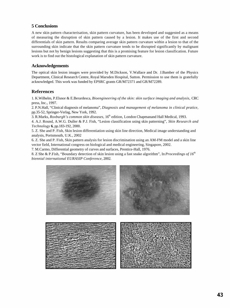
5 ConclusionsA new skin pattern characterisation, skin pattern curvature, has been developed and suggested as a meansof measuring the disruption of skin pattern caused by a lesion. It makes use of the first and seconddifferentials of skin pattern. Results comparing average skin pattern curvature within a lesion to that of thesurrounding skin indicate that the skin pattern curvature tends to be disrupted significantly by malignantlesions but not by benign lesions suggesting that this is a promising feature for lesion classification. Futurework is to find out the histological explanation of skin pattern curvature.

AcknowledgementsThe optical skin lesion images were provided by M.Dickson, V.Wallace and Dr. J.Bamber of the PhysicsDepartment, Clinical Research Centre, Royal Marsden Hospital, Sutton. Permission to use them is gratefullyacknowledged. This work was funded by EPSRC grants GR/M72371 and GR/M72289.

References1. K.Wilhelm, P.Elsnor & E.Berardesca, Bioengineering of the skin: skin surface imaging and analysis, CRCpress, Inc., 1997.2. P.N.Hall, “Clinical diagnosis of melanoma”, Diagnosis and management of melanoma in clinical pratice,pp.35-52, Springer-Verlag, New York, 1992.3. R.Marks, Roxburgh’s common skin diseases, 16th edition, London Chapmanand Hall Medical, 1993.4. A.J. Round, A.W.G. Duller & P.J. Fish, “Lesion classification using skin patterning”, Skin Research andTechnology 6, pp.183-192, 2000.5. Z. She and P. Fish, Skin lesion differentiation using skin line direction, Medical image understanding andanalysis, Portsmouth, U.K., 20026. Z. She and P. Fish, Skin pattern analysis for lesion discrimination using an AM-FM model and a skin linevector field, International congress on biological and medical engineering, Singapore, 2002.7. M.Carmo, Differential geometry of curves and surfaces, Prentice-Hall, 1976.8. Z She & P.Fish, “Boundary detection of skin lesion using a fast snake algorithm”, In Proceedings of 16th

biennial international EURASIP Conference, 2002.

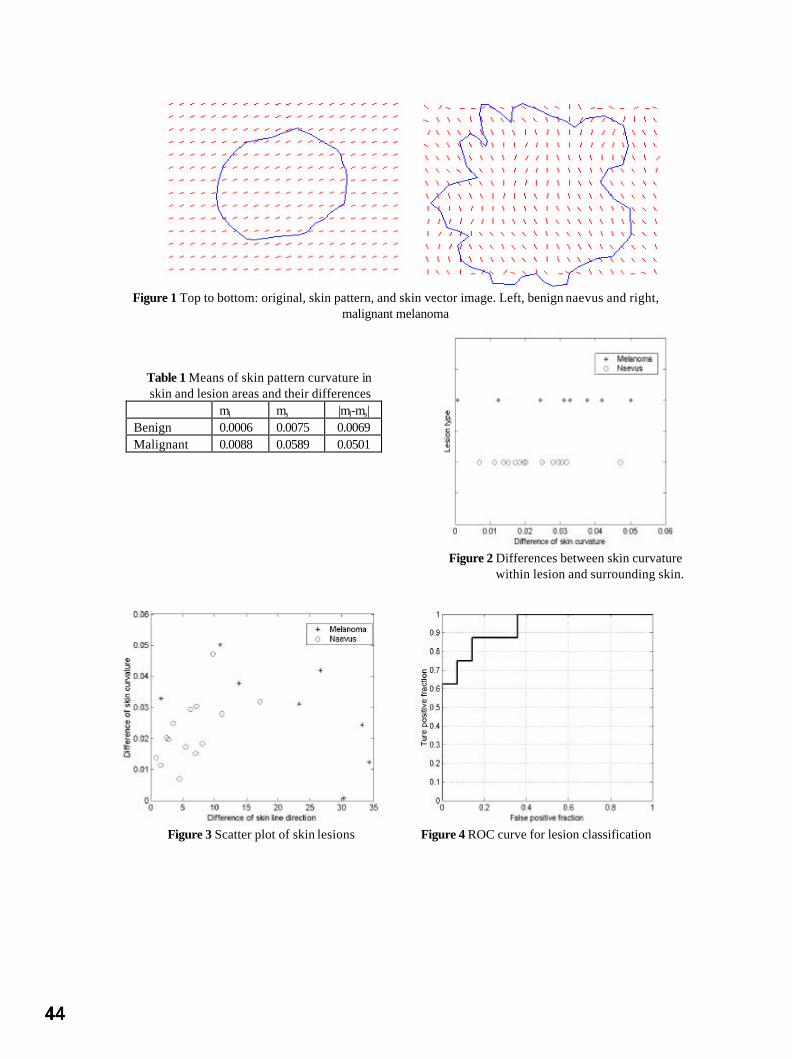
Figure 1 Top to bottom: original, skin pattern, and skin vector image. Left, benign naevus and right,

malignant melanoma

Table 1 Means of skin pattern curvature inskin and lesion areas and their differences

ml ms |ml-ms|Benign 0.0006 0.0075 0.0069Malignant 0.0088 0.0589 0.0501

Figure 2 Differences between skin curvaturewithin lesion and surrounding skin.

Figure 3 Scatter plot of skin lesions Figure 4 ROC curve for lesion classification

Registration of ultrasound breast images acquired froma conical geometry

J A Shipley 1, F A Duck 1, B T Thomas 2

1. Medical Physics Department, Royal United Hospital, Bath, BA1 3NG, UK.2. Computer Science Department, Bristol University, Bristol, BS8 1UB, UK.

Abstract

A system to acquire 3D ultrasound datasets of a patient’s breast is under development. Setsof in vivo images have been acquired by capturing images from radial planes as aconventional transducer is mechanically rotated about a cone encapsulating the breasttissue. Each set corresponds to rotating the transducer at a different, fixed, distance fromthe apex of the cone, chosen so that the volume of tissue imaged at one position overlapsslightly with the next, to allow for subsequent image registration. This paper addresses theproblem of registering pairs of these datasets, accounting for tissue motion during theacquisition.The technique developed is applied to the acquired data at reduced resolution. The datasetfrom closer to the apex of the cone is divided into non-overlapping subsets. Each subset iscomposed of narrow image strips perpendicular to the skin surface, taken from severaladjacent images. The normalized cross-correlation between each of these subsets,displaced to possible positions in the dataset further from the apex, is calculated.Correlation information for each subset is combined with knowledge of the relative locationsof the subsets, within an iterative Bayesian framework, to estimate the most likelydisplacement of each subset. In the region of overlap, all the subsets from one locationacross the width of the original images are selected. The displacement of each subset inthis line is used to define the seam between the two datasets, and this information is used tojoin the two sets together, without overlap, at full resolution.

1. Method

Present 2D ultrasound imaging technology generates cross sectional images of limited area. Inorder to build extended 3D datasets from such 2D images accurate registration techniques basedupon the image content will, in general, be required. This work addresses this problem in aspecific anatomical and geometrical context, but the techniques developed are applicable to thegeneral problem of reconstructing 3D ultrasound datasets. The advantage of a 3D dataset of thecomplete patient’s breast is increased tissue interaction and localisation information. Automationreduces operator dependence and increases repeatability. It is crucial that the imaging systemachieves high quality images, and also important that the breast tissue is not significantlydistorted from its natural shape as this would disguise tissue architecture changes which candiscriminate different disease states. These reasons underpin our choice of a conical scanninggeometry, with the transducer held parallel to the skin surface.

A mechanical system has been designed andbuilt to allow automated acquisition ofultrasound images of a patient's breast1 (fig.1). The system requires the patient to lieprone, and a cone is fitted around the breast,to stabilise the mobile tissue. The cone ispositioned to hold the nipple at the apex, withthe breast walls pushed gently against thesides, and a coupling medium preventing anyair gaps. The cone contains a cling filmwindow running from the apex to the rim. Aconventional ultrasound linear array is held at a fixed position along this window, its scan planein the radial direction. The entire mechanism, including cone and transducer is rotated by a

Figure 1. Image acquisition system

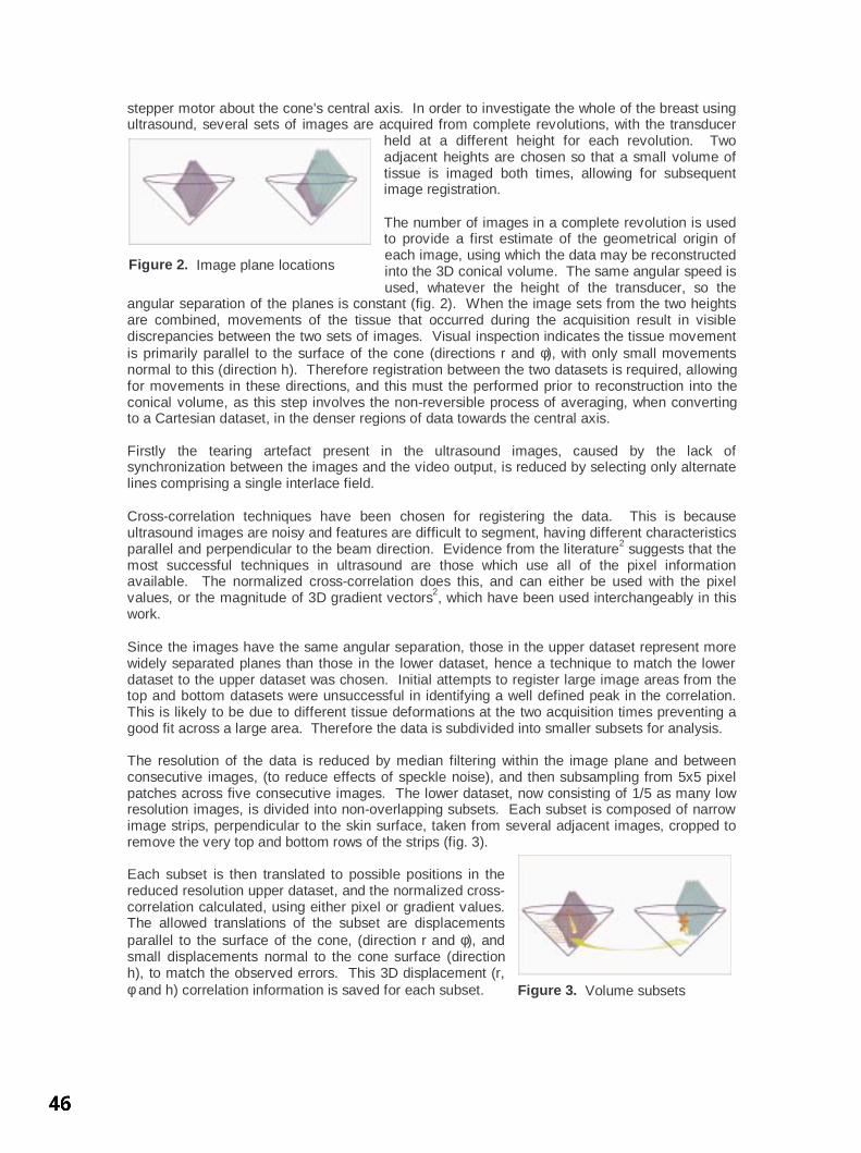
Figure 3. Volume subsets

Figure 2. Image plane locations

stepper motor about the cone's central axis. In order to investigate the whole of the breast usingultrasound, several sets of images are acquired from complete revolutions, with the transducer

held at a different height for each revolution. Twoadjacent heights are chosen so that a small volume oftissue is imaged both times, allowing for subsequentimage registration.

The number of images in a complete revolution is usedto provide a first estimate of the geometrical origin ofeach image, using which the data may be reconstructedinto the 3D conical volume. The same angular speed isused, whatever the height of the transducer, so the

angular separation of the planes is constant (fig. 2). When the image sets from the two heightsare combined, movements of the tissue that occurred during the acquisition result in visiblediscrepancies between the two sets of images. Visual inspection indicates the tissue movementis primarily parallel to the surface of the cone (directions r and φ), with only small movementsnormal to this (direction h). Therefore registration between the two datasets is required, allowingfor movements in these directions, and this must the performed prior to reconstruction into theconical volume, as this step involves the non-reversible process of averaging, when convertingto a Cartesian dataset, in the denser regions of data towards the central axis.

Firstly the tearing artefact present in the ultrasound images, caused by the lack ofsynchronization between the images and the video output, is reduced by selecting only alternatelines comprising a single interlace field.

Cross-correlation techniques have been chosen for registering the data. This is becauseultrasound images are noisy and features are difficult to segment, having different characteristicsparallel and perpendicular to the beam direction. Evidence from the literature2 suggests that themost successful techniques in ultrasound are those which use all of the pixel informationavailable. The normalized cross-correlation does this, and can either be used with the pixelvalues, or the magnitude of 3D gradient vectors2, which have been used interchangeably in thiswork.

Since the images have the same angular separation, those in the upper dataset represent morewidely separated planes than those in the lower dataset, hence a technique to match the lowerdataset to the upper dataset was chosen. Initial attempts to register large image areas from thetop and bottom datasets were unsuccessful in identifying a well defined peak in the correlation.This is likely to be due to different tissue deformations at the two acquisition times preventing agood fit across a large area. Therefore the data is subdivided into smaller subsets for analysis.

The resolution of the data is reduced by median filtering within the image plane and betweenconsecutive images, (to reduce effects of speckle noise), and then subsampling from 5x5 pixelpatches across five consecutive images. The lower dataset, now consisting of 1/5 as many lowresolution images, is divided into non-overlapping subsets. Each subset is composed of narrowimage strips, perpendicular to the skin surface, taken from several adjacent images, cropped toremove the very top and bottom rows of the strips (fig. 3).

Each subset is then translated to possible positions in thereduced resolution upper dataset, and the normalized cross-correlation calculated, using either pixel or gradient values.The allowed translations of the subset are displacementsparallel to the surface of the cone, (direction r and φ), andsmall displacements normal to the cone surface (directionh), to match the observed errors. This 3D displacement (r,φ and h) correlation information is saved for each subset.

Figure 4.Adjacent subsets

Figure 5. Seam

Figure 6. Registered images

The repeating nature of structures within the breast tissue result in small datasets fitting inseveral different places. Therefore there is a need to incorporate the knowledge of the relativepositions of each of the subsets. This is done within a Bayesian framework, following theexample of Noble etal.3 and Hayton et al.4.

Firstly the rigid displacement between the two datasets is calculated, by averaging together thecorrelation information from all the subsets. This is taken as the initial estimate for thedisplacement of every subset.

The knowledge that a particular displacement is unlikely unless adjacentsubsets also show a fit at a similar position is incorporated. Therefore the r,h and φ displacement correlation information for each subset is taken, andmodified according to the last estimates of the displacement in that subsetand in the four immediately adjacent subsets (fig. 4). Gaussian distributions(r, h, and φ steps taken as unit steps for the Gaussian), centred at each ofthese five current estimated fit positions, and weighted by the cross-correlation at that position, are added together, along with a non zerobackground probability. This summed probability is used to multiply thecentral subset's 3D displacement correlation information. A new estimate ofthe displacement for the central subset is taken as the most likely value in this modifiedcorrelation information. This process of updating the correlation information according to thecurrent estimated displacements, and then updating the estimate, is iterated through until thegreatest change in the estimated displacement for any subset is less than a threshold value.

In the region of the overlap the subsets have well defined estimateddisplacements. All the subsets from one location across the width of theoriginal images in this region are selected, i.e. a circle of subsets around thecone. The displacement of these selected subsets are used to define theseam between the two datasets (fig. 5). The pixels up to this seam from thelower datasets are joined with the pixels in the upper dataset above thisseam. Interpolation is used to estimate the displacements for the fullresolution images and then the nearest radial plane selected.

2. Results

The algorithm has been run on a small sample ofpatient datasets, and promising results obtained.

Figure 6 shows an example of the output of thealgorithm, showing the registered images on the left,and just the upper image from an adjacent radial planeon the right. It demonstrates that overall there is agood fit, although small discrepancies are visiblealong the fit line.

3. Discussion

The use of the iterative Bayesian approach has made a technique which is noise tolerant androbust, and able to non-rigidly register the two sets of ultrasound data together.

Low resolution images have been used in this work. One aim of this is to reduce the effects ofspeckle noise. The speckle is a high amplitude high frequency noise artefact, inherently presentin ultrasound imaging. The precise pattern is critically dependent on the path of the ultrasoundthrough the tissue, and so exactly the same pattern would not be expected when imaging the

same tissue region on the two separate occasions. Therefore we wish to decrease the effects ofspeckle, but without losing sharpness. The approach taken uses a median filter and thensubsamples the data. An additional advantage of this is the reduction in the size of the datasetsand hence the computational requirements.

Further simplification has been added to limit the degrees of freedom of movement allowedwhen fitting the data. Inspection of the datasets indicated that movement of tissue between thetwo scanning times generally occurred parallel to the surface of the cone, with only smallmovements perpendicular to this. Therefore the subsamples are allowed to move more widely inthe former plane, with separate datasets being defined every five pixels in the r and φ directions,and only small movements in the latter direction, (h), with no division into separate datasets inthis direction.

The calculated displacements between the datasets are based on the low resolution images, andso errors of the order of five pixels are expected. Therefore the two sets of data are cropped andjoined at a seam, to avoid the blurring effect which would be created if the data was overlappedand averaged (compounded). This is an unusual approach to take in ultrasound wherecompounding is popular due to its value in reducing noise and artefacts.

The next step will be to implement a similar technique on the higher resolution images, startingfrom the fit position determined from the low resolution data. To remain robust against noise,especially speckle noise, a similar iterative Bayesian technique will be appropriate. However,when aiming for the higher level of accuracy, deformation in the h direction will becomesignificant. This could in principle be allowed for by extending the technique to subdivide thedata in the h direction, although this would increase the complexity significantly.

Currently the performance of the algorithm has to be assessed by visual inspection. However,the correlation information measured during the processing will provide a good source of datafrom which to determine how successful the registration has been. A quality factor could beautomatically derived from this data to indicate confidence in the processing for a specific pair ofimage datasets. This will be available to the clinician, for whom it is crucial to know how muchthey can rely on the accuracy of the data presented to them. This is especially the case in breastdisease, where if the registration has been performed incorrectly a small diseased region couldbe entirely excluded from the image.

In the context of this project there are two remaining registration challenges. The first is toregister data from the start and end of the transducer revolution. The second is to correct forrefraction and depth errors, caused by sound speed variations, which result in a misalignment ofthe images where they overlap each other around the central axis of the cone. The capability ofthe registration technique described to resolve these discrepancies will be explored.

Acknowledgement

This project is supported by Department of Health NEAT award A126.

References

1 JA Shipley, FA Duck ,DA Goddard, MR Hillman, M Halliwell, 2002. An automated quantitative volumetricbreast ultrasound data acquisition system. Proc UK Radiology Congress 2002:18.2 R. Rohling, A. Gee and L. Berman. Automatic registration of 3-D ultrasound images. UltrasoundMedicine Biol 24:841-854.3 J. Alison Noble, Dana Dawson, Jonathan Lindner, Jiri Sklenar, Sanjiv Kaul. Automated nonrigidalignment of clinical myocardial contrast echocardiography image sequences: comparison with manualalignment. Ultrasound Med Biol 28:115-123.4 Paul M Hayton, Michael Brady, Stephen M Smith, Niall Moore, 1999. A non-rigid registration algorithmfor dynamic breast MR images. Artificial Intelligence 114:125-156.

Colour normalisation of retinal images

Keith A Goatmana∗, A David Whitwama, A Manivannana, John A Olsonb, and Peter F Sharpa

aDepartment of Bio-Medical Physics and Bioengineering, Aberdeen University andbEye Clinic, Aberdeen Royal Infirmary, Foresterhill, Aberdeen, AB25 2ZD

Abstract. The development of a nationwide eye screening programme for the detection of diabetic retinopathyhas generated much interest in automated screening tools. Currently most such systems analyse only intensityinformation — discarding colour information if it is present. Including colour information in the classifica-tion process is not trivial; large natural variations in retinal pigmentation result in colour differences betweenindividuals which tend to mask the more subtle variation between the important lesion types. This study inves-tigated the effectiveness of three colour normalisation algorithms for reducing the background colour variationbetween subjects. The normalisation methods were tested using a set of colour retinal fundus camera imagescontaining four different lesions which are important in the screening context. Regions of interest were drawnon each image to indicate the different lesion types. The distribution of chromaticity values for each lesiontype from each image was plotted, both without normalisation and following application of each of the threenormalisation techniques. Histogram specification of the separate colour channels was found to be the mosteffective normalisation method, increasing the separation between lesion type clusters in chromaticity spaceand making possible robust use of colour information in the classification process.

1 Introduction

Diabetic retinopathy is currently the major cause of blindness in the UK working-age population. The fact thatblindness can usually be delayed and often prevented, providing the disease is caught sufficiently early, has recentlyprompted the establishment of a nationwide screening programme. Since approximately 2% of the populationare diabetic, and annual screening has been recommended, the screening programme will generate a very largenumber of images for analysis. It is therefore not surprising that interest in automated screening techniques [1–3]has increased rapidly in the last few years. However, despite high resolution colour cameras being the acceptedstandard for screening programmes, automated software tends currently to base its analysis on intensity informationalone, either from ‘red-free images’ or using the green channel of RGB colour images. More than a decade agoGoldbaum et al. (1990) [4] showed significant differences in the colour measurements of lesions in retinal images.Since then little interest has been shown in colour classification of retinal images. In practice, while models existto identify abnormal coloured objects within the retinal image [5,6], without some form of colour normalisation oradaptation for the background pigmentation the large variation in natural retinal pigmentation across the populationconfounds discrimination of the relatively small variations between the different lesion types.

The human visual system is a poor spectral analyser; our perception of colour is based on the responses of onlythree receptor types sensitive to three bands of wavelengths. The consequence of this is that widely differingspectra produce the exactly the same colour perception. Colour cameras also use only three receptors, since thisis all that is required to match human perception of colour. Given the remitted spectrum it is possible to calculatethe red, green and blue colour channels values. However the inverse problem is hugely under-determined, hencechanges which may be deduced using a multi-channel spectrum analyser will not necessarily be detectable usingonly three colour sensors. A feature of human vision is that it adapts automatically and subconsciously to relativelylarge changes in the illuminating spectrum so that white objects are still perceived as being white. A similar effectis seen, for instance, if an image is projected onto a screen which is cream coloured; white objects in the projectedimage are still perceived as being white. This process is known as colour constancy. In contrast to human vision,colour cameras do not adapt automatically to changes in illumination. The lesion colour measured by the cameradepends on:

1. Lesion composition: All the lesions are composed of different materials with different reflection, absorption,and scattering properties.

2. Lesion density: All lesions vary in their size and thickness. The density of the lesion controls how muchlight is transmitted/reflected by the lesion (i.e. the colour can vary from the pure lesion colour to almost theretinal background colour).

∗Email: [email protected]

3. Scattered/reflected light: The colour and intensity of light scattered and/or reflected within the retina itself(probably negligible in a healthy, bleached retina) and the orbit.

4. Lens colouration: The lens becomes increasingly yellow (absorbing blue wavelengths) with age abovearound 30 years.

Note that all the lesions, except drusen, are positioned in front of all the pigmented retinal tissue (i.e. in front ofthe RPE, choroid and photoreceptors). All the lesions are of a similar colour and occupy a relatively small area ofthe complete colour space.

2 Method

Three colour normalisation algorithms originally intended for making colour images invariant with respect to thecolour of the illumination were investigated for their ability to make the retinal images invariant with respect tobackground pigmentation variation between individuals. Colour normalisation does not aim to find the true objectcolour, but to transform the colour so as to be invariant with respect to changes in the illumination — withoutlosing the ability to differentiate between the objects of interest. The three methods tested were:

1. Greyworld: The greyworld normalisation assumes that changes in the illuminating spectrum may be mod-elled by three constant multiplicative factors applied to the red, green, and blue channels. Since the meanvalues of the red, green, and blue channels will be multiplied by the same constants dividing each colourchannel by the respective mean value removes the dependence on the multiplicative constant. An itera-tive variation of the greyworld normalisation [7] (which includes intensity normalisation) was not found toperform significantly better.

2. Histogram equalisation: Histogram equalisation of the individual red, green, and blue channels representsa more powerful normalisation transformation than the greyworld method [8]. It is based on the observationthat for each colour channel pixel rank order is maintained under different illuminants, i.e. if under oneilluminant the red values of two pixels are r1 and r2, where r1 < r2, then under another illuminant, althoughthe magnitudes of r1 and r2 may change, r1 should still be less than r2 (there are, however, some conditionswhere this will not be true). Histogram equalisation is a non-linear transform which maintains pixel rankand is capable of normalising for any monotonically increasing colour transform function. The proportionof the different tissue types must be similar in all images to be normalised. Equalisation tends to exaggeratethe contribution of the blue channel (the normal retina reflects little blue light).

3. Histogram specification: Histogram specification [9] transforms the red, green, and blue histograms tomatch the shapes of three specific histograms, rather than simply equalising them. This has the advantage ofproducing more realistic looking images than those generated by equalisation, and it does not exaggerate thecontribution of the blue channel. For this study the reference histograms were taken from an arbitrary normalimage with good contrast and coloration. Histogram specification has been used before for normalisingretinal colour to aid the detection of hard exudates [10].

In order to compare the normalisation methods a dataset of 18 colour retinal fundus camera images was com-piled, where each image was known to contain at least one of the following lesion types which are important forretinopathy screening:

• Cotton wool spots (CWS): Swelling of the nerve fibre layer axoplasm in response to retinal ischaemia,transforming it from transparent to highly reflective, appearing bright (slightly blue) white. They can be verydense (for instance they may completely block fluorescence emanating from beneath them in an angiogram).They have ill-defined edges (hence their name). They usually disappear spontaneously after around 8 weeks.

• Hard exudates (HE): Lipid deposits in the inner nuclear layer as a result of vascular leakage. They arehighly reflective and appear bright yellow, often with a distinctive spatial distribution.

• Blot haemorrhages (BH): Leakage of blood in the inner nuclear layer. They appear dark red.

• Drusen: Debris deposited below the retinal epithelium layer (RPE) and collected in Bruch’s membrane dueto the turnover of retinal receptor pigments. They appear yellow. Although not related to diabetic retinopathy(they are more commonly associated with age related macular degeneration) they have a similar appearanceto HE and are therefore a confounding factor in the identification of HE.

The images were acquired using a Topcon fundus camera and recorded on 35 mm colour slide film. The imageswere digitised (approx. 1000 dpi) using a Nikon Coolscan 4000ED slide scanner, producing RGB colour imageswith 8 bits per colour channel. The retinal images are circular; masks were generated automatically by simplethresholding of the green colour channel followed by 5 × 5 median filtering to exclude the dark background fromthe colour normalisation calculations. Regions of interest were drawn around the different lesions for all the imagesand masks produced with a specific greylevel value representing each lesion type. Five of the images containedCWS, fourteen contained HE, and six contained BH. Only two of the images contained drusen. The same regionof interest masks were used to analyse the images before and after normalisation.

Colour may be represented independently of its intensity by dividing the red, green and blue channel values by thesum of the three channels, i.e.

r = R/(R +G + B), g = G/(R +G + B), b = B/(R +G + B)

This reduces the three-dimensional RGB colour space cube to a two-dimensional triangular space (since the thirdordinate is always one minus the sum of the other two). The resulting intensity normalised coordinates are knownas chromaticity coordinates. For each image the average chromaticity coordinate for each lesion type present wascalculated. In the chromaticity space, a line between any two points passes through all the colours which may beformed by mixing the colours represented by the end points. In this application the lesion colour may vary frompure lesion almost to the background colour so the different lesion types are expected to radiate from the region ofthe chromaticity space which represents the background colouration.

3 Results

Figure 1(a) plots the average lesion colours in each image without any normalisation. The ellipses shown arecentred on the mean position for each lesion type, with the major axis aligned with the direction of maximumvariance (found using the Hotelling transform). The radius of the major axis represents two standard deviations inthe direction of that axis. The minor axis length represents two standard deviations in the orthogonal direction. Allfour lesion chromaticity values are seen to overlap. Figure 1(b) shows the effect of the greyworld normalisation,which partially separates the lesion clusters, in particular differentiating the haemorrhages. Figure 1(c) shows theresult of equalisation, which also differentiates the haemorrhages, but appears to increase the overlap in the otherlesion types. Finally the result following histogram specification is shown in figure 1(d), which shows the clearestseparation of the lesion clusters.

4 Conclusions

Three normalisation techniques were tested on a set of retinal images. Histogram specification was found to be themost effective normalisation method, improving the clustering of the different lesion types, removing at least someof the variation due to retinal pigmentation differences between individuals. Colour classification is not intendedto replace existing intensity-based classification but to augment it and improve overall classification accuracy.

It was not anticipated that histogram specification should perform so much better than equalisation. One possibleexplanation is the exaggerated contribution of the blue component following equalisation, which possibly losessubtle but important differences in the blue values due to equalisation quantisation.

An important question is whether the differences in retinal background pigmentation are modelled acceptably asa variation in the colour of the illumination. While this is a safe assumption for changes due to lens colouration(since all the incident and remitted light are so filtered), it is less so for background pigmentation changes sincenot all retinal tissues are equally affected (i.e. the only contribution for non-pigmented tissues such as the opticdisc and highly reflective lesions is from scattered and reflected light from pigmented tissue). Clearly the modelis inadequate for dealing with local pigmentation variations across an individual retina. However, despite thesereservations the results appear to show that an average correction is much better than applying no correction to theimages.

Variation in colour due to scattering in surrounding tissue and reflections within the orbit can be greatly reduced byimaging using a confocal scanning laser ophthalmoscope (SLO) rather than a fundus camera. Early results usingour colour SLO [11] appear to show much less variation in lesion chromaticity, resulting in less overlap betweenlesions even prior to normalisation.

0.1 0.2 0.3 0.4 0.5 0.6 0.7 0.8 0.9 10.05

0.1

0.15

0.2

0.25

0.3

0.35

0.4

0.45

0.5

r

g

Equalisation

CWSHEBHDRUSEN

0.55 0.6 0.65 0.7 0.75 0.80.18

0.2

0.22

0.24

0.26

0.28

0.3

0.32

0.34

0.36

r

g

Specification

CWSHEBHDRUSEN

0.3 0.4 0.5 0.6 0.7 0.8 0.9 10.15

0.2

0.25

0.3

0.35

0.4

r

g

Chromaticity

CWSHEBHDRUSEN

0.05 0.1 0.15 0.2 0.25 0.3 0.35 0.4 0.450.15

0.2

0.25

0.3

0.35

0.4

0.45

0.5

r

g

Greyworld

CWSHEBHDRUSEN

PSfrag replacements

(a) (b)

(c) (d)

Figure 1. Chromaticity plots: (a) No normalisation, (b) Greyworld normalisation, (c) Histogram equalisation, (d)Histogram specification.

References

1. J. H. Hipwell, F. Strachan, J. A. Olson et al. “Automated detection of microaneurysms in digital red-free photographs: adiabetic retinopathy screening tool.” Diabetic Medicine 17, pp. 588–594, 2000.

2. B. M. Ege, O. K. Hejlesen, O. V. Larsen et al. “Screening for diabetic retinopathy using computer based image analysisand statistical classification.” Computer Methods & Programs in Biomedicine 62, pp. 165–175, 2000.

3. C. Sinthanayothin, J. F. Boyce, T. H. Williamson et al. “Automated detection of diabetic retinopathy on digital fundusimages.” Diabetic Medicine 19, pp. 105–112, 2002.

4. M. H. Goldbaum, N. P. Katz, M. R. Nelson et al. “The discrimination of similarly colored objects in computer images ofthe ocular fundus.” Investigative Ophthalmology & Visual Science 31, pp. 617–623, 1990.

5. M. Hammer & D. Schweitzer. “Quantitative reflection spectroscopy at the human ocular fundus.” Physics in Medicine andBiology 47, pp. 179–191, 2002.

6. S. J. Preece & E. Claridge. “Monte Carlo modelling of the spectral reflectance of the human eye.” Physics in Medicineand Biology 47, pp. 2863–2877, 2002.

7. G. D. Finlayson, B. Schiele & J. Crowley. “Comprehensive colour image normalisation.” In Proceedings of the EuropeanConference on Computer Vision, pp. 475–490. Springer-Verlag, 1998.

8. S. H. Hordley, G. D. Finlayson, G. Schaefer et al. “Illuminant and device invariant colour using histogram equalisation.”Technical Report SYS-C02-16, UEA, 2002.

9. R. C. Gonzalez & R. E. Woods. Digital image processing. Prentice Hall, second edition, 2002.10. A. Osareh, M. Mirmehdi, B. Thomas et al. “Classification and localisation of diabetic-related eye disease.” In Proceedings

of the European Conference on Computer Vision, pp. 502–516. Springer-Verlag, 2002.11. P. Vieira, A. Manivannan, P. F. Sharp et al. “True colour imaging of the fundus using a scanning laser ophthalmoscope.”

Physiological Measurement 23, pp. 1–10, 2002.

Nonlinear fusion for enhancing Digitally Subtracted Angiograms

Robert J Kinga , Maria Petroub, Kevin Wellsa and Declan Johnsonc

a School of Electronics and Physical Sciences, University of Surrey, Guildford, GU2 7XHb Informatics and Telematics Institute, CERTH, PO Box 361, Thessaloniki, 57001, Greece

c Department of Neuroradiology, Atkinson Morley’s Hospital, Wimbledon, London, SW20 0NE

Abstract. The image quality of Digital Subtraction Angiograms (DSA) is limited by high image noise and poorcontrast of smaller vessels. In this paper we present a nonlinear data fusion system that combines the temporaland spatial information contained within a set of consecutive DSA frames, to provide an output which displaysenhanced contrast between vessel and background regions of the vascular tree. Results are compared againstthe mean and median averages of the set and the method is found to increase vessel contrast.

1 Introduction

Digital Subtraction Angiography (DSA) allows the visualisation of blood vessels via injection of contrast media.Often it is desirable to obtain a reference image which displays the vascular tree morphology, e.g. for use duringimage-guided catheter surgery. Images extracted from DSA sequences suffer from low signal-to-noise ratio andsmall blood vessels may appear particularly faint. In this paper we present a nonlinear data fusion system that com-bines information from a set of consecutive frames in a DSA sequence to provide an output frame with enhancedcontrast between vessel and background regions. This provides a better reference image and can also be used as aprecursor to subsequent segmentation.

Put simply, data fusion is the process of combining multiple sources of data. A good example of a data fusionarchitecture is provided by the brain. Data from several physical sensors (eyes, ears, haptic sensors etc.) arecombined with abstract information such as past experience, and processed to create a description of the localenvironment. Much research on data fusion has been carried out, e.g. for autonomous control for robots [1][2], automobiles [3] and other vehicles [4]. Data fusion is also being used for geoscience & remote sensingapplications [5] and medical imaging applications [6]. Image data for this work was obtained from a PhilipsIntegris fluoroscopy system, recorded onto DVCPRO format digital video tape via sampling of the video signalinput to the fluoroscopy system monitor. Our data “sources” are a set of frames ( pixel, 8-bit) takenfrom a DSA sequence showing the injection of contrast media into the bloodstream. The information extractedrepresents the distribution of X-ray transmission over the 2D imaging plane.

The methodology behind this fusion approach is based on the nonlinear fusion system proposed by Steinhage andassociates [7] [8] [9] [10]. The basis of the system is to represent physical measurements of the system (i.e. sensorreadings) as local stable points or “attractors” of a dynamic system [7]. The dynamics are solved iteratively usingthe Euler method to yield a representation (or “estimate”) of the physical state of the system. Prior to computation,we simplify the system by converting each 2D image into a one dimensional sequence using a Hilbert [11] scanpath.

2 Methodology

Nonlinear dynamics uses the principle of “attractors” [7], a local stable point in the derivative of the state variable with respect to position . An attractor has

and negative gradient such that if an attractor is

pushed slightly along the axis, the negative gradient will push the system back towards the stable point, correctingfor the slight perturbation. Conversely, a point with a positive gradient

is called a “repellor”, an unstable

point where a small perturbation will cause the state variable to move in the direction of the displacement.

! #" $&%')(+* ,-.0/21436587 (1)

where defines the attractor for a sensor which takes a measurement (pixel intensity value) of the system atposition . 9" $ is the state variable for which the derivative is being calculated, the X-ray transmission. is:Email: [email protected];On leave of absence from School of Electronics and Physical Sciences, University of Surrey

the position along the one dimensional sequence, thus #" $ is a function that describes how the pixel intensity

fluctuates along the 1D sequence. is a weighting factor which can be assumed to be unity. is the “width” of theattractor and determines the size of the basin of attraction created by the stable point. Because the width is finite,attractors have a finite region of influence, hence the term “local” stable point.

Computation uses a sliding window of frames, taken from the DSA injection sequence. Each 2D frameis converted into a one dimensional sequence using a Hilbert scan path [11]. This path maximises the time spentin local neighbourhoods within the image and so preserves spatial information more so than, for example, rasterscanning. Each position, , along the sequence records the value of X-ray transmission (via the grey-level intensity)at a certain location

" $ and time.

As the 1D sequences are traversed, a potential well function is computed at each pixel location. tells ushow quickly the value of

will move away from

( if changes by away from ( . This is formed on

the basis of sensor data (over the time period of frames) and also a priori knowledge. From initialisation with #" $ Median " $ " $ " $ % , the Euler method is used to solve the dynamics and yield an estimatefor

at each location within the frame.

! " ! $# %'& ! (" %'& ! (2) ) ! and %'& ! control the relative strengths of sensor and a priori knowledge contributions. The ratio *,+-*between these two terms was empirically found to provide the best image contrast. We now discuss the formationof

" ! and" %'& ! terms, the contributions from sensor readings and a priori knowledge.

2.1 Sensor contributions

The sensor contribution term (" ! ) in equation 2 takes the same form as equation 1," ! " $ . / " $ " ( $8%10325476 " $ #" ( $&% 8 9 (3)

where " $ is the reading of sensor : at position . #" ( $ is the nonlinear estimate for the state at the previousposition, ( . is the width of the attractor for sensor : and is its individual weighting. Given frames, wehave measurements at each position , with an attractor representing its grey-level intensity. These are summedto produce a potential at each pixel that is determined by the distribution of grey-level intensities at that locationin each frame. The summation process generally reduces the number of local stable points in the system. Whichof these points is selected at each iteration depends upon the previous estimate for the system. Thus the weakestattractor could be selected if it had the same location as the attractor from the previous step. However, if othersensors continued to add together to form a stronger attractor, this would soon influence the output more forcibly.

2.2 A priori knowledge contribution

The fusion scheme can be thought of as a weighted election, each frame effectively “voting” for a certain intensityvalue at each pixel. Given a set of frames in which contrast agent is flowing, pixels can have a range of values.High intensities correspond to background regions, low intensities may represent the presence of contrast agent- i.e. blood vessel. For a certain pixel location, if all frames record similar intensity values, the output will bea similarly valued estimate. However, consider the case where contrast agent reaches a pixel location within thetime period of interest. The set of frames will therefore have a mixed population of intensities. To enhance thevisibility of vessels we must favour low over high intensity values. This is achieved by using an a priori knowledgeterm that favours intensity values that are lower than the median," %'& ! " $ . / <; " $ >= " $&%?+ " $ = " $

+ otherwise(4)

" $ is the grey-level intensity value for pixel position and frame : . = " $ is the median pixel intensity atposition , = " $ Median " $ " $ " $ % .The " $ = " $ condition is required to avoid favouring intensities higher than the median and consequentlyfailing to trace vessels where the majority of the frames contain contrast agent. The term provides a sliding scale

of emphasis, the greater the distance from the median, the greater the influence. However, the system does notjump from one low intensity outlier to the next due to the calculation strategy which relies upon the past history ofthe system to help make decisions.

2.3 Results and Discussion

The right hand column of figure 1 shows the nonlinear output results produced from running the system with , ! * , & ! * , widths and normalised weights, increasing towards the end of the

set. These parameter values were found to provide the best image contrast defined by (

1 .

We compare these results with the mean and median averages, displayed in the left and centre columns of thefigure. Figure 2 plots vessel contrast (defined as against frame number. To produce this contrast measure, pixels

Mean Median Nonlinear

frame10

frame25

frame40

Figure 1. Mean, Median and nonlinear output frames for a set of frames, starting at frames 10, 25 and 40.For display purposes, only a centrally placed * >* pixel window is shown. All images are displayed usingthe same colourscale.

are classified as either vessel or background by a manually segmented mask. Figure 2 shows that for startingframes , the nonlinear method produces increased vessel contrast by enhancing each vessel as soon as itappears. The mean and median averages only increase the contrast significantly once the majority of frames inthe set record a high concentration of contrast media. Beyond , contrast within the nonlinear output fallsbelow that of the averages due to the contrast agent bolus moving out of the main vessel segments - see the lowerright image of figure 1.

Figure 2. Contrast measure versus frame number for nonlinear ( ), median ( ) and mean ( ) frames.

3 Conclusions

In this paper we have presented a nonlinear fusion system designed to enhance the contrast of vessels in DSAimages. Results presented are contrasted against the mean and median averages. The method is found to enhancethe visibility of blood vessels during the infusion of contrast agent.

Acknowledgements

This work was supported by EPSRC through a doctoral training grant. We would also like to acknowledge thegenerous support from the Royal Society/Wolfson Foundation for enabling this work.

References

1. A. Steinhage & R. Menzner. “Nonlinear attractor dynamics for guiding an anthropomorphic robot by means of speechcommands.” In Proceedings of the 7th International Symposium on Intelligent Robotic Systems, pp. 177–180. 1999.

2. A. Steinhage & G. Schoner. “Self-calibration based on invariant view recognition: Dynamic approach to navigation.” InRobotics and autonomous systems, volume 20. Elsevier Science, Amsterdam, 1997.

3. U. Handmann, T. Kalinke, C. Tzomakas et al. “An image processing system for driver assistance.” Image and VisionComputing 27, pp. 367–376, 2000.

4. S. Majumder, S. Scheding & H. F. Durrant-Whyte. “Multisensor data fusion for underwater navigation.” Robotics andAutonomous Systems 35, pp. 97–108, 2001.

5. L. See & R. J. Abrahart. “Multi-model data fusion for hydrological forecasting.” Computers and Geosciences 27, pp. 987–994, 2001.

6. S. Lai & M. Fang. “A hierarchical neural network algorithm for robust and automatic windowing of mr images.” ArtificialIntelligence in Medicine 19, pp. 97–119, 2000.

7. A. Steinhage. “Nonlinear attractor dynamics: A new approach to sensor fusion.” In Sensor fusion and decentralized controlin robotic systems II, volume 3839, pp. 31–42. Proceedings of the SPIE, SPIE publishing, 1999.

8. A. Steinhage, C. Winkel & K. Gorontzi. “Attractor dynamics to fuse strongly perturbed sensor data.” In IEEE 1999International Geoscience And Remote Sensing Symposum (IGARSS 1999), volume 2, pp. 1217–1219. 1999.

9. A. Steinhage & C. Winkel. “A robust, self-calibrating data fusion archetecture.” In IEEE 2000 International GeoscienceAnd Remote Sensing Symposum (IGARSS 2000), volume 3, pp. 963–965. 2000.

10. A. Steinhage & C. Winkel. “Dynamical systems for sensor fusion and classification.” In IEEE 2001 International Geo-science And Remote Sensing Symposum (IGARSS 2001), volume 2, pp. 855–857. 2001.

11. S. Kamata, R. O. Eason & E. Kawaguchi. “An implementation of the hilbert scanning algorithm and its applications to datacompression.” Institute of Electronics, Information and Communication Engineers (IEICE) Transactions on Informationand Systems 76(4), pp. 420–428, April 1993.

Characterising pattern asymmetry in pigmented skin lesions

Ela Claridge1, Jonathan Powell2 and Ahmet Orun1

1School of Computer Science, The University of Birmingham Birmingham, U.K. 2Department of Plastic Surgery, Addenbrooke’s Hospital, Cambridge, U.K.

Abstract. In clinical diagnosis of pigmented skin lesions asymmetric pigmentation is often indicative of melanoma. This paper describes a method and measures for characterizing lesion symmetry. The estimate of mirror symmetry is computed first for a number of axes at different degrees of rotation with respect to the lesion centre. The statistics of these estimates are the used to assess the overall symmetry. The method is applied to three different lesion representations showing the overall pigmentation, the pigmentation pattern, and the pattern of dermal melanin. The best measure is a 100% sensitive and 96% specific indicator of melanoma on a test set of 33 lesions, with a separate training set consisting of 66 lesions.

1. Introduction

In clinical diagnosis of pigmented skin lesions a lack of symmetry in the pattern of pigmentation deems the lesion suspicious. This association between asymmetry and malignancy is reflected in a number of scoring schemes in dermatology, such as the Seven-Point Checklist [1] and the American ABCDE list. In dermatoscopy clinicians are instructed to look out for asymmetry in the pattern of pigmentation and to distinguish it from asymmetry in lesion shape which is supposed to have little diagnostic value in this technique [2]. Most existing computer methods (e.g. [3]), however, concentrate on shape symmetry measures.

Human observers are known to be able to detect symmetric patterns with great ease, but are not so good at fine grading of the asymmetry [4]. They also tend to respond more to symmetry of shape than to symmetry of a co-existing pattern [4]. Our earlier study has shown that both the inter-observer and intra-observer repeatability are moderate (both around 65%) when assessing the symmetry of skin lesions [5]. These facts have motivated us to develop objective symmetry measures for pigmented skin lesions and to evaluate how well they correlate with histological diagnosis of a lesion as malignant melanoma and also with clinical assessment.

2. Methods and measures

Image analysis research has produced a number of methods for finding either the best or all axes of symmetry in images of potentially symmetric objects and patterns [6]. Many of these algorithms incorporate a means of comparing the degree of symmetry amongst a number of putative symmetry axes in order to select the best one. In this work we do not reject those inferior axes, but instead compute statistics related to all the putative axes. These statistics are then used as an indicator of the degree of symmetry. The hypothesis is that normal lesions would show the higher degree of symmetry than abnormal ones.

2.1 Finding the best symmetry axis

A measure by which the best symmetry axis can be found is based on the Smith & Jenkinson’s symmetry score [6]. Their algorithm also provides a method for finding and evaluating a number of putative symmetry axes.

For all possible orientations ϕi of the reflective symmetry axis, A(ϕi) For all lines B(r) perpendicular to the A(ϕi), placed at a distance r from the start of the axis A(ϕi) Compute symmetry scores, s(x), for each point x along B(r) Find the best centre of symmetry on B(r), i.e. point xp which has the best symmetry score, sr(xp) Add the best symmetry score (sr(xp)) to the total score S(ϕi,*) for axis A(ϕi), i.e. S(ϕi, xp) = S(ϕi, xp) + sr (xp) Find the maximum of all the scores in S(ϕi,*); The angle ϕi for which Si = maxi(S(ϕi,*) is the best axis of symmetry.

The symmetry score is computed using the following formula:

s(x) = ∑abs(Ix+i + Ix-i) - ∑abs(Ix+i - Ix-i) *

∑abs(Ix+i + Ix-i) + ∑abs(Ix+i - Ix-i) + g (1)

where Ix is the image value at position x along B(r). Parameters g and are derived from global and local contrast respectively and their role is to compensate for otherwise excessively high values of s(x) in uniform

areas of the image. Symmetry measures S(ϕi,*) are computed for 16 discrete orientations, i.e. i = 1, …, 16.

The original algorithm is designed to find the best axis of symmetry. In this work we are interested in estimating the degree of symmetry for the lesion. Therefore, in addition to choosing the axis with the largest score to be the symmetry axis, all the scores Si are retained, their features extracted and combined into a number of measures which characterise the lesion symmetry.

2.2 Symmetry scores and their properties

A useful analysis of the symmetry scores is carried out in the original article (figure 2 in [6]). The following features are associated with a good symmetry axis (see Figure 1, left): (1) the plot of the scores is unimodal, i.e. there is a single major peak in S(∗, x) (2) the higher the peak the better the underlying symmetry (3) the smaller the spread of the peak the better the underlying symmetry (4) the less skewed the peak, the better the underlying symmetry.

(a) (b)

Figure 1. (a) Two plots of S(∗, x) exemplifying poor and good symmetry scores; (b) The plot of one of the global symmetry indicators, d(ϕ) = stdev( S(ϕ, x) ).

Quantitative indicators corresponding to the above characteristics can be computed as follows: (1) u = | medianx( S(ϕ, x) ) - averagex( S(ϕ, x) ) | (2) m = maxx( S(ϕ, x) ) (3) d = stdevx( S(ϕ, x) ) (computed as though S(*,x) were a probability distribution) (4) k = | skew( S(ϕ, x) ) | (computed as though S(*,x) were a probability distribution)

In the above expressions, the perfect symmetry will yield u = 0, m = 1, d = 0 and k = 0.

2.3 Global symmetry measures

In the design of global symmetry measures the maximum score is assigned to a pattern showing “the repetition of exactly similar parts facing a centre” [The Concise Oxford Dictionary], i.e. a pattern with perfect rotational symmetry. In terms of the quantitative indicators u, m, d and k computed for each angle ϕ, i.e. u(ϕ), m(ϕ), d(ϕ) and k(ϕ), such pattern will attain the perfect symmetry scores for all the angles ϕ. Departures from symmetry will decrease the scores, thus the more symmetric the image, the more angles will show high scores. Based on this reasoning, the following global symmetry measures have been defined as follows:

av_m = averageϕ( m ) the higher av_m, the higher is the average symmetry score across all the angles, the better the overall symmetry

sd_m = sdϕ( m ) the higher sd_m the more variability in symmetry for different angles, the worse the overall symmetry

max_m = maxϕ( m ) the higher max_m the better the single mirror symmetry

av_d = averageϕ( d ) the higher av_d the greater the average spread of S(*,x), the less symmetric the pattern

min_d = minϕ( d ) the higher min_d the less symmetry shown by the best symmetry axis and thus by the pattern as a whole

max_d = maxϕ( d ) the higher max_d the less symmetry shown by the worst symmetry axis; low value indicates the overall good symmetry.

sd_d = sdϕ( d ) the higher sd_d the more variability in spread of S(ϕ,x) across different angles ϕ; this may indicate a highly asymmetric pattern if sd_m is high or max_m is low; or a pattern with at least one good mirror symmetry if max_m is high.

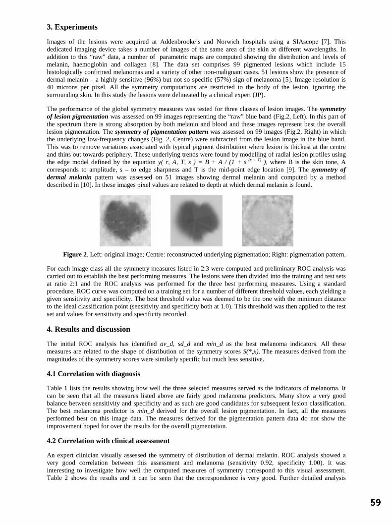
3. Experiments

Images of the lesions were acquired at Addenbrooke’s and Norwich hospitals using a SIAscope [7]. This dedicated imaging device takes a number of images of the same area of the skin at different wavelengths. In addition to this “raw” data, a number of parametric maps are computed showing the distribution and levels of melanin, haemoglobin and collagen [8]. The data set comprises 99 pigmented lesions which include 15 histologically confirmed melanomas and a variety of other non-malignant cases. 51 lesions show the presence of dermal melanin – a highly sensitive (96%) but not so specific (57%) sign of melanoma [5]. Image resolution is 40 microns per pixel. All the symmetry computations are restricted to the body of the lesion, ignoring the surrounding skin. In this study the lesions were delineated by a clinical expert (JP).

The performance of the global symmetry measures was tested for three classes of lesion images. The symmetry of lesion pigmentation was assessed on 99 images representing the “raw” blue band (Fig.2, Left). In this part of the spectrum there is strong absorption by both melanin and blood and these images represent best the overall lesion pigmentation. The symmetry of pigmentation pattern was assessed on 99 images (Fig.2, Right) in which the underlying low-frequency changes (Fig. 2, Centre) were subtracted from the lesion image in the blue band. This was to remove variations associated with typical pigment distribution where lesion is thickest at the centre and thins out towards periphery. These underlying trends were found by modelling of radial lesion profiles using the edge model defined by the equation y( r, A, T, s ) = B + A / (1 + s (r – T) ), where B is the skin tone, A corresponds to amplitude, s – to edge sharpness and T is the mid-point edge location [9]. The symmetry of dermal melanin pattern was assessed on 51 images showing dermal melanin and computed by a method described in [10]. In these images pixel values are related to depth at which dermal melanin is found.

Figure 2. Left: original image; Centre: reconstructed underlying pigmentation; Right: pigmentation pattern.

For each image class all the symmetry measures listed in 2.3 were computed and preliminary ROC analysis was carried out to establish the best performing measures. The lesions were then divided into the training and test sets at ratio 2:1 and the ROC analysis was performed for the three best performing measures. Using a standard procedure, ROC curve was computed on a training set for a number of different threshold values, each yielding a given sensitivity and specificity. The best threshold value was deemed to be the one with the minimum distance to the ideal classification point (sensitivity and specificity both at 1.0). This threshold was then applied to the test set and values for sensitivity and specificity recorded.

4. Results and discussion

The initial ROC analysis has identified av_d, sd_d and min_d as the best melanoma indicators. All these measures are related to the shape of distribution of the symmetry scores S(*,x). The measures derived from the magnitudes of the symmetry scores were similarly specific but much less sensitive.

4.1 Correlation with diagnosis

Table 1 lists the results showing how well the three selected measures served as the indicators of melanoma. It can be seen that all the measures listed above are fairly good melanoma predictors. Many show a very good balance between sensitivity and specificity and as such are good candidates for subsequent lesion classification. The best melanoma predictor is min_d derived for the overall lesion pigmentation. In fact, all the measures performed best on this image data. The measures derived for the pigmentation pattern data do not show the improvement hoped for over the results for the overall pigmentation.

4.2 Correlation with clinical assessment

An expert clinician visually assessed the symmetry of distribution of dermal melanin. ROC analysis showed a very good correlation between this assessment and melanoma (sensitivity 0.92, specificity 1.00). It was interesting to investigate how well the computed measures of symmetry correspond to this visual assessment. Table 2 shows the results and it can be seen that the correspondence is very good. Further detailed analysis

indicated that all the patterns considered highly asymmetric were also judged as such by the clinician. The same was the case for the least asymmetric patterns. In the “grey” area in between, computer measures tended to grade patterns as being more symmetric than the clinician did. This needs to be investigated further, for example to reject the possibility that the clinician would subconsciously assess the pattern less symmetric if there was other evidence indicating melanoma.

av_d sd_d min_d Symmetry of lesion pigmentation as melanoma predictor

Sens. Spec. Sens. Spec. Sens. Spec. training 0.70 0.78 0.60 0.71 0.80 0.80

test 0.80 0.75 0.80 0.75 1.00 0.96 all 0.73 0.78 0.67 0.71 0.80 0.82

Symmetry of the pigmentation pattern as melanoma predictor Sens. Spec. Sens. Spec. Sens. Spec.

training 0.80 0.79 0.70 0.78 1.00 0.73 test 0.80 0.71 1.00 0.61 0.80 0.67 all 0.87 0.76 0.80 0.71 0.93 0.69

Symmetry of dermal melanin as melanoma predictor Sens. Spec. Sens. Spec. Sens. Spec.

training 0.67 0.68 0.56 0.92 0.67 0.80 test 0.75 0.61 0.75 0.77 0.52 0.70 all 0.69 0.66 0.62 0.89 0.62 0.76

Table 1. Sensitivity and specificity of various measures as melanoma predictor for three types of image data.

Symmetry of dermal melanin av_d sd_d min_d Sens. Spec. Sens. Spec. Sens. Spec.

training 0.79 0.80 0.88 0.90 0.67 0.80 test 0.91 0.67 0.82 0.83 0.50 0.70 all 0.80 0.75 0.86 0.88 0.62 0.76

Table 2. The degree of correspondence between the clinical and the computer assessment of symmetry.

5. Conclusions

The measures designed to evaluate the overall symmetry of the lesion have been shown to perform well as melanoma indicators. They were also shown to correlate well with the clinical assessment of asymmetry of dermal melanin. Work is in progress to incorporate these measures into a classification scheme for differentiating between melanoma and other pigmented skin lesions. Acknowledgements

This work has been supported by EPSRC grant GR/M53035.

References

1. MacKie R (1985) An illustrated guide to the recognition of early malignant melanoma. Dept. of Dermatology, Glasgow. 2. Menzies S et al (1996) An Atlas of Surface Microscopy of Pigmented Skin Lesions: McGraw-Hill. 3. Stoecker et al (1992) Automatic detection of asymmetry in skin tumors. Comp Med Imaging and Graphics 16, 191-197. 4. Hibbin A (2001) Perception of natural symmetry: a comparison of human vision and a computer model. MSc Thesis,

School of Computer Science and Psychology, The University of Birmingham. 5. Moncrieff M, Cotton S, Claridge E and Hall PN (2002) Spectrophotometric Intracutaneous Analysis: a new technique

for imaging pigmented skin lesions. British Journal of Dermatology 146(3), 448-457. 6. Smith S, Jenkinson M (1999) Accurate robust symmetry estimation. Medical Image Understanding and Analysis 1999,

Hawkes D et al. (Eds.), 61-64. 7. http://www.siascope.com 8. Claridge E, Cotton S, Hall P, Moncrieff M (2002) From colour to tissue histology: Physics based interpretation of

images of pigmented skin lesions. Medical Image Computing and Computer-Assisted Intervention - MICCAI’2002. Dohi T and Kikinis R (Eds). LNCS 2488, vol I, 730-738: Springer.

9. Claridge E, Orun A (2002) Modelling of edge profiles in pigmented skin lesions. Medical Image Understanding and Analysis 2002, Houston A, Zwiggelaar R (Eds.), 53-56.

10. Cotton, S.D., Claridge, E., Hall, P.N. (1997) Noninvasive skin imaging. Information Processing in Medical Imaging, LNCS 1230, 501-507.

Automatic Construction of Statistical Shape Models for Protein SpotAnalysis in Electrophoresis Gels

Mike Rogersa∗ , Jim Grahama and Robert P. Tongeb

aImaging Science and Biomedical Engineering, University of Manchester,bProtein Science, Enabling Science and Technology (Biology), AstraZeneca,

Alderley Park, Macclesfield, Cheshire, UK.

Abstract. Proteomics research relies heavily on electrophoresis gels, which are complex images containingmany protein ‘spots’. The identification and quantification of these spots is a bottleneck in the proteomicsworkflow. We describe a statistical model of protein spot appearance that is both general enough to representunusual spots, and specific enough to introduce constraints on the interpretation of complex images. We proposea robust method of automatic model construction that is used to circumvent manual model construction whichis subjective and time-consuming. We show that the statistical model of spot appearance is able to fit to imagedata more closely than the commonly used spot parameterisations which are based solely on Gaussian anddiffusion formulations.

1 Introduction

Proteomics is the study of the complete set of proteins in a cell or organism throughout the entire life-cycle. It is hoped thatthis research will enhance understanding of cell function in general and, more specifically, it will also identify proteins thatcan be used as drug targets and disease markers. The main barrier to proteomics research is complexity. It is estimated thattotal number of proteins in a human cell could be as large as 500,000. Key to any analysis are separation and detectiontechnologies. A well-established and widely used technology is 2-Dimensional Electrophoresis (2-DE). This processseparates protein mixtures by iso-electric point (pI) and molecular weight (MW). Separation results from two separatediffusion processes which are driven along orthogonal axes in a polyacrimide gel, resulting in a grid of protein strains.The separated proteins are visualised by pre or post staining, yielding an image, containing protein ‘spots’. A segmentfrom such a 2-DE gel image is shown in figure 1. In practice, 3,000-4,000 spots can be visualised on a single gel image,each representing an individual protein strain. The analysis of these complex gel images is a significant bottleneck in theproteomics research workflow [1].

Image analysis of 2-DE gels requires the identification of a large number of individual spots. These must be characterisedfor further analysis of the sample. One of the first steps in any spot detection algorithm is the segmentation of individualspots from the background. After the segmentation step, spots are quantified and represented as a list of parameters overwhich further analysis can be carried out. Commonly, protein spot models are used to aid quantification by imposingconstraints, which in turn improves the robustness of the solution. The most commonly used spot model is a Gaussianfunction [2]. Figure 1(a) shows an example of a typical protein spot with a Gaussian profile. This model is assumed toprovide a good representation of most spots present in most gel images. However, it has been shown that Gaussian modelsproduce an inadequate fit to some protein spots, most notably large volume, saturated spots [3]. Figure 1(b) shows anexample of a high volume protein spot exhibiting a saturated, ‘flat-top’ shape. Bettens [3] addressed this shortcoming byproposing a model based on the physics of the spot formation. Protein spots are formed by a diffusion process, which isonly adequately represented by a Gaussian when the initial concentration distribution occupied by the sample has a smallarea. Bettens’ diffusion model more adequately represents spots in the gel when this assumption is not met.

Both the Gaussian and diffusion models assume perfect diffusion across the gel medium. Spots created by a perfectdiffusion process will be regular and symmetric. In practice, the diffusion process is not perfect and spots can be formedwith unpredictable, unusual shapes. An example of such a spot is shown in Figure 1(c). To represent more adequately thefull range of observed spot shape, we have developed a new protein spot model that is both flexible enough to representirregular shape variation and specific enough to retain usable constraints on the interpretation of gel images. The physicalprocess by which irregular spots are formed is extremely complex. It would be daunting task to directly estimate all thephysical variables affecting spot formation. Instead, we have used a Point Distribution Model (PDM) [4] to representobserved variation in spot shape. Gaussian convolution simulates the diffusion process and forms a full model of spotappearance. In section 2 we describe the model, together with an automatic method for model construction. Results of anevaluation of the model and a discussion are presented in sections 3 and 4.

∗Email: [email protected], WWW: http://www.isbe.man.ac.uk/∼mdr/personal.html

(a)

(b)

(c)

Figure 1. A segment from a silver stained 2-DE gel image. Each visible ‘spot’ is an individual protein strain. Examplesof individual protein spots are shown with contour lines and as a 3D surface. (a) Gaussian, (b) ‘Flat-top’, (c) Irregular.

Figure 2. Spot model formation. A flat shape is convolved with a bi-variate Gaussian kernel, which is equivalent to adiffusion process.

k=1(48%)

k=2(34%)

k=3(9%)

k=3(3%)

k=2(38%)

k=1(51%)

(a) Standard PCA (b) Robust PCA (c) Down-weightedboundaries

Figure 3. Robust model construction. (a) The first 3 of 10 modes (±2 std.dev.) of a PDM built using a standard PCA. (b)The first 3 of 6 modes of a PDM built using Robust PCA. Both models were trained with the same data. (c) Four examplesof boundary shapes that were down-weighted to 0 by the robust PCA.

0.0E+00

5.0E-03

1.0E-02

1.5E-02

2.0E-02

2.5E-02

3.0E-02

1 2 3 4 5 6 7 8 9 10

Group

r

Gaussian

Diffusion

Statistical

0.0E+00

2.0E-03

4.0E-03

6.0E-03

8.0E-03

1.0E-02

1.2E-02

1.4E-02

1 2 3 4 5 6 7 8 9 10

Group

r

Gaussian

Diffusion

StatisticalModel

Gaussian

Diffusion

Statistical

(Fluorescent)r

5.11×10-3

4.94×10-3

3.63×10-3

(Silver)r

8.3×10-3

7.83×10-3

7.49×10-3

(a) Mean residuals (b) Silver (c) Fluorescent

Figure 4. (a) Mean residual after model fitting to 403 spots in the silver image and 573 spots in the fluorescent image. (b)and (c) mean residualr of model fit plotted by increasing spot volume for each model. Spot volume group 1 contains thesmallest 10% of spots by volume, rising to group 10 which contains the largest 10% of spots by volume.

2 Modelling Protein Spot Shape and Appearance

To represent observed variation in protein spot shape we have used a PDM trained with a set of protein spot boundaries.The PDM only represents shape, but we require a full model of spot appearance. Protein spot formation in 2-DE gelsis a diffusion process which is equivalent to convolution of an initial concentration distribution with a 2-D Gaussiankernel. We have assumed the initial concentration distribution can be represented as a flat 2-D shape within the boundaryrepresented by the shape model. This flat shape is convolved with a bi-variate Gaussian kernel giving a full model of spotappearance. Figure 2 shows an example of the full spot appearance model. We define our model using the parametervector~p = (B, I, x0, y0, σx, σy, s,~bs) , whereB is an additive background term,I is spot intensity,x0 andy0 controllocation,σx andσy control the spread of the Gaussian along the two directions of diffusion,s is a scaling for the spot shape(from the alignment procedure) and~bs is a vector of PDM shape parameters. This model is equivalent to the bi-variateGaussian whens = 0, and is equivalent to the diffusion model when the shape parameters,~bs , represent an ellipticalshape.

2.1 Automatic Spot Model Construction

Section 2 described the basis of the models we use. Here we address the practical issue of building the model: determiningthe training shapes from spot images and calculating the distributions of parameter values. In many applications of PDMs,manual marking of landmark points has been used. Due to the complexity of the images, and the number of spots requiredto build a model, this is an impractical strategy in this case. We proceed by segmenting the spots in the training images,smoothing the boundaries obtained using a general shape representation and making the landmark points evenly spacedround the resulting boundary. As the boundaries are extracted from real image data, a number of overlapping spots willbe represented. These need to be detected and excluded from the training data, as their inclusion would bias the modeland result in reduced specificity.

2.1.1 Generating the Training Set

Raw spot boundaries are obtained by thresholding the Laplacian of Gaussian transform of the training gel images (Gaus-sianσ = 5). The resulting boundaries are smoothed using a Fourier shape descriptor [5] resulting in a parametrisationof the spot shape by the Fourier coefficients (5 harmonics). Spot appearance is modelled by convolving this smoothedshape with a Gaussian kernel, in the same way described in section 2. The parameters of this spot appearance model arethen optimised to improve the fit to the original image data using a Levenberg Marquardt gradient descent algorithm. Thisprovides an adjusted parametrisation of the shape matched to the image data. In this way the shapes used to build ourstatistical model are derived from our model of spot appearance, rather than the somewhat arbitrary data-driven segmen-tation. Using a Fourier representation in this strategy does not impose any explicit shape constraints on the boundariesextracted. The PDM landmark representation is obtained from the resulting spot shapes by placing 25 evenly spacedpoints around the boundary.

2.1.2 Robust Model Building

Automatic generation of training shapes will include incorrect shapes in the model. These shapes are the result of un-separated overlapping multi-spot groups. The Fourier shape representation imposes no explicit shape constraints, otherthan smoothness, so it is not possible to filter these incorrect segmentations at that stage. We could filter the resultingshapes by hand, but this would be a highly time consuming and subjective process. Rather, we have chosen to reduce theinfluence of such shapes by using Robust Principal Component Analysis [6] in the model building. We expect the numberof incorrect shapes to be small and their shape to be unusual, and therefore they can only influence the model as outliersin the shape distribution. Robust PCA iteratively reduces the influence of outliers on the resulting model. The effect ofthe robust PCA can be seen in Figure 3. The figure shows two PDMs, one built using standard PCA (Figure 3(a)) and onebuilt using robust PCA (Figure 3(b)). The models were generated from the same training data. Both models representthe spots by principal components that retain 99% of the observed variance, in the robust case this is 99% of the varianceremaining after the iterative weighting procedure. The standard model represents the retained variance in the training datausing 10 modes, whereas the robust model requires only 6 modes. The contribution of each mode to the total variance ofthe training set is shown for each model. The first mode of the standard model represents a large variation in aspect ratiowith an apparent ’waist’ becoming visible at the extremes of the mode. This mode would allow the model to representmultiple overlapping spots, which is undesirable. There is no mode in the robust model that allows shapes with ’waists’.Figure 3(c) shows examples of shapes that have been treated as outliers by the robust analysis. They all represent highlyuncharacteristic shapes and several are clearly multiple spots.

3 Evaluation of Models

We have compared the results for fitting the statistical spot model to image data with those achieved using the Gaus-sian and diffusion models. The experimental procedure was as follows: spot regions were detected in a test imageusing a watershed algorithm. Each of the spot models was fitted to each spot region using a Levenberg-Marquardtnon-linear optimisation algorithm to determine the best model parameters, minimising the following residual:r =∑

x,y∈R

[(S(x, y|~p)− I(x, y))2 /

(nR(Imax

R − IminR )

)]whereR is the region of the image over which fitting takes

place,x, y ∈ R are the coordinates of the pixels within the fitting region,I(x, y) are image values,S(x, y|~p) are themodel values given the parameter vectors,Imax

R , IminR are the maximum and minimum image values within the region,

andnR is the number of pixels within the region. This residual provides a measure of model fit error that is normalisedwith respect to the intensity of the spot (which we have approximated asImax

R − IminR ) and the size of the fitting region

(the number of pixelsnR). This residual form allows direct comparisons of fit quality to be made between high and lowvolume spots. The three models were fitted to 403 watershed delineated spots from a silver stained E.coli gel (375x228pixels, 8 bit) and 573 spots from a gel stained with a fluorescent dye (2896x2485 pixels, 24 bit). The silver image islow-resolution and contains many saturated and overlapping spots, whereas the fluorescent image is much higher qualityand contains fewer saturated or overlapping spots.

The mean residualsr for each model after fitting to all regions in both images are shown in Figure 4(a). In general thefitting results for the fluorescent image are better due to the higher resolution of the image data. The statistical modelresults in the smallest average residual after fitting for both images. Figure 4 also shows the mean residual for each spotmodel and image, grouped by volume. Group one contains the smallest 10% of spots by volume, rising to group 10 whichcontains the largest 10% of spots by volume. In both cases, the largest improvements in fit made by the statistical modelare associated with the largest spot volumes. We have assumed that high volume spots are more likely to produce unusualspot shapes, which, we have argued, are the best represented by the statistical model. For the silver image, small andmedium volume spots (groups 1-6) give fits for the Gaussian, diffusion and statistical diffusion models that are almostequivalent. However, the statistical model results in reductions in residual for all volume groups of the fluorescent image.This suggests that in the fluorescent image all spot groups contain shape variation away from Gaussian assumptions, eventhe smallest spots by volume. This trend is not visible in the silver image data and this may be due to the low-resolutionof the image preventing full convergence. For all spot volume groups the statistical model results in fits that are betterthan or equivalent to the fits of the other two models. This is achieved in both images despite large visual and resolutiondifferences. These results demonstrate that the statistical model is able to fit well to a wide variety of gel image types.This is to be expected, as the model has the most degrees of freedom. We have demonstrated elsewhere [7], that the modelachieves this increase in fit accuracy without an associated decrease in model specificity.

4 Concluding Remarks

In this paper, we have described a statistical model of protein spot appearance, together with a automatic constructionalgorithm which takes into account the complexity of the image data. This model is both flexible and specific enoughto represent the true range of protein spot appearance found in complex 2-DE gel images without the need to develop asophisticated theoretical model of the physical processes driving irregular spot formation.

References

1. T. Voss & P. Haberl. “Observations on the reproducability and matching efficiency of two-dimensional electrophoresis gels: Con-sequences for comprehensive data analysis.”Electrophoresis21, pp. 3345–3350, 2000.

2. J. I. Garrels. “The QUEST system for quantitative anaylsis of two-dimensional gels.”Journal of Biological Chemistry264(9),pp. 5269–5282, March 1989.

3. E. Bettens, P. Scheunders, D. Van Dyck et al. “Computer analysis of two-dimensional electrophoresis gels: A new segmentationand modelling algorithm.”Electrophoresis18, pp. 792–798, 1997.

4. T. F. Cootes, C. J. Taylor, D. H. Cooper et al. “Active Shape Models - their training and application.”Computer Vision and ImageUnderstanding61(1), pp. 38–59, January 1995.

5. L. H. Staib & J. S. Duncan. “Boundary finding with parametrically deformable models.”IEEE Transactions on Pattern Analysisand Machine Intelligence14(11), pp. 1061–1075, November 1992.

6. N. A. Campbell. “Robust procedures in multivariate analysis I: Robust covariance estimation.”Applied Statistics29(3), pp. 231–237,1980.

7. M. Rogers, J. Graham & R. P. Tonge. “Statistical models of shape for the analysis of protein spots in 2-D electrophoresis gelimages.”Proteomics3(6), pp. to appear, June 2003.

Modelling an average planar shape

Jeong-Gyoo Kima∗and J. Alison Noblea

aMedical Vision Laboratory, Department of Eng. Science, Oxford University, UK.

Abstract. A new methodology for the generation of an average shape from images is presented. It aims torepresent standard shapes of internal organs. Most existing methods have used landmarks in describing a shape.The new method does not rely on landmarks but accommodates global structure of a shape. It is based onmeasure theory via a stochastic process. We consider 2D shape in this paper. The proposed shape model is fora deformable object and uses a Gaussian distribution in the theory, which characterises the point distributionover a continuum. A number of examples of synthetic and real data for average shape estimation are presentedto illustrate the approach.

1 Introduction

There is an important relationship between shape of a biological structure and its function. This paper focuseson representing a standard shape of an internal organ such as a heart. The representation of a standard shape isof importance; a standard shape of a normal subject (so-called atlas) can be used to assess a diseased subject.Particularly, in this paper we are interested in deformable shapes.In modelling a shape we consider three subproblems: identifying a shape, describing shape variations, and defin-ing an average shape. The new methodology does not depend on landmarks but seeks a global description of afeature-based model exhibiting local deformation.In modelling a shape space, various methods have been proposed. Kendall’s approach [8] using the Procrustesmetric defines a shape is what remains when location, size, and rotational effects are filtered out by similaritytransformations. It forms a manifold with the Procrustean metric, where a shape is represented by a point on asphere. This model concerns only similarity transformations. Bookstein’s shape space [1] is also built on a dif-ferential manifold. A triangular shape (characterised by three points) is represented by a point in the complexplane and so on a sphere; but differs from Kendall’s method in the choice of metric. Those models are built ona strong theoretical foundation but are not flexible enough to represent a biological object. Pennec et al’s [10]view geometrical features as a combination of a feature (such as a point or curve) with a transformation. Both thefeature set and the transformation set constitute differential manifolds, respectively, with relevant invariant metrics.In their model, transforming a feature in the Euclidean space is regarded as a pair. Hence, transforming can beclearly formulated in the model. However, the transformations involved in this model can currently only explainrigid body transformations. They adopt the Frechet mean and have applied their model to data fusion [10].Deformable models defined by an energy minimisation mechanism [7] [2] have been an active area of medicalimaging and shape analysis. Bookstein’s [2] decomposition of deformation, by affine and non-affine transforma-tions, accelerated research of related topics. Bookstein expresses the displacement between two sets of landmarksusing the fundamental solution of a biharmonic equation. He adopts bending energy, a bit differently from [7] andformulates a warp function. The whole warp of the displacement is visualised as a thin-plate spline. This methodhas been widely applied in many areas. Cootes et al’s model [4], for an average shape, a Point Distribution Modelis efficient and easy to apply and test. In particular, shape variations are described by eigenstructure in a com-prehensive manner. Their model called Active Shape Model is currently popular and widely adapted. However,the intrinsic linearity of the model sometimes results in an average shape that deviates from a population wheresamples have few clear landmarks. There were a number of methods trying to represent anatomical atlases, e.g.,[5] [9]. However, these are not formal, theoretically sound models of a standard shape. The methods introducedabove mostly characterise a model in terms of landmarks. The manual landmarking process for these methods istedious and automated process often has limited accuracy.We propose a new approach adopting measure theory (including probability) to account for a shape represented bya point set in 2D. The point set is assumed to be dense and can be regarded as a continuous curve in its model. Thenew methodology does not look for individual landmarks, but global structure of a shape accommodating varioustypes of deformation. The new method for modelling a shape space is introduced in the section 2 and the resultingaverage shape of some examples generated from the methodology is presented in section 3. Section 4 presents adiscussion of the new methodology and conclusions of the current work.

∗[email protected].

2 A 2D shape space based on measure theory

Representation of a shape from uncertain medical images has its foundations upon partial knowledge about im-ages. Probability theory is a proper tool for estimating whole from partial knowledge. Measure theory providesa generalisation of the concepts of size to arbitrary sets and provides the basic framework for probability theory.These are relevant, especially, for random features not composed of formulated shapes.In this paper, a shape diffused in the plane is regarded as Brownian motion and the Wiener measure space is em-ployed for generation of an average shape of samples and to account for their deformation. A deformation modelshould be able to accommodate the range of variations found in the samples. The deformation is described bycylinder sets in the Wiener space. The Wiener measure is a Gaussian probability distribution function (pdf). Theaverage value of curves at a point where a cylinder set is defined is evaluated using the Wiener measure.A number of methods in shape analysis use a point distribution, mostly a uniform distribution. The distributionmay explain small deformations. These are relevant for models with clear landmarks. However, it does not explainshape variation well where large deformation occurs and may produce an average deviated from populations for amodel having few or no clear landmarks. The new approach in this paper uses a point distribution of samples butdiffers from conventional methods in that it accommodates a distribution of continuum simultaneously.We consider a point-set as a sample, which in our case is data extracted from images. We assume that samples aredense. In the model, a shape is identified by a continuous curve, more strictly, by a continuous and real-valuedfunction defined on a bounded interval. All samples are first aligned using affine transformations. For a shaperepresented by a closed curve, the proposed method is restricted to the cases where curves and their interiors forma simply connected set in 2D. The set may not be convex because the method can be applied to star shaped objects,but it is not applicable to a shape of spirals or with self-intersection.

2.1 Wiener measure space

The Wiener measure space originates from Brownian motion. Some notations are indispensable in introducing thenew method. For a brief introduction of the Wiener measure space employed in the model, see [6]. We mostlyfollow notations from [6] here.Let C0[a, b] be the set of real-valued continuous functions on [a, b] with x(a) = 0. N. Wiener demonstrated theexistence of a countably additive probability measurem on C0[a, b] such that ifn is a natural number,a = t0 <t1 < . . . < tn ≤ b andαj , βj are extended real numbers such that−∞ ≤ αj ≤ βj ≤ ∞(j = 1, 2 . . . , n), then

m(x ∈ C0[a, b] : αj < x(tj) ≤ βj , j = 1, 2, ..., n) =∫ βn

αn

· ·∫ β1

α1

Wn(t, U)dU (1)

where

Wn(t, U) =1√

(2π)n(t1 − t0) . . . (tn − tn−1)e−

∑n

j=1

(uj−uj−1)2

2(tj−tj−1) (2)

andt0 = a. The resulting measure formulated by equation (1) is called theWiener measure. SubsetsI of C0[a, b]in the expression in equation (1) is calledcylinder setsand illustrated in Figure 1(a). The setC0[a, b] with theWiener measurem is called theWiener measure space(or Wiener space).A stochastic process defined on the Wiener space is used in modelling a shape space. Astochastic processwith

20

40

60

80

30

210

60

240

90

270

120

300

150

330

180 0

Figure 1. (a) An illustration of 3 cylinder sets (expressed by thick vertical bars) att1, t2, andt3 on continuouscurves (b) Synthetic data (curves) to be given in section 3.1 and cylinder sets (expressed by radial bars) on them

parameter setT and underlying probability spaceΩ is a functionX : T × Ω → R such thatX(t, ·) is a randomvariable (i.e., a measurable function) for everyt andT is a linearly ordered set. We follow the notationXt for astochastic process rather thanX(t, ·) to distinguish the parametert from the variablex for integration.

−50 0 50−80

−60

−40

−20

0

20

40

60

80

−50 0 50−80

−60

−40

−20

0

20

40

60

80

(a) Average with Gaussian distribution (b) Average with uniform distributionFigure 2. Synthetic data expressed by 5 curves (continuous lines) and theiraverageoverlaid as a dotted curve

2.2 Model description and an average shape

Let us assume we are given a set ofm curves (point-sets) representing data, sayx1, . . . , xm, wherex ∈ C0[a, b]and choose a linearly ordered subset of(a, b], sayT = t1, t2, . . . , tn. A cylinder set at each pointtj ∈ (a, b] isdefined as follows. The boundaries,αj andβj , of cylinder sets are determined by the setx1(tj), . . . , xm(tj),so that the deformation over allx’s at tj is quantified. The cylinder sets are represented by the setsIj = x ∈C0[a, b] : αj < x(tj) ≤ βj for everytj ∈ T . The cylinder set in equation (1) at eachtj in the model is one-dimensional. As the cylinder sets are defined at eachtj , all the curves included in the cylinder sets are representedby a stochastic process defined on the Wiener space.The stochastic process expressing the model isXtj : Xtj (x) = x(tj), tj ∈ T. The distribution of eachXt isa Gaussian,N(0, t − a) [12]. As eachXtj (x) in the stochastic process is a measurable function on the Wienerspace, we can evaluate an average value ofXtj (x) over allx’s, an average value of the measurable function (forthe definition, see [11]) as follows:

Xtj =

βj∫αj

1√2π(tj−t0)

u e−u2

2(tj−a) du

βj∫αj

1√2π(tj−t0)

e−u2

2(tj−a) du

(3)

Both the numerator and denominator correspond to the case ofn = 1, t0 = a andu0 = 0 in equation (2). Thevalue notated byXtj , in equation (3) is the average of allx(tj) over the set of allx’s, the set of all curves involvedin defining the cylinderIj . The value is assigned attj and the point(tj , Xtj ) is always located within the cylinderset. Hence, it is always located within the scope of deformation in the sample. In the model based on the Wienermeasure space, an average value attj is evaluated with an independent distribution for each cylinder set and this isdone successively alongt. In the new methodology, we define a curve in the plane represented by discrete valuesand notated by the set(tj , Xtj ), tj ∈ T as the average curve over the samples. The average curve explainsdeformation very well.

3 Results

3.1 Application to Synthetic data

An example of applying the approach to 2D synthetic data is shown in Figure 2. This example is to account forhow the model explains the variety of shapes in the case of dissimilar shapes because shapes acquired from medicalimages of an internal organ are similar. Each of 5 curves (samples) consists of 100 points and represented by acontinuous curve. A series of global affine transformations is applied to the curves so that they are centred onthe origin and notated byx1, . . . , x5. Then cylinder sets are defined at equally spacedt on a bounded interval,(0, 2π] in this example. The smallest and biggest values ofx(tj) at tj are then determined, definingαj andβj ,respectively. In this example, they are determined on a neighbourhood oftj to accommodate all deformationsexisting in the curves. These values represent the range of deformation which is depicted by radial bars in Figure1(b). The average curve of the data evaluated from the formula (6) is illustrated in Figure 2(left). An averagecalculated by a uniform distribution is in Figure 2(right) for comparison. The latter shows that its average tends tofollow the majority of a population but does not accept large deformations embedded in a population. On the otherhand, the former well explains large deformations as well as small deformations.

150 200 250 300 350

50

100

150

200

250

300

4 cardiac curves, raw data

−50 0 50 100

−100

−50

0

50

100

tranformed curves and their average (dots)

Figure 3. Raw cardiac data,x1, · · · , x4 (left) and theiraverageoverlaid (right).

3.2 Application to real data

A set of data was acquired using automated echocardiographic image tracking software, calledQuamusTM de-veloped by Mirada Solutions Ltd1. Data is depicted in Figure 3 (left) as 4 curves; each curve consists of 300points. The images used in the example are long axis 4-chamber images of 4 different subjects. These are for thesame point in the cardiac cycle, at the end of diastole. The aligned curves are drawn in Figure 3 (right) with theiraverage curve using formula (6) overlaid.

4 Discussion

We have presented a new methodology employing a stochastic process on the Wiener space. This methodology isdealing with information about the distribution for points extracted from images. The set of curves are dealt withby a stochastic process whose distribution is Gaussian. In particular, the model expresses deformation embeddedin samples regardless of the deformation being small or large. Current methods for extracting data from medicalimages depend on landmarks (one notable exception is the work of Pennec). Even those bearing other forms canbe regarded as variants of landmarks; one fundamentally has to rely on distributed points over images in medicalimage analysis. Considering this, the adaptation of Wiener measure fits the nature of our purpose because theWiener measure employed in the shape space provides a point distribution over a continuum. In the examplespresented in section 3, the positions of cylinder sets are chosen uniformly. However, an optimal way of the choiceof the positions, according to some intrinsic property of an object, must be involved to make the method robust.The proposed model could be applied to the problem of registration and developed to a 3D model. It could be alsoimproved with a matching method for unlabelled point sets [3]. Theses topics are the subject of on-going work.

References

1. F.L. Bookstein, Size and shape spaces for landmark data in two dimensions,Satst. Sci.1, pp. 181-221, 238-242, 1986.2. F.L. Bookstein, Principal warps: Thin-plate splines and the decomposition of deformation,IEEE Trans. on PAMIvol. 11:6

pp. 567-585, June 1989.3. H. Chui and A. Rangarajan, Learning an atlas from unlabeled point-sets,MMBIA, 2001.4. TF. Cootes, CJ. Taylor, DH. Cooper and J. Graham, Active Shape Models - their training and application,Computer Vision

and Image Understanding, Vol. 61, No. 1 pp. 38-59, 1995.5. A.C. Evans, W. Dai, L. Collins, P. Neelin, and S. Marrett, Warping of a computerized 3D atlas to match brain image volumes

for quantitative neuroanatomical and functional analysis,SPIE: Medical Imaging III,p.264-274, 1991.6. G.W. Johnson and M.L. Lapidus,The Feynman Integral and Feynman’s operational calculus, Oxford University Press,

2000.7. M. Kass, A. Witkin, D. Terzopoulos, Snakes, Active contour models,Int. J. Computer Vision, vol. 1, pp.321-331, 1988.8. D.G. Kendall, Shape-manifolds, procrustes metrics, and complex projective spaces,Bull. of London Math. Soc.16, pp.

81-121, 1984.9. M.I. Miller, G.E.Christensen, Y. Amit, and U. Grenander, Mathematical textbook of deformable neuroanatomies,Proc. Natl.

Acad. Sci. USAVol. 90, pp. 11944-11948, 1993.10. X. Pennec, and N. Ayache, Uniform distribution, distance and expectation problems for geometric features processing,J.

of Mathematical Imaging and Vision, 9, pp. 46-67, 1998.11. W. Rudin,Real and Complex Analysis(3rd ed.), McGraw-Hill Inc., 1987.12. J. Yeh,Stochastic processes and the Wiener integral, Marcel Dekker Inc., 1973.

1http://www.mirada-solutions.com. The authors thank Mirada Solutions Ltd for providing Quamus software.

Corresponding Locations of Knee Articular Cartilage ThicknessMeasurements by Modelling the Underlying Bone

Tomos G. Williamsa∗, Christopher J. Taylora, ZaiXiang Gaoa and John C. Watertonb

aImaging Science and Biomedical Engineering, University of Manchester, Manchester, U.K.bEnabling Science & Technology, AstraZeneca, Alderley Park, Macclesfield, Cheshire, U.K.

Abstract.Sub-millimetre changes in articular cartilage thickness over short time-scales are too small to be detected byindividual pairs of MR scans of the knee joint. This paper presents a method for corresponding and comparingchanges in a population of patients. Continuous surfaces are constricted from parallel slice segmentations ofthe femoral bone and cartilage in knee in a set of patients at two time-points; 0 and 6 months. An optimisedStatistical Shape Model of the bone provides a set of corresponding locations across the set of bone surfacesfrom which 3D measurements of the cartilage thickness can be taken. The method is illustrated by applying it toa small set of patient whose corresponding cartilage thickness measurements can be aggregated and comparedbetween two time points. This approach could be employed to investigate and quantify the effect of debilitatingdiseases such a osteoarthritis on articular cartilage.

1 Introduction

Osteoarthritis is a major cause of suffering and disability which causes degeneration of articular cartilage, althoughcharacterising cartilage and bone changes during disease progression is still the subject of current research [10].MR imagery of the knee can be used to monitor cartilage damage in vivo [2, 12]. Most studies suggest that totalcartilage volume and mean thickness are relatively insensitive to disease progression [7,3,14]. There is evidence tosuggest that osteoarthritis causes regional changes in cartilage structure with some regions exhibiting thinning orloss of cartilage whilst swelling may occur elsewhere on the articular surface. For this reason, localised measuresof cartilage thickness are likely to provide a fuller picture of the changes in cartilage during the disease process.In healthy subjects knee articular cartilage is, on average, only2mm thick [4, 6] and thickness changes over theshort time scale useful in drug development (6–12 months), are likely to be in the sub-millimetre region. It isunlikely that such small changes will be detected in individual pairs of MR scans given practical scan resolutionsand segmentation accuracies. Previous work has shown that small but systematic changes in thickness betweentwo time points can be measured in a group of subjects by registering the set of cartilage segmentations andcomputing mean change at each point of the cartilage surface [16]. These studies used elastic registration ofthe segmented cartilage shapes in normal volunteers. This has two obvious problems: there is no guarantee thatanatomically equivalent regions of cartilage are corresponded, even in normal subjects, and the correspondencesbecome unpredictable when the cartilage shape changes during disease (particularly when there is loss from themargins).

In this paper we propose using the underlying bone as an anatomical frame of reference for corresponding cartilagethickness maps between subjects over time. This has the advantage that anatomically meaningful correspondencescan be established, that are stable over time because the disease does not cause significant changes in overall boneshape. We find correspondences between anatomically equivalent points on the bone surface for different subjectsusing the minimum description length method of Davies el al. [5] which finds the set of dense correspondencesbetween a group of surfaces that most simply account for the observed variability. This allows normals to be firedfrom equivalent points on each bone surface, leading to directly comparable maps of cartilage thickness.

2 Method

MR images of the knee were obtained using T1 weighted fat-suppressed spoiled 3D gradient echo sequence to visu-alise cartilage and a T2 weighted sequence to visualise the endosteal bone surface, both with0.625×0.615×1.6mmresolution. Semi-automatic segmentations of the femoral cartilage and endosteal surface of the femur were per-formed slice-by-slice using the EndPoint software package (Imorphics, Manchester, UK). These slice segmenta-tions were used to build continuous 3D surfaces, an MDL model of the bone was constructed and standardisedthickness maps were generated as described in some detail below. The data used contained images of both left andright knees. To simplify subsequent processing, all left knees were reflected about the medial axis of the femur sothey could be treated as equivalent to right knees.

∗[email protected]

2.1 Surface Generation

Continuous surface representations of the bone and cartilage parallel slice segmentations are required in order toallow 3D measurements to be taken at any point. To provide a common reference across all examples, each bonesegmentation was truncated to include a length of femoral shaft proportional to the width of the femoral head.Where adjacent segmentations differed significantly, additional contour lines were inserted at the mid line of thetwo segmentations. Surface construction from the cartilage segmentations proved challenging due to significantvariation between neighbouring slices and the thin, curved shape of the cartilage. Various documented approachesproved unable to produce plausible surfaces [8, 13] so an alternative surface construction method specifically forarticular cartilage was developed. During cartilage surface constriction, regions of the segments were categorisedas eitherspans(connecting two segments) orridges (overhangs where the surface is closed and connected toitself). Surface generation was performed by triangulation of these regions. Figure 1 illustrates the resultant boneand cartilage surfaces for one patient.

2.2 Bone Statistical Shape Model

We adopted the method of Davies et al. [5] to find an optimal set of dense correspondences between the bonesurfaces. They were pre-processed to move their centroids to the origin and scaled so that the Root Mean Square ofthe vertices’ distance from the centroid was unity. This initial scaling facilitated model optimisation by minimisingthe effect of differences in the overall size of the examples on the shape model. Additional pose refinement isincorporated in the optimisation process. Each bone surface was mapped onto a common reference; an unit sphereis chosen since it possessed the same topology as the bone and provides a good basis for the manipulation of thepoints by reducing the number of point parameters from the three Cartesian points of the shape vertices to twospherical coordinates. The diffusion method of Brechbuhler [1] was used to produce the spherical mappings .A set of equally spaced points were defined on the surface of the unit sphere and mapped back onto each bonesurface by finding their position on the spherically mapped surfaces — the triangle on which they are incidentand their precise position on this triangle in barycentric coordinates — and computing the same location on thecorresponding triangle on the original surface. This provided a first approximation to a set of corresponding pointsacross the population of bone surfaces. At this stage there is, however, no reason to expect anatomical equivalencebetween corresponding points

The automatic model optimisation method of Davies at al. [5] is based on finding the set of dense correspondencesover a set of shapes that produce the ‘simplest’ linear statistical shape model. A minimum description length(MDL) objective function is used to measure model complexity, and optimised numerically with respect to thecorrespondences. The basic idea is that ‘natural’ correspondences give rise to simple explanations of the variabilityin the data. One shape example was chosen as a reference shape and the positions of its correspondence pointsremained fixed throughout. The optimisation process involved perturbing the locations of the correspondencepoints of each shape in turn optimising the MDL objective function. Two independent methods of modifying thepositions of the correspondence points were used: global pose and local Cauchy transform perturbations on theunit sphere. Global pose optimisation involved finding the six parameters (x y z translation and rotation) appliedto the correspondence points of a shape that minimise the objective function. Reducing the sizes of the shapestrivially reduces the MDL objective function so the scale of each shape was fixed throughout the optimisation.

Local perturbation of the correspondence points on the unit sphere, guaranteed to maintain shape integrity, isachieved by using Cauchy kernels to locally re-parametrise the surface. Each kernel has the effect of attractingpoints toward the point of application. The range of the effect depends on the size of the kernel. One step in theoptimisation involved choosing a shape at random, optimising the objective function with respect to the pose, placea kernel of random width (from an interval) at random points on the unit sphere and finding the amplitude (size ofeffect) that optimised the objective function. This was repeated until convergence.

2.3 Measuring Cartilage Thickness from the Bone

Different measures of cartilage thickness have been proposed, all taking their initial reference points from theexosteal surface of the cartilage [4,9,11,15]. Our work differs in that the reference points for the measurements aretaken from the endosteal surface of the cortical bone along 3D normals to the bone surface at the correspondencepoints determined as described above. On firing a normal out of the bone surface, the expected occurrence is toeither find no cartilage, as is the case around regions of the bone not covered by any articular cartilage, or intersectwith the cartilage surface at two points, on its inner and outer surfaces. The thickness of the cartilage is recorded asthe distance along the bone normal between its points of intersection with the inner and outer cartilage surface. By

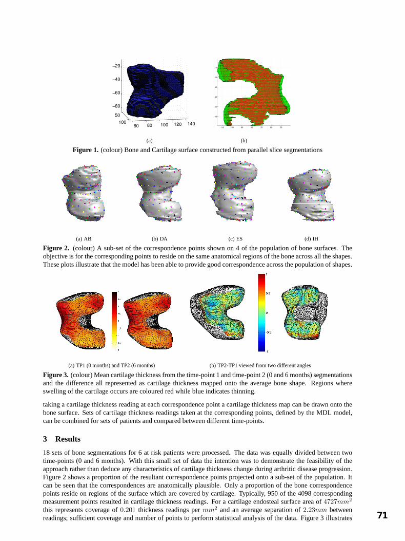
50100

60 80 100 120 140

−80

−60

−40

−20

(a)

5060708090100110

20

30

40

50

60

70

(b)

Figure 1. (colour) Bone and Cartilage surface constructed from parallel slice segmentations

(a) AB (b) DA (c) ES (d) IH

Figure 2. (colour) A sub-set of the correspondence points shown on 4 of the population of bone surfaces. Theobjective is for the corresponding points to reside on the same anatomical regions of the bone across all the shapes.These plots illustrate that the model has been able to provide good correspondence across the population of shapes.

(a) TP1 (0 months) and TP2 (6 months) (b) TP2-TP1 viewed from two different angles

Figure 3. (colour) Mean cartilage thickness from the time-point 1 and time-point 2 (0 and 6 months) segmentationsand the difference all represented as cartilage thickness mapped onto the average bone shape. Regions whereswelling of the cartilage occurs are coloured red while blue indicates thinning.

taking a cartilage thickness reading at each correspondence point a cartilage thickness map can be drawn onto thebone surface. Sets of cartilage thickness readings taken at the corresponding points, defined by the MDL model,can be combined for sets of patients and compared between different time-points.

3 Results

18 sets of bone segmentations for 6 at risk patients were processed. The data was equally divided between twotime-points (0 and 6 months). With this small set of data the intention was to demonstrate the feasibility of theapproach rather than deduce any characteristics of cartilage thickness change during arthritic disease progression.Figure 2 shows a proportion of the resultant correspondence points projected onto a sub-set of the population. Itcan be seen that the correspondences are anatomically plausible. Only a proportion of the bone correspondencepoints reside on regions of the surface which are covered by cartilage. Typically, 950 of the 4098 correspondingmeasurement points resulted in cartilage thickness readings. For a cartilage endosteal surface area of4727mm2

this represents coverage of0.201 thickness readings permm2 and an average separation of2.23mm betweenreadings; sufficient coverage and number of points to perform statistical analysis of the data. Figure 3 illustrates

how populations of results can be combined and compared. Mean thickness measurements for each correspondingpoint are displayed as colour maps on the mean bone shape. The results for time points 0 and 6 months scans areillustrated together with the difference between these aggregate maps. The difference map demonstrates thinningof cartilage in the load-bearing regions such as the patellofemoral (middle left) and medial tibiofemoral (upperright) compartments which is analogous to the finding reported in a diurnal study [16]. A larger study will berequired to draw firm conclusions.

4 Conclusions and Further work

We have demonstrated the feasibility of using the underlying bone as a reference for cartilage thickness measure-ments. The bone provides a stable reference for examining surfaces built from segmentations of cartilage scanstaken at different time points. Inter-patient comparisons can be achieved by building and optimising a Statisti-cal Shape Model of the femoral head. Cartilage thickness measurements are taken over all bone examples at theresultant corresponding locations which allows for the aggregation of results from a population of patients andcomparisons between sets of patients.

The approach was illustrated by applying it to a small population of 18 bone segmentations divided betweentwo time-points. Two sets of measurements were combined to produce mean thickness maps which were thencompared to each other to illustrate a comparative cartilage thickness map illustrating regional cartilage thicknesschanges. The immediate requirement is to complete larger scale experiments and extend the approach to the other(tibial and patellal) articular surfaces of the knee joint. Further refinement of the surface construction and imageregistration of the bone and cartilage scans could yield greater accuracy in cartilage thickness measurements.

References

1. C. Brechbuhler, G. Gerig, and O. Kubler. Parametrization of closed surfaces for 3-D shape-description.Computer Visionand Image Understanding, 61(2):154–170, 1995.

2. R. Burgkart, C. Glaser, A. Hyhlik-Durr, K. H. Englmeier, M. Reiser, and F. Eckstein. Magnetic resonance imaging-based assessment of cartilage loss in severe osteoarthritis — accuracy, precision, and diagnostic value.Arthritis Rheum.,44:2072–2077, 2001.

3. F. M. Cicuttini, A. E. Wluka, and S. L. Stuckey. Tibial and femoral cartilage changes in knee osteoarthritis.Ann. Rheum.Dis., 60:977–980, 2001.

4. Z. A. Cohen, D. M. McCarthy, S. D. Kwak, P. Legrand, F. Fogarasi, E. J. Ciaccio, and G. A. Ateshian. Knee cartilagetopography, thickness, and contact areas from MRI: in-vitro calibration and in-vivo measurements.Osteoarthritis andCartilage, 7:95–109, 1999.

5. Rhodri H Davies, Carole J Twining, Tim F Cootes, John C Waterton, and Chris T Taylor. A minimum description lengthapproach to statistical shape modelling.IEEE Trans. on Medical Imaging, 21(5):525–537, May 2002.

6. F. Eckstein, M. Winzheimer, J. Hohe, K. H. Englmeier, and M. Reiser. Interindividual variability and correlation amongmorphological parameters of knee joint cartilage plates: analysis with threedimensional MR imaging.OsteoarthritisCartilage, 9:101–111, 2001.

7. Stephen J Gandy, Alan D Brett, Paul A Dieppe, Michael J Keen, Rose A Maciwicz, Chris J Taylor, and John C Waterton.No change in volume over three years in knee osteoarthritis. InProc. Intl. Soc. Magnetic Resonance, page 79, 2001.

8. Bernhard Geiger.Three-dimensional modeling of human organs and its application to diagnosis and surgical planning.These de doctorat en sciences,Ecole Nationale Superieure des Mines de Paris, France, 1993.

9. J Hohe, G Ateshian, M Reiser, KH Englmeier, and F Eckstein. Surface size, curvature analysis, and assessment of kneejoint incongruity with MRI in-vivo. Magnetic Resonance in Medicine, 47(3):554–561, 2002.

10. J. A. Martin and J. A. Buckwalter. Aging, articular cartilage chondrocyte senescence and osteoarthritis.Biogerontology,3:257–264, 2002.

11. C. A. McGibbon, D. E. Dupuy, W. E. Palmer, and D. E. Krebs. Cartilage and subchondral bone thickness distribution withMR imaging.Acad. Radiol., 5:20–25, 1998.

12. Charles G Peterfy. Magnetic resonance imaging in rheumatoid arthritis: Current status and future directions.Journal ofRheumatology, 28(5):1134–1142, May 2001.

13. S. P. Raya and J. K. Udupa. Shape-based interpolation of multidimensional objects.IEEE Trans. on Medical Imaging,9(1):32–42, 1990.

14. T. Stammberger, J. Hohe, K. H. Englmeier, M. Reiser, and F. Eckstein. Elastic registration of 3D cartilage surfaces fromMR image data for detecting local changes in cartilage thickness.Magn. Reson. Med., 44(4):592–601, 2000.

15. S. K. Warfield, M. Kaus, F. A. Jolesz, and R. Kikinis. Adaptive, template moderated, spatially varying statistical classifi-cation.Med. Image Anal., 4(1):43–55, 2000.

16. John C Waterton, Stuart Solloway, John E Foster, Michael C Keen, Stephen Grady, Brian J Middleton, Rose A Maciewicz,Iain Watt, Paul A Dieppe, and Chris J Taylor. Diurnal variation in the femoral articular cartilage of the knee in young adulthumans.Magnetic Resonance in Medicine, 43:126–132, 2000.

Statistical Shape Modelling of the Levator Ani

Su-Lin Lee1,2, Paramate Horkaew1, Ara Darzi2, Guang-Zhong Yang1,2

1 Royal Society/Wolfson Foundation MIC Laboratory, Department of Computing 2 Department of Surgical Oncology and Technology

Imperial College, London, UK

Abstract. Defective pelvic organ support due to injuries of the levator ani is a common problem in women and its intervention requires a thorough understanding of its morphology and function. To this end, accurate delineation of three-dimensional surfaces of the levator ani plays an important part. In this paper, we propose to build a statistical shape model (SSM) of the levator ani and describe a segmentation technique based on the optimised control point arrangement and the SSM. The SSM was derived by the use of harmonic shape embedding with the MDL objective function for parameter optimisation, whilst segmentation was performed by fitting the model to a user defined set of control points. The value of the technique was demonstrated with data acquired from a group of 11 asymptomatic subjects.

1 Introduction

Pain, urinary or faecal incontinence, or constipation can be the results of injuries to the levator ani due to childbirth [1]. Locating the injuries is of prime importance for the prescription of suitable treatment such as pelvic floor exercises or surgery. Due to its clear tissue contrast, conventional 2D MR imaging techniques have been used relatively extensively for the assessment of the levator ani [2], with diagnosis made on the position of the organs such as the rectum and bladder, with respect to structural landmarks. 3D representation of the levator ani is a recent approach [3-5] that has yielded findings that differentiate between symptomatic and asymptomatic patients. Visual comparison has shown a continuum in levator volume degradation, loss of sling integrity and laxity in the order of asymptomatic, genuine stress incontinence and prolapse. It has also been found that the lack of volume of the levator ani can be an indication of pelvic floor dysfunction [6, 7]. In both studies, the levator ani was manually segmented from a set of image slices which is a time consuming process. Reducing the amount of data required to segment the entire levator surface would significantly simplify the process.

The purpose of this paper is to propose a method of segmenting the levator surface by using a user defined set of control points and a statistical shape model (SSM). Cootes et al [8] have investigated shape models and their use in automatic segmentation of images. Model based segmentation requires the entire set of control points to be deformed under the constraints of predefined heuristics describing the shape in the images. With SSM, a smaller set of points can be used to characterise the shape, therefore users can quickly determine landmarks associated with primary features of the surface. As the surface of the levator is topologically homeomorphic to a compact 2D manifold with boundary (sheet topology), the statistical shape model was built by using a method by Horkaew and Yang [9].

2 Methodology

The image data for this study were acquired with a Siemens Sonata 1.5T scanner. Eleven nulliparous, female subjects (22.6±1.4 years of age) were recruited for the study with informed consent and all subjects were scanned in the supine position. A turbo spin echo not-zone selective sequence (TR=1500ms, TE=130ms, slice thickness=3mm) was used to acquire 32-36 T2-weighted, transverse images for each of the eleven subjects studied. The levator ani was manually segmented from each data set by using an in-house developed 3D Slicer that allows for interactive visualisation in any arbitrary plane. The control points (also selected in the 3D Slicer) selected for shape restoration were the two most anterior points and one most posterior point on the levator surface in 4 image planes.

Triangulated surfaces (each forming a mesh M) were generated for the eleven levators and each was parameterised onto a unit quadrilateral base domain [10]. Each vertex was uniquely defined in the internal mapping by the minimisation of metric dispersion – a measure of the extent to which regions of small diameter are distorted when mapped. The harmonic map [11] corresponding to the minimisation of the total energy of the configuration of the points over the base domain was solved by computing its piecewise linear approximation [12],

[ ] ( ) ( )

∈−=

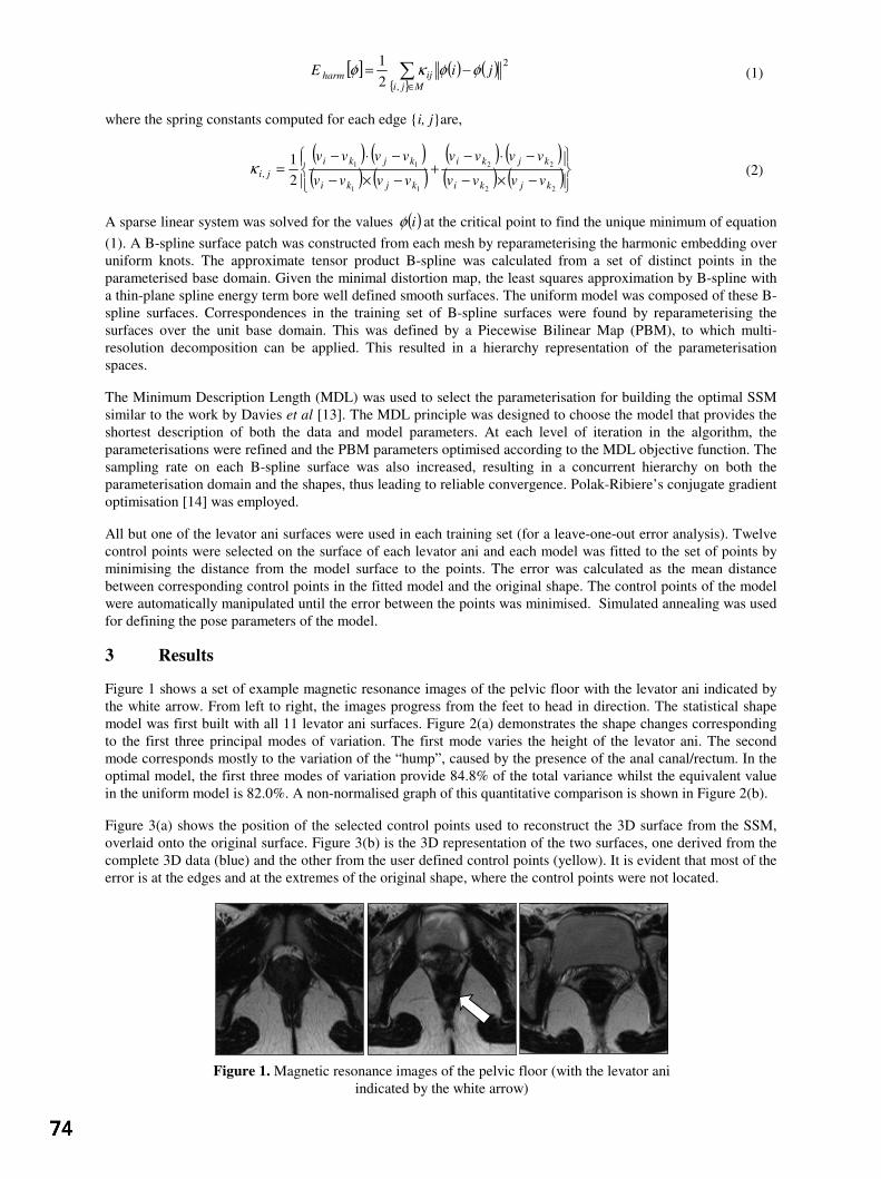
Mjiijharm jiE

,

2

21 φφκφ (1)

where the spring constants computed for each edge i, jare,

( ) ( )( ) ( )

( ) ( )( ) ( )

−×−

−⋅−+

−×−

−⋅−=

22

22

11

11

21

,kjki

kjki

kjki

kjkiji vvvv

vvvv

vvvv

vvvvκ (2)

A sparse linear system was solved for the values ( )iφ at the critical point to find the unique minimum of equation (1). A B-spline surface patch was constructed from each mesh by reparameterising the harmonic embedding over uniform knots. The approximate tensor product B-spline was calculated from a set of distinct points in the parameterised base domain. Given the minimal distortion map, the least squares approximation by B-spline with a thin-plane spline energy term bore well defined smooth surfaces. The uniform model was composed of these B-spline surfaces. Correspondences in the training set of B-spline surfaces were found by reparameterising the surfaces over the unit base domain. This was defined by a Piecewise Bilinear Map (PBM), to which multi-resolution decomposition can be applied. This resulted in a hierarchy representation of the parameterisation spaces.

The Minimum Description Length (MDL) was used to select the parameterisation for building the optimal SSM similar to the work by Davies et al [13]. The MDL principle was designed to choose the model that provides the shortest description of both the data and model parameters. At each level of iteration in the algorithm, the parameterisations were refined and the PBM parameters optimised according to the MDL objective function. The sampling rate on each B-spline surface was also increased, resulting in a concurrent hierarchy on both the parameterisation domain and the shapes, thus leading to reliable convergence. Polak-Ribiere’s conjugate gradient optimisation [14] was employed.

All but one of the levator ani surfaces were used in each training set (for a leave-one-out error analysis). Twelve control points were selected on the surface of each levator ani and each model was fitted to the set of points by minimising the distance from the model surface to the points. The error was calculated as the mean distance between corresponding control points in the fitted model and the original shape. The control points of the model were automatically manipulated until the error between the points was minimised. Simulated annealing was used for defining the pose parameters of the model.

3 Results

Figure 1 shows a set of example magnetic resonance images of the pelvic floor with the levator ani indicated by the white arrow. From left to right, the images progress from the feet to head in direction. The statistical shape model was first built with all 11 levator ani surfaces. Figure 2(a) demonstrates the shape changes corresponding to the first three principal modes of variation. The first mode varies the height of the levator ani. The second mode corresponds mostly to the variation of the “hump”, caused by the presence of the anal canal/rectum. In the optimal model, the first three modes of variation provide 84.8% of the total variance whilst the equivalent value in the uniform model is 82.0%. A non-normalised graph of this quantitative comparison is shown in Figure 2(b).

Figure 3(a) shows the position of the selected control points used to reconstruct the 3D surface from the SSM, overlaid onto the original surface. Figure 3(b) is the 3D representation of the two surfaces, one derived from the complete 3D data (blue) and the other from the user defined control points (yellow). It is evident that most of the error is at the edges and at the extremes of the original shape, where the control points were not located.

Figure 1. Magnetic resonance images of the pelvic floor (with the levator ani indicated by the white arrow)

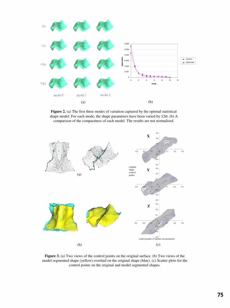
(b)

Figure 3. (a) Two views of the control points on the original surface. (b) Two views of the model segmented shape (yellow) overlaid on the original shape (blue). (c) Scatter plots for the

control points on the original and model segmented shapes.

Figure 2. (a) The first three modes of variation captured by the optimal statistical shape model. For each mode, the shape parameters have been varied by ±2σ. (b) A

comparison of the compactness of each model. The results are not normalised.

-0.3

-0.2

-0.1

0

0.1

0.2

0.3

-0.3 -0.2 -0.1 0 0.1 0.2 0.3

-0.3

-0.2

-0.1

0

0.1

0.2

0.3

-0.3 -0.2 -0.1 0 0.1 0.2 0.3

-0.3

-0.2

-0.1

0

0.1

0.2

0.3

-0.3 -0.2 -0.1 0 0.1 0.2 0.3

(a)

(c)

original shape control points

control points of surface reconstructed

X

Z

Y

(b)

(a)

0 0.001 0.002 0.003 0.004 0.005 0.006

0 2 4 6 8 10 12 mode

eig

enva

lue

Uniform Optimised

For the assessment of these errors, Figure 3(c) is a scatter plot (original shape points versus fitted model points) of all the B-spline surface control points in 3D space for one shape during a leave-one-out exercise. The regression line has also been plotted (average regression ratio 0.86893).

4 Discussion and Conclusion

With this study, the number of control points used was limited to twelve and were placed within 4 image planes. These can be increased if time permits to allow additional features to be prominent. Overall, there are no limitations to the proposed technique with regard to number of control points and their positions on the surface. Our future work will be focussed on applying the modelling technique to the investigation on muscle dynamics, where spatial correspondence of optimal control points of the SSM will need to be established.

In summary, we have proposed a segmentation method based on a statistical shape model. The statistical shape model was created with the use of harmonic shape embedding and an objective function based on MDL. Quantitative results from the 11 subjects demonstrate the potential of this method. We believe that statistical shape modelling is the way forward for studying the levator ani and that the proposed segmenting technique is an effective means of delineating its morphology from the anatomically complex pelvic floor region.

Acknowledgements

The authors would like to thank S Masood, L Crowe and DN Firmin for their assistance in MR data acquisition for this study.

References

1. JC Healy, S Halligan, RH Reznek, et al. Patterns of Prolapse in Women with Symptoms of Pelvic Floor Weakness: Assessment with MR Imaging. Radiology, 203, 1997. 77-81.

2. JR Fielding, L Hoyte and L Schierlitz. MR Imaging of Pelvic Floor Relaxation. Journal of Women’s Imaging, 2, 2000. 82-87.

3. K Singh, M Jakab, WMN Reid, et al. Three-dimensional magnetic resonance imaging assessment of levator ani morphologic features in different grades of prolapse. Am J Obstet Gynecol, 188, 2003, 910-915.

4. L Hoyte, L Schierlitz, K Zou, et al. Two- and 3-dimensional MRI comparison of levator ani structure, volume, and integrity in women with stress incontinence and prolapse. Am J Obstet Gynecol, 185(1), 2001.

5. K Duchicela, et al. MRI of the Aging Female Pelvic Floor; A 3D Perspective of its Principal Organization. International Continence Society Congress, Seoul, 2001.

6. L Hoyte, JR Fielding, E Versi et al. MR-based three-dimensional modelling of levator ani: First studies of muscle volume and geometry in living women with normal GU function, prolapse and genuine stress incontinence. Archivos Espanoles de Urologia, 54, 2001.

7. JR Fielding, H Dumanli, A Schreyer, et al. MR–based three dimensional modelling of the normal pelvic floor in women: quantification of muscle mass. Am J Radiol, 174, 2000. 657-660.

8. TF Cootes, CJ Taylor, DH Cooper, et al. Active Shape Models – Their Training and Application. Computer Vision and Image Understanding, 61(1), 1995. 38-59.

9. P Horkaew and G-Z Yang. Optimal Deformable Surface Models for 3D Medical Image Analysis. IPMI, 2003. (in press) 10. MS Floater. Meshless Parameterization and B-spline Surface Approximation, in The Mathematics of Surfaces IX, R

Cipolla dn R Martin (eds.). Springer-Verlag, 2000, 1-18. 11. AP Fordy and JC Wood. Harmonic Maps and Integrable Systems. Aspects of Mathematics, volE23, Vieweg,

Braunschweig/Wiesbaden, 1994. 12. M Eck, T DeRose, T Dutchamp, et al. Multiresolution Analysis of Arbitrary Meshes. Computer Graphics Proceedings

SIGGRAPH, 1995. 173-182. 13. RH Davies, CJ Twining, TF Cootes, et al. A Minimum Description Length Approach to Statistical Shape Modelling.

TMI, 2002. 14. WH Press, SA Teukolsky, WT Vetterling and BP Flannery. Numerical Recipes in C, 2nd edn. Cambridge University

Press, 1996. ISBN 0-521-43108-5.

An active contour model to segment foetal cardiac ultrasound data

I. Dindoyala*, T. Lambroua, J. Denga, C. F. Ruffb, A. D. Linneya and A. Todd-Pokropeka

aDepartment of Medical Physics and Bioengineering, University College London (UCL) and bUCL Hospitals NHS Trust (UCLH), 1st Floor, Shropshire House, 11-20 Capper Street, London, WC1E 6JA, United Kingdom.

Abstract. Segmentation of the prenatal heart can be used to examine the cardiac function and to aid in the assessment of congenital heart disease. This paper presents an active contour model to segment the ventricles of a temporal sequence of long-axis sliced foetal cardiac data. The algorithm uses image energy in the form of a Generalised Gradient Vector Flow (GGVF) field to drive a contour initialised as a circle towards salient features in the first frame of the sequence. The motion of the ventricular wall was modelled by rigid-body deformation between frames to enable the contours to remain within their respective chambers before the snake was allowed to capture the non-rigid deformation. The algorithm was compared to manual tracings of the chambers by a foetal cardiologist. Preliminary results from application to an eleven frame sequence spanning one cardiac cycle produced a correlation coefficient of 0.92 and 0.91 for the left and right ventricles respectively. Root mean square errors of the perpendicular distances between the automatic contours and expert tracings vary between 1 and 4.5 pixels over the cardiac cycle. Future work will involve moving towards a three dimensional (3D) approach to the snake to segment the chambers.

1 Introduction

Congenital heart disease occurs in 8 out of 1000 live births [1] and can be diagnosed in-utero by real-time echocardiography [2]. Segmentation of foetal cardiac chambers can be used to measure their size and shape as a function of time and serve as a diagnostic aid into the state of the myocardium when there are functional and or structural abnormalities present. In the past few authors have addressed segmentation of foetal cardiac data. Interactive grey-level thresholding was applied to the entire dataset by Deng et al 2001 [3] to extract the cardiac chambers but can lead to dropout of structures below the user-defined threshold level. Lassige et al 2000 [4] developed a snake to look for septal defects (pathological holes in the inter-atrial or inter-ventricular septum) using the level-set approach that allows the contour to occupy multiple foetal cardiac chambers simultaneously. An alternative approach to segmentation of the foetal cardiac chambers without deformable models can be found in a paper by Siqueira and co-workers [5], in which a cluster-based segmentation of temporal foetal slices was produced. The algorithm was constructed around a self-organising map that analysed the probability density functions of patterns found in foetal heart images. These maps were post-processed by k-means clustering and a neural network examined the mean and variance of randomly sampled areas in the image and identified the most significant regions. Their method measured foetal cardiac structures which showed agreement with the manual measurements made by physicians.

In recent years deformable model approaches to segment and track the motion of the cardiac walls in ultrasound data have been in the form of fitting elastic contours or a membrane to the structures. Several cardiac contour finding algorithms involve the use of the previous contour as initialisation for the next frame as in Sánchez and co-workers [6]. This may involve a mesh or contour to be guided by predictions in the motion between frames as it follows the endocardium [7]. It is becoming increasingly common in snake models applied to cardiac datasets to use in addition to spatial shape constraints, some temporal continuity between frames [8, 9].

This paper presents an active contour model paradigm applied to a temporal sequence of long-axis slices of the foetal cardiac ventricles. The segmentation results from the algorithm are then presented and compared with manually drawn curves by a foetal cardiologist. Finally the results of the algorithm and future work are discussed.

2 Materials and Methods

2.1 Data acquisition

The volumetric foetal heart dataset was acquired using paired Acuson scanners (Acuson Corporation, Mountain View, CA) with a phased-array transducer operating at a frequency range of 5-8MHz [10]. The image resolution was 256x256 pixels at 8-bit quantisation; with a pixel size of 0.26 millimetres (mm) in the fan beam plane and 0.5mm between slices. An automated online-triggering procedure developed by Deng et al 2001 [3] enabled the

* Author email: [email protected]

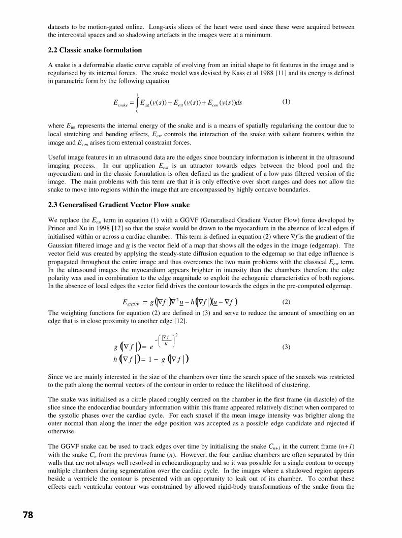
datasets to be motion-gated online. Long-axis slices of the heart were used since these were acquired between the intercostal spaces and so shadowing artefacts in the images were at a minimum.

2.2 Classic snake formulation

A snake is a deformable elastic curve capable of evolving from an initial shape to fit features in the image and is regularised by its internal forces. The snake model was devised by Kass et al 1988 [11] and its energy is defined in parametric form by the following equation

dssvEsvEsvEE conextsnake ∫ ++=1

0int ))(())(())(( (1)

where Eint represents the internal energy of the snake and is a means of spatially regularising the contour due to local stretching and bending effects, Eext controls the interaction of the snake with salient features within the image and Econ arises from external constraint forces.

Useful image features in an ultrasound data are the edges since boundary information is inherent in the ultrasound imaging process. In our application Eext is an attractor towards edges between the blood pool and the myocardium and in the classic formulation is often defined as the gradient of a low pass filtered version of the image. The main problems with this term are that it is only effective over short ranges and does not allow the snake to move into regions within the image that are encompassed by highly concave boundaries.

2.3 Generalised Gradient Vector Flow snake

We replace the Eext term in equation (1) with a GGVF (Generalised Gradient Vector Flow) force developed by Prince and Xu in 1998 [12] so that the snake would be drawn to the myocardium in the absence of local edges if initialised within or across a cardiac chamber. This term is defined in equation (2) where ∇f is the gradient of the Gaussian filtered image and u is the vector field of a map that shows all the edges in the image (edgemap). The vector field was created by applying the steady-state diffusion equation to the edgemap so that edge influence is propagated throughout the entire image and thus overcomes the two main problems with the classical Eext term. In the ultrasound images the myocardium appears brighter in intensity than the chambers therefore the edge polarity was used in combination to the edge magnitude to exploit the echogenic characteristics of both regions. In the absence of local edges the vector field drives the contour towards the edges in the pre-computed edgemap.

( ) ( )( )fufhufgEGGVF ∇−∇−∇∇= 2 (2)

The weighting functions for equation (2) are defined in (3) and serve to reduce the amount of smoothing on an edge that is in close proximity to another edge [12].

( )( ) ( )fgfh

efg K

f

∇−=∇

=∇

∇−

1

2

(3)

Since we are mainly interested in the size of the chambers over time the search space of the snaxels was restricted to the path along the normal vectors of the contour in order to reduce the likelihood of clustering.

The snake was initialised as a circle placed roughly centred on the chamber in the first frame (in diastole) of the slice since the endocardiac boundary information within this frame appeared relatively distinct when compared to the systolic phases over the cardiac cycle. For each snaxel if the mean image intensity was brighter along the outer normal than along the inner the edge position was accepted as a possible edge candidate and rejected if otherwise.

The GGVF snake can be used to track edges over time by initialising the snake Cn+1 in the current frame (n+1) with the snake Cn from the previous frame (n). However, the four cardiac chambers are often separated by thin walls that are not always well resolved in echocardiography and so it was possible for a single contour to occupy multiple chambers during segmentation over the cardiac cycle. In the images where a shadowed region appears beside a ventricle the contour is presented with an opportunity to leak out of its chamber. To combat these effects each ventricular contour was constrained by allowed rigid-body transformations of the snake from the

previous frame. After the snake Cn segmented frame n the positions of the snaxels within the curve were stored as well as the grey-level profiles that run along the normals to the contour. The Cn contour was then used to initialise Cn+1 and was iteratively scaled and translated to fit the chamber. The absolute difference of the grey-level profiles from the current curves in frames n+1 and n was used as a cost function to determine the optimum rigid-body transformation to apply to the initial Cn+1 contour. After modelling this rigid-body motion, the snake was allowed to evolve and capture the non-rigid deformation of the chamber. Although this approach computes the transformations solely based on the segmentation results of the first frame, we found that diastolic phases provided the most undemanding chambers for the GGVF snake to segment unaided. Towards end-diastole the motion of the heart is at a minimum; captured frames around this cardiac time point within the dataset are more likely to appear similar and can be used to confirm the initial segmentation.

3 Results and Discussions

Manual drawing of contours on the images by a foetal cardiologist was used as a gold standard to assess the quality of the segmentation process. The algorithm was applied to long-axis slices of the heart and a selection of the segmentation results for an eleven-frame sequence within one cardiac cycle is shown in figure 1 and overlaid manual curves in figure 2. The endocardial surface of the foetal heart comprises a complex interwoven muscular structure and so is highly irregular in appearance [13] unlike the comparatively smooth epicardium. It is clear that the automated contours appear less complex in shape when compared to the expert tracings. This is due to the appearance of the fine surface structure of the endocardium as weak reflectors in the ultrasound images. In this instance it is possible for Eint to overcome the Eext term and impose smoothing constraints on the contour. Future work will address this problem of unnecessary smoothing by incorporating a priori knowledge of the endocardium into the snake model. Linear regression by least squares was calculated on the manual and automatic segmented areas and the Pearson correlation coefficient (R-value) was determined. This showed that the computer-segmented areas are linearly correlated with the manually defined regions with coefficients of 0.92 and 0.91 for the left and right ventricles respectively. The slopes of these lines are 1.19 for the left and 1.15 for the right ventricle. These values are greater than 1 and positive indicating that the algorithm over-segments the required area when compared to the manual curves. This is confirmed in Bland-Altman plots in figure 3 where the bias is positive signifying over-segmentation for both left and right ventricles. The spread is roughly centred about the mean and most if not all of the points fall within the 95% confidence interval. These plots shows that by comparing areas defined by the manual and automatic curves, the algorithm produces less fluctuation and systematic bias in segmentation of the left ventricle when compared to the segmentation of the right (mean 26 with standard deviation 15 and mean 84 with standard deviation 46 for the left and right ventricles respectively). Since comparison of areas is not an accurate assessment of shape matching, perpendicular distances that separate the automatic and manual curves were computed to obtain a measure of the error in segmentation of the ventricular boundaries. The root mean square value of these perpendicular distances was found to vary between 1 and 4.5 pixels over the cardiac cycle for both left and right ventricles.

Figure 1 (a) Some results of endocardiac segmentation by the algorithm on a single long-axis slice showing the phases of one cardiac cycle in raster scan order starting from end-diastole. In this four-chamber view the top cavities are the left and right atria and below these are the left and right ventricles. (b) The corresponding endocardiac segmentation by a foetal cardiologist.

Figure 2 Some examples of segmentation of the ventricles by the algorithm with overlaid manual contours. The automatic contours are in black and those drawn by the expert in grey.

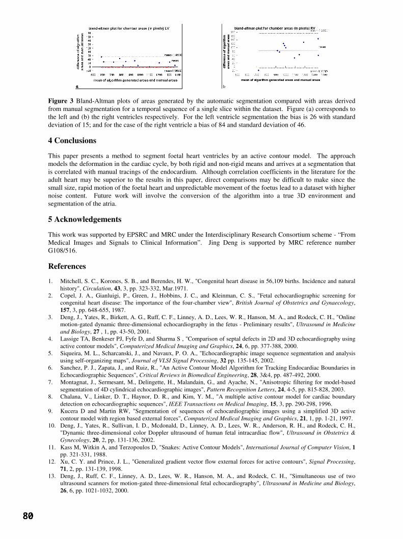
Figure 3 Bland-Altman plots of areas generated by the automatic segmentation compared with areas derived from manual segmentation for a temporal sequence of a single slice within the dataset. Figure (a) corresponds to the left and (b) the right ventricles respectively. For the left ventricle segmentation the bias is 26 with standard deviation of 15; and for the case of the right ventricle a bias of 84 and standard deviation of 46.

4 Conclusions

This paper presents a method to segment foetal heart ventricles by an active contour model. The approach models the deformation in the cardiac cycle, by both rigid and non-rigid means and arrives at a segmentation that is correlated with manual tracings of the endocardium. Although correlation coefficients in the literature for the adult heart may be superior to the results in this paper, direct comparisons may be difficult to make since the small size, rapid motion of the foetal heart and unpredictable movement of the foetus lead to a dataset with higher noise content. Future work will involve the conversion of the algorithm into a true 3D environment and segmentation of the atria.

5 Acknowledgements

This work was supported by EPSRC and MRC under the Interdisciplinary Research Consortium scheme - “From Medical Images and Signals to Clinical Information”. Jing Deng is supported by MRC reference number G108/516.

References

1. Mitchell, S. C., Korones, S. B., and Berendes, H. W., "Congenital heart disease in 56,109 births. Incidence and natural history", Circulation, 43, 3, pp. 323-332, Mar.1971.

2. Copel, J. A., Gianluigi, P., Green, J., Hobbins, J. C., and Kleinman, C. S., "Fetal echocardiographic screening for congenital heart disease: The importance of the four-chamber view", British Journal of Obstetrics and Gynaecology, 157, 3, pp. 648-655, 1987.

3. Deng, J., Yates, R., Birkett, A. G., Ruff, C. F., Linney, A. D., Lees, W. R., Hanson, M. A., and Rodeck, C. H., "Online motion-gated dynamic three-dimensional echocardiography in the fetus - Preliminary results", Ultrasound in Medicine and Biology, 27 , 1, pp. 43-50, 2001.

4. Lassige TA, Benkeser PJ, Fyfe D, and Sharma S , "Comparison of septal defects in 2D and 3D echocardiography using active contour models", Computerized Medical Imaging and Graphics, 24, 6, pp. 377-388, 2000.

5. Siqueira, M. L., Scharcanski, J., and Navaux, P. O. A., "Echocardiographic image sequence segmentation and analysis using self-organizing maps", Journal of VLSI Signal Processing, 32 pp. 135-145, 2002.

6. Sanchez, P. J., Zapata, J., and Ruiz, R., "An Active Contour Model Algorithm for Tracking Endocardiac Boundaries in Echocardiographic Sequences", Critical Reviews in Biomedical Engineering, 28, 3&4, pp. 487-492, 2000.

7. Montagnat, J., Sermesant, M., Delingette, H., Malandain, G., and Ayache, N., "Anisotropic filtering for model-based segmentation of 4D cylindrical echocardiographic images", Pattern Recognition Letters, 24, 4-5, pp. 815-828, 2003.

8. Chalana, V., Linker, D. T., Haynor, D. R., and Kim, Y. M., "A multiple active contour model for cardiac boundary detection on echocardiographic sequences", IEEE Transactions on Medical Imaging, 15, 3, pp. 290-298, 1996.

9. Kucera D and Martin RW, "Segmentation of sequences of echocardiographic images using a simplified 3D active contour model with region based external forces", Computerized Medical Imaging and Graphics, 21, 1, pp. 1-21, 1997.

10. Deng, J., Yates, R., Sullivan, I. D., Mcdonald, D., Linney, A. D., Lees, W. R., Anderson, R. H., and Rodeck, C. H., "Dynamic three-dimensional color Doppler ultrasound of human fetal intracardiac flow", Ultrasound in Obstetrics & Gynecology, 20, 2, pp. 131-136, 2002.

11. Kass M, Witkin A, and Terzopoulos D, "Snakes: Active Contour Models", International Journal of Computer Vision, 1 pp. 321-331, 1988.

12. Xu, C. Y. and Prince, J. L., "Generalized gradient vector flow external forces for active contours", Signal Processing, 71, 2, pp. 131-139, 1998.

13. Deng, J., Ruff, C. F., Linney, A. D., Lees, W. R., Hanson, M. A., and Rodeck, C. H., "Simultaneous use of two ultrasound scanners for motion-gated three-dimensional fetal echocardiography", Ultrasound in Medicine and Biology, 26, 6, pp. 1021-1032, 2000.

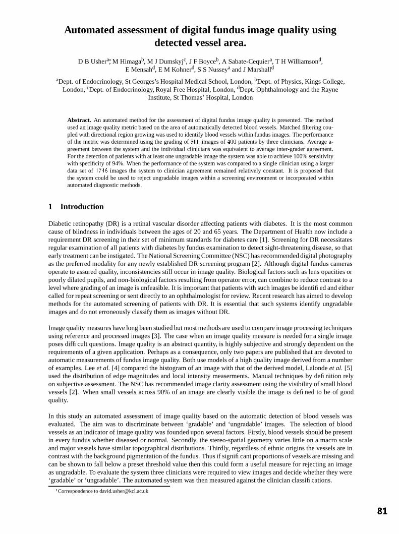
Automated assessment of digital fundus image quality usingdetected vessel area.

D B Ushera , M Himagab, M J Dumskyjc, J F Boyceb, A Sabate-Cequiera, T H Williamsond,E Mensahd, E M Kohnerd, S S Nusseya and J Marshalld

aDept. of Endocrinology, St Georges’s Hospital Medical School, London, bDept. of Physics, Kings College,London, cDept. of Endocrinology, Royal Free Hospital, London, dDept. Ophthalmology and the Rayne

Institute, St Thomas’ Hospital, London

Abstract. An automated method for the assessment of digital fundus image quality is presented. The methodused an image quality metric based on the area of automatically detected blood vessels. Matched filtering cou-pled with directional region growing was used to identify blood vessels within fundus images. The performanceof the metric was determined using the grading of

images of patients by three clinicians. Average a-

greement between the system and the individual clinicians was equivalent to average inter-grader agreement.For the detection of patients with at least one ungradable image the system was able to achieve 100% sensitivitywith specificity of 94%. When the performance of the system was compared to a single clinician using a largerdata set of images the system to clinician agreement remained relatively constant. It is proposed thatthe system could be used to reject ungradable images within a screening environment or incorporated withinautomated diagnostic methods.

1 Introduction

Diabetic retinopathy (DR) is a retinal vascular disorder affecting patients with diabetes. It is the most commoncause of blindness in individuals between the ages of 20 and 65 years. The Department of Health now include arequirement DR screening in their set of minimum standards for diabetes care [1]. Screening for DR necessitatesregular examination of all patients with diabetes by fundus examination to detect sight-threatening disease, so thatearly treatment can be instigated. The National Screening Committee (NSC) has recommended digital photographyas the preferred modality for any newly established DR screening program [2]. Although digital fundus camerasoperate to assured quality, inconsistencies still occur in image quality. Biological factors such as lens opacities orpoorly dilated pupils, and non-biological factors resulting from operator error, can combine to reduce contrast to alevel where grading of an image is unfeasible. It is important that patients with such images be identified and eithercalled for repeat screening or sent directly to an ophthalmologist for review. Recent research has aimed to developmethods for the automated screening of patients with DR. It is essential that such systems identify ungradableimages and do not erroneously classify them as images without DR.

Image quality measures have long been studied but most methods are used to compare image processing techniquesusing reference and processed images [3]. The case when an image quality measure is needed for a single imageposes difficult questions. Image quality is an abstract quantity, is highly subjective and strongly dependent on therequirements of a given application. Perhaps as a consequence, only two papers are published that are devoted toautomatic measurements of fundus image quality. Both use models of a high quality image derived from a numberof examples. Lee et al. [4] compared the histogram of an image with that of the derived model, Lalonde et al. [5]used the distribution of edge magnitudes and local intensity measerments. Manual techniques by definition relyon subjective assessment. The NSC has recommended image clarity assessment using the visibility of small bloodvessels [2]. When small vessels across 90% of an image are clearly visible the image is defined to be of goodquality.

In this study an automated assessment of image quality based on the automatic detection of blood vessels wasevaluated. The aim was to discriminate between ‘gradable’ and ‘ungradable’ images. The selection of bloodvessels as an indicator of image quality was founded upon several factors. Firstly, blood vessels should be presentin every fundus whether diseased or normal. Secondly, the stereo-spatial geometry varies little on a macro scaleand major vessels have similar topographical distributions. Thirdly, regardless of ethnic origins the vessels are incontrast with the background pigmentation of the fundus. Thus if significant proportions of vessels are missing andcan be shown to fall below a preset threshold value then this could form a useful measure for rejecting an imageas ungradable. To evaluate the system three clinicians were required to view images and decide whether they were‘gradable’ or ‘ungradable’. The automated system was then measured against the clinician classifications.

Correspondence to [email protected]

2 Methods

Digital retinal images of 2546 eyes from 1273 consecutive patients were obtained from a DR screening program.The screening centre employed a Topcon TRC-NW5S non-mydriatic digital fundus camera and stored images inJPEG format. All images were of field and centred on the macula. Their resolution was pixelsequating to a pixel width of m.

2.1 Automated detection of blood vessels

An automated method for the identification of blood vessels was applied to each of the images. This method hasbeen previously described in detail by Himaga et al. [6]. The method initially used the technique of matchedfiltering. Two Gaussian-shaped kernels were applied to each image, one designed to match a small section of alarge vessel while the other was smaller and was designed to match sections of smaller blood vessels. The kernelswere applied rotated through 12 angles ranging from to , each at intervals, in order to reflect the rangeof orientations of blood vessels. A direction dependent recursive region growing algorithm was then applied toextract the blood vessels using the results of the matched filtering. Finally an applied threshold classified pixels asrepresenting areas of vessels or otherwise. It has previously been shown that this method achieved a sensitivity of81% and a specificity of 91% for the detection of blood vessels in a total of 20 digital fundus images [6].

The total count of pixels classified as ‘vessels’ within each image then became the image quality metric score, V. Athreshold, , was then set such that images with blood vessels metric scores above were classified as ‘gradable’,while images with counts below were classed as ‘ungradable’. Patients were identified as ungradable if the imageof either eye were classified ‘ungradable’. The metric was applied at various sensitivity levels by varying .

2.2 Validation

The automated classification results were then compared to two separate gold standards. The first was the collatedresults from three clinicians, A, B and C, who classified the images of patients, Gold standard 1 (GS1). Amajority decision was used to combine the results of the clinicians. The second gold standard was formed byclinician A who classified the eyes of a further patients, Gold standard 2 (GS2). The diagnostic performanceof the image quality metric was then measured using sensitivity (true positive rate) and specificity (1 - false positiverate). Results recorded at each applied value of the threshold, , were combined to produce a Receiver OperatorCharacteristic (ROC) curve. Agreement between the clinicians and the proposed method was calculated usingkappa statistics, , where values within the ranges of - , - , and - correspond to moderate,substantial, and almost perfect agreement respectively [7].

3 Results

The results of the first gold standard grading, (GS1), are shown in Table 1. Clinician A accepted the highest numberof images as ‘gradable’ while clinician C accepted the least. Calculated agreement between each of the cliniciansin terms of grading images can be seen in table 2.

Imageclassification Clinician A Clinician B Clinician C‘ungradable’ 41 (5.1%) 51 (6.4%) 70 (8.8%)‘gradable’ 759 (94.9%) 749 (93.6%) 730 (91.2%)

Table 1. Gold standard grading # 1 (GS1) between ‘gradable’ and ‘ungradable’ images.

Clinician B Clinician CClinician A 0.67 (0.55 - 0.79) 0.66 (0.54 - 0.78)Clinician B - 0.63 (0.51 - 0.75)

Table 2. Inter-grader agreement between the three clinicians for the classification of images (GS1). Values showncorrespond to calculated values with the corresponding 95% confindence interval in parentheses.

The average inter-grader agreement was ! " (95% Confidence Interval: $#% ), demonstrating sub-stantial agreement. Within the GS2, clinician A classified &' (*) images as ‘ungradable’. Figure 1 showsexample results of the blood vessel detection method as applied to three primary images of varying quality. ImageA (Figure 1(a)) was classified as ‘gradable’ by all three clinicians. Image B (Figure 1(b)) shows a large region near

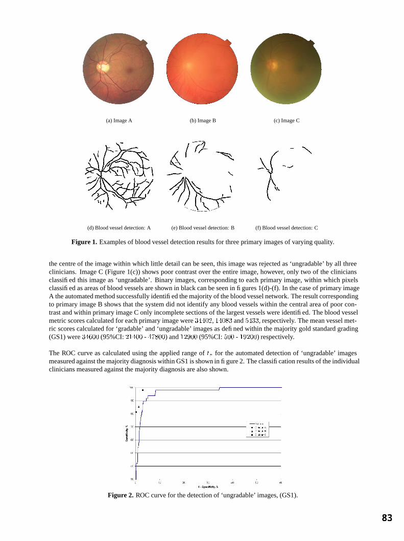
(a) Image A (b) Image B (c) Image C

(d) Blood vessel detection: A (e) Blood vessel detection: B (f) Blood vessel detection: C

Figure1. Examples of blood vessel detection results for three primary images of varying quality.

the centre of the image within which little detail can be seen, this image was rejected as ‘ungradable’ by all threeclinicians. Image C (Figure 1(c)) shows poor contrast over the entire image, however, only two of the cliniciansclassified this image as ‘ungradable’. Binary images, corresponding to each primary image, within which pixelsclassified as areas of blood vessels are shown in black can be seen in figures 1(d)-(f). In the case of primary imageA the automated method successfully identified the majority of the blood vessel network. The result correspondingto primary image B shows that the system did not identify any blood vessels within the central area of poor con-trast and within primary image C only incomplete sections of the largest vessels were identified. The blood vesselmetric scores calculated for each primary image were , and , respectively. The mean vessel met-ric scores calculated for ‘gradable’ and ‘ungradable’ images as defined within the majority gold standard grading(GS1) were (95%CI: - ) and (95%CI: - ) respectively.

The ROC curve as calculated using the applied range of for the automated detection of ‘ungradable’ imagesmeasured against the majority diagnosis within GS1 is shown in figure 2. The classification results of the individualclinicians measured against the majority diagnosis are also shown.

Figure2. ROC curve for the detection of ‘ungradable’ images, (GS1).

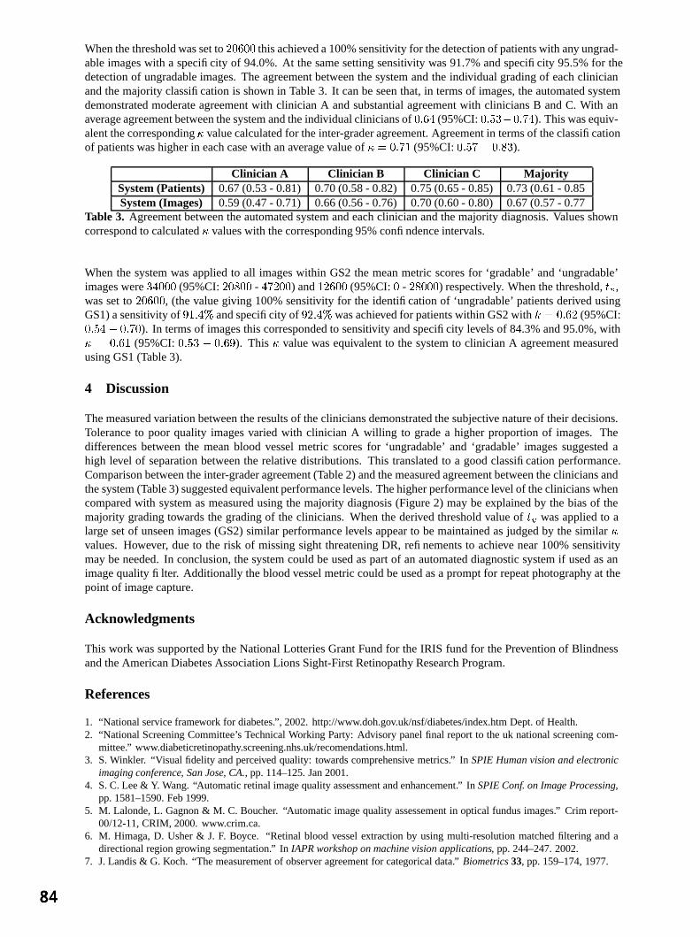
When the threshold was set to this achieved a 100% sensitivity for the detection of patients with any ungrad-able images with a specificity of 94.0%. At the same setting sensitivity was 91.7% and specificity 95.5% for thedetection of ungradable images. The agreement between the system and the individual grading of each clinicianand the majority classification is shown in Table 3. It can be seen that, in terms of images, the automated systemdemonstrated moderate agreement with clinician A and substantial agreement with clinicians B and C. With anaverage agreement between the system and the individual clinicians of (95%CI: # ). This was equiv-alent the corresponding value calculated for the inter-grader agreement. Agreement in terms of the classificationof patients was higher in each case with an average value of (95%CI: # ).

Clinician A Clinician B Clinician C MajoritySystem(Patients) 0.67 (0.53 - 0.81) 0.70 (0.58 - 0.82) 0.75 (0.65 - 0.85) 0.73 (0.61 - 0.85System(Images) 0.59 (0.47 - 0.71) 0.66 (0.56 - 0.76) 0.70 (0.60 - 0.80) 0.67 (0.57 - 0.77

Table 3. Agreement between the automated system and each clinician and the majority diagnosis. Values showncorrespond to calculated values with the corresponding 95% confindence intervals.

When the system was applied to all images within GS2 the mean metric scores for ‘gradable’ and ‘ungradable’images were (95%CI: - ) and (95%CI: - ) respectively. When the threshold, ,was set to , (the value giving 100% sensitivity for the identification of ‘ungradable’ patients derived usingGS1) a sensitivity of

( and specificity of ( was achieved for patients within GS2 with (95%CI:

# ). In terms of images this corresponded to sensitivity and specificity levels of 84.3% and 95.0%, with! " (95%CI: $#%

). This value was equivalent to the system to clinician A agreement measuredusing GS1 (Table 3).

4 Discussion

The measured variation between the results of the clinicians demonstrated the subjective nature of their decisions.Tolerance to poor quality images varied with clinician A willing to grade a higher proportion of images. Thedifferences between the mean blood vessel metric scores for ‘ungradable’ and ‘gradable’ images suggested ahigh level of separation between the relative distributions. This translated to a good classification performance.Comparison between the inter-grader agreement (Table 2) and the measured agreement between the clinicians andthe system (Table 3) suggested equivalent performance levels. The higher performance level of the clinicians whencompared with system as measured using the majority diagnosis (Figure 2) may be explained by the bias of themajority grading towards the grading of the clinicians. When the derived threshold value of was applied to alarge set of unseen images (GS2) similar performance levels appear to be maintained as judged by the similar values. However, due to the risk of missing sight threatening DR, refinements to achieve near 100% sensitivitymay be needed. In conclusion, the system could be used as part of an automated diagnostic system if used as animage quality filter. Additionally the blood vessel metric could be used as a prompt for repeat photography at thepoint of image capture.

Acknowledgments

This work was supported by the National Lotteries Grant Fund for the IRIS fund for the Prevention of Blindnessand the American Diabetes Association Lions Sight-First Retinopathy Research Program.

References

1. “National service framework for diabetes.”, 2002. http://www.doh.gov.uk/nsf/diabetes/index.htm Dept. of Health.2. “National Screening Committee’s Technical Working Party: Advisory panel final report to the uk national screening com-

mittee.” www.diabeticretinopathy.screening.nhs.uk/recomendations.html.3. S. Winkler. “Visual fidelity and perceived quality: towards comprehensive metrics.” In SPIE Human vision and electronic

imaging conference, San Jose, CA., pp. 114–125. Jan 2001.4. S. C. Lee & Y. Wang. “Automatic retinal image quality assessment and enhancement.” In SPIE Conf. on Image Processing,

pp. 1581–1590. Feb 1999.5. M. Lalonde, L. Gagnon & M. C. Boucher. “Automatic image quality assessement in optical fundus images.” Crim report-

00/12-11, CRIM, 2000. www.crim.ca.6. M. Himaga, D. Usher & J. F. Boyce. “Retinal blood vessel extraction by using multi-resolution matched filtering and a

directional region growing segmentation.” In IAPR workshop on machine vision applications, pp. 244–247. 2002.7. J. Landis & G. Koch. “The measurement of observer agreement for categorical data.” Biometrics 33, pp. 159–174, 1977.

3D Markov Random Field Binary Texture Model:Preliminary Results

Lilian Blot∗and Reyer Zwiggelaar†

School of Information System, University of East Anglia, UK

Abstract. Texture analysis and synthesis is an important field in computer vision. Since the late sixties,numerous techniques have been developed for the synthesis and analysis of texture in 2D images. However,only a few models have been presented to synthesize 3D texture images and in most cases 2D texture mappingis used to emulate this process. In addition, most of the techniques used for the analysis of texture in 3D medicalimages, such as CT and MRI, are based on 2D models applied to each slice followed by reconstruction of thevolume. This approach does not use all available information contained in the data. A more robust solutionis given by solid texture modelling. The paper describes a novel approach to solid texture modelling based onMarkov random fields.

1 Introduction

Texture analysis and synthesis is an important field in computer vision. Since the late sixties, numerous tech-niques have been developed for the synthesis and analysis of texture in 2D images. The synthesis and analysisof 2D texture have always been closely related and many techniques like Markov random fields [1], grey-levelco-occurrence matrices [2], auto-regression modelling [3] and fractal modelling [4] can be applied in both do-mains. Unfortunately, in 3D the relation between the two domains is less exploited (a short review on 3D texturemodelling can be found in [5]).

In medical imaging (see Fig. 1 for examples), the most common techniques to deal with volumetric images is toslice the volume in 2D cross-sections and subsequently apply a 2D texture analysis model on each slice. Subse-quently the volume is interpolated from the stack of analyzed slices. However, such an approach is less satisfactoryas most of the embodied information along the axial direction of the stack is not taken into account. Fig. 2 showstwo volumetric texture which can not be differentiate if seen from they axis. When the volume information istaken into account the two textures are clearly different.

(a) (b) (c)

Figure 1. Examples of three volumetric image acquisition modalities which are slices of (a) a brain MRI, (b) achest CT and (c) a breast ultrasound.

The aim of this project is to develop a common model to synthesize and analyze volumetric texture. Our initialapproach to the problem is to synthesize texture based on an approach that can be used to analysis. Solid texturemodelling is the most suitable approach if we are concerned with the synthesis of complex textured objects or theanalysis of volumetric texture.

2 Texture Modelling

In this section we describe a solid texture model based on Markov random fields. We are interested in generatingtexture based on a stochastic process to ensure micro-texture. The grey-level values of the voxels(x, y, z) are the

∗email: [email protected]†email: [email protected]

(a) (b) (c)

Figure 2. Two texture volumes (top and bottom rows) decomposed into slices taken along (a) thex-axis, (b) they-axis, and (c) thez-axis. These grey-level images have been synthesized with the Markov random field modeldescribed in this paper.

random variable and are notedξxyz. In our approach the grey-levelξxyz of a voxel is not independent of the grey-level values of neighboring voxels. We aim at modelling the correlations between the set of grey-levels,ξxyz.We first deal with the binary problem before extending the model to grey-level texture.

We need to define the notion of neighboring voxels. In our case two voxels are neighbor if they are connected. Theorder of the Markov random field (MRF) is determined by the distance between two neighbors. Fig. 3 shows twoneighborhood configurations. Grey voxels form the first order neighborhood while white and grey voxels form thesecond order (relative to the voxel in the center of the cube).

Figure 3. Neighbors of the pointξxyz. Grey representsthe first order neighborhood and white represents thesecond order neighborhood.

Figure 4. Description ofC, the set of connected points.The setC is composed of pair of points linked by astraight line. In this figure seven elements ofC areshown. The eighth element ofC is the set of all thesecond order neighbors of the center point.

The probability of a voxel(x, y, z) having the grey-level valuek depends on its neighbors and is denotedPξxyz =k|neighbors. This probability is binomial with parameterθ(T ) = exp(T )

1+exp(T ) andG is the number of grey-levels.When consideringG > 2 we have

Pξxyz = k|neighbors =(

G− 1k

)(exp(T )

1 + exp(T )

)k(1

1 + exp(T )

)G−1−k

k ∈ 0, 1, ..., G− 1

For the binary model we have

Pξxyz = k|neighbors =exp(T )

1 + exp(T )k ∈ 0, 1

whereT is neighborhood dependant.

2.1 First Order Texture Model

The texture properties are defined by the functionT given by

T (ξxyz) = b0 + bx(ξx−1,y,z + ξx+1,y,z) + by(ξx,y−1,z + ξx,y+1,z) + bz(ξx,y,z−1 + ξx,y,z+1)

whereb0, bx, by, bz is the set of parameters of the model. The MRF is isotropic ifbx = by = bz, anisotropicotherwise.

2.2 Second Order Texture Model

When considering first order MRF26 neighborhood configurations are possible compared to226 in the secondorder case. For sampling reason we need to reduce the number of configurations. To each neighborhood configu-ration we assign a potentialU(neighbors) given by

U(ξx1y1z1 , ξx2y2z2 , ..., ξxmymzm

)=

i=|C|∑

i=1, ci∈ CV (ci) 2i

andV (ci) = 0 if all voxels in ci have value0, 1 otherwise.

Fig. 4 shows the elementsci of the setC. C is composed of eight ordered elements (the order has no influence onthe model), seven elements are pairs of voxels and the eighth element contains all the neighbors of the center voxel.In doing so we have reduced the number of configuration from226 to 28. The correlation between neighboringvoxels is expressed by

Pξxyz = k|U(ξx1y1z1 , ξx2y2z2 , ..., ξxmymzm

)= q =

exp(T )1 + exp(T )

k ∈ 0, 1, q ∈ 0, ..., 255

Similarly to the first order, the parametersbi of the model are embodied in the functionT given by

T (ξx1y1z1 , ξx2y2z2 , ..., ξxmymzm) = b0 +i=|C|∑

i=1, ci∈ Cbi V (ci)

3 Results

To synthesize the MRF texture we use the algorithm developed in [6] and used by Cross and Jain [1]. We startfrom a uniform noise (see Fig. 5) and then iteratively swap two random voxels with different grey-level valuesif the obtained texture has a higher probabilityP (Y ) than the original textureP (X) (P (X) andP (Y ) are theproduct of the conditional probability of all voxels). We proceed until a stable state is reached. In pseudo-code thisis represented as:

while not stable dochoose two voxels v1 and v2 with ξv1 6= ξv2

if P (Y ) ≥ P (X) then switch v1 and v2

elseu=uniform random on [0, 1]if

(P (Y )/P (X)

)> u then switch v1 and v2

end elseend while

Samples of synthetic binary textures are shown in Fig. 5. The textures are generated according to various settingsof the Markov random field. The volumes are representative of typical texture properties that can be obtained suchas isotropic textures (Fig. 5b,d), anisotropic textures (Fig. 5c,e,f) and strong directionality (Fig. 5f). We have nottried to simulate realistic textures as the extraction of the MRF parameters will need the analysis of the real medicaldata which is an area of future development .

4 Discussion and Conclusions

As shown a large variety of texture can be generated where 2D information is not sufficient to described theirproperties. This demonstrates the limitation of approaches considering only textural features from 2D slices. Thisemphasizes the necessity to develop novel approaches to the analysis of medical modalities such as CT or MRI.

A first attempt to the synthesis of grey-level solid texture shows good results (see Fig. 2 and 6). Unfortunatelythe increased complexity prohibits its direct use to the analysis of such texture. One of the possible direction forthe analysis of grey-level texture is the thresholding of the image followed by the analysis of the obtained binary

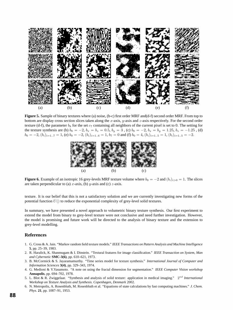
(a) (b) (c) (d) (e) (f)

Figure 5. Sample of binary textures where (a) noise, (b-c) first order MRF and(d-f) second order MRF. From top tobottom are display cross section slices taken along thex-axis,y-axis andz-axis respectively. For the second ordertexture (d-f), the parameterb8 for the setc7 containing all neighbors of the current pixel is set to 0. The setting forthe texture synthesis are (b)b0 = −2, bx = bz = 0.5, by = 3 , (c) b0 = −2, bx = by = 1.25, bz = −1.25 , (d)b0 = −2, (bi)i=1..7 = 1, (e)b0 = −2, (bi)i=1..6 = 1, b7 = 0 and (f)b0 = 4, (bi)i=1..5 = 1, (bi)i=1..5 = −2.

(a) (b) (c)

Figure 6. Example of an isotropic 16 grey-levels MRF texture volume whereb0 = −2 and(bi)i>0 = 1. The slicesare taken perpendicular to (a)x-axis, (b)y-axis and (c)z-axis.

texture. It is our belief that this is not a satisfactory solution and we are currently investigating new forms of thepotential functionU() to reduce the exponential complexity of grey-level solid textures.

In summary, we have presented a novel approach to volumetric binary texture synthesis. Our first experiment toextend the model from binary to grey-level texture were not conclusive and need further investigation. However,the model is promising and future work will be directed to the analysis of binary texture and the extension togrey-level modelling.

References

1. G. Cross & A. Jain. “Markov random field texture models.”IEEE Transactions on Pattern Analysis and Machine Intelligence5, pp. 25–39, 1983.

2. R. Haralick, K. Shanmugam & I. Dinstein. “Textural features for image classification.”IEEE Transaction on System, Manand CyberneticSMC-3(6), pp. 610–621, 1973.

3. B. McCormick & S. Jayaramamurthy. “Time series model for texture synthesis.”International Journal of Computer andInformation Sciences3(4), pp. 329–343, 1974.

4. G. Medioni & Y.Yasumoto. “A note on using the fractal dimension for segmentation.”IEEE Computer Vision workshopAnnapolis, pp. 694–702, 1978.

5. L. Blot & R. Zwiggelaar. “Synthesis and analysis of solid texture: application in medical imaging.”2nd InternationalWorkshop on Texture Analysis and Synthesis. Copenhagen, Denmark2002.

6. N. Metropolis, A. Rosenbluth, M. Rosenbluth et al. “Equations of state calculations by fast computing machines.”J. Chem.Phys.21, pp. 1087–91, 1953.

The Work of Reading Mammograms and the Implications for Computer-Aided Detection Systems

Mark Hartswooda, Rob Proctera, Mark Rouncefieldb, Roger Slacka and James Souttera

aSchool of Informatics, University of Edinburgh, Edinburgh, EH8 9LW bComputing Department, Lancaster University, Lancaster, LA1 4YR

Abstract. We examine the ways that readers make sense of mammograms in context, showing how a consideration of the social aspects of this work might illuminate practice and suggest ways for the building of computer-based tools to support such work. We show how sense-making is a situated activity and raise some concerns as to the ways that technologies have been developed to support reading may impact negatively upon the very practice they were intended to support. We show how it is important to consider technologies in use and discuss how they might be developed to support real world use, as opposed to some idealised formulation of it. We conclude with some outline suggestions towards better user interfaces for computer-aided detection systems, in particular, and for digital imaging systems in general.

1 Introduction

The practice of breast screening calls for readers to exercise a combination of perceptual skills to find what may be faint and small features in a complex visual environment, and interpretative skills to classify them appropriately – i.e., as benign or suspicious. Current UK NHS breast screening practice is for each mammogram to be ‘double read’, i.e., assessed independently by two readers [1]. Because of the growing shortage of trained readers, there is interest in using computer-aided detection (CADe) systems to replace double reading with a single reader using a CADe system. We report here ethnographic studies of readers using a CADe system which we conducted during clinical trials.

2 Method

As a complement to the quantitative emphasis of the conventional clinical trial, we used ethnographic investigative and evaluative techniques [7]. Ethnography argues for understanding the situatedness of individual activities and of the wider work setting, highlighting the interdependencies between activities, and stressing the ‘practical participation’ of individuals in the collaborative achievement of work. For the purposes of designing and developing computer-based tools, the advantage of applying ethnographic methods lies in the ‘sensitising’ they promote to the real-world character of activities in context and, consequently, in the opportunity to help ensure that systems resonate with the circumstances of use. This is, we argue, particularly important to medical work, where the lack of attention to work practice has been responsible for many failures of IT systems.

3 The Trial

The CADe system being trialed was the R2 Imagechecker. In order to assess the system’s impact on reader performance, a conventional clinical trial design was used. Prompted and unprompted conditions were prepared using three sets of 60 historical cases [9]. In both conditions, readers were shown ‘current’ mammograms (but not previous mammograms, or any patient notes) for each case in turn, and asked to indicate areas of concern and to make a decision as to whether the case should be recalled for further investigation using a four point decision scale: 1. Recall; 2. Discuss but probably recall; 3. Discuss but probably no recall; 4. No Recall. In the prompted condition, readers additionally examined the prompts generated by the system before making their decision. Before the trial was run, each reader was given a brief explanation of how the CADe system worked, emphasising that it was intended to be used for detection rather than for diagnosis. Readers were told that the system ‘spotted’ masses and calcifications and about the appropriate prompts. They were also advised that the threshold of sensitivity of the system had been set such that there would inevitably be a lot of false prompts; and warned that since this was a trial set there would be more cancers than in a ‘normal’ reading session.

4 Observations

As part of the trial, readers were observed doing the various test sets and then asked about their experiences of using the prompts. Readers were also taken back to cases identified in the test set where they had appeared to have had difficulty or spent a long time making their decision and asked to talk through any problems or issues

to do with the prompts and their decisions. Although there were variations in how readers approached the trial, the fieldwork extract below gives some idea of the process observed:

Case 10: Looking at film – using a blank film to mask area outside that of immediate interest. Magnifying glass. Looking at booklet prompts - looking back at film. “This is a case where without the prompt I’d probably let it go ... but seeing the prompt I’ll probably recall ... it doesn’t look like a mass but she’s got quite difficult dense breasts ... I’d probably recall …” Marks decision.

The main strengths of the CADE system in supporting this kind of work seemed to lay in picking up subtle signs – signs that some readers felt they might have missed – and stimulating interaction between reader and the available technology by motivating them to re-examine the mammogram. As one reader said:

“Those micros that the computer picked up … I might have missed it if I was reading in a hurry … I’d certainly missed them on the oblique … This one here the computer certainly made me look again at the area. I thought they were very useful, they make me look more closely at the films … I make my own judgement ... but if the prompt is pointing things out I will go and look at it again.”

There was also a perception that the CADE system was more consistent than readers might be:

“... it’s just the fact that it’s more consistent than you are ... because it’s a machine.”

Readers also frequently express the opinion that they are better at ‘spotting’ some cancers – as having skills or deficiencies in noticing particular types of object within films. This was another area where the CADe prompts were seen as useful, as both compensating in some (consistent) way for any individual weaknesses of the reader and as a reminder of ‘good practice’:

“My approach tends to be to look for things that I know I’m not so good at ... there are certain things that you do have to prompt yourself to look at, one of them being the danger areas.”

Amongst the weaknesses identified by readers was the distracting appearance of too many prompts:

“This is quite distracting … there’s an obvious cancer there (pointing) but the computer’s picked up a lot of other things ... there’s so many prompts ... especially benign calcifications ... you’ve already looked and seen there are lots of benign calcs.”

The CADe system was also seen to prompt the ‘wrong’ things – benign features or artefacts of the mammogram generation process: “... what the computer has picked up is benign ... it may even be talcum powder … I’m having trouble seeing the calc its picked up there … (pointing). I can only think its an artefact on the film.”

At the same time, the CADe system was seen to be missing obvious prompts that raised wider issues to do with trusting and ‘understanding’ the system:

“I’m surprised the computer didn’t pick that up ... my eye went to it straight away.”

Our wider studies of breast screening show how reading mammograms is a thoroughgoingly social enterprise and is achieved in, and through, the making available of features that are relevant to the community of readers as opposed to some idealised individual cogniser [6]. It is for this reason that we turn to the work of Goodwin and, in particular, his notion of ‘professional vision’ [4], to explicate the social, intersubjectively available nature of doing reading. In mammography, a reader has to learn how to interpret the features on the mammogram and what they mean, as well as how to find them. We have described how readers ‘repertoires of manipulation’ make features visible [6]. Methods for doing this include using the magnifying glass and adopting particular search patterns:

“Start at top at armpit … come down … look at strip of tissue in front of armpit … then look at bottom ... then behind each nipple ... the middle of the breast.”

Readers also attempt to ‘get at’ a lesion by measuring with rulers, pens or hands from the nipple in order to find a feature in the arc; comparing in the opposite view; aligning scans; looking ‘behind’ the scans; ‘undressing lesions’ by tracing strands of fibrous tissues into and out of the lesion area and so on. A magnifying glass may be used to assess the shape, texture and arrangement of calcifications or, where the breast is dense, the mammogram may be removed and taken to a separate light box. These repertoires of manipulations are an integral part of the embodied practice of reading mammograms. Such features are not work arounds, but an integral part of the ecology of practice built up in and as a part of doing reading mammograms.

The positioning of an object in a particular area of the breast renders it more suspicious than if it had been elsewhere. At the same time, certain areas within the mammogram are regarded as more difficult than others to interpret and readers particularly orient to them in their examinations. As one reader noted:

“I do … I have areas where I know I’m weak at seeing … you know ones that you’ve missed ... one is over the muscle there ... its just because the muscle is there ... if you don’t make a conscious effort to look there you tend not to see that bit of breast and the other area is right down in the chest wall – breast and chest wall area ... because in older women the cancers tend to be in the upper outer quadrant so I look in that area very carefully ... it depends on the type of breast really.”

We would also stress the self-reflective nature of readers’ behaviour. Readers know about their own strengths and weaknesses (in one centre, a reader is referred to as ‘the calcium king’ because of his ability to detect calcifications; a member of another centre is referred to as ‘Mrs Blobby’ because of her ability to detect lesions in dense areas). Readers are sensitive towards the set of criteria for correctness and what is required for the satisfaction of the maxims that constitute it.

5 Discussion

It is important to note that the CADe system should not be taken to make reading mammograms less uncertain – decisions still have to be made and these fall to the readers. Prompts are ‘docile’ in that their character is simply to draw the reader’s attention to candidate features as opposed to say what should be done with them. That a prompt occurs is a meaningful thing, but what to do about it is still a readers’ matter. In other words, the system still requires the professional vision of the reader to remedy prompts as what they accountably are. A reader makes what is seen or prompted accountable in, and through, the embodied practices of professional vision. That a mammogram feature or a prompt is there is not of itself constitutive of a lesion or other accountable thing, it must be worked up through these embodied practices and ratified in the professional domain of scrutiny. The CADe system knows – and can know – nothing of what it is to be a competent reader and what it is to look for features in a mammogram beyond its algorithms, and the reader must ‘repair’ what the system shows, making it accountable in, and through, their professional vision. This is, as we have argued, a thoroughgoingly social procedure and, as such, something that the CADe system cannot be a part of. Beyond its algorithms, the CADe system cannot account for what it has and has not prompted, and it cannot be queried as a colleague can.

Readers used prompts to develop some understanding of the CADe system’s scope and function. However, they occasionally held incorrect notions about, e.g., the system prompting for asymmetry and were often baffled by the high level of false positive prompts. In part, this ability to make sense of how the system behaves also impacts on issues of dependability and trust in the system. We have argued elsewhere that how readers use prompts to inform their decision-making, and how they make sense of a CADe system’s behaviour, may be important for maximising effectiveness [5]. We find that readers rationalise false prompts by devising explanations or accounts of its behaviour that were grounded in the properties of the mammogram image. This points to general issues concerning trust – users’ perception of the reliability of the evidence generated by such tools – and how trust is influenced by users’ capacity for making sense of how the system behaves. The need to account for a prompt – even if it is dismissed – distracts the reader. In other words, its docile prompts often call attention to features that the readers have decided are not important enough to merit attention.

The CADe system prompts features that are not cancers, as well as missing features that may be obviously cancers to the reader. For example, normal features in the breast such as calcified arteries or crossing linear tissues can be prompted as micro-calcifications, while other normal features such as ducts and tissue radiating from the nipple or inadvertent crossing of parenchymal tissue can produce a prompt for a cancerous mass. That the system prompts features other than the cancer is regarded as problematic but still in need of account. It might be said that the system works too well, providing not just too many prompts, but prompting features that a skilled reader would not accept as promptable. In part this is a feature of the technology that the readers (at least in this trial) effectively ‘forget’, but which might be incorporated into readers’ ‘biography’ of the system in time.

How do readers construct, achieve or make sense of the system? Following Schutz, we might argue that readers render mammograms intelligible using a mosaic of ‘recipe knowledge’: “a kind of organisation by habits, rules and principles which we regularly apply with success.” [8]. While the common experiences and rules embodied in the ‘mosaic’ are always open to potential revision they are, nevertheless, generally relied upon for all practical purposes as furnishing criterion by which adequate sense may be assembled and practical activities – reading the mammogram – realised. Of course, in everyday interaction with colleagues any breakdown in sense is rapidly repaired and ‘what is going on’ readily understood. But, when the other participant in the interaction is a computer, difficulties can arise as readers (in this case) characteristically rush to premature and often mistaken

conclusions about what has happened, what is happening, what the system ‘meant’, what the system is ‘thinking’, and so on. The problem is, of course, that the CADe system is not capable of reciprocating the perspective of the skilled practitioner.

It would therefore seem desirable to increase the scope for a CADe system to be ‘self-accounting’ [2] through the provision of richer and more sophisticated user interfaces. It is certainly possible to conceive of richer representations of a CADe system’s behaviour, but it is an open question as to whether such representations could be sufficiently contexted in a manner that would enable readers to use them easily and in any meaningful sense. It seems to us that such representations are not accounts in themselves, but resources for the realisation of accounts in context. We argue that even a series of representations from which readers could choose may not provide sufficient detail to answer all conceivable ‘why that now’ types of questions.

6 Conclusions

The current generation of CADe systems are designed with user interfaces that presume that all readers need to see is the bare and unadorned prompt. Our ethnographic investigations of the CADe system on trial show, however, that this presumption is false. Indeed, we would argue that as digital imaging systems, in this and other medical work domains, evolve from performing basic image rendering to incorporate increasingly sophisticated image processing, then users’ interactional requirements become more demanding.

It is clear from our study that readers need an understanding of what the CADe system has prompted and why. The key problem we observe is that the system does not provide accounts of its behaviour. The docile nature of the prompts generated requires the reader to formulate ad hoc an explanation for their presence. Thus, there is a need for the reader to engage in some kind of retrospective search for what it is that the CADe system might have ‘meant’ or ‘intended’. Without the possibility of being able to assemble an account from the source, so to speak, the reader has to develop some notion of the potentialities of the system – which, as we have seen, may or may not be consistent with what the CADe system actually does.

If readers are to ‘trust’ CADe systems, they need accounts of why prompts come – or come not – to be there. It is also important to consider how far accounts of prompts might be intrusive and thereby impact negatively on the work of readers. We therefore need to consider what these accounts would look like and for whom they would be intended. In other words, these accounts must be designed to relevant to readers’ concerns. We suggest that one way of moving towards assembling readers’ accounts is for CADe system developers to work with closely with readers as the latter become acquainted with the system’s performance characteristics over time.

Acknowledgements

We would like to thank the readers who participated in this study for their time and patience. Also, we are grateful to Paul Taylor and his colleagues at CHIME for giving us the opportunity to carry out this study. This work was supported by the EPSRC under grant number GR/ R24517/01.

References

1. Blanks, R., Wallis, M. and Moss, S. A comparison of cancer detection rates achieved by breast cancer screening programmes by number of readers, for one and two view mammography: results from the UK National Health Service breast screening programme. Journal of Medical Screening, Vol. 5(4), p. 195-201, 1998.

2. Dourish, P. and Button, G. On “Technomethodology”: Foundational relationships between Ethnomethodology and System Design. Human-Computer Interaction 13(4), 1998, pp. 395-432.

3. Garfinkel, H. Studies in Ethnomethodology. Englewood Cliffs, NJ: Prentice-Hall, 1967. 4. Goodwin, C. Professional Vision. American Anthropologist. 96; 606-633, 1994. 5. Hartswood, M. and Procter, R. Computer-aided mammography: a case study of coping with fallibility in a skilled

decision-making task. In Johnson, C. (Ed.), Special issue on Human Error and Computer Systems, Journal of Topics in Health Information Management, vol. 20(4), May, p. 38-54, 2000.

6. Hartswood, M., Procter, R., Rouncefield, M. and Slack, R. Cultures of Reading in Mammography. To be published in Francis, D. and Hester, S. (Eds.), Orders of Ordinary Action: Respecifying Sociological Knowledge. Ashgate Publishing, 2003.

7. Hughes, J., King, V., Rodden, T. and Anderson, R. Moving Out from the Control Room: Ethnography and Systems Design. In Proceedings of the ACM Conference on Computer-Supported Cooperative Work. ACM Press, p. 429-439, 1994.

8. Schutz, A. Collected Papers Vol. 2: Studies in social theory. Den Haag: Martinus Niijhoff, 1964. 9. Champness, J., Taylor, P. and Given-Wilson, R. Impact of computer-placed prompts on sensitivity and specificity with

different groups of mammographic film readers. In Proc. 6th Int. Workshop on Digital Mammography, 2002.

Automatic generation of Regions Of Interest for Radionuclide Renograms

David C Barber

Department of Medical Imaging and Medical Physics

Central Sheffield Teaching Hospitals, Glossop Road, Sheffield S10 2JF

Abstract. Automatic generation of kidney regions of interest for radionuclide renograms is possible by defining a reference image and reference regions, using a non-linear image registration algorithm to map a totalised image from a patient to the reference image and using the mapping produced to map the predefined reference regions back onto the patient image. The accuracy of the automatically derived regions is evaluated by comparison with regions drawn independently by experienced operators. The median success factors, a measure of the overlap between automatic and manual regions, over 49 kidneys was 0.95 and the average linear displacement between the boundaries of the automatic and manual regions was 0.43 in units of pixel dimensions.

1 Introduction One of the principal uses of image segmentation, in terms of the number of patients involved, is the use of regions-of-interest (ROI) in Nuclear Medicine. These are invariably drawn manually, although there is evidence that ROI drawn on the same subject can be quite operator dependent. White et al [1] compared two operator drawn regions of interest using a success factor, defined as the area of the intersection of the regions divided by the average area of the regions and obtained intra-operator variability of 0.94 and inter-operator variability of 0.93. A reliable and automatic method of drawing ROI would be useful clinically and would help to standardise analysis between clinics. In the analysis of radionuclide renograms an ROI is drawn around each kidney to allow the total activity in the kidney to be estimated as a function of time. Background regions, often automatically derived from the kidney regions, are drawn to allow background subtraction. In spite of the widespread use of ROI analysis in clinical practice in Nuclear Medicine there is still no general method of drawing ROI automatically. The images are low resolution compared to many other modalities and are noisy, both of which makes identification and delineation of edges difficult. Other approaches to renogram analysis using factor analysis have been explored. The aim of this approach is to extract curves representing the variation in activity with time in various homogeneous structure in the study, such as the kidney and bladder, from a low dimensional factor space derived from the study. Although extensively researched there is little evidence that these techniques have made much impact clinically. Indeed Martel [2] showed that there was little gain over using optimal ROI. Jose [3] has proposed a method for generation of ROI for kidneys which uses a combination of dynamic information, multi-level intensity segmentation, neural network identification of segments associated with the kidneys and morphological operations to generate kidney ROIs. However, this approach is specific to kidneys and as far as we are aware has not been extended to other areas of the body. Jose [3] reports median success factors of 0.9 for a 30 renogram clinical test set. In this paper we propose the use of image registration to generate reliable and robust ROI for radionuclide renograms. Houston et al [4] described the use of image registration to generate automatic ROI for cardiac studies using an affine transform. However, the affine transform is in general too restrictive and non-linear transforms are required. ROI generation using registration is generic, in the sense that the domain knowledge is completely separated from the algorithm and trainable, in the sense that exemplar data can be used to define how the ROI is drawn. It does not rely on any assumptions about organ boundaries being defined by appropriate intensity levels or gradient values. 2 Theory The aim of registration is to map an image m(x,y), the moved image, to an image f(x,y), the fixed image. We assume that such a mapping is possible in that there is a one-to-one mapping which converts m(x,y) to f(x,y) such that the intensity values completely match (in the absence of noise). Then the moved and fixed images can be related by

where ∆x(x,y) and ∆y(x,y) together constitute the mapping function.

)y,x(f))y,x(yy),y,x(xx(m =∆+∆+

In the current work we modify equation (1) by adding an extra term

)y,x(f)y,x(s))y,x(yy),y,x(xx(m =∆−∆+∆+ (1)

which deals with the residual differences between the two images. In this form, the mapping function (including the ∆s(x,y) term) is clearly non-unique. However, if smoothness constraints are imposed on the mapping functions unique solutions are possible. One such constraint is to expand the mapping functions in terms of a set of basis functions φi(x,y). We can show that, for images close together

)y,x(sym

yf)y,x(y

21

xm

xf)y,x(x

21)z,y,x(m)z,y,x(f ∆−

∂∂

+∂∂

∆+

∂∂

+∂∂

∆=− (2)

and if the mapping function is expanded in terms of the basis functions

∑∑∑ φ−

∂∂

+∂∂

φ+

∂∂

+∂∂

φ=−iall

isiiall

iyiiall

ixi )y,x(aym

yf)y,x(a

21

xm

xf)y,x(a

21)y,x(m)y,x(f

where each of the summations is a component of the mapping function expanded in terms of the basis functions and this equation can be written in vector matrix form as

Tamf =−

where a is a vector of the coefficients of the basis function expansions of the mapping functions. Provided the number of pixels is greater than the number of elements in a, we have an over-determined set of equations and can solve for the elements of a and hence obtain the mapping. Simple linear basis functions define an affine mapping. In the present work local (bilinear) basis functions are used. In this case the elements of a represent the mapping values at points on a grid defined by the central points of the local basis functions. We can sensibly apply additional smoothness constraints to the values in a. Computation of a is an iterative (gradient descent) process. If an is the current estimate of a the next increment ∆a is given by

[ ] ( )nt

nt1tt LL))((TLL)(TT aamfa λ−−λ+β=∆

− where λ is a parameter controlling the overall force of the smoothing constraint, β is a separate and independent parameter controlling the relative importance of the amplitude term compared to the spatial terms and L is a Laplacian operator. [TtT(β) + λLtL] is a sparse matrix and the above equation can be solved very efficiently using gradient descent methods. Inclusion of the ∆s(x,y) in equation 1 without constraint results in a trivial solution in that ∆s(x,y) can be set to f – m. However, consider equation 2. The difference between f and m is made up of contributions from three terms. If each of these terms contributes equal amounts to the differences between f and m then since the gradients are relatively non-smooth functions ∆x and ∆y will be smoother than ∆s. The smoothest way of accounting for the difference between f and m is as far as possible to utilise the first two terms and then evoke ∆s when all else fails. The total smoothing value is given by

)s(L)y(L)x(L ∆β+∆+∆ where β controls the relative importance of the smoothness of the spatial and intensity mappings. Values of λ and β can be found which minimise the condition number of [TtT(β) + λLtL] and these are the values used in this work. The mapping functions are computed using image data within a registration region around the kidneys.

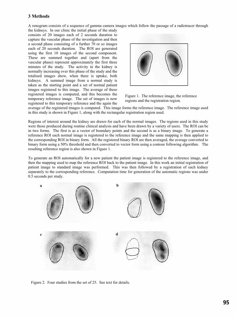
3 Methods A renogram consists of a sequence of gamma camera images which follow the passage of a radiotracer through the kidneys. In our clinic the initial phase of the study consists of 20 images each of 2 seconds duration to capture the vascular phase of the investigation and then a second phase consisting of a further 70 or so images each of 20 seconds duration. The ROI are generated using the first 10 images of the second component. These are summed together and (apart from the vascular phase) represent approximately the first three minutes of the study. The activity in the kidney is normally increasing over this phase of the study and the totalised images show, when there is uptake, both kidneys. A summed image from a normal study is taken as the starting point and a set of normal patient images registered to this image. The average of these registered images is computed, and this becomes the temporary reference image. The set of images is now registered to this temporary reference and the again the average of the registered images is computed. This image forms the reference image. The reference image used in this study is shown in Figure 1, along with the rectangular registration region used. Regions of interest around the kidney are drawn for each of the normal images. The regions used in this study were those produced during routine clinical analysis and have been drawn by a variety of users. The ROI can be in two forms. The first is as a vector of boundary points and the second is as a binary image. To generate a reference ROI each normal image is registered to the reference image and the same mapping is then applied to the corresponding ROI in binary form. All the registered binary ROI are then averaged, the average converted to binary form using a 50% threshold and then converted to vector form using a contour following algorithm. The resulting reference region is also shown in Figure 1. To generate an ROI automatically for a new patient the patient image is registered to the reference image, and then the mapping used to map the reference ROI back to the patient image. In this work an initial registration of patient image to standard image was performed. This was then followed by a registration of each kidney separately to the corresponding reference. Computation time for generation of the automatic regions was under 0.5 seconds per study.

Figure 2. Four studies from the set of 25. See text for details.

a b

c d

Figure 1. The reference image, the reference regions and the registration region.

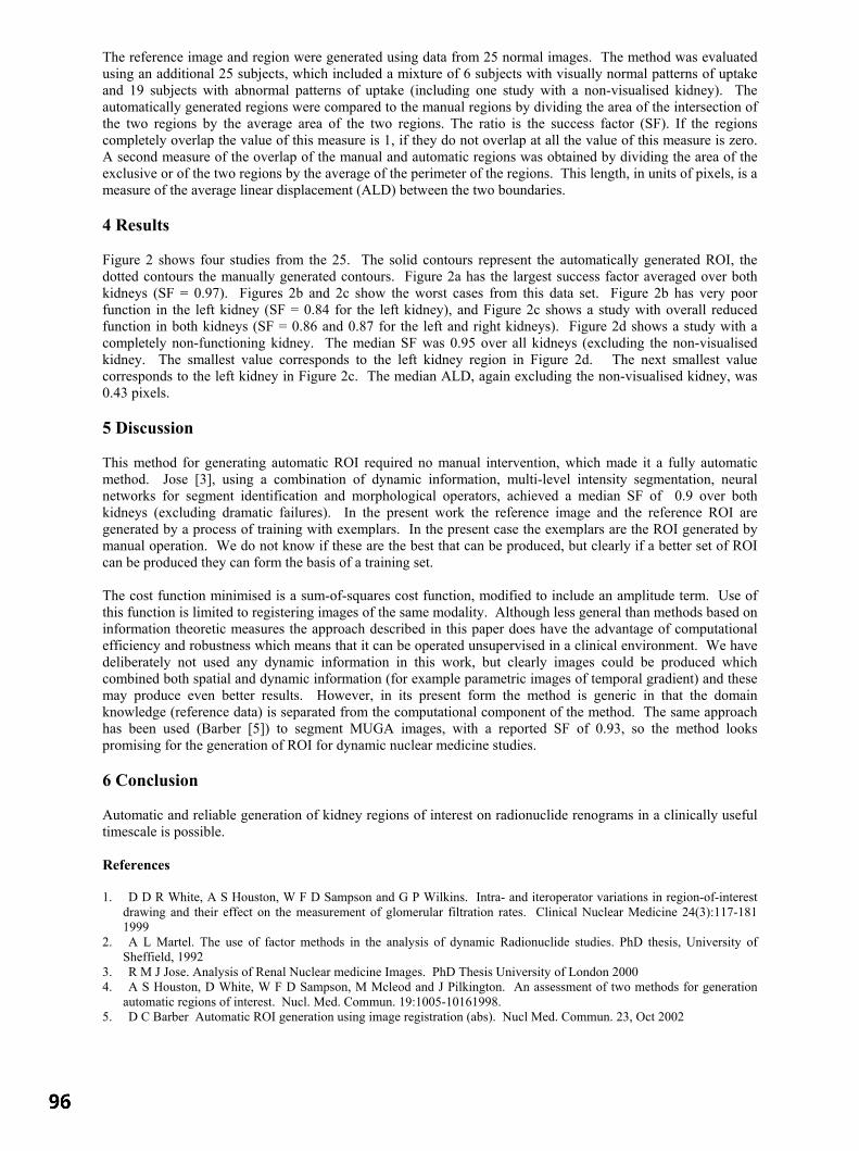
The reference image and region were generated using data from 25 normal images. The method was evaluated using an additional 25 subjects, which included a mixture of 6 subjects with visually normal patterns of uptake and 19 subjects with abnormal patterns of uptake (including one study with a non-visualised kidney). The automatically generated regions were compared to the manual regions by dividing the area of the intersection of the two regions by the average area of the two regions. The ratio is the success factor (SF). If the regions completely overlap the value of this measure is 1, if they do not overlap at all the value of this measure is zero. A second measure of the overlap of the manual and automatic regions was obtained by dividing the area of the exclusive or of the two regions by the average of the perimeter of the regions. This length, in units of pixels, is a measure of the average linear displacement (ALD) between the two boundaries. 4 Results Figure 2 shows four studies from the 25. The solid contours represent the automatically generated ROI, the dotted contours the manually generated contours. Figure 2a has the largest success factor averaged over both kidneys (SF = 0.97). Figures 2b and 2c show the worst cases from this data set. Figure 2b has very poor function in the left kidney (SF = 0.84 for the left kidney), and Figure 2c shows a study with overall reduced function in both kidneys (SF = 0.86 and 0.87 for the left and right kidneys). Figure 2d shows a study with a completely non-functioning kidney. The median SF was 0.95 over all kidneys (excluding the non-visualised kidney. The smallest value corresponds to the left kidney region in Figure 2d. The next smallest value corresponds to the left kidney in Figure 2c. The median ALD, again excluding the non-visualised kidney, was 0.43 pixels. 5 Discussion This method for generating automatic ROI required no manual intervention, which made it a fully automatic method. Jose [3], using a combination of dynamic information, multi-level intensity segmentation, neural networks for segment identification and morphological operators, achieved a median SF of 0.9 over both kidneys (excluding dramatic failures). In the present work the reference image and the reference ROI are generated by a process of training with exemplars. In the present case the exemplars are the ROI generated by manual operation. We do not know if these are the best that can be produced, but clearly if a better set of ROI can be produced they can form the basis of a training set. The cost function minimised is a sum-of-squares cost function, modified to include an amplitude term. Use of this function is limited to registering images of the same modality. Although less general than methods based on information theoretic measures the approach described in this paper does have the advantage of computational efficiency and robustness which means that it can be operated unsupervised in a clinical environment. We have deliberately not used any dynamic information in this work, but clearly images could be produced which combined both spatial and dynamic information (for example parametric images of temporal gradient) and these may produce even better results. However, in its present form the method is generic in that the domain knowledge (reference data) is separated from the computational component of the method. The same approach has been used (Barber [5]) to segment MUGA images, with a reported SF of 0.93, so the method looks promising for the generation of ROI for dynamic nuclear medicine studies. 6 Conclusion Automatic and reliable generation of kidney regions of interest on radionuclide renograms in a clinically useful timescale is possible. References 1. D D R White, A S Houston, W F D Sampson and G P Wilkins. Intra- and iteroperator variations in region-of-interest

drawing and their effect on the measurement of glomerular filtration rates. Clinical Nuclear Medicine 24(3):117-181 1999

2. A L Martel. The use of factor methods in the analysis of dynamic Radionuclide studies. PhD thesis, University of Sheffield, 1992

3. R M J Jose. Analysis of Renal Nuclear medicine Images. PhD Thesis University of London 2000 4. A S Houston, D White, W F D Sampson, M Mcleod and J Pilkington. An assessment of two methods for generation

automatic regions of interest. Nucl. Med. Commun. 19:1005-10161998. 5. D C Barber Automatic ROI generation using image registration (abs). Nucl Med. Commun. 23, Oct 2002

Investigation of Shape Changes in the Lateral VentriclesAssociated with Schizophrenia : A Morphometric Study Using a

Three-Dimensional Point Distribution Model

Kolawole Babalolaa∗, Jim Grahama, Lili Kopalab, and Robert Vandorpeb

aUniversity of Manchester, Imaging Science & Biomedical Engineering,bDalhousie University, Department of Psychiatry

Abstract. A previous publication [1] described the use of a transportation method to improve point to pointcorrespondences in the construction of three-dimensional point distribution models (PDMs). Using PDMscreated in the described manner, we have carried out morphometric analysis of the lateral ventricles of a groupof schizophrenic and control subjects to investigate possible shape differences associated with schizophrenia.Applying discriminant analysis to the most important shape parameters obtained from the PDM, the meansof the schizophrenic and control groups are significantly different (p< 10−13). The shape changes observedwere localised to three regions : the temporal horn (its tip near the amygdala, and along its body near theparahippocampal fissure), the central part of the lateral ventricles around the corpus callosum, and the tip of theanterior horn in the region of the frontal lobe. The differences in the temporal region and anterior horns are inregions close to structures thought to be implicated in schizophrenia.

1 Introduction

Schizophrenia is a serious brain disorder which is accompanied by altered brain structure. Interest in investigationof shape changes of the lateral ventricles due to schizophrenia can be attributed to the work of Johnstone et al. [2]who showed that schizophrenia is accompanied by an increase in the volume of the lateral ventricles. Severalgroups e.g. [3] [4], are currently developing methods to investigate whether specific localised shape changes occurin the lateral ventricles and other neuroanatomic structures due to schizophrenia and other brain diseases.

Because of the wide range of natural variability in the shape of structures in the human body, statistical approachesto measuring differences in shape are desirable. Statistical shape models (SSMs) use samples from control and/ordisease populations, the training set, to learn the variability in the structures being modelled. They can thereforeallow separation of shape changes due to disease in the presence of natural variation, and provide better charac-terisation of differences between populations than volumetric techniques. A diverse number of SSMs have beendescribed. However, these all need a method of representing shape, establishing correspondence across the trainingset and obtaining shape differences qualitatively and/or quantitatively.

The particular SSM we use here is the point distribution model (PDM) [5], which characterises shape by a smallnumber of “modes of shape variation”, providing a compact parameterisation. We apply linear discriminant anal-ysis (LDA) to the shape parameters to characterise inter-group differences.

2 Related Work

Buckley et al. [6] use 48 manually defined landmarks corresponding to curvature extrema on the surface of theventricles of 20 schizophrenic patients and 20 control subjects to investigate shape differences. They consideredthe whole ventricular system and reported no overall shape differences between the entire patient group and theentire schizophrenic group. However, when only the males of both groups were considered, significant shapedifferences were identified in the proximal juncture of the temporal horn and in the foramen of Monro.

Gerig et al. [3] performed shape analysis on the lateral ventricles of 5 pairs of monozygotic and 5 pairs of dizygotictwins. Ventricles were mapped to a unit sphere and decomposed into a summation of spherical harmonic functions.The first order harmonics were used to impose correspondence between points and the measure of shape differ-ences was the mean squared distance between corresponding points on the surfaces. They showed that, withoutnormalisation for ventricular size, no significant differences were seen between the two groups. However, afternormalisation using the volumes of the ventricles, the right lateral ventricles of the two groups are significantlydifferent. They concluded that shape measures reveal new information in addition to size or volumetric differences,which might assist in the understanding of structural differences due to neuroanatomical diseases.

∗Email: [email protected]

Narr et al. [4] obtained average maps of anatomical differences based on voxel values of the limbic structuresand the lateral ventricles of 25 schizophrenic and 28 control subjects. Their analysis showed significant shapedifferences in the left lateral ventricles. In particular, there was enlargement of the superior part and the posteriorhorn. There were also noticeable differences in the part of the lateral ventricles in the vicinity of the caudate head.

Our approach has aspects in common with [6] and [3]. We build PDMs based on corresponding landmark pointsacross a training set. The landmark points are used to generate a small number of shape parameters controllingthe modes of variation of the shapes. The use of this parametric description distinguishes our approach from thatof [6]. However, the parameters are devised from the training data, unlike those of [3].

3 Materials and Method

3.1 Data

Volumetric T2 MR scans of 30 controls (14-45 years, 13 female, 17 male) and 39 age and sex matched schizophren-ics (14-45 years, 9 female, 30 male) were used in this study. The scans were independently acquired in the sagittal,coronal and axial orientations. Each slice had 256 x 256 voxels, with in-plane size of 0.86mm by 0.86mm forsagittal and axial orientations, and 0.78mm by 0.78mm for the coronal orientation. For all orientations the slicethickness was 5mm and the intra-slice gap was 1mm. All images were corrected for MR inhomogeniety [7], andthe three views of each subject were combined by rigid registration and interpolation to give 3D images witheffective resolution of 0.78mm x 0.78mm x 0.78mm. The lateral ventricles were segmented using a 3D edge de-tector [8] and edge segments were manually linked to form closed contours in each slice with the guidance of aneuroradiologist. The contours of the left lateral ventricles were reflected to give the same pose as those of theright, giving an evaluation set of 138 ventricles for this study.

For each subject, brain size parameters were obtained as follows. Skull stripping was performed on each MRimage [9], and ellipsoids were fitted to the resulting brains. The lengths of the three principal axes of the ellipsoidswere stored as the brain size parameters. The ventricular surfaces were aligned to a canonical coordinate systemusing their centroids and the three principal axes obtained from the distribution of the coordinates of their surfacepoints. The brain size parameters were then used to scale each object centred ventricle independently in the threeorthogonal directions for normalisation for brain size with respect to the brain size of an arbitrarily chosen templatebrain. This was necessary to remove the influence of brain shape on ventricular shape.

3.2 Point Distribution Models

A PDM [5] reparameterises a shape described by surface landmark points to a smaller set of shape parametersusing equation 1

x = x + Pb . (1)

x is the vector of the coordinates of surface landmarks of a particular shape,x is the average of these vectorsover a training set.P is the matrix whose columns are the eigenvectors corresponding to the largestk eigenvaluesof the covariance matrix of the shape vectors.b is a vector of weights of dimensionk. Due to correlations inpoint positions,k can be much smaller than the number of landmark points.b then becomes a vector ofk shapeparameters which are equivalent tox as a description of the shape.

It is necessary to locatecorrespondinglandmark points on all the surfaces in the training set. In the case of 2DPDMs this can be achieved by manual annotation. However, in 3D this becomes difficult and prohibitively labour-intensive. Davies et al. [10] have shown that the specificity of a SSM depends critically on finding accuratelycorresponding landmark points. Several approaches have been made towards automatic landmark generation in3D, including the use of spherical harmonic parameterisation [3] and optimisation of the shape models [10]. Herewe identify landmarks from the set of “crest points” on the ventricle surface using a modification of the methoddue to Subsol [11]. Correspondence is established using non-rigid registration of the surfaces and minimisation ofEuclidean distance expressed as a transportation cost.

3.3 Construction of the 3D PDM of the Lateral Ventricle

Crest points, which are curvature extrema on the ventricles, are used as automatically derived anatomical landmarkshere. According to the definition of [11] they are points where lines of principal maximal curvature on a surface

have maximum values. Crest lines are the locus of crest points and impose an ordering on crest points. The useof crest points and crest lines in the creation of 3D PDMs of the ventricles has been described previously [1].This also gives details of the transportation algorithm used to improve the correspondences obtained from the crestpoints, showing it gives a greater number of matches and greater symmetry of matches when compared with anIterative Closest Point (ICP) method.

To create the 3D PDM, one ventriclevt was used as a template and its surface represented by vertices and vertexfaces defined by triangular triplets of the vertices. The initial triangulation produced about 10,000 vertices, butfor computational reasons these were decimated to give about 1,000 vertices. Crest lines were obtained for eachventricle and normalised with respect to the template as described in section 3.1. The crest lines of each of theremaining 137 ventriclesvi ∈ v1, . . . ,v137 were matched in a pairwise manner to those of the chosen template,vt. The matches were in both directions i.e.vt → vi andvi → vt, using the transportation method and a post-processing step to enforce monotonicity. Matching was performed over 30 iterations: ten iterations each of rigidalignment, affine alignment, and spline warping successively as described in [11].

Although the transportation-based method gives symmetric results for matches in both directions when the numberof crest points are equal, the results are not guaranteed to be symmetric when the number of crest points are notequal, which in general is the case with matching ventricles. Therefore, from each matched pair (vt → vi andvi → vt), a subset of matches occurring on parts of crest lines that were symmetrically matched in both directionswere extracted. Although this decreases the number of matched points used in the subsequent transformation, itgives greater confidence that they are valid matches. For the present case, 1,586± 167 crest points (79% of thetotal number matched) were on symmetrically matched crest lines for the transportation-based method, and 964±160 (70% of the total number matched) for the ICP-based method. The symmetric subset of matched points areused to obtain coefficients defining a final spline based warp allowing transformation of the vertex points ofvt

onto the surface of eachvi. The spline based warps are defined in [11].

3.4 Shape Analysis

The parameters of theb vectors are used to define a shape space using the firstk eigenvalues in the PDM (k=30in the present case, explaining over 99% of the observed variance). Each member of the training set is a pointwithin thisk-dimensional space, represented by a vectorbk. To characterise shape differences between the groupswe conducted a LDA (see e.g. [12]) using Fisher’s criterion. This provides a “discriminant vector” in shapespace along which the difference between the groups is most marked. We can quantify the shape differencesby projecting the individual shape vectors onto the discriminant vector to provide a scalar value representing theindividual shapes. The nature of the shape differences between the groups can be visualised by reconstructing theshapes corresponding to the group means. Specific differences correspond to locations on the shape where largemovements occur between the reconstructed shapes.

4 Results

Figure 1(a) shows the results of projection onto the discriminant vector. The difference in the means was statisti-cally significant (p< 10−13 by a t-test). Figure 1(b) shows the difference between the means of the schizophrenicgroup and that of the control group colour-mapped onto a ventricular surface. The greatest differences were in theregion of the tip of the anterior horn (8mm), in the region of the temporal horn (between 2mm and 6mm), aroundthe central part of the main body of the ventricle in the region of the corpus callosum (between 4mm and 6mm).

5 Discussion

The results of the morphometric analysis are similar to those of [4] in that they show differences localised to thetemporal horn in the region of the parahippocampal fissure, and in the anterior part of the lateral ventricle nearthe frontal lobe. However, we also found differences in the central part of the lateral ventricle in the region of thecorpus callosum. Although [6] also report differences in the temporal horn of male schizophrenics, they did notfind differences in the pooled groups of male and females as we have reported here. Schizophrenia is a complexdisease and, as the results of the linear discriminant analysis shows, there is a considerable overlap in the ventriclesof schizophrenics and normals. Hence we do not propose we have a method that allows the discrimination oflateral ventricles into schizophrenic and none schizophrenic groups. However, studies of this sort may help inunderstanding and monitoring schizophrenia. In this study we combined left and right ventricles of both males

−30

−20

−10

0

10

20

30

40V

alue

for

proj

ectio

n on

to d

iscr

imin

ant v

ecto

r

SchizophrenicsControls

(a) Projections of the points in 30-dimensional shape space onto thediscriminant vector (group means in filled black)

2 4 6 8 10

(b) Colour mapped ventricle showing the areas of differences be-tween the schizophrenic group and the control group

Figure 1. Results of shape analysis

and females. We have also removed all overall volume effects by isotropic scaling of the ventricles prior to shapemodelling. The observed differences are residual differences in shape in addition to any volumetric differences.Future work will include investigating age and gender effects as well as comparing left and right asymmetry.

6 Acknowledgements

We would like to thank Dr Donna Lang of University of British Columbia for help with the MR images, theEpidaure group of INRIA, France for Marching Lines code, Professor P. Klienschmidt of Passau University forcode for the assignment problem, and Professors Alan Jackson and Bill Deakin of Manchester University forassistance in interpreting the results.

References

1. K. O. Babalola, J. Graham, L. Kopala et al. “Using the transportation algorithm to improve point correspondences in theconstruction of 3D PDMs.” InProceedings of Medical Image Understanding and Analysis, pp. 141–144. BMVA, 2002.

2. E. C. Johnstone, T. J. Crow, C. D. Frith et al. “Cerebral ventricular size and cognitive impairment in chronic schizophrenia.”Lancet7992(2), pp. 924–926, 1976.

3. G. Gerig, M. Styner, D. Jones et al. “Shape analysis of brain ventricles using SPHARM.” InProceedings of IEEE Workshopon Mathematical Methods in Biomedical Image Analysis, pp. 171–178. IEEE, 2001.

4. K. L. Narr, P. M. Thompson, T. Sharma et al. “Three-dimensional mapping of tempro-limbic regions and the lateralventricles in schizophrenia: Gender effects.”Bioligcal Psychiatry50, pp. 84–97, 2001.

5. T. F. Cootes, A. Hill, C. J. Taylor et al. “The use of active shape models for locating structures in medical images.”Imageand Vision Computing12(6), pp. 355–366, 1994.

6. P. Buckley, D. Dean, F. L. Bookstein et al. “Three-dimensional magnetic resonance-based morphometrics and ventriculardysmorphology in schizophrenia.”Biolgical Psychiatry45, pp. 62–67, 1999.

7. E. A. Vokurka, N. A. Thacker & A. Jackson. “A fast model-independent method for automatic correction of intensitynonuniformity in MRI data.”Journal of Magnetic Resonance Imaging10(4), pp. 550–562, 1999.

8. O. Monga, R. Deriche, G. Malandain et al. “Recursive filtering and edge tracking: two primary tools for 3D edge detection.”Image and Vision Computing9(4), pp. 203–214, 1991.

9. S. Smith. “Fast robust automated brain extraction.”Human Brain Mapping17(3), pp. 143–155, 2002.10. R. H. Davies, C. J. Twining, T. F. Cootes et al. “3D statistical shape models using direct optimisation of description length.”

In Proceedings of European Conferernce on Computer Vision, volume 2350(3), pp. 3–20. LCNS, 2002.11. G. Subsol, J. P. Thirion & N. Ayache. “A scheme for automatically building three-dimensional morphometric anatomical

atlases: Application to a skull atlas.”Medical Image Analysis2(1), pp. 37–60, 1998.12. D. J. Hand.Discrimination and Classification (Chapter 4). John Wiley &Sons, 1981.

A Non-Euclidean Metric for the Classification of Variations inMedical Images

Carole Twining∗ and Stephen Marsland∗

Imaging Science and Biomedical Engineering, University of Manchester, Manchester M13 9PT, UK

Abstract. The analysis of deformation fields, such as those generated by non-rigid registration algorithms, iscentral to the quantification of normal and abnormal variation of structures in registered images. The correctchoice of representation is an integral part of this analysis. This paper presents methods for constructing multi-dimensional diffeomorphic representations of deformations. We demonstrate that these representations aresuitable for the description of medical image-based deformations in 2 and 3 dimensions. We show (using a setof 2D outlines of ventricles) that the non-Euclidean metric inherent in this representation is superior to the usualad hoc Euclidean metrics in that it enables more accurate classification of legal and illegal variations.

1 IntroductionNon-rigid registration algorithms [1, 2] automatically generate dense (i.e., pixel-to-pixel or voxel-to-voxel) corre-spondences between pairs and sets of images with the aim of aligning analogous ‘structures’. The deformationfields implicit in this correspondence contain information about the variability of structures across the set, and inorder to analyse quantitatively this variability, we need to be able to analyse the set of deformation fields. Suchanalysis must be based (either implicitly or explicitly) on a particular mathematical representation of the deforma-tion field. Previous work on modelling dense 2D and 3D deformation fields has either used the densely-sampleddeformation vectors directly (e.g., [3,4]), or has employed a smooth, continuous representation of these (e.g., [5]).However, neither of these methods guarantees that the deformation field is diffeomorphic.We contend that the appropriate representation should be continuous and diffeomorphic. Where such a correspon-dence is not actually physically meaningful (e.g., in the case where additional structures such as tumours appear),this should be indicated by the warp parameters assuming atypical values. When we are considering the correspon-dence between discrete and bounded objects such as brains, it is also desirable that the warps themselves shouldbe discrete and bounded. This leads us to suggest that a suitable representation is that of the group of continuousdiffeomorphisms with some appropriate set of boundary conditions. Such a representation can be constructed us-ing an approach based on Geodesic Interpolating Splines (GIS) [6]. In previous work [6,7] it has been shown thatthis approach also allows the construction of a metric on the diffeomorphism group.In this paper we demonstrate the construction of these diffeomorphic representations using a variety of splinebases. We show that these representations generate warps that are suitable for the task in hand, giving biologically‘plausible’ warps in both two and three dimensions, whilst being of a relatively low dimensionality. We furtherstudy the significance of the metric (geodesic) distances between warps, and show that using it provides a measureof atypical variation that has greater discriminatory power than naıve measures based on the ad hoc use of aEuclidean metric on the space of warp parameters.

2 The Geodesic Interpolating SplineWe consider a vector-valued spline function~f(~x), ~x ∈ Rn that interpolates between data values at a set ofknotpoints~xi : i = 1 toN, where~f(~xi) = ~fi, that can be expressed as the minimiser of a functional Lagrangianof the form:

E[~f]

=∫

Rn

d~x∥∥∥L~f(~x)

∥∥∥2

+N∑

i=1

λi

(~f(~xi)− ~fi

), (1)

whereL is some scalar differential operator. The first term in the Lagrangian is the smoothing term; the secondterm with the Lagrange multipliersλi ensures that the spline fits the data at the knotpoints. The choice ofoperatorL and boundary conditions defines a particular spline basis. The general solution can be written in theform:

~f(~x) = ~g(~x) +N∑

i=1

~αiG(~x, ~xi), (2)

where the affine functiong is a solution ofL~g(~x) = 0 and the Green’s functionG is a solution of:(L†L

)G(~x, ~y) ∝

δ(~x− ~y), with L† is the Lagrange dual ofL. For more details, see [8]. The choice of Green’s function depends onthe boundary conditions and smoothness appropriate to the problem considered. Suggestion of different possibleGreen’s functions are given in [8], here we focus on the Clamped-Plate Spline (CPS), which has the boundary con-ditions that it is identically zero on and outside the unit ball [9]. We contend that such boundary conditions are theappropriate choice for images of discrete objects such as brains; other types of images may require different bound-ary conditions. The biharmonic CPS (L†L = (∇2)2) in 2 dimensionsG2

2, and the triharmonic (L†L = (∇2)3)CPS in 3 dimensionsG3

3, have Green’s functions ( [9,10]):

∗Joint first authors.carole.twining,stephen.marsland @man.ac.uk

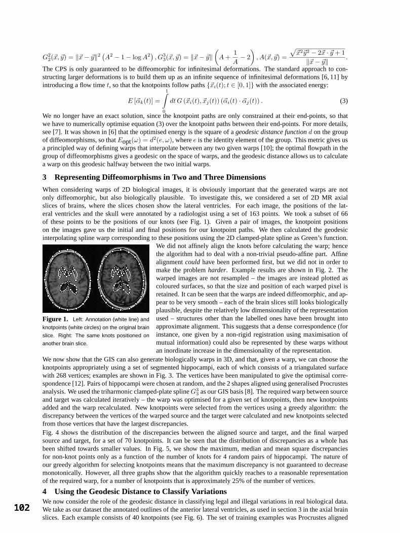
G22(~x, ~y) = ‖~x− ~y‖2 (

A2 − 1− log A2), G3

3(~x, ~y) = ‖~x− ~y‖(

A +1A− 2

), A(~x, ~y) =

√~x2~y2 − 2~x · ~y + 1

‖~x− ~y‖ .

The CPS is only guaranteed to be diffeomorphic for infinitesimal deformations. The standard approach to con-structing larger deformations is to build them up as an infinite sequence of infinitesimal deformations [6, 11] byintroducing a flow timet, so that the knotpoints follow paths~xi(t); t ∈ [0, 1] with the associated energy:

E [~αk(t)] =

1∫

0

dtG (~xi(t), ~xj(t)) (~αi(t) · ~αj(t)) . (3)

We no longer have an exact solution, since the knotpoint paths are only constrained at their end-points, so thatwe have to numerically optimise equation (3) over the knotpoint paths between their end-points. For more details,see [7]. It was shown in [6] that the optimised energy is the square of ageodesic distance functiond on the groupof diffeomorphisms, so thatEopt(ω) = d2(e, ω), wheree is the identity element of the group. This metric gives usa principled way of defining warps that interpolate between any two given warps [10]; the optimal flowpath in thegroup of diffeomorphisms gives a geodesic on the space of warps, and the geodesic distance allows us to calculatea warp on this geodesic halfway between the two initial warps.

3 Representing Diffeomorphisms in Two and Three Dimensions

When considering warps of 2D biological images, it is obviously important that the generated warps are notonly diffeomorphic, but also biologically plausible. To investigate this, we considered a set of 2D MR axialslices of brains, where the slices chosen show the lateral ventricles. For each image, the positions of the lat-eral ventricles and the skull were annotated by a radiologist using a set of 163 points. We took a subset of 66of these points to be the positions of our knots (see Fig. 1). Given a pair of images, the knotpoint positionson the images gave us the initial and final positions for our knotpoint paths. We then calculated the geodesicinterpolating spline warp corresponding to these positions using the 2D clamped-plate spline as Green’s function.

Figure 1. Left: Annotation (white line) and

knotpoints (white circles) on the original brain

slice. Right: The same knots positioned on

another brain slice.

We did not affinely align the knots before calculating the warp; hencethe algorithm had to deal with a non-trivial pseudo-affine part. Affinealignmentcould have been performed first, but we did not in order tomake the problemharder. Example results are shown in Fig. 2. Thewarped images are not resampled – the images are instead plotted ascoloured surfaces, so that the size and position of each warped pixel isretained. It can be seen that the warps are indeed diffeomorphic, and ap-pear to be very smooth – each of the brain slices still looks biologicallyplausible, despite the relatively low dimensionality of the representationused – structures other than the labelled ones have been brought intoapproximate alignment. This suggests that a dense correspondence (forinstance, one given by a non-rigid registration using maximisation ofmutual information) could also be represented by these warps withoutan inordinate increase in the dimensionality of the representation.

We now show that the GIS can also generate biologically warps in 3D, and that, given a warp, we can choose theknotpoints appropriately using a set of segmented hippocampi, each of which consists of a triangulated surfacewith 268 vertices; examples are shown in Fig. 3. The vertices have been manipulated to give the optimisal corre-spondence [12]. Pairs of hippocampi were chosen at random, and the 2 shapes aligned using generalised Procrustesanalysis. We used the triharmonic clamped-plate splineG3

3 as our GIS basis [8]. The required warp between sourceand target was calculated iteratively – the warp was optimised for a given set of knotpoints, then new knotpointsadded and the warp recalculated. New knotpoints were selected from the vertices using a greedy algorithm: thediscrepancy between the vertices of the warped source and the target were calculated and new knotpoints selectedfrom those vertices that have the largest discrepancies.Fig. 4 shows the distribution of the discrepancies between the aligned source and target, and the final warpedsource and target, for a set of 70 knotpoints. It can be seen that the distribution of discrepancies as a whole hasbeen shifted towards smaller values. In Fig. 5, we show the maximum, median and mean square discrepanciesfor non-knot points only as a function of the number of knots for 4 random pairs of hippocampi. The nature ofour greedy algorithm for selecting knotpoints means that the maximum discrepancy is not guaranteed to decreasemonotonically. However, all three graphs show that the algorithm quickly reaches to a reasonable representationof the required warp, for a number of knotpoints that is approximately 25% of the number of vertices.

4 Using the Geodesic Distance to Classify VariationsWe now consider the role of the geodesic distance in classifying legal and illegal variations in real biological data.We take as our dataset the annotated outlines of the anterior lateral ventricles, as used in section 3 in the axial brainslices. Each example consists of 40 knotpoints (see Fig. 6). The set of training examples was Procrustes aligned

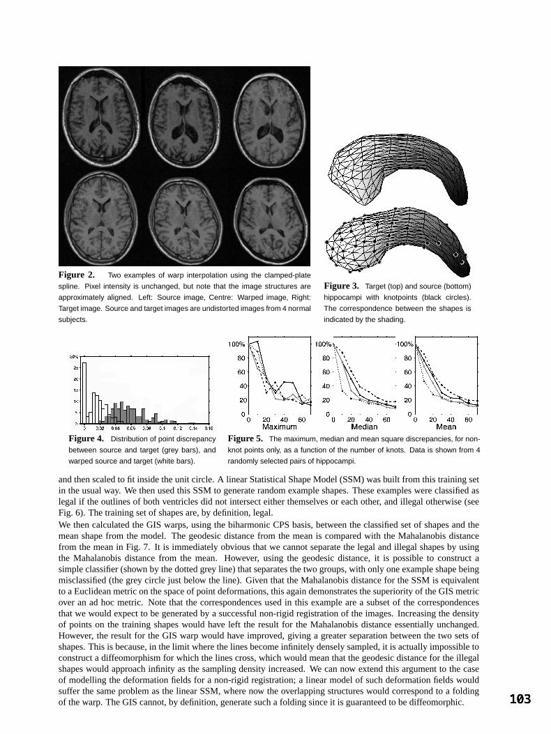
Figure 2. Two examples of warp interpolation using the clamped-plate

spline. Pixel intensity is unchanged, but note that the image structures are

approximately aligned. Left: Source image, Centre: Warped image, Right:

Target image. Source and target images are undistorted images from 4 normal

subjects.

Figure 3. Target (top) and source (bottom)

hippocampi with knotpoints (black circles).

The correspondence between the shapes is

indicated by the shading.

Figure 4. Distribution of point discrepancy

between source and target (grey bars), and

warped source and target (white bars).

Figure 5. The maximum, median and mean square discrepancies, for non-

knot points only, as a function of the number of knots. Data is shown from 4

randomly selected pairs of hippocampi.

and then scaled to fit inside the unit circle. A linear Statistical Shape Model (SSM) was built from this training setin the usual way. We then used this SSM to generate random example shapes. These examples were classified aslegal if the outlines of both ventricles did not intersect either themselves or each other, and illegal otherwise (seeFig. 6). The training set of shapes are, by definition, legal.We then calculated the GIS warps, using the biharmonic CPS basis, between the classified set of shapes and themean shape from the model. The geodesic distance from the mean is compared with the Mahalanobis distancefrom the mean in Fig. 7. It is immediately obvious that we cannot separate the legal and illegal shapes by usingthe Mahalanobis distance from the mean. However, using the geodesic distance, it is possible to construct asimple classifier (shown by the dotted grey line) that separates the two groups, with only one example shape beingmisclassified (the grey circle just below the line). Given that the Mahalanobis distance for the SSM is equivalentto a Euclidean metric on the space of point deformations, this again demonstrates the superiority of the GIS metricover an ad hoc metric. Note that the correspondences used in this example are a subset of the correspondencesthat we would expect to be generated by a successful non-rigid registration of the images. Increasing the densityof points on the training shapes would have left the result for the Mahalanobis distance essentially unchanged.However, the result for the GIS warp would have improved, giving a greater separation between the two sets ofshapes. This is because, in the limit where the lines become infinitely densely sampled, it is actually impossible toconstruct a diffeomorphism for which the lines cross, which would mean that the geodesic distance for the illegalshapes would approach infinity as the sampling density increased. We can now extend this argument to the caseof modelling the deformation fields for a non-rigid registration; a linear model of such deformation fields wouldsuffer the same problem as the linear SSM, where now the overlapping structures would correspond to a foldingof the warp. The GIS cannot, by definition, generate such a folding since it is guaranteed to be diffeomorphic.

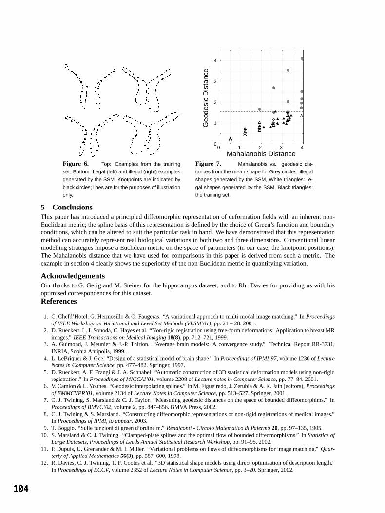
Figure 6. Top: Examples from the training

set. Bottom: Legal (left) and illegal (right) examples

generated by the SSM. Knotpoints are indicated by

black circles; lines are for the purposes of illustration

only.

0 1 2 3 4 0

1

2

3

4

Geo

desi

c D

ista

nce

Mahalanobis Distance Figure 7. Mahalanobis vs. geodesic dis-

tances from the mean shape for Grey circles: illegal

shapes generated by the SSM, White triangles: le-

gal shapes generated by the SSM, Black triangles:

the training set.

5 ConclusionsThis paper has introduced a principled diffeomorphic representation of deformation fields with an inherent non-Euclidean metric; the spline basis of this representation is defined by the choice of Green’s function and boundaryconditions, which can be altered to suit the particular task in hand. We have demonstrated that this representationmethod can accurately represent real biological variations in both two and three dimensions. Conventional linearmodelling strategies impose a Euclidean metric on the space of parameters (in our case, the knotpoint positions).The Mahalanobis distance that we have used for comparisons in this paper is derived from such a metric. Theexample in section 4 clearly shows the superiority of the non-Euclidean metric in quantifying variation.

AcknowledgementsOur thanks to G. Gerig and M. Steiner for the hippocampus dataset, and to Rh. Davies for providing us with hisoptimised correspondences for this dataset.References

1. C. Chefd’Hotel, G. Hermosillo & O. Faugeras. “A variational approach to multi-modal image matching.” InProceedingsof IEEE Workshop on Variational and Level Set Methods (VLSM’01), pp. 21 – 28. 2001.

2. D. Rueckert, L. I. Sonoda, C. Hayes et al. “Non-rigid registration using free-form deformations: Application to breast MRimages.”IEEE Transactions on Medical Imaging18(8), pp. 712–721, 1999.

3. A. Guimond, J. Meunier & J.-P. Thirion. “Average brain models: A convergence study.” Technical Report RR-3731,INRIA, Sophia Antipolis, 1999.

4. L. LeBriquer & J. Gee. “Design of a statistical model of brain shape.” InProceedings of IPMI’97, volume 1230 ofLectureNotes in Computer Science, pp. 477–482. Springer, 1997.

5. D. Rueckert, A. F. Frangi & J. A. Schnabel. “Automatic construction of 3D statistical deformation models using non-rigidregistration.” InProceedings of MICCAI’01, volume 2208 ofLecture notes in Computer Science, pp. 77–84. 2001.

6. V. Camion & L. Younes. “Geodesic interpolating splines.” In M. Figueiredo, J. Zerubia & A. K. Jain (editors),Proceedingsof EMMCVPR’01, volume 2134 ofLecture Notes in Computer Science, pp. 513–527. Springer, 2001.

7. C. J. Twining, S. Marsland & C. J. Taylor. “Measuring geodesic distances on the space of bounded diffeomorphims.” InProceedings of BMVC’02, volume 2, pp. 847–856. BMVA Press, 2002.

8. C. J. Twining & S. Marsland. “Constructing diffeomorphic representations of non-rigid registrations of medical images.”In Proceedings of IPMI, to appear. 2003.

9. T. Boggio. “Sulle funzioni di green d’ordine m.”Rendiconti - Circolo Matematico di Palermo20, pp. 97–135, 1905.10. S. Marsland & C. J. Twining. “Clamped-plate splines and the optimal flow of bounded diffeomorphisms.” InStatistics of

Large Datasets, Proceedings of Leeds Annual Statistical Research Workshop, pp. 91–95. 2002.11. P. Dupuis, U. Grenander & M. I. Miller. “Variational problems on flows of diffeomorphisms for image matching.”Quar-

terly of Applied Mathematics56(3), pp. 587–600, 1998.12. R. Davies, C. J. Twining, T. F. Cootes et al. “3D statistical shape models using direct optimisation of description length.”

In Proceedings of ECCV, volume 2352 ofLecture Notes in Computer Science, pp. 3–20. Springer, 2002.

An evaluation of deformation-based morphometry in thedeveloping human brain and detection of volumetric changes

associated with preterm birthJ.P. Boardman1 K. Bhatia2 S.Counsell3 J.Allsop 3 O. Kapellou1

M. A. Rutherford1,3 A. D. Edwards1 J.V. Hajnal1

D. Rueckert2

1 Departmentof Paediatrics,ObstetricsandGynaecology, Facultyof Medicine,ImperialCollegeLondon2 VisualInformationProcessingGroup,Departmentof ComputingImperialCollegeLondon

3 RobertSteinerMagneticResonanceUnit, ImagingSciencesDepartment,MRC Clinical SciencesCentre,ImperialCollegeLondon

Abstract. Deformation-basedmorphometryenablesthe automaticquantificationof neuroanatomicaldiffer-encesby measuringregionalshapeandvolumedifferencesbetweenanatlas(or referencespace)andthepopu-lation underinvestigation.In this paperwe usedeformation-basedmorphometricmethodsto studyvolumetricdifferencesbetweenpreterminfantsat term equivalentageandterm born controlsusinghigh-resolutionMRimaging. We investigatetheinfluenceof thechoiceof atlason resultsobtainedusingdeformation-basedmor-phometry. For thispurposeweconstructedthreedifferentatlasesof termborninfantsandusedthemto comparethebrainsof thepreterminfants(at termequivalentage)andthetermcontrolgroups.A non-rigidregistrationalgorithmwas usedto mapall 3 atlasesinto a commoncoordinatesystemandvolumetricdifferenceswereextracted.Our resultsdemonstratesignificantvolumedifferencesbetweenpreterminfants(at termequivalentage)andthe control groupin the ventricularsystem,cerebrospinalfluid spacesanteriorlyandthe basalgan-glia. Volumetricchangesareconsistentbetweenall threemapsof volumechangeandindicatethat theresultsobtainedusingdeformation-basedmorphometryarelargely independentof thechoiceof thereferencespace.

1 Introduction

Pretermdeliveryaffects5% of all deliveriesandits consequencescontributeto significantindividual,medicalandsocialproblemsglobally. The principle morbidity amongsurvivors is neurological,resultingfrom the profoundeffect of pretermbirth on the developingbrain: half of all infantsborn at lessthan25 weekshave neurodevel-opmentalimpairmentat 30 monthsof ageandin lessimmatureinfantsneuropsychiatricproblemsarecommonin the teenageyears[1, 2]. This groupof infantscanbe studiedto evaluatethe neuroimagingcorrelatesof cog-nitive andbehavioural impairments.Most imagingstudiesof the pretermbrain have usedultrasoundandhaveshown thatmajordestructive lesionssuchasperiventricularleucomalaciaandhaemorrhagicparenchymalinfarctareassociatedwith motor impairment,but theselesionsdo not occurcommonlyenoughto accountfor the highprevalenceof neuropsychiatricdisordersseenin this group [3]. However, high resolutionmagneticresonance(MR) imagingdetectsmoresubtleabnormalitiesandshowsthatearlyfocal lesionsarecommonin preterminfantsat birth andcanchangeor resolve with time, andthatsubsequentdiffusewhite matterandcorticalabnormalitiesarecommonat termequivalentage[4]. Theanatomicalphenotypeof thesechangesandhow they relateto adverseneuropsychiatricoutcomehasnot beencharacterised.

2 Methods

Computationalmorphometryhasbeenusedin a numberof neurological[5–8] andneurodevelopmental[9–12]disordersto capturenovel informationaboutnon-focalbrain changes.However, mostof theseapproacheshavebeenappliedto the maturebrain. In this paperwe usea high dimensionalnon-rigid registrationalgorithm[13]to examinemorphometricdifferencesbetweenpretermandtermborninfants,andinvestigatetheinfluenceof thechoiceof atlasonresultsobtained.For thispurposewehaveanalyzedtheMR imagesof 66preterminfants(median29.6,range26-34weekspost-menstrualage)at termequivalentage(38 to 42 weeks),togetherwith thosefrom 11termcontrol infants(median39.6,range38-42weekspost-menstrualage).Ethicalpermissionfor this studywasgrantedby theHammersmithHospitalResearchEthicsCommitteeandinformedparentalconsentwasobtainedforeachinfant. Infantsweresedatedfor theexaminationbut nonerequiredmechanicalventilationat thetime of MRimaging. Pulseoximetry, electrocardiographicandtelevisual monitoringwereusedthroughoutthe examinationwhich wasattendedby a paediatrician.For someanalyseswe defineda subgroupof 36 individualswith a post-menstrualageof lessthan30 weeks. A 1.5 T EclipseMR system(Philips Medical Systems,Cleveland,Ohio)wasusedto acquirehigh resolutionT1 weightedimages(TR=30ms,TE=4.5ms,flip angle= 30

). In additionto

conventionalT1 andT2 weightedimageacquisition,volumedatasetswereacquiredin contiguoussagittalslices(in-planematrix size256 256,FOV = 25cm)with a voxel sizeof 1.0 1.0 1.6mm

.

2.1 Non-rigid Registration

In orderto maptheanatomyof eachsubject

into theanatomyof theatlas it is necessaryto employ non-rigidtransformationssuchaselasticor fluid transformations.We areusinga non-rigid registrationalgorithmwhichhasbeenpreviously appliedsuccessfullyto a numberof differentregistrationtasks[14,15]. Local deformations

aremodelledusingfree-formdeformations(FFD),

! #"

$% " &' " ! ()+*-,. / 0. / 12. ! (1)

where*

denotesthe control pointswhich parameterisethe transformation.The optimal transformationis foundby minimisinga costfunctionassociatedwith theglobal transformationparametersaswell asthe local transfor-mationparameters.Thecostfunctioncomprisestwo competinggoals:thefirst termrepresentsthecostassociatedwith thevoxel-basedsimilarity measure,in this casenormalisedmutualinformation[16], while thesecondtermcorrespondsto a regularisationtermwhich constrainsthe transformationto besmooth[14]. The resultingtrans-formation

mapseachpoint in theanatomyof thereferencesubject to thecorrespondingpoint in theanatomy

of thesubject

.

2.2 Deformation-based morphometry

To comparethe neuroanatomicalphenotpyesof the two groupswe selectedMR imagesof threeinfantsborn atterm which formed threedifferent referencespacesto which T1 weightedvolumedatasetsfrom 66 pretermatterm equivalentage(PAT) and11 term born controlswereregistered.In the first step,we calculatedthe globaltransformationbetweenthe subjectsandthe atlascorrectingfor scaling,skew, rotationandtranslation.We thenappliedthenon-rigidregistrationalgorithmusingamulti-resolutionschemewith controlspacingof 20mm,10mm,5mm and2.5mm. The resultingcontrol point meshdefinesa 354 continuousandanalytic representationof thedeformationfield which describesthepoint-wise3D displacementvectorsthatarerequiredto warpeachdatasetto thereferenceimage.

Theregistrationsbetweensubjectsandreferencesubjecthavebeencarriedout for all threereferencesubjectsandall registeredimageswerecheckedfor artefactsandaccurateanatomicallocalisationby visual inspection.In allcasesregistrationachieveda visuallyplausiblealignmentof anatomicalstructures.

2.3 Data Analysis

To calculateregionalvolumechangesthedeterminantof theJacobianof thedeformationfield is usedto quantifydifferencesbetweenregisteredimagesandreference.The determinantof the Jacobianfor any given locationinthereferencecoordinatesystemfor eachindividual providesanestimateof thepoint-wisevolumechangeof thatindividual with respectto the atlas. Valuesabove 1 indicatetissueexpansionandwhile valuesbelow 1 indicatetissuecontraction.To evaluatetheconsistency of thedeformation-basedapproach,we calculatedvolumechangemapsbetweeneachsubject6 andall threereferencesubjects,87:9 , 87 4 and 87 . We alsoregistered87 4 and87 to 87:9 whichallowsusto transformeachvolumechangemapinto thecoordinatesystemof 87:9 . To correctfor possibleregional volumedifferencesbetweenthe referencesubjects,the volumechangemapsarescaledbythe Jacobiandeterminantof the transformationbetweenthe two referencesubjects. If the registrationshadnoassociatederrors, the resultingvolume changemapswould identical regardlessof the choiceof the referencesubject. In addition,we have calculatedthe effect size to detectregional volume differencesbetweenthe twogroups[6,8,17]: ; =<> @? <A B >CDA (2)

Here <> and <> denotethe meanJacobianvalue at

for group A and B while B >CDA denotesthestandarddeviationof theJacobianvaluesat

for thepooledgroup.

3 Results

A quantitativecomparisonof theresultsof theregionalvolumetricdifferencesbetweenthepretermandtermborninfantsis shown in table1: while areassuchasthe basalgangliaaresmallerin the preterminfants,otherareasincludingtheventriclesarelargerin thepretermgroup.Table1 alsoshows theeffect of usingdifferentreferencesubjectsasthestandardspacein whichto comparethevolumechanges.Boththeeffectsizeandthevolumechangeshow a largedegreeof consistency regardlessof thereferencesubjectused.A qualitativecomparisonof theeffectsizeis shown in Figure1: the isolinesrepresentregionsof equaleffect sizeandin the top row (a)-(c) the tissuecontainedwithin theisoline,a regionwithin thebasalganglia,is morecontractedin thepretermat termequivalent

(a) (b) (c)

(d) (e) (f)Figure 1. This figure shows examplesagittal,axial, andcoronalslicesillustrating the spatialdistribution of theeffect sizeof theJacobiandeterminantin bothgroupssuperimposedon a referenceimage.Theisolinesrepresentregionsof equaleffectsizeandin thetop row (a)-(c)thetissuecontainedwithin theisoline(effectsize

;FE ?GIH J),

a region within thebasalganglia,is morecontractedin thepreterminfantsgroupcomparedto thetermcontrols.The isolinesin figures(d)-(f) show areasof relative tissueexpansionin thepretermgroupcomparedto the terminfants. Theseareasarelocalisedto the lateralventricularsystem(effect size

;LKNM H O) andthe interhemispheric

fissureanteriorly, andcerebrospinalfluid spacesaroundthe frontal lobes(effect size

;PKQM HSR) (not shown in this

figure).Thesetissuedistributionsof morphometricchangewerereplicatedusingthreedifferentreferenceimages.

Effect size VolumechangeROI Subjectgroup 87:9 87 4 87 87:9 87 4 87 pre-term

K30weeks -0.89 -0.76 -0.87 79% 84% 75%Basalganglia

pre-term

E30weeks -1.04 -0.84 -0.99 72% 79% 74 %

pre-term

K30weeks 0.47 0.46 0.41 123% 129% 122%Ventricles

pre-term

E30weeks 0.75 0.70 0.68 127% 131% 127%

Table 1. Comparisonof theeffect sizeandthevolumechangemeasurementsin theventriclesandbasalgangliafor all referencesubject87:9 , 87 4 and 87 (notethatthevolumechangemeasurementsareexpressedrelative tothecoordinatesystemof referencesubject87:9 ).

agegroupcomparedto the term controls. The isolinesin row (d)-(f) show areasof relative tissueexpansioninthepretermgroupcomparedto theterminfants.Theseareasarelocalisedto thelateralventricularsystemandthecerebrospinalfluid spacesaroundthefrontal lobes.

4 Discussion

We have useda high dimensionalnon-rigidregistrationalgorithmin a deformation-basedmorphometricstudyofa largedatasetof neonatalMR brainimages.Thetechniquehasidentifiedmorphometricchangesassociatedwithpretermbraininjury thatpersistat termequivalentage.We have observedrelative ventriculomegaly, wideningofthe interhemisphericfissureandcerebrospinalfluid spacesanteriorly, andlocalisedtissuecontractionwithin thebasalganglia.Theseobservationsareconsistentwith previsouly reportedresults:ventriculomegalyandwideningof theanteriorinterhemisphericfissurehavebothbeenreportedin preterminfantsat termequivalentage,but thesechangeshavenotbeenquantified[3]. In separatestudiesusingdiffusionweightedMR imagingwehavefoundthattheapparentdiffusioncoefficient (ADC) valueof frontal lobewhite matter(adjacentto anteriorinterhemisphericfissure)is higherthanADC valuesin otherbrainregions.In futureanalysesthis tool couldbeusedto explorethe

relationshipbetweenADC valuesandmorphometricchange.It is possiblethattheresultsareaffectedby errorintheregistrationprocesswhich is currentlya featureinherentto all non-rigidregistrationalgorithms,andrepresentsan areafor future development.A secondareaof investigationwithin our groupis concernedwith definingtheoptimalmethodof parametricor non-parametricanalysisto determinesignificantdifferencesin effectsizebetweengroups.We arecurrentlyexploring thedatafor violationsof theassumptionsrequiredby eachtypeof analysis.

In conclusionthis studydemonstratesthe utility andconsistency of a non-rigid imageregistrationalgorithmindefining the morphometricphenotypeof pretermbrain injury. We have demonstratedthe consistency of thesebiologically plausiblefindingsusingthreedifferentreferencesubjects.The identificationof regionsof tissueex-pansion(lateralventriclesandcerebrospinalfluid spaces)andtissuecontraction(within thebasalganglia)seemslargely independentof the choiceof referenceanatomyused.Othermetricsof shapechangecouldbe extractedandstatisticalanalysesappliedin orderto furthercharacterisethesechanges;specifically, studyinginfantslongi-tudinally throughoutthis periodof braindevelopment,andexploring datasetsfor associatedlocationsof volumechangewill furtherknowledgeof theneuroanatomicsequenceof injury. Definingthephenotypeof pre-termbraininjury will enablerelationshipswith collateralclinical, imaging,biochemicalor geneticdatato beexplored.There-fore thetechniqueprovidesanopportunityto relatestructureto functionaloutcome,andoffersa quantitative toolfor testinghypothesesconcerningtheaetiologyof injury, andtheefficacy of preventativestrategies.

References1. N. S. Wood,N. Marlow, K. Costeloe,A. T. Gibson,andW. R. Wilkinson. Neurologicanddevelopmentaldisability after

extremelypretermbirth. New England Journal of Medicine, 343(6):429–430,2000.2. N. Botting,A. Powls,R.W. Cooke,andN. Marlow. Attentiondeficithyperactivity disordersandotherpsychiatricoutcomes

in very low birthweightchildrenat12 years.J Child Psychol Psychiatry, pages931–941,1997.3. E. F. Maalouf,P. J. Duggan,M. A. Rutherford,S. J. Counsell,A. M. Fletcher, M. Battin, F. Cowan,andA. D. Edwards.

Magneticresonanceimagingof thebrainin a cohortof extremelypreterminfants.Journal of Pediatrics, 135(3):351–357,1999.

4. E. Maalouf, P. J. Duggan,andS. Counsellet al. Comparisonof cranialultrasoundandmr imagingin pre-terminfants.Pediatrics, pages719–727,2001.

5. N. C. Fox, W. R. Crum,R. I. Scahill,J.M. Stevens,J.C. Janssen,andM. N. Rossor. Imagingof onsetandprogressionofAlzheimer’s diseasewith voxel-compressionmappingof serialmagneticresonanceimages.Lancet, 358:201–205,2001.

6. C. Davatzikos, M. Vaillant, S. M. Resnick,J. L. Prince,S. Letovsky, andR. N. Bryan. A computerizedapproachformorphologicalanalysisof thecorpuscallosum.Journal of Computer Assisted Tomography, 20:88–97,1996.

7. J. G. Cseransky, S. Joshi,L. Wang,J. W. Haller, M. Gado,J. P. Miller, U. Grenander, andM. I. Miller. Hippocampalmorphometryin schizophreniaby high-dimensionalbrain mapping. In Proc. Natl. Acad. Sci. USA, volume 95, pages11406–11411,1998.

8. C. Studholme,V. Cardenas,N. Schuff, H. Rosen,Miller B, andM. Weiner. Detectingspatiallyconsitentstructuraldif-ferencesin alzheimer’s andfronto temporaldementiausingdeformationmorphometry. In Fourth Int. Conf. on MedicalImage Computing and Computer-Assisted Intervention (MICCAI ’01), pages41–48,2001.

9. P. M. Thompson,J.N. Giedd,R.P. Woods,D. MacDonald,A. C.Evans,andA. W. Toga.Growth patternsin thedevelopingbraindetectedby continuummechanicaltensormaps.Nature, 404:190–193,March2000.

10. P. M. Thomson,T. D. Cannon,K. L. Narr, T. van Erp, V.-P. Poutanen,M. Huttunen,J. Lonnqvist, Standertskjold-NordenstamC.-G,J.Kaprio,M. Khaledy, R. Dali, C. I. Zoumalan,andA. W. Toga.Geneticinfluencesonbrainstructure.Nature Neuroscience, 4(12):1–6,2001.

11. E. B. Isaacs,C. J. Edmonds,A. Lucas,andD. G. Gadian.Calculationdifficulties in childrenof very low birthweight– aneuralcorrelate.Brain, 124:1701–1707,2001.

12. B. S. Peterson,B. Vohr, andL. H. Staibet al. Regionalbrainvolumeabnormalitiesandlong-termcognitive outcomeinpre-terminfants.JAMA, pages1939–1947,2000.

13. D. Rueckert, L. I. Sonoda,E. Denton,S. Rankin,C. Hayes,D. L. G. Hill, M. Leach,andD. J. Hawkes. Comparisonandevaluationof rigid andnon-rigid registrationof breastMR images. In Proc. SPIE Medical Imaging 1999: ImageProcessing, pages78–88,SanDiego,CA, 1999.

14. D. Rueckert,L. I. Sonoda,C. Hayes,D. L. G. Hill, M. O. Leach,andD. J.Hawkes.Non-rigid registrationusingfree-formdeformations:Applicationto breastMR images.IEEE Transactions on Medical Imaging, 18(8):712–721,1999.

15. J. A. Schnabel,D. Rueckert, M. Quist, J. M. Blackall, A. D. CastellanoSmith, T. Hartkens,G. P. Penney, W. A. Hall,H. Liu, C.L. Truwit, F. A. Gerritsen,D. L. G.Hill, andD. J.Hawkes.A genericframework for non-rigidregistrationbasedon non-uniformmulti-level free-formdeformations.In Fourth Int. Conf. on Medical Image Computing and Computer-Assisted Intervention (MICCAI ’01), LectureNotesin ComputerScience,pages573–581,Utrecht, NL, October2001.Springer-Verlag.

16. C. Studholme,D. L. G. Hill, andD. J. Hawkes. An overlapinvariantentropy measureof 3D medicalimagealignment.Pattern Recognition, 32(1):71–86,1998.

17. A. MachadoandJ.Gee.Atlas warpingfor brainmorphometry. In Proc. SPIE Medical Imaging 1999: Image Processing,1998.

Image-based ghost reduction of amplitude discontinuities in-space by method of generalised projections (MGP)

K J Leea , M N J Paleya, J M Wild a, D C Barberb, I D Wilkinsona and P D Griffithsa

aAcademic Unit of Radiology, University of Sheffield, UKbDepartment of Medical Physics and Clinical Engineering, Royal Hallamshire Hospital, Sheffield, UK.

Abstract. Previously, we have described the use of projections to correct for -space phase discontinuities insingle- and multi-shot echo-planar imaging (EPI). This work extends the method to -space amplitude disconti-nuities. We tested the algorithm by simulation for Fourier and radial -space with ghosting arising from regularand random discontinuities. We find that amplitude ghosts in Fourier -space require an a priori model toreduce the number of degrees of freedom to approximately 7, equivalent to an 8 interleaved EPI image. On theother hand, radial -spaces do not require such constraints and random amplitude variations can be successfullycorrected by MGP.

1 Introduction

Single-shot EPI covers the entire -space in a single acquisition but suffers from field inhomogeneity artifactsdue to low bandwidth in the phase-encode direction (PE). Interleaved EPI was proposed by McKinnon [1] toovercome these artifacts, but it suffers from ghosting artifacts in the PE direction due to amplitude and phasediscontinuities in -space. The former can arise due to insufficient recovery between interleaves, while thelatter arises due to gradient reversal [2]. Amplitude discontinuities are also present in other interleaved acquisitionssuch as GRASE and FSE [3]. In general, -space lines are no longer collected sequentially, and in an -shotacquisition the discontinuities occur after -space lines giving a complex ghosting pattern [4]. In multi-shotEPI, amplitude discontinuities are usually minimised by adjusting flip angle [1]. Other solutions are the use ofphase-encode ordering and or reference scans without phase-encoding to provide a template for normalisation [3].We have reported the use of the method of generalised projections (MGP) as an image-based method for phasecorrection [5, 6]. We found that MGP works only if we impose constraints through some a priori model of phasevariation in order to reduce the degrees of freedom. In this paper, we ask: Does MGP also work for amplitudediscontinuities in interleaved EPI? Does it also require a model of ghosting to reduce the degrees of freedom? Wealso investigate how well the method works with radially acquired -space.

2 Method

2.1 Outline of algorithm

Let the uncorrected -space be . The iterative algorithm is started with (1)

The ghosted image, is reconstructed by inverse Fourier transform

! "$#% '& ( (2)

Our first piece of a priori knowledge is that ghosts should not be present outside the parent. With a manual orautomatic mask, a region of support (ROS) is defined around the parent image in the ghosted image, and the pixelsoutside the ROS are masked to zero. This constitutes a projection operation )* onto the set+ , & ! *-.! 0/ for ! 21354 ( (3)

where 4 is the region of support. We write the resulting masked image as

76 ! "8)9! (4)

The Fourier transform of the masked image, 6 :# & 76 ! ( (5);[email protected]

is taken as the model -space. Now we make the hypothesis that the magnitude of the -space lines in the modelis more correct than the original -space, so we multiply the original -space with the ratio of the magnitudes ofmodel line:original line for each line, keeping the phase unchanged. <= " > @?9 (6)

where the scalar ?9 is the ratio of intensities of lines,

?9 BA!C 6 EDF AA!C EDF A (7)

We obtain an estimate of the corrected image by inverse Fourier transform:

<=.! "$# % & <=. G( (8)

Because we keep the phase unchanged, equations (6) to (8) constitute a projection )H on to a set:+ H2 & ! *- arg I > KJ> arg I KJLM ( (9)

Is+ H a convex set? If N and are two elements of

+ H , then their Fourier transforms, O and

, have the samephases, and therefore their linear combination:P

G8Q>OR S0ET,UVQ G (10)

also has the same phase. Taking the inverse FT:W ! 8QN! S0ET,UVQK! (11)

must also be an element of+ H and so the set is convex, and convergence to a deghosted solution is assured with

the iterative projections algorithm: <=XY)=HZ)9 [7]. Unfortunately the two constraints represented by+ and+ H , i.e. specification of a region of support and phase, do not yield a unique solution. In fact there are an infinite

number of solutions. Without loss of generality we consider one column of -space grid. The constraints areequivalent to an equation: ?9 :# &'[ E\! ( (12)

where [ is the top-hat function of the ROS, ?9 F is an arbitrary amplitude modulation, " the original -space with the correct phase. The function \! can always be found from

\! # % & ?9 ([ (13)

In summary, for any ?9 , a solution can always be found which is zero outside the ROS and which after Fouriertransform has the same phase as the original -space. The convex constraints mean that projections can be usedto find this solution. We now make the hypothesis that in interleaved EPI, as with phase variation, we can imposeadditional constraints by using a priori knowledge to model the amplitude variations, and that this will allow thealgorithm to converge on a solution which is also the desired uncorrupted image. The simplest model assumesthat the amplitude of echoes in each interleaf differs from those of other interleaves by a constant fraction only.The additional constraint does not change the convexity of the modified set as the argument above applies toany arbitrary amplitude modulation, and therefore we can expect convergence of a projections algorithm. Thenumber of variables the algorithm needs to find is reduced from ]^)`_ , the number of phase encode lines, to(number of interleaves U$T ).2.2 Interleaved EPI

We performed simulations on a test axial human brain image (see Fig 1(a)), acquired with a spin-echo EPI sequencewith 128 phase encode lines, with centre of -space on the 33rd line. To test the algorithm without constraints,each phase encode line in raw -space was multiplied by a random fraction to generate the corrupted -space.The algorithm was run until the change in consecutive amplitude corrections was ab/c T.d . The mean absolutedifference between final and test image within the ROS, e , was used a measure of success. To test the algorithmunder model constraints, all lines belonging to the same interleaf were multiplied by the same randomly chosenfraction. The highest intensity line corresponding to a particular interleaf was used to find the normalisation factorfor all other lines in that interleaf. The ROS and other measures were as above. Simulations for 2, 4, 8, 16, and 32interleaves were performed.

2.3 Projection reconstruction

We performed simulations on data from a real phantom (Fig 2(a)) which comprised 128 radial lines over 180 f .All lines in the complex -space was multiplied by a random fraction. Reconstruction from complex radial -space was by 1d inverse FT, to give a sinogram. The phase information was removed by taking the magnitude ofthe sinogram. The streaked image is reconstructed from the sinogram by filtered backprojection using MATLABiradon function. The ghosted image is then masked manually and the resulting image reprojected to a sinogram(using the MATLAB radon function), and 1d FT to give the model -space for MGP correction. All magnitudeswere expressed as a ratio relative to an arbitrary line. Assessment was qualitative.

3 Results

3.1 Interleaved EPI

The algorithm converged in all cases to solutions with reduced ghosting outside the ROS. Fig. 1(c) shows theresulting severely corrupted image after correction without constraints. With model constraints, Figs. 1(d) to 1(m)show images before and after correction, with simulated number of interleaves = 2, 4, 8, 16, 32. The algorithm isable to correct for low numbers of interleaves only, up to approximately = 8. With large , the ghosting outsidethe ROS is suppressed, but the parent image becomes very blurred with loss of detail. In general, the numberof iterations before convergence increased with increasing number of degrees of freedom, ranging from around 5iterations for 2 interleaves to over 50 iterations with 32 interleaves.

3.2 Projection reconstruction

Figs 2(b) and 2(c) shows the streaked image before and after correction with 5 iterations, showing good imagerestoration and suppression of artifacts.

4 Discussion

Results with interleaved EPI show that the method works only if the amplitude variation is modelled to reducethe number of variables in the problem to approximately 7 for our test image. Modelling reduced the space ofsolutions so that the algorithm found the original image, or else images very near it. However, with more degreesof freedom, the convergence point becomes increasingly dependent on initial conditions and made the algorithmineffective. With radial projections, amplitude modulation is not usually a problem because views can always benormalised to the central -space data point, which is sampled by all views. Here, MGP was able to recover theamplitude corrections without requiring a model of ghosting. We hope to apply MGP to other sequences which areaffected by both amplitude and phase discontinuities e.g. GRASE.

References

1. G. C. McKinnon. “Ultrafast interleaved gradient-echo-planar imaging on a standard scanner.” Magn Reson. Med. 30(5),pp. 609–616, 1993.

2. H. Bruder, H. Fischer, H. E. Reinfelder et al. “Image reconstruction for echo planar imaging with nonequidistant k-spacesampling.” Magn Reson Med 23(2), pp. 311–323, 1992.

3. D. A. Feinberg & K. Oshio. “GRASE (gradient- and spin-echo) MR imaging: a new fast clinical imaging technique.”Radiology 181(2), pp. 597–602, 1991.

4. S. B. Reeder, E. Atalar, J. B. D. Bolster et al. “Quantification and reduction of ghosting artifacts in interleaved echo- planarimaging.” Magn Reson. Med. 38(3), pp. 429–439, 1997.

5. K. J. Lee, D. C. Barber, M. N. Paley et al. “Image-based EPI ghost correction using an algorithm based on projection ontoconvex sets (POCS).” Magn Reson Med. 47(4), pp. 812–817, 2002.

6. K. J. Lee, D. C. Barber, M. N. Paley et al. “Image-based ghost reduction in interleaved EPI by method of generalisedprojections (MGP).” In Proceedings of Medical Image Understanding and Analysis, pp. 181–184. BMVA, Jul 2002.

7. D. C. Youla & H. Webb. “Image restoration by the method of convex projections: Part I, theory.” IEEE Trans. Med. ImagingMI-1(2), pp. 81–94, 1982.

(a) g:hji (b) g:hji'k i'lnmo (c) g:h5i'k iqp'lEr

(d) g:hji'k i'l!sqt (e) g:h5i'k iqiqir (f) g:h5i'k iqpqpqpqu (g) g:hji'k iqiqivm (h) g:h5i'k i'lnmqm

(i) g:hji'k iqiqtqi (j) g:h5i'k i'l!sqi (k) g:hji'k i'lql!o (l) g:hji'k iqpquvm (m) g:h5i'k iqpqiqoFigure 1. (a) deghosted slice for simulation. Each following pair of images shows simulated ghosting and resultof MGP correction. e = mean absolute difference between figure and test image. (b),(c) no model constraints;(d),(e) 2-interleaves; (f),(g) 4-interleaves; (h),(i) 8-interleaves; (j),(k) 16-interleaves; (l),(m) 32-interleaves.

(a) (b) (c)

Figure 2. Real phantom (a) original test image (b) Streaked (c) MGP corrected.

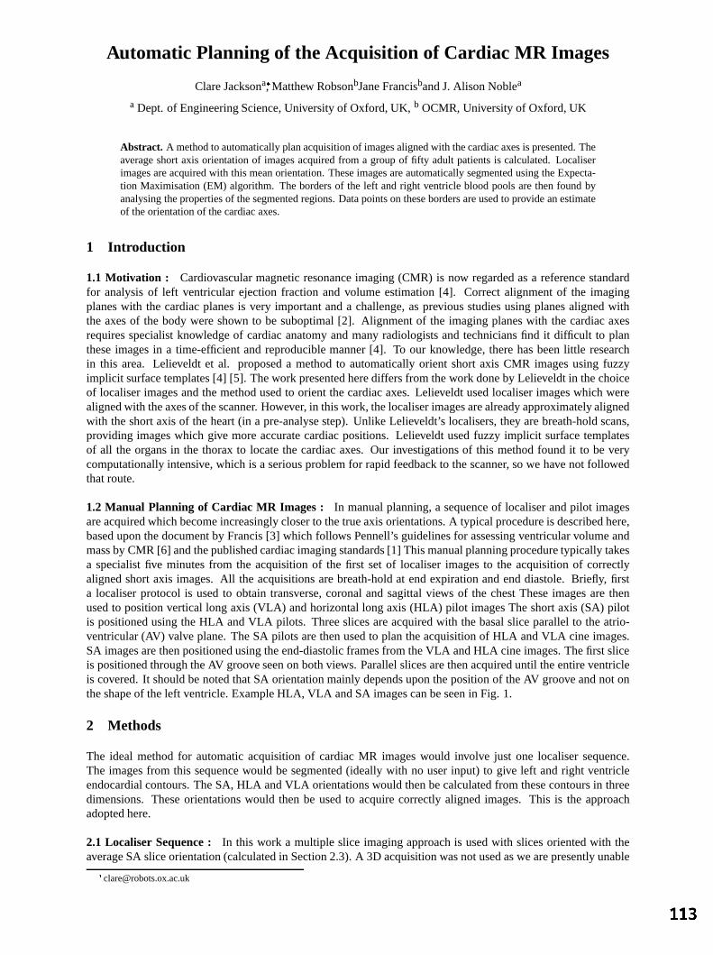
Automatic Planning of the Acquisition of Cardiac MR Images

Clare Jacksona

, Matthew RobsonbJane Francisband J. Alison Noblea

a Dept. of Engineering Science, University of Oxford, UK, b OCMR, University of Oxford, UK

Abstract. A method to automatically plan acquisition of images aligned with the cardiac axes is presented. Theaverage short axis orientation of images acquired from a group of fifty adult patients is calculated. Localiserimages are acquired with this mean orientation. These images are automatically segmented using the Expecta-tion Maximisation (EM) algorithm. The borders of the left and right ventricle blood pools are then found byanalysing the properties of the segmented regions. Data points on these borders are used to provide an estimateof the orientation of the cardiac axes.

1 Introduction

1.1 Motivation : Cardiovascular magnetic resonance imaging (CMR) is now regarded as a reference standardfor analysis of left ventricular ejection fraction and volume estimation [4]. Correct alignment of the imagingplanes with the cardiac planes is very important and a challenge, as previous studies using planes aligned withthe axes of the body were shown to be suboptimal [2]. Alignment of the imaging planes with the cardiac axesrequires specialist knowledge of cardiac anatomy and many radiologists and technicians find it difficult to planthese images in a time-efficient and reproducible manner [4]. To our knowledge, there has been little researchin this area. Lelieveldt et al. proposed a method to automatically orient short axis CMR images using fuzzyimplicit surface templates [4] [5]. The work presented here differs from the work done by Lelieveldt in the choiceof localiser images and the method used to orient the cardiac axes. Lelieveldt used localiser images which werealigned with the axes of the scanner. However, in this work, the localiser images are already approximately alignedwith the short axis of the heart (in a pre-analyse step). Unlike Lelieveldt’s localisers, they are breath-hold scans,providing images which give more accurate cardiac positions. Lelieveldt used fuzzy implicit surface templatesof all the organs in the thorax to locate the cardiac axes. Our investigations of this method found it to be verycomputationally intensive, which is a serious problem for rapid feedback to the scanner, so we have not followedthat route.

1.2 Manual Planning of Cardiac MR Images : In manual planning, a sequence of localiser and pilot imagesare acquired which become increasingly closer to the true axis orientations. A typical procedure is described here,based upon the document by Francis [3] which follows Pennell’s guidelines for assessing ventricular volume andmass by CMR [6] and the published cardiac imaging standards [1] This manual planning procedure typically takesa specialist five minutes from the acquisition of the first set of localiser images to the acquisition of correctlyaligned short axis images. All the acquisitions are breath-hold at end expiration and end diastole. Briefly, firsta localiser protocol is used to obtain transverse, coronal and sagittal views of the chest These images are thenused to position vertical long axis (VLA) and horizontal long axis (HLA) pilot images The short axis (SA) pilotis positioned using the HLA and VLA pilots. Three slices are acquired with the basal slice parallel to the atrio-ventricular (AV) valve plane. The SA pilots are then used to plan the acquisition of HLA and VLA cine images.SA images are then positioned using the end-diastolic frames from the VLA and HLA cine images. The first sliceis positioned through the AV groove seen on both views. Parallel slices are then acquired until the entire ventricleis covered. It should be noted that SA orientation mainly depends upon the position of the AV groove and not onthe shape of the left ventricle. Example HLA, VLA and SA images can be seen in Fig. 1.

2 Methods

The ideal method for automatic acquisition of cardiac MR images would involve just one localiser sequence.The images from this sequence would be segmented (ideally with no user input) to give left and right ventricleendocardial contours. The SA, HLA and VLA orientations would then be calculated from these contours in threedimensions. These orientations would then be used to acquire correctly aligned images. This is the approachadopted here.

2.1 Localiser Sequence : In this work a multiple slice imaging approach is used with slices oriented with theaverage SA slice orientation (calculated in Section 2.3). A 3D acquisition was not used as we are presently unable

[email protected]

HLA VLA SA

Figure 1. Example horizontal long axis (HLA), vertical long axis (VLA) and short axis (SA) images

original imageGaussian mixture model

segmentation using EM algorithm field prior modelafter applying Markov random

Figure 2. Segmentation using the EM-MRF algorithm

to acquire isotropic voxels of high resolution in the required imaging time. The acquisition is optimised for edgesharpness, high contrast between blood and myocardium and to be compatible with a single breath-hold. Allimages are acquired using a 1.5 Tesla Siemens Sonata. A 20 slice acquisition is used with a 280 340mm fieldof view, a 1.8 1.8mm in-plane resolution and a 7.5mm slice thickness with a 7.5mm gap between slices. A“true FISP” sequence is used with a 60

flip angle. The RF reception is on 2 elements of the spine array coiland 6 channels of the anterior phased array coil. ECG gating is used and breath-hold commands are issued viathe intercom system. The location of the heart can be estimated with sufficient accuracy to guarantee that this iscovered by the slices used.

2.2 Segmentation of Left and Right Ventricle Blood Pools : A Gaussian mixture model is fit to the central(10th) image in the localiser sequence using the Expectation Maximisation (EM) algorithm as described in Ye etal. [7]. We use five Gaussians for the mixture model. Ye improved the segmentation by applying a Markov RandomField (MRF) prior model. The results of applying the EM algorithm then the MRF model to a localiser image canbe seen in Fig. 2. Although the MRF model does improve the segmentation, it was decided that the degree ofimprovement did not justify the extra processing time required for the work presented here. The pixel valueswhich correspond to the points of overlap between each Gaussian in the model are then calculated. The imageis smoothed by replacing each pixel value with the average value of its eight neighbours. Pixels are classified asbelonging to one of the five models depending on their value. A set of morphological filtering operations wereconstructed using empirically determined parameters derived from a training set of images. These operations areused to identify the left (LV) and right ventricle (RV) regions. This process is illustrated in Fig. 3. This processis repeated for all the images in the localiser sequence using the parameters of the Gaussian mixture model foundby fitting it to the 10th image. Boundaries of the regions found for a localiser sequence can be seen in Fig. 4.The positions of the centroids of both the left and right ventricle regions are compared to their means over all 20images. Images where the positions of the centroids are less than one standard deviation from their means are thendisplayed. The user can then choose to reject images where the regions have not been correctly located.

The normal to the SA is then found by fitting a straight line to the centroids of all the LV regions. The centre ofthe middle SA slice is set to lie on this line and to be in the middle of the points used for the fit. The SA, VLA andHLA are set as being at right angles to each other, although, as was discussed in Section 1, this is not necessarilythe case when this procedure is performed manually. The centres of the HLA and VLA slices are also defined asbeing in the same position as the centre of the middle SA slice. This point will be the origin of the heart axes. Theposition on the RV boundary which is furthest away from this SA and its angle around the SA vector are then foundfor each image. The normal to the VLA is defined as passing through the heart axes origin, being perpendicularto the SA and at the average of these angles. The normal to the HLA is then easily found as it is perpendicular toboth the SA and the HLA normals.

all blood pool regionsand solidity>0.5

area>0.01 x image sizemin eccentricity

choose region with fill all pixels insideconvex hull = LV region

remaining regions witharea > 0.01 x image size

fill holes in region= RV region

centroid is closest tocentroid of LV region

split regions usingerosion then dilation

Figure 3. Location of the LV and RV using mathematical morphological operations

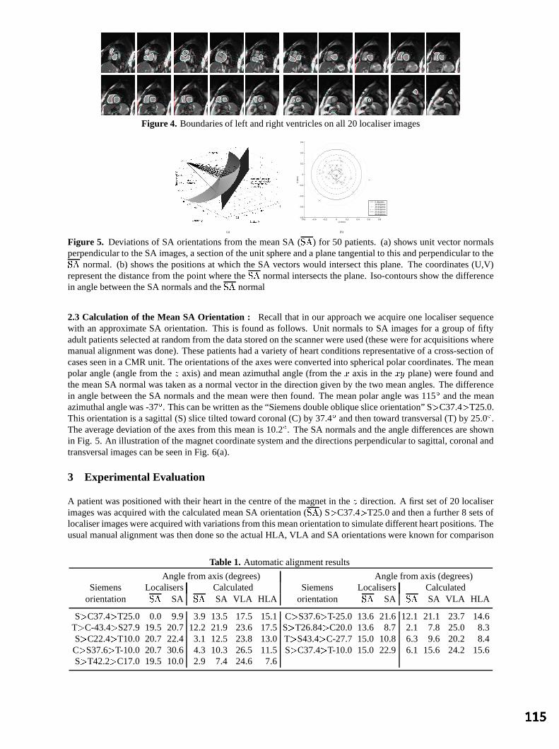
Figure 4. Boundaries of left and right ventricles on all 20 localiser images

(a)

−0.6 −0.4 −0.2 0 0.2 0.4 0.6 0.8−0.8

−0.6

−0.4

−0.2

0

0.2

0.4

0.6

U (mm)

V (

mm

)

5 degrees10 degrees15 degrees20 degrees25 degrees30 degrees

(b)

Figure 5. Deviations of SA orientations from the mean SA (

) for 50 patients. (a) shows unit vector normalsperpendicular to the SA images, a section of the unit sphere and a plane tangential to this and perpendicular to the

normal. (b) shows the positions at which the SA vectors would intersect this plane. The coordinates (U,V)represent the distance from the point where the

normal intersects the plane. Iso-contours show the difference

in angle between the SA normals and the

normal

2.3 Calculation of the Mean SA Orientation : Recall that in our approach we acquire one localiser sequencewith an approximate SA orientation. This is found as follows. Unit normals to SA images for a group of fiftyadult patients selected at random from the data stored on the scanner were used (these were for acquisitions wheremanual alignment was done). These patients had a variety of heart conditions representative of a cross-section ofcases seen in a CMR unit. The orientations of the axes were converted into spherical polar coordinates. The meanpolar angle (angle from the axis) and mean azimuthal angle (from the axis in the plane) were found andthe mean SA normal was taken as a normal vector in the direction given by the two mean angles. The differencein angle between the SA normals and the mean were then found. The mean polar angle was 115

and the meanazimuthal angle was -37

. This can be written as the “Siemens double oblique slice orientation” S C37.4 T25.0.This orientation is a sagittal (S) slice tilted toward coronal (C) by 37.4

and then toward transversal (T) by 25.0

.The average deviation of the axes from this mean is 10.2

. The SA normals and the angle differences are shownin Fig. 5. An illustration of the magnet coordinate system and the directions perpendicular to sagittal, coronal andtransversal images can be seen in Fig. 6(a).

3 Experimental Evaluation

A patient was positioned with their heart in the centre of the magnet in the direction. A first set of 20 localiserimages was acquired with the calculated mean SA orientation (

) S C37.4 T25.0 and then a further 8 sets of

localiser images were acquired with variations from this mean orientation to simulate different heart positions. Theusual manual alignment was then done so the actual HLA, VLA and SA orientations were known for comparison

Table 1. Automatic alignment results

Angle from axis (degrees) Angle from axis (degrees)Siemens Localisers Calculated Siemens Localisers Calculated

orientation

SA

SA VLA HLA orientation

SA

SA VLA HLA

S C37.4 T25.0 0.0 9.9 3.9 13.5 17.5 15.1 C S37.6 T-25.0 13.6 21.6 12.1 21.1 23.7 14.6T C-43.4 S27.9 19.5 20.7 12.2 21.9 23.6 17.5 S T26.84 C20.0 13.6 8.7 2.1 7.8 25.0 8.3S C22.4 T10.0 20.7 22.4 3.1 12.5 23.8 13.0 T S43.4 C-27.7 15.0 10.8 6.3 9.6 20.2 8.4C S37.6 T-10.0 20.7 30.6 4.3 10.3 26.5 11.5 S C37.4 T-10.0 15.0 22.9 6.1 15.6 24.2 15.6S T42.2 C17.0 19.5 10.0 2.9 7.4 24.6 7.6

Transversal(z)

Sagittal(x)

Coronal(y)

(a) The magnet coordinate system(arrows show normals to image planes)

−0.8 −0.6 −0.4 −0.2 0 0.2 0.4 0.6−0.8

−0.6

−0.4

−0.2

0

0.2

0.4

0.6

U (mm)

V (

mm

)

Localiser SA

Calculated SA

5 degrees10 degrees15 degrees20 degrees25 degrees30 degrees

(b) SA

−0.8 −0.6 −0.4 −0.2 0 0.2 0.4 0.6−0.8

−0.6

−0.4

−0.2

0

0.2

0.4

0.6

U (mm)

V (

mm

)

5 degrees10 degrees15 degrees20 degrees25 degrees30 degrees

(c) VLA

−0.8 −0.6 −0.4 −0.2 0 0.2 0.4 0.6−0.8

−0.6

−0.4

−0.2

0

0.2

0.4

0.6

U (mm)

V (

mm

)

5 degrees10 degrees15 degrees20 degrees25 degrees30 degrees

(d) HLA

Figure 6. Magnet coordinate system and variation of calculated SA, VLA and HLA

purposes. The angles of the different localiser sequences as shown in Table 1 together with the angles betweenthe calculated orientations,

and the manually aligned SA, HLA and VLA orientations. Figure 6 shows (b) the

SA orientations of the localisers and the corresponding calculated SA, (c) VLA and (d) HLA orientations. Theorientations are displayed as intersections of the normals to the images with three planes in a similar way to Fig. 5.The planes are centred on the mean calculated SA, VLA and HLA orientations and, therefore, show the variability.The average variations of the calculated orientations from their means were 5.6, 4.6 and 4.2

for the SA, VLA andHLA respectively. (b) illustrates that very similar axes orientations were calculated from all nine sets of localiserimages. The angle between the mean calculated SA angle for the 9 cases and the manually aligned SA was 12.8

.This angle was 22.8

for the VLA and 11.9

for the HLA. This shows that the method is reproducible but thatthe axis orientations, especially that of the VLA, differ from those found manually. The average variation from a“reference standard” of the SA orientations automatically found by Lelieveldt was 12.2

[4].

4 Discussion and Further Work

We have developed an approach to automated cardiac axes alignment which uses one localiser sequence andautomated image processing. The current approach is semi-automatic and gave results which were reproduciblebut showed some inconsistencies with the manual approach. As was described in Section 1, although the manuallyaligned long axis does align with the long axis of the heart in the mid-plane, it does not align with the axis towardthe apex. Similarly, the SA would be expected to be perpendicular to the long axis. This is not always the caseas, in the manual approach, there is a tendency to align the SA slice with the AV groove (which may or maynot be perpendicular to the long axis as defined previously). There are reasons for all these “tweaks”, which areeither historical (e.g. that is the approach that cardiologists use for ultrasound), or due to other analysis steps (i.e.determining the cardiac volume through summing the volumes of multiple slices). Another point is that the VLAis not necessarily perpendicular to the HLA, as might have been expected by those definitions. It highlights thatanatomical definitions can differ from computational model definitions. This is discussed in [6]. However, for thisapplication, it appears that a simple computational definition is adequate. Further work will focus on assessingthe significance and relevance of axes that are not mutually orthogonal. The variability of manually aligned axespositions between specialists will also be investigated further. An important next step will be to integrate thisplanning capability into the running of the MRI system and automating remaining steps which presently requireinteractivity.

References

1. M. D. Cerqueira et al., “Standardized Myocardial Segmentation and Nomenclature for Tomographic Imaging of the Heart”,Circulation, 105(4), pp539-542, 2002.

2. G. B. Cranney et al., “Left Ventricular Volume Measurement Using Cardiac Axis Nuclear Magnetic Resonance Imaging”,Circulation, 82(1), pp154-163, 1990.

3. J. Francis, “How to do a Left Ventricular Function Study”http://www.cardiov.ox.ac.uk/ocmr/lvfunction.htm

4. B.P.F. Lelieveldt et al., “Automated Observer-independent Acquisition of Cardiac Short-Axis MR Images: A Pilot Study”,Radiology, 221(2), pp537-542, 2001.

5. B.P.F. Lelieveldt et al., “Anatomical Modeling with Fuzzy Implicit Surface Templates” Comput. Vision Image Understand.,80, pp1-20, 2000.

6. D. Pennell, “Ventricular volume and mass by CMR”, Journal of Cardiovascular Magnetic Resonance, 4(4), pp507-513,2002.

7. X. Ye et al., “High Resolution LV Segmentation of MR Images of Mouse Heart Based on a Partial-Pixel Effect and EM-MRFAlgorithm” Proc. ISBI 2002

Inter-subject Comparison of Brain Connectivity usingDiffusion-Tensor Magnetic Resonance Imaging

Philip A Cooka∗and Daniel C Alexandera

aDepartment of Computer Science, University College London, Gower Street, London WC1E 6BT, UK

Abstract. Research into fibre tracking within the brain has been prominent in recent literature. Several studieshave found fibre structure that is consistent with known anatomy in the major tracts. We present a model of fibreconnectivity using a weighted graph. In this initial investigation, we examine consistency of the connectivitygraph among individuals by modelling their variation with Principal Component Analysis. We assess the qualityof the model by the goodness of fit to unseen data, for a range of graph vertex sizes. We conclude that the brainshould be divided into no more than 32 vertices to achieve reasonable inter-subject consistency with our fibretracking algorithm.

1 Introduction and Background

Diffusion-Weighted Magnetic Resonance Imaging (DW-MRI) allowsin-vivo imaging of diffusing water moleculesas they interact with microscopic cellular structures. Many studies have used the Diffusion Tensor (DT) [1] tomodel the statistical properties of diffusing water molecules within the brain. Within brain white matter, theorganized fibre bundles impose anisotropic restrictions on the mobility of water molecules, which are consequentlylikely to diffuse farther along the fibres than across them. White matter can be contrasted with other brain tissueusing conventional MR modalities, but DW-MRI is uniquely able to probe the fibre orientation.

Several studies have used DT-MRI to perform “tractography” –in-vivo reconstruction of the trajectory of whitematter axonal fibres. Tractography aims to determine the path that these fibres follow between their synapticjunctions. The anatomical connectivity within the brain is interesting for studies of brain function, and also forthe investigation of white matter abnormalities. Detailed reviews of the published tractography techniques canbe found in [2] and [3]. The tractography techniques described to date have produced results that are consistentwith the known anatomy of the major fibre pathways in the brain, but these results cannot be validated sufficientlyfor clinical applications. It is important to note that present DT-MRI images are restricted to resolutions of a fewmillimetres, which is much greater than the diameter of individual white matter fibres (about 0.001 mm) [4]. The“fibres” recovered from tractography are not fibres themselves but the estimated path of organized fibre bundles.

Jones, Griffin, Alexander, et al [5] studied the inter-subject coherence of fibre orientation within DT-MRI imageson the voxel scale, in ten healthy subjects. The images were registered into a common space to align the anatomicalfeatures of the brains for comparison. Using a quantitative measure of eigenvector coherence, Jones showed thatthe angular coherence within the group was stronger in some areas of the brain than in other areas.

The long term goal of our research is to develop a robust technique to model the fibre connectivity informationembedded in DW-MRI images. Statistics of such a model could be used to quantify the variation in connectivityamong individuals. This is interesting both to the study of natural anatomical variations, and for the study anddiagnosis of diseases where white matter abnormalities may be present. Scalar indices derived from DT-MRI havebeen used to study white matter diseases such as multiple sclerosis [6] and schizophrenia [7], but these studies donot address the patterns of fibre connectivity. The study of connectivity disorders is a potential future applicationof our model.

In this study, we use a weighted graph to represent the connectivity between evenly segmented volumes of braintissue in the space of a DT-MRI image. We use Principal Component Analysis (PCA) to find the most significantmodes of variation in these graphs using a training set of seven healthy volunteers. We reconstruct images from fourother healthy volunteers from the principal components of the training set. We show that the principal componentsof the training set can closely approximate the non-training data when the brain is divided into a cubic grid of 0.1litre vertices.

∗email: [email protected]

2 Method

2.1 Outline of connectivity graph algorithm

1. Define the vertices of the graph in a reference image.

2. For each subject image:

(a) Compute a registration warp from the image to the reference image.

(b) Place tractography seeds in the centre of all voxels in the unwarped image.

(c) While there are unused seeds:

i. Attempt to track a fibre from the next seed.ii. If a fibre is found:

A. Remove any remaining seeds along the fibre path.B. Apply registration warp to fibre.C. Add fibre to subject’s graph.

We used the fourth order Runge-Kutta method to track fibres. This method has the advantage of being reasonablysimple and fast to compute. After a fibre was computed, we removed the seeds along the fibre trajectory so thatit would be counted only once. Each fibre was ended when it reached a point where diffusion anisotropy wasbelow a level consistent with white matter. This method was shown by Basser, Pajevic, Pierpaoli et al [8] toproduce anatomically plausible results. We discarded tracked fibres shorter than 30mm. Such fibres do exist inthe brain but tractography performs best in the longer, wider fibre tracts, where the results can be compared toknown anatomy. The value of 30mm represents a subjective threshold and quantitative validation of tractographyis required to establish which fibres can be reliably tracked in the brain.

The connectivity graph is a weighted graph where the vertices are volumes of brain tissue. The graph is a symmet-ric, sparsely populated (most pairs of vertices have no fibre connections) adjacency matrix,g. Each entrygij of theadjacency matrix is the number of fibres that pass through verticesi andj. We normalize the graph (see equation1) to remove variation in the absolute size of the fibre tracts.

We defined twelve graphs by covering the brain with a cubic grid of vertices, ranging from3× 10−4 litres to 0.39litres. The vertices were defined in the space of a reference image from a healthy male volunteer. We registeredthe subject images to the reference image using software from the FSL suite, (Oxford University, UK [9]).

2.2 Modelling connectivity variation

In the absence of errors, variation in inter-subject graphs would be caused by variation in position of the fibrebundles (different vertices connected), or variation in the relative sizes of the tracts (different weights). With realdata, some of the variation will be errors introduced during the registration and tractography processes. Increasingthe vertex size absorbs some of the errors in the fibre trajectories at the expense of reducing the descriptive powerof the connectivity graph.

We used PCA to model the variation in a space of much smaller dimension than that of the data. We consider theadjacency matrix as a vector ind2-dimensional space (equation 1), whered is the number of vertices:

x =1Z

(g11, g12 . . . g1d, g21 . . . gdd)T

, whereZ =

√√√√ d∑j=1

d∑i=1

g2ij (1)

Any n points ind2-dimensional space (whered2 ≥ n) define a subspace of maximum dimensionn− 1, and all ofthese points can be described as a linear combination ofn− 1 orthogonal basis vectors. PCA finds an orthogonalbasis for the data as well as the variance in the position of the training data along each basis vector.

We used seven principal componentfemale subject images as the training set for our experiment. Images from afurther four subjects (three male, one female) were transformed into the Principal Component space to test howwell the principal components can describe the variation outside the training set. Withn = 7 training samples there

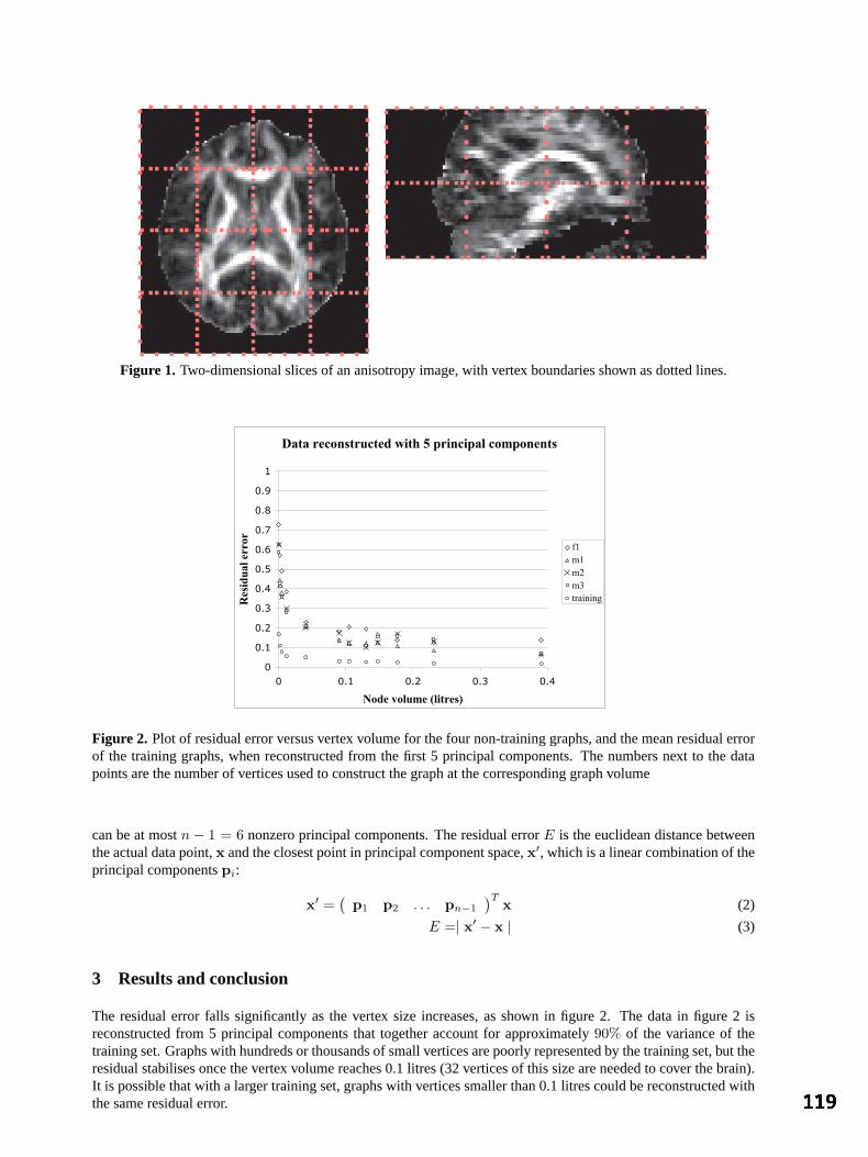
Figure 1. Two-dimensional slices of an anisotropy image, with vertex boundaries shown as dotted lines.

Data reconstructed with 5 principal components

0

0.1

0.2

0.3

0.4

0.5

0.6

0.7

0.8

0.9

1

0 0.1 0.2 0.3 0.4

Node volume (litres)

Res

idua

l err

or

f1m1m2m3training

Figure 2. Plot of residual error versus vertex volume for the four non-training graphs, and the mean residual errorof the training graphs, when reconstructed from the first 5 principal components. The numbers next to the datapoints are the number of vertices used to construct the graph at the corresponding graph volume

can be at mostn − 1 = 6 nonzero principal components. The residual errorE is the euclidean distance betweenthe actual data point,x and the closest point in principal component space,x′, which is a linear combination of theprincipal componentspi:

x′ =(

p1 p2 . . . pn−1

)Tx (2)

E =| x′ − x | (3)

3 Results and conclusion

The residual error falls significantly as the vertex size increases, as shown in figure 2. The data in figure 2 isreconstructed from 5 principal components that together account for approximately90% of the variance of thetraining set. Graphs with hundreds or thousands of small vertices are poorly represented by the training set, but theresidual stabilises once the vertex volume reaches 0.1 litres (32 vertices of this size are needed to cover the brain).It is possible that with a larger training set, graphs with vertices smaller than 0.1 litres could be reconstructed withthe same residual error.

4 Discussion and future work

This work is at an early stage and several problems remain to be solved. The cubic grid covers the whole brain,which means that fibres anywhere in the brain can contribute to the graph but guarantees that erroneous fibre tracescan find vertices to connect. A sparse set of vertices, placed along known white matter fibres, would exclude someparts of the brain from analysis, but might provide better results because random fibre trajectories would be lesslikely to connect two vertices. This may allow us to use smaller vertices without incurring such large errors.

We are currently developing a replacement for the vertex grid with a smaller set of vertices defined by anatomicallandmarks. We are also investigating probabilistic tracking algorithms, which may provide a more robust estimateof fibre connectivity.

Acknowledgements

We would like to thank Dr Olga Ciccarelli, Institute of Neurology, UCL, for providing the data used in this work.This work was funded by the EPSRC IRC on medical imaging.

References

1. PJ Basser, J Matiello, and D Le Bihan. MR diffusion tensor spectroscopy and imaging.Biophysical Journal, 66:259–267,1994.

2. Susumu Mori and Peter C. M. van Zijl. Fiber tracking: principles and strategies: a technical review.NMR In Biomedicine,15:468–480, 2002.

3. N. F. Lori, E. Akbudak, J. S. Shimony, T. S. Cull, A. Z. Snyder, R. K. Guillory, and T. E. Conturo. Diffusion tensor fibertracking of human brain connectivity: aquisition methods, reliability analysis and biological results.NMR In Biomedicine,15:493–515, 2002.

4. Stephen G Waxman (Editor).Physiology and Pathobiology of Axons. Raven Press, 1978.5. Derek K Jones, Lewis D Griffin, Daniel C Alexander, Marco Catani, Mark A Horsfield, Robert Howard, and Steve C R

Williams. J. InProc Intl Soc Mag Reson Med, page 1122, 2002.6. Roland Bammer, Michael Augustin, Siegrid Strasser-Fuchs, Thomas Seifert, Peter Kapeller, Rudolf Stollberger, Franz

Ebner, Hans-Peter Hartung, and Franz Fazekas. Magnetic resonance diffusion tensor imaging for characterizing diffuse andfocal white matter abnormalities in multiple sclerosis.Magnetic Resonance in Medicine, 44:583–591, 2000.

7. Lim; KO, Hedehus; M, and Moseley; M. Compromised white matter tract integrity in schizophrenia inferred from diffusiontensor imaging.Arch. Gen. Psychiatry, 56:367–374, 1999.

8. Peter J Basser, Sinisa Pajevic, Carlo Pierpaoli, Jeffrey Duda, and Akram Aldroubi. In vivo fiber tractography using DT-MRIdata.Magnetic Resonance in Medicine, 44:625–632, 2000.

9. Jenkinson; M. and Smith; S. A global optimisation method for robust affine registration of brain images.Medical ImageAnalysis, 5(2):143–156, 2001.

Segmentation of Dermatoscopic Images by

Iterative Segmentation Algorithm

M. I. Rajaba, M. S. Woolfsonb and S. P. Morganc

[email protected], [email protected], [email protected]

School of Electrical and Electronic Engineering, University of Nottingham,

University Park, Nottingham, NG7 2RD, UK

Abstract. Since the introduction of epiluminescence microscopy (ELM), image analysis tools have been extended to the field of dermatology, as an attempt to algorithmically reproduce clinical evaluation. Accurate image segmentation of skin lesions is one of the key steps for useful, early, and non-invasive diagnosis of cutaneous melanomas. In this paper, a new segmentation technique has been developed to extract the true border that reveals the global structure irregularity (indentations and protrusions), which may suggest excessive cell growth or regression of a melanoma. The algorithm is applied to the Blue channel of the RGB colour vectors to distinguish lesions from the skin and proceed with grey scale morphology and background noise reduction to enhance and filter the image of lesion. The algorithm also does not depend on the use of rigid threshold values, because the isodata algorithm that is used determines an optimal threshold iteratively. Preliminary experiments are performed on digitised clinical photographs and also pigmented networks captured with the ELM technique. We demonstrate that we can enhance and delineate pigmented networks in skin lesions visually, and make them accessible for further analysis and classification.

1 Introduction

Trained dermatologists in the use of dermatoscopy or epiluminescence microscopy (ELM) can improve their diagnostic accuracy of melanoma from about 65% using the unaided eye to approximately 80% with the benefit of ELM [1]. However, even with ELM, a trained dermatologist can be deceived at least 20% of the time by the appearance of a melanoma. Low rate of correct classification of clinical diagnosis [2] calls for the development of both digitised ELM (DELM) and automated image analysis systems. For example, a recently developed PC-based pilot system by Binder et al. [3] promises to automatically segment the digitised ELM images, measuring 107 morphological parameters. A neural network classifier trained with these features is able to differentiate between benign and malignant melanoma.

This paper demonstrates the use of an iterative segmentation algorithm as a tool for determining the borders of real skin lesions as an aid to skin lesion diagnosis. The algorithm has been developed and compared with other developed Neural Network techniques and also the automatic segmentation method by Xu et al [4]. Initial experiments have been done on synthetic lesions, and the work has been written up in a paper [5]. The next section shows the method applied. This is followed in section 3 by results and discussions demonstrating the segmentation method. Conclusions are drawn in section 4.

2 Method of Processing Pigmented Networks

The weak contrast within the pigmented network does not allow colour-based segmentation to extract pigmented networks directly. However, extracting homogeneous and differently coloured regions within the lesions is a robust method for separating lesions from surrounding skin [2]. As an example of analysing pigmented network, Fisher et al. [2] develop a colour based segmentation algorithm, which is applied to Karhunen loeve transformation of the RGB colour vectors. Because the pigmented network and the background do not have homogeneous luminance, the result of segmentation is enhanced in a circular region to limit the problem of heterogeneous regions.

In this work the following processing steps are followed to delineate pigmented networks and make them accessible for further statistical analysis and classification. We suggest the processing of lesion images using the Blue channel of the RGB colour space followed by the grey scale morphology and intensity mapping to enhance and filter regions containing a pigmented network. Assuming that the previous steps assist to provide equal region probabilities then a simple iterative scheme would segment the image into binary regions containing the lesion and the background. This process is depicted in Table.1. In contrast with the above example of segmentation, the region processed is equal to the full size of image.

Step1: Source image Source image = Blue channel of R,G,B colour image Step2: Noise reduction Grey morphology Subtract median background noise Step3: Lesion enhancement Map intensities with appropriate function Smooth Step4: Optimal thresholding Optimal thresholding Step5: delineate object Outline binary object Step6: Object analysis Set the minimum object Diameter and Area Scan the binary image Until

MinSize < Area < MaxSize

Table 1. General algorithm steps to delineate colour lesion. Step 1. We use the blue channel of the intensity of an RGB colour skin lesion image as the first step. This approach has been demonstrated to provide the best results in global and dynamic thresholding algorithms [6]. Step 2. Because real skin images often contain features such as hair and other small objects, we have added a grey scale morphological opening operation followed by a close operation as the first step of data reduction without destroying the morphological structure of the pigmented network [2,6]. The opening operation is expected to smooth objects and removes isolated pixels and the close operation performs smoothing and filling in small holes. For optimum use of the algorithm it is useful to remove the background intensity of skin surrounding the lesion. This is estimated by calculating the median of two strip windows from the top and bottom of an image, each of size pixels, where w is the full image width [4]. 10×w Step 3. A mapping function F(Φ) is used here to map the intensities I to enhance features at the boundary;

( )( )22 2/exp1)( σΦ−−=Φ kF (1)

where

( ) 755432 IcIcIcI ++=Φ (2)

where kc 1= (3)

F(Φ) achieves less redundancy in the colour map than the Gaussian transformation used in [4] which makes it more suitable to map a wide range of intensities so that the lesion can be distinguished from the background. Another advantage here is that when mapping images of low noise variations, small σ, in the background (e.g. ELM images) then the function tends not to magnify that noise. The selection of the standard deviation (σ) of this mapping function is automatically determined according to the estimated standard deviation of the background surrounding the lesion; in the same manner when subtracting background median noise (Step 2). Small smoothing Gaussian kernels are adopted at this stage for two reasons: (i) to assist the extraction of morphological structure of the pigmented network, (ii) large smoothing is not necessary because the preprocessing steps of morphological operations already provide the robust noise reduction.

Step 4. The thresholding algorithm described by Madisett et al as an isodata algorithm [7] is used here to find an optimum auto-threshold value T for an image. This value would segment the image into binary regions containing the lesion and the background. The histogram is initially segmented into two parts using an initial threshold value of T0=2(B-1), where B is the number of bits. For an 8-bit intensity image B=8 and T0=128. The sample mean of the gray values associated with foreground pixels ( m ) and the sample mean of the gray

values associated with the background pixels are ( m ) computed. A new generated threshold value T is computed as the average of these two sample means. The process is repeated, based upon the new generated threshold, until the threshold value does not change any more:

0,f

0,b k

( ) 11,1, 2 −−− =+= kkkbkfk TTuntilmmT (4)

Step 5. Delineation is applied to binary objects that result from optimal thresholding (step 4). The logic rule in this binary process simply follows “any foreground pixel with at least one background pixel in the 3x3 neighbourhood is left unchanged, otherwise it is changed to the background colour” [8]. Step 6. This process is useful to analyse an image with multiple lesions or to correct errors caused in the delineation process such as the delineation of thick and dark hair. Scanning across the image is performed and a condition or a set of conditions reached. For example, a condition to check the area of the object between minimum and maximum size would eliminate unnecessary size of object: . MaxSizeAreaMinSize <<

3 Experiments and Discussion

We have processed thirty images of skin images. The first twenty images are captured by digitised clinical photographs [4]. We have chosen these low quality images to test the robustness of the algorithm to delineate images with clear skin texture. The other ten images are captured with the ELM technique. Successful delineated of the most noisy clinical photograph colour lesions are achieved. This preliminary test experiment demonstrates the robustness of the algorithm against wide range of noise such as skin texture, light reflections, and noise artefacts (see fig.1).

(a) (b) (c)

(d) (e) (f)

Figure1. Demonstration of iterative segmentation algorithm. (a) Gray intensities of blue channel. (b) Morphological operations followed by noise subtraction of median background. (c) Intensity mapping by function . (d) Edge outline of binary segment at an optimal threshold. (e) Analysis of the resulting objects and eliminating the small objects. Labels are also used to check the success of the process, MinSize=0. (f) Excluding small objects, which are labelled as No. 1 to 6.

)(F Φ

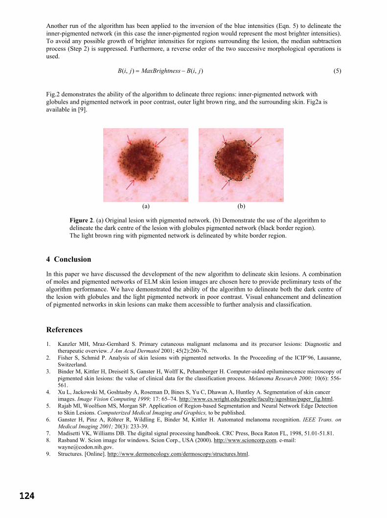
Another run of the algorithm has been applied to the inversion of the blue intensities (Eqn. 5) to delineate the inner-pigmented network (in this case the inner-pigmented region would represent the most brighter intensities). To avoid any possible growth of brighter intensities for regions surrounding the lesion, the median subtraction process (Step 2) is suppressed. Furthermore, a reverse order of the two successive morphological operations is used.

),(),( jiBessMaxBrightnjiB −= (5)

Fig.2 demonstrates the ability of the algorithm to delineate three regions: inner-pigmented network with globules and pigmented network in poor contrast, outer light brown ring, and the surrounding skin. Fig2a is available in [9].

(a) (b)

Figure 2. (a) Original lesion with pigmented network. (b) Demonstrate the use of the algorithm to delineate the dark centre of the lesion with globules pigmented network (black border region). The light brown ring with pigmented network is delineated by white border region.

4 Conclusion

In this paper we have discussed the development of the new algorithm to delineate skin lesions. A combination of moles and pigmented networks of ELM skin lesion images are chosen here to provide preliminary tests of the algorithm performance. We have demonstrated the ability of the algorithm to delineate both the dark centre of the lesion with globules and the light pigmented network in poor contrast. Visual enhancement and delineation of pigmented networks in skin lesions can make them accessible to further analysis and classification. References

1. Kanzler MH, Mraz-Gernhard S. Primary cutaneous malignant melanoma and its precursor lesions: Diagnostic and therapeutic overview. J Am Acad Dermatol 2001; 45(2):260-76.

2. Fisher S, Schmid P. Analysis of skin lesions with pigmented networks. In the Proceeding of the ICIP’96, Lausanne, Switzerland.

3. Binder M, Kittler H, Dreiseitl S, Ganster H, Wolff K, Pehamberger H. Computer-aided epiluminescence microscopy of pigmented skin lesions: the value of clinical data for the classification process. Melanoma Research 2000; 10(6): 556-561.

4. Xu L, Jackowski M, Goshtasby A, Roseman D, Bines S, Yu C, Dhawan A, Huntley A. Segmentation of skin cancer images. Image Vision Computing 1999; 17: 65–74. http://www.cs.wright.edu/people/faculty/agoshtas/paper_fig.html.

5. Rajab MI, Woolfson MS, Morgan SP. Application of Region-based Segmentation and Neural Network Edge Detection to Skin Lesions. Computerized Medical Imaging and Graphics, to be published.

6. Ganster H, Pinz A, Röhrer R, Wildling E, Binder M, Kittler H. Automated melanoma recognition. IEEE Trans. on Medical Imaging 2001; 20(3): 233-39.

7. Madisetti VK, Williams DB. The digital signal processing handbook. CRC Press, Boca Raton FL, 1998, 51.01-51.81. 8. Rasband W. Scion image for windows. Scion Corp., USA (2000). http://www.scioncorp.com. e-mail:

[email protected]. 9. Structures. [Online]. http://www.dermoncology.com/dermoscopy/structures.html.

Segmentation of Mammograms Using a Weighted Gaussian MixtureModel and Hidden Markov Random Field

Keir Bovis and Sameer Singh

PANN Research, Department of Computer Science, University of Exeter, Exeter, EX4 4PT, UK.

In this study we evaluate the relative utility of four approaches to statistical model-based image segmentation of 200digitised abnormal mammograms from the Digital Database of Screening Mammograms (DDSM). Each model is con-structed by employing combinations of a Weighted Gaussian Mixture Model (WGMM) and a Markov Random Field(MRF) in a supervised and unsupervised manner. Maximum likelihood estimates of model parameters are obtained us-ing the Expectation-Maximisation (EM) algorithm. The segmentation performance is evaluated by calculating the areaunder the Receiver Operating Characteristic (ROC) curve, Az. The main contribution of this paper is the specificationand evaluation of the relative utility of each model in segmenting a data-set of mammograms comprising the completespectrum of varying mammographic breast density. We show that that the adoption of a supervised WGMM/MRFapproach gives the best result over all test mammograms (Az=0.73).

Keywords: Mammography, image segmentation, Gaussian Mixture Model (GMM), Markov Random Field (MRF).

1 Introduction

The aim of image segmentation is to divide an image into parts that have strong correlation with objects of the realworld contained in the image. Region based segmentation methods attempt to find border between regions. Statisticalapproaches label pixels according to class conditional probabilities based on the distribution of the input feature data.Extensive research has focused on the use of a Gaussian Mixture Model (GMM) to model such conditional probabilities.The performance of a GMM as a model of the observed data has been shown to give good results as long as the differentclasses are well separated in the input feature space. This though is not always the case and several studies have addressedthis problem by incorporating a Markov Random Field (MRF) hidden model capturing the spatial constraints of pixelclass labels [7, 8].

Within this study we evaluate a supervised and unsupervised approach to the segmentation of a test image using aWeighted Gaussian Mixture Model (WGMM) and a WGMM regularised with a MRF [2]. The aim of the segmentationis to label pixels as belonging to one of two classes, normal or abnormal. This study offers novelty in two areas:

1. The specification of four different combinations of WGMM and MRF models adopting a supervised learning andunsupervised strategy for the segmentation of mammograms images.

2. An evaluation of the relative utility of the four segmentation approaches on a large set of mammograms taken fromthe Digital Database of Screening Mammograms (DDSM) [5] covering the complete spectrum of mammographicbreast densities defined by the American College of Radiology (ACR) Breast Imaging Reporting and Data Systems(BI-RADS). This lexicon identifies four mammographic breast density types: 1.) the breast is almost entirely fat;2.) There are scattered fibroglandular densities; 3.) The breast tissue is heterogeneously dense; 4.) the breasttissue is extremely dense.

2 GMM and MRF Modelling

The observed image model uses a GMM to model the Probability Density Function (PDF) of an input feature space x,given that each sample belongs to one of L independent class labels

, using J Gaussian functions ,

mixed with a set of mixing coefficients , thus !#"$"&%&('*)+-,#. + /0 1 + . We combine the PDF’s foreach class using a WGMM to model the unconditional density such that each class distribution, 0 2 !3"$" % , isweighted by 45 thus, 67 !3"8" ':9 ,#. 4; < !#"$" % . The WGMM allows us to model the PDF’s ofeach class independently with 1 or more Gaussian centres. The parameters 1 + of the j’th component Gaussian comprisethe mean /= + , covariance > + and mixing coefficient + . The Expectation-Maximisation (EM) algorithm provides anestimate of a maximum likelihood solution for the complete set of parameters for all Gaussian functions of a given class

distribution, l, !3"$" % together with the class weights 4; . This is achieved by iteratively maximising a likelihoodfunction across all data samples for each class, normal and abnormal.

Within this study we propose the use of an MRF to regularise the resultant observed model. This reduces classificationerror associated with classes that are poorly differentiated in the input feature space when using the WGMM. The MRFis used to model the spatial constraints of the pixel class labels in the segmented image. The class labels associatedwith a pixel are assumed to be a realisation of a random process where the probability that pixel

?belongs to a given

class, depends on the class labels of neighbouring pixels@

from a given neighbourhood A ? , thus, B? B@C5DFE 6- B? B@HG A ? - .We evaluate four strategies for the use of a WGMM in the segmentation of a test mammogram. Two of the methods aresupervised such that the model parameters for the WGMM are learnt from an independent training set JILKNMHMPO ILKNMHM

"QSRO %

,the others are unsupervised ILKNMHMPT ILKNMHM

"QSRT %

. Two of the approaches constrain the WGMM with a MRF inan attempt to improve the resultant segmentation ILKNMHM

"8QSRO ILKNMHM

"8QSRT %

.

3 Materials and Methods

The segmentation evaluation is performed on 200 mammograms each containing lesions taken from the Digital Databaseof Screening Mammograms (DDSM). Each mammogram has been assigned to one of the BI-RADS mammographicbreast density groupings by an expert radiologist. There are fifty mammograms for each breast density grouping. Wehave previously proposed a method to predict the mammographic breast density [3], but in this study the partitioning hasbeen performed manually on the basis of the DDSM ground-truth. Additionally, a further fifty normal mammograms areselected for each breast type, although the performance of each strategy in their segmentation is not reported here, theiruse being limited as training images only. Results for each segmentation strategy will be reported using ROC analysis,quoting the mean Az value over all test images, within a given breast density grouping.

The grouping of mammograms by breast density type is only applicable to the supervised approaches. Supervisedapproaches segmenting a mammogram with a specific breast density type, use a trained observed intensity model con-structed with only training samples from that same breast type. Thus, each trained observed intensity model will bespecialised in the segmentation of a mammogram with a specific breast type.

As each breast type group comprises of 100 images (n=50 abnormal, n=50 normal), in order that an unbiased evalua-tion can be presented, and such that all 50 abnormal image can be segmented, a 5-fold cross-validation strategy [1] isadopted. Normal mammograms appear in training sets only and no abnormal image appears in a test and training setsimultaneously. For each of the five folds, equal numbers of normal and suspicious pixels are used to represent trainingexamples from each respective class. Evaluation of the performance on test of each strategy is determined using theexpert radiologist ground-truths, although an a posteriori probability estimate is only given for pixels lying within thepreviously segmented breast profile generated using a technique proposed by Chandrasekhar and Attikiouzel [4]. Bydoing this, the computational complexity of the test image segmentation is reduced.

A cross-validation approach is used to determine the optimal number of component Gaussians, m, for each class and foreach breast type. The determined value of m is then used for all training folds comprising each breast type. To determinethe optimal value of m, models with a different number of components are trained and evaluated with a ILKNMHM Ostrategy, using an independent validation set. Model fitness is quantified by examining the log-likelihood resulting fromthe validation set. Training files used are created by taking 200 samples randomly drawn with replacement from eachnormal and abnormal image for each breast type. The data-set contains fifty training images per breast type, (n=25abnormal, n=25 normal) giving a training set size of 10,000 samples per breast type. Repeating the procedure for thefifty remaining separate validation images, results in a validation set of 10,000 samples per breast type. Figure 1 showsthe log-likelihood obtained by applying each trained model of order m, to the independent validation set for each class.The selected model order is indicated by a circle for each breast type in each graph. Using the trained WGMM, eachtest image is segmented according to each of the four different segmentation strategies ILKNMHM O , ILKNMHM _ MLUWV O ,ILKNMHM T and ILKNMHM _ MLUWV T .

4 Results

The performance of the segmentation strategies are evaluated on the basis of being able to differentiate abnormal pixelsfrom normal. A high performing segmentation strategy will be therefore judged as the one that has a high sensitivityin the correct detection of abnormal pixels whilst minimising the number of false-alarms, i.e. normal pixels incorrectlylabelled as class abnormal. MAP segmentation is not performed but the a posteriori probability estimates for each pixelin the test image are used to construct a ROC curve. By calculating the area under the curve, Az, as an indicator of thequality of the segmentation [6], a mean Az value is quoted for each strategy over all 50 abnormal test images for eachbreast type. These results are presented in Table 1. An example of the resultant segmentation using each strategy is

Table 1. Mean Az for each breast type and segmentation strategy, winning strategies shown in bold.

Breast Type ILKNMHM O ILKNMHM"8QSRO ILKNMHM T ILKNMHM

"QSRT

1 0.68 0.70 0.66 0.592 0.66 0.66 0.66 0.603 0.72 0.80 0.75 0.754 0.66 0.76 0.68 0.74

Mean 0.68 0.73 0.68 0.67

shown in Figure 2.

Reviewing these results, it can be seen that the supervised strategy combining an observed and hidden MRF model out-performs all others for each breast type. The performance of this method, ILKNMHM

"QSRO can interestingly be observed

to be worse for the fatty breast types (types 1 and 2) compared with the denser types (types 3 and 4). This is in contrastto the clinical observations that the former breast types are deemed easier to interpret by an expert radiologist. A simpleexplanation for this phenomenon might be attributable to the model order selection where m=1 for the abnormal classof the fatty breast types. A more sophisticated approach to determining model order might improve the segmentationof these breast types, but this is outside the scope of this thesis. Without the hidden model the supervised strategy isinferior to the corresponding unsupervised approach on the denser breasts. These results justify the utility of a super-vised paradigm utilising a hidden model compared with other approaches in the segmentation of abnormal digitisedmammograms.

5 Conclusions

The motivation for the use of a statistical image model has been presented based on a Gaussian Mixture Model (GMM)as an observed intensity model, and a Markov Random Field (MRF) as a hidden image model. By extending previouslyproposed algorithms utilising the Expectation-Maximisation (EM) algorithm for parameter estimation, a novel imple-mentation in the form of a Weighted Gaussian Mixture Model (WGMM) constrained with a Markov Random Field hasbeen evaluated. Four approaches to segmentation using the WGMM model have been evaluated on synthetic, compositetextured and mammographic images

By combining a hidden model of class labels using a MRF within the WGMM, the results presented give evidence thata more robust segmentation is produced together with regions that are more homogeneous. The use of a supervisedlearning paradigm in estimating the parameters of the observed model, circumvents initialisation problems occurring inthe unsupervised approach and that may lead to degraded segmentation performance.

References

1. C. M. Bishop. Neural Networks for Pattern Recognition. Oxford University Press, 1995.2. K. J. Bovis. An Adaptive Knowledge Based Model for Detecting Masses in Screening Mammograms. PhD thesis, PANN Research,

School of Engineering & Computer Science, University of Exeter, Exeter, UK, 2003.3. K. J. Bovis and S. Singh. Classification of mammographic breast density using a combined classifier paradigm. In Proceedings of

Medical Image Understanding and Analysis (MIUA2002), Portsmouth, UK, Jul 2002.4. R. Chandrasekhar and Y. Attikiouzel. A simple method for automatically locating the nipple on mammograms. IEEE Transactions

on Medical Imaging, 16(5):483–494, 1997.5. M. Heath, K. Bowyer, D. Kopans, R. Moore, and P. Kegelmeyer Jr. The digital database for screening mammography, 2000.6. M. A. Kiupinski and M. A. Anastasio. Multiobjective genetic optimization of diagnostic classifiers with implications for generating

receiver operating characteristic curves. IEEE Transactions on Medical Imaging, 18(8):675–685, 1999.7. K Van Leemput, F. Maes, D. Vandermeulen, and P. Suetens. Automated model-based tissue classification of MR images of the

brain. IEEE Transactions on Medical Imaging, 18(10):897–908, 1999.8. Y Zhang, M. Brady, and S. Smith. Segmentation of brain MR images through a hidden markov random field model and the

expectation-maximisation algorithm. IEEE Transactions on Medical Imaging, 20(1):45–57, 2001.

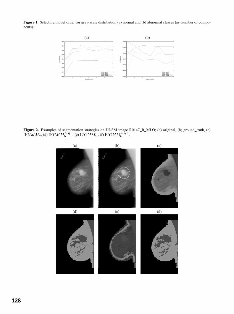
Figure 1. Selecting model order for grey-scale distribution (a) normal and (b) abnormal classes (m=number of compo-nents).

(a) (b)

-8400

-8200

-8000

-7800

-7600

-7400

-7200

-7000

-6800

1 2 3 4 5 6 7

Log-

likel

ihoo

d

Model order (m)

Breast type 1Breast type 2Breast type 3Breast type 4

-15000

-14000

-13000

-12000

-11000

-10000

-9000

1 2 3 4 5 6 7

Log-

likel

ihoo

d

Model order (m)

Breast type 1Breast type 2Breast type 3Breast type 4

Figure 2. Examples of segmentation strategies on DDSM image R0147_R_MLO; (a) original, (b) ground_truth, (c)ILKNMHMXO , (d) ILKNMHM"8QSRO , (e) ILKNMHM5T , (f) ILKNMHM

"8QSRT .

(a) (b) (c)

(d) (c) (d)

Prostate Segmentation: A Comparative Study

Yanong Zhua∗, Reyer Zwiggelaara†and Stuart Williamsb

aSchool of Information Systems, University of East Anglia, NorwichbDepartment of Radiology, Norfolk and Norwich University Hospital, Norwich

Abstract. To segment the prostate in Magnetic Resonance (MR) images is an important task whilst diagnosing,staging and treatment of prostate cancer. Due to its anatomical location and its similarity to surrounding tissue,the prostate is difficult to segment. Manually outlining the gland is time-consuming and tedious, so more effec-tive methods, which should be (semi-)automatic, become essential. In this paper, we discuss two approacheswhich are based on Active Shape Modelling (ASM) [1, 2] and a Polar Transform approach (PTA) [3]. Bothapproaches are compared to manual segmentation.

1 Introduction

Prostate cancer is the second leading cause of death from cancer in men, exceeded only by lung cancer. Prostatecancer accounts for 27% of all male cancers and 13% of male cancer related deaths [4]. In Western populations, theincidence of the disease has increased significantly over the last 35 years, making its diagnosis and management amajor health issue. In the UK, 13,500 new cases are currently diagnosed annually [5].

Magnetic Resonance Imaging (MRI) is a very important modality for the diagnosis, staging and follow-up ofprostate diseases. The prostate is anatomically divided into peripheral, central and transitional zones. For a normalprostate, there are increased signal intensity in the peripheral zone and decreased signal intensity in both centraland transitional zones on T2- weighted MR images. When diseases are developing in the prostate, the size and/orthe signal intensity of these zones will change, which makes it possible to make a diagnosis from image data.

In this paper, we concentrate on the automatic segmentation of the prostate in MR images. The shape and thesignal intensity of the prostate can vary both with time, as some diseases are developing, and between individuals.Due to the variability, the interpretation of prostate disease from image data is difficult. A number of authorshave described possible approaches to medical image segmentation. Kass et al. [6] describedsnakeswhich em-ploy a deformable contour to fit the shape of interest. Yezzi et al. [7] described a geometric snake model forsegmentation of medical imagery. Dryden and Mardia [8] described statistical models of shape. Ladak et al [9]used model-based Discrete Dynamic Contour (DDC) for prostate segmentation from ultrasound images. ActiveShape Modelling (ASM) [1, 2] provides another approach to the segmentation of the prostate in MR images. Aparameterised shape model can represent shape variability in the training sets. With enough representative trainingexamples, such a model is able to represent any variations of the prostate. Moreover, when the best fitting in-stance is generated, its parameters can be used for further processing, such as staging and classification of prostatediseases.

2 Data

Our data set includes 24 male pelvis transverse MRI sequences, totalling 532 images. All images were obtainedon a 1.5 Tesla magnet (Sigma, GE Medical Systems, Milwaukee, USA) using a phased array pelvic coil, with24 × 24cm field of view,256 × 512 matrix, 3mm slice thickness and 0.5mm interslice gap. Different types ofprostate abnormalities are included. Fig. 1 shows two typical examples from the data set. In Fig. 1 on the leftthere are minor benign hypertrophic changes in the central zone. The peripheral zone architecture is generallypreserved, with some patchy loss of the normal high T2 signal, in keeping with some malignant infiltration. Thereis no extracapsular extension present. In Fig. 1 on the right there are marked benign hypertrophic changes withinthe central zone, with resultant compression of the peripheral zone to a thin rim of tissue. However, the visibleperipheral zone does return reduced signal, suggesting that some tumour is present. Evidence of extracapsularspread is present within the MRI volume (but not on this slice).

All images were manually annotated by an expert radiologist and shapes are represented by landmarks. A landmarkis defined as a point of correspondence on each object that matches between and within populations [8]. Thirty-two landmarks are used to depict the outline of the gland. For training purpose, all the slices from three randomly∗email: [email protected]†email: [email protected]

Figure 1. Axial view prostate MRI examples.

selected volumes were chosen from the complete data set (only slices containing the prostate were used).Theremaining volumes form the test data.

3 Methods

3.1 Active Shape Models

Using a shape model, the shape variability in a training set can be represented. The images in the training set arelabelled so that the shape of each object of interest is marked with some key landmark points. The shapes fromthe training examples are aligned in order to be able to compare equivalent points from different shapes. Tangentspace projection is used to reduce the dimensionality. Once a set of aligned shapes is available, we can generate astatistical model of shape variation by applying Principal Component Analysis to the landmark vectors describingthe shapes in the training set [1]. With the deformable shape model we can generate a basic shape and fit it to theobject of interest in an unseen image. Image interpretation or segmentation is treated as an optimisation processthat examines a region around each landmark to find a better match for this landmark and calculate the adjustmentto the shape parameters to best fit the new found landmarks. In practise, to segment prostate MR images, theprostate central zones on all the example images are manually outlined and 32 landmarks are used for each. Sincethe central gland is nearly oval-shaped, we choose the four intersection points of the outline and the vertical andhorizontal axes through the centre of gravity as the key landmarks. On each of the four outline sections, sevenlandmarks were redistributed evenly. Subsequently the ASM algorithm is applied to the annotated training images.

3.2 Polar Transform Approach

A second, semi-automatic, approach to segment the prostate in MR images, based on Polar Transform space hasbeen developed [3]. To segment the prostate, the gland and the surrounding tissue are extracted into a polartransform using

x = xc + r cos(θ)y = yc + r sin(θ) (1)

where(x, y) is a position in the original image,(r, θ) represents the polar transform space, and(xc, yc) representsthe centre with respect to which the polar transform is obtained. Bilinear interpolation is used to sample the originaldata and the result is inversed so that a dark boundary in the original image is shown as a bright ridge in the polartransform. Lindberg’s approach [10] was used to extract ridges in the polar transform. Since the centre of the polartransform is within the prostate, it was assumed that the boundary of the prostate will appears as a band across allthe orientations in the polar transform. Curvilinear structures were tracked across the image to find the longest onewhich should represent the prostate boundary. An inverse polar transform is used to project the tracked curvilinearstructure back onto the original prostate image.

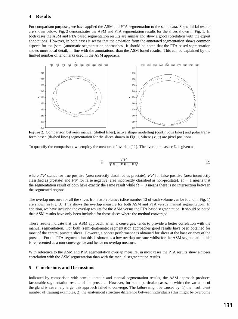
4 Results

For comparison purposes, we have applied the ASM and PTA segmentation to the same data. Some initial resultsare shown below. Fig. 2 demonstrates the ASM and PTA segmentation results for the slices shown in Fig. 1. Inboth cases the ASM and PTA based segmentation results are similar and show a good correlation with the expertannotations. However, in both cases it seems that the deviation from the annotated segmentation shows commonaspects for the (semi-)automatic segmentation approaches. It should be noted that the PTA based segmentationshows more local detail, in line with the annotations, than the ASM based results. This can be explained by thelimited number of landmarks used in the ASM approach.

210 220 230 240 250 260 270 280 290 300

210

220

230

240

250

260

270

280

290

300

x

y

210 220 230 240 250 260 270 280 290 300

210

220

230

240

250

260

270

280

290

300

x

yFigure 2. Comparison between manual (dotted lines), active shape modelling (continuous lines) and polar trans-form based (dashed lines) segmentation for the slices shown in Fig. 1, where(x, y) are pixel positions.

To quantify the comparison, we employ the measure of overlap [11]. The overlap measureΩ is given as

Ω =TP

TP + FP + FN(2)

whereTP stands for true positive (area correctly classified as prostate),FP for false positive (area incorrectlyclassified as prostate) andFN for false negative (area incorrectly classified as non-prostate).Ω = 1 means thatthe segmentation result of both have exactly the same result whileΩ = 0 means there is no intersection betweenthe segmented regions.

The overlap measure for all the slices from two volumes (slice number 13 of each volume can be found in Fig. 1)are shown in Fig. 3. This shows the overlap measure for both ASM and PTA versus manual segmentation. Inaddition, we have included the overlap results for the ASM versus the PTA based segmentation. It should be notedthat ASM results have only been included for those slices where the method converged.

These results indicate that the ASM approach, when it converges, tends to provide a better correlation with themanual segmentation. For both (semi-)automatic segmentation approaches good results have been obtained formost of the central prostate slices. However, a poorer performance is obtained for slices at the base or apex of theprostate. For the PTA segmentation this is shown as a low overlap measure whilst for the ASM segmentation thisis represented as a non-convergence and hence no overlap measure.

With reference to the ASM and PTA segmentation overlap measure, in most cases the PTA results show a closercorrelation with the ASM segmentation than with the manual segmentation results.

5 Conclusions and Discussions

Indicated by comparison with semi-automatic and manual segmentation results, the ASM approach producesfavourable segmentation results of the prostate. However, for some particular cases, in which the variation ofthe gland is extremely large, this approach failed to converge. The failure might be caused by: 1) the insufficientnumber of training examples, 2) the anatomical structure difference between individuals (this might be overcome

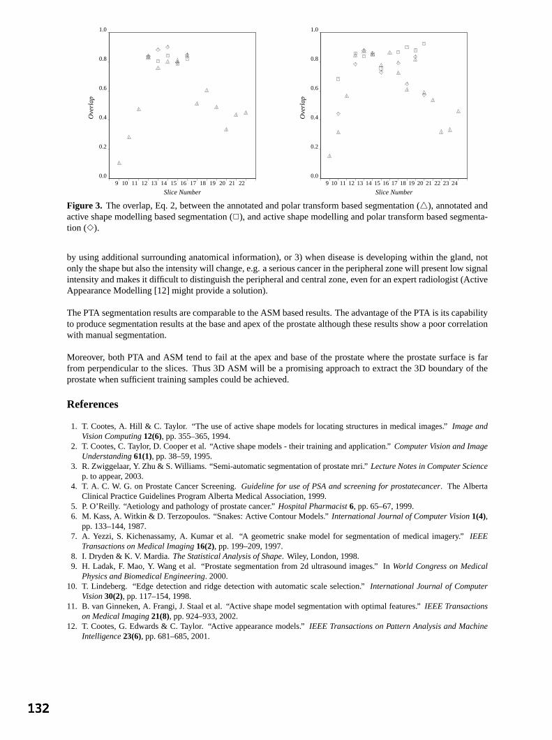
Slice Number

Ove

rlap

9 10 11 12 13 14 15 16 17 18 19 20 21 22 0.0

0.2

0.4

0.6

0.8

1.0

Slice Number

Ove

rlap

9 10 11 12 13 14 15 16 17 18 19 20 21 22 23 24 0.0

0.2

0.4

0.6

0.8

1.0

Figure 3. The overlap, Eq. 2, between the annotated and polar transform based segmentation (4), annotated andactive shape modelling based segmentation (2), and active shape modelling and polar transform based segmenta-tion (3).

by using additional surrounding anatomical information), or 3) when disease is developing within the gland, notonly the shape but also the intensity will change, e.g. a serious cancer in the peripheral zone will present low signalintensity and makes it difficult to distinguish the peripheral and central zone, even for an expert radiologist (ActiveAppearance Modelling [12] might provide a solution).

The PTA segmentation results are comparable to the ASM based results. The advantage of the PTA is its capabilityto produce segmentation results at the base and apex of the prostate although these results show a poor correlationwith manual segmentation.

Moreover, both PTA and ASM tend to fail at the apex and base of the prostate where the prostate surface is farfrom perpendicular to the slices. Thus 3D ASM will be a promising approach to extract the 3D boundary of theprostate when sufficient training samples could be achieved.

References

1. T. Cootes, A. Hill & C. Taylor. “The use of active shape models for locating structures in medical images.”Image andVision Computing12(6), pp. 355–365, 1994.

2. T. Cootes, C. Taylor, D. Cooper et al. “Active shape models - their training and application.”Computer Vision and ImageUnderstanding61(1), pp. 38–59, 1995.

3. R. Zwiggelaar, Y. Zhu & S. Williams. “Semi-automatic segmentation of prostate mri.”Lecture Notes in Computer Sciencep. to appear, 2003.

4. T. A. C. W. G. on Prostate Cancer Screening.Guideline for use of PSA and screening for prostatecancer. The AlbertaClinical Practice Guidelines Program Alberta Medical Association, 1999.

5. P. O’Reilly. “Aetiology and pathology of prostate cancer.”Hospital Pharmacist6, pp. 65–67, 1999.6. M. Kass, A. Witkin & D. Terzopoulos. “Snakes: Active Contour Models.”International Journal of Computer Vision1(4),

pp. 133–144, 1987.7. A. Yezzi, S. Kichenassamy, A. Kumar et al. “A geometric snake model for segmentation of medical imagery.”IEEE

Transactions on Medical Imaging16(2), pp. 199–209, 1997.8. I. Dryden & K. V. Mardia.The Statistical Analysis of Shape. Wiley, London, 1998.9. H. Ladak, F. Mao, Y. Wang et al. “Prostate segmentation from 2d ultrasound images.” InWorld Congress on Medical

Physics and Biomedical Engineering. 2000.10. T. Lindeberg. “Edge detection and ridge detection with automatic scale selection.”International Journal of Computer

Vision30(2), pp. 117–154, 1998.11. B. van Ginneken, A. Frangi, J. Staal et al. “Active shape model segmentation with optimal features.”IEEE Transactions

on Medical Imaging21(8), pp. 924–933, 2002.12. T. Cootes, G. Edwards & C. Taylor. “Active appearance models.”IEEE Transactions on Pattern Analysis and Machine

Intelligence23(6), pp. 681–685, 2001.

Histological parametric maps of the human ocular fundus:preliminary results

FelipeOrihuela-Espina,Ela ClaridgeandStephenJ.Preece

Schoolof ComputerScience,University of Birmingham,Edgbaston,B152TT, Birmingham, UK

Abstract. Specificcoloursobserved in imagesof the ocular fundus dependon the architectureof its layersand the optical propertiesand quantitiesof any pigments present. Thesecolourscanbe predictedfrom theparametersdescribingtheoculartissuecomposition usinga physics-based modelof light transport.Thispaperreportspreliminaryresultsof theapplicationof the inverseprocessby which theparameterscanbeestimatedfrom imagecolours.This is achievedby relatingthecolourof eachimagepixel to theclosestmatchingcolourpredictedby thelight transportmodel,andhenceto theparameterswhich generatedit. Thespatialdistributionandestimatedquantityof eachparameteris shown in a separateimagecalledparametricmap. Thefirst para-metricmapsof RetinalPigmentEpithelium(RPE)melanin,choroidalmelaninandchoroidalblood computedby thismethodshow a distributionof pigmentswhich is generallyconsistent with physiology.

1 Introduction

Thepupil of theeye providesanopening through which theinterior of theeye (theocularfundus)canbeexam-ined. This is clearly usefulfor the diagnosisof eye disorders.However, the fundus is alsoa unique locationatwhichbloodvesselscanbedirectlyobservedandthis makesit valuablefor thediagnosisof diseasesaffecting thevascularsystem,suchasdiabetes.Many abnormal conditionsaremanifestedthrough local changesin thefunduscolouration or through the appearanceof unusual colours. The long term objective of this work is to relatethecolours seenin thefundusto its condition andto any pathologicalchanges.

The colour of the fundus dependson several factorsincluding the architecture of its layersandthe nature anddensityof any pigments present[1]. Quantitativecharacterisationof thesefeaturesshouldbepossibleif a one-to-onerelationshipexistsbetweenthesephysiological factors,andthespectralintensitydistribution (SID) of thelightremittedfrom thetissue[2] under a givenincident light. This approachhasbeenshown to work for theskin [3].In thiswork, it is applied to theocularfundusto createparametricmapsof thekey ocular pigments. Although thisresearchwork is at preliminary stage,theearly resultsfor thehealthyfundus look promising. It is hoped that inthelong termtheresultsof this researchwill beusedto helpwith thediagnosisof diabeticretinopathy, which isthemostcommoncauseof blindnessin theUK’s working population [4].

2 Outline of the method

The methodinvolves threemain steps. The first stepis to determine the composition of the ocular tissueandspecificallythe propertiesof its optically active components,their spatialarrangement andtheir physiologicallyplausibleranges. This informationis usuallytaken from the previously publishedliterature. Thenext stepis topredict the entire rangeof colourswhich canoccurin thehealthytissueandto relatethemto tissueparameters.Thisyieldsamodelof tissuecolourationbasedonamathematicalmodelof theoptical radiation transport. Finally,thetissueparametersfor aparticularcaseareestimatedfrom its colours.Thisis doneby relatingthecolour of eachpixel in a colour imageto thehistologicalparameters usingthemodel of colourationcomputedpreviously. Thedistributionof eachparameteris shown in aseparatemonochromeimagecalledaparametricmap.A collectionofthesemapswasshown to bevaluablein diagnosisof skindisorders [5].

3 Methods

3.1 The structure and optical properties of the ocular fundus

The human ocularfunduscomprisesa number of optically andanatomically distinct layersasshown in Fig. 1.Its colour is determined primarily by theblood in thechoroid andfurther significantlymodified by theamountsof pigment melaninin the RPEandin the Choroid. The internalretinais transparent exceptfor a few vessels,thusreflectinglittle light. Light is highly scatteredby the collagenin the choroidal layer. The colour of blood

Email: (F.O.Espina,E.Claridge,S.J.Preece)@cs.bham.ac.uk

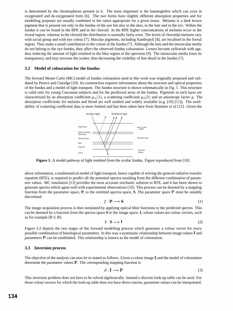
is determined by the chromophorespresentin it. The most important is the haemoglobin which can exist inoxygenatedand de-oxygenatedform [6]. The two forms have slightly different absorption propertiesand formodelling purposesareusuallycombined in the ratiosappropriatefor a given tissue. Melanin is a dark brownpigment that is presentnot only in thefundus of theeye but alsoin theskin, in thehair andin theiris. Within thefundus it canbefound in theRPEandin thechoroid. In theRPEhigher concentrationsof melaninoccurin thefovealregion, whereas in thechoroid thedistribution is normally fairly even. Thelevelsof choroidal melaninvarywith racialgroup andwith eyecolour[7]. Macularpigments,includingXanthopyll [8], arelocalisedin thefovealregion. They makeasmallcontributionto thecolour of thefundus[7]. Althoughthelensandtheintraocular mediado not belongto theeye fundus,they affect theobserved funduscolouration. Lensesbecomeyellowish with age,thusreducing theamount of light remittedin theblueregion of thespectrum[9]. Theintraocular medialosesitstransparency andmayincreasethescatter, thusdecreasing thevisibility of finedetailin thefundus[7].

3.2 Model of colouration for the fundus

Theforward MonteCarlo(MC) modelof funduscolourationusedin this work wasoriginally proposedandvali-datedby PreeceandClaridge[10]. Its construction requiresinformationaboutthestructure andopticalpropertiesof thefundusanda model of light transport. Thefundusstructureis shown schematicallyin Fig. 1. This structureis valid only for young Caucasiansubjectsandfor theperifovealareasof the fundus. Pigments in eachlayerarecharacterized by an absorption coefficient , a scatteringcoefficient andananisotropy factor . Theabsorption coefficients for melaninandblood arewell studiedandwidely available(e.g.[10] [11]). The avail-ability of scatteringcoefficient datais morelimited andhasbeentakenherefrom Hammeret al [12]. Giventhe

Pupil Plane

RPE

Neural Retina

Inner LimintingMembrane

Choroid

Sclera

Intra−ocularmedia

Remitted LightIncident light

Posterior

Receptor layer

fundus

Figure 1. A modelpathwayof light remittedfrom theocular fundus.Figurereproducedfrom [10].

above information,amathematicalmodelof light transport, hencecapableof solvingthegeneralradiativetransferequation (RTE), is required to predict all thepotentialspectraresultingfrom thedifferentcombinationof param-etervalues.MC simulation[13] providesthemostaccuratestochasticsolutionto RTE, andit hasbeenshown togeneratespectrawhichagreewell with experimentalobservations[10]. Thisprocesscanbedenotedby amappingfunction from theparameter space,P, to the remittedspectraspace,S. Theparameterspace mustbe suitablydiscretised.

(1)

Theimageacquisitionprocessis thensimulatedby applying opticalfilter functionsto thepredictedspectra.Thiscanbedenotedby a function from thespectraspaceS to theimagespace,I, whosevaluesarecolour vectors,suchasfor example[R G B].

(2)

Figure3.2 depicts the two stagesof the forward modelling processwhich generatesa colour vector for everypossiblecombinationof histological parameters.In thiswayasystematicrelationshipbetweenimagevalues andparameters canbeestablished.This relationship is known asthemodel of colouration.

3.3 Inversion process

Theobjectiveof theanalysiscannow bere-statedasfollows. Givenacolour image andthemodelof colourationdetermine theparametervalues . Thecorresponding mapping function is

(3)

This inversionproblem doesnot have to besolvedalgebraically. Insteada discretelook-up tablecanbeused.Forthosecolourvectors for whichthelook-uptabledoesnothavedirectentries,parametervaluescanbeinterpolated.

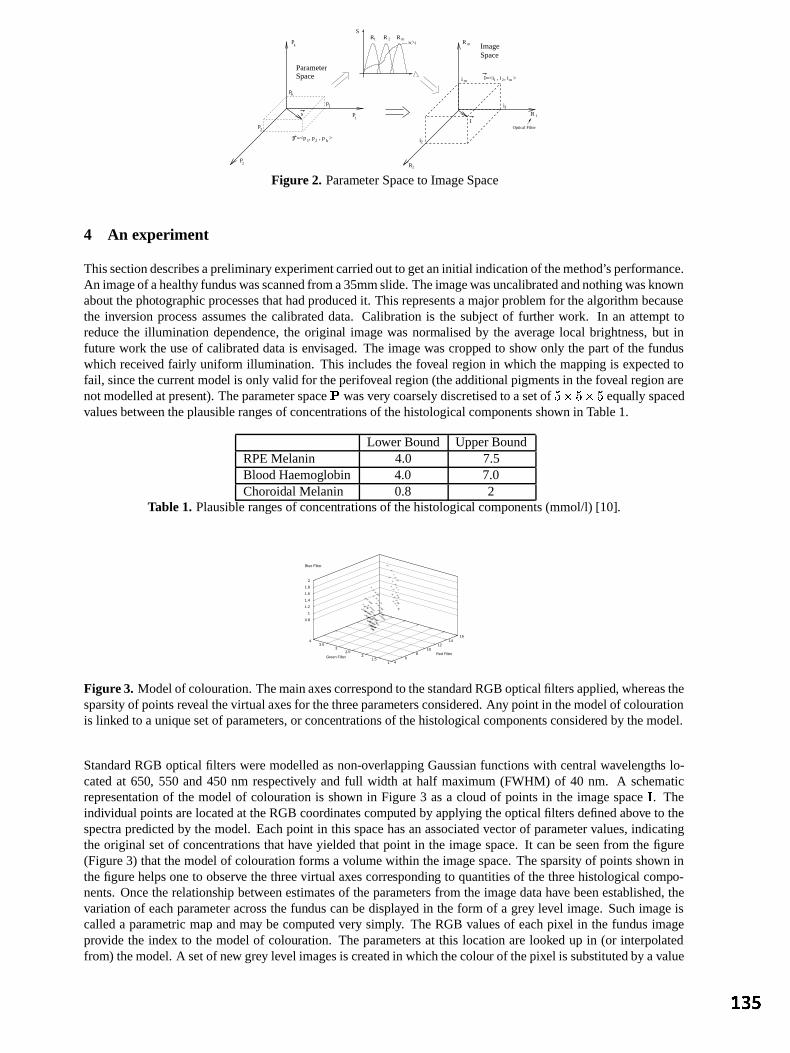
P

P

RS

p

p

R

p

P

s

Optical Filter

R

R1

2

1 2

m

m

I

I=<i , i , i >

2

i1

i

i

mSpaceParameter

Image

1

k

2

k

1

2

1 2p =<p , p , p >k

Space

mh( )

R

1R

2

Figure 2. ParameterSpaceto ImageSpace

4 An experiment

Thissectiondescribesapreliminaryexperimentcarriedoutto getaninitial indication of themethod’sperformance.An imageof ahealthyfunduswasscannedfroma35mmslide.Theimagewasuncalibratedandnothingwasknownabout thephotographic processesthathadproducedit. This representsa majorproblem for thealgorithm becausethe inversion process assumesthe calibrateddata. Calibrationis the subjectof further work. In an attempttoreduce the illumination dependence,the original imagewasnormalisedby the average local brightness,but infuture work theuseof calibrateddatais envisaged.The imagewascropped to show only thepartof the funduswhich received fairly uniform illumination. This includesthe foveal region in which themapping is expectedtofail, sincethecurrent model is only valid for theperifovealregion (theadditional pigments in thefovealregion arenotmodelledatpresent). Theparameterspace wasvery coarselydiscretisedto asetof "!# "!# equally spacedvaluesbetweentheplausiblerangesof concentrationsof thehistologicalcomponents shown in Table1.

LowerBound UpperBoundRPEMelanin 4.0 7.5BloodHaemoglobin 4.0 7.0Choroidal Melanin 0.8 2

Table 1. Plausiblerangesof concentrationsof thehistological components(mmol/l) [10].

11.5

22.5

33.5

4

Green Filter

46

810

1214

16

Red Filter

0.8

1

1.2

1.4

1.6

1.8

2

Blue Filter

Figure 3. Modelof colouration.Themainaxescorrespondto thestandard RGBopticalfiltersapplied, whereasthesparsityof points revealthevirtual axesfor thethreeparametersconsidered.Any point in themodelof colourationis linkedto a uniquesetof parameters,or concentrationsof thehistological componentsconsideredby themodel.

StandardRGB opticalfilters weremodelledasnon-overlappingGaussianfunctionswith centralwavelengths lo-catedat 650, 550 and450 nm respectively and full width at half maximum(FWHM) of 40 nm. A schematicrepresentation of the modelof colouration is shown in Figure3 asa cloud of pointsin the imagespace . Theindividual pointsarelocatedat theRGB coordinatescomputedby applying theopticalfilters definedabove to thespectrapredictedby themodel. Eachpoint in this spacehasanassociatedvectorof parametervalues,indicatingtheoriginal setof concentrationsthathave yieldedthat point in the imagespace.It canbe seenfrom the figure(Figure3) thatthemodel of colourationformsa volumewithin theimagespace.Thesparsityof pointsshown inthefigurehelpsoneto observe thethreevirtual axescorresponding to quantitiesof thethreehistological compo-nents.Oncetherelationship betweenestimatesof theparameters from theimagedatahave beenestablished,thevariationof eachparameteracrossthe funduscanbedisplayed in the form of a grey level image.Suchimageiscalleda parametric mapandmaybecomputedvery simply. TheRGB valuesof eachpixel in the fundus imageprovide the index to the modelof colouration. Theparameters at this locationarelooked up in (or interpolatedfrom) themodel.A setof new grey level imagesis createdin whichthecolour of thepixel is substitutedby avalue

representing themagnitudeof thegiven parameter.

5 Results and discussion

Preliminaryresultsareshown in Figure4. Although the mapping is very crude, the mapsexhibit a distributionof pigmentswhich is generally consistentwith physiology. TheRPEmelaninlevels increasetowardsthe fovealregion. In thecentralfoveal areathe incorrectly low levelsof melanin aremostlikely causedby thepresenceofmacularpigments which arenot representedby the model. The levels of choroidal melanindo not show muchspatialvariation acrossthe fundus, asexpected. Blood levelsareshown in two maps,onefocusingon largeandmediumretinalvessels,theotheronblood level variations in thechoroid. It canbeseenthattheretinalvesselsarepickedupwell. Whencontrastis stretched, somevariationsin thechoroidal blood startshowing up,however, theirinterpretationwouldbeprematurebecausethelackof imagecalibration certainly introducedlargemapping errors.Both mapsshow high levelsof bloodin thecentreof fovealregion, which is incorrect. This is likely to have beencausedby themacular pigments,similarly to theRPEmelaninmapdiscussedabove.

Figure 4. Fromleft to right: Original Image; RPEMelaninParametricMap; Choroidal MelaninParametricMap;BloodParametric Map(Main vessels);BloodParametric Map(Choroidalvariations).

6 Conclusion

Thepreliminary resultsreportedin thispaperindicatethataphysics-basedinterpretationof thecoloursin theocularfundusis feasible.Thefirst parametricmapsof RPSmelanin,choroidal melaninandchoroidal blood computedbythis method generally show thedistribution of theabove pigments consistentwith physiology. Furtherwork is inprogressto include additional ocularpigmentsin themodel,to calibrateor normalisetheinput imagedata,andtoincreasetheresolutionwith which thephysiologicalparametersarediscretised.

References

1. I. C. Michaelson. Textbook of the fundus of the eye. Churchill Livingstone,third edition,1980. ISBN 0-443-01782-4.2. S.R. Arridge & J.C. Hebden.“Optical imagingin medicine:II. modellingandreconstruction.” Physics in Medicine and

Biology 42, pp.841–853,1997.3. S. D. Cotton,E. Claridge& P. N. Hall. “Noninvasive skin imaging.” In J. Duncan& G. Gindi (editors),Information

Processing in Medical Imaging IPMI’97, pp.501–506.Springer, 1997.LNCS1230.4. D. R. Owens,R. L. Gibbins,E. Kohnertetal. “Diabetic retinopathyscreening.” Diabetic Medicine 17, pp.493–494, 2000.5. M. Moncrieff, S. CottonD’Oyly, E. Claridgeet al. “Spectrophotometricintracutaneous analysis:a new techniquefor

imagingpigmentedskin lesions.” British Journal of Dermatology 146, pp.448–457,2002.6. S.D. Cotton. A non-invasive imaging system for assisting in the diagnosis of malignant melanoma. Ph.D.thesis,School

of ComputerScience,FEB1998.Universityof Birmingham.7. F. C. Delori & K. P. Pflibsen. “Spectralreflectanceof the humanocularfundus.” Applied Optics 28(6), pp. 1061–1077,

1989.8. S.F. Chen,Y. Chang& J.C. Wu. “The spatialdistribution of macularpigments in humans.” Current Eye Research 23(6),

pp.422–434,2001.9. J.Xu, J.Pokorny & V. C. Smith. “Optical densityof humanlens.” Journal of the Optical Society of America A - Optics,

Image Science and Vision 14(5), pp.953–960,1997.10. S. J. Preece& E. Claridge. “Monte Carlo modellingof the spectralreflectanceof the humaneye.” Physics in Medicine

and Biology 47, pp.2863–2877,JUL 2002.11. S.L. Jacques& S.Prahl.“http://omlc.ogi.edu/spectra.” OregonMedicalLaserCenter.12. M. Hammer, A. Roggan,D. Schweitzeret al. “Optical propertiesof the ocular fundus tissues- an in-vitro studyusing

the double integration spheretechniqueand inversemontecarlo simulation.” Physics in Medicine and Biology 40(6),pp.963–978,1995.

13. L. Wang& S.L. Jacques.Monte Carlo Modelling of Light Transport in Multi-Layered Tissues in Standard C. Universityof TexasM. D. AndersonCancerCenter, 1998.

Texture Segmentation in Mammograms

ReyerZwiggelaara, Lilian Blota, David Rabab andErikaR.E.Dentonc

aSchoolof InformationSystems,Universityof EastAnglia, NorwichbComputerVisionandRoboticsGroup,Universityof Girona,Girona,Spain

cDepartmentof BreastImaging,Norfolk andNorwichUniversityHospital,Norwich

Abstract. We have investigateda combinationof statisticalmodellingandexpectationmaximisationfor atexture basedapproachto the segmentationof mammographicimages. Texture modelling is basedon theimplicit incorporationof spatialinformationthroughthe introductionof a set-permutation-occurrencematrix.Statisticalmodelling is usedfor dimensionalityreduction,datageneralisationand noiseremoval purposes.Expectationmaximisationmodellingof theresultingfeaturevectorprovidesthebasisfor imagesegmentation.Thedevelopedsegmentationresultsareusedfor automaticmammographicrisk assessment.

1 Introduction

Texture is oneof the leastunderstoodareasin computervision andthis lack of understandingis reflectedin thead-hocapproachestaken to datefor texture basedsegmentationtechniques.Althoughno generictexture modelhasemergedsofar a numberof problemspecificapproacheshave beendevelopedsuccessfully[1]. Althoughthedescribedapproachis developedwith oneparticularapplicationin mind,wedobelievethatit is genericwithin thefield of medicalimageunderstanding.

SinceWolfe’s [2, 3] original investigationinto the correlationbetweenmammographicrisk and the perceivedbreastdensitya numberof automaticapproacheshave beendeveloped[4–6]. Examplemammogramsareshownin Fig. 1. Someof thesemethodsare basedon grey-level distributions whilst othersincorporatesomeaspectof spatialcorrelationor texture measure.While all thesemethodsachieve somecorrelationwith manualvisualassessmentin generalthey arenotasgoodasexpertintra-observeragreement.Theaccurateandrobustestimationof mammographicdensitycanbe usedfor risk modellingandpossiblyto determinescreeningintervals withinbreastscreeningprogrammes.

(a) (b)Figure 1. Fatty (a)anddense(b) mammographicimages.

It is our thesisthat the relative sizeof segmentedimageregions,representingdistinct anatomicaltissueclasses,is correlatedwith mammographicrisk assessment.Statisticalmodellingin combinationwith expectationmaximi-sation(EM) [7] is usedfor thesegmentationof mammographicimages.To our knowledge,we introducea newconcept,theset-permutation-occurrencematrix,asa texturefeaturevector. Realistictexturemodellingis possibleasspatialinformationis implicitly incorporated.To achievesegmentationanumberof stepsarerequired:a) infor-mationgatheringwhich transformstheoriginal datain a multi-scalerepresentation;b) texture featureextractionwhichusestheset-permutation-occurrencematrixconceptto generateafeaturevectoratapixel level; c) statisticalmodellingto provide a morecompactandgeneralisedrepresentationof thedata;d) EM clusteringto divide thedatain anoptimalsetof classes;ande) imagesegmentationwhichusestheclassesfor eachpixel. Therelativesizeof thesegmentedimageregionsis used,in combinationwith anearest-neighbourclassifier, to estimatethedensityfor eachmammogram.

email: [email protected]

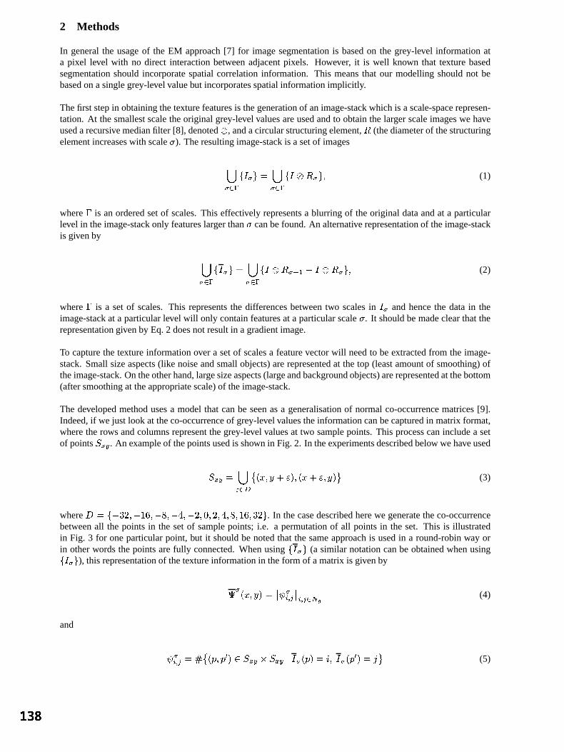
2 Methods

In generalthe usageof the EM approach[7] for imagesegmentationis basedon the grey-level informationata pixel level with no direct interactionbetweenadjacentpixels. However, it is well known that texture basedsegmentationshouldincorporatespatialcorrelationinformation. This meansthat our modellingshouldnot bebasedonasinglegrey-level valuebut incorporatesspatialinformationimplicitly.

Thefirst stepin obtainingthetexturefeaturesis thegenerationof animage-stackwhich is a scale-spacerepresen-tation. At thesmallestscaletheoriginal grey-level valuesareusedandto obtainthe largerscaleimageswe haveusedarecursivemedianfilter [8], denoted

, andacircularstructuringelement, (thediameterof thestructuring

elementincreaseswith scale ). Theresultingimage-stackis a setof images

(1)

where is anorderedsetof scales.This effectively representsa blurring of theoriginal dataandat a particularlevel in theimage-stackonly featureslargerthan canbefound.An alternativerepresentationof theimage-stackis givenby

(2)

where is a setof scales.This representsthe differencesbetweentwo scalesin andhencethe datain theimage-stackat a particularlevel will only containfeaturesat a particularscale . It shouldbemadeclearthattherepresentationgivenby Eq.2 doesnot resultin a gradientimage.

To capturethetexture informationover a setof scalesa featurevectorwill needto beextractedfrom the image-stack.Smallsizeaspects(like noiseandsmallobjects)arerepresentedat thetop (leastamountof smoothing)oftheimage-stack.Ontheotherhand,largesizeaspects(largeandbackgroundobjects)arerepresentedatthebottom(aftersmoothingat theappropriatescale)of theimage-stack.

The developedmethodusesa modelthat canbe seenasa generalisationof normalco-occurrencematrices[9].Indeed,if we just look at theco-occurrenceof grey-level valuestheinformationcanbecapturedin matrix format,wheretherows andcolumnsrepresentthegrey-level valuesat two samplepoints. This processcanincludea setof points . An exampleof thepointsusedis shown in Fig. 2. In theexperimentsdescribedbelow wehaveused

"!$#&%(' *),+.-"/0 %(' +1-*)/32 (3)

where 4 657398:;36<;3>=;$7@?@7*=@<38:A57 . In thecasedescribedherewe generatetheco-occurrencebetweenall the pointsin the setof samplepoints; i.e. a permutationof all pointsin the set. This is illustratedin Fig. 3 for oneparticularpoint, but it shouldbenotedthat thesameapproachis usedin a round-robinway orin otherwordsthepointsarefully connected.Whenusing (a similar notationcanbeobtainedwhenusing

), this representationof thetextureinformationin theform of amatrix is givenby

B %C' A)/DFEHG I(J KML ICJ K "NPO (4)

and

G I(J K RQ # %HS ST /U VXWYV,Z %[S /\^]@ %[S&T /_a` 2 (5)

where Q denotesthenumberof elementsin a setand bXc denotesthesetof grey-level values.It shouldbenotedthat this approachprovidesa differentdescriptionthanthat would be provided by usinga setof co-occurrencematrices.

Figure 2. Samplepoints V . Figure 3. Samplepointsconnectivity.

Insteadof usingthe co-occurrenceof the grey-level valuesit is possibleto usethe occurrenceof the grey-leveldifference.Again, this is usingthesamesetof samplepoints V (seeFigs2 and3) at eachscale(i.e. level intheimage-stack).As we areusingtheoccurrenceof thegrey-level differencevaluesour grey-level co-occurrencematrixreducesto avector. Effectively this is analignmentof thecolumnsof theco-occurrencematrixwith respectto thediagonal(i.e. wherethedifferencein grey-level valuesis equalto zero)anda subsequentsummationovertherows. Whenusingthedifferenceimage-stackrepresentation(seeEq. 2) the featurevectorat a singlescaleisgivenby

d %C' *)/\eEgf I L I "hji O (6)

whereb,c is thesetof grey-levels, a givenscale,k N O is thesetof grey-level differencesand

f I lQ # %HS S&T /U VXWYV,Z %HS /P %HST /\m] 2 (7)

where,again,Q denotesthenumberof elementsin a set.

Thetexturefeaturedescribedaboveis extractedatapixel level andcombiningthetexturefeaturesoverall possiblescalesresultsin a featurevector. We have usedprincipal componentanalysis[10] to provide a morecompactrepresentationof thefeaturevector.

3 Results

TheEM approach[7] is usedto determinea setof classesfrom thefeaturevectorswhich canbeusedto segmenttheimages.Althoughof interest,it is computationallyimpracticalto basetheEM modellingontheoriginaltexturefeaturevectorasthishasa largenumberof elements(ahighdimensionality)andtendsto besparse.All theresultspresentedin this sectionarebasedon a PCA reducedfeaturevectorwherewe typically capture95%of thedatavariation(the dimensionalityof thedatawasapproximatelyreducedby a factorof ten). The EM andstatisticalmodellingprocesstakeonly thebreastareainto accountwhilst excludingthepectoralmuscleandthebackground.For theEM approachthenumberof classeswassetequalto six [11].

To testour thesisthattherelative sizeof thesegmentedregionsis linkedto mammographicrisk a smallsubsetoftheMammographicImagesAnalysisSociety(MIAS) databasewasused[12,13]. All the imageswereassessedby mammographicexpertswho provided an estimateof the proportionof densetissuein eachmammogram.Thesegmentationresults,basedon EM andstatisticalmodellingusing or , canalsobeusedto obtainthe relative sizeof the segmentedregionsfor eachclass. This featureis usedasour classificationspace.Thecorrelationbetweentherelativeregionsizedistributionandtheestimatedproportionof densetissue,whenusinga

nearestneighbourclassifieron a leave-one-outbasisfor , canbefoundin Table1. This shows anagreementfor 86%of themammograms(thisdecreasesto 66%whenusing n . Thiscompareswell with aninter-observeragreementof 45%. The intra-observer agreementon theuseddatasetis 89%. In addition,whenusingthesamedatasetandclassificationapproach,resultsbasedon theapproachesdevelopedby Byng [5] andKarssemeijer[4]show anagreementof 67%and81%,respectively.

ExpertClassification0-10% 11-25% 26-50% 51-75%

Aut

omat

icC

lass

ifica

tion 0-10% 6 0 0 0

11-25% 0 5 2 026-50% 2 1 8 051-75% 0 0 0 12

Table 1. Comparisonof thedensityestimateasgivenby anexpertradiologistandautomaticsegmentation.Basedon .4 Conclusions

Wehaveshown thatacombinationof EM andstatisticalmodellingresultsin arobustapproachto thesegmentationof mammographicimages. We have introduceda texture featurevectorbasedon a set-permutation-occurrencematrixwhichcapturesbothspatialandlocalgrey-level information.Theuseof thistypeof matrixwill needfurtherdevelopmentto exploreits limitationsandfull potential.It shouldbenotedthatsomefundamentalquestions,suchas the influenceof the size and shapeof the distribution of samplepoints V , needfurther investigation. Inaddition,thedevelopedtexturesegmentationapproachwill befully evaluatedonsyntheticandnaturaltextures.

We have shown that the segmentationresultscanbe usedto provide valuableinformation in the estimationofmammographicdensityand thereforpossiblyfor mammographicrisk assessment.The developedapproachiscomparableto expert intra-observer variation,shows considerableimprovementon the inter-observer agreementandcomparesfavourablewith existing techniques.

Acknowledgement

We would like to thankGlynisWivell for markingthedata.

References

1. T. Reed& J. Dubuf. “A review of recenttexture segmentationand feature-extraction techniques.” Computer Vision,Graphics and Image Processing 57(3), pp.359–372,1993.

2. J. Wolfe. “Risk for breastcancerdevelopmentdeterminedby mammographicparenchymalpattern.” Cancer 37(5),pp.2486–2492,1976.

3. N. Boyd, J. Byng, R. Long et al. “Quantitative classificationof mammographicdensitiesandbreastcancerrisk: resultsfrom thecanadiannationalbreastscreeningstudy.” Journal of the National Cancer Institute 87, pp.670–5,1995.

4. N. Karssemeijer. “Automatedclassificationof parenchymalpatternsin mammograms.” Phys. Med. Biol. 43, pp.365–378,1998.

5. J.Byng,M. Yaffe,G.Lockwoodetal. “Automatedanalysisof mammographicdensitiesandbreastcarcinomarisk.” Cancer80(1), pp.66–74,1997.

6. J.Heine& R.Velthuizen.“A statisticalmethodologyfor mammographicdensitydetection.” Medical Physics 27, pp.2644–2651,2000.

7. P. Demster, N. Laird & D. Rubin. “Maximum likelihoodfrom incompletedatavia theemalgorithm.” Journal of the RoyalStatistical Society B 39, pp.1–38,1977.

8. R. Zwiggelaar, T. Parr, J.Schummet al. “Model-baseddetectionof spiculatedlesionsin mammograms.” Medical ImageAnalysis 3(1), pp.39–62,1999.

9. M. Haralick. “Statisticalandstructuralapproachesto texture.” Proceedings of the IEEE 67(5), pp.786–804,1979.10. I. Jolliffe. Principal Component Analysis. SpringerVerlag,1986.11. R.Zwiggelaar, P. Planiol,J.Marti etal. “Em texturesegmentationof mammographicimages.” oprq International Workshop

on Digital Mammography Bremen, Germany, pp.223–227,2002.12. L. Blot, E. Denton& R. Zwiggelaar. “Risk assessment:theuseof backgroundtexture in mammographicimaging.” o prq

International Workshop on Digital Mammography Bremen, Germany, pp.541–543,2002.13. J. Suckling,J. Parker, D. Danceet al. “The mammographicimagesanalysissocietydigital mammogramdatabase.” In

D. Gale,Astley & Cairns(editors),Digital Mammography, pp.375–378.Elsevier, 1994.

Thick Emulsion Holography and Medical Tomography.

Peter Thompson and Graham Saxby.

The Department of Medical Physicss Doncaster Royal Infirmary, Thorne Road, Doncaster.

DN2 5LT.

ABSTRACT

We report a new method for recording multiple-exposure holograms in order to synthesize a monochromatic 3D image from a series of medical tomograms. The object was to produce high-resolution images with a wide viewing angle and a high diffraction efficiency, which could be viewed unaided in white light. A spatial light modulator is the key component of the holographic system, and this is used to display a sequence of two-dimensional views that can be recorded sequentially on holographic plates.

1. Introduction A number of researchers have attempted to produce volume multiplexed holograms from medical data with varying degrees of success. Perhaps the best known of these are the researchers at Voxel, who developed their method for producing high-resolution holograms and put it on the market by the end of 1994. The Voxel holograms exhibit monochromatic images with 256 levels of grey scale, and over 200 slices combined in an image. Although they are effectively synthetic holograms made up from a number of 2D images, all the basic depth cues are available with the reconstruction of the third dimension, with the rear images being visible through the images at the front. Now, in Doncaster, we have developed a new setup for recording holograms that can be viewed directly in white light, are easier to produce and can be viewed from different perspectives without distortion or ambiguity. 2. Method This technique is designed to incorporate cross-sectional images of a three-dimensional object such as those produced by computerised tomography (CT) and magnetic resonance (MR) scans. An expanded and collimated laser beam is transmitted through the image of a tomographic slice displayed on a high-resolution, 1024*768 XGA LCD. The image is then projected on to the rear of a diffusing screen, thus representing the “object” in traditional holography. Once the first slice has been exposed, the next slice can be displayed, the screen having been repositioned at a new distance from the holographic plate incremented by the scan slice interval. Again an exposure is made and the process continued until the entire subject volume is recorded as an integrated holographic image. The images are stacked one on top of the other within the thick emulsion of the plate, and this is essentially the same principle as that employed by Voxel. 2.1 Voxel’s Method The optical setup used by Voxel involves splitting the beam into two separate paths, one to illuminate a spatial light modulator, (SLM) and the other to act as a reference beam. In order to achieve this, Voxel have used a voltage-adjustable wave plate under computer control, to split the beam and thus adjust the beam ratio [1]. This allows them to both keep the beam ratio as low as possible and at the same time at a constant level for every slice used. When using a high beam ratio, the holographic plate is repeatedly exposed to the plane wave from the reference beam and this can limit the number of exposures possible before the emulsion becomes saturated. This can make it necessary to increase the exposure time so that subsequent exposures receive more energy than the first. This is to increase the number of multiple-exposures that can be superimposed, without the problem of holographic reciprocity law failure, (HLRF). HRLF is the chronological decrease in diffraction efficiency when multiple exposures are recorded with equal energy. A twofold decrease in diffraction efficiency has been experimentally observed, [2], when six holograms were superimposed on the same holographic plate.

The Voxel holograms are transmission holograms and as such cannot be viewed in white light without the aid of a dispersion compensation unit. This idea was developed by Kaveh Bazargan, [3] and uses a compact light source, diffraction grating, collimating element and direction selective filter to eliminate the chromatic dispersion produced when viewing transmission holograms by white light. Voxel use transmission holograms because the spatial frequency of the fringes recorded is lower than those found in a reflection hologram, and this places less strain on the resolving power of the emulsion [4]. They also suggest that the apparatus used for producing transmission holograms is less susceptible to vibration. 2.2 Plane and Volume Holograms In order to explain the difference between our technique and the one used by Voxel it is first necessary to explain the differences between a plane hologram and a volume hologram, Fig1). As the angle between the object beam and the reference beam changes, so does the spacing between the fringes in the emulsion. A plane or surface hologram has the image only on the surface. This means that the fringes are almost perpendicular to the plane of the emulsion. If the angle is between 450 and 900 the fringe spacing becomes small enough for the recording process to be taking place throughout the volume of thickness of the emulsion. As the emulsion becomes thicker and/or the angle increases, the Bragg condition becomes more dominant and the fringe planes are more nearly parallel to the emulsion surface. This type of hologram is called a volume hologram. In a volume reflection hologram, the reference beam strikes the plate from the opposite side to the object beam. A reflection hologram can be viewed very satisfactorily in white light. The distance between the fringes is a function of the wavelength of the light used to produce the hologram and is constant. Only the wavelength of light that matches the fringe spacing will be reflected towards the viewer.

OB RB<450 PLANE TRANSMISSION HOLOGRAM

RB>450 HOLOGRAPHIC PLATE VOLUME TRANSMISSION HOLOGRAM

RB=1800

IN-LINE VOLUME REFLECTION HOLOGRAM

Figure 1)

2. Optical Set-up Used Very few reflection holograms are made in-line or with 1800 difference between the object and reference beams. This is because in order to reconstruct and view the image, you have to look directly into the light source you are using to playback the hologram. With a reflection type hologram you can get around this by using angle 100 less than 1800 in-line format. It is this in-line format that we are using as part of our setup, with a reference beam created by light reflected back from a mirror positioned just behind the holographic plate. Because a lens is used to collect and collimate the light projected on to the diffusing screen, the image of the object reflected back towards the plate directly coincides with the image of the object incident on the emulsion. Fig 2)

Collimating Lens Holographic Plate

SLM

OB RB

Collimated Laser Beam

Projection Lens Diffusing Screen Mirror

Moving Stage

Figure 2) 3. Results 3.1 Advantages of the Set-up Used Because the reflected image that acts as a reference beam is exactly the same size as the object image produced for each two-dimensional slice, only that part of the emulsion that covered by that image is exposed for each of n exposures. Also, the ratio of the object beam (OB) to the reference beam (RB) is constant for every slice and should remain close to the ideal 1:1 ratio required for multiple-exposure holograms. If you add to this the increased stability provided by using a single beam rather than a split beam set-up and the white light viewing, then the advantages are very exciting, but the diffraction efficiency and sharpness of the images produced using this technique have been inferior to those produced using the Voxel method. 3.2 The Spatial Light Modulator Tests of the quality of our SLM have shown inherent problems with a device of this type. The pixels of an LCD are constantly being refreshed and their effective optical distances may thereby fluctuate. The LCD modulates by absorption of the rotated polarisation of light and LCDs typically waste up to 90% of the available laser light. The LCDs structure has a number of surface interfaces, which back-reflect and absorb light. Also the fill factor for a LCD is typically only 70%, [5]. The fill factor for our SLM is unknown. The measured transmittance as around 20% and it may be that our spatial light modulator is inefficient and requires more laser power to overcome its deficiencies. A small residual “twitching” of each pixel as the array is electrically scanned will reduce the diffraction efficiency of a hologram created using an LCD due to degradation of laser beam coherence. With our SLM there is a clear degradation in diffraction efficiency when comparing a hologram made with a transparency with one made with the SLM using similar exposure and geometry. The contrast ratio is given by the manufacturer as 150:1 and is low because the LCD’s black base line is not completely opaque. At the black level the power density level measured was typically 0.21 µW. 3.3 Hologram Recording Materials We have been able to make small format holograms with a degree of success, initially on Agfa 8E75HD film emulsions that require an exposure of about 60 to 100 µJ.cm2. We have also used Birenheide BB-640, 2.5 inch square glass plates, that require at least 3-4 times the exposure. These have a grain size that is a great deal smaller than the Agfa film, which is 20 to 25 nm. The results have been promising. It is obviously easier using

plates than film and the small plates can be illuminated with an adequate power density when using a 30mW laser. Using a 30 mW He:Ne laser limits the amount of light available for making holograms. This situation does not improve when using the SLM, as typically only 21% of available light is transmitted through the display. Unfortunately the Birenheide plates are no longer available from the original source and we have now switched to 4 by 5 inch Slavich PFG-01 plates. Up to now we have not managed to use these successfully, due to the longer exposure times required with our current laser. This is because the area of the projected laser image used to fill the larger format plates has increased. 3.4 Pyrochrome Processing High spatial frequencies are required with reflection holography and a typical resolution between 4000 and 6000 cycles/mm is required. By using Pyrochrome processing it is possible to produce bright, low noise high-resolution reflection holograms without having to be over critical with respect to exposure and development times [6]. It is also possible to control the colour of the final hologram by adding a controlled quantity of sodium sulphite to the developer. Discussion We have developed a new method for making volume-multiplexed holograms and in the future we intend to explore the following ideas: • The effects of using a 50 mW diode laser (650nm) instead of a 35 mW He:Ne laser. • Making our own silver bromide holographic recording materials with different emulsion thicknesses. • The use of image processing to produce high contrast images that are segmented and rendered. • Using area partitioning to display volume multiplexed holograms from different perspectives. References 1. A. Wolfe and Stephen Hart, Voxel, “Digital Volumetric Holograms for Medical Imaging” SPIE Web, OE Reports. 2. K. M. Johnson, Lambertus Hesselink “Multiple Exposure Holographic Display of CT Medical Data” SPIE 367,

Processing and Display of Three-dimensional Data pp. 149-154, 1982. 3. K. Bazargan, “A Practical, Portable System for White-Light Display of Transmission Holograms using Dispersion

Compensation”, SPIE 523, Applications of Holography pp. 24-25, 1985. 4. K. J. Drinkwater and S. J. Hart, “Multiplexed Holography for the Display of Three-Dimensional Information”, Forth

International Symposium on Optical and Optoelectronic Applied Science and Engineering, pp. 37-44, March 1987. 5. S. Ryder. S. Nesbitt and S. L. Smith,” Holographic Recording using a Digital Micromirror Device”,

Massachusetts Institute of Technology, SPIE. 6. W. Spierings, “Pyrochrome” Processing Yields Colour-Controlled Results with Silver-Halide Materials”, Holosphere

Article. www.Holoprint.com

Imaging the Pigments of Human Skin with a Technique which is Invariant to Changes in Surface Geometry and Intensity of

Illuminating LightStephen Preece, Symon Cotton and Ela Claridge*

Astron Clinica, The Mount, Toft, Cambridge, CB3 7RL.*The School of Computer Science, University of Birmingham, Edgbaston, Birmingham, B15 2TT.

Abstract:A technique is described which enables quantitative histological data to be recovered from conventional digital images. Methodology is developed around the concept of image ratios, which are shown to be invariant to scene geometry and illumination intensity. Key to the success of this technique, is a function which maps uniquely from a vector if image ratios to the corresponding vector of histological parameters. The existence of this function is established using mathematical techniques drawn from differential geometry. The methodology is formulated generally then applied to a two-parameter model of human skin. A function relating image ratios to concentrations of melanin and blood is established and used to process a standard RGB image. The technique successfully maps out the distribution of blood and melanin across the entire image.

1 Method

As light optical radiation propagates through skin it is both scattered and absorbed. Scattering primarily occurs from the underlying tissue structure whilst absorption tends to result from the tissue pigments. Healthy skin can be considered the two-layered structure, depicted in figure 1. Incoming light first passes through the epidermis.

No scattering occurs in this layer but the presence of the pigment melanin to be absorbed. The light then passes into the dermis where it is scatteredbeing absorbed by the pigment haemoglobin. It has been argued [1,2] sufficient to model radiation transport within skin. If scattering coefficiencoefficients for haemoglobin and melanin are known, then is it possible tspecific wavelength. This allows the corresponding fraction of remitted ltheory at discrete wavelengths, across an appropriate spectral range, a remi

In healthy skin three parameters are required to describe all histologicalmelanin, concentration of dermal blood and thickness of the dermal lavariation in terms of a 3-D parameter space, with axes: melanin, blooparameters have differing effects on the remitted spectrum, every point wto a unique spectrum, which can be obtained by using the Kubelkaconvolving the spectrum with the spectral response curves of the imagobtain RGB values that correspond to a given point within parameter spacRGB vectors to corresponding points in parameter space, it is possible given image. This information can then be displayed in the form of greyfundamental principle has been used by Cotton and Claridge [4,5] to dpigmented lesions. This application uses a four-parameter model of hum

Figure 1: Tissue structure of normal skin

Dermis

Epidermis

Remitted light

Incoming light

causes a fraction of the incoming light by the underlying collagen as well as that the Kubelka-Munk theory [3] is ts for collagen and specific absorption o apply the Kubelka-Munk theory at a ight to be predicted. By applying this ttance spectrum can be constructed.

variation: concentration of epidermal yer. It is convenient to think of the d and dermal thickness. As the three ithin the parameter space corresponds -Munk model of light transport. By e acquisition system, it is possible to e. By constructing a mapping, relating to recover parameter values across a -scale image, or parametric map. This evelop a system capable to analysing an skin, the three parameters already

described, with the addition of melanin in the dermal layer. This system has been developed into a commercially available system by Aston Clinica and is proving to be of immense value to clinicians in their diagnosis of melanoma. Although proving effective, the system requires exact calibration of the illuminating light source and does not take into account any variation in surface geometry. This latter assumption can result in inaccuracies when skin is imaged in the vicinity of a joint. In the following section a technique is described for recovering histological parameters from image data in a way that is insensitive to scene geometry and illumination intensity. This method is then applied to a two-parameter model of skin.

1.1 Achieving invariance to surface geometry and illumination intensity

The dichromatic reflection model, first proposed by Shafer [6], states that light remitted from an object is the sum of two components, the ‘body’ component and the ‘surface’ component. The body component refers to physical processes occurring after penetration of light into the material and the surface term to reflections that take place at the surface of the object. By using a system of cross-polarised filters on the illuminating source and the image acquisition system, it is possible to eliminate the surface component of reflection. This leaves only the body term, which is the product of a geometric factor and a colour term. The technique described here is applicable to problems, in which the spectral characteristics of the illuminating light source are known a priori. For such a system the illuminating light may be written as

)()( 00 λελ EE =

where 0ε is a wavelength independent scaling factor determined by the intensity of the light source but which does not change with wavelength. This allows the dichromatic reflection model to be written as

∫= λλλλε dRSEi no

n )()()(

where K0εε = and K is the geometric factor in the body term of the dichromatic reflection model. The function Rn(λ) defines the spectral response of the nth filter and Sn(λ) the remitted spectrum of the illuminated tissue. If an image acquisition system measures an N+1 dimensional vector of image values, then a vector of image quotients can be defined as

Rrr ∈= +

1

1

1

3

1

2 ,....,,ii

ii

ii N

where R denotes the N-dimensional space of image ratios. All components of this vector will be independent of the constant ε and thus independent of illumination intensity and any geometrical factors in the imaged scene. The situation in which K histological parameters are required to describe all histological variation is considered and an appropriate parameter vector defined as

where P denotes the K-dimensional space of parameter variation. If a function exists which maps uniquely from any vector of image ratios to the corresponding vector of scene parameters, then it is possible to recover histological parameters from image data in a way that is insensitive to scene geometry and illuminating light. This idea, of dividing two image values, has been used successfully by Healey [7] who was able to identify metal and dielectric materials in a segmented image independently of scene geometry.

1.2 Establishing Uniqueness

Any function, which is to map from the space of image ratios to parameter space to must be 1-1. If this is not the case, ambiguity will arise as it could be possible to recover more that one set of parameter values from a given vector of image ratios. To establish this condition, it is first necessary to consider with the function f, which maps from points in parameter space to points in the space of image ratios. This function is a vector valued function of a vector variable and is defined as

Ppp ∈= Kppp ,...,, 21

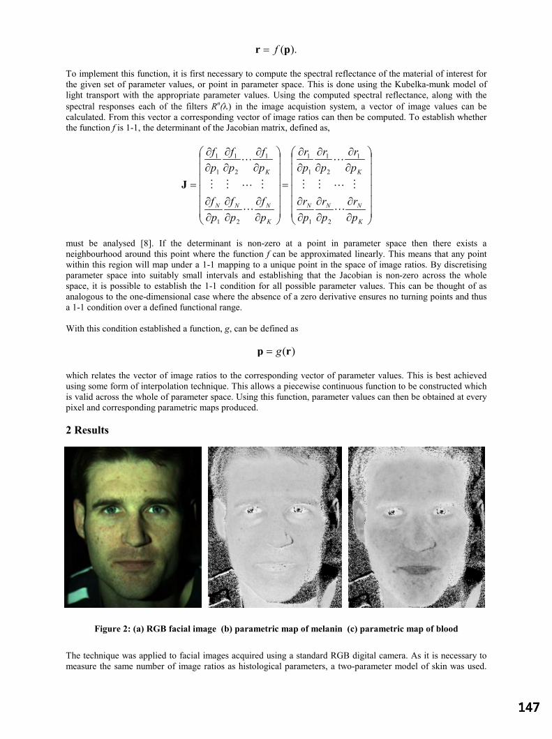
).(pr f=

To implement this function, it is first necessary to compute the spectral reflectance of the material of interest for the given set of parameter values, or point in parameter space. This is done using the Kubelka-munk model of light transport with the appropriate parameter values. Using the computed spectral reflectance, along with the spectral responses each of the filters Rn(λ) in the image acquistion system, a vector of image values can be calculated. From this vector a corresponding vector of image ratios can then be computed. To establish whether the function f is 1-1, the determinant of the Jacobian matrix, defined as,

∂∂

∂∂

∂∂

∂∂

∂∂

∂∂

=

∂∂

∂∂

∂∂

∂∂

∂∂

∂∂

=

K

NNN

K

K

NNN

K

pr

pr

pr

pr

pr

pr

pf

pf

pf

pf

pf

pf

L

MLMM

L

L

MLMM

L

21

1

2

1

1

1

21

1

2

1

1

1

J

must be analysed [8]. If the determinant is non-zero at a point in parameter space then there exists a neighbourhood around this point where the function f can be approximated linearly. This means that any point within this region will map under a 1-1 mapping to a unique point in the space of image ratios. By discretising parameter space into suitably small intervals and establishing that the Jacobian is non-zero across the whole space, it is possible to establish the 1-1 condition for all possible parameter values. This can be thought of as analogous to the one-dimensional case where the absence of a zero derivative ensures no turning points and thus a 1-1 condition over a defined functional range.

With this condition established a function, g, can be defined as

)(rp g=

which relates the vector of image ratios to the corresponding vector of parameter values. This is best achieved using some form of interpolation technique. This allows a piecewise continuous function to be constructed which is valid across the whole of parameter space. Using this function, parameter values can then be obtained at every pixel and corresponding parametric maps produced.

2 Results

Figure 2: (a) RGB facial image (b) parametric map of melanin (c) parametric map of blood

The technique was applied to facial images acquired using a standard RGB digital camera. As it is necessary to measure the same number of image ratios as histological parameters, a two-parameter model of skin was used.

The dermal thickness was measured using the system developed by Astron Clinica [9] and assumed to be constant across the face. This is thought to be a reasonable assumption as, although thickness varies between individuals, it is fairly constant for a relatively small area of an individual.

Using the responses of the imaging acquisition system along with the spectral characteristics of the illuminating light source, a 2-D vector of image ratios was computed for every point in a discretised parameter space. From a consideration of the determinant of the Jacobian, uniqueness was established. Using this discrete data was constructed using a triagle-based cubic interpolation method which was implemented in matlab. This function was used to process the image shown in figure 2a to produce the parametric maps of melanin and blood. These have been shown in figures 2b and 2c respectively.

The images show that the method is able to differentiate between melanin and blood born pigments. The melanin image demonstrates how moles are detected, there being two under the left eye which do not show in the blood parametric map. The images also demonstrate the uniform distribution of melanin across the face. This is in contrast to the uneven distribution of blood, which tends to have locally increased concentrations, for example in the lips and where spots are present.

3 Discussion

Preliminary results suggest that the technique described in this paper could enable parametric maps to be produced independently of curvature in an imaged scene. With an invariance to illumination intensity, it will not be necessary to accurately position the camera and illuminating light source before image acquisition. This will allow much wider application of the system developed by Cotton and Claridge [4,5].

Work is now underway to increase the number of histological parameters in the model to allow analysis of more complex skin lesions. This should enable the development of a system that can assist clinicians in the diagnosis of non-melanoma skin cancer, such as basal cell carcinoma that tends to occur on the face. It will also allow for the assessment of wounds where it is not possible to make contact with the imaged tissue, such as with diabetic foot ulcers.

It is envisaged that this methodology will be applicable to imaging other tissues. Two potential applications have so far been identified. These are imaging the ocular fundus [10,11] and the gastrointestinal tract. Success in both these applications requires a system which is able to recover histological data in a way which is invariant to surface geometry and illuminating light. Thus, the methodology presented in this article could prove key to their success.

References:

1. R. Anderson & J.A. Parish “The Optics of Human Skin”, Journal of Investigative Dermatology 77, pp 13-19, 1981.2. M. J. C. van Germert et al. “Skin Optics”, IEEE Transactions on Biomedical Imaging Engineering 36, pp 1146-1154,

1989.3. P. Kubelka & F. Munk “Ein Beitrag zur Optik der Farbanstriche”, Z. Tech. Opt. 11, pp 593-611.4. S. Cotton & E. Claridge. “Developing a Predictive Model of Human Skin Colouring.” In Proceedings of SPIE Medical

Imaging, vol. 2708, pp. 814-825, 1996.5. S. Cotton & E. Claridge. “Non-invasive Monitoring Skin Imaging.” In Proceedings Information Processing in Medical

Imaging, vol. 1230, pp 501-507, 1997.6. S.A. Shafer “Using Colour to Separate Reflection Components”, Color Research Application 10, pp 210-218, 1985.7. G. Healey “Using Colour for Geometry-Insensitive Segmentation”, Journal of the Optical Society of America 6, pp 920-

937, 1989.8. M. Lipschutz. Differential Geometry. McGraw-Hill Book Company, New York, 1989.9. M. Mondrieff et al. “Spectrophotometric intracutaneous analysis: a new technique for imaging pigmented skin lesions”,

British Journal of Dermatology 146, pp 448-457, 2002.10. S.J. Preece & E. Claridge “Monte Carlo Modelling of the Spectral Reflectance of the Human Eye.” Physics in Medicine

and Biology 47, pp 2863-2877, 2002.11. S.J. Preece & E. Claridge “Physics Based Medical Image Understanding of the Colouration of the Ocular Fundus with

Application to Detection of Diabetic Retinopathy.” In Proceedings of Medical Image Understanding and Analysis 2000, pp. 7-10, 2000.

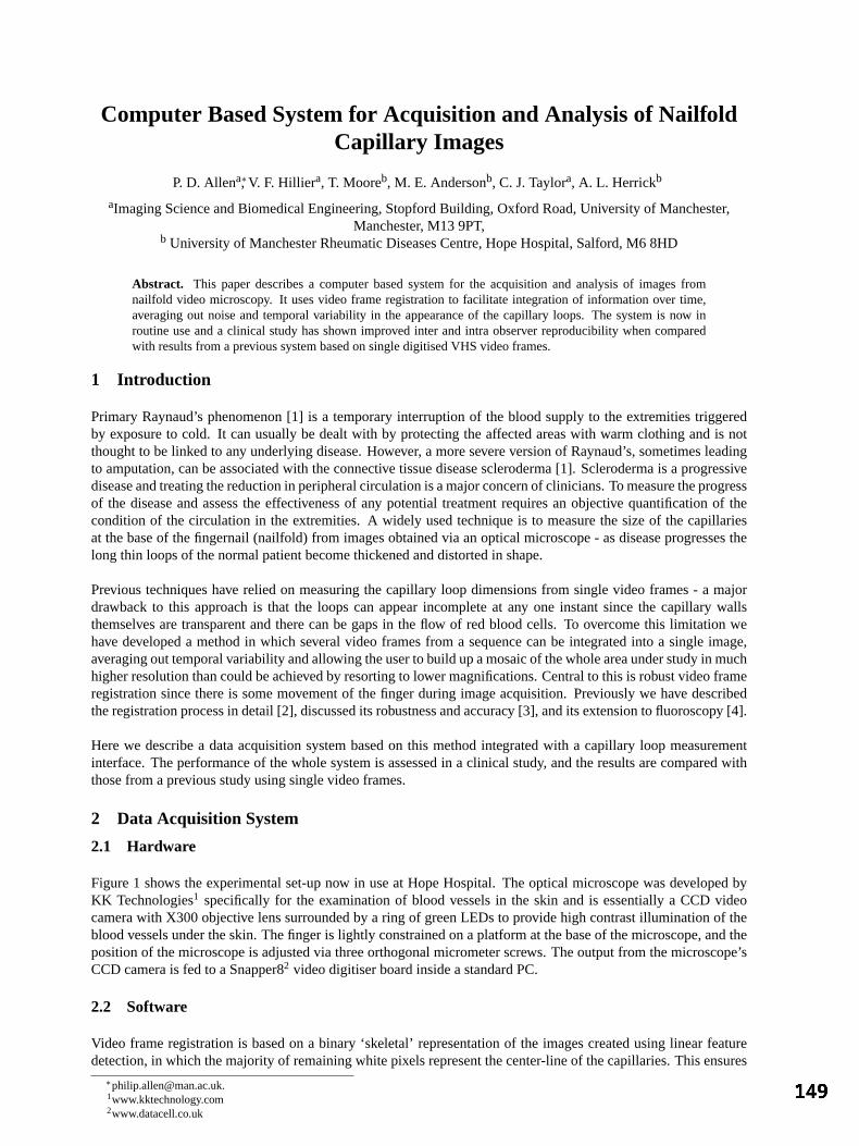
Computer Based System for Acquisition and Analysis of NailfoldCapillary Images

P. D. Allena∗, V. F. Hilliera, T. Mooreb, M. E. Andersonb, C. J. Taylora, A. L. Herrickb

aImaging Science and Biomedical Engineering, Stopford Building, Oxford Road, University of Manchester,Manchester, M13 9PT,

b University of Manchester Rheumatic Diseases Centre, Hope Hospital, Salford, M6 8HD

Abstract. This paper describes a computer based system for the acquisition and analysis of images fromnailfold video microscopy. It uses video frame registration to facilitate integration of information over time,averaging out noise and temporal variability in the appearance of the capillary loops. The system is now inroutine use and a clinical study has shown improved inter and intra observer reproducibility when comparedwith results from a previous system based on single digitised VHS video frames.

1 Introduction

Primary Raynaud’s phenomenon [1] is a temporary interruption of the blood supply to the extremities triggeredby exposure to cold. It can usually be dealt with by protecting the affected areas with warm clothing and is notthought to be linked to any underlying disease. However, a more severe version of Raynaud’s, sometimes leadingto amputation, can be associated with the connective tissue disease scleroderma [1]. Scleroderma is a progressivedisease and treating the reduction in peripheral circulation is a major concern of clinicians. To measure the progressof the disease and assess the effectiveness of any potential treatment requires an objective quantification of thecondition of the circulation in the extremities. A widely used technique is to measure the size of the capillariesat the base of the fingernail (nailfold) from images obtained via an optical microscope - as disease progresses thelong thin loops of the normal patient become thickened and distorted in shape.

Previous techniques have relied on measuring the capillary loop dimensions from single video frames - a majordrawback to this approach is that the loops can appear incomplete at any one instant since the capillary wallsthemselves are transparent and there can be gaps in the flow of red blood cells. To overcome this limitation wehave developed a method in which several video frames from a sequence can be integrated into a single image,averaging out temporal variability and allowing the user to build up a mosaic of the whole area under study in muchhigher resolution than could be achieved by resorting to lower magnifications. Central to this is robust video frameregistration since there is some movement of the finger during image acquisition. Previously we have describedthe registration process in detail [2], discussed its robustness and accuracy [3], and its extension to fluoroscopy [4].

Here we describe a data acquisition system based on this method integrated with a capillary loop measurementinterface. The performance of the whole system is assessed in a clinical study, and the results are compared withthose from a previous study using single video frames.

2 Data Acquisition System

2.1 Hardware

Figure 1 shows the experimental set-up now in use at Hope Hospital. The optical microscope was developed byKK Technologies1 specifically for the examination of blood vessels in the skin and is essentially a CCD videocamera with X300 objective lens surrounded by a ring of green LEDs to provide high contrast illumination of theblood vessels under the skin. The finger is lightly constrained on a platform at the base of the microscope, and theposition of the microscope is adjusted via three orthogonal micrometer screws. The output from the microscope’sCCD camera is fed to a Snapper82 video digitiser board inside a standard PC.

2.2 Software

Video frame registration is based on a binary ‘skeletal’ representation of the images created using linear featuredetection, in which the majority of remaining white pixels represent the center-line of the capillaries. This ensures

∗[email protected]

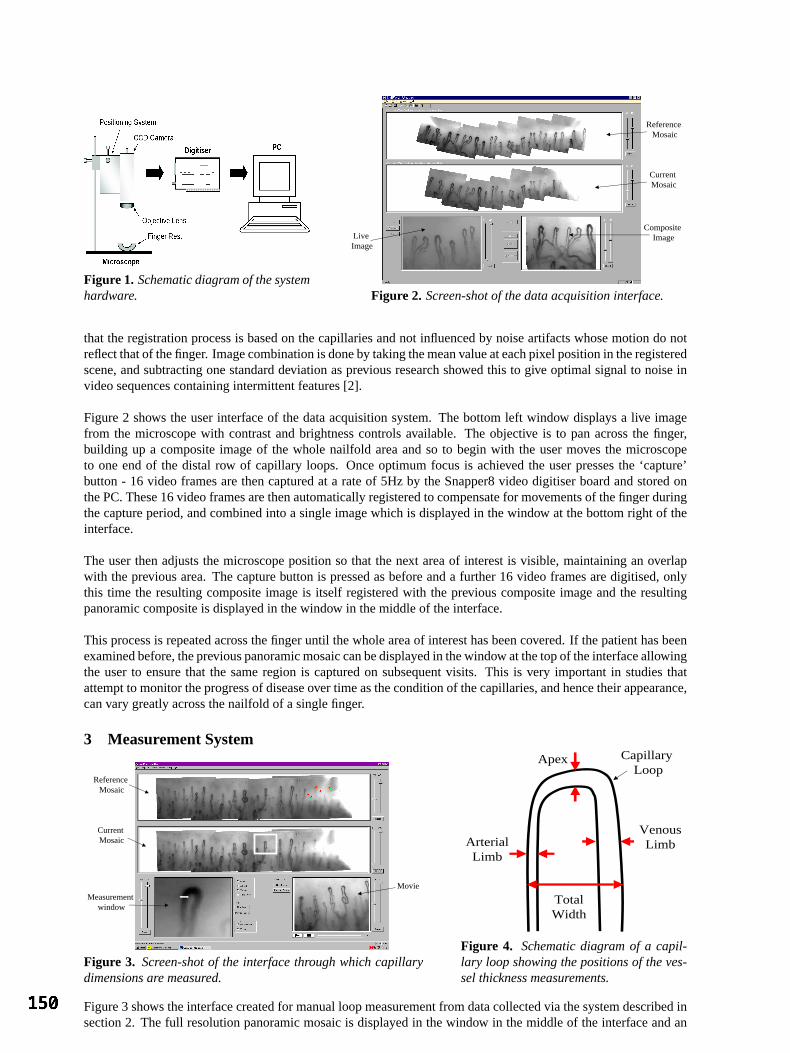
Figure 1. Schematic diagram of the systemhardware.

Live Image

Composite Image

Current Mosaic

Reference Mosaic

Figure 2. Screen-shot of the data acquisition interface.

that the registration process is based on the capillaries and not influenced by noise artifacts whose motion do notreflect that of the finger. Image combination is done by taking the mean value at each pixel position in the registeredscene, and subtracting one standard deviation as previous research showed this to give optimal signal to noise invideo sequences containing intermittent features [2].

Figure 2 shows the user interface of the data acquisition system. The bottom left window displays a live imagefrom the microscope with contrast and brightness controls available. The objective is to pan across the finger,building up a composite image of the whole nailfold area and so to begin with the user moves the microscopeto one end of the distal row of capillary loops. Once optimum focus is achieved the user presses the ‘capture’button - 16 video frames are then captured at a rate of 5Hz by the Snapper8 video digitiser board and stored onthe PC. These 16 video frames are then automatically registered to compensate for movements of the finger duringthe capture period, and combined into a single image which is displayed in the window at the bottom right of theinterface.

The user then adjusts the microscope position so that the next area of interest is visible, maintaining an overlapwith the previous area. The capture button is pressed as before and a further 16 video frames are digitised, onlythis time the resulting composite image is itself registered with the previous composite image and the resultingpanoramic composite is displayed in the window in the middle of the interface.

This process is repeated across the finger until the whole area of interest has been covered. If the patient has beenexamined before, the previous panoramic mosaic can be displayed in the window at the top of the interface allowingthe user to ensure that the same region is captured on subsequent visits. This is very important in studies thatattempt to monitor the progress of disease over time as the condition of the capillaries, and hence their appearance,can vary greatly across the nailfold of a single finger.

3 Measurement System

Measurement window

Current Mosaic

Reference Mosaic

Movie

Figure 3. Screen-shot of the interface through which capillarydimensions are measured.

Apex

VenousLimbArterial

Limb

TotalWidth

Capillary Loop

Figure 4. Schematic diagram of a capil-lary loop showing the positions of the ves-sel thickness measurements.

Figure 3 shows the interface created for manual loop measurement from data collected via the system described insection 2. The full resolution panoramic mosaic is displayed in the window in the middle of the interface and an

enlarged view of a portion of this mosaic is displayed in the window on the bottom left of the interface. This is thewindow in which the user makes the measurements and the region which it displays can be chosen by clicking onthe current mosaic window above.

Figure 4 shows the capillary dimensions measured in previous studies [5] and also adopted in this system. The userselects the appropriate dimension from a set of radio buttons and then, using the mouse, clicks either side of thecapillary at the desired points - the left button beginning the measurement, and the right button closing it. A lineis drawn between the two points, using a different colour for each of the dimensions. To distinguish which sideof the loop is arterial and which is venous, the user must be able to see which way the blood was flowing throughthe loop and so the original 16 frames that made up the scene containing that particular loop are played back in amovie sequence in the window at the bottom right of the interface. This movie view is also zoomable since it isnecessary to be able to see the individual blood cells. If data from a previous visit is available it can be displayedat the top of the interface with the previous measurements superimposed on the mosaic image, so that the samecapillaries can be measured at the same measurement points.

4 Clinical Study

To asses the above system as a practical clinical tool a study was carried out to quantify the inter and intra observerreliability and explore any possible relationship between the size of the capillaries and disease group. A patientgroup consisting of 48 healthy controls, 21 Primary Raynaud’s (PRP), 40 Limited scleroderma (LSSc - skin diseaserestricted to extremities) and 11 Diffuse scleroderma (DSSc - skin disease affecting proximal limbs and/or trunk)were examined using the method described above. An observer reproducibility study was performed on a sub-setof the data containing 10 controls, 10 Primary Raynaud’s, and 10 SSc. For each patient, five capillary loops weremeasured from the ring finger of the non dominant hand and the mean across the five loops was taken for each ofthe four dimensions measured (figure 4).

For both inter and intra observer reliability, two studies were made - a ‘blind’ study in which the observer hadno access to the previous measurements so that neither the same capillaries nor the same measurement positionscould be guaranteed, and a second in which the observercould see the previous mosaic with the measurementpoints visible.

These results were compared with those of a study by Bukhari et al [5] using a previous video capillaroscopy systemat Hope Hospital. In this system a video microscope was connected to a VHS video recorder and measurementswere made from single video frames digitised from the video tape. This did not allow any reference to previousmeasurement positions to be made during the data acquisition or measurement phases. Bukhari’s study was similarin its patient group to ours but used the mean of all the visible capillaries in a 3mm length of the distal row, whichtranslates to roughly 15 loops for controls and about 10 for scleroderma.

For all inter/intra-observer studies the bias and limits of agreement [6] were calculated and all dimensions werelog transformed to achieve normality in both studies.

4.1 Observer Reproducibility

Apex Arterial Venous Total−60

−40

−20

0

20

40

60

80

Bias

with

limits

of a

gree

men

t (%

)

Figure 5. Bias and limits of agreement for theinter-observer study. Current study - circles, cur-rent study ‘blind’ - triangles, Bukhari - squares.

Apex Arterial Venous Total

−40

−30

−20

−10

0

10

20

30

40

50

Bias

with

limits

of a

gree

men

t (%

)

Figure 6. Bias and limits of agreement for theintra-observer study. Current study - circles, cur-rent study ‘blind’ - triangles, Bukhari - squares.

Figure 5 shows the results of the inter observer study and figure 6 shows the results of the intra observer studyfor both this and previous work. For our ‘non-blind’ intra observer test there was a relationship between observer

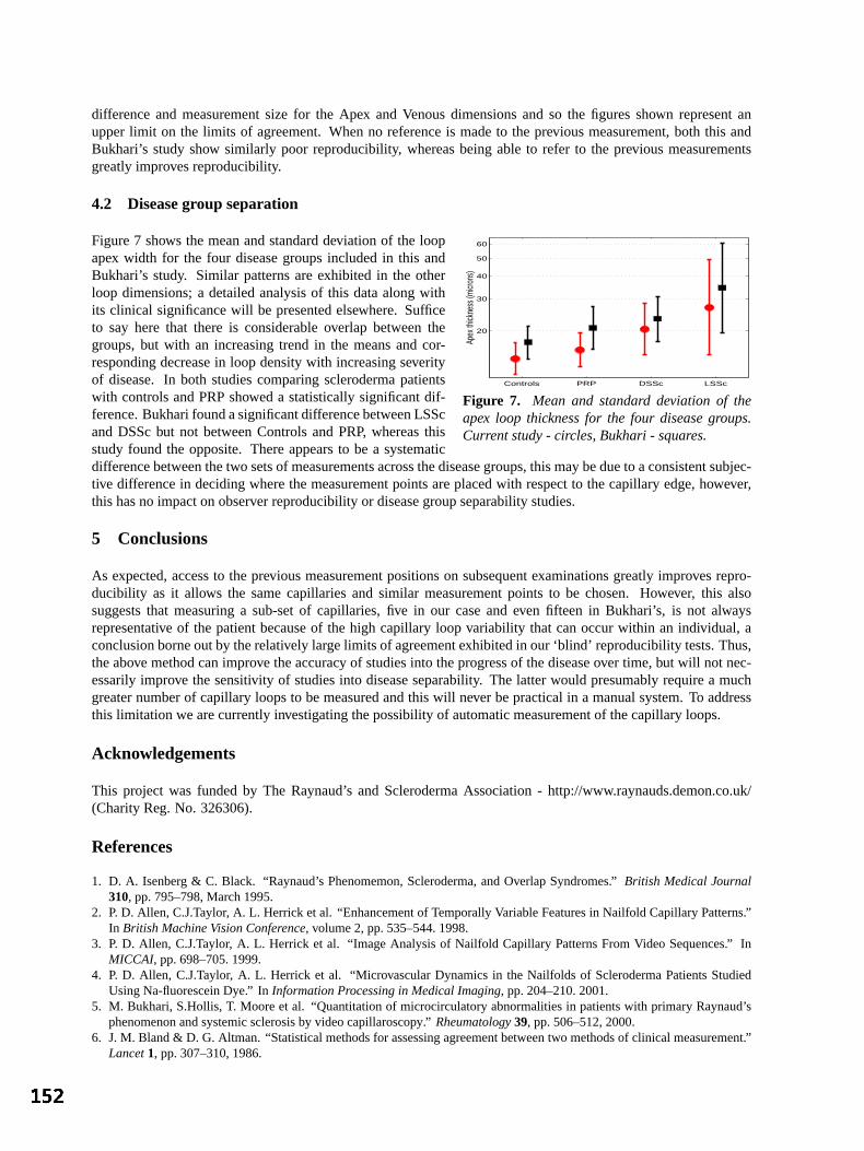
difference and measurement size for the Apex and Venous dimensions and so the figures shown represent anupper limit on the limits of agreement. When no reference is made to the previous measurement, both this andBukhari’s study show similarly poor reproducibility, whereas being able to refer to the previous measurementsgreatly improves reproducibility.

4.2 Disease group separation

Figure 7 shows the mean and standard deviation of the loop

Controls PRP DSSc LSSc

20

30

40

50

60

Apex

thick

ness

(micr

ons)

Figure 7. Mean and standard deviation of theapex loop thickness for the four disease groups.Current study - circles, Bukhari - squares.

apex width for the four disease groups included in this andBukhari’s study. Similar patterns are exhibited in the otherloop dimensions; a detailed analysis of this data along withits clinical significance will be presented elsewhere. Sufficeto say here that there is considerable overlap between thegroups, but with an increasing trend in the means and cor-responding decrease in loop density with increasing severityof disease. In both studies comparing scleroderma patientswith controls and PRP showed a statistically significant dif-ference. Bukhari found a significant difference between LSScand DSSc but not between Controls and PRP, whereas thisstudy found the opposite. There appears to be a systematicdifference between the two sets of measurements across the disease groups, this may be due to a consistent subjec-tive difference in deciding where the measurement points are placed with respect to the capillary edge, however,this has no impact on observer reproducibility or disease group separability studies.

5 Conclusions

As expected, access to the previous measurement positions on subsequent examinations greatly improves repro-ducibility as it allows the same capillaries and similar measurement points to be chosen. However, this alsosuggests that measuring a sub-set of capillaries, five in our case and even fifteen in Bukhari’s, is not alwaysrepresentative of the patient because of the high capillary loop variability that can occur within an individual, aconclusion borne out by the relatively large limits of agreement exhibited in our ‘blind’ reproducibility tests. Thus,the above method can improve the accuracy of studies into the progress of the disease over time, but will not nec-essarily improve the sensitivity of studies into disease separability. The latter would presumably require a muchgreater number of capillary loops to be measured and this will never be practical in a manual system. To addressthis limitation we are currently investigating the possibility of automatic measurement of the capillary loops.

Acknowledgements

This project was funded by The Raynaud’s and Scleroderma Association - http://www.raynauds.demon.co.uk/(Charity Reg. No. 326306).

References

1. D. A. Isenberg & C. Black. “Raynaud’s Phenomemon, Scleroderma, and Overlap Syndromes.”British Medical Journal310, pp. 795–798, March 1995.

2. P. D. Allen, C.J.Taylor, A. L. Herrick et al. “Enhancement of Temporally Variable Features in Nailfold Capillary Patterns.”In British Machine Vision Conference, volume 2, pp. 535–544. 1998.

3. P. D. Allen, C.J.Taylor, A. L. Herrick et al. “Image Analysis of Nailfold Capillary Patterns From Video Sequences.” InMICCAI, pp. 698–705. 1999.

4. P. D. Allen, C.J.Taylor, A. L. Herrick et al. “Microvascular Dynamics in the Nailfolds of Scleroderma Patients StudiedUsing Na-fluorescein Dye.” InInformation Processing in Medical Imaging, pp. 204–210. 2001.

5. M. Bukhari, S.Hollis, T. Moore et al. “Quantitation of microcirculatory abnormalities in patients with primary Raynaud’sphenomenon and systemic sclerosis by video capillaroscopy.”Rheumatology39, pp. 506–512, 2000.

6. J. M. Bland & D. G. Altman. “Statistical methods for assessing agreement between two methods of clinical measurement.”Lancet1, pp. 307–310, 1986.

Department of Computing, Imperial College, 180 Queen’s Gate, SW7 2BZ, London, UK Email: me, ajchung, [email protected]

A Novel Method for Simulating Soft Tissue Deformation

Mohamed A. ElHelw, Adrian Chung and Guang-Zhong Yang

Department of Computing, Imperial College, London

Abstract. This paper describes a novel method for simulating soft tissue deformation with image-based rendering. It is based on the association of depth map with colour texture and the incorporation of micro-surface details to generate photo-realistic images representing soft tissue deformations. In a pre-processing step, the depth map describing the surface is separated into two distributions corresponding to macro- and micro-surface details. During user interactive simulation, deformation resulting from tissue-instrument interaction is rapidly calculated by modifying a coarse mass-spring model fitted to the macro-surface model. Micro-surface details are subsequently augmented to the modified model with 3D image warping. The proposed technique drastically reduces the polygonal count required to model the scene, whilst preserving deformed small surface details and offering a high level of photorealism.

1 Introduction Over the last ten years there has been a strong movement towards improved techniques of minimal access

surgery. Endoscopy, including bronchoscopy and laparoscopy is the most common procedure in minimal access surgery, which is carried out through natural body openings or small artificial incisions. If handled properly, endoscopes are completely harmless to patients. Diagnostic endoscopy can achieve its clinical goals with minimal inconvenience to patients. Compared with conventional techniques, patient trauma and hospitalisation can be greatly reduced and diagnostic accuracy and therapeutic success increased. However, the complexity of instrument controls, restricted vision and mobility, difficult hand-eye co-ordination and the lack of tactile perception require a high degree of manual dexterity of the operator. Consequently much attention has been paid to new training methods for these skills. Computer simulation provides an attractive possibility for certain aspects of this training, particularly for hand eye co-ordination. The benefits of endoscopic training through computer simulation, rather than the traditionally performed one-to-one apprenticeship schemes, are now well accepted in the medical community. It has been proven to be an economical and time saving solution for acquiring, as well as assessing basic surgical skills.

Hitherto, a significant amount of research has been carried out in the area of minimal access surgical simulators. One of the major challenges of these systems is the creation of photo-realistic rendering. Due to the complexity of geometry used to represent internal body organs and the fact that they are all non-rigid, the realism of deformations is one of the key issues of surgery simulation [6]. In this paper we present a novel technique for soft tissue modelling which offers both visual realism and realistic interactive tissue deformations. This is accomplished by combining the promise of photo-realism set by image-based rendering with the simplicity of mass-spring tissue deformation modelling. 1.1 Image-Based Rendering

Image-based rendering (IBR) has established itself as a powerful alternative to conventional geometry-based computer graphics. A set of images or depth-enhanced images is used to synthesise novel views of either synthetic or real environments. The simplest form of IBR method is texture mapping [5], which was the first technique to represent complex materials that are hard to model and render. A major limitation of texture mapping is that texture mapped surfaces still appear as 2-D images painted onto flat polygons. They lack 3D details and don’t exhibit appropriate parallax as the viewpoint changes. To address these problems, several extensions have been proposed. Blinn [2] developed a bump mapping technique that enables the surface to appear dimpled by applying perturbations to surface normals. The results, however, are not always convincing especially when viewed from certain positions, as silhouette edges can appear to pass through depressions [13]. Other methods such as height fields and displacement maps have proven to be either difficult to calculate or computationally prohibitive. Better illusion of depth can be achieved at interactive frame rates by using image-based rendering methods, in which the colour texture image is associated with a depth map used in the image generation process. This is referred to as Image-Based Rendering by Warping (IBRW) [12]. The depth map is used with the texture image to model surface details. At run-time, the depth information at each image point is projected onto the viewing manifold to achieve realistic rendering. 1.2 Soft Tissue Modelling

Deformable tissues can be geometrically represented as a set of surfaces or volumes. The choice of representation is dependent on two factors: computational efficiency and physical accuracy [7]. Surface models

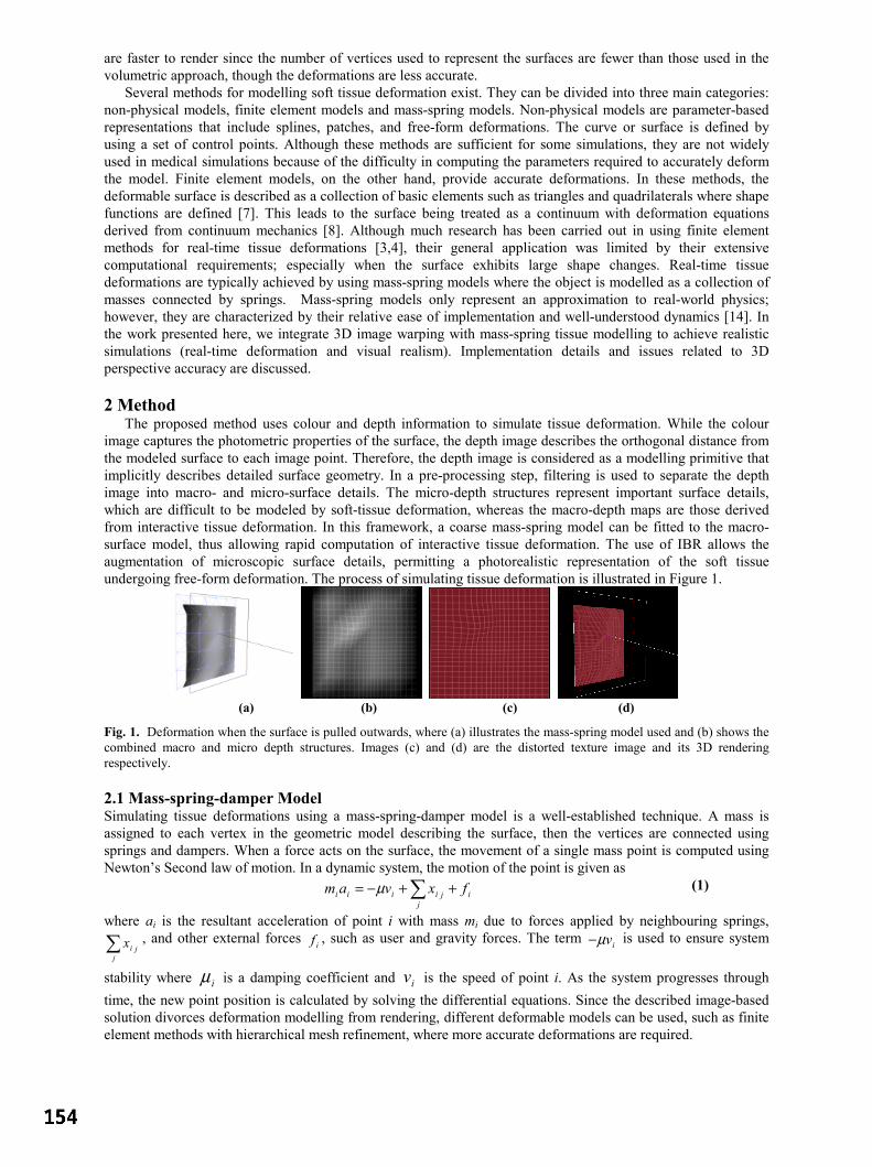
are faster to render since the number of vertices used to represent the surfaces are fewer than those used in the volumetric approach, though the deformations are less accurate.

Several methods for modelling soft tissue deformation exist. They can be divided into three main categories: non-physical models, finite element models and mass-spring models. Non-physical models are parameter-based representations that include splines, patches, and free-form deformations. The curve or surface is defined by using a set of control points. Although these methods are sufficient for some simulations, they are not widely used in medical simulations because of the difficulty in computing the parameters required to accurately deform the model. Finite element models, on the other hand, provide accurate deformations. In these methods, the deformable surface is described as a collection of basic elements such as triangles and quadrilaterals where shape functions are defined [7]. This leads to the surface being treated as a continuum with deformation equations derived from continuum mechanics [8]. Although much research has been carried out in using finite element methods for real-time tissue deformations [3,4], their general application was limited by their extensive computational requirements; especially when the surface exhibits large shape changes. Real-time tissue deformations are typically achieved by using mass-spring models where the object is modelled as a collection of masses connected by springs. Mass-spring models only represent an approximation to real-world physics; however, they are characterized by their relative ease of implementation and well-understood dynamics [14]. In the work presented here, we integrate 3D image warping with mass-spring tissue modelling to achieve realistic simulations (real-time deformation and visual realism). Implementation details and issues related to 3D perspective accuracy are discussed. 2 Method

The proposed method uses colour and depth information to simulate tissue deformation. While the colour image captures the photometric properties of the surface, the depth image describes the orthogonal distance from the modeled surface to each image point. Therefore, the depth image is considered as a modelling primitive that implicitly describes detailed surface geometry. In a pre-processing step, filtering is used to separate the depth image into macro- and micro-surface details. The micro-depth structures represent important surface details, which are difficult to be modeled by soft-tissue deformation, whereas the macro-depth maps are those derived from interactive tissue deformation. In this framework, a coarse mass-spring model can be fitted to the macro-surface model, thus allowing rapid computation of interactive tissue deformation. The use of IBR allows the augmentation of microscopic surface details, permitting a photorealistic representation of the soft tissue undergoing free-form deformation. The process of simulating tissue deformation is illustrated in Figure 1.

(a) (b) (c) (d)

Fig. 1. Deformation when the surface is pulled outwards, where (a) illustrates the mass-spring model used and (b) shows the combined macro and micro depth structures. Images (c) and (d) are the distorted texture image and its 3D rendering respectively.

2.1 Mass-spring-damper Model Simulating tissue deformations using a mass-spring-damper model is a well-established technique. A mass is assigned to each vertex in the geometric model describing the surface, then the vertices are connected using springs and dampers. When a force acts on the surface, the movement of a single mass point is computed using Newton’s Second law of motion. In a dynamic system, the motion of the point is given as

∑ ++−=j

ijiiii fxvam µ (1)

where ai is the resultant acceleration of point i with mass mi due to forces applied by neighbouring springs,

∑j

jix , and other external forces if , such as user and gravity forces. The term ivµ− is used to ensure system

stability where iµ is a damping coefficient and iv is the speed of point i. As the system progresses through time, the new point position is calculated by solving the differential equations. Since the described image-based solution divorces deformation modelling from rendering, different deformable models can be used, such as finite element methods with hierarchical mesh refinement, where more accurate deformations are required.

2.2 3D Image Warping By using the plenoptic function approximation [1], which describes everything visible from a given point in

space, we define the mappings from one image to another as image warps [9]. 3D image warping is a geometric operation where visible reference image points with depth are mapped onto a target image. Along with the reference camera model, the depth values provide a representation of the structure of the scene. A 3D point X seen through two different image planes as shown in Figure 2a, can be defined by using Equation 2.

22221111 xMtCxMtCX +=+= (2) 111

2211

212 )()( xMMCCMxx −− +−= δ (3)

where, 1C and 2C are centres of projection of the reference and target cameras, M1 and M2 define the reference and target camera models, x1=(u1,v1) and x2 =(u2,v2) are reference and target camera image plane points and t1 and t2 are reference and target camera constant scaling factors, all respectively. By expanding and rearranging terms of Equation 2, the 3D image warping Equation 3 can be derived[9], where )( 1xδ is the depth at reference image point x1. A new image can therefore be rendered from a nearby target viewpoint by projecting the reference image pixels to their 3D positions and then re-projecting them onto the target image plane.

(a) (b)

Figure 2. (a) A 3D point X can be defined by using the camera centre-of projection Ci, image plane point xi and scalar value ti along the ray di form Ci through xi for both reference and target cameras, where i=1 and 2 respectively (b) If the reference and target camera image planes coincide, 3D image warping equation simplifies to relief texture mapping equations.

Having the reference image represented with a parallel projection camera model and by making both reference and target image planes coincide, as illustrated in Figure 2b, the warping equation simplifies to the relief texture mapping equations [10],

),().().(),().().(

11

1112 vudisplbafbac

vudisplcbfucbau

×+××+×

= (4) ),().().(

),().().(

11

1112 vudisplbafbac

vudisplacfvacbv

×+×

×+×= (5)

where a and b

are the reference camera image plane basis vectors in Euclidean space, c is the vector from target viewpoint to the origin of the reference image plane, f

is the vector perpendicular to the reference image plane, disp(u1,v1) is the depth at reference image plane point (u1,v1), and (u2,v2) is the target image plane point. Relief texturing is used in the presented image-based approach to render deformed surface. The relief texture mapping process is carried out in two steps [11]: first, an intermediate image is generated by warping the source image to a viewing plane that has exactly the same position, dimensions and orientation as the destination polygon, then the intermediate image is texture mapped onto the destination polygon using texture mapping hardware.

3 Results To demonstrate the visual realism achieved by using the described technique, two deformable tissue simulation experiments have been implemented. The first system employs conventional geometry-based tissue deformation with a mass-spring model, while the second uses the described image-based soft method. Two views from both systems are shown in Figure 3, from which it is evident that the proposed method provides enhanced visual realism and improved image quality over conventional methods. It can be seen that when the tissue is deformed, the 3D structure of micro-surface elements is still preserved resulting in rich surface details (Figures 3a and 3c). Moreover, the texture pixelisation problem is minimised because the texture image is dynamically generated for each frame. This becomes noticeable when the surface is viewed at sharp angles or from near viewpoints. The accuracy of the proposed method is established through error analysis by comparing it to the conventional polygon-based method.

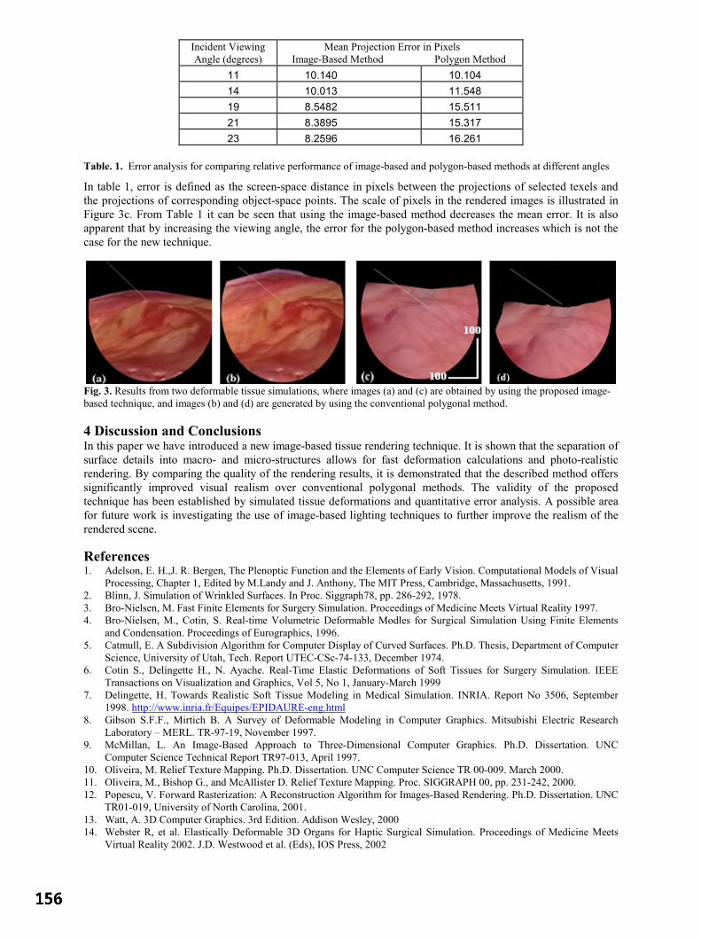
Incident Viewing Angle (degrees)

Mean Projection Error in Pixels Image-Based Method Polygon Method

11 10.140 10.104 14 10.013 11.548 19 8.5482 15.511 21 8.3895 15.317 23 8.2596 16.261

Table. 1. Error analysis for comparing relative performance of image-based and polygon-based methods at different angles

In table 1, error is defined as the screen-space distance in pixels between the projections of selected texels and the projections of corresponding object-space points. The scale of pixels in the rendered images is illustrated in Figure 3c. From Table 1 it can be seen that using the image-based method decreases the mean error. It is also apparent that by increasing the viewing angle, the error for the polygon-based method increases which is not the case for the new technique.

Fig. 3. Results from two deformable tissue simulations, where images (a) and (c) are obtained by using the proposed image-based technique, and images (b) and (d) are generated by using the conventional polygonal method. 4 Discussion and Conclusions In this paper we have introduced a new image-based tissue rendering technique. It is shown that the separation of surface details into macro- and micro-structures allows for fast deformation calculations and photo-realistic rendering. By comparing the quality of the rendering results, it is demonstrated that the described method offers significantly improved visual realism over conventional polygonal methods. The validity of the proposed technique has been established by simulated tissue deformations and quantitative error analysis. A possible area for future work is investigating the use of image-based lighting techniques to further improve the realism of the rendered scene.

References 1. Adelson, E. H.,J. R. Bergen, The Plenoptic Function and the Elements of Early Vision. Computational Models of Visual

Processing, Chapter 1, Edited by M.Landy and J. Anthony, The MIT Press, Cambridge, Massachusetts, 1991. 2. Blinn, J. Simulation of Wrinkled Surfaces. In Proc. Siggraph78, pp. 286-292, 1978. 3. Bro-Nielsen, M. Fast Finite Elements for Surgery Simulation. Proceedings of Medicine Meets Virtual Reality 1997. 4. Bro-Nielsen, M., Cotin, S. Real-time Volumetric Deformable Modles for Surgical Simulation Using Finite Elements

and Condensation. Proceedings of Eurographics, 1996. 5. Catmull, E. A Subdivision Algorithm for Computer Display of Curved Surfaces. Ph.D. Thesis, Department of Computer

Science, University of Utah, Tech. Report UTEC-CSc-74-133, December 1974. 6. Cotin S., Delingette H., N. Ayache. Real-Time Elastic Deformations of Soft Tissues for Surgery Simulation. IEEE

Transactions on Visualization and Graphics, Vol 5, No 1, January-March 1999 7. Delingette, H. Towards Realistic Soft Tissue Modeling in Medical Simulation. INRIA. Report No 3506, September

1998. http://www.inria.fr/Equipes/EPIDAURE-eng.html 8. Gibson S.F.F., Mirtich B. A Survey of Deformable Modeling in Computer Graphics. Mitsubishi Electric Research

Laboratory – MERL. TR-97-19, November 1997. 9. McMillan, L. An Image-Based Approach to Three-Dimensional Computer Graphics. Ph.D. Dissertation. UNC

Computer Science Technical Report TR97-013, April 1997. 10. Oliveira, M. Relief Texture Mapping. Ph.D. Dissertation. UNC Computer Science TR 00-009. March 2000. 11. Oliveira, M., Bishop G., and McAllister D. Relief Texture Mapping. Proc. SIGGRAPH 00, pp. 231-242, 2000. 12. Popescu, V. Forward Rasterization: A Reconstruction Algorithm for Images-Based Rendering. Ph.D. Dissertation. UNC

TR01-019, University of North Carolina, 2001. 13. Watt, A. 3D Computer Graphics. 3rd Edition. Addison Wesley, 2000 14. Webster R, et al. Elastically Deformable 3D Organs for Haptic Surgical Simulation. Proceedings of Medicine Meets

Virtual Reality 2002. J.D. Westwood et al. (Eds), IOS Press, 2002

Using autostereoscopic displays as a complementary visual aid tothe surgical stereo microscope in Augmented Reality surgery

R.J. Lapeer, A.C. Tan, G. Alusi and A. Linney

School of Computing Sciences, University of East Anglia, NorwichDept. of Medical Physics and Bioengineering - University College London

St.Bartholomews Hospital London.

Abstract. In the context of our research on Augmented Reality based surgical navigation for stereoscopicmicroscope based ENT surgery, we aim to use autostereoscopic displays as a complementary visual aid. Weperformed an experiment to evaluate the depth perception capabilities from four stereoscopic visual aids: thesurgical microsope, the SHARP twin LCD autostereoscopic display, the DTI Virtual Window 2015XLS flatpanel autostereoscopic display and the naked eye. Five expert and five non-expert subjects performed an unbi-ased depth test to assess the autostereoscopic displays using the naked eye and microscope as the gold standard.The SHARP display was considered to allow sufficient lateral and longitudinal freedom whilst providing ac-curate stereo vision. The DTI display, though much lighter and easy to manipulate than the SHARP, did showpromising results, eventhough not all subjects were at ease with the overall display quality and correspondingstereoscopic quality.

1 Introduction

There are three realistic and feasible solutions to augment images captured from a surgical microscope with vir-tual images. The first approach is to inject the virtual images (after registration) in the microscope’s optics. Thisapproach was successfully implemented by Edwards et al [4]. An alternative solution is to use a head-mounteddisplay (HMD) based (lightweight) microscope. This approach was pioneered by Birkfellner and Figl et al [5] andshows great promise. Finally, the third approach is the one we suggest, by using an autostereoscopic display inconjunction with the microscope. We explain shortly why we opt for this particular solution.The stereoscopic surgical microscope is used for a variety of ENT procedures. Though, an invaluable tool for suchinterventions, it has a number of drawbacks when used for long periods. Typically, surgeons suffer from eye strainand back and cervical spine complaints because of the bent-over position. Although a visualisation aid such as amicroscope, which captures and magnifies an area of interest of the surgical scene is always needed, excessive usecan be avoided if an alternative, complementary device such as an autostereoscopic display is present. Autostereo-scopic displays have been successfully evolved in the last couple of years and more recently, flat panel versionshave been commercialised.Although an autostereoscopic display could be used for any surgical intervention requiring the microscope, theyhave also specific advantages for augmented reality based surgical navigation. The stereo pair of images, capturedby a pair of CCD cameras mounted on the microscope (Figure 2(c)), can be converted from RGB to digital formatand overlaid with virtual images. The digital video format then allows the blending of both virtual and real images.This also avoids auxilliary hardware adaptations typically needed for alternative augmentation approaches such asinjecting the virtual images into the microscope optics [4] or the use of head-mounted microscopes [5].Despite this advantage, the ultimate question remains whether autosteoroscopic displays provide sufficient qualityin stereoscopic vision? To answer this question, we designed a depth experiment to assess two autostereoscopicdisplays, the SHARP micro-twin LCD display and the DTI Virtual Window 2015XLS flat panel display. Fiveexperts in using the surgical stereo microscope and five non-experts were tested. The surgical microscope and the‘naked’ eye were used as the gold standard (the former in particular for the experts).The next section discusses in brief the technology of autostereoscopic displays, the experimental setup and proto-col. The sections thereafter report the experimental results followed by a discussion and conclusion.

2 Autostereoscopic displays

Stereoscopic displays, requiring the user to wear special glasses, have been in use for several years. However,many of these systems suffer from uncomfortable eye-wear, control wires, cross-talk levels up to 10% and otherimage degrading effects such as image flicker and reduced image brightness [6]. Autostereoscopic displays requireno viewing aids and are thus more comfortable to use. They do suffer from limited viewing freedom as compared

Contact: Dr. Rudy Lapeer - [email protected]

Autostereoscopic display SHARP micro-optic twin DTI Virtual Window 2015XLSLCD panels 2 SHARP TFT LCD 1 Active Matrix TFT LCDSize 10.4inch 15.0inchPixel pitch 0.33mm0.33mm 0.297mm0.297mmResolution 640480 1024(512)768Longitudinal viewing freedom 550-990mm 609-813mmLateral viewing freedeom 480mm 150mm

Table 1. Technical specifications of the SHARP micro-optic twin LCD display and the DTI 2015XLS flat paneldisplay.

to shutter-based systems, a disadvantage we will cover later on. Their principle of operation is based on opticaloutput producing two ‘windows’ separated by a plane, which allow the left and right eye to see a different image(Figure 1(a)). Besides the restricted lateral viewing freedom, there is a restriction in the longitudinal direction aswell (Figure 1(b)).The SHARP micro-optic twin display (Figure 2(a)) has two LCD displays of which a stereo pair of images isgenerated using two mirrors, a beam splitter and a beam combiner (see Figure 1(c)). As there is a display for eachimage, full resolution is guaranteed though the complex optic system results in the SHARP being relatively heavy(around 20kg) and large, especially in the depth dimension.The DTI Virtual Window 2015XLS display (Figure 2(b)) is a flat panel display and therefore much lighter andsmaller than the SHARP. Though, it only contains one LCD display and therefore the horizontal resolution ishalved. Figure 1(d) shows the principle of creating two windows by using a mask which selects alternate pixelcolumns for left and right images respectively.Table 1 shows the specifications of the two displays.

3 Experimental results

The experiment aims to test depth perception (along the z-axis). Therefore any assessment based on planar (x-y)evaluation needs to be eliminated. The test should also be solely based on visual feedback (i.e. no force or touch-based feedback). The use of other visual cues such as focus should be eliminated as well.Two Allen keys, one of which fixed, the other one movable, were used to perform level-matching in the z-directionsolely based on vision. The movable key was fixed into a three translational degree of freedom micrometer device.The keys were relatively rotated so that the flat part of the movable key was opposite the sharp edge of the fixedkey. This was to avoid matching using x-y correspondence or focus (see Figure 2(d)).Before the experiments, the keys were level-matched by an operator using a dial indicator. The operator thenchecked the position of the z-slide of the micrometer. He/she then placed the movable key up or down and thesubject had to level-match the keys using stereo vision only. The subject first ‘guesses’ the position of the movablekey, i.e. whether it is above or below the fixed key. Any mistake in this initial ‘guess’ would indicate that either theexperimental setup/condition for this particular visual aid had been corrupted or that the subject may not correctlyinterpret the image. If this condition was controlled the experiment could carry on. Six trials for each visual aid,i.e. the DTI display, the SHARP display, the ZEISS surgical microscope and the ‘naked’ eye were then performedby the subject. The depth level error was noted after each trial as was the time needed to complete six trials for aparticular device.In total, 12 subjects participated of which experimental results of two people with poor stereo parallax cues (whoperformed poor on all tests) were eventually disregarded, leaving five subjects in the expert group and five subjectsin the non-expert (control) group.Table 2 shows the average absolute value of the errors and the corresponding standard deviation for experts andnon-experts respectively, for each visual aid. To take the absolute value of this error is justified as no trends werefound in being below or above the target. Numbers are reported to three decimals accuracy though the overallsystem setup error was 0.05mm.

4 Discussion

One has to be careful with the interpretation of experimental results, especially if (non-robust) statistics such asaverages are reported on a relatively small-sized sample. However,Table 2 shows interesting results which appearto make sense. The most obvious observation is the performance of the experts group on the surgical microscopeas compared to the non-experts group. The former group performs significantly better than the latter (p=0.05), asone would expect. The real objective of the experiments was to assess the auto-stereoscopic displays and more

Figure 1. (a) The principle of ‘windows’ in autostereoscopic displays; (b) Longitudinal viewing freedom inautostereoscopic displays; (c) The SHARP micro-optic twin display stereoscopic principle; (d) The DTI 2015XLSflat panel display stereoscopic principle. source (a),(b),(c): Woodgate et al. [6]; source (d): DTI Virtual Window2015XLS manual [3].

(a) (b)

(c) (d)Figure 2. (a) The SHARP micro-optic twin display;(b) The DTI Virtual Window 2015XLS flat panel display;(c) Experimental setup with SHARP, DTI and microscope with mounted cameras; (d) Micrometers for depthmeasurement and dial indicator to set gold standard. The movable Allen key - centre left; indicated by arrow (2) -is changed in z-level by the micrometer device’s z-adjustment - bottom adjustment knob; indicated by arrow (1).

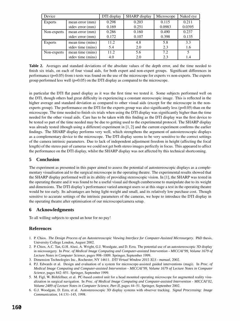
Device DTI display SHARP display Microscope Naked eyeExperts mean error (mm) 0.298 0.203 0.115 0.211

stdev error (mm) 0.169 0.251 0.0983 0.0395Non-experts mean error (mm) 0.286 0.160 0.490 0.237

stdev error (mm) 0.172 0.107 0.398 0.135Experts mean time (mins) 11.2 4.8 5.8 3.3

stdev time (mins) 5.4 2.0 2.3 1.6Non-experts mean time (mins) 11.2 5.6 7.2 5

stdev time (mins) 4.0 2.0 2.3 1.4

Table 2. Averages and standard deviations of the absolute values of the depth error, and the time needed tofinish six trials, on each of four visual aids, for both expert and non-expert groups. Significant differences inperformance (p=0.05) from t-tests was found on the use of the microscope for experts vs non-experts. The expertsgroup performed less well (p=0.05) on the DTI display as compared to the microscope.

in particular the DTI flat panel display as it was the first time we tested it. Some subjects performed well onthe DTI, though others had great difficulty in experiencing a constant stereoscopic image. This is reflected in thehigher average and standard deviation as compared to other visual aids (except for the microscope in the non-experts group). The performance on the DTI for the experts group was also significantly less (p=0.05) than on themicroscope. The time needed to finish six trials when using the DTI display was significantly higher than the timeneeded for the other visual aids. Care has to be taken with this finding as the DTI display was the first device tobe tested so part of the time needed may be due to getting used to the experimental protocol. The SHARP displaywas already tested (though using a different) experiment in [1, 2] and the current experiment confirms the earlierfindings. The SHARP display performs very well, which strengthens the argument of autostereoscopic displaysas a complementary device to the microscope. The DTI display seems to be very sensitive to the correct settingsof the camera intrinsic parameters. Due to lack of independent adjustment freedom in height (affecting the focallength) of the stereo pair of cameras we could not get both stereo images perfectly in focus. This appeared to affectthe performance on the DTI display, whilst the SHARP display was not affected by this technical shortcoming.

5 Conclusion

The experiment as presented in this paper aimed to assess the potential of autostereoscopic displays as a comple-mentary visualisation aid to the surgical microscope in the operating theatre. The experimental results showed thatthe SHARP display performed well in its ability of providing stereoscopic vision. In [1], the SHARP was tested inthe operating theatre and it was found to be a useful visual aid though cumbersome to manipulate due to its weightand dimensions. The DTI display’s performance varied amongst users so at this stage a test in the operating theatrewould be too early. Its advantages are being light-weight and small, and its relatively low purchase cost. Thoughsensitive to accurate settings of the intrinsic parameters of the cameras, we hope to introduce the DTI display inthe operating theatre after optimisation of our microscope/camera setup.

6 Acknowledgments

To all willing subjects to spend an hour for no pay!

References

1. P. Chios. The Design Process of an Autostereoscopic Viewing Interface for Computer-Assisted Microsurgery. PhD thesis,University College London, August 2002.

2. P. Chios, A.C. Tan, G.H. Alusi, A. Wright, G.J. Woodgate, and D. Ezra. The potential use of an autostereoscopic 3D displayin microsurgery. In Proc. of Medical Image Computing and Computer-assisted Intervention - MICCAI’99, Volume 1679 ofLecture Notes in Computer Science, pages 998–1009. Springer, September 1999.

3. Dimension Technologies Inc., Rochester, NY 14611. DTI Virtual Window 2015 XLS - manual, 2002.4. P.J. Edwards et al. Design and evaluation of a system for microscope-assisted guided interventions (magi). In Proc. of

Medical Image Computing and Computer-assisted Intervention - MICCAI’99, Volume 1679 of Lecture Notes in ComputerScience, pages 842–851. Springer, September 1999.

5. M. Figl, W. Birkfellner, et al. PC-based control unit for a head mounted operating microscope for augmented reality visu-alization in surgical navigation. In Proc. of Medical Image Computing and Computer-assisted Intervention - MICCAI’02,Volume 2489 of Lecture Notes in Computer Science, Part II, pages 44–51. Springer, September 2002.

6. G.J. Woodgate, D. Ezra, et al. Autostereoscopic 3D display systems with observer tracking. Signal Proccessing: ImageCommunication, 14:131–145, 1998.

Automatic Capillary Measurement

Kaiyan Fenga, P. D. Allena, T. Mooreb, A. L. Herrickb, and Chris J. Taylorb

aDivision of Imaging Science, Stopford Building, Oxford Road, University of Manchester, M13 9PT, UK,bUniversity of Manchester,Rheumatic Diseases Centre, Hope Hospital, Salford, M6 8HD, UK

Abstract. Microscope images of nailfold capillaries can be used to investigate changes in the peripheral cir-culation in Raynaud’s disease. In particular, there is evidence that they may help in differentiating betweenPrimary Raynaud’s, which relatively benign, and scleroderma, which is more serious. We describe a methodof enhancing capillary images so that other structures are ignored, then measuring vessel width and tortuosityautomatically. We show good agreement between automatically measured capillary width and the manuallymeasured width. We also show that combining width and tortuosity may be useful in classifying subjects intonormal control, Primary Raynaud’s and Secondary Raynaud’s groups.

1 Introduction

We describe a method for measuring the changes in the vessels of the nailfold in patients suffering from Raynaud’sdisease. Raynaud’s phenomenon is caused by interruption to the blood supply, and can be classified as primaryor secondary. The peripheral vessels in individuals with primary Raynaud’s respond abnormally to external andinternal stimuli (eg cold or emotional stress) but have no underlying vascular disease. Individuals with secondaryRaynaud’s have underlying vascular disease, such as scleroderma. Previous studies have suggested that it may bepossible to distinguish between them by observing the form of the blood vessels in the nailfold. Normal controlstend to exhibit narrow, straight and regularly organised vessels, whilst subjects with Primary Raynaud’s have widervessels, and those with secondary Raynaud’s still wider and more tortuous vessels [1]. Peripheral vessels can beimaged non-invasively using nailfold microscopy (the nailfold is the strip of skin immediately adjacent to the fingernail). Examples of nailfold microscope images for a normal control and Secondary Raynaud’s patient are shownin Fig. 1.

Existing quantitative studies have involved manual measurement of vessel width [2]. No quantitative studies oftortuosity have been reported. There is thus significant clinical interest in automated methods of measuring vesselwidth and tortuosity.

Figure 1. Nailfold Capillaroscopy Images (they are inverted) Taken from a) Normal Control Subject and b)Raynaud’s phenomenon subject.

In the remainder of the paper we describe an automated method of measuring vessel width and tortuosity, fromnailfold microscope images. Methods from mathematical morphology are used to enhance the vessels, deriveorientation maps, and measure the average vessel width and the dispersion of vessel orientations.

2 Enhancing Capillaries

Due to a large amount of noise, illumination variation and the presence of confounding structure in the capillaryimages, we choose first to enhance the vessels.

2.1 Directional Opening

Thackray et al. [3] used the supremum of rotating directional openings to enhance vascular structures. We adopt asimilar idea. We definefθ(~x) as the directional opening of an imagef(~x) with a linear structuring element at angle

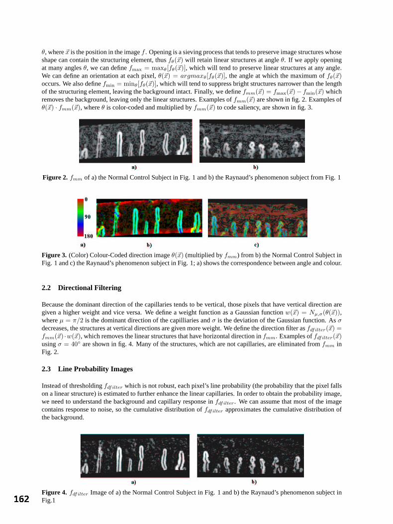
θ, where~x is the position in the imagef . Opening is a sieving process that tends to preserve image structures whoseshape can contain the structuring element, thusfθ(~x) will retain linear structures at angleθ. If we apply openingat many anglesθ, we can definefmax = maxθ[fθ(~x)], which will tend to preserve linear structures at any angle.We can define an orientation at each pixel,θ(~x) = argmaxθ[fθ(~x)], the angle at which the maximum offθ(~x)occurs. We also definefmin = minθ[fθ(~x)], which will tend to suppress bright structures narrower than the lengthof the structuring element, leaving the background intact. Finally, we definefmm(~x) = fmax(~x)− fmin(~x) whichremoves the background, leaving only the linear structures. Examples offmm(~x) are shown in fig. 2. Examples ofθ(~x) · fmm(~x), whereθ is color-coded and multiplied byfmm(~x) to code saliency, are shown in fig. 3.

Figure 2. fmm of a) the Normal Control Subject in Fig. 1 and b) the Raynaud’s phenomenon subject from Fig. 1

Figure 3. (Color) Colour-Coded direction imageθ(~x) (multiplied byfmm) from b) the Normal Control Subject inFig. 1 and c) the Raynaud’s phenomenon subject in Fig. 1; a) shows the correspondence between angle and colour.

2.2 Directional Filtering

Because the dominant direction of the capillaries tends to be vertical, those pixels that have vertical direction aregiven a higher weight and vice versa. We define a weight function as a Gaussian functionw(~x) = Nµ,σ(θ(~x)),whereµ = π/2 is the dominant direction of the capilliaries andσ is the deviation of the Gaussian function. Asσdecreases, the structures at vertical directions are given more weight. We define the direction filter asfdfilter(~x) =fmm(~x) ·w(~x), which removes the linear structures that have horizontal direction infmm. Examples offdfilter(~x)usingσ = 40 are shown in fig. 4. Many of the structures, which are not capillaries, are eliminated fromfmm inFig. 2.

2.3 Line Probability Images

Instead of thresholdingfdfilter which is not robust, each pixel’s line probability (the probability that the pixel fallson a linear structure) is estimated to further enhance the linear capillaries. In order to obtain the probability image,we need to understand the background and capillary response infdfilter. We can assume that most of the imagecontains response to noise, so the cumulative distribution offdfilter approximates the cumulative distribution ofthe background.

Figure 4. fdfilter Image of a) the Normal Control Subject in Fig. 1 and b) the Raynaud’s phenomenon subject inFig.1

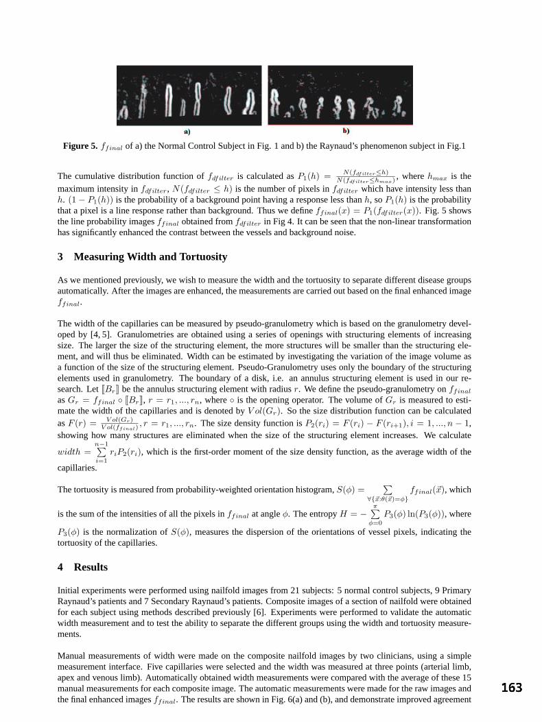
Figure 5. ffinal of a) the Normal Control Subject in Fig. 1 and b) the Raynaud’s phenomenon subject in Fig.1

The cumulative distribution function offdfilter is calculated asP1(h) = N(fdfilter≤h)N(fdfilter≤hmax) , wherehmax is the

maximum intensity infdfilter, N(fdfilter ≤ h) is the number of pixels infdfilter which have intensity less thanh. (1− P1(h)) is the probability of a background point having a response less thanh, soP1(h) is the probabilitythat a pixel is a line response rather than background. Thus we defineffinal(x) = P1(fdfilter(x)). Fig. 5 showsthe line probability imagesffinal obtained fromfdfilter in Fig 4. It can be seen that the non-linear transformationhas significantly enhanced the contrast between the vessels and background noise.

3 Measuring Width and Tortuosity

As we mentioned previously, we wish to measure the width and the tortuosity to separate different disease groupsautomatically. After the images are enhanced, the measurements are carried out based on the final enhanced imageffinal.

The width of the capillaries can be measured by pseudo-granulometry which is based on the granulometry devel-oped by [4, 5]. Granulometries are obtained using a series of openings with structuring elements of increasingsize. The larger the size of the structuring element, the more structures will be smaller than the structuring ele-ment, and will thus be eliminated. Width can be estimated by investigating the variation of the image volume asa function of the size of the structuring element. Pseudo-Granulometry uses only the boundary of the structuringelements used in granulometry. The boundary of a disk, i.e. an annulus structuring element is used in our re-search. Let[[Br]] be the annulus structuring element with radiusr. We define the pseudo-granulometry onffinal

asGr = ffinal [[Br]], r = r1, ..., rn, where is the opening operator. The volume ofGr is measured to esti-mate the width of the capillaries and is denoted byV ol(Gr). So the size distribution function can be calculatedasF (r) = V ol(Gr)

V ol(ffinal), r = r1, ..., rn. The size density function isP2(ri) = F (ri) − F (ri+1), i = 1, ..., n − 1,

showing how many structures are eliminated when the size of the structuring element increases. We calculate

width =n−1∑i=1

riP2(ri), which is the first-order moment of the size density function, as the average width of the

capillaries.

The tortuosity is measured from probability-weighted orientation histogram,S(φ) =∑

∀~x:θ(~x)=φffinal(~x), which

is the sum of the intensities of all the pixels inffinal at angleφ. The entropyH = −π∑

φ=0

P3(φ) ln(P3(φ)), where

P3(φ) is the normalization ofS(φ), measures the dispersion of the orientations of vessel pixels, indicating thetortuosity of the capillaries.

4 Results

Initial experiments were performed using nailfold images from 21 subjects: 5 normal control subjects, 9 PrimaryRaynaud’s patients and 7 Secondary Raynaud’s patients. Composite images of a section of nailfold were obtainedfor each subject using methods described previously [6]. Experiments were performed to validate the automaticwidth measurement and to test the ability to separate the different groups using the width and tortuosity measure-ments.

Manual measurements of width were made on the composite nailfold images by two clinicians, using a simplemeasurement interface. Five capillaries were selected and the width was measured at three points (arterial limb,apex and venous limb). Automatically obtained width measurements were compared with the average of these 15manual measurements for each composite image. The automatic measurements were made for the raw images andthe final enhanced imagesffinal. The results are shown in Fig. 6(a) and (b), and demonstrate improved agreement

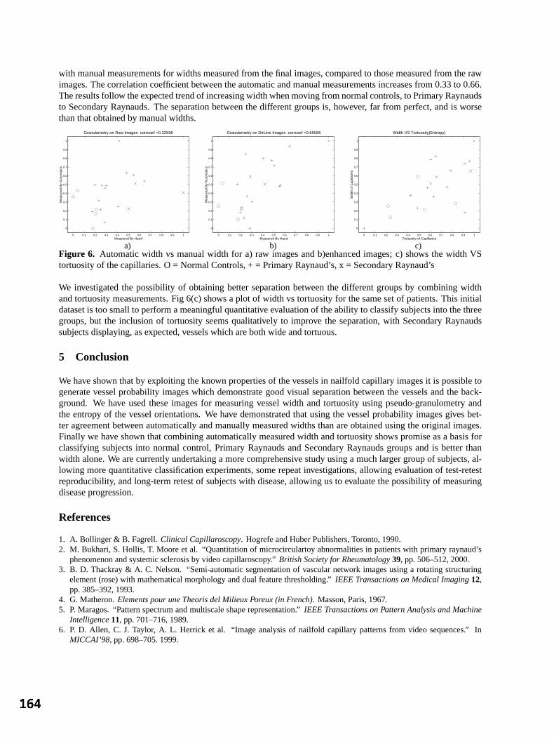
with manual measurements for widths measured from the final images, compared to those measured from the rawimages. The correlation coefficient between the automatic and manual measurements increases from 0.33 to 0.66.The results follow the expected trend of increasing width when moving from normal controls, to Primary Raynaudsto Secondary Raynauds. The separation between the different groups is, however, far from perfect, and is worsethan that obtained by manual widths.

0 0.1 0.2 0.3 0.4 0.5 0.6 0.7 0.8 0.9 1

0

0.1

0.2

0.3

0.4

0.5

0.6

0.7

0.8

0.9

1

Mea

sure

d B

y A

utom

atic

s

Measured By Hand

Granulometry on Raw Images corrcoef =0.32596

0 0.1 0.2 0.3 0.4 0.5 0.6 0.7 0.8 0.9 1

0

0.1

0.2

0.3

0.4

0.5

0.6

0.7

0.8

0.9

1

Mea

sure

d B

y A

utom

atic

s

Measured By Hand

Granulometry on DirLine Images corrcoef =0.65585

0 0.1 0.2 0.3 0.4 0.5 0.6 0.7 0.8 0.9 1

0

0.1

0.2

0.3

0.4

0.5

0.6

0.7

0.8

0.9

1

Wid

th o

f Cap

illar

ies

Tortuosity of Capillaries

Width VS Tortuosity(Entropy)

a) b) c)Figure 6. Automatic width vs manual width for a) raw images and b)enhanced images; c) shows the width VStortuosity of the capillaries. O = Normal Controls, + = Primary Raynaud’s, x = Secondary Raynaud’s

We investigated the possibility of obtaining better separation between the different groups by combining widthand tortuosity measurements. Fig 6(c) shows a plot of width vs tortuosity for the same set of patients. This initialdataset is too small to perform a meaningful quantitative evaluation of the ability to classify subjects into the threegroups, but the inclusion of tortuosity seems qualitatively to improve the separation, with Secondary Raynaudssubjects displaying, as expected, vessels which are both wide and tortuous.

5 Conclusion

We have shown that by exploiting the known properties of the vessels in nailfold capillary images it is possible togenerate vessel probability images which demonstrate good visual separation between the vessels and the back-ground. We have used these images for measuring vessel width and tortuosity using pseudo-granulometry andthe entropy of the vessel orientations. We have demonstrated that using the vessel probability images gives bet-ter agreement between automatically and manually measured widths than are obtained using the original images.Finally we have shown that combining automatically measured width and tortuosity shows promise as a basis forclassifying subjects into normal control, Primary Raynauds and Secondary Raynauds groups and is better thanwidth alone. We are currently undertaking a more comprehensive study using a much larger group of subjects, al-lowing more quantitative classification experiments, some repeat investigations, allowing evaluation of test-retestreproducibility, and long-term retest of subjects with disease, allowing us to evaluate the possibility of measuringdisease progression.

References

1. A. Bollinger & B. Fagrell.Clinical Capillaroscopy. Hogrefe and Huber Publishers, Toronto, 1990.2. M. Bukhari, S. Hollis, T. Moore et al. “Quantitation of microcirculartoy abnormalities in patients with primary raynaud’s

phenomenon and systemic sclerosis by video capillaroscopy.”British Society for Rheumatology39, pp. 506–512, 2000.3. B. D. Thackray & A. C. Nelson. “Semi-automatic segmentation of vascular network images using a rotating structuring

element (rose) with mathematical morphology and dual feature thresholding.”IEEE Transactions on Medical Imaging12,pp. 385–392, 1993.

4. G. Matheron.Elements pour une Theoris del Milieux Poreux (in French). Masson, Paris, 1967.5. P. Maragos. “Pattern spectrum and multiscale shape representation.”IEEE Transactions on Pattern Analysis and Machine

Intelligence11, pp. 701–716, 1989.6. P. D. Allen, C. J. Taylor, A. L. Herrick et al. “Image analysis of nailfold capillary patterns from video sequences.” In

MICCAI’98, pp. 698–705. 1999.

Fast 3D Mean Shift Filter applied to CT Images

Gustavo Fernandez Domınguez, Horst Bischof∗, Reinhard Beichel, and Franz Leberl

Institute for Computer Graphics and Vision, Graz University of Technology,Inffeldgasse 16/2, A-8010, Graz, Austria

Abstract. We present a novel3D mean shift filtering algorithm to denoiseCT data sets. The mean shiftalgorithm is well suited for filtering and segmentation of images, but application for large size3D medicaldata sets require a lot of computing time. In this paper we propose an efficient approximation of the3D meanshift algorithm using sub-sampling techniques. Experimental results on variousCT data sets are presented.Quantitative validation of the results consists of applying the output filtered data sets as input to a segmentationprocedure for the extraction of the portal vein tree. We compare the developed approach against other variantsof the MS filter, and a classical filter technique. Experiments show that the developed filter is efficient andprovides a good approximation to the3D mean shift method.Keywords: Mean shift filter, sub-sampling techniques, nonlinear filtering.

1 Introduction

In the last years, different nonlinear filtering methods have been developed and used as a preprocessing step for im-age data including medical images. In particular, nonlinear methods such as wavelet denoising methods [1,2] andtechniques based on anisotropic diffusion [3,4] provide very good results. Themean shift(MS) algorithm belongsto the class of nonlinear methods. The algorithm is based on theMS method proposed by Fukunaga et al. [5].The MS method estimates the probability density function (pdf) from the data. Application areas of theMSalgorithm include denoising and segmentation [6, 7], and analysis of video motion [8]. However, the large size ofmedical data sets requires a lot of computing time when theMS algorithm is applied. Therefore, we introduce anapproximation of the3D−MS filter. This approximation consists of using a reduced set of voxels for each datapoint to be filtered instead of using the complete set of voxels. This reduction is obtained selecting points from theneighbouring slices of the current slice to be processed. Our goal is twofold: i) Obtain a filter quality similar to theoriginal3D−MS filter and, ii) reduce the execution times as far as possible.This paper is structured as follows: In Section 2 we briefly outline the main ideas of theMS algorithm. In Sec-tion 3 the new approach is presented. In Section 4 the proposed filter is compared to other versions of theMSfilter, and a traditional filter technique. Discussions are presented in Section 5.

2 Mean Shift

TheMS is a nonparametric method which tries to estimate the probability density function (pdf) from the dataof a feature space. Fukunaga et al. [5] proposed the method already in1975, and Cheng rediscovers it for clusteranalysis [9].MS algorithm was developed by Comaniciu and Meer [6,7], as a technique for the analysis of multi-modal feature spaces. The goal of that analysis is to delineate the cluster regions present in the feature space. Thisspace is constructed from the spatial coordinates and the gray values of each pixel or voxel. TheMS algorithmwas presented as a method to detect the modes of the associated pdf. TheMS method estimates the pdf of the datausing the so-called Parzen window density estimator [10]. Givenn data pointsxi, i = 1, ..., n in the d-dimensionalspace<d, the multivariate kernel density estimator with kernelKH (x) computed at the pointx is given by

f (x) =1n

n∑i=1

KH (x− xi) . (1)

The profile of a kernelKH (x) is introduced as a functionk such that

KH (x) = ckk(‖ x ‖2

), (2)

whereck is the normalization constant which makesKH integrate to one. The normal kernel characterized by theGaussian function [11] is one of the most common used kernels. Comaniciu et al. [7] showed that the mean shiftvectormh,G (x) is proportional to the normalized density gradient

mh,G (x) ∝ ∇fh,K (x)fh,G (x)

, (3)

∗Corresponding author: [email protected]

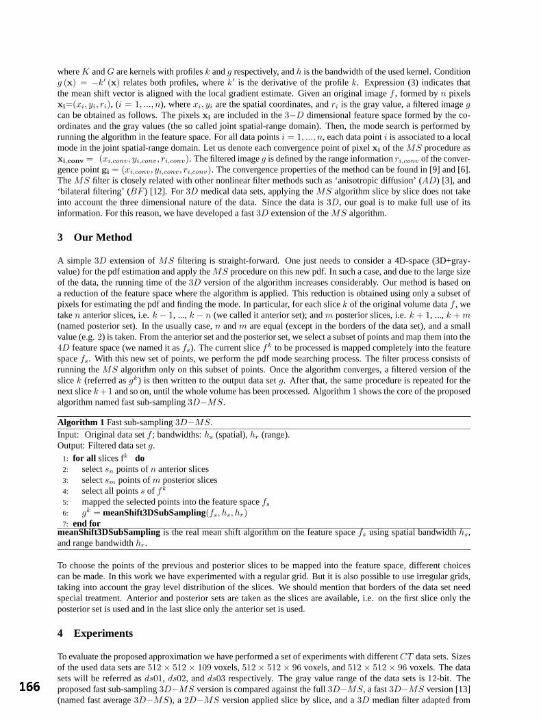
whereK andG are kernels with profilesk andg respectively, andh is the bandwidth of the used kernel. Conditiong (x) = −k′ (x) relates both profiles, wherek′ is the derivative of the profilek. Expression (3) indicates thatthe mean shift vector is aligned with the local gradient estimate. Given an original imagef , formed byn pixelsxi=(xi, yi, ri), (i = 1, ..., n), wherexi, yi are the spatial coordinates, andri is the gray value, a filtered imagegcan be obtained as follows. The pixelsxi are included in the3−D dimensional feature space formed by the co-ordinates and the gray values (the so called joint spatial-range domain). Then, the mode search is performed byrunning the algorithm in the feature space. For all data pointsi = 1, ..., n, each data pointi is associated to a localmode in the joint spatial-range domain. Let us denote each convergence point of pixelxi of theMS procedure asxi,conv = (xi,conv, yi,conv, ri,conv). The filtered imageg is defined by the range informationri,conv of the conver-gence pointgi = (xi,conv, yi,conv, ri,conv). The convergence properties of the method can be found in [9] and [6].TheMS filter is closely related with other nonlinear filter methods such as ‘anisotropic diffusion’ (AD) [3], and‘bilateral filtering’ (BF ) [12]. For3D medical data sets, applying theMS algorithm slice by slice does not takeinto account the three dimensional nature of the data. Since the data is3D, our goal is to make full use of itsinformation. For this reason, we have developed a fast3D extension of theMS algorithm.

3 Our Method

A simple 3D extension ofMS filtering is straight-forward. One just needs to consider a 4D-space (3D+gray-value) for the pdf estimation and apply theMS procedure on this new pdf. In such a case, and due to the large sizeof the data, the running time of the3D version of the algorithm increases considerably. Our method is based ona reduction of the feature space where the algorithm is applied. This reduction is obtained using only a subset ofpixels for estimating the pdf and finding the mode. In particular, for each slicek of the original volume dataf , wetaken anterior slices, i.e.k − 1, ...,k − n (we called it anterior set); andm posterior slices, i.e.k + 1, ...,k + m(named posterior set). In the usually case,n andm are equal (except in the borders of the data set), and a smallvalue (e.g.2) is taken. From the anterior set and the posterior set, we select a subset of points and map them into the4D feature space (we named it asfs). The current slicefk to be processed is mapped completely into the featurespacefs. With this new set of points, we perform the pdf mode searching process. The filter process consists ofrunning theMS algorithm only on this subset of points. Once the algorithm converges, a filtered version of theslicek (referred asgk) is then written to the output data setg. After that, the same procedure is repeated for thenext slicek+1 and so on, until the whole volume has been processed. Algorithm 1 shows the core of the proposedalgorithm named fast sub-sampling3D−MS.

Algorithm 1 Fast sub-sampling3D−MS.Input: Original data setf ; bandwidths:hs (spatial),hr (range).Output: Filtered data setg.

1: for all slices fk do2: selectsn points ofn anterior slices3: selectsm points ofm posterior slices4: select all pointss of fk

5: mapped the selected points into the feature spacefs

6: gk = meanShift3DSubSampling(fs, hs, hr)7: end for

meanShift3DSubSamplingis the real mean shift algorithm on the feature spacefs using spatial bandwidthhs,and range bandwidthhr.

To choose the points of the previous and posterior slices to be mapped into the feature space, different choicescan be made. In this work we have experimented with a regular grid. But it is also possible to use irregular grids,taking into account the gray level distribution of the slices. We should mention that borders of the data set needspecial treatment. Anterior and posterior sets are taken as the slices are available, i.e. on the first slice only theposterior set is used and in the last slice only the anterior set is used.

4 Experiments

To evaluate the proposed approximation we have performed a set of experiments with differentCT data sets. Sizesof the used data sets are512 × 512 × 109 voxels,512 × 512 × 96 voxels, and512 × 512 × 96 voxels. The datasets will be referred asds01, ds02, andds03 respectively. The gray value range of the data sets is12-bit. Theproposed fast sub-sampling3D−MS version is compared against the full3D−MS, a fast3D−MS version [13](named fast average3D−MS), a 2D−MS version applied slice by slice, and a3D median filter adapted from

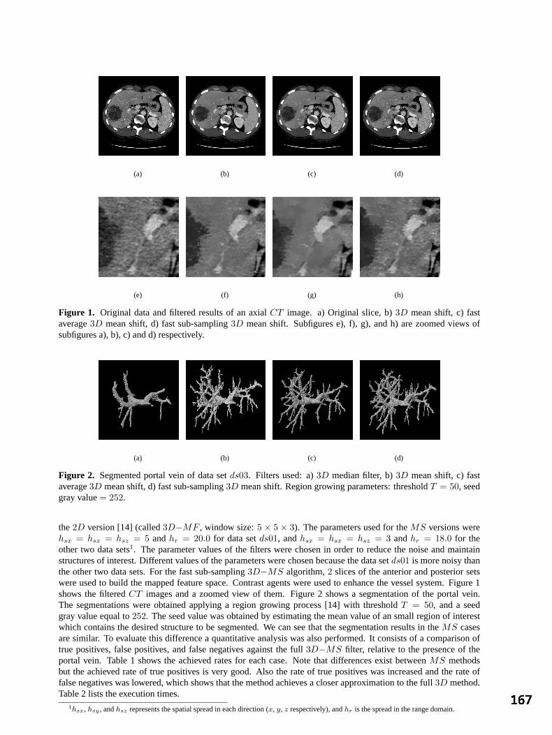
(a) (b) (c) (d)

(e) (f) (g) (h)

Figure 1. Original data and filtered results of an axialCT image. a) Original slice, b)3D mean shift, c) fastaverage3D mean shift, d) fast sub-sampling3D mean shift. Subfigures e), f), g), and h) are zoomed views ofsubfigures a), b), c) and d) respectively.

(a) (b) (c) (d)

Figure 2. Segmented portal vein of data setds03. Filters used: a)3D median filter, b)3D mean shift, c) fastaverage3D mean shift, d) fast sub-sampling3D mean shift. Region growing parameters: thresholdT = 50, seedgray value= 252.

the2D version [14] (called3D−MF , window size:5 × 5 × 3). The parameters used for theMS versions werehsx = hsx = hsz = 5 andhr = 20.0 for data setds01, andhsx = hsx = hsz = 3 andhr = 18.0 for theother two data sets1. The parameter values of the filters were chosen in order to reduce the noise and maintainstructures of interest. Different values of the parameters were chosen because the data setds01 is more noisy thanthe other two data sets. For the fast sub-sampling3D−MS algorithm,2 slices of the anterior and posterior setswere used to build the mapped feature space. Contrast agents were used to enhance the vessel system. Figure 1shows the filteredCT images and a zoomed view of them. Figure 2 shows a segmentation of the portal vein.The segmentations were obtained applying a region growing process [14] with thresholdT = 50, and a seedgray value equal to252. The seed value was obtained by estimating the mean value of an small region of interestwhich contains the desired structure to be segmented. We can see that the segmentation results in theMS casesare similar. To evaluate this difference a quantitative analysis was also performed. It consists of a comparison oftrue positives, false positives, and false negatives against the full3D−MS filter, relative to the presence of theportal vein. Table 1 shows the achieved rates for each case. Note that differences exist betweenMS methodsbut the achieved rate of true positives is very good. Also the rate of true positives was increased and the rate offalse negatives was lowered, which shows that the method achieves a closer approximation to the full3D method.Table 2 lists the execution times.

1hsx, hsy , andhsz represents the spatial spread in each direction (x, y, z respectively), andhr is the spread in the range domain.

Data set Measure 3D-MF 2D-MS Fast average 3D-MS Fast sub-sampling 3D-MS

ds01 True positives 60.29 74.42 74.48 80.94

False positives 0.80 1.33 1.33 1.56

False negatives 39.71 25.58 25.52 19.06

ds02 True positives 58.75 89.22 90.23 91.46

False positives 3.68 4.02 4.02 4.07

False negatives 41.25 10.78 9.77 8.54

ds03 True positives 57.19 94.00 94.01 96.62

False positives 0.45 1.32 1.32 1.15

False negatives 42.81 6.00 5.99 3.38

Table 1. Percentage of true positives, false positives, and false negatives relative to the real3D−MS algorithm.Filter methods:3D median filter (3D-MF),2D mean shift (2D-MS), fast average3D mean shift (Fast average3D-MS), fast sub-sampling3D mean shift (Fast sub-sampling 3D-MS).

Data set 3D-MF 2D-MS 3D-MS Fast average 3D-MS Fast sub-sampling 3D-MS

ds02 429 208 3912 142 845

ds03 681 347 5064 354 799

Table 2. Execution times in seconds for different filter methods.

5 Conclusions and Future Work

This paper has presented a novel extension of theMS method for denoisingCT data sets. The approach is basedon the combination of a data reduction of the feature space and theMS algorithm. Experiments onCT datasets, indicate that the proposed method obtains similar results to the real3D−MS algorithm, with faster execu-tion times. Other experiments show that segmentations are similar in quantitative and qualitative comparisons.Influence of mapping functions to obtain the subsampled points will be explored in future research.

Acknowledgements

The authors gratefully acknowledge the financial support of the Austrian Research Foundation (FWF) under projectnumber P-14897. The originalMS software available at [15] was properly adapted for our purposes.

References

1. D. Donoho & I. M. Johnstone. “Ideal spatial adaptation via wavelet shrinkage.”Biometrika81, pp. 425–455, 1994.2. S. Mallat.A Wavelet Tour of Signal Processing. Academic Press, 2nd Edition, Elsevier Science, 1999.3. P. Perona & J. Malik. “Scale-space and edge detection using anisotropic diffusion.”IEEE Trans. Pattern Analysis and

Machine Intelligence12-7, pp. 629–639, 1990.4. K. Krissian, G. Malandain, N. Ayache et al. “Model-based multiscale detection of 3D vessels.” InProceedings of Computer

Vision and Pattern Recognition, pp. 722–727. IEEE, 1998.5. K. Fukunaga & L. D. Hostetler. “The estimation of the gradient of a density function, with applications in pattern recogni-

tion.” IEEE Trans. Information Theory21, pp. 32–40, 1975.6. D. Comaniciu.Nonparametric Robust Methods for Computer Vision. Ph.D. thesis, ECE Department, Rutgers University,

July 2001.7. D. Comaniciu & P. Meer. “Mean shift: A robust approach toward feature space analysis.”IEEE Trans. Pattern Recognition

and Machine Intelligence24-5, pp. 603–619, 2002.8. D. Comaniciu & V. Ramesh. “Mean shift and optimal prediction for efficient object tracking.” InProceedings of Interna-

tional Conference on Image Processing, Vancouver, Canada, volume 3, pp. 70–73. IEEE, 2000.9. Y. Cheng. “Mean shift, mode seeking, and clustering.”IEEE Trans. Pattern Analysis and Machine Intelligence17-8,

pp. 790–799, 1995.10. R. O. Duda, P. E. Hart & D. G. Stork.Pattern Classification. Wiley-Interscience, New York, 2nd Edit., 2000.11. A. K. Jain.Fundamentals of Digital Image Processing. Prentice Hall, New Jersey, 1989.12. C. Tomasi & R. Manduchi. “Bilateral filtering for gray and color images.” InProceedings of 6th International Conference

on Computer Vision, New Delhi, India, pp. 839–846. IEEE, 1998.13. G. Fernandez, H. Bischof & R. Beichel. “Nonlinear filters on3D CT imaging− bilateral filter and mean shift filter.” In

Proceedings of 8th Computer Vision Winter Workshop, pp. 21–26. 2003.14. R. Gonzalez & R. Woods.Digital Image Processing. Addison Wesley, Massachusetts, 1992.15. www.caip.rutgers.edu/riul. “www.caip.rutgers.edu/riul/research/code.html.” 2001.

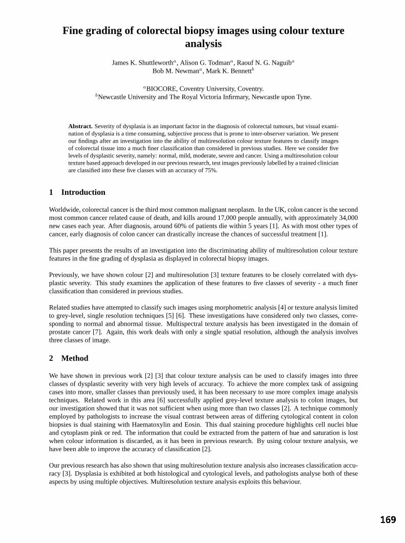
Fine grading of colorectal biopsy images using colour textureanalysis

James K. Shuttlewortha, Alison G. Todmana, Raouf N. G. Naguiba

Bob M. Newmana, Mark K. Bennettb

aBIOCORE, Coventry University, Coventry.bNewcastle University and The Royal Victoria Infirmary, Newcastle upon Tyne.

Abstract. Severity of dysplasia is an important factor in the diagnosis of colorectal tumours, but visual exami-nation of dysplasia is a time consuming, subjective process that is prone to inter-observer variation. We presentour findings after an investigation into the ability of multiresolution colour texture features to classify imagesof colorectal tissue into a much finer classification than considered in previous studies. Here we consider fivelevels of dysplastic severity, namely: normal, mild, moderate, severe and cancer. Using a multiresolution colourtexture based approach developed in our previous research, test images previously labelled by a trained clinicianare classified into these five classes with an accuracy of 75%.

1 Introduction

Worldwide, colorectal cancer is the third most common malignant neoplasm. In the UK, colon cancer is the secondmost common cancer related cause of death, and kills around 17,000 people annually, with approximately 34,000new cases each year. After diagnosis, around 60% of patients die within 5 years [1]. As with most other types ofcancer, early diagnosis of colon cancer can drastically increase the chances of successful treatment [1].

This paper presents the results of an investigation into the discriminating ability of multiresolution colour texturefeatures in the fine grading of dysplasia as displayed in colorectal biopsy images.

Previously, we have shown colour [2] and multiresolution [3] texture features to be closely correlated with dys-plastic severity. This study examines the application of these features to five classes of severity - a much finerclassification than considered in previous studies.

Related studies have attempted to classify such images using morphometric analysis [4] or texture analysis limitedto grey-level, single resolution techniques [5] [6]. These investigations have considered only two classes, corre-sponding to normal and abnormal tissue. Multispectral texture analysis has been investigated in the domain ofprostate cancer [7]. Again, this work deals with only a single spatial resolution, although the analysis involvesthree classes of image.

2 Method

We have shown in previous work [2] [3] that colour texture analysis can be used to classify images into threeclasses of dysplastic severity with very high levels of accuracy. To achieve the more complex task of assigningcases into more, smaller classes than previously used, it has been necessary to use more complex image analysistechniques. Related work in this area [6] successfully applied grey-level texture analysis to colon images, butour investigation showed that it was not sufficient when using more than two classes [2]. A technique commonlyemployed by pathologists to increase the visual contrast between areas of differing cytological content in colonbiopsies is dual staining with Haematoxylin and Eosin. This dual staining procedure highlights cell nuclei blueand cytoplasm pink or red. The information that could be extracted from the pattern of hue and saturation is lostwhen colour information is discarded, as it has been in previous research. By using colour texture analysis, wehave been able to improve the accuracy of classification [2].

Our previous research has also shown that using multiresolution texture analysis also increases classification accu-racy [3]. Dysplasia is exhibited at both histological and cytological levels, and pathologists analyse both of theseaspects by using multiple objectives. Multiresolution texture analysis exploits this behaviour.

2.1 Image Acquisition

In total, 60 5µm slices from colorectal biopsy tissue were investigated. These samples exhibit various stages ofdysplastic progression. Staining was performed using Haematoxylin and Eosin. The slides were digitised andclassified by a qualified histopathologist with a specialism in gastro-intestinal cancers. The resulting images are768 × 576 pixels, examples of which are shown in Figure 1. In our previous experiments [2] [3], regions of theslide were selected to ensure that the image contained only tissue of one class. In this study we consider the morechallenging situation in which entire samples are used.

Figure 1. An example image from each class.

2.2 Texture analysis and classification

Entropy∑

i

∑j P (i, j) log P (i, j) Contrast

∑i

∑j(i− j)2P (i, j)

Correlation∑

i

∑j

(i−ux)(j−uy)P (i,j)σxσy

Homogeneity∑

i

∑j

P (i,j)1+|i−j|

Dissimilarity∑

i

∑j P (i, j)|i− j| Angular Second Moment (ASM)

∑i

∑j P (i, j)2

Energy√

ASM Horizontal mean (µx)∑

i

∑j iP (i, j)

Vertical stdv (σy)√

σ2y Horizontal variance (σ2

x)∑

i

∑j P (i, j)(i− µx)2

Vertical variance (σ2x)

∑i

∑j P (i, j)(j − µy)2 Horizontal stdv (σx)

√σ2

x

Vertical mean (µy)∑

i

∑j jP (i, j)

Table 1. Texture measurements extracted from co-occurrence matrices

Co-occurrence matrices [8] [9] have been used in the past to extract texture information for many applications,including medical image analysis [10] [11]. The co-occurrence matrix is constructed by first determining a pairingrelationship. The pairing relationship, often expressed as a distance,d, and angle,θ, is used to pick pairs of pixelsfrom the image. All pixel pairs matching the pairing relationship are analysed, and their values used to populatea matrix such that the values of the two pixels (source and target) are used as row and column identifiers in thematrix. The cell identified by the values of the pixel pairs is incremented for each valid pair. The co-occurrencematrix then contains the number of times two pixels with any given value occur in the image, separated by thepairing relationship.

For our work rotational invariance is necessary, and so co-occurrence matrices are calculated with the angle be-tween pixel pairs set toθ, θ + 90, θ + 180 andθ + 270 degrees. The final co-occurrence matrix is calculated byaveraging these four intermediate matrices. This also means that horizontal and vertical measures are now thesame. For example, horizontal and vertical mean are now the same and are referred to simply as mean.

Normalisation of a matrix is carried out by dividing each element by the total number of valid pairs. So, for anormalised matrix,P , P (i, j) is the probability of the source pixel having valuei and the target pixel having valuej for any given pair of pixels matching the pairing relationship. A normalised co-occurrence matrix is constructedfor each image in our data set. From this matrix each of the features in Table 1 is extracted.

In an earlier study [2], we demonstrated that colour texture information improves the accuracy of classification.Building on this approach, we extract the features described in Table 1 from each channel of the RGB and HSBrepresentations of the data.

Features that indicate dysplasia are visible at different levels of magnification, corresponding to cytological andhistological disorganisation. Pathologists, therefore, use multiple objectives to asses dysplasia at these levels. Thesize, shape and stain uptake of thecellschange as dysplasia becomes more severe, which affects the visible textureof the images at a high resolution. By pathologists, this is evaluated at high magnification. Using texture analysis,this is measured with values ofd between 1 and 4. The abnormal growth and rate of replication also cause thetissueto appear disorganised at a lower magnification, in the merging and branching of crypts, and in more severecases, loss of differentiation. This structural exhibition of dysplasia has been measured usingd at 40, 60, 80 and100, with neighbouring pixels also taken into account using a Gaussian average at the source and target with aradius,r = 15 andσ = 15.

Classification has been carried out using discriminant analysis to determine which features correlate with dysplasticseverity, and to asses the ability of these features to classify the images.

3 Results

Specificity and sensitivity are difficult to define where the classification involves more than two groups. Insteadwe present figures that indicate similar characteristics, but which are easily calculated and understood. If wedefine downward misclassifications as cases of abnormal tissue being classified as normal, in a two class systemfor example, and upwards misclassifications as the opposite, we can see that fewer downwards misclassificationsis similar to increased sensitivity, and fewer upwards misclassifications is similar to increased specificity. In thisexperiment, downwards classifications accounted for 10% of cases, and upwards classifications accounted for 15%.

Table 2 shows the actual and predicted classifications. Overall, this is a classification accuracy of 75%.

Actual↓ Predicted→ Normal Mild Moderate Severe Cancer

Normal 12 0 0 0 1Mild 1 10 0 4 0Moderate 0 2 13 1 0Severe 1 2 3 4 0Cancer 0 0 0 0 6

Table 2. Actual classifications and those predicted by discriminant analysis

Discriminant analysis reduced the necessary features to just nine, shown in Table 3

Correlation of the green component at 100 pixelsEntropy of the hue component at 4 pixelsASM of the green component at 100 pixels ASM of the green component at 40 pixelsContrast of the red component at 1 pixel Entropy of the blue component at 80 pixelsMean of the saturation component at 100 pixelsEnergy of the green component at 4 pixelsASM of the green component at 4 pixels

Table 3. Discriminating features

4 Discussion

The results presented above clearly show that there is a strong correlation between multiresolution colour texturefeatures and the severity of dysplasia in colon biopsy images. While this is a drop in accuracy from our previousresults which achieved an accuracy of over 98%, it is important to note that the complexity of the task has been

increased by removing the selection of a region of interest and by increasing the number of groups from three tofive. Hence, a direct comparison is inappropriate.

With reference to Table 3, it is interesting to note that although previous research has used grey-level features toclassify images of this type, none of the features accounting for the majority of variability in this study are takenfrom the brightness channel.

Five of the nine features selected by discriminant analysis use large values ford, indicating that the measure-ments of lower resolution, structural deformities are at least as important as the more commonly used fine texturemeasurements. Again, these features have previously been overlooked.

Bosman [12] states that problems with inter- and intra-observer variation in the assessment of dysplasia are mainlydue to two things: a lack of clearly defined morphological criteria, and the enforcement of a discrete classificationon a process that is intrinsically continuous. We have attempted to overcome the first of these problems by usingtextural features rather than morphological features, thereby removing the need to obtain an accurate segmentationof structures in the images. We propose that a possible solution to the second problem may be found through aninvestigation of the relative weightings associated with the discriminating features identified in this study.

References

1. M. Quinn, P. Babb, A. Brock et al.Cancer trends in England and Wales 1950-1999. Office for National Statistics, 2001.2. J. K. Shuttleworth, A. G. Todman, R. N. G. Naguib et al. “Colour texture analysis using co-occurrencematrices for

classification of colon cancer images.” InProceedings of the IEEE Canadian Conference on Electrical and ComputerEngineering. 2002.

3. J. K. Shuttleworth, A. G. Todman, R. N. G. Naguib et al. “Multiresolution colour texture analysis for classifying coloncancer images.” October 2002. Proceedings of the joint 4th Annual International Conference of the EMBS and AnnualFall Meeting of the BMES.

4. P. W. Hamilton, D. C. Allen, P. C. H. Watt et al. “Classification of normal colorectal mucosa and adenocarcinoma bymorphometry.”Histopathology11, 1987.

5. A. N. Esgiar, R. N. G. Naguib, B. S. Sharif et al. “Microscopic image analysis for quantitative measurement and featureidentification of normal and cancerous colonic mucosa.”IEEE Transactions on Information Technology in Biomedicine2(3), pp. 197–203, 1998.

6. P. W. Hamilton, P. H. Bartels, D. Thompson et al. “Automated location of dysplastic fields on colorectal histology usingimage texture analysis.”Journal of Pathology182, pp. 68–75, 1997.

7. M. A. Roula, A. Bouridane & P. Miller. “Multispectral analysis of chromatin texture for automatic grading of prostaticneoplasia.” InProceedings of Medical Image Understanding and Analysis (MIUA). 2002.

8. R. M. Haralick.Handbook of Pattern Recognition and Image Processing, chapter 11: Statistical Image Texture Analysis.Academic Press, Inc., 1986.

9. R. M. Haralick, K. Shanmugam & I. Dinstein. “Textural features for image classification.”IEEE Transactions on Systems,Man, and Cybernetics3(6), pp. 610–621, 1973.

10. B. Weyn, G. V. D. Wouwer, M. Koprowski et al. “Value of morphometry, texture analysis, densitometry and histometry inthe differential diagnosis and prognosis of malignant mesothelioma.”Journal of Pathology180, pp. 581–589, 1999.

11. A. Bernasconi, S. B. Antel, D. L. Collins et al. “Texture analysis and morphological processing of magnetic resonanceimaging assist detection of focal cortical dysplasia in extra-temporal partial epilepsy.”Annals of Neurology49, 2001.

12. P. F. T. Bosman. “Dysplasia classification: Pathology in disgrace?”Journal of Pathology194, pp. 143–144, 2001.

Enhanced display of pulmonary embolism in simultaneous dual isotope ventilation/perfusion planar scintigraphy

Campbell J Reid1 , Sarah Misson1 , John S Fleming1 , Laura Sawyer2, S Alex Hoffmann1 , Nimi Nagaraj1

1: Department of Nuclear Medicine, Southampton General Hospital, Southampton SO16 6YD 2: Department of Medical Physics, Royal United Hospital, Combe Park, Bath BA1 3NG

Abstract Ventilation-perfusion (or VQ) planar scintigraphy is a commonly used tool for the diagnosis of pulmonary embolism. Diagnosis is made based on areas that are normal in the ventilation image and abnormal in the perfusion image. Simultaneous acquisition of ventilation and perfusion images offers several advantages over separate acquisition. However, it is hampered by downscatter of photons from the ventilation acquisition window into the perfusion acquisition window. To overcome this, a novel scatter correction algorithm was developed on the basis of phantom experiments. Another factor that limits VQ scanning is the subjectivity and difficulty of interpreting image pairs displayed as separate images. To overcome this, an automatic interpretation algorithm was developed. Clinical trials, including Spearman’s ranked correlation coefficient tests and t-tests, have shown that the scatter correction algorithm is successful in removing scatter. Visual inspection of the interpretation algorithm shows that it works well, although a full clinical trial still needs to be carried out on it. In summary, novel scatter correction and interpretation algorithms have been implemented for the enhanced display of pulmonary embolism in ventilation/perfusion planar scintigraphy.

1 Introduction Pulmonary embolism is a potentially life-threatening condition that occurs when an embolus becomes trapped in a pulmonary artery or one of its branches, blocking blood flow to one or more segments of the lung. About 10% of patients die within an hour of a major blockage occurring [1]. Ventilation-perfusion (or VQ) scintigraphy is a routine test used in the diagnosis of pulmonary embolism. It consists of performing a ventilation study using 81mKr-labelled technegas (190 keV), and a perfusion study using 99mTc-labelled macroaggregated albumen (140keV). VQ scintigraphy is the modality of choice because it is non-invasive, inexpensive, readily available, gives little radiation dose, can be performed rapidly and causes little discomfort to the patient. A diagnosis of pulmonary embolism is determined on the number and extent of areas of the lung that are normal in the ventilation image and abnormally low in the perfusion image. However, visual interpretation of the image pairs displayed as separate images is difficult and subjective and this is the motivation for moving to a method of display that is more robust. Initially, registration of separately acquired ventilation and perfusion images was tried, but this did not prove to be sufficiently reliable. Simultaneous acquisition of ventilation and perfusion images would therefore be preferable since, as well as saving time, the images would naturally be registered. However, downscattering of photons from the Krypton acquisition window into the Technetium acquisition window limits the applicability of such simultaneous dual isotope acquisition. To solve this problem, a simultaneous dual isotope scanning protocol and a scatter correction algorithm were developed, based on phantom experiments. In addition, an interpretation algorithm was developed and used in conjunction with the ventilation images and scatter-corrected perfusion images to highlight potentially embolic areas of the lung. 2 Method 2.1 Scatter correction i The single isotope scanning protocol VQ scanning is commonly performed using 99mTc (technetium) labelled macro aggregated albumen (MAA) for perfusion and 81mKr (krypton) labelled technegas for ventilation. The scans are performed on a single-headed DSXi GE gamma camera. The perfusion image is produced by giving the patient an intravenous injection of 100MBq of 99mTc-MAA. The aggregate particles are 10-40µm in diameter, which means that when the particles reach the lungs they become lodged in the terminal arterioles and other precapillary vessels. The number of particles that become trapped indicates the relative pulmonary arterial blood flow to different segments within the lung. Ventilation imaging is performed using 81mKr from an 81Rb (rubidium) generator mixed with oxygen or air in a breathing apparatus that is given to the patient via a mouthpiece. Perfusion images are acquired at four different views, which are subsequently followed by ventilation images. Both sets of images are acquired for 2×105 counts. The views used are:

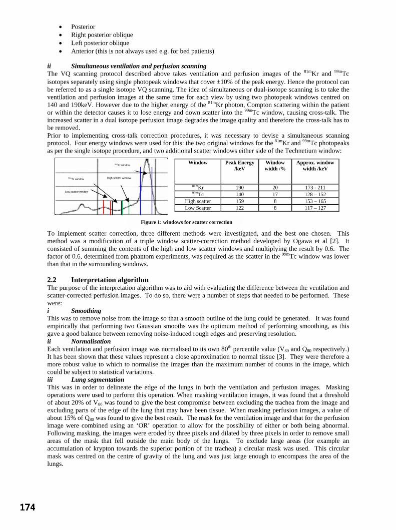
• Posterior • Right posterior oblique • Left posterior oblique • Anterior (this is not always used e.g. for bed patients)

ii Simultaneous ventilation and perfusion scanning The VQ scanning protocol described above takes ventilation and perfusion images of the 81mKr and 99mTc isotopes separately using single photopeak windows that cover ±10% of the peak energy. Hence the protocol can be referred to as a single isotope VQ scanning. The idea of simultaneous or dual-isotope scanning is to take the ventilation and perfusion images at the same time for each view by using two photopeak windows centred on 140 and 190keV. However due to the higher energy of the 81mKr photon, Compton scattering within the patient or within the detector causes it to lose energy and down scatter into the 99mTc window, causing cross-talk. The increased scatter in a dual isotope perfusion image degrades the image quality and therefore the cross-talk has to be removed. Prior to implementing cross-talk correction procedures, it was necessary to devise a simultaneous scanning protocol. Four energy windows were used for this: the two original windows for the 81mKr and 99mTc photopeaks as per the single isotope procedure, and two additional scatter windows either side of the Technetium window:

To implement scatter correction, three different methods were investigated, and the best one chosen. This method was a modification of a triple window scatter-correction method developed by Ogawa et al [2]. It consisted of summing the contents of the high and low scatter windows and multiplying the result by 0.6. The factor of 0.6, determined from phantom experiments, was required as the scatter in the 99mTc window was lower than that in the surrounding windows. 2.2 Interpretation algorithm The purpose of the interpretation algorithm was to aid with evaluating the difference between the ventilation and scatter-corrected perfusion images. To do so, there were a number of steps that needed to be performed. These were: i Smoothing This was to remove noise from the image so that a smooth outline of the lung could be generated. It was found empirically that performing two Gaussian smooths was the optimum method of performing smoothing, as this gave a good balance between removing noise-induced rough edges and preserving resolution. ii Normalisation Each ventilation and perfusion image was normalised to its own 80th percentile value (V80 and Q80 respectively.) It has been shown that these values represent a close approximation to normal tissue [3]. They were therefore a more robust value to which to normalise the images than the maximum number of counts in the image, which could be subject to statistical variations. iii Lung segmentation This was in order to delineate the edge of the lungs in both the ventilation and perfusion images. Masking operations were used to perform this operation. When masking ventilation images, it was found that a threshold of about 20% of V80 was found to give the best compromise between excluding the trachea from the image and excluding parts of the edge of the lung that may have been tissue. When masking perfusion images, a value of about 15% of Q80 was found to give the best result. The mask for the ventilation image and that for the perfusion image were combined using an ‘OR’ operation to allow for the possibility of either or both being abnormal. Following masking, the images were eroded by three pixels and dilated by three pixels in order to remove small areas of the mask that fell outside the main body of the lungs. To exclude large areas (for example an accumulation of krypton towards the superior portion of the trachea) a circular mask was used. This circular mask was centred on the centre of gravity of the lung and was just large enough to encompass the area of the lungs.

Window Peak Energy /keV

Window width /%

Approx. window width /keV

81mKr 190 20 173 - 211 99mTc 140 17 128 – 152

High scatter 159 8 153 – 165 Low Scatter 122 8 117 – 127

99mTc window

81mKr window

Low scatter window

High scatter window

Figure 1: windows for scatter correction

iv Filtration The next step in the image processing chain was to filter the original ventilation and scatter-corrected perfusion images, so that their statistical fluctuations would be suppressed prior to comparison. A variety of different filters were examined. A Butterworth filter, with a cut-off of 0.16 and an order of 20, was found to give the best compromise between noise reduction and preservation of low spatial frequencies that could contain diagnostically useful information. v Comparison of ventilation and perfusion images For the purposes of comparing the relative number of counts in ventilation and perfusion images, several algorithms have already been developed. Among these are subtraction algorithms and quotient algorithms [4]. It was noticed that these two algorithms suffer from drawbacks. In particular, subtraction algorithms tend to underestimate the significance of relative changes in the number of counts at the edges of the lung where counts per pixel are lower, whilst quotient algorithms tend to overestimate this significance. In order to overcome these drawbacks, a novel approach was developed. This approach sought to find the percentage changes in the number of counts, by calculating max[(V-Q)/V], and max[(Q-V)/Q], where V and Q are the ventilation and perfusion images respectively, both having been filtered, normalised and segmented as described above. The two images generated by these two algorithms would then be displayed with a threshold of 0 and a saturation of 1. To evaluate this novel technique with respect to the existing techniques, the quotient image (V/Q) was calculated and displayed with a threshold of 0 and a saturation of 10, and the subtraction images (i.e. max[V-Q, 0] and max[Q-V,0]) were calculated and displayed with a threshold of 0 and a saturation of 1. To display the results of these algorithms, a colour scale was created. This colour scale had white as its threshold colour and red as its saturation colour so that emboli towards the edge of the lung would have a strong contrast against the white background. Since the images were consistently scaled, the different colours could be interpreted as representing a specific range of perfusion loss. vi Abnormal tissue windowing The mean and standard deviation number of counts of the ventilation and perfusion images of each of a group of five patients designated as normal were found. From these values, the mean mean (µ) and the RMS standard deviation (σ) of the number of counts was found for each of the four views: anterior, posterior, right posterior oblique and left posterior oblique. The performances of two thresholds ((µ+3σ) and (µ+2σ)) were compared for each of the following three algorithms: V/Q displayed between 0 and 10, max[V-Q, 0] displayed between 0 and 1, and max[(V-Q)/V, 0] displayed between 0 and 1. A single erode and dilate was used to remove stray noise from each of these windows. 2.3 Evaluation of techniques To test the scatter correction algorithm, 20 pairs of ventilation/perfusion images were presented to two different observers (a consultant physicist and a consultant doctor). These pairs of images corresponded to 10 patients, with two pairs for each patient: one corresponding to single isotope ventilation/perfusion images, and the other corresponding to the scatter-corrected dual isotope ventilation/perfusion images. The single-isotope method was regarded as being the truth. Of these 10 patients, 6 had unmatched defects, two were normal and two had matched defects. A score was given to each lobe of the lung based on the likelihood of it containing an embolism. For each observer, a Spearman’s ranked correlation coefficient was used to assess both the simultaneous lobe scores versus the truth and, in order to test the observer’s consistency, the repeated truth scores versus the truth. In addition, a t-test was performed between the scatter-corrected lobe scores minus the truth, and the repeated truth minus the truth. To evaluate the interpretation algorithm, the output of each individual step was checked visually for consistency and accuracy. 3 Results 3.1 Scatter correction The Spearman’s ranked correlation coefficient tests all gave results at the 99% significance level, with the exception of observer A’s scatter-corrected lobe score versus the single-isotope lobe score, which gave a result at the 95% significance level. The scatter plots for these comparisons are shown on the next page. These show the correlation visually.

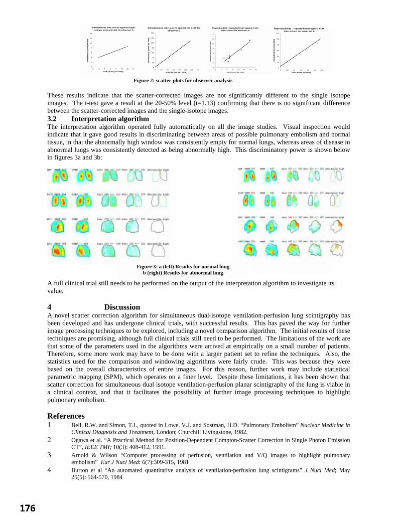
These results indicate that the scatter-corrected images are not significantly different to the single isotope images. The t-test gave a result at the 20-50% level (t=1.13) confirming that there is no significant difference between the scatter-corrected images and the single-isotope images. 3.2 Interpretation algorithm The interpretation algorithm operated fully automatically on all the image studies. Visual inspection would indicate that it gave good results in discriminating between areas of possible pulmonary embolism and normal tissue, in that the abnormally high window was consistently empty for normal lungs, whereas areas of disease in abnormal lungs was consistently detected as being abnormally high. This discriminatory power is shown below in figures 3a and 3b:

A full clinical trial still needs to be performed on the output of the interpretation algorithm to investigate its value. 4 Discussion A novel scatter correction algorithm for simultaneous dual-isotope ventilation-perfusion lung scintigraphy has been developed and has undergone clinical trials, with successful results. This has paved the way for further image processing techniques to be explored, including a novel comparison algorithm. The initial results of these techniques are promising, although full clinical trials still need to be performed. The limitations of the work are that some of the parameters used in the algorithms were arrived at empirically on a small number of patients. Therefore, some more work may have to be done with a larger patient set to refine the techniques. Also, the statistics used for the comparison and windowing algorithms were fairly crude. This was because they were based on the overall characteristics of entire images. For this reason, further work may include statistical parametric mapping (SPM), which operates on a finer level. Despite these limitations, it has been shown that scatter correction for simultaneous dual isotope ventilation-perfusion planar scintigraphy of the lung is viable in a clinical context, and that it facilitates the possibility of further image processing techniques to highlight pulmonary embolism. References 1 Bell, R.W. and Simon, T.L, quoted in Lowe, V.J. and Sostman, H.D. “Pulmonary Embolism” Nuclear Medicine in

Clinical Diagnosis and Treatment, London; Churchill Livingstone, 1982. 2 Ogawa et al. “A Practical Method for Position-Dependent Compton-Scatter Correction in Single Photon Emission

CT”, IEEE TMI; 10(3): 408-412, 1991. 3 Arnold & Wilson “Computer processing of perfusion, ventilation and V/Q images to highlight pulmonary

embolism” Eur J Nucl Med: 6(7):309-315, 1981 4 Burton et al “An automated quantitative analysis of ventilation-perfusion lung scintigrams” J Nucl Med; May

25(5): 564-570, 1984

Simultaneous lobe scores against single-isotope scores (truth) for observer A

0

2

4

6

8

10

12

14

0 2 4 6 8 10 12 14

truth (score per lobe)

sim

ulta

neou

s (s

core

per

lobe

)

Simultaneous lobe scores against the truth for observer B

0

20

40

60

80

100

120

140

0 20 40 60 80 100 120 140

truth (score per lobe)

sim

ulta

neou

s (s

core

per

lobe

)

Reproducibiliy - repeated truth against truth lobe scores for observer A

0

2

4

6

8

10

12

14

0 2 4 6 8 10 12 14

truth (score per lobe)

repe

ated

trut

h (s

core

per

lobe

)

Reproducibility - repeated truth against truth lobe scores for observer B

0

20

40

60

80

100

120

0 20 40 60 80 100 120

truth (score per lobe)

repe

ated

trut

h (s

core

per

lobe

)

Figure 2: scatter plots for observer analysis

Figure 3: a (left) Results for normal lung b (right) Results for abnormal lung

Analysis of Total Hip Replacements Using Active Ellipses

Stuart Kerrigan1, Stephen McKenna1, Ian W. Ricketts1 and Carlos Wigderowitz2

1Division of Applied Computing, University of Dundee, Dundee, Scotland, DD1 4HN2Orthopaedic and Trauma Surgery, Ninewells Hospital and Medical School, Dundee, Scotland, DD1 9SY

Abstract. A new method for the measurement of acetabular wear in total hip replacements is proposed. Itis more automated than previous methods and uses standard clinical radiographs. Active ellipses with priorknowledge of the intended contour are used to search for the boundaries of the femoral head and acetabularrim. A set of radiographs were manually annotated and the characteristics of these boundaries were learned.Two ellipses were sequentially placed on each radiograph, the first deforming around the boundary of thefemoral head, the second placed using the previously learned model and converging to the wire marker on theacetabular rim. Once both ellipses had converged the distance between their two centres was estimated as ameasure of wear. The method was validated by comparison with a labour intensive method in which ellipseswere fitted to27 manually selected points. The active ellipses method was found to be more repeatable and thetwo methods agreed to the extent that they were considered clinically interchangeable.

1 Introduction

Over 40,000 total hip replacement (THR) operations are performed annually within the UK and over 5,000 of theseare revisions [1]. The majority of failures are due to the displacement of the centre of the femoral head relative tothe centre of the acetabular cup (see Figure 1a) [2]. The aim of the research reported here is to create a new methodfor the analysis of THRs that is more automated, precise, accurate and repeatable than existing methods. There areclear benefits in providing early detection of implant failure, evaluation of surgical techniques and evaluation ofimplant designs.

Analysis of THRs is conducted by a variety of methods including manual methods such as overlaying concentriccircular transparencies on the radiograph and annotation via pencil and rulers on the film or a digitizing tablet.A more automated method is roentgen stereophotogrammetric analysis (RSA) [3] which requires the insertion ofmarkers used as reference points in follow up X-rays. Since the markers are inserted during the operation it cannotbe used retrospectively. Semi-automated image processing techniques have been implemented [4], [5] for use withstandard radiographs. These techniques use edge detection but do not use any prior knowledge of the distinctcontour of the femoral head or wire rim and require considerable user interaction. Also of note are Cootes andTaylor’s Active Shape Models (ASMs), deformable models trained using examples to locate structures in images,in particular hip implants [6]. They have not been used for the measurement of acetabular wear.

Figure 1. a) A radiograph of the Zimmer CPT prosthesis. b) Annotation of the femoral head with 9 approximatelyequi-spaced points. Numbers correspond to the order of annotation. c) Annotation of the acetabular rim showingthe ordering of points on the right wing of the rim. Points are concentrated in areas of high curvature.

2 Method

The method proposed uses active ellipses and models of the normalised grey-level derivatives around the boundaryof the femoral head and the acetabular rim. These models are learned from a set of manually digitized and annotated

1) skerrigan, stephen, [email protected], 2) [email protected]

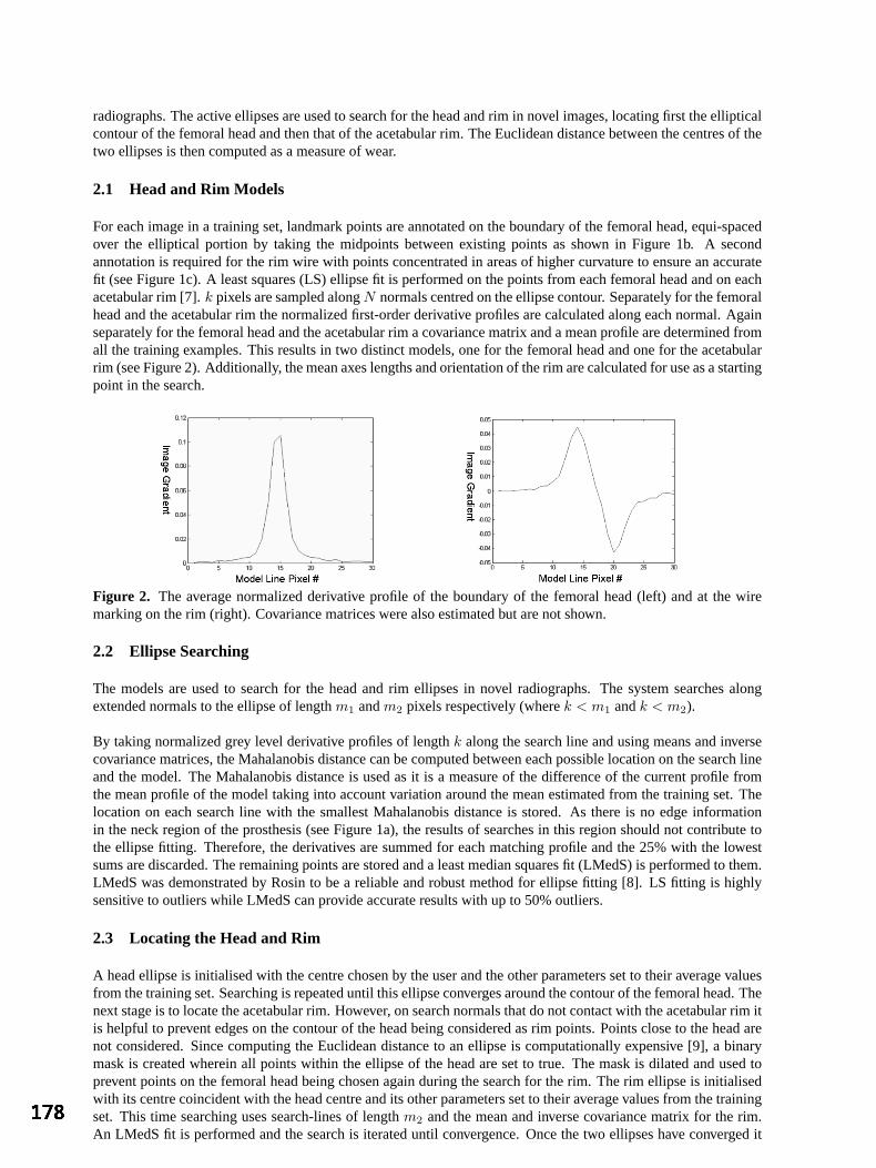
radiographs. The active ellipses are used to search for the head and rim in novel images, locating first the ellipticalcontour of the femoral head and then that of the acetabular rim. The Euclidean distance between the centres of thetwo ellipses is then computed as a measure of wear.

2.1 Head and Rim Models

For each image in a training set, landmark points are annotated on the boundary of the femoral head, equi-spacedover the elliptical portion by taking the midpoints between existing points as shown in Figure 1b. A secondannotation is required for the rim wire with points concentrated in areas of higher curvature to ensure an accuratefit (see Figure 1c). A least squares (LS) ellipse fit is performed on the points from each femoral head and on eachacetabular rim [7].k pixels are sampled alongN normals centred on the ellipse contour. Separately for the femoralhead and the acetabular rim the normalized first-order derivative profiles are calculated along each normal. Againseparately for the femoral head and the acetabular rim a covariance matrix and a mean profile are determined fromall the training examples. This results in two distinct models, one for the femoral head and one for the acetabularrim (see Figure 2). Additionally, the mean axes lengths and orientation of the rim are calculated for use as a startingpoint in the search.

Figure 2. The average normalized derivative profile of the boundary of the femoral head (left) and at the wiremarking on the rim (right). Covariance matrices were also estimated but are not shown.

2.2 Ellipse Searching

The models are used to search for the head and rim ellipses in novel radiographs. The system searches alongextended normals to the ellipse of lengthm1 andm2 pixels respectively (wherek < m1 andk < m2).

By taking normalized grey level derivative profiles of lengthk along the search line and using means and inversecovariance matrices, the Mahalanobis distance can be computed between each possible location on the search lineand the model. The Mahalanobis distance is used as it is a measure of the difference of the current profile fromthe mean profile of the model taking into account variation around the mean estimated from the training set. Thelocation on each search line with the smallest Mahalanobis distance is stored. As there is no edge informationin the neck region of the prosthesis (see Figure 1a), the results of searches in this region should not contribute tothe ellipse fitting. Therefore, the derivatives are summed for each matching profile and the 25% with the lowestsums are discarded. The remaining points are stored and a least median squares fit (LMedS) is performed to them.LMedS was demonstrated by Rosin to be a reliable and robust method for ellipse fitting [8]. LS fitting is highlysensitive to outliers while LMedS can provide accurate results with up to 50% outliers.

2.3 Locating the Head and Rim

A head ellipse is initialised with the centre chosen by the user and the other parameters set to their average valuesfrom the training set. Searching is repeated until this ellipse converges around the contour of the femoral head. Thenext stage is to locate the acetabular rim. However, on search normals that do not contact with the acetabular rim itis helpful to prevent edges on the contour of the head being considered as rim points. Points close to the head arenot considered. Since computing the Euclidean distance to an ellipse is computationally expensive [9], a binarymask is created wherein all points within the ellipse of the head are set to true. The mask is dilated and used toprevent points on the femoral head being chosen again during the search for the rim. The rim ellipse is initialisedwith its centre coincident with the head centre and its other parameters set to their average values from the trainingset. This time searching uses search-lines of lengthm2 and the mean and inverse covariance matrix for the rim.An LMedS fit is performed and the search is iterated until convergence. Once the two ellipses have converged it

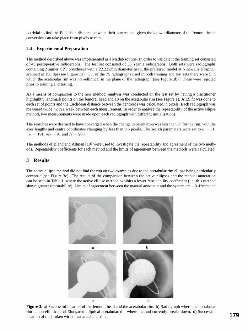
is trivial to find the Euclidean distance between their centres and given the known diameter of the femoral head,conversion can take place from pixels to mm.

2.4 Experimental Preparation

The method described above was implemented as a Matlab routine. In order to validate it the training set consistedof 45 postoperative radiographs. The test set consisted of 30 Year 1 radiographs. Both sets were radiographscontaining Zimmer CPT prostheses with a 22.225mm diameter head, the preferred model at Ninewells Hospital,scanned at 150 dpi (see Figure 3a). Out of the 75 radiographs used in both training and test sets there were 5 inwhich the acetabular rim was non-elliptical in the plane of the radiograph (see Figure 3b). These were rejectedprior to training and testing.

As a means of comparison to the new method, analysis was conducted on the test set by having a practitionerhighlight 9 landmark points on the femoral head and 18 on the acetabular rim (see Figure 1). A LS fit was done toeach set of points and the Euclidean distance between the centroids was calculated in pixels. Each radiograph wasmeasured twice, with a week between each measurement. In order to analyse the repeatability of the active ellipsemethod, two measurements were made upon each radiograph with different initialisations.

The searches were deemed to have converged when the change in orientation was less than6 for the rim, with theaxes lengths and centre coordinates changing by less than0.5 pixels. The search parameters were set tok = 31,m1 = 191, m2 = 91 andN = 200.

The methods of Bland and Altman [10] were used to investigate the repeatability and agreement of the two meth-ods. Repeatability coefficients for each method and the limits of agreement between the methods were calculated.

3 Results

The active ellipse method did not find the rim on two examples due to the acetabular rim ellipse being particularlyeccentric (see Figure 3c). The results of the comparison between the active ellipses and the manual annotationcan be seen in Table 1, where the active ellipse method exhibits a lower repeatability coefficient (i.e. this methodshows greater repeatability). Limits of agreement between the manual annotator and the system are−0.42mm and

Figure 3. a) Successful location of the femoral head and the acetabular rim. b) Radiograph where the acetabularrim is non-elliptical. c) Elongated elliptical acetabular rim where method currently breaks down. d) Successfullocation of the broken wire of an acetabular rim.

0.47mm. These limits of agreement are well below values of migration considered clinically relevant and thus theactive ellipse method could replace the manual annotation method.

Technique RepeatabilityCoefficient (mm)

Manual Annotation 1.70Active Ellipse 1.35

Table 1. Repeatability coefficients for the methods using a) LS fitting to 27 manually selected points and b) LMedSfitting using active ellipse models.

4 Discussion

The robust active ellipses method has been compared to a more labour intensive method involving least squaresfitting to 27 manually selected points. The active ellipses method was found to be more repeatable and the twomethods agreed to the extent that they are clinically interchangeable.

Searching for the acetabular rim does not work with particularly elongated ellipses (see Figure 3c). If there is anadditional wire marker inside the cup (see Figure 3b) it should be possible to estimate wear by fitting an ellipseto this instead of the rim. The method presented here could be extended to other prosthesis designs given suitabletraining data. It should also be possible to build additional models to locate the edge of plastic or metal-backedrims without wire marking.

Future work will include use in a clinical study of wear, comparison with other methods (such as RSA), the effecton the repeatability of decreasing the convergence criteria decided upon in Section 2.4 and general improvementof the LMedS fitting. The limitation towards dealing with eccentric rims is being investigated via consideration ofthe merits of geometric ellipse fitting [9].

Despite these limitations the advantages over existing methods remain. These include exploitation of the differencebetween the profiles of the contours of the femoral head and acetabular rim, robustness as the method is able to copewith deformities of the wire marker while maintaining an elliptical shape (see Figure 3d) and the direct applicationof the shape model to measuring acetabular wear.

Acknowledgements

Special thanks to Jeremy Martindale of the Surgical Skills Unit, Ninewells, for use of the radiographs, KarthikPingle for help with the comparative method, Lynda Cochrane for drawing attention to Bland and Altman’s methodand Zimmer Corporation for funding this research.

References

1. A. Murray, D.W. Carr & C. Bulstrode. “Which primary total hip replacement?”Journal of Bone and Joint Surgery77-B,pp. 520–527, 1995.

2. M. Huo & S. Cook. “Speciality update: What’s new in hip arthroplasty.”Journal of Bone and Joint Surgery83-A,pp. 1598–1610, 2001.

3. J. Karrholm. “Roentgen stereophotogrammetry: An overview of orthopedic applications.”Acta Orthop Scand60, pp. 491–503, 1989.

4. S. Shaver, T. Brown, S. Hillis et al. “Digital edge-detection measurement of polyethylene wear after total hip arthroplasty.”Journal of Bone and Joint Surgery79-A, pp. 690–700, 1997.

5. F. Hatfield, R. Hall, R. King et al. “Image analysis of wear in total hip replacements.”Proceedings of Medical ImageUnderstanding and Analysis2001.

6. A. Redhead, A. Kotcheff, C. Taylor et al. “An automated method for assessing routine radiographs of patients with totalhip replacements.”Proceedings of the Institution of Mechanical Engineers211, pp. 145–154, 1997.

7. A. Fitzgibbon, M. Pilu & R. Fisher. “Direct least square fitting of ellipses.”IEEE Transactions on Pattern Analysis andMachine Intelligence21(5), pp. 476–480, 1999.

8. P. Rosin. “Further five-point fit ellipse fitting.”Graphical Models and Image Processing61(5), pp. 245–259, 1999.9. S. J. Ahn, W. Rauh & H. J. Warnecke. “Least-squares orthogonal distances fitting of circle, sphere, ellipse, hyperbola and

parabola.”Pattern Recognition34, pp. 2283–2303, 2001.10. J. Bland & D. Altman. “Statistical methods for assessing agreement between two methods of clinical measurement.”

Lanceti, pp. 307–310, 1986.

An Automated Algorithm for Breast Background Segmentation

Styliani Petroudia∗, Michael Bradya

aMedical Vision Laboratory, Engineering Science, Oxford University,Ewert House, Ewert Place, Summertown, Oxford, OX2 7DD, United Kingdom

Abstract. Accurate and robust segmentation of breast and non-breast regions is a basic requirement for im-age analysis of mammograms. Unfortunately, the problem is made difficult by the presence of labels, digitiserwedges, and the weakly controlled way in which the breast is positioned in the mammography machine. Thispaper describes an accurate and robust algorithm for automatic breast-background segmentation. The algorithmis based on intrinsic image properties and can be easily adapted to images with different gray-scales and resolu-tions. A reliable skin-background boundary is particularly important for mammogram registration and featureextraction. The new segmentation technique is compared to other methods and its performance is illustratedwith examples.

1 Introduction

Breast cancer is one of the leading causes of death for women. Computer Aided Diagnosis (CAD) techniques arecrucial tools for the analysis of mammographic images and for developing algorithms to aid in the early detectionof breast cancer. CAD, and every other mammographic image processing problem such as 3D reconstruction ofthe breast and non-rigid registration of mammograms, depend upon accurate segmentation of the breast regionfrom the background. Casual inspection of a mammogram suggests that this is a trivial problem which mightbe solved, for example, by thresholding. Unfortunately, such simple algorithms are not effective, as the problemis made difficult by the presence of labels, digitiser wedges, and the weakly controlled way in which the breastis positioned in the mammography machine. Segmentation of the breast region is generally considered to be aneasier problem for full-field digital mammograms; but these are not yet widely available, and there are, in any case,millions of mammograms awaiting digitisation and analysis.

An x-ray mammogram is a projection of a compressed breast with an intensity range between the low intensitiesof the background and the high intensities of the digitiser artefacts. Evaluation of the transition between theregions is difficult due to the high optical density of the skin and subcutaneous tissue. This is a direct result of themammographic processing technique [1], since due to the compression applied to the breast during mammogramacquisition, the breast edge is mainly composed of fat.

Various techniques have been implemented for addressing the breast-border segmentation step. Algorithms inthe literature include use of local gray-value range on modified histogram analysis, border region search methodsbased on the gradient of gray values, [2] [3], etc. Ferrari et al.’s [4] skin-air boundary segmentation algorithmapplies contrast correction with a logarithmic operation applied to the entire image as a contrast correction stepfollowed by thresholding. However, extensive smoothing eliminates the nipple contour in a number of cases.Karssemeijer [1] applies global thresholding that results in a binarized image of the breast region. The method isstraightforward and fast, but not very reliable as it always results in underestimation of the breast region and lossof the nipple contour.

Highnam and Brady [5] developed an algorithm for breast-background segmentation as a first step in their newStandard Mammogram Form model. Linear Hough transforms are applied to the mammogram, in the areas wherethe film edges should appear. A gradient operator is applied to the resulting image followed by thresholding toremove background pixels that have lower gradients. Any wrongly marked pixels are removed with binary mor-phological erosion. A closing operator is applied to make the breast and background regions into coherent areas.Some morphological post-processing may be required to remove labels and touch the breast edge for smoothness.The segmentation is found to be efficient and robust. However, in mammograms, the background pixels near thelabels may also have gradients higher than the rest of the background and this could have the effect of introducingwrong breast regions. Sometimes the breast border appears somewhat jagged, and the nipple is not preserved.

This paper reports a new, fully automated breast and background region segmentation technique that reliablyidentifies the breast area, removes any labels and digitiser introduced wedges, and provides a smooth breast contour.Importantly, it also preserves the nipple, a key landmark for registration and three dimensional reconstruction.

∗Email: [email protected]

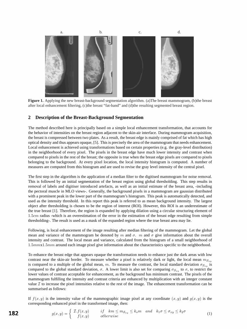
a. b. c. d.

Figure 1. Applying the new breast-background segmentation algorithm. (a)The breast mammogram, (b)the breastafter local enhancement filtering, (c)the breast “fat-band” and (d)the resulting segmented breast region.

2 Description of the Breast-Background Segmentation

The method described here is principally based on a simple local enhancement transformation, that accounts forthe behavior of intensities on the breast region adjacent to the skin-air interface. During mammogram acquisition,the breast is compressed between two plates. As a result, the breast edge is mainly comprised of fat which has highoptical density and thus appears opaque, [5]. This is precisely the area of the mammogram that needs enhancement.Local enhancement is achieved using transformations based on certain properties (e.g. the gray-level distribution)in the neighborhood of every pixel. The pixels in the breast edge have much lower intensity and contrast whencompared to pixels in the rest of the breast; the opposite is true when the breast edge pixels are compared to pixelsbelonging to the background. At every pixel location, the local intensity histogram is computed. A number ofmeasures are computed from this histogram and are used to revise the gray level intensity of the central pixel.

The first step in the algorithm is the application of a median filter to the digitised mammogram for noise removal.This is followed by an initial segmentation of the breast region using global thresholding. This step results inremoval of labels and digitiser introduced artefacts, as well as an initial estimate of the breast area, -includingthe pectoral muscle in MLO views-. Generally, the background pixels in a mammogram are gaussian distributedwith a prominent peak in the lower part of the mammogram’s histogram. This peak is automatically detected, andused as the intensity threshold. In this report this peak is referred to as mean background intensity. The largestobject after thresholding is chosen to be the region of interest (ROI). However, this ROI is an underestimate ofthe true breast [1]. Therefore, the region is expanded by applying dilation using a circular structuring element of1.5cm radius -which is an overestimation of the error in the estimation of the breast edge resulting from simplethresholding-. The result is used as a mask of the expanded region where the true breast area may lie.

Following, is local enhancement of the image resulting after median filtering of the mammogram. Let the globalmean and variance of the mammogram be denoted bym andσ. m andσ give information about the overallintensity and contrast. The local mean and variance, calculated from the histogram of a small neighborhood of1.5mmx1.5mm around each image pixel give information about the characteristics specific to the neighborhood.

To enhance the breast edge that appears opaque the transformation needs to enhance just the dark areas with lowcontrast near the skin-air border. To measure whether a pixel is relatively dark or light, the local meanmSxy

is compared to a multiple of the global mean,m. To measure the contrast, the local standard deviationσSxy iscompared to the global standard deviation,σ. A lower limit is also set for comparingσSxy to σ, to restrict thelower values of contrast acceptable for enhancement, as the background has minimum contrast. The pixels of themammogram fulfilling the intensity and contrast criteria are enhanced by multiplication with an integer constantvalueI to increase the pixel intensities relative to the rest of the image. The enhancement transformation can besummarised as follows:

If f(x, y) is the intensity value of the mammographic image pixel at any coordinate(x, y) and g(x, y) is thecorresponding enhanced pixel in the transformed image, then:

g(x, y) = I.f(x, y) if km ≤ mSxy ≤ kom and k1σ ≤ σxy ≤ k2σ

f(x, y) otherwise(1)

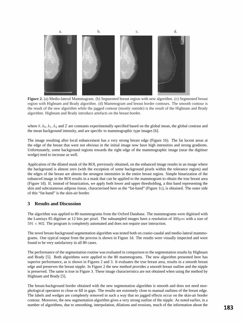
a. b. c. d.

Figure 2. (a) Medio-lateral Mammogram. (b) Segmented breast region with new algorithm. (c) Segmented breastregion with Highnam and Brady algorithm. (d) Mammogram and breast border contours. The smooth contour isthe result of the new algorithm while the jagged contour (mostly outside) is the result of the Highnam and Bradyalgorithm. Highnam and Brady introduce artefacts on the breast border.

wherek, k0, k1, k2 andI are constants experimentally specified based on the global mean, the global contrast andthe mean background intensity, and are specific to mammographic type images [6].

The image resulting after local enhancement has a very strong breast edge (Figure 1b). The fat lucent areas atthe edge of the breast that were not obvious in the initial image now have high intensities and strong gradients.Unfortunately, some background regions towards the right edge of the mammographic image (near the digitiserwedge) tend to increase as well.

Application of the dilated mask of the ROI, previously obtained, on the enhanced image results in an image wherethe background is almost zero (with the exception of some background pixels within the tolerance region) andthe edges of the breast are almost the strongest intensities in the entire breast region. Simple binarization of theenhanced image in the ROI results in a mask that can be applied to the mammogram to obtain the true breast area(Figure 1d). If, instead of binarization, we apply both lower and upper thresholding, a thin band representing theskin and subcutaneous adipose tissue, characterised here as the “fat-band” (Figure 1c), is obtained. The outer sideof this “fat-band” is the skin-air border.

3 Results and Discussion

The algorithm was applied to 80 mammograms from the Oxford Database. The mammograms were digitised withthe Lumisys 85 digitiser at 12 bits per pixel. The subsampled images have a resolution of300µm with a size of591× 802. The program is completely automated and does not require user interaction.

The novel breast-background segmentation algorithm was tested both on cranio-caudal and medio-lateral mammo-grams. One typical output from the process is shown in Figure 1d. The results were visually inspected and werefound to be very satisfactory in all 80 cases.

The performance of the segmentation routine was evaluated in comparison to the segmentation results by Highnamand Brady [5]. Both algorithms were applied to the 80 mammograms. The new algorithm presented here hassuperior performance, as is shown in Figures 2 and 3. It evaluates the true breast area, results in a smooth breastedge and preserves the breast nipple. In Figure 2 the new method provides a smooth breast outline and the nippleis preserved. The same is true in Figure 3. These image characteristics are not obtained when using the method byHighnam and Brady [5].

The breast-background border obtained with the new segmentation algorithm is smooth and does not need mor-phological operators to close or fill in gaps. The results are extremely close to manual outlines of the breast edge.The labels and wedges are completely removed in such a way that no jagged effects occur on the skin-air bordercontour. Moreover, the new segmentation algorithm gives a very strong outline of the nipple. As noted earlier, in anumber of algorithms, due to smoothing, interpolation, dilations and erosions, much of the information about the

a. b. c. d.

Figure 3. (a) Cranio-Caudal Mammogram. (b) Segmented breast region with new algorithm. (c) Segmented breastregion with Highnam and Brady algorithm. (d) Mammogram and breast border contours. The smooth contour thatpreserves the nipple is the result of the new algorithm while the other contour is the result of the Highnam andBrady algorithm.

nipple is lost or falsified. When the edge “fat-band” is estimated, the nipple is clearly outlined in both the inner andouter side. In cases where the nipple is not in profile, it is outlined in the leftmost side of the “fat-band” (Figure1c). This result is very important in nipple detection especially in cases where the nipple is inside the breast edgeand consequently very difficult to detect. Moreover, the “fat-band” can be used in algorithms for more accurateestimation of breast thickness during mammogram acquisition.

4 Conclusions

A new method for breast segmentation based on local enhancement is presented. An intermediate step of thealgorithm provides a strong outline of the nipple in all cases, independently of whether the nipple is in profileor not. Accurate segmentation of the breast boundary is very important in providing the correct breast regionfor CAD analysis. It is important in developing automated, quantitative and objective measures for early breastcancer diagnosis, evaluation and clinical assessment. Since a number of measures rely on the skin-line positionfor feature extraction, inaccurate breast boundary estimation may have a negative effect on the results. The initialevaluation results for this segmentation algorithm are very promising and this algorithm has since been used asa pre-processing step to improve the performance of CAD systems, to perform nipple detection and to improveregistration algorithms, [7].

Acknowledgements

The authors would like to acknowledge and thank Cancer Research UK for supporting this work. In addition theauthors thank Mirada Solutions (http:///www.mirada-solutions.com) for the Standard Mammogram Form genera-tion software.

References

1. N. Karssemeijer. “Automated classification of parenchymal patterns in mammograms.”Physics in Medicine and Biology43, pp. 365–378, 1998.

2. U. Bick, M. Giger, R. Schmidt et al. “Automated segmentation of digitized mammograms.”Academic Radiology2, pp. 1–9,1995.

3. R. Chandrasekhar & Y. Attikiouzel. “Automatic breast border segmentation by background modeling and subtraction.” InInternational Workshop on Digital Mammography 2000, pp. 560–565. 2000.

4. R. Ferrari, R. Rangayyan, J. Desautels et al. “Segmentation of mammograms: Identification of the skin-air boundary,pectoral muscle, and fibroglandular disc.” InInternational Workshop on Digital Mammography 2000, pp. 573–579. 2000.

5. R. Highnam & M. Brady.Mammographic Image Analysis. Kluwer Academic Publishers, 1999.6. R. Gonzalez & R. Woods.Digital Image Processing. Addison-Wesley Publishing Company, 1993.7. K. Marias, C. P. Behrenbruch, M. Brady et al. “Multi-scale landmark selection for improved registration of temporal

mammograms.” InInternational Workshop on Digital Mammography 2000, pp. 581–585. 2000.

An Artificially Evolved Vision System for Segmenting Skin LesionImages

Mark E. Roberts and Ela Claridge∗

School of Computer Science, University of Birmingham, B15 2TT, UK

Abstract. We present a novel technique where a medical image segmentation system is evolved using ge-netic programming. The evolved system was trained on just 8 images outlined by a clinical expert and gener-alised well, achieving high performance rates on over 90 unseen test images (average sensitivity 88% , averagespecificity 96%). This method learns by example and produces fully automatic algorithms needing no humaninteraction or parameter tuning, and although complex, runs in approximately 4 seconds.

1 Introduction

In many areas of medicine, images are used as a diagnostic aid, but images in themselves only partially contribute.Crucially, input comes from interpretation of the image by an expert using the power of the human visual system.This human system works in real time, does not need carefully tuned parameters, and perhaps most importantly, isable to learn by example to recognise general image features. These qualities provide the inspiration for this work.We present here a method which learns by example, and produces fully automatic, parameter-free algorithms toidentify given features.

The diagnosis of malignant melanoma at the primary care level is difficult because at the early stages it maylook similar to innocent pigmented lesions – “moles”. Moderate diagnostic rates achieved by dermatologists [1]confirm this difficulty and for this reason there is a growing body of work on using image analysis methods to aidthe diagnosis of melanoma [2]. The diagnosis first requires the segmentation of the lesion from the surroundingskin, which is a difficult task, mainly due to the variability in lesion appearance. Some lesions are well delineatedand make good contrast with the skin, whereas others are indistinct, variegated and difficult to see by an untrainedeye. The published methods use a variety of approaches, including threshold-based methods [3], colour clusteringand distance functions in a colour space [3,4], edge modeling [5,6] and various combinations of these [7].

What these methods have in common is the fact that they all have been developed by image analysis experts, inmost cases informed by clinical practitioners. This paper describes a very different approach, in which expertisein image analysis is not necessary for being able to create a well performing image processing system, in thiscase for lesion segmentation. This is achieved through the use of an evolutionary computation technique - geneticprogramming (GP) in which a lesion segmentation system is automatically evolved, purely on the basis of examplesegmentations provided by an expert clinician. The paper first outlines the concept of genetic programming. Thisis followed by the description of a study in lesion segmentation using GP, its results and discussion.

2 Materials and Methods

2.1 Pigmented Lesion Images

A set of 100 pigmented lesion images is used in this study. The images were acquired using a SIAscope [8], adevice designed specifically for skin imaging, that takes a number of images of the same area of the skin at differentwavelengths. In its normal mode of operation it uses an optical model of the skin to compute parametric mapsshowing the distribution and levels of individual histological components of the skin such as melanin, haemoglobinand collagen [8]. In this study images acquired in the blue band are used because of strong absorption by bothmelanin and blood makes the lesions stand out against the skin background. Image resolution is 40 microns perpixel and a circular area with radius of 280 pixels is used. A ”ground truth” data set in the form of binary images,is created from outlines drawn by a clinical expert at Addenbrooke’s Hospital, Cambridge, UK.

2.2 Genetic Programming

Genetic Programming (GP) is a powerful extension to the genetic algorithm (GA) paradigm which evolves popu-lations of computer programs as opposed to the simplistic binary strings used in GAs. These programs are repre-

∗Email: M.E.Roberts,[email protected]

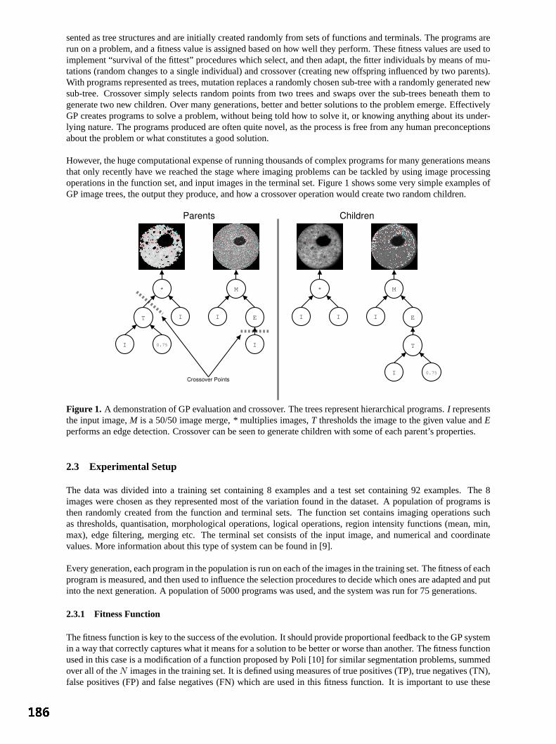
sented as tree structures and are initially created randomly from sets of functions and terminals. The programs arerun on a problem, and a fitness value is assigned based on how well they perform. These fitness values are used toimplement “survival of the fittest” procedures which select, and then adapt, the fitter individuals by means of mu-tations (random changes to a single individual) and crossover (creating new offspring influenced by two parents).With programs represented as trees, mutation replaces a randomly chosen sub-tree with a randomly generated newsub-tree. Crossover simply selects random points from two trees and swaps over the sub-trees beneath them togenerate two new children. Over many generations, better and better solutions to the problem emerge. EffectivelyGP creates programs to solve a problem, without being told how to solve it, or knowing anything about its under-lying nature. The programs produced are often quite novel, as the process is free from any human preconceptionsabout the problem or what constitutes a good solution.

However, the huge computational expense of running thousands of complex programs for many generations meansthat only recently have we reached the stage where imaging problems can be tackled by using image processingoperations in the function set, and input images in the terminal set. Figure 1 shows some very simple examples ofGP image trees, the output they produce, and how a crossover operation would create two random children.

T

I

M

I E

I

*

I

M

I E

*

I

T

I

I

0.75

0.75

Crossover Points

Parents Children

Figure 1. A demonstration of GP evaluation and crossover. The trees represent hierarchical programs.I representsthe input image,M is a 50/50 image merge,* multiplies images,T thresholds the image to the given value andEperforms an edge detection. Crossover can be seen to generate children with some of each parent’s properties.

2.3 Experimental Setup

The data was divided into a training set containing 8 examples and a test set containing 92 examples. The 8images were chosen as they represented most of the variation found in the dataset. A population of programs isthen randomly created from the function and terminal sets. The function set contains imaging operations suchas thresholds, quantisation, morphological operations, logical operations, region intensity functions (mean, min,max), edge filtering, merging etc. The terminal set consists of the input image, and numerical and coordinatevalues. More information about this type of system can be found in [9].

Every generation, each program in the population is run on each of the images in the training set. The fitness of eachprogram is measured, and then used to influence the selection procedures to decide which ones are adapted and putinto the next generation. A population of 5000 programs was used, and the system was run for 75 generations.

2.3.1 Fitness Function

The fitness function is key to the success of the evolution. It should provide proportional feedback to the GP systemin a way that correctly captures what it means for a solution to be better or worse than another. The fitness functionused in this case is a modification of a function proposed by Poli [10] for similar segmentation problems, summedover all of theN images in the training set. It is defined using measures of true positives (TP), true negatives (TN),false positives (FP) and false negatives (FN) which are used in this fitness function. It is important to use these

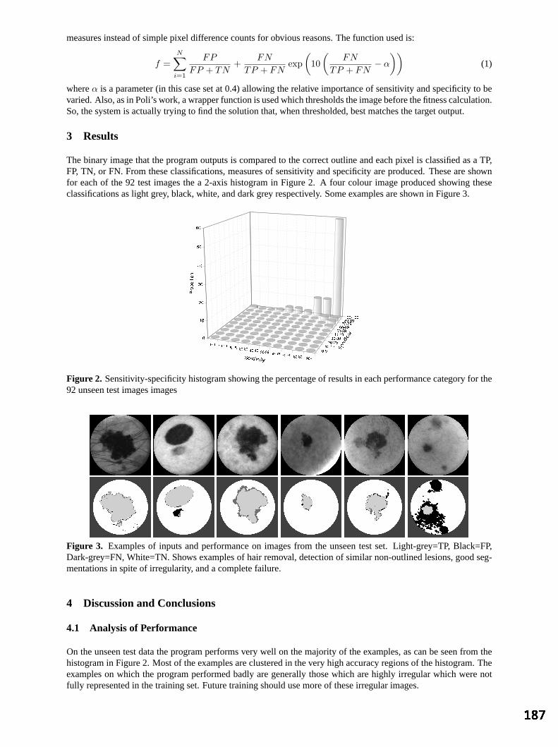
measures instead of simple pixel difference counts for obvious reasons. The function used is:

f =N∑

i=1

FP

FP + TN+

FN

TP + FNexp

(10

(FN

TP + FN− α

))(1)

whereα is a parameter (in this case set at 0.4) allowing the relative importance of sensitivity and specificity to bevaried. Also, as in Poli’s work, a wrapper function is used which thresholds the image before the fitness calculation.So, the system is actually trying to find the solution that, when thresholded, best matches the target output.

3 Results

The binary image that the program outputs is compared to the correct outline and each pixel is classified as a TP,FP, TN, or FN. From these classifications, measures of sensitivity and specificity are produced. These are shownfor each of the 92 test images the a 2-axis histogram in Figure 2. A four colour image produced showing theseclassifications as light grey, black, white, and dark grey respectively. Some examples are shown in Figure 3.

Figure 2. Sensitivity-specificity histogram showing the percentage of results in each performance category for the92 unseen test images images

Figure 3. Examples of inputs and performance on images from the unseen test set. Light-grey=TP, Black=FP,Dark-grey=FN, White=TN. Shows examples of hair removal, detection of similar non-outlined lesions, good seg-mentations in spite of irregularity, and a complete failure.

4 Discussion and Conclusions

4.1 Analysis of Performance

On the unseen test data the program performs very well on the majority of the examples, as can be seen from thehistogram in Figure 2. Most of the examples are clustered in the very high accuracy regions of the histogram. Theexamples on which the program performed badly are generally those which are highly irregular which were notfully represented in the training set. Future training should use more of these irregular images.

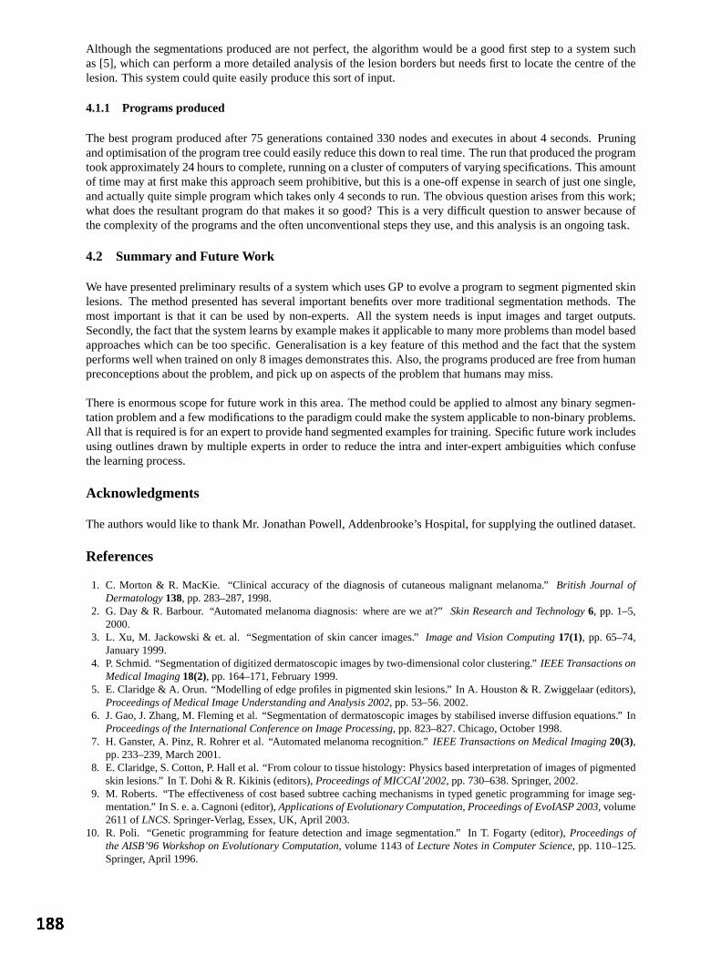
Although the segmentations produced are not perfect, the algorithm would be a good first step to a system suchas [5], which can perform a more detailed analysis of the lesion borders but needs first to locate the centre of thelesion. This system could quite easily produce this sort of input.

4.1.1 Programs produced

The best program produced after 75 generations contained 330 nodes and executes in about 4 seconds. Pruningand optimisation of the program tree could easily reduce this down to real time. The run that produced the programtook approximately 24 hours to complete, running on a cluster of computers of varying specifications. This amountof time may at first make this approach seem prohibitive, but this is a one-off expense in search of just one single,and actually quite simple program which takes only 4 seconds to run. The obvious question arises from this work;what does the resultant program do that makes it so good? This is a very difficult question to answer because ofthe complexity of the programs and the often unconventional steps they use, and this analysis is an ongoing task.

4.2 Summary and Future Work

We have presented preliminary results of a system which uses GP to evolve a program to segment pigmented skinlesions. The method presented has several important benefits over more traditional segmentation methods. Themost important is that it can be used by non-experts. All the system needs is input images and target outputs.Secondly, the fact that the system learns by example makes it applicable to many more problems than model basedapproaches which can be too specific. Generalisation is a key feature of this method and the fact that the systemperforms well when trained on only 8 images demonstrates this. Also, the programs produced are free from humanpreconceptions about the problem, and pick up on aspects of the problem that humans may miss.

There is enormous scope for future work in this area. The method could be applied to almost any binary segmen-tation problem and a few modifications to the paradigm could make the system applicable to non-binary problems.All that is required is for an expert to provide hand segmented examples for training. Specific future work includesusing outlines drawn by multiple experts in order to reduce the intra and inter-expert ambiguities which confusethe learning process.

Acknowledgments

The authors would like to thank Mr. Jonathan Powell, Addenbrooke’s Hospital, for supplying the outlined dataset.

References

1. C. Morton & R. MacKie. “Clinical accuracy of the diagnosis of cutaneous malignant melanoma.”British Journal ofDermatology138, pp. 283–287, 1998.

2. G. Day & R. Barbour. “Automated melanoma diagnosis: where are we at?”Skin Research and Technology6, pp. 1–5,2000.

3. L. Xu, M. Jackowski & et. al. “Segmentation of skin cancer images.”Image and Vision Computing17(1), pp. 65–74,January 1999.

4. P. Schmid. “Segmentation of digitized dermatoscopic images by two-dimensional color clustering.”IEEE Transactions onMedical Imaging18(2), pp. 164–171, February 1999.

5. E. Claridge & A. Orun. “Modelling of edge profiles in pigmented skin lesions.” In A. Houston & R. Zwiggelaar (editors),Proceedings of Medical Image Understanding and Analysis 2002, pp. 53–56. 2002.

6. J. Gao, J. Zhang, M. Fleming et al. “Segmentation of dermatoscopic images by stabilised inverse diffusion equations.” InProceedings of the International Conference on Image Processing, pp. 823–827. Chicago, October 1998.

7. H. Ganster, A. Pinz, R. Rohrer et al. “Automated melanoma recognition.”IEEE Transactions on Medical Imaging20(3),pp. 233–239, March 2001.

8. E. Claridge, S. Cotton, P. Hall et al. “From colour to tissue histology: Physics based interpretation of images of pigmentedskin lesions.” In T. Dohi & R. Kikinis (editors),Proceedings of MICCAI’2002, pp. 730–638. Springer, 2002.

9. M. Roberts. “The effectiveness of cost based subtree caching mechanisms in typed genetic programming for image seg-mentation.” In S. e. a. Cagnoni (editor),Applications of Evolutionary Computation, Proceedings of EvoIASP 2003, volume2611 ofLNCS. Springer-Verlag, Essex, UK, April 2003.

10. R. Poli. “Genetic programming for feature detection and image segmentation.” In T. Fogarty (editor),Proceedings ofthe AISB’96 Workshop on Evolutionary Computation, volume 1143 ofLecture Notes in Computer Science, pp. 110–125.Springer, April 1996.

Segmentation of cardiac MR images using a 4D probabilistic atlasand the EM algorithm

M. Lorenzo-Valdesa, G. I. Sanchez-Ortiza, R. Mohiaddinb, D. Rueckerta

aVisualInformationProcessingGroup,Departmentof Computing,ImperialCollegeof Science,Technology, andMedicine,180Queen’sGate,LondonSW72BZ, UnitedKingdom

b Royal BromptonandHarefieldNHS Trust,Sydney Street,London,UnitedKingdom

Abstract. In thispaperanautomaticatlas-basedsegmentationalgorithmfor 4D cardiacMR imagesis proposed.Thealgorithmisbasedonthe4D extensionof theexpectationmaximisation(EM) algorithm.TheEM algorithmusesa 4D probabilisticcardiacatlasto estimatetheinitial modelparametersandto integratespatially-varyinga-priori informationinto theclassificationprocess.It providesspaceandtime-varyingprobabilitymapsfor theleft andright ventricle,themyocardium,andbackgroundstructuressuchastheliver, stomach,lungsandskin.Thesegmentationalgorithmalsoincorporatesspatialandtemporalcontextual informationby using4D MarkovRandomFields(MRF). Validationagainstmanualsegmentationsandcomputationof thecorrelationbetweenmanualandautomaticsegmentationon 2493D volumeswerecalculated.Resultsshow thattheprocedurecansuccessfullysegmenttheleft ventricle(LV) (r=0.95),myocardium(r=0.83)andright ventricle(RV) (r=0.91).

1 Introduction

In MagneticResonanceImaging (MRI) of the cardiovascularsystem,an accurateidentificationof the bordersof theventriclesandmyocardiumis essentialto quantitatively analysecardiacfunctionsuchasejectionfractionor wall motion thickening. Several approacheshave beenproposedfor the automaticsegmentationof cardiacstructuresin MR images(for a review see[1]). Recently, several techniquesbasedon active appearancemodels(AAM) have emergedshowing improvedreliability andconsistency [2]. However, theapplicability is restrictedto theMR imagingsequenceusedfor trainingsincetheintensityappearanceanddistribution is anexplicit partofthestatisticalmodel.Mostof thesetechniqueswork only for 2D eventhoughextensionsto 3D havebeenrecentlyproposed [3]. This paperproposesan approachwhich combinesthe expectationmaximisation(EM) algorithmanda 4D probabilisticatlasof theheartfor theautomaticsegmentationof 4D cardiacMR images.Methodsbasedon theEM algorithmhavebeenpreviouslyproposedfor theclassificationof MR imagesof thebrain [4,5] wherethey alsoincludecontextual informationinto the EM algorithmby meansof Markov RandomFields(MRF). Inthis work we usean extensionof the EM algorithmto 4D (spaceand time) andMRFs to segmenta complete4D sequenceof cardiacimages.We alsousea 4D probabilisticcardiacatlasto includespatiallyandtemporallyvaryinga-priori informationinto theEM segmentation.

2 Methods

2.1 EM algorithm

TheEM algorithmis aniterativeprocedurethatestimatesthemaximumlikelihoodfor theobserveddataby max-imising thelikelihoodfor theestimatedcompletedata.Thecompletedatacomprisesof theobserveddataandthemissingdata. The algorithmconsistsof two steps:The first oneis the expectation step,wherethe missingdataareestimatedby finding the maximumlikelihoodparameterestimatesfor the observeddata. The secondstepisthemaximisation step,wherethemaximumlikelihoodfor theobserveddataareestimatedby maximisingthelike-lihood for theestimatedcompletedata. In our case,theobserveddataarethesignalintensitiesof theMR imagesequence,andthemissingdatais thecorrectclassificationof the imagesequenceaccomplishedwith helpof theparametersthatdescribethemeanandvarianceof eachclass(anatomicalstructure),which areusuallymodelledby a Gaussiandistribution. Givena setof

classes,the probability thatclass hasgeneratedvoxel value at

position is givenby theclassificationstep: ! #"! $"%(1)

where '&)( +*,-,., 0/ and 12(435678 / . Here 35 is themeanintensityof class and 7:9 is thevarianceof theintensitiesin class . Theestimationof theparametersof eachclassis givenby:

35;=< < (2)

7 9 < > ? A@B35?9< 5 (3)

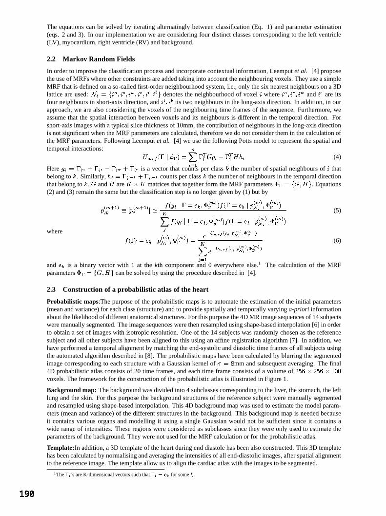
The equationscanbe solved by iteratingalternatinglybetweenclassification(Eq. 1) andparameterestimation(eqs.2 and3). In our implementationwe areconsideringfour distinctclassescorrespondingto the left ventricle(LV), myocardium,right ventricle(RV) andbackground.

2.2 Markov Random Fields

In orderto improve theclassificationprocessandincorporatecontextual information,Leemputet al. [4] proposetheuseof MRFswhereotherconstraintsareaddedtakinginto accounttheneighbouringvoxels.They useasimpleMRF thatis definedon a so-calledfirst-orderneighbourhoodsystem,i.e.,only thesix nearestneighbourson a 3Dlattice areused: CD =( FE FG FH FI KJ ?L / denotesthe neighbourhoodof voxel where FE ?G KH and FI areitsfour neighboursin short-axisdirection,and KJ ?L its two neighboursin thelong-axisdirection. In addition,in ourapproach,we arealsoconsideringthevoxelsof theneighbouringtime framesof thesequence.Furthermore,weassumethat the spatialinteractionbetweenvoxels andits neighboursis different in the temporaldirection. Forshort-axisimageswith a typical slicethicknessof 10mm,thecontributionof neighboursin thelong-axisdirectionis notsignificantwhentheMRF parametersarecalculated,thereforewedonotconsiderthemin thecalculationoftheMRF parameters.Following Leemputet al. [4] we usethefollowing Pottsmodelto representthespatialandtemporalinteractions: M'NPOQ > SRT E

U5VXW SY 5UZ\[ (4)

Here W ] _^ Y a` Y _b Y ac is a vectorthat countsper class the numberof spatialneighboursof thatbelongto . Similarly, [ ' edf6g Y _dah6g countsperclass thenumberof neighboursin thetemporaldirectionthatbelongto . V and Z are

ji matricesthattogetherform theMRF parametersk R l( V Z / . Equations

(2) and(3) remainthesamebut theclassificationstepis no longergivenby (1) but by

Am NPn oa p+q AmNPn o rs t vuw6 k m

N ox t yuw AmN oz| k m

N oR t vu k mN ox t > u m

N oz k mN oR (5)

where

t u ~ mN oz k m

N oR u!A6A? m I? 4 5 o u : 5F m IK. . 5 5 o (6)

and uw is a binary vector with 1 at the kth componentand 0 everywhereelse.1 The calculationof the MRFparametersk R 2( V Z / canbesolvedby usingtheproceduredescribedin [4].

2.3 Construction of a probabilistic atlas of the heart

Probabilistic maps:Thepurposeof theprobabilisticmapsis to automatetheestimationof the initial parameters(meanandvariance)for eachclass(structure)andto providespatiallyandtemporallyvaryinga-priori informationaboutthelikelihoodof differentanatomicalstructures.For thispurposethe4D MR imagesequencesof 14subjectsweremanuallysegmented.Theimagesequenceswerethenresampledusingshape-basedinterpolation[6] in orderto obtaina setof imageswith isotropicresolution.Oneof the14 subjectswasrandomlychosenasthereferencesubjectandall othersubjectshave beenalignedto this usinganaffine registrationalgorithm[7]. In addition,wehave performeda temporalalignmentby matchingtheend-systolicanddiastolictime framesof all subjectsusingtheautomatedalgorithmdescribedin [8]. Theprobabilisticmapshave beencalculatedby blurring thesegmentedimagecorrespondingto eachstructurewith a Gaussiankernelof 7 mm andsubsequentaveraging.Thefinal4D probabilisticatlasconsistsof 20 time frames,andeachtime frameconsistsof a volumeof ! i i *.!voxels.Theframework for theconstructionof theprobabilisticatlasis illustratedin Figure1.

Background map: Thebackgroundwasdividedinto 4 subclassescorrespondingto theliver, thestomach,theleftlung andtheskin. For this purposethebackgroundstructuresof thereferencesubjectweremanuallysegmentedandresampledusingshape-basedinterpolation.This 4D backgroundmapwasusedto estimatethemodelparam-eters(meanandvariance)of thedifferentstructuresin thebackground.This backgroundmapis neededbecauseit containsvariousorgansandmodelling it usinga single Gaussianwould not be sufficient sinceit containsawide rangeof intensities.Theseregionswereconsideredassubclassessincethey wereonly usedto estimatetheparametersof thebackground.They werenot usedfor theMRF calculationor for theprobabilisticatlas.

Template:In addition,a 3D templateof theheartduringenddiastolehasbeenalsoconstructed.This 3D templatehasbeencalculatedby normalisingandaveragingtheintensitiesof all end-diastolicimages,afterspatialalignmentto thereferenceimage.Thetemplateallow usto align thecardiacatlaswith theimagesto besegmented.

1The ’s areK-dimensionalvectorssuchthat T for some .

PSfragreplacements

Segmentation Separation BlurringAveraging

Volunteer1

Volunteer2

VolunteerN

Figure 1. Constructionof theprobabilisticatlas.

3 Automatic segmentation

In the first stepof the automaticsegmentationthe 3D templatewas registeredto the end-diastolictime frameof theMR sequenceby usinganaffine registration.This producesa transformationwhich spatiallyalignsthe4Dprobabilisticatlasto theMR imagesequence.A temporalalignmentwasperformedusingtheautomatedalgorithmdescribedin [8]. Subsequently, a maskwasgeneratedfor eachclass(LV, RV, myocardiumandbackground)in theprobabilisticatlasby usingonly thoseareasthathada probabilityhigherthan50%of belongingto thatclass.Forthebackgroundeachsubclasswasusedasa mask.Sincetheatlaswasalreadyalignedwith theMR image,eachof thesemaskswasusedto calculatetheinitial modelparameters(meanandvariance)of eachclassandsubclass.Having theinitial modelparametersallowsusto performthefirst classificationof theimagesequenceby assigningtheclasswith thehighestprobabilityfor avoxelatposition . Thebackgroundhadfour probabilitiescorrespondingto eachsubclassandonly thehighestwasconsideredastheprobabilityof thebackgroundof thatspecificvoxel. Insummary, theEM algorithminterleavesfour steps:classificationof thevoxelswith theinitial parameters(Eq. 1),estimationof theGaussianparameters(eqs.2 and3), estimationof theMRF parametersandclassificationusingall the parameters(Eq. 5). The probabilisticatlasconstrainedthe classificationsinceit provideda spatiallyandtemporallyvaryingprior probability for eachtissueclass . ClassificationusingtheEM algorithmwasrepeateduntil thevaluesof theparametersdid notchangesignificantly. All theparameters(mean,varianceandMRF model)werere-estimatedat eachiteration.

4 Results

Cardiacshort-axisimageswereacquiredat Royal BromptonHospital,London,UK, from 12 healthyvolunteersusinga SiemensSonata1.5T scannerwith a TrueFispsequenceand ! i i *. voxels. Similarly, two moreimagesequenceswereacquiredatGuy’sHospital,London,UK usingaPhilipsGyroscanIntera1.5Tscanner. Eachimagesequenceconsistedof 10 to 26 time frames,involving a total of 249volumetricdatasets.Thefield of viewrangedbetween300-350mm, thethicknessof sliceswas10mmandthetotal acquisitiontime wasapproximately15 minutes. In order to avoid bias,we usedthe ’ leave oneout’ testwherethe imageset to be segmentedwasnot usedin theconstructionof its correspondingatlas.Theresultsof theautomaticsegmentationwerecomparedagainstthoseobtainedby manuallysegmentingthe14 4D imagesequences.In orderto assesstheperformanceoftheautomaticsegmentationthe volumesof the ventriclesandmyocardiumwerecalculatedandlinear regressionanalysiswasusedto comparethemanuallyandtheautomaticallysegmentedimages.Figure2 shows theresultsfor the automaticsegmentationwhenconsideringonly the neighbouringvoxels in the short-axisdirections.Thecorrelationfor theLV, myocardiumandRV is +T , ¡£¢¢ and ¡ , respectively. Figure3 presentstheresultsof theautomaticsegmentationincludingalsotheneighbouringvoxels in thetemporaldirectionwherean improvementis noticeable,especiallyin themyocardium( ¤T !¥ ) andRV ( ¤¡ ¡* ). The resultsfor theLV arelargely unchanged( ¦¡ ). Theautomaticsegmentationfor a completesequenceof 26 framestook 25minuteswith anaverageof 20 iterationsfor theEM algorithmto converge.

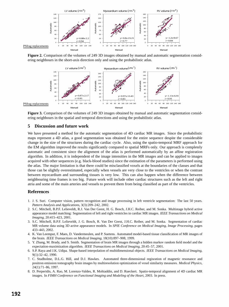
0 20 40 60 80 100 120 140

0

20

40

60

80

100

120

140

LV volume

ManualAuto

mat

ic

0 20 40 60 80 100 120 140 160

0

25

50

75

100

125

150

175

Myocardium volume

Manual

Auto

mat

ic

0 20 40 60 80 100 120 140 160

0

20

40

60

80

100

120

140

160

RV volume

Manual

Auto

mat

ic

y=0.88x−2.2r=0.94

y=0.8x−23.21r=0.77

y=1.2x−8.67r=0.84

PSfragreplacements

( §©¨Pª )( §©¨Pª )( §©¨Pª )

Figure 2. Comparisonof thevolumesof 2493D imagesobtainedby manualandautomaticsegmentationconsid-eringneighboursin theshort-axisdirectiononly andusingtheprobabilisticatlas.

0 20 40 60 80 100 120 140

0

20

40

60

80

100

120

140

LV volume

Manual

Auto

mat

ic

0 20 40 60 80 100 120 140 160

0

20

40

60

80

100

120

140

160

Myocardium volume

Manual

Auto

mat

ic

0 20 40 60 80 100 120 140 160

0

20

40

60

80

100

120

140

160

RV volume

Manual

Auto

mat

ic

y=0.87x−2.17r=0.95

y=0.97x−13.43r=0.83

y=1.13x−6.91r=0.91

PSfragreplacements

( §©¨ ª )( §>¨ ª )( §©¨ ª )

Figure 3. Comparisonof thevolumesof 2493D imagesobtainedby manualandautomaticsegmentationconsid-eringneighboursin thespatialandtemporaldirectionsandusingtheprobabilisticatlas.

5 Discussion and future work

We have presenteda methodfor the automaticsegmentationof 4D cardiacMR images.Sincethe probabilisticmapsrepresenta 4D atlas,a goodsegmentationwasobtainedfor the entiresequencedespitethe considerablechangein the sizeof the structuresduring the cardiaccycle. Also, usingthe spatio-temporalMRF approachfortheEM algorithmimprovedtheresultssignificantlycomparedto spatialMRFsonly. Our approachis completelyautomaticand consistentsince the alignmentof the atlas is performedautomaticallyby an affine registrationalgorithm. In addition,it is independentof the imageintensitiesin theMR imagesandcanbeappliedto imagesacquiredwith othersequences(e.g.black-bloodstudies)sincetheestimationof theparametersis performedusingtheatlas.Themajor limitation is that therecouldbemisclassifiedvoxelsat theboundariesof theclassesandthatthosecanbeslightly overestimated,especiallywhenvesselsarevery closeto theventriclesor whenthecontrastbetweenmyocardiumandsurroundingtissuesis very low. This canalso happenwhen the differencebetweenneighbouringtime framesis too big. Futurework will includeothercardiacstructuressuchasthe left andrightatriaandsomeof themainarteriesandvesselsto preventthemfrom beingclassifiedaspartof theventricles.

References

1. J. S. Suri. Computervision, patternrecognitionandimageprocessingin left ventriclesegmentation:The last 50 years.Pattern Analysis and Applications, 3(3):209–242,2002.

2. S.C.Mitchell, B.P.F. Lelieveldt, R.J.VanDer Geest,H. G. Bosch,J.H.C.Reiber, andM. Sonka.Multistagehybrid activeappearancemodelmatching:Segmentationof left andright ventriclesin cardiacMR images.IEEE Transactions on MedicalImaging, 20:415–423,2001.

3. S.C.Mitchell, B.P.F. Lelieveldt, J. G. Bosch,R. Van Der Geest,J.H.C.Reiber, andM. Sonka. Segmentationof cardiacMR volumedatausing3D active appearancemodels. In SPIE Conference on Medical Imaging, Image Processing, pages433–443,2002.

4. K. VanLeemput,F. Maes,D. Vandermeulen,andP. Suetens.Automatedmodel-basedtissueclassificationof MR imagesofthebrain. IEEE Transactions on Medical Imaging, 18(10):897–908,1999.

5. Y. Zhang,M. Brady, andS.Smith.Segmentationof brainMR imagesthroughahiddenmarkov randomfield modelandtheexpectation-maximizationalgorithm. IEEE Transactions on Medical Imaging, 20:45–57,2001.

6. S.P. RayaandJ.K.Udipa. Shape-basedinterpolationof multidimensionalobjects.IEEE Transactions on Medical Imaging,9(1):32–42,1990.

7. C. Studholme,D.L.G. Hill, and D.J. Hawkes. Automatedthree-dimensionalregisration of magneticresonanceandpositronemissiontomographybrainimagesby multiresolutionoptimizationof voxel similarity measures.Medical Physics,24(1):71–86,1997.

8. D. Perperidis,A. Rao,M. Lorenzo-Valdes,R. Mohiaddin,andD. Rueckert. Spatio-temporalalignmentof 4D cardiacMRimages.In FIMH Conference on Functional Imaging and Modeling of the Heart, 2003. In press.

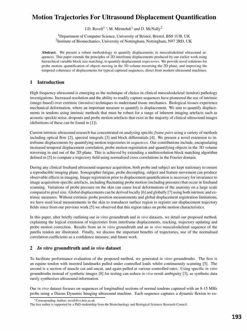
Motion Trajectories For Ultrasound Displacement Quantification

J.D. Revell1 ∗, M. Mirmehdi1 and D. McNally2

1Department of Computer Science, University of Bristol, Bristol, BS8 1UB, UK2Institute of Biomechanics, University of Nottingham, Nottingham, N97 2RD, UK

Abstract. We present a robust methodology to quantify displacements in musculoskeletal ultrasound se-quences. This paper extends the principles of 2D interframe displacements produced by our earlier work usinghierarchical variable block size matching, to quantify displacement trajectories. We provide novel solutions forprobe motion, quantification of objects moving in the 3D volume traversing the 2D plane, and improving thetemporal coherence of displacements for typical captured sequences, direct from modern ultrasound machines.

1 Introduction

High frequency ultrasound is emerging as the technique of choice in clinical musculoskeletal (tendon) pathologyinvestigations. Increased resolution and the ability to readily capture sequences have pioneered the use of intrinsic(image-based) over extrinsic (invasive) techniques to understand tissue mechanics. Biological tissues experiencemechanical deformation, where an important measure to quantify is displacement. We aim to quantify displace-ments in tendons using intrinsic methods that must be robust for a range of inherent imaging artefacts such asacoustic speckle noise, dropouts and probe motion artefacts that exist in the majority of clinical ultrasound images(definitions of these can be found in [1]).

Current intrinsic ultrasound research has concentrated on analysing specific frame pairs using a variety of methodsincluding optical flow [2], spectral integrals [3] and block differentials [4]. We present a novel extension to in-terframe displacements by quantifying motion trajectories in sequences. Our contributions include, encapsulatingincreased temporal displacement correlation, probe motion registration and quantifying objects in the 3D volumetraversing in and out of the 2D plane. This is achieved by extending a multiresolution block matching algorithmdefined in [5] to compute a trajectory field using normalised cross correlations in the Fourier domain.

During any clinical freehand ultrasound sequence acquisition, both probe and subject are kept stationary to ensurea reproducible imaging plane. Sonographer fatigue, probe decoupling, subject and feature movement can produceobservable effects in imaging. Image registration prior to displacement quantification is necessary for invariance toimage acquisition-specific artefacts, including fluctuating probe motion (including pressure) that occur in freehandscanning. Variations of probe pressure on the skin can cause local deformations of the anatomy on a large scalecompared to pixel size. Global displacements can be derived locally [6] and globally [7] using both intrinsic and ex-trinsic measures. Without extrinsic probe position measurements and global displacement registration limitations,we have used local measurements in the skin to transducer surface region to register our displacement trajectoryfields since from our previous work [5] we observed that this region takes on probe motion characteristics.

In this paper, after briefly outlining our in vitro groundtruth and in vivo datasets, we detail our proposed method,explaining the logical extension of trajectories from interframe displacements, tracking, trajectory updating andprobe motion correction. Results from an in vitro groundtruth and an in vivo musculoskeletal sequence of thepatella tendon are illustrated. Finally, we discuss the important benefits of trajectories, use of the normalisedcorrelation coefficients as a confidence measure, and future work.

2 In vitro groundtruth and in vivo dataset

To facilitate performance evaluation of the proposed method, we generated in vitro groundtruths. The first isan equine tendon with inserted landmarks pulled under controlled loads whilst continuously scanning [5]. Thesecond is a section of muscle cut and uncut, and again pulled at various controlled rates. Using specific in vitrogroundtruths instead of synthetic images [8] for testing can reduce in vivo result ambiguity [3], as synthetic datararely synthesises ultrasound information.

Our in vivo dataset focuses on sequences of longitudinal sections of normal tendons captured with an 8-15 MHzprobe using a Diasus Dynamic Imaging ultrasound machine. Each sequence captures a dynamic flexion to ex-

∗Corresponding Author: [email protected] first author is supported by a PhD studentship from the Biotechnology and Biological Sciences Research Council.

tension of the muscle giving rise to tendon displacement. The tendons anisotropic fibrillar texture [9] [10] meansthat any slight obliquity of the angle of incidence or curvilinearity, can obscure or mimic texture details and createaperture problems. Here we present results on the patella tendon, an area of high clinical interest due to the demandfor improved understanding of patellar tendinopathy (athletes knee). More dynamic results can be found online 1.

3 Motion Trajectories

In [5] we previously defined a multiscale block matching pyramid initialised by a regular lattice R, sampling by P×Q (typically 8×8 or 4×4) an initial ultrasound frame f t. Blocks of M ×N , where M ,N = 64, 32, 16, 8, 4wereused to increasingly improve displacement accuracy for R till M = P and N = Q. Using spatial convolution weminimised the mean squared error between candidate blocks I in a search region I ′ from ft and ft+1 respectively,to find the optimum displacement.

Here we determine the local disparity between I and I ′ by identifying the maximum correlation coefficient usingnormalised cross correlation (NCC). We now define I as a zero padded candidate block so that I, I ′ = M × N ,enabling the NCC to be performed in the frequency domain using the FFT for efficiency, defined

c =F−1I∗I ′√∫ ∫ |I|2 · ∫ ∫ |I ′|2

leading to 0 ≤ c ≤ 1 (1)

where I and I ′ denotes the Fourier transform of blocks I and I ′ respectively, F−1 the inverse Fourier transformand ∗ the complex conjugate. By multiplying the spectral components, the DC element is filtered out removingany global illumination and high frequency noise. Furthermore, by normalising the correlation, invariance to meanintensity fluctuations is achieved. The spatial displacement vector d = (d1, d2) is then estimated from locating themaximum correlation coefficient. For each block in R the NCC is performed at multiple block scales, using theprevious d as I and I ′ offsets, allowing a varying smoothness constraint across each I for all scales.

Trajectories represent the temporal tracking of features sequentially through a sequence using the NCC for featurelocation. NCC tracking is sensitive to imaging scale, rotation and perspective distortions. In this context minimalperspective and rotation distortions potentially exist, however, the NCC does enable equal sized patterns to bedetected by a rotation distortion of 5 to 10 [11]. Image scale distortions are more prominent, and by using themultiscale NCC we achieve scale invariance and improved accuracy from local illumination variations.

At this stage we have quantified an optimal displacement d for each block in f t lattice R yielding an interframedisplacement field dR. For sequences, this process is repeated for every frame pair in the sequence to give:

dtR . . . dt+n

R = NCC(ft, ft+1) . . . (ft+n, ft+n+1) (2)

After quantifying interframe displacements using R, we redefine R, offset by the prior displacement field d tR.

Consequent tracking, results in a displacement vector with temporal history h, a trajectory defined for each originalblock in R, hence producing a trajectory field. A powerful benefit from the trajectory definition is h which has adirect relationship with temporal displacement coherence.

Tracking, especially in long sequences, requires feature identification in each next frame f t+1 for inclusion orexclusion update. Potential causes of trajectory update are features traversing in the 2D plane, 3D volume, atimage boundaries and occlusion, producing potential trajectory clusters and voids. A new trajectory is included bycomparing each d to neighbours in R centred in the range A×B, with an Euclidean distance > P ×Q. Similarly,trajectories are flagged for exclusion if any neighbouring final positions in A×B conflict, by a proximity thresholddefined empirically. Trajectory results in Figs. 1 and 2 are illustrated in black for R and red for updates (for colourimages please see online1).

We use the assumption that the intensity signal from the skin to transducer represents probe motion δ xy . Globaldisplacement and trajectory field registration is achieved by using the mean displacement, δ µ

xy , in this region, andupdating the fields respectively using:

d =(d1 + δµ

y , d2 + δµx

)(3)

1http://www.cs.bris.ac.uk/home/revell

4 Experimental Results

Fig. 1(a) shows a sample frame of our in-vitro groundtruth, a partially cut muscle segment under x-axial linearload. Figs. 1(b) and 1(c) are typical interframe and trajectory displacement field results respectively, sampling atP × Q = 4 using block scales M × N , where M ,N = 16, 8. Fig. 1(b) illustrates large linear displacementslocated at the cut as the muscle is pulled. The trajectory field in Fig. 1(c) highlights biased muscle movement tothe right as the cut opens, resulting in new trajectories (inclusion update, shown in red) between the cut edges.

(a) Cut Muscle (post strain) (b) Interframe Displacement Field (c) Trajectory Field h = 4

Figure 1. (a) In-vitro groundtruth muscle segment, (b) Interframe displacment field, (c) Trajectory Field.

Figs. 2(a), 2(b) and 2(c) are (lognormal) longitudinal sagittal sections of the patella tendon, traversing left to rightfrom extension to flexion in 1 second and captured at 30Hz. The trajectory fields in Figs. 2(d), 2(e) and 2(f) wereproduced by sampling at P × Q = 8 using multiple block scales M × N , where M ,N = 64, 32, 16, 8, withh = 10. All trajectory fields are post probe motion registration using (3), resulting in approximate stationarity inthe upper skin region so that throughout the sequence this region is constrained to d ≈ 0. All trajectories show hightemporal correlation for all frames in the sequence. New trajectories (inclusion update, shown in red) appear atimage boundaries from the horizontal movement, and several appear in the central plane from 3D movement. Thetrajectories highlight very linear displacements in the tendon as expected, and temporal displacement correlationand structure in lower regions of well defined acoustic speckle noise, that mimic the tendon motion.

(a) Patella Tendon f10 (b) Patella Tendon f20 (c) Patella Tendon f30

(d) Trajectory Field h10 ⇒ (f1 tof10) (e) Trajectory Field h10 ⇒ (f11 tof20) (f) Trajectory Field h10 ⇒ (f21 tof30)

Figure 2. (a)-(c) In vivo patella tendon for f t=10,20,30, (d)-(f) Displacement trajectory fields.

An example of probe motion correction showing significant probe movement can be observed at f 20 through tof30, as illustrated in Fig. 3 for the patella tendon sequence in Fig. 2(f). Fig. 3 compares both trajectory update andprobe translational displacement results. Throughout the sequence probe y-axial displacement was approximatelyzero, with any supported deviations potentially due to probe pressure. After f 20, x-axial displacement increasedto approximately 3 pixels, with the mean used for trajectory correction, resetting approximate stationarity in the

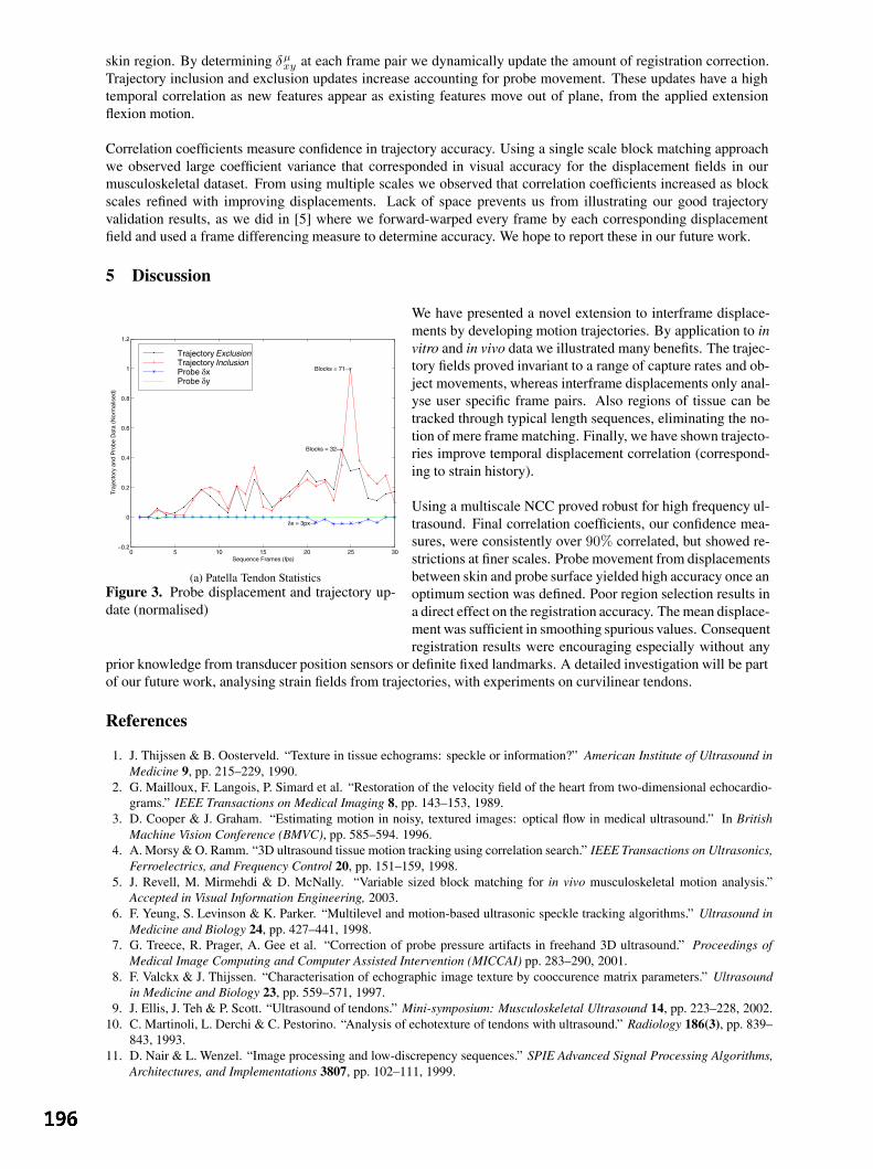
skin region. By determining δµxy at each frame pair we dynamically update the amount of registration correction.

Trajectory inclusion and exclusion updates increase accounting for probe movement. These updates have a hightemporal correlation as new features appear as existing features move out of plane, from the applied extensionflexion motion.

Correlation coefficients measure confidence in trajectory accuracy. Using a single scale block matching approachwe observed large coefficient variance that corresponded in visual accuracy for the displacement fields in ourmusculoskeletal dataset. From using multiple scales we observed that correlation coefficients increased as blockscales refined with improving displacements. Lack of space prevents us from illustrating our good trajectoryvalidation results, as we did in [5] where we forward-warped every frame by each corresponding displacementfield and used a frame differencing measure to determine accuracy. We hope to report these in our future work.

5 Discussion

0 5 10 15 20 25 30−0.2

0

0.2

0.4

0.6

0.8

1

1.2

δx = 3px→

Blocks = 71→

Blocks = 32→

Sequence Frames (fps)

Tra

ject

ory

and

Pro

be D

ata

(Nor

mal

ised

)

Trajectory ExclusionTrajectory InclusionProbe δxProbe δy

(a) Patella Tendon StatisticsFigure 3. Probe displacement and trajectory up-date (normalised)

We have presented a novel extension to interframe displace-ments by developing motion trajectories. By application to invitro and in vivo data we illustrated many benefits. The trajec-tory fields proved invariant to a range of capture rates and ob-ject movements, whereas interframe displacements only anal-yse user specific frame pairs. Also regions of tissue can betracked through typical length sequences, eliminating the no-tion of mere frame matching. Finally, we have shown trajecto-ries improve temporal displacement correlation (correspond-ing to strain history).

Using a multiscale NCC proved robust for high frequency ul-trasound. Final correlation coefficients, our confidence mea-sures, were consistently over 90% correlated, but showed re-strictions at finer scales. Probe movement from displacementsbetween skin and probe surface yielded high accuracy once anoptimum section was defined. Poor region selection results ina direct effect on the registration accuracy. The mean displace-ment was sufficient in smoothing spurious values. Consequentregistration results were encouraging especially without any

prior knowledge from transducer position sensors or definite fixed landmarks. A detailed investigation will be partof our future work, analysing strain fields from trajectories, with experiments on curvilinear tendons.

References

1. J. Thijssen & B. Oosterveld. “Texture in tissue echograms: speckle or information?” American Institute of Ultrasound inMedicine 9, pp. 215–229, 1990.

2. G. Mailloux, F. Langois, P. Simard et al. “Restoration of the velocity field of the heart from two-dimensional echocardio-grams.” IEEE Transactions on Medical Imaging 8, pp. 143–153, 1989.

3. D. Cooper & J. Graham. “Estimating motion in noisy, textured images: optical flow in medical ultrasound.” In BritishMachine Vision Conference (BMVC), pp. 585–594. 1996.

4. A. Morsy & O. Ramm. “3D ultrasound tissue motion tracking using correlation search.” IEEE Transactions on Ultrasonics,Ferroelectrics, and Frequency Control 20, pp. 151–159, 1998.

5. J. Revell, M. Mirmehdi & D. McNally. “Variable sized block matching for in vivo musculoskeletal motion analysis.”Accepted in Visual Information Engineering, 2003.

6. F. Yeung, S. Levinson & K. Parker. “Multilevel and motion-based ultrasonic speckle tracking algorithms.” Ultrasound inMedicine and Biology 24, pp. 427–441, 1998.

7. G. Treece, R. Prager, A. Gee et al. “Correction of probe pressure artifacts in freehand 3D ultrasound.” Proceedings ofMedical Image Computing and Computer Assisted Intervention (MICCAI) pp. 283–290, 2001.

8. F. Valckx & J. Thijssen. “Characterisation of echographic image texture by cooccurence matrix parameters.” Ultrasoundin Medicine and Biology 23, pp. 559–571, 1997.

9. J. Ellis, J. Teh & P. Scott. “Ultrasound of tendons.” Mini-symposium: Musculoskeletal Ultrasound 14, pp. 223–228, 2002.10. C. Martinoli, L. Derchi & C. Pestorino. “Analysis of echotexture of tendons with ultrasound.” Radiology 186(3), pp. 839–

843, 1993.11. D. Nair & L. Wenzel. “Image processing and low-discrepency sequences.” SPIE Advanced Signal Processing Algorithms,

Architectures, and Implementations 3807, pp. 102–111, 1999.

Dealing with cardiovascular motion for strain imaging in the liverAlexander F. Kolen*, Jeffrey C. Bamber

Joint Department of Physics, Institute of Cancer Research and Royal Marsden NHS Trust,Sutton, Surrey SM2 5PT, UK

Abstract. Elastography or elasticity imaging, which uses ultrasound to image internal tissue strain due to anapplied external displacement, can display elastic inhomogeneities such as stiff tumours and heat-ablatedtissue with high contrast in static situations. However, its application to liver in vivo is problematic becausethe organ is already in motion. In a previous study, we characterised the cardiovascular component of livermotion, with the objective of understanding it well enough to propose strategies for its correction and tosimulate it in computer and phantom experiments when testing these strategies [1].

This paper presents the extension of this earlier study, in which we have now developed, tested andevaluated several strategies for dealing with cardiovascular motion for the application of elastography in theliver. The evaluation was carried out in part using a phantom, containing soft gelatine with a stiffer inclusion,that was subjected to an independent, cyclic motion while being manually palpated using an ultrasoundimaging transducer. As a result of this study, several strategies to deal with cardiovascular motion wereimplemented successfully and shown to provide worthwhile improvements in elastographic image quality.

1 IntroductionElastography (a technique to image internal tissue strain) of in vivo liver can be problematic because the

organ is continuously subjected to unwanted internal motion, such as cardiovascular activity. It has beenrecognised by others [2, 3] that these pre-existing motions cause problems in temperature (strain) imaging and,as will be shown in this study they are also problematic for ultrasonic elasticity imaging. In previous work, thecardiovascular component of liver motion was characterised, with the objective of understanding it well enoughto propose strategies for its correction [1]. The motion patterns of some liver segments were found to becomplex, but they were also cyclic and repeatable, indicating that motion compensation should be possible.Furthermore, it was proposed that the data obtained could be used to design simulations in computer andphantom experiments, for testing suggested motion compensation strategies. This paper reports the results ofsuch experiments, using phantoms.

2 Aims and objectivesOur long term aim is to assess the feasibility to apply freehand ultrasonic elasticity imaging to the liver

for the purpose of detecting elastic inhomogeneities. This particular study had two objectives. The first objectivewas to investigate whether cardiac motion is problematic for conventional freehand elasticity imaging, and toassess the severity and nature of artefacts as a function of the relative amplitude of the cardiac motion. Phantomexperiments are ideal for this purpose since degraded image quality in the presence of motion may be comparedwith images obtained from the same object when stationary. The second objective was to test and comparevarious motion correction and motion utilisation strategies designed to improve the quality of the elasticityimages acquired in vivo in the liver. Again, tissue phantoms provide a useful controlled situation in which toobjectively compare alternative compensation techniques.

3 Materials and methodsThis paper presents a study in which we evaluated experimentally the following strategies for dealing

with cardiovascular motion for ultrasonic elasticity imaging in the liver:(1) Identify a time window in the heart cycle where the cardiac motion is negligible compared to the externally

applied motion.(2) Identify periodic moments in the heart cycle for combined phase-shifted (gated acquisition) multistep strain

estimation.(3) Extrapolation and subtraction of pre-existing motion if an external stress is applied (this included two

alternative extrapolation algorithms, which will be described later).(4) Utilise the cardiovascular motion component to produce internal strain.

These motion compensation strategies were evaluated using a gelatine phantom containing a stiffinclusion in a homogeneous soft background, which was subjected to simulated cardiac motion while beingmanually palpated and imaged using the ultrasound transducer.

For this study an arbitrary ratio R, between the externally applied motion and simulated cardiac motion,measured at the centre of the lesion, was defined as a convenient quantity to vary, and in order to investigate thelimits of performance of the motion correction strategy: * [email protected]

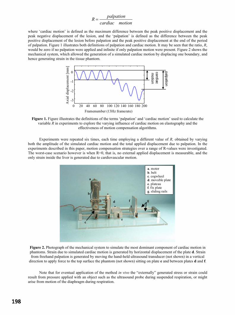
motioncardiacpalpationR =

where ‘cardiac motion’ is defined as the maximum difference between the peak positive displacement and thepeak negative displacement of the lesion, and the ‘palpation’ is defined as the difference between the peakpositive displacement of the lesion before palpation and the peak positive displacement at the end of the periodof palpation. Figure 1 illustrates both definitions of palpation and cardiac motion. It may be seen that the ratio, R,would be zero if no palpation were applied and infinite if only palpation motion were present. Figure 2 shows themechanical system, which allowed the generation of a simulated cardiac motion by displacing one boundary, andhence generating strain in the tissue phantom.

0 20 40 60 80 100 120 140 160 180 200-3

-2

-1

0

Framenumber (13Hz framerate)

Axi

al d

ispla

cem

ent [

mm

]palpation

cardiac m

otion

Figure 1. Figure illustrates the definitions of the terms ‘palpation’ and ‘cardiac motion’ used to calculate thevariable R in experiments to explore the varying influence of cardiac motion on elastography and the

effectiveness of motion compensation algorithms.

Experiments were repeated six times, each time employing a different value of R, obtained by varyingboth the amplitude of the simulated cardiac motion and the total applied displacement due to palpation. In theexperiments described in this paper, motion compensation strategies over a range of R-values were investigated.The worst-case scenario however is when R=0, that is, no external applied displacement is measurable, and theonly strain inside the liver is generated due to cardiovascular motion.

b

a

c

d

e

f g

a. motorb. beltc. cogwheeld. movable platee. plateauf. fix plateg. sliding rails

Figure 2. Photograph of the mechanical system to simulate the most dominant component of cardiac motion inphantoms. Strain due to simulated cardiac motion is generated by horizontal displacement of the plate d. Strainfrom freehand palpation is generated by moving the hand-held ultrasound transducer (not shown) in a vertical

direction to apply force to the top surface the phantom (not shown) sitting on plate e and between plates d and f.

Note that for eventual application of the method in vivo the “externally” generated stress or strain couldresult from pressure applied with an object such as the ultrasound probe during suspended respiration, or mightarise from motion of the diaphragm during respiration.

4 ResultsFigure 3 illustrates a series of elasticity images of the phantom that was subjected to a cyclic motion

while being manually palpated using an ultrasound imaging transducer, as described above. The dark grey levelin the elasticity images indicates low strain, associated either with the stiff lesion or with regions exposed to lowstress due to the boundary conditions of the experiment. The bright areas indicate high strain, i.e. either lowstiffness or high stress. These results, and others like them, showed that elasticity imaging without motioncompensation was difficult for situations in which the amplitude of the palpation was less than 1.5 times theamplitude of the cardiac motion (see figure 3 top row of elasticity images). In practice, this ratio might be easy toachieve for superficial tissue structures, but for deeply situated tissue structures, the amount of displacement dueto the externally applied strain could be relatively small.

Time windowing and phase-shifted multistep strain imaging (suggested motion correction methods 1 and2) were, with the currently used data-acquisition system, unsuccessful. These strategies for motion compensationwere therefore not considered applicable for experiments in vivo and the results from these methods are thereforenot shown in figure 3. However, when in the future ultrasound equipment with higher frame-rates becomeavailable, this method of motion compensation should be re-considered.

2.15mm0.00mm

∞

2.01mm0.52mm

3.87

0.76mm0.51mm

1.49

1.32mm2.65mm

0.49

0.00mm0.81mm

0.00

2.63mm1.40mm

1.88

PalpationCardiac motion

R

No motion compensation

Motioncorrectionbased on

frequency extrapolation

Motioncorrectionbased on template

extrapolation

Motionutilisationmagnitude

of strain

Figure 3. A gelatine phantom, containing a spherical lesion stiffer than the homogeneous soft background, wassubjected to external applied compression and simulated cardiac motion. The top row of elasticity images was

obtained using no motion compensation algorithms. The second and third rows show elasticity images generatedafter correcting for the simulated cardiac motion using extrapolation techniques based on analysing thefrequency components of displacement and generating an average cardiac-cycle displacement template,

respectively. The bottom row shows the elasticity images in which all the strain that was present in the imagewas used to derive the strain distribution. The trend of decreasing quality of the strain images with decreasing R

was observed when no motion compensation technique was applied. In all the elasticity images that wereprocessed with algorithms designed to deal with pre-existing motion, the quality of the elasticity images

improved and in almost all cases the stiff lesion was more visible than without processing.

The method of subtracting pre-existing motion by characterising it and then extrapolating to predict theundesired displacement during the period of the palpation was successfully implemented using two differentapproaches: (1) based on the analysing the frequency components of the simulated cardiac motion and (2) based

on a computing a template of the typical simulated cardiac motion during any one cycle. In cases where theamplitude of the palpation was more than 0.5 times the amplitude of the simulated cardiac motion, the lesion wasstill clearly visible in the strain image. For smaller ratios, strain imaging using this type of motion correction wasunsuccessful in that it was difficult to visualise the lesion and its associated background strain pattern (see figure3, second and third rows of elasticity images).

The idea of using all axial tissue motion, whether its origin is from external palpation, cardiac activity oreven breathing, has been successfully implemented. One of the causes of image degradation when performingstrain imaging without motion correction is that not all of the axial motion that is present in the tissue willcontribute to the formation of the strain image. In the worst case, if the axial motion is repetitive with no netdisplacement of the tissue, the resulting mean axial displacement over one cycle would be zero. In such asituation, the strain over time would cancel itself out (mean value equals zero) and would produce a zero strainfield. A very simple solution to this would be to take the absolute or unsigned value of the strain between eachsuccessive frame instead of a signed value. All the axial motion in the image would then contribute to theformation of the axial strain image (see figure 3 bottom rows of elasticity images).

5 DiscussionThe proposed strategies in this study were developed as a means of compensating for cardiac motion in

ultrasonic elasticity imaging of the liver. However, some of the techniques for motion compensation might beapplicable to other organs that are subjected to motion, either due to cardiovascular motion or respirationactivity. Similarly, some may be extended to elasticity imaging methods that are not based on ultrasound, such asMRI-elastography, as well as to non-elastographic imaging methods, such as ultrasonic temperature imaging [4]or attenuation imaging [5].

A further area of application of the motion characterisation and motion correction strategies developed inthis study could be in external beam therapy, such as radiotherapy and focused ultrasound surgery, where organmotion can increase the margins on the delivered dose, reduce the tumour control probability and increase thetoxicity to organs at risk.

6 ConclusionsAfter analysing the internal liver motion, several strategies were suggested for minimising the effects of

pre-existing motion on the procedure of generating an elasticity image. For relatively simple sinusoidal motions,a technique that works well is that of subtracting the predicted cyclic motion obtained by extrapolating data thatwas obtained before palpation. Performance was found to be similar, whether the extrapolation was achievedusing the frequency components of the motion or its typical behaviour per cycle (as represented by a template).However, because real cardiovascular motion is more complex than our simulated motion, our extrapolationalgorithms need to be improved to predict the motion sufficiently in order to use this technique in vivo and this islikely to be most feasible for the template-based method.

As a result of this study, we suggest the different strategies for dealing with cardiovascular motion maybe needed for different parts of the liver. For example, in some parts of the liver the strain generated bycardiovascular motion alone may be sufficient to create an elastogram of adequate quality. In other parts of theliver this is unlikely to be the case and strain signal-to-noise ratio will suffer. Then, of course, externalcompression may be sufficient without motion compensation. However, if a single general approach to deal withcardiac motion is desired, we suggest that for each elastogram pre-existing motion data be acquired prior tocompression. Using these data, parameters can be derived for extrapolation to subtract the pre-existing motionduring external compression. The results shown in Figure 3 suggest that employing such a method does at leastdo no harm to elasticity image quality when motion compensation is not required.

References1 AF Kolen, JC Bamber and EE Ahmed EE (2002) Analysis of cardiovascular liver motion for application to elasticity

imaging of the liver in vivo. pp. 25-28 in: Houston A, Zwiggelaar R (eds.) Proceedings of the sixth annual conference onmedical image understanding and analysis. ISBN 1901725219, British Machine Vision Association.

2 C Simons, P VanBaren and E Ebbini “Motion compensation algorithm for non-invasive two-dimensional temperatureestimation using diagnostic pulse-echo ultrasound.” In SPIE proceedings: Surgical applications of Energy, San Jose:1998.

3 T Varghese, JA Zagzebski, Q Chen et al. “Ultrasound monitoring of temperature change during radiofrequency ablation:preliminary in-vivo results.” Ultrasound in Medicine & Biology 2002, 28(3), pp. 321-329.

4 NR Miller, JC Bamber and GR ter Haar “Fundamental limitations of noninvasive temperature imaging by means ofultrasound echo strain estimation.” Ultrasound in Medicine & Biology 2002, 28(10), pp.1319-1333.

5 NL Bush, I Rivens, GR ter Haar, et al. “Acoustic properties of lesions generated with an ultrasound therapy system.”Ultrasound in Medicine & Biology 1993, 19(9), pp. 789-801

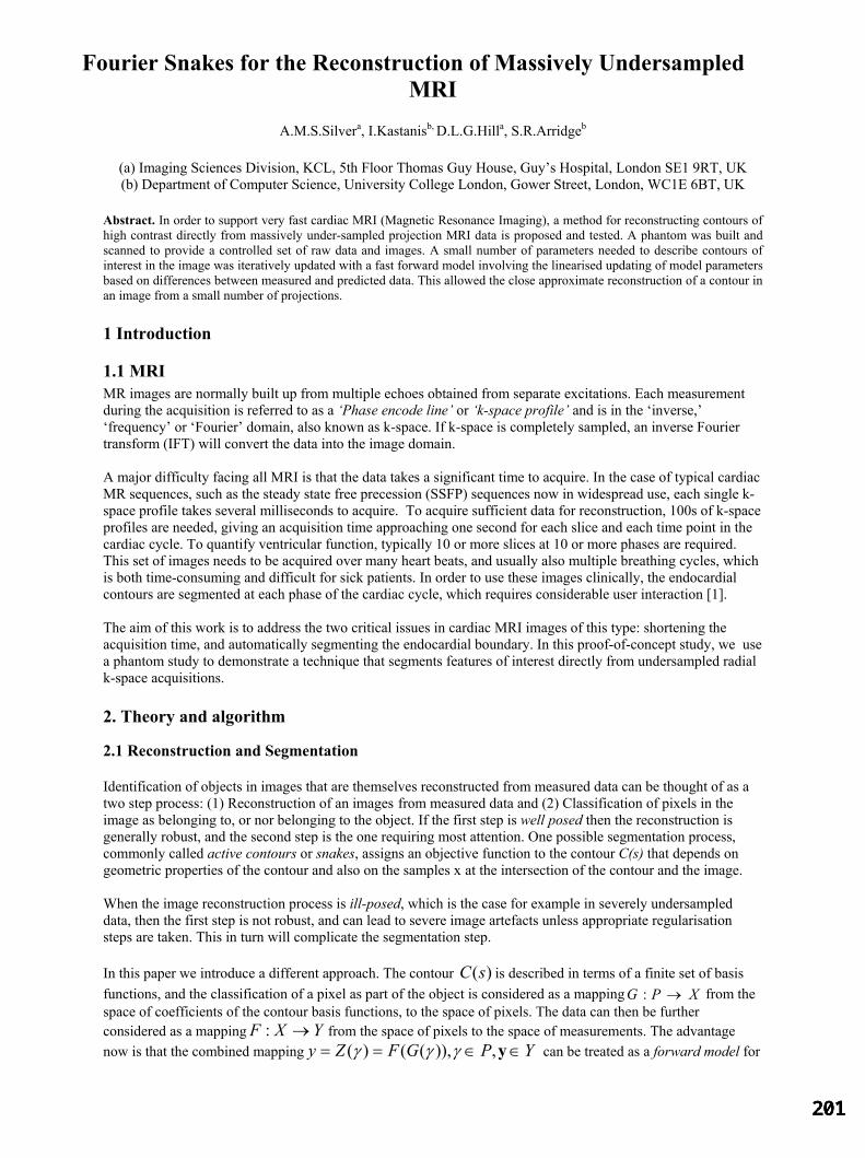
Fourier Snakes for the Reconstruction of Massively Undersampled MRI

A.M.S.Silvera, I.Kastanisb, D.L.G.Hilla, S.R.Arridgeb

(a) Imaging Sciences Division, KCL, 5th Floor Thomas Guy House, Guy’s Hospital, London SE1 9RT, UK (b) Department of Computer Science, University College London, Gower Street, London, WC1E 6BT, UK

Abstract. In order to support very fast cardiac MRI (Magnetic Resonance Imaging), a method for reconstructing contours of high contrast directly from massively under-sampled projection MRI data is proposed and tested. A phantom was built and scanned to provide a controlled set of raw data and images. A small number of parameters needed to describe contours of interest in the image was iteratively updated with a fast forward model involving the linearised updating of model parameters based on differences between measured and predicted data. This allowed the close approximate reconstruction of a contour in an image from a small number of projections. 1 Introduction

1.1 MRI MR images are normally built up from multiple echoes obtained from separate excitations. Each measurement during the acquisition is referred to as a ‘Phase encode line’ or ‘k-space profile’ and is in the ‘inverse,’ ‘frequency’ or ‘Fourier’ domain, also known as k-space. If k-space is completely sampled, an inverse Fourier transform (IFT) will convert the data into the image domain. A major difficulty facing all MRI is that the data takes a significant time to acquire. In the case of typical cardiac MR sequences, such as the steady state free precession (SSFP) sequences now in widespread use, each single k-space profile takes several milliseconds to acquire. To acquire sufficient data for reconstruction, 100s of k-space profiles are needed, giving an acquisition time approaching one second for each slice and each time point in the cardiac cycle. To quantify ventricular function, typically 10 or more slices at 10 or more phases are required. This set of images needs to be acquired over many heart beats, and usually also multiple breathing cycles, which is both time-consuming and difficult for sick patients. In order to use these images clinically, the endocardial contours are segmented at each phase of the cardiac cycle, which requires considerable user interaction [1]. The aim of this work is to address the two critical issues in cardiac MRI images of this type: shortening the acquisition time, and automatically segmenting the endocardial boundary. In this proof-of-concept study, we use a phantom study to demonstrate a technique that segments features of interest directly from undersampled radial k-space acquisitions. 2. Theory and algorithm 2.1 Reconstruction and Segmentation Identification of objects in images that are themselves reconstructed from measured data can be thought of as a two step process: (1) Reconstruction of an images _from measured data and (2) Classification of pixels in the image as belonging to, or nor belonging to the object. If the first step is well posed then the reconstruction is generally robust, and the second step is the one requiring most attention. One possible segmentation process, commonly called active contours or snakes, assigns an objective function to the contour C(s) that depends on geometric properties of the contour and also on the samples x at the intersection of the contour and the image. When the image reconstruction process is ill-posed, which is the case for example in severely undersampled data, then the first step is not robust, and can lead to severe image artefacts unless appropriate regularisation steps are taken. This in turn will complicate the segmentation step. In this paper we introduce a different approach. The contour C is described in terms of a finite set of basis )(sfunctions, and the classification of a pixel as part of the object is considered as a mapping G from the XP →:space of coefficients of the contour basis functions, to the space of pixels. The data can then be further considered as a mapping from the space of pixels to the space of measurements. The advantage now is that the combined mapping

YXF →:y YPGFZ ∈∈== y,)),(()( γγγ can be treated as a forward model for

the measurement of the object, and determining the object boundary can be considered as an inverse problem. In this paper we consider the case of undersampled MRI data, and we consider the inverse problem as identification of the contour _ that produces the best least squares fit of the forward model to the measured data. The method is based on a technique described in [2]. 2.2 Model Based Approach - The forward mapping If the region boundary is sufficiently smooth, it can be represented for example in the form )(sC

∑=

=

=

θ

θγ

θγN

ny

nyn

xn

xn

s

ssysx

sC1 )(

)()()(

)( (1)

where )(snθ is some periodic and differentiable basis function, is the number of these basis functions and

. A representation of the form (1) does not have such limitations as convexity for admissible domains, but it does have the drawback that it is difficult to set constraints such as non-self-intersection. This difficulty is handled in a special way as described below.

θN[ ]01∈s

Let γ denote the vector of all boundary shape coefficients, that is,

TyN

yxN

x ),,,,,( 11 θθγγγγγ KK=

The goal is now to express the discretization of the forward model as a mapping from the boundary coefficients γ to data z. This is done in three steps.

1. Classification of pixels as inside, outside or intercepted by a given region boundaryC .Let )(s 0:)( ≠∩ΩΩ= smms CCB

denote the set of elements intercepted byC . )(s2. Determination of intersections of pixel edges with a given boundary . The goal is to find the

exact intersection points

)(sCs

mm ss 21 , of C(s) and the pixel edges for each pixel ( sm CB∈ )Ω The

intersection of with the edge from vertex N)(sC i to Nj is obtained using a binary search algorithm. 3. Pixels are assigned contrast c if inside C, 0 if outside, and an intermediate value proportional to the area

of intersection if the pixel is intersected by C. The above constitutes the implementation of mapping G. The mapping F is simply a Fourier Transform followed by subsampling in k-space, or alternatively an undersampled Radon Transform. 2.3 Model Based Approach - The Inverse Problem Although F is linear, G is non-linear, so the combined mapping Z=FG is non-linear and the solution of the inverse problem will require an iterative approach. One well-known method is a Newton method which iteratively updates the solution estimate

( ) ( ))()()()( *1*1 kkkkkk ZgJIJJ γγλγγγγ −++=−+ (2)

where is the linearisation of the combined mapping Z=FG, and λ is a control parameter. Since F is )( kJ γ

linear we have where XFJJ = ( )( ) ( )( )k

GJ kX

γγγγγ

=∂∂

= is the Jacobian of the mapping G.

Finally, we can find the components of efficiently as follows XJ

2.4 The Algorithm

Figure 1. The Algorithm

The function of the algorithm is shown in Figure 1. At each iteration, the Fourier snake parameters, p, are transformed into a contour image X using knowledge of expected image contrast, from which a sinogram y is produced by the Radon transform F. This is then compared to the measured data g by subtraction, producing the difference sinogram r. The linearised inverse F* computed from the Jacobian of G is then used to produce the parameter updates ∆p which are added to the parameters. As regions of high intensity gradient in the sinogram indicate candidate boundaries, an extension of the model replaces F with a forward model that generates an intensity derivative along each sinogram line, in which case a gradient operator is applied to the measured data to obtain g, prior to the comparison and update stages. The iterations are finished when the model is only updated by a suitably small amount. 3. Experimental Method Phantom Design In order to produce a controlled set of images and data, an imaging phantom was built comprising an acrylic cuboid tank with an open top which could contain acrylic tubes of varying diameters screwed into the base. The tank and tubes could contain fluids to provide the desired image contrast. Figure 2 shows one possible layout.

Figure 2. Design view of Phantom Figure 3. Experimental Fully Sampled Image

The solutions used were varying concentrations of Magnevist™, a Gadolinium (Gd) Chelate used clinically for MR imaging. As the aim was only to simulate an image with properties approximating to typical cardiac cine images, it was not important to simulate the exact T1 and T2 values of thoracic tissues and blood.

Scanning Parameters Different configurations of tube position, size and fluid or air content were scanned in order to provide a comprehensive set of images for testing. The basic aim of the algorithm is to match a contour to the boundary of

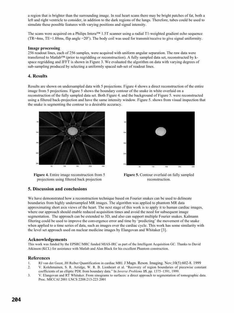
a region that is brighter than the surrounding image. In real heart scans there may be bright patches of fat, both a left and right ventricle to consider, in addition to the dark regions of the lungs. Therefore, tubes could be used to simulate these possible features with varying positions and signal intensity. The scans were acquired on a Philips Intera™ 1.5T scanner using a radial T1-weighted gradient echo sequence (TR=4ms, TE=1.88ms, flip angle =20°). The body coil was used for transmit/receive to give signal uniformity. Image processing 256 readout lines, each of 256 samples, were acquired with uniform angular separation. The raw data were transferred to Matlab™ (prior to regridding or reconstruction). A fully sampled data set, reconstructed by k-space regridding and IFFT is shown in Figure 3. We evaluated the algorithm on data with varying degrees of sub-sampling produced by selecting a uniformly spaced sub-set of readout lines. 4. Results Results are shown on undersampled data with 5 projections. Figure 4 shows a direct reconstruction of the entire image from 5 projections. Figure 5 shows the boundary contour of the snake in white overlaid on a reconstruction of the fully sampled data set. Both Figure 4. and the background of Figure 5. were reconstructed using a filtered back-projection and have the same intensity window. Figure 5. shows from visual inspection that the snake is segmenting the contour to a desirable accuracy.

Figure 4. Entire image reconstruction from 5

projections using filtered back projection Figure 5. Contour overlaid on fully sampled

reconstruction. 5. Discussion and conclusions We have demonstrated how a reconstruction technique based on Fourier snakes can be used to delineate boundaries from highly undersampled MR images. The algorithm was applied to phantom MR data approximating short axis views of the heart. The next stage of this work is to apply it to human cardiac images, where our approach should enable reduced acquisition times and avoid the need for subsequent image segmentation. The approach can be extended to 3D, and also can support multiple Fourier snakes. Kalmann filtering could be used to improve the convergence error and time by ‘predicting’ the movement of the snake when applied to a time series of data, such as images over the cardiac cycle. This work has some similarity with the level set approach used on nuclear medicine images by Elangovan and Whitaker [3]. Acknowledgements This work was funded by the EPSRC/MRC funded MIAS-IRC as part of the Intelligent Acquisition GC. Thanks to David Atkinson (KCL) for assistance with Matlab and Alan Black for his excellent Phantom construction. References 1. RJ van der Geest, JH Reiber Quantification in cardiac MRI. J Magn. Reson. Imaging. Nov;10(5):602-8. 1999 2. V. Kolehmainen, S. R. Arridge, W. R. B. Lionheart et al. “Recovery of region boundaries of piecewise constant

coefficients of an elliptic PDE from boundary data.” In Inverse Problems 15, pp. 1375–1391, 1999. 3. V. Elangovan and RT Whitaker. From sinograms to surfaces: a direct approach to segmentation of tomographic data.

Proc. MICCAI 2001 LNCS 2208:213-223 2001

Volume reconstruction from sparse 3D ultrasonography.

Mark J Goodinga∗, Stephen Kennedyb and J Alison Noblea

aMedical Vision Laboratory, University of Oxford, UKbNuffield Dept. of Obstetrics and Gynaecology, University of Oxford, John Radcliffe Hospital, UK

Abstract. 3D freehand ultrasound has extensive application for organ volume measurement and has been shownto have better reproducibility than estimates of volume made from 2D measurement followed by interpolation to3D. One key advantage of free-hand ultrasound is that of image compounding, but this advantage is lost in manyautomated reconstruction systems. A novel method is presented for the automated segmentation and surfacereconstruction of organs from sparse 3D ultrasound data. Preliminary results are demonstrated for simulateddata, and two cases of in-vivo data; breast ultrasound and imaging of ovarian follicles.

1 Introduction

Ultrasound imaging is used widely in clinical medicine. Its benefits include speed, low cost and the limited ex-posure risk associated with it. A review of 3D scanning techniques can be found in [1]. Free-hand 3D ultrasoundscanning produces sparse data-sets, but benefit may be derived from image compounding to reduce noise and ar-tifacts, where image planes intersect [2]. Free-hand 3D also allows multiple views of the same organ, which canbe used to circumvent problems associated with acoustic shadowing. There are two main techniques for objectreconstruction from such scanning; those in which segmentation of images is performed prior to object recon-struction and those which perform it after image reconstruction. In the former case the benefit of compoundingis lost [2]. A review of medical applications of image segmentation and object reconstruction is presented in [1].Our interest primarily lies in the use of these methods in ovarian follicular volume estimation during assisted re-production techniques such as in-vitro fertilisation (IVF). The use of automated methods for object reconstruction,for this clinical application, has been limited [3, 4]; In general it appears that most reconstruction methods, withthe exception of [4], adopt the approach of segmentation prior to object reconstruction.

In this paper we present a novel method whereby segmentation is performed simultaneously to surface fitting,to preserve the benefit of spatial compounding, using a Level Set method [5] which allows for the simultaneousreconstruction of multiple objects. Although not limited to these applications, preliminary results are presented forin-vivo data from free-hand 3D breast ultrasound and ovarian scans.

2 Reconstruction method

Level Set methodology is a powerful tool which finds application in many fields including medical image segmen-tation and object reconstruction [5]. The essence of the approach is to define a boundary implicitly in a higherdimensional function, for example a curve (1D) is represented by the zero level set (φ = 0) of a surface,φ (2D).The advantage of this representation is that complex topology and surface evolution, for example curve merging,can be handled in an elegant manner. A full explanation of the method can be found in [5]. The main equationsolved by the method is:

φt + F |∇φ| = 0 (1)

where the embedded function,φ(t), is evolved over time using a speed function,F , such that the zero level set,φ = 0, at timeT = ∞ is the optimal solution for the application of interest; in our case, the segmentation andreconstruction of sparse ultrasound data. Equation 1 may be numerically minimised by defining the iterative updateequation:

φnew = φold −∆TF |∇φ| (2)

where∆T is a small time step. A speed function,F , must be defined for the application of interest. A method forreconstructing an object from sparse known edge points was presented in [6], whereF was defined as:

F = ∇d.∇φ

|∇φ|+

d

p∇.

∇φ

|∇φ|(3)

Hered is the distance to the nearest edge point andp is the weighting factor controlling the smoothness of the solu-tion. In this case the speed function finds the weighted minimal surface to the edge points. Although such a method

∗[email protected]

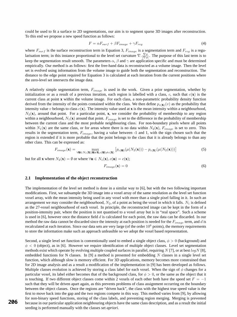
could be used to fit a surface to 2D segmentations, our aim is to segment sparse 3D images after reconstruction.To this end we propose a new speed function as follows:

F = αFsurf + βFimage + γFreg (4)

whereFsurf is the surface reconstruction term in Equation 3,Fimage is a segmentation term andFreg is a regu-larisation term; in this instance proportional to the level set curvature∇. ∇φ

|∇φ| . The purpose of this last term is tokeep the segmentation result smooth. The parametersα, β andγ are application specific and must be determinedempirically. Our method is as follows: first the free-hand data is reconstructed as a volume image. Then the levelset is evolved using information from the volume image to guide both the segmentation and reconstruction. Thedistance to the edge point required for Equation 3 is calculated at each iteration from the current positions wherethe zero-level set intersects the image data.

A relatively simple segmentation term,Fimage is used in the work. Given a prior segmentation, whether byinitialization or as a result of a previous iteration, each region is labelled with a class,c, such thatc(x) is thecurrent class at pointx within the volume image. For each class, a non-parametric probability density functionderived from the intensity of the points contained within the class. We then definepc(x)(v) as the probability thatintensity valuev belongs to classc(x). The intensity value used atx is the mean intensity within a neighbourhood,N2(x), around that point. For a particular point,x, we consider the probability of membership to any regionwithin a neighbourhood,N1(x) around that point.Fimage is set to the difference in the probability of membershipbetween the current class and the most probable neighbouring class. For non-boundary pixels where all pointswithin N1(x) are the same class, or for areas where there is no data withinN2(x), Fimage is set to zero. Thisresults in the segmentation term,Fimage, having a value between -1 and 1, with the sign chosen such that theregion is extended if it is more probable that the point belongs to the class that it is already belongs to than anyother class. This can be expressed as:

Fimage(x) = max∀u∈N1(x)|u6=x,c(u) 6=c(x)

[pc(u)(µ(N2(x)))− pc(x)(µ(N2(x)))

](5)

but for allx whereN2(x) = ∅ or where∀u ∈ N1(x), c(u) = c(x);

Fimage(x) = 0 (6)

2.1 Implementation of the object reconstruction

The implementation of the level set method is done in a similar way to [6], but with the two following importantmodifications. First, we subsample the 3D image into a voxel array of the same resolution as the level set functionvoxel array, with the mean intensity being used in any voxel with more than a single pixel falling in it. In such anarrangement we may consider the neighbourhood,N2, of a point as being the voxel in which it falls.N1 is definedas the 27-voxel neighbourhood of each voxel. In principle, the reconstructed image can be kept in the form of aposition-intensity pair, where the position is not quantised to a voxel array but is in “real space”. Such a schemeis used in [6], however once the distance fieldd is calculated for each point, the raw data can be discarded. In ourmethod the raw data cannot be discarded since the intensity at each position is needed for theFimage term, andd isrecalculated at each iteration. Since our data sets are very large (of the order106 points), the memory requirementsto store the information make such an approach unfeasible so we adopt the voxel based representation.

Second, a single level set function is conventionally used to embed a single object class,φ > 0 (background) andφ < 0 (object), as in [6]. However we require identification of multiple object classes. Level set segmentationmethods exist which operate by evolving multiple coupled surfaces in parallel, requiringN [7], or at bestlogN [8],embedded functions for N classes. In [9] a method is presented for embeddingN classes in a single level setfunction, which although slow is memory efficient. For 3D applications, memory becomes more constrained thanfor 2D image analysis and as a result a modification of the implementation in [9] has been developed as follows.Multiple classes evolution is achieved by storing a class label for each voxel. When the sign ofφ changes for aparticular voxel, its label either becomes that of the background class, forφ > 0, or the same as the object that itis touching. If two different object classes come within 2 voxels of each other both have the speed setF = −1such that they will be driven apart again, as this prevents problems of class assignment occurring on the boundarybetween the object classes. Once the regions are “driven back”, the class with the highest true speed value is thefirst to move back into the gap and the two regions compete in this way. This method varies from [9], by allowingfor non-binary speed functions, storing of the class labels, and preventing region merging. Merging is preventedbecause in our particular application neighbouring objects have the same class description, and as a result the initialseeding is performed manually with the classes setapriori.

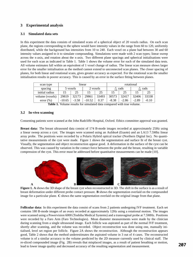
3 Experimental analysis

3.1 Simulated data sets

In this experiment the data consists of simulated scans of a spherical object of 20 voxels radius. On each scanplane, the regions corresponding to the sphere would have intensity values in the range from 60 to 120, uniformlydistributed, while the background has intensities from 10 to 240. Each voxel on a plane had between 30 and 60intensity values assigned to it to simulate compounding. Simulations were made with 2 scan types; linear sweepacross the x-axis, and rotation about the x-axis. Two different plane spacings and spherical initialisations wereused for each scan as indicated in Table 1. Table 1 shows the volume error for each of the simulated data tests.All volume estimates fall within an equivalent of 1 voxel change of radius. The linear scan measure shows largererror for the smaller initialisation as the method cannot extend to unconnected scan planes. The closer spacing ofplanes, for both linear and rotational scans, gives greater accuracy as expected. For the rotational scan the smallerinitialisation results in poorer accuracy. This is caused by an error in the surface fitting between planes.

scan type linear rotationalspacing 5 voxels 2 voxels π

12 rads π24 rads

initial radius 15 25 15 25 15 25 15 25volume (voxels) 29819 32173 29861 33493 30573 32417 32406 33338

error (%) -10.65 -3.58 -10.52 0.37 -8.38 -2.86 -2.89 -0.10Table 1. Volume results for simulated data compared with true volume.

3.2 In-vivo scanning

Consenting patients were scanned at the John Radcliffe Hospital, Oxford. Ethics committee approval was granted.

Breast data: The breast ultrasound data consist of 174 B-mode images recorded at approximately 25Hz usinga linear sweep across a cyst. The images were scanned using an AuIdea4 (Esaote) and an LA13 7.5Mhz lineararray probe. The positions were recorded by a Polaris Hybrid optical tracker (Northern Digital Inc). No quanti-tative measurements of the cyst were made. Figure 1 shows the segmentation and surface fit of the breast cyst.Visually, the segmentation and object reconstruction appear good. A deformation in the surface of the cyst can beobserved. This was caused by variation in the contact force between the probe and the breast, resulting in variablecompression of the cyst. This error must be addressed before quantitative measurements can be made [10].

A B CFigure 1. A shows the 3D shape of the breast cyst when reconstructed in 3D. The shift in the surface is as a result ofbreast deformation under different probe contact pressure.B shows the segmentation overlaid on the compoundedimage for a particular plane.C shows the same segmentation overlaid on the original image from that plane.

Follicular data: In this experiment the data consist of scans from 2 patients undergoing IVF treatment. Each setcontains 180 B-mode images of an ovary recorded at approximately 12Hz using a rotational motion. The imageswere scanned using a Powervision 6000 (Toshiba Medical Systems) and a transvaginal probe at 7.5MHz. Positionswere recorded by a Faro Arm (Faro Technologies). Mean diameter measurements were made by the clinicianduring scanning from a single ultrasound image. Each follicle was aspirated as part of the normal IVF treatment,shortly after scanning, and the volume was recorded. Object reconstruction was done using one, manually ini-tialised, level set region per follicle. Figure 2A shows the reconstruction. Although the reconstruction appearsgood, Table 2 shows that the method underestimates the aspirated volume in 3 out of 4 cases. The reconstructedvolume is of a similar accuracy to the volume predicted by the 2D measure currently used by clinical staff. There-sliced compounded image (Fig. 2B) reveals that misplaced images, as a result of patient breathing or motion,lead to lower image quality and decreased accuracy of the resulting segmentation and measurement.

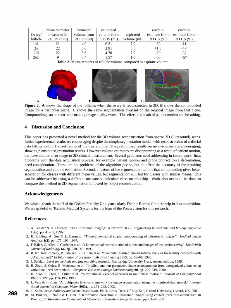
mean diameter estimated estimated error in error inOvary/ measured in volume from volume from aspirated estimate from estimate fromfollicle 2D US (mm) 2D US (ml) 3D US (ml) volume (ml) 2D US (%) 3D US (%)

1/i 21 4.9 6.21 7.0 -30 -112/i 22 5.6 2.91 5.5 +1.8 -472/ii 22 5.6 4.70 7.0 -20 -322/iii 9 0.4 1.57 1.0 -60 +57

Table 2. Measurements of follicle volume compared to aspirate volume

A B CFigure 2. A shows the shape of the follicles when the ovary is reconstructed in 3D.B shows the compoundedimage for a particular plane.C shows the same segmentation overlaid on the original image from that plane.Compounding can be seen to be making image quality worse. This effect is a result of patient motion and breathing.

4 Discussion and Conclusion

This paper has presented a novel method for the 3D volume reconstruction from sparse 3D (ultrasound) scans.Initial experimental results are encouraging despite the simple segmentation model, with reconstruction of artificialdata falling within 1 voxel radius of the true volume. The preliminary results on in-vivo scans are encouraging,showing plausible segmentation results. However volume estimates are disappointing as a result of patient motion,but have similar error range to 2D clinical measurement. Several problems need addressing in future work: first,problems with the data acquisition process, for example patient motion and probe contact force deformation,need consideration. These are not problems of the algorithmper se, but do affect the accuracy of the resultingsegmentation and volume estimation. Second, a feature of the segmentation term is that compounding gives betterseparation for classes with different mean values, but segmentation will fail for classes with similar means. Thiscan be addressed by using a different measure to calculate class membership. Work also needs to be done tocompare this method to 2D segmentation followed by object reconstruction.

Acknowledgements

We wish to thank the staff of the Oxford Fertility Unit, particularly Debbie Barber, for their help in data acquisition.We are grateful to Toshiba Medical Systems for the loan of the Powervision for this research.

References

1. A. Fenster & D. Downey. “3-D ultrasound imaging: A review.”IEEE Engineering in medicine and biology magazine15(6), pp. 41–51, 1996.

2. R. Rohling, A. Gee & L. Berman. “Three-dimensional spatial compounding of ultrasound images.”Medical ImageAnalysis1(3), pp. 177–193, 1997.

3. F. Balen, C. Allen, J. Gardener et al. “3-Dimensional reconstruction of ultrasound images of the uterine cavity.”The BritishJournal of Radiology66, pp. 588–591, 1993.

4. B. ter Haar Romeny, B. Titulaer, S. Kalitzin et al. “Computer assisted human follicle analysis for fertility prospects with3D ultrasound.” InInformation Processing in Medical Imaging 1999, pp. 56–69. 1999.

5. J. Sethian.Level set methods and fast marching methods. Cambridge University Press, second edition, 1999.6. H. Zhao, S. Osher, B. Merriman et al. “Implicit and non-parametric shape reconstruction from unorganized points using

variational level set method.”Computer Vision and Image Understanding80, pp. 295–319, 2000.7. H. Zhao, T. Chan, S. Osher et al. “A variational level set approach to multiphase motion.”Journal of Computational

Physics127, pp. 179–195, 1996.8. L. Vese & T. Chan. “A multiphase level set framework for image segmentation using the mumford-shah model.”Interna-

tional Journal of Computer Vision50(3), pp. 271–293, 2002.9. T. Kadir. Scale, Saliency and Scene Description. Ph.D. thesis, Dept. Of Eng. Sci., Oxford University, Oxford, UK, 2002.

10. M. Burcher, J. Noble & L. Han. “Deformation correction in ultrasound images using contact force measurements.” InProc. IEEE Workshop on Mathematical Methods in Biomedical Image Analysis, pp. 63–70. 2001.

Author Index A pageAlexander DC 117Allen PD 149, 161Allsop J 105Alusi G 157Anderson ME 149Arridge SR 201Astley S 9Atkinson D 21 B Babalola K 97Bamber JC 197Barber DC 29, 93, 109Batchelor PG 21Beichel R 165Bennett MK 169Bhatia K 105Bischof H 165Blot L 85, 137Blythe R 21Board M 9Boardman JP 105Bolt L 13Bovis K 125Boyce JF 25, 81Brady M 181 C Calamante F 21Chung A 33, 153Claridge E 57, 133, 145, 185Connelly A 21Cook PA 117Cootes TF 5Cotton S 145Counsell S 105 D Darzi A 73Deligianni F 33Deng J 77Denton ERE 137Dindoyal I 77Dominguez GF 165Duck FA 45Dumskyj M 25, 81 E Edwards AD 105

ElHelw MA 153 F Feng K 161Fish PJ 41Fleming JS 13, 173Francis J 113 G Gao Z 69Goatman KA 49Goodling MJ 205Graham J 61, 97Griffiths PD 109 H Hajnal JV 105Hamdy FC 29Hartswood M 89Herrick AL 149, 161Hill DLG 21, 201Hillier VF 149Himaga M 25, 81Hoffmann SMA 13, 173Horkaew P 73Houston AS 13 J Jackson C 113Johnson D 53 K Kapellou O 105Kastanis I 201Kemp PM 13Kennedy S 205Kerrigan S 177Kim J-G 65King RJ 53Kohner EM 81Kolen AF 197Kopala L 97 L Lacey AJ 17Lambrou T 77Lapeer RJ 157Leberl F 165Lee KJ 109Lee S-L 73

Linney AD 77, 157Lorenzo-Valdes M 189 M Macleod MA 13Manivannan A 49Marshall J 81Marsland S 101McKenna S 177McNally D 193Mehta S 29Mensah E 81Mirmehdi M 193Misson S 173Mohiaddin R 189Moore T 149, 161Morgan SP 121 N Nagaraj N 173Naguib RNG 169Newman BM 169Noble JA 37, 65, 113, 205Nussey SS 25, 81 O Olson JA 49 Orihuela-Espina F 133Orun A 57 P Paley MN 109Petrou M 53Petroudi S 181Powell J 57 Preece SJ 133, 145Procter R 89 R Raba D 137Rajab MI 121Reid CJ 173Revell JD 193Ricketts IW 177Roberts ME 185Robson M 113Rogers M 61Rose CJ 1Rouncefield M 89Rueckert D 105, 189Ruff CF 77Rutherford MA 105 S Sabate-Cequier A 25, 81Sanchez-Ortiz GI 189

Sanders L 13Sawyer L 173Saxby G 141Scott IM 5Scott MLJ 17Sharp PF 49She Z 41Shipley JA 45Shuttleworth JK 169Silver AMS 201Singh S 125Slack R 89Soutter J 89 T Tan AC 157Taylor CJ 1, 5, 69, 149, 161Thacker NA 17Thomas BT 45Thompson P 141Todd-Pokropek A 77Todman AG 169Tonge RP 61Tournier D 21Twining C 101 U Usher D 25, 81 V van Beek E 29Vandorpe R 97 W Waterton JC 69Wells K 53 White DRR 13Whitwam AD 49Wigderowitz C 177Wild JM 29, 109Wilkinson ID 109Williams S 129Williams TG 69Williamson TH 25, 81Woolfson MS 121Wyatt PP 37 Y Yang G-Z 33, 73, 153 Z Zhu Y 129Zwiggelaar R 85, 129, 137