Media, Pulpit, and Populist Persuasion: Evidence from ...

Media, Pulpit, and Populist Persuasion:Evidence from Father Coughlin

Tianyi Wang∗

Abstract

New technologies make it easier for charismatic individuals to influ-ence others. This paper studies the political impact of the first populistradio personality in American history. Father Charles Coughlin blendedpopulist demagoguery, anti-Semitism, and fascist sympathies to createa hugely popular radio program that attracted tens of millions of listen-ers throughout the 1930s. I evaluate the short- and long-term impactsof exposure to Father Coughlin’s radio program. Exploiting variationin the radio signal strength as a result of topographic factors, I find thata one standard deviation increase in exposure to Coughlin’s anti-FDRbroadcast reduced FDR’s vote share by about two percentage pointsin the 1936 presidential election. Effects were larger in counties withmore Catholics and persisted after Father Coughlin left the air. An al-ternative difference-in-differences strategy exploiting Coughlin’s switchin attitude towards FDR during 1932-1936 confirms the results. More-over, I find that places more exposed to Coughlin’s broadcast in the late1930s were more likely to form a local branch of the pro-Nazi German-American Bund, sell fewer war bonds during WWII, and harbor morenegative feelings towards Jews in the long run.

Keywords: Mass Media, Charismatic Leader, Religion, Anti-Semitism,Populism, Great Depression

∗Department of Economics, University of Pittsburgh, 4901 Wesley W. Posvar Hall, 230South Bouquet Street Pittsburgh, PA 15260. Email: [email protected]. I am extremelygrateful to Randy Walsh, Osea Giuntella, and Allison Shertzer for their guidance and sup-port throughout this project. I also thank Stefano DellaVigna, Andreas Ferrara, MatthewGentzkow, Taylor Jaworski, Melissa Kearney, Daniel I. Rees, Richard Van Weelden, Eu-gene White and participants at the Applied Microeconomics Brown Bag at the Universityof Pittsburgh, the 2019 Southern Economic Association Annual Conference, the 2019 Eco-nomic History Association Annual Meeting, the 2019 Cliometric Society Annual Conference,the 2019 Social Science History Association Annual Meeting, and the 2020 Mountain WestEconomic History Conference for their helpful comments and suggestions.

1

1 Introduction

New media and communication technologies make it easier for charismatic

individuals to influence others. The 2016 U.S. presidential election and the

rise of populist leaders across the world heighten the concern that individuals,

through their charisma and media savviness, can manipulate public opinions

for political gain. How and to what extent can charismatic individuals ex-

ploit the media to shape political outcomes? This paper studies the political

impact of the first populist radio personality in American history. Father

Charles Coughlin blended populist demagoguery, anti-Semitism, and fascist

sympathies to create one of the first loyal mass audiences in broadcasting his-

tory, attracting tens of millions of listeners throughout the 1930s (Warren,

1996). This paper assembles a unique data set to evaluate the short- and

long-term impact of exposure to Father Coughlin’s radio program.

Roman Catholic priest Charles Coughlin embraced radio broadcasting

when radio was a new and rapidly exploding technology during the 1920s. For

the first time one could broadcast to a mass audience over long distances. Ini-

tially airing religious sermons, Father Coughlin switched to broadcast almost

exclusively his opinions on social and economic issues following the onset of

the Great Depression. In a nation mired in its worst economic crisis, Coughlin

became the voice of the people against the nation’s economic and financial

elites. A charismatic orator, Coughlin became seen as the champion of the

common man and referred to as the “Radio Messiah” (Warren, 1996). By the

mid-1930s, Coughlin had developed a weekly national audience of 30 million,

making Father Coughlin the most listened to regular radio speaker in the world

during the 1930s (Brinkley, 1982).

A supporter of Franklin D. Roosevelt and the New Deal during FDR’s

early presidency, Coughlin grew disillusioned with the Roosevelt administra-

tion over time and became its harsh denouncer by 1936, largely because FDR

did not follow Coughlin’s proposal to address the depression (Tull, 1965). Ac-

cusing FDR of being “anti-God” and a puppet controlled by both international

bankers and communists, Coughlin co-founded a third political party, which

2

proposed a populist alternative to challenge FDR in the 1936 presidential

election. By the late 1930s, Father Coughlin had become more extreme in his

broadcast and transformed into a major anti-Semitic icon, fascist sympathizer,

and isolationist in pre-war America.

The episode of Father Coughlin provides a unique opportunity to study

the impact of media manipulation by a charismatic individual. My baseline

analysis examines the impact of exposure to Father Coughlin’s radio program

on voting outcomes in the presidential election of 1936, the year in which

Coughlin harshly attacked the Roosevelt administration. I collect unique data

on the location and technical details of Coughlin’s transmitters in 1936, which

allow me to predict the signal strength of Coughlin’s radio program across

space. Notably, Coughlin’s transmitters changed little over time since 1933,

when he was supporting FDR. It is therefore unlikely that the transmitter

location in 1936 was directly functional to Coughlin’s opposition to FDR.

Nonetheless, reception of Father Coughlin’s broadcast could be correlated

with other county characteristics that might influence voting outcomes. To

address this concern, I employ a strategy pioneered by Olken (2009) to exploit

the variation in Coughlin’s signal strength resulting from topographic factors.

Specifically, I regress the outcomes on the signal strength of Coughlin’s radio

program, while controlling for the hypothetical signal strength when there is

no geographic or topographic obstacles such as mountains and hills. Hence,

identification comes from the residual variation in signal strength as a result

of idiosyncratic topographic factors along the signal transmission route, which

I find to be uncorrelated with past voting outcomes and a large set of pre-

existing county socioeconomic variables.

I find that counties more exposed to Father Coughlin’s radio program

displayed lower support for FDR in the 1936 presidential election. Specifically,

a one standard deviation increase in Coughlin signal strength reduced FDR’s

vote share by 2.4 percentage points, or about 4 percent relative to the mean.

The effect was larger in counties with more Roman Catholics, consistent with

Father Coughlin’s greater influence on Catholics.

To show that the results did not reflect the effect of exposure to radio

3

programs in general, I run a falsification test using exposure to national radio

network stations that did not carry Coughlin’s program. In a statistical horse

race between Coughlin and non-Coughlin exposure, I find that what mattered

was exposure to Coughlin’s stations and not exposure to other stations, sug-

gesting that the effect was unique to Coughlin’s radio program.

Moreover, in another identification strategy, I exploit Coughlin’s switch

in attitude towards FDR during 1932-1936 and panel data during the period

in a difference-in-differences framework. Exploiting within-county variation,

the difference-in-differences strategy controls for any time-invariant differences

across counties and for statewide shocks to counties. Findings from this strat-

egy confirms the baseline results, which also hold under a series of additional

robustness checks, further increasing the causal interpretation of the results.

Exploring persistence of the effects, I find that exposure to Father Cough-

lin’s broadcast continued to dampen FDR’s vote shares in 1940 and 1944, the

last year in which FDR ran for reelection. The negative effects on Demo-

cratic vote shares became smaller after FDR died in office and persisted in the

following two decades, although declining over time.

Because of Father Coughlin’s more extreme stance in the late 1930s, I turn

to examine the effects of Coughlin exposure in the late 1930s on anti-Semitism

and civilian support for America’s involvement in WWII. I collect unique data

from FBI records, which allow me to identify all cities with a local branch of

the pro-Nazi German-American Bund in 1940. I find that cities with a one

standard deviation higher exposure to Father Coughlin’s radio program in the

late 1930s were about 9 percentage points more likely to have a local branch

of the pro-Nazi German-American Bund.

Moreover, using county-level WWII war bond sales data, I find that higher

exposure to Coughlin’s radio program in the late 1930s was also associated with

lower per capita purchase of war bonds. Specifically, a one standard deviation

higher Coughlin exposure was associated with 17 percent lower per capita

purchase of war bonds in 1944, suggesting that Father Coughlin’s isolationist

stance likely dampened public support for the war effort.

Lastly, using individual survey data from the American National Election

4

Studies (ANES), I find that individuals in places with a one standard deviation

higher exposure to Coughlin’s broadcast in the late 1930s were associated

with a 1.6 percent rise in negative feelings towards Jews even in the long

run, although the estimate is not precise. In contrast, I do not find such an

association between exposure to Coughlin and feelings towards other minorities

whom Coughlin did not attack, such as blacks or Catholics, suggesting that

the finding does not reflect a change in attitudes towards minorities in general.

This paper is closely related to the literature on the political persuasion

of media (for surveys of this literature, see DellaVigna and Gentzkow (2010);

Prat and Stromberg (2013); Enikolopov and Petrova (2015); Zhuravskaya et al.

(2019)). Previous work has studied media backed by large institutions, such

as the state or major media organizations.1 This paper focuses on media used

by a charismatic individual, and in particular, a charismatic leader. The po-

litical influence of charismatic individuals, such as politicians, opinion leaders,

and media personalities across a variety of media platforms, has become in-

creasingly evident in recent years, including during the 2016 U.S. presidential

election (Marwick and Lewis, 2017). For instance, the use of Twitter by Don-

ald Trump is widely considered (even by Trump himself) to have contributed to

his election in 2016. Yet, there exists little empirical evidence on the political

impact of media wielded by charismatic individuals.

I study the extent to which an individual charismatic leader can manip-

ulate the media to influence voting behavior. Related to my work is that of

Garthwaite and Moore (2013) who study the effects of political endorsements

by celebrities. They show that Oprah Winfrey’s endorsement of Barack Obama

1For instance, Adena et al. (2015) finds that radio controlled by Nazi Germany con-tributed to the support for the Nazi Party and anti-Semitism in Nazi Germany. DellaVignaand Kaplan (2007) finds that the entry of Fox News increased Republican vote shares in bothU.S. presidential and senatorial elections. Enikolopov et al. (2011) finds that the only inde-pendent national TV channel in Russia increased votes for opposition parties and reducedsupport for the government party in the 1999 parliamentary election. Besides, Durante et al.(2019) finds that exposure to Italy’s Mediaset all-entertainment TV program increased sup-port for Berlusconi’s party and for populism in general. An exception, however, is Xiong(2018), who studies the political premium of TV celebrity and finds that Ronald Reagan’stenure as the host of a 1950s entertainment TV program translated into electoral supportduring his presidential campaign in 1980.

5

brought approximately 1 million additional votes to him during the 2008 U.S.

Democratic Presidential Primary. In contrast, instead of examining political

endorsements, I focus on the impact of a charismatic demagogue (O’Toole,

2019; Harris, 2009; Warren, 1996; Brinkley, 1982; Bennett, 1969; Lee and Lee,

1939) who uses the media to spread propaganda and misinformation. To my

knowledge, this paper is the first in the literature to empirically document how

a charismatic leader, as an individual, can manipulate the media to influence

voting and political preferences. Moreover, this paper contributes to a broader

literature by exploring the role of religion in political persuasion, which has

gone largely unexplored. Finally, the historical context which I consider pro-

vides a novel opportunity to not only examine short-term effects of exposure

to charismatic leaders, but to also consider the long-term effects of such expo-

sure. While little studied, my results suggest that these long-term effects can

be both statistically and economically significant.

By exploring arguably the darkest episode of anti-Semitism in American

history, this paper also adds to the literature on media and inter-group an-

imosity (Bursztyn et al., 2019; Muller and Schwarz, 2019a,b; Adena et al.,

2015; DellaVigna et al., 2014; Yanagizawa-Drott, 2014), on religious extrem-

ism (Iannaccone and Berman, 2006), and more specifically, on anti-Semitism

(Becker and Pascali, 2019; Johnson and Koyama, 2019; Finley and Koyama,

2018; Anderson et al., 2017; Voigtlaender and Voth, 2012). Previous work on

anti-Semitism has almost exclusively focused on the European context. Orga-

nized anti-Semitism reached unprecedented levels in inter-war America, and

Father Coughlin is widely considered its foremost proponent (Strong, 1941;

Lee and Lee, 1939). This paper studies an important episode of anti-Semitism

in America, which has received little attention in the literature.

Furthermore, this paper contributes to the relatively new and growing

literature studying populism. Existing work so far has largely focused on the

determinants of populism, exploring its economic and cultural roots (Ingle-

hart and Norris, 2019; Fukuyama, 2018; Colantone and Stanig, 2018a,b; Autor

et al., 2017; Goodhart, 2017; Gidron and Hall, 2017). There is still little evi-

dence on the extent to which media matter to populist leaders. The findings

6

of this paper are particularly relevant to today’s ongoing debate on the role

of media in the rise of populism (Couttenier et al., 2019; Durante et al., 2019;

Zhuravskaya et al., 2019). Lastly, this paper also contributes to the social

science literature examining Father Coughlin (Warren, 1996; Brinkley, 1982;

Bennett, 1969; Tull, 1965).

2 Historical Background: Radio and Father

Coughlin

Radio as a new communication technology entered American households in

the early 1920s. Providing a variety of music, shows, and information, radio

soon became a popular form of household entertainment. Figure A.1 shows

that the share of American families owning a radio set rose from zero in 1920

to approximately 40 percent by 1930, and it further increased to about 80

percent by 1940; the number of radio stations also increased rapidly during

1920-1940. As a result, the period is often dubbed the Golden Age of Radio.

Radio was central to the rise of Father Coughlin from a local Roman

Catholic priest to a national figure. In 1926, Coughlin started as a priest at

the National Shrine of the Little Flower church in Royal Oak, Michigan, just

outside of Detroit. He quickly embraced radio to broadcast his weekly theolog-

ical teachings from the Detroit station WJR. A charismatic orator on the radio,

Coughlin soon attracted a loyal audience in the Midwest and became known

as the “radio priest.” Indeed, one listener claimed that Coughlin possessed

such a mesmerizing voice “that anyone turning past it almost automatically

returned to hear it again” (Bennett, 1969).

The onset of the Great Depression and the ensuing human suffering, how-

ever, convinced Father Coughlin to switch to broadcast almost exclusively

social and economic commentaries. He described American society as con-

trolled by powerful “banksters,” “plutocrats,” “atheistic Marxists,” and “in-

ternational (commonly understood to mean Jewish) financiers,” whom Cough-

lin blamed for the catastrophe of ordinary American citizens (Warren, 1996).

7

Father Coughlin’s outspokenness on the nation’s economic plight brought him

fame as a champion of the common man, but his controversial statements

were often considered demagogic by others (Bennett, 1969; Tull, 1965; Brink-

ley, 1982).

The CBS national network picked up Coughlin’s radio program in 1930,

which made Father Coughlin a household name. Coughlin’s increasingly con-

troversial statements about the economic and financial elites as well as his

refusal to tone down, however, led the CBS to drop his program a year later

(Warren, 1996). In response, Father Coughlin purchased airtime from indi-

vidual stations and formed his own radio network, and his weekly radio show

was soon broadcast again every Sunday afternoon to a national audience. The

Gallup Poll in April 1938 estimated retrospectively that 27.5% of Americans

listened regularly to Father Coughlin’s radio program before the 1936 presi-

dential election.2 This would put Coughlin’s listenership at above 30 million

in the mid-1930s. During the same period, Coughlin also received on aver-

age more than 10,000 unsolicited letters a day from his listeners, often with a

small donation enclosed (Brinkley, 1982). This would make Father Coughlin

the most listened to regular radio speaker as well as the person receiving the

most letters in the world during the 1930s (Brinkley, 1982). It is therefore

not surprising that many contemporary observers regarded Father Coughlin

as the second most influential public figure in the U.S., next only to President

Franklin D. Roosevelt.

Initially a supporter during FDR’s early presidency, Father Coughlin

coined the phrase “Roosevelt or Ruin” in 1933 following FDR’s election (Tull,

1965). Coughlin, however, grew disillusioned with the Roosevelt adminis-

tration over time and deemed the New Deal administration unsuccessful at

addressing the nation’s social and economic problems. In November 1934

Coughlin founded his own organization, the National Union for Social Justice

(NUSJ), to promote ideologies and policies which he believed would lead to

greater prosperity and social justice.3 The Roosevelt administration, however,

2The number is calculated by the author based on the April 1938 Gallup Poll data fromthe Roper Center for Public Opinion Research: https://ropercenter.cornell.edu/

3Appendix B provides the 16 principles of the National Union Social Justice that Father

8

https://ropercenter.cornell.edu/

did not follow Coughlin’s proposals. By 1936, Coughlin had become a harsh

denouncer of the Roosevelt administration (Tull, 1965). With the new slogan

“Roosevelt and Ruin,” Father Coughlin accused FDR of being “anti-God”

and a “great betrayer and liar” controlled by both international bankers and

communists.

In 1936, Father Coughlin co-founded a third political party, the Union

Party, together with old-age pension advocate Francis Townsend and Gerald

L. K. Smith, who replaced Huey Long as the head of the Share Our Wealth

movement following Long’s assassination in 1935. The Union Party selected

Republican Senator William Lemke from North Dakota as the party’s candi-

date and proposed a populist alternative to challenge FDR in the 1936 presi-

dential election.

Father Coughlin had become more extreme by the late 1930s. Throughout

1938-1939, Coughlin’s radio broadcast and weekly newspaper, Social Justice,

were overtly anti-Semitic (Warren, 1996). He portrayed Jews as malicious

aliens associated with communism and made bitter personal attacks on lead-

ing rabbis and Jewish organizations (O’Toole, 2019). He blamed Jews for

inciting the European conflicts, supported pro-Nazi organizations in America

such as the German-American Bund, and serialized in his weekly newspaper

the Protocols of the Elders of Zion, the notorious fake document purporting

Jewish plans for world domination (O’Toole, 2019). Some of Father Coughlin’s

writings in his newspaper even followed Joseph Goebbels’ speeches verbatim

(Warren, 1996). In 1938, Coughlin also played an instrumental role in form-

ing a paramilitary and anti-Semitic organization, the Christian Front, which

specialized in harassing and beating up Jews and vandalizing Jewish prop-

erty across major U.S. cities (O’Toole, 2019). Besides, Father Coughlin was

also a staunch supporter for American isolationism. Calling FDR “the world’s

chief warmonger,” Coughlin vehemently opposed America’s entry into WWII

and endorsed the leading U.S. isolationist organization, the American First

Committee.

Father Coughlin’s controversial activities eventually led to his downfall.

Coughlin outlined at its founding in November 1934.

9

In late 1939, the National Association of Broadcasters (NAB) introduced a

new self-regulation code that prohibited radio stations from discussing contro-

versial issues in sponsored programs, a rule that many believe was introduced

specifically to rein in Father Coughlin (Warren, 1996). Following this new rule,

almost no station were willing to sell Coughlin airtime, which forced him off the

air in 1940. Shortly following the Pearl Harbor attack, the federal government

further invoked the Espionage Act of 1917 and banned postal circulation of

Coughlin’s weekly newspaper in 1942 because of its seditious content. Church

superiors also ordered Coughlin to relinquish any political involvement or to

give up his priesthood. Father Coughlin chose to return to his parish duties

in 1942 and refrained from the public sphere thereafter.

3 Data

My baseline empirical work relates exposure to Father Coughlin’s anti-FDR

broadcast in 1936 to voting outcomes in the 1936 presidential election. In

this section, I describe the data employed in the baseline analysis, including

data used to measure exposure to Father Coughlin’s radio program, electoral

outcomes, and other county characteristics.

3.1 Exposure to Father Coughlin’s Radio Program

A challenge to study Father Coughlin’s impact on the 1936 presidential elec-

tion is the lack of data measuring exposure to Coughlin’s radio program in

1936 at a fine-grained geographic level. For this project, I assemble a unique

data set from several sources that is particularly suited to measure the political

impacts of Father Coughlin. To proceed, I identify all the radio stations that

Coughlin used for his weekly broadcasts in 1936 from the historical magazine

Broadcasting. Figure A.2 displays the location of the stations, showing a total

of 33 stations. For each of Coughlin’s station, I collect technical details from

the 1936 Broadcasting Yearbook, which provide me with the transmitter fre-

quency, power, and height. I then use this information to calculate the signal

10

strength of Father Coughlin’s radio program across U.S. counties in 1936.

Radio signal transmission obeys the laws of electromagnetic propagation.

In the free space (i.e. assuming the earth is smooth and without any geo-

graphic or topographic obstacles), signal strength is inversely proportional to

the square of the distance from the transmitter (Olken, 2009). In actual trans-

mission, however, the presence of geographic or topographic obstacles, such as

mountains or hills, would lead to diffraction and greater transmission loss in

signal. I calculate the signal transmission loss with a professional radio prop-

agation software based on the Irregular Terrain Model (ITM). The ITM was

developed by the U.S. government in the 1960s and typically used by radio

and TV engineers to predict signal strength of broadcasts.4

Following Olken (2009), I calculate the transmission loss for each transmitter-

county pair using the ITM algorithm.5 I then deduct the transmission loss from

the power of the transmitter to get the predicted signal strength, where signal

strength is measured in decibel-milliwatts (dBm). Finally, for each county

I use the maximum predicted signal strength across all transmitters as the

predicted signal strength in that county.

Panel A of Figure 1 shows the predicted signal strength of Father Cough-

lin’s radio program across counties, where stronger signals are shown with

darker colors.6 Previous studies (Olken, 2009; Enikolopov et al., 2011; Adena

et al., 2015) have shown that signal strength is a strong predictor for the actual

audience size. Because county-level listenership data of Coughlin’s radio pro-

gram are not available, I follow Durante et al. (2019) and use the continuous

4Benjamin Olken has kindly shared the software with me. The ITM software has alsobeen used to calculate radio signal strength in historical settings by Adena et al. (2015)in the context of Nazi Germany and by Gagliarducci et al. (ming) in the context of Italyduring WWII.

5I use the centroid of each county as the receiving location.6Evidently the Cincinnati station is the most powerful station, with its signal dominating

a large number of counties. This is because the Cincinnati station WLW was chosen by thefederal government to experiment with high power broadcasting and authorized to broadcastat 500 kW between 1935 and 1939, while all other stations were operating at 50 kW or less.WLW was one of Coughlin’s stations in 1936. My results are robust to simply removing thisstation from Coughlin’s radio network or using 50 kW as its power, which was its originalpower before 1935, to calculate the signal strength. Hence, my results are not driven by theCincinnati station.

11

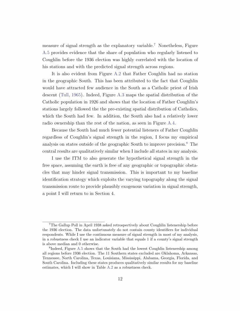
measure of signal strength as the explanatory variable.7 Nonetheless, Figure

A.5 provides evidence that the share of population who regularly listened to

Coughlin before the 1936 election was highly correlated with the location of

his stations and with the predicted signal strength across regions.

It is also evident from Figure A.2 that Father Coughlin had no station

in the geographic South. This has been attributed to the fact that Coughlin

would have attracted few audience in the South as a Catholic priest of Irish

descent (Tull, 1965). Indeed, Figure A.3 maps the spatial distribution of the

Catholic population in 1926 and shows that the location of Father Coughlin’s

stations largely followed the the pre-existing spatial distribution of Catholics,

which the South had few. In addition, the South also had a relatively lower

radio ownership than the rest of the nation, as seen in Figure A.4.

Because the South had much fewer potential listeners of Father Coughlin

regardless of Coughlin’s signal strength in the region, I focus my empirical

analysis on states outside of the geographic South to improve precision.8 The

central results are qualitatively similar when I include all states in my analysis.

I use the ITM to also generate the hypothetical signal strength in the

free space, assuming the earth is free of any geographic or topographic obsta-

cles that may hinder signal transmission. This is important to my baseline

identification strategy which exploits the varying topography along the signal

transmission route to provide plausibly exogenous variation in signal strength,

a point I will return to in Section 4.

7The Gallup Poll in April 1938 asked retrospectively about Coughlin listenership beforethe 1936 election. The data unfortunately do not contain county identifiers for individualrespondents. While I use the continuous measure of signal strength in most of my analysis,in a robustness check I use an indicator variable that equals 1 if a county’s signal strengthis above median and 0 otherwise.

8Indeed, Figure A.5 shows that the South had the lowest Coughlin listenership amongall regions before 1936 election. The 11 Southern states excluded are Oklahoma, Arkansas,Tennessee, North Carolina, Texas, Louisiana, Mississippi, Alabama, Georgia, Florida, andSouth Carolina. Including these states produces qualitatively similar results for my baselineestimates, which I will show in Table A.2 as a robustness check.

12

3.2 Voting Data and County Characteristics

The main outcomes of interest of my baseline analysis consist of vote shares

(in percentage points) of the Democratic Party (FDR), the Republican Party,

and other parties in each county in the 1936 presidential election. Some of my

analyses also use vote shares from past and later presidential elections. These

data come from the ICPSR Study 8611 data set (Clubb et al., 2006). Figure

A.6 shows FDR’s vote share across counties in the 1936 presidential election.

County-level socioeconomic variables are obtained from several sources.

From the ICPSR 2896 data set (Haines, 2010), I obtain a rich set of 1930

county demographics, measuring county population and population by gen-

der, race, birth place, age, literacy, employment status, radio ownership, and

farm characteristics. I use the 1930 Census IPUMS microdata to compute for

each county its mean occupational income score and shares of employment

in manufacturing and in agriculture. The 1926 Census of Religious Bodies

provides me with the share of population belonging to each religious denomi-

nation at the county level in 1926, which allows me to measure the population

share of Roman Catholics. I use ArcGIS to generate additional county-level

geographic characteristics, including area, elevation, and terrain ruggedness.9

4 Empirical Strategy

The objective of my baseline empirical work is to study the impact of exposure

to Father Coughlin’s radio program on voting outcomes in the 1936 presidential

election. Notably, the location of Father Coughlin’s stations in 1936 were

mostly the same as that in 1933, when Coughlin was supportive of FDR.

Figure A.2 maps Coughlin’s stations in 1936, which shows that 25 out of the

33 (or about 76%) stations in 1936 were already in Coughlin’s network in 1933,

when Coughlin was still a strong supporter for FDR. It is therefore unlikely

that station location in 1936 was intentionally driven by Coughlin’s opposition

9I measure elevation and ruggedness at county centroids, consistent with what I did forsignal strength.

13

to FDR.10

Nonetheless, reception of Coughlin’s broadcast might have been corre-

lated with other local characteristics (e.g. distance to major cities) that could

have influenced voting behavior in 1936. To address this concern, I employ an

empirical strategy pioneered by Olken (2009) and exploit plausibly exogenous

variation in Coughlin’s signal strength resulting from topographic factors.11

Specifically, I regress the outcomes of interest on the actual signal strength

(Signal), while controlling for the hypothetical signal strength in the free

space (SignalFree) where the earth is assumed to be free of any topographic

obstacles, such as mountains or hills, that diffract and weaken radio signal

transmission. Crucially, the variable SignalFree controls for a county’s prox-

imity to a transmitter as well as the power of the transmitter. Therefore, once

controlling for SignalFree, identification of the coefficient of Signal comes

from variation in diffraction patterns caused by topographic obstacles along

the signal transmission route. Figure 1 shows the actual (ITM-predicted) sig-

nal strength of Coughlin’s radio program and the hypothetical signal strength

in the free space.

Because a county’s own topography could also potentially influence its

political outcomes, I control for various local geographic characteristics of the

county, including the county’s surface area, altitude, and terrain ruggedness

as well as the square terms of each of these geographic variables. Therefore, I

only exploit residual variation in signal strength resulting from the topography

along the signal transmission route outside the county, which is arguably more

exogenous.12 Furthermore, I include state fixed effects to compare counties

within the same state in all my analyses.

I run the following regression for my baseline analysis:

10While Coughlin’s radio network clearly expanded westward between 1933 and 1936,the results are robust to restricting the sample to counties only in the Northeast and theMidwest, where station location changed little over time.

11A similar strategy has also been used by Durante et al. (2019), DellaVigna et al. (2014),and Yanagizawa-Drott (2014).

12The exceptions are the counties that contained Coughlin stations. I will provide ro-bustness checks by dropping these counties as well as the areas surrounding them.

14

V otec = βSignalc + γSignalFreec + δ′Xc + ηs + εc (1)

where V otec is the vote share (in percentage points) received by a party in

county c in the 1936 presidential election. Signalc is the actual signal strength

of Father Coughlin’s radio program in county c in 1936. SignalFreec is the

hypothetical signal strength in the free space. Xc is a vector of county baseline

controls for local geographic characteristics, socioeconomic characteristics, and

past voting outcomes. ηs are state fixed effects, controlling for any differences

across states that might influence voting. εc is the error term. Standard errors

are corrected for clustering at the state level. To ease the interpretation of

the results, I standardize signal strength such that it has a mean of zero and

a standard deviation of one.

The coefficient β provides the reduced-form estimate of the effect of ex-

posure to Father Coughlin’s radio program. The identification assumption

is that Signal is not correlated with unobserved factors that influence voting

outcomes, conditional on all the covariates in equation (1). While the assump-

tion is ultimately untestable, I support the conditional exogeneity assumption

through balance and placebo tests by examining the correlation of Signal with

pre-existing county socioeconomic characteristics and past voting outcomes.

In Table 1, I examine the correlation between Coughlin’s signal strength

in 1936 and 1930 county socioeconomic characteristics. As seen in column 2,

Signal is significantly correlated with quite a few socioeconomic variables in

the univariate regression. This is not surprising given that Father Coughlin’s

stations were mostly in large cities in the Northeast and the Midwest. Signal,

however, becomes more balanced across the set of 17 socioeconomic character-

istics after I control in column 4 for the free-space signal, state fixed effects,

and local geographic characteristics. In fact, SignalFree, state fixed effects,

and local geographic characteristics explain about 30-60 percent of the overall

variation of most of the socioeconomic variables. Conditional on the additional

covariates, Signal is no longer correlated with most pre-existing demographic

or industrial characteristics, although it is still correlated with the share of el-

derly, unemployment rate, and radio ownership. To be conservative, I include

15

all the socioeconomic characteristics in Table 1 as controls in equation (1).

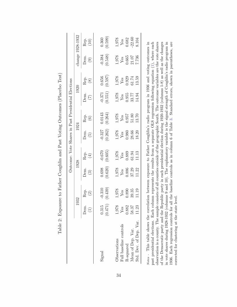
In Table 2, I perform a series of placebo tests by examining the correlation

between Signal and Democratic and Republican vote shares in past presiden-

tial elections before 1936. Conditional the full set of baseline controls, Signal

is not significantly correlated with any of the past electoral outcomes dur-

ing the period 1920-1932 (column 1-8) or with changes in electoral outcomes

between 1928 and 1932 (column 9-10); the estimated coefficients are also gen-

erally small. The results suggest that exposure to Father Coughlin’s radio

program in 1936 was not systematically correlated with pre-existing politi-

cal preferences in either levels or trends, providing support to the conditional

exogeneity assumption of equation (1).

5 Father Coughlin and Presidential Elections

In this section, I present the results on the impact of exposure to Father

Coughlin’s radio program on presidential election voting outcomes. I focus on

the presidential election of 1936, the year in which Father Coughlin harshly

attacked FDR in his radio broadcasts and co-founded the Union Party to

challenge FDR in the presidential race.

5.1 Baseline Results

Table 3 shows the estimated effects of exposure to Father Coughlin’s broad-

cast on voting in the 1936 presidential election. I find that exposure to Father

Coughlin’s radio program had a large negative effect on the support for FDR in

the 1936 presidential election. Based on column 1, without any control, a one

standard deviation increase in exposure to Father Coughlin’s radio program

was associated with a reduction in FDR’s vote share by about 3.8 percentage

points. The results are robust and of similar magnitudes when adding in differ-

ent controls in subsequent columns, including state fixed effects, the free-space

signal, and county geographic and socioeconomic characteristics. In column 6,

after further controlling for past electoral outcomes, the estimated coefficient

16

changes little. Based on column 6, which is my preferred specification that

includes all baseline controls, a one standard deviation increase in exposure to

Coughlin’s radio program reduced FDR’s vote share by about 2.4 percentage

points, which is about 4 percent relative to the mean of FDR’s vote share.

Column 7 of the table, which uses the Republican Party’s vote share as the

outcome, shows that most of the reduction in FDR’s vote share as a result of

exposure to Coughlin went to the Republican Party. A one standard deviation

increase in exposure to Coughlin’s radio program increased the Rupublican

vote share by about 2 percentage points. The voting data set unfortunately

does not contain separate voting results for different third parties in 1936, even

though the Union Party received most of the votes among third parties.13

The data limitation makes it difficult to examine the effect on the Union

Party specifically. I therefore combine the vote shares of all other parties into

one category and use it as the outcome in Column 8. Column 8 shows that

exposure to Father Coughlin increased the support for other parties by about

0.4 percentage points, although the effect is not precisely estimated. Taken as

a whole, Table 3 suggests that exposure to Father Coughlin’s radio program

reduced support for FDR in the 1936 presidential election.

Next, I turn to examine the role of religion in Father Coughlin’s persua-

sion. As a Roman Catholic priest, Father Coughlin likely had greater influence

among the Catholic population. Indeed, based on a Gallup Poll survey in De-

cember 1938, Panel B of Figure A.7 shows that more than 60% of Catholics

approved of what Father Coughlin said in general, much higher than other re-

ligious groups did. I therefore expect that exposure to Father Coughlin’s radio

program to have a larger effect in counties with more Catholics. To test this

hypothesis, I include in my regression interaction terms between Signal and an

indicator variable that equals 1 if a county’s population share of Catholics was

in the top quartile of the distribution among all counties and 0 otherwise.14

Table 4 reports the estimates based on this regression. Consistent with

13In 1936, votes for the Union Party represented 73.5% of all the votes that went to thirdparties.

14Results based on a continuous measure of the population share of Catholics are similarand shown in Table A.1.

17

the expectation, the effects estimated are larger in highly Catholic counties.

Here the effect of Signal in highly Catholic counties is equal to the sum of

the coefficient on Signal and that on the interaction term Signal × Catholic.

Based on column 1, a one standard deviation increase in Coughlin exposure

reduced FDR’s votes by about 3.4 percentage points in highly Catholic coun-

ties. Column 2 shows that there was no differential effect on the support for

the Republican Party in highly Catholic counties. In contrast, Coulumn 3

shows that a one standard deviation increase in Coughlin exposure increased

the support for other parties by about 1.4 percentage points in highly Catholic

counties, which most likely reflect an increase in support for Coughlin’s Union

Party since it was the dominant third party in 1936. Taken together, Table 4 is

consistent with Father Coughlin having a greater influence on Catholic voters

and suggests the possibility for religion to be exploited for political persuasion.

A potential concern remains that the baseline results may simply reflect

exposure to radio programs in general instead of exposure to Father Cough-

lin. To address this concern, I collect data on NBC and CBS network radio

stations that did not carry Coughlin’s broadcast and run a falsification test.

Specifically, I use the same method to predict the signal strengths from the

non-Coughlin stations and then include the non-Coughlin signal strengths (in-

cluding free-space signals) in my baseline regression to perform a statistical

horse race. Table 5 reports these results. As seen in Table 5, the estimated

effects of exposure to non-Coughlin stations are much smaller in magnitude

and statistically insignificant, while the estimates for exposure to Coughlin’s

stations remain strong and similar as in the baseline. The statistical horse race

between Coughlin and non-Coughlin stations suggests that it was exposure to

Father Coughlin’s radio program, instead of exposure to radio programs in

general, that reduced support for FDR in 1936.

5.2 Evidence from a Difference-in-Differences Strategy

A unique feature of my empirical setting is Father Coughlin’s switch in his

attitude towards FDR between 1932 and 1936. Although Father Coughlin

18

was pro-FDR in the 1932 presidential election, Coughlin did not explicitly

broadcast his support for FDR in his radio program until FDR had won the

election (Warren, 1996; Tull, 1965). In a private letter written to FDR during

the 1932 presidential campaign, Father Coughlin expressed strong support for

FDR but stated that he could not take a stand publicly or endorse a particular

candidate because his priesthood forbade him to do so (Tull, 1965). Yet, by

1936, Coughlin had taken an explicit stand against FDR and made that public

through his radio program. Therefore, I would expect places more exposed to

Father Coughlin’s radio program in 1936 to display a greater reduction in

support for FDR between 1932 and 1936.

To exploit the change in Father Coughlin’s attitude between 1932 and

1936, I turn to a difference-in-differences specification using the 1932-1936

panel and exploit only within-county variation over time. Specifically, I run

the following regression:

V otect = βSignalc × Postt +Xc × Postt + σc + ηst + εct (2)

where Signalc is the predicted signal strength of Father Coughlin’s radio pro-

gram in county c in 1936. Postt is an indicator for post-1932, which equals

1 in 1936 and 0 in 1932. σc are county fixed effects, which control for any

time-invariant county characteristics. ηst are state-by-year fixed effects, which

control for statewide shocks to all counties in each state. In some specifica-

tions, I further control for the interactions between all my baseline county

characteristics Xc and Postt, which allow each baseline county characteris-

tic to have a differential effect on voting over time. The standard errors are

corrected for clustering at the county level.

Table 6 reports the results from the difference-in-differences specification,

which substantially confirm the baseline results. Column 1 of Table 6 shows

that, controlling for county fixed effects and year fixed effects, a one standard

deviation increase in exposure to Father Coughlin’s radio program decreased

FDR’s vote share by about 1.5 percentage points. The estimated effects re-

main robust after controlling for state-by-year fixed effects in column 2 and, if

anything, become slightly larger when controlling for the interactions between

19

baseline county characteristics and the Post dummy in column 3. Column 4

and 5 of the table show that the estimated effects for the Republican party

and for other parties remain similar in magnitudes as found in the baseline

and become more precisely estimated.

The identifying assumption of the difference-in-differences specification is

that vote shares in counties with different levels of exposure to Father Coughlin

would have followed parallel trends absent of Father Coughlin’s radio program.

Results in columns 9 and 10 of Table 2 are consistent with the parallel trends

assumption by showing that exposure to Coughlin’s radio program in 1936

was not significantly correlated with changes in vote shares during 1928-1932.

Here, I provide additional support for the parallel trends assumption using an

event study on a relatively longer panel. Specifically, I run equation (2) on

the panel of 1912-1944, replacing Postt with year dummies and using 1932

as the omitted category. The period of 1912-1944 covers all four presidential

elections (1932-1944) involving FDR as well as five elections before.

Figure 2 presents the event study graph for Democratic vote shares. As

seen from this figure, the estimates in the five pre-periods are relatively small in

magnitudes and not significantly different from that in 1932; the lack of a clear

trend before 1936 supports the parallel trends assumption. The estimates for

the period 1936-1944 suggest that higher exposure to Father Coughlin’s radio

program in 1936 reduced support for FDR in each of FDR’s re-elections since

1936. The negative effects appear to increase in magnitude over time. Based

on the 1944 estimate, relative to FDR’s vote share in 1932, a one standard

deviation higher exposure to Father Coughlin’s radio program lowered FDR’s

vote share by about 3.7 percentage points in the 1944 election. Overall, the

event study exercise largely confirms the baseline findings.

5.3 Additional Robustness Checks

I perform several additional robustness checks on my baseline results using

FDR’s 1936 vote share as the outcome variable and report them in Table A.2.

In column 1 of the table, I verify that the results are not driven by particular

20

parametric assumptions by using a binary measure of signal that equals 1 if

the signal strength was above the median and 0 otherwise. The results are

robust to using the binary measure. In column 2, I drop counties within 100

miles from any Coughlin’s stations in 1936 to verify that big cities or their

surrounding regions do not drive the results.15 Counties further away from a

station generally had a smaller population and their exposure to Coughlin’s

broadcast was more likely exogeneous.

In column 3, I control for the free-space signal more flexibly, including the

squared and the cubic terms of the the free-space signal in the baseline regres-

sion as additional controls. The results still hold. Column 4 shows that the

results are also robust to controlling for county-level New Deal expenditures

using data from Fishback et al. (2003), including per capita New Deal grant,

relief, and loans.

In column 5, I examine the effect on the full sample of counties including

the South. The coefficient becomes somewhat smaller and less precisely esti-

mated (p-value = 0.104), possibly because of Father Coughlin’s much lower

listenership in the South. But the result is qualitatively similar and indicates

an overall negative effect of exposure to Father Coughlin on voting for FDR in

1936. In column 6, I weight the baseline regression using county population,

and the estimate changes little. The robustness of the results to this series of

additional checks further support the causal interpretation of the results.

5.4 Persistence after 1936

Father Coughlin was forced off the air in the spring of 1940. Did exposure to

Father Coughlin’s radio program have persistent effects on presidential voting

in the long run? To explore this question, I turn to examine the effects of

exposure to Father Coughlin in 1936 on voting outcomes in later presidential

elections.

While Figure 2 shows that exposure to Father Coughlin continued to

negatively affect FDR when FDR ran for re-elections in 1940 and 1944, it is

15The results are qualitatively similar when focusing on counties that were 150, 200, 250or 300 miles away from any Coughlin’s stations.

21

less clear how early exposure to Father Coughlin would affect later presidential

voting after FDR passed away in office in 1945, five years after Coughlin left

the air. The negative effects on the Democratic Party could vanish after 1945

if voters associated Coughlin’s attacks only with FDR himself, and the effects

could persist if voters associated the attacks on the New Deal and the Roosevelt

administration with the Democratic party.

Figure A.8 plots the estimated coefficients on Signal from separate re-

gressions, in which the outcomes are the Democratic vote shares in each pres-

idential election from 1936 and 1972, the last year covered by the ICPSR

Study 8611 dataset (Clubb et al., 2006). The figure shows that exposure to

Father Coughlin continued to negatively affect the Democratic vote shares in

the long run. The effects, however, appear to decrease after FDR passed away

in 1945 and decline over time until disappearing in 1972. The persistence of

the effects suggests that Father Coughlin’s attack on the Roosevelt adminis-

tration possibly shaped many voters’ attitudes towards the Democratic party

and highlights the impact of influential opinion leaders like Father Coughlin.

6 Father Coughlin, Anti-Semitism, and Civil-

ian Support for WWII

By the late 1930s, Father Coughlin had become a leading anti-Semitic icon,

fascist sympathizer, and isolationist advocate in pre-war America (Tull, 1965;

Brinkley, 1982; Warren, 1996). I now turn to examine the impact of Coughlin’s

radio broadcast on measures of anti-Semitism, fascist sympathies, and support

for the war effort among Americans.

6.1 Civilian Support for America’s War Effort

First, I examine whether exposure to Father Coughlin’s radio program affected

civilian support for America’s war effort during WWII. To carry out this ex-

ercise, I use data on county-level WWII bond sales in 1944, which come from

the 1947 County and City Yearbooks. I divide total bond sales by county pop-

22

ulation to obtain per capita sales of WWII bonds in each county. For the ease

of interpretation, I use the natural log of per capita war bond sales as the

outcome variable. To measure exposure to Father Coughlin’s radio program,

I collect data on Coughlin’s stations in 1939 and use the ITM software to

measure their signal strength across counties as I did in the baseline analysis.

I then run a similar regression as in equation (1), regressing war bond sales in

1944 on the signal strength of Coughlin’s radio program in 1939.

Table 7 reports the results from this exercise. To be consistent with my

baseline results, I again focus on regions outside of the geographic South.16

Across different specifications, exposure to Father Coughlin’s radio program

in 1939 is associated with lower per capita war bond sales in 1944. Based on

column 5, conditional on all the controls, a one standard deviation increase in

Coughlin signal is associated with a 17% decrease in per capita WWII bond

sales. The results suggests that exposure to Father Coughlin’s radio program

in the late 1930s lowered civilian support for America’s war effort.

6.2 Evidence from the German-American Bund

In a broadcast following Nazi Germany’s Kristallnacht in November 1938,

Father Coughlin notoriously labeled the attacks on Jews as a defense against

communism (Warren, 1996). Based on the December 1938 Gallap Poll, Figure

A.7 shows that while close to 60% of Catholics approved of what Coughlin

said in general, less than 20% of Jews did. It is natural to wonder whether

exposure to Father Coughlin’s anti-Semitic broadcasts throughout the period

of 1938-1939 affected anti-Semitism in America.

A challenge to study anti-Semitism or fascist sympathies in pre-war Amer-

ica, however, is the lack of data measuring these outcomes. To overcome the

challenge, I collect new data from the FBI records on the German-American

Bund, the leading anti-Semitic and pro-Nazi organization in pre-war America

(Strong, 1941). The data allow me to identify all the cities with a local branch

of the Bund in 1940, a total of 54 cities.

16Results based on the full sample of counties are qualitatively similar and remain sta-tistically significant at the 5 percent level.

23

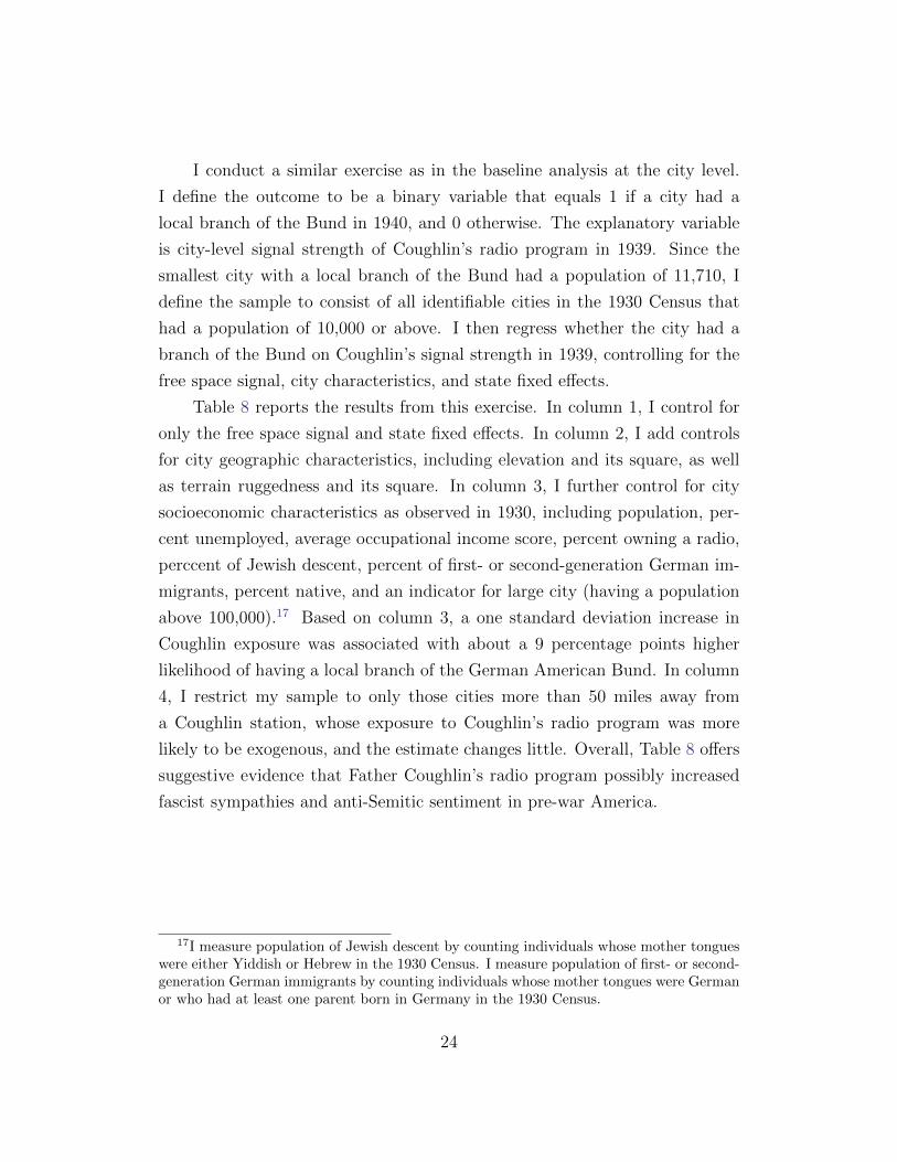
I conduct a similar exercise as in the baseline analysis at the city level.

I define the outcome to be a binary variable that equals 1 if a city had a

local branch of the Bund in 1940, and 0 otherwise. The explanatory variable

is city-level signal strength of Coughlin’s radio program in 1939. Since the

smallest city with a local branch of the Bund had a population of 11,710, I

define the sample to consist of all identifiable cities in the 1930 Census that

had a population of 10,000 or above. I then regress whether the city had a

branch of the Bund on Coughlin’s signal strength in 1939, controlling for the

free space signal, city characteristics, and state fixed effects.

Table 8 reports the results from this exercise. In column 1, I control for

only the free space signal and state fixed effects. In column 2, I add controls

for city geographic characteristics, including elevation and its square, as well

as terrain ruggedness and its square. In column 3, I further control for city

socioeconomic characteristics as observed in 1930, including population, per-

cent unemployed, average occupational income score, percent owning a radio,

perccent of Jewish descent, percent of first- or second-generation German im-

migrants, percent native, and an indicator for large city (having a population

above 100,000).17 Based on column 3, a one standard deviation increase in

Coughlin exposure was associated with about a 9 percentage points higher

likelihood of having a local branch of the German American Bund. In column

4, I restrict my sample to only those cities more than 50 miles away from

a Coughlin station, whose exposure to Coughlin’s radio program was more

likely to be exogenous, and the estimate changes little. Overall, Table 8 offers

suggestive evidence that Father Coughlin’s radio program possibly increased

fascist sympathies and anti-Semitic sentiment in pre-war America.

17I measure population of Jewish descent by counting individuals whose mother tongueswere either Yiddish or Hebrew in the 1930 Census. I measure population of first- or second-generation German immigrants by counting individuals whose mother tongues were Germanor who had at least one parent born in Germany in the 1930 Census.

24

6.3 Public Attitudes towards Jews in the Long Run

Lastly, to explore the impact of Father Coughlin’s radio program on the public

attitudes towards Jews in the long run, I turn to individual survey data from

the nationally representative American National Election Studies (ANES).

Since the 1960s, the ANES have asked about respondents’ feelings towards

Jews in several rounds of surveys using a feeling thermometer question.18

Specifically, the question asked about the respondents’ feelings of warmth to-

wards Jews (and other groups of people) on a scale from 0 to 100, with 100

being the warmest. I use this feeling thermometer variable (ranging from 0

to 100) as the outcome and run a similar regression as in equation (1) at the

individual level. To do that, I pool together all ANES surveys in which feeling

thermometer measurements on Jews are available, including the years of 1964,

1966, 1968, 1972, 1976, 1988 and 1992. This provides me with more than

11,500 individuals from 228 counties. I measure exposure to Coughlin’s anti-

Semitic radio program using the predicted signal strength of Coughlin’s radio

program across counties in 1939. The county identifiers in the ANES data

allow me to assign exposure to Father Coughlin’s radio program to individuals

based on the counties they lived in. Unfortunately, the ANES survey did not

ask about the counties in which the respondents grew up, which would more

likely capture exposure to Coughlin. Therefore, the results from this exercise

should be interpreted with more caution.

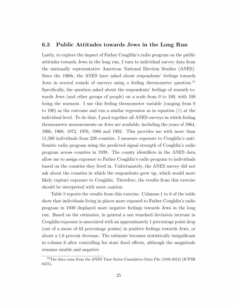
Table 9 reports the results from this exercise. Columns 1 to 6 of the table

show that individuals living in places more exposed to Father Coughlin’s radio

program in 1939 displayed more negative feelings towards Jews in the long

run. Based on the estimates, in general a one standard deviation increase in

Coughlin exposure is associated with an approximately 1 percentage point drop

(out of a mean of 63 percentage points) in positive feelings towards Jews, or

about a 1.6 percent decrease. The estimate becomes statistically insignificant

in column 6 after controlling for state fixed effects, although the magnitude

remains sizable and negative.

18The data come from the ANES Time Series Cumulative Data File (1948-2012) (ICPSR8475).

25

To verify that the results do not reflect a change in attitudes towards

minorities in general, I redo the exercise using feelings towards blacks and

towards Catholics as the outcomes in columns 7 and 8. Consistent with the

fact that Father Coughlin did not speak against these other minority groups,

I find that exposure to Coughlin did not negatively affect attitudes towards

blacks or towards Catholics. Nonetheless, because of the long-run nature of

the outcomes in this exercise, I cautiously interpret these results as suggestive

evidence that exposure to Father Coughlin’s radio program might have lasting

effects on public attitudes towards Jews.

7 Conclusion

New media and information technologies make it easier for charismatic indi-

viduals to influence others. Yet, the possibility that a charismatic individual

can shape political outcomes with the media remains largely unexplored. This

paper assembles a unique data set to study the political impacts of the first

populist radio personality in American history. I find that exposure to Father

Coughlin’s radio program attacking the New Deal administration decreased

support for FDR in the 1936 presidential election. Specifically, a standard de-

viation increase in Coughlin exposure reduced FDR’s vote share by about 2.4

percentage points. The effect was more pronounced in counties with a greater

share of Catholics and persisted after Father Coughlin left the air. Moreover, I

find evidence that places more exposed to Father Coughlin’s anti-Semitic and

isolationist radio program in the late 1930s were more likely to form a local

branch of the pro-Nazi German-American Bund, sell fewer WWII war bonds,

and harbor more negative feelings towards Jews in the long run.

My findings provide the first systematic evidence that a charismatic indi-

vidual can manipulate the media to influence voting behavior and suggest the

potential for religion to be exploited in political persuasion. Although specific

to the episode of Father Coughlin, the results provide more general insights

on the power of charismatic individuals armed with the media to influence

political preferences.

26

References

Adena, M., R. Enikolopov, M. Petrova, V. Santarosa, and E. Zhuravskaya(2015). Radio and the Rise of the Nazis in Prewar Germany. The QuarterlyJournal of Economics 130, 1885–1939.

Anderson, R. W., N. Johnson, and M. Koyama (2017). Jewish Persecutionsand Weather Shocks, 1100-1800. Economic Journal 127, 924–958.

Autor, D., D. Dorn, G. Hanson, and K. Majlesi (2017). Importing PoliticalPolarization? The Electoral Consequences of Rising Trade Exposure. MITWorking Paper .

Becker, S. O. and L. Pascali (2019). Religion, Division of Labor, and Conflict:Anti-Semitism in Germany over 600 Years. American Economic Review 109,1764–1804.

Bennett, D. H. (1969). Demagogues in the Depression: American Radicals andthe Union Party, 1932-1936. Rutgers University Press. New Brunswick.

Brinkley, A. (1982). Voices of Protest: Huey Long, Father Coughlin and theGreat Depression. Alfred A. Knopf. New York.

Bursztyn, L., G. Egorov, R. Enikolopov, and M. Petrova (2019). Social Mediaand Xenophobia: Evidence from Russia. NBER Working Paper No. 26567..

Clubb, J. M., W. H. Flanigan, and N. H. Zingale (2006). Electoral Datafor Counties in the United States: Presidential and Congressional Races,1840–1972 (ICPSR 8611).

Colantone, I. and P. Stanig (2018a). The Economic Determinants of the “Cul-tural Backlash”: Globalization and Attitudes in Western Europe. mimeo.

Colantone, I. and P. Stanig (2018b). The Trade Origins of Economic Na-tionalism: Import Competition and Voting Behavior in Western Europe.American Journal of Political Science 62, 936–953.

Couttenier, M., S. Hatte, M. Thoenig, and S. Vlachos (2019). The Logic of Fear- Populism and Media Coverage of Immigrant Crimes. CEPR DiscussionPaper No. DP13496..

DellaVigna, S., R. Enikolopov, V. Mironova, M. Petrova, and E. Zhuravskaya(2014). Cross-Border Effects of Foreign Media: Serbian Radio and Na-tionalism in Croatia. American Economic Journal: Applied Economics 6,103–132.

27

DellaVigna, S. and M. Gentzkow (2010). Persuasion: Empirical Evidence.Annual Review of Economics 2 (6), 643–669.

DellaVigna, S. and E. Kaplan (2007). The Fox News Effect: Media Bias andVoting. The Quarterly Journal of Economics 122, 1187–1234.

Durante, R., P. Pinotti, and A. Tesei (2019). The Political Legacy of Enter-tainment TV. American Economic Review 109, 2497–2530.

Enikolopov, R. and M. Petrova (2015). Media Capture. In S. Anderson,J. Waldfogel, and D. Stromberg (Eds.), Handbook of Media Economics, Vol-ume 1, pp. 687–700. Elsevier.

Enikolopov, R., M. Petrova, and E. Zhuravskaya (2011). Media and PoliticalPersuasion: Evidence from Russia. American Economic Review 111, 3253––3285.

Finley, T. and M. Koyama (2018). Plague, Politics, and Pogroms: The BlackDeath, the Rule of Law, and the Persecution of Jews in the Holy RomanEmpire. The Journal of Law and Economics 61, 253–277.

Fishback, P. V., S. Kantor, and J. J. Wallis (2003). Can the New Deal’s ThreeRs be Rehabilitated? A Program-by-Program, County-by-County Analysis.Explorations in Economic History 40, 278–307.

Fukuyama, F. (2018). Identity - The Demand for Dignity and the Politics ofResentment. Farrar, Strauss and Giroux. New York.

Gagliarducci, S., M. G. Onorato, F. Sobbrio, and G. Tabellini (Forthcoming).War of the Waves: Radio and Resistance during World War II. AmericanEconomic Journal: Applied Economics .

Garthwaite, C. and T. J. Moore (2013). Can Celebrity Endorsements AffectPolitical Outcomes? Evidence from the 2008 US Democratic PresidentialPrimary. Journal of Law, Economics, & Organization 29, 355–384.

Gidron, N. and P. A. Hall (2017). The Politics of Social Status: Economicand Cultural Roots of the Populist Right. British Journal of Sociology 68,S57–S84.

Goodhart, D. (2017). The Road to Somwhere - The New Tribes Shaping BritishPolitics. Penguin Books.

28

Haines, M. (2010). Historical, Demographic, Economic, and Social Data: TheUnited States, 1790–2002 (ICPSR 2896).

Harris, P. (2009). Glenn Beck and the Echoes of Charles Coughlin. TheGuardian.

Iannaccone, L. R. and E. Berman (2006). Religious Extremism: The Good,the Bad, and the Deadly. Public Choice 128, 109–129.

Inglehart, R. and P. Norris (2019). Cultural Backlash: Trump, Brexit andAuthoritarian-Populism. Cambridge University Press. New York.

Johnson, N. D. and M. Koyama (2019). Persecution and Toleration: The LongRoad to Religious Freedom. Cambridge University Press. Cambridge.

Lee, A. M. and E. B. Lee (1939). The Fine Art of Propaganda: A Study of Fa-ther Coughlin’s Speeches. The Institute for Propaganda Analysis. Harcourt,Brace and Company. New York.

Marwick, A. and R. Lewis (2017). Media Manipulation and DisinformationOnline. Technical report, Data and Society.

Muller, K. and C. Schwarz (2019a). Fanning the Flames of Hate: Social Mediaand Hate Crime. Working Paper .

Muller, K. and C. Schwarz (2019b). From Hashtag to Hate Crime: Twitterand Anti-Minority Sentiment. Working Paper .

Olken, B. (2009). Do Television and Radio Destroy Social Capital? Evi-dence from Indonesian Villages. American Economic Journal: Applied Eco-nomics 1, 1–33.

O’Toole, F. (2019). The Irish Priest Who Paved Way for Donald Trump. TheIrish Times .

Prat, A. and D. Stromberg (2013). The Political Economy of Mass Media. InD. Acemoglu, M. Arellano, and E. Dekel (Eds.), Advances in Economics andEconometrics: Tenth World Congress. Cambridge University Press. Cam-bridge.

Strong, D. S. (1941). Organized Anti-Semitism in America: The Rise of GroupPrejudice During the Decade 1930-1940. American Council on Public Af-fairs. Washington, D.C.

29

Tull, C. J. (1965). Father Coughlin and the New Deal. Syracuse UniversityPress. Syracuse.

Voigtlaender, N. and H.-J. Voth (2012). Persecution Perpetuated: The Me-dieval Origins of Anti-Semitic Violence in Nazi Germany. The QuarterlyJournal of Economics 127, 1339–1392.

Warren, D. (1996). Radio Priest: Charles Coughlin, the Father of Hate Radio.The Free Press. New York.

Xiong, H. (2018). The Political Premium of Television Stardom. WorkingPaper..

Yanagizawa-Drott, D. (2014). Propaganda and Conflict: Theory and Evidencefrom the Rwandan Genocide. The Quarterly Journal of Economics 129,1947—-1994.

Zhuravskaya, E., M. Petrova, and R. Enikolopov (2019). Political Effects ofthe Internet and Social Media. Annual Review of Economics .

30

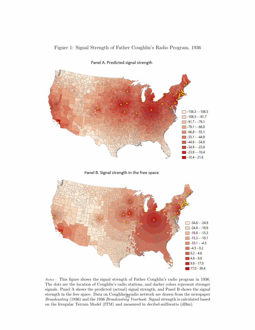
Figure 1: Signal Strength of Father Coughlin’s Radio Program, 1936

Notes - This figure shows the signal strength of Father Coughlin’s radio program in 1936.The dots are the location of Coughlin’s radio stations, and darker colors represent strongersignals. Panel A shows the predicted (actual) signal strength, and Panel B shows the signalstrength in the free space. Data on Coughlin’s radio network are drawn from the newspaperBroadcasting (1936) and the 1936 Broadcasting Yearbook. Signal strength is calculated basedon the Irregular Terrain Model (ITM) and measured in decibel-milliwatts (dBm).

31

Figure 2: Impact of Coughlin Exposure on Democratic Vote Shares (EventStudy)

Notes - This figure plots the event study estimates of exposure to Father Coughlin’s radioprogram in 1936 on Democratic vote shares in presidential elections during 1912-1944. Theestimates come from a single OLS regression following an alternative version of equation (2),in which Postt is replaced with year dummies, with the year of 1932 as the omitted category.The explanatory variable is the Democratic vote share in each presidential election. Theexplanatory variables are the signal strength of Coughlin’s radio program in 1936 interactedwith year dummies. Each regression controls for county fixed effects, state-by-year fixed ef-fects, and baseline county characteristics (SignalFree, geographic, socioeconomic, and pastvoting controls) interacted with year dummies. Standard errors are corrected for clusteringat the state level. The dots are the estimated coefficients and the vertical lines representthe 95% confidence intervals.

32

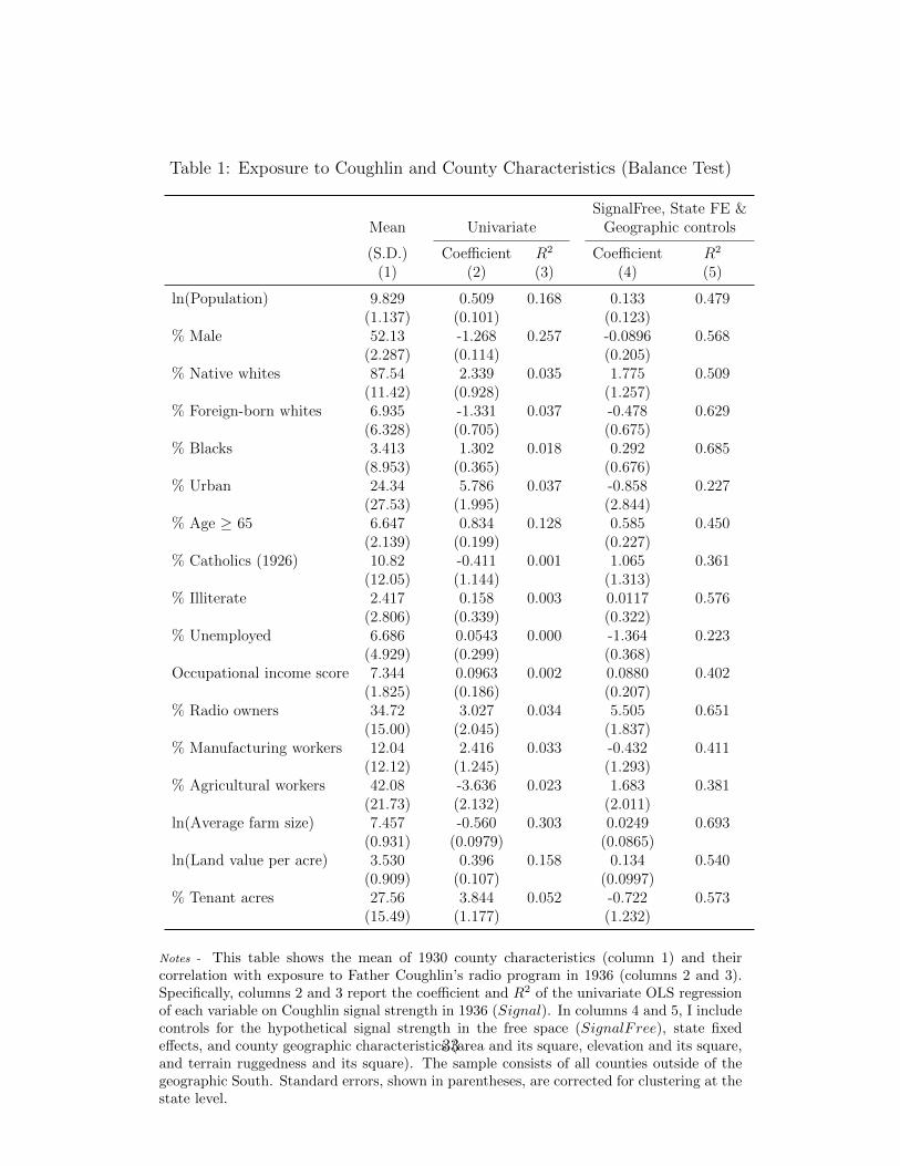
Table 1: Exposure to Coughlin and County Characteristics (Balance Test)

SignalFree, State FE &Mean Univariate Geographic controls

(S.D.) Coefficient R2 Coefficient R2

(1) (2) (3) (4) (5)

ln(Population) 9.829 0.509 0.168 0.133 0.479(1.137) (0.101) (0.123)

% Male 52.13 -1.268 0.257 -0.0896 0.568(2.287) (0.114) (0.205)

% Native whites 87.54 2.339 0.035 1.775 0.509(11.42) (0.928) (1.257)

% Foreign-born whites 6.935 -1.331 0.037 -0.478 0.629(6.328) (0.705) (0.675)

% Blacks 3.413 1.302 0.018 0.292 0.685(8.953) (0.365) (0.676)

% Urban 24.34 5.786 0.037 -0.858 0.227(27.53) (1.995) (2.844)

% Age ≥ 65 6.647 0.834 0.128 0.585 0.450(2.139) (0.199) (0.227)

% Catholics (1926) 10.82 -0.411 0.001 1.065 0.361(12.05) (1.144) (1.313)

% Illiterate 2.417 0.158 0.003 0.0117 0.576(2.806) (0.339) (0.322)

% Unemployed 6.686 0.0543 0.000 -1.364 0.223(4.929) (0.299) (0.368)

Occupational income score 7.344 0.0963 0.002 0.0880 0.402(1.825) (0.186) (0.207)

% Radio owners 34.72 3.027 0.034 5.505 0.651(15.00) (2.045) (1.837)

% Manufacturing workers 12.04 2.416 0.033 -0.432 0.411(12.12) (1.245) (1.293)

% Agricultural workers 42.08 -3.636 0.023 1.683 0.381(21.73) (2.132) (2.011)

ln(Average farm size) 7.457 -0.560 0.303 0.0249 0.693(0.931) (0.0979) (0.0865)

ln(Land value per acre) 3.530 0.396 0.158 0.134 0.540(0.909) (0.107) (0.0997)

% Tenant acres 27.56 3.844 0.052 -0.722 0.573(15.49) (1.177) (1.232)

Notes - This table shows the mean of 1930 county characteristics (column 1) and theircorrelation with exposure to Father Coughlin’s radio program in 1936 (columns 2 and 3).Specifically, columns 2 and 3 report the coefficient and R2 of the univariate OLS regressionof each variable on Coughlin signal strength in 1936 (Signal). In columns 4 and 5, I includecontrols for the hypothetical signal strength in the free space (SignalFree), state fixedeffects, and county geographic characteristics (area and its square, elevation and its square,and terrain ruggedness and its square). The sample consists of all counties outside of thegeographic South. Standard errors, shown in parentheses, are corrected for clustering at thestate level.

33

Tab

le2:

Exp

osure

toF

ather

Cou

ghlin

and

Pas

tV

otin

gO

utc

omes

(Pla

ceb

oT

est)

Ou

tcom

e:V

ote

Sh

ares

inP

ast

Pre

siden

tial

Ele

ctio

ns

1932

1928

1924

1920

chan

ge19

28-1

932

Dem

.R

ep.

Dem

.R

ep.

Dem

.R

ep.

Dem

.R

ep.

Dem

.R

ep.

(1)

(2)

(3)

(4)

(5)

(6)

(7)

(8)

(9)

(10)

Sig

nal

0.31

5-0

.310

0.69

8-0

.670

-0.3

270.

0143

-0.3

710.

656

-0.3

840.

360

(0.4

71)

(0.4

39)

(0.6

20)

(0.6

05)

(0.2

62)

(0.2

64)

(0.5

51)

(0.5

97)

(0.5

48)

(0.5

99)

Ob

serv

atio

ns

1,97

81,

978

1,97

81,

978

1,97

81,

978

1,97

81,

978

1,97

81,

978

Fu

llb

asel

ine

contr

ols

Yes

Yes

Yes

Yes

Yes

Yes

Yes

Yes

Yes

Yes

R-s

qu

ared

0.88

20.

890

0.88

60.

889

0.98

00.

957

0.95

50.

929

0.66

50.

682

Mea

nof

Dep

.V

ar.

58.3

739

.35

37.2

961

.94

28.6

651

.80

33.7

761

.74

21.0

7-2

2.60

Std

.D

ev.

ofD

ep.

Var

.11

.23

11.1

911

.22

11.1

318

.20

13.7

014

.94

13.5

97.

736

8.10

4

Notes-

Th

ista

ble

show

sth

eco

rrel

atio

nb

etw

een

exp

osu

reto

Fath

erC

ou

gh

lin

’sra

dio

pro

gra

min

1936

an

dvoti

ng

ou

tcom

esin

pas

tp

resi

den

tial

elec

tion

s.E

ach

colu

mn

rep

rese

nts

the

resu

lts

from

ase

para

teO

LS

regre

ssio

nfo

llow

ing

equ

ati

on

(1),

wh

ere

each

obse

rvat

ion

isa

cou

nty

.T

he

sam

ple

con

sist

sof

all

cou

nti

esou

tsid

eof

the

geo

gra

phic

Sou

th.

Th

eou

tcom

eva

riab

les

are

the

vote

share

sof

the

Dem

ocr

atic

par

tyan

dth

eR

epub

lic

par

tyin

each

pre

sid

enti

al

elec

tion

du

rin

g1920-1

932

(colu

mn

s1-8

)as

wel

las

the

chan

ges

invo

tesh

ares

du

rin

g19

28-1

932

(col

um

ns

9an

d10).

Th

eex

pla

nato

ryva

riab

leis

the

sign

al

stre

ngth

of

Cou

gh

lin

’sra

dio

pro

gra

min

1936

.E

ach

regr

essi

onco

ntr

ols

for

all

the

bas

elin

eco

ntr

ols

as

inco

lum

n6

of

Tab

le3.

Sta

nd

ard

erro

rs,

show

nin

pare

nth

eses

,are

corr

ecte

dfo

rcl

ust

erin

gat

the

stat

ele

vel.

34

Tab

le3:

Exp

osure

toF

ather

Cou

ghlin

and

1936

Vot

ing

Outc

omes

Ou

tcom

e:V

ote

Sh

ares

(%)

inth

e19

36P

resi

den

tial

Ele

ctio

nfo

r

FD

RL

and

on(D

emocr

at)

(Rep

ub

lica

n)

Oth

ers

(1)

(2)

(3)

(4)

(5)

(6)

(7)

(8)

Sig

nal

-3.7

99-2

.120

-3.0

18-4

.023

-2.7

79-2

.399

1.97

60.

424

(0.5

40)

(1.1

44)

(1.3

01)

(0.9

71)

(0.8

35)

(0.5

81)

(0.6

09)

(0.3

53)

Ob

serv

atio

ns

2,00

72,

007

2,00

72,

007

1,99

61,

978

1,97

81,

978

Sta

teF

EY

esY

esY

esY

esY

esY

esY

esS

ign

alF

ree

Yes

Yes

Yes

Yes

Yes

Yes

Geo

grap

hic

contr

ols

Yes

Yes

Yes

Yes

Yes

Soci

oec

onom

icco

ntr

ols

Yes

Yes

Yes

Yes

Pas

tel

ecto

ral

contr

ols

Yes

Yes

Yes

R-s

qu

ared

0.09

10.

391

0.39

30.

417

0.54

80.

818

0.85

40.

656

Mea

nof

Dep

.V

ar.

57.1

157

.11

57.1

157

.11

57.0

356

.95

40.3

42.

701

Std

.D

ev.

ofD

ep.

Var

.11

.51

11.5

111

.51

11.5

111

.46

11.4

511

.77

3.58

3

Notes-

Th

ista

ble

show

sth

ees

tim

ated

effec

tsof

exp

osu

reto

Fath

erC

ou

gh

lin

’sra

dio

pro

gra

min

1936

on

voti

ng

inth

e1936

pre

sid

enti

al

elec

tion

.E

ach

colu

mn

rep

rese

nts

the

resu

lts

from

ase

para

teO

LS

regre

ssio

nfo

llow

ing

equ

ati

on

(1),

wh

ere

each

ob

serv

ati

on

isa

cou

nty

.T

he

sam

ple

con

sist

sof

all

cou

nti

esou

tsid

eof

the

geo

gra

ph

icS

ou

th.

Th

eou

tcom

eva

riab

les

are

FD

R’s

vote

share

sin

colu

mn

s1-6

,th

eR

epu

bli

can

par

ty’s

vot

esh

are

inco

lum

n7,

an

doth

erp

art

ies’

vote

share

inco

lum

n8,

all

mea

sure

din

per

centa

ge

poin

ts.

The

exp

lan

ator

yva

riab

leis

the

sign

alst

ren

gth

ofC

ou

gh

lin

’sra

dio

pro

gra

min

1936.SignalFree

isth

ehyp

oth

etic

al

sign

al

stre

ngth

inth

efr

eesp

ace.

Geo

grap

hic

contr

ols

incl

ud

eth

eco

unty

’sare

aan

dit

ssq

uare

,el

evati

on

an

dit

ssq

uare

,an

dte

rrain

rugged

nes

san

dit

ssq

uar

e.S

oci

oec

onom

icco

ntr

ols

are

list

edin

Tab

le1

an

din

clu

de

the

natu

ral

log

of

the

pop

ula

tion

,th

ep

op

ula

tion

share

sof

male

s,b

lack

s,n

ativ

ew

hit

es,

fore

ign

-bor

nw

hit

es,

urb

an

pop

ula

tion

,p

op

ula

tion

aged

65

or

ab

ove,

Cath

oli

cs,

illi

tera

te,

un

emp

loye

d,

fam

ilie

sw

ith

ara

dio

,m

ean

occ

up

atio

nal

inco

me

scor

e,sh

are

of

emp

loym

ent

inm

anu

fact

uri

ng,

share

of

emp

loym

ent

inagri

cult

ure

,n

atu

ral

log

ofav

erag

efa

rmsi

ze,

nat

ura

llo

gof

farm

lan

dva

lue

per

acr

e,and

share

of

farm

lan

dby

tenant

farm

ers.

Past

elec

tora

lco

ntr

ols

incl

ud

eav

erag

evo

tesh

ares

ofth

eD

emocr

atic

part

yand

of

the

Rep

ub

lica

np

art

yas

wel

las

aver

age

vote

rtu

rnou

td

uri

ng

1920-1

928.

Sta

nd

ard

erro

rs,

show

nin

par

enth

eses

,ar

eco

rrec

ted

for

clu

ster

ing

at

the

state

level

.

35

Table 4: Effects in Counties with a Large Share of Catholics

Outcome: Vote Shares in 1936

Dem. Rep. Others(1) (2) (3)

Signal × Catholic -1.341 -0.0963 1.440(0.460) (0.352) (0.349)

Signal -2.051 2.014 0.0373(0.607) (0.625) (0.386)

Catholic -0.708 0.756 -0.0442(0.696) (0.579) (0.352)

Observations 1,978 1,978 1,978Full baseline controls Yes Yes YesR-squared 0.820 0.854 0.672Mean of Dep. Var. 56.95 40.34 2.701Std. Dev. of Dep. Var. 11.45 11.77 3.583

Notes - This table shows the estimated effects of Coughlin exposure on voting in the 1936presidential elections in counties with high and low shares of Catholic population. Eachcolumn represents the results from a separate OLS regression where each observation is acounty. The sample consists of all counties outside of the geographic South. The outcomevariables are FDR’s vote share in column 1, the Republican vote share in column 2, andother parties’ vote share in column 3. Catholic is a dummy variable that equals 1 if thecounty’s population share of Roman Catholics was in the top quartile of the distributionand 0 otherwise. Each regression controls for all the baseline controls as in column 6 ofTable 3. Standard errors, shown in parentheses, are corrected for clustering at the statelevel.

36

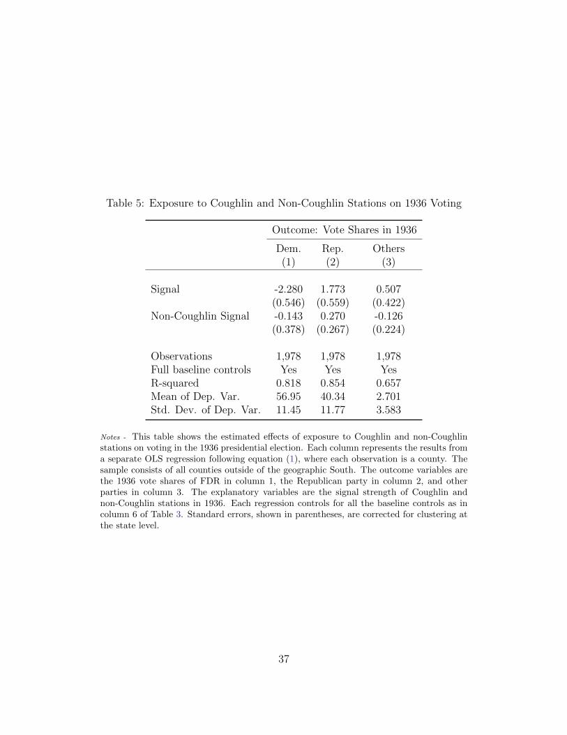
Table 5: Exposure to Coughlin and Non-Coughlin Stations on 1936 Voting



Signal -2.280 1.773 0.507(0.546) (0.559) (0.422)

Non-Coughlin Signal -0.143 0.270 -0.126(0.378) (0.267) (0.224)


Notes - This table shows the estimated effects of exposure to Coughlin and non-Coughlinstations on voting in the 1936 presidential election. Each column represents the results froma separate OLS regression following equation (1), where each observation is a county. Thesample consists of all counties outside of the geographic South. The outcome variables arethe 1936 vote shares of FDR in column 1, the Republican party in column 2, and otherparties in column 3. The explanatory variables are the signal strength of Coughlin andnon-Coughlin stations in 1936. Each regression controls for all the baseline controls as incolumn 6 of Table 3. Standard errors, shown in parentheses, are corrected for clustering atthe state level.

37

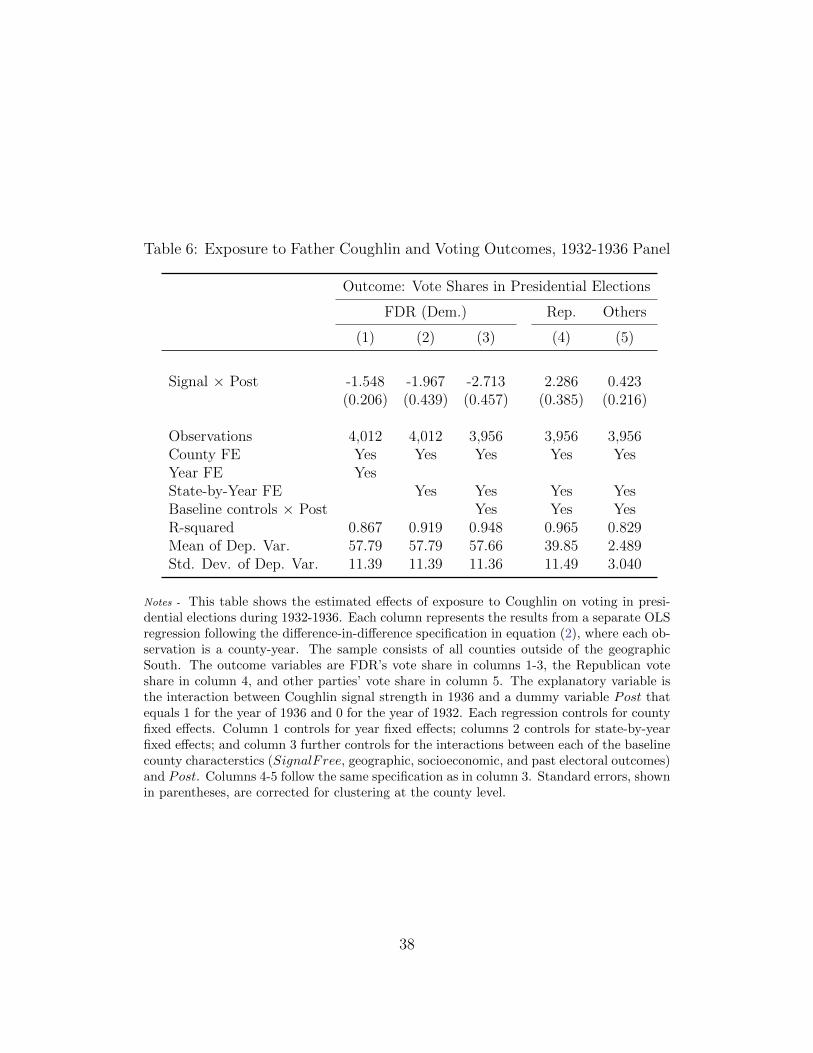
Table 6: Exposure to Father Coughlin and Voting Outcomes, 1932-1936 Panel

Outcome: Vote Shares in Presidential Elections

FDR (Dem.) Rep. Others

(1) (2) (3) (4) (5)

Signal × Post -1.548 -1.967 -2.713 2.286 0.423(0.206) (0.439) (0.457) (0.385) (0.216)

Observations 4,012 4,012 3,956 3,956 3,956County FE Yes Yes Yes Yes YesYear FE YesState-by-Year FE Yes Yes Yes YesBaseline controls × Post Yes Yes YesR-squared 0.867 0.919 0.948 0.965 0.829Mean of Dep. Var. 57.79 57.79 57.66 39.85 2.489Std. Dev. of Dep. Var. 11.39 11.39 11.36 11.49 3.040

Notes - This table shows the estimated effects of exposure to Coughlin on voting in presi-dential elections during 1932-1936. Each column represents the results from a separate OLSregression following the difference-in-difference specification in equation (2), where each ob-servation is a county-year. The sample consists of all counties outside of the geographicSouth. The outcome variables are FDR’s vote share in columns 1-3, the Republican voteshare in column 4, and other parties’ vote share in column 5. The explanatory variable isthe interaction between Coughlin signal strength in 1936 and a dummy variable Post thatequals 1 for the year of 1936 and 0 for the year of 1932. Each regression controls for countyfixed effects. Column 1 controls for year fixed effects; columns 2 controls for state-by-yearfixed effects; and column 3 further controls for the interactions between each of the baselinecounty characterstics (SignalFree, geographic, socioeconomic, and past electoral outcomes)and Post. Columns 4-5 follow the same specification as in column 3. Standard errors, shownin parentheses, are corrected for clustering at the county level.

38

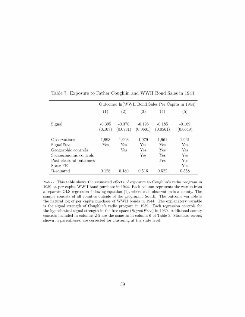
Table 7: Exposure to Father Coughlin and WWII Bond Sales in 1944

Outcome: ln(WWII Bond Sales Per Capita in 1944)

(1) (2) (3) (4) (5)

Signal -0.395 -0.378 -0.195 -0.185 -0.169(0.107) (0.0731) (0.0601) (0.0561) (0.0649)

Observations 1,993 1,993 1,979 1,961 1,961SignalFree Yes Yes Yes Yes YesGeographic controls Yes Yes Yes YesSocioeconomic controls Yes Yes YesPast electoral outcomes Yes YesState FE YesR-squared 0.128 0.180 0.516 0.522 0.558

Notes - This table shows the estimated effects of exposure to Coughlin’s radio program in1939 on per capita WWII bond purchase in 1944. Each column represents the results froma separate OLS regression following equation (1), where each observation is a county. Thesample consists of all counties outside of the geographic South. The outcome variable isthe natural log of per capita purchase of WWII bonds in 1944. The explanatory variableis the signal strength of Coughlin’s radio program in 1939. Each regression controls forthe hypothetical signal strength in the free space (SignalFree) in 1939. Additional countycontrols included in columns 2-5 are the same as in column 6 of Table 3. Standard errors,shown in parentheses, are corrected for clustering at the state level.

39

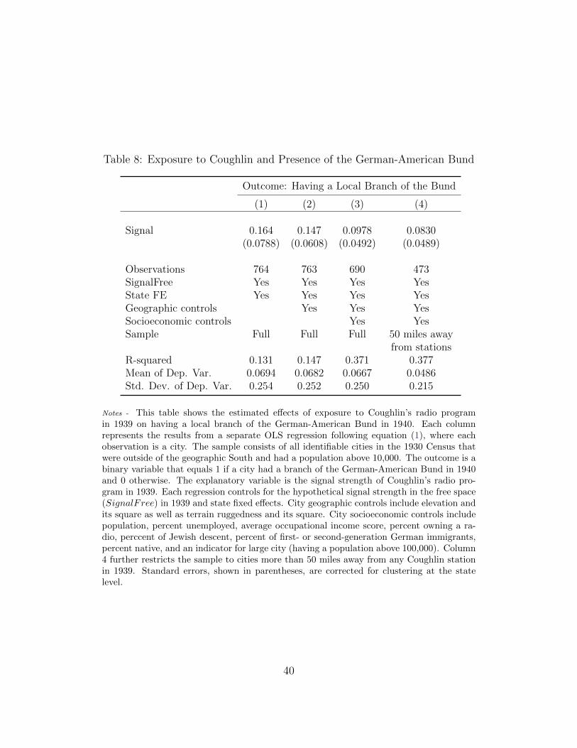
Table 8: Exposure to Coughlin and Presence of the German-American Bund

Outcome: Having a Local Branch of the Bund

(1) (2) (3) (4)

Signal 0.164 0.147 0.0978 0.0830(0.0788) (0.0608) (0.0492) (0.0489)

Observations 764 763 690 473SignalFree Yes Yes Yes YesState FE Yes Yes Yes YesGeographic controls Yes Yes YesSocioeconomic controls Yes YesSample Full Full Full 50 miles away

from stationsR-squared 0.131 0.147 0.371 0.377Mean of Dep. Var. 0.0694 0.0682 0.0667 0.0486Std. Dev. of Dep. Var. 0.254 0.252 0.250 0.215

Notes - This table shows the estimated effects of exposure to Coughlin’s radio programin 1939 on having a local branch of the German-American Bund in 1940. Each columnrepresents the results from a separate OLS regression following equation (1), where eachobservation is a city. The sample consists of all identifiable cities in the 1930 Census thatwere outside of the geographic South and had a population above 10,000. The outcome is abinary variable that equals 1 if a city had a branch of the German-American Bund in 1940and 0 otherwise. The explanatory variable is the signal strength of Coughlin’s radio pro-gram in 1939. Each regression controls for the hypothetical signal strength in the free space(SignalFree) in 1939 and state fixed effects. City geographic controls include elevation andits square as well as terrain ruggedness and its square. City socioeconomic controls includepopulation, percent unemployed, average occupational income score, percent owning a ra-dio, perccent of Jewish descent, percent of first- or second-generation German immigrants,percent native, and an indicator for large city (having a population above 100,000). Column4 further restricts the sample to cities more than 50 miles away from any Coughlin stationin 1939. Standard errors, shown in parentheses, are corrected for clustering at the statelevel.

40

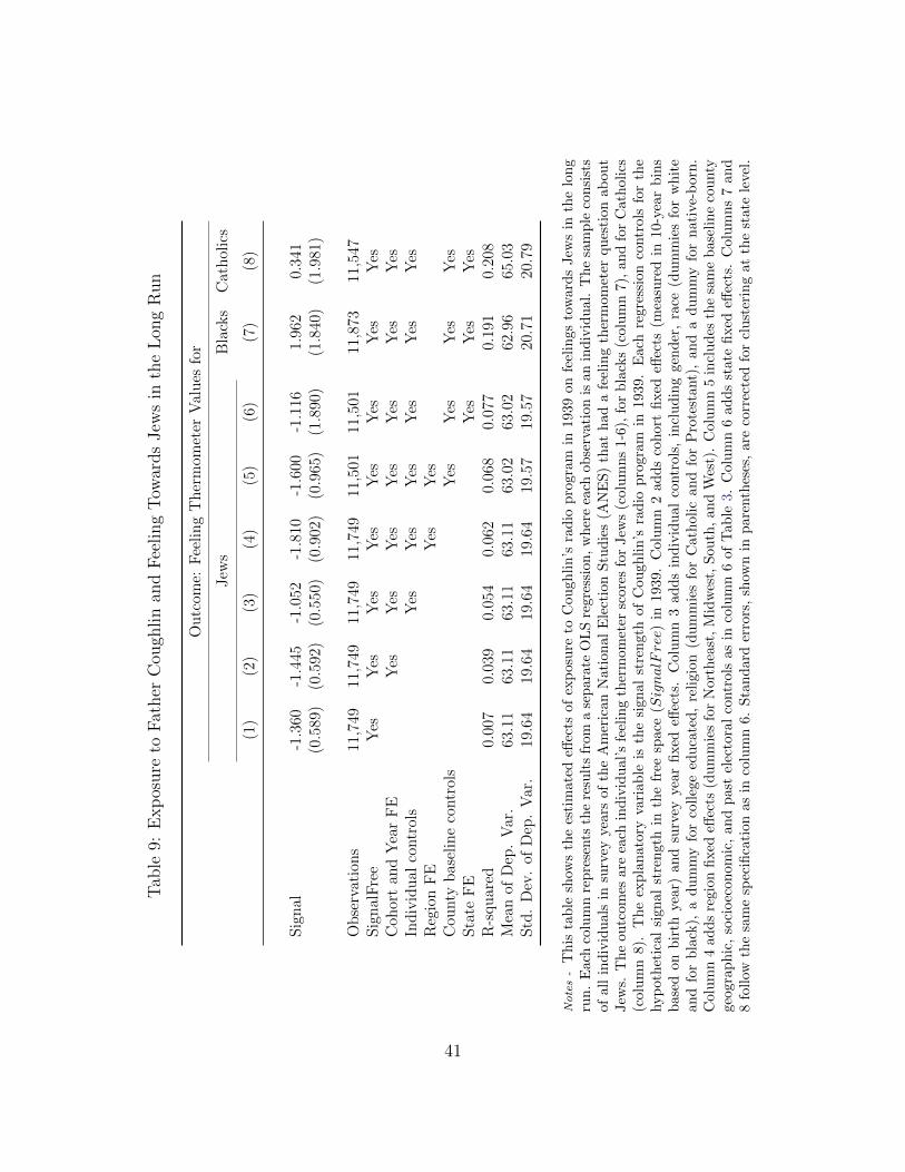
Tab

le9:

Exp

osure

toF

ather

Cou

ghlin

and

Fee

ling

Tow

ards

Jew

sin

the

Lon

gR

un

Ou

tcom

e:F

eeli

ng

Th

erm

omet

erV

alu

esfo

r

Jew

sB

lack

sC

ath

olic

s

(1)

(2)

(3)

(4)

(5)

(6)

(7)

(8)

Sig

nal

-1.3

60-1

.445

-1.0

52-1

.810

-1.6

00-1

.116

1.96

20.

341

(0.5

89)

(0.5

92)

(0.5

50)

(0.9

02)

(0.9

65)

(1.8

90)

(1.8

40)

(1.9

81)

Ob

serv

atio

ns

11,7

4911

,749

11,7

4911

,749

11,5

0111

,501

11,8

7311

,547

Sig

nal

Fre

eY

esY

esY

esY

esY

esY

esY

esY

esC

ohor

tan

dY

ear

FE

Yes

Yes

Yes

Yes

Yes

Yes

Yes

Ind

ivid

ual

contr

ols

Yes

Yes

Yes

Yes

Yes

Yes

Reg

ion

FE

Yes

Yes

Cou

nty

bas

elin

eco

ntr

ols

Yes

Yes

Yes

Yes

Sta

teF

EY

esY

esY

esR

-squ

ared

0.00

70.

039

0.05

40.

062

0.06

80.

077

0.19

10.

208

Mea

nof

Dep

.V

ar.

63.1

163

.11

63.1

163

.11

63.0

263

.02

62.9

665

.03

Std

.D

ev.

ofD

ep.

Var

.19

.64

19.6

419

.64

19.6

419

.57

19.5

720

.71

20.7

9

Notes-

Th

ista

ble

show

sth

ees

tim

ated

effec

tsof

exp

osu

reto

Cou

gh

lin

’sra

dio

pro

gra

min

1939

on

feel

ings

tow

ard

sJew

sin

the

lon

gru

n.

Eac

hco

lum

nre

pre

sents

the

resu

lts

from

ase

para

teO

LS

regre

ssio

n,

wh

ere

each

ob

serv

ati

on

isan

indiv

idu

al.

Th

esa

mp

leco

nsi

sts

ofal

lin

div

idu

als

insu

rvey

year

sof

the

Am

eric

anN

ati

on

al

Ele

ctio

nS

tud

ies

(AN

ES

)th

at

had

afe

elin

gth

erm

om

eter

qu

esti

on

ab

ou

tJew

s.T

he

outc

omes

are

each

ind

ivid

ual

’sfe

elin

gth

erm

om

eter

score

sfo

rJew

s(c

olu

mn

s1-6

),fo

rb

lack

s(c

olu

mn

7),

an

dfo

rC

ath

oli

cs(c

olu

mn

8).

Th

eex

pla

nat

ory

vari

able

isth

esi

gnal

stre

ngth

of

Cou

gh

lin

’sra

dio

pro

gra

min

1939.

Each

regre

ssio

nco

ntr

ols

for

the

hyp

oth

etic

alsi

gnal

stre

ngt

hin

the

free

spac

e(S

ignalF

ree)

in1939.

Colu

mn

2ad

ds

coh

ort

fixed

effec

ts(m

easu

red

in10-y

ear

bin

sb

ased

onb

irth

yea

r)an

dsu

rvey

yea

rfi

xed

effec

ts.

Colu

mn

3ad

ds

ind

ivid

ual

contr

ols

,in

clu

din

ggen

der

,ra

ce(d

um

mie

sfo

rw

hit

ean

dfo

rb

lack

),a

du

mm

yfo

rco

lleg

eed

uca

ted

,re

ligio

n(d

um

mie

sfo

rC

ath

oli

can

dfo

rP

rote

stant)

,an

da

du

mm

yfo

rn

ati

ve-

born

.C

olu

mn

4ad

ds

regi

onfi

xed

effec

ts(d

um

mie

sfo

rN

ort

hea

st,

Mid

wes

t,S

ou

th,

an

dW

est)

.C

olu

mn

5in

clu

des

the

sam

eb

ase

lin

eco

unty

geog

rap

hic

,so

cioec

onom

ic,

and

pas

tel

ecto

ral

contr

ols

as

inco

lum

n6

of

Tab

le3.

Colu

mn

6ad

ds

state

fixed

effec

ts.

Colu

mn

s7

an

d8

foll

owth

esa

me

spec

ifica

tion

asin

colu

mn

6.S

tan

dard

erro

rs,

show

nin

pare

nth

eses

,are

corr

ecte

dfo

rcl

ust

erin

gat

the

state

level

.

41

For Online Publication

Appendix A: Supplemental Figures and Tables

42

Figure A.1: Radio in America, 1920-1940

Notes - Data are drawn from the 1940 Broadcasting Yearbook.

43

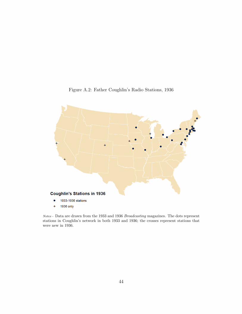
Figure A.2: Father Coughlin’s Radio Stations, 1936

Notes - Data are drawn from the 1933 and 1936 Broadcasting magazines. The dots representstations in Coughlin’s network in both 1933 and 1936; the crosses represent stations thatwere new in 1936.

44

Figure A.3: Percent of Catholics in Population, 1926

Notes - Data are drawn from the 1926 Census of Religious Bodies. Darker colors representhigher shares of Catholics.

45

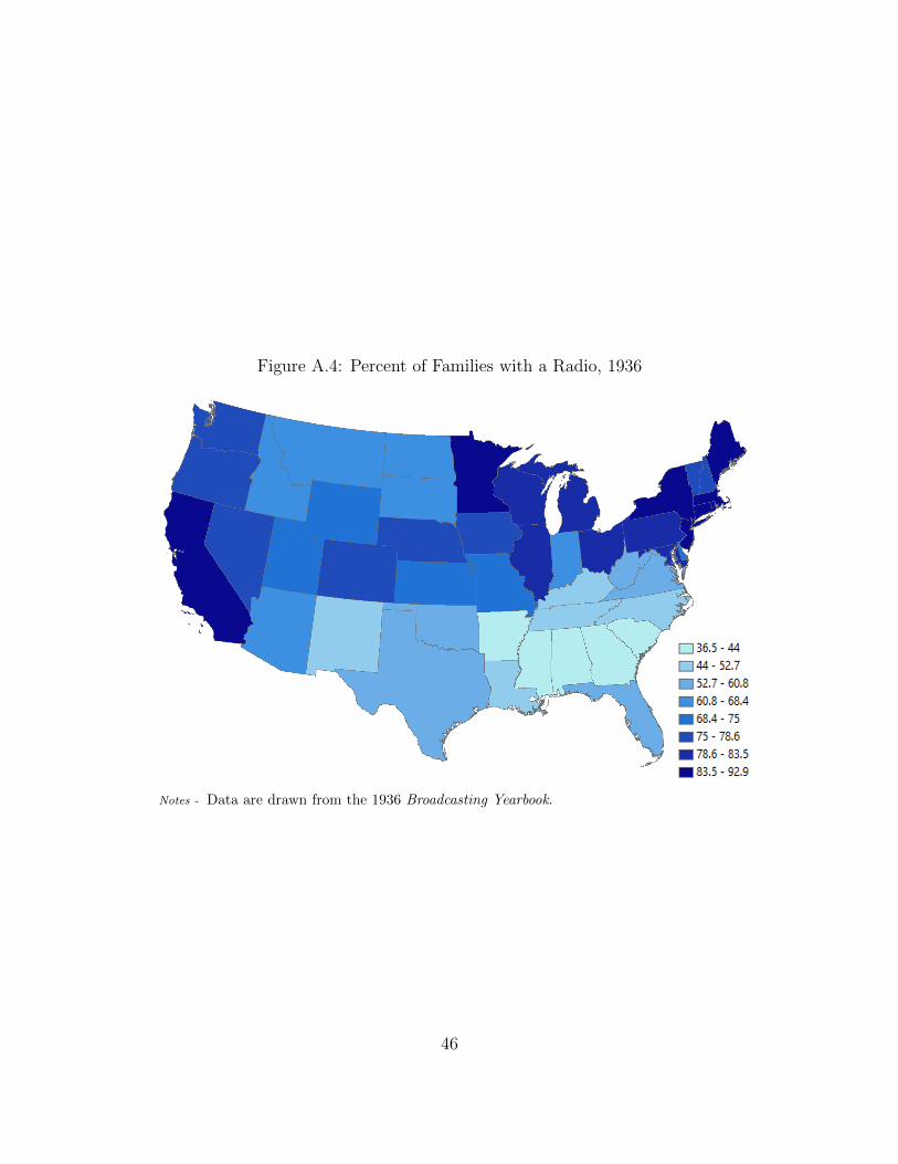
Figure A.4: Percent of Families with a Radio, 1936

Notes - Data are drawn from the 1936 Broadcasting Yearbook.

46

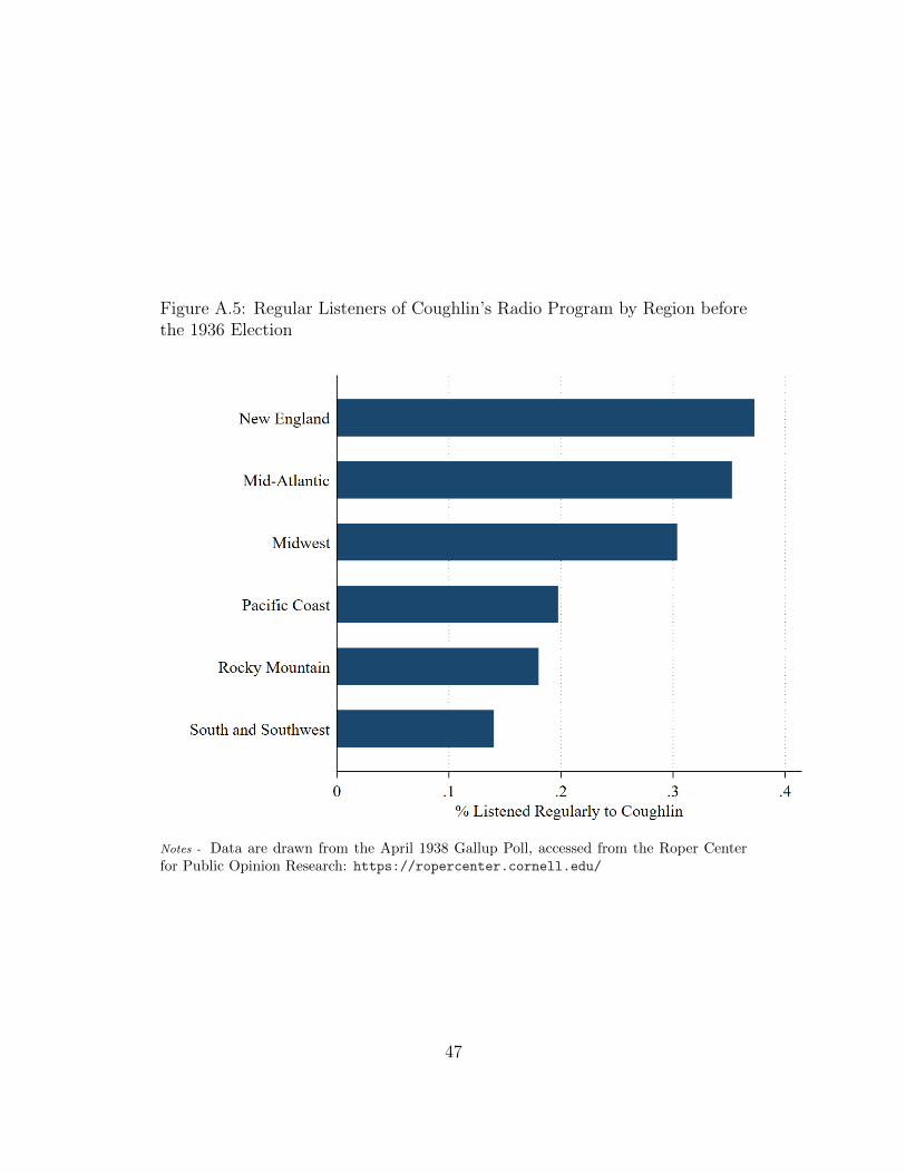
Figure A.5: Regular Listeners of Coughlin’s Radio Program by Region beforethe 1936 Election

Notes - Data are drawn from the April 1938 Gallup Poll, accessed from the Roper Centerfor Public Opinion Research: https://ropercenter.cornell.edu/

47


Figure A.6: FDR’s Vote Shares (Percentage Points) in the 1936 PresidentialElection

Notes - Data are drawn from the ICPSR 8611 data set (Clubb et al., 2006).

48

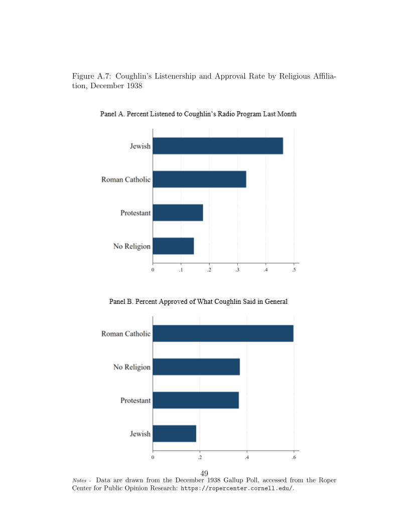
Figure A.7: Coughlin’s Listenership and Approval Rate by Religious Affilia-tion, December 1938

Notes - Data are drawn from the December 1938 Gallup Poll, accessed from the RoperCenter for Public Opinion Research: https://ropercenter.cornell.edu/.

49


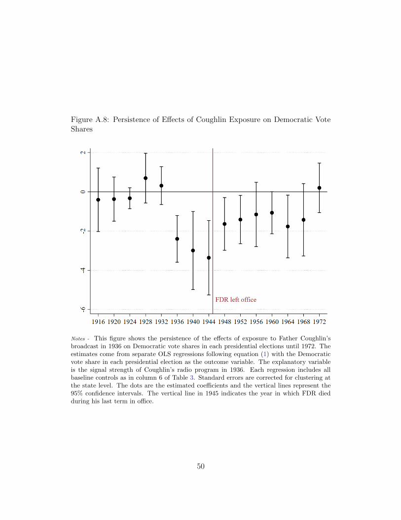
Figure A.8: Persistence of Effects of Coughlin Exposure on Democratic VoteShares

Notes - This figure shows the persistence of the effects of exposure to Father Coughlin’sbroadcast in 1936 on Democratic vote shares in each presidential elections until 1972. Theestimates come from separate OLS regressions following equation (1) with the Democraticvote share in each presidential election as the outcome variable. The explanatory variableis the signal strength of Coughlin’s radio program in 1936. Each regression includes allbaseline controls as in column 6 of Table 3. Standard errors are corrected for clustering atthe state level. The dots are the estimated coefficients and the vertical lines represent the95% confidence intervals. The vertical line in 1945 indicates the year in which FDR diedduring his last term in office.

50

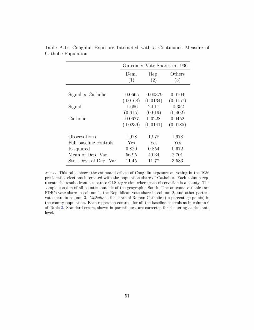
Table A.1: Coughlin Exposure Interacted with a Continuous Measure ofCatholic Population



Signal × Catholic -0.0665 -0.00379 0.0704(0.0168) (0.0134) (0.0157)

Signal -1.666 2.017 -0.352(0.615) (0.619) (0.402)

Catholic -0.0677 0.0228 0.0452(0.0239) (0.0141) (0.0185)


Notes - This table shows the estimated effects of Coughlin exposure on voting in the 1936presidential elections interacted with the population share of Catholics. Each column rep-resents the results from a separate OLS regression where each observation is a county. Thesample consists of all counties outside of the geographic South. The outcome variables areFDR’s vote share in column 1, the Republican vote share in column 2, and other parties’vote share in column 3. Catholic is the share of Roman Catholics (in percentage points) inthe county population. Each regression controls for all the baseline controls as in column 6of Table 3. Standard errors, shown in parentheses, are corrected for clustering at the statelevel.

51

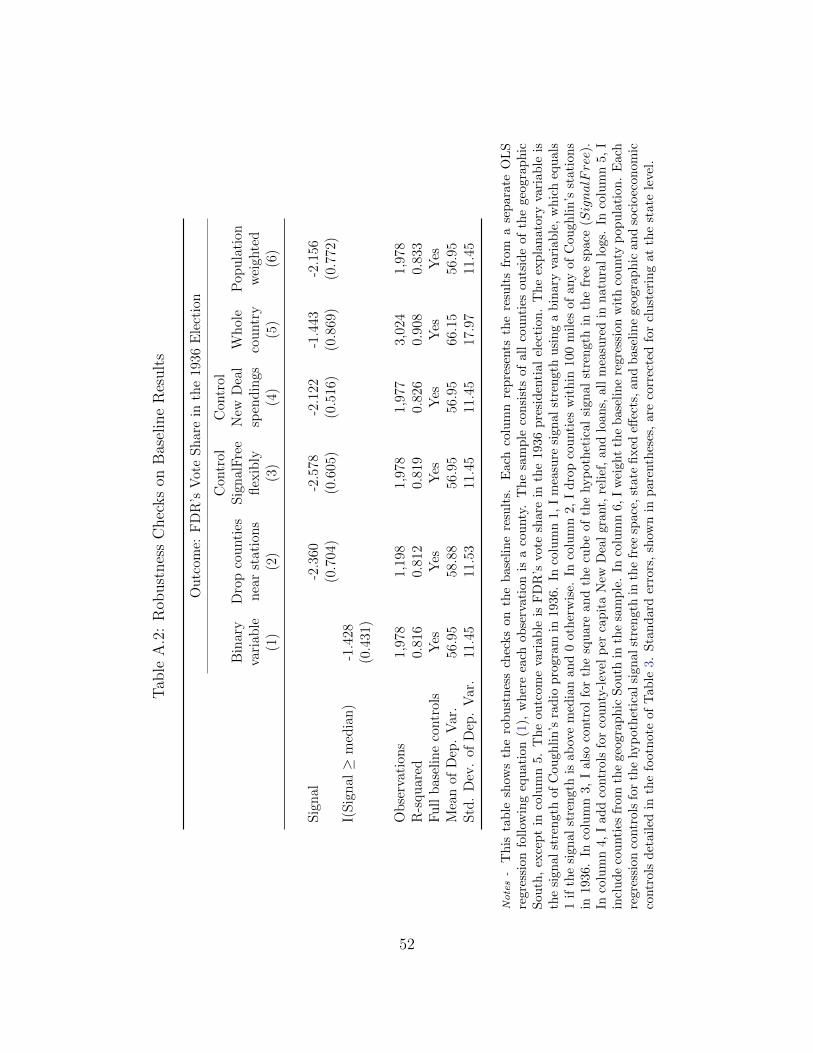
Tab

leA

.2:

Rob

ust

nes

sC

hec

ks

onB

asel

ine

Res

ult

s

Ou

tcom

e:F

DR

’sV

ote

Sh

are

inth

e19

36E

lect

ion

Con

trol

Con

trol

Bin

ary

Dro

pco

unti

esS

ign

alF

ree

New

Dea

lW

hol

eP

opu

lati

onva

riab

len

ear

stat

ion

sfl

exib

lysp

end

ings

cou

ntr

yw

eigh

ted

(1)

(2)

(3)

(4)

(5)

(6)

Sig

nal

-2.3

60-2

.578

-2.1

22-1

.443

-2.1

56(0

.704

)(0

.605

)(0

.516

)(0

.869

)(0

.772

)I(

Sig

nal

≥m

edia

n)

-1.4

28(0

.431

)

Ob

serv

atio

ns

1,97

81,

198

1,97

81,

977

3,02

41,

978

R-s

qu

ared

0.81

60.

812

0.81

90.

826

0.90

80.

833

Fu

llb

asel

ine

contr

ols

Yes

Yes

Yes

Yes

Yes

Yes

Mea

nof

Dep

.V

ar.

56.9

558

.88

56.9

556

.95

66.1

556

.95

Std

.D

ev.

ofD

ep.

Var

.11

.45

11.5

311

.45

11.4

517

.97

11.4

5

Notes-

Th

ista

ble

show

sth

ero

bu

stn

ess

chec

ks

on

the

base

lin

ere

sult

s.E

ach

colu

mn

rep

rese

nts

the

resu

lts

from

ase

para

teO

LS

regr

essi

onfo

llow

ing

equ

atio

n(1

),w

her

eea

chob

serv

ati

on

isa

cou

nty

.T

he

sam

ple

con

sist

sof

all

cou

nti

esou

tsid

eof

the

geo

gra

phic

Sou

th,

exce

pt

inco

lum

n5.

Th

eou

tcom

eva

riab

leis

FD

R’s

vote

share

inth

e1936

pre

sid

enti

al

elec

tion

.T

he

exp

lan

ato

ryva

riab

leis

the

sign

alst

ren

gth

ofC

ough

lin

’sra

dio

pro

gram

in1936.

Inco

lum

n1,

Im

easu

resi

gn

al

stre

ngth

usi

ng

ab

inary

vari

ab

le,

wh

ich

equ

als

1if

the

sign

alst

ren

gth

isab

ove

med

ian

and

0oth

erw

ise.

Inco

lum

n2,

Id

rop

cou

nti

esw

ith

in100

mil

esof

any

of

Cou

gh

lin

’sst

ati

on

sin

1936

.In

colu

mn

3,I

also

contr

olfo

rth

esq

uare

an

dth

ecu

be

of

the

hyp

oth

etic

al

sign

al

stre

ngth

inth

efr

eesp

ace

(SignalF

ree)

.In

colu

mn

4,I

add

contr

ols

for

cou

nty

-lev

elp

erca

pit

aN

ewD

eal

gra

nt,

reli

ef,

an

dlo

ans,

all

mea

sure

din

natu

ral

logs.

Inco

lum

n5,

Iin

clu

de

cou

nti

esfr

omth

ege

ogra

ph

icS

outh

inth

esa

mp

le.

Inco

lum

n6,

Iw

eight

the

base

lin

ere

gre

ssio

nw

ith

cou

nty

pop

ula

tion

.E

ach

regr

essi

onco

ntr

ols

for

the

hyp

othet

ical

sign

alst

ren

gth

inth

efr

eesp

ace

,st

ate

fixed

effec

ts,

an

db

ase

lin

egeo

gra

ph

ican

dso

cioec

on

om

icco

ntr

ols

det

aile

din

the

foot

not

eof

Tab

le3.

Sta

nd

ard

erro

rs,

show

nin

pare

nth

eses

,are

corr

ecte

dfo

rcl

ust

erin

gat

the

state

leve

l.

52

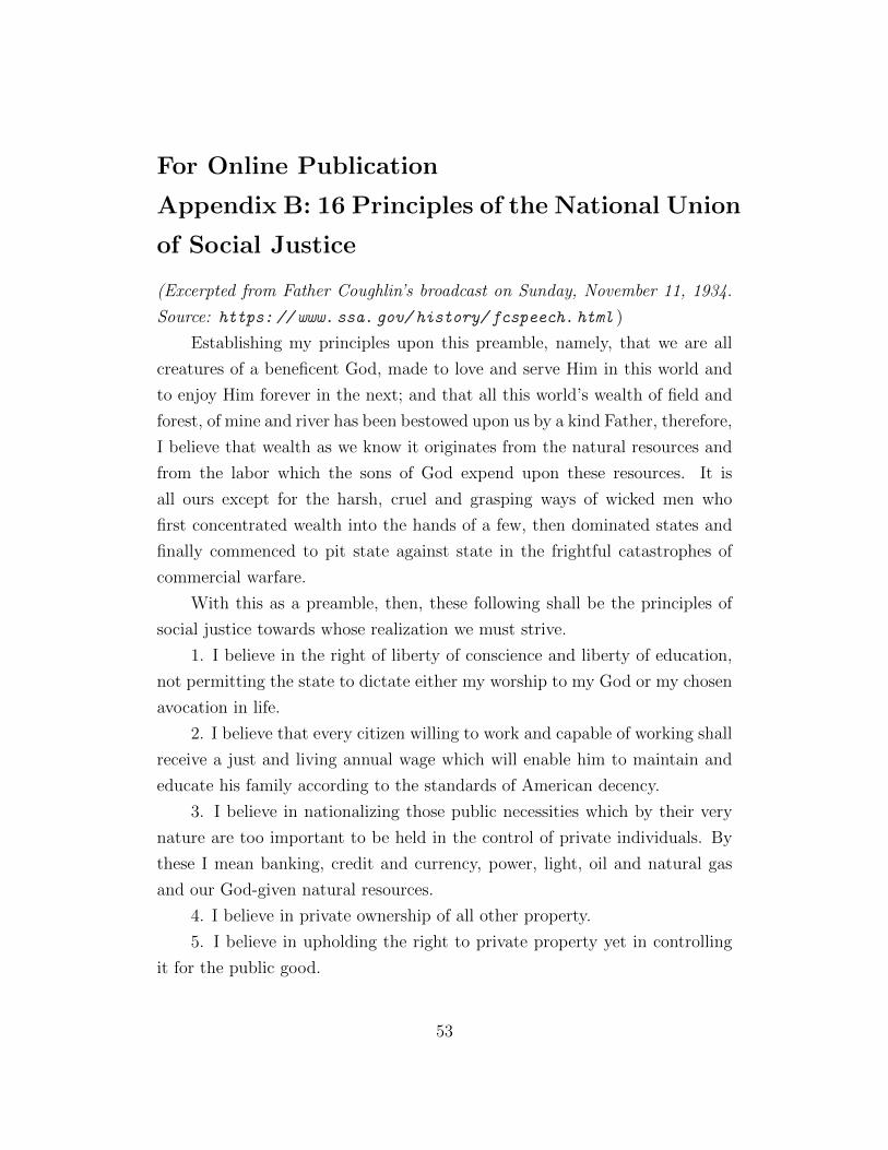
For Online Publication

Appendix B: 16 Principles of the National Union

of Social Justice

(Excerpted from Father Coughlin’s broadcast on Sunday, November 11, 1934.

Source: https: // www. ssa. gov/ history/ fcspeech. html )

Establishing my principles upon this preamble, namely, that we are all

creatures of a beneficent God, made to love and serve Him in this world and

to enjoy Him forever in the next; and that all this world’s wealth of field and

forest, of mine and river has been bestowed upon us by a kind Father, therefore,

I believe that wealth as we know it originates from the natural resources and

from the labor which the sons of God expend upon these resources. It is

all ours except for the harsh, cruel and grasping ways of wicked men who

first concentrated wealth into the hands of a few, then dominated states and

finally commenced to pit state against state in the frightful catastrophes of

commercial warfare.

With this as a preamble, then, these following shall be the principles of

social justice towards whose realization we must strive.

1. I believe in the right of liberty of conscience and liberty of education,

not permitting the state to dictate either my worship to my God or my chosen

avocation in life.

2. I believe that every citizen willing to work and capable of working shall

receive a just and living annual wage which will enable him to maintain and

educate his family according to the standards of American decency.

3. I believe in nationalizing those public necessities which by their very

nature are too important to be held in the control of private individuals. By

these I mean banking, credit and currency, power, light, oil and natural gas

and our God-given natural resources.

4. I believe in private ownership of all other property.

5. I believe in upholding the right to private property yet in controlling

it for the public good.

53

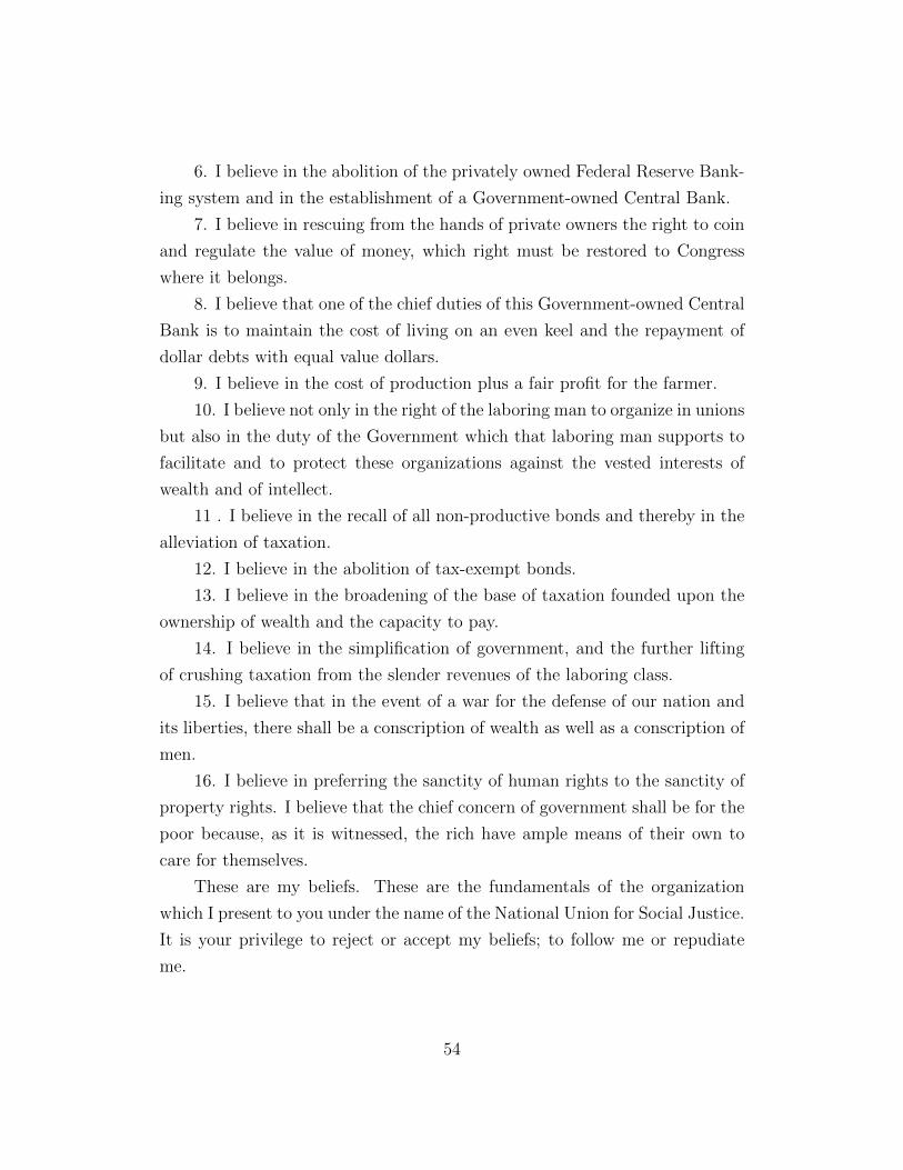
https://www.ssa.gov/history/fcspeech.html

6. I believe in the abolition of the privately owned Federal Reserve Bank-

ing system and in the establishment of a Government-owned Central Bank.

7. I believe in rescuing from the hands of private owners the right to coin

and regulate the value of money, which right must be restored to Congress

where it belongs.

8. I believe that one of the chief duties of this Government-owned Central

Bank is to maintain the cost of living on an even keel and the repayment of

dollar debts with equal value dollars.

9. I believe in the cost of production plus a fair profit for the farmer.

10. I believe not only in the right of the laboring man to organize in unions

but also in the duty of the Government which that laboring man supports to

facilitate and to protect these organizations against the vested interests of

wealth and of intellect.

11 . I believe in the recall of all non-productive bonds and thereby in the

alleviation of taxation.

12. I believe in the abolition of tax-exempt bonds.

13. I believe in the broadening of the base of taxation founded upon the

ownership of wealth and the capacity to pay.

14. I believe in the simplification of government, and the further lifting

of crushing taxation from the slender revenues of the laboring class.

15. I believe that in the event of a war for the defense of our nation and

its liberties, there shall be a conscription of wealth as well as a conscription of

men.

16. I believe in preferring the sanctity of human rights to the sanctity of

property rights. I believe that the chief concern of government shall be for the

poor because, as it is witnessed, the rich have ample means of their own to

care for themselves.

These are my beliefs. These are the fundamentals of the organization

which I present to you under the name of the National Union for Social Justice.

It is your privilege to reject or accept my beliefs; to follow me or repudiate

me.

54

Media, Pulpit, and Populist Persuasion: Evidence from ...

Documents