Media Persuasion through Slanted Language: Evidence from ...

Barcelona GSE Working Paper Series

Working Paper nº 1177

Media Persuasion through Slanted Language: Evidence from

the Coverage of Immigration Milena Djourelova

May 2020

Media Persuasion through Slanted Language:

Evidence from the Coverage of Immigration ∗

Milena Djourelova†

May 2020

Abstract

Can the language used by mass media to cover policy relevant issues affect readers’

policy preferences? I examine this question for the case of immigration, exploiting

an abrupt ban on the term ”illegal immigrant” in wire content distributed to media

outlets by the Associated Press (AP). Using text data on AP dispatches and the content

of a large number of US print and online outlets, I find that after the ban articles

mentioning ”illegal immigrant” decline by 28% in outlets that rely on AP relative to

others. This change in language appears to have had a tangible impact on readers’

views on immigration. Following AP’s ban, individuals exposed to outlets relying more

heavily on AP tend to support less restrictive immigration and border security policies.

The effect is driven by frequent readers and does not apply to views on issues other

than immigration.

Keywords: Mass media, media slant, framing, immigration

JEL Classification: D72, L82, Z13

∗Universitat Pompeu Fabra, Barcelona GSE and IPEG. I acknowledge financial support from the SpanishMinistry of Economy and Competitiveness through Predoctoral Grant BES2016-076728. I thank RubenDurante, Ruben Enikolopov, Maria Petrova, Brian Knight and David Stromberg for helpful suggestions andcomments. Preliminary draft, comments welcome.†UPF. E-mail: [email protected]

1

1 Introduction

Political actors choose carefully the words they put out in the media. In the US, Republicans

and Democrats often use strikingly different language to describe the same issue, in an

attempt to promote views favorable to their platform. Republican politicians and right-

leaning media speak about the “Chinese virus”, the “death tax”, and “illegal immigrants”,

while Democrats and left-leaning media refer to the same issues as “Covid-19”, the “estate

tax”, and “undocumented immigrants”.1

Although slanted language is widespread in political rhetoric, evidence on its persua-

siveness, i.e. on whether it can indeed sway readers in the intended direction, is lacking.

This question poses an empirical challenge for at least two reasons. First, votes-maximizing

politicians and profit-maximizing media have a clear incentive to choose their slant to appeal

to the audience’s preference for like-minded content (Gentzkow and Shapiro 2006). Second,

slanted language can be accompanied by other politically motivated choices, ranging from

selective emphasis on certain issues, to outright endorsement of policies or candidates, which

are likely to independently affect the policy views of the audience.

To overcome these challenges, I propose a supply-side source of variation in media slant. I

take advantage of the fact that many US media outlets source some of their content from the

Associated Press (AP) – a newswire agency that gathers and distributes news to subscribing

outlets. Since AP distributes a single news feed to all subscribers, their aim is to produce

neutral coverage that appeals to outlets from all sides of the political spectrum (Fenby 1986).

This philosophy has led to extremely strict and rigid guidelines for the use of politically

sensitive language.

I exploit an abrupt reversal in AP’s guidelines on the use of a specific politically sensitive

1The implicit policy positions behind these phrases are easy to recognize. “The Chinese virus” is pre-sumably an attempt to shift responsibility for the crisis to China (https://edition.cnn.com/2020/03/20/politics/donald-trump-china-virus-coronavirus/index.html). “Death tax” highlights the allegedunfairness of taxing the deceased, while “estate tax” draws attention to the wealth of the people it appliesto (https://www.businessinsider.com/death-tax-or-estate-tax-2017-10?r=US&IR=T). “Illegal immi-grants” underscores the transgression of crossing the border, while “undocumented immigrants” presents theissue of legal status as a formality (https://www.al.com/news/2018/07/illegal_vs_undocumented_the_he.html).

2

term – “illegal immigrant”. In April 2013, after years of resisting requests to revise its guide-

lines on the language on immigration, AP abruptly switched from officially recommending

the term “illegal immigrant” to refer to people living in the US without legal authorization,

to banning its use in AP wire articles.

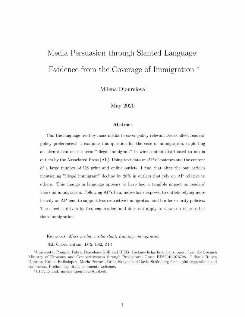
The ban happened at a time when the issue of immigration, and the language used to talk

about it, was extremely politicized. Figure 1 illustrates the partisan divide in use of “illegal

immigrant” in political speech and in the media.2 In Congress, Republican representatives

mention “illegal immigrant” about 50% of the time they mention “immigrant”, while this

frequency is less than 5% among Democrats. Similarly, the term appears twice as frequently

in the right-leaning Fox News and Washington Times, compared to the left-leaning MSNBC

and Washington Post.

Beyond the clear political charge of the banned term, the setting of AP’s ban has several

features that make it attractive to study the causal effects of slanted language. Since the

decision on the ban was taken centrally by AP executives, and given that AP serves thousands

of subscribers with different ideological positions, the ban is plausibly exogenous from the

perspective of any individual subscribing outlet. In other words, the ban produces variation

in an input to the editorial production function that is orthogonal to the views of end-readers.

Furthermore, media outlets differ in the extent to which they rely on AP’s input. This allows

me to compare outlets with different degrees of use of this input, i.e. different AP-intensity,

and the views of their respective readers before vs after the ban.

I start off my analysis by documenting how the ban affected AP’s language, using the

text of all immigration-related AP dispatches released between 2009 and 2017. I find that,

as intended, the ban caused the term “illegal immigrant” to instantaneously disappear from

AP’s feed, but caused no sharp change in the frequency of the word “immigrant”. As a

substitute for “illegal”, the new guidelines suggested the phrase “living in the county ille-

2The reason for this divide can be traced back to deliberate party strategy. For example, “illegal immi-grant” was advocated by Republican strategist Frank Luntz, who is famous for developing talking points forRepublican candidates and for coining terms such as “death tax” (instead of “estate tax” or “inheritancetax”) and “climate change” (instead of “global warming”). Luntz has urged Republicans to always use theterm “illegal immigrant” and to put an emphasis on border security, calling the linguistic distinction between“illegal immigrant” and “undocumented immigrant” the “political battle of the decade” (Luntz 2007).

3

gally” or “without legal permission”. However, text analysis reveals that these reformulations

compensate for at most half of the decline in mentions of “illegal immigrant” in dispatches

containing the word “immigrant”, and that no other phrase fills the remaining gap. Hence,

at least half of the treatment in this natural experiment consists of substitution from “illegal

immigrant” to “immigrant”, without any reference to legal status.

I then track how this change in AP’s language diffuses into the language of AP-subscribing

outlets, using text data from more than 2000 print and online outlets. I employ a difference-in-

difference strategy comparing the monthly number of “illegal immigrant” articles relative to

“immigrant” articles before and after the ban, in media outlets with different AP-intensity at

baseline. Specifically, I measure AP-intensity as the share of “immigrant” articles published

by each outlet in the 12 months prior to the ban that either credit AP explicitly, or are flagged

by a plagiarism detection algorithm comparing their text to that of recent AP dispatches.3

My results suggest a large degree of diffusion – one standard deviation in AP-intensity

causes a decline in the frequency of “illegal immigrant” articles by 14%. Put differently,

outlets with positive AP-intensity decrease their use of the term by on average 28% com-

pared to ones with zero AP-intensity, and for outlets in the top quartile of the AP-intensity

distribution this decline reaches 60%. This effect is driven mostly by articles copied from AP,

as opposed to original ones. As with AP dispatches, I find that the ban had no effect on the

volume of immigration coverage, measured by mentions of “immigrant” over total articles.

Finally, I exploit AP’s ban to identify the effect of “illegal immigrant” articles on readers’

views on immigration policy, using pre- and post-ban waves of the Cooperative Congressional

Election Study (CCES). To identify the reduced form effect of the ban, I employ a difference-

in-difference strategy comparing CCES respondents before and after the ban, in counties with

different AP-intensity of locally circulated newspapers. Alternatively, to scale magnitudes

in terms of the effect of “illegal immigrant” articles circulated in the respondent’s county,

I instrument their number (normalized by the number of “immigrant” articles) with the

interaction of county-level AP-intensity and the timing of the ban. This strategy accounts

3This procedure aims to capture the use of AP copy in cases when AP is credited as a source, and in onesin which AP is not credited (Cage et al. 2020).

4

for time-invariant effects of other county characteristics correlated with AP-intensity, but

relies on the assumption that their effect on readers did not change in coincidence with

the timing of the ban. I address this threat by controlling for a wide range of baseline

characteristics interacted with time.

The results suggest that one standard deviation higher AP-intensity of locally circulated

newspapers is associated with 0.7 percentage points, or 1.25% lower public support for in-

creasing border security after the ban. This implies a persuasion rate of 1.5 to 3.8% for

the treatment of 1 standard deviation higher AP-intensity, which translates into (at least) 9

fewer “illegal immigrant” per year.

While this result applies to the sample of all CCES respondents, it is more pronounced

for regular print newspaper readers, who represent 33% of the sample. On the other hand,

the effect is stronger among respondents with (self-reported) lower interest in politics. This

is consistent with passive news consumers being more persuadable by slanted language.

I observe a similar shift in support for restricting immigration in 3 out of the 4 policy

questions I am able to track across pre- and post-ban survey waves4, as well in an index

aggregating all immigration-related CCES questions including rotating ones. However, this

effect appears to be specific to policy preferences related to immigration. I find no significant

change in responses on other issues that traditionally split along party lines, such as abortion,

gay marriage or taxes and redistribution. On net, the relatively small change in views on

immigration seems to be insufficient to sway voting intentions for Republican candidates.

This paper contributes to a large literature on the effects of media on political attitudes

and outcomes. One strand exploits quasi-random or experimentally manipulated variation

in access to a particular media outlet to estimate its causal effects (DellaVigna and Kaplan

2007; Martin and Yurukoglu 2017; Enikolopov et al. 2011; Durante et al. 2019; Gerber et al.

2009). By design, the “treatment” in this strategy consists of the bundle of editorial choices

that differentiate the outlet of interest from alternative sources of information. Fewer studies

4The effect of the ban is significant for support for increasing border security, for allowing police to questionsuspected illegal immigrants, and for fining firms that employ illegal immigrants. It is not significant foropposition to amnesty.

5

are focused on a specific mechanism of media persuasion – e.g. the volume of coverage of a

politician or a politically sensitive issue (Snyder and Stromberg 2010) or direct endorsement

of candidates for office (Chiang and Knight 2011). This paper fits into the second category,

but differs by studying a different and arguably more subtle mechanism – that of slanted

language.5

This paper is also closely related to a literature on slant in the language used by media

and politicians (Groseclose and Milyo 2005; Gentzkow and Shapiro 2010; Gentzkow et al.

2019), which has focused on the measurement of slant and on studying of its determinants.

Gentzkow and Shapiro (2010) show that the attitudes of consumers explain about 20% of

the variation in slant. Here I study the reverse direction of causality – from exposure to

slanted language towards the political views of readers, trying to separate this channel from

the tendency of media outlets to serve consumers’ preference for like-minded content.

My findings suggest that views on immigration are sensitive to small changes in the fram-

ing of the issue. This is in line with recent work documenting a large degree of misinformation

regarding the characteristics of immigrants in the US and Europe and showing that policy

views can shift in response to correcting misperceptions (Grigorieff et al. 2019; Alesina et al.

2019; Hatte et al. 2019).

Framing effects, which occur when differences in the presentation of an issue affect indi-

viduals’ responses, are subject to a large literature in the fields of communication and social

psychology (Stromberg 2015; Scheufele and Tewksbury 2007; Chong and Druckman 2007).

This can be conceptualized as individuals trading off different concerns when evaluating an

issue, and the frame changing the relative weight of these concerns. In this context, read-

ing about “illegal immigrants” rather than about “immigrants” may increase the weight on

concerns about border security, due to the fact that the former phrase includes direct infor-

mation on legal status and the latter does not (rational framing). On the other hand, reading

5It is not clear a priori how the persuasive effect of slanted language might compare to that of moreobvious biases (say, direct electoral endorsements). On the one hand, slanted language is a mild treatment.On the other hand, more direct biases are easier for readers to notice and discount by either switching awayfrom the biased media outlet or by taking its ideological stance into account when making political choices(Durante and Knight 2012; Chiang and Knight 2011).

6

about “illegal immigrants” rather than about “immigrants living in the country without legal

permission” conveys the same information content, but may still be an effective frame if it

more easily brings to mind concerns that have in the past been connected to the term “illegal

immigrant”, such as border security (behavioral framing). In terms of methodology, most

of the existing evidence of framing effects comes from survey experiments, while this paper

provides large-scale observational evidence.

The rest of the paper is organized as follows. In section 2 I discuss the details of the

ban and analyze how the text of immigration-related articles distributed by AP changed. In

section 3 I track the propagation of AP’s language into the language of AP-dependent media.

In section 4 I analyze the effect of the ban on attitudes related to immigration policy.

2 The Ban and It’s Effect on AP’s Language

2.1 Background

The term ‘illegal immigrant” was dropped from AP’s guidelines on April 3rd 2013. The

decision was rather unexpected since AP had previously resisted pressures from the advocacy

groups to change their language policy.6 Up until the change was announced, AP’s guidelines

stated that “illegal immigrant” was the preferred term while the alternative endorsed by the

left – “undocumented immigrant” – was not allowed as AP considers it legally inaccurate (as

continues to be the case to this day).

Appendix A presents the exact formulation of AP’s guidelines before and after April

2013. As “illegal immigrant” was banned, AP proposed the following substitutes: “living /

entering the county illegally / without legal permission”.7 Yet, AP executives recognized in

their statement that these alternatives are likely harder for writers to use in text compared

to the simple label “illegal” (https://blog.ap.org/announcements/illegal-immigrant-

6https://www.sfexaminer.com/national-news/society-for-professional-journalists-says-

using-the-term-illegal-immigrant-is-unconsitutional/7According to the guidelines, the ban does not concern “illegal immigrant” used in direct quotes, or the

phrase “illegal immigration”.

7

no-more). I return to this point in the interpretation of the results. The ban took effect

immediately in the online guidelines guidelines, which are also embedded in text editors (see

figure A1).

2.2 Data

To analyze how the language used by AP changed in response to the ban, I obtain the text of

all immigration-related AP-articles released in the period 2009-2017 from Factiva (https://

global.factiva.com). I search the database for mentions of the word “immigrant” (singular

or plural), limiting the source to “Associated Press Newswires” and record the date, headline,

word-count and full text of each article.

2.3 Text Analysis Results

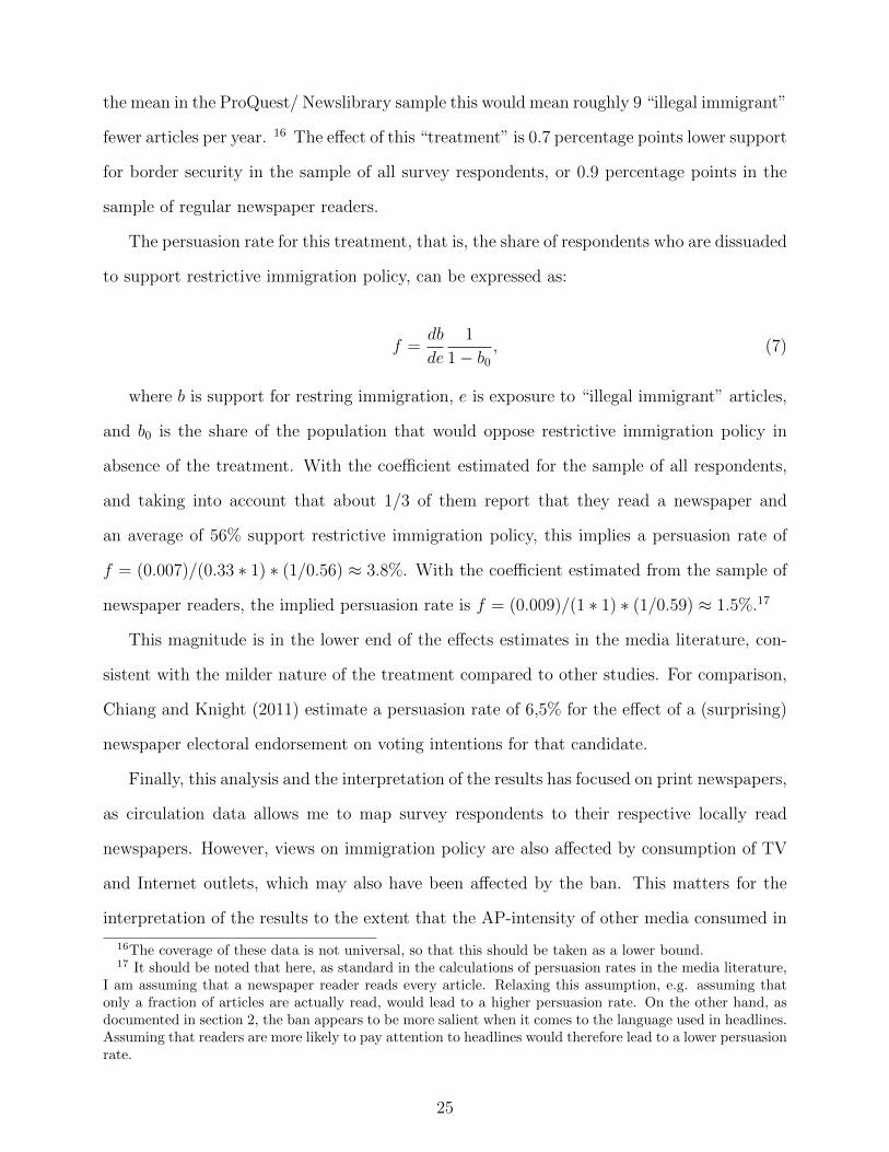
As a first check of how AP’s language on the issue of immigration changed after the ban, I

examine the headlines released by AP. Figure 3 depicts the most frequent 3-grams encountered

in headlines of “immigrant” dispatches. The label “illegal” clearly features prominently before

the ban, and virtually disappears after. Rather than substitute “illegal” by another adjective,

many headlines appear to simply omit any direct reference to legal status. Appendix A

illustrates this point with two examples of AP dispatches covering the same issue – state

laws on immigrants drivers licenses – but released just before vs just after the ban.

The timing of this change in language coincides very precisely with the announcement

of the ban. Figure 4 shows the monthly number of AP dispatches mentioning the phrase

“illegal immigrant” as percent of dispatches mentioning “immigrant”. This percentage drops

from an average of 40% in the period before April 2013, to less than 5% after, suggesting

close to perfect compliance.8 The lower panel of the same figure suggests no sharp change in

the total volume of articles mentioning the word “immigrant”.

To examine more systematically the potential substitutes for the banned term “illegal”, I

8Note that this figure includes mentions of “illegal immigrant” in direct quotes, which are not affected bythe ban.

8

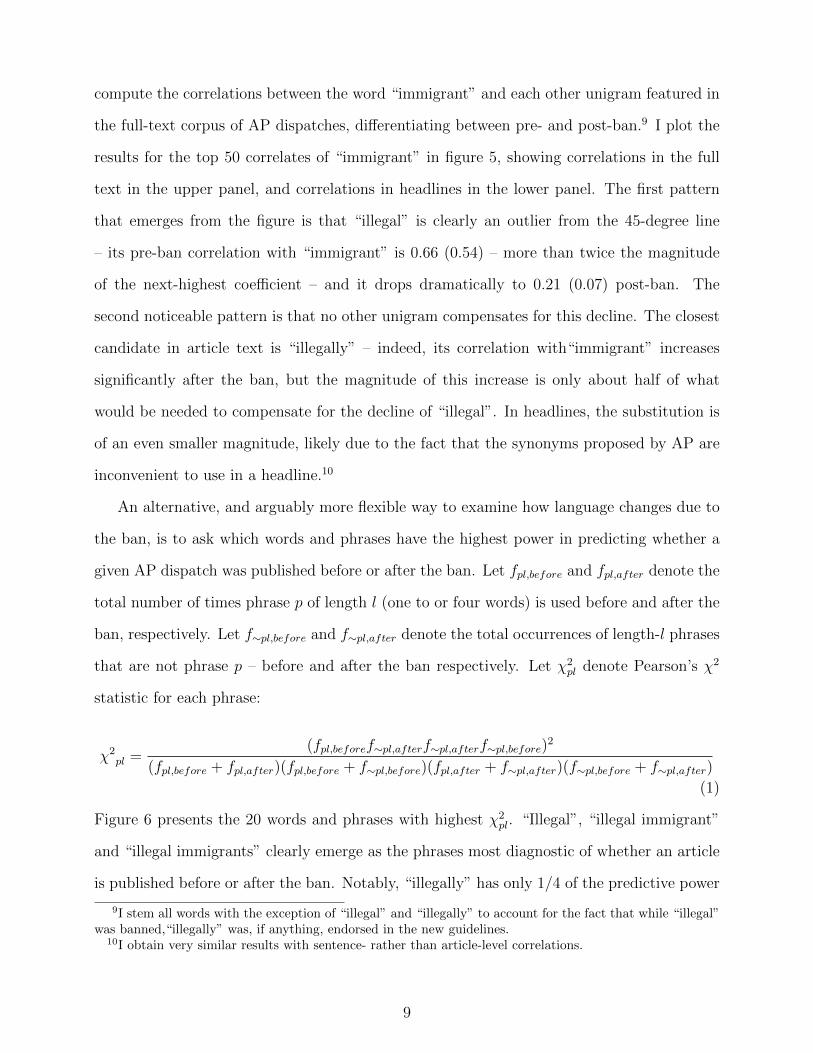
compute the correlations between the word “immigrant” and each other unigram featured in

the full-text corpus of AP dispatches, differentiating between pre- and post-ban.9 I plot the

results for the top 50 correlates of “immigrant” in figure 5, showing correlations in the full

text in the upper panel, and correlations in headlines in the lower panel. The first pattern

that emerges from the figure is that “illegal” is clearly an outlier from the 45-degree line

– its pre-ban correlation with “immigrant” is 0.66 (0.54) – more than twice the magnitude

of the next-highest coefficient – and it drops dramatically to 0.21 (0.07) post-ban. The

second noticeable pattern is that no other unigram compensates for this decline. The closest

candidate in article text is “illegally” – indeed, its correlation with“immigrant” increases

significantly after the ban, but the magnitude of this increase is only about half of what

would be needed to compensate for the decline of “illegal”. In headlines, the substitution is

of an even smaller magnitude, likely due to the fact that the synonyms proposed by AP are

inconvenient to use in a headline.10

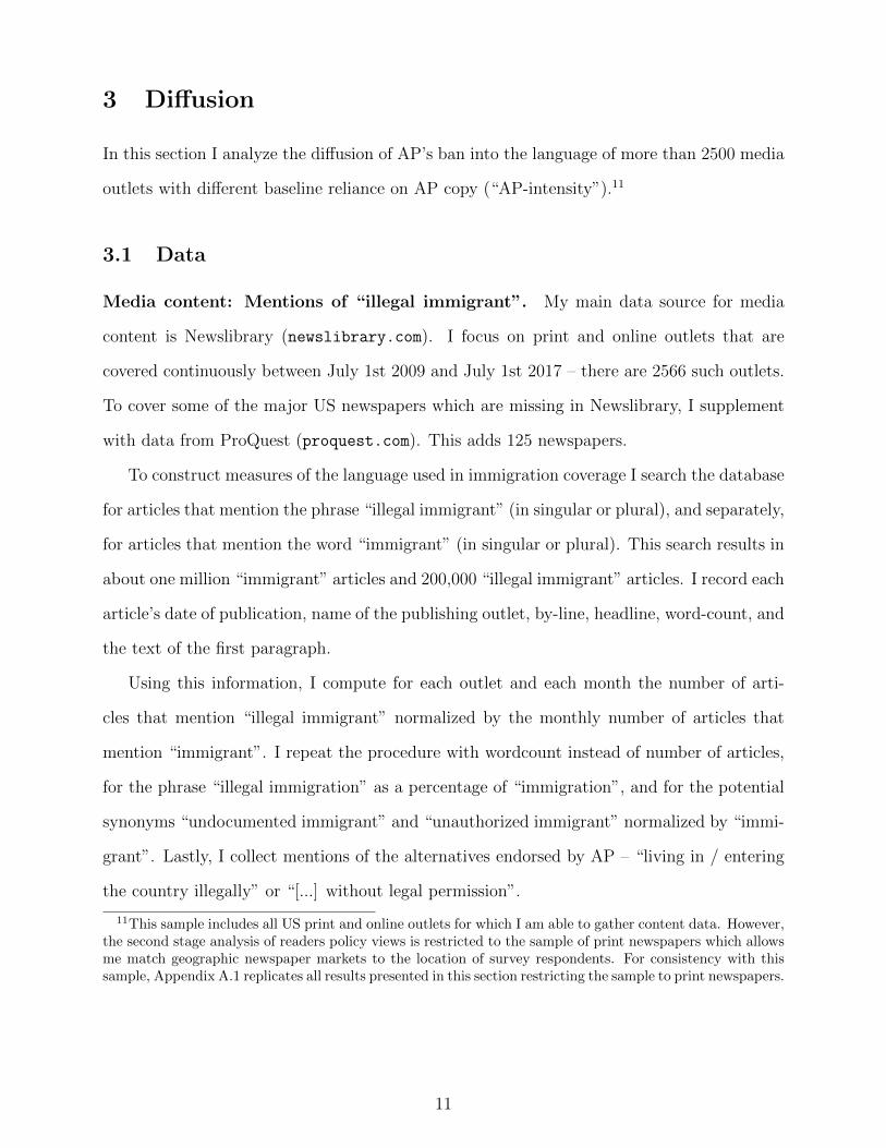
An alternative, and arguably more flexible way to examine how language changes due to

the ban, is to ask which words and phrases have the highest power in predicting whether a

given AP dispatch was published before or after the ban. Let fpl,before and fpl,after denote the

total number of times phrase p of length l (one to or four words) is used before and after the

ban, respectively. Let f∼pl,before and f∼pl,after denote the total occurrences of length-l phrases

that are not phrase p – before and after the ban respectively. Let χ2pl denote Pearson’s χ2

statistic for each phrase:

χ2pl =

(fpl,beforef∼pl,afterf∼pl,afterf∼pl,before)2

(fpl,before + fpl,after)(fpl,before + f∼pl,before)(fpl,after + f∼pl,after)(f∼pl,before + f∼pl,after)

(1)

Figure 6 presents the 20 words and phrases with highest χ2pl. “Illegal”, “illegal immigrant”

and “illegal immigrants” clearly emerge as the phrases most diagnostic of whether an article

is published before or after the ban. Notably, “illegally” has only 1/4 of the predictive power

9I stem all words with the exception of “illegal” and “illegally” to account for the fact that while “illegal”was banned,“illegally” was, if anything, endorsed in the new guidelines.

10I obtain very similar results with sentence- rather than article-level correlations.

9

of “illegal”, confirming that AP’s synonyms were adopted only partially.

To rule out the possibility that these results reflects a shift in topics occupying the news

cycle over the sample period, in appendix A I repeat the exercise separately for each of five

topics estimated with a Latent Dirichlet Allocation (LDA) model. The estimated topics can

be labeled as follows: law enforcement, immigration-related legislation, immigrants’ integra-

tion and social issues, international issues such as the refugee crisis in Europe, and elections

(Figure C1). The results discussed above are confirmed within each topic (with the exception

of the χ2 ranking within the international affairs topic).

Finally, I examine whether the ban on “illegal immigrant” was part of a broader trend to-

wards more liberal slant in AP’s immigration coverage. I compute a measure of immigration-

specific slant based on the similarity of AP’s language to that used by Republicans vs

Democrats in Congress, following Gentzkow and Shapiro (2010). In order to isolate the

influence of the ban from other dimensions of AP’s language, I also do compute a version

of slant excluding any phrases containing the phrase “illegal immigrant” and its substitutes.

Appendix A.1 describes this procedure in detail. Figure 7 presents the evolution of the 2

versions of the slant over time. The one that does not account for the ban on “illegal im-

migrant” follows closely the trend for AP’s use of this phrase. This is intuitive since use of

“illegal immigrant” is highly predictive of a Republican speaker in Congress (see figure 1),

and therefore receives a high weight in the measure of overall slant. Once it is excluded and

we focus on other dimensions of language, the trend in slant appears stable over time, with

an only slight change at the time of the ban.

Taking these results together, the analysis of AP text suggests that: (1) As intended, the

label “illegal” virtually disappears after the ban; (2) This decline is only partially compen-

sated by the substitutes proposed by AP, while the remainder appears to omit any direct

reference to legal status; (3) Other dimensions of AP’s language did not change dramatically

with the ban.

10

3 Diffusion

In this section I analyze the diffusion of AP’s ban into the language of more than 2500 media

outlets with different baseline reliance on AP copy (“AP-intensity”).11

3.1 Data

Media content: Mentions of “illegal immigrant”. My main data source for media

content is Newslibrary (newslibrary.com). I focus on print and online outlets that are

covered continuously between July 1st 2009 and July 1st 2017 – there are 2566 such outlets.

To cover some of the major US newspapers which are missing in Newslibrary, I supplement

with data from ProQuest (proquest.com). This adds 125 newspapers.

To construct measures of the language used in immigration coverage I search the database

for articles that mention the phrase “illegal immigrant” (in singular or plural), and separately,

for articles that mention the word “immigrant” (in singular or plural). This search results in

about one million “immigrant” articles and 200,000 “illegal immigrant” articles. I record each

article’s date of publication, name of the publishing outlet, by-line, headline, word-count, and

the text of the first paragraph.

Using this information, I compute for each outlet and each month the number of arti-

cles that mention “illegal immigrant” normalized by the monthly number of articles that

mention “immigrant”. I repeat the procedure with wordcount instead of number of articles,

for the phrase “illegal immigration” as a percentage of “immigration”, and for the potential

synonyms “undocumented immigrant” and “unauthorized immigrant” normalized by “immi-

grant”. Lastly, I collect mentions of the alternatives endorsed by AP – “living in / entering

the country illegally” or “[...] without legal permission”.

11This sample includes all US print and online outlets for which I am able to gather content data. However,the second stage analysis of readers policy views is restricted to the sample of print newspapers which allowsme match geographic newspaper markets to the location of survey respondents. For consistency with thissample, Appendix A.1 replicates all results presented in this section restricting the sample to print newspapers.

11

Identifying articles copied from AP. I classify an article as sourced from AP if either

one of two conditions is true: (1) AP is explicitly mentioned in the first paragraph (e.g.

“according to AP”), or (2) a large portion of the text of the article is verbatim identical of

to the text of a recent AP dispatch.

To capture the cases in which AP is credited explicitly, I search for mentions of “Associated

Press” or “AP” in the lead paragraph or byline of the article. A similar procedure was

employed by Gentzkow and Shapiro (2010) to identify and, in their case, exclude news-wire

content. Their audit of excluded articles suggests that “virtually all” articles identified in

this way are indeed wire-copy. However, if media outlets use AP-content without explicit

attribution, this procedure alone is likely to produce false negatives. Evidence on copying

from the French news wire AFP suggests that this may indeed be a common occurrence

(Cage et al. 2020).

Therefore, I additionally run the text of each article through a plagiarism-detection algo-

rithm. The goal is to detect articles in which large portions of text are verbatum copy from

an AP dispatch released in the previous day. I describe this procedure in detail in Appendix

A.2.

AP-Intensity. To proxy a media outlet’s exposure to changes in AP style, I measure the

rate of copying from AP over the 12-months prior to the announcement of the ban. I focus

on this period to avoid concerns about potential endogenous selection into or out of AP use

based on the change in AP’s language policy. I measure AP-intensity as the the number of

articles copied from AP per 1000 articles in this period – either credited to AP explicitly or

flagged by plagiarism detection. Since this variable contains many zeros and has a skewed

distribution, I take the inverse hyperbolic sine transformation.

3.2 Empirical Strategy

To estimate the rate of diffusion from AP’s language into that of AP-subscribing outlets,

I implement a Difference-in-Difference strategy with contiguous treatment. Specifically, I

12

exploit the time-variation produced by the announcement of the ban and variation across

media outlets in their exposure to the ban, proxied by AP-intensity. I estimate equations of

the following form:

Illimm/Immmt = αm + βt + ρAPintensitym × PostBant + εmt, (2)

where Illimm/Immmt denotes the number of articles in media outlet m and month t that

mention the phrase ”illegal immigrant” as percent of articles mentioning “immigrant”, APm

is AP-intensity measured in the 12 months prior to the ban, PostBant is a dummy for post-

April 2013, and αm and βt are outlet- and calendar month FEs respectively. Standard errors

are clustered at the outlet level. To account for the fact that Illimm/Immmt is imprecisely

estimated when the denominator, i.e. the number of “immigrant” articles is low, which is

a frequent occurrence at monthly frequency, in my preferred specification this regression is

weighted by the number of “immigrant” articles.

The identifying assumption of this strategy is that the frequency of ”illegal immigrant”

articles in outlets with high AP-intensity vs outlets with low AP-intensity would have followed

parallel trends in the absence of the ban.

3.3 Results

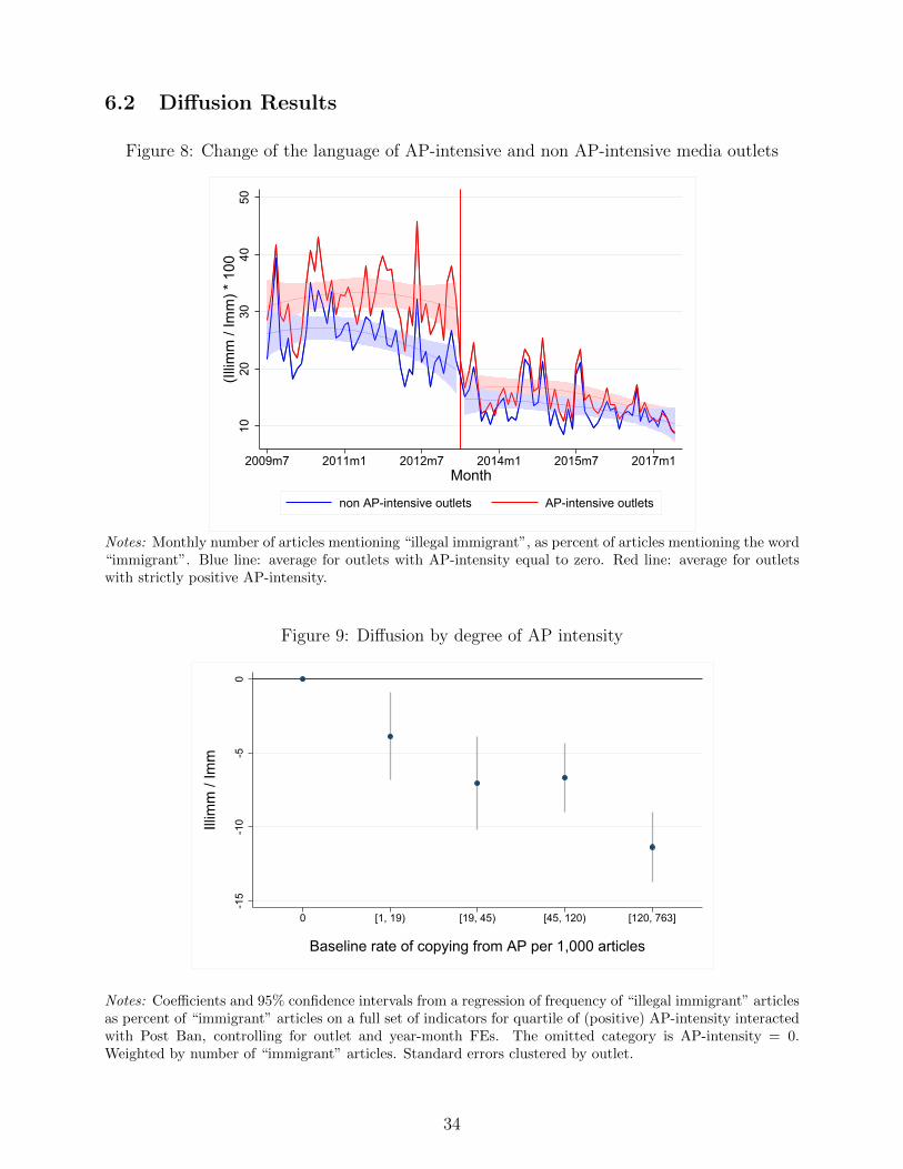
Preliminary evidence. Before proceeding to the estimation of the regression specified in

2, I examine visually the raw frequency of “illegal immigrant” articles in AP-intensive vs non

AP-intensive outlets. Figure 8 shows these two series. While non AP-intensive media appear

to gradually decrease their use of the term already prior to the ban, the use by AP-intensive

media remains flat and quite high up until it exhibits a sharp decline coinciding with the

ban. This pattern is in line with anecdotal evidence. For a long time, AP was resistant to

demands to change their language policy, while in other media use of the term was gradually

declining due to the controversy surrounding it. The figure also suggests that the ban was

somewhat of an aggregate shock: even non AP-intensive media experience a decline at the

13

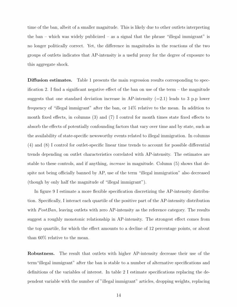
time of the ban, albeit of a smaller magnitude. This is likely due to other outlets interpreting

the ban – which was widely publicized – as a signal that the phrase “illegal immigrant” is

no longer politically correct. Yet, the difference in magnitudes in the reactions of the two

groups of outlets indicates that AP-intensity is a useful proxy for the degree of exposure to

this aggregate shock.

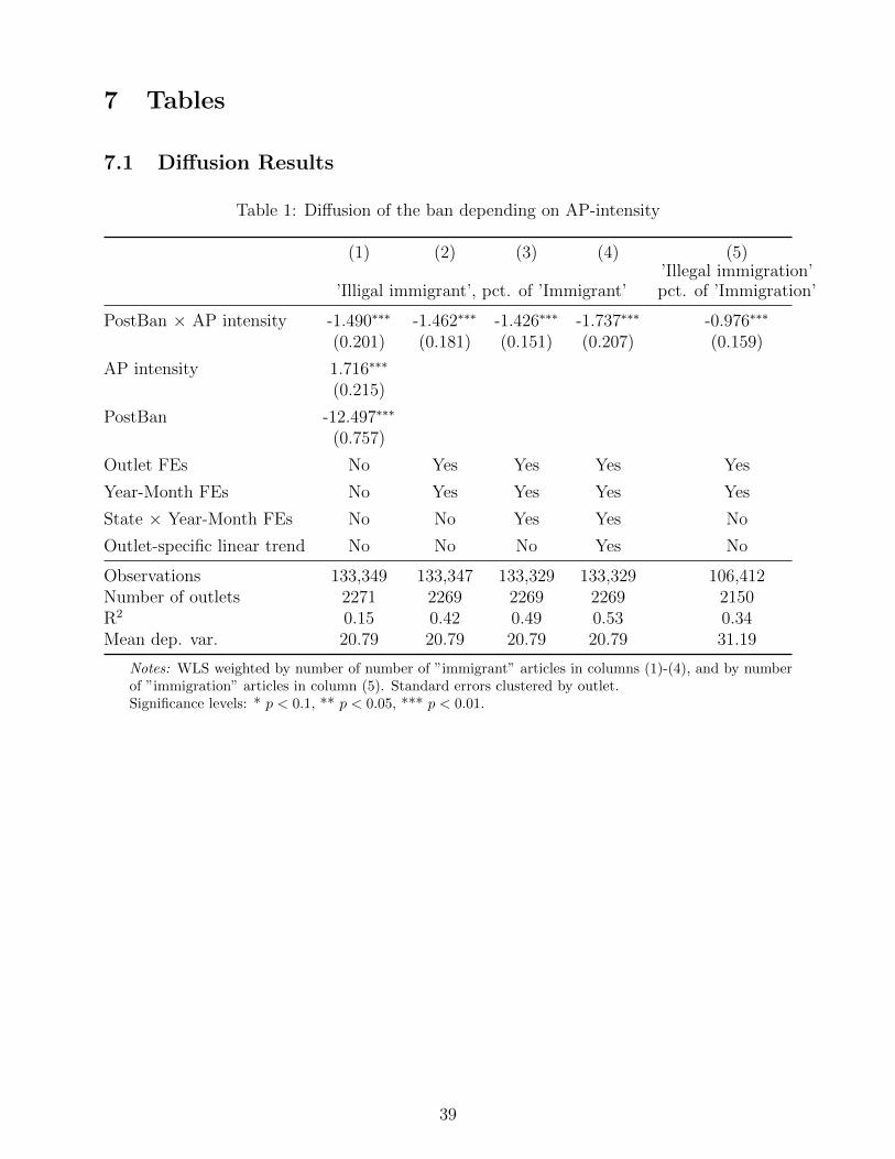
Diffusion estimates. Table 1 presents the main regression results corresponding to spec-

ification 2. I find a significant negative effect of the ban on use of the term – the magnitude

suggests that one standard deviation increase in AP-intensity (=2.1) leads to 3 p.p lower

frequency of “illegal immigrant” after the ban, or 14% relative to the mean. In addition to

month fixed effects, in columns (3) and (7) I control for month times state fixed effects to

absorb the effects of potentially confounding factors that vary over time and by state, such as

the availability of state-specific newsworthy events related to illegal immigration. In columns

(4) and (8) I control for outlet-specific linear time trends to account for possible differential

trends depending on outlet characteristics correlated with AP-intensity. The estimates are

stable to these controls, and if anything, increase in magnitude. Column (5) shows that de-

spite not being officially banned by AP, use of the term “illegal immigration” also decreased

(though by only half the magnitude of “illegal immigrant”).

In figure 9 I estimate a more flexible specification discretizing the AP-intensity distribu-

tion. Specifically, I interact each quartile of the positive part of the AP-intensity distribution

with PostBan, leaving outlets with zero AP-intensity as the reference category. The results

suggest a roughly monotonic relationship in AP-intensity. The strongest effect comes from

the top quartile, for which the effect amounts to a decline of 12 percentage points, or about

than 60% relative to the mean.

Robustness. The result that outlets with higher AP-intensity decrease their use of the

term“illegal immigrant” after the ban is stable to a number of alternative specifications and

definitions of the variables of interest. In table 2 I estimate specifications replacing the de-

pendent variable with the number of ”illegal immigrant” articles, dropping weights, replacing

14

number of articles with word-count and with number of headlines, replacing continuous AP-

intensity with a dummy for positive AP-intensity, and replacing PostBan with the time-series

of “illegal immigrant” articles (normalized by “immigrant” articles) released monthly by AP.

In table 3 I run the baseline regression with variations of the AP-intensity variable.

Instead of accounting for both credited copying and plagiarism from AP, in column (2) I

consider only the share of articles credited to AP, and in column (3) – only the share of

articles flagged by plagiarism detection. The two measures have a correlation of 0.56 and

yield very similar results to the baseline. In column (4), rather than examining the sample

of ‘immigrant” articles, I consider articles on any topic and define AP-intensity as the share

of total articles published the 12 months before the ban that credit AP. Finally, as a placebo

exercise, in column (5) I consider use of Reuters rather than AP. Since the Reuters news-

wire did not change their style rules regarding “illegal immigrant”, prior reliance on Reuters

should not be associated with the degree of reaction to the ban. Indeed, I find no change in

use of the term depending on Reuters-intensity.

Diffusion over time. To verify that trends in the use of “illegal immigrant” in high- versus

low-AP-intensity outlets did not start to diverge already prior the ban, I split the interaction

of AP intensity and Post Ban into a set of interactions with quarterly leads and lags. The

results are plotted in figure 10. I find that if anything, the relative frequency of“illegal

immigrant” seems to increase up until the ban (in other words, trends were diverging rather

than converging), at which point it falls abruptly. The decline is persistent, in line with the

permanently low supply of “illegal immigrant” AP dispatches.

In figure 11 I decompose this effect into articles copied from by AP (with or without

credit) vs. original content, and find that it is driven primarily by articles sourced from AP.

Table D4 presents the decomposed effects on “illegal immigrant” articles credited to AP, on

those flagged by my plagiarism detection algorithm but not credited to AP, and on the rest,

all expressed in percent of total “immigrant” articles. The results suggest large effects for

the first two categories relative to their respective means, and a small (but significant) effect

15

for the third.

Heterogeneity by slant. Media outlets decide on the extent to which they use want to use

AP dispatches and are free to edit their language as they wish. Therefore, a natural question

is whether the diffusion effect applies only to left-leaning outlets, which are presumably more

likely to agree with AP’s new language. To answer this question I analyze a sub-sample

of about 340 newspapers which I can match to the index of political slant constructed by

Gentzkow and Shapiro (2010). Splitting this sample at the 33rd and 66th percentile with

respect to this measure of ideological leaning, I find that the magnitude of the decline is indeed

largest for left-leaning outlets, but also negative and significant for centrist and right-leaning

newspapers (table 5).

Synonyms and volume of immigration coverage. Having established that the change

in AP’s language diffused into the language used to talk about immigration across different

media outlets, in table 6 I examine whether it also affected the volume of immigration cover-

age. As with AP-dispatches, I find that the synonyms proposed by AP (“live(-ing)/enter(-ing)

the country illegally / without legal permission”) compensated only partially for the decline

in the phrase“illegal immigrant”. Also consistent with the language of AP dispatches, I find

that the number of articles mentioning the word “immigrant” (normalized by total articles)

was not affected by ban. I same null-effect for articles mentioning the word “immigration”

over total articles.

To sum up, several features of the post-ban language of AP dispatches diffuse into the lan-

guage used by media outlets, consistent with the result that copied articles drive the majority

of the effect. Crucially, since the volume of immigration coverage remains unaffected, this is

primarily a shock to slanted language and not to other features of immigration coverage.

16

4 Effects on Readers’ Views on Immigration Policy

In this section I analyze how the ban affected public opinion on immigration policy by

comparing pre- and post-ban responses in the CCES electoral survey for respondents living

in counties with different AP-intensity of locally circulated newspapers.

4.1 Data

4.1.1 Aggregation to the county level.

Since the CCES survey does not ask which newspaper the respondent reads, I rely on county

of residence to assess exposure to locally circulated newspapers. Therefore, the first step in

this analysis is to aggregate my measures of newspapers’ content to the county level. To

do so, I obtain data on the geographic distribution of daily newspapers’ circulation from

Alliance of Audited Media (AAM). I use their Fall 2012 report, which includes circulation

by newspaper and zip-code from the most recent audit prior to this date, and aggregate

zip-code level data to the county level.12 Finally, since AAM does not collect geographically

disaggregated data for low-circulation newspapers, I impute these observations with data on

total circulation from the Editor and Publishes yearbooks, assuming that small newspapers

circulate mainly in the county of their headquarters.13

I match this data to the sample of Newslibrary/ProQuest media outlets based on the

name, town and state of the newspaper. I then keep counties for which newspapers matched

to the Newslibrary/ProQuest sample account for at least 90% of total county circulation.

This ensures that the county-level data on newspapers’ content is measured with reasonable

precision. The resulting dataset contains about about 2300 counties (out of a total of 3000),

and 800 daily newspapers (out of a total of 1200).

I aggregate AP-intensity to the county level by averaging the AP-intensity of newspapers

circulated within the county (in number of AP-sourced articles per 1000), weighting each

12For the largest nationally circulated newspapers AAM only reports circulation at the DMA level. Forthese cases I assign circulation to counties in proportion to voting-age population.

13The same procedure is used by Seamans and Zhu (2014).

17

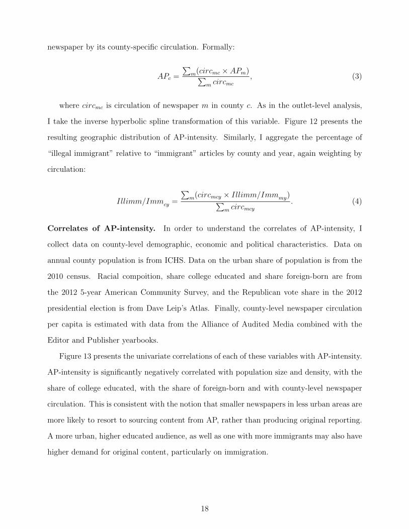
newspaper by its county-specific circulation. Formally:

APc =

∑m(circmc × APm)∑

m circmc

, (3)

where circmc is circulation of newspaper m in county c. As in the outlet-level analysis,

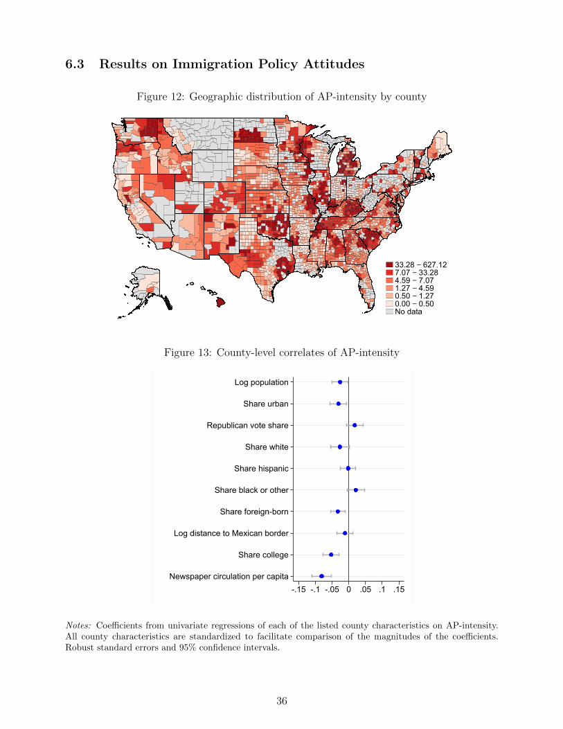
I take the inverse hyperbolic spline transformation of this variable. Figure 12 presents the

resulting geographic distribution of AP-intensity. Similarly, I aggregate the percentage of

“illegal immigrant” relative to “immigrant” articles by county and year, again weighting by

circulation:

Illimm/Immcy =

∑m(circmcy × Illimm/Immmy)∑

m circmcy

. (4)

Correlates of AP-intensity. In order to understand the correlates of AP-intensity, I

collect data on county-level demographic, economic and political characteristics. Data on

annual county population is from ICHS. Data on the urban share of population is from the

2010 census. Racial compoition, share college educated and share foreign-born are from

the 2012 5-year American Community Survey, and the Republican vote share in the 2012

presidential election is from Dave Leip’s Atlas. Finally, county-level newspaper circulation

per capita is estimated with data from the Alliance of Audited Media combined with the

Editor and Publisher yearbooks.

Figure 13 presents the univariate correlations of each of these variables with AP-intensity.

AP-intensity is significantly negatively correlated with population size and density, with the

share of college educated, with the share of foreign-born and with county-level newspaper

circulation. This is consistent with the notion that smaller newspapers in less urban areas are

more likely to resort to sourcing content from AP, rather than producing original reporting.

A more urban, higher educated audience, as well as one with more immigrants may also have

higher demand for original content, particularly on immigration.

18

4.1.2 The CCES Survey

To assess how public opinion on immigration policy changed in response to the ban, I use

a large nationally representative survey – the Cooperative Congressoional Election Study

(CCES). CCES is a repeated cross-section with more than 50,000 respondents per wave (with

smaller waves in some years), carried out roughly every 2 years.14 The survey is administered

online and a large portion of participants are YouGov panelists. Conveniently for my setting,

a large share of survey respondents (33%) report that they regularly read a newspaper in

print (i.e. that they have done so in the day before the survey).

Views on Immigration Policy. Each CCES respondent is asked to select the immigration

policies she thinks the US government should undertake, out of a list of options. The set

of policies differs in each wave – see Appendix A.3 for the full list. Two policies appear

consistently in all years between 2009 and 2017: “Increase the number of border patrols on

the U.S.-Mexican border” and “Grant legal status to all illegal immigrants who have held jobs

and paid taxes for at least 3 years, and not been convicted of any felony crimes”.

For each policy, I code support for restricting immigration (e.g. increasing border control/

not granting amnesty) as 1, and opposition as 0. I also compute an index aggregating choices

on all 9 immigration policies featured in the questionnaire in the respective year, including

rotating ones. I recode each choice in the direction of restricting immigration, and take the

average across all standardized choices (following Kling et al. (2007)).

Views on policies other than immigration. As placebo outcomes, I also collect data

on CCES questions that relate to policy issues other than immigration. Specifically, I create

(1) A dummy variable for opposing a woman’s right to choose to have an abortion under

any circumstances; (2) A dummy variable for preferring to cut public spending rather than

increase taxes; (3) A dummy variable for opposing gay marriage; (4) A dummy variable for

believing that the state of the economy has gotten worse over the past year.

14To the best of my knowledge, CCES is the only large-scale survey conducted between 2009 and 2017 thatasks questions related to views on immigration policy.

19

4.2 Empirical Strategy

To identify the effect of exposure to the phrase ”illegal immigrant” on views on immigration

policy, I estimate 2SLS equations of the following form:

Xcy = αc + βy + ρ Illimm/Immcy + φyWc + εcy, (5)

Illimm/Immcy = αc + βy + γAPc × PostBany + φyWc + εcy (6)

where Xcy denotes immigration policy preferences of respondents in county c and year

y, Illimmcy denotes the percent“illegal immigrant” relative to “immigrant” articles read in

that county and year, APc is the average AP-intensity of newspapers circulated in county c,

PostBany is an indicator equal to one for survey waves carried out after 2013, and αc and

βy are county and survey-year fixed effects respectively. Standard errors are clustered by

county.

The first-stage equation has the same form as the difference-in-difference specification

from the previous section, but now estimated at the county and survey-year level (instead of

media outlet and month). The excluded instrument for the potentially endogenous frequency

of “illegal immigrant” articles Illimm/Immcy is the interaction of AP-intensity with an

indicator for the period after the ban APc × PostBany. The approach is thus akin to a

shift-share strategy where PostBan is an aggregate shock and APc is local exposure to that

shock.

Since the identifying variation is at the county × survey-year level, this equation can

be estimated by aggregating individual survey responses up to that level. Alternatively, it

can be estimated at the respondent-level. This has the advantage of allowing to control for

respondent characteristics which are likely to correlate with immigration policy attitudes.

The identifying assumption is that the interaction of AP intensity with the timing of

the ban affects policy views only through exposure to the term ”illegal immigrant”. Time-

invariant county-characteristics correlated with AP intensity are absorbed by county fixed

effects. Therefore, if observed or unobserved characteristics are to confound my results, their

20

effect on attitudes would have to change at the same as the ban took effect. To account for

this possibility, I examine the sensitivity of the estimates to controlling for a host of county

characteristics measured at baseline and interacted with survey-year fixed effects (see figure

13 for the list of controls and their correlation with AP-intensity).

Finally, the effect identified by equation 5 is a local average treatment effect – it applies

to readers of newspapers that change their language on immigration solely due to the change

in the input supplied by AP. Such newspapers are likely to have a less pronounced stance

on immigration policy and potentially more persuadable readers compared to the readers of

always- or never-takers. I return to this point in the discussion of the results.

4.3 Results

First stage. I start off by replicating the analysis of the diffusion of the ban for this new

sample and unit of observation, i.e. aggregating newspapers’ data to the county times year

level (the 1st stage of equation 5). The results presented in figure 14 suggest that in this

sample 1 standard deviation increase in AP-intensity ( = 1.5 ) is associated with 9.5% lower

use of the term “illegal immigrant” after the ban.

Reduced form and 2SLS. I then turn to the reduced form effect of the ban on support

for restrictive immigration policies. In column (1) of table 7, I examine the effect on an index

aggregating all immigration-related CCES questions, conditional on respondent characteris-

tics and baseline county controls interacted with time. In columns (2) to (5) I examine each

component of the index that I am able to look at separately, i.e. each question that is asked

at least once before the ban and at least once after. With the exception of the question on

amnesty, the results suggest a significant negative reduced form effect of the ban of support

for restrictive policies. The magnitudes range from 1.2% to 2% reduction in support for

a given policy for 1 standard deviation higher AP-intensity. Similar results obtain at the

county-level, with the dependent variable collapsed by county times survey-year (table D6).

In table 8 I estimate the 2SLS version of equation 5 for the same set of outcomes, again

21

conditioning on respondent characteristics and county controls interacted with time. Here,

the coefficient of interest is the second stage effect of locally circulated “illegal immigrant”

articles on support for restrictive immigration policies. The results mirror those of the reduced

form – an increase in such articles has a significantly positive effect on support for restrictive

policies (with the exception of amnesty). The magnitudes range from 0.9% to 1.4% increase

in support for a given policy for 1 percentage point (or 4.8%) higher share of locally circulated

“illegal immigrant” articles. These results are also confirmed at the county level (table D7).

Since the border question is the only one (apart from the one on amnesty) that is asked

in each CCES wave in the period of interest, I focus on this question for the remainder of this

section. This has the advantage of holding the definition of the dependent variable constant

over time, whereas the index aggregates policies of different severity in each wave, making

comparisons over time harder to interpret.

Table 9 presents the reduced form and 2SLS effects on support for border security with

alternative controls. In the first column, instead of including county and year fixed effects,

I present the main effects of PostBan and AP − intensity. The results mimic those from

table 1. Consistent with the fact that AP-intensive outlets had a higher frequency of “illegal

immigrant” articles before the ban, immigration policy views in such counties were more

conserve before the ban (main effect on AP-intensity is positive). As with its effect on use

of “illegal immigrant”, the ban appears to be somewhat of an aggregate shocks to views on

border security (the main effect of PostBan is negative), but it is amplified by AP-intensity.

The coefficient on the interaction of PostBan with AP-intensity is stable to the inclusion of

fixed effects and to county controls interacted with time, which absorb the possibly changing

effect of these controls on readers’ views. It is also robust to the inclusion of year × state

fixed effects, which absorb the effect of any state-level policy changes – if anything, the 2SLS

increase in magnitude.

In figure 15, I estimate a flexible version of the reduced form equation, splitting the

distribution of AP-intensity into quartiles and interacting each one with an indicator for the

period after the ban, leaving the first quartile as the baseline category. The results suggest

22

that the effect is monotonic in AP-intensity.

Reduced form effect over time. To examine the dynamics of the reduced form effect,

I estimate a regression including a full set of interaction of AP-intensity with indicators for

survey waves, leaving the 2012 as the baseline category. In this analysis I can furthermore

add the survey years 2007 and 2017, in order to examine longer-term trends. The results

show no evidence of pre-trends (figures 16) – instead, the shift in policy views happens in

the period after the ban, and remains roughly constant in following waves.

Robustness. In table 10 I test the robustness of the results to different versions of AP-

intensity – using either attribution to AP or plagiarism detection to identify AP-sourced

articles, and extending the definition to all articles, instead of ones on immigration. This

yields very similar results to the baseline (columns 1 to 4 and 5 to 6). Instead, I find no

differential effect of the ban depending on Reuters-intensity (column 4). This is reassuring

since it suggests that the effect is specific to AP, rather than to the use of news wires in

general.

Heterogeneity: newspaper readership and political interest. In the above results

I considered the sample of all CCES respondents. Yet, respondents who regularly read a

newspaper are likely more exposed to the treatment. Therefore, in table 11 I split the sample

into respondents who report that they have not read a newspaper in the past 24 hours, those

who report that they have, and those who report that they have read a newspaper in print.

This analysis has the caveat that the newspaper readership question was not asked in the

2012 wave, so that sample size and power are reduced. Yet, the results suggests a stronger

magnitude of the effect among (self-reported) frequent newspaper readers.

On the other hand, engaged news consumers may be less easily swayed by slanted lan-

guage, while passive consumers with weak priors may be more persuadable. To test this

hypothesis, I split the sample into respondents with high vs low level of (self-reported) in-

23

terest in politics.15 The results in table 12 suggest that the effects are indeed stronger for

respondents with low interest in politics. This holds in the full sample, as well as conditional

on frequent newspaper readership (with the caveat of lower power in the latter case).

Views on other policies. If these results reflect a general change in political leanings

that by chance happens to be correlated with AP-intensity, we would expect that support

for other policies endorsed by the Republican party is also affected in the same direction.

In table 13 I present the results of a placebo exercise that tests for an effect on support for

policies related to taxation, abortion, gay rights, and the respondent’s assessment of the state

of the economy. I find no significant effect of the on any of these outcomes.

Voting. Was the change in immigration policy views enough to shift voting choices? The

answer appears to be no – in table 14 I show that the ban had no effect on intentions to

vote for the Republican candidate in elections for various offices. One interpretation of these

results is that the effect on voters’ views on immigration may not have been large enough to

affect voting choices. I do however detect a statistically significant negative effect of the ban

on disapproval of President Obama (columns 4 and 8 of table 14). This is in line with the

previous results, given Obama’s immigration reform agenda.

4.4 Magnitudes

To facilitate interpretation of the magnitudes of the estimated effects and comparison to

other studies in the media literature, it is useful to express them in terms of persuasion rates.

The persuasion rate is defined as the share of people who change their behavior, or in this

case – change their survey answer, in response to the treatment, out of the ones who could

have potentially done so (DellaVigna and Gentzkow 2010).

Expressed in terms of one standard deviation higher AP-intensity, the estimated treatment

effect suggests 9.5% fewer “illegal immigrant” over “immigrant” articles per year. Relative to

15The exact wording of the question is as follows: Some people seem to follow what’s going on in governmentand public affairs most of the time, whether there’s an election going on or not. Others aren’t that interested.Would you say you follow what’s going on in government and public affairs?

24

the mean in the ProQuest/ Newslibrary sample this would mean roughly 9 “illegal immigrant”

fewer articles per year. 16 The effect of this “treatment” is 0.7 percentage points lower support

for border security in the sample of all survey respondents, or 0.9 percentage points in the

sample of regular newspaper readers.

The persuasion rate for this treatment, that is, the share of respondents who are dissuaded

to support restrictive immigration policy, can be expressed as:

f =db

de

1

1− b0, (7)

where b is support for restring immigration, e is exposure to “illegal immigrant” articles,

and b0 is the share of the population that would oppose restrictive immigration policy in

absence of the treatment. With the coefficient estimated for the sample of all respondents,

and taking into account that about 1/3 of them report that they read a newspaper and

an average of 56% support restrictive immigration policy, this implies a persuasion rate of

f = (0.007)/(0.33 ∗ 1) ∗ (1/0.56) ≈ 3.8%. With the coefficient estimated from the sample of

newspaper readers, the implied persuasion rate is f = (0.009)/(1 ∗ 1) ∗ (1/0.59) ≈ 1.5%.17

This magnitude is in the lower end of the effects estimates in the media literature, con-

sistent with the milder nature of the treatment compared to other studies. For comparison,

Chiang and Knight (2011) estimate a persuasion rate of 6,5% for the effect of a (surprising)

newspaper electoral endorsement on voting intentions for that candidate.

Finally, this analysis and the interpretation of the results has focused on print newspapers,

as circulation data allows me to map survey respondents to their respective locally read

newspapers. However, views on immigration policy are also affected by consumption of TV

and Internet outlets, which may also have been affected by the ban. This matters for the

interpretation of the results to the extent that the AP-intensity of other media consumed in

16The coverage of these data is not universal, so that this should be taken as a lower bound.17 It should be noted that here, as standard in the calculations of persuasion rates in the media literature,

I am assuming that a newspaper reader reads every article. Relaxing this assumption, e.g. assuming thatonly a fraction of articles are actually read, would lead to a higher persuasion rate. On the other hand, asdocumented in section 2, the ban appears to be more salient when it comes to the language used in headlines.Assuming that readers are more likely to pay attention to headlines would therefore lead to a lower persuasionrate.

25

a given county is positively correlated with that of locally circulated newspapers. In that

case, the results would be interpreted as a combined media exposure effect, rather than a

per-article effect.

5 Conclusion

This paper has documented a large degree of diffusion of the language used by news wires to

media outlets. Changes in their language rules, which are determined centrally rather than

in consideration of the political leanings of the owners or readers of a particular media outlet,

are therefore a useful source of variation to estimate the effects of media slant on readers.

Applying this strategy, I find evidence consistent with exposure to the term “illegal immi-

grant” in local media shifting preferences towards more restrictive immigration policy. This

provides proof of concept for the hypothesis that politically slanted language can have a per-

suasive impact. However, this evidence is limited to the setting of unauthorized immigration

and to exposure to one particular term. More work is needed to understand the external

validity of this mechanism of media persuasion.

26

References

Alesina, A., A. Miano, and S. Stantcheva (2019): “Immigration and Redistribution,”NBER Working Paper 24733.

Cage, J., N. Herve, and M.-L. Viaud (2020): “The Production of Information in anOnline World: Is Copy Right?” Review of Economic Studies, forthcoming.

Chiang, C.-F. and B. Knight (2011): “Media Bias and Influence: Evidence from News-paper Endorsements,” Review of Economic Studies, 78(3), 795–820.

Chong, D. and J. N. Druckman (2007): “The Logic of Fear: Populism and the MediaCoverage of Immigrants Crimes,” Annual Review of Political Science, 10, 103–26.

DellaVigna, S. and M. Gentzkow (2010): “Persuasion: Empirical Evidence,” AnnualReview of Economics, 2, 643–669.

DellaVigna, S. and E. Kaplan (2007): “The Fox News Effect: Median Bias and Vot-ing,” Quarterly Journal of Economics, 112(3), 1187–1234.

Durante, R. and B. Knight (2012): “Partisan Control, Media Bias, and Viewer Re-sponses: Evidence from Berlusconi’s Italy,” Journal of the European Economic Association,10(3), 451–481.

Durante, R., P. Pinotti, and A. Tesei (2019): “The Political Legacy of EntertainmentTV,” American Economic Review.

Enikolopov, R., M. Petrova, and E. Zhuravskaya (2011): “Media and PoliticalPersuasion: Evidence from Russia,” American Economic Review, 101(7), 3253–85.

Fenby, J. (1986): The International News Services, Schocken Books.

Gentzkow, M. and J. M. Shapiro (2006): “Media Bias and Reputation,” Journal ofPolitical Economy, 114(2).

——— (2010): “What Drives Media Slant? Evidence from U.S. Daily Newsapers,” Econo-metrica, 78, 35–71.

Gentzkow, M., J. M. Shapiro, and M. Taddy (2019): “Measuring Group Differencesin High-Dimensional Choices: Method and Application to Congressional Speech,” Econo-metrica, 87(4), 1307–1340.

Gerber, A. S., D. Karlan, and D. Bergan (2009): “Does the Media Matter? AField Experiment Measuring the Effect of Newspapers on Voting Behavior and PoliticalOpinions,” American Economic Journal: Applied Economics, 1(2), 35–52.

Grigorieff, A., C. Roth, and D. Ubfal (2019): “Does Information Change AttitudesTowards Immigrants? Representative Evidence from Survey Experiments,” .

Groseclose, T. and J. Milyo (2005): “A Measure of Media Bias,” Quarterly Journal ofEconomics, 120(4), 1191–1237.

27

Hatte, S., M. Thoening, and S. Vlachos (2019): “The Logic of Fear: Populism andthe Media Coverage of Immigrants Crimes,” .

Kling, J. R., J. B. Liebman, and L. F. Katz (2007): “Experimental Analysis of Neigh-borhood Effects,” Econometrica, 75(1), 83–119.

Luntz, F. (2007): Words That Work: It’s Not What You Say, It’s What People Hear.

Martin, G. J. and A. Yurukoglu (2017): “Bias in Cable News: Persuasion and Polar-ization,” American Economic Review, 107(9), 2565–99.

Scheufele, D. and D. Tewksbury (2007): “Framing, agenda setting, and priming: theevolution of three media effects models,” Journal of Communication, 57(1), 9–20.

Seamans, R. and F. Zhu (2014): “Responses to Entry in Multi-Sided Markets: TheImpact of Craigslist on Local Newspapers,” Management Science, 60(2), 265–540.

Snyder, J. M. and D. Stromberg (2010): “Press Coverage and Political Accountability,”Journal of Political Economy, 118(2), 355–408.

Stromberg, D. (2015): “Media and Politics,” Annual Review of Economics, 7, 173–205.

28

6 Figures

6.1 Background and Text Analysis of AP Dispatches

Figure 1: “Illegal Immigrant” in congressional speech and in left- and right-leaning media

010

2030

4050

(Illim

m /

Imm

) * 1

00

Democrat Republican

Congressional Speech

010

2030

4050

(Illim

m /

Imm

) * 1

00

MSNBC Fox News

Cable TV

010

2030

4050

(Illim

m /

Imm

) * 1

00

Washington Post Washington Times

Newspapers

Notes: Frequency of mentions of “illegal immigrant” relative to “immigrant” in congressionalspeech, in cable TV (comparing MSNBC and Fox News) and in newspapers (comparing theWashington Post and the Washington Times) in the years 2009 to 2017. Data sources:Congressional Record, GDELT TV Archive and ProQuest respectively.

29

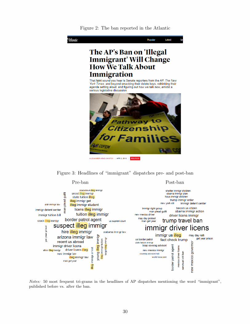
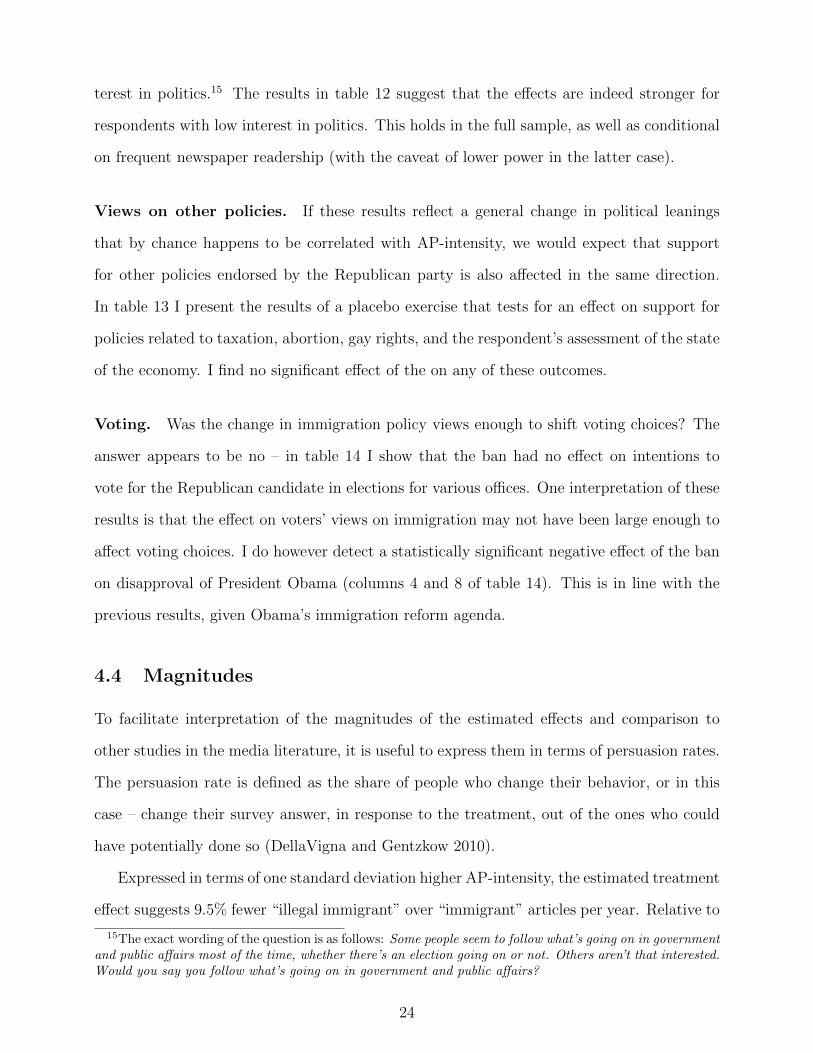
Figure 2: The ban reported in the Atlantic

Figure 3: Headlines of “immigrant” dispatches pre- and post-ban

Pre-ban Post-ban

Notes: 50 most frequent tri-grams in the headlines of AP dispatches mentioning the word “immigrant”,published before vs. after the ban.

30

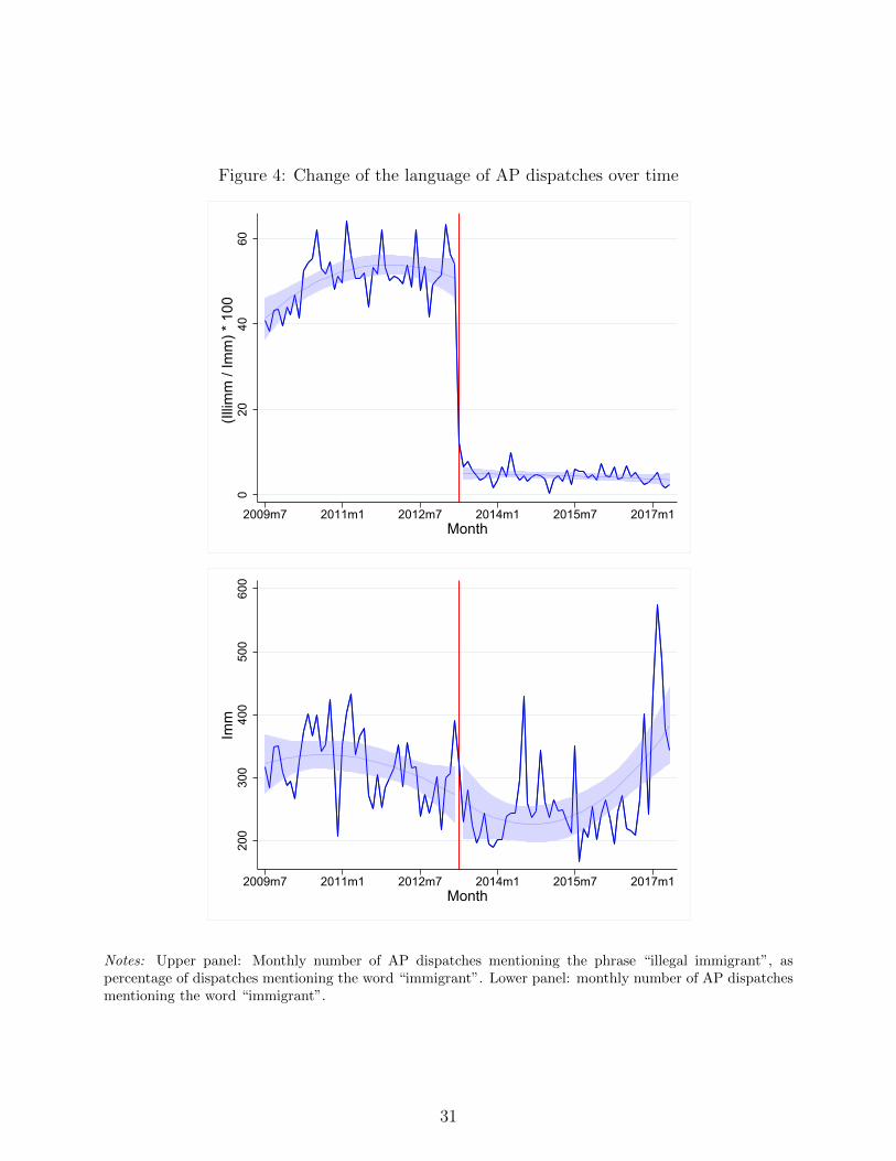
Figure 4: Change of the language of AP dispatches over time

020

4060

(Illim

m /

Imm

) * 1

00

2009m7 2011m1 2012m7 2014m1 2015m7 2017m1Month

200

300

400

500

600

Imm

2009m7 2011m1 2012m7 2014m1 2015m7 2017m1Month

Notes: Upper panel: Monthly number of AP dispatches mentioning the phrase “illegal immigrant”, aspercentage of dispatches mentioning the word “immigrant”. Lower panel: monthly number of AP dispatchesmentioning the word “immigrant”.

31

Figure 5: Correlates of the word “immigrant” before and after the ban

Full text (inlc. headline)

immigr

status

deport

advoclicensenforcpolici

appli

lawlegally

countriallowundocuresiddrivercitizenship

pewcitizen

feder

estimobtainpermitforeignborn

advocaci

elignumberhomelandmexicocrimin

defer

qualifi

livewithout

securprogram

perman

iceissustate

applic

unauthorcard

administrgetbroughtidentif

illegal

illegally

legal

.1.2

.3.4

.5.6

.7Po

st-b

an a

ssci

atio

n w

ith 'i

mm

igra

nt(s

)'

.1 .2 .3 .4 .5 .6 .7Pre-ban association with 'immgrant(s)'

Headlines only

licens

tuitiondriverchildren

younganti

advockid

collegsmuggldeportharborallow

detenthelpstudentbilldetain

protectaidrescu

programhire

transportscholarshipcriminbeatdefraudguiltidriveadvocacigroupcenterundocudenitexafound

sheltergetstatepolici

custodicountivanarrest

holdsentencillegal

legalillegally.1

.2.3

.4.5

.6.7

Post

-ban

ass

ocia

tion

with

'im

mig

rant

(s)'

.1 .2 .3 .4 .5 .6 .7Pre-ban association with 'immgrant(s)'

Notes: Top 50 unigrams with highest association with the word ”immigrant”, before and after the ban.Association defined as the rate of occurrence within the same dispatch. Derivatives of ’immigr’ and ’illeg’are not stemmed for illustration purposes as they are treated differently in AP’s guidelines.

Figure 6: Phrases most predictive of post-ban publishing date

Full text (inlc. headline)

0 20 40 60 80 100 1202

abbottfrancis

presidentialsuspected illegal immigrants

islamic statearizona law

syriansuspected illegal

syriapresident

immigrants country illegallyunaccompanied

sanctuaryillegallytwitter

arizonarefugees

illegal immigrantillegal immigrants

illegal

Headlines only

0 20 40 60 80 100 1202

travel banpm

california thingsariz

bcnews digest

editorials texaseditorials texas newspapers

texas newspapersap top

news digest pmdigest pm

lawsanctuary

tximmigration law

illegal immigrantthings

illegal immigrantsillegal

Notes: Top 20 n-grams (n ∈ 1, 2, 3) in “immigrant” dispatches that are most predictive of a post-banpublishing date (based on χ2 test).

32

Figure 7: Change of slant over time

0.5

11.

52

Slan

t

2009q3 2011q3 2013q3 2015q3 2017q3Quarter

Excl. 'illegal' Incl. 'illegal'

Notes: Evolution of the immigration-specific slant of AP dispatches. Higher values indicate more right-leaningslant. Red line: baseline measure of slant. Blue line: slant computed excluding any phrases containing “illegalimmigrant” or its substitutes.

33

6.2 Diffusion Results

Figure 8: Change of the language of AP-intensive and non AP-intensive media outlets

1020

3040

50(Il

limm

/ Im

m) *

100

2009m7 2011m1 2012m7 2014m1 2015m7 2017m1Month

non AP-intensive outlets AP-intensive outlets

Notes: Monthly number of articles mentioning “illegal immigrant”, as percent of articles mentioning the word“immigrant”. Blue line: average for outlets with AP-intensity equal to zero. Red line: average for outletswith strictly positive AP-intensity.

Figure 9: Diffusion by degree of AP intensity

-15

-10

-50

Illim

m /

Imm

0 [1, 19) [19, 45) [45, 120) [120, 763]

Baseline rate of copying from AP per 1,000 articles

Notes: Coefficients and 95% confidence intervals from a regression of frequency of “illegal immigrant” articlesas percent of “immigrant” articles on a full set of indicators for quartile of (positive) AP-intensity interactedwith Post Ban, controlling for outlet and year-month FEs. The omitted category is AP-intensity = 0.Weighted by number of “immigrant” articles. Standard errors clustered by outlet.

34

Figure 10: Diffusion over time

-3-2

-10

1

Illim

m /

Imm

-8 -6 -4 -2 0 2 4 6 8

Semesters Pre/ Post Ban

Notes: Coefficients and 95% confidence intervals from a regression of frequency of “illegal immigrant” articlesas percent of “immigrant” articles on full set of indicators for semester pre-/post-ban interacted with AP-intensity, controlling for outlet and year-month FEs. The omitted category is the semester before the ban.Weighted by number of “immigrant” articles. Standard errors clustered by outlet.

Figure 11: Diffusion over time: AP-sourced vs original articles

-2-1

01

Illim

m /

Imm

-8 -6 -4 -2 0 2 4 6 8

Semesters Pre/ Post Ban

Original articles AP-sourced articles

Notes: Green: Articles sourced from AP (attributed or plagiarized). Blue: All other articles. Coefficientsand 95% confidence intervals from a regression of frequency of “illegal immigrant” articles as percent of “im-migrant” articles on full set of indicators for semester pre-/post-ban interacted with AP-intensity, controllingfor outlet and year-month FEs. The omitted category is the semester before the ban. Weighted by numberof “immigrant” articles. Standard errors clustered by outlet.

35

6.3 Results on Immigration Policy Attitudes

Figure 12: Geographic distribution of AP-intensity by county

33.28 − 627.127.07 − 33.284.59 − 7.071.27 − 4.590.50 − 1.270.00 − 0.50No data

Figure 13: County-level correlates of AP-intensity

Log population

Share urban

Republican vote share

Share white

Share hispanic

Share black or other

Share foreign-born

Log distance to Mexican border

Share college

Newspaper circulation per capita-.15 -.1 -.05 0 .05 .1 .15

Notes: Coefficients from univariate regressions of each of the listed county characteristics on AP-intensity.All county characteristics are standardized to facilitate comparison of the magnitudes of the coefficients.Robust standard errors and 95% confidence intervals.

36

Figure 14: Diffusion over time: county × year level

-1.5

-1-.5

0.5

2009 2010 2011 2012 2013 2014 2015 2016Year

Notes: Point estimates and 95% confidence intervals on the interactions of AP-intensity with year, conditionalon year and county FEs. Standard errors clustered by county.

Figure 15: Support for increasing border security: Reduced form effect by quartile of AP-intensity

-.04

-.03

-.02

-.01

0.0

1

Illim

m /

Imm

[0, 0.7) [0.7, 5) [5, 16) [16, 661)

Baseline rate of copying from AP per 1,000 articles

Notes: Point estimates and 95% confidence intervals on the interactions of AP-intensity with survey year,conditional on year and county FEs, respondent controls, and county controls interacted with year FEs. Re-spondent controls: age, age squared gender, indicators for race, college, and 1st or 2nd generation immigrant.County controls: log population, racial composition, share foreign born, share college degree, log incomeper capita, share urban, republican vote share (2012 pres. election) – 2012 levels interacted with year FEs.Standard errors clustered by county.

37

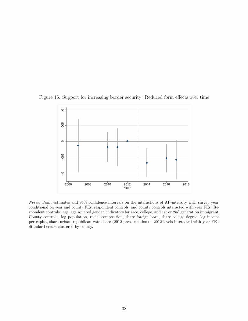
Figure 16: Support for increasing border security: Reduced form effects over time

-.01

-.005

0.0

05.0

1

2006 2008 2010 2012 2014 2016 2018Year

Notes: Point estimates and 95% confidence intervals on the interactions of AP-intensity with survey year,conditional on year and county FEs, respondent controls, and county controls interacted with year FEs. Re-spondent controls: age, age squared gender, indicators for race, college, and 1st or 2nd generation immigrant.County controls: log population, racial composition, share foreign born, share college degree, log incomeper capita, share urban, republican vote share (2012 pres. election) – 2012 levels interacted with year FEs.Standard errors clustered by county.

38

7 Tables

7.1 Diffusion Results

Table 1: Diffusion of the ban depending on AP-intensity

(1) (2) (3) (4) (5)

’Illigal immigrant’, pct. of ’Immigrant’’Illegal immigration’pct. of ’Immigration’

PostBan × AP intensity -1.490∗∗∗ -1.462∗∗∗ -1.426∗∗∗ -1.737∗∗∗ -0.976∗∗∗

(0.201) (0.181) (0.151) (0.207) (0.159)

AP intensity 1.716∗∗∗

(0.215)

PostBan -12.497∗∗∗

(0.757)

Outlet FEs No Yes Yes Yes Yes

Year-Month FEs No Yes Yes Yes Yes

State × Year-Month FEs No No Yes Yes No

Outlet-specific linear trend No No No Yes No

Observations 133,349 133,347 133,329 133,329 106,412Number of outlets 2271 2269 2269 2269 2150R2 0.15 0.42 0.49 0.53 0.34Mean dep. var. 20.79 20.79 20.79 20.79 31.19

Notes: WLS weighted by number of number of ”immigrant” articles in columns (1)-(4), and by numberof ”immigration” articles in column (5). Standard errors clustered by outlet.Significance levels: * p < 0.1, ** p < 0.05, *** p < 0.01.

39

Table 2: Alternative specifications

Not normalized Unweighted Word-count Headlines AP dummy Elasticity

(1) (2) (3) (4) (5) (6)Log(1 + ’Illegal Immigrant’) ’Illigal immigrant’, pct. of ’Immigrant’

PostBan × AP intensity -0.058∗∗∗ -1.607∗∗∗ -1.755∗∗∗ -1.071∗∗∗

(0.005) (0.124) (0.209) (0.285)

PostBan × I[AP-int > 0] -5.541∗∗∗

(1.059)

(Illimm/Imm)AP × AP intensity 0.121∗∗∗

(0.022)

Outlet FEs Yes Yes Yes Yes Yes Yes

Year-Month FEs Yes Yes Yes Yes Yes Yes

Observations 216,709 133,347 124,232 18,976 133,347 131,920Number of outlets 2271 2269 2160 1414 2269 2269R2 0.56 0.21 0.36 0.24 0.42 0.42Mean dep. var. 0.34 19.52 19.17 14.46 19.52 20.93

Notes: Replication of column (3) of table 1 with the following modifications: (1) Replacing the dependent variable with the log of 1 + number of ”illegalimmigrant” articles and dropping weights; (2) Regression without weights; (3) Replacing number of articles with word-count; (4) Replacing articleswith number of headlines; (5) Replacing continuous AP-intensity with a dummy for positive AP-intensity; (6) Replacing PostBan with the time-seriesof “illegal immigrant” articles (normalized by “immigrant” articles) released monthly by AP. Standard errors clustered by outlet.Significance levels: * p < 0.1, ** p < 0.05, *** p < 0.01.

40

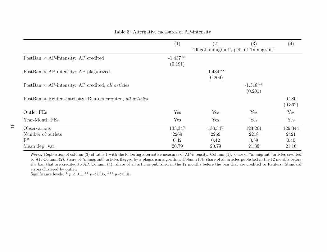
Table 3: Alternative measures of AP-intensity

(1) (2) (3) (4)’Illigal immigrant’, pct. of ’Immigrant’

PostBan × AP-intensity: AP credited -1.437∗∗∗

(0.191)

PostBan × AP-intensity: AP plagiarized -1.434∗∗∗

(0.209)

PostBan × AP-intensity: AP credited, all articles -1.318∗∗∗

(0.201)

PostBan × Reuters-intensity: Reuters credited, all articles 0.280(0.362)

Outlet FEs Yes Yes Yes Yes

Year-Month FEs Yes Yes Yes Yes

Observations 133,347 133,347 123,261 129,344Number of outlets 2269 2269 2218 2421R2 0.42 0.42 0.39 0.40Mean dep. var. 20.79 20.79 21.39 21.16

Notes: Replication of column (3) of table 1 with the following alternative measures of AP-intensity. Column (1): share of “immigrant” articles creditedto AP. Column (2): share of “immigrant” articles flagged by a plagiarism algorithm. Column (3): share of all articles published in the 12 months beforethe ban that are credited to AP. Column (4): share of all articles published in the 12 months before the ban that are credited to Reuters. Standarderrors clustered by outlet.Significance levels: * p < 0.1, ** p < 0.05, *** p < 0.01.

41

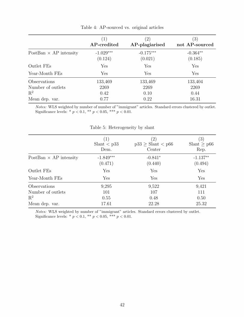
Table 4: AP-sourced vs. original articles

(1) (2) (3)AP-credited AP-plagiarised not AP-sourced

PostBan × AP intensity -1.029∗∗∗ -0.175∗∗∗ -0.364∗∗

(0.124) (0.021) (0.185)

Outlet FEs Yes Yes Yes

Year-Month FEs Yes Yes Yes

Observations 133,469 133,469 133,404Number of outlets 2269 2269 2269R2 0.42 0.10 0.44Mean dep. var. 0.77 0.22 16.31

Notes: WLS weighted by number of number of ”immigrant” articles. Standard errors clustered by outlet.Significance levels: * p < 0.1, ** p < 0.05, *** p < 0.01.

Table 5: Heterogeneity by slant

(1) (2) (3)Slant < p33

Dem.p33 ≥ Slant < p66

CenterSlant ≥ p66

Rep.

PostBan × AP intensity -1.849∗∗∗ -0.841∗ -1.137∗∗

(0.471) (0.440) (0.494)

Outlet FEs Yes Yes Yes

Year-Month FEs Yes Yes Yes

Observations 9,295 9,522 9,421Number of outlets 101 107 111R2 0.55 0.48 0.50Mean dep. var. 17.61 22.28 25.32

Notes: WLS weighted by number of ”immigrant” articles. Standard errors clustered by outlet.Significance levels: * p < 0.1, ** p < 0.05, *** p < 0.01.

42

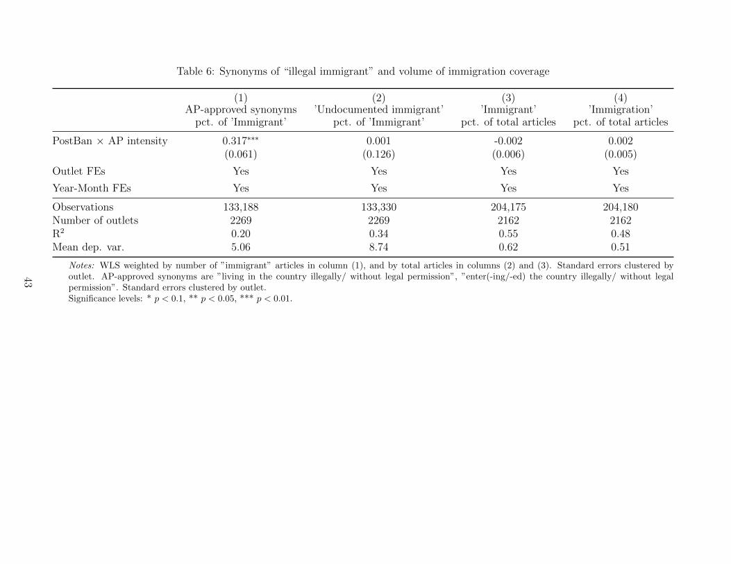
Table 6: Synonyms of “illegal immigrant” and volume of immigration coverage

(1) (2) (3) (4)AP-approved synonyms

pct. of ’Immigrant’’Undocumented immigrant’

pct. of ’Immigrant’’Immigrant’

pct. of total articles’Immigration’

pct. of total articles

PostBan × AP intensity 0.317∗∗∗ 0.001 -0.002 0.002(0.061) (0.126) (0.006) (0.005)

Outlet FEs Yes Yes Yes Yes

Year-Month FEs Yes Yes Yes Yes

Observations 133,188 133,330 204,175 204,180Number of outlets 2269 2269 2162 2162R2 0.20 0.34 0.55 0.48Mean dep. var. 5.06 8.74 0.62 0.51

Notes: WLS weighted by number of ”immigrant” articles in column (1), and by total articles in columns (2) and (3). Standard errors clustered byoutlet. AP-approved synonyms are ”living in the country illegally/ without legal permission”, ”enter(-ing/-ed) the country illegally/ without legalpermission”. Standard errors clustered by outlet.Significance levels: * p < 0.1, ** p < 0.05, *** p < 0.01.

43

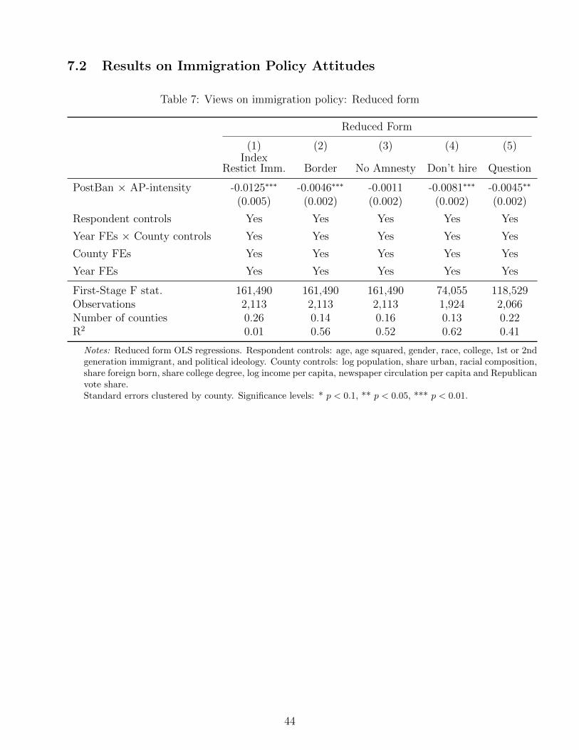
7.2 Results on Immigration Policy Attitudes

Table 7: Views on immigration policy: Reduced form

Reduced Form

(1) (2) (3) (4) (5)Index

Restict Imm. Border No Amnesty Don’t hire Question

PostBan × AP-intensity -0.0125∗∗∗ -0.0046∗∗∗ -0.0011 -0.0081∗∗∗ -0.0045∗∗

(0.005) (0.002) (0.002) (0.002) (0.002)

Respondent controls Yes Yes Yes Yes Yes

Year FEs × County controls Yes Yes Yes Yes Yes

County FEs Yes Yes Yes Yes Yes

Year FEs Yes Yes Yes Yes Yes

First-Stage F stat. 161,490 161,490 161,490 74,055 118,529Observations 2,113 2,113 2,113 1,924 2,066Number of counties 0.26 0.14 0.16 0.13 0.22R2 0.01 0.56 0.52 0.62 0.41

Notes: Reduced form OLS regressions. Respondent controls: age, age squared, gender, race, college, 1st or 2ndgeneration immigrant, and political ideology. County controls: log population, share urban, racial composition,share foreign born, share college degree, log income per capita, newspaper circulation per capita and Republicanvote share.Standard errors clustered by county. Significance levels: * p < 0.1, ** p < 0.05, *** p < 0.01.

44

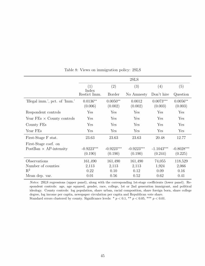
Table 8: Views on immigration policy: 2SLS

2SLS

(1) (2) (3) (4) (5)Index

Restict Imm. Border No Amnesty Don’t hire Question

’Illegal imm.’, pct. of ’Imm.’ 0.0136∗∗ 0.0050∗∗ 0.0012 0.0073∗∗∗ 0.0056∗∗

(0.006) (0.002) (0.002) (0.003) (0.003)

Respondent controls Yes Yes Yes Yes Yes

Year FEs × County controls Yes Yes Yes Yes Yes

County FEs Yes Yes Yes Yes Yes

Year FEs Yes Yes Yes Yes Yes

First-Stage F stat. 23.63 23.63 23.63 20.48 12.77

First-Stage coef. onPostBan × AP-intensity -0.9223∗∗∗ -0.9223∗∗∗ -0.9223∗∗∗ -1.1043∗∗∗ -0.8028∗∗∗

(0.190) (0.190) (0.190) (0.244) (0.225)

Observations 161,490 161,490 161,490 74,055 118,529Number of counties 2,113 2,113 2,113 1,924 2,066R2 0.22 0.10 0.12 0.09 0.16Mean dep. var. 0.01 0.56 0.52 0.62 0.41

Notes: 2SLS regressions (upper panel), along with the corresponding 1st-stage coefficients (lower panel). Re-spondent controls: age, age squared, gender, race, college, 1st or 2nd generation immigrant, and politicalideology. County controls: log population, share urban, racial composition, share foreign born, share collegedegree, log income per capita, newspaper circulation per capita and Republican vote share.Standard errors clustered by county. Significance levels: * p < 0.1, ** p < 0.05, *** p < 0.01.

45

Table 9: Support for increasing border control

Reduced Form 2SLS

(1) (2) (3) (4) (5) (6) (7)”Increase the number of border patrols on the US-Mexican border.”: Selected

PostBan × AP-intensity -0.0044∗∗∗ -0.0049∗∗∗ -0.0046∗∗∗ -0.0046∗∗

(0.002) (0.002) (0.002) (0.002)

AP intensity 0.0047∗∗∗

(0.002)

PostBan -0.0186∗∗∗

(0.006)

’Illegal imm.’, pct. of ’Imm.’ 0.0055∗∗ 0.0050∗∗ 0.0065∗∗

(0.002) (0.002) (0.003)

Respondent controls Yes Yes Yes Yes Yes Yes Yes

Year FEs × County controls No No Yes Yes No Yes Yes

County FEs No Yes Yes Yes Yes Yes Yes

Year FEs No Yes Yes Yes Yes Yes Yes

Year × State FEs No No No Yes No No Yes

First-Stage F stat. . . . . 9.90 23.63 12.19

First stage coef onPostBan × AP-intensity -0.8859∗∗∗ -0.9223∗∗∗ -0.7104∗∗∗

(0.282) (0.190) (0.204)

Observations 162,057 161,943 161,490 161,490 161,943 161,490 161,490Number of counties 2,236 2,122 2,113 2,113 2,122 2,113 2,113R2 0.12 0.14 0.14 0.14 0.10 0.10 0.10Mean dep. var. 0.56 0.56 0.56 0.56 0.56 0.56 0.56

Notes: Reduced form OLS regressions in the left hand-side panel, 2SLS regressions in the right hand-side panel. Respondentcontrols: age, age squared, gender, race, college, 1st or 2nd generation immigrant, and political ideology. County controls: logpopulation, share urban, racial composition, share foreign born, share college degree, log income per capita, newspaper circulationper capita and Republican vote share.Standard errors clustered by county. Significance levels: * p < 0.1, ** p < 0.05, *** p < 0.01.

46

Table 10: Support for increasing border control: Alternative measures of AP-intensity

Reduced Form 2SLS

(1) (2) (3) (4) (5) (6) (7)Border Border Border Border Border Border Border

PostBan × AP-intensity: AP credited -0.0047∗∗∗

(0.001)

PostBan × AP-intensity: Plagiarism detection -0.0037∗∗

(0.002)

PostBan × AP-intensity: AP credited, all articles -0.0028∗∗

(0.001)

PostBan × Reuters-intensity: Reuters credited, all articles -0.0006(0.003)

’Illegal imm.’, pct. of ’Imm.’ 0.0057∗∗∗ 0.0047∗ 0.0050∗∗

(0.002) (0.002) (0.002)

Respondent controls Yes Yes Yes Yes Yes Yes Yes

Year FEs × County controls Yes Yes Yes Yes Yes Yes Yes

County FEs Yes Yes Yes Yes Yes Yes Yes

Year FEs Yes Yes Yes Yes Yes Yes Yes

First-Stage F stat. . . . . 20.11 16.69 14.86

PostBan × AP-intensity: AP credited -0.8255∗∗∗

(0.184)PostBan × AP-intensity: Plagiarism detection -0.8004∗∗∗

(0.196)PostBan × AP-intensity: AP credited, all articles -0.5729∗∗∗

(0.149)

Observations 161490 161490 148271 149681 161490 161490 148271Number of counties 2113 2113 1767 1789 2113 2113 1767R2 0.14 0.14 0.14 0.14 0.10 0.10 0.10Mean dep. var. 0.56 0.56 0.55 0.55 0.56 0.56 0.55

Notes: Reduced form OLS regressions in the left hand-side panel, 2SLS regressions in the right hand-side panel. Respondent and county controls as in previoustable. Significance levels: * p < 0.1, ** p < 0.05, *** p < 0.01.

47

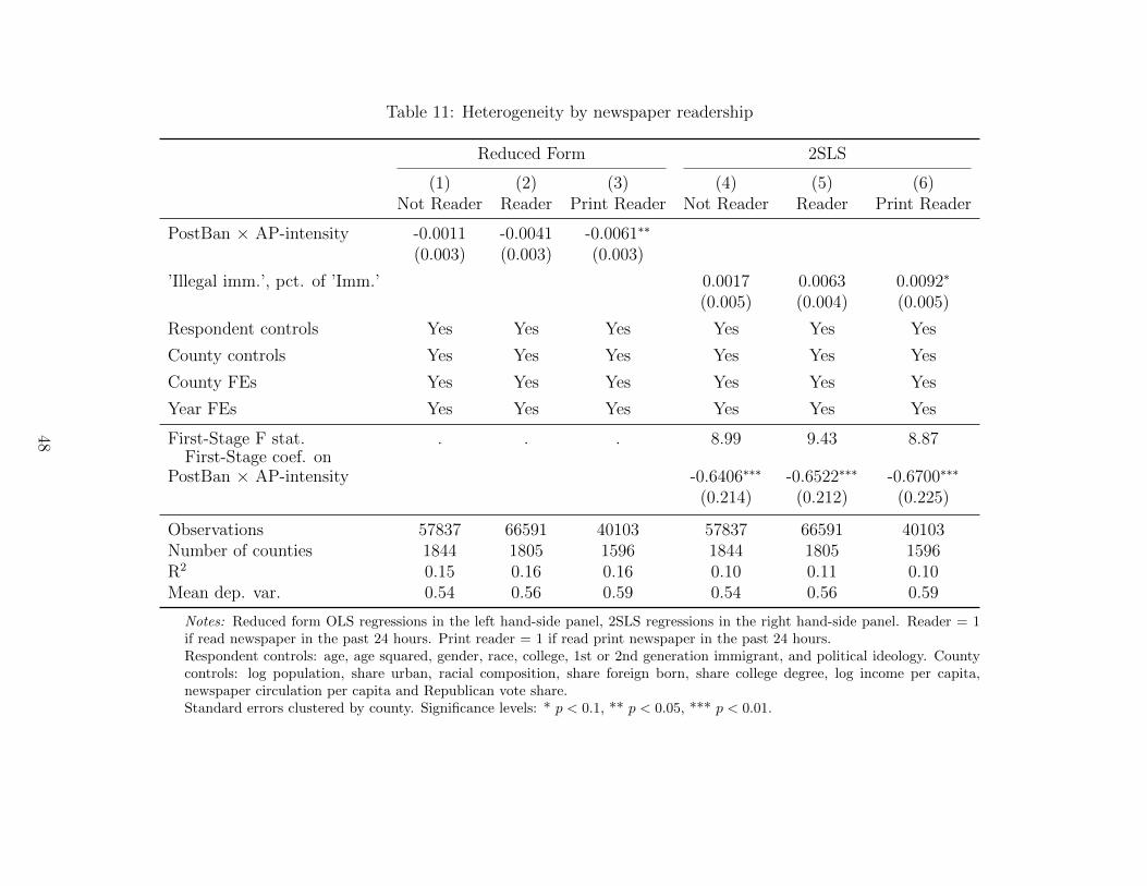
Table 11: Heterogeneity by newspaper readership

Reduced Form 2SLS

(1) (2) (3) (4) (5) (6)Not Reader Reader Print Reader Not Reader Reader Print Reader

PostBan × AP-intensity -0.0011 -0.0041 -0.0061∗∗

(0.003) (0.003) (0.003)

’Illegal imm.’, pct. of ’Imm.’ 0.0017 0.0063 0.0092∗

(0.005) (0.004) (0.005)

Respondent controls Yes Yes Yes Yes Yes Yes

County controls Yes Yes Yes Yes Yes Yes

County FEs Yes Yes Yes Yes Yes Yes

Year FEs Yes Yes Yes Yes Yes Yes

First-Stage F stat. . . . 8.99 9.43 8.87First-Stage coef. on

PostBan × AP-intensity -0.6406∗∗∗ -0.6522∗∗∗ -0.6700∗∗∗

(0.214) (0.212) (0.225)

Observations 57837 66591 40103 57837 66591 40103Number of counties 1844 1805 1596 1844 1805 1596R2 0.15 0.16 0.16 0.10 0.11 0.10Mean dep. var. 0.54 0.56 0.59 0.54 0.56 0.59

Notes: Reduced form OLS regressions in the left hand-side panel, 2SLS regressions in the right hand-side panel. Reader = 1if read newspaper in the past 24 hours. Print reader = 1 if read print newspaper in the past 24 hours.Respondent controls: age, age squared, gender, race, college, 1st or 2nd generation immigrant, and political ideology. Countycontrols: log population, share urban, racial composition, share foreign born, share college degree, log income per capita,newspaper circulation per capita and Republican vote share.Standard errors clustered by county. Significance levels: * p < 0.1, ** p < 0.05, *** p < 0.01.

48

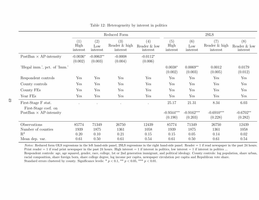
Table 12: Heterogeneity by interest in politics

Reduced Form 2SLS

(1) (2) (3) (4) (5) (6) (7) (8)High

interestLow

interestReader & high

interestReader & low

interestHigh

interestLow

interestReader & high

interestReader & low

interest

PostBan × AP-intensity -0.0036∗ -0.0063∗∗ -0.0008 -0.0112∗

(0.002) (0.003) (0.004) (0.006)

’Illegal imm.’, pct. of ’Imm.’ 0.0038∗ 0.0069∗∗ 0.0012 0.0179(0.002) (0.003) (0.005) (0.012)

Respondent controls Yes Yes Yes Yes Yes Yes Yes Yes

County controls Yes Yes Yes Yes Yes Yes Yes Yes

County FEs Yes Yes Yes Yes Yes Yes Yes Yes

Year FEs Yes Yes Yes Yes Yes Yes Yes Yes

First-Stage F stat. . . . . 25.17 21.31 8.34 6.03

First-Stage coef. onPostBan × AP-intensity -0.9344∗∗∗ -0.9162∗∗∗ -0.6910∗∗∗ -0.6702∗∗

(0.190) (0.203) (0.228) (0.282)

Observations 85774 71349 26750 12439 85774 71349 26750 12439Number of counties 1939 1875 1361 1058 1939 1875 1361 1058R2 0.20 0.10 0.21 0.15 0.15 0.05 0.14 0.02Mean dep. var. 0.61 0.50 0.61 0.54 0.61 0.50 0.61 0.54

Notes: Reduced form OLS regressions in the left hand-side panel, 2SLS regressions in the right hand-side panel. Reader = 1 if read newspaper in the past 24 hours.Print reader = 1 if read print newspaper in the past 24 hours. High interest = 1 if interest in politics, low interest = 1 if interest in politics ...Respondent controls: age, age squared, gender, race, college, 1st or 2nd generation immigrant, and political ideology. County controls: log population, share urban,racial composition, share foreign born, share college degree, log income per capita, newspaper circulation per capita and Republican vote share.Standard errors clustered by county. Significance levels: * p < 0.1, ** p < 0.05, *** p < 0.01.

49

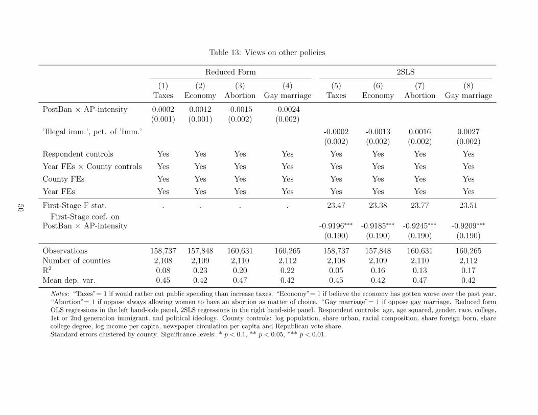
Table 13: Views on other policies

Reduced Form 2SLS

(1) (2) (3) (4) (5) (6) (7) (8)Taxes Economy Abortion Gay marriage Taxes Economy Abortion Gay marriage

PostBan × AP-intensity 0.0002 0.0012 -0.0015 -0.0024(0.001) (0.001) (0.002) (0.002)

’Illegal imm.’, pct. of ’Imm.’ -0.0002 -0.0013 0.0016 0.0027(0.002) (0.002) (0.002) (0.002)

Respondent controls Yes Yes Yes Yes Yes Yes Yes Yes

Year FEs × County controls Yes Yes Yes Yes Yes Yes Yes Yes

County FEs Yes Yes Yes Yes Yes Yes Yes Yes

Year FEs Yes Yes Yes Yes Yes Yes Yes Yes

First-Stage F stat. . . . . 23.47 23.38 23.77 23.51

First-Stage coef. onPostBan × AP-intensity -0.9196∗∗∗ -0.9185∗∗∗ -0.9245∗∗∗ -0.9209∗∗∗

(0.190) (0.190) (0.190) (0.190)

Observations 158,737 157,848 160,631 160,265 158,737 157,848 160,631 160,265Number of counties 2,108 2,109 2,110 2,112 2,108 2,109 2,110 2,112R2 0.08 0.23 0.20 0.22 0.05 0.16 0.13 0.17Mean dep. var. 0.45 0.42 0.47 0.42 0.45 0.42 0.47 0.42

Notes: “Taxes”= 1 if would rather cut public spending than increase taxes. “Economy”= 1 if believe the economy has gotten worse over the past year.“Abortion”= 1 if oppose always allowing women to have an abortion as matter of choice. “Gay marriage”= 1 if oppose gay marriage. Reduced formOLS regressions in the left hand-side panel, 2SLS regressions in the right hand-side panel. Respondent controls: age, age squared, gender, race, college,1st or 2nd generation immigrant, and political ideology. County controls: log population, share urban, racial composition, share foreign born, sharecollege degree, log income per capita, newspaper circulation per capita and Republican vote share.Standard errors clustered by county. Significance levels: * p < 0.1, ** p < 0.05, *** p < 0.01.

50

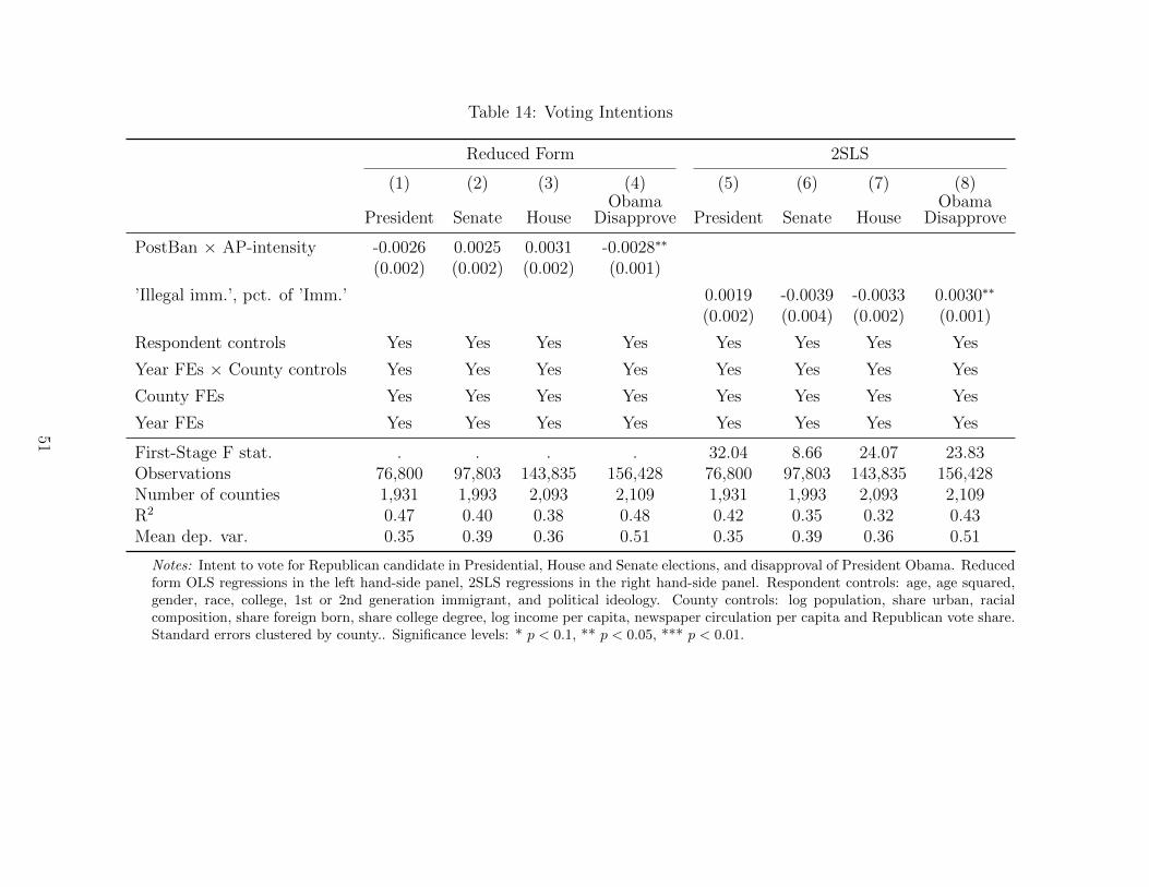
Table 14: Voting Intentions

Reduced Form 2SLS

(1) (2) (3) (4) (5) (6) (7) (8)

President Senate HouseObama

Disapprove President Senate HouseObama

Disapprove

PostBan × AP-intensity -0.0026 0.0025 0.0031 -0.0028∗∗

(0.002) (0.002) (0.002) (0.001)

’Illegal imm.’, pct. of ’Imm.’ 0.0019 -0.0039 -0.0033 0.0030∗∗

(0.002) (0.004) (0.002) (0.001)

Respondent controls Yes Yes Yes Yes Yes Yes Yes Yes

Year FEs × County controls Yes Yes Yes Yes Yes Yes Yes Yes

County FEs Yes Yes Yes Yes Yes Yes Yes Yes

Year FEs Yes Yes Yes Yes Yes Yes Yes Yes

First-Stage F stat. . . . . 32.04 8.66 24.07 23.83Observations 76,800 97,803 143,835 156,428 76,800 97,803 143,835 156,428Number of counties 1,931 1,993 2,093 2,109 1,931 1,993 2,093 2,109R2 0.47 0.40 0.38 0.48 0.42 0.35 0.32 0.43Mean dep. var. 0.35 0.39 0.36 0.51 0.35 0.39 0.36 0.51

Notes: Intent to vote for Republican candidate in Presidential, House and Senate elections, and disapproval of President Obama. Reducedform OLS regressions in the left hand-side panel, 2SLS regressions in the right hand-side panel. Respondent controls: age, age squared,gender, race, college, 1st or 2nd generation immigrant, and political ideology. County controls: log population, share urban, racialcomposition, share foreign born, share college degree, log income per capita, newspaper circulation per capita and Republican vote share.Standard errors clustered by county.. Significance levels: * p < 0.1, ** p < 0.05, *** p < 0.01.

51

A Appendix: Background on the AP Stylebook

The Stylebook entry before the ban

illegal immigrant Used to describe those who have entered the countryillegally, it is the preferred term, rather than illegal alien or undocumentedworker.Do not use the shortened term illegals.

The Stylebook entry after the ban

illegal immigration Entering in a country in violation of civil or criminallaw. Except in direct quotes essential to the story, use illegal only to referto an action, not a person: illegal immigration, but not illegal immigrant.Acceptable variations include living in or entering a county illegally orwithout legal permission.Expect in direct quotations, do not use the terms illegal alien, an illegal,illegals or undocumented.Do not describe people as violating immigration laws without attribution.Specify wherever possible how someone entered the country illegally andfrom where. Crossed the border? Overstayed a visa? What nationality?People who were brought into the county as children should not be de-scribed as having immigrated illegally. For people guaranteed a temporaryright to remain in the U.S. under the Deferred Action for Childhood Ar-rivals program, use temporary resident status, with details on the programlower in the story.

52

Figure A1: AP style after the ban

53

A Appendix: Data

A.1 Computation of Slant

In this section I describe the procedure for computing an index for the immigration-specific

slant of AP dispatches released in each quarter. This follows the method developed by

Gentzkow and Shapiro (2010).

I start off with the set of all Congressional speeches for the period 2009-2017 that mention

the word “immigrant” and find the 500 phrases (3 to 4-grams) that are most predictive of

the speakers’ party based on the Pearson’s χ2 statistic. In one version of the slant measure,

in this step I exclude phrases that contain the term “illegal immmigrant” and its substitutes.

For this set of phrases, I compute their relative frequency in the speech of each Congres-

sional representative: fpc = fpc/∑

p fpc. I then regress relative frequency an indicator for the

party of the representative, obtaining phrase-specific intercept and slope coefficients αp and

βp.

Finally, I compute the relative frequency of each phrase in AP dispatches released in

a given quarter – fpq – and regress (fpq − ap) on bp. The resulting slope coefficient is the

quarter-specific measure of slant.

A.2 Plagiarism Detection Algorithm

In this section I describe the algorithm I use to identify “immigrant” articles that are copied

from AP but do not necessarily credit AP.

The first step of the algorithm is to assign to each article a set of AP dispatches that

could potentially have been used in the writing of the article. I focus on AP dispatches

released in the day before publication and mentioning the word “immigrant”.18 This is a

simplified version of the procedure used in Cage et al. (2020), which first clusters articles by

the event they cover, and then forms the set of potentially plagiarized articles as those that

18I do not use contemporaneous (same-day) AP-dispatches because the origin of the content is moreambiguous in this case – text similarity could be due the media outlet copying AP, or to AP redistributingcontent produced by a member outlet.

54

cover the same event and are published prior to the article of interest. The second step in the

algorithm is to compute a measure of verbatim copying. I pre-process all texts by removing

punctuation and stop-words, stemming, and tokenizing into 5-grams. I then measure the

share of the article’s text that is identical to each paired dispatch and take the maximum

over all paired dispatches. I label an article as copied from AP if the maximum text overlap

exceeds 20% (equivalent to 70 characters, relative to the mean text length of 350).

Figure B1 presents the relationship between copying and crediting AP, plotting the av-

erage share of credited articles by bin of the copy-rate distribution (i.e. by share of text

overlapping with an AP dispatch). It is notable that even among articles whose lead para-

graph is virtually identical to an AP dispatch (with 90-100% identical text), the rate of

crediting AP never exceeds 60%. In other words, relying on attribution to AP alone would

have missed a substantial volume of copied articles. When collapsed at the media outlet level

however, the correlation between the two measures is 0.83.

Figure B1: AP-copy rate: Attribution and plagiarism

0.2

.4.6

Shar

e AP

-cre

dite

d

0-10

%

10-2

0%

20-3

0%

30-4

0%

40-5

0%

50-6

0%

60-7

0%

70-8

0%

80-9

0%

90-1

00%

Copy rate

55

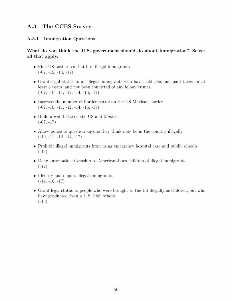
A.3 The CCES Survey

A.3.1 Immigration Questions

What do you think the U.S. government should do about immigration? Selectall that apply.

• Fine US businesses that hire illegal immigrants.(-07, -12, -14, -17)

• Grant legal status to all illegal immigrants who have held jobs and paid taxes for atleast 3 years, and not been convicted of any felony crimes.(-07, -10, -11, -12, -14, -16, -17)

• Increase the number of border patrol on the US-Mexican border.(-07, -10, -11, -12, -14, -16, -17)

• Build a wall between the US and Mexico.(-07, -17)

• Allow police to question anyone they think may be in the country illegally.(-10, -11, -12, -14, -17)

• Prohibit illegal immigrants from using emergency hospital care and public schools.(-12)

• Deny automatic citizenship to American-born children of illegal immigrants.(-12)

• Identify and deport illegal immigrants.(-14, -16, -17)

• Grant legal status to people who were brought to the US illegally as children, but whohave graduated from a U.S. high school.(-16)

—————————————————————-

56

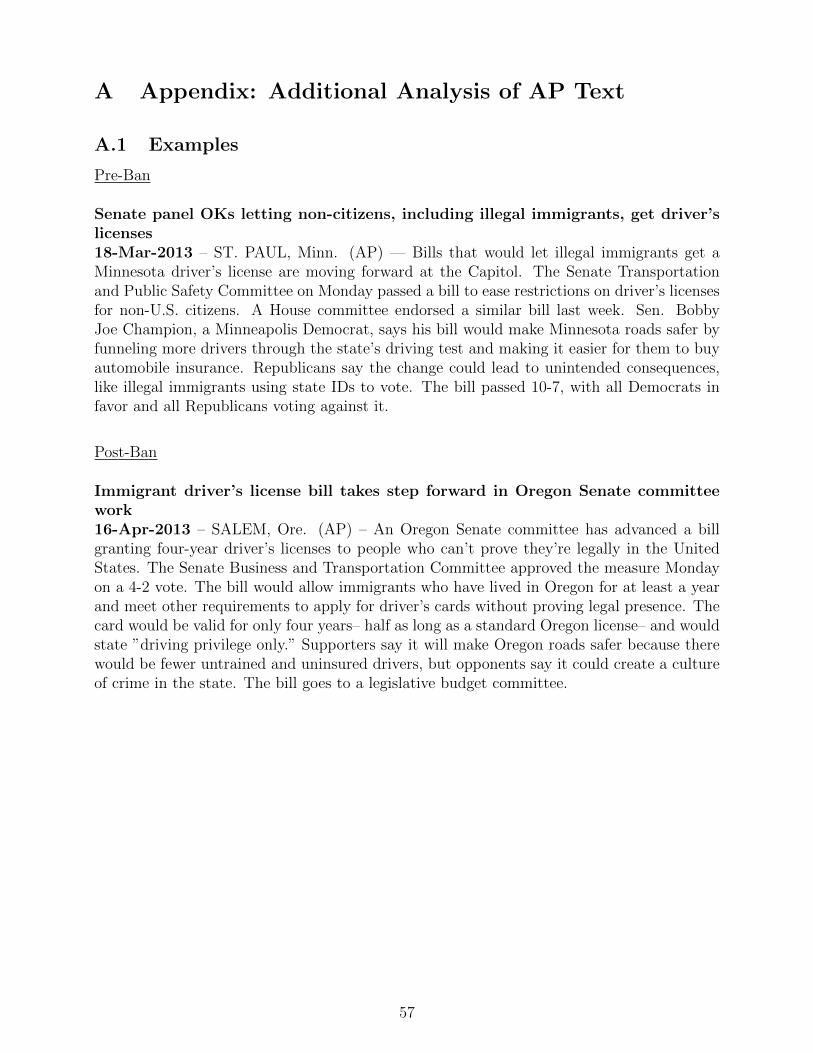
A Appendix: Additional Analysis of AP Text

A.1 Examples

Pre-Ban

Senate panel OKs letting non-citizens, including illegal immigrants, get driver’slicenses18-Mar-2013 – ST. PAUL, Minn. (AP) — Bills that would let illegal immigrants get aMinnesota driver’s license are moving forward at the Capitol. The Senate Transportationand Public Safety Committee on Monday passed a bill to ease restrictions on driver’s licensesfor non-U.S. citizens. A House committee endorsed a similar bill last week. Sen. BobbyJoe Champion, a Minneapolis Democrat, says his bill would make Minnesota roads safer byfunneling more drivers through the state’s driving test and making it easier for them to buyautomobile insurance. Republicans say the change could lead to unintended consequences,like illegal immigrants using state IDs to vote. The bill passed 10-7, with all Democrats infavor and all Republicans voting against it.

Post-Ban

Immigrant driver’s license bill takes step forward in Oregon Senate committeework16-Apr-2013 – SALEM, Ore. (AP) – An Oregon Senate committee has advanced a billgranting four-year driver’s licenses to people who can’t prove they’re legally in the UnitedStates. The Senate Business and Transportation Committee approved the measure Mondayon a 4-2 vote. The bill would allow immigrants who have lived in Oregon for at least a yearand meet other requirements to apply for driver’s cards without proving legal presence. Thecard would be valid for only four years– half as long as a standard Oregon license– and wouldstate ”driving privilege only.” Supporters say it will make Oregon roads safer because therewould be fewer untrained and uninsured drivers, but opponents say it could create a cultureof crime in the state. The bill goes to a legislative budget committee.

57

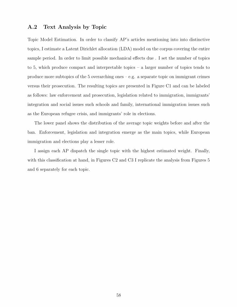
A.2 Text Analysis by Topic

Topic Model Estimation. In order to classify AP’s articles mentioning into into distinctive

topics, I estimate a Latent Dirichlet allocation (LDA) model on the corpus covering the entire

sample period. In order to limit possible mechanical effects due . I set the number of topics

to 5, which produce compact and interpretable topics – a larger number of topics tends to

produce more subtopics of the 5 overarching ones – e.g. a separate topic on immigrant crimes

versus their prosecution. The resulting topics are presented in Figure C1 and can be labeled

as follows: law enforcement and prosecution, legislation related to immigration, immigrants’

integration and social issues such schools and family, international immigration issues such

as the European refugee crisis, and immigrants’ role in elections.

The lower panel shows the distribution of the average topic weights before and after the

ban. Enforcement, legislation and integration emerge as the main topics, while European

immigration and elections play a lesser role.

I assign each AP dispatch the single topic with the highest estimated weight. Finally,

with this classification at hand, in Figures C2 and C3 I replicate the analysis from Figures 5

and 6 separately for each topic.

58

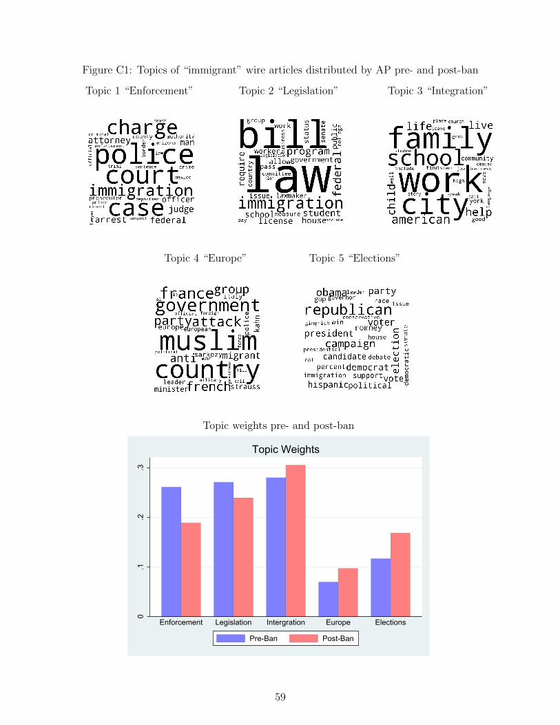
Figure C1: Topics of “immigrant” wire articles distributed by AP pre- and post-ban

Topic 1 “Enforcement” Topic 2 “Legislation” Topic 3 “Integration”

Topic 4 “Europe” Topic 5 “Elections”

Topic weights pre- and post-ban

0.1

.2.3

Enforcement Legislation Intergration Europe Elections

Topic Weights

Pre-Ban Post-Ban

59

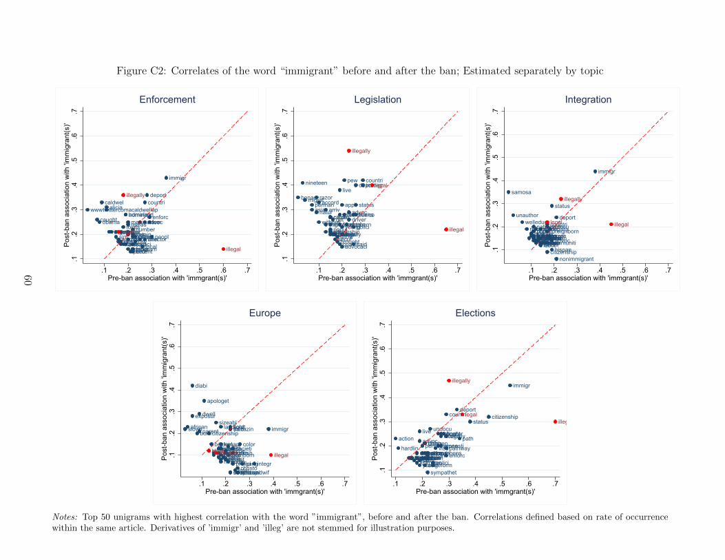
Figure C2: Correlates of the word “immigrant” before and after the ban; Estimated separately by topic

immigr

deportcountri

enforciceadvoccustom

peopl

homelandadministrmani

director

releasnumber

crimindetent

caldwel

detain

alicia

local

focuscan

agencsecurlaw

remov

saidpolici

feder

govern

programadvocaci

bedfacil

percent

across

serious

sincmonth

prioriti

recent

obama

holdstatus

wwwtwittercomacaldwellap

caught

illegal

illegally

legal

.1.2

.3.4

.5.6

.7Po

st-b

an a

ssoc

iatio

n w

ith 'i

mm

igra

nt(s

)'

.1 .2 .3 .4 .5 .6 .7Pre-ban association with 'immgrant(s)'

Enforcement

countriimmigrdeport

pew

status

live

licensmexicoadvocappli

driverresid

polici

estim

obtain

razor

nineteen

foreignborn

accord

young

arrivcamegetcitizen

said

legally

perman

mexican

migrat

natur

undocuallow

elig

asia

permitpopulnumbercitizenship

benac

peoplsecur

advocaci

without

qualifibroughtapplicwork illegal

illegally

legal

.1.2

.3.4

.5.6

.7Po

st-b

an a

ssoc

iatio

n w

ith 'i

mm

igra

nt(s

)'.1 .2 .3 .4 .5 .6 .7Pre-ban association with 'immgrant(s)'

Legislation

immigr

status

deportcountriundoculegallyforeignborn

samosa

manilawcitizenenforc

advochelp

comenativeborn

communiti

polici

liveborder

popul

hispan

americangroup

welcom

welleducreform

fearresid

unauthor

unit

nonimmigrant

childrennumberhomeland

identiflaborworker

pew

citizenship

becomrecentpercentarrivamongmexican

collegeeduc

illegal

illegally

legal

.1.2

.3.4

.5.6

.7Po

st-b

an a

ssoc

iatio

n w

ith 'i

mm

igra

nt(s

)'

.1 .2 .3 .4 .5 .6 .7Pre-ban association with 'immgrant(s)'

Integration

immigr

diabi

apologet

kolatthilosarrazin

color

sizeabllandlord

dwell

integr

societiantiturkish

exposur

gang

citizenship

kenanswedewareraskingerman

mani

parent

live

proficichristo

bestsellegally

permitsurggermanbornguest

born

ambival

african

husbandwiftoler

racistdoenermutat

slowli

children

newcomturk

shopkeepinfest

illegalillegallylegal

.1.2

.3.4

.5.6

.7Po

st-b

an a

ssoc

iatio

n w

ith 'i

mm

igra

nt(s

)'

.1 .2 .3 .4 .5 .6 .7Pre-ban association with 'immgrant(s)'

Europe

immigr

citizenshipdeport

statuscountri

pathlegallyborderallowcitizenbroughtundocu

pathwayamnestihispan

live

enforcvisa

childrenlatinoadvocpermit

permancomprehensdreamestim

policipew

overhaul

reformalien

unauthorsecur

unitstancgrant

act

action

younghighachievparent

sympathet

foreignbornkrikorianresidsoften

hardlin

illegal

illegally

legal

.1.2

.3.4

.5.6

.7Po

st-b

an a

ssoc

iatio

n w

ith 'i

mm

igra

nt(s

)'

.1 .2 .3 .4 .5 .6 .7Pre-ban association with 'immgrant(s)'

Elections

Notes: Top 50 unigrams with highest correlation with the word ”immigrant”, before and after the ban. Correlations defined based on rate of occurrencewithin the same article. Derivatives of ’immigr’ and ’illeg’ are not stemmed for illustration purposes.

60

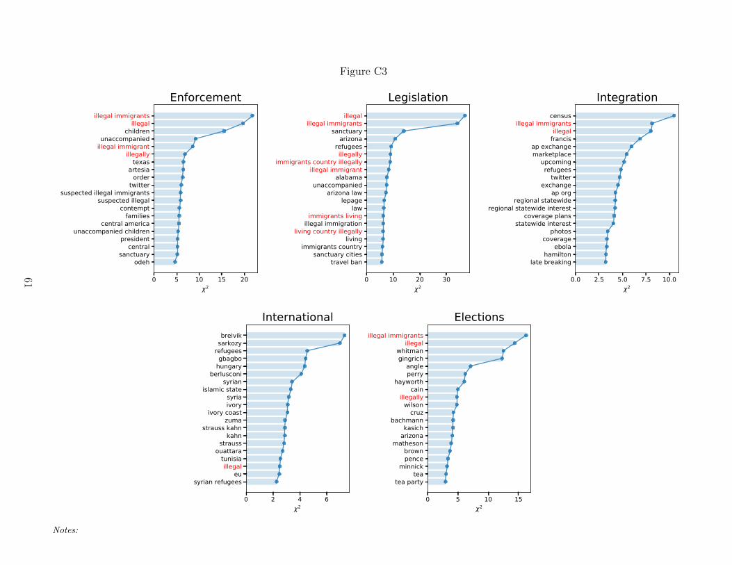
Figure C3

0 5 10 15 202

odehsanctuary

centralpresident

unaccompanied childrencentral america

familiescontempt

suspected illegalsuspected illegal immigrants

twitterorder

artesiatexas

illegallyillegal immigrantunaccompanied

childrenillegal

illegal immigrants

Enforcement

0 10 20 302

travel bansanctuary cities

immigrants countryliving

living country illegallyillegal immigration

immigrants livinglaw

lepagearizona law

unaccompaniedalabama

illegal immigrantimmigrants country illegally

illegallyrefugees

arizonasanctuary

illegal immigrantsillegal

Legislation

0.0 2.5 5.0 7.5 10.02

late breakinghamilton

ebolacoverage

photosstatewide interest

coverage plansregional statewide interest

regional statewideap org

exchangetwitter

refugeesupcoming

marketplaceap exchange

francisillegal

illegal immigrantscensus

Integration

0 2 4 62

syrian refugeeseu

illegaltunisia

ouattarastrauss

kahnstrauss kahn

zumaivory coast

ivorysyria

islamic statesyrian

berlusconihungarygbagbo

refugeessarkozybreivik

International

0 5 10 152

tea partytea

minnickpencebrown

mathesonarizonakasich

bachmanncruz

wilsonillegally

cainhayworth

perryangle

gingrichwhitman

illegalillegal immigrants

Elections

Notes:

61

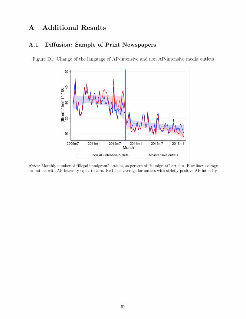
A Additional Results

A.1 Diffusion: Sample of Print Newspapers

Figure D1: Change of the language of AP-intensive and non AP-intensive media outlets

1020

3040

50(Il

limm

/ Im

m) *

100

2009m7 2011m1 2012m7 2014m1 2015m7 2017m1Month

non AP-intensive outlets AP-intensive outlets

Notes: Monthly number of “illegal immigrant” articles, as percent of “immigrant” articles. Blue line: averagefor outlets with AP-intensity equal to zero. Red line: average for outlets with strictly positive AP-intensity.

62

Figure D2: Diffusion by degree of AP intensity

-15

-10

-50

5

Illim

m /

Imm

0 [1, 20) [20, 45) [45, 122) [122, 695)

Baseline rate of copying from AP per 1,000 articles

Notes: Coefficients and 95% confidence intervals from a regression of frequency of “illegal immigrant” articlesas percent of “immigrant” articles on a full set of indicators for quartile of (positive) AP-intensity interactedwith Post Ban, controlling for outlet and year-month FEs. The omitted category is AP-intensity = 0.Weighted by number of “immigrant” articles. Standard errors clustered by outlet.

Figure D3: Diffusion over time

-3-2

-10

1

Illim

m /

Imm

-8 -6 -4 -2 0 2 4 6 8

Semesters Pre/ Post Ban

Notes: Coefficients and 95% confidence intervals from a regression of frequency of “illegal immigrant” articlesas percent of “immigrant” articles on full set of indicators for semester pre-/post-ban interacted with AP-intensity, controlling for outlet and year-month FEs. The omitted category is the semester before the ban.Weighted by number of “immigrant” articles. Standard errors clustered by outlet.

63

Figure D4: Diffusion over time: AP-sourced vs original articles

-3-2

-10

1

Illim

m /

Imm

-8 -6 -4 -2 0 2 4 6 8

Semesters Pre/ Post Ban

Original articles AP-sourced articles

Notes: Green: Articles sourced from AP (attributed or plagiarized). Blue: All other articles. Coefficientsand 95% confidence intervals from a regression of frequency of “illegal immigrant” articles as percent of “im-migrant” articles on full set of indicators for semester pre-/post-ban interacted with AP-intensity, controllingfor outlet and year-month FEs. The omitted category is the semester before the ban. Weighted by numberof “immigrant” articles. Standard errors clustered by outlet.

64

Table D1: Diffusion of the ban depending on AP-intensity

(1) (2) (3) (4) (5)

’Illigal immigrant’, pct. of ’Immigrant’’Illegal immigration’pct. of ’Immigration’

PostBan × AP intensity -1.235∗∗∗ -1.228∗∗∗ -1.299∗∗∗ -1.791∗∗∗ -0.785∗∗∗

(0.230) (0.216) (0.177) (0.251) (0.150)

AP intensity 0.982∗∗∗

(0.249)

PostBan -14.378∗∗∗

(0.990)

Outlet FEs No Yes Yes Yes Yes

Year-Month FEs No Yes Yes Yes Yes

State × Year-Month FEs No No Yes Yes No

Outlet-specific linear trend No No No Yes No

Observations 63,820 63,820 63,568 63,568 52,297Number of outlets 815 815 813 813 733R2 0.20 0.43 0.53 0.56 0.35Mean dep. var. 21.68 21.68 21.64 21.64 32.34

Notes: WLS weighted by number of number of ”immigrant” articles in columns (1)-(4), and by numberof ”immigration” articles in column (5). Standard errors clustered by outlet.Significance levels: * p < 0.1, ** p < 0.05, *** p < 0.01.

65

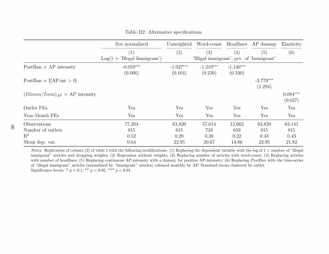
Table D2: Alternative specifications

Not normalized Unweighted Word-count Headlines AP dummy Elasticity

(1) (2) (3) (4) (5) (6)Log(1 + ’Illegal Immigrant’) ’Illigal immigrant’, pct. of ’Immigrant’

PostBan × AP intensity -0.059∗∗∗ -1.027∗∗∗ -1.219∗∗∗ -1.140∗∗∗

(0.006) (0.164) (0.239) (0.340)

PostBan × I[AP-int > 0] -3.779∗∗∗

(1.294)

(Illimm/Imm)AP × AP intensity 0.084∗∗∗

(0.027)

Outlet FEs Yes Yes Yes Yes Yes Yes

Year-Month FEs Yes Yes Yes Yes Yes Yes

Observations 77,204 63,820 57,014 12,662 63,820 63,141Number of outlets 815 815 733 659 815 815R2 0.52 0.20 0.38 0.22 0.43 0.43Mean dep. var. 0.64 22.95 20.67 14.86 22.95 21.82

Notes: Replication of column (3) of table 1 with the following modifications: (1) Replacing the dependent variable with the log of 1 + number of ”illegalimmigrant” articles and dropping weights; (2) Regression without weights; (3) Replacing number of articles with word-count; (4) Replacing articleswith number of headlines; (5) Replacing continuous AP-intensity with a dummy for positive AP-intensity; (6) Replacing PostBan with the time-seriesof “illegal immigrant” articles (normalized by “immigrant” articles) released monthly by AP. Standard errors clustered by outlet.Significance levels: * p < 0.1, ** p < 0.05, *** p < 0.01.

66

Table D3: Alternative measures of AP-intensity

(1) (2) (3) (4)’Illigal immigrant’, pct. of ’Immigrant’

PostBan × AP-intensity: AP credited -1.073∗∗∗

(0.225)

PostBan × AP-intensity: AP plagiarized -1.269∗∗∗

(0.241)

PostBan × AP-intensity: AP credited, all articles -0.963∗∗∗

(0.231)

PostBan × Reuters-intensity: Reuters credited, all articles 0.660(0.520)

Outlet FEs Yes Yes Yes Yes

Year-Month FEs Yes Yes Yes Yes

Observations 63,820 63,820 57,220 57,604Number of outlets 815 815 740 748R2 0.43 0.43 0.41 0.41Mean dep. var. 21.68 21.68 23.12 23.01

Notes: Replication of column (3) of table 1 with the following alternative measures of AP-intensity. Column (1): AP-intensity defined as share of“immigrant” articles published in the 12 months before the ban that are either credited to AP or flagged by a plagiarism algorithm (baseline). Column(2): share of “immigrant” articles credited to AP. Column (3): share of “immigrant” articles flagged by a plagiarism algorithm. Column (4): share ofall articles published in the 12 months before the ban that are credited to AP. Standard errors clustered by outlet.Significance levels: * p < 0.1, ** p < 0.05, *** p < 0.01.

67

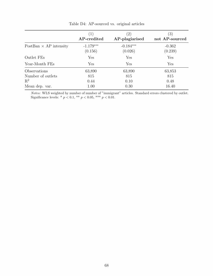
Table D4: AP-sourced vs. original articles

(1) (2) (3)AP-credited AP-plagiarised not AP-sourced

PostBan × AP intensity -1.179∗∗∗ -0.184∗∗∗ -0.362(0.156) (0.026) (0.239)

Outlet FEs Yes Yes Yes

Year-Month FEs Yes Yes Yes

Observations 63,890 63,890 63,853Number of outlets 815 815 815R2 0.44 0.10 0.48Mean dep. var. 1.00 0.30 16.40

Notes: WLS weighted by number of number of ”immigrant” articles. Standard errors clustered by outlet.Significance levels: * p < 0.1, ** p < 0.05, *** p < 0.01.

68

Table D5: Synonyms of “illegal immigrant” and volume of immigration coverage

(1) (2) (3) (4)AP-approved synonyms

pct. of ’Immigrant’’Undocumented immigrant’

pct. of ’Immigrant’’Immigrant’

pct. of total articles’Immigration’

pct. of total articles

PostBan × AP intensity 0.294∗∗∗ 0.053 -0.005 -0.004(0.080) (0.162) (0.005) (0.004)

Outlet FEs Yes Yes Yes Yes

Year-Month FEs Yes Yes Yes Yes

Observations 63,810 63,863 70,111 70,110Number of outlets 815 815 733 733R2 0.21 0.39 0.54 0.46Mean dep. var. 5.21 8.31 0.63 0.50

Notes: WLS weighted by number of ”immigrant” articles in column (1), and by total articles in columns (2) and (3). Standard errors clustered byoutlet. AP-approved synonyms are ”living in the country illegally/ without legal permission”, ”enter(-ing/-ed) the country illegally/ without legalpermission”. Standard errors clustered by outlet.Significance levels: * p < 0.1, ** p < 0.05, *** p < 0.01.

69

A.2 Views on Immigration Policy

Table D6: Views on immigration policy: Reduced form; county-level

Reduced Form

(1) (2) (3) (4) (5)Index

Restrict Imm. Border No Amnesty Don’t hire Question

PostBan × AP-intensity -0.0206∗ -0.0086∗∗ -0.0035 -0.0117∗∗ -0.0082∗

(0.011) (0.003) (0.004) (0.005) (0.004)

Year FEs × County controls Yes Yes Yes Yes Yes

County FEs Yes Yes Yes Yes Yes

Year FEs Yes Yes Yes Yes Yes

First-Stage F stat. 9,239 9,239 9,239 3,536 7,232Observations 2,104 2,104 2,104 1,768 2,040Number of counties 0.39 0.35 0.38 0.58 0.41R2 0.26 0.61 0.59 0.67 0.49

Notes: Reduced form OLS regressions in the left hand-side panel. County controls: log population, share urban,racial composition, share foreign born, share college degree, log income per capita, newspaper circulation percapita and Republican vote share. Significance levels: * p < 0.1, ** p < 0.05, *** p < 0.01.

70

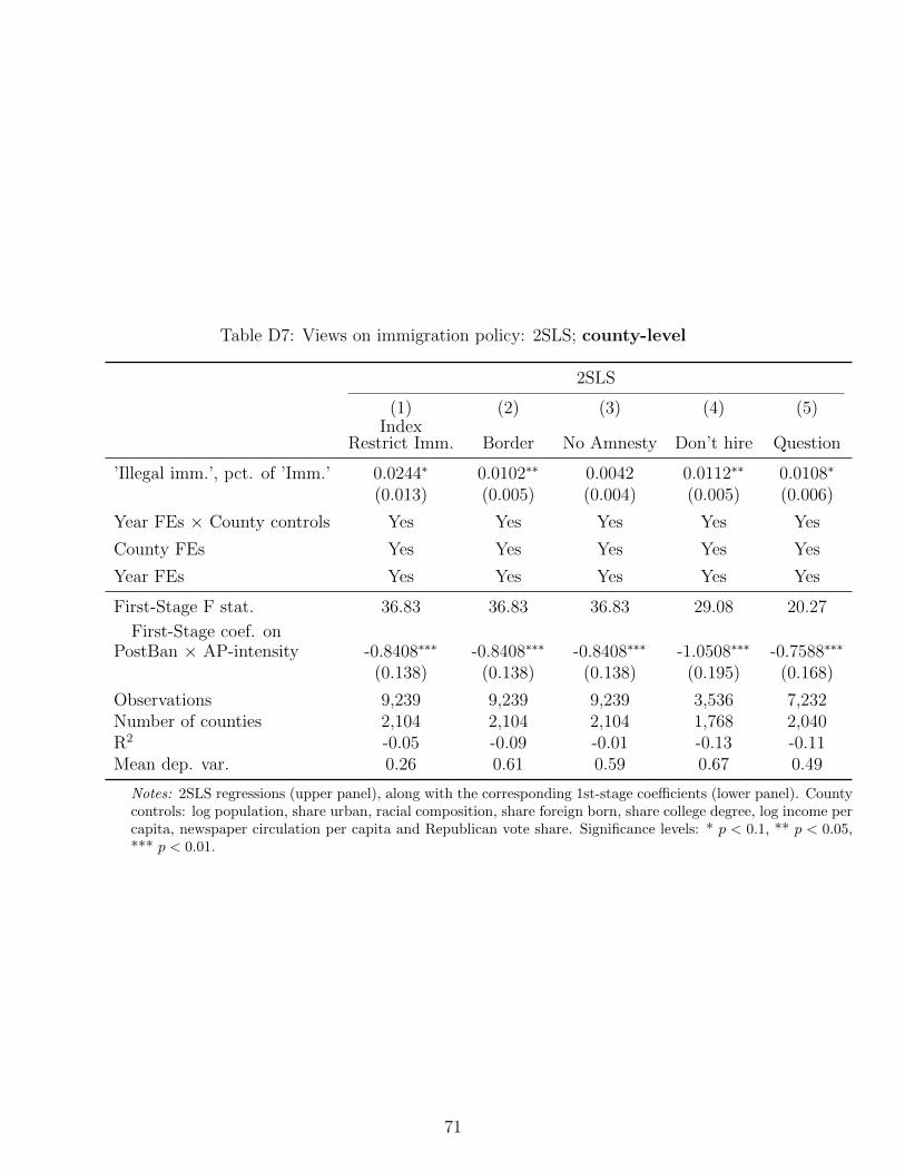
Table D7: Views on immigration policy: 2SLS; county-level

2SLS

(1) (2) (3) (4) (5)Index

Restrict Imm. Border No Amnesty Don’t hire Question

’Illegal imm.’, pct. of ’Imm.’ 0.0244∗ 0.0102∗∗ 0.0042 0.0112∗∗ 0.0108∗

(0.013) (0.005) (0.004) (0.005) (0.006)

Year FEs × County controls Yes Yes Yes Yes Yes

County FEs Yes Yes Yes Yes Yes

Year FEs Yes Yes Yes Yes Yes

First-Stage F stat. 36.83 36.83 36.83 29.08 20.27

First-Stage coef. onPostBan × AP-intensity -0.8408∗∗∗ -0.8408∗∗∗ -0.8408∗∗∗ -1.0508∗∗∗ -0.7588∗∗∗

(0.138) (0.138) (0.138) (0.195) (0.168)

Observations 9,239 9,239 9,239 3,536 7,232Number of counties 2,104 2,104 2,104 1,768 2,040R2 -0.05 -0.09 -0.01 -0.13 -0.11Mean dep. var. 0.26 0.61 0.59 0.67 0.49

Notes: 2SLS regressions (upper panel), along with the corresponding 1st-stage coefficients (lower panel). Countycontrols: log population, share urban, racial composition, share foreign born, share college degree, log income percapita, newspaper circulation per capita and Republican vote share. Significance levels: * p < 0.1, ** p < 0.05,*** p < 0.01.

71

Table D8: Support for increasing border security: county-level

Reduced Form 2SLS

(1) (2) (3) (4) (5) (6) (7)”Increase the number of border patrols on the US-Mexican border.”: Selected

PostBan × AP-intensity -0.0083∗∗ -0.0079∗∗ -0.0086∗∗ -0.0098∗∗

(0.003) (0.003) (0.003) (0.004)

AP intensity 0.0093∗∗∗

(0.003)

PostBan -0.0186(0.012)

’Illegal imm.’, pct. of ’Imm.’ 0.0082∗∗ 0.0102∗∗ 0.0121∗∗

(0.004) (0.005) (0.005)

Year FEs × County controls No No Yes Yes No Yes Yes

County FEs No Yes Yes Yes Yes Yes Yes

Year FEs No Yes Yes Yes Yes Yes Yes

Year × State FEs No No No Yes No No Yes

First-Stage F stat. . . . . 44.40 36.83 31.70

First-Stage coef. onPostBan × AP-intensity -0.9661∗∗∗ -0.8408∗∗∗ -0.8140∗∗∗

(0.145) (0.138) (0.144)

Observations 9,407 9,274 9,239 9,224 9,274 9,239 9,224Number of counties 2,245 2,112 2,104 2,101 2,112 2,104 2,101R2 0.01 0.34 0.35 0.36 -0.07 -0.09 -0.11Mean dep. var. 0.61 0.61 0.61 0.61 0.61 0.61 0.61

Notes: Reduced form OLS regressions in the left hand-side panel, 2SLS regressions in the right hand-side panel. County controls:log population, share urban, racial composition, share foreign born, share college degree, log income per capita, newspapercirculation per capita and Republican vote share. Significance levels: * p < 0.1, ** p < 0.05, *** p < 0.01.

72