Media Influence on Implicit and Explicit Language Attitudes by Hayley E. Heaton A dissertation submitted in partial fulfillment of the requirements for the degree of Doctor of Philosophy (Linguistics) in The University of Michigan 2018 Doctoral Committee: Professor Anne L. Curzan, Chair Professor Julie E. Boland Professor Kristen Harrison Professor Barbra Meek

Welcome message from author
This document is posted to help you gain knowledge. Please leave a comment to let me know what you think about it! Share it to your friends and learn new things together.
Transcript

Media Influence on Implicit and Explicit Language Attitudes
by
Hayley E. Heaton
A dissertation submitted in partial fulfillment
of the requirements for the degree of
Doctor of Philosophy
(Linguistics)
in The University of Michigan
2018
Doctoral Committee:
Professor Anne L. Curzan, Chair
Professor Julie E. Boland
Professor Kristen Harrison
Professor Barbra Meek


ii
ACKNOWLEDGEMENTS
To thank everyone who deserves it, I would have to add at least another chapter to my
dissertation. I’ll spare everyone from that and try to give an abbreviated version here.
First off, thank you to my committee members and everyone at the University of
Michigan Linguistics Department for guiding and supporting me through this journey. To Anne
Curzan, who has been a mentor in all aspects of my academic life from research to teaching to
career goals. I am privileged to have had the opportunity to work with her in both an outreach
and a research capacity. Her support is unmatched and I wouldn’t be here without her guidance
and ambitious-but-reachable goals. To Robin Queen who has also been an invaluable adviser,
mentor, and supporter throughout my time at Michigan as well. Beyond her research and
teaching expertise, her advice on everything from writing to work-life balance provided
perspective going through a PhD program and preparing for an academic career. She encouraged
me to ask ambitious research questions and implement those ideas into workable studies. While
she wasn’t able to serve on my committee, her contributions are evident throughout the
dissertation, and knowing she had my back was a tremendous help throughout the process. To
Julie Boland and Kris Harrison whose willingness and excitement to be involved in the project
made it possible to create the interdisciplinary dissertation that I had dreamed of. To Barb Meek
who joined less than two months before my defense to add her perspective and to talk through
my work from yet another disciplinary point of view.
The faculty and staff of the University of Michigan Linguistics Department support,
encouragement, and feedback throughout my time here, especially Pam Beddor, Jelena
Krivokapic, Jon Brennan, Will Styler, Marlyse Baptista, Carmel O’Shannessy, Savi
Namboodiripad, and Debby Keller-Cohen as well as Sandie Petee, Jen Nguyen, and Talisha
Winston. Thanks also to the NC State linguistics faculty, who helped inspire me to be not only a
researcher but to make linguistics an act of service and representation above all else, and to my
Emory linguistics professors, who introduced me to the field of sociolinguistics and speech
perception.

iii
Thanks to my cohort-mates, Dave Ogden, Kate Sherwood, and Sagan Blue. I couldn’t
have asked for a better group of people to spend six years to go through grad school with,
whether we were talking through giant whiteboards of research idea, doing semantics homework,
pushing hypothetical lovely cakes off of elevated surfaces, or having an elusive cohort dinner.
Thanks to Alicia Stevers (and Dan and Emmett) for unflinching support and the reminders to
keep things in perspective. And to Batia Snir, Will Nediger, Ariana Bancu, Marcus Berger,
Jiseung Kim, Marjorie Herbert, Emily Sabo, Dom Bouavichith, Dominique Canning, Rachel
Weissler, Yourdanis Sedarous, and everyone I’ve had the privilege to share time with in the
program for your feedback and friendship. I was lucky to also get to spend two years with some
amazing people at NC State. They set a high standard for collegiality that I will be forever
grateful for. All of you have my gratitude and love.
Shannah, Mary, Winnie, Caroline, Ryan, and Betsy, you are the best friends, conference
buddies, and Dragon Con partners a girl could ask for. When school was overwhelming, you all
kept me grounded. I was also lucky to find an amazing church to call my church home here. First
Baptist Church has shown me what church community means at its best. Thanks especially to the
choir, The Gathering, and Pastors Paul and Stacey Simpson Duke. Stacey in particular has been
an inspiration in the face of hardship and has shown how to walk through the most difficult of
times with grace and hope. I wouldn’t have made it to where I am without each and every one of
you.
Finally, my family. All of you have been overwhelmingly supportive as I embarked on
this adventure. Above all, my parents, Bob and Carol Heaton, have stood by me and my
decisions even when we weren’t 100% sure how they would turn out. They’ve smiled and cried
with me though the ups and downs of grad school and life. I’m truly lucky to be able to call such
amazing people my parents. Go Team Heaton! We did it!

iv
TABLE OF CONTENTS
Acknowledgements....................................................................................................... ii
List of Figures................................................................................................................ viii
List of Tables................................................................................................................. x
List of Appendices......................................................................................................... xii
Abstract.......................................................................................................................... xiii
Chapter 1: Introduction and Literature Review............................................................. 1
1.1 General introduction.................................................................................... 1
1.2 Explicit and implicit language attitudes and the Associative-
Propositional Evaluation Model........................................................................
3
1.2.1 Explicit and implicit attitudes....................................................... 3
1.2.2 Malleability of implicit and explicit attitudes............................... 5
1.2.3 The Associative-Propositional Evaluation (APE) model............. 6
1.2.4 Malleability according to the APE model.................................... 7
1.3 Media influence in sociolinguistics............................................................. 9
1.4 Media influence in social psychology and communications....................... 12
1.5 Perceived realism in media influence and sociolinguistics......................... 16
1.6 Research questions and hypotheses............................................................. 18
1.7 Structure of dissertation............................................................................... 20
Chapter 2: Methodological Design and Contribution.................................................... 22
2.1 Introduction................................................................................................. 22
2.2 Linguistic attitudinal object......................................................................... 23

v
2.3 Experimental design.................................................................................... 26
2.3.1 Television media primes............................................................... 26
2.3.2 Media prime validity testing......................................................... 29
2.3.3 Implicit experimental design........................................................ 32
2.3.4 Implicit attitudes materials........................................................... 34
2.3.5 Explicit attitudes experimental design.......................................... 37
2.3.6 Explicit attitudes materials........................................................... 40
2.3.7 Validity testing of explicit attitudes materials.............................. 42
2.4 Speaker information variable....................................................................... 43
2.5 Demographic information............................................................................ 44
2.6 Summary and contribution.......................................................................... 45
Chapter 3: Categorization of Accents as Native or Imitated......................................... 47
3.1 Background.................................................................................................. 48
3.1.1 Identification of imitated accents................................................. 50
3.1.2 The present study.......................................................................... 53
3.2 Methods....................................................................................................... 54
3.2.1 Materials....................................................................................... 54
3.2.2 Participants................................................................................... 55
3.2.3 Procedure...................................................................................... 55
3.3 Results......................................................................................................... 56
3.4 Discussion.................................................................................................... 59
3.5 Summary...................................................................................................... 63
Chapter 4: Implicit Attitudes Experiment..................................................................... 64
4.1 Background.................................................................................................. 64
4.2 Methods....................................................................................................... 69

vi
4.2.1 Participants................................................................................... 69
4.2.2 Procedure...................................................................................... 69
4.3 Results......................................................................................................... 70
4.3.1 Success of the IAT as a measure of implicit attitudes.................. 70
4.3.2 Malleability of the IAT................................................................. 73
4.3.3 Speaker information and demographic variables......................... 76
4.3.4 Individual analysis........................................................................ 78
4.4 Discussion.................................................................................................... 81
4.5 Summary...................................................................................................... 87
Chapter 5: Explicit Attitudes Experiment..................................................................... 89
5.1 Background.................................................................................................. 89
5.2 Methods....................................................................................................... 90
5.2.1 Participants................................................................................... 91
5.2.2 Procedure...................................................................................... 91
5.3 Results......................................................................................................... 92
5.3.1 Baseline results............................................................................. 92
5.3.2 Condition effects........................................................................... 96
5.3.3 Demographic variable: Self-identified race.................................. 103
5.3.4 Demographic variable: Southern TV............................................ 106
5.4 Discussion.................................................................................................... 109
5.4.1 Condition effects........................................................................... 109
5.4.2 Speaker information..................................................................... 112

vii
5.4.3 Demographic variables................................................................. 113
5.5 Summary...................................................................................................... 115
Chapter 6: Discussion and Conclusions........................................................................ 117
6.1 Empirical contribution................................................................................. 118
6.1.1 Influence of scripted television on accents................................... 118
6.1.2 Manifestation of implicit and explicit attitudes............................ 121
6.1.3 Categorization............................................................................... 124
6.2 Theoretical contribution.............................................................................. 126
6.3 Applied/practical contribution..................................................................... 129
6.4 Methodological improvements and future directions.................................. 130
6.5 Conclusion................................................................................................... 135
Appendices.................................................................................................................... 136
References..................................................................................................................... 147

viii
LIST OF FIGURES
Figure 2.1: The Southern Vowel Shift (adapted from Labov 1996).............................. 25
Figure 2.2: Visual representation of the IAT................................................................. 34
Figure 2.3: View of the experiment from the perspective of the participant (left) and
researcher (right)........................................................................................................
40
Figure 3.1: Proportion of correct and incorrect categorizations for each region and
native status....................................................................................................................
58
Figure 3.2: Proportion of each signal detection outcome by region.............................. 59
Figure 4.1: Pre- and post-test reaction times by stereotypical and
counterstereotypical test block.......................................................................................
71
Figure 4.2: Participant reaction times categorizing audio of speakers as Midwestern
or Southern in Block 1...................................................................................................
73
Figure 4.3: D-scores in the pre- and posttest IATs by condition................................... 75
Figure 4.4: D-scores in the pre- and posttest IATs organized by whether the
participant received speaker information.......................................................................
75
Figure 4.5: D-scores in the pre- and posttest IATs organized by participant exposure
to Southern television.....................................................................................................
77
Figure 4.6: D-scores in the pre- and posttest IATs organized by participant self-
identified gender............................................................................................................
78
Figure 4.7: Individual participant D-scores organized from lowest pretest to highest.. 79
Figure 5.1: Average ratings for status adjectives of regional speakers on a scale of 1
to 7..................................................................................................................................
94
Figure 5.2: Average ratings for solidarity adjectives of regional speakers on a scale
of 1 to 7..........................................................................................................................
95
Figure 5.3: Average baseline and evaluation ratings for individual adjectives ............ 96

ix
Figure 5.4: Average evaluation ratings for each adjective by condition........................ 100
Figure 5.5: Interaction between condition and speaker information for competence
ratings in the evaluation in the RA.................................................................................
101
Figure 5.6: Change score by adjective and condition.................................................... 103
Figure 5.7: Average evaluation ratings by adjective for those who did and did not
self-identify as White.....................................................................................................
105
Figure 5.8: Average ratings by adjective and test for those who did (left) and did not
(right) self-identify as White..........................................................................................
106
Figure 5.9: Average ratings by adjective and test for those who did and did not have
favorite television shows with Southern character.........................................................
107
Figure 5.10: Average ratings by adjective and test for those who did (left) and did
not (right) have favorite television shows with Southern characters.............................
108

x
LIST OF TABLES
Table 2.1: Average ratings (on a scale with 1 being the negative and 7 being the
positive..e.g. Unkind-kind, incompetent-competent) of each of the characters.............
30
Table 2.2: Most and least appropriate traits for each character..................................... 31
Table 2.3: Phonological features in each of the IAT audio stimuli............................... 35
Table 4.1: Blocks for the IAT........................................................................................ 69
Table 4.2: Linear regression results for the posttest IAT............................................... 74
Table 4.3: Linear regression results for the IAT change scores..................................... 76
Table 4.4: Linear regression results for the posttest IAT with demographic variables
only.................................................................................................................................
77
Table 4.5: D-scores for sociolinguistic IATs using audio stimuli and/or ASE.............. 82
Table 5.1: Linear regression results for the status rating testing the interaction
between baseline and condition.....................................................................................
97
Table 5.2: Linear regression results for the solidarity rating testing the interaction
between baseline and condition.....................................................................................
97
Table 5.3: Linear regression results for the composite status rating.............................. 98
Table 5.4: Linear regression results for the composite solidarity rating........................ 98
Table 5.5: Linear regression results for condition by adjective..................................... 100
Table 5.6: Change score regression results for condition by adjective.......................... 102
Table 5.7: Linear regression results for self-identified race with those who did not
identify as White as the comparison group....................................................................
105
Table 5.8: Change score regression results for self-identified race with those who did
not identify as White as the comparison group..............................................................
106

xi
Table 5.9: Linear regression results for Southern television with those who did not
watch Southern TV as the comparison group................................................................ 107
Table 5.10: Change score regression results for Southern television with those who
did not watch Southern television as the comparison group..........................................
108

xii
LIST OF APPENDICES
Appendix A: Distracter Questions................................................................................. 136
Appendix B: Research Assistant Script......................................................................... 137
Appendix C: Explicit Attitudes Experiment Evaluation................................................ 138
Appendix D: "Please Call Stella" Passage..................................................................... 140
Appendix E: Speakers for categorization task, pseudonyms used for anonymity,
organized by region and nativeness...............................................................................
141
Appendix F: Speakers for categorization task organized by successful categorization
by participants................................................................................................................
142
Appendix G: Implicit Attitudes Pre-Experiment Instructions Script............................. 143
Appendix H: D-score results and change score for each participant............................. 144
Appendix I: Explicit Attitudes Pre-Experiment Instructions Script.............................. 146

xiii
ABSTRACT
Sociolinguists often assume that media influences language attitudes, but that assumption
has not been tested using a methodology that can attribute cause. This dissertation examines
implicit and explicit attitudes about American Southern English (ASE) and the influence
television has upon them. Adapting methodologies and constructs from sociolinguistics, social
psychology, and communications studies, I test listener attitudes before and after exposure to
stereotypically unintelligent and counterstereotypically intelligent representations of Southern-
accented speakers in scripted fictional television. The first attitudes experiment tests implicit
attitudes through an Implicit Association Test (IAT). This experiment also serves to test
sociolinguistic use of the IAT with a more holistic accent as opposed to single linguistic features.
The second attitudes experiment tests the effect of television exposure on explicit attitudes
towards an ASE-accented research assistant (RA). The experiments also investigate the influence
of listener knowledge of regional origin of actors (speaker information), listener perception of
how closely television represents the world around them (perceived realism), listener exposure to
the South, and listener identity. The hypothesis is that those who hear counterstereotypically
intelligent Southern characters will rate a Southern-accented research assistant higher in
intelligence than those who hear stereotypically unintelligent Southern characters. The same
pattern will hold in the auditory-based IAT. Accents in both the implicit and explicit attitudes
experiments are viewed holistically, including multiple features rather than focusing on the most
salient features. To clarify results related to the speaker information and perceived realism
variables, a separate experiment tests how successful listeners are at differentiating natives from
performers of regionally accented American English.
Results indicate that televised representations of Southern accents affect explicit, but not
implicit attitudes. Participants who heard intelligent Southern characters rated an ASE-accented
RA higher in competence than those who heard unintelligent Southern characters. Several
demographic variables influenced results regardless of the stereotypicality of the speakers that
the listener heard in the television clips, including self-identified race and exposure to Southern

xiv
television. While implicit attitudes were not affected by television in this case, the IAT was
successfully adapted for use with a holistic accent rather than a single feature and also captures
associations between an L1 regional accent and a specific stereotype of that accent. I discuss
these results in regard to language attitudes at large as well as their implications for an indirect
language change model, the Associative-Propositional Evaluation (APE) model of attitudes, and
cultivation theory. The dissertation argues that scripted television does influence language
attitudes, but in more complex ways than a simple cause-and-effect relationship. While television
can affect explicit attitudes towards individual speakers, implicit attitude shift is more difficult
and may need more time and/or need a direct cause for a shift to occur. Regardless of media
influence, language attitudes are affected by identity and demographic features listeners bring
into the interaction with speakers.

1
CHAPTER 1
Introduction and Literature Review
1.1 General Introduction
The Stupid Southerner. The Aggressive New Yorker. The Clever Brit. The Ditsy Valley
Girl. Language attitudes about groups of speakers are widespread within the United States and
often well known enough to be stereotypes. One potential source of these widespread attitudes
and stereotypes is media.1 Yet linguistic inquiry largely addresses media in terms of its effect on
language change and particularly standardization. Milroy and Milroy (1999), for instance, note
that “although radio, film and television may not have had much influence on everyday speech,
they are amongst the many influences that promote the consciousness of the standard and
maintain its position” (31). Here, Milroy and Milroy frame media influence in terms of its effect
on speech. Attitudes come in only tangentially if one considers promotion and maintenance of
standard varieties of language an attitudinal issue. The advancement of linguistic and social
stereotypes of non-standard dialects is not addressed. Stuart-Smith and Ota (2014) note this focus
on media influence in terms of standardization, while also highlighting that studies that have
actually looked at media’s influence on standardization have not found convincing results even
as researchers continue to advance the idea. How, then, should we explore the connection
between language attitudes and media?
Some sociolinguists have suggested or implied that language attitudes are spread through
media exposure based on the theory that seeing language variation in association with
stereotypical, often negative, characteristics supports negative attitudes (e.g. Lippi-Green 2012).
Pappas (2008), for instance, notes that popular knowledge of postalveolar /l/ and /n/, stigmatized
regional variants in Modern Greek, had a “meteoric” rise due to the variants’ appearance in
popular television shows representing stereotypical speakers with those features. According to
Pappas, “these uses of the stereotype in popular culture reflect attitudes that are common in the
younger generation” (495). The implication is not just that these stereotypes spread to the
1 I refer primarily here (and onwards) to media in the form of radio, television, and movies.

2
population as a whole through their use in media, but that the media, specifically television,
played a key role in popular knowledge of this linguistic stereotype. Kristiansen (2014) presents
evidence for an attitudinally based model of language change through media using language
attitudes as a mediating factor.2 This study will be discussed in more detail later, but, of
particular note, the effect of language attitudes on language change is tested while the effect of
media on language attitudes remains an assumption. Androutsopoulos (2014), in the introductory
chapter of Mediatization and Sociolinguistic Change, notes that “the role of media in lexical
innovation and change...is thus readily acknowledged, but excluded from analysis. The same
holds true for the impact of mass media on language awareness and attitudes” (14).
The claim of media influence has not been tested using causal methodologies. Through
this research project, I explore the assumption that representations of accented speakers on
television affect explicit language attitudes towards an actual person with those linguistic
characteristics as well as implicit attitudes towards the accent in question. Additionally, this
research works towards building an interdisciplinary methodology to test media influence on
language attitudes comparable to media influence research in other fields.
In the past, linguistic researchers have approached media studies from the standpoint of
production rather than perception, focusing primarily on production of linguistic features in
radio, television, and film. Less research deals with perception of regional and social accents,
particularly in fictional media. When non-standard accents and dialects are part of media
performances, they are generally there for a purpose, most commonly to characterize, to relate
authenticity, and/or to extend the plot (Queen 2015). As a result, media accents and dialects can
build on or extend stereotypes. For instance, one way to characterize a speaker as being
unintelligent is to have that character speak with a non-standard dialect like American Southern
English, a dialect whose speakers are stereotyped as being unintelligent. The use of accents and
dialects in conjunction with stereotypical characteristics arguably reinforces these existing
attitudes and ideologies.
This chapter provides background for several key areas. The first section addresses
language attitudes from both an explicit and implicit standpoint, particularly focusing on their
malleability. The Associative-Propositional Evaluation (APE) model (Gawronski &
2 Stuart-Smith (2007) refers to this indirect influence a “traditional view.” Moving forward, I will refer to either the
attitudinal model of language change or as Kristiansen’s model, since his test of it provides a clear relatively recent
example of the model in action.

3
Bodenhausen 2011) is used to frame these attitudes from a cognitive perspective and to provide
an explanation for a specific set of circumstances in which implicit attitudes are malleable. The
second section turns to media influence in sociolinguistic research. After that, media influence in
social psychology and communications is outlined as one potential avenue for changing both
implicit and explicit attitudes. In this sphere, media appears to influence attitudes about different
social variables, such as race and gender. These studies are used to frame, differentiate, and
predict how media might influence and mold implicit and explicit language attitudes. These
media studies show complex relationships between media consumption, attitudes, and a wide
variety of mediating factors. Perceived realism, as one of those mediating factors, is highlighted
and detailed as it relates to both media influence in general and to the linguistic concept of
phonological calibration. Finally, I outline the research questions and goals of the experiments
and the hypotheses produced in response to them.
1.2 Explicit and implicit language attitudes and the Associative Propositional Evaluation
model
1.2.1 Explicit and implicit attitudes
Adults possess wide-ranging knowledge of social factors associated with different speech
styles and dialects. For the most part, study of this knowledge has been measured through
explicit means in which individuals express their attitudes through measures like semantic
differential questionnaires (Garrett 2010). Extensive study has mapped various attitudinal
patterns across dialects and languages. Speakers of standard dialects of English are ranked higher
on status attributes (e.g. intelligence, wealth) and lower on solidarity attributes (e.g.
amusingness, friendliness), while speakers of marked dialects rank higher in solidarity and/or
lower in status (Lambert 1967; Edwards 1982; Sebastian & Ryan 1985; Luhman 1990; Giles,
Henwood, Coupland, Harriman, & Coupland 1992; Preston 1999; Jarvella, Bang, Jakobsen, &
Mees 2001; Heaton & Nygaard 2011). This pattern is not isolated to English (Cremona & Bates
1977; Demirci & Kleiner 1999; Jeon, Cukor-Avila, & Rector 2013).
Measures of explicit attitudes rely on the individual expressing conscious opinions about
accents or speakers of accents. The individual has control over what they express in the measure.
If an individual knows that their attitudes are being evaluated, they may revise them, particularly
if the reported attitudes would frame the individual in a negative light (e.g. Garrett 2010). For

4
instance, an individual may view people from races not their own as unpleasant, but also know
that (1) their reaction is based upon societal prejudice and/or (2) expressing that view could lead
to the individual being categorized as racist. In the case of explicit measures of attitude, the
individual has the agency to report attitudes different from what they actually believe. Campbell-
Kibler (2013) summarizes this perspective well:
It [explicit measure of attitudes] has the disadvantage, however, of collecting
responses based on introspection and consciously offered opinion. Participants
may not always be able to consciously consider the language forms of interest in
order to provide their opinions of them, because they are not aware of the forms
or hold a distorted view of how and when they are used. Even if individuals are
aware of their linguistic attitudes and possess the language with which to report
them, they may be reluctant to do so, particularly if the attitudes are socially
charged. (308)
Over the past decade, the experimental spotlight has shifted to accommodate study of
implicit language attitudes, those attitudes that might be categorized as unconscious or
automatic. These studies are delving into the more deeply entrenched, automatic associations
individuals have formed. While psychology experiments use a variety of implicit measures,
sociolinguistic study has begun with a focus on the Implicit Association Test (IAT), a test which
measures associations between two sets of categorical variables through reaction times (see
Section 2.3.5 for more detail). Associations have been shown between dialects and positive or
negative adjectives (Babel 2010, Pantos 2010, Redinger 2010), as well as between American
geographic regions, specific phonological features, careers, and educatedness (Campbell-Kibler
2012, Campbell-Kibler 2013, Loudermilk 2015). While studies of explicit attitudes indicate other
factors that can contribute to individual attitudes (e.g. region of origin (Preston 1996, 1999)),
implicit language attitudes studies have tested the associations themselves rather than factors that
might affect associations.
It should also be noted here that language attitudes “are not a singular, static
phenomenon. Rather, they affect, and are affected by, numerous elements in a virtually endless
recursive fashion” (Cargile, Giles, Ryan, & Bradac 1994; 215). Attitudes are not set traits of an
individual; they shift. As we look at attitudes, we are looking at what might trigger these changes
and, particularly, what might cause extreme changes in both the short and long term.
1.2.2 Malleability of implicit and explicit attitudes
Attitudinal research in psychology supports the idea that implicit and explicit attitudes are
the result of different processes. Results of implicit and explicit measures oftentimes do not

5
correlate with each other. These differences are sometimes framed as differences in malleability:
explicit attitudes are changeable with exposure to short-term stimuli while implicit attitudes
remain stable (Gawronski & Strack 2004; Egloff & Schmukle 2002; Rydell & McConnell 2006
Experiment 1). I will not spend a great deal of time talking about malleability of explicit
attitudes. Their changeability is addressed through the ability of individuals to control them and
will further be demonstrated in Section 1.4, as the media-based studies discussed there are
exclusively based upon explicit measures of attitude. These studies largely show that responses
to explicit measures do shift in response to primes.
Research on implicit attitudes, however, provides more conflicting evidence in terms of
stability of these attitudes. Egloff and Schmukle (2002) tested the validity and reliability of the
IAT as a measure of an individual’s self-perceived anxiety by testing participant associations
between themselves (self versus other) and anxiety (anxious versus calm). In addition to the IAT
itself, participants were told the test would be used as part of a job interview in which they
needed to make a good impression. This instruction encouraged attempts to mask associations
the participant might have between themselves and anxiety. In other words, they would try to
control the outcome of the test by masking their self-perception that they are anxious. The results
were unaffected by participant attempts to mask associations between self and anxiety; the
association between self and anxiety was still reflected. This finding was taken as a sign of a lack
of malleability in the implicit associations. It is difficult to say, however, if the participants were
truly attempting to mask their anxiety since they were not told explicitly to do so. Perhaps the
instruction alone was not enough to trigger attempts to control the IAT result.
Kim (2003) found that groups who were given a specific strategy and told to mask their
implicit attitudes were successful at the task by slowing their negative association between a
group and trait, in this case between Black and unpleasantness. They could not, however, change
their lack of association between Black and the positive trait of pleasantness. In order to
successfully mask the negative association, participants needed to be given a strategy; those who
were not given a strategy did not differ significantly from those who were not given any
instructions to mask their associations. These results indicate the potential for some minor
controllability of automatic attitudes, but only if the strategy is employed and only for a specific
part of the association. When no strategy is employed, as would likely occur in everyday
interactions, automatic attitudes remained inflexible.

6
Not all research reflects this lack of malleability. Some evidence points to implicit
attitudes being susceptible to change after a single exposure to stimuli (Wittenbrink, Judd, &
Park 2001; Blair, Ma, & Lenton 2001; Blair 2002; Rydell & McConnell 2006 Experiment 5).
Lowery, Curtis, and Sinclair (2001) demonstrate that implicit attitudes are susceptible to shifts
depending on social context by showing differences in implicit evaluations depending upon the
race of the experimenter. They also found reduced levels of automatic bias when they told the
participants to avoid prejudiced responses. Similarly, Rydell and McConnell (2006) found that
priming participants with negative pictures led to negative associations with a person in the IAT
while priming participants with positive pictures led to positive associations. This experiment,
though, tested associations with a fictional person introduced through the experiment rather than
evaluating already existing attitudes about a group, which (as will become evident below) may
be a key difference.
Foroni and Mayr (2005) showed that implicit associations about the pleasantness and
unpleasantness of flowers and insects can be reversed if participants read different stories.
Participants took an IAT after reading a counterstereotypical scenario in which flowers were
poisonous and insects vital to maintaining food sources, then took the same IAT again after
reading a stereotypical scenario where flowers were the food source maintainers and insects were
poisonous. IATs taken after the counterstereotypical narrative shifted away from the
expected/stereotypical associations to reflect the associations in the narrative.
Thus, the reality of attitude malleability is not as simple as one being malleable and the
other not. It is much more complex and, as we will see, potentially explained through the
Associative-Propositional Evaluation model.
1.2.3 The Associative-Propositional Evaluation (APE) model
Language attitudes studies have clearly mapped out how groups view other dialect groups
evaluatively, but not the cognitive attitudinal processes behind them. For this dissertation, I draw
on the Associative-Propositional Evaluation (APE) model (Gawronski & Bodenhausen 2006a,
2006b, 2007, 2011) to frame these attitudinal processes in order to better understand how media
might influence them. The model has two main components connecting implicit and explicit
attitudes to one another: associative and propositional processes. According to the APE model,
all attitudes (implicit and explicit) are stored in memory as associations, which are activated by
associative processes. Implicit and explicit attitudes are the result of independent processes

7
involving those associations that can both directly and indirectly influence each other. Implicit
evaluations are the result of activation of one of many associations related to an attitude object.
Activation of associations depends upon what the stimulus is and how it is presented (Gawronski
& Bodenhausen 2011). For example, viewers have more positive attitudes towards Black faces
when those faces are presented with the background of a basketball court or family barbeque
than when they’re presented with a prison or graffiti wall background (Wittenbrink, Judd, & Park
2001). Individuals display different implicit attitudes towards old and young faces of Black and
White individuals if the individuals are tasked with categorizing them by age versus by race
(Gawronski, Cunningham, LeBel, & Deutsch 2010). Implicit attitudes towards an individual can
shift depending on instruction as well. Participants have more positive attitudes about Michael
Jordan when they categorize him by his career as opposed to his race (Mitchell, Nosek, and
Banaji 2003). Thus, the same attitude object (whether that object is an unfamiliar face or a well-
known individual) has multiple associations that can be activated. The associative process
depends upon the information that is presented and/or is salient in the moment.
Implicit attitudes capture activated associations and initiate a series of propositions that
the individual can accept or reject. An individual’s explicit evaluations result from a process
validating these propositions based on the individual’s determination of whether the proposition
is logical based on their subjective knowledge and experience (a.k.a logical consistency)
(Gawronski & Bodenhausen 2011). For example, in a task where participants must categorize
weapons and hand tools, individuals primed with Black faces categorized tools as weapons more
often than those primed with White faces (Payne 2001). According to the APE model, if an
association between Black faces and weapons is activated, the proposition “This person is
dangerous because what they are holding might be a weapon” could be activated. The individual
then has control over whether they validate that proposition. The individual may recognize that
the association is incorrect and/or subjective and not reflective of the person or object that
activated the association. They may, therefore, not validate the proposition and instead find
another proposition to validate in its stead. The individual cannot control the activation of the
association, but can control the propositions they validate and express.
1.2.4 Malleability according to the APE model
According to the APE model, implicit attitudes are malleable under certain conditions.
Specifically, they depend on (1) what associations are activated, (2) the experiences and

8
knowledge of the individual, and (3) the individual’s dedication to logical consistency. In the
case of Foroni and Mayr’s (2005) study, they presented a narrative which created new
associations (or at least activated different associations). Rydell and McConnell (2006) did the
same with pictures. Gregg, Seibt, and Banaji (2006) found that both automatic (implicit) and
controlled (explicit) preferences were malleable in attitude formation but, once created,
controlled preferences remained malleable while automatic preferences became fixed. They
conclude that automatic attitudes, once formed, become difficult to modify.3 The attitudes may
change over time, but those changes take just that: time, and often exposure to some event or
object to modify these more ingrained attitudes. From an APE perspective, the creation of new
attitudes leads to activation of new associations while the existing attitudes remain unmodified
because alternate associations are not presented.
In this framework, the studies that found no change in implicit attitudes did nothing that
would activate different or create new associations. Thus, APE predicts that if an individual is
given an alternative association, their implicit attitudes will shift accordingly. The implicit
evaluation is measuring a different activated association. Explicit evaluations remain the more
easily malleable of the attitudes in APE. They are shifted by different sets of propositions being
activated by associations and the willingness of individuals to validate them. If, for example, an
individual has an association between Southern and unintelligent, but also knows that non-
standard dialect speakers face prejudice and that prejudice and discrimination are bad, they will
not validate the Southern-unintelligent proposition and will, instead, find an alternate proposition
within their proposition set to validate in explicit measure. The Southern-unintelligent
association still exists and will manifest in implicit evaluations; the individual, however, has
agency in the process of validation and can exercise control over their explicit evaluations.
The substitution that occurs when an original proposition is not validated changes and/or
strengthens the accepted proposition as the primary associated proposition. Importantly, negation
through propositions (e.g. telling someone that Southerners are not dumb) is not an effective way
to change existing associations. In fact, the negation may conversely strengthen the association it
is trying to negate since the association must be activated in order to be negated (Wegner 1994).
3 Gregg, Seibt, and Banaji (2006) also raise questions as to what studies actually define as malleability. It may refer
to significant difference without actually changing directionality (i.e. the participant sees insects as more pleasant
than before, but not necessarily fully positive). Others may consider only a full change in directionality (i.e. insects
are seen as more pleasant than before AND are fully seen as positive). These factors should certainly be considered
in evaluating findings.

9
Successful shift in associations depends upon creation of new associations (Gawronski &
Bodenhausen 2011). Rather than telling an individual “Southern people are not dumb,” a more
effective strategy for changing associations, and thus implicit attitudes, would be to tell them
“Southern people are smart.” In other words, when trying to change attitudes, showing a
counterexample creating a new association is more important than negating the existing
association.
In sum, explicit attitudes have been shown to be malleable, at least with short-term
priming, in attitudes studies within the fields of psychology and communications. Within
sociolinguistics, malleability has been less explored experimentally. Implicit attitudes are
malleable under certain circumstances. It is unclear whether those circumstances can be met with
linguistic stimuli alone. Answering these questions will (1) answer theoretical questions about
malleability of language attitudes, a particularly important question to answer if attitudes are
assumed to mediate language change from media; (2) take steps towards understanding the role
of media in maintenance of language attitudes and stereotyping; and (3) situate language
attitudes studies more clearly within attitudinal studies in psychology and communications.
1.3 Media influence in sociolinguistics
The previous section established that both implicit and explicit attitudes are malleable if
certain conditions are met. Short-term priming can change explicit attitudes by activating
different associations or offering alternative propositions for validation, though it is unclear how
permanent those changes are. Implicit attitudes change when associations with other traits are
created or activated through different contexts or the presentation of alternate narratives (e.g.
flowers are harmful, insects are helpful). The ability for narrative to potentially change attitudes
leads to questions of how television media, as a dispenser of narratives, could contribute to
attitude maintenance and shift.
Media-based studies within sociolinguistics have not focused on attitudinal activation.
Instead, research tends to focus on language change and usage as well as reflection of societal
linguistic norms. In this section, I briefly discuss how media has been used in sociolinguistic
study of language change and link the study of attitudes to these studies of language change.
One fundamental factor in language change is social interaction. Traditionally, social
interaction equates to an interaction, usually face-to-face, in which there are at least two people

10
involved who are able to respond to one another. Kristiansen (2014) refers to language in these
types of interactions as immediate language. Media, at first glance, lacks the interactive element
of immediate language; a viewer cannot speak to a character on television and receive a real-time
response. Because of this, the role of media in day-to-day language use is often dismissed by
linguists (Kristiansen 2014).
However, according to Parasocial Contact Theory, parasocial interaction, or interactions
via media in which an individual is watching people or characters speak and act, can create
responses similar to face-to-face interactions in viewers (Schiappa, Gregg, & Hewes 2005; Ortiz
& Harwood 2007; Harwood & Vincze 2012). Not only can parasocial interaction elicit similar
emotional responses as face-to-face interactions, parasocial contact can have the same effects as
actual intergroup contact. Eyal and Cohen (2006) found that some viewers who have parasocial
relationships with television characters experience the emotions of a real-life break-up when that
television show goes off the air. Fujioka (1999) found that Japanese and White students had
different stereotypes of African Americans based on different contact with African Americans on
television. They suggest that media influences viewers’ perception of groups and that this effect
is particularly strong when contact with the group is limited outside of media.
If parasocial interactions can stimulate similar responses as real-world interactions, the
same should also be true of language in media.4 Thus, we also have mediated language, language
involving speakers who are separated by time and/or space due to some form of technology that
prevents live response from occurring (Kristiansen 2014). A key distinction here is the ability to
respond live. Telephone conversations would fall into the realm of immediate language because
of the ability of the participants to respond to each other in real time despite being spatially
separate. Mediated language has been and continues to be a part of the American experience and
a point of intergroup contact, particularly with the rapid saturation of television sets in personal
homes (Bushman & Huesmann 2001) and the ease of access to media via the Internet.
When mediated language has been studied, its influence on language change has been
mixed. Vocabulary can be reflected and spread through the media (Trudgill 1986, Rice &
4 Media alone should not be claimed as the sole contributing factor in attitudes and behavior, both language and
otherwise. As Bushman and Huesmann (2001) state, “The theme...is not that media violence is the cause of
aggression and violence in our society, or even that it is the most important cause. The theme is that accumulating
research evidence has revealed that media violence is one factor that contributes significantly to aggression and
violence in our society” (223-4). Thus, any assertions as to the effect of media made here are to be taken as one
factor among many that contribute to attitudinal and behavioral effects.

11
Woodsmall 1998, Charkova 2007, Tagliamonte & Roberts 2005). Phonological and morpho-
syntactic changes prove more difficult to attribute to media. These features are more structurally
based and, therefore, more deeply entrenched in the cognitive system. Consequently, some claim
such features are not affected by television priming (Trudgill 2014, Chambers 1998).5
Social interaction alone is likely not the cause of language variation. Another important
factor is what individuals bring to an interaction (Giles et al. 1992; Auer & Hinskens 2005;
Babel 2010). Engagement with a television program, for example, can encourage uptake of
linguistic forms not native to a speaker’s dialect. TH-fronting and L-vocalization, features of
Cockney English in London, began appearing in Glaswegian with acceleration in their uptake in
the 1990s (Stuart-Smith, Price, Timmins, & Gunter 2013). The spread of these dialect features
appears to be due to a combination of linguistic and social practices, which included contact with
Londoners, manifestation of Glaswegian street style, and psychological engagement with
Eastenders, a program that takes place in London. What’s more, Stuart-Smith et al. (2013)
determine that these changes are driven by individuals, indicating that a focus on individual
differences among participants may be an important part of the analysis. Thus, language change
in the form of dialect diffusion is influenced by sets of social practices, both linguistic and extra-
linguistic, including psychological engagement with television programs.
While a direct relationship between language change and media appears tenuous for the
time being, attitudes may serve as a mediating factor. Using Denmark and Norway as examples,
Kristiansen (2014) proposes that mediated language leads to attitudinal effects, which can lead to
changes in immediate language. Broadcast media has limited influence on immediate language,
but significant influence on ideology. He notes:
My argument is not that TV influenced people’s speech directly, but that it did so
indirectly by changing SLI [Standard Language Ideology] in a way that is less likely to
have happened in the same way, or to the same extent, without TV...Thus, the media in
general and TV in particular not only expose people to greater quantities of Copenhagen
speech than before, and in that sense change the conditions for (at least passive)
appropriation, they also make Copenhagen variation available in ways that might trigger
the development of new representations and evaluations. (115)
5 These assertions are based primarily upon Anglo-based research. Language change appears to occur in phonology
and morpho-syntax in conjunction with media consumption in non-Anglo-based research, particularly in
standardization of dialects in Denmark (Kristiansen 2014), Japan (Ota & Takano 2014), and Brazil (Naro 1981;
Naro & Scherre 1996; Scherre & Naro 2014), though media is not the strongest predictor of change (i.e. education is
stronger).

12
Due to the striking similarity in attitudinal patterns across the country, Kristiansen proposes a set
of common sources at play, one of which is media. Media in Denmark represents primarily
Copenhagen speech; the country has generally negative attitudes towards dialect diversity.
Norwegian media, however, broadcasts a diverse representation of dialects; Norway is more
accepting of dialect diversity in immediate language.6
Thus, the attitudinal model Kristiansen posits holds that mediated language affects
language ideologies and these ideologies affect language change. Kristiansen finds evidence for
the second part of this model dealing with language ideology affecting language change. So far,
though, there is no experimental evidence for the first half purporting that mediated language
affects language ideologies, nor are specific attitudes tested beyond positivity towards dialect
diversity. Stuart-Smith (2007) looked at the effect of watching Eastenders on Glaswegian
attitudes towards London English. She found no effects. The attitudinal object, however, was an
abstract accent rather than a person who speaks with that accent.
Kristiansen’s model focuses on general attitudes towards diversity rather than specific
stereotypes cultivated by media. It focuses on exposure to a variety of dialects other than the
standard rather than how those dialects are represented. With the focus of the model on language
change, this leaves an open question of whether any representation of dialect diversity is positive
or whether negatively stereotyped dialects will have negative effects.
1.4 Media influence in social psychology and communications
While sociolinguists have focused on media influence on language change, researchers in
social psychology and communications have explored the varied ways the media can influence
attitudes and behaviors. Media, particularly television, is a pervasive part of American lives. By
1985, 98% of homes in the US had a television set (Bushman & Huesmann 2001). More
recently, online streaming services have increased accessibility. In 2016, 49% of consumers in
the US paid for online streaming services. The number is even higher (60%) for younger
generations (Westcott, Lippstreu, & Cutbill 2017). As of the third quarter of 2017, approximately
55 million Americans subscribe to Netflix, a little less than half of Netflix’s total subscriber base
(Molla 2018), while many television channels have their own streaming options (e.g. HBOGo)
and others are implementing paid online streaming services for both shows airing on television
6 It is unclear whether the relationship here is one of causality or reinforcement.

13
and original programming (e.g. CBS All Access). Free online video-sharing platforms offer
access to clips from television shows and movies as well as programming from content creators
exclusive to the platform, like YouTube, whose most popular channel has 54.1 million
subscribers worldwide (McAlone 2017).7
This is all to say that Americans have the potential to be exposed to television with little
effort on their part. For consumers, the ease of access to media also means ease of access to
contact with social groups they might not otherwise be exposed to. This ease of access offers
ease of parasocial intergroup contact, which can benefit individuals who might not interact with
many outgroups otherwise. It also means that viewers are exposed to a multitude of negative
representations of outgroups that could be potentially harmful if they reinforce stereotypes. Thus,
with the accessibility of television and the ability of television to mediate intergroup contact,
gauging influence the media might have on attitudes and behavior is of increasing importance.
Influence8 encompasses anything from changes in Likert scale attribute measures of self and
others to differences in compassionate behavior towards a disabled individual to shifting level of
suggested payment to a research assistant. These wide-ranging effects indicate the variety of
different ways media might influence viewers’ perceptions of themselves and others, particularly
stigmatized social groups.
Media can affect attitudes towards race (Ford 1997; Dixon 2008), sex (Ward,
Hansbrough, & Walker 2005; Pike & Jennings 2005), body image and self esteem (Agliata &
Tantleff-Dunn 2004; Bell, Lawton, & Dittmar 2007; Anschutz, Engels, Van Leeuwe, & van
Strien 2009; Martins & Harrison 2012; Mulgrew, Kostas, & Rendell 2013), and violence
(Friedlander, Connolly, Pepler, & Craig 2013). Media viewing also correlates with aggression
and sexual behavior (Huesmann, Moise-Titus, Podolski, & Eron 2003; Bartholow, Bushman, &
Sestir 2006; L’Engle, Brown, & Kenneavy 2006; Willoughby, Adachi, & Good 2012). In a
correlative study, Dixon (2008) found that participants who watched more crime news were
more likely to assign high culpability to Black suspects than White suspects. Those who saw
more crime stories with Black criminals were also more likely to judge a Black person as being
violent. Disturbingly, a three-year longitudinal study found that adolescents who consume more
7 That number has risen to 62 million as of May 2018.
8 “Media effects” and “media influence” is often juxtaposed with “active audiences” in that “media effects” refers
specifically to the media affecting a passive viewer rather than an audience actively engaging with the media they
consume. I take the latter view in which the audience is engaging with media.

14
aggressive media perpetrate more dating violence, an effect that is mediated by more violence-
tolerant attitudes in relation to dating taken up by long-term viewers of aggressive media
(Friedlander et al. 2013). Finally, individuals who play violent video games show lower P300
amplitudes (indicated desensitization) when they see violent images than those who play non-
violent games. Those with lower P300 amplitudes also showed more aggressive behavior; they
would choose to sound a louder noise into the headphones of a competitor when the competitor
lost.9 These results held true even when baseline aggressiveness was accounted for, indicating
that the result was not simply due to aggressive individuals being drawn to violent games
(Bartholow, Bushman, & Sestir 2006).
The three studies detailed above represent several important findings. Bartholow et al.
(2006) show that consumption of media can have effects that manifest cognitively and that those
effects can also affect the way that consumers treat individuals (at least individuals they think
exist but cannot see). The study by Friedlander et al. (2013) exemplifies the importance of
mediating factors by showing that those who consumed more violent media were more likely to
become perpetrators of dating violence if they had more tolerant attitudes towards dating
violence overall. Without the attitudes’ mediation, the relationship would not show up in the
results. Dixon (2008) makes links to theory by attributing his findings to chronic stereotype
activation, which is postulated to lead to frequently activated stereotypes being activated more
automatically over time, and selective exposure, the idea that people attend to information that
fits their preconceived notions and dismiss evidence that counters it. Dixon concludes that
stereotype activation is most likely behind his result and that the chronic activation of stereotypes
through the news leads to “increased accessibility of stereotypical constraints linking Blacks with
violent crime” (121).
This chronic activation of stereotypes is a key component in cultivation theory, a robust
theory that accounts for the relationship between media consumption and viewer attitudes. In
short, the theory states that the more media a viewer consumes, the more their world-view will
reflect what is seen in that media (Gerbner, Gross, Jackson-Beeck, Jeffries-Fox, & Signorielli
1978; Morgan & Shanahan 2010). Chronic activation of stereotypes via television strengthens
9 No actual competitor existed. The participant played a game with a computer in which they were set-up to lose the
first round and half the rest of the trials. They were told they were playing against another person and that whoever
won the round got to choose the level of sound the loser heard through a set of headphones. Participants who had
lower P300s sent higher levels of sounds to their supposed competitor than those with higher P300s.

15
associations with stereotypes and, thus, makes them more likely to be activated in contexts
outside of media. Studies that examine cultivation theory find robust short-term results, like
those found in Dixon’s study. The theory itself, however, is framed as a long-term effect. The
crux of cultivation theory is the long-term effect: that the short term priming that occurs is a
mechanism to explain how media might affect viewers over weeks, months, or years. A viewer
must consume media over an extended period of time, not just once, in order for the messages to
become associated with groups, thus becoming automatically activated stereotypes, constructs,
and/or schemas.
Thus, the theory seems to capture what is happening in many of the studies referenced
above. Media consumers (especially consumers of televised media) are activating stereotypes or
schemas over and over again, making those stereotypes more accessible and, thus, more easily
activated when they encounter the attitudinal object both in media and outside of it. Due to the
longitudinal implications of the theory and its reliance on correlations, however, it is difficult to
show evidence for it definitively. Short-term priming experiments cannot be assumed to reflect
long-term permanent changes in attitudes or behaviors, while longitudinal studies risk
uncontrolled confounding factors (e.g. a control group watches television with the variable being
controlled in the time between measures in a longitudinal experiment). Correlational data can
account for effects to a degree, but, as we well know, definitive causation cannot be attributed
using correlations alone. Thus, cultivation theory runs into the issue of being virtually impossible
to prove. The argument for cultivation can be strengthened, however, with enough short-term
evidence showing similar patterns across a variety of attitudes and behaviors and with models
incorporating social variables like individual viewing habits, favorite television shows, and
engagement with particular shows or characters,
Cultivation theory has been applied to visible characteristics (e.g. race, gender) and
concepts (e.g. crime rates, likelihood of being a victim of a crime, likelihood of death).
Presumably, it then would also pertain to linguistic factors. Hearing the same accent associated
with the same character type over and over again would chronically activate a stereotype enough
that that stereotype would activate when the accent is encountered outside of media.

16
1.5 Perceived realism in media influence and sociolinguistics
Cultivation theory on the surface risks framing the viewer as a passive participant in the
media-viewing process. Viewers absorb what is put before them with no agency in the matter.
Media controls them. Since the inception of cultivation theory, the idea of the passive viewer has
become antiquated. Now, the viewer is considered an active participant in the media
consumption process. Viewers bring their own expectations, viewing styles, and individual traits
to media interactions, all of which can mediate what they take from media. Thus, when
accounting for media consumption in attitudes, researchers must also account for what the
viewer is bringing to the interaction and how the viewer experiences media.
Perceived realism is one of the more robust mediators found in media psychology
research. Hall (2009) broadly defines perceived realism as “the way media content is seen by the
audience to relate to the real world” (424). Studies vary in how they frame the concept; some
focus on what the media is doing in relation to the real world while others focus on the viewers’
subjective perception of the media’s relation to the real world. As Hall points out, “Audience
members’ subjective perceptions of media realism are distinct from the objective relationship
between a media portrayal and its subject” (424). When focusing on the interaction between
media and viewer as this project frames it, the important consideration is the audience’s
subjective perception. While the objective measure of how media and reality align is important
for other aspects of study, for the purposes of influence on audience attitude and behavior, it
doesn’t matter how well (or not) media representations match with reality if the audience
member sees it as truly representative of the real world.
Broadly, this view of media realism could be framed in the same way as production and
perception in linguistics. The objective relationship between media and subject is production.
This relationship represents how reality is being produced on television (or whatever media one
is looking at) and how that production matches up in terms of accuracy to the real world. The
audience’s subjective perception of media is the perception element. It signifies how the
representation offered by the media is accepted (or not) and integrated (or not) into the viewer’s
own cognitive system. Here, objective accuracy means little. If the audience perceives a
representation as accurate, that perception may inform the viewer’s cognitive representations of
whatever is being represented. Imagine a Southern character on a current television show. The
Southern character has an antiquated accent that no longer exists in the South or may use a

17
variety of salient features that are not specific to any one locality within the region. Objectively,
the production of the Southern accent is inaccurate. A viewer, though, may not have access to
Southern speakers and, thus, may not recognize the inaccuracy. Subjectively, they may view this
accent and characterization that goes along with it as accurate and integrate that belief into their
cognitive representation of Southerners.
What happens, then, when viewers know content is fictional (that it is a scripted crime
drama on television, for instance) but elements of the content might objectively be accurate (like
the accent)? While perceived realism isn’t a construct linguists typically refer to, phonological
calibration captures a similar idea. Knowledge about a speaker can influence speech perception.
In particular, phonological calibration based upon supposed (sometimes false) knowledge about
a speaker can lead to perceptual differences in vowels (Niedzielski 1999; Strand 1999; Hay &
Drager 2010; Hay, Drager, & Warren 2010). In her seminal study, Niedzielski (1999) had
listeners pick which synthesized vowel matched the vowel from a speech sample. The listeners
all heard the same speaker, but half of them were told the speaker was from Detroit, Michigan
and the other half that the speaker was from Windsor, Ontario. Listeners who thought they were
hearing a Canadian speaker perceived Canadian raising more than the listeners who thought they
were hearing a Michigan speaker. Those who thought they were hearing a Michigan speaker also
did not perceive vowels as being affected by the Northern Cities Shift, but rather labeled the
vowels as the more standard variant. Niedzielski concluded that listeners “use social information
to calibrate the phonological space of speakers” (84) and that “stereotypes about given language
varieties do affect the way in which listeners calibrate the phonological space of speakers of
those varieties” (84). This type of effect can shift vowel perception with as little as the presence
of a stuffed toy animal that is associated with an area (kangaroos for Australia and kiwis or New
Zealand in the case of Hay and Drager (2010)).
According to these findings, then, perception of an accent can be shifted by the
introduction of additional social information. In Niedzielski (1999) in particular, giving the
participant information about where the speaker was from (whether that information was true or
not) influenced phonological calibration. This additional information gives the listener a fuller
picture of the accented speaker. Again, this may not actually reflect factual information about the
speaker, but rather information the listener thinks they know about the speaker. This, in turn,
may influence how real or authentic the listener perceives the accent to be. I will refer to this

18
effect as speaker information, though I work towards a definition of a new construct I refer to as
perceived accent/dialect realism through the dissertation.
1.6 Research questions and hypotheses
With this dissertation, I test how television exposure to stereotypical and
counterstereotypical representations of accented speakers affects viewer language attitudes and
how perceived realism and speaker information may contribute to models of linguistic media
influence. Along the way, I make connections to theoretical concepts like the APE model and
cultivation theory
The overall goals are both methodological and empirical. The methodological goal is to
establish a foundation upon which to build an interdisciplinary methodology to test the effects of
media on language attitudes. This method is meant to complement and augment research on
language attitudes via media by experimentally testing assumptions about media and language
attitudes. The empirical goal is to test the potential causal role of media in explicit and implicit
language attitudes in order to evaluate the role of media in cultivating language attitudes, as well
as how similar this process might be to other attitudes.
I also aim to further establish the IAT as a method to study implicit language attitudes by
using it to test specific stereotypes associated with a bundled group of accent features. In order to
clarify the role of speaker information, I begin by testing whether participants can discern native
accented speakers from performers. If knowing an actor is a native speaker of an accent has an
effect on language attitude shift, can listeners tell speakers are native speakers just from hearing
them or do they need to be explicitly told? Thus, I ask the following research questions and make
corresponding hypothesis:
RQ1: Can listeners differentiate speakers using their native regional accent
from speakers performing a non-native regional accent?
H1: Listeners will be able to differentiate between native and non-native
speakers of American regional accents they are familiar with, but not ones
they do not have experience with.
RQ1 is a preliminary question that must be answered to make sense of the potential results in the
implicit and explicit attitudes experiments. Thus, I address the relevant literature surrounding
that question in Chapter 3, where the experiment is detailed.

19
The next research questions address the main focus of the dissertation: the influence
media, specifically television, has on implicit and explicit language attitudes as well as mediating
factors that may contribute to results. For implicit attitudes:
RQ2: Is the IAT effective when multiple accent features are present with a
specific accent stereotype? Specifically, can the IAT capture associations
between a more holistic ASE accent and lack of intelligence?
RQ3: How are implicit attitudes towards accents affected by short-term
television media exposure?
RQ4: Are implicit attitudes towards accents affected by perceived realism, speaker
information, or other social variables the viewer brings into the media interaction
after in short-term television media exposure?
According to the APE model, narratives can activate new or different associations
that are reflected in implicit attitudes. Narratives from television shows could be enough
to trigger a new association. In order to shift attitudes, we cannot simply negate
previously held stereotypes, but rather must provide a counterstereotype framed
positively. For instance, one could not just show that Southerners are not dumb, but must
show instead that Southerners are smart. With that in mind, I make the following
hypotheses:
H2: The IAT will successfully capture associations between a multi-feature
ASE accent and lack of intelligence.
H3: Implicit measures of attitude will display stronger associations between a
stereotyped accent and corresponding trait after short-term priming from
scripted fictional television clips portraying a stereotype-supporting narrative
compared to a counterstereotypical narrative.
H4: Implicit attitudes will shift depending upon speaker information and
perceived realism in regard to scripted fictional television clips. Receiving
speaker information will facilitate attitudes shifts in the direction of
stereotypical associations by priming those already existing associations in the
listener. Those with higher perceived realism will be more likely to shift in
response to the scripted fictional television they are exposed to, whether it is
stereotypical or counterstereotypical.

20
Finally, the research questions for explicit attitudes are as follows:
RQ5: What role does television play in explicit language attitudes towards
speakers of accents? Does exposure to stereotypical or counterstereotypical
representations of accented speakers on television affect viewers’ attitudes
towards a speaker with the same accent in a face-to-face interaction?
RQ6: What role does knowledge that an actor is a native speaker of an accent
play in explicit language attitudes? Do perceived realism, speaker
information, or social variables the viewer brings into the interaction
contribute to attitudes towards speakers met face-to-face?
Stereotypical representations and associations will activate already existing
propositions. Counterstereotypical representations could give the viewer a reason to fail
to validate a previously held stereotype-based proposition and instead validate a
proposition to acknowledge the counterstereotype. I, therefore, hypothesize that:
H5: Viewers who are exposed to televised representation of a stereotyped
accented speaker will more strongly exhibit attitudes reflecting those
stereotypes towards an actual speaker they interact with who has that accent
compared to viewers who are exposed to counterstereotypical accented
speakers.
H6: Telling a media consumer that a speaker is a native speaker of an accent
group will affect explicit attitudes towards an actual speaker with that accent.
Those with higher perceived realism will be more likely to take up
stereotypical or counterstereotypical attitudes in response to the scripted
television clips they are exposed to.
1.7 Structure of dissertation
In Chapter 2, I present an overview of the methodology describing the linguistic
attitudinal object, the experimental paradigm I adapted from social psychology, the specific
experimental design I implemented, the stimuli and measures used in the experiments, and the
methodological contribution of the dissertation.
Chapter 3 discusses a categorization experiment I conducted to clarify the implications of
any speaker information findings in later chapters. This experiment is designed to establish

21
whether listeners can categorize speakers as natives or performers based on voice alone without
being given information about the speaker. The results are discussed as they pertain to media
data in which viewers may or may not know the origin of a speaker they are hearing.
Chapters 4 and 5 detail the Implicit Attitudes Experiment and Explicit Attitudes
Experiment, respectively. I discuss the participants and specific procedure, then the results of the
experiment, including effects of social variables. Comparisons are made both within and between
groups.
The sixth chapter reviews the results of all the studies in combination. It discusses the
empirical, theoretical, and practical implications of the findings. It also addresses places for
methodological improvements and directions for future study. The chapter finishes by
summarizing the main conclusions of the dissertation.

22
CHAPTER 2
Methodological Design and Contribution
2.1 Introduction
Linguists have struggled to integrate causal experimental study of media influence into
sociolinguistic research in part because of the inherent difficulty of causal study of media
influence across fields. The media influence studies that are able to represent causal relationships
must account for numerous confounding factors as well as what measures are both sensitive to
and appropriate for capturing constructs that are at times vaguely defined. As discussed in
Chapter 1, studies that do incorporate causal elements show varying types and degrees of
influence on both attitudes and behavior.
As with all media influence studies, accounting for confounding factors is a Herculean
task. To create a study that is both “clean” of confounding variables and ecologically valid
appears, at this point, impossible. Still, linguists should strive to examine, define, and detail
media influence on language attitudes, particularly if we want to build models of language
attitude formation, maintenance, and change, not to mention language attitudes’ role in language
change. This dissertation tests methodologies adapted from psychology and communications to
provide a starting point for studying the influence of media on language attitudes and to motivate
future research in that vein. I will address several factors that may confound results throughout
the dissertation and propose how we might account for those factors in future studies using the
foundation established here. Once this baseline is set, future studies can build upon and improve
it to gain a fuller understanding of language attitudes in social cognition.
This dissertation reports on two experiments testing different aspects of the relationship
between language attitudes and television media.10
The methodologies link these experiments to
experiments dealing with other attitudinal objects in social psychology, communications, and
linguistics, making them novel within sociolinguistics. These links between fields allow for
10
Three experiments total are reported, but one does not directly addressing language attitudes and television. It
instead focuses on clarifying the influence of one potential confounding factor: the listener’s ability to differentiate
native regional accented speakers from performers.

23
comparisons between attitudes towards language and attitudes towards other social variables
(e.g. race, gender) found in communications and social psychology research. The experiments in
this dissertation have the dual goals of establishing an experimental baseline for media influence
on language attitudes11
and developing methodologies to study media influence on language
attitudes in the future.
I have discussed background in language attitudes, media influence, perceived realism,
and speaker information. I now turn to the methods as they pertain to the studies presented here.
In this chapter, I first detail the selection of the attitudinal object (read: linguistic variety). I then
discuss the experimental design of the implicit attitudes study and the explicit attitudes study and
show the validity testing results necessary for the materials in the experiment. I detail the
perceived realism manipulation and other demographic factors that may contribute to results.
2.2 Linguistic attitudinal object
To test the questions of media’s effect on language attitudes established in Chapter 1, the
studies for this dissertation evaluate attitudes towards American Southern English (ASE) accents.
Rather than framing my attitudinal object as linguistic variables, I will refer to the linguistic
variety or accent.12
I am less interested in individual linguistic variables at this juncture and am
instead reporting on attitudes towards a variety as a whole as it would likely be encountered “in
the wild,” whether that is in the form of immediate language or mediated language.
For the purposes of this dissertation, accent (phonological features) not dialect
(phonological, morphosyntactic, lexical features) is used. The focus on phonology controls for
potential confounding factors introduced by the use of morphological, syntactic, and/or lexical
features. Using accents keeps all experimental stimuli, particularly the television scripts, as
similar as possible. Future studies may (and should) incorporate other dialect features.
Thus, rather than reporting on one or more individual phonological variables, I approach
the linguistic attitudinal object as a bundle of phonological features that combine to form ASE
and index particular identities. ASE is still a broad categorization, however, with many sub-
11
Influence here specifically refers to short-term effect with potential insight into long-term effects, to be discussed
in Section 2.5 12
Kristiansen (2014) asserts that linguists should be clear in discussions of variables versus varieties. Though he is
speaking from a language change perspective, the distinction is pertinent here as well. Accents and dialects may
remain stable (in that they continue to exist in the face of media standardization) while specific linguistic features
shift. Individuals may use different types or degrees of variants and still be considered speakers of the same accent
or dialect.

24
dialects within it. The focus on general ASE phonology rather than a specific local accent is
purposeful. Many ASE-accented characters, particularly those played by non-Southern actors,
use a variety of features without actually honing in on one specific accent (Heaton 2012). This
approach to dialect representation in media is not an uncommon practice. Native American
characters in media often speak what Meek (2006) refers to as Hollywood Indian English, “a
composite of grammatical ‘abnormalities’ that marks the way Indians speak and differentiates
their speech from Standard American English” (95). Hollywood Indian English includes
grammatical and lexical features from multiple varieties of American Indian English. Children’s
cartoons use combinations of different features from national accents to give characters
(typically villains) generic foreign accents (e.g. Slavic-accented gangsters in The Adventures of
Tin-Tin) (Dobrow & Gidney 1998). Thus, I focus on Southern phonological features in general
as these may better represent what a viewer will encounter on television, whether an actor is
embodying a speaker from a specific area or not.
ASE was selected as the linguistic variety for several reasons. The variety is the most
identified regional dialect of the United States (Preston 1999). Several specific stereotypes are
associated with it (Reed 1986) as well as many social characteristics. Most notably for this
particular set of experiments, Southern accents are rated high on solidarity (e.g. friendly,
trustworthy) and low on status (e.g. smart, successful) (Preston 1999, Heaton & Nygaard 2011).
Southern stereotypes are prominent in the media. Older television shows such as The Beverly
Hillbillies and The Dukes of Hazzard rely on stereotypes of rebellion, the good ol’ boy, and a
general lack of intelligence to convey humor while more recent shows like The Closer and
Justified continue to promote the Southern rebel stereotype, albeit less conspicuously. Southern
accents in the media frequently appear with a connotation of unintelligence, over-politeness,
friendliness, religiosity, and/or racism. Thus, as a salient dialect group with specific associations
that media makers often utilize to characterize speakers, Southern accents serve as a good
starting point for examining how media might affect treatment of accented speakers.
The phonology of ASE includes the Southern Vowel Shift (SVS), velar nasal (ING)
fronting, and the PIN-PEN merger. In the SVS, seen in Figure 2.1 below, tense and lax front
vowels reverse positions: /ɪ /, /Ɛ/, and /æ/ shift forward and up; /i/ and /e/ shift back and down
(Labov, Ash, & Boberg 2006). Back vowels are fronted. This fronting occurs across many US

25
dialects (Labov, Ash, & Boberg 2006), but is more advanced in the South in that fronting occurs
in contexts that are otherwise dispreferred in other regional dialects (Fridland 2012).
Figure 2.1: The Southern Vowel Shift (adapted from Labov 1996).
A weakened /ai/ glide13
is a particularly salient feature of Southern varieties. Within the
South, weakening can differ by phonological context. Many varieties will weaken the /ai/ glide
when it occurs before voiced consonants (“bide”) or open syllables (“buy”), but not before
voiceless consonants (“bite”). Some varieties weaken in both voiced and voiceless contexts.
Velar nasal (ING) fronting, while not a vocalic feature, is recognized as one of the most
salient features of Southern speech. Southerners are said to front their velar nasals even in formal
situations (Labov 2001), though this assertion has not been definitively demonstrated through
production studies. Velar nasal fronting correlates with socioeconomic status (Labov 1966;
Shuy, Wolfram, & Riley 1967; Labov 2001), but additionally is linked to gender (Labov 1966)
and less formal registers across dialects. While no production studies over the past three decades
have confirmed the assertion that Southern varieties front their velar nasals more than other
regional dialects, listeners tend to label speakers with fronted velar nasals as Southern
(Campbell-Kibler 2008) and the association between the South and velar nasal fronting is strong
(Houston 1985; Labov 2001).
13
I refer to weakening rather than monophthongization because Southern /ai/ can be weak but still have glide. In
other words, the /ai/ is not fully monophthongized, but is weak enough to be differentiated from the fully glided /ai/
of other dialects.

26
2.3 Experimental Design
Many studies of media influence depend on correlations as evidence of effects. While
correlative studies are important in establishing links, they cannot show definitive causality.
Some experimental studies have shown promising results in indicating causality of media
influence. For example, girls show lower body satisfaction after viewing music videos with thin
women (Bell, Lawton, & Dittmar 2007). Under the guise of a memory task, girls either watched
music videos depicting thin female models, heard music soundtracks, or performed word
learning tasks. They filled out measures evaluating body satisfaction and self-esteem before and
after the videos. The girls who saw the music videos showed significantly less body image
satisfaction after viewing. Self-esteem was initially predicted to moderate the effect of the videos
with girls with higher self esteem being more resilient against the images. This was not the case.
All girls were affected similarly regardless of self-esteem. This finding represents not only the
influence of media on attitudes, but the speed with which media influence can take root. After
just three music videos (approximately ten minutes total), the participants appeared to have
unconsciously internalized the information presented to them. Thus, priming of attitudes occurs
quickly, with as little as ten minutes of exposure.
Experimental design when measuring explicit attitudes must mask the true purpose of the
study. Implicit attitudes measures need not be as surreptitious but, as they are newer to the field
of sociolinguistics, they are in need of further study in relation to linguistic data. Potential
mediating factors must also be considered in order to build the complex relationship between
attitudes and media. Here, I discuss the media clip primes and the design of the explicit and
implicit attitudes experiments.
2.3.1 Television media primes
The television media primes for this experiment were adapted from two aired television
episodes and an unaired pilot.14
The scenes were each two to three minutes long and had two to
three characters. Each scene had one more intelligent character and one less intelligent character
to prime the intelligence stereotype associated with Southerners. For these characters, less
intelligence generally refers to intelligence in terms of book smarts or education; the characters
are all smart in their own ways. These characters could not be irredeemably stupid so as to be
one-dimensional. They also needed to come across as less intelligent regardless of what accent
14
The unaired pilot has since been converted into an award-winning short film script.

27
they spoke with since in one condition the character would have a Midwestern or Western
accent. Validity testing confirmed these standards (see Section 2.3.2 for details on validity
testing).
Scripts. Scene 1 was adapted from an episode of the USA Network comedy Psych. The
show follows Shawn, a man with photographic memory who serves as a police consultant by
pretending to be psychic, and his best friend Gus, a pharmaceutical consultant who sets up their
psychic investigation agency and helps with cases. While Shawn is highly adept at putting
together clues to solve cases, he comes across as ditzy, not having the book smarts that Gus has
about a seemingly endless array of topics from medicine to astronomy to spelling bees. For the
stimuli, a scene from the episode “The Old and the Restless” (Ensler & Nigam 2008) was used in
which Shawn and Gus are pretending to be doctors to gain access to a comatose patient with the
ultimate goal of getting information about the patient from medical interns. Shawn does not
understand the medical jargon the intern speaking to them uses and, thus, comes across as less
intelligent in that regard, though he is smart enough to imitate a doctor to get the information in
the first place.
Scene 2 was adapted from an unaired pilot episode of a comedy called Royally Duped
(Khaw 2016). A queen is trying to marry off her bachelor son, Erik, who has been refusing
marriage for years and would rather spend his time focusing on the kingdom and his own
interests. He is intelligent and uses his intelligence to better the kingdom financially and
diplomatically. Erik’s cousin, Eli, relies on his good looks to get him places in life and has no
interest in the finances and betterment of the kingdom through knowledge. The scene selected is
one in which Erik and Eli are talking about Eli’s upcoming marriage. Eli reveals that he is
visiting Erik’s family for Erik’s engagement party, much to Erik’s surprise as he had not known
he was engaged. The scene highlights the differences in Erik and Eli’s intelligence while also
focusing on Eli’s vanity and Erik’s realization that his mother is behind his newly discovered
engagement.
Scene 3 was adapted from Scifi Channel’s Stargate SG-1. In the show, teams of four
people go through a device called a stargate that leads to other planets. The team is composed of
Jack O’Neill, a military leader; Samantha Carter, a scientist and military officer; Daniel Jackson,
an archeologist and linguist; and Teal’c, a stoic alien the team encountered and recruited in the
first episode of the show. While Jack is intelligent when it comes to military strategy and leading

28
his team, he is often portrayed as clueless when it comes to the scientific and cultural sides of
exploration. The scene comes from the episode “Window of Opportunity” (DeLuise, Mallozzi, &
Mullie 2000). The Stargate facility has been caught in a time loop after encountering an alien
scientist working on an altar on a different planet. Jack and Teal’c are the only ones aware of the
loops and remember events from one loop to the next. In the scene, Jack and Teal’c are trying to
explain to Daniel what’s happening to figure out a way to stop the time loops.
For each scene, names and references that might identify the show were changed or
removed so as not to prime existing attitudes if the viewer had seen the show before. Previous
experience with the shows might affect the perceptions of the clips. Thus, Shawn became Billy,
Gus became Charlie, stargates become windows, etc. A question was included in the
comprehension questions asking whether the participant recognized the show the clip was from.
A few guessed correctly, but none with enough confidence to be of concern.15
Recordings. The clips were recorded in a sound booth at University of Michigan using
Audacity. An omnidirectional microphone was set up in the middle of the room at the level of a
chair. The actors sat around it approximately the same distance apart and acted out the scripts.
Actors were recruited through emails to local theatre companies and paid $20 per hour
for their services. Two of the actors auditioned with Southern accents.16
They recorded Scenes 1
and 2 in one session. The third scene was added after the first recording session, so three of the
actors came in for an additional session. Recording took less than half an hour per scene.
The experimental conditions call for two versions of each scene, one in which the less
intelligent character has a Southern accent and the more intelligent character has a Midwestern
accent and one in which the more intelligent character has a Southern accent and the less
intelligent character a Midwestern accent. The actors recorded at least two takes of the scene in
which the Southern-accented actor played the less intelligent character. Multiple takes were used
so that any errors could be corrected and edited into a final cut of the scene and so that the native
Southern researcher could suggest improvements between takes. After the scene was recorded
satisfactorily, the actors switched roles so that the Southern-accented actor was playing the more
intelligent role and the recording process was repeated.
15
Answers were categorized as guesses if they had a question mark after them, as in “maybe from a show like
Psych?” 16
While these actors were not native Southerners, they tested as Southern, had formal accent training, and received
feedback from a native Southerner during recording. Using non-native Southerners also replicates the use of non-
Southern actors to play Southern characters that often occurs in television and movies.

29
The actors received the scripts in advance so they could rehearse on their own. Each
session began with time for the actors to rehearse together in the sound booth without the
researcher present. Once they were comfortable, the researcher entered the sound booth and sat
in the room with the actors while they recorded the clips to (1) keep volume in check and (2)
ensure Southern accent features were coming through in the actors who were intended to be
speaking with Southern accents.
Only audio was recorded for these scenes. Visuals were not included to avoid visual
confounding factors (though future studies should begin incorporating visual data for ecological
validity).
2.3.2 Media prime validity testing
Ten undergraduate students recruited from university classes tested whether the materials
were valid representations of the accents and concepts they were intended to represent. They
received $15 for their participation. All validity testing referred to in this chapter was performed
by these ten testers.
In order for the condition manipulation to be successful, the television clips had to have
(1) a discernibly less intelligent character, (2) a discernibly more intelligent character, (3) a
character with an ASE accent, and (4) at least one character with a non-ASE accent.
To test the content of the scripts, validity testers were asked to read the scripts for each of
the clips. After each script, they filled out a questionnaire rating each character from the script on
eight attributes, then noting which of the attributes was most appropriate for the character and
least appropriate for the character. The latter questions were to evaluate what traits were most
salient in the characters. They also listened to selections from each of the clips and noted (1) if
the speakers in the clips had different accents from one another and (2) if so, what regional
accents were represented.
Scene 1 had the characters Billy, Charlie, and Student. Scene 2 featured Erik and Eli.
Scene 3 featured Jacob and Neil with Dante speaking a few lines as well. Billy, Eli, and Neil
represented the less intelligent characters.
Results of the ratings portion of the pilot test are below. Ratings were made based only
on reading the scripts to ensure each of the less intelligent characters read as less intelligent
regardless of accent. The three less intelligent characters all averaged at 3 or below in ratings of
competence and intelligence. The other characters were all rated at 6 or above on competence

30
and intelligence with the exception of Charlie, who was perhaps seen as less of an expert
compared to the medical student who also spoke in the selected clip.
Competent Intelligent Reliable Agreeable Cheerful Kind Friendly
Less
intelligent
characters
Billy 2.1 2.4 3.5 3.3 4.9 4.3 4.6
Eli 2.5 2.6 2.5 2.7 4.4 3 4.2
Neil 3 2.6 3.5 3.6 3.5 5 4.1
More
intelligent
characters
Charlie 5.5 5 5.3 4.9 3.9 4.3 4
Student 6.2 6.4 6 5.4 4.3 4.8 4.7
Erik 6.7 6.5 5.5 3.8 2.8 4.2 3.5
Jacob 6.2 6.5 5.5 3.6 3.3 4.2 4.1
Dante 6 6.2 5.3 3.8 2.9 4 3.7
Table 2.1: Average ratings (on a scale with 1 being the negative and 7 being the positive..e.g.
Unkind-kind, incompetent-competent) of each of the characters.
Participants were also asked to name which adjective seemed most and least appropriate
for each character in free response format. There were a wide variety of answers (see Table 2.2
below). Importantly, lack of intelligence or competence was often listed as most appropriate
and/or intelligence as least appropriate for the less intelligent characters. Competence and
intelligence were often listed as most appropriate for the more intelligent characters.

31
Most appropriate Least appropriate
Billy unintelligent (50%) unkind, intelligent, reliable, uncheerful
(20% each)
Charlie agreeable (40%) cheerful (40%)
Student intelligent (50%) incompetent (30%)
Eli cheerful (40%) intelligent (40%)
Erik competent (40%) cheerful (50%)
Jacob intelligent (70%) cheerful (40%)
Dante intelligent (40%) agreeable, unintelligent, kind, cheerful
(20% each)
Neil incompetent (40%) intelligent, competent (30% each)
Table 2.2: Most and least appropriate traits for each character.
These two different measures of intelligence of the characters within the scripts verify
that each clip has one more and one less intelligent character and that intelligence is a stand-out
trait within the clips. The adjective rating measure shows a clear pattern in which the intended
less intelligent character is perceived as less intelligent and the intended more intelligent
character is perceived as more intelligent. The free-write listing of traits indicates that
intelligence of the characters tended to a primary salient feature of the characters within the clips.
To test the voices of the actors in the television clips, each participant listened to 20
seconds of the recording of the scene with the actors. Participants noted whether they heard
different accents and, if so, what they were. For the manipulation to work, the Southern
characters must reliably be identified as Southern and the non-Southern characters reliably
identified as any region other than Southern. The question was asked as a free response question
rather than multiple choice to ensure that region was the salient social variable associated with
the accents.
One participant listed the same information word-for-word for all the characters within a
scene. I did not include that participant in this part of the analysis for that reason.
All Southern-accented characters across scenes and conditions were reliably rated as
Southern. The non-Southern characters were not rated as Southern. Thus, the Southern-accented

32
actors were interpreted as Southern and the non-Southern-accented actors were judged as not
Southern.
2.3.3 Implicit experimental design
The experiment was a pretest-prime-distracter-posttest design. The pretest and posttest
were both IATs measuring associations between Southern or Midwestern accents and Dumb or
Smart words. The prime was the television clips described above. The distracter was
comprehension questions about the primes. Two conditions were created. In Condition A,
participants heard the television clips that had the less intelligent character played with a
Southern accent (stereotypical condition). In Condition B, participants heard the clips with the
more intelligent Southern-accented character (counterstereotypical condition).
The researcher set up the experiment and read the participant a scripted17
overview of the
experiment’s instructions. The participant was told they were participating in a media study
looking at differences in perception and comprehension when media was presented in audio
only, visual only, and audio-visual form. All participants were told they were in the audio only
condition to explain the lack of visual stimuli in the recordings. This disguised experimental
purpose was the same as the one given to the participants in the explicit attitudes study (see
Section 2.3.5). While implicit measures are supposedly less affected by the participant knowing
the purpose of the experiment, many participants were in the same classes as participants in the
explicit study, and I did not want to risk the experimental purpose being revealed to a participant
if they were friends with another participant who participated before them. For the pre- and
posttests, participants were simply told they were performing a categorization task involving
words and voices.
The categorization task was, in fact, the Implicit Association Test (IAT). While the
design of the explicit attitudes experiment is the more novel addition to linguistic research, it was
this measure that was under investigation in the implicit experiment. The IAT is a relatively new
addition to sociolinguistic research, only having appeared within the last decade. I describe the
IAT here, then detail sociolinguistic research that utilizes the IAT in Chapter 4.
The IAT is a robust indicator of implicit attitudes that tests associations between concepts
and evaluations (positive/negative, pleasant/unpleasant) or stereotypes (smart/dumb,
friendly/aggressive). Developed by Greenwald, McGhee, and Schwartz (1998), it has been used
17
A script was used here to ensure each participant received the same information in the same order.

33
consistently in social and cognitive psychology studies since its inception and, more recently, by
sociolinguists. The IAT can vary in its implementation, but follows the same general structure. It
is split into five (or seven if you consider Blocks 3b and 5b different from Blocks 3a and 5a)
consecutive blocks.
Take, for example, the IAT testing the association between race and weapons. Blocks 1,
2, and 4 are training. Blocks 3 and 5 are the test blocks. In Block 1, the label “Black American”
appears on one side of the screen and “White American” on the other. Faces appear on the center
of the screen below the labels and the participant must press a predetermined button on the same
side of the keyboard as the label that matches the face. In Block 2, the labels are replaced with
“harmless object” and “weapon” and the same procedure is run with pictures of weapons and
harmless objects (e.g. guns, maces; Coke bottles, ice cream cones). Block 3 is the first test block.
The labels change to “Black American or harmless object” on one side and “White American or
weapon” is on the other side. The participant sees pictures of all the stimuli they’ve encountered
so far (white and black faces and pictures of weapons and harmless objects). If the picture is
either a Black face or a harmless object, participants press the button on the corresponding side;
if the picture is either a White face or a weapon, participants press the button on the other side.
Block 4 changes the side of the screen for one of the sets of labels. In other words, it repeats
Block 2 but with the labels on opposite sides of the screen from where they were before. The
second test block, Block 5, tests the reverse associations. One side of the screen reads “Black
American or weapon” and the other “White American or harmless object.” The results of the test
are based on reaction times. If participants associate Black faces with weapons, they will respond
faster to the congruent/stereotypical block (in this case, Block 5, an image of a Black face or a
weapon when those two labels are paired (“Black American or weapon”)) compared to the
incongruent/counterstereotypical block (in this case, Block 3, the unexpected association (“Black
American or harmless object”)).
The implicit methodology allows for testing of pre- and posttest results as well as results
between conditions. Both of these results are important in determining the malleability (or not)
of implicit attitudes. My version of the IAT also incorporates multiple accent features, allowing
for the conceptualization of accents as bundles rather than as a single feature at a time, which
more closely reflects real-world experience with accents. This will be further discussed in
Chapter 4.

34
2.3.4 Implicit attitudes materials
The pretest and posttest were IATs testing associations between regional accents
(Southern and Midwestern) and stereotype-specific adjectives (Dumb and Smart). The prime was
the television clips described in Section 2.3.1. The distracter was comprehension questions about
the primes described in below. Validity testing of the implicit materials is also discussed here as
the validity testing was an integral part of the selection of certain materials for the instrument.
Adjectives and voices were randomized within each block. Half the participants heard the
congruent/stereotypical block as Block 3; the other half heard it as Block 5. The
counterbalancing was to ensure that any effects found were not order effects (i.e. the
practice/conditioning in Blocks 2 and 3 making Blocks 4 and 5 difficult).
Blocks are visualized below in Figure 2.2.
Figure 2.2: Visual representation of the IAT.
IAT audio stimuli. Three phrases were used as the audio stimuli in the IAT. These
phrases were selected through validity testing of eight sentences created by the experimenter to
highlight different aspects of the Southern Vowel Shift and (ING) fronting. The sentences were
all five to six syllables long with a pronoun or determiner in the first syllable and a Southern
accent feature in the second syllable and at least the last syllable.

35
The eight sentences were read by four speakers, two from the Midwest and two from the
South. The Midwesterners were from southern Michigan. The Southerners were from Alabama
and Texas. All the speakers were white males in their 20s and 30s. Validity testers listened to
each sentence and identified whether the speaker was from the South or the Midwest. They also
indicated how confident they were in their answers on a scale of 1 (not at all) to 7 (very).
Sentences with the highest correct identification and confidence ratings were selected. Those
sentences were it’s raining outside, the three hollow trees fell, and we’re meeting the duke. For
each sentence three of the speakers were identified with 100% accuracy and one with 90%
(meaning one person misidentified the speaker).
An initial pilot test of the IAT showed that five to six syllables was too long a stimuli for
a test like the IAT. The sentences were broken down into two to three syllable phrases. Three
phrases from the two sentences with the highest correct identification and confidence ratings
were selected. The phrases were it’s raining, outside, and trees fell. Each phrase had one to two
Southern accent features focusing particularly on /ai/ glide weakening, velar nasal fronting, /ei/
backing and lowering, and /ɛ/ fronting and raising. Note that the vowel in trees could also be
affected by the SVS by backing and lowering. Perceptually this did not seem to occur, thus it is
not included in the accent features described.
/ai/ glide
weakening
Velar nasal
fronting
/ei/ backing and
lowering
/ɛ/ fronting and
raising
It’s
raining
x x
Outside x
Trees fell x
Table 2.3: Phonological features in each of the IAT audio stimuli.
Each phrase was between 0.5 and 0.75 seconds long. The phrases were edited in
Audacity to have 0.05 seconds of silence at the beginning of the clip. This silence was to ensure
consistency between clips so as to not throw off the reaction time-based results of the test.
IAT adjectives. Ten adjectives, five associated with smart and five associated with dumb,
were used as the visual stimuli. Adjectives were selected through validity testing. Each validity
tester was given a sheet of paper split into halves. The top half instructed “List as many
synonyms for intelligence or words associated with intelligence as you can think of.” The bottom

36
half instructed “List as many antonyms for intelligence or as many words associated with a lack
of intelligence as you can think of.” Participant responses were entered into an Excel spreadsheet
and alphabetized for tallying. The five most frequent synonyms and five most frequent antonyms
were used in the IAT.
For synonyms, participants produced between three and eleven words with an average of
7.4. For antonyms, they produced between two and nine words with an average of 5.9. The most
common antonyms were stupid (9), dumb (8), slow (5), idiotic and incompetent (4), dim (or dim-
witted), foolish, and uneducated (3), and dopey, dull, and moronic (2). Dumb was already being
used as the category label and was therefore discarded. Slow was discarded to avoid a
confounding association with the stereotype that Southerners talk slow. Thus, stupid, idiotic,
incompetent, foolish, and dim were selected.
The most common synonyms were smart (or smarts) (10), clever and wise (5), and
brainy, competent, and genius (4). Smart was already being used as the category label and was
therefore discarded. Competent was discarded so as to not cause confusion with incompetent.
Because intelligence was the trait of interest, it was included. Thus, the adjectives selected were
clever, wise, brainy, genius, and intelligent.
Distracter task. After each television clip, the participant was asked several questions
about the clips. Questions included what might happen next and what the participant thought of
the characters (for full instrument, see Appendix A). The participants were told these questions
were the primary measure for the experiment. In reality, they were developed to (1) mask the
true purpose of the explicit study, (2) give further insight into the quantitative results through
additional qualitative data in future analyses, and (3) to include a place to administer the
perceived realism measure. As the focus of this dissertation is primarily quantitative and
methodological, these responses are not included in the analysis of the dissertation.
Perceived realism measure. General and specific perceived realism have been absent
from sociolinguistic research on media up to this point. Their inclusion adds potential
moderating and mediating factors18
to consider in sociolinguistic media influence as well as what
type of knowledge might affect linguistic social cognition.
18
The general perceived realism responses serve more in a moderator capacity as general perceived realism is
something the participant brings to the media interaction that may affect the strength of the relationship between
variables and outcomes. The specific perceived realism responses were direct reactions to the presented clips and

37
Seven total questions assessed perceived realism measuring both general and specific
realism. Five of those gauged General Perceived Realism of the participant towards television as
a whole. Participants rated the following statements from Rubin (1983) on a scale of 1 (not at all)
to 7 (definitely): “Television presents things as they really are in life”; “If I see something on
television, I can’t be sure it is really that way”; “Television lets me see how other people live”;
“Television does not show life as it really is”; “Television lets me see what happens in other
places as if I were really there.” Two of the questions were structured negatively such that 1
(rather than 7) would be a positive answer. This negation was included to ensure participants
were paying attention to the questions. This measure appeared after the distracter questions for
the final clip immediately preceding the posttest.
Specific Perceived Realism was measured through two questions adapted from Green
(2004) (which itself adapts the measure from Elliott, Rudd, and Good (1983)): “The dialogue is
realistic/believable” and “People in this clip are like people you might know.” The same 1 to 7
scale was used. These questions were asked after each clip mixed in with the comprehension
questions. Each participant, then, was assigned one general perceived realism score (low, mid, or
high) and six specific realism scores (two for each clip).
2.3.5 Explicit attitudes experimental design
The explicit attitudes experimental design was more complex than the implicit in large
part due to the necessary masking of the experimental purpose and the incorporation of a face-to-
face interaction with an ASE-accented speaker, which was vital in evaluating attitudes towards a
specific person rather than an ASE accent in general. The experiment was a pretest-prime-
distracter-stimuli-posttest design. The pretest, or baseline, rated six speakers of three regional
American accents on ten adjectives using a 7-point Likert scale. The prime was the television
clips described above. The distracter was comprehension questions about the primes. The test
stimuli was a debriefing read by a Southern-accented RA. The posttest, or evaluation, was a 7-
point Likert scale semantic differential rating of the RA set within a larger evaluation of the
experiment. Two conditions were created. In Condition A, participants heard the television clips
that had the less intelligent character played with a Southern accent (stereotypical condition). In
represent more of a mediating influence as it may explain how or why a relationship between variables and
outcomes occurs.

38
Condition B, participants heard the clips with the more intelligent Southern-accented character
(counterstereotypical condition).
Masking the study’s purpose was vital to the explicit attitudes results due to the
susceptibility of these measures to change if the participant was conscious of what was being
measured. The key design feature of the experiment, then, was the masking of the stimuli. I
based this design feature on a set of successful psychology experiments looking at effects of the
race of an experimenter on participant behavior (McConnell & Leibold 2001). Participants in
McConnell and Leibold’s study interacted with a White experimenter whose shift was
supposedly ending three quarters of the way through the experiment. When the White
experimenter left, a Black experimenter replaced her. Interactions between the participant and
both experimenters were recorded on video and analyzed in addition to both implicit and explicit
attitudes measures. McConnell and Leibold discuss a multitude of results, but most importantly
for the present study, they found that the White experimenter received more positive behavior
than the Black experimenter while successfully masking the purpose of the study.
In my experiment, the researcher set up the experiment and read the participant a
scripted19
overview of the experiment’s instructions. The participant was told they were
participating in a media study looking at differences in perception and comprehension when
media was presented in audio only, visual only, and audio-visual form. All participants were told
they were in the audio only condition to explain the lack of visual stimuli in the recordings. They
were told they would complete all the parts of the experiment, then receive more information
about the experiment before being asked to fill out an evaluation of the experiment under the
guise of the experiment being new to the lab and the lab wanting feedback about what was
successful and what needed improvement. As in McConnell and Leibold’s protocol, the
researcher explained that she had to step out for a meeting. She explained further that if she had
not returned by the time the participant finished the experiment, a research assistant (who was
reading at a separate table in the room) would debrief them on the purpose of the study and set
up the evaluation. The RA was, in fact, a native Southern-accented male hired as a compatriot in
the study.
As in the implicit design, the experiment had two conditions. Again, only difference
between the conditions was the television audio clips. The experiment began with the baseline in
19
A script was used here to ensure each participant received the same information in the same order.

39
which the participant rated speakers with different American regional accents on semantic
differential rating scales of traits associated with status and solidarity. Participants were told they
were rating actors they might hear in the clips in the interest of rating the voices in a neutral
context. The prime was three television audio clips discussed in detail in Section 2.3.1. Each clip
had a more and a less intelligent character. The experimental conditions varied by the accent of
the characters. The less intelligent character had an ASE accent in the stereotypical condition;
the more intelligent character has an ASE accent in the counterstereotypical condition.
Comprehension and perception questions after each clip serve as the distracter task. The
distraction component as included to (1) elicit qualitative feedback that may clarify quantitative
patterns and (2) serve as the decoy measure of the experiment to mask the true purpose of the
study. These questions were mostly open-ended and had no right or wrong answer. The set of
distracter questions also included the perceived realism measure discussed in Section 2.3.4.
Following the last set of distracter questions, the participant was told they were finished with the
experiment. They exited the experimental area and were met by the ASE-accented RA. The
interaction with the Southern-accented RA provided the exposure stimuli for the critical posttest
portion of the experiment. This interaction came in the form of a scripted debriefing explaining
more about the supposed purpose of the experiment. The RA then set up an evaluation of the
experiment on the computer. Among many other questions, the evaluation contained another
semantic differential rating, this time focusing on the RA, as the posttest measure. The RA texted
the researcher once the participant began the evaluation. The experimenter returned to the room
and paid the participant once the evaluation was finished. See Figure 2.3 below for visual
representations of the participant and researcher views of the experiment.

40
Figure 2.3: View of the experiment from the perspective of the participant (left) and researcher
(right).
This methodology allows for both the comparison of attitudes before and after stimuli
and the comparison of posttest data between conditions. These results test short-term effects of
exposure to linguistics stereotypes (and counterstereotypes) on television.
2.3.6 Explicit attitudes materials
The television audio clips, distracter questions, and perceived realism measure were the
same as those described in sections 2.3.1 and 2.3.4.
Attitudes baseline stimuli. The first six sentences of the Rainbow Passage were used for
the baseline. The Rainbow Passage was selected as the baseline because it captures features
across a multitude of accents. Six white male speakers in their 20s and 30s read the selected
passage. Two speakers spoke with Midwestern/Northern accents, two with Southern accents, and
two with Western accents. The first six sentences (transcribed below) result in a 20-30 second
recording.
When the sunlight strikes raindrops in the air, they act as a prism and form a rainbow.
The rainbow is a division of white light into many beautiful colors. These take the shape
of a long round arch, with its path high above, and its two ends apparently beyond the
horizon. There is, according to legend, a boiling pot of gold at one end. People look, but

41
no one ever finds it. When people look for something beyond their reach, their friends
say they’re looking for the pot of gold at the end of the rainbow.
Speakers were recorded in a sound booth at the University of Michigan using an
omnidirectional microphone and Audacity. All four of the actors who performed the media clips
were heard in the baseline. The two Southern speakers were the actors who put on ASE accents
in the clips. They were actually from the Midwest. Participants were told they were rating the
speakers they may hear in the television clips in a neutral context.
Attitudes baseline measure. The baseline was measured using a 7-point semantic
differential scale. The six speakers were rated on ten adjective pairs. A 7-point Likert scale was
selected to give more chance for variability due to the potential for a small effect. Previous
research has shown that 7-point Likert scales are comparable to 5-point Likert scales (Dawes
2008, Preston, & Colman 2000) and that 7-point scales are favored in terms of participant
usability (Preston & Colman 2000). McConnell and Leibold (2001) also use a 7-point scale in
the semantic differential scales in their experiment.
The adjective pairs were selected from previous studies of language attitudes (Giles et al.
1992; Preston 1999; Heaton & Nygaard 2011).20
Five adjectives that group with status and relate
to intelligence and five filler adjectives that group with solidarity were selected (Heaton &
Nygaard 2011). The intelligence adjective pairs were incompetent-competent, not educated-
educated, dumb-smart, unimportant-important, and unreliable-reliable. Solidarity adjective pairs
were not sociable-sociable, dislike-like, gloomy-cheerful, dishonest-honest, and untrustworthy-
trustworthy.
Evaluation stimuli. The RA debriefing passage was formulated to include a variety of
Southern features. The RA was a white male graduate student from Alabama working on his
doctoral degree. He was paid $20/hour for his work. The passage itself took approximately two
to three minutes to read. The RA read from a script to ensure each participant got the same
information and linguistic input. The full text of the passage can be found in Appendix B.
Evaluation measure. The evaluation was populated mostly with filler questions to distract
the participant from the true purpose of the experiment. These questions included rating the
20
Adjectives were selected from previously existing lists rather than brainstormed specifically for the groups in
question via focus groups (as in Campbell-Kibler, Preston). With the focus on broad effects of television/media
focusing specifically on the unintelligence stereotype of ASE speakers, it would not have been prudent to find
attitudes specific to the sample at hand. Instead, the focus is on broad effects that could appear in any group across
the country.

42
sound quality, rating the acting in the clips, and rating the environment of the experiment.
Several questions asked the participant free response questions or asked for elaborate further on
an answer. The participant was also asked to rate the researcher who gave them instructions
before the experiment and the researcher who explained the experiment to them after it was
finished.21
The full evaluation text can be found in Appendix C.
The latter rating of the RA is what was truly of interest for the results. Eight adjective
pairs were rated, again on a 7-point scale, with four pairs dealing with intelligence and four pairs
serving as fillers. Decisions to not include certain pairs were determined by how feasible it was
that the trait would matter for a researcher or research assistant. For instance, it would be
reasonable to ask whether a researcher comes across as intelligent and trustworthy, but not to ask
about the researcher’s importance and general sociability.
For the intelligence adjectives, dumb-smart, unreliable-reliable, and incompetent-
competent were carried over from the baseline. Unintelligent-intelligent was added. Not
educated-educated and unimportant-important were eliminated as they seemed odd to include in
a rating of an RA hired by the lab. For the filler adjectives, untrustworthy-trustworthy and
gloomy-cheerful were carried over from the baseline. Unfriendly-friendly and rude-cordial were
added. Not sociable-sociable, dislike-like, and dishonest-honest were eliminated.
2.3.7 Validity testing of explicit attitudes materials
Baseline speakers. Participants had to circle what region each of the baseline speakers
was from. They were given a list of potential regions to choose from. Speakers were consistently
interpreted as being from the intended region, though the South was occasionally confounded
with the Southwest and the North/Great Lakes with the Northwest, as described below.
RA script. Pilot testers for the RA debriefing each heard a section of the RA reading the
script. They identified the region of origin of the speaker; how sure they were of their
identification; how accented the speaker was; how likely it was the speaker was from a rural
area, a suburban area, and an urban area; whether the speaker was lower, working, middle, or
upper class; and whether the speaker was blue or white collar. Ratings were all made on a scale
of 1 (not at all) to 7 (extremely).
21
The question included the stipulation that if the same experimenter introduced and debriefed the participant, they
were to rate the experimenter specifically on the debriefing portion of the experiment. Due to the set-up of the
experiment, such a situation would never occur, but this stipulation was included to mask the purpose of the
experiment.

43
The RA was rated as Southern by nine out of the ten pilot testers (one rated him as
Southwestern) with an average confidence rating of 5.6 out of 7. His accentedness averaged 5.7.
Seven out of ten judged him as middle class and three as working; six said he was likely a white
collar worker and four blue collar. Rurality of the RA proved difficult for raters to judge.
Average rating of chances the speaker was rural were 4.6, urban were 3.5, and suburban 4. Keep
in mind 4 is the middle point of the scale that would be considered neutral. Thus, the RA is
discernibly Southern and comes across as middle class while white/blue collar status was more
ambiguous. The RA is slightly favored as being from a rural area, but all the ratings of
rurality/urbanness fell within +/- 0.6 of the neutral rating. The RA, then, may sound rural, but not
as assuredly so as he sounded Southern with its confidence rate of 5.6.
2.4 Speaker information variable
In addition to the linguistic stereotype, the effect of the presence or absence of
information about the actors in the television audio clips was measured. Some participants were
told where the speakers are from. The Southern-accented speakers were said to be from South
Carolina, Georgia, or Tennessee; the non-Southern-accented speakers were said to be from
California, Nevada, or Utah. In fact, all of the speakers were from the Midwest.
This manipulation serves as a test for future investigation of phonological calibration and
the creation of a new construct I refer to as linguistic perceived accent/dialect realism. The test
will reveal whether any existing effects can be influenced by knowledge that a speaker is
supposedly a native of the region their accent is from. Phonological calibration occurs regardless
of where the speaker is actually from (Niedzielski 1999). Rubin (1992) finds that participants
heard different accents with different faces even if they hear the same recording. These studies
show the overriding effect assumed knowledge about a speaker can have on perception. Both
Niedzielski and Rubin use native speakers, though those dialects are then perceived as different
due to speaker information and phonological calibration. In this dissertation, the speaker is not a
native speaker. Phonological calibration and speaker information will have to override any
information the listener has that might indicate a speaker might actually be a speaker of a less
stigmatized variety than the one they are speaking. It is a similar concept with a slightly different
set-up.

44
2.5 Demographic information
In addition to participants’ perceived media realism, several other individual
demographic factors may come into play in the results. Before beginning the study, participants
filled out a demographic form. The form was associated with the data using a number to protect
the participant’s identity.
All answers were self-identified (fill-in-the-blank) rather than selections from a pre-
determined list with the exception of year in school and whether they were a native speaker of
English. Self-identification was employed to avoid any unintentional prejudice in provided
selections as well as to allow participants to present their own identity rather than pick what
might be closest to them. As individual differences are a key part of media influence, fully
capturing the participants’ self-identity is a vital part of the methodological process as the basis
through which people interact with the world.
The demographic form included gender, ethnicity, place of birth, places participant had
lived, places they had spent significant time, regional identity, native English speaker, other
languages spoken, year of school, major, favorite television genres, and favorite television
shows. Two factors were of particular importance: place-based questions (Southern experience)
and favorite television shows (Southern television).
Place-based questions (birth, have lived, significant time, regional identity): Significant
time was defined as one month or more and/or repeated vacation spots (e.g. going to Florida for
one week every year). These questions were combined into a Southern Experience factor. People
from the South have different perceptions of ASE particularly compared to speakers from
Michigan (Preston 1999). If a person has spent any significant time in the South, their
perceptions might be different than those whose contact with the South has been primarily
parasocial.
Southern television: The question about favorite television shows was used to determine
if participants received extensive parasocial exposure to Southern characters via television.
Several methods could have been selected to capture this factor. I chose self-identified free-listed
programs rather than selections from a list (1) to not limit the participant to shows I was familiar
with (I am, for instance, not familiar with many of the original programs on Hulu and Amazon
Prime), (2) to avoid fatigue of having to go down a long list of television shows, and (3) to
facilitate listing the first shows that came to mind, presumably those that are most salient in the

45
moment. Listing the television shows captures what is on the participant’s mind in the moment
and, thus, what might be cognitively activated as they head into the study. Southern television is
also a key factor for evaluating the effect of long-term or particularly engaged exposure to a
program. As such, it can be indicative of effects of cultivation. If cultivation is in play,
participants should display attitudes that reflect the shows they watch, like, and/or relate to. From
the favorite shows question, a yes or no was assigned for Southern television. A yes meant one or
more of the shows listed had at least one main character that was Southern.
2.6 Summary and contribution
This dissertation adapts several methodologies, some already present in sociolinguistic
research, others not. These methodologies have the potential to help us better determine causal
effects in sociolinguistic media research as well as other determining factors that we as linguists
should be aware of not only for media influence and language attitudes research, but for social
cognition at large.
The Explicit Attitudes Experiment tests a methodology to determine whether there is a
causal (rather than correlative) relationship between television representations of accented
speakers and stereotypical attitudes towards actual speakers of that variety. The method is
dependent upon successful (harmless) masking of the true purpose of the study. Thus, this
experiment provides one way to keep the participants naive to the experimental purpose while
still working towards attributing a causal relationship between attitudes and media.
The Implicit Attitudes Experiment is also focused on the relationship between television
and attitudes towards an accent, but has the additional aim of further evaluating the IAT as a
sociolinguistic instrument. Using the experimental design in this dissertation begins an
exploration of the malleability of implicit attitudes in sociolinguistics. This exploration already
exists in the field of social psychology. It also tests the IAT using bundles of features (a more
realistic expectation for how a person would encounter an accent in the real world) and a specific
linguistic stereotype. As implicit attitudes take longer to change, they could be indicative of
longer term effects and, thus, cultivation theory.
The speaker information, perceived realism, and demographic variables address a few of
many potential factors that may interact with the relationship between language attitudes and
television. General and Specific Perceived Realism work in a similar way to demographic factors

46
that were incorporated into the study. Individuals bring different experiences to the media they
consume. Those experiences affect how they view media and what they may take from it. As
sociolinguistic media influence studies move forward, linguists must be able to account for these
experiences in their models.
Overall, these methodological choices work not only towards more fully investigating
language attitudes and factors that might form or maintain them, but also towards setting
language attitudes within the broader framework of attitudinal study in social psychology and
communications.

47
CHAPTER 3
Categorization of Accents as Native or Imitated
Listeners are not blank slates when they come into experiments like the ones detailed in
Chapters 4 and 5. Before the attitudes experiments, then, it is necessary to establish how reliably
listeners can distinguish between natives and performers of accents, particularly in the analysis
of the Speaker Information variable.22
As a reminder, the Speaker Information variable refers to
whether participants were told where the actors were from before each of the audio television
clips. If no speaker information was given, the listeners would presumably rely on their own
intuitions of speaker nativeness, which is why the question of how well these intuitions serve
listeners is important in the context of this dissertation.
When a listener receives speaker information, their ability to successfully identify a
performed accent might override the provided knowledge about a speaker’s origin, thus
potentially diminishing phonological calibration.23
It may be, however, that the given
information overrides the ability to identify performed accents, even if the information given is
false (e.g. an incorrect but confident assertion made by a fellow viewer). Those who did not
receive speaker information may be able to tell that actors are performing accents, which may
lower their perceived realism.24
If a listener cannot successfully identify a performed accent, the information given about
the speaker would be the only way participants could tell where the speaker was from. Those
with no speaker information would be left blind. The listener’s perceived realism would remain
unaffected. Thus, we must know whether participants can categorize native speakers and
22
Note that when I reference speakers here, I refer to the people who recorded stimuli used in perception
experiments. Their voices are being judged in the perception experiments. When I reference participants, I refer to
an experiment taker making judgments about a speaker. In the Speaker Information variable, the speakers are actors
in the television audio clips. 23
Recall that phonological calibration is when a listener hears an accent because they believe a speaker belongs to a
particular group. The group knowledge calibrates them to hear phonological signals that are not necessarily present
in the signal. In Niedzielski’s (1999) case, listeners who thought speakers were from Ontario perceived vowels as
more Canadian than those who thought the speakers were from Michigan, even though the listeners were hearing the
same speech sample. 24
Recall from Chapter 1 that perceived realism is how reflective of the real world the audience finds media content.
Perceived realism, then, is how much an audience member perceives media to be real.

48
performers in order to fully understand potential effects of speaker information and perceived
realism and to draw informed conclusions from results in Chapters 4 and 5.
3.1 Background
Research on identifying regional accents is much more common than research on whether
speakers are natives or imitators of an accent. Listeners can generally categorize regional
speakers of their language at an above-chance level (Preston 1993, Van Bezooijen & Gooskens
1999, Van Bezooijen & Ytsma 1999, Clopper & Pisoni 2004a). How far above chance remains
questionable, with some studies that show only moderate success at categorization with
indications of struggles on the part of the participant (Williams, Garrett, & Coupland 1999),
though often the result depends upon study design. Clopper and Pisoni (2004a), for example,
used a thorough design that measured production of acoustic features in speech samples of
regional accents before testing perception. They found that listeners correctly selected speakers
from six regional dialects at a level only slightly above chance. Listeners were more adept at
identifying speakers from three broad regional categories: South, New England, and North.
Listeners also did well at categorizing speakers from the North Midland,25
though that may be
because many of the listeners were from that region and, thus, were either familiar with it or
were actual speakers of the dialect (and, as such, aware of the nuances of the accent). The
authors suggest that the sentences in the task had more perceptual cues for the most identifiable
regions. For instance, categorization of New England speakers was better for a sentence with r-
lessness than a sentence without. R-lessness is perceived as one of the more common and salient
features of the New England dialect.
With categorization success falling only slightly above chance, Clopper and Pisoni
conclude that, overall, categorizing is difficult for naive listeners. Listeners can do it to a degree,
but do not do as well with specific regions compared to broader categorizations. I would also
hypothesize that the broad regions successfully categorized all have a degree of enregisterment.
As Johnstone (2011) succinctly states, enregisterment is “the process by which sets of linguistic
forms become ideologically linked with social identities” (657). New England and the South in
particular seem to be more enregistered than other regional dialects, though the Northern Cities
25
The North Midland region included the northern halves of Ohio, Indiana, and Illinois as well as parts of Iowa,
South Dakota, Nebraska, and Kansas.

49
Shift seems to be heading that way as well (Campbell-Kibler 2013). These regions are imitated
(often in media) and have several associated stereotypes that indicate a degree of enregisterment.
These enregistered cues may make it easier to identify speakers from a region, though the cues
may not necessarily always capture authentic speakers and instead be based on particularly
salient or stereotyped features as they appear in media and general imitations.
Identifying accents involves more than perceptual cues in the speech signal, though.
Ability to discern accents is influenced by variables the listener brings to the interaction as well.
Of particular importance is experience in the form of residential history. Clopper and Pisoni
(2004b) found that participants who had lived in three or more states (referred to as “army brats”
by the authors) performed better on the six-region categorization task than those who had only
lived in one state (referred to as “homebodies” by the authors). The army brats’ increased
exposure to different accents improved their ability to differentiate between the perceptual cues
needed to categorize accents. They could make clearer differentiations between regional accents
compared to the homebodies. All listeners were better at recognizing accented speakers from the
region they had lived in or were currently living in, though army brats were better not only at
categorization overall, but also at categorizing speakers from regions in which they had lived.
The listeners with more experience, then, were aware of the specific features of their region to
successfully recognize speakers with those accents.
Clopper and Pisoni’s study highlights two main points of importance to consider for the
present study. First, while listeners are not particularly adept at categorizing regional accents,
listeners with more exposure to different accent regions are better at categorizing regional
accents overall regardless of exposure to specific regions. Second, the more experience a listener
has with a specific accent region, the more adept they are at differentiating that region from other
regions. In particular, listeners in Clopper and Pisoni’s studies use perceptual cues acquired
through experience to identify three broad regional accents (New England, South, and North) as
well as region where they currently live (North Midland).
These cues, however, may not necessarily signal an authentic accent. A speaker could
imitate an accent and be categorized as a speaker of that accent while (1) using features in a way
that does not match actual speakers’ usage and (2) portraying linguistic and social stereotypes

50
associated with the accent. Linguistic stereotypes26
do, of course, sometimes have a basis in the
reality of the accent. Many times in media, though, those linguistic stereotypes are accompanied
by social stereotypes (through character actions and content of speech) that can essentialize or
simplify speakers of the accent. Use of stereotypes with accent features may distort a listener’s
conception of a speaker of that accent, particularly if those cues are used in conjunction with
other social variables that can build upon and reinforce stereotypes regardless of their veracity.
Thus, using perceptual, potentially enregistered, cues to identify a regional accent may still lead
to incorrect judgments of authenticity versus imitation (i.e. the listener may not be able to
differentiate between a native and an imitated accent), which can lead to cognitive
representations of an accent group that do not match that accent group. This, in turn, can lead to
the building of negative stereotypes that Lippi-Green (2012) frames as the media solidifying
negative stereotypes of non-standard accented speakers. The question is whether listeners can
identify when a speaker is using their native accent or imitating a non-native one.
3.1.1 Identification of imitated accents
Very little research on identifying native versus imitated or performed27
accents has taken
place in the United States. Most studies investigate voice disguise within the field of forensic
linguistics. Tate (1979) is the only available linguistic study on imitation in the US. She asked
whether Floridians could correctly distinguish native and imitating speakers of the Southern
dialect used in North Central Florida. The study was preliminary with results from only ten
listeners reported. No follow-up study appears. Listeners heard speech samples from a mix of
native speakers of a North Central Florida dialect (which is characterized as Southern), untrained
speakers of General American28
imitating Southern speech, and actors who are native General
American speakers imitating Southern speech. The General American speakers were also
recorded speaking General American. The listeners could discern Southern from General
American dialects. More importantly, the listeners could tell the native from imitating speakers
two thirds of the time, and showed no difference between trained and untrained speakers. The
26
In referring to linguistic stereotypes, I refer to the most salient linguistic features of a dialect that are generally
well above level of consciousness for listeners 27
Many studies refer to dialects as imitated rather than performed. These studies examine dialects outside of media
and/or in a forensic context. I will use the terminology each paper uses to describe their results. Thus, for the
purposes of this chapter, imitated and performed will refer to the same action: a speaker attempting to speak a
dialect not native to them. Performed simply adds an additional connotation of characterization and a media context. 28
This term is how Tate characterizes the accent.

51
actors were categorized as native Southern speakers more often than the untrained speakers, but
not to a significant degree.
Thus, according to this preliminary study, listeners from a dialect area can distinguish
native from imitated dialects two thirds of the time with no significant difference between
judgments of nativeness of trained actors and untrained speakers. No production study
accompanied the perception study, so there is no way to tell what acoustic cues might be leading
to this difference in imitation judgments. Since the listeners were native speakers of the dialect in
question, the listeners would be familiar with the nuances of the accent and, thus, be more adept
at identifying when a speaker is imitating the accent rather than using it natively.
Zetterholm (2007) also tested production and perception of imitated accents focusing this
time on impersonation in Sweden. The study used two professional and one amateur
impersonator. The professionals and amateurs used different features and the amateur did not
acoustically fully capture the impersonation. Despite this, all three impersonators were judged to
have successfully impersonated the target. Thus, global features may be enough to successfully
impersonate a person, even if deeper acoustic analysis reveals differences. Impersonation is
much more precise than imitation in that impersonation is meant to fully embody an individual.
Imitation allows more leeway for success as it does not necessarily have to exactly match the
target. Zetterholm’s findings indicate that, perceptually, there is no difference between trained
and untrained speakers in accent imitation.
Other studies in Europe have shown some success in identifying native versus imitated
dialects. Moosmuller (2010) found that Viennese listeners could successfully identify whether a
sentence was spoken by a non-native imitating a Viennese accent based on the use of a single
phonological feature of the accent. While the study is framed as identifying native speakers, the
study itself is focused on the lower class Viennese accent, specifically the dark lateral variant.
All the speakers used in the study were non-native speakers of the Viennese dialect. Moosmuller
was interested in what the actors did with the dark lateral variant to imitate the Viennese accent
and whether any of the imitations would be perceived as authentic (native). Thus, the true focus
was on how much accurate use of dark /l/ affected imitation judgments and how accurate an
imitation is, rather than how well people discern native from imitated. Sentences that followed
phonetic constraints correctly were more often judged as native. Those with errors (dark /l/
where clear /l/ should be, in particular) were not judged native as often. Non-native Viennese

52
listeners did not correctly identify native usage of dark /l/ as often as Viennese listeners (though
it is unclear whether the Viennese listeners were also speakers of the Viennese dialect).
In addition, the actors producing the sentences differed from expected variation. While
Viennese speakers usually overgeneralized clear /l/ and used it in contexts dark /l/ could be used
(thus avoiding a stigmatized feature), the actors putting on the Viennese accent overgeneralized
in the opposite direction; they used dark /l/ in contexts where clear /l/ would be used.29
Moosmuller concludes that listeners can be fooled by imitated accents for individual utterances,
but not whole samples. Listeners will eventually notice inconsistencies and inaccuracies of an
imitator’s performance. It is not clear, however, where the threshold lies in terms of how much
of a speech sample listeners need before they will recognize imitation.
Listeners could also successfully identify native Viennese accents, but showed no
evidence of knowledge of the social nuances of dark /l/’s use. For instance, women tend to avoid
dark /l/ in the Viennese dialect. However, women were readily judged as native speakers in this
study when they used dark /l/. Moosmuller concludes that listeners are aware of the
phonetics/phonology of the dialect (like hyperdialectism), but not all stereotypes (e.g. who would
use the dialect). This conclusion is problematic as the dialect, not the speakers themselves, is not
the object of judgment. If a listener is told to judge whether an accent is being imitated, they may
dismiss other pertinent social information about the accent. Still, this study provides promising
evidence that imitation can be judged by listeners somewhat successfully (though, like Clopper
and Pisoni’s regional categorization findings, perhaps not impressively successfully).
Neuhauser and Simpson (2007) found that German listeners could identify an imitated L2
accent in the form of Germans imitating foreigners speaking German (i.e. Germans imitating L2
accents), but could not identify French and Americans speaking German with an authentic L2
accent. Listeners also had to identify the accent the speakers were using. They did better at that
task. Thus, listeners could correctly say what was being imitated but not whether the person
speaking was a native or an imitator. The authors believed this had to do with linguistic
stereotypes and variability. The relative ease with which imitated accents were identified could
be due to the presence of stereotypical features in the imitated accent, making it easier to identify
even without following detailed linguistic norms of native speakers. Authentic accented
29
This pattern seems to be reflected in the United States as well. R-less-ness is declining in Southern dialects
(Thomas 2007), yet tends to one of the more relied upon features in media representations of Southern speakers
(Shuttlesworth 2007).

53
speakers, though, show a great deal of variability from one speaker to the next, making it more
difficult to pinpoint authenticity.
Neuhauser and Simpson’s results may appear to contrast with Clopper and Pisoni’s
findings that listeners can struggle to categorize accents. Neuhauser and Simpson, however, were
looking at accents associated with countries (France, Germany, USA), which differ from each
other far more than US regional accents (in that French is from a different language family and,
though German and English are in the same language family, they are not mutually intelligible).
Categorizations in this case may be easier because there are broad perceptual cues to listen for
that indicate accents from different languages or L2 accents. Individual judgments of the
speaker, however, will be more challenging because it is difficult to differentiate broad
perceptual cues and individual differences.
3.1.2 The present study
The present experiment determines level of difficulty US listeners experience when
differentiating speakers using their native regional accents from speakers imitating a non-native
accent. Rather than focusing on one accent feature (like Moosmuller’s focus on the dark lateral
variant), I use combinations of features to test categorization of a more holistic accent. Thus, I
ask:
RQ1: Can listeners differentiate speakers using their native regional accent
from speakers performing a non-native regional accent?
The studies discussed above show that listeners can identify accents and native versus
imitated accent features to a degree, but not necessarily carry that ability over to correct
identification of a native versus imitated speaker. Thus, I hypothesize that US listeners will not
be able to discern natives from imitators of regional accents unless they have had exposure to
that region.
H1: Listeners will be able to differentiate between native and non-native
speakers of American regional accents they are familiar with, but not ones
they do not have experience with. Specifically, Northern listeners will not be
able to differentiate between native and non-native speakers of Southern
accents.

54
3.2 Methods
Participants took part in a categorization experiment. Each participant heard sentences
spoken in three American regional accents (Southern, Northeastern, and Northern30
) by either a
native or an imitator. After each sentence, they categorized the speaker as Native or Performer.
The Southern categorization is the primary focus in this chapter as it directly relates to the
attitudes experiments detailed in the chapters that follow.
3.2.1 Materials
Three white male speakers in their 20s and early 30s from three accent groups (South,
Northeast, and North) were selected. These regions were selected in light of Clopper and Pisoni’s
(2004a) findings that South, New England, and North are the most broadly identifiable regions.
In their study, South and New England clustered as most dissimilar from other regions, which
indicates that they would be the most easily perceptually identifiable regions. The North was
selected not only because it is the other broadly identifiable region in Clopper and Pisoni’s study,
but also because it is the region in which the study took place. Most of the participants were
either from this region or have experience with the region.
Speakers were either taken from the Speech Accent Archive (Weinberger 2015) or
recruited and recorded in a sound booth reading the “Please Call Stella” passage (see Appendix
D).31
The passage was designed to elicit regional differences in English speakers. Speakers
recruited for the imitated accent sentences first recorded the passage in their own accent then
listened to two examples of the dialect they were to imitate from the Speech Accent Archive
until they were comfortable recording an imitation of a non-native accent. They could repeat the
recording as many times as they wished, though most only chose to hear each passage once or
twice and no speaker listened to a recording more than three times. The speaker then recorded
the passage. Usually the passage only needed to be recorded once. If the speaker felt
uncomfortable or if there were disfluencies that could not be easily edited out, additional
recordings were made.
30
I use the term “Northern” here because that is the characterization of this region used by Preston and by Clopper
and Pisoni. The term may be interchangeable with what many would characterize as Midwestern. 31
With one exception, none of the speakers had accent imitation experience. Speakers who had received accent
imitation training (e.g. actors) were not targeted in speaker recruitment. Recall that Tate (1979) found no differences
in ability of listeners to distinguish between trained versus untrained speakers imitating a Southern accent.
Zetterholm (2007) also found no perceptual difference between trained and untrained impersonators.

55
Three, six- to seven-word phrases were selected from the passage as stimuli. Each
sentence was selected to include features that would reflect the Southern, Northern, and
Northeastern regions. The selected phrases were “five thick slabs of blue cheese,” “we also need
a small plastic snake,” and “and a big toy frog for the kids.” Thus, 27 phrases were spoken by
native-accented speakers (three speakers x three accent groups x three sentences) and 27 phrases
by speakers imitating a non-native accent for a total of 54 sentences. All of the sentences were
heard and categorized by each of the participants.
3.2.2 Participants
Participants were recruited from a list of undergraduate students who had expressed
interest in participating in the implicit and explicit attitudes experiments.32
Each participant
received an email explaining the experiment with a link to the experiment at the end of the email.
They received a $10 Amazon gift card via email for their participation at the completion of the
experiment. Sixty-two participants completed the experiment of the 67 who started it. Sixty-three
percent of participants identified as female and 61% as White or Caucasian. Additionally, 63%
were from Michigan and 81% said they identified with the Midwest or a specific Midwestern
state.
No participants were from the South or identified with the South. Real world and
mediated interactions with the South were measured with the same questions as the attitudes
experiments (see Section 2.5). Ninety percent had no Southern experience, and six participants
noted exposure to the South, predominantly through family members or yearly vacations. Only
23% of participants identified shows with Southern characters as their favorites. Most who did
identified The Walking Dead and House of Cards, though 30 Rock and Archer also made
multiple appearances.33
3.2.3 Procedure
The experiment was run online using Qualtrics. Participants were asked to categorize
each speaker they heard as a Native or a Performer. The region the speaker was supposed to be
32
The categorization experiment took place after the attitudes experiments. Running the categorization experiment
after the attitudes experiments allowed me to test from the pool of participants who took part in the study (and thus
measure ability of those who were potentially in the study) without priming potential participants about the focus on
ASE in the attitudes experiments. 33
Again, note that just because the participant did not list a show with a primary Southern character does not mean
that the participant does not watch shows with Southern characters. Many crime procedurals, for instance, have one-
off characters with Southern accents. By asking their favorite shows in open-ended form, I focused on shows that
the participant presumably consumes frequently or in high quantities and that they pay attention to, thus capturing a
degree of the construct of engagement.

56
from appeared above the sound file. This was so that categorization would not be confounded
with potential inability to distinguish American regional accents. Participants filled out the
demographic information form first. They then completed the test portion categorizing the 54
phrases. The phrases were randomized to counteract order effects. There was no timed
component, and each phrase could be repeated as many times as the participant desired.
Following the experiment, the participants were directed to an independent Google form
where they could enter necessary information to receive compensation while remaining
anonymous. The experiment took an average of 20 minutes to complete in its entirety (including
filling out demographic information) with a minimum of 6.5 minutes. Several participants appear
to have begun the experiment then took a break, so maximum duration is difficult to determine.
3.3 Results
The results were analyzed as a signal detection study. Signal detection breaks binary
categorizations into four results: hits (native categorized as native), correct rejection (performer
categorized as performer), false alarm (performer categorized as native), and miss (native
categorized as performer). Due to an error, the third sentence for the Southern performers was
excluded from the analysis.34
An ANOVA revealed no significant differences between sentences in terms of correct
categorization (F=0.268, p=0.766). Speakers for Sentence 1 (“five thick slabs of blue cheese”)
were successfully identified as natives or performers 56.65% of the time, Sentence 2 (“we also
need a small plastic snake”) 54.19% of the time, and Sentence 3 (“and a big toy frog for the
kids”) 58.03% of the time. Thus, no sentence was more difficult to categorize than the others.
A d’ score was calculated for each participant by subtracting false alarms from hits and
multiplying it by a Z score. The Z score was calculated in R (R Core Team 2013) using qnorm
function of the average proportion of hits. This d’ score determines how successful listeners were
at judging native speakers as native speakers. The central score of zero indicates that hits and
false alarms are equal. Thus, scores close to zero indicate that participants are equally likely to
get the answer right or wrong when categorizing native speakers.
34
An error in labeling resulted in a different phrase (“and maybe a snack for her brother Bob”) playing for the third
sentence of the Southern performers.

57
One-sample t-tests were performed on the d’ scores. Significant p-values indicate that
listeners can discern native speakers from performers. Tests were performed on all the results as
well as for each accent region. Results for the Southern speakers were not significant (t=1.416,
p=0.162). Participants’ scores were not significantly higher than 0, indicating no difference
between hits and false alarms. Thus, listeners had difficulty differentiating natives from
performers and instead characterized both as natives. Results for Northeastern speakers (t=4.647,
p<0.001) and Northern speakers (t=6.141, p<0.001) were significant, however. Participants had
scores significantly higher than 0, indicating that they were adept at discerning hits from false
alarms. They could tell that a native speaker was a native speaker and that a performer was not.
Figure 3.1 below visualizes the proportion of correct and incorrect responses participants
gave for natives and performers of each region. For the NE, North, and South natives, the pink
bar (on the left of each grouping) indicates proportion of correct categorizations as native (a hit)
out of all the times the native speakers from that region was categorized. The blue bar (on the
right of each grouping) indicates an incorrect categorization as a performer (a miss). For the
performers from each region, then, the pink bars show proportion of correct categorization as
performers (correct rejection) and the blue bars the proportion of incorrect categorizations of
performers as natives (false alarms). Performers had closer proportions of incorrect to correct
responses than natives across all regions. For Southern performers, the incorrect proportion is
actually higher than the proportion of correct answers. That the proportion of incorrect answers
is higher for performers may indicate a tendency for participants to categorize a speaker as a
native when they are unsure, though it could just be that participants are worse at identifying
performers or the performers were particularly adept at imitating regional accents.

58
Figure 3.1: Proportion of correct and incorrect categorizations for each region and native
status.
In order to further investigate this pattern, I performed a test to determine response bias.
Response bias analyses test for a tendency to prefer one response over another. The response bias
is calculated by multiplying the sum of the z-transformed hits and false alarms by -0.5 to get a c-
score.35
The false alarm rate is higher than the hit rate if the c-value is negative. This result
would indicate that participants favor categorizing a speaker as native. The response bias results
indicate that “Native” was the preferred answer, though the c-score was closer to zero for the
performers from each region and was actually positive for Southern performers.
In Figure 3.2, each of the four potential outcomes in signal detection is broken down by
region. Each bar indicates the proportion of answers for that region for that outcome. Misses had
the lowest proportion overall, which may support the idea that participants favored categorizing a
speaker as a native. Still, the South has a noticeably higher proportion of misses and also clearly
has a higher proportion of false alarms compared to the Northeast and North. For hits and correct
rejections, participants were most successful at categorizing Northern natives. Thus, the correct
35
c=-0.5[z(hits)+z(falsealarms)]

59
categorizations were higher for the Northern speakers, then the Northeastern speakers, while
listeners struggled more with Southern speakers.
Figure 3.2: Proportion of each signal detection outcome by region.
Linear regressions were run on the data to test the effect of social variables on the results.
None had a significant effect. Surprisingly, this included Southern experience and Southern
television exposure.
3.4 Discussion
Listeners could differentiate native from performed accents, but only for regions they
were more likely to be familiar with. Thus, H1 is confirmed. Listeners successfully differentiated
native and performed Northern and Northeastern accents, but not Southern accents. I will move
forward with the implications for the experiments in Chapters 4 and 5 focusing primarily on the
result for Southern speakers, as Southern accents are the focus of the rest of the dissertation.
Thinking broadly about language attitudes research and media influence, these findings
have a couple of significant potential implications. First, viewers may be more accepting of
imitations involving linguistic stereotypes in media when they are unfamiliar with the accent. A
viewer may dismiss a stereotyped accent in a familiar accent as being funny or wrong. For an

60
unfamiliar accent, though, that representation may be added to their cognitive representation of
that accent. So, in terms of this study, Michigan viewers who hear an extremely stereotyped
Midwestern accent may laugh at (or perhaps take offense to) the stereotypicality of the accent.
That specific accent may be added to the cognitive representation of that accent, but it will be
countered by the various other representations of the accent they have encountered. When the
same Michigan viewer hears an extremely stereotyped Southern accent, however, they may not
have the same cognitive resources to reflect more variety within their representation of a
Southern accent. This representation then becomes one of their primary representations of the
accent.36
Stereotyped accents in and of themselves are not necessarily problematic. When they
become associated with negative social stereotypes, then issues may arise.
The categorization experiment also provides evidence for the difficulty listeners may
have determining nativeness of accented speakers from regions the listeners are unfamiliar with.
Like Tate (1979), this experiment found that listeners can categorize natives and performers of
their own native region and, similar to Clopper and Pisoni (2004b), that listeners can more easily
identify regions they have more experience with (though Clopper and Pisoni’s study focused on
identification of regional origin rather than nativeness). This experiment, then, shows how
successful identification of ASE nativeness is for listeners who are not from the South and with a
focus on an accent as a whole rather specific features.
This experiment has multiple implications for imitation research, including forensic
linguistic research. The primary focus of the experiment in the context of this dissertation,
however, is to determine what abilities listeners brought into the attitudes experiments in
Chapters 4 and 5. I turn to those implications now. The ability to distinguish native from
performer affects the interpretation of any results involving the Speaker Information and
Perceived Realism variables. Listeners who received speaker information were told the ASE-
accented speakers were actually from the South. In fact, none of the actors were from the South.
This ability, then, could jeopardize the speaker information variable and, in turn lower perceived
realism since the listener may know they were being lied to. Perceived realism could also be
affected if listeners without speaker information could tell the ASE-accented speakers were not
36
This analysis draws heavily from ideas within exemplar theory. I do not intend to champion that particular theory
and do not have enough evidence in this particular experiment to authoritatively connect my results to it. It does
provide a potential interpretation of the meaning the Categorization experiment has for language attitudes though.

61
from the South. Their knowledge or suspicion that the actors were imitating an accent could
lower perceived realism.
As it turns out, listeners could not differentiate natives from performers of an ASE
accent. Because listeners could not distinguish Southern natives from performers, any attitude
shifts after television audio exposure in the attitudes experiments cannot be attributed to
identifying the mediated speakers as performers of the ASE accent. Thus, it leaves open the
possibility that perceived realism and speaker information might affect the listener. Listeners’
perceived realism would not be lowered due to identifying a performed accent. Any trends or
significance pertaining to speaker information should not be due to a general ability to tell
whether the Southern actors were performing the accent. Phonological calibration may occur in
those who receive speaker information without having to override or compete with existing
ability to determine accent nativeness. If attitudes do not shift, the methodology may not fully
capture the intended constructs or, in the most pessimistic interpretation, the null results indicate
that there are no effects to be seen. Since the methodology used in this dissertation is new, the
former conclusion should be drawn over the latter.
In addition, speaker information may be more important for accents listeners have less
experience with because it is their only reliable source of information. In cases where individuals
can identify nativeness, it remains unclear whether phonological calibration would override
actual knowledge in uptake of attitudes from media like it does in sound perception. Future
iterations of this study should further examine this phenomenon to determine exactly what effect
phonological calibration and ability to discern accents have on attitudes (particularly through the
lens of media). In that vein, each participant’s ability to identify performed accents should be
measured and used as an individual variable in analysis as well.
Thus, if listeners have experience with a group, they are more able to differentiate natives
from imitators at above chance level, though still not flawlessly. When they have less experience
with a group, they are less able to differentiate native speakers from performers. Importantly, the
groups that listeners do not have experience with may be more affected by parasocial intergroup
contact, which makes the attitudinal shifts seen in Chapter 5 (explicit attitudes experiment)
significant from a practical/applied perspective as well.
It is particularly interesting that listeners were able to discern Northeastern native
accents, but not Southern, despite both (1) not being the native region for most listeners and (2)

62
being highly enregistered accents. I attribute this difference to experience. Participants in this
study, students at University of Michigan, are more likely to encounter Northeasterners than
Southerners based on student demographics.37
At University of Michigan, the number of
undergraduates from the state of New York alone is higher than the number of students from the
entirety of the South.38
New Jersey is also represented well enough to be worthy of note
(University of Michigan 2017). These Midwesterners, then, may have a clearer idea of
Northeastern accents.
While experience is the most likely explanation, the stimuli could also have played a role
in categorization effects. For now, I am not completely sure how, though. Enregisterment has
come up several times already. I do not, however, believe categorization effects in this case are
reliant on the presence of enregistered features. In that case, the assumption would be that the
stimuli had more enregistered features of Northeastern accents compared with Southern accents.
None of the stimuli had r-less-ness.39
Enregistered features may help in the overall differentiation
between regions, but not necessarily in the differentiation between native and performed accent.
In fact, enregistered features may damage ability to identify nativeness. Cognitive
representations and cues for features that have been enregistered may include less nuance,
particularly in the case of an accent listeners already lack experience in.
Implicit attitudes studies show that listeners are aware of features that characterize
regions. Campbell-Kibler (2013) found that Ohioans were aware of Southern features in an IAT
and attributes that awareness in part to Southern accents being enregistered. She notes, though,
that “they [Ohioans] show much less awareness of the Inland North regional dialect which is
only partially enregistered in the area” (Campbell-Kibler 2013, 307). Yet this awareness does not
appear to transfer to identifiability. Clopper and Pisoni (2004a) found that listeners have some
difficulty identifying regionally accented speakers from sound clips alone. Taking identification
a step further, the results of this chapter’s experiment indicate that participants struggle to
identify native iterations of an accent compared to performances when they’re unfamiliar with
the accent. While Campbell-Kibler’s participants were less aware of regional dialects aside from
37
At least seven of the participants also had significant experience with the Northeast (e.g. lived or vacationed
there). 38
And a generous definition of the South at that, including several states on the outskirts that are ambiguously
Southern (e.g. Oklahoma, Missouri). Florida was not included in the calculation. Even if it had been, it would not
have put the total at or above that of New York. 39
R-less-ness could signal either the Northeast or the South but was found to be a particularly salient acoustic cue
for the Northeast by Clopper and Pisoni (2004a).

63
the heavily enregistered South, participants in the present study were able to identify Northern
and Northeastern native accents better than Southern, though the tasks in Campbell-Kibler’s
study and here, where participants were given the region of the speaker to avoid identification
confounding categorization, were clearly different. Thus, participants may be aware of
enregistered features, but that ability does not appear to help identification of native speakers
unless listeners are already familiar with the accent.
I also considered how many speakers from each accent were taken from the Speech
Accent Archive (see Appendix E for list of speakers and recording source). Perhaps those
speakers had been selected for the Archive because their accents were so clearly representative
of nativeness. All three native speakers from the Northeast were taken from the Archive. Two of
the three Southern natives were as well. Speakers were ranked by how successfully listeners
categorized them (see Appendix F). The Southern Archive speakers came in third and fourteenth.
The Northeastern Archive speakers came in fourth, sixth, and twelfth. Thus, experience seems to
be the most likely explanation for the difficulty in categorizing Southern speakers, though
acoustic analysis of the stimuli may provide more definitive answers.
3.5 Summary
The categorization experiment asked participants to identify whether a speaker was using
their native regional accent or imitating a non-native regional accent with a particular focus on
ASE accents. Listeners could differentiate Northern and Northeastern native speakers from
performers, but not Southern. This experiment serves to clarify results and eliminate a possible
confounding variable in the coming chapters. It also establishes that nativeness of ASE accents is
difficult to discern outside of the South and expands the role of experience in general accent
identification to include identification of accent nativeness.

64
CHAPTER 4
Implicit Attitudes Experiment
4.1 Background
As noted in Chapter 1, according to the APE model, implicit attitudes are the result of
automatic responses based on the immediate activation of cognitive representations. A person
may not be aware they have an implicit attitude or bias. If they are aware of their bias, implicit
measures are designed such that the participant cannot hide those biases (i.e. the biases will show
up in the test even if the participant is trying to hide them).
One popular method of measuring implicit attitudes is the IAT. The IAT measures
reaction times as a means to evaluate associations between two sets of binary concepts,
evaluations, or stereotypes. The test shows robust results linking concepts of race, gender, sexual
orientation, and other social categories to evaluations and stereotypes that supposedly reveal
underlying biases in the test taker.40
Implicit attitudes are framed as being resistant to change.
Some social psychology literature, however, appears to reveal that attitudes are malleable under
certain conditions. Of particular interest, counterstereotypical narratives can shift IAT results
away from expected stereotypical associations (see section 1.2.2 for more detail).
Implicit attitudes are comparatively new to the study of sociolinguistics. Some early uses
of the IAT in sociolinguistic study used it as a supplement to show evaluative attitudes towards
particular groups. Babel (2010), for example, used an IAT to supplement a study testing phonetic
accommodation to Australian English by New Zealand speakers. Those who accommodated
more to Australian English tended to have more positive implicit associations with Australia. Her
stimuli representing Australia and New Zealand, however, were pictures of maps, people, and
images associated with the countries, not sound samples. Thus, the IAT, while supplementing a
sociolinguistic study, did not utilize audio clips as stimuli for the test. Associations were with
Australia and New Zealand rather than Australian English and New Zealand English.
40
Recall from Chapter 2 that evaluations refer to associations that capture valence (e.g. positive/negative, good/bad,
pleasant/unpleasant). Stereotypes refer to traits that may describe the concept without explicit reference to valence
(e.g. smart/dumb, amusing/boring, friendly/aggressive).

65
Redinger (2010) tested associations between positive and negative attributes and written
representations of Luxembourgish and French. Participants were five Luxembourgish students.
They were faster to categorize positive attributes when those attributes were linked with
Luxembourgish as opposed to French. These findings indicate preliminary evidence that
Luxembourgish students view written representations of Luxembourgish more positively than
French. With a sample size of only five, however, the results can only be preliminary. The results
are also kept as raw reaction times without the usual data transformations performed in studies
using the IAT. D-scores, the means by which IAT results are usually analyzed, were not
calculated.
Babel and Redinger importantly linked the IAT to sociolinguistic study, but do so using
visual rather than aural representations. Pantos (2010)41
adapted the IAT to include audio rather
than visual stimuli. His study measured evaluative attitudes towards US and Korean-accented
English. His stimuli for US and Korean English were audio clips of eight, three- to eight-syllable
words and phrases taken from a recorded passage. The evaluative adjectives were words with
positive or negative valence. US English was consistently associated with more positive
evaluations than Korean English, even when Korean-accented speakers were rated more
positively in explicit attitudes measures.
Pantos’ innovative use of audio pivotally established the IAT as a measure of implicit
language attitudes and opened the IAT to use by sociolinguists interested in implicit attitudes
towards phonological variation. His use of multiple phrases with a variety of features allowed for
measurement of attitudes towards the holistic accents, though it is left unclear exactly what
accent features might be present in the data and whether the features consistently appeared
within the same position within the stimuli. His use of US-accented English against Korean-
accented English shows that the IAT is sensitive enough to capture these associations with an L2
accent. Whether the IAT is sensitive enough to do the same with a stigmatized L1 English accent
remains unknown. Pantos’ IAT also shows the effectiveness of the IAT at a general evaluative
level, but does not address whether implicit measures are sensitive enough to capture specific
linguistic stereotypes – or, vice versa, whether specific linguistic stereotypes are salient at an
41
Several publications by Pantos follow the 2010 publication of his dissertation. Each of these appears to be
describing the results found in the dissertation (Pantos and Perkins (2013), Pantos (2014), and Pantos (2015) all use
the same stimuli and the experiments have the same number of participants). I will, therefore, reference the 2010
dissertation as the primary source for these results as I discuss them.

66
implicit level. The test of evaluative attitudes towards foreign accents worked for the purposes of
his study, but leaves open the possibility that a sociolinguistic IAT may not be sensitive enough
to capture (1) more specific stereotypes associated with accent groups and (2) differences
between more closely related accents, like regional variation.
Two studies begin to address these issues, though neither addresses both of them within
the same experiment using a holistic accent. These studies focus primarily on testing associations
between single ASE features, geographic region, careers, and education. Campbell-Kibler (2012)
showed associations between linguistic features and social meanings beyond positive and
negative associations. Her iteration of the IAT tested salient features of ASE (namely velar nasal
fronting and /ai/ glide weakening) and geographic regions and professions. Her first experiment
established a relationship between the dialect, geographic region, and occupation using written
variations of ASE and written names of regions and professions. ASE variants were associated
with the South and with blue-collar jobs. In her second experiment, she used recorded speech
rather than written words to represent ASE variants. The ASE variants were, again, more
associated with the South. These results show not only that auditory stimuli can be used in the
IAT to represent linguistic variables, but also that the IAT can pick up on implicit associations
between salient ASE dialect features and social meaning in the form of expected professions.
Loudermilk (2015) took a single feature and linked it to a specific stereotype. In his
investigation, participants completed IATs testing associations between (ING) and education.42
His stimuli for (ING) were audio recordings of eight words that had an [ɪŋ] ending and their
eight [ɪn] counterparts. For education, eight written adjectives synonymous with
intelligence/education were used alongside eight synonyms for unintelligence/lack of education.
The result shows strong associations between [ɪn] and uneducatedness. He split his results into a
high IAT and low IAT group at the median score of 0.675.43
The average score for the high
group was 0.83. The average score for the low group was 0.4.
So, Campbell-Kibler and Loudermilk both test specific stereotypes associated with
specific ASE features. These associations are important to establish moving forward, particularly
in advancing sociolinguistic use of the IAT. The focus on singular features, however, may fail to
42
Loudermilk pilot-tested IATs associating intelligence/education, gender, and socio-economic status with (ING) to
determine which showed the strongest association with the linguistic variable. Education showed the strongest
association and, thus, was used for the experiment. 43
The reason for this split was for another part of the experiment that is not pertinent to the discussion here.

67
capture implicit attitudes towards accents as a whole in a comparable way to explicit attitude
measure of holistic attitudes towards accents or accented speakers. The use of the most salient
features, while excellent for establishing the IAT works by increasing the likelihood of features
being recognized as regional variants, also means the more subtle phonological cues of ASE that
a listener may encounter in a real-world interaction remain untested. By incorporating more than
one feature into the IAT (as Pantos does in his studies), I test general attitudes towards an L1
accent rather than attitudes towards a specific feature that may appear in multiple accents or
speech styles. Thus, I ask:
RQ2: Is the IAT effective when multiple accent features are present with a specific
accent stereotype? Specifically, can the IAT capture associations between a more
holistic ASE accent and lack of intelligence?
Previous research in psychology has resulted in contradicting evidence as to the
malleability of implicit attitudes. According to the APE model, listeners’ implicit attitudes (in the
form of associations) will shift if a new or different association can be activated. Studies that
show implicit attitudes to be malleable may be doing so by activating new or different
associations through changing a preceding narrative to activate counterstereotypical associations.
Recall Foroni and Mayr’s study from Section 1.2.2. Flowers are usually associated with
pleasantness and insects with unpleasantness, but a narrative in which flowers are poisonous and
insects help preserve food sources shifts participants’ implicit attitudes away from stereotypical
associations that appear in an IAT taken before reading the counterstereotypical narrative.
Television can serve as a purveyor of narratives. If television presents a narrative that
activates an alternative association or creates a new one, then, will that narrative be accepted by
the viewer? Thus, I also ask:
RQ3: How are implicit attitudes towards accents affected by short-term
television media exposure?
RQ4: Are implicit attitudes towards accents affected by perceived realism, speaker
information, or other social variables the viewer brings into the media interaction
after in short-term television media exposure?
The goals of using the IAT were twofold. First, the IAT is used differently here than in
previous iterations. Campbell-Kibler established that the IAT can successfully be used with
audio in place of visual stimuli and showed that salient individual dialect features are associated

68
with the region they originate from as well as with certain careers. She used single words with
velar nasal fronting, one of the most salient of Southern features (though one that is also
associated heavily with different levels of formality as well). Meanwhile, Loudermilk (2015)
showed that the IAT captures associations between salient individual dialect features and specific
linguistic stereotypes (in this case, the uneducated [ɪn] user, a feature heavily associated with
ASE accents), but tested it with only one feature, again a feature which is associated with
formality as well as with Southernness. Pantos does test multiple accent features, but does so
using an L2 accent and evaluative rather than stereotypical traits.
These prior studies establish that (1) the IAT can be used productively in sociolinguistics
and (2) the IAT shows associations between features and accent regions. I extend these studies
by examining accent-specific stereotypes and their associations with L1 accented speakers. I also
include more than velar nasal fronting to get a more general idea of how the IAT works with
different accent features and determine whether it works only for the most salient features.
Thus, I pose the following hypotheses:
H2: The IAT will successfully capture associations between a multi-feature
ASE accent in the form of short spoken phrases and lack of intelligence in the
form of adjectival synonyms for dumb.
H3: Listeners will have stronger associations between a multi-feature ASE
accent and unintelligence after short-term priming from scripted fictional
television clips portraying a stereotype-supporting narrative with unintelligent
ASE-accented characters compared to a counterstereotypical narrative with
intelligent ASE-accented characters.
H4: Implicit attitudes towards ASE accents will shift depending upon speaker
information and perceived realism in regard to scripted fictional television
clips. Receiving speaker information will facilitate implicit associations to
shift in the direction of the stereotypical association between ASE accents and
unintelligence by priming those already existing associations in the listener.
Listeners with higher perceived realism will be more likely to shift in response
to the scripted fictional television clips they are exposed to, regardless of
whether those clips are stereotypical or counterstereotypical.

69
4.2 Methods
The experiment is a pretest-prime-distracter-posttest design. For more on the
experimental design and materials, see Sections 2.3.3 and 2.3.4.
4.2.1 Participants
Participants were 40 students at the University of Michigan (38 undergraduate and 2
graduate). They were recruited by email, flyers, and class announcements. Each participant
received $15 for completing the experiment. The only requirements were that they be native
speakers of American English and be older than age 18. The native speaker of American English
requirement was because non-native American English speakers may have less experience with
American regional dialects and, thus, may introduce a confounding factor. Twenty-nine
participants identified as Midwestern. Of the remaining eleven, the majority identified as
Northeastern. None identified as Southern.
4.2.2 Procedure
The experiment took place in a lab at the University of Michigan using Superlab 4.5. The
lab was an open room with computers situated on tables along the walls. In order to give the
participant privacy, a 5-panel screen was set up around the computer.
The participants took an IAT testing associations between speaker regionality and
intelligence (see Table 4.1).
Block Function Items assigned to left key
response
Items assigned to right
key response
1 Practice Southern audio Midwestern audio
2 Practice Dumb words Smart words
3 Test (stereotypical) Southern audio + Dumb
words
Midwestern audio + Smart
words
4 Practice Smart words Dumb words
5 Test
(counterstereotypical)
Southern audio + Smart
words
Midwestern audio + Dumb
words
Table 4.1: Blocks for the IAT. Note that for half the participants, Block 3 was the stereotypical
test block and for the other half the stereotypical test block was Block 5.

70
Participants were asked to read and sign a consent form and complete a demographic
form. They then sat behind the screen in front of a computer. The experimenter explained what
the participant would be doing (see Appendix G for a transcript of experimenter directions). The
IAT was characterized as a categorization task. Thus, the participant was told they would be
completing a categorization task, listening to and answering questions about several television
clips, then completing another categorization task. They were also given pen and paper and told
they could use it if they wished to take notes about the television clips. If the participant had no
questions, they were allowed to begin.
All instructions (including those given by the experimenter) appeared on the computer
screen. Before Block 1, the audio phrases used in the IAT were played along with their
associated labels (audio with Midwestern and Southern). This introduction was given so the
participant would have familiarity with the stimuli and not spend significant time early in the
experiment figuring out whether an unfamiliar speaker was Southern or Midwestern. The point
of the study, after all, was not to see whether listeners could differentiate Midwestern from
Southern, but rather whether they associated Southern and Midwestern with intelligence. Before
Block 2, the participants saw what adjectives were associated with the labels smart and dumb.
This, again, was given so the participant knew what to expect from each category and did not
have to spend the first part of the block processing meanings of new words. Following the
experiment, the experimenter asked the participants how it went (many commented on the
difficulty of the IAT) and if they had any other questions. They were then paid and could leave.
The trials within each block were randomized. The media clips were also randomized.
The experiment took between 30 and 40 minutes. Each IAT took approximately ten minutes to
complete. The rest of the time depended upon length of instruction reading time and length of
answers to the open-ended comprehension questions.
4.3 Results
4.3.1 Success of the IAT as a measure of implicit attitudes
The IAT did successfully capture associations between the multi-feature ASE accent and
lack of intelligence in comparison to intelligence associations with Midwestern accents. Figure
4.1 shows the reaction times for the test blocks of the IATs separated into pre- and posttest. A
visual analysis of the patterns indicates support for predictions. The stereotypical block had

71
faster reaction times than the counterstereotypical block. These faster block reactions indicate
that participants categorize stimuli more quickly when Southern and Dumb are on one side of the
screen and Midwestern and Smart on the other side, offering support for associations between
those concepts. Thus, an initial look at the data shows participants more easily associate the
multi-accented Southern accent with Dumb than they do Midwestern accents.
Figure 4.1: Pre- and post-test reaction times by stereotypical and counterstereotypical test
block.
Greenwald, Nosek, and Banaji (2003) stipulated several data transformations when
analyzing IAT output. These stipulations were applied to the data. Any reaction times below 300
ms were discarded; out of 6680 trials, only 22, or 0.33%, were discarded for this reason. Any
participant who had more than 10% of their responses above 10,000 ms were also discarded
(there were none). When a participant mis-categorized a stimulus, 600 ms were added to the
reaction time for that trial.
IAT reaction time outputs were converted into D-scores based on the means and pooled
variances of the reaction times in the stereotypical and counterstereotypical blocks (see
Greenwald et al. 1998; Greenwald et al. 2003; and for linguistic uses Campbell-Kibler 2012). D-
scores were calculated using the IAT package in R (Martin 2016). The output is a score between
-2 and 2 that indicates an effect size for each individual participant. Effect sizes can be low (at

72
least 0.15), moderate (between 0.35 and 0.5), and high (above 0.5). These effect sizes indicate
the strength of the difference between the stereotypical and counterstereotypical blocks for each
participant. Higher effect sizes indicate more difference between the blocks. A positive score
indicates the associations are as hypothesized (in this case, Southern accents are associated with
dumb adjectives and Midwestern with smart); a negative score indicates the opposite. For each
participant’s D-scores, see Appendix H.
Statistical analyses were performed using R. One-sample t-tests evaluated whether the
predicted effects were present by testing whether D-scores were above 0.15. Looking at all the
IATs together (both pretest and posttest), the D-score average was 0.23, significantly higher than
0.15 (t=2.435, p=0.017), indicating a low effect in the predicted direction.
Both pre- and posttest scores were above the 0.15 threshold for low effect size. The
pretest D-scores averaged 0.288, significantly above the low effect size threshold (t=2.634,
p=0.012). The score did not reach the moderate effect size threshold of 0.35 (t=-1.192, p=0.24).
Thus, the first IAT shows that participants associate Southern accents with Dumb more so than
Midwestern accents and the effect size indicating the difference between the stereotypical and
counterstereotypical blocks was significantly above low and approaching moderate. Posttest D-
scores averaged 0.175, above the 0.15 low effect size cut-off, but not significantly so (t=0.622,
p=0.538). Overall, then, participants’ implicit associations reflect stereotypical attitudes towards
Southern accents by crossing the threshold the reach low effect size. These associations are
stronger in the pretest than the posttest, as demonstrated by the pretest’s statistical significance.
Thus, H2 is supported. The IAT does successfully capture associations between a multi-
feature ASE accent and lack of intelligence.
Of note are the reaction times in Block 1, the block in which participants categorized the
voices only. These reaction times are noticeably higher than the other blocks as well as the
results of the first IAT experiments in Greenwald et al. (1998) that utilized visual stimuli. In
Block 1 of the pretest, participants took an average of 1191.39 ms to categorize Midwestern
speakers and 1068.24 ms to categorize Southern speakers (see Figure 4.2). In the posttest, those
averages drop to 928.40 and 866.22, respectively. An ANOVA evaluating test (pre or post) and
speaker origin (Midwestern or Southern) produced significant effects, but no interactions.
Follow-up t-tests revealed that in the pretest, Southern speakers were categorized significantly
faster than Midwesterners (t=3.973, p<0.001). In the posttest the difference was again significant

73
in the same direction but to a lesser degree (t=2.892, p=0.004). Thus, participants always
categorized the Southern speakers faster than the Midwestern speakers. They also seem to get
better at the task in the posttest, perhaps because of the additional exposure to ASE and
Midwestern accents in the media clips.
Figure 4.2: Participant reaction times categorizing audio of speakers as Midwestern or Southern
in Block 1.
The longer Block 1 reaction times are likely due to the length of the stimuli. Rather than a
single image or single spoken word, a multi-syllable phrase must be heard and parsed. As this
occurs across all of the conditions, comparisons are still valid within this experiment. The
delayed reaction times are worth noting for future studies that might integrate phrases and feature
bundles as stimuli.
4.3.2 Malleability of the IAT
To test malleability of the IAT and answer RQ3, a pre-post regression was run. This
regression answers the question of whether condition affects the posttest IAT accounting for the
pretest IAT. A change score regression was also run. The change score was calculated by
subtracting the pretest D-score from the posttest D-score. Positive numbers indicate the second
(posttest) IAT was higher while negative numbers indicate the first (pretest) IAT was higher. The
change score regression, then, addresses the question of whether the media clips were shifting

74
participants’ attitudes rather than a between-subjects examination of condition effects. For
individual change scores, see Appendix H.
The linear regression was run using the {lm} function in R to analyze effects of
condition, speaker information, and demographic variables. This section will cover the condition
changes within that regression and the next will cover speaker information and demographic
effects. The regression had the posttest IAT D-score as the dependent variable. Variables
included condition and speaker information (as the main variables of interest in the experiment)
as well as gender, Southern television exposure, and perceived realism as potentially influential
variables. Demographic variables were selected for the analysis by graphing the variables by
condition and looking for patterns that indicated potential differences. Results of the regression
are in Table 4.2.
Estimate Std. Error t value p-value
Pretest IAT 0.33607 0.11679 2.877 0.00698 **
Condition (B) -0.03074 0.07358 -0.418 0.67882
Speaker Information
(Yes)
-0.02277 0.07791 -0.292 0.77187
Gender (Male) 0.13373 0.08562 1.562 0.12787
Southern Television
(Yes)
-0.13987 0.08975 -1.558 0.12868
Perceived Realism
(Mid)
0.10956 0.07531 1.455 0.15520
Table 4.2: Linear regression results for the posttest IAT.
Only pretest rating is significant (t=2.877, p=0.007). The pretest has significantly higher,
and thus significantly more stereotypical, associations compared to the posttest IAT. Neither
condition (t=-0.418, p=0.68) nor speaker information (t=-0.292, p=0.78) were significant (see
Figures 4.3 and 4.4).

75
Figure 4.3: D-scores in the pre- and posttest IATs by condition.
Figure 4.4: D-scores in the pre and posttest IATs organized by whether the participant received
speaker information.
The lack of significant results in the posttest between conditions indicates that there will likely
be no difference in the change score regression examining whether there is within-subject change

76
in IAT scores. The change score regression was run using the same covariates as the pre-post
regression, but replacing posttest D-score with difference between IATs as the dependent
variable. Pretest was not included as a covariate as the change score already accounts for it.
Unsurprisingly, a change score regression showed no significant differences in any of the
covariates, including condition and speaker information (see Table 4.3).
Estimate Std. Error t value p-value
Condition (B) 0.07808 0.10133 0.771 0.446
Speaker Information
(Yes)
0.12703 0.10495 1.210 0.234
Gender (Male) -0.05640 0.11717 -0.481 0.633
Southern Television
(Yes)
0.11257 0.12422 0.906 0.371
Perceived Realism
(Mid)
-0.12040
0.10435 -1.154 0.257
Table 4.3: Linear regression results for the IAT change scores.
4.3.3 Demographic variables
RQ4 asked not only about speaker information, but also perceived realism and other
demographic variables. Because Condition and Speaker Information were not significant, a
separate linear regression was run testing only the demographic variables and pretest, excluding
Condition and Speaker Information (see Table 4.4).44
Of those covariates, again, only pretest
score was significant (t=2.936, p=0.006). Southern television exposure and gender, though,
trended towards significance. Those with Southern television exposure trended towards having
less stereotypical associations than those who did not in the posttest (t=-1.739, p=0.091) and
males trended towards having more stereotypical associations than females (t=1.694, p=0.099).
Change score regressions showed no significant results.
44
This modeling was suggested by the Consulting for Statistics, Computing, & Analytics Research program. The R
code was lm(posttest~pretest+gender+southern_tv+pr).

77
Estimate Std. Error t value p-value
Pretest IAT 0.32292 0.10998 2.936 0.00584 **
Gender (Male) 0.13956 0.08240 1.694 0.09921 .
Southern Television
(Yes)
-0.14680 0.08441 -1.739 0.09081 .
Perceived Realism
(Mid)
0.11021 0.07299 1.510 0.14003
Table 4.4: Linear regression results for the posttest IAT with demographic variables only.
For Southern television exposure, those with Southern television exposure trended
towards having less stereotypical associations in the posttest than those who did not have
Southern television exposure. As Figure 4.5 illustrates, participants have similar D-scores in the
pretest. In the posttest, those without Southern television exposure have stronger stereotypical
associations than those with it, regardless of media exposure. Figure 4.5 also shows that those
with Southern television exposure show slightly more change in the pretest to posttest (0.2
compared to 0.08), though these patterns are not significant.
Figure 4.5: D-scores in the pre- and posttest IATs organized by participant exposure to Southern
television.

78
For gender, all participants self-identified as “male” or “female.” Males trended towards
having more stereotypical associations in the posttest than females (t=1.694, p=0.099). As Figure
4.6 illustrates, that same pattern holds in the pretest as well. Males also show slightly less change
between the pre- and posttest compared to females, though these patterns are not significant.
Figure 4.6: D-scores in the pre and posttest IATs organized by participant self-identified gender.
4.3.4 Individual analysis
Because of the potential for individual differences in effects, I compared participants
looking for patterns that stood out from the norms of the data. Figure 4.7 presents the D-scores
for each of the participants both pre- and posttest. Potential patterns of interest ended up being:
Negative D-scores, particularly those with negative scores for both IATs
D-scores that were comparatively stable from pre to posttest (of which there were
only three: Participants 24, 28, and 31)
Participants with higher D-scores (or D-scores closer to zero) in the posttest than
pretest (most participants’ D-scores went down from pretest to posttest)
Participants whose scores changed from negative to positive or positive to negative
Particularly large shift (as seen in Participant 23, for instance)
Participants with exposure to Southern television and/or general Southern experience

79
Figure 4.7: Individual participant D-scores organized from lowest pretest to highest.
I compared these participants looking for similarities in their demographic data. No
variables stood out as potential causes for these patterns. Even in groups with as few as four
participants, there were differences in every demographic category. Condition, Speaker
Information, and whether the stereotypical block was Block 3 or Block 5 also provided no
explanation for the sometimes radical shifts in D-score.
The only potential patterns came in looking at the pre- and posttest scores without any
other governing variables. This pattern matches the general findings in the previous section in
which only pretest was significant in the regressions. With one exception, all of the D-scores
above 0.6 occur in the pretest; all of those participants’ posttest D-scores drop substantially. Of
the eight participants above 0.6 in the pretest, one stays approximately the same in the posttest
(0.69 to 0.71), one drops 0.13 from 0.63 to 0.50, and all the others drop between 0.23 and 0.62.
These participants have more room to drop, but it may be that a particular set of people show

80
practice effects in the IAT. No demographic feature collected seems to unite those who had
particularly high pretest scores. The eight highest IAT pretest participants self-identified as
White, but with the majority of the participants doing so, this isn’t much of a pattern to build on.
The pretest had a wider range of D-scores than the posttest. To further explore potential
effects of pretest on change score, I took the absolute value of the change scores in order to
evaluate the degree of the change rather than direction of the change. A change from -0.7 to -0.1
should be counted as the same as a change from 0.7 to 0.1 for the purposes of this particular
comparison. The average change for participants whose pretest fell in the moderate to high effect
size range (above +/-0.35) was 0.324. Participants with a pretest between 0 and +/-0.35 had an
average change of 0.261. In other words, those with pretest IATs in the moderate or higher effect
size range lowered their posttest score by 0.324 while those with lower pretest scores changed by
0.261. Thus, those with higher pretests show slightly more change than those with lower pretest
scores, though the difference isn’t necessarily large enough to mean anything.
If the difference is meaningful, it could simply be that those with higher pretest scores
have more room to change. Alternatively, those with higher pretest scores, and thus stronger
stereotypical associations between accents and intelligence, may be particularly affected by
hearing accented speakers regardless of whether the speakers match their stereotypical
associations or not. Or perhaps those participants are particularly affected by experience or
practice with the test itself. The higher D-score in the pretest could also be a manifestation of
difficulty with the test. Having done the IAT once, they then had an easier time with the posttest
IAT (though previous IAT research does not indicate this should be the case).
Another very preliminary pattern emerged in looking at the participants whose D-scores
changed the most regardless of whether that change was negative (posttest was lower than the
pretest) or positive (pretest was higher than the posttest). Three participants (Participants 10, 23,
and 32) had pretest scores 0.5 or more higher than their posttest scores in the positive direction.
This indicates that in the pretest they held stereotypical associations between accent and
intelligence and in the posttest those associations were closer to counterstereotypical. In fact, one
of these participants fully shifted from stereotypical to counterstereotypical associations. All of
these participants were in the counterstereotypical condition, meaning they heard the television
clips with the intelligent Southern characters. Two participants (Participants 15 and 19) had
pretest scores 0.5 or more higher than their posttest scores in the negative direction. This

81
indicates that in the pretest they held counterstereotypical associations between accent and
intelligence and in the posttest those associations were closer to stereotypical. In this case, both
participants shifted from negative to positive D-scores, indicating a full shift in association.
Those participants were both in the stereotypical condition in which they heard stereotypically
unintelligent Southern characters. Thus, those with the biggest changes were in conditions that
could facilitate these shifts and could, thus, indicate an effect.
While potentially promising, this pattern is weak and does not hold beyond those with the
highest change scores. In each case, the next highest differences (-0.48 and 0.49) were in the
opposite condition. Of the 15 participants who had positive change scores (moving them closer
to stereotypical association), seven were in the stereotypical condition, the condition that you
would expect to facilitate such a change. Of the 25 people who had negative change scores
(moving them closer to counterstereotypical associations), 12 were in the counterstereotypical
condition. Thus the pattern matching direction of change with experimental condition dissipates,
beyond the most extreme changes.
So, the individual analysis reveals no particular patterns in within-subject variability.
This variability raises questions about the test-retest reliability of the IAT, particularly since the
two IATs were taken within an hour of one another. These questions will be explored further in
the next section.
4.4 Discussion
The Implicit Attitudes Experiment indicates that the expected associations are made
between bundled accent features and accent-specific stereotypes. These implicit attitudes do not
appear to be malleable, though the pretest did tend to have higher response times and effect sizes
across all blocks and conditions. In general, this finding suggests that people associate Southern
accents with lack of intelligence and/or Midwestern accents with being smart.
There are three main points to take from this experiment to be discussed in this section.
First, as stated above, the IAT works for multiple features and specific linguistic stereotypes,
though the effect appears to be somewhat diminished compared to previous sociolinguistic
studies that utilize the IAT. Second, implicit language attitudes were not malleable in this case.
That does not mean they are not malleable at all, but rather that this particular method may not

82
have captured it. Third, the IAT provides insight into an as of yet unexplored piece of language
attitudes research, but should be used carefully due to potential reliability issues.
While the IAT was successfully implemented in this experiment, the effect sizes it
produced were smaller than those seen in other sociolinguistic studies. The stereotypical
associations remain in the low effect size range. It is important to note, however, that
associations in the sociolinguistic IAT vary considerably. Table 4.5 details sociolinguistic IAT
results and situates the results of this study within that literature.
Linguistic feature Evaluation/Stereotype IAT D-score Source
IN’-ING (spoken) Education 0.83 Loudermilk 2015
(high IAT group)
IN’-ING (written) Profession 0.44 Campbell-Kibler
2012
IN’-ING (spoken) Education 0.4 Loudermilk 2015
(low IAT group)
IN’-ING (written) State 0.38 Campbell-Kibler
2012
Korean accent-US accent
(spoken, unknown features)
Pleasantness 0.33 Pantos 2010
IN’-ING (spoken) State 0.3 Campbell-Kibler
2012
ASE (spoken, 4 features) Intelligence (pretest) 0.29 Heaton 2018
ASE (spoken, 4 features) Intelligence (posttest) 0.18 Heaton 2018
Table 4.5: D-scores for sociolinguistic IATs using audio stimuli and/or ASE.
This weaker association may be due to the inclusion of multiple features in an L1 non-
standard accent. Most of these studies focus on one linguistic feature at a time. While this
method allows for linguists to pinpoint exactly what feature is associated with what stereotype or
evaluation, the participant knows exactly what they are listening for. When a person encounters a
speaker, they do not necessarily have this expectation. They must listen for combinations of
features. The cognitive load is, thus, higher, which may result in weaker associations since
accents are, in fact, difficult to place (Clopper & Pisoni 2004a). While this experiment has short
stimuli in relation to what one might encounter in day-to-day speaking interactions, it still
includes enough features to raise the cognitive load. Participants know they are listening for

83
particular features, but they are not always the most salient features of ASE and they occur in
random order. The combination of multiple features and the inclusion of less salient features may
result in stereotypical associations that aren’t as strong as other IATs find.
The result of Block 1 is interesting in itself. Participants were slower to identify the
Midwestern-accented speakers. As the vast majority of the participants were from the Midwest
and/or identified as Midwestern, it would make sense for them to identify Midwestern accents
more quickly, as per Clopper and Pisoni’s (2004b) findings on exposure and experience
discussed in Chapter 3. However, it may be the case that because the Midwestern accent is
unmarked to them, they are, in fact, slower at rapid identification of it. The less familiar and,
therefore, marked Southern accent may be more easily identified then not only because it is
different, but also because of the strong stereotypes associated with the region and accent and
potentially enregisterment of the accent.
With those results in mind, then, RQ2 is answered and H2 is confirmed. This opens up
RQ3 dealing with the potential malleability of the IAT. In general, implicit attitudes are seen as
stable. Foroni and Mayr, however, showed that participants who read a dystopian narrative in
which flowers are poisonous and insects helpful can weaken stereotypical associations. The
present experiment did not find the same results. Overall, media exposure to counterstereotypical
associations did not facilitate shifts in implicit attitudes. Thus, H3 was not supported.
This lack of significance does not necessarily mean the effect does not exist. It simply
means it was not captured with the present methodology. Perhaps the clips did not provide
enough exposure to shift attitudes. Exposure was approximately ten minutes, which reflects
exposure in psychology studies. Language attitudes may require more time, though.
Similarly, television does serve as a way to communicate narratives, but perhaps not as
strongly or obviously as the narrative in Foroni and Mayr’s study. The message may not have
been explicit enough to cause a shift. Foroni and Mayr postulated that their narrative was
effective because it provides a cause for the shift towards counterstereotypical associations. The
event that caused the dystopian future resulted in the reversal of pleasantness for flowers and
insects. The narratives presented in the television clips did not provide any reason why the ASE-
accented character was intelligent. This lack of cause could have contributed to a failure to create
a new association. Future studies should implement a narrative with more direct focus on accents
and/or intelligence to see if that focus can trigger a shift. Media clips could be longer to allow for

84
a cause in the reversal of stereotypical associations. Alternatively, a cause for the
counterstereotype could be integrated into the short description of the television clip participants
read before each clip plays, though this may lead to questions of whether a shift is caused by the
written narrative or the actual aural representation of the speaker.
A final explanation for the lack of malleability may be that language attitudes are
cognitively different than the attitudes tested in the studies that found malleability. Our cognitive
representations of flowers and insects would likely differ from those of Southern and
Midwestern accents. Further research on this question should focus on (1) clarifying the narrative
presented to the listener and (2) investigating potential cognitive differences between
accents/dialects and other concepts tested in IATs.
Most demographic variables did not affect results, meaning H4 was not supported.
Interestingly, Southern television exposure trended towards significance, though it did not reach
a fully significant effect. In other words, participants with exposure to Southern television
trended towards having less stereotypical associations after media exposure. This result is
somewhat puzzling since it does not interact with stereotypicality of media exposure. One would
expect that those with Southern television exposure would be more exposed to stereotypes of
Southern speakers and, therefore, have stronger associations that are more easily activated when
presented with the stereotypical Southern characters in this experiment. It seems, though, that
regardless of condition, prior exposure to ASE in media lowers stereotypical associations. It may
be, then, that more exposure to Southern television means consumption of a broader range of
ASE-accented speakers that could counter stereotypes.
There is also a potential effect based on the object being rated. Perhaps listeners’ pretest
results are based on associations with a disembodied accent that is stereotyped. Hearing an actual
speaker in the form of the characters in the clips highlights that the speaker is not a disembodied
voice, but an individual. This may shift the association from a disembodied voice to a more
concrete person. Associations with the accented speaker, then, may be more forgiving than
associations with a voice. If this is the case, watching Southern television may activate
associations with accented speakers more often. That prior exposure then would lead to faster
activation and/or responses weakening stereotypical associations to a greater degree. This
hypothesis is, of course, very preliminary. The results of this experiment cannot provide any

85
more in-depth analysis of this potential effect. The results of the explicit attitudes study will shed
more light on this theory.
Gender also trended towards significance with self-identified males showing stronger
stereotypical associations compared to females. This finding may be a reflection of attitudes in
general. Even in children, boys seem more susceptible to uptake of stereotypes and/or failure to
accept counterstereotypes (Pike & Jennings 2005). The trending pattern in this chapter indicates
the pattern seems to hold for language attitudes as well.
Despite these nascent patterns, the individual analysis reveals potential problems with the
use of the IAT. Implicit attitudes are generally expected to remain stable. Yet the individual
analysis here reveals a great deal of variation within the same individual, a finding that is even
more concerning considering the tests were taken within about 20 minutes of each other. Only
three participants out of 40 maintained similar results from pre to posttest. Yet there were no
identifiable patterns in the data to indicate what might be the cause of such variation.
This variability raises questions about the IAT’s test-retest reliability. The issue of
reliability is not new to the IAT or implicit measures at large. Blanton and Jaccard (2015)
highlight several potential issues with the use of the IAT, particularly in media research. Most
pertinent for this experiment, implicit measures as a whole are particularly susceptible to random
error. This error can come in the form of nonsystematic error that causes random noise in the
data (a sound startles the participant for a trial, the participant is distracted by their mental to-do
list as a stimulus appears) or transitory error that affects every trial of an entire test (e.g. mood).
Random error is a part of any experiment, but can be particularly detrimental to implicit studies
that are reliant upon reaction times (Blanton & Jaccard 2015). It is easier to avoid or control for
in laboratory settings, but could be problematic for platforms like Mechanical Turk where the
experimenter cannot know the environment the participant is in. In linguistic studies where
listening to short sound bites is a vital methodological component, these distractions could be
even more detrimental.
This random error can lead to variation over repeated administration. Blanton and Jaccard
note that test-retest correlation is lower than preferable for the IAT. The goal is generally to have
a correlation of 0.7 between tests. Eleven studies using multiple iterations of the IAT found
correlations to be between 0.31 and 0.85 with an average of 0.55. The correlation between the
pre and posttest IAT in the present study was 0.43, lower than the 0.7 goal.

86
Looking beyond the IAT, implicit measures lack convergent validity; different implicit
tests do not necessarily show comparable results, which may mean each implicit measure is
evaluating a different aspect of implicit attitudes. One measure may only be capturing a small
piece of a larger construct (Blanton & Jaccard 2015). Sociolinguists, then, should work towards
adapting other implicit attitudes measures for linguistic use.
One final challenge Blanton and Jaccard issue is to not assume implicit and explicit
attitudes are completely separate entities. Explicit attitudes should be measured alongside
implicit attitudes and included in statistical models. Unfortunately, I could not do this for this set
of studies. A key component to the Explicit Attitudes Study was that its purpose remain hidden
from participants, which the inclusion of a pre- and posttest IAT could not guarantee. This
integration of attitudes is one of the primary goals of this research moving forward though.
None of these challenges are to say sociolinguists should not be using the IAT or implicit
measures in studies. Every methodology has drawbacks. Blanton and Jaccard note that the issue
with many of the concerns they point out is that the issues are not being acknowledged and
accounted for in research. The test-retest reliability of the IAT is not at issue so long as
researchers are not assuming high correlations between iterations of the test. Lack of convergent
validity is also not a problem so long as researchers acknowledge that different implicit measures
may be reflecting different constructs. I note these challenges here to highlight the complexity
and nuance within implicit attitudes research so that sociolinguists can integrate those ideas into
methodology building moving forward.
Before closing the discussion, I want to highlight the choice to equate implicit
associations and implicit attitudes. Throughout the chapter, I equate the IAT, a measure of
implicit associations, with a measure implicit attitudes. Associations, however, can exist due to
classical conditioning effects without necessarily reflecting a fully-fledged attitude. A viewer
may see a particular character type speak with a certain accent enough times that they expect that
accent and character type to be paired, but that does not necessarily reflect their own attitudes.
While I understand this differentiation is valuable in many contexts, in the case of the IAT with
associations being made between groups of people (whether grouped by race, gender, or accent
group) and traits, separation of a conditioned response and actual bias is difficult. The listener
may well know the associations are a conditioned response and, thus, not valid and they may not
act on them because they know consciously that these associations are not valid. The response,

87
however, still shows some form of link between the groups and concepts. In a similar vein, both
associations and implicit attitudes are characterized as links made between groups and traits that
the perceiver has little to no control over. As noted in the criticisms of the IAT, the IAT does not
necessarily reflect results of other implicit tests. Thus, it is important to highlight that the
associations measured in the IAT may be a subset within a larger construct of an individual’s
implicit attitudes. For the purposes of this study, I interpret implicit associations in the IAT as
reflecting these implicit attitudes. That is not to say, however, that these implicit associations are
a complete reflection of an individual’s implicit attitudes but rather the piece captured by the
IAT.
Implicit measures of language attitudes are an important next step in theorizing and
cognitively mapping language attitudes. As with any measure, though, they must be used with
thoughtfulness and care. An important first step is to integrate more and varied implicit measures
into sociolinguistic research. These instruments may measure different constructs, which can
reveal different aspects of implicit attitudes that may be beyond the scope of the IAT. Constructs
being measured with implicit instruments must be defined so that conclusions are not too broad
for the scope of the project. We should also be working towards integrating implicit and explicit
measures into the same experiments so that explicit attitudes can be accounted for in implicit
models. Many of the critiques presented here only apply in certain circumstances. It may be that
an experiment or a theoretical paradigm accounts for some of the challenges presented. So long
as researchers are thinking about these challenges and accounting for them in their methods and
models, implicit measures can be used effectively. With these precautions in place, implicit
measures can successfully open new avenues to study language attitudes.
4.5 Summary
The IAT can capture associations between a multi-feature ASE accent and the specific
linguistic stereotype that ASE accents indicate lack of intelligence. These associations were not
as strong as previous iterations of the IAT in sociolinguistic research, potentially because the
inclusion of multiple phonological features and inclusion of less salient ASE features raised the
cognitive load for the listener. Despite evidence that narratives can shift IAT results away from
stereotypical associations, television clips representing counterstereotypical ASE speakers did
not shift implicit attitudes. Three explanations are posited: the narrative was not explicit enough

88
about the counterstereotypical nature of the representation, the narrative did not provide a cause
for the shift away from the stereotype, and/or language is cognitively different than other
attitudes that are malleable. Finally, the IAT (and implicit measures in general) provides a new
way to explore language attitudes, but should be used with caution due to critiques dealing with
test-retest reliability, random error, and convergent validity. Sociolinguists should supplement
the IAT with additional implicit measures and include explicit measure in future models of
implicit language attitudes (and language attitudes at large).

89
CHAPTER 5
Explicit Attitudes Experiment
5.1 Background
In Chapter 4, the IAT was shown to reflect associations between ASE accents and lack of
intelligence. These associations capture the relationship between an abstract accent and a
stereotype. In following with the APE model, the associations activated by an accent will also
activate propositions that the listener can accept or reject. An accepted proposition manifests in
the form of the listener’s explicit attitudes.
This chapter shifts attention from implicit to explicit attitudes. While the implicit study
measures attitudes towards an accent itself, the explicit study explores attitudes about an actual
person who speaks with an ASE accent. Thus, the Explicit Attitudes Experiment described in this
chapter tests whether television can prime propositions (manifested as explicit attitudes) about
accented speakers, not accents themselves, and how these propositions affect attitudes towards
an ASE-accented speaker with whom the listener has interacted. This differentiation is
particularly important in light of the possibility that abstract accents and accented speakers may
be rated differently, as noted in Chapter 4. The Explicit Attitudes Experiment more clearly
differentiates ratings of accents compared to accented speaker and can more authoritatively
speak to this proposal.
Media has been shown to influence viewers’ attitudes towards a number of social groups
(see Section 1.4 for a more detailed review of these findings). Many of these studies, however,
are correlative, so a causal relationship cannot be reliably determined. Within sociolinguistics,
there seems to be an underlying assumption that media influences language attitudes (detailed in
Section 1.3). This assumption has yet to be established through experimental means. Stuart-
Smith (2007) did test the relationship between viewing of Eastenders and attitudes towards
London English, but found that watching the show did not “promote positive attitudes towards a
London accent” (146). Her study, though, focused on attitudes towards an abstract accent rather
than actual speakers of that accent. This subtle difference may be vital in capturing attitudinal

90
effects, as there may be separate associations for abstract accents and accented speakers. This
separation would lead to differences in activated propositions.
In this chapter, I investigate the interplay between televised representations of accented
speakers and attitudes towards accented speakers.
RQ5: What role does television play in explicit language attitudes towards
speakers of accents? Does exposure to stereotypical or counterstereotypical
representations of accented speakers on television affect viewers’ attitudes
towards a speaker with the same accent in a face-to-face interaction?
As in Chapter 4, I also explore the role of speaker information, perceived realism
and other social variables on attitudes.
RQ6: What role does knowledge that an actor is a native speaker of an accent
play in explicit language attitudes? Do perceived realism, speaker
information, or social variables the viewer brings into the interaction
contribute to attitudes towards speakers met face-to-face?
Previous attitudes research shows strong evidence of the ASE-unintelligent link
(e.g. Preston 1996, Heaton & Nygaard 2011). The results in Chapter 4 confirm that link
in implicit attitude form. Thus, I hypothesize:
H5: Listeners who are exposed to television audio clips with stereotypically
unintelligent ASE-accented speakers will more strongly exhibit attitudes
reflecting that stereotype towards an actual ASE-accented speaker they
interact with post-exposure compared to listeners who are exposed to
counterstereotypically intelligent ASE-accented speakers.
H6: Giving listeners speaker information about speakers in television audio
clips will affect explicit attitudes about intelligence towards an actual speaker
with that accent. Listeners with higher perceived realism will be more likely
to take up stereotypical or counterstereotypical attitudes in response to the
stereotypicality of the television audio clips they are exposed to.
5.2 Methods
The details of the methodology can be found in Section 2.3 with the specifics of the
experimental design in Section 2.3.5.

91
5.2.1 Participants
Participants were 20 undergraduates at the University of Michigan. They were recruited
by email, flyers, and class announcements. Each participant received $15 for completing the
experiment. Like the Implicit Attitudes Experiment, the only requirements were that they be
native speakers of American English older than age 18. Fourteen participants were from the
Midwest. Only one identified as Southern.
5.2.2 Procedure
Like the Implicit Attitudes Experiment, the experiment took place in a lab at the
University of Michigan using Superlab 4.5. Again, the lab was an open room with computers
situated on tables along the walls with a 5-panel screen set up around the computer to ensure
participant privacy, a particularly important assurance during the evaluation portion of the
experiment. The screen created a pseudo-room in which the participant could complete the
experiment without feeling as if the experimenter or RA were looking over their shoulder.
As with the implicit experiment, participants came into the lab and were asked to read
and sign a consent form and complete a demographic form. The participant was then seated at
the computer behind the screen. The experimenter orally read the instructions to the participant
(see Appendix I for instructions script) and were also given pen and paper so they could take
notes about the television clips if they wished. The oral instructions included a note that the
experimenter giving the instructions would be leaving for a meeting in a few minutes and that if
she had not returned then the RA would give the debriefing and set up the evaluation. If the
participant did not have any questions, they were instructed to put on headphones and begin the
experiment.
All oral instructions also appeared on the computer before each part of the experiment.
The baseline attitudes test was explained as a rating of the voices of actors they may hear in the
clips so that the researcher could get a sense of what the actors’ voices elicit in a neutral context.
The six baseline voices were randomized.
Before the three clips, the participant was again reminded that they are in the audio only
condition. Hard copies of the scripts were provided.45
The participants were told the clips were
recreated by community theater actors to avoid confounding factors like background music. The
45
Scripts were provided to ensure participants did not have difficulty comprehending what was said, which could
confound ratings. The scripts could be eliminated in future studies in order to increase ecological validity.

92
clips were randomized. Following each clip, the open-ended distracter questions were posed
along with the two Specific Perceived Realism questions. These questions always appeared in
the same order. After all the clips and questions, the five General Perceived Realism questions
were posed. A note on the screen then told the participant they had completed the experiment.
They were debriefed by the RA, who then set up the evaluation. The evaluation questions were
all presented in a set order. The two questions rating the experimenter and RA had ten
randomized semantic differential ratings within them. As soon as the participant sat down to fill
out the evaluation, the RA texted the experimenter that she could return to the room. When the
participant completed the evaluation, the experimenter asked them how it went and if they had
any other questions, then thanked them for their participation and paid them.
The entire experiment took anywhere from 35 minutes to a little over an hour to complete
depending on level of detail the participant included in the open-ended distracter questions.
5.3 Results
Results were analyzed primarily using linear regressions in R. I first analyzed the
baseline results to see if the status-solidarity difference between Southern and non-Southern
accents appeared. Then, I analyzed the full dataset for condition differences as well as speaker
information and demographic effects.
5.3.1 Baseline results
Before addressing the main questions of the experiment, I analyzed participant attitudes
towards the six regional baseline voices. This analysis was meant to confirm that the voices were
eliciting status-solidarity patterns. Patterns of status and solidarity within language attitudes are
consistent enough that looking for expected patterns can serve as a manipulation check. The
Southern voices should be higher in solidarity and lower in status compared to the Northern and
Western voices. Differences between the Northern and Western voices were not expected,
though it is possible the Northern voices could receive higher ratings on both status and
solidarity adjectives as most of the participants were from Michigan.
Averages from the two speakers for each region were calculated to create a composite
regional score for South, North, and West. Important, reliable, honest, and trustworthy all had
one outlier each. All of these outliers were in ratings of the Northern speakers. One participant
rated the Northern speakers higher on importance, and the other participants rated the Northern

93
speakers lower on reliability, honesty, and trustworthiness. These outliers fell just outside the
acceptability range. I did not remove them from the data since they did not cause any shifts in
statistical assumptions.
I ran ANOVAs and corresponding Tukey HSD tests for composite status and solidarity
ratings as well as each adjective across the three regions. The composite status variable was
created for each participant by averaging ratings of competence, educatedness, importance,
reliability, and smartness. Likewise, the composite solidarity variable was created by averaging
ratings of cheerfulness, honesty, likability, sociability, and trustworthiness. The ANOVA results
were significant for both status (F=-6.256, p=0.002) and solidarity (F=38.58, p<0.001). Tukey
HSD tests were run on the adjectives with significant results in the ANOVAs. For the composite
status measure, the South was significantly lower than the North (p=0.002) and trended towards
significance in comparison to the West (p=0.07). The North and West were not significantly
different (p=0.40). The composite solidarity ratings showed the South was rated significantly
higher than the North (p<0.001) and West (p<0.001) while the North and West did not differ
from one another (p=0.46).
I also ran ANOVAS on each of the individual adjectives. Validity testing showed overall
similar patterns across status adjectives and solidarity adjectives, but with minor differences that
indicate different aspects of status and solidarity are being captured by each adjective. Evaluating
each adjective will allow for a deeper analysis of the status and solidarity constructs. Using
multiple comparisons with the same hypothesis, however, requires statistical accommodation. I
applied a Bonferroni correction by dividing the alpha level, or level of significance, by the
number of comparisons. In this case, I divided 0.05 by 5 to get 0.01. Thus, for the individual
adjective ANOVAs to reach the same level of significance as the composite measures, the p-
values need to be 0.01 or lower. The ANOVA results showed significant differences in
cheerfulness (F=34.39, p<0.001), educatedness (F=6.636, p=0.003), likability (F=25.11,
p<0.001), smartness (F=6.513, p=0.003), and sociability (F=25.47, p<0.001). There were no
significant differences in competence (F=1.493, p=0.233), honesty (F=1.801, p=0.174),
importance (F=0.812, p=0.449), reliability (F=0.078, p=0.925), and trustworthiness (F=0.207,
p=0.813).

94
Tukey HSD tests were run on the adjectives with significant results in the ANOVAs.
Again, using multiple comparisons with the same hypothesis required statistical accommodation.
The Bonferroni correction was applied and 0.05 was divided by 5. Thus, once again, for the
Tukey tests to reach the same level of significance as the composite measures, the p-values
needed to be 0.01 or lower.
For Status adjectives, the South was significantly less educated (p=0.004) and less smart
(p=0.003) than the North. The West just missed being rated significantly higher than the South in
education (p=0.015) and was not significantly different from the South in smartness (p=0.03).
There were no statistically significant differences between the North and West (see Figure 5.1
below).
Figure 5.1: Average ratings for status adjectives of regional speakers on a scale of 1 to 7.
For Solidarity adjectives, the South was significantly more cheerful, likeable, and
sociable (all p<0.001). There were no differences between the North and West (see Figure 5.2).

95
Figure 5.2: Average ratings for solidarity adjectives of regional speakers on a scale of 1 to 7.
In sum, the South was rated significantly higher in solidarity and lower in status than the
North and West. Specifically, the South was rated lower than the North and West on
cheerfulness, likeability, and sociability. The North and West were rated significantly higher
than the South on status adjectives educated and smart. Thus, the hypothesized pattern does
hold, though it seems the positive association with solidarity traits may be stronger than the
negative association with status traits.
In addition to the baseline analysis, a visual analysis of the data indicated that the
baseline adjective ratings for the ASE-accented voices were consistently lower than the
evaluation adjective ratings of the ASE-accented RA. This pattern held across all five adjectives
that carried over from baseline to evaluation (cheerful, competent, reliable, smart, trustworthy).
A repeated-measures ANOVA was run testing the interaction of test (baseline or evaluation) and
adjective on ratings. Tests came out as significant (F=30.55, p<0.001). As a whole, the baseline
averaged 1.25 points lower than the evaluation. There was also an interaction between test and
adjective (F=2.841, p=0.23). Due to this interaction, I ran follow-up paired t-tests. To account for
multiple comparisons, p-values needed to be lower than 0.01 to reach significance. The baseline
rating was significantly lower than the evaluation for cheerfulness (t=-2.839, p=0.008),

96
competence (t=-4.313, p<0.001), reliability (t=-4.222, p<0.001), smartness (t=-6.574, p<0.001),
and trustworthiness (t=-3.457, p=0.001). Thus, the baseline voices were always lower than the
evaluation ratings for the RA (see Figure 5.3 below).
Figure 5.3: Average baseline and evaluation ratings for individual adjectives.
5.3.2 Condition effects
Having confirmed that the baseline reflects language attitudes as expected, we now turn
to the main questions of the experiment: how does television influence language attitudes?
The hypothesis can be tested in multiple ways. I performed several analyses to be
thorough. The first set of analyses were in the form of linear models evaluating differences in the
evaluation rating and treating the baseline as a covariate. As in Chapter 4, the pre-post regression
was most appropriate. Like the pretest IAT in Chapter 4, the baseline is treated as a trait of the
participant coming into the test that should be accounted for in the regression. This regression
answers the question of whether condition affects evaluation ratings accounting for the baseline
rating. I also ran regressions using a change score to explore the potential of media to change
participants’ attitudes. This score was calculated for each participant by subtracting the baseline
rating from the evaluation rating.

97
Several covariates could have been included in the regression, including baseline rating,
condition, speaker information, and the participants’ gender, race, Southern television exposure,
and perceived realism. Linear regressions were run on the evaluation ratings for composite status
and solidarity testing the interaction between baseline and condition first. The baseline-condition
interaction was included to check randomization of the sample. If one condition had a sample
that had higher ratings than the other, that would need to be accounted for in the models as an
explanatory factor for any significant results obtained. The baseline-condition interaction was not
significant (see Tables 5.1 and 5.2) and was, therefore, excluded from further analysis.
Estimate Std. Error t value p-value
Baseline -0.1865 0.389 -0.490 0.63111
Condition (B) -0.6960 2.4065 -0.289 0.77612
Baseline*Condition
(B)
0.1677 0.4927 0.340 0.73804
Table 5.1: Linear regression results for the status rating testing the interaction between baseline
and condition.
Estimate Std. Error t value p-value
Baseline -0.0380 0.5048 -0.075 0.9409
Condition (B) -1.1726 3.2689 -0.359 0.7245
Baseline*Condition
(B)
0.1810 .06321 0.286 0.7782
Table 5.2: Linear regression results for the solidarity rating testing the interaction between
baseline and condition.
Visualizations of race and Southern television by condition showed potential patterns of
interest. They were, therefore, included in the model. Thus, the linear regression model included
condition and speaker information and their interaction (as the primary independent variables of
interest), the baseline rating (to account for existing attitudes), and race and Southern television
exposure (due to effects seen across multiple models).46
I first tested the composite status and
solidarity ratings using this linear regression. Due to multiple comparisons, the usual 0.05
46
The R code for this was lm(evaluation~baseline+condition*speakerinfo+white_not+southern_tv)

98
significance level must be divided by two to account for the split of the data into status and
solidarity. Thus, p-values must be 0.025 or lower to reach significance. The full results are in
Tables 5.3 and 5.4.
Estimate Std. Error t value p-value
Condition (B) 1.0992 0.4474 2.457 0.02768 .
Speaker Information
(Yes)
0.7022 0.4262 1.648 0.12168
Race (White) -0.8193 0.2927 -2.799 0.01421 *
Southern Television
(Yes)
-1.1653 0.3207 -3.634 0.00271 **
Condition*Speaker
Information
-1.3017 0.6267 -2.077 0.05670
Table 5.3: Linear regression results for the composite status rating.
Those in the counterstereotypical condition trended towards rating the RA higher in status, but
the effect just misses statistical significance (t=2.457, p=0.028). This pattern will be examined
further later in this section. Race and Southern television both reach significance. Those who
self-identify as White rated the RA lower than those who did not; those with Southern television
experience rated the RA lower than those without. Due to consistent race and Southern television
exposure effects, those results will be discussed in Section 5.3.3 and 5.3.4 respectively.
Estimate Std. Error t value p-value
Condition (B) 0.08866 0.49641 0.179 0.8608
Speaker Information
(Yes)
0.03025 0.47290 0.064 0.9499
Race (White) -0.81092 0.32479 -2.497 0.0256 .
Southern Television
(Yes)
-0.48109 0.35579 -1.352 0.1978
Condition*Speaker
Information
-0.32269 0.69539 -0.464 0.6498
Table 5.4: Linear regression results for the composite solidarity rating.

99
None of the solidarity variables were statistically significant. The only variable that nears
significance is race, which just misses significance (t=-2.497, p=0.0256).
In order to more deeply explore the status and potential solidarity effects, linear
regressions were run in R for each of the five individual adjectives with the same covariates. Due
to multiple comparisons, the usual 0.05 significance level must be divided by five to account for
the five adjective comparisons. Thus, to reach significance, p-values must be 0.01 or lower. The
significant results split into what I consider condition effects (stereotypicality condition and
speaker information) and demographic effects (self-identified race and Southern television
exposure). In this section, I will report the condition effects by adjective. Sections 5.3.3 and 5.3.4
will focus upon the demographic effects.
Condition had a significant effect on competence (see Table 5.3). Those who saw the
counterstereotypical television clips rated the RA as more competent than those who saw the
stereotypical clips (t=3.461, p=0.004). Smartness just missed significance (t=2.587, p=0.02).
This finding supports H5, though not as robustly as might be expected based on the strength of
the assumption that language attitudes are influenced by media. Ratings of adjectives in the
stereotypical condition remain comparatively consistent across all five adjectives (see Figure
5.4). This stability indicates that the significant difference is due to fluctuations in ratings in the
counterstereotypical condition. I’m not sure why this would occur except that perhaps hearing
the counterstereotypical ASE-accented characters opens up the option for the ASE-accented RA
to be rated according to their skills rather than their accent. This explanation does not account for
the uniformity of the stereotypical condition ratings, though, which I would have expected to
show the same patterns of status and solidarity as the baseline. Further analysis in the form of
change score regressions may be more revealing.

100
Figure 5.4: Average evaluation ratings for each adjective by condition.
Estimate Std. Error t value p-value
Cheerful -0.21006 0.83447 -0.252 0.805
Competent 1.502727 0.434127 3.461 0.00421 **
Reliable 0.8651 0.6373 1.358 0.19770
Smart 1.0489 0.4055 2.587 0.02257 .
Trustworthy 0.7941 0.5194 1.529 0.15027
Table 5.5: Linear regression results for condition by adjective.
Speaker information47
just missed significance in ratings of competence. Those who
received speaker information trended towards rating the RA higher than those who did not
(t=2.785, p=0.015). What is more interesting here is that there is a significant interaction with
condition (see Figure 5.5 below). Listeners rated the RA as more competent when they heard
47
Recall that the speaker information variable refers to whether the participant was given information about where
the actors in the clips were from. The participant was always told the Southern-accented actor was from a Southern
state and the non-Southern-accented actor from a Western state. In fact, all the actors were from the Midwest.

101
stereotypically unintelligent Southern characters and received information about where the actors
in the television clips were from compared to those who heard the counterstereotypically
intelligent Southern characters (t=-3.239, p=0.007). Those who received information about actor
background and heard the stereotypical clips rated the RA 6.6 on competence. Those without
speaker information in the counterstereotypical and stereotypical condition rated the RA 6.4 and
6.2 respectively on competence. Those who did not receive speaker information who heard the
stereotypical clips rated the RA 5.8. No other adjectives showed significant interactions between
Condition and Speaker Information.
Figure 5.5: Interaction between condition and speaker information for competence ratings in the
evaluation of the RA.
This large difference between those who did and did not receive speaker information in
the stereotypical condition may reflect patterns found in research on automatic and controlled
components of stereotypes and prejudice. Devine (1989) discusses a model which differentiates
high- and low-prejudice individuals in terms of their reactions and their knowledge of cultural
stereotypes. Devine asserts that low-prejudice individuals are able to control their reactions due
to knowledge of cultural stereotypes and their own rejection of those stereotypes; they
recognized the stereotype is being activated and, thus, controlled the manifestation of it in their
attitudes. In the present study, the presentation of speaker information may in actuality be

102
priming participants’ cultural knowledge of regionally-based stereotypes. When the participants
in the stereotypical condition heard the unintelligent Southerner, they may have been more aware
of the stereotype and have had more control over their reactions due to that awareness. Those in
the counterstereotypical condition may have been primed in the same way, but they did not hear
a reinforcement of the stereotype and, thus, did not work to counteract it.
Another potential explanation of the difference may be that listeners who heard
counterstereotypical representations were less affected by speaker information. Stereotypical
representations, though, leave room for influence. In the stereotypical condition, the
unintelligence stereotype may be reinforced by knowledge that an actor is actually from the
South. Listeners who heard this reinforced stereotype may be even more impressed by the ASE-
accented RA holding a position that requires intelligence. The high competence rating may then
be an overcompensation of sorts rewarding the ASE-accented RA for going against the
stereotype.
The pre-post regression shows television media influence on viewers’ attitudes about the
competence of an accented RA when the baseline score is framed as a trait of the viewer. The
question of individual change remains: does television media shift individual viewers’ ratings of
an accented speaker? Change score regressions were run using the same models as the pre-post
regressions. The model included condition, speaker information, and their interaction, plus race
and Southern television.
No results reached full significance in the change score regression. Competence and
reliability came closest, but are still well out of significance range accounting for multiple
comparisons (See Table 5.6).
Estimate Std. Error t value p-value
Cheerful -0.06807 0.77590 -0.088 0.93134
Competent 1.5450 0.8418 1.835 0.08780 .
Reliable 1.3878 0.7290 1.904 0.07770 .
Smart 0.9202 0.9429 0.976 0.34568
Trustworthy 0.7786 0.5343 1.457 0.16710
Table 5.6: Change score regression results for condition by adjective.

103
Figure 5.6: Change score by adjective and condition.
Despite this lack of significance, Figure 5.6 reveals an interesting pattern. Solidarity traits
(cheerfulness and trustworthiness) show more change in the stereotypical condition while status
traits (competence, smartness, and reliability) show more change in the counterstereotypical
condition. In Figure 5.6, the blue bars representing the change scores in the stereotypical
condition are higher than the orange counterstereotypical condition bars for cheerful and
trustworthy. The orange counterstereotypical bars exceed the blue stereotypical bars for the
status traits competent, smart, and reliable. This pattern may serve as a very preliminary
indication that stereotypically unintelligent representations of ASE-accented speakers activate
solidarity stereotypes whereas the counterstereotypically intelligent representations activate
status stereotypes. As these results were not statistically significant, I hesitate to draw any further
conclusions than noting the pattern at this juncture. It may, however, be worth further
investigation in future studies.
5.3.3 Demographic variable: Self-identified race
The first of the two demographic variables that showed consistent significance across
models was race. Self-identified race was split into those who self-identified as White and those
who did not. The division into White versus Not White is not an elegant way to deal with race.

104
For the purposes of this analysis, it was a prudent place to start for several reasons. The use of
self-identification led to multiple groups with only one or two participants. This was not
unexpected, but with the statistical model used, the degrees of freedom were too low for this
particular experiment to include all of the categories. There was an almost even split between
those who did and those who did not identify as White. A preliminary exploration of the data
revealed that the binary split captured a key division within my participants that is deserving of
further study on its own. Since race was not the primary focus of the experiment, it made sense
to evaluate the patterns in the data. I do acknowledge, however, that framing race in this way
loses much of the nuance of the construct. Future study focusing on self-identified race of
participants in language attitudes should utilize a statistical model that will accommodate a
multitude of racial identifications.
For all adjectives, those who did not identify as White rated the RA higher compared to
those who identified as White regardless of condition (see Figure 5.7). This difference was
significant for competence (t=-3.313, p=0.006) and trustworthiness (t=-4.048, p=0.001). The
significant adjectives also capture both status (competence) and solidarity (trustworthiness)
traits. Thus, it seems those who do not identify as White are more positive towards the ASE-
accented RA than those who do regardless of what is being rated or media condition.

105
Figure 5.7: Average evaluation ratings by adjective for those who did and did not self-identify as
White.
Estimate Std. Error t value p-value
Cheerful -1.14310 0.65324 -1.750 0.104
Competent -1.046268 0.315807 -3.313 0.00561**
Reliable -1.0276 0.4561 -2.253 0.04218
Smart -0.4056 0.2787 -1.456 0.16924
Trustworthy -1.6123 0.3983 -4.048 0.00138 **
Table 5.7: Linear regression results for self-identified race with those who did not identify as
White as the comparison group.
The change score regression further clarifies the race effect. For all adjectives except
smart, those who did not identify as White had significantly more change than those who did
(see Table 5.8 below). The non-White participants (the right of the two graphs in Figure 5.8) had
both lower baseline and higher evaluation ratings than the White participants (the left of the two
graphs in Figure 5.8).

106
Figure 5.8: Average ratings by adjective and test for those who did (left) and did not (right) self-
identify as White.
Estimate Std. Error t value p-value
Cheerful -1.36555 0.50765 -2.690 0.01760 .
Competent -1.9160 0.5508 -3.479 0.00369 **
Reliable -1.6303 0.4769 -3.418 0.00416 **
Smart -1.0861 0.6169 -1.761 0.10013
Trustworthy -1.8929 0.3496 -5.415 9.11e-05 ***
Table 5.8: Change score regression results for change scores for self-identified race with those
who did not identify as White as the comparison group.
Taken together, these regressions show a robust effect of self-identified race on language
attitude shift. Reasons for this finding will be discussed further in Section 5.4.
5.3.4. Demographic variable: Southern television
The second significant demographic variable was Southern television. Southern
television indicates whether a person lists a favorite television show with a main or recurring
Southern character. Listeners who did not have exposure to Southern television gave
significantly higher evaluation ratings for competence (t=-4.497, p=0.001), smartness (t=-3.790,
p=0.002), and trustworthiness (t=-3.823, p=0.002) compared to those who did have Southern
television exposure (see Figure 5.9 and Table 5.9). As with race, models testing interactions
between Southern television and condition showed no significant results and the significant

107
adjectives also spanned both status and solidarity traits. Thus, exposure to Southern television
seems to lead to lower evaluations of the ASE-accented RA regardless of what is being rated or
media condition.
Figure 5.9: Average ratings by adjective and test for those who did and did not have favorite
television shows with Southern characters.
Estimate Std. Error t value p-value
Cheerful 0.18517 0.58421 0.317 0.756
Competent -1.500492 0.333639 -4.497 0.00060***
Reliable -0.9205 0.4367 -2.108 0.05504
Smart -1.1380 0.3002 -3.790 0.00225 **
Trustworthy -1.4267 0.3732 -3.823 0.00211 **
Table 5.9: Linear regression results for Southern television with those who did not watch
Southern television as the comparison group.
In this case, the change score regression does not add much clarity. Only trustworthiness
showed a significant shift (see Figure 5.10 and Table 5.10 below). Listeners without exposure to
Southern television changed from baseline to evaluation significantly more than those with
exposure (t=-3.824, p=0.002). The change is primarily due to the higher evaluation score. As

108
seen in Figure 5.12, the ratings for trustworthiness are comparable in the baseline for those with
(on the left) and without (on the right) exposure to Southern television. The rating in the
Southern television exposure group ticks up approximately half a point in the evaluation while it
jumps almost a full point in the group without Southern exposure. Thus, it seems Southern
television exposure leads to lower evaluations regardless of adjective and condition and less
shifting of trustworthiness scores towards an actual ASE-accented speaker. Potential reasons for
this pattern are discussed in Section 5.4.
Figure 5.10: Average ratings by adjective and test for those who did (left) and did not (right)
have favorite television shows with Southern characters.
Estimate Std. Error t value p-value
Cheerful 0.11345 0.55611 0.204 0.84129
Competent -0.7416 0.6034 -1.229 0.23929
Reliable -0.8130 0.5225 -1.556 0.14199
Smart -0.5336 0.6758 -0.790 0.44293
Trustworthy -1.4643 0.3829 -3.824 0.00186 **
Table 5.10: Change score regression results for Southern television with those who did not
watch Southern television as the comparison group.

109
5.4 Discussion
In this experiment, participants rated an ASE-accented speaker they interacted with after
hearing unintelligent (stereotypical) or intelligent (counterstereotypical) ASE-accented speakers
in television clips. The experiment tested whether television media can prime or shift language
attitudes and, more broadly, whether television primes and/or creates alternate propositions for a
listener to accept about a speaker. It also evaluated the potential effect of information about a
speaker and perceived realism on language attitudes.
Results show multiple patterns. H5 is supported. Counterstereotypical representations of
ASE-accented speakers trigger higher evaluations for the ASE-accented RA in competence. H6
receives partial support. If a listener hears stereotypically unintelligent ASE-accented characters
and is given no information about the regional origin of the actor playing the character, they rate
the RA as less competent on average. In the same stereotypically unintelligent condition, those
who do receive speaker origin information rate the RA high on competence. The two
demographic effects in self-identified race and Southern television exposure represent robust
findings that indicate not only influence in this specific study, but also the potential to play a role
across language attitudes research.
5.4.1 Condition effects
Media exposure affected ratings of competence in hypothesized directions. Interestingly,
there were not significant differences in the change between baseline and evaluation, indicating
that while condition did influence evaluation ratings, they did not influence them enough to
trigger significant change within participants.
While these results support the claim that media influences language attitudes, they do
not necessarily reflect the strong effects that might be expected from such a widely held
assumption, particularly in the change score regression. The visualization of the change scores
(see Figure 5.6) may provide a hint to the reason there were not strong condition effects in the
change score regression. While participants in the counterstereotypical condition showed more
change in all three of the status adjectives, those in the stereotypical condition showed greater
change in the two solidarity adjectives. In other words, if someone heard intelligent Southerners,
their ratings of status shifted more; if they heard unintelligent Southerners, their ratings of
solidarity shifted more. This pattern may indicate that stereotypically portrayed ASE accents

110
trigger solidarity associations more so than status associations. The IAT results indicated an
association with lack of intelligence, but that does not mean there is not also an association with
solidarity adjectives (an association that may be even stronger than the status/intelligence
association). Perhaps focusing on those adjectives would provide stronger associations than those
found with intelligence.
It may also be that the new methodology could be improved to better capture attitude
shifts in individuals. There are two key places this improvement can happen: the explicit
measure and the priming television clips. First, the early participants in the experiment showed
ceiling effects in their evaluation ratings of the RA. The RA was given the highest rating on the
7-point semantic differential scale for every adjective. Because of this effect, the first several
participants were dropped from analysis and an instruction was added emphasizing the
importance of honest ratings where the highest rating indicated excellence and a more middle
rating (e.g. 5) indicated a good score. Once this instruction was added, participants started giving
more varied (though still high) scores. Even with the shift down into the 5 to 6 range, smaller
shifts in attitude may not be fully captured when a scale is seven points. Studies in psychology
show that a 1 to 7 scale is favored in terms of participant usability and comparability to other
studies and, as seen in the baseline analysis, fully captures language attitudes differences
between accent groups. Still, a more sensitive measure less prone to ceiling effects may be
necessary moving forward as the semantic differential scale may not have fully captured the
explicit attitude change within individuals. It may be prudent to explore other explicit attitudes
measures in the future. It is also notable that, in most cases, evaluation average ratings were
above the middle score of 4. When the ASE-accented RA is being rated lower on competence,
for example, that usually means he was rated in the 5-6 range rather than the 6-7 range. Thus, the
RA is not being judged as incompetent, just less competent.
Another option to counter ceiling effects would be to incorporate a mistake on the part of
the RA. This strategy is utilized within psychology research. For instance, Coyne, Archer, and
Eslea (2004) measured the effects of direct and indirect aggression in media using participant
ratings towards a research confederate. The research confederate was told to act arrogant and
demeaning towards the group of participants (all middle school students) as he took up a short
but difficult puzzle test that was supposedly part of the experiment. He made comments about
other groups doing better on the test, saying the data from the present group is useless. After the

111
confederate leaves the room, groups of participants watch either a media clip with direct
aggression, indirect aggression, or a control non-aggressive clip. Participants were later told the
confederate was up for a raise and asked several questions about how much money the
confederate should get and if the confederate should be rehired the next year. Students in both
aggression conditions gave the confederate lower evaluative ratings overall than those in the no-
aggression condition. Those in the no-aggression condition also recommended more money for a
raise (£25.85 out of a possible 100) compared to those in the direct and indirect aggression
conditions, who recommended £14.71 and £7.33 respectively. This study shows not only the
influence of aggressive media, but also lower ratings overall of an individual who exhibits a
negative trait. On a 5-point Likert scale, the mean ratings for the confederate were 2.51, 1.78,
and 1.75 for the no-aggression, direct aggression, and indirect aggression groups. These ratings
are well below the rating ceiling of 5. The inclusion of a negative attribute that affects the
participants, then, led to low ratings. The effect of the negative interaction was so strong that it
influenced ratings that were thought to have a direct effect on how much money the confederate
would get and how likely he was to be rehired. Thus, incorporation of a mistake or negative
attribute should counter ceiling effects that appeared in the present experiment. A mistake made
by an ASE-accented RA when a participant is primed with the unintelligence stereotype may be
punished more harshly in ratings than by those primed with the intelligence counterstereotype,
particularly if the mistake costs the participant time.
I would also like to highlight here the lower overall ratings in the baseline compared to
the evaluation. In Chapter 4, I proposed one of the reasons for the difference in pre and post IAT
score differences may be that the posttest score has an association with accented speakers rather
than an abstract accent. Participants had been exposed to characters reflecting that ASE accents
reach beyond abstract voices and belong to people with varying backgrounds/situations. I also
highlighted this as a potential reason behind the lack of significant results in previous studies of
media influence on attitudes. The result in this chapter provides stronger support for this
proposal. Participants had to be instructed to give stricter ratings when they were rating an actual
accented speaker compared to the abstract voices they heard in the baseline. Though they were
told the speakers in the baseline were actors they would be hearing later in the experiment, the
content of the baseline passage did not reflect nuances of different characters and situations.
These implications will be discussed more in Chapter 6.

112
As was potentially the case in the implicit study, the television clips may not have
provided a strong enough short-term prime. More explicit references to intelligence may be
necessary, though finding those clips in television scripts may prove difficult (or perhaps not
with the prevalence of the stereotype). Perhaps sustained consumption of these linguistic
stereotypes would lead to a different outcome. The patterns in the Southern television variable
may support this explanation and additionally support a third explanation: that other variables
(e.g. speaker information, perceived realism, demographic variables) mediate uptake of language
attitudes.
5.4.2 Speaker information
The analysis found that speaker information interacted with condition in evaluations of
the RA’s competence, but otherwise had no effect on attitudes. In the results section, I proposed
that this pattern may occur as a reaction against and rejection of regional stereotypes or as sort of
reward or overcompensation for the ASE-accented RA not falling into the unintelligent
Southerner stereotype. Those that rated the RA highest heard stereotypical media clips that were
reinforced by speaker information confirming the actors were from the South. This
reinforcement either primes or strengthens the stereotype. Without speaker information, the
stereotypical clips triggered lower ratings of competence (though still by no means judgments of
incompetence, falling at 5.8 out of 7). For those in the counterstereotypical condition, speaker
information was not as important because they were already primed with ASE-accented
characters in intelligent positions.
Further exploration of this effect is needed. If either explanation is true, it means speaker
information may influence reactions to accented individuals if stereotypical media
representations of that accent are consumed. There are limits to the result, though. None of the
other adjectives showed this pattern and sample size must be considered. Each of the four groups
had only five participants. Wide-reaching conclusions cannot be drawn from such a small
sample. The pattern does, however, indicate a potential direction to look to in the future as
sociolinguists further explore the role of speaker information.
The speaker information hypothesis relied primarily upon the assumption that perceived
realism would shift with exposure to speaker information. If a participant knew a speaker’s
region of origin, participants would report higher perceived realism and, thus, strengthen the
associations between accent and traits (or create new associations in the case of the

113
counterstereotypical condition). Listeners’ perceived realism scores, however, were unaffected
by speaker information.
Perceived realism deserves further attention. The measure in this dissertation relies upon
an overall sense of perceived realism of television. Though the measure was given after fictional
television clips which could have primed answers dealing with that genre, there is no guarantee
that is the case. The measure could be applied to televised news, reality television shows,
scripted fictional television, etc. Future iterations of this kind of study should focus on more
specific perceived realism. These measures would more accurately evaluate perceived realism of
what the viewer just saw. While two questions were included in this experiment, a much more
in-depth measure should be used to fill out the analysis more and more fully capture specific
perceived realism. Perhaps a person generally does not perceive television as real except for a
particular genre or television show (particularly in the era of fake news). Engagement with a
television show would also influence this; more engagement with a show may lead to higher
perceived realism. Engagement may have effects of its own and deserves attention as well.
Unfortunately, the scope of this dissertation could not include engagement as a variable outside
of the favorite television show question in the demographic questionnaire. As this variable was
one of the demographic variables with the strongest effects, engagement may prove a fruitful
path in future investigations of language attitudes in media.
5.4.3. Demographic variables
Extensive demographic information was collected about the participants. Most did not
show evidence of influencing results. Regional identity and non-mediated exposure to Southern
accents could not be meaningfully analyzed since participants almost uniformly identified as
Midwestern without exposure to the South.
Two demographic variables, self-identified race and watching Southern television, did
show the influence of factors the listener brings to interactions. These patterns appeared
regardless of condition. Racial self-identity had a significant effect on several adjective ratings.
Not only did those who do not self-identify as White have lower baseline scores for the Southern
speakers, they had higher evaluation scores. This pattern led to significant differences in change
scores compared to their White self-identifying peers.
I propose that additional stereotypes might have been at play. Another strong stereotype
associated with ASE accents is that of the racist Southerner. Despite not being actively primed,

114
these associations may have been triggered, activating additional propositions that the accent is
racist. In the baseline, the accent remained abstract without a person attached to it, so those who
do not identify as White may not have been inclined to rate the accent high on any of the
adjectives. After having a positive interaction with an ASE-accented speaker in the form of the
RA, though, they may have overcorrected to an extreme, rewarding the RA for not fitting the
racist stereotype. I’ve already discussed the theory that listeners are more forgiving when they
are rating a speaker rather than an abstract accent. This effect may be exaggerated in this case
because of the potential association with racism in those who are most at risk of being affected
by racism.
The other significant demographic effect (dealing with Southern television) points to
potential cultivation effects. Recall that cultivation theory posits that viewers’ world views shift
to reflect what they see in the media they consume. In my study, those who identify shows with
Southern characters as their favorite show rate the RA lower on several traits and show less
change from baseline to evaluation in trustworthiness of the RA. Thus, those who do not have
favorite Southern television shows change more in their ratings of trustworthiness.
At first glance, this finding is unexpected. With the unintelligence stereotype often
appearing in television media, why would trustworthiness and not any of the status adjectives be
in flux here? A closer look at the shows listed by the participants revealed that most were
consuming television that did not solely reflect the unintelligence stereotype. In fact, many of the
shows featured Southern characters who are outright smart (e.g. Ainsley in The West Wing) or
featured a multitude of Southern characters with more nuanced characteristics (e.g. The Walking
Dead). None of the shows had characters playing the unintelligent stereotype regularly. Several
of them, however, feature Southern characters who are untrustworthy (e.g Frank in House of
Cards). It may be that consuming this television in which Southerners are smart but potentially
untrustworthy cultivates the idea that Southerners cannot be trusted. Thus, those who consume
that television in my study would be slower to rate the Southern RA as trustworthy after such a
short interaction. This wariness towards the Southern RA could be due to long-term engagement
with and consumption of television that propagates the idea that ASE speakers are untrustworthy
alongside existing stereotypes of the unintelligent Southerner leading to the lower ratings of
competence and smartness.

115
These demographic results indicate the importance of features and identities a participant
brings into an experiment. Further data collection and analysis focusing on these effects is
necessary before a more definitive conclusion is reached. In the case of Southern television,
those who consumed Southern television tended to have lower posttest ratings than those who
did not. Even without significance, this pattern brings into question why trustworthiness would
be singled out when many of the Southern characters are also smart. It could be that
trustworthiness (or lack thereof) is the most prominent feature attached to the character and, thus,
shifts in the intelligence ratings go unchanged. Perhaps the intelligence stereotypes are stronger
and, thus, harder to change even with shifts in other variables. Future experiments should take a
deeper look at the influence of these variables.
5.5 Summary
This experiment tests the theory that television influences viewers’ attitudes towards
accented speakers. Using a methodology modified from social psychology and communications,
I tested attitudes towards an actual ASE-accented speaker following a baseline attitudes test and
exposure to either stereotypically unintelligent or counterstereotypically intelligent ASE-
accented characters in television shows. Results showed support of theories proposing media
influence on language attitudes, at least in the form of television media. Preliminary evidence
also supports the idea that speaker information could play a role in language attitudes, though a
larger sample size is needed to make more definitive statements about that role. The most robust
results highlighted the influence of variables individuals bring to the interaction, though. Self-
identified race may produce a different perspective on accent variation leading to robust
differences in attitudes. Cultivation effects may influence specific traits, particularly
trustworthiness in this case.
This experiment also highlighted several ways in which the methodology could be
changed to better capture the ideas and constructs at play. Future experiments should explore
different explicit measures and a wider focus including not just intelligence stereotypes, but also
ones involving solidarity. These methodological challenges make the trending effects found in
change score all the more promising for future research. Now that a foundation has been set, it
can be built upon to better capture the constructs involved in language attitudes and their
shifting. Thus, these results indicate support for H5, and parts of H6, though on a more complex

116
level (speaker info was an interaction, demographic info wasn’t dependent on condition). The
trends are promising for future research, particularly if the proposed improvements to the
methodology (to be discussed in Chapter 6) are implemented.

117
CHAPTER 6
Discussion and Conclusions
This dissertation proposed six research questions to explore the influence of
representations of accented speakers in scripted fictional television on language attitudes of the
viewer. The two main questions (RQ3 and RQ5) asked whether implicit and explicit attitudes
towards ASE accents and speakers are affected by short-term television exposure in the form of
audio from three adapted television clips. Two additional questions (RQ4 and RQ6) explored
variables that may affect influence of fictional television on attitudes. The remaining two
questions established integral information for answering and interpreting the main and secondary
research questions: Does the implicit measure effectively capture what it is meant to (RQ2) and
can listeners differentiate between native and imitated regional accents (RQ1)? Answering these
six questions explores the complex ways television media, attitudes (both implicit and explicit),
and social cognition work together, as well as the cognitive mechanisms behind attitudes, which
can help build theories and models of language attitude uptake, maintenance, and change. The
questions raise real-world implications for treatment of accented speakers. Several of the
questions also have empirical and theoretical implications on their own beyond the other
questions.
This final chapter synthesizes the results of each of the experiments and reports on their
implications together and separately. First, I discuss empirical contributions. Then, I discuss
theoretical implications for language attitudes, interactions between language attitudes and
communications theories (specifically cultivation theory and perceived realism), the attitudinal
model of media-influenced language change Kristiansen builds from, and the APE model. After
that, I discuss the practical/applied contributions of the experimental results. Finally, I discuss
methodological improvements and future directions for a research program using these
experiments as a foundation. I close with a brief overview of the dissertation’s conclusions.

118
6.1 Empirical contribution
6.1.1 Influence of scripted television on accents
Television media influence on attitudes was the true focus on the dissertation. Linguists
tend to assume that media influences language attitudes, though most of the research on media in
linguistics deals with language change. This dissertation shows that media in the form of scripted
television can influence language attitudes, though the degree of that influence varies by attitude
type (explicit or implicit) and the influence is not as robust as expected based on the strength of
the assumption of influence. Influence comes primarily in explicit attitudes, which shifted the
way listeners rated an actual speaker of an accent. Priming intelligence stereotypes about ASE
speakers led to lower ratings of an actual ASE-accented speaker in one intelligence-related trait,
at least in the short term.
Media’s influence on language attitudes does not occur in isolation; listeners bring their
own experiences and identities to the interaction with media. Self-identified race, for instance,
had a robust effect in the explicit attitudes study, which I proposed was due to a combination of
associations between ASE accents and racism in the baseline and overcompensation for a
positive interaction with an ASE-accented speaker in the evaluation. Listeners are also not
passive in the viewing process, but instead actively engage with material. Perceived realism can
play a role here. The perceived realism measure in this study quantified the degree to which
viewers believe television depicts the real world. A viewer with high perceived realism will be
more affected by what they see on television because they perceive it to be more reflective of the
real world compared to someone with low perceived realism (Hall 2009). I applied these
concepts of perceived realism and engagement through the Southern television variable, a
general perceived realism measure, and the speaker information variable. The speaker
information variable began to touch on what I consider perceived accent/dialect realism, or how
authentic a listener perceives an accent to be.
Neither perceived realism nor speaker information were consistently significant. Speaker
information did have an interaction with competence in explicit attitudes. This finding may
indicate that speaker information influences propositional processes, but not associative ones.
The presentation of speaker information may well prime regional origin in the minds of the
listener. Those propositions relating to regional origin are more likely to be activated and
selected by the listener. In this case, the same associations may exist — between ASE accents

119
and unintelligence, for instance — but a different set of propositions would be primed based on
the given information. Because there were so few participants in each of the groups for speaker
information, further study is needed to test what may be happening here.
Several demographic variables affected results regardless of condition. Exposure to
Southern television affected results in both the implicit and explicit experiments. The Southern
television variable captures a degree of listener engagement. If a listener lists a TV show with a
Southern character as their favorite, they (1) have likely watched the show attentively, (2) likely
relate to the show in some way, and (3) think of that show easily, indicating it is salient and
primed cognitively. The effects of Southern television patterned similarly in implicit and explicit
attitudes. Implicit attitudes were more stereotypical (ASE accents were associated with
unintelligence) in the posttest IAT regardless of condition for those with Southern television
exposure. The ASE-accented RA was rated lower in competence and trustworthiness by those
with Southern television exposure. Thus, engagement with Southern television has a robust
effect on attitudes of status across both attitude types.
The anomaly within the data was the lower trustworthiness rating towards the RA for
those with Southern television exposure. I hypothesized in Chapter 5 that this finding is a
reflection of the specific shows listeners are engaging with. Many of the listed shows have more
nuanced representations of Southern speakers. Some even feature outright intelligent Southern
speakers. Many of these intelligent Southern speakers use their intelligence for less than
trustworthy purposes though. The most prominent example is the duplicitous Frank Underwood
in House of Cards. My working theory is that listeners who engage with Southern television still
present the pervasive Southern-unintelligent links that continue to persist in media. Those
representations are still activated when a character is intelligent. As discussed in Chapter 1,
according to APE theory, the negation of a proposition activates the association intended to be
negated, which ends up strengthening the association (Wegner 1994). Even when Southern
characters are intelligent, there is often some kind of comment made about it in the show
highlighting that the character is not dumb.48
The fact that several of these Southern characters
are also untrustworthy, though, creates a new association that is also being primed or activated
48
This assertion is made from my own experience watching television shows with Southern characters for research,
not based upon extensive analysis. An analysis of how intelligent Southern characters are framed discursively would
add to this analysis in the future.

120
when ASE accents are heard. Thus, listeners with Southern television exposure may be reflecting
both the pervasive old unintelligent stereotype and the newer untrustworthy association.
This Southern television variable had a robust effect on the results regardless of
condition. The demographic effects exemplify the complexity of the attitudinal process.
Individuals bring a multitude of traits into a televison interaction and an attitudinal evaluation. In
order to accurately model attitudes results and, thus, cognitive representations of accents,
language attitudes researchers should consider demographic variables, especially engagement
with television and other medai featuring the accent groups being studied. It may be prudent for
language attitudes researchers to include a question gauging engagement with media in their
participants so they can account for media representations of the social groups they are
evaluating attitudes towards.
Implicit attitudes were not influenced by media despite the presentation of the alternative
association in the counterstereotypical condition. This is not to say that listeners implicit attitudes
could not be shifted by media, though. Foroni and Mayr (2005) proposed that their successful
shift of implicit attitudes could have been due to providing a cause for such a shift to occur.
Perhaps the same is true of accented speakers; listeners need a reason for their implicit attitudes
to shift. This explanation would fit within the broader scheme of implicit and explicit attitudes.
Implicit attitudes take longer to shift (see Rydell & McConnell 2006). That longer period to
induce malleability could be because listeners’ cognitive representations are shifting slowly as
they are presented with a cause to shift within a narrative. Causes for shifts are not always
immediately evident. Over time, though, the cause may build support until eventually enough
evidence is supplied to shift implicit attitudes.
Recall the APE model that posited that implicit attitudes are activated in the form of
associative processes, leading to activation of propositions that the listener either accepts or
rejects as explicit attitudes. While this dissertation cannot speak to implicit and explicit attitudes
within the same individual, it can posit patterns to look for in future studies that do. Listeners do
have associations between ASE accents and lack of intelligence. Television representations
either supported those associations and gave the listener no alternate propositions or presented a
counternarrative that gave the listener different propositions (that an ASE-accented speaker
could be intelligent). When stereotypical associations were triggered by the clips, propositions

121
dealing with the unintelligence of ASE speakers were not rejected leading to lower ratings of the
ASE-accented speaker.
What this means for sociolinguists is that scripted fictional television appears to affect
explicit language attitudes, at least in the short term. Long-term effects are unclear, though with
the effects of Southern television, cultivation theory may come into play. Of the most immediate
import for sociolinguists are (1) the implications for indirect effects of media on language
change, which will be discussed in Section 6.2 and (2) the practical implications of media’s
influence on attitudes, which will be discussed in Section 6.3.
6.1.2 Manifestation of implicit and explicit attitudes
The experiments had several implications not related to television media influence.
Looking generally at implicit and explicit attitudes, listeners reflect patterns found in previous
research. ASE-accented features and speakers are associated with lack of intelligence in the
pretest IAT and baseline explicit measures. For the explicit measure, this finding was a
manipulation check; it appears that nothing has shifted in the public consciousness enough to
change perceptions that Southerners are low in status and high in solidarity. While these general
patterns held as expected, it seems that listeners have stronger explicit attitudes about solidarity
than status when they first encounter an ASE accent. Solidarity adjectives had stronger
significance effects in the baseline attitudes of the explicit experiment (see Section 5.3.1). That
these patterns appear in the baseline means they are not being influenced by media primes or
priming that place is important (as might occur with the presentation of speaker information).
When listeners hear Southern accents, the attitudes triggered may be about solidarity with status
as a secondary association. Optimistically, it is also possible that negative status associations
with ASE accents are weakening. I am unaware of studies that have found stronger associations
with status or with solidarity in the past or if researchers only look at these categories in
juxtaposition to one another (i.e. one is high, the other is low). This makes it difficult to say
whether there is actual change in explicit attitudes of status and solidarity towards ASE accents
or if solidarity traits have always been the stronger association. The status associations certainly
still exist strongly enough to see shifts demonstrated in this dissertation. Perhaps, though, even
stronger effects would exist if solidarity associations were tested.
The implicit attitudes pretest served not only as a pretest but also as an overall evaluation
of the IAT’s ability to capture associations between a multi-feature ASE accent and specific

122
stereotypes associated with that accent. Earlier work has shown that the IAT is sensitive enough
to capture associations between single features and evaluative traits, single features and
stereotypical traits, and, in one case, multi-feature L2 accent and evaluative traits. An L1 accent
is more similar to what would be considered standard and, as noted in Chapter 3, listeners
struggle to categorize L1 accents by region. Stereotype-specific traits may not be linked closely
enough to accent features to be captured with the IAT. Neither of these sensitivity concerns
ended up coming to fruition. Listeners’ implicit attitudes about regional accents were picked up
by the IAT. The associations were weaker, though. I attribute these weaker associations not
necessarily to weaker stereotypes (the weaker associations are indicated by lower D-scores,
which indicate the degree to which stereotypical associations are held), but to split attention.
Listeners have to split their focus from one accent feature and listen for multiple features.
IATs for accents and accent features differ from other IATs due to the difficulty of
capturing attitudes towards a holistic accent. A picture can indicate gender or race but not an
accent, at least not from a holistic perspective. Tests of single features are excellent for
evaluating associations between those features and traits, but if linguists wants to look at implicit
attitudes towards Southern accents as a whole, the task is more difficult. Accents are made up of
combinations of features. Previous sociolinguistic IAT studies also test the most salient ASE
features that will have the strongest indexical connections to region and stereotypes. This is not
to criticize those studies. They are vital to sociolinguistic investigation of implicit language
attitudes. I only mean to say that we should also be looking at ways to implicitly measure
attitudes towards holistic accents including less salient linguistic features.
Listeners do not necessarily have weaker associations with holistic accents. Instead, I
believe that singular features of previous studies have stronger indexical connections to the traits
they’re being associated with by nature of being a single feature. Associations with the multi-
feature accent are more spread out. It would make sense that those salient, single features would
have strong indexical connections to specific traits (region especially but also education in the
case of ING fronting), especially for non-Southerners whose cognitive representations of
Southern speakers may be built not on experience with speakers but on stereotypical
representations of speakers in media. The multi-feature IAT highlights that combinations of
features make up accents, not single features alone, so these bundles of features can be connected
to multiple associations and not necessarily strongly to region, especially for people not from

123
that region. For example, listeners know (ING) fronting is a Southern feature if that is what
they’re listening for specifically, but couched in another phrase with other features, it has the
potential to index other identities as well.
The attitudinal difference in explicit attitudes towards accented speakers notably does not
cross the intelligent/unintelligent line. That is to say, the rating stays above the neutral middle
rating so that even when the accented speaker is judged as less competent, they are not being
judged as incompetent. In fact, no listener rated the speaker below 4 on any of the intelligence
traits. This was not the case in the baseline ratings for the explicit attitudes. Averages stayed
above the midpoint rating, but multiple individual ratings were below the neutral 4. Attitudes
towards the accented RA are only negative when compared to speakers from other regions, at
least in this case where the RA has a neutral or positive interaction with the participant (the
practical implications of which I will discuss in Section 6.3).
This pattern of above-neutral ratings of the speaker highlights another finding of the
attitudes portion of the experiments. In both the implicit and explicit experiments, the results
after the television primes (and the interaction with an accented speaker in the explicit
experiment) were what I characterize as more lenient: the explicit ratings of the accented speaker
were higher than the ratings of the baseline speakers and the implicit posttest showed lower
stereotypical associations than the pretest. Both of these shifts coincide with exposure to
television clips that could trigger associations with an accented speaker as opposed to a
disembodied accent. The clips build an idea that accents are not isolated but rather attached to a
person that listeners are making judgments about. The explicit study goes further to shift from
accent to accented speaker by introducing the actual accented speaker as the attitudinal object for
the posttest. I tried to control for this (somewhat unknowingly) in the explicit baseline by telling
participants the voices they heard were actors. There was little in the baseline to actually link the
voices to concrete speakers, though. The context of the baseline reading passage was the neutral
Rainbow Passage and there was nothing aside from the short note to trigger a shift away from
thinking about a disembodied accent.
I propose that the social implications of rating an accented speaker rather than a
disembodied accent shift the results of the attitude studies. I would not go so far at this juncture
as to say there are different cognitive representations (or somewhat differentiated cognitive
representations) for accents versus accented speakers, though this could be a hypothesis in a

124
more cognitively focused experiment. The evaluation measure in particular (but also potentially
the IAT posttest) was affected by specifically rating a speaker with whom the participant had
recently had a positive experience. It is likely more difficult to rate a person low compared to a
disembodied voice. There is not enough evidence in this dissertation to go beyond a proposal
about ratings of accent versus accented speakers. Further research should investigate this pattern.
It may add another facet to language attitudes research differentiating accents and accented
speakers.
6.1.3 Categorization
Listeners could not differentiate natives from performers of unfamiliar regional accents in
the categorization study. This indicates that the performed accents in the studies did not affect
results. The categorization results were meant to clarify speaker information and perceived
realism results in particular. Speaker information was largely not a factor in the analyses. In
combination with the categorization result, this finding seems to indicate that speaker
information has no effect on attitudes. If listeners had been able to differentiate natives from
imitators of ASE, the lack of significance in speaker information could have been attributed to
this ability overriding the information they were given and stopping phonological calibration
from occurring.
I am not ready to fully dismiss speaker information, despite the categorization results.
There was a significant interaction in competence ratings of the ASE-accented RA. In this case,
the categorization experiment results could support speaker information as the driving force
behind that difference, or at least they cannot deny it as a potential force at play. Without the
ability to differentiate native from performer, the speaker information is all the listener has to go
on, assuming the listener does not have a false sense of confidence in their ability to determine
nativeness or a reason to dismiss the information presented to them. For this study, the
participant had no reason to question the information given to them. There was no reason for
them to suspect they were being lied to. Thus, I am tentatively concluding that participant
confidence in the information given to them was not compromised and speaker information
could be at play in the results.
As noted in Chapter 3, the categorization experiment had many implications outside of its
implications for the implicit and explicit studies. When it comes to unfamiliar accents, even (or
perhaps especially) highly enregistered ones, listeners cannot determine authenticity from a short

125
phrase or sentence. This result relates directly to Clopper and Pisoni (2004a, 2004b), who found
that listeners with more experience with different regional accents were better at categorizing
accents by region. Tate (1979) found preliminary evidence that North Central Florida listeners
could differentiate native from performed accents from their home region. Tate’s listeners were
very familiar with the Southern accent they were categorizing as native speakers of that accent.
In the case of this dissertation, listeners were not familiar with the Southern accents they were
categorizing. This lack of familiarity is reflected in their struggles to identify nativeness only in
the Southern speakers. They do much better with accented speakers from their home region and a
nearby region they are more likely to encounter at the university. Thus, listeners may have what
might be described as more detailed or accurate representations of accents in their home region
or regions they’re more exposed to whereas they do not have the same intuitions as native
regional speakers for other regional accents.
It should be noted that the length of the stimuli was short. Moosmuller (2010) concluded
that listeners making nativeness judgments could be fooled for individual utterances, but that
whole samples would be more difficult. The implication here is that a speaker can successfully
imitate a native regionally accented speaker for a short period of time but will eventually slip up
and make a mistake that will give them away as an imitator. It may be that the phrases in the
categorization experiment were short enough that listeners could not identify performers of the
unfamiliar Southern accent, but could identify performed accents in the longer television clips
presented in the attitudes experiments. The question remains, though, what the threshold is that
will “give away” a performer. Would the three-minute clips still be too short to reveal an
unfamiliar accent? And what features would give the speaker away as a non-native?
It is also unclear how my findings work with Neuhauser and Simpson’s (2007) proposal
that it is difficult to identify native speakers because of the wide variation within authentic
accented speakers. Performers have a limited repertoire they can learn and implement, usually
based on salient features of accents. Accented speakers in their native accent have more
“acceptable” variation and idiolects. What, then, would constitute a mistake on the part of an
imitator that would give them away as a non-native speaker if a native speaker is allowed more
leeway in usable variation? Is it not how much variation is used but rather how that variation is
used (e.g. dark /l/ occurring in unfavored environments in Moosmuller’s Viennese study)?

126
Further investigation should explore these effects and how they may play into media
representations and potentially perceived accent/dialect realism.
6.2 Theoretical contribution
Three seemingly disparate interdisciplinary theories work together to explain media
influence in language attitudes. From psychology, the APE model frames attitudes as associative
and propositional processes that are linked to one another but also separate. From
communications, cultivation theory posits that the media consumed by viewers shapes viewers’
perception of the non-mediated world. From linguistics, a model of language change built upon
by Tore Kristiansen proposes that media influences language attitudes which, in turn, influence
language change. Each of these has its own implications for the study as well as connections to
one another.
Gawronski & Bodenhausen (2011) synthesize several predictions APE makes for implicit
and explicit attitude change. Implicit attitude shift depends on the activated association, the
individual’s experience, and individual’s dedication to logical consistency. Counterstereotypical
narratives may present a cause for the shift to occur that can support logical consistency. Explicit
attitudes change when different propositions are validated. New or different propositions can be
offered externally as well. An outside party could tell someone that ASE-accented individuals
are smart in order to shift explicit attitudes of that person. The offered alternative proposition
cannot be a simple negation of the old proposition, though. That activates the old proposition,
which strengthens it further.
These predictions seem to play out in the results of my experiments. The IAT results
reflect an association linking ASE accents with unintelligence. This association then activates
related propositions (e.g. “ASE-accented speakers are dumb”). The baseline explicit attitudes
reflect a validation of these propositions in that Southern voices were rated lower on status
adjectives. The media primes, however, present an alternative proposition in the
counterstereotypical condition. This alternative proposition (that an ASE-accented speaker can
be smart) appears to be validated as the listeners who heard the clips with intelligent ASE-
accented characters rated the RA higher in status adjectives in the evaluation compared to those
who heard unintelligent ASE-accented characters. The media primes were not, however, strong
enough to activate a different association or to challenge the individual’s experience or logical
consistency and, thus, shift implicit attitudes. The posttest IAT remained unchanged by

127
condition. It is possible that the media primes were not strong enough to create new associations.
Similarly, it takes time for an individual to build enough experiences to override already existing
experiences and challenge logical consistency. Because the implicit and explicit studies are
separate here, it is difficult to say with full confidence that the APE model is supported.
However, the findings do seem to match predictions, so the APE model garners modest support
through this set of studies.
Engagement with Southern television may also provide support for the APE model.
Assuming viewers accept what they are watching as true (which is, admittedly, a large
assumption — see Stuart Hall’s work on preferred and oppositional readings), consumption of
and engagement with television with Southern characters could present different propositions the
viewer could validate as true of ASE-accented speakers. The repeated acceptance of different
propositions could then create new associations and, thus, shift implicit attitudes. For the most
part, listeners with Southern television exposure followed expected patterns. They showed more
stereotypical views of ASE-accented speakers. The trustworthiness finding, however, does not
match expectations. It does, however, reflect television that the viewers were engaging with:
programs with less trustworthy ASE-accented speakers. It is possible that the repeated
presentation of untrustworthy Southerners led to the repeated validation of a new proposition
(again, assuming these presentations are accepted as true by the viewer). Implicit attitudes tested
here were only in regard to intelligence, so it is not possible to speak to whether the
trustworthiness proposition has been taken up as an association/implicit attitude. This is certainly
an area to investigate in the future, though.
The Southern television results largely following expected patterns brings up cultivation
theory. Cultivation theory, like parts of the APE model, proposes the uptake of repeated
propositions as true. Rather than focusing on individual attitudes differentiating implicit and
explicit, though, cultivation theory deals with longitudinal shifts in world view expressed
explicitly by media viewers. The longitudinal nature of the theory makes it difficult to
empirically test; most supportive findings are based on short-term exposure to control for
confounding variables. The stereotype-consistent findings in the Southern television variable do
match up with predictions the theory makes. Those who watch more Southerners on television
are more likely to encounter stereotypes about Southerners, especially one as pervasive as the
unintelligence stereotype. The repeated engagement with this stereotype then leads to acceptance

128
of it as true. Correlation is not out of the picture as an explanatory factor here. It could be that
people with more stereotypical views of Southerners engage more with Southern television. The
pretest results do not reflect this, though. The significant findings were all in the posttest
accounting for the pretest as a covariate. If stereotypical views were driving Southern television
viewing, the pretest/baseline should have captured that. Thus, cultivation theory seems a
plausible explanation, particularly taken together with the APE model.
The final theory builds from Kristiansen’s (2014) exploration of the proposal that media
influences language change by influencing attitudes. Kristiansen tests the relationship between
attitudes and language change, but does not test media influence on attitudes empirically. The
results in this dissertation support the latter as-of-yet untested piece of the model. Television can
influence attitudes, so the language change Kristiansen reports could be influenced tangentially
by media through attitude shift. The relationship between television and attitudes is there; how
strong it is remains unclear. Kristiansen’s theory differs from the exploration of accent here in
that his model focuses more on general attitudes towards dialect diversity rather than specific
stereotypes. The question was left open whether any representation of diversity is good or if
negatively stereotyped dialects have negative effects on media consumers. The latter appears to
be supported in the experiments discussed here. It is possible that viewers who see dialect
diversity, even portrayed negatively, will be more open to dialect diversity. Their attitudes
towards the speakers of those dialects, though, may not be as accepting, which may lead to
repercussions for negatively portrayed accented speakers. General viewer attitudes may be more
accepting, but their treatment of accented speakers of non-standard varieties may not reflect that
acceptance, which could lead to external consequences for those speakers as well as internal
consequences for the speaker, such as linguistic insecurity. The role of media, specifically
scripted fictional television, then, could be a piece within more complicated models of
sociolinguistic factors involved in language change.
In terms of theory, then, APE is one potential mechanism that explains how cultivation
theory works. Cultivation, in turn, is one explanation of how media influences attitudes in
Kristiansen’s model. The condition effects and Southern television variable offer support for
these theories.

129
6.3 Applied/Practical contribution
As noted in regard to the attitudinal model of media’s role in language change, the
experiments discussed here indicate that representation alone does not necessarily have positive
effects on attitudes towards accented speakers. Stereotypical representations of accented
speakers can result in lower ratings of Southern-accented speakers in a real-life evaluation. Thus,
these mediated representations affect results of evaluations that may well have real consequences
for the speakers being evaluated.
Sociolinguistic research has long established the effects of accent-based discrimination in
housing (Purnell, Idsardi, & Baugh 1999), jobs (Lippi-Green 2012), education (Rubin 1992,
Lippi-Green 2012) and the justice system (Rickford & King 2016). In previous sections, I
highlighted that listeners have above-neutral ratings of the ASE-accented speaker. Status ratings
in particular are lower when compared to speakers of other regional varieties, but not necessarily
overtly negative on their own. Even without overtly negative attitudes, however, these findings
could have implications for prejudice and discrimination based on accent. If, for instance, an
ASE-accented speaker is interviewing for a job outside (or even within) the South, they may be
perceived as less competent than their competitor. Note that they are not perceived as
incompetent, but the perception of less competence would nonetheless put them at a
disadvantage. The issue is not the polarity of the attitude but rather the attitude relative to other
speakers.
As evidenced through numerous language attitudes studies, this pattern of non-standard
speakers being negatively evaluated based on their speech is not anything that hasn’t been seen
before, though that the speaker is not seen as outright incompetent but rather less competent is
potentially more optimistic than past attitudes experiments imply. The influence of television,
however, adds new facets to potential accent-based prejudice and discrimination. Television may
serve as a maintainer of these attitudes or as a source for those who have no other exposure to the
accent groups represented. The representations of accented speakers on television may have very
real consequences for speakers of those accents not only through the advancement of stereotypes
that contribute to linguistic discrimination established in housing, jobs, education, and the justice
system, but also in the uptake of attitudes by the speakers and treatment of those speakers that
can lead to linguistic insecurity.

130
On a more positive note, the fact that counterstereotypically intelligent television clips
led to higher competence ratings of the RA indicates that television could be a way to address
and counter this discrimination. More and varied representations of Southern (and non-standard
accent speakers of all varieties) would provide more nuanced representations of non-standard
speakers that could promote counterstereotypes (or at least curb stereotypes). There is already
evidence that varied inputs can shift attitudes and/or actions. For instance, video games with
prosocial behavior promote prosocial attitudes and behavior in several age groups (Gentile,
Anderson, Yukawa, Ihori, Saleem, Ming, & Sakamoto 2009) and songs that promote gender
equality positively shift attitudes towards women (Greitemeyer, Hollingdale, & Traut-Mattausch
2015). Representations of stigmatized accents would need to go beyond simply telling viewers a
negation of the stereotype, though. Otherwise, stereotypical associations may be strengthened, as
noted earlier, since the stereotype would have to be activated to be negated. Thus, it is important
to present characters with stigmatized accents who have multifacted identities. Over time, those
multifacted characters may present enough cause for viewers to accept the alternative
association. Television, and media at large, can also serve as a place to encourage intergroup
contact. Parasocial contact (discussed in Chapter 1) can offer the same benefits as face-to-face
intergroup contact. Multifaceted and nuanced characters with stigmatized accents can broaden
the representations viewers have of those accents through parasocial contact.
Media literacy programs can also help counter negative media influence. Intervention
videos, for example, can keep girls from taking up negative body satisfaction after seeing thin
models (Halliwell, Easun, & Harcourt 2011). Media literacy teaching critical evaluation of media
leads to a better understanding of media violence (as unrealistic) and advertisements for smoking
and unhealthy foods (Bickham & Slaby 2012). Both of these programs deal with very concrete
ideas. Body image, violence, smoking, and food are all objects that can be seen. Accent poses a
challenge in that it is not seen and is linked to other attributes that then lead to stereotyping and
potentially negative outcomes. Still, media literacy programs are a potential source linguists
could turn to address the advancement of linguistic stereotypes in media.
6.4 Methodological improvement and future studies
The methodology utilized here sets up a fruitful path for linguists interested in exploring
media influence on attitudes. The experiments performed in this dissertation not only produced

131
results of empirical and theoretical importance, but also point to directions for methodological
improvement and future study.
Perhaps most importantly, implicit and explicit attitudes should be incorporated into the
same experiment. Chapter 4 shows the first part of the APE model; Chapter 5 shows the second.
These clarify what it takes to (1) shift associations and (2) motivate selection of different
propositions. For methodological reasons, I could not include implicit and explicit measures in
the same experiment. Having them together would have confounded results because even if
people did not outright guess the purpose of the study, they might have been unconsciously
primed.49
Now that they have been established separately, a key next step is to work on
combining them within the same study without priming the purpose of the study. This
combination will allow for more definitive assertions about the APE model. It will also allow for
the inclusion of explicit attitudes as a covariate in statistical models of implicit attitudes data. As
noted in Chapter 4, implicit measures are particularly susceptible to random error. Including
factors like explicit attitudes can help build more accurate models as well as acknowledge the
linked-but-still-separate status of implicit and explicit attitudes. In that vein, another beneficial
individual variable to include would be an individual’s ability to differentiate natives from
performers of accents. The categorization experiment successfully demonstrated that Michigan-
based listeners struggled to categorize natives and performers of Southern accents. As an
individual variable, this would be even more informative. Because people’s abilities do not
always match what they think they are able to do, another interesting variable would be a
measure of confidence in their answer. This variable would supplement actual ability to
differentiate native from performed accents with perception of ability to make such a
differentiation.
Speaker information and perceived realism deserve further attention. Speaker information
in a basic sense served as a pilot test for one of many potential influencing factors to look at in
future studies. While it was not consistently significant, it did show some promise in trends and,
in one case, a significant interaction. In the context of these experiments, it is difficult to
differentiate speaker information from simple priming of region as a salient indexical category.
49
An unexpected issue with priming was that I was doing this experiment in a linguistics department. That alone
would tip off participants more than a psychology department (with many different subfields) would. I was able to
avoid it to a degree by framing the study as discourse- and perception-focused, but disguising an explicit language
attitudes study taking place in a linguistics department did pose a challenge.

132
My goal for speaker information is to adapt it with the idea of phonological calibration and to
use that as the basis for a perceived accent/dialect realism construct. As noted in 6.1.1, perceived
accent/dialect realism is a measure of how true-to-life a listener believes an accent to be. It does
not have to reflect the actual authenticity of the accent, but rather how authentic the listener
thinks it is. Previous research on phonological calibration shows the perception (or priming) of a
speaker being from a certain place shifts the sounds a listener reports hearing. It would be
interesting to investigate this effect more deeply and see if that effect can occur organically
through a listener guessing with confidence how authentic a mediated accent is, then seeing if
that perceived accent/dialect realism affects uptake of attitudes. My guess would be that higher
perceived accent/dialect realism would lead to more uptake of stereotypes, but that remains an
untested hypothesis.
Perceived realism also deserves further attention. The measure used here was general
perceived realism. With the individual variability found in the implicit study and the role
individual experiences played in results a specific measure for what is seen would more
accurately reflect the listeners’ experience. This specific measure can pinpoint the nuances in
experience and realism – which may reflect differences by character and genre – compared to a
general measure of perceived realism encompassing all media, which could conceivably include
scripted, reality, and news programs. These nuances are particularly important in evaluating how
real a listener perceives different pieces of media to be (e.g. one specific clip, character, show).
For example, a science-fiction show may depict time travel that the viewer deems unrealistic, but
the relationships in the show may be very reflective of reality to the same viewer. Similarly,
engagement could be explored further. Listing favorite television shows was effective, but
captures just one aspect of engagement. It could potentially be combined with the specific
perceived realism measure.
Different measures should be explored both for implicit and explicit attitudes. For
implicit attitudes, exploration of several measures would benefit linguistic understanding of
implicit language attitudes. As Blanton and Jaccard (2015) note, convergent validity is low for
implicit measures, which may indicate they are measuring different constructs. Incorporating
these potentially different constructs would develop models of implicit language attitudes with
more detail. In order to implement this improvement, more implicit measures would need to be
adapted for sociolinguistic use. With that in mind, it may take more time to achieve this

133
particular goal. In the meantime, the IAT can be further honed for sociolinguistic use with both
singular features and multi-feature accents. A practice round of the IAT would ensure the pre- to
posttest difference found in Chapter 4 was not due to unfamiliarity with the test in the pretest.
For explicit attitudes, the ceiling effect in the evaluation was especially problematic. A
different (or perhaps a supplementary) measure could counter that effect. Another way to counter
the ceiling effect would be to add in a mistake or some kind of negative trait on the part of the
research assistant. A mistake that makes the RA seem incompetent may be punished more
harshly by those who have seen stereotypical clips. A behavioral element could also be
incorporated. Rydell and McConnell (2006) had participants seat themselves in a rolling chair
near a seat where an individual they had been trained to have positive or negative attitudes
towards would supposedly sit. Participants moved the chair differently depending on implicit and
explicit attitudes toward the individual who would be sitting with them.50
Finally, more and different media clips should be utilized. The clips in this experiment
provided approximately ten minutes of exposure to scripted fictional television. While this
amount of time has been effective in psychology research, perhaps more is needed for accent,
particularly to trigger implicit attitude change. To fully engage with implicit attitude shift,
studies like these should utilize clips that somehow show a cause for the attitude shift. These
clips could also explore different genres (e.g. news stories).
In terms of future directions, studies like this should also be performed in other regions.
Performing this particular study in the South would provide a needed contrast to the Midwestern-
based results. Next steps should also expand to different regional accents and eventually
approach different social accents based on race, gender, sexual orientation, etc. These social
identities often have visual cues associated with them that regional accents don’t necessarily
have. For instance, a visually-based IAT can evaluate attitudes towards race and gender with
pictures of faces, but the same is not true of regional accents. It is unclear if this difference would
have an effect on results or not, but it is a variable to consider. Social identities should lead into
the investigation of intersectional identities using this framework. In these experiments, a white
male RA may be given more leniency when it comes to accent. In other words, his accent may
50
Including all the modifications I am proposing here (implicit and explicit measures, controlling for categorization
on an individual level as well as confidence in their categorization, practice with the IAT, a behavioral element)
would create a study that would take far too long for a participant to complete. It would be difficult to account for
participant fatigue.

134
play less of a role than his appearance as a white male, at least when the participant has a
positive interaction with him. Would the same be true of, for instance, a Black woman?
Based on the strong associations with solidarity found in the baseline results in Chapter 5,
solidarity should be used as a comparison as well as (or perhaps instead of) intelligence. This
may be difficult with Southern stereotypes because the intelligence association is one way; there
are stereotypes about unintelligent ASE speakers, but not necessarily intelligent ones. The
solidarity equivalent to the unintelligent Southerner is the friendly Southerner. Solidarity,
however, can go both ways in that there are Southern stereotypes based on both friendliness and
unfriendliness. Reed (1986) highlights several unfriendly Southerner stereotypes, most
prominently the hillbilly stereotype. The solidarity association came through clearly in the
present set of experiments, however, so perhaps this would not be an issue.
Several notable findings from the experiments deserve further attention. The disembodied
accent/accented speaker differentiation has implications for language attitudes research at large.
The demographic effects based on self-identified race and gender should also be explored
further. Self-identified race especially should be approached from a less binary perspective than
it was in this particular set of experiments. It remains unclear whether phonological calibration
would override actual knowledge in uptake of attitudes from media like it does in sound
perception. Future iterations of this study should further examine this phenomenon to determine
exactly what effect phonological calibration and ability to discern accents have on attitudes
(particularly through the lens of media).
Finally, to add more linguistic analysis, future studies should look at whether particular
features are identifiable as imitated. This question not only addresses categorization and
authenticity research, but also delves into language processing. Are particular features more
helpful to listeners as they make imitation judgments? When, if ever, does a listener correctly
associate native or imitated dialect features with the nativeness of the speaker? What makes this
connection? And why were the listeners in Moosmuller’s and Neuhauser and Simpson’s studies
unable to make it?
The ultimate goal of studies like these is to use actual television clips as stimuli/primes.
For now, it is too early to do so. The foundation is still being set and actual television clips
would introduce too many confounding variables. Once patterns are established with audio clips,
however, it will be important to expand to include audio-visual as well. It will increase the

135
ecological validity of the study since viewers usually watch television with audio and visual. In
that regard, it may prove helpful to actually perform the study that served as a cover for the
explicit attitudes study (investigating perceptual and comprehension differences when
listeners/viewers just hear audio, just see visual, or hear audio and see visual clips together).
There is also the effect of paralinguistic features to consider. Ray & Zahn (1999) found that
paralinguistic features had a greater effect than linguistic features on attitudes comparing
Standard American English to New Zealand English. Phenomena like the McGurk Effect also
show the difference visual information can make in perception. The eventual inclusion of these
factors will help further determine the intricacies of attitude activation and how propositions get
selected. For now, though, the goal is to further develop studies empirically and causally testing
media’s influence on language attitudes so sociolinguists can continue to build more complex
and inclusive models of language attitudes.
6.5 Conclusion
This dissertation has combined language attitudes research with attitudes research in
social psychology and communications focusing specifically on the influence of media on
attitude uptake and shift. It has shown that a set of assumptions about the influence of linguistic
representations in media on attitudes are correct, but perhaps too simplistic. The interactions
between accent, attitudes, media, and social cognition are much more complex than a simple
cause-and-effect relationship; viewer traits and primed information also affect attitude shift. In
addition, the results indicate a methodological distinction should be made between attitudes
towards accents and accented speakers as these may differ in the mind of the viewer/listener.
There is little research on media influence on language attitudes and even less focusing
on attitudes towards actual accented speakers rather than generalized accents. This dissertation
begins to address this disparity by engaging with interdisciplinary theories and methodologies to
advance sociolinguistic understanding of language attitudes and social cognition. There are many
exciting directions to take research on media influence on language attitudes maintenance and
change. I hope future research will continue to link disciplines to advance methodologies and
build language attitudes theories, explore the complex relationship between media and language
attitudes, and investigate how media representations of accent might affect viewers’ attitudes and
behavior towards actual accented speakers.

136
APPENDICES
Appendix A
Distracter Questions
What do you think happens next?
What did you think about the characters? What stood out about each?
What did you like or dislike? What would you change?
What kind of show do you see this scene being a part of?
Would you watch this show? Did it draw you in or interest you? Why or why not?
Did you recognize the clip?
Any other thoughts?

137
Appendix B
Research Assistant Script
Hayley had to step out for her meeting like I think she mentioned she might have to at the
beginning of the study, so I’m gonna be the one to debrief you. The purpose of the study was to
see how lack of visual stimuli might affect how people view and interpret a tv show. As a
linguistics lab, we’re interested in how language/speech works with other techniques to show
characterization and plot. We know language and dialogue are used for these purposes, but no
studies have really worked to pull these apart and analyze how dialogue alone might affect the
viewer. There’s a similar issue in media effects research where researchers look at how ideas
about race and sex and other visually identifiable traits might stem from media, but nothing to do
with what’s being said or how information and characterization are presented through language.
This experiment is an exploratory one to see what people might pick up on differently when they
have just audio, just visual, or both audio and visual. We’re hoping to use this as a pilot study to
see whether this is a viable direction to go in and, if it is, where fruitful first directions to look
might be.

138
Appendix C
Explicit Attitudes Experiment Evaluation
Rate the sound quality.
Terrible 1 2 3 4 5 6 7 Excellent
Rate the quality of acting in Clip 1.
Terrible 1 2 3 4 5 6 7 Excellent
Rate the quality of acting in Clip 2.
Terrible 1 2 3 4 5 6 7 Excellent
Rate the experimental set-up (computer location, privacy, comfort).
Terrible 1 2 3 4 5 6 7 Excellent
Rate the environment of the lab.
Terrible 1 2 3 4 5 6 7 Excellent
Could anything be improved?
Did the initial instructions fully prepare you for the experiment?
Yes
No
If no, what could be improved?
Rate the researcher who gave opening instructions.
Incompetent 1 2 3 4 5 6 7 Competent
Unfriendly 1 2 3 4 5 6 7 Friendly
Unintelligent 1 2 3 4 5 6 7 Intelligent
Untrustworthy 1 2 3 4 5 6 7 Trustworthy

139
Rude 1 2 3 4 5 6 7 Cordial
Dumb 1 2 3 4 5 6 7 Smart
Unreliable 1 2 3 4 5 6 7 Reliable
Gloomy 1 2 3 4 5 6 7 Cheerful
Did the researcher’s explanation after the tasks fully inform you of the experiment?
Yes
No
If no, how could the debriefing be improved?
Rate the RA who gave debriefed you (if different from RA giving instructions).
Incompetent 1 2 3 4 5 6 7 Competent
Unfriendly 1 2 3 4 5 6 7 Friendly
Unintelligent 1 2 3 4 5 6 7 Intelligent
Untrustworthy 1 2 3 4 5 6 7 Trustworthy
Rude 1 2 3 4 5 6 7 Cordial
Dumb 1 2 3 4 5 6 7 Smart
Unreliable 1 2 3 4 5 6 7 Reliable
Gloomy 1 2 3 4 5 6 7 Cheerful
Any additional comments? _

140
Appendix D
“Please Call Stella” Passage
Please call Stella. Ask her to bring these things with her from the store: Six spoons of fresh snow
peas, five thick slabs of blue cheese, and maybe a snack for her brother Bob. We also need a
small plastic snake and a big toy frog for the kids. She can scoop these things into three red bags,
and we will go meet her Wednesday at the train station.
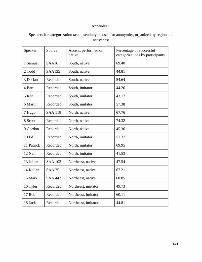
141
Appendix E
Speakers for categorization task, pseudonyms used for anonymity, organized by region and
nativeness
Speaker Source Accent, performed or
native
Percentage of successful
categorizations by participants
1 Samuel SAA16 South, native 69.40
2 Todd SAA135 South, native 44.81
3 Dorian Recorded South, native 54.64
4 Bart Recorded South, imitator 44.26
5 Ken Recorded South, imitator 43.17
6 Martin Recorded South, imitator 57.38
7 Hugo SAA 118 North, native 67.76
8 Scott Recorded North, native 74.32
9 Gordon Recorded North, native 45.36
10 Ed Recorded North, imitator 51.37
11 Patrick Recorded North, imitator 69.95
12 Neil Recorded North, imitator 41.53
13 Julian SAA 103 Northeast, native 47.54
14 Kellan SAA 251 Northeast, native 67.21
15 Mark SAA 442 Northeast, native 68.85
16 Tyler Recorded Northeast, imitator 49.73
17 Bob Recorded Northeast, imitator 60.11
18 Jack Recorded Northeast, imitator 44.81

142
Appendix F
Speakers for categorization task organized by successful categorization by participants
Speaker Source Accent, performed or
native
Percentage of successful
categorizations by participants
8 Scott Recorded North, native 74.32
11 Patrick Recorded North, imitator 69.95
1 Samuel SAA 16 South, native 69.40
15 Mark SAA 442 Northeast, native 68.85
7 Hugo SAA 118 North, native 67.76
14 Kellan SAA 251 Northeast, native 67.21
17 Bob Recorded Northeast, imitator 60.11
6 Martin Recorded South, imitator 57.38
3 Dorian Recorded South, native 54.64
10 Ed Recorded North, imitator 51.37
16 Tyler Recorded Northeast, imitator 49.73
13 Julian SAA 103 Northeast, native 47.54
9 Gordon Recorded North, native 45.36
2 Todd SAA 135 South, native 44.81
18 Jack Recorded Northeast, imitator 44.81
4 Bart Recorded South, imitator 44.26
5 Ken Recorded South, imitator 43.17
12 Neil Recorded North, imitator 41.53

143
Appendix G
Implicit Attitudes Pre-Experiment Instructions Script
You’re going to be doing an accent and word categorization task, listening to some media clips,
then doing another accent and word categorization task. This experiment is looking at the ways
different modes of input affect our experiences with television and what we take from it. We’re
looking at what differences there may be between people who just hear audio input, people who
just see visual input, and people who both hear audio and see visual input. You’re going to be in
the audio only condition.
The media cips are recreated by community theatre actors as closely as possible to the source
material. After each clip, you’ll be asked a few free response questions. These are just giving
your perceptions of the clips. There are no right or wrong answers. After all three clips, you’ll
answer five quick questions about your own attitudes about television. We aren’t asking for any
sensitive information, but just in case, all your responses are anonymous.
For the categorization task, you’ll see adjectives or hear voices and have to categorize them as
belonging to a certain category as quickly as you can. The categories will appear on either side of
the computer screen. If the word or voice belongs to the category on the left, you’ll press the D
key. If it belongs to the category on the right side of the screen, you’ll press the K key. All of the
instructions will appear on the screen before the task.
As a heads up, there may be some overlap with the voices when you respond particularly
quickly.
Do you have any questions?

144
Appendix H
D-score results and change score for each participant
Participant Pretest IAT D-score Posttest IAT D-score Change score
(Posttest-Pretest)
1 0.75567 0.4032 -0.3525
2 -0.0175 0.05523 0.07274
3 0.30613 0.1687 -0.1374
4 0.46645 0.33525 -0.1312
5 0.48618 0.32794 -0.1583
6 0.05023 -0.3107 -0.3609
7 0.52569 0.31993 -0.2058
8 0.13971 0.19266 0.05296
9 0.21451 0.51602 0.30151
10 0.41875 -0.2263 -0.6451
11 0.27773 0.05287 -0.2249
12 -0.0018 -0.2645 -0.2627
13 0.80753 0.57042 -0.2371
14 0.63162 0.49712 -0.1345
15 -0.099 0.56269 0.66169
16 0.29694 -0.0878 -0.3848
17 0.06772 0.17955 0.11183
18 -0.1339 0.23221 0.36606
19 -0.3137 0.21044 0.52413
20 -0.563 -0.0718 0.49116
21 -0.0463 -0.385 -0.3387
22 0.39014 0.0721 -0.318

145
23 0.84464 0.21796 -0.6267
24 0.3287 0.36325 0.03454
25 0.37673 0.0647 -0.312
26 0.27404 0.36418 0.09014
27 0.64351 0.32704 -0.3165
28 0.69386 0.70799 0.01414
29 -0.1585 -0.0428 0.11569
30 0.50913 0.19194 -0.3172
31 0.34726 0.41857 0.0713
32 0.84398 0.32039 -0.5236
33 0.27574 -0.2034 -0.4791
34 0.65355 0.31976 -0.3338
35 0.06613 -0.0711 -0.1373
36 0.44683 0.09883 -0.348
37 0.49706 0.13449 -0.3626
38 0.32159 -0.0606 -0.3822
39 -0.0332 0.2962 0.32938
40 -0.0825 0.20854 0.29102

146
Appendix I
Explicit Attitudes Pre-Experiment Instructions Script
In this experiment, we’re looking at how different modes of input affect perceptions of media.
You’ve been assigned to a condition where you hear audio only of television clips.
First, you’re going to give us some impressions of actors based on their voices.
Then you’ll listen to three clips from television shows recreated by theater actors. They’re
recreating the clips as exactly as possible. Everything should be as it was in the original clip, just
without things like background music.
After each clip, you’ll answer several free response questions about the clips. These will just be
about your perceptions. There will be no right or wrong answers. We’re not asking for any
sensitive information, but your answers will all be anonymous. Once you finish the three clips
and their associated questions, you’ll be done with the experiment. You can come out from the
work station and I’ll tell you more about the study.
This is a new methodology for the lab. After I give you a little more information about the study,
I’ll ask that you fill out a quick evaluation. Including the evaluation, the study should take
around 45 minutes.
Be as open as possible with the ratings in the evaluation. It’s important for us to know where we
can improve. The scale is 1 to 7. Seven is considered exceptional. Five is good.
I have to step out for a meeting, so if I’m not back by the time you finish, the other research
assistant will give you the feedback and set up the evaluation.
Do you have any questions?

147
References
Agliata, D., & Tantleff-Dunn, S. (2004). The impact of media exposure on males’ body image.
Journal of Social and Clinical Psychology, 23(1), 7–22.
Androutsopoulos, J. (2014). Mediatization and sociolinguistic change. Key concepts, research
traditions, open issues. In Mediatization and Sociolinguistic Change (pp. 3–48). Berlin:
De Gruyter.
Anschutz, D., Engels, R., Van Leeuwe, J., & van Strien, T. (2009). Watching your weight? The
relations between watching soaps and music television and body dissatisfaction and
restrained eating in young girls. Psychology and Health, 24(9), 1035–1050.
Auer, P., & Hinskens, F. (2005). The role of interpersonal accommodation in a theory of
language change. In P. Auer, F. Hinskens, & P. Kerswell (Eds.), Dialect Change:
Convergence and Divergence in European Languages (pp. 335–357). Cambridge:
Cambridge University Press.
Babel, M. (2010). Dialect convergence and divergence in New Zealand English. Language in
Society, 39(4), 437–456. https://doi.org/10. 1017/S00474045 10000400
Bartholow, B. D., Bushman, B. J., & Sestir, M. A. (2006). Chronic Violent Video Game
Exposure and Desensitization to Violence: Behavioral and Event-Related Brain Potential
Data. Journal of Experimental Social Psychology, 42(4), 532–539.
Bell, B. T., Lawton, R., & Dittmar, H. (2007). The impact of thin models in music videos on
adolescent girls’ body dissatisfaction. Body Image, 4, 137–145.
Bickham, D. S., & Slaby, R. G. (2012). Effects of a Media Literacy Program in the US on
Children’s Critical Evaluation of Unhealthy Media Messages about Violence, Smoking,
and Food. Journal of Children and Media, 6(2), 255–271.
https://doi.org/10.1080/17482798.2012.662031
Blair, I. V. (2002). The malleability of automatic stereotypes and prejudice. Personality and
Social Psychology Review, 6(3), 242–261.
Blair, I. V., Ma, J. E., & Lenton, A. P. (2001). Imagining stereotypes away: The moderation of
implicit stereotypes through mental imagery. Journal of Personality and Social
Psychology, 81(5), 828–841. https://doi.org/I0.1037//0022-3514.81.5.828
Bushman, B., & Huesmann, L. (2001). Effects of televised violence on aggression. In D. Singer
& J. Singers (Eds.), Handbook of Children and the Media (pp. 223–254). Thousand
Oaks, CA: Sage.
Campbell-Kibler, K. (2008). I’ll be the judge of that: Diversity in Social Perceptions of (ING).
Language in Society, 37(5), 637–659.
Campbell-Kibler, K. (2012). The Implicit Association Test and sociolinguistic meaning. Lingua,
122(7), 753–763. https://doi.org/10.1016/j.lingua.2012.01.002

148
Campbell-Kibler, K. (2013). Connecting attitudes and language behavior via implicit
sociolinguistic cognition. In S. Grondelaers & T. Kristiansen (Eds.), Experimental studies
of changing language standards in contemporary Europe (1st ed., pp. 307–329).
Cargile, A. C., Giles, H., Ryan, E. B., & Bradac, J. J. (1994). Language Attitudes as a Social
Process: A Conceptual Model and New Directions. Language & Communication, 14(3),
211–236.
Chambers, J. K. (1998). TV makes people sound the same. In L. Bauer & P. Trudgill (Eds.),
Language Myths (pp. 123–131). New York: Penguin.
Charkova, K. D. (2007). A Language Without Borders: English Slang and Bulgarian Learners of
English. Language Learning, 57(3), 369–416.
Clopper, C. G., & Pisoni, D. B. (2004a). Some acoustic cues for the perceptual categorization of
American English regional dialects. Journal of Phonetics, 32, 111–140.
https://doi.org/10.1016/S0095-4470(03)00009-3
Clopper, C. G., & Pisoni, D. B. (2004b). Homebodies and army brats: Some effects of early
linguistic experience and residential history on dialect categorization. Language
Variation and Change, 16, 31–48. https://doi.org/10.10170S0954394504161036
Coyne, S. M., Archer, J., & Eslea, M. (2004). Cruel intentions on television and in real life: Can
viewing indirect aggression increase viewers’ subsequent indirect aggression? Journal of
Experimental Child Psychology, 88(3), 234–253.
https://doi.org/10.1016/j.jecp.2004.03.001
Cremona, C., & Bates, E. (1977). The Development of Attitudes Toward Dialect in Italian
Children. Journal of Psycholinguistic Research, 6(3), 223–232.
Dawes, J. (2008). Do data characteristics change according to the number of scale points used ?
An experiment using 5 point, 7 point and 10 point scales. International Journal of Market
Research, 50(1), 61–104.
DeLuise, P. (2000, August 4). Window of Opportunity [Television episode]. Stargate SG-1.
Vancouver, BC: Scifi Channel.
Demirci, M., & Kleiner, B. (1999). The Perceptions of Turkish Dialects. In D. Preston (Ed.),
Handbook of Perceptual Dialectology (Vol. 1, pp. 263–281). Philadelphia: John
Benjamins Publishing Company.
Devine, P. G. (1989). Stereotypes and Prejudice: Their Automatic and Controlled Components.
Journal of Personality and Social Psychology, 56(1), 5–18.
Dixon, T. (2008). Crime news and racialized beliefs: Understanding the relationship between
local news viewing and perceptions of African Americans and crime. Journal of
Communication, 58, 106–125. https://doi.org/10.1111/j.1460-2466.2007.00376.x

149
Dobrow, J. R., & Gidney, C. L. (1998). The Good, the Bad, and the Foreign: The Use of Dialect
in Children’s Animated Television. Annals of the American Academy of Political and
Social Science, 557, 105–119.
Edwards, J. (1982). Language attitudes and their implication among English speakers. In E. B.
Ryan & H. Giles (Eds.), Attitudes towards language variation: Social and applied
contexts (pp. 20–33). London: Edward Arnold.
Egloff, B., & Schmukle, S. C. (2002). Predictive validity of an Implicit Association Test for
assessing anxiety. Journal of Personality and Social Psychology, 83(6), 1441–1455.
https://doi.org/10.1037//0022-3514.83.6.1441
Elliott, W., Rudd, R., & Good, L. (1983). Measuring the perceived reality of television:
Perceived plausibility, perceived superficiality and the degree of personal utility.
Presented at the Annual Meeting of the Association for Education in Journalism and
Mass Communication.
Ensler, J. (2008, January 18). The Old and the Restless [Television episode]. Psych. Vancouver,
BC: USA Network.
Eyal, K., & Cohen, J. (2006). When good friends say goodbye: A parasocial breakup study.
Journal of Broadcasting & Electronic Media, 50(3), 502–523.
https://doi.org/10.1207/s15506878jobem5003_9
Ford, T. E. (1997). Effects of stereotypical television portrayals of African-Americans on person
perception. Social Psychology Quarterly, 60(3), 266–278.
Foroni, F., & Mayr, U. (2005). The power of a story: New, automatic associations from a single
reading of a short scenario. Psychonomic Bulletin & Review, 12(1), 139–144.
Fridland, V. (2012). Rebel Vowels: How Vowel Shift Patterns are Reshaping Speech in the
Modern South. Language and Linguistics Compass, 6(3), 183–192.
https://doi.org/10.1002/lnc3.325
Friedlander, L. J., Connolly, J. A., Pepler, D. J., & Craig, W. M. (2013). Extensiveness and
persistence of aggressive media exposure as longitudinal risk factors for teen dating
violence. Psychology of Violence, 3(4), 310–322. https://doi.org/10.1037/a0032983
Fujioka, Y. (1999). Television Portrayals and African-American Stereotypes: Examination of
Television Effects When Direct Contact Is Lacking. Journalism & Mass Communication
Quarterly, 76(1), 52–75. https://doi.org/10.1177/107769909907600105
Garrett, P. (2010). Attitudes to Language. Cambridge: Cambridge University Press.
Gawronski, B., & Bodenhausen, G. V. (2006a). Associative and propositional processes in
evaluation: An integrative review of implicit and explicit attitude change. Psychological
Bulletin, 132(5), 692–731.

150
Gawronski, B., & Bodenhausen, G. V. (2006b). Associative and propositional processes in
evaluation: Conceptual, empirical, and metatheoretical issues: Reply to Albarracín, Hart,
and McCulloch (2006), Kruglanski and Dechesne (2006), and Petty and Briñol (2006).
Psychological Bulletin, 132(5), 745–750.
Gawronski, B., & Bodenhausen, G. V. (2007). Unraveling the processes underlying evaluation:
Attitudes from the perspective of the APE model. Social Cognition, 25(Special Issue:
What is an Attitude?), 687–717.
Gawronski, B., & Bodenhausen, G. V. (2011). The Associative–Propositional Evaluation Model:
Theory, Evidence, and Open Questions. In Advances in Experimental Social Psychology
(Vol. 44, p. 380). San Diego: Academic Press.
Gawronski, B., Cunningham, W. A., LeBel, E. P., & Deutsch, R. (2010). Attentional influences
on affective priming: Does categorization influence spontaneous evaluations of multiply
categorizable objects? Cognition and Emotion, 24(6), 1008–1025.
https://doi.org/10.1080/02699930903112712
Gawronski, B., & Strack, F. (2004). On the propositional nature of cognitive consistency:
Dissonance changes explicit, but not implicit attitudes. Journal of Experimental Social
Psychology, 40(4), 535–542. https://doi.org/10.1016/j.jesp.2003.10.005
Gentile, D. A., Anderson, C. A., Yukawa, S., Ihori, N., Saleem, M., Ming, L. K., Sakamoto, A.
(2009). The Effects of Prosocial Video Games on Prosocial Behaviors: International
Evidence From Correlational, Longitudinal, and Experimental Studies. Personality and
Social Psychology Bulletin, 35(6), 752–763. https://doi.org/10.1177/0146167209333045
Gerbner, G., Gross, L., Jackson-Beeck, M., Jeffries-Fox, S., & Signorielli, N. (1978). Cultural
Indicators: Violence Profile No. 9. Journal of Communication, 28(3), 176–206.
Giles, H., Henwood, K., Coupland, N., Harriman, J., & Coupland, J. (1992). Language Attitudes
and Cognitive Mediation. Human Communication Research, 18(4), 500–527.
Green, M. C. (2004). Transportation Into Narrative Worlds: The Role of Prior Knowledge and
Perceived Realism. Discourse Processes, 38(2), 247–266.
https://doi.org/10.1207/s15326950dp3802_5
Greenwald, A. G., McGhee, D. E., & Schwartz, J. L. K. (1998). Measuring Individual
Differences in Implicit Cognition: The Implicit Association Test. Journal of Personality
and Social Psychology, 74(6), 1464–1480.
Greenwald, A. G., Nosek, B. A., & Banaji, M. R. (2003). Understanding and Using the Implicit
Association Test: I. An Improved Scoring Algorithm. Journal of Language and Social
Psychology, 85(2), 197–216. https://doi.org/10.1037/0022-3514.85.2.197
Gregg, A. P., Seibt, B., & Banaji, M. R. (2006). Easier done than undone: Asymmetry in the
malleability of implicit preferences. Journal of Personality and Social Psychology, 90(1),
1–20. https://doi.org/10.1037/0022-3514.90.1.1

151
Greitemeyer, T., Hollingdale, J., & Traut-Mattausch, E. (2015). Changing the Track in Music
and Misogyny: Listening to Music With Pro-Equality Lyrics Improves Attitudes and
Behavior Toward Women. Psychology of Popular Media Culture, 4(1), 56–67.
https://doi.org/10.1037/a0030689
Hall, A. E. (2009). Perceptions of Media Realism and Reality TV. In R. L. Nabi & M. B. Oliver
(Eds.), Media Processes and Effects (pp. 423–438). Thousand Oaks, CA: SAGE.
Halliwell, E., Easun, A., & Harcourt, D. (2011). Body dissatisfaction: Can a short media literacy
message reduce negative media exposure effects amongst adolescent girls? British
Journal of Health Psychology, 16(2), 396–403.
https://doi.org/10.1348/135910710X515714
Harwood, J., & Vincze, L. (2012). Undermining Stereotypes of Linguistic Groups through
Mediated Intergroup Contact. Journal of Language and Social Psychology, 31(2), 157–
175. https://doi.org/10.1177/0261927X12438358
Hay, J., & Drager, K. (2010). Stuffed toys and speech perception. Linguistics, 48(4), 865–892.
https://doi.org/10.1515/ling.2010.027
Hay, J., Drager, K., & Warren, P. (2010). Short-term Exposure to One Dialect Affects
Processing of Another. Language and Speech, 53(4), 447–471.
https://doi.org/10.1177/0023830910372489
Heaton, H. (2012). As Seen on TV: An Acoustic Analysis of the Portrayal of American Southern
Dialect in Fictional Television Programs (MA Thesis). North Carolina State University,
Raleigh, NC.
Heaton, H., & Nygaard, L. C. (2011). Charm or Harm: Effect of Passage Content on Listener
Attitudes Toward American English Accents. Journal of Language and Social
Psychology, 30(2), 202–211. https://doi.org/10.1177/0261927X10397288
Huesmann, L. R., Moise-Titus, J., Podolski, C.-L., & Eron, L. D. (2003). Longitudinal relations
between children’s exposure to TV violence and their aggressive and violent behavior in
young adulthood: 1977-1992. Developmental Psychology, 39(2), 201–221.
https://doi.org/10.1037/0012-1649.39.2.201
Jarvella, R. J., Bang, E., Jakobsen, A. L., & Mees, I. M. (2001). Of mouths and men: Non-native
listeners’ identification and evaluation of English. International Journal of Applied
Linguistics, 11(1), 37–56. https://doi.org/10.1111/1473-4192.00003
Jeon, L., Cukor-Avila, P., & Rector, P. (2013). Mapping dialect perceptions in a variationist
framework. Presented at the New Ways of Analyzing Variation (NWAV) 42, Pittsburgh,
PA.
Johnstone, B. (2011). Dialect enregisterment in performance. Journal of Sociolinguistics, 15(4),
657–679.

152
Khaw, W. (2015). Royally Duped: A Fairytale Gone Askew. Television script.
Kim, D.-Y. (2003). Voluntary controllability of the Implicit Association Test (IAT). Social
Psychology Quarterly, 66(1), 83–96.
Kristiansen, T. (2014). Does mediated language influence immediate language? In J.
Androutsopoulos (Ed.), Mediatization and Sociolinguistic Change (pp. 99–126). Berlin,
Germany: de Gruyter.
Labov, W. (1966). The Social Stratification of English in New York City. Washington DC:
Center for Applied Linguistics.
Labov, W. (1996). The Organization of Dialect Diversity in North America [University of
Pennsylvania]. Retrieved from http://www.ling.upenn.edu/phono_atlas/ICSLP4.html
Labov, W. (2001). Principles of Linguistic change. Oxfor: Blackwell.
Labov, W., Ash, S., & Boberg, C. (2006). Atlas of North American English: Phonetics,
Phonology, and Sound Change. New York: Mouton de Gruyter.
Lambert, W. E. (1967). A Social Psychology of Bilingualism. Journal of Social Issues, 23(2),
91–109. https://doi.org/10.1111/j.1540-4560.1967.tb00578.x
L’Engle, K. L., Brown, J. D., & Kenneavy, K. (2006). The mass media are an important context
for adolescents’ sexual behavior. Journal of Adolescent Health, 38, 186–192.
https://doi.org/10.1016/j.jadohealth.2005.03.020
Lippi-Green, R. (2012). English with an Accent (2nd ed.). New York: Routledge.
Loudermilk, B. C. (2015). Implicit attitudes and the perception of sociolinguistic variation. In A.
Prikhodkine & D. Preston (Eds.), Responses to Language Variation: Variability,
processes and outcomes (pp. 137–156). Philadelphia: John Benjamins Publishing
Company.
Lowery, B. S., Hardin, C. D., & Sinclair, S. (2001). Social influence effects on automatic racial
prejudice. Journal of Personality and Social Psychology, 81(5), 842–855.
https://doi.org/1O.1O37//O022-35I4.8I.5.842
Luhman, R. (1990). Appalachian English Stereotypes: Language Attitudes in Kentucky.
Language in Society, 19(3), 331–348.
Martin, D. (2016). Cleaning and Visualizing Implicit Association Test (IAT) Data. Dan Martin.
Retrieved from https://cran.r-project.org/web/packages/IAT/IAT.pdf
Martins, N., & Harrison, K. (2012). Racial and gender differences in the relationship between
children’s television use and self-esteem: A longitudinal panel study. Communication
Research, 39(3), 338–357. https://doi.org/10.1177/0093650211401376

153
McAlone, N. (2017). These are the 18 most popular YouTube stars in the world — and some are
making millions. Retrieved March 2, 2018, from http://www.businessinsider.com/most-
popular-youtuber-stars-salaries-2017
McConnell, A. R., & Leibold, J. M. (2001). Relations among the Implicit Association Test,
Discriminatory Behavior, and Explicit Measures of Racial Attitudes. Journal of
Experimental Social Psychology, 37, 435–442. https://doi.org/10.1006/jesp.2000.1470
Meek, B. A. (2006). And the Injun goes “How!”: Representations of American Indian English in
white public space. Language in Society, 35, 93–128.
https://doi.org/10.10170S0047404506060040
Milroy, J., & Milroy, L. (1999). Authority in language: Investigating language prescription and
standardisation (3rd ed.). London: Routledge.
Mitchell, J. P., Nosek, B. A., & Banaji, M. R. (2003). Contextual Variations in Implicit
Evaluation. Journal of Experimental Psychology: General, 132(3), 455–469.
https://doi.org/10.1037/0096-3445.132.3.455
Molla, R. (2018). Netflix now has nearly 118 million streaming subscribers globally. Retrieved
March 2, 2018, from https://www.recode.net/2018/1/22/16920150/netflix-q4-2017-
earnings-subscribers
Moosmuller, S. (2010). The role of stereotypes, phonetic knowledge, and phonological
knowledge in the evaluation of dialect authenticity. In Proceedings of the Workshop
“Sociophonetics, at the crossroads of speech variation, processing and communication”
(pp. 49–52). Pisa: Scuola Normale Superiore. https://doi.org/10.2422/7642-434-
2.2012.13
Morgan, M., & Shanahan, J. (2010). The State of Cultivation. Journal of Broadcasting &
Electronic Media, 54(2), 337–355.
Mulgrew, K. E., Volcevski-Kostas, D., & Rendell, P. G. (2013). The effect of music video clips
on adolescent boy’s body image, mood, and schema activation. Journal of Youth and
Adolescence, 43(1), 92–103. https://doi.org/10.1007/s10964-013-9932-6
Naro, A. J. (1981). The Social and Structural Dimensions of Syntactic Changes. Language,
57(1), 63–98. https://doi.org/10.2307/414287
Naro, A., & Scherre, M. M. P. (1996). Contact with Media and Linguistic Variation. In J.
Arnold, R. Blake, B. Davidson, S. Schwenter, & J. Solomon (Eds.), Sociolinguistic
Variation Data, Theory, and Analysis. Palo Alto, CA: CSLI Publications.
Neuhausser, S., & Simpson, A. P. (2007). Imitated or Authentic? Listeners’ judgments of foreign
accents. In Proceedings of the XVIth ICPhS (pp. 1805–1808). Saarbrucken, Germany.

154
Niedzielski, N. (1999). The effect of social information on the perception of sociolinguistic
variables. Journal of Language and Social Psychology, 18(1), 62–85.
https://doi.org/10.1177/0261927X99018001005
Ortiz, M., & Harwood, J. (2007). A Social Cognitive Theory Approach to the Effects of
Mediated Intergroup Contact on Intergroup Attitudes. Journal of Broadcasting &
Electronic Media, 51(4), 615–631. https://doi.org/10.1080/08838150701626487
Ota, I., & Takano, S. (2014). The Media Influence on Language Change in Japanese
Sociolinguistic Contexts. In Mediatization and Sociolinguistic Change (pp. 171–203).
Berlin, Germany: de Gruyter.
Pantos, A. J. (2010). Measuring implicit and explicit attitudes toward foreign-accented speech
(Dissertation). Rice University, Houston, TX.
Pappas, P. A. (2008). Stereotypes, variation and change: Understanding the change of coronal
sonorants in a rural variety of Modern Greek. Language Variation and Change, 20(3),
493–526. https://doi.org/10.1017/S0954394508000173
Payne, B. K. (2001). Prejudice and Perception: The Role of Automatic and Controlled Processes
in Misperceiving a Weapon. Journal of Personality and Social Psychology, 81(2), 181–
192. https://doi.org/10.I037//0O22-3514.81.2.181
Pike, J. J., & Jennings, N. A. (2005). The effects of commercials on children’s perceptions of
gender appropriate toy use. Sex Roles, 52(1/2), 83–91. https://doi.org/10.1007/s11199-
005-1195-6
Preston, C. C., & Colman, A. M. (2000). Optimal number of response categories in rating scales:
Reliability, validity, and discriminating power, and respondent preferences. Acta
Psychologica, 104(1), 1–15.
Preston, D. (1993). Folk dialectology. In D. Preston (Ed.), American Dialect Research (pp. 333–
378). Philadelphia: John Benjamins.
Preston, D. (1999). A language attitude approach to the perception of regional variety. In D.
Preston (Ed.), Handbook of Perceptual Dialectology (pp. 359–373). Amsterdam: John
Benjamins Publishing Company.
Preston, D. (1996). Where the worst English is spoken. In Focus on the USA (pp. 297–360).
Amsterdam: John Benjamins.
Purnell, T., Idsardi, W., & Baugh, J. (1999). Perceptual and Phonetic Experiments on American
English Dialect Identification. Journal of Language and Social Psychology, 18, 10–30.
https://doi.org/10.1177/0261927X99018001002
Queen, R. (2015). Vox Popular: The Surprising Life of Language in the Media. Malden, MA:
Wiley-Blackwell.

155
R Core Team. (2013). R: A language and environment for computing (Version R Studio).
Redinger, D. (2010). Language attitudes and code-switching behaviour in a multilingual
educational context: the case of Luxembourg (Dissertation). University of York, York,
United Kingdom.
Reed, J. (1986). Southern Folk, Plain and Fancy. Athens, Georgia: University of Georgia Press.
Rice, M., & Woodsmall, L. (1988). Lessons from Television: Children’s Word Learning When
Viewing. Child Development, 59, 420–429.
Rickford, J., & King, S. (2016). Language and linguistics on trial: Hearing Rachel Jeantel (and
other vernacular speakers) in the courtroom and beyond. Language, 92(4), 948–988.
https://doi.org/10.1353/lan.2016.0078
Rubin, A. M. (1983). Television uses and gratifications: The interactions of viewing patterns and
motivations. Journal of Broadcasting, 27, 37–51.
Rubin, D. L. (1992). Nonlanguage factors affecting undergraduate’s judgments of nonnative
English-speaking teaching assistants. Research in Higher Education, 33, 511–531.
Rydell, R. J., & McConnell, A. R. (2006). Understanding Implicit and Explicit Attitude Change:
A Systems of Reasoning Analysis. Journal of Personality and Social Psychology, 91(6),
995–1008. https://doi.org/10.1037/0022-3514.91.6.995
Scherre, M. M. P., & Naro, A. J. (2014). Sociolinguistic Correlates of Negative Evaluation:
Variable Concord in Rio de Janeiro. Language Variation and Change, 26(3), 185–212.
Schiappa, E., Gregg, P. B., & Hewes, D. E. (2005). The Parasocial Contact Hypothesis.
Communication Monographs, 72(1), 92–115.
https://doi.org/10.1080/0363775052000342544
Sebastian, R. J., & Ryan, E. B. (1985). Speech Cues and Social Evaluation: Markers of Ethnicity,
Social Class, and Age. In Recent Advances in Language Communication and Social
Psychology (pp. 112–143). London: Lawrence Erlbaum.
Shuttlesworth, R. (2007). Southern English in Television and Film. In M. Montgomery & E.
Johnson (Eds.), The New Encyclopedia of Southern Culture: Language (2nd ed., Vol. 5,
pp. 193–197). Chapel Hill: University of North Carolina Press.
Shuy, R. W., Wolfram, W. A., & Riley, W. K. (1967). Linguistic Correlates of Social
Stratification in Detroit Speech (Final Report No. Cooperative Research Report 6-1347).
Washington DC: U.S. Office of Education.
Strand, E. (1999). Uncovering the role of gender stereotypes in speech perception. Journal of
Language and Social Psychology, 18(1), 86–99.

156
Stuart-Smith, J. (2007). The Influence of the Media. In C. Llamas, L. Mullany, & P. Stockwell
(Eds.), The Routledge Companion to Sociolinguistics (pp. 140–148). New York:
Routledge.
Stuart-Smith, J., & Ota, I. (2014). Media models, “the shelf” and stylistic variation in East and
West: rethinking the influence of the media on language variation and change. In
Mediatization and Sociolinguistic Change (pp. 127–170). Berlin: De Gruyter.
Stuart-Smith, J., Price, G., Timmins, C., & Gunter, B. (2013). Television can also be a factor in
language change: Evidence from an urban dialect. Language, 89(3), 501–536.
https://doi.org/10.1353/lan.2013.0041
Tagliamonte, S., & Roberts, C. (2005). So Weird; So Cool; So Innovative: The Use of
Intensifiers in the Television Series “Friends.” American Speech, 80(3), 280–300.
Tate, D. (1979). Preliminary data on dialect in speech disguise. In H. Hollien & P. Hollien
(Eds.), Current issues in the phonetic sciences: Proceedings of the IPS-77 Congress (pp.
847–850). Berlin: John Benjamins Publishing Co.
Thomas, E. (2007). R in Southern English. In M. Montgomery & E. Johnson (Eds.), The New
Encyclopedia of Southern Culture: Language (2nd ed., Vol. 5, pp. 189–190). Chapel Hill:
University of North Carolina Press.
Trudgill, P. (1986). Dialects in Contact. Oxford: Blackwell.
Trudgill, P. (2014). Diffusion, drift, and the irrelevance of media influence. Journal of
Sociolinguistics, 18(3), 214–222. https://doi.org/DOI: 10.1111/josl.12070
University of Michigan. (2017). Student Profile [University of Michigan]. Retrieved March 2,
2018, from https://admissions.umich.edu/apply/freshmen-applicants/student-profile
Van Bezooijen, R., & Gooskens, C. (1999). Identification of language varieties: The contribution
of different linguistic levels. Journal of Language and Social Psychology, 18, 31–48.
Van Bezooijen, R., & Ytsma, J. (1999). Accents of Dutch: Personality impression, divergence,
and identifiability. Belgian Journal of Linguistics, 13, 105–129.
Ward, L. M., Hansbrough, E., & Walker, E. (2005). Contributions of music video exposure to
Black adolescent gender and sexual schemas. Journal of Adolescent Research, 20(2),
143–166. https://doi.org/10.1177/0743558404271135
Wegner, D. M. (1994). Ironic processes of mental control. Psychological Review, 101, 24–52.
Weinberger, S. (2018, March 2). Speech Accent Archive [George Mason University]. Retrieved
from http://accent.gmu.edu
Westcott, K., Lippstreu, S., & Cutbill, D. (2017). Digital democracy survey, 11th edition: A
multi-generational view of technology, media, and telecom trends (Survey analysis No.

157
11th edition). Deloitte. Retrieved from
https://www2.deloitte.com/us/en/pages/technology-media-and-
telecommunications/articles/digital-democracy-survey-generational-media-consumption-
trends.html
Williams, A., Garrett, P., & Coupland, N. (1999). Dialect recognition. In Handbook of
Perceptual Dialectology (pp. 345–358). Philadelphia: John Benjamins.
Willoughby, T., Adachi, P. J. C., & Good, M. (2012). A longitudinal study of the association
between violent video game play and aggression among adolescents. Developmental
Psychology, 48(4), 1044–1057. https://doi.org/10.1037/a0026046
Wittenbrink, B., Judd, C. M., & Park, B. (2001). Spontaneous prejudice in context: variability in
automatically activated attitudes. Journal of Personality and Social Psychology, 81(5),
815–827. https://doi.org/10.1037//0022-3514.81.5.815
Zetterholm, E. (2007). Detection of Speaker Characteristics Using Voice Imitation. In C. Müller
(Ed.), Speaker Classification II (pp. 192–205). Berlin, Germany: Springer-Verlag Berlin
Heidelberg.
Related Documents