Mechanistic modeling of mass transport phenomena in Forward Osmosis Arnout D’Haese ............... 1111111 GHENT UNIVERSITY 11:.0.. FACULTY OF BIOSCIENCE ENGINEERING

Welcome message from author
This document is posted to help you gain knowledge. Please leave a comment to let me know what you think about it! Share it to your friends and learn new things together.
Transcript
Mechanistic modeling of mass transport phenomena in Forward Osmosis
Arnout D’Haese
............... 1111111
GHENT UNIVERSITY
11:.0.. FACULTY OF ~ BIOSCIENCE ENGINEERING

Mechanistic modeling of
mass transport phenomena
in Forward Osmosis
ir. Arnout D’Haese
Supervisor: prof. dr. ir. Arne R.D. Verliefde
Dissertation submitted in fulfillment of the requirements for the degree of
Doctor (Ph.D.) in Applied Biological Sciences: Environmental Technology
Department of Applied Analytical and Physical Chemistry
Particle and Interfacial Technology Group
Faculty of Bioscience Engineering
Ghent University
Academic year 2016-2017
1/!.0., FACULTY OF G ~ BIOSCIENCE ENGINEERIN
~ 1111111
GHENT UNIVERSITY

Supervisor
prof. dr. ir. Arne Verliefde
Department of Applied Analytical and Physical Chemistry, PaInT
Ghent University
Chair of the examination committee
prof. dr. ir. Frank Devlieghere
Department of Food Safety and Food Quality
Ghent University
Board of Examiners
prof. dr. Viatcheslav Freger
Wolfson Department of Chemical Engineering
Technion - Israel Institute of Technology
prof. dr. Pierre Le-Clech
School of Chemical Engineering
University of New South Wales
prof. dr. ir. Wolfgang Gernjak
Water Supply and Advanced Treatment
Catalan Institute for Water Research (ICRA)
prof. dr. ir. Ingmar Nopens
Department of Mathematical Modelling, Statistics and Bioinformatics
Ghent University
prof. dr. ir. Paul Van der Meeren
Department of Applied Analytical and Physical Chemistry, PaInT
Ghent University
Dean of the Faculty of Bioscience Engineering
prof. dr. ir. Marc Van Meirvenne
Rector of Ghent University
prof. dr. Anne De Paepe

Dutch translation of the title:
Mechanistisch modelleren van massatransportfenomenen in directe osmose
Copyright 2017 ©
The author and supervisor give the authorization to consult this work for per-
sonal use only. Every other use is subject to copyright laws. Permission to
reproduce any material contained in this work should be obtained from the
author.
Citing this PhD
D’Haese, A. (2017) Mechanistic modeling of mass transport phenomena in For-
ward Osmosis, PhD thesis, Ghent University, Belgium
ISBN 978-90-5989-962-9
Summary
Forward Osmosis (FO) is a membrane process which is developed with the aim
of recovering water from heavily impaired water sources, such as raw or par-
tially treated wastewater, wastewater sludges or specific industrial wastewater
streams. It can also be used to concentrate valuable products in food and phar-
maceutical industry. During FO, feed solution is contacted with a draw solution
through a semi-permeable membrane; water is abstracted from the feed solu-
tion due to the elevated osmotic pressure of the draw solution. This osmotic
pressure is generated by a draw solute, often but not always a mineral salt,
which is rejected by the membrane. As the feed solution is commonly a heav-
ily impaired water source, the feed solution likely contains numerous solutes
of varying sizes. The FO membrane however is not perfectly semi-permeable:
both inorganic and organic solutes of sufficiently small sizes can pass the mem-
brane at reduced rates compared to water; this pertains to feed solutes as well
as the draw solute. As a result, during FO, there are three distinct fluxes: a
water flux from feed to draw solution, a flux of feed solutes towards the draw
solution and a flux of draw solutes towards the feed solution (reverse solute
diffusion, RSD). In this thesis, mass transport phenomena encountered during
FO are tested experimentally and mechanistic models describing mass trans-
port phenomena are presented.
Chapter 2 investigates water and draw solute fluxes. Water and draw solute
fluxes are mutually dependent: water flux is generated by the osmotic pres-
sure difference across the active layer and thus on the draw solute concen-
tration difference, but the draw solute is subject to concentration polarization
phenomena at the active layer because of water flux. Consequently, predicting
water and draw solute fluxes requires iterative models which are more com-
plex compared to pressure-driven membrane systems. In this chapter, a novel
model is presented in which the membrane structural parameter, membrane
water and draw solute permeabilities are obtained from FO tests only. In this
model, concentration-dependent diffusivity of the draw solute during active
layer transport is introduced, as well as during internal concentration polariza-
tion (ICP). The model was thoroughly tested by performing FO tests using CTA
and TFC membranes in both orientations and by using four draw solutes (NaCl,
Na2SO4, MgCl2 and MgSO4) for each membrane and each orientation. Mem-
brane characterization allowed the estimation of the support layer tortuosity,
which was compared with previous research on transport through porous me-
dia. It was found that in AL-FS mode, realistic tortuosity values were obtained,
while tortuosity was likely overestimated in AL-DS mode. The hypothesis that
the difference in draw solute mass transfer resistance was caused by electrovis-
cosity was explored, and it was found that this could account for about 10% of
the resistance difference.
In Chapter 3, transport of organic micropollutants (OMPs) commonly present
in wastewater is studied. As the OMP flux and RSD are oppositely directed,
it is conceivable that RSD would hinder OMP transport. Furthermore, ionic
draw solutes establish a Donnan electrostatic potential across the membrane,
causing electromigration of charged OMPs. By changing the water activity in
the draw solution, solute-membrane affinity is changed as well. In order to
study these phenomena, OMP rejection tests were performed using the same
draw solutes as in chapter 2, as well as simple OMP diffusion tests. No relation
was found between OMP fluxes and RSD. Charge interactions between OMPs
and draw solutes were observed, with the difference between FO and sim-
ple diffusion being especially remarkable. The hypothesis of electromigration
was tested by measuring the electrostatic potential difference between feed
and draw solution during FO. This was however found to not be able to ex-
plain the OMP permeability pattern: when comparing simple diffusion and FO
tests, OMP permeability responded inversely compared to what was predicted
based on electromigration. The OMP permeability pattern could however be
explained by Donnan dialysis. Solute-membrane affinity was probed using sur-
face tension analysis, yielding the surface free energy of interaction. In some
cases, surface free energy could predict solute partitioning, but in other cases,
predictions were poor. The current model of surface free energy likely does not
capture all relevant interactions.
In Chapter 4, a peculiar observation was made. Uncharged, organic solutes
displayed negative rejection during FO: the solutes were enriched by the mem-
brane, rather than being rejected. Current membrane transport models were
reviewed, and it was shown that using current models the observed rejection
pattern could not be reproduced. Negative rejection was subsequently mod-
eled as either Langmuir adsorption of the solutes onto the membrane followed
by convectively coupled transport, or as the consequence of strong salting in by
the draw solute. Although both models are mechanistically very different, they
both yielded excellent agreement with the experimental data. However, the
latter model is from a physical point of view very unlikely: uncharged organic
solutes are prone to salting out rather than salting in, so a higher rather than
lower rejection is expected. The solutes tested in this chapter were furthermore
known to be prone to salting out, which was confirmed by GC measurements
in this study as well. When testing rejection using the same membrane and
solutes at the same fluxes but using reverse osmosis (RO) instead of FO, pos-
itive rejection was found - the conventional result. This shows that the draw
solute was altering the solute-membrane affinity. Surface tension analysis was
again used to calculate solute-membrane affinity; this yielded qualitative but
not quantitative agreement. This was likely due to the inability of surface
tension analysis to capture all relevant mechanisms by which ionic solutes in-
fluence the solubility of uncharged solutes.
In Chapter 5, the influence of long-term biofouling on FO operation and OMP
rejection was investigated, as well as the fate of OMPs in closed loop FO-RO ap-
plications. It was found that FO flux was not hindered significantly by biofoul-
ing. OMP rejection was generally slightly decreased, possibly by cake-enhanced
concentration polarization. The fate of OMPs in closed loop FO-RO applica-
tions was assessed by comparing the rejection of OMPs by FO and RO mem-
branes, followed by dynamically modeling the OMP fluxes and mass present in
the closed loop. The FO-RO combination is a very likely combination of pro-
cesses if FO membranes can produce sufficiently high fluxes using relatively
dilute draw solutions: RO is the most energy-efficient process to abstract fresh
water from a solution with an osmotic pressure roughly between 20 and 80
bars. The model predicted that, if OMP rejection by the FO membrane was
lower than that of the RO membrane, OMPs would accumulate in the draw
solution to concentrations exceeding the FO feed solution. It then follows that
a process is needed to remove the OMPs in the draw solution loop, which could
be attained by adsorptive or oxidative processes.
This thesis is concluded in 2 final chapters. In Chapter 6, general conclusions
of the work presented in this thesis are discussed, as well as future prospects
of FO. It is argued that the future of FO depends on the availability of opti-
mized membranes, which would simultaneously have to produce a high flux,
be fouling and cleaning resistant, abrasion resistant and display a high feed
and draw solutes rejection. Finally, in Chapter 7, the author’s views on the
water crisis and environmental crisis in general are discussed. In this chap-
ter, it is argued that humanity appropriates an excessively large share of the

planet’s available fresh water sources, and consequently scarcity is the result
of overdrawing natural supplies rather than a low availability of fresh water.
Furthermore, arguments are formulated against our current technology-only
approach to mitigate ecological problems.

Samenvatting
Directe Osmose (FO) is een membraanproces dat ontwikkeld wordt met het
oog op het terugwinnen van water uit zwaar vervuilde bronnen, zoals onbe-
handeld afvalwater, afvalwater slib of specifieke industriële afvalwaterbron-
nen. FO kan ook toegepast worden om waardevolle producten te concentreren
in de voedings- of farmaceutische industrie. Tijdens FO wordt een voedingso-
plossing in contact gebracht met een aanzuigoplossing, de drawoplossing, door
middel van een semi-permeabel membraan. Water wordt onttrokken aan de
voedingsoplossing door de hoge osmotische druk van de drawoplossing, deze
osmotische druk wordt gegenereerd door een opgeloste stof, de draw solute,
dewelke wordt tegengehouden door het membraan. Aangezien de voedingso-
plossing een sterk vervuilde oplossing is, bevat deze allerhande opgeloste stof-
fen van uiteenlopend formaat. Het FO membraan is echter geen perfecte bar-
rière: zowel organische als inorganische opgeloste stoffen kunnen - ongewenst
- doorheen het membraan getransporteerd worden aan sterk verlaagde snel-
heid in vergelijking met water, en dit geldt voor zowel draw solutes als voor
opgeloste stoffen in de voedingsoplossing. Dit resulteert in drie verschillende
fluxen tijdens FO: er is de waterflux van de voedingsoplossing naar de dra-
woplossing, de flux van draw solute van de drawoplossing naar de voeding-
soplossing (ook aangeduid als RSD) en ook fluxen van opgeloste stoffen in de
voedingsoplossing naar de drawoplossing. In deze thesis werden massatrans-
portfenomenen in FO experimenteel onderzocht en werden mechanistische
modellen opgesteld om deze fenomenen te beschrijven.
In hoofdstuk 2 werden water- en draw solute fluxen onderzocht. De water- en
draw solute fluxen zijn onderling afhankelijk: water flux wordt gegenereerd
door het osmotische drukverschil aan weerszijden van de actieve laag van
het membraan, dit drukverschil is op zijn beurt afhankelijk van de draw so-
lute concentraties aan de actieve laag. De draw solute is echter het voor-
werp van concentratie polarisatie: door water flux doorheen het membraan
wordt draw solute aangevoerd naar of afgevoerd van de actieve laag. Als
gevolg zijn er iteratieve of benaderende modellen nodig om fluxen in FO te
voorspellen, deze modellen zijn complexer in vergelijking met de modellen
die fluxen in drukgedreven membraanprocessen beschrijven. In dit hoofdstuk
wordt een nieuw model beschreven dat toelaat de membraan structurele pa-
rameter, water- en draw solute permeabiliteit te bepalen enkel aan de hand
van FO testen. Concentratie-afhankelijke diffusiviteit van de draw solute werd
geïntroduceerd tijdens transport doorheen de actieve laag; deze werd eveneens
in rekening gebracht tijdens interne concentratiepolarisatie (ICP). Het model
werd uitvoerig getest door middel van FO testen gebruik makend van twee
membraantypes (CTA en TFC) in beide oriëntaties en gebruik makend van vier
draw solutes (NaCl, Na2SO4, MgCl2 and MgSO4) voor elk membraan en oriën-
tatie. Membraankarakterisatie liet ook toe om de tortuositeit van de steun-
laag te schatten, deze werd vervolgens vergeleken met eerder onderzoek naar
transport doorheen poreuze media. Er werd vastgesteld dat in AL-FS oriëntatie
realistische tortuositeit waarden werden bekomen, daar waar deze in AL-DS
overschat werden. De hypothese dat dit het gevolg was van elektroviscositeit
werd onderzocht, en er werd besloten dat dit fenomeen slechts zo’n 10% van
het verschil in weerstand tegen draw solute transport kon verklaren.
In hoofdstuk 3 werd het transport van organische micropolluenten bestudeerd,
veelvuldig voorkomend in afvalwater. Aangezien de OMP flux en RSD in tegengestelde
richting gaan, is het denkbaar dat RSD het transport van OMPs zou hinderen.
Verder creëert membraantransport van ionaire opgeloste stoffen (zoals de draw
solute) een elektrostatisch potentiaalverschil, de Donnan potentiaal, dewelke
elektromigratie van geladen OMPs veroorzaakt. Door de chemische activiteit
van het water in de draw oplossing te veranderen, verandert eveneens de
affiniteit van opgeloste stoffen voor het membraan. Om deze fenomenen te on-
derzoeken, werden OMP retentietesten uitgevoerd gebruik makend van dezelfde
vier draw solutes als in hoofdstuk 2, als ook van OMP diffusietesten. Er werd
geen relatie vastgesteld tussen RSD en OMP fluxen. Ladingsinteracties tussen
geladen OMPs en draw solutes werden waargenomen, waarbij vooral het ver-
schil tussen FO en diffusietesten opmerkelijk was. De hypothese van elektro-
migratie werd getest door het potentiaalverschil tussen voedingsoplossing en
draw oplossing te meten tijdens FO testen. Daaruit bleek dat geladen OMPs
doorgaans sneller doorheen het membraan getransporteerd werden ondanks
een ongunstig potentiaalverschil in vergelijking met diffusietesten: elektromi-
gratie was dus van ondergeschikt belang. Donnan dialyse bleek echter wel een
goede verklaring te zijn voor het permeabiliteitspatroon van geladen OMPs.
De affiniteit van opgeloste stoffen voor het membraan werd getest door middel
van oppervlaktespanningsanalyse, waaruit de Gibbs vrije energie van interactie
berekend kon worden. In sommige gevallen bleek deze Gibbs vrije energie een
goede voorspeller van partitionering van OMPs, in andere gevallen waren de
voorspellingen slecht. Er zijn echter nog veel onbekenden in het domein van
oppervlaktechemie: zo is er nog geen theorie die correct Lewis zuur-base inter-
acties kan voorspellen, evenmin is er duidelijkheid over de invloed van water
en zouten op de oppervlaktespanning van hydrofiele polymeren.
Hoofdstuk 4 behandelt een uitzonderlijke waarneming. Ongeladen organis-
che opgeloste stoffen vertoonden negatieve retentie tijdens FO: de opgeloste
stoffen werden aangerijkt door het membraan, eerder dan te worden tegenge-
houden. Bestaande membraantransport modellen werden onderzocht, en het
werd aangetoond dat de huidige modellen het waargenomen retentiepatroon
niet konden reproduceren. Negatieve retentie werd vervolgens gemodelleerd
ofwel als zijnde de opeenvolging van Langmuir adsorptie en convectief gekop-
peld transport, ofwel als het gevolg van sterke "salting in" in de draw oplossing.
Hoewel beide modellen mechanistisch sterk verschillen, konden ze beiden zeer
goed gefit worden aan de experimentele data. Het tweede model is echter va-
nuit fysisch oogpunt zeer onwaarschijnlijk: ongeladen organische stoffen ver-
tonen doorgaans "salting out", waardoor juist een hogere retentie verwacht zou
worden. "Salting out" is ook al beschreven voor de opgeloste stoffen gebruikt in
dit hoofdstuk, wat ook bevestigd werd door GC metingen. Wanneer dezelfde
opgeloste stoffen en membraan getest werden aan dezelfde fluxen in omge-
keerde osmose (RO) in plaats van FO werd wel positieve retentie waargenomen
- het gebruikelijke resultaat. Dit toont aan dat de draw solute de affiniteit van
de opgeloste stoffen voor het membraan wijzigde. Oppervlaktespanningsanal-
yse werd opnieuw toegepast om adsorptie te voorspellen, dit resulteerde in
kwalitatieve maar geen kwantitatieve overeenkomst met experimentele data.
Waarschijnlijk kan oppervlaktespanningsanalyse niet alle relevante mechanis-
men kwantificeren waarmee ionaire opgeloste stoffen de oplosbaarheid van
ongeladen organische stoffen beïnvloeden.
In hoofdstuk 5 werd de invloed van lange termijn biofouling op FO werk-
ing en OMP retentie onderzocht, als ook het gedrag van OMPs in kringloop
FO-RO installaties. De FO waterflux werd nauwelijks gehinderd door de bio-
fouling. OMP retentie was algemeen iets lager, waarschijnlijk ten gevolge van
toegenomen externe concentratiepolarisatie. Het gedrag van OMPs in FO-RO
kringlopen werd onderzocht door de retentie van OMPs te testen tijdens FO
en RO, waarna OMP fluxen en concentratie in de kringloop dynamisch gemod-
elleerd werd. De FO-RO kringloop is een zeer aannemelijke combinatie van
processen indien FO membranen voldoende waterflux kunnen genereren door
middel van relatief verdunde draw oplossingen, omdat RO het meest efficiënte
proces is zoet water te onttrekken aan oplossingen met een osmotische druk
van 20-80 bar. Het model voorspelde dat, wanneer de OMP retentie van FO
lager is dan deze van RO, OMPs accumuleren in de draw oplossing tot concen-
traties hoger dan de voedingsconcentratie. Daaruit volgt dat een additioneel
proces nodig is om OMPs te verwijderen uit de kringloop, bv. door middel van
adsorptie of oxidatie.
Deze thesis wordt afgesloten door twee concluderende hoofdstukken. In hoofd-
stuk 6 worden algemene conclusies uit dit werk gepresenteerd en bediscussieerd,
als ook de toekomst van FO. Er wordt in dit hoofdstuk beargumenteerd dat de
toekomst van FO afhangt van de beschikbaarheid van geoptimaliseerde mem-
branen: deze membranen zouden simultaan een hoge waterflux leveren, een
hoge retentie van opgeloste stoffen vertonen en resistent zijn tegen biofouling,
chemische reiniging en wrijving met particulair materiaal in de voeding. Finaal
geeft de auteur in hoofdstuk 7 zijn kijk op de waterproblematiek en, meer al-
gemeen, de ecologische crisis waarin we ons bevinden. Er wordt getoond hoe
de mensheid een disproportioneel groot deel van het beschikbare zoet water op
Aarde opeist. Bijgevolg wordt beargumenteerd dat schaarste eerder te wijten
is aan overexploitatie dan aan het ontbreken van zoet water. Verder worden
ook argumenten geleverd tegen de focus op technologische oplossingen voor
ecologische problemen.

Glossary
A Membrane water permeability, m/(s·Pa)
Am Membrane surface area, m2
B Membrane permeability coefficient, m/s
D Solute diffusion coefficient, m2/s
Js solute flux, mol/(m2s)
Jw water flux, m/s
Jads rate of adsorption, mol/(m2s)
K Solute resistivity, m/s
Kc Convective hindrance factor, -
Kd Diffusive hindrance factor, -
L effective membrane thickness, m
R universal gas constant, J/(mol·K)
Rx rejection under condition x, -
S Structural parameter, m
Π Osmotic pressure, Pa
Σ0 concentration of total adsorption sites, mol/m3
Σa concentration of occupied adsorption sites, mol/m3
α Solute to solvent membrane permeability ratio, -
xiii
V partial molar volume, m3/mol
ε porosity, -
ε0 Vacuum permittivity, F/m
εr Relative permittivity, -
γ Activity coefficient, -
κ Reciprocal electrical double layer thickness, 1/m
µ Chemical potential, J/(K·mol)
φ Partitioning coefficient, -
ψ0 Surface potential, V
σ Reflection coefficient, -
σ0 Surface charge density, C/m2
τ tortuosity, -
cD Concentration in draw solution, mol/m3
cF Concentration in feed solution, mol/m3
cAE Concentration at the active layer - external solution interface, mol/m3
cAS Concentration at the active layer - support layer interface, mol/m3
cSE Concentration at the support layer - external solution interface, mol/m3
ka rate constant of adsorption, m/s
l membrane thickness, m
ts Support layer thickness, m
v Solute to solvent molar volume ratio, -
vn Number of negative ions per molecule of electrolyte, -
vp Number of positive ions per molecule of electrolyte, -
zn Valence of negative ion, -
zp Valence of positive ion, -
Acronyms
AL-DS Active Layer facing Feed Solution
AL-FS Active Layer facing Feed Solution
CA Cellulose Acetate
CD Convection-Diffusion model
CTA Cellulose Triacetate
DS Draw Solute
ECP External Concentration Polarization
FO Forward Osmosis
ICP Internal Concentration Polarization
MF Microfiltration
NF Nanofiltration
NP Nernst-Planck model
RO Reverse Osmosis
RSD Reverse Draw Solute Diffusion
SD Solution-Diffusion model
SK Spiegler-Kedem model
xv

TFC Thin Film Composite
UF Ultrafiltration
Contents
1 Introduction 1
1.1 Forward Osmosis: a short description . . . . . . . . . . . . . . . 2
1.2 Possible FO applications . . . . . . . . . . . . . . . . . . . . . . 7
1.3 On the origin of osmotic pressure . . . . . . . . . . . . . . . . . 9
1.4 FO membrane structure and synthesis . . . . . . . . . . . . . . 12
1.4.1 FO membrane synthesis . . . . . . . . . . . . . . . . . . 12
1.4.2 Active layer . . . . . . . . . . . . . . . . . . . . . . . . . 13
1.4.3 Support layer . . . . . . . . . . . . . . . . . . . . . . . . 15
1.5 Mass transfer during osmosis . . . . . . . . . . . . . . . . . . . 16
1.5.1 Active layer permeability and rejection mechanisms . . . 16
1.5.2 Concentration polarization . . . . . . . . . . . . . . . . 19
1.5.3 Modeling mass transport . . . . . . . . . . . . . . . . . . 22
1.6 Trace solutes: experimental rejection and modeling . . . . . . . 24
1.7 Research Questions . . . . . . . . . . . . . . . . . . . . . . . . . 30
2 A refined water and draw solute flux model for FO: model develop-
ment and validation 33
2.1 Introduction . . . . . . . . . . . . . . . . . . . . . . . . . . . . . 34
2.2 Theory . . . . . . . . . . . . . . . . . . . . . . . . . . . . . . . . 36
2.2.1 Mass transport through the membrane active layer . . . 36
2.2.2 Mass transport through the support layer . . . . . . . . 39
2.2.3 Mass transport through the external polarization layers . 41
2.2.4 Electrostatic interactions of the draw solute and active
layer . . . . . . . . . . . . . . . . . . . . . . . . . . . . . 42
2.3 Materials and Methods . . . . . . . . . . . . . . . . . . . . . . . 44
2.3.1 Model structure . . . . . . . . . . . . . . . . . . . . . . . 44
xvii
2.3.2 Draw solutes and properties . . . . . . . . . . . . . . . . 46
2.3.3 Membranes and membrane properties . . . . . . . . . . 48
2.3.4 FO setup . . . . . . . . . . . . . . . . . . . . . . . . . . . 49
2.3.5 Water and draw solute flux determination . . . . . . . . 50
2.4 Results and Discussion . . . . . . . . . . . . . . . . . . . . . . . 51
2.4.1 FO flux tests and model selection . . . . . . . . . . . . . 51
2.4.2 Influence of diffusivity refinement and electrostatic inter-
actions on flux predictions . . . . . . . . . . . . . . . . . 54
2.4.3 The Jw/Js ratio and its role in assessing model quality . 58
2.4.4 Membrane permeability coefficients . . . . . . . . . . . 63
2.4.5 Support layer structural parameter and tortuosity . . . . 68
2.5 Conclusions . . . . . . . . . . . . . . . . . . . . . . . . . . . . . 73
2.A Appendix . . . . . . . . . . . . . . . . . . . . . . . . . . . . . . 74
2.A.1 Experimental flux data . . . . . . . . . . . . . . . . . . . 74
3 Organic micropollutant transport: influence of draw solutes on OMP
transport and membrane surface free energy 77
3.1 Introduction . . . . . . . . . . . . . . . . . . . . . . . . . . . . . 78
3.2 Materials and Methods . . . . . . . . . . . . . . . . . . . . . . . 80
3.2.1 Chemicals and membranes . . . . . . . . . . . . . . . . 80
3.2.2 FO setup . . . . . . . . . . . . . . . . . . . . . . . . . . . 81
3.2.3 FO OMP rejection and analysis . . . . . . . . . . . . . . 83
3.2.4 OMP diffusion protocol . . . . . . . . . . . . . . . . . . 84
3.2.5 Contact angle and surface energy determination . . . . 85
3.2.6 Open Circuit Voltage (OCV) . . . . . . . . . . . . . . . . 87
3.2.7 OMP data analysis . . . . . . . . . . . . . . . . . . . . . 87
3.3 Results and Discussion . . . . . . . . . . . . . . . . . . . . . . . 90
3.3.1 RSD, OMP permeability and Steric hindrance between
OMPs and draw solutes . . . . . . . . . . . . . . . . . . 90
3.3.2 Interactions between charged OMPs and draw solutes . 95
3.3.3 Correlating OMP permeability with OMP steric parameters102
3.3.4 Surface tension of membranes in brines and influence on
OMP permeability . . . . . . . . . . . . . . . . . . . . . 104
3.4 Conclusions . . . . . . . . . . . . . . . . . . . . . . . . . . . . . 112
3.A Appendix . . . . . . . . . . . . . . . . . . . . . . . . . . . . . . 113
3.A.1 Solid Phase Extraction protocol . . . . . . . . . . . . . . 113
3.A.2 Organic Micropollutants used in this dissertation . . . . 114
4 Negative rejection of uncharged organic solutes in FO 119
4.1 Introduction . . . . . . . . . . . . . . . . . . . . . . . . . . . . . 120
4.2 Materials and methods . . . . . . . . . . . . . . . . . . . . . . . 121
4.2.1 Chemicals . . . . . . . . . . . . . . . . . . . . . . . . . . 121
4.2.2 FO setup and test protocols . . . . . . . . . . . . . . . . 124
4.2.3 RO setup and test protocols . . . . . . . . . . . . . . . . 126
4.2.4 Analysis . . . . . . . . . . . . . . . . . . . . . . . . . . . 126
4.2.5 Modeling . . . . . . . . . . . . . . . . . . . . . . . . . . 127
4.2.6 Predicting tracer adsorption . . . . . . . . . . . . . . . . 127
4.3 Results: observed rejection . . . . . . . . . . . . . . . . . . . . . 131
4.3.1 FO rejection . . . . . . . . . . . . . . . . . . . . . . . . . 131
4.3.2 RO rejection . . . . . . . . . . . . . . . . . . . . . . . . 132
4.4 Membrane transport theory in the context of negative solute re-
jection . . . . . . . . . . . . . . . . . . . . . . . . . . . . . . . . 133
4.4.1 Existing models describing negative rejection . . . . . . 133
4.4.2 Novel model development . . . . . . . . . . . . . . . . . 139
4.5 Novel model performance . . . . . . . . . . . . . . . . . . . . . 142
4.5.1 Convergence . . . . . . . . . . . . . . . . . . . . . . . . 142
4.5.2 Parameter interpretation . . . . . . . . . . . . . . . . . . 143
4.6 Coupled fluxes . . . . . . . . . . . . . . . . . . . . . . . . . . . 149
4.7 FO versus RO: salting out . . . . . . . . . . . . . . . . . . . . . 149
4.8 Conclusions . . . . . . . . . . . . . . . . . . . . . . . . . . . . . 154
5 Organic Micropollutants in closed-loop FO: influence of biofouling
and OMP build-up 155
5.1 Introduction . . . . . . . . . . . . . . . . . . . . . . . . . . . . . 156
5.2 Modeling of OMPs build-up in closed loop applications . . . . . 157
5.3 Materials and Methods . . . . . . . . . . . . . . . . . . . . . . . 159
5.3.1 FO setup . . . . . . . . . . . . . . . . . . . . . . . . . . . 159
5.3.2 Streaming Potential measurements . . . . . . . . . . . . 159
5.3.3 Pressure-driven membrane systems . . . . . . . . . . . . 160
5.3.4 Fouling protocol . . . . . . . . . . . . . . . . . . . . . . 161
5.3.5 Trace organic compounds rejection protocol . . . . . . . 162
5.3.6 Chemicals and analysis . . . . . . . . . . . . . . . . . . . 162
5.3.7 Foulant characterization . . . . . . . . . . . . . . . . . . 163
5.4 Results . . . . . . . . . . . . . . . . . . . . . . . . . . . . . . . . 164
5.4.1 OMPs rejection by clean FO, NF and RO membranes . . 164
5.4.2 Influence of model foulants in FO OMPs rejection . . . . 167
5.4.3 Biofouling in FO . . . . . . . . . . . . . . . . . . . . . . 168
5.4.4 Transport mechanisms and draw concentration modeling 176
5.5 Conclusions . . . . . . . . . . . . . . . . . . . . . . . . . . . . . 182
6 Conclusions and recommendations for future research 183
6.1 General conclusions . . . . . . . . . . . . . . . . . . . . . . . . 184
6.1.1 Mass transfer mechanisms in FO . . . . . . . . . . . . . 184
6.1.2 Conclusion 1: water and draw solute flux predictions
are improved when accounting for draw solute diffusiv-
ity concentration dependence . . . . . . . . . . . . . . . 184
6.1.3 Conclusion 2: solute flux can be either coupled with or
uncoupled from water flux, depending on solute size . . 186
6.1.4 Conclusion 3: Draw solutes modulate OMP transport . . 187
6.1.5 Conclusion 4: OMPs accumulate in the draw solution
when used as a closed-loop FO-RO system . . . . . . . . 188
6.2 General discussion and future research . . . . . . . . . . . . . . 189
6.2.1 Water and draw solute flux modeling . . . . . . . . . . . 189
6.2.2 Organic solute transport . . . . . . . . . . . . . . . . . . 192
6.2.3 Applying FO . . . . . . . . . . . . . . . . . . . . . . . . . 197
7 A wider scope:
the water crisis and technological solutions for environmental prob-
lems 205
7.1 The water crisis . . . . . . . . . . . . . . . . . . . . . . . . . . . 206
7.2 The need for a contraction of human activity . . . . . . . . . . . 212
Acknowledgements 219
Curriculum Vitae 223

Chapter 1
Introduction
1
1. Introduction
1.1 Forward Osmosis: a short description
Osmosis is a spontaneous process in which a solvent flux arises due to a sol-
vent chemical activity gradient across a membrane: the solvent flows from the
membrane side with a high solvent chemical activity to the low activity side.
In the case of osmosis, this chemical activity gradient originates from (excess)
solutes dissolved in the solvent on one side of the membrane, and is referred
to as osmotic pressure. Other gradients can induce solvent flux as well, such as
thermo-osmosis in the case of a temperature difference or pressure in the case
of reverse osmosis. The word pressure in osmotic pressure is important: osmotic
pressure can be converted into or counteracted by hydrostatic pressure. This
will be discussed in section 1.3. Forward Osmosis (FO) is an engineered ver-
sion of osmosis, using purpose-made semi-permeable membranes without the
application of hydrostatic pressure [1]. The solvent is commonly water, how-
ever, membrane processes operating on organic solvents exist as well, such as
organic nanofiltration. In this dissertation, all FO experiments were performed
using aqueous solutions. Solutions will therefore denote aqueous solutions un-
less specified otherwise.
In osmosis, the membrane is much more permeable towards water, the sol-
vent, than it is towards solutes; hence, the water flux is much greater than
solute fluxes on a molar basis. This is not the case for all membrane processes:
there are also membrane processes transporting gases or ions. In FO literature
and throughout this dissertation, the solution from which water is extracted is
referred to as the feed solution, while the solution absorbing water is referred to
as the draw solution. The solute in the draw solution, creating the driving force
for osmosis to occur, will be likewise referred to as the draw solute. Water pass-
ing through the membrane is denoted as permeate. As osmotic pressure and
hydrostatic pressure can be combined or can counteract each other, a number
of different processes can be defined depending on the application of hydro-
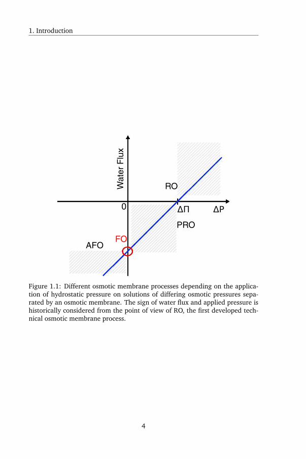
static pressure on one of the two solutions. This is illustrated in Figure 1.1,
defining the four possible combinations of hydrostatic and osmotic pressure.
FO is spontaneous osmosis without the application of hydrostatic pressure. If
hydrostatic pressure is applied to the FO feed solution, the process is called PAO
or pressure-assisted osmosis: hydrostatic pressure is applied to the feed solu-
tion to increase water flux [2]. If hydrostatic pressure is applied on the draw
solution, but not exceeding the draw solution osmotic pressure, the process is
2
A short description
called PRO or pressure-retarded osmosis [1]. In PRO, water still flows towards
the draw solution against a hydrostatic pressure gradient but along an osmotic
pressure gradient. Consequently, hydrostatic pressure in the draw solution fur-
ther increases due to water flux, allowing the conversion of osmotic pressure
into mechanical work or into electricity [3]. PRO could theoretically be used
to convert the mixing energy liberated upon mixing for instance fresh water
and seawater into electricity. In the fourth process, reverse osmosis (RO), hy-
drostatic pressure is applied to the draw solution exceeding the draw solution
osmotic pressure, causing fresh water to flow from the draw solution to the
feed solution. During RO, the draw solution is separated into fresh water and
a more concentrated remaining solution called RO brine or concentrate. RO
performs the opposite of osmosis, hence the name. It is also immediately clear
that RO cannot be a spontaneous process: a solute concentration gradient is
created across the membrane, while externally applied pressure is needed to
establish this gradient. Of the 4 processes, RO was the first to be technically
developed and optimized after the invention of practically useful membranes
by Sidney Loeb and Srinivasa Sourirajan. The other 3 processes have recently
become the subject of an intense research effort, although FO and PRO were
briefly explored in the 1970s and early 1980s by Loeb and others [4, 5, 6, 3].
RO is currently the only osmotic membrane process that has reached a fully de-
veloped, commercial stage: it is applied at very large scale to produce potable
water from seawater in arid or densely populated areas around the world. A re-
lated process using slightly more permeable membranes is called nanofiltration
(NF), which is widely used for purification of fresh water to remove hardness-
causing ions and soluble organic matter. With water and energy scarcity be-
coming more and more likely in the future, there is renewed interest in other
membrane processes as well, which could be used to produce clean water or
electricity.
As the process of osmosis continues in an isolated system, the feed solution
volume decreases and the solutes present in the feed are concentrated, while
the reverse is happening on the other side of the membrane: the draw so-
lution increases in volume and is becoming diluted. If the process would be
allowed to continue indefinitely, the process would approach an equilibrium
state where the osmotic pressure difference between both solutions disappears
and no more water flux would occur. From an application point of view, the
process should be stopped long before reaching equilibrium: water flux is pro-
3
1. Introduction
ΔP
Wat
er F
lux
ΔΠ0
RO
PRO
FOAFO
Figure 1.1: Different osmotic membrane processes depending on the applica-tion of hydrostatic pressure on solutions of differing osmotic pressures sepa-rated by an osmotic membrane. The sign of water flux and applied pressure ishistorically considered from the point of view of RO, the first developed tech-nical osmotic membrane process.
4
A short description
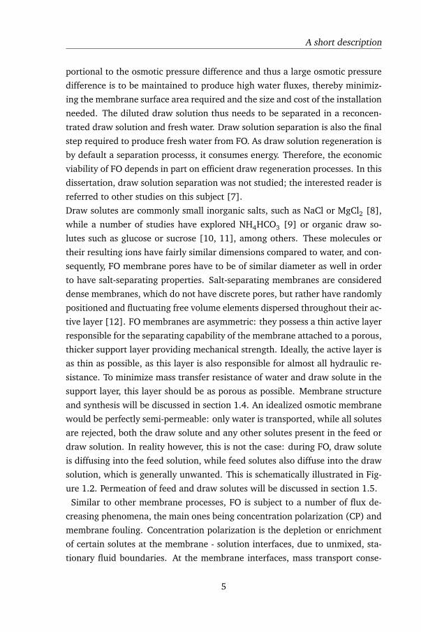
portional to the osmotic pressure difference and thus a large osmotic pressure
difference is to be maintained to produce high water fluxes, thereby minimiz-
ing the membrane surface area required and the size and cost of the installation
needed. The diluted draw solution thus needs to be separated in a reconcen-
trated draw solution and fresh water. Draw solution separation is also the final
step required to produce fresh water from FO. As draw solution regeneration is
by default a separation processs, it consumes energy. Therefore, the economic
viability of FO depends in part on efficient draw regeneration processes. In this
dissertation, draw solution separation was not studied; the interested reader is
referred to other studies on this subject [7].
Draw solutes are commonly small inorganic salts, such as NaCl or MgCl2 [8],
while a number of studies have explored NH4HCO3 [9] or organic draw so-
lutes such as glucose or sucrose [10, 11], among others. These molecules or
their resulting ions have fairly similar dimensions compared to water, and con-
sequently, FO membrane pores have to be of similar diameter as well in order
to have salt-separating properties. Salt-separating membranes are considered
dense membranes, which do not have discrete pores, but rather have randomly
positioned and fluctuating free volume elements dispersed throughout their ac-
tive layer [12]. FO membranes are asymmetric: they possess a thin active layer
responsible for the separating capability of the membrane attached to a porous,
thicker support layer providing mechanical strength. Ideally, the active layer is
as thin as possible, as this layer is also responsible for almost all hydraulic re-
sistance. To minimize mass transfer resistance of water and draw solute in the
support layer, this layer should be as porous as possible. Membrane structure
and synthesis will be discussed in section 1.4. An idealized osmotic membrane
would be perfectly semi-permeable: only water is transported, while all solutes
are rejected, both the draw solute and any other solutes present in the feed or
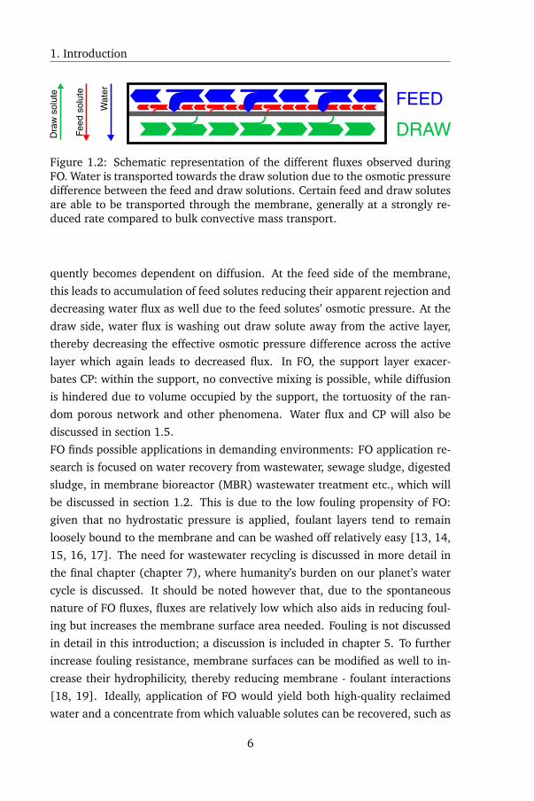
draw solution. In reality however, this is not the case: during FO, draw solute
is diffusing into the feed solution, while feed solutes also diffuse into the draw
solution, which is generally unwanted. This is schematically illustrated in Fig-
ure 1.2. Permeation of feed and draw solutes will be discussed in section 1.5.
Similar to other membrane processes, FO is subject to a number of flux de-
creasing phenomena, the main ones being concentration polarization (CP) and
membrane fouling. Concentration polarization is the depletion or enrichment
of certain solutes at the membrane - solution interfaces, due to unmixed, sta-
tionary fluid boundaries. At the membrane interfaces, mass transport conse-
5
1. Introduction
FEED
DRAW
Wat
er
Fee
d so
lute
Dra
w s
olut
e
Figure 1.2: Schematic representation of the different fluxes observed duringFO. Water is transported towards the draw solution due to the osmotic pressuredifference between the feed and draw solutions. Certain feed and draw solutesare able to be transported through the membrane, generally at a strongly re-duced rate compared to bulk convective mass transport.
quently becomes dependent on diffusion. At the feed side of the membrane,
this leads to accumulation of feed solutes reducing their apparent rejection and
decreasing water flux as well due to the feed solutes’ osmotic pressure. At the
draw side, water flux is washing out draw solute away from the active layer,
thereby decreasing the effective osmotic pressure difference across the active
layer which again leads to decreased flux. In FO, the support layer exacer-
bates CP: within the support, no convective mixing is possible, while diffusion
is hindered due to volume occupied by the support, the tortuosity of the ran-
dom porous network and other phenomena. Water flux and CP will also be
discussed in section 1.5.
FO finds possible applications in demanding environments: FO application re-
search is focused on water recovery from wastewater, sewage sludge, digested
sludge, in membrane bioreactor (MBR) wastewater treatment etc., which will
be discussed in section 1.2. This is due to the low fouling propensity of FO:
given that no hydrostatic pressure is applied, foulant layers tend to remain
loosely bound to the membrane and can be washed off relatively easy [13, 14,
15, 16, 17]. The need for wastewater recycling is discussed in more detail in
the final chapter (chapter 7), where humanity’s burden on our planet’s water
cycle is discussed. It should be noted however that, due to the spontaneous
nature of FO fluxes, fluxes are relatively low which also aids in reducing foul-
ing but increases the membrane surface area needed. Fouling is not discussed
in detail in this introduction; a discussion is included in chapter 5. To further
increase fouling resistance, membrane surfaces can be modified as well to in-
crease their hydrophilicity, thereby reducing membrane - foulant interactions
[18, 19]. Ideally, application of FO would yield both high-quality reclaimed
water and a concentrate from which valuable solutes can be recovered, such as
6
Possible FO applications
nutrient recovery from wastewater and wastewater treatment sludge.
1.2 Possible FO applications
FO is widely regarded as a low fouling propensity membrane process, as was
mentioned earlier, and FO membranes can reject most feed solutes and sus-
pended matter. As a result, FO is a niche process which can be applied on
highly fouling and/or highly saline feed streams. Such feeds are wastewater,
sludges resulting from wastewater treatment and anaerobic digestion, oil and
gas drilling wastewater, landfill leachate and liquid foods [20, 21, 22].
In wastewater treatment, both the produced water and concentrate are of in-
terest. Vast amounts of wastewater are produced [23]: in the order of 450
km3 annualy; reusing wastewater could decrease pressure on pristine water
sources. At the same time, wastewater often contains resources of interest.
Plant macronutrients such as nitrogeneous compounds, phosphate and potas-
sium end up in domestic and food industry wastewater. Phosphate and potas-
sium are predominantly produced from non-renewable mineral deposits [24],
while fixing nitrogen through the Haber-Bosch process is an energetically costly
endeavor. Wastewater also contains organic compounds, which can be con-
verted to bio-energy as methane gas or to chemical feedstocks through fermen-
tation or thermal processing. Currently, both nutrient extraction processes and
harvesting of bio-energy are often impeded by their low concentrations in do-
mestic wastewater [24, 25, 26]. Different separation processes and treatment
strategies are therefore investigated in order to yield economically viable re-
source recovery [25], which all share a concentration stage at the start of the
treatment train, either through biological or physico-chemical means.
FO is a suitable concentration stage for wastewater, as it extracts water while
rejecting the vast majority of all feed solutes and suspended matter. FO can be
used as a replacement of ultrafiltration (UF) or microfiltration (MF) in mem-
brane bioreactors (MBRs), called osmotic MBR (OMBR), which is operated
either aerobically or anaerobically. A possible downside of using OMBRs is
the accumulation of salts: salts present in the feed are concentrated, while re-
verse draw solute diffusion can add more salts - depending on the choice of
draw solute. Excess salts could hinder bacterial metabolism [27], which would
then hinder nutrient or energy recovery: bacterial metabolism and growth is
used to mineralize organic matter yielding inorganic nutrients, and to produce
7
1. Introduction
methane or volatile fatty acids through fermentation. A solution is to use UF
as a bleed on the feed: a relatively small amount of water is abstracted from
the feed through an UF membrane, which retains suspended matter but does
not retain salts. The UF permeate is then a high salinity, suspended matter-free
and nutrient-rich stream [28]. OMBRs are currently challenged by low water
fluxes: compared to UF or MF, the flux through FO membranes is easily more
than an order of magnitude lower, therefore significantly increasing the capital
cost of an OMBR. Also, all water extracted by FO has to be separated again
from the diluted draw solution, which inherently costs energy. Given the high
production rate of wastewater, the energy consumption rate by FO systems
would be high as well.
FO can also be used to dehydrate highly saline wastewater, originating from
certain industrial activities such as oil and gas extraction [29, 30, 31]. In this
case, the wastewater is too saline to be discharged, so the wastewater is de-
hydrated to the point where salts can be removed by crystalization. This is
known as zero-liquid discharge: all water from the feed is removed and salt
crystals are harvested as solids, thereby avoiding salinization of receiving soil
or water bodies. FO is applied before but not during crystalization: the fi-
nal dehydration is done using thermal means, as crystalization of salts on the
membrane surface is unwanted. The latter phenomenon, known as scaling,
reduces fluxes through the membrane and can also cause physical damage to
the membrane. When the feed is highly saline, the draw solution obviously
has to possess a high osmotic pressure as well. Draw solution regeneration is
then only possible using thermal means, as reverse osmosis cannot be used at
osmotic pressures exceeding 80 bar (corresponding roughly to a 1.2 M NaCl
solution, about one fifth of the concentration at saturation).
In the case of valuable streams in food and pharmaceutical industry, the main
focus is on the production of a concentrate with suitable characteristics [21,
31]. This means that reverse draw solute diffusion becomes a very impor-
tant process parameter: excessive leakage of the draw solution could spoil the
concentrate. For example, when fruit juice is being concentrated, sucrose is a
suitable draw solute: reverse diffusion of sucrose will be low as it is a fairly
large molecule, and fruit juice already has a high sucrose content [32]. The
gentle process conditions of FO are a major advantage in food and pharma-
ceutical industry: the process takes place at about ambient temperature and
pressure, which ensures minimal loss of nutritional value or loss of activity
8
On the origin of osmotic pressure
of pharmaceutical products. FO appears to be a very suitable technology in
food industry: dehydration of liquid food products is widely practiced and FO
retains nutritional value and aroma compounds much better than thermal or
vacuum processes, while energy consumption is likely much lower as well. Fur-
thermore, as the concentrate has a high value, the economics of FO are more
favorable compared to wastewater treatment. FO has been investigated exten-
sively for food and beverage concentration [32], and commercial FO module
producers such as FTS and Porifera offer food-safe systems.
1.3 On the origin of osmotic pressure
The chemical activity of a solvent or solute i at isothermic conditions containing
variable amounts of a dissolved solute and at variable pressure is given by:
dµi = RTdxixi
+ vdp (1.1)
with xi being the mole fraction of the solvent, and v being the solvent molar
volume. The solvent will be denoted by subscript l. The solvent chemical
potential at xl = 1 (pure solvent) is considered a reference situation, and is
denoted by superscript 0 in subsequent equations. Dissolving a solute in the
solvent decreases the solvent mole fraction: a volume of solution is shared by
solvent and solute, and so xl < 1. Integration between xl = 1 and xl = c with
xl < 1 yields for incompressible fluids:
µl(x) = µ0l +RTln(xl) + v(P (x)− P0) (1.2)
For xl < 1, ln(xl) < 0 showing that addition of solute decreases the chemical
activity of the solvent. Equation 1.2 is only valid for ideal solutions. Ideal solu-
tions assume no solute-solvent interactions nor preferential self-interaction of
the solute or solvent; solute and solvent are merely mixed in a certain volume
of solution. This is however not the case for most solutions: ideal behavior is
approached for very similar substances (for example, mixing hexane and hep-
tane), but this is not true for most solutions, especially aqueous solutions. In
that case, the solvent concentration is multiplied with a solute activity coeffi-
9
1. Introduction
cient γi for the specific solute-solvent pair, yielding solvent activity:
al = γixl (1.3)
Rewriting equation 1.2 and taking into account equation 1.3 yields:
∆µ = RTln(al) + v∆P (1.4)
It is clear from equation 1.4 that ∆µ can become zero by modulating ∆P , in
which the reduced activity due to the presence of a solute is neutralized by
increasing the hydrostatic pressure:
∆P = −RTvln(al) (1.5)
The pressure at which ∆µ becomes 0 in equation 1.4 and at which equation
1.5 is valid, is called the osmotic pressure, which will be denoted as ∆Π. Draw
solute concentration will be referred to as xd; in molar terms, the draw solute
concentration is low compared to the water concentration. For xd ≈ 0 and
consequently xl ≈ 1, γi ≈ 1, and thus ln(al) ≈ ln(xl). Still at xd ≈ 0, ln(al)
can be expanded as Taylor series, and only retaining the first 2 terms yields:
ln(xl) ≈ 1− xl. In molar fraction terms, xd = 1− xl, which leads to:
∆P =RT
vxd ≈
RT
v
cdcl
(1.6)
In equation 1.6, draw solute mole fraction was converted to concentration,
using the approximation that at low solute mole fraction:
xd =moles solute
moles solute+moles solvent≈ moles solute
moles solvent(1.7)
For the solvent, at low xd, vcl = 1, equation 1.6 reduces to the well-known
expression of osmotic pressure as the van ’t Hoff law:
∆Π = jcdRT (1.8)
in which j is a correction factor for the solute concentration in the case of so-
lutes splitting into multiple ions per molecule upon dissolving. The van ’t Hoff
law is valid at low solute concentrations; at high solute concentrations, devi-
10
Osmotic pressure
ation is noted due to the solute activity coefficient deviating from 1. In some
cases however, deviation is limited: for NaCl, the deviation is at most 20 %
throughout its entire solubility range.
The above derivation of osmotic pressure clearly indicates the origin of osmotic
pressure: osmotic pressure arises due the decreased concentration of solvent
in a solution compared to pure solvent. To reformulate, in a certain volume of
pure solvent, a fixed number of solvent molecules are to be found. If a solute
is added, then the number of solvent molecules in the same volume element
decreases as this volume is now shared with solute molecules (disregarding
electrostriction). The total volume of the solution has now increased and the
solvent concentration decreased, implying that the same number of solvent
molecules can now be found in a larger volume. Thereby, the likelihood is
decreased of finding a solvent molecule at any specific location within the so-
lution, and at the same time solvent molecules can now be found in a larger
volume. The solvent entropy has clearly increased upon dissolving a solute.
Similarly, the solute’s entropy has increased as well.
If entropy increases for both the solvent and solute upon dissolving of the so-
lute, one would expect solubility of solutes to increase indefinitely. For some
solutes, this is true: for instance, quite a few alcohols, polysaccharides and
polyethylene oxide are miscible with water in all proportions [33]. For many
solutes however, this is not the case: for instance, NaCl has a solubility limit
of 5.5 M or 359 g/L. This is due to attractive solute - solute interactions
(∆G121 < 0) and decreasing solute - solvent interactions at increasing solute
concentrations, while for infinitely soluble solutes, solute - solute interactions
are repulsive (∆G121 > 0) [33, 34], with ∆G121 denoting the Gibbs free energy
of self-interaction of a solute (1) dissolved in a solvent (2). From an entropy
point of view, solute - solvent interactions enforce a cage-like structure on wa-
ter: a cavity is formed around the solute, which is inherently unfavorable as
this imposes a structure on water, thereby causing a local decrease of entropy
[34]. For finitely soluble compounds, at a certain solute concentration, the to-
tal system has reached maximal entropy: entropy increase from mixing solute
and solvent is matched by local entropy decrease. At this solute concentration,
the solubility limit is reached.
11
1. Introduction
1.4 FO membrane structure and synthesis
In this section, structural characteristics of FO membranes are discussed, fol-
lowed by a brief overview of membrane synthesis methods. FO membranes are
asymmetric membranes: a thin active layer provides the separating capability
of the membrane, which is supported by a much thicker support layer provid-
ing mechanical strength. Membrane characteristics can be divided by active
layer and support layer characteristics, while membranes are synthesized us-
ing predominantly phase inversion (PI) or interfacial polymerization, leading
to thin film composite (TFC) membranes. Polymers predominantly used for FO
membrane synthesis are polyamide (PA) and polyethersulfone (PES) for the
active layer and support layer respectively of TFC membranes, and cellulose
triacetate (CTA) for PI membranes.
1.4.1 FO membrane synthesis
Phase inversion is a precipitation process in which a polymer is rapidly pre-
cipitated, causing the formation of a dense film. The process starts by cast-
ing a polymer solution onto a plate and spreading out the solution to attain
certain thickness. Subsequently, the solvent in which the polymer is soluble
is replaced by another solvent in which the polymer is insoluble, called the
non-solvent, which is typically done by immersing the plate in a non-solvent
bath. The solvent and non-solvent are mutually soluble or miscible. Due to the
introduction of the non-solvent and removal of the solvent, the polymer will
start to precipitate, forming a dense film at the polymer - non-solvent interface
which becomes the active layer of the membrane. As the process continues, the
non-solvent diffuses into the polymer film: due to kinetic effects, precipitation
deeper into the polymer film will create a porous structure comprising of zones
of dense polymer alternating with pores. This porous zone is the support layer
of the membrane.
TFC membranes are formed using interfacial polymerization which takes place
on the active layer of a preformed membrane, often a UF membrane, becom-
ing the support layer of the TFC membrane. TFC membranes hold some ad-
vantages over PI membranes: the separate production of the support layer and
active layer allows the tailoring of both layers separately. For TFC membranes
having a PA active layer, which is most common, the PA layer is synthesized
12
FO Membranes
in situ at the active layer of what will become the support layer. This is done
by contacting two solutions containing different monomers, causing the for-
mation of a PA film. For PA TFC membranes, the monomers are trimesoyl
chloride (TMC), a reactive and aromatic tricarboxylic acid derivative, and a
diamine, such as phenylene diamine or piperazine. TMC and the diamine are
dissolved in an apolar solvent and water respectively, with the solvents being
non-miscible, in order to maintain an interface at the site of polymerization.
Films are self-closing during synthesis: monomers diffuse into the solution of
the other monomer type, condensing at the interface of both solutions, thereby
closing pores through which the monomers were diffusing. Once a closed film
is formed, monomer diffusion is strongly hindered and the reaction is termi-
nated. The use of the aromatic phenylene diamine yields fully aromatic PA
films in which the polymer strands can be stacked more efficiently compared
to when the non-aromatic piperazine is used; the former resulting in films with
reduced permeability compared to the latter [35]. Consequently, fully aromatic
films find use in RO membranes, while semi-aromatic polyamide films find use
in NF membranes. Many variations are possible, such as blending different
monomers or varying the reaction time, again showing the versatility of this
process. For FO membranes, the most widely used membrane was a PI CTA
membrane produced by HTI (Albany, OR, USA). In recent years, TFC FO mem-
branes have become commercially available from companies such as Porifera,
Toray or Aquaporin.
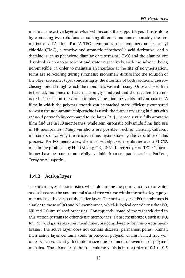
1.4.2 Active layer
The active layer characteristics which determine the permeation rate of water
and solutes are the amount and size of free volume within the active layer poly-
mer and the thickness of the active layer. The active layer of FO membranes is
similar to those of RO and NF membranes, which is logical considering that FO,
NF and RO are related processes. Consequently, some of the research cited in
this section pertains to other dense membranes. Dense membranes, such as FO,
RO, NF, and gas separation membranes, are considered to be non-porous mem-
branes: the active layer does not contain discrete, permanent pores. Rather,
their active layer contains voids in between polymer chains, called free vol-
ume, which constantly fluctuate in size due to random movement of polymer
moieties. The diameter of the free volume voids is in the order of 0.1 to 0.5
13
1. Introduction
nm for PA [36, 37], a slightly larger value of 0.65 nm has been reported for
CTA [38]. For NF membranes, the free volume voids are larger and are in the
transition zone towards permanent pores. The free volume fraction within a
polymer is reported to be in the order of 7 - 9% for PA as measured by PALS
(Positron Annihilation Lifetime Spectroscopy) [36]. These results agree well
with those obtained by Freger [39] who studied swelling of isolated PA active
layers in water, finding swelling ratios of 5 - 12 % for RO membranes. Free
volume and the degree of swelling are strongly correlated [40] but are how-
ever not completely interchangeable as swelling causes the polymer chains to
extend thereby increasing the free volume [38]. For CTA and other cellulose
esters, the free volume fraction as measured by PALS is somewhat lower: 2%
has been reported for CTA [38] and 4 - 5% for a number of other cellulose
esters [41, 42].
The tricarboxylic monomer TMC used in PA films enables the formation of
crosslinks, which creates a macro-molecular 3D-polymer network rather than
individual polymer chains. Both simulation and membrane characterization
results [43, 39] suggest that a 3D-polymer network is inherently more perme-
able than an array of unlinked linear polymer chains, such as CTA: it is theo-
rized that 3D-polymer networks contain a much larger permanent void fraction
within the polymer, where diffusivity of solvent and solutes is relatively high,
while the separation of solvent from solutes takes place in thin zones of high
polymer density [39]. In arrays of unlinked polymer chains however, a much
smaller permanent void fraction causes hindrance against diffusion for solutes
and solvent over a longer distance. This can be seen in the free volume results
presented above as well. Separation is then achieved by increased hindrance
of solutes compared to the solvent, at a cost of decreased solvent permeabil-
ity. Crosslinked polymer networks cannot be produced using phase inversion
(disregarding post-processing): PI membranes are produced from polymer so-
lutions, while crosslinked polymers are inherently insoluble. In a crosslinked,
macro-molecular polymer network, a solvent cannot completely wet and en-
velop polymer chains, which is needed for solubilization, because the polymer
chains are covalently bound to each other. The above reasoning again shows
why TFC membranes are superior to PI membranes; consequently, their mar-
ket share dominates over PI membranes [44]. CTA is an uncharged polymer,
however, the surface charge of CTA membranes has been shown to be slightly
negative, which could be due to surface oxidation resulting in carboxylic acid
14
FO Membranes
groups or due to the adsorption of poorly hydrated anions [45]. TFC mem-
branes on the other hand, contain both amine and carboxylic acid functional
groups, and, due to the higher concentration of carboxylic acid groups in the
PA polymer, TFC membranes have a net negative surface charge [46, 47].
PA TFC RO and NF membranes have an active layer thickness of around 200
and 20 nm respectively based on AFM measurements of active layers isolated
from their support [39]. This isolation procedure is only possible for TFC mem-
branes: PI membranes are composed of a single polymer with the active layer
gradually transitioning into the support layer. The active layer thickness of
PI membranes can however be determined by PALS: for cellulose acetate FO
membranes prepared using different PI conditions, the resulting active layer
was found to vary from 100 to 800 nm [41].
1.4.3 Support layer
The support layer has no direct influence over the separating properties of
a membrane, as these are determined by the active layer, but it has a pro-
found influence on mass transfer, especially for FO. Important characteristics
are the support thickness, porosity, tortuosity and hydrophilicity. Compared to
NF and RO membranes, the support layer in FO membranes is much thinner:
the support does not need to be able to withstand high pressure because no
hydrostatic pressure is applied; support thickness is generally between 50 and
100 µm [9, 48]. Porosity and tortuosity are somewhat related: theoretical and
empirical study on porous media has shown that tortuosity is inversely related
to porosity [49]. Tortuosity can furthermore be limited by producing support
layers having finger-like macrovoids perpendicular to the active layer [50, 51],
these macrovoids can be produced by tweaking the process parameters of PI.
Tortuosity cannot be measured directly, but can be inferred from mass transfer
modeling, which will be discussed in section 1.5. Huang and McCutcheon have
shown that increasing the support pore size subsequently increases FO water
flux as well, although an optimal pore size exists beyond which the active layer
is no longer supported, causing the membrane to fail [52]. Potentially very
porous and low tortuosity support layers can be produced using electrospin-
ning. Using this technique, a non-woven fabric of fibers less than 1 µm can be
produced. This contrasts with a more sponge-like structure of support layers
produced by phase inversion. However, poor adhesion between active and sup-
15
1. Introduction
port layers has been reported as well [53]. Finally, McCutcheon and Elimelech
have shown that hydrophobicity of the support layer reduces water flux, likely
due to incomplete hydration of the support layer [54]: small air bubbles would
remain trapped in the support layer after hydration of the membrane, thereby
blocking liquid mass transfer in the support layer.
1.5 Mass transfer during osmosis
In FO, all fluxes are spontaneous, and can be divided in three categories: the
water flux, feed solutes flux and draw solute flux. The draw solute flux is di-
rected oppositely with respect to the other fluxes, and is referred to as reverse
draw solute diffusion (RSD). The water flux and draw or feed solute fluxes are
determined by both active layer properties and driving forces for flux across the
active layer, being osmotic pressure in the case of water flux and concentration
differences in the case of feed and draw solute fluxes. As the draw solute
simultaneously generates the osmotic pressure difference and is subject to con-
centration polarization, no explicit expression for water flux can be written. As
a result, water and draw solute fluxes have to be modeled iteratively. Rejection
of feed and draw solutes is determined by the active layer properties, but con-
centration polarization causes the apparent rejection to be different from the
real rejection.
1.5.1 Active layer permeability and rejection mechanisms
FO membranes are permeable to some extent to solutes up until the size of
their free volume voids, solutes larger than the free volume voids cannot en-
ter the membrane and are therefore rejected due to steric hindrance. Because
there is a size distribution of free volume voids and their dimensions are subject
to random fluctuation as well, the maximum solute size which can permeate
through the membrane cannot be sharply defined. Commonly, the upper so-
lute size limit is expressed as the molecular weight cut off (MWCO), being the
molecular weight of an organic solute showing a rejection of 90 %. This is
however not a strict definition. For CTA FO membranes, the MWCO lies in the
order of 250 g/mole [31], which is higher compared to RO membranes and
comparable to tight NF membranes. TFC FO membranes reportedly show im-
proved rejection of organic solutes [45], consequently, their MWCO is lower as
16
Mass transfer
well. Steric hindrance is caused by dimensional restrictions, while the MWCO
denotes the weight of a solute. Molecular dimensions and weight are obvi-
ously correlated, but it has been shown that projected molecular surface area
correlates stronger with rejection than molecular weight [55]. In addition,
non-steric rejection mechanisms are not taken into account in the MWCO. Ions
of salts commonly used as draw solutes, such as Mg2+, Na+, NH +4 , Cl– , SO 2 –
4
or HCO –3 , are fairly small ions, with effective hydrated radii in the order of
0.2 - 0.4 nm [56, 57]. The hydrated ions are thus somewhat larger than water,
but still smaller than the free volume voids present in the membrane active
layers. It is clear that rejection of ionic solutes, especially small inorganic ions,
has to stem from membrane interactions other than steric hindrance. Aside
from steric hindrance, ionic solutes are also subject to electrostatic repulsion,
electromigration and dielectric exclusion.
A charged membrane surface will cause electrostatic repulsion of solution co-
ions causing low co-ion permeation. Counterions will be electrostatically at-
tracted to the membrane and permeate relatively fast due to electromigration,
but due to charge neutrality during steady-state transport, the permeability of
counterions will be low as well. In this case, an electric potential difference
called Donnan potential will develop across the membrane: the Donnan poten-
tial will counter the effect of counterion electromigration, thereby decreasing
counterion permeation and increasing co-ion permeation [58]. Assuming one
of the salts in the system is present at a much higher concentration than other
salts, such as an ionic draw solute, then the electric field established across
the membrane will be dominated by the ionic permeances of the dominant salt
ions. The electric field will also cause electro-migration of other ions present
in the draw or feed solution, which can cause negative rejection of mobile feed
ions [59, 60]. Charge-neutral ion exchange across the membrane is possible as
well: ions permeate across the membrane in both directions and equal amounts
of charge, which is called Donnan dialysis. In FO, Donnan dialysis can occur
between feed and draw solute ions [61, 62], depending on the mobility of the
ions.
Dielectric exclusion is an electrostatic interaction between an ionic solute and a
polarization charge induced on the surface of the membrane polymer. Because
the relative permittivity of the polymer is much lower than that of water, the
induced polarization charge has the same sign as the ion, regardless of the ion
charge. This causes additional electrostatic repulsion of the ion [63, 64, 65]. A
17
1. Introduction
second dielectric phenomenon is the decrease of the water relative permittivity
in confined, sub-nanometer sized pores, increasing the solvation free energy
of ions. This is caused by steric constraints: the very high relative permittivity
of water (∼80 at ambient temperature compared to 2 - 5 for organic poly-
mers) is due to the dipolar nature of water, which stems from its asymmetric
structure and the large difference between oxygen and hydrogen electronega-
tivity. The high relative permittivity can however only be attained when water
molecules can gyrate in response to an applied electrical field, however, in a
sub-nanometer confined space, gyration is hindered. As a result, electrostatic
interactions between water and ions inside pores are weakened [63]. Conse-
quently, nano-confined water is a poorer solvent for ions than bulk water, and
transport of ions is reduced. Through this mechanism, ions can be rejected by
pores which are of similar diameter as a hydrated ion.
The diffusivity of species permeating through the active layer decreases rela-
tive to their bulk diffusivity as their size approaches the free volume void size
of the membrane: movement of both water and solutes becomes increasingly
hindered as their size approaches that of the voids in which they reside. In
PA TFC RO membranes, the diffusivity of water was found to be 2 - 3 times
lower than its bulk diffusivity [66]. Diffusivity of small organic solutes such as
ethylene glycol, glycerol and 3 mono-alcohols in another TFC RO membrane
were measured by Draževic et al [40], finding that diffusivity of the solutes
was reduced with factors of 10-4 - 10-6. This shows that steric hindrance in RO
membranes increases swiftly with increasing solute size, causing dramatic dif-
fusivity reduction of the solutes involved. FO membranes are somewhat more
permeable, however, similar steep increases when the solute size approaches
free volume void size are to be expected as well. In membranes with larger
pore size, hindrance against diffusion is reduced: when studying hindered
transport in crosslinked PVA films with a pore size of 2.24 nm (correspond-
ing with a loose NF or very tight UF membrane), diffusivity reductions of 10-3
- 10-4 were found for organic pigments with molecular weights of 200 - 1000
g/mole [67]. Compared to organic solutes, diffusion of inorganic salts appears
to be much more hindered at first sight. For instance, assume an FO membrane
has a NaCl permeability coefficient of 4·10-8 m/s and the effective NaCl con-
centration difference across the active layer is 1 mole/L, then JNaCl = 4·10-5
mole/(m2s). Assume now the active layer would be suddenly removed, and
bulk diffusion would occur between both solutions, then the instantaneous dif-
18
Mass transfer
fusive flux would be 8 mole/(m2s) if we assume an active layer thickness of
200 nm and a bulk diffusivity of 1.6·10-9 m2/s of NaCl. The difference is a fac-
tor of 2·105, even though Na+ and Cl– are relatively small and poorly hydrated
ions. This difference however is not due to hindered diffusion: ion diffusivity
study in RO active layers has shown that hindrance against diffusion in SWC1
and ESPA4 RO membranes only amounted to a factor of about 10-2 [68]. A low
salt permeation rate in RO, NF and FO is due to low partitioning of inorganic
electrolytes into the membranes.
1.5.2 Concentration polarization
Similar to other mass transfer processes, FO is subject to concentration polar-
ization (CP). CP is the formation a concentration difference between a bulk
solution and a fluid boundary layer, such as a solution - membrane interface,
due to unequal mass transfer rates of the different species. CP can be dilutive or
concentrative, depending on whether the solute(s) concentration in the inter-
face decreases or increases respectively. In pressure-driven membrane systems,
such as RO and NF, CP appears externally (ECP) at the feed solution - mem-
brane interface. In FO on the other hand, ECP appears twice: at both the feed
and draw solution - membrane interfaces. CP also appears internally (ICP) in
FO: depending on the membrane orientation, the draw solute is diluted in the
support layer (dilutive ICP), or feed solutes combined with leaked draw solute
accumulate in the support layer (concentrative ICP). In the former case, the
membrane is oriented with the active layer facing the feed solution (AL-FS),
while in the latter case, the active layer is facing the draw solution (AL-DS).
The latter case is also the membrane orientation employed during PRO, which
is why some texts refer to this as "PRO mode". This orientation prevents ac-
tive layer delamination when the draw solution is pressurized during PRO: in
AL-DS orientation, the hydrostatic pressure compresses the active layer against
the backing of the support layer, while in AL-FS orientation, a pressurized draw
solution would cause the active layer to tear off the support layer. The concen-
tration profiles of both membrane orientations are shown in Figure 1.3. FO has
2 ECP boundaries, one concentrative and one dilutive [69, 70, 71], because FO
is a membrane contactor process: the feed and draw solution are contacted
by the FO membrane and both solutions are recirculated. In contrast, RO and
NF depend solely on a feed solution; flux is produced due to the application
19
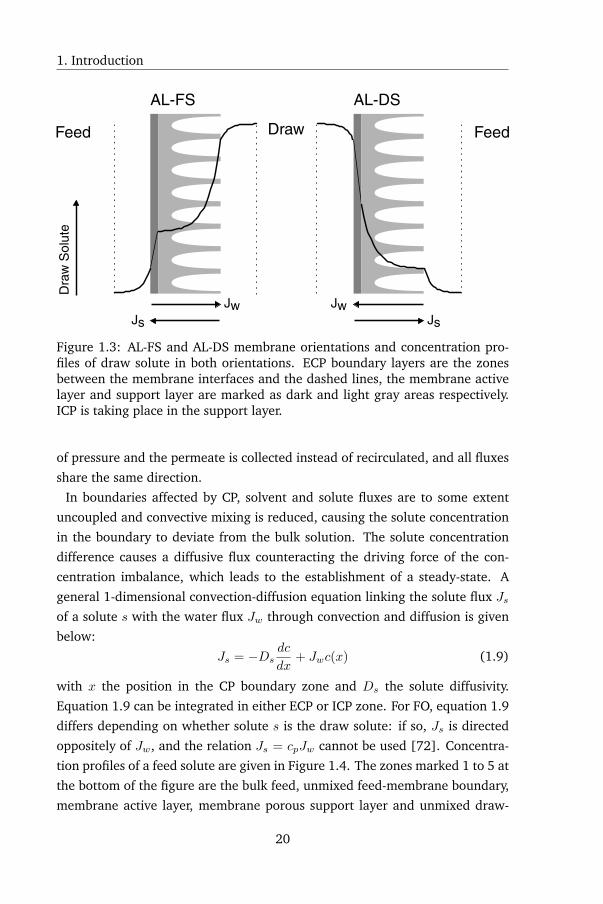
1. Introduction
Feed Draw Feed
Dra
w S
olut
e
AL-FS AL-DS
Jw JwJsJs
Figure 1.3: AL-FS and AL-DS membrane orientations and concentration pro-files of draw solute in both orientations. ECP boundary layers are the zonesbetween the membrane interfaces and the dashed lines, the membrane activelayer and support layer are marked as dark and light gray areas respectively.ICP is taking place in the support layer.
of pressure and the permeate is collected instead of recirculated, and all fluxes
share the same direction.
In boundaries affected by CP, solvent and solute fluxes are to some extent
uncoupled and convective mixing is reduced, causing the solute concentration
in the boundary to deviate from the bulk solution. The solute concentration
difference causes a diffusive flux counteracting the driving force of the con-
centration imbalance, which leads to the establishment of a steady-state. A
general 1-dimensional convection-diffusion equation linking the solute flux Jsof a solute s with the water flux Jw through convection and diffusion is given
below:
Js = −Dsdc
dx+ Jwc(x) (1.9)
with x the position in the CP boundary zone and Ds the solute diffusivity.
Equation 1.9 can be integrated in either ECP or ICP zone. For FO, equation 1.9
differs depending on whether solute s is the draw solute: if so, Js is directed
oppositely of Jw, and the relation Js = cpJw cannot be used [72]. Concentra-
tion profiles of a feed solute are given in Figure 1.4. The zones marked 1 to 5 at
the bottom of the figure are the bulk feed, unmixed feed-membrane boundary,
membrane active layer, membrane porous support layer and unmixed draw-
20
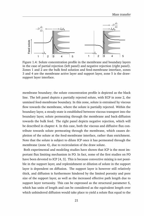
Mass transfer
Jwcp
Jw
JwcpF
eed
solu
te
Jw
1 2 3 4 5 1 2 3 4 5
Figure 1.4: Solute concentration profile in the membrane and boundary layersin the case of partial rejection (left panel) and negative rejection (right panel).Zones 1 and 2 are the bulk feed solution and feed-membrane interface, zones3 and 4 are the membrane active layer and support layer, zone 5 is the draw-support layer interface.
membrane boundary; the solute concentration profile is depicted as the black
line. The left panel depicts a partially rejected solute, with ECP in zone 2, the
unmixed feed-membrane boundary. In this zone, solute is entrained by viscous
flow towards the membrane, where the solute is partially rejected. Within the
boundary layer, a steady-state is established between viscous transport into the
boundary layer, solute permeating through the membrane and back-diffusion
towards the bulk feed. The right panel depicts negative rejection, which will
be described in chapter 4. In this case, both the viscous and diffusive flux con-
tribute towards solute permeating through the membrane, which causes de-
pletion of the solute at the feed-membrane interface, rather than enrichment.
Note that the solute is subject to dilute ICP once it has permeated through the
membrane (zone 4), due to recirculation of the draw solute.
Both experimental and modeling studies have shown that ICP is the most im-
portant flux limiting mechanism in FO. In fact, some of the first studies on FO
have been devoted to ICP [4, 3]. This is because convective mixing is not possi-
ble in the support layer, and replenishment or dilution of solute in the support
layer is dependent on diffusion. The support layer is however still relatively
thick, and diffusion is furthermore hindered by the limited porosity and pore
size of the support layer, as well as the increased effective path length due to
support layer tortuosity. This can be expressed as the structural parameter S,
which has units of length and can be considered as the equivalent length over
which unhindered diffusion would take place to yield a solute flux equal to the
21
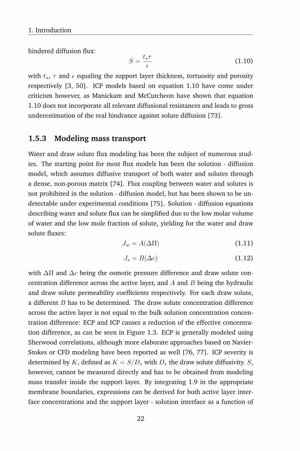
1. Introduction
hindered diffusion flux:
S =tsτ
ε(1.10)
with ts, τ and ε equaling the support layer thickness, tortuosity and porosity
respectively [3, 50]. ICP models based on equation 1.10 have come under
criticism however, as Manickam and McCutcheon have shown that equation
1.10 does not incorporate all relevant diffusional resistances and leads to gross
underestimation of the real hindrance against solute diffusion [73].
1.5.3 Modeling mass transport
Water and draw solute flux modeling has been the subject of numerous stud-
ies. The starting point for most flux models has been the solution - diffusion
model, which assumes diffusive transport of both water and solutes through
a dense, non-porous matrix [74]. Flux coupling between water and solutes is
not prohibited in the solution - diffusion model, but has been shown to be un-
detectable under experimental conditions [75]. Solution - diffusion equations
describing water and solute flux can be simplified due to the low molar volume
of water and the low mole fraction of solute, yielding for the water and draw
solute fluxes:
Jw = A(∆Π) (1.11)
Js = B(∆c) (1.12)
with ∆Π and ∆c being the osmotic pressure difference and draw solute con-
centration difference across the active layer, and A and B being the hydraulic
and draw solute permeability coefficients respectively. For each draw solute,
a different B has to be determined. The draw solute concentration difference
across the active layer is not equal to the bulk solution concentration concen-
tration difference: ECP and ICP causes a reduction of the effective concentra-
tion difference, as can be seen in Figure 1.3. ECP is generally modeled using
Sherwood correlations, although more elaborate approaches based on Navier-
Stokes or CFD modeling have been reported as well [76, 77]. ICP severity is
determined by K, defined as K = S/Ds with Ds the draw solute diffusivity. S,
however, cannot be measured directly and has to be obtained from modeling
mass transfer inside the support layer. By integrating 1.9 in the appropriate
membrane boundaries, expressions can be derived for both active layer inter-
face concentrations and the support layer - solution interface as a function of
22
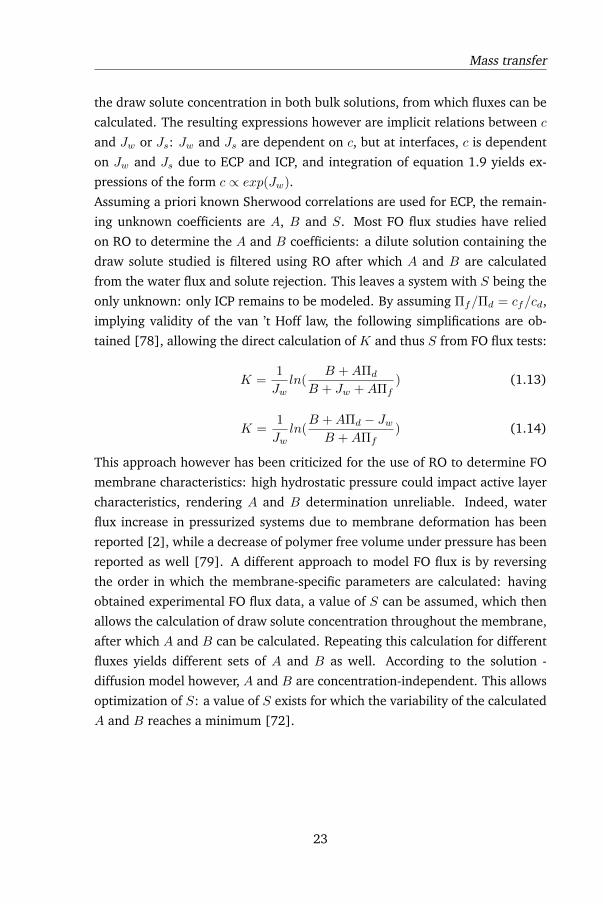
Mass transfer
the draw solute concentration in both bulk solutions, from which fluxes can be
calculated. The resulting expressions however are implicit relations between c
and Jw or Js: Jw and Js are dependent on c, but at interfaces, c is dependent
on Jw and Js due to ECP and ICP, and integration of equation 1.9 yields ex-
pressions of the form c ∝ exp(Jw).
Assuming a priori known Sherwood correlations are used for ECP, the remain-
ing unknown coefficients are A, B and S. Most FO flux studies have relied
on RO to determine the A and B coefficients: a dilute solution containing the
draw solute studied is filtered using RO after which A and B are calculated
from the water flux and solute rejection. This leaves a system with S being the
only unknown: only ICP remains to be modeled. By assuming Πf/Πd = cf/cd,
implying validity of the van ’t Hoff law, the following simplifications are ob-
tained [78], allowing the direct calculation of K and thus S from FO flux tests:
K =1
Jwln(
B +AΠd
B + Jw +AΠf) (1.13)
K =1
Jwln(
B +AΠd − JwB +AΠf
) (1.14)
This approach however has been criticized for the use of RO to determine FO
membrane characteristics: high hydrostatic pressure could impact active layer
characteristics, rendering A and B determination unreliable. Indeed, water
flux increase in pressurized systems due to membrane deformation has been
reported [2], while a decrease of polymer free volume under pressure has been
reported as well [79]. A different approach to model FO flux is by reversing
the order in which the membrane-specific parameters are calculated: having
obtained experimental FO flux data, a value of S can be assumed, which then
allows the calculation of draw solute concentration throughout the membrane,
after which A and B can be calculated. Repeating this calculation for different
fluxes yields different sets of A and B as well. According to the solution -
diffusion model however, A and B are concentration-independent. This allows
optimization of S: a value of S exists for which the variability of the calculated
A and B reaches a minimum [72].
23
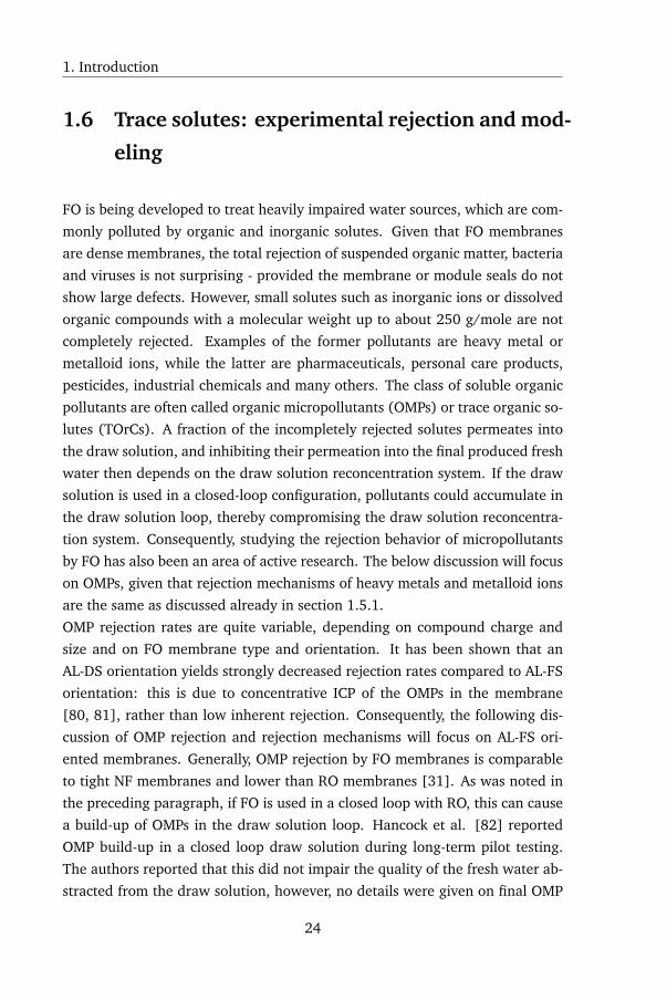
1. Introduction
1.6 Trace solutes: experimental rejection and mod-
eling
FO is being developed to treat heavily impaired water sources, which are com-
monly polluted by organic and inorganic solutes. Given that FO membranes
are dense membranes, the total rejection of suspended organic matter, bacteria
and viruses is not surprising - provided the membrane or module seals do not
show large defects. However, small solutes such as inorganic ions or dissolved
organic compounds with a molecular weight up to about 250 g/mole are not
completely rejected. Examples of the former pollutants are heavy metal or
metalloid ions, while the latter are pharmaceuticals, personal care products,
pesticides, industrial chemicals and many others. The class of soluble organic
pollutants are often called organic micropollutants (OMPs) or trace organic so-
lutes (TOrCs). A fraction of the incompletely rejected solutes permeates into
the draw solution, and inhibiting their permeation into the final produced fresh
water then depends on the draw solution reconcentration system. If the draw
solution is used in a closed-loop configuration, pollutants could accumulate in
the draw solution loop, thereby compromising the draw solution reconcentra-
tion system. Consequently, studying the rejection behavior of micropollutants
by FO has also been an area of active research. The below discussion will focus
on OMPs, given that rejection mechanisms of heavy metals and metalloid ions
are the same as discussed already in section 1.5.1.
OMP rejection rates are quite variable, depending on compound charge and
size and on FO membrane type and orientation. It has been shown that an
AL-DS orientation yields strongly decreased rejection rates compared to AL-FS
orientation: this is due to concentrative ICP of the OMPs in the membrane
[80, 81], rather than low inherent rejection. Consequently, the following dis-
cussion of OMP rejection and rejection mechanisms will focus on AL-FS ori-
ented membranes. Generally, OMP rejection by FO membranes is comparable
to tight NF membranes and lower than RO membranes [31]. As was noted in
the preceding paragraph, if FO is used in a closed loop with RO, this can cause
a build-up of OMPs in the draw solution loop. Hancock et al. [82] reported
OMP build-up in a closed loop draw solution during long-term pilot testing.
The authors reported that this did not impair the quality of the fresh water ab-
stracted from the draw solution, however, no details were given on final OMP
24
Trace solutes
concentrations. It does however raise doubts about FO-RO in closed-loop being
a double barrier against OMPs.
Charged compounds generally show high rejection (90% or above) and little
size-dependence, as was noted in many studies [82, 11, 81, 83, 31]. Although
most FO membranes have a negative surface charge, rejection of cationic OMPs
is equally high as anionic OMP rejection [82]. This could be due to Donnan
exclusion or dielectric exclusion. For uncharged compounds, more variable re-
jection is seen: influences of solute size (as correlated with molecular weight)
and of solute hydrophobicity [82, 31] have been reported, although other stud-
ies have not found an influence of hydrophobicity [45, 83]. It should be noted
however that for hydrophobic compounds, rejection is a two-stage process: in
a first stage, the solute adsorbs onto the membrane, because most polymers
are less polar than water. This causes preferential adsorption of the solute and
partitioning in the polymer phase, but not permeation through the membrane.
The observed rejection of the hydrophobic OMPs is very high during the first
stage. Following that is a breakthrough stage, in which the feed side of the
membrane becomes saturated and diffusion of the OMPs into the membrane
takes place. At a certain point, saturation of the active layer is complete and
the OMPs permeate through the membrane, yielding generally a low rejection
[84]. It is possible that from the above mentioned FO studies, no reliable con-
clusion regarding the influence of OMP hydrophobicity can be drawn due to
different experimental run times between studies: benchtop experiments typi-
cally last between a few to 24 hours. In the case of strong solute adsorption, a
steady-state solute permeation will not be reached in that timeframe [85]. So-
lute - membrane affinity, which is more general concept than hydrophobicity
and is based on Gibbs free energy of interaction, has been shown to influ-
ence OMP rejection in NF by modulating OMP partitioning into the membrane
[86, 87]. As this also pertains to non-hydrophobic solutes, it is not necessar-
ily an adsorption-mediated interaction. OMP size is, unsurprisingly, inversely
proportional to OMP permeability [84, 31, 83]. Although molecular weight is
often used as a measure of solute size because of its straightforward applica-
tion, molecular dimensions such as width or projected surface area offer better
correlations with solute rejection [88, 89]. The concepts of diffusion through
polymer free volume and molecular weight cut off have been discussed in sec-
tion 1.5.1.
Models describing solute transport in FO membranes can be categorized based
25
1. Introduction
on whether they are mechanistic or black box, and for models of the for-
mer type, on the assumption of porous or non-porous transport. In the fol-
lowing discussion, only mechanistic models will be highlighted. The inter-
ested reader is referred to the studies by Spiegler and Kedem on irreversible
thermodynamics-based membrane transport models [90]. Mechanistically, porous
and diffusional transport models differ with regards to convective transport:
convective coupling of solvent and solute fluxes is assumed in porous transport,
while in the solution-diffusion model, convective transport is assumed to be ab-
sent [91]. Consequently, both models will be referred to as solution-diffusion
(SD) and convection-diffusion (CD) models. The following discussion will fo-
cus on transport of uncharged solutes, as charged solutes complicate transport
modeling significantly: electromigration, Donnan exclusion and dielectric ex-
clusion all come into play simultaneously. Further elaboration of charged so-
lute transport is outside of the scope of this introduction, and the interested
reader is referred to the studies by Yaroshchuk, Bowen, Szymczyk and others
[63, 64, 92, 93, 58, 94, 95, 96] for more information.
Although FO membranes are dense membranes, the upper limit of their free
volume void size lies in the transition zone between solution-diffusion trans-
port and porous transport. According to the statistical thermodynamics calcu-
lations of Longuet-Higgins and Austin [97], the transition zone starts at a pore
radius of 0.45, which equals 2 times the radius of water. In pores below this
size, water molecules would not be able to develop a parabolic flow pattern
typical for porous transport, and transport would be limited to a diffusional
mechanism. The transition zone was also discussed by Baker [98] based on
the comparison of experimental rejection data of RO, NF and tight UF mem-
branes. At the low end of the membrane pore size, RO membranes reject all
solutes to a high degree, while at the high end, tight UF membranes still re-
ject divalent salts such as MgSO4 and somewhat larger solutes such as sucrose
fairly well, while monovalent salts such as NaCl and small solutes such as glyc-
erol are rejected poorly (<50 %), indicative of sieving and porous transport.
NF membranes span a pore size range which is intermediate: the permeability
of water, salt and small organics changes dramatically with small changes in
the membrane pore size. The equations governing water and solute transport
for the SD model have been given in section 1.5.3, equations 1.11 and 1.12.
26
Trace solutes
Rejection of an uncharged feed solute is defined as:
R = 1− cpcm
(1.15)
with cp and cm being the feed solute concentration in the permeate and the
feed solution - membrane interface. Combining equations 1.12 and 1.15 yields
the following relation:
RSD =Jw
B + Jw(1.16)
From equation 1.16, it is clear that rejection is 0 for Jw = 0 and rejection is 1 for
Jw → ∞. Porous transport on the other hand is composed of both diffusional
and convective transport. Membrane pores are assumed to be cylindrical or
slit-like and transect the membrane end-to-end. The equation describing cou-
pled convective and diffusive solute transport has likewise been given in sec-
tion 1.5.2, equation 1.9. Integration of equation 1.9 between both membrane
interfaces yields the following well-known expression for uncharged solute re-
jection:
RCD = 1− βφKc
1− (1− φKc)exp(−JwKcLD∞Kd
)(1.17)
with Kc, Kd, φ, β, D∞ and L being the hindrance factors against convection
and diffusion respectively, the solute partitioning coefficient, ECP factor, solute
diffusivity in the bulk solution and the active layer structural parameter com-
posed of thickness, porosity and tortuosity. In equation 1.17, the exponential
term contains the ratio of convective to diffusive transport rates, called the Pé-
clet number: Pe = JwKcLD∞Kd
. Both the hindrance factors and solute partitioning
coefficient are functions of the dimensionless solute size, defined as: λ = rsrp
with rs and rp being the solute and pore radius. The CD model thus offers a
way to calculate the effective membrane pore size: if the relations between λ
and the hindrance factors and partition coefficient are known, λ can be calcu-
lated explicitly, which combined with dimensional data of the studied solute(s)
yields rp. Relations between Kc, Kd and λ have been developed by Bungay
and Brenner [99] and Deen [100, 101], among others.
Both SD and CD-type models have been used successfully to model OMP rejec-
tion in FO, but also in NF and RO. CD models were used by Xie et al. [11, 45]
to relate FO membrane properties to OMP rejection. It was found that the pore
radii of both the HTI CTA and TFC FO membranes were around 0.40 nm, even
27
1. Introduction
though the TFC membrane exhibited better OMP rejection than the CTA mem-
branes. This was hypothesized to be due to stronger pore hydration of the TFC
membrane, creating a lower effective pore radius. The pore sizes obtained by
Xie et al. appear to be rather high compared to the results obtained by Wang et
al. [87], who studied the pore size of 2 NF and 1 brackish water RO membrane
under different pH and salinity conditions, finding a pore radius of 0.30 - 0.35
nm for the most permeable NF membrane, with the other membranes having
pore radii of 0.2 to 0.25 nm. This difference could be due to the different so-
lute partitioning models employed by both authors: Xie et al. assumed only
steric interactions, while the partitioning model used by Wang et al. included
both solute-membrane affinity and steric interactions. Kong et al. has used the
SD model to model the transport of haloacetic acids [83] and pharmaceuticals
[102]. FO and RO were compared using the same membrane, finding very
similar permeability coefficients in both cases. Model fitting of rejection in AL-
DS orientation did not yield good correlation, which could be due to errors in
the current models for the membrane structural parameter, as was discussed
previously.
Although mechanistically different, the solution-diffusion model and convection-
diffusion models yield similar results at low water fluxes. This is illustrated in
Figure 1.5, where calculated solute rejection by both models is shown (disre-
garding ECP). In Figure 1.5, for the SD model, a solute permeability coefficient
of 1·10-6 was assumed, while for the CD model φ = 0.15 and Kc = 1 were
assumed. Then, by fitting only the Péclet number of the CD model, a solute
rejection curve very similar to the SD curve was obtained. However, for a flux
of 10-4 m/s, the SD model rejection is 0.99, while it is 0.85 (=1-φ) for the CD
model. The upper limit of equation 1.17 shows the different behavior of CD
models compared to the SD model: for Jw → ∞, R = 1 − βφKc for the CD
model, while R = 1 for the SD model. This difference is due to convective
solute transport: partially sieved solutes are entrained by the water flux and
consequently, at their limiting rejection, their flux increases proportionally with
water flux. In the SD model on the other hand, solute flux is constant and the
solute rejection increases asymptotically to 1 with increasing water flux: the
solute flux is asymptotically infinitely diluted by the water flux. Water fluxes
high enough to approach the limiting rejection are hard to reach experimen-
tally, thus the flux region where the models deviate is largely inaccessible: for
FO and RO, a flux of 10-5 µm/s is already very high. This is shown below, by
28
Trace solutes
analyzing the Péclet number. The condition for approaching the limiting flux
is Pe >> 1, when convective transport dominates over diffusive transport. In
the denominator, D∞ and Kd are in the order of 10-9 to 10-10 and 10-3 to 10-4
respectively, yielding 10-12 to 10-14. This is in the same order of magnitude as
the numerator, with Jw, Kc and L being in the order of 10-6 to 10-5, 1 and
10-8 - 10-7 respectively yielding 10-14 - 10-12. The resulting Péclet number thus
ranges from about 0.1 to 10, with Pe ≈ 1 being a realistic estimate. Taking into
account experimental error inherent in experimental data, and the difference
between both models becomes unnoticeable.
The use of current pore flow models for dense membranes has however been
criticized from another perspective: the calculation of the hindrance factors
Kc and Kd depends on equations obtained from theoretical analysis of particle
movement in long and cylindrical pores, with the particles being significantly
larger than their solvent (i.e. the solvent is considered a continuous phase)
[99, 100, 101]. This theoretical analysis is referred to as hindered transport
theory (HTT), and was originally developed to model transport of micron-sized
particles, such as red blood cells in capillaries [99]. Both assumptions are how-
ever not true for small solutes diffusing through dense membranes: it has been
shown that the solvent continuity assumption breaks down for aqueous solu-
tions containing particles with a radius smaller than 0.5 nm [98], while the
active layer does not consist of cylindrical pores but can realistically be repre-
sented as a sponge-like structure with cavities interconnected by narrow and
short passages [40]. Direct measurement of diffusivity of small organic solutes
in membrane active layers has shown that Kd obtained by HTT overpredicted
experimental solute diffusivity by 2 to 3 orders of magnitude [40, 67]. This
does not necessarily invalidate HTT for sub-nanometer sized solutes: it dis-
proves the currently used HTT analysis for small solutes. The use of current
HTT relations has however yielded good predictions for dense membrane re-
jection of small solutes. This discrepancy can be due to the fact that φ and
Kc or Kd are always present as a single product (taking into account that an
equivalent expression for the Péclet number is JwφKcLD∞φKd
) in the CD model [101],
while the experimental setup employed by Draževic et al. and Dlamini et al.
allowed bypassing φ, thereby directly measuring Kd [40, 67]. Errors from non-
applicable HTT relations could thus be compensated by incorrect estimations
of φ.
29
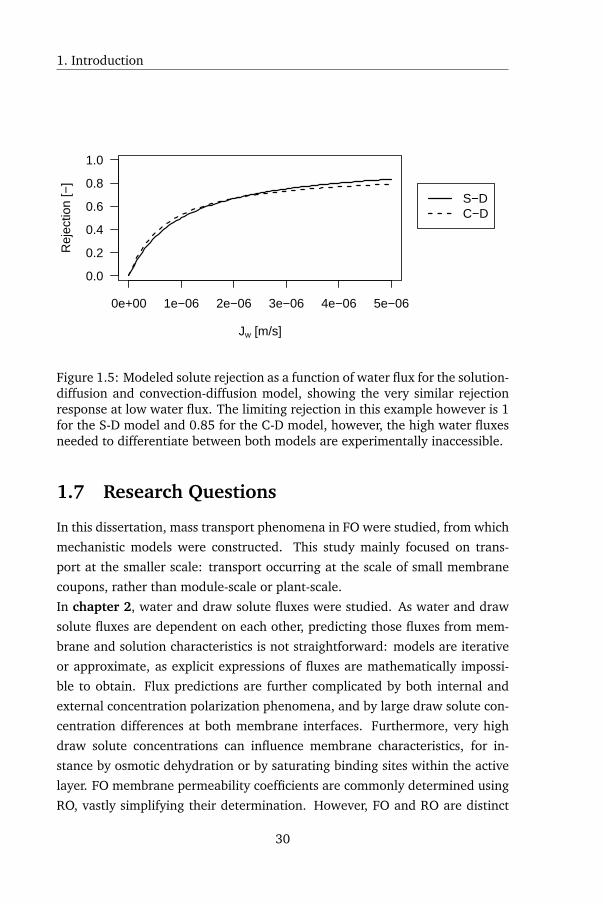
1. Introduction
0e+00 1e−06 2e−06 3e−06 4e−06 5e−06
0.0
0.2
0.4
0.6
0.8
1.0
Jw [m/s]
Rej
ectio
n [−
]
S−DC−D
Figure 1.5: Modeled solute rejection as a function of water flux for the solution-diffusion and convection-diffusion model, showing the very similar rejectionresponse at low water flux. The limiting rejection in this example however is 1for the S-D model and 0.85 for the C-D model, however, the high water fluxesneeded to differentiate between both models are experimentally inaccessible.
1.7 Research Questions
In this dissertation, mass transport phenomena in FO were studied, from which
mechanistic models were constructed. This study mainly focused on trans-
port at the smaller scale: transport occurring at the scale of small membrane
coupons, rather than module-scale or plant-scale.
In chapter 2, water and draw solute fluxes were studied. As water and draw
solute fluxes are dependent on each other, predicting those fluxes from mem-
brane and solution characteristics is not straightforward: models are iterative
or approximate, as explicit expressions of fluxes are mathematically impossi-
ble to obtain. Flux predictions are further complicated by both internal and
external concentration polarization phenomena, and by large draw solute con-
centration differences at both membrane interfaces. Furthermore, very high
draw solute concentrations can influence membrane characteristics, for in-
stance by osmotic dehydration or by saturating binding sites within the active
layer. FO membrane permeability coefficients are commonly determined using
RO, vastly simplifying their determination. However, FO and RO are distinct
30
Research Questions
processes: the low salinity during RO and hydrostatic pressure exerted dur-
ing RO are not encountered during FO, which casts doubts on the applicability
of RO-determined membrane permeability coefficients in FO. In this chapter,
an iterative model is presented in which membrane permeability coefficients
and membrane structural parameter are determined using FO tests only. The
novelty of this research lies in the incorporation the influence of high salinity,
concentration-dependence of draw solute diffusivity, density and viscosity, as
well as the careful analysis of the obtained membrane characteristics.
In chapter 3, the transport of organic micropollutants is investigated. Organic
micropollutant rejection by FO will be one of the defining characteristics if
FO is to be applied as a water reclamation process, since OMPs could render
produced water unfit for potable reuse. In FO, the draw solute could exert
additional influence on the rejection of OMPs, besides membrane characteris-
tics. OMP rejection can be modulated by for instance charge interactions in the
case of charged OMPs and by OMP-membrane affinity. Provided that the draw
solute is an ionic species, both of the above OMP-membrane interactions are
influenced by draw solutes as well. The effect of draw solutes on OMP trans-
port through FO membranes has however not yet been studied in detail yet.
Currently, it is hypothesized that the draw solute flux hinders OMP fluxes, as
the draw solute flux is oppositely directed. This study sets out to quantify flux
hindrance using different draw solutes as well as OMP diffusion tests. Charge
interactions such as electromigration and Donnan dialysis have been described
in other membrane systems, but have not yet been quantified in FO. The effect
of draw solutes on solute-membrane affinity has not yet been studied. In fact,
the influence of salts on surface free energy of hydrated polymers has been
very poorly studied in general. In this study, surface energy was quantified by
measuring contact angles on brine-soaked membrane coupons.
Chapter 4 deals with negative rejection of uncharged organic solutes. Nega-
tive rejection implies that solutes are enriched by the membrane, rather than
being rejected. This is a rare phenomenon, in contrast to negative rejection of
specific ions in multi-ionic solutions: organic solutes are always larger than wa-
ter molecules, thus, they exhibit a lower diffusivity and more steric hindrance
upon membrane passage compared to water. Current membrane transport the-
ory was explored to yield a model fitted to the observed rejection pattern pre-
sented in this chapter: certain models allow for negative rejection in the case
of high solute-membrane affinity. Using analysis of the limits of the different
31
1. Introduction
models, it was shown that the current models could not explain the observed
rejection pattern. New mechanistic models were then developed, based on
other mechanisms than high solute-membrane affinity. Such mechanisms are
adsorption followed by coupled transport or salting-in; two models, one for
each mechanism, are presented and discussed.
In chapter 5, the effects of biofouling on FO and on OMP rejection were ex-
plored. Biofouling could negatively impact water flux, although this is not
necessarily the case. Likewise, rejection could be impacted as well, both favor-
ably or unfavorably. Furthermore, the behavior of OMPs in closed loop FO-RO
installations was simulated. When FO and RO are used in a closed loop, the RO
stage will encounter any contaminants passing through the FO stage. Because
the draw solution in a closed loop is used continuously for a large number of
cycles, contaminants could build up inside the loop, which could cause the RO
permeate to be contaminated by these contaminants.
32
Chapter 2
A refined water and draw solute fluxmodel for FO: model development andvalidation
Adapted from:
Arnout D’Haese, Machawe Motsa, Paul Van der Meeren, Arne Verliefde, A
refined draw solute flux model in forward osmosis: Theoretical considerations
and experimental validation, Journal of Membrane Science 522 (2017), 316-
331
33
2. Modeling water & draw solute flux
2.1 Introduction
In this chapter, a water and draw solute flux model is presented based only on
FO flux tests, which can be used to determine key membrane characteristics.
The model is experimentally validated using clean water tests: feed solutes are
only taken into account by the osmotic pressure they might generate which has
a flux-lowering effect. As was explained in the introduction of this dissertation,
water flux is generated by an osmotic pressure difference across the membrane
active layer, in which water flows from the feed solution of low osmotic poten-
tial to the draw solution of high osmotic potential. Additionally, a draw solute
flux from the draw to the feed solution arises due to imperfect draw solute
retention, called reverse draw solute diffusion (RSD). When studying flux be-
havior in FO, however, draw solute concentrations on both sides of the active
layer are not easily experimentally accessible, due to both internal and external
concentration polarization phenomena. The draw solute concentrations at the
active layer interfaces generate water and draw solute fluxes, but are subject
of those fluxes at the same time: water flux entrains draw solute away from
the membrane interface at the draw side; at the feed side, solutes are enriched
at the membrane interface. As a result, fluxes in FO cannot be easily predicted.
Several studies have been devoted to modeling and predicting fluxes in FO,
and different models have been reported as well.
The first studies on flux modeling were performed by Loeb et al. and Lee et al.
[4, 6, 3]. In their models, concepts and their approximate calculations were
introduced which are still in use current flux models such as internal concen-
tration polarization (ICP) and K, the resistance to draw solute transport in
the porous support layer, from which the structural parameter S is derived. It
was also noted that ICP can be either dilutive when the membrane is operated
in AL-FS mode (active layer facing the feed solution) (FO), or concentrative,
when the membrane is operated in AL-DS mode (active layer facing the draw
solution) (PRO). These ICP approximations were adopted in subsequent stud-
ies, with a number of studies focusing on ECP and the effect of membrane
orientation on ICP and water flux [103, 104, 105]. Other studies focused on
reverse draw solute diffusion [106, 61, 70] and on the membrane structural pa-
rameter [77, 69, 73]. To date, only one study presented a model in which FO
fluxes are modeled using an FO-only approach [72], as the original approxima-
tions rely on membrane water and solute permeability coefficients determined
34
Introduction
using RO. Tiraferri et al. (2013) noted differences between membrane per-
meability coefficients obtained using only FO data compared to the RO-based
methods, which then yielded different structural parameters as well. As no
hydraulic pressure is applied in FO, using an FO-only approach to modeling
seems preferable. Additionally, when determining membrane characteristics
using RO, typically, pure water or very dilute solutions of draw solutes are used
with no or negligible osmotic pressure. This is however not representative of
the conditions under which FO is operated: membranes are exposed to very
high salinity and draw solutions are used with osmotic pressures of several
hundreds bar.
Multiple flux modeling studies reported only water fluxes or employed opti-
mization criteria based only on water fluxes [77, 71], neglecting RSD. More-
over, in many studies, NaCl was the only draw solute used, including when
RSD was studied [106, 70, 72, 73]. NaCl solutions however show ’ideal’ be-
havior in many ways: the osmotic pressure of NaCl solutions is well predicted
by the van ‘t Hoff law and both NaCl diffusivity and solution viscosity show
only minor changes as a function of concentration, with for instance the diffu-
sion coefficient differing at most 7.5% between 0 and 5M. However, this is not
necessarily the case for other draw solutes. Concentration dependence of draw
solute diffusivity during ICP has been incorporated in some studies [77, 105].
However, membrane permeability of draw solutes is also dependent on draw
solute diffusivity, where the large concentration differences encountered be-
tween feed and draw solutions are not yet taken into account. Electrostatic
interactions between salts and charged membranes have been shown to influ-
ence salt transport in NF and RO [107, 108]. In FO transport models however,
electrostatic interactions have not been incorporated when estimating mem-
brane permeability coefficients of charged draw solutes.
In this chapter, a novel FO-only model is presented in which water and draw so-
lute transport is modeled according to the solution-diffusion model, using new
expressions for the solute permeability coefficient which takes into account
concentration dependence of draw solute diffusivity during transport across
the membrane active layer. Electrostatic interactions between draw solutes and
the active layer are considered as well, according to the charge concentration
polarization model. Model results were assessed based on Jw, Js, as well as
the Jw/Js ratio; the importance of the Jw/Js ratio for flux models is discussed.
The model was thoroughly tested, using two membrane types (CTA and TFC)
35
2. Modeling water & draw solute flux
in both AL-FS and AL-DS mode. Flux tests were performed using four min-
eral salt draw solutes (NaCl, Na2SO4, MgCl2 and MgSO4), yielding contrasting
flux patterns depending on draw solute and membrane properties. Membrane
characterization furthermore allowed the calculation of the support layer ap-
parent tortuosity by determining the support layer thickness and porosity; a
discussion of tortuosity is included as well.
2.2 Theory
Throughout this chapter, water flux and the reverse draw solute flux will be
referred to as Jw and Js respectively, as FO tests and modeling were performed
using only ultrapure water and draw solutes. In the following section a uni-
dimensional section of the membrane is considered, which is assumed to be
oriented perpendicular to the x-axis. The active layer is situated at the ori-
gin and has an infinitesimal thickness, and the support layer with thickness tsspans from x = 0 to x = ts. The contribution of the active layer to the over-
all membrane thickness is ignored, because the thickness of the active (∼ 100
nm) and support layer (∼ 100 µm) differ by about 3 orders of magnitude. Mass
transport is considered in four distinct regions: across the active layer, in the
support layer and in a dilutive and concentrative external polarization layer.
These regions are considered distinct because the modes of mass transport are
different in each region. In figure 1.3, these regions are illustrated for both
AL-FS and AL-DS orientation.
2.2.1 Mass transport through the membrane active layer
In this study, water and draw solute transport through FO membranes are mod-
eled using the solution-diffusion model. FO membranes are dense membranes
showing a high rejection of solutes, and possess a relatively low water perme-
ability. Furthermore, the process of osmosis requires at least partial decoupling
of solute and solvent fluxes [93]. Such membrane processes have been suc-
cessfully modeled using the solution-diffusion model [74]. According to the
solution-diffusion model, solvent (Jw) and solute (Js) fluxes can be accurately
approximated by a linear dependence on their respective driving forces. In the
case of osmosis, the driving forces are the osmotic pressure difference (∆Π)
and solute concentration difference (∆c) across the active layer respectively,
36
Theory
given in equations 2.1 and 2.2 [74]. In these equations, AS designates the
active layer - support layer interface, while AE designates the active layer -
external solution interface, with the external solution being either the feed or
draw solution. The proportionality factors for Jw and Js, A and B respectively,
are generally considered to be constant membrane properties regardless of the
magnitude of the driving forces.
Jw = A(ΠAS −ΠAE) (2.1)
Js = B(cAS − cAE) (2.2)
During steady-state operation, mass conservation applies, so the fluxes of species
i through any two sections at x and x + δx are equal. The model presented in
this study extends previous flux models by taking into account the influence
of draw solute concentration on draw solute diffusivity during transport across
the active layer. According to solution-diffusion theory, the solute permeability
coefficient for a species i equals [74]:
Bi =DiφiL
(2.3)
with Di equaling the solute diffusion coefficient, φi the partition coefficient
of species i into the membrane active layer and L the thickness of the active
layer. The diffusion coefficient can be assumed to be constant during transport
through the active layer in the case of strongly diluted solutes, as is for instance
the case for trace feed solutes, or very poorly rejected solutes for which the feed
and permeate concentrations are similar. This is however not the case for draw
solutes in FO. The equation for Js was modified accordingly:
Js = B∗Dw(cAS − cAE) (2.4)
with B∗ the membrane permeability at infinite draw solute dilution and Dw a
weighted factor for the concentration dependence of the draw solute diffusion
coefficient, normalized to the diffusion coefficient at infinite dilution (D(0)):
Dw =
∫ cAS
cAFD(c)dc
(cAS − cAF )D(0)(2.5)
37
2. Modeling water & draw solute flux
In this study, diffusivity for the different draw solutes were sourced from Lobo
[109], who has provided a comprehensive overview of experimental values of
diffusion coefficients of electrolytes at varying concentrations. As is customary
for fitting variables to data dependent on ionic activity, a polynomial in c(1/2)
is fitted to the data [110], with ai being empirical constants:
Db = a0 + a1c(1/2) + a2c+ a3c
(3/2) + a4c2 (2.6)
In the above derivation, the assumption is made that the solute diffusivity as
a function of concentration within the active layer will at most differ by a
constant factor from the diffusivity in bulk solution. Generally, diffusivity in
a direction x is proportional to the chemical potential gradient and inversely
proportional to the drag force f [111]:
D ∼ 1
f
∂µ
∂x(2.7)
with µ:
µ = µ0 +RTln(γc) (2.8)
The activity coefficient γ is dependent on both the solute concentration and the
solvent. However, in the Debye-Hückel model, the solvent only contributes to
γ by its relative permitivity εr, which for organic polymers is low and generally
considered concentration-independent. Extending the Debye-Hückel model to
take into account non-ideality by short-range and long-range interactions, such
as in the N-Wilson-NRF and Pitzer-Debye-Hückel model [112], enthalpic inter-
action parameters are introduced, which are again concentration independent.
Given the strong hydration of relatively small ions (as are ions of the draw
solutes used here), the enthalpic interaction between the active layer polymer
and the ions can be assumed to be small. As for the drag force f : the direc-
tion of Jw and Js is opposite, which causes Jw and Js to hinder each other.
However, both fluxes are relatively low in dense membranes, and in terms of
molecules passing through the active layer, Jw vastly outnumbers Js. It is thus
assumed that even if the Jw/Js ratio is not constant, the influence of draw
solute concentration on f will be small. Water and draw solute fluxes are mod-
eled using both the conventional expression for Js (equation 2.2) and the mod-
ified expression (equation 2.4). Model versions using the diffusivity-corrected
expression for Js will be referred to as BDiff .
38
Theory
2.2.2 Mass transport through the support layer
Transport through the support layer is hindered by ICP: convective mixing of
the solution present in the support layer is inhibited, and diffusive fluxes are
hindered by the support layer increased tortuosity and decreased porosity com-
pared to bulk solutions. Bui et al. [71] recently showed that mass transfer to
and from the support layer influences mass transfer within the support layer
as well, however, this was not due to convective mixing within the support
layer. In this study, fluxes are modeled based on the extended Nernst-Planck
equation, in which the flux of a solute i is expressed as:
−Js = Jwc−Ddc
dx− zscDF
RT
dψ
dx(2.9)
with D, c and zs being the effective diffusion coefficient, concentration and
valence of solute s. The draw solute flux is considered negative, because its
direction is opposite of the water flux. Electrokinetic interactions within the
support layer are ignored in this paper; only electrostatic effects on draw solute
partitioning in the active layer are considered (see subsection 2.2.4). Quantifi-
cation of these interactions within the support layer requires determination of
the support layer pore size and surface charge density, which will be the subject
of further study. Evidence for these interactions is presented in section 2.4.5.
The Nernst-Planck equation thus reduces to:
−Js = Jwc−Ddc
dx(2.10)
The factor relating the solute effective diffusivity to its bulk diffusivity is in FO
literature routinely expressed as the support porosity divided by tortuosity [3,
1, 103]. However, when deriving expressions for both convective and diffusive
fluxes, the tortuosity appears as a squared term [113, 114] with tortuosity
defined as τ = ∆l/∆x, with l the actual path length and x being the straight
path length. To add further confusion, tortuosity is defined by some authors as
τ = (∆l/∆x)2 [49]. This point is however not clarified in FO literature. In this
study, tortuosity will refer to ∆l/∆x, yielding:
D =Dbε
τ2(2.11)
39
2. Modeling water & draw solute flux
When D is considered constant as a function of draw solute concentration,
equation 2.10 can be integrated with the following boundary conditions, with
cAS and cSE being the draw solute concentration at the active layer - support
layer and at the support layer - external solution interfaces respectively:{x = 0⇔ c = cAS
x = ts ⇔ c = cSE
}
yielding for cAS:
cAS = cSE exp(−JwtsD
) +JsJw
[exp(−JwtsD
)− 1] (2.12)
The membrane structural parameter S and solute resistivity K, taking into
account the squared tortuosity, are defined as [3, 50]:
S =tsτ
2
ε= KDb (2.13)
Rewriting equation 2.12 accordingly yields:
cAS = cSE exp(−JwK) +JsJw
[exp(−JwK)− 1] (2.14)
and for the solute resistivity:
K =1
Jwln(
Js + JwcSEJs + JwcAS
) (2.15)
However, the draw solute concentration difference at both interfaces can be
large and, as shown in section 2.2.1, diffusivity is dependent on chemical po-
tential and solution viscosity; the latter in turn is also influenced by solute
concentration. Incorporating the concentration dependence of draw solute dif-
fusivity in ICP models yields better model convergence [10, 105]. Rearranging
equation 2.10 and substitution of D by equation 2.6 yields the following differ-
ential equation:
dc
dx=
Js + Jwc(x)
(a0 + a1c(1/2) + a2c+ a3c(3/2) + a4c2)ε/τ2(2.16)
Although equation 2.16 can be integrated, the resulting equation is particularly
lengthy and cumbersome. It was therefore decided to evaluate equation 2.16
40
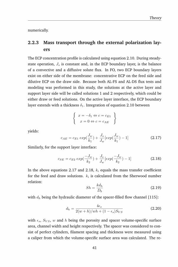
Theory
numerically.
2.2.3 Mass transport through the external polarization lay-ers
The ECP concentration profile is calculated using equation 2.10. During steady-
state operation, Js is constant and, in the ECP boundary layer, is the balance
of a convective and a diffusive solute flux. In FO, two ECP boundary layers
exist on either side of the membrane: concentrative ECP on the feed side and
dilutive ECP on the draw side. Because both AL-FS and AL-DS flux tests and
modeling was performed in this study, the solutions at the active layer and
support layer side will be called solutions 1 and 2 respectively, which could be
either draw or feed solutions. On the active layer interface, the ECP boundary
layer extends with a thickness δ1. Integration of equation 2.10 between{x = −δ1 ⇔ c = cE1
x = 0⇔ c = cAE
}
yields:
cAE = cE1 exp(Jwk1
) +JsJw
[exp(Jwk1
)− 1] (2.17)
Similarly, for the support layer interface:
cSE = cE2 exp(−Jwk2
) +JsJw
[exp(−Jwk2
)− 1] (2.18)
In the above equations 2.17 and 2.18, ki equals the mass transfer coefficient
for the feed and draw solutions. ki is calculated from the Sherwood number
relation:
Sh =kdhDb
(2.19)
with dh being the hydraulic diameter of the spacer-filled flow channel [115]:
dh =4εs
2(w + h)/wh+ (1− εs)SV S(2.20)
with εs, SV S , w and h being the porosity and spacer volume-specific surface
area, channel width and height respectively. The spacer was considered to con-
sist of perfect cylinders, filament spacing and thickness were measured using
a caliper from which the volume-specific surface area was calculated. The re-
41
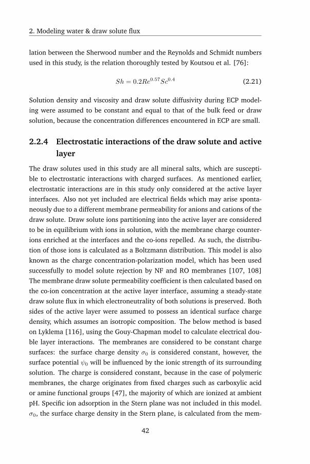
2. Modeling water & draw solute flux
lation between the Sherwood number and the Reynolds and Schmidt numbers
used in this study, is the relation thoroughly tested by Koutsou et al. [76]:
Sh = 0.2Re0.57Sc0.4 (2.21)
Solution density and viscosity and draw solute diffusivity during ECP model-
ing were assumed to be constant and equal to that of the bulk feed or draw
solution, because the concentration differences encountered in ECP are small.
2.2.4 Electrostatic interactions of the draw solute and activelayer
The draw solutes used in this study are all mineral salts, which are suscepti-
ble to electrostatic interactions with charged surfaces. As mentioned earlier,
electrostatic interactions are in this study only considered at the active layer
interfaces. Also not yet included are electrical fields which may arise sponta-
neously due to a different membrane permeability for anions and cations of the
draw solute. Draw solute ions partitioning into the active layer are considered
to be in equilibrium with ions in solution, with the membrane charge counter-
ions enriched at the interfaces and the co-ions repelled. As such, the distribu-
tion of those ions is calculated as a Boltzmann distribution. This model is also
known as the charge concentration-polarization model, which has been used
successfully to model solute rejection by NF and RO membranes [107, 108]
The membrane draw solute permeability coefficient is then calculated based on
the co-ion concentration at the active layer interface, assuming a steady-state
draw solute flux in which electroneutrality of both solutions is preserved. Both
sides of the active layer were assumed to possess an identical surface charge
density, which assumes an isotropic composition. The below method is based
on Lyklema [116], using the Gouy-Chapman model to calculate electrical dou-
ble layer interactions. The membranes are considered to be constant charge
surfaces: the surface charge density σ0 is considered constant, however, the
surface potential ψ0 will be influenced by the ionic strength of its surrounding
solution. The charge is considered constant, because in the case of polymeric
membranes, the charge originates from fixed charges such as carboxylic acid
or amine functional groups [47], the majority of which are ionized at ambient
pH. Specific ion adsorption in the Stern plane was not included in this model.
σ0, the surface charge density in the Stern plane, is calculated from the mem-
42
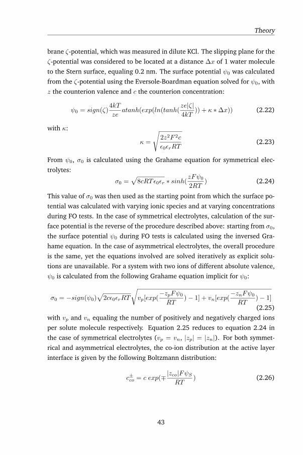
Theory
brane ζ-potential, which was measured in dilute KCl. The slipping plane for the
ζ-potential was considered to be located at a distance ∆x of 1 water molecule
to the Stern surface, equaling 0.2 nm. The surface potential ψ0 was calculated
from the ζ-potential using the Eversole-Boardman equation solved for ψ0, with
z the counterion valence and c the counterion concentration:
ψ0 = sign(ζ)4kT
zeatanh(exp(ln(tanh(
ze|ζ|4kT
)) + κ ∗∆x)) (2.22)
with κ:
κ =
√2z2F 2c
ε0εrRT(2.23)
From ψ0, σ0 is calculated using the Grahame equation for symmetrical elec-
trolytes:
σ0 =√
8cRTε0εr ∗ sinh(zFψ0
2RT) (2.24)
This value of σ0 was then used as the starting point from which the surface po-
tential was calculated with varying ionic species and at varying concentrations
during FO tests. In the case of symmetrical electrolytes, calculation of the sur-
face potential is the reverse of the procedure described above: starting from σ0,
the surface potential ψ0 during FO tests is calculated using the inversed Gra-
hame equation. In the case of asymmetrical electrolytes, the overall procedure
is the same, yet the equations involved are solved iteratively as explicit solu-
tions are unavailable. For a system with two ions of different absolute valence,
ψ0 is calculated from the following Grahame equation implicit for ψ0:
σ0 = −sign(ψ0)√
2cε0εrRT
√vp[exp(
−zpFψ0
RT)− 1] + vn[exp(
−znFψ0
RT)− 1]
(2.25)
with vp and vn equaling the number of positively and negatively charged ions
per solute molecule respectively. Equation 2.25 reduces to equation 2.24 in
the case of symmetrical electrolytes (vp = vn, |zp| = |zn|). For both symmet-
rical and asymmetrical electrolytes, the co-ion distribution at the active layer
interface is given by the following Boltzmann distribution:
c±co = c exp(∓|zco|FψSRT
) (2.26)
43
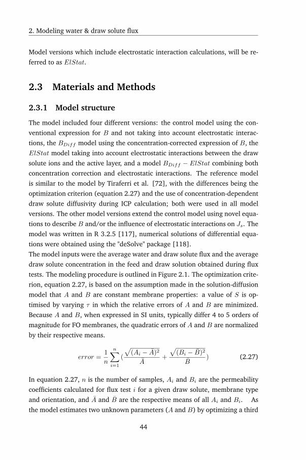
2. Modeling water & draw solute flux
Model versions which include electrostatic interaction calculations, will be re-
ferred to as ElStat.
2.3 Materials and Methods
2.3.1 Model structure
The model included four different versions: the control model using the con-
ventional expression for B and not taking into account electrostatic interac-
tions, the BDiff model using the concentration-corrected expression of B, the
ElStat model taking into account electrostatic interactions between the draw
solute ions and the active layer, and a model BDiff − ElStat combining both
concentration correction and electrostatic interactions. The reference model
is similar to the model by Tiraferri et al. [72], with the differences being the
optimization criterion (equation 2.27) and the use of concentration-dependent
draw solute diffusivity during ICP calculation; both were used in all model
versions. The other model versions extend the control model using novel equa-
tions to describe B and/or the influence of electrostatic interactions on Js. The
model was written in R 3.2.5 [117], numerical solutions of differential equa-
tions were obtained using the "deSolve" package [118].
The model inputs were the average water and draw solute flux and the average
draw solute concentration in the feed and draw solution obtained during flux
tests. The modeling procedure is outlined in Figure 2.1. The optimization crite-
rion, equation 2.27, is based on the assumption made in the solution-diffusion
model that A and B are constant membrane properties: a value of S is op-
timised by varying τ in which the relative errors of A and B are minimized.
Because A and B, when expressed in SI units, typically differ 4 to 5 orders of
magnitude for FO membranes, the quadratic errors of A and B are normalized
by their respective means.
error =1
n
n∑i=1
(
√(Ai − A)2
A+
√(Bi − B)2
B) (2.27)
In equation 2.27, n is the number of samples, Ai and Bi are the permeability
coefficients calculated for flux test i for a given draw solute, membrane type
and orientation, and A and B are the respective means of all Ai and Bi. As
the model estimates two unknown parameters (A and B) by optimizing a third
44
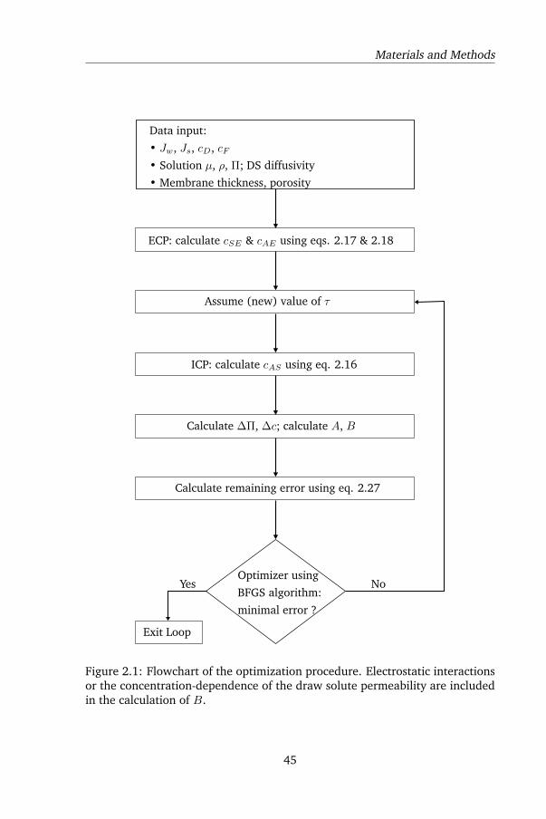
Materials and Methods
Data input:
• Jw, Js, cD, cF• Solution µ, ρ, Π; DS diffusivity
• Membrane thickness, porosity
ECP: calculate cSE & cAE using eqs. 2.17 & 2.18
Assume (new) value of τ
ICP: calculate cAS using eq. 2.16
Calculate ∆Π, ∆c; calculate A, B
Calculate remaining error using eq. 2.27
Optimizer using
BFGS algorithm:
minimal error ?
NoYes
Exit Loop
Figure 2.1: Flowchart of the optimization procedure. Electrostatic interactionsor the concentration-dependence of the draw solute permeability are includedin the calculation of B.
45
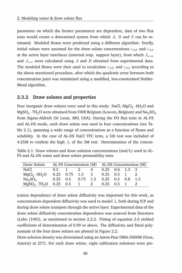
2. Modeling water & draw solute flux
parameter on which the former parameters are dependent, data of two flux
tests would create a determined system from which A, B and S can be es-
timated. Modeled fluxes were predicted using a different algorithm: briefly,
initial values were assumed for the draw solute concentrations cAE and cAS
at the active layer interfaces (external resp. support layer), from which Jw,m
and Js,m were calculated using A and B obtained from experimental data.
The modeled fluxes were then used to recalculate cAE and cAS according to
the above mentioned procedure, after which the quadratic error between both
concentration pairs was minimized using a modified, box-constrained Nelder-
Mead algorithm.
2.3.2 Draw solutes and properties
Four inorganic draw solutes were used in this study: NaCl, MgCl2 ·6H2O and
MgSO4 ·7H2O were obtained from VWR Belgium (Leuven, Belgium) and Na2SO4
from Sigma-Aldrich (St Louis, MO, USA). During the FO flux tests in AL-FS
and AL-DS mode, each draw solute was used in four concentrations (see Ta-
ble 2.1), spanning a wide range of concentrations as a function of fluxes and
solubility. In the case of AL-DS NaCl TFC tests, a 5th test was included of
4.25M to confirm the high Js of the 3M test. Determination of the concen-
Table 2.1: Draw solutes and draw solution concentrations (mol/L) used in AL-FS and AL-DS water and draw solute permeability tests
Draw Solute AL-FS Concentration (M) AL-DS Concentration (M)NaCl 0.5 1 2 4 0.25 0.6 1.3 3MgCl2 ·6H2O 0.25 0.75 1.5 3 0.25 0.5 1 2Na2SO4 0.25 0.5 0.75 1.5 0.25 0.5 0.8 1.5MgSO4 ·7H2O 0.25 0.5 1 2 0.25 0.5 1 2
tration dependence of draw solute diffusivity was important for this work, as
concentration-dependent diffusivity was used to model Js both during ICP and
during draw solute transport through the active layer. Experimental data of the
draw solute diffusivity concentration dependence was sourced from literature
(Lobo [109]), as mentioned in section 2.2.2. Fitting of equation 2.6 yielded
coefficients of determination of 0.99 or above. The diffusivity and fitted poly-
nomials of the four draw solutes are plotted in Figure 2.2.
Draw solution density was determined using an Anton Paar DMA-5000M (Graz,
Austria) at 25°C. For each draw solute, eight calibration solutions were pre-
46
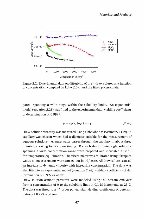
Materials and Methods
0 1000 2000 3000 4000 5000
0.0e+00
5.0e−10
1.0e−09
1.5e−09
Concentration [mol/m3]
Diff
usiv
ity [m
2 /s] NaCl
Na2SO4MgCl2MgSO4
Figure 2.2: Experimental data on diffusivity of the 4 draw solutes as a functionof concentration, compiled by Lobo [109] and the fitted polynomials.
pared, spanning a wide range within the solubility limits. An exponential
model (equation 2.28) was fitted to the experimental data, yielding coefficients
of determination of 0.9999.
y = a1exp(a2c) + a3 (2.28)
Draw solution viscosity was measured using Ubbelohde viscosimetry [119]. A
capillary was chosen which had a diameter suitable for the measurement of
aqueous solutions, i.e. pure water passes through the capillary in about three
minutes, allowing for accurate timing. For each draw solute, eight solutions
spanning a wide concentration range were prepared and incubated at 25°C
for temperature equilibration. The viscosimeter was calibrated using ultrapure
water, all measurements were carried out in triplicate. All draw solutes caused
an increase in dynamic viscosity with increasing concentration. The data was
also fitted to an exponential model (equation 2.28), yielding coefficients of de-
termination of 0.997 or above.
Draw solution osmotic pressures were modeled using OLI Stream Analyzer
from a concentration of 0 to the solubility limit in 0.1 M increments at 25°C.
The data was fitted to a 4th order polynomial, yielding coefficients of determi-
nation of 0.999 or above.
47
~ ~ ~ 00 ee e e e e~e~eoeo
2. Modeling water & draw solute flux
2.3.3 Membranes and membrane properties
The membranes used in this study, were cellulose tri-acetate (CTA) membranes
with embedded support (ES) and thin film composite membranes (TFC), both
provided by HTI (OR, USA). The membrane structural parameter S was mod-
eled, and the parameters from which S is derived were calculated (equation
2.13). Measurement of the support tortuosity τ is challenging, but both sup-
port layer thickness ts and porosity ε are experimentally accessible. The contri-
bution of the thin active layer was ignored during thickness and porosity mea-
surements. For the CTA-ES membranes, two methods were used to measure the
support thickness: firstly, a digital micrometer caliper measured the thickness
in at least 10 different spots on a membrane soaked in deionized water, which
yielded a thickness of 90.8 ± 0.4 µm. However, SEM micrographs of CTA-ES
membranes showed that the membranes do not have a uniform thickness due
to the corrugated surface [9]. Therefore, the results obtained by the digital
micrometer caliper were checked by measuring the volume displaced upon im-
mersing a membrane sample of known dimensions in a water-filled graduated
cylinder. As expected, the immersion method yielded a slightly lower mem-
brane thickness of 85.4 ± 1.1 µm: the caliper would be conceivably touching
the outer edges of the corrugated surface, thereby overestimating the aver-
age thickness. The thickness obtained by immersion was used in subsequent
calculations. For the TFC membranes, SEM micrographs have shown fairly
smooth surfaces. Consequently, its thickness was measured using the caliper
only, yielding 115.1.± 0.3 µm, in accordance with an earlier report [48].
Membrane porosity was determined gravimetrically. Using the average mem-
brane thickness, the volume of a specific membrane sample can be calculated.
Membrane porosity was subsequently determined by measuring the volume
of water lost upon dehydration at 60 °C until constant weight of a sample of
known dimensions soaked in ultrapure water, which was done in triplicate.
The CTA-ES and TFC membrane porosities were 56.6 ± 1.0 % and 64.2 ± 0.4
% respectively. To the best of the authors’ knowledge, this is the first time the
porosities of the HTI CTA-ES and TFC membranes are reported.
In order to model electrostatic interactions between draw solutes and the mem-
brane active layer, the surface charge density was determined, which was cal-
culated from the ζ-potential (see section 2.2.4). The ζ-potential of the CTA-ES
membrane had been determined earlier [120]. The ζ-potential of the TFC
48
Materials and Methods
membrane was determined using a SurPASS Electrokinetic Analyzer (Anton
Paar GmbH, Graz, Austria), using 10mM KCl solutions. To study the effects of
ion adsorption in the Stern plane, the ζ-potential of the TFC membrane was
also determined using 10mM MgCl2. The ζ-potential of the CTA-ES membrane
at ambient pH was -4.0 ± 0.3 mV, yielding a surface charge density σ0 of -0.98
· 10-3 C/m2. The TFC membrane had a ζ-potential of -12.5 ± 0.6 mV in KCl,
yielding a σ0 of -3.09 · 10-3 C/m2. When substituting KCl for MgCl2, the ζ-
potential of the TFC membrane was diminished to -1.8 ± 0.5 mV, indicating
adsorption of Mg+2 on the active layer.
2.3.4 FO setup
A schematic overview of the FO setup is provided in Figure 2.3. The membrane
cell had the following flow channel dimensions: length 250 mm , width 50
mm, height 1 mm. The flux was recorded by datalogging the weight of the so-
lution in the active layer side compartment, using an OHaus Pioneer 4201 scale
(OHaus, NJ, USA) and a LabVIEW script. Feed solution conductivity was mea-
sured using a Consort C3020 multi-parameter analyser with SK10T electrode.
Both feed and draw solutions were equilibrated in a temperature-controlled
bath prior to the FO tests. The temperature of the active layer side compart-
ment was controlled using a Julabo F26 (Labortechnik, Selbach, Germany) set
at 25°C, the support layer side compartment was insulated. Feed and draw
solutions were pumped using Masterflex L/S peristaltic pumps (Cole-Parmer,
USA); crossflow velocity was maintained at 0.2 m/s. To ensure that there was
no hydraulic pressure difference between the feed and draw solution before en-
tering the membrane module, pulsation dampeners were used which were fit-
ted with a connection between their headspaces, consisting of a long and small
diameter tube. There was no liquid transport or convective gas flux through
this tube.
49
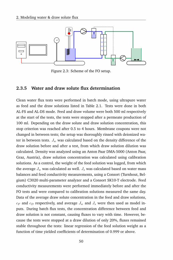
2. Modeling water & draw solute flux
Figure 2.3: Scheme of the FO setup.
2.3.5 Water and draw solute flux determination
Clean water flux tests were performed in batch mode, using ultrapure water
as feed and the draw solutions listed in Table 2.1. Tests were done in both
AL-FS and AL-DS mode. Feed and draw volume were both 500 ml respectively
at the start of the tests, the tests were stopped after a permeate production of
100 ml. Depending on the draw solute and draw solution concentration, this
stop criterion was reached after 0.5 to 4 hours. Membrane coupons were not
changed in between tests; the setup was thoroughly rinsed with deionized wa-
ter in between tests. Jw was calculated based on the density difference of the
draw solution before and after a test, from which draw solution dilution was
calculated. Density was analyzed using an Anton Paar DMA-5000 (Anton Paar,
Graz, Austria), draw solution concentration was calculated using calibration
solutions. As a control, the weight of the feed solution was logged, from which
the average Jw was calculated as well. Js was calculated based on water mass
balances and feed conductivity measurements, using a Consort (Turnhout, Bel-
gium) C3020 multi-parameter analyzer and a Consort SK10-T electrode. Feed
conductivity measurements were performed immediately before and after the
FO tests and were compared to calibration solutions measured the same day.
Data of the average draw solute concentration in the feed and draw solutions,
cF and cD respectively, and average Jw and Js were then used as model in-
puts. During batch flux tests, the concentration difference between feed and
draw solution is not constant, causing fluxes to vary with time. However, be-
cause the tests were stopped at a draw dilution of only 20%, fluxes remained
stable throughout the tests: linear regression of the feed solution weight as a
function of time yielded coefficients of determination of 0.999 or above.
50
Results and Discussion
2.4 Results and Discussion
2.4.1 FO flux tests and model selection
The experimental flux data is given in tabulated form in Appendix. Gener-
ally, both water and draw solute fluxes were higher when either chloride draw
solutes, the TFC membrane or AL-DS orientation were used. Examples are
given in Figure 2.4: in the left panel, draw solute fluxes through the CTA-ES
membrane in AL-FS mode are depicted showing the higher fluxes of the chlo-
ride draw solutes. In the right panel of Figure 2.4, water fluxes obtained using
MgSO4 are depicted. The higher membrane permeability of the TFC membrane
is apparent from the high fluxes obtained in AL-DS mode, while the fluxes in
AL-FS mode are very similar for both membranes, showing the effect of the
higher structural parameter. This will be discussed in sections 2.4.4 and 2.4.5.
Four different model versions were used to predict the membrane permeability
coefficients, A and B, and the structural parameter S. Model convergence was
assessed by recalculating Jw and Js starting from cF and cD, using the values
for A, B and S obtained from analysis of experimental data. Pearson corre-
lation coefficients were calculated between experimental and modeled Jw, Jsand the Jw/Js ratio, ranking of the model versions was based on averaged coef-
ficients as is shown in Table 2.2. Table 2.2 shows that theElStat+BDiff model
version offered the best flux predictions. Averaging of the coefficients shown
in Table 2.2 was done as follows: for each model, correlation coefficients were
averaged for all membranes, membrane orientations and draw solutes. As the
Jw/Js ratio was predicted poorly in some cases, averaged coefficients not in-
cluding the Jw/Js ratio are shown as well. The variable quality of the Jw/Jspredictions is shown for the case of TFC in AL-DS orientation in Figure 2.5: the
trend for NaCl was poorly predicted; the Jw/Js ratio for the other draw solutes
was predicted much better by the BDiff and BDiff + ElStat model versions.
The Jw/Js ratio and its importance in flux modeling is discussed in more detail
in section 2.4.3.
The model versions differed in the calculation of B and Js, with the calcula-
tion of A and Jw remaining unchanged. Consequently, all model versions were
able to accurately predict Jw, all yielding an average correlation coefficient of
0.993. Because the ElStat+BDiff model version yielded the best fitting pre-
dictions, much of the following discussion of membrane parameters is drawn
51
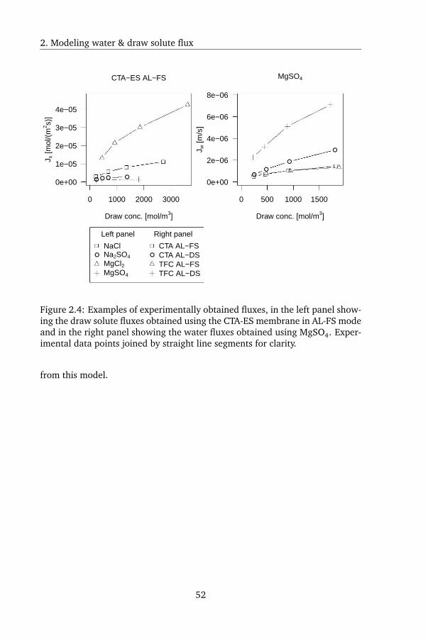
2. Modeling water & draw solute flux
0 1000 2000 3000
0e+00
1e−05
2e−05
3e−05
4e−05
Draw conc. [mol/m3]
J s [m
ol/(
m2 s)
]
● ● ● ●
CTA−ES AL−FS
● ●
Left panel Right panel
NaClNa2SO4
MgCl2MgSO4
CTA AL−FSCTA AL−DSTFC AL−FSTFC AL−DS
0 500 1000 1500
0e+00
2e−06
4e−06
6e−06
8e−06
Draw conc. [mol/m3]
J w [m
/s]
●●
●
●
MgSO4
Figure 2.4: Examples of experimentally obtained fluxes, in the left panel show-ing the draw solute fluxes obtained using the CTA-ES membrane in AL-FS modeand in the right panel showing the water fluxes obtained using MgSO4. Exper-imental data points joined by straight line segments for clarity.
from this model.
52
-
-
-
-
-I
/',/ /',/
/ /',
_ o ----0 ~D
fil-+-F-+ I I
D
/',
+
I
/',
/ + +
/ +
/
-------------+
_____...-€t -:; g}-1<1x
- m
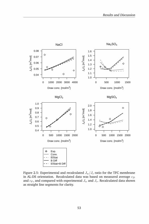
Results and Discussion
0 1000 2000 3000 4000
0.04
0.05
0.06
0.07
0.08
Draw conc. [mol/m3]
J w/J
s [m
3 /mol
]
NaCl
0 500 1000 1500
1.0
1.1
1.2
1.3
1.4
1.5
1.6
Draw conc. [mol/m3]
J w/J
s [m
3 /mol
]
Na2SO4
0 500 1000 1500 2000
0.4
0.5
0.6
0.7
0.8
0.9
1.0
Draw conc. [mol/m3]
J w/J
s [m
3 /mol
]
MgCl2
Exp.Conv.ElStatB DiffElStat+B Diff
0 500 1000 1500 2000
1.0
1.2
1.4
1.6
1.8
2.0
Draw conc. [mol/m3]
J w/J
s [m
3 /mol
]
MgSO4
Figure 2.5: Experimental and recalculated Jw/Js ratio for the TFC membranein AL-DS orientation. Recalculated data was based on measured average cDand cF , and compared with experimental Jw and Js. Recalculated data shownas straight line segments for clarity.
53
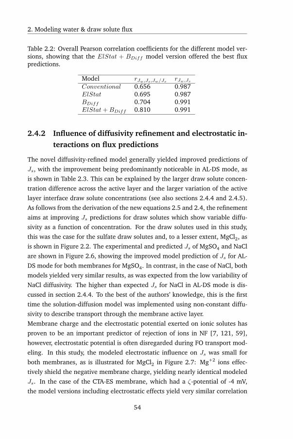
2. Modeling water & draw solute flux
Table 2.2: Overall Pearson correlation coefficients for the different model ver-sions, showing that the ElStat + BDiff model version offered the best fluxpredictions.
Model rJw,Js,Jw/Js rJw,JsConventional 0.656 0.987ElStat 0.695 0.987BDiff 0.704 0.991ElStat+BDiff 0.810 0.991
2.4.2 Influence of diffusivity refinement and electrostatic in-teractions on flux predictions
The novel diffusivity-refined model generally yielded improved predictions of
Js, with the improvement being predominantly noticeable in AL-DS mode, as
is shown in Table 2.3. This can be explained by the larger draw solute concen-
tration difference across the active layer and the larger variation of the active
layer interface draw solute concentrations (see also sections 2.4.4 and 2.4.5).
As follows from the derivation of the new equations 2.5 and 2.4, the refinement
aims at improving Js predictions for draw solutes which show variable diffu-
sivity as a function of concentration. For the draw solutes used in this study,
this was the case for the sulfate draw solutes and, to a lesser extent, MgCl2, as
is shown in Figure 2.2. The experimental and predicted Js of MgSO4 and NaCl
are shown in Figure 2.6, showing the improved model prediction of Js for AL-
DS mode for both membranes for MgSO4. In contrast, in the case of NaCl, both
models yielded very similar results, as was expected from the low variability of
NaCl diffusivity. The higher than expected Js for NaCl in AL-DS mode is dis-
cussed in section 2.4.4. To the best of the authors’ knowledge, this is the first
time the solution-diffusion model was implemented using non-constant diffu-
sivity to describe transport through the membrane active layer.
Membrane charge and the electrostatic potential exerted on ionic solutes has
proven to be an important predictor of rejection of ions in NF [7, 121, 59],
however, electrostatic potential is often disregarded during FO transport mod-
eling. In this study, the modeled electrostatic influence on Js was small for
both membranes, as is illustrated for MgCl2 in Figure 2.7: Mg+2 ions effec-
tively shield the negative membrane charge, yielding nearly identical modeled
Js. In the case of the CTA-ES membrane, which had a ζ-potential of -4 mV,
the model versions including electrostatic effects yield very similar correlation
54
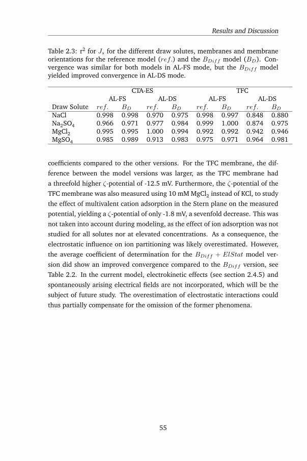
Results and Discussion
Table 2.3: r2 for Js for the different draw solutes, membranes and membraneorientations for the reference model (ref.) and the BDiff model (BD). Con-vergence was similar for both models in AL-FS mode, but the BDiff modelyielded improved convergence in AL-DS mode.
CTA-ES TFCAL-FS AL-DS AL-FS AL-DS
Draw Solute ref. BD ref. BD ref. BD ref. BDNaCl 0.998 0.998 0.970 0.975 0.998 0.997 0.848 0.880Na2SO4 0.966 0.971 0.977 0.984 0.999 1.000 0.874 0.975MgCl2 0.995 0.995 1.000 0.994 0.992 0.992 0.942 0.946MgSO4 0.985 0.989 0.913 0.983 0.975 0.971 0.964 0.981
coefficients compared to the other versions. For the TFC membrane, the dif-
ference between the model versions was larger, as the TFC membrane had
a threefold higher ζ-potential of -12.5 mV. Furthermore, the ζ-potential of the
TFC membrane was also measured using 10 mM MgCl2 instead of KCl, to study
the effect of multivalent cation adsorption in the Stern plane on the measured
potential, yielding a ζ-potential of only -1.8 mV, a sevenfold decrease. This was
not taken into account during modeling, as the effect of ion adsorption was not
studied for all solutes nor at elevated concentrations. As a consequence, the
electrostatic influence on ion partitioning was likely overestimated. However,
the average coefficient of determination for the BDiff + ElStat model ver-
sion did show an improved convergence compared to the BDiff version, see
Table 2.2. In the current model, electrokinetic effects (see section 2.4.5) and
spontaneously arising electrical fields are not incorporated, which will be the
subject of future study. The overestimation of electrostatic interactions could
thus partially compensate for the omission of the former phenomena.
55
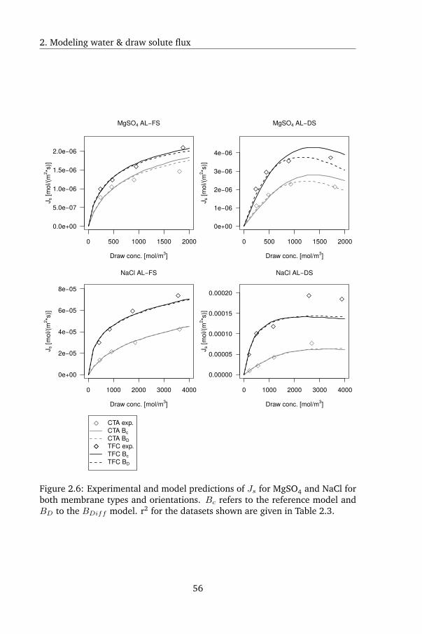
2. Modeling water & draw solute flux
0 1000 2000 3000 4000
0e+00
2e−05
4e−05
6e−05
8e−05
Draw conc. [mol/m3]
J s[m
ol/(m
2 *s)]
NaCl AL−FS
0 1000 2000 3000 4000
0.00000
0.00005
0.00010
0.00015
0.00020
Draw conc. [mol/m3]
J s[m
ol/(m
2 *s)]
NaCl AL−DS
0 500 1000 1500 2000
0.0e+00
5.0e−07
1.0e−06
1.5e−06
2.0e−06
Draw conc. [mol/m3]
J s[m
ol/(m
2 *s)]
MgSO4 AL−FS
0 500 1000 1500 2000
0e+00
1e−06
2e−06
3e−06
4e−06
Draw conc. [mol/m3]
J s[m
ol/(m
2 *s)]
MgSO4 AL−DS
CTA exp.CTA BcCTA BDTFC exp.TFC BcTFC BD
Figure 2.6: Experimental and model predictions of Js for MgSO4 and NaCl forboth membrane types and orientations. Bc refers to the reference model andBD to the BDiff model. r2 for the datasets shown are given in Table 2.3.
56
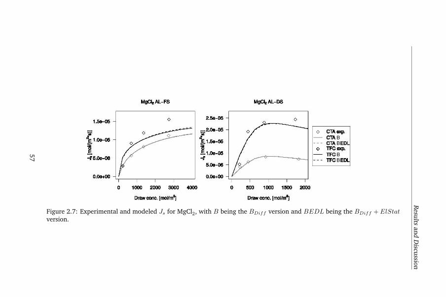
Results
andD
iscussion
BB
BB
Figure 2.7: Experimental and modeled Js for MgCl2, with B being the BDiff version and BEDL being the BDiff + ElStatversion.
57
1.58-05
=ii "e 1.08-05
I -rs.Oe-08
0.08+00
0
MgCI1 AL-FS
1000 2000 3000 4000
Draw conc. [moVm~
2.5e-05
,2.08-05
.s 1.58-05 ~ .§.1.08-05 -r
5.08-08
0.08+00
MgCI:!AL-DS
o CTAexp. CTA CTA EDL
o TFCexp. TFC TFC EDL
0 500 1000 1500 2000
Draw conc. [mollm&_l
2. Modeling water & draw solute flux
2.4.3 The Jw/Js ratio and its role in assessing model quality
When assuming validity of both the solution-diffusion model and the van ’t Hoff
equation for a given draw solute at any draw solution concentration, then the
resulting ratio of Jw/Js should be constant for any draw solution concentra-
tion, and independent from both ICP and ECP [106]. However, experimental
Jw/Js ratios for all draw solutes, membrane types or membrane orientations
showed concentration-dependent trends, as is shown for the AL-DS tests in Fig-
ures 2.5 and 2.8. This trend can be explained by the draw solute activity coeffi-
cients being dependent on concentration, leading to concentration-dependence
of the draw solute colligative properties such as diffusivity and osmotic pres-
sure. Combined with the concentration dependence of viscosity, draw solute
diffusivity and osmotic pressure diverge as a function of draw solute concentra-
tion, yielding a non-constant Jw/Js ratio. A modeled example of ICP influence
is shown in Figure 2.9, in which the Jw/Js ratio is calculated for different val-
ues of τ for MgSO4 in AL-DS tests. The Jw/Js ratio increases with increasing
MgSO4 concentration because diffusivity decreases while the osmotic pressure
increases. The build-up of MgSO4 with increasing τ at high draw concentra-
tions causes the draw solute concentration at both active layer interfaces to
rise, which then due to decreasing MgSO4 diffusivity at higher concentrations
depresses Js more than Jw is depressed by increasing S. Another explanation
for non-constant Jw/Js ratios could be saturation of the membrane active layer,
causing decreased partitioning of salts into the active layer at elevated concen-
trations. This has been found for both TFC [122] and CA membranes [123],
however, the decreased partitioning was mainly found at lower concentrations,
with the strongest decrease taking place below 0.5M.
As can be seen from Tables 2.2 and Figures 2.5 and 2.8, the Jw/Js ratio is
poorly predicted compared to Jw and Js. This can be due to experimental
error, as the ratio of two experimentally determined datasets causes increas-
ing error propagation. Another explanation would be that relevant parameters
are not yet included in the model, which cause the modeled and experimental
Jw/Js ratio to deviate: in that case, the residual error on Jw and Js is not
spread randomly but is concentration dependent. These deviating trends in
modeled Jw and Js are inherently diverging: the fitted A, B and S represent
the closest fit, with the influence of the unknown parameter(s) being divided
among the fitted parameters. Concentration-dependent model divergence can
58
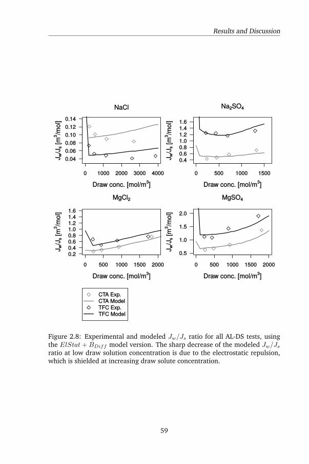
Results and Discussion
Figure 2.8: Experimental and modeled Jw/Js ratio for all AL-DS tests, usingthe ElStat + BDiff model version. The sharp decrease of the modeled Jw/Jsratio at low draw solution concentration is due to the electrostatic repulsion,which is shielded at increasing draw solute concentration.
59
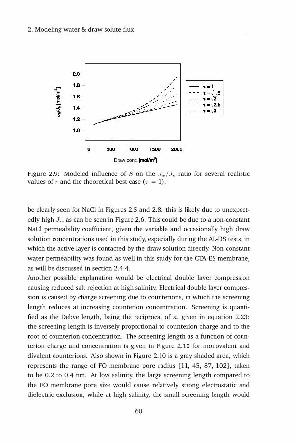
2. Modeling water & draw solute flux
Draw conc.
Figure 2.9: Modeled influence of S on the Jw/Js ratio for several realisticvalues of τ and the theoretical best case (τ = 1).
be clearly seen for NaCl in Figures 2.5 and 2.8: this is likely due to unexpect-
edly high Js, as can be seen in Figure 2.6. This could be due to a non-constant
NaCl permeability coefficient, given the variable and occasionally high draw
solution concentrations used in this study, especially during the AL-DS tests, in
which the active layer is contacted by the draw solution directly. Non-constant
water permeability was found as well in this study for the CTA-ES membrane,
as will be discussed in section 2.4.4.
Another possible explanation would be electrical double layer compression
causing reduced salt rejection at high salinity. Electrical double layer compres-
sion is caused by charge screening due to counterions, in which the screening
length reduces at increasing counterion concentration. Screening is quanti-
fied as the Debye length, being the reciprocal of κ, given in equation 2.23:
the screening length is inversely proportional to counterion charge and to the
root of counterion concentration. The screening length as a function of coun-
terion charge and concentration is given in Figure 2.10 for monovalent and
divalent counterions. Also shown in Figure 2.10 is a gray shaded area, which
represents the range of FO membrane pore radius [11, 45, 87, 102], taken
to be 0.2 to 0.4 nm. At low salinity, the large screening length compared to
the FO membrane pore size would cause relatively strong electrostatic and
dielectric exclusion, while at high salinity, the small screening length would
60
2.0
1.8 "'" :§ 1.6 0 .§.
~ 1.4
1.2
1.0
0 500 1000 1500
[moVm~
2000
't = 1 <=ill '=,/2 '- ,/2.5 '=,'8
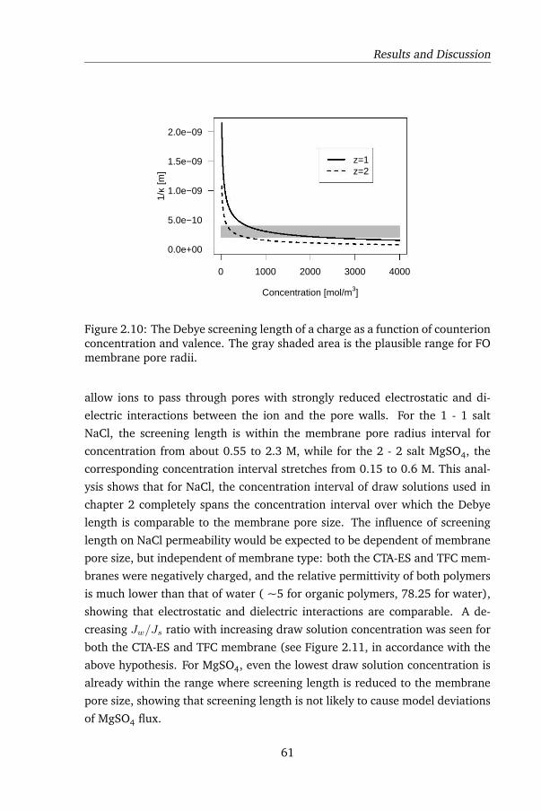
Results and Discussion
0 1000 2000 3000 4000
0.0e+00
5.0e−10
1.0e−09
1.5e−09
2.0e−09
Concentration [mol/m3]
1/κ
[m]
z=1z=2
Figure 2.10: The Debye screening length of a charge as a function of counterionconcentration and valence. The gray shaded area is the plausible range for FOmembrane pore radii.
allow ions to pass through pores with strongly reduced electrostatic and di-
electric interactions between the ion and the pore walls. For the 1 - 1 salt
NaCl, the screening length is within the membrane pore radius interval for
concentration from about 0.55 to 2.3 M, while for the 2 - 2 salt MgSO4, the
corresponding concentration interval stretches from 0.15 to 0.6 M. This anal-
ysis shows that for NaCl, the concentration interval of draw solutions used in
chapter 2 completely spans the concentration interval over which the Debye
length is comparable to the membrane pore size. The influence of screening
length on NaCl permeability would be expected to be dependent of membrane
pore size, but independent of membrane type: both the CTA-ES and TFC mem-
branes were negatively charged, and the relative permittivity of both polymers
is much lower than that of water ( ~5 for organic polymers, 78.25 for water),
showing that electrostatic and dielectric interactions are comparable. A de-
creasing Jw/Js ratio with increasing draw solution concentration was seen for
both the CTA-ES and TFC membrane (see Figure 2.11, in accordance with the
above hypothesis. For MgSO4, even the lowest draw solution concentration is
already within the range where screening length is reduced to the membrane
pore size, showing that screening length is not likely to cause model deviations
of MgSO4 flux.
61
EJ
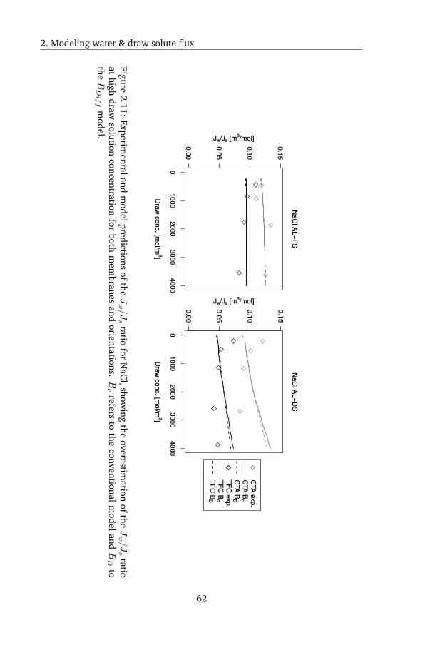
2. Modeling water & draw solute flux
Figure2.11:
Experimentaland
modelpredictions
oftheJw/Js
ratiofor
NaC
l,showing
theoverestim
ationofthe
Jw/Js
ratioat
highdraw
solutionconcentration
forboth
mem
branesand
orientations.Bc
refersto
theconventional
model
andBD
tothe
BDiff
model.
62
Results and Discussion
2.4.4 Membrane permeability coefficients
The membrane parameters A, B, S and apparent tortuosity τ as calculated by
the BDiff + ElStat model are given in Table 2.4.
The calculated water permeability of the CTA-ES membrane was similar for all
draw solutes in AL-FS mode, which was decreased however in AL-DS mode
according to the osmotic pressure of the draw solutions used. The decrease
of A is illustrated in Figure 2.12: for each set of flux tests using a given draw
solute and membrane orientation, the mean osmotic pressure the active layer
was subjected to was calculated using the modeled interface concentrations
cAE and cAS . A linear dependence was found of the mean A as a function of
the mean osmotic pressure (r 2=0.96, p < 2e-5), yielding a pure water perme-
ability of 1.27 · 10 -12 m/(Pa·s), and a water permeability decrease of 0.75%
per bar of osmotic pressure. These results highlight the need to characterize FO
membranes using FO tests: osmotic dehydration and the resulting decrease of
water permeability would not be apparent using RO tests and tracer amounts
of draw solute. Decreased water permeability of chemically similar cellulose
acetate membranes was noted by Mehta and Loeb as well [5]. The pure water
permeability is in accordance with the study by Tiraferri et al., who also used
an FO-only method [72]. However, RO characterization of CTA-ES membranes
often find higher water permeabilities [10, 69, 71], which was confirmed by
our benchmarking tests as well. This discrepancy shows that the CTA-ES mem-
brane reacts differently to hydraulic and osmotic pressure: applying hydraulic
pressure leads to increased rather than decreased water permeability, which
could be due to membrane deformation [2].
The TFC membrane was found to be considerably more permeable than the
CTA-ES membrane, in accordance with earlier study [48]. In contrast to the
CTA-ES membrane, no proportionality between A and the osmotic pressure the
active layer was subjected to could be discerned (r2: 0.009, p=0.82) (see figure
2.13), however, water permeability was reduced when using MgSO4, and to a
lesser extent, MgCl2 (see Table 2.4). This phenomenon, albeit more subtle, has
been noticed before for NF membranes [124]. A possible explanation could be
absorption of Mg+2 in the active layer, causing additional hindrance for water
transport. A limited reduction of active layer porosity due to ion adsorption
has been reported, the effect on water permeability was however not reported
[122].
63
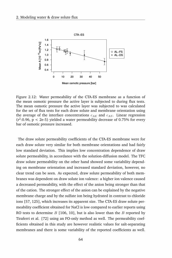
2. Modeling water & draw solute flux
Figure 2.12: Water permeability of the CTA-ES membrane as a function ofthe mean osmotic pressure the active layer is subjected to during flux tests.The mean osmotic pressure the active layer was subjected to was calculatedfor the set of flux tests for each draw solute and membrane orientation usingthe average of the interface concentrations cAE and cAS . Linear regression(r2:0.96, p < 2e-5) yielded a water permeability decrease of 0.75% for everybar of osmotic pressure increased.
The draw solute permeability coefficients of the CTA-ES membrane were for
each draw solute very similar for both membrane orientations and had fairly
low standard deviation. This implies low concentration dependence of draw
solute permeability, in accordance with the solution-diffusion model. The TFC
draw solute permeability on the other hand showed some variability depend-
ing on membrane orientation and increased standard deviation, however, no
clear trend can be seen. As expected, draw solute permeability of both mem-
branes was dependent on draw solute ion valence: a higher ion valence caused
a decreased permeability, with the effect of the anion being stronger than that
of the cation. The stronger effect of the anion can be explained by the negative
membrane charge and by the sulfate ion being hydrated in contrast to chloride
ions [57, 125], which increases its apparent size. The CTA-ES draw solute per-
meability coefficient obtained for NaCl is low compared to earlier reports using
RO tests to determine B [106, 10], but is also lower than the B reported by
Tiraferri et al. [72] using an FO-only method as well. The permeability coef-
ficients obtained in this study are however realistic values for salt-separating
membranes and there is some variability of the reported coefficients as well.
64
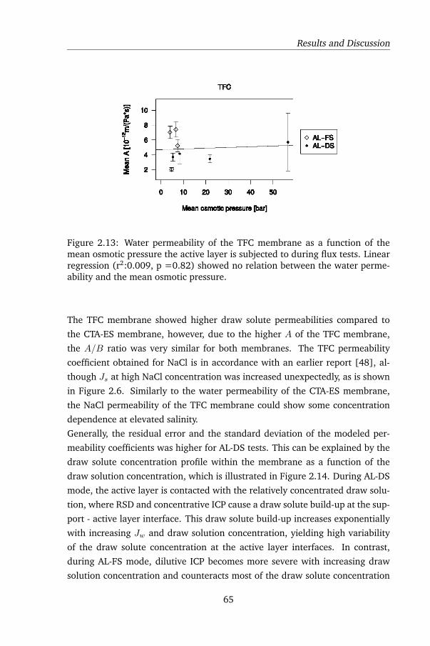
Results and Discussion
Figure 2.13: Water permeability of the TFC membrane as a function of themean osmotic pressure the active layer is subjected to during flux tests. Linearregression (r2:0.009, p =0.82) showed no relation between the water perme-ability and the mean osmotic pressure.
The TFC membrane showed higher draw solute permeabilities compared to
the CTA-ES membrane, however, due to the higher A of the TFC membrane,
the A/B ratio was very similar for both membranes. The TFC permeability
coefficient obtained for NaCl is in accordance with an earlier report [48], al-
though Js at high NaCl concentration was increased unexpectedly, as is shown
in Figure 2.6. Similarly to the water permeability of the CTA-ES membrane,
the NaCl permeability of the TFC membrane could show some concentration
dependence at elevated salinity.
Generally, the residual error and the standard deviation of the modeled per-
meability coefficients was higher for AL-DS tests. This can be explained by the
draw solute concentration profile within the membrane as a function of the
draw solution concentration, which is illustrated in Figure 2.14. During AL-DS
mode, the active layer is contacted with the relatively concentrated draw solu-
tion, where RSD and concentrative ICP cause a draw solute build-up at the sup-
port - active layer interface. This draw solute build-up increases exponentially
with increasing Jw and draw solution concentration, yielding high variability
of the draw solute concentration at the active layer interfaces. In contrast,
during AL-FS mode, dilutive ICP becomes more severe with increasing draw
solution concentration and counteracts most of the draw solute concentration
65
TFC
~ 10
'[ 8 It ~ • b 6 os :::. < 4 I1 I c I ::E 2 "
' 0 10 20 30 40 50
Maan osmotlc pressure [bar]
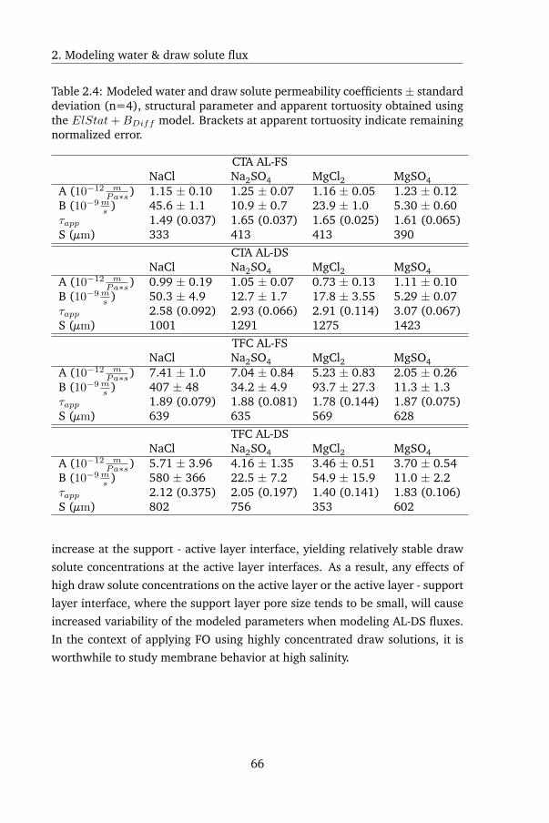
2. Modeling water & draw solute flux
Table 2.4: Modeled water and draw solute permeability coefficients± standarddeviation (n=4), structural parameter and apparent tortuosity obtained usingthe ElStat+BDiff model. Brackets at apparent tortuosity indicate remainingnormalized error.
CTA AL-FSNaCl Na2SO4 MgCl2 MgSO4
A (10−12 mPa∗s) 1.15 ± 0.10 1.25 ± 0.07 1.16 ± 0.05 1.23 ± 0.12
B (10−9ms ) 45.6 ± 1.1 10.9 ± 0.7 23.9 ± 1.0 5.30 ± 0.60
τapp 1.49 (0.037) 1.65 (0.037) 1.65 (0.025) 1.61 (0.065)S (µm) 333 413 413 390
CTA AL-DSNaCl Na2SO4 MgCl2 MgSO4
A (10−12 mPa∗s) 0.99 ± 0.19 1.05 ± 0.07 0.73 ± 0.13 1.11 ± 0.10
B (10−9ms ) 50.3 ± 4.9 12.7 ± 1.7 17.8 ± 3.55 5.29 ± 0.07
τapp 2.58 (0.092) 2.93 (0.066) 2.91 (0.114) 3.07 (0.067)S (µm) 1001 1291 1275 1423
TFC AL-FSNaCl Na2SO4 MgCl2 MgSO4
A (10−12 mPa∗s) 7.41 ± 1.0 7.04 ± 0.84 5.23 ± 0.83 2.05 ± 0.26
B (10−9ms ) 407 ± 48 34.2 ± 4.9 93.7 ± 27.3 11.3 ± 1.3
τapp 1.89 (0.079) 1.88 (0.081) 1.78 (0.144) 1.87 (0.075)S (µm) 639 635 569 628
TFC AL-DSNaCl Na2SO4 MgCl2 MgSO4
A (10−12 mPa∗s) 5.71 ± 3.96 4.16 ± 1.35 3.46 ± 0.51 3.70 ± 0.54
B (10−9ms ) 580 ± 366 22.5 ± 7.2 54.9 ± 15.9 11.0 ± 2.2
τapp 2.12 (0.375) 2.05 (0.197) 1.40 (0.141) 1.83 (0.106)S (µm) 802 756 353 602
increase at the support - active layer interface, yielding relatively stable draw
solute concentrations at the active layer interfaces. As a result, any effects of
high draw solute concentrations on the active layer or the active layer - support
layer interface, where the support layer pore size tends to be small, will cause
increased variability of the modeled parameters when modeling AL-DS fluxes.
In the context of applying FO using highly concentrated draw solutions, it is
worthwhile to study membrane behavior at high salinity.
66
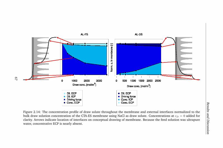
Results
andD
iscussion
Figure 2.14: The concentration profile of draw solute throughout the membrane and external interfaces normalized to thebulk draw solution concentration of the CTA-ES membrane using NaCl as draw solute. Concentrations at cD = 0 added forclarity. Arrows indicate location of interfaces on conceptual drawing of membrane. Because the feed solution was ultrapurewater, concentrative ECP is nearly absent.
67
AL-FS
Draw conc. [moVm3]
Dii.ECP • Dii.ICP • Driving force • Conc. ECP
:::::::: Cl)
] E Q)
E .5 d Ë 6 z
AL-OS
Draw conc. [mol/m3]
• Dil. ECP • Driving force • Conc.ICP
Conc. ECP
2. Modeling water & draw solute flux
2.4.5 Support layer structural parameter and tortuosity
The structural parameter S is conventionally regarded as a membrane prop-
erty independent of the draw solute or membrane orientation used, which has
been recently shown to be erroneous [73]. Both membranes showed some
variability of S between the different draw solutes in AL-FS mode, however,
more variability was seen in AL-DS mode as well as considerable increases or
decreases of S for each draw solute between both membrane orientations (see
Table 2.4). The structural parameters in AL-FS mode are in line with earlier
reports [8, 72], and an increase of S in AL-DS mode has been reported as well
[73]. There are no clear trends in S based on draw solute properties: S ap-
pears to increase with increasing draw solute ion valence in both membrane
orientations for the CTA-ES membrane, but, for the TFC membrane, this trend
is reversed (see Table 2.4). Effects of draw solution osmotic pressure or vis-
cosity on S [10] were not noticeable for both membranes: in the former case,
the chloride salts produce a higher osmotic pressure than the sulfate salts at
similar concentrations but no anion-based clustering of S was apparent. In the
latter case, the magnesium salts cause a more pronounced viscosity increase
compared to the sodium salts, but again no cation-based clustering based can
be discerned. Molecular weight or ion size could also not predict structural
parameter trends: in the former case, draw solute molecular weight increases
according to NaCl, MgCl2, MgSO4 and Na2SO4, and in the latter case, the sum
of hydrated ion radii increases according to NaCl, MgSO4, Na2SO4 and MgCl2[57, 125, 110]; similar trends can however not be discerned in the calculated
S. Both draw solute molecular weight and ion size would affect the draw so-
lute diffusivity, which is already accounted for when calculating S.
Structural changes to support layer pores, such as collapsing due to osmotic
dehydration or blockage due to binding of draw solute [126] or viscosity me-
diated effects require high draw solution concentrations in the support layer.
However, assuming that most of the resistance against draw solute diffusion is
taking place near the active layer - support layer interface where support layer
pores are the smallest, analysis of modeled cAS showed that draw solute con-
centrations were generally low in this interface region compared to the bulk
draw solutions for most of the flux tests. This is illustrated for the CTA-ES
membrane in Figure 2.14. In this case using NaCl, which yielded the lowest
A/B ratio of 25 · 10-6 Pa-1, cAS only exceeded 1M during the flux test using the
68
Results and Discussion
most concentrated draw solution in both modes. Furthermore, analysis of cASshowed that S was higher as cAS was lower. In the case of CTA-ES in AL-DS
mode using MgSO4 for instance, the calculated cAS did not exceed 0.1M for
the flux tests with the lower concentrated 3 out of the 4 draw solutions, with
S being 1422 µm. During AL-FS mode, the lowest calculated cAS MgSO4 con-
centration was 0.16M, and S was 390 µm. Similar trends were found for the
other draw solutes as well. For the TFC membrane, cAS in AL-DS was generally
somewhat higher compared to the CTA-ES membrane due to the higher Js and
Jw, which were caused by the higher A and B parameters, likewise, in AL-FS
mode, cAS was lower due to more severe ICP. As a result, TFC cAS was similar
at lower bulk draw solution concentrations for both modes , and was higher
for AL-DS at higher bulk draw solution concentrations. The TFC S for each
draw solute was similar for both membrane orientations, with the exception
of MgCl2, where S obtained during AL-DS tests was about 40 % lower than
in AL-FS tests. This analysis indicates that S is increased at low draw solution
concentration.
This phenomenon could be partially explained by the electro-viscous effect, in
which the apparent solution viscosity is increased due to electrical double layer
interactions between an electrolyte and the walls of the porous medium. Co-
ion and counter-ion partitioning at the solution interface combined with con-
vective flow produce both a streaming current and streaming potential, which
causes the co-ions to diffuse in the opposite direction of the convective flow
in which they are enriched, thereby hindering the convective flow and increas-
ing the apparent solution viscosity [127]. In this case, reduced draw solute
diffusivity rather than increased apparent viscosity could explain the increased
structural parameter, as the effect on viscosity is modest ( ∼ 20% viscosity in-
crease in pores of 5 - 10 nm) [128, 129]. The electro-viscous effect becomes
more pronounced as both the pore size of the porous medium and the elec-
trolyte concentration decrease, as the electrical double layer decays exponen-
tially with distance to the charged surface and is shielded by counter-ions. This
supports the assumption that the support layer region close to the active layer
interface contributes most to S. According to the electroviscous hypothesis, the
modeled S would be higher when using a subset of the flux data with lower
cAS , which is illustrated for the CTA-ES membrane in Figure 2.15. The CTA-
ES membrane datasets for each draw solute were divided according to draw
solution concentration in three subsets of two flux tests for which S was calcu-
69
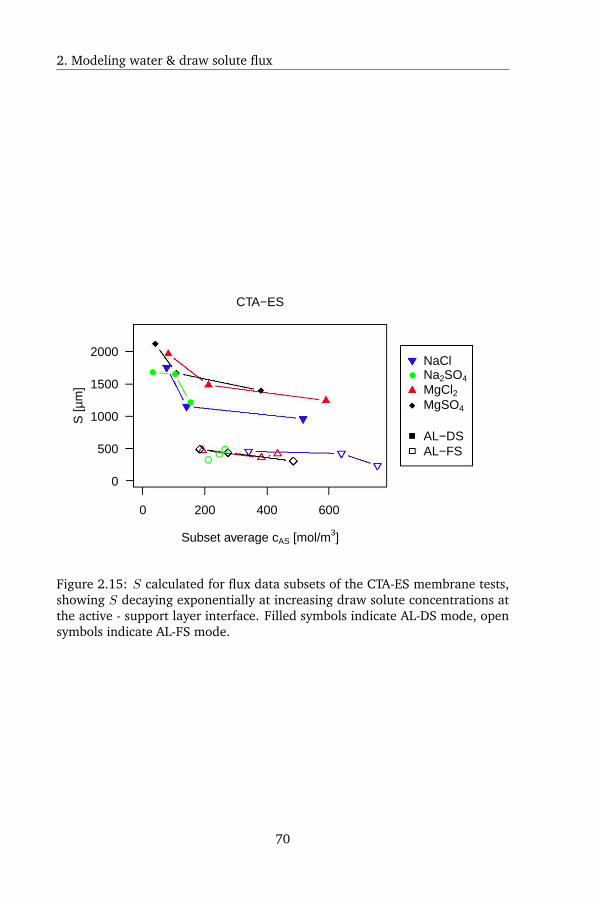
2. Modeling water & draw solute flux
0 200 400 600
0
500
1000
1500
2000
● ●
●
●●
●
Subset average cAS [mol/m3]
S [µ
m]
CTA−ES
●
NaClNa2SO4
MgCl2MgSO4
AL−DSAL−FS
Figure 2.15: S calculated for flux data subsets of the CTA-ES membrane tests,showing S decaying exponentially at increasing draw solute concentrations atthe active - support layer interface. Filled symbols indicate AL-DS mode, opensymbols indicate AL-FS mode.
70
~
• • D
Results and Discussion
lated; yielding subsets with the lowest, middle and highest two draw solution
concentrations and their corresponding subset structural parameter, Ssub. An
exponential decay of Ssub was seen with increasing cAS in AL-DS mode, while
no clear trend could be discerned in AL-FS mode. It was also noted that while
Ssub decreases with increasing cAS , it remained higher in AL-DS mode com-
pared to AL-FS mode even at the highest cAS . This was also confirmed by
additional flux tests, in which the NaCl AL-DS tests were repeated with 0.1 M
NaCl feed solution instead of ultrapure water (suppressing the electrical dou-
ble layer), which yielded a S decrease of 12.6 % compared to the AL-DS tests
using ultrapure water as feed, but it was still 2.3 times larger than the S ob-
tained in AL-FS tests. Due to the higher permeability of the TFC membrane
and thus higher draw solute concentrations in the active layer interfaces, the
electroviscous effect would be strongly reduced. In order to assess the impact
of the electro-viscous effect on ICP in FO, the current transport models can be
extended, taking into account the reduced electrolyte diffusivity. These results
also show that electrokinetic effects such as the electro-viscous effect can be
used to characterize FO membranes, as the study of the electro-viscous effect
has been used to characterize UF membranes [128, 129] and colloidal mem-
brane fouling [130].
The difference between S obtained in AL-FS versus AL-DS mode, after account-
ing for electroviscosity, could be explained by considering the active layer -
support layer interface as a zone where partial decoupling of convective water
and solute fluxes takes place, rather than a sharp boundary between purely dif-
fusive transport in the active layer and coupled transport in the support layer.
The larger solute molecules would be more hindered than water and conse-
quently, both convective and diffusive transport of solutes would be reduced
to different degrees. In the case of AL-FS mode, this would counteract ICP, as
draw solute molecules are not easily entrained by Jw towards the bulk draw
solution, yielding a low apparent S. In AL-DS mode however, with fluxes in
the opposite direction, draw solute molecules entering the support layer due
to RSD would face additional hindrance when diffusing towards the bulk feed
solution, yielding a high apparent S. This hypothesis would explain why S
is different for a given draw solute depending on membrane orientation, and
would also explain why S is different for different draw solutes. Both the mem-
brane orientation and draw solute dependence of S cannot be explained using
the current definition of S, extending this definition will be the topic of future
71
2. Modeling water & draw solute flux
research.
Using equation 2.13, the apparent tortuosity, τ , was calculated from S (see
Table 2.4). An overview of theoretical and empirical models of tortuosity as a
function of porosity is provided by Shen and Chen [49]. Realistic values for τ
at a porosity of 0.5 are in the order of√
1.5 to√
3. The apparent tortuosities
measured in this study are within this range for the CTA-ES AL-FS tests, as are
both of the MgCl2 TFC tests. The other apparent tortuosities are likely overes-
timates because not all resistance to solute diffusion has been accounted for, as
was discussed in the previous paragraphs. This was noted by Manickam and
McCutcheon as well [73]: using a well-characterized track-etched membrane
as a support layer allowed a priori calculation of the structural parameter. Cal-
culation of S from FO flux tests however yielded much higher values for S,
and, interestingly, S was larger for AL-DS tests and for tests at low draw solu-
tion concentration, in accordance with the electroviscosity hypothesis.
Van Brakel and Heertjes [113] suggested including a constrictivity factor as
well into equation 2.11, which was also suggested by Zhao et al. [10]. Con-
strictivity is a dimensionless factor between 0 and 1 which takes into account
the varying pore diameter: narrow sections within pores do not influence tortu-
osity or porosity, yet they do cause additional hindrance. The effects of solution
viscosity will also be accounted for by constrictivity: narrow pore sections will
cause more hindrance as the solution viscosity increases, which is again not
accounted for by either tortuosity or porosity. In the model presented in this
study, constrictivity was not included, for two reasons: firstly, the variable draw
solute diffusivity during ICP is based on experimental data. From the Stokes-
Einstein law and as mentioned in section 2.2.1, it is clear that diffusivity is
inversely proportional to solution viscosity, so the reduced diffusivity due to
increased viscosity at high draw solution concentration is already accounted
for. Secondly, the draw solutes are all small mineral salts with hydrated ionic
radii in the order of 0.3 nm. The steric effects of narrow pores will thus be
small and will affect all draw solutes almost equally, making the constrictivity
factor superfluous in this case. Further research using draw solutes of different
sizes and well-characterized membranes could reveal whether the inclusion of
a constrictivity factor is of added value.
72
Conclusions
2.5 Conclusions
In this study, a model is presented estimating the membrane water and draw
solute permeability, structural parameter and apparent tortuosity using only
FO tests, which was experimentally validated using two FO membranes in both
orientations and using four different draw solutes, all mineral salts. The results
presented in this study show that this method is preferable to RO-based meth-
ods: draw solute-specific membrane interactions would not have been noticed
using RO tests, such as the decreasing water permeability of the CTA-ES and
TFC membranes at increasing osmotic pressure and when using magnesium-
based draw solutes respectively. These interactions would otherwise have con-
tributed to increased errors in subsequent modeling. The flux model in this
study was expanded by taking into account concentration-dependent diffusiv-
ity of the draw solutes during transport through the membrane active layer,
which was found to improve Js predictions, especially in AL-DS mode. Elec-
trostatic repulsion of co-ions at the active layer interfaces was studied and was
found to be of limited importance in FO: at the ζ-potentials measured for both
membranes and the elevated salt concentrations in the draw solutions, the
effect of co-ion repulsion on Js was small. However, including electrostatic
repulsion in flux modeling did yield improved prediction of the Jw/Js ratio.
The model was able to predict Jw and Js well, however, the Jw/Js ratio was
sometimes predicted poorly, indicating that relevant parameters are still miss-
ing from FO transport models, or that membrane characteristics are influenced
by high salinity.
Characterization of both membranes allowed the calculation of the apparent
tortuosity, which in some cases was realistic given the membranes’ porosity,
and in other cases was unrealistically high. Calculated tortuosities were gener-
ally higher in AL-DS mode, when the draw solute concentration in the support
layer was low. This study has shown that the calculated structural parameter
was dependent on the draw solute and membrane orientation. A possible par-
tial explanation including indirect evidence was offered in the electroviscous
effect, an additional explanation could be steric hindrance of the draw solute
at the active layer - support layer interface. Further research is needed to test
both hypotheses and incorporate them into structural parameter models.
This study furthermore extends FO transport models to high salinity environ-
ments by introducing solute concentration-dependent active layer and support
73
2. Modeling water & draw solute flux
layer transport. It is shown that membrane permeability, both of water and so-
lutes, at elevated solute concentrations is not necessarily constant: a decreased
water permeability of the CTA-ES membrane was observed, while the NaCl
flux was higher than predicted in the TFC membrane at high draw solution
concentration. Because fluxes in FO are generally limited, draw solution con-
centration is generally high and thus FO membrane performance should also
be evaluated at high salinity.
2.A Appendix
2.A.1 Experimental flux data
The experimental flux data which was the input of the model presented in
chapter 2 is given in Tables 2.5 and 2.6 for the CTA-ES and TFC membrane
respectively.
74
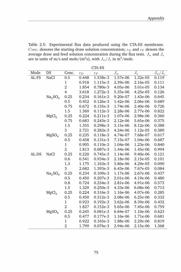
Appendix
Table 2.5: Experimental flux data produced using the CTA-ES membrane.Conc. denotes the starting draw solution concentration; cD and cF denote theaverage draw and feed solution concentration during the flux tests. Jw and Jsare in units of m/s and mole/(m2s), with Jw/Js in m3/mole.
CTA-ESMode DS Conc. cD cF Jw Js Jw/JsAL-FS NaCl 0.5 0.448 1.538e-3 1.57e-06 1.32e-05 0.119
1 0.918 1.115e-3 2.39e-06 2.16e-05 0.1112 1.854 0.780e-3 4.05e-06 3.01e-05 0.1344 3.618 1.272e-3 5.35e-06 4.25e-05 0.126
Na2SO4 0.25 0.234 0.161e-3 9.20e-07 1.43e-06 0.6450.5 0.452 0.126e-3 1.42e-06 2.06e-06 0.6890.75 0.672 0.135e-3 1.74e-06 2.40e-06 0.7261.5 1.369 0.112e-3 2.28e-06 2.77e-06 0.822
MgCl2 0.25 0.224 0.211e-3 1.07e-06 2.98e-06 0.3600.75 0.683 0.243e-3 2.12e-06 5.65e-06 0.3751.5 1.355 0.298e-3 3.15e-06 8.12e-06 0.3883 2.721 0.282e-3 4.24e-06 1.12e-05 0.380
MgSO4 0.25 0.235 0.118e-3 4.74e-07 7.68e-07 0.6170.5 0.458 0.131e-3 7.15e-07 1.04e-06 0.6871 0.905 0.110e-3 1.04e-06 1.23e-06 0.8402 1.813 0.087e-3 1.44e-06 1.45e-06 0.994
AL-DS NaCl 0.25 0.220 0.745e-3 1.14e-06 9.40e-06 0.1210.6 0.541 0.934e-3 2.18e-06 2.15e-05 0.1011.3 1.175 1.163e-3 3.86e-06 4.29e-05 0.0903 2.682 1.393e-3 6.43e-06 7.67e-05 0.084
Na2SO4 0.25 0.234 0.109e-3 1.17e-06 2.67e-06 0.4370.5 0.450 0.207e-3 2.01e-06 4.19e-06 0.4800.8 0.724 0.234e-3 2.81e-06 4.91e-06 0.5731.5 1.329 0.250e-3 4.33e-06 6.08e-06 0.713
MgCl2 0.25 0.224 0.316e-3 1.16e-06 4.07e-06 0.2850.5 0.450 0.312e-3 2.08e-06 6.25e-06 0.3321 0.923 0.192e-3 3.62e-06 8.39e-06 0.4322 1.827 0.152e-3 5.65e-06 7.45e-06 0.759
MgSO4 0.25 0.245 0.081e-3 6.84e-07 1.10e-06 0.6230.5 0.477 0.177e-3 1.16e-06 1.71e-06 0.6811 0.922 0.165e-3 1.88e-06 2.29e-06 0.8192 1.799 0.076e-3 2.94e-06 2.15e-06 1.368
75
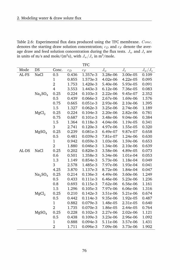
2. Modeling water & draw solute flux
Table 2.6: Experimental flux data produced using the TFC membrane. Conc.denotes the starting draw solution concentration; cD and cF denote the aver-age draw and feed solution concentration during the flux tests. Jw and Js arein units of m/s and mole/(m2s), with Jw/Js in m3/mole.
TFCMode DS Conc. cD cF Jw Js Jw/JsAL-FS NaCl 0.5 0.436 1.357e-3 3.28e-06 3.00e-05 0.109
1 0.855 1.573e-3 4.02e-06 4.22e-05 0.0952 1.753 1.420e-3 5.40e-06 5.93e-05 0.0914 3.553 1.443e-3 6.12e-06 7.36e-05 0.083
Na2SO4 0.25 0.224 0.103e-3 2.22e-06 9.45e-07 2.3520.5 0.439 0.066e-3 2.67e-06 1.69e-06 1.5760.75 0.665 0.051e-3 2.93e-06 2.10e-06 1.3951.5 1.327 0.062e-3 3.25e-06 2.74e-06 1.189
MgCl2 0.25 0.224 0.104e-3 2.20e-06 2.82e-06 0.7810.75 0.687 0.101e-3 3.48e-06 9.04e-06 0.3841.5 1.364 0.118e-3 4.04e-06 1.19e-05 0.3413 2.741 0.120e-3 4.97e-06 1.55e-05 0.320
MgSO4 0.25 0.239 0.081e-3 6.49e-07 9.87e-07 0.6580.5 0.481 0.039e-3 7.81e-07 1.24e-06 0.6301 0.942 0.059e-3 1.03e-06 1.59e-06 0.6532 1.880 0.046e-3 1.34e-06 2.10e-06 0.639
AL-DS NaCl 0.25 0.202 0.820e-3 3.58e-06 4.89e-05 0.0730.6 0.501 1.358e-3 5.34e-06 1.01e-04 0.0531.3 1.149 0.854e-3 5.73e-06 1.18e-04 0.0493 2.578 1.485e-3 7.97e-06 1.93e-04 0.0414.25 3.870 1.137e-3 8.72e-06 1.84e-04 0.047
Na2SO4 0.25 0.214 0.136e-3 4.49e-06 3.60e-06 1.2490.5 0.433 0.111e-3 6.46e-06 5.23e-06 1.2360.8 0.693 0.115e-3 7.62e-06 6.56e-06 1.1611.5 1.296 0.105e-3 7.97e-06 6.06e-06 1.316
MgCl2 0.25 0.210 0.142e-3 3.51e-06 5.21e-06 0.6740.5 0.442 0.114e-3 9.35e-06 1.92e-05 0.4871 0.882 0.079e-3 1.48e-05 2.31e-05 0.6402 1.735 0.070e-3 1.86e-05 2.44e-05 0.764
MgSO4 0.25 0.228 0.102e-3 2.27e-06 2.02e-06 1.1210.5 0.438 0.109e-3 3.23e-06 2.96e-06 1.0921 0.888 0.094e-3 5.11e-06 3.57e-06 1.4312 1.711 0.096e-3 7.09e-06 3.73e-06 1.902
76
Chapter 3
Organic micropollutant transport: in-fluence of draw solutes on OMP trans-port and membrane surface free en-ergy
Adapted from:
Arnout D’Haese, Klaas Schoutteten, Tim Van Kerrebroeck, Julie Vanden Buss-
che, Lynn Vanhaecke, Arne Verliefde, Elucidating interactions between Organic
Micropollutants and Draw Solutes in Forward Osmosis In preparation
77

3. OMP transport
3.1 Introduction
In this chapter, the transport of organic micropollutants (OMPs) during FO is
studied. OMPs are anthropogenic organic compounds present in waste wa-
ter typically at concentrations in the ng/L to µg/L range. This group of com-
pounds consists of, among others, pharmaceuticals, personal care products,
flame retardants and pesticides. One potential consequence of chronic expo-
sure to OMPs is endocrine disruption [131]. Although some controversy re-
mains whether endocrine disruption has significant effects on humans [132,
133], the effects of endocrine disruption caused by estrogenic compounds in
aquatic vertebrates have been reported [134]. As FO would be applied pri-
marily on heavily impaired feeds such as wastewater or wastewater sludges,
OMP rejection is an important characteristic of FO processes. Commonly used
CTA FO membranes cannot be regarded as a total barrier against OMPs: the
rejection of CTA FO membranes is reported to be comparable to tight NF mem-
branes, with a molecular weight cutoff in the order of 200 Da [81, 135], and
a lower OMP rejection compared to RO membranes [82] (see also chapter 5).
TFC appear to be superior to CTA membranes with regards to OMP rejection.
Xie et al. [45] found that for their CTA and TFC membranes, pore size was sim-
ilar while OMP rejection was higher for the TFC membrane at similar fluxes.
In this study however, the aim was not to achieve an as high as possible OMP
rejection, but to study how OMP transport interacts with draw solutes.
Compared to the related membrane processes NF and RO, FO operating con-
ditions are hypersaline: the draw solute is often an inorganic salt and is used
at high concentrations in order to produce sufficiently high water fluxes. Com-
bined with a membrane more permeable than an SWRO membrane, this causes
considerable reverse salt diffusion (RSD), a salt flux in the opposite direction
of the water flux. RSD is absent in NF and RO: salt flux in NF and RO tends
to be smaller and has the same direction as the water flux. RSD can thus
have a distinct influence on the fluxes of water and feed solutes, unique to
FO. RSD causes the establishment of an electrical field between the feed and
draw solutions due to the unequal membrane permeability of the different
draw solute ions [93], the electrical field created by the dominant draw so-
lute ions (in terms of concentration) then alters the permeation of ionic feed
species through electromigration [92, 60]. Unequal ion concentrations across
the membrane of feed and draw solutes, combined with unequal ion perme-
78
Introduction
ability, are also driving forces for Donnan dialysis [62] where permeable feed
and draw ions of the same polarity are exchanged. High permeability of spe-
cific ions of cellulose triacetate (CTA) membranes has been reported as well
[136]: NO –3 for instance permeates easily through CTA membranes and is
readily exchanged with other high-permeability anions. The transport of OMPs
is reportedly also impacted by RSD: a reduced OMP flux in FO when using
high-RSD draw solutes was noted by Xie et al. [11, 137] compared to low-
RSD draw solutes. The authors proposed a steric mechanism: draw solute ions
would block membrane pores, thereby hindering OMP permeation.
The impact of RSD on OMP permeability has however not been studied in de-
tail: Xie et al. [11, 137] performed a very limited number of experiments with
a low number of OMPs, as studying RSD was not the main focus of their stud-
ies. Charge interactions between RSD and charged organic feed solutes have
only been studied in the context of fouling [138, 139], where the increased
salinity at the feed solution - membrane interface induces colloidal destabi-
lization and cake-enhanced osmotic pressure [140]. The influence of draw
solutes on OMP-membrane interactions likewise has not been studied yet. The
membrane affinity of organic feed solutes in aqueous medium, as expressed
by ∆GMLS , has been used to predict solute partitioning at the membrane in-
terface, yielding accurate solute flux predictions [86, 87] and has also been
used to predict membrane fouling [141, 139]. Hurwitz et al. [142] studied
the surface of a XLE BWRO membrane using contact angle titration, showing
that the membrane surface tension became more Lewis basic and less Lewis
acidic as a function of increasing NaCl concentration. It follows that RSD can
also influence solute - membrane affinity, although this has not been tested yet.
Surface tension analysis of polyacrylate by Rillosi et al. [143] has also shown
that the surface tension of hydrophilic polymers differs between dried and hy-
drated states, with the polymer becoming less hydrophobic and becoming a
stronger Lewis base. Surface tension analysis of polymers wetted by brines has
however not yet been performed.
FO membrane orientation has been shown to severely impact observed OMP re-
jection [144]: in AL-FS mode, the observed rejection is slightly decreased com-
pared to the real rejection due to external concentration polarization (ECP),
while a much larger decrease is noted in AL-DS mode due to concentrative
internal concentration polarization. ECP is however fairly limited for most mi-
cropollutants, due to the relatively low fluxes obtained in FO and the high
79
3. OMP transport
diffusivity of small molecules. ICP however is much more severe than ECP: the
micropollutant molecules are entrained into the porous membrane support,
from which they can only be removed by permeation through the membrane
or by strongly hindered back-diffusion out of the support layer. Consequently,
the micropollutant concentration is strongly increased in the porous support in
AL-DS mode leading to reduced observed rejection [144, 83]. For these rea-
sons, all FO tests were performed in AL-FS mode in this study.
In this study, the relation between draw solutes and OMP permeability is ex-
plored. The hypothesis of RSD hindering OMP permeation is tested by deter-
mining OMP permeability for FO tests performed using 4 different inorganic
draw solutes (NaCl, MgCl2, Na2SO4 and MgSO4) and using OMP diffusion
tests in the absence of draw solutes or water flux. According to this hypothe-
sis, OMP and draw solute fluxes are coupled: a negative correlation between
OMP permeability and draw solute permeability would be expected, as well
as higher OMP permeability during diffusion tests. Steric hindrance between
OMPs and draw solutes was investigated both for individual OMPs as well as
for averaged OMP permeabilities for charge-based groups. Steric hindrance
between OMPs and the membrane was furthermore assessed by correlating
OMP structural properties to OMP permeability. In order to assess the impor-
tance of electromigration on the flux of charged OMPs, Open Circuit Voltage
(OCV) measurements were carried out for all draw solutes during FO opera-
tion. Lastly, the influence of draw solutes on membrane surface tension was
tested by measuring contact angles on membranes soaked in brines of the dif-
ferent draw solutes.
3.2 Materials and Methods
3.2.1 Chemicals and membranes
The membranes used in this study were Cellulose triacetate (CTA) membrane
with an embedded mesh support (HTI, USA). 4 inorganic draw solutes were
used: NaCl, MgCl2 ·6H2O and MgSO4 ·7H2O were obtained from VWR Bel-
gium and Na2SO4 from Sigma-Aldrich (Diegem, Belgium). Each draw solute
was used in 5 concentrations during FO OMP rejection tests (see Table 3.1)
spanning a wide range, so as to yield contrasting fluxes. Fluxes varied between
0.5 µm/s to 4.3 µm/s depending on draw solute and draw solution concentra-
80
Materials and Methods
tion.
A mix of 27 OMPs with differing physico-chemical characteristics was used; a
list of which is given in Appendix, section 3.A.2. All OMPs were obtained from
Sigma-Aldrich and were used as received. OMPs were spiked in the FO feed
solution at a concentration of 10 µg/L and were dosed from a stock solution of
2 mg/L; the latter was aliquoted and frozen after preparation. Thawed aliquots
were stored in brown glass bottles at 4°C and used within 3 months.
Table 3.1: Draw solutes and draw solution concentrations (mole/L) used in FOOMP rejection tests
Draw Solute Concentration (M)NaCl 0.25 0.5 1 2 3MgCl2 ·6H2O 0.25 0.5 1 2 3Na2SO4 0.25 0.5 0.75 1 1.25MgSO4 ·7H2O 0.25 0.5 0.75 1 2
3.2.2 FO setup
A schematic overview of the FO setup is provided in Figure 3.1. The membrane
flow channel had the following dimensions: 250 mm, width 50 mm, height 1
mm. A diamond-type RO feed spacer was used on both feed and draw side
of the membrane, crossflow velocity was maintained at 0.2 m/s using Mas-
terflex L/S pumps (Cole-Parmer). The flux was recorded by datalogging the
weight of the feed solution, using an OHaus Defender 5000 scale (OHaus, NJ,
USA) and a LabVIEW script. Draw solution conductivity was measured using a
Consort C3020 multi-parameter analyser and SK23T electrode (Consort, Turn-
hout, Belgium). The temperature of the feed solution was controlled using a
Julabo F26 Temperature Controller (Labortechnik, Selbach, Germany) set at
25°C, the draw compartment was insulated. The FO setup was equipped with
a draw solution reconcentration system using solid draw solute and controlled
via a LabVIEW script. This allowed to keep the draw solute concentration
constant without causing volume changes of the draw solution. If the conduc-
tivity of the draw solution decreased to below a set-point, a solenoid valve was
briefly activated which caused draw solution to flow through a vessel which
contained solid draw solute. A small amount of salt dissolved in the draw so-
lution, thereby re-concentrating it, after which the conductivity was measured
again and the cycle repeated if necessary. The draw solution was stirred to
81
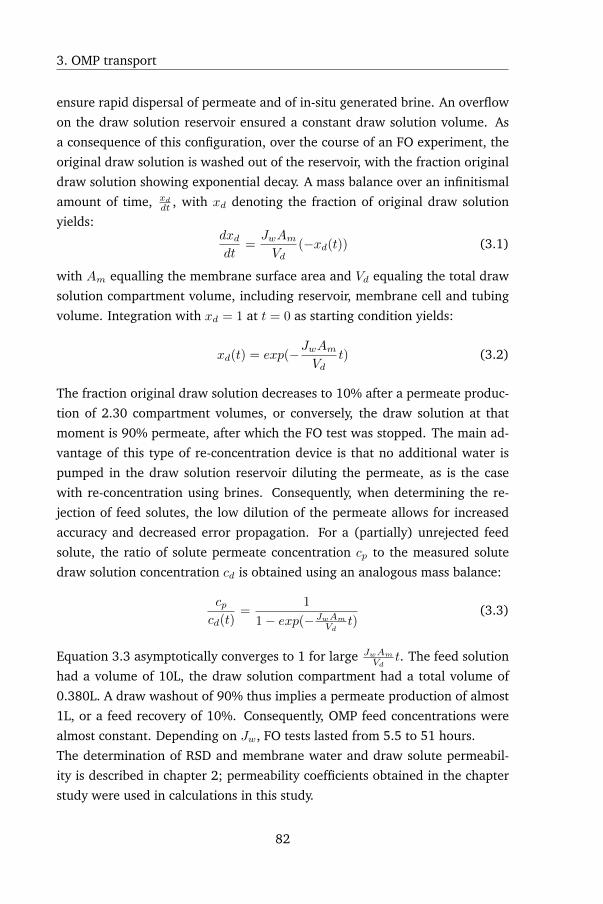
3. OMP transport
ensure rapid dispersal of permeate and of in-situ generated brine. An overflow
on the draw solution reservoir ensured a constant draw solution volume. As
a consequence of this configuration, over the course of an FO experiment, the
original draw solution is washed out of the reservoir, with the fraction original
draw solution showing exponential decay. A mass balance over an infinitismal
amount of time, xd
dt , with xd denoting the fraction of original draw solution
yields:dxddt
=JwAmVd
(−xd(t)) (3.1)
with Am equalling the membrane surface area and Vd equaling the total draw
solution compartment volume, including reservoir, membrane cell and tubing
volume. Integration with xd = 1 at t = 0 as starting condition yields:
xd(t) = exp(−JwAmVd
t) (3.2)
The fraction original draw solution decreases to 10% after a permeate produc-
tion of 2.30 compartment volumes, or conversely, the draw solution at that
moment is 90% permeate, after which the FO test was stopped. The main ad-
vantage of this type of re-concentration device is that no additional water is
pumped in the draw solution reservoir diluting the permeate, as is the case
with re-concentration using brines. Consequently, when determining the re-
jection of feed solutes, the low dilution of the permeate allows for increased
accuracy and decreased error propagation. For a (partially) unrejected feed
solute, the ratio of solute permeate concentration cp to the measured solute
draw solution concentration cd is obtained using an analogous mass balance:
cpcd(t)
=1
1− exp(−JwAm
Vdt)
(3.3)
Equation 3.3 asymptotically converges to 1 for large JwAm
Vdt. The feed solution
had a volume of 10L, the draw solution compartment had a total volume of
0.380L. A draw washout of 90% thus implies a permeate production of almost
1L, or a feed recovery of 10%. Consequently, OMP feed concentrations were
almost constant. Depending on Jw, FO tests lasted from 5.5 to 51 hours.
The determination of RSD and membrane water and draw solute permeabil-
ity is described in chapter 2; permeability coefficients obtained in the chapter
study were used in calculations in this study.
82
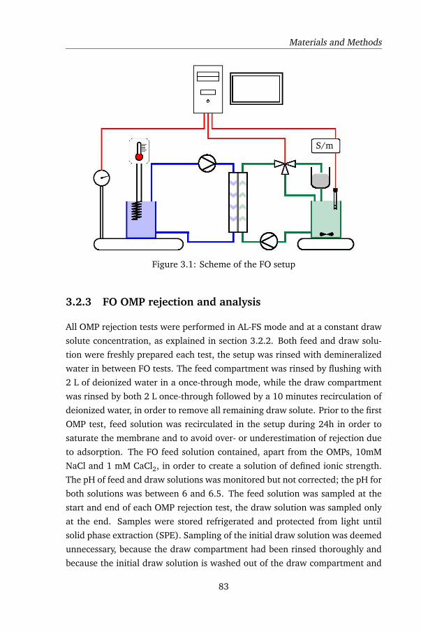
Materials and Methods
S/m
Figure 3.1: Scheme of the FO setup
3.2.3 FO OMP rejection and analysis
All OMP rejection tests were performed in AL-FS mode and at a constant draw
solute concentration, as explained in section 3.2.2. Both feed and draw solu-
tion were freshly prepared each test, the setup was rinsed with demineralized
water in between FO tests. The feed compartment was rinsed by flushing with
2 L of deionized water in a once-through mode, while the draw compartment
was rinsed by both 2 L once-through followed by a 10 minutes recirculation of
deionized water, in order to remove all remaining draw solute. Prior to the first
OMP test, feed solution was recirculated in the setup during 24h in order to
saturate the membrane and to avoid over- or underestimation of rejection due
to adsorption. The FO feed solution contained, apart from the OMPs, 10mM
NaCl and 1 mM CaCl2, in order to create a solution of defined ionic strength.
The pH of feed and draw solutions was monitored but not corrected; the pH for
both solutions was between 6 and 6.5. The feed solution was sampled at the
start and end of each OMP rejection test, the draw solution was sampled only
at the end. Samples were stored refrigerated and protected from light until
solid phase extraction (SPE). Sampling of the initial draw solution was deemed
unnecessary, because the draw compartment had been rinsed thoroughly and
because the initial draw solution is washed out of the draw compartment and
83
3. OMP transport
replaced by permeate. Earlier method development tests and modeling results
had shown that traces of remaining OMPs had an insignificant contribution to
the calculated rejection. Both the draw and feed solution containers were cov-
ered to inhibit photo-degradation of OMPs.
Samples of 200 ml were extracted using Oasis HLB 200 mg SPE cartridges
(Waters, MA, USA). 6 internal standards were added to each experimental and
calibration sample, details are provided in Appendix, section 3.A.1. 11 cali-
bration samples in log2 dilution were prepared for each SPE and HPLC run,
allowing quantification of rejection from 0 to 99.5%. The SPE protocol is pro-
vided in Appendix, section 3.A.1.
Samples were analyzed through UHPLC-HRMS (Benchtop Exactive Orbitrap
Mass spectrometer, Thermo-Scientific, San José, CA, USA), details of which
are provided by Bertelkamp et al. [145]. The SPE and U-HPLC-HRMS meth-
ods were validated by reproducibility tests in triplicate, showing an average
standard deviation of 2.6% for the combination of both methods, and cali-
bration curves for each OMP attained coefficients of determination of 0.99.
Chromatography data was analyzed using the Xcalibur software package.
3.2.4 OMP diffusion protocol
Diffusional OMP transport was studied during tests in which no draw solutes
were present and no water transport occurred. As there was no water trans-
port, when discussing diffusion tests, "feed" pertains to the solution to which
OMPs were dosed and "permeate" to the solution where OMPs diffused to-
wards. The feed and permeate compartment had a volume of 10 and 2 L
respectively, both were shielded from light and closed off completely to limit
evaporative losses. Both compartments were filled with a 0.1 mM NaCl solu-
tion, which was subsequently recirculated for 3 days in order to allow both
compartments to equilibrate so that no net transport of water or ions was tak-
ing place when the OMPs were dosed. The absence of mass transport was
confirmed by logging the weight of the feed solution. OMPs were dosed at a
concentration of 20 µg/L. Samples of 0.250 L were taken of both solutions af-
ter 0, 1, 2, 4 and 7 days. The volume change of both solutions was taken into
account during data analysis.
Samples were prepared using SPE and analysed using U-HPL-HRMS accord-
ing to the above described methods. The membrane permeability coefficient
84
Materials and Methods
(BOMP ) for each OMP was determined according to the method described by
Kim et al. [146] and Yoon et al. [147]. The method is based on a pseudo-steady
state implementation of Fick’s first law of diffusion, which yields the following
expression for the concentration difference between feed and permeate:
cf,t − cp,t = exp(−BOMPAmt(1
Vf+
1
Vp))(cf,0 − cp,0) (3.4)
in whichAm is the membrane surface area, t is time, c is the OMP concentration
with the subscripts f , p, 0 and t denoting feed, permeate, starting time and
current time respectively.
3.2.5 Contact angle and surface energy determination
To study the influence of draw solutes on membrane surface tension, contact
angles were measured on membrane samples saturated by demineralized wa-
ter or solutions of the 4 studied draw solutes according to the van Oss - Good
method [33]. Membrane samples were cut to fit a microscopy slide and soaked
in a salt solution for at least 24h. When starting the measurements, one side
of a microscopy slide was covered with a flat layer of filter paper which was
wetted with the same salt solution as the membrane sample. On top of the
filter paper, the membrane sample was placed, with the active layer facing up.
The active layer was then wiped dry, the sample was placed on the measuring
platform, which was then covered by a transparent hood fitted with a slit to
allow deposition of the test liquids. The purpose of the hood was to delay the
drying out of the membrane sample and maintain a constant humidity. 3 test
liquids were used to determine sessile contact angles: water, glycerol and di-
iodomethane.
Contact angles were measured using a Krüss DSA-10 MK3 goniometer. Angles
were measured on both sides of the drop simultaneously using a circular sec-
tion fitting to the drop. The average of both angles was used in subsequent
calculations, provided that the left and right angle were quasi identical. To
take the spreading of drops over time into account, data was acquired every
second during 1 minute after deposition. When a drop is deposited, there is
an initial phase of relatively fast spreading and equilibration, followed ideally
by a much longer stable phase, during which an equilibrium angle can be de-
termined. However, angles generally showed slow and steady decline during
85
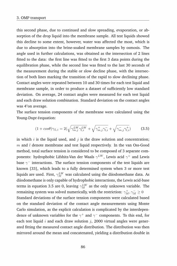
3. OMP transport
this second phase, due to continued and slow spreading, evaporation, or ab-
sorption of the drop liquid into the membrane sample. All test liquids showed
this decline to some extent, however, water was affected the most, which is
due to absorption into the brine-soaked membrane samples by osmosis. The
angle used in further calculations, was obtained as the intersection of 2 lines
fitted to the data: the first line was fitted to the first 3 data points during the
equilibration phase, while the second line was fitted to the last 30 seconds of
the measurement during the stable or slow decline phase, with the intersec-
tion of both lines marking the transition of the rapid to slow declining phase.
Contact angles were repeated between 10 and 30 times for each test liquid and
membrane sample, in order to produce a dataset of sufficiently low standard
deviation. On average, 24 contact angles were measured for each test liquid
and each draw solution combination. Standard deviation on the contact angles
was 4°on average.
The surface tension components of the membrane were calculated using the
Young-Dupré equation:
(1 + cosθ)γL,i = 2(√γLWm,j γ
LWl,i +
√γ+m,jγ
−l,i +
√γ−m,jγ
+l,i) (3.5)
in which i is the liquid used, and j is the draw solution and concentration;
m and l denote membrane and test liquid respectively. In the van Oss-Good
method, total surface tension is considered to be composed of 3 separate com-
ponents: hydrophobic Lifshitz-Van der Waals γLW , Lewis acid γ+ and Lewis
base γ− interactions. The surface tension components of the test liquids are
known [33], which leads to a fully determined system when 3 or more test
liquids are used. First, γLWM was calculated using the diiodomethane data. As
diiodomethane is only capable of hydrophobic interactions, the Lewis acid-base
terms in equation 3.5 are 0, leaving γLWM as the only unknown variable. The
remaining system was solved numerically, with the restriction: γ+M , γ
−M ≥ 0
Standard deviations of the surface tension components were calculated based
on the standard deviation of the contact angle measurements using Monte
Carlo simulation, as the explicit calculation is complicated by the interdepen-
dence of unknown variables for the γ+ and γ− components. To this end, for
each test liquid i and each draw solution j, 2000 virtual angles were gener-
ated fitting the measured contact angle distribution. The distribution was then
mirrored around the mean and concatenated, yielding a distribution double in
86
Materials and Methods
size with the mean being exactly equal to the mean of the experimental dis-
tribution. The standard deviation of the surface tension components was then
calculated from the resulting set of 4000 values per liquid and draw solution.
3.2.6 Open Circuit Voltage (OCV)
The open circuit voltage (OCV) between feed and draw solution was measured
for all draw solutes using a pair of diffusion halfcells with a CTA membrane
sample clamped in between. OCV was measured using a BioLogic VSP poten-
tiostat. 1 Ag/AgCl electrode was placed in each halfcell. Initial testing had
shown that the position of the electrode had no influence on the measured
potential: given that no current was either applied or allowed to run between
both solutions, the influence of solution resistance was negligible. The refer-
ence electrode was inserted into the feed solution and the working electrode
in the draw solution. Both halfcells were stirred using magnetic stirrers. Ex-
periments were run during 0.5 to 2 hours, depending on equilibration time
needed. In between measurements using the same draw solution at different
concentrations, the setup was briefly rinsed; when switching to another draw
solute, the setup was rinsed multiple times with demineralized water followed
by equilibration of the membrane with demineralized water during 1 hour in
order to desorb ions originating from the preceding draw solute.
The data was fitted to an exponential decay approaching an asymptote (a1 in
equation 3.6), the value of the asymptote was taken to be the equilibrium OCV.
The equilibrium OCV was assumed to be the stable OCV measured after initial
equilibration of the membrane with the draw solute and after establishment of
stable water and draw solute fluxes. Equilibration time greatly depended on
ion desorption during rinsing: when the membrane was thoroughly desorbed
because a new draw solute was going to be used, equilibration time increased
significantly.
OCV = a1 + a2exp(a3t) (3.6)
3.2.7 OMP data analysis
Membrane partition coefficients
In the feed-membrane or membrane-permeate interphase, there are 2 possible
states for the solute to be in: either dissolved in the water phase, or partitioned
87
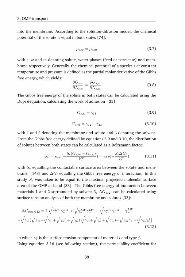
3. OMP transport
into the membrane. According to the solution-diffusion model, the chemical
potential of the solute is equal in both states [74]:
µs,w = µs,m (3.7)
with s, w and m denoting solute, water phases (feed or permeate) and mem-
brane respectively. Generally, the chemical potential of a species i at constant
temperature and pressure is defined as the partial molar derivative of the Gibbs
free energy, which yields:∂Gs,w∂Ns,w
=∂Gs,m∂Ns,m
(3.8)
The Gibbs free energy of the solute in both states can be calculated using the
Dupré equation, calculating the work of adhesion [33]:
Gs,w = γ13 (3.9)
Gs,m = γ12 − γ23 (3.10)
with 1 and 2 denoting the membrane and solute and 3 denoting the solvent.
From the Gibbs free energy defined by equations 3.9 and 3.10, the distribution
of solutes between both states can be calculated as a Boltzmann factor:
φB = exp(−Sc(Gs,m −Gs,w)
kT) = exp(−Sc∆Gi
kT) (3.11)
with Sc equalling the contactable surface area between the solute and mem-
brane [148] and ∆Gi equalling the Gibbs free energy of interaction. In this
study, Sc was taken to be equal to the maximal projected molecular surface
area of the OMP at hand [33]. The Gibbs free energy of interaction between
materials 1 and 2 surrounded by solvent 3, ∆G132, can be calculated using
surface tension analysis of both the membrane and solutes [33]:
∆Gmws132 = 2[√γLWm γLWw +
√γLWs γLWw −
√γLWm γLWs − γLWw
+
√γ+w (
√γ−m+
√γ−s +
√γ−w )+
√γ−w (
√γ+m+
√γ+s +
√γ+w )−
√γ+mγ−s −
√γ−mγ
+s ]
(3.12)
in which γji is the surface tension component of material i and type j.
Using equation 3.16 (see following section), the permeability coefficient for
88
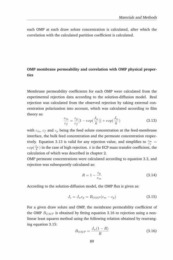
Materials and Methods
each OMP at each draw solute concentration is calculated, after which the
correlation with the calculated partition coefficient is calculated.
OMP membrane permeability and correlation with OMP physical proper-
ties
Membrane permeability coefficients for each OMP were calculated from the
experimental rejection data according to the solution-diffusion model. Real
rejection was calculated from the observed rejection by taking external con-
centration polarization into account, which was calculated according to film
theory as:cmcf
=cpcf
[1− exp(Jwk
)] + exp(Jwk
) (3.13)
with cm, cf and cp being the feed solute concentration at the feed-membrane
interface, the bulk feed concentration and the permeate concentration respec-
tively. Equation 3.13 is valid for any rejection value, and simplifies to cmcf
=
exp(Jwk ) in the case of high rejection. k is the ECP mass transfer coefficient, the
calculation of which was described in chapter 2.
OMP permeate concentrations were calculated according to equation 3.3, and
rejection was subsequently calculated as:
R = 1− cpcm
(3.14)
According to the solution-diffusion model, the OMP flux is given as:
Js = Jwcp = BOMP (cm − cp) (3.15)
For a given draw solute and OMP, the membrane permeability coefficient of
the OMP BOMP is obtained by fitting equation 3.16 to rejection using a non-
linear least squares method using the following relation obtained by rearrang-
ing equation 3.15:
BOMP =Jw(1−R)
R(3.16)
89
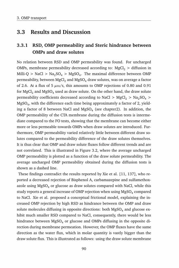
3. OMP transport
3.3 Results and Discussion
3.3.1 RSD, OMP permeability and Steric hindrance betweenOMPs and draw solutes
No relation between RSD and OMP permeability was found. For uncharged
OMPs, membrane permeability decreased according to: MgCl2 > diffusion in
Milli-Q > NaCl > Na2SO4 > MgSO4. The maximal difference between OMP
permeability, between MgCl2 and MgSO4 draw solutes, was on average a factor
of 2.6. At a flux of 5 µm/s, this amounts to OMP rejections of 0.80 and 0.91
for MgCl2 and MgSO4 used as draw solute. On the other hand, the draw solute
permeability coefficients decreased according to NaCl > MgCl2 > Na2SO4 >
MgSO4, with the difference each time being approximately a factor of 2, yield-
ing a factor of 8 between NaCl and MgSO4 (see chapter2). In addition, the
OMP permeability of the CTA membrane during the diffusion tests is interme-
diate compared to the FO tests, showing that the membrane can become either
more or less permeable towards OMPs when draw solutes are introduced. Fur-
thermore, OMP permeability varied relatively little between different draw so-
lutes compared to the permeability difference of the draw solutes themselves.
It is thus clear that OMP and draw solute fluxes follow different trends and are
not correlated. This is illustrated in Figure 3.2, where the average uncharged
OMP permeability is plotted as a function of the draw solute permeability. The
average uncharged OMP permeability obtained during the diffusion tests is
shown as a dashed line.
These findings contradict the results reported by Xie et al. [11, 137], who re-
ported a decreased rejection of Bisphenol A, carbamazepine and sulfamethox-
azole using MgSO4 or glucose as draw solutes compared with NaCl, while this
study reports a general increase of OMP rejection when using MgSO4 compared
to NaCl. Xie et al. proposed a conceptual frictional model, explaining the in-
creased OMP rejection by high RSD as hindrance between the OMP and draw
solute molecules diffusing in opposite directions: both MgSO4 and glucose ex-
hibit much smaller RSD compared to NaCl, consequently, there would be less
hindrance between MgSO4 or glucose and OMPs diffusing in the opposite di-
rection during membrane permeation. However, the OMP fluxes have the same
direction as the water flux, which in molar quantity is vastly bigger than the
draw solute flux. This is illustrated as follows: using the draw solute membrane
90
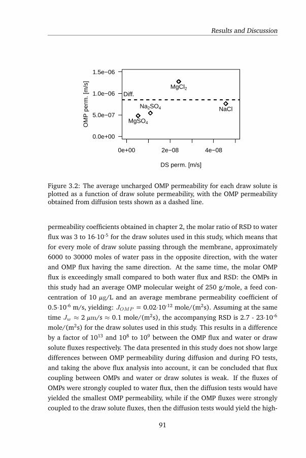
Results and Discussion
0e+00 2e−08 4e−08
0.0e+00
5.0e−07
1.0e−06
1.5e−06
Diff.
NaClNa2SO4
MgCl2
MgSO4
DS perm. [m/s]
OM
P p
erm
. [m
/s]
Figure 3.2: The average uncharged OMP permeability for each draw solute isplotted as a function of draw solute permeability, with the OMP permeabilityobtained from diffusion tests shown as a dashed line.
permeability coefficients obtained in chapter 2, the molar ratio of RSD to water
flux was 3 to 16·10-5 for the draw solutes used in this study, which means that
for every mole of draw solute passing through the membrane, approximately
6000 to 30000 moles of water pass in the opposite direction, with the water
and OMP flux having the same direction. At the same time, the molar OMP
flux is exceedingly small compared to both water flux and RSD: the OMPs in
this study had an average OMP molecular weight of 250 g/mole, a feed con-
centration of 10 µg/L and an average membrane permeability coefficient of
0.5·10-6 m/s, yielding: JOMP = 0.02·10-12 mole/(m2s). Assuming at the same
time Jw ≈ 2 µm/s ≈ 0.1 mole/(m2s), the accompanying RSD is 2.7 - 23·10-6
mole/(m2s) for the draw solutes used in this study. This results in a difference
by a factor of 1013 and 108 to 109 between the OMP flux and water or draw
solute fluxes respectively. The data presented in this study does not show large
differences between OMP permeability during diffusion and during FO tests,
and taking the above flux analysis into account, it can be concluded that flux
coupling between OMPs and water or draw solutes is weak. If the fluxes of
OMPs were strongly coupled to water flux, then the diffusion tests would have
yielded the smallest OMP permeability, while if the OMP fluxes were strongly
coupled to the draw solute fluxes, then the diffusion tests would yield the high-
91
0
0 0
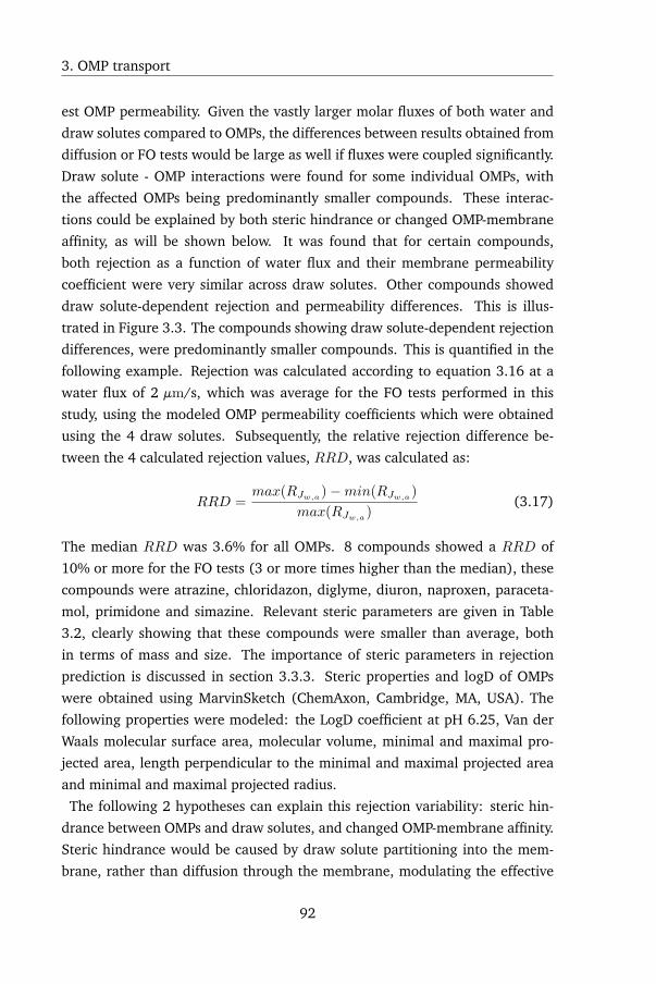
3. OMP transport
est OMP permeability. Given the vastly larger molar fluxes of both water and
draw solutes compared to OMPs, the differences between results obtained from
diffusion or FO tests would be large as well if fluxes were coupled significantly.
Draw solute - OMP interactions were found for some individual OMPs, with
the affected OMPs being predominantly smaller compounds. These interac-
tions could be explained by both steric hindrance or changed OMP-membrane
affinity, as will be shown below. It was found that for certain compounds,
both rejection as a function of water flux and their membrane permeability
coefficient were very similar across draw solutes. Other compounds showed
draw solute-dependent rejection and permeability differences. This is illus-
trated in Figure 3.3. The compounds showing draw solute-dependent rejection
differences, were predominantly smaller compounds. This is quantified in the
following example. Rejection was calculated according to equation 3.16 at a
water flux of 2 µm/s, which was average for the FO tests performed in this
study, using the modeled OMP permeability coefficients which were obtained
using the 4 draw solutes. Subsequently, the relative rejection difference be-
tween the 4 calculated rejection values, RRD, was calculated as:
RRD =max(RJw,a
)−min(RJw,a)
max(RJw,a)
(3.17)
The median RRD was 3.6% for all OMPs. 8 compounds showed a RRD of
10% or more for the FO tests (3 or more times higher than the median), these
compounds were atrazine, chloridazon, diglyme, diuron, naproxen, paraceta-
mol, primidone and simazine. Relevant steric parameters are given in Table
3.2, clearly showing that these compounds were smaller than average, both
in terms of mass and size. The importance of steric parameters in rejection
prediction is discussed in section 3.3.3. Steric properties and logD of OMPs
were obtained using MarvinSketch (ChemAxon, Cambridge, MA, USA). The
following properties were modeled: the LogD coefficient at pH 6.25, Van der
Waals molecular surface area, molecular volume, minimal and maximal pro-
jected area, length perpendicular to the minimal and maximal projected area
and minimal and maximal projected radius.
The following 2 hypotheses can explain this rejection variability: steric hin-
drance between OMPs and draw solutes, and changed OMP-membrane affinity.
Steric hindrance would be caused by draw solute partitioning into the mem-
brane, rather than diffusion through the membrane, modulating the effective
92
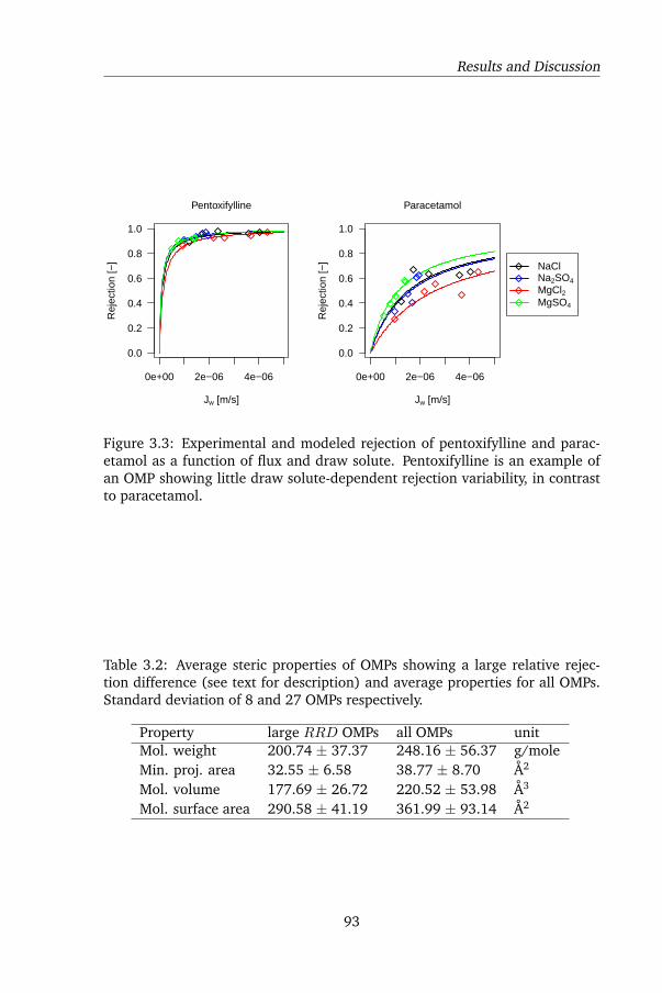
Results and Discussion
0e+00 2e−06 4e−06
0.0
0.2
0.4
0.6
0.8
1.0
Jw [m/s]
Rej
ectio
n [−
]
Pentoxifylline
0e+00 2e−06 4e−06
0.0
0.2
0.4
0.6
0.8
1.0
Jw [m/s]
Rej
ectio
n [−
]
Paracetamol
NaClNa2SO4
MgCl2MgSO4
Figure 3.3: Experimental and modeled rejection of pentoxifylline and parac-etamol as a function of flux and draw solute. Pentoxifylline is an example ofan OMP showing little draw solute-dependent rejection variability, in contrastto paracetamol.
Table 3.2: Average steric properties of OMPs showing a large relative rejec-tion difference (see text for description) and average properties for all OMPs.Standard deviation of 8 and 27 OMPs respectively.
Property large RRD OMPs all OMPs unitMol. weight 200.74 ± 37.37 248.16 ± 56.37 g/moleMin. proj. area 32.55 ± 6.58 38.77 ± 8.70 Å2
Mol. volume 177.69 ± 26.72 220.52 ± 53.98 Å3
Mol. surface area 290.58 ± 41.19 361.99 ± 93.14 Å2
93
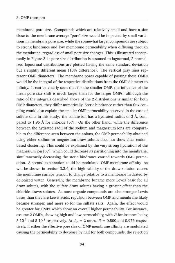
3. OMP transport
membrane pore size. Compounds which are relatively small and have a size
close to the membrane average "pore" size would be impacted by small varia-
tions in membrane pore size, while the somewhat larger compounds are subject
to strong hindrance and low membrane permeability when diffusing through
the membrane, regardless of small pore size changes. This is illustrated concep-
tually in Figure 3.4: pore size distribution is assumed to lognormal, 2 normal-
ized lognormal distributions are plotted having the same standard deviation
but a slightly different mean (10% difference). The vertical gray lines rep-
resent OMP diameters. The membrane pores capable of passing these OMPs
would be the integral of the respective distributions from the OMP diameter to
infinity. It can be clearly seen that for the smaller OMP, the influence of the
mean pore size shift is much larger than for the larger OMPs: although the
ratio of the integrals described above of the 2 distributions is similar for both
OMP diameters, they differ numerically. Steric hindrance rather than flux cou-
pling would also explain the smaller OMP permeability observed in the case of
sulfate salts in this study: the sulfate ion has a hydrated radius of 3 Å, com-
pared to 1.95 Å for chloride [57]. On the other hand, while the difference
between the hydrated radii of the sodium and magnesium ions are compara-
ble to the difference seen between the anions, the OMP permeability obtained
using either sodium or magnesium draw solutes does not show clear cation-
based clustering. This could be explained by the very strong hydration of the
magnesium ion [57], which could decrease its partitioning into the membrane,
simultaneously decreasing the steric hindrance caused towards OMP perme-
ation. A second explanation could be modulated OMP-membrane affinity. As
will be shown in section 3.3.4, the high salinity of the draw solution causes
the membrane surface tension to change relative to a membrane hydrated by
deionized water. Generally, the membrane became more Lewis basic for all
draw solutes, with the sulfate draw solutes having a greater effect than the
chloride draws solutes. As most organic compounds are also stronger Lewis
bases than they are Lewis acids, repulsion between OMP and membrane likely
became stronger, and more so for the sulfate salts. Again, the effect would
be greater for OMPs which show an overall higher permeability. For instance,
assume 2 OMPs, showing high and low permeability, with B for instance being
5·10-7 and 5·10-8 respectively. At Jw = 2 µm/s, R = 0.800 and 0.976 respec-
tively. If either the effective pore size or OMP-membrane affinity are modulated
causing the permeability to decrease by half for both compounds, the rejection
94
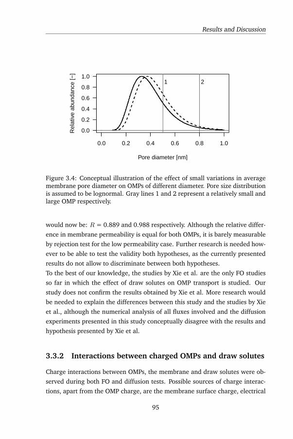
Results and Discussion
0.0 0.2 0.4 0.6 0.8 1.0
0.0
0.2
0.4
0.6
0.8
1.0
Pore diameter [nm]
Rel
ativ
e ab
unda
nce
[−]
1 2
Figure 3.4: Conceptual illustration of the effect of small variations in averagemembrane pore diameter on OMPs of different diameter. Pore size distributionis assumed to be lognormal. Gray lines 1 and 2 represent a relatively small andlarge OMP respectively.
would now be: R = 0.889 and 0.988 respectively. Although the relative differ-
ence in membrane permeability is equal for both OMPs, it is barely measurable
by rejection test for the low permeability case. Further research is needed how-
ever to be able to test the validity both hypotheses, as the currently presented
results do not allow to discriminate between both hypotheses.
To the best of our knowledge, the studies by Xie et al. are the only FO studies
so far in which the effect of draw solutes on OMP transport is studied. Our
study does not confirm the results obtained by Xie et al. More research would
be needed to explain the differences between this study and the studies by Xie
et al., although the numerical analysis of all fluxes involved and the diffusion
experiments presented in this study conceptually disagree with the results and
hypothesis presented by Xie et al.
3.3.2 Interactions between charged OMPs and draw solutes
Charge interactions between OMPs, the membrane and draw solutes were ob-
served during both FO and diffusion tests. Possible sources of charge interac-
tions, apart from the OMP charge, are the membrane surface charge, electrical
95
3. OMP transport
potential differences between feed and draw solution due to the establishment
of a Donnan potential or ion exchange.
During simple diffusion, the membrane charge had a profound influence on
OMP permeability. The CTA membrane has a small negative zeta potential at
ambient pH of -4 mV (see chapter 5), which caused a high permeability of
cationic OMPs and a low permeability of anionic OMPs. This is illustrated in
Figure 3.5, where the influence of membrane charge on OMP permeability is
evident. Membrane permeability was on average 1.25·10-6 m/s for cationic
OMPs during diffusion, 1.5 and 15 times higher than uncharged and anionic
OMP membrane permeability respectively. This is consistent with earlier re-
ports for negatively charged NF and RO membranes [84, 149, 150]
During FO however, this rejection pattern was not reproduced: rejection of
cationic OMPs was consistently high, generally more than 95%, yielding per-
meabilities almost 2 orders of magnitude lower than during diffusion tests.
Anionic OMPs were rejected slightly less during FO compared to during dif-
fusion: membrane permeability increased at most with a factor of 2.5. The
rejection and permeability of cationic and anionic OMPs was of the same order
during FO, while being very different during simple diffusion. There is thus
a clear influence of FO operation on the permeability of charged OMPs, while
behavior of uncharged OMPs is very similar in FO and diffusion tests. Average
permeabilities for each group of OMPs and for each draw solute are given in
Table 3.3, as well as the permeability relative to simple diffusion and the aver-
age rank of the 5 treatments. The rank was calculated by ranking the modeled
permeabilities ascending for each compound, which was then averaged for the
charge-based subsets. A rank of 5 for a given treatment thus indicates that the
highest membrane permeability was obtained for all compounds applying that
treatment, as was the case for the cationic OMPs during simple diffusion. Some
patterns are easily discerned when comparing the charge-based subsets. Firstly,
if the draw solute provides a divalent co-ion for a charged OMP, OMP perme-
ability decreases, and vice versa: cationic OMP permeability is lowest when
using MgCl2 and the highest when using Na2SO4 (disregarding the simple dif-
fusion tests). Likewise, anionic OMP permeability is highest when using MgCl2and lowest when using Na2SO4 (again disregarding the simple diffusion tests).
NaCl and MgSO4 FO tests always yielded intermediary results. Secondly, com-
pared to simple diffusion, cationic OMP permeability decreased strongly during
FO while anionic OMP permeability only showed a gentle increase.
96
Results and Discussion
These results imply that during FO, electrostatic forces are changed compared
to simple diffusion, and that the changes for all draw solutes are somewhat
similar: compared to simple diffusion, the introduction of a draw solute in
the system causes a shift of permeability in the same direction for both cationic
and anionic OMPs, only the magnitude of the shift differs from one draw solute
to the next. In this paragraph, electro-migration will be explored as a possi-
ble explanation for the interactions between draw solutes and charged OMPs.
Electro-migration is the flux of a charged species in response to an electric
field. The electric field in this case would be the Donnan potential which spon-
taneously arises during FO. This is due to different membrane permeabilities of
the different draw solute ions [93], creating a charge imbalance between feed
and draw solution at the start of an FO test, after which the generated Donnan
potential creates a steady-state by slowing down the flux of the more mobile
ion. During steady-state, RSD is charge neutral and the Donnan potential is
constant.
Based on the OMP permeability data presented in Table 3.3, a negative electro-
static potential of the feed solution relative to the draw solution is expected:
this would both accelerate transport of anionic OMPs and retard transport
of cationic OMPs. Open circuit voltage (OCV) measurements however could
not confirm our expectation: a negative electrostatic potential was only found
when using MgCl2 (≈ -120 mV); for both sulfate salts, the OCV was small and
positive (< 100 mV), while it was fairly large for NaCl (≈ 0.65 V at 2 M). OCV
results are shown in Figure 3.6. For both the chloride and sulfate salts, the OCV
is lower for the magnesium salts compared to sodium salts: considering that
the Mg2+ ion is much stronger hydrated than the Na+ ion, a lower permeabil-
ity and thus less positive OCV is to be expected as well. However, one would
expect that membrane permeability of SO 2 –4 would be smaller than that of
Cl– , as was observed in chapter 2 where, for the same draw solutes, the chlo-
ride salts showed a membrane permeability which was on average a factor of
4 higher than the sulfate salts. Thus, the OCV of Na2SO4 or MgSO4 would be
expected to be more positive than those of NaCl or MgCl2, which is however
contradicted by experimental results. Furthermore, the OCV results diverge as
a function of draw solute, unlike the shifts in charged OMP permeability seen
when comparing the OMP FO and diffusion tests: the direction of the OMP per-
meability change is the same for each draw solute, only the magnitude differs.
The study of OCV in FO warrants further attention: the OCV results at present
97
3. OMP transport
cannot be linked satisfactory to either charged OMP permeability or draw so-
lute permeability. It can however be concluded that electro-migration appears
to be of limited practical importance under the experimental conditions dis-
cussed here. The limited importance of electro-migration for OMPs has been
reported in NF as well [151], where electro-migration was found to account
for at most 2.1% of the total charged OMP flux, with diffusion accounting for
about 95 % and convective transport for the remaining 3%.
Donnan dialysis should be considered as well, given the vastly higher ion con-
centrations in the draw solution compared to the feed solution. Donnan dialy-
sis is an ion exchange process where co-ions are exchanged across a membrane
in a charge-neutral exchange under the influence of an ion concentration dif-
ference across a membrane [152, 62, 153]. During FO, diffusion of ions will be
driven predominantly by the vast concentration difference of the draw solute
ions across the membrane rather than the OMP concentration difference. As-
suming that draw solute cations diffuse more readily through the membrane,
as is suggested by the OCV measurements, the system can restore electroneu-
trality in two ways: either by co-diffusion of draw solute anions, or by ion
exchange with a feed cation, such as a cationic OMP [62]. The rate of draw
solute cation - cationic OMP exchange would then be in part determined by
the membrane permeability of the draw solute anion: a more mobile draw
anion would co-diffuse easily compared to a less mobile draw anion, thereby
lowering exchange of draw cations by cationic OMPs. This is supported by our
experimental data: comparing the average membrane permeability of cationic
OMPs in Table 3.3, it is seen that OMP permeability is lower for the chlo-
ride salts compared to the sulfate salts, with the sulfate salts having a lower
diffusivity than the chloride salts [109]. A similar effect can be seen for the
anionic OMPs, albeit much less pronounced: this is likely due to the negative
membrane charge. A remaining discrepancy between the Donnan dialysis hy-
pothesis and the experimental data is the strong reduction of cationic OMP
permeability during FO compared to simple diffusion. Considering that the
flux of draw solute ions is large compared to the OMP flux, as was discussed
in the preceding section, one would expect a larger driving force for both an-
ion and cation exchange: increased anionic OMP permeability was observed,
despite even the positive electrostatic potential of the feed solution for three
out of four draw solutes, in contrast to the strong decrease of cationic OMP
permeability. Possible explanations of the latter could be firstly competition for
98
Results and Discussion
ion adsorption sites: given that the CTA membrane has a small negative surface
charge, it is reasonable to assume that cations adsorb to or in the membrane
and are thus to a small extent enriched in the membrane active layer. Dur-
ing simple diffusion, the aggregate concentration of ionized species was low,
while during FO however, the much larger draw solute concentration could
saturate the membrane thereby preventing the enrichment of the membrane
phase with cationic OMPs [122, 154]. Secondly, there could be steric hin-
drance during membrane permeation due to ions present in the membrane,
as was discussed in the preceding section as well. Thirdly, the presence of a
driving force for water transport could cause a response of the membrane poly-
mer, affecting for instance the polymer free volume, rendering the membrane
inherently less permeable as is known from pressure-driven systems [79, 155].
Similarly, in chapter 2, reduced water permeability was reported for the CTA-
ES membrane at increasing osmotic pressure. Taking into account that only the
cationic OMPs show a reduced membrane permeability in the presence of draw
solutes in contrast with the anionic OMPs showing an increased permeability,
the first explanation seems the most logical. It can be concluded that Donnan
dialysis currently offers the best explanation for the draw solute - charged OMP
interactions. In order to test this hypothesis, charged OMP permeability would
be determined in the presence of a non-permeating counterion combined with
sensitive co-ion concentration measurements in the feed.
99
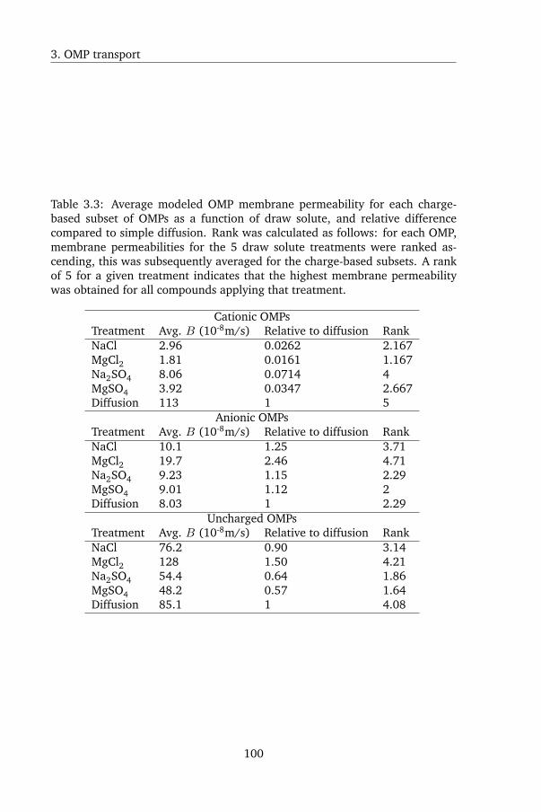
3. OMP transport
Table 3.3: Average modeled OMP membrane permeability for each charge-based subset of OMPs as a function of draw solute, and relative differencecompared to simple diffusion. Rank was calculated as follows: for each OMP,membrane permeabilities for the 5 draw solute treatments were ranked as-cending, this was subsequently averaged for the charge-based subsets. A rankof 5 for a given treatment indicates that the highest membrane permeabilitywas obtained for all compounds applying that treatment.
Cationic OMPsTreatment Avg. B (10-8m/s) Relative to diffusion RankNaCl 2.96 0.0262 2.167MgCl2 1.81 0.0161 1.167Na2SO4 8.06 0.0714 4MgSO4 3.92 0.0347 2.667Diffusion 113 1 5
Anionic OMPsTreatment Avg. B (10-8m/s) Relative to diffusion RankNaCl 10.1 1.25 3.71MgCl2 19.7 2.46 4.71Na2SO4 9.23 1.15 2.29MgSO4 9.01 1.12 2Diffusion 8.03 1 2.29
Uncharged OMPsTreatment Avg. B (10-8m/s) Relative to diffusion RankNaCl 76.2 0.90 3.14MgCl2 128 1.50 4.21Na2SO4 54.4 0.64 1.86MgSO4 48.2 0.57 1.64Diffusion 85.1 1 4.08
100
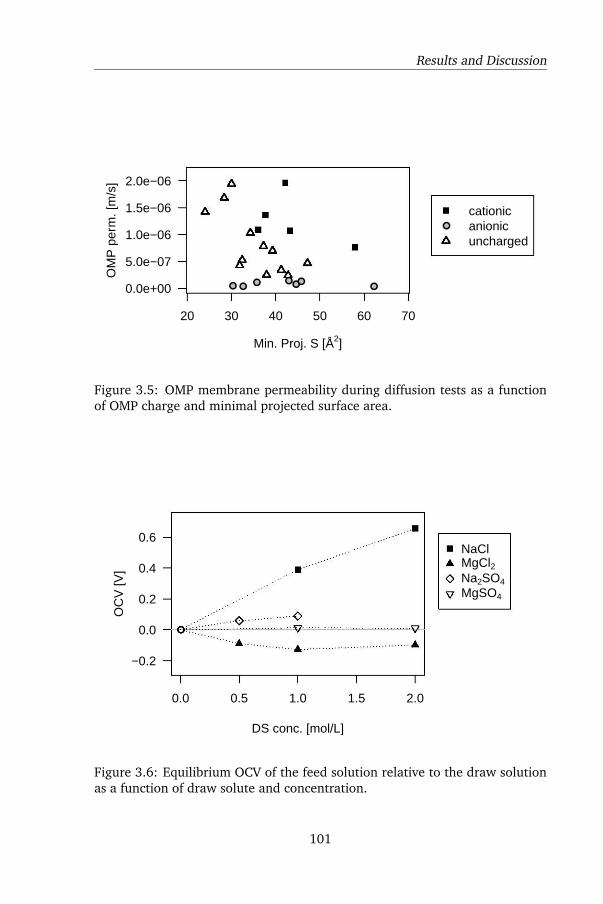
Results and Discussion
20 30 40 50 60 70
0.0e+00
5.0e−07
1.0e−06
1.5e−06
2.0e−06
●● ●● ●●●
Min. Proj. S [Å2]
OM
P p
erm
. [m
/s]
●
cationicanionicuncharged
Figure 3.5: OMP membrane permeability during diffusion tests as a functionof OMP charge and minimal projected surface area.
●
0.0 0.5 1.0 1.5 2.0
−0.2
0.0
0.2
0.4
0.6
DS conc. [mol/L]
OC
V [V
]
●●●
NaClMgCl2Na2SO4
MgSO4
Figure 3.6: Equilibrium OCV of the feed solution relative to the draw solutionas a function of draw solute and concentration.
101
/::;. • /::;.
/::;. • t::.• • LJ
b /::;./::;. • /::;.~ /::;.
.. ··· .. ····
.. .. ·· D
· ~ · ·· · · ·~'\)'-
. :Á. ..... • ........... ······ · ···· ......
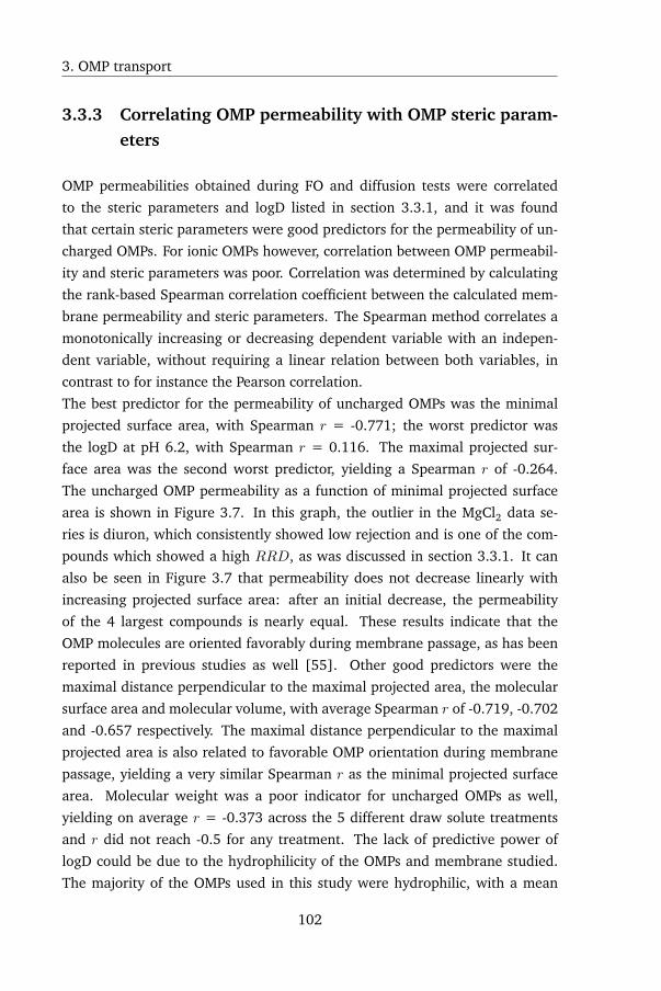
3. OMP transport
3.3.3 Correlating OMP permeability with OMP steric param-eters
OMP permeabilities obtained during FO and diffusion tests were correlated
to the steric parameters and logD listed in section 3.3.1, and it was found
that certain steric parameters were good predictors for the permeability of un-
charged OMPs. For ionic OMPs however, correlation between OMP permeabil-
ity and steric parameters was poor. Correlation was determined by calculating
the rank-based Spearman correlation coefficient between the calculated mem-
brane permeability and steric parameters. The Spearman method correlates a
monotonically increasing or decreasing dependent variable with an indepen-
dent variable, without requiring a linear relation between both variables, in
contrast to for instance the Pearson correlation.
The best predictor for the permeability of uncharged OMPs was the minimal
projected surface area, with Spearman r = -0.771; the worst predictor was
the logD at pH 6.2, with Spearman r = 0.116. The maximal projected sur-
face area was the second worst predictor, yielding a Spearman r of -0.264.
The uncharged OMP permeability as a function of minimal projected surface
area is shown in Figure 3.7. In this graph, the outlier in the MgCl2 data se-
ries is diuron, which consistently showed low rejection and is one of the com-
pounds which showed a high RRD, as was discussed in section 3.3.1. It can
also be seen in Figure 3.7 that permeability does not decrease linearly with
increasing projected surface area: after an initial decrease, the permeability
of the 4 largest compounds is nearly equal. These results indicate that the
OMP molecules are oriented favorably during membrane passage, as has been
reported in previous studies as well [55]. Other good predictors were the
maximal distance perpendicular to the maximal projected area, the molecular
surface area and molecular volume, with average Spearman r of -0.719, -0.702
and -0.657 respectively. The maximal distance perpendicular to the maximal
projected area is also related to favorable OMP orientation during membrane
passage, yielding a very similar Spearman r as the minimal projected surface
area. Molecular weight was a poor indicator for uncharged OMPs as well,
yielding on average r = -0.373 across the 5 different draw solute treatments
and r did not reach -0.5 for any treatment. The lack of predictive power of
logD could be due to the hydrophilicity of the OMPs and membrane studied.
The majority of the OMPs used in this study were hydrophilic, with a mean
102
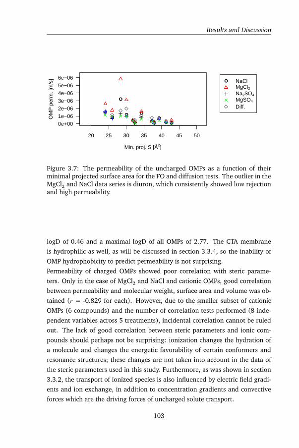
Results and Discussion
●
●
●●
●
●
●
●
●● ●
●
20 25 30 35 40 45 50
0e+001e−062e−063e−064e−065e−066e−06
Min. proj. S [Å2]
OM
P p
erm
. [m
/s]
● NaClMgCl2Na2SO4
MgSO4
Diff.
Figure 3.7: The permeability of the uncharged OMPs as a function of theirminimal projected surface area for the FO and diffusion tests. The outlier in theMgCl2 and NaCl data series is diuron, which consistently showed low rejectionand high permeability.
logD of 0.46 and a maximal logD of all OMPs of 2.77. The CTA membrane
is hydrophilic as well, as will be discussed in section 3.3.4, so the inability of
OMP hydrophobicity to predict permeability is not surprising.
Permeability of charged OMPs showed poor correlation with steric parame-
ters. Only in the case of MgCl2 and NaCl and cationic OMPs, good correlation
between permeability and molecular weight, surface area and volume was ob-
tained (r = -0.829 for each). However, due to the smaller subset of cationic
OMPs (6 compounds) and the number of correlation tests performed (8 inde-
pendent variables across 5 treatments), incidental correlation cannot be ruled
out. The lack of good correlation between steric parameters and ionic com-
pounds should perhaps not be surprising: ionization changes the hydration of
a molecule and changes the energetic favorability of certain conformers and
resonance structures; these changes are not taken into account in the data of
the steric parameters used in this study. Furthermore, as was shown in section
3.3.2, the transport of ionized species is also influenced by electric field gradi-
ents and ion exchange, in addition to concentration gradients and convective
forces which are the driving forces of uncharged solute transport.
103
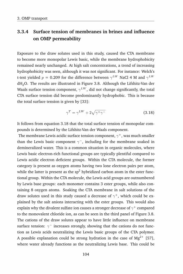
3. OMP transport
3.3.4 Surface tension of membranes in brines and influenceon OMP permeability
Exposure to the draw solutes used in this study, caused the CTA membrane
to become more monopolar Lewis basic, while the membrane hydrophobicity
remained nearly unchanged. At high salt concentrations, a trend of increasing
hydrophobicity was seen, although it was not significant. For instance: Welch’s
t-test yielded p = 0.209 for the difference between γLW NaCl 4 M and γLW
dH2O. The results are illustrated in Figure 3.8. Although the Lifshitz-Van der
Waals surface tension component, γLW , did not change significantly, the total
CTA surface tension did become predominantly hydrophobic. This is because
the total surface tension is given by [33]:
γT = γLW + 2√γ+γ− (3.18)
It follows from equation 3.18 that the total surface tension of monopolar com-
pounds is determined by the Lifshitz-Van der Waals component.
The membrane Lewis acidic surface tension component, γ+, was much smaller
than the Lewis basic component γ−, including for the membrane soaked in
demineralized water. This is a common situation in organic molecules, where
Lewis basic electron-rich functional groups are typically plentiful compared to
Lewis acidic electron deficient groups. Within the CTA molecule, the former
category is present as oxygen atoms having two lone electron pairs per atom,
while the latter is present as the sp2 hybridized carbon atom in the ester func-
tional group. Within the CTA molecule, the Lewis acid groups are outnumbered
by Lewis base groups: each monomer contains 3 ester groups, while also con-
taining 8 oxygen atoms. Soaking the CTA membrane in salt solutions of the
draw solutes used in this study caused a decrease of γ+, which could be ex-
plained by the salt anions interacting with the ester groups. This would also
explain why the divalent sulfate ion causes a stronger decrease of γ+ compared
to the monovalent chloride ion, as can be seen in the third panel of Figure 3.8.
The cations of the draw solutes appear to have little influence on membrane
surface tension: γ− increases strongly, showing that the cations do not func-
tion as Lewis acids neutralizing the Lewis basic groups of the CTA polymer.
A possible explanation could be strong hydration in the case of Mg2+ [57],
where water already functions as the neutralizing Lewis base. This could be
104
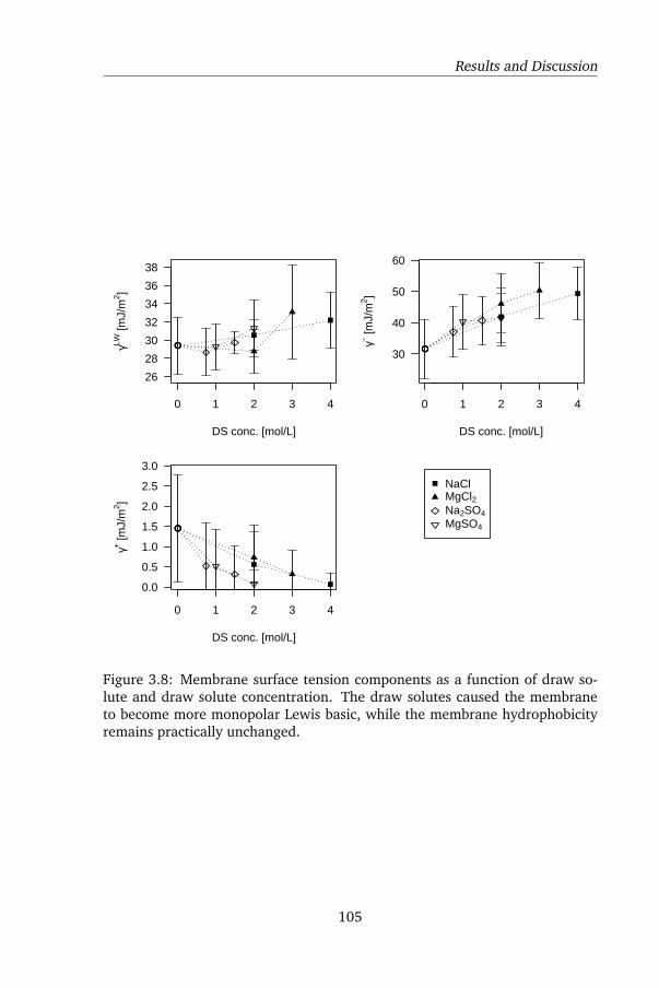
Results and Discussion
●
0 1 2 3 4
26
28
30
32
34
36
38
DS conc. [mol/L]
γLW [m
J/m
2 ]
●●● ●
0 1 2 3 4
30
40
50
60
DS conc. [mol/L]
γ− [m
J/m
2 ]
●●●
●
0 1 2 3 4
0.0
0.5
1.0
1.5
2.0
2.5
3.0
DS conc. [mol/L]
γ+ [m
J/m
2 ]
●●●
NaClMgCl2Na2SO4MgSO4
Figure 3.8: Membrane surface tension components as a function of draw so-lute and draw solute concentration. The draw solutes caused the membraneto become more monopolar Lewis basic, while the membrane hydrophobicityremains practically unchanged.
105
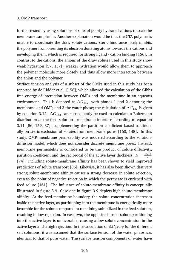
3. OMP transport
further tested by using solutions of salts of poorly hydrated cations to soak the
membrane samples in. Another explanation would be that the CTA polymer is
unable to coordinate the draw solute cations: steric hindrance likely inhibits
the polymer from orienting its electron donating atoms towards the cations and
enveloping them, which is required for strong ligand - cation binding [156]. In
contrast to the cations, the anions of the draw solutes used in this study show
weak hydration [57, 157]: weaker hydration would allow them to approach
the polymer molecule more closely and thus allow more interaction between
the anion and the polymer.
Surface tension analysis of a subset of the OMPs used in this study has been
reported by de Ridder et al. [158], which allowed the calculation of the Gibbs
free energy of interaction between OMPs and the membrane in an aqueous
environment. This is denoted as ∆G132, with phases 1 and 2 denoting the
membrane and OMP, and 3 the water phase; the calculation of ∆G132 is given
by equation 3.12. ∆G132 can subsequently be used to calculate a Boltzmann
distribution at the feed solution - membrane interface according to equation
3.11 [86, 159, 87], supplementing the partition coefficient based tradition-
ally on steric exclusion of solutes from membrane pores [160, 148]. In this
study, OMP membrane permeability was modeled according to the solution-
diffusion model, which does not consider discrete membrane pores. Instead,
membrane permeability is considered to be the product of solute diffusivity,
partition coefficient and the reciprocal of the active layer thickness: B = Dmφl
[74]. Including solute-membrane affinity has been shown to yield improved
predictions of solute transport [86]. Likewise, it has also been shown that very
strong solute-membrane affinity causes a strong decrease in solute rejection,
even to the point of negative rejection in which the permeate is enriched with
feed solute [161]. The influence of solute-membrane affinity is conceptually
illustrated in figure 3.9. Case one in figure 3.9 depicts high solute-membrane
affinity. At the feed-membrane boundary, the solute concentration increases
inside the active layer, as partitioning into the membrane is energetically more
favorable for the solute compared to remaining solubilized in the feed solution,
resulting in low rejection. In case two, the opposite is true: solute partitioning
into the active layer is unfavorable, causing a low solute concentration in the
active layer and a high rejection. In the calculation of ∆GMWS for the different
salt solutions, it was assumed that the surface tension of the water phase was
identical to that of pure water. The surface tension components of water have
106
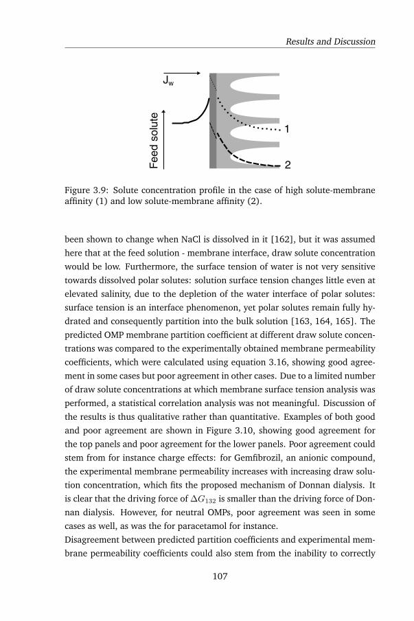
Results and Discussion
Fee
d so
lute
Jw
1
2
Figure 3.9: Solute concentration profile in the case of high solute-membraneaffinity (1) and low solute-membrane affinity (2).
been shown to change when NaCl is dissolved in it [162], but it was assumed
here that at the feed solution - membrane interface, draw solute concentration
would be low. Furthermore, the surface tension of water is not very sensitive
towards dissolved polar solutes: solution surface tension changes little even at
elevated salinity, due to the depletion of the water interface of polar solutes:
surface tension is an interface phenomenon, yet polar solutes remain fully hy-
drated and consequently partition into the bulk solution [163, 164, 165]. The
predicted OMP membrane partition coefficient at different draw solute concen-
trations was compared to the experimentally obtained membrane permeability
coefficients, which were calculated using equation 3.16, showing good agree-
ment in some cases but poor agreement in other cases. Due to a limited number
of draw solute concentrations at which membrane surface tension analysis was
performed, a statistical correlation analysis was not meaningful. Discussion of
the results is thus qualitative rather than quantitative. Examples of both good
and poor agreement are shown in Figure 3.10, showing good agreement for
the top panels and poor agreement for the lower panels. Poor agreement could
stem from for instance charge effects: for Gemfibrozil, an anionic compound,
the experimental membrane permeability increases with increasing draw solu-
tion concentration, which fits the proposed mechanism of Donnan dialysis. It
is clear that the driving force of ∆G132 is smaller than the driving force of Don-
nan dialysis. However, for neutral OMPs, poor agreement was seen in some
cases as well, as was the for paracetamol for instance.
Disagreement between predicted partition coefficients and experimental mem-
brane permeability coefficients could also stem from the inability to correctly
107
3. OMP transport
assess γAB from contact angle measurements on solid substrates. In a solid and
dried state, organic compounds are typically monopolar Lewis basic: during
crystallization, Lewis basic groups are oriented towards Lewis acidic groups,
thereby neutralizing them. The measured γ−d is then the residual γ− [163, 33],
with subscript d denoting the dried state:
γ−d = γ− − γ+ (3.19)
This was the case for the CTA membrane as well: contact angle analysis on
dried samples yielded γ+d = 0 and γ−d = 11 mJ/m2, in contrast to the low but
detectable γ+ of 1.45 mJ/m2 in the hydrated state. It can be seen however
that the above equality of equation 3.19 does not hold in the case of CTA: the
γ− component in the hydrated state is 31.7 mJ/m2, a difference of 20 mJ/m2
compared to the dried state, while the γ+ component is only 1.45 mJ/m2. The
Lifshitz-Van der Waals component also differs somewhat between the dried and
hydrated state: 36.5 and 29.4 mJ/m2 respectively. No theory exists yet explain-
ing the surface tension of wetted polymers or predicting γAB surface tension
components in general [33]. Hydrated polymer surface tension has not been
studied much, only a few relevant reports were found. Rillosi and Buckton
[143] studied mucoadhesion between mucin and a polyacrylate polymer, and
performed surface tension analysis on both dried and hydrated polyacrylate
samples. Their results likewise showed reduced polymer hydrophobicity and
a large increase in the polar surface tension components in a hydrated state,
also disobeying equation 3.19. Our results, and those reported by Rillosi and
Buckton as well, show that the surface tension of a hydrated polymer can, at
present, not be determined reliably from surface tension analysis performed on
dried samples. Hurwitz et al. [142] approached the subject from a different
angle, using brine droplets as probe liquids on dried membrane samples, also
finding an increased Lewis base component. Their approach however cannot
determine changes in membrane hydrophobicity: this requires the use of fully
apolar test liquid, commonly diiodomethane or alpha-bromonaphtalene. Our
results have obvious ramifications for membrane studies, as most membrane
processes operate in a wetted state: prediction of solute-membrane interac-
tions could be erroneous. Further method development is furthermore needed
to assess the validity of surface tension analysis of hydrated surfaces.
Similarly to polymers, the γ−d and γ+d tend to be underestimated and absent
108
Results and Discussion
respectively for small molecules as well: the γ+d component was 0 for all com-
pounds. Solubilized molecules however will interact with the solvent or inter-
faces by both Lewis basic and Lewis acidic moieties. The procedure to deter-
mine correct values of γ+ and γ− is elaborated upon by Docoslis et al. [163]
and van Oss [33], involving both contact angle and solubility measurements
and relating surface tension components obtained from the dried and solubi-
lized state by equation 3.19. The solubility of a compound can be related to
the interfacial tension between solvent and solute by [33]:
∆G121 = −2γ12 =kT
Scln(s) (3.20)
with ∆G121, γ12, Sc and s being the Gibbs free energy of association between
2 solubilized solute molecules, the surface tension between solute and solvent,
the contactable surface area between 2 solute molecules and the solubility of
the solute in molar ratio respectively. As was mentioned above, equation 3.19
appears not to hold for dried versus hydrated polymer samples. More research
is needed to assess equation 3.19: it is conceivable that small solutes, which are
fully hydrated and move independently in solution, behave different compared
with insoluble but hydrated polymer chains. From their insolubility follows
that polymer - polymer interactions are still dominant compared with polymer
- water interactions, which translates into ∆G121 < 0, or γ12 > 0. Polymers
are furthermore capable of coiling or, for branched polymers such as CTA, re-
orienting side groups. Both equation 3.11 and equation 3.20 are furthermore
sensitive towards the choice of the contactable surface area. In the case of
equation 3.11, Verliefde et al. [86] proposed Sc = πr2s/2, based on an sur-
face integration procedure developed by Bhattacharjee et al. and assuming
porous flow [148], while van Oss [33] proposed the molecular maximal pro-
jected area for Sc. It is conceivable that steric constraints are to be taken into
account as well: flexible, "flat" molecules will be able to interact more easily
with molecules of their own size or bigger compared to rigid or highly sub-
stituted molecules [166]. The correct assessment of Sc thus warrants further
study.
As mentioned earlier, the number of draw solute concentrations at which mem-
brane surface tension analysis was performed was too low to enable meaning-
ful statistical analysis. This is due to the labor- and time-intensive nature of
contact angle measurement: for each draw solute concentration, the average
109
3. OMP transport
number of drops measured was 24 and 3 test liquids are needed for each sam-
ple as well. The labor- and time-intensive nature of contact angle analysis
impedes rapid screening of large numbers of samples. The high number of
repetitions is needed to attenuate error propagation in subsequent calculation;
error propagation is considerable none the less. This is due to the high num-
ber of sources of errors: when calculating ∆G132, contact angle measurements
contribute to 6 independent sources of errors, disregarding confidence inter-
vals of the properties of the test liquids themselves. Monte Carlo simulation
was used to determine the standard deviation of the calculated surface tension
components and was found to be fairly large, as can be seen in Figure 3.8,
even though the average standard deviation on the contact angles was only 4.4
°. More convenient and less error prone force balance measurement methods
are needed to allow wider use of surface tension analysis.
110
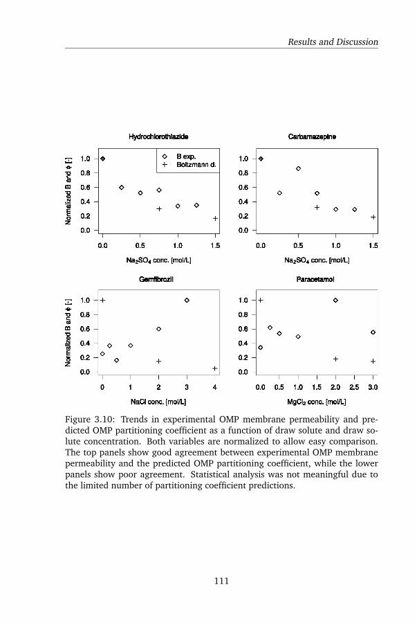
Results and Discussion
Figure 3.10: Trends in experimental OMP membrane permeability and pre-dicted OMP partitioning coefficient as a function of draw solute and draw so-lute concentration. Both variables are normalized to allow easy comparison.The top panels show good agreement between experimental OMP membranepermeability and the predicted OMP partitioning coefficient, while the lowerpanels show poor agreement. Statistical analysis was not meaningful due tothe limited number of partitioning coefficient predictions.
111
Hydrochlorothlazldo Csrbamazoplno
:I: 1.0 • I~ B exp. 1.0 • <> Bottzmann d.
<> .., 0.8 0.8 c .. "' 0.6 <> <> 0.6
~ <> <> <> 0.4 0.4 .,
+ <> <> + <> <> e 0 0.2 + 0.2 + z
0.0 0.0
0.0 0.5 1.0 1.5 0.0 0.5 1.0 1.5
Na2804 conc. [moi/L] Na2S04 conc. [moVL]
Gomllbrozll Paracetamol
:I: 1.0 - + <> 1.0 + <> <> .., c 0.8- 0.8 .. "' 0.6- <> 0.6 <> 'll <> <> <>
•• 0.4- <> <> 0.4 ., <> g 0.2 - <> <> + 0.2 + + z 0.0- + 0.0
0 2 3 4 0.0 0.5 1.0 1.5 2.0 2.5 3.0
NaCI conc. [moi/L] MgCI2 conc. [moVL]
3. OMP transport
3.4 Conclusions
In this study, transport of OMPs through a FO CTA membrane was systemat-
ically studied, with the emphasis on draw solute - OMP interactions. 4 inor-
ganic draw solutes were used, being NaCl, MgCl2, Na2SO4 and MgSO4. RSD
proved to have little influence on OMP transport, as did the water flux: RSD
and water flux are between 8 and 13 orders of magnitude larger than OMP
flux in molar terms, yet the OMP flux during simple diffusion tests (without
RSD and water flux) was entirely comparable to OMP flux during FO tests for
uncharged OMPs. This is in line with the solution-diffusion model, in contrast
to convection-diffusion models describing porous flow. For uncharged OMPs,
steric parameters showed good correlation with OMP permeability, the param-
eters showing the best correlation were the minimal projected surface area,
molecular surface area and molecular volume. For charged OMPs, steric corre-
lations were generally very poor, both during FO and simple diffusion. Charge
interactions between charged OMPs, the membrane and draw solutes were
very clearly present: cationic OMP flux was strongly reduced during FO tests
compared to diffusion tests, while anionic OMP flux was increased. The de-
crease of cationic OMP flux is hypothesized to be due to membrane saturation
by draw solute cations, but further research is needed to test this hypothesis.
The hypothesis that this change in transport was due to electromigration in a
spontaneously established electrical field between the feed and draw solution
was tested by open circuit voltage measurements using a potentiostat. The
hypothesis of electromigration was discarded, as the measured electrical fields
had a polarity opposite of what was expected from OMP flux data for 3 out
of 4 draw solutes. We consider Donnan dialysis currently as the most fitting
explanation.
Surface tension analysis of membrane samples wetted by the different draw
solutions showed that the membrane became a monopolar Lewis base at in-
creasing salt concentration. This response was more pronounced for the sul-
fate salts compared to the chloride salts, showing noticeable interaction be-
tween the draw solute anion and polymer Lewis acid groups. Conversely, no
effect of the cation on the membrane surface tension was seen, showing that
the cations tested in this study were more or less inert with regards to the
polymer. Likewise, OMP permeability in FO showed draw solute anion-based
clustering, but not so for draw solute cations. The membrane surface tension
112
Appendix
was quite different when comparing dried and hydrated samples, disobeying
the combining rule proposed by van Oss used to relate the surface tension
components of a compound in pure solid state and solubilized. This is likely
due to the remaining significant polymer self-interactions in a hydrated poly-
mer sample contrasting with full solubilization. The membrane surface tension
and OMP membrane surface tension was used to calculate ∆G132 at different
draw solute concentrations, which was then compared to experimentally deter-
mined OMP membrane permeability coefficients. Both good and poor agree-
ment between ∆G132 and membrane permeability coefficients was found, with
the poor agreement in some cases being due to charge interactions. In other
cases, poor agreement could be due to the surface tension of the OMPs, which
was determined on pure solid samples, and is subject to underestimation of the
γ+ and γ− components.
3.A Appendix
3.A.1 Solid Phase Extraction protocol
The SPE cartridges used are Oasis HLB cartridges (6cc, 200 mg sorbent/cartridge,
30 µm particle size) (Waters, MA, USA). Calibration samples were prepared in
deionized water using stock solutions of each OMP in MeOH having a concen-
tration of 200 mg/L. A total of 11 calibration samples were prepared in an
approximately 2-fold dilution series, spanning a range of 0.05 to 40 µg l−1, ac-
commodating both feed and permeate samples. The protocol below applies to
both calibration and experimental samples equally. 6 internal standards were
added to all samples, the internal standards are listed in Table 3.4.
1. Sample volume is adjusted to 200 ml and samples are equilibrated to
room temperature.
2. All samples are spiked with internal standards, see Table 3.4.
3. SPE cartridges are conditioned using 2 ml MeOH, HPLC quality, after
which most of the MeOH is allowed to drain, keeping the adsorbent bed
wetted. From this point onwards, the cartridges should not be allowed
to dry out during the extraction.
4. Because the sample volume is considerably larger than the cartridge vol-
ume, samples are loaded using syphons. The cartridges are filled with 6
113
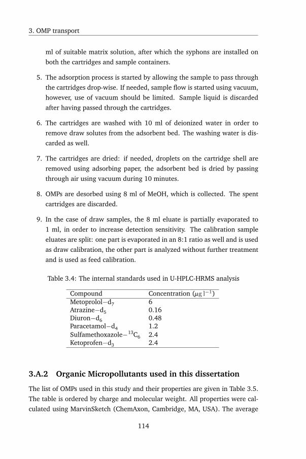
3. OMP transport
ml of suitable matrix solution, after which the syphons are installed on
both the cartridges and sample containers.
5. The adsorption process is started by allowing the sample to pass through
the cartridges drop-wise. If needed, sample flow is started using vacuum,
however, use of vacuum should be limited. Sample liquid is discarded
after having passed through the cartridges.
6. The cartridges are washed with 10 ml of deionized water in order to
remove draw solutes from the adsorbent bed. The washing water is dis-
carded as well.
7. The cartridges are dried: if needed, droplets on the cartridge shell are
removed using adsorbing paper, the adsorbent bed is dried by passing
through air using vacuum during 10 minutes.
8. OMPs are desorbed using 8 ml of MeOH, which is collected. The spent
cartridges are discarded.
9. In the case of draw samples, the 8 ml eluate is partially evaporated to
1 ml, in order to increase detection sensitivity. The calibration sample
eluates are split: one part is evaporated in an 8:1 ratio as well and is used
as draw calibration, the other part is analyzed without further treatment
and is used as feed calibration.
Table 3.4: The internal standards used in U-HPLC-HRMS analysis
Compound Concentration (µg l−1)Metoprolol−d7 6Atrazine−d5 0.16Diuron−d6 0.48Paracetamol−d4 1.2Sulfamethoxazole−13C6 2.4Ketoprofen−d3 2.4
3.A.2 Organic Micropollutants used in this dissertation
The list of OMPs used in this study and their properties are given in Table 3.5.
The table is ordered by charge and molecular weight. All properties were cal-
culated using MarvinSketch (ChemAxon, Cambridge, MA, USA). The average
114
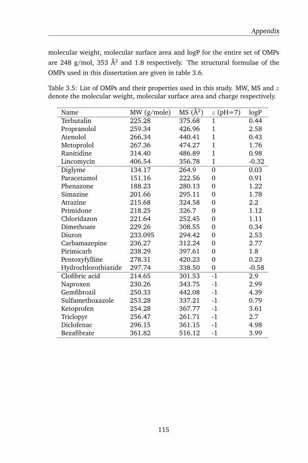
Appendix
molecular weight, molecular surface area and logP for the entire set of OMPs
are 248 g/mol, 353 Å2 and 1.8 respectively. The structural formulae of the
OMPs used in this dissertation are given in table 3.6.
Table 3.5: List of OMPs and their properties used in this study. MW, MS and zdenote the molecular weight, molecular surface area and charge respectively.
Name MW (g/mole) MS (Å2) z (pH=7) logPTerbutalin 225.28 375.68 1 0.44Propranolol 259.34 426.96 1 2.58Atenolol 266.34 440.41 1 0.43Metoprolol 267.36 474.27 1 1.76Ranitidine 314.40 486.89 1 0.98Lincomycin 406.54 356.78 1 -0.32Diglyme 134.17 264.9 0 0.03Paracetamol 151.16 222.56 0 0.91Phenazone 188.23 280.13 0 1.22Simazine 201.66 295.11 0 1.78Atrazine 215.68 324.58 0 2.2Primidone 218.25 326.7 0 1.12Chloridazon 221.64 252.45 0 1.11Dimethoate 229.26 308.55 0 0.34Diuron 233.095 294.42 0 2.53Carbamazepine 236.27 312.24 0 2.77Pirimicarb 238.29 397.61 0 1.8Pentoxyfylline 278.31 420.23 0 0.23Hydrochlorothiazide 297.74 338.50 0 -0.58Clofibric acid 214.65 301.53 -1 2.9Naproxen 230.26 343.75 -1 2.99Gemfibrozil 250.33 442.08 -1 4.39Sulfamethoxazole 253.28 337.21 -1 0.79Ketoprofen 254.28 367.77 -1 3.61Triclopyr 256.47 261.71 -1 2.7Diclofenac 296.15 361.15 -1 4.98Bezafibrate 361.82 516.12 -1 3.99
115
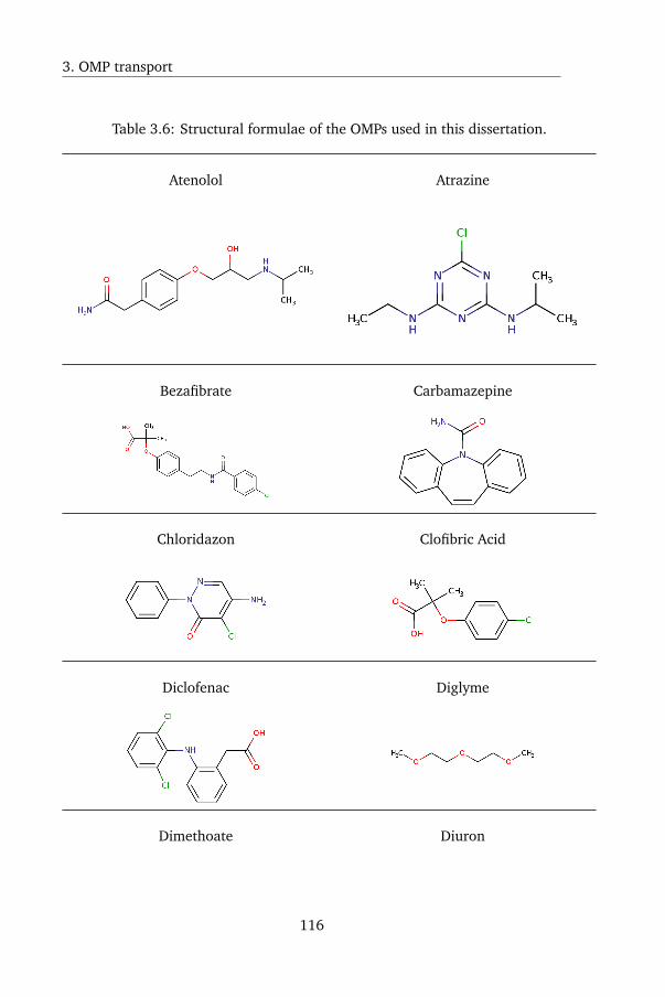
3. OMP transport
Table 3.6: Structural formulae of the OMPs used in this dissertation.
Atenolol Atrazine
Bezafibrate Carbamazepine
Chloridazon Clofibric Acid
Diclofenac Diglyme
Dimethoate Diuron
116
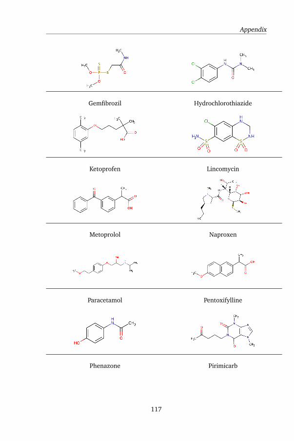
Appendix
Gemfibrozil Hydrochlorothiazide
Ketoprofen Lincomycin
Metoprolol Naproxen
Paracetamol Pentoxifylline
Phenazone Pirimicarb
117
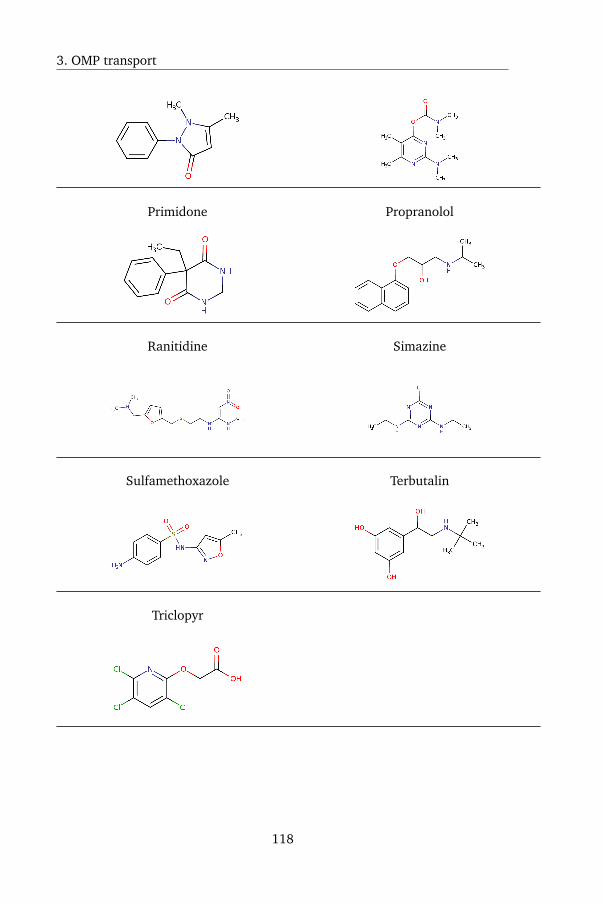
3. OMP transport
Primidone Propranolol
Ranitidine Simazine
Sulfamethoxazole Terbutalin
Triclopyr
118
Chapter 4
Negative rejection of uncharged organicsolutes in FO
Adapted from:
Arnout D’Haese, Ilse Deleersnyder, Pieter Vermeir, Arne Verliefde, Modeling
negative rejection of uncharged organic solutes in Forward Osmosis In prepa-ration
119
4. Negative rejection
4.1 Introduction
Negative rejection of feed solutes by membranes, implying enrichment of feed
solute in the permeate, is a relatively rare phenomenon. In this chapter, neg-
ative rejection of organic, uncharged solutes during forward osmosis (FO) is
described and modeled. Much of the research into negative rejection has fo-
cused on organic solvent nanofiltration (OSN), as negative rejection is encoun-
tered more frequently in non-aqueous solutions [75, 167, 168]. Compared
to organic liquids, water has a very small molar volume, high diffusivity, is
strongly polar and has a high surface tension; the latter causes strong solute-
water and water-membrane interactions. Consequently, the contribution of
pressure to the chemical potential of water during membrane filtration is small
[74, 75], and the diffusivity of aqueous solutes is almost always considerably
lower than the diffusivity of water. In OSN, however, solvent molar volume
is larger while the surface tension of solute and solvent are more likely to be
similar compared to aqueous solutions, allowing for stronger solute-membrane
interactions. Negative rejection is observed with solutes showing high solute-
membrane affinity, and rejection decreases further with increasing solute size
due to increasing molar volume, as was observed by Postel et al. [167] for
homologue series of alkanes, styrene and ethylene glycol oligomers, and pre-
dicted using generalized solution-diffusion models by Paul [75] and Malakhov
and Volkov [168]. The decreased rejection with increasing solute size can seem
contradictory, as larger solutes are also more subject to steric hindrance dur-
ing membrane passage which increases their rejection. However, larger solutes
have a larger molar volume, which increases the influence of a pressure differ-
ence on their flux (see equation 38 in [74] and [75]).
In aqueous solutions, negative rejection has been observed mainly for ionic so-
lutes. In nanofiltration, negative rejection of ions has been studied in depth
by Yaroshchuk [59] who defines a number of different mechanisms which can
cause negative rejection. Such mechanisms are: Donnan potential decreas-
ing the rejection of mobile counterions, enrichment of ions in the membrane
phase of charged membranes (particularly charge-mosaic membranes), or the
acceleration of ions in the membrane phase. Perry and Linder [169] pre-
sented a modified Spiegler-Kedem model including a Donnan exclusion cor-
rection which could describe negative ion rejection. Negative rejection of
uncharged organic solutes in aqueous solutions has been observed, a well-
120
Materials and methods
described case being phenolic compounds permeating through cellulose ac-
etate (CA) RO membranes [170, 161, 171]. It was noted that rejection became
more negative with increasing pressure, and negative rejection was explained
as a combination of strong adsorption of phenolic compounds on CA and an
increase of their chemical potential due to the exerted pressure, similar to the
generalized solution-diffusion model. Mandale and Jones [172] observed neg-
ative rejection of 5 uncharged, non-dissociable organic compounds in the pres-
ence of Na2HPO4 during NF. The results were interpreted using the model
presented by Perry and Linder; assuming that the organic compounds were in
fact partially charged. This assumption appears questionable: the organics, 3
sugars, an alcohol and caffeine, were required to substitute for Na+ ions ac-
cording to the Donnan model, even though all of those compounds are Lewis
bases [33] and hold no permanent charges.
In this study, strong negative rejection of uncharged organic solutes during
FO is reported, with the solutes being 7 alcohols and formamide. The rejec-
tion pattern observed in function of flux was different compared to the above
mentioned studies. Current membrane transport models are briefly reviewed
within the context of negative solute rejection, and it is shown why current
models cannot predict the rejection patterns presented in this study. A new
model is developed, based on sequential Langmuir-type adsorption followed
by washing out of the adsorbed solutes by the water flux; the latter process
assumes flux coupling and is modeled using a convection-diffusion model. Re-
jection was studied in both FO and RO using the same solutes and membrane,
with RO yielding positive rejection. Differences between FO and RO results
are discussed, and flux coupling as well as the possibility of salting-out are
explored.
4.2 Materials and methods
4.2.1 Chemicals
The tracers used in this study were non-ionic organic compounds: 7 alcohols
and formamide. Properties of the tracers are given in Table 4.1. All organics
were obtained from Sigma-Aldrich and were used as received. NaCl was used
as a draw solute, in concentrations ranging from 0.15 to 5.3M. The alcohols
were used at a concentration of 100 mg/L each, and were used as a mixture.
121
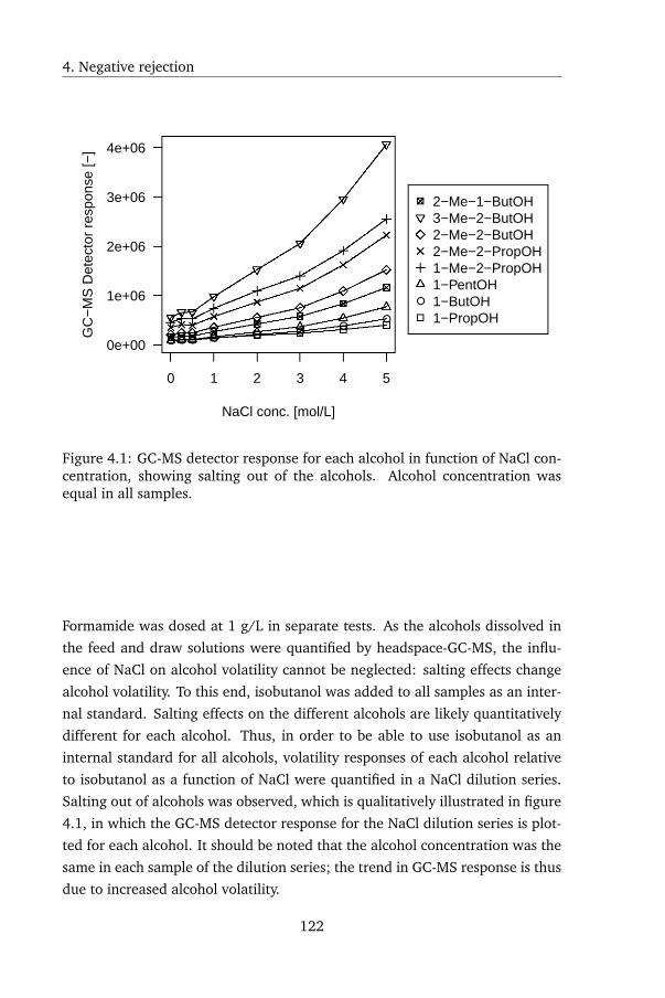
4. Negative rejection
0 1 2 3 4 5
0e+00
1e+06
2e+06
3e+06
4e+06
NaCl conc. [mol/L]
GC
−M
S D
etec
tor
resp
onse
[−]
● ● ● ● ● ●●
●
●
2−Me−1−ButOH3−Me−2−ButOH2−Me−2−ButOH2−Me−2−PropOH1−Me−2−PropOH1−PentOH1−ButOH1−PropOH
Figure 4.1: GC-MS detector response for each alcohol in function of NaCl con-centration, showing salting out of the alcohols. Alcohol concentration wasequal in all samples.
Formamide was dosed at 1 g/L in separate tests. As the alcohols dissolved in
the feed and draw solutions were quantified by headspace-GC-MS, the influ-
ence of NaCl on alcohol volatility cannot be neglected: salting effects change
alcohol volatility. To this end, isobutanol was added to all samples as an inter-
nal standard. Salting effects on the different alcohols are likely quantitatively
different for each alcohol. Thus, in order to be able to use isobutanol as an
internal standard for all alcohols, volatility responses of each alcohol relative
to isobutanol as a function of NaCl were quantified in a NaCl dilution series.
Salting out of alcohols was observed, which is qualitatively illustrated in figure
4.1, in which the GC-MS detector response for the NaCl dilution series is plot-
ted for each alcohol. It should be noted that the alcohol concentration was the
same in each sample of the dilution series; the trend in GC-MS response is thus
due to increased alcohol volatility.
122
" V
<> x + "' D
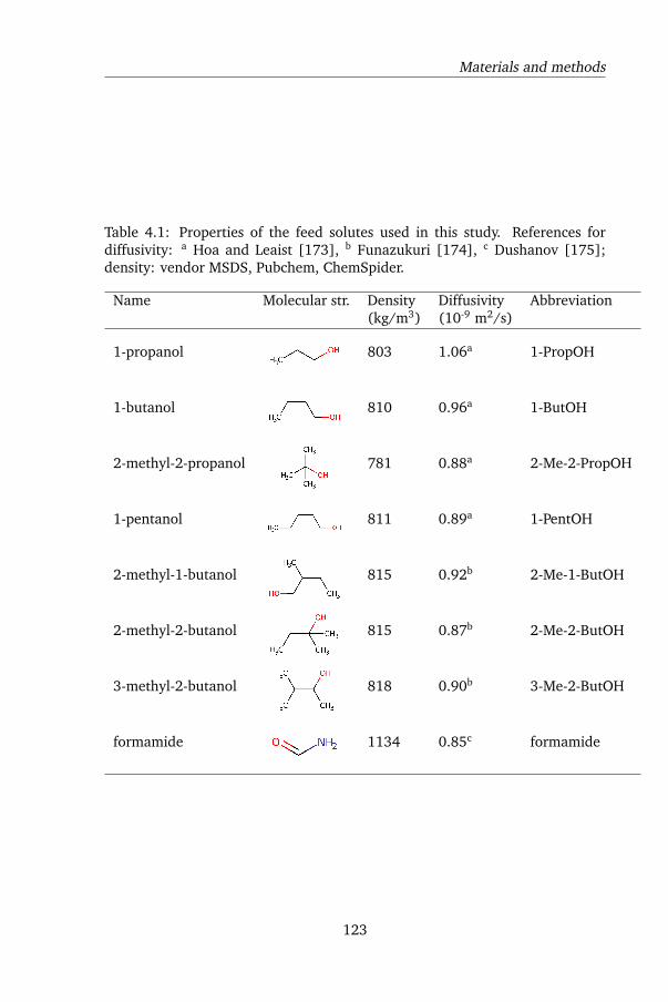
Materials and methods
Table 4.1: Properties of the feed solutes used in this study. References fordiffusivity: a Hoa and Leaist [173], b Funazukuri [174], c Dushanov [175];density: vendor MSDS, Pubchem, ChemSpider.
Name Molecular str. Density Diffusivity Abbreviation(kg/m3) (10-9 m2/s)
1-propanol 803 1.06a 1-PropOH
1-butanol 810 0.96a 1-ButOH
2-methyl-2-propanol 781 0.88a 2-Me-2-PropOH
1-pentanol 811 0.89a 1-PentOH
2-methyl-1-butanol 815 0.92b 2-Me-1-ButOH
2-methyl-2-butanol 815 0.87b 2-Me-2-ButOH
3-methyl-2-butanol 818 0.90b 3-Me-2-ButOH
formamide 1134 0.85c formamide
123
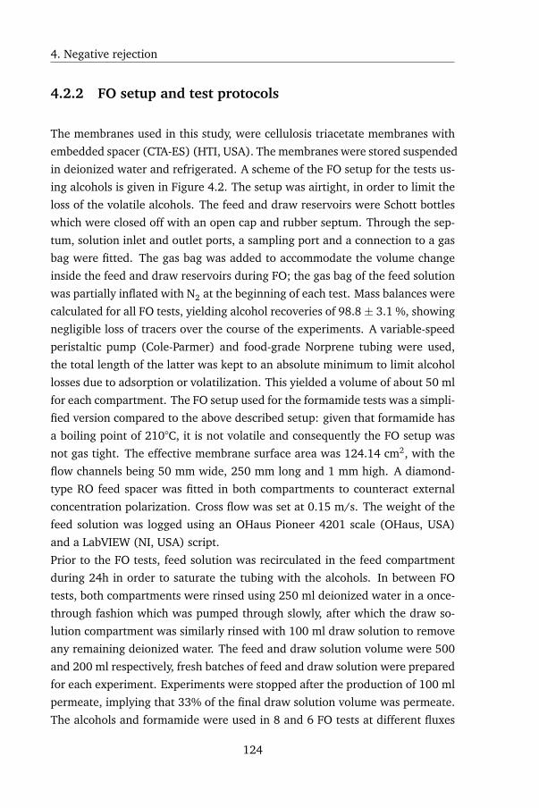
4. Negative rejection
4.2.2 FO setup and test protocols
The membranes used in this study, were cellulosis triacetate membranes with
embedded spacer (CTA-ES) (HTI, USA). The membranes were stored suspended
in deionized water and refrigerated. A scheme of the FO setup for the tests us-
ing alcohols is given in Figure 4.2. The setup was airtight, in order to limit the
loss of the volatile alcohols. The feed and draw reservoirs were Schott bottles
which were closed off with an open cap and rubber septum. Through the sep-
tum, solution inlet and outlet ports, a sampling port and a connection to a gas
bag were fitted. The gas bag was added to accommodate the volume change
inside the feed and draw reservoirs during FO; the gas bag of the feed solution
was partially inflated with N2 at the beginning of each test. Mass balances were
calculated for all FO tests, yielding alcohol recoveries of 98.8 ± 3.1 %, showing
negligible loss of tracers over the course of the experiments. A variable-speed
peristaltic pump (Cole-Parmer) and food-grade Norprene tubing were used,
the total length of the latter was kept to an absolute minimum to limit alcohol
losses due to adsorption or volatilization. This yielded a volume of about 50 ml
for each compartment. The FO setup used for the formamide tests was a simpli-
fied version compared to the above described setup: given that formamide has
a boiling point of 210°C, it is not volatile and consequently the FO setup was
not gas tight. The effective membrane surface area was 124.14 cm2, with the
flow channels being 50 mm wide, 250 mm long and 1 mm high. A diamond-
type RO feed spacer was fitted in both compartments to counteract external
concentration polarization. Cross flow was set at 0.15 m/s. The weight of the
feed solution was logged using an OHaus Pioneer 4201 scale (OHaus, USA)
and a LabVIEW (NI, USA) script.
Prior to the FO tests, feed solution was recirculated in the feed compartment
during 24h in order to saturate the tubing with the alcohols. In between FO
tests, both compartments were rinsed using 250 ml deionized water in a once-
through fashion which was pumped through slowly, after which the draw so-
lution compartment was similarly rinsed with 100 ml draw solution to remove
any remaining deionized water. The feed and draw solution volume were 500
and 200 ml respectively, fresh batches of feed and draw solution were prepared
for each experiment. Experiments were stopped after the production of 100 ml
permeate, implying that 33% of the final draw solution volume was permeate.
The alcohols and formamide were used in 8 and 6 FO tests at different fluxes
124
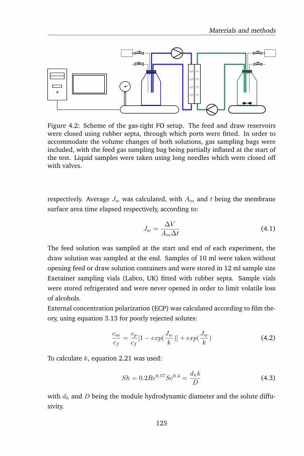
Materials and methods
Figure 4.2: Scheme of the gas-tight FO setup. The feed and draw reservoirswere closed using rubber septa, through which ports were fitted. In order toaccommodate the volume changes of both solutions, gas sampling bags wereincluded, with the feed gas sampling bag being partially inflated at the start ofthe test. Liquid samples were taken using long needles which were closed offwith valves.
respectively. Average Jw was calculated, with Am and t being the membrane
surface area time elapsed respectively, according to:
Jw =∆V
Am∆t(4.1)
The feed solution was sampled at the start and end of each experiment, the
draw solution was sampled at the end. Samples of 10 ml were taken without
opening feed or draw solution containers and were stored in 12 ml sample size
Exetainer sampling vials (Labco, UK) fitted with rubber septa. Sample vials
were stored refrigerated and were never opened in order to limit volatile loss
of alcohols.
External concentration polarization (ECP) was calculated according to film the-
ory, using equation 3.13 for poorly rejected solutes:
cmcf
=cpcf
[1− exp(Jwk
)] + exp(Jwk
) (4.2)
To calculate k, equation 2.21 was used:
Sh = 0.2Re0.57Sc0.4 =dhk
D(4.3)
with dh and D being the module hydrodynamic diameter and the solute diffu-
sivity.
125
4. Negative rejection
4.2.3 RO setup and test protocols
The RO setup consisted of a Sterlitech HP4750 stirred cell having a membrane
surface area of 12.0 cm2 fitted with a PTFE stirrer bar to provide cross flow.
This cell has a low hold-up volume of 1 ml and a feed volume of 300 ml. Mem-
brane coupons were compacted at 30 bars until constant flux, which lasted 2
hours. RO tests were performed at 5, 10, 14, 20, 25 and 30 bars. Permeate
was collected in glass-only gas sampling syringes in order to avoid sample con-
tamination. The first 5 ml of permeate were discarded, after which 10 ml was
collected. The syringe was placed on a OHaus Adventurer Pro 410 scale which
was datalogged for flux measurements. The feed solution was used for 3 RO
tests, after which it was discarded and fresh feed solution was prepared. The
stirrer was set to 250 rpm, which corresponded with a stirrer tip velocity of
0.26 m/s. Sample handling and storing was as described in the previous sec-
tion. The external concentration polarization mass transfer coefficient k was
calculated according to [176]:
k = 0.23D
r(ν
D)1/3(
ωr2
ν)0.567 (4.4)
with ν, D, ω and r being the kinematic viscosity, solute diffusion coefficient,
angular velocity and stirrer radius. This then allowed the calculation of the
real rejection, with Robs being the observed rejection, according to:
R =Robsexp(
Jwk )
(1−Robs) +Robs ∗ exp(Jwk )(4.5)
4.2.4 Analysis
Alcohols were analyzed using headspace-GC-MS. In all samples, calibration
samples and standards, isobutanol was used as an internal standard. In order
to account for changes in alcohol volatility as a function of NaCl, 8 alcohol stan-
dards in a NaCl dilution series spanning 0 to 5M were prepared, and the rela-
tive deviation compared to the isobutanol response was measured. At 5M NaCl,
volatiliy of the analytes relative to isobutanol was in the range of 75 - 135%,
clearly showing that volatility deviations could not be ignored. Headspace GC-
MS analysis was done using an Agilent 6890 GC equiped with a Gerstel MPS
headspace injection system. The sample vials were incubated at 80°C prior to
126
Materials and methods
sampling. The syringe temperature was maintained at 90°C, the syringe was
flushed during 60 seconds prior to sampling. The injection volume was 2500
µl. The inlet temperature was set at 230°C at a pressure of 10 kPa. A split ratio
of 50:1 was used; using helium as carrier gas. The GC was equiped with an
Agilent 7HG-G007-11 column of 30 m length and 0.25 µm film thickness. The
GC oven temperature was ramped from 35°C to 300°C, using an initial ramp
rate of 3°/min for 10 minutes followed by 20°/min for the remaining 8 minutes
runtime.
Formamide was quantified using an AutoAnalyzer3 (Bran+Luebbe, Germany)
which detects NH3 using the salicylate-nitroprusside method. Formamide sam-
ples were acid hydrolyzed using 1M H2SO4, method development tests had
shown full hydrolysis within 2 hours. In order to take matrix effects of the
draw solution into account, a standard addition protocol was followed using 3
additional sampling points spiked with (NH4)2SO4.
4.2.5 Modeling
All modeling was done in R 3.3.1 [117]. Parameter optimization was done
using a modified, box-constrained Nelder-Mead simplex algorithm, minimizing
the residual sum of squared errors between fitted and observed rejection.
4.2.6 Predicting tracer adsorption
Negative rejection is modeled using Langmuir adsorption followed by convec-
tively coupled solute transport. In order to predict adsorption of the tracers to
the membrane, the thermodynamic model proposed by van Oss is used [33]
(equation 3.12):
∆G1w2 = (√γLW1 −
√γLW2 )2 − (
√γLW1 −
√γLWw )2 − (
√γLW2 −
√γLWw )2
+2[
√γ+w (
√γ−1 +
√γ−2 −
√γ−w )+
√γ−w (
√γ+
1 +
√γ+
2 −√γ+w )−
√γ−1 γ
+2 −
√γ+
1 γ−2 ]
(4.6)
with superscripts LW , +, − indicating the Lifshitz-Van der Waals, Lewis acid
and Lewis base surface tension component respectively. Subscripts 1, 2 and w
indicate phases 1 and 2, being the solute and membrane, and water. The sur-
face tension components of formamide are known, as formamide is often used
127
4. Negative rejection
as a test liquid in contact angle determination. The surface tension compo-
nents of NaCl solutions were taken from literature [162]. The surface tension
components of the alcohols however were not known, and were experimen-
tally determined. To this end, the total surface tension was measured using
the Wilhelmy plate method. Additionally, contact angles on PTFE and the sol-
ubility of glucose in the alcohols were measured. Because the total surface
tension of the alcohols was low (20 - 25 mJ/m2), contact angles could not
be measured on polar surfaces such as glass: these materials have total sur-
face tensions exceeding those of the alcohols, causing complete spreading of
droplets. This provides 3 independent data sources for the 3 unknown surface
tension parameters, which are related to the total surface tension as follows:
γT = γLW + 2√γ+γ− (4.7)
As a control, methanol and ethanol were also included in these tests, as esti-
mations of the surface tension components of methanol and ethanol have been
made earlier [33]. Additional contact angle measurements on dried and wet-
ted membrane samples were performed according to the method described in
section 3.2.5.
Wilhelmy plate method
According to the Wilhelmy plate method, the additional weight exerted on a
fully wetted, thin plate being slowly lifted out of a liquid is related to the total
surface tension of the liquid according to [177]:
γT cos(θ) =∆w
l(4.8)
with cos(θ), ∆w and l being the contact angle between the liquid and the
plate, the additional weight exerted on the plate and the circumference of the
plate respectively. For a fully wetted plate, θ = 0 and thus cos(θ) = 1, sim-
plifying equation 4.8. The plates used in this study were microscopy cover
slips, which were suspended from a balance. A beaker of sufficient diameter
filled with alcohol was gently raised until the liquid surface fully contacted
the lower edge of the plate. The beaker was then gently lowered, creating a
curved meniscus between the alcohol and the plate, which caused increasing
additional weight. Shortly before the meniscus breaks from the plate, the ad-
128
Materials and methods
ditional weight reaches a maximum. This maximum was recorded and used
in the calculation of the total surface tension. The total surface tension of the
majority of the alcohols was known [178, 179, 180, 181]; agreement between
published and experimental values was very good.
Contact angles on PTFE
PTFE is an apolar polymer with a surface tension low enough to yield measur-
able contact angles (θ > 10°) with the alcohols. As PTFE generally has a fairly
rough surface, the sample was polished prior to contact angle measurement.
There is some variation in the surface tension published for PTFE [182], which
could be due to polymer impurities or blends. It was therefore decided to char-
acterize the PTFE sample at hand using contact angle measurements with 3
test liquids as was described in section 3.2.5. The method was simplified, as
the PTFE sample was dry and did not need to be covered. This yielded γLW =
17 mJ/m2, γ− = 2 mJ/m2 and γ+ = 0 mJ/m2 for the PTFE sample. The PTFE
sample thus exhibited a small but significant Lewis basic component. Subse-
quently, alcohol contact angles were measured also according to the simplified
method described above.
Glucose solubility
The solubility of a solute in a solvent is related to the interfacial surface tension
γ12 between phases 1 and 2, being the solute and solvent [163, 33]:
2Acγ12 = −kT ln(S) (4.9)
with Ac and S being the contactable surface area between solute and solvent
and the solubility in molar ratio respectively. γ12 is given by:
γ12 = γT1 + γT2 − 2(√γLW1 γLW2 +
√γ+
1 γ−2 +
√γ−1 γ
+2 ) (4.10)
The solute can be a liquid or a solid: equation 4.9 is also applicable for liquid
miscibility. Alcohols, being of intermediate polarity, are substantially soluble or
miscible with many liquids. Furthermore, as the alcohol molecules have both a
polar and apolar domain in their structure, they are able to orient themselves
favorably in the interface between a polar and apolar phase, leading to erro-
neous surface tension measurements [33]. It was therefore decided to use a
129
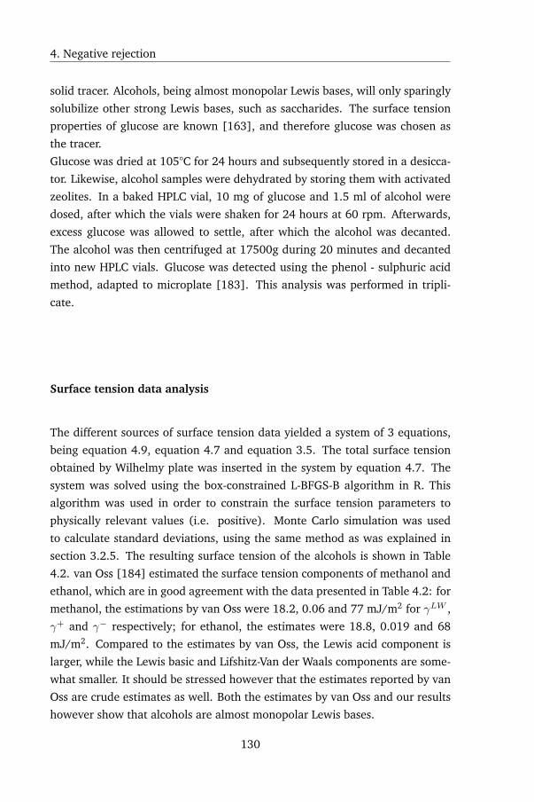
4. Negative rejection
solid tracer. Alcohols, being almost monopolar Lewis bases, will only sparingly
solubilize other strong Lewis bases, such as saccharides. The surface tension
properties of glucose are known [163], and therefore glucose was chosen as
the tracer.
Glucose was dried at 105°C for 24 hours and subsequently stored in a desicca-
tor. Likewise, alcohol samples were dehydrated by storing them with activated
zeolites. In a baked HPLC vial, 10 mg of glucose and 1.5 ml of alcohol were
dosed, after which the vials were shaken for 24 hours at 60 rpm. Afterwards,
excess glucose was allowed to settle, after which the alcohol was decanted.
The alcohol was then centrifuged at 17500g during 20 minutes and decanted
into new HPLC vials. Glucose was detected using the phenol - sulphuric acid
method, adapted to microplate [183]. This analysis was performed in tripli-
cate.
Surface tension data analysis
The different sources of surface tension data yielded a system of 3 equations,
being equation 4.9, equation 4.7 and equation 3.5. The total surface tension
obtained by Wilhelmy plate was inserted in the system by equation 4.7. The
system was solved using the box-constrained L-BFGS-B algorithm in R. This
algorithm was used in order to constrain the surface tension parameters to
physically relevant values (i.e. positive). Monte Carlo simulation was used
to calculate standard deviations, using the same method as was explained in
section 3.2.5. The resulting surface tension of the alcohols is shown in Table
4.2. van Oss [184] estimated the surface tension components of methanol and
ethanol, which are in good agreement with the data presented in Table 4.2: for
methanol, the estimations by van Oss were 18.2, 0.06 and 77 mJ/m2 for γLW ,
γ+ and γ− respectively; for ethanol, the estimates were 18.8, 0.019 and 68
mJ/m2. Compared to the estimates by van Oss, the Lewis acid component is
larger, while the Lewis basic and Lifshitz-Van der Waals components are some-
what smaller. It should be stressed however that the estimates reported by van
Oss are crude estimates as well. Both the estimates by van Oss and our results
however show that alcohols are almost monopolar Lewis bases.
130
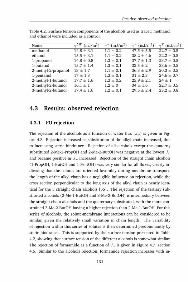
Results: observed rejection
Table 4.2: Surface tension components of the alcohols used as tracer; methanoland ethanol were included as a control.
Name γLW (mJ/m2) γ+ (mJ/m2) γ− (mJ/m2) γT (mJ/m2)methanol 14.8 ± 3.1 1.1 ± 0.2 47.5 ± 5.5 22.7 ± 0.5ethanol 15.5 ± 3.1 1.1 ± 0.2 38.2 ± 4.6 22.2 ± 0.51-propanol 14.8 ± 0.8 1.3 ± 0.1 37.7 ± 1.3 23.7 ± 0.51-butanol 15.7 ± 1.4 1.3 ± 0.1 33.5 ± 2 23.6 ± 0.52-methyl-2-propanol 13 ± 1.7 1.1 ± 0.1 36.3 ± 2.9 20.3 ± 0.51-pentanol 17 ± 1.3 1.3 ± 0.1 31 ± 2.3 24.6 ± 0.72-methyl-1-butanol 17.7 ± 1.6 1.3 ± 0.2 25.9 ± 2.1 24 ± 12-methyl-2-butanol 16.1 ± 1 1.2 ± 0 34 ± 1.6 22.7 ± 0.53-methyl-2-butanol 17.4 ± 1.6 1.2 ± 0.1 29.5 ± 2.4 23.2 ± 0.8
4.3 Results: observed rejection
4.3.1 FO rejection
The rejection of the alcohols as a function of water flux (Jw) is given in Fig-
ure 4.3. Rejection increased as substitution of the alkyl chain increased, due
to increasing steric hindrance. Rejection of all alcohols except the quaterny
substituted 2-Me-2-PropOH and 2-Me-2-ButOH was negative at the lowest Jwand became positive as Jw increased. Rejection of the straight chain alcohols
(1-PropOH, 1-ButOH and 1-PentOH) was very similar for all fluxes, clearly in-
dicating that the solutes are oriented favorably during membrane transport:
the length of the alkyl chain has a negligible influence on rejection, while the
cross section perpendicular to the long axis of the alkyl chain is nearly iden-
tical for the 3 straight chain alcohols [55]. The rejection of the tertiary sub-
stituted alcohols (2-Me-1-ButOH and 3-Me-2-ButOH) is intermediary between
the straight chain alcohols and the quaternary substituted, with the more con-
strained 3-Me-2-ButOH having a higher rejection than 2-Me-1-ButOH. For this
series of alcohols, the solute-membrane interactions can be considered to be
similar, given the relatively small variation in chain length. The variability
of rejection within this series of solutes is then determined predominantly by
steric hindrance. This is supported by the surface tension presented in Table
4.2, showing that surface tension of the different alcohols is somewhat similar.
The rejection of formamide as a function of Jw is given in Figure 4.7, section
4.5. Similar to the alcohols rejection, formamide rejection increases with in-
131
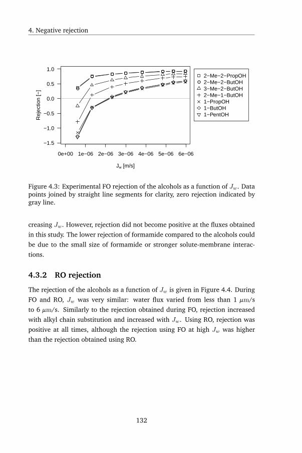
4. Negative rejection
0e+00 1e−06 2e−06 3e−06 4e−06 5e−06 6e−06
−1.5
−1.0
−0.5
0.0
0.5
1.0
Jw [m/s]
Rej
ectio
n [−
] ●
●● ● ● ● ● ●
●
2−Me−2−PropOH2−Me−2−ButOH3−Me−2−ButOH2−Me−1−ButOH1−PropOH1−ButOH1−PentOH
Figure 4.3: Experimental FO rejection of the alcohols as a function of Jw. Datapoints joined by straight line segments for clarity, zero rejection indicated bygray line.
creasing Jw. However, rejection did not become positive at the fluxes obtained
in this study. The lower rejection of formamide compared to the alcohols could
be due to the small size of formamide or stronger solute-membrane interac-
tions.
4.3.2 RO rejection
The rejection of the alcohols as a function of Jw is given in Figure 4.4. During
FO and RO, Jw was very similar: water flux varied from less than 1 µm/s
to 6 µm/s. Similarly to the rejection obtained during FO, rejection increased
with alkyl chain substitution and increased with Jw. Using RO, rejection was
positive at all times, although the rejection using FO at high Jw was higher
than the rejection obtained using RO.
132
Membrane transport theory in the context of negative solute rejection
0e+00 1e−06 2e−06 3e−06 4e−06 5e−06 6e−06
0.0
0.2
0.4
0.6
0.8
1.0
Jw [m/s]
Rej
ectio
n [−
]
●
●●
●●● ●
2−Me−2−PropOH2−Me−2−ButOH3−Me−2−ButOH2−Me−1−ButOH1−PropOH1−ButOH1−PentOH
Figure 4.4: Experimental RO rejection of the alcohols as a function of Jw. Datapoints joined by straight line segments for clarity, zero rejection indicated bygray line.
4.4 Membrane transport theory in the context of
negative solute rejection
4.4.1 Existing models describing negative rejection
Dense membrane processes are often modeled using the solution-diffusion (SD)
model. Certain alternative versions of this model have been proposed, such as
adsorption-solution-diffusion [85] or generalization of the SD model lacking
simplifications regarding coupled diffusion, membrane affinity and the non-
linear effect of pressure on solvent and solute transport [75]. High solute-
membrane affinity causes preferential partitioning of the solute into the mem-
brane phase, reducing its rejection, while the effect of pressure on solute trans-
port increases the flux of large molecules relative to smaller ones. Other popu-
lar models are the Spiegler-Kedem (SK) model [90] based on irreversible ther-
modynamics, and mechanistic models based on the extended Nernst-Planck
equation [58]. For uncharged solutes, as is the case in this study, the extended
Nernst-Planck reduces to a convection-diffusion model (CD), of which the co-
efficients can be interpreted using irreversible thermodynamics [90] or using
133

4. Negative rejection
binary Maxwell-Stefan coupled transport. Certain models do not allow nega-
tive rejection, such as the classical SD and SK models, while generalized SDand CD model can yield negative rejection. The latter models, however, yield a
different rejection pattern as a function of Jw compared to the results obtained
in this study, as will be shown below. Because the widely used SD and SK mod-
els do not allow negative rejection, and because the generalized SD and CDyield different negative rejection patterns than the one observed in this study,
there is a clear need for extending current membrane transport theory.
In the classical SD model , Js is proportional to the solute concentration differ-
ence across the membrane, with the membrane permeability coefficient B as
the rate constant:
Js = B(cf − cp) (4.11)
Given that Js = cpJw, this leads to the following expression for rejection:
RSD =Jw
B + Jw(4.12)
which, for a finite and positive B leads to the following limits:
limJw→0
RSD = 0 & limJw→∞
RSD = 1
showing that solute rejection in the classical SD model is always positive.
Williams et al. [85] used an extended SD model with adsorption, in order to
explain significant reduction of Jw through TFC membranes in the presence of
trace amounts of substituted phenols (∼ 10 - 100 mg/L). They reasoned that
the membrane active layer had a finite number of available sites which could
be occupied by either water or solute; in their model, solute adsorption thus
causes flux decline by blocking water passage. In the expression of Js with
Langmuir adsorption, cf and cp are substituted by Langmuir isotherms:
Js = B∗(b0cf
1 + b0cf− b0cp
1 + b0cp) (4.13)
It can be easily seen from equation 4.13 that for positive and finite values for
B∗ and b0, negative rejection is again impossible. For any cf < cp, it is true
that b0cf1+b0cf
<b0cp
1+b0cpyielding Js < 0, which would equal transport of permeate
solute towards the feed solution. Equation 4.13 can also be formulated using
other adsorption isotherms, such as Henry’s law. This however does not change
134
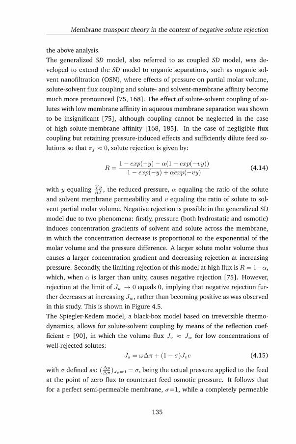
Membrane transport theory in the context of negative solute rejection
the above analysis.
The generalized SD model, also referred to as coupled SD model, was de-
veloped to extend the SD model to organic separations, such as organic sol-
vent nanofiltration (OSN), where effects of pressure on partial molar volume,
solute-solvent flux coupling and solute- and solvent-membrane affinity become
much more pronounced [75, 168]. The effect of solute-solvent coupling of so-
lutes with low membrane affinity in aqueous membrane separation was shown
to be insignificant [75], although coupling cannot be neglected in the case
of high solute-membrane affinity [168, 185]. In the case of negligible flux
coupling but retaining pressure-induced effects and sufficiently dilute feed so-
lutions so that πf ≈ 0, solute rejection is given by:
R =1− exp(−y)− α(1− exp(−vy))
1− exp(−y) + αexp(−vy)(4.14)
with y equaling V pRT , the reduced pressure, α equaling the ratio of the solute
and solvent membrane permeability and v equaling the ratio of solute to sol-
vent partial molar volume. Negative rejection is possible in the generalized SD
model due to two phenomena: firstly, pressure (both hydrostatic and osmotic)
induces concentration gradients of solvent and solute across the membrane,
in which the concentration decrease is proportional to the exponential of the
molar volume and the pressure difference. A larger solute molar volume thus
causes a larger concentration gradient and decreasing rejection at increasing
pressure. Secondly, the limiting rejection of this model at high flux is R = 1−α,
which, when α is larger than unity, causes negative rejection [75]. However,
rejection at the limit of Jw → 0 equals 0, implying that negative rejection fur-
ther decreases at increasing Jw, rather than becoming positive as was observed
in this study. This is shown in Figure 4.5.
The Spiegler-Kedem model, a black-box model based on irreversible thermo-
dynamics, allows for solute-solvent coupling by means of the reflection coef-
ficient σ [90], in which the volume flux Jv ≈ Jw for low concentrations of
well-rejected solutes:
Js = ω∆π + (1− σ)Jvc (4.15)
with σ defined as: ( ∆p∆π )Jv=0 = σ, being the actual pressure applied to the feed
at the point of zero flux to counteract feed osmotic pressure. It follows that
for a perfect semi-permeable membrane, σ=1, while a completely permeable
135
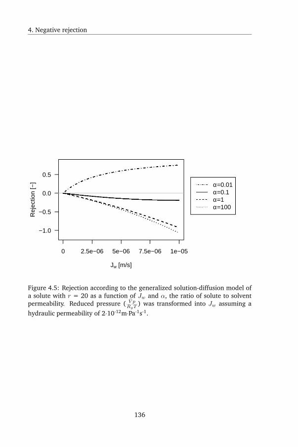
4. Negative rejection
−1.0
−0.5
0.0
0.5
0 2.5e−06 5e−06 7.5e−06 1e−05
Jw [m/s]
Rej
ectio
n [−
] α=0.01α=0.1α=1α=100
Figure 4.5: Rejection according to the generalized solution-diffusion model ofa solute with r = 20 as a function of Jw and α, the ratio of solute to solventpermeability. Reduced pressure ( V p
RgT) was transformed into Jw assuming a
hydraulic permeability of 2·10-12m·Pa-1s-1.
136
· ..
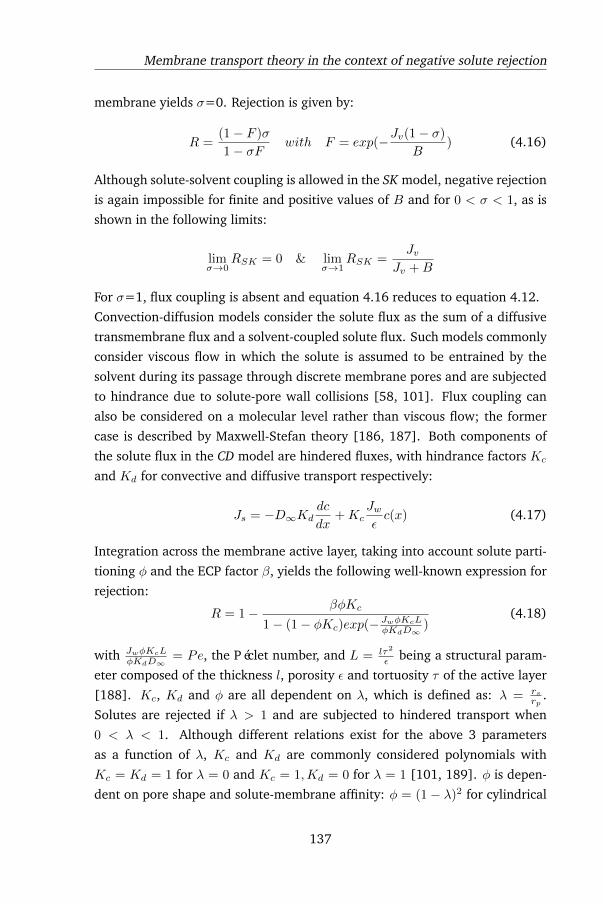
Membrane transport theory in the context of negative solute rejection
membrane yields σ=0. Rejection is given by:
R =(1− F )σ
1− σFwith F = exp(−Jv(1− σ)
B) (4.16)
Although solute-solvent coupling is allowed in the SK model, negative rejection
is again impossible for finite and positive values of B and for 0 < σ < 1, as is
shown in the following limits:
limσ→0
RSK = 0 & limσ→1
RSK =Jv
Jv +B
For σ=1, flux coupling is absent and equation 4.16 reduces to equation 4.12.
Convection-diffusion models consider the solute flux as the sum of a diffusive
transmembrane flux and a solvent-coupled solute flux. Such models commonly
consider viscous flow in which the solute is assumed to be entrained by the
solvent during its passage through discrete membrane pores and are subjected
to hindrance due to solute-pore wall collisions [58, 101]. Flux coupling can
also be considered on a molecular level rather than viscous flow; the former
case is described by Maxwell-Stefan theory [186, 187]. Both components of
the solute flux in the CD model are hindered fluxes, with hindrance factors Kc
and Kd for convective and diffusive transport respectively:
Js = −D∞Kddc
dx+Kc
Jwεc(x) (4.17)
Integration across the membrane active layer, taking into account solute parti-
tioning φ and the ECP factor β, yields the following well-known expression for
rejection:
R = 1− βφKc
1− (1− φKc)exp(−JwφKcLφKdD∞
)(4.18)
with JwφKcLφKdD∞
= Pe, the Péclet number, and L = lτ2
ε being a structural param-
eter composed of the thickness l, porosity ε and tortuosity τ of the active layer
[188]. Kc, Kd and φ are all dependent on λ, which is defined as: λ = rsrp
.
Solutes are rejected if λ > 1 and are subjected to hindered transport when
0 < λ < 1. Although different relations exist for the above 3 parameters
as a function of λ, Kc and Kd are commonly considered polynomials with
Kc = Kd = 1 for λ = 0 and Kc = 1,Kd = 0 for λ = 1 [101, 189]. φ is depen-
dent on pore shape and solute-membrane affinity: φ = (1− λ)2 for cylindrical
137
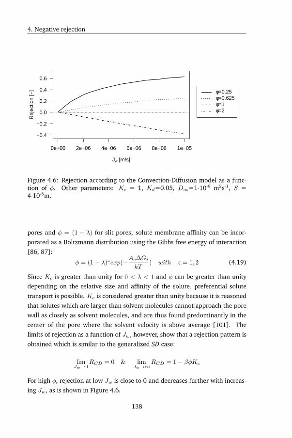
4. Negative rejection
0e+00 2e−06 4e−06 6e−06 8e−06 1e−05
−0.4
−0.2
0.0
0.2
0.4
0.6
Jw [m/s]
Rej
ectio
n [−
] φ=0.25φ=0.625φ=1φ=2
Figure 4.6: Rejection according to the Convection-Diffusion model as a func-tion of φ. Other parameters: Kc = 1, Kd=0.05, D∞=1·10-9 m2s-1, S =4·10-6m.
pores and φ = (1 − λ) for slit pores; solute membrane affinity can be incor-
porated as a Boltzmann distribution using the Gibbs free energy of interaction
[86, 87]:
φ = (1− λ)zexp(−Ac∆GikT
) with z = 1, 2 (4.19)
Since Kc is greater than unity for 0 < λ < 1 and φ can be greater than unity
depending on the relative size and affinity of the solute, preferential solute
transport is possible. Kc is considered greater than unity because it is reasoned
that solutes which are larger than solvent molecules cannot approach the pore
wall as closely as solvent molecules, and are thus found predominantly in the
center of the pore where the solvent velocity is above average [101]. The
limits of rejection as a function of Jw, however, show that a rejection pattern is
obtained which is similar to the generalized SD case:
limJw→0
RCD = 0 & limJw→∞
RCD = 1− βφKc
For high φ, rejection at low Jw is close to 0 and decreases further with increas-
ing Jw, as is shown in Figure 4.6.
138
Membrane transport theory in the context of negative solute rejection
4.4.2 Novel model development
In this study, the inability of existing transport models to explain negative re-
jection patterns as presented in section 4.3.1 is shown, which is addressed by
presenting 2 novel models. Both models assume solute adsorption of some
kind: in the first model, solute is ’absorbed’ in the draw solution in which
salting-in occurs: the solute activity is strongly depressed by the draw solute,
effectively trapping the solute in the draw solution. In the second model, solute
adsorption on the membrane followed by washing out into the draw solution
is assumed.
In equation 4.11, which is based on Fick’s law, ideal behavior of sufficiently
dilute feed solutes is assumed. If, however, this assumption would not be true,
for instance due to vastly different feed and draw solution composition, rejec-
tion could become negative. Returning to the assumption in the SD model that
flux is driven by continuous chemical potential gradients [74], the flux of a
solute s can be written as:
Js = −kscsdµsdx
(4.20)
with ks being a rate constant. During osmosis, under isobaric and isothermal
conditions, the chemical potential of s (being uncharged) is given by:
µs = µ0 +RTln(γscs) (4.21)
Total differentiation of µs with respect to x leads to:
dµsdx
= RT (1
γ
dγ
dx+
1
c
dc
dx) (4.22)
Which yields for Js, with equation 4.22 integrated between the feed and per-
meate side, assuming linear gradients for γ and c:
Js =ksRT
lcsln(
γfγp
) +ksRT
l(cf − cp) = Bcsln(
γfγp
) +B(cf − cp) (4.23)
This model will be referred to as SDγ. It can be seen that when an activity coef-
ficient gradient is absent (γf = γp), equation 4.23 reduces to the conventional
expression of Js (see equation 4.11). In equation 4.23, cs is an average solute
concentration, intermediate between cf and cp. Assuming cs = cf implies that
ks is the rate constant at the feed-membrane interface. Using this assumption,
139
4. Negative rejection
rejection can expressed analytically:
R =Jw −Bln(
γfγp
)
B + Jw(4.24)
Setting R = 0 in equation 4.24, it is easily verified that:
(JwB
)R=0 = lnγfγp
(4.25)
For γf = γp, this implies that Jw = 0, which is the result obtained in the clas-
sical SD model. If salting in occurs however, γf > γp is valid and the flux at
zero rejection becomes Jw,R=0 = Bln(γfγp
). The influence of the draw solute on
organic solute activity will be discussed in sections 4.5.2 and 4.7. When fitting
equations 4.23 or 4.24, the absolute values of γf and γp are not of importance;
only their ratio is. Consequently, γf was set to equal 1 during fitting, with the
resulting γp being relative to γf . This reduces the number of fitted parameters
to 2: B and γp.
In the second model, adsorption of feed solutes to the membrane followed by
washing out is considered, which implies coupling of the solvent and solute
fluxes as was described for the CD model. Consequently, the flux of feed so-
lutes is considered to consist of two sequential processes: initially, feed solutes
are adsorbed in the membrane causing enrichment relative to the feed at a
rate Jads. Subsequently, the solutes desorb and are entrained by the water flux
due to significant interactions between the solute and water, yielding the trans-
membrane solute flux Js. At steady-state, the rate of adsorption is matched by
the rate of desorption and entrainment: Jads = Js.
The rate of adsorption Jads, is given by:
Jads = Js = kacm(Σ0 − Σa) (4.26)
in which ka is a rate constant, Σ0 and Σa are the total and occupied concen-
tration of adsorption sites in the membrane respectively and cm is the solute
concentration at the feed solution - membrane interface. Rearranging equation
4.26 for Σa, the concentration of adsorbed solute, yields:
Σa =kacmΣ0 − Js
kacm(4.27)
140
Membrane transport theory in the context of negative solute rejection
Secondly, the adsorbed solute is considered to be susceptible to washing out:
this implies both that the solute interacts significantly with water, and that Jsis partially coupled to Jw. Js for the uncharged feed solutes is given by the CDmodel, see equation 4.17. The boundary conditions for equation 4.17 are: at
the feed side of the membrane, the solute concentration is given by Σa, at the
draw side, the solute concentration is given by cp. Integration and substitution
of Σa with equation 4.27 then yields:
Js =φKckaΣ0cmJw
kacm(1− (1− φKc)exp(−JwφKcLφKdD∞
)) + φKcJw(4.28)
The solute partition coefficient φ can be lumped with Kc and Kd, as φ only
appears as a product with the hindrance factors Kc and Kd [101], yielding the
compounded parameters K∗c and K∗d . Rejection is then given as:
R = 1− K∗c kaΣ0
kacm(1− (1−K∗c )exp(−JwK∗cL
K∗dD∞)) +K∗c Jw
(4.29)
This model will be referred to as CDL, as it combines Langmuir adsorption with
convection-diffusion-type coupled transport.
Examining the limits of equation 4.29 with respect to ka and S0 yields the
following results for ka:
limka→0
RCDL = 1 & limka→∞
RCDL = 1− K∗cΣ0
cm(1− (1−K∗c )exp(−JwK∗cL
K∗dD∞))
which show that for a very low adsorption rate, rejection equals 1, and that
for a very high adsorption rate, the rejection limit resembles equation 4.18. In
the latter case, the membrane is saturated with adsorbed solute and Js is dom-
inated by hindered transport through the membrane. The limits of equation
4.29 for Σ0 are:
limΣ0→0
RCDL = 1 & limΣ0→∞
RCDL = −∞
showing that Σ0, the total concentration of adsorption sites, is the driving force
for solute transport. At very high adsorption capacity, the driving force for
adsorption is high as well resulting in strong enrichment of the adsorbing solute
compared to the feed solution and very low rejection.
141
4. Negative rejection
Equations 4.28 and 4.29 have 5 parameters to be fitted to experimental data
(Kc,Kd,L,ka and Σ0). When hindered transport theory correlations for Kc and
Kd are used [101, 189], 4 variables remain: Kc and Kd are then replaced
by λ. In this study, no such correlations were used, as it has been shown
recently that such correlations were poor predictors of hindrance factors in
dense membranes [40, 67]. Independent measurements of adsorption capacity
and rate can provide estimates for ka and Σ0. If no adsorption measurements
are performed, the model can be simplified as follows: in equation 4.26, setting
Σ0 to unity lumps ka and Σ0 together as a single variable k∗a describing the
maximal adsorption rate. Likewise, in the Peclet number, L∗ can be defined
to include K∗d : L∗ = L/K∗d . The resulting simplifications yield a model with 3
parameters to be fitted, which was assessed in this study without independently
determined adsorption isotherms.
4.5 Novel model performance
4.5.1 Convergence
Both the SDγ and the CDL model werer fitted accurately to the negative rejec-
tion for formamide (r2:0.904 and 0.885 resp.), while the other models failed
to produce meaningful results, as is shown in Figure 4.7. The rejection of
formamide remained barely negative at the highest flux, which explains why
models incapable of predicting negative rejection failed. For the alcohol re-
jection tests, similarly accurate predictions were obtained: r2 was on average
0.991 (min. 0.981, max 0.997) for the CDL model, the results of which are
shown in Figure 4.8. The SDγ model yielded an average r2 of 0.985 (min.
0.973, max 0.989). Predictions obtained using both models showed negligible
differences for formamide as well as alcohol rejection, with the lower r2 for
formamide due to experimental error.
Although both new models yielded very similar results, they are mechanisti-
cally different: in the classical SD model, from which the SDγ model is de-
rived, Jw and Js are uncoupled, implying that Js would maintain the same
rate at the same concentration difference between feed and permeate side, re-
gardless of diminishing Jw. In contrast, the CDL model is based on coupled
fluxes. As a result, the CDL and SDγ model behave differently at very low
Jw: for the CDL model, limJw→0RCDL = 1 − S0
cm, while for the SDγ model,
142
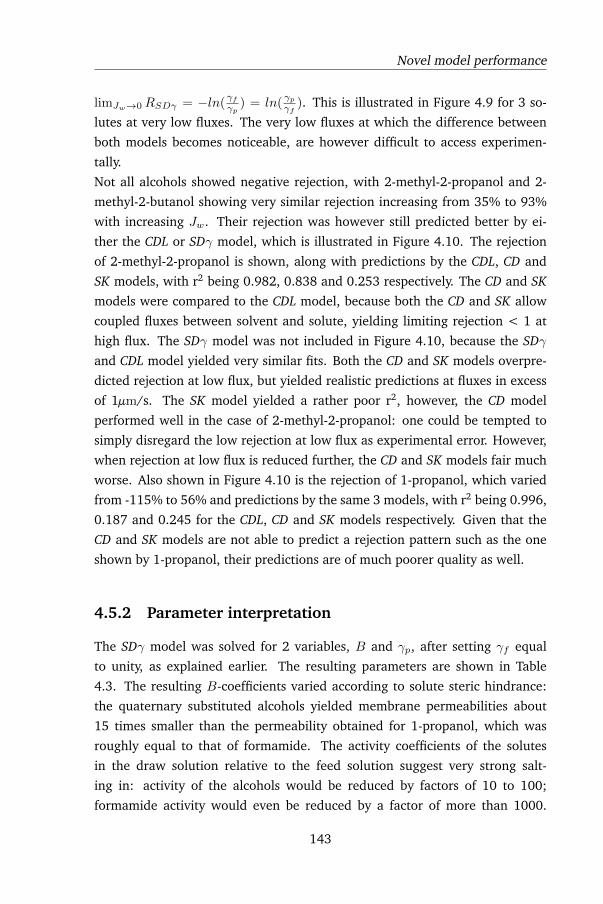
Novel model performance
limJw→0RSDγ = −ln(γfγp
) = ln(γpγf
). This is illustrated in Figure 4.9 for 3 so-
lutes at very low fluxes. The very low fluxes at which the difference between
both models becomes noticeable, are however difficult to access experimen-
tally.
Not all alcohols showed negative rejection, with 2-methyl-2-propanol and 2-
methyl-2-butanol showing very similar rejection increasing from 35% to 93%
with increasing Jw. Their rejection was however still predicted better by ei-
ther the CDL or SDγ model, which is illustrated in Figure 4.10. The rejection
of 2-methyl-2-propanol is shown, along with predictions by the CDL, CD and
SK models, with r2 being 0.982, 0.838 and 0.253 respectively. The CD and SKmodels were compared to the CDL model, because both the CD and SK allow
coupled fluxes between solvent and solute, yielding limiting rejection < 1 at
high flux. The SDγ model was not included in Figure 4.10, because the SDγand CDL model yielded very similar fits. Both the CD and SK models overpre-
dicted rejection at low flux, but yielded realistic predictions at fluxes in excess
of 1µm/s. The SK model yielded a rather poor r2, however, the CD model
performed well in the case of 2-methyl-2-propanol: one could be tempted to
simply disregard the low rejection at low flux as experimental error. However,
when rejection at low flux is reduced further, the CD and SK models fair much
worse. Also shown in Figure 4.10 is the rejection of 1-propanol, which varied
from -115% to 56% and predictions by the same 3 models, with r2 being 0.996,
0.187 and 0.245 for the CDL, CD and SK models respectively. Given that the
CD and SK models are not able to predict a rejection pattern such as the one
shown by 1-propanol, their predictions are of much poorer quality as well.
4.5.2 Parameter interpretation
The SDγ model was solved for 2 variables, B and γp, after setting γf equal
to unity, as explained earlier. The resulting parameters are shown in Table
4.3. The resulting B-coefficients varied according to solute steric hindrance:
the quaternary substituted alcohols yielded membrane permeabilities about
15 times smaller than the permeability obtained for 1-propanol, which was
roughly equal to that of formamide. The activity coefficients of the solutes
in the draw solution relative to the feed solution suggest very strong salt-
ing in: activity of the alcohols would be reduced by factors of 10 to 100;
formamide activity would even be reduced by a factor of more than 1000.
143
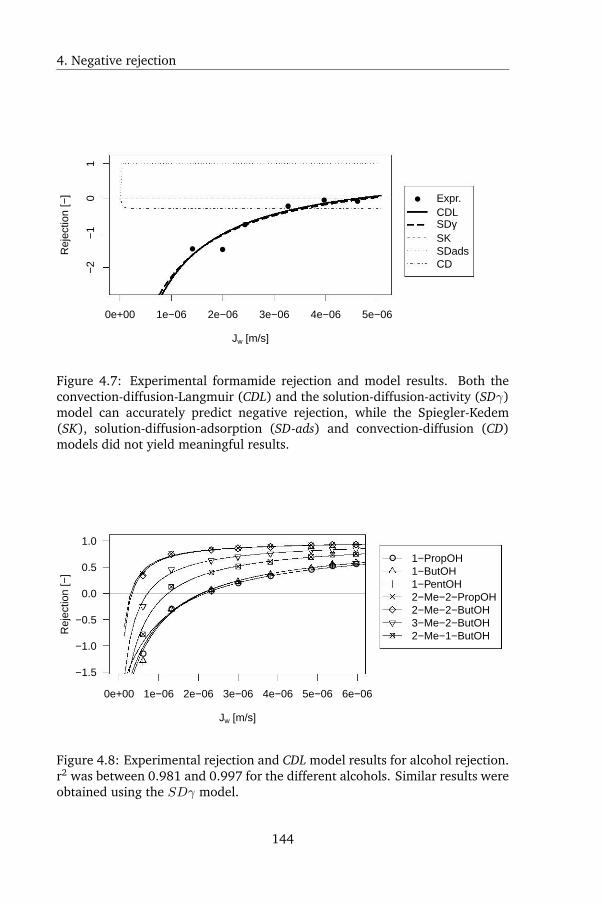
4. Negative rejection
0e+00 1e−06 2e−06 3e−06 4e−06 5e−06
−2
−1
01
Jw [m/s]
Rej
ectio
n [−
]
● ●
●
●● ● ● Expr.
CDLSDγSKSDadsCD
Figure 4.7: Experimental formamide rejection and model results. Both theconvection-diffusion-Langmuir (CDL) and the solution-diffusion-activity (SDγ)model can accurately predict negative rejection, while the Spiegler-Kedem(SK), solution-diffusion-adsorption (SD-ads) and convection-diffusion (CD)models did not yield meaningful results.
●
●
●●
●●
● ●
0e+00 1e−06 2e−06 3e−06 4e−06 5e−06 6e−06
−1.5
−1.0
−0.5
0.0
0.5
1.0
Jw [m/s]
Rej
ectio
n [−
]
● 1−PropOH1−ButOH1−PentOH2−Me−2−PropOH2−Me−2−ButOH3−Me−2−ButOH2−Me−1−ButOH
Figure 4.8: Experimental rejection and CDL model results for alcohol rejection.r2 was between 0.981 and 0.997 for the different alcohols. Similar results wereobtained using the SDγ model.
144
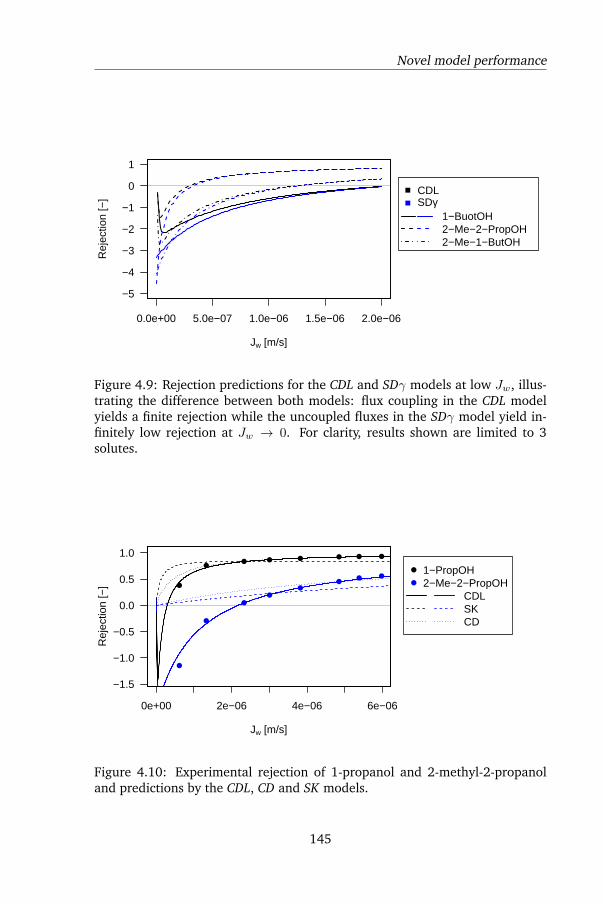
Novel model performance
0.0e+00 5.0e−07 1.0e−06 1.5e−06 2.0e−06
−5
−4
−3
−2
−1
0
1
Jw [m/s]
Rej
ectio
n [−
]
CDLSDγ
1−BuotOH2−Me−2−PropOH2−Me−1−ButOH
Figure 4.9: Rejection predictions for the CDL and SDγ models at low Jw, illus-trating the difference between both models: flux coupling in the CDL modelyields a finite rejection while the uncoupled fluxes in the SDγ model yield in-finitely low rejection at Jw → 0. For clarity, results shown are limited to 3solutes.
●
●
●●
●●
● ●
●
●● ● ● ● ● ●
0e+00 2e−06 4e−06 6e−06
−1.5
−1.0
−0.5
0.0
0.5
1.0
Jw [m/s]
Rej
ectio
n [−
]
●
●
1−PropOH2−Me−2−PropOH
CDLSKCD
Figure 4.10: Experimental rejection of 1-propanol and 2-methyl-2-propanoland predictions by the CDL, CD and SK models.
145
4. Negative rejection
These values are clearly unrealistic: reported changes of activity of polar non-
electrolytes as a function of electrolyte concentration lie in the region of 0.1 - 10
[190]. Furthermore, differences are not only quantitative but also qualitative:
NaCl has the tendency to increase rather than decrease non-electrolyte activity
[190, 191, 192]. This was also seen in the NaCl dilution series which was used
to correct for alcohol volatility during headspace-GC-MS analysis as well: the
detector response increased with increasing NaCl concentration, showing qual-
itatively that alcohol activity was increased (see figure 4.1). Increased Henry
coefficients have been used to quantify salting out and calculate Setchenov con-
stants [193] (see next section). In the case of formamide, which is highly polar
and can dissolve significant amounts of NaCl (in contrast to the alcohols used
in this study), it is conceivable that its activity would be decreased by NaCl, but
a factor of 1000 is unrealistic. Thus, although the SDγ model yielded a very
good fit to the experimental rejection, the underlying assumption that solute
activity was reduced in the draw solution is contradicted by GC-MS data.
The CDL model was solved for 3 lumped, tunable variables: K∗c , k∗a and L∗.
In the CDL model, the 3 fitted variables are compounds, as was mentioned
in section 4.4.2: K∗c is the product of Kc and φ, k∗a is the product of ka and
Σ0, yielding a single parameter describing the maximum adsorption rate, and
L∗ = LK∗d = lτ2
φKdε, with l, τ and ε being the thickness, tortuosity and poros-
ity of the membrane active layer respectively. Assuming for the alcohols that
Kc ≈ 1, K∗c = φ, showing that the alcohols are enriched in the membrane
phase by a factor of 4 to 5 compared to the feed solution. The same assumption
for formamide yields a substantially higher enrichment of 185, which is also ap-
parent from the much lower rejection of formamide compared to the alcohols:
formamide rejection was still negative at Jw = 4.6 µm/s, while for the alco-
hols showing the lowest rejection, rejection became positive at Jw ≈ 2 µm/s.
The maximal adsorption rate, k∗a, showed high variability: unsurprisingly, the
adsorption rate of alcohols decreased as steric hindrance increased: k∗a was
3.26·10-6 for 1-propanol, the smallest alcohol and having a linear alkyl chain,
while k∗a was 0.41 and 0.42·10-6 for the most hindered alcohols, 2-methyl-2-
propanol and 2-methyl-2-butanol respectively. At R = 0, equation 4.29 can be
rearranged to give:
(k∗a)R=0 =K∗c Jw
K∗c − cm(1−K∗c )exp(−JwK∗cL
D∞)
(4.30)
146
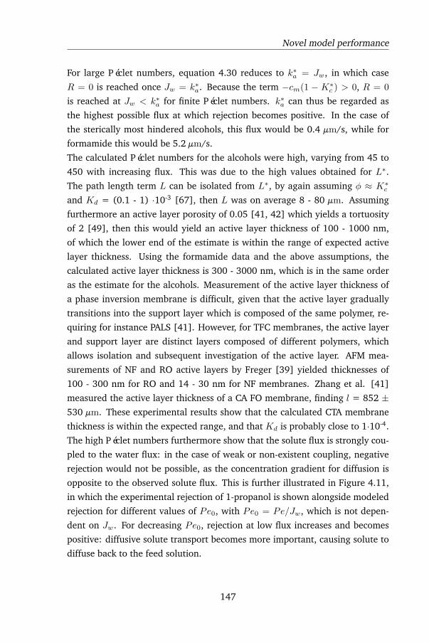
Novel model performance
For large Péclet numbers, equation 4.30 reduces to k∗a = Jw, in which case
R = 0 is reached once Jw = k∗a. Because the term −cm(1 − K∗c ) > 0, R = 0
is reached at Jw < k∗a for finite Péclet numbers. k∗a can thus be regarded as
the highest possible flux at which rejection becomes positive. In the case of
the sterically most hindered alcohols, this flux would be 0.4 µm/s, while for
formamide this would be 5.2 µm/s.
The calculated Péclet numbers for the alcohols were high, varying from 45 to
450 with increasing flux. This was due to the high values obtained for L∗.
The path length term L can be isolated from L∗, by again assuming φ ≈ K∗c
and Kd = (0.1 - 1) ·10-3 [67], then L was on average 8 - 80 µm. Assuming
furthermore an active layer porosity of 0.05 [41, 42] which yields a tortuosity
of 2 [49], then this would yield an active layer thickness of 100 - 1000 nm,
of which the lower end of the estimate is within the range of expected active
layer thickness. Using the formamide data and the above assumptions, the
calculated active layer thickness is 300 - 3000 nm, which is in the same order
as the estimate for the alcohols. Measurement of the active layer thickness of
a phase inversion membrane is difficult, given that the active layer gradually
transitions into the support layer which is composed of the same polymer, re-
quiring for instance PALS [41]. However, for TFC membranes, the active layer
and support layer are distinct layers composed of different polymers, which
allows isolation and subsequent investigation of the active layer. AFM mea-
surements of NF and RO active layers by Freger [39] yielded thicknesses of
100 - 300 nm for RO and 14 - 30 nm for NF membranes. Zhang et al. [41]
measured the active layer thickness of a CA FO membrane, finding l = 852 ±530 µm. These experimental results show that the calculated CTA membrane
thickness is within the expected range, and that Kd is probably close to 1·10-4.
The high Péclet numbers furthermore show that the solute flux is strongly cou-
pled to the water flux: in the case of weak or non-existent coupling, negative
rejection would not be possible, as the concentration gradient for diffusion is
opposite to the observed solute flux. This is further illustrated in Figure 4.11,
in which the experimental rejection of 1-propanol is shown alongside modeled
rejection for different values of Pe0, with Pe0 = Pe/Jw, which is not depen-
dent on Jw. For decreasing Pe0, rejection at low flux increases and becomes
positive: diffusive solute transport becomes more important, causing solute to
diffuse back to the feed solution.
147
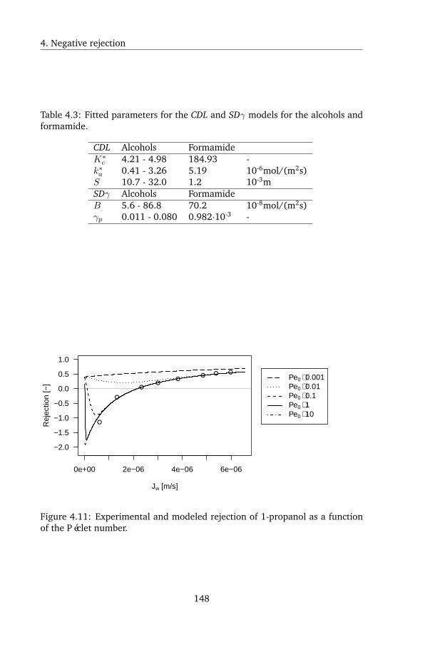
4. Negative rejection
Table 4.3: Fitted parameters for the CDL and SDγ models for the alcohols andformamide.
CDL Alcohols FormamideK∗c 4.21 - 4.98 184.93 -k∗a 0.41 - 3.26 5.19 10-6mol/(m2s)S 10.7 - 32.0 1.2 10-3mSDγ Alcohols FormamideB 5.6 - 86.8 70.2 10-8mol/(m2s)γp 0.011 - 0.080 0.982·10-3 -
0e+00 2e−06 4e−06 6e−06
−2.0
−1.5
−1.0
−0.5
0.0
0.5
1.0
Jw [m/s]
Rej
ectio
n [−
]
●
●
●●
●● ● ●
Pe0 ⋅ 0.001Pe0 ⋅ 0.01Pe0 ⋅ 0.1Pe0 ⋅ 1Pe0 ⋅ 10
Figure 4.11: Experimental and modeled rejection of 1-propanol as a functionof the Péclet number.
148
Coupled fluxes
4.6 Coupled fluxes
In the CDL model, coupled fluxes of water and the solutes are assumed. In
fact, disregarding excessively strong salting in, negative rejection would not
be possible without flux coupling. Flux coupling can be experimentally shown
by plotting Js as a function of Jw. In the case of uncoupled fluxes, which are
assumed in the classical solution-diffusion model, no correlation between Js
and Jw would exist, while otherwise a positive correlation would be seen. In
order to compare both water and solute fluxes in terms of velocity, the solute
fluxes were converted to velocity as follows:
vs =Jsv
xf(4.31)
In equation 4.31, v and xf are the solute’s molar volume and feed molar frac-
tion respectively, yielding solute velocity in units of m/s, similar to Jw. The
results for the alcohols during both FO (left panel) and RO (right panel) are
shown in figure 4.12. The solute velocity is considerably higher than the water
flux, which can be explained by the difference in molar volumes between wa-
ter and the alcohols, the latters’ molar volume is roughly 5 times larger than
the molar volume of water. It can be clearly seen that solute velocity increases
with increasing water flux, both during FO and RO. Coupling is clearly stronger
for the less sterically hindered alcohols as well. At low fluxes, solute velocity
is higher in FO, as was to be expected given the negative rejection. At high
fluxes, solute velocity in FO appears to reach a plateau and slightly declines.
This could be due to hindrance between the increasing RSD and alcohol fluxes,
or due to osmotic dehydration of the membrane (see Figure 2.12) which causes
increased steric hindrance between the membrane and permeating solutes. In
RO on the other hand, hardly any decline can be seen: solute fluxes increase
linearly with water flux. A clear structure - transport mode relation can be
seen as well: the more an alcohol is subject to steric hindrance, the weaker the
correlation between water and solute flux.
4.7 FO versus RO: salting out
FO and RO rejection of the alcohols was very different, despite using the same
membrane and same solutes, and rejection tests were performed at the same
149
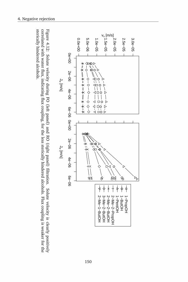
4. Negative rejection
0e+00
2e−06
4e−06
6e−06
0.0e+00
5.0e−06
1.0e−05
1.5e−05
2.0e−05
2.5e−05
3.0e−05
Jw [m
/s]
vs [m/s]
●
●
●●
●●
●●
0e+00
2e−06
4e−06
6e−06
Jw [m
/s]
●
●
●
●
●●
●
1−P
ropOH
1−B
utOH
1−P
entOH
2−M
e−2−
PropO
H2−
Me−
2−B
utOH
3−M
e−2−
ButO
H2−
Me−
1−B
utOH
Figure4.12:
Solutevelocity
duringFO
(leftpanel)
andR
O(right
panel)filtration.
Solutevelocity
isclearly
positivelycorrelated
with
water
flux,indicatingflux
coupling,forthe
lesssterically
hinderedalcohols.
Fluxcoupling
isw
eakerfor
thesterically
hinderedalcohols.
150
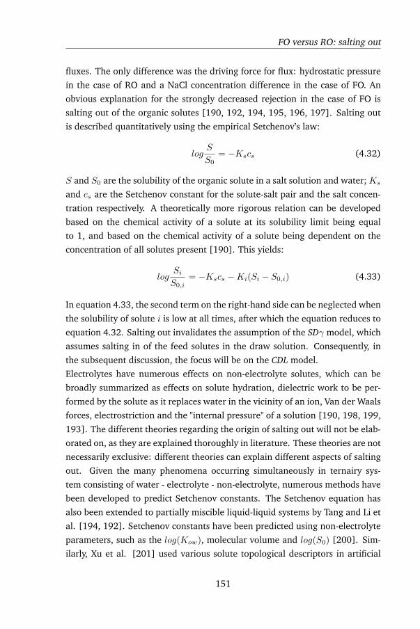
FO versus RO: salting out
fluxes. The only difference was the driving force for flux: hydrostatic pressure
in the case of RO and a NaCl concentration difference in the case of FO. An
obvious explanation for the strongly decreased rejection in the case of FO is
salting out of the organic solutes [190, 192, 194, 195, 196, 197]. Salting out
is described quantitatively using the empirical Setchenov’s law:
logS
S0= −Kscs (4.32)
S and S0 are the solubility of the organic solute in a salt solution and water; Ks
and cs are the Setchenov constant for the solute-salt pair and the salt concen-
tration respectively. A theoretically more rigorous relation can be developed
based on the chemical activity of a solute at its solubility limit being equal
to 1, and based on the chemical activity of a solute being dependent on the
concentration of all solutes present [190]. This yields:
logSiS0,i
= −Kscs −Ki(Si − S0,i) (4.33)
In equation 4.33, the second term on the right-hand side can be neglected when
the solubility of solute i is low at all times, after which the equation reduces to
equation 4.32. Salting out invalidates the assumption of the SDγ model, which
assumes salting in of the feed solutes in the draw solution. Consequently, in
the subsequent discussion, the focus will be on the CDL model.
Electrolytes have numerous effects on non-electrolyte solutes, which can be
broadly summarized as effects on solute hydration, dielectric work to be per-
formed by the solute as it replaces water in the vicinity of an ion, Van der Waals
forces, electrostriction and the "internal pressure" of a solution [190, 198, 199,
193]. The different theories regarding the origin of salting out will not be elab-
orated on, as they are explained thoroughly in literature. These theories are not
necessarily exclusive: different theories can explain different aspects of salting
out. Given the many phenomena occurring simultaneously in ternairy sys-
tem consisting of water - electrolyte - non-electrolyte, numerous methods have
been developed to predict Setchenov constants. The Setchenov equation has
also been extended to partially miscible liquid-liquid systems by Tang and Li et
al. [194, 192]. Setchenov constants have been predicted using non-electrolyte
parameters, such as the log(Kow), molecular volume and log(S0) [200]. Sim-
ilarly, Xu et al. [201] used various solute topological descriptors in artificial
151
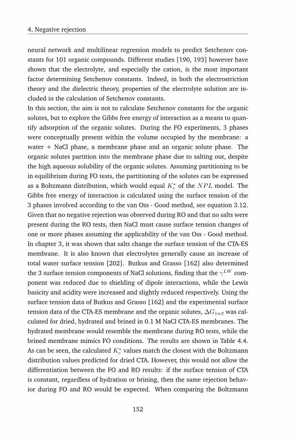
4. Negative rejection
neural network and multilinear regression models to predict Setchenov con-
stants for 101 organic compounds. Different studies [190, 193] however have
shown that the electrolyte, and especially the cation, is the most important
factor determining Setchenov constants. Indeed, in both the electrostriction
theory and the dielectric theory, properties of the electrolyte solution are in-
cluded in the calculation of Setchenov constants.
In this section, the aim is not to calculate Setchenov constants for the organic
solutes, but to explore the Gibbs free energy of interaction as a means to quan-
tify adsorption of the organic solutes. During the FO experiments, 3 phases
were conceptually present within the volume occupied by the membrane: a
water + NaCl phase, a membrane phase and an organic solute phase. The
organic solutes partition into the membrane phase due to salting out, despite
the high aqueous solubility of the organic solutes. Assuming partitioning to be
in equilibrium during FO tests, the partitioning of the solutes can be expressed
as a Boltzmann distribution, which would equal K∗c of the NPL model. The
Gibbs free energy of interaction is calculated using the surface tension of the
3 phases involved according to the van Oss - Good method, see equation 3.12.
Given that no negative rejection was observed during RO and that no salts were
present during the RO tests, then NaCl must cause surface tension changes of
one or more phases assuming the applicability of the van Oss - Good method.
In chapter 3, it was shown that salts change the surface tension of the CTA-ES
membrane. It is also known that electrolytes generally cause an increase of
total water surface tension [202]. Butkus and Grasso [162] also determined
the 3 surface tension components of NaCl solutions, finding that the γLW com-
ponent was reduced due to shielding of dipole interactions, while the Lewis
basicity and acidity were increased and slightly reduced respectively. Using the
surface tension data of Butkus and Grasso [162] and the experimental surface
tension data of the CTA-ES membrane and the organic solutes, ∆G1w2 was cal-
culated for dried, hydrated and brined in 0.1 M NaCl CTA-ES membranes. The
hydrated membrane would resemble the membrane during RO tests, while the
brined membrane mimics FO conditions. The results are shown in Table 4.4.
As can be seen, the calculated K∗c values match the closest with the Boltzmann
distribution values predicted for dried CTA. However, this would not allow the
differentiation between the FO and RO results: if the surface tension of CTA
is constant, regardless of hydration or brining, then the same rejection behav-
ior during FO and RO would be expected. When comparing the Boltzmann
152
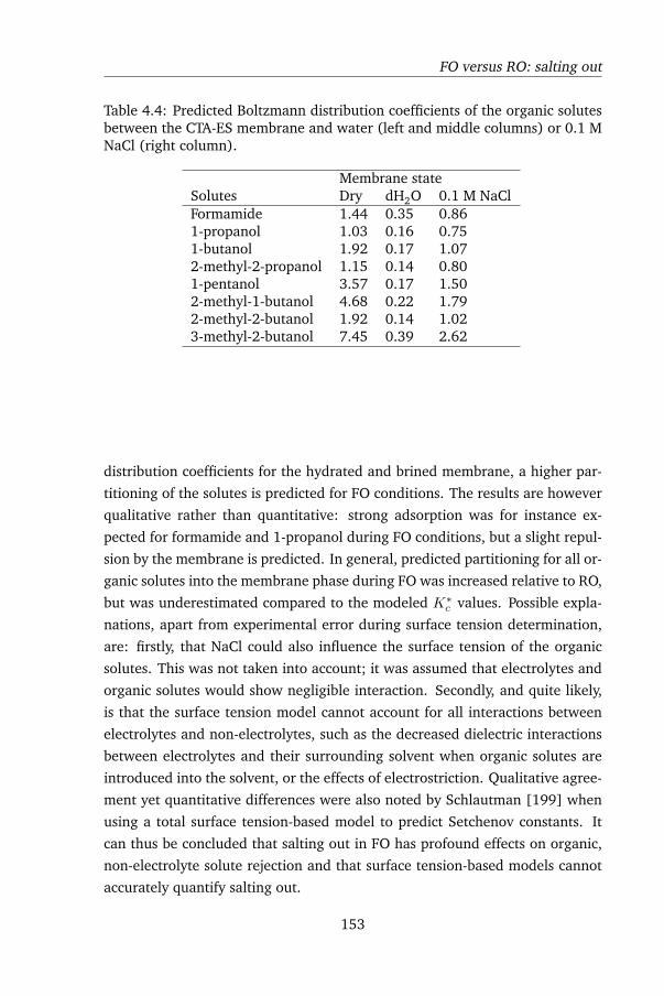
FO versus RO: salting out
Table 4.4: Predicted Boltzmann distribution coefficients of the organic solutesbetween the CTA-ES membrane and water (left and middle columns) or 0.1 MNaCl (right column).
Membrane stateSolutes Dry dH2O 0.1 M NaClFormamide 1.44 0.35 0.861-propanol 1.03 0.16 0.751-butanol 1.92 0.17 1.072-methyl-2-propanol 1.15 0.14 0.801-pentanol 3.57 0.17 1.502-methyl-1-butanol 4.68 0.22 1.792-methyl-2-butanol 1.92 0.14 1.023-methyl-2-butanol 7.45 0.39 2.62
distribution coefficients for the hydrated and brined membrane, a higher par-
titioning of the solutes is predicted for FO conditions. The results are however
qualitative rather than quantitative: strong adsorption was for instance ex-
pected for formamide and 1-propanol during FO conditions, but a slight repul-
sion by the membrane is predicted. In general, predicted partitioning for all or-
ganic solutes into the membrane phase during FO was increased relative to RO,
but was underestimated compared to the modeled K∗c values. Possible expla-
nations, apart from experimental error during surface tension determination,
are: firstly, that NaCl could also influence the surface tension of the organic
solutes. This was not taken into account; it was assumed that electrolytes and
organic solutes would show negligible interaction. Secondly, and quite likely,
is that the surface tension model cannot account for all interactions between
electrolytes and non-electrolytes, such as the decreased dielectric interactions
between electrolytes and their surrounding solvent when organic solutes are
introduced into the solvent, or the effects of electrostriction. Qualitative agree-
ment yet quantitative differences were also noted by Schlautman [199] when
using a total surface tension-based model to predict Setchenov constants. It
can thus be concluded that salting out in FO has profound effects on organic,
non-electrolyte solute rejection and that surface tension-based models cannot
accurately quantify salting out.
153
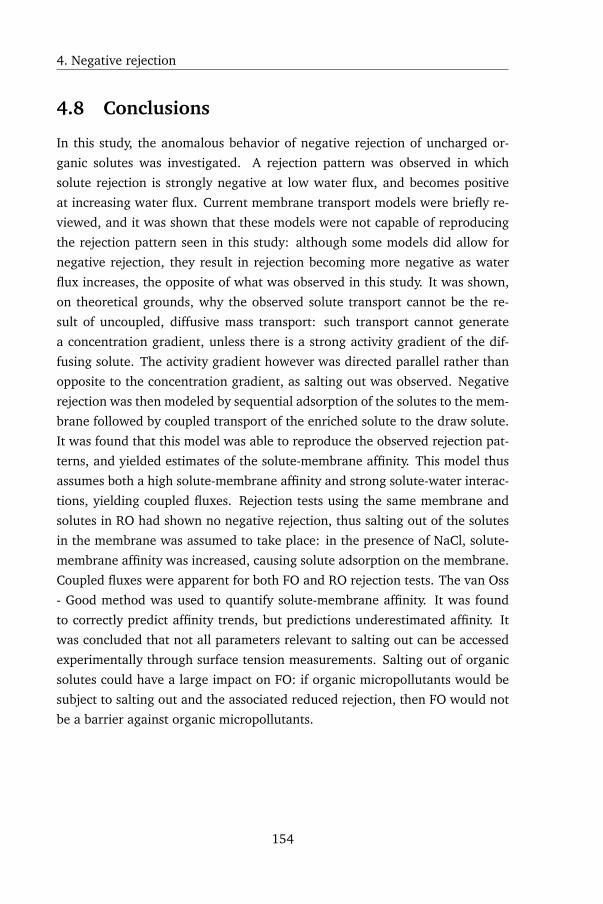
4. Negative rejection
4.8 Conclusions
In this study, the anomalous behavior of negative rejection of uncharged or-
ganic solutes was investigated. A rejection pattern was observed in which
solute rejection is strongly negative at low water flux, and becomes positive
at increasing water flux. Current membrane transport models were briefly re-
viewed, and it was shown that these models were not capable of reproducing
the rejection pattern seen in this study: although some models did allow for
negative rejection, they result in rejection becoming more negative as water
flux increases, the opposite of what was observed in this study. It was shown,
on theoretical grounds, why the observed solute transport cannot be the re-
sult of uncoupled, diffusive mass transport: such transport cannot generate
a concentration gradient, unless there is a strong activity gradient of the dif-
fusing solute. The activity gradient however was directed parallel rather than
opposite to the concentration gradient, as salting out was observed. Negative
rejection was then modeled by sequential adsorption of the solutes to the mem-
brane followed by coupled transport of the enriched solute to the draw solute.
It was found that this model was able to reproduce the observed rejection pat-
terns, and yielded estimates of the solute-membrane affinity. This model thus
assumes both a high solute-membrane affinity and strong solute-water interac-
tions, yielding coupled fluxes. Rejection tests using the same membrane and
solutes in RO had shown no negative rejection, thus salting out of the solutes
in the membrane was assumed to take place: in the presence of NaCl, solute-
membrane affinity was increased, causing solute adsorption on the membrane.
Coupled fluxes were apparent for both FO and RO rejection tests. The van Oss
- Good method was used to quantify solute-membrane affinity. It was found
to correctly predict affinity trends, but predictions underestimated affinity. It
was concluded that not all parameters relevant to salting out can be accessed
experimentally through surface tension measurements. Salting out of organic
solutes could have a large impact on FO: if organic micropollutants would be
subject to salting out and the associated reduced rejection, then FO would not
be a barrier against organic micropollutants.
154
Chapter 5
Organic Micropollutants in closed-loopFO: influence of biofouling and OMPbuild-up
Adapted from:
Arnout D’Haese, Pierre Le-Clech, Sam Van Nevel, Kim Verbeken, Stuart Khan,
Arne Verliefde, Trace organic solutes in closed-loop forward osmosis applica-
tions: Influence of membrane fouling and modeling of solute build-up, WaterResearch 47 (2013), 14, 5232-5244
155
5. Long-term biofouling
5.1 Introduction
In this chapter, long-term biofouling of an FO membrane is studied, and its
effects on OMP rejection. This study was also the first study to consider the
fate of OMPs in a closed-loop FO-RO system. In this study, the FO system was
inoculated with activated sludge and fed water spiked with nutrients in order
to stimulate spontaneous biofilm growth. The spiked water simulated impaired
surface water or treated wastewater.
Impaired water sources, such as waste water treatment plant (WWTP) efflu-
ents, are commonly contaminated with organic micropollutants (OMPs) [203,
204]. Conventional waste water treatment systems, such as coagulation, trick-
ling filters, sand filters and activated sludge remove OMPs to varying degree,
but often unsatisfactory when waste water is to be reclaimed. Svenson et al.
[205] found an increased removal rate of estrogenic compounds in treatment
media with an increased bioactivity. Ternes [206] found a OMPs removal rate
varying between 10 and almost 100% for pharmaceuticals in German WWTPs,
which is the same conclusion reached by Van De Steene et al. [207] who also
found removal rates varying from 0 to almost 100%.
For the practical implementation of FO, maintaining a high rejection of OMPs
under different operating conditions is a key challenge, especially if FO is used
to produce reclaimed water from WWTP in- or effluent. Alturki et al. [208]
noted that rejection of OMPs by FO in an osmotic MBR (OMBR), of which the
sludge was conditioned to the tested OMPs, was consistently high for the so-
lutes with a molecular weight above 266 g/mole, while the rejection of smaller
solutes appeared to relate to their biodegradation susceptibility. This could
indicate that the actual rejection rates of the smaller solutes were quite low.
Hancock et al. [82] have tested OMP-rejection in both bench- and pilot-scale
installations, using MBR-treated domestic waste water as a feed. The rejec-
tion of hydrophobic nonionic compounds by FO appeared to improve with in-
creasing TSS concentration in the feed, which could indicate sorption of these
compounds onto the TSS and subsequent filtration of the TSS. The rejection of
mainly negatively charged organic solutes was consistently high, regardless of
the TSS concentration.
Although previous studies have investigated OMP rejection by FO membranes,
there is still relatively limited knowledge on the actual transport mechanisms
of these solutes in FO, which contrasts the transport of OMPs in pressure-driven
156
Modeling of OMPs build-up in closed loop applications
processes such as NF and RO [58, 146, 209, 86, 210]. In addition, although
the influence of fouling by several water matrices on rejection of OMPs has
been investigated in practice, most studies have not tried to identify underly-
ing mechanisms of influence of fouling on rejection.
When FO is used to reclaim water from impaired sources, the effect of draw
solution regeneration in a closed-loop system on the OMPs concentration in
the final product water has not been investigated yet. Hancock et al. reported
a build-up of OMPs in the draw solution [82] when using RO to regenerate
the FO draw solution (consisting of NaCl) in a closed-loop configuration. Cath
et al. [211] made a similar observation in a closed loop FO-RO configuration.
Although both groups reported a total rejection of OMPs by the combined FO-
RO system in the order of 99%, the statement of FO-RO being a double barrier
against micropollutants has not been thoroughly assessed in closed-loop sys-
tems. Both groups reported that the build-up of OMPs in the draw solution
was caused by a higher rejection of OMPs by RO than by FO [211, 82]; Han-
cock et al., 2011). A OMPs build up in the draw solution might negatively
impact the OMPs concentration in the final permeate. It is therefore impera-
tive to investigate the fate of OMPs when FO is used in a closed loop system.
In this study, different model foulants were used to foul FO membranes and
effects on FO rejection of 20 pharmaceuticals was studied. In addition, long-
term biofouling experiments were carried out, in which the biofouled mem-
brane was extensively characterized and again the effect on the FO rejection of
pharmaceuticals was investigated. The build-up of OMPs in the draw solution
is systematically studied and modeled in closed-loop FO-RO/NF applications,
and the potential implications for potable water production are discussed.
5.2 Modeling of OMPs build-up in closed loop ap-
plications
To investigate the effect of this build-up on the final OMP concentration in
the produced potable water, the concentration of trace organics in the draw
solution of the FO and in the RO permeate were modeled as a function of cycle
time. Solute transport through a dense membrane can occur due to diffusion,
convection, or a combination of both, as will be clearly shown in the results
below. For all transport mechanisms, the FO permeate solute concentration is
157
5. Long-term biofouling
defined as: cp =< Js > / < Jw > with < Js > and < Jw > being the average
solute and water flux respectively. For diffusive transport, the solute flux is
given by Fick’s law of diffusion:
Js = −Dm,sdc
dx(5.1)
with−Dm,s the solute diffusion coefficient in the membrane phase. Integration
across the membrane and rearranging leads to the following equation for the
solute concentration in the FO permeate, cp:
cp =B[cf − cs(1− y)]
Jw +By(5.2)
in which B = Dm,sε/∆x is the solute mass transfer coefficient, cf and cs the
initial solute concentration present in the feed and in the draw solution prior
to dilution by FO respectively, and y the fraction of draw solution originating
from permeate. In the case of convective transport, the solute concentration in
the permeate is given by:
cp = Kc,scf (5.3)
When both convection and diffusion contribute to solute transport, the FO per-
meate solute concentration is given by:
cp =Js,Diff + Js,Conv
Jw=B[cf − cs(1− y)]
Jw +By+Kc,scf (5.4)
In this model, the RO rejection rate was assumed to be constant, regardless of
the solute concentration in the draw solution. The solute concentration in the
RO permeate is then given by:
cp,RO = (1−RRO)cd (5.5)
with cp,RO and cd the solute RO permeate and draw solution concentration
respectively, and RRO the solute RO rejection rate. The solute concentration in
the RO concentrate is given by:
cconc =RROcd1− y
(5.6)
158
Materials and Methods
The solute concentration in the RO concentrate, cconc, of cycle t is then substi-
tuted in equation 5.2 or 5.4 as cs of cycle t + 1. The model was solved both
recursively and as a steady-state in R 3.3.0 [117].
5.3 Materials and Methods
5.3.1 FO setup
The FO membranes used in this study, were CTA-ES membranes produced by
HTI (Albany, Oregon, USA). Membrane properties are given in chapter 2. The
membrane orientation in this study was in AL-FS mode. The membrane cell
was a transparent polycarbonate cell, with the flow channel having the fol-
lowing dimensions: length 250 mm, width 50 mm, height 1 mm and a mem-
brane surface area of 124 cm2 . The membrane cell was oriented horizontally,
with the feed channel on top. Feed and draw solution were delivered to the
membrane module in counter-current mode, both at a cross-flow velocity of
0.20 m/s, by peristaltic pumps (Cole-Parmer Metrohm, Belgium). The volume
and salt concentration of the draw solution were controlled using a Biostat
B (Sartorius, Germany) which pumped out excess draw solution and dosed
a concentrated salt solution to restore the draw solution’s salt concentration.
Salt leakage was checked by measuring the conductivity of the feed solution.
The Biostat algorithms were controlled using a conductivity probe by Consort
(Turnhout, Belgium), measuring the conductivity of the draw solution. The wa-
ter flux was measured by logging the weight of the excess draw solution using
an OHaus 5000 Xtreme scale which was logged using a LabVIEW script. The
flux was corrected for the dosed salt solution and the draw solution density. A
scheme of the FO setup is given in Fig. 5.1.
5.3.2 Streaming Potential measurements
The streaming potential of the FO membrane was determined using a PMMA
clamping cell, which has a flow channel of 76.2 mm by 25.4 mm, the dimen-
sions of a microscopy glass slide. For each test, 2 membrane samples were fixed
to microscopy glass slides with the same membrane side facing the test liquid.
They were inserted in the cell with a polypropylene membrane spacer sand-
wiched in between them, to ensure liquid flow past the membrane surface. The
159
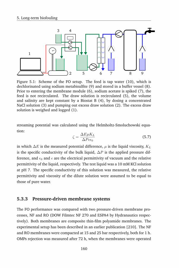
5. Long-term biofouling
1
2
3 4
5 6 7 8 9
Figure 5.1: Scheme of the FO setup. The feed is tap water (10), which isdechlorinated using sodium metabisulfite (9) and stored in a buffer vessel (8).Prior to entering the membrane module (6), sodium acetate is spiked (7), thefeed is not recirculated. The draw solution is recirculated (5), the volumeand salinity are kept constant by a Biostat B (4), by dosing a concentratedNaCl solution (3) and pumping out excess draw solution (2). The excess drawsolution is weighed and logged (1).
streaming potential was calculated using the Helmholtz-Smoluchowski equa-
tion:
ζ =∆EµKL
∆Pεε0(5.7)
in which ∆E is the measured potential difference, µ is the liquid viscosity, KL
is the specific conductivity of the bulk liquid, ∆P is the applied pressure dif-
ference, and ε0 and ε are the electrical permittivity of vacuum and the relative
permittivity of the liquid, respectively. The test liquid was a 10 mM KCl solution
at pH 7. The specific conductivity of this solution was measured, the relative
permittivity and viscosity of the dilute solution were assumed to be equal to
those of pure water.
5.3.3 Pressure-driven membrane systems
The FO performance was compared with two pressure-driven membrane pro-
cesses, NF and RO (DOW Filmtec NF 270 and ESPA4 by Hydranautics respec-
tively). Both membranes are composite thin-film polyamide membranes. The
experimental setup has been described in an earlier publication [210]. The NF
and RO membranes were compacted at 15 and 25 bar respectively, both for 1 h.
OMPs rejection was measured after 72 h, when the membranes were operated
160
Materials and Methods
at a flux of 5.55 µm/s (=20 L/(m2h)). Rejection was calculated as follows:
R = 1− cpcf
(5.8)
with cp and cf being the permeate and feed concentration respectively.
5.3.4 Fouling protocol
Model foulants
Sodium alginate and Bovine Serum Albumine (BSA) were used as model foulants
in this study. FO membrane fouling was induced by filtration of a solution con-
taining 200 mg/L of either sodium alginate or BSA. The draw solution was a
3 M NaCl solution, the duration of the fouling run was 10 h. The flux was on
average 2.58 µm/s for the clean membrane test, and for the BSA and alginate
fouling tests 2.44 and 2.36 µm/s respectively.
Long-term biofouling and analysis
Biofouling was induced by incubating the feed spacer for 24 h in a solution of
10 mL settled activated sludge in 800 mL of water. The sludge was acquired
from the municipal waste water treatment plant Ossemeersen, Ghent. After
incubation, the spacer was gently rinsed to remove any particulate matter. The
feed during the biofouling experiments was tap water, which was dechlorinated
by dosing sodium metabisulfite, Na2S2O5, in a buffer vessel at a concentration
of 1.5 mg/L, residence time in the buffer vessel was 20 min. The feed was also
spiked with sodium acetate at a concentration of 100 mg/L after the buffer ves-
sel outlet, which was chosen as an easily assimilable organic compound (AOC)
as a substrate for biofilm growth. The draw solution was a 0.5 M sodium
chloride solution. The feed solution was single use, except during the OMPs
rejection tests. The draw solution was continuously recirculated; it was never
discharged and refilled.
The growth of the biofilm was monitored visually and by measuring the pres-
sure drop over both the feed and draw spacer channels. The pressure drop
increase was calculated as a ratio of the pressure drop compared to the initial
pressure drop, in which the initial pressure drop is an average of the pressure
drop measured during the first two days of the experiment.
161
5. Long-term biofouling
5.3.5 Trace organic compounds rejection protocol
An OMP stock solution was prepared by dissolving 20 mg of each OMP in 10 L
of deionized water. The OMPs used in this study and relevant physico-chemical
properties are listed in section 3.A.2. If the OMP was obtained in ionized form,
care was taken that 20 mg of the active compound was added. The stock
solution was stored in a glass bottle in the dark and refrigerated and was used
within one month. During the OMP FO rejection tests, the feed was changed
to a 10 L solution of deionized water spiked with 10 mL OMP stock, yielding
a feed solution with a OMP concentration of 2 µg/L. The rejection of OMPs by
the FO membrane was determined after recirculating the feed solution for 24
h, which ensured sufficient adsorption of solutes to the membrane or tubing
to equilibrate [212]. The rejection rate was calculated as stated above (Eq.
(1)), taking into account the volume of permeate produced, the volume of
draw solution initially present, the volume of draw solution replenishment was
dosed and the average OMPs concentration in the feed during the experiment.
This yields the following expression for the permeate concentration, cp:
cp =cd(Vp + Vd + Vb)
Vp(5.9)
with cd being the OMPs concentration in the draw solution at the end of the
experiment, Vp , Vd and Vb being the volume of the permeate, initial draw solu-
tion and brine dosed to reconcentrate the draw solution. The pharmaceuticals
rejection protocols for NF and RO have been described previously [210].
5.3.6 Chemicals and analysis
The draw solute used in the FO experiments was technical sodium chloride
(98%) obtained from VWR (Leuven, Belgium). Sodium metabisulfite was ob-
tained from Sigma-Aldrich (Diegem, Belgium) at ACS reagent quality (98-
100%). Sodium alginate and BSA were obtained from Sigma-Aldrich at FDA
certified and 96% quality respectively. All OMPs were obtained from Sigma-
Aldrich at purity of 98% or above.
Pharmaceutical concentrations were determined using solid phase extraction
(SPE) on Oasis HLB cartridges (Waters, USA), followed by HPLC-tandem MS.
The sample preparation analytical methods were previously published by Sacher
et al. [213].
162
Materials and Methods
5.3.7 Foulant characterization
SEM-EDX
Membrane samples were fixated using formaldehyde and subsequently desic-
cated during 24 h prior to SEM analysis. SEM micrographs of biofouled FO
membrane samples were made using a Philips XL30 SEM microscope using a
tungsten filament and a SUTW detector. Samples were sputter-coated with
gold using an SCD 005 Cool Sputter Coater (Bal-Tec, Germany) at a current
of 25 µA for 30-90 s. Both secondary electron and back scattered electron
detection were used.
ATP content of biofilm
The bioactivity of the fouling layer of the long-term FO fouling, induced by
inoculation and spiking with sodium acetate, was assessed by quantifying the
ATP content of the fouling layer. This was done using the BacTiter-Glo micro-
bial viability assay kit (Promega, USA). Samples were taken from (i) the feed
and draw solution, (ii) the membrane surface at the feed solution-side (three 4
cm 2 samples at the inlet, middle and outlet), and (iii) the membrane surface
at the draw solution side (one 4 cm2 sample at the draw solution inlet). The
feed solution sample was taken from the buffer vessel. The membrane samples
were taken immediately after harvesting the fouled membrane and were stored
at -20 °C until analysis two days later. Biomass was harvested by scraping the
fouling layer off of the membrane samples, followed by mild sonication dur-
ing 30 s to disrupt the biofilm structure. Two different ATP extraction meth-
ods were used, one using cell wall hydrolyzing enzymes and one using both
enzymatic means and dimethylsulfoxide (DMSO), at a concentration of 2%
(vol/vol), with the DMSO-enhanced extraction yielding better results [214].
The blanks in this assay were samples of PCR water (Sigma-Aldrich). Dilution
series of a standard ATP solution were made spanning six orders of magnitude,
from 0.1 pM to 10 nM, one series for the purely enzymatic method and one
for the DMSO-enhanced extraction method. The detection limit was defined
as the mean light detector output of the blanks plus three times the standard
deviation of the blanks. The detection limit corresponded to an ATP concentra-
tion of 10 pM, thus the data for 0.1 and 1 pM was ignored in the calculation of
the calibration curves.
163
5. Long-term biofouling
5.4 Results
5.4.1 OMPs rejection by clean FO, NF and RO membranes
The draw solution in FO processes can be reconcentrated using NF (when diva-
lent salts or nanoparticles are the draw solute) or RO membranes. This implies
that the trace contaminant concentration in the final product water is not only
determined by FO rejection, but by the reconcentration system rejection as
well. For this reason, the OMPs rejection was compared between FO, NF and
RO.
OMP rejection in NF and RO is governed by different processes, which can
be broadly divided in steric, electric and dielectric phenomena. Steric hin-
drance is an important mechanism, as has been demonstrated in multiple stud-
ies [215, 216]. Steric hindrance is dependent on both solute size and pore
size, as well as on solute geometry. A second rejection mechanism is electro-
static repulsion, which is of importance for polyamide membranes, as their
surface contains ionizable functional groups. Charged solutes are rejected by
a charged membrane either due to the solute and membrane having the same
charge [217], or by Donnan exclusion. Electrostatic repulsion also influences
steric hindrance, because the charge of functional groups at the membrane
surface can alter the conformation of polymer chains. Electrostatic repulsion
is believed to cause shrinking of the membrane pores by some authors [218],
due to polymer chains adopting an extended conformation, while other studies
have found increased pore sizes when the active layer became charged [84].
Solute-membrane affinity also influences rejection by changing the partitioning
of the solute in the membrane matrix, as was noted and incorporated in models
in several studies [215, 86, 219]. As most polyamide membranes are moder-
ately hydrophobic, as shown by their water contact angle, hydrophobic solutes
are absorbed in the membrane matrix. Very hydrophobic solutes (log Kow > 4)
show a high rejection initially, due to absorption, followed by a breakthrough
as the membrane becomes saturated with the solute [84].
The water flux of the FO was set at 2.58 µm/s, while the NF and RO flux were
set at 5.55 µm/s. The higher flux in the NF and RO influences rejection, but it
was deemed realistic in practical applications, because a diluted draw solution
should not contain any appreciable amount of natural organic matter or inor-
ganic foulants. Thus, a higher NF and RO flux would be feasible and would
164
Results
limit capital expenditure when constructing an FO-MBR.
The results of OMP rejection by clean FO, RO and NF membranes are shown in
Figure 5.2. RO clearly has the highest rejection rate of the three processes in
this study, with a pharmaceutical rejection that is consistently 96% or higher.
NF and FO have comparable rejection rates which are markedly lower than RO
rejection. Negatively charged compounds are consistently rejected at a rate of
95% or more, and are rejected to a higher degree by both NF and RO than
by FO. This could be due to the composition of the active layer: the FO mem-
brane in this study is composed of cellulose tri-acetate, which is uncharged.
Streaming potential measurements of the FO membrane revealed a small neg-
ative charge of -6.6 mV, possibly originating from anion adsorption. The OMPs
rejection by FO can be increased by using TFC membranes [220]. The NF and
RO membranes on the other hand, have a negatively charged polyamide active
layer at neutral pH. Unbound carboxylic acid groups on these active layers can
create negative charges on the membrane surface by deprotonation at neutral
pH [142]. For positively charged or neutral compounds, the NF and FO rejec-
tion is more variable and lower, varying for FO from 45% for paracetamol to
91% for primidone. The lower rejection by NF compared to RO is likely caused
by decreased steric hindrance in NF due to larger pore size. There is a weak
correlation between rejection and molecular weight, indicating that aside from
steric hindrance also solute-membrane interactions influence rejection. Indeed,
models incorporating solute-membrane affinity based on the Gibbs free energy
of interaction have been shown to predict rejection in NF and RO better than
models based only on steric interactions [210, 86]. Developing such models
for FO will be the subject of future work.
Although solute transport and rejection in FO is likely to share many charac-
teristics with the pressure driven processes NF and RO, due to the similarity in
pore size and membrane material, the high salinity of the draw solution and re-
verse permeation of the draw solute however could alter transport mechanisms
and rejection of different solutes, as noted by [11]. However, more research is
needed to systematically study the influence of draw solute type, concentration
and reverse permeation rate on trace organic rejection.
165
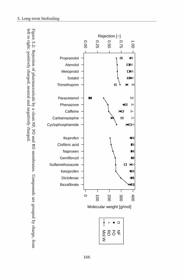
5. Long-term biofouling
Propranolol
Atenolol
Metoprolol
Sotalol
Trimethoprim
Paracetamol
Phenazone
Caffeine
Carbamazepine
Cyclophosphamide
Ibuprofen
Clofibric acid
Naproxen
Gemfibrozil
Sulfamethoxazole
Ketoprofen
Diclofenac
Bezafibrate
0.00
0.25
0.50
0.75
1.00
Rejection [−]
●●
●●
●
●
●●
●
●
●●
●
●●
●
●
●
0 100
200
300
400
Molecular weight [g/mol]
●
NF
FO
RO
Mol.W
.
Figure5.2:
Rejection
ofpharm
aceuticalsby
aclean
NF,
FOand
RO
mem
branes.C
ompounds
aregrouped
bycharge,
fromleft
toright:
positivelycharged,neutraland
negativelycharged.
166
~
Slfl;l
Bfl;l
~
1+1 ~
~
I+S ~
I+E3 iE'!
IEl ~
~
~
H
lfll
lflll
IEl ~
IEt!
~
IEl
I ~ . D
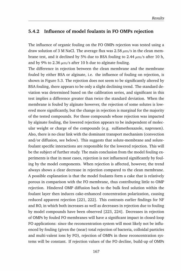
Results
5.4.2 Influence of model foulants in FO OMPs rejection
The influence of organic fouling on the FO OMPs rejection was tested using a
draw solution of 3 M NaCl. The average flux was 2.58 µm/s in the clean mem-
brane test, and it declined by 5% due to BSA fouling to 2.44 µm/s after 10 h,
and by 9% to 2.36 µm/s after 10 h due to alginate fouling.
The difference in rejection between the clean membrane and the membrane
fouled by either BSA or alginate, i.e. the influence of fouling on rejection, is
shown in Figure 5.3. The rejection does not seem to be significantly altered by
BSA fouling, there appears to be only a slight declining trend. The standard de-
viation was determined based on the calibration series, and significant in this
test implies a difference greater than twice the standard deviation. When the
membrane is fouled by alginate however, the rejection of some solutes is low-
ered more significantly, but the change in rejection is marginal for the majority
of the tested compounds. For those compounds whose rejection was impacted
by alginate fouling, the lowered rejection appears to be independent of molec-
ular weight or charge of the compounds (e.g. sulfamethoxazole, naproxen).
Also, there is no clear link with the dominant transport mechanism (convection
and/or diffusion, see below). This suggests that solute-membrane and solute-
foulant specific interactions are responsible for the lowered rejection. This will
be the subject of further study. The main conclusion from the model fouling ex-
periments is that in most cases, rejection is not influenced significantly by foul-
ing by the model components. When rejection is affected, however, the trend
always shows a clear decrease in rejection compared to the clean membrane.
A possible explanation is that the model foulants form a cake that is relatively
porous in comparison with the FO membrane, thus contributing little to OMP
rejection. Hindered OMP diffusion back to the bulk feed solution within the
foulant layer then induces cake-enhanced concentration polarization, causing
reduced apparent rejection [221, 222]. This contrasts earlier findings for NF
and RO, in which both increases as well as decreases in rejection due to fouling
by model compounds have been observed [223, 224]. Decreases in rejection
of OMPs by fouled FO membranes will have a significant impact in closed-loop
FO applications: since the reconcentration system will most likely not be influ-
enced by fouling (given the (near) total rejection of bacteria, colloidal particles
and multi-valent ions by FO), rejection of OMPs in these reconcentration sys-
tems will be constant. If rejection values of the FO decline, build-up of OMPs
167
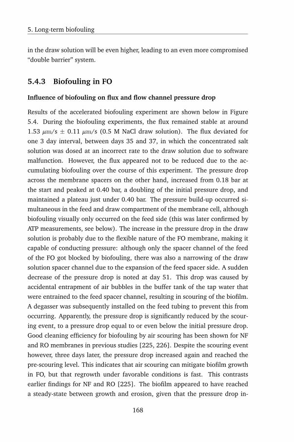
5. Long-term biofouling
in the draw solution will be even higher, leading to an even more compromised
“double barrier” system.
5.4.3 Biofouling in FO
Influence of biofouling on flux and flow channel pressure drop
Results of the accelerated biofouling experiment are shown below in Figure
5.4. During the biofouling experiments, the flux remained stable at around
1.53 µm/s ± 0.11 µm/s (0.5 M NaCl draw solution). The flux deviated for
one 3 day interval, between days 35 and 37, in which the concentrated salt
solution was dosed at an incorrect rate to the draw solution due to software
malfunction. However, the flux appeared not to be reduced due to the ac-
cumulating biofouling over the course of this experiment. The pressure drop
across the membrane spacers on the other hand, increased from 0.18 bar at
the start and peaked at 0.40 bar, a doubling of the initial pressure drop, and
maintained a plateau just under 0.40 bar. The pressure build-up occurred si-
multaneous in the feed and draw compartment of the membrane cell, although
biofouling visually only occurred on the feed side (this was later confirmed by
ATP measurements, see below). The increase in the pressure drop in the draw
solution is probably due to the flexible nature of the FO membrane, making it
capable of conducting pressure: although only the spacer channel of the feed
of the FO got blocked by biofouling, there was also a narrowing of the draw
solution spacer channel due to the expansion of the feed spacer side. A sudden
decrease of the pressure drop is noted at day 51. This drop was caused by
accidental entrapment of air bubbles in the buffer tank of the tap water that
were entrained to the feed spacer channel, resulting in scouring of the biofilm.
A degasser was subsequently installed on the feed tubing to prevent this from
occurring. Apparently, the pressure drop is significantly reduced by the scour-
ing event, to a pressure drop equal to or even below the initial pressure drop.
Good cleaning efficiency for biofouling by air scouring has been shown for NF
and RO membranes in previous studies [225, 226]. Despite the scouring event
however, three days later, the pressure drop increased again and reached the
pre-scouring level. This indicates that air scouring can mitigate biofilm growth
in FO, but that regrowth under favorable conditions is fast. This contrasts
earlier findings for NF and RO [225]. The biofilm appeared to have reached
a steady-state between growth and erosion, given that the pressure drop in-
168
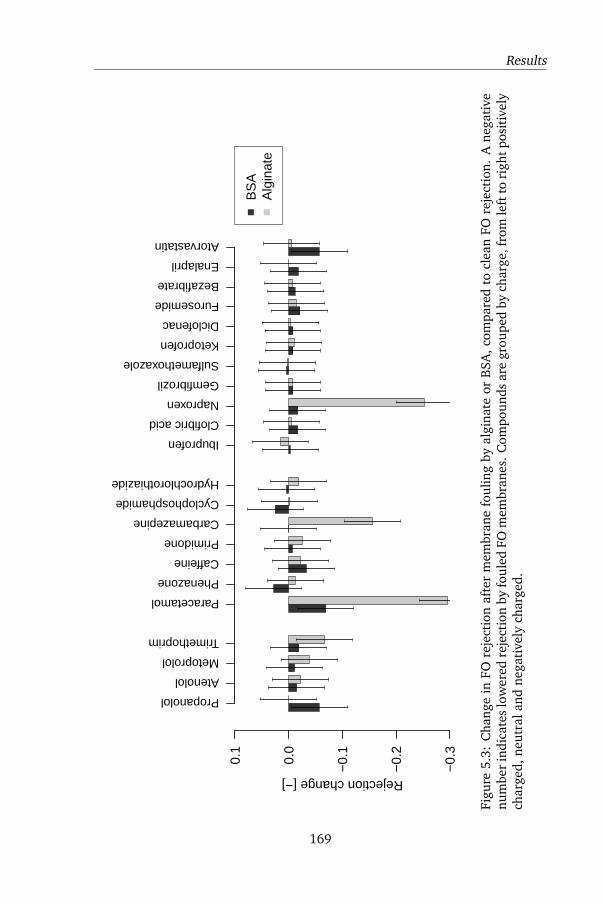
Results
Rejection change [−]
−0.
3
−0.
2
−0.
1
0.0
0.1
Propanolol
Atenolol
Metoprolol
Trimethoprim
Paracetamol
Phenazone
Caffeine
Primidone
Carbamazepine
Cyclophosphamide
Hydrochlorothiazide
Ibuprofen
Clofibric acid
Naproxen
Gemfibrozil
Sulfamethoxazole
Ketoprofen
Diclofenac
Furosemide
Bezafibrate
Enalapril
Atorvastatin
BS
AA
lgin
ate
Figu
re5.
3:C
hang
ein
FOre
ject
ion
afte
rm
embr
ane
foul
ing
byal
gina
teor
BSA
,com
pare
dto
clea
nFO
reje
ctio
n.A
nega
tive
num
ber
indi
cate
slo
wer
edre
ject
ion
byfo
uled
FOm
embr
anes
.C
ompo
unds
are
grou
ped
bych
arge
,fro
mle
ftto
righ
tpos
itiv
ely
char
ged,
neut
rala
ndne
gati
vely
char
ged.
169

5. Long-term biofouling
0 10 20 30 40 50 60
0.0e+00
5.0e−07
1.0e−06
1.5e−06
Time [days]
J w [m
/s]
0.0
0.2
0.4
0.6
0.8
Pre
ssur
e dr
op [b
ar]
FluxP FeedP Draw
Figure 5.4: Flux and pressure drop increase across feed and draw spacerscaused by biofilm growth.
crease, caused by biofilm regrowth, again stabilizes around 0.40 bar.
Influence of biofouling on the rejection of trace organics
The rejection of pharmaceuticals by the biofouled FO membrane was tested
twice with the same biofouled membrane. The first rejection test was after 8
days of biofilm growth. At that time the biofilm formation was still ongoing,
as is shown by the increasing pressure drop, and the biofilm thickness was hy-
pothesized to still be relatively small. The second rejection test was performed
49 days after the start of the experiment. At that point, biofilm formation had
almost reached a steady state, as discussed above. The results of both tests are
given in Figure 5.5 relative to the difference in rejection with the clean mem-
brane (a negative rejection indicating a decrease in rejection compared to the
clean membrane). The presence of a developing biofilm appears to slightly al-
ter OMPs rejection, leading to a slightly higher rejection of neutral solutes and
a lower rejection of some negatively charged solutes. For positively charged
compounds, no clear trend can be seen. A fully developed biofilm caused a
more pronounced reduction in the rejection of positively charged compounds
and a less clear trend in the rejection of negatively charged compounds com-
pared to the developing biofilm. Differences in OMPs rejection behavior of the
170
Results
two biofilm growth stages is likely due to differences in the composition of the
extracellular matrix and bacterial cell walls. The relatively minor differences
in OMPs rejection, lead to the conclusion that biofilm formation only has a
limited impact on FO rejection, which appears to corroborate findings from NF
and RO membranes [210]. The difference in rejection by a clean membrane
and rejection by a biofouled membrane is for the majority of compounds 10%
or less. Hancock et al. [82] also noticed an increased OMPs rejection by an
FO membrane fouled by activated sludge in the case of non-ionic compounds.
The high rejection of charged compounds by FO was confirmed in this study as
well.
Biofilm characterization
The ATP concentration of the feed and draw solution and the ATP concentra-
tion of the biofilm samples are shown in Table 5.1. The biofilm was sampled
upon harvesting, 67 days after the start of the experiment. A number of studies
have correlated ATP measurements in fresh water and drinking water environ-
ments to cell concentrations [227, 214, 228], these estimates range from about
1.7·10-17 to 13.7·10-17 g ATP/cell. Possible cell concentrations are calculated
based on this range.
van der Wielen and van der Kooij [228] studied ATP concentrations in unchlo-
rinated drinking water in the Netherlands, and reported ATP concentrations
ranging from 0.32 ng/L to 28.0 ng/L Berney et al. [227] reported ATP concen-
trations of 0.016 to0.055 ng/L in unchlorinated drinking water in Switzerland.
These concentrations are considerably lower than the feed ATP concentration
of this test. A possible explanation is that the feed in this test was potable fresh
water, but it was stored in a large underground buffer during two days prior
to use. Furthermore, the feed was sampled in the dechlorination buffer ves-
sel of the experimental setup. Additional microbial growth in this vessel could
further increase the amount of active microbial biomass. Growth of biomass in
the feed lines was visually confirmed. Sodium acetate was chosen as a model
AOC and was spiked in the feed as a nutrient for biofilm development. The ATP
concentration in the biofilm samples show that the ATP content of the biofilm
lowers as the distance to the sodium acetate solution inlet increases. This indi-
cates that the AOC was being metabolized as the feed passes over the biofilm.
The draw side of the membrane remained devoid of any visible biofilm for-
mation during the entire experiment, and the ATP concentration of the draw
171
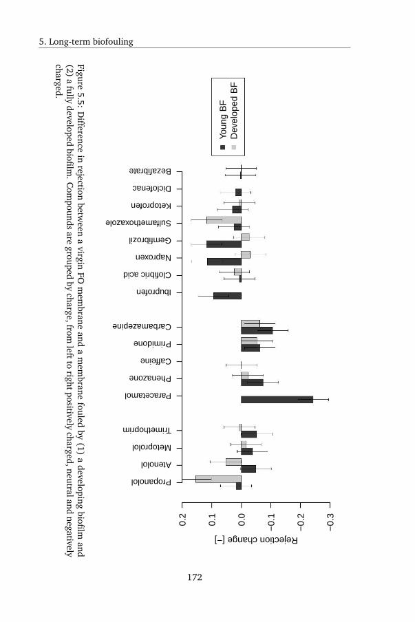
5. Long-term biofouling
Rejection change [−]
−0.
3
−0.
2
−0.
1
0.0
0.1
0.2
Propanolol
Atenolol
Metoprolol
Trimethoprim
Paracetamol
Phenazone
Caffeine
Primidone
Carbamazepine
Ibuprofen
Clofibric acid
Naproxen
Gemfibrozil
Sulfamethoxazole
Ketoprofen
Diclofenac
Bezafibrate
Youn
g B
FD
evel
oped
BF
Figure5.5:
Difference
inrejection
between
avirgin
FOm
embrane
anda
mem
branefouled
by(1)
adeveloping
biofilmand
(2)a
fullydeveloped
biofilm.
Com
poundsare
groupedby
charge,fromleftto
rightpositivelycharged,neutraland
negativelycharged.
172
• •
• I • • I 9 I
D R
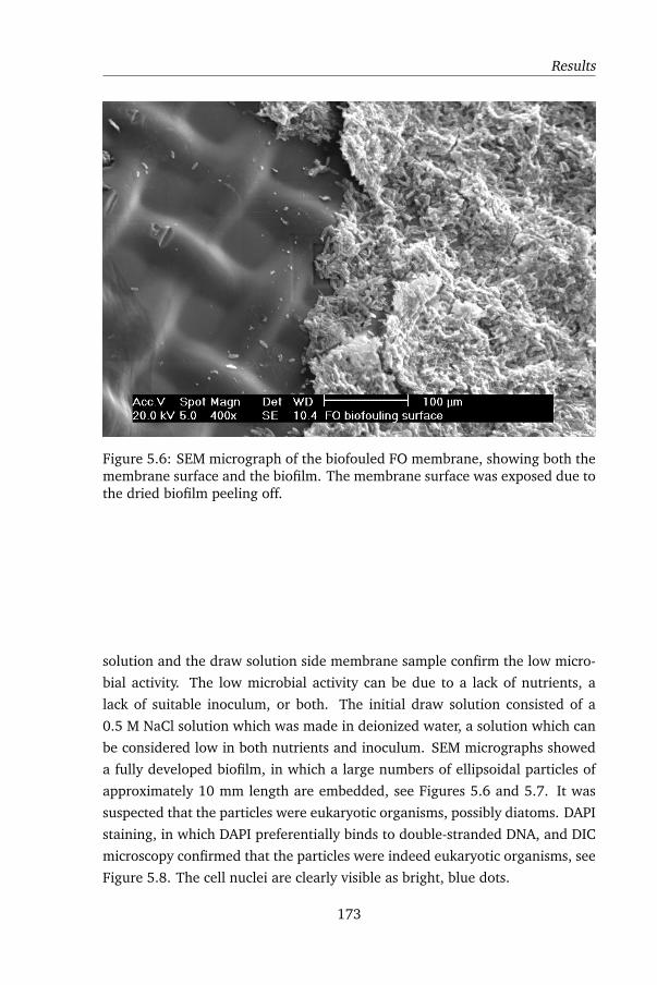
Results
Figure 5.6: SEM micrograph of the biofouled FO membrane, showing both themembrane surface and the biofilm. The membrane surface was exposed due tothe dried biofilm peeling off.
solution and the draw solution side membrane sample confirm the low micro-
bial activity. The low microbial activity can be due to a lack of nutrients, a
lack of suitable inoculum, or both. The initial draw solution consisted of a
0.5 M NaCl solution which was made in deionized water, a solution which can
be considered low in both nutrients and inoculum. SEM micrographs showed
a fully developed biofilm, in which a large numbers of ellipsoidal particles of
approximately 10 mm length are embedded, see Figures 5.6 and 5.7. It was
suspected that the particles were eukaryotic organisms, possibly diatoms. DAPI
staining, in which DAPI preferentially binds to double-stranded DNA, and DIC
microscopy confirmed that the particles were indeed eukaryotic organisms, see
Figure 5.8. The cell nuclei are clearly visible as bright, blue dots.
173
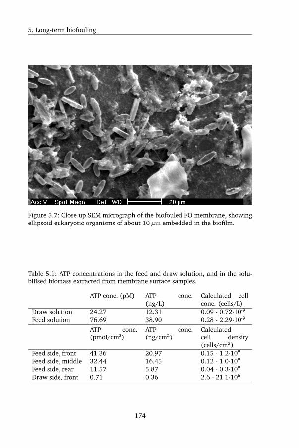
5. Long-term biofouling
Figure 5.7: Close up SEM micrograph of the biofouled FO membrane, showingellipsoid eukaryotic organisms of about 10 µm embedded in the biofilm.
Table 5.1: ATP concentrations in the feed and draw solution, and in the solu-bilised biomass extracted from membrane surface samples.
ATP conc. (pM) ATP conc.(ng/L)
Calculated cellconc. (cells/L)
Draw solution 24.27 12.31 0.09 - 0.72·10-9
Feed solution 76.69 38.90 0.28 - 2.29·10-9
ATP conc.(pmol/cm2)
ATP conc.(ng/cm2)
Calculatedcell density(cells/cm2)
Feed side, front 41.36 20.97 0.15 - 1.2·109
Feed side, middle 32.44 16.45 0.12 - 1.0·109
Feed side, rear 11.57 5.87 0.04 - 0.3·109
Draw side, front 0.71 0.36 2.6 - 21.1·106
174
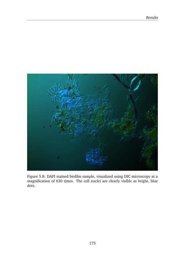
Results
Figure 5.8: DAPI stained biofilm sample, visualized using DIC microscopy at amagnification of 630 times. The cell nuclei are clearly visible as bright, bluedots.
175
5. Long-term biofouling
5.4.4 Transport mechanisms and draw concentration mod-eling
Diffusive versus convective transport
To investigate FO transport mechanisms and differentiate between diffusive
and convectively coupled transport of OMPs, an experiment was carried out in
which OMPs were only spiked in the feed solution in one run, and then in both
the feed and draw solutions in similar concentrations in the next run. In case
solute transport would only be occurring by diffusive transport, there would be
no net mass transfer of the solute from the feed to the draw solution when the
solute is present in equimolar quantities in both solutions. This follows from
Fick’s law of diffusion, in which the driving force for mass transfer is a gradient
in concentration, as is shown in equation 5.1.
In the hypothetical case of purely convectively coupled transport, there would
be mass transfer of the solute in the same direction as the solvent flux in both
cases (i.e., when the feed concentration is higher or equal to than the draw
solution concentration). The results of the mass transfer tests are plotted in
Figure 5.9. From the figure, it is apparent that for most solutes, mass trans-
fer drops to almost zero when the solute concentration in the draw solution
is equal to the concentration of the feed. This indicates that for the majority
of solutes, diffusive transport dominates. For caffeine, convective transport is
clearly significant, but solute transport is not equally high in both cases, indicat-
ing that solute transport is probably a combination of convection and diffusion.
For sulfamethoxazole, on the other hand, transport is similar in both cases, in-
dicating that transport is dominated by convective transport. Sulfamethoxazole
is the only charged solute in this test. We suspect that convective transport
dominates when the affinity of the solute for water (expressed as a negative
free energy of interaction) is larger than the affinity for the membrane matrix.
For sulfamethoxazole, this seems plausible, given that it is negatively charged
at neutral pH and has a predicted logD coefficient of -0.54, and that the CTA
membrane matrix has a high electron-donating surface tension component (see
chapter 3). The results clearly show that the dominant transport mechanism of
OMPs is not only dependent on the membrane and water flux, but also largely
depends on the solute properties. The relative contributions of diffusion and
convection to solute mass transfer relate to the solute diffusion coefficients in
the membrane, as well as the ratios of the solute size to the membrane pore
176
Results
size, and also solute-membrane affinity [146].
Modeling of solute accumulation in draw solution and concentration in
product water
When FO is used to reclaim water and RO is used to reconcentrate the draw
solution, the higher rejection of trace organics by RO than by FO will lead to
an accumulation of trace organics in the draw solution. This system of FO-RO
in closed loop was modeled for different solute transport mechanisms: purely
diffusive, convectively coupled transport and mixed, convection-diffusion so-
lute transport. For solutes transported diffusively, the solute concentration in
the draw solution at steady state is given by:
cd =yBcf
yB + Jw(1−RRO)(5.10)
In the case of convectively coupled solute transport, the concentration again
reaches a steady state. Convectively coupled transport implies that there would
be no diffusive flux from the draw solution to the FO feed, leading to continued
accumulation until the RO solute flux equals the FO solute flux. The solute
concentration at steady state is given by:
cd =cfKc,sy
1−RRO(5.11)
At the steady-state, the solute RO permeate concentration is determined by
the FO rejection of the solute. This implies that RO rejection influences only
the steady state solute concentration in the draw solution, but not the solute
concentration in the RO permeate. This is shown by the derivation of the steady
state RO permeate solute concentration, which is:
cp,RO = cd(1−RRO) = cfKc,sy (5.12)
The solute concentration in the RO permeate of the FO draw solution was com-
pared with RO permeate if the impaired water was subjected to RO treatment
directly, without an FO barrier in between. This was calculated for diffusive
and convective transport, see Table 5.2. A high rejection was modeled as 98%,
and a low rate as 50%. In all cases, the dilution ratio of the FO draw solu-
tion equals 0.5. A higher dilution ratio causes solutes to accumulate to higher
177
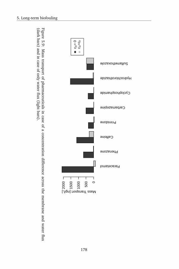
5. Long-term biofouling
Paracetamol
Phenazone
Caffeine
Primidone
Carbamazepine
Cyclophosphamide
Hydrochlorothiazide
Sulfamethoxazole
Mass Transport [ng/L]
0
500
1000
1500
2000
c D=
0c D
=c F
Figure5.9:
Mass
transportof
pharmaceuticals
incase
ofa
concentrationdifference
acrossthe
mem
braneand
water
flux(dark
bars)and
incase
ofonlyw
aterflux
(lightbars).
178
Results
levels. The added value of FO is defined as:
AddedV alue(%) = 100(1− cp,FO−ROcp,RO
) (5.13)
with cp,FO−RO the solute concentration in the RO permeate of the combined
FO-RO installation, and cp,RO the solute concentration in the RO permeate if
the feed would be subjected to RO treatment directly.
It was found that for diffusive transport, if FO and RO rejection is equal (cases 1
and 3), the double barrier causes an additional removal of roughly 60% of the
OMPs. This would be more or less the case for most charged compounds tested
in this study. A graph of OMP concentrations in the FO and RO permeate and
in the draw loop for case 1 is given in Figure 5.10, showing the increasing OMP
concentration in the draw loop and the decreasing OMP concentration in the
FO permeate as the system approaches equilibrium. If, however, FO rejection
is low while RO rejection is high (case 2), the added value of the double bar-
rier is marginal. In this study, this would be the case for paracetamol, caffeine
and carbamazepine. In case 3, rejection by both the FO and RO membrane is
low, leading to on the one hand a higher added value of the double barrier,
but simultaneously also to a relatively high contaminant concentration in the
product water. This could for instance be the case if NF instead of RO is used
to reconcentrate the draw solution. Given the higher water permeability of NF
compared to RO membranes, using NF would require less membrane surface
area and less pumping power. The draw solute would have to be modified
however, as most NF membranes show a poor rejection of monovalent ions,
leading to another drawback of using NF for reconcentration: multivalent ions
or large molecular weight solutes also show a decreased osmotic potential and
low diffusion coefficient, making for a less efficient draw solution [8]. In case
4, FO rejection is higher than that of the RO membrane. This was not the
case for any compound tested in this study, however, if such an FO membrane
would be developed, this would lead to a high added value of the double bar-
rier. For convective transport, there is again an added value of FO in cases 5,
7and 8. However, in case 6 (low FO and high RO rejection), the added value
of FO is negative. This case is the most common based on the experimental
rejection values of this study, as is illustrated by sulfamethoxazole. In the case
of sulfamethoxazole, indications of strong convectively coupled transport were
found in this study. The rejection by FO and RO was 95.4 and 99.8%, respec-
179
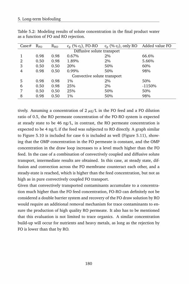
5. Long-term biofouling
Table 5.2: Modeling results of solute concentration in the final product wateras a function of FO and RO rejection.
Case# RFO RRO cp (% cf), FO-RO cp (% cf), only RO Added value FODiffusive solute transport
1 0.98 0.98 0.67% 2% 66.6%2 0.50 0.98 1.89% 2% 5.66%3 0.50 0.50 20% 50% 60%4 0.98 0.50 0.99% 50% 98%
Convective solute transport5 0.98 0.98 1% 2% 50%6 0.50 0.98 25% 2% -1150%7 0.50 0.50 25% 50% 50%8 0.98 0.50 1% 50% 98%
tively. Assuming a concentration of 2 µg/L in the FO feed and a FO dilution
ratio of 0.5, the RO permeate concentration of the FO-RO system is expected
at steady state to be 46 ng/L, in contrast, the RO permeate concentration is
expected to be 4 ng/L if the feed was subjected to RO directly. A graph similar
to Figure 5.10 is included for case 6 is included as well (Figure 5.11), show-
ing that the OMP concentration in the FO permeate is constant, and the OMP
concentration in the draw loop increases to a level much higher than the FO
feed. In the case of a combination of convectively coupled and diffusive solute
transport, intermediate results are obtained. In this case, at steady state, dif-
fusion and convection across the FO membrane counteract each other, and a
steady-state is reached, which is higher than the feed concentration, but not as
high as in pure convectively coupled FO transport.
Given that convectively transported contaminants accumulate to a concentra-
tion much higher than the FO feed concentration, FO-RO can definitely not be
considered a double barrier system and recovery of the FO draw solution by RO
would require an additional removal mechanism for trace contaminants to en-
sure the production of high quality RO permeate. It also has to be mentioned
that this evaluation is not limited to trace organics. A similar concentration
build-up will occur for nutrients and heavy metals, as long as the rejection by
FO is lower than that by RO.
180
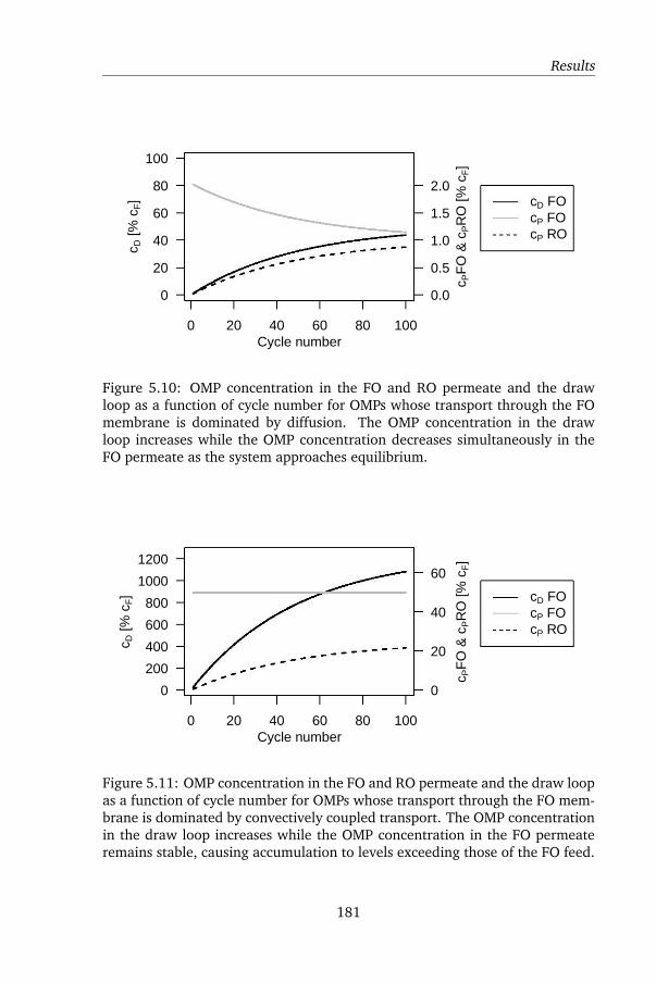
Results
0 20 40 60 80 100
0
20
40
60
80
100
0.0
0.5
1.0
1.5
2.0
Cycle number
c D [%
cF]
c PF
O &
cPR
O [%
cF]
cD FOcP FOcP RO
Figure 5.10: OMP concentration in the FO and RO permeate and the drawloop as a function of cycle number for OMPs whose transport through the FOmembrane is dominated by diffusion. The OMP concentration in the drawloop increases while the OMP concentration decreases simultaneously in theFO permeate as the system approaches equilibrium.
0 20 40 60 80 100
0
200
400
600
800
1000
1200
0
20
40
60
Cycle number
c D [%
cF]
c PF
O &
cPR
O [%
cF]
cD FOcP FOcP RO
Figure 5.11: OMP concentration in the FO and RO permeate and the draw loopas a function of cycle number for OMPs whose transport through the FO mem-brane is dominated by convectively coupled transport. The OMP concentrationin the draw loop increases while the OMP concentration in the FO permeateremains stable, causing accumulation to levels exceeding those of the FO feed.
181
~~~~~~~--------·
5. Long-term biofouling
5.5 Conclusions
In this study, it was shown that OMP rejection by CTA-ES FO membranes is
comparable to NF but lower than RO rejection for the compounds tested in this
study. The FO unit was operated at a lower flux than the NF and RO, which
would be realistic in a FO-MBR process. Model foulants caused a slight de-
crease in rejection for most compounds (10% drop or less), while the rejection
of some were significantly negatively impacted. The water flux decreased by
10%. It can thus be concluded that, at fairly low flux, the impact of fouling
is limited, both on flux and on OMP rejection. Fouling by long-term biofilm
growth caused FO rejection to vary as a function of biofilm age, although over-
all biofilm influence was limited, which again could be due to the low FO
flux. OMP transport analysis showed that for neutral solutes, diffusion was the
dominant transport mechanism. Modeling revealed an undesirable build-up of
trace organics in a FO-RO closed loop system, which limits the usefulness of FO
when OMPs are transported diffusively. When compounds are transported con-
vectively, OMP build-up even leads to a higher OMPs concentration in the RO
product water compared to water production with only RO. Modeling results
suggest that FO OMP rejection, being the first barrier against OMPs in a FO-RO
system, has a profound influence on OMP rejection by the system as a whole.
Attaining an as high as possible OMP rejection by FO is therefore advisable.
182

Chapter 6
Conclusions and recommendations forfuture research
183
6. Conclusions
6.1 General conclusions
6.1.1 Mass transfer mechanisms in FO
In this dissertation, mass transfer phenomena in FO were studied, mainly focus-
ing on the transport of dissolved solutes. Different phenomena have been ob-
served during solute transport, which implies that different models are needed
to describe solute transport. To aid in model selection, a tree diagram is shown
in Figure 6.1. The decision tree does not include transport mechanisms spe-
cific for charged compounds such as electromigration, ion exchange or Donnan
dialysis, as these phenomena were not the main focus of this work. Adsorption
is included, as adsorption in part provided a mechanistic explanation for the
negative rejection observed in chapter 4. Both coupled (chapter 4) and uncou-
pled fluxes (chapter 3) were observed as well; this will be discussed in sections
6.1.3 and 6.2.2.
6.1.2 Conclusion 1
Water and draw solute flux predictions are improved whenaccounting for draw solute diffusivity concentration depen-dence; further model refinement is possible
The results presented in chapter 2 show that considering the concentration
dependence of the draw solute diffusivity yields an improved fit, especially
when the draw solute concentration difference across the active layer is large.
Flux prediction improvement had been noticed earlier when considering draw
solute diffusivity concentration dependence during ICP [10, 105]. The model
presented in chapter 2 incorporated draw solute diffusivity concentration de-
pendence both during ICP and during active layer transport. This model has
shown to be able to predict water and draw solute fluxes for different mem-
brane types, draw solutes and using both membrane orientations.
The model however did not yield constant values for the structural parameter
S of the support layer for each membrane type with regards to draw solute or
membrane orientation. As was shown in Figure 2.15, some draw solute con-
centration dependence exists as well in the estimates of S, thus, the choice of
draw solution concentration when performing experimental flux tests has an
influence on the resulting estimate of S. In other words, relevant variables
184
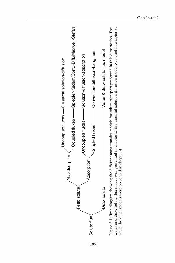
Conclusion 1
Sol
ute
flux
Fee
d so
lute
Dra
w s
olut
e
Ads
orpt
ion
No
adso
rptio
nC
oupl
ed fl
uxes
Unc
oupl
ed fl
uxes
Spi
egle
r-K
edem
/Con
v.-D
iff./M
axw
ell-S
tefa
n
Con
vect
ion-
diffu
sion
-Lan
gmui
r
Cla
ssic
al s
olut
ion-
diffu
sion
Sol
utio
n-di
ffusi
on-a
dsor
ptio
n
Wat
er &
dra
w s
olut
e flu
x m
odel
Cou
pled
flux
es
Unc
oupl
ed fl
uxes
Figu
re6.
1:Tr
eedi
agra
msh
owin
gth
edi
ffer
ent
mas
str
ansf
erm
odel
sfo
rso
lute
tran
spor
tpr
esen
ted
inth
isdi
sser
tati
on.
The
wat
eran
ddr
awso
lute
flux
mod
elw
aspr
esen
ted
inch
apte
r2,
the
clas
sica
lsol
utio
n-di
ffus
ion
mod
elw
asus
edin
chap
ter
3,w
hile
the
othe
rm
odel
sw
ere
pres
ente
din
chap
ter
4.
185
6. Conclusions
are lacking or some variables show salt type and concentration dependence.
This implies that currently for each draw solute and membrane orientation,
flux tests spanning a wide draw solute concentration range are necessary to
obtain a value of S before fluxes can be predicted at different feed and draw
concentrations.
6.1.3 Conclusion 2
Solute flux can be either coupled with or uncoupled from wa-ter flux, depending on solute size
Different organic solutes were used in this dissertation, ranging from small
molecules barely larger than water such as formamide or 1-propanol in chap-
ter 4, to much larger micropollutants in chapters 3 and 5. As was shown by
numerical analysis of water, draw solute and OMP fluxes during both FO and
simple diffusion in chapter 3, OMP fluxes were not coupled to either water
or draw solute fluxes. Using the same membrane however, strong flux cou-
pling was observed in chapter 4. This is due to the size difference between
the different solutes: solutes with a size somewhat similar to water, are also
subject to comparable steric hindrance by the membrane polymer, while si-
multaneously engaging in solute-water interactions. The force balance is thus
favors solute-water interactions. Large solutes on the other hand, are subject to
much stronger steric hindrance, therefore, frictional solute-membrane interac-
tions dominate the force balance, effectively uncoupling solute flux from water
flux. In chapter 3, it was shown that the minimal projected area of a molecule
was the best predictor of membrane permeability for uncharged solutes, with
Spearman r=-0.771 (see also Figure 3.7). In table 6.1, minimal projected areas
are compared between water, the solutes used in chapter 4 and the OMPs. For
the CTA membrane, the transition between coupled and uncoupled transport
appears to occur around 25 Å2. This implies that organic solutes with a mini-
mal projected area below 25 Å2 will generally be poorly rejected regardless of
the water flux, while larger solutes will generally better rejected, especially at
high water flux.
186
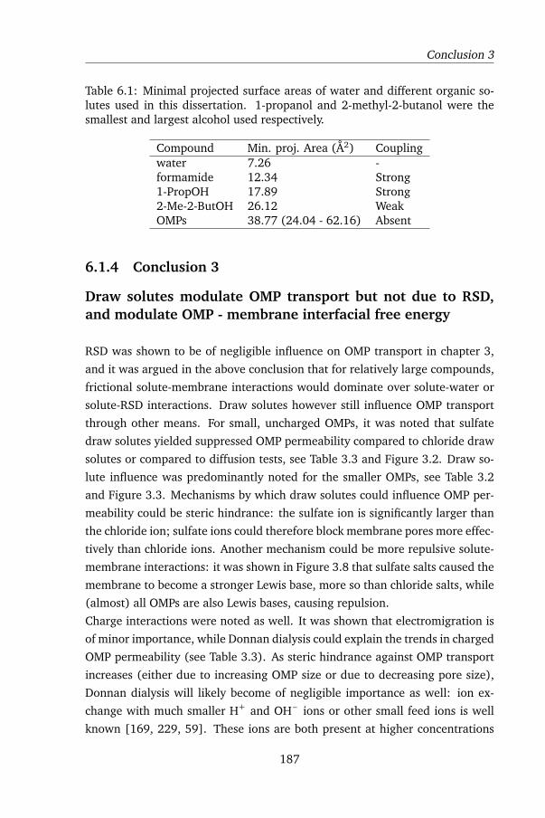
Conclusion 3
Table 6.1: Minimal projected surface areas of water and different organic so-lutes used in this dissertation. 1-propanol and 2-methyl-2-butanol were thesmallest and largest alcohol used respectively.
Compound Min. proj. Area (Å2) Couplingwater 7.26 -formamide 12.34 Strong1-PropOH 17.89 Strong2-Me-2-ButOH 26.12 WeakOMPs 38.77 (24.04 - 62.16) Absent
6.1.4 Conclusion 3
Draw solutes modulate OMP transport but not due to RSD,and modulate OMP - membrane interfacial free energy
RSD was shown to be of negligible influence on OMP transport in chapter 3,
and it was argued in the above conclusion that for relatively large compounds,
frictional solute-membrane interactions would dominate over solute-water or
solute-RSD interactions. Draw solutes however still influence OMP transport
through other means. For small, uncharged OMPs, it was noted that sulfate
draw solutes yielded suppressed OMP permeability compared to chloride draw
solutes or compared to diffusion tests, see Table 3.3 and Figure 3.2. Draw so-
lute influence was predominantly noted for the smaller OMPs, see Table 3.2
and Figure 3.3. Mechanisms by which draw solutes could influence OMP per-
meability could be steric hindrance: the sulfate ion is significantly larger than
the chloride ion; sulfate ions could therefore block membrane pores more effec-
tively than chloride ions. Another mechanism could be more repulsive solute-
membrane interactions: it was shown in Figure 3.8 that sulfate salts caused the
membrane to become a stronger Lewis base, more so than chloride salts, while
(almost) all OMPs are also Lewis bases, causing repulsion.
Charge interactions were noted as well. It was shown that electromigration is
of minor importance, while Donnan dialysis could explain the trends in charged
OMP permeability (see Table 3.3). As steric hindrance against OMP transport
increases (either due to increasing OMP size or due to decreasing pore size),
Donnan dialysis will likely become of negligible importance as well: ion ex-
change with much smaller H+ and OH– ions or other small feed ions is well
known [169, 229, 59]. These ions are both present at higher concentrations
187
6. Conclusions
and much less subject to steric hindrance.
6.1.5 Conclusion 4
OMPs accumulate in the draw solution when used as a closed-loop FO-RO system
The results presented in chapter 5 show that OMP rejection is not affected
to a large extent by biofouling, but the modeling shows that OMPs accumulate
in the draw solution loop. OMP rejection tests in this study had shown that
OMP rejection of charged compounds generally increased, while uncharged
OMPs showed a rejection decrease. Accumulation of OMPs depended on the
rejection performance of the FO membrane relative to the RO membrane: if
the FO membrane was more permeable (as is generally the case), OMPs would
accumulate to levels exceeding the feed concentration. This would obviously
lead to increased OMP concentrations in the RO permeate, which is the final
product water of a FO-RO closed loop installation. If an OMP is transported
diffusively (uncoupled fluxes), one would expect that the feed and closed loop
OMP concentrations are equal at steady-state operation. However, once an
OMP has diffused into the draw solution, it would be subject to dilutive con-
centration polarization, similar to the draw solute. This is shown conceptually
in Figure 6.2. The implications for OMBRs are clear: if the produced water is
intended for potable reuse, the FO membrane should possess an OMP perme-
ability as low or lower than the RO membrane. Otherwise, post-treatment of
the RO permeate or in-line treatment of the draw solution are needed, which
would lead to significant additional capital and operational costs.
188
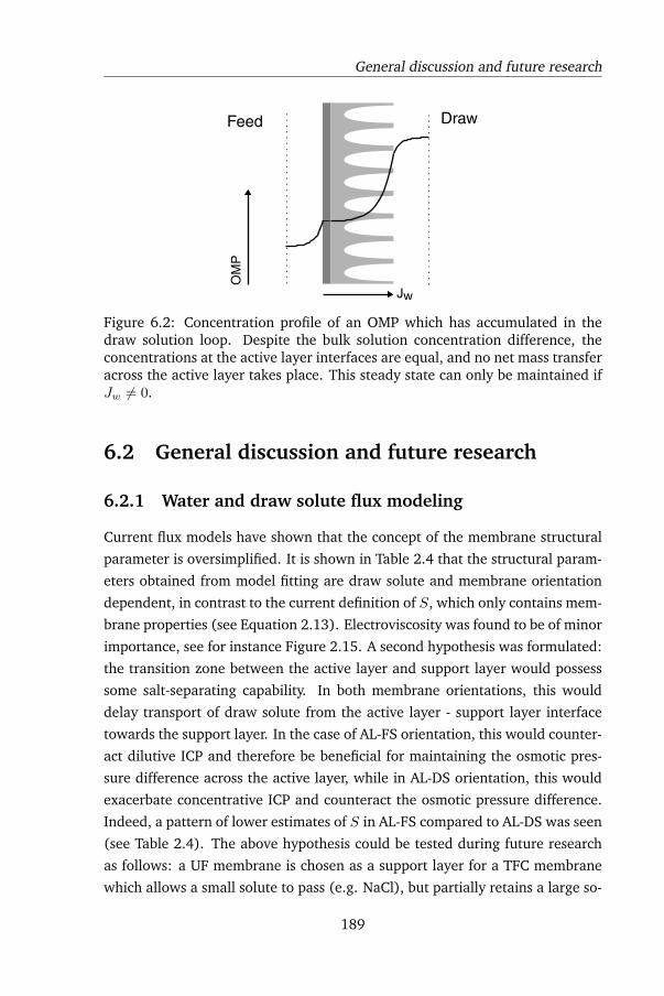
General discussion and future research
Feed Draw
OM
P
Jw
Figure 6.2: Concentration profile of an OMP which has accumulated in thedraw solution loop. Despite the bulk solution concentration difference, theconcentrations at the active layer interfaces are equal, and no net mass transferacross the active layer takes place. This steady state can only be maintained ifJw 6= 0.
6.2 General discussion and future research
6.2.1 Water and draw solute flux modeling
Current flux models have shown that the concept of the membrane structural
parameter is oversimplified. It is shown in Table 2.4 that the structural param-
eters obtained from model fitting are draw solute and membrane orientation
dependent, in contrast to the current definition of S, which only contains mem-
brane properties (see Equation 2.13). Electroviscosity was found to be of minor
importance, see for instance Figure 2.15. A second hypothesis was formulated:
the transition zone between the active layer and support layer would possess
some salt-separating capability. In both membrane orientations, this would
delay transport of draw solute from the active layer - support layer interface
towards the support layer. In the case of AL-FS orientation, this would counter-
act dilutive ICP and therefore be beneficial for maintaining the osmotic pres-
sure difference across the active layer, while in AL-DS orientation, this would
exacerbate concentrative ICP and counteract the osmotic pressure difference.
Indeed, a pattern of lower estimates of S in AL-FS compared to AL-DS was seen
(see Table 2.4). The above hypothesis could be tested during future research
as follows: a UF membrane is chosen as a support layer for a TFC membrane
which allows a small solute to pass (e.g. NaCl), but partially retains a large so-
189
6. Conclusions
lute (e.g. sucrose). FO flux tests are then performed using both the small and
large solute as draw solute. According to the above hypothesis, for the small
solute, the fitted structural parameter should be independent of the membrane
orientation while an orientation dependence for the large solute should be ob-
served for the same membrane. The hypothesis could also be tested in silico:
a single support layer pore can be constructed where in one end draw solute
molecules appear or disappear (due to RSD) for AL-DS and AL-FS orientation
respectively, and a water flux is established due to the osmotic pressure gen-
erated by the draw solute. For simplicity, the bulk feed and draw solution
can be regarded as an infinitely large sink or reservoir respectively of draw so-
lute molecules. As the system reaches a steady-state, the active layer interface
draw solute concentrations can then show membrane orientation dependence,
depending on support layer pore size. The model approach would furthermore
allow to study the influence of pore geometry: a pore can be considered a long
cylinder of constant radius, a cone or a succession of voids connected by nar-
row passages. The former case is the assumed pore shape in many transport
models, the middle case would represent a support layer pore averaged over
the entire support layer thickness, while the latter case is likely the most real-
istic representation of small, nanometer sized pores [40]. A third possibility,
related to the previous hypothesis, is that pore size of the support layer should
be incorporated. It has been shown that tortuosity is pore size-dependent,
depending on the type of tortuosity. Tortuosity can be defined as simply ge-
ometric: the shortest path length within pores between two points, with the
path comprised of straight line segments. In this case, tortuosity is not depen-
dent on pore size. However, in the case of diffusional or viscous transport, the
conductance of a pore depends on the second and fourth power of the pore size
respectively [188]. Therefore, the effective tortuosity will be different for dif-
ferent draw solutes and membrane orientations, as mass transport hindrance
then also depends on the draw solute concentration gradient as a function of
on the pore size of the support layer and thus location within the membrane.
For example, in the case of AL-FS orientation, the largest draw solute concen-
tration gradient in the support layer is towards the outwards interface, where
support pores tend to be large, while in the case of AL-DS orientation, the
largest concentration gradient is close to the active layer, where pores tend to
be much smaller. Originally, the structural parameter was considered to be a
membrane parameter, independent from draw solute properties [3, 230]. The
190
Water and draw solute flux modeling
above formulated hypothesis of draw solute hindered transport renders this
concept unlikely: mass transfer resistance would also depend on draw solute
charge, size and membrane orientation.
In the current model, flux coupling between water and draw solutes was ig-
nored during transport across the active layer. It was shown however in chapter
4 that strong flux coupling is possible, see figure 4.12. Furthermore, also shown
in Figure 4.12, alcohol fluxes reached a plateau and decreased slightly at in-
creasing draw solution concentration, which could indicate hindrance between
oppositely directed fluxes. Coupled fluxes would be described using Maxwell-
Stefan theory, rather than Fick. This model would however suffer from the un-
certainty regarding the properties of nano-confined water (and nano-confined
draw solute ions): the driving force for Maxwell-Stefan transport is a chemical
potential gradient, dµ/dz, in which dµ is substituted for mole fraction and ac-
tivity in the case of liquid transport, but activities of nano-confined water and
ions are likely quite different compared to bulk phase properties. Mole fraction
estimates on the other hand can be obtained easily from free volume and poly-
mer swelling studies combined with experimental rejection tests. If the draw
solute is an ionic substance, both ions should be considered separate phases
as well: as is evident from Figure 3.6, both ions permeate independently. The
model should in that case also include an electromotive term. A suitable start-
ing point would then be the extended Nernst-Planck equation, which contains
diffusive, coupled and electromotive terms.
Accurate flux modeling is needed when FO is to be applied at large scale, as
system design and process control will require flux estimates. This implies
that both clean water fluxes and the effects of fouling on fluxes should be re-
liably predicted. The model presented in chapter 2 does not consider fouling
yet. A straightforward way to include fouling, would be by adding a (possibly)
charged, porous layer on top of the active layer, similar to the support layer.
Solutes within this layer would then be subject to cake-enhanced concentration
polarization (CECP) [221], causing increased feed osmotic pressure and thus
reduced water flux and reduced apparent rejection as well. This model exten-
sion would however require detailed knowledge of fouling layer thickness and
structural properties. Compared to pressure-driven membrane processes, FO is
harder to control: contrary to hydrostatic pressure, draw solution concentra-
tion cannot be changed quickly - assuming large draw solution volume changes
are unwanted. Flux could be controlled by changing the draw solution recir-
191
6. Conclusions
culation rate: if this rate is reduced, the draw solution will be more dilute on
average within the membrane module. In this case, the accuracy of external
concentration polarization models becomes more important.
6.2.2 Organic solute transport
In this dissertation, it was shown that transport of organic solutes can be ei-
ther coupled with or uncoupled from the water flux (see conclusion 2), and
that organic solute transport is modulated by draw solutes (see conclusion 3,
chapter 3 and section 4.6). Flux coupling was observed for relatively small
solutes while relatively larger solutes did not show flux coupling; transport of
the latter was modeled using the classical solution-diffusion model. Although
this observation can be conceptually explained using a frictional force balance,
this contradicts hindered transport theory (HTT). HTT states that, at a solute
size approaching the pore size, the convective coupling term approaches unity
while the diffusive hindrance term approaches zero. In other words, solute flux
due to diffusion stops because of excessive frictional solute-membrane interac-
tions, while the solute (encompassing the entire pore diameter) is entrained
by the solvent flux and thus permeates at the same rate as the solvent flux
[99, 100, 101]. This apparent contradiction can be reconciled upon examina-
tion of the initial assumptions made in HTT: HTT was developed to describe
the movement of macromolecules and colloids in porous media. Under those
circumstances, water is a continuous solvent: each macromolecule or colloid
is dispersed by thousands to millions of water molecules. Flow through pores
wide enough to accommodate such macromolecules is viscous flow, following
Hagen-Poiseuille’s law. In osmotic membranes, such as FO or RO membranes,
the characteristics of water flux are quite different. In conclusion 2, it was
stated that the transition between coupled and uncoupled flux occurred around
25 Å2. Assuming circular pore cross section and that this size corresponds to
the average membrane pore size, the resulting pore diameter would be 5.6 Å.
At such a small pore diameter, water is no longer a continuous solvent [98]:
water flux no longer obeys Hagen-Poiseuille’s law and can no longer be consid-
ered viscous flow [97]. Likewise, the Stokes-Einstein relation also depends on
the assumption of a continuous solvent; this relation also breaks down as the
solute size approaches the solvent size [231, 232]. As water is no longer a con-
tinuous solvent in pores of osmotic membranes, solute entrainment by viscous
192
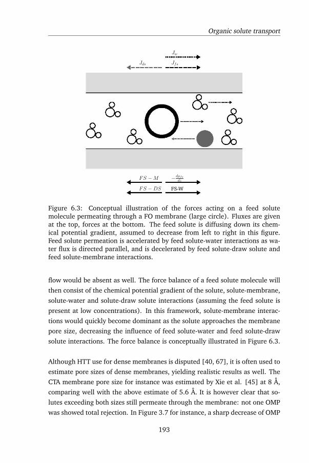
Organic solute transport
Jw
JfsJds
−dµfsdz
FS-WFS −DS
FS −M
Figure 6.3: Conceptual illustration of the forces acting on a feed solutemolecule permeating through a FO membrane (large circle). Fluxes are givenat the top, forces at the bottom. The feed solute is diffusing down its chem-ical potential gradient, assumed to decrease from left to right in this figure.Feed solute permeation is accelerated by feed solute-water interactions as wa-ter flux is directed parallel, and is decelerated by feed solute-draw solute andfeed solute-membrane interactions.
flow would be absent as well. The force balance of a feed solute molecule will
then consist of the chemical potential gradient of the solute, solute-membrane,
solute-water and solute-draw solute interactions (assuming the feed solute is
present at low concentrations). In this framework, solute-membrane interac-
tions would quickly become dominant as the solute approaches the membrane
pore size, decreasing the influence of feed solute-water and feed solute-draw
solute interactions. The force balance is conceptually illustrated in Figure 6.3.
Although HTT use for dense membranes is disputed [40, 67], it is often used to
estimate pore sizes of dense membranes, yielding realistic results as well. The
CTA membrane pore size for instance was estimated by Xie et al. [45] at 8 Å,
comparing well with the above estimate of 5.6 Å. It is however clear that so-
lutes exceeding both sizes still permeate through the membrane: not one OMP
was showed total rejection. In Figure 3.7 for instance, a sharp decrease of OMP
193
.................. ~------- -------~
&·················•
8o 0-------~ 8o 8o 8o ~---· 8o
6. Conclusions
permeability can be seen around 30 Å2, but at larger OMP sizes, permeability
appears to decay very slowly. This could be due to the polymer structure of the
membrane: CTA membranes are phase-inversion membranes of linear, non-
crosslinked polymers. As such, they do not possess the kind of pores which are
traditionally assumed in transport models, namely, long cylinders of circular
cross section. Rather, pores are voids between polymer chains, but because the
chains are not crosslinked, pore size is not well defined: large molecules could
intercalate between polymer chains, exceeding the void of the pore, and slowly
permeate through the membrane. No solute size cutoff would be seen in that
case, as appears to be the case for the CTA membrane. TFC membranes on the
other hand have highly crosslinked active layers; their pore size is thus defined.
Consequently, a relatively sharp cutoff would be expected. To further test this
hypothesis, rejection tests of long duration and including large OMPs could be
performed using both crosslinked and non-crosslinked membranes.
Salting out of organic feed solutes could have a large impact on FO process per-
formance: enrichment of organics in the membrane would make FO a rather
poor barrier against OMPs. Salting out was not universally observed: in chap-
ter 3, no negative rejection or clear signs of salting out of OMPs were found;
membrane permeability of OMPs during FO and simple diffusion was similar
(disregarding charge interactions), in contrast to the alcohols and formamide
in chapter 4. This is likely due to the concentration difference of the OMPs
compared to the organic solutes used in the negative rejection tests, and the
fact that salting out is concentration-dependent (see equations 4.32 and 4.33).
OMPs were spiked at 10 µg/L, while the organics in the negative rejection tests
were spiked at 100 mg/L or 1 g/L in the case of formamide. Taking into account
the higher average molecular weight of the OMPs, this leads to a relative molar
concentration difference of around 30 000. On the other hand, some OMPs
have a very low aqueous solubility (for instance, S0(atrazine) ≈ 10 mg/L),
which means that even at the low concentration of 10 µg/L, these compounds
are relatively closer to their solubility limit than the alcohols and formamide.
The lack of evidence for salting out could also be due to the increased steric
hindrance that the OMPs experience during membrane permeation: for the
alcohols, the sterically hindered 2-methyl-2-propanol and 2-methyl-2-butanol
also did not show negative rejection. It was predicted that their rejection would
be negative only for fluxes below 0.4 µm/s. Similarly, the effects of salting
out of OMPs on OMP rejection could be masked by steric hindrance, render-
194
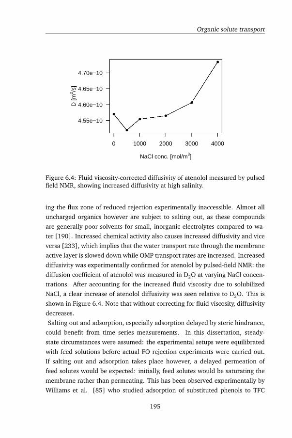
Organic solute transport
●
●
●
●
●
●
0 1000 2000 3000 4000
4.55e−10
4.60e−10
4.65e−10
4.70e−10
NaCl conc. [mol/m3]
D [m
2 /s]
Figure 6.4: Fluid viscosity-corrected diffusivity of atenolol measured by pulsedfield NMR, showing increased diffusivity at high salinity.
ing the flux zone of reduced rejection experimentally inaccessible. Almost all
uncharged organics however are subject to salting out, as these compounds
are generally poor solvents for small, inorganic electrolytes compared to wa-
ter [190]. Increased chemical activity also causes increased diffusivity and vice
versa [233], which implies that the water transport rate through the membrane
active layer is slowed down while OMP transport rates are increased. Increased
diffusivity was experimentally confirmed for atenolol by pulsed-field NMR: the
diffusion coefficient of atenolol was measured in D2O at varying NaCl concen-
trations. After accounting for the increased fluid viscosity due to solubilized
NaCl, a clear increase of atenolol diffusivity was seen relative to D2O. This is
shown in Figure 6.4. Note that without correcting for fluid viscosity, diffusivity
decreases.
Salting out and adsorption, especially adsorption delayed by steric hindrance,
could benefit from time series measurements. In this dissertation, steady-
state circumstances were assumed: the experimental setups were equilibrated
with feed solutions before actual FO rejection experiments were carried out.
If salting out and adsorption takes place however, a delayed permeation of
feed solutes would be expected: initially, feed solutes would be saturating the
membrane rather than permeating. This has been observed experimentally by
Williams et al. [85] who studied adsorption of substituted phenols to TFC
195
6. Conclusions
membranes. In their study, non-steady-state adsorption was apparent during
the first three to four hours of their experiments. Performing similar experi-
ments in FO would be quite complicated, as the FO permeate is mixed with
the draw solution. As a result, when a FO rejection test has just started, a very
small amount of permeate is mixed with the draw solution, rendering solute
detection analytically challenging and also causing significant error propaga-
tion. Given that salting out is a concentration-dependent process, depending
both on the salt and organic solute concentrations, and given that large concen-
tration gradients exist within FO membranes during operation, it is conceivable
that within a membrane, gradients of solute-membrane affinity would exist as
well. Currently, such gradients are not incorporated in any model, although
such gradients could cause higher or lower than expected rejection. Further-
more, TFC membranes are composed of multiple polymers, with each polymer
having certain surface chemistry characteristics. This could contribute to affin-
ity gradients as well.
Solute-membrane affinity was predicted to decrease with increasing salinity
due to the membrane becoming a strong monopolar Lewis base, while most
(if not all) organic compounds are much stronger Lewis bases than they are
Lewis acids, causing repulsion. Much remains unknown however: because
surface tension analysis of the OMPs was performed on solid OMP, only their
apolar surface tension component can be determined with some certainty (see
equation 3.19). It has also been shown that the surface tension of a solid is
quite different compared to the same substance’s liquid surface tension [33].
How this relates to the surface tension of a dissolved solute warrants further
study as well. Furthermore, the surface tension components of the CTA poly-
mer are apparently susceptible to electrolytes, but it is not yet known whether
this is the case as well for small organic solutes. The results presented in this
dissertation are thus at best indicative. Reduced OMP permeability seen for
the sulfate draw solutes could also be due to reduced solute-membrane affin-
ity, as sulfate salts turned the membrane into a stronger Lewis base compared
to chloride salts. This decreased solute-membrane affinity is in stark contrast
with the salting out of alcohols in chapter 4: their increased solute-membrane
affinity was necessary for negative rejection to occur. It is also expected that
the change in membrane and OMP surface tension due to salinity is different
from possible changes occurring during RO: not only is the salinity different,
but also the water activity. Consider the reference state of pure water at atmo-
196
Applying FO
spheric pressure, µ0. In FO, the water activity is reduced in order to produce
flux by the addition of a draw solute: µ < µ0. In RO on the other hand,
the water activity of the feed is increased by applying hydrostatic pressure,
producing pure water at atmospheric pressure at the permeate side: µ > µ0.
Uncertainty regarding surface tension is also introduced by the concentration
profile of draw solute across the membrane: as was shown in chapter 2, for
membranes oriented in AL-FS mode, the draw solute concentration decreases
significantly from the draw side of the membrane to the feed side. What is the
draw solute concentration at the active layer interface, and what are the effects
of the section of active layer below the interface, where the draw solute con-
centration is higher? This again leads to questions regarding solute-membrane
affinity gradients within a membrane. The study of surface tension is also a
field in which new theoretical insights are needed: there is no theory quantita-
tively predicting Lewis acid or base strength of liquids or solids and neither is
there a theory predicting their decay length [148, 33]. When applying surface
tension-based methods within membrane pores, there is the additional prob-
lem of properties of confined water and solutes, which may be different from
properties obtained from bulk phase.
6.2.3 Applying FO
The focus of this dissertation were mass transport phenomena through FO
membranes, while practical FO applications, membrane development and draw
solution regeneration were not studied. Gaining fundamental insights into
membrane mass transport phenomena would aid in the design and operation
of membrane installations. Future research recommendations specifically for
mass transport phenomena were formulated in the above sections, while in this
section FO applications are discussed and how the research presented in this
dissertation could aid in FO applications. Generally, FO membranes should
possess high solutes rejection, anti-fouling properties, adequate mechanical
strength while having low mass transfer resistance in the support layer and
chemical resistance to be able to operate in harsh environments and produce
high quality permeate. The FO process as a whole should be operated at a rela-
tively low draw solution concentration, in order to allow economically feasible
draw solution regeneration.
Membrane fouling is the most important factor limiting membrane perfor-
197
6. Conclusions
mance when using feeds containing significant amounts of suspended matter,
which would be the typical feed for FO. Results presented in chapter 5 show
the low impact of biofouling on FO, in line with the often stated low foul-
ing propensity of FO. Fouling resistance can be further increased through sur-
face modification of membranes and spacers. This is commonly accomplished
by grafting highly hydrophilic functional groups on the active layer such as
polyethylene glycol, polyglycerol, polydopamine or other zwitterionic polymers
[234, 18, 19]. The ∆G132 of foulants with a highly hydrophilic membrane sur-
face in aqueous solution is in all likelihood going to be positive: attractive
water-membrane interaction will dwarf attractive foulant-membrane interac-
tions.
Contrary to fouling, mechanical stability of FO membranes in OMBR applica-
tions has not been studied in detail yet. To this end, the author has studied
accelerated membrane abrasion at the University of New South Wales, under
the guidance of prof. Pierre Le-Clech. In MBR-type applications, membranes
can come into contact with particulate matter which could puncture or abrade
the active layer: fine screens in wastewater treatment plants (if present) typi-
cally have grid openings of 250 µm, allowing smaller particles to pass. As FO
membranes are dense membranes used in engineered osmosis processes, they
rely on the salt separating capability of their active layer. Damage to the active
layer causes increased permeability of the membrane to both water and draw
solute. This damage cannot be mitigated by cake filtration, as is the case for UF
and MF membranes: filtration cakes do not possess meaningful salt-separating
properties. HTI CTA and TFC membranes were exposed to granular activated
carbon (GAC) particles and glass beads with particle diameters of 0 to 800 µm
at elevated concentrations, which were recirculated during 24 hours at a cross
flow velocity of 0.2 m/s. Membrane damage was assessed using RO perme-
ability tests and SEM micrographs. It was found that the TFC membrane was
susceptible to abrasive damage: damage was clearly visible after exposure to
both glass beads and activated carbon particles, see panels A and B in Figure
6.5 for GAC and glass beads respectively. The damage caused by GAC was
much more severe compared to the glass beads: glass beads exposure caused
a modest permeability increase (factor of 2.5), while GAC abrasion caused loss
of salt separating capability. Glass is a harder material than activated carbon
but in these tests, damage due to GAC was much more profound. This could
be due to particle roughness: the glass beads were smooth, spherical particles
198
Applying FO
while the GAC particles had rough and jagged edges, as can be seen in Fig-
ure 6.6. In reality, both smooth and rough or sharp particles are likely to be
encountered: particles such as grains of sand which have been subjected to sig-
nificant erosion are likely to be smooth, while particles liberated from recently
ground or broken material are likely much rougher or sharper, such as shards of
glass. Curiously, surface heterogeneity of the TFC membrane was seen as well:
patches of darker colored active layer were seen where glass particles would at-
tach strongly to the membrane, see panel D of Figure 6.5. The CTA membrane
was much more abrasion resistant. After 24 hours of exposure to GAC, the per-
meability was hardly increased, and SEM micrographs only showed very small
scratches, see panel C in of Figure 6.5. Although not yet tested, it is conceivable
that the presence of a cake layer could protect the membrane: abrasion and
fouling could be competing processes for mass deposition and removal from
the membrane. Scouring with particulate polymeric material has been used as
a membrane cleaning technique [235]. These preliminary results show that
abrasion could be an important factor limiting FO membrane lifetime in OMBR
applications, unless the feed solution is sieved thoroughly in order to remove
particulate matter. If extensive pretreatment of the feed is necessary to protect
FO membranes, the cost and complexity of the treatment train increases and
the advantage of FO is diminished. The results also show that abrasion resis-
tance is strongly dependent on active layer composition, allowing membranes
to be tailored to be more abrasion resistant. Membrane integrity was assessed
by measuring salt permeability. However, the passage of pathogens (especially
viruses) through a membrane is more problematic in the case of potable reuse
of wastewater. If a virus passes through a defect in an FO membrane, it then
ends up in the draw solution. To be able to pass into the permeate, it then also
needs to pass through the draw regeneration process. For some regeneration
processes such as RO or MD, this is very unlikely, while for other processes such
as ED, this is easily achieved. This reasoning shows that a FO system needs a
double barrier: if defects are introduced in the FO membrane through physical
wear and tear, the second barrier has to safeguard produced water quality.
Currently, FO as a water reclamation process in wastewater treatment is not
yet economically viable: the generated water flux is too low. OMBRs with RO
draw solution regeneration are not yet competitive with an MF-RO-AOP treat-
ment train due to high energy use by the RO and high material cost of the FO
membranes [236]. In order for the FO process to become economically viable,
199
6. Conclusions
optimized FO membranes should be used which produce a high enough flux
at low draw solution concentration. This would simultaneously limit the mem-
brane surface area needed for a certain water production capacity, thereby
limiting capital costs, and also limit the cost of regenerating the draw solu-
tion, thereby limiting the operational costs. Water flux can be increased by
membrane modification. Specifically, flux increases can be accomplished by
increasing the permeability of the active layer and/or by decreasing ICP by
creating a thin, porous and hydrophilic support layer. Increasing active layer
permeability is possible: the use of NF-like FO membranes has been reported
[51, 237]. However, increased active layer permeability comes at a price: for
a given active layer composition, there is a trade-off between increasing the
water permeability and simultaneously decreasing solutes rejection [238]. A
decreased solutes rejection implies a higher draw solute loss and also a lower
rejection of feed solutes. The draw solute loss in turn can be limited by us-
ing relatively large molecules and/or multivalent ions. Here, a trade-off exists
as well: large solutes exhibit a relatively low diffusivity, which, due to the
spontaneous nature of FO flux, limits flux as well. Furthermore, low feed so-
lute rejection leads to accumulation of micropollutants in the draw solution
loop, as was shown in chapter 5, which would necessitate additional treatment
of the draw solution. Therefore, it seems preferable to produce membranes
showing a high selectivity rather than a high permeability. This has been ar-
gued for RO as well: additional permeability increases would hardly decrease
energy expenditure, while a higher selectivity could significantly decrease the
need for polishing or second-pass RO treatment [239]. An interesting approach
to selectively increasing the water permeability is embedding aquaporin pro-
teins or carbon nanotubes (CNT) in the membrane active layer. Incorporating
aquaporins or CNTs would increase only the water permeability without in-
creasing the permeability for other solutes, thereby avoiding the need for post-
treatment. Aquaporins are the naturally occurring water transport proteins
through cellular membranes, which allow cells to exchange water with their
surroundings. As cellular pH and ion concentrations are tightly controlled by
other membrane proteins, aquaporins display a very high selectivity towards
water transport [240]. Several research groups have studied the embedding of
aquaporin proteins in synthetic membranes instead of biological membranes,
in order to create high flux and high selectivity membranes, with the Danish
company Aquaporin currently commercializing this technology. As aquaporins
200
Applying FO
are natural proteins, embedding them in synthetic membranes and scaling up
production is challenging [241]. Similar to aquaporins, carbon nanotubes also
display a high selectivity: their apolar walls and small radius rejects ionic and
large solutes. High flux membranes could be produced from arrays of aligned
CNTs, but the production of such arrays is inherently complex and expensive
[242].
Mitigating ICP by optimizing support layer structure is another route to in-
crease flux. When synthesizing a support layer by phase inversion, pores are
formed in a polymer matrix. Close to the active layer, the support polymer can
be likened to a continuous phase, with the pores being dispersed among it.
The opposite is possible as well: synthesizing a support layer from fine poly-
mer filaments by electrospinning creates a very open, scaffold-like structure.
The tensile strength of electrospun fiber mats can be increased by (solvent)
sintering, which joins individual filaments and creates a crosslinked matrix
[243, 244]. The porosity of electrospun support layers is reportedly in the
range of 80 - 85 % [245]; according to the relation of tortuosity as a func-
tion of porosity proposed by Tomadakis and Sotirchos for random arrays of
overlapping cylinders, the corresponding tortuosity is 1.08 - 1.11 [246, 49].
These properties are vastly superior to those of phase inversion support layers:
the porosity and tortuosity obtained for the HTI CTA and TFC membranes in
chapter 2 were in the order of 0.5 and 1.8 respectively. Electrospun support
layers of FO TFC membranes have shown to yield high fluxes, with the fluxes
obtained in AL-DS and AL-FS mode being very similar, which shows that ICP is
strongly reduced [245, 53]. Song et al. [245] reported water fluxes in excess
of 30 L/(m2h) using a NaCl 0.5M draw solution, compared to 6 L/(m2h) for
the HTI CTA membrane. However, the decreased surface area of support layer
polymer at the top face of the support layer causes weak attachment of the
polyamide layer to the support layer, causing delamination and membrane fail-
ure [53], similar to support layers having too large pores at their top face [52].
To provide adequate backing, it appears that a thin transition layer between
the electrospun support and the active layer is needed, with all layers being co-
valently attached to neighboring layers to prevent delamination, at the cost of
ICP increase. Another membrane modification to increase water flux is increas-
ing the support layer hydrophilicity. Commonly used support layer polymers
such as PES are hydrophobic, which hinders wetting of pores. Consequently,
some pores remain filled by air. As these gas-filled pores are not contributing to
201
6. Conclusions
water and draw solute transport, the effective structural parameter increases
[54]. Support layer hydrophilicity can be increased by coating it with poly-
dopamine [247] or ionic surfactants [53] or by flushing the membranes with
solvent solutions (such as isopropanol) which do not damage the active layer
and lower the solution’s surface tension [48]. Decreasing ICP only comes with
one trade-off: the support layer has to provide sufficient mechanical strength
to the membrane. As long as this is the case, decreasing ICP is purely bene-
ficial. Compared to increasing active layer permeability, ICP mitigation seems
preferable.
As membrane performance increases and internal mass transfer resistance de-
creases, external mass transfer resistance becomes limiting. When using con-
ventional CTA or TFC membranes, ECP for small organic and inorganic solutes
is often negligible. If membrane flux increases however, this is no longer the
case, at which point module and spacer design will have to optimized as well.
Ultimately, external mass transfer is the limiting factor in membrane processes,
as the transport of rejected solutes or draw solute in the laminar boundary
layers is dependent on solute diffusivity. It would be interesting to model the
maximal attainable flux in FO, based on the diffusivity of water and draw so-
lutes for a theoretical membrane possessing a completely porous support layer.
This would then represent a best-case scenario, after which realistic membrane
properties can be added. The best-case scenario could then be used to compare
real membranes with, in order to quantify their degree of optimization.
FO membranes and applications are in the midst of an intensive research and
optimization effort. Although impressive results have already been obtained in
terms of tailored membranes and FO system design, there is still room for im-
provement: the above discussion shows that there are many parallel research
topics for improving FO membranes. Different areas of optimization could
furthermore be combined as well. As to the applicability or price of FO: FO
applications are inherently fairly complex and energy-intensive, as at least 2
processes are needed to produce fresh water and a concentrate stream from an
impaired water source. The choice of using FO on a certain feed stream will
therefore depend on the value or disposal cost of that feed stream and whether
less complex treatment options are applicable. From a thermodynamic point
of view, FO is inefficient: water from an impaired feed stream with an activ-
ity lower than unity first moves to a solution of even lower water activity, after
which pure water is extracted from the former solution at a higher cost in terms
202
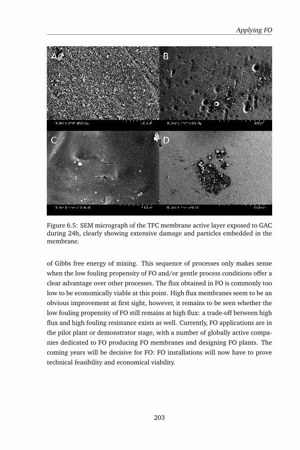
Applying FO
Figure 6.5: SEM micrograph of the TFC membrane active layer exposed to GACduring 24h, clearly showing extensive damage and particles embedded in themembrane.
of Gibbs free energy of mixing. This sequence of processes only makes sense
when the low fouling propensity of FO and/or gentle process conditions offer a
clear advantage over other processes. The flux obtained in FO is commonly too
low to be economically viable at this point. High flux membranes seem to be an
obvious improvement at first sight, however, it remains to be seen whether the
low fouling propensity of FO still remains at high flux: a trade-off between high
flux and high fouling resistance exists as well. Currently, FO applications are in
the pilot plant or demonstrator stage, with a number of globally active compa-
nies dedicated to FO producing FO membranes and designing FO plants. The
coming years will be decisive for FO: FO installations will now have to prove
technical feasibility and economical viability.
203
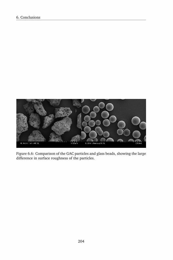
6. Conclusions
Figure 6.6: Comparison of the GAC particles and glass beads, showing the largedifference in surface roughness of the particles.
204

Chapter 7
A wider scope:the water crisis and technological so-lutions for environmental problems
205
7. A wider scope
Throughout this dissertation, FO, a high-tech water treatment technology was
explored, without justifying in detail why such a high-tech technology would
be needed in the first place. Therefore, in this chapter, I will briefly discuss the
water crisis humanity is currently facing and will increasingly face in the com-
ing decades. The applicability and capability of technology in alleviating this
crisis will be highlighted. Lastly, more generally, the ecological crisis humanity
is causing and the role of technology in that crisis will be briefly discussed as
well, where it will be shown that purely technological solutions are inherently
insufficient to avert the destruction of earth’s ecosystems.
7.1 The water crisis
Humanity uses a tremendous amount of water, mainly for agricultural pro-
duction, and to a lesser extent for industrial production and for direct hu-
man consumption. Available, renewable fresh water is liquid water which is
provided by solar-powered precipitation. Fossil fresh water reserves exist as
well, such as deep aquifers in desert areas, but these resources are not replen-
ished and tapping them causes depletion. The available, renewable fresh water
moves through the hydrological cycles by evapotranspiration (ET) and runoff
to sea. In 1996, humanity already appropriated 26 % of global ET amounting
to 18200 km3/y, and 17% of runoff amounting to 6780 km3/y [248]. In total,
this amounted to 23% of all renewable fresh water supply being used by hu-
manity. However, in the case of runoff, about 70% is unavailable because of the
remoteness of its location (arctic regions, rain forests) and because about half
of the runoff is stormwater, which is produced at massive flow rates in short
time spans due to intense precipitation which cannot be contained. Taking the
availability into account, appropriation of runoff in 1996 rises to 54%. Since
1996, the world population has grown from with 1.6 billion people from 5.8 to
7.4 billion in just 20 years, which obviously results in increased appropriation
as well. The growth rate of runoff withdrawal is estimated to be 10 - 12 %
every decade [249], while the growth rate of ET appropriation is assumed to
be much smaller. The latter is due to ET appropriation being linked to agricul-
tural production, and the potential arable land being almost completely used
by now [248, 250]. This means that humans, a single species on this planet,
are currently consuming around 30% of all planetary available fresh water. To
put this into perspective, humanity annually uses an amount of fresh water suf-
206
The water crisis
ficient to entirely flood Belgium with a 1 kilometer thick layer of fresh water.
Agricultural production is by about an order of magnitude the largest consumer
of fresh water. According to the United Nations, human fresh water consump-
tion is categorized as 75% going to agriculture, 20% to industrial production
and 5% to direct human consumption [249]. The share used in agriculture
has been estimated to be much higher still by Hoekstra and Mekonnen at 92%
[251], with industry and direct consumption being 4.4 and 3.6% respectively.
Regardless of the exact value, agricultural water consumption is inherently
very high: plants rely on evaporation to transport nutrients and photosynthate.
Physiological water use of plants ranges from 320 - 800 g water/g dry biomass
produced; taking into account water evaporated from soil or paddies, this ra-
tio increases to 1000 for highly efficient drip irrigation systems, and reaches
a global average of 5000 g water/g dry biomass [252]. For modern staple
crop breeds, annual harvestable photosynthate is around 50% of total produc-
tion; the specific water consumption of edible plant products rather than plant
biomass is thus twice as high as the above ratio [252]. For animal products,
the specific water consumption is much higher still: the water consumption of
animal feed production has to be multiplied by the animals’ feed conversion
efficiency, to which the water directly consumed by the animals and other ser-
vice water is added [253]. Unsurprisingly, water consumption per calorie of
beef is 20 times larger than per calorie of cereals; water consumption for beef
production averages 15.4 m3 water/kg meat. Even the most efficiently pro-
duced animal products, being milk, eggs and chicken meat, require 1.5 times
more water than protein-rich pulses [253]. Eating a modestly-sized steak of
100 g is thus coupled to a water consumption of about 1.5 m3, more than ten-
fold the daily per capita drinking water consumption of the average Belgian!
Assuming for instance a very modest daily diet consisting of 300 g of dry plant
products produced at an average 5000 g water/g biomass and 100 g of chicken
meat yields an associated water consumption of about 2 m3, roughly equal to
2 weeks of average per capita Belgian water consumption. Compared to the
water needed to produce our food, the amount of water directly consumed as
drinking water becomes almost negligible.
Despite drinking water being a tiny fraction of our water consumption, in 2008,
1.1 billion people did not have access to improved drinking water facilities, and
2.4 billion people did not have access to sanitation facilities. Consequently, sur-
face water is polluted by faecal matter in regions where sanitation facilities are
207
7. A wider scope
lacking. This causes 2 million deaths annually, mostly of children under the age
of 5, due to water-borne diseases [249]. Thanks to efforts made as outlined in
the Millenium Development Goals, access to safe drinking water has improved,
halving the number of people lacking access compared to 2008 by 2015 [254].
After consumption, water is either transformed into wastewater or is lost to
evaporation. During agricultural production, especially plant production, con-
sumed water is predominantly lost to evaporation. Industrial and household
consumption of water returns a significant portion as wastewater: annual
wastewater production is estimated at 450 km3, of which 330 km3 is domestic
wastewater [23]. Hoekstra and Mekonnen [251] calculated that the wastew-
ater footprint (all sources combined) is 15% of the total water human foot-
print, a higher estimate than the former. Compared to the above mentioned
amounts of annually consumed water in agricultural production, the volume
of wastewater produced is small: it is smaller by about an order of magnitude.
It can thus be concluded that wastewater reuse can at most augment fresh wa-
ter needs in agriculture, but cannot substitute for precipitation or ground water
stocks. Wastewater reuse can however be of added value in arid or other water-
stressed regions, increasing the otherwise limited supply of drinking water or
industrial water. Depending on the origin of the wastewater and the intended
use of reclaimed water, different treatment options are available, each having
associated capital, energy and material costs.
Providing potable water, be it from surface or ground water, reused wastewater
or seawater desalination, costs a considerable amount of energy. The energy
cost of producing potable water from surface or ground water varies strongly,
with the main determining factor being pumping energy. Often, ground water
and surface water are of high initial quality, so the treatment and disinfection
cost is low. Producing water from deep aquifers or transporting water over
long distances increases the embedded energy cost. For instance, the specific
pumping energy cost for drinking water in the state of California varies from
0 kWh/m3 for gravity-fed collection and distribution networks in the more hu-
mid, northern part of the state to 3.7 kWh/m3 in the dry, southern part of
the state, where water is pumped in from hundreds of kilometers away and
over significant elevation. Treatment costs of high quality fresh water sources
are low: in the order of 0.025 kWh/m3 [255]. The treatment cost increases
as the source quality decreases: seawater desalination, at 50% recovery, car-
ries a thermodynamic minimal energy cost of 1.06 kWh/m3. State-of-the-art
208
The water crisis
seawater RO desalination process stages are able to produce fresh water at
1.8 kWh/m3, at an impressive 60% thermodynamic efficiency; when pre- and
post-treatment are included however, the energy cost at plant-scale increases
to 3 - 4 kWh/m3 [256]. Energy use at plant-scale could be reduced if higher
selectivity membranes can be used: post-treatment to remove boron or dis-
infection byproducts such as NMDA would then be superfluous [239]. Direct
potable reuse of wastewater (DPR) at present is typically realized using a treat-
ment train of conventional activated sludge → MF or UF → RO → AOPs. FO
opens very interesting perspectives in DPR: by harvesting water from wastewa-
ter or resulting wastewater treatment sludges, a concentrate is simultaneously
produced rich in organic carbon and nutrients as well as clean water, which
is referred to as the "Sewer Mining" concept. This concentrate can be put to
use: nutrients can be recovered [257, 27, 28], while the organic carbon can
be converted into energy [258] or chemical products [259, 260, 261]. When
using FO and RO in a closed-loop, the accumulation of micropollutants in the
draw solution loop poses a significant problem, as was shown in chapter 5. At
locations near an ocean, this problem can be avoided by using seawater as the
draw solution in a once-through mode [211]: wastewater is contacted with
seawater through an FO membrane, after which the diluted seawater is used
as an RO feed. This system has the advantage of simplifying the DPR treatment
train: ideally, the activated sludge stage, MF/UF and AOPs can be omitted. In
terms of energy use and cost, conventional DPR and FO-RO are comparable,
an advantage for FO has been reported [262], while others find the conven-
tional treatment train still outperforming FO [236] with the main disadvantage
being the low flux during FO. In terms of economic viability, low FO flux has
also been shown to be the main limiting factor [263]. FO-RO, seawater desali-
nation and conventional DPR all have quite comparable energy expenditures
[262]. All 3 processes use RO, and although in FO-RO and conventional DPR
the osmotic pressure of the RO feed solution is reduced or is negligible respec-
tively, the energy savings are expended by additional processes such as FO or
the pre- and/or post-treatment of the RO stage. This leads to the conclusion
that wastewater reuse is expensive compared to treating already high qual-
ity surface or ground water: in terms of energy, the difference is 2 orders of
magnitude. Potable reuse is therefore limited to water-stressed regions, where
conventional drinking water sources are overdrawn, such as California, Bel-
gium [264] and Singapore. There is still a considerable margin for innovation
209
7. A wider scope
to bring the energy and economic cost of desalination and DPR down, by ap-
proaching the thermodynamic limit of desalination closer at plant-scale and by
valorizing concentrates.
If agricultural production is constrained by the availability of fresh water, sea-
water desalination can augment supplies of irrigation water, either directly or
indirectly through agriculturally reused wastewater originating from desali-
nated seawater. Irrigation water produced through desalination needs to be of
higher purity than potable water: boron and chloride levels have to be reduced
more than for potable water. This can be done for instance by a second pass
RO [265, 239], with obvious increased energy costs, rasing total energy costs
to 3-7 kWh/m3. In this paragraph, the use of desalination to provide water for
staple crops and high value crops will be explored. Staple crops are starchy
and protein rich crops produced at high-volume, being maize, wheat, rice and
soybeans; these crops provide the bulk of calories and protein consumed by
humanity and our livestock alike, and are responsible for about half of all agri-
cultural water consumption [266]. Piringer and Steinberg [267] calculated
for wheat an average embedded energy cost of 3.9 MJ/kg or 1.08 kWh/kg of
dried grains in the US, with half of this cost originating from nitrogen fertil-
izer. Assuming as a worst-case that all water is supplied through desalinated
irrigation water, and an average crop water usage of 5000 g water/g biomass
and 50% harvestable biomass, 10 m3 water/kg dried wheat is needed. It is
immediately clear that providing desalinated seawater as irrigation water is
energetically very costly: even at a state-of-the-art performance of 3 kWh/m3,
the energy cost of the desalination alone is 30 times the current energy cost of
the finished product, not including pumping energy expended for water trans-
port between desalination plant and fields. Assuming an electricity cost of 0.12
C/kWh [268], best case desalination would cost close to 4 C/kg wheat, roughly
25 times the price at which this commodity is currently traded. Clearly, desali-
nation cannot provide irrigation water for staple crops, neither energetically
nor economically.
For high-value, high-productivity crops, grown in greenhouses and/or drip-
irrigated, using desalinated or recycled wastewater can be profitable. Crops
include fruit and vegetables, such as tomatoes, peppers, fruit trees and vine-
yards: their high value reduces the impact of a high water cost. Because de-
salinated water contains almost no dissolved solids before remineralization,
desalinated water can leach salts from salinized soils during irrigation, restor-
210
The water crisis
ing productivity to those soils, or can be blended with relatively saline locally
sourced irrigation water [269]. Practicing drip-irrigation in greenhouses vastly
increases the water use efficiency as mentioned earlier, but comes at a steep
material and energy price: for drip irrigation, a cubic meter of water saved
compared to flood irrigation comes at the cost of one liter of oil [252]. FO can
be applied as well in this setting: using concentrated fertilizer solution as draw
and wastewater as feed, a sufficiently dilute fertilizer solution can be produced
[270]. Although the energy cost of this type of crop production is high, yield
and value of the produce is high as well. This type of production is common in
Mediterranean and Middle Eastern countries; notably, Spain and Israel make
extensive use of desalinated irrigation water [269]. No clear conclusions can
be drawn with regards to the desirability of using desalinated irrigation water
for high-value crops: crop production in greenhouses is energy-intensive in any
case. Fresh produce is also refrigerated during storage and transport, with the
latter commonly being truck or plane transport which is more energy-intensive
than bulk transport of dried staple grains [271]. In other words, there are
many other sources of energy and capital expenditure in the life cycle of high-
value crops apart from using desalinated irrigation water.
Throughout this section, it is clear how closely water and energy are linked:
energy is needed during transportation, treatment and sanitation of water.
Likewise, water is needed during energy production: for instance, as energy
carrier in hydro-electric installations, as cooling water in thermal power sta-
tions or during fuel extraction and mining processes. This is referred to as the
"water-energy nexus", as both high-quality fresh water and energy are becom-
ing scarce and are closely intertwined. To further summarize this section, a
few conclusions can be drawn. Firstly, humanity is claiming a disproportion-
ately large share of the planet’s available fresh water and, in spite of that, is still
faced with water stress and shortage. Most of this appropriated water is used
in agriculture, with food products having large embedded water costs; animal
products stand out in this regard. Despite the relatively small amount of appro-
priated water being used as drinking water, vast numbers of people still do not
have access to safe drinking water. Many more people do not have access to
sanitation facilities. This is mostly an economical problem: the production and
distribution of safe drinking water and collection and sanitation of wastewater
are energy- and capital-intensive processes; some developing countries cannot
afford these investments and/or lack the infrastructure to sustain them. It was
211

7. A wider scope
also shown that seawater desalination is already a fairly efficient process, while
efficiency gains and new added value products in water sanitation are possible
and wanted. Due to the inherent high energy cost of desalination, agricultural
use of desalination is limited to high-value crops grown in energy-intensive
settings. Staple crops provide the vast majority of calories and protein for hu-
manity and its livestock, but these crops cannot be grown using desalinated
water from both an economical and energetic point of view.
7.2 The need for a contraction of human activity
Humanity is currently causing an unprecedented ecological crisis, with the wa-
ter crisis described above making up only a small part of it. Symptoms of
this ecological crisis are, among others, biodiversity loss, climate change, the
depletion of non-renewable and renewable feedstocks and pollution of water,
land and air. Attempts to solve this crisis up until now are heavily focused on
providing technological solutions, however, our continued strive for economic
growth and total disregard of demographic growth is hardly questioned at all.
In the preceding section, the water crisis was briefly sketched, showing that it is
mostly a problem at the supply side: humanity appropriates a very large share
of the global fresh water supply, causing water stress and water shortages, and
is increasingly forced to resort to energy-intensive means to acquire sufficient
amounts of fresh water. Below, I will formulate 3 separate, stand-alone ar-
guments as to why technological solutions will not solve our environmental
problems and why our disregard for the negative consequences of economic or
demographic growth is exacerbating the current crisis.
The first argument is based on thermodynamics. Planet earth is a system of
finite size, finite energy stores which receives a finite energy flux as solar radi-
ation. Our whole life and everything we do in it, from a physical point of view,
are non-spontaneous processes. In fact, non-spontaneous processes are what
separates living organisms from non-living matter. Non-spontaneous processes
inherently cost energy, and have a theoretical, entropy-neutral lower bound-
ary below which it is impossible for the process to continue. Real processes
inherently produce entropy, so the lower limit cannot be reached and conse-
quently the true energy cost of any process is higher than the theoretical limit.
The above argument is valid for biological as well as technological processes,
and thus has wide ramifications. For living organisms, minimal nutritional re-
212
Contracting human activity
quirements and maximal growth rates are imposed by thermodynamic consid-
erations: photosynthetic production is ultimately constrained by solar energy
flux, animal growth rates are likewise constrained by energy density and di-
gestibility of feed, and sustaining highly structured and coordinated cellular
and bodily functions inherently costs energy. Consequently, a certain amount
of food has to be produced in a certain amount of time to feed humanity, which
can be regarded as a "nutritional flux". The limited growth rate of crops and
livestock inevitably leads to the parallel production of large numbers of plants
and animals on a large surface area, rather than serial production of small
numbers of plants and animals on a small surface area at a very high rate in
order to sustain this nutritional flux. This inevitably leads to high land us-
age for agricultural production to feed the human population. Efficiency gains
through technological interventions or the changing of dietary preferences in
favor of plant-based, low-impact diets cannot indefinitely offset increased land
usage due to population growth; these measures merely allow us to approach
the thermodynamic optimum more closely on a per-capita basis. This analysis
shows that, in an optimized agricultural production system, land use for agri-
cultural production grows proportional with human population growth. This
leads to the conclusion that indefinite population growth cannot be sustained:
at some point, land requirements, water, fertilizer and/or energy inputs needed
would exceed the amounts of those inputs available on our planet, even if
our food production system and diets would be 100% thermodynamically opti-
mized. This also shows why a large human population inevitably causes a large
loss of natural ecosystems and the biodiversity harbored in those ecosystems:
land cannot be used to sustain a high biodiversity and to produce agricultural
output simultaneously: in agriculture, primary photosynthetic production is
harvested either for direct human consumption or to feed livestock, rendering
primary production capacity unavailable for non-domesticated organisms. This
is called human appropriation of net primary production (HANPP). Currently,
HANPP is estimated at 25% [272, 273], although a higher estimate of 40%
has been calculated as well [274]. Land area modified by human activity now
stands at 54 ± 5 % [275], the 46% as of yet unaltered includes deserts, arctic
tundra and high mountain ranges - land unsuitable for agriculture or human
habitation. Clearly, there is not much room left for growth: our species is al-
ready occupying literally half of our planet, with the remaining half being of
significantly inferior quality. Humanity must urgently face the inevitable con-
213
7. A wider scope
sequences of demographic growth. Although optimization might allow us to
cram evermore people into this world for some time to come, quality of life for
humanity and the quality of the ecosystems on which we depend will increas-
ingly suffer [276].
For man-made goods, services and technological processes, the minimal energy
cost likewise imposes some constraints. If we consider that a rising standard
of living is correlated with increasing consumption of goods and services, then
a high standard of living inherently has a large ecological impact as well. Pro-
duction of goods and services can be made more efficient, but likewise, there is
a lower limit of energy use, below which the product or service can no longer
function. In environmental economics, the energy use per amount of GDP pro-
duced is a widely used metric to assess energy efficiency of the economy as a
whole. Decoupling of GDP from energy implies that for each amount of en-
ergy used (or greenhouse gases emitted), a larger amount of GDP is produced,
which enables continued economic growth without increasing the associated
ecological burdens [277]. Given that there are lower limits to the produc-
tion and use efficiency of all goods and services, decoupling economic growth
from ecological burden is equally finite. The thermodynamic argument clearly
shows the need to switch to a no-growth system, both economically and de-
mographically: indefinite growth and indefinite efficiency gains are physically
impossible.
A second argument is based on consumer behavior and the dynamics of eco-
nomic growth. Technological innovation will generally yield optimized, more
efficient, more user-friendly and more widely applicable goods and services.
Although energy, water or material cost for a single unit of production or con-
sumer consumption might have a lower ecological impact compared to the
obsolete products, the general improvement and lower cost of the new prod-
uct or service will induce increased consumption, thereby partially or com-
pletely offsetting efficiency gains. Part of this dynamic is known as the Jevon’s
paradox: an increased production efficiency causes a product-specific price de-
crease, which then causes increased consumption depending on demand elas-
ticity [278, 279]. A more general reformulation is offered by the Khazzoom-
Brookes postulate [280]. There are examples abound: increasing fuel effi-
ciency of combustion and jet engines has led to a massive increase in road
transport and airborne travel, which in the decades after World War II became
safe and accessible to the general population. Likewise, high performance and
214
Contracting human activity
efficient mass production of electronic devices enabled a total diffusion of these
appliances in society. For all of these appliances or services, it holds true that
on a specific use basis, use has become more efficient: for example, fuel usage
per passenger per kilometer of air travel was in 2000 only 30% of the 1960
level [281]. At the same time, worldwide increased use of these appliances or
services is vastly overshooting any efficiency gains: fossil fuel consumption is
still increasing at a rate much higher than population growth [277]. In our
dietary pattern, the same mechanism can be discerned: optimization of agri-
cultural practices, mainly during the first half of the 20th century, has led to a
large increase in the consumption of animal products in developed countries,
and the same shift is apparent in countries where the general population has
seen an increased standard of living in recent years [252]. The above examples
clearly illustrate decoupling of energy use from GDP growth, but only relativedecoupling is seen: the GDP grows much faster than energy or material use,
but the latter either remains steady or grows at a slower pace. Absolute decou-
pling, GDP growth combined with decreasing energy and material use, is not
observed [277]. An additional effect of the Khazzoom-Brookes postulate is that
efficiency gains of a certain product which are not (completely) offset by in-
creased consumption of the same product, can still be offset by consumption of
other products. The reason is that consumer expendable budget has increased
due to the non-offset efficiency gains, after which that increased budget can
be spent on unrelated consumption. It follows that an actual decrease of the
environmental burden associated with consumption through production opti-
mization can only be attained if rebound effects are actively avoided through
policy measures [278, 282]. This leads to the conclusion that technological
innovation alone will not bring about a decrease of humanity’s ecological bur-
den.
A third argument is based on the symptoms of the ecological crisis itself. Anal-
ysis of the damage caused to our planet allows the categorization of the symp-
toms of this crisis, as well as ranking their severity. This analysis [283, 284]
shows that the most severe damage is being done to our planet’s biodiversity.
Humanity is causing extinction of other species at an unprecedented rate: our
profound negative influence on global biodiversity is called the "Holocene ex-
tinction" or "6th mass extinction event". We are well on our way to match the
damage done by the impact of the Chicxulub comet 65 million years ago, which
wiped out nearly all large reptile species and paved the way for mammalian
215
7. A wider scope
species to become dominant. Humanity played a major role in the quaternary
extinction event, in which the majority of megafauna (animals being as large or
larger than humans) became extinct at the end of the last ice age: much of this
damage was done in pre-industrial or even pre-agricultural times due to the
susceptibility of these species to hunting [285, 286]. At present, between one
quarter and half of all mammalian, shark, coral, amphibian and reptile species
are threatened with extinction. The victims of this current wave of extinction
are much smaller animal species and plants, the main reasons for their demise
are habitat loss and habitat fragmentation [287]. As mentioned earlier, human-
ity currently claims half of all available land. Moreover, the species currently
threatened, even if they would not go extinct, have been reduced significantly
in numbers and have consequently lost most of their genetic variability. This is
also a form of biodiversity loss, which is less obvious than complete extinction,
but is affecting many more, if not almost all, species on earth. This intraspecies
loss of biodiversity increases the susceptibility of the affected species to in-
breeding, genetic drift, diseases and decreases their resilience in the face of
changing environmental conditions, such as climate change or habitats altered
due to human activity. Stopping further biodiversity loss has a very straight-
forward but similarly impossible solution: immediately stopping further appro-
priation of wilderness by humanity, combined with restoration of biodiversity
within land used for human purposes. Both protective and restorative mea-
sures obviously do not require technology; rather, they are the absence of it.
Currently, however, it is very unlikely that either measure can be implemented
at a meaningful scale: human population increases with more than 80 million
per year, and is set to almost reach 10 billion in 2050, an increase of 35% in
as many years [288]. As discussed earlier, land use for agricultural production
changes proportional to human population for optimized systems, so increasing
or even maintaining the current area of wilderness or similar high-biodiversity
regions is highly unlikely in the coming decades. Given that land most suitable
for agriculture has long been cultured [252, 275, 289], this vast population
increase will make feeding humanity challenging as well. For the decades after
2050, the outlook is actually worse still: UN population models do predict a
slowing down of human population growth, but growth is sustained through-
out the entire 21st century, set to reach 11.2 billion by 2100 [288]. In fact,
without deliberate intervention, human population will not decrease sponta-
neously: no population model predicts a global spontaneous fertility decrease
216
Contracting human activity
below replacement level [288].
The second most severe ecological problem according to the analysis by Rock-
ström et al. is climate change [283, 284]. Switching from fossil fuels to renew-
able energy, or at least to carbon-neutral energy sources, obviously demands
considerable technological intervention. However, we do not have time left
for the various types of research (from basic to applied research) and prod-
uct development needed to introduce new energy sources at full scale: we
are close to surpassing the safe limit of temperature change which has been
agreed upon by the IPCC and world political leaders. The safe limit was set at
1.5°C temperature increase at the United Nations Climate Change Conference
of 2015 in Paris, while the previously agreed upon limit was 2°C. Currently,
global average temperatures have already increased with 1.35°C compared to
pre-industrial times, and "committed" temperature increases are very likely to
surpass both safe limits [290]. Committed temperature increase is the final
increase when a new thermal equilibrium is reached based on current green-
house gases concentrations, as there is a decades-long lag between the emission
of greenhouse gases, the actual temperature increase of the atmosphere over
land and the effects of that temperature increase on terrestrial ecosystems. For
marine ecosystems, the lag time is much longer still. This implies that in order
to stop climate change within safe bounds, ambitious and far-reaching actions
are very urgently needed, which go well beyond the gradual introduction of
carbon-neutral energy sources. In other words, climate change will have to be
fought in the coming decades with the technology already at hand and with
non-technological societal and lifestyle changes.
The author is not optimistic with regards to the ecological crisis humanity is
causing. In my opinion, the most pressing issue is finding a way to manage de-
mographic and economic contraction, so that this contraction can be achieved
in a controlled and peaceful manner, which then transitions into a stable, no-
growth system. There is currently no consensus on how to transition from our
current system to a no-growth system, worse still, there is no consensus either
on how a no-growth system would function. Even worse still, there is signifi-
cant disbelief and resistance to change with regards to the ecological problems
humanity is causing, and there is doubt about the inherent feasibility of a no-
growth system. Simply halting the growth of physical resource claims and rates
of pollution is not enough: for instance, the rate of greenhouse gas emissions
and fossil fuel usage have to decrease to practically zero as soon as possible
217
7. A wider scope
if we are to avoid catastrophic climate change, and our current high-intensity
agricultural system is dependent on vast amounts of fossil fuels and phosphate,
all mined from non-renewable ores [24]. A controlled, peaceful economic and
demographic contraction has however never been achieved: contraction has
so far only occurred in times of crisis. Additionally, the longer we wait to take
action, the more drastic those actions have to become to avert catastrophic
damage, and the less likely those measures are to succeed. A first stark warn-
ing on the unsustainability of society was given by the Club of Rome (CoR) in
1972, a warning which was then attacked and disregarded. Recently, the CoR
model predictions of the period 1972 - 2012 have been compared to statistical
data, showing how our current trajectory is mostly following the CoR businessas usual scenario, with discrepancies tending towards the comprehensive tech-nology scenario. In the latter scenario, society is assumed to make a concerted
effort to maximize resource extraction through technological innovation. Both
scenarios are predicted to lead to resource depletion and system crash by the
end of this century, with the comprehensive technology scenario undergoing a
more abrupt and severe crash [291].
It is one of the defining characteristics of our species to modify our surround-
ings through technological intervention rather than abide by constraints im-
posed by our surroundings. In the last few centuries, the expansion of our col-
lective knowledge and technological innovation has been truly impressive and
unprecedented. Now, we are increasingly facing constraints not simply from
our surroundings but from our entire planet. Environmental technology can
assist humanity in organizing a stabilized society with minimized ecological
impact, but this can only be done when humanity decides to respect funda-
mental planetary constraints.
218

Acknowledgements
When I started working at PaInT, I didn’t know anything about membranes
and had forgotten quite a bit of the maths and physics from the early years of
Bioscience engineering - who needs those if you’re graduating in genetics and
microbial biotechnology, right? The subject Arne was proposing did sound very
interesting though - a technology to harvest pure water from heavily polluted
sources, hardly impacted by fouling. So, I bid goodbye to biotech and dived
into membrane science. A decision I haven’t regretted a single day!
Arne, thank you for giving me the opportunity to work and study at PaInT.
Thank you for offering ideas, for proofreading my texts, and for the trust when
experiments didn’t go right or dragged on too long. I’ve seen our group grow
at an impressive rate thanks to your ambition and immense dedication, and I’m
sure the future of our group is bright as well. I’ve also really enjoyed working
at PaInT: your enthusiasm and upbeat mood are inspiring.
Paul, although we haven’t worked closely together, I want to thank you for your
occasional theoretical input. I’ve come to know you as a kind, thoughtful and
astoundingly intelligent person.
Marjo, Seba and Klaas, you were there from quite early on as well. Thanks
for the good times we’ve had over the years. Marjo, apparently we’re not only
good office mates, but we’re also good at koala spotting! Seba, thanks for
the many chats and tips on wildlife spotting, running, cycling, ... Best of luck
finishing your PhD in the coming year. Klaas, thanks for the many, many HPLC
samples you’ve diligently injected, as well as for the South Park-related (and
other) banter.
Cristina, we ended up working together a bit longer than one summer. I’m glad
that project yielded such a nice result - thanks to your commitment. Thank
you for the Friday evenings at Koepuur, and thank you for teaching me some
interesting Italian vocabulary.
219
My other PaInT and ISOFYS colleagues, thanks for the great atmosphere in the
labs, the after work football matches or running sessions or just general banter.
A special thanks to our international visitors Machawe, Oranso and Gaetan.
Machawe and Oranso, you were in Ghent as well from very early on. It was
really fun hosting you, and I’ve come to appreciate the courage it takes to be
so far away from home for extended periods of time. Gaetan, thanks for you
hospitality, whether in Ghent, Sydney or Girona. I’ll be happy to reciprocate
any time.
Pierre, thank you for hosting me at UNSW, despite all the administrative barri-
ers. I’ve had a great time in Sydney, both professionally and personally. Thank
you for being so welcoming and engaged in our project. Barbara, a big thank
you being such a great host. I’ve met heaps of cool people in Sydney, in large
part thanks to you.
To all of my former thesis students, thanks for the effort you’ve put into this
project. To the students in general, thank you for the great atmosphere in the
lab, and the occasional lab and Christmas parties.
I also want to thank the members of my board of examiners for their construc-
tive criticism. Your comments have greatly improved the quality of my thesis.
I would also like to acknowledge the Interreg project IMPROVED, which par-
tially funded this research.
Naast het werk zou ik graag ook mijn vrienden en familie bedanken.
Aan mijn familie en schoonfamilie: bedankt voor de praktische hulp onderweg
en de interesse in mijn doctoraat. Met deze thesis is het hopelijk duidelijk wat
ik de afgelopen jaren gedaan heb.
De Boys, bedankt voor de alumni-weekends en dinner parties. De kans bestaat
dat ik in de academische wereld blijf rondhangen, dus jullie kunnen nog lang
volhouden dat ik niet werk. Stephanie, dankzij jouw contacten zijn we in Wit-
Rusland geraakt - een onvergetelijke ervaring. Veel succes met je doctoraat!
Pieter-Jan, Chloë, Thomas, Steven, Gijs: een dikke merci voor de fietstochtjes,
barbeques en feestjes de afgelopen jaren. Heel leuk ook dat jullie in Gent zijn
gebleven!
Pieter, al heel lang zijn we compagnons de route, zelfs in academia. Mogen er
nog veel streekbier- en metal-avonden volgen!
Last but definitely not least: een speciale dankjewel voor Stien. Dankjewel
om mijn gebrek aan tijd en aandacht voor je de afgelopen jaren te tolereren.
Dankjewel om me praktische beslommeringen uit handen te nemen. Dankjewel

om mijn grootste supporter te zijn, ik ben graag ook die van jou!

Curriculum Vitae
Personal information
Arnout K.H. D’Haese
°18 - 01 - 1986
Peter Benoitlaan 147
9050 Gentbrugge
Belgium
+32 497 046134
Email: [email protected], [email protected]
Education
2004: High school, Sint-Lodewijkscollege, Lokeren
Ancient Greek - Mathematics 6
2010: Master in bioscience engineering, cell- and genebiotechnology,
Ghent University
Master scription: Biochar as a soil amendment in polluted and unpollutedsoils (Dutch)Graduated with distinction
2011 - present: Doctoral training program, Doctor in Applied biological
Sciences: Environmental technology
Current position: Assisting Academic Personnel
223
Publications
2013
A. D’Haese, P. Le-Clech, S. Van Nevel, K. Verbeken, E. R. Cornelissen, S.
J. Khan, A. R. D. Verliefde, Trace organic solutes in closed-loop forward
osmosis applications: Influence of membrane fouling and modeling of
solute build-up, Water research 47 (14) (2013) 5232–5244
2014
M. M. Motsa, B. B. Mamba, A. D’Haese, E. M. Hoek, A. R. Verliefde, Or-
ganic fouling in forward osmosis membranes: The role of feed solution
chemistry and membrane structural properties, Journal of Membrane Sci-ence 460 (2014) 99–109
2015
O. Agboola, J. Maree, R. Mbaya, A. Kolesnikov, R. Sadiku, A. Verliefde,
A. D’Haese, Microscopical characterizations of nanofiltration membranes
for the removal of nickel ions from aqueous solution, Korean Journal ofChemical Engineering 32 (4) (2015) 731–742
T. Mahlangu, J. Thwala, B. Mamba, A. D’Haese, A. Verliefde, Factors gov-
erning combined fouling by organic and colloidal foulants in cross-flow
nanofiltration, Journal of Membrane Science 491 (July) (2015) 53–62
2016
G. Blandin, H. Vervoort, A. D’Haese, K. Schoutteten, J. V. Bussche, L.
Vanhaecke, D. T. Myat, P. Le-Clech, A. R. Verliefde, Impact of hydraulic
pressure on membrane deformation and trace organic contaminants re-
jection in pressure assisted osmosis (PAO), Process Safety and Environ-mental Protection 102 (2016) 316–327
T. Mahlangu, K. Schoutteten, A. D’Haese, J. Van den Bussche, L. Van-
haecke, J. Thwala, B. Mamba, A. Verliefde, Role of permeate flux and spe-
cific membrane-foulant-solute affinity interactions in transport of trace
organic solutes through fouled nanofiltration (NF) membranes, Journalof Membrane Science 518 (2016) 203–215
A. D’Haese, M. M. Motsa, P. Van der Meeren, A. R. Verliefde, A refined
draw solute flux model in forward osmosis: Theoretical considerations
and experimental validation, Journal of Membrane Science 522 (2017)
316–331
Accepted for publication
C. Cagnetta, A. D’Haese, M. Coma, R. Props, B. Buysschaert, A. Ver-
liefde, K. Rabaey, Increased carboxylate production in high-rate activated
A-sludge by forward osmosis thickening, Chemical Engineering Journal
In preparation
A. D’Haese, I. De Leersnyder, P. Vermeir, A. Verliefde, Modeling negative
rejection of uncharged organics in Forward Osmosis, In preparation
A. D’Haese, T. Van Kerrebroeck, K. Schoutteten, J. Vanden Bussche, L.
Vanhaecke, A. Verliefde, Elucidating interactions between Organic Mi-
cropollutants and Draw Solutes in Forward Osmosis, In preparation
J. C. Ortega-Bravo, A. D’Haese, D. Harmsen, K. Schoutteten, A. R. Ver-
liefde, L. Vanhaecke, J. Vanden Bussche, D. Jeison, E. R. Cornelissen, Or-
ganic micro-pollutant rejection and accumulation in closed-loop FO/RO:
a pilot plant study, In preparation
Conference contributions
2011
Young Water Professionals (Leuven, Belgium), IWA regional conference:
Poster presentation
Biofouling of a Forward Osmosis membrane alters the rejection rate of mi-cropollutants
Water Quality and Technology (Phoenix, AZ, USA) AWWA: Oral presen-
tation
Electro-oxidation of trace organics in model Forward Osmosis draw solu-tions
2012
Euromembrane 2012 (London, UK), EMS: Poster presentation
Trace organics rejection in NF/RO and FO: model development and influenceof fouling
2013
Micropolluents and Ecohazards (Zürich, Switserland), IWA: Oral presen-
tation
Organic Micropollutant transport in Forward Osmosis
2014
Membrane Symposium and Posterday (Aachen, Germany), RWTH Aachen:
Poster presentation
Organic Micropollutant transport in Forward Osmosis: influence of drawsolute
2015
Membrane Technology Conference (Orlando, Florida, USA), AMTA-AWWA:
Poster presentation
Organic Micropollutant transport in Forward Osmosis: influence of drawsolute
2016
Interfaces Against Pollution (Lleida, Spain), IAP: Oral presentation
Transport of OMPs through FO membranes: influence of OMP and drawsolute properties
International conference on sustainable water processing (Sitges, Spain),
Elsevier: Oral presentation
Transport of OMPs through FO membranes: influence of OMP and drawsolute properties
International Forward Osmosis Summit (Sydney, Australia), IFOA: Oral
and Poster presentation
Transport of OMPs through FO membranes: influence of OMP and drawsolute properties (Oral)A refined draw solute flux model in Forward Osmosis (Poster)
International Membrane Science and Technology Conference (IMSTEC)
(Adelaide, Australia), MSA: Oral presentation
Transport of OMPs through FO membranes: influence of OMP and drawsolute properties
2017
Membrane Technology Conference (Long Beach, California, USA), AMTA-
AWWA: Oral presentation
A refined draw solute flux model in Forward Osmosis
International Research Stays
Sept - Dec 2015: UNESCO Centre for Membrane Science and Technology,
group of prof. dr. Pierre Le-Clech, UNSW, Sydney, Australia
Study on abrasion of FO membranes by feed particulate matter
Awards
Wetsus WaterCampus Business Challenge 2014: Winner
Stand-alone solar drinking water production unit
IMSTEC 2016 conference: Travel grant
Master theses tutored
2011-2012
Anh Tran Kieu, Master of Environment Sanitation
Fouling aspects in forward osmosis and pressure-retarded osmosis duringdesalination
2012-2013
Kristof Plovie, Master of Bioscience Engineering: Environmental Technol-
ogy
Valorisatie van geconcentreerd A-slib door middel van anaerobe vergisting

Tinfong Ip, Master of Bioscience Engineering: Environmental Technology
Energiebehoefte en waterkwaliteit van een compacte FO unit voor drinkwa-terproductie
2013-2014
Ben Tinck, Master of Bioscience Engineering: Environmental Technology
Removal of pharmaceuticals by (novel) forward osmosis membranes
Wouter Spanoghe, Master of Bioscience Engineering: Environmental Tech-
nology
Novel, stand-alone membrane unit for drinking water production, using so-lar energy
2014-2015
Evelyn De Meyer, Master of Bioscience Engineering: Agriculture
Optimalisatie van de regeneratie van de thermolytische drawoplossing bijforward osmose
Niels Loobuyck, Master of Bioscience Engineering: Environmental Tech-
nology
Novel, stand-alone membrane unit for drinking water production, using so-lar energy
Tim Van Kerrebroeck, Master of Bioscience Engineering: Environmental
Technology
Transport of organic micropollutants by Forward Osmosis membranes
2015-2016
Mieke Decorte, Master of Bioscience Engineering: Environmental Tech-
nology
Novel, stand-alone membrane unit for drinking water production, using so-lar energy
Teaching
Colloid and Surface Chemistry
Academic year 2011-2012
Computer exercises

Process Engineering 2
Academic years 2011-2012, 2012-2013, 2013-2014, 2014-2015
Computer exercises and grading
Reaction Kinetics and Reactors
Academic years 2011-2012
Computer exercises and grading
Environmental Sanitation
Academic year 2011-2012
Practical exercises
Membrane Technology
Academic year 2014-2015
Practical exercises
Environmental Technology
Academic years 2012-2013, 2013-2014, 2014-2015, 2015-2016
Practical exercises, 1 theory class (2014-2015)

Bibliography
[1] T. Cath, a. Childress, M. Elimelech, Forward osmosis: Principles, appli-
cations, and recent developments, Journal of Membrane Science 281 (1-
2) (2006) 70–87. doi:10.1016/j.memsci.2006.05.048.
[2] G. Blandin, A. R. Verliefde, C. Y. Tang, A. E. Childress, P. Le-Clech,
Validation of assisted forward osmosis (AFO) process: Impact of hy-
draulic pressure, Journal of Membrane Science 447 (2013) 1–11.
doi:10.1016/j.memsci.2013.06.002.
[3] K. L. Lee, R. W. Baker, H. K. Lonsdale, Membranes for power generation
by pressure-retarded osmosis, Journal of Membrane Science 8 (1981)
141–171.
[4] G. D. Mehta, S. Loeb, Internal polarization in the porous substructure of
a semipermeable membrane under pressure-retarded osmosis, Journal
of Membrane Science 4 (1978) 261–265.
[5] G. D. Mehta, S. Loeb, Performance of permasep B-9 and B-10 mem-
branes in various osmotic regions and at high osmotic pressures, Jour-
nal of Membrane Science 4 (3) (1979) 335–349. doi:10.1016/S0376-
7388(00)83312-8.
[6] S. Loeb, A two-coefficient water transport equation for pressure-
retarded osmosis, Journal of Membrane Science 4 (1979) 361–362.
[7] H. Luo, Q. Wang, T. C. Zhang, T. Tao, A. Zhou, L. Chen, X. Bie,
A review on the recovery methods of draw solutes in forward os-
mosis, Journal of Water Process Engineering 4 (2014) 212–223.
doi:10.1016/j.jwpe.2014.10.006.
231
[8] A. Achilli, T. Y. Cath, A. E. Childress, Selection of inorganic-based draw
solutions for forward osmosis applications, Journal of Membrane Sci-
ence 364 (1-2) (2010) 233–241. doi:10.1016/j.memsci.2010.08.010.
[9] J. R. McCutcheon, R. L. McGinnis, M. Elimelech, A novel ammo-
nia—carbon dioxide forward (direct) osmosis desalination process, De-
salination 174 (1) (2005) 1–11. doi:10.1016/j.desal.2004.11.002.
[10] S. Zhao, L. Zou, Relating solution physicochemical proper-
ties to internal concentration polarization in forward osmo-
sis, Journal of Membrane Science 379 (1-2) (2011) 459–467.
doi:10.1016/j.memsci.2011.06.021.
[11] M. Xie, L. D. Nghiem, W. E. Price, M. Elimelech, Comparison of the
removal of hydrophobic trace organic contaminants by forward os-
mosis and reverse osmosis., Water research 46 (8) (2012) 2683–92.
doi:10.1016/j.watres.2012.02.023.
[12] M. Mulder, Basic principles of Membrane Technology, 2nd Edition,
Springer, 1996.
[13] B. Mi, M. Elimelech, Chemical and physical aspects of organic fouling of
forward osmosis membranes, Journal of Membrane Science 320 (1-2)
(2008) 292–302. doi:10.1016/j.memsci.2008.04.036.
[14] B. Mi, M. Elimelech, Organic fouling of forward osmosis mem-
branes: Fouling reversibility and cleaning without chemical
reagents, Journal of Membrane Science 348 (1-2) (2010) 337–345.
doi:10.1016/j.memsci.2009.11.021.
[15] R. Valladares Linares, V. Yangali-Quintanilla, Z. Li, G. Amy, NOM and
TEP fouling of a forward osmosis (FO) membrane: Foulant identifica-
tion and cleaning, Journal of Membrane Science 421-422 (2012) 217–
224. doi:10.1016/j.memsci.2012.07.019.
[16] R. Valladares Linares, Z. Li, M. Abu-Ghdaib, C.-H. Wei, G. Amy, J. S.
Vrouwenvelder, Water harvesting from municipal wastewater via os-
motic gradient: An evaluation of process performance, Journal of Mem-
brane Science 447 (2013) 50–56. doi:10.1016/j.memsci.2013.07.018.
[17] R. Valladares Linares, Z. Li, V. Yangali-Quintanilla, Q. Li, G. Amy,
Cleaning protocol for a FO membrane fouled in wastewater reuse,
Desalination and Water Treatment 51 (25-27) (2013) 4821–4824.
doi:10.1080/19443994.2013.795345.
[18] A. Nguyen, S. Azari, L. Zou, Coating zwitterionic amino acid l-DOPA to
increase fouling resistance of forward osmosis membrane, Desalination
312 (2013) 82–87. doi:10.1016/j.desal.2012.11.038.
[19] X. Li, T. Cai, C. Chen, T.-s. Chung, Negatively charged hyper-
branched polyglycerol grafted membranes for osmotic power gener-
ation from municipal wastewater, Water Research 89 (2016) 50–58.
doi:10.1016/j.watres.2015.11.032.
[20] S. Zhao, L. Zou, C. Y. Tang, D. Mulcahy, Recent developments in forward
osmosis: Opportunities and challenges, Journal of Membrane Science
396 (2012) 1–21. doi:10.1016/j.memsci.2011.12.023.
[21] V. Sant’Anna, L. D. F. Marczak, I. C. Tessaro, V. Sant’Anna, L. D. F. Mar-
czak, I. C. Tessaro, Membrane concentration of liquid foods by forward
osmosis: Process and quality view, Journal of Food Engineering 111 (3)
(2012) 483–489. doi:10.1016/j.jfoodeng.2012.01.032.
[22] B. D. Coday, P. Xu, E. G. Beaudry, J. Herron, K. Lampi, N. T.
Hancock, T. Y. Cath, The sweet spot of forward osmosis: Treat-
ment of produced water, drilling wastewater, and other complex
and difficult liquid streams, Desalination 333 (1) (2014) 23–35.
doi:10.1016/j.desal.2013.11.014.
[23] J. Mateo-Sagasta, L. Raschid-sally, A. Thebo, Global Wastewater and
Sludge Production, Treatment and Use, in: P. Drechsel, M. Qadir,
D. Wichelns (Eds.), Wastewater: Economic Asset in an Urbanizing
World, 1st Edition, Springer Netherlands, Dordrecht, 2015, Ch. 2, pp.
15–25. arXiv:arXiv:1011.1669v3, doi:10.1007/978-94-017-9545-6.
URL http://link.springer.com/10.1007/978-94-017-9545-6
[24] V. Smil, Phosphorus in the Environment : Natural Flows and Human
Interferences, Annual Review of Energy and the Environment 25 (2000)
53–88.
[25] W. Verstraete, P. Van de Caveye, V. Diamantis, Maximum use of
resources present in domestic "used water", Bioresource Technology
100 (23) (2009) 5537–5545. doi:10.1016/j.biortech.2009.05.047.
[26] W. S. Lee, A. S. M. Chua, H. K. Yeoh, G. C. Ngoh, A review of the pro-
duction and applications of waste-derived volatile fatty acids, Chemical
Engineering Journal 235 (2014) 83–99. doi:10.1016/j.cej.2013.09.002.
[27] R. W. Holloway, A. Achilli, T. Y. Cath, The osmotic membrane bioreactor:
a critical review, Environ. Sci.: Water Res. Technol. 1 (5) (2015) 581–
605. doi:10.1039/C5EW00103J.
[28] R. W. Holloway, A. S. Wait, A. Fernandes da Silva, J. Herron, M. D.
Schutter, K. Lampi, T. Y. Cath, Long-term pilot scale investigation of
novel hybrid ultrafiltration-osmotic membrane bioreactors, Desalination
363 (2015) 64–74. doi:10.1016/j.desal.2014.05.040.
[29] R. L. McGinnis, N. T. Hancock, M. S. Nowosielski-Slepowron, G. D.
McGurgan, Pilot demonstration of the NH3/CO2 forward osmosis de-
salination process on high salinity brines, Desalination 312 (2013) 67–
74. doi:10.1016/j.desal.2012.11.032.
[30] K. L. Hickenbottom, N. T. Hancock, N. R. Hutchings, E. W. Appleton,
E. G. Beaudry, P. Xu, T. Y. Cath, Forward osmosis treatment of drilling
mud and fracturing wastewater from oil and gas operations, Desalina-
tion 312 (2013) 60–66. doi:10.1016/j.desal.2012.05.037.
[31] B. D. Coday, B. G. M. Yaffe, P. Xu, T. Y. Cath, Rejection of trace
organic compounds by forward osmosis membranes: a literature re-
view., Environmental science {&} technology 48 (7) (2014) 3612–3624.
doi:10.1021/es4038676.
[32] N. K. Rastogi, Opportunities and challenges in application of ultrasound
in food processing, Crit Rev Food Sci Nutr 51 (8) (2011) 705–722.
doi:10.1080/10408391003770583.
[33] C. J. van Oss, Interfacial Forces in Aqueous Media, 2nd Edition, Taylor
and Francis Group, LLC, 2006.
[34] P. F. B. Gonçalves, H. Stassen, Calculation of the free energy of solva-
tion from molecular dynamics simulations, Pure and Applied Chemistry
76 (1) (2004) 231–240.
[35] V. Kolev, V. Freger, Hydration, porosity and water dynam-
ics in the polyamide layer of reverse osmosis membranes: A
molecular dynamics study, Polymer 55 (6) (2014) 1420–1426.
doi:10.1016/j.polymer.2013.12.045.
[36] X. Li, T.-S. Chung, Effects of Free Volume in Thin-Film Composite Mem-
branes on Osmotic Power Generation, American Institute of Chemi-
cal Engineers 59 (12) (2013) 4749–4761. arXiv:arXiv:1402.6991v1,
doi:10.1002/aic.
[37] T. Fujioka, N. Oshima, R. Suzuki, W. E. Price, L. D. Nghiem, Probing
the internal structure of reverse osmosis membranes by positron anni-
hilation spectroscopy: Gaining more insight into the transport of water
and small solutes, Journal of Membrane Science 486 (2015) 106–118.
doi:10.1016/j.memsci.2015.02.007.
[38] S. Zhang, R. Zhang, Y. C. Jean, D. R. Paul, T. S. Chung, Cellulose es-
ters for forward osmosis: Characterization of water and salt transport
properties and free volume, Polymer (United Kingdom) 53 (13) (2012)
2664–2672. doi:10.1016/j.polymer.2012.04.024.
[39] V. Freger, Swelling and Morphology of the Skin Layer of Polyamide Com-
posite Membranes : An Atomic Force Microscopy Study, Environmental
science {&} technology 38 (11) (2004) 3168–3175.
[40] E. Draževic, K. Košutic, V. Kolev, V. Freger, Does hindered transport
theory apply to desalination membranes?, Environmental Science and
Technology 48 (19) (2014) 11471–11478. doi:10.1021/es502085p.
[41] S. Zhang, K. Y. Wang, T.-S. Chung, H. Chen, Y. C. Jean, G. Amy, Well-
constructed cellulose acetate membranes for forward osmosis: Min-
imized internal concentration polarization with an ultra-thin selec-
tive layer, Journal of Membrane Science 360 (1-2) (2010) 522–535.
doi:10.1016/j.memsci.2010.05.056.
[42] R. C. Ong, T. S. Chung, B. J. Helmer, J. S. De Wit, Characteristics of
water and salt transport, free volume and their relationship with the
functional groups of novel cellulose esters, Polymer (United Kingdom)
54 (17) (2013) 4560–4569. doi:10.1016/j.polymer.2013.06.043.
[43] J. Cadotte, Reverse osmosis membrane (1977).
URL https : / / docs . google . com / viewer ? url = patentimages .
storage.googleapis.com/pdfs/US4039440.pdf
[44] A. Giwa, N. Akther, V. Dufour, S. W. Hasan, A critical review on recent
polymeric and nano- enhanced membranes for reverse osmosis, RSC
Advances 6 (2016) 8134–8163. doi:10.1039/C5RA17221G.
[45] M. Xie, L. D. Nghiem, W. E. Price, M. Elimelech, Relating rejection of
trace organic contaminants to membrane properties in forward osmosis:
Measurements, modelling and implications, Water Research 49 (2014)
265–274. doi:10.1016/j.watres.2013.11.031.
[46] A. Tiraferri, M. Elimelech, Direct quantification of negatively charged
functional groups on membrane surfaces, Journal of Membrane Science
389 (2012) 499–508. doi:10.1016/j.memsci.2011.11.018.
[47] L. a. Perry, O. Coronell, Reliable, bench-top measurements of
charge density in the active layers of thin-film composite and
nanocomposite membranes using quartz crystal microbalance
technology, Journal of Membrane Science 429 (2013) 23–33.
doi:10.1016/j.memsci.2012.11.023.
[48] J. Ren, J. R. Mccutcheon, A new commercial thin film composite
membrane for forward osmosis, Desalination 343 (2014) 187–193.
doi:10.1016/j.desal.2013.11.026.
[49] L. Shen, Z. Chen, Critical review of the impact of tortuosity on dif-
fusion, Chemical Engineering Science 62 (14) (2007) 3748–3755.
doi:10.1016/j.ces.2007.03.041.
[50] N. Y. Yip, A. Tiraferri, W. A. Phillip, J. D. Schiffman, M. Elimelech, High
Performance Thin-Film Composite Forward Osmosis Membrane, Envi-
ronmental science & technology 44 (10) (2010) 3812–3818.
[51] Q. Saren, C. Q. Qiu, C. Y. Tang, Synthesis and characterization of
novel forward osmosis membranes based on layer-by-layer assem-
bly., Environmental science & technology 45 (12) (2011) 5201–8.
doi:10.1021/es200115w.
[52] L. Huang, J. R. McCutcheon, Impact of support layer pore
size on performance of thin film composite membranes for for-
ward osmosis, Journal of Membrane Science 483 (2015) 25–33.
doi:10.1016/j.memsci.2015.01.025.
[53] N.-N. Bui, M. L. Lind, E. M. V. Hoek, J. R. McCutcheon, Electro-
spun nanofiber supported thin film composite membranes for engi-
neered osmosis, Journal of Membrane Science 385-386 (2011) 10–19.
doi:10.1016/j.memsci.2011.08.002.
[54] J. R. McCutcheon, M. Elimelech, Influence of membrane support layer
hydrophobicity on water flux in osmotically driven membrane pro-
cesses, Journal of Membrane Science 318 (1-2) (2008) 458–466.
doi:10.1016/j.memsci.2008.03.021.
[55] B. Van Der Bruggen, J. Schaep, D. Wilms, C. Vandecasteele, Influence
of molecular size , polarity and charge on the retention of organic
molecules by nanofiltration, Journal of Membrane Science 156 (1999)
29–41.
[56] A. G. Volkov, S. Paula, D. W. Deamer, Two mechanisms of permeation of
small neutral molecules and hydrated ions across phospholipid bilayers,
Bioelectrochemistry and bioenergetics 42 (January 1996) (1997) 153–
160.
[57] M. Y. Kiriukhin, K. D. Collins, Dynamic hydration numbers for biolog-
ically important ions, Biophysical Chemistry 99 (2) (2002) 155–168.
doi:10.1016/S0301-4622(02)00153-9.
[58] W. R. Bowen, a.W. Mohammad, N. Hilal, a.W. Mohammad, N. Hilal,
Characterisation of nanofiltration membranes for predictive purposes -
use of salts , uncharged solutes and atomic force microscopy, Journal of
Membrane Science 126.
[59] A. E. Yaroshchuk, Negative rejection of ions in pressure-driven mem-
brane processes., Advances in colloid and interface science 139 (1-2)
(2008) 150–73. doi:10.1016/j.cis.2008.01.004.
[60] N. Pages, A. Yaroshchuk, O. Gibert, J. L. Cortina, Rejection of
trace ionic solutes in nanofiltration: Influence of aqueous phase
composition, Chemical Engineering Science 104 (2013) 1107–1115.
doi:10.1016/j.ces.2013.09.042.
[61] N. T. Hancock, W. a. Phillip, M. Elimelech, T. Y. Cath, Bidirec-
tional permeation of electrolytes in osmotically driven membrane pro-
cesses., Environmental science & technology 45 (24) (2011) 10642–51.
doi:10.1021/es202608y.
[62] X. Lu, C. Boo, M. Elimelech, Bidirectional Diffusion of Ammonium and
Sodium Cations in Forward Osmosis: Role of Membrane Active Layer
Surface Chemistry and Charge, Environmental Science & Technology
48 (2014) 14369–14376.
[63] a. E. Yaroshchuk, Dielectric exclusion of ions from membranes., Ad-
vances in colloid and interface science 85 (2-3) (2000) 193–230.
[64] a. Yaroshchuk, Non-steric mechanisms of nanofiltration: superposition
of Donnan and dielectric exclusion, Separation and Purification Technol-
ogy 22-23 (1-2) (2001) 143–158. doi:10.1016/S1383-5866(00)00159-
3.
[65] S. Bandini, D. Vezzani, Nanofiltration modeling: the role of dielectric
exclusion in membrane characterization, Chemical Engineering Science
58 (15) (2003) 3303–3326. doi:10.1016/S0009-2509(03)00212-4.
[66] X. Zhang, D. G. Cahill, O. Coronell, B. J. Mariñas, Absorp-
tion of water in the active layer of reverse osmosis mem-
branes, Journal of Membrane Science 331 (1-2) (2009) 143–151.
doi:10.1016/j.memsci.2009.01.027.
[67] D. S. Dlamini, S. Levchenko, M. Bass, B. B. Mamba, E. M. V.
Hoek, J. M. Thwala, V. Freger, Solute hindrance in non-porous
membranes: An ATR-FTIR study, Desalination 368 (2015) 60–68.
doi:10.1016/j.desal.2015.03.009.
[68] S. Bason, Y. Oren, V. Freger, Characterization of ion transport in thin
films using electrochemical impedance spectroscopy II : Examination of
the polyamide layer of RO membranes, Journal of Membrane Science
302 (2007) 10–19. doi:10.1016/j.memsci.2007.05.007.
[69] M. C. Y. Wong, K. Martinez, G. Z. Ramon, E. M. V. Hoek, Im-
pacts of operating conditions and solution chemistry on osmotic mem-
brane structure and performance, Desalination 287 (2012) 340–349.
doi:10.1016/j.desal.2011.10.013.
[70] C. Suh, S. Lee, Modeling reverse draw solute flux in forward osmo-
sis with external concentration polarization in both sides of the draw
and feed solution, Journal of Membrane Science 427 (2013) 365–374.
doi:10.1016/j.memsci.2012.08.033.
[71] N.-N. Bui, J. T. Arena, J. R. McCutcheon, Proper accounting of mass
transfer resistances in forward osmosis: Improving the accuracy of
model predictions of structural parameter, Journal of Membrane Sci-
ence 492 (2015) 289–302. doi:10.1016/j.memsci.2015.02.001.
[72] A. Tiraferri, N. Y. Yip, A. P. Straub, S. Romero-Vargas Castril-
lon, M. Elimelech, A method for the simultaneous determina-
tion of transport and structural parameters of forward osmosis
membranes, Journal of Membrane Science 444 (2013) 523–538.
doi:10.1016/j.memsci.2013.05.023.
[73] S. S. Manickam, J. R. McCutcheon, Model thin film composite mem-
branes for forward osmosis: Demonstrating the inaccuracy of existing
structural parameter models, Journal of Membrane Science 483 (2015)
70–74. doi:10.1016/j.memsci.2015.01.017.
[74] J. G. Wijmans, R. W. Baker, The solution-diffusion model: a review, Jour-
nal of Membrane Science 107 (1-2) (1995) 1–21. doi:10.1016/0376-
7388(95)00102-I.
[75] D. Paul, Reformulation of the solution-diffusion theory of reverse
osmosis, Journal of Membrane Science 241 (2) (2004) 371–386.
doi:10.1016/j.memsci.2004.05.026.
[76] C. P. Koutsou, S. G. Yiantsios, a.J. Karabelas, a.J. Karabelas, A
numerical and experimental study of mass transfer in spacer-filled
channels: Effects of spacer geometrical characteristics and Schmidt
number, Journal of Membrane Science 326 (1) (2009) 234–251.
doi:10.1016/j.memsci.2008.10.007.
[77] M. Park, J. J. Lee, S. Lee, J. H. Kim, Determination of a
constant membrane structure parameter in forward osmosis pro-
cesses, Journal of Membrane Science 375 (1-2) (2011) 241–248.
doi:10.1016/j.memsci.2011.03.052.
[78] S. Loeb, L. Titelman, E. Korngold, J. Freiman, Effect of porous sup-
port fabric on osmosis through a Loeb-Sourirajan type asymmetric mem-
brane, Journal of Membrane Science 129 (1997) 243–249.
[79] Q. Deng, C. S. Sundar, Y. C. Jean, Pressure dependence of free-volume
hole properties in an epoxy polymer, The Journal of Physical Chemistry
96 (1) (1992) 492–495. doi:10.1021/j100180a088.
[80] X. Jin, Q. She, X. Ang, C. Y. Tang, Removal of boron and arsenic by
forward osmosis membrane: Influence of membrane orientation and
organic fouling, Journal of Membrane Science 389 (2012) 182–187.
doi:10.1016/j.memsci.2011.10.028.
[81] A. A. Alturki, J. a. McDonald, S. J. Khan, W. E. Price, L. D. Nghiem,
M. Elimelech, Removal of trace organic contaminants by the forward
osmosis process, Separation and Purification Technology 103 (2013)
258–266. doi:10.1016/j.seppur.2012.10.036.
[82] N. T. Hancock, P. Xu, D. M. Heil, C. Bellona, T. Y. Cath, Comprehensive
bench- and pilot-scale investigation of trace organic compounds rejec-
tion by forward osmosis., Environmental science & technology 45 (19)
(2011) 8483–90. doi:10.1021/es201654k.
[83] F. xin Kong, H. wei Yang, X. mao Wang, Y. F. Xie, Rejection
of nine haloacetic acids and coupled reverse draw solute per-
meation in forward osmosis, Desalination 341 (1) (2014) 1–9.
doi:10.1016/j.desal.2014.02.019.
[84] C. Bellona, J. E. Drewes, P. Xu, G. Amy, Factors affecting the rejection
of organic solutes during NF/RO treatment–a literature review., Water
research 38 (12) (2004) 2795–809. doi:10.1016/j.watres.2004.03.034.
[85] M. E. Williams, J. A. Hestekin, C. N. Smothers, D. Bhattacharyya, Sep-
aration of Organic Pollutants by Reverse Osmosis and Nanofiltration
Membranes: Mathematical Models and Experimental Verification, In-
dustrial and Engineering Chemistry Research 38 (September) (1999)
3683–3695. doi:10.1021/ie990140l.
[86] A. R. D. Verliefde, E. R. Cornelissen, S. G. J. Heijman, E. M. V. Hoek, G. L.
Amy, B. Van der Bruggen, J. C. Van Dijkt, Influence of solute-membrane
affinity on rejection of uncharged organic solutes by nanofiltration mem-
branes., Environmental science & technology 43 (7) (2009) 2400–6.
[87] J. Wang, Y. Mo, S. Mahendra, E. M. Hoek, Effects of water
chemistry on structure and performance of polyamide composite
membranes, Journal of Membrane Science 452 (2014) 415–425.
doi:10.1016/j.memsci.2013.09.022.
[88] B. Van der Bruggen, J. Schaep, W. Maes, D. Wilms, C. Vandecas-
teele, Nanofiltration as a treatment method for the removal of pes-
ticides from ground waters, Desalination 117 (1-3) (1998) 139–147.
doi:10.1016/S0011-9164(98)00081-2.
[89] Y. Kiso, T. Kon, T. Kitao, K. Nishimura, Rejection properties of alkyl ph-
thalates with nanofiltration membranes, Journal of Membrane Science
182 (2001) 205–214.
[90] K. S. Spiegler, O. Kedem, Thermodynamics of hyperfiltration (reverse
osmosis): criteria for efficient membranes, Desalination 1 (4) (1966)
311–326. doi:10.1016/S0011-9164(00)80018-1.
[91] J. Wang, D. S. Dlamini, A. K. Mishra, M. T. M. Pendergast, M. C. Y. Wong,
B. B. Mamba, V. Freger, A. R. D. Verliefde, E. M. V. Hoek, A critical review
of transport through osmotic membranes, Journal of Membrane Science
454 (2014) 516–537. doi:10.1016/j.memsci.2013.12.034.
[92] A. Yaroshchuk, X. Martínez-Lladó, L. Llenas, M. Rovira, J. de Pablo,
Solution-diffusion-film model for the description of pressure-driven
trans-membrane transfer of electrolyte mixtures: One dominant salt and
trace ions, Journal of Membrane Science 368 (1-2) (2011) 192–201.
doi:10.1016/j.memsci.2010.11.037.
[93] A. Yaroshchuk, M. L. Bruening, E. E. Licón Bernal, Solution-
Diffusion–Electro-Migration model and its uses for analysis of nanofil-
tration, pressure-retarded osmosis and forward osmosis in multi-
ionic solutions, Journal of Membrane Science 447 (2013) 463–476.
doi:10.1016/j.memsci.2013.07.047.
[94] W. R. Bowen, J. S. Welfoot, Modelling the performance of membrane
nanofiltration — critical assessment and model development, Chemical
Engineering Science 57 (2002) 1121–1137.
[95] A. Szymczyk, P. Fievet, Investigating transport properties of nanofil-
tration membranes by means of a steric, electric and dielectric exclu-
sion model, Journal of Membrane Science 252 (1-2) (2005) 77–88.
doi:10.1016/j.memsci.2004.12.002.
[96] a. Szymczyk, N. Fatinrouge, P. Fievet, C. Ramseyer, a. Vi-
donne, Identification of dielectric effects in nanofiltration of metal-
lic salts, Journal of Membrane Science 287 (1) (2007) 102–110.
doi:10.1016/j.memsci.2006.10.025.
[97] H. C. Longuet-Higgins, G. Austin, The kinetics of osmotic transport
through pores of molecular dimensions., Biophysical journal 6 (2)
(1966) 217–224. doi:10.1016/S0006-3495(66)86652-3.
[98] R. W. Baker, Membrane Technology and Applications, John Wiley &
Sons, 2004. doi:10.1002/0470020393.
URL http://doi.wiley.com/10.1002/0470020393
[99] P. M. Bungay, H. Brenner, The motion of a closely-fitting sphere in a
fluid-filled tube, International Journal of Multiphase Flow 1 (1973) 25–
56.
[100] W. M. Deen, Hindered Transport of Large Molecules in Liquid-Filled
Pores, American Institute of Chemical Engineers 33 (9) (1987) 1409–
1425.
[101] P. Dechadilok, W. M. Deen, Hindrance Factors for Diffusion and Con-
vection in Pores, Industrial & Engineering Chemistry Research 45 (21)
(2006) 6953–6959. doi:10.1021/ie051387n.
[102] F.-x. Kong, H.-w. Yang, Y.-q. Wu, X.-m. Wang, Y. F. Xie, Rejection of
pharmaceuticals during forward osmosis and prediction by using the so-
lution–diffusion model, Journal of Membrane Science 476 (2015) 410–
420. doi:10.1016/j.memsci.2014.11.026.
[103] J. R. McCutcheon, M. Elimelech, Influence of concentrative and di-
lutive internal concentration polarization on flux behavior in forward
osmosis, Journal of Membrane Science 284 (1-2) (2006) 237–247.
doi:10.1016/j.memsci.2006.07.049.
[104] C. H. Tan, H. Y. Ng, Modified models to predict flux behavior in for-
ward osmosis in consideration of external and internal concentration
polarizations, Journal of Membrane Science 324 (1-2) (2008) 209–219.
doi:10.1016/j.memsci.2008.07.020.
[105] C. H. Tan, H. Y. Ng, Revised external and internal concentration polar-
ization models to improve flux prediction in forward osmosis process,
Desalination 309 (2013) 125–140. doi:10.1016/j.desal.2012.09.022.
[106] W. a. Phillip, J. S. Yong, M. Elimelech, Reverse draw solute permeation
in forward osmosis: modeling and experiments., Environmental science
& technology 44 (13) (2010) 5170–6. doi:10.1021/es100901n.
[107] J. Luo, Y. Wan, Effects of pH and salt on nanofiltration-a crit-
ical review, Journal of Membrane Science 438 (2013) 18–28.
doi:10.1016/j.memsci.2013.03.029.
[108] Y.-L. Lin, C.-H. Lee, Elucidating the Rejection Mechanisms of
PPCPs by Nanofiltration and Reverse Osmosis Membranes, Indus-
trial & Engineering Chemistry Research 53 (16) (2014) 6798–6806.
doi:10.1021/ie500114r.
[109] V. M. Lobo, Mutual diffusion coefficients in aqueous electrolyte solu-
tions, Pure and Applied Chemistry 65 (12) (1993) 2613–2640.
[110] D. A. McQuarrie, J. D. Simon, Physical chemistry: a molecular approach,
1st Edition, University Science Books, 1997.
[111] P. C. Hiemenz, Principles of colloid and surface chemistry, 2nd Edition,
Marcel Dekker, 1986.
[112] A. Haghtalab, S. H. Mazloumi, A nonelectrolyte local composition model
and its application in the correlation of the mean activity coefficient of
aqueous electrolyte solutions, Fluid Phase Equilibria 275 (1) (2009) 70–
77. doi:10.1016/j.fluid.2008.09.017.
[113] J. van Brakel, P. M. Heertjes, Analysis of diffusion in macroporous me-
dia in terms of a porosity, a tortuosity and a constrictivity factor, Inter-
national Journal of Heat and Mass Transfer 17 (9) (1974) 1093–1103.
doi:10.1016/0017-9310(74)90190-2.
[114] N. Epstein, On tortuosity and the tortuosity factor in flow and diffusion
through porous media, Chemical Engineering Science 44 (3) (1989)
777–779. doi:10.1016/0009-2509(89)85053-5.
[115] G. Schock, A. Miquel, Mass transfer and pressure loss in spiral wound
modules, Desalination 64 (1987) 339–352.
[116] J. Lyklema, Fundamentals of Interface and Colloid Science, 1st Edition,
Academic Press, Wageningen, 1995.
[117] R Core Team, R: A Language and Environment for Statistical Computing
(2016).
URL https://www.r-project.org/
[118] K. Soetaert, T. Petzoldt, R. W. Setzer, Solving Differential Equations in
R: Package deSolve, Journal of Statistical Software 33 (9) (2010) 1–25.
[119] L. Ubbelohde, Viscosimeter (1933).
[120] A. D’Haese, P. Le-Clech, S. Van Nevel, K. Verbeken, E. R. Cornelissen,
S. J. Khan, A. R. D. Verliefde, Trace organic solutes in closed-loop for-
ward osmosis applications: Influence of membrane fouling and mod-
eling of solute build-up., Water research 47 (14) (2013) 5232–5244.
doi:10.1016/j.watres.2013.06.006.
[121] S. Bhattacharjee, J. C. Chen, M. Elimelech, Coupled model of concentra-
tion polarization and pore transport in crossflow nanofiltration, AIChE
Journal 47 (12) (2001) 2733–2745. doi:10.1002/aic.690471213.
[122] X. Zhang, D. G. Cahill, O. Coronell, B. J. Marinas, Partitioning of salt ions
in FT30 reverse osmosis membranes, Applied Physics Letters 91 (18)
(2007) 181904. doi:10.1063/1.2802562.
[123] K. Mori, H. Ohya, S. I. Semenova, T. Kawahara, M. Aihara, Y. Negishi,
T. Fujimoto, Diffusional characteristics of sodium chloride in symmetri-
cal cellulose acetate membranes measured by an unsteady-state dialysis
method, Desalination 127 (3) (2000) 225–249. doi:10.1016/S0011-
9164(00)00013-8.
[124] P. Eriksson, Water and salt transport through two types of polyamide
composite membranes, Journal of Membrane Science 36 (C) (1988)
297–313. doi:10.1016/0376-7388(88)80024-3.
[125] B. Tansel, J. Sager, T. Rector, J. Garland, R. F. Strayer, L. Levine,
M. Roberts, M. Hummerick, J. Bauer, Significance of hydrated radius
and hydration shells on ionic permeability during nanofiltration in dead
end and cross flow modes, Separation and Purification Technology
51 (1) (2006) 40–47. doi:10.1016/j.seppur.2005.12.020.
[126] H. Matsuyama, M. man Kim, D. R. Lloyd, Effect of extraction and dry-
ing on the structure of microporous polyethylene membranes prepared
via thermally induced phase separation, Journal of Membrane Science
204 (1-2) (2002) 413–419. doi:10.1016/S0376-7388(02)00052-2.
[127] L. Ren, D. Li, W. Qu, Electro-Viscous Effects on Liquid Flow in Mi-
crochannels, Journal of Colloid and Interface Science 233 (1) (2001)
12–22. doi:10.1006/jcis.2000.7262.
[128] I. H. Huisman, P. Prádanos, J. I. Calvo, A. Hernández, Electrokinetic
characterization of ultrafiltration membranes by streaming potential,
electroviscous effect, and salt retention, Journal of Membrane Science
178 (1-2) (2000) 55–64. doi:10.1016/S0376-7388(00)00479-8.
[129] Y. R. Qiu, J. Qi, Electrokinetic characterization of poly(vinyl bu-
tyral) hollow fiber membranes by streaming potential and electro-
viscous effect, Journal of Membrane Science 425-426 (2013) 71–76.
doi:10.1016/j.memsci.2012.09.021.
[130] S. De, S. Bhattacharjee, Flux decline during cross flow membrane fil-
tration of electrolytic solution in presence of charged nano-colloids: A
simple electrokinetic model, Journal of Colloid and Interface Science
353 (2) (2011) 530–536. doi:10.1016/j.jcis.2010.09.085.
[131] C. M. Markey, B. S. Rubin, A. M. Soto, C. Sonnenschein, Endocrine dis-
ruptors: from Wingspread to environmental developmental biology, The
Journal of Steroid Biochemistry and Molecular Biology 83 (1-5) (2002)
235–244. doi:10.1016/S0960-0760(02)00272-8.
[132] A. Giwercman, Estrogens and phytoestrogens in male infer-
tility., Current opinion in urology 21 (6) (2011) 519–526.
doi:10.1097/MOU.0b013e32834b7e7c.
[133] R. M. Sharpe, N. E. Skakkebaek, Male reproductive disorders and the
role of endocrine disruption: Advances in understanding and identifica-
tion of areas for future research, Pure and Applied Chemistry 75 (11-12)
(2003) 2023–2038. doi:10.1351/pac200375112023.
[134] J. P. Sumpter, A. C. Johnson, Lessons from Endocrine Disruption and
Their Application to Other Issues Concerning Trace Organics in the
Aquatic Environment, Environmental science {&} technology 39 (12)
(2005) 4321–4332.
[135] N. T. Hancock, P. Xu, M. J. Roby, J. D. Gomez, T. Y. Cath, Towards direct
potable reuse with forward osmosis: Technical assessment of long-term
process performance at the pilot scale, Journal of Membrane Science
445 (2013) 34–46. doi:10.1016/j.memsci.2013.04.056.
[136] G. J. Irvine, S. Rajesh, M. Georgiadis, W. A. Phillip, Ion selective
permeation through cellulose acetate membranes in forward osmo-
sis., Environmental science & technology 47 (23) (2013) 13745–53.
doi:10.1021/es403581t.
[137] M. Xie, L. D. Nghiem, W. E. Price, M. Elimelech, Impact of humic acid
fouling on membrane performance and transport of pharmaceutically
active compounds in forward osmosis, Water Research 47 (13) (2013)
4567–4575. doi:10.1016/j.watres.2013.05.013.
[138] Q. She, X. Jin, Q. Li, C. Y. Tang, Relating reverse and for-
ward solute diffusion to membrane fouling in osmotically driven
membrane processes., Water research 46 (7) (2012) 2478–2486.
doi:10.1016/j.watres.2012.02.024.
[139] M. M. Motsa, B. B. Mamba, A. R. Verliefde, Combined colloidal and
organic fouling of FO membranes: The influence of foulant–foulant in-
teractions and ionic strength, Journal of Membrane Science 493 (2015)
539–548. doi:10.1016/j.memsci.2015.06.035.
[140] C. Boo, S. Lee, M. Elimelech, Z. Meng, S. Hong, Colloidal fouling in
forward osmosis: Role of reverse salt diffusion, Journal of Membrane
Science 390-391 (2012) 277–284. doi:10.1016/j.memsci.2011.12.001.
[141] X. Jin, X. Huang, E. M. V. Hoek, Role of specific ion interactions in
seawater RO membrane fouling by alginic acid., Environmental science
& technology 43 (10) (2009) 3580–7.
[142] G. Hurwitz, G. R. Guillen, E. M. V. Hoek, Probing polyamide mem-
brane surface charge, zeta potential, wettability, and hydrophilicity with
contact angle measurements, Journal of Membrane Science 349 (1-2)
(2010) 349–357. doi:10.1016/j.memsci.2009.11.063.
[143] M. Rillosi, G. Buckton, Modelling Mucoadhesion by Use of Sur-
face Energy Terms Obtained from the Lewis Acid–Lewis Base Ap-
proach. II. Studies on Anionic, Cationic, and Unionisable Poly-
mers, Pharmaceutical Research: An Official Journal of the Ameri-
can Association of Pharmaceutical Scientists 12 (5) (1995) 669–675.
doi:10.1023/A:1016299223369.
[144] X. Jin, C. Y. Tang, Y. Gu, Q. She, S. Qi, Boric acid permeation in for-
ward osmosis membrane processes: modeling, experiments, and im-
plications., Environmental science & technology 45 (6) (2011) 2323–
2330. doi:10.1021/es103771a.
[145] C. Bertelkamp, K. Schoutteten, L. Vanhaecke, J. Vanden Bussche,
C. Callewaert, N. Boon, N. Singhal, J. P. van der Hoek, A. R. D. Verliefde,
A laboratory-scale column study comparing organic micropollutant re-
moval and microbial diversity for two soil types, Science of the Total En-
vironment 536 (2015) 632–638. doi:10.1016/j.scitotenv.2015.07.056.
[146] T.-U. Kim, J. E. Drewes, R. Scott Summers, G. L. Amy, Solute trans-
port model for trace organic neutral and charged compounds through
nanofiltration and reverse osmosis membranes., Water research 41 (17)
(2007) 3977–88. doi:10.1016/j.watres.2007.05.055.
[147] J. Yoon, G. Amy, Y. Yoon, Transport of target anions , chromate ( Cr ( VI
)), arsenate ( As ( V )), and perchlorate ( ClO 2 4 ), through RO , NF
, and UF membranes, Water Science and Technology 51 (6-7) (2005)
327–334.
[148] S. Bhattacharjee, A. Sharma, P. K. Bhattacharya, Estimation and Influ-
ence of Long Range Solute . Membrane Interactions in Ultrafiltration,
Industrial {&} Engineering Chemistry Research 35 (9) (1996) 3108–
3121.
[149] C. Bellona, J. E. Drewes, The role of membrane surface charge and so-
lute physico-chemical properties in the rejection of organic acids by NF
membranes, Journal of Membrane Science 249 (1-2) (2005) 227–234.
doi:10.1016/j.memsci.2004.09.041.
[150] A. Verliefde, E. R. Cornelissen, S. G. J. Heijman, J. Verberk, G. L. Amy,
B. Van der Bruggen, J. C. van Dijk, A. Verliefde, E. R. Cornelissen, S. G. J.
Heijman, J. Verberk, G. L. Amy, B. Van der Bruggen, J. C. van Dijk,
The role of electrostatic interactions on the rejection of organic solutes
in aqueous solutions with nanofiltration, Journal of Membrane Science
322 (1) (2008) 52–66. doi:10.1016/j.memsci.2008.05.022.
[151] F.-x. Kong, H.-w. Yang, X.-m. Wang, Y. F. Xie, Assessment of the hin-
dered transport model in predicting the rejection of trace organic com-
pounds by nanofiltration, Journal of Membrane Science 498 (2015) 57–
66. doi:10.1016/j.memsci.2015.09.062.
[152] P. Suter, J. P. Rosenbusch, Determination of the Donnan effect in equi-
librium dialysis and a simple method for its correction, Analytical Bio-
chemistry 82 (1) (1977) 109–114. doi:10.1016/0003-2697(77)90139-
7.
[153] M. Vanoppen, G. Stoffels, C. Demuytere, W. Bleyaert, A. R. D. Verliefde,
Increasing RO efficiency by chemical-free ion-exchange and Donnan
dialysis: Principles and practical implications, Water Research 80 (0)
(2015) 59–70. doi:10.1016/j.watres.2015.04.030.
[154] A. Yaroshchuk, Y. Zhu, M. Bondarenko, M. L. Bruening, Deviations from
Electroneutrality in Membrane Barrier Layers: A Possible Mechanism
Underlying High Salt Rejections, Langmuir 32 (11) (2016) 2644–2658.
doi:10.1021/acs.langmuir.5b04588.
[155] Q. Deng, Y. C. Jean, Free-Volume Distributions of an epoxy polymer
probed by positron annihilation: pressure dependence, Macromolecules
Di (26) (1993) 30–34.
[156] G. W. Gokel, W. M. Leevy, M. E. Weber, Crown Ethers: Sensors for Ions
and Molecular Scaffolds for Materials and Biological Models, Chemical
reviews 104 (2004) 2723–2750. doi:10.1021/cr020080k.
[157] R. Mancinelli, a. Botti, F. Bruni, M. a. Ricci, F. E. Amaldi, R. Tre,
V. Navale, Hydration of Sodium , Potassium , and Chloride Ions in Solu-
tion and the Concept of Structure Maker / Breaker, Simulation (2007)
13570–13577.
[158] D. J. de Ridder, A. R. D. Verliefde, K. Schoutteten, B. Van Der Lin-
den, S. G. J. Heijman, I. Beurroies, R. Denoyel, G. L. Amy, J. C. Van
Dijk, Relation between interfacial energy and adsorption of organic
micropollutants onto activated carbon, Carbon 53 (2013) 153–160.
doi:10.1016/j.carbon.2012.10.042.
[159] A. Galama, J. Post, M. Cohen Stuart, P. Biesheuvel, Validity of the
Boltzmann equation to describe Donnan equilibrium at the mem-
brane–solution interface, Journal of Membrane Science 442 (2013)
131–139. doi:10.1016/j.memsci.2013.04.022.
[160] B. D. Mitchell, W. M. Deen, Theoretical effects of macromolecule con-
centration and charge on membrane rejection coefficients, Journal of
Membrane Science 19 (1984) 75–100.
[161] T. Matsuura, S. Sourirajan, Reverse osmosis separation of phenols in
aqueous solutions using porous cellulose acetate membranes. (1972).
doi:10.1002/app.1972.070161008.
[162] M. A. Butkus, D. Grasso, Impact of Aqueous Electrolytes on Interfacial
Energy, Journal of Colloid and Interface Science 181 (200) (1998) 172–
181.
[163] a. Docoslis, R. Giese, C. van Oss, Influence of the water–air interface
on the apparent surface tension of aqueous solutions of hydrophilic so-
lutes, Colloids and Surfaces B: Biointerfaces 19 (2) (2000) 147–162.
doi:10.1016/S0927-7765(00)00137-5.
[164] C. J. van Oss, R. F. Giese, Role of the properties and structure of liquid
water in colloidal and interfacial systems, Journal of Dispersion Science
and Technology 25 (5) (2004) 631–655. doi:10.1081/DIS-200027316.
[165] M. Manciu, E. Ruckenstein, Ions near the air/water interface: I. Com-
patibility of zeta potential and surface tension experiments, Colloids and
Surfaces A: Physicochemical and Engineering Aspects 400 (2012) 27–
35. doi:10.1016/j.colsurfa.2012.02.038.
[166] D. W. Stephan, "Frustrated Lewis Pairs": a Concept for New Reactivity
and Catalysis, Organic & Biomolecular Chemistry 6 (9) (2008) 1535–
1539. doi:10.1039/b802575b.
[167] S. Postel, G. Spalding, M. Chirnside, M. Wessling, On negative reten-
tions in organic solvent nanofiltration, Journal of Membrane Science
447 (2013) 57–65. doi:10.1016/j.memsci.2013.06.009.
[168] A. Malakhov, A. Volkov, Application of coupled solution-diffusion model
in organic solvent nanofiltration: Positive and negative rejection of so-
lutes, Separation Science and Technology 6395 (May) (2015) 2198–
2210. doi:10.1080/01496395.2015.1031403.
[169] M. Perry, C. Linder, Intermediate reverse osmosis ultrafiltration (RO UF)
membranes for concentration and desalting of low molecular weight or-
ganic solutes, Desalination 71 (3) (1989) 233–245. doi:10.1016/0011-
9164(89)85026-X.
[170] H. K. Lonsdale, U. Merten, M. Tagami, Phenol transport in cellulose
acetate membranes (1967). doi:10.1002/app.1967.070110917.
URL http://doi.wiley.com/10.1002/app.1967.070110917

[171] H. Burghoff, K. Lee, W. Pusch, Characterisation of transport across
cellulose-acetate membranes in the presence of strong solute-membrane
interactions, J. App. Ploy. Sci 25 (1980) 323.
[172] S. Mandale, M. Jones, Membrane transport theory and the interac-
tions between electrolytes and non-electrolytes, Desalination 252 (1-3)
(2010) 17–26. doi:10.1016/j.desal.2009.11.007.
[173] L. Hao, D. G. Leaist, Binary Mutual Diffusion Coefficients of Aqueous
Alcohols. Methanol to 1-Heptanol, Journal of Chemical and Engineering
Data 41 (1996) 210–213. doi:10.1021/je950222q.
[174] T. Funazukuri, Infinite Dilution Binary Diffusion Coefficients of C 5 -
Monoalcohols in the Temperature Range from 273.2 K to 353.2 K at 0.1
MPa, Journal of Chemical & Engineering Data 44 (1999) 73–76.
[175] E. B. Dushanov, K. T. Kholmurodov, K. Yasuoka, E. A. Krasavin, A com-
parative MD analysis of the structural and diffusion properties of for-
mamide/water and ethanol/water mixtures on TiO2 and Pt surfaces,
in: 5th Japan-Russia International Workshop MSSMBS, 2013.
[176] A. Wahab Mohammad, Simple mass transfer experiment using NF mem-
branes.pdf, Chemical Engineering Education 34 (3) (2000) 264–267.
[177] A. J. G. Allan, Wilhelmy’s plate and Young’s equation, Journal of colloid
science 13 (1958) 273–274.
[178] DataPhysics, Surface tension values of some common test liquids for
surface energy analysis (2006).
URL www.surface-tension.de
[179] Technical data sheet - 1-butanol (2012).
URL http://msdssearch.dow.com/PublishedLiteratureDOWCOM/
dh{\_}08ac/0901b803808ac9ed.pdf?filepath=oxysolvents/pdfs/
noreg/327-00014.pdf{\&}fromPage=GetDoc
[180] Product Information n-Pentanol (2002).
URL http://msdssearch.dow.com/PublishedLiteratureDOWCOM/
dh{\_}0119/0901b803801195b1.pdf?filepath=oxysolvents/pdfs/
noreg/327-00016.pdf{\&}fromPage=GetDoc
[181] 2-methyl-2-butanol (2016).
URL https : / / pubchem . ncbi . nlm . nih . gov / compound /
2-methyl-2-butanol{\#}section=pH
[182] Surface energy data for PTFE (2009).
URL http://www.accudynetest.com/polymer{\_}surface{\_}data/
ptfe.pdf
[183] T. Masuko, A. Minami, N. Iwasaki, T. Majima, S. I. Nishimura,
Y. C. Lee, Carbohydrate analysis by a phenol-sulfuric acid method
in microplate format, Analytical Biochemistry 339 (1) (2005) 69–72.
doi:10.1016/j.ab.2004.12.001.
[184] C. J. Van Oss, M. K. Chaudhury, R. J. Good, Interfacial Lifshitz-van der
Waals and polar interactions in macroscopic systems, Chemical Reviews
88 (6) (1988) 927–941. doi:10.1021/cr00088a006.
[185] D. Bhanushali, S. Kloos, D. Bhattacharyya, Solute transport in solvent-
resistant nanofiltration membranes for non-aqueous systems : experi-
mental results and the role of solute – solvent coupling, Journal of Mem-
brane Science 208 (2002) 343–359. doi:Pii S0376-7388(02)00315-0.
[186] R. Krishna, J. Wesselingh, The Maxwell-Stefan approach to mass
transfer, Chemical Engineering Science 52 (6) (1997) 861–911.
doi:10.1016/S0009-2509(96)00458-7.
[187] P. J. A. M. Kerkhof, M. A. M. Geboers, Analysis and extension of the
theory of multicomponent fluid diffusion, Chemical Engineering Science
60 (12) (2005) 3129–3167. doi:10.1016/j.ces.2004.12.042.
[188] B. Ghanbarian, A. G. Hunt, R. P. Ewing, M. Sahimi, Tortuosity in Porous
Media: A Critical Review, Soil Science Society of America Journal 77 (5)
(2013) 1461–1477. doi:10.2136/sssaj2012.0435.
[189] V. Silva, P. Prádanos, L. Palacio, A. Hernández, Alternative pore
hindrance factors : What one should be used for nanofiltra-
tion modelization ?, Desalination 245 (1-3) (2009) 606–613.
doi:10.1016/j.desal.2009.02.026.
[190] F. A. Long, Activity Coefficients of Nonelectrolyte Solutes in Aqueous
Salt Solutions., Chemical reviews.
[191] J. J. Malinowski, A. J. Daugulis, Salt Effects in Extraction of Ethanol ,
1 -Butanol and Acetone from Aqueous Solutions, AIChE Journal 40 (9)
(1994) 1459–1465.
[192] Z. Li, Y. Tang, Y. Liu, Y. Li, Salting effect in partially miscible systems of
n-butanol-water and butanone-water 1. Determination and correlation
of liquid-liquid equilibrium data, Fluid Phase Equilibria 105 (2) (1995)
241–258. doi:10.1016/0378-3812(94)02616-9.
[193] M. Görgényi, J. Dewulf, H. Van Langenhove, K. Héberger,
Aqueous salting-out effect of inorganic cations and an-
ions on non-electrolytes, Chemosphere 65 (2006) 802–810.
doi:10.1016/j.chemosphere.2006.03.029.
[194] Y. Tang, Z. Li, Y. Li, Salting effect in partially miscible systems of n-
butanolwater and butanonewater 2. An extended Setschenow equation
and its application, Fluid Phase Equilibria 105 (2) (1995) 241–258.
doi:10.1016/0378-3812(94)02616-9.
[195] Y. G. Wu, M. Tabata, T. Takamuku, A. Yamaguchi, T. Kawaguchi,
N. H. Chung, An extended Johnson–Furter equation to salting-out
phase separation of aqueous solution of water-miscible organic solvents,
Fluid Phase Equilibria 192 (1-2) (2001) 1–12. doi:10.1016/S0378-
3812(01)00620-3.
[196] A. Turner, M. C. Rawling, The influence of salting out on the sorption of
neutral organic compounds in estuaries., Water research 35 (18) (2001)
4379–4389.
[197] A. Turner, Salting out of chemicals in estuaries: implications for contam-
inant partitioning and modelling, The Science of The Total Environment
314-316 (2003) 599–612. doi:10.1016/S0048-9697(03)00076-7.
[198] R. Aveyard, M. Saleem, Salt effects on adsorbed nonelectrolytes, Cana-
dian journal of Chemistry 55 (1977) 4018–4027.
[199] M. A. Schlautman, S. Yim, E. R. Carraway, J. Hoon, B. E. Herbert, Test-
ing a surface tension-based model to predict the salting out of poly-
cyclic aromatic hydrocarbons in model environmental solutions, Water
research 38 (2004) 3331–3339. doi:10.1016/j.watres.2004.04.031.
[200] N. Ni, S. H. Yalkowsky, Prediction of Setschenow constants, Interna-
tional journal of pharmaceutics 254 (December 2002) (2003) 167–172.
doi:10.1016/S0378-5173(03)00008-5.
[201] J. Xu, L. Wang, L. Wang, G. Liang, X. Shen, W. Xu, Prediction of
Setschenow constants of organic compounds based on a 3D struc-
ture representation, Chemometrics and Intelligent Laboratory Systems
107 (1) (2011) 178–184. doi:10.1016/j.chemolab.2011.03.006.
[202] Y. Levin, Thermodynamics of Surface Tension : Application to Elec-
trolyte Solutions, Journal of Statistical Physics 110 (March) (2003)
825–834.
[203] C. G. Daughton, T. a. Ternes, Pharmaceuticals and personal care prod-
ucts in the environment: agents of subtle change?, Environmental
health perspectives 107 Suppl (1999) 907–938.
[204] T. a. Ternes, M. Bonerz, N. Herrmann, D. Löffler, E. Keller, B. B.
Lacida, A. C. Alder, Determination of pharmaceuticals, iodinated con-
trast media and musk fragrances in sludge by LC tandem MS and
GC/MS, Journal of Chromatography A 1067 (1-2) (2005) 213–223.
doi:10.1016/j.chroma.2004.10.096.
[205] A. Svenson, A. S. Allard, M. Ek, Removal of estrogenicity in Swedish mu-
nicipal sewage treatment plants., Water research 37 (18) (2003) 4433–
4443. doi:10.1016/S0043-1354(03)00395-6.
[206] T. A. Ternes, Occurrence of drugs in german sewage treatment plants
and rivers, Water research 32 (11).
[207] J. C. Van De Steene, C. P. Stove, W. E. Lambert, A field study
on 8 pharmaceuticals and 1 pesticide in Belgium: removal rates
in waste water treatment plants and occurrence in surface water.,
The Science of the total environment 408 (16) (2010) 3448–3453.
doi:10.1016/j.scitotenv.2010.04.037.
[208] A. Alturki, J. McDonald, S. J. Khan, F. I. Hai, W. E. Price, L. D. Nghiem,
Performance of a novel osmotic membrane bioreactor (OMBR) system:
flux stability and removal of trace organics., Bioresource technology 113
(2012) 201–6. doi:10.1016/j.biortech.2012.01.082.
[209] G. Z. Ramon, M. C. Y. Wong, E. M. V. Hoek, Transport through
composite membrane, part 1: Is there an optimal support mem-
brane?, Journal of Membrane Science 415-416 (2012) 298–305.
doi:10.1016/j.memsci.2012.05.013.
[210] S. Botton, A. R. D. Verliefde, N. T. Quach, E. R. Cornelis-
sen, Influence of biofouling on pharmaceuticals rejection in NF
membrane filtration., Water research 46 (18) (2012) 5848–60.
doi:10.1016/j.watres.2012.07.010.
[211] T. Y. Cath, N. T. Hancock, C. D. Lundin, C. Hoppe-Jones, J. E. Drewes, A
multi-barrier osmotic dilution process for simultaneous desalination and
purification of impaired water, Journal of Membrane Science 362 (1-2)
(2010) 417–426. doi:10.1016/j.memsci.2010.06.056.
[212] K. Kimura, G. Amy, J. Drewes, Y. Watanabe, Adsorption of hydropho-
bic compounds onto NF/RO membranes: an artifact leading to overes-
timation of rejection, Journal of Membrane Science 221 (1-2) (2003)
89–101. doi:10.1016/S0376-7388(03)00248-5.
[213] F. Sacher, F. T. Lange, H.-J. Brauch, I. Blankenhorn, Pharmaceuticals in
groundwaters Analytical methods and results of a monitoring program
in Baden-W{ü}rttemberg, Germany, Journal of Chromatography A 938
(2001) 199–210.
[214] F. Hammes, F. Goldschmidt, M. Vital, Y. Wang, T. Egli, Measure-
ment and interpretation of microbial adenosine tri-phosphate (ATP)
in aquatic environments., Water research 44 (13) (2010) 3915–3923.
doi:10.1016/j.watres.2010.04.015.
[215] T. Fujioka, L. D. Nghiem, S. J. Khan, J. a. McDonald, Y. Poussade, J. E.
Drewes, Effects of feed solution characteristics on the rejection of N-
nitrosamines by reverse osmosis membranes, Journal of Membrane Sci-
ence 409-410 (2012) 66–74. doi:10.1016/j.memsci.2012.03.035.
[216] L. D. Nghiem, P. J. Coleman, C. Espendiller, Mechanisms under-
lying the effects of membrane fouling on the nanofiltration of
trace organic contaminants, Desalination 250 (2) (2010) 682–687.
doi:10.1016/j.desal.2009.03.025.
[217] L. D. Nghiem, A. I. Schäfer, M. Elimelech, Role of electrostatic inter-
actions in the retention of pharmaceutically active contaminants by a
loose nanofiltration membrane, Journal of Membrane Science 286 (1-
2) (2006) 52–59. doi:10.1016/j.memsci.2006.09.011.
[218] A. E. Childress, M. Elimelech, Relating Nanofiltration Membrane Per-
formance to Membrane Charge (Electrokinetic) Characteristics, En-
vironmental Science {&} Technology 34 (17) (2000) 3710–3716.
doi:10.1021/es0008620.
[219] A. Verliefde, E. R. Cornelissen, S. G. J. Heijman, J. Verberk, G. L. Amy,
B. Van der Bruggen, J. C. van Dijk, A. Verliefde, E. R. Cornelissen,
S. G. J. Heijman, J. Verberk, G. L. Amy, B. Van der Bruggen, J. C. van
Dijk, a.R.D. Verliefde, E. R. Cornelissen, S. G. J. Heijman, J. Verberk,
G. L. Amy, B. Van der Bruggen, J. C. van Dijk, Construction and vali-
dation of a full-scale model for rejection of organic micropollutants by
NF membranes, Journal of Membrane Science 339 (1-2) (2009) 10–20.
doi:10.1016/j.memsci.2009.03.038.
[220] X. Jin, J. Shan, C. Wang, J. Wei, C. Y. Tang, Rejection of pharmaceuticals
by forward osmosis membranes., Journal of hazardous materials 227-
228 (2012) 55–61. doi:10.1016/j.jhazmat.2012.04.077.
[221] E. M. V. Hoek, M. Elimelech, Cake-Enhanced Concentration Polarization
: a new fouling mechanism for salt-rejecting membranes, Environmental
science & technology 37 (24) (2003) 5581–5588.
[222] H. Ng, M. Elimelech, Influence of colloidal fouling on rejection of trace
organic contaminants by reverse osmosis, Journal of Membrane Science
244 (1-2) (2004) 215–226. doi:10.1016/j.memsci.2004.06.054.
[223] T. Fujioka, S. J. Khan, J. a. McDonald, R. K. Henderson, Y. Pous-
sade, J. E. Drewes, L. D. Nghiem, Effects of membrane fouling
on N-nitrosamine rejection by nanofiltration and reverse osmosis
membranes, Journal of Membrane Science 427 (2013) 311–319.
doi:10.1016/j.memsci.2012.09.055.
[224] L. D. Nghiem, S. Hawkes, Effects of membrane fouling on the nanofil-
tration of trace organic contaminants, Desalination 236 (1-3) (2009)
273–281. doi:10.1016/j.desal.2007.10.077.
[225] E. R. Cornelissen, L. Rebour, D. van der Kooij, L. P. Wessels, Optimization
of air/water cleaning (AWC) in spiral wound elements, Desalination
236 (1-3) (2009) 266–272. doi:10.1016/j.desal.2007.10.076.
[226] E. Cornelissen, J. Vrouwenvelder, S. Heijman, X. Viallefont, D. Van-
derkooij, L. Wessels, Periodic air/water cleaning for control of biofoul-
ing in spiral wound membrane elements, Journal of Membrane Science
287 (1) (2007) 94–101. doi:10.1016/j.memsci.2006.10.023.
[227] M. Berney, M. Vital, I. Hülshoff, H.-U. Weilenmann, T. Egli,
F. Hammes, Rapid, cultivation-independent assessment of microbial vi-
ability in drinking water., Water research 42 (14) (2008) 4010–4018.
doi:10.1016/j.watres.2008.07.017.
[228] P. W. J. J. van der Wielen, D. van der Kooij, Effect of water compo-
sition, distance and season on the adenosine triphosphate concentra-
tion in unchlorinated drinking water in the Netherlands., Water research
44 (17) (2010) 4860–4867. doi:10.1016/j.watres.2010.07.016.
[229] J. Gilron, N. Gara, O. Kedem, Experimental analysis of negative salt
rejection in nanofiltration membranes, Journal of Membrane Science
185 (2) (2001) 223–236. doi:10.1016/S0376-7388(00)00639-6.
[230] A. Achilli, A. E. Childress, Pressure retarded osmosis: From the vision of
Sidney Loeb to the first prototype installation — Review, Desalination
261 (3) (2010) 205–211. doi:10.1016/j.desal.2010.06.017.
[231] C. R. Wilke, P. Chang, Correlation of diffusion coefficients
in dilute solutions, AIChE Journal 1 (2) (1955) 264–270.
doi:10.1002/aic.690010222.
[232] M. Sharma, S. Yashonath, Breakdown of the Stokes-Einstein relation-
ship: role of interactions in the size dependence of self-diffusivity.,
The journal of physical chemistry. B 110 (34) (2006) 17207–11.
doi:10.1021/jp064364a.
[233] R. Baierlein, The elusive chemical potential, American Journal of
Physics 69 (4) (2001) 423. doi:10.1119/1.1336839.
[234] G. Cheng, Z. Zhang, S. Chen, J. D. Bryers, S. Jiang, Inhibition of bacterial
adhesion and biofilm formation on zwitterionic surfaces., Biomaterials
28 (29) (2007) 4192–9. doi:10.1016/j.biomaterials.2007.05.041.
[235] J. Wang, B. Wu, S. Yang, Y. Liu, A. G. Fane, J. W. Chew, Character-
izing the scouring efficiency of Granular Activated Carbon (GAC) par-
ticles in membrane fouling mitigation via wavelet decomposition of ac-
celerometer signals, Journal of Membrane Science 498 (2016) 105–115.
doi:10.1016/j.memsci.2015.09.061.
[236] R. W. Holloway, L. Miller-robbie, M. Patel, J. R. Stokes, J. Munakata-
marr, J. Dadakis, T. Y. Cath, Life-cycle assessment of two potable water
reuse technologies : MF / RO / UV – AOP treatment and hybrid osmotic
membrane bioreactors, Journal of Membrane Science 507 (2016) 165–
178. doi:10.1016/j.memsci.2016.01.045.
[237] L. Setiawan, R. Wang, K. Li, A. G. Fane, Fabrication of novel
poly(amide–imide) forward osmosis hollow fiber membranes
with a positively charged nanofiltration-like selective layer,
Journal of Membrane Science 369 (1-2) (2011) 196–205.
doi:10.1016/j.memsci.2010.11.067.
[238] N. Y. Yip, M. Elimelech, Performance Limiting Effects in Power Gener-
ation from Salinity Gradients by Pressure Retarded Osmosis, Environ-
mental science & technology 45 (2011) 10273–10282.
[239] J. R. Werber, A. Deshmukh, M. Elimelech, The Critical Need for In-
creased Selectivity, Not Increased Water Permeability, for Desalina-
tion Membranes, Environmental Science {&} Technology Letters 3 (4)
(2016) 112–120. doi:10.1021/acs.estlett.6b00050.
[240] P. Agre, The Aquaporin Water Channels, Proceedings of the American
Thoracic society 3 (2006) 5–13. doi:10.1513/pats.200510-109JH.
[241] C. Y. Tang, Y. Zhao, R. Wang, C. Hélix-nielsen, A. G. Fane, Desalination
by biomimetic aquaporin membranes : Review of status and prospects,
Desalination 308 (2013) 34–40. doi:10.1016/j.desal.2012.07.007.
[242] R. Das, E. Ali, S. Bee, A. Hamid, S. Ramakrishna, Z. Zaman,
Carbon nanotube membranes for water purification : A bright
future in water desalination, Desalination 336 (2014) 97–109.
doi:10.1016/j.desal.2013.12.026.
[243] a. Kumar, R. Jose, K. Fujihara, J. Wang, S. Ramakrishna, Structural and
Optical Properties of Electrospun TiO 2 Nanofibers, Chemistry of Mate-
rials 19 (26) (2007) 6536–6542. doi:10.1021/cm702601t.
[244] T. Andric, L. D. Wright, B. L. Taylor, J. W. Freeman, Fabrication and
characterization of three-dimensional electrospun scaffolds for bone tis-
sue engineering, Journal of Biomedical Materials Research - Part A 100
A (8) (2012) 2097–2105. doi:10.1002/jbm.a.34045.
[245] X. Song, Z. Liu, D. D. Sun, Nano gives the answer: breaking the bot-
tleneck of internal concentration polarization with a nanofiber com-
posite forward osmosis membrane for a high water production rate.,
Advanced materials (Deerfield Beach, Fla.) 23 (29) (2011) 3256–60.
doi:10.1002/adma.201100510.
[246] M. M. Tomadakis, S. V. Sotirchos, Transport properties of random
arrays of freely overlapping cylinders with various orientation dis-
tributions, The Journal of Chemical Physics 98 (1) (1993) 616.
doi:10.1063/1.464604.
[247] J. T. Arena, B. McCloskey, B. D. Freeman, J. R. McCutcheon, Surface
modification of thin film composite membrane support layers with poly-
dopamine: Enabling use of reverse osmosis membranes in pressure re-
tarded osmosis, Journal of Membrane Science 375 (1-2) (2011) 55–62.
doi:10.1016/j.memsci.2011.01.060.
[248] S. L. Postel, G. C. Daily, P. R. Ehrlich, Human Appropriation of Renew-
able Fresh Water, Science 271 (5250) (1996) 785–788.
[249] UNEP, Vital Water Graphics - An Overview of the State of the World’s
Fresh and Marine Waters, 2nd Edition, UNEP, Nairobi, Kenia, 2008.
URL http://www.unep.org/dewa/vitalwater/index.html
[250] K.-H. Erb, C. Lauk, T. Kastner, A. Mayer, M. C. Theurl, H. Haberl, Ex-
ploring the biophysical option space for feeding the world without de-
forestation, Nature Communications 7:11382 (November 2015) (2016)
1–9. doi:10.1038/pj.2016.37.
[251] A. Y. Hoekstra, M. Mekonnen, The water footprint of humanity, Pro-
ceedings of the National Academy of Sciences 109 (9) (2012) 49–60.
arXiv:arXiv:1408.1149, doi:10.1016/B978-0-12-799968-5.00007-5.
[252] V. Smil, Feeding the World: A Challenge for the Twenty-First Century,
The MIT Press, Cambridge, MA, 1999.
[253] M. M. Mekonnen, A. Y. Hoekstra, A Global Assessment of the Water
Footprint of Farm Animal Products, Ecosystems 15 (3) (2012) 401–415.
doi:10.1007/s10021-011-9517-8.
[254] WHO/UNICEF, 25 Years Progress on Sanitation and Drinking Water:
2015 Update and MDG Assessment, Tech. rep., World Health Organiza-
tion, Geneva, Switzerland (2015). doi:ISBN 978 92 4 150914 5.
URL http : / / www . who . int / water{\ % }7B{\ % }25{\ % }7D7B{\ %
}7B{\ _ }{\ % }7D{\ % }7B{\ % }25{\ % }7D7Dsanitation{\ % }7B{\ %
}25{\ % }7D7B{\ % }7B{\ _ }{\ % }7D{\ % }7B{\ % }25{\ % }7D7Dhealth /
publications/jmp-2015-update/en/http://www.who.int/water{\_
}sanitation{\_}health/publications/jmp-2015-update/en/http:
//www.who.int/water{\%}25257B{\_}{\%}25257Dsanitati
[255] G. Klein, M. Krebs, V. Hall, T. O’Brien, B. B. Blevins, California’s Water –
Energy Relationship, Tech. Rep. November (2005). doi:CEC-700-2005-
011-SF.
[256] M. Elimelech, W. a. Phillip, The future of seawater desalination: energy,
technology, and the environment., Science (New York, N.Y.) 333 (6043)
(2011) 712–7. doi:10.1126/science.1200488.
[257] R. W. Holloway, A. E. Childress, K. E. Dennett, T. Y. Cath, Forward os-
mosis for concentration of anaerobic digester centrate., Water research
41 (17) (2007) 4005–14. doi:10.1016/j.watres.2007.05.054.
[258] K. Lutchmiah, a. R. D. Verliefde, K. Roest, L. C. Rietveld,
E. R. Cornelissen, Forward osmosis for application in wastewa-
ter treatment: a review., Water research 58 (0) (2014) 179–97.
doi:10.1016/j.watres.2014.03.045.
[259] Y. H. Cho, H. D. Lee, H. B. Park, Integrated membrane processes for
separation and purification of organic acid from a biomass fermentation
process, Industrial and Engineering Chemistry Research 51 (30) (2012)
10207–10219. doi:10.1021/ie301023r.
[260] P. Pal, J. Nayak, Development and analysis of a sustainable tech-
nology in manufacturing acetic acid and whey protein from waste
cheese whey, Journal of Cleaner Production 112 (2015) 59–70.
doi:10.1016/j.jclepro.2015.07.085.
[261] C. Cagnetta, A. D’Haese, M. Coma, R. Props, B. Buysschaert, A. Ver-
liefde, K. Rabaey, Increased carboxylate production in high-rate acti-
vated A-sludge by forward osmosis thickening, Chemical Engineering
Journal.
[262] A. Teusner, G. Blandin, P. Le-Clech, Augmenting water sup-
ply by combined desalination/water recycling methods: an eco-
nomic assessment., Environmental technology 0 (0) (2016) 1–9.
doi:10.1080/09593330.2016.1189972.
[263] G. Blandin, A. R. D. Verliefde, C. Y. Tang, P. Le-Clech, Opportuni-
ties to reach economic sustainability in forward osmosis-reverse osmo-
sis hybrids for seawater desalination, Desalination 363 (2015) 26–36.
doi:10.1016/j.desal.2014.12.011.
[264] E. Van Houtte, J. Verbauwhede, Operational experience with indirect
potable reuse at the Flemish Coast, Desalination 218 (1-3) (2008) 198–
207. doi:10.1016/j.desal.2006.08.028.
[265] D. L. Shaffer, N. Y. Yip, J. Gilron, M. Elimelech, Seawater desalination
for agriculture by integrated forward and reverse osmosis: Improved
product water quality for potentially less energy, Journal of Membrane
Science 415-416 (2012) 1–8. doi:10.1016/j.memsci.2012.05.016.
[266] C. A. Quist-Jensen, F. Macedonio, E. Drioli, Membrane technology for
water production in agriculture: Desalination and wastewater reuse,
Desalination 364 (2015) 17–32. doi:10.1016/j.desal.2015.03.001.
[267] G. Piringer, J. L. Steinberg, Reevaluation of energy use in wheat produc-
tion in the United States, Journal of Industrial Ecology 10 (1-2) (2006)
149–167.
[268] Eurostat, Energy Price Statistics (2016).
URL http : / / ec . europa . eu / eurostat / statistics-explained /
index.php/Energy{\_}price{\_}statistics{\#}Electricity{\_
}prices{\_}for{\_}industrial{\_}consumers
[269] S. Burn, M. Hoang, D. Zarzo, F. Olewniak, E. Campos, B. Bolto,
O. Barron, Desalination techniques - A review of the opportuni-
ties for desalination in agriculture, Desalination 364 (2015) 2–16.
doi:10.1016/j.desal.2015.01.041.
[270] S. Phuntsho, H. K. Shon, S. Hong, S. Lee, S. Vigneswaran, A
novel low energy fertilizer driven forward osmosis desalination for
direct fertigation: Evaluating the performance of fertilizer draw so-
lutions, Journal of Membrane Science 375 (1-2) (2011) 172–181.
doi:10.1016/j.memsci.2011.03.038.
[271] P. Roy, D. Nei, T. Orikasa, Q. Xu, H. Okadome, N. Naka-
mura, T. Shiina, A review of life cycle assessment (LCA) on some
food products, Journal of Food Engineering 90 (1) (2009) 1–10.
doi:10.1016/j.jfoodeng.2008.06.016.
[272] H. Haberl, K. H. Erb, F. Krausmann, V. Gaube, A. Bondeau, C. Plutzar,
S. Gingrich, W. Lucht, M. Fischer-Kowalski, Quantifying and mapping
the human appropriation of net primary production in earth’s terres-
trial ecosystems, Proceedings of the National Academy of Sciences 104
(2007) 12942–12947. doi:10.1073/pnas.0704243104.
[273] F. Krausmann, K.-H. Erb, S. Gingrich, H. Haberl, A. Bondeau, V. Gaube,
C. Lauk, C. Plutzar, T. D. Searchinger, Global human appropriation
of net primary production doubled in the 20th century, Proceedings
of the National Academy of Sciences 110 (25) (2013) 10324–10329.
doi:10.1073/pnas.1211349110.
[274] P. M. Vitousek, P. R. Ehrlich, A. H. Ehrlich, P. a. Matson, Human Ap-
propriation of the Products of Photosynthesis, BioScience 36 (6) (1986)
368–373. doi:10.2307/1310258.
[275] R. Hooke, Land Transfomation by Humans: A Review, GSA Today
22 (12) (2012) 4–10. doi:10.1130/GSAT151A.1.Figure.
[276] B. Alcott, Population matters in ecological economics, Ecological Eco-
nomics 80 (2012) 109–120. doi:10.1016/j.ecolecon.2012.06.001.
[277] T. Jackson, J. Oliver-Solà, T. Jackson, Prosperity without Growth? – The
transition to a sustainable economy, Tech. Rep. 6, University of Surrey,
Surrey, UK (2009). doi:10.1016/j.jclepro.2009.07.001.
[278] B. Alcott, Jevons’ paradox, Ecological Economics 54 (1) (2005) 9–21.
doi:10.1016/j.ecolecon.2005.03.020.
[279] J. M. Polimeni, R. I. Polimeni, Jevons’ Paradox and the myth of tech-
nological liberation, Ecological Complexity 3 (4) (2006) 344–353.
doi:10.1016/j.ecocom.2007.02.008.
[280] H. D. Saunders, The Khazzoom-Brookes postulate and neoclassical
growth, Energy Journal 13 (4) (1992) 131–148.
[281] P. Peeters, J. Middel, A. Hoolhorts, Fuel efficiency of commercial air-
craft: An overview of historical and future trends, Tech. Rep. November,
National Aerospace Laboratory NLR: Amsterdam (2005).
URL https://www.transportenvironment.org/sites/te/files/
media/2005-12{\_}nlr{\_}aviation{\_}fuel{\_}efficiency.pdf
[282] B. Alcott, Impact caps: why population, affluence and technology strate-
gies should be abandoned, Journal of Cleaner Production 18 (6) (2010)
552–560. doi:10.1016/j.jclepro.2009.08.001.
[283] J. Rockström, W. Steffen, K. Noone, Å. Persson, F. S. Chapin, E. Lam-
bin, T. M. Lenton, M. Scheffer, C. Folke, H. J. Schellnhuber, B. Nykvist,
C. A. de Wit, T. Hughes, S. van der Leeuw, H. Rodhe, S. Sörlin, P. K.
Snyder, R. Costanza, U. Svedin, M. Falkenmark, L. Karlberg, R. W.
Corell, V. J. Fabry, J. Hansen, B. Walker, D. Liverman, K. Richardson,
P. Crutzen, J. Foley, A safe operating space for humanity, Nature 14 (2).
arXiv:461472a, doi:10.1038/461472a.
[284] J. Rockström, W. L. Steffen, K. Noone, Å. Persson, F. S. Chapin Iii,
J. Rockstrom, W. L. Steffen, K. Noone, A. Persson, F. S. Chapin, E. Lam-
bin, T. M. Lenton, M. Scheffer, C. Folke, H. J. Schellnhuber, B. Nykvist,
C. a. De Wit, T. Hughes, S. Van Der Leeuw, H. Rodhe, S. Sorlin, P. K. Sny-
der, R. Costanza, U. Svedin, M. Falkenmark, L. Karlberg, R. W. Corell,
V. J. Fabry, J. Hansen, B. Walker, D. Liverman, K. Richardson, P. Crutzen,
J. Foley, E. Lambin, T. M. Lenton, M. Scheffer, C. Folke, H. J. Schellnhu-
ber, B. Nykvist, C. a. De Wit, T. Hughes, S. Van Der Leeuw, H. Rodhe,
S. Sörlin, P. K. Snyder, R. Costanza, U. Svedin, M. Falkenmark, L. Karl-
berg, R. W. Corell, V. J. Fabry, J. Hansen, B. Walker, D. Liverman,
K. Richardson, P. Crutzen, J. Foley, Planetary Boundaries : Exploring
the Safe Operating Space for Humanity, Ecology and Society 14 (2).
arXiv:461472a, doi:10.1038/461472a.
[285] D. A. Burney, T. F. Flannery, Fifty millennia of catastrophic extinctions
after human contact, Trends in Ecology and Evolution 20 (7) (2005)
395–401. doi:10.1016/j.tree.2005.04.022.
[286] M. A. Carrasco, A. D. Barnosky, R. W. Graham, Quantifying the extent
of north american mammal extinction relative to the pre-anthropogenic
baseline, PLoS ONE 4 (12). doi:10.1371/journal.pone.0008331.
[287] IUCN, The IUCN Red List of Threatened Species - Version 2016-2
(2016).
URL http://www.iucnredlist.org/
[288] P. D. United Nations, Department of Economic and Social Affairs, World
Population Prospects: The 2015 Revision, Key Findings and Advance
Tables, Tech. rep., United Nations, Department of Economic and Social
Affairs, Population Division (2015).
[289] R. Seppelt, A. M. Manceur, J. Liu, E. P. Fenichel, S. Klotz, Synchronized
peak-rate years of global resources use, Ecology and Society 19 (4).
doi:10.5751/ES-07039-190450.
[290] C. Huntingford, L. M. Mercado, High chance that current at-
mospheric greenhouse concentrations commit to warmings greater
than 1.5C over land., Scientific reports 6 (April) (2016) 30294.
doi:10.1038/srep30294.
[291] G. M. Turner, On the Cusp of Global Collapse?, Gaia 21 (2012) (2012)
116–124.
Related Documents