Mechanisms of water supply and vegetation demand govern the seasonality and magnitude of evapotranspiration in Amazonia and Cerrado

Page 1

MsCBBLNKZHMSa

b

c

d

e

f

g

h

i

j

k

l

m

n

o

p

q

r

s

t

u

v

Uw

x

y

z

a

b

Cc

a

ARRA

f

h0

Agricultural and Forest Meteorology 191 (2014) 33–50

Contents lists available at ScienceDirect

Agricultural and Forest Meteorology

j our na l ho me page: www.elsev ier .com/ locate /agr formet

echanisms of water supply and vegetation demand govern theeasonality and magnitude of evapotranspiration in Amazonia anderradoradley O. Christoffersena,b,∗, Natalia Restrepo-Coupea,c, M Altaf Araind, Ian T. Bakere,runo P. Cestaro f, Phillippe Ciaisg, Joshua B. Fisherh, David Galbraith i,j, Xiaodan Guank,indsey Guldenk,l, Bart van den Hurkm, Kazuhito Ichiin, Hewlley Imbuzeiroo, Atul Jainp,aomi Levineq, Gonzalo Miguez-Machor, Ben Poulters, Debora R. Roberti t,oichi Sakaguchib, Alok Sahoou, Kevin Schaeferv, Mingjie Shik, Hans Verbeeckw,ong-Liang Yangk, Alessandro C. Araújox, Bart Kruijty, Antonio O. Manziz,umberto R. da Rochaf, Celso von Randowaa, Michel N. Muzabb, Jordan Borakcc,arcos H. Costao, Luis Gustavo Gonc alves de Gonc alvesbb,cc, Xubin Zengb,

cott R. Saleskaa

Department of Ecology and Evolutionary Biology, University of Arizona, Tucson, AZ, USADepartment of Atmospheric Sciences, University of Arizona, Tucson, AZ, USAPlant Functional Biology and Climate Change Cluster, University of Technology, Sydney, AustraliaSchool of Geography and Earth Sciences, McMaster University, Hamilton, ON, CanadaAtmospheric Science Department, Colorado State University, Fort Collins, CO, USADepartamento de Ciências Atmosfericas, IAG, Universidade de São Paulo, São Paulo, BrazilLSCE CEA-CNRS-UVSQ, Orme des Merisiers, F-91191 Gif-sur-Yvette, FranceJet Propulsion Laboratory, California Institute of Technology, Pasadena, CA, USAEnvironmental Change Institute, School of Geography and the Environment, University of Oxford, Oxford OX1 3QY, UKSchool of Geography, University of Leeds, Leeds, UKCenter for Integrated Earth System Science, Department of Geological Sciences, The University of Texas at Austin, Austin, TX, USAExxonMobil Upstream Research Company, Houston, TX, USARoyal Netherlands Meteorological Institute (KNMI), De Bilt, NetherlandsFaculty of Symbiotic Systems Science, Fukushima University, JapanDep Agricultural Engineering, Federal University of Vic osa, Vic osa, MG, BrazilDepartment of Atmospheric Sciences, University of Illinois at Urbana-Champaign, Urbana, IL, USADepartment of Organismic and Evolutionary Biology, Harvard University, Cambridge, MA, USAPhysics Faculty, Universidade de Santiago de Compostela, Santiago de Compostela, Galicia, SpainSwiss Federal Research Institute WSL, Dynamic Macroecology, Birmensdorf, SwitzerlandDept of Physics, Federal University of Santa Maria, Santa Maria, RS, BrazilCenter for Research on Environment and Water, IGES, Calverton, MD, USANational Snow and Ice Data Center, Cooperative Institute for Research in Environmental Sciences, University of Colorado at Boulder, Boulder, CO 80309,SALaboratory of Plant Ecology, Ghent University, Ghent, BelgiumEmbrapa Amazônia Oriental, Belém, PA, BrazilWageningen University & Research Center, Wageningen, NetherlandsInstituto Nacional de Pesquisas da Amazônia (INPA), Manaus, AM, Brazil

a Centro de Ciência do Sistema Terrestre (CCST), Instituto Nacional de Pesquisas Espaciais (INPE), Cachoeira Paulista, SP, Brazilb Earth System Science Interdisciplinary Center, University of Maryland, College Park, Hydrological Sciences Laboratory, NASA Goddard Space Flightenter, USA

c Centro de Previsão de Tempo e Estudos Climáticos (CPTEC), Instituto Nacional de Pesquisas Espaciais (INPE), Cachoeira Paulista, SP, Brazil

r t i c l e i n f o

rticle history:eceived 14 August 2013eceived in revised form 4 February 2014ccepted 17 February 2014

a b s t r a c t

Evapotranspiration (E) in the Amazon connects forest function and regional climate via its role in pre-cipitation recycling However, the mechanisms regulating water supply to vegetation and its demand forwater remain poorly understood, especially during periods of seasonal water deficits In this study, we

∗ Corresponding author at: Present address: School of GeoSciences, Crew Building, King’s Buildings, University of Edinburgh, Edinburgh EH9 3JN, UK. Tel.: +1 520 626 5838;ax: +1 520 621 9190.

E-mail addresses: [email protected], [email protected] (B.O. Christoffersen).

ttp://dx.doi.org/10.1016/j.agrformet.2014.02.008168-1923/© 2014 Elsevier B.V. All rights reserved.

Page 2

34 B.O. Christoffersen et al. / Agricultural and Forest Meteorology 191 (2014) 33–50

Keywords:Tropical forestEvapotranspirationDeep rootsGroundwaterCanopy stomatal conductanceIntrinsic water use efficiency

address two main questions: First, how do mechanisms of water supply (indicated by rooting depth andgroundwater) and vegetation water demand (indicated by stomatal conductance and intrinsic water useefficiency) control evapotranspiration (E) along broad gradients of climate and vegetation from equatorialAmazonia to Cerrado, and second, how do these inferred mechanisms of supply and demand compareto those employed by a suite of ecosystem models? We used a network of eddy covariance towers inBrazil coupled with ancillary measurements to address these questions With respect to the magnitudeand seasonality of E, models have much improved in equatorial tropical forests by eliminating most dryseason water limitation, diverge in performance in transitional forests where seasonal water deficits aregreater, and mostly capture the observed seasonal depressions in E at Cerrado However, many mod-els depended universally on either deep roots or groundwater to mitigate dry season water deficits, therelative importance of which we found does not vary as a simple function of climate or vegetation In addi-tion, canopy stomatal conductance (gs) regulates dry season vegetation demand for water at all exceptthe wettest sites even as the seasonal cycle of E follows that of net radiation In contrast, some models sim-ulated no seasonality in gs, even while matching the observed seasonal cycle of E. We suggest that canopydynamics mediated by leaf phenology may play a significant role in such seasonality, a process poorlyrepresented in models Model bias in gs and E, in turn, was related to biases arising from the simulatedlight response (gross primary productivity, GPP) or the intrinsic water use efficiency of photosynthesis(iWUE). We identified deficiencies in models which would not otherwise be apparent based on a simplecomparison of simulated and observed rates of E. While some deficiencies can be remedied by parame-ter tuning, in most models they highlight the need for continued process development of belowgroundhydrology and in particular, the biological processes of root dynamics and leaf phenology, which via theircontrols on E, mediate vegetation-climate feedbacks in the tropics.

1

ntEirclofmcecftemmcGfaAG

csg12cc(gbn

r

. Introduction

Evapotranspiration (E) in the Amazon is the dominant con-ection between forest function and regional climate, primarilyhrough its role in precipitation recycling (Victoria et al., 1991;ltahir and Bras, 1994). Global circulation model (GCM) stud-es which simulate the effects of deforestation have shown aeduction of rainfall downwind (Walker et al., 1995), implying aoupling between the integrity of the Amazonian hydrometero-ogical system and forest function. Such a coupling presents anpportunity for a positive feedback under climate change: shoulduture rainfall in the Amazon decrease and forests downregulate

etabolism via stomatal closure, rainfall reductions basin-wideould be exacerbated and further threaten forest integrity (Bettst al., 2004). Loss of a significant area of Amazon forest due tolimate change, deforestation, or a combination of both can haveurther impacts globally due to hydrometerological teleconnec-ions (Werth and Avissar, 2002) or carbon cycle feedbacks (Coxt al., 2000). However, much uncertainty remains surroundingodeling forest response to climate anomalies, due to both toodel process differences/parameters or due to uncertainty in

limate projections (Huntingford et al., 2008; Sitch et al., 2008;albraith et al., 2010; Poulter et al., 2012). This paper seeks to

urther investigate model process uncertainty by focusing on mech-nisms controlling the seasonality and magnitude of E in themazon basin using a data-model intercomparison approach (deonc alves et al., 2013).

Recent syntheses using data from eddy covariance measures ofarbon, water, and energy exchange across Amazonia indicate aimple dependency of E on net radiation (Rn) for forest types ran-ing from seasonally wet to seasonally dry forests (Shuttleworth,988; Hasler and Avissar, 2007; Juarez et al., 2007; da Rocha et al.,002, 2009; Fisher et al., 2009). However, this stands in starkontrast to many model predictions which instead have histori-ally simulated an annual E cycle in phase with precipitation (P)Shuttleworth, 1991; Bonan, 1998; Dickinson et al., 2006), sug-

esting that E is limited by water availability. Such a discrepancyetween models and data indicates that knowledge of the mecha-isms which regulate E remain poorly understood.

Uncertainty in ecosystem land surface models (LSMs) withespect to E fluxes can be broadly grouped into those aspects

© 2014 Elsevier B.V. All rights reserved.

relating to the supply of water to vegetation belowground andthose involved in vegetation response to changes in water supply.In recent years, attention has been almost singularly focused on fix-ing the supply side of the problem, implementing deep soil and/ordeep roots (Ichii et al., 2007; Baker et al., 2008; Grant et al., 2009;Harper et al., 2010; Verbeeck et al., 2011), root hydraulic redistri-bution (Lee et al., 2005), unconfined aquifers (Oleson et al., 2008;Fan and Miguez-Macho, 2010; Miguez-Macho and Fan, 2012), orchanges to the numerical solution of the Richards equation for soilwater fluxes (Zeng and Decker, 2009) to improve seasonal patternsof soil moisture and/or the seasonality of ecosystem metabolism.Despite the attention given to these ecohydrological mechanisms,little is known as to the relative contribution of soil physical versusbiological mechanisms mediating supply.

On the other hand, control of the demand of water by vege-tation in response to changes in water supply may be an equallyimportant mechanism regulating the seasonality and magnitude ofE. These have received comparatively less attention as a focus formodel improvements. Canopy stomatal conductance and intrinsicwater use efficiency (iWUE) are two key mechanisms controllingvegetation demand for water, respectively, in relation to atmo-spheric vapor pressure deficit (D) and ecosystem photosynthesis(GPP) arising from the ‘photosynthesis-transpiration’ compromise(Lloyd et al., 2002; Beer et al., 2009). The degree to which stomataregulate transpiration (Et) independent of environmental condi-tions in the Amazon has been the topic of debate (Avissar andWerth, 2004; Costa et al., 2004). The conclusions of syntheses ofeddy covariance measures of the seasonality of E in the Amazonhave largely emphasized the secondary role of vegetation demandacross a range of forest types (Costa et al., 2004; Juarez et al., 2007;da Rocha et al., 2002, 2009; Fisher et al., 2009), but recent work sug-gests that forests indeed exhibit varying degrees of control on theseasonal exchange of water in their canopies (Costa et al., 2010).Much of what is known about the functioning of stomata remainsphenomenological; at the leaf-level, attempts at forming a solidmechanistic basis of stomatal function have proven to be a chal-lenge (Buckley, 2005; Peak and Mott, 2011).

The range of control points for E within the soil–plant–

atmosphere continuum calls for a critical assessment of the ‘state-of-art’ mechanisms employed to predict E in ecosystem LSMs.We do so by addressing those involved in both the supply

Page 3

and F

(ednlvprd

sorawtbpptdaiewpttpr

2

2

oCttcicefsrtsmiFsppavusstwrot

B.O. Christoffersen et al. / Agricultural

belowground) and demand (aboveground) side. To be clear, thenvironment and vegetation both control aspects of supply andemand, the former being regulated by soil water and the rootetworks which exploit it (ecohydrological mechanisms) and the

atter regulated both by the atmosphere (e.g., net radiation andapor pressure deficit) and stomata (the latter representing eco-hysiological mechanisms). This paper seeks to disentangle theelative role of abiotic and biotic controls on both supply andemand, and use these findings to evaluate modeled E.

We begin with a data-model comparison of the magnitude andeasonality of E from equatorial Amazonia to Cerrado and its first-rder correlation with available energy (i.e., do models get theight answer?). This motivates a second-order analysis of supplynd demand from observational and modeling perspectives (i.e.,hat are the mechanisms, and do models get the right answer for

he right reasons?). With respect to water supply, we discriminateetween the relative roles of capillary flux from groundwater (ahysical mechanism; “bringing the water to the trees”) and rootsenetrating deep into the soil (a biological mechanism; “takinghe trees to the water”) in regulating E during seasonal watereficits. Next, with respect to vegetation demand for water, wessess how seasonal patterns of canopy stomatal conductancempact the seasonality of E, and how canopy intrinsic water usefficiency (iWUE; photosynthesis per unit evaporative potential ofater through stomata) mediates the relationship between grosshotosynthesis (GPP) and E. We use the available data to answerhese questions while evaluating the suite of models with respect tohese mechanisms of supply and demand. Finally, we derive a sim-le model benchmark which incorporates both right answer/righteason aspects of data-model intercomparison.

. Materials and methods

.1. Site descriptions, grouping, and observational data

We selected five forest sites and one Cerrado site from a networkf eddy covariance towers in Brazil called ‘BrasilFlux’ (Restrepo-oupe et al., 2013), where measurements of climate and theurbulent exchange of water, carbon, and momentum at the ecosys-em level had been made. General characteristics of the vegetation,limate, and soil at each site are given in Table 1. We grouped sitesnto three site groups based on similarities in the seasonality of pre-ipitation (P) as well as net radiation (Rn) and latitude: equatorialvergreen forests (K34, K67, K83 sites), transitional semideciduousorests, which are semideciduous or ecotonal to Cerrado along theouth-southeast margin of the Amazon (RJA, BAN sites), and Cer-ado (savanna; PDG site), the southernmost site which is not withinhe Amazon basin (Fig. 1). The duration and strength of the dry sea-on (defined as months where P < 100 mm) varied from short andoderate at the K34 evergreen tropical forest site to long and/or

ntense at the PDG Cerrado and BAN ecotonal sites (Table 1 andig. 1). In this paper, “equatorial forest” is not intended to be repre-entative of Amazonian equatorial forests in general, since the sitesresented occur mostly on highly weathered, relatively nutrient-oor soils, in contrast to western Amazonia where soils are shallownd more nutrient-rich which support forests with higher rates ofegetation productivity and turnover (Quesada et al., 2012). Ourse of the term “transitional forest” differs somewhat from othertudies (e.g., da Rocha et al. (2002, 2009)), as it includes both theemideciduous forest RJA site which is proximal to but not withinhe forest-Cerrado ecotone and the seasonally flooded BAN site

hich is within the forest-Cerrado ecotone and contains both cer-

adão (tall ∼18-m trees) and cerrado sensu stricto (closed canopyf small 5 m-tall trees interspersed with taller 7–10 m trees). Theower at the PDG Cerrado site is situated within a zone of cerrado

orest Meteorology 191 (2014) 33–50 35

sensu stricto (da Rocha et al., 2002, 2009). For additional site charac-teristics and ecosystem behavior, see Restrepo-Coupe et al. (2013)and references therein and da Rocha et al. (2002, 2009).

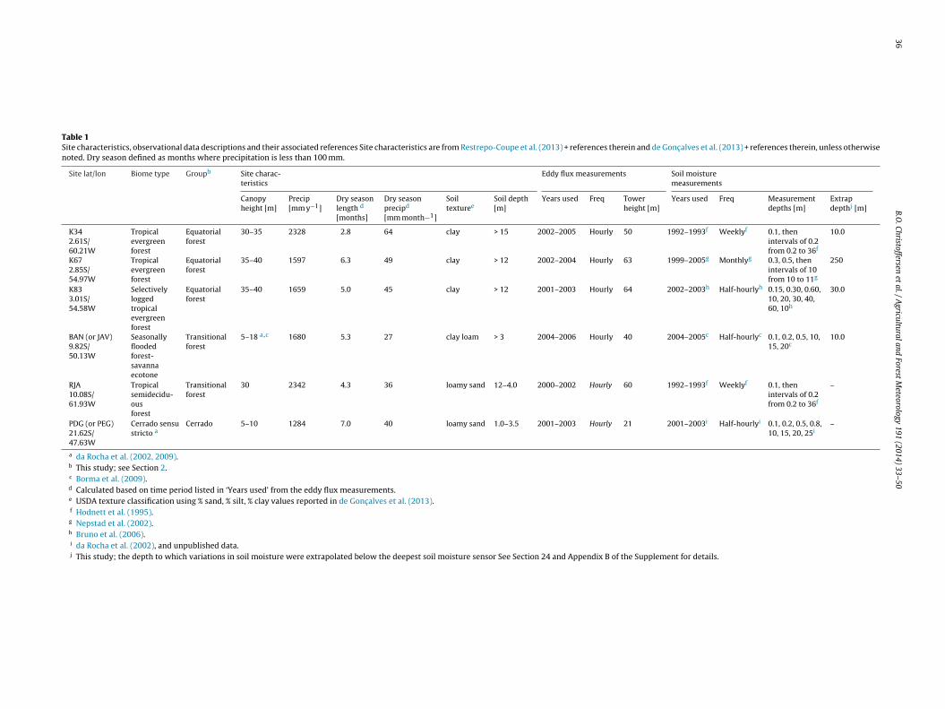
Table 1 also lists the temporal coverage and frequency of theclimate measurements, eddy covariance data, and ancillary soilmoisture data which are available at each site, in addition to theinstallation depths of soil moisture sensors. All eddy covariancedata have been processed according to a common protocol and areaggregated to an hourly timestep (Restrepo-Coupe et al., 2013).Soil moisture datasets were assimilated from various sources(see Table 1). The soil moisture data collection frequency rangedfrom near-continuous (half-hourly) to monthly and the monitoreddepths were variable across sites (data processing described in sec-tion 24 below and Appendix B in the Supplement).

2.2. Ecosystem model overview and selection

We used three to four years of climate measurements ofshort and long wave radiation, precipitation, air temperature,atmospheric pressure, humidity and horizontal wind speed todrive a suite of ecosystem models (23 variants in total) at eachof the six sites according to a common spinup and initializa-tion protocol. Participating models were part of the Large ScaleBiosphere–Atmosphere Experiment in Amazonia Data Model Inter-comparison Project (LBA-DMIP; de Gonc alves et al., 2013). Allmodels simulated ecosystem-level evapotranspiration (E) but usedvarying degrees of complexity for representing water supply andvegetation demand. 21 of the 23 model variants simulated a soilmoisture store upon which vegetation draws for transpiration, butdiffered in the vertical resolution and depth of soil layers simulated(spanning 1.5–15 m), as well as the rooting depth used across sites.In most models, soil depth is synonymous with rooting depth. Fiveadditional models simulated a groundwater store (also referred toas an unconfined aquifer) which could exchange water with thesoil (both into and out). Table A2 in the supplementary informa-tion contains information on the models’ soil depth, pedotransfermodel and bottom boundary condition, in addition to the numberof soil layers and rooting depths used across sites, and the asso-ciated model reference. On the demand side, 21 of the 23 modelvariants simulated canopy stomatal conductance (gs), using oneof four principal schemes to solve for gs, E, and leaf-level pho-tosynthesis (if simulated) given ambient incoming radiation, airtemperature, and humidity: Jarvis-type (Jarvis, 1976) (four modelvariants), Leuning-type (Leuning et al., 1995) (four model vari-ants), Ball-Woodrow-Berry-Collatz (Ball et al., 1987; Collatz et al.,1991) (11 model variants), or a constant ratio of internal to externalleaf CO2 concentration (2 model variants). Table A3 in the sup-plementary information gives the stomatal closure equations andparameter values for each model, and the associated model ref-erence. For further information on details of model spinup andinitialization procedures, see de Gonc alves et al. (2013) and refer-ences therein. Further documentation on the models analyzed herecan be found in Balsamo et al. (2009), Best et al. (2011), Clapp andHornberger (1978), Clark et al. (2011), Cox et al. (1998), de Rosnayand Polcher (1998), Ducoudre et al. (1993), Foley et al. (1996),Gerten et al. (2004), Haxeltine and Prentice (1996), Jacobs (1994),Krinner et al. (2005), Medvigy et al. (2009), Monteith (1995), Niuet al. (2011), Oleson et al. (2010), Running and Coughlan (1988),Schaefer et al. (2008), Sellers et al. (1996), Van den Hurk et al.(2000), Verseghy (1991) and Zhan et al. (2003).

2.3. Atmospheric and vegetation controls on E

We conducted a first-order assessment of the realism of mech-anisms regulating E in the models by comparing the degree towhich energy available to evaporate water controlled E, in models

Page 4

36

B.O.

Christoffersen et

al. /

Agricultural

and Forest

Meteorology

191 (2014)

33–50

Table 1Site characteristics, observational data descriptions and their associated references Site characteristics are from Restrepo-Coupe et al. (2013) + references therein and de Gonc alves et al. (2013) + references therein, unless otherwisenoted. Dry season defined as months where precipitation is less than 100 mm.

Site lat/lon Biome type Groupb Site charac-teristics

Eddy flux measurements Soil moisturemeasurements

Canopyheight [m]

Precip[mm y−1]

Dry seasonlength d

[months]

Dry seasonprecipd

[mm month−1]

Soiltexturee

Soil depth[m]

Years used Freq Towerheight [m]

Years used Freq Measurementdepths [m]

Extrapdepthj [m]

K342.61S/60.21W

Tropicalevergreenforest

Equatorialforest

30–35 2328 2.8 64 clay > 15 2002–2005 Hourly 50 1992–1993f Weeklyf 0.1, thenintervals of 0.2from 0.2 to 36f

10.0

K672.85S/54.97W

Tropicalevergreenforest

Equatorialforest

35–40 1597 6.3 49 clay > 12 2002–2004 Hourly 63 1999–2005g Monthlyg 0.3, 0.5, thenintervals of 10from 10 to 11g

250

K833.01S/54.58W

Selectivelyloggedtropicalevergreenforest

Equatorialforest

35–40 1659 5.0 45 clay > 12 2001–2003 Hourly 64 2002–2003h Half-hourlyh 0.15, 0.30, 0.60,10, 20, 30, 40,60, 10h

30.0

BAN (or JAV)9.82S/50.13W

Seasonallyfloodedforest-savannaecotone

Transitionalforest

5–18 a,c 1680 5.3 27 clay loam > 3 2004–2006 Hourly 40 2004–2005c Half-hourlyc 0.1, 0.2, 0.5, 10,15, 20c

10.0

RJA10.08S/61.93W

Tropicalsemidecidu-ousforest

Transitionalforest

30 2342 4.3 36 loamy sand 12–4.0 2000–2002 Hourly 60 1992–1993f Weeklyf 0.1, thenintervals of 0.2from 0.2 to 36f

–

PDG (or PEG)21.62S/47.63W

Cerrado sensustricto a

Cerrado 5–10 1284 7.0 40 loamy sand 1.0–3.5 2001–2003 Hourly 21 2001–2003i Half-hourlyi 0.1, 0.2, 0.5, 0.8,10, 15, 20, 25i

–

a da Rocha et al. (2002, 2009).b This study; see Section 2.c Borma et al. (2009).d Calculated based on time period listed in ‘Years used’ from the eddy flux measurements.e USDA texture classification using % sand, % silt, % clay values reported in de Gonc alves et al. (2013).f Hodnett et al. (1995).g Nepstad et al. (2002).h Bruno et al. (2006).i da Rocha et al. (2002), and unpublished data.j This study; the depth to which variations in soil moisture were extrapolated below the deepest soil moisture sensor See Section 24 and Appendix B of the Supplement for details.

Page 5

B.O. Christoffersen et al. / Agricultural and Forest Meteorology 191 (2014) 33–50 37

F spirats es), (bm xes ar

vwbecHwapvcatPmm

teaa(r(Reseenaet

ig. 1. Mean seasonal climatology (precipitation; P, net radiation; Rn, and evapotraneries data from multiple sites grouped by (a) equatorial forests (K34, K67, K83 sitean monthly precipitation (mm month−1) or (e) number of dry season months Bo

ersus in observations, during the dry season (defined as monthshere P < 100 mm). We quantified this control by regressing (for

oth models and observations) daily mean LE (W m−2) on incomingnergy and extracting the slope and R2 values. The slope indi-ates the relative partitioning of available energy between LE and

(higher slopes mean more LE, i.e., a lower Bowen ratio, = H/LE),hile values of R2 indicate the degree to which variability in avail-

ble energy drives LE, as opposed to other variables (e.g., vaporressure deficit, aerodynamic conductance, or soil water stress). R2

alues closer to 1 indicate that a large fraction of variation in LEan be explained by variation in available energy. We applied thispproach uniformly across both simulations and eddy flux observa-ions, pooling the data across sites by each site grouping (single siteDG in the case of Cerrado). We interpreted consistency betweenodel-derived and observation-derived R2 and slope values as oneetric of realism of modeled controls on E.For these regressions, we approximated available energy with

he sum of latent and sensible heat (LE + H). Using LE + H as anstimate of available energy instead of Rn is an approach recentlydopted by a pan-tropical review of LE (Fisher et al., 2009) as anlternative to filtering out periods of poor energy budget closureperiods when LE + H fall short of net radiation, Rn), which caneduce the number of daily replicates comprising a monthly meanCosta et al., 2010). We recognize that such an approach inflates2 values and increases the slope, but absolute values are not themphasis here. Rather, we sought a means by which to assess site-ite and model-data differences in the responses of LE to availablenergy in a way that was not confounded by varying degrees ofnergy budget closure in the observations. This allowed us to elimi-

ate the possibility that differences in regression slopes or R2 valuescross sites or between models and observations were due to thenergy budget closure problem (since some sites’ closure is betterhan others and all models have near-perfect closure).

ion; E) in equivalent water flux units (mm month−1) based on pooled monthly time) transitional forests (RJA, BAN sites), and (c) Cerrado (PDG site). Maps display (d)ound grouped sites match those around corresponding water flux figures.

2.4. Supply-side analysis of the seasonality of E: coupling withsoil moisture measurements

All models presented were verified to have balanced the waterbudget; i.e., the following equation was always satisfied (deGonc alves et al., 2013) to within 5 mm month−1.

P − E − Qs − Qsb + Qg↑ = �Si + �So + �Ss

�t(1)

where the left-hand side represents the net water flux into thesystem in units of mm month−1 and the right hand side is themonth-to-month differenced water storage of the system (�t inmonths). P is the precipitation, E the total evapotranspiration, Qs

the surface runoff, Qsb >the subsurface drainage, Qg↑ the verticalor lateral recharge to the soil from groundwater (positive fromgroundwater to unsaturated soil), �Si the change in canopy inter-cepted water, �So the change in ponded surface open water, and�Ss is the change in total soil moisture. At the monthly timescale,�Si and �So for all models were comparatively much smaller than�Ss.

We used a water budget approach to analyze supply-side mech-anisms governing the seasonality of E. We combined precipitationand estimates of E with ancillary soil moisture measurements toestimate (as a residual) the seasonality of total runoff and ground-water recharge. This gave us all of the major components of thewater budget for each site, and allowed us to infer the relative rolesof upward capillary flux from groundwater and deep root uptakein sustaining dry season rates of E. These two mechanisms differ-

entially impact both the magnitude and timing of the variability intotal soil moisture; thus, quantifying the variability of and timing ofchanges in �Ss provides a means for validating model mechanismsof water supply.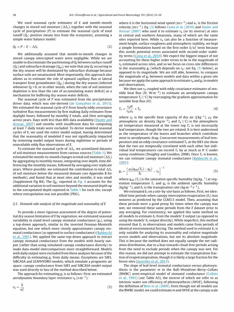

Page 6

3 and F

ccrs

Q

su(tsatwdm

dWtdaAactbu

oebfyom(atw

2

tvaemecpmwdSsw

a

r

8 B.O. Christoffersen et al. / Agricultural

We used seasonal cycle estimates of E and month–monthhanges in stored soil moisture (�Ss), together with the seasonalycle of precipitation (P) to estimate the seasonal cycle of totalunoff (Qt; positive means loss from the ecosystem), assuming aimple water balance model:

t = P − E − �Ss (2)

We additionally assumed that month-to-month changes intored canopy intercepted water were negligible. While we arenable to discriminate the partitioning of Qt between surface runoffQs) and subsurface drainage (Qsb), we note that any Qt occurring inhe dry season will be dominated by subsurface drainage becauseurface soils are unsaturated. Most importantly, this approach alsollows us to estimate the role of upward capillary flux or lateralransport from groundwater (Qg↑) during the dry season (inferredhenever Qt < 0, or in other words, when the rate of soil moistureepletion is less than the rate of accumulating water deficit) as aechanism for buffering dry season water deficits.The seasonal cycle of P was estimated from the precipitation

river data, which was site-derived (de Gonc alves et al., 2013).e estimated the seasonal cycle of E from hourly eddy covariance

urbulent flux measurements by first making daily estimates fromaylight hours, followed by monthly E totals, and then averagingcross years. Days with less than 80% data availability (Hasler andvissar, 2007) and months with insufficient data for computingt least 7 daily totals were excluded. To derive modeled seasonalycles of E, we used the entire model output, having determinedhat the seasonality of modeled E was not significantly impactedy removing model output hours during nighttime or periods ofnavailable eddy flux observations of E.

To estimate the seasonal cycle of �Ss, we assimilated datasetsf soil moisture measurements from various sources (Table 1). Westimated the month-to-month changes in total soil moisture (�Ss)y aggregating to monthly means, integrating over depth, time dif-erencing the monthly means, followed by averaging over replicateears. Where possible, we estimated the contribution to total �Ss

f soil moisture below the measured domain (see Appendix B forethods), and found that at most sites and months, it was small

Supplement Fig B4). The Qg↑ reported in Fig. 4 accounts for thedditional variation in soil moisture beyond the measured depth upo the extrapolated depth reported in Table 1 for each site, excepthere extrapolation was not possible (PDG).

.5. Demand-side analysis of the magnitude and seasonality of E

To provide a more rigorous assessment of the degree of poten-ial dry season limitation of E by vegetation, we estimated seasonalariability in stand-level canopy stomatal conductance (gs), using

top-down approach, similar to the inverted Penman-Monteithquation, but one which more closely approximates canopy sto-atal conductance (as opposed to surface conductance) (Baldocchi

t al., 1991). We applied the same top-down approach to extractanopy stomatal conductance from the models with hourly out-ut (rather than using simulated canopy conductance directly) toake data-model intercomparison more straightforward. Modelsith daily output were excluded from these analyses because of theifficulty in estimating gs from daily means. Exceptions are SiB3,iBCASA and LEAFHYDRO models, which simulate a prognostic airpace; canopy conductance from SiB3 and SiBCASA model outputas used directly in lieu of the method described below.

The approach for estimating gs is as follows: First, we estimated

erodynamic boundary layer resistance rb (s m−1):

b = u

u2∗(3)

orest Meteorology 191 (2014) 33–50

where u is the horizontal wind speed (m s−1) and u∗ is the frictionvelocity (m s−1). Eq. (3) follows Costa et al. (2010) and Hasler andAvissar (2007) who used it to estimate rb (or its inverse) at sitesin central and southern Amazonia, many of which are the samesites reported here. While rb can also be a function of measure-ment height, surface roughness and atmospheric stability, we kepta simple formulation based on the first-order u/u2∗ term becausethis avoids potential errors associated with second-order stabil-ity terms (Costa et al., 2010). We expect the biggest impact of notaccounting for these higher order terms to be in the magnitude ofrb estimated across sites, and so we focus on cross-site differencesin the seasonality gs (which depends on rb; see Eq. (5) below), asopposed to its magnitude. We are still able, however, to comparethe magnitude of gs between models and data within a given sitebecause we apply the same approach to estimate rb and gs in modelsand observations.

We then use rb coupled with eddy covariance estimates of sen-sible heat flux (H; W m−2) to estimate an aerodynamic canopytemperature Tv (◦C) by rearranging the gradient approximation forsensible heat flux (H):

Tv = rbH

cp�a+ Ta (4)

where cp is the specific heat capacity of dry air (J kg−1), �a theatmospheric air density (kg m−3), and Ta (◦C) is the atmosphericair temperature measured at the tower top Tv is not necessarilyleaf temperature, though the two are related. It is best understoodas the temperature of the leaves and branches which contributemost to aerodynamic drag. Concurrent measurements of leaf tem-perature and an eddy covariance-estimated Tv at the K83 site showthat the two are temporally correlated with each other but indi-vidual leaf temperatures can exceed Tv by as much as 8 ◦C undersunny conditions (Doughty and Goulden, 2008). Once Tv is known,we can estimate canopy stomatal conductance (Baldocchi et al.,1991):

gs =[

�a(qsat(Tv) − qa)Et

− rb

]−1

(5)

where qsat (Tv) is the saturation specific humidity (kg kg−1) at veg-etation temperature Tv and qa is the ambient specific humidity(kg kg−1), and Et is the transpiration rate (kg m−2 s−1).

We estimated Et on a site-by-site basis as follows. First, we iden-tified time periods when canopy interception evaporation (Ei) wasnonzero as predicted by the CLM3.5 model. Then, assuming thatthese periods were a good proxy for times when the canopy waswet, we removed these same periods from the E dataset prior toany averaging. For consistency, we applied this same method onall models to estimate Et from the models’ E output (as opposed tousing the models’ Et output directly). While imperfect, this methodensured that Et in observations and models came from periods ofidentical environmental forcing. The method used to estimate Et isonly suitable for analyzing its seasonality and relative magnitudeacross models and observations, but not its absolute magnitude.This is because the method does not equally sample the net radi-ation distribution, due to a bias towards cloud-free periods arisingfrom the need to exclude periods when the canopy was wet. Forthis reason, we did not attempt to estimate the transpiration frac-tion of evapotranspiration, though it is likely a large fraction for theforest sites (Jasechko et al., 2013).

The slope of leaf-level stomatal conductance versus photosyn-thesis is the parameter m in the Ball–Woodrow–Berry–Collatz(BWBC) semi-empirical model of stomatal conductance (Collatz

et al., 1991) (see Table A3), the inverse of which we refer to asintrinsic water use efficiency of photosynthesis (iWUE), followingthe definition of Beer et al. (2009). Even though not all models usethe BWBC model, we could estimate m and iWUE at the canopy scale

Page 7

B.O. Christoffersen et al. / Agricultural and Forest Meteorology 191 (2014) 33–50 39

Fig. 2. Modeled (colored lines or symbols) and observed (black points and error bars) mean seasonal cycle of E based on monthly time series data averaged (±1 standarddeviation) across multiple sites grouped by (a) equatorial forest (K34, K67, K83), (b) transitional forest (RJA and BAN) and (c) Cerrado/savanna (PDG). For (a) and (b), errorb represw

fstrtzolgngswmuaaamew

ars incorporate inter-site and interannual variability, whereas for (c), error bars

here precipitation < 100 mm).

or those which simulate GPP in addition to E. We estimated m as thelope of the best fit line between gs and GPPnorm = GPP × (h/ca) andook iWUE = 1/m, where ca and h are ambient CO2 mole fraction andelative humidity, respectively. Because the intercept of this rela-ionship across the majority of models and observations was nearero, we forced all fits through the origin. While the flux towerbservations were nearly linear, many models were slightly non-inear at high levels of GPPnorm and were also affected by outliers ins We dealt with this issue by fitting models with a 2nd degree poly-omial through the lower quantile of gs (as opposed to the mean ofs which would have been affected by outliers) and estimated thelope at an intermediate value of GPPnorm = 30 × 104 �mol m−2 s−1

here the fitted polynomial was approximately linear. We esti-ated the uncertainty about observed iWUE as the inverse of the

pper and lower quartile fits of m ∼ GPPnorm and uncertainty in GPPs the pooled standard deviation about the daily mean (across daysnd years). With estimates of iWUE and GPPnorm, we were able to

ddress the degree to which some of the spread in the simulatedagnitude of E across models could be related to compensating

rrors in these variables which regulate vegetation demand forater.

ent interannual variability only. Gray shaded region denotes dry season (months

2.6. Site and model representation in analyses

Sites were represented in analyses as follows. For the first-orderanalysis of the seasonality of E (Fig. 2) and its control by avail-able energy (Fig. 3), we sought to show how the sites behaved inaccord to their site grouping along the north-south gradient of cli-mate and vegetation. In these figures, we present the observed andmodeled data either averaged (Fig. 2) or pooled (Fig. 3) within eachsite grouping. In analyses of supply (Fig. 4) and demand (Figs. 5–7),a site-specific approach was more appropriate because we wereadjoining ancillary soil moisture data or momentum and carbonfluxes to the water flux data. In these figures, we selected onesite to represent each of the three site groups. We selected K67to represent the equatorial forests since this site had the best dataquality and coverage and because model–model differences weremost apparent at this site compared to K34 and K83. We selectedthe seasonally flooded BAN site for the transitional forests in anal-

yses of water supply because this site behaved most differentlywhen compared to the equatorial forest and Cerrado sites. How-ever, mechanisms of water supply at the BAN site should not beinterpreted to be characteristic of RJA or transitional forest sites in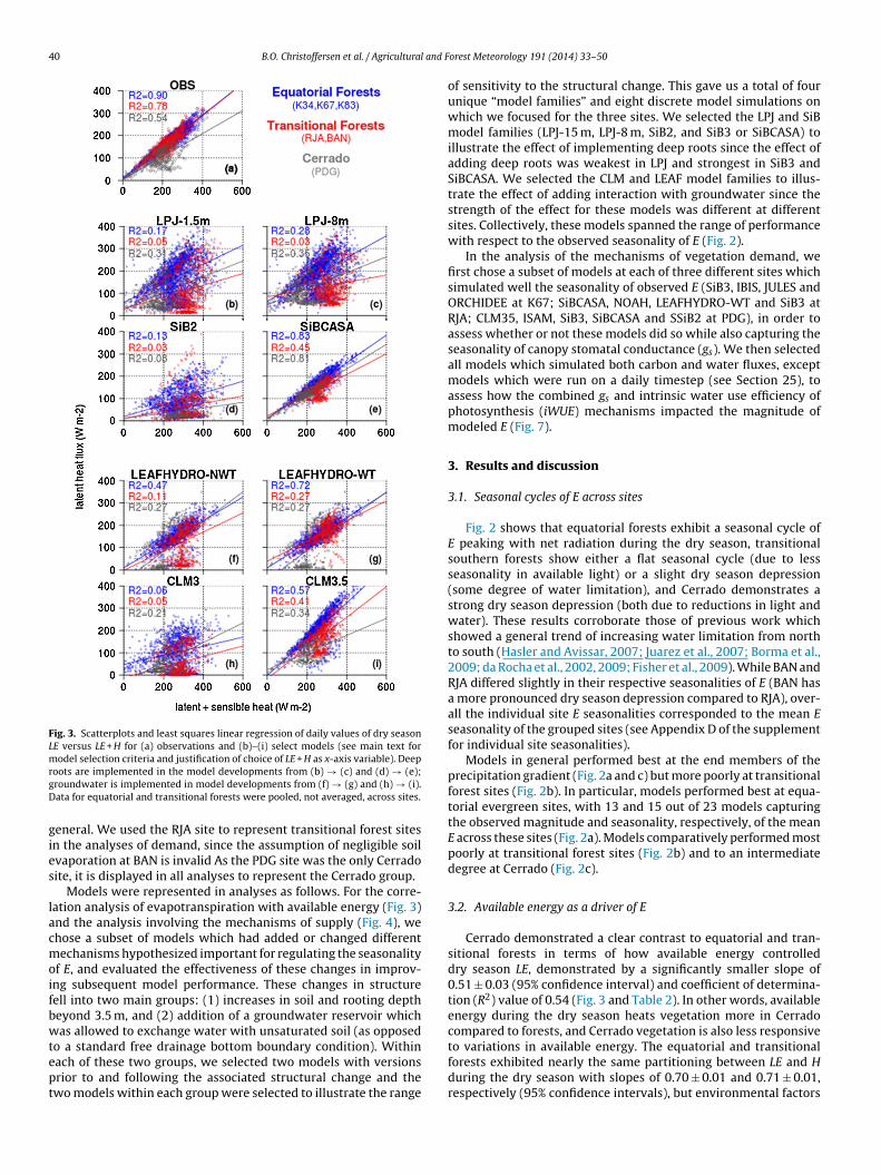

Page 8

40 B.O. Christoffersen et al. / Agricultural and F

Fig. 3. Scatterplots and least squares linear regression of daily values of dry seasonLE versus LE + H for (a) observations and (b)–(i) select models (see main text formodel selection criteria and justification of choice of LE + H as x-axis variable). DeeprgD

gies

lacmoifbwtept

oots are implemented in the model developments from (b) → (c) and (d) → (e);roundwater is implemented in model developments from (f) → (g) and (h) → (i).ata for equatorial and transitional forests were pooled, not averaged, across sites.

eneral. We used the RJA site to represent transitional forest sitesn the analyses of demand, since the assumption of negligible soilvaporation at BAN is invalid As the PDG site was the only Cerradoite, it is displayed in all analyses to represent the Cerrado group.

Models were represented in analyses as follows. For the corre-ation analysis of evapotranspiration with available energy (Fig. 3)nd the analysis involving the mechanisms of supply (Fig. 4), wehose a subset of models which had added or changed differentechanisms hypothesized important for regulating the seasonality

f E, and evaluated the effectiveness of these changes in improv-ng subsequent model performance. These changes in structureell into two main groups: (1) increases in soil and rooting deptheyond 3.5 m, and (2) addition of a groundwater reservoir whichas allowed to exchange water with unsaturated soil (as opposed

o a standard free drainage bottom boundary condition). Withinach of these two groups, we selected two models with versionsrior to and following the associated structural change and thewo models within each group were selected to illustrate the range

orest Meteorology 191 (2014) 33–50

of sensitivity to the structural change. This gave us a total of fourunique “model families” and eight discrete model simulations onwhich we focused for the three sites. We selected the LPJ and SiBmodel families (LPJ-15 m, LPJ-8 m, SiB2, and SiB3 or SiBCASA) toillustrate the effect of implementing deep roots since the effect ofadding deep roots was weakest in LPJ and strongest in SiB3 andSiBCASA. We selected the CLM and LEAF model families to illus-trate the effect of adding interaction with groundwater since thestrength of the effect for these models was different at differentsites. Collectively, these models spanned the range of performancewith respect to the observed seasonality of E (Fig. 2).

In the analysis of the mechanisms of vegetation demand, wefirst chose a subset of models at each of three different sites whichsimulated well the seasonality of observed E (SiB3, IBIS, JULES andORCHIDEE at K67; SiBCASA, NOAH, LEAFHYDRO-WT and SiB3 atRJA; CLM35, ISAM, SiB3, SiBCASA and SSiB2 at PDG), in order toassess whether or not these models did so while also capturing theseasonality of canopy stomatal conductance (gs). We then selectedall models which simulated both carbon and water fluxes, exceptmodels which were run on a daily timestep (see Section 25), toassess how the combined gs and intrinsic water use efficiency ofphotosynthesis (iWUE) mechanisms impacted the magnitude ofmodeled E (Fig. 7).

3. Results and discussion

3.1. Seasonal cycles of E across sites

Fig. 2 shows that equatorial forests exhibit a seasonal cycle ofE peaking with net radiation during the dry season, transitionalsouthern forests show either a flat seasonal cycle (due to lessseasonality in available light) or a slight dry season depression(some degree of water limitation), and Cerrado demonstrates astrong dry season depression (both due to reductions in light andwater). These results corroborate those of previous work whichshowed a general trend of increasing water limitation from northto south (Hasler and Avissar, 2007; Juarez et al., 2007; Borma et al.,2009; da Rocha et al., 2002, 2009; Fisher et al., 2009). While BAN andRJA differed slightly in their respective seasonalities of E (BAN hasa more pronounced dry season depression compared to RJA), over-all the individual site E seasonalities corresponded to the mean Eseasonality of the grouped sites (see Appendix D of the supplementfor individual site seasonalities).

Models in general performed best at the end members of theprecipitation gradient (Fig. 2a and c) but more poorly at transitionalforest sites (Fig. 2b). In particular, models performed best at equa-torial evergreen sites, with 13 and 15 out of 23 models capturingthe observed magnitude and seasonality, respectively, of the meanE across these sites (Fig. 2a). Models comparatively performed mostpoorly at transitional forest sites (Fig. 2b) and to an intermediatedegree at Cerrado (Fig. 2c).

3.2. Available energy as a driver of E

Cerrado demonstrated a clear contrast to equatorial and tran-sitional forests in terms of how available energy controlleddry season LE, demonstrated by a significantly smaller slope of0.51 ± 0.03 (95% confidence interval) and coefficient of determina-tion (R2) value of 0.54 (Fig. 3 and Table 2). In other words, availableenergy during the dry season heats vegetation more in Cerradocompared to forests, and Cerrado vegetation is also less responsive

to variations in available energy. The equatorial and transitionalforests exhibited nearly the same partitioning between LE and Hduring the dry season with slopes of 0.70 ± 0.01 and 0.71 ± 0.01,respectively (95% confidence intervals), but environmental factors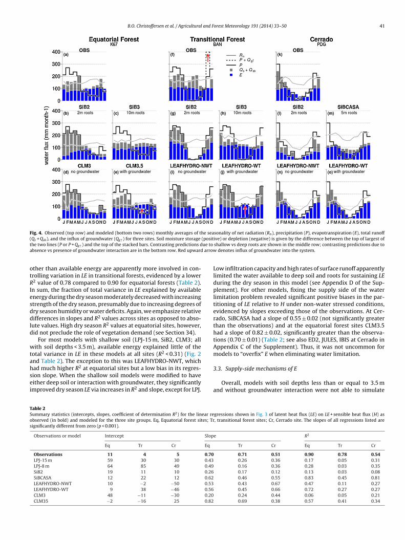

Page 9

B.O. Christoffersen et al. / Agricultural and Forest Meteorology 191 (2014) 33–50 41

Fig. 4. Observed (top row) and modeled (bottom two rows) monthly averages of the seasonality of net radiation (Rn), precipitation (P), evapotranspiration (E), total runoff( (positt ue to

a arrow

otRIesddld

wtahsei

TSos

Qs + Qsb), and the influx of groundwater (Qg↑) for three sites. Soil moisture storage

he two lines (P or P + Qg↑) and the top of the stacked bars. Contrasting predictions dbsence vs presence of groundwater interaction are in the bottom row. Red upward

ther than available energy are apparently more involved in con-rolling variation in LE in transitional forests, evidenced by a lower2 value of 0.78 compared to 0.90 for equatorial forests (Table 2).

n sum, the fraction of total variance in LE explained by availablenergy during the dry season moderately decreased with increasingtrength of the dry season, presumably due to increasing degrees ofry season humidity or water deficits. Again, we emphasize relativeifferences in slopes and R2 values across sites as opposed to abso-

ute values. High dry season R2 values at equatorial sites, however,id not preclude the role of vegetation demand (see Section 34).

For most models with shallow soil (LPJ-15 m, SiB2, CLM3; allith soil depths < 3.5 m), available energy explained little of the

otal variance in LE in these models at all sites (R2 < 0.31) (Fig. 2nd Table 2). The exception to this was LEAFHYDRO-NWT, which

ad much higher R2 at equatorial sites but a low bias in its regres-ion slope. When the shallow soil models were modified to haveither deep soil or interaction with groundwater, they significantlymproved dry season LE via increases in R2 and slope, except for LPJ.

able 2ummary statistics (intercepts, slopes, coefficient of determination R2) for the linear rebserved (in bold) and modeled for the three site groups. Eq, Equatorial forest sites; Trignificantly different from zero (p < 0.001).

Observations or model Intercept Slop

Eq Tr Cr Eq

Observations 11 4 5 0.70LPJ-15 m 59 30 30 0.43LPJ-8 m 64 85 49 0.49SiB2 19 11 10 0.26SiBCASA 12 22 12 0.62LEAFHYDRO-NWT 10 −2 −50 0.53LEAFHYDRO-WT 9 38 −46 0.56CLM3 48 −11 −30 0.20CLM35 −2 −16 25 0.82

ive) or depletion (negative) is given by the difference between the top of largest ofshallow vs deep roots are shown in the middle row; contrasting predictions due to

denotes influx of groundwater into the system.

Low infiltration capacity and high rates of surface runoff apparentlylimited the water available to deep soil and roots for sustaining LEduring the dry season in this model (see Appendix D of the Sup-plement). For other models, fixing the supply side of the waterlimitation problem revealed significant positive biases in the par-titioning of LE relative to H under non-water stressed conditions,evidenced by slopes exceeding those of the observations. At Cer-rado, SiBCASA had a slope of 0.55 ± 0.02 (not significantly greaterthan the observations) and at the equatorial forest sites CLM3.5had a slope of 0.82 ± 0.02, significantly greater than the observa-tions (0.70 ± 0.01) (Table 2; see also ED2, JULES, IBIS at Cerrado inAppendix C of the Supplement). Thus, it was not uncommon formodels to “overfix” E when eliminating water limitation.

3.3. Supply-side mechanisms of E

Overall, models with soil depths less than or equal to 3.5 mand without groundwater interaction were not able to simulate

gressions shown in Fig. 3 of latent heat flux (LE) on LE + sensible heat flux (H) as, transitional forest sites; Cr, Cerrado site. The slopes of all regressions listed are

e R2

Tr Cr Eq Tr Cr

0.71 0.51 0.90 0.78 0.54 0.26 0.36 0.17 0.05 0.31 0.16 0.36 0.28 0.03 0.35 0.17 0.12 0.13 0.03 0.08 0.46 0.55 0.83 0.45 0.81 0.43 0.67 0.47 0.11 0.27 0.45 0.66 0.72 0.27 0.27

0.24 0.44 0.06 0.05 0.21 0.69 0.38 0.57 0.41 0.34

Page 10

42 B.O. Christoffersen et al. / Agricultural and Forest Meteorology 191 (2014) 33–50

Table 3Observed (in boldface) and modeled annual totals, monthly maxima, and the month in which the maximum occurs for the upward capillary flux of groundwater into soil(Qg↑) at the three sites presented in Fig. 4. “OBS-a” and “OBS-b” refer to the inferred Qg↑ flux occurring at the depth of the extrapolated soil moisture and the deepest soilmoisture sensor, respectively (see Table 1 and Appendix B of the supplement).

Observations or model Total (mm year−1) Monthly maximum (mm month−1) Month of maximum

BAN K67 PDG BAN K67 PDG BAN K67 PDG

OBS-a 211 24 – 201 13 – Nov Jun –OBS-b 229 22 44 204 18 16 Nov Dec JunCLM35 14 137 0 14 35 0 Nov Aug –CLM4CN 204 278 10 49 54 3 Aug Oct NovISAM 0 0 11 0 0 7 – – Nov

119

EA(sSawsisaCsttab(ts

bbtepwtgm

osmu1fmasoJJtCstTi2tM

LEAFHYDRO-WT 416 92 0

without a dry season depression (Fig. 4b, d, g, i, l, n; see alsoppendix D of the Supplement). Addition of an unconfined aquifer

CLM3.5, LEAFHYDRO-WT models) produced a similar effect on dryeason water stress as did addition of deep soil and roots (LPJ-8 m,iB3, SiBCASA models). Increasing the soil depth or addition of anquifer in most models decreased total runoff and increased theater storage capacity of soil (or soil-aquifer system, for models

imulating one), providing a buffer for dry season deficits. In allnstances, where models erroneously predict a dry season depres-ion in E, models overestimate wet season total runoff (Qs + Qsb)nd underestimate wet season soil water storage (e.g., SiB2 andLM3 models in Figs. 3–4). Therefore, we deem simulation of theeasonal patterns of soil moisture recharge and discharge criticalo an accurate prediction of the seasonality of E. An exception tohis was the LEAFHYDRO model, where addition of an aquifer wasccompanied by an increase in drainage out of the soil column,ut this was an artifact of a fixed water table depth in this modelseasonal water table variation in this model requires a represen-ation of topography, and hence, was not possible with these 1Dimulations) (Miguez-Macho and Fan, 2012).

At the equatorial evergreen forest site K67, SiB3 and CLM3.5oth had seasonal patterns of E that closely matched observations,ut diverged in their simulated attribution of the soil water balanceo seasonal patterns of soil moisture storage and runoff (Fig. 4c and). SiB3 had large seasonal swings in stored soil moisture accom-anied by a low rate of total runoff throughout the entire year,hile CLM3.5 had lower seasonal variation in soil moisture, in addi-

ion to substantial dry season upward capillary flux (Qg↑) fromroundwater (simulated water table depth was 3.6–4.8 m in thisodel).A comparison to the water budget analysis derived from the

bserved seasonal cycles of P, E, and �Ss provides the neces-ary insight to discriminate among the dry season supply-sideechanisms used in the models. We infer a negligible role for

pward capillary flux from a groundwater (does not exceed8 mm month−1) in regulating dry season E at the K67 equatorialorest site (Fig. 4a and Table 3). The observations indicated that soil

oisture storage in the unsaturated rooting domain to 11 m wasble to endure a cumulative ∼340 mm reduction to sustain the dryeason water deficit (Supplement Figure B4d). At this site, nearly allf the total runoff (Qs + Qsb) occurs during the wet season months ofanuary–May, with minimal drainage during the dry season monthsune–Oct (i.e., nearly all of the reduction in soil moisture duringhe dry season is due to root uptake). This stands in contrast withLM3.5 (Fig. 4e) and other models (Supplement Fig D2) whose dryeason E rates were sustained in part by capillary fluxes from belowhe simulated rooting zone. Absence of shallow groundwater in theapajós region is also corroborated by anecdotal evidence reported

n the literature (reported at depths of ∼100 m in Nepstad et al.,002; Belk et al., 2007), but it is important to note that water tableshis deep are not characteristic of Amazonia in general (Miguez-

acho and Fan, 2012). The observations further bound the degree

26 0 Jul Oct –

of seasonal variation in soil moisture predicted by deep-root mod-els (e.g., variation SiB3 is too large; Fig. 4c).

The transitional forest BAN differed dramatically in its seasonalhydrology from that at K67; it has a shallow water table and floodsduring the wet season. Consequently, the two model approaches(deep roots and groundwater) diverged in terms of the mechanismof dry season water supply, despite similarities in their respectiveseasonalities of E (Fig. 4h and j). LEAFHYDRO-WT with water tabledynamics (Fig. 4j) simulates seasonal changes in water storage anddepletion entirely from groundwater instead of from the unsatu-rated rooting domain. SiB3 with deep roots (Fig. 4h), on the otherhand, drew upon stored soil moisture from deep layers (to 10 m)to make up for dry season water deficits. While both models withthese modifications simulate the overall seasonality of E well, theobservations indicated slight reductions in E during the dry seasonin June through September, which were best captured by SiB3.

Surprisingly, the water budget analysis for the BAN site (Bormaet al., 2009) revealed that observed seasonal patterns of soil mois-ture storage and groundwater flux were not consistent with eitherof the deep soil/deep roots or groundwater formulations (Fig. 4f,hand j). While groundwater fluxes are significant (total annual influxof 211 mm year−1), their timing (almost all during the month ofNovember) is not such that they contribute significantly to dryseason E (Table 3). Rather, stored soil moisture to 2 m depth ismore than sufficient to supply the entire dry season E water deficit,evidenced by reductions in soil moisture which exceed E losses,resulting in significant total runoff (Qs + Qsb) occurring throughoutthe dry season (Fig. 4f). A large influx of groundwater into the sys-tem is inferred during the month of November because soil waterincreases by nearly double the incoming precipitation, even whenthe soil moisture measurements are not extrapolated beyond themeasurement domain (Table 3). The abrupt influx of groundwa-ter (Qg↑) into this system occurs not because of soil type or depth,but because of this site’s proximity to a floodplain (Borma et al.,2009), and no further net influx of groundwater after November isrecorded because the soil quickly becomes and remains saturatedthroughout the flooding period. This highlights the importance ofmodeling groundwater fluctuations as a 2-dimensional topograph-ically driven process, in which orientation in relation to drainagebasins makes a big difference (Fan and Miguez-Macho, 2010). Onthe other hand, the role of persistent deep roots regulating E atthis site is likely also be limited, given the presumed anoxic soilconditions which persist during the flooding period.

At the Cerrado site PDG, we inferred a small (16 mm month−1)upward groundwater flux during the dry season months of Juneand July (Fig. 4k). However, this is probably an artifact and likelyrepresents root uptake below 2.5 m. Soil moisture measurementsextended to a depth of 2.5 m only at this site (Table 1) and we

were unable to extrapolate variations in soil moisture beyond thisdepth (see Appendix B of the Supplement). We argue that the16 mm month−1 water flux during these months actually repre-sents deep root uptake (beyond 25 m) because a large dry season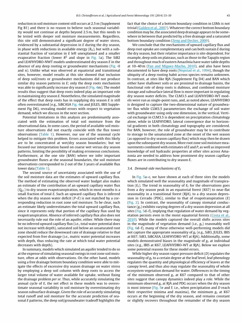

Page 11

and F

rFibteiseaaasoswrioomd

cotohafpFgot

tTa(swrasenbnzewd

atuibltatsts

B.O. Christoffersen et al. / Agricultural

eduction in soil moisture content still occurs at 2.5 m (Supplementig B1) and there is no reason to believe such seasonal variabil-ty would not continue at depths beyond 2.5 m, but this needs toe tested with deeper soil moisture measurements. Regardless,his site still demonstrated a significant degree of water stress,videnced by a substantial depression in E during the dry season,n phase with reductions in available energy (Rn), but with a sub-tantial fraction of variation in E left unexplained and a smallervaporative fraction (lower R2 and slope in Fig. 3a). The SiB2nd LEAFHYDRO-NWT models underestimated dry season E in thebsence of any deep rooting or groundwater mechanisms (Fig. 4lnd n). Unlike what was observed at equatorial and transitionalites, however, model results at this site showed that inclusionf deep soil/roots or groundwater mechanisms did not produceimilar dry season patterns in E; only the deep roots mechanismas able to significantly increase dry season E (Fig. 4m). The model

esults thus suggest that deep roots indeed play an important rolen maintaining dry season E. Nonetheless, the simulated magnitudef the effect that deep roots has in supplying dry season E is stillften overestimated (e.g., SiBCASA Fig. 4m and JULES, IBIS Supple-ent Fig D6), revealing model errors with respect to vegetation

emand, which we discuss in the next section.Potential limitations in this analysis are predominantly asso-

iated with the estimation of total soil moisture from thebservational data. In some cases, the period of available soil mois-ure observations did not exactly coincide with the flux towerbservations (Table 1). However, our use of the seasonal cycleelped to mitigate this problem. Errors associated with this likelyre to be concentrated at wet/dry season boundaries; but weocused our interpretation based on coarse wet versus dry seasonatterns, limiting the possibility of making erroneous conclusions.urthermore, at the one site (BAN) where we infer importantroundwater fluxes at the seasonal boundaries, the soil moisturebservations corresponded to 2 out of the 3 years of available fluxower data (Table 1).

The second source of uncertainty associated with the use ofhe soil moisture data are the estimates of upward capillary flux.he method of estimating the observed water budget also makesn estimate of the contribution of an upward capillary water fluxQg↑) to dry season evapotranspiration, which in most months is amall fraction of total E. Such an upward capillary flux is inferredhen the dry season water deficit (P–E) is not matched by a cor-

esponding reduction in root zone soil moisture. To be clear, suchn estimate likely underestimates the total upward capillary flux,ince it represents only that portion of the capillary flux used byvapotranspiration. Absence of inferred capillary flux also does notecessarily rule out the role of an aquifer, either. While there maye no inferred upward capillary flux (i.e., total water potential doesot increase with depth), saturated soil below an unsaturated rootone should reduce the downward rate of drainage relative to thatxpected from free drainage (i.e., matric water potential increasesith depth, thus reducing the rate at which total water potentialecreases with depth).

In summary, models which simulated an aquifer tended to do sot the expense of simulating seasonal swings in root zone soil mois-ure, often at odds with observations. On the other hand, modelssing a free drainage bottom boundary condition were able to mit-

gate the effects of excessive dry season drainage on water stressy employing a deep soil column with deep roots to access the

arger total volume of water available for uptake, without fixinghe drainage problem per se. Thus, while accurately simulating thennual cycle of E, the net effect in these models was to overes-

imate seasonal variability in soil moisture by overestimating dryeason subsurface drainage. Given the role of accurately simulatingotal runoff and soil moisture for the accurate prediction of sea-onal E patterns, the deep soil/groundwater tradeoff highlights the

orest Meteorology 191 (2014) 33–50 43

fact that the choice of a bottom boundary condition in LSMs is nottrivial (Gulden et al., 2007). Whatever the correct bottom boundarycondition may be, the associated deep drainage appears to be some-where in between that predicted by a free drainage and a saturatedbottom boundary condition (Zeng and Decker, 2009).

We conclude that the mechanisms of upward capillary flux anddeep root uptake are complementary and can both sustain E duringthe dry season, but their relative importance is site-dependent. Forexample, deep soils on plateaus, such as those in the Tapajós regionand throughout much of eastern Amazônia have water table depthsat 10–40 m (Fan and Miguez-Macho, 2010), and also have beendocumented to have deep roots (Nepstad et al., 1994), though theubiquity of a deep rooting habit across species remains unknown.In contrast, at sites like RJA (Supplement Fig D4) and BAN whicheither have shallower soils or are proximal to drainage basins, thefunctional role of deep roots is dubious, and combined moisturestorage and subsurface lateral flow is more important in regulatingdry season water deficits. The CLM3.5 and LEAFHYDRO-WT mod-els were run as single-point runs, and, as noted above, LEAFHYDROis designed to capture the two-dimensional nature of groundwa-ter flux while CLM3.5 parameterizes the exchange of soil waterwith groundwater using only one dimension, in the vertical. Verti-cal exchange in CLM3.5 is dependent on precipitation climatologyalone, while in LEAFHYDRO, lateral convergence due to horizon-tal gradients in both climatology and topography are considered.For BAN, however, the role of groundwater may be to contributeto storage to the unsaturated zone at the onset of the wet season(as opposed to dry season capillary flux) which may then be drawnupon the subsequent dry season. More root zone soil moisture mea-surements combined with estimates of E and P, as well as improvedknowledge of soil hydraulic properties at other sites across Ama-zonia are needed to address how prominent dry season capillaryfluxes are in contributing to dry season E.

3.4. Demand-side mechanisms of Et

In Fig. 5a–c, we have shown at each of three sites the modelswhich simulated well the seasonality and magnitude of transpira-tion (Et). The trend in seasonality of Et for the observations goesfrom a dry season peak in an equatorial forest (K67) to near-flatseasonality in a transitional forest (RJA), to a dry season depres-sion in Cerrado (PDG), similar to that of evapotranspiration (E)(Fig. 2). In contrast, the seasonality of canopy stomatal conduc-tance (gs) exhibits varying degrees of a dry season depression at allsites (Fig. 5d–f), implying that regulation of water demand by veg-etation persists even in the moist equatorial forests (Costa et al.,2010). While the models captured the overall shifts across sitesin the magnitude of vegetation demand (i.e., gs) reasonably well(Fig. 6d–f), many of these otherwise well-performing models didnot capture the appropriate seasonality of gs (e.g., SiB3, JULES, IBISat K67; SiB3, SiBCASA, LEAFHYDRO-WT at RJA). Additionally, somemodels demonstrated biases in the magnitude of gs at individualsites (e.g., IBIS at K67, LEAFHYDRO-WT at RJA). Below we exploresome potential reasons for these model errors.

While higher dry season vapor pressure deficit (D) regulates theseasonality of gs to a certain degree at the leaf level, leaf phenologyregulates the quantity and physiological efficiency of leaves at thecanopy level, and thus also may regulate the seasonality of wholeecosystem vegetation demand for water. Differences in the timingof the minimum observed gs at K67 compared to that of othersites suggest that canopy dynamics indeed play a role. While theminimum observed gs at RJA and PDG occurs when the dry season

is most intense (Fig. 5e and f; i.e., when precipitation and D reachtheir respective minima and maxima), the minimum gs at K67occurs at the beginning of the dry season, and remains constantor slightly recovers throughout the remainder of the dry season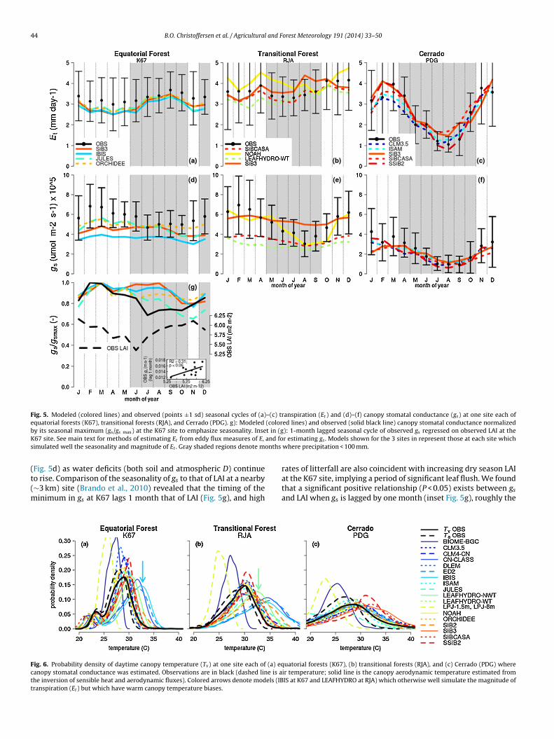

Page 12

44 B.O. Christoffersen et al. / Agricultural and Forest Meteorology 191 (2014) 33–50

Fig. 5. Modeled (colored lines) and observed (points ±1 sd) seasonal cycles of (a)–(c) transpiration (Et ) and (d)–(f) canopy stomatal conductance (gs) at one site each ofequatorial forests (K67), transitional forests (RJA), and Cerrado (PDG). g): Modeled (colored lines) and observed (solid black line) canopy stomatal conductance normalizedb t in (gK and fos onths

(t(m

Fctt

y its seasonal maximum (gs/gs max) at the K67 site to emphasize seasonality. Inse67 site. See main text for methods of estimating Et from eddy flux measures of E,

imulated well the seasonality and magnitude of Et . Gray shaded regions denote m

Fig. 5d) as water deficits (both soil and atmospheric D) continue

o rise. Comparison of the seasonality of gs to that of LAI at a nearby∼3 km) site (Brando et al., 2010) revealed that the timing of the

inimum in gs at K67 lags 1 month that of LAI (Fig. 5g), and high

ig. 6. Probability density of daytime canopy temperature (Tv) at one site each of (a) eqanopy stomatal conductance was estimated. Observations are in black (dashed line is ahe inversion of sensible heat and aerodynamic fluxes). Colored arrows denote models (IBranspiration (Et ) but which have warm canopy temperature biases.

): 1-month lagged seasonal cycle of observed gs regressed on observed LAI at ther estimating gs . Models shown for the 3 sites in represent those at each site whichwhere precipitation < 100 mm.

rates of litterfall are also coincident with increasing dry season LAI

at the K67 site, implying a period of significant leaf flush. We foundthat a significant positive relationship (P < 0.05) exists between gs

and LAI when gs is lagged by one month (inset Fig. 5g), roughly the

uatorial forests (K67), (b) transitional forests (RJA), and (c) Cerrado (PDG) whereir temperature; solid line is the canopy aerodynamic temperature estimated fromIS at K67 and LEAFHYDRO at RJA) which otherwise well simulate the magnitude of

Page 13

and Forest Meteorology 191 (2014) 33–50 45

aritmutosp

mmscaadtTgEarpdicoascFrot

uswt(iifrdmsgsai

ttTaeaitc(wK

Fig. 7. Observations (“OBS”) and models plotted in intrinsic water use efficiency(iWUE)—gross primary production (GPP) plot space with text color corresponding tomodeled Et relative to observed Et , where red (blue) models underestimate (over-estimate) Et by at least 0.5 mm/day iWUE and GPP are the mean values observed

B.O. Christoffersen et al. / Agricultural

mount of time required for new leaf expansion. This corroboratesecent work (Restrepo-Coupe et al., 2013) which demonstrates themportance of canopy leaf flush driving the seasonality of photosyn-hesis across the Amazon basin. In contrast to these observations,

any models which captured the seasonality of E consistentlynderestimated seasonal variability in gs. Collectively, this suggestshat the discrepancy between observed and modeled seasonalityf vegetation water demand at equatorial and transitional forestites K67 and RJA is due in part to such biological rhythms of leafhenology, a process poorly represented in vegetation models.

Other models which simulated well both the seasonality andagnitude of Et at times exhibited a systematic low bias in theagnitude of gs. An exploration of the canopy temperatures (Tv) of

ome of these models (IBIS at K67, LEAFHYDRO at RJA) revealed aorresponding warm bias (see arrows in Fig. 6). These models areble to capture the magnitude of E and Et at these sites presum-bly because this warm bias contributes to a larger vapor pressureeficit in these models which, given the same atmospheric condi-ions, drives a larger vapor flux at low gs. The counteracting effect ofv bias, however, was not enough to offset more extreme biases ins in other models, resulting in corresponding errors in simulatedt. For example, warm-biased models ED2 and CN-CLASS (Fig. 6and b) consistently underestimated Et. Finally, two models whichun at a daily timestep, LPJ and Biome-BGC, use mean air tem-eratures to estimate leaf temperature, and as a consequence ofisregarding diurnal variability in temperature and radiative heat-

ng at the leaf surface, they consistently underestimated daytimeanopy temperatures at all sites (Fig. 6a–c). Simple formulationsf canopy temperature using information on diurnal air temper-ture ranges could be readily employed to ameliorate this bias. Inum, these examples emphasize how biases in canopy temperaturean have important consequences for vegetation water demand.urthermore, models must accurately simulate vapor fluxes at theight canopy temperature because of the temperature dependencyf photosynthesis (Rubisco activity, light capture) and leaf respira-ion.

In addition to canopy stomatal conductance, the intrinsic waterse efficiency of photosynthesis (iWUE), or photosynthesis per unittomatal conductance, is also an important control on vegetationater demand. Higher (lower) iWUE implies vegetation is pho-

osynthesizing at a lower (higher) internal to ambient CO2 ratioLloyd et al., 2002; Beer et al., 2009), and its variation across sitesn Amazonia and Cerrado may reflect site differences in soil fertil-ty, vegetation composition, or both. It is an important diagnosticor modeled E in addition to gs because it governs how the lightesponse of photosynthesis is translated into evaporative losses. Toemonstrate the interaction between GPP and iWUE on simulatedagnitudes of E, in Fig. 7 we have arrayed models in a ‘GPP–iWUE

pace’ for select sites across the climate and vegetation compositionradient (K67, RJA, and PDG), with simulated magnitudes of tran-piration (Et) represented by color: models in black text simulated

mean Et within the observed mean Et + - 0.5 mm d−1, and modelsn red and blue text fell below and above this range, respectively.

Mean site GPP decreased with Et along the climate and vegeta-ion composition gradient from equatorial forests to Cerrado, buthere was no systematic trend in iWUE across the gradient (Fig. 7).he lack of a difference in iWUE between forest and Cerrado atn annual average scale does not preclude the existence of differ-nces in the seasonality of iWUE across sites, which we did notnalyze. Still, this analysis demonstrates that site-site differencesn the magnitude of E are not due to differences in iWUE; rather,he drivers of the magnitude of E appear to be common to those

ontrolling the magnitude of GPP. The PDG Cerrado site has a GPPmean ± 95% confidence interval) of 3.2 ± 1.7 �mol CO2 m−2 s−1

hich is less than half that of RJA (7.7 ± 1.8 �mol CO2 m−2 s−1) or67 (8.2 ± 1.4 �mol CO2 m−2 s−1). It is possible that the low soil

or predicted for each site. Box represents observational error, which for iWUE isestimated as the inverse of the slopes of the 25th and 75th quantile regressions ofgs ∼ GPP × (h/ca). GPP error estimated as ±1 standard deviation (For interpretation ofthe color information in this figure legend, the reader is referred to the web versionof the article.).

Page 14

46 B.O. Christoffersen et al. / Agricultural and Forest Meteorology 191 (2014) 33–50

Table 4Model benchmarking of the magnitude of transpiration fluxes (Et) across biomes with respect to vegetation demand for water. Note that mean Et is not representative ofan annual mean (see Section 2). ‘High’, ‘low’, and ‘

√’ denote models whose mean values are greater than, less than, or within the observational error (taken as a constant

0.5 mm/day for Et). The last column evaluates whether models do (‘√

’) or do not (‘x’) match the observed Et , while also matching all four observed magnitudes of vegetationdemand (columns 1–4).

gs Tv GPP iWUE Model Mean Et Right Et? Right Et , Right demand?

Equatorial forests (K34, K67, K83)Low

√Low

√SIB2 1.92 Low x

Low High√

High ED2 2.33 Low xLow

√HTESSEL 2.47 Low x

Low√

High High SSiB2 2.48 Low xLow

√LEAFHYDRO-NWT 2.53 Low x

Low√

LEAFHYDRO-WT 2.61 Low xLow High

√High CN-CLASS 2.66 Low x

Low√ √

High ISAM 2.72 Low xLow Low

√ √SiBCASA 2.99 Low x√ √

High√

SiB2-mod 3.18√

xLow High

√High IBIS 3.19

√x

Low√ √

High JULES 3.20√

xLow

√ √High SiB3 3.24

√x

Low√

High High ORCHIDEE 3.36√

x√ √ √ √NOAH-MP 3.54

√ √√ √ √ √

OBS 3.59√ √

High√

High High CLM35 4.07 High xHigh

√High

√CLM4-CN 4.29 High x

Transitional forest (RJA only)Low

√CLM3 1.42 Low x

Low High Low√

SiB2 1.53 Low xLow High Low

√ED2 2.22 Low x

Low√

High High SSiB2 2.89 Low x√High Low

√JULES 3.00 Low x

Low High LEAFHYDRO-NWT 3.03 Low x√ √HTESSEL 3.04 Low x

Low High√

High IBIS 3.04 Low xLow High LEAFHYDRO-WT 3.19 Low xLow High

√High CN-CLASS 3.20 Low x

Low√ √ √

ISAM 3.27√

xLow

√ √ √SiBCASA 3.45

√x√ √ √ √

OBS 3.73√ √

√ √ √ √CLM4-CN 3.86

√ √√ √ √ √

NOAH-MP 4.01√ √

√ √ √ √SiB3 4.01

√ √√

High High√

SiB2-mod 4.18√

x√ √High

√ORCHIDEE 4.46 High x√ √

High√

CLM35 4.58 High x

Cerrado (PDG)Low

√Low Low SiB2 0.61 Low x

Low√

Low Low CN-CLASS 1.07 Low x√ √CLM3 1.09 Low x√ √

High√

SiB2-mod 1.34 Low x√High

√High NOAH-MP 1.44 Low x√ √

High High ED2 1.92√

x√ √ √ √CLM4-CN 1.95

√ √√ √ √

High CLM35 2.00√

x√ √LEAFHYDRO-NWT 2.06

√ √√

High High High SSiB2 2.08√

x√ √LEAFHYDRO-WT 2.12

√ √√ √ √ √

ISAM 2.13√

x√ √ √ √OBS 2.18

√ √√

High High√

SiB3 2.29√

x√ √HTESSEL 2.51

√ √√ √

High High SiBCASA 2.51√

x√ √High High ORCHIDEE 2.62

√x

fsaatc

o

√ √High High IBIS

High Low High√

JULES

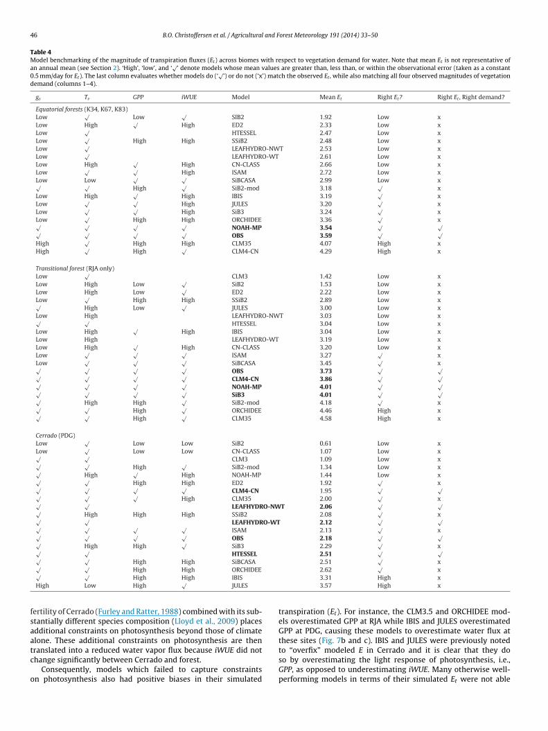
ertility of Cerrado (Furley and Ratter, 1988) combined with its sub-tantially different species composition (Lloyd et al., 2009) placesdditional constraints on photosynthesis beyond those of climatelone. These additional constraints on photosynthesis are then

ranslated into a reduced water vapor flux because iWUE did nothange significantly between Cerrado and forest.

Consequently, models which failed to capture constraintsn photosynthesis also had positive biases in their simulated

3.31 High x3.57 High x

transpiration (Et). For instance, the CLM3.5 and ORCHIDEE mod-els overestimated GPP at RJA while IBIS and JULES overestimatedGPP at PDG, causing these models to overestimate water flux atthese sites (Fig. 7b and c). IBIS and JULES were previously noted

to “overfix” modeled E in Cerrado and it is clear that they doso by overestimating the light response of photosynthesis, i.e.,GPP, as opposed to underestimating iWUE. Many otherwise well-performing models in terms of their simulated Et were not able

Page 15

and F

tpawtntaitts

asibIopmb2aiG

irbsg(towpavitbotdR

3

amtsrgtswtstwodu

B.O. Christoffersen et al. / Agricultural

o capture variations in GPP and iWUE in concert across sites. Thisroblem was especially apparent in Cerrado, where models suchs SSiB2, ORCHIDEE, SiBCASA, CLM35 and ED2 overestimated GPPhile also overestimating iWUE, which allowed them to simulate

he appropriate magnitude of Et, but with the incorrect mecha-isms (Fig. 7c). Overall model spread in GPP was greatest in theransitional forest of RJA (Fig. 7b), while model spread in iWUE waslso large, both of which combine to explain the large model spreadn simulated E in transitional forests (Fig. 2b). In contrast, most ofhe model spread in simulated E in equatorial forests (Fig. 2a) is dueo variation in simulated iWUE, not GPP, as evidenced by the K67ite (Fig. 7a).

One of the reasons for model bias in iWUE can simply bettributed to parameter values in their associated stomatal clo-ure equation (equations and parameters given in Table A3). Fornstance, ED2, IBIS and CNCLASS tended to overestimate iWUEecause of lower values of m, equal to 8, 8, and 6, respectively.

t should be noted that one model (ISAM) was able to capture mostf the variation in the magnitude of Et across sites with the appro-riate mechanistic responses of iWUE and GPP (Fig. 7b and c). Thisodel incorporates nutrient (nitrogen) cycles into whole-system

iogeochemical processes, including photosynthesis (Jain et al.,009) and associated stomatal responses The CLM4-CN model, also

model incorporating nutrient cycling, also captures the variationn E, iWUE, and GPP across sites, except for a small positive bias inPP at K34.

These results highlight the challenge facing models not tomprove simulations of tropical forests at the expense of Cer-ado. That Cerrado would exhibit dynamics not easily representedy models which were improved with tropical forests in mindhould not be surprising; Cerrado is quite far from being analo-ous to seasonally dry forest both in terms of phylogenetic distancePennington et al., 2000; Pennington et al., 2009) and species func-ional traits (Hoffmann et al., 2012). Models which captured somef the biome differences in E as well as GPP and iWUE were modelshich account for nutrient limitations on forest and savanna eco-hysiology, but we did not do the necessary analyses to confirm thiss fact. Nevertheless, this supports recent evidence that basin-wideariation in nutrients play an important role in governing patternsn productivity (Quesada et al., 2012) and by extension, evapo-ranspiration. Regardless, model improvements in Cerrado and itsoundary with forest will require modeling the synergistic effectsf soil fertility and disturbance via fire, since these mechanisms arehe primary factors controlling the relative productivity and abun-ance of trees and grasses at this ecotone (Furley and Ratter, 1988;atter, 1992).

.5. Model benchmarking

We have shown that models can simulate the correct magnitudend seasonality of E from equatorial Amazonia to Cerrado usingultiple supply and demand side mechanisms, and the observa-

ions have provided important constraints these mechanisms. Aingle comprehensive metric of performance for each model withespect to simulated magnitudes and seasonalities of E that inte-rates both supply and demand regulatory mechanisms is beyondhe scope of this paper. However, based on our analysis of demand-ide mechanisms with respect to the magnitude of Et, we presenthat a model benchmark might look like in Table 4. For equa-

orial (K34, K67, K83), transitional (RJA only), and Cerrado (PDG)ites, models and observations are ordered by increasing magni-ude of transpiration (Et) (not an annual mean). We then summarize

hether or not models simulated with high or low bias, or within

bservational error, the four variables regulating vegetation wateremand (gs, Tv, GPP, iWUE) in columns 1–4, in addition to Et (col-mn 7). A model which simulates a magnitude of Et within the

orest Meteorology 191 (2014) 33–50 47

observational error while also simulating the four demand vari-ables within observational error, we deem does so “for the rightreasons” (column 8), at least with respect to demand-side mecha-nisms regulating vegetation water demand.

Six, six, and 11 models “get the right answer” at the equatorialforest sites, the RJA transitional forest site, and the PDG Cerrado site,respectively: that is, they simulate the magnitude of Et to within±0.5 mm day−1 of the observations (Table 4). At none of these sites,however, did a majority of these models do so for the right reasons.PDG was the site with the greatest number of models (five) doingso for the right reasons, but only two of these models were modelswhich also simulated carbon fluxes. In sum, the model benchmarkhas identified model deficiencies which would not have otherwisebeen apparent based on a simple model-data comparison of evapo-transpiration flux.

4. Conclusions

This study was undertaken to accomplish two main objectives:First, to establish how mechanisms of water supply and vegeta-tion water demand control evapotranspiration (E) along a climateand vegetation composition gradient from equatorial Amazonia toCerrado; and second, to evaluate these mechanisms in a suite ofecosystem models. Encouragingly, most models are now able tosimulate with relative accuracy the magnitude and seasonality ofE at equatorial sites and Cerrado, but transitional forests continueto pose challenges for models. However, we identified some defi-ciencies in models which would not otherwise be apparent basedon a simple comparison of simulated and observed magnitude andseasonal cycle of E.

We showed that the mechanisms of upward capillary flux anddeep root uptake are complementary mechanisms of water sup-ply and can both sustain E during the dry season, but their relativeimportance is site-dependent. Some models prescribed deep rootsat all sites (e.g., LPJ-8 m) or manipulated rooting depth via opti-mization/sensitivity analysis (e.g., BIOME-BGC, ORCHIDEE, SiB3,IBIS), while others (e.g., CLM, ISAM, NOAH-MP) relied on ground-water recharge based solely on precipitation climatology and soiltexture, to make up for dry season water deficits. In contrast,the observations indicated that the relative importance of thesetwo mechanisms did not vary as a simple function of climateor location along the climate and vegetation composition gradi-ent. Consequently, models often simulated well the seasonality ofE, but with the incorrect mechanism of water supply. While thereal principles which govern the relative magnitude of deep rootactivity and capillary fluxes remain to be elucidated, contrastingthe LEAFHYDRO-WT point simulations analyzed here with resultsfrom a previous study (Miguez-Macho and Fan, 2012) suggests thatboth the magnitude and seasonal timing of capillary fluxes is gov-erned just as much by local topography and proximity to drainagebasins as by climatology and soil texture. Capturing these effectsin models, therefore, will require not only simulation of lateralsubsurface water flow (a two-dimensional process), but spatial res-olutions much higher than the typical GCM simulation (1◦ × 1◦).Most importantly, however, the analysis of water supply highlightsunanswered questions regarding deep root activity, both from anecological point of view as to which trade-offs govern deep roots(as a plant trait) within and across tropical forest communities, andfrom a mechanistic view as to the quantity of water and nutrientstransported through them.

We also showed that, while most equatorial and transitional

forests demonstrated a seasonal cycle of transpiration (Et) whichclosely followed that of net radiation, vegetation water demandvia canopy stomatal conductance was still a moderate to significantcontrol. Some models, however, which simulated well the seasonal

Page 16

4 and F

ccswiotlMtuomaiotbtrm

mtt2mvweteait

A

dawLMvAKtw

Ap(aaSAoAdtEcci

8 B.O. Christoffersen et al. / Agricultural

ycle of Et and its control by net radiation did so with near-constantanopy stomatal conductance throughout most of the year. We pre-ented evidence at an equatorial site(Restrepo-Coupe et al., 2013)hich suggests that the quantity and age distribution of leaves

n the canopy plays just as significant a role in the seasonalityf canopy stomatal conductance as does leaf-level stomatal con-rol, implying that some of the data-model discrepancy is due toeaf phenology, a process poorly represented in vegetation models.

odel biases in the magnitude of canopy stomatal conductance, inurn, could be related to light response (GPP) or the intrinsic waterse efficiency of photosynthesis (iWUE), in addition to its effectn canopy temperatures. We found that most of the variation inodeled rates of E at an equatorial site was explained by iWUE, but

t Cerrado, many models were characterized by a “cryptic bias”,.e., biases in both iWUE and GPP partially cancelled each otherut, leading to modeled magnitudes of E indistinguishable fromhe observations. While modeled E bias at the equatorial site cane remedied by a simple optimization scheme tuning the magni-ude of the Ball-Berry parameter m, model issues at Cerrado wouldequire better parameterization of both Vcmax (light response) and.

Most importantly, these analyses highlight how model improve-ents need to focus on biological controls on E in addition

o physical mechanisms, especially given the predominance ofranspiration fluxes in total evapotranspiration (Jasechko et al.,013). This will require continued and expanded efforts toonitor root and canopy demographic processes in relation to

ariability in available water, nutrients and light. These effortsill realize maximum benefit when conducted at sites with

xisting ecosystem-level eddy covariance measurement infrastruc-ure, allowing these sub-scale processes to inform controls oncosystem-level processes. Integrating these biological responsesnd feedbacks to the processes of water cycling, therefore, willmprove our understanding of vegetation-climate feedbacks in theropics.

cknowledgments

Author contributions First author B.O.C. and senior author S.R.S.esigned the analyses. B.O.C. conducted the analyses. Seconduthor N.R.C. provided BrasilFlux database support. B.O.C. and S.R.S.rote the paper with contributions from N.R.C., P.C., J.B.F., D.G.,

.G., G.M.-M., B.P., K.Sa., K.Sc., H.V., Z.-L.Y., B.K., M.H.C., and X.Z.odel output and contributions to model classification were pro-

ided by M.A.A., I.T.B., B.P.C., J.B.F., D.G., X.G., L.G., Bv.dH., K.I., H.I.,.J., N.L., G.M.-M., B.P., D.R.R., K.Sa., A.S., K.Sc., M.S., H.V. and Z.-L.Y.ey datasets and insights into their appropriate analysis were con-

ributed by A.C.A., B.K., A.O.M., H.R.dR. and C.vR. LBA-DMIP projectas coordinated by M.N.M., J.B., M.H.C., L.G.G.dG., X.Z. and S.R.S.

This research was funded by the National Aeronautics and Spacedministration (NASA) (LBA investigation CD-32 and the LBA-DMIProject, award #NNX09AL52G), the National Science FoundationAmazon-PIRE, NSF award #OISE-0730305), and the Gordonnd Betty Moore Foundation’s Andes-Amazon Initiative. HRdRcknowledges FAPESP (08-581203) for aiding field data collection.oil moisture data for the RJA field site were collected under theBRACOS project and made available by the UK Institute of Hydrol-gy and the Instituto Nacional de Pesquisas Espaciais (Brazil).BRACOS was a collaboration between the Agencia Brasileirae Cooperac ão and the UK Overseas Development Administra-ion. B.O.C. acknowledges support from a Graduate Research

nvironmental Fellowship (GREF)-U.S. DOE Global Change Edu-ation Program, as well as an NSF Amazon-PIRE fellowship. J.B.F.ontributed to this paper from the Jet Propulsion Laboratory, Cal-fornia Institute of Technology, under a contract with the National

orest Meteorology 191 (2014) 33–50

Aeronautics and Space Administration. We thank Reto Stoecklifor initial generation of gap-filled meteorological driver data, andEnrique Rosero for discussions helping to frame some analyses forthis paper. We are indebted to both LBA and ABRACOS projects,and their field technicians, without whose efforts to establish andpreserve the quality of datasets used here, this paper would nothave been possible. We are grateful to two anonymous reviewerswhose comments greatly improved the clarity of this paper.

Appendix A.

List of symbols, definitions, and units used in the paper (TableA1) and descriptions of the soil hydrology (Table A2) and stomatalconductance (Table A3) sub-model components for all LBA-DMIPmodels.

Appendix B.

Full description of the methods used to obtain composite sea-sonal cycles of �Ss.

Appendix C.

A version of Fig. 3 in main text which includes the entire set ofLBA-DMIP models.

Appendix D.

Figure sets encompassing all sites and the entire set of modelsfor the water budget analysis given in Fig. 4 of the main text.

Appendix E. Supplementary data

Supplementary data associated with this article can be found,in the online version, at http://dx.doi.org/10.1016/j.agrformet.2014.02.008.

References

Avissar, R., Werth, D., 2004. Comments on “The regional evapotranspiration of theAmazon”. Reply Journal of Hydrometeorology 5 (6), 1281.

Baker, I.T., et al., 2008. Seasonal drought stress in the Amazon: Reconciling modelsand observations. Journal of Geophysical Research, 113.

Baldocchi, D., Luxmoore, R.J., Hatfield, J.L., 1991. Discerning the forest from thetrees: an essay on scaling canopy stomatal conductance. Agricultural and ForestMeteorology 54, 197–226.

Ball, J.T., Woodrow, I.E., Berry, J.A., 1987. A model predicting stomatal conductanceand its contribution to the control of photosynthesis under different environ-mental conditions. In: Biggins, I. (Ed.), Progress in Photosynthesis Research.Martinus Nijhoff, Netherlands, pp. 221–224.

Balsamo, G., et al., 2009. A revised hydrology for the ECMWF model: verificationfrom field site to terrestrial water storage and impact in the integrated forecastsystem. Journal of Hydrometeorology 10 (3), 623–643.

Beer, C., et al., 2009. Temporal and among-site variability of inherent water useefficiency at the ecosystem level. Global Biogeochemical Cycles 23 (2).

Belk, E.L., et al., 2007. Modeling the effects of throughfall reduction on soil water con-tent in a Brazilian Oxisol under a moist tropical forest. Water Resources Research43 (8), W08432.

Best, M.J., et al., 2011. The Joint UK Land Environment Simulator (JULES), modeldescription—Part 1: energy and water fluxes. Geoscientific Model Development4 (3), 677–699.

Betts, R.A., et al., 2004. The role of ecosystem–atmosphere interactions in simu-lated Amazonian precipitation decrease and forest dieback under global climatewarming. Theoretical and Applied Climatology 78 (1–3), 157–175.

Bonan, G., 1998. The land surface climatology of the NCAR land surface model cou-pled to the NCAR Community Climate Model. Journal of Climate 11, 1307–1326.

Borma, L.S., et al., 2009. Atmosphere and hydrological controls of the evapotranspi-

ration over a floodplain forest in the Bananal Island region. Amazonia Journal ofGeophysical Research-Biogeosciences 114, G01003.

Brando, P.M., et al., 2010. Seasonal and interannual variability of climate and vegeta-tion indices across the Amazon. Proceedings of the National Academy of Sciences107 (33), 14685–14690.

Page 17

and F

B

B

C

C

C

C

C

C

C

d

d

d

d

D

D

E

F

F

F

F

G

G

G

G

H

H

H

H

H

H

I

B.O. Christoffersen et al. / Agricultural

runo, R.D., da Rocha, H.R., de Freitas, H.C., Goulden, M.L., Miller, S.D., 2006. Soil mois-ture dynamics in an eastern Amazonian tropical forest. Hydrological Processes20 (12), 2477–2489.

uckley, T.N., 2005. The control of stomata by water balance. New Phytologist 168(2), 275–292.

lapp, R.B., Hornberger, G.M., 1978. Empirical equations for some soil hydraulicproperties. Water Resources Research 14 (4), 601–604.

lark, D.B., et al., 2011. The Joint UK Land Environment Simulator (JULES), modeldescription—Part 2: carbon fluxes and vegetation dynamics. Geoscientific ModelDevelopment 4 (3), 701–722.

ollatz, G.J., Ball, J.T., Grivet, C., Berry, J.A., 1991. Physiological and environmentalregulation of stomatal conductance, phtosynthesis and transpiration: a modelthat includes a laminar boundary layer. Agricultural and Forest Meteorology 54,107–136.

osta, M.H., et al., 2010. Atmospheric versus vegetation controls of Amazonian trop-ical rain forest evapotranspiration: are the wet and seasonally dry rain forestsany different? Journal of Geophysical Research-Biogeosciences, 115.

osta, M.H., Souza, J.D.C., Ribeiro, A., 2004. Comments on “The regional evapotrans-piration of the Amazon”. Journal of Hydrometeorology 5 (6), 1279–1280.

ox, P.M., Huntingford, C., Harding, R.J., 1998. A canopy conductance and photosyn-thesis model for use in a GCM land surface scheme. Journal of Hydrology, 79–94,212-213.

ox, P.M., Betts, R.A., Jones, C.D., Spall, S.A., Totterdell, I.J., 2000. Acceleration of globalwarming due to carbon-cycle feedbacks in a coupled climate model. Nature 408,184–187.

a Rocha, H.R., et al., 2002. Measurements of CO exchange over a woodland savanna(Cerrado sensu stricto) in southeast Brazil. Biota Tropica 2 (1), BN01702012002.

a Rocha, H.R., et al., 2009. Patterns of water and heat flux across a biome gradientfrom tropical forest to savanna in Brazil. Journal of Geophysical Research-Biogeosciences, 114.

e Gonc alves, L.G.G., et al., 2013. Overview of the large-scale biosphere–atmosphereexperiment in Amazonia Data Model Intercomparison Project (LBA-DMIP). Agri-cultural and Forest Meteorology 182–183, 111–127.

e Rosnay, P., Polcher, J., 1998. Modelling root water uptake in a complex land sur-face scheme coupled to a GCM. Hydrology and Earth System Sciences 2 (2–3),239–255.

ickinson, R.E., et al., 2006. The community land model and its climate statistics as acomponent of the community climate system model. Journal of Climate 19 (11),2302–2324.

ucoudre, N.I., Laval, K., Perrier, A., 1993. Sechiba, a new set of parameterizationsof the hydrologic exchanges at the land atmosphere interface within the lmdatmospheric general-circulation model. Journal of Climate 6 (2), 248–273.

ltahir, E.A.B., Bras, R.L., 1994. Precipitation recycling in the Amazon Basin. QuarterlyJournal of the Royal Meteorological Society 120 (518), 861–880.

an, Y., Miguez-Macho, G., 2010. Potential groundwater contribution to Amazonevapotranspiration. Hydrology and Earth System Sciences 14 (10), 2039–2056.

isher, J.B., et al., 2009. The land–atmosphere water flux in the tropics. Global ChangeBiology 15 (11), 2694–2714.

oley, J.A., et al., 1996. An integrated biosphere model of land surface processes, ter-restrial carbon balance, and vegetation dynamics. Global Biogeochemical Cycles10 (4), 603–628.

urley, P.A., Ratter, J.A., 1988. Soil resources and plant communities of the cen-tral Brazilian cerrado and their development. Journal of Biogeography 15 (1),97–108.

albraith, D., et al., 2010. Multiple mechanisms of Amazonian forest biomass lossesin three dynamic global vegetation models under climate change. New Phyto-logist 187 (3), 647–665.

erten, D., Schaphoff, S., Haberlandt, U., Lucht, W., Sitch, S., 2004. Terrestrial vegeta-tion and water balance—hydrological evaluation of a dynamic global vegetationmodel. Journal of Hydrology 286 (1–4), 249–270.

rant, R.F., et al., 2009. Modeling the carbon balance of Amazonian rain forests:resolving ecological controls on net ecosystem productivity. Ecological Mono-graphs 79 (3), 445–463.

ulden, L.E., et al., 2007. Improving land-surface model hydrology: Is an explicitaquifer model better than a deeper soil profile? Geophysical Research Letters34 (9).

arper, A.B., et al., 2010. Role of deep soil moisture in modulating climate in theAmazon rainforest. Geophysical Research Letters, 37.

asler, N., Avissar, R., 2007. What controls evapotranspiration in the amazon basin?Journal of Hydrometeorology 8 (3), 380–395.

axeltine, A., Prentice, I.C., 1996. BIOME3: An equilibrium terrestrial biospheremodel based on ecophysiological constraints, resource availability, and com-petition among plant functional types. Global Biogeochemical Cycles 10 (4),693–709.

odnett, M.G., Pimentel da Silva, L., da Rocha, H.R., Senna, Cruz, 1995. Seasonalsoil water storage changes beneath central Amazonian rainforest and pasture.Journal of Hydrology 170, 233–254.

offmann, W.A., et al., 2012. Ecological thresholds at the savanna-forest boundary:how plant traits, resources and fire govern the distribution of tropical biomes.Ecology Letters 15 (7), 759–768.

untingford, C., et al., 2008. Towards quantifying uncertainty in predictions of

Amazon ‘dieback’. Philosophical Transactions of the Royal Society B-BiologicalSciences 363 (1498), 1857–1864.

chii, K., et al., 2007. Constraining rooting depths in tropical rainforests using satellitedata and ecosystem modeling for accurate simulation of gross primary produc-tion seasonality. Global Change Biology 13 (1), 67–77.

orest Meteorology 191 (2014) 33–50 49

Jacobs, C.M.J., 1994. Direct Impact of Atmospheric CO2 Enrichment on RegionalTranspiration. Wageningen Agricultural University.

Jain, A., et al., 2009. Nitrogen attenuation of terrestrial carbon cycle response toglobal environmental factors. Global Biogeochemical Cycles 23 (4), GB4028.

Jarvis, P.G., 1976. The interpretation of the variations in leaf water potential andstomatal conductance found in canopies in the field. Philosophical Transactionsof the Royal Society B: Biological Sciences 273 (927), 593–610.

Jasechko, S., et al., 2013. Terrestrial water fluxes dominated by transpiration. Nature496 (7445), 347–350.

Juarez, R.I.N., Hodnett, M.G., Fu, R., Goulden, M.L., von Randow, C., 2007. Control ofdry season evapotranspiration over the Amazonian forest as inferred from obser-vations at a southern Amazon forest site. Journal of Climate 20 (12), 2827–2839.

Krinner, G., et al., 2005. A dynamic global vegetation model for studies of thecoupled atmosphere–biosphere system. Global Biogeochemical Cycles 19 (1),http://dx.doi.org/10.1029/2003GB002199.

Lee, J.E., Oliveira, R.S., Dawson, T.E., Fung, I., 2005. Root functioning modifies seasonalclimate. Proceedings of the National Academy of Sciences of the United Statesof America 102 (49), 17576–17581.

Leuning, R., Kelliher, F.M., Depury, D.G.G., Schulze, E.D., 1995. Leaf nitrogen, photo-synthesis conductance and transpiration—scaling from leaves to canopies. PlantCell and Environment 18 (10), 1183–1200.

Lloyd, J., et al., 2009. Ecophysiology of forest and savanna vegetation. In: Keller,M., Bustamente, M., Gash, J., Silva Dias, P. (Eds.), Amazonia and Global Change,Geophysical Monograph Series. AGU, Washington, DC.

Lloyd, J., et al., 2002. Seasonal and annual variations in the photosynthetic produc-tivity and carbon balance of a central Siberian pine forest. Tellus 54B, 590–610.

Medvigy, D., Wofsy, S.C., Munger, J.W., Hollinger, D.Y., Moorcroft, P.R., 2009. Mecha-nistic scaling of ecosystem function and dynamics in space and time: ecosystemdemography model version 2. Journal of Geophysical Research 114 (G1).

Miguez-Macho, G., Fan, Y., 2012. The role of groundwater in the Amazon watercycle: 2 Influence on seasonal soil moisture and evapotranspiration. Journal ofGeophysical Research-Atmospheres, 117.

Monteith, J.L., 1995. Accomodation between transpiring vegetation and the convec-tive boundary layer. Journal of Hydrology 166, 251–263.

Nepstad, D.C., et al., 1994. The role of deep roots in the hydrological and carboncycles of Amazonian forests and pastures. Nature 372 (6507), 666–669.

Nepstad, D.C., et al., 2002. The effects of partial throughfall exclusion on canopyprocesses, aboveground production, and biogeochemistry of an Amazon forest.Journal of Geophysical Research 107 (D20).

Niu, G.-Y., et al., 2011. The community Noah land surface model with multipa-rameterization options (Noah-MP): 1. Model description and evaluation withlocal-scale measurements. Journal of Geophysical Research 116 (D12).

Oleson, K.W., et al., 2008. Improvements to the community land model and theirimpact on the hydrological cycle. Journal of Geophysical Research 113 (G1).

Oleson, K.W., et al., 2010. Technical Description of Version 40 of the Community LandModel (CLM). National Center for Atmospheric Research, Boulder, CO, USA.

Peak, D., Mott, K.A., 2011. A new, vapour-phase mechanism for stomatal responsesto humidity and temperature. Plant, Cell & Environment 34 (1), 162–178.

Pennington, R.T., Lavin, M., Oliveira, A., 2009. Woody plant diversity, evolution, andecology in the tropics: perspectives from seasonally dry tropical forests. AnnualReview of Ecology Evolution and Systematics, 437–457.

Pennington, R.T., Prado, D.E., Pendry, C.A., 2000. Neotropical seasonally dry forestsand quaternary vegetation changes. Journal of Biogeography 27 (2), 261–273.

Poulter, B., et al., 2012. Robust dynamics of Amazon dieback to climate changewith perturbed ecosystem model parameters. Global Change Biology 16 (9),2476–2495.

Quesada, C.A., et al., 2012. Basin-wide variations in Amazon forest structureand function are mediated by both soils and climate. Biogeosciences 9 (6),2203–2246.

Ratter, J.A., 1992 Transitions between Cerrado and Forest Vegetation in Brazil In:P.A. Furley, J. Proctor and J.A. Ratter (Editors), Nature and Dynamics of Forest-Savanna Boundaries Chapman & Hall, London, pp 417-429.

Restrepo-Coupe, N., et al., 2013. What drives the seasonality of photosynthesis acrossthe Amazon basin? A cross-site analysis of eddy flux tower measurements fromthe Brasil flux network. Agricultural and Forest Meteorology 182, 128–144.

Running, S.W., Coughlan, J.C., 1988. A general model of forest ecosystem process forregional applications I. Hydrologic balance, canopy gas exchange and primaryproduction processes. Ecological Modelling 42, 125–154.

Schaefer, K., et al., 2008. Combined simple biosphere/Carnegie-Ames-Stanfordapproach terrestrial carbon cycle model. Journal of Geophysical Research 113(G3).

Sellers, P.J., et al., 1996. A revised land surface parameterization (SiB2) for atmo-spheric GCMs. Part I: model formulation. Journal of Climate 9, 676–705.

Shuttleworth, W.J., 1988. Evaporation from Amazonian rainforest. Proceedings ofthe Royal Society of London, Series B Biological Sciences 233 (1272), 321–346.

Shuttleworth, W.J., 1991. Insight from large-scale observational studies of landatmosphere interactions. Surveys in Geophysics 12 (1–3), 3–30.

Sitch, S., et al., 2008. Evaluation of the terrestrial carbon cycle, future plant geogra-phy and climate-carbon cycle feedbacks using five Dynamic Global VegetationModels (DGVMs). Global Change Biology 14 (9), 2015–2039.

Van den Hurk, B.J.J.M., Viterbo, P., Beljaars, A.C.M., Betts, A.K., 2000. Offline Validation

of the ERA40 Surface Scheme. European Centre for Medium-Range WeatherForecasts.

Verbeeck, H., et al., 2011. Seasonal patterns of CO2 fluxes in Amazon forests: fusion ofeddy covariance data and the ORCHIDEE model. Journal of Geophysical Research116 (G2).

Page 18

5 and F

V

V

W

0 B.O. Christoffersen et al. / Agricultural

erseghy, D.L., 1991. CLASS—A Canadian Land Surface Scheme for GCMs. 1. Soilmodel. International Journal of Climatology 11 (2), 111–133.

ictoria, R.L., Martinelli, L.A., Mortatti, J., Richey, J., 1991. Mechanisms of waterrecycling in the Amazon Basin—isotopic insights. Ambio 20 (8), 384–387.

alker, G.K., Sud, Y.C., Atlas, R., 1995. Impact of the ongoing amazonian deforesta-tion on local precipitation—a GCM simulation study. Bulletin of the AmericanMeteorological Society 76 (3), 346–361.

orest Meteorology 191 (2014) 33–50

Werth, D., Avissar, R., 2002. The local and global effects of Amazon deforestation.Journal of Geophysical Research-Atmospheres 107 (D20).

Zeng, X., Decker, M., 2009. Improving the numerical solution of soil moisture-basedRichards equation for land models with a deep or shallow water table. Journalof Hydrometeorology 10, 308–319.

Zhan, X., Xue, Y., Collatz, G.J., 2003. An analytical approach for estimating CO2 andheat fluxes over the Amazonian region. Ecological Modelling 162 (1–2), 97–117.