Mechanisms leading to singular-vector growth for FASTEX cyclones

Q. J. R. Meteorol. Soc. (2002), 128, pp. 131–148

Mechanisms leading to singular-vector growth for FASTEX cyclones

By A. MONTANI¤ and A. J. THORPEUniversity of Reading, UK

(Received 5 September 2000; revised 2 July 2001)

SUMMARY

Calculations of localized singular vectors (SVs) are performed using the European Centre for Medium-Range Weather Forecasts prediction model and the dynamical properties responsible for the SVs’ growth areinvestigated. Potential vorticity (PV) diagnostics are used to investigate the dynamical processes responsible forSV growth in terms of total energy and PV. The independent evolution of perturbations initially con� ned either inthe lower or in the upper troposphere is considered in order to identify the more dynamically active regions withinan SV. The extent to which balanced-� ow theory, valid in idealized models of non-normal growth, can be appliedduring the evolution of SVs is also examined. It is found that the part of the SV located below 500 hPa plays amajor role in the interaction processes between the perturbation and the basic-state � elds and is responsible forthe SVs’ energy growth. SVs are also shown to grow in terms of PV due to SV advection of the basic-state PVhorizontal gradients. Perturbations initially con� ned at low levels can propagate vertically more ef� ciently thanthose localized above 500 hPa and the interaction with the upper-level basic-state � elds is much more effective,leading to PV growth. If SVs are calculated with the total-energy norm, their initial state is found to be somewhatout of balance, because of a relative lack of amplitude in the vorticity component. During their evolution, SVsachieve a more balanced con� guration.

KEYWORDS: Balance dynamics Potential vorticity

1. INTRODUCTION

The growth of perturbations within a � ow has been the subject of much investigationsince the pioneering work of Charney (1947) and Eady (1949), who used quasi-geostrophic (QG) models in which perturbations, referred to as normal modes, couldgrow because of the conversion of potential into kinetic energy, due to warm (cold)air moving upwards (downwards) and northwards (southwards). The normal modesare so called because they have � xed structure during their time evolution, with theiramplitude changing exponentially with time. The models used to obtain these resultsare very simple in order to obtain analytical solutions; nevertheless, normal modes haveproved to be very useful in providing information about the growth of real baroclinicsystems in the atmosphere. Further research on normal-mode perturbations (Simmonsand Hoskins 1976, 1977) has provided solutions in primitive-equation models whichinclude the sphericity of the earth, the existence of meridionally varying zonal-windpro� les and of a realistic tropopause. Within the frame of QG models, it is also possibleto identify perturbations which exhibit non-modal growth (to distinguish from thenormal-mode growth typical of the normal modes). In Farrell (1982) and (1989), theseperturbations are found to have growth rates exceeding, for a limited time, those typicalof the fastest growing normal mode. The time-changing three-dimensional structure ofthese perturbations plays a crucial role during the different phases of their life cycle.In fact, this type of perturbation is initially tilted against the vertical wind shear; then,it is vertically stacked at the end of the growth and, � nally, tilts with the shear whileit is decaying. Farrell (1990) also shows that the forecast reliability of the atmospheric� ow in the short and medium range can be highly affected by the presence of fast-growing perturbations not of normal-mode form. Since then, much research has beendevoted to investigating the so-called optimal perturbations, which can grow the fastest,for example in terms of energy, within a limited time interval.¤ Corresponding author: ARPA-SMR, Viale Silvani 6, 40122 Bologna, Italy. e-mail: [email protected]° Royal Meteorological Society, 2002.

131

132 A. MONTANI and A. J. THORPE

Leading singular vectors (SVs) are the fastest growing perturbations which maxi-mize the total-energy perturbation during an optimization time interval and are, there-fore, also referred to as optimal perturbations (Palmer et al. 1998). In simpli� ed models,their time-changing vertical structure closely resembles the behaviour of the modes dealtwith by Farrell (1982), the SVs exhibiting a marked tilt against the wind shear at initialtime, while being vertically stacked at optimization time. The calculation of SVs isoperationally performed at the European Centre for Medium-Range Weather Forecasts(ECMWF) in order to generate the initial conditions for the perturbed members of theEnsemble Prediction System (Molteni et al. 1996). More recently, attention has beenfocused on the capability of a few localized SVs to highlight sensitive regions, whereanalysis errors, if present, would grow quickly with time (Buizza et al. 1993; Buizza andMontani 1999). During the experimental campaign of the Fronts and Atlantic Storm-Track EXperiment (FASTEX) (Clough et al. 1998; Joly et al. 1999), SVs were used as asuccessful tool to improve, via targeted observations, short and medium-range weatherprediction (Gelaro et al. 1999; Langland et al. 1999; Montani et al. 1999).

In the meantime, less attention has been paid to aspects concerning the dynamics ofthe perturbations used to identify regions of incipient perturbation growth. This paperinvestigates those aspects of SV dynamics which will provide some insight into theirrelationship with basic-state � elds and into the dynamical properties at the core oftheir development. The aim is to examine the theoretical results from previous studiesabout perturbation growth in idealized models and assess their applicability to ‘real’cyclogenesis events. The mechanisms leading to the growth of both normal and non-normal modes have traditionally been investigated making use of potential vorticity(PV) diagnostics, which proved to be a valuable tool for explaining simply the dynamicsinvolved in the growth of both idealized perturbations and baroclinic systems (Hoskinset al. 1985; Davis and Emanuel 1991). More recently, Badger and Hoskins (2001) makeuse of PV diagnostics to investigate perturbation growth in idealized models. In the lightof the results provided by PV diagnostics, when applied to time-evolving perturbations,the dynamical processes responsible for SV growth in terms of total energy and PVwill be investigated. In order to detect more (and less) dynamically active sections of anSV, the independent and linear evolution of perturbations initially con� ned either in thelower or in the upper troposphere will be considered. The mechanisms responsible forthe SVs’ PV growth will be given particular attention, focusing on the regions wherethe perturbation interacts most effectively with the basic state. Finally, the extent towhich SVs are balanced perturbations will be investigated; the limits of applicability ofbalanced-� ow theory will be considered during the evolution of the perturbation. Thiswill enable us to assess the ability of SVs to provide a basis upon which to give goodestimates of fast-growing (and balanced) analysis errors.

In section 2, some details about the experimental set-up are given, while section 3presents the PV formalism, when applied to time-evolving perturbations. In section 4,the growth of vertically con� ned perturbations is assessed, in terms of total energy andPV. The balance properties of SVs are examined in section 5 and, � nally, conclusionsare drawn in section 6.

2. EXPERIMENTAL SET-UP

The mathematical description of the singular-vector technique, when applied topredictability problems, is well documented in several papers (Buizza and Palmer 1995;Molteni et al. 1996). In this paper, SVs are computed at spectral triangular truncationT63, with 19 vertical levels (T63L19), using the total-energy norm at both initial and

SINGULAR-VECTOR DYNAMICS 133

� nal time. The possible dependence of SV properties on the choice of the initial-timenorm is discussed in section 5, while, for more details about SVs and norms, the reader isreferred to Palmer et al. (1998). The optimization time interval (OTI) and the veri� cationregion over which SVs are constrained to maximize total energy (Buizza 1994), areadjusted for the different case-studies. The cyclogenesis events investigated in this paperinclude:

² some of the Intensive Observing Periods (IOPs) studied during FASTEX, held inJanuary and February 1997 (Clough et al. 1998);

² one case-study investigated during the pre-experiment campaign, held duringwinter 1995/96 and referred to as pre-FASTEX (Buizza and Montani 1999);

² a case of cyclogenesis in the North Atlantic during October 1996, referred to asthe ‘Lili’ case (Browning et al. 1998, 2000; Montani 1998).

3. MATHEMATICAL FORMALISM

(a) Potential vorticity of a perturbationThe de� nition of the Ertel–Rossby potential vorticity is given by:

PV D1

½. f C / ¢ rµ; (1)

where ½ is the density of the atmosphere, f is the Coriolis term, the relative vorticity,µ the potential temperature and r is the three-dimensional gradient. We split PV intothe basic state, PV, and the perturbation, PV0, contributions. For large-scale motion,the vertical-velocity terms are usually small. If the expression for PV0 is linearizedby neglecting the terms with products of perturbation quantities and the hydrostaticequation is used, the expression for the potential vorticity of a perturbation is

PV0 D ¡g

³.f C »/

@µ 0

@pC » 0 @µ

@p¡

@v

@p

@µ 0

@x¡

@v0

@p

@µ

@xC

@u

@p

@µ 0

@yC

@u0

@p

@µ

@y

´; (2)

where µ , v and u denote basic-state quantities, while µ 0, v0 and u0 denote perturbationcontributions. All terms on the right-hand side of Eq. (2) were computed separately, us-ing the SV components for the perturbation quantities and the related background � eldsfor the basic-state contributions. More precisely, the background � elds are taken fromECMWF’s deterministic high-resolution forecast, which also provides the trajectory onwhich SVs are computed. The calculation reveals that the last four terms (related to hor-izontal gradients of potential temperature) are negligible when compared with the otherones. In addition to this, the main contribution to PV0 comes from the term involving thevertical gradient of perturbation potential temperature, a lesser (but non negligible) con-tribution being given by the third term of Eq. (2). Therefore, the simpli� ed expressionfor PV0, used in the following calculations, is given by:

PV0 D ¡g

³.f C » /

@µ 0

@pC » 0 @µ

@p

´: (3)

(b) Linearized potential-vorticity equation for a perturbation

As in the previous subsection, let PV D PV C PV0. In addition to this, two differenttime derivatives are de� ned as:

D

DtD

@

@tC u ¢ r;

D

DtD

@

@tC u ¢ r; (4)

134 A. MONTANI and A. J. THORPE

where, in the latter expression, the advection is with only the basic-state velocity. ThePV equation with a source term S on the right-hand side can be written as:

D

DtPV D S: (5)

It is assumed, as a working hypothesis, that the same source term is responsible for thechange in time of PV, when advected with u. In other words, the source term can onlyaffect the potential vorticity of the background � eld, while PV0 can only be modi� ed byexchanging potential vorticity with the basic state, without involving the source term.This implies:

D

DtPV D

@

@tPV C u ¢ rPV D S: (6)

Subtracting Eq. (6) from Eq. (5) and linearizing the result gives the prognostic equationdescribing the time evolution of a PV perturbation:

D

DtPV0 D ¡u0 ¢ rPV: (7)

Hence, at a particular height (or pressure level), the amplitude of PV0 will changewith time, if the perturbation is located within a region with horizontal basic-state PVgradients. In the case of no gradients, this reduces to one of PV-constant perturbations.According to Eq. (7), the basic-state � ow interacts with the perturbation in such a waythat PV0 is not conserved. Because of the linearity of Eq. (7), this interaction is one way.Therefore, PV does not respond to the changing PV0 and acts like a reservoir of PV,which can only be modi� ed by the source term. The perturbation can grow where theinteraction process with the basic state is most effective. Preferred regions for the growthin amplitude of PV0 seem to be those layers of the atmosphere around the tropopause, asthey are characterized by intense horizontal gradients, due to the sloping tropopause.It should be noticed, however, that PV gradients can be found in the lower troposphere,so leading to PV0 growth there also.

4. EVOLUTION OF VERTICALLY CONFINED PERTURBATIONS

(a) Potential vorticity of a singular vectorThe ideas presented in the previous section can be exploited to understand the role

played by upper- and lower-level structures in the time evolution of SVs. Figure 1(a)shows a vertical cross-section, plotted in terms of PV0 at 48±N, of the most amplifyingSV, valid at 00 UTC 18 February¤. The perturbation is made up of a succession ofelongated � laments of positive and negative PV0, which extend throughout the wholetroposphere, tilting to the west with height. (The initial amplitude of PV0 is consistentwith the requirement of unit total energy.) As a consequence, a projection of this � eld onthe horizontal plane covers a very broad area, a few thousand km long (from about 30±Wto 70±W), while its vertical extent is limited to about 10 km. Therefore, the perturbationcan be regarded as quasi-horizontal. The main peak in PV is located in the lowertroposphere, at around 780 hPa (model level 14). Nevertheless, a non-negligible signalis also present in the upper troposphere, above 500 hPa (model level 11), indicating thepossibility of upper-level forcing being responsible for the perturbation growth.¤ This SV was calculated with OTI D 36 hours, maximizing total energy over the geographical region extendingbetween 50–65±N and 0–20±W.

SINGULAR-VECTOR DYNAMICS 135

75W 60W 45W 30W 15W 0W 15E

LONGITUDE

75W 60W 45W 30W 15W 0W 15E

18

16

14

12

10

8

6

4

2

MO

DE

L LE

VE

L

H

H

L

L

75W 60W 45W 30W 15W 0W 15E

LONGITUDE

75W 60W 45W 30W 15W 0W 15E

18

16

14

12

10

8

6

4

2

MO

DE

L LE

VE

L

HL

Figure 1. (a) Perturbation potential vorticity (PV0) vertical cross-section at 48±N of the � rst singular vector atinitial time (00 UTC 18 February 1997); (b) the same but at 58±N and at optimization time (12 UTC 19 February1997). Contour intervals: 0.004 potential-vorticity units (PVU) (a) and 0.04 PVU (b). Model levels correspond to

the following pressure levels: level 8 ’ 250 hPa, level 12 ’ 595 hPa, level 18 ’ 995 hPa.

0 10 20 30TOTAL ENERGY

16

12

8

4

LE

VE

L N

0 10 20 30TOTAL ENERGY

16

12

8

4

LE

VE

L N

0 10 20 30TOTAL ENERGY

16

12

8

4

LE

VE

L N

Figure 2. (a) Vertical pro� le of total energy (m2s¡2) for the singular vector .SV/ D 1 at initial time (00 UTC18 February, dashed line, values multiplied by 100) and � nal time (12 UTC 19 February, solid line); (b) the same

but for the top-SV; (c) the same but for the bot-SV.

The PV structure of the perturbation at � nal time (after 36 hours of linear evolution)is shown, in a vertical cross-section at 58±N, in Fig. 1(b). The SV exhibits a markedgrowth in PV amplitude, the contour interval in Fig. 1(b) being ten times that in Fig. 1(a).There is no longer a westward tilt with height and much of the SV structure is composedof two vertical � laments of PV of opposite sign, extending throughout the troposphereand peaking both at the tropopause and at 850 hPa. In addition to this, the energy ofthe SV has grown remarkably at all levels, as shown by Fig. 2(a), maximizing the totalenergy inside the veri� cation region. Therefore, the process of untilting the initiallysloping � laments by the sheared basic-state � ow seems to be associated with the growthof the perturbation in terms of PV (in addition to that of energy). This picture canbe related to that presented by Badger and Hoskins (2001), where the growth of an

136 A. MONTANI and A. J. THORPE

idealized perturbation is studied in the Eady model. The effect of ‘unshielding’ (dueto the shear which advects each level in a different way) can be recognized in Fig. 1,where the sloping � laments of SV PV are ‘tipped over’ by the sheared basic-state wind,so producing the � nal-time pattern.

(b) ‘Bisected’ perturbationsLet us consider the relative importance of the upper and lower portions of a pertur-

bation for its growth. In the experiments performed by Badger and Hoskins (2001), therapid growth of an idealized perturbation was favoured, for short optimization times, ifthe perturbation was initially placed at the mid-level between the lower boundary andthe tropopause (at about 700 hPa). This can be explained by considering a localizedperturbation as being made up of a pair of waves with initially opposite vertical tilts.The component which tilts against the shear, grows and propagates upwards, whilst thatwhich tilts with the shear will decay, propagating downwards. Therefore, a perturbation,initially localized at low levels, can bene� t from this upward propagation much morethan a perturbation located at the tropopause and can grow more effectively. In orderto examine the validity of these � ndings for ‘real’ cases, it is necessary to evaluate themagnitude of the role played by the different portions of the elongated sloping � lamentspresented before. Therefore, the SV was ‘bisected’ at model level 11 (located approxi-mately at 500 hPa), so generating two new perturbations:

² an initially upper-level-con� ned SV (top-SV), with non-zero � elds above 500 hPa;the temperature, divergence and vorticity components of the top-SV are the same asthose of the full SV between model levels 1 and 10 and identically zero lower down;

² an initially lower-level-con� ned SV (bot-SV), with non-zero structure only be-tween 500 hPa and the surface (that is, from model level 11 to 19).

Once these perturbations have linearly (and independently) evolved with time for36 hours, their � nal structure, when compared with that of the full SV at optimizationtime, will indicate which regions are of crucial importance for the growth of perturba-tions in terms of energy (per unit mass) and PV. No further constraints are applied duringthe evolution of both top-SV and bot-SV, whose � nal-time structures will be examinedin the next two subsections. The attention will be focused only on the perturbationsderived from the fastest growing SV, although the same remarks can be made for theless amplifying perturbations.

(c) Evolution of perturbation total energyIf the growth in energy is examined for both ‘bisected’ perturbations, it can be seen

that, at � nal time, the total-energy vertical pro� les of the top-SV and of the bot-SV arenoticeably different. Figure 2(b) shows that the growth rate of the top-SV is very limited,the energy of the perturbation slightly increasing at the tropopause. On the other hand,the energy ampli� cation of the bot-SV at optimization time (Fig. 2(c)) is almost as muchas that obtained considering the full perturbation (shown in Fig. 2(a) for reference).However, we need to recognize that the three perturbations do not have the same amountof initial energy. While the initial-time total-energy norm of the full SV (Efull

i ) is,because of the normalization, exactly 1 m2s¡2, the same is not true for the top-SV andthe bot-SV perturbations, being E

topi D 0:1 m2s¡2 and Ebot

i D 0:9 m2s¡2, respectively.

Therefore, the � nal-time total energies (E fullf , E

topf and Ebot

f ) have to be divided bythe starting values, in order to compare the relative growths of the three perturbations(denoted by Gfull, Gtop and Gbot, respectively). This leads to the non-dimensional ratios

SINGULAR-VECTOR DYNAMICS 137

TABLE 1. RELATIVE ENERGY GROWTH OF THE FULL SINGU-LAR VECTOR (SV), THE TOP-SV AND THE BOT-SV (Gfull , Gtop

AND Gbot , RESPECTIVELY) FOR THE FIVE FASTEX IOPS ANDFOR THE LILI CASE (LAST ROW)

Initial time OTI (h) Gfull Gtop Gbot

1 February 1997 18 UTC 36 103.0 13.2 101.04 February 1997 18 UTC 36 227.0 52.4 188.08 February 1997 12 UTC 36 245.0 15.2 236.0

17 February 1997 18 UTC 42 303.0 51.8 247.018 February 1997 00 UTC 36 199.0 31.5 179.026 October 1996 12 UTC 48 72.0 29.4 52.7

The initial time and optimization time interval (OTI) for all casesare also given.

Gfull D 199, Gtop D 31:5 and Gbot D 179: these values clearly indicate the growth limitsencountered by a perturbation placed at initial time in the upper troposphere as comparedwith one localized below 500 hPa. The initially lower-level con� ned perturbation growsalmost as much as the full SV, indicating the crucial role played by that part of theperturbation located in the lower half of the troposphere. This � nding is in goodagreement, from a qualitative point of view, with the results of Hoskins et al. (2000) andBadger and Hoskins (2001), who identify the lower troposphere as the location where aperturbation can experience rapid growth. In their work, for relatively long OTIs (abouttwo days), both the upward propagation mechanism and the coupling of interior PV andsurface baroclinicity were found to contribute to the energy growth. Moreover, if theinitial perturbation was placed lower in the troposphere, more room was given to theupward propagation, this making energy growth more ef� cient. Therefore, we con� rmhere that, when real case-studies of perturbation growth are investigated within a fullgeneral-circulation model (GCM), a key property of fast-growing perturbations is thevertical propagation of total energy.

However, the � nal-time peaks in total energy for the full SV and for the bot-SVare located at a lower altitude than those at initial time. This is true also for the otherFASTEX cases, the only exception being IOP 11 (18 UTC 4 February 1997), wherethe � nal-time energy maximum is approximately at the tropopause (Montani et al.1999). According to the ‘usual picture’, SV growth can be explained in terms of upward(and eastward) propagation (Buizza and Palmer 1995). This is only partly con� rmedby the above results. Nevertheless, our � ndings are in good agreement with the studyperformed by Hoskins et al. (2000), who also found signi� cant energy growth close tothe surface for perturbations with long OTIs. Therefore, it is con� rmed that the ‘usualpicture’ is not fully borne out, since the energy increases signi� cantly also at low levelsby normal-mode-like growth through PV coupling leading to near-surface perturbations.

Very similar remarks can be made for the other FASTEX case-studies. For eachcase, the fastest growing SV was ‘bisected’, obtaining the top-SV and the bot-SVperturbations. Then, the linear and independent evolutions of the three perturbationswere compared by looking at the ratios Gfull, Gtop and Gbot. The results are summarizedin Table 1. It can be seen that, in all the FASTEX cases, the energy growth for theperturbation initially con� ned in the lower troposphere is almost as much as thatexhibited by the full SV (Gbot · Gfull). In addition to this, the � nal-time horizontalstructures of the bot-SV and of the full SV, if plotted in terms of temperature orvorticity (not shown), are very similar to each other, both in shape and in amplitudeof the signal. On the other hand, the energy increase of the top-SV is much more

138 A. MONTANI and A. J. THORPE

limited (Gtop ¿ Gfull): total-energy propagation down from the upper troposphere doescontribute to the full SV growth, although to a much lesser extent in comparison withthe bot-SV. Hence, the lower-half of the SV structure can be identi� ed as the crucial oneto target in order to locate regions of perturbation development.

These comments have to be reconsidered when the last row of the table is examined.It gives the 48-hour relative energy growth of the � rst SV, together with those of thetop-SV and full-SV, as calculated for the Lili case-study. As discussed in Montani(1998), this case is characterized by presenting the sensitive regions located in the uppertroposphere, at about 400 hPa. In addition to this, upper-level processes were shown toplay an important role throughout the evolution of the cyclone and of the forecast errors(Browning et al. 1998, 2000). These conclusions are con� rmed by the behaviour of the‘bisected’ perturbations. Unlike the other cases, the energy growth of the bot-SV is verysmall and a signi� cant difference exists between Gbot and Gfull. On the other hand,Gtop has a more or less average value. Both upper- and lower-level structures contributeto the growth of the perturbation, but with the majority coming from the perturbationinitially con� ned at low levels. Nevertheless, the sum of both ‘bisected’ perturbationsneeds to be considered in order to recover, at � nal time, a good approximation of thehorizontal and vertical structure of the full SV. The need for some low-level structurefor more rapid growth is more evident if the initial SV is ‘bisected’ at 700 hPa andthe two new perturbations so obtained are linearly evolved for 48 hours (not shown).At � nal time, the relative energy growth at low levels noticeably exceeds (by almostfour times) that of the perturbation initially con� ned above 700 hPa, although 80%of the initial energy is stored in the upper perturbation. Therefore, also in cases ofSVs peaking in the upper troposphere, mid- and low-tropospheric interaction processesbetween perturbation and the basic � ow cannot be neglected, since they still play animportant role in the development of the perturbation itself.

(d ) Evolution of perturbation potential vorticityNow, let us consider the growth of the three perturbations in terms of PV. As an

example, the behaviour of the � rst SV, of the top-SV and of the bot-SV is shown for thecase-study of IOP 17. In the previous section, it was shown that PV growth was givenby Eq. (7). It is worth remembering that perturbations can grow in a baroclinic � owwith rPV D 0 (Farrell 1989). Hence D=Dt .PV0/ D 0, but nevertheless perturbationscan experience energy growth. The applicability of the results predicted by this lastequation to SV-like perturbations in real cases, is investigated from a qualitative pointof view.

Figure 3 shows, for each of the perturbations considered, the 12-hourly evolutionof the absolute value of PV0 maximum at two signi� cant levels, located in the lowertroposphere (model level 15, at about 850 hPa) and at the tropopause (model level 9, at325 hPa). The full SV (solid lines in the � gure) exhibits an increase in the maximumamplitude not only at the tropopause, but also at lower levels, throughout the entireevolution of the perturbation, apart from a slight decrease in the upper-level maximumin the last 6 hours of the evolution. This is due to the existence of intense PV gradients,associated with a low-level front (not shown) and located in the vicinity of the regionwhere the SV has most of its structure. During the 42 hours of linear evolution, themaximum amplitude increases at low levels by about 20 times, the growth beingmore marked in the second half of the evolution. (Note, however, that the growth inperturbation energy of this period is by a factor of about 300. This means that the SVis over ten times more ef� cient at energy growth than at PV0 growth. Although not

SINGULAR-VECTOR DYNAMICS 139

0 6 12 18 24 30 36 42TIME (HRS)

0.0

0.1

0.2

0.3

PV

(P

VU

)

Time evolution of SV PV; T0 = 19970217, 18UTC

L = 9; top­ SV L = 15; top­ SV L = 9; bot­ SV L = 15; bot­ SV L = 9; full SV L = 15; full SV

Figure 3. Time evolution (every 12 hours) of the modulus of PV0 maximum (in potential-vorticity units) atmodel levels 9 (located approximately at 325 hPa, points denoted by 1) and 15 (850 hPa, denoted by r) for thefull singular vector (SV) (solid lines), for the top-SV (dashed lines) and for the bot-SV (dotted lines). Initial time:

18 UTC 17 February; � nal time: 12 UTC 19 February.

guaranteed a priori, this result should not be surprising, given that the SVs are designedto optimize perturbation total energy, not perturbation PV.)

If the upper part of the initial perturbation is removed, as in the bot-SV, the growthis only partially reduced, as shown by the dotted lines of Fig. 3. Nevertheless, the � nal-time horizontal and vertical structures of the perturbation are very similar to that of thefull SV. Above 500 hPa, u0 D 0 initially in Eq. (7). Nevertheless, the upward propagationof total energy towards the tropopause acts in such a way that the perturbation velocitiesgrow quickly with time especially at higher levels, enabling the interaction with thebasic-state PV gradient. Therefore, the growth of PV0 occurs in the upper troposphere.The situation changes dramatically if the lower portion of the SV is initially removed,so leaving the perturbation (referred to as top-SV) with a non-zero structure only above500 hPa. In the previous subsection, this perturbation was shown to have a limitedenergy growth. Now, the top-SV almost conserves the initial amount of PV0 throughoutits evolution, as shown by the dashed lines of the � gure. The perturbation propagateswith the system and behaves like an edge wave at the tropopause, with only small PVgrowth due to the small energy growth. The lack of low-level structure causes u0 inEq. (7) to grow very little with time at any level, especially in the � rst 24 hours ofevolution, when it has D=Dt .PV0/ ¼ 0. At the end of the integration, the maximumamplitude at the tropopause has only increased 2.5 times; this is almost negligible incomparison with the growth rates obtained when the lower-tropospheric part of theperturbation was strongly involved in the perturbation growth.

The case-study of IOP 17 was characterized by an intense mid- and low-troposphericPV anomaly, which followed the cyclone during its evolution across the Atlantic in the

140 A. MONTANI and A. J. THORPE

‘form’ of a low-level front. This caused a remarkable growth of PV0 at 850 hPa forboth the full SV and the bot-SV perturbations. In the other FASTEX cyclones, therewere no other examples of such intense PV gradients just above the boundary layer.Therefore, the picture of perturbation growth for the three perturbations investigatedso far has to be partially modi� ed from that shown in Fig. 3. In the other cases, thelinear evolution of the 36-hour full SV indicates a modest growth of PV0 in the lowertroposphere. Although the perturbation velocity increases quickly with time (not shown)at all levels, the lack of an intense PV gradient in the lower troposphere prevents asubstantial increase of PV0 during the evolution. Very similar comments can be madewhen the bot-SV is considered. The growth is slightly more limited than for the fullperturbation, with a modest increase of the absolute value of PV0 maximum at lowlevels. Finally, the behaviour of the top-SV is analogous to that of the previous case:almost no upper-level PV0 growth in the � rst 18 hours of the evolution. These � ndingsshow that the time evolution of SV-like perturbations can be qualitatively expressed, interms of PV growth, by the prognostic Eq. (7). A crucial role is played by the height ofthe level where the perturbation peaks. A more marked PV growth is encountered whenthe starting perturbation is localized in the lower rather than in the upper troposphere.If the perturbation is initially con� ned around the tropopause, it propagates like aneutral perturbation. The results obtained by the evolution of the bot-SV highlightthe importance of low-level interaction and vertical propagation in allowing effectiveinteraction with the basic state, thus enabling PV0 growth.

5. BALANCE PROPERTIES OF SINGULAR VECTORS

(a) Introduction to the balance problemIdealized models of perturbation growth are based on balance ideas, according

to which the structure and evolution of the perturbations have to satisfy particulardynamical properties. In this work, the applicability of these ideas to ‘real’ perturbationsis assessed by testing the ability of SVs to reproduce results already found in simplemodels, in which balanced perturbations can grow.

Both normal- and non-normal-mode theories have been developed to considerperturbation growth in QG models, while SVs are operationally calculated usingprimitive-equation models. Therefore, it is not guaranteed ‘a priori’ that SVs can satisfytypical properties of perturbations computed within QG models, where high-frequencygravity waves (GWs) are not admitted as a solution of the equations of motion. On theother hand, GWs are a possible solution in primitive-equation models and their presencecan give rise to rapid oscillations in the basic-state forecast � elds, radiating energy awayand producing stability problems. For this reason, an initialization (so-called nonlinearnormal-mode initialization, NNMI) is performed between the analysis and the forecastcycle in order to reduce these oscillations as much as possible. A linear version of theNNMI is also performed at the beginning of the calculation of SVs (Buizza et al. 1993),so as to get, in theory, balanced perturbations, without unbalanced components whichcould be a source of GWs. But, the constraints imposed by the initialization may turnout to be incompatible with the SVs’ properties dictated by the norm used to calcu-late them (in particular, the norm at initial time). As an example, SVs calculated withenstrophy and kinetic-energy norms (Palmer et al. 1998) produce perturbations with avorticity component, but with the temperature part being forced to be zero. These kindsof perturbations are by construction unbalanced at initial time and may produce GWs inthe � rst hours of their time evolution within the primitive-equation model.

SINGULAR-VECTOR DYNAMICS 141

On the other hand, the total-energy SVs (TESVs) calculated here appear to be more‘reasonable’ perturbations, with four non-zero components: temperature, divergence,vorticity and logarithm of surface pressure. These quantities are calculated to be con-sistent with the linear equations of motion and thermodynamics, but with the constraintof unitary total energy of the SV at initial time (Buizza et al. 1993; Errico 2000a).Since TESVs represent non-normal perturbations which maximize total energy (Buizzaand Palmer 1995), then the temperature, vorticity and divergence components mightbe expected to be ‘partitioned’ in such a way that the time-evolving structure of theperturbation satis� es the requirements of balance � ow theory. If this is not the case,the perturbation may produce GWs, implying that a certain amount of energy mightbe radiated away instead of travelling with the perturbation. Therefore, the extent towhich TESVs are balanced perturbations, throughout their evolution, is investigated inthe following subsections.

(b) Mathematical formulationIt is thought that atmospheric dynamics can often be closely approximated by the

so-called nonlinearbalance equation, a diagnostic relationship between the geopotential8 and the stream function à (Holton 1992). The nonlinear balance equation is derivedfrom the divergence equation with a number of assumptions valid for large-scale motion.Among the various assumptions¤, the non-divergent component of the horizontal � ow(vnd) is supposed to be at least one order of magnitude larger than the irrotational part(virr), that is vnd À virr. The nonlinear balance equation is the basis of the way manyforecast models � lter out the GW solutions. If the � elds are decomposed into a basic-state part (8; à ) and a perturbation part (80; à 0), it is possible to rewrite the nonlinearbalance equation for perturbation (SV-like) quantities. If this latter equation is linearizedaround a basic state (since small-amplitude perturbations are dealt with) the so-called‘curvature terms’ can be shown to be negligible.

Therefore, it is possible to work out the linear balance equation, r280 D r ¢.f rà 0/. This equation can be simpli� ed by assuming that geostrophic theory is ap-plicable to the time-evolving SVs. The validity of the geostrophic approximation willbe assessed in the next subsections. In the meanwhile, f can be approximated by theconstant value f0, the Coriolis parameter at a � xed latitude (in this case, 45±N), and theperturbation vorticity is de� ned as » 0 D r2à 0. After some mathematical steps involvingthe vertical differentiation of the linear balance equation, the appropriateness of balanceis assessed by determining whether or not the equality

@» 0

@pD

1

f0r2

³@80

@p

´(8)

holds for SV-like perturbations. If the hydrostatic equation and the gas law are used, itis possible to derive from Eq. (8) the � nal relationship

@» 0

@.ln p/D ¡

R

f0r2T 0; (9)

T 0 being the temperature perturbation and R the gas constant for dry air. This is the� nal form of the linear balance equation to be used here and the extent to which TESVssatisfy this equation during their evolution is investigated in the next subsections.¤ For a description of the other hypotheses, the reader is referred to Montani (1998).

142 A. MONTANI and A. J. THORPE

a)

H H

H

L L

b)

HL

c)

HL

d)

Figure 4. Singular vector .SV/ D 1 valid at 12 UTC 10 March 1996: left-hand side ((a) and (c)) and right-handside ((b) and (d)) of Eq. (9) plotted at 2 model levels, located approximately at 690 hPa (level 13, (a) and (b)) and

850 hPa (level 15, (c) and (d)). Contour interval: 4 £ 10¡6 s¡1 .

(c) Balance properties at initial timeThe left-hand side (LHS) and right-hand side (RHS) of Eq. (9) were calculated and

plotted separately; then, similarities and differences were analysed. Here, the resultsfor the pre-FASTEX case-study of 10 March 1996 (investigated in Buizza and Montani1999) are presented as they are typical. Although the plots show the � rst SV only, thesame results apply also to less amplifying perturbations.

Figure 4 shows the LHS and RHS of Eq. (9) at two different model levels in themiddle lower troposphere. The same contour interval is used in (a) and (c) as in (b)and (d), which should have a similar number of contours if the SVs were balancedperturbations. Almost no signal is evident on the LHS, with some structure in the westAtlantic being noticeable just above the boundary layer (c). On the other hand, the signalon the RHS is quite distinct, with a westward tilted wave-train structure similar to thatof the SV itself when plotted in terms of temperature (Buizza et al. 1993).

The vertical differentiation on the LHS of Eq. (9) was performed using two dif-ferent schemes and, unless otherwise stated, the former scheme was used (the verticaldifferencing used is consistent with both the model and the energy norm used, so noinconsistencies in balance are introduced):

² the former one is the ECMWF standard vertical differentiation scheme; the LHSat level k is given by (vertical resolution 21p):

³@»

@ ln p

´

k

D»k¡1 ¡ »kC1

2 ¢ ln.pk¡ 1

2=p

kC 12/I

SINGULAR-VECTOR DYNAMICS 143

0 1|D|/|V|

200

400

600

800

1000

pres

sure

(hP

a)

Vertical profiles of |D|/|V|

SV at initial timeSV at final timeBasic state at final time

Figure 5. Vertical pro� les of the ratio between the horizontal averages of the modulus of divergence and vorticityfor singular vector .SV/ D 1 at initial time (valid at 12 UTC 10 March 1996, dotted line), for SV D 1 at � nal time(12 UTC 12 March 1996, dashed line) and for the basic state at � nal time (solid line); in the text, the � rst two

pro� les are referred to as R0, the third one as R.

² the latter one is a more accurate scheme, where the differentiation is carried outat mid levels and the resolution is twice as high as before; the LHS at level k C 1=2 isgiven by (vertical resolution 1p):

³@»

@ ln p

´

kC 12

D»k ¡ »kC1

ln.pk=pkC1/;

where pk D 0:5.pk¡ 1

2C p

kC 12/.

In either scheme, the two members of Eq. (9) are different both in amplitude andstructure. The initial-time amplitude of the vorticity perturbation on the LHS is too smallto counterbalance the scaled (via R=f0) Laplacian of temperature of the RHS. This isespecially true at about 690 hPa, where the maximum on the RHS is almost one orderof magnitude larger than on the LHS (Figs. 4(a) and (c)).

As a further test, the existence (or lack) of balance for SVs at initial time can bechecked without the involvement of the temperature structure and of vertical differ-entiations. Let us consider the amplitudes of horizontal averages of the modulus ofdivergence (jD 0jxy ) and vorticity (j» 0jxy ) perturbations. The ratio R0 ´ jD 0jxy=j» 0jxy

provides a different method to assess balance properties. From the assumptions involvedin the derivation of Eq. (9), the vorticity is about one order of magnitude bigger than thedivergent part of the � ow. In other words,

jvndj À jvirrj ) j» jxy À jDjxy : (10)

Figure 5 (solid pro� le) shows that the inequality sign in Eq. (10) applies well forbasic-state quantities (denoted with an overbar), which are such that R ´ jDjxy=j» jxy 2

144 A. MONTANI and A. J. THORPE

.0:1; 0:2/, apart from the boundary layer, where the divergent component of the � ow islarger¤. In the case of SVs, the situation is different. Vertical pro� les of R0 at initial timeindicate that the average divergence and vorticity are almost of comparable amplitude.Figure 5 (dotted line) shows that the ratio is greater than 0.5 in the lower troposphere,with a peak of 0.8 in the layer where SVs were found to have the largest amplitude.This implies that, at initial time, the average divergence component of an SV is about afactor of four too large to have perturbations satisfying the properties required by simplemodels of perturbation growth. Therefore, a calculation was performed with the vorticitybeing arti� cially multiplied by four at all levels and grid points. In this case, not onlyis the ratio R0 reduced, but a greater similarity, in terms of amplitude and structure, isfound between the LHS and RHS of Eq. (9).

(d ) Balance properties at optimization timeAs SVs evolve with time, the equality in Eq. (9) becomes valid and at optimization

time (that is, after 48 hours of linear evolution) balance is eventually satis� ed. Infact, the panels of Fig. 6 indicate the close similarity in structure and amplitudeof the two sides of the equation, both parts peaking inside the SVs’ veri� cationregion and with the maximum of the signal concentrated in the lower troposphere((c) and (d)). The amplitudes of both members have increased with time, the contourinterval being � ve times the one at initial time. Therefore, the evolution of a fast-growing perturbation within a primitive-equation model is such that the unbalancedcomponents are progressively damped with time, so leaving at optimization time onlythat fraction of the perturbation compatible with balance. Some differences still remain,mainly con� ned to the boundary layer, where balance assumptions have a more limitedvalidity. The achievement of a balanced perturbation � ow is underlined by the amplitudeof the ratio between horizontal averages of the modulus of divergence and vorticityperturbations. The dashed pro� le in Fig. 5 indicates values for R0 smaller than thoseattained at initial time. In particular, the ratio is quite small (around 0.25) at thetropopause, around model level 8 (and 9), where the maximum amplitude in perturbationenergy is usually located (Buizza and Palmer 1995).

These � ndings partly modify the conclusions drawn by Szunyogh et al. (1997),claiming that SVs, calculated with a linear version of a low-resolution (T10L18)GCM, were highly unbalanced perturbations at initial time, if the thermal-wind balanceequation was considered†. Their results indicated that, at initial time, the velocity � eldswere about ten times smaller than would be required to balance the temperature � eldsand that SV growth was mainly due to geostrophic adjustment processes in which thestream-function perturbation adjusted to the temperature � eld. The results presentedso far indicate, at least from a qualitative point of view, that SVs calculated using ahigher-resolution model (namely, a T63L19 dry-linear version of the ECMWF forecastmodel) are initially not fully balanced perturbations, although the amount of imbalanceis considerably smaller (less than half) than that calculated in the experiments at lowerresolution. The second set of results about the � nal-time structure of the SVs is similarto those by Szunyogh et al. (1997), who also found that SVs evolved with time towardsmore balanced perturbations. On the other hand, our results are in good agreement withrecent studies which thoroughly examine the dynamical balance properties of singularvectors (Errico and Langland 1999; Errico 2000b), where it is found that TESVs,¤ Strictly speaking, the solid pro� le is valid at 12 UTC 12 March 1996, but similar ones are obtained also at othertimes (for the basic state only).† Therefore, the balance equation used in this work is different, in some aspects, from that used by Szunyoghet al. (1997).

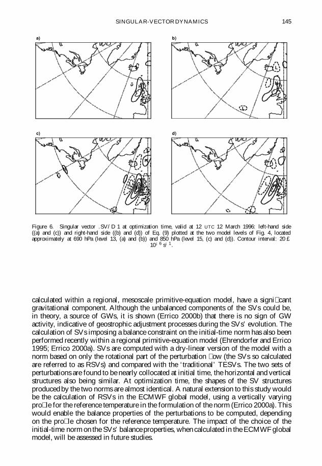
SINGULAR-VECTOR DYNAMICS 145

H

L

L

a)

H

L

L

b)

H

H

H

L

L

L

L

c)

HL

L

L

d)

Figure 6. Singular vector .SV/ D 1 at optimization time, valid at 12 UTC 12 March 1996: left-hand side((a) and (c)) and right-hand side ((b) and (d)) of Eq. (9) plotted at the two model levels of Fig. 4, locatedapproximately at 690 hPa (level 13, (a) and (b)) and 850 hPa (level 15, (c) and (d)). Contour interval: 20 £

10¡6 s¡1 .

calculated within a regional, mesoscale primitive-equation model, have a signi� cantgravitational component. Although the unbalanced components of the SVs could be,in theory, a source of GWs, it is shown (Errico 2000b) that there is no sign of GWactivity, indicative of geostrophic adjustment processes during the SVs’ evolution. Thecalculation of SVs imposing a balance constraint on the initial-time norm has also beenperformed recently within a regional primitive-equation model (Ehrendorfer and Errico1995; Errico 2000a). SVs are computed with a dry-linear version of the model with anorm based on only the rotational part of the perturbation � ow (the SVs so calculatedare referred to as RSVs) and compared with the ‘traditional’ TESVs. The two sets ofperturbations are found to be nearly collocated at initial time, the horizontal and verticalstructures also being similar. At optimization time, the shapes of the SV structuresproduced by the two norms are almost identical. A natural extension to this study wouldbe the calculation of RSVs in the ECMWF global model, using a vertically varyingpro� le for the reference temperature in the formulation of the norm (Errico 2000a). Thiswould enable the balance properties of the perturbations to be computed, dependingon the pro� le chosen for the reference temperature. The impact of the choice of theinitial-time norm on the SVs’ balance properties, when calculated in the ECMWF globalmodel, will be assessed in future studies.

146 A. MONTANI and A. J. THORPE

6. CONCLUSIONS

This investigation of aspects of SV dynamics led us to consider the mechanismsinvolved in the rapid growth experienced by this kind of perturbation. The extent towhich simple models of perturbation growth can explain the evolution of SVs, wasexamined.

The tipping over of elongated PV perturbations by the basic-state sheared � owis associated with the energy growth of the SV, con� rming the results obtained withsimpler models. The portion of the SVs located below 500 hPa was found to play amajor role in the interaction processes between the perturbation and the basic-state � eldsand to be responsible for the development of the perturbation. In particular, the relativeincrease of energy is related to the vertical propagation of the perturbation as well asto the coupling of interior PV and surface baroclinicity. It is important to underline thatthe latter mechanism contributes to the energy growth at low levels, with the main � nal-time peak often being located just above the boundary layer. A perturbation initiallylocalized in the lower part of the troposphere experiences growth of almost the sameorder as the full SV, while a perturbation placed at initial time above 500 hPa shows amuch more limited total-energy increase. On the other hand, the Lili case, characterizedby upper-level sensitivity at initial time, shows that both upper and lower-level processesprovide almost equal contributions to the amount of energy growth. SVs also grow interms of PV when their velocity components can interact with basic-state PV horizontalgradients. The growth in PV experienced by an SV is usually more marked at thetropopause, where these gradients are more intense and the perturbation can interacteffectively with the basic state and grow. Perturbations localized at initial time in theupper troposphere propagate with almost constant PV, because of the lack of growthin the perturbation � elds. Perturbations initially con� ned at low levels can propagatevertically more ef� ciently and the interaction with the upper-level basic-state � elds ismuch more effective.

Finally, the applicability of balance dynamics, valid in idealized models of non-modal growth, is discussed for the SVs, assessing their balance properties when theperturbations are calculated with the total-energy norm. The initial state of SVs is foundto be out of balance, because of a lack of amplitude in the vorticity component, beingabout a factor of four too small. During the evolution, SVs tend to achieve a morebalanced con� guration; balance is satis� ed at optimization time.

ACKNOWLEDGEMENTS

The authors thank ECMWF for providing the computing facilities which made thiswork possible. We are grateful to the anonymous referees for their helpful comments andto Roberto Buizza, Tim Palmer, Jan Barkmeijer and Jake Badger for useful discussions.A. Montani was supported during this study by a Gassiot Committee studentship award.

REFERENCES

Badger, J. and Hoskins, B. J. 2001 Simple initial value problems and mechanisms for baroclinicgrowth. J. Atmos. Sci., 58, 38–49

Browning, K. A., Vaughan, G. andPanagi, P.

1998 Analysis of an ex-tropical cyclone after its reintensi� cation asa warm-core extratropical cyclone. Q. J. R. Meteorol. Soc.,124, 2329–2356

Browning, K. A., Thorpe, A. J.,Montani, A., Parsons, D.,Grif� ths, M., Panagi, P. andDicks, E. M.

2000 Interaction of tropopause depressions with an ex-tropical cycloneand sensitivity of forecasts to analysis errors. Mon. WeatherRev., 128, 2734–2755

SINGULAR-VECTOR DYNAMICS 147

Buizza, R. 1994 Location of optimal perturbations using a projector operator.Q. J. R. Meteorol. Soc., 120, 1646–1681

Buizza, R. and Montani, A. 1999 Targeting observations using singular vectors. J. Atmos. Sci., 56,2965–2985

Buizza, R. and Palmer, T. N. 1995 The singular-vector structure of the atmospheric global circula-tion. J. Atmos. Sci., 52, 1434–1456

Buizza, R., Tribbia, J., Molteni, F.and Palmer, T. N.

1993 Computation of optimal unstable structures for a numericalweather prediction model. Tellus, 45A, 388–407

Charney, J. G. 1947 The dynamics of long waves in a baroclinic westerly current.J. Meteorol. , 4, 135–162

Clough, S. A., Lean, H. W.,Roberts, N. M., Birkett, H.,Charboureau, J.-P., Dixon, R.,Grif� ths, M., Hewson, T. D.and Montani, A.

1998 ‘A JCMM overview of FASTEX IOPs’. Internal Report 81. JointCentre for Mesoscale Meteorology, Dept. of Meteorology,Earley Gate, Reading, UK

Davis, C. A. and Emanuel, K. A. 1991 Potential vorticity diagnostics of cyclogenesis. Mon. WeatherRev., 119, 1929–1953

Eady, E. J. 1949 Long waves and cyclone waves. Tellus, 1, 33–52Ehrendorfer, M. and Errico, R. M. 1995 Mesoscale predictability and the spectrum of optimal perturba-

tions. J. Atmos. Sci., 52, 3475–3500Errico, R. M. 2000a Interpretations of the total energy and rotational energy norms

applied to determination of singular vectors. Q. J. R.Meteorol. Soc., 126, 1581–1599

2000b The dynamical balance of leading singular vectors in a primitive-equation model. Q. J. R. Meteorol. Soc., 126, 1601–1618

Errico, R. M. and Langland, R. 1999 Notes on the appropriateness of ‘bred modes’ for generating ini-tial perturbations used in ensemble prediction. Tellus, 51A,431–441

Farrell, B. F. 1982 The initial growth of disturbances in a baroclinic � ow. J. Atmos.Sci., 39, 1663–1686

1989 Optimal excitation of baroclinic waves. J. Atmos. Sci., 46, 1193–1206

1990 Small error dynamics and the predictability of atmospheric � ows.J. Atmos. Sci., 47, 2409–2416

Gelaro, R., Langland, R. H.,Rohaly, G. D. andRosmond, T. E.

1999 An assessment of the singular vector approach to targeted observ-ing using the FASTEX data set. Q. J. R. Meteorol. Soc., 125,3299–3327

Holton, J. R. 1992 An introduction to dynamic meteorology. Academic Press, SanDiego, USA

Hoskins, B. J., McIntyre, M. E. andRobertson, A. W.

1985 On the use and signi� cance of isentropic potential vorticity maps.Q. J. R. Meteorol. Soc., 111, 877–946

Hoskins, B. J., Buizza, R. andBadger, J.

2000 The nature of singular vector growth and structure. Q. J. R.Meteorol. Soc., 126, 1565–1580

Joly, A., Browning, K. A.,Bessemoulin, P.,Cammas, J.-P., Caniaux, G.,Chalon, J.-P., Dirks, R.,Emanuel, K. A., Gall, R.,Hewson, T. D.,Hildebrand, P. H.,Jorgensen, D., Lalaurette, F.,Langland, R. H., Lemaitre, Y.,Mascart, P., Moore, J. A.,Persoon, P. O. G., Roux, F.,Shapiro, M. A., Snyder, C.,Toth, Z. and Wakimoto, R. M.

1999 Overview of the � eld phase of the Fronts and Atlantic Storm-Track EXperiment (FASTEX) project. Q. J. R. Meteorol.Soc., 125, 3131–3163

Langland, R. H., Gelaro, R.,Rohaly, G. D. andShapiro, M. A.

1999 Targeted observations in FASTEX: Adjoint-based targeting pro-cedures and data impact experiments in IOPs-17 and 18.Q. J. R. Meteorol. Soc., 125, 3241–3270

Molteni, F., Buizza, R.,Palmer, T. N. andPetroliagis, T.

1996 The ECMWF Ensemble Prediction System: Methodology andvalidation. Q. J. R. Meteorol. Soc., 122, 73–119

Montani, A. 1998 ‘Targeting of observations to improve forecasts of cyclogenesis ’.PhD thesis, University of Reading

Montani, A., Thorpe, A. J.,Buizza, R. and Unden, P.

1999 Forecast skill of the ECMWF model using targeted observationsduring FASTEX. Q. J. R. Meteorol. Soc., 125, 3219–3240

148 A. MONTANI and A. J. THORPE

Palmer, T. N., Gelaro, R.,Barkmeijer, J. and Buizza, R.

1998 Singular vectors, metrics and adaptive observations. J. Atmos.Sci., 55, 633–653

Simmons, A. J. and Hoskins, B. J. 1976 Baroclinic instability on the sphere: Normal modes of the prim-itive and quasi-geostrophic equations. J. Atmos. Sci., 33,1454–1477

Simmons, A. J. and Hoskins, B. J. 1977 Baroclinic instability on the sphere: Solutions with a more realis-tic tropopause. J. Atmos. Sci., 34, 581–588

Szunyogh, I., Kalnay, E. andToth, Z.

1997 A comparison of Lyapunov and optimal vectors in a low-resolution GCM. Tellus, 49A, 200–227