Mechanising first-order temporal resolution

Information and Computation 199 (2005) 55–86

www.elsevier.com/locate/ic

Mechanising first-order temporal resolution

Boris Koneva,∗,1, Anatoli Degtyarevb, Clare Dixona,Michael Fishera, Ullrich Hustadta

aDepartment of Computer Science, University of Liverpool, Liverpool, UKbDepartment of Computer Science, King’s College London, Strand, London, UK

Received 1 December 2003; revised 31 August 2004Available online 8 February 2005

Abstract

First-order temporal logic is a concise and powerful notation, with many potential applications in bothComputer Science and Artificial Intelligence. While the full logic is highly complex, recent work on monod-ic first-order temporal logics has identified important enumerable and even decidable fragments. Althougha complete and correct resolution-style calculus has already been suggested for this specific fragment, thiscalculus involves constructions too complex to be of practical value. In this paper, we develop a machine-oriented clausal resolution method which features radically simplified proof search. We first define a normalform for monodic formulae and then introduce a novel resolution calculus that can be applied to formulaein this normal form. By careful encoding, parts of the calculus can be implemented using classical first-orderresolution and can, thus, be efficiently implemented. We prove correctness and completeness results for thecalculus and illustrate it on a comprehensive example. An implementation of the method is briefly discussed.© 2004 Elsevier Inc. All rights reserved.

Keywords: Clausal resolution; Temporal logics; Monodic fragment

∗ Corresponding author.E-mail addresses: [email protected] (B. Konev), [email protected] (A. Degtyarev), [email protected]

(C. Dixon), [email protected] (M. Fisher), [email protected] (U. Hustadt).1 On leave from Steklov Institute of Mathematics at St. Petersburg.

0890-5401/$ - see front matter © 2004 Elsevier Inc. All rights reserved.doi:10.1016/j.ic.2004.10.005

56 B. Konev et al. / Information and Computation 199 (2005) 55–86

1. Introduction

In its propositional form, linear, discrete temporal logic [15,38,43] has been used in a wide varietyof areas within Computer Science and Artificial Intelligence, for example robotics [48], databases[51], hardware verification [33], and agent-based systems [45]. In particular, propositional temporallogics have been applied to:

• the specification and verification of reactive (e.g., distributed or concurrent) systems [38];• the synthesis of programs from temporal specifications [36,44];• the semantics of executable temporal logic [18,19];• algorithmic verification via model-checking [6,32]; and• knowledge representation and reasoning [2,16,53].

Although recognised as both a much more powerful and natural formalism [25,27], first-ordertemporal logic has generally been avoided due to completeness problems. In particular, the set ofvalid formulae of this logic is not recursively enumerable [1,49,50]. However, recent work by Hod-kinson et al. [31] has shown that a specific fragment of first-order temporal logic, termed themonodicfragment, has the completeness (and sometimes even decidability) property. This breakthrough hasled to considerable research activity examining the monodic fragment, in terms of decidable classes,extensions, applications and mechanisation, and promises important advances for the future offormal methods for reactive systems.In order to effectively utilise monodic temporal logics, we require tools mechanising their proof

methods. Concerning proof methods for monodic temporal logics, general tableau and resolutioncalculi have already been defined, in [35] and [7,8], respectively. However, neither of these is par-ticularly practical: given a formula � to be tested for satisfiability, the tableau method requiresrepresentation of all possible first-order models of first-order subformulae of �, while the resolu-tion method involves all possible combinations of temporal clauses in the clause normal form of �.Thus, improved methods are required.In this paper, we focus on an important subclass of temporal models, having a wide range of ap-

plications, for example in spatio-temporal logics [28,55] and temporal description logics [3], namelythose models that have expanding domains. In such models, the domains over which first-orderterms range can only increase at each temporal step. The focus on this class of models allows us toproduce a simplified clausal resolution calculus, termed the fine-grained resolution calculus, which ismore amenable to efficient implementation. Thus, we here describe such an implementable calculus,consider its properties and extend the results to constant-domain problems. We also describe animplementation of this fine-grained calculus and its use on a range of problems. This represents thefirst practically useful tool for handling monodic first-order temporal logics.The organisation of the paper is the following. In Section 2 we define the expanding domain

monodic fragment. In Section 3 we introduce the divided separated normal form (DSNF) for mo-nodic temporal formulae and describe how monodic temporal formulae are translated into DSNF.In Sections 4 and 5 we introduce the fine-grained resolution calculus and provide completenessresults for the fine-grained resolution calculus relative to the completeness of the general resolutioncalculus [7]. A number of examples will be given, showing how the fine-grained resolution calculusworks in practice. In Section 7 we briefly describe how constant-domain problems can be handled,

B. Konev et al. / Information and Computation 199 (2005) 55–86 57

through a translation of the formulae. Sections 8 and 9 are devoted to an implementation of fine-grained resolution and to its applications. Finally, in Section 10 we consider conclusions and futurework.

2. First-order temporal logic

First-order (discrete linear time) temporal logic, FOTL, is an extension of classical first-orderlogic with operators that deal with a discrete and linear model of time (isomorphic to �, and themost commonly used model of time). The vocabulary of FOTL consists of:

• Predicate symbols P0, P1, . . . each of which is of some fixed arity (null-ary predicate symbols arecalled propositions);

• Individual variables x0, x1, . . .;• Individual constants c0, c1, . . .;• Booleans ∧, ¬, ∨,⇒, ≡, true (‘true’), false (‘false’);• Quantifiers ∀ and ∃;• Temporal operators (‘always in the future’), ♦ (‘sometime in the future’), ❤ (‘at the nextmoment’), U (until), and W (weak until).

There are no function symbols or equality in this FOTL language, but it does contain constants.The set of FOTL-formulae is defined in the standard way [20,31]:

• Booleans true and false are FOTL-formulae;• if P is an n-ary predicate symbol and ti, 1 � i � n, are variables or constants, then P(t1, . . . , tn) isan (atomic) FOTL-formula;

• if � and are FOTL-formulae, so are ¬�, � ∧ , � ∨ , �⇒ , and � ≡ ;• if � is an FOTL-formula and x is a variable, then ∀x� and ∃x� are FOTL-formulae;• if � and are FOTL-formulae, then so are �, ♦�, ❤�, �U , and �W .

A literal is an atomic formula or its negation.For a given formula, �, const(�) denotes the set of constants occurring in �. We write �(x) to

indicate that �(x) has at most one free variable x (if not explicitly stated otherwise). A formula havingno free occurrences of variables is called closed.Intuitively, FOTL formulae are interpreted in first-order temporal structures which are sequences

M of worlds,M = M0,M1, . . . with truth values in different worlds being connected via temporaloperators.More formally, for every moment of time n � 0, there is a corresponding first-order structure,

Mn = 〈Dn, In〉, where every Dn is a non-empty set such that whenever n < m, Dn ⊆ Dm, and Inis an interpretation of predicate and constant symbols over Dn. We require that the interpreta-tion of constants is rigid. Thus, for every constant c and all moments of time i, j � 0, we haveIi(c) = Ij(c).A (variable) assignment a is a function from the set of individual variables to ∪n∈�Dn. We de-

note the set of all assignments by A. The set of variable assignments An corresponding toMn is a

58 B. Konev et al. / Information and Computation 199 (2005) 55–86

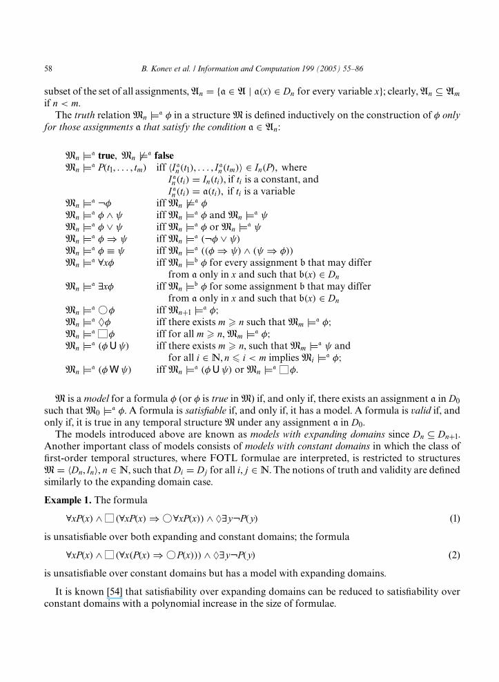
subset of the set of all assignments,An = {a ∈ A | a(x) ∈ Dn for every variable x}; clearly,An ⊆ Am

if n < m.The truth relationMn |=a � in a structureM is defined inductively on the construction of � only

for those assignments a that satisfy the condition a ∈ An:

Mn |=a true, Mn �|=a falseMn |=a P(t1, . . . , tm) iff 〈I an(t1), . . . , I an(tm)〉 ∈ In(P), where

I an(ti) = In(ti), if ti is a constant, andI an(ti) = a(ti), if ti is a variable

Mn |=a ¬� iffMn �|=a �

Mn |=a � ∧ iffMn |=a � andMn |=a

Mn |=a � ∨ iffMn |=a � orMn |=a

Mn |=a �⇒ iffMn |=a (¬� ∨ )Mn |=a � ≡ iffMn |=a ((�⇒ ) ∧ ( ⇒ �))

Mn |=a ∀x� iffMn |=b � for every assignment b that may differfrom a only in x and such that b(x) ∈ Dn

Mn |=a ∃x� iffMn |=b � for some assignment b that may differfrom a only in x and such that b(x) ∈ Dn

Mn |=a ❤� iffMn+1 |=a �;Mn |=a ♦� iff there exists m � n such thatMm |=a �;Mn |=a � iff for all m � n,Mm |=a �;Mn |=a (�U ) iff there exists m � n, such thatMm |=a and

for all i ∈ �, n � i < m impliesMi |=a �;Mn |=a (�W ) iffMn |=a (�U ) orMn |=a �.

M is a model for a formula � (or � is true inM) if, and only if, there exists an assignment a in D0such thatM0 |=a �. A formula is satisfiable if, and only if, it has a model. A formula is valid if, andonly if, it is true in any temporal structureM under any assignment a in D0.The models introduced above are known as models with expanding domains since Dn ⊆ Dn+1.

Another important class of models consists of models with constant domains in which the class offirst-order temporal structures, where FOTL formulae are interpreted, is restricted to structuresM = 〈Dn, In〉, n ∈ �, such thatDi = Dj for all i, j ∈ �. The notions of truth and validity are definedsimilarly to the expanding domain case.

Example 1. The formula

∀xP(x) ∧ (∀xP(x)⇒ ❤∀xP(x)) ∧ ♦∃y¬P(y) (1)

is unsatisfiable over both expanding and constant domains; the formula

∀xP(x) ∧ (∀x(P(x)⇒ ❤P(x))) ∧ ♦∃y¬P(y) (2)

is unsatisfiable over constant domains but has a model with expanding domains.

It is known [54] that satisfiability over expanding domains can be reduced to satisfiability overconstant domains with a polynomial increase in the size of formulae.

B. Konev et al. / Information and Computation 199 (2005) 55–86 59

The set of valid formulae of first-order temporal logic is not recursively enumerable. So, providingcompletemethods for solving the satisfiability or validity problem for this logic in its full generality isimpossible. Furthermore, it is known that even “small” fragments of FOTL, such as the two-variablemonadic fragment (where all predicates are unary), are not recursively enumerable [31,39]. However,the set of validmonodic formulae (see Definition 1 below) is known to be finitely axiomatisable [56].

Definition 1. An FOTL-formula � is called monodic if, and only if, any subformula of the form T ,where T is one of ❤, , ♦ (or 1T 2, where T is one of U , W ), contains at most one free variable.

Example 2. The formulae

∀x ∃yP(x, y) and ∀x P(x, c)

are monodic, whereas the formula

∀x∀y(P(x, y)⇒ P(x, y))

is non-monodic.

We note that the addition of either equality or function symbols to the monodic fragment gener-ally leads to the loss of recursive enumerability [56]. Moreover, although the two variable monodicfragmentwithout equality is decidable [31], it was proved in [9] that the two variable monadic monodicfragment with equality is not even recursively enumerable. However, in [30] it was shown that theguarded monodic fragment with equality is decidable.

3. Divided separated normal form (DSNF)

Resolution calculi for first-order logic require that first-order formulae are transformed to a clas-sical clause normal form [42], before the inference rules of the calculus can be applied. Similarly, thetemporal resolution calculus which will be defined in Section 4 as well as the fine-grained resolutionwhich will be defined in Section 5 require first-order temporal formulae to be transformed into aparticular normal form. We define this normal form below.

Definition 2.A temporal step clause is a formula either of the form p ⇒ ❤l, where p is a propositionand l is a propositional literal, or (P(x)⇒ ❤M(x)), where P(x) is a unary atom andM(x) is a unaryliteral. We call a clause of the first type an (original) ground step clause, and of the second type an(original) non-ground step clause. Note that the term ‘original’ is used here to distinguish these stepclauses from other notions (derived, merged, etc. step clauses) that are introduced later.

Temporal step clauses are the key elements of the normal form, providing a description of howinformation is transferred from one temporal instant to the next.

Definition 3.Amonodic temporal problem in Divided Separated Normal Form (DSNF) is a quadruple〈U , I ,S , E〉, where

(1) the universal part, U , is given by a finite set of arbitrary closed first-order formulae;(2) the initial part, I , is, again, given by a finite set of arbitrary closed first-order formulae;

60 B. Konev et al. / Information and Computation 199 (2005) 55–86

(3) the step part, S , is given by a finite set of original (ground and non-ground) temporal stepclauses, the left-hand sides of step clauses are pairwise distinct; and

(4) the eventuality part, E , is given by a finite set of clauses of the form ♦L(x) (a non-ground even-tuality clause) and ♦l (a ground eventuality clause), where l is a propositional literal and L(x)is a unary non-ground literal.

Note that, in a monodic temporal problem, we do not allow two different temporal step clauseswith the same left-hand sides. (A problem containing two different temporal step clauses with thesame left-hand sides can be easily transformed by renaming into one without.)In what follows, we will not distinguish between a finite set of formulae X and the conjunction∧ X of formulae within the set. With each monodic temporal problem, we associate the formula

I ∧ U ∧ ∀xS ∧ ∀xE .Now, whenwe talk about particular properties of a temporal problem (e.g., satisfiability, validity,

logical consequences, etc.) we refer to properties of the associated formula.Arbitrary monodic first-order temporal formulae can be transformed into DSNF. The transfor-

mation is based on using a renaming technique to substitute non-atomic subformulae and replacingtemporal operators by their fixed point definitions as described, e.g., in [21]; it consists of a sequenceof steps.

(1) Transform a given monodic formula to negation normal form. (To assist understanding of thetransformation, we list here some equivalences used in this step.)

∀x(¬ �(x) ≡ ♦¬�(x));∀x(¬♦�(x) ≡ ¬�(x));∀x(¬ ❤�(x) ≡ ❤¬�(x));

∀x(¬(�(x)U (x)) ≡ ¬ (x)W (¬�(x) ∧ ¬ (x)));∀x(¬(�(x)W (x)) ≡ ¬ (x)U (¬�(x) ∧ ¬ (x))).

If the transformations above are applied in a naive way, the size of the result may grow ex-ponentially; we may have to use renaming [42,52] in order to keep the size of the transformedformula linear in the size of the original formula.

(2) Recursively rename each innermost temporal subformulae, ❤�(x),♦�(x), �(x), �(x)U (x),�(x)W (x) by a new unary predicate P(x) (using a new name for each subformula). Renamingintroduces formulae defining P(x) of the following form:

(a) ∀x(P(x)⇒ ❤�(x)); (c) ∀x(P(x) ⇒ �(x));(b) ∀x(P(x)⇒ �(x)W (x)); (d) ∀x(P(x)⇒ �(x)U (x));

(e) ∀x(P(x)⇒ ♦�(x)).

Since we are only interested in satisfiability, we use implications instead of equivalencesrenaming positive occurrences of subformulae, see also [42,52].Formulae of the form (a) above are already in DSNF after renaming complex first-or-

der formulae from the right-hand side; first-order clauses from this renaming are put in theuniversal part. This kind of renaming is assumed implicitly in the following.

B. Konev et al. / Information and Computation 199 (2005) 55–86 61

(3) Formulae of the form (b), (c), and (d) require extra transformation by removing the temporaloperators using their fixed point definitions (see [21]):

∀x(P(x)⇒ �(x)) is satisfiability equivalent to

∀x(P(x)⇒ R(x)) ∧ ∀x(R(x)⇒ ❤R(x)) ∧ ∀x(R(x)⇒ �(x)),

∀x(P(x)⇒ (�(x)U (x))) is satisfiability equivalent to

∀x(P(x)⇒ ♦ (x)) ∧ ∀x(P(x)⇒ (�(x) ∨ (x)))∧ ∀x(P(x)⇒ (S(x) ∨ (x))) ∧ ∀x(S(x)⇒ ❤(�(x) ∨ (x)))∧ ∀x(S(x)⇒ ❤(S(x) ∨ (x))),and ∀x(P(x)⇒ (�(x)W (x))) is satisfiability equivalent to

∀x(P(x)⇒ (�(x) ∨ (x))) ∧ ∀x(P(x)⇒ (S(x) ∨ (x)))∧ ∀x(S(x)⇒ ❤(�(x) ∨ (x))) ∧ ∀x(S(x)⇒ ❤(S(x) ∨ (x))),where R(x) and S(x) are new unary predicates.

(4) Finally, formulae of the form (e) are transformed into DSNF as follows:∀x(P(x)⇒ ♦L(x)) is satisfiability equivalent (see [7]) to

∀x((P(x) ∧ ¬L(x))⇒ waitforL(x)) (3)

∀x(waitforL(x)⇒ ❤(waitforL(x) ∨ L(x))) (4)

∀x(♦¬waitforL(x)) (5)

where waitforL(x) is a new unary predicate.

Theorem 1 (see [7], Theorem 1). The transformation described above reduces any monodic first-ordertemporal formula � to monodic temporal problem P in DSNF with at most linear increase in the sizeof the problem such that � is satisfiable over constant and expanding domains if, and only if, P issatisfiable over constant and expanding domains, respectively.

Example 3. Consider the temporal formula ∃x ♦∀y∀z∃u (x, y , z, u) where (x, y , z, u) does notcontain temporal operators. To reduce it to DSNF, we first, rename the innermost temporal sub-formula by a new predicate, P1,

∃x P1(x) ∧ ∀x[P1(x)⇒ ♦∀y∀z∃u (x, y , z, u)].

Next, we rename the first ‘ ’-formula, introducing P3, and the subformula under the ‘♦’ operator,introducing P2,

∃xP3(x) ∧ ∀x[P1(x)⇒♦P2(x)]∧ ∀x[P2(x)⇒∀y∀z∃u (x, y , z, u)]∧ ∀x[P3(x)⇒ P1(x)],

62 B. Konev et al. / Information and Computation 199 (2005) 55–86

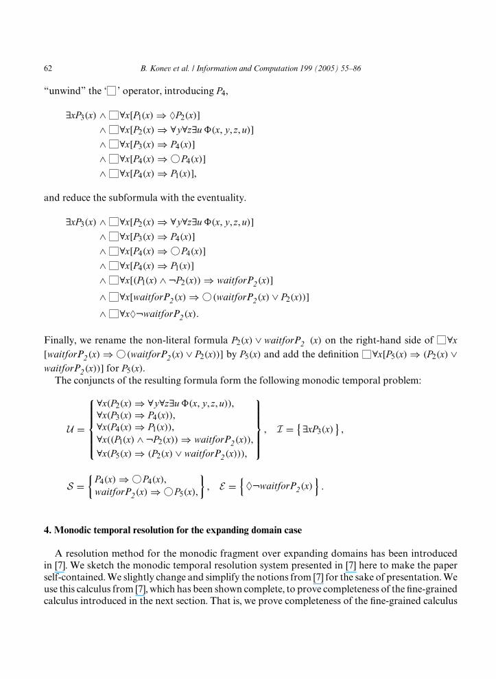
“unwind” the ‘ ’ operator, introducing P4,

∃xP3(x) ∧ ∀x[P1(x)⇒ ♦P2(x)]∧ ∀x[P2(x)⇒ ∀y∀z∃u (x, y , z, u)]∧ ∀x[P3(x)⇒ P4(x)]∧ ∀x[P4(x)⇒ ❤P4(x)]∧ ∀x[P4(x)⇒ P1(x)],

and reduce the subformula with the eventuality.

∃xP3(x) ∧ ∀x[P2(x)⇒ ∀y∀z∃u (x, y , z, u)]∧ ∀x[P3(x)⇒ P4(x)]∧ ∀x[P4(x)⇒ ❤P4(x)]∧ ∀x[P4(x)⇒ P1(x)]∧ ∀x[(P1(x) ∧ ¬P2(x))⇒ waitforP2(x)]∧ ∀x[waitforP2(x)⇒ ❤(waitforP2(x) ∨ P2(x))]∧ ∀x♦¬waitforP2(x).

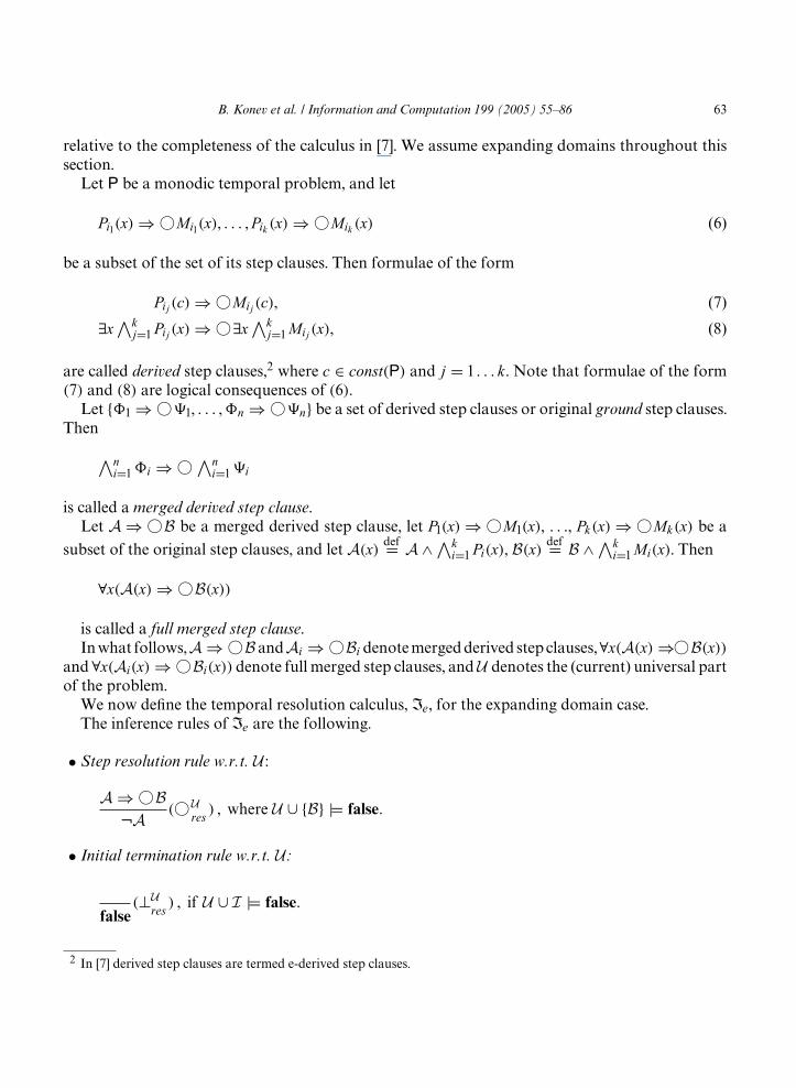
Finally, we rename the non-literal formula P2(x) ∨ waitforP2 (x) on the right-hand side of ∀x[waitforP2(x)⇒ ❤(waitforP2(x) ∨ P2(x))] by P5(x) and add the definition ∀x[P5(x)⇒ (P2(x) ∨waitforP2(x))] for P5(x).The conjuncts of the resulting formula form the following monodic temporal problem:

U =

∀x(P2(x)⇒ ∀y∀z∃u (x, y , z, u)),∀x(P3(x)⇒ P4(x)),∀x(P4(x)⇒ P1(x)),∀x((P1(x) ∧ ¬P2(x))⇒ waitforP2(x)),∀x(P5(x)⇒ (P2(x) ∨ waitforP2(x))),

, I = {∃xP3(x)} ,

S ={P4(x)⇒ ❤P4(x),waitforP2(x)⇒ ❤P5(x),

}, E =

{♦¬waitforP2(x)

}.

4. Monodic temporal resolution for the expanding domain case

A resolution method for the monodic fragment over expanding domains has been introducedin [7]. We sketch the monodic temporal resolution system presented in [7] here to make the paperself-contained.We slightly change and simplify the notions from [7] for the sake of presentation.Weuse this calculus from [7], which has been shown complete, to prove completeness of the fine-grainedcalculus introduced in the next section. That is, we prove completeness of the fine-grained calculus

B. Konev et al. / Information and Computation 199 (2005) 55–86 63

relative to the completeness of the calculus in [7]. We assume expanding domains throughout thissection.Let P be a monodic temporal problem, and let

Pi1(x)⇒ ❤Mi1(x), . . . , Pik (x)⇒ ❤Mik (x) (6)

be a subset of the set of its step clauses. Then formulae of the form

Pij (c)⇒ ❤Mij(c), (7)

∃x∧kj=1 Pij (x)⇒ ❤∃x∧k

j=1Mij(x), (8)

are called derived step clauses,2 where c ∈ const(P) and j = 1 . . . k . Note that formulae of the form(7) and (8) are logical consequences of (6).Let { 1 ⇒ ❤"1, . . . , n ⇒ ❤"n} be a set of derived step clauses or original ground step clauses.

Then

∧ni=1 i ⇒ ❤∧n

i=1"i

is called a merged derived step clause.Let A ⇒ ❤B be a merged derived step clause, let P1(x)⇒ ❤M1(x), . . ., Pk(x)⇒ ❤Mk(x) be a

subset of the original step clauses, and let A(x) def= A ∧ ∧ki=1 Pi(x), B(x) def= B ∧ ∧k

i=1Mi(x). Then

∀x(A(x)⇒ ❤B(x))

is called a full merged step clause.Inwhat follows,A ⇒ ❤B andAi ⇒ ❤Bi denotemergedderived step clauses,∀x(A(x)⇒ ❤B(x))

and ∀x(Ai(x)⇒ ❤Bi(x)) denote full merged step clauses, andU denotes the (current) universal partof the problem.We now define the temporal resolution calculus, Ie, for the expanding domain case.The inference rules of Ie are the following.

• Step resolution rule w.r.t. U :

A ⇒ ❤B¬A ( ❤U

res) , where U ∪ {B} |= false.

• Initial termination rule w.r.t. U:

false(⊥U

res) , if U ∪ I |= false.

2 In [7] derived step clauses are termed e-derived step clauses.

64 B. Konev et al. / Information and Computation 199 (2005) 55–86

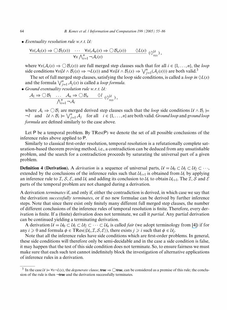
• Eventuality resolution rule w.r.t. U:

∀x(A1(x)⇒ ❤B1(x)) · · · ∀x(An(x)⇒ ❤Bn(x)) ♦L(x)∀x∧n

i=1¬Ai(x)(♦U

res) ,

where ∀x(Ai(x)⇒ ❤Bi(x)) are full merged step clauses such that for all i ∈ {1, . . . , n}, the loopside conditions ∀x(U ∧ Bi(x)⇒ ¬L(x)) and ∀x(U ∧ Bi(x)⇒ ∨n

j=1(Aj(x))) are both valid.3

The set of full merged step clauses, satisfying the loop side conditions, is called a loop in ♦L(x)and the formula

∨nj=1Aj(x) is called a loop formula.

• Ground eventuality resolution rule w.r.t. U:A1 ⇒ ❤B1 . . . An ⇒ ❤Bn ♦l∧n

i=1¬Ai

(♦Ures) ,

where Ai ⇒ ❤Bi are merged derived step clauses such that the loop side conditions U ∧ Bi |=¬l and U ∧ Bi |= ∨n

j=1Aj for all i ∈ {1, . . . , n} are both valid.Ground loop and ground loopformula are defined similarly to the case above.

Let P be a temporal problem. By TRes(P) we denote the set of all possible conclusions of theinference rules above applied to P.Similarly to classical first-order resolution, temporal resolution is a refutationally complete sat-

uration-based theorem proving method, i.e., a contradiction can be deduced from any unsatisfiableproblem, and the search for a contradiction proceeds by saturating the universal part of a givenproblem.

Definition 4 (Derivation). A derivation is a sequence of universal parts, U = U0 ⊂ U1 ⊂ U2 ⊂ · · ·,extended by the conclusions of the inference rules such that Ui+1 is obtained from Ui by applyingan inference rule to I , S , E , and Ui and adding its conclusion to Ui to obtain Ui+1. The I , S and Eparts of the temporal problem are not changed during a derivation.

A derivation terminates if, and only if, either the contradiction is derived, in which case we say thatthe derivation successfully terminates, or if no new formulae can be derived by further inferencesteps. Note that since there exist only finitely many different full merged step clauses, the numberof different conclusions of the inference rules of temporal resolution is finite. Therefore, every der-ivation is finite. If a (finite) derivation does not terminate, we call it partial. Any partial derivationcan be continued yielding a terminating derivation.A derivation U = U0 ⊂ U1 ⊂ U2 ⊂ · · · ⊂ Un is called fair (we adopt terminology from [4]) if for

any i � 0 and formula � ∈ TRes(〈Ui, I ,S , E〉), there exists j � i such that � ∈ Uj .Note that all the inference rules have side conditions which are first-order problems. In general,

these side conditions will therefore only be semi-decidable and in the case a side condition is false,it may happen that the test of this side condition does not terminate. So, to ensure fairness we mustmake sure that each such test cannot indefinitely block the investigation of alternative applicationsof inference rules in a derivation.

3 In the case U |= ∀x¬L(x), the degenerate clause, true ⇒ ❣true, can be considered as a premise of this rule; the conclu-sion of the rule is then ¬true and the derivation successfully terminates.

B. Konev et al. / Information and Computation 199 (2005) 55–86 65

Note 1. In this section, we intentionally do not consider the classical concept of redundancy (see[4]) and deletion rules over sets of first-order formulae Ui . We come to the issue of redundancy anddeletion rules in Section 5 where we present a machine-oriented calculus.

Let P = 〈U , I ,S , E〉 be a monodic temporal problem, then the set of formulaePc = 〈U , I ,S , E ∪ {♦L(c) | ♦L(x) ∈ E , c ∈ const(P)}〉

is termed the constant flooded form of P. (Strictly speaking, Pc is not in DSNF: we have to renameground eventualities by propositions.) Evidently, Pc is satisfiability equivalent to P.

Theorem 2 (see [7, Theorem 10]). The rules of Ie preserve satisfiability over expanding domains. If amonodic temporal problem P is unsatisfiable over expanding domains, then any fair derivation in Iefrom Pc successfully terminates.

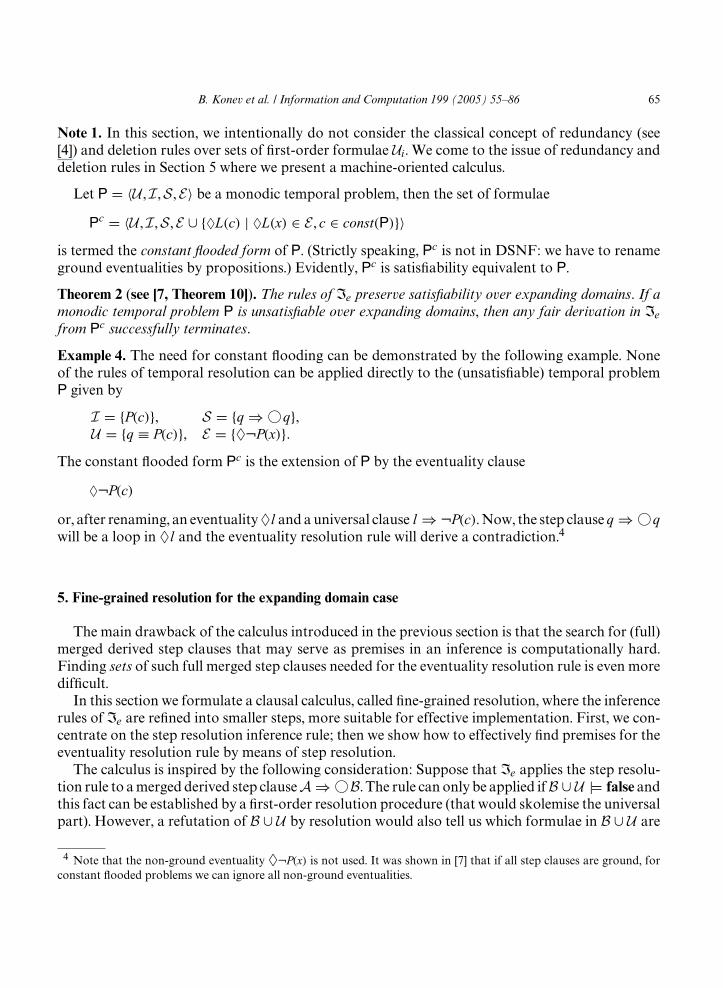
Example 4. The need for constant flooding can be demonstrated by the following example. Noneof the rules of temporal resolution can be applied directly to the (unsatisfiable) temporal problemP given by

I = {P(c)}, S = {q⇒ ❤q},U = {q ≡ P(c)}, E = {♦¬P(x)}.

The constant flooded form Pc is the extension of P by the eventuality clause

♦¬P(c)or, after renaming, an eventuality♦l and a universal clause l⇒ ¬P(c). Now, the step clause q⇒ ❤q

will be a loop in ♦l and the eventuality resolution rule will derive a contradiction.4

5. Fine-grained resolution for the expanding domain case

The main drawback of the calculus introduced in the previous section is that the search for (full)merged derived step clauses that may serve as premises in an inference is computationally hard.Finding sets of such full merged step clauses needed for the eventuality resolution rule is even moredifficult.In this section we formulate a clausal calculus, called fine-grained resolution, where the inference

rules of Ie are refined into smaller steps, more suitable for effective implementation. First, we con-centrate on the step resolution inference rule; then we show how to effectively find premises for theeventuality resolution rule by means of step resolution.The calculus is inspired by the following consideration: Suppose that Ie applies the step resolu-

tion rule to amerged derived step clauseA ⇒ ❤B. The rule can only be applied ifB ∪ U |= false andthis fact can be established by a first-order resolution procedure (that would skolemise the universalpart). However, a refutation of B ∪ U by resolution would also tell us which formulae in B ∪ U are

4 Note that the non-ground eventuality ♦¬P(x) is not used. It was shown in [7] that if all step clauses are ground, forconstant flooded problems we can ignore all non-ground eventualities.

66 B. Konev et al. / Information and Computation 199 (2005) 55–86

involved in the derivation of a contradiction. Thus, not only canwe check the side conditions for therules of Ie by means of first-order resolution, but also search for clauses to merge at the same time.In contrast to Ie which can be applied to monodic temporal problems 〈U , I ,S , E〉 where the

universal part U and the initial part I are sets of arbitrary closed first-order formulae, fine-grainedresolution operates on temporal problems where U and I are given by sets of first-order clauses.Definition 5. Let P be a monodic temporal problem. We define a set S(P) of initial, universal, andstep clauses, called the result of clausification P, as follows.

(1) Step clauses from P are in S(P).(2) For every original non-ground step clause

P(x)⇒ ❤M(x)

and every constant c ∈ const(P), the clauseP(c)⇒ ❤M(c) (9)

is in S(P).(3) Clauses obtained by clausification of the universal and initial parts, as if there is no connectionwith temporal logic at all, are also in S(P). The resulting clauses are called universal clauses andinitial clauses, respectively. In the beginning, universal and initial clauses do not have commonSkolem constants and functions.

Note that fine-grained resolution operates typed clauses (every clause is marked as “initial,”“universal,” or “step”). In contrast to derivations by Ie which proceed by extending the universalpart of a temporal problem while keeping all other parts of a temporal problem constant, fine-grained resolution might not only derive new universal clauses, but also additional initial clausesand step clauses of the form

C ⇒ ❤D, (10)

where C is a conjunction of propositions, unary predicates of the form P(x), and ground formulaeof the form P(c), where P is a unary predicate symbol and c is a constant occurring in the problemgiven originally; D is a disjunction of arbitrary literals.We consider initial and universal clauses as literal multisets, and step clauses of the form (10) as

ordered pairs of literal multisets. We assume basic knowledge of classical first-order resolution (see,for example, [4,5,37]).Fine-grained resolution differs from the calculus Ie in two aspects: First, instead of the step

resolution and the initial termination rule of Ie, we use fine-grained step resolution, a set of deduc-tion and deletion rules operating on clausified problems; second, we use a particular algorithm,called FG-BFS, to determine the loops to which we apply the ground and non-ground eventualityresolution rule of Ie.Let us first define the deduction rules of fine-grained step resolution. In the following, we as-

sume that different premises and conclusions of the deduction rules have no variables in common;variables may be renamed if necessary.

B. Konev et al. / Information and Computation 199 (2005) 55–86 67

• First-order resolution between two universal clauses and factoring on a universal clause. The resultis a universal clause.

• First-order resolution between an initial and a universal clause, between two initial clauses, andfactoring on an initial clause. The result is an initial clause.

• Fine-grained (restricted) step resolution.

C1 ⇒ ❤(D1 ∨ L) C2 ⇒ ❤(D2 ∨ ¬M)(C1 ∧ C2)% ⇒ ❤(D1 ∨ D2)% ,

where C1 ⇒ ❤(D1 ∨ L) and C2 ⇒ ❤(D2 ∨ ¬M) are step clauses and % is a most general unifierof the literals L and M such that % does not map variables from C1 or C2 into a constant or afunctional term.5

C1 ⇒ ❤(D1 ∨ L) D2 ∨ ¬NC1% ⇒ ❤(D1 ∨ D2)% ,

where C1 ⇒ ❤(D1 ∨ L) is a step clause, D2 ∨ ¬N is a universal clause, and % is a most generalunifier of the literals L and N such that % does not map variables from C1 into a constant or afunctional term.

• Right factor.

C ⇒ ❤(D ∨ L ∨M)C% ⇒ ❤(D ∨ L)% ,

where % is a most general unifier of the literals L and M such that % does not map variables fromC into a constant or a functional term.

• Clause conversion.A step clause of the form C ⇒ ❤false is rewritten into the universal clause6 ¬C .

A (linear) proof by fine-grained resolution of a clause C from a set of clauses S is a sequenceof clauses C1, . . . ,Cm such that C = Cm and each clause Ci is either an element of S or else theconclusion by a deduction rule applied to clauses from premises C1, . . . ,Ci−1. A proof of false iscalled a refutation.

Example 5. Fine-grained step resolution without the restriction on substitutions would, certainly,lead to unsoundness: Consider the monodic problem given by

U = {u1 : ∃x¬Q(x), u2 : ∀x(P(x) ∨ Q(x))}, I = ∅,S = {s1 : P(x)⇒ ❤Q(x)}, E = ∅,

which is satisfiable. After skolemisation, U s = {us1 : ¬Q(c), us2 : P(x) ∨ Q(x)}. Unrestricted reso-lution would derive us3 : ¬P(c) from us1 and s1, and then a contradiction from us1, us2, and us3.

5 This restriction justifies skolemisation of the universal part: Skolem constants from one moment of time do notpropagate to the previous moment.6 Here, and further, ¬(L1(x) ∧ · · · ∧ Lk(x)) abbreviates (¬L1(x) ∨ · · · ∨ ¬Lk(x)).

68 B. Konev et al. / Information and Computation 199 (2005) 55–86

The restriction that a most general unifier % applied to step clauses C ⇒ ❤D does not map a var-iable in C into a Skolem constant is violated since % maps the variable x in s1 to the constant c.Thus, the restriction we impose on step resolution inferences prevents the derivation of the clauseus3 and, therefore, prevents the derivation of a contradiction.

Example 6. It might seem that the restriction onmost general unifiers is too strong andmay destroycompleteness of the calculus. For example, at first glance it may appear that, under this restriction,it is not possible to deduce a contradiction from the following (unsatisfiable) temporal problem Pgiven by

I = {∀xP (x)}, U = {¬Q(c)},S = {P (x)⇒ ❤Q(x)}, E = ∅.

However, we can derive a contradiction because we apply our calculus to S(P) which containsan additional step clause

P(c)⇒ ❤Q(c).

Then, a contradiction can be easily derived from the additional, universal, and initial clauses.

We will now prove some basic results which will help us to establish the completeness of ourcalculus.

Definition 6. A clause of the form C ⇒ ❤false, where C is of the same form as in (10), is called afinal clause.

Lemma 3. Let ( be a proof of a final clause C ⇒ ❤false by the rules of fine-grained resolution,except the clause conversion rule, from a set of step clauses S and a set of universal clauses U . Thenthere exists a merged derived step clause A ⇒ ❤B such that B ∪ U |= false and A = ∃̃C , where ∃̃denotes existential quantification over all free variables.

Proof. Let

{Pi(xi)⇒ ❤Mi(xi) | i = 1 . . . K},{pi ⇒ ❤li | i = 1 . . . L}

be the set of all step clauses from S involved in ( where pi ⇒ ❤li denotes either a ground stepclause, or an derived step-clause of the form (9) added by clausification (w.l.o.g., we assume that allthe variables x1, . . ., xK are pairwise distinct). We assume that ( is tree-like, that is, no clause in (is used more than once as an premise for an inference rule; we may make copies of the clauses in(in order to make it tree-like.Note that (by accumulating the most general unifiers used in the proof) it is possible to construct

a finite set of instances of these clauses (and universal clauses) such that there exists a tree-likeproof of C ⇒ ❤false from this new set of clauses and all most general unifiers used in the proofare identity substitutions.7 That is, there exist substitutions {%i,j | i = 1 . . . K , j = 1 . . . si} such that7 The condition that premises of the non-ground binary resolution rule should be variable disjoint may be violated here;note, however, that this condition is needed for completeness, not correctness.

B. Konev et al. / Information and Computation 199 (2005) 55–86 69

{Pi(xi)%i,j ⇒ ❤Mi(xi)%i,j | i = 1 . . . K , j = 1 . . . si},{pi ⇒ ❤li | i = 1 . . . L} (11)

(together with some instances of universal clauses) contribute to the proof of C ⇒ ❤false whereall most general unifiers used in the proof are identity substitutions, and, furthermore,

C =K∧i=1

si∧j=1Pi(xi)%i,j ∧

L∧i=1pi.

Note further (induction) that due to our restriction on the step resolution rule, for any i, j, thesubstitution %i,j maps xi into a free variable.Let us group the instances of the step clauses according to the value of the substitutions %i,j . We

introduce an equivalence relation * on the clauses from (11) as follows: For every i, j, i′, j′ we have(Pi(xi)%i,j ⇒ ❤Mi(xi)%i,j , Pi′(xi′)%i′,j′ ⇒ ❤Mi′(xi′)%i′,j′

) ∈ *if, and only if, xi%i,j = xi′%i′,j′ (it can be easily checked that * is indeed an equivalence relation).Let N be the number of equivalence classes of (11) by *; let Ik be the set of indexes of the kthequivalence class (we refer to clauses from (11) by indexes of the corresponding substitutions).Let Ck = ∧

(i,j)∈Ik Pi(xi)%i,j , for every k , 1 � k � N ; let C0 = ∧Li=1 pi . Note that C = ∧N

k=1 Ck ∧C0, and that the Ck are pairwise disjoint. Let Dk = ∧

(i,j)∈Ik Mi(xi)%i,j , let D0 =∧Li=1 li, let D =∧N

k=1Dk ∧ D0. Note that ∀̃D ∧ U |= false. Note further that if we replace the free variable of Dkwith a fresh constant, ck , there still exists a refutation from

∧Nk=1D(ck) ∧ D0 and universal claus-

es (with most general unifiers applied to universal and intermediate clauses only). It follows that∧Nk=1 ∃xDk(x) ∧ D0 ∧ U |= false.It suffices to note that (

∧Nk=1 ∃xCk(x) ∧ C0)⇒ ❤(

∧Nk=1 ∃xDk(x) ∧ D0) is a merged derived step

clause. �Lemma 4. Let P = 〈U , I ,S , E〉 be a monodic temporal problem and S =S(P) be the result of clausifi-cation P. Let A ⇒ ❤B be a merged derived step clause such that B ∪ U |= false. Then there exists afinal clause C ⇒ ❤false, proved by fine-grained resolution from S, such that A implies ∃̃C.Proof.We show that the final clause needed, C ⇒ ❤false, can be proved from S by the deductionrules of fine-grained resolution except the clause conversion rule.The clause A ⇒ ❤B is merged from derived clauses of the form (8):

{∃x∧sij=1 Pij (x)⇒ ❤∃x∧si

j=1Mij(x) | i = 1 . . . K}and original ground step clauses and derived clauses of the form (7):

{pi ⇒ ❤li | i = 1 . . . L}.

Again, as in the proof of Lemma 3, pi ⇒ ❤li denotes either an original ground step clause or aclause of the form (7). (We simplify indexing for the sake of presentation.)

70 B. Konev et al. / Information and Computation 199 (2005) 55–86

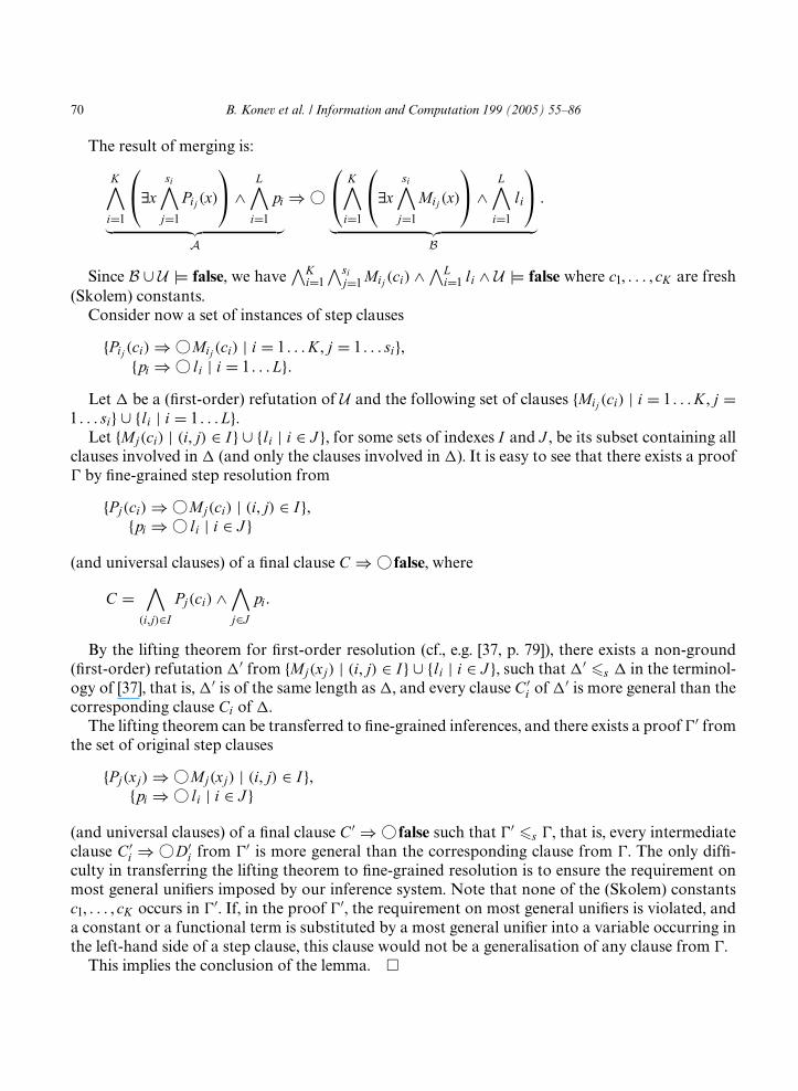
The result of merging is:

K∧i=1

∃x

si∧j=1Pij (x)

∧

L∧i=1pi

︸ ︷︷ ︸A

⇒ ❤

K∧i=1

∃x

si∧j=1Mij(x)

∧

L∧i=1li

︸ ︷︷ ︸B

.

Since B ∪ U |= false, we have∧Ki=1

∧sij=1Mij(ci) ∧

∧Li=1 li ∧ U |= false where c1, . . . , cK are fresh

(Skolem) constants.Consider now a set of instances of step clauses

{Pij (ci)⇒ ❤Mij(ci) | i = 1 . . . K , j = 1 . . . si},{pi ⇒ ❤li | i = 1 . . . L}.

Let ( be a (first-order) refutation of U and the following set of clauses {Mij(ci) | i = 1 . . . K , j =1 . . . si} ∪ {li | i = 1 . . . L}.Let {Mj(ci) | (i, j) ∈ I} ∪ {li | i ∈ J }, for some sets of indexes I and J , be its subset containing all

clauses involved in ( (and only the clauses involved in (). It is easy to see that there exists a proof, by fine-grained step resolution from

{Pj(ci)⇒ ❤Mj(ci) | (i, j) ∈ I},{pi ⇒ ❤li | i ∈ J }

(and universal clauses) of a final clause C ⇒ ❤false, where

C =∧(i,j)∈I

Pj(ci) ∧∧j∈Jpi.

By the lifting theorem for first-order resolution (cf., e.g. [37, p. 79]), there exists a non-ground(first-order) refutation(′ from {Mj(xj) | (i, j) ∈ I} ∪ {li | i ∈ J }, such that(′ �s ( in the terminol-ogy of [37], that is,(′ is of the same length as(, and every clause C ′

i of(′ is more general than the

corresponding clause Ci of (.The lifting theorem can be transferred to fine-grained inferences, and there exists a proof ,′ from

the set of original step clauses

{Pj(xj)⇒ ❤Mj(xj) | (i, j) ∈ I},{pi ⇒ ❤li | i ∈ J }

(and universal clauses) of a final clause C ′ ⇒ ❤false such that ,′ �s ,, that is, every intermediateclause C ′

i ⇒ ❤D′i from ,′ is more general than the corresponding clause from ,. The only diffi-

culty in transferring the lifting theorem to fine-grained resolution is to ensure the requirement onmost general unifiers imposed by our inference system. Note that none of the (Skolem) constantsc1, . . . , cK occurs in ,′. If, in the proof ,′, the requirement on most general unifiers is violated, anda constant or a functional term is substituted by a most general unifier into a variable occurring inthe left-hand side of a step clause, this clause would not be a generalisation of any clause from ,.This implies the conclusion of the lemma. �

B. Konev et al. / Information and Computation 199 (2005) 55–86 71

Lemma 5. Let P = 〈U , I ,S , E〉 be a monodic temporal problem and S =S(P) be the result of clau-sification. Let C ⇒ ❤false be an arbitrary final clause proved by fine-grained step resolution fromS . Then there exists a derivation U = U0 ⊆ U1 ⊆ · · · by the step resolution rule of Ie and a mergedderived step clause A ⇒ ❤B such that B ∪ Ui |= false, for some i � 0, and A = ∃̃C.Proof. Since C ⇒ ❤false is provable, there exists a proof , of this final clause, by fine-grained res-olution. We prove the lemma by induction on the number of applications of the clause conversionrule in ,. For the base case, when the clause conversion rule does not contribute to ,, the statementof the lemma follows directly from Lemma 3.Suppose that we have proved the lemma for proofs containing less than n applications of the

clause conversion rule, and let , contain n such applications. Let us consider the first application ofthe clause conversion rule in ,, and let this rule be applied to a final clause D⇒ ❤false. Thus, theproof , is of the form:(,D⇒ ❤false,¬D,(′, where( does not contain applications of the clauseconversion rule, and (′ contains n− 1 application of this rule. By Lemma 3, there exists a mergedderived step clause A′ ⇒ ❤B′ such that B′ ∪ U |= false and A′ = ∃̃D. Let the temporal problemP′ be 〈U ∪ {¬D}, I ,S , E〉. Now, it is possible to repeat the subproof ( by fine-grained resolutionfrom S(P′), the clause ¬D is already in S(P′), so the subproof (′ can also be repeated. Therefore,there exists a proof ,′ of C ⇒ ❤false from S(P′) which contains n− 1 applications of the clauseconversion rule. Then the Lemma follows from the induction hypothesis. �Lemma 6. Let P = 〈U , I ,S , E〉 be a monodic temporal problem and S = S(P) be the result of clau-sification. Let U = U0 ⊆ U1 ⊆ · · · be a derivation by the step resolution rule of Ie. Let A ⇒ ❤B be amerged derived step clause such that B ∪ Ui |= false, for some i � 0. Then there exists a final clauseC ⇒ ❤false, proved by fine-grained resolution from S , such that A implies ∃̃C.Proof. The lemma easily follows from Lemma 4 by induction on i. �Lemma 5 ensures the soundness of fine-grained step resolution. Lemma 6 says that the conclusion

of an application of the clause conversion rule, ¬C , subsumes the conclusion of an application ofthe step resolution rule of Ie, ¬A.Theorem 7.The calculus consisting of the rules of fine-grained step resolution, together with the groundand non-ground eventuality resolution rules, is sound and complete for constant flooded monodic tem-poral problems over expanding domains.

Proof. Soundness follows from Lemma 5.Suppose now that a temporal problem P = 〈U , I ,S , E〉 is unsatisfiable. Then there exists a termi-

nating derivation U = U0 ⊆ U1 ⊆ U2 ⊆ · · · ⊆ Un. Let us for every i = 1, . . . , n consider the formulaui = Ui \ Ui−1 (that is, ui is the formula added to Ui−1 by a rule of Ie; in particular, un = false). Letuk be derived by the step resolution rule. Then, by Lemma 6, there exists a final clause Ck ⇒ ❤falseproved by fine-grained resolution from S(〈Uk−1, I ,S , E〉) such that ¬uk implies ∃̃Ck , which means∀̃¬Ck implies uk , where ∀̃ denotes universal quantification over free variables. Let u′k = ∀̃¬Ck . It canbe easily seen that the result of replacing u with u′ in the derivation U = U0 ⊆ U1 ⊆ U2 ⊆ · · · ⊆ Unis still a correct terminating derivation in Ie. �So far, we have not discussed redundancy elimination and various refinements (e.g., ordering refine-

ments) for fine-grained resolution. However, no modern automated proof-search procedure wouldbe successful without these computer-oriented techniques [4]. We extend fine-grained resolution

72 B. Konev et al. / Information and Computation 199 (2005) 55–86

with deletion rules, which eliminate redundant clauses during proof search, and discuss briefly thepossibility of refinements here.

• First-order deletion. (First-order) subsumption and tautology deletion in universal clauses;subsumption and tautology deletion in initial clauses; subsumption of initial clauses by universalclauses (but not vice versa).

• Temporal deletion.A universal clause D2 subsumes a step clause C1 ⇒ ❤D1 if D2 subsumes D1 or D2 subsumes¬C1.A step clause C1 ⇒ ❤D1 subsumes a step clause C2 ⇒ ❤D2 if there exists a substitution % suchthat D1% ⊆ D2 and ¬C1% ⊆ ¬C2.A step clauseC ⇒ ❤D is a tautology ifD is a tautology. (Note that, since we do not have negativeoccurrences to the left-hand side of step clauses, C cannot be false).Tautologies and subsumed clauses are deleted.

We have to consider now derivations over sets of clauses. We adopt the terminology from [4,41].If a clause C is a tautology or is subsumed by a clause from a set of clauses S, we say that C isredundantwith respect to S. A (theorem proving) derivation by fine-grained resolution is a sequenceof sets of clauses S0 ✄ S1 ✄ · · · such that every Si+1 differs from Si by either adding the conclusionof a deduction rule (that is, a deduction rule of fine-grained step resolution or the ground or non-ground eventuality resolution rule) or else deleting a clause by a deletion rule. We say that a clauseC is derived by fine-grained resolution from S0 if C ∈ Si for some i. A clause C is called persistent in a

derivation S0 ✄ S1 ✄· · · if there exists j � 0 such that for every k � j we have C ∈ Sk . A theorem

proving derivation S0 ✄ S1 ✄ · · · is fair if for every clause C that can be obtained by a deduction

rule from non-redundant persistent clauses of the derivation, either C ∈ ⋃j�0 Sj or C is redundant

w.r.t.⋃j�0 Si , that is, in a fair derivation no inference from non-redundant persistent clauses is

postponed indefinitely.Note that the proof of completeness given above (in particular, the proof of Lemma 4) may not

work in the presence of deletion rules. To show that any fair theorem derivation by fine-grainedresolution from the clausification of an unsatisfiable temporal problem will eventually produce aclause set Si containing a contradiction, we consider constrained calculi, that is, resolution overconstrained clauses with constraint inheritance [40]. It is known that such inference systems arecomplete and, moreover, compatible with practical redundancy elimination rules [41]. Here, wetake into account that there are no clauses with equality, and therefore all sets are well-constrainedin the terminology of [41].Then, instead of ground clauses of the formPj(ci) ⇒ ❤Mj(ci)

we consider their constrained representationsPj(xi) ⇒ ❤Mj(xi) · {xi = ci}.

Recall that, in accordance with the semantics of constrained clauses, a clause C · T represents theset of all ground instances C% where % is a solution of T . In our case, there is exactly one solutionof xi = ci given by the substitution {xi → ci}. So, the semantics of

B. Konev et al. / Information and Computation 199 (2005) 55–86 73

Pj(xi) ⇒ ❤Mj(xi) · {xi = ci}is just

Pj(ci) ⇒ ❤Mj(ci).

Then all clauses originating from the universal part have empty constraints and all step clauseshave constraints as defined above, and there exists a non-ground proof of a constrained final clausewith constraint inheritance. Note that the (Skolem) constants c1, . . . , ck may only occur in con-straints but not in clauses themselves. It suffices to note that in this case inferences with constraintinheritance admit only two kinds of substitutions into xi: either {xi → ci} (however, this will notoccur because ci occurs only in constraints), or {xi → xi′ } where xi′ is bound by the same constraint{xi′ = ci}. The case of matching xi and y where y originates from the universal part is solved by thesubstitution {y → xi}. A non-ground inference of a final clause, satisfying the conditions on substi-tutions in the fine-grained resolution rules, can be extracted from this constrained proof implying,thus, the conclusion of Lemma 4.Then the machinery from [40] can be used to prove completeness of fine-grained resolution with

redundancy elimination and refinements.

Theorem 8. If a constant flooded monodic temporal problem P is unsatisfiable, then any fair theoremproving derivation by fine-grained resolution from S(P) will derive a contradiction.

6. Loop search

In this section we show that fine-grained step resolution can also be used to find the appro-priate set of full merged clauses to which we need to apply the ground or non-ground eventual-ity resolution rule. Our method is based on the breadth-first search (BFS) algorithm presentedin [7]; we give the algorithm in Fig. 1. (In turn, the breadth-first search algorithm for monod-ic temporal resolution is essentially based on the search algorithm for propositional temporalresolution [10,11].) As in [7], for simplicity, we consider non-ground eventualities only. The algo-rithm and the proof of its properties for the ground case can be obtained by considering mergedderived step clauses instead of the general case and by deleting the parameter “x” andquantifiers.The results from [7] (Lemmas 7–10, Theorem 9) can be summarised as follows.

Theorem 9. Let P be a temporal problem and ♦L(x) ∈ E . Then the BFS algorithm terminates subjectto termination of all first-order validity tests. If BFS returns a value other than false, then its output isa loop formula in L(x).

In addition, temporal resolution is complete if we restrict ourselves to loops found by the BFSalgorithm.In order to effectively find a loop by the breadth-first search algorithm, given a formula with at

most one free variable (x) we have to be able to find the set of all full merged clauses of the form∀x(A(x)⇒ ❤B(x)) such that the formula

∀x(B(x) ∧ U ⇒ (x))

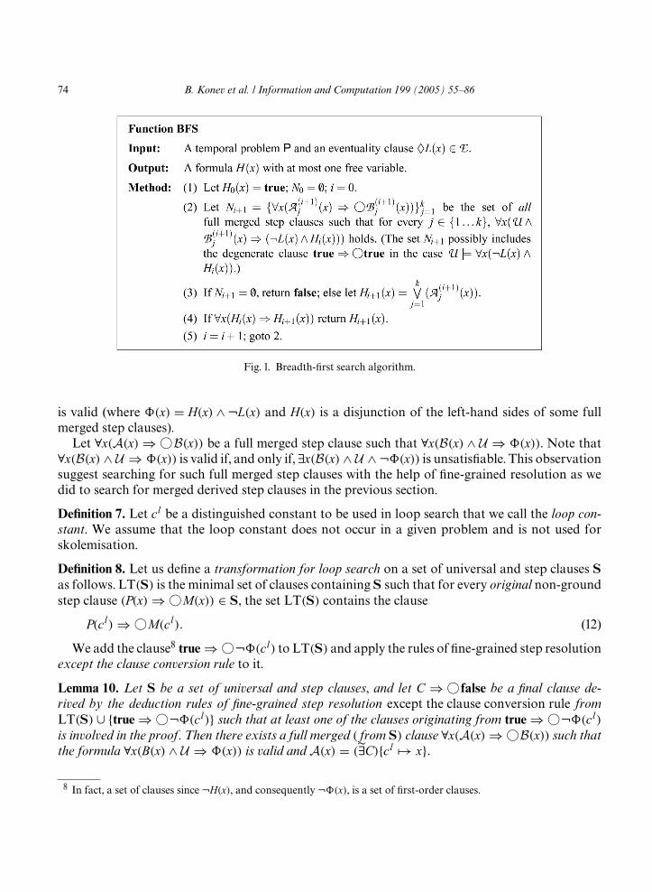
74 B. Konev et al. / Information and Computation 199 (2005) 55–86

Fig. 1. Breadth-first search algorithm.

is valid (where (x) = H(x) ∧ ¬L(x) and H(x) is a disjunction of the left-hand sides of some fullmerged step clauses).Let ∀x(A(x)⇒ ❤B(x)) be a full merged step clause such that ∀x(B(x) ∧ U ⇒ (x)). Note that

∀x(B(x) ∧ U ⇒ (x)) is valid if, and only if, ∃x(B(x) ∧ U ∧ ¬ (x)) is unsatisfiable. This observationsuggest searching for such full merged step clauses with the help of fine-grained resolution as wedid to search for merged derived step clauses in the previous section.

Definition 7. Let cl be a distinguished constant to be used in loop search that we call the loop con-stant. We assume that the loop constant does not occur in a given problem and is not used forskolemisation.

Definition 8. Let us define a transformation for loop search on a set of universal and step clauses Sas follows. LT(S) is the minimal set of clauses containing S such that for every original non-groundstep clause (P(x)⇒ ❤M(x)) ∈ S, the set LT(S) contains the clause

P(cl)⇒ ❤M(cl). (12)

We add the clause8 true ⇒ ❤¬ (cl) to LT(S) and apply the rules of fine-grained step resolutionexcept the clause conversion rule to it.

Lemma 10. Let S be a set of universal and step clauses, and let C ⇒ ❤false be a final clause de-rived by the deduction rules of fine-grained step resolution except the clause conversion rule fromLT(S) ∪ {true ⇒ ❤¬ (cl)} such that at least one of the clauses originating from true ⇒ ❤¬ (cl)is involved in the proof. Then there exists a full merged ( from S) clause ∀x(A(x)⇒ ❤B(x)) such thatthe formula ∀x(B(x) ∧ U ⇒ (x)) is valid and A(x) = (̃∃C){cl → x}.

8 In fact, a set of clauses since ¬H(x), and consequently ¬ (x), is a set of first-order clauses.

B. Konev et al. / Information and Computation 199 (2005) 55–86 75

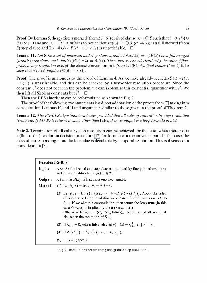
Proof.ByLemma5, there exists amerged (fromLT (S)) derived clauseA⇒ ❤B such that {¬ (cl)} ∪B ∪ U |= false andA = ∃̃C . It suffices to notice that ∀x((A ⇒ ❤B){cl → x}) is a full merged (fromS) step clause and ∃x(¬ (x) ∧ B{cl → x} ∧ U) is unsatisfiable. �Lemma 11. Let S be a set of universal and step clauses, and let ∀x(A(x)⇒ ❤B(x)) be a full merged(from S) step clause such that ∀x(B(x) ∧ U ⇒ (x)).Then there exists a derivation by the rules of fine-grained step resolution except the clause conversion rule from LT(S) of a final clause C ⇒ ❤falsesuch that ∀xA(x) implies (̃∃C){cl → x}).Proof. The proof is analogous to the proof of Lemma 4. As we have already seen, ∃x(B(x) ∧ U ∧¬ (x)) is unsatisfiable, and this can be checked by a first-order resolution procedure. Since theconstant cl does not occur in the problem, we can skolemise this existential quantifier with cl. Wethen lift all Skolem constants but cl. �Then the BFS algorithm can be reformulated as shown in Fig. 2.The proof of the following two statements is a direct adaptation of the proofs from [7] taking into

consideration Lemmas 10 and 11 and arguments similar to those given in the proof of Theorem 7.

Lemma 12. The FG-BFS algorithm terminates provided that all calls of saturation by step resolutionterminate. If FG-BFS returns a value other than false, then its output is a loop formula in L(x).

Note 2. Termination of all calls by step resolution can be achieved for the cases when there existsa (first-order) resolution decision procedure [17] for formulae in the universal part. In this case, theclass of corresponding monodic formulae is decidable by temporal resolution. This is discussed inmore detail in [7].

Fig. 2. Breadth-first search using fine-grained step resolution.

76 B. Konev et al. / Information and Computation 199 (2005) 55–86

Theorem 13. The calculus consisting of the rules of fine-grained step resolution, together with the bothground and non-ground eventuality resolution rules, is complete for constant flooded monodic temporalproblems over expanding domains if we restrict ourselves to loops found by the FG-BFS algorithm.

Example 7. Let us consider a monodic temporal problem P given by

U ={∀x(B(x)⇒ A(x) ∧ ¬L(x)),l⇒ ∃xA(x),

}, I = ∅,

S = {s1 : A(x)⇒ ❤B(x)}, E = {e1 : ♦L(x), e2 : ♦l}.We chose such a trivial example specifically to be able to demonstrate thoroughly the steps of

our proof-search algorithm.

We clausify U and obtain

U s =u1 : ¬B(x) ∨ A(x),u2 : ¬B(x) ∨ ¬L(x),u3 : ¬l ∨ A(c).

.

Since the original problem does not contain any constants (the only constant c is introduced byskolemisation), constant flooding does not introduce additional step clauses.

• Step resolutionWe can deduce the following clauses by fine-grained step resolution:

s2 : A(x)⇒ ❤A(x) ( s1, u1)s3 : A(x)⇒ ❤¬L(x) ( s1, u2)

With this additional clauses, the set of clauses is saturated. Now we try to find a loop in ♦L(x).• Loop search for ♦L(x)The input to the BFS algorithm is the set S = {u1, u2, u3, s1, s2, s3} and the eventuality ♦L(x). Instep (1) of the algorithm, we set H0(x) = true; N0 = ∅; and i = 0. In step (2), we first computeLT(S) which is given by {lt1 : A(cl)⇒ ❤B(cl)}.From S1 = LT(S) ∪ {true ⇒ ❤L(cl)} we deduce the following clauses by fine-grained step res-olution (except the clause conversion rule):

l2 : A(cl)⇒ ❤A(cl) (lt1, u1)l3 : A(cl)⇒ ❤¬L(cl) (lt1, u2)l4 : true ⇒ ❤¬B(cl) (u2, l1)l5 : A(cl)⇒ ❤false (l3, l1)

The set of clauses is saturated. The set N1 of all new final clauses is {A(cl)⇒ ❤false}. Since N1is not empty, in step (3) we set H1(x) to A(x). Obviously, ∀x(H0(x)⇒ H1(x)) is not true, so we goback to step (2) of the algorithm.

B. Konev et al. / Information and Computation 199 (2005) 55–86 77

Now the set S2 = LT(S) ∪ {l6 : true ⇒ ❤(¬A(cl) ∨ L(cl))} and we deduce from it the followingclauses:

l7 : A(cl)⇒ ❤A(cl) (lt1, u1)l8 : A(cl)⇒ ❤¬L(cl) (lt1, u2)l9 : true ⇒ ❤(¬B(cl) ∨ L(cl)) (u1, l6)l10 : true ⇒ ❤(¬B(cl) ∨ ¬A(cl)) (u2, l6)l11 : A(cl)⇒ ❤L(cl) (l7, l6)l12 : A(cl)⇒ ❤¬A(cl) (l8, l6)l13 : true ⇒ ❤¬B(cl) (u2, l9)l14 : A(cl)⇒ ❤¬B(cl) (l8, l9)l15 : A(cl)⇒ ❤false (l8, l11)

The set of clauses is saturated. The set N2 of all new final clauses is {A(cl)⇒ ❤false}. Since N2is not empty, in step (3) we obtain H2(x) = A(x).As ∀x(H1(x)⇒ H2(x)), the algorithm terminates in step (4) and returns the loop A(x).

• Eventuality resolutionWe can apply now the eventuality resolution rule whose conclusion is

u4 : ¬A(x).• Step resolutionSince this conclusion extends the set of universal clauses, additional inferences by step resolutionmay now be possible. Indeed, we are able to derive

u5 : ¬l ( u3, u4)using u4.Since the set of clauses has been extended, it is also possible that additional loops can be found.

However, instead of searching for a loop for ♦L(x) again, we now focus on the eventuality ♦l.• Loop search for ♦lThe input to the FG-BFS is S = {u1, u2, u3, u4, u5, s1, s2, s3}. In step (1) of the algorithm, we setH0(x) = true; N0 = ∅; and i = 0. In step (2), we first compute LT(S), which is given by {lt1 :A(cl)⇒ ❤B(cl)}. From S1 = LT(S) ∪ {l16 : true ⇒ ❤l} we can deduce:l17 : true ⇒ ❤false ( l16, u5)

that is, a contradiction. Therefore, the loop is true.• Eventuality resolutionWe can apply now the eventuality resolution rule whose conclusion is ¬true.This means that we have derived a contradiction, and the problem is unsatisfiable.

Note 3.As the example above shows, the presence of clauses of the form (9), introducedby clausifica-tion, and (12), introduced by the transformation for loop search, might lead to repeated derivations(with free variables and with constants). This can be avoided, however, if instead of generating theseclauses, we relax the conditions on substitutions in the definition of rules of fine-grained resolution

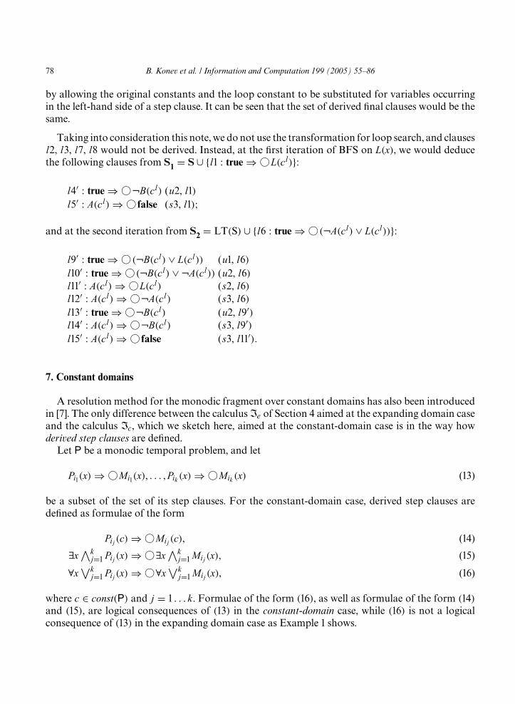
78 B. Konev et al. / Information and Computation 199 (2005) 55–86

by allowing the original constants and the loop constant to be substituted for variables occurringin the left-hand side of a step clause. It can be seen that the set of derived final clauses would be thesame.

Taking into consideration this note, we do not use the transformation for loop search, and clausesl2, l3, l7, l8 would not be derived. Instead, at the first iteration of BFS on L(x), we would deducethe following clauses from S1 = S ∪ {l1 : true ⇒ ❤L(cl)}:

l4′ : true ⇒ ❤¬B(cl) (u2, l1)l5′ : A(cl)⇒ ❤false (s3, l1);

and at the second iteration from S2 = LT(S) ∪ {l6 : true ⇒ ❤(¬A(cl) ∨ L(cl))}:

l9′ : true ⇒ ❤(¬B(cl) ∨ L(cl)) (u1, l6)l10′ : true ⇒ ❤(¬B(cl) ∨ ¬A(cl)) (u2, l6)l11′ : A(cl)⇒ ❤L(cl) (s2, l6)l12′ : A(cl)⇒ ❤¬A(cl) (s3, l6)l13′ : true ⇒ ❤¬B(cl) (u2, l9′)l14′ : A(cl)⇒ ❤¬B(cl) (s3, l9′)l15′ : A(cl)⇒ ❤false (s3, l11′).

7. Constant domains

A resolution method for the monodic fragment over constant domains has also been introducedin [7]. The only difference between the calculus Ie of Section 4 aimed at the expanding domain caseand the calculus Ic, which we sketch here, aimed at the constant-domain case is in the way howderived step clauses are defined.Let P be a monodic temporal problem, and let

Pi1(x)⇒ ❤Mi1(x), . . . , Pik (x)⇒ ❤Mik (x) (13)

be a subset of the set of its step clauses. For the constant-domain case, derived step clauses aredefined as formulae of the form

Pij (c)⇒ ❤Mij(c), (14)

∃x∧kj=1 Pij (x)⇒ ❤∃x∧k

j=1Mij(x), (15)

∀x∨kj=1 Pij (x)⇒ ❤∀x∨k

j=1Mij(x), (16)

where c ∈ const(P) and j = 1 . . . k . Formulae of the form (16), as well as formulae of the form (14)and (15), are logical consequences of (13) in the constant-domain case, while (16) is not a logicalconsequence of (13) in the expanding domain case as Example 1 shows.

B. Konev et al. / Information and Computation 199 (2005) 55–86 79

Other notions (merged derived and full merged step clauses) and the inference system are definedin exactly the same way as those for the calculus Ie in Section 4 based on the new definition ofa derived step clause. It is shown in [7] that the calculus Ic is sound and complete for monodictemporal problems over constant domains.Note that if derived step clauses of the form (16) participate in merging, the conclusion of the

step resolution rule contains an existentially quantified formula (the negation of the universallyquantified left-hand side of the derived step clause). Clausifying such formulae would require ex-tending the signature; therefore, the machinery of Section 5 does not work for the constant-domaincase, and we cannot construct a fine-grained resolution calculus for the constant-domain case. In-stead, in order to be able to use our procedure for establishing unsatisfiability of constant-domainproblems, we simply reduce satisfiability over constant domains to satisfiability over expandingdomains.Let P = 〈U , I ,S , E〉 be a temporal problem. The temporal problem Exp(P) is defined as follows.

The universal, initial, and eventuality parts of Exp(P) are that of P; the step part consists of all stepclauses from S together with all derived step clauses of the form (16). More precisely, in order to fitthe definition of a temporal problem, we have to rename complex expressions in the derived stepclauses.

Proposition 14. A temporal problem P is satisfiable over constant domains if, and only if, the temporalproblem Exp(P) is satisfiable over constant domains.

Proof. If P = 〈U , I ,S , E〉 and Exp(P) = 〈U ′, I ,S ′, E〉 then U ⊆ U ′ and S ⊆ S ′. So, if Exp(P) is sat-isfiable then P is satisfiable. On the other hand, over constant domains, derived step clauses of theform (16) are logical consequences of the step part S , which means that over constant domains Pimplies Exp(P). So, if P is satisfiable then Exp(P) is satisfiable. �Proposition 15. For any temporal problem P, the temporal problem Exp(P) is satisfiable over constantdomains if, and only if, the temporal problem Exp(P) is satisfiable over expanding domains.

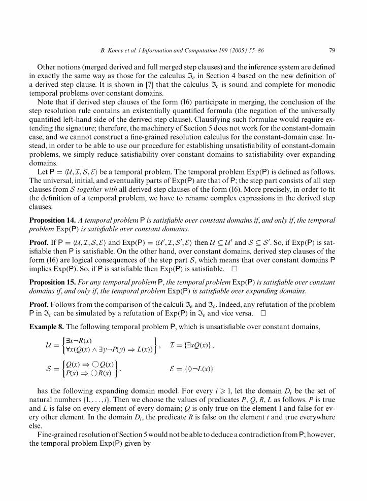
Proof. Follows from the comparison of the calculi Ie and Ic. Indeed, any refutation of the problemP in Ic can be simulated by a refutation of Exp(P) in Ie and vice versa. �Example 8. The following temporal problem P, which is unsatisfiable over constant domains,

U ={∃x¬R(x)∀x(Q(x) ∧ ∃y¬P(y)⇒ L(x))

}, I = {∃xQ(x)} ,

S ={Q(x)⇒ ❤Q(x)

P(x)⇒ ❤R(x)

}, E = {♦¬L(x)}

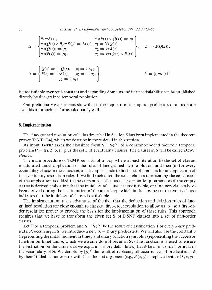
has the following expanding domain model. For every i � 1, let the domain Di be the set ofnatural numbers {1, . . . , i}. Then we choose the values of predicates P , Q, R, L as follows. P is trueand L is false on every element of every domain; Q is only true on the element 1 and false for ev-ery other element. In the domain Di, the predicate R is false on the element i and true everywhereelse.Fine-grained resolutionof Section 5wouldnot be able todeduce a contradiction fromP; however,

the temporal problem Exp(P) given by

80 B. Konev et al. / Information and Computation 199 (2005) 55–86

U =

∃x¬R(x), ∀x(P(x) ∨ Q(x))⇒ p3,∀x(Q(x) ∧ ∃y¬R(y)⇒ L(x)), q1 ⇒ ∀xQ(x),∀x(Q(x))⇒ p1, q2 ⇒ ∀xR(x),∀x(P(x))⇒ p2, q3 ⇒ ∀x(Q(x) ∨ R(x))

, I = {∃xQ(x)} ,

S =Q(x)⇒ ❤Q(x), p1 ⇒ ❤q1,P(x)⇒ ❤R(x), p2 ⇒ ❤q2,

p3 ⇒ ❤q3

, E = {♦¬L(x)}

is unsatisfiable over both constant and expanding domains and its unsatisfiability can be establisheddirectly by fine-grained temporal resolution.

Our preliminary experiments show that if the step part of a temporal problem is of a moderatesize, this approach performs adequately well.

8. Implementation

The fine-grained resolution calculus described in Section 5 has been implemented in the theoremprover TeMP [34], which we describe in more detail in this section.As input TeMP takes the clausified form S = S(P) of a constant-flooded monodic temporal

problem P = 〈U , I ,S , E〉 plus the set E of eventuality clauses. The clauses in S will be called DSNFclauses.The main procedure of TeMP consists of a loop where at each iteration (i) the set of clauses

is saturated under application of the rules of fine-grained step resolution, and then (ii) for everyeventuality clause in the clause set, an attempt is made to find a set of premises for an application ofthe eventuality resolution rules. If we find such a set, the set of clauses representing the conclusionof the application is added to the current set of clauses. The main loop terminates if the emptyclause is derived, indicating that the initial set of clauses is unsatisfiable, or if no new clauses havebeen derived during the last iteration of the main loop, which in the absence of the empty clauseindicates that the initial set of clauses is satisfiable.The implementation takes advantage of the fact that the deduction and deletion rules of fine-

grained resolution are close enough to classical first-order resolution to allow us to use a first-or-der resolution prover to provide the basis for the implementation of these rules. This approachrequires that we have to transform the given set S of DSNF clauses into a set of first-orderclauses.Let P be a temporal problem and S = S(P) be the result of clausification. For every k-ary pred-

icate, P , occurring in S, we introduce a new (k + 1)-ary predicate P̃ . We will also use the constant 0(representing the initial moment in time), and unary function symbols s (representing the successorfunction on time) and h, which we assume do not occur in S. (The function h is used to ensurethe restriction on the unifiers as we explain in more detail later.) Let � be a first-order formula inthe vocabulary of S. We denote by [�]T the result of replacing all occurrences of predicates in �by their “tilded” counterparts with T as the first argument (e.g., P (x, y) is replaced with P̃ (T , x, y)).

B. Konev et al. / Information and Computation 199 (2005) 55–86 81

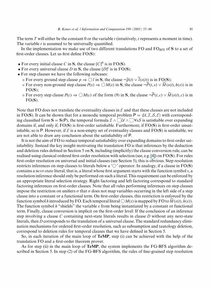
The term T will either be the constant 0 or the variable t (intuitively, t represents a moment in time).The variable t is assumed to be universally quantified.In the implementation we make use of two different translations FO and FOBFS of S to a set of

first-order clauses. Let us first define FO(S):

• For every initial clause C in S, the clause [C]0 is in FO(S).• For every universal clause D in S, the clause [D]t is in FO(S).• For step clauses we have the following subcases:

◦ For every ground step clause p ⇒ ❤l in S, the clause ¬p̃ (t) ∨ l̃(s(t)) is in FO(S);◦ For every non-ground step clause P(x)⇒ ❤M(x) in S, the clause ¬P̃ (t, x) ∨ M̃ (s(t), h(x)) is inFO(S);

◦ For every step clause P(c)⇒ ❤M(c) of the form (9) in S, the clause ¬P̃ (t, c) ∨ M̃ (s(t), c) is inFO(S).

Note that FO does not translate the eventuality clauses in E and that these clauses are not includedin FO(S). It can be shown that for a monodic temporal problem P = 〈U , I ,S , E〉 with correspond-ing clausified form S = S(P), the temporal formula I ∧ U ∧ ∀xS is satisfiable over expandingdomains if, and only if, FO(S) is first-order satisfiable. Furthermore, if FO(S) is first-order unsat-isfiable, so is P. However, if E is a non-empty set of eventuality clauses and FO(S) is satisfiable, weare not able to draw any conclusion about the satisfiability of P.It is not the aim of FO to reduce temporal satisfiability over expanding domains to first-order sat-

isfiability. Instead the key insight motivating the translation FO is that inferences by the deductionand deletion rules defined in Section 5 on S, including (implicitly) the clause conversion rule, can berealised using classical ordered first-order resolution with selection (see, e.g. [4]) on FO(S). For rulesfirst-order resolution on universal and initial clauses (see Section 5), this is obvious. Step resolutionrestricts inferences on step clauses to literals below a ‘ ❤’ operator. In analogy, if a clause in FO(S)contains a next-state literal, that is, a literal whose first argument starts with the function symbol s, aresolution inference should only be performed on such a literal. This requirement can be enforced byan appropriate literal selection strategy. Right factoring and left factoring correspond to standardfactoring inferences on first-order clauses. Note that all rules performing inferences on step clausesimpose the restriction on unifiers % that % does not map variables occurring in the left side of a stepclause into a constant or a functional term. On first-order clauses, this restriction is enforced by thefunction symbol h introduced byFO.Each temporal literal ❤M(x) ismapped byFO to M̃ (s(t), h(x)).The function symbol h “shields” the variable x from being instantiated by a constant or functionalterm. Finally, clause conversion is implicit on the first-order level: If the conclusion of an inferencestep involving a clause C containing next-state literals results in clause D without any next-stateliterals, thenD corresponds to the translation of a universal clause. The standard redundancy elimi-nation mechanisms for ordered first-order resolution, such as subsumption and tautology deletion,correspond to deletion rules for temporal clauses that we have defined in Section 5.So, in each iteration of the main loop of TeMP, step (i) can be achieved with the help of the

translation FO and a first-order theorem prover.As for step (ii) in the main loop of TeMP, the system implements the FG-BFS algorithm de-

scribed in Section 5. In step (2) of the FG-BFS algorithm, the rules of fine-grained step resolution

82 B. Konev et al. / Information and Computation 199 (2005) 55–86

are applied with the exception of the clause conversion rule. To enforce this restriction, we use avariant FOBFS of FO. Let Si+1 be a monodic temporal problem in clausified form as defined in step(2) of the FG-BFS algorithm. Then FOBFS(Si+1) is defined as follows:

• For every universal clause D in Si+1, the clause [D]t is in FOBFS(Si+1).• For every ground step clause p ⇒ ❤l in Si+1, the clause ¬p̃ (0) ∨ l̃(s(t)) is in FOBFS(Si+1), andfor every non-ground step clause P(x)⇒ ❤M(x) in Si+1, the clause ¬P̃ (0, x) ∨ M̃ (s(t), h(x)) is inFOBFS(Si+1).

Recall that initial clauses do not contribute to loop search, so we should not include their trans-lation into FOBFS(Si+1). Again, the motivation for FOBFS is that saturation of Si+1 under the rulesof fine-grained step resolution except the clause conversion rule corresponds to the saturation ofFOBFS(Si+1) under ordered first-order resolution as described above. In particular, clauses consist-ing only of literals whose first argument is 0 in the saturation of FOBFS(Si+1) correspond to finalclauses (up to negation). Using this criterion it is straightforward to extract those clauses from thesaturation of FOBFS(Si+1) to form the set Ni+1 which is the outcome of step (2) of the FG-BFSalgorithm and to proceed with step (3).Finally, note that it is straightforward to see whether a clause in FO(S) is the result of translating

an initial, a universal, or a (non-)ground step clause. This makes it possible to compute FOBFS(S)from FO(S) instead of from S. Also, the conclusion of an application of one of the eventuality res-olution rules can directly be computed as a set of first-order clauses of the appropriate form. Thus,there is no need to ever translate clauses in FO(S) back to DSNF clauses. Instead, after translatingthe input given to TeMP once using FO we can continue to operate with first-order clauses.The task of saturating clause sets with ordered first-order resolution simulating step resolution is

delegated to the kernel of the first-order resolution proverVampire [46], which is linked to the wholesystem as a C++ library. Minor adjustments have been made in the functionality of Vampire toaccommodate step resolution: a special mode for literal selection has been introduced such that ina clause containing a next-state literal only next-state literals can be selected. At the moment, theresult of a previous saturation step, augmented with the result of an application of the eventualityresolution rules, is resubmitted to the Vampire kernel, although no non-redundant inferences areperformed between the clauses from the already saturated part. This is only a temporary solu-tion, and in the future Vampire will support incremental input in order to reduce communicationoverhead.To illustrate the effectiveness of this approach, we have appliedTeMP to each of the examples of

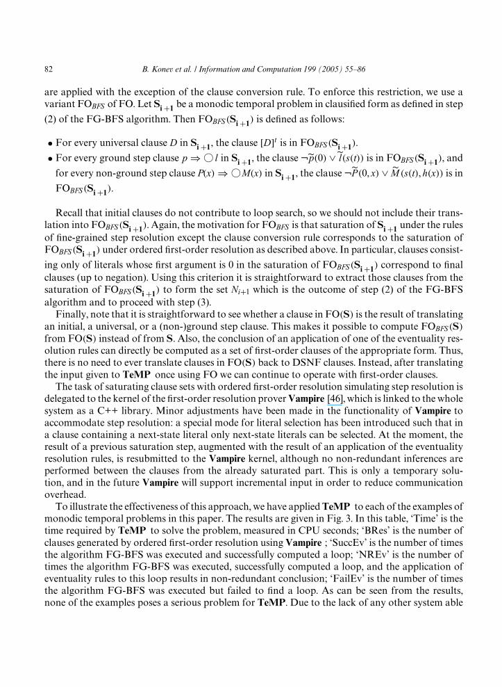
monodic temporal problems in this paper. The results are given in Fig. 3. In this table, ‘Time’ is thetime required by TeMP to solve the problem, measured in CPU seconds; ‘BRes’ is the number ofclauses generated by ordered first-order resolution usingVampire ; ‘SuccEv’ is the number of timesthe algorithm FG-BFS was executed and successfully computed a loop; ‘NREv’ is the number oftimes the algorithm FG-BFS was executed, successfully computed a loop, and the application ofeventuality rules to this loop results in non-redundant conclusion; ‘FailEv’ is the number of timesthe algorithm FG-BFS was executed but failed to find a loop. As can be seen from the results,none of the examples poses a serious problem for TeMP. Due to the lack of any other system able

B. Konev et al. / Information and Computation 199 (2005) 55–86 83

Fig. 3. Performance of TeMP on sample monodic temporal problems.

to solve problems in monodic first-order temporal logic, we cannot compare the performance ofTeMP to that of other provers. However, in [34] we have compared TeMP to decision proceduresfor propositional linear time temporal logic with quite positive results.

9. Applications and case studies

We have applied TeMP to problems from several domains, in particular, to examples specifiedin the temporal logics of knowledge (the fusion of propositional linear-time temporal logic withmulti-modal S5) and to verification problems.Whilst problems formalised in the temporal logic of knowledge canbe solvedusingproofmethods

for combined modal and propositional temporal logics [13], we translate them into monodic first-order temporal logic and apply TeMP to the result of transformation providing thus a practicalpossibility of solving those problems. Translations from the temporal logics of knowledge intoFOTL are given in [26]; we also incorporate ideas from [47] to translate some of the modal logicaxioms in a way suitable for TeMP. Moreover, the transformation maps formulae in the tempo-ral logics of knowledge into a subclass of the monodic fragment which is decidable by temporalresolution (see Note 2).A specification of the game Cluedo (a deduction game where reasoning about knowledge is es-

sential) in temporal logics of knowledge is given in [12], for a particular play of the game. At pointsin the game, certain properties can be proved, for example that one player knows another playerholds a particular card. Both the specification and properties to be proved have been translatedinto monodic first-order temporal logic and the proof carried out using TeMP.A temporalised version of the well known muddy children problem (see, for example [16]) spec-

ified in temporal logics of knowledge has been translated to monodic first-order temporal log-ic and relevant properties proved using TeMP. A similar approach can be taken for the proofof properties of security protocols specified in temporal logics of knowledge (see, for example[14]).

84 B. Konev et al. / Information and Computation 199 (2005) 55–86

Work within the Liverpool Verification Laboratory9 has utilised TeMP in formal verification.In particular, in a collaboration withMotorola, TeMP was used to support the verification of soft-ware designs. Recent work within the laboratory has involved identifying a class of Abstract StateMachines [29] that can be translated into a monodic fragment of first-order temporal logic suitablefor input to TeMP. This allows TeMP to be used as the basis for verification of a range of soft-ware/hardware designs (given using Abstract State Machines) [24]. Recent work has examined theverification of infinite state systems (something that is impossible using traditional model-checking)and has shown how, for a significant class of systems, such verification problems can be translatedinto a monodic formula suitable for input to TeMP [22,23]. We successfully used TeMP for fullyautomatic verification of cache coherence protocols [22].

10. Conclusion

We have here described a fine-grained resolution calculus for monodic first-order temporal logicover expanding domains. Soundness of the fine-grained resolution calculus is easy to prove andcompleteness is shown relative to the completeness proof for the expanding domain for the non-fine-grained version [7]. While the implementation based on the general calculus would involvegenerating all subsets of the step clauses with which to apply the step and eventuality resolutionrules, the fine-grained resolution inference rules can be implemented directly using any appropriatefirst-order theorem prover for classical logic. This makes the new calculus presented here particu-larly amenable to efficient implementation. In this paper, we have also shown a simple method forextending the applicability of the implementation to constant-domain problems.Our future work consists of two main aspects: improving the implementation and application to

a wider range of real world examples.

Acknowledgments

Finally, we thank the anonymous referees for helpful comments and suggestions. We acknowl-edge support for this from EPSRC via research Grants GR/R45376/01 and GR/R45369/01.

References

[1] M. Abadi, The power of temporal proofs, Theoretical Computer Science 65 (1989) 34–85.[2] A. Artale, E. Franconi, Temporal description logics, in:M. Fisher, D. Gabbay, L. Vila (Eds.), Handbook of TemporalReasoning in Artificial Intelligence, vol. 1, Elsevier, Amsterdam, 2004.

[3] A. Artale, E. Franconi, F. Wolter, M. Zakharyaschev, A temporal description logic for reasoning over conceptualschemas and queries, in: Proceedings of JELIA 2002, vol. 2424, LNCS, Springer, Berlin, 2002, pp. 98–110.

[4] L. Bachmair, H. Ganzinger, Resolution theorem proving, in: A. Robinson, A. Voronkov (Eds.), Handbook of Auto-mated Reasoning, Elsevier, Amsterdam, 2001, pp. 19–99 (Chapter 2).

9 http://www.csc.liv.ac.uk/liverlab.

B. Konev et al. / Information and Computation 199 (2005) 55–86 85

[5] C.-L. Chang, R.C.-T. Lee, Symbolic Logic and Mechanical Theorem Proving, Academic Press, New York, 1971.[6] E.M. Clarke, O. Grumberg, D.A. Peled, Model Checking, MIT Press, Cambridge, MA, 1999.[7] A. Degtyarev, M. Fisher, B. Konev, Monodic temporal resolution, ACM Transactions on ComputationalLogic, in press. Preliminary version available as Technical Report ULCS-03-001, The University of Liverpool,http://www.csc.liv.ac.uk/research.

[8] A. Degtyarev, M. Fisher, Towards first-order temporal resolution, in: Proceedings of KI 2001, vol. 2174, LNCS,Springer, Berlin, 2001, pp. 18–32.

[9] A. Degtyarev, M. Fisher, A. Lisitsa, Equality and monodic first-order temporal logic, Studia Logica 72 (2) (2002)147–156.

[10] C. Dixon, Temporal resolution using a breadth-first search algorithm, Annals of Mathematics and Artificial Intelli-gence 22 (1998) 87–115.

[11] C. Dixon, Using Otter for temporal resolution, in: Advances in Temporal Logic, Kluwer, Dordrecht, 2000, pp.149–166.

[12] C. Dixon, Miss Scarlett in the Ballroom with the Lead Piping, in: Proceedings of ECAI 2004, IOS Press, 2004.[13] C.Dixon,M.Fisher,M.Wooldridge,Resolution for temporal logics of knowledge, Journal ofLogic andComputation8 (3) (1998) 345–372.

[14] C. Dixon, M.-C.F. Gago, M. Fisher, W. van der Hoek, Using temporal logics of knowledge in the formal verificationof security protocols, in: Proceedings of TIME 2004, IEEE Computer Society Press, Silver Spring, MD, 2004, pp.148–151.

[15] E.A. Emerson, Temporal and modal logic, in: J. van Leeuwen (Ed.), Handbook of Theoretical Computer Science,Elsevier, Amsterdam, 1990, pp. 997–1072 (Chapter 16).

[16] R. Fagin, J. Halpern, Y. Moses, M. Vardi, Reasoning about Knowledge, MIT Press, Cambridge, MA, 1995.[17] C. Fermüller, A. Leitsch, U. Hustadt, T. Tammet, Resolution decision procedures, in: A. Robinson, A. Voronkov(Eds.), Handbook of Automated Reasoning, vol. 2, Elsevier, Amsterdam, 2001, pp. 1791–1850 (Chapter 25).

[18] M. Fisher, An introduction to executable temporal logics, Knowledge Engineering Review 11 (1) (1996) 43–56.[19] M. Fisher, A temporal semantics for concurrentmetatem, Journal of Symbolic Computation 22 (5/6) (1997) 627–648.[20] M. Fisher, A normal form for temporal logics and its applications in theorem proving and execution, Journal ofLogic and Computation 7 (4) (1997) 429–456.

[21] M. Fisher, C. Dixon, M. Peim, Clausal temporal resolution, ACMTransactions on Computational Logic 2 (1) (2001)12–56.

[22] M. Fisher, A. Lisitsa, Deductive verification of cache coherence protocols, in: Proceedings of 3rd InternationalWork-shop onAutomatedVerification ofCritical Systems (AVoCS 2003), Technical ReportDSSE–TR–2003–2,Universityof Southampton, 2003, pp. 177–186.

[23] M. Fisher, A. Lisitsa, Temporal deductive verification of cache coherence protocols, Technical Report ULCS-03-024,The University of Liverpool, http://www.csc.liv.ac.uk/research.

[24] M. Fisher, A. Lisitsa, Monodic ASMs and temporal verification, in: Proceedings ASM 2004, vol. 3065, LNCS,Springer, Berlin, 2004, pp. 95–110.

[25] D. Gabbay, I. Hodkinson, M. Reynolds, in: Temporal Logic: Mathematical Foundations and Computational As-pects, vol. 1, Oxford University Press, Oxford, 1994.

[26] D.M. Gabbay, A. Kurucz, F. Wolter, M. Zakharyaschev, Many-Dimensional Modal Logics: Theory and Applica-tions, Elsevier, Amsterdam, 2003.

[27] D. Gabbay, M. Reynolds, M. Finger, in: Temporal Logic: Mathematical Foundations and Computational Aspects,vol. 2, Oxford University Press, Oxford, 2000.

[28] D. Gabelaia, R. Kontchakov, A. Kurucz, F. Wolter, M. Zakharyaschev, On the computational complexity of spat-io-temporal logics, in: Proceedings of FLAIRS 2003, AAAI Press, 2003, pp. 460–464.

[29] Y. Gurevich, Logician in the land of OS: Abstract State Machines at Microsoft, in: Proceedings of LICS 2001, IEEEComputer Society, Silver Spring, MD, 2001, pp. 129–136.

[30] I. Hodkinson, Monodic packed fragment with equality is decidable, Studia Logica 72 (2002) 185–197.[31] I. Hodkinson, F. Wolter, M. Zakharyaschev, Decidable fragments of first-order temporal logics, Annals of Pure andApplied Logic 106 (2000) 85–134.

[32] G.J. Holzmann, Design and Validation of Computer Protocols, Prentice-Hall, Englewood Cliffs, NJ, 1991.

86 B. Konev et al. / Information and Computation 199 (2005) 55–86

[33] G.J. Holzmann, The model checker spin, IEEE Transactions on Software Engineering 23 (5) (1997) 279–295.[34] U. Hustadt, B. Konev, A. Riazanov, A. Voronkov,TeMP: A temporal monodic prover, in: Proceedings IJCAR 2004,vol. 3097, LNAI, Springer, Berlin, 2004, pp. 326–330.

[35] R. Kontchakov, C. Lutz, F. Wolter, M. Zakharyaschev, Temporalising tableaux, Studia Logica 76 (1) (2004) 91–134.[36] O. Kupferman, M. Vardi, Synthesis with incomplete information, in: 2nd International Conference on TemporalLogic, Manchester, 1997, pp. 91–106.

[37] A. Leitsch, The Resolution Calculus, Springer, Berlin, 1997.[38] Z. Manna, A. Pnueli, The Temporal Logic of Reactive and Concurrent Systems: Specification, Springer, Berlin, 1992.[39] S. Merz, Decidability and incompleteness results for first-order temporal logic of linear time, Journal of AppliedNon-Classical Logics 2 (1992) 139–156.

[40] R. Nieuwenhuis, A. Rubio, Theorem proving with ordering and equality constrained clauses, Journal of SymbolicComputation 19 (4) (1995) 321–351.

[41] R.Nieuwenhuis,A.Rubio, Paramodulation-based theoremproving, in:A.Robinson,A.Voronkov (Eds.),Handbookof Automated Reasoning, Elsevier, Amsterdam, 2001, pp. 371–443 (Chapter 7).

[42] A. Nonnengart, C. Weidenbach, Computing small clause normal forms, in: A. Robinson, A. Voronkov (Eds.), Hand-book of Automated Reasoning, Elsevier, Amsterdam, 2001, pp. 335–370 (Chapter 6).

[43] A. Pnueli, The temporal logic of programs, in: Proceedings of the Eighteenth Symposium on the Foundations ofComputer Science (FOCS), 1977, pp. 46–57.

[44] A. Pnueli, R. Rosner, On the synthesis of a reactive module, in: Proceedings of Sixteenth Annual ACM Symposiumon Principles of Programming Languages, 1989, pp. 179–190.

[45] A.S. Rao,M.P.Georgeff,Decision procedures for BDI logics, Journal of Logic andComputation 8 (3) (1998) 293–343.[46] A. Riazanov, A. Voronkov, The design and implementation of Vampire, AI Communications 15 (2–3) (2002) 91–110.[47] R.A. Schmidt, U. Hustadt, A principle for incorporating axioms into the first-order translation of modal formulae,in: Proceedings of CADE-19, vol. 2741, LNAI, Springer, Berlin, 2003, pp. 412–426.

[48] M.P. Shanahan, Solving the Frame Problem, MIT Press, Cambridge, MA, 1997.[49] A. Szalas, Concerning the semantic consequence relation in first-order temporal logic, Theoretical Computer Science47 (1986) 329–334.

[50] A. Szalas, L. Holenderski, Incompleteness of first-order temporal logic with until, Theoretical Computer Science 57(1988) 317–325.

[51] A. Tansel (Ed.), Temporal Databases: Theory, Design, and Implementation, Benjamin/Cummings, Menlo Park, CA,1993.

[52] G. Tseitin, On the complexity of derivations in propositional calculus, in: J. Siekmann, G. Wrightson (Eds.), Auto-mation of Reasoning (Classical Papers on Computational Logic), vol. 2, Springer, Berlin, 1983, pp. 466–483 (originalpaper (in Russian) appeared in 1968).

[53] F. Wolter, M. Zakharyaschev, Temporalizing description logics, in: Frontiers of Combining Systems II, 2000, pp.379–401.

[54] F. Wolter, M. Zakharyaschev, Decidable fragments of first-order modal logics, Journal of Symbolic Logic 66 (2001)1415–1438.

[55] F. Wolter, M. Zakharyaschev, Qualitative spatio-temporal representation and reasoning: a computational perspec-tive, in: ExploringArtificial Intelligence in theNewMillenium,MorganKaufmann, LosAltos, CA, 2002, pp. 175–216.

[56] F. Wolter, M. Zakharyaschev, Axiomatizing the monodic fragment of first-order temporal logic, Annals of Pure andApplied logic 118 (2002) 133–145.