Mechanical Strength Modeling and Optimization of Lateritic Solid Block with 4% Mound Soil Inclusion

American Journal of Engineering Research (AJER) 2015 American Journal of Engineering Research (AJER)

e-ISSN: 2320-0847 p-ISSN : 2320-0936

Volume-4, Issue-5, pp-178-192

www.ajer.org Research Paper Open Access

w w w . a j e r . o r g

Page 178

Mechanical Strength Modeling and Optimization of Lateritic

Solid Block with 4% Mound Soil Inclusion

Onuamah, P.N.1, Ezeokpube G.C.

2

1(Department of Civil Engineering Enugu State Univetrsity of Science and Technology, Enugu,

Nigeria 2(Department of Civil Engineerin, Michael Okpara University of Agriculture, Umudike,

Abia State, Nigeria)

ABSTRACT :The work is an investigation for the model development and optimization of the compressive

strength of solid sandcrete block with mound soil inclusion. The study applies the Scheffe’s optimization

approach to obtain a mathematical model of the form f(xi1,xi2,xi3,,xi4), where xi are proportions of the concrete

components, viz: cement, mound soil, laterite, and water. Scheffe’s experimental design techniques are followed

to mould various solid block samples measuring 450mm x 225mm x 150mm and tested for 28 days strength. The

task involved experimentation and design, applying the second order polynomial characterization process of the

simplex lattice method. The model adequacy is checked using the control factors. Finally a software is prepared

to handle the design computation process to take the desired property of the mix, and generate the optimal mix

ratios.

Keywords: Sandcrete, Pseudo-component, Simplex-lattice, optimization, Experimental matrix

I. INTRODUCTION The construction of structures is a regular operation which heavily involves sandcrete blocks for load

bearing or non-load bearing walls. The cost/stability of this material has been a major issue in the world of

construction where cost is a major index. This means that the locality and the usability of the available materials

directly impact on the achievable development of any area as well as the attainable level of technology in the

area.As it is, concrete is the main material of construction, and the ease or cost of its production accounts for the

level of success in the area of environmental upgrading involving the construction of new roads, buildings,

dams, water structures and the renovation of such structures. To produce the concrete several primary

components such as cement, sand, gravel and some admixtures are to be present in varying quantities and

qualities. Unfortunately, the occurrence and availability of these components vary very randomly with location

and hence the attendant problems of either excessive or scarce quantities of the different materials occurring in

different areas. Where the scarcity of one component prevails exceedingly, the cost of the concrete production

increases geometrically. Such problems obviate the need to seek alternative materials for partial or full

replacement of the scarce component when it is possible to do so without losing the quality of the concrete.

1.1 Optimization Concept

The target of planning is the maximization of the desired outcome of the venture. In order to maximize

gains or outputs it is often necessary to keep inputs or investments at a minimum at the production level. The

process involved in this planning activity of minimization and maximization is referred to as optimization [1]. In

the science of optimization, the desired property or quantity to be optimized is referred to as the objective

function. The raw materials or quantities 4hose amount of combinations will produce this objective function are

referred to as variables. The variations of these variables produce different combinations and have different

outputs. Often the space of variability of the variables is not universal as some conditions limit them. These

conditions are called constraints. For example, money is a factor of production and is known to be limited in

supply. The constraint at any time is the amount of money available to the entrepreneur at the time of

investment. Hence or otherwise, an optimization process is one that seeks for the maximum or minimum value

and at the same time satisfying a number of other imposed requirements [2]. The function is called the objective

function and the specified requirements are known as the constraints of the problem.

American Journal of Engineering Research (AJER) 2015


Page 179

Everybody can make concrete but not everybody can make structural concrete. Structural concrete are

made with specified materials for specified strength. Concrete is heterogeneous as it comprises sub-materials.

Concrete is made up of fine aggregates, coarse aggregates, cement, water, and sometimes admixtures. [3] report

that modern research in concrete seeks to provide greater understanding of its constituent materials and

possibilities of improving its qualities. For instance, Portland cement has been partially replaced with ground

granulated blast furnace slag (GGBS), a by–product of the steel industry that has valuable cementatious

properties [4].

1.2 Concrete Mix Optimization

The task of concrete mix optimization implies selecting the most suitable concrete aggregates from the

data base. Several methods have been applied. Examples are by [10], [17]. [11] proposed an approach which

adopts the equilibrium mineral assemblage concept of geochemical thermodynamics as a basis for establishing

mix proportions. [8] reports that optimization of mix designs require detailed knowledge of concrete properties.

Low water-cement ratios lead to increased strength but will negatively lead to an accelerated and higher

shrinkage. Apart from the larger deformations, the acceleration of dehydration and strength gain will cause

cracking at early ages.

1.3 Modeling

Modeling involves setting up mathematical formulations of physical or other systems. Many factors of different

effects occur in nature in the world simultaneously dependently or independently. When they interplay they

could inter-affect one another differently at equal, direct, combined or partially combined rates variationally, to

generate varied natural constants in the form of coefficients and/or exponents. The challenging problem is to

understand and asses these distinctive constants by which the interplaying factors underscore some unique

natural phenomenon towards which their natures tend, in a single, double or multi phase system.

For such assessment a model could be constructed for a proper observation of response from the

interaction of the factors through controlled experimentation followed by schematic design where such simplex

lattice approach of the type of [9] optimization theory could be employed. Also entirely different physical

systems may correspond to the same mathematical model so that they can be solved by the same methods. This

is an impressive demonstration of the unifying power of mathematics [10].

II. LITERATURE REVIEW In the past ardent researchers have done works in the behavior of concrete under the influence of its

components. With given proportions of aggregates the compressive strength of concrete depends primarily upon

age, cement content, and the cement-water ratio [11]. Of all the desirable properties of hardened concrete such

as the tensile, compressive, flexural, bond, shear strengths, etc., the compressive strength is the most convenient

to measure and is used as the criterion for the overall quality of the hardened concrete [2]. Optimization of mix

designs require detailed knowledge of concrete properties. The task of concrete mix optimization implies

selecting the most suitable concrete aggregates from a data base. Mathematical models have been used to

optimize some mechanical properties of concrete made from Rice Husk Ash (RHA), - a pozolanic waste [9],and

[12]. Macrofaunal activities in soil are known to affect the nutrient and organic matter dynamics and structure of

the soil. Such changes in soil properties have profound influences on the productivity of the ecosystem.

Termites are the dominant macrofaunal group found in the tropical soils. Termites process considerable

quantities of soil materials in their mound building activities. Such activities might have potential effects on

carbon sequestration, nutrient cycling, and soil texture [13].

The result of a study on some characteristics of laterite- cement mix containing termite mound soil

(50% by weight of laterite) as replacement of laterite are presented by [14]. The study showed that laterite-

mound soil mix stabilized with 6% cement could serve as a base course for roads for agricultural trafficking in

rural areas where mound soils are abundant. The inclusion of mound soil in mortar matrix resulted in a

compressive strength value of up to 40.08N/mm2, and the addition of 5% of mound soil to a concrete mix of

1:2:4:0.56 (cement: sand: coarse aggregate: water) resulted in an increase of up to 20.35% in compressive

strength [15]. Simplex is a structural representation (shape) of lines or planes joining assumed positions or

points of the constituent materials (atoms) of a mixture, and they are equidistant from each other [16]. When

studying the properties of a q-component mixture, which are dependent on the component ratio only the factor

space is a regular (q-1)–simplex [17]. Simplex lattice designs are saturated, that is, the proportions used for each

factor have m + 1 equally spaced levels from 0 to 1 (xi = 0, 1/m, 2/m, … 1), and all possible combinations are

derived from such values of the component concentrations, that is, all possible mixtures, with these proportions

are used [17].



Page 180

Sandcrete blocks are masonry units used in all types of masonry constructions such as interior and

exterior load bearing walls, fire walls party walls, curtain walls, panel walls, partition, backings for other

masonry, facing materials, fire proofing over structured steel members, piers, pilasters columns, retaining walls,

chimneys, fireplaces, concrete floors, patio paving units, curbs and fences [18]. The block is defined by ASIM

as hollow block when the cavity area exceeds 25% of the gross cross-sectional area, otherwise it belongs to the

solid category [18]. [19] stated that methods of compaction during moulding has a marked effect on the strength

of sandcrete blocks. Hence, it was found that blocks from factories achieving compaction by using wooden

rammers had higher strength than those compacted by mechanical vibration, except when the vibration is carried

out with additional surcharge.

III. BACKGROUND THEORY This is a theory where a polynomial expression of any degrees, is used to characterize a simplex lattice

mixture components. In the theory only a single phase mixture is covered. The theory lends path to a unifying

equation model capable of taking varying mix component variables to fix equal mixture properties. The

optimization that follows selects the optimal ratio from the component ratios list that is automatedly generated.

This theory is the adaptation to this work of formulation of response function for compressive strength of

sandcrete block.

3.1 Simplex Lattice

Simplex is a structural representation (shape) of lines or planes joining assumed positions or points of

the constituent materials (atoms) of a mixture [16], and they are quidistant from each other. Mathematically, a

simplex lattice is a space of constituent variables of X1, X2, X3,……, and Xi which obey these laws:

X ≠ negative ……………………………………………………………………. (1)

0 ≤ xi ≤ 1

∑xi = 1

i=1

That is, a lattice is an abstract space.

To achieve the desired strength of concrete, one of the essential factors lies on the adequate proportioning of

ingredients needed to make the concrete. [9] developed a model whereby if the compressive strength desired is

specified, possible combinations of needed ingredients to achieve the compressive strength can easily be

predicted by the aid of computer, and if proportions are specified the compressive strength can easily be

predicted.

3.2 Simplex Lattice Method

In designing experiment to attack mixture problems involving component property diagrams the property

studied is assumed to be a continuous function of certain arguments and with a sufficient accuracy it can be

approximated with a polynomial [17]. When investigating multi-components systems the use of experimental

design methodologies substantially reduces the volume of an experimental effort. Further, this obviates the need

for a spatial representation of complex surface, as the wanted properties can be derived from equations while the

possibility to graphically interpret the result is retained.

As a rule the response surfaces in multi-component systems are very intricate. To describe such surfaces

adequately, high degree polynomials are required, and hence a great many experimental trials. A polynomial of

degree n in q variable has Cn

q+n coefficients. If a mixture has a total of q components and x1 be the proportion of

the ith

component in the mixture such that,

xi>= 0 (i=1,2, ….q), . . . . . . . . (2)

then the sum of the component proportion is a whole unity i.e.

X1 + x2 + x3 + x4 = 1 or ∑xi – 1 = 0 …. .. .. .. (3)

where i = 1, 2, …., q… Thus the factor space is a regular (q-1) dimensional simplex. In (q-1) dimensional

simplex if q = 2, we have 2 points of connectivity. This gives a straight line simplex lattice. If q=3, we have a

triangular simplex lattice and for q = 4, it is a tetrahedron simplex lattice, etc. Taking a whole factor space in the

design we have a (q,m) simplex lattice whose properties are defined as follows:

i. The factor space has uniformly distributed points,



Page 181

ii. Simplex lattice designs are saturated [17]. That is,

the proportions used for each factor have m + 1 equally spaced levels from 0

to 1 (xi = 0, 1/m, 2/m, … 1), and all possible combinations are derived from

such values of the component concentrations, that is, all possible mixtures,

with these proportions are used.

Hence, for the quadratic lattice (q,2), approximating the response surface with the second degree polynomials

(m=2), the following levels of every factor must be used 0, ½ and 1; for the fourth order (m=4) polynomials,

the levels are 0, 1/4, 2/4, 3/4 and 1, etc; [9] showed that the number of points in a (q,m) lattice is given by

Cq+m-1 = q(q+1) … (q+m-1)/m! …………….. .. .. .. .. (4)

3.2.1 The (4,2) Lattice Model

The properties studied in the assumed polynomial are real-valued functions on the simplex and are termed

responses. The mixture properties were described using polynomials assuming a polynomial function of degree

m in the q-variable x1, x2 ……, xq, subject to equation 3.1, and will be called a (q,m) polynomial having a

general form:

Ŷ= b0 +∑biXi + ∑bijXiXj + … + ∑bijk + ∑bi1i2…inXi1Xi2…Xin …… .. .. (5)

i≤1≤q i≤1<j≤q i≤1<j<k≤q

Ŷ = b0 +b1X1 + b2X2 + b3X3 + b4X4 + b12X1X2 + b13X1X3 + b14X1X4 + b24X2X4 + b23X2X3+ b34X3X4

b11X21 + b22X

22+ b33X

23 + b44X

24 … … (6)

where b is a constant coefficient.

The relationship obtainable from Eqn (6) is subjected to the normalization condition of Eqn. (3) for a sum of

independent variables. For a ternary mixture, the reduced second degree polynomial can be obtained as follows:

From Eqn. (3)

X1+X2 +X3 +X4 =1 …………………………………. (7)

i.e

b0 X2 + b0X2+ b0 X3+ b0X4 = b0 …………………………….. (8)

Multiplying Eqn. (3.7) by X1, X2, x3, x4, in succession gives

X12 = X1 - X1X2 - X1X3 - X1X4

X22 = X2 - X1X2 - X2X3 - X2X4 ……………………….. (9)

X32 = X3 - X1X3 - X2X3 - X3X4

X42 = X4 - X1X4 - X2X4 - X3X4

Substituting Eqn. (8) into Eqn. (9), we obtain after necessary transformation that

Ŷ = (b0 + b1 + b11 )X1 + (b0 + b2 + b22 )X2 + (b0 + b3 + b33)X3 + (b0 + b4 + b44)X4 +

(b12 - b11 - b22)X1X2 + (b13 - b11 - b33)X1X3 + (b14 - b11 - b44)X1X4 + (b23 - b22 -

b33)X2X3 + (b24 - b22 - b44)X2X4 + (b34 - b33 - b44)X3X4 … .. ... (10)

If we denote

βi = b0 + bi + bii

and βij = bij - bii - bjj,

then we arrive at the reduced second degree polynomial in 6 variables:

Ŷ = β1X1+ β2X2 + β3X3 + β4X4 + β12X1X2+ β13X1X3 + β14X1X4+ β23X2X23+ β24X2X4 +

β34X3X4

. . (11 )

Thus, the number of coefficients has reduced from 15 in Eqn 6 to 10 in Eqn 11. That is, the reduced second

degree polynomial in q variables is

Ŷ = ∑ βiXi +∑βijXi .. .. .. .. .. .. (12 )



Page 182

q X=1

q

3.2.2 Construction of Experimental/Design Matrix

From the coordinates of points in the simplex lattice, we can obtain the design matrix. We recall that the

principal coordinates of the lattice, only a component is 1 (Table 1) zero.

Table 1 Design matrix for (4,2) Lattice

N X1 X2 X3 X4 Yexp

1 1 0 0 0 Y1

2 0 1 0 0 Y2

3 0 0 1 0 Y3

4 0 0 0 1 Y4

5 ½ 1/2 0 0 Y12

6 ½ 0 1/2 0 Y13

7 1//2 0 0 1/2 Y14

8 0 1/2 1/2 0 Y23

9 0 1/2 0 1/2 Y24

10 0 0 1/2 1/2 Y34

Hence if we substitute in Eqn. (11), the coordinates of the first point (X1=1, X2=0, X3=0,and X4=0, Fig (3.1), we

get that Y1= β1.

And doing so in succession for the other three points in the tetrahedron, we obtain

Y2= β2, Y3= β3, Y4= β4 . . . . . . . (13)

The substitution of the coordinates of the fifth point yields

Y12 = ½ X1 + ½X2 + ½X1.1/2X2

= ½ β1 + ½ β 2 + 1/4 β12

But as βi = Yi then

Y12 = ½ β1 - ½ β 2 - 1/4 β12

Thus

β12 = 4 Y12 - 2Y1 - 2Y2 . . . . . (14)

And similarly,

β13 = 4 Y13 - 2Y1 - 2Y2

β23 = 4 Y23 - 2Y2 - 2Y3

etc.

Or generalizing,

βi = Yiand βij = 4 Yij - 2Yi - 2Yj . . . . . . .(15)

which are the coefficients of the reduced second degree polynomial for a q-component mixture, since the four

points defining the coefficients βij lie on the edge. The subscripts of the mixture property symbols indicate the

relative content of each component Xi alone and the property of the mixture is denoted by Yi.

3.2.3 Actual and Pseudo Components

The requirements of the simplex that

∑ Xi = 1

makes it impossible to use the normal mix ratios such as 1:3, 1:5, etc, at a given water/cement ratio. Hence a

transformation of the actual components (ingredient proportions) to meet the above criterion is unavoidable.

Such transformed ratios say X1(i)

, X2(i)

, and X3(i)

and X4(i)

for the ith

experimental points are called pseudo

components. Since X1, X2 and X3 are subject to ∑ Xi = 1, the transformation of cement:mound soil:laterite:water

at say 0.30 water/cement ratio cannot easily be computed because X1, X2,X3 and X4 are in pseudo expressions

X1(i)

, X2(i)

, and X3(i)

.For the ith

experimental point, the transformation computations are to be done.

The arbitrary vertices chosen on the triangle are A1(1:5.6:2.4:0.3), A2(1:5:3:0.32) A3(1:4.8:3.2:0.33), and

A4(1:5.8:2.2:0.28), based on experience and earlier research reports.



Page 183

A(1:0.64:15.72:0.49)

D(1:0.69:16.80:0.55)

B

(1:0.62:15.12:0.52)

C(1:0.58:14.21:0.35)

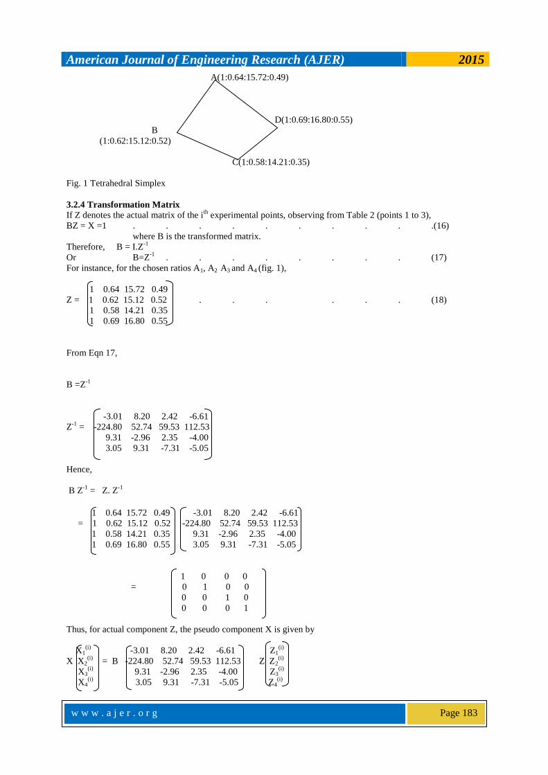
Fig. 1 Tetrahedral Simplex

3.2.4 Transformation Matrix

If Z denotes the actual matrix of the ith

experimental points, observing from Table 2 (points 1 to 3),

BZ = X =1 . . . . . . . . . .(16)

where B is the transformed matrix.

Therefore, B = I.Z-1

Or B=Z-1

. . . . . . . . (17)

For instance, for the chosen ratios A1, A2 A3 and A4 (fig. 1),

1 0.64 15.72 0.49

Z = 1 0.62 15.12 0.52 . . . . . . (18)

1 0.58 14.21 0.35

1 0.69 16.80 0.55

From Eqn 17,

B =Z-1

-3.01 8.20 2.42 -6.61

Z-1

= -224.80 52.74 59.53 112.53

9.31 -2.96 2.35 -4.00

3.05 9.31 -7.31 -5.05

Hence,

B Z-1

= Z. Z-1

1 0.64 15.72 0.49 -3.01 8.20 2.42 -6.61

= 1 0.62 15.12 0.52 -224.80 52.74 59.53 112.53

1 0.58 14.21 0.35 9.31 -2.96 2.35 -4.00

1 0.69 16.80 0.55 3.05 9.31 -7.31 -5.05

1 0 0 0

= 0 1 0 0

0 0 1 0

0 0 0 1

Thus, for actual component Z, the pseudo component X is given by

X1(i)

-3.01 8.20 2.42 -6.61 Z1(i)

X X2(i)

= B -224.80 52.74 59.53 112.53 Z Z2(i)

X3(i)

9.31 -2.96 2.35 -4.00 Z3(i)

X4(i)

3.05 9.31 -7.31 -5.05 Z4(i)



Page 184

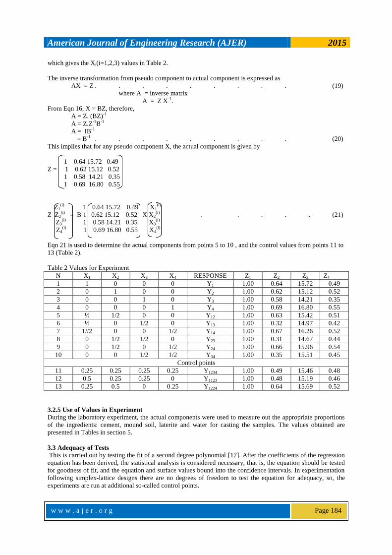
which gives the Xi(i=1,2,3) values in Table 2.

The inverse transformation from pseudo component to actual component is expressed as

AX = Z . . . . . . . . . (19)

where A = inverse matrix

A = Z X-1

.

From Eqn 16, X = BZ, therefore,

A = Z. (BZ)-1

A = Z.Z

-1B

-1

A = IB

-1

= B

-1 . . . . . . . . . (20)

This implies that for any pseudo component X, the actual component is given by

1 0.64 15.72 0.49

Z = 1 0.62 15.12 0.52

1 0.58 14.21 0.35

1 0.69 16.80 0.55

Z1(i)

1 0.64 15.72 0.49 X1(i)

Z Z2(i)

= B 1 0.62 15.12 0.52 X X2(i)

. . . . . (21)

Z3(i)

1 0.58 14.21 0.35

X3(i)

Z4

(i) 1 0.69 16.80 0.55 X4

(i)

Eqn 21 is used to determine the actual components from points 5 to 10 , and the control values from points 11 to

13 (Table 2).

Table 2 Values for Experiment

N X1 X2 X3 X4 RESPONSE Z1 Z2 Z3 Z4

1 1 0 0 0 Y1 1.00 0.64 15.72 0.49

2 0 1 0 0 Y2 1.00 0.62 15.12 0.52

3 0 0 1 0 Y3 1.00 0.58 14.21 0.35

4 0 0 0 1 Y4 1.00 0.69 16.80 0.55

5 ½ 1/2 0 0 Y12 1.00 0.63 15.42 0.51

6 ½ 0 1/2 0 Y13 1.00 0.32 14.97 0.42

7 1//2 0 0 1/2 Y14 1.00 0.67 16.26 0.52

8 0 1/2 1/2 0 Y23 1.00 0.31 14.67 0.44

9 0 1/2 0 1/2 Y24 1.00 0.66 15.96 0.54

10 0 0 1/2 1/2 Y34 1.00 0.35 15.51 0.45

Control points

11 0.25 0.25 0.25 0.25 Y1234 1.00 0.49 15.46 0.48

12 0.5 0.25 0.25 0 Y1123 1.00 0.48 15.19 0.46

13 0.25 0.5 0 0.25 Y1224 1.00 0.64 15.69 0.52

3.2.5 Use of Values in Experiment

During the laboratory experiment, the actual components were used to measure out the appropriate proportions

of the ingredients: cement, mound soil, laterite and water for casting the samples. The values obtained are

presented in Tables in section 5.

3.3 Adequacy of Tests

This is carried out by testing the fit of a second degree polynomial [17]. After the coefficients of the regression

equation has been derived, the statistical analysis is considered necessary, that is, the equation should be tested

for goodness of fit, and the equation and surface values bound into the confidence intervals. In experimentation

following simplex-lattice designs there are no degrees of freedom to test the equation for adequacy, so, the

experiments are run at additional so-called control points.



Page 185

1≤i<j≤q 1≤i≤q

The number of control points and their coordinates are conditioned by the problem formulation and experiment

nature. Besides, the control points are sought so as to improve the model in case of inadequacy. The accuracy of

response prediction is dissimilar at different points of the simplex. The variance of the predicted response, SY2,

is obtained from the error accumulation law. To illustrate this by the second degree polynomial for a quaternary

mixture, the following points are assumed:

Xi can be observed without errors [17].

The replication variance, SY2, is similar at all design points, and

Response values are the average of ni and nij replicate observations at appropriate points of the simplex

Then the variance SŶi and SŶij will be

(SŶ2)i=SY

2/ni . . . . . . . . (22)

SŶ2)ij=SY

2/nij. . . . . . . . . (23)

In the reduced polynomial,

Ŷ = β1X1+ β2X2 + β3X3 + β4X4 + β12X1X2+ β13X1X3 + β14X1X4+ β23X2X23+ β24X2X4 +

β34X3X4 . . . .(24)

If we replace coefficients by their expressions in terms of responses,

βi = Yi and βij = 4Yij – 2Yi – 2Yj

Ŷ = Y1X1 + Y 2X2 + Y 3X3++ Y4X4 +(4Y12 – 2Y1 – 2Y2 )X1X2 + (4Y13 – 2Y1 – 2Y3)X1X3 + (4Y14 – 2Y1 –

2Y4)X1X4 + (4Y23 – 2Y2 - 2Y3 )X2X3 + (4Y24 – 2Y2 - 2Y4 )X2X4+ (4Y34 – 2Y3 - 2Y4 )X3X4

= Y1(X1 – 2X1X2 –2X1X3 -2X1X4 )+ Y2(X2 - 2X1X2 - 2X2X3 -2X2X4)+ Y3(X3 - 2X1X3 + 2X2X3 +2X3X4) +

Y4(X4 - 2X1X4 + 2X2X4 +2X3X4) + 4Y12X1X2 + 4Y13X1X3 + 4Y14X1X4 + 4Y23X2X3 + 4Y24X2X4 + 4Y34X3X4 .

. . . . . . (25)

Using the condition X1+X2 +X3 +X4 =1, we transform the coefficients at Yi

X1 – 2X1X2 – 2X1X3 - 2X1X4=X1 – 2X1(X2 + X3 +X4)

= X1 – 2X1(1 - X1) = X1(2X1 – 1) and so on. . (26)

Thus

Ŷ = X1(2X1 – 1)Y1 + X2(2X2 – 1)Y2 + X3(2X3 – 1)Y3+ X4(2X4 – 1)Y4+ 4Y12X1X2+ 4Y13X1X3+ 4Y14X1X4+

4Y23X2X3 + 4Y24X2X4 + 4Y34X3X4 . . . . . (27)

Introducing the designation

ai = Xi(2X1 – 1) and aij = 4XiXj . . . . . (27a)

and using Eqns (3.22) and (3.230) give the expression for the variance SY2.

SŶ2 =

SY2 (∑aii/ni + ∑ajj/nij) . . . . .. (28)



Page 186

1≤i≤q 1≤i<j≤q

If the number of replicate observations at all the points of the design are equal, i.e. ni=nij= n, then all the

relations for SŶ2 will take the form

SŶ2 =

SY2ξ/n . . . . . . . . . . (29)

where, for the second degree polynomial,

ξ = ∑ai2 + ∑aij

2

. . (30)

As in Eqn (30), ξ is only dependent on the mixture composition. Given the replication variance and the number

of parallel observations n, the error for the predicted values of the response is readily calculated at any point of

the composition-property diagram using an appropriate value of ξ taken from the curve.

Adequacy is tested at each control point, for which purpose the statistic is built:

t = ∆Y/(SŶ2 + SY

2) = ∆Yn

1/2 /(SY(1 + ξ)

1/2 . . . . . . (31)

where ∆Y = Yexp – Ytheory . . . . . . . . (32)

and n = number of parallel observations at every point.

The t-statistic has the student distribution, and it is compared with the tabulated value of tα/L(V) at a level of

significance α, where L = the number of control points, and V = the number for the degrees of freedom for the

replication variance.

The null hypothesis is that the equation is adequate is accepted if tcal< tTable for all the control points.

The confidence interval for the response value is

Ŷ - ∆ ≤ Y ≤ Ŷ + ∆ . . . . . . . .

(3.33)

∆ = tα/L,k SŶ . . . . . . . . . (34)

where k is the number of polynomial coefficients determined.

Using Eqn (29) in Eqn (34)

∆ = tα/L,k SY(ξ/n)1/2

. . . . . . . . (35)

IV. METHODOLOGY To be a good structural material, the material should be homogeneous and isotropic. The Portland

cement, sandcrete or concrete are none of these, nevertheless they are popular construction materials [20].The

necessary materials required in the manufacture of the sandcrete in the study are cement, mound soil, laterite

and water.

4.1 Materials

The Laterite materiasl were collected at Emene area of Enugu State and conformed to BS 882 and

belongs to zone 1 of the ASHTO classification. The mound soil were collected from bushes in the same area.

The water for use is pure drinking water which is free from any contamination i.e. nil Chloride content, pH =6.9,

and Dissolved Solids < 2000ppm. Ordinary Portland cement is the hydraulic binder used in this project and

sourced from the Dangote Cement Factory, and assumed to comply with the Standard Institute of Nigeria (NIS)

1974, and kept in an air-tight bag.



Page 187

i

i

n

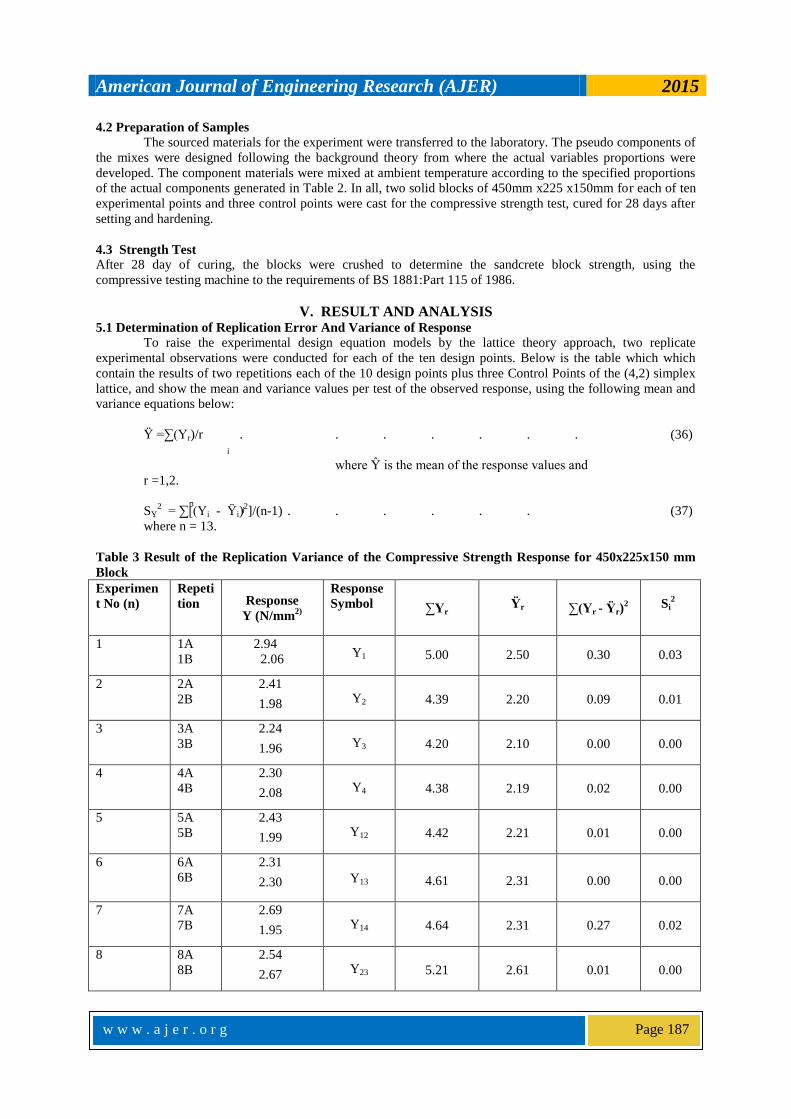
4.2 Preparation of Samples

The sourced materials for the experiment were transferred to the laboratory. The pseudo components of

the mixes were designed following the background theory from where the actual variables proportions were

developed. The component materials were mixed at ambient temperature according to the specified proportions

of the actual components generated in Table 2. In all, two solid blocks of 450mm x225 x150mm for each of ten

experimental points and three control points were cast for the compressive strength test, cured for 28 days after

setting and hardening.

4.3 Strength Test

After 28 day of curing, the blocks were crushed to determine the sandcrete block strength, using the

compressive testing machine to the requirements of BS 1881:Part 115 of 1986.

V. RESULT AND ANALYSIS 5.1 Determination of Replication Error And Variance of Response

To raise the experimental design equation models by the lattice theory approach, two replicate

experimental observations were conducted for each of the ten design points. Below is the table which which

contain the results of two repetitions each of the 10 design points plus three Control Points of the (4,2) simplex

lattice, and show the mean and variance values per test of the observed response, using the following mean and

variance equations below:

Ÿ =∑(Yr)/r . . . . . . . (36)

where Ŷ is the mean of the response values and

r =1,2.

SY2 = ∑[(Yi - Ÿi)

2]/(n-1) . . . . . . (37)

where n = 13.

Table 3 Result of the Replication Variance of the Compressive Strength Response for 450x225x150 mm

Block

Experimen

t No (n)

Repeti

tion Response

Y (N/mm2)

Response

Symbol ∑Yr

Ÿr ∑(Yr - Ÿr)2

Si2

1 1A

1B

2.94

2.06 Y1

5.00 2.50 0.30 0.03

2 2A

2B

2.41

1.98

Y2 4.39 2.20 0.09 0.01

3 3A

3B

2.24

1.96

Y3 4.20 2.10 0.00 0.00

4 4A

4B

2.30

2.08

Y4 4.38 2.19 0.02 0.00

5 5A

5B

2.43

1.99

Y12 4.42 2.21 0.01 0.00

6 6A

6B

2.31

2.30

Y13 4.61 2.31 0.00 0.00

7 7A

7B

2.69

1.95

Y14 4.64 2.31 0.27 0.02

8 8A

8B

2.54

2.67

Y23 5.21 2.61 0.01 0.00



Page 188

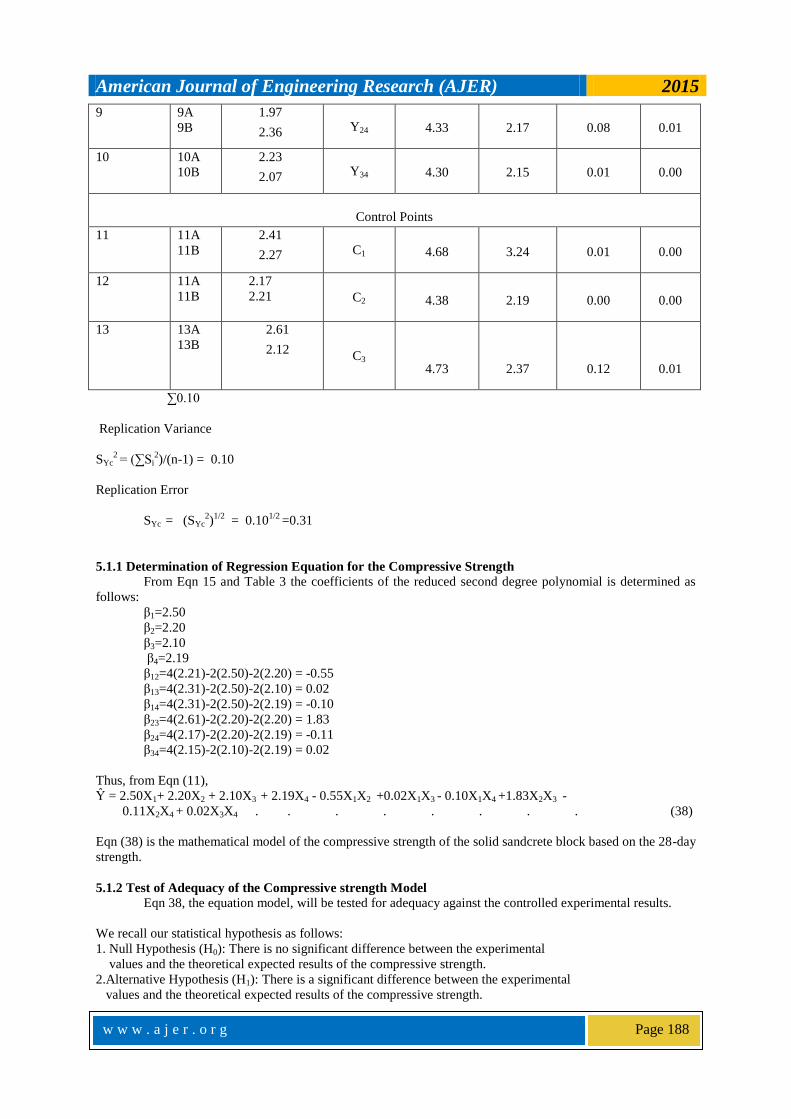
9 9A

9B

1.97

2.36

Y24 4.33 2.17 0.08 0.01

10 10A

10B

2.23

2.07

Y34 4.30 2.15 0.01 0.00

Control Points

11 11A

11B

2.41

2.27

C1 4.68 3.24 0.01 0.00

12 11A

11B

2.17

2.21 C2 4.38 2.19 0.00 0.00

13 13A

13B

2.61

2.12

C3 4.73 2.37 0.12 0.01

∑0.10

Replication Variance

SYc2 = (∑Si

2)/(n-1) = 0.10

Replication Error

SYc = (SYc2)

1/2 = 0.10

1/2 =0.31

5.1.1 Determination of Regression Equation for the Compressive Strength

From Eqn 15 and Table 3 the coefficients of the reduced second degree polynomial is determined as

follows:

β1=2.50

β2=2.20

β3=2.10

β4=2.19

β12=4(2.21)-2(2.50)-2(2.20) = -0.55

β13=4(2.31)-2(2.50)-2(2.10) = 0.02

β14=4(2.31)-2(2.50)-2(2.19) = -0.10

β23=4(2.61)-2(2.20)-2(2.20) = 1.83

β24=4(2.17)-2(2.20)-2(2.19) = -0.11

β34=4(2.15)-2(2.10)-2(2.19) = 0.02

Thus, from Eqn (11),

Ŷ = 2.50X1+ 2.20X2 + 2.10X3 + 2.19X4 - 0.55X1X2 +0.02X1X3 - 0.10X1X4 +1.83X2X3 -

0.11X2X4 + 0.02X3X4 . . . . . . . . (38)

Eqn (38) is the mathematical model of the compressive strength of the solid sandcrete block based on the 28-day

strength.

5.1.2 Test of Adequacy of the Compressive strength Model

Eqn 38, the equation model, will be tested for adequacy against the controlled experimental results.

We recall our statistical hypothesis as follows:

1. Null Hypothesis (H0): There is no significant difference between the experimental

values and the theoretical expected results of the compressive strength.

2.Alternative Hypothesis (H1): There is a significant difference between the experimental

values and the theoretical expected results of the compressive strength.



Page 189

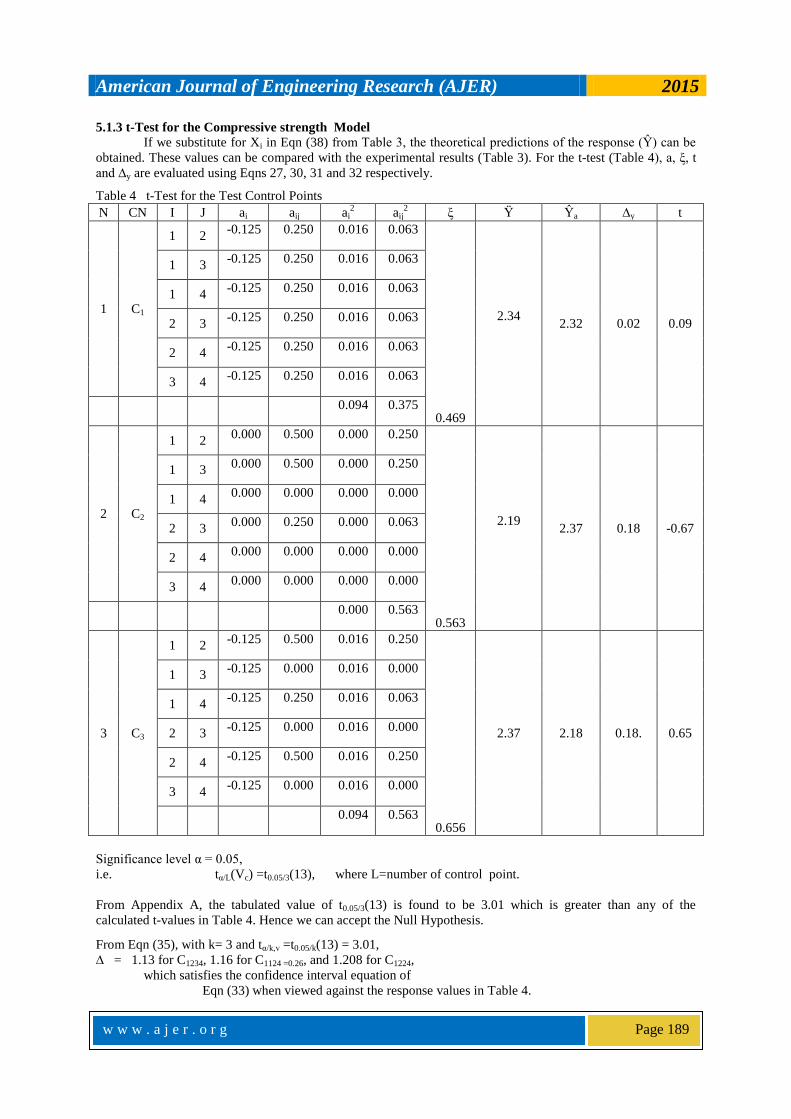
5.1.3 t-Test for the Compressive strength Model

If we substitute for Xi in Eqn (38) from Table 3, the theoretical predictions of the response (Ŷ) can be

obtained. These values can be compared with the experimental results (Table 3). For the t-test (Table 4), a, ξ, t

and ∆y are evaluated using Eqns 27, 30, 31 and 32 respectively.

Table 4 t-Test for the Test Control Points

N CN I J ai aij ai2 aij

2 ξ Ÿ Ŷa ∆y t

1 C1

1 2 -0.125 0.250 0.016 0.063

0.469

2.34

2.32 0.02 0.09

1 3 -0.125 0.250 0.016 0.063

1 4 -0.125 0.250 0.016 0.063

2 3 -0.125 0.250 0.016 0.063

2 4 -0.125 0.250 0.016 0.063

3 4 -0.125 0.250 0.016 0.063

0.094 0.375

2 C2

1 2 0.000 0.500 0.000 0.250

0.563

2.19

2.37 0.18 -0.67

1 3 0.000 0.500 0.000 0.250

1 4 0.000 0.000 0.000 0.000

2 3 0.000 0.250 0.000 0.063

2 4 0.000 0.000 0.000 0.000

3 4 0.000 0.000 0.000 0.000

0.000 0.563

3 C3

1 2 -0.125 0.500 0.016 0.250

0.656

2.37 2.18 0.18. 0.65

1 3 -0.125 0.000 0.016 0.000

1 4 -0.125 0.250 0.016 0.063

2 3 -0.125 0.000 0.016 0.000

2 4 -0.125 0.500 0.016 0.250

3 4 -0.125 0.000 0.016 0.000

0.094 0.563

Significance level α = 0.05,

i.e. tα/L(Vc) =t0.05/3(13), where L=number of control point.

From Appendix A, the tabulated value of t0.05/3(13) is found to be 3.01 which is greater than any of the

calculated t-values in Table 4. Hence we can accept the Null Hypothesis.

From Eqn (35), with k= 3 and tα/k,v =t0.05/k(13) = 3.01,

∆ = 1.13 for C1234, 1.16 for C1124 =0.26, and 1.208 for C1224,

which satisfies the confidence interval equation of

Eqn (33) when viewed against the response values in Table 4.



Page 190

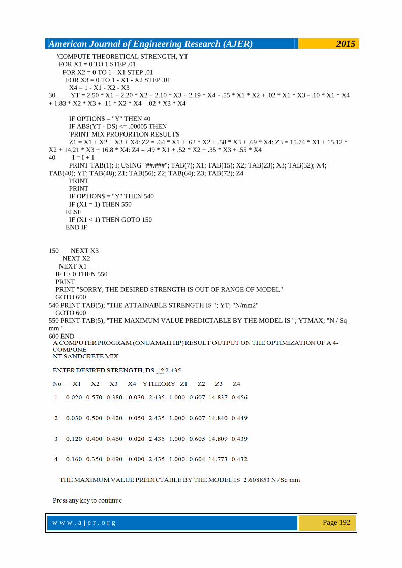
5.2 Computer Program

The computer program is developed for the model (Appendix 1). In the program any desired

Compressive Strength can be specified as an input and the computer processes and prints out possible

combinations of mixes that match the property, to the following tolerance:

Compressive Strength - 0.00005 N/mm2,

Interestingly, should there be no matching combination, the computer informs the user of this. It also checks the

maximum value obtainable with the model.

5.2.1 Choosing a Combination

It can be observed that the strength of 2.435 N/sq mm yielded 4 combinations. To accept any particular

proportions depends on the factors such as workability, cost and honeycombing of the resultant lateritic

concrete.

IV. Conclusion and Recommendation 6.1 Conclusion

Simplex design was applied successfully to prove that the modulus of lateritic concrete is a function of

the proportion of the ingredients (cement, mound soil, laterite and water), but not the quantities of the materials

[16]. The maximum compressive strength obtainable with the compressive strength model is 2.61 N/sq mm. See

the computer run outs which show all the possible lateritic concrete mix options for the desired modulus

property, and the choice of any of the mixes is the user’s. One can also draw the conclusion that the maximum

values achievable, within the limits of experimental errors, is quite below that obtainable using sand as

aggregate. This is due to the predominantly high silt content of laterite. It can be observed that the task of

selecting a particular mix proportion out of many options is not easy, if workability and other demands of the

resulting lateritic concrete have to be satisfied. This is an important area for further research work. The project

work is a great advancement in the search for the applicability of laterite and mound soil in concrete mortar

production in regions where sand is extremely scarce with the ubiquity of laterite. The paper provides an

optimized design perspective of the use of admixtures instead of undersigned percentage addition which is

currently prevalent in the concrete industry of the world.

6.2 Recommendations

From the foregoing study, the following could be recommended:

i) The model can be used for the optimization of the strength of concrete made from cement, mound soil, laterite

and water.

ii) Laterite aggregates cannot adequately substitute sharp sand aggregates for heavy

construction.

iii) More research work need to be done in order to match the computer recommended mixes with the

workability of the resulting concrete.

iii) The accuracy of the model can be improved by taking higher order polynomials of the simplex.

REFERENCES [1] Orie, O.U., Osadebe, N.N., “Optimization of the Compressive Strength of Five Component Concrete Mix Using Scheffe’s

Theory – A case of Mound Soil Concrete”, Journal of the Nigerian Association of Mathematical Physics, 14, pp. 81-92, May, 2009.

[2] Majid, K.I., Optimum Design of Structure( Butterworths and Co., Ltd, London, pp. 16, 1874).

[3] David, J., Galliford, N., Bridge Construction at Hudersfield Canal, Concrete, Number 6, 2000. [4] Ecocem Island Ltd, Ecocem GBBS Cement. The Technically Superior and Environmentally Friendly Cement”, 56 Tritoville

Road Sand Dublin 4 Island, 19.

[5] Mohan, Muthukumar, M. and Rajendran, M., Optimization of Mix Proportions of Mineral Aggregates Using Box Jenken Design of Experiments( Ecsevier Applied Science, Vol. 25, Issue 7, pp. 751-758, 2002).

[6] Simon, M., (1959), “Concrete Mixture Optimization Using Statistical Models, Final Report, Federal Highway Administration,

National Institutes and Technology, NISTIR 6361, 1999. [7] Nordstrom, D.K. and Munoz, J.I., Geotechnical Thermodynamics ( Blackwell Scientific Publications, Boston, 1994).

[8] Bloom, R. and Benture, A. “Free and restrained Shrinkage of Normal and High Strength Concrete”, int. ACI Material Journal,

92(2), 1995, pp. 211-217. [9] Schefe, H., (1958), Experiments with Mixtures, Royal Statistical Society journal. Ser B., 20, 1958. pp 344-360, Rusia.

[10] Erwin, K., Advanced Engineering Mathematics(8th Edition, John Wiley and Sons, (Asia) Pte. Ltd, Singapore, pp. 118-121 and

40 – 262). [11] Reynolds, C. and Steedman, J.C., Reinforced Concrete Designers Handbook( View point Publications, 9th Edition, 1981, Great

Britain).

[12] Obam, S.O. and Osadebe, N.N., Mathematical Models for Optimization of some Mechanical properties of Concrete made from Rice Husk Ash, Ph.D Thesis, of Nigeria, Nsukka, 2007.



Page 191

[13] Fageria, N.K. and Baligar, V.C. Properties of termite mound soils and responses of rice and bean to n, p, and k fertilization on

such soil.. Communications in Soil Science and Plant Analysis. 35(15-16), 2004

[14] Udoeyo F.F. and Turman M. Y. Mound Soil As A Pavement Material, Global Jnl Engineering Res. 1(2) , 2002: 137-144. [15] Felix, F.U., Al, O.C., and Sulaiman, J., Mound Soil as a Construction Material in Civil Engineering, 12(13), pp. 205-211, 2000.

16. Garmecki, L., Garbac, A., Piela, P., Lukowski, P., Material Optimization System: Users Guide(Warsaw University of

Technology Internal Report, 1994). [16] Jackson, N., Civil Engineering Materials( RDC Arter Ltd, Hong Kong, 1983).

[17] Akhanarova, S. and Kafarov, V., Experiment and Optimization in Chemistry and Chemical Engineering (MIR Publishers,

Mosco, 1982, pp. 213 - 219 and 240 – 280). [18] R.C., (1973), Materials of Construction(, Mc Graw-Hill Book Company, USA).

[19] Obodo D.A., Optimization of Component Mix in Sandcrete Blocks Using Fine Aggregates from Different Sources, UNN, 1999. [20] Wilby, C.B., Structural Concrete( Butterworth, London, UK, 1983, Tropical Laterite in Botswana, 2003-2004).

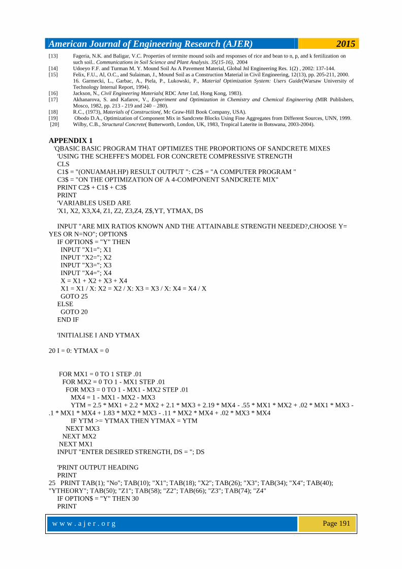
APPENDIX 1 'QBASIC BASIC PROGRAM THAT OPTIMIZES THE PROPORTIONS OF SANDCRETE MIXES

'USING THE SCHEFFE'S MODEL FOR CONCRETE COMPRESSIVE STRENGTH

CLS

C1$ = "(ONUAMAH.HP) RESULT OUTPUT ": C2$ = "A COMPUTER PROGRAM "

C3$ = "ON THE OPTIMIZATION OF A 4-COMPONENT SANDCRETE MIX"

PRINT C2$ + C1$ + C3$

PRINT

'VARIABLES USED ARE

'X1, X2, X3,X4, Z1, Z2, Z3,Z4, Z$,YT, YTMAX, DS

INPUT "ARE MIX RATIOS KNOWN AND THE ATTAINABLE STRENGTH NEEDED?,CHOOSE Y=

YES OR N=NO"; OPTION$

IF OPTION$ = "Y" THEN

INPUT "X1="; X1

INPUT "X2="; X2

INPUT "X3="; X3

INPUT "X4="; X4

X = X1 + X2 + X3 + X4

X1 = X1 / X: X2 = X2 / X: X3 = X3 / X: X4 = X4 / X

GOTO 25

ELSE

GOTO 20

END IF

'INITIALISE I AND YTMAX

20 I = 0: YTMAX = 0

FOR MX1 = 0 TO 1 STEP .01

FOR MX2 = 0 TO 1 - MX1 STEP .01

FOR MX3 = 0 TO 1 - MX1 - MX2 STEP .01

MX4 = 1 - MX1 - MX2 - MX3

YTM = 2.5 * MX1 + 2.2 * MX2 + 2.1 * MX3 + 2.19 * MX4 - .55 * MX1 * MX2 + .02 * MX1 * MX3 -

.1 * MX1 * MX4 + 1.83 * MX2 * MX3 - .11 * MX2 * MX4 + .02 * MX3 * MX4

IF YTM >= YTMAX THEN YTMAX = YTM

NEXT MX3

NEXT MX2

NEXT MX1

INPUT "ENTER DESIRED STRENGTH, DS = "; DS

'PRINT OUTPUT HEADING

PRINT

25 PRINT TAB(1); "No"; TAB(10); "X1"; TAB(18); "X2"; TAB(26); "X3"; TAB(34); "X4"; TAB(40);

"YTHEORY"; TAB(50); "Z1"; TAB(58); "Z2"; TAB(66); "Z3"; TAB(74); "Z4"

IF OPTION$ = "Y" THEN 30

PRINT



Page 192

'COMPUTE THEORETICAL STRENGTH, YT

FOR X1 = 0 TO 1 STEP .01

FOR X2 = 0 TO 1 - X1 STEP .01

FOR X3 = 0 TO 1 - X1 - X2 STEP .01

X4 = 1 - X1 - X2 - X3

30 YT = 2.50 * X1 + 2.20 * X2 + 2.10 * X3 + 2.19 * X4 - .55 * X1 * X2 + .02 * X1 * X3 - .10 * X1 * X4

+ 1.83 * X2 * X3 + .11 * X2 * X4 - .02 * X3 * X4


IF ABS(YT - DS) <= .00005 THEN

'PRINT MIX PROPORTION RESULTS

Z1 = X1 + X2 + X3 + X4: Z2 = .64 * X1 + .62 * X2 + .58 * X3 + .69 * X4: Z3 = 15.74 * X1 + 15.12 *

X2 + 14.21 * X3 + 16.8 * X4: Z4 = .49 * X1 + .52 * X2 + .35 * X3 + .55 * X4

40 I = I + 1

PRINT TAB(1); I; USING "##.###"; TAB(7); X1; TAB(15); X2; TAB(23); X3; TAB(32); X4;

TAB(40); YT; TAB(48); Z1; TAB(56); Z2; TAB(64); Z3; TAB(72); Z4

PRINT

PRINT


IF (X1 = 1) THEN 550

ELSE

IF (X1 < 1) THEN GOTO 150

END IF

150 NEXT X3

NEXT X2

NEXT X1

IF I > 0 THEN 550

PRINT

PRINT "SORRY, THE DESIRED STRENGTH IS OUT OF RANGE OF MODEL"

GOTO 600

540 PRINT TAB(5); "THE ATTAINABLE STRENGTH IS "; YT; "N/mm2"

GOTO 600

550 PRINT TAB(5); "THE MAXIMUM VALUE PREDICTABLE BY THE MODEL IS "; YTMAX; "N / Sq

mm "

600 END